Determinants, contexts, and measurements of customer loyalty

Determinants, contexts, and

measurements of customer loyalty

A dissertation presented

By

Mitja Pirc

To

The Department of Economics and Business

in partial fulfillment of the requirements

for the degree of

Doctor of Philosophy

In the subject of

Management

Universitat Pompeu Fabra

Barcelona, Spain

August 2008

2

© 2008 – Mitja Pirc

All rights reserved.

3

Abstract

In this thesis I address three research questions related to the process of consumers’

judgment and decision making (JDM) and in particular customer loyalty. The underlying

assumption is that consumers use inputs (determinants) in forming judgments or making

decisions. These determinants can be diverse, ranging from consumer perceptions to

objective factors. Further, the context in which economic exchanges take place also

influences the JDM process. In addition, various measures are used to capture consumer

JDM outcomes, which can cause consumer to process information in different ways.

The first research question is about how contexts influence the salience (i.e., relevance,

importance) of determinants used in JDM. In particular, the determinants I focus on are

costs associated with products or services as they reflect the value of economic exchanges

between consumers and companies. There are several cost dimensions available to

consumers as inputs in JDM and a proposition is developed with regards to which cost

dimension is more salient.

The second research question addresses how determinants differ in their influence on

customer loyalty. Loyalty is frequently measured by asking customers to forecast their

future behavior, with two commonly used forms: intentions and expectations. I build on

the difference between intentions and expectations to propose that determinants of loyalty

differ in whether they are inward-looking (more control), such as satisfaction and attitude

towards switching, or outward-looking (less control), such as trust and switching cost.

The third research paper of this thesis explores further how determinants influence

customer loyalty. A concept of a counterbalance effect is introduced, when two causal

pathways exist between determinants and loyalty and have opposite effects (positive,

negative). A counterbalance effect can cause the total effect to diminish, or that either of

the two causal pathways dominates and therefore both a positive and a negative effect can

be found. The counterbalance effect provides a novel explanation for some of the

discrepancies found in the literature about the effects of loyalty determinants.

4

Contents

Abstract .........................................................................................................................3

Contents.........................................................................................................................4

Acknowledgments .........................................................................................................7

1. Introduction.......................................................................................................................8

2. It matters how you pay: Cost type salience depends on the payment mechanism ...13

2.1. Introduction ..........................................................................................................13

2.2. Theory and propositions.......................................................................................15

2.2.1. Types of costs, consumer judgment and decision making ............................15

2.2.2. Payment mechanisms ....................................................................................16

2.2.3. Consumer resources, attention, and salience of costs....................................17

2.2.4. Overview of the studies .................................................................................19

2.3. Study 1: Metro commuting...................................................................................19

2.3.1. Research design .............................................................................................20

2.3.2. Analysis and results .......................................................................................21

2.4. Study 2: Mobile telecommunications...................................................................24

2.4.1. Research design .............................................................................................25


2.5. Study 3: Skiing trip...............................................................................................27

2.5.1. Research design .............................................................................................28


2.6. General discussion................................................................................................32

2.6.1. Contribution to theory ...................................................................................32

2.6.2. Managerial implications ................................................................................33

2.6.3. Limitations and future research .....................................................................34

5

3. Using the Intentions and Expectations perspectives to explore the influence of

determinants of loyalty.......................................................................................................35

3.1. Introduction ..........................................................................................................35

3.2. Theory and hypotheses .........................................................................................37

3.2.1. Customer loyalty and its determinants ..........................................................37

3.2.2. The intentions and expectations perspective .................................................38

3.2.3. The roles of determinants of loyalty..............................................................39

3.3. Study analysis and results.....................................................................................41

3.3.1. Research design .............................................................................................41

3.3.2. Measurement model ......................................................................................43

3.3.3. Structural path model with determinants of loyalty ......................................46

3.3.4. Comparing coefficients between the switching intentions and

expectations .............................................................................................................49





4. Counterbalance effect of determinants of loyalty: Usage and Satisfaction...............54

4.1. Introduction ..........................................................................................................54

4.2. Theory and proposition ........................................................................................56

4.2.1. Determinants of loyalty and their effects ......................................................56

4.2.2. Complexity of economic exchange systems..................................................57

4.2.3. Counterbalance proposition...........................................................................59

4.2.4. Test used for the counterbalance effect .........................................................59

4.3. Study 1: Usage as a determinant of loyalty..........................................................61

4.3.1. Counterbalance conditions ............................................................................62

4.3.2. Research design .............................................................................................63


6

4.4. Study 2: Satisfaction as a determinant of loyalty .................................................66

4.4.1. Counterbalance conditions ............................................................................67

4.4.2. Research design .............................................................................................68

4.4.3. Measurement model ......................................................................................70

4.4.4. Testing the counterbalance effect ..................................................................71





References............................................................................................................................77

A Appendix to Chapter 2 ..................................................................................................84

A.1 Appendix for study 1: Metro commuting.............................................................85

A.2 Appendix for study 3: Skiing trip.........................................................................87

B Appendix to Chapter 3...................................................................................................92

B.1 Measures used for study constructs ......................................................................93

7

Acknowledgments

My doctoral studies have been an important period in my life allowing me to learn and

grow as a researcher. I was fortunate to have two supervisors, Antonio Ladron and Robin

Hogarth, who have always been supporting and have helped me immensely with my

research. I have gained a lot from their guidance both as a researcher and as a person.

I would like to thank Michael Greenacre for being on my thesis proposal committee and

for providing me with feedback on my research. I am very grateful to Gert Corneliessen for

providing me with valuable feedback on my thesis chapters. I have also had the pleasure to

learn from numerous faculty members at Pompeu Fabra, either through coursework or

while interacting at seminars. I would like to thank Magnus Soderlund from Stockholm

School of Economics and Martin Boehm and Garen Markarian from Instituto de Empresa.

During my stay in Barcelona I have been fortunate to meet many interesting people and

formed lasting friendships with Milos Bozovic, Tomaz Cajner, Margherita Comola, Jose

Antonio Dorich, Andrea Christina Felfe, Benjamin Golez, Andraz Kavalar, Rasa

Karapandza, Gueorgui Kolev, Tomas Lejarraga, Marta Maras, Arturo Ormeno, Juan

Manuel Puerta, Elena Reutskaja, Francisco Geronimo Ugarte Beldwell, and Blaz Zakelj. I

would like to thank Clara for being an important person in my life and sharing my troubles

and joy in the process of writing this thesis.

I am very grateful to Marta Araque, Gemma Burballa, Mireia Monroig, and Marta Aragay

from GPEFM office for their support. I would like to acknowledge the AGAUR grant that

has made my PhD studies possible.

My parents, Andreja and Milan, have always supported my decisions in life and have

helped me with every step on the way. My brother Matej has always been there for me and

is the best brother I could have. I am immensely grateful for having such a loving and

supporting family.

8

Chapter 1

Introduction

Subject matter and structure of this thesis

Consumers frequently form judgments and make decisions when interacting with

companies in the marketplace. Consumer judgments represent how they perceive different

dimensions of economic exchanges, such as satisfaction with a product or service,

perceived value for money, or trust in a specific company. Consumer decisions lead to

actions, such as purchasing a product, upgrading a service, or changing a provider.

Judgments and decisions that consumers make impact relationships in the marketplace.

Companies therefore strive to understand the process of judgment and decision making

(JDM) as well as the factors that influence it. With this knowledge companies can better

manage relationships with their customers, optimize the use of resources, and develop new

products and services. Understanding consumer JDM is important also for policy makers

and governments as they can use it to improve public services as well as to protect

consumers.

In this thesis I address three research questions related to the process of consumers’ JDM.

All three topics share a common framework (Figure 1.1), based on the idea that consumers

use inputs (determinants) in forming judgments or making decisions. These determinants

can be diverse, ranging from consumer perceptions to objective factors. In addition, the

9

context in which economic exchanges take place also influences the consumer JDM

process.

Figure 1.1: Basic framework of consumer JDM

There are many different judgments that consumers can form and many decision they can

take. The research questions in this thesis center primarily on customer loyalty as the

outcome of consumer JDM process. Loyalty can be measured both as a behavior (e.g.,

actual act of changing a service provider), which reflects a decision, or as a perception

(e.g., intention to remain loyal), which reflects a judgment.

The research papers in Chapters 2 to 4 form the core of this thesis. Even though they

represent independent pieces of research, they all build on the framework presented in

Figure 1.1 to analyze (primarily) consumer loyalty. The models, methods, and findings of

these three chapters complement each other and provide a fuller understanding of

consumer JDM with particular emphasis on loyalty. The first paper focuses on the effect of

the context on consumer JDM, the second paper explores how using different measures of

loyalty influences JDM process, and the third paper studies the roles that determinants play

with regards to customer loyalty. The title “Determinants, contexts, and measurements of

customer loyalty” therefore reflects the topics of all three research questions. The thesis

concludes with references and appendices related to specific chapters.

Chapter 2: It matters how you pay: Cost type salience depends on the payment

mechanism

The first research question is about how contexts influence the salience (i.e., relevance,

importance) of determinants used in JDM. In particular, the determinants I focus on are

Consumer Judgment

or Decision Making

Context

A

B

Determinants

10

costs associated with products or services as they are one of the key inputs in JDM,

reflecting the value of economic exchanges between consumers and companies.

In simple economic exchanges the cost used as an input in JDM is straightforward, e.g. a

price of a book purchased in a bookstore last week. However, in certain contexts with

sequential consumption (e.g., mobile phone services) different dimensions of costs can be

salient to consumers, e.g. the average cost per unit of consumption (a phone call) or the

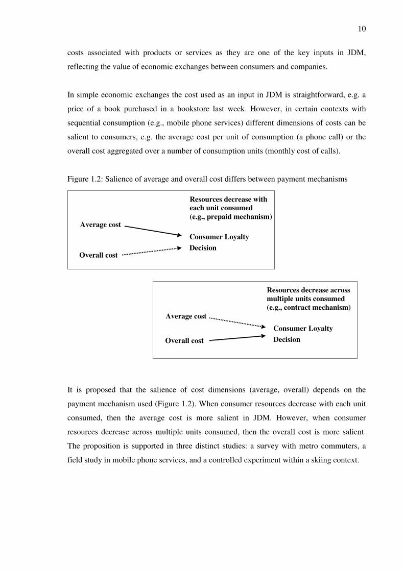
overall cost aggregated over a number of consumption units (monthly cost of calls).

Figure 1.2: Salience of average and overall cost differs between payment mechanisms

It is proposed that the salience of cost dimensions (average, overall) depends on the

payment mechanism used (Figure 1.2). When consumer resources decrease with each unit

consumed, then the average cost is more salient in JDM. However, when consumer

resources decrease across multiple units consumed, then the overall cost is more salient.

The proposition is supported in three distinct studies: a survey with metro commuters, a

field study in mobile phone services, and a controlled experiment within a skiing context.

Consumer Loyalty

Decision

Resources decrease with

each unit consumed

(e.g., prepaid mechanism)

Overall cost

Average cost

Consumer Loyalty

Decision

Resources decrease across

multiple units consumed

(e.g., contract mechanism) Average cost

Overall cost

11

Chapter 3: Using the Intentions and Expectations perspectives to explore the

influence of determinants of loyalty

The second research question addresses how determinants differ in their influence on

consumer JDM. The particular consumer behavior that I study is customer loyalty to a

specific company. Despite numerous studies addressing the influence of determinants of

loyalty, there is still no agreement about what roles they play with regards to loyalty.

Different determinants have been proposed as central, such as satisfaction, trust, and

switching costs.

However, loyalty is frequently measured by asking customers to forecast their future

behavior, with two commonly used forms: intentions and expectations. Previous research

has suggested that the intentions perspective is more inward-looking, focusing on reasons

and motivation for future behavior, while the expectations perspective is more outward-

looking, focusing on factors beyond the individual’s control. I build on this difference

between intentions and expectations to propose that determinants of loyalty differ in

whether they are inward-looking (more control), such as satisfaction and attitude towards

switching, or outward-looking (less control), such as trust and switching cost (Figure 1.3).

Figure 1.3: Intentions and expectations perspectives to understand roles of determinants

A study is designed, where the following determinants are collected: satisfaction, trust,

switching cost, and attitude towards switching, while loyalty is measured with both

intentions and expectations questions. Satisfaction and attitude towards switching are

found to be better predictors of loyalty intentions and thus supported as inward-looking

determinants. Switching costs and trust are on the other hand better predictors of loyalty

expectations and thus supported as outward-looking determinants.

Loyalty Expectation

Context

Loyalty Intention

Inward-looking

determinants

(e.g., satisfaction)

Outward-looking

determinants

(e.g., switching cost)

12

Chapter 4: Counterbalance effect of determinants of loyalty: Usage and Satisfaction

The third research paper of this thesis explores two further issues related to how

determinants influence customer loyalty. Although research has identified different

possible determinants of customer loyalty, the nature of their influence is still unclear.

First, for some determinants there is no agreement whether their effect on loyalty is

positive or negative, like for example usage of services or products. Second, for some other

determinants, such as customer satisfaction, there is an overall consensus about their

influence; however the proposed effect is sometimes empirically supported and other times

the effect is not found.

Figure 1.4: Counterbalance effect of usage on loyalty, when usage increases variable cost

When researching determinants, it is typically assumed that they have a simple and direct

effect on loyalty. In this paper, multiple causal pathways (direct and indirect) are explored

between loyalty and its determinants (Figure 1.4). Further, a concept of a counterbalance

effect is introduced, which is a consequence of a situation when the two causal pathways

have opposite effects (positive, negative). A counterbalance effect can cause the total effect

to diminish, like in the case of satisfaction, or that either of the two causal pathways

dominates and therefore a positive or a negative effect is found, as in the example of usage.

The proposed counterbalance effect is tested with two determinants of loyalty: usage and

satisfaction. Usage is found to have a positive direct effect on loyalty and a negative

indirect effect mediated through costs. Satisfaction is found to have a positive direct effect

on loyalty and a negative indirect effect mediated through the variable of marketplace

satisfaction.

+

_ +

Consumer loyalty

decision

Context

Mediator

(e.g., cost) _

Determinant

(e.g., usage)

13

Chapter 2

It matters how you pay: Cost type salience

depends on the payment mechanism

2.1. Introduction

Costs associated with products or services represent one of the key inputs used by

consumers in judgment and decision making (Heath and Soll, 1996; Bolton and Lemon,

1999; Soman, 2001). They reflect the value of economic exchanges and are therefore

important for consumers. Understanding the effects of past costs can help companies

predict and possibly influence consumers’ decisions (e.g., loyalty, upgrade) and judgments

(e.g., satisfaction). This in turn has a direct effect on the bottom line financial performance.

A cost is said to be salient (i.e., relevant, important) to consumers when they respond to

changes in the level of that specific cost (Sterman, 1989). In the case of simple economic

exchanges the candidate for the salient cost is straightforward, e.g. a price of a book

purchased in a bookstore last week. However, many economic exchanges are more

complex with sequential consumption episodes and embedded payment mechanisms. For

example, mobile phone services are used on a continuing basis and can be paid by a

contract or a prepaid mechanism. Further examples are found in commuting, internet

service, retail banking, gyms, and theater. Therefore, within the sequential economic

14

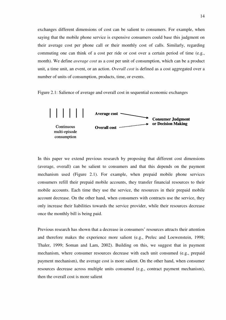
exchanges different dimensions of cost can be salient to consumers. For example, when

saying that the mobile phone service is expensive consumers could base this judgment on

their average cost per phone call or their monthly cost of calls. Similarly, regarding

commuting one can think of a cost per ride or cost over a certain period of time (e.g.,

month). We define average cost as a cost per unit of consumption, which can be a product

unit, a time unit, an event, or an action. Overall cost is defined as a cost aggregated over a

number of units of consumption, products, time, or events.

Figure 2.1: Salience of average and overall cost in sequential economic exchanges

In this paper we extend previous research by proposing that different cost dimensions

(average, overall) can be salient to consumers and that this depends on the payment

mechanism used (Figure 2.1). For example, when prepaid mobile phone services

consumers refill their prepaid mobile accounts, they transfer financial resources to their

mobile accounts. Each time they use the service, the resources in their prepaid mobile

account decrease. On the other hand, when consumers with contracts use the service, they

only increase their liabilities towards the service provider, while their resources decrease

once the monthly bill is being paid.

Previous research has shown that a decrease in consumers’ resources attracts their attention

and therefore makes the experience more salient (e.g., Prelec and Loewenstein, 1998;

Thaler, 1999; Soman and Lam, 2002). Building on this, we suggest that in payment

mechanism, where consumer resources decrease with each unit consumed (e.g., prepaid

payment mechanism), the average cost is more salient. On the other hand, when consumer

resources decrease across multiple units consumed (e.g., contract payment mechanism),

then the overall cost is more salient

Consumer Judgment or Decision Making

Overall cost

Average cost

Continuous

multi-episode

consumption

Consumer Judgment or Decision Making

Overall cost

Average cost

Continuous

multi-episode

consumption

15

Understanding which cost dimension is more salient can help companies better manage

customer perceived costs. For example, mobile phone service providers often offer

discounts for consumers, which are directed to either the average cost per phone call or to

the overall monthly cost. From the providers’ perspective these costs could be seen as

interchangeable; however consumers can think of them as not being equally important.

The paper is organized as follows. First, we review previous literature on costs, payment

mechanisms, and consumer judgment and decision making, from which we derive the

central proposition about the salience of types of costs. Then we present three empirical

studies which test the proposition: a survey with metro commuters, a field study with users

of mobile phone services, and a controlled experiment in a skiing trip context. The paper

concludes with clarifying our contributions to theory, managerial implications, limitations,

and directions for future research.

2.2. Theory and propositions

2.2.1. Types of costs, consumer judgment and decision making

When being involved in economic exchanges with companies, consumers frequently make

decisions and judgments using different cues as inputs. A cue is said to be salient (i.e.,

relevant, important) to consumers when they respond to changes in the level of that

specific cue (Sterman, 1989). Previous literature has identified a number of cues that are

salient to consumers, such as cost and quality. Understanding which cues are more salient

helps companies in managing relationships with their customers in terms of customer value

and loyalty.

When using the cost information consumers need to come up with a mental representation

of the past cost which answers the question “How much is this costing me?“ (Prelec and

Loewenstein, 1998; Soman, 2001; Soman and Lam, 2002). With simple transactions, such

as buying a book in a bookstore, the salient cost is simply the cost of the book. However,

many economic exchanges are complex with sequential consumption episodes and

16

embedded payment mechanisms, examples of which were discussed in the introduction to

this paper. Within these sequential economic exchanges there are different types of costs

that consumers can find relevant.

In this paper two types of cost are explored. Average cost is a cost defined per unit of

consumption, which can be a product unit, a time unit, an event, or an action. Overall cost

is a cost aggregated over a number of consumption units, products, time, or events.

Choosing the unit of consumption to which the average cost refers, depends on a specific

product/service category (Prelec and Loewenstein, 1998). For example, for mobile phone

services the consumption unit could be a phone call, while for commuting it could be one

ride. In the field of economics a typical cost type used in analysis is the marginal cost.

However, in many sequential economic exchanges the marginal costs can differ across

units consumed (e.g., each phone call can have a different cost) and therefore the average

cost is reflecting the cost per unit. In addition to this, in the case of flat rate tariffs the

marginal cost is zero, while the average cost captures the cost assigned to each unit

consumed.

2.2.2. Payment mechanisms

In modern economies consumers can pay in many different ways. Cash and credit cards are

examples of general payment mechanisms. They can be used across different products and

services and do not form a part of an offering. Embedded payment mechanisms on the

other hand form a part of a service or a product offering. For example, mobile service

providers offer a prepaid or a contract payment mechanism, while commuting can be paid

for by using a per-ride ticket or a monthly ticket. Further examples of embedded payment

mechanisms can be found in other contexts such as gyms, renting movies, and theatre.

Recent research on payment mechanisms features two distinct streams. The first stream

focuses on how consumer choose different payment mechanisms (e.g., Prelec and

Loewenstein, 1998; Miravete, 2003; Della Vigna and Malmendier, 2006; Lambrecht and

Skiera, 2006). Prelec and Loewenstein (1998) have shown that when purchasing a durable

(e.g., a washing machine) consumers are more willing to take a loan, however, when

purchasing a vacation they prefer to prepay. The reason is that consumers try to match the

17

payment mechanism with a consumption pattern. Lambrecht and Skiera (2006) have

identified several consumer characteristics which influence the choice of a specific

payment mechanism. These characteristics are the desire to control costs, overestimation of

consumption, and the aversion for increasing costs. Therefore, both context and consumer

characteristics need to be scrutinized when exploring the effect of payment mechanisms on

the salience of cost.

The second stream of research focuses on the effects of a specific payment mechanism

after the choice for a payment mechanism has been made. Prelec and Simester (2001) have

shown that people are willing to pay more when instructed to pay with a credit card than

when paying with cash. The reason is that consumers are willing to accept a higher amount

of liability (credit card) compared to a resource decrease (cash). It has also been proposed

that paying with cash attracts consumers’ attention more than paying with credit cards and

consequently consumers remember costs better when paying with cash (Soman, 2001).

This paper contributes to this second stream of research, dealing with the effects of

payment mechanisms after a choice of payment mechanism has been made.

2.2.3. Consumer resources, attention, and salience of costs

The link between consumer resources, consumption, and consumer attention is first

explained in the context of mobile phone services. Consumers, who pay for mobile phone

services with a prepaid mechanism, first transfer resources to their mobile accounts. With

each usage their resources in the prepaid mobile account decrease. On the other hand,

when contractual consumers use the service they increase their liabilities (debt) towards the

service provider and their resources get decreased when paying the monthly bill.

In such sequential economic exchanges, each time a unit is consumed (e.g., one phone call)

one of the following occurs:

(i) a decrease in consumer resources (consumer assets in various accounts, such as bank

accounts and accounts related to specific services or products),

(ii) an increase in consumer liabilities (consumer debt with regards to services, products),

(iii) no change to consumer resources or liabilities (e.g., in the case of flat rates)

18

Previous research has shown that of all three outcomes above, consumers pay the most

attention to a decrease in resources (Prelec and Loewenstein, 1998; Gourville and Soman,

1998; Prelec and Simester, 2001; Soman, 2001; Soman and Lam, 2002). Therefore, when a

cost type is linked to a decrease in resources it is more salient than when linked to the other

two outcomes (Thaler, 1999; Soman and Lam, 2002).

This is similar to the findings related to the difference of paying with cash (a resource

decrease) versus credit cards (a liability increase). Prelec and Simester (2001) have found

that the willingness to pay with the credit card is larger compared to paying with cash. It is

important to remark that previous research has used the concepts of wealth (resources

minus liabilities) and resources interchangeably.

Let us further explore the mobile phone service example. When using a prepaid payment

mechanism, consumer resources decrease with each phone call (consumption unit), which

in turn makes the average cost per phone call more salient. Similarly, when using a

contract payment mechanism resources decrease when paying the monthly bill (across

multiple consumption units), which makes the monthly cost of phone calls more salient.

Therefore, when resources decrease with each unit consumed, consumers take a local

perspective such that the average cost becomes more salient. On the other hand, when

consumer resources decrease across multiple consumption units, a global perspective is

taken, making the overall cost more salient. Payment mechanisms differ in the moment in

which consumer resources decrease and consequently influence the salience of the average

versus the overall cost.

Proposition:

When resources decrease with each unit consumed, then the average cost is more salient.

When resources decrease across multiple consumption units, then the overall cost is more

salient

19

2.2.4. Overview of the studies

We test our proposition using three service categories and their specific (existing)

embedded payment mechanisms. The first study is a survey with commuters. The second

study is a field study in mobile telecommunications based on customer behavior data. The

third study is a controlled experiment in the context of skiing trip done with graduate

students. The three studies are complementary both in terms of the context and the method.

Different dependent variables are used in each of the studies in order to explore the

proposition with regards to different decisions and judgments. Table 2.1 shows the

classification of payment mechanisms in each of the studies together with the predictions

about the more salient cost type.

Table 2.1: Summary of studies, payment mechanisms, and proposed salient cost.

Context Payment

mechanism

When consumer

resources decrease with

each unit consumed, then

Average cost is more

salient

When consumer resources

decrease across a number

of consumption units then,

Overall cost is more

salient

Study 1: metro

commuting

Per ride ticket Average cost

Monthly ticket Overall cost

Study 2:

mobile services

Prepaid Average cost

Contract Overall cost

Study 3:

skiing trip

Daily ski

tickets

Average cost

Multi-day pass Overall cost

2.3. Study 1: Metro commuting

In this first study we explore which type of the costs is more salient with regards to

consumers’ perceived value for money, which is defined as the utility of a product or a

20

service as perceived by customers (Zeithaml, 1988). Perceived value is based on

comparing the received benefits and the cost associated with these benefits.

The setting for this study is a survey involving metro commuters. Two embedded payment

mechanisms are studied: monthly tickets and per ride tickets. The monthly ticket payment

mechanism allows commuters to make as many trips as they want within one month from

the date of the purchase. The commuters who pay per ride can either buy a single ticket or

a bundle of ten single tickets; with each trip (ride) they spend one single ticket. We test

whether salience of the average (per ride) cost and the overall (monthly) cost differ

between payment mechanisms.

2.3.1. Research design

The participants were 80 randomly selected metro commuters in a metropolitan area. They

were surveyed when exiting one of three selected metro stations in the city centre. The

respondents were told that the research was conducted for academic purposes and were not

compensated for participation. Out of the 80 commuters surveyed, 33 used monthly passes

and 47 were paying per ride. (The survey had been pre-tested with 35 graduate students to

ensure the clarity of questions used.)

The respondents were asked to indicate the level of value for money metro commuting

offers for them on a ten-point scale (Value Initial, 1 = “poor value”, 10 = “good value”; cf.,

Zeithaml, 1988). The participants were further asked how many trips they make in a

typical week including weekends (Weekly number of trips). Next, all commuters were

presented with two hypothetical situations. First, they were asked to imagine that their

monthly cost of metro commuting would increase by 25 percent. Then we have asked them

to indicate the level of value for money again (Value Overall). Second, the participants

were also asked to imagine that their average cost per ride would increase by 25 percent,

and to assess the value for money (Value Average). The order in which both hypothetical

situations were presented was counterbalanced, as the order of presenting can influence

outcomes (Podsakoff et al, 2003).

21

2.3.2. Analysis and results

In Table 2.2 we present the perceived value that commuters reported in each of the two

conditions for each of the two payment mechanisms, before and after the hypothetical

information about the cost increase were given. The first column shows values for money

for the commuters paying per month and the second column shows changes for the

commuters paying per trip. The increase in (overall or average) cost is perceived as a

negative (disutility) from the commuters’ perspective. As the commuters in the two

payment mechanisms have different initial perceived value we need to take this into

account when analyzing differences between the two groups. Impact Average is the

absolute difference between the Value Average and Value Initial, while Impact Overall is

the absolute difference between Value Overall and Value Initial.

Table 2.2: Means of perceived Value for money in hypothetical situations.

Figures 2.2 and 2.3 show the change in the perceived value caused by the cost increase in

the two presented scenarios. Figure 2.2 shows the results of the condition where the

average cost was increased 25 percent and Figure 2.3 shows the results for the condition

where the overall cost was increased 25 percent.

Monthly tickets Pay per trip

Value Initial - initial perceived value 8.2 7.9

Value Overall - overall cost increases 25% 7.0 7.6

Value Average - average cost increases 25% 7.7 7.1

Impact Overall (Value Overall – Value Initial) - 1.2 - .3

Impact Average (Value Average – Value Initial) - .5 - .8

N 33 47

22

Figure 2.2: Initial value for money and value for money when Average cost increases

Figure 2.3: Initial value for money and value for money when Overall cost increases

In the condition with a 25 percent increase in the average cost, the cost information

decreased perceived value to a larger extent for commuters paying per trip than commuters

using monthly tickets (variable Impact Average; F 1, 78= 7.88, p = .006). Therefore,

increasing the average cost has a stronger effect on the commuters paying per trip.

In the condition with a 25 percent increase in the overall cost, the cost information

decreased perceived value to a larger extent for commuters using monthly tickets than

6

7

8

Current

situation

25% Increase in

Average cost

Value

Monthly

tickets

Pay per

trip tickets

8.2

7.9

7.1

7.7

6

7

8

Current

situation

25% Increase in

Overall cost

Value

Monthly

tickets

Pay per

trip tickets

8.2

7.9

7.0

7.6

23

commuters paying per trip (variable Impact Overall; F 1, 78 = 71.51, p < .001). Increasing

the overall cost has a stronger effect on the commuters with monthly tickets.

To test for the difference in cost salience between payment mechanisms, two regressions

are done with the decreases in perceived value, Impact Average and Impact Overall, as the

two dependent variables (Table 2.3). The linear regressions include the covariates (Initial

Value, Weekly number of trips) and the control for the order effect. The variable Pay per

trip indicates the payment mechanism of the participants and is coded 1 for the pay-per-trip

commuters and 0 for the monthly-ticket commuters. First Average Condition variable

indicates the order of the two hypothetical situations, and is coded 1 if first the average

cost was changed and 0 if first the overall cost was changed.

Table 2.3: Regressions with covariates and controlling for order effect

Independent variables Dependent variables

Impact Average - β (s.e.) Impact Overall - β (s.e.)

Pay per trip - .45 (.14) * .90 (.11) *

Initial perceived value - .29 (.07) * - .23 (.07) *

Weekly number of trips .05 (.01) ** n.s.

First Average Condition n.s. n.s.

Model (4 df; N = 80) F = 8.46 (<.001), R2

= .31 F = 28.1 (<.001), R2

= .60

* - p < .05; ** - p < .01; n.s. – not significant; β – reg. coefficient; s.e. – standard error

The coefficient of the Pay per trip variable is negative and significant for the variable

Impact Average (Table 2.3). The commuters paying per trip react more to an increase in

the average cost compared to the commuters with monthly tickets. The regression

coefficient of the Pay per trip variable is positive and significant for the variable Impact

Overall. An increase in the overall cost has a bigger effect on the monthly ticket

commuters than the commuters paying per ride.

The variable Initial Perceived Value has a negative and significant effect on both

dependent variables. This means that the commuters with a higher initial evaluation of

24

value for money react more to the change in either of the costs. The variable Weekly

number of trips has a positive and significant effect on the variable Impact Average;

however the effect on the variable Impact Overall is not significant. This means that the

more frequently commuters use the metro the more they react to a change in the average

cost. The order of the conditions is not significant for either of the dependent variables.

This first study provides support that there is a difference in cost type salience between

consumers using different payment mechanisms. The survey of metro commuters allowed

us to take the participants’ currently used payment mechanisms and previous experience

into account.

2.4. Study 2: Mobile telecommunications

The second study is designed to test the proposition in a field setting, using non-

experimental secondary data. A context of mobile phone services is chosen as both the

average and the overall cost vary across consumers. This allows us to observe the impact

of costs in a natural setting without using hypothetical situations. Two embedded payment

mechanisms are explored: a prepaid payment mechanism and a contract payment

mechanism. The consumers that use the prepaid mechanism first need to refill their mobile

account and with each usage resources are deducted from their mobile account. On the

other hand, when the contract consumers use the service they increase their liabilities

towards the service provider, while their resources get decreased when paying an overall

monthly bill. Consumers in both payment mechanisms are charged per minute of a phone

call.

The dependent variable in this second study is the variable of exiting the relationship with

the service provider. It captures the consumer’s action to stop using the services of the

specific provider. This could happen when consumers decide to change the service

provider. The difference in the salience of the average and the overall cost is tested

between the prepaid and the contract payment mechanism.

25


This study uses customer behavior data from the billing database of a major northern-

european mobile telephone service provider. Each record within the database represents

information related to one SIM card. A random sample of 9868 customers was selected by

using a unique number assigned to each customer by the provider. The sampled population

included all active customers (positive monthly cost) in the month of April 2004.

The following variables were extracted from the database for further analysis. Overall cost

of calls is the overall cost of all calls made in the given month, and Other monthly costs is

the overall cost of all the other mobile services (fixed monthly cost, SMS, voicemailbox,

data, etc.) used in the given month. By keeping the fixed contract fee separate from

ongoing cost, a comparison is possible between the prepaid and the contract payment

mechanism. Average cost per call was calculated from the monthly cost of calls and the

number of phone calls. Further, for each customer the SIM activation date was available,

which was used to calculate a variable Length of relationship, measuring the elapsed time

from activating the mobile account. All the variables mentioned in this paragraph were

measured in March 2004.

Figure 2.4: The scheme of pattern of usage when customer is exiting the relationship

The dependent variable of interest is the customer's act of exiting the relationship with the

service provider. Within the contract mechanism customers need to inform the service

provider that they wish to terminate the relationship. However, within the prepaid

mechanism this is not neccessary as customers simply stop using the service. The common

characteristic of exiting is that in a specific month customers use the service, which is

March 2004 April 2004 May 2004

Customer

usage level

26

followed by no service usage after exiting the relationship. The dependent variable Exiting

has value 1 if there is a drop from using the service in March 2004 to not using the service

in May in 2004 (Figure 2.4).


In this section we test the proposition that payment mechanisms influence the salience of

costs. As Exiting is a binary variable, a logistic regression is used with independent

variables Average cost per call, Overall cost of calls, Other monthly costs, and Length of

relationship. Two regressions are run, one for each of the payment mechanisms. All the

variables are standardized.

Table 2.4: Two logistic regression models of Exiting

Independent variables Dependent variable – Exiting - β (e)

Contract customers Prepaid customers

Average cost per call n.s. 34 (.13) *

Overall cost of calls .47 (.16) * n.s.

Other monthly costs (SMS, data,etc.) .45 (.12) * .28 (.11) *

Length of relationship n.s. n.s.

N 3868 6000

Likelihood ratio Chi-Square 18.9 28.4

Correct case classification .72 .63


As we can observe in the Table 2.4, the regression coefficient of the variable Average cost

is not significant for the contract customers, while it is significant and positive for the

prepaid customers. The prepaid customers are therefore more sensitive to the information

about average cost. The variable Overall cost has a positive and significant regression

coefficient for the contract customers. The effect of Monthly cost for the prepaid customers

is not significant. The contract customers are more sensitive to the information about

27

overall cost. Costs have positive effects on exiting the relationship with the service

provider, which is in line with the previous literature saying that costs are seen as negative

from the customers’ perspective.

In this field study further support was found for the proposition that cost type salience

differs between payment mechanisms. Analysis was based on historical customer behavior

data without experimental interference and hypothetical changes in costs.

This means that for contract customers the overall cost is more salient as input information

in the decision whether or not to stop using the services of this provider. Customers using a

prepaid system, however, seem to represent the cost of using their mobile phones in terms

of average cost, and the information regarding these average cost is more salient in their

decision whether or not to stop using the services of a certain provider.

2.5. Study 3: Skiing trip

The results from the first two studies provide support for the difference in the cost salience

between payment mechanisms. However, this difference could also be explained by

various other effects: a self-selection effect (Lambrecht and Skiera, 2001), an exposure

effect (Soman and Gourville, 2001), and a cognitive effort effect (Soman, 2001).

Individuals with different characteristics can self-select different payment mechanisms and

the observed salience effect can be due to this self-selection. The information to which

individuals are exposed is normally more salient compared to the unexposed information.

When cognitive effort is required to calculate the specific information, then this

information is less salient. In order to control for these influences this third study is

designed as a controlled experiment. A similar approach has been applied before by Prelec

and Simester (2001) when controlling for external effects on the willingness to pay by

credit cards versus cash.

The context of the third study is a hypothetical multi-day ski trip and builds on a similar

context used by Soman and Gourville (2001). Two randomly assigned embedded payment

28

mechanisms were used: a daily ticket and a four-day ski pass. After “experiencing” the

payment mechanisms in a computer environment, participants were presented with to two

independent ski trip options: one with the increased average cost and the other with the

increased overall cost. Next, we have asked participants about the likelihood of choosing

each of the offered ski trip options. We test whether assigned payment mechanism

influences the reaction of respondents to changes in cost types (average, overall).


The participants were graduate students at a public university in a metropolitan area and

were contacted by email. Within the email there was an invitation to participate in a study

for academic purposes. Out of the 223 contacted students, 74 responded to an online

questionnaire (a 33 percent response rate). The respondents were not compensated for their

participation.

For each of the respondents a specific internet address was generated, pointing to a self-

report online form linked to his or her email address. The form was available online for a

period of two weeks in April 2007, which is the time frame suggested for an online data

collection by Llieva, Baron, and Healy (2002). The participants were told to imagine they

have just started a four day ski trip and that each day they had to make a decision whether

they want to go skiing or not. Each respondent was randomly assigned to one of the two

payment mechanisms. In the first payment mechanism the participants were instructed that

each day that they decide to go skiing they need to purchase a daily ticket. In the second

payment mechanism the participants were told that they have purchased a four day ski

pass. Respondents in both groups were informed that the cost of one day of skiing was 30

euros and the cost of four days of skiing was 120 euros.

Next, both groups were led through a computer-simulated hypothetical multi-day ski trip in

order to experience the payment mechanism they were assigned to. Every “day” of skiing

the participants had to make a decision whether they would go skiing or not. Between each

decision related to skiing we inserted a filler task, intended to create a perception of

temporally separate decisions. A four-day ski trip experience was compressed into

approximately ten minutes of respondent’s time. Computer-simulated “compressed”

29

experiences have been shown to do a good job of simulating actual consumer experiences

(Burke et al, 1992; Soman, 2001).

After the four-day ski experience, the participants were presented with two independent

hypothetical options for skiing in the future. After being presented with each of the options

they were asked about the likelihood of choosing it. The first option (a seven day ski trip)

featured an increase in the overall cost (210 euros) while the average cost remained the

same (30 euros per day). The variable Increased Overall Cost measured the likelihood that

respondents would choose this option (1 = “very unlikely” and 7 = “very likely”). The

second option (a three day ski trip) featured an increase in the average cost (40 euros per

day) while keeping the same overall cost (120 euros). The variable Increased Average Cost

measured the likelihood (same seven point scale as before) that the respondents would

choose the skiing option with the increased average cost. The presentation order of new ski

options was counterbalanced. The following variables were also collected: Gender,

measuring the gender of the participants, and Number of days skiing, measuring how many

days per year the participants usually go skiing.


Figure 2.5 presents the means of likelihood of choosing each of the options for each of the

payment mechanisms. The option with the increased average cost is preferred by the users

of the four-day ski pass compared to the users of daily tickets (F1, 72= 8.07, p = .006). The

participants in the daily tickets payment are more sensitive to changes in the average cost

as their resources decrease with each unit consumed (one day of skiing).

The option with the increased overall cost is preferred by the users of daily tickets

compared to the four-day ski pass users (F1, 72= 3.29, p = .074). The four-day ski pass

draws participants’ attention to the overall cost as resources decrease across multiple unit

of consumption (days of skiing). The proposition is thus supported for the average cost as

well as the overall cost.

30

Figure 2.5: Means of Likelihood of choosing hypothetical ski trip options under different

payment mechanisms

Next, two regression analyses are done and the dependent variables are the likelihoods to

choose the options with Increased Average Cost and Increased Overall Cost (Table 2.5).

The regressions include the covariates (Number of days skiing, Skier, and Gender) as well

as the order of the hypothetical future skiing options. The assigned payment mechanism is

recorded with the variable Daily ticket, which has the value of 1 in the case of the daily

ticket payment and 0 otherwise. Further, the variable Skier has the value 1 if the

respondent normally spends more than zero days per year skiing and 0 otherwise. The

variable Increased Average Cost First indicates the order of the two conditionings and has

the value 1 when the option with increased average cost is first and 0 if the order is

reversed.

The variable Daily ticket has a negative effect of on the likelihood to choose the option

with the Increased Average Cost. This implies that the increased average cost is less

attractive for the daily tickets holders compared to the four-day ski pass holders. Therefore,

the daily ticket holders are more sensitive to information about the average cost compared

to the four-day ski pass holders. The variable Daily ticket has a positive effect on the

variable Increased Overall Cost. The four-day ski pass holders are more sensitive to an

increase in the overall cost.

0

0,5

1

1,5

2

2,5

3

3,5

4

4,5

New ski option with

increased Average Cost

New ski option with

increased Overall Cost

Lik

eli

hood

of

choo

sin

g

Daily tickets (37)

Four day ski-pass (37)

2.9

4.1 3.9

3.3

0

0,5

1

1,5

2

2,5

3

3,5

4

4,5

New ski option with

increased Average Cost

New ski option with

increased Overall Cost

Lik

eli

hood

of

choo

sin

g

Daily tickets (37)

Four day ski-pass (37)

2.9

4.1 3.9

3.3

31

Table 2.5: Two regression models including covariates and order effect

Independent variables Dependent variables

Increased

Average Cost (β, s.e.)

Increased

Overall Cost (β, s.e.)

Intercept 2.58 (.68) ** 2.48 (.76) **

Daily ticket - 1.05 (.35) * 0.93 (.39) *

Number of days skiing .12 (.03) ** .15 (.03) **

Skier 1.09 (.35) * .79 (.37) *

Increased Average Cost First 1.17 (.35) * - 1.05 (.35) *

Gender n.s. n.s.

Model (5 df; N = 74) F = 9.56, R2

= .39 F = 7.03, R2

= .33


The existing participants’ motivation for skiing is measured in terms of whether they ski at

all as well as in terms of the average number of days they ski in a typical year. The

motivation has a positive effect on the likelihood of choosing either of the offered future

skiing options.

In this third study we can observe a significant and strong order effect which was not

present in the first study. This difference can be explained by having used different

dependent variables. In the metro study both dependent variables have measured the value

judgments in the case of the cost increase, while in the ski trip study the dependent

variables have measured the likelihood of choosing new ski trips. When choosing the

second ski option, participants could have taken into account the budgetary constraint

based on choosing the first option.

The effect of payment mechanisms on the cost salience is supported even when controlling

for several other possible effects: a self-selection effect (a randomized design was used), an

exposure effect (both cost types were presented simultaneously), a cognitive effort effect

(the relation between average and overall cost was simple), and an effect of ecological

factors (previous motivation and experience of the respondents was taken into account).

32

2.6. General discussion

2.6.1. Contribution to theory

In this paper we focused on economics exchanges with sequential consumption episodes,

within which we addressed the salience of cost types in consumer judgment and decision

making. We developed a proposition that the payment mechanism used influences the

salience of different types of costs. The underlying reason is that payment mechanisms

differ in whether resources decrease with each unit consumed (e.g., prepaid mobile) or

across multiple units consumed (e.g., contract mobile). In the case, when resources

decrease with each unit consumed, then consumers take a local perspective and

consequently the average cost becomes more salient. However, when resources decrease

across multiple units consumed, then a global perspective is taken with the overall cost

being more salient. The proposition was supported across three diverse studies: a survey in

metro commuting, a field study in mobile phone services, and a controlled experiment

within a skiing trip context.

When modeling consumer’s utility as a function of gains and losses, prospect theory deals

explicitly with the influence of changes in costs (Kahneman and Tversky, 1979; Thaler,

1999). This model has two key elements; the first one is that there is only one dimension of

cost included and the second one is that changes in costs are compared to a reference point.

Our study shows that different cost dimensions can be relevant to consumers and each of

them can have its own reference point. This indicates that in certain contexts the reference

cost is not one-dimensional as implicitly assumed before (Kalyanaram and Winer, 1995;

Kahneman and Tversky, 1979). A possible extension would be to define the utility

function over a multidimensional cost space to allow for multiple cost dimensions and

reference points.

Previous research has suggested the when consuming prepaid services or products,

consumer do no feel that they are using their resources (e.g., Prelec and Loewenstein,

1998). In this paper we claim that in some contexts, like metro commuting or mobile

phone services, a prepaid consumption is not necessarily considered as free. This paper

thus builds on Shafir and Thaler (2006) who have proposed that in some cases (e.g., gym

33

membership or wine) advance purchases are perceived as investments. This dilemma is

also linked to researchers interchangeably using the concepts of consumer resources and

consumer wealth (resources – liabilities). However, simple financial transactions just

create shifts in consumer resources and do not decrease consumer wealth. It is the

consumption which can reduce resources or increase liabilities and thus influence wealth.

Focus should therefore move from observing pure financial transaction to consumption

episodes.

2.6.2. Managerial implications

Our findings suggest that payment mechanisms influence the salience of types of costs

(average, overall). In the case when the average cost type is more important, companies

should focus on managing this cost dimension. For example, in the prepaid mobile services

free calls would be offered instead of offering a percentage reduction when refilling the

mobile account. On the other hand, when the overall cost is more important this should be

the cost dimension to manage. Again, in the mobile phone services context the contract

customers should be offered discounts on their monthly bills instead of a free usage of

services. These two examples are aimed at increasing customer loyalty. However, these

findings should be placed within the context of a specific industry as well as a specific

company. In addition, practitioners need to take into account that simultaneous marketing

actions are frequently being run which are aiming at different goals.

Managers should be aware that the payment mechanism is influencing how consumers

process the cost information. Therefore, the choice and the design of payment mechanisms

play an important role when developing new services or products. In addition,

understanding the differences between payment mechanisms can provide an insight about

how to attract competitors’ customers as well as how to increase the loyalty of own

customers.

Many companies collect data about their customers’ choices and behavior as a part of their

business processes or in an effort to develop knowledge about their customers. These data

are used to build different predictive models, such as retention (loyalty), cross- and up-sell

models. Costs are also included in these models as independent variables and were shown

34

to have important role. Therefore, knowing, which cost type is more important, can help

improve the predictive accuracy of the above mentioned models.

2.6.3. Limitations and future research

The research done in this paper faces several limitations which also represent future

research opportunities. The richness of payment mechanisms and the specifics of economic

exchange contexts would require further investigation in terms of generalizing these

findings. Even though this paper covers three distinct contexts, there might be some

structural differences of importance and tests in other consumption contexts are needed.

In certain contexts companies have developed complex payment mechanisms. An example

are recent marketing promotions for internet services, where the initial months are priced at

a much lower rate (e.g., 9 Euros) followed by an actual monthly rate (e.g., 57 euros).

Another example is found in loans related to cars which are frequently based on a three tier

payment: an initial sizeable payment (e.g., 9000 euros), followed by smaller monthly

payments (e.g., 300 euros), and in the end again a sizeable payment (e.g., 8000 euros.).

Future research could address how to further develop the proposition in order to account

for these complex payment mechanisms.

To conclude, payment mechanisms represent the way resources flow from the consumer to

the company providing services or products. A variety of payment mechanisms are

continuously being introduced to the market to match the nature of services and products

as well as to facilitate their consumption. Recent research has contributed significantly to

our understanding of payment mechanisms and their effects, which is important for

consumers, marketers, and also policy makers. The findings in this paper thus extend the

knowledge in this area and open several interesting directions for future research.

35

Chapter 3

Using the Intentions and Expectations perspectives

to explore the influence of determinants of loyalty

3.1. Introduction

The field of marketing has come to a consensus that understanding and maintaining

customer loyalty is critical for companies’ financial performance (Reichheld, 1996;

Zeithaml et al, 2006). However, there is still a lack of agreement about the influence of

determinants of loyalty and various have been proposed as central, for example,

satisfaction, trust, and switching costs (Szymanski and Henard, 2001; Morgan and Hunt,

1994; Burnham, Frils, and Mahajan, 2003). When managers aim to maintain customer

loyalty, they are faced with many candidates for the focal determinant. For example, they

could decide to invest in keeping customers satisfied or could decide to design contracts

and procedures to increase customer switching costs. However, the determinants chosen by

managers differ in how they influence loyalty. Therefore, a misunderstanding, about what

roles determinants play, can lead managers to focus on the less relevant determinants and

use resources without achieving desired results. In this paper we propose a way to

distinguish how different determinants influence customer loyalty, which could represent a

competitive advantage for companies.

36

When studying customer loyalty and its determinants, researchers frequently measure

loyalty by asking customers to forecast their future behavior. There are two ways of

forming questions about customer forecasts that are commonly used: intentions (e.g., “Do

you intend to be loyal to a specific provider?”) and expectations (e.g., “Do you expect to be

loyal to a specific provider?”). Previous research about individual forecasting has

suggested that asking about intentions or expectations differs in terms of how individuals

think about future events and behaviors (Warshaw and Davis, 1985). Intentions measure a

conscious intention based on determinants which are under the respondent’s control, such

as motivation, attitudes, abilities, or beliefs. Expectations on the other hand measure a self-

prediction of one’s own future, which takes into account factors beyond the individual’s

control. These external factors include the ease or difficulty of performing the behavior as

well as the anticipated obstacles.

The following example further illustrates the difference between intentions and

expectations: “I intend to lose weight” and “I expect to lose weight”. Individuals might

have a motivation or a reason to lose weight which is expressed in the intentions form.

However, they are also aware that there are influential factors beyond their control, which

are expressed in the expectations form. These external factors additionally prevent

individuals from losing weight and include eating out as well as choices of other people.

Using intentions or expectations question triggers different cognitive processes and

consequently consumers use different sources of information to construct forecasts of

future behavior (Sheppard, Hartwick, and Warshaw, 1988; Bettman, Luce, and Payne,

1998).

We build on this difference between intentions and expectations to explore the roles of

determinants in forecasting loyalty. A study is designed to measure loyalty and its

determinants. As measures of customer loyalty we use both the loyalty intentions questions

and the loyalty expectations questions. The selected determinants are four commonly used

predictors of loyalty: customer satisfaction, trust, attitude toward switching, and financial

switching costs. We hypothesize that these determinants differ in terms of what control

consumers have over them, with inward-looking determinants having a higher level of

control and outward-looking determinants having a lower level of control. Exposing

consumers to the intentions and expectations perspectives enables us to test the inward or

the outward-looking nature of determinants.

37

In the next section, we present in more detail the conceptual difference between the

intentions and expectations perspective. Further, we discuss selected determinants

(satisfaction, trust, switching costs, and attitude towards switching) and their effects on

customer loyalty. Based on previous findings we develop hypotheses about how these

determinants influence loyalty intentions and loyalty expectations. Next, the research

design is presented with a survey as a means of collecting multiple items for each of the

variables used. Based on the hypotheses, a structural equation model is proposed and tested

with other models for the effects of the determinants. In the end, conclusions, managerial

implications, and limitations are discussed.

3.2. Theory and hypotheses

3.2.1. Customer loyalty and its determinants

A number of different determinants of loyalty have been proposed in the literature,

grounded in theory and supported with empirical studies. Determinants of loyalty can be

divided into two groups, the perceptual determinants (e.g., satisfaction, trust) and the

behavioral determinants (e.g., the number of items purchased). The group of perceptual

determinants has recently received an increased attention compared to the behavioral

determinants. There is also a consensus in the field of marketing, that the effects of the

behavioral determinants are mediated through the perceptual ones. In addition, hypotheses

about the effects of perceptual determinants can be generalized across product and service

categories. However, in many situations the behavioral determinants are the only data

managers have about their customers, collected either through loyalty programs or

information systems supporting operational processes.

Despite numerous studies, we still do not have a full understanding of how determinants

influence loyalty and which are the central ones that managers should focus on (Brady et

al, 2005). In this study, we have selected a group of four commonly used perceptual

determinants: customer satisfaction, trust, customer switching costs, and attitude towards

38

switching (Szymanski and Henard, 2001; Morgan and Hunt, 1994; Burnham et al, 2003;

Bansal and Taylor, 1999). The aim is to further explore the nature and influence of these

selected determinants. In the following sections, the intentions and expectations

perspectives are presented, based on which we discuss each of the determinants and

develop related hypotheses.

3.2.2. The intentions and expectations perspective

As mentioned earlier, we use two different forms of questions to measure consumers’

loyalty forecasts: intentions and expectations. The purpose is to expose consumers to

different perspectives on loyalty, which are hypothesized to influence the process of

constructing forecasts. The differing effects of these two forms are based on a Warshaw

and Davis’s (1985) proposition that intentions and expectations differ as measures of

forecasts. Intention is defined as a statement of conscious intention, while expectation is a

self-prediction of one's own future behavior. Apart from the weight loss example in the

previous section, further examples can be found with regards to consumer decisions. When

consumers say that they intend to switch their internet service provider or change to a new

car, they focus on their current situation and the reasons for the intended action. However,

when they express their expectation about switching the internet service provider or a

changing to a new car, they take into account additional external factors. An example of a

positive external factor could be a potential attractive offer from a competitive provider;

while an example of a negative external factor might the information about the additional

cost (e.g., taxes) associated with purchasing a new car.

Individuals can therefore take two different perspectives on their future behavior. Within

the intentions perspective they tend to focus on a conscious intention to perform future

behavior. The resulting forecast is mainly based on the factors under the respondent’s

control, such as the reasons (motivation) to perform the behavior and the attitude towards

performing the behavior (Warshaw and Davis, 1985; Ajzen, 1991; Soderlund, 2003). We

shall call these the inward-looking factors. The expectations perspective is however based

on a cognitive appraisal of the factors which are beyond respondent’s control. Examples of

these outward-looking factors include the obstacles and risk associated with performing the

behavior (Warshaw and Davis, 1985; Ajzen, 1991).

39

The loyalty intentions (e.g., “I intend to be a loyal customer.”) and the loyalty expectations

(e.g., “I expect to be a loyal customer.”) are frequently and interchangeably used to

measure customers’ forecast of their future loyalty behavior. Based in earlier discussion,

the two measures of loyalty forecasts are proposed to be different constructs.

H1: Loyalty intentions and loyalty expectations are different constructs.

3.2.3. The roles of determinants of loyalty

As discussed in the previous section, loyalty intentions and loyalty expectations cause

consumers to view future behavior in different ways. When forming a loyalty intention

(LI) forecast, consumers focus more on the inward-looking determinants over which they

have a higher level control. On the contrary, when forming a loyalty expectation (LE),

forecasts focus more on the outward-looking determinants with a lower level of control. By

acknowledging the inward and the outward nature of determinants, we can develop

hypotheses for each of them about how well they predict loyalty intentions and

expectations.

Customer satisfaction has been extensively studied in the marketing literature (Fornell,

1992; Oliver, 1997; Garbarino and Johnson, 1999) and has been shown to be an important

determinant, positively related to loyalty. These findings have achieved a high level of

awareness among practitioners and it is frequently claimed that satisfied customers are

more loyal. We base the definition of customer satisfaction on Johnson and Fornell (1991)

as the customer’s overall evaluation of the performance of an offering to date. Satisfaction

is a judgment, constructed and internalized based on consumers’ personal experience with

a service or a product. It is an evaluation of the past performance and as such it does not

take into account future external factors. Bansal and Taylor (1999) as well as Soderlund

and Ohman (2005) have proposed that satisfaction is an entity with a relatively high level

of control and thus an inward-looking determinant. Based on the discussion in the

preceding section, customer satisfaction should have more weight in the intentions

perspective compared to the expectations perspective.

H2a: Satisfaction predicts loyalty intentions better than loyalty expectations.

40

Attitude towards switching behavior has been frequently proposed as a determinant of

loyalty (Ajzen and Fishbein, 1980; Bansal and Taylor, 1999). It is defined as the degree to

which a person has a favorable or an unfavorable evaluation or appraisal of the behavior in

question. Bansal and Taylor (1999) have found support that attitude towards switching

behavior is conceptually different from perceived behavioral control. Attitude towards

future behavior therefore represents the individual’s own attitude and is less based on

external factors. Ajzen (1991) has proposed that attitude toward this behavior is more

inward-looking and a better predictor of intentions. The hypothesized distinction in

predicting the intention and the expectation forecast is thus similar to the one expressed for

satisfaction.

H2b: Attitude towards switching predicts loyalty intentions better than loyalty

expectations.

Trust is another determinant of loyalty which has recently received much attention and has

been claimed to be a better predictor of loyalty than satisfaction (Morgan and Hunt, 1994;

Burnham, Frels, and Mahajan, 2003). It is defined as the expectation held by customers

that the provider is dependable and can be relied on to deliver on promises (Morgan and

Hunt, 1994). When asked about the level of trust in a specific company, customers imagine

future events and how the company would keep its promises or resolve problems that could

occur. Trust is therefore an evaluation of the company’s future performance and explicitly

includes factors that go beyond the control of the respondent. We can consider trust as a

positive determinant of loyalty with an outward-looking nature, which is more closely

linked to the expectations perspective.

H2c: Trust predicts loyalty expectations better than loyalty intentions.

Switching costs are related to the act of switching the provider and have been shown to

influence loyalty positively. Various forms of switching costs have been discussed in the

literature: procedural, psychological, financial, relational, and legal (Burnham et al, 2003).

In this study, the focus is on the perceived financial switching cost, which acts as a barrier

for customers, decreases their switching behavior, and therefore increases their loyalty.

Examples of financial switching costs are penalty fees or costs related to setting up a new

service or purchasing a new product. Similarly, when changing a retailer, consumers can

face an increase in the transportation cost. Financial switching costs are therefore

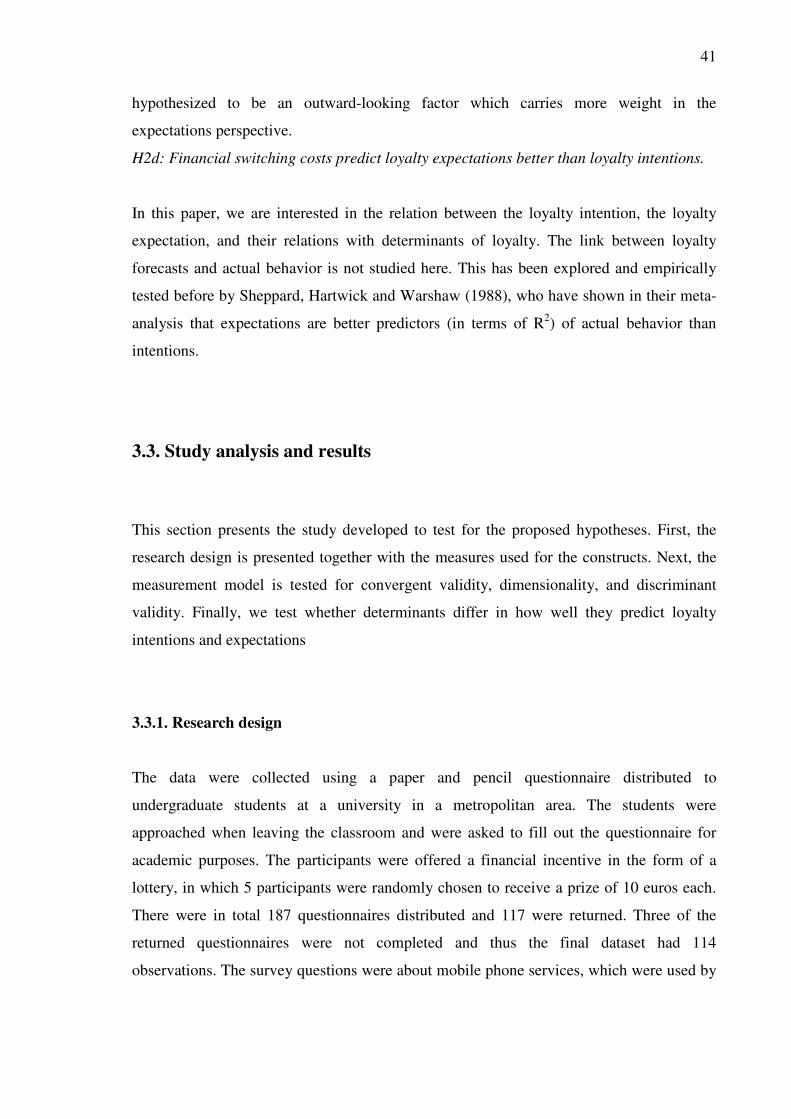
41

hypothesized to be an outward-looking factor which carries more weight in the

expectations perspective.

H2d: Financial switching costs predict loyalty expectations better than loyalty intentions.

In this paper, we are interested in the relation between the loyalty intention, the loyalty

expectation, and their relations with determinants of loyalty. The link between loyalty

forecasts and actual behavior is not studied here. This has been explored and empirically

tested before by Sheppard, Hartwick and Warshaw (1988), who have shown in their meta-

analysis that expectations are better predictors (in terms of R2) of actual behavior than

intentions.

3.3. Study analysis and results

This section presents the study developed to test for the proposed hypotheses. First, the

research design is presented together with the measures used for the constructs. Next, the

measurement model is tested for convergent validity, dimensionality, and discriminant

validity. Finally, we test whether determinants differ in how well they predict loyalty

intentions and expectations


The data were collected using a paper and pencil questionnaire distributed to

undergraduate students at a university in a metropolitan area. The students were

approached when leaving the classroom and were asked to fill out the questionnaire for

academic purposes. The participants were offered a financial incentive in the form of a

lottery, in which 5 participants were randomly chosen to receive a prize of 10 euros each.

There were in total 187 questionnaires distributed and 117 were returned. Three of the

returned questionnaires were not completed and thus the final dataset had 114

observations. The survey questions were about mobile phone services, which were used by

42

all the respondents. A pre-study had been done with 32 graduate students in order to ensure

the clarity of items used.

Table 3.1: Items used for constructs and tests of the measurement model

Items Loading Error C α VE VS

Switching Intention

I1 I plan to change my mobile services provider. .81 .24 .77 .88 .73 .56

I2 I intend to start using another provider. .69 .35 .65

I3 I will change my provider within the next year. .80 .23 .78

Switching Expectation

E1 I expect to change my provider in the future. .78 .22 .77 .90 .73 .47

E2 How likely is that you will stay with your current

mobile phone services provider? .76 .24 .76

E3 How likely is that you will change it in the future? .76 .28 .71

Satisfaction

S1 How satisfied or dissatisfied are you with your

current mobile phone services provider? .83 .16 .84 .93 .80 .71

S2 Overall, how do you feel about it? .86 .11 .89

S3 How well does it meet your needs at this time? .80 .29 .70

Trust

T1 I feel can trust my mobile phone services provider. .82 .23 .77 .88 .71 .71

T2 My provider is responsive to customers’ problems. .70 .34 .65

T3 I feel my mobile services provider is reliable. .75 .26 .75

Attitude towards switching

A1 It would take me a lot of effort to choose another

mobile services provider. .64 .29 .56 .84 .61 .56

A2 I do not feel like going through the whole process of

changing the mobile provider. .76 .31 .70

A3 Going through the process of changing to another

provider would be an unpleasant experience. .67 .32 .60

Perceived financial switching cost

F1 Changing my mobile provider would cost me

money. .83 .21 .84 .90 .79 .31

F2 If I choose another services provider my costs will

go up. .80 .19 .77

F3 Changing my mobile service provider would have

significant financial impact for me. * .34 .11 .32

Satorra-Bentler scaled χ2 = 161.17 (104 df); p-value = .000; NFI = .88; NNFI = .93; CFI = .95;

RMSEA = .071 (90% interval: .048-.091); * - item F3 is not used in the measurement model

C= Communality; α= Cronbach Reliability; VE=Variance Extracted;

VS= Maximum Variance Shared (Fornell & Larcker test)

43

The dependent variables were consumers’ forecasts of switching their mobile provider in

the future. The items for the constructs of switching intentions and switching expectations

were measured on a ten-point scale and based on Warshaw and Davis (1985), Zeithaml,

Berry, and Parasuraman (1996), and Soderlund and Ohman (2005). Satisfaction was

measured using items from Fornell (1992). Attitude toward the switching was based on

Bansal and Taylor (1999). Trust was measured in line with Morgan and Hunt (1994).

Switching costs measured in financial terms were based on the work of Bansal and Taylor

(1999), Burnham, Frels, and Mahajan (2003), and Jones, Mothersbaugh, and Beaty (2002).

For all determinants of loyalty a seven-point scale was used. All the variables were

cognitive, subjective variables and therefore each was measured using three items (Table

3.1). Table 3.1 also includes tests of the measurement model.

3.3.2. Measurement model

The variables of interest in this study are perceptual determinants, collected through a

survey and each based on multiple items. Testing the relations between variables is based

on a structural equation modeling. The difference in the switching intentions and the

switching expectations constructs (hypothesis H1) is explored by testing the measurement

model: convergent validity test, dimensionality test, and discriminant validity test (Kline,

1998). Testing the hypotheses H2a to H2d is based on comparing how selected

determinants influence different dependent variables (intentions and expectations). The

comparison is based on the fit of structural models.

Table 3.2: Correlations of study constructs (the data are standardized)

X1 X2 X3 X4 X5

X1 - Switching Intention

X2 - Switching Expectation .67

X3 - Satisfaction -.83 -.47

X4 - Attitude towards switching -.20 -.26 -.43

X5 - Trust -.78 -.56 .83 -.32

X6 - Perceived financial switching cost -.45 -.65 .11 .20 .05

44

The correlations of the constructs are reported in Table 3.2. The exploratory factor analysis

is done, using the principal component analysis and the varimax rotation. The Cronbach’s

alpha supports the reliability of the constructs with values between .84 and .93 (Table 3.1).

The F3 item for the perceived financial switching cost construct has a low loading (.34)

and a low communality (.32) compared with other items in the factor analysis. The

measurement model without the item F3 has a significantly better fit and this item is

removed from further analysis. By examining the items F1, F2, and F3, we can observe

that the items F1 and F2 measure the absolute impact of switching costs, while F3

measures the impact relative to respondents’ overall wealth. The switching costs in

absolute terms seem to matter for consumers, however compared to their overall wealth

they could be perceived as not so relevant. This could explain low loadings of F3.

The convergent validity is tested with a confirmatory factor analysis including all the

constructs (Bagozzi, Yi, and Philips, 1991). A common method factor is included as a

means of accounting for random and systematic errors (Podsakoff et al, 2003). With

regards to testing structural equation models, there is no consensus about which test is best

for evaluating the fit of the model. Several different tests are therefore used jointly as

advised by Marsh (1994). We use a chi-square test with a scaling correction to improve the

approximation of the goodness-of-fit test statistics (Satorra and Bentler, 1988). An

acceptable model fit is indicated when a chi-square value divided by degrees of freedom is

less than 5. Next the following fit indices are also used with acceptable fits indicated by

specific values: NNFI (Non-Normed Fit Index) and CFI (Comparative Fit Index) values

exceeding .90 and a RMSEA (Root Mean Square Error) value less than .08 (Marsh, 1994).

In Table 3.1 we can observe that the measurement model has a satisfactory fit: Satorra-

Bentler scaled chi-square = 161.17 (104 df); NFI = .88; NNFI = .93; CFI = .95; RMSEA =

.071 (.048-.091). Both the exploratory and the confirmatory factor analysis support the

convergent validity of constructs.

The discriminant validity between variables exists when there is a low correlation between

items measuring different variables. The following test, proposed by Fornell and Larcker

(1981), is used. For each of the variables we calculate the variance extracted (VE) by the

items used to measure this specific variable. Next, the variance shared (VS) of a specific

variable is the highest variance shared with any other variable used in the analysis. When

for a specific variable the variance extracted (VE) is larger than the variance shared (VS),

45

then it is sufficiently different from other variables. From Table 3.1 we can conclude that

all the variables satisfy the discriminant validity test.

The validity of the construct aggregation is tested with the dimensionality test (Bagozzi

and Edwards, 1998). Two structural models are compared; one with the switching

intentions and the switching expectations modeled as a single construct (Figure 3.1) and

another, where they are modeled as two different constructs (Figure 3.2). Both models also

include all the other variables.

Figure 3.1: One factor model Figure 3.2: Two factor model

Comparing the fit of structural equation models is based on the standard test of a chi-

square difference (Anderson and Gerbing, 1988; Brady et al, 2005). The chi-square

difference is the chi-square fit statistic for one model minus the corresponding value for the

second model. The difference in the chi-square statistic is evaluated against the

corresponding difference in the degrees of freedom. If the chi-square difference is

significant, then there is a difference in the model fit.

The single-factor model (Figure 3.1) has the following fit: Satorra-Bentler scaled chi-

square = 250.80 (109 df); NFI = .79; NNFI = .83; CFI = .87; RMSEA = .11 (.090 -.125).

The two-factor model (Figure 3.2) has the following fit: Satorra-Bentler scaled chi-square

= 161.17 (105 df); NFI = .88; NNFI = .93; CFI = .95; RMSEA = .071 (.048-.091). The

two-factor model fits the data better as the chi-square difference is significant (chi-square

difference = 89.63; difference in degrees of freedom = 4; p < .01). The measurement model

is therefore supported by all three tests: the convergent validity test, the dimensionality

test, and the discriminant validity test.

Switching Intentions & Expectations

I1

I2

I3

E1

E2

E3

Switching Intentions & Expectations

I1

I2

I3

E1

E2

E3

Switching Intentions

Switching Expectations

I1

I2

I3

E1

E2

E3



I1

I2

I3

E1

E2

E3

46

3.3.3. Structural path model with determinants of loyalty

The difference between the switching intentions and the switching expectations constructs

is further tested using determinants of loyalty as the explanatory variables. Three structural

models are explored, the first one with a single dependent variable (Figure 3.3), the second

one with two dependent variables (Figure 3.4), and the third model with two dependent

variables, however including the effect that the intentions variable has on the expectations

variable (Figure 3.5). In all three models four explanatory constructs are used: satisfaction,

trust, perceived financial switching cost, and attitude towards switching.

Figure 3.3: The model of determinants of loyalty and one dependent variable.

Trust

Switching Intentions &

Expectations

Attitude towards

the switching

Satisfaction

Perceived Financial

switching cost

S1

S2

S3

F1

F2

T1

T2

T3

A1

A2

A3

I1

I2

I3

E1

E2

E3

Trust

Switching Intentions &

Expectations

Attitude towards

the switching

Satisfaction

Perceived Financial

switching cost

S1

S2

S3

F1

F2

T1

T2

T3

A1

A2

A3

I1

I2

I3

E1

E2

E3

47

Figure 3.4: The model of loyalty determinants and two dependent variables

Figure 3.5: The model with two dependent variables, where intentions influence

expectations

In Table 3.3 the comparison of models is done with corresponding fit indices. As we can

observe the best model is the simple two dependent variables model shown in Figure 3.4.

Using the difference in chi-square and the difference in degrees of freedom, the selected

models are compared and the model shown in Figure 3.4 fits data significantly better than

Trust


Attitude towards the switching

Satisfaction


Perceived Financial switching cost

S1

S2

S3

F1

F2

T1

T2

T3

A1

A2

A3

I1

I2

I3

E1

E2

E3

Trust



Satisfaction



S1

S2

S3

F1

F2

T1

T2

T3

A1

A2

A3

I1

I2

I3

E1

E2

E3

Trust



Satisfaction



S1

S2

S3

F1

F2

T1

T2

T3

A1

A2

A3

I1

I2

I3

E1

E2

E3

Trust



Satisfaction



S1

S2

S3

F1

F2

T1

T2

T3

A1

A2

A3

I1

I2

I3

E1

E2

E3

48

the two models in Figures 3.3 and 3.5. Therefore, this is an additional support that

intentions and expectations are different constructs.

Table 3.3: Testing models for the difference in the path coefficients

Fit indices Models

df χ2 NNFI CFI RMSEA

Model fit comparison

Single factor

(Figure 3.3)

109 301.54 .76 .81 .110 ∆ χ2

/ ∆ df = 22.88 **

Two factor (Figure 3.4) 104 187.13 .90 .93 .077 Best model

Two factor with

interaction (Figure 3.5)

103 236.47 .85 .88 .092 ∆ χ2

/ ∆ df = 49.43 **

** - significant at p < .01

Table 3.4: Direct effects of determinants of loyalty

Dependent variables - β (s.e.)

Independent variables Switching Intention Switching Expectation

Satisfaction - .57 (.23) ** n.s.

Attitude towards switching - .52 (.19) ** n.s.

Trust - .44 (.21) * - .73 (.23) **

Perceived switching cost - .24 (.09) ** .49 (.14) **

R2 .51 .32

Overall fit indices: Satorra-Bentler scaled χ2 = 187.13 (104 df); p-value = .000; NFI = .88;

NNFI = .90; CFI = .93; RMSEA = .077 (.061-.091); * - p < .05; ** - p < .01

β – regression coefficient; s.e. – standard error

Table 3.4 shows the specific results of testing the most appropriate model, the structural

model with two dependent variables (Figure 3.4). For each of the dependent variables the

coefficients of determinants are shown together with their standard errors. All the studied

49

determinants have been previously found to have a positive effect on loyalty. The

dependent variables are switching (disloyalty) forecasts and the obtained negative sign of

coefficients corresponds to the literature.

3.3.4. Comparing coefficients between the switching intentions and expectations

In hypotheses H2a to H2d we have proposed that the determinants of loyalty differ in how

they influence the switching intentions and the switching expectations. In Table 3.3 we can

observe that the coefficients between the intentions and the expectations appear to be

different, which is in line with H2a to H2d. Both satisfaction and attitude towards

switching have a stronger effect on switching intention than switching expectation. On the

other hand, trust and perceived switching costs have a stronger effect on expectations than

intentions. In order to test whether these differences in coefficients are significant, the two

factor model based on Figure 3.4 is taken as the baseline model. Next, for each of the

determinants a constrained structural model is constructed, where the coefficient of the

specific determinant is held equal for both dependent variables. For example, the

constrained model for satisfaction is based on Figure 3.4 with the constraint that the two

coefficients for the switching intentions and the switching expectations are the same.

The baseline (unconstrained) model and the four constrained structural models are tested

for fit and the fit indices are found in the Table 3.5. Next, the fit of each of the four

constrained structural models is compared with the fit of the baseline model. The chi-

square difference test provides support that the baseline model fits the data significantly

better than any of the constrained models. Therefore, support is found for each of the

hypotheses H2a to H2d. Based on these empirical results we can conclude that the

switching intentions and the switching expectations differ in their explanatory variables.

50

Table 3.5: Testing models for the difference in the path coefficients

Fit indices Constrained coefficient

in the model (hypothesis) df χ2 NNFI CFI RMSEA

Model comparison

(all ∆ df = 1)

None (baseline model) 104 187.13 .90 .93 .077 Baseline model

Satisfaction (H2a) 105 257.34 .82 .85 .112 ∆ χ2

= 70.21 **

Attitude towards

switching (H2b)

105 223.78 .85 .88 .093 ∆ χ2

= 36.65 **

Trust (H2c) 105 205.07 .87 .91 .088 ∆ χ2

= 17.94 **

Switching cost (H2d) 105 217.67 .86 .90 .092 ∆ χ2

= 30.54 **

** - significant at p < .01



The purpose of this paper is to extend our understanding of how determinants influence

customer loyalty. We base our study on the difference between the intentions and

expectations perspectives. A proposition was made that measuring customer loyalty with

these two perspectives triggers different cognitive processes with regards to forecasting

loyalty. When customers are asked about their intentions, they tend to take a more inward-

looking perspective and focus on the factors that are under their control, such as their own

motivation and reasons for future behavior. On the other hand, when customers are asked

about their expectations, they tend to take a more outward-looking perspective and focus

more on the factors beyond their control, such as the obstacles and risk associated with

loyalty behavior.

51

We find support that determinants of loyalty differ in how they influence loyalty intentions

and expectations. These differences in effects are based on the inward or outward-looking

nature of determinants. Satisfaction and Attitude towards switching are more inward-

looking determinants and are found to be better predictors of loyalty intentions as opposed

to loyalty expectations. On the other hand, Trust and Perceived financial switching costs

are more outward-looking and are found to be better predictors of loyalty expectations as

opposed to loyalty intentions.

This study therefore contributes to the discussion about the roles and influence of

determinants of loyalty (e.g., Oliver, 1999; Brady et al, 2005). As mentioned previously,

there is still no agreement about which determinants are central to loyalty. Our results

suggest that satisfaction is the most important determinant for loyalty intentions, while

trust is the most important determinant for loyalty expectations. In previous research, either

intentions or expectations have been used to capture forecasts and therefore differing

empirical findings can be due to researchers using different measures.

Loyalty intentions and expectations have been previously proposed to be different

constructs (Warshaw and Davis, 1985; Sheppard et al, 1988; Soderlund and Ohman, 2005).

Here, a stronger support is provided, as they differ both in the measurement model as well

as how they are influenced by determinants (Zaltman et al, 1982).

The question now remains, which of the two measures of loyalty should be used, when

aiming to identify its determinants? The answer is that they can both be useful, given that it

is understood that they evoke different perspectives. When loyalty behavior with few

obstacles is explored, such as word-of-mouth, then the intentions perspective might

provide a better insight about which determinants matter most. However, when the studied

loyalty behavior is more complex and depends on external factors, such as switching the

service provider, then the expectations perspective might be more suitable.


Marketing researchers interchangeably use intentions and expectations measures, which

can lead to misleading findings about how determinants influence loyalty. When

52

measuring loyalty with an intention question, inward-looking determinants, such as

satisfaction, would be supported as central. However, if loyalty expectations were used,

then outward-looking determinants, such as trust and switching costs, would emerge as key

to customer loyalty. Using different measures would lead to different findings and

therefore different focus and actions in loyalty programs.

The intentions and expectations measures provide different views on loyalty and can both

be of interest to managers. Loyalty intentions signal customer’s motivation to remain loyal,

which can lead to a positive word of mouth, willingness to pay more, or up-grade the

service. However, companies would also like their customers to stay loyal even in the case

of a bad service or a competitive offer. The construct of loyalty expectation signals this

deeper commitment to the current provider. In order to achieve a higher level of loyalty

expectation, companies should refocus their attention and resources to build trust with their

customers as well as to increase perceived switching costs (e.g., penalty fees).

Our findings are important both for companies that are defending their customer base,

typically incumbents, as well as companies trying to expand their customer base, typically

new entrants in the market. The first group is working heavily on increasing satisfaction,

trust, switching costs, and attitude towards switching behavior. On the contrary, the new

entrants try to win customers over by decreasing switching costs and changing attitude

towards switching by making it easier for customers to switch. The new entrants can also

try to undermine trust in the incumbent.


Previous research has identified that expectations are better predictors of actual behavior

compared to intentions (Sheppard et al, 1988; Soderlund and Ohman, 2005). A limitation

of this study is that an actual behavior was not measured. This would make the study richer

and provide a further test of the relation between loyalty forecasts and behavior.

Nevertheless, the focus of this study is on the relation between determinants of loyalty and

forecasts of loyalty. Understanding this aspect of loyalty is important as many academics

and practitioners use customer forecasts and not actual behavior to measure loyalty, draw

conclusions, and make decisions.

53

The second limitation comes from the sample, both in terms of the small sample size as

well as the student population. The hypotheses would need to be tested using a broader

population and a bigger sample. Nevertheless, as the effects are found within such a

homogenous group, it is proposed that they are also present in the broader population.

Further studies done in other industries and countries would provide tests for generalizing

the proposition.

Another important limitation is that only switching behavior was studied. Zeithaml et al

(1996) have proposed that in order to gain the full picture of relevant factors in customer

relationship management, one needs to study a broader set of behaviors: such as positive

and a negative word of mouth, complaining, cross, and up-selling. In addition to this,

effects of other determinants of loyalty would need to be explored, such as value for

money, quality, cost, length of relationship, and customer characteristics (e.g. gender or

age).

54

Chapter 4

Counterbalance effect of determinants of loyalty:

Usage and Satisfaction

4.1. Introduction

Customer loyalty remains one of the key topics on managers’ agenda, driven by findings

that changes in loyalty can have a big impact on a financial performance of companies

(Reichheld, 1996; Zeithaml et al, 2006). Different possible determinants of customer

loyalty have been identified; however their influence on loyalty is still unclear. In this

paper we focus on two issues with regards to the influence of determinants. First, for some

determinants, mixed empirical results involving both a positive and a negative effect have

been found. An example of such a determinant is the level of customer’s usage of products

or services, which in some studies has been found to have a positive effect on loyalty,

while in others the supported effect was negative. Second, for some other determinants

there is a consensus about how they influence loyalty, however their effect is not always

found. An example of the later is customer satisfaction which has a positive effect on

loyalty, however many studies have found that satisfied customers are not necessarily

loyal.

55

This uncertainty about the effects of determinants can cause problems for companies.

Consider a situation, where managers intend to influence a determinant, which has been

found to have both a positive and a negative effect on loyalty. An effort to increase loyalty

could turn out to have the opposite effect and actually cause loyalty to decrease. In other

situations, intentions to increase loyalty can be fruitless and the associated costs then lead

to a negative financial impact.

Figure 4.1: An example of a counterbalance effect of usage in the case of variable costs

Figure 4.1 shows an example of a mobile phone service usage as a determinant of loyalty.

Mobile phone service usage by itself is beneficial for consumers and thus has a positive

direct effect on loyalty. However, in the context of mobile services there are variable costs,

which are positively related to usage. Therefore, usage drives up costs, which negatively

influence loyalty, and consequently usage can have a negative indirect effect on loyalty,

mediated through costs.

When researching loyalty, the hypothesized influence of a determinant is implicitly

assumed to be direct and to have either a positive or a negative effect. In addition, effects

are typically presented in a simple manner; such as, if you influence a specific determinant,

then loyalty will follow. However, economic exchanges are complex systems1, where

multiple causal pathways are common between independent and dependent variables

(Bagozzi, 1975; Reidenbach and Oliva, 1981, Sterman, 2000). We define a counterbalance

effect to exist when a positive and a negative effect coexist, with one being direct and the

other indirect.

1 System is defined as a set of entities, real or abstract, comprising a whole where each component interacts

with or is related to at least one other component (Sterman, 2000).

+

_

+Customer loyalty

decision

Context

Usage

Cost_

+

_

+Customer loyalty

decision

Context

Usage

Cost_

56

In this paper, we challenge the implicit assumption that determinants influence loyalty with

simple effects. A hypothesis is proposed that some determinants have multiple causal

pathways with opposite signs and thus a counterbalance effect. The causal pathways (direct

and indirect) can neutralize each other and diminish the total effect, which could explain

why some determinants do not always translate into loyalty. On the other hand, the direct

effect could prevail in some contexts and the indirect effect in others, which could be the

reason why for some determinants sometimes positive and other times negative effects are

found.

In the next section, we discuss determinants of loyalty and their effects, develop the

counterbalance proposition, and explain a test based on partial mediation. This is followed

by testing the counterbalance effect in two distinct studies. In the first study, the effects of

usage are tested with consumer behavior data. In the second study, the effects of

satisfaction with the provider are tested with survey data. Next, findings and contributions

of this paper are discussed and managerial implications are presented. Finally, we

acknowledge the limitations related to testing the propositions as well as provide

suggestions for further research.

4.2. Theory and proposition

4.2.1. Determinants of loyalty and their effects

Various determinants of loyalty have been identified in marketing research and can be

divided into two groups: perceptual determinants and behavioral determinants (Verhoef et

al, 2007). The perceptual determinants are related to how customers perceive different

dimensions of a customer-firm relationship and are normally subjective constructs, such as,

satisfaction, trust, perceived value, and perceived switching costs (Johnson and Fornell,

1991; Morgan and Hunt, 1994; Sirdeshmukh, Singh, and Sabol, 2002; Burnham, Frels, and

Mahajan, 2003). On the contrary, the behavioral determinants are consequences of

customer actions and can be objectively measured, such as, usage, length of relationship,

and number of products or services purchased (Bolton and Lemon, 1999; Keaveney and

57

Parthasarathy, 2001; Ganesh, Arnold, and Reynolds, 2000; Verhoef, 2003). The effects of

the behavioral determinants are typically modeled as mediated through the perceptual

determinants. However, understanding how behavioral determinants influence loyalty is

important as in many situations these variables are the only information (from customer

databases) available to companies about their customers.

Numerous studies have been dedicated to determinants of loyalty. Nevertheless, there is

still a lack of a unifying framework about how determinants influence loyalty and what are

the signs of their effects (positive or negative). An example of such a determinant is

customer usage of products or services (Bolton and Lemon, 1999). Keaveney and

Parthasarthy (2001) have found support that usage has a positive effect on loyalty. On the

other hand, Prelec and Loewenstein (1998) have suggested that in product categories with

variable costs, usage can have both a positive and a negative effect on loyalty. The authors

however have not proposed a model nor tested for the effect of costs on loyalty. For some

other determinants, there is an agreement on how they influence loyalty, however their

effects are not always found to be significant. For example, loyal customers are typically

satisfied; however satisfied customers are not necessarily loyal (Oliver, 1999). Usage and

satisfaction are the two determinants of loyalty studied in this paper and are further

discussed in the next sections, where each of the studies is explained in more detail.

4.2.2. Complexity of economic exchange systems

A system is defined as a set of components, real or abstract, where each component

interacts with or is related to at least one other component (Sterman, 2000). Each system

can have various subsystems, depending on where researchers put the boundaries of the

studied subsystem. Sterman (2000) has proposed that there are two types of complexities

found in systems: a detail complexity and a dynamic complexity. The detail complexity is

related to which components are in the system, while the dynamic complexity is related to

the dynamic structure between the components.

An economic exchange system consists of a customer and a company, including flows of

goods or services and related financial compensations. Economic exchanges have been

proposed to be complex systems, both in terms of their dynamics as well as the factors that

58

influence them (Boulding, 1956; Bagozzi, 1975; Coleman, 1986; Reidenbach and Oliva,

1981; Cronin et al, 2000; Brady et al, 2005).

There are two interrelated perspectives to account for the detail complexity in economic

exchanges when loyalty and its determinants are explored. First, some researchers propose

that an existing determinant has several different subdimensions, which are proposed to be

different construct. For example, Ganesh, Arnold, and Reynolds (2000) have proposed that

there are two types of involvement: a purchase and an ego involvement. Similarly,

Burnham, Frels, and Mahajan (2003) have suggested three types of switching costs: a

financial, a procedural, and a relational switching cost.

Second, the detail complexity can be also addressed by redefining the boundaries of the

studied system and thus including additional determinants of loyalty. For example, Mittal,

Tsiros, and Kumar (1999) have studied a consumption system consisting of two

subsystems, a product (car) subsystem and a service (car repair service) subsystem. These

two subsystems are closely linked and consumers were found to attribute the outcomes in

one subsystem to factors in the other subsystem. In particular, satisfaction with the car was

found to have a positive effect on loyalty to the car repair service. On the other hand,

satisfaction with the car repair service had a positive effect on loyalty to the same car

brand.

When it comes to the dynamic complexity there are three types of effects frequently

proposed: moderating effects, mediating (indirect) effects, and non-linear relations. For

example, customer characteristics have been found to moderate the effect satisfaction has

on loyalty (Mittal and Kamakura, 2001; Homburg and Giering, 2001); the variable

satisfaction influences loyalty with different strengths for each gender. Further, the

variable trust has been found to mediate the effect of satisfaction (Garbarino and Johnson,

1999; Sirdeshmukh, Singh, and Sabol, 2002). Trust as a determinant of loyalty mediates

the indirect effect that satisfaction has on loyalty. In addition, recent research has

emphasized the non-linear relation influence of some determinants of loyalty, such as

customer characteristics and satisfaction (e.g., Mittal and Kamakura, 2001; Homburg,

Koschate, and Hoyer, 2005).

59

4.2.3. Counterbalance proposition

In complex systems, multiple causal pathways are common between independent and

dependent variables (Sterman, 2000). This coexistence of multiple effects is possible when

apart from a direct effect there is also an indirect effect, mediated through another variable.

However, these causal pathways can have opposite effects (positive and negative) on the

dependent variable, which is termed a counterbalance effect. The counterbalance effect

takes into account an indirect (mediated) effect and is therefore classified as a dynamic

complexity phenomenon. An example of a counterbalance effect of usage was discussed in

the introduction to this paper. In particular, usage has a direct positive effect on loyalty and

when linked to a variable cost, it can have an indirect negative effect, mediated through

costs. Some determinants can therefore have a counterbalance effect on loyalty. This could

provide an explanation for both the incoherent sign of effects, i.e. positive and negative

effects, as well the neutralized total effects, i.e. lack of effect, for some determinants.

Research Proposition:

Determinants of loyalty can have two simultaneous causal pathways, a direct and an

indirect. These two causal pathways can have different (positive and negative) effects on

loyalty, a counterbalance effect.

4.2.4. Test used for the counterbalance effect

In this section we present the test for the counterbalance effect. It is based on a test for

partial mediation, developed by Baron and Kenny (1986). When testing for partial

mediation, models as in Figure 4.2 are explored, where an independent variable has both a

direct and an indirect, partially mediated, effect. Throughout this section we use an

example of mobile phone services with the following variables: usage as an independent

variable, cost as a mediator, and customer loyalty as an outcome variable.

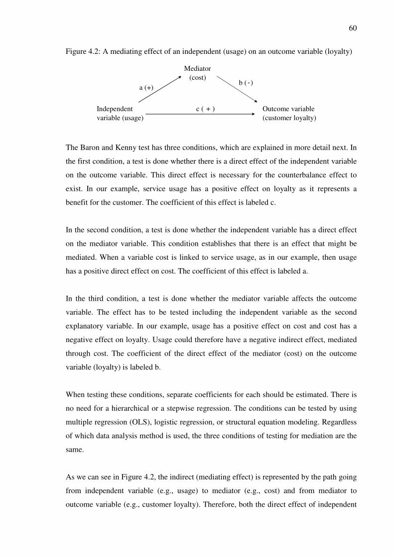
60

Figure 4.2: A mediating effect of an independent (usage) on an outcome variable (loyalty)

The Baron and Kenny test has three conditions, which are explained in more detail next. In

the first condition, a test is done whether there is a direct effect of the independent variable

on the outcome variable. This direct effect is necessary for the counterbalance effect to

exist. In our example, service usage has a positive effect on loyalty as it represents a

benefit for the customer. The coefficient of this effect is labeled c.

In the second condition, a test is done whether the independent variable has a direct effect

on the mediator variable. This condition establishes that there is an effect that might be

mediated. When a variable cost is linked to service usage, as in our example, then usage

has a positive direct effect on cost. The coefficient of this effect is labeled a.

In the third condition, a test is done whether the mediator variable affects the outcome

variable. The effect has to be tested including the independent variable as the second

explanatory variable. In our example, usage has a positive effect on cost and cost has a

negative effect on loyalty. Usage could therefore have a negative indirect effect, mediated

through cost. The coefficient of the direct effect of the mediator (cost) on the outcome

variable (loyalty) is labeled b.

When testing these conditions, separate coefficients for each should be estimated. There is

no need for a hierarchical or a stepwise regression. The conditions can be tested by using

multiple regression (OLS), logistic regression, or structural equation modeling. Regardless

of which data analysis method is used, the three conditions of testing for mediation are the

same.

As we can see in Figure 4.2, the indirect (mediating effect) is represented by the path going

from independent variable (e.g., usage) to mediator (e.g., cost) and from mediator to

outcome variable (e.g., customer loyalty). Therefore, both the direct effect of independent

Mediator

(cost)

Independent

variable (usage)

Outcome variable

(customer loyalty)

a (+)

c ( + )

b ( - )

61

variable on mediator (coefficient a) and the direct effect of mediator on outcome variable

(coefficient b) have to be different from zero. This is equal to the product of coefficients a

and b, a*b, to be different from zero. The value of a*b, is the indirect effect and is called

the amount of mediation. To test the null hypothesis that a*b = 0, one can test that both

coefficients a and b are zero; however, a single test is more common and highly

recommended (MacKinnon, Lockwood, Hoffman, West, and Sheets, 2002). When going

through the conditions of Baron and Kenny test, we obtain the value of the coefficient a

and its standard error, labeled as sa, as well as the value of the coefficient b and its standard

error, labeled as sb. Next, we calculate the value of a*b / sqrt (b2*sa

2 +

a

2*sb

2) and treat the

ratio as a Z test (Sobel, 1982). Other tests for mediation have been proposed, but the Sobel

test is by far the most commonly reported (Shrout and Bolger, 2002).

We test the existence of the counterbalance effect with two studies. In the first study we

explore the effect of usage as a behavioral determinant; while in the second study we

explore the effect of satisfaction as a perceptual determinant. Both studies are explained in

the next sections.

4.3. Study 1: Usage as a determinant of loyalty

Usage as a determinant of customer loyalty has been included in a number of studies;

however there is no unifying framework on how it influences loyalty. In addition, the

empirical evidence is mixed with support for both a positive and a negative effect. For

example, Keaveney and Parthasarthy (2001) have proposed that frequent usage provides

customers with more accurate and realistic performance expectations and thus decreases

possible dissatisfactions. They have further argued that frequent usage also increases the

knowledge and the positive attitude towards a specific service or product. Therefore,

customers with a higher level of usage would thus find it harder to change the product or

the service they are using. This framework however does not address the relation between

usage and costs. Prelec and Loewenstein (1998) have suggested that in contexts with

variable costs, usage has both a positive and a negative effect on loyalty. This is because

usage represents a benefit for customers and positively influences loyalty. However, in

62

some contexts usage increases cost and cost represents a disutility for consumers.

Therefore, the higher the usage of a service or product, the higher the cost, and

consequently the higher the likelihood for consumers to be disloyal.

In this first study, we explore the effect of usage on customer loyalty within a mobile

phone service context. Given the variable costs within mobile services, we test the

proposition that usage has a counterbalance, both a positive and a negative, effect on

loyalty.

4.3.1. Counterbalance conditions

In this section three conditions are developed to test the counterbalance effect of usage.

The dependent variable used here is the customers’ act of exiting the relationship with their

mobile service provider in a specific month (disloyalty). In the next paragraphs all three

conditions for counterbalance effect are presented with this dependent variable.

When customers exit the relationship with their service provider, this represents an act of

disloyalty. The variable usage has a positive effect on loyalty and therefore has a negative

effect on exiting. Based on this, we develop the first Baron and Kenny condition:

Condition 1a: Usage has a negative effect on Exiting.

The context of mobile phone services involves variable costs. Therefore, with an increase

in the service usage the customer costs increase as well. The second condition is the

following:

Condition 1b: Usage has a positive effect on Costs.

Increasing costs negatively influence customer perceived value and loyalty. Therefore,

costs have a positive effect on exiting the relationship (disloyalty). Since usage has a

positive effect on costs, it could have a positive indirect effect on exiting, mediated through

costs.

Condition 1c: Costs have a direct effect on Exiting and mediate a positive effect of Usage.

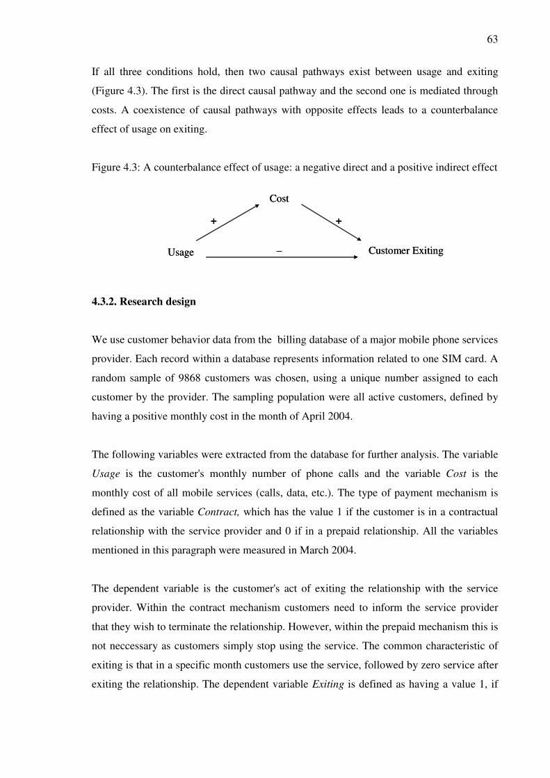
63

If all three conditions hold, then two causal pathways exist between usage and exiting

(Figure 4.3). The first is the direct causal pathway and the second one is mediated through

costs. A coexistence of causal pathways with opposite effects leads to a counterbalance

effect of usage on exiting.

Figure 4.3: A counterbalance effect of usage: a negative direct and a positive indirect effect


We use customer behavior data from the billing database of a major mobile phone services

provider. Each record within a database represents information related to one SIM card. A

random sample of 9868 customers was chosen, using a unique number assigned to each

customer by the provider. The sampling population were all active customers, defined by

having a positive monthly cost in the month of April 2004.

The following variables were extracted from the database for further analysis. The variable

Usage is the customer's monthly number of phone calls and the variable Cost is the

monthly cost of all mobile services (calls, data, etc.). The type of payment mechanism is

defined as the variable Contract, which has the value 1 if the customer is in a contractual

relationship with the service provider and 0 if in a prepaid relationship. All the variables

mentioned in this paragraph were measured in March 2004.

The dependent variable is the customer's act of exiting the relationship with the service

provider. Within the contract mechanism customers need to inform the service provider

that they wish to terminate the relationship. However, within the prepaid mechanism this is

not neccessary as customers simply stop using the service. The common characteristic of

exiting is that in a specific month customers use the service, followed by zero service after

exiting the relationship. The dependent variable Exiting is defined as having a value 1, if

Cost

Usage Customer Exiting

+

_

+

Cost


+

_

+

64

there is a drop from using the service in March 2004 to not using the service in May 2004;

otherwise the variable Exiting has a value 0.


In this section the analysis and the results of testing the counterbalance effect are

presented. Condition 1a is tested with a logistic regression on the binary dependent

variable Exiting, Usage as the independent variable, and Contract as a moderating variable.

The first column of Table 4.1 shows the regression coefficients with the coefficient of

Usage being significant and negative. The coefficient of the variable Contract is also

significant and negative, which means that the contract customers have a lower likelihood

of exiting than the prepaid customers. There is no moderating effect found for the variable

Contract. Condition 1a is supported as Usage has a negative effect on Exiting for both the

prepaid and the contract customers.

Table 4.1: Testing a counterbalance effect of usage

Condition 1a:

Log. regression

Condition 1b:

Linear regression

Condition 1c:

Log. regression

Exiting (β, s.e.) Cost (β, s.e.) Exiting (β, s.e.)

Usage - .99 (.37) ** .81 (.01) ** - 1.40 (.42) **

Cost n.s.

Contract - .91 (.22) ** .24 (.01) ** - .94 (.23) **

Usage X Contract n.s. - .19 (.01) ** n.s.

Cost X Contract .41 (.17) **

Model (N=9868) χ2

= 79.1 (5 df),

p < .001

R2

= .59 χ2

= 85.3 (7 df),

p < .001

** - significant at .01; n.s. – not significant; β – reg. coefficient, s.e. – standard error

Condition 1b is tested with a linear regression on the dependent variable Cost, the

independent variable Usage, and the moderating variable Contract (Table 4.1, second

column). The variable Contract has a significant moderating effect. The coefficient of

65

Usage for the prepaid customers is .81 (.01) and for the contract customers is .62 (.81 - .19)

(.01). Therefore, the variable Usage has a positive effect on Cost for both the prepaid and

the contract customers and Condition 1b is supported.

Condition 1c is tested with a logistic regression, where Exiting is the dependent variable,

Usage and Cost are the independent variables, and Contract is the moderator (Table 4.1,

third column). For the prepaid customers (Contract = 0), the coefficient for the variable

Cost is not significant and therefore the third condition is not supported. The coefficient of

Usage is significant as well as the coefficient of the interaction between Cost and Contract.

Condition 1c is supported for the contract customers.

The mediation effect for the contract customers is also tested with the Sobel statistic,

which is - 4.73 and significant (p < .01) (Sobel, 1982; Baron and Kenny, 1986). The value

of a*b is therefore found to differ from zero and the mediation hypothesis is supported.

The findings of this first study are the following. The counterbalance effect of Usage on

Exiting is not supported for the prepaid customers (Figure 4.4). However, for the contract

customers Usage has a negative direct effect and a positive indirect effect on Exiting

(Figure 4.5). We therefore find counterbalance effect to exist in one payment mechanism,

while support for the other one is not found. Based on this we conclude that usage can have

a counterbalance effect on customer loyalty, however it seems that the existence of the

effect depends on the context.

Figure 4.4: A counterbalance effect of Usage for the Prepaid customers

Figure 4.5: A counterbalance effect of Usage for the Contract customers

Cost


+ .81

- 1.40

n.s.

Cost


+ .81

- 1.40

n.s.

Cost


+ .62

- 1.40

+ .41

Cost


+ .62

- 1.40

+ .41

66

4.4. Study 2: Satisfaction as a determinant of loyalty

Customer satisfaction has been studied extensively in the marketing literature and has been

shown to be an important determinant, positively related to loyalty (Johnson and Fornell,

1991; Oliver, 1997; Szymanski and Henard, 2001). These results have achieved a high

level of awareness among practitioners and it is frequently proposed that satisfied

customers are more loyal. However, there is a puzzle with regards to satisfaction, as loyal

customers are typically satisfied, but satisfaction does not universally translate into loyalty

(Oliver, 1999). Jones and Sasser (1995) have also commented that “merely satisfying

customers that have the freedom to make choices is not enough to keep them loyal”.

Reichheld (1996) has gone further and coined the term “satisfaction trap” since of those

customers claiming to be satisfied or very satisfied, between 65% and 85% defect.

Our effort to resolve the puzzle with satisfaction as a determinant of loyalty leads to a

marketing literature suggesting a broader, marketplace view on customer-firm

relationships. It has been suggested that customers are seldom isolated from the

marketplace information, including the information about competitors and partners (Oliver,

1999). In addition, customers form opinions about different providers in the market as well

as opinions about how a specific marketplace is functioning (Coleman, 1986; Wright,

2002).

The effect that satisfaction has on customer loyalty is typically studied within a customer-

firm (dyadic) subsystem, which is implicitly assumed to be complete. The need to go

beyond the customer-firm subsystem to understand customer loyalty has been explicitly

proposed by Mittal, Kumar, and Tsiros (1999). In this study, we extend the system between

a customer and a provider to include an industry variable, implicitly accounting for

competitors. We use the variable marketplace satisfaction, which measures overall

satisfaction with service providers in the marketplace. The variable is based on customers’

own experiences and information available from the marketplace, such as advertising and

word of mouth (Nijssen, Singh, Sirdeshmukh, and Holzmueller, 2003). This process takes

place over time and is adjusted both for new experiences and new information.

Marketplace satisfaction can also be thought of as satisfaction with a prototypical firm in a

specific industry (Crawford, Sherman, and Hamilton, 2002). Nijssen et al (2003) have

67

included industry variables in studying determinants of loyalty; however they have not

explored whether marketplace satisfaction is a (partial) mediator of a relation between

satisfaction with a specific provider and loyalty.

In this paper, we hypothesize that marketplace satisfaction mediates the effect of

satisfaction and creates an indirect causal pathway, resulting in a counterbalance effect.

This mechanism and the conditions related to the counterbalance test are explained in more

detail in the next section. Survey data from mobile telecommunications customers are used

to test this proposition.

4.4.1. Counterbalance conditions

In this second study the mobile phone services context is explored with the dependent

variable customer’s switching intention (disloyalty). All the conditions for the

counterbalance test are formed with this dependent variable.

Numerous studies have theoretically proposed and empirically supported a positive direct

effect of satisfaction on loyalty (Szymanski and Henard, 2001). Satisfaction therefore has a

negative direct effect on switching intentions (disloyalty).

Condition 2a: Provider Satisfaction has a negative effect on Switching Intentions.

Marketplace satisfaction emerges as a result of customers aggregating their own

experiences and other information from the marketplace. Customers’ evaluation of the

current relationship with the provider influences their satisfaction with the market in

general. We hypothesize that satisfaction with the current provider has a positive effect on

marketplace satisfaction.

Condition 2b: Provider Satisfaction has a positive effect on Marketplace Satisfaction.

Marketplace satisfaction measures the evaluation of the marketplace in general. If the

overall evaluation of the marketplace is good, than all other things being equal, this implies

a better evaluation of other service providers in the market. A positive evaluation of the

marketplace would make the competitors look more attractive and thus would have a

positive effect on switching intentions.

68

Condition 2c: Marketplace Satisfaction has a positive effect on Switching Intentions and

mediates a positive indirect effect of Provider Satisfaction.

If support is found for all three conditions, then two causal pathways exist between

provider satisfaction and switching intention (Figure 4.6). The first is the direct causal

pathway and the second one is mediated through marketplace satisfaction. A coexistence

of causal pathways with opposite effects leads to a counterbalance effect of the variable

usage on the variable exiting.

Figure 4.6: A counterbalance effect of Provider Satisfaction on Switching Intention


The variables of interest in this study are perceptual determinants of loyalty and were

collected using a survey, measuring three items for each of the constructs (Table 4.2). A

paper and pencil questionnaire was distributed to undergraduate students at a university in

a metropolitan area. The students were approached when leaving the lecture room and

were asked to fill out the questionnaire for academic purposes. The participants were

offered a financial incentive in form of a lottery, in which 5 participants were randomly

chosen to receive a prize of 10 euros each. There were in total 187 questionnaires

distributed and 117 were returned. Three of the returned questionnaires were not

completed and thus the final dataset had 114 observations. The survey questions were

related to mobile phone services, which were used by all the respondents. A pre-study had

been done with 32 graduate students in order to ensure the clarity of items used.

The first two columns of the Table 4.2 present the items used in for measuring constructs

in this study. The rest of Table 4.2 shows the results of testing the measurement model,

which are discussed in the next section.

Marketplace

Satisfaction

Provider

SatisfactionSwitching Intention

+

_

+

Marketplace

Satisfaction

Provider

SatisfactionSwitching Intention

+

_

+

69

Table 4.2: Variables, their items, and testing the measurement model

Items Constructs Loading Error C α VE VS


I1 I plan to change my mobile service provider. .91 .24 .77 .88 .73 .56

I2 I intend to start using another provider. .77 .35 .65

I3 I will change my provider within the next year. .86 .23 .78

Provider Satisfaction

S1 How satisfied or dissatisfied are you with your

current mobile phone service provider? .92 .16 .84 .93 .80 .71

S2 Overall, how do you feel about your service

provider? .95 .11 .89

S3 How well does it meet your needs at this time? .82 .29 .70

Marketplace satisfaction

M1 People are generally happy with the mobile

phone service providers.

.68 .29 .61 .84 .70 .58

M2 In general mobile phone service providers treat

customer correctly.

.78 .31 .73

M3 In general mobile phone service providers solve

customer problems efficiently.

.73 .32 .67

χ

2 = 48.24 (24 df); p-value= .002; NFI= .93; NNFI= .95; CFI= .96; RMSEA= .70 (.51-.93)

C= Communality; α= Cronbach Reliability; VE=Variance Extracted; VS= Max. Variance

Shared

The focal dependent variable in this study is related to customer loyalty. Zeithaml, Berry,

and Parassuraman (1996) define customer loyalty intention as “an intention to perform a

diverse set of behaviors that signal a motivation to maintain an ongoing relationship with

the focal firm, including allocating a higher share of the category wallet to the specific

service provider, engaging in positive word of mouth, and repeat purchasing”. We however

focus on the intention that customers will switch their service provider, which therefore

represents a disloyalty intention. The specific variable Switching Intentions is measured

using three items on a ten-point scale proposed by Zeithaml, Berry, and Parasuraman

(1996) (Table 4.2).

70

Johnson and Fornell (1991) have defined customer satisfaction as a customer’s overall

evaluation of the performance of an offering to date. Provider Satisfaction was measured

using three items on a seven-point point scale building on Fornell's (1992) study (Table

4.2).

The variable Marketplace Satisfaction measures how are customers satisfied with the

marketplace in general. The chosen items were based on Fornell et al (1996) and Nijssen et

al (2003). There were three items used on a seven-point scale (Table 4.2).

4.4.3. Measurement model

The variables used in this second study are measured with multiple items and therefore the

conditions for the partial mediation are tested by fitting structural models. However, first

the measurement model needs to be tested for a convergent and a discriminant validity

(Table 4.2). The exploratory factor analysis is based on the principal component analysis

and the varimax rotation. The obtained Cronbach’s alphas range from .84 to .94 and

support the convergence of items for each of the constructs. The confirmatory factor

analysis provides additional support for the fit of the measurement model with the

following fit indices: χ

2 = 48.24 (24 df); p-value = .002; NFI = .93; NNFI = .95; CFI = .96;

RMSEA = .070 (0.51-.093). An acceptable model fit has χ2 / df less than 5, NNFI (Non-

Normed Fit Index) and CFI (Comparative Fit Index) values exceeding .90 and RMSEA

(Root Mean Square Error) values less than .08 (Marsh, 1994). The convergent validity is

therefore supported both by the exploratory and the confirmatory factor analysis.

The discriminant validity between variables exists when there is a low correlation between

items measuring different variables. The following test, proposed by Fornell and Larcker

(1981), is used for discriminant validity. For each of the variables the variance extracted

(VE) is calculated, which is the variance extracted by the items used to measure this

specific variable. Next, the variance shared (VS) of a specific variable is the highest

variance shared with any other variable used in the analysis. When for a specific variable

the variance extracted (VE) is larger than the variance shared (VS), then it is sufficiently

different from other variables. From Table 4.2 we can conclude that all the variables satisfy

the discriminant validity test.

71

4.4.4. Testing the counterbalance effect

The starting point for testing the counterbalance effect is the structural model shown in

Figure 4.7. Next, for each of the three conditions we explain the corresponding sub-model

of the basic model in Figure 4.7. Condition 2a is tested with a sub-model where Switching

Intention is the dependent variable and Provider Satisfaction is the independent variable.

For Condition 2b a sub-model is used with Marketplace Satisfaction as the dependent

variable and Provider Satisfaction as the independent variable. The third model, used to

test Condition 2c, includes Switching Intention as the dependent variable, Provider

Satisfaction as the independent variable and Marketplace Satisfaction as the mediator.

Figure 4.7: Overall structural model of the counterbalance effect of Provider Satisfaction

Table 4.3: Testing Conditions 2a and 2b (β – regression coefficient; s.e. – standard error)

Dependents variables

Independent Variable Condition 2a (β, s.e.)

Switching Intention

Condition 2b (β, s.e.)

Marketplace Satisfaction

Provider Satisfaction - .66 (.09) ** .40 (.08) **

Overall fit indices

NFI=.93; NNFI=.92; CFI= .94;

RMSEA=.61(.42 -.79); p < .05

NFI=.95; NNFI=.94; CFI=.97;

RMSEA=.50 (.36 -.70); p < .05

** - significance at .01

Tests for Conditions 2a and 2b are reported in Table 4.3. We can observe from the overall

fit indices that both structural models provide a satisfactory fit. The effect of Provider


Switching Intention


C1

C2

C3

S1

S2

S3

I1

I2

I3

a b

c’Provider Satisfaction

Switching Intention


C1

C2

C3

S1

S2

S3

I1

I2

I3

a b

c’

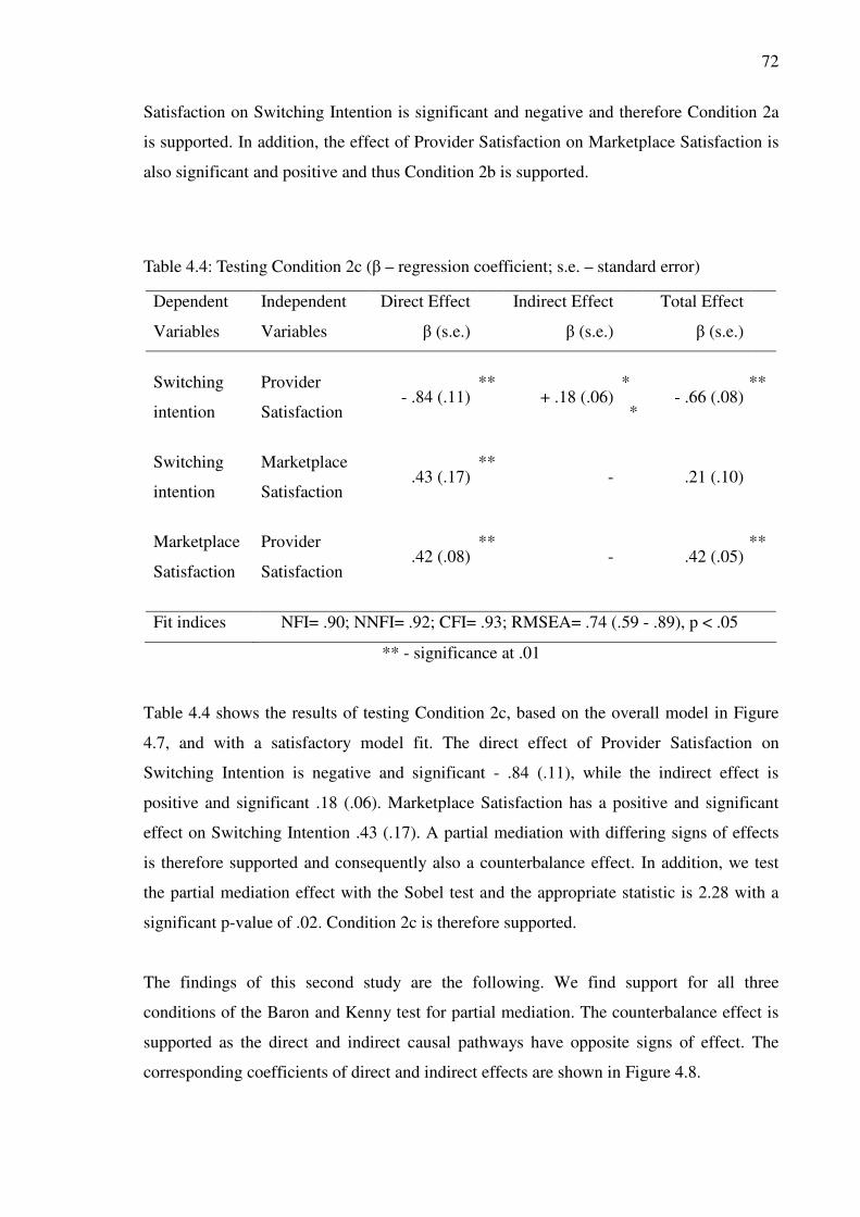
72

Satisfaction on Switching Intention is significant and negative and therefore Condition 2a

is supported. In addition, the effect of Provider Satisfaction on Marketplace Satisfaction is

also significant and positive and thus Condition 2b is supported.

Table 4.4: Testing Condition 2c (β – regression coefficient; s.e. – standard error)

Dependent

Variables

Independent

Variables

Direct Effect

β (s.e.)

Indirect Effect

β (s.e.)

Total Effect

β (s.e.)

Switching

intention

Provider

Satisfaction - .84 (.11)

** + .18 (.06)

*

* - .66 (.08)

**

Switching

intention

Marketplace

Satisfaction .43 (.17)

** -

.21 (.10)

Marketplace

Satisfaction

Provider

Satisfaction .42 (.08)

** -

.42 (.05)

**

Fit indices NFI= .90; NNFI= .92; CFI= .93; RMSEA= .74 (.59 - .89), p < .05

** - significance at .01

Table 4.4 shows the results of testing Condition 2c, based on the overall model in Figure

4.7, and with a satisfactory model fit. The direct effect of Provider Satisfaction on

Switching Intention is negative and significant - .84 (.11), while the indirect effect is

positive and significant .18 (.06). Marketplace Satisfaction has a positive and significant

effect on Switching Intention .43 (.17). A partial mediation with differing signs of effects

is therefore supported and consequently also a counterbalance effect. In addition, we test

the partial mediation effect with the Sobel test and the appropriate statistic is 2.28 with a

significant p-value of .02. Condition 2c is therefore supported.

The findings of this second study are the following. We find support for all three

conditions of the Baron and Kenny test for partial mediation. The counterbalance effect is

supported as the direct and indirect causal pathways have opposite signs of effect. The

corresponding coefficients of direct and indirect effects are shown in Figure 4.8.

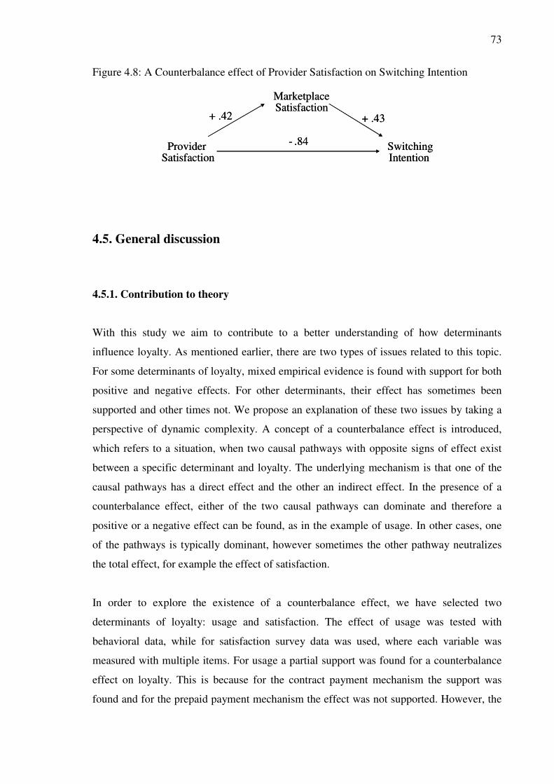
73

Figure 4.8: A Counterbalance effect of Provider Satisfaction on Switching Intention



With this study we aim to contribute to a better understanding of how determinants

influence loyalty. As mentioned earlier, there are two types of issues related to this topic.

For some determinants of loyalty, mixed empirical evidence is found with support for both

positive and negative effects. For other determinants, their effect has sometimes been

supported and other times not. We propose an explanation of these two issues by taking a

perspective of dynamic complexity. A concept of a counterbalance effect is introduced,

which refers to a situation, when two causal pathways with opposite signs of effect exist

between a specific determinant and loyalty. The underlying mechanism is that one of the

causal pathways has a direct effect and the other an indirect effect. In the presence of a

counterbalance effect, either of the two causal pathways can dominate and therefore a

positive or a negative effect can be found, as in the example of usage. In other cases, one

of the pathways is typically dominant, however sometimes the other pathway neutralizes

the total effect, for example the effect of satisfaction.

In order to explore the existence of a counterbalance effect, we have selected two

determinants of loyalty: usage and satisfaction. The effect of usage was tested with

behavioral data, while for satisfaction survey data was used, where each variable was

measured with multiple items. For usage a partial support was found for a counterbalance

effect on loyalty. This is because for the contract payment mechanism the support was

found and for the prepaid payment mechanism the effect was not supported. However, the



SwitchingIntention

+ .42

- .84

+ .43



SwitchingIntention

+ .42

- .84

+ .43

74

counterbalance effect is based on how usage is related to costs and how costs are related to

loyalty. As payment mechanisms influence these relations, they could also influence

whether usage has a counterbalance effect. The underlying explanation can be based on the

salience of cost types explored in Chapter 1 of this thesis.

Marketing theory has proposed a positive direct effect of satisfaction on loyalty, which

however, has not been always empirically supported. Our proposition to resolve this puzzle

is that satisfaction has a counterbalance effect on loyalty. In order to test this proposition,

we have extended the studied system to include an industry variable: marketplace

satisfaction. The indirect effect of satisfaction was hypothesized and found to be mediated

through marketplace satisfaction. This finding therefore provides an explanation of why

satisfaction does not necessarily lead to loyalty. Even though a negative causal pathway

was identified, it is not very unlikely that the total effect of satisfaction would be reversed

to negative. Syzmanski and Henard (2001) have not found a single study in their meta-

analysis, where satisfaction would have a negative effect on loyalty. When testing the

effects of satisfaction, we have in addition to the dynamic complexity (mediation) also

taken into account the detail complexity (industry variable).


Managers aim to keep customers loyal as a part of their efforts to improve companies’

financial performance. Therefore, it is important for them to understand how determinants

(in their sector) relate to loyalty. One of the main purposes of this paper is to raise

awareness among managers about the dynamic complexity between determinants and

loyalty. Too frequently the influence of determinants has been presented in a simple way,

i.e. if you influence a specific factor then loyalty will follow. However, economic

exchanges are complex systems and as a consequence determinants can have a

counterbalance effect on loyalty. This can either cause the total effect to diminish, like in

the case of satisfaction, or can lead to evidence for differing signs of effect, like in the case

of usage.

By examining the dynamic structure of an economic exchange system, managers can

understand how and when counterbalance effects occur. In the case of usage, the effect

75

depends on how usage is related to costs. This relation is influenced by the design of the

payment mechanism and also differs between customers. Therefore, the existence of a

counterbalance effect depends on choices of managers as well as choices and behavior of

consumers. Managers should pay particular attention to determinants of loyalty, for which

both a positive and a negative effect is possible. The reason is the danger that influencing

such determinants, in an effort to increase loyalty, can actually cause loyalty to decrease.

Satisfaction could also influence loyalty in a context dependent way. One of the key

contextual factors could be the interdependence between satisfaction with a specific

provider and satisfaction with the marketplace in general. This link could be sector

specific, could depend on the similarity between providers, and also how customers

perceive the sector in general. The variable satisfaction has been normally found to have

either a positive or no effect on loyalty and therefore managers do not risk decreasing

loyalty with their intentions to increase it. However, running these marketing activities is

costly both in terms of managers’ attention and resources deployed. Therefore, when no

effect on loyalty is achieved, then the efforts to increase satisfaction can have a negative

effect on company’s financial performance,


A major limitation of this paper is that we have only explored the mobile phone services.

This sector has some distinct characteristics, which could influence the findings in this

paper. The core services offered (calls, SMS, data, etc.) are standardized and do not differ

between providers. This could lead consumers to perceive providers as similar and thus

form the basis of the counterbalance effect of satisfaction. Testing the counterbalance

effect in other sectors is therefore needed.

Another limitation of this paper is that only two of all the possible determinants of loyalty

are studied. Other common determinants would have to be tested, both behavioral and

perceptual, such as trust, value for money, switching costs, quality, and customer

characteristics (e.g., gender or age). For each of these determinants, first, multiple causal

pathways would need to be identified grounded in theory and supported in previous

studies. Next, direct and indirect effects would have to be tested whether they are positive

76

or negative. Further research would also need to include a broader set of loyalty behavior

as a dependent variable; such as positive and negative word of mouth, complaining, cross,

and up-selling.

77

References

Ajzen, Icek (1991), “The Theory of Planned Behavior”, Organizational Behavior and

Human Decision Processes, 50 (1991), 179-211

Ajzen, Icek and Martin Fishbein (1980), Understanding Attitudes and Predicting Social

Behavior, Englewood Cliff, NJ: Prentice Hall

Anderson, James C. and David W. Gerbing (1988). “Structural equation modeling in

practice: A review and recommended two step approach”, Psychological Bulletin,

103 (May), 411-423

Bagozzi, Richard P. (1975), “Marketing as Exchange”, Journal of Marketing; Oct. 1975;

pg. 32

Bagozzi, Richard P. and Jeffrey R. Edwards (1998), “A general approach for representing

constructs in organizational research”, Organizational Research Methods, Vol. 1,

No. 1, 45-87

Bagozzi, Richard P., Youjaer Yi and Lynn W. Phillips (1991), “Assessing Construct

Validity in Organizational Research”, Administrative Science Quarterly, 36 (1991):

421-458

Bansal, Harvir S. and Shirley F. Taylor (1999), “The Service Provider Switching Model

(SPSM)”, Journal of Service Research, Volume 2, No 2, November 1999, 200-218

Baron, Reuben M, and David A. Kenny (1986), “The Moderator-Mediator Variable

Distinction in Social Psychological Research: Conceptual, Strategic, and Statistical

Considerations”, Journal of Personality and Social Psychology, 1986, Vol. 51, No.

6, 1173-1182

Bettman, James R., Mary Frances Luce, and John W. Payne (1999). “Constructive

Consumer Choice Processes”, Journal of Consumer Research, Vol. 25, No. 3 (Dec.,

1998), 187-217

Bolton, Ruth N. and Katherine N. Lemon (1999), “A Dynamic Model of Customers’

Usage of Services: Usage as an Antecedent and Consequence of Satisfaction”,

Journal of Marketing Research, Vol. 36 (May 1999), 171 – 186.

Boulding, Kenneth E. (1956), “General systems theory: The skeleton of science”,

Management Science, Special Double Issue Vol. 6 Nos. 1-2 2004, pp 127-139

78

Brady, Michael K., Gary A. Knight, J. Joseph Cronin Jr., G. Tomas, M. Hult, and Bruce D.

Keillor (2005), “Removing the contextual lens: A multinational, multi-setting

comparison of service evaluation models”, Journal of Retailing, 81 (3, 2005), 215-

230

Burke, Raymond R., Bari A. Harlam, Barbara E. Kahn, and Leonard M. Lodish (1992),

”Comparing Dynamic Consumer Choice in Real and Computer-Simulated

Environments”, Journal of Consumer Research, Vol. 19, No. 1 (Jun., 1992), 71-82.

Burnham, Thomas A., Judy L. Frils, and Vijay Mahajan (2003), “Consumer Switching

Costs: A Typology, Antecedents, and Consequences”, Journal of the Academy of

Marketing Science, Apr 2003; 31: 109 - 126

Coleman, James S. (1986), “Psychological Structure and Social Structure in Economic

Models”, The Journal of Business, Vol. 59, No. 4, Part 2: The Behavioral

Foundations of Economic Theory (October, 1986)

Crawford, Matthew T., Steven J. Sherman, and David L. Hamilton (2002), “Perceived

Entitativity, Stereotype Formation, and the Interchangeability of Group Members”,

Journal of Personality and Social Psychology, 2002, Vol. 83, No. 5, 1076 – 1094

Cronin, Joseph J. Jr., Michael K. Brady, G. Hult, and M. Tomas (2000), “Assessing the

Effects of Quality, Value, and Customer Satisfaction on Consumer Behavioral

Intentions in Service Environments”, Journal of Retailing, Volume 76 (2), 193-218

Della Vigna, Stefano, and Ulrike Malmendier (2006), ”Paying not to go to the gym”,

American Economic Review, Vol. 96, Nr. 3, 694-719.

Fornell, Claes (1992), “A National Customer Satisfaction Barometer: The Swedish

Experience”, Journal of Marketing, Vol. 56, No. 1 (Jan., 1992), 6-21

Fornel, Claes and David F. Larcker (1981), “Evaluating Structural Equation Models with

Unobservable Variables and Measurement Error”, Journal of Marketing Research,

Vol. 18, No. 1 (Feb., 1981), 39 – 50

Fornell, Claes, Michael D. Johnson, Eugene W. Anderson, Jaesung Cha, and Barbara

Everitt Bryant (1996), “The American Customer Satisfaction Index: Nature, Purpose,

and Findings”, Journal of Marketing, Vol. 60, No. 4 (Oct., 1996), 7-18

Ganesh, Jaishankar, Mark J. Arnold, and Kristy E. Reynolds (2000), “Understanding the

Customer Base of Service Providers: An Examination of the Differences Between

Switchers and Stayers”, Journal of Marketing, Vol. 64 (July 2000) 65-87

79

Garbarino, Ellen and Mark S. Johnson (1999), ”The Different Roles of Satisfaction, Trust

and Commitment for Relational and Transactional Consumers”, Journal of

Marketing, Vol. 63 No. 2 (April, 1999), 70-87

Gourville, John T. and Dilip Soman (1998), “Payment Depreciation: The Behavioral

Effects of Temporally Separating Payments from Consumption”, Journal of

Consumer Research, Vol. 25, September 1998, 160-74

Heath, Chip and Jack Soll (1996), “Mental Budgeting and Consumer Decisions”, Journal

of Consumer Research, 23 (June), 40-52

Homburg, Christian and Annette Giering (2001), “Moderators of the Relationship Between

Customer Satisfaction and Loyalty – An Empirical Analysis”, Psychology and

Marketing, Vol. 18 (1) (January 2001), 43 – 66

Homburg, Christian, Nicole Koschate, and Wayne D. Hoyer (2005), “Do Satisfied

Customers Really Pay More? A Study of the Relationship between Customer

Satisfaction and Willingness to Pay”, Journal of Marketing, Vol. 69 (April 2005),

84-96

Johnson, Michael D. and Claes Fornell (1991), “A framework for comparing customer

satisfaction across individuals and product categories”, Journal of Economic

Psychology, Vol. 12, No. 2, pp. 267-286

Jones, Michael A., David L. Mothersbaugh, and Sharon E. Beatty (2002), “Why customers

stay: measuring the underlying dimensions of services switching costs and managing

their differential strategic outcomes”, Journal of Business Research, Volume

55, Number 6, June 2002, pp. 441-450 (10)

Jones, Thomas O. and W. Sasser (1995), “Why Satisfied Customers Defect”, Harvard

Business Review, November-December, 1995, Vol. 73, Issue 6, pg.88, 14p

Kahneman, Daniel and Amos Tversky (1979), “Prospect Theory: An Analysis of Decision

Under Risk”, Econometrica, 47 (March), 263-91

Kalyanaram, Gurumurthy and Russel S. Winer (1995), “Empirical Generalizations From

Reference Price Research”, Marketing Science, Vol. 14, No.3, Part 2 of 2, 1995

Kline, Rex B. (1998), Principles and practice of structural equation modeling, Guilford

Press, New York

Keaveney, Susan M. and Madhavan Parthasarathy (2001), “Customer Switching Behavior

in Online Services: An Exploratory Study of the Role of Selected Attitudinal,

Behavioral, and Demographic Factors”, Academy of Marketing Science, Journal,

Fall 2001; 29, 4, pg. 374

80

Llieva, J., Baron. S., and Healy, N.M. (2002), “Online surveys in marketing research: pros

and cons”, International Journal of Market Research, Vol. 44, No.3, 361-76

Lambrecht, Anja and Bernd Skiera (2006), ”Paying Too Much and Being Happy About It:

Existence, Causes and Consequences of Tariff-Choice Biases”, Journal of Marketing

Research, May 2006, 212-23

MacKinnon, David P., Chondra M. Lockwood, Jeanne M. Hoffman, Stephen G. West, and

Virgil Sheets (2002), “A comparison of methods to test the significance of the

mediated effect”, Psychological Methods, 7, 83-104

Marsh, Hert W. (1994), “Confirmatory Factor Analysis Models of Factor Invariance: A

Multifaceted Approach,” Structural Equation Modeling, 1 (1), 5-34

Miravete, Eugenio J. (2003), “Choosing the Wrong Calling Plan? Ignorance and

Learning”, The American Economic Review, Volume 93, Number 1, 1 March 2003,

297-310

Mittal, Vikas, and Wagner A. Kamakura, (2001), ”Satisfaction, Repurchase Intent, and

Repurchase Behavior: Investigating the Moderating Effect of Customer

Characteristics”, Journal of Marketing Research, Vol. 38 (February 2001), 131 – 142

Mittal, Vikas, Pankaj Kumar, and Michael Tsiros (1999), ”Attibute-Level Performance,

Satisfaction, and Behavioral Intentions over Time: A Consumption-System

Approach”, Journal of Marketing, Vol. 63 (April 1999), 88-101

Morgan, Robert M. and Shelby D. Hunt(1994), “ The Commitment-Trust Theory of

Relationship Marketing”, Journal of Marketing, Vol. 58 (July 1994), 20-38

Nijssen, Edwin, Jagdip Singh, Deepak Sirdeshmukh, and Hartmut Holzmueller (2003),

“Investigating Industry Context Effects in Consumer-Firm Relationships:

Preliminary Results From a Dispositional Approach”, Journal of the Academy of

Marketing Science, Volume 31, No. 1, 46-60

Oliver, Richard L. (1997), Satisfaction: a behavioral perspective on the consumer,

McGraw Hill

Oliver, Richard L. (1999), “Whence Consumer Loyalty?”, Journal of Marketing, Vol. 63,

Fundamental Issues and Directions for Marketing (Special issue 1999), 33-44

Podsakoff, Philip M., Scott B. Mackenzie, Jeong-Yeon Lee, and Nathan P. Podsakoff

(2003), “Common Method Bias and Behavioral Research: A Critical Review of the

Literature and Recommended Remedies”, Journal of Applied Psychology, 2003, Vol.

88, No. 5, 879–903

81

Prelec, Drazen and George Loewenstein (1998), “The Red and The Black: Mental

Accounting of Savings and Debt”, Marketing Science, Vol. 17, No. 1, 4-28

Prelec, Drazen and Duncan Simester (2001), “Always Leave Home Without It: A Further

Investigation of the Credit-Card Effect on Willingness to Pay”, Marketing Letters,

12:1, 5-12

Reichheld, Frederick F. (1996), “Learning from Customer Defections”, Harvard Business

Review, March/April, pp. 56-69

Reidenbach, Eric R. and Terence A. Oliva (1981), “General Living Systems Theory and

Marketing: A Framework for Analysis”, Journal of Marketing, 45:4 (1981: Fall), pg.

30

Satorra, Albert and Peter M. Bentler (1988), “Scaling corrections for chi-square statistics

in covariance structure analysis”, Proceedings of the American Statistical

Association, 1988

Schwarz, Norbert (2004), “Metacognitive Experiences in Consumer Judgment and

Decision Making”, Journal of Consumer Psychology, 2004, Vol. 14, No. 4, pages

332 – 348

Shafir, Eldar, and Richard Thaler (2006), “Invest now, drink later, spend never: On the

mental accounting of delayed consumption”, Journal of Economic Psychology, 2006,

Vol. 27, Nr. 5, 694-712

Sheppard, Blair H., Jon Hartwick, and Paul R. Warshaw (1988), “The Theory of Reasoned

Action: A Meta-Analysis of Past Research with Recommendations for Modifications

and Future Research”, Journal of Consumer Research, Vol. 15, No. 3 (December,

1988), 325-343

Shrout, Patrick E., and Niall Bolger (2002), “Mediation in Experimental and Non-

experimental Studies: New Procedures and Recommendations”, Psychological

Methods, 2002, Vol. 7, No. 4, 442-44

Sirdeshmukh, Deepak, Jagdip Singh, and Barry Sabol (2002), “Consumer Trust, Value,

and Loyalty in Relational Exchanges”, Journal of Marketing, Vol. 66 (January,

2002), 15-37

Sobel, Michael E. (1982), “Asymptotic confidence intervals for indirect effect in structural

equation models”, in S. Leinhardt (Ed.) Sociological Methodology, 1982 (290-312),

Washington DC: American Sociological Association

82

Soderlund, Magnus (2003), “The retrospective and the prospective mind and the temporal

framing of customer satisfaction”, European Journal of Marketing, Vol. 37, No. 10,

2003, 1375-1390

Soderlund, Magnus and Niclas Ohman (2005), “Assessing behavior before it becomes

behavior: An examination of the role of intentions as a link between satisfaction and

repatronizing behavior”, International Journal of Service Industry Management, Vol.

16, No.2, 2005, 169-185

Soman Dilip (2001), “Effects of Payment Mechanism of Spending Behavior: The Role of

Rehearsal and Immediacy of Payments”, Journal of Consumer Research, Vol. 27,

March

Soman, Dilip (2003), “The Effect of Payment Transparency on Consumption: Quasy-

Experiments from the Field”, Marketing Letters 14:3, 173-83

Soman, Dilip and Vivian M. W. Lam (2002), “The Effects of Prior Spending on Future

Spending Decisions: The Role of Acquisition Liabilities and Payments”, Marketing

Letters, 13:4, 359-72

Sterman, John D. (1989), “Modeling Managerial Behavior: Misperceptions of Feedback in

a Dynamic Decision Making Experiment”, Management Science, Vol. 35, No. 3,

March

Sterman, John D. (2000), Business dynamics: systems thinking and modeling for a complex

world, McGraw-Hill Higher Education

Szymanski, David M. and David H. Henard (2001), “Customer Satisfaction: A Meta-

Analysis of the Empirical Evidence”, Journal of the Academy of Marketing Science,

Volume 29, No.1, 16-35

Thaler, Richard D. (1999), “Mental Accounting Matters”, Journal of Behavioral Decision

Making, 12, 183-206 (1999)

Verhoef, Peter C. (2003), “Understanding the Effect of Customer Relationship

Management Efforts on Customer Retention and Customer Share Development”,

Journal of Marketing, Vol. 67 (October 2003), 30 – 45

Verhoef, Peter C., Fred Langerak, and Bas Donkers (2007), “Understanding brand and

dealer retention in the new car market: The moderating role of brand tier”, Journal of

Retailing, 83, (1, 2007), 97-113

Warshaw, Paul R. and Fred D. Davis (1985), “Disentangling behavioral intention and

behavioral expectation”, Journal of Experimental Social Psychology, (1985), 21:33,

213-228

83

Warshaw, Paul R., Blair H. Sheppard, and Jon Hartwick (1985), “The Intention and Self-

Prediction of Goals and Behavior”, in Advances in Marketing Communication, ed.

Richard P. Bagozzi, Greenwich, CT: JAI

Wright, Peter (2002), “Marketplace Metacognition and Social Intelligence”, Journal of

Consumer Research, Vol. 28, March 2002. pg. 677

Zaltman, Gerald, Karen LeMasters and Michael Heffring (1982), Theory Construction in

Marketing, John Willey & Sons

Zeithaml, Valarie A. (1988), “Consumer Perceptions of Price, Quality, and Value: A

Means-End Model and Synthesis of Evidence”, Journal of Marketing, Vol. 52 (July

1988), 2-22

Zeithaml, Valarie A., Leonard L. Berry, and A. Parasuraman (1996), “The Behavioral

Consequences of Service Quality”, Journal of Marketing, Vol. 60, No. 2 (April,

1996), 31-46

Zeithaml, Valarie A., Ruth N. Bolton, John Deighton, Timothy L. Keiningham, Katherine

N. Lemon, and Andrew, J. Petersen (2006), “Forward-Looking Focus. Can Firms

Have Adaptive Foresight?”, Journal of Service Research, Vol. 9, No. 2, 168-183

84

A Appendix to Chapter 2

85

A.1 Appendix for study 1: Metro commuting

Estudio sobre los hábitos de consumo en el metro

1. Utiliza usted el metro frequentemente? � Si � No

2. Que tipo de billete utiliza usted normalmente?

a) Abono mensual b) Bono 10 Viajes c) Billete sencillo d) Otro

3. Cual es su gasto mensual en billetes/abono de metro? ________

4. Cuantos viajes hace usted por semana (incluido el fin de semana)? _________

5. Por el precio que le cuesta viajar en metro, usted diria que viajar en metro tiene un

Valor malo 1 2 3 4 5 6 7 8 9 10 Valor bueno

6. Imaginese que su gasto mensual aumentase un 25%. Usted diria que viajar en metro

tiene un


7. Imaginese que su gasto medio por viaje aumentase un 25%. Usted diria que viajar en

metro tiene un


86

English translation of the Metro commuting survey document used

Study about the usage habits of metro commuters

1. Do you use metro regularly? � Yes � No

2. What type of ticket do you normally use?

a) Monthly b) T10 tickets c) Single ticket d) Other

3. What is your monthly metro commuting cost? ________

4. How many trips do you do in a typical week (including weekends)? _______

5. What value for money do you think metro commuting offers?

Poor value 1 2 3 4 5 6 7 8 9 10 Good value

6. Imagine that your total monthly cost of metro commuting would increase 25%. What

value for money would metro commuting be in this case?


7. Imagine that your average cost per metro trip would increase 25%. What value for

money would metro commuting be in this case?


87

A.2 Appendix for study 3: Skiing trip

Daily tickets version in normal text, Four-day ski pass marked with italics where different.

The purpose of this questionnaire is to collect data for a study which will represent a part

of doctoral thesis. I would like to thank you very much in advance for participating. In the

questionnaire there will be some hypothetical situations for which you are asked to try to

imagine and respond to questions linked to the situations.

---------------------------------------------------- new page -------------------------------------------

Imagine you are going skiing with your friends to Andorra. You will be staying at the ski

resort for four days. You have already paid for the transport and hotel. Each day when you

decide to go skiing you need to purchase a daily ski ticket. The price of one day of skiing is

30 euros, thus four days of skiing would total 120 euros. You will be skiing from inclusive

Thursday to Sunday.

(Imagine you are going skiing with your friends to Andorra. You will be staying at the ski

resort for four days. You have already paid for the transport and hotel. Upon arrival you

purchase a four-day ski pass. The price of the four day pass is in total 120 euros, which is

30 euros per one day of skiing. You will be skiing from inclusive Thursday to Sunday.)

---------------------------------------------------- new page -------------------------------------------

1. DAY1: Thursday morning

You have just woken up on Thursday morning. After the breakfast you check the snow

conditions at the hotel information desk. There is plenty of snow to guarantee good skiing

and the weather forecast is sunny throughout the whole day.

Will you purchase a daily ski ticket today? (Will you use the ski pass today?)

a) Yes

88

b) No

---------------------------------------------------- new page -------------------------------------------

2. DAY1: Thursday evening

After having enjoyed a nice day you decide to go out for dinner. You have located two

restaurants close to your hotel with affordable prices. One is serving Italian food and the

other is serving tapas.

Which restaurant will you choose?

a) Italian

b) Tapas

---------------------------------------------------- new page -------------------------------------------

3. DAY2: Friday morning

It is Friday morning. You decide to have breakfast at a cafe close to the hotel. You engage

into conversation with the owner and he tells you that there will be great skiing conditions

today.


a) Yes

b) No

---------------------------------------------------- new page -------------------------------------------

4. DAY2: Friday evening

It is Friday evening and you decide to explore local bars and go out for some drinks with

your friends. There are several places around. Your friends can not decide whether to go to

a an Irish pub or to a modern club.

Which place would you prefer to go to?

a) Irish Pub

b) Club

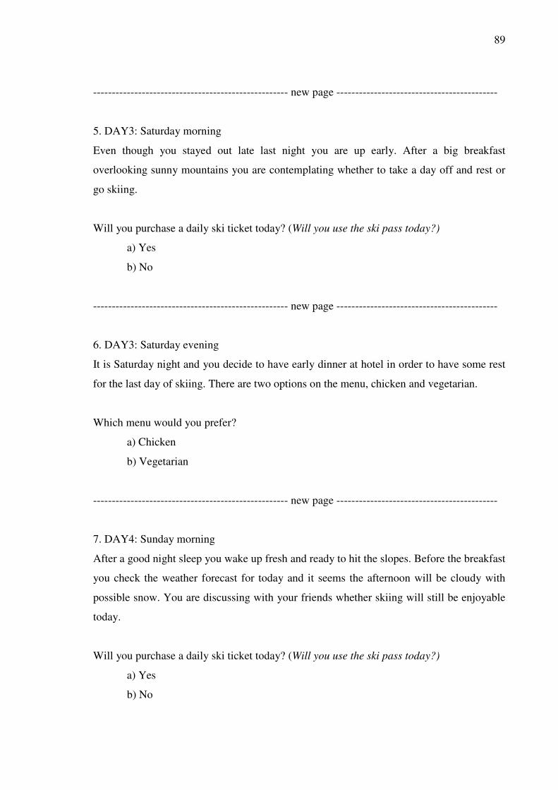
89

---------------------------------------------------- new page -------------------------------------------

5. DAY3: Saturday morning

Even though you stayed out late last night you are up early. After a big breakfast

overlooking sunny mountains you are contemplating whether to take a day off and rest or

go skiing.


a) Yes

b) No

---------------------------------------------------- new page -------------------------------------------

6. DAY3: Saturday evening

It is Saturday night and you decide to have early dinner at hotel in order to have some rest

for the last day of skiing. There are two options on the menu, chicken and vegetarian.

Which menu would you prefer?

a) Chicken

b) Vegetarian

---------------------------------------------------- new page -------------------------------------------

7. DAY4: Sunday morning

After a good night sleep you wake up fresh and ready to hit the slopes. Before the breakfast

you check the weather forecast for today and it seems the afternoon will be cloudy with

possible snow. You are discussing with your friends whether skiing will still be enjoyable

today.


a) Yes

b) No

90

---------------------------------------------------- new page -------------------------------------------

8. DAY4: Sunday evening

After spending some days in Andorra it is time for you to return home. You settle all

outstanding bills. There is an option to drive directly home or stop on the way to have

some food.

Which option would you prefer?

a) Going directly home

b) Having some food

---------------------------------------------------- new page -------------------------------------------

9. Some days after your return home, a friend of yours suggests going skiing again in one

month’s time. You would stay at the same hotel and would go to the same ski resort.

However this time you would go skiing for 7 days. As before each day when you decide to

go skiing you need to purchase a daily ski ticket. The price of one day of skiing is 30

euros, thus seven days of skiing would total 210 euros. The ski conditions are expected to

be great.

(Some days after your return home, a friend of yours is suggesting going skiing again in a

one month’s time. You would stay at the same hotel and would go to the same ski resort.

However this time you would go skiing for 7 days. The seven day ski pass costs 210 euros,

which is 30 euros per day. The ski conditions are expected to be great.)

How likely are you to go skiing again for 7 days at the same ski resort?

Very Unlikely (1) ............................Very Likely (7)

---------------------------------------------------- new page -------------------------------------------

10. Another friend of yours is suggesting a three day ski trip in two weeks’ time. You

would stay at the same hotel however you would go skiing to another slope. This slope has

longer runs and is supposed to be more fun. As before each day when you decide to go

91

skiing you need to purchase a daily ski ticket. The price of one day of skiing is 40 euros,

thus three days of skiing would total 120 euros. Skiing conditions are expected to be great.

(Another friend of yours is suggesting a three day ski trip in two weeks’ time. You would

stay at the same hotel however you would go skiing to another slope. This slope has longer

runs and is supposed to be more fun. The three day ski pass costs 120 euros, which is 40

euros per day. Skiing conditions are expected to be great.)

How likely are you to go for this three days ski trip to a new ski resort?

Very Unlikely (1) ............................Very Likely (7)

---------------------------------------------------- new page -------------------------------------------

11. How many days do you normally go skiing in a typical year? __________

---------------------------------------------------- new page -------------------------------------------

12. What is your gender?

a) Male

b) Female

92

B Appendix to Chapter 3

93

B.1 Measures used for study constructs

Switching Intentions (ten-point scale, »do not agree at all« / » agree completely«)

I1: I plan to change my mobile phone service provider.

I2: I intend to start using another provider.

I3: I will change my provider within the next year.

Switching Expectations (ten-point scale)

E1: I expect to change my provider in the future. (”do not agree at all” / ”agree

completely”)

E2: How likely is that you will change it in the future? (”very unlikely” /”very likely”)

E3: How likely is that you will stay with your current mobile service provider? (as above)

Overall Satisfaction (seven-point scale) (”very dissatisfied” / ”very satisfied”)

S1: How satisfied or dissatisfied are you with your current mobile phone service provider?

S2: Overall, how do you feel about it? (”very unhappy” / ”very happy”)

S3: How well does it meet your needs at this time? (”extremely poor” / ”extremely well”)

Trust (seven-point scale, ”do not agree at all” / ”agree completely”)

T1: I feel can trust my mobile phone service provider.

T2: My provider is responsive to customers’ problems.

T3: I feel my service provider is reliable.

Attitude towards switching (seven-point scale, ”do not agree at all” / ”agree completely”)

A1: It would take me a lot of effort to choose another mobile service provider.

A2: I do not feel like going through the whole process of changing the mobile provider.

A3: Going through the process of changing the provider would be an unpleasant

experience.

Switching cost (seven-point scale, ”do not agree at all” / ”agree completely”)

F1: Changing my mobile service provider would cost me money.

F2: If I choose another service provider my costs will go up.

F3: Changing my mobile service provider would have significant financial impact for me.

Determinants, contexts, and measurements of customer loyalty

Documents

Transcript of Determinants, contexts, and measurements of customer loyalty