Detection of time-varying signals in event-related fMRI designs

This article appeared in a journal published by Elsevier. The attachedcopy is furnished to the author for internal non-commercial researchand education use, including for instruction at the authors institution

and sharing with colleagues.

Other uses, including reproduction and distribution, or selling orlicensing copies, or posting to personal, institutional or third party

websites are prohibited.

In most cases authors are permitted to post their version of thearticle (e.g. in Word or Tex form) to their personal website orinstitutional repository. Authors requiring further information

regarding Elsevier’s archiving and manuscript policies areencouraged to visit:

http://www.elsevier.com/copyright

Detection of time-varying signals in event-related fMRI designs

Jack Grinband a,b,⁎, Tor D. Wager c, Martin Lindquist d, Vincent P. Ferrera b, Joy Hirsch a

a Program in Imaging and Cognitive Sciences, Columbia University, New York, New York 10032, USAb David Mahoney Center for Brain and Behavior Research, Columbia University, New York, New York 10032, USAc Department of Psychology, Columbia University, New York, New York 10032, USAd Department of Statistics, Columbia University, New York, New York 10032, USA

a b s t r a c ta r t i c l e i n f o

Article history:Received 26 March 2008Revised 8 July 2008Accepted 31 July 2008Available online 16 August 2008

In neuroimaging research on attention, cognitive control, decision-making, and other areas where responsetime (RT) is a critical variable, the temporal variability associated with the decision is often assumed to beinconsequential to the hemodynamic response (HDR) in rapid event-related designs. On this basis, themajority of published studies model brain activity lasting less than 4 s with brief impulses representing theonset of neural or cognitive events, which are then convolved with the hemodynamic impulse responsefunction (HRF). However, electrophysiological studies have shown that decision-related neuronal activity isnot instantaneous, but in fact, often lasts until the motor response. It is therefore possible that smalldifferences in neural processing durations, similar to human RTs, will produce noticeable changes in the HDR,and therefore in the results of regression analyses. In this study we compare the effectiveness of traditionalmodels that assume no temporal variance with a model that explicitly accounts for the duration of very briefepochs of neural activity. Using both simulations and fMRI data, we show that brief differences in durationare detectable, making it possible to dissociate the effects of stimulus intensity from stimulus duration, andthat optimizing the model for the type of activity being detected improves the statistical power, consistency,and interpretability of results.

© 2008 Elsevier Inc. All rights reserved.

Introduction

Over the past two decades, the development of functionalmagnetic resonance imaging (fMRI) technology has generated nearexponential growth in neuroimaging research and its clinicalapplications (Bandettini, 2007). The most commonly used methodfor analyzing the blood oxygenation level-dependent (BOLD) changesin fMRI is based on the general linear model (GLM). A typicalexperiment consists of generating a hypothetical cognitive or neuralmodel of brain activity and using multiple linear regression to searchfor voxels correlated with the predicted response. In classic blockdesigns, the duration of each regressor in the regression modelmatches the duration of the stimulus block. As blocks shorten to 4 s orless, the current convention is to switch to using ‘impulse functions’ ofarbitrarily short duration, rather than simply continue shorteningblocks to match the length of the stimulus. While this may produceaccurate results when the cognitive/neural events are of constantduration (20% of event-related studies; Fig. 1B), the majority (80%) ofevent-related studies involves choice-related neural processes thatcan vary in duration with the subject's RT. In 95% of event-related

studies containing a decision process (Fig. 1E), the duration of thedecision period is assumed to be constant and is typically modeled bythe convolution of a constant height, finite impulse function (i.e. aKronecker delta function) positioned at event onset with a canonicalhemodynamic response function (Friston, 2003, Friston et al., 1994;Henson, 2003; Josephs et al., 1997).

Although this method can often detect task-related fMRI activity, itmakes the implicit assumption that the underlying neural or cognitiveprocess is a brief, essentially zero duration, event (i.e. an impulse). Thissimplification is generally thought to have little or no impact on theresults. In fact, due to the low-pass filtering properties of the BOLDresponse (Zarahn et al., 1997), it has been argued that the shape of thephysiological hemodynamic response (HDR) to brief stimuli (b 4 s) isequal to the theoretical hemodynamic impulse response function(HRF), making the constant impulse model a good approximation tothe actual BOLD response (Henson, 2003). However, it has been shownthat stimulus durations as small as 34 ms (Glover, 1999; Rosen et al.,1998; Savoy et al., 1995) and onset asynchronies as low as 50 ms(Bellgowan et al., 2003; Henson et al., 2002; Kim et al., 1997; Menonet al., 1998; Miezin et al., 2000; Richter et al., 2000) can elicitdetectable BOLD responses, suggesting that small differences in theonset or duration of modeled events may be important.

If the assumption of equivalence between impulse functions andshort (100 ms–4 s) blocks (or boxcars) does not hold, then it should bepossible to dissociate the effects of stimulus intensity from stimulus

NeuroImage 43 (2008) 509–520

⁎ Corresponding author. 710West 168th Street, Neurological Institute-B41, New York,NY 10032, USA. Fax: +1 212 342 0855.

E-mail address: [email protected] (J. Grinband).

1053-8119/$ – see front matter © 2008 Elsevier Inc. All rights reserved.doi:10.1016/j.neuroimage.2008.07.065

Contents lists available at ScienceDirect

NeuroImage

j ourna l homepage: www.e lsev ie r.com/ locate /yn img

duration in event-related designs. Moreover, any discriminabledifferences between these models would suggest that the shape ofthe BOLD response should be optimized for the type of activity beingdetected. For example, impulse functions might best model neuralactivity at stimulus onset, whereas brief epochs might best captureactivity that is sustained throughout stimulus processing. Potentialdifferences between impulse- and short epoch-based models may bemagnified by the fact that response times (RTs) in many studies varyacross trials. Such variations have been shown in animal research to berelated to the variations in the duration of decision-related neuronalfiring (Janssen and Shadlen, 2005; Maimon and Assad, 2006; Ratcliffet al., 2007; Schall, 2003; Shadlen and Newsome, 2001; Snyder et al.,2006), and such variability in response time is the basis for a variety ofdecision-making models (Ratcliff, 2005). In addition, several fMRIstudies have demonstrated that the HDR to a decision process is likely

to vary with the time it takes to elicit the subject's response (Connollyet al., 2005; Formisano et al., 2002; Kruggel et al., 2000; Menon et al.,1998). Importantly, temporal variability is rarely an explicit experi-mental manipulation, but nevertheless exists implicitly as a distribu-tion of response times. RTs for simple, suprathreshold detection tasks(simple RTs) typically range from 200 to 500 ms, whereas choiceresponses between multiple options (choice RTs) start at around 400ms and can range up to tens of seconds depending on speed-accuracytradeoffs, task complexity, arousal, age, clinical status, etc (Verhaeghenet al., 2006, 2003). Thus, decision-related behavioral responses tomany types of brief stimuli—such as those elicited by attention,memory, cognitive control, language, anddecision-making processes—are likely to elicit neural activity that (a) persists overmuch of the timebetween stimulus presentation and response, and (b) varies induration from trial to trial (Fig. 2A).

Fig. 1. Survey statistics. We surveyed 170 published fMRI studies to characterize how the GLM is used to analyze imaging data. (A) Block and event-related designs were equallycommon. (B) Most event-related studies made inferences about a time-varying decision process. (C) Although response times were recorded in 82% of event-related studies with adecision component, only 9% actually used this information to construct a regression model for detecting brain activity. (D) Most studies assumed that there were no significantdifferences in HRF shape across subjects. (E) In event-related fMRI studies that made inferences about variable duration decision processes, a majority (95%) assumed that the shapeof HDRs did not vary across trials or trial types, and 84% assumed that both shape and intensity did not vary across trials. (F) All of the major analysis platforms were represented andno obvious relationship between platform type and model type was found.

510 J. Grinband et al. / NeuroImage 43 (2008) 509–520

It has been proposed that modeling temporal variability in the dataincreases statistical power and captures an important source ofinformation about the relationship between brain activity and psycho-physical performance (Buchel et al., 1998; Friston, 2003; Henson, 2003;Josephs and Henson, 1999). Models that incorporate information abouttrial-to-trial variation in RT (or other psychophysiological parameters)into the GLM are often called ‘parametric modulation’ models. In theparametric (or variable impulse) approach, a participant's mean-centered RTs are used to modulate the amplitude of an impulsefunction. The modulated impulse function is then convolved with theHRF and added as an additional regressor in the GLM. Brain regions forwhich the amplitude of the primary, unmodulated regressor issignificantly non-zero are interpreted as task-related. Conversely, brainregions forwhich the amplitudeof themodulated regressor is significantare interpreted as being sensitive to trial-to-trial variations in RT.

An alternative method is the variable epoch approach, whichinvolves modeling each trial with a boxcar epoch function whoseduration is equal to the RT of the trial. A single regressor is thenconstructed from these boxcars to use in the GLM. This approachmakes the critical assumption that the cognitive and neural basis ofdecision-related activity is accurately represented by the diffusion (orrace) model of decision-making (Ratcliff, 2005; Ratcliff et al., 2007).The diffusion model is supported by electrophysiological studies inhumans (Philiastides et al., 2006) and non-human primates (Janssenand Shadlen, 2005; Maimon and Assad, 2006; Ratcliff et al., 2007;Schall, 2003; Shadlen and Newsome, 2001; Snyder et al., 2006) inwhich neuronal activity (or firing rate) is sustained or even increasesup to the time of the behavioral response. Thus, compared to theconstant impulse approach, the variable epoch model attempts tomore faithfully represent the physiological processes related to

Fig. 2. GLMmodels used in fMRI analysis. (A) A hypothetical event-related fMRI experiment inwhich the subject responded to the presentation of a stimulus. Assuming a linear time-invariant (LTI) system, the constant duration stimulus produces sensory neuronal responses and sensory BOLD responses that are also constant in duration. However,electrophysiological evidence (Janssen and Shadlen, 2005; Maimon and Assad, 2006; Ratcliff et al., 2007; Schall, 2003; Shadlen and Newsome, 2001; Snyder et al., 2006) shows thatthe same constant duration stimulus will typically produce variable duration decision-related neural responses, characterized by a subject's RT distribution. An LTI system predictsthat the decision-related BOLD response will vary in both shape and intensity from trial to trial. (B) We tested the efficacy of four regression models against a hypothetical decision-related cognitive/neural process that varied in duration on each trial. The constant impulse model consists of an impulse function positioned at the onset of each event. The constantepoch model consists of a 2 s epoch positioned on the TR nearest the onset of the neural event. The variable impulse model is a two-regressor model that uses a constant impulseregressor and a modulator regressor whose height is proportional to the demeaned durations of the process. All the models were convolved with a canonical double gammahemodynamic response function.

511J. Grinband et al. / NeuroImage 43 (2008) 509–520

decision-making inmany brain regions. In our previous work, we usedthis model to locate RT-sensitive brain regions in a decision-makingtask and confirmed model accuracy using model-free (GLM-free)analysis methods (Grinband et al., 2006).

In the current study, the variable epoch model was comparedagainst three other models: a constant impulse model (the mostcommon model, used in 70% of event-related studies in our survey;Fig. 1E), the variable impulse model that includes a mean-centeredparametric modulator (11% of event-related studies), and a constantepoch model (a variation of the constant impulse approach in whichthe impulses are binned within each 2 s TR; 14% of event-relatedstudies). This paper uses simulations and fMRI data to explore thedifferences in the predictions made by these models and demon-strates that, even for brief events, they are not equivalent. Our datasuggest that when detecting time-varying signals, such as thosegenerated by a behavioral response, the variable epoch model isphysiologically plausible, and has higher power and reliability fordetecting brain activation.

Materials and methods

Analysis of published methods

To determine how often GLM analyses incorporated RT intodecision-related regressors, we surveyed all fMRI studies from Jan 1,2007 to May 30, 2007 published in the following journals: HumanBrain Mapping, Nature, Nature Neuroscience, Neuroimage, Neuron,and Science. A total of 170 articles were assessed. Only articlesreporting results of original fMRI research were included. A summaryof these studies is presented in Fig. 1. We characterized the imageanalysis methods used in each study along six dimensions: use ofblock vs. event-related designs, inferences about temporal processing,measurement and modeling of RT, impulse- vs. epoch-based model-ing, the use of the canonical HRF, and the software package used.

For block vs. event-related designs (Fig. 1A), studies that containedboth a block and an event-related component were labeled as “event-related.” For constant vs. variable duration designs (Fig. 1B), weidentified studies that did not modulate durations. These includedstudies where the stimulus duration was constant and no responserequired, studies where the subject was required to perform a task fora constant duration, or studies where decisions were made but noinferences about decision-related activity was made in the conclu-sions of the paper. The variable duration designs included studies thatmade inferences about decision-related activity or studies thatexplicitly manipulated stimulus duration.

For measurement and modeling of RT (Fig. 1C), in cases where theuse of RT was not mentioned, it was assumed that RT was neithercollected nor included in the regression model. The percent of studiesin which RT was measured/modeled, was calculated by taking thenumber of studies in which the RT was measured/modeled anddividing this value by the number of studies in which a response wasrequired and conclusions weremade about the response-related brainactivity. To determine whether the length of RT affected the likelihoodof incorporating RT information into themodel, we recorded themeanRT of the condition with the longest RT. For the use of canonical HRFfunctions (Fig. 1D), it was assumed that the canonical HRF was usedunless otherwise specified. For the impulse- vs. epoch-based model-ing (Fig. 1E), the variable impulse models were defined as thosemodels in which the modulator was a regressor of interest and wasused to detect brain activity. Thus, impulse models that only includedmodulated “confound” regressors (such as those for head motion,respiration, or cardiac-related artifacts) were labeled as constantimpulse models. In instances where the nature of the model wasunclear (n = 8), the corresponding authors of the papers werecontacted. For the software package used (Fig. 1F), in cases wheremultiple software packages were used to process data, only the

package used to perform the statistical analysis was included in thefrequency calculations.

Simulations

To test the efficacy of the four regression models to detect time-varying brain activity, we simulated a cognitive process that varied induration across trials and tested model performance by measuringpower and false positive rate (FPR). Simulations were performedassuming a linear, time-invariant (LTI) system (Boynton et al., 1996).While nonlinearities are known to exist (Birn et al., 2001; Huettel andMcCarthy, 2000; Miller et al., 2001; Vazquez and Noll, 1998; Wager etal., 2005), the LTI system was adequate for exploring the differencesbetween linear models commonly applied to fMRI data. Theincorporation of non-linear effects is a further potential refinementof regression models that is outside the scope of the current paper.

The power simulation consisted of four steps: (1) a simulatedneuronal time series was created consisting of a series of boxcars withrandomly generated durations; (2) this neural model was convolvedwith a canonical HRF to create the simulated BOLD time series; (3) AR(1) noise was added to the time series; (4) linear regression wasperformed between the simulated data and each of the four regressionmodels. This process was repeated 10000 times to compute thepercent of true positives detected by each model. The false positivesimulation consisted only of steps (3) and (4) to compute the percentof false positives detected by each model.

Creation of simulated cognitive/neural eventsThe duration and inter-trial variability of the cognitive process to

be detected is an important variable that may impact the choice ofmodel. Therefore, we created simulated RTs based on RT distributionsfrom our previously published empirical study of a two-alternative,forced-choice categorization task (Grinband et al., 2006). In the task,10 subjects categorized line segments as “long” or “short.” We fit agamma function to the RT distributions of each of 10 subjects (Fig.S1A) and averaged the gamma parameters to generate a mean gammadistribution (α = 1.7, β = 0.4, minimum value = 0.5; Fig. S1B) with RTmean = 0.84 s and s.d. = 0.64 s. Simulated neural process durationswere randomly drawn from the resulting gamma distribution. Thus,the simulated neural events consisted of a series of boxcars whosedurations are distributed similarly to observed RTs in a simpleperceptual decision-making task.

Variable inter-event intervals were selected from a uniform distribu-tionwith aminimumof 4 s andamaximumof 7 s, values commonlyusedin fMRI experiments. The total duration of each simulated run was5.5min. To simulate the autocorrelation present in real fMRI time series,we added AR(1) noise to each time series with phi = 0.3.

Linear models testedThe fourmodels used to detect this neural process are illustrated in

Fig. 2B. The variable epoch model was created using the samevariable-length boxcars and, consequently, must necessarily fit betterthan the other models. However, the question of interest is not whichmodel fits better, but whether there are any appreciable differencesbetween the models in their ability to detect brain activity. Our nullhypothesis states that: For brief (b 4 s) stimulus durations, there are nosignificant differences between models that assume a constant shapeof the HDR (i.e. ignore differences in duration of neural processes) andthose that explicitly account for the duration differences betweentrials. For the variable impulse and constant impulse models, themodel's representation of the neural process was generated by placinga 50 ms epoch at the onset of the process. The constant epoch modelassumes that the temporal resolution of the neural process and theBOLD response is equal to the TR and, thus, consists of short epochsequal to the inter-scan interval (TR = 2 s). It was constructed bypositioning the 2 s epoch on the TR interval closest to the onset of the


neural process and convolving with the HRF. This is in contrast to theconstant impulse model, which assumes that the temporal resolutionof the BOLD response is equal to the TR but the resolution of the neuralprocess is 50 ms. The constant regressors (impulse and epoch) hadamplitudes equal to 1. The modulator regressor was created by mean-centering the neural durations, normalizing the range of durations to± 0.5, and setting the amplitude of each impulse equal to thecorresponding normalized duration.

Performance metricsThe performancemetrics of interestwere true positive rate (power)

and false positive rate (FPR). We evaluated power and FPR at differenteffect sizes using the Pearson correlation coefficient between themodel and the data. To compute power, 10,000 simulated data timeseries of signal + AR(1) noise were generated for each effect size andthe fraction of true positives was calculated for each model type. Thesignal component of each time series consisted of a random sample ofgamma distributed RTs and uniformly distributed inter-trial intervals.To compute FPR, we generated 10,000 AR(1) noise time series and thefraction of positive results was calculated for each model type.

To compare the relative contribution of mismodeling shape vs.mismodeling amplitude, we computed the effect of shape differencesin the variable amplitude case by measuring the amount of varianceexplained by the impulsemodel when each trial was fit independentlyof all other trials. In this case, the best amplitude fit is found using anincorrect shape for each trial (i.e. the canonical impulse response). Thedegree of error for each trial is determined by the duration of theepoch — longer durations have greater deviation from the canonicalresponse and therefore a larger error. The mean error is determined asa weighted mean of the RT distribution, Γ(α = 1.7, β = 0.4, min value =0.5, mean = 0.84 s, s.d. = 0.64 s). Although, shape and amplitude arenormally coupled, this procedure allows us to estimate the effect ofmismodeling amplitude independently from the effect of mismodel-ing the shape of the HDR.

Visual stimulation experiments

The goal of this study was to determine how model selectionaffects the ability to detect time-varying BOLD responses. We neededa task that couldmodulate the duration of a neural process in a preciseand reproducible way. However, although an actual decision-makingtask would introduce temporal variability into the BOLD signal, itwould also generate unknown sources of variability related to thecognitive aspects of the task. These unknown cognitive effects wouldbe impossible to model or dissociate from the temporal variability.Thus, to isolate the effect of the temporal variance from other sources,we conducted two flashing checkerboard experiments. Because theflashing checkerboard stimulus primarily activates visual cortex, anarea with known response characteristics, it gave us precise andreproducible control over the duration of a neural process. Moreover,the resulting visual activation is known to be sustained throughoutvisual stimulation, though it is often strongest at the onset of astimulus (Logothetis et al., 2001), in the same way as decision-relatedneuronal activity (Janssen and Shadlen, 2005; Maimon and Assad,2006; Ratcliff et al., 2007; Schall, 2003; Shadlen and Newsome, 2001;Snyder et al., 2006). We were then able to use the time-varying,visually evoked responses as a proxy for time-varying, decision-related responses. Thus, using passive visual stimuli instead of adecision-making task allowed us both to (1) isolate the effects oftemporal variability in the BOLD response from the confoundingeffects of decision-related brain activity, and to (2) determinewhetherthe simulations and the actual fMRI results lead to similar conclusions.

Experiment 1 — Dissociating signal intensity from durationTo determine whether differences in HDR shape due to stimulus

intensity and stimulus duration are detectable and dissociable at the

level of an individual, one subject viewed flashing checkerboards(7.5 Hz) of variable contrast intensity and duration. The stimuli eithervaried in contrast (5%,10%, 20%, and 40%)whilemaintaining a constantduration (0.25 s) or in duration (0.25 s, 0.75 s,1.3 s, 3.5 s) with a constantcontrast intensity (5%). All eight experimental conditions wererandomly intermixed. Each trial type was presented twice per run.During the inter-trial interval, a fixation point was presented against agray background. The subject was scanned for 6 runs of 6min 48 s each.

Experiment 2 — Sensitivity and consistency of GLM analysisEight subjects viewed flashing checkerboards of constant contrast

intensity (20%) but variable duration to test the effects of modelselection on sensitivity, consistency, and false positive rate acrossindividuals. The duration of each checkerboard stimulus wasrandomly drawn from the same mean gamma distribution (Fig. S1B)used in the simulations, which is typical of human choice RTvariability. The inter-trial interval was randomly jittered using auniform distribution with a minimum of 4 s and a maximum of 7 s.During rest, subjects viewed a fixation point against a gray back-ground. Each subject was scanned for 5 runs of 5 min 30 s each.

Image acquisitionImaging experiments were conducted using a 1.5T GE TwinSpeed

Scanner using a standard GE birdcage head coil. Structural scans wereperformed using the 3D SPGR sequence (124 slices; 256 × 256; FOV =200 mm). Functional scans for Experiment 1 were performed usingEPI-BOLD (TE = 39; TR = 1.0 s; 13 slices; 64 × 64; FOV = 200 mm; voxelsize = 3 mm × 3 mm × 4.5 mm). Functional scans for Experiment 2were performed using EPI-BOLD (TE = 60; TR = 2.0 s; 29 slices; 64 × 64;FOV = 200 mm; voxel size = 3 mm × 3 mm × 4.5 mm). All imageanalysis was done using the FMRIB Software Library (FSL; http://www.fmrib.ox.ac.uk/fsl/) and Matlab (Mathworks, Natick, MA; http://www.mathworks.com). The data were motion corrected (FSL-MCFLIRT),high-pass filtered (at 0.02 Hz), and spatially smoothed (full width athalf maximum = 5 mm).

Image analysisStandard statistical parametric mapping techniques (FSL-FEAT)

were performed prior to registration to MNI152 space (lineartemplate). Multiple linear regression was used to identify voxelsthat correlated with specific sensory events (i.e. flashing checker-boards). A primary statistical threshold for activation was set at p =0.01. Since our goal was to evaluate the absolute number of voxelsdetected by the different models and because all comparisons weremade between different models for the same data set, no correctionfor multiple comparisons was made. Inter-subject group analyseswere performed in standard MNI152 space by applying the FSL-FLIRTregistration transformation matrices to the parameter estimates. Foreach run, the transformation matrices were created by registering viamutual information (1) the midpoint volume to the first volume using6 degrees of freedom, (2) the first volume to the SPGR structural imageusing 6 degrees of freedom, and (3) the SPGR to the MNI152 templateusing 12 degrees of freedom. These three matrices were concatenatedand applied to each statistical image. Ventricular masks were createdusing FSL-FAST by first segmenting each high-resolution brain intothree tissue types: gray matter, white matter, and CSF. Then the CSFpartial volume maps were transformed into the subject's functionalspace of each individual run and thresholded at 0.95 to ensure that nomore than 5% of the volume of each voxel in the mask contained grayor white matter.

Consistency measurementsThe quality of each model can be evaluated by its ability to

consistently detect the same pattern of activated voxels for a givenstimulus. We used Cronbach's alpha (Cronbach, 1951), a measure ofinter-subject consistency, to calculate the mean correlation between


the spatial activation patterns of the occipital cortex across the fiveruns. Alpha was calculated for each subject as

α ¼ NrN − 1ð Þr þ 1

ð1Þ

where N is the number of runs (N = 5) and r ̄ is the average of allpairwise Pearson correlation coefficients between the Z-statistic maps(across voxels). To test for significant differences between models thealphas were normalized using Fisher's Z-transform:

Zα ¼ 0:5 log1þ α1 − α

� �: ð2Þ

A paired Student's t-test to the Zα scores was used to compare thevariable epoch model against each of the other models.

Variability of HRF estimatesThe constant impulsemodel is often used to estimate the theoretical

hemodynamic impulse response. We compared the quality of theimpulse estimate with that of the variable epoch model by measuringthe variance in the HRF estimate across runs. The HRF estimate wascomputedusing FLOBS (Woolrich et al., 2004), a three-function basis setthat restricts the parameter estimates of each basis function to generatephysiologically plausible results. The two models were convolved witheach of the FLOBS basis functions and an F-test on the three convolvedfunctions was performed; for each significant voxel within the occipitalcortex, the parameter estimates for the basis functions were used toreconstruct the fitted HRF shape, i.e. HRF = PE1 ⁎ f1 + PE2 ⁎ f2 + PE3 ⁎ f3,where PE is a parameter estimate and f is a FLOBS basis function. TheHRF estimates were then averaged across all significant voxels in theoccipital cortex. Region of interest masks of the occipital cortex weremanually generated for each subject using the calcarine and parieto-occipital sulci as landmarks. To determinewhether the variances of thetwo HRF estimates were different from each other, we used Levene'sTest for Equality of Variance (Levene, 1960):

W ¼ ∑N − kð Þ∑

ini zi − zð Þ2

k − 1ð Þ∑i∑jzij − zj� �2 ð3Þ

where N is the total number of observations, ni is the set ofobservations within group i, and k is the number of groups, zij ¼jxij−xij is the absolute deviation fromwithin groupmeans, zi ¼ ∑j zij=ni

is the average absolute deviation from the group mean, andz ¼ ∑i ∑j zij=N. Here, N = 16, and k = 2.

Results

Survey

Of 170 fMRI studies, 48% were blocked and 44% were event-related; the remaining 8% were not easily classifiable (Fig. 1A).Stimulus or response duration was important in 80% of event-relateddesigns (Fig. 1B). The remaining 20% involved tasks that maintainedconstant stimulus/response durations (for example, primary sensoryor primary motor-related studies) or did not make inferences aboutdecision-related brain activity. In event-related studies in whichdecision-making was important, RT wasmeasured 82% of the time butmodeled only 9% of the time (Fig. 1C). Furthermore, only 16% of thestudies (Fig. 1E) actually included RTs, in some form, in theirregression model; that is, 84% of event-related studies with a decisioncomponent made the assumption that the time necessary to process astimulus or to generate a response was constant for all trials and trialtypes. Similarly, only 4% of event-related studies (Fig. 1D) estimatedindividual HRFs for each subject; 96% assumed no differences in HRFshape existed between subjects.

The majority of event-related studies with a decision component(69%) used constant impulses convolved with the canonical HRF torepresent the decision events (Fig. 1E); 11% used the variable impulsemodel to account for parametric modulations in their design,14% usedthe constant epoch model, and 5% used the variable epoch approach.Moreover, the large majority (95%) of event-related designs assumedthat there were no significant differences in the shape of the HDRbetween trials or trial types; 84% assumed there were no significantdifferences in either shape or intensity of the HDR. The mean RT ofstudies that incorporated temporal information was 1270 ms (s.d. =727 ms, min = 680 ms, max = 2560 ms). The mean RT for studies thatdid not incorporate temporal informationwas 1036 ms (s.d. = 529 ms,min = 256 ms, max = 2100 ms). There was no significant differencebetween the two groups (T-test, p = 0.35). There was a broaddistribution of software packages used with no apparent systematicdifferences in how regressors were modeled between fMRI analysispackages (Fig. 1F).

Simulations

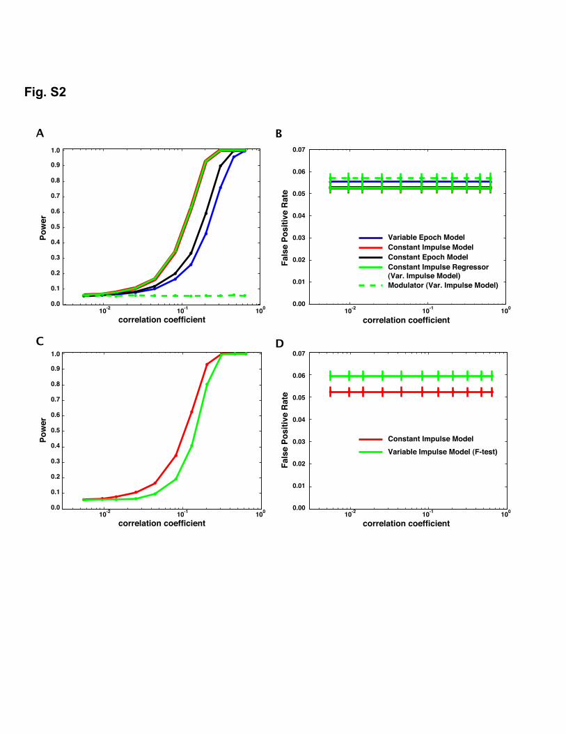
We tested the null hypothesis that the constant epoch and the twoimpulse models were as effective as the variable epoch model atdetecting brain activity that varies in duration from trial to trial (i.e.the type of activity generated in decision-making experiments). Theeffectiveness of the four regression models to detect neural activitywas computed by comparing the fraction of true positives (i.e. power)and false positives for each model. Fig. 3A shows that the variableepoch model has greater statistical power for detecting time-varyingneural activity. This was necessarily the case, as the simulated trueresponse was identical to the regressor used in the variable epochmodel. However, the critical issue was whether the variable epochmodel produced significantly better results than the other models inthe presence of physiological noise. At a correlation coefficient of 0.1 (aplausible value for a robust fMRI response; Fig. 3A), the power of thevariable epochmodel was 0.55, while the constant impulsemodel wasonly 0.23 — a 58% reduction in power. Furthermore, the modulatorregressor from the variable impulse model had the lowest power ofany of the regressors (power = 0.18), a 67% reduction compared to thevariable epoch model, suggesting that impulse modulation did notprovide an adequate model to capture activity related to variableduration events. The constant epoch model performed only slightlybetter than the constant impulse model (power = 0.28), a 49%reduction compared to the variable epoch model. The results werereversed when the variable epoch model was used to detect constantduration activity; that is, the constant impulse model outperformedthe variable epoch model when detecting a constant neural process(Fig. S2). The false positive rate was controlled appropriately at p =0.05 in all analyses and was not affected bymodel type (Fig. 3B). Thesedata suggest that for event-related designs, the type of model mattersand that commonly used approximations, which ignore durations ofevents, are less able to detect time-varying BOLD activity than hasbeen previously appreciated.

Since the variable impulse model has one more regressor than theother models, it is more flexible at fitting the data than the singleregressor models. We used an F-test to determine if the two-regressorvariable impulse model had more detection power than the one-regressor variable epoch model. The variable epoch model had higherpower than the variable impulsemodel despite having one less degreeof freedom (Fig. 3C). The false positive rate was controlled appro-priately at p = 0.05 (Fig. 3D).

These simulations show that even for events that have a meanduration of less than 1.0 s, the procedure used to model trial-to-trialvariability has a substantial impact on statistical power. This is alsotrue for durations typical of simple RTs, which have mean durationssignificantly smaller than choice RTs (though the effect diminishes asRTs become smaller; Fig. S3). Two main factors explain these results.


First, the constant impulse and constant epoch models assumeconstant HDR amplitudes for all trials. While a seemingly reasonablesimplification, our results show that ignoring trial-to-trial variationseven for brief events results in substantial mismodeling. Secondly, theimpulse models (constant and variable) assume that the duration ofthe neural activity is not different from zero for brief events. Thus,although the variable impulse model allows the amplitude of the HDRto bemodulated in height, the shape of the HDR for all trials in the twomodels is required to remain constant. Our results suggest that trial-to-trial variations in duration are not fully captured by modulation ofamplitude.

Fig. S4 and Fig. 4 illustrate in more detail why the models are notequivalent. Fig. S4 shows the size of the difference between thepredicted and actual response when modeling a variable durationneural process (Fig. S4A) as if it was a constant impulse (Fig. S4B); thetwo models make quite different predictions about the shape andamplitude of the fMRI time series (Fig. S4C). Fig. 4 describes thedifferences in the shape of the HDR during changes in stimulusamplitude (red) and stimulus duration (blue). Fig. 4A shows predictedresponses after convolutionwith a canonical HRF for events ranging inamplitude and duration from 0 to 4000 ms (in steps of 500 ms). Thegraph shows that modulations in stimulus amplitude and duration

produce divergent responses—even after convolving very brief eventswith a canonical HRF. For a stimulus duration of 1.0 s, the correlationbetween the impulse response and the epoch response is R2 = 0.92,whereas for a stimulus duration of 3.0 s, the correlation is much lower,R2 = 0.54 (Fig. 4B).

To compute the relative contribution of mismodeling shape vs.amplitude of the HDR, we computed the mean percent varianceexplained by the impulse model across trials when the durations aregamma distributed in the same way as our RT distribution. In oursimulations, mismodeling of shape accounted for 12% of themismodeling effect; mismodeling of amplitude accounted for theother 88%.

Imaging

Based on our simulations, we developed several predictions thatwe tested using fMRI. First, if the convolution of neural activity with aHRF is an accurate model of HDRs, then duration-modulation andamplitude modulation should generate different HDR shapes (Fig. 4A).Specifically, amplitude modulation should vary the rise time of theHDR, with more intense stimuli resulting in more rapid signalincreases and greater evoked amplitudes. Duration-modulation, by

Fig. 3. Detection power and false positive rate for eachmodel. Each model was used to detect a simulated time-varying signal. Each data point consisted of 10,000 simulated runs. (A)The variable epoch model (blue) has significantly higher detection power as a function of effect size (Pearson's correlation coefficient) than all the other models. Although theimprovement in power is a function of run length, the results provide an estimate of the relative cost of using the other models in detecting time-varying signals. (B) All the modelshave similar false positive rates. (C) The variable impulse model (two regressors; green) has higher power than the variable epoch model (single regressor; blue) for small effect sizes.However, this comes at a substantial cost due to an increase in false positive rate (D). Error bars represent standard deviation (note: error bars are too small to be visible in A and C).


contrast, should result in a quickly saturating (constant) rise time, buta linearly increasing time-to-peak for the HDR. This hypothesis wastested in Experiment 1. Second, the variable epoch model should bemore powerful than other models at detecting variable duration,visually evoked activity in the presence of physiological noise,

resulting in a significantly greater number of suprathreshold voxelsin occipital cortex. Our third and fourth predictions were that thevariable epoch model should result in activation patterns with higherreliability across runs and lower inter-subject variability than othermodels. These predictions were tested in Experiment 2.


Experiment 1 — Dissociating signal intensity from durationAs the stimulus contrast increased, the amplitude of the response

increased (Fig. 4C, red). More importantly, as the model in Fig. 4Apredicts, the initial slope increased linearly (Fig. 4D, red; linearregression, slope = 5.8 × 10−5, p = 0.0050, intercept = 0.0011, p =0.0093, df = 52) but the time to reach maximum BOLD response didnot change (Fig. 4E, red; linear regression, slope = − 0.0059, p = 0.70,intercept = 3.2, p = 2 × 10− 13, df = 47). The reverse pattern was evidentwhen increasing stimulus duration. Although the amplitude increasedwith stimulus duration (Fig. 4C, blue; polynomial regression, quad-ratic term = − 0.0010, p = 0.0037, linear term = 0.0044, p = 0.0006,intercept = 0.0027, p = 0.84, df = 47), the initial slope reached a

constant value at a stimulus duration of 1.3 s, but showed a linearlyincreasing time of peak response (Fig. 4E, blue; linear regression,slope = 0.70, p = 0.00032, intercept = 2.9, p = 1 × 10−14, df = 50).

Experiment 2 — Sensitivity and consistency of GLM analysisWe compared the performance of each of the regression models to

detect visually evoked responses in occipital cortex by comparing thenumber of significant voxels generated by each model. We alsocompared the consistency of the results generated by each modelusing three measures: (1) peak Z-score across runs, (2) reliability ofthe spatial activation pattern across runs (assessed with Cronbach'salpha), and (3) inter-subject variability of the estimated HRF (assessed

Fig. 4. Dissociating changes in intensity from changes in duration. (A) The canonical HRF was convolved with either an impulse of variable height (red) or an epoch of variableduration (0–4000 ms in 500 ms steps; blue). When only intensity is modulated, the shape of the HDR is constant, varies only in height, and is identical to the theoretical HRF (red).However, when duration is the critical variable, both the shape and height of the response vary (blue). (B)We calculated the Pearson's correlation coefficient, R2, between the impulsemodel (or HRF) and the variable duration HDRs. The percent of temporal variance explained by the impulse model decreases as a function of duration. When the duration of theneural process is 3 s, the impulse model can only explain half of the variance in the data. (C) Data from the visual cortex of a single subject viewing flashing checkerboards of variablecontrast (5%,10%, 20%, 40%) with a constant duration (0.25 s, left panel) and variable duration (0.25 s, 0.75 s, 1.3 s, 3.5 s) but constant intensity (5%, right panel). The circles indicate thepeak intensity for each trial type. (D) As predicted by the LTI model in (A), the slope of the HDRs in (C, red) increases linearly with stimulus intensity (red). However, for stimulusdurations greater than ~1.3 s, the slope of the HDRs in (C, blue) remains constant (blue). Error bars represent standard error. (E) As stimulus intensity increases, the time at which theHDRs reach their peak intensity remains constant (red), as predicted by the LTI model in (A). In contrast, the time to peak is linearly related to stimulus duration (blue). Error barsrepresent standard error.

Fig. 5. Detection power and consistency of detected response. (A) When a neural process (in this case a flashing checkerboard) has variable duration across trials, the variable epochmodel detects a greater number of significant voxels on each 5.5 min run than the othermodels. (B) The same pattern is true at the group level (mixed-effects analysis; n=8 subjects).The variable impulsemodel has amuch less consistent response across runs and across subjects, resulting in a large drop in sensitivity at the group level. (C) An example of themixed-effects group level activation maps demonstrates that the variable epoch model showed higher Z-statistics and detects many more significant voxels than the other models. Theunthresholded activation maps show that the variable impulse model has a similar, but non-significant, spatial distribution of activity in the visual cortex.


with Levene's Test). We predicted that the variable epoch modelwould have significantly better fits to the data, a more consistentdistribution of active voxels, and lower variance in the HRF estimate.

Fig. 4A shows that the variable epoch model was able to detectmore active voxels than the other models across a range of thresholds.We counted the number of significant voxels detected within thevisual cortex for each functional run and tested whether the epochmodel detected significantly more active voxels (paired t-test,significant at p b 0.05, df = 7). At a voxel detection threshold of p =0.01, the variable epoch model detected an average of 525 (s.e. = 84)active voxels per run, compared to only 383 (s.e. = 83, p = 0.0005)voxels for the constant impulse model (Fig. 5A). This comprises a 27%decrease in the number of detected voxels. The constant epoch modeldetected 31% fewer voxels than the variable epoch model (meandetected = 361, s.e. = 78, p = 0.0008). The constant impulse regressorand modulator generated 406 (s.e. = 86, p = 0.0006) and 250 (s.e. = 68,p = 0.0005) activated voxels, respectively. The variable epoch modelalso detected more voxels than the F-test of the variable impulsemodel (mean detected = 380, s.e. = 56, p = 0.0014, 28% reduction; Fig.S5). Thus, for individual functional runs, the variable epoch modeldetected significantly more active voxels than all other models(including the F-test of the variable impulse regressors) at alldetection threshold levels (p-values).

The improvement in performance of the variable epoch model alsogeneralized to the group level, across subjects. At a threshold of p = 0.01,the variable epochmodel detected 8793 significant voxels compared toonly 6520 voxels (26% decrease) for the constant impulse model and5694 voxels (38% decrease) for the constant epoch model (Fig. 5B). Thelargest decrease in power was demonstrated by the two-regressor,variable impulse model; the constant impulse and modulatorregressors generated only 147 and 473 significantly activated voxels(Fig. 5B). The corresponding group activation maps (thresholded at p =0.01 and unthresholded) are illustrated in Fig. 5C. This large reductionin sensitivity of the variable impulse model at the group level is due tothe decreased consistency of the spatial activation pattern at theindividual level for the variable impulse model when compared withthe variable epoch model (see Cronbach's alpha below). The primaryreason for the decreased consistency at the individual level is that thevariable impulse model attempts to account for a single source oftemporal variance as if it were two independent sources: a constantintensity, zero duration component and a zero duration, variableintensity component with intensity proportional to duration. Thesetwo arbitrary transformations produce regressors that do not closelymatch the data, resulting in low power for each regressor.

To test for differences in the false positive rate between themodels,we counted the number of significant voxels detected within theventricles. Ventricular masks were created by thresholding the partialvolume maps such that gray and/or white matter accounted for nomore than 5% of the volume of each CSF voxel. The number of activevoxels within each mask was counted and normalized by the total CSFvolume. There were no significant differences between the variableepoch regressor and any of the other regressors (paired t-test, p = 0.58for constant epoch model, p N 0.93 for all others). However, the F-testfor the variable impulse model detected 40.8% more significant voxelsin the ventricles and surrounding CSF than the variable epoch model(paired t-test, p = 0.039).

Since the “true” activation pattern is unknown, it is possible thatthe greater number of significant voxels detected by the variableepochmodel may be due to factors other than greatermodel detectionpower. An additional test of model quality is the degree of consistencyin the detected brain activity. We evaluated the consistency of thebrain activation generated by each model in three ways: (1)significance of activation, (2) Cronbach's alpha, and (3) variability ofthe HRF estimate.

The variable epoch model generated higher statistical significancevalues (Z-scores) compared to the other models. The mean peak Z-

score across runs was determined for the visual cortex of each subject.The mean peak Z-score was significantly higher for the epoch modelusing a paired t-test (p b 0.05, df = 7; variable epochmodel: μ = 6.4, σ =1.7; constant epoch model: μ = 5.4, σ = 1.5, p = 0.0007; constantimpulse model: μ = 5.6, σ = 1.5, p = 0.019; variable impulse, constantregressor: μ = 5.8, σ = 1.7, p = 0.0030; variable impulse, modulator: μ =4.8, σ = 0.5, p = 0.0051), indicating that the variable epoch modelexplains a greater proportion of the variance than the other models.The difference in mean peak Z-scores also extended to the groupactivation map (variable epoch model: μ = 5.7; constant epoch model:μ = 4.9; constant impulse model: μ = 4.8; variable impulse, constantregressor: μ = 2.5; variable impulse, modulator: μ = 2.6).

To evaluate the consistency of the spatial activation pattern acrossruns for each subject, we compared Cronbach's alpha (Cronbach,1951)of the unthresholded Z-scores.Within the occipital cortex, the variableepoch model generated a more consistent spatial pattern ofactivation (α = 0.74) across runs than the other models (constantimpulse α = 0.62; constant epoch α = 0.56; variable impulse, constantregressor α = 0.64, modulator α = 0.59). Higher alpha values for thevariable epoch model, as compared with the other models, weresignificant at p b 0.05 using a paired t-test (Table S1).

As a final measure of consistency, we compared the variance of theestimated HRF. The constant impulsemodel is often used to estimate acustom HRF for individual subjects. It is commonly assumed that thetheoretical HRF is equal to the measured HDR. However, as was

Fig. 6. Quality of the HRF estimate. (A) The variable epoch model generates a mean HRFestimate across subjects with lower variance than the constant impulse model. Shadedregions represent one standard deviation. (B) Levene's Test for Equality of Variance wasused to determine whether the variances were significantly different. The dotted linerepresents the significance threshold, set at pb0.05, F(1,14)=4.6. The majority of thetime points have significantly higher variance for the impulse HRF estimate than for thevariable epoch HRF estimate. Note that the crossover points at 7.5 s and 14.2 s are theonly regions where the variance for the epoch HRF exceeds the variance for the impulseHRF.


demonstrated in Fig. 4, the HRF and HDR are equal only when thestimulus duration is close to zero. To determine the effect ofestimating the HRF by treating time-varying signals as impulses, weused FLOBS, a basis set constructed to generate plausible HRF shapes(Woolrich et al., 2004). Fig. 6A shows that the variance of theestimated HRF using the constant impulse model (red) is dramaticallylarger than the variable epoch model (blue). Fig. 6B shows that thisdifference in variance was significant for most of the time points usingLevene's Test for Equality of Variance (Levene, 1960).

Discussion

In fMRI studies that use block designs, the regressors are almostuniversally constructed as boxcar functionswith block durations equalto the duration of the stimulus. Regressors that are designed in thisway are meant to detect neural activity with onset and offset timesthat match the stimulus. As blocks shorten to 4 s or less, theconvention in the field is to switch to using impulse functions, ratherthan to continue shortening blocks to match the length of thestimulus. The resulting regressor assumes that the hemodynamicimpulse response function (HRF) and the hemodynamic response(HDR) are equal, and that every trial produces an identical BOLDresponse. Although the variable epoch method is rarely used (Fig. 1E),it has several advantages. First, the variable epoch model provideshigher detection power for neural activity whose durations vary witha known psychophysical parameter (such as RT). Second, in suchregions, the variable epoch method generates higher Z-statistics,more reliable patterns of activation, and HRF estimates with lowerinter-subject variability. Finally, the variable epoch model is a morephysiologically plausible representation of decision-related activity —

neuronal activity bursts have an appreciable (non-zero) duration thatin many cases covaries with response time.

Convolving variable duration epochswith a canonical HRF results inHDRs that are different from those generated by convolving impulses(Figs. 4 and S3). A critical issue is whether this theoretical difference isdetectable under conditions of physiological noise. It has been arguedthat the HDR to a short duration neural process is not appreciablydifferent from the HRF (Henson, 2003) due to high hysteresis(temporal smoothness) in the BOLD response (Zarahn et al., 1997).However, accounting for inter-subject variability in the shape of theHRF by using a subject's own HRF in the regression model producesmore robust statistical parametric maps than using the canonical HRF(Aguirre et al., 1998; Handwerker et al., 2004). Furthermore,mismodeling of the HRF, as well as temporal mismatches betweenthe neural activity and the regression model, can result in significantdecrements in power (Hernandez et al., 2002). These results suggestthat differences in the shape of the HDR are detectable and importanteven under conditions of high auto-correlated noise. Our imaging datademonstrate that even for durations as brief as a few hundredmilliseconds, modulation of intensity or duration results in differentshapes of the BOLD response (Fig. 4). Explicitly modeling thesedifferences increases statistical power (Figs. 3 and S2) and can result indramatic increases in the number of voxels detected (Fig. 5).

Another weakness of the constant impulse model is its predictionthat the size of theHDR remains constant across events.While thismaybe a good model for passively viewed stimuli of equal durations, it isunlikely to generate optimal results when a response is required fromthe subject and when psychophysical measures can be incorporatedinto the regression model. Even for simple reaction-time tasks inwhich a subject presses a button in response to a signal onset, responsetimes can vary by hundreds of milliseconds (Menon et al., 1998;Verhaeghen et al., 2006; Verhaeghen et al., 2003). Recordings fromsingle neurons have shown that the time taken to make a responsedepends on neural processing times in decision-related brain regions(Janssen and Shadlen, 2005; Maimon and Assad, 2006; Ratcliff et al.,2007; Schall, 2003; Shadlen and Newsome, 2001; Snyder et al., 2006).

Furthermore, positive correlations between decision time and theonset of the BOLD response have been demonstrated using fMRI(Connolly et al., 2005; Formisano et al., 2002; Kruggel et al., 2000;Menon et al.,1998). Thus, since the time necessary to perform amentaloperation has variable, finite duration and is related to neuralprocessing time, it is not surprising that time-varying decision-relatedactivity may be better detected by a RT-related, variable epochregressor than a non-varying, zero duration impulse regressor.

Studies that account for decision time usually do so by modulatingthe height of the impulse response (Buchel et al., 1998; Friston, 2003;Henson, 2003; Josephs and Henson, 1999). If the true neural activityvaries in time, the variable impulse model significantly underper-forms the variable epoch model when used for signal detectiondespite the extra degree of freedom (Figs. 5 and S5). Thus, theadditional flexibility provided by the modulator is not sufficient toaccurately represent time-varying neural activity.

It is important to point out that response time is merely anestimate of the time necessary to make a decision. Specifically, itprovides an upper limit on the duration of the neural activity that isinvolved in forming the response. It may be possible to generate moreprecise bounds on the decision period by using psychophysical modelsor electrophysiological recording techniques. For example, RT taskscan provide estimates of the durations of the sensory, motor, andchoice components of the decision (Posner, 1978; Sternberg, 2001)whereas EEG can provide estimates of different neural componentsthat can then be included in the regressionmodel (Gerson et al., 2005;Goldman et al., 2002; Goncalves et al., 2006; Osman et al., 1992).

Alternative methods of modeling fMRI data

Although the variable epoch model outperforms the variableimpulse model when detecting known time-varying signals, theflexibility of the variable impulse model could potentially allow abetter fit to the data when the nature of the time-varying signal isunknown. In fact, flexibility can be maximized by adding a series oforthogonal basis functions to the regression design matrix. Decidingwhether to use a single, variable epoch regressor or multiple,orthogonal regressors for modeling time-varying signals is deter-mined by the specific aims of the study.

There are two common aims when performing regression analysis:prediction and detection. Some studies are interested in developingmodels that can make accurate predictions of the brain's response.Because a predictive model is not known a priori, it has to bedetermined from the data itself using an optimized set of basisfunctions. Optimized basis functions are typically orthogonalized, but,as a result, do not necessarily represent physiologically plausibleneural responses (e.g. a series of FIR filters, or sinusoids, or a basis setcreated from the principal components of HDRs such as FLOBS).

In other studies, an a priori cognitive or neural model is assumed tobe true and a set of basis functions is created that represents theexpected physiological response in the brain. In this case, theregression model is used to detect voxels that have a similar temporalpattern as predicted by the cognitive/neural model. Such voxels aresaid to be involved in the computation of the cognitive or neuralprocess that generated the model. Importantly, such models are notorthogonalized because it is important to maintain equivalencebetween the cognitive/neural model and the regression model inorder to provide explanatory power. However, it is possible to add‘nuisance’ regressors that reduce the residual, but that are not used forinference and that do not affect the explanatory power of thecognitive/neural model. For example, the main regressor of interestis often orthogonalized with respect to some other variable, forexample, head motion parameters to account for non-linear effects ofhead motion, temporal derivatives to account for constant temporaloffsets of the model, or even a constant epoch regressor to improvethe specificity of a variable epoch regressor.


Moreover, when regression is used for signal detection, the shapeof each response-related regressor should match the predictedresponse-related neural activity. Thus, for certain cases, the impulsemodel may be optimal; in fact, the detection of constant durationactivity requires a regressor consisting of boxcars or impulses ofconstant duration. For example, stimulus onsets and offsets, as well assimple motor responses, are best modeled by impulse functions. Apassively observed two-second tone or a three-second sinusoidalgrating is best modeled by a two- and three-second constant epoch,respectively. However, the majority of event-related studies makeinferences about decision-making activity (Fig. 1B). Since decisionprocesses have variable duration, incorporating estimates of RT (orother temporal measures of the decision process) into fMRI analysesusing the variable epoch approach can produce improvements inpower, reliability, and interpretability.

Acknowledgments

We would like to thank Ted Yanagihara, Peter Freed, Arno Klein,Jason Steffener, Tobias Teichert, Franco Pestilli, Kristen Klemenhagen,Eric Zarahn, and Luiz Pessoa for reading the manuscript and providingmany useful comments, and Steve Dashnaw for spending many, manyhours helping collect data. This research was supported byT32MH015174 (JG), T32EY013933 (JG), NSF 0631637 (TDW), NSF0631637 (ML), MH073821 (VPF), and fMRI Research Grant (JH).

Appendix A. Supplementary data

Supplementary data associated with this article can be found, inthe online version, at doi:10.1016/j.neuroimage.2008.07.065.

References

Aguirre, G.K., Zarahn, E., D'Esposito, M., 1998. The variability of human, BOLDhemodynamic responses. NeuroImage 8, 360–369.

Bandettini, P., 2007. Functional MRI today. Int. J. Psychophysiol. 63, 138–145.Bellgowan, P.S., Saad, Z.S., Bandettini, P.A., 2003. Understanding neural system

dynamics through task modulation and measurement of functional MRI amplitude,latency, and width. Proc. Natl. Acad. Sci. U. S. A. 100, 1415–1419.

Birn, R.M., Saad, Z.S., Bandettini, P.A., 2001. Spatial heterogeneity of the nonlineardynamics in the FMRI BOLD response. Neuroimage 14, 817–826.

Boynton, G.M., Engel, S.A., Glover, G.H., Heeger, D.J., 1996. Linear systems analysis offunctional magnetic resonance imaging in human V1. J. Neurosci. 16, 4207–4221.

Buchel, C., Holmes, A.P., Rees, G., Friston, K.J., 1998. Characterizing stimulus–responsefunctions using nonlinear regressors in parametric fMRI experiments. Neuroimage8, 140–148.

Connolly, J.D., Goodale, M.A., Goltz, H.C., Munoz, D.P., 2005. fMRI activation in thehuman frontal eye field is correlated with saccadic reaction time. J. Neurophysiol.94, 605–611.

Cronbach, L.J., 1951. Coefficient alpha and the internal structure of tests. Psychometrika16, 291–334.

Formisano, E., Linden, D.E., Di Salle, F., Trojano, L., Esposito, F., Sack, A.T., Grossi, D.,Zanella, F.E., Goebel, R., 2002. Tracking the mind's image in the brain I: time-resolved fMRI during visuospatial mental imagery. Neuron 35, 185–194.

Friston, K.J., 2003. Introduction: experimental design and statistical parametricmapping. In: Frackowiak, R.S.J., Friston, K.J., Frith, C., Dolan, R., Friston, K.J., Price,C.J., Zeki, S., Ashburner, J., Penny, W.D. (Eds.), Human Brain Function. AcademicPress.

Friston, K.J., Jezzard, P., Turner, R., 1994. Analysis of functional MRI time-series. Hum.Brain. Mapp. 1, 153–171.

Gerson, A.D., Parra, L.C., Sajda, P., 2005. Cortical origins of response time variabilityduring rapid discrimination of visual objects. Neuroimage 28, 342–353.

Glover, G.H., 1999. Deconvolution of impulse response in event-related BOLD fMRI.Neuroimage 9, 416–429.

Goldman, R.I., Stern, J.M., Engel Jr., J., Cohen, M.S., 2002. Simultaneous EEG and fMRI ofthe alpha rhythm. Neuroreport 13, 2487–2492.

Goncalves, S.I., de Munck, J.C., Pouwels, P.J., Schoonhoven, R., Kuijer, J.P., Maurits, N.M.,Hoogduin, J.M., Van Someren, E.J., Heethaar, R.M., Lopes da Silva, F.H., 2006.Correlating the alpha rhythm to BOLD using simultaneous EEG/fMRI: inter-subjectvariability. Neuroimage 30, 203–213.

Grinband, J., Hirsch, J., Ferrera, V.P., 2006. A neural representation of categorizationuncertainty in the human brain. Neuron 49, 757–763.

Handwerker, D.A., Ollinger, J.M., D'Esposito, M., 2004. Variation of BOLD hemodynamicresponses across subjects and brain regions and their effects on statistical analyses.Neuroimage 21, 1639–1651.

Henson, R., 2003. Analysis of fMRI time series. In: Frackowiak, R.S.J., Friston, K.J., Frith, C.,Dolan, R., Friston, K.J., Price, C.J., Zeki, S., Ashburner, J., Penny, W.D. (Eds.), HumanBrain Function. Academic Press.

Henson, R.N.A., Price, C.J., Rugg, M.D., Turner, R., Friston, K.J., 2002. Detecting latencydifferences in event-related BOLD responses: application to words versus non-words and initial versus repeated face presentations. Neuroimage 15, 83–97.

Hernandez, L., Badre, D., Noll, D., Jonides, J., 2002. Temporal sensitivity of event-relatedfMRI. Neuroimage 17, 1018–1026.

Huettel, S.A., McCarthy, G., 2000. Evidence for a refractory period in the hemodynamicresponse to visual stimuli as measured by MRI. Neuroimage 11, 547–553.

Janssen, P., Shadlen, M.N., 2005. A representation of the hazard rate of elapsed time inmacaque area LIP. Nat. Neurosci. 8, 234–241.

Josephs, O., Henson, R.N., 1999. Event-related functional magnetic resonance imaging:modelling, inference and optimization. Philos. Trans. R. Soc. Lond. B. Biol. Sci. 354,1215–1228.

Josephs, O., Turner, R., Friston, K.J.,1997. Event-related fMRI. Hum. Brain.Mapp. 5, 243–248.Kim, S.G., Richter, W., Ugurbil, K., 1997. Limitations of temporal resolution in functional

MRI. Magn. Reson. Med. 37, 631–636.Kruggel, F., Zysset, S., von Cramon, D.Y., 2000. Nonlinear regression of functional MRI

data: an item recognition task study. Neuroimage 12, 173–183.Levene, H.,1960. Robust tests for equality of variances. In: Olkin, I. (Ed.), Contributions to

Probability and Statistics: Essays in Honor of Harold Hotelling. Stanford UniversityPress, Palo Alto, pp. 278–292.

Logothetis, N.K., Pauls, J., Augath, M., Trinath, T., Oeltermann, A., 2001. Neurophysio-logical investigation of the basis of the fMRI signal. Nature 412, 150–157.

Maimon, G., Assad, J.A., 2006. A cognitive signal for the proactive timing of action inmacaque LIP. Nat. Neurosci. 9, 948–955.

Menon, R.S., Luknowsky, D.C., Gati, J.S., 1998. Mental chronometry using latency-resolved functional MRI. Proc. Natl. Acad. Sci. U. S. A. 95, 10902–10907.

Miezin, F.M., Maccotta, L., Ollinger, J.M., Petersen, S.E., Buckner, R.L., 2000. Characteriz-ing the hemodynamic response: effects of presentation rate, sampling procedure,and the possibility of ordering brain activity based on relative timing. Neuroimage11, 735–759.

Miller, K.L., Luh, W.M., Liu, T.T., Martinez, A., Obata, T., Wong, E.C., Frank, L.R., Buxton, R.B., 2001. Nonlinear temporal dynamics of the cerebral blood flow response. Hum.Brain. Mapp. 13, 1–12.

Osman, A., Bashore, T.R., Coles, M.G., Donchin, E., Meyer, D.E., 1992. On the transmissionof partial information: inferences from movement-related brain potentials. J. Exp.Psychol. Hum. Percept. Perform. 18, 217–232.

Philiastides, M.G., Ratcliff, R., Sajda, P., 2006. Neural representation of task difficulty anddecision making during perceptual categorization: a timing diagram. J. Neurosci.26, 8965–8975.

Posner, M., 1978. Chronometric Exploration of Mind. Oxford University Press, New York.Ratcliff, R., 2005. Measuring the Mind: Speed, Control, and Age. Oxford University Press,

Oxford; New York.Ratcliff, R., Hasegawa, Y.T., Hasegawa, R.P., Smith, P.L., Segraves, M.A., 2007. Dual

diffusion model for single-cell recording data from the superior colliculus in abrightness-discrimination task. J. Neurophysiol. 97, 1756–1774.

Richter, W., Somorjai, R., Summers, R., Jarmasz, M., Menon, R.S., Gati, J.S., Georgopoulos,A.P., Tegeler, C., Ugurbil, K., Kim, S.G., 2000. Motor area activity during mentalrotation studied by time-resolved single-trial fMRI. J. Cogn. Neurosci. 12, 310–320.

Rosen, B.R., Buckner, R.L., Dale, A.M., 1998. Event-related functional MRI: past, present,and future. Proc. Natl. Acad. Sci. U. S. A. 95, 773–780.

Savoy, R.L., Bandettini, P.A., O'Craven, K.M., Kwong, K.K., Davis, T.L., Baker, J.R., Weisskoff,R.M., Rosen, B.R., 1995. Proc. Soc. Magn. Reson. Med. Third. Sci. Meeting. Exhib. 2,450.

Schall, J.D., 2003. Neural correlates of decision processes: neural and mentalchronometry. Curr. Opin. Neurobiol. 13, 182–186.

Shadlen, M.N., Newsome,W.T., 2001. Neural basis of a perceptual decision in the parietalcortex (area LIP) of the rhesus monkey. J. Neurophysiol. 86, 1916–1936.

Snyder, L.H., Dickinson, A.R., Calton, J.L., 2006. Preparatory delay activity in the monkeyparietal reach region predicts reach reaction times. J. Neurosci. 26, 10091–10099.

Sternberg, S., 2001. Separate modifiability, mental modules, and the use of pure andcomposite measures to reveal them. Acta. Psychol. (Amst). 106, 147–246.

Vazquez, A.L., Noll, D.C.,1998. Nonlinear aspects of the BOLD response in functional MRI.Neuroimage 7, 108–118.

Verhaeghen, P., Cerella, J., Basak, C., 2006. Aging, task complexity, and efficiency modes:the influence of workingmemory involvement on age differences in response timesfor verbal and visuospatial tasks. Neuropsychol. Dev. Cogn. B Aging. Neuropsychol.Cogn. 13, 254–280.

Verhaeghen, P., Steitz, D.W., Sliwinski, M.J., Cerella, J., 2003. Aging and dual-taskperformance: a meta-analysis. Psychol. Aging. 18, 443–460.

Wager, T.D., Vazquez, A., Hernandez, L., Noll, D.C., 2005. Accounting for nonlinear BOLDeffects in fMRI: parameter estimates and a model for prediction in rapid event-related studies. Neuroimage 25, 206–218.

Woolrich, M.W., Behrens, T.E., Smith, S.M., 2004. Constrained linear basis sets for HRFmodelling using Variational Bayes. Neuroimage 21, 1748–1761.

Zarahn, E., Aguirre, G., D'Esposito, M., 1997. A trial-based experimental design for fMRI.Neuroimage 6, 122–138.


Fig. S1

A B

C

correlation coefficient



Variable Epoch ModelConstant Impulse ModelConstant Epoch ModelConstant Impulse Regressor (Var. Impulse Model)Modulator (Var. Impulse Model)

Constant Impulse Model Variable Impulse Model (F-test)

Pow

er

0.0

0.1

0.2

0.3

0.4

0.5

0.6

0.7

0.8

0.9

1.0

0.00

0.01

0.02

0.03

0.04

0.05

0.06

0.07

0.00

0.01

0.02

0.03

0.04

0.05

0.06

0.07

Fals

e Po

sitiv

e R

ate

Fals

e Po

sitiv

e R

ate

D

Pow

er

0.0

0.1

0.2

10-2 10-1 100 10-2 10-1 100

10-2 10-1 100 10-2 10-1 100

0.3

0.4

0.5

0.6

0.7

0.8

0.9

1.0


Fig. S2

B C

D




Variable Epoch ModelConstant Impulse ModelConstant Epoch ModelConstant Impulse Regressor (Var. Impulse Model)Modulator (Var. Impulse Model)

Variable Epoch Model Variable Impulse Model (F-test)

Pow

er

0.0

0.1

0.2

0.3

0.4

0.5

0.6

0.7

0.8

0.9

1.0

0.00

0.01

0.02

0.03

0.04

0.05

0.06

0.07

0.00

0.01

0.02

0.03

0.04

0.05

0.06

0.07

Fals

e Po

sitiv

e R

ate

Fals

e Po

sitiv

e R

ate

E

Pow

er

0.0

0.1

0.2

10-2 10-1 100 10-2 10-1 100

10-2 10-1 100 10-2 10-1 100

0.3

0.4

0.5

0.6

0.7

0.8

0.9

1.0


A

time (s)0 0.5 1.0 1.5 2.0 2.5 3.0 3.5

simple RTschoice RTs

Fig. S1

Fig. S3

0

1

0

1

0 50 100 150 200 250 300 350

0

time (s)

variabledurationactivity

constantimpulsemodel

HRFconvolved

A

B

C

Fig. S4

p-value

0

100

200

300

400

500

600

700

10-310-410-5 10-2

Subject Level

Variable EpochVariable Impulse (F-test)

# of

sig

nific

ant v

oxel

s

Fig. S5

Detection of time-varying signals in event-related fMRI designs

Documents

Transcript of Detection of time-varying signals in event-related fMRI designs