Detection of stressed oil palms from an airborne sensor using optimized spectral indices

Modified vegetation indices for Ganoderma disease detection in oil palm from field spectroradiometer data

Helmi Z.M. Shafri,a M. Izzuddin Anuar,b and M. Iqbal Saripanc

aGeomatics Engineering Unit, Department of Civil Engineering, Universiti Putra Malaysia

(UPM), 43400 Serdang, Selangor, Malaysia [email protected]

bInstitute of Advanced Technology (ITMA), Universiti Putra Malaysia (UPM), 43400 Serdang, Selangor, Malaysia

[email protected] cComputer and Communication Engineering Department, Universiti Putra Malaysia

(UPM),43400 Serdang, Selangor, Malaysia [email protected]

Abstract. High resolution field spectroradiometers are important for spectral analysis and mobile inspection of vegetation disease. The biggest challenges in using this technology for automated vegetation disease detection are in spectral signatures pre-processing, band selection and generating reflectance indices to improve the ability of hyperspectral data for early detection of disease. In this paper, new indices for oil palm Ganoderma disease detection were generated using band ratio and different band combination techniques. Unsupervised clustering method was used to cluster the values of each class resultant from each index. The wellness of band combinations was assessed by using Optimum Index Factor (OIF) while cluster validation was executed using Average Silhouette Width (ASW). 11 modified reflectance indices were generated in this study and the indices were ranked according to the values of their ASW. These modified indices were also compared to several existing and new indices. The results showed that the combination of spectral values at 610.5nm and 738nm was the best for clustering the three classes of infection levels in the determination of the best spectral index for early detection of Ganoderma disease. Keywords: hyperspectral, band ratio, clustering, plant stress, oil palm, Ganoderma disease. 1 INTRODUCTION

Malaysian oil palms currently account for 51% of world oil palm production and Malaysia is the biggest and highest producer of oil palm products [1]. However, oil palm plantations in Malaysia are facing problems associated with Ganoderma disease infection that reduces the quantity and quality of the oil palms product and resulting in economic loss to the country. Ganoderma is also known as white rot fungus which is an organism that causes damages and economic loss of oil palm in several regions in the world [2]. The white rot term is derived from the fungus that degrades specifically the lignin component of wood and exposed the white cellulose part. Ganoderma fungus is spread by spores and grows in the non-living features of oil palms [2,3]. Recently, the applications of hyperspectral data have extended over wider areas such as plant species discrimination, nutrient content assessment, stress detection, and disease detection [4-7]. This is because of its capability to provide narrow bandwidths that give information about the conditions and properties based on spectral signatures. Different objects might have different spectral signatures and hyperspectral sensor is a tool that could give us more information over a wide region of the spectrum. Hyperspectral data have been successfully used to quantify the canopy characteristics of numerous vegetations types [4, 8].

Journal of Applied Remote Sensing, Vol. 3, 033556 (12 October 2009)

© 2009 Society of Photo-Optical Instrumentation Engineers [DOI: 10.1117/1.3257626]Received 12 Feb 2009; accepted 7 Oct 2009; published 12 Oct 2009 [CCC: 19313195/2009/$25.00]Journal of Applied Remote Sensing, Vol. 3, 033556 (2009)

Downloaded from SPIE Digital Library on 26 Oct 2009 to 12.46.35.11. Terms of Use: http://spiedl.org/terms

mailto:hzms04@

mailto:[email protected]

mailto:[email protected]

A good discrimination of 27 saltmarsh coastal wetland vegetations could be achieved by using the combination of six bands (404nm, 628nm, 771nm, 1398nm, 1803nm, and 2183 nm which consist of blue, red and near-infrared bands [4]. In ecotope mapping, suitable classification and band selection techniques of hyperspectral data successfully achieved a classification accuracy of nearly 70% [8]. Despite the success of hyperspectral remote sensing techniques for detecting various types of diseases in agricultural crops, the study on the feasibility of hyperspectral technology in detecting Ganoderma disease in oil palm is very limited. The existing research on oil palm using hyperspectral data are presented in [5,7]. However, these research are not extensive and the results stated that there is no clear significant difference between different oil palms with different levels of stress.

A preliminary research on oil palm found that the Jeffries-Matusita (J-M) spectral distance between healthy and mild symptom of Ganoderma infected oil palm trees is small [7] and did not satisfy the threshold of √1.9 ≈ 1.378 which is the acceptable spectral distance between two distinct classes [9]. Band selection is important in hyperspectral data analysis because there is trade-off between higher spectral resolution and reduced signal-to-noise ratio which means that higher spectral resolution contains more noise than multispectral data. Thus, appropriate positioning of significant spectral bands is needed in order to obtain information about the object of interest and remove spectral bands that contain noise [10]. The use of non-parametric statistical approaches such as Partial Least Square Discriminant Analysis (PLSDA) and Mann-Whitney U Test was proposed in the literature for identifying significant and insignificant bands of hyperspectral data for detecting stress on apple trees and disease detection on oil palm trees [6,7]. Similarly, the use of Mann-Whitney U Test was proposed for selecting significant bands in differentiating species on coastal saltmarsh [4]. The selection of significant bands is crucial because hyperspectral data normally gives redundant information [6]. Techniques such as band ratios and normalized differences have been proven efficient in developing indices used to assess the conditions of vegetation [11]. Indices were also developed for vegetation health assessment and vegetation types discrimination [12,13]. It was proposed that the indices can be integrated with several aspects of forest physiological condition [12] and indices can also be used for efficient real-time discrimination of image objects that are usually affected by their radiometry [13]. Indices are used to describe some features that can be explained by several variables such as the difference between vegetation species that can be identified by absorption peaks and derivative of the reflectance spectra [13]. There have been several researches that focused on developing new indices to describe the difference between vegetation species, cover and vegetation stress [12-14]. The relationship between several existing indices such as Normalized Difference Vegetation Index (NDVI), Modified Simple Ratio Index (MSR) and several other indices with chlorophyll contents had been studied [15] and it was found that combination of reflectance at 705nm and 750nm from red band is the best for the existing indices modification to satisfy their objectives.

Airborne hyperspectral data such as DAISEX (Digital Airborne Imaging Spectrometer Experiment) had also been used and spectral indices generated in order to retrieve several sets of biophysical parameters such as atmospheric parameters, surface reflectance, vegetation parameters and thermal measurements [16]. The study had included the effect of spectral/angular variability of the data taken to develop a sophisticated model that can be used for better measurements of the biophysical parameters. The result indicated that LAI measurements are acceptable but determination of chlorophyll contents is still not satisfactory. Thus, some modifications or improvements must be done for better determination of the biophysical parameters. Research done suggested that indices are suitable for various applications that need fast result because indices reduce the abundance of significant variables into single values that can represent the whole [17]. Ratioing and normalized difference techniques were used for

Journal of Applied Remote Sensing, Vol. 3, 033556 (2009)


assessment of Balsam Fir vigor using two bands [12]. These two bands were selected from spectral range of 350nm to 2500nm. In another research, hyperspectral remote sensing data were used to develop several indices that are capable to discriminate Mediterranean vegetation species [13]. Spectral ratioing techniques based on known spectral indicators such as derivatives and their characteristics such as peaks and valleys in the derivatives of reflectance spectra were used. The results showed that derivatives give better discrimination between the Mediterranean vegetation species. In this research, the general objective is to evaluate the feasibility of hyperspectral remote sensing in detecting Ganoderma disease in oil palms by discriminating different classes of oil palm healthiness levels. To achieve this objective, investigations involving the determination of the best band selections and development of modified indices will be conducted. 2 METHODOLOGY 2.1 Data acquisition and pre-processing The hyperspectral data used were in spectral reflectance. This data were taken from three classes of oil palm healthiness levels that comprised of non infected oil palm trees (T1), mild symptom of Ganoderma infection (T2) and severe symptom of Ganoderma infection (T3).

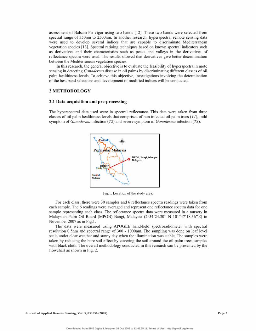
Fig.1. Location of the study area.

For each class, there were 30 samples and 6 reflectance spectra readings were taken from each sample. The 6 readings were averaged and represent one reflectance spectra data for one sample representing each class. The reflectance spectra data were measured in a nursery in Malaysian Palm Oil Board (MPOB) Bangi, Malaysia (2°54’24.30’’ N 101°47’18.36’’E) in November 2007 as in Fig.1. The data were measured using APOGEE hand-held spectroradiometer with spectral resolution 0.5nm and spectral range of 300 - 1000nm. The sampling was done on leaf level scale under clear weather and sunny day when the illumination was stable. The samples were taken by reducing the bare soil effect by covering the soil around the oil palm trees samples with black cloth. The overall methodology conducted in this research can be presented by the flowchart as shown in Fig. 2.



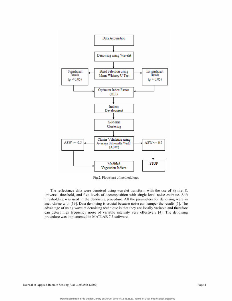
Fig.2. Flowchart of methodology.

The reflectance data were denoised using wavelet transform with the use of Symlet 8, universal threshold, and five levels of decomposition with single level noise estimate. Soft thresholding was used in the denoising procedure. All the parameters for denoising were in accordance with [19]. Data denoising is crucial because noise can hamper the results [5]. The advantage of using wavelet denoising technique is that they are locally variable and therefore can detect high frequency noise of variable intensity very effectively [4]. The denoising procedure was implemented in MATLAB 7.5 software.



Fig. 3. Reflectance spectra of T1, T2 and T3 (460nm – 959nm).

Figure 3 shows the reflectance spectra data of T1, T2 and T3 after denoising. The graphs consist of the minimum, maximum and average values of reflectance spectra of the three classes. The dashed lines represent the minimum and maximum reflectance spectra of each class while the solid lines represent the average reflectance spectra of the classes. The green line represents T1, blue line represents T2 and red line represents T3. Fig. 3 shows that there are overlaps between the reflectance spectra of the three classes. Thus, visual interpretation by naked eye on the reflectance spectra difference between the classes is not suitable. Statistical analysis is preferable when dealing with this problem. Comparative statistical analysis such as Mann-Whitney U Test would be suitable for this purpose. 2.2 Data processing Hyperspectral data measure reflectance spectra from features in high resolution of wavelength up to 0.5nm. But hyperspectral data often give too much information and in reality, only several significant wavelengths are needed to show different reflectance spectra information. The extraction of the significant wavelengths will normally involve processes such as feature extraction, feature selection and pattern recognition [20]. Comparative statistical analysis such as Mann Whitney U Test can be used to select the significant and insignificant bands for vegetation indices development. 2.2.1 Band selection The denoised data using wavelet technique were then analyzed to find the best wavelengths that can describe the difference between the three classes. In this research, band selection method was applied to the reflectance spectra of the three classes using Mann-Whitney U Test with significance level 0.05. This band selection method was proposed by [4, 21]. Mann-Whitney U Test compares two group or sets of data when there is no significant difference in the probability distribution among them. The advantage of this method is that it can be used for small set sample size and does not require normality assumption. Null hypothesis of the test is that there is no difference in the mean of the populations from which the two sample groups were taken (the populations are identical) and alternative hypothesis is that there is a difference in the mean of two populations (the populations are not identical) [18].



Using this method, the difference between reflectance spectra was investigated by pairing the classes a pair at a time. In this case, there are three possible pairs that were analyzed using Mann-Whitney U Test which were T1 versus T2, T1 versus T3 and T2 versus T3. The results are P values for each pair where the P values show the values of significance of difference for each wavelength. The significant wavelengths are wavelengths that have P values lower than 0.05. The class pairs were then summarized in a histogram. The histogram was calculated by counting the number of significant bands at each wavelength for all class pairs. The histograms indicate the frequency of significant wavelengths and which wavelengths are relatively more important for discriminating all classes. Then, high frequencies of significant difference from the histogram were chosen as the best ranges of wavelengths that have the ability to separate the three classes. The results from frequency plot were also used to select the ranges of significant and insignificant bands. The method used in identifying the significant and insignificant bands is proposed by [7]. Then the significant bands were utilized for developing modified indices for the Ganoderma disease detection in oil palm trees. 2.2.2 Index development The significant and insignificant bands were then used to create indices that can best describe the three classes. In this research, the focus is on developing vegetation indices for detecting Ganoderma disease. The goal in creating and modifying existing vegetation indices is to reduce the multiple or hyper bands of data to a single data number in predicting information about the features of interest; for example, biomass, Leaf Area Index (LAI) or vegetation cover. Vegetation indices are useful to extract information from remotely sensed data and many of the indices give redundant information about features and must be analyzed carefully and systematically. Generally, vegetation indices input consist of reflectance or any other transformed data of reflectance from green, near infrared and infrared electromagnetic spectrum. Healthy green vegetation has high absorption in the visible region except in green band while in the infrared region the reflectance is high. Most vegetation indices are based on the fact that there is a significant difference in the shape of the green vegetation, senescent vegetation and soil curve or spectral signatures. One of the most successful existing vegetation index developed is Normalized Difference Vegetation Index (NDVI). NDVI was transformed into Transformed Vegetation Index (TVI) and then modified into another version of TVI to eliminate negative values resulted by TVI [22]. These two existing vegetation indices give high values of output when there are high amount of photosynthesis activities available in vegetations. In this paper, vegetation indices that are related to bare soil information or atmospheric information were ignored because the data collected have minimum source of soil and atmospheric disturbance as the data were taken on ground level. Furthermore, one of the techniques for vegetation indices development is band ratioing. Band ratioing is a data transformation method where the main objective is to minimize the effects of environmental conditions that come from topographic slope and aspect, shadow and changing of illumination angle and intensity [16]. Band combination of the significant bands were implemented based on the work done by [12] that ratioed the reflectance spectra values of 711nm and 913nm to produce an index for Balsam Fir vigor. Wavelengths that have the most significant difference is equal to the bands that have the lowest P values while wavelengths that have insignificant difference are the bands that have the highest P values[12]. Additionally, reflectance based indices were also generated by using the lowest and highest P values wavelength throughout the whole spectrum (460nm to 959nm).



Ratio of spectral bands needs us to identify the band combinations that are the most effective, accurate and economical in separating each class from all others. Separability indices known as divergence and J-M distance were proposed which select a set of features for which the maximum separability between any pair of classes is the largest [23]. Both methods require complex computation and high effort in analysis. But a more simple method known as OIF has been proposed by [24] that attempts to search for maximum information content from each possible band combinations. Thus, OIF was used in this study to find the best combination of a pair of bands that can be ratioed to produce modified indices suitable for Ganoderma disease in oil palm trees detection. Optimum Index Factor (OIF) developed by [24] can be used to rank the utility of various combinations of band ratio. In OIF, the lower the correlation between the bands, the greater the information of the band ratio output with each band has their own unique information. The OIF is defined as:

( )∑

∑

=

== 3

1

3

1

js

kk

rAbs

sOIF , (1)

Where; sk = Standard deviation of band k. rs = Absolute value of correlation coefficient. Large OIF values indicate that the band combinations have the most information as measured by variance [22]. Different band combinations were also used to modify the available vegetation related indices to see whether these best wavelengths can improve the separability between the three classes of oil palm healthiness. Indices used in this study were Normalized Difference Vegetation Index (NDVI), Infrared Percentage Vegetation Index (IPVI) and Transformed Vegetation Index (TVI). After the new indices were generated, the indices values were then analyzed to examine their capability in separating the three classes. The indices were analyzed using K means clustering, which is a method to partition remote sensing data. 2.2.3 Clustering This method partitions the available data into K mutually exclusive clusters and returns the index values for the cluster to which it has been assigned in each observation. K means treat each observation in the data as an object that has a position in feature space. K means operate by finding partition for each data in a cluster and the data must be as close to each other and far from objects in other clusters as possible. Each cluster in the partition is distinct by its associated objects and by its centroid or center. Centroid is the point where the sum of distances from all objects data in a cluster is minimized [25]. K means compute different cluster centroid for each distance measure iterations to get the minimum of distances sums with respect to the earlier distance measurement. In other words, K means use iterative algorithm that minimizes the sum of distance from each data to its cluster centroid. The final results are clusters that are well separated. In K means the user can control the initial centroid positions and the maximum iteration number [25]. To analyze how well the clusters were separated after K means clustering was executed, silhouette plots were used.



2.2.4 Cluster validation The silhouette plot displays a measure of how close each point in one cluster to points in the neighboring clusters. The silhouette width swi in Equation 2 has a range from -1 to 1, with the value +1 defines that data points are very distant from neighboring clusters. 0 values indicate that the data points are not particularly in one cluster or another. While value of -1 shows that the data points are probably assigned in a wrong cluster [26]. If the results give a large silhouette width this means that the observations are well clustered. But silhouette with small values mean that they are scattered between clusters. Silhouette plot is useful in estimating number of group and analyze the wellness of cluster output. For example, we were given an observation as i, we then denote the average dissimilarity to all other points in its own cluster as a, for any other cluster assigned as c, we let d(i,c) represents the average dissimilarity of i to all objects in cluster c and finally we let b, to denote the minimum of these average dissimilarities d(i,c). The silhouette width for the i-th observation is:

),max(

)(ii

iii ba

absw −= , (2)

The ASW can be calculated by averaging swi over all observations

∑=

=n

iisw

nsw

1

1, (3)

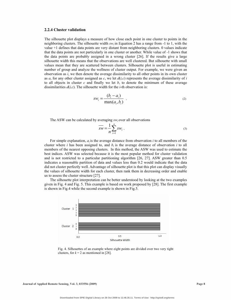
For simple explanation, ai is the average distance from observation i to all members of the cluster where i has been assigned to, and bi is the average distance of observation i to all members of the nearest opposing clusters. In this method, the ASW was used to estimate the best indices. ASW was selected because it is the most popular method for cluster validation and is not restricted to a particular partitioning algorithm [26, 27]. ASW greater than 0.5 indicates a reasonable partition of data and values less than 0.2 would indicate that the data did not cluster perfectly well. Advantage of silhouette plot is that this plot can display visually the values of silhouette width for each cluster, then rank them in decreasing order and enable us to assess the cluster structure [27]. The silhouette plot interpretation can be better understood by looking at the two examples given in Fig. 4 and Fig. 5. This example is based on work proposed by [28]. The first example is shown in Fig.4 while the second example is shown in Fig.5.

Fig. 4. Silhouettes of an example where eight points are divided over two very tight clusters, for k = 2 as mentioned in [28].



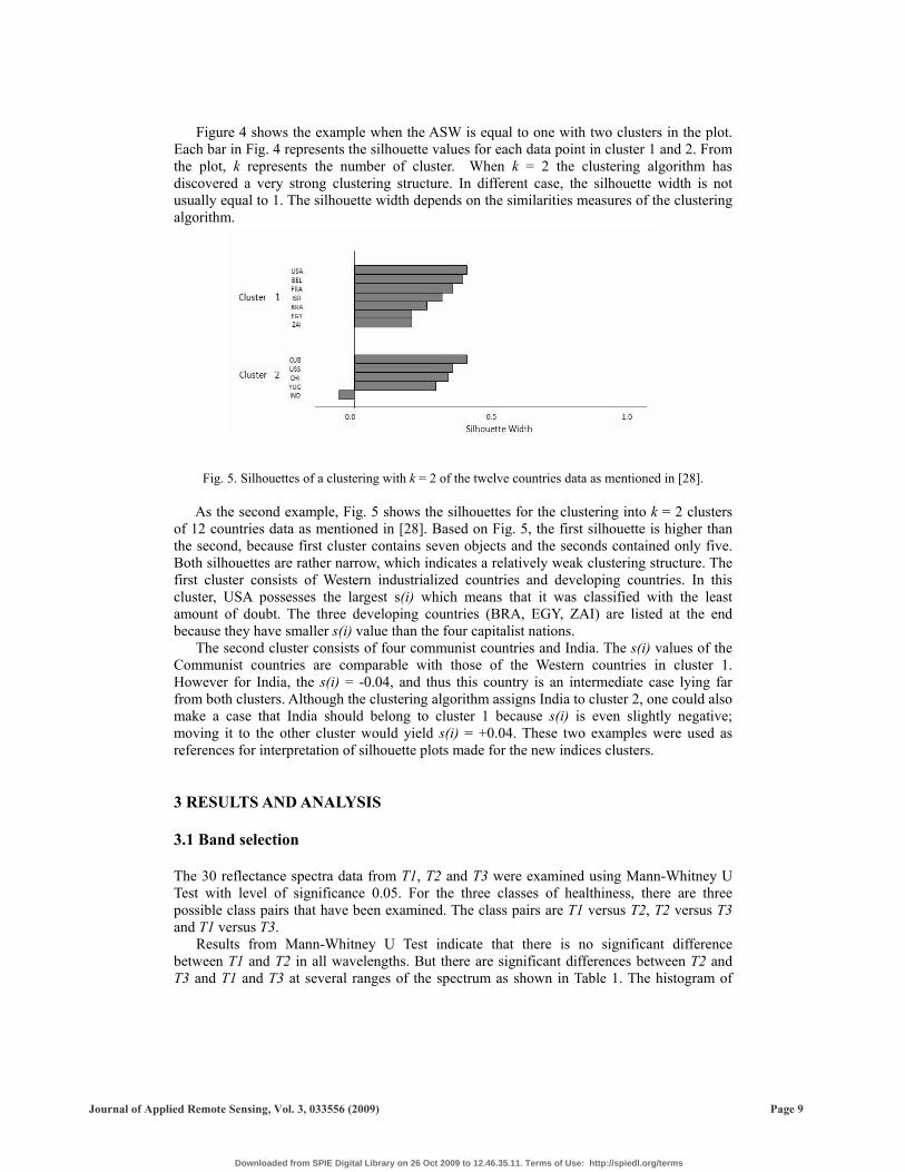
Figure 4 shows the example when the ASW is equal to one with two clusters in the plot. Each bar in Fig. 4 represents the silhouette values for each data point in cluster 1 and 2. From the plot, k represents the number of cluster. When k = 2 the clustering algorithm has discovered a very strong clustering structure. In different case, the silhouette width is not usually equal to 1. The silhouette width depends on the similarities measures of the clustering algorithm.

Fig. 5. Silhouettes of a clustering with k = 2 of the twelve countries data as mentioned in [28].

As the second example, Fig. 5 shows the silhouettes for the clustering into k = 2 clusters of 12 countries data as mentioned in [28]. Based on Fig. 5, the first silhouette is higher than the second, because first cluster contains seven objects and the seconds contained only five. Both silhouettes are rather narrow, which indicates a relatively weak clustering structure. The first cluster consists of Western industrialized countries and developing countries. In this cluster, USA possesses the largest s(i) which means that it was classified with the least amount of doubt. The three developing countries (BRA, EGY, ZAI) are listed at the end because they have smaller s(i) value than the four capitalist nations. The second cluster consists of four communist countries and India. The s(i) values of the Communist countries are comparable with those of the Western countries in cluster 1. However for India, the s(i) = -0.04, and thus this country is an intermediate case lying far from both clusters. Although the clustering algorithm assigns India to cluster 2, one could also make a case that India should belong to cluster 1 because s(i) is even slightly negative; moving it to the other cluster would yield s(i) = +0.04. These two examples were used as references for interpretation of silhouette plots made for the new indices clusters. 3 RESULTS AND ANALYSIS 3.1 Band selection The 30 reflectance spectra data from T1, T2 and T3 were examined using Mann-Whitney U Test with level of significance 0.05. For the three classes of healthiness, there are three possible class pairs that have been examined. The class pairs are T1 versus T2, T2 versus T3 and T1 versus T3. Results from Mann-Whitney U Test indicate that there is no significant difference between T1 and T2 in all wavelengths. But there are significant differences between T2 and T3 and T1 and T3 at several ranges of the spectrum as shown in Table 1. The histogram of



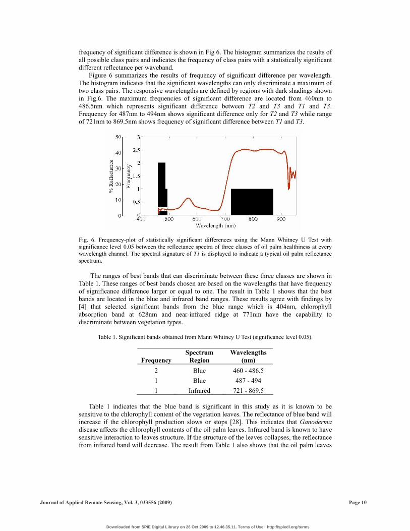
frequency of significant difference is shown in Fig 6. The histogram summarizes the results of all possible class pairs and indicates the frequency of class pairs with a statistically significant different reflectance per waveband. Figure 6 summarizes the results of frequency of significant difference per wavelength. The histogram indicates that the significant wavelengths can only discriminate a maximum of two class pairs. The responsive wavelengths are defined by regions with dark shadings shown in Fig.6. The maximum frequencies of significant difference are located from 460nm to 486.5nm which represents significant difference between T2 and T3 and T1 and T3. Frequency for 487nm to 494nm shows significant difference only for T2 and T3 while range of 721nm to 869.5nm shows frequency of significant difference between T1 and T3. Fig. 6. Frequency-plot of statistically significant differences using the Mann Whitney U Test with significance level 0.05 between the reflectance spectra of three classes of oil palm healthiness at every wavelength channel. The spectral signature of T1 is displayed to indicate a typical oil palm reflectance spectrum. The ranges of best bands that can discriminate between these three classes are shown in Table 1. These ranges of best bands chosen are based on the wavelengths that have frequency of significance difference larger or equal to one. The result in Table 1 shows that the best bands are located in the blue and infrared band ranges. These results agree with findings by [4] that selected significant bands from the blue range which is 404nm, chlorophyll absorption band at 628nm and near-infrared ridge at 771nm have the capability to discriminate between vegetation types.

Table 1. Significant bands obtained from Mann Whitney U Test (significance level 0.05).

Frequency Spectrum

Region Wavelengths

(nm) 2 Blue 460 - 486.5 1 Blue 487 - 494 1 Infrared 721 - 869.5

Table 1 indicates that the blue band is significant in this study as it is known to be sensitive to the chlorophyll content of the vegetation leaves. The reflectance of blue band will increase if the chlorophyll production slows or stops [28]. This indicates that Ganoderma disease affects the chlorophyll contents of the oil palm leaves. Infrared band is known to have sensitive interaction to leaves structure. If the structure of the leaves collapses, the reflectance from infrared band will decrease. The result from Table 1 also shows that the oil palm leaves



structure have been affected by Ganoderma disease. Wavebands from visible and infrared regions were the common wavebands that are used in developing vegetation indices because of their significant changes influenced by the amount of chlorophyll contents and the cells structures of the vegetation leaves [30]. The visible spectrum region is sensitive to the amount of the chlorophyll contents of the vegetations while infrared region is sensitive to the structure of the leaves while the middle infrared region is known to be sensitive to the water content of the vegetations [31]. The visible and infrared showed inverse linear relationship where the relative reflectance from the visible will decrease while the reflectance in infrared range will increase if the vegetation suffers from stress or disease [32]. Results shown in Table 2 indicate that the significant bands for Ganoderma disease are different from the significant bands used for differentiating vegetation types as proposed by [4] and [12]. The significant bands for this purpose were also different from the significant bands for mangrove species discrimination as proposed by [33].

Table 2. Significant and insignificant wavelengths.

Spectrum Range

Wavelengths (nm) Significant (nm) Insignificant (nm)

Blue 460 - 486.5 462 486 Blue 487 - 494 487 493

Infrared 721 - 869.5 749 851 Full range 460 - 959 738 610.5

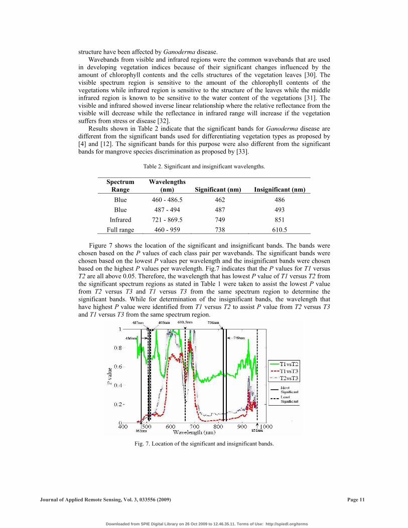
Figure 7 shows the location of the significant and insignificant bands. The bands were

chosen based on the P values of each class pair per wavebands. The significant bands were chosen based on the lowest P values per wavelength and the insignificant bands were chosen based on the highest P values per wavelength. Fig.7 indicates that the P values for T1 versus T2 are all above 0.05. Therefore, the wavelength that has lowest P value of T1 versus T2 from the significant spectrum regions as stated in Table 1 were taken to assist the lowest P value from T2 versus T3 and T1 versus T3 from the same spectrum region to determine the significant bands. While for determination of the insignificant bands, the wavelength that have highest P value were identified from T1 versus T2 to assist P value from T2 versus T3 and T1 versus T3 from the same spectrum region.

Fig. 7. Location of the significant and insignificant bands.



This result shows that the significant bands for different vegetation types are different. These findings also improve the work done by [5] by proving that there are several significant bands identified that are able to discriminate oil palms based on their healthiness class that are influenced by the biophysical and chemical characteristics of the oil palm leaves. However, reflectance spectra data still cannot discriminate between healthy (T1) and mild symptom of Ganoderma disease in oil palm (T2) effectively. The significant and insignificant bands can be used further to develop indices that might differentiate T1 and T2 more effectively. 3.2 Indices development New indices introduced in this study are known as A1, A2, B1, B2, C1, C2, D1, D2, NDVI a, IPVI a, and TVI a. From the information shown in Table 2, eight different reflectance based indices were generated using band ratio method and coded with A1 and A2 for 460 – 486.5nm, B1 and B2 for 487 – 494nm and C1 and C2 for 721 – 869.5nm, which are focused on certain regions of the spectrum. There are also D1 and D2 indices with the input selected from the full range of electromagnetic spectrum in use. All the new reflectance indices are shown in Table 3.

Table 3. The list of new reflectance indices based on band ratio.

Spectrum

Range Reflectance

Indices Blue A1 = 486/462 A2 = 462/486 Blue B1 = 493/487 B2 = 487/493

Infrared C1 = 851/749 C2 = 749/851 Full Range D1 = 738/610.5 D2 = 610.5/738

For assessment of the new indices, available default indices that use 670 nm, 800nm [34] and indices modified by [15] that use 705nm and 750nm were used to be compared with the new indices output. The OIF results from Table 4 show that the best combinations of bands are 610.5 and 738 nm because the OIF value is the highest compared to other band combinations. The default combinations that are usually being used as vegetation features extraction give lower values of OIF, but compared to other possible band combinations, 670 nm and 800 nm are still better for vegetation analysis using reflectance spectra. Results obtained from Table 3 and 4 are in agreement as combinations of 610.5nm and 738nm give more information about the T1, T2 and T3 dissimilarity.

Table 4. OIF Result for Possible Band Combinations.

Rank Band combinations OIF

1 610.5,738 48.388 2 670,800 33.503 3 705,750 21.983 4 749,851 13.546 5 462,468 3.323 6 487,493 2.529

The combinations of 610.5nm and 738nm were also used for modifying indices. Table 5



shows the algorithm for indices that have been modified with NIR refers to near infrared and R is red band. The default wavelengths input for the default indices is 800 nm for NIR and 670nm for R. In this paper, the modified indices were coded as NDVI a, IPVI a, and TVI a. Then K means clustering was used to cluster the indices values into three possible classes. 3.3 Clustering For visual interpretation of separability between these indices, K means clustering were used to cluster the index values and determine the centroid of the cluster generated. For input, three sets of the indices values from each classes as shown in Table 3 were analyzed and then the number of desired cluster were set to 3 while the number of iteration were set to 5 as default. For analyzing the K means output visually, the assessment on how well the clusters were separated was analyzed using silhouette plot.

Table 5. Modified indices by different band combination methods.

Indices Default Indices (nm) Modified Indices (nm)

NDVIa RNIRR

+−NIR

5.610738

5.610738

RNIRRNIR

−−

IPVIa RNIRNIR

+

5.610738

738

RNIRNIR

+

TVIa )5.0(

)5.0(5.0 +×

++ NDVIAbs

NDVIAbsNDVI )5.0(

)5.0(5.0 +×

++ NDVIaAbs

NDVIaAbsNDVIa

3.4 Cluster validation Based on Table 6 and Fig.8, all the ASW values are more than 0.5. This means that the data are well clustered in probability of three clusters and the ASW values were then arranged based on ranks to choose the best indices. The ranking was done based on the value generated by the ASW formulae in Eq. (3). The top rank is given to the index with the highest ASW value and vice versa. ASW values those are larger than 0.5 indicate good clustering. Rank 1 represents the best index which is D2 index and decreases thorough the column. Based on Table 6, the best index that can cluster the index values for T1, T2 and T3 is D2 followed by TVI a. D2 index is the best because the ASW value is 0.6441. NDVI a has the same ASW value as IPVI a in third place, while A1 gets the fifth place and then the other indices based on descending ranks are NDVI[15], IPVI [15], TVI [15], D1, Default TVI, Default NDVI, Default IPVI, C2, C1, A2, B2 and B1. Table 6 shows that NDVI with combination of 610.5nm and 738nm is better to differentiate between different levels of Ganoderma disease in oil palm trees than NDVI using 705nm and 750nm wavelengths as proposed by [15]. The lowest is B1 index with ASW value of 0.5403. B1 value still shows good clustering effort of the three clusters but the ASW value is the lowest compared to the other indices values.



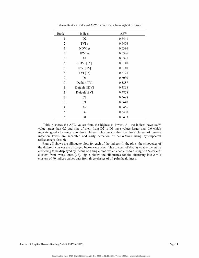
Table 6. Rank and values of ASW for each index from highest to lowest.

Rank Indices ASW 1 D2 0.6441 2 TVI a 0.6406 3 NDVI a 0.6386 3 IPVI a 0.6386 5 A1 0.6321 6 NDVI [15] 0.6140 6 IPVI [15] 0.6140 8 TVI [15] 0.6125 9 D1 0.6030

10 Default TVI 0.5887 11 Default NDVI 0.5868 11 Default IPVI 0.5868 12 C2 0.5698 13 C1 0.5640 14 A2 0.5466 15 B2 0.5438 16 B1 0.5403

Table 6 shows the ASW values from the highest to lowest. All the indices have ASW value larger than 0.5 and nine of them from D2 to D1 have values larger than 0.6 which indicate good clustering into three classes. This means that the three classes of disease infection levels are separable and early detection of Ganoderma using hyperspectral reflectance is feasible.

Figure 8 shows the silhouette plots for each of the indices. In the plots, the silhouettes of the different clusters are displayed below each other. This manner of display enable the entire clustering to be displayed by means of a single plot, which enable us to distinguish ‘clear cut’ clusters from ‘weak’ ones [28]. Fig. 8 shows the silhouettes for the clustering into k = 3 clusters of 90 indices values data from three classes of oil palm healthiness.



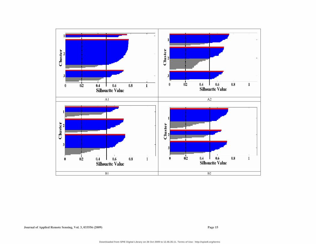
A1 A2

B1 B2



C1 C2

D1 D2



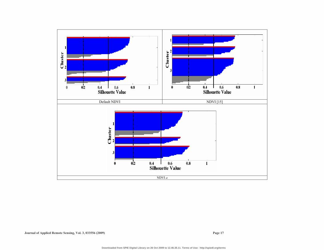
Default NDVI NDVI [15]

NDVI a



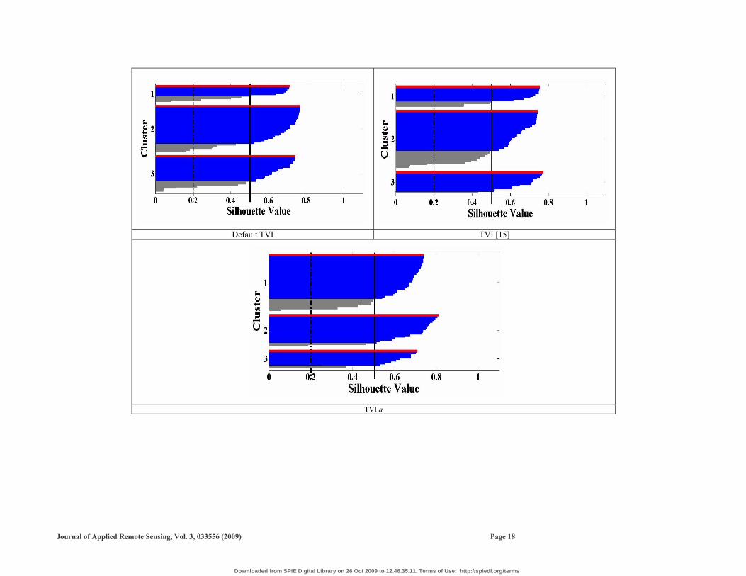
Default TVI TVI [15]

TVI a



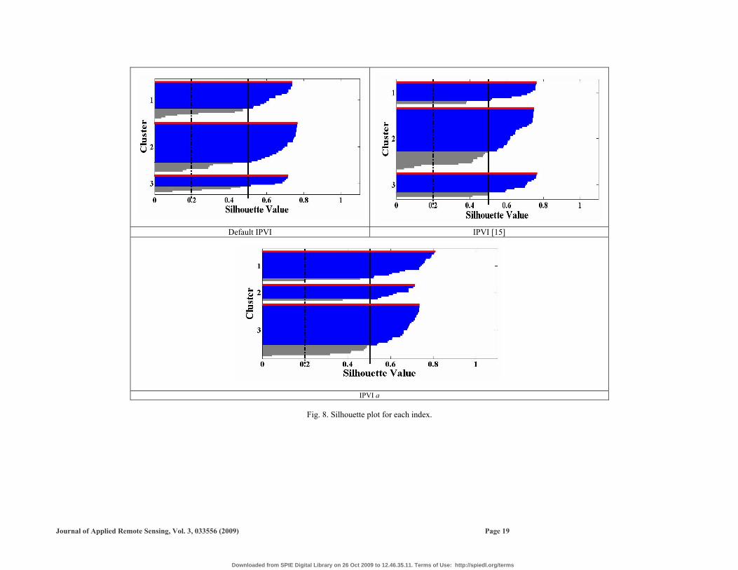
Default IPVI IPVI [15]

IPVI a

Fig. 8. Silhouette plot for each index.



The y-axis of the plot represents each of the 90 silhouette values for each of the index value by means of its three character level which is class 1, 2 and 3. The x-axis represents the silhouette values scales. Red silhouette regions represent the highest silhouette value in a cluster while the blue silhouette regions represent the silhouette values that exceed the threshold of 0.5 for good clustering. The grey silhouette regions represent the silhouette values that below than 0.5 and 0.2. From the plots, the indices values of each class are clustered in the possible three existing clusters because there are no negative values between the clusters except for C1 index where there are some negative values in cluster 2 and 3 meaning that there are some outliers between those clusters. This negative value also indicates that some of the values are an intermediate case lying far from cluster 2 and 3. The negative value indicates that some of the index values can be in either both clusters 2 or 3. The narrow width of cluster 2 and 3 of C1 index also indicate that they are relatively weak clustering structure. On the other hand, cluster 1, which has wider silhouette width, suggests that it has a strong clustering structure. This concept is applicable for all the plots in Fig.8. The vertical dash-dot line represents 0.2 boundary values and the vertical bold line represents 0.5 boundary values for silhouette plot. Clusters with silhouette bar values below 0.2 indicate that the observations for T1, T2 and T3 are not well clustered and when the values of silhouette exceed 0.5 means that the three classes are well clustered. For D2 index, the ASW values are the highest compared to all other indices. The silhouette plot for D2 index in Fig.8 shows that cluster 2 has the narrowest silhouette width above 0.5 compared to cluster 1 and 3. This indicates that clustering for class 2 did not contains many index values due to value similarities that D2 index has with T1, T2 and T3. Fig.8 also indicates that there are no plots that have a well balanced of silhouette width for all the possible three clusters. This is due to the values of the healthy and mild symptom of Ganoderma disease that not very distinctively separable but have some mixture of reflectance values as mentioned in Fig. 3 earlier. These findings indicate that although D2 index can be assumed to be the best index to discriminate between the three classes based on the ASW value, one should never merely accept the ASW at its face value, but also look at the graphical output itself to find what caused it [28]. The first silhouette bars in all three clusters in D2 index plot that are highlighted by red bar have values above than 0.6 and slightly exceed 0.8. This indicates that at least one of the index values from each cluster was classified with the least amount of doubt. Thus, they are perfectly suited for the assigned cluster. D2 index silhouette plot that highlighted by blue colour also shows that majority of silhouette bars are above the acceptable threshold of good clustering (0.5) which indicates that majority of the D2 indices values are separable for the three classes that allow the discrimination of the three classes. Only few silhouette bars of each cluster have values below than 0.5 which are highlighted by grey colour. The majority of silhouette values above 0.5 had made D2 index acceptable in discriminating the three classes based on the ASW and the structure of silhouette bars for each data in each cluster. The grey silhouette bars indicate that there are small ambiguities that come from overlapping values of reflectance spectra of the three classes.



4 CONCLUSIONS This study has contributed to the development of new indices that can be used to discriminate between healthy and two levels of Ganoderma infection in oil palm trees. Band selection results show that the significant bands can only discriminate between T2 and T3 and T1 and T3 classes statistically. The significant and insignificant bands are located in the blue and infrared electromagnetic regions and these bands were then used for creating and modifying vegetation indices. By using OIF, band combinations of 610.5nm and 738nm are the best that can give unique information about the three classes because of low correlation coefficient and high OIF values. Results from ASW plot that exceed 0.6 are for A1, D1, D2, NDVI a, IPVI a and TVI a and the best index is D2 with ASW value of 0.6441. These results satisfy the results obtained from OIF analysis. With the ability of the indices to cluster the three classes with an acceptable threshold, early detection of Ganoderma disease in oil palm is feasible by using hyperspectral technique. For further development, the indices can be applied to airborne hyperspectral mapping for large scale Ganoderma disease detection. References [1] Malaysia Palm Oil Council (MPOC), ‘Malaysian Palm Oil Industry,’

http://www.mpoc.org.my/main_ind_01.asp (accessed 21 August 2008). [2] J. Flood, P. D. Bridge, and M. Holderness, Preface. Ganoderma Disease in Perennial

Crops, CABI Publishing, Wallingford, U.K. (2000a). [3] R. R. M. Paterson, M. Holderness, J. Kelley, R. Miller, and E. O`Grady, "In vitro

biodegradation of oil palm stem using macroscopic fungi from South East Asia: a Preliminary Investigation," Ganoderma Diseases of Perennial Crops, J. Flood, P. D. Bridge, and M. Holderness, Eds., pp. 129-138, CABI Publishing, Wallingford, U.K. (2000).

[4] K. S. Schmidt and A. K. Skidmore, "Spectral discrimination of vegetation types in a coastal wetland," Rem. Sens. Environ. 85, 91-108 (2002) [doi: 10.1016/S0034-4257(02)00196-7].

[5] C. C. D. Lelong, M. Lanore, and J. P. Caliman, "Evaluation of hyperspectral remote sensing relevance to estimate oil palm trees nutrition status," Second Recent Advances in Quantitative Remote Sensing (RAQRS'II), J. A. Sobrino , Ed., Int. Symp. Recent Adv. Quantitative Rem. Sens. 2, 147-152 (2006).

[6] S. Delalieux, J. V. Aardt, W. Keulemans, E. Schrevens, and P. Coppin, "Detection of biotic stress (Venturia Inaequalis) in apple trees using hyperspectral data: Non-parametric statistical approaches and physiological implications," Eur. J. Agron. 27, 130-143 (2007) [doi:10.1016/j.eja.2007.02.005].

[7] H. Z. M. Shafri and M. I. Anuar, "Hyperspectral signal analysis for detecting disease infection in oil palms," IEEE Int. Conf. Comp. Electrical Eng., 312-316 (2008) [doi: 10.1109/ICCEE.2008.196].

[8] J. C. Chan and D. Paelinkx, "Evaluation of random forest and adaboost tree-based ensemble classification and spectral band selection for ecotope mapping using airborne hyperspectral imagery," Rem. Sens. Environ. 112, 2999-3011 (2008) [doi:10.1016/j.rse.2008.02.011].

[9] V. Thomas., P. Treitz, D. Jelinski, J. Miller, P. LaFleur, and J. H. McCaughney, "Image classification of northern peat-land complex using spectral and plant community data," Rem. Sens. Environ. 84, 83-99 (2003) [doi:10.1016/S0034-4257(02)00099-8].

[10] J. C. Price, "Band selection procedure for multispectral scanners," Appl. Opt. 33, 3281-88 [doi:10.1364/AO.33.003281].

[11] G. A. Carter, "Ratios of leaf reflectance in narrow wavebands as indicators of plant



http://dx.doi.org/10.1016/S0034-4257%2802%2900196-7

http://dx.doi.org/10.1016/S0034-4257%2802%2900196-7

http://dx.doi.org/10.1016/j.eja.2007.02.005

http://dx.doi.org/10.1016/S0034-4257%2802%2900099-8

stress," Int. J. Rem. Sens. 15, 697-703 (1994) [doi: 10.1080/01431169408954109]. [12] J. E. Luther and A. L. Carroll, "Development of an index of Balsam Fir vigor by foliar

reflectance spectra," Rem. Sens. Environ. 69, 241-252 (1999) [doi:10.1016/S0034-4257(99)00016-4].

[13] R. Rud, M. Shoshany, V. Alchanatis, and Y. Cohen,"Applications of spectral features’s ratio for improving classification partially calibrated hyperspectral imagery: a case study of separating Mediterranean vegetation species," J. Real-Time Image Proc. 1, 143-152 (2006) [doi:10.1007/s11554-006-0015-8].

[14] C. R. Perry Jr. and L. F. Lautenschlager, "Functional equivalence of spectral vegetation indices," Rem. Sens. Environ. 14, 169-182 (1984) [doi:10.1016/0034-4257(84)90013-0].

[15] W. Chaoyang, N. Zheng, T. Quan, and H. Wenjiang, "Estimating chlorophyll content from hyperspectral vegetation indices: Modeling and validation," Agric. Forest Meteorol. 148, 1230-1241 (2008) [doi:10.1016/j.agrformet.2008.03.005].

[16] J. F. Moreno, F. Baret, M. Leroy, M. Menenti, M. Rast, and M. Shaepman, "Retrieval of vegetation properties from combined hyperspectral/multiangular optical measurements: results from the DAISEX campaigns," IEEE Int. Geosci. Rem. Sens. Symp. 4, 2875-2877 (2003) [doi:10.1109/IGARSS.2003.1294616].

[17] M. M. Verstraete and B. Pinty, "Designing optimal spectral indexes for remote sensing applications," IEEE Trans. Geosci. Rem. Sens. 34, 1254-1265 (1996) [doi: 10.1109/36.536541].

[18] T. Buyong, Spatial Statistics for Geographic Information Science, Penerbit Universiti Teknologi Malaysia, Johor, Malaysia (2006).

[19] H. Z. M. Shafri and M. R. M. Yusof, "Determination of optimal wavelet denoising parameters for red edge feature extraction from hyperspectral data," J. Appl. Rem. Sens. 3, 033533 (2009) [doi:10.1117/1.3155804].

[20] C. Chen, Signal and Image Processing for Remote Sensing, pp. 25, CRC Press, New York (2007).

[21] J. J. Mitchell and N. F. Glenn, "Leafy Spurge (Euphorbia esula) classification performance using hyperspectral and multispectral sensors," Rangeland Ecol. Manage. 62, 16-27 (2009) [doi: 10.2111/08-100].

[22] J. R. Jensen, Introductory Digital Image Processing: A Remote Sensing Perspective, 2nd ed., Prentice Hall Series in Geographic Information Science, Upper Saddle River, New Jersey (1996).

[23] P. Swain and S. Davis, Remote Sensing: The Quantitative Approach, McGraw-Hill, New York (1978).

[24] P. S. Chavez, S. C. Guptill, and J. A. Bowell, "Image processing techniques for thematic mapper data," Technical Papers, 50th Annual Meeting of the American Soc. Photog. 2, 728–742 (1984).

[25] MATLAB toolbox documentation online help, 2007, http://www.mathworks.com (accessed 5 December 2008).

[26] L. Kaufman and P. J. Rousseeuw, Finding Groups in Data: An Intro Introduction to Cluster Analysis, Wiley, New York (1990).

[27] W. L. Martinez and A.R. Martineza, Exploratory Data Analysis with MATLAB, CRC Press, London, UK (2005).

[28] P. J. Rousseeuw, "Silhouettes: a graphical aid to the interpretation and validation of cluster analysis," J. Comp. App. Math. 20, 53-56 (1987).

[29] R. M. McCoy, Field Method in Remote Sensing, Guilford Press, New York, 72 pp. (2005).

[30] S. L. Ustin, D. A. Roberts, J. A. Gamon, G. P. Asner, and R. O. Grenn, "Using imaging spectroscopy to study ecosystem processes and properties," Biosci. 54, 523-534 (2004) [doi: 10.1641/0006-3568(2004)054[0523:UISTSE]2.0.CO].



http://dx.doi.org/10.1016/S0034-4257%2899%2900016-4

http://dx.doi.org/10.1016/S0034-4257%2899%2900016-4

http://dx.doi.org/10.1016/0034-4257%2884%2990013-0

http://dx.doi.org/10.1016/0034-4257%2884%2990013-0

http://dx.doi.org/10.1016/j.agrformet.2008.03.005

[31] H. R. Xu, Y. B. Ying, X. P. Fu, and S.P. Zhu, "Near-infrared spectroscopy in detecting leaf miner damage on tomato leaf," Biosystem Eng. 96, 447-454 (2007) [doi:10.1016/j.biosystemseng.2007.01.008].

[32] P. J. Gibson, C. H. Power, S. E. Goldin, and K. T. Rudahl, Introductory Remote Sensing: Digital Image Processing and Applications, pp. 115-121, Routledge, U.K. (2000).

[33] L. Wang and W. P. Sousa "Distinguishing mangrove species with laboratory measurements of hyperspectral leaf reflectance," Int. J. Rem. Sens. 30, 1267-1281 (2009) [doi: 10.1080/01431160802474014].

[34] J. W. Rouse, R. H. Haas, J. A. Schell, D. W. Deering, and J. C. Harlan, "Monitoring the vernal advancement and retrogradation of natural vegetation," NASA/GSFC, Final Report, 1-137, Greenbelt, MD(1974).

Helmi Z. M. Shafri received his BSc in Surveying degree from RMIT University,

Melbourne, Australia in 1998. He obtained his PhD in remote sensing from the University of Nottingham, UK in 2003 and is now the Head of Geomatics Engineering Unit, Department of Civil Engineering, Universiti Putra Malaysia (UPM). His major research interests are hyperspectral remote sensing data analysis and algorithm development.

M. Izzuddin Anuar received the B.Sc in Remote Sensing from Universiti Teknologi

Malaysia (UTM), Skudai, Johor, Malaysia in 2007. He is currently working towards a MSc degree specializing in hyperspectral signal processing and analysis at Universiti Putra Malaysia (UPM).

M. Iqbal Saripan is a lecturer at the Department of Computer and Communication

Engineering, Faculty of Engineering, Universiti Putra Malaysia (UPM).



http://dx.doi.org/10.1016/j.biosystemseng.2007.01.008

Detection of stressed oil palms from an airborne sensor using optimized spectral indices

Documents

Transcript of Detection of stressed oil palms from an airborne sensor using optimized spectral indices