Crop and Irrigation Water Management Using High Resolution Airborne Remote Sensing

Christopher M. U. Neale, Hari Jayanthi1 and James L. Wright2

Abstract

This paper offers a historical retrospective on the remote sensing of crop coefficients for obtaining actual crop evapotranspiration. We present recently developed crop coefficients for bean and potato and show the usefulness of high-resolution airborne imagery for monitoring temporal changes and characterizing in-field variability of crop growth.

Introduction

The use of remote sensing for obtaining evapotranspiration from natural and agricultural surfaces is becoming mainstream as recent research (some of which are being presented at this workshop) has shown the tremendous potential that this technology has in spatially retrieving this important hydrological variable. The two basic approaches in development are (1) the solution of the energy balance equation using remotely sensed surface temperatures and reflectance to obtain certain variables and components of this equation and (2) the crop coefficient and reference ET approach where the crop coefficient is obtained through canopy reflectance measurements. In either approach, the applications have been developed through careful ground-radiometry studies in controlled field conditions or using airborne imagery at different spatial resolutions to apply the methods over larger areas. As examples of these studies is research by Reginato et al. (1985), Neale et al. (1989), Moran et al. (1994), Kustas et al. (1994) and Bausch (1995). In this paper we attempt to show the value of using calibrated high-resolution imagery to extend results from sub-field level remote sensing studies to larger fields and areas, a necessary step in the use of these methodologies with satellite imagery. We concentrate on the crop coefficient approach for obtaining actual crop water use in individual fields and over larger irrigated areas. As precision agricultural applications become more common, the need for higher resolution satellite imagery will be required to improve spatial ET and yield estimates.

1 Department of Biological and Irrigation Engineering, Utah State University, Logan, Utah, 84322-4105 2 ARS-USDA, Northwest Irrigation & Soils Research Laboratory, Kimberly, Idaho ID-83341

Neale, Jayanthi and Wright, 2003 Page 1 ICID Workshop on Remote Sensing of ET for Large Regions, 17 Sept. 2003

Historical Background Evapotranspiration (ET) represents the simultaneous loss of water from soil surface (evaporation, E) and plant body (transpiration, T). The term reference evapotranspiration (ref-ET) was defined to “represent the upper limit or maximum ET that occurs under given climatic conditions with a field having a well watered agricultural crop with an aerodynamically rough surface, such as alfalfa with 0.3 to 0.45 m (12 to 18 inches) of top growth” (Jensen et al. 1970). Presently either grass (Allen et al. 1998) or alfalfa (Wright 1982) is taken as reference crop surfaces depending on the agro-climatology of the area. Canopy linkages with ET: Gates and Hanks (1967) observed that leaf area, stage of growth, canopy cover and ground shading, row spacing and orientation, and light reflection for potato and sugar beet crops influenced plant ET. Penman et al. (1967) studied the relation between the leaf area and canopy shading of the ground and conceptualized full cover stage - when the plants in the adjacent rows overlapped and masked the underlying soil from direct sunlight. Ritchie and Burnett (1971) measured the fractional ground cover, dry matter production and leaf area for dry land cotton and identified a threshold LAI (of 2.7) at which potential evaporation was reached from row crops; and beyond the threshold canopy LAI, evaporation was maximum, practically independent of plant factors until soil water was observed to limit evaporation. Tanner and Jury (1976) outlined a range of LAI and percent ground cover values for barley, bean, corn, cotton, potato, safflower and wheat crops at which crop ET approaches maximum ET. No single unique LAI value was observed at which the crops attained maximum ET; and the percent ground cover values varied even more. Crop coefficients: Crop coefficients (Kc) relate the potential evaporative demands of a field crop to that from a reference evaporating surface. Jensen et al. (1970) stated that crop coefficients represented the combined effects of plant path resistance to water movement from soil to the evaporating surfaces, and the resistances to the diffusion of water vapor from the evaporating surfaces to the atmosphere in the crop and the reference crop. Crop coefficients are formulated either on the basis of environmental factors (mainly temperature) influencing crop phenology or on the basis of how the crop develops its canopy during the growth season. Environmental crop coefficients: Crops have individual temperature and photo period requirements for initiating and completing their growth cycles. The sums of mean daily temperature (between certain temperature ranges) have been used to calculate heat units necessary for the crop to attain different stages in its growth cycle, defined as growing degree day (GDD)(Everson et al. 1976). This empirical approach has been found to be an effective predictor of crop phenology (Sammis 1985, Amos et al. 1989, Hunsaker 1999).

Neale, Jayanthi and Wright, 2003 Page 2 ICID Workshop on Remote Sensing of ET for Large Regions, 17 Sept. 2003

Crop canopy based coefficients: The manner in which the crop canopy develops its morphology over time and the way it intercepts radiation and shades the underlying soil form the basis of crop canopy based crop coefficients. Grattan et al. (1998) developed a simple crop coefficient method based on the percent shading (ground cover) for vegetable crops. Wright (1982) proposed a dual basal crop coefficient approach - which splits the total crop coefficient into crop transpiration (Kcb) and soil evaporation (Ks) fractions. The Kcb component represents the crop evaporative conditions from soil conditions whose surface is dry (direct evaporation from soil surface is minimum), and the crop growth is not limited by water, insect, climatological or physiological factors. The Kcb curve is constructed based on (a) the time between planting to effective cover normalized by percent time, and (b) the time in days after effective cover to harvest. The utilization of basal crop coefficients requires the information on the dates of planting and effective full cover. Effective full cover (EFC) was defined as that stage of crop growth when the crop ET is maximum relative to reference ET, and the corresponding crop coefficient attains its maximum value. Stegman et al. (1980) indicated that in case of agricultural crops, the ET rate at EFC reached a potential rate when the LAI was about 3.0 and the ground cover was about 75%. Neale et al. (1989) reported that the LAI values at EFC for corn varied between 2.8 and 3.2, based on 6 years of experimental data. Ahmed (1997) reported that the ground cover at EFC stage for alfalfa and corn was 80%. In general, it is observed that there may not be a single unique LAI threshold at EFC as it is dependent on crop canopy (shape, size, architecture, etc.) and root system development. Crop development is seldom uniform in nature, and it varies over space and time. A single crop coefficient curve may not account for the within-field variability induced by varying soil, soil water and nutrients, local weather anomalies and different agronomic practices. Canopy reflectance based crop coefficients: Jackson et al. (1980) found similarities between the mean crop coefficient (KC) for small grain to the ratio of the perpendicular vegetation index (PVI) for wheat to PVI of wheat at full canopy cover. Heilman et al. (1982) investigated the relationship between percent cover and reflectance-based perpendicular vegetation index (PVI) for alfalfa. Neale et al. (1989) related the crop canopy reflectance to basal crop coefficients for corn, developing an operational technique for estimating actual crop ET. The reflectance based crop coefficient (Kcr) was derived by linearly transforming the seasonal normalized difference vegetation index (NDVI) using the percent shading and leaf area measurements to establish the EFC and relate it to the basal crop coefficient by Wright (1982). Bausch (1995) found that using NDVI (in linear transformation to obtain Kcb) for a dark colored soil background overestimated Kcb for corn by 24 percent or more, and suggested using a soil adjusted vegetation index (SAVI) with an adjustment factor (L) of 0.5 (Huete 1988) to minimize the soil influences for sparse to dense vegetation conditions. It was

Neale, Jayanthi and Wright, 2003 Page 3 ICID Workshop on Remote Sensing of ET for Large Regions, 17 Sept. 2003

reported that SAVI reached a peak of 0.7 when corn attained EFC. Neale et al. (1996) developed SAVI based crop coefficients for alfalfa, and grain crops like barley, corn, wheat, and cotton to estimate corresponding crop ET.

Recent Developments Over the last few years, we have worked on further extending the reflectance-based crop coefficient methodology to non-grain crops grown in southern Idaho, namely beans, potatoes and sugar beets. This research was conducted near the USDA-ARS research facility in Kimberly, Idaho. The methodology used in the past for the development of reflectance-based crop coefficients called for concurrent measurements of actual crop ET, reference ET, canopy biophysical parameters (leaf area index, biomass, percent cover, plant height and width), canopy reflectance, percent shading and soil moisture. The lysimeters installed at Kimberly were used in the 1970’s and 1980’s to obtain the necessary data for developing basal crop coefficients for several crops, culminating in the paper by Wright (1982). We conducted our research in the same climatic, soil and experimental conditions as reported in Wright (1982), collecting the necessary canopy biophysical variables to bridge the original lysimeter ET data and our canopy reflectance measurements. The canopy reflectance was measured throughout the season, around solar noon, using an Exotech 4-band radiometer with Thematic Mapper bands TM1 through TM4. The SAVI at EFC (maximum ET) was obtained by relating the average SAVI from several bean fields at the corresponding LAI and percent cover observed by Wright (1982) during his lysimeter studies with the same crop. It can be seen from Fig.1(a) that the actual crop growth was slower at the beginning of the season, when compared to expected crop growth defined by the basal crop coefficient curve. The same growth pattern was captured by the aerial data as shown by the growth curve of ground Kcr for the field. The validation of the reflectance based crop coefficient curve was accomplished by simulating the root zone soil water balance using both basal and reflectance based crop coefficients and comparing them with the actual root zone soil water changes assessed by neutron probe measurements in Fig.1(b). There is a good match between the estimated soil water variations using both coefficients with the actual seasonal soil profiles. At full cover stage the Kcr based available soil water was 1.2% less than the actual measured value (the Kcb based estimate of the soil water was 2.4% less than the actual measured value).

Neale, Jayanthi and Wright, 2003 Page 4 ICID Workshop on Remote Sensing of ET for Large Regions, 17 Sept. 2003

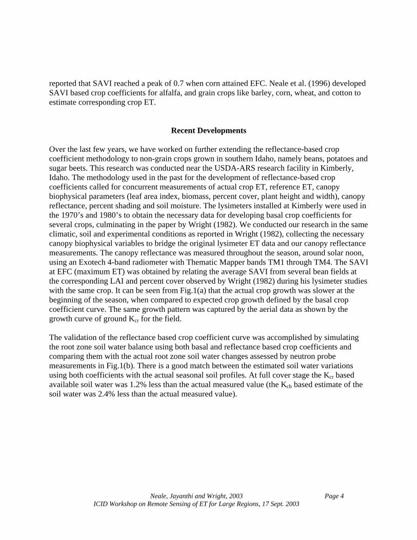
Fig. 1(a) Figure 1(a). Comparison of ground based and beans with basal crop coefficient (Kcb); (b) com(Kcb) and reflectance based crop coefficients (root zone. Fig.2a compares the seasonal growth profile obasal crop coefficient for potato grown under the estimates of soil water in the root zone by measured soil water from neutron probe measucoefficients) match well with the actual soil w Fig.3 shows the soil and potato crop growth vaspectral images. The patterns of fertile and eropatterns through the season. The crop emergedweek of July. Furthermore the soil patterns alsmaturity and governed the rates of senescencetremendous variation in crop growth (and thus

Neale, Jayanthi an ICID Workshop on Remote Sensing of

Fig. 1(b)

aerial reflectance (Kcr) based crop coefficients for parison of soil water simulations using basal

Kcr) with the actual soil water measurements in the

f reflectance based crop coefficient with that of the a center pivot irrigation system. Fig.2b compares using both crop coefficients with the actual rements. The soil water estimates (using both crop

ater storage measurements throughout the season.

riability in the center pivot in the time series multi ded soils were observed to influence crop growth on 6th June and attained full cover during the third o influenced the plant stand duration during the in the field. The midseason images also show the ly Kcr ) within the field.

d Wright, 2003 Page 5 ET for Large Regions, 17 Sept. 2003

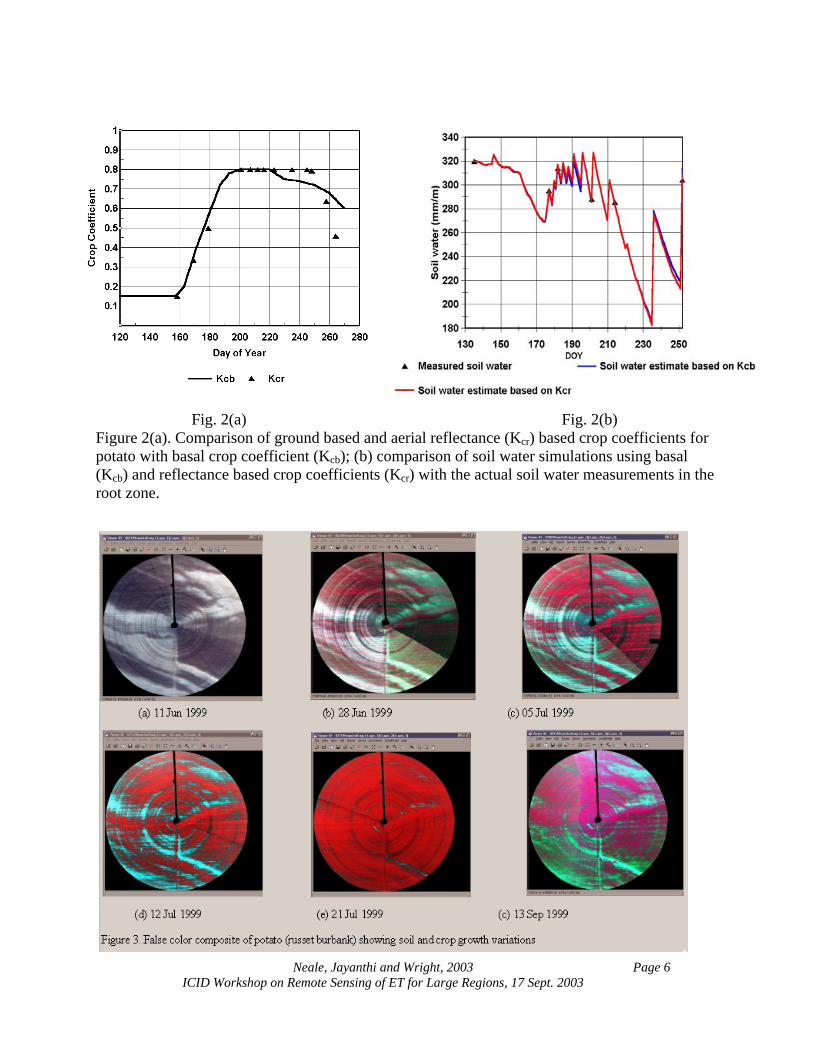
Fig. 2(a) Fig. 2(b) Figure 2(a). Comparison of ground based and aerial reflectance (Kcr) based crop coefficients for potato with basal crop coefficient (Kcb); (b) comparison of soil water simulations using basal (Kcb) and reflectance based crop coefficients (Kcr) with the actual soil water measurements in the root zone.

Neale, Jayanthi and Wright, 2003 Page 6 ICID Workshop on Remote Sensing of ET for Large Regions, 17 Sept. 2003

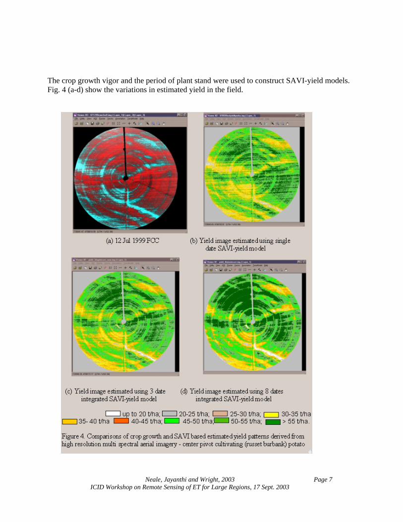
The crop growth vigor and the period of plant stand were used to construct SAVI-yield models. Fig. 4 (a-d) show the variations in estimated yield in the field.

Neale, Jayanthi and Wright, 2003 Page 7 ICID Workshop on Remote Sensing of ET for Large Regions, 17 Sept. 2003

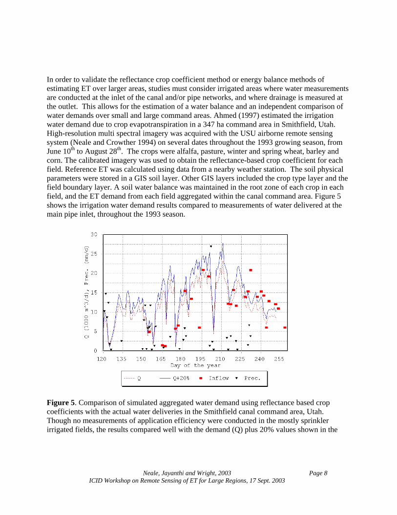
In order to validate the reflectance crop coefficient method or energy balance methods of estimating ET over larger areas, studies must consider irrigated areas where water measurements are conducted at the inlet of the canal and/or pipe networks, and where drainage is measured at the outlet. This allows for the estimation of a water balance and an independent comparison of water demands over small and large command areas. Ahmed (1997) estimated the irrigation water demand due to crop evapotranspiration in a 347 ha command area in Smithfield, Utah. High-resolution multi spectral imagery was acquired with the USU airborne remote sensing system (Neale and Crowther 1994) on several dates throughout the 1993 growing season, from June 10th to August 28th. The crops were alfalfa, pasture, winter and spring wheat, barley and corn. The calibrated imagery was used to obtain the reflectance-based crop coefficient for each field. Reference ET was calculated using data from a nearby weather station. The soil physical parameters were stored in a GIS soil layer. Other GIS layers included the crop type layer and the field boundary layer. A soil water balance was maintained in the root zone of each crop in each field, and the ET demand from each field aggregated within the canal command area. Figure 5 shows the irrigation water demand results compared to measurements of water delivered at the main pipe inlet, throughout the 1993 season. Figure 5coefficieThough irrigated

. Comparison of simulated aggregated water demand using reflectance based crop nts with the actual water deliveries in the Smithfield canal command area, Utah. no measurements of application efficiency were conducted in the mostly sprinkler fields, the results compared well with the demand (Q) plus 20% values shown in the

Neale, Jayanthi and Wright, 2003 Page 8 ICID Workshop on Remote Sensing of ET for Large Regions, 17 Sept. 2003

graph. The exercise also shows that the water deliveries were higher than necessary to replenish ET at the end of the season. A similar study was conducted by D’Urso (2001), who mapped crop coefficients from Landsat Thematic Mapper satellite imagery. Satellite data based canopy reflectance was used to estimate surface albedo, leaf area index and crop height.. The estimated water demands in the Gromola irrigation district were compared with the measured irrigation water releases during the 1994 season. A good agreement was reported between the measured and simulated monthly irrigation volumes at district and primary levels but significant differences were also reported at secondary and tertiary field scales and for time intervals shorter than one month. Trezza (2002) applied SEBAL (Bastiaanssen 1995) to estimate ET from local and regional agricultural areas in southern Idaho using Landsat ETM+ and Landsat 5 TM thermal imagery. The extrapolation of instantaneous ET (at the time of satellite overpass) to 24-hour ET values was based on the self-preservation theory of daytime fluxes that state constancy of the ratio between actual and reference ET during the daytime (Shuttleworth et al. 1989, Brutsaert and Sugita 1992) – which is essentially synonymous to the crop coefficient. Seasonal ET between March and October was estimated by applying the synonymous crop coefficient approach to interpolate between the satellite derived estimates, and was found to be within 3% of the total ET measured at the lysimeter site. Romero (2003) while studying different evaporative fraction approaches for extrapolating short period measurements of ET to daily estimates, showed that the Eta/Etr, or in other words, the crop coefficient, remains constant throughout the day. This demonstrates the appropriateness of the reflectance-based crop coefficient approach coupled with good ground-based meteorological measurements for reference ET estimation.

Future Perspectives

Canopy reflectance based crop coefficient methodology has been validated for grain, non-grain and forage crops. Crop water needs are assessed from the actual condition of the standing crop in the field. There are 2 directions in which high resolution airborne multi spectral imagery can work and contribute significantly in the assessment of large scale ET mapping: (1) macro scale studies with the portrayal of the spatial variability of the actual water demands in the study area, developing its linkages with the variability of actual crop yields, and (2) micro scale research by investigating the causative factors that lead to spatial variability of actual crop growth (soil effects, stress effects on canopy geometry, leaf orientation, etc.). Our future research in yield modeling will consider the effects of actual ET on yield in addition to the leaf area duration and will require high resolution multi spectral imagery to capture the in-field variability. The current medium resolution multi spectral satellite sensors would not be able to address the above issues, and future suite of high resolution sensors need the high resolution airborne multi spectral data to

Neale, Jayanthi and Wright, 2003 Page 9 ICID Workshop on Remote Sensing of ET for Large Regions, 17 Sept. 2003

serve as validation platforms (through such studies) before they become operational. Ultimately the usefulness of remote sensing in the estimation of irrigation water demand, crop yield and precision agricultural applications will depend on the turn around time between the image acquisition and dissemination of derived information. As the existing suite of commercial satellite systems have not been able to respond reliably, high-resolution airborne multi spectral systems still have a significant role to play in the remote sensing of irrigated agriculture.

References Ahmed, R. H. 1997. “Estimating crop water requirements of a command area using multi spectral video imagery and geographic information systems,” Ph.D dissertation, Utah State University, Logan, Utah. Allen, R. G., Pereira, L. S., Raes, D., Smith, M. (1998). “Crop evapotranspiration. Guidelines for computing crop water requirements”, FAO Irrigation and Drainage Paper, No:56, Food and Agricultural Organization, Rome. Amos, B. R., Stone, L. R., and Bark, L. D. 1989. Fraction of thermal units as the base for an evapotranspiration crop coefficient curve for corn. Journal of Agronomy, 81:713-717. Bastiaanssen, W. G. M. 1995. “Regionalization of surface flux densities and moisture indicators in composite terrain,” Ph.D dissertation, Wageningen Agricultural University, Wageningen, Netherlands. Bausch, W. C. 1995. Remote sensing of crop coefficients for improving the irrigation scheduling of corn. Agricultural Water Management, 27:55-68. Brutsaert, W. H., and Sugita, M. 1992. Application of self-preservation in the diurnal evolution of the surface energy budget to determine daily evaporation. Journal of Geophysical Research. 97:18,377-18,382. D’ Urso, G. 2001. “Simulation and management of on-demand irrigation systems: A combined agrohydrological and remote sensing approach,” PhD dissertation, Wageningen University, Waginengen, The Netherlands. Everson, D. O., Amos, D. R., and Rice, K. A. 1976. Growing degree days systems for Idaho. University of Idaho Bulletin No.551.

Neale, Jayanthi and Wright, 2003 Page 10 ICID Workshop on Remote Sensing of ET for Large Regions, 17 Sept. 2003

Gates, D. M., and Hanks, R. J. 1967. Plant Factors Affecting Evapotranspiration. Irrigation of Agricultural Lands. America Society of Agronomy, Madison, WI, Pp:506-521. Grattan, S. R., Bowers, W., Dong, A., Snyder, R. L., Carrol, J. J., and George, W. 1998. New crop coefficients estimate ware use of vegetables, row crops. California Agriculture, 52(1):16-21. Heilman, J. L., Heilman, W. E., and Moore, D. G. (1982). Evaluating the crop coefficient using spectral reflectance. Agronomy Journal, 74:967-971. Huete, A. R. 1988. A soil adjusted vegetation index (SAVI). Remote Sensing of Environment, 25, 295-309. Hunsaker, D. J. 1999. Basal crop coefficients and water use for early maturity cotton. Transactions of ASAE, 42(4):927-936. Jensen, M. E., Robb, D. C. N., and Franzoy, C. E. 1970. Scheduling Irrigations Using Climate-Soil Estimating Soil Moisture Depletion from Climate-Crop-Soil Data. Journal of Irrigation and Drainage Division, American Society of Civil Engineers. 96:25-28. Kustas, W. P., Perry, P., Doraiswamy, P. C., and Moran, M. S. 1994. Using satellite data to extrapolate evapotranspiration estimates in time and space over a semi-arid rangeland basin. Remote Sensing of Environment, 49:275-286. Moran, M. S., Clarke, T. R., Inoue, Y., and Vidal, A. 1994. Estimating crop water deficit using the relation between surface-air temperature and spectral vegetation index. Remote Sensing of Environment, 49(3):246-263. Neale, C. M. U., Bausch, W., and Heermann, D. 1989. Development of reflectance-based crop coefficients for corn. Transactions of ASAE, 32(6):1891-1899. Neale, C. M. U., Ahmed, R. H., Moran, M. S., Pinter, Jr., P. J., Qi, J., and Clarke, T. R. 1996. Estimating cotton seasonal evapotranspiration using canopy reflectance. Proceedings of the International Conference on Evapotranspiration and Irrigation Scheduling: November 3-6, San Antonio, Texas. Neale, C. M. U., and Crowther, B. G. 1994. An airborne multispectral video/radiometer remote sensing system: Development and calibration. Remote Sensing of Environment. 32(3):187-194.

Neale, Jayanthi and Wright, 2003 Page 11 ICID Workshop on Remote Sensing of ET for Large Regions, 17 Sept. 2003

Penman, H. L., Angus, D. E., and Bavel, C. H. M. 1967. Microclimatic factors affecting Evaporation and Transpiration. Irrigation of Agricultural Lands. America Society of Agronomy, Madison, WI, Pp:483-505. Reginato. R. J., Jackson, R. D., and Pinter, Jr., P. J. 1985. Evapotranspiration calculated from remote multi spectral and ground station meteorological data. Remote Sensing of Environment, 18:75-89. Ritchie, J. T., and Burnett, E. 1971. Dryland Evaporative Flux in a Subhumid Climate: II. Plant Influences. Journal of Agronomy. 63:56-62. Romero, M. G. 2003. “Daily Evapotranspiration Estimation by Means of Evaporative Fraction and Reference Evapotranspiration Fraction” Ph.D dissertation, Utah State University, Logan, USA. 175 p. Sammis, T. W., Mapel, C. L., Lugg, D. G., Lansford, R. R., and McGuckin, J. T. 1985. Evapotranspiration crop coefficients predicted using growing degree days. Transactions of ASAE, 28(3):773-780. Shuttleworth, W. J., Girney, R. J., Hsu, A. Y., and Ormsby, J. P. 1989. The variation in energy partition at surface flux sites. Proceedings of the third IAHS International Assembly, Baltimore, MD, 67-74. Stegman, E. C., Musick, J. T., and Stewart. J. L. 1980. Irrigation water management. Ed:M.E. Jensen, Design and Operation of Farm Irrigation Systems, St.Joseph, MI:ASAE, pp.769. Tanner, C. B., and Jury, W. A. 1976. Estimating evaporation and transpiration from a row crop during incomplete cover. Agronomy Journal, 68:239-243. Trezza, R. 2002. “Evapotranspiration using a satellite-based surface energy balance with standardized ground control,” Ph.D dissertation, utah State University, Logan, USA. Wright, J. L. 1982. New evapotranspiration crop coefficients. Journal of Irrigation and Drainage, ASCE, 108(1):57-74.

Neale, Jayanthi and Wright, 2003 Page 12 ICID Workshop on Remote Sensing of ET for Large Regions, 17 Sept. 2003