DETECTION OF LOCAL ANOMALIES IN HIGH RESOLUTION

HYPERSPECTRAL IMAGERY USING GEOSTATISTICAL FILTERING

AND LOCAL SPATIAL STATISTICS

PIERRE GOOVAERTS BioMedware, Inc. 516 North State Street, Ann Arbor, MI 48104

Abstract. This paper describes a methodology to detect patches of disturbed soils in high resolution hyperspectral imagery, which involves successively a multivariate statistical analysis (principal component analysis, PCA) of all spectral bands, a geostatistical filtering of regional background in the first principal components using factorial kriging, and finally the computation of a local indicator of spatial autocorrelation to detect local clusters of high or low reflectance values as well as anomalies. The approach is illustrated using one meter resolution data collected in Yellowstone National Park. Ground validation data demonstrate the ability of the filtering procedure to reduce the proportion of false alarms, and its robustness under low signal to noise ratios. By leveraging both spectral and spatial information, the technique requires little or no input from the user, and hence can be readily automated.

1 Introduction

Spatial data are periodically collected and processed to monitor, analyze and interpret developments in our changing environment. Remote sensing is a modern way of data collecting and has seen an enormous growth since launching of modern satellites and development of airborne sensors. In particular, the recent availability of high spatial resolution hyperspectral (HSRH) imagery offers a great potential to significantly enhance environmental mapping and our ability to model spatial systems (Aspinall etal., 2002; Marcus, 2002). Following Jacquez et al. (2002), HSRH images refer to images with resolutions of less than 5 meters and including data collected over 64 or more bands of electromagnetic radiation for each pixel.

High spatial resolution imagery contains a remarkable quantity of information that could be used to analyze spatial breaks (boundaries), areas of similarity (clusters), and spatial autocorrelation (associations) across the landscape. This paper addresses the specific issue of soil disturbance detection, which could indicate the presence of land mines or recent movements of troop and heavy equipment. A challenge presented by soil detection is to retain the measurement of fine-scale features (i.e. mineral soil changes, organic content changes, vegetation disturbance related changes, aspect changes) while still covering proportionally large spatial areas. An additional difficulty is that no ground data might be available for the calibration of spectral signatures, and little might be known about the size of patches of disturbed soils to be detected. Precise

105

2004, 105-114. © 2005 Springer. Printed in the Netherlands.

ticsO. Leuangthong and C. V. Deutsch (eds.), Geostatis Banff

106 P. GOOVAERTS

and accurate soil disturbance identification typically requires: (1) identification of a potential target (soil disturbance) of interest, (2) removal of confusion (the environmental setting), and (3) target (soil disturbance) confirmation. These different steps should be automated as much as possible to allow for the fast processing of multiple images, while false positives should be reduced to a manageable level.

A major challenge facing the use of HSRH data is the development of new, spatially explicit tools that exploit both the spectral and spatial dimensions of the data.Semivariograms allow one to detect multiple scales of spatial variability, and the spectral values can then be decomposed into the corresponding spatial components using factorial kriging (Goovaerts, 1997; Wackernagel, 1998). This technique has first been used in geochemical exploration to distinguish large isolated values (pointwise anomalies) from groupwise anomalies that consist of two or more neighboring values just above the chemical detection limit (Sandjivy, 1984). Ma and Royer (1988) have applied the same technique to image restoration, filtering and lineament enhancement, while Wen and Sinding-Larsen (1997) have analyzed sonar images. More recently, Van Meirvenne and Goovaerts (2002) applied factorial kriging to the filtering of multiple SAR images, strengthening relationships with land characteristics, such as topography and land use. None of these studies has however tackled the issue of automatic analysis and processing of large series of correlated spectral bands.

This paper describes a new approach that combines geostatistical filtering with local cluster analysis used in health sciences for the detection of clusters and outliers in cancer mortality rates (Jacquez and Greiling, 2003). The methodology is applied to HSRH imagery collected in Yellowstone National Park, and performances are assessed using ground data. Sensitivity analysis is conducted to investigate the impact of spectral resolution, signal to noise ratio, and kernel detection size on classification accuracy.

2 Geostatistical Methodology

Consider the problem of detecting, across an image, single or aggregated pixels that are significantly different from the surrounding ones. The information available consists of K variables (i.e. original spectral values or combinations of those) recorded at each of the N nodes of the image, {zk(ui), i=1,…,N; k=1,…,K}. The proposed approach proceeds in two steps:

1. The regional variability (i.e. spatial background) of the image is filtered in order to highlight local anomalies, which are values that depart from the surrounding mean.

2. At each location across the filtered image the value of a detection kernel, whose size corresponds to the expected size of a patch of disturbed soil, is compared to neighborhood values and flagged as anomaly if its value is significantly higher or lower than surrounding pixel values.

2.1 GEOSTATISTICAL FILTERING

The first step involves removing from each image (i.e. original spectral bands or principal components) the low-frequency component or regional variability. For the k-th

DETECTION OF LOCAL ANOMALIES IN HYPERSPECTRAL IMAGERY 107

image, the low-frequency component, denoted mk, is estimated at each location u as a linear combination of the n surrounding pixel values:

n

iikikk zm

1

)()( uu withn

iik

11 (1)

where ik is the weight assigned to the i-th observation in the filtering window of size n.The main feature of this filtering technique is that the weights ik are tailored to the spatial pattern of correlation displayed by each image and assessed using the semivariogram. These weights are computed as solution of the following system of linear equations (kriging of the local mean):

1

,10)()(

1

1n

jjk

jikn

jjk ,ni- uuu

(2)

where k(ui-uj) is the semivariogram of the k-th image for the separation vector between ui and uj, and (u) is a Lagrange multiplier that results from minimizing the estimation variance subject to the unbiasedness constraint on the estimator.

2.2 DETECTION OF ANOMALIES USING THE LISA STATISTIC

The second step amounts at scanning each filtered image, looking for local values that are significantly lower or higher than the surrounding values and might indicate the presence of disturbed soils. This procedure requires the definition of:

1. Detection kernel, whose size corresponds to the expected size of a patch of disturbed soil,

2. LISA neighborhood including the pixels surrounding the detection kernel, 3. Target area which is the area to be analyzed.

An example of these three parameters is provided in Figure 1.

Figure 1. Illustration of key parameters used in the detection procedure.

108 P. GOOVAERTS

The detection of local anomalies is based on the local Moran’s I, which is the most commonly used LISA (Local Indicator of Spatial Autocorrelation) statistic (Anselin, 1995). It is computed for each pixel of coordinates u as:

J

iikkk r

Jr

1

)(1

)()(LISA uuu (3)

where )(ukr is the average value of the residuals, rk(u)=zk(u)-mk(u), over the detection kernel centered on pixel of coordinates u, and J is the number of pixels in the LISA neighborhood (e.g. J=12 and kernel comprises 4 pixels for the example of Figure 1). Since the residuals have zero mean, the LISA statistic takes negative values if the kernel average is much lower (or higher) than the surrounding values. In other words the kernel average is below the global zero mean while the neighborhood average is above the global zero mean, or conversely, which indicates the presence of anomalies. Clusters of low or high values will lead to positive values of the LISA statistic (e.g. both kernel and neighborhood averages are jointly above zero or below zero).

In addition to the sign of the LISA statistic, its magnitude informs on the extent to which kernel and neighborhood values differ. To test whether this difference is significant or not, a Monte Carlo simulation is conducted, which consists in sampling randomly the target area and computing the corresponding simulated neighborhood averages. This operation is repeated many times (e.g. 1,000 draws) and these simulated values are multiplied by the detection kernel average )(ukr to produce a set of 1,000 simulated values of the LISA statistic at u. This set represents a numerical approximation of the probability distribution of the LISA statistic at u, under the assumption of spatial independence. The observed LISA statistic, LISAk(u), can then be compared to the probability distribution, allowing the computation of the probability that this observed value could be exceeded (so-called p-value):

}ionrandomizat|)({Prob)( uu kk LISALp

(4)

Large p-values thus indicate large negative LISA statistic, corresponding to small values surrounded by high values or the reverse (anomalies or presence of negative local autocorrelation). Conversely, small p-values correspond to large positive LISA statistic which indicates clusters of high or low values (positive autocorrelation).

The last step is to combine the K p-values computed for the set of K images. Two novel statistics were developed to summarize for each node u the information provided by the K bands and to detect target pixels:

1. Average p-value over the subset of K’ bands that display negative LISA statistic:

K

k

K

kk kiKpki

KS

111 );('and)();(

'

1)( uuuu (5)

with i(u;k) = 1 if LISAk(u) < 0, and zero otherwise. Large S1 values indicate local anomalies (i.e. sample LISA statistic in the left tail of the distribution).

DETECTION OF LOCAL ANOMALIES IN HYPERSPECTRAL IMAGERY 109

2. Average absolute deviation of p-values from 0.5 through the K bands:

|0.5-)(|1

)(1

2

K

kkp

KS uu

(6)

Large S2 values indicate either clusters or anomalies (i.e. sample LISA in either tails of the distribution).

The detection procedure requires applying a threshold to the maps of statistics S1 or S2

and classifying as disturbed soils all pixels exceeding this probability threshold. Instead of selecting a single threshold arbitrarily, it is better to select a series of thresholds and see how the proportion of pixels correctly or incorrectly classified as disturbed soils evolves. This information can then be summarized in the so-called Receiver Operating Characteristics (ROC) curve that plots the probability of false alarm versus the probability of detection.

3 Case study

The new methodology was tested on a vegetation plot located in the northern boundary area of Yellowstone National Park. The objective is to detect 4 blue tarps of 4m2 area in the image (131 69 pixels). These four targets mainly correspond to the white pixels in the image of Figure 2 (left), and are denoted by the black squares in the right image. These data were collected using the Probe-1 sensor, a 128-band hyperspectral system operated by Earth Search Systems, Inc. To obtain 1 m resolution data, this sensor was mounted on a helicopter flying approximately 600 m above the ground. Following atmospheric correction, the images were degraded in order to investigate the robustness of the approach with respect to spatial resolution and signal to noise ratio. The data were first spectrally resampled to 2-5 times lower resolutions, by simply selecting one out of every 2 to 5 bands. Noise was added to simulate 50:1 signal-to-noise ratio (SNR) and 100:1 SNR, according to: Rsn( )=Rs( )[1+{N(0,1)/SNR( )}], where Rsn( ) is the simulated, noisy spectrum, Rs( ) is the spectrum that has been spectrally resampled, N(0,1) is a Gaussian random number with a zero mean and unit variance, and SNR( ) is the simulated signal-to-noise ratio.

Figure 2. Probe 1, color-infrared image of the experimental site, and location of 16 tarp pixels (black) that are interpreted as disturbed soils to be detected.

110 P. GOOVAERTS

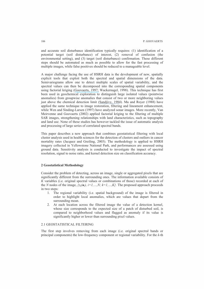
Figure 3. Maps of the first two principal components for the HSRH image, and the results of the geostatistical filtering of the regional background.

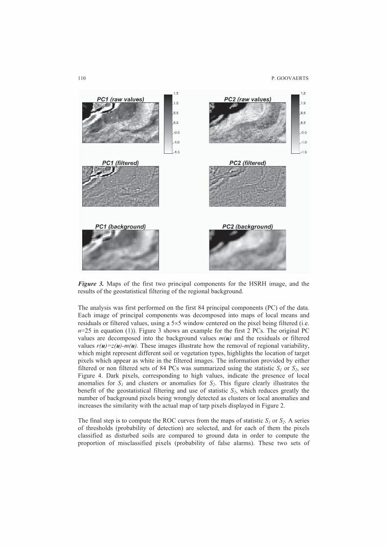
The analysis was first performed on the first 84 principal components (PC) of the data. Each image of principal components was decomposed into maps of local means and residuals or filtered values, using a 5 5 window centered on the pixel being filtered (i.e. n=25 in equation (1)). Figure 3 shows an example for the first 2 PCs. The original PC values are decomposed into the background values m(u) and the residuals or filtered values r(u)=z(u)-m(u). These images illustrate how the removal of regional variability, which might represent different soil or vegetation types, highlights the location of target pixels which appear as white in the filtered images. The information provided by either filtered or non filtered sets of 84 PCs was summarized using the statistic S1 or S2, see Figure 4. Dark pixels, corresponding to high values, indicate the presence of local anomalies for S1 and clusters or anomalies for S2. This figure clearly illustrates the benefit of the geostatistical filtering and use of statistic S2, which reduces greatly the number of background pixels being wrongly detected as clusters or local anomalies and increases the similarity with the actual map of tarp pixels displayed in Figure 2.

The final step is to compute the ROC curves from the maps of statistic S1 or S2. A series of thresholds (probability of detection) are selected, and for each of them the pixels classified as disturbed soils are compared to ground data in order to compute the proportion of misclassified pixels (probability of false alarms). These two sets of

DETECTION OF LOCAL ANOMALIES IN HYPERSPECTRAL IMAGERY 111

probabilities are then plotted to generate the ROC curve. Figure 5 shows an example of such curves for detection using either statistic S1 or S2 computed from filtered or non-filtered images. The main conclusions are:

1. The filtering and use of statistic S2 (black solid curve) allows the detection of all tarp pixels for a probability of false alarms not exceeding 0.20.

2. Detection of 60% of tarp pixels can be done with small probability of false alarm (vertical part of the ROC curve) and these pixels correspond to high purity in term of tarp content. Pixels that contain a mixture of tarp and other materials (i.e. bare soil, grass) are much more difficult to detect and generate an increase in the proportion of false alarms which can be fairly dramatic if no filtering is performed and only anomalies are searched (i.e. use of statistic S1).

.30

.32

.34

.36

.38

.40

Figure 4. Maps of statistics S1 and S2 computed from the first 84 principal components before and after (bottom maps) filtering of the regional background.

Figure 5. Receiver Operating Characteristics (ROC) curves obtained for the statistics S1

(thin dotted line) and S2 (solid line). Black curves are obtained from the filtered values, while the gray curves refer to original values (without geostatistical filtering).

112 P. GOOVAERTS

Extensive sensitivity analysis has been conducted to assess the performance of the methodology under several conditions, such as:

1. Selection of subsets of PCs based on the strength of spatial correlation.

2. Choice of detection kernels of various sizes.

3. Decrease in signal to noise ratio and spectral resolution.

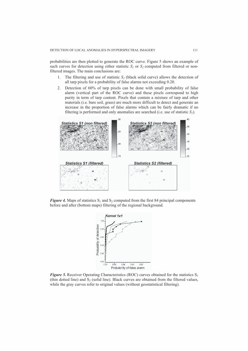
Instead of summarizing the information provided by the first 84 PCs, statistics S1 and S2

were computed for each PC separately and their average for both tarp and background pixels are plotted versus the rank/order of the PC in Figure 6 (top graph). Differences between tarp (black) and background (gray) pixels tend to attenuate as the order of the component increases and the spatial correlation of the image decreases (thick black curve). Subsets of PCs were thus retained based on a spatial correlation threshold of 0.5 or 0.25, plus the set of the first 25 PCs. The ROC curves indicate an increase in the proportion of false alarms when using fewer PCs. All ROC curves computed hereafter will be based on the first 25 PCs, thereby providing a balance between shorter CPU time (16.0 seconds versus 54.5 for 84 PCs on a Pentium 3.20 GHz) and slightly more false alarms.

Figure 6. Plot of spatial correlation (lag=1 pixel) and value of statistics S1 (thin dotted line) and S2 (solid line) for either tarp pixels (black) or background pixels (gray), versus the order of the principal component (top graph). Bottom graphs show the ROC curves obtained for the first 25 PCs and two subsets based on the level of spatial correlation.

DETECTION OF LOCAL ANOMALIES IN HYPERSPECTRAL IMAGERY 113

All results presented so far were obtained using a detection kernel of one pixel, which does not require any prior information regarding the size of the object to be detected. The benefit of tailoring the detection kernel to the size of the object was investigated by performing the classification and computing the ROC curves for three types of kernel: 1 1, 2 1 and 2 2. Figure 7 (top row) shows that that the use of kernels 2 1 and 2 2improves detection performances of statistic S1, while more false alarms occur when using statistic S2. Indeed, statistic S1 searches for local anomalies of size equal to the kernel, while S2 detects both clusters and anomalies. The impact of the signal to noise (SN) ratio was investigated by adding a given proportion of noise to reflectance values before performing PCA. Figure 7 (middle row) shows the ROC curves obtained for increasing levels of noise (SN=100:1 to SN=50:1). As intuitively expected, noisy signals tend to blur the detection of anomalies, leading to a larger proportion of false alarms, although statistic S2 on filtered signal is very robust.

The last test consisted in investigating how a decrease in spectral resolution would affect the quality of the detection. Figure 7 (bottom row) shows the ROC curves obtained for the original signal with 84 PCs, and then for one half (WV2, 42 PCs) and one third (WV3, 28 PCs) of the number of principal components. As for the signal to noise ratio, ROC curves indicate poorer performances when using the degraded image.

Figure 7. Receiver Operating Characteristics (ROC) curves obtained for three types of detection kernel, two signal to noise (SN) ratios, and three spectral resolutions (WV).

114 P. GOOVAERTS

4 Conclusions

This paper presented and demonstrated the efficacy of a geostatistical approach to detecting disturbed soils in high spatial resolution hyperspectral imagery. The technique uses PCA to reduce dimensionality of the imagery, employs geostatistical filtering to remove regional background and enhance local signal, and applies a Local Indicator of Spatial Autocorrelation to identify patches of disturbed soils. In all scenarios, fewer false alarms were obtained when using the filtered signal and statistic S2 to summarize information across bands. Image degradation through addition of noise or reduction of spectral resolution tends to blur the detection of anomalies, leading to more false alarms, in particular for the identification of the few mixed pixels.

In this paper the methodology was used to detect regular patches on a simple landscape. Similar results were obtained when applying the approach to more complex landscapes with multiple targets of various sizes and shapes (results not shown). Because it employs geostatistical filtering, the method is robust under low signal to noise ratios. By leveraging both spectral and spatial information, the technique requires little or no input from the user, and hence can be readily automated. Following our results a Pentium 3.20 GHz would allow the processing of a 1000×1000 scene including 25 bands within 18 minutes. Future research will investigate the benefit of processing directly the spectral bands instead of their principal components.

Acknowledgements

This work was supported by NAVAIR SBIR Phase I N02-172, and data were kindly provided by Andrew Marcus from the University of Oregon.

References

Anselin, L., Local indicators of spatial association-LISA, Geographical Analysis, vol. 27, 1995, p. 93-115.Aspinall, R.J., Marcus, W.A., and Boardman, J.W., Considerations in collecting, processing, and analysing

high spatial resolution hyperspectral data for environmental investigations, Journal of Geographical Systems, vol. 4, 2002, p. 15-29.

Goovaerts, P., Geostatistics for Natural Resources Evaluation, Oxford University Press, 1997. Jacquez, G.M. and Greiling, D.A., Local clustering in breast, lung and colorectal cancer in Long Island, New

York, International Journal of Health Geography, vol. 2, no. 3, 2003. Jacquez, G.M., Marcus, W.A., Aspinall, R.J. and Greiling, D.A., Exposure assessment using high spatial

resolution hyperspectral (HSRH) imagery, Journal of Geographical Systems, vol. 4, 2002, p. 15-29. Ma, Y.Z., and Royer, J.J., Local geostatistical filtering : application to remote sensing, Sciences de la Terre,

Serie Informatique, vol. 27, 1988, p. 17-36.Marcus, W.A., Mapping of stream microhabitats with high spatial resolution hyperspectral imagery, Journal of

Geographical Systems, vol. 4, 2002, p. 113-126. Sandjivy, L., The factorial kriging analysis of regionalized data. Its application to geochemical prospecting. In

Geostatistics for Natural Resources Characterization, edited by G. Verly, M. David, A.G. Journel, and A. Marechal, Dordrecht: Reidel, 1984, p. 559-571.

Van Meirvenne, M. and Goovaerts, P., Accounting for spatial dependence in the processing of multitemporal SAR images using factorial kriging, International Journal of Remote Sensing, vol. 23, 2002, p. 371-387.

Wackernagel, H., Multivariate Geostatistics, Springer-Verlag, 1998. Wen, R. and Sinding-Larsen, R., Image filtering by factorial kriging sensitivity analysis and application to

Gloria side-scan sonar images, Mathematical Geology, vol. 29, no. 5, 1997, p. 433-468.