Computational Statistics & Data Analysis 52 (2008) 3128–3147www.elsevier.com/locate/csda

Modelling residuals dependence in dynamic life tables:A geostatistical approach

A. Debóna, F. Montesb,∗, J. Mateuc, E. Porcuc, M. Bevilacquad

aUniversidad Politécnica de Valencia, Dpto. de Estadística e I.O. Aplicadas y Calidad, SpainbUniversitat de València, Dpt. d’Estadística i I.O., Spain

cUniversitat Jaume I, Dpt. de Matemàtiques, SpaindUniversità di Padova, Dpt. di Scienze Statistiche, Italy

Available online 19 August 2007

Abstract

The problem of modelling dynamic mortality tables is considered. In this context, the influence of age on data graduation needs tobe properly assessed through a dynamic model, as mortality progresses over the years. After detrending the raw data, the residualsdependence structure is analysed, by considering them as a realisation of a homogeneous Gaussian random field defined on R × R.This setting allows for the implementation of geostatistical techniques for the estimation of the dependence and further interpolationin the domain of interest. In particular, a complex form of interaction between age and time is considered, by taking into account azonally anisotropic component embedded into a nonseparable covariance structure. The estimated structure is then used for predictionof mortality rates, and goodness-of-fit testing is performed through some cross-validation techniques. Comments on validity andinterpretation of the results are given.© 2007 Elsevier B.V. All rights reserved.

Keywords: Dynamic life tables; Geometric anisotropy; Kriging; Lee–Carter; Median polish; Zonal anisotropy

1. Introduction

Mortality forecasts are nowadays widely used to create and modify retirement pension schemes, disability insurancesystems and other social security programmes. During the 20th century, huge increases in life expectancy have followedmedical and scientific breakthroughs. Forecasting mortality usually serves practical purposes, for improvements thereincould have enormous social and financial implications.

The graduation of mortality data by means of parametric methodology has been widely addressed in the literature(Forfar et al., 1988; Renshaw, 1991; Debón et al., 2005). Nonparametric procedures have also been used (Gavin et al.,1993, 1994, 1995 and Debón et al., 2006b). The proposed methodology in these papers deals with static graduation,i.e. with the influence of age on data graduation. However, mortality progresses over the years, but these methods donot take this fact into account, as they were designed to analyse data corresponding to one year in particular or, inthe case of several years, they use aggregated figures. The concept of dynamic tables solves this problem by jointly

∗ Corresponding author. Tel.: +34 963544306; fax: +34 963543238.E-mail address: montes@uv.es (F. Montes).

0167-9473/$ - see front matter © 2007 Elsevier B.V. All rights reserved.doi:10.1016/j.csda.2007.08.006

A. Debón et al. / Computational Statistics & Data Analysis 52 (2008) 3128–3147 3129

analysing mortality data corresponding to a series of consecutive years. This approach allows to study the calendareffect’s influence on mortality.

The representation of the evolution of mortality via dynamic models is an extremely important current issue, andwidely extended over actuaries, statisticians or demographers, where clear examples can be found in, for instance,Benjamin and Pollard (1992), Tabeau et al. (2001), Pitacco (2004), Wong-Fupuy and Haberman (2004), Debón et al.(2006a) and Booth (2006). Most of these methods adapt traditional laws to the new situation, however, none of themconsiders the existing dependence structure among the data, even though some authors consider that this dependenceshould be modelled (Booth et al., 2002; Renshaw and Haberman, 2003a). One of the most outstanding models, andalso more frequently used by actuaries, is the Lee–Carter model (Lee and Carter, 1992).

Booth (2006) reviews the development of new and sophisticated methods for mortality forecasting. Hyndman andUllah (2007) treat the underlying process as functional data and provide estimation and forecasting that are robust tooutliers. Debón et al. (2004) introduce, as an alternative to classical methods, methods of fitting and prediction basedon geostatistical techniques, which exploit the dependence structure existing among the residuals. They consider thedynamic life table as a two-way table on an equally spaced grid in either the vertical (age) or horizontal (year) direction,and the data are decomposed into a deterministic large-scale variation (trend) plus a stochastic small-scale variation(error)

Z(x, t) = �(x, t) + �(x, t), (1)

where x ∈ R+ denotes the age and t is time expressed in years.In this paper we consider a nonstationary random field of the type (1), where the nonstationary component is

exclusively explained by the trend, which is a function of the coordinates (x, t) ∈ R2. The residuals are shown to bezero mean and weakly stationary. We model the trend function, for both males and females, by using three differentmethodologies, that are well known under the names of Lee–Carter model (LC, for short), extended Lee–Carter model(LC2), and median polish (MP). This allows to obtain six sets of residuals (as males and females are separated in orderto highlight differences between them), that are modelled by means of geostatistical techniques. We show that theseresiduals exhibit an anisotropic component, and model it using the techniques proposed by Porcu et al. (2006, 2007).We finally forecast the mortality rates on a period for which we have no data.

We analyse Spanish mortality data corresponding to the period 1980–2001. The first 20 years, from 1980 to 1999,are used to fit the models, and the last two, 2000–2001, are considered as a validation set for measuring the accuracyof the predictions.

The plan of the paper is as follows. Section 2 briefly presents the methodologies used for trend estimation (Lee–Carterand median-polish) and for the residual analysis. Section 3 shows the results of applying different methods to model themortality data corresponding to the period 1980–1999 in Spain. Predictions for future years are obtained and analysedin Section 4, where, in particular, predictions for years 2000 and 2001 are compared with the real data. The paper endswith some conclusions.

2. Fitting and prediction of death probability qxt

2.1. Models for trend estimation

Lee–Carter models. The Lee–Carter model, developed in Lee and Carter (1992), consists of fitting the followingfunction to the central mortality rates,

mxt = exp(ax + bxkt + �(x, t)),

or, equivalently

ln(mxt ) = ax + bxkt + �(x, t), (2)

where the notation �(x, t) is consistent with considering the residuals as a random field as described in Section 2.2.In the previous two expressions, the double subscript refers to the age (x), and to the year or the corresponding unit of

time (t). The parameters ax and bx are age-dependent, and kt is a specific mortality index for each year or unit of time.

3130 A. Debón et al. / Computational Statistics & Data Analysis 52 (2008) 3128–3147

The residuals �(x, t), that are assumed to be Gaussian with mean 0 and variance �2�, reflect the historical influences of

each specific age that are not captured by the model.To model death probability qxt in terms of Eq. (2), we use an extended version (see Debón et al., 2007) that we will

be applied to logit(qxt ), as follows:

ln

(qxt

1 − qxt

)= ax +

r∑i=1

bixk

it + �(x, t). (3)

The rationale for the use of the logit transform follows from the remark in Lee (2000), where the author points out thatnothing ensures that estimates of qxt obtained from (2) will not exceed 1. The extended version is suggested by Boothet al. (2002) and Renshaw and Haberman (2003b), where the authors indicate that the interaction between age and timecan be better captured by adding terms to (2).

Two constraints are needed in order to get a unique solution. Lee and Carter (1992) propose that∑

xbix =1 and

∑t k

it =

0. The structure is then invariant under either of the parameter transformations, (ax, bx/c, ckt ) or (ax +cbx, bx, kt −c),for any constant c. In our application to the mortality Spanish data, we have used (3) with r =1 and r =2, consequentlythe corresponding models will be named LC and LC2, respectively. The estimation of the parameters in (3) is carriedout by means of maximum likelihood methods (ML, for short), as proposed by Brouhns et al. (2002).

Median polish. A dynamic life table can also be considered as a two-way table on an equally spaced grid in either thevertical (age) or horizontal (year) direction. In this context, the deterministic trend of mortality rate can be decomposedas the sum of three effects

qxt = � + rx + ct , (4)

where � defines an overall effect, rx a row effect due to the age, ct a column effect due to the year. A median-polishalgorithm (Cressie, 1993) is used to estimate the overall effect, �, row effects, rx , and column effects, ct . For particulartheoretical properties of the median polish, we refer the interested reader to Cressie (1993). Here, it is worth stressingthat this is a nonparametric method and it is, with respect to other detrending methods, less sensitive to the presence ofoutliers and less biased than other methods based on the use of mean operators.

2.2. Residual analysis: a geostatistical approach

Throughout the paper we make reference to real-valued homogeneous (or weakly stationary) zero mean Gaussianrandom fields (H/SRF for short) {�(x) : x ∈ D ⊆ R2}, where the coordinate x = (x, t)′, e.g. (age, time). Homo-geneity means that the expected value is constant (in this case identically equal to zero), and the covariance functioncov(�(x), �(y)) = E�(x)�(y) := C(h), with h = y − x, the separation vector between two points lying in D, and whereC : R2 → R is a positive definite function, i.e. satisfies

n∑i=1

aiaj C(xi − xj )�0,

for all finite collections of real numbers {ai}ni=1 and points xi ∈ D. With alternative notation, Christakos (2000) callsthis property permissibility. A classical result in Bochner (1933) sets up the equivalence between covariance functionsand characteristic functions of non-negative finite measures. Namely, a continuous function C as defined above ispositive definite if and only if it is the Fourier transform of a non-negative measure F on Rd , i.e.

C(h) =∫

R2ei�′h dF(�). (5)

If, additionally, F is absolutely continuous with respect to the Lebesgue measure, then (5) can be written as

C(h) =∫

R2ei�′hf (�) d(�), (6)

and f : Rd → R+ is called the spectral density of the H/SRF .

A. Debón et al. / Computational Statistics & Data Analysis 52 (2008) 3128–3147 3131

distance

variogra

m

nugget

sill

range

0.0

0 2 4 6 8 10 12 14

1.0

2.0

3.0

4.0

5.0

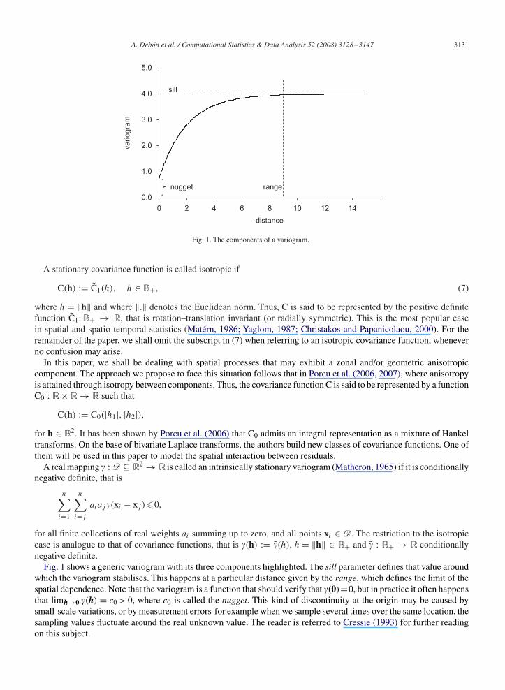
Fig. 1. The components of a variogram.

A stationary covariance function is called isotropic if

C(h) := C1(h), h ∈ R+, (7)

where h = ‖h‖ and where ‖.‖ denotes the Euclidean norm. Thus, C is said to be represented by the positive definitefunction C1: R+ → R, that is rotation–translation invariant (or radially symmetric). This is the most popular casein spatial and spatio-temporal statistics (Matérn, 1986; Yaglom, 1987; Christakos and Papanicolaou, 2000). For theremainder of the paper, we shall omit the subscript in (7) when referring to an isotropic covariance function, wheneverno confusion may arise.

In this paper, we shall be dealing with spatial processes that may exhibit a zonal and/or geometric anisotropiccomponent. The approach we propose to face this situation follows that in Porcu et al. (2006, 2007), where anisotropyis attained through isotropy between components. Thus, the covariance function C is said to be represented by a functionC0 : R × R → R such that

C(h) := C0(|h1|, |h2|),for h ∈ R2. It has been shown by Porcu et al. (2006) that C0 admits an integral representation as a mixture of Hankeltransforms. On the base of bivariate Laplace transforms, the authors build new classes of covariance functions. One ofthem will be used in this paper to model the spatial interaction between residuals.

A real mapping � : D ⊆ R2 → R is called an intrinsically stationary variogram (Matheron, 1965) if it is conditionallynegative definite, that is

n∑i=1

n∑i=j

aiaj �(xi − xj )�0,

for all finite collections of real weights ai summing up to zero, and all points xi ∈ D. The restriction to the isotropiccase is analogue to that of covariance functions, that is �(h) := �(h), h = ‖h‖ ∈ R+ and � : R+ → R conditionallynegative definite.

Fig. 1 shows a generic variogram with its three components highlighted. The sill parameter defines that value aroundwhich the variogram stabilises. This happens at a particular distance given by the range, which defines the limit of thespatial dependence. Note that the variogram is a function that should verify that �(0)=0, but in practice it often happensthat limh→0 �(h) = c0 > 0, where c0 is called the nugget. This kind of discontinuity at the origin may be caused bysmall-scale variations, or by measurement errors-for example when we sample several times over the same location, thesampling values fluctuate around the real unknown value. The reader is referred to Cressie (1993) for further readingon this subject.

3132 A. Debón et al. / Computational Statistics & Data Analysis 52 (2008) 3128–3147

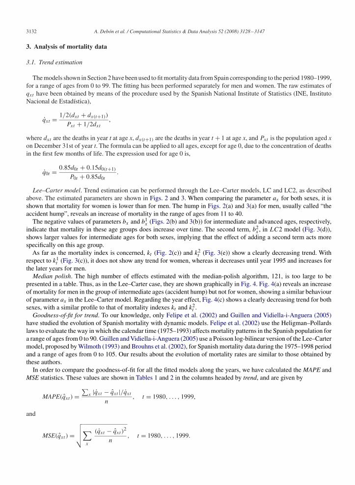
3. Analysis of mortality data

3.1. Trend estimation

The models shown in Section 2 have been used to fit mortality data from Spain corresponding to the period 1980–1999,for a range of ages from 0 to 99. The fitting has been performed separately for men and women. The raw estimates ofqxt have been obtained by means of the procedure used by the Spanish National Institute of Statistics (INE, InstitutoNacional de Estadística),

qxt = 1/2(dxt + dx(t+1))

Pxt + 1/2dxt

,

where dxt are the deaths in year t at age x, dx(t+1) are the deaths in year t + 1 at age x, and Pxt is the population aged xon December 31st of year t. The formula can be applied to all ages, except for age 0, due to the concentration of deathsin the first few months of life. The expression used for age 0 is,

q0t = 0.85d0t + 0.15d0(t+1)

P0t + 0.85d0t

.

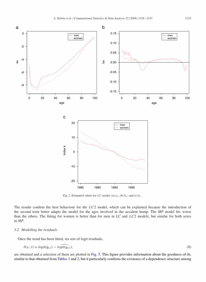
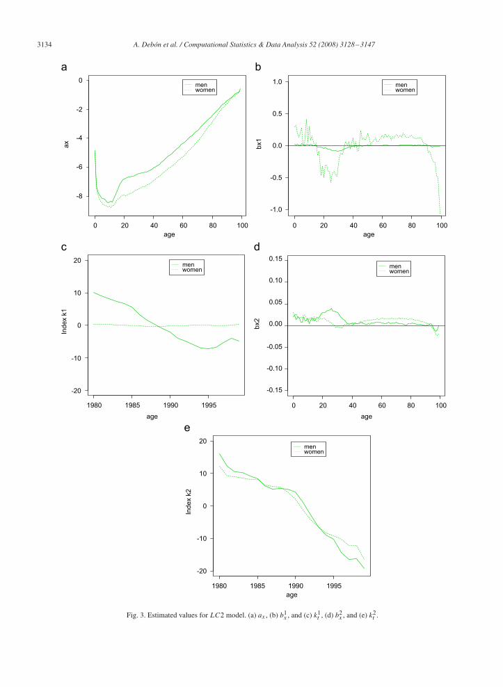
Lee–Carter model. Trend estimation can be performed through the Lee–Carter models, LC and LC2, as describedabove. The estimated parameters are shown in Figs. 2 and 3. When comparing the parameter ax for both sexes, it isshown that mortality for women is lower than for men. The hump in Figs. 2(a) and 3(a) for men, usually called “theaccident hump”, reveals an increase of mortality in the range of ages from 11 to 40.

The negative values of parameters bx and b1x (Figs. 2(b) and 3(b)) for intermediate and advanced ages, respectively,

indicate that mortality in these age groups does increase over time. The second term, b2x , in LC2 model (Fig. 3(d)),

shows larger values for intermediate ages for both sexes, implying that the effect of adding a second term acts morespecifically on this age group.

As far as the mortality index is concerned, kt (Fig. 2(c)) and k2t (Fig. 3(e)) show a clearly decreasing trend. With

respect to k1t (Fig. 3(c)), it does not show any trend for women, whereas it decreases until year 1995 and increases for

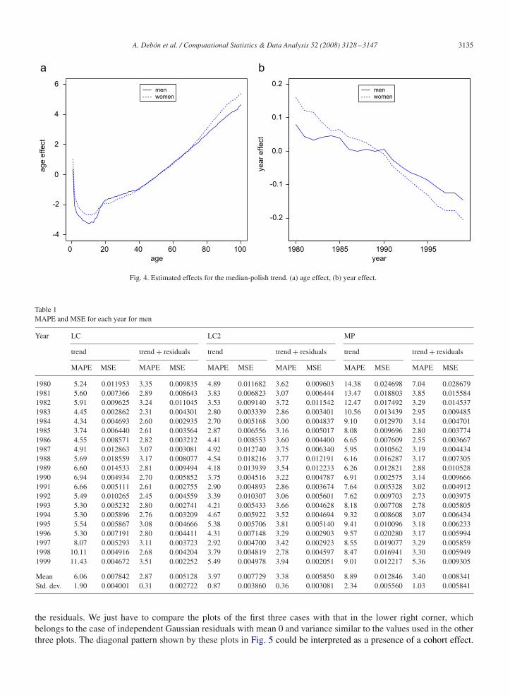
the later years for men.Median polish. The high number of effects estimated with the median-polish algorithm, 121, is too large to be

presented in a table. Thus, as in the Lee–Carter case, they are shown graphically in Fig. 4. Fig. 4(a) reveals an increaseof mortality for men in the group of intermediate ages (accident hump) but not for women, showing a similar behaviourof parameter ax in the Lee–Carter model. Regarding the year effect, Fig. 4(c) shows a clearly decreasing trend for bothsexes, with a similar profile to that of mortality indexes kt and k2

t .Goodness-of-fit for trend. To our knowledge, only Felipe et al. (2002) and Guillen and Vidiella-i-Anguera (2005)

have studied the evolution of Spanish mortality with dynamic models. Felipe et al. (2002) use the Heligman–Pollardslaws to evaluate the way in which the calendar time (1975–1993) affects mortality patterns in the Spanish population fora range of ages from 0 to 90. Guillen and Vidiella-i-Anguera (2005) use a Poisson log-bilinear version of the Lee–Cartermodel, proposed by Wilmoth (1993) and Brouhns et al. (2002), for Spanish mortality data during the 1975–1998 periodand a range of ages from 0 to 105. Our results about the evolution of mortality rates are similar to those obtained bythese authors.

In order to compare the goodness-of-fit for all the fitted models along the years, we have calculated the MAPE andMSE statistics. These values are shown in Tables 1 and 2 in the columns headed by trend, and are given by

MAPE(qxt ) =∑

x |qxt − qxt |/qxt

n, t = 1980, . . . , 1999,

and

MSE(qxt ) =√√√√∑

x

(qxt − qxt )2

n, t = 1980, . . . , 1999.

A. Debón et al. / Computational Statistics & Data Analysis 52 (2008) 3128–3147 3133

0 20 40 60 80 100

-8

-6

-4

-2

0

age

ax

0 20

-20

20

-10

10

0

40 60 80 100

-0.15

-0.10

-0.05

0.00

0.05

0.10

0.15

agebx

menwomen

menwomen

menwomen

1980 1985 1990 1995

Ind

ex k

Fig. 2. Estimated values for LC model. (a) ax , (b) bx , and (c) kt .

The results confirm the best behaviour for the LC2 model, which can be explained because the introduction ofthe second term better adapts the model for the ages involved in the accident hump. The MP model fits worsethan the others. The fitting for women is better than for men in LC and LC2 models, but similar for both sexesin MP.

3.2. Modelling the residuals

Once the trend has been fitted, six sets of logit residuals,

�(x, t) = logit(qxt ) − logit(qxt ), (8)

are obtained and a selection of them are plotted in Fig. 5. This figure provides information about the goodness-of-fit,similar to that obtained from Tables 1 and 2, but it particularly confirms the existence of a dependence structure among

3134 A. Debón et al. / Computational Statistics & Data Analysis 52 (2008) 3128–3147

menwomen

menwomen

menwomen

menwomen

menwomen

0 20 40 60 80 100 0 20 40 60 80 100

1980 1985 1990 1995 0 20 40 60 80 100

ageage

age

1980 1985 1990 1995

-8

-6

-4

-2

0

age

ax

-1.0

-0.5

0.0

0.5

1.0

age

bx1

-20

-10

0

10

20

0

10

20

Ind

ex k

1

-0.15

-0.10

-0.05

0.00

0.05

0.10

0.15b

x2

-20

-10

Ind

ex k

2

Fig. 3. Estimated values for LC2 model. (a) ax , (b) b1x , and (c) k1

t , (d) b2x , and (e) k2

t .

A. Debón et al. / Computational Statistics & Data Analysis 52 (2008) 3128–3147 3135

0 20 40 60 80 100

-4

-2

0

2

4

6

age

ag

e e

ffe

ct

menwomen

1980 1985 1990 1995

-0.2

-0.1

0.0

0.1

0.2

yearye

ar

eff

ect

menwomen

Fig. 4. Estimated effects for the median-polish trend. (a) age effect, (b) year effect.

Table 1MAPE and MSE for each year for men

Year LC LC2 MP

trend trend + residuals trend trend + residuals trend trend + residuals

MAPE MSE MAPE MSE MAPE MSE MAPE MSE MAPE MSE MAPE MSE

1980 5.24 0.011953 3.35 0.009835 4.89 0.011682 3.62 0.009603 14.38 0.024698 7.04 0.0286791981 5.60 0.007366 2.89 0.008643 3.83 0.006823 3.07 0.006444 13.47 0.018803 3.85 0.0155841982 5.91 0.009625 3.24 0.011045 3.53 0.009140 3.72 0.011542 12.47 0.017492 3.29 0.0145371983 4.45 0.002862 2.31 0.004301 2.80 0.003339 2.86 0.003401 10.56 0.013439 2.95 0.0094851984 4.34 0.004693 2.60 0.002935 2.70 0.005168 3.00 0.004837 9.10 0.012970 3.14 0.0047011985 3.74 0.006440 2.61 0.003564 2.87 0.006556 3.16 0.005017 8.08 0.009696 2.80 0.0037741986 4.55 0.008571 2.82 0.003212 4.41 0.008553 3.60 0.004400 6.65 0.007609 2.55 0.0036671987 4.91 0.012863 3.07 0.003081 4.92 0.012740 3.75 0.006340 5.95 0.010562 3.19 0.0044341988 5.69 0.018559 3.17 0.008077 4.54 0.018216 3.77 0.012191 6.16 0.016287 3.17 0.0073051989 6.60 0.014533 2.81 0.009494 4.18 0.013939 3.54 0.012233 6.26 0.012821 2.88 0.0105281990 6.94 0.004934 2.70 0.005852 3.75 0.004516 3.22 0.004787 6.91 0.002575 3.14 0.0096661991 6.66 0.005111 2.61 0.002755 2.90 0.004893 2.86 0.003674 7.64 0.005328 3.02 0.0049121992 5.49 0.010265 2.45 0.004559 3.39 0.010307 3.06 0.005601 7.62 0.009703 2.73 0.0039751993 5.30 0.005232 2.80 0.002741 4.21 0.005433 3.66 0.004628 8.18 0.007708 2.78 0.0058051994 5.30 0.005896 2.76 0.003209 4.67 0.005922 3.52 0.004694 9.32 0.008608 3.07 0.0064341995 5.54 0.005867 3.08 0.004666 5.38 0.005706 3.81 0.005140 9.41 0.010096 3.18 0.0062331996 5.30 0.007191 2.80 0.004411 4.31 0.007148 3.29 0.002903 9.57 0.020280 3.17 0.0059941997 8.07 0.005293 3.11 0.003723 2.92 0.004700 3.42 0.002923 8.55 0.019077 3.29 0.0058591998 10.11 0.004916 2.68 0.004204 3.79 0.004819 2.78 0.004597 8.47 0.016941 3.30 0.0059491999 11.43 0.004672 3.51 0.002252 5.49 0.004978 3.94 0.002051 9.01 0.012217 5.36 0.009305

Mean 6.06 0.007842 2.87 0.005128 3.97 0.007729 3.38 0.005850 8.89 0.012846 3.40 0.008341Std. dev. 1.90 0.004001 0.31 0.002722 0.87 0.003860 0.36 0.003081 2.34 0.005560 1.03 0.005841

the residuals. We just have to compare the plots of the first three cases with that in the lower right corner, whichbelongs to the case of independent Gaussian residuals with mean 0 and variance similar to the values used in the otherthree plots. The diagonal pattern shown by these plots in Fig. 5 could be interpreted as a presence of a cohort effect.

3136 A. Debón et al. / Computational Statistics & Data Analysis 52 (2008) 3128–3147

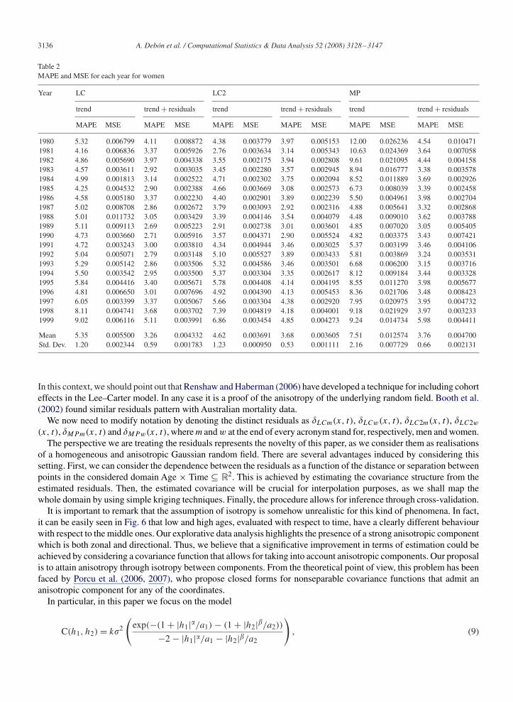
Table 2MAPE and MSE for each year for women

Year LC LC2 MP

trend trend + residuals trend trend + residuals trend trend + residuals

MAPE MSE MAPE MSE MAPE MSE MAPE MSE MAPE MSE MAPE MSE

1980 5.32 0.006799 4.11 0.008872 4.38 0.003779 3.97 0.005153 12.00 0.026236 4.54 0.0104711981 4.16 0.006836 3.37 0.005926 2.76 0.003634 3.14 0.005343 10.63 0.024369 3.64 0.0070581982 4.86 0.005690 3.97 0.004338 3.55 0.002175 3.94 0.002808 9.61 0.021095 4.44 0.0041581983 4.57 0.003611 2.92 0.003035 3.45 0.002280 3.57 0.002945 8.94 0.016777 3.38 0.0035781984 4.99 0.001813 3.14 0.002522 4.71 0.002302 3.75 0.002094 8.52 0.011889 3.69 0.0029261985 4.25 0.004532 2.90 0.002388 4.66 0.003669 3.08 0.002573 6.73 0.008039 3.39 0.0024581986 4.58 0.005180 3.37 0.002230 4.40 0.002901 3.89 0.002239 5.50 0.004961 3.98 0.0027041987 5.02 0.008708 2.86 0.002672 3.79 0.003093 2.92 0.002316 4.88 0.005641 3.32 0.0028681988 5.01 0.011732 3.05 0.003429 3.39 0.004146 3.54 0.004079 4.48 0.009010 3.62 0.0037881989 5.11 0.009113 2.69 0.005223 2.91 0.002738 3.01 0.003601 4.85 0.007020 3.05 0.0054051990 4.73 0.003660 2.71 0.005916 3.57 0.004371 2.90 0.005524 4.82 0.003375 3.43 0.0074211991 4.72 0.003243 3.00 0.003810 4.34 0.004944 3.46 0.003025 5.37 0.003199 3.46 0.0041061992 5.04 0.005071 2.79 0.003148 5.10 0.005527 3.89 0.003433 5.81 0.003869 3.24 0.0035311993 5.29 0.005142 2.86 0.003506 5.32 0.004586 3.46 0.003501 6.68 0.006200 3.15 0.0037161994 5.50 0.003542 2.95 0.003500 5.37 0.003304 3.35 0.002617 8.12 0.009184 3.44 0.0033281995 5.84 0.004416 3.40 0.005671 5.78 0.004408 4.14 0.004195 8.55 0.011270 3.98 0.0056771996 4.81 0.006650 3.01 0.007696 4.92 0.004390 4.13 0.005453 8.36 0.021706 3.48 0.0084231997 6.05 0.003399 3.37 0.005067 5.66 0.003304 4.38 0.002920 7.95 0.020975 3.95 0.0047321998 8.11 0.004741 3.68 0.003702 7.39 0.004819 4.18 0.004001 9.18 0.021929 3.97 0.0032331999 9.02 0.006116 5.11 0.003991 6.86 0.003454 4.85 0.004273 9.24 0.014734 5.98 0.004411

Mean 5.35 0.005500 3.26 0.004332 4.62 0.003691 3.68 0.003605 7.51 0.012574 3.76 0.004700Std. Dev. 1.20 0.002344 0.59 0.001783 1.23 0.000950 0.53 0.001111 2.16 0.007729 0.66 0.002131

In this context, we should point out that Renshaw and Haberman (2006) have developed a technique for including cohorteffects in the Lee–Carter model. In any case it is a proof of the anisotropy of the underlying random field. Booth et al.(2002) found similar residuals pattern with Australian mortality data.

We now need to modify notation by denoting the distinct residuals as �LCm(x, t), �LCw(x, t), �LC2m(x, t), �LC2w

(x, t), �MPm(x, t) and �MPw(x, t), where m and w at the end of every acronym stand for, respectively, men and women.The perspective we are treating the residuals represents the novelty of this paper, as we consider them as realisations

of a homogeneous and anisotropic Gaussian random field. There are several advantages induced by considering thissetting. First, we can consider the dependence between the residuals as a function of the distance or separation betweenpoints in the considered domain Age × Time ⊆ R2. This is achieved by estimating the covariance structure from theestimated residuals. Then, the estimated covariance will be crucial for interpolation purposes, as we shall map thewhole domain by using simple kriging techniques. Finally, the procedure allows for inference through cross-validation.

It is important to remark that the assumption of isotropy is somehow unrealistic for this kind of phenomena. In fact,it can be easily seen in Fig. 6 that low and high ages, evaluated with respect to time, have a clearly different behaviourwith respect to the middle ones. Our explorative data analysis highlights the presence of a strong anisotropic componentwhich is both zonal and directional. Thus, we believe that a significative improvement in terms of estimation could beachieved by considering a covariance function that allows for taking into account anisotropic components. Our proposalis to attain anisotropy through isotropy between components. From the theoretical point of view, this problem has beenfaced by Porcu et al. (2006, 2007), who propose closed forms for nonseparable covariance functions that admit ananisotropic component for any of the coordinates.

In particular, in this paper we focus on the model

C(h1, h2) = k�2

(exp(−(1 + |h1|�/a1) − (1 + |h2|�/a2))

−2 − |h1|�/a1 − |h2|�/a2

), (9)

A. Debón et al. / Computational Statistics & Data Analysis 52 (2008) 3128–3147 3137

Men LC

0.0

0.2

0.4

0.6

Men LC2

0.0

0.2

0.4

0.6

Women MP

0.0

0.2

0.4

0.6

Independent

0.0

0.2

0.4

80

60

40

20

0

1995199019851980

80

60

40

20

0

1995199019851980

80

60

40

20

0

1995199019851980

80

60

40

20

0

1995199019851980

Fig. 5. Residuals for some of the three models compared with independent residuals.

where k is a normalisation constant so that C(h1, h2) = �2, which is the variance of the underlying random field. Theparameters ai , i =1, 2 measure the scale over directions hi , and 0 < �, ��1 are smoothing parameters. This covariancefunction allows for geometric and zonal anisotropy and it is easily interpretable as every parameter has a specificmeaning in terms of range and smoothness.

Estimation of the five parameters characterising the structure dependence in (9) may be performed through leastsquares as well as likelihood methods. In this paper, estimation is performed through composite likelihood methods,for whose mathematical details we refer the reader to Curriero and Lele (1999) and to the space-time extension treatedby Bevilacqua et al. (2007). The estimates are shown in Table 3.

Once estimates are obtained, they can be used to implement the empirical covariance function, that is crucialfor prediction purposes. In particular, we assume the mean is known, and thus the best linear unbiased predic-tor (BLUP, for short) takes the name of simple kriging predictor in geostatistics, even if in this case it is moreappropriate to call it kriging of the residuals. For the remainder of the paper, we use equivalently this nomencla-ture. Thus, for every age x fixed the simple kriging predictor for time t, say �t , can be written as �t = c′

0C−1�t ,with C the var-cov matrix of the predictor variables, c0 the vector containing the covariance between the

3138 A. Debón et al. / Computational Statistics & Data Analysis 52 (2008) 3128–3147

lc2 men:h1 direction

distance

variogra

m

lc2 men:h2 direction

distance

variogra

m

lc2 women:h1 direction

distance

variogra

m

0

0.000

0.001

0.002

0.003

0.004

0.000

0.005

0.010

0.015

0.0200.005

variogra

m

0.000

0.005

0.000

0.002

0.004

0.006

0.000

0.002

0.001

0.003

0.004

0.005

0.006

0.010

0.015

0.020

0.025

5 10 15 20

0 5 10 15 20

0 5 10 15 200 5 10 15 20

200 40 60 80 100

200 40 60 80 100

lc2 women:h2 direction

distance

variogra

m

mp men:h2 direction

distance

variogra

m

0.000

0.005

0.010

0.015

0.020

0.025

0.030

0.035

mp women:h2 direction

distance

Fig. 6. Comparison of some of the empirical variograms calculated from the six sets of residuals. From up-left to down-right: LC2 for men, directionh1; LC2 for men, direction h2; LC2 for women, direction h1; LC2 for women, direction h2; MP for men, direction h2; MP for women, direction h2.

predictand and the predictor, and �t the vector of the observed residuals. For well known results, the associatedkriging variance is

�2t = �2

t − c′0C−1c0, (10)

A. Debón et al. / Computational Statistics & Data Analysis 52 (2008) 3128–3147 3139

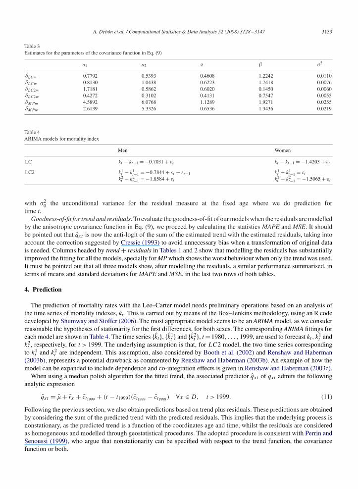
Table 3Estimates for the parameters of the covariance function in Eq. (9)

a1 a2 � � �2

�LCm 0.7792 0.5393 0.4608 1.2242 0.0110�LCw 0.8130 1.0438 0.6223 1.7418 0.0076�LC2m 1.7181 0.5862 0.6020 0.1450 0.0060�LC2w 0.4272 0.3102 0.4131 0.7547 0.0055�MPm 4.5892 6.0768 1.1289 1.9271 0.0255�MPw 2.6139 5.3326 0.6536 1.3436 0.0219

Table 4ARIMA models for mortality index

Men Women

LC kt − kt−1 = −0.7031 + εt kt − kt−1 = −1.4203 + εt

LC2 k1t − k1

t−1 = −0.7844 + εt + εt−1 k1t − k1

t−1 = εt

k2t − k2

t−1 = −1.8584 + εt k2t − k2

t−1 = −1.5065 + εt

with �20 the unconditional variance for the residual measure at the fixed age where we do prediction for

time t.Goodness-of-fit for trend and residuals. To evaluate the goodness-of-fit of our models when the residuals are modelled

by the anisotropic covariance function in Eq. (9), we proceed by calculating the statistics MAPE and MSE. It shouldbe pointed out that qxt is now the anti-logit of the sum of the estimated trend with the estimated residuals, taking intoaccount the correction suggested by Cressie (1993) to avoid unnecessary bias when a transformation of original datais needed. Columns headed by trend + residuals in Tables 1 and 2 show that modelling the residuals has substantiallyimproved the fitting for all the models, specially for MP which shows the worst behaviour when only the trend was used.It must be pointed out that all three models show, after modelling the residuals, a similar performance summarised, interms of means and standard deviations for MAPE and MSE, in the last two rows of both tables.

4. Prediction

The prediction of mortality rates with the Lee–Carter model needs preliminary operations based on an analysis ofthe time series of mortality indexes, kt . This is carried out by means of the Box–Jenkins methodology, using an R codedeveloped by Shumway and Stoffer (2006). The most appropriate model seems to be an ARIMA model, as we considerreasonable the hypotheses of stationarity for the first differences, for both sexes. The corresponding ARIMA fittings foreach model are shown in Table 4. The time series {kt }, {k1

t } and {k2t }, t =1980, . . . , 1999, are used to forecast kt , k

1t and

k2t , respectively, for t > 1999. The underlying assumption is that, for LC2 model, the two time series corresponding

to k1t and k2

t are independent. This assumption, also considered by Booth et al. (2002) and Renshaw and Haberman(2003b), represents a potential drawback as commented by Renshaw and Haberman (2003b). An example of how themodel can be expanded to include dependence and co-integration effects is given in Renshaw and Haberman (2003c).

When using a median polish algorithm for the fitted trend, the associated predictor qxt of qxt admits the followinganalytic expression

qxt = � + rx + ct1999 + (t − t1999)(ct1999 − ct1998) ∀x ∈ D, t > 1999. (11)

Following the previous section, we also obtain predictions based on trend plus residuals. These predictions are obtainedby considering the sum of the predicted trend with the predicted residuals. This implies that the underlying process isnonstationary, as the predicted trend is a function of the coordinates age and time, whilst the residuals are consideredas homogeneous and modelled through geostatistical procedures. The adopted procedure is consistent with Perrin andSenoussi (1999), who argue that nonstationarity can be specified with respect to the trend function, the covariancefunction or both.

3140 A. Debón et al. / Computational Statistics & Data Analysis 52 (2008) 3128–3147

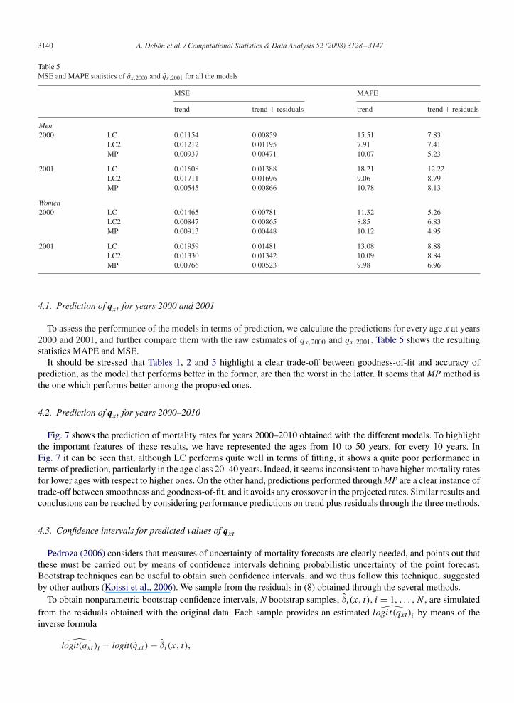
Table 5MSE and MAPE statistics of qx,2000 and qx,2001 for all the models

MSE MAPE

trend trend + residuals trend trend + residuals

Men2000 LC 0.01154 0.00859 15.51 7.83

LC2 0.01212 0.01195 7.91 7.41MP 0.00937 0.00471 10.07 5.23

2001 LC 0.01608 0.01388 18.21 12.22LC2 0.01711 0.01696 9.06 8.79MP 0.00545 0.00866 10.78 8.13

Women2000 LC 0.01465 0.00781 11.32 5.26

LC2 0.00847 0.00865 8.85 6.83MP 0.00913 0.00448 10.12 4.95

2001 LC 0.01959 0.01481 13.08 8.88LC2 0.01330 0.01342 10.09 8.84MP 0.00766 0.00523 9.98 6.96

4.1. Prediction of qxt for years 2000 and 2001

To assess the performance of the models in terms of prediction, we calculate the predictions for every age x at years2000 and 2001, and further compare them with the raw estimates of qx,2000 and qx,2001. Table 5 shows the resultingstatistics MAPE and MSE.

It should be stressed that Tables 1, 2 and 5 highlight a clear trade-off between goodness-of-fit and accuracy ofprediction, as the model that performs better in the former, are then the worst in the latter. It seems that MP method isthe one which performs better among the proposed ones.

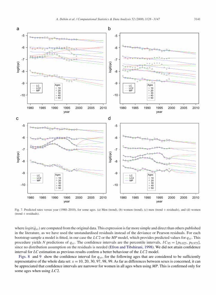
4.2. Prediction of qxt for years 2000–2010

Fig. 7 shows the prediction of mortality rates for years 2000–2010 obtained with the different models. To highlightthe important features of these results, we have represented the ages from 10 to 50 years, for every 10 years. InFig. 7 it can be seen that, although LC performs quite well in terms of fitting, it shows a quite poor performance interms of prediction, particularly in the age class 20–40 years. Indeed, it seems inconsistent to have higher mortality ratesfor lower ages with respect to higher ones. On the other hand, predictions performed through MP are a clear instance oftrade-off between smoothness and goodness-of-fit, and it avoids any crossover in the projected rates. Similar results andconclusions can be reached by considering performance predictions on trend plus residuals through the three methods.

4.3. Confidence intervals for predicted values of qxt

Pedroza (2006) considers that measures of uncertainty of mortality forecasts are clearly needed, and points out thatthese must be carried out by means of confidence intervals defining probabilistic uncertainty of the point forecast.Bootstrap techniques can be useful to obtain such confidence intervals, and we thus follow this technique, suggestedby other authors (Koissi et al., 2006). We sample from the residuals in (8) obtained through the several methods.

To obtain nonparametric bootstrap confidence intervals, N bootstrap samples, �i (x, t), i = 1, . . . , N , are simulatedfrom the residuals obtained with the original data. Each sample provides an estimated logit(qxt )i by means of theinverse formula

logit(qxt )i = logit(qxt ) − �i (x, t),

A. Debón et al. / Computational Statistics & Data Analysis 52 (2008) 3128–3147 3141

1980 1985 1990 1995 2000 2005 2010

-10

-9

-8

-7

-6

-5

year

logit(q

x)

Ages

1020304050

LCLC2MP

1980 1985 1990 1995 2000 2005 2010

yearlo

git(q

x)

Ages

1020304050

LCLC2MP

1980 1985 1990 1995 2000 2005 2010

year

logit(q

x)

Ages

1020304050

LCLC2MP

1980 1985 1990 1995 2000 2005 2010

-10

-9

-8

-7

-6

-5

-10

-9

-8

-7

-6

-5

-10

-9

-8

-7

-6

-5

year

logit(q

x)

Ages

1020304050

LCLC2MP

Fig. 7. Predicted rates versus year (1980–2010), for some ages. (a) Men (trend), (b) women (trend), (c) men (trend + residuals), and (d) women(trend + residuals).

where logit(qxt ) are computed from the original data. This expression is far more simple and direct than others publishedin the literature, as we have used the unstandardised residuals instead of the deviance or Pearson residuals. For eachbootstrap sample a model is fitted, in our case the LC2 or the MP model, which provides predicted values for qxt . Thisprocedure yields N predictions of qxt . The confidence intervals are the percentile intervals, IC95 = [p0.025, p0.975],since no distribution assumption on the residuals is needed (Efron and Tibshirani, 1998). We did not attain confidenceinterval for LC estimation as previous results confirm a better behaviour of the LC2 model.

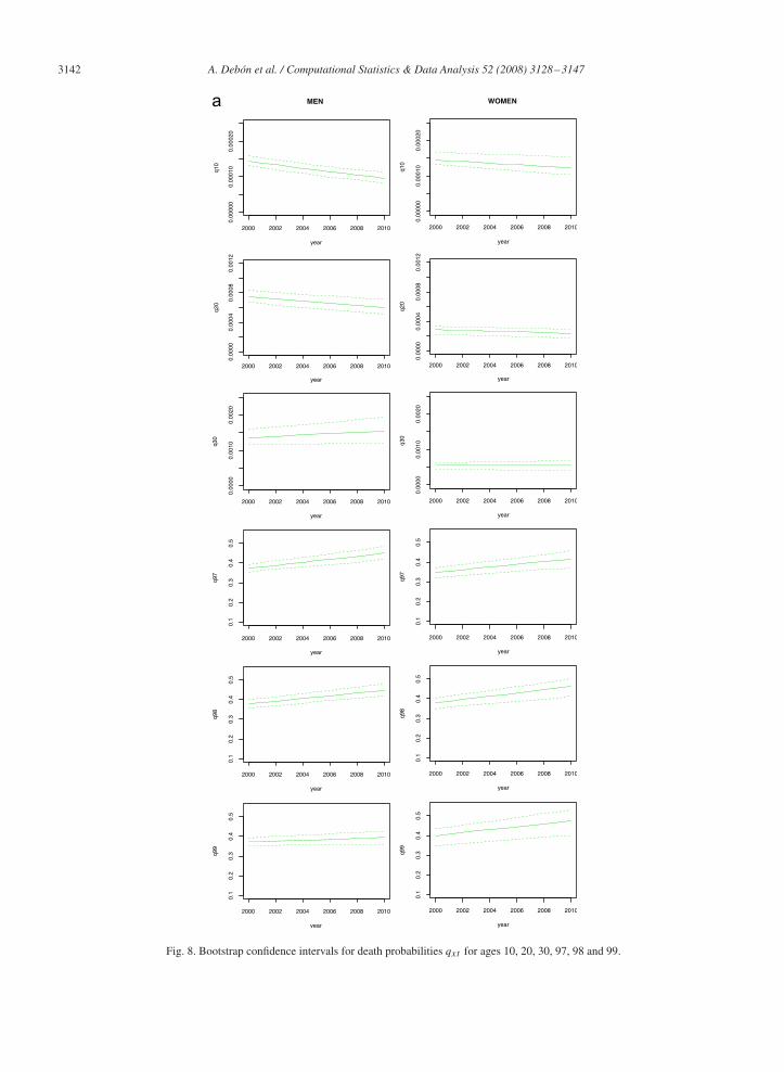
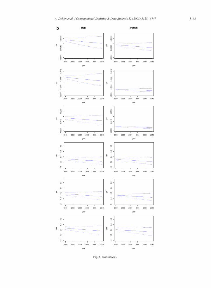
Figs. 8 and 9 show the confidence interval for qxt , for the following ages that are considered to be sufficientlyrepresentative of the whole data set: x = 10, 20, 30, 97, 98, 99. As far as differences between sexes is concerned, it canbe appreciated that confidence intervals are narrower for women in all ages when using MP. This is confirmed only forsome ages when using LC2.

3142 A. Debón et al. / Computational Statistics & Data Analysis 52 (2008) 3128–3147

Fig. 8. Bootstrap confidence intervals for death probabilities qxt for ages 10, 20, 30, 97, 98 and 99.

A. Debón et al. / Computational Statistics & Data Analysis 52 (2008) 3128–3147 3143

Fig. 8. (continued).

3144 A. Debón et al. / Computational Statistics & Data Analysis 52 (2008) 3128–3147

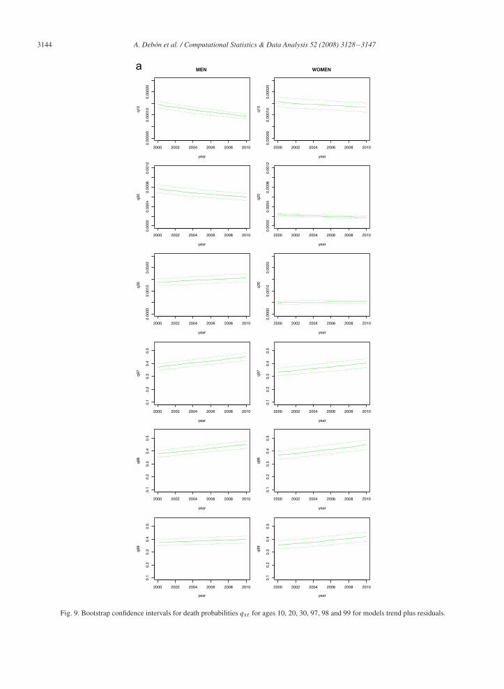
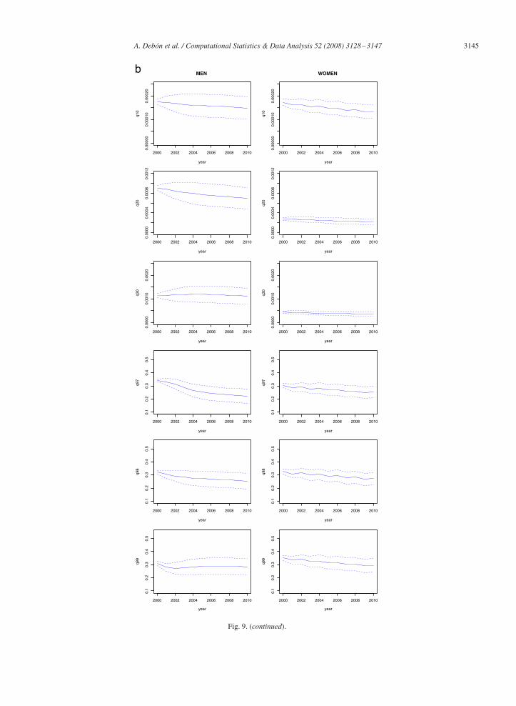
Fig. 9. Bootstrap confidence intervals for death probabilities qxt for ages 10, 20, 30, 97, 98 and 99 for models trend plus residuals.

A. Debón et al. / Computational Statistics & Data Analysis 52 (2008) 3128–3147 3145

Fig. 9. (continued).

3146 A. Debón et al. / Computational Statistics & Data Analysis 52 (2008) 3128–3147

It should be stressed that MP highlights a decreasing trend for all the ages, whilst LC2 emphasises exactly theopposite, above all for middle and old ages. The reason of this may be found in the fact that predictions performedthrough MP are based on contiguous years, whilst LC2 considers all past observations. Similar conclusions can bedrawn by considering trend plus residuals simultaneously.

5. Conclusions

We have proposed a new model for modelling and prediction of mortality rates. This model is based on a median-polish algorithm, which is easily interpretable and allows for observing the evolution along years and ages of theobserved phenomenon, with a relatively low computational cost. Also, the results in terms of prediction performanceare very satisfactory.

The residuals have been modelled through a geostatistical approach, where the novelty is represented by the fact thatwe took into account an anisotropic component by considering componentwise isotropy. The results were considerablyimproved both in terms of fitting and prediction performances, as confirmed by the diagnostics obtained through theMAPE and MSE statistics in Tables 1, 2 and 5. The fact that these measures are significantly lower, clearly implies a betterbehaviour for any considered ages. This result is particularly important if taking into account the intrinsic problemsassociated to prediction over very old ages. As pointed out by Wong-Fupuy and Haberman (2004), inaccuracies inrecording ages in official statistics and high variability in the estimates due to small exposures to risk are commonproblems when estimating mortality rates for the oldest age groups.

Modelling the residuals allows to interpolate and predict missing data through kriging. In addition, as we know theexact expression for the variance of the prediction, the calculation of the corresponding confidence intervals for futurepredictions is clearly simplified. The so obtained confidence intervals are almost equivalent (in terms of widths) tothose obtained through bootstrap techniques, as highlighted in Figs. 9 and 8, even though the bootstrap-based intervalstake into account any uncertainty inherent to prediction, as stated by Koissi et al. (2006).

We believe that the approach proposed in this paper can be very useful for modelling mortality rates, as it hasbeen shown to be very flexible, allowing to incorporate, through several approaches, a deterministic component withcovariates, and a stochastic one, exhibiting complex forms of interaction. Taking into account that our approach modelsthe dependence exhibited by the residuals, and that Fig. 5 highlights a cohort effect, it seems natural to think thatthis dependence is shown in form of a cohort effect. Thus, it would be interesting to compare our results with thosepotentially obtained when applying the model proposed by Renshaw and Haberman (2006) which adds the cohorteffect to the traditional model of Lee–Carter.

Acknowledgments

This work was partially supported by a grant from MEyC (Ministerio de Educación y Ciencia, Spain, project MTM-2004-06231). The authors are indebted to the anonymous referees whose suggestions improved the original manuscript.

References

Benjamin, B., Pollard, J., 1992. The Analysis of Mortality and Other Actuarial Statistics. sixth ed. Butterworth-Heinemann, London.Bevilacqua, M., Mateu, J., Porcu, E., Gaetan, C., 2007. Composite likelihood methods for space-time covariance model estimation. Technometrics,

to appear.Bochner, S., 1933. Monotone funktionen, Stieltjes integrale und harmonische analyse. Math. Ann. 108, 378–410.Booth, H., 2006. Demographic forecasting: 1980 to 2005 in review. Internat. J. Forecasting 22 (3), 547–582.Booth, H., Maindonald, J., Smith, L., 2002. Applying Lee–Carter under conditions of variable mortality decline. Population Stud. 56 (3), 325–336.Brouhns, N., Denuit, M., Vermunt, J., 2002. A Poisson log-bilinear regression approach to the construction of projected lifetables. Insurance Math.

Econom. 31 (3), 373–393.Christakos, G., 2000. Modern Spatiotemporal Geostatistics. Oxford University Press, Oxford.Christakos, G., Papanicolaou,V., 2000. Norm-dependent covariance permissibility of weakly homogeneous spatial random fields. Stochastic Environ.

Res. Risk Assessment 14 (6), 1–8.Cressie, N., 1993. Statistics for Spatial Data. revised ed. Wiley, New York.Curriero, F.C., Lele, S., 1999. A composite likelihood approach to semivariogram estimation. J. Agricultural Biological Environ. Statist. 4, 9–28.Debón, A., Martínez-Ruiz, F., Montes, F., 2004. Dynamic life tables: a geostatistical approach. In: 8th International Congress on Insurance:

Mathematics & Economics, Rome, Italy.

A. Debón et al. / Computational Statistics & Data Analysis 52 (2008) 3128–3147 3147

Debón, A., Montes, F., Sala, R., 2005. A comparison of parametric models for mortality graduation. Application to mortality data of the Valenciaregion (Spain). Statist. Oper. Res. Trans. 29 (2), 269–287.

Debón, A., Montes, F., Sala, R., 2006a. A comparison of models for dynamical life tables. Application to mortality data of the Valencia region(Spain). Lifetime Data Anal. 12 (2), 223–244.

Debón, A., Montes, F., Sala, R., 2006b. A comparison of nonparametric methods in the graduation of mortality: application to data from the Valenciaregion (Spain). Internat. Statist. Rev. 74 (2), 215–233.

Debón, A., Montes, F., Puig, F., 2007. Modelling and forecasting mortality in Spain. Eur. J. Oper. Res., doi:10.1016/j.ejor.2006.07.050.Efron, B., Tibshirani, R., 1998. An Introduction to the Bootstrap. CRC Press, Boca Ratón, FL.Felipe, A., Guillén, M., Pérez-Marín, A., 2002. Recent mortality trends in the Spanish population. British Actuar. J. 8 (4), 757–786.Forfar, D., McCutcheon, J., Wilkie, A., 1988. On graduation by mathematical formula. J. Inst. Actuar. 115 part I (459), 1–149.Gavin, J., Haberman, S., Verrall, R., 1993. Moving weighted average graduation using kernel estimation. Insurance Math. Econom 12 (2), 113–126.Gavin, J., Haberman, S., Verrall, R., 1994. On the choice of bandwidth for kernel graduation. J. Inst. Actuar. 121, 119–134.Gavin, J., Haberman, S., Verrall, R., 1995. Graduation by kernel and adaptive kernel methods with a boundary correction. Trans. Soc. Actuar. XLVII,

173–209.Guillen, M., Vidiella-i-Anguera, A., 2005. Forecasting Spanish natural life expectancy. Risk Anal. 25 (5), 1161–1170.Hyndman, R.J., Ullah, Md.S., 2007. Robust forecasting of mortality and fertility rates: a functional data approach. Comput. Statist. Data Anal. 51

(10), 4942–4956.Koissi, M., Shapiro, A., Högnäs, G., 2006. Evaluating and extending the Lee–Carter model for mortality forecasting confidence interval. Insurance

Math. Econom. 38 (1), 1–20.Lee, R., 2000. The Lee–Carter method for forecasting mortality, with various extensions and applications. North Amer. Actuar. J. 4 (1), 80–91.Lee, R., Carter, L., 1992. Modelling and forecasting U.S. mortality. J. Amer. Statist. Assoc. 87 (419), 659–671.Matérn, B., 1986. Spatial Variation. second ed.. Springer, Berlin.Matheron, G., 1965. Les Variables Régionalisées et leur Estimation. Masson et Cie, Paris.Pedroza, C., 2006. A bayesian forecasting model: predicting U.S. male mortality. Biostatistics 7 (4), 530–550.Perrin, O., Senoussi, R., 1999. Reducing non-stationary random fields to stationarity and isotropy using a space deformation. Statist. Probab. Lett.

48 (1), 23–32.Pitacco, E., 2004. Survival models in dynamic context: a survey. Insurance Math. Econom. 35 (2), 279–298.Porcu, E., Gregori, P., Mateu, J., 2006. Nonseparable stationary anisotropic space time covariance functions. Stochastic Environ. Res. RiskAssessment

21, 113–122.Porcu, E., Mateu, J., Bevilacqua, M., 2007. Covariance functions which are stationary or nonstationary in space and stationary in time. Statist.

Neerlandica 61 (3), 358–382.Renshaw, A., 1991. Actuarial graduation practice and generalised linear models. J. Inst. Actuar. 118 (II), 295–312.Renshaw, A., Haberman, S., 2003a. Lee–Carter mortality forecasting: a parallel generalized linear modelling approach for England and Wales

mortality projections. J. Roy. Statist. Soc. C 52 (1), 119–137.Renshaw, A., Haberman, S., 2003b. Lee–Carter mortality forecasting with age specific enhancement. Insurance Math. Econom. 33 (2), 255–272.Renshaw, A., Haberman, S., 2003c. Lee–Carter mortality forecasting incorporating bivariate time series. Actuarial Research paper No. 153, City

University, London.Renshaw, A., Haberman, S., 2006. A cohort-based extension to the Lee–Carter model for mortality reduction factors. Insurance Math. Econom. 38

(3), 556–570.Shumway, R., Stoffer, D., 2006. Time Series Analysis and its Applications with R Examples. Springer, New York.Tabeau, E., van den Berg Jeths, A., Heathcote, C., 2001. A Review of Demographic Forecasting Models for Mortality. Forecasting in Developed

Countries: From description to explanation. Kluwer Academic Publishers, Dordrecht.Wilmoth, J., 1993. Computational methods for fitting and extrapolating the Lee–Carter model of mortality change. Technical Report, Department

of Demography, University of California, Berkeley.Wong-Fupuy, C., Haberman, S., 2004. Projecting mortality trends: recent developments in the United Kingdom and the United States. North Amer.

Actuar. J. 8 (2), 56–83.Yaglom, A.M., 1987. Correlation Theory of Stationary and Related Random Functions. Springer, New York.