1

Design of Mobile Gas Sensor Systems for Industrial Processes

David Simões da Silvaa, Carla I. Pinheiroa, Prof. Rui M. Filipeb

a DEQ, Instituto Superior Técnico, Universidade de Lisboa, Av. Rovisco Pais, nº 1, 1049-001 Lisboa, Portugal;

b ADEQ, Instituto Superior de Engenharia de Lisboa, Rua Conselheiro Emídio Navarro, 1 1959-007 Lisboa

The study of mobile gas sensors’ spatial distribution around varied equipment configurations was

performed. The difference between mobile and static sensors was briefly addressed and two alternatives to the

sensor concentration sensitivity were proposed and compared. The possibility of temporary dead-zones, i.e.

temporary uncontrolled zones, during control was discussed. The results yielded a reduction in sensors needed

for the mobile sensor system due to the possibility of temporary dead-zones’ existence. Analytical solutions for

the minimization problem were presented and an agent based program with different heuristics was created in

MATLAB for the prediction of the minimal amount of required sensors. The analytical solutions to the mobile

problem were both centred on allowing all dead-zones to reach the maximum dead-zone time of 5 s. Both

approaches were compared in three distinct equipment geometries: an 11 m pipeline, a small pressurization

station and a 10 m high distillation column. These solutions presented a minimum amount of sensors required

equal to a sixth of the control volume’s cubic meters. The programs’ best possible minimum was determined to

be twice the amount of the analytical solutions and is only achieved for certain equipment geometries, with

possible over dimensioning of the solution. It was also determined that the programs’ results possess higher

redundancy than the analytical solutions. Therefore, industrial implementation should be studied case by case,

with pros and cons weighted using the tools developed in this work.

Keywords: MATLAB, agent based modelling, GRASP, PSO, mobile gas sensors, drones, equipment control.

Introduction

The motivation for the subject of this work

was the important industrial issue of flammable

gases’ early detection and the fact that a reliable

method for positioning static gas sensors doesn’t

exist. Therefore, the aim of this work was to create

a model of mobile sensors dedicated to the leaks

identification of flammable gases with and without

a programming method.

Currently, the industry has developed many

ways of effectively detecting gas leaks, each with

its advantages and disadvantages. There are three

different categories, as proposed by Murvay and

Silea, to define gas sensing methods: “non-

technical, hardware based and software based”

methods.1

Non-technical methods are solely based on

human capabilities and since the human senses are

fallible, this approach presents obvious limitations.

Hardware methods use equipment that control

changes in physical properties directly on the

exterior of the equipment that we want to control,

while software based methods use the data read on

the equipment itself and infer the probability of a

leak when specific parameters change.1

Most of the hardware methods require the

implementation of multiple components along the

equipment if we desire continuous control, which

increases the costs as the size of the equipment

rises. Therefore, the hardware methods are mostly

2

used as a maintenance tool. This is why software

methods are used as a complement to the hardware

methods.1

With this premise in mind, we proposed the

hypothesis of reducing the number of sensing

equipment by allowing it to move along and around

the equipment in order to fully monitor it and

reduce the operation costs by reducing the hardware

quantity required through automation of movement.

We considered for this purpose flying drones as a

medium and chose vapour sensing technology to go

with it.

Although the chosen sensing method is a

proven technology, advances in drone technology

are not yet at the required level, but show sufficient

promises to be considered as viable in a medium to

close future. Companies such as Parrot and DJI are

constantly pushing the limits of commercial drone

technology and their respective performances.2, 3, 4

Sensing technology is also evolving

continuously, becoming highly performant with the

use of nanotechnological fabrication processes. A

recent thesis work has shown that for a

nanostructured tungsten oxide basis, the lowest

detection limit of hydrogen can be as little as

10 ppm.5 The current average detection

concentration is worse, yet still considerably lower

than the lower explosive limit (LEL) concentration

of 40,000 ppm.

The requirements for simulating a system of

drones with sensing capabilities led to the choice of

agent based modelling programming as well as the

use of the MATLAB programming language. The

ability to separate individual sensors into agents

with identical set of rules from which emergent

swarm behaviour emerges was the main

consideration for this choice.6

Likewise, the use of heuristics was needed in

order to reduce computational times while

obtaining a close to optimal solution. Furthermore,

the goal of using heuristics was to improve on

redundancy issues arising with analytical solutions.

The heuristics used were heavily inspired by

particle swarm optimisation (PSO) and greedy

randomized adaptive search procedures (GRASP).7

PSO is a heuristic method used commonly in

bird flock simulations as well as any other swarm

like group in which each single element has the

same goal. PSO is relevant for our work as in many

aspects the drones behave like a flock of birds.

They try to avoid each other, hence not moving to

where another bird/drone is or has just been and

they both look for the highest output; food in the

birds’ case and for the drones dead-zone time,

defined as how long a given volume can be left to

fill up with maximum hydrogen leak flow before

the lower explosive limit of hydrogen is reached.

The difference being that the food distribution

diminishes with time, as birds consume it, whereas

the dead-zone time continuously increases with the

absence of a drone.7

Meanwhile, a GRASP algorithm incorporates

multiple sub heuristics working for the benefit of

the higher order GRASP heuristic, called

metaheuristic. At the same time, a greedy algorithm

is called greedy, as it constantly reexamines

variables that increase or decrease as time passes.

At each tick, it chooses the best solution, minimum

or maximum depending on its objective,

subjectively deciding between equivalent solutions,

in order to build up an overall solution to the

problem. A randomized greedy metaheuristic is any

greedy metaheuristic that includes elements of

randomness in its process. The drone simulation

used in this paper is partially inspired in simple

GRASP techniques, as for instance each drone

chooses the best solution from a selected amount of

destinations, although even results are broken

arbitrarily.

3

Case Study

Before we could start modeling the mobile

sensor system, initial information had to be

gathered. Furthermore, as the detection sensitivity

of gas vapor sampling sensors is defined in

concentration as opposed to an effective range, we

developed two opposing models of sensor detection

range.

Both models assume that detection occurs if

the sensitivity concentration threshold is passed in a

volume of one cubic meter in which the sensor is

located at the center. The difference between

models lies in the volume’s geometry. The first one

is cubical while the second model is spherical.

Both models were tested under the same

conditions and assumptions. We used 10 ppm as

detection limit for the detection of hydrogen as

suggested by Kukkola.5 We used 100 atm of gas

pressure as it was found to be the highest common

pressure in equipment under normal operating

conditions.8, 9

We defined a leak flow using the maximum

wall thickness l used in pipelines of 7.2 mm10

and

an arbitrary leak diameter d of 1 mm, with the

Knudsen formula for molecular flow (1) provided

by KVS.11

𝑞 =√2𝜋

6√𝑅𝑇

𝑀

𝑑3

𝑙(𝑝1 − 𝑝2) (1)

In order to obtain a realistic although

approximate value of the leak flow q, we assumed

the temperature and outside pressure to be ambient,

i.e. 298.15 K and 1 atm respectively. The value and

units chosen for R, the universal gas constant, was

8.314 m3

Pa K−1

mol−1

and we used 0.001 m for the

leak’s diameter. The result was the following

volumetric flow value of q = 6.395 x 10-3

m3

atm s-1

or 6395 ml atm s-1

.

We used the lower explosive limit (LEL) of

hydrogen as provided by Ren & Paerton of

4 % (V/V).12

We also assumed that drones move

between adjacent cubical volumes’ centers in 1 s.

All the above data allowed us to determine the

possibility of dead-zones. The resulting dead-zone

time was determined to be 6.09 s, time which we

reduced to 5 s in order to be more restrictive and

have a safer approach.

Subsequently, the equipment geometry was

defined, as well as its surrounding control volume,

which can be observed in figure 1 for the initial

10 m pipeline test case.

Figure 1: Visual representation of the volume to be controlled

around the pipeline.

Next, we assumed that leaks flowed into a

virtual volume, called leak volume, of one cubic

meter and would not disperse or flow further from

the leak’s origin. With this, we verified that

overlapping of leak volume and detection volume

would ensure detection. Due to the high output of

the leak and the low detection concentration limit of

the sensors, only a fraction of overlap is needed to

guarantee detection.

At the same time, two scenarios were devised:

one in which sensors are static and another in which

they’re mobile. Both models, cubical and spherical,

were then tested in the two scenarios and according

to the following criteria: number of sensors needed

to cover all the control volume and percentage of

maximum overlap between two adjacent sensor’s

detection volumes, both data which we want to

minimize. Furthermore, percentages of dead- zones,

4

which we want to maximize, were compared. The

results can be seen in table 1.

Table 1: Case and model results comparison.

Case Model Sensors Max

overlap %

Dead-

zone %

Static Cubical 40 5.37 0

Spherical 40 39.93 0

Mobile Cubical 8 5.37 80

Spherical 8 31.20 80

The results clearly show that the mobile case

requires fewer sensors than the static case, while

there is no difference in using either the spherical or

cubical detection volume. We chose therefore to

use the more convenient cubical model.

A quick study of possible drone collisions was

performed, concluding that depending on drone size

and in certain movement configurations, collisions

were in fact possible, but that with the proper

software, collision issues can be overcome and

hence were ignored in our work.

The first iteration proposed for the drone’s

movement was an analytical solution to the

problem. As detection volumes are cubical with

1 m3 of volume, we can divide any given control

volume in such 1 m3 units. Likewise, given the

maximum dead-zone time allowed of 5 s we know

that to perform a control loop, a drone, moving at a

pace of 1 control volume per second, will control 5

volumes and then return to its origin on the sixth

second. We defined this as the small loop

configuration. A total of 6 volumes, configured in

such a way that after six seconds all volumes have

been controlled and the drone is back at the initial

volume.

Any volume broken down into x cubical

volume elements has therefore a minimum sensor

requirement of x divided by 6. Incidentally, this

number is the same as the number of loops present

along the control volume. These can be opened up

and combined to create a single big loop in which

drones follow each other in a train like fashion with

an interval of 5 empty volume elements between

each other.

The issue with both small and big analytical

loop approaches is the lack of redundancy. In fact,

if one sensor is malfunctioning without the

operator’s knowledge, then a section of six volumes

is not being controlled at all in the small loop

configuration, while in the big loop configuration

there is a portion of volumes that reaches 11 s of

dead-zone time and this failure propagates along

the entire system.

There are ways to mitigate these effects, such

as creating intermediate loops, such a 12 volume

elements binary loops, or adding additional sensors

in order to reduce the interval between subsequent

drones.

To look for increased redundancy solutions,

we decided to test the implementation of heuristics

in an agent based modelling program developed in

MATLAB. In fact, according to Katta: A heuristic

is a method used to solve a problem in such a way

that assumptions are taken as premise to most likely

lead to a near optimal solution without the

guarantee of the solution being the absolute

optimum.13

We developed 5 different heuristics for our

drone’s movement decision making. By using the

time since last being controlled (tsc) displayed by

adjacent volume elements, the first heuristic (H1)

decides to move the drones towards the volume

element with maximum tsc value regardless of

spatial orientation and breaks ties in order of first

maximum encountered during the geometrically

constant screening process. In case of no free

adjacent space, or “stuck “event, the drone waits in

place until the next computing cycle.

In heuristic 2 (H2) the drones choose

identically to heuristic 1 (H1), but if a “stuck” event

5

occurs it will join a queue in which it tries to move

once more after all other drones have passed before

it. This is designed to gum out the issues of

programming sequentiality and simulate a more

parallel movement process.

Heuristic 3 (H3) is based on heuristic 2 and

shares all its rules, but when confronted to multiple

equivalent maxima during the drone’s choosing

process, the concerned drone will cede his place

just like a non-movable drone does in heuristic 2

and then chooses a heading once according to

heuristic 1 during the second pass. The aim is to

eventually have the multiple maxima reduced to

only one, when the concerned drone is allowed to

choose from its surroundings again.

Heuristic 4 (H4) is based on heuristic 1, but

with the added restriction that the drone’s

movement is only allowed when tsc is above 3

seconds. The aim of this heuristic is to artificially

increase the efficiency of the program’s solution in

situations where the average time since last checked

is a low value.

Heuristic 5 (H5) is based on heuristic 1, but

diagonal movement of the drones is not allowed.

Movement is restricted to the six main axes. The

aim of this heuristic is to add more order in the

drones’ movement and try to reduce bizarre

trajectories with many kinks; the expectation being

to have smoother straighter paths and less

backtracking.

Next, the best possible solution for heuristic 1

was determined. Since all our heuristics are based

on heuristic 1, a deterministic sequential pattern can

be tested. Consequentially, we can explore all

solution provided by the multiple possible

outcomes of the arbitrary tie breaks applied in

heuristic 1 in a brute force type of approach.

Hence, when using the same 6 volume

elements as determined in the loop configuration,

starting with a single sensor and adding one sensor

when a configuration is found to allow tsc to

exceed 5 s, we concluded that 2 sensors is the

absolute minimum required to effectively and

indefinitely control a group of 6 adjacent volume

elements when the drones use the basic movement

process based on maximum tsc values, as described

in heuristic 1. We called this the best possible

program result.

This means that no matter how much we

would try to refine upon heuristic 1, the best

possible result obtainable would be the double of

the value obtained with the analytical loop

configuration result.

We then implemented all of the above

heuristics into a coherent MATLAB program in

which both sensors/drones and volume elements

were considered as agents and therefore defined as

mathematical objects. Both received individual

properties and we devised a list creation process to

store the agents as well as access and modify their

properties. Further details can be found in

reference 14

.

The drones’ movement was initially

programmed as coordinate sensitive to allow for a

complete freedom of movement, yet the resolution

of a system of three parametric equations with up to

27 restrictions based on parametric equations

themselves to solve in MATLAB was out of our

range of abilities. This fact, led us to choose a

volume tied movement. This means that sensors

travel at varying speed, but move from adjacent

volume element’s center to center in a constant 1 s.

Mathematical tools for the sensors to analyze

their surroundings for sensor presence were

implemented as well as the heuristics that define a

drone’s heading choice. Details, like ensuring

drones don’t choose the same destination, were fine

tuned.

Finally, we started the program with a single

sensor, adding more sensors if the maximum tsc

6

condition failed. The success condition given was

the conservation of tsc under the allowed threshold

in all volume elements for a given interval of time.

The resulting number of sensors was the minimum

required for running the heuristic for a given

interval of time.

Results

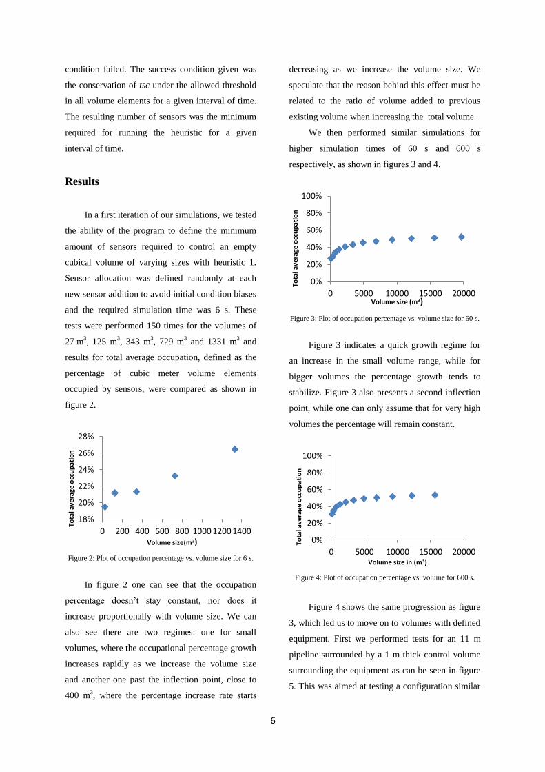
In a first iteration of our simulations, we tested

the ability of the program to define the minimum

amount of sensors required to control an empty

cubical volume of varying sizes with heuristic 1.

Sensor allocation was defined randomly at each

new sensor addition to avoid initial condition biases

and the required simulation time was 6 s. These

tests were performed 150 times for the volumes of

27 m3, 125 m

3, 343 m

3, 729 m

3 and 1331 m

3 and

results for total average occupation, defined as the

percentage of cubic meter volume elements

occupied by sensors, were compared as shown in

figure 2.

Figure 2: Plot of occupation percentage vs. volume size for 6 s.

In figure 2 one can see that the occupation

percentage doesn’t stay constant, nor does it

increase proportionally with volume size. We can

also see there are two regimes: one for small

volumes, where the occupational percentage growth

increases rapidly as we increase the volume size

and another one past the inflection point, close to

400 m3, where the percentage increase rate starts

decreasing as we increase the volume size. We

speculate that the reason behind this effect must be

related to the ratio of volume added to previous

existing volume when increasing the total volume.

We then performed similar simulations for

higher simulation times of 60 s and 600 s

respectively, as shown in figures 3 and 4.

Figure 3: Plot of occupation percentage vs. volume size for 60 s.

Figure 3 indicates a quick growth regime for

an increase in the small volume range, while for

bigger volumes the percentage growth tends to

stabilize. Figure 3 also presents a second inflection

point, while one can only assume that for very high

volumes the percentage will remain constant.

Figure 4: Plot of occupation percentage vs. volume for 600 s.

Figure 4 shows the same progression as figure

3, which led us to move on to volumes with defined

equipment. First we performed tests for an 11 m

pipeline surrounded by a 1 m thick control volume

surrounding the equipment as can be seen in figure

5. This was aimed at testing a configuration similar

18%

20%

22%

24%

26%

28%

0 200 400 600 800 1000 1200 1400

Tota

l ave

rage

occ

up

atio

n

Volume size(m3)

0%

20%

40%

60%

80%

100%

0 5000 10000 15000 20000To

tal a

vera

ge o

ccu

pat

ion

Volume size (m3)

0%

20%

40%

60%

80%

100%

0 5000 10000 15000 20000

Tota

l ave

rage

occ

up

atio

n

Volume size in (m3)

7

to the one used in defining the sensor’s detection

range.

Figure 5: Visual representation of the volume elements used for

the simulations with pipe in the centre.

Simulations were performed from 60 to 6000 s

of simulation time, still under random sensor

allocation and using heuristic 1. The occupation

percentages resulting from the simulation were

sensibly smaller than for the previous empty

cubical volume case, while the average of minimum

required amount of sensors can be seen in figure 6.

Figure 6: Average sensor number needed vs. simulation time for

random allocation 11 m pipeline control.

In figure 7 we performed non-random sensor

allocation to begin comparison of different

heuristics with each other. The non-random sensor

allocation performs the addition of a new sensor at

the point where the program detects the first

volume element with tsc value higher than allowed,

while leaving the previous sensors at their current

location.

Figure 7: Sensor number needed vs. simulation time for non-

random allocation 11 m pipeline control (H1).

In figure 8 the blue diamonds are the results

for the non-random allocation test and they have

always values higher than all the other random

allocation tests. This is due to random allocation

allowing the emergence of favourable patterns in

which the simulation time requested can be

sustained while maintaining the tsc value under the

defined limit, but which would eventually need

more sensors if simulation times were longer. We

are forced to choose the most restrictive answer to

ensure safety and this means choosing the highest

minimum result we get. Therefore the non-random

allocation proves to be a better tool than the random

allocation and we decided to proceed with tests in

the non-random allocation branch.

Figure 8: Non-random vs. random sensor allocation for 11 m

pipe simulation (60 to 600 s).

We continued with performing tests for all

other heuristics in order to determine the one

performing closest to the program’s best possible

0

10

20

30

40

0 2000 4000 6000 8000

Ave

rage

se

nso

rs n

ee

de

d

Simulation time (s)

0

10

20

30

40

50

0 2000 4000 6000 8000

Nu

mb

er

of

sen

sors

Simulation time (s)

20

25

30

35

40

0 200 400 600

Nu

mb

er

of

sen

sors

Simulation time (s)

8

result. The maxima encountered can be seen in

tables 2a and 2b.

Table 2a: Minimum sensors required for 11m pipeline control

according to different methods for 6000s.

Method Analytical loop

configuration

Program’s

best possible

result

H 1

Max.

sensors 15 30 40

Table 2b: Minimum sensors required for 11 m pipeline control

according to different methods for 6000 s.

Method H 2 H 3 H 4 H 5

(@600 s)

Max.

sensors 40 39 43 43

We proceeded to test other equipment such as

a pressure station and a distillation column under

non-random allocation, but solely for heuristics 1 to

3 as heuristics 4 and 5 showed poor performance.

The results can be observed in tables 3 and 4.

Table 3: Minimum sensors required for designed pressure station

control with 3 heuristics for 6000 s.

Method

Program’s

best possible

result

H 1 H 2 H 3

Max.

sensors 26 27 26 27

Table 4: Minimum sensors required for designed distillation

column control with 3 heuristics for 6000 s.

Method

Program’s

best possible

result

H 1 H 2 H 3

Max.

sensors 46 51 53 51

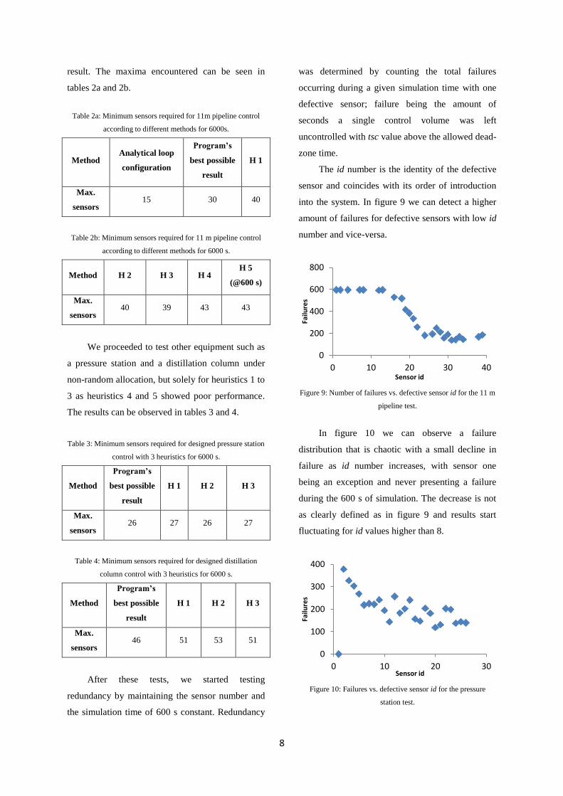
After these tests, we started testing

redundancy by maintaining the sensor number and

the simulation time of 600 s constant. Redundancy

was determined by counting the total failures

occurring during a given simulation time with one

defective sensor; failure being the amount of

seconds a single control volume was left

uncontrolled with tsc value above the allowed dead-

zone time.

The id number is the identity of the defective

sensor and coincides with its order of introduction

into the system. In figure 9 we can detect a higher

amount of failures for defective sensors with low id

number and vice-versa.

Figure 9: Number of failures vs. defective sensor id for the 11 m

pipeline test.

In figure 10 we can observe a failure

distribution that is chaotic with a small decline in

failure as id number increases, with sensor one

being an exception and never presenting a failure

during the 600 s of simulation. The decrease is not

as clearly defined as in figure 9 and results start

fluctuating for id values higher than 8.

Figure 10: Failures vs. defective sensor id for the pressure

station test.

0

200

400

600

800

0 10 20 30 40

Failu

res

Sensor id

0

100

200

300

400

0 10 20 30

Failu

res

Sensor id

9

Figure 11, resembles closely the high id range

of figure 9’s results, indicating that most sensors

controlling a distillation tower have a lower failure

count than the sensors used in the 11 m pipeline

control.

Figure 11: Failures vs. defective sensor id for the distillation

column test.

A summary of maximum failures compared to

the analytical loop configuration performances can

be observed in table 5.

Table 5: Analytical loop configuration failures vs. maximum

Heuristic 1 failures for all equipment

Equipment 11 m

pipe

Pressure

station

Distillation

column

Loop

configuration

failures

3595 3595 3595

Maximum

failures 595 378 554

Straight away we can see that the applied

heuristics are much more robust when subjected to

sensor failures than the analytical loop

configurations and hence, they are more redundant.

Conclusions

According to the loop configurations, one

sensor can cover six volumes at all times. This

means that for any given total volume, the total

occupation percentage will be of one sixth or

approximately 17 %. Both the big and the small

loop configurations offer the same level of

efficiency but with different outcomes in the event

of sensor failure.

The empty cubical volume tests showed that

for lower simulation times and smaller volumes,

favourable configurations can appear that are not

stable over the long run, requiring extreme

simulation times for stability. Also, in this test, the

program with heuristic 1 is not efficient at all, as it

offers results always superior than 50 % of

occupation.

In the 11 m pipeline tests, for heuristic 1 using

random allocation we get a result of 38.58 %

maximum coverage. This result is close to the

program’s best possible result of 34 %. The most

likely explanation for the discrepancy is the

increased amount of unfavourable drone

configurations, which increases as the symmetry of

the system rises.

The differences between the various heuristics

applied to the non-random allocation tests are

subtle. The maximum of heuristic 2 is the same as

heuristic 1, due to blocked sensors most likely

being a rare occurrence.

Heuristic 3 shows a very small improvement

of one sensor, most likely due to the fact that by

having some multiple maxima resolved by previous

sensors, the totality of sensors are working slightly

better together and obtain better results.

Heuristic 4 is less efficient than all the others,

most likely due to the fact that by allowing

movement only after 3 seconds have passed, most

volumes will be too far into the process of dead-

zone and sensors will have trouble catching up with

the volumes that require verification.

Heuristic 5 is even worse than heuristic 4, as

removing diagonal movement only removes

degrees of freedom to the sensors choice, limiting

its effectiveness.

0

100

200

300

400

500

600

0 20 40 60

Failu

res

Sensor id

10

The program’s best possible result for the

pressure station is 26 sensors. With heuristics 1 and

3 we obtained 27 sensors and for heuristic 2 we

matched the program’s best possible result. The

more asymmetric geometry of the pressure station

lowers the chances of encountering equivalent tsc

maxima from which to choose from and hence

reduces the possibility for unfavourable drone

patterns.

The distillation column tests performed almost

identically to the 11 m pipeline tests, leading to

identical conclusions.

The redundancy tests for all equipment

geometries showed lower failure events as opposed

to the analytical loop configurations, meaning the

heuristics are more redundant.

At the same time, tests showed a separation

between sensors. Some will have higher

redundancy than others. The equipment geometry

determines their distribution. Failure graphs can

therefore be used for determination of the

program’s performance for specific geometries.

In conclusion, the analytical loop

configurations are the most drone effective

solutions, but with clear redundancy problems,

while the heuristic approaches offer better

redundancy, but will perform poorly for certain

equipment geometries. It is possible to opt for a

mixt small and big loop configuration, but the final

choice remains at the operator’s discretion.

Furthermore, we recommend waiting for drone

technologies to improve, before applying mobile

drone sensor control systems.

Further areas of study originating from this

work are collision avoidance, additional heuristics

as well as additional equipment geometries testing.

Also future approaches can consider the inclusion

of diffusion and convection of the leak’s escaping

gases, as well as the rewriting of the MATLAB

program in a different programming language, such

as C++. Finally, further possible fields of study are

testing of high volumes with high simulation times,

as well as performing equipment cost optimization

analyses.

References

(1) Murvay P., Silea I. (2012). A survey on gas leak detection

and localization techniques. In Elsevier: Journal of Loss

Prevention in the Process Industries.

(2) Parrot Blog (2014). [www document]. [Accessed 13 June

2014]. http://blog.parrot.com/2014/01/07/parrot-

minidrone/

(3) DJI Store (2014). [www document]. [Accessed 13 June

2014]. https://store.dji.com/buy/phantom-2-vision-plus-

with-extra-battery

(4) DJI Youtube (2014). [www document]. [Accessed 13

June 2014].

https://www.youtube.com/watch?v=VhDAILW9UAE

(5) Kukkola J. (2013) Gas sensors based on nanostructured

tungsten oxides. University of Oulu. Oulu. Acta

Universitatis Oulensis C 462.

(6) Lukszo Z., Nikolic I., van Dam K. (2013) Agent-Based

Modelling of Socio-Technical Systems, volume 9,

Springer.

(7) Burke E. K. & Kendall G. Search Methodologies

Introductory, Tutorials in Optimization and Decision

Support Techniques, 2014.

(8) American Gas Association (2014). [www document].

[Accessed 15 September 2014].

http://www.aga.org/KC/ABOUTNATURALGAS/CONS

UMERINFO/Pages/NGDeliverySystem.aspx

(9) Sletfjerding, E. (1999) Friction Factor in Smooth and

Rough Gas Pipelines. PhD Thesis. Norwegian University

of Science and Technology, Tronheim.

(10) PNGRB (2009). [www document]. [Accessed 16

September 2014].

http://www.pngrb.gov.in/GSR808(E).pdf

(11) KVS Vakuum- und Lecksuchtechnik (2014). [www

document]. [Accessed 16 September 2014].

http://www.leakdetection-technology.com/science/the-

flow-of-gases-in-leaks

(12) Ren & Pearton, Semiconductor Device-Based Sensors for

Gas, Chemical, and Biomedical Applications, 2011.

(13) Katta G. M. (2003) Optimization Models For Decision

Making. University of Michigan, Ann Arbor.

(14) Simões da Silva D. (2015) Design of Mobile Gas Sensor

Systems for Industrial Processes. MSc Thesis. IST,

University of Lisbon, Lisbon.