Flow simulations with ultra-low Reynolds numbers over rigid ...
Upload
khangminh22Category
view
0download
0
626
NN
T:
20
20
IPP
AT
01
8
Design of an ultra-low-power
communication system for leadless
pacemaker synchronizationThese de doctorat de l’Institut Polytechnique de Paris
preparee a Telecom Paris - C2S
Ecole doctorale n626 Ecole doctorale Institut Polytechnique de Paris (ED IP Paris)Specialite de doctorat : Information, communications, electronique
These presentee et soutenue a Palaiseau, le 29/05/2020, par
MIRKO MALDARI
Composition du Jury :
Sandro Carrara
Professeur, EPFL (STI IMT ICLAB) President
Noelle Lewis
Professeur, Universite de Bordeaux (IMS - Laboratoire de
l’Integration du Materiau au Systeme)Rapporteur
Pierre-Yves Joubert
Professeur, Universite Paris Sud (C2N CNRS, Universite Paris
Saclay)Rapporteur
Philippe Ritter
Cardiologue, CHU de Bordeaux Examinateur
Youcef Haddab
Docteur-Ingenieur, Microport CRM (COE-ELEC) Examinateur
Patricia Desgreys
Professeur, Telecom Paris (C2S) Directeur de these
Chadi Jabbour
Maıtre de Conference, Telecom Paris (C2S) Co-directeur de these

Ad Adele, Ewa e Nicola
Acknowledgements
Questo lavoro non e soltanto frutto di tre splendidi anni di ricerca, ma il risultato
dell’apprendimento di una vita intera. Percio, ringrazio, innanzitutto, la mia famiglia
per avermi trasmesso la consapevolezza che non ci sono limiti irrangiungibili qualora il
desiderio e accompagnato dalla giusta dose di determinazione e impegno.
Un remerciement special va a Lise (heureusement, il n’y a pas que les decouvertes sci-
entifiques dans la vie !) pour avoir partage les dernieres annees avec moi.
Je tiens a remercier tous les supeviseurs de mon projet de these: Chadi, Karima, Pa-
tricia, et Youcef. J’ai eu la chance d’etre encadre par vous pour votre competences et
qualitees humaines.
Merci a tous mes collegues chez Microport pour les bons moments passes ensemble.
Une mention speciale a Theoa, Stephane, Marc, Mous, Ashu, Giulia et Luca pour le
support; a Delphine et Rafa pour avoir collabore a la reussite du projet.
I thank all the people involved in the ITN program. This project, indeed, was far
beyond my expectations, thanks to the incredible people I met in this journey.
Comment ne pas remercier Leslie, pour les magnifiques annees de collocations. Tu
as rendu extremement simple et agreable partager la vie de tous les jours (bon, a excep-
tion de quelques points de suture et de France Inter pour faire semblant d’ecouter les
infos le matin).
Finally, I would like to thank all my friends. The past moments spent with you make
me retrace my life and the present moments make it valuable.
ii
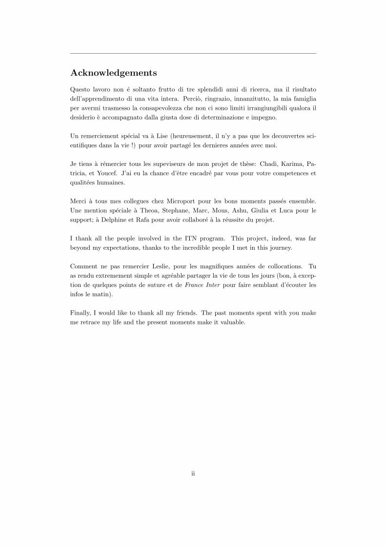
Titre : Conception d’un systeme de communication pour des pacemakers sans fils avec gestion de puissance
Mots cles : In-Body Communication, IBC, HBC, LCP, Leadless pacemakers, Ultra-low-power design
Resume : L’objectif de nos etudes etait de propo-
ser des solutions optimisees pour la communication
entre pacemakers sans sondes (LCP en Anglais) afin
de permettre la synchronisation de la therapie entre
dispositifs implantes dans des chambres cardiaques
differentes. L’Intra-Body Communication (IBC) est
consideree comme une solution prometteuse. Il s’agit
d’une communication qui utilise les tissue biologiques
comme moyen de transmission. Les attenuations des
canaux de communication ont ete caracterises en uti-
lisant un model de thorax verifie grace a des es-
sais in vivo. Un recepteur a tres faible consomma-
tion a ete concu en technologie CMOS avec une sen-
sibilite qui respecte les niveaux des signaux issus
de la caracterisation du canal intra-cardiaque. Afin
de minimiser la consommation du recepteur et, en
consequence, reduire l’impact du circuit en termes
de longevite du dispositif, une strategie innovante
de communication a ete proposee. Les resultats de
recherche demontrent la faisabilite d’une synchroni-
sation entre LCPs fondee sur la telemetrie, ouvrant
la voie a la realisation de systemes multi-dispositifs
pour ameliorer la qualite du traitement de patients qui
souffrent de bradycardie. Ce travail fait partie du projet
WiBEC, un projet multidisciplinaire qui vise a conce-
voir des technologies sans fils pour des dispositifs im-
plantables.
Title : Communication system design for leadless pacemaker synchronization with power management
Keywords : In-Body Communication, IBC, HBC, LCP, Leadless pacemakers, Ultra-low-power design
Abstract : Our research focused on power optimi-
zed solutions for the communication between Lead-
less Cardiac Pacemakers (LCP) to allow a synchroni-
zed therapy among devices implanted in different car-
diac chambers. A promising solution is the Intra-Body
Communication (IBC), which uses biological tissues
as transmission medium. The attenuation of the com-
munication channels were characterized using an ac-
curate torso model that has been verified by means of
in-vivo experiments. An ultra-low power receiver has
been designed in CMOS technology according to the
sensitivity requirement coming from the intra-cardiac
channel characterization. Moreover, a novel commu-
nication strategy has been proposed to minimize the
power consumption of the receiver reducing the im-
pact in terms of device longevity. The research results
show the feasibility of a telemetry driven synchroniza-
tion of LCPs, paving the way toward multiple-leadless
pacemaker systems that might improve the quality of
treatment of the bradycardia patients. This work was
part of the WiBEC project. It is a multi-disciplinary pro-
ject aiming to develop the wireless technologies for
novel implantable devices.
WiBEC - Wireless in-Body Environment
A Horizon 2020 Innovative Training Network
Description : WiBEC (Wireless In-Body Environment) is an Innovative Training Network for 16 young resear-
chers, who will be recruited and trained in coordinated manner by Academia, Industry, and Medical Centres.
WIBEC’s main objective is to provide high quality and innovative doctoral training to develop the wireless
technologies for novel implantable devices that will contribute to the improvement in quality and efficacy of
healthcare. Two devices will be used as a focus for the individual researcher’s projects; cardiovascular im-
plants and ingestible capsules to investigate gastro intestinal problems. These devices will enable medical
professionals to have timely clinical information at the point of care. The medical motivation is to increase
survival rates and improvement of health outcomes with easy and fast diagnosis and treatment. The goal for
homecare services is to improve quality of life and independence for patients by enabling ambient assisted
living (AAL) at home. In this particular ETN, inter-sectorial and multi-discipline work is essential, as the topic
requires cooperation between medical and engineering institutions and industry. Thus, the WIBEC consortim
is composed of 3 Universities, 2 hospitals, and 3 companies located in different countries in Europe.
Institut Polytechnique de Paris91120 Palaiseau, France
Resume en francais
Introduction
Chaque annee, plus d’un million de stimulateurs cardiaques (pacemaker en anglais) sont
implantes dans le monde afin de traiter les patients qui souffrent de bradycardie. Un
pacemaker classique est constitue d’un boitier sous-cutane, qui integre l’electronique du
dispositif et des sondes qui permettent de rejoindre par voie trans-veineuse le cœur du
patient. Les pacemakers peuvent utiliser jusqu’a trois sondes en fonction des besoins
pour mieux traiter la pathologie du patient. Grace aux avancees technologiques, notam-
ment l’augmentation de la densite des batteries et la miniaturisation des circuits, il est
possible d’integrer toutes les fonctionnalites du pacemaker dans des petites capsules, en
preservant une longevite du dispositif de plus de dix ans. Ce genre de dispositif, qui
fusionne le boitier et la sonde du pacemaker classique est connu comme stimulateur car-
diaque sans sonde, ou plus communement appele en anglais leadless cardiac pacemaker
(LCP). Le LCP est un dispositif implantable qui est fixe directement aux chambres car-
diaques en utilisant un catheter trans-veineux. D’un point de vu clinique, le LCP est plus
attractif que les stimulateurs cardiaques classiques pour des raisons de securite, mais ses
fonctionnalites sont encore limitees. Actuellement, le LCP peut stimuler seulement le
ventricule droit, ce qui lui permet d’etre seulement une alternative au pacemaker mono-
chambre. Helas, une therapie de stimulation cardiaque mono-chambre interesse une
population tres limitee de patients qui souffrent de bradycardies. Donc, il y a un grand
potentiel curatif avec la creation d’un systeme de stimulation multi-chambre sans sondes.
Il s’agit d’un systeme multi-nodale de LCPs qui communiquent entre eux pour synchro-
niser la stimulation entre chaque nœud. Les types de communication classiquement
utilises pour les dispositifs implantables, tel que le RF et la communication inductive,
sont des solutions sous-optimales en termes de taille et de consommation de puissance.
Des etudes recentes, ont demontre la faisabilite d’une stimulation multi-nodale synchro-
nisee grace a la communication Intracorporelle. La communication Intracorporelle, ou
iii
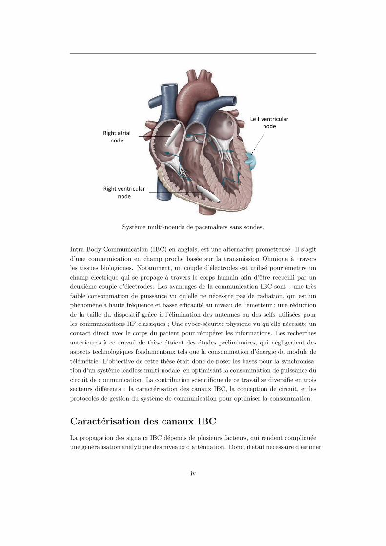
Right atrial
node
Le ventricular
node
Right ventricular
node
Systeme multi-noeuds de pacemakers sans sondes.
Intra Body Communication (IBC) en anglais, est une alternative prometteuse. Il s’agit
d’une communication en champ proche basee sur la transmission Ohmique a travers
les tissues biologiques. Notamment, un couple d’electrodes est utilise pour emettre un
champ electrique qui se propage a travers le corps humain afin d’etre recueilli par un
deuxieme couple d’electrodes. Les avantages de la communication IBC sont : une tres
faible consommation de puissance vu qu’elle ne necessite pas de radiation, qui est un
phenomene a haute frequence et basse efficacite au niveau de l’emetteur ; une reduction
de la taille du dispositif grace a l’elimination des antennes ou des selfs utilisees pour
les communications RF classiques ; Une cyber-securite physique vu qu’elle necessite un
contact direct avec le corps du patient pour recuperer les informations. Les recherches
anterieures a ce travail de these etaient des etudes preliminaires, qui negligeaient des
aspects technologiques fondamentaux tels que la consommation d’energie du module de
telemetrie. L’objective de cette these etait donc de poser les bases pour la synchronisa-
tion d’un systeme leadless multi-nodale, en optimisant la consommation de puissance du
circuit de communication. La contribution scientifique de ce travail se diversifie en trois
secteurs differents : la caracterisation des canaux IBC, la conception de circuit, et les
protocoles de gestion du systeme de communication pour optimiser la consommation.
Caracterisation des canaux IBC
La propagation des signaux IBC depends de plusieurs facteurs, qui rendent compliquee
une generalisation analytique des niveaux d’attenuation. Donc, il etait necessaire d’estimer
iv
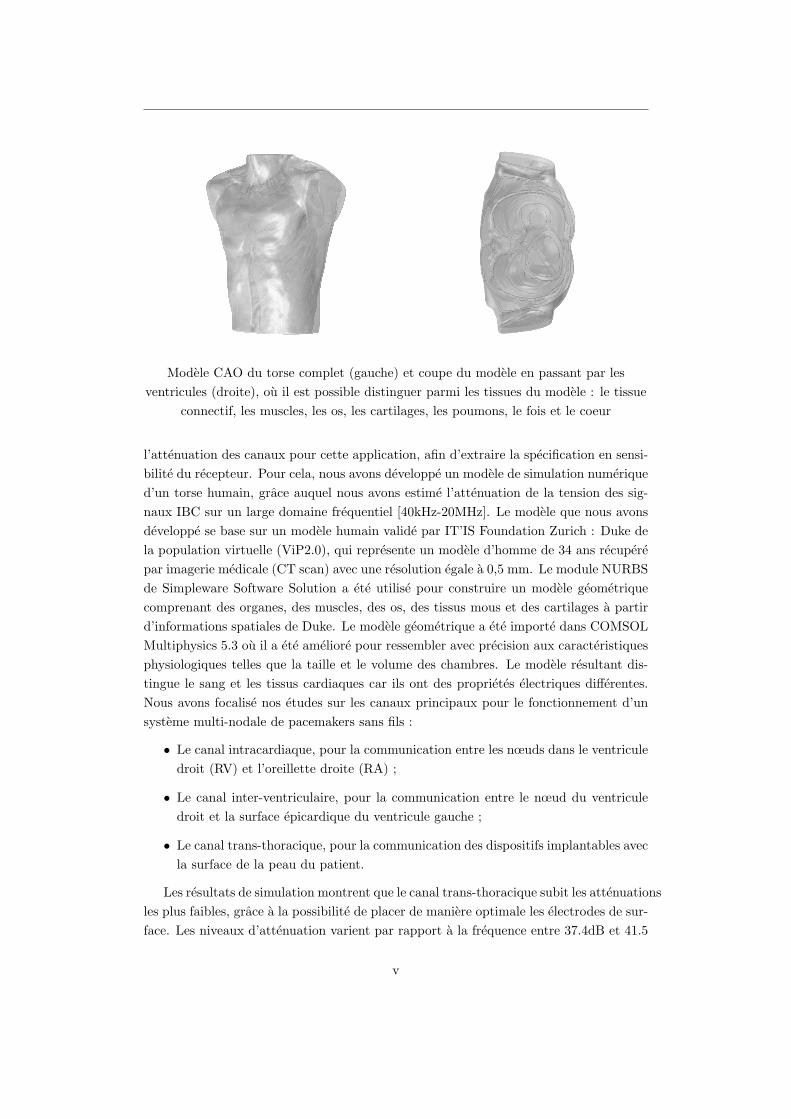
Modele CAO du torse complet (gauche) et coupe du modele en passant par les
ventricules (droite), ou il est possible distinguer parmi les tissues du modele : le tissue
connectif, les muscles, les os, les cartilages, les poumons, le fois et le coeur
l’attenuation des canaux pour cette application, afin d’extraire la specification en sensi-
bilite du recepteur. Pour cela, nous avons developpe un modele de simulation numerique
d’un torse humain, grace auquel nous avons estime l’attenuation de la tension des sig-
naux IBC sur un large domaine frequentiel [40kHz-20MHz]. Le modele que nous avons
developpe se base sur un modele humain valide par IT’IS Foundation Zurich : Duke de
la population virtuelle (ViP2.0), qui represente un modele d’homme de 34 ans recupere
par imagerie medicale (CT scan) avec une resolution egale a 0,5 mm. Le module NURBS
de Simpleware Software Solution a ete utilise pour construire un modele geometrique
comprenant des organes, des muscles, des os, des tissus mous et des cartilages a partir
d’informations spatiales de Duke. Le modele geometrique a ete importe dans COMSOL
Multiphysics 5.3 ou il a ete ameliore pour ressembler avec precision aux caracteristiques
physiologiques telles que la taille et le volume des chambres. Le modele resultant dis-
tingue le sang et les tissus cardiaques car ils ont des proprietes electriques differentes.
Nous avons focalise nos etudes sur les canaux principaux pour le fonctionnement d’un
systeme multi-nodale de pacemakers sans fils :
• Le canal intracardiaque, pour la communication entre les nœuds dans le ventricule
droit (RV) et l’oreillette droite (RA) ;
• Le canal inter-ventriculaire, pour la communication entre le nœud du ventricule
droit et la surface epicardique du ventricule gauche ;
• Le canal trans-thoracique, pour la communication des dispositifs implantables avec
la surface de la peau du patient.
Les resultats de simulation montrent que le canal trans-thoracique subit les attenuations
les plus faibles, grace a la possibilite de placer de maniere optimale les electrodes de sur-
face. Les niveaux d’attenuation varient par rapport a la frequence entre 37.4dB et 41.5
v
dB pour la capsule dans le RV, entre 45 et 50 dB pour une capsule dans le RA. Grace
a cette etude nous avons identifie le meilleur placement des electrodes de surface pour
minimiser les niveaux d’attenuation. Une premiere electrode doit etre place sur la ligne
medio-claviculaire du cinquieme espace intercostal, une deuxieme electrode a l’extremite
mediane du quatrieme espace intercostal. Le canal trans-thoracique est essentiel pour
la programmation du dispositif et pour recuperer les donnees pendant le suivi du pa-
tient. Toutefois, les consultations de suivi sont des evenements rares compares aux
autres activites d’un tel systeme de dispositifs implantables ; donc, cette communica-
tion n’impacte pas le budget de consommation moyenne du stimulateur cardiaque.
Le canal inter-ventriculaire a ete defini entre la capsule dans le RV et des sondes
ponctuelles placees sur la surface du ventricule gauche (LV). Les meilleurs resultats
sont obtenus pour les sondes a courte distance de la capsule RV. L’attenuation du
canal inter-ventriculaire a des valeurs entre 45dB et 80dB selon la longueur du canal
et la frequence. Toutefois l’ecart d’attenuation entre les sondes proches et les plus
distantes diminue avec la frequence. Cela est du a l’augmentation de la conductivite des
tissus biologiques avec l’augmentation de la frequence. Les canaux les plus longs ont un
benefice majeur a l’augmentation de la conductivite. Le canal inter-ventriculaire sert a
mettre en communication un stimulateur intracardiaque dans le ventricule droit et un
stimulateur epicardique place sur la surface externe du ventricule gauche.
L’orientation des capsules joue un role important pour les attenuations des signaux
IBC, les meilleurs resultats se manifestent avec une orientation parallele. Cependant,
le placement des stimulateurs cardiaques doit prioriser l’optimalisation de la therapie,
qui varie avec la population des patients. Pour cette raison, le canal intracardiaque
a ete estime a la fois pour le meilleur et le pire cas. Le canal intracardiaque a des
attenuations entre 72dB et 55dB, selon l’orientation et la frequence. Le canal intracar-
diaque a des valeurs d’attenuations inferieures dans la plage des MHz grace a la plus
grande conductivite des tissus.
Pour verifier les resultats de simulation nous avons mis en place un systeme de mesure
flottant pour eviter des erreurs systemiques du aux boucles de terre. Pour interfacer les
instruments de mesure avec les tissus biologiques, nous avons utilise des prototypes de
capsules de pacemaker sans sondes. Notamment la capsule d’emission a ete connectee
a un generateur de tension sur batterie (DSO8060) et une capsule de reception a ete
connectee a un oscilloscope sur batterie (Fluke 190-110). Afin de detecter les signaux
nous avons integre un amplificateur de tension a l’interieur de la capsule de reception.
L’amplificateur a ete prototype avec des COTS afin d’obtenir un large produit gain-
bande et un faible bruit. Le gain de l’amplificateur a ete regle a 36dB avec une bande
passante entre 20kHz et 60MHz.
Afin de verifier le systeme de mesure, nous avons fait des essais preliminaires in-
vitro grace a une technique de notre realisation basee sur une solution saline de NaCl,
ou la concentration a ete reglee pour suivre la conductivite des tissus cardiaques dans
la plage frequentielle d’interet. Les mesures in-vitro ont ete reproduites sur COMSOL
vi
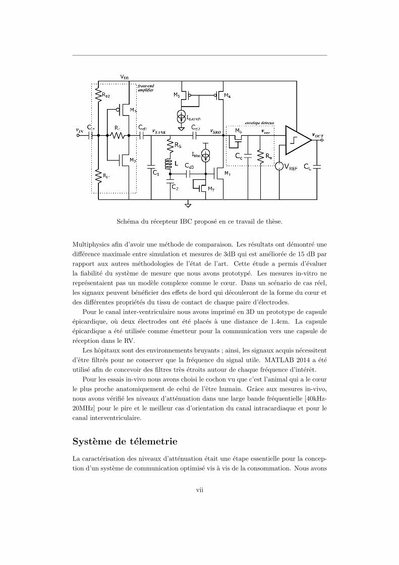
Schema du recepteur IBC propose en ce travail de these.
Multiphysics afin d’avoir une methode de comparaison. Les resultats ont demontre une
difference maximale entre simulation et mesures de 3dB qui est amelioree de 15 dB par
rapport aux autres methodologies de l’etat de l’art. Cette etude a permis d’evaluer
la fiabilite du systeme de mesure que nous avons prototype. Les mesures in-vitro ne
representaient pas un modele complexe comme le cœur. Dans un scenario de cas reel,
les signaux peuvent beneficier des effets de bord qui decouleront de la forme du cœur et
des differentes proprietes du tissu de contact de chaque paire d’electrodes.
Pour le canal inter-ventriculaire nous avons imprime en 3D un prototype de capsule
epicardique, ou deux electrodes ont ete places a une distance de 1.4cm. La capsule
epicardique a ete utilisee comme emetteur pour la communication vers une capsule de
reception dans le RV.
Les hopitaux sont des environnements bruyants ; ainsi, les signaux acquis necessitent
d’etre filtres pour ne conserver que la frequence du signal utile. MATLAB 2014 a ete
utilise afin de concevoir des filtres tres etroits autour de chaque frequence d’interet.
Pour les essais in-vivo nous avons choisi le cochon vu que c’est l’animal qui a le cœur
le plus proche anatomiquement de celui de l’etre humain. Grace aux mesures in-vivo,
nous avons verifie les niveaux d’attenuation dans une large bande frequentielle [40kHz-
20MHz] pour le pire et le meilleur cas d’orientation du canal intracardiaque et pour le
canal interventriculaire.
Systeme de telemetrie
La caracterisation des niveaux d’attenuation etait une etape essentielle pour la concep-
tion d’un systeme de communication optimise vis a vis de la consommation. Nous avons
vii
specifie les contraintes du systeme de communication intracardiaque. Nous avons fait
une analyse quantitative afin d’evaluer les specifications d’un emetteur-recepteur pour
la synchronisation des stimulateurs cardiaques sans sondes. La specification la plus con-
traignante concerne les niveaux d’emission afin d’eviter des interferences avec les signaux
physiologiques de l’activite neuronale. Selon l’ICNIRP, plus la frequence est elevee, plus
le risque de perturber la conduction du systeme nerveux est faible. Pour cela, nous
avons choisi une frequence porteuse dans le domaine des MHz. Cependant, la consom-
mation de puissance des circuits integres augmente avec la frequence. Etant donne que
l’objectif principal est d’optimiser la consommation d’energie de l’emetteur-recepteur,
la complexite de la modulation doit etre maintenue aussi faible que possible pour as-
souplir les exigences de performance de l’emetteur-recepteur. On-Off Keying (OOK) et
Frequency-Shift Keying (FSK) sont des schemas de modulation viables pour la concep-
tion de recepteurs a tres faible puissance. La modulation FSK, en general, necessite
plus de puissance cote recepteur par rapport aux signaux modules OOK en raison de
la necessite d’une reference de frequence interne pour demoduler les signaux entrants.
Les recepteurs FSK ont generalement des debits binaires plus eleves que les recepteurs
OOK. Cependant, la synchronisation LCP ne necessite pas de communications a haut
debit. Considerant que la contrainte de latence est respectee, le message d’evenement
cardiaque se reduit a une information binaire permettant au module de communication
de travailler avec une demodulation mono bit. Ainsi, nous avons prefere la technique
de modulation OOK a la FSK afin de reduire la complexite et la consommation de
puissance du module de telemetrie.
Une etude de l’etat de l’art des recepteurs OOK a tres faible consommation a mis
en evidence deux types d’architecture de recepteur : les recepteurs quasi-passifs et les
recepteurs super-regeneratifs (SRR). Les recepteurs quasi-passifs sont bases sur des tech-
niques de redressement du signal communement utilisees pour le transfert d’energie sans
fil. Cette methode est adaptee pour atteindre les valeurs de consommation d’energie
inferieure au micro Watt. D’ailleurs, Les recepteurs quasi-passifs ont generalement une
faible sensibilite en raison de l’activation de la tension de seuil de diode, et necessitent
des technologies CMOS de petite taille pour minimiser les pertes. L’architecture Super-
Regenerative est une approche elegante pour minimiser la consommation d’energie tout
en augmentant la sensibilite des recepteurs OOK. Ce type de recepteur nous convient car
il peut obtenir des gains extremement eleves en minimisant les blocs a haute frequence.
En effet, il est possible d’obtenir une amplification RF extremement elevee et un fil-
trage a bande etroite avec une consommation de courant limitee grace a l’architecture
SRR. Le cœur du SRR est un oscillateur dont l’amplificateur a un gain dependant du
temps. Au-dessus d’une valeur de gain critique, l’oscillateur est capable de satisfaire le
premier critere de Barkhausen, qui est necessaire pour induire l’instabilite. Un signal de
commande pilote l’evolution temporelle du gain pour contrebalancer periodiquement la
dispersion de l’oscillateur. En consequence, le systeme alterne des periodes instables, ou
il instaure des oscillations, et des periodes d’amortissement, ou le signal de commande
viii
eteint les oscillations. Le circuit de resonnance est couple avec le signal d’entree. Ainsi,
la reponse de l’oscillateur varie en fonction de l’amplitude et de la frequence du signal
d’entree. Le deuxieme dispositif actif requis par le SRR est l’amplificateur de transcon-
ductance a faible bruit (LNTA) a l’avant du recepteur. Le LNTA a une double fonction
: il injecte dans le reservoir de l’oscillateur une quantite de courant proportionnelle a
l’amplitude du signal d’entree, et il isole l’interface d’entree des oscillations provenant
du SRO en reduisant la fuite qui provoquerait des emissions involontaires.
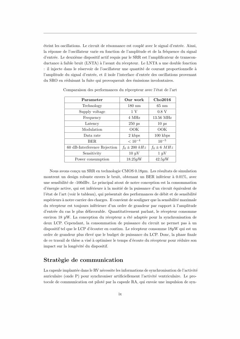
Comparaison des performances du repcepteur avec l’etat de l’art
Parameter Our work Cho2016
Technology 180 nm 65 nm
Supply voltage 1 V 0.8 V
Frequency 4 MHz 13.56 MHz
Latency 250 µs 10 µs
Modulation OOK OOK
Data rate 2 kbps 100 kbps
BER < 10−4 10−5
60 dB-Interference Rejection f0 ± 200 kHz f0 ± 6 MHz
Sensitivity 10 µV 1 µV
Power consumption 18.25µW 42.5µW
Nous avons concu un SRR en technologie CMOS 0.18µm. Les resultats de simulation
montrent un design robuste envers le bruit, obtenant un BER inferieur a 0.01%, avec
une sensibilite de -100dBv. Le principal atout de notre conception est la consommation
d’energie active, qui est inferieure a la moitie de la puissance d’un circuit equivalent de
l’etat de l’art (voir le tableau), qui presentait des performances de debit et de sensibilite
superieurs a notre carrier des charges. Il convient de souligner que la sensibilite maximale
du recepteur est toujours inferieure d’un ordre de grandeur par rapport a l’amplitude
d’entree du cas le plus defavorable. Quantitativement parlant, le recepteur consomme
environ 18 µW. La conception du recepteur a ete adaptee pour la synchronisation de
deux LCP. Cependant, la consommation de puissance du circuit ne permet pas a un
dispositif tel que le LCP d’ecouter en continu. Le recepteur consomme 18µW qui est un
ordre de grandeur plus eleve que le budget de puissance du LCP. Donc, la phase finale
de ce travail de these a vise a optimiser le temps d’ecoute du recepteur pour reduire son
impact sur la longevite du dispositif.
Strategie de communication
La capsule implantee dans le RV necessite les informations de synchronisation de l’activite
auriculaire (onde P) pour synchroniser artificiellement l’activite ventriculaire. Le pro-
tocole de communication est pilote par la capsule RA, qui envoie une impulsion de syn-
ix
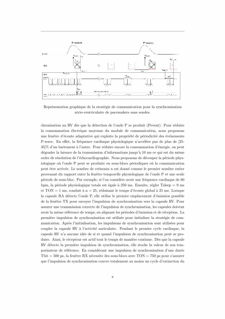
Representation graphique de la strategie de communication pour la synchronisation
atrio-ventriculaire de pacemakers sans sondes.
chronisation au RV des que la detection de l’onde P se produit (Pevent). Pour reduire
la consommation electrique moyenne du module de communication, nous proposons
une fenetre d’ecoute adaptative qui exploite la propriete de periodicite des evenements
P-wave. En effet, la frequence cardiaque physiologique n’accelere pas de plus de [25-
35]% d’un battement a l’autre. Pour reduire encore la consommation d’energie, on peut
degrader la latence de la transmission d’informations jusqu’a 10 ms ce qui est du meme
ordre de resolution de l’echocardiographie. Nous proposons de decouper la periode phys-
iologique ou l’onde P peut se produire en sous-blocs periodiques ou la communication
peut etre activee. Le nombre de creneaux n est donne comme le premier nombre entier
provenant du rapport entre la fenetre temporelle physiologique de l’onde P et une seule
periode de sous-bloc. Par exemple, si l’on considere avoir une frequence cardiaque de 60
bpm, la periode physiologique totale est egale a 250 ms. Ensuite, regler Tsleep = 9 ms
et TON = 1 ms, conduit a n = 25, reduisant le temps d’ecoute global a 25 ms. Lorsque
la capsule RA detecte l’onde P, elle utilise le premier emplacement d’emission possible
de la fenetre TX pour envoyer l’impulsion de synchronisation vers la capsule RV. Pour
assurer une transmission correcte de l’impulsion de synchronisation, les capsules doivent
avoir la meme reference de temps, en alignant les periodes d’emission et de reception. La
premiere impulsion de synchronisation est utilisee pour initialiser la strategie de com-
munication. Apres l’initialisation, les impulsions de synchronisation sont utilisees pour
coupler la capsule RV a l’activite auriculaire. Pendant le premier cycle cardiaque, la
capsule RV n’a aucune idee de si et quand l’impulsion de synchronisation peut se pro-
duire. Ainsi, le recepteur est actif tout le temps de maniere continue. Des que la capsule
RV detecte la premiere impulsion de synchronisation, elle stocke la valeur de son tem-
porisateur de reference. En considerant une impulsion de synchronisation d’une duree
Tbit = 500 µs, la fenetre RX necessite des sous-blocs avec TON = 750 µs pour s’assurer
que l’impulsion de synchronisation couvre totalement au moins un cycle d’extinction du
x
SRR.
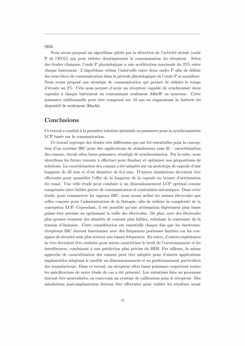
Nous avons propose un algorithme pilote par la detection de l’activite atriale (onde
P de l’ECG) qui peut reduire drastiquement la consommation du recepteur. Selon
des etudes cliniques, l’onde P physiologique a une acceleration maximale du 25% entre
chaque battement. L’algorithme estime l’intervalle entre deux ondes P afin de definir
des sous-blocs de communication dans la periode physiologique ou l’onde-P se manifeste.
Nous avons propose une strategie de communication qui permet de reduire le temps
d’ecoute au 2%. Cela nous permet d’avoir un recepteur capable de synchroniser deux
capsules a chaque battement en consommant seulement 340nW en moyenne. Cette
puissance additionnelle peut etre compense sur 10 ans en augmentant la batterie du
dispositif de seulement 30mAh.
Conclusions
Ce travail a conduit a la premiere solution optimisee en puissance pour la synchronisation
LCP basee sur la communication.
Ce travail regroupe des etudes tres differentes qui ont ete essentielles pour la concep-
tion d’un systeme IBC pour des applications de stimulateurs sans fil : caracterisation
des canaux, circuit ultra basse puissance, strategie de synchronisation. Par la suite, nous
identifions les futurs travaux a effectuer pour finaliser et optimiser nos propositions de
solutions. La caracterisation des canaux a ete adaptee sur un prototype de capsule d’une
longueur de 33 mm et d’un diametre de 6,4 mm. D’autres simulations devraient etre
effectuees pour quantifier l’effet de la longueur de la capsule en termes d’attenuation
du canal. Une telle etude peut conduire a un dimensionnement LCP optimal comme
compromis entre faibles pertes de communication et contraintes mecaniques. Dans cette
etude, pour transmettre les signaux IBC, nous avons utilise les memes electrodes que
celles concues pour l’administration de la therapie, afin de reduire la complexite de la
conception LCP. Cependant, il est possible qu’une attenuation legerement plus basse
puisse etre atteinte en optimisant la taille des electrodes. De plus, avec des electrodes
plus grosses viennent des densites de courant plus faibles, relachant la contrainte de la
tension d’emission. Cette consideration est essentielle chaque fois que les emetteurs-
recepteurs IBC doivent fonctionner avec des frequences porteuses limitees car les con-
signes de securite sont plus strictes aux basses frequences. En outre, d’autres experiences
in vivo devraient etre realisees pour mieux caracteriser le bruit de l’environnement et les
interferences, conduisant a une prediction plus precise du BER. Par ailleurs, la meme
approche de caracterisation des canaux peut etre adoptee pour d’autres applications
implantables adaptant le modele au dimensionnement et au positionnement particuliers
des transducteurs. Dans ce travail, un recepteur ultra basse puissance respectant toutes
les specifications de notre etude de cas a ete presente. Les variations liees au processus
doivent etre neutralisees, en concevant un systeme de calibration pour le recepteur. Des
simulations post-implantation doivent etre effectuees pour valider les resultats avant
xi
l’integration du circuit. Ensuite, le circuit doit etre teste a l’aide de signaux externes
pour valider nos resultats. Ces tests preliminaires ont pour but de valider les perfor-
mances du recepteur super-regeneratif en fonction du signal d’amortissement propose.
Une fois qu’une operation correcte de l’architecture suggeree sera verifiee, une version
complete de l’emetteur-recepteur doit etre concue. En particulier, un generateur de
courant stable est necessaire pour generer le signal d’amortissement de l’oscillateur et
un circuit d’emission a haut rendement doit etre concu. La strategie suggeree dans ce
travail peut reduire considerablement la consommation d’energie pour la synchronisation
des systemes multi-nodales de stimulateurs sans sondes. Les systemes LCP multi-nœuds
ont ete choisis comme principale plateforme applicative de nos etudes. Cependant, la
strategie de synchronisation pourrait etre adoptee par n’importe quel couple de disposi-
tifs, y compris le LCP implante dans le RV et un autre dispositif capable de detecter
l’onde P comme les dispositifs sous-cutanes (c’est-a-dire les enregistreurs de boucle,
sous-cutane-ICD). Pour valider la strategie, je propose de synthetiser le materiel et les
signaux de controle de la technique proposee dans un FPGA. Ensuite, des experiences
in vivo doivent etre effectuees pour evaluer a quel point le systeme est proche d’une
parfaite synchronisation auriculo-ventriculaire.
Ce travail a demontre la faisabilite d’une synchronisation basee sur la communi-
cation pour le stimulateur cardiaque sans fil (LCP) via la communication galvanique
intracorporelle (IBC). Le systeme a ete analyse a partir de la caracterisation des canaux
amenant a la’etablissement des specifications de l’emetteur-recepteur. Ces specifications
ont ete utilisees pour concevoir un recepteur ultra-faible puissance en technologie CMOS
0,18 µm pour analyser le bilan de puissance requis par ce type de solutions. Le bilan
de puissance du recepteur a ete nettement ameliore grace a une strategie de communi-
cation adaptable conduisant a un protocole de synchronisation econome en energie. Les
resultats de ces travaux ont abouti a la soumission de trois brevets a l’institut francais
des brevets :
• M.Maldari. Systeme medical implantable pour mesurer un parametre physiologique,
PA122168FR, 2019.
• M.Maldari. Systeme pour realiser une mesure d’impedance cardiographie, PA126089FR,
2019.
• M.Maldari. Procede et systeme de communication entre plusieurs dispositifs medicaux
implantables, PA127465FR, 2020.
En ce qui concerne la diffusion de ces travaux, un article de conference internationale et
un article de revue ont ete publies a ce jour :
• M. Maldari, K. Amara, I. Rattalino, C. Jabbour, and P. Desgreys. Human Body
Communication channel characterization for leadless cardiac pacemakers, 25th
IEEE International Conference on Electronic Circuits (ICECS), 2018.
xii
• M. Maldari, M. Albatat, J. Bergsland, Y. Haddab, C. Jabbour, and P. Desgreys.
Wide frequency characterization of intra-body communication for leadless pace-
makers, IEEE Transaction on Biomedical Engineering, 2020.
Un autre article de revue est en cours de soumission suite a la selection de ce travail
par URSI-France parmi les meilleurs quatres theses en Radio-science du 2021. De plus,
deux œuvres sans actes ont ete presentees :
• M. Maldari. Human Body Communication for leadless pacemaker applications,
International Micro-electronics Assembly and Packaging Society (iMAPS) Lyon,
2017.
• Mirko Maldari, Karima Amara, Chadi Jabbour, Patricia Desgreys. Human Body
Communication channel modeling for leadless cardiac pacemaker applications, GDR
SOC2 Paris, 2018.
xiii
Contents
1 Introduction 1
1.1 Objectives of this work . . . . . . . . . . . . . . . . . . . . . . . . . . . . 3
1.2 Manuscript outline . . . . . . . . . . . . . . . . . . . . . . . . . . . . . . 3
2 Context of the work 4
2.1 Anatomy . . . . . . . . . . . . . . . . . . . . . . . . . . . . . . . . . . . 4
2.1.1 The rib cage . . . . . . . . . . . . . . . . . . . . . . . . . . . . . 4
2.1.2 The Heart . . . . . . . . . . . . . . . . . . . . . . . . . . . . . . . 6
2.2 Electrophysiology . . . . . . . . . . . . . . . . . . . . . . . . . . . . . . . 9
2.2.1 Cardiac Rhythm Disorders . . . . . . . . . . . . . . . . . . . . . 12
2.2.2 Cardiac Rhythm Management devices . . . . . . . . . . . . . . . 14
2.3 Leadless Pacemakers . . . . . . . . . . . . . . . . . . . . . . . . . . . . . 16
2.3.1 Accelerometer-based atrioventricular synchronization . . . . . . . 17
2.3.2 Multi-node LCP systems . . . . . . . . . . . . . . . . . . . . . . 18
2.4 Intra Body Communication (IBC) . . . . . . . . . . . . . . . . . . . . . 20
3 IBC channel characterization 23
3.1 Simulations . . . . . . . . . . . . . . . . . . . . . . . . . . . . . . . . . . 23
3.1.1 Geometrical considerations . . . . . . . . . . . . . . . . . . . . . 23
3.1.2 Dielectric properties of human body tissues . . . . . . . . . . . . 24
3.1.3 Finite Element Method . . . . . . . . . . . . . . . . . . . . . . . 25
3.1.4 Quasi-static approximation . . . . . . . . . . . . . . . . . . . . . 27
3.1.5 Simulation methodology . . . . . . . . . . . . . . . . . . . . . . . 28
3.1.6 Simulation results . . . . . . . . . . . . . . . . . . . . . . . . . . 35
3.2 Measurements . . . . . . . . . . . . . . . . . . . . . . . . . . . . . . . . . 44
3.2.1 inter-electrode impedance measurements . . . . . . . . . . . . . . 44
3.2.2 Measurement setup . . . . . . . . . . . . . . . . . . . . . . . . . . 46
xiv
3.2.3 In vitro verification . . . . . . . . . . . . . . . . . . . . . . . . . . 49
3.2.4 in vivo verification . . . . . . . . . . . . . . . . . . . . . . . . . . 52
3.3 Discussion . . . . . . . . . . . . . . . . . . . . . . . . . . . . . . . . . . . 59
4 Ultra-Low-Power transceiver 61
4.1 Transceiver requirements . . . . . . . . . . . . . . . . . . . . . . . . . . . 61
4.1.1 Average current consumption . . . . . . . . . . . . . . . . . . . . 61
4.1.2 Latency . . . . . . . . . . . . . . . . . . . . . . . . . . . . . . . . 62
4.1.3 Maximum emitting voltage . . . . . . . . . . . . . . . . . . . . . 62
4.1.4 Modulation . . . . . . . . . . . . . . . . . . . . . . . . . . . . . . 63
4.1.5 Bit Error Rate (BER) . . . . . . . . . . . . . . . . . . . . . . . . 64
4.2 OOK receiver state of the art . . . . . . . . . . . . . . . . . . . . . . . . 66
4.3 Super-Regenerative Receiver (SRR) . . . . . . . . . . . . . . . . . . . . 68
4.3.1 Analytic model of the SRR . . . . . . . . . . . . . . . . . . . . . 69
4.4 SRR design . . . . . . . . . . . . . . . . . . . . . . . . . . . . . . . . . . 72
4.4.1 Receiver design . . . . . . . . . . . . . . . . . . . . . . . . . . . . 72
4.5 SRR Simulation result . . . . . . . . . . . . . . . . . . . . . . . . . . . . 90
4.5.1 Reference simulation . . . . . . . . . . . . . . . . . . . . . . . . . 91
4.5.2 Process, voltage and temperature (PVT) variation . . . . . . . . 99
4.6 Conclusion . . . . . . . . . . . . . . . . . . . . . . . . . . . . . . . . . . 102
5 Communication strategy 104
5.1 Communication protocol description . . . . . . . . . . . . . . . . . . . . 104
5.1.1 Duty cycle optimization for AV synchronization . . . . . . . . . . 106
5.1.2 Communication window synchronization . . . . . . . . . . . . . . 108
5.2 Algorithms for communication based dual chamber LCP system . . . . . 111
5.2.1 Synchronization algorithm of the RA capsule . . . . . . . . . . . 111
5.2.2 Synchronization algorithm of the RV capsule . . . . . . . . . . . 114
5.3 Digital circuit implementation . . . . . . . . . . . . . . . . . . . . . . . . 116
5.3.1 Digital circuit description . . . . . . . . . . . . . . . . . . . . . . 117
5.3.2 Time evolution of digital signals . . . . . . . . . . . . . . . . . . 120
5.4 Discussion . . . . . . . . . . . . . . . . . . . . . . . . . . . . . . . . . . . 122
6 Conclusions and Future work 123
6.1 Summary of the main results . . . . . . . . . . . . . . . . . . . . . . . . 123
6.2 Future works . . . . . . . . . . . . . . . . . . . . . . . . . . . . . . . . . 125
6.3 Scientific contribution and publications . . . . . . . . . . . . . . . . . . . 126
Appendices 140
xv

A Analytical study of the SRR 141
A.1 Time domain analysis . . . . . . . . . . . . . . . . . . . . . . . . . . . . 141
A.2 Frequency domain analysis . . . . . . . . . . . . . . . . . . . . . . . . . 145
A.3 Noise analysis . . . . . . . . . . . . . . . . . . . . . . . . . . . . . . . . . 146
xvi
List of Figures
2.1 Anatomy of the thoracic cage . . . . . . . . . . . . . . . . . . . . . . . . 5
2.2 Anatomy of heart chambers . . . . . . . . . . . . . . . . . . . . . . . . . 6
2.3 Electric conduction system of the heart. . . . . . . . . . . . . . . . . . . 8
2.4 Action Potential of myocardium cells [1] . . . . . . . . . . . . . . . . . . 9
2.5 Electrophysiology of the heart through the conduction system [1] . . . . 10
2.6 Sinus arrest event [2] . . . . . . . . . . . . . . . . . . . . . . . . . . . . . 13
2.7 AV block of type II . . . . . . . . . . . . . . . . . . . . . . . . . . . . . . 13
2.8 Atrial fibrillation event . . . . . . . . . . . . . . . . . . . . . . . . . . . . 13
2.9 Standard Cardiac Pacemaker on the left hand side and Leadless Cardiac
Pacemaker (Nanostim, St. Jude) on the right hand side. . . . . . . . . . 17
2.10 AVS percentage of Micra™ during different maneuvers. . . . . . . . . . . 18
2.11 LCP network for CRT therapy. The heart figure has been modified and
reprinted by permission of Pearson Education, Inc., New York, New York
[3]. . . . . . . . . . . . . . . . . . . . . . . . . . . . . . . . . . . . . . . . 19
2.12 Galvanic IBC scheme . . . . . . . . . . . . . . . . . . . . . . . . . . . . . 20
2.13 Different types of Intra-Body Communication. . . . . . . . . . . . . . . . 21
3.1 Piecewise linear versus piecewise quadratic approximation . . . . . . . . 26
3.2 Torso CAD model imported in COMSOL environment. Cross sectional
cut of the torso CAD model. . . . . . . . . . . . . . . . . . . . . . . . . 28
3.3 Heart CAD model modified to include the outer fat layer. . . . . . . . . 29
3.4 Leadless pacemaker prototype used for IBC channel studies. Distal and
proximal electrodes are spaced apart 33 mm. The can of the prototype
has a diameter of 6.4 mm. . . . . . . . . . . . . . . . . . . . . . . . . . . 30
xvii
LIST OF FIGURES
3.5 Positioning of the capsule in the right atrium showing. Parallel position-
ing in the left side image, whereas a perpendicular positioning is shown
in right side image. The distance between the centers of the capsules is
the same in both cases and equal to 9cm. . . . . . . . . . . . . . . . . . 30
3.6 Point shaped probes placement on the left ventricle epicardial surface of
the heart model. A coloured shade of the epicardium show the poten-
tial distribution of IBC signals when emitted from the RV capsule at
frequency equal to 40kHz. . . . . . . . . . . . . . . . . . . . . . . . . . . 33
3.7 Positioning of the capsule in the right atrium showing. Parallel position-
ing in the left side image, whereas a perpendicular positioning is shown
in right side image. The distance between the centers of the capsules is
the same in both cases and equal to 9cm. . . . . . . . . . . . . . . . . . 34
3.8 Attenuation levels of the intra-cardiac channel (RVRA) for best case
(green line) and worst-case (red line) positioning of RA capsule . . . . . 35
3.9 Positions of the RA capsule for the best-case (right) and worst-case (left).
Electric field lines are represented in red, whereas isopotential surfaces
are represented in green. 5 isopotential surfaces are plotted, where each
subsequent isosurface differs of 2mV from the previous one . . . . . . . 36
3.10 Fat effect on intra-cardiac channel for IBC . . . . . . . . . . . . . . . . . 37
3.11 Attenuation levels of the intra-cardiac channel (RARV) for best case
(green line) and worst-case (red line) positioning of RA capsule . . . . . 37
3.12 Positions of the RA capsule for the best-case (right) and worst-case (left).
Electric field lines are represented in red. 5 isopotential surfaces are
plotted, where each subsequent isosurface differs of 2mV from the previous
one . . . . . . . . . . . . . . . . . . . . . . . . . . . . . . . . . . . . . . . 38
3.13 Attenuation levels of 5 epicardial probes set on the left ventricle: P1
(d=7.7cm), P2(d=7.2cm), P3(d=6.0cm), P4(d=4.9cm), P5(d=3.8cm) . 39
3.14 Graphical representation of simulation results for frequency equal to 40kHz,
where both epicardial (rainbow color table) and body (thermal color ta-
ble) surface potentials are represented. Electric field line distribution is
shown in red. . . . . . . . . . . . . . . . . . . . . . . . . . . . . . . . . . 40
3.15 Attenuation levels of trans-thoracic channel having distance between RV
distal electrode and the body surface equal to 3.52cm . . . . . . . . . . 40
3.16 Trans-thoracic channel for out-in Intra Body Communication. On the left
hand side the results using the emitter having inter-electrode distance
equal to 7 cm. On the right hand side the placement of the Dirichlet
boundary condition used to emulate patch electrodes on the body surface. 41
3.17 Trans-thoracic channel for out-in Intra Body Communication. On the
left hand side the results using the emitter having inter-electrode distance
equal to 12.5 cm. On the right hand side the placement of the Dirichlet
boundary condition used to emulate patch electrodes on the body surface. 42
xviii
LIST OF FIGURES
3.18 Attenuation comparison of the inter-ventricular (top) and intra-cardiac
(bottom) channels between simulations performed with the simple geom-
etry model (dashed line) and the accurate model (solid line) proposed in
this work. . . . . . . . . . . . . . . . . . . . . . . . . . . . . . . . . . . . 43
3.19 Results of parametric simulation with respect to receiving input resistance
for the intra-cardiac channel. . . . . . . . . . . . . . . . . . . . . . . . . 44
3.20 Overall inter-electrode impedance. Zpol,Ei represents the polarization
impedance of the electrode i, whereas the bulk impedance Zbulk represents
the opposition of the electrolyte to ionic conduction. . . . . . . . . . . . 45
3.21 Measurement results of the inter-electrode impedance of the measurement
devices in the frequency range [100 - 40k]Hz. Endocardial capsule proto-
type is represented by triangular markers, whereas Epicardial device by
circular ones. . . . . . . . . . . . . . . . . . . . . . . . . . . . . . . . . . 45
3.22 Measurement setup used for galvanic IBC measurements . . . . . . . . . 46
3.23 Schematic of the differential amplifier integrated in the capsule, where
C1=C2=200nF, R1=R3=100Ω, R2=R4=6.8kΩ, R5=100Ω, R6=100Ω and
R7=100Ω. . . . . . . . . . . . . . . . . . . . . . . . . . . . . . . . . . . . 47
3.24 Epicardial capsule used for in vivo experiments. . . . . . . . . . . . . . . 47
3.25 Leadless capsule rototype for in vivo measurement. On the right the
printed circuit board for the integration of the differential amplifier. . . 48
3.26 Comparison between sampled and processed signals. . . . . . . . . . . . 49
3.27 Custom phantom used for preliminary verification. Dimension of the tank
were 50 cm x 36 cm x 26 cm containing 40 l of solution. . . . . . . . . . 50
3.28 Reproduction of the phantom used for preliminary verification in COM-
SOL environment. . . . . . . . . . . . . . . . . . . . . . . . . . . . . . . 51
3.29 Verification results of in vitro measurements. Both measurement (blue
solid line) and simulation (red dashed line) were performed in parallel
orientation and channel length of 3cm. . . . . . . . . . . . . . . . . . . . 51
3.30 View of the access to the heart during in vivo measurements. (a) Silicon
slice for anchoring RV apex. (b) Coaxial cables of RV capsule (white)
and LV epicardial patch (black). (c) Forceps to secure suture stitches. . 52
3.31 View of the access to the heart for the placement of the sonometric crystals 53
3.32 Full bridge rectifier used to retrieve the envelope of the IBC signal . . . 54
3.33 X-Ray images of worst-case (left) and best case (right) positioning during
in vivo experiment . . . . . . . . . . . . . . . . . . . . . . . . . . . . . . 55
3.34 Measurement results of in vivo experiments for the intra-cardiac channel,
where solid lines represent in vivo trials, whereas dashed line represent
simulations for both best-case and worst-case positioning. . . . . . . . . 56
3.35 In vivo measurement results for the inter-ventricular channel, where the
solid line represents the in vivo trial, whereas the dashed line represents
simulation results. . . . . . . . . . . . . . . . . . . . . . . . . . . . . . . 56
xix
LIST OF FIGURES
3.36 The maximum amplitude swing of the envelope (bottom signal) referred
to ECG (top signal) over one cardiac cycle. The abscissa represents the
time, whereas the ordinates represents the voltage of the signals . . . . . 57
3.37 The minimum amplitude swing of the envelope (3rd signal from the top)
referred to ECG (1st signal from the top) and LV volume change (2nd
signal from the top) over one cardiac cycle. The abscissa represents the
time, whereas the ordinates represents the voltage of the signals. . . . . 58
3.38 Long-time representation of the envelope amplitude. In green the raw
envelope signal, in red the envelope signal low-pass filtered at 20 Hz; in
purple the envelope signal low-pass filtered at 0.7 Hz . . . . . . . . . . . 58
4.1 Example of OOK signal for LCP synchronization . . . . . . . . . . . . . 65
4.2 Example of OOK signal for LCP synchronization in frequency domain . 65
4.3 Power consumption of Ultra-low-power OOK receivers proposed in the
literature . . . . . . . . . . . . . . . . . . . . . . . . . . . . . . . . . . . 67
4.4 Block diagram of a Super-Regenerative Receiver . . . . . . . . . . . . . 68
4.5 Evolution of the input signal through super-regenerative receivers accord-
ing to the damping function ζ . . . . . . . . . . . . . . . . . . . . . . . . 69
4.6 Block scheme of a Super-Regenerative Receiver . . . . . . . . . . . . . . 73
4.7 block scheme of the feedback circuit . . . . . . . . . . . . . . . . . . . . 74
4.8 Ideal model of single transistor LC-oscillators . . . . . . . . . . . . . . . 75
4.9 CMOS representation of the Pierce oscillator . . . . . . . . . . . . . . . 76
4.10 CMOS inverter circuit and its voltage trans-characteristics . . . . . . . . 79
4.11 Inverter-based amplifier with resistive feedback . . . . . . . . . . . . . . 81
4.12 Equivalent circuit of the front-end amplifier . . . . . . . . . . . . . . . . 82
4.13 Testbench of the ideal front-end amplifier . . . . . . . . . . . . . . . . . 83
4.14 Testbech of the inverter-based amplifier with RLC output load . . . . . 84
4.15 Simulation results of the front-end amplifier analysis, where the yellow
dotted line represents the result of the ideal front-end amplifier, whereas
the red solid line represents the results of the proposed inverter-based
amplifier . . . . . . . . . . . . . . . . . . . . . . . . . . . . . . . . . . . . 85
4.16 Passive envelope detector circuit . . . . . . . . . . . . . . . . . . . . . . 86
4.17 Circuit representation of the ideal comparator with its voltage transfer
function . . . . . . . . . . . . . . . . . . . . . . . . . . . . . . . . . . . . 87
4.18 Self-biased comparator . . . . . . . . . . . . . . . . . . . . . . . . . . . . 88
4.19 Proposed comparator circuit in Virtuoso© environment . . . . . . . . . 89
4.20 Testbench of the comparator building block . . . . . . . . . . . . . . . . 90
4.21 Output response of the self-biased comparator . . . . . . . . . . . . . . . 90
4.22 Schematic of the Receiver circuit . . . . . . . . . . . . . . . . . . . . . . 91
4.23 Time evolution of the quenching signal . . . . . . . . . . . . . . . . . . . 92
4.24 Test bench circuit of the proposed Super-Regenerative receiver . . . . . 93
4.25 Time evolution of the input signal through the proposed receiver . . . . 94
xx
LIST OF FIGURES
4.26 Output response of the parametric simulation with respect to the ampli-
tude of the input signal . . . . . . . . . . . . . . . . . . . . . . . . . . . 95
4.27 Output response of the parametric simulation with respect to the fre-
quency of the input signal . . . . . . . . . . . . . . . . . . . . . . . . . . 96
4.28 Normalized input sensitivity with respect to the resonance frequency. . . 97
4.29 Transient analysis considering the start-up time of the receiver. . . . . . 98
4.30 Results of a parametric simulation about temperature variation . . . . . 100
4.31 Simulation results of process-related variation (worst-power). A paramet-
ric simulation is shown acting on the initial current of the quench signal
during the regenerative period . . . . . . . . . . . . . . . . . . . . . . . . 101
4.32 Simulation results of supply voltage variation. . . . . . . . . . . . . . . . 102
5.1 Communication-based synchronization of dual chamber LCP system . . 106
5.2 Sub-block representation of the emitter time-window . . . . . . . . . . . 107
5.3 Sub-block representation of the receiver time-window . . . . . . . . . . . 108
5.4 Transmission of the P-wave detection from the RA caspule to the RV
capsule, using the SRR . . . . . . . . . . . . . . . . . . . . . . . . . . . . 109
5.5 Representation of the main timing of the synchronization strategy . . . 110
5.6 Synchronization algorithm for the RA capsule . . . . . . . . . . . . . . . 112
5.7 Asynchronous routine of the algorithm for the RA capsule . . . . . . . . 113
5.8 Asynchronous routine of the algorithm for the RV capsule . . . . . . . . 114
5.9 Synchronization algorithm for the RV capsule . . . . . . . . . . . . . . . 115
5.10 Communication window for synchronization purposes . . . . . . . . . . . 116
5.11 Datapath of for the calculation of the delay interval for the communication
module. . . . . . . . . . . . . . . . . . . . . . . . . . . . . . . . . . . . . 118
5.12 time diagram for the P wave estimation . . . . . . . . . . . . . . . . . . 121
A.1 Evolution of the input signal through super-regenerative receivers accord-
ing to the damping function ζ . . . . . . . . . . . . . . . . . . . . . . . . 142
xxi
List of Tables
2.1 Pacemaker international nomenclature . . . . . . . . . . . . . . . . . . . 15
3.1 Heart chamber volumes of the CAD model . . . . . . . . . . . . . . . . . 31
3.2 Conductivity and Permittivity values used to define the interpolating
curves . . . . . . . . . . . . . . . . . . . . . . . . . . . . . . . . . . . . . 32
3.3 Liquid phantom characteristics . . . . . . . . . . . . . . . . . . . . . . . 49
3.4 Pathloss comparison . . . . . . . . . . . . . . . . . . . . . . . . . . . . . 60
4.1 transceiver specification for LCP synchronization . . . . . . . . . . . . . 66
4.2 Variables of the output response of the SRR when the input signal vin(t)
is applied . . . . . . . . . . . . . . . . . . . . . . . . . . . . . . . . . . . 70
4.3 Corner analysis . . . . . . . . . . . . . . . . . . . . . . . . . . . . . . . . 101
4.4 Performance of the receiver designed . . . . . . . . . . . . . . . . . . . . 103
xxii

Nomenclature
ADC Analog Digital Converter, page 54
AV atrioventricular, page 8
AVB Atrioventricular Block, page 12
AVS Atrioventricular Synchronization, page 17
AWGN Additive White Gaussian Noise, page 65
BER Bit Error Rate, page 64
BS Body Surface, page 31
CEM Computational Electromagnetic Modeling, page 21
CHF Congestive Heart Failure, page 18
CMOS Complementary Metal-Oxide Semiconductor, page 61
CMRR Common Mode Rejection Ratio, page 48
CRM Cardiac Rhythm Management, page 14
CRT Cardiac Resynchronization Therapy, page 16
ECG electrocardiogram, page 11
EGM Electrogram, page 111
FEM Finite Element Method, page 25
FIR Finite Impulse Response, page 48
FPGA Field Programmable Gate Array, page 126
xxiii
NOMENCLATURE
FSK Frequency-Shift Keying, page 63
FSM Finite State Machine, page 121
HF high-frequency, page 62
IBC Intra Body Communication, page 20
ICD Implantable Cardioverter Defibrillator, page 15
ICNIRP International Commission on Non-Ionizing Radiation Protection, page 62
INPI Institut National de la Propriete Industrielle, page 127
ITN Innovatie training network, page 3
LCP Leadless Cardiac Pacemaker, page 16
LNA Low Noise Amplifier, page 67
LNTA Low Noise Transconductance Amplifier, page 68
LV Left Ventricle, page 18
LV Left Ventricle, page 53
MSB Most Significant Bit, page 119
OOK On-Off Keying, page 63
PAC Premature Atrial Contraction, page 12
PVC Premature Ventricular Contraction, page 12
RA Right Atrium, page 29
RAA Right Atrial Appendage, page 7
RV Right Ventricle, page 29
SA sinoatrial, page 8
SAR Specific Absorption Rate, page 62
SRR Super Regenerative Receiver, page 67
xxiv
1Introduction
A Statistical study revealed that more than 2% of the adult population suffer from
Cardiac arrhythmias [4]. Cardiac arrhythmias are heart rhythm abnormalities caused
by malfunctions of the conductive system of the heart such as premature contractions,
bradycardia, supraventricular tachycardia, and ventricular tachycardia.
Bradycardia is a slow and/or irregular rhythm that is not sufficient to pump enough oxy-
genated blood to the rest of the body. Bradyarrhythmia can manifest as atrial activity
arrest, inability to increase heartbeat rate during exercise (chronotropic incompetence)
or atrioventricular conduction blocks.
Cardiac Pacemakers are used to treat bradycardia patients, whenever the symptoms
persist to drug administration. Pacemaker devices must sense spontaneous heartbeat
and pace by electric stimulation whenever the heartbeat rate is considered too slow.
Conventional pacemakers consist of a subcutaneous control unit and intravenously im-
planted intra-cardiac leads.
The leads are the weakest links in present systems since they can dislodge, cause infec-
tion, thrombosis [5], endo-carditis [6], mechanical damage, and pneumothorax. [7, 8].
The yearly rate of lead-related complications is approximately 1.6% [9]. With more than
four million implanted CRMDs worldwide, around 65 000 lead-related complications oc-
cur every year. Malfunctioning or infected leads often require extraction, which is not a
simple procedure, requiring surgery and transesophageal echocardiographic monitoring.
Improved electronics and smaller batteries have made leadless pacemakers possible.
Leadless Cardiac Pacemakers (LCP) are self-contained devices consisting of sensors,
a current injector, a telemetry module, and an integrated battery unit [10]. They are
designed to be implanted inside the right ventricle through a transvenous catheter [11].
From a clinical point of view, current LCPs may be superior from a safety perspective,
but their functionality is limited. At present, they only pace the right ventricle (VVI
pacing) and can only be used as an alternative for ventricular single-chamber pacemak-
ers which are only used for a fraction of the pacemaker patients.
Single chamber pacemakers are rarely used since they do not maintain AV synchronicity,
1
CHAPTER 1. INTRODUCTION
leading to increased risk of stroke and heart failure, which is substantially reduced with
dual-chamber pacemakers or cardiac resynchronization therapy (CRT) [12].
There is, therefore, a large potential for further innovation to create devices that provide
multi-chamber leadless pacing [13]. A multi-nodal LCP system requires a communica-
tion network between all the nodes implanted in multiple chambers.
Standard wireless communication approaches for implants, such as radiofrequency and
inductive coupling are suboptimal solutions because they require: 1) dedicated compo-
nents (antennas and coils), increasing the size of the implant; 2) high power consumption,
reducing battery lifetime, which is a critical issue in permanent implants.
A promising alternative solution is galvanic Intra-Body Communication (IBC), which is
a near field communication method based on Ohmic transmission through body tissues.
In IBC, an electrode pair is used to build up an electric field that propagates through
the human body reaching a second electrode pair used to receive the signal [14].
The advantages of IBC are: 1) ultra-low power requirement; 2) no additional antenna
is required since the pacing electrodes may be used to generate the electric field for the
communication; 3) minimal risk of eavesdropping since direct contact with the body is
strictly required to form a channel [15].
Since the introduction of IBC communication by Zimmerman in 1996 [16], several stud-
ies have considered the human body as a communication channel. Most of those studies
are focused on body-surface communications [17, 18, 19], leading IEEE to include it as
a physical layer in IEEE802.15.6 standard for Wireless Body Area Networks (WBAN)
under the name of Human Body Communication (HBC).
A Recent study characterized galvanic IBC for intra-cardiac communication in the fre-
quency range of 1 kHz to 1 MHz [20], where in vivo and ex vivo measurements were
performed using electrodes injected through the heart wall that is not a real represen-
tation of actual LCP systems. Moreover, the measurement system was not completely
isolated from the ground, limiting the reliability of the attenuation values of the channel
according to measurement setup studies performed in [21]. Inter-electrode and channel
length distances were limited to 15 mm and 60 mm. Surprisingly, there was no signifi-
cant difference among measurements with channel lengths bigger than 50 mm [22], likely
due to ground coupling issues. The same authors showed the advantage of frequencies
higher than 1 MHz in further work [23] pointing out the need for a broader characteriza-
tion of the intra-cardiac channel. Therefore, to build efficient IBC transceivers for LCP
applications, a more accurate and broader characterization of communication channels
is needed.
The firsts attempts of multi-node pacing using physically separate devices proved the
clinical feasibility of both dual chamber and CRT-P leadless pacing [22, 20]. The au-
thors suggested a telemetry-based synchronization of LCPs, using the IBC. However,
this solution was verified using off-the-shelf components, without assessing the power
2

CHAPTER 1. INTRODUCTION
optimization of the circuitry.
This doctoral thesis was carried out as a part of the WiBEC (Wireless in-Body En-
vironment Communication) project, which was an Innovative Training Network (ITN)
funded by the European Commission. The WIBEC project aimed to develop wireless
technologies for novel implantable devices, contributing to the improvement in quality
and efficacy of healthcare [24].
1.1 Objectives of this work
The objective of this doctoral thesis is to lay the foundations for the synchronization
of multi-node LCP systems, assessing the power optimization of the communication
circuitry. Indeed, this work consists of a system study to find out a power-optimized
solution for the communication module.
In particular, the Intra-Body Communication was chosen as preferred kind of telemetry
for three main reasons: size optimization (i.e. no antenna or any other additional trans-
ducer is required), emitted power efficiency (i.e. no radiation), and data security (i.e.
contact with the patient is strictly required).
The scientific contribution of this work relies on three different field: IBC channel char-
acterization, ultra-low-power circuit design, and protocols for power-efficient atrioven-
tricular synchronization.
1.2 Manuscript outline
The manuscript is organized as follow:
• chapter 2 gives some background knowledge about the context of this work, point-
ing out its clinical relevance;
• chapter 3 reports the preliminary studies we performed about the channel charac-
terization for LCP applications, consisting of numerical simulations, measurement
system prototyping, and in vivo verification;
• chapter 4 points out the transceiver requirement based on the estimated loss of
the preliminary studies and describe the process that led us to design an ultra-
low-power receiver for LCP synchronization purposes;
• chapter 5 deals with a communication strategy to further reduce the power con-
sumption of the receiver;
• finally, in chapter 6, we summarize the key findings of this research and conclude
pointing out the future work leading to the LCP prototype for a multi-node pacing
system.
3
2Context of the work
This chapter aims to give a background to understand the clinical relevance of the ob-
jectives of this work.
The Leadless pacemaker is an implant device intended to be fixed at the endocardium
of bradycardia patients. Thus, the environment of the object of study is the heart and,
more generally, the rib cage, whose anatomy is roughly described in the first section of
this chapter.
A clinical background about the normal electrophysiology of the heart is given in sec-
tion 2.2, followed by the pathological conditions caused by the dysfunction of the heart
conduction system.
Further, we introduce Cardiac Rhythm Management (CRM) devices, used to counter-
act drug resistant pathologies. In section 2.3, the LCP is introduced, explaining its
clinical advantages over conventional pacemakers and its current limits. Contrarily to
conventional pacemakers, LCPs can only pace a single location in the heart, arising the
necessity of multi-node LCP systems, that are described in subsection 2.3.2. Multi-node
LCP systems require reliable solutions to synchronize every single device.
The Intra-Body Communication (IBC) is a convenient technology, described in sec-
tion 2.4, which seems tailored to LCP applications.
2.1 Anatomy
This section aims to describe the environment of the communication. The anatomy
description of the rib cage and the heart are based on a worldwide known atlas of
anatomy, ideated and illustrated by F.H.Netter [25].
2.1.1 The rib cage
The thorax is the superior part of the trunk, whose shape resembles a cylinder or a
truncated cone. The thoracic cavity is separated from the abdominal cavity by the
4
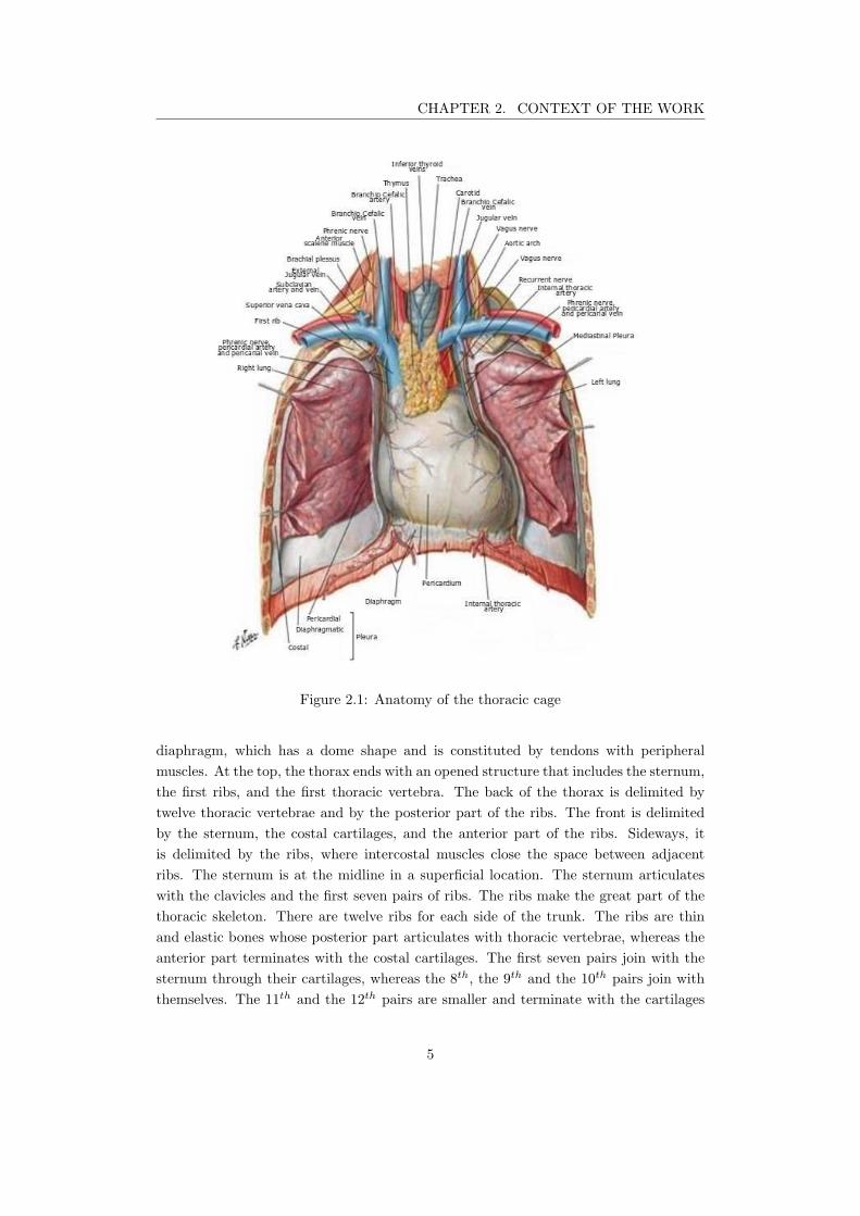
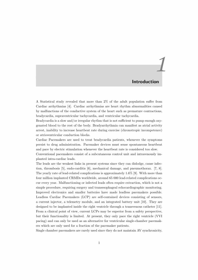
CHAPTER 2. CONTEXT OF THE WORK
Figure 2.1: Anatomy of the thoracic cage
diaphragm, which has a dome shape and is constituted by tendons with peripheral
muscles. At the top, the thorax ends with an opened structure that includes the sternum,
the first ribs, and the first thoracic vertebra. The back of the thorax is delimited by
twelve thoracic vertebrae and by the posterior part of the ribs. The front is delimited
by the sternum, the costal cartilages, and the anterior part of the ribs. Sideways, it
is delimited by the ribs, where intercostal muscles close the space between adjacent
ribs. The sternum is at the midline in a superficial location. The sternum articulates
with the clavicles and the first seven pairs of ribs. The ribs make the great part of the
thoracic skeleton. There are twelve ribs for each side of the trunk. The ribs are thin
and elastic bones whose posterior part articulates with thoracic vertebrae, whereas the
anterior part terminates with the costal cartilages. The first seven pairs join with the
sternum through their cartilages, whereas the 8th, the 9th and the 10th pairs join with
themselves. The 11th and the 12th pairs are smaller and terminate with the cartilages
5
CHAPTER 2. CONTEXT OF THE WORK
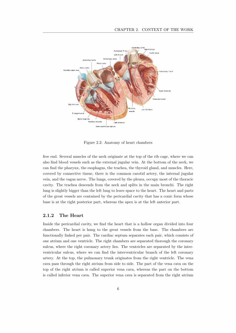
Figure 2.2: Anatomy of heart chambers
free end. Several muscles of the neck originate at the top of the rib cage, where we can
also find blood vessels such as the external jugular vein. At the bottom of the neck, we
can find the pharynx, the esophagus, the trachea, the thyroid gland, and muscles. Here,
covered by connective tissue, there is the common carotid artery, the internal jugular
vein, and the vagus nerve. The lungs, covered by the pleura, occupy most of the thoracic
cavity. The trachea descends from the neck and splits in the main bronchi. The right
lung is slightly bigger than the left lung to leave space to the heart. The heart and parts
of the great vessels are contained by the pericardial cavity that has a conic form whose
base is at the right posterior part, whereas the apex is at the left anterior part.
2.1.2 The Heart
Inside the pericardial cavity, we find the heart that is a hollow organ divided into four
chambers. The heart is hung to the great vessels from the base. The chambers are
functionally linked per pair. The cardiac septum separates each pair, which consists of
one atrium and one ventricle. The right chambers are separated thorough the coronary
sulcus, where the right coronary artery lies. The ventricles are separated by the inter-
ventricular sulcus, where we can find the interventricular branch of the left coronary
artery. At the top, the pulmonary trunk originates from the right ventricle. The vena
cava pass through the right atrium from side to side. The part of the vena cava on the
top of the right atrium is called superior vena cava, whereas the part on the bottom
is called inferior vena cava. The superior vena cava is separated from the right atrium
6
CHAPTER 2. CONTEXT OF THE WORK
appendage through the terminal sulcus. The right pulmonary veins join the right part
of the left atrium, whereas the left pulmonary veins join the left atrium from the left.
The branches of the pulmonary trunk lie on the surface of the left atrium. Hither, they
join both the left and the right lungs. In the coronary sulcus between the left atrium
and the left ventricle, we can find the coronary sinus. Here, the cardiac veins converge,
collecting the blood from the heart muscle.
2.1.2.1 The right atrium
The right atrium can be divided into a smooth posterior wall where it joins with the
venae cavae, and a trabecular wall, which represents the embryonal right atrium. Those
two parts are separated by the crista terminalis, which internally corresponds to the
terminal sulcus. Several pectinate muscles originate from the terminal sulcus covering
the free wall of the right atrium. Between the pectinate muscles, the wall of the atrium
is very thin. At the superior part of the right ventricle, we find the right atrial ap-
pendage (RAA), which is a triangular purse filled with pectinate muscles. For its shape
and location, the RAA is utilized as an easy access for surgical interventions. At the
posteromedial part of the right atrium, we find the interatrial septum, where we find
the fossa ovalis, which is a slight depression that can be used to pass a lead in the left
atrium. In the middle of the frontal part, we can find the tricuspid valve, which gives
access to the right ventricle.
2.1.2.2 The right ventricle
The right ventricle chamber can be divided into an influx part, where we find the tri-
cuspid valve and an efflux part where we find the pulmonary trunk. The efflux part
is considerably smoother compared to the influx part, which is covered by trabeculae.
Papillar muscles join the cuspids of the tricuspid valve through the chordae tendineae.
The pulmonary trunk originates from the top of the right ventricle; further, it splits in
the pulmonary arteries.
2.1.2.3 The left atrium
The left atrium is characterized by a smooth wall, which is thicker than the right atrium
wall. From both sides, the left atrium gives access to the heart for the blood coming
from the pulmonary veins. At the anterior part, we find the left atrium appendage that
contains small pectinate muscles.
2.1.2.4 The left ventricle
The left ventricle has an elliptic shape with a truncated superior part. Here, we find
the mitral valve and the aortic valve. The left ventricle valves are close to each other
and are separated only by a fibrous septum. The average thickness of the left ventricle
7
CHAPTER 2. CONTEXT OF THE WORK
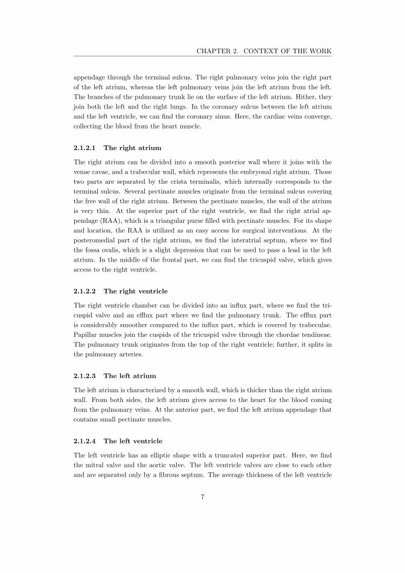
Figure 2.3: Electric conduction system of the heart.
wall is usually three times bigger than the right ventricle one. In the left ventricle, we
can find trabeculae carnae, especially toward the apex of the heart. A small part of the
interventricular septum, placed under the cuspids of the aortic valve, is made of a thin
membrane. The rest of the interventricular septum is made of muscles.
2.1.2.5 The conduction system
The conduction system is made of specific heart cells that are histologically different than
the rest of the heart muscle [26]. Those cells do not participate in muscle contraction, but
rather they generate and propagate electric pulses that are responsible for the heartbeat.
The conduction system, depicted in Figure 2.3, is constituted by the sino-atrial node,
the AV node, the common AV bundle, the His bundle, the right and the left branches
of the common AV bundle, and the peripheral branches of Purkinje. Additionally, there
is also another group of atrial fibers that are considered to be part of the conduction
system. They are the Bachmann’s bundle and the internodal tracts of the right atrium.
The sino-atrial node is placed in the right atrium at the junction with the superior vena
cava corresponding on the epicardial surface to the crista terminalis. Several branches
originate from the sinoatrial (SA) node to connect the atrioventricular (AV) node.
The AV node is placed on the floor of the right atrium to the left of the coronary
sinus orifice. The common AV bundle takes origin from the bottom part of the AV
node and descend the membranous part of the septum. At the junction between the
membranous part and the muscular part of the septum, the common AV bundle splits
into two branches that descend the septum from both sides. The left branch immediately
splits into several branches distributed on the whole surface of the left ventricle. At the
peripheral part, both the left and the right branches split up, forming the Purkinje fibers.
Those fibers spread over the ventricular walls. The Bachmann’s bundle is responsible
for the conduction in the left atrium, and it takes origin from one of the branches of the
8
CHAPTER 2. CONTEXT OF THE WORK
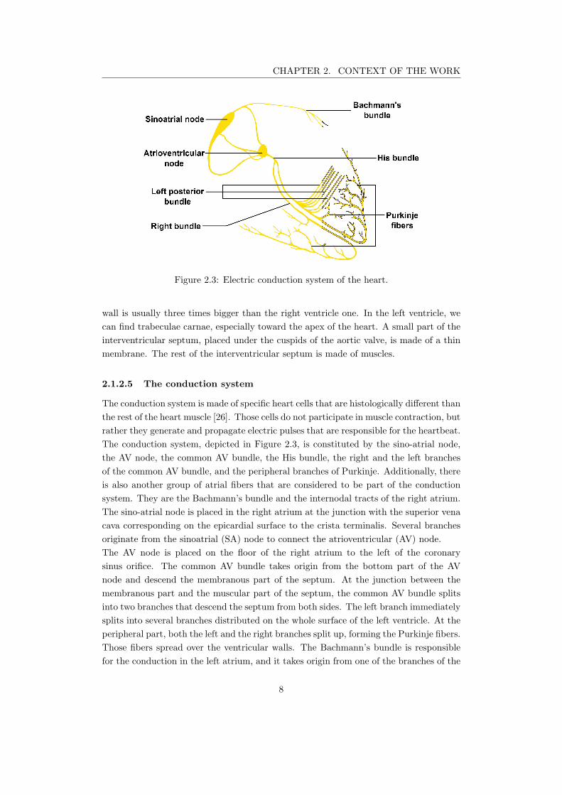
Figure 2.4: Action Potential of myocardium cells [1]
internodal tracts.
2.2 Electrophysiology
In healthy hearts, the contraction is driven by an electrical impulse that has its origin
in a group of cells called pacemaker cells. The impulse propagates in a coordinated way
using the conduction system and arrives in all the heart fibers inducing the contraction.
The electrical activities of cells can be measured through their membrane potential that
is defined as the voltage difference between the inner and the outer surfaces of the cell
membrane.
The voltage drop across the membrane is generated by the difference in ionic concen-
tration between the intracellular fluid and the extra-cellular fluid. The main ionic con-
centrations regulating the membrane potential are the Sodium (Na+) and Potassium
(K+) ions. The concentration of K+ of the intracellular fluid is 30 times greater than
the concentration of the extra-cellular fluid. In contrast, the concentration of Na+ is 30
times lower than the concentration of the extra-cellular fluid [25].
9
CHAPTER 2. CONTEXT OF THE WORK
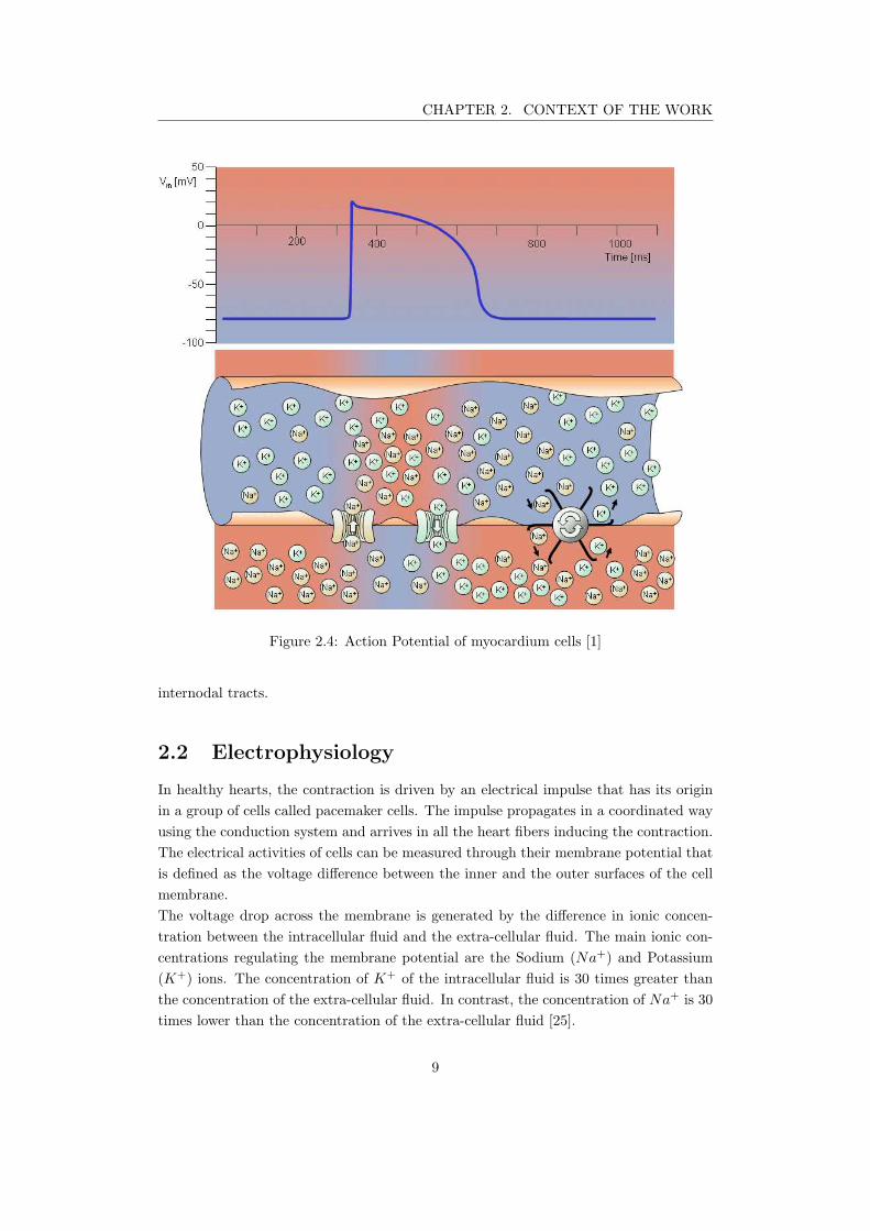
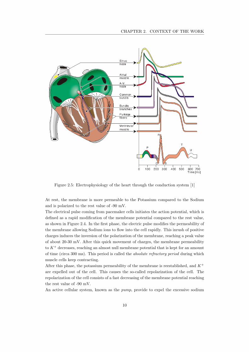
Figure 2.5: Electrophysiology of the heart through the conduction system [1]
At rest, the membrane is more permeable to the Potassium compared to the Sodium
and is polarized to the rest value of -90 mV.
The electrical pulse coming from pacemaker cells initiates the action potential, which is
defined as a rapid modification of the membrane potential compared to the rest value,
as shown in Figure 2.4. In the first phase, the electric pulse modifies the permeability of
the membrane allowing Sodium ions to flow into the cell rapidly. This inrush of positive
charges induces the inversion of the polarization of the membrane, reaching a peak value
of about 20-30 mV. After this quick movement of charges, the membrane permeability
to K+ decreases, reaching an almost null membrane potential that is kept for an amount
of time (circa 300 ms). This period is called the absolute refractory period during which
muscle cells keep contracting.
After this phase, the potassium permeability of the membrane is reestablished, and K+
are expelled out of the cell. This causes the so-called repolarization of the cell. The
repolarization of the cell consists of a fast decreasing of the membrane potential reaching
the rest value of -90 mV.
An active cellular system, known as the pump, provide to expel the excessive sodium
10
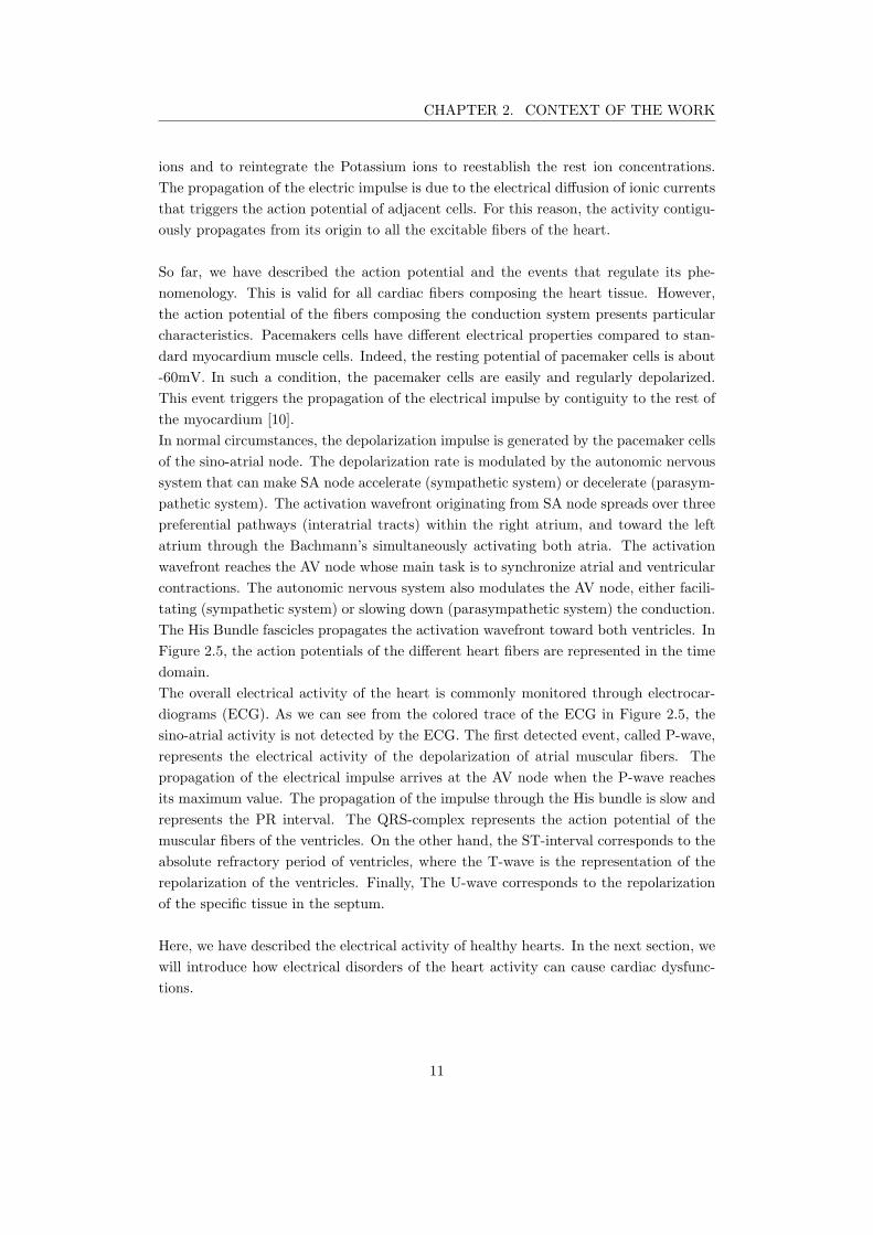
CHAPTER 2. CONTEXT OF THE WORK
ions and to reintegrate the Potassium ions to reestablish the rest ion concentrations.
The propagation of the electric impulse is due to the electrical diffusion of ionic currents
that triggers the action potential of adjacent cells. For this reason, the activity contigu-
ously propagates from its origin to all the excitable fibers of the heart.
So far, we have described the action potential and the events that regulate its phe-
nomenology. This is valid for all cardiac fibers composing the heart tissue. However,
the action potential of the fibers composing the conduction system presents particular
characteristics. Pacemakers cells have different electrical properties compared to stan-
dard myocardium muscle cells. Indeed, the resting potential of pacemaker cells is about
-60mV. In such a condition, the pacemaker cells are easily and regularly depolarized.
This event triggers the propagation of the electrical impulse by contiguity to the rest of
the myocardium [10].
In normal circumstances, the depolarization impulse is generated by the pacemaker cells
of the sino-atrial node. The depolarization rate is modulated by the autonomic nervous
system that can make SA node accelerate (sympathetic system) or decelerate (parasym-
pathetic system). The activation wavefront originating from SA node spreads over three
preferential pathways (interatrial tracts) within the right atrium, and toward the left
atrium through the Bachmann’s simultaneously activating both atria. The activation
wavefront reaches the AV node whose main task is to synchronize atrial and ventricular
contractions. The autonomic nervous system also modulates the AV node, either facili-
tating (sympathetic system) or slowing down (parasympathetic system) the conduction.
The His Bundle fascicles propagates the activation wavefront toward both ventricles. In
Figure 2.5, the action potentials of the different heart fibers are represented in the time
domain.
The overall electrical activity of the heart is commonly monitored through electrocar-
diograms (ECG). As we can see from the colored trace of the ECG in Figure 2.5, the
sino-atrial activity is not detected by the ECG. The first detected event, called P-wave,
represents the electrical activity of the depolarization of atrial muscular fibers. The
propagation of the electrical impulse arrives at the AV node when the P-wave reaches
its maximum value. The propagation of the impulse through the His bundle is slow and
represents the PR interval. The QRS-complex represents the action potential of the
muscular fibers of the ventricles. On the other hand, the ST-interval corresponds to the
absolute refractory period of ventricles, where the T-wave is the representation of the
repolarization of the ventricles. Finally, The U-wave corresponds to the repolarization
of the specific tissue in the septum.
Here, we have described the electrical activity of healthy hearts. In the next section, we
will introduce how electrical disorders of the heart activity can cause cardiac dysfunc-
tions.
11
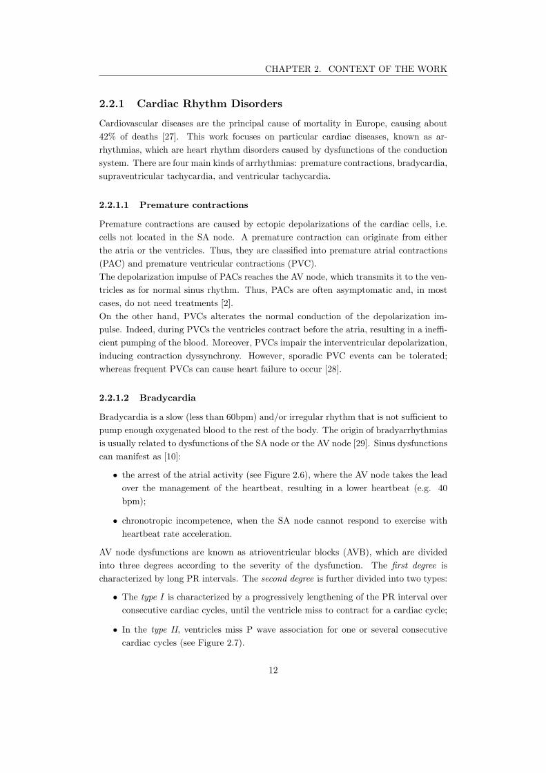
CHAPTER 2. CONTEXT OF THE WORK
2.2.1 Cardiac Rhythm Disorders
Cardiovascular diseases are the principal cause of mortality in Europe, causing about
42% of deaths [27]. This work focuses on particular cardiac diseases, known as ar-
rhythmias, which are heart rhythm disorders caused by dysfunctions of the conduction
system. There are four main kinds of arrhythmias: premature contractions, bradycardia,
supraventricular tachycardia, and ventricular tachycardia.
2.2.1.1 Premature contractions
Premature contractions are caused by ectopic depolarizations of the cardiac cells, i.e.
cells not located in the SA node. A premature contraction can originate from either
the atria or the ventricles. Thus, they are classified into premature atrial contractions
(PAC) and premature ventricular contractions (PVC).
The depolarization impulse of PACs reaches the AV node, which transmits it to the ven-
tricles as for normal sinus rhythm. Thus, PACs are often asymptomatic and, in most
cases, do not need treatments [2].
On the other hand, PVCs alterates the normal conduction of the depolarization im-
pulse. Indeed, during PVCs the ventricles contract before the atria, resulting in a ineffi-
cient pumping of the blood. Moreover, PVCs impair the interventricular depolarization,
inducing contraction dyssynchrony. However, sporadic PVC events can be tolerated;
whereas frequent PVCs can cause heart failure to occur [28].
2.2.1.2 Bradycardia
Bradycardia is a slow (less than 60bpm) and/or irregular rhythm that is not sufficient to
pump enough oxygenated blood to the rest of the body. The origin of bradyarrhythmias
is usually related to dysfunctions of the SA node or the AV node [29]. Sinus dysfunctions
can manifest as [10]:
• the arrest of the atrial activity (see Figure 2.6), where the AV node takes the lead
over the management of the heartbeat, resulting in a lower heartbeat (e.g. 40
bpm);
• chronotropic incompetence, when the SA node cannot respond to exercise with
heartbeat rate acceleration.
AV node dysfunctions are known as atrioventricular blocks (AVB), which are divided
into three degrees according to the severity of the dysfunction. The first degree is
characterized by long PR intervals. The second degree is further divided into two types:
• The type I is characterized by a progressively lengthening of the PR interval over
consecutive cardiac cycles, until the ventricle miss to contract for a cardiac cycle;
• In the type II, ventricles miss P wave association for one or several consecutive
cardiac cycles (see Figure 2.7).
12
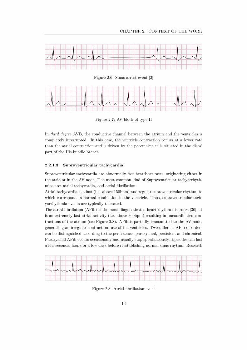
CHAPTER 2. CONTEXT OF THE WORK
Figure 2.6: Sinus arrest event [2]
Figure 2.7: AV block of type II
In third degree AVB, the conductive channel between the atrium and the ventricles is
completely interrupted. In this case, the ventricle contraction occurs at a lower rate
than the atrial contraction and is driven by the pacemaker cells situated in the distal
part of the His bundle branch.
2.2.1.3 Supraventricular tachycardia
Supraventricular tachycardia are abnormally fast heartbeat rates, originating either in
the atria or in the AV node. The most common kind of Supraventricular tachyarrhyth-
mias are: atrial tachycardia, and atrial fibrillation.
Atrial tachycardia is a fast (i.e. above 150bpm) and regular supraventricular rhythm, to
which corresponds a normal conduction in the ventricle. Thus, supraventricular tach-
yarrhythmia events are typically tolerated.
The atrial fibrillation (AFib) is the most diagnosticated heart rhythm disorders [30]. It
is an extremely fast atrial activity (i.e. above 300bpm) resulting in uncoordinated con-
tractions of the atrium (see Figure 2.8). AFib is partially transmitted to the AV node,
generating an irregular contraction rate of the ventricles. Two different AFib disorders
can be distinguished according to the persistence: paroxysmal, persistent and chronical.
Paroxysmal AFib occurs occasionally and usually stop spontaneously. Episodes can last
a few seconds, hours or a few days before reestablishing normal sinus rhythm. Research
Figure 2.8: Atrial fibrillation event
13

CHAPTER 2. CONTEXT OF THE WORK
studies have shown that around 40% people with AFib have paroxysmal AFib [31]. Per-
sistent AFib is defined as an AFib episode that lasts more than one week, requiring
medical treatments to be stopped. Chronic AFib is defined as AFib event lasting for
many years. It is common that patients suffering from Paroxysmal AFib gradually de-
velop chronic AFib [32]. Indeed, statistical researches have shown that 9 to 30% of all
cases of paroxysmal AFib progress into more chronic cases after 1 year.
2.2.1.4 Ventricular tachycardia
Tachycardia is manifest in the opposite way of bradycardia: the heart beats too fast and,
in some cases, irregularly. The tachycardia beat rate varies from more than 100bpm up
to 400bpm. In such a condition, the heart is not able to work efficiently and can fall
to Ventricular Fibrillation when only 10% of the blood is ejected from ventricles due
to uncoordinated contraction. It is an extremely dangerous disease that can lead to
Sudden Cardiac Death.
2.2.1.5 Congestive Heart Failure (CHF)
Congestive Heart Failure occurs when the heart is not able to respond to the oxygen
demand of the body due to an inefficient and or weak contractions of the ventricles.
CHF can be thought as the inefficiency of the heart ventricles to regulate the blood
flow, due to ventricular dyssynchrony.
2.2.2 Cardiac Rhythm Management devices
Arrhythmia disorders are first treated with medications and, in some cases, with surgical
operations. For some critical cases, medications are not sufficient to counteract heart
dysfunctions. To overcome drug immune arrhythmias, it is a standard procedure to
implant Cardiac Rhythm Management (CRM) devices. There are as many medical
devices as there are kinds of arrhythmia.
2.2.2.1 Pacemakers
Cardiac Pacemakers are used to treat bradycardia patients. Pacemaker devices must
sense spontaneous heartbeat and pace by electric stimulation whenever the heartbeat
rate is too slow.
Conventional pacemakers consists of a hermetically sealed Titanium can, containing
electronic components and a battery. The can is subcutaneously implanted in the chest
below the collarbone. One or more leads are used to reach the heart chambers from
the can. The leads are used to release electric stimuli and to sense local depolarization
of the heart tissue.The number of the leads varies according to the severity degree of
the heart dysfunction. Pacemaker with a single lead can be used to sense and pace
a single location of the heart and are known as Single Chamber Pacemakers. These
14
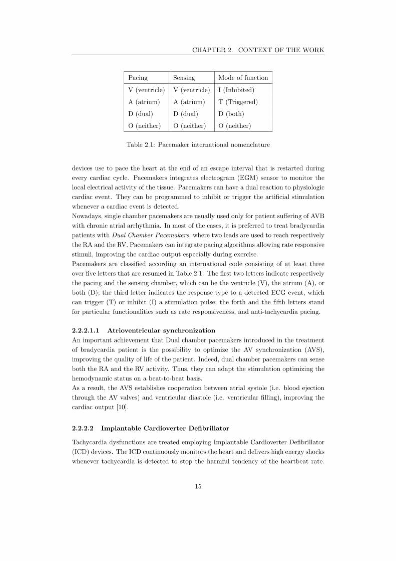
CHAPTER 2. CONTEXT OF THE WORK
Pacing Sensing Mode of function
V (ventricle) V (ventricle) I (Inhibited)
A (atrium) A (atrium) T (Triggered)
D (dual) D (dual) D (both)
O (neither) O (neither) O (neither)
Table 2.1: Pacemaker international nomenclature
devices use to pace the heart at the end of an escape interval that is restarted during
every cardiac cycle. Pacemakers integrates electrogram (EGM) sensor to monitor the
local electrical activity of the tissue. Pacemakers can have a dual reaction to physiologic
cardiac event. They can be programmed to inhibit or trigger the artificial stimulation
whenever a cardiac event is detected.
Nowadays, single chamber pacemakers are usually used only for patient suffering of AVB
with chronic atrial arrhythmia. In most of the cases, it is preferred to treat bradycardia
patients with Dual Chamber Pacemakers, where two leads are used to reach respectively
the RA and the RV. Pacemakers can integrate pacing algorithms allowing rate responsive
stimuli, improving the cardiac output especially during exercise.
Pacemakers are classified according an international code consisting of at least three
over five letters that are resumed in Table 2.1. The first two letters indicate respectively
the pacing and the sensing chamber, which can be the ventricle (V), the atrium (A), or
both (D); the third letter indicates the response type to a detected ECG event, which
can trigger (T) or inhibit (I) a stimulation pulse; the forth and the fifth letters stand
for particular functionalities such as rate responsiveness, and anti-tachycardia pacing.
2.2.2.1.1 Atrioventricular synchronization
An important achievement that Dual chamber pacemakers introduced in the treatment
of bradycardia patient is the possibility to optimize the AV synchronization (AVS),
improving the quality of life of the patient. Indeed, dual chamber pacemakers can sense
both the RA and the RV activity. Thus, they can adapt the stimulation optimizing the
hemodynamic status on a beat-to-beat basis.
As a result, the AVS establishes cooperation between atrial systole (i.e. blood ejection
through the AV valves) and ventricular diastole (i.e. ventricular filling), improving the
cardiac output [10].
2.2.2.2 Implantable Cardioverter Defibrillator
Tachycardia dysfunctions are treated employing Implantable Cardioverter Defibrillator
(ICD) devices. The ICD continuously monitors the heart and delivers high energy shocks
whenever tachycardia is detected to stop the harmful tendency of the heartbeat rate.
15
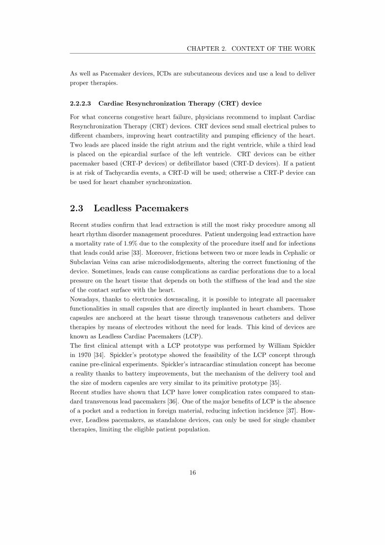
CHAPTER 2. CONTEXT OF THE WORK
As well as Pacemaker devices, ICDs are subcutaneous devices and use a lead to deliver
proper therapies.
2.2.2.3 Cardiac Resynchronization Therapy (CRT) device
For what concerns congestive heart failure, physicians recommend to implant Cardiac
Resynchronization Therapy (CRT) devices. CRT devices send small electrical pulses to
different chambers, improving heart contractility and pumping efficiency of the heart.
Two leads are placed inside the right atrium and the right ventricle, while a third lead
is placed on the epicardial surface of the left ventricle. CRT devices can be either
pacemaker based (CRT-P devices) or defibrillator based (CRT-D devices). If a patient
is at risk of Tachycardia events, a CRT-D will be used; otherwise a CRT-P device can
be used for heart chamber synchronization.
2.3 Leadless Pacemakers
Recent studies confirm that lead extraction is still the most risky procedure among all
heart rhythm disorder management procedures. Patient undergoing lead extraction have
a mortality rate of 1.9% due to the complexity of the procedure itself and for infections
that leads could arise [33]. Moreover, frictions between two or more leads in Cephalic or
Subclavian Veins can arise microdislodgements, altering the correct functioning of the
device. Sometimes, leads can cause complications as cardiac perforations due to a local
pressure on the heart tissue that depends on both the stiffness of the lead and the size
of the contact surface with the heart.
Nowadays, thanks to electronics downscaling, it is possible to integrate all pacemaker
functionalities in small capsules that are directly implanted in heart chambers. Those
capsules are anchored at the heart tissue through transvenous catheters and deliver
therapies by means of electrodes without the need for leads. This kind of devices are
known as Leadless Cardiac Pacemakers (LCP).
The first clinical attempt with a LCP prototype was performed by William Spickler
in 1970 [34]. Spickler’s prototype showed the feasibility of the LCP concept through
canine pre-clinical experiments. Spickler’s intracardiac stimulation concept has become
a reality thanks to battery improvements, but the mechanism of the delivery tool and
the size of modern capsules are very similar to its primitive prototype [35].
Recent studies have shown that LCP have lower complication rates compared to stan-
dard transvenous lead pacemakers [36]. One of the major benefits of LCP is the absence
of a pocket and a reduction in foreign material, reducing infection incidence [37]. How-
ever, Leadless pacemakers, as standalone devices, can only be used for single chamber
therapies, limiting the eligible patient population.
16
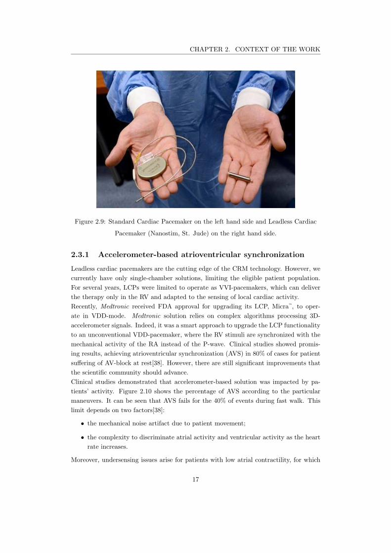
CHAPTER 2. CONTEXT OF THE WORK
Figure 2.9: Standard Cardiac Pacemaker on the left hand side and Leadless Cardiac
Pacemaker (Nanostim, St. Jude) on the right hand side.
2.3.1 Accelerometer-based atrioventricular synchronization
Leadless cardiac pacemakers are the cutting edge of the CRM technology. However, we
currently have only single-chamber solutions, limiting the eligible patient population.
For several years, LCPs were limited to operate as VVI-pacemakers, which can deliver
the therapy only in the RV and adapted to the sensing of local cardiac activity.
Recently, Medtronic received FDA approval for upgrading its LCP, Micra™, to oper-
ate in VDD-mode. Medtronic solution relies on complex algorithms processing 3D-
accelerometer signals. Indeed, it was a smart approach to upgrade the LCP functionality
to an unconventional VDD-pacemaker, where the RV stimuli are synchronized with the
mechanical activity of the RA instead of the P-wave. Clinical studies showed promis-
ing results, achieving atrioventricular synchronization (AVS) in 80% of cases for patient
suffering of AV-block at rest[38]. However, there are still significant improvements that
the scientific community should advance.
Clinical studies demonstrated that accelerometer-based solution was impacted by pa-
tients’ activity. Figure 2.10 shows the percentage of AVS according to the particular
maneuvers. It can be seen that AVS fails for the 40% of events during fast walk. This
limit depends on two factors[38]:
• the mechanical noise artifact due to patient movement;
• the complexity to discriminate atrial activity and ventricular activity as the heart
rate increases.
Moreover, undersensing issues arise for patients with low atrial contractility, for which
17
CHAPTER 2. CONTEXT OF THE WORK
Figure 2.10: AVS percentage of Micra™ during different maneuvers.
the atrial contraction does not exceed the detection threshold of the accelerometer signal.
Thus, the AVS is guaranteed for a limited patient population, during a limited amount
of time (at rest).
Even though, the study demonstrated the benefit in terms of cardiac output when AVS
is obtained, it is possible that missing the AVS can lead to a progressive evolution of
the disease toward the congestive heart failure (CHF)[39].
To overcome the limits of the LCP, the scientific community has been spending efforts
to propose multiple-chamber solutions.
2.3.2 Multi-node LCP systems
To implement all the functional modes of conventional pacemakers, two or more LCPs
might be implanted in different chambers of the heart. For example, a leadless CRT-P
system is represented in Figure 2.11, where two endocardial LCP are placed respectively
in the RV and in the RA; whereas an epicardial LCP is placed on the external surface
of the LV.
Recently, Bereuter et al. performed the firsts attempts of multi-node pacing using phys-
ically separate devices, proving the clinical feasibility of both dual chamber and CRT-P
leadless pacing [22, 20]. In particular, the authors suggested a telemetry-based synchro-
nization of LCPs, using a conductive communication, known in the scientific community
18
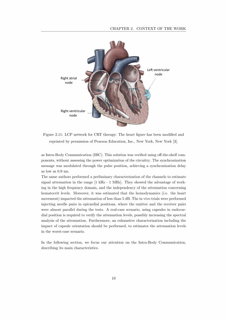
CHAPTER 2. CONTEXT OF THE WORK
Right atrial
node
Le ventricular
node
Right ventricular
node
Figure 2.11: LCP network for CRT therapy. The heart figure has been modified and
reprinted by permission of Pearson Education, Inc., New York, New York [3].
as Intra-Body Communication (IBC). This solution was verified using off-the-shelf com-
ponents, without assessing the power optimization of the circuitry. The synchronization
message was modulated through the pulse position, achieving a synchronization delay
as low as 0.9 ms.
The same authors performed a preliminary characterization of the channels to estimate
signal attenuation in the range [1 kHz - 1 MHz]. They showed the advantage of work-
ing in the high frequency domain, and the independency of the attenuation concerning
hematocrit levels. Moreover, it was estimated that the hemodynamics (i.e. the heart
movement) impacted the attenuation of less than 5 dB. The in vivo trials were performed
injecting needle pairs in epicardial positions, where the emitter and the receiver pairs
were almost parallel during the tests. A real-case scenario, using capsules in endocar-
dial position is required to verify the attenuation levels, possibly increasing the spectral
analysis of the attenuation. Furthermore, an exhaustive characterization including the
impact of capsule orientation should be performed, to estimates the attenuation levels
in the worst-case scenario.
In the following section, we focus our attention on the Intra-Body Communication,
describing its main characteristics.
19
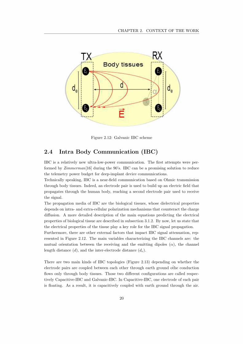
CHAPTER 2. CONTEXT OF THE WORK
Figure 2.12: Galvanic IBC scheme
2.4 Intra Body Communication (IBC)
IBC is a relatively new ultra-low-power communication. The first attempts were per-
formed by Zimmerman[16] during the 90’s. IBC can be a promising solution to reduce
the telemetry power budget for deep-implant device communications.
Technically speaking, IBC is a near-field communication based on Ohmic transmission
through body tissues. Indeed, an electrode pair is used to build up an electric field that
propagates through the human body, reaching a second electrode pair used to receive
the signal.
The propagation media of IBC are the biological tissues, whose dielectrical properties
depends on intra- and extra-cellular polarization mechanisms that counteract the charge
diffusion. A more detailed description of the main equations predicting the electrical
properties of biological tissue are described in subsection 3.1.2. By now, let us state that
the electrical properties of the tissue play a key role for the IBC signal propagation.
Furthermore, there are other external factors that impact IBC signal attenuation, rep-
resented in Figure 2.12. The main variables characterizing the IBC channels are: the
mutual orientation between the receiving and the emitting dipoles (α), the channel
length distance (d), and the inter-electrode distance (de).
There are two main kinds of IBC topologies (Figure 2.13) depending on whether the
electrode pairs are coupled between each other through earth ground othe conduction
flows only through body tissues. Those two different configurations are called respec-
tively Capacitive-IBC and Galvanic-IBC. In Capacitive-IBC, one electrode of each pair
is floating. As a result, it is capacitively coupled with earth ground through the air.
20
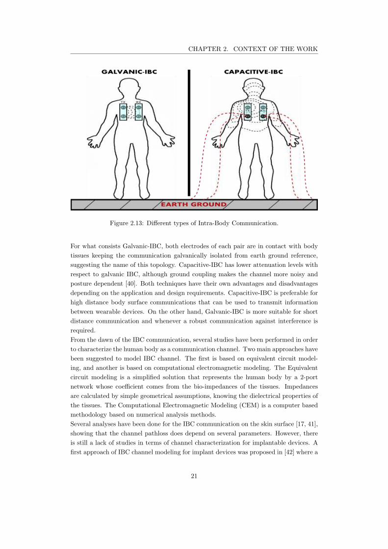
CHAPTER 2. CONTEXT OF THE WORK
Figure 2.13: Different types of Intra-Body Communication.
For what consists Galvanic-IBC, both electrodes of each pair are in contact with body
tissues keeping the communication galvanically isolated from earth ground reference,
suggesting the name of this topology. Capacitive-IBC has lower attenuation levels with
respect to galvanic IBC, although ground coupling makes the channel more noisy and
posture dependent [40]. Both techniques have their own advantages and disadvantages
depending on the application and design requirements. Capacitive-IBC is preferable for
high distance body surface communications that can be used to transmit information
between wearable devices. On the other hand, Galvanic-IBC is more suitable for short
distance communication and whenever a robust communication against interference is
required.
From the dawn of the IBC communication, several studies have been performed in order
to characterize the human body as a communication channel. Two main approaches have
been suggested to model IBC channel. The first is based on equivalent circuit model-
ing, and another is based on computational electromagnetic modeling. The Equivalent
circuit modeling is a simplified solution that represents the human body by a 2-port
network whose coefficient comes from the bio-impedances of the tissues. Impedances
are calculated by simple geometrical assumptions, knowing the dielectrical properties of
the tissues. The Computational Electromagnetic Modeling (CEM) is a computer based
methodology based on numerical analysis methods.
Several analyses have been done for the IBC communication on the skin surface [17, 41],
showing that the channel pathloss does depend on several parameters. However, there
is still a lack of studies in terms of channel characterization for implantable devices. A
first approach of IBC channel modeling for implant devices was proposed in [42] where a
21
CHAPTER 2. CONTEXT OF THE WORK
boundary conditioned problem is analytically solved for IBC communication in a limb.
The study shows the importance of the geometry of the model despite the fact that an
approximated body model was used.
This chapter started with a rough anatomical description of the rib cage, in which
most of the galvanic-IBC signals, emitted by LCPs, will be confined. The organ which
is directly related to the application is the heart. Thus, we gave a background on
the cardiac electrophysiology, pointing out the microscopic phenomena though the con-
duction system of the heart. Then, a summary of the main disorders related to the
conduction system were reported, followed by the implant devices used to counteract
each cardiac rhythm abnormality. A particular attention was given to the cardiac pace-
maker, pointing out its main characteristics and limitations. It was shown that Leadless
Cardiac Pacemakers reduce post-surgical complication rates compared to conventional
pacemakers, integrating all the components in a single capsule. The Leadless pacemaker
was described, focusing on the solutions to establish atrioventricular synchronization.
We have seen that accelerometer-based solutions can achieve good AVS results at rest;
however the performance of such a technique is highly impacted by the physical activity.
Multi-node LCP systems can overcome this limit using wireless communication to syn-
chronize the devices. The Intra-Body Communication seems the most suitable physical
layer for LCP communication. Thus, the work of this study focuses on IBC technology.
In the next chapter, we deal with preliminary studies related to the characterization of
the communication channels. This is an essential step to design power-efficient commu-
nication modules for LCP applications.
22
3IBC channel characterization
The World Medical Association agreed in the Declaration of Helsinki that animals should
only be used in biomedical research when it is clear that their use is required to achieve
an important outcome, and where no other feasible method is available [43].
Here, we propose a methodology to estimate IBC attenuation for leadless pacemaker
applications using in silico simulations. This methodology allows fast estimations of the
channel attenuation that can reduce the number of experiments required. The model
was then verified with in-vivo measurements using a novel experimental setup.
3.1 Simulations
In Silico experiments have improved in the last decades thanks to the increasing of power
calculation of computers. Among other things, they can be used for a preliminary es-
timation of the attenuation in human body. In this section, we propose a method for
IBC channel characterization using an accurate torso model. First, some physical con-
sideration are pointed out to explain the importance of having accurate models when
considering IBC signals. All IBC channels involved in Leadless Cardiac Pacemakers
are investigated. In particular, the attenuation results of three different channels are
pointed out: Intra-cardiac channel, Inter-ventricular channel, and Trans-thoracic chan-
nel. Then, the mathematical method and the methodology are described. For the sake
of completeness, we compare the results between the accurate torso model and another
one that was constructed by simple geometrical shapes.
3.1.1 Geometrical considerations
The Electric Field flux enclosed in the surface Σ, generated by a continuous distribution
of charges, is characterized by the charge spatial density ρ(x, y, z), as stated by the
Gauss’law. The Gauss’law is represented by equation (3.1), where the integral enclosed
by surface Σ represents the total charge contained in the volume τ .
23
CHAPTER 3. IBC CHANNEL CHARACTERIZATION
Φ(E) =1
ǫ0
∫Σ
ρ(x, y, z)dτ. (3.1)
The emitting dipole of IBC channel generates an Electric field whose flux obeys
to Equation 3.1. Human body is an anisotropic environment where the analysis of
the electric field distribution is not analytically straightforward. Thus, software based
numerical computations can be used to study the Electric Field in such a complex
volume. To do so, we used an accurate human torso model with a geometrical resolution
of 0.5 mm that is described in detail in subsection 3.1.5.
3.1.2 Dielectric properties of human body tissues
Dielectric properties of materials have been the object of empirical studies for more than
a century and several models based on the relaxation constant have been proposed so
far by the scientific community. The simplest way to model dielectrics is given by the
Debye formula that is shown in (3.2)
ǫ∗ = ǫ∞ +∆ǫ
1 + (jωτ)+
σ
jωǫ0, (3.2)
where ǫ∞ represents the permittivity value far above the relaxation frequency, ǫs is the
static permittivity, ∆ǫ = (ǫ∞ − ǫs) is called dielectric strength, τ is the relaxation time
and σ is the conductivity, while ǫ0 is the permittivity of the free space. Body tissues
are complex materials whose permittivities experience more than a single relaxation
constant. This could arise from the superposition of several relaxation processes due to
different polarization effects [44]. This behavior was firstly discovered in 1941 by two
brothers called Robert H. and Kenneth S. Cole who introduced an additional factor α
to Debye’s equation as shown in eq.3.3. This equation, known as Cole-Cole equation,
better fit the relaxation constant concerning its frequency behavior.
ǫ∗ = ǫ∞ +∆ǫ
1 + (jωτ)1−α
+σs
jωǫ0. (3.3)
In the early nineties, Camelia Gabriel measured over 20 biological tissue in the frequency
range between 10Hz and 20GHz. To fit the measurements, she proposed a four-term
Cole-Cole equation that is shown in 3.4 [45]. This equation considers separately the
different polarization effects that are experienced in biological tissues.
ǫ∗ = ǫ∞ +
4∑n=1
∆ǫn
1 + (jωτ)1−αn
+σs
jωǫ0. (3.4)
Our study is based on Gabriel et al. work whose data are publicly available in several
database such as the web application of the Institute of Applied Physics of CNR [46].
24
CHAPTER 3. IBC CHANNEL CHARACTERIZATION
3.1.3 Finite Element Method
The Finite Element Method (FEM) is a numerical technique that allows solving prob-
lems of partial differential equations with an elegant approach. The FEM applies the
old concept of ”divide et impera” to mathematics. Indeed, the FEM is used to solve
problems in complex regions, called domains, dividing it in several sub-elements, called
meshes. The problem is solved independently for each mesh and then sum up each
contribution to find the global solution. Mathematically speaking, the FEM relies on
the method of weighted residuals and on the concept of shape function that was well
interpreted by Galerkin in early fifties of the XX century.
Hereafter, some mathematical concepts are treated to let the reader have a grasp of
what FEM consists in without too many details since an exhaustive description of the
method is out of the scope of this manuscript, and a more detailed description can be
found in the literature [47].
Let us consider the Poisson equation that analytically describes several physical phenom-
ena such as electrodynamics. In particular, we will consider one-dimension problems,
but a the generalization to 2D or 3D domains is straightforward.
∂2φ
∂x2= −
ρ
ǫ. (3.5)
The FEM finds approximated solutions introducing an error, the residual, that is defined
as the difference between the true solution and the approximated solution:
R(φ, x) ≡ −
∂2φ
∂x2−
ρ
ǫ. (3.6)
We can now multiply the residual function by a weighting function W (x) and force the
integral of the overall expression to zero.
∫
L
0
W (x)R(φ, x)dx = 0. (3.7)
According to Galerkin’s approach, the weights are set equal to the shape functions
Ni(x). The problem is synthesized to a set of linear equations with the same number of
equations as unknowns.
∫
L
0
Ni(x)
[
−
d2φ
dx2−
ρ
ǫ
]
dx = 0. (3.8)
Integrating by part the second derivative term, we can reduce the complexity of the
problem to an equation of order one, called weak formulation.
∫
L
0
dN(x)
dx
dφ
dxdx−N(x)
dφ
dx
∣
∣
∣
∣
L
0
−
∫
L
0
N(x)ρ
ǫ= 0. (3.9)
The FEM relies on piece-wise polynomial approximations whose accuracy depend on
the degree of the polynomials chosen as O(hn), where h is the length of the meshing
element and n is the degree of the polynomial. Using the weak form of the problem allows
25

CHAPTER 3. IBC CHANNEL CHARACTERIZATION
Figure 3.1: Piecewise linear versus piecewise quadratic approximation
to use linear approximation, but higher order can be applied to reach lower errors, with
the cost of increasing the number of linear equation and consequently the computational
effort of the solver [47].
The first decision that must be faced approaching the FEM concerns the number
of nodes and the geometry of the meshing elements. For each node, there is a shape
function N(x) such that N(e)i (xi) = 1 and Ni(xj) = 0 when i 6= j. Using the shape
functions, it is possible to represent the function φ(x) as the sum of each contribution
coming from each meshing element such that
φ(x) =
n+1∑
i=1
N(e)i (x)φi, (3.10)
where φi is the value of φ(x) on the node i and N(e)i is the set of shape functions for the
element e. This new representation of φ(x) can be used to solve the problem 3.9. The
FEM proposed so far is adapted to solve steady-state problems, but it is also possible
to extend the method to time variant problems. In this case φ(x) becomes φ(x, t) where
t is the time variable. However, it is required to specify the initial condition φ0(x) to
find the particular solution of the problem [47]. On the other hand, shape functions are
only space dependent and φ(x, t) can be represented as
φ(x, t) =
n+1∑
i=1
Ni(x)φi(t). (3.11)
At each node of the mesh, a set of linear algebraic equations must be solved. The
description of the numerical method to find out the approximated solution using the
FEM is widely described in the literature [47] and it is out of the scope of this manuscript.
26
CHAPTER 3. IBC CHANNEL CHARACTERIZATION
3.1.4 Quasi-static approximation
Maxwell’s equations can fully describe electromagnetic phenomena such as IBC signals.
However, the complexity of the set of equations would require a massive amount of time
to find a convergent solution. Quasi-static set of equations provide an intermediate level
between static analysis and the complete electrodynamics. Indeed, quasi-static assump-
tions decouple Electric field E and Magnetic field H since the velocity of the magnetic
field field flux B does not contribute to Electric field magnitude and vice versa as can
be seen from the set of equations (3.12), where the magnetic current density and mag-
netic charges have been neglected since we suppose that no magnetic sources are applied.
Maxwell’s equations: Quasi-Static approximation:
∇×H = ∂D∂t
+ J
∇× E = −∂B∂t
∇ · B = 0
∇ · D = ρ
=⇒
∇×H = ∂D∂t
+ J
∇× E ≈ 0
∇ · D = ρ
(3.12)
Let us now point out the error introduced by Quasi-static assumption. To do so, we
will find the contribution of the magnetic field to the electric field for the solution of the
classical Maxwell’s equation. Maxwell’s equation are analytically solved as the solution
of the inhomogeneous Helmoltz equation. In stationary domain, the electric field can be
fully determined from the magnetic vector potential A and the scalar electric potential
V as shown in the set of equations (3.13).
E = −jωA−∇V
A = µ4π
∫
V ′
Jse−jkR
RdV ′
V = 14π(σ+jωǫ)
∫
V ′
ρe−jkR
RdV ′
(3.13)
The error introduced using Quasi-Static equations comes from the magnetic contribution
to E that can be described as 3.14 [48, 15].
|ωA
∇V| = |ω2µǫR2
tx|, (3.14)
where ω is the angular frequency, Rtx is the dipole length of the emitter in meters,
µ and ǫ are respectively the magnetic permeability and the electric permittivity of the
transmission medium.
It is our interest to have a wide frequency characterization of the IBC channel attenu-
ation for Multi-node leadless pacemaker applications. In this work, we decided to set the
upper frequency limit to 20 MHz to approach the IBC-band chosen by the IEEE com-
munity, which is defined as Human Body Communication (HBC) in the IEEE802.15.6
standard [49].
Knowing that µtissue ≈ µair, ǫblood(20 MHz) = 154.56 and setting the length Rtx =
33mm, that is the length of the LCP prototype used in this study, we find a relative
error of almost 3%, that can be considered as an acceptable limit.
27
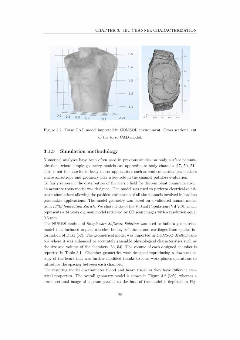
CHAPTER 3. IBC CHANNEL CHARACTERIZATION
Figure 3.2: Torso CAD model imported in COMSOL environment. Cross sectional cut
of the torso CAD model.
3.1.5 Simulation methodology
Numerical analyses have been often used in previous studies on body surface commu-
nications where simple geometry models can approximate body channels [17, 50, 51].
This is not the case for in-body sensor applications such as leadless cardiac pacemakers
where anisotropy and geometry play a key role in the channel pathloss evaluation.
To fairly represent the distribution of the eletric field for deep-implant communication,
an accurate torso model was designed. The model was used to perform electrical quasi-
static simulations allowing the pathloss estimation of all the channels involved in leadless
pacemaker applications. The model geometry was based on a validated human model
from IT'IS foundation Zurich. We chose Duke of the Virtual Population (ViP2.0), which
represents a 34 years old man model retrieved by CT scan images with a resolution equal
0.5 mm.
The NURBS module of Simpleware Software Solution was used to build a geometrical
model that included organs, muscles, bones, soft tissue and cartilages from spatial in-
formation of Duke [52]. The geometrical model was imported in COMSOL Multiphysics
5.3 where it was enhanced to accurately resemble physiological characteristics such as
the size and volume of the chambers [53, 54]. The volume of each designed chamber is
reported in Table 3.1. Chamber geometries were designed reproducing a down-scaled
copy of the heart that was further modified thanks to local work-planes operations to
introduce the spacing between each chamber.
The resulting model discriminates blood and heart tissue as they have different elec-
trical properties. The overall geometry model is shown in Figure 3.2 (left), whereas a
cross sectional image of a plane parallel to the base of the model is depicted in Fig-
28
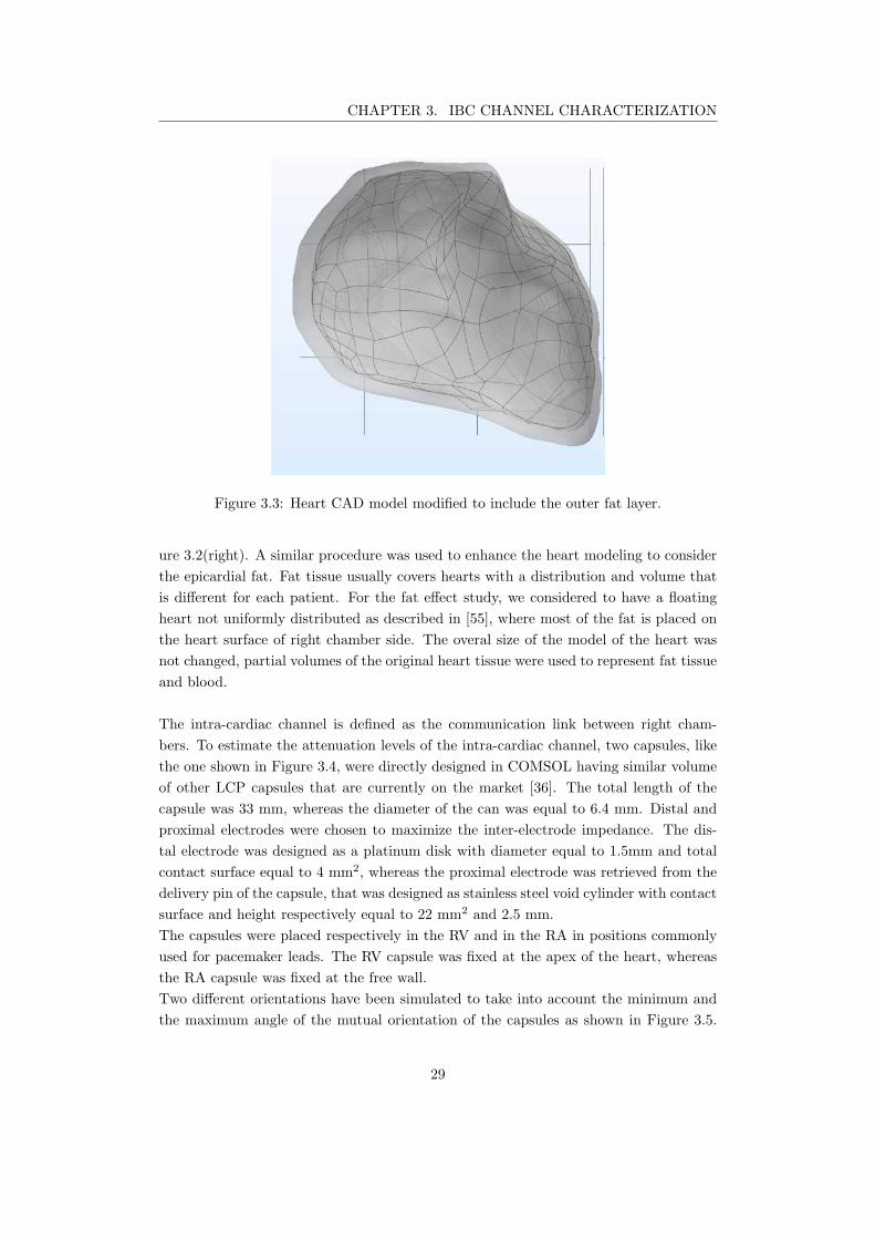
CHAPTER 3. IBC CHANNEL CHARACTERIZATION
Figure 3.3: Heart CAD model modified to include the outer fat layer.
ure 3.2(right). A similar procedure was used to enhance the heart modeling to consider
the epicardial fat. Fat tissue usually covers hearts with a distribution and volume that
is different for each patient. For the fat effect study, we considered to have a floating
heart not uniformly distributed as described in [55], where most of the fat is placed on
the heart surface of right chamber side. The overal size of the model of the heart was
not changed, partial volumes of the original heart tissue were used to represent fat tissue
and blood.
The intra-cardiac channel is defined as the communication link between right cham-
bers. To estimate the attenuation levels of the intra-cardiac channel, two capsules, like
the one shown in Figure 3.4, were directly designed in COMSOL having similar volume
of other LCP capsules that are currently on the market [36]. The total length of the
capsule was 33 mm, whereas the diameter of the can was equal to 6.4 mm. Distal and
proximal electrodes were chosen to maximize the inter-electrode impedance. The dis-
tal electrode was designed as a platinum disk with diameter equal to 1.5mm and total
contact surface equal to 4 mm2, whereas the proximal electrode was retrieved from the
delivery pin of the capsule, that was designed as stainless steel void cylinder with contact
surface and height respectively equal to 22 mm2 and 2.5 mm.
The capsules were placed respectively in the RV and in the RA in positions commonly
used for pacemaker leads. The RV capsule was fixed at the apex of the heart, whereas
the RA capsule was fixed at the free wall.
Two different orientations have been simulated to take into account the minimum and
the maximum angle of the mutual orientation of the capsules as shown in Figure 3.5.
29
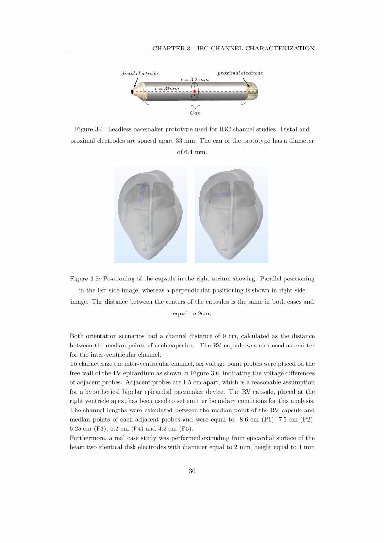
CHAPTER 3. IBC CHANNEL CHARACTERIZATION
distal electrode proximal electrode
Can
•m
l = 33mm
r = 3.2 mm
Figure 3.4: Leadless pacemaker prototype used for IBC channel studies. Distal and
proximal electrodes are spaced apart 33 mm. The can of the prototype has a diameter
of 6.4 mm.
Figure 3.5: Positioning of the capsule in the right atrium showing. Parallel positioning
in the left side image, whereas a perpendicular positioning is shown in right side
image. The distance between the centers of the capsules is the same in both cases and
equal to 9cm.
Both orientation scenarios had a channel distance of 9 cm, calculated as the distance
between the median points of each capsules. The RV capsule was also used as emitter
for the inter-ventricular channel.
To characterize the inter-ventricular channel, six voltage point probes were placed on the
free wall of the LV epicardium as shown in Figure 3.6, indicating the voltage differences
of adjacent probes. Adjacent probes are 1.5 cm apart, which is a reasonable assumption
for a hypothetical bipolar epicardial pacemaker device. The RV capsule, placed at the
right ventricle apex, has been used to set emitter boundary conditions for this analysis.
The channel lengths were calculated between the median point of the RV capsule and
median points of each adjacent probes and were equal to: 8.6 cm (P1), 7.5 cm (P2),
6.25 cm (P3), 5.2 cm (P4) and 4.2 cm (P5).
Furthermore, a real case study was performed extruding from epicardial surface of the
heart two identical disk electrodes with diameter equal to 2 mm, height equal to 1 mm
30
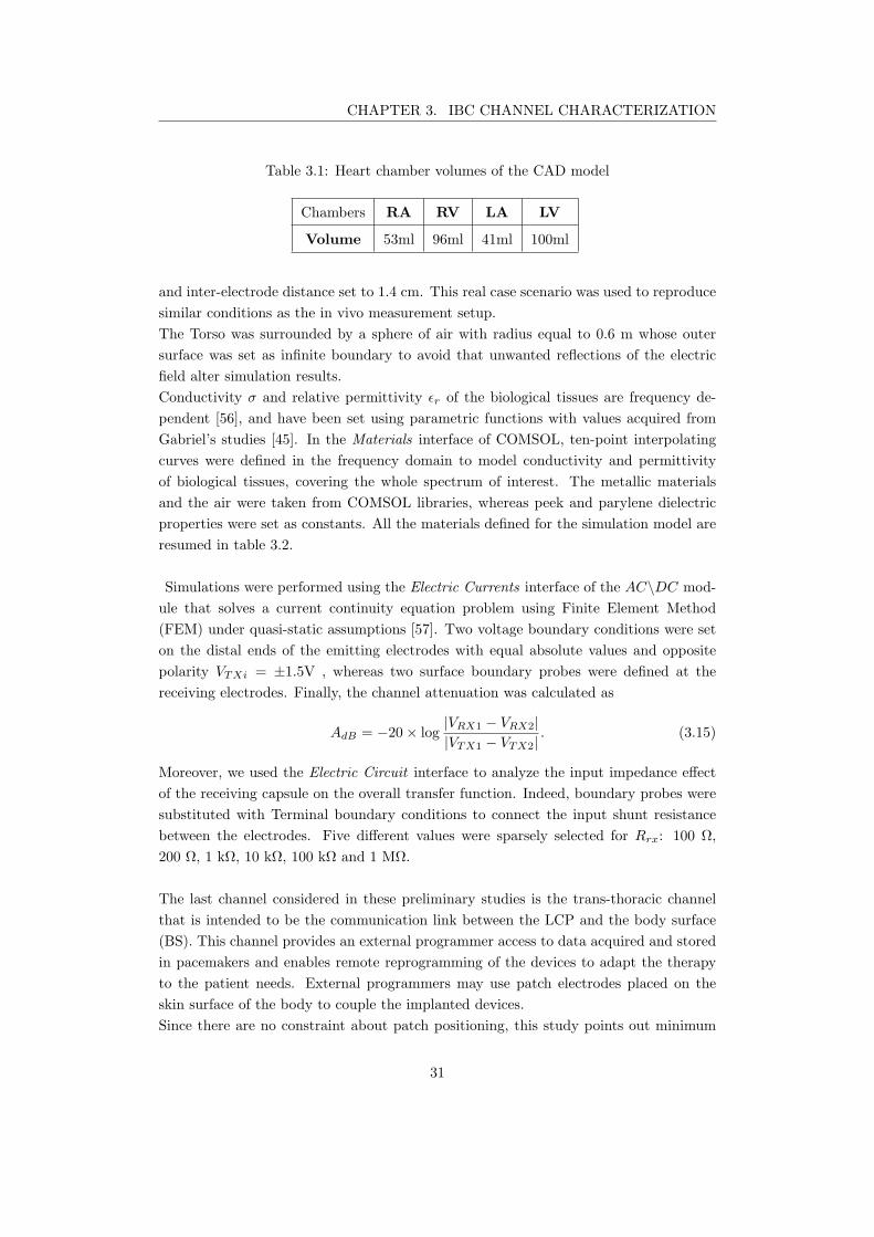
CHAPTER 3. IBC CHANNEL CHARACTERIZATION
Table 3.1: Heart chamber volumes of the CAD model
Chambers RA RV LA LV
Volume 53ml 96ml 41ml 100ml
and inter-electrode distance set to 1.4 cm. This real case scenario was used to reproduce
similar conditions as the in vivo measurement setup.
The Torso was surrounded by a sphere of air with radius equal to 0.6 m whose outer
surface was set as infinite boundary to avoid that unwanted reflections of the electric
field alter simulation results.
Conductivity σ and relative permittivity ǫr of the biological tissues are frequency de-
pendent [56], and have been set using parametric functions with values acquired from
Gabriel’s studies [45]. In the Materials interface of COMSOL, ten-point interpolating
curves were defined in the frequency domain to model conductivity and permittivity
of biological tissues, covering the whole spectrum of interest. The metallic materials
and the air were taken from COMSOL libraries, whereas peek and parylene dielectric
properties were set as constants. All the materials defined for the simulation model are
resumed in table 3.2.
Simulations were performed using the Electric Currents interface of the AC\DC mod-
ule that solves a current continuity equation problem using Finite Element Method
(FEM) under quasi-static assumptions [57]. Two voltage boundary conditions were set
on the distal ends of the emitting electrodes with equal absolute values and opposite
polarity VTXi = ±1.5V , whereas two surface boundary probes were defined at the
receiving electrodes. Finally, the channel attenuation was calculated as
AdB = −20× log|VRX1 − VRX2|
|VTX1 − VTX2|. (3.15)
Moreover, we used the Electric Circuit interface to analyze the input impedance effect
of the receiving capsule on the overall transfer function. Indeed, boundary probes were
substituted with Terminal boundary conditions to connect the input shunt resistance
between the electrodes. Five different values were sparsely selected for Rrx: 100 Ω,
200 Ω, 1 kΩ, 10 kΩ, 100 kΩ and 1 MΩ.
The last channel considered in these preliminary studies is the trans-thoracic channel
that is intended to be the communication link between the LCP and the body surface
(BS). This channel provides an external programmer access to data acquired and stored
in pacemakers and enables remote reprogramming of the devices to adapt the therapy
to the patient needs. External programmers may use patch electrodes placed on the
skin surface of the body to couple the implanted devices.
Since there are no constraint about patch positioning, this study points out minimum
31
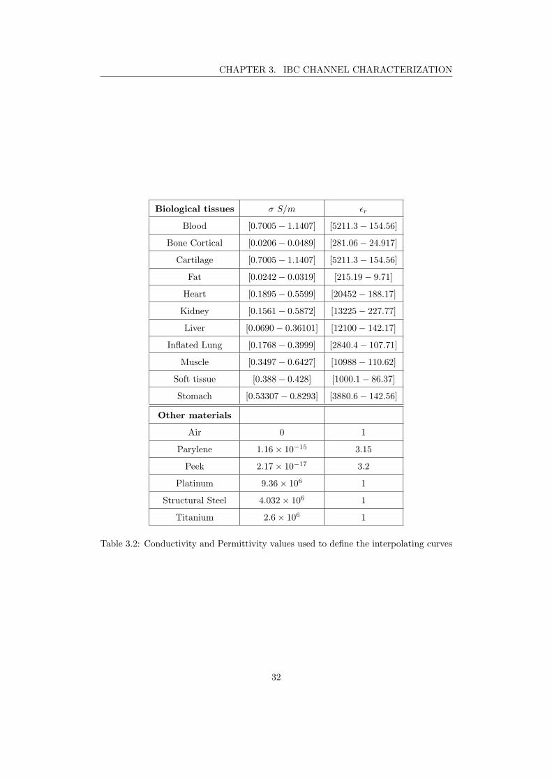
CHAPTER 3. IBC CHANNEL CHARACTERIZATION
Biological tissues σ S/m ǫr
Blood [0.7005− 1.1407] [5211.3− 154.56]
Bone Cortical [0.0206− 0.0489] [281.06− 24.917]
Cartilage [0.7005− 1.1407] [5211.3− 154.56]
Fat [0.0242− 0.0319] [215.19− 9.71]
Heart [0.1895− 0.5599] [20452− 188.17]
Kidney [0.1561− 0.5872] [13225− 227.77]
Liver [0.0690− 0.36101] [12100− 142.17]
Inflated Lung [0.1768− 0.3999] [2840.4− 107.71]
Muscle [0.3497− 0.6427] [10988− 110.62]
Soft tissue [0.388− 0.428] [1000.1− 86.37]
Stomach [0.53307− 0.8293] [3880.6− 142.56]
Other materials
Air 0 1
Parylene 1.16× 10⁻¹⁵ 3.15
Peek 2.17× 10⁻¹⁷ 3.2
Platinum 9.36× 10⁶ 1
Structural Steel 4.032× 10⁶ 1
Titanium 2.6× 10⁶ 1
Table 3.2: Conductivity and Permittivity values used to define the interpolating curves
32
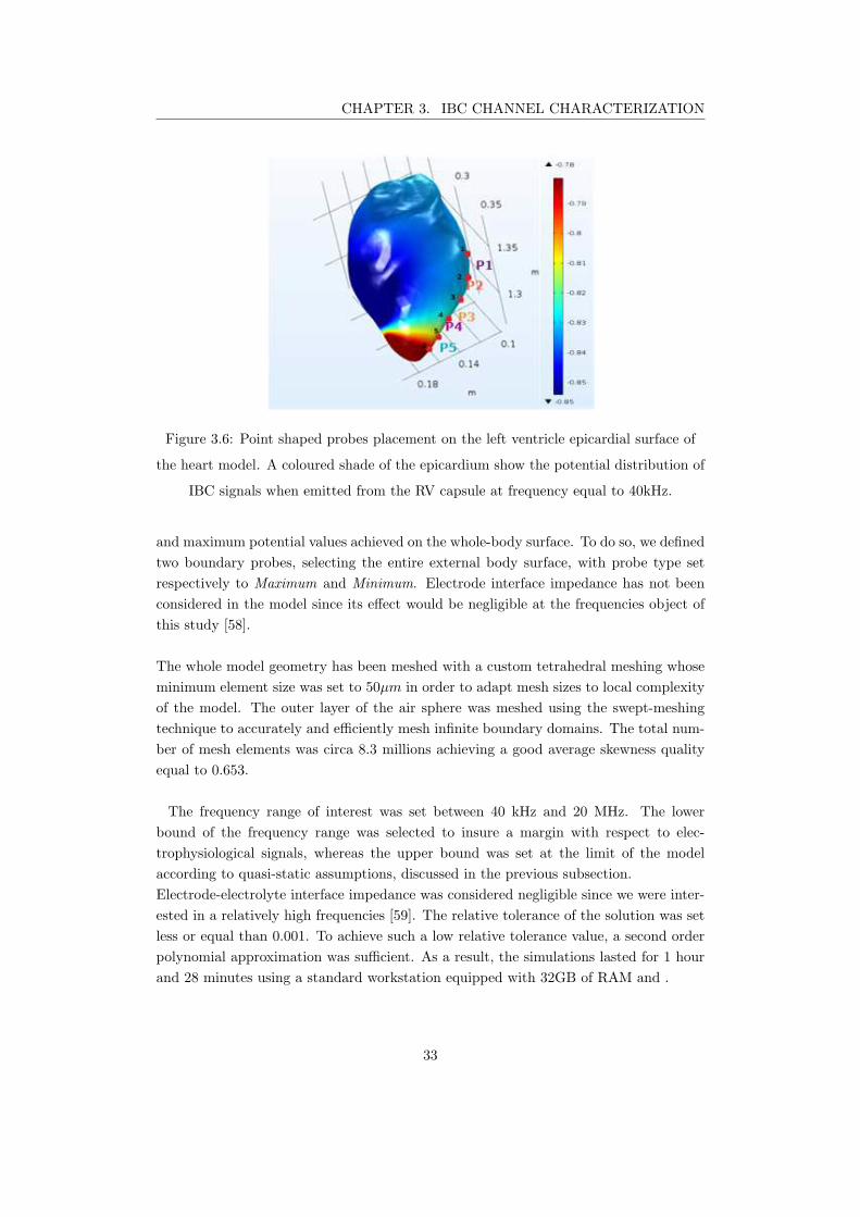
CHAPTER 3. IBC CHANNEL CHARACTERIZATION
Figure 3.6: Point shaped probes placement on the left ventricle epicardial surface of
the heart model. A coloured shade of the epicardium show the potential distribution of
IBC signals when emitted from the RV capsule at frequency equal to 40kHz.
and maximum potential values achieved on the whole-body surface. To do so, we defined
two boundary probes, selecting the entire external body surface, with probe type set
respectively to Maximum and Minimum. Electrode interface impedance has not been
considered in the model since its effect would be negligible at the frequencies object of
this study [58].
The whole model geometry has been meshed with a custom tetrahedral meshing whose
minimum element size was set to 50µm in order to adapt mesh sizes to local complexity
of the model. The outer layer of the air sphere was meshed using the swept-meshing
technique to accurately and efficiently mesh infinite boundary domains. The total num-
ber of mesh elements was circa 8.3 millions achieving a good average skewness quality
equal to 0.653.
The frequency range of interest was set between 40 kHz and 20 MHz. The lower
bound of the frequency range was selected to insure a margin with respect to elec-
trophysiological signals, whereas the upper bound was set at the limit of the model
according to quasi-static assumptions, discussed in the previous subsection.
Electrode-electrolyte interface impedance was considered negligible since we were inter-
ested in a relatively high frequencies [59]. The relative tolerance of the solution was set
less or equal than 0.001. To achieve such a low relative tolerance value, a second order
polynomial approximation was sufficient. As a result, the simulations lasted for 1 hour
and 28 minutes using a standard workstation equipped with 32GB of RAM and .
33
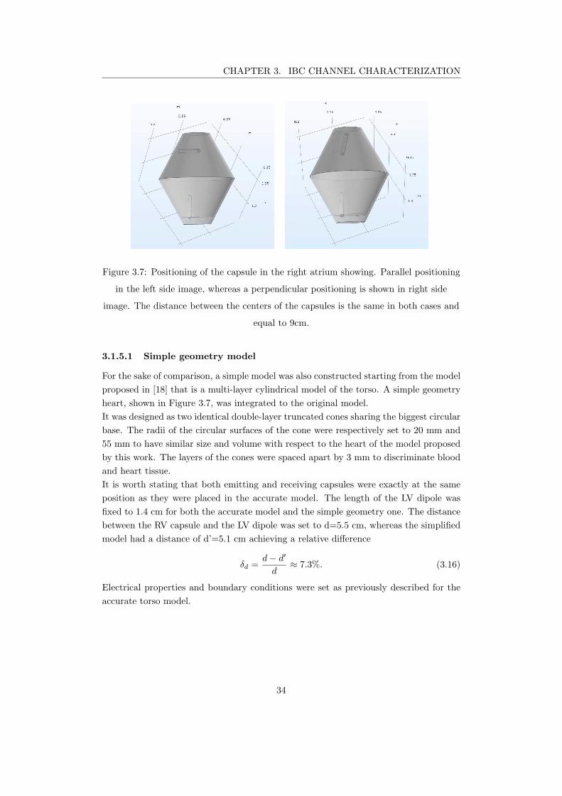
CHAPTER 3. IBC CHANNEL CHARACTERIZATION
Figure 3.7: Positioning of the capsule in the right atrium showing. Parallel positioning
in the left side image, whereas a perpendicular positioning is shown in right side
image. The distance between the centers of the capsules is the same in both cases and
equal to 9cm.
3.1.5.1 Simple geometry model
For the sake of comparison, a simple model was also constructed starting from the model
proposed in [18] that is a multi-layer cylindrical model of the torso. A simple geometry
heart, shown in Figure 3.7, was integrated to the original model.
It was designed as two identical double-layer truncated cones sharing the biggest circular
base. The radii of the circular surfaces of the cone were respectively set to 20 mm and
55 mm to have similar size and volume with respect to the heart of the model proposed
by this work. The layers of the cones were spaced apart by 3 mm to discriminate blood
and heart tissue.
It is worth stating that both emitting and receiving capsules were exactly at the same
position as they were placed in the accurate model. The length of the LV dipole was
fixed to 1.4 cm for both the accurate model and the simple geometry one. The distance
between the RV capsule and the LV dipole was set to d=5.5 cm, whereas the simplified
model had a distance of d’=5.1 cm achieving a relative difference
δd =d− d
′
d≈ 7.3%. (3.16)
Electrical properties and boundary conditions were set as previously described for the
accurate torso model.
34
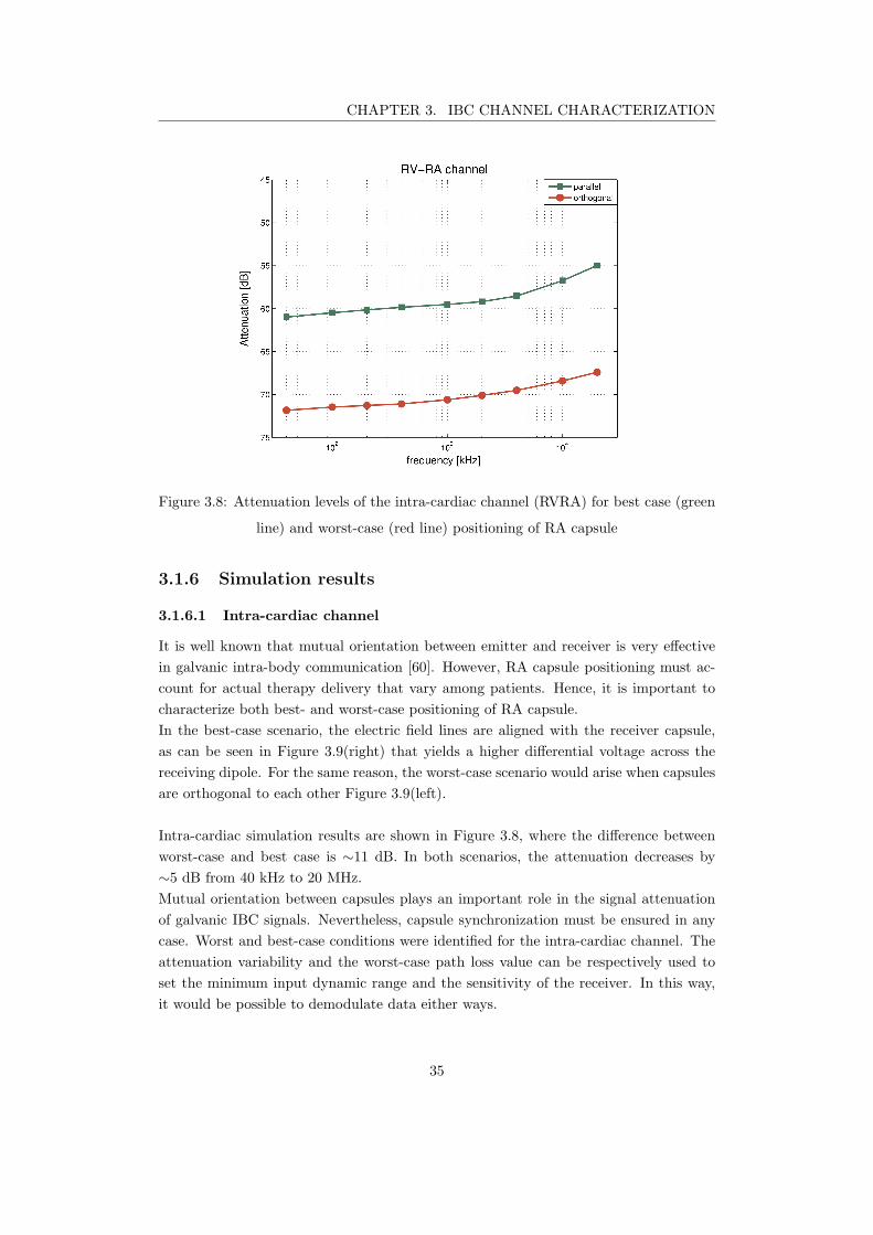
CHAPTER 3. IBC CHANNEL CHARACTERIZATION
Figure 3.8: Attenuation levels of the intra-cardiac channel (RVRA) for best case (green
line) and worst-case (red line) positioning of RA capsule
3.1.6 Simulation results
3.1.6.1 Intra-cardiac channel
It is well known that mutual orientation between emitter and receiver is very effective
in galvanic intra-body communication [60]. However, RA capsule positioning must ac-
count for actual therapy delivery that vary among patients. Hence, it is important to
characterize both best- and worst-case positioning of RA capsule.
In the best-case scenario, the electric field lines are aligned with the receiver capsule,
as can be seen in Figure 3.9(right) that yields a higher differential voltage across the
receiving dipole. For the same reason, the worst-case scenario would arise when capsules
are orthogonal to each other Figure 3.9(left).
Intra-cardiac simulation results are shown in Figure 3.8, where the difference between
worst-case and best case is ∼11 dB. In both scenarios, the attenuation decreases by
∼5 dB from 40 kHz to 20 MHz.
Mutual orientation between capsules plays an important role in the signal attenuation
of galvanic IBC signals. Nevertheless, capsule synchronization must be ensured in any
case. Worst and best-case conditions were identified for the intra-cardiac channel. The
attenuation variability and the worst-case path loss value can be respectively used to
set the minimum input dynamic range and the sensitivity of the receiver. In this way,
it would be possible to demodulate data either ways.
35
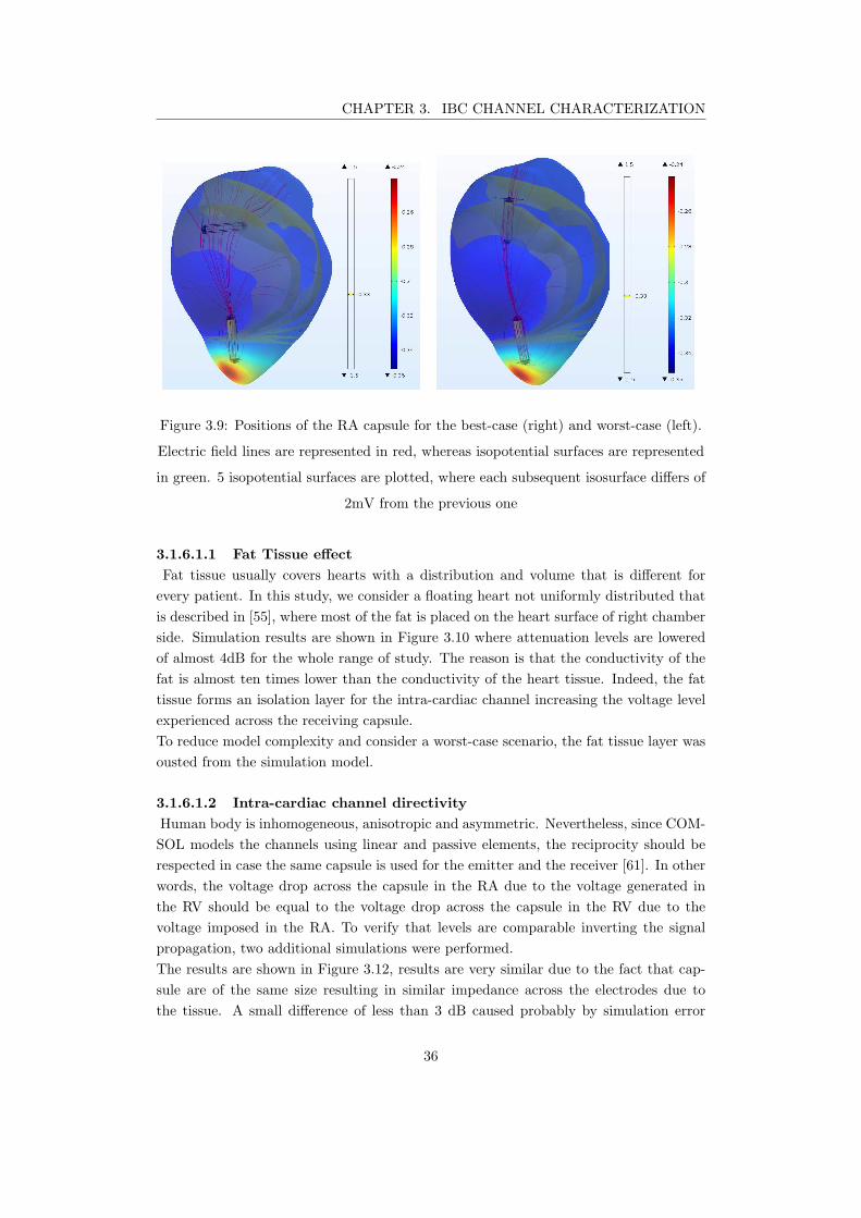
CHAPTER 3. IBC CHANNEL CHARACTERIZATION
Figure 3.9: Positions of the RA capsule for the best-case (right) and worst-case (left).
Electric field lines are represented in red, whereas isopotential surfaces are represented
in green. 5 isopotential surfaces are plotted, where each subsequent isosurface differs of
2mV from the previous one
3.1.6.1.1 Fat Tissue effect
Fat tissue usually covers hearts with a distribution and volume that is different for
every patient. In this study, we consider a floating heart not uniformly distributed that
is described in [55], where most of the fat is placed on the heart surface of right chamber
side. Simulation results are shown in Figure 3.10 where attenuation levels are lowered
of almost 4dB for the whole range of study. The reason is that the conductivity of the
fat is almost ten times lower than the conductivity of the heart tissue. Indeed, the fat
tissue forms an isolation layer for the intra-cardiac channel increasing the voltage level
experienced across the receiving capsule.
To reduce model complexity and consider a worst-case scenario, the fat tissue layer was
ousted from the simulation model.
3.1.6.1.2 Intra-cardiac channel directivity
Human body is inhomogeneous, anisotropic and asymmetric. Nevertheless, since COM-
SOL models the channels using linear and passive elements, the reciprocity should be
respected in case the same capsule is used for the emitter and the receiver [61]. In other
words, the voltage drop across the capsule in the RA due to the voltage generated in
the RV should be equal to the voltage drop across the capsule in the RV due to the
voltage imposed in the RA. To verify that levels are comparable inverting the signal
propagation, two additional simulations were performed.
The results are shown in Figure 3.12, results are very similar due to the fact that cap-
sule are of the same size resulting in similar impedance across the electrodes due to
the tissue. A small difference of less than 3 dB caused probably by simulation error
36
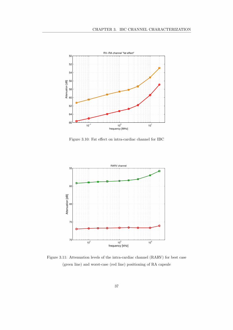
CHAPTER 3. IBC CHANNEL CHARACTERIZATION
10−1
100
101
50
52
54
56
58
60
62
64
66
RV−RA channel "fat effect"
frequency [MHz]
Attenuation [dB
]
Figure 3.10: Fat effect on intra-cardiac channel for IBC
102
103
104
55
60
65
70
75
RARV channel
frequency [kHz]
Att
en
ua
tio
n [
dB
]
Figure 3.11: Attenuation levels of the intra-cardiac channel (RARV) for best case
(green line) and worst-case (red line) positioning of RA capsule
37
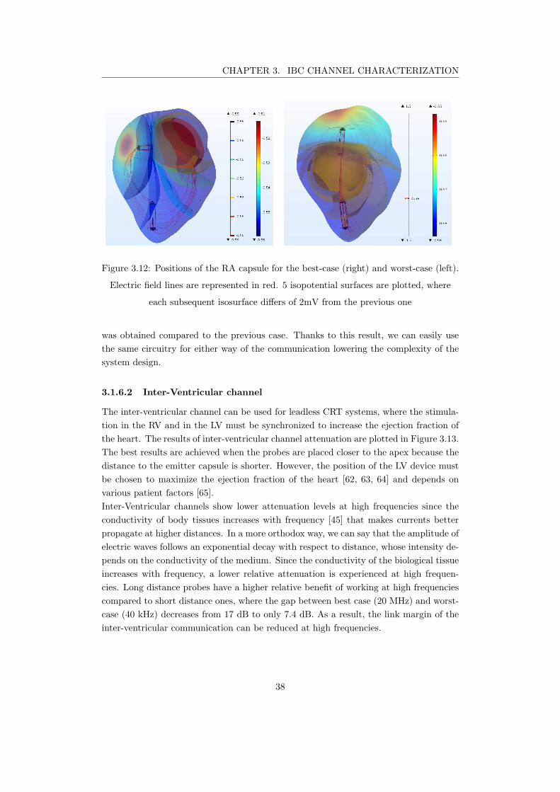
CHAPTER 3. IBC CHANNEL CHARACTERIZATION
Figure 3.12: Positions of the RA capsule for the best-case (right) and worst-case (left).
Electric field lines are represented in red. 5 isopotential surfaces are plotted, where
each subsequent isosurface differs of 2mV from the previous one
was obtained compared to the previous case. Thanks to this result, we can easily use
the same circuitry for either way of the communication lowering the complexity of the
system design.
3.1.6.2 Inter-Ventricular channel
The inter-ventricular channel can be used for leadless CRT systems, where the stimula-
tion in the RV and in the LV must be synchronized to increase the ejection fraction of
the heart. The results of inter-ventricular channel attenuation are plotted in Figure 3.13.
The best results are achieved when the probes are placed closer to the apex because the
distance to the emitter capsule is shorter. However, the position of the LV device must
be chosen to maximize the ejection fraction of the heart [62, 63, 64] and depends on
various patient factors [65].
Inter-Ventricular channels show lower attenuation levels at high frequencies since the
conductivity of body tissues increases with frequency [45] that makes currents better
propagate at higher distances. In a more orthodox way, we can say that the amplitude of
electric waves follows an exponential decay with respect to distance, whose intensity de-
pends on the conductivity of the medium. Since the conductivity of the biological tissue
increases with frequency, a lower relative attenuation is experienced at high frequen-
cies. Long distance probes have a higher relative benefit of working at high frequencies
compared to short distance ones, where the gap between best case (20 MHz) and worst-
case (40 kHz) decreases from 17 dB to only 7.4 dB. As a result, the link margin of the
inter-ventricular communication can be reduced at high frequencies.
38
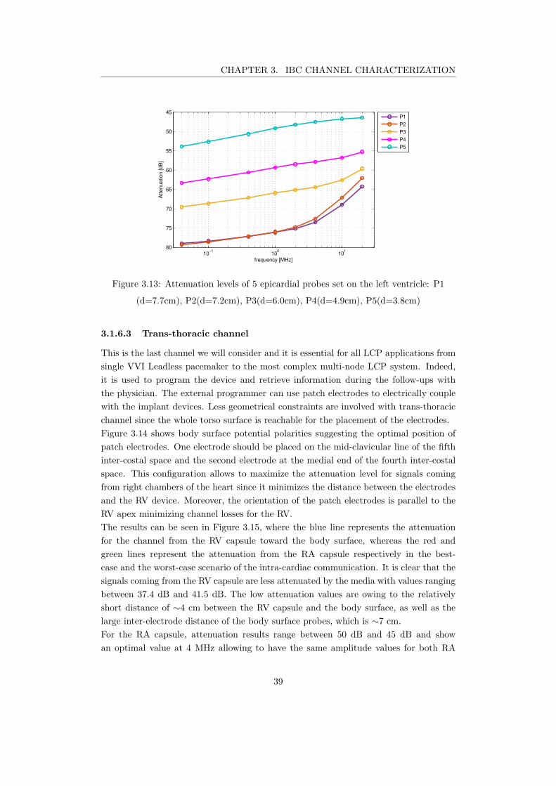
CHAPTER 3. IBC CHANNEL CHARACTERIZATION
10−1
100
101
45
50
55
60
65
70
75
80
frequency [MHz]
Att
en
ua
tio
n [
dB
]
P1
P2
P3
P4
P5
Figure 3.13: Attenuation levels of 5 epicardial probes set on the left ventricle: P1
(d=7.7cm), P2(d=7.2cm), P3(d=6.0cm), P4(d=4.9cm), P5(d=3.8cm)
3.1.6.3 Trans-thoracic channel
This is the last channel we will consider and it is essential for all LCP applications from
single VVI Leadless pacemaker to the most complex multi-node LCP system. Indeed,
it is used to program the device and retrieve information during the follow-ups with
the physician. The external programmer can use patch electrodes to electrically couple
with the implant devices. Less geometrical constraints are involved with trans-thoracic
channel since the whole torso surface is reachable for the placement of the electrodes.
Figure 3.14 shows body surface potential polarities suggesting the optimal position of
patch electrodes. One electrode should be placed on the mid-clavicular line of the fifth
inter-costal space and the second electrode at the medial end of the fourth inter-costal
space. This configuration allows to maximize the attenuation level for signals coming
from right chambers of the heart since it minimizes the distance between the electrodes
and the RV device. Moreover, the orientation of the patch electrodes is parallel to the
RV apex minimizing channel losses for the RV.
The results can be seen in Figure 3.15, where the blue line represents the attenuation
for the channel from the RV capsule toward the body surface, whereas the red and
green lines represent the attenuation from the RA capsule respectively in the best-
case and the worst-case scenario of the intra-cardiac communication. It is clear that the
signals coming from the RV capsule are less attenuated by the media with values ranging
between 37.4 dB and 41.5 dB. The low attenuation values are owing to the relatively
short distance of ∼4 cm between the RV capsule and the body surface, as well as the
large inter-electrode distance of the body surface probes, which is ∼7 cm.
For the RA capsule, attenuation results range between 50 dB and 45 dB and show
an optimal value at 4 MHz allowing to have the same amplitude values for both RA
39

CHAPTER 3. IBC CHANNEL CHARACTERIZATION
Figure 3.14: Graphical representation of simulation results for frequency equal to
40kHz, where both epicardial (rainbow color table) and body (thermal color table)
surface potentials are represented. Electric field line distribution is shown in red.
10−1
100
101
35
40
45
50
55
Trans−thoracic channel
frequency [MHz]
Att
en
ua
tio
n [
dB
]
RV
RA vert.
RA horz.
Figure 3.15: Attenuation levels of trans-thoracic channel having distance between RV
distal electrode and the body surface equal to 3.52cm
40
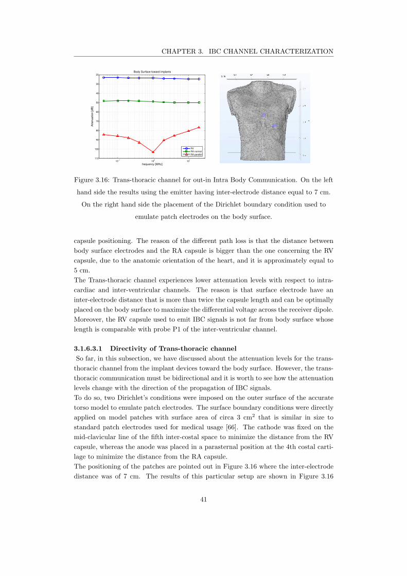
CHAPTER 3. IBC CHANNEL CHARACTERIZATION
10−1
100
101
20
30
40
50
60
70
80
90
100
110
Body Surface toward implants
frequency [MHz]
Attenuation [dB
]
RV
RA normal
RA parallel
Figure 3.16: Trans-thoracic channel for out-in Intra Body Communication. On the left
hand side the results using the emitter having inter-electrode distance equal to 7 cm.
On the right hand side the placement of the Dirichlet boundary condition used to
emulate patch electrodes on the body surface.
capsule positioning. The reason of the different path loss is that the distance between
body surface electrodes and the RA capsule is bigger than the one concerning the RV
capsule, due to the anatomic orientation of the heart, and it is approximately equal to
5 cm.
The Trans-thoracic channel experiences lower attenuation levels with respect to intra-
cardiac and inter-ventricular channels. The reason is that surface electrode have an
inter-electrode distance that is more than twice the capsule length and can be optimally
placed on the body surface to maximize the differential voltage across the receiver dipole.
Moreover, the RV capsule used to emit IBC signals is not far from body surface whose
length is comparable with probe P1 of the inter-ventricular channel.
3.1.6.3.1 Directivity of Trans-thoracic channel
So far, in this subsection, we have discussed about the attenuation levels for the trans-
thoracic channel from the implant devices toward the body surface. However, the trans-
thoracic communication must be bidirectional and it is worth to see how the attenuation
levels change with the direction of the propagation of IBC signals.
To do so, two Dirichlet’s conditions were imposed on the outer surface of the accurate
torso model to emulate patch electrodes. The surface boundary conditions were directly
applied on model patches with surface area of circa 3 cm2 that is similar in size to
standard patch electrodes used for medical usage [66]. The cathode was fixed on the
mid-clavicular line of the fifth inter-costal space to minimize the distance from the RV
capsule, whereas the anode was placed in a parasternal position at the 4th costal carti-
lage to minimize the distance from the RA capsule.
The positioning of the patches are pointed out in Figure 3.16 where the inter-electrode
distance was of 7 cm. The results of this particular setup are shown in Figure 3.16
41
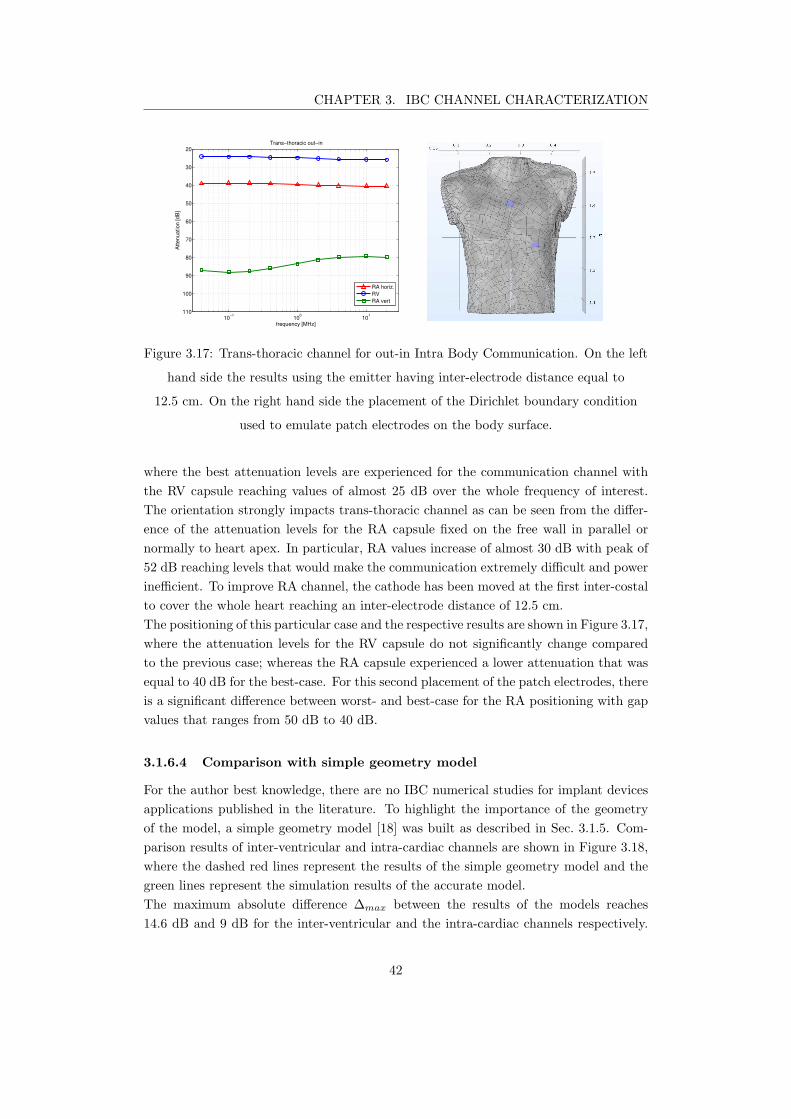
CHAPTER 3. IBC CHANNEL CHARACTERIZATION
10−1
100
101
20
30
40
50
60
70
80
90
100
110
Trans−thoracic out−in
frequency [MHz]
Attenuation [dB
]
RA horiz.
RV
RA vert
Figure 3.17: Trans-thoracic channel for out-in Intra Body Communication. On the left
hand side the results using the emitter having inter-electrode distance equal to
12.5 cm. On the right hand side the placement of the Dirichlet boundary condition
used to emulate patch electrodes on the body surface.
where the best attenuation levels are experienced for the communication channel with
the RV capsule reaching values of almost 25 dB over the whole frequency of interest.
The orientation strongly impacts trans-thoracic channel as can be seen from the differ-
ence of the attenuation levels for the RA capsule fixed on the free wall in parallel or
normally to heart apex. In particular, RA values increase of almost 30 dB with peak of
52 dB reaching levels that would make the communication extremely difficult and power
inefficient. To improve RA channel, the cathode has been moved at the first inter-costal
to cover the whole heart reaching an inter-electrode distance of 12.5 cm.
The positioning of this particular case and the respective results are shown in Figure 3.17,
where the attenuation levels for the RV capsule do not significantly change compared
to the previous case; whereas the RA capsule experienced a lower attenuation that was
equal to 40 dB for the best-case. For this second placement of the patch electrodes, there
is a significant difference between worst- and best-case for the RA positioning with gap
values that ranges from 50 dB to 40 dB.
3.1.6.4 Comparison with simple geometry model
For the author best knowledge, there are no IBC numerical studies for implant devices
applications published in the literature. To highlight the importance of the geometry
of the model, a simple geometry model [18] was built as described in Sec. 3.1.5. Com-
parison results of inter-ventricular and intra-cardiac channels are shown in Figure 3.18,
where the dashed red lines represent the results of the simple geometry model and the
green lines represent the simulation results of the accurate model.
The maximum absolute difference ∆max between the results of the models reaches
14.6 dB and 9 dB for the inter-ventricular and the intra-cardiac channels respectively.
42
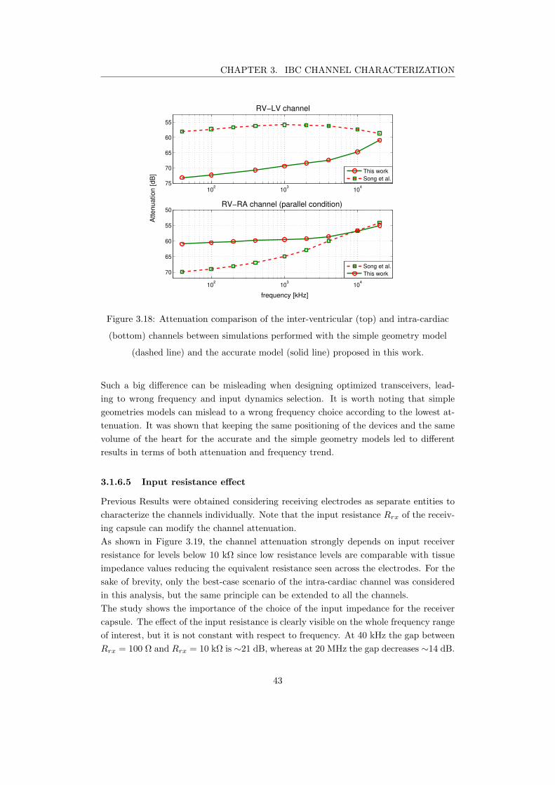
CHAPTER 3. IBC CHANNEL CHARACTERIZATION
102
103
104
55
60
65
70
75
RV−LV channel
frequency [kHz]
102
103
104
50
55
60
65
70
RV−RA channel (parallel condition)
Att
en
ua
tio
n [
dB
]
This work
Song et al.
Song et al.
This work
Figure 3.18: Attenuation comparison of the inter-ventricular (top) and intra-cardiac
(bottom) channels between simulations performed with the simple geometry model
(dashed line) and the accurate model (solid line) proposed in this work.
Such a big difference can be misleading when designing optimized transceivers, lead-
ing to wrong frequency and input dynamics selection. It is worth noting that simple
geometries models can mislead to a wrong frequency choice according to the lowest at-
tenuation. It was shown that keeping the same positioning of the devices and the same
volume of the heart for the accurate and the simple geometry models led to different
results in terms of both attenuation and frequency trend.
3.1.6.5 Input resistance effect
Previous Results were obtained considering receiving electrodes as separate entities to
characterize the channels individually. Note that the input resistance Rrx of the receiv-
ing capsule can modify the channel attenuation.
As shown in Figure 3.19, the channel attenuation strongly depends on input receiver
resistance for levels below 10 kΩ since low resistance levels are comparable with tissue
impedance values reducing the equivalent resistance seen across the electrodes. For the
sake of brevity, only the best-case scenario of the intra-cardiac channel was considered
in this analysis, but the same principle can be extended to all the channels.
The study shows the importance of the choice of the input impedance for the receiver
capsule. The effect of the input resistance is clearly visible on the whole frequency range
of interest, but it is not constant with respect to frequency. At 40 kHz the gap between
Rrx = 100 Ω and Rrx = 10 kΩ is ∼21 dB, whereas at 20 MHz the gap decreases ∼14 dB.
43
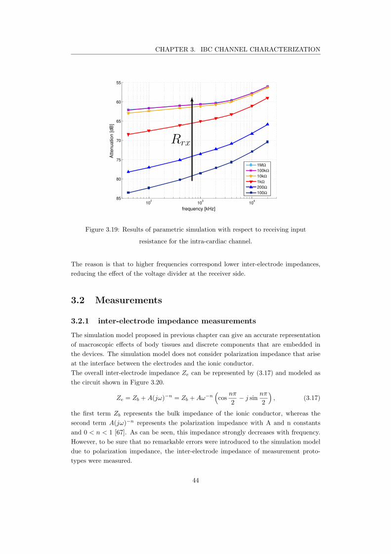
CHAPTER 3. IBC CHANNEL CHARACTERIZATION
102
103
104
55
60
65
70
75
80
85
frequency [kHz]
Att
en
ua
tio
n [
dB
]
1MΩ
100kΩ
10kΩ
1kΩ
200Ω
100Ω
Rrx
Figure 3.19: Results of parametric simulation with respect to receiving input
resistance for the intra-cardiac channel.
The reason is that to higher frequencies correspond lower inter-electrode impedances,
reducing the effect of the voltage divider at the receiver side.
3.2 Measurements
3.2.1 inter-electrode impedance measurements
The simulation model proposed in previous chapter can give an accurate representation
of macroscopic effects of body tissues and discrete components that are embedded in
the devices. The simulation model does not consider polarization impedance that arise
at the interface between the electrodes and the ionic conductor.
The overall inter-electrode impedance Ze can be represented by (3.17) and modeled as
the circuit shown in Figure 3.20.
Ze = Zb +A(jω)−n = Zb +Aω−n
(
cosnπ
2− j sin
nπ
2
)
, (3.17)
the first term Zb represents the bulk impedance of the ionic conductor, whereas the
second term A(jω)−n represents the polarization impedance with A and n constants
and 0 < n < 1 [67]. As can be seen, this impedance strongly decreases with frequency.
However, to be sure that no remarkable errors were introduced to the simulation model
due to polarization impedance, the inter-electrode impedance of measurement proto-
types were measured.
44
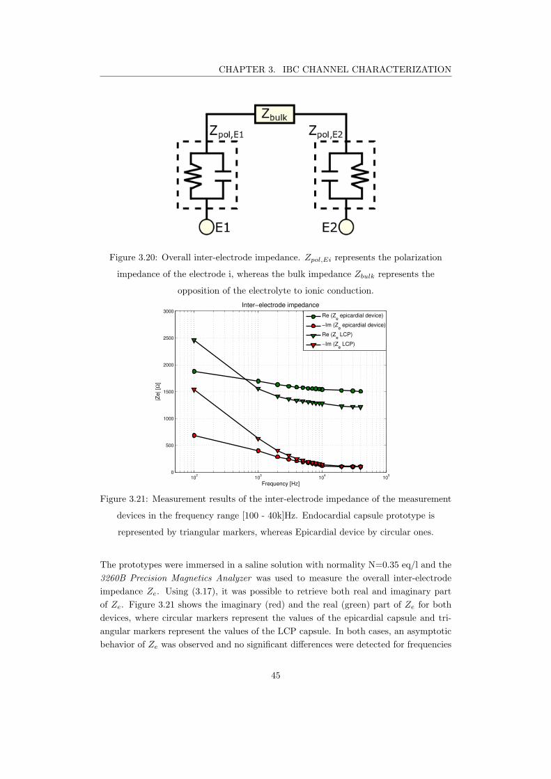
CHAPTER 3. IBC CHANNEL CHARACTERIZATION
Figure 3.20: Overall inter-electrode impedance. Zpol,Ei represents the polarization
impedance of the electrode i, whereas the bulk impedance Zbulk represents the
opposition of the electrolyte to ionic conduction.
102
103
104
105
0
500
1000
1500
2000
2500
3000
Inter−electrode impedance
Frequency [Hz]
|Ze| [Ω
]
Re (Z
e epicardial device)
−Im (Ze epicardial device)
Re (Ze LCP)
−Im (Ze LCP)
Figure 3.21: Measurement results of the inter-electrode impedance of the measurement
devices in the frequency range [100 - 40k]Hz. Endocardial capsule prototype is
represented by triangular markers, whereas Epicardial device by circular ones.
The prototypes were immersed in a saline solution with normality N=0.35 eq/l and the
3260B Precision Magnetics Analyzer was used to measure the overall inter-electrode
impedance Ze. Using (3.17), it was possible to retrieve both real and imaginary part
of Ze. Figure 3.21 shows the imaginary (red) and the real (green) part of Ze for both
devices, where circular markers represent the values of the epicardial capsule and tri-
angular markers represent the values of the LCP capsule. In both cases, an asymptotic
behavior of Ze was observed and no significant differences were detected for frequencies
45
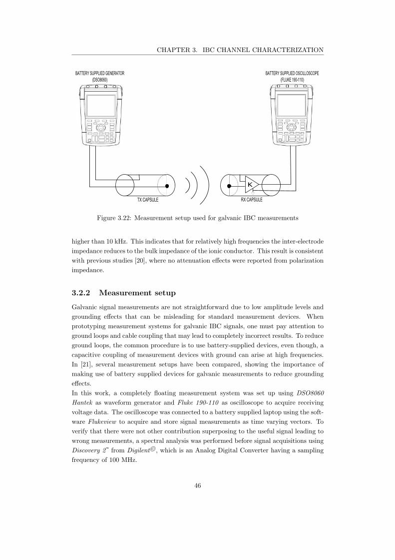
CHAPTER 3. IBC CHANNEL CHARACTERIZATION
K
TX CAPSULE RX CAPSULE
BATTERY SUPPLIED GENERATOR
(DSO8060)
BATTERY SUPPLIED OSCILLOSCOPE
(FLUKE 190-110)
Figure 3.22: Measurement setup used for galvanic IBC measurements
higher than 10 kHz. This indicates that for relatively high frequencies the inter-electrode
impedance reduces to the bulk impedance of the ionic conductor. This result is consistent
with previous studies [20], where no attenuation effects were reported from polarization
impedance.
3.2.2 Measurement setup
Galvanic signal measurements are not straightforward due to low amplitude levels and
grounding effects that can be misleading for standard measurement devices. When
prototyping measurement systems for galvanic IBC signals, one must pay attention to
ground loops and cable coupling that may lead to completely incorrect results. To reduce
ground loops, the common procedure is to use battery-supplied devices, even though, a
capacitive coupling of measurement devices with ground can arise at high frequencies.
In [21], several measurement setups have been compared, showing the importance of
making use of battery supplied devices for galvanic measurements to reduce grounding
effects.
In this work, a completely floating measurement system was set up using DSO8060
Hantek as waveform generator and Fluke 190-110 as oscilloscope to acquire receiving
voltage data. The oscilloscope was connected to a battery supplied laptop using the soft-
ware Flukeview to acquire and store signal measurements as time varying vectors. To
verify that there were not other contribution superposing to the useful signal leading to
wrong measurements, a spectral analysis was performed before signal acquisitions using
Discovery 2™ from Digilent©, which is an Analog Digital Converter having a sampling
frequency of 100 MHz.
46
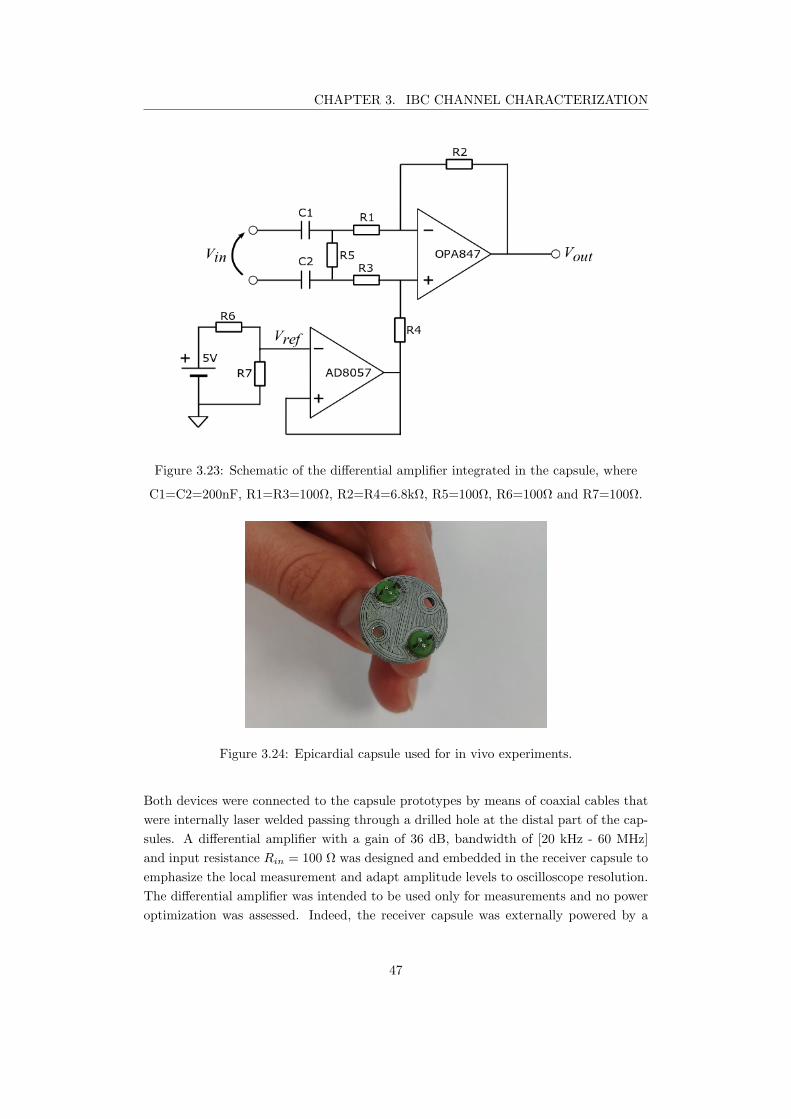
CHAPTER 3. IBC CHANNEL CHARACTERIZATION
Figure 3.23: Schematic of the differential amplifier integrated in the capsule, where
C1=C2=200nF, R1=R3=100Ω, R2=R4=6.8kΩ, R5=100Ω, R6=100Ω and R7=100Ω.
Figure 3.24: Epicardial capsule used for in vivo experiments.
Both devices were connected to the capsule prototypes by means of coaxial cables that
were internally laser welded passing through a drilled hole at the distal part of the cap-
sules. A differential amplifier with a gain of 36 dB, bandwidth of [20 kHz - 60 MHz]
and input resistance Rin = 100 Ω was designed and embedded in the receiver capsule to
emphasize the local measurement and adapt amplitude levels to oscilloscope resolution.
The differential amplifier was intended to be used only for measurements and no power
optimization was assessed. Indeed, the receiver capsule was externally powered by a
47
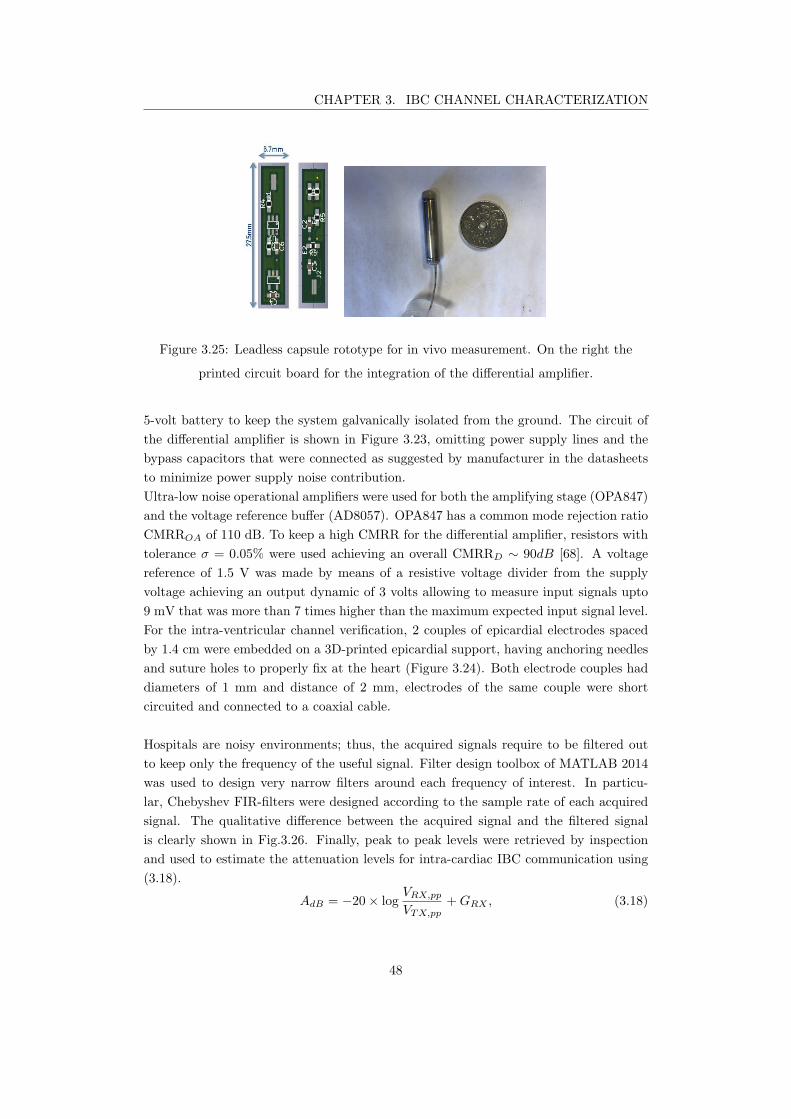
CHAPTER 3. IBC CHANNEL CHARACTERIZATION
Figure 3.25: Leadless capsule rototype for in vivo measurement. On the right the
printed circuit board for the integration of the differential amplifier.
5-volt battery to keep the system galvanically isolated from the ground. The circuit of
the differential amplifier is shown in Figure 3.23, omitting power supply lines and the
bypass capacitors that were connected as suggested by manufacturer in the datasheets
to minimize power supply noise contribution.
Ultra-low noise operational amplifiers were used for both the amplifying stage (OPA847)
and the voltage reference buffer (AD8057). OPA847 has a common mode rejection ratio
CMRROA of 110 dB. To keep a high CMRR for the differential amplifier, resistors with
tolerance σ = 0.05% were used achieving an overall CMRRD ∼ 90dB [68]. A voltage
reference of 1.5 V was made by means of a resistive voltage divider from the supply
voltage achieving an output dynamic of 3 volts allowing to measure input signals upto
9 mV that was more than 7 times higher than the maximum expected input signal level.
For the intra-ventricular channel verification, 2 couples of epicardial electrodes spaced
by 1.4 cm were embedded on a 3D-printed epicardial support, having anchoring needles
and suture holes to properly fix at the heart (Figure 3.24). Both electrode couples had
diameters of 1 mm and distance of 2 mm, electrodes of the same couple were short
circuited and connected to a coaxial cable.
Hospitals are noisy environments; thus, the acquired signals require to be filtered out
to keep only the frequency of the useful signal. Filter design toolbox of MATLAB 2014
was used to design very narrow filters around each frequency of interest. In particu-
lar, Chebyshev FIR-filters were designed according to the sample rate of each acquired
signal. The qualitative difference between the acquired signal and the filtered signal
is clearly shown in Fig.3.26. Finally, peak to peak levels were retrieved by inspection
and used to estimate the attenuation levels for intra-cardiac IBC communication using
(3.18).
AdB = −20× logVRX,pp
VTX,pp
+GRX , (3.18)
48
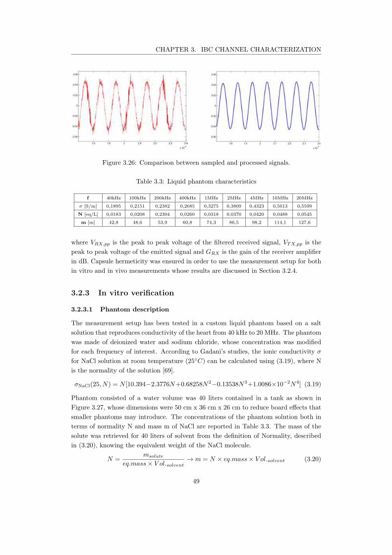
CHAPTER 3. IBC CHANNEL CHARACTERIZATION
Figure 3.26: Comparison between sampled and processed signals.
Table 3.3: Liquid phantom characteristics
f 40kHz 100kHz 200kHz 400kHz 1MHz 2MHz 4MHz 10MHz 20MHz
σ [S/m] 0,1895 0,2151 0,2382 0,2685 0,3275 0,3809 0,4323 0,5013 0,5599
N [eq/L] 0,0183 0,0208 0,2304 0,0260 0,0318 0,0370 0,0420 0,0488 0,0545
m [m] 42,8 48,6 53,9 60,8 74,3 86,5 98,2 114,1 127,6
where VRX,pp is the peak to peak voltage of the filtered received signal, VTX,pp is the
peak to peak voltage of the emitted signal and GRX is the gain of the receiver amplifier
in dB. Capsule hermeticity was ensured in order to use the measurement setup for both
in vitro and in vivo measurements whose results are discussed in Section 3.2.4.
3.2.3 In vitro verification
3.2.3.1 Phantom description
The measurement setup has been tested in a custom liquid phantom based on a salt
solution that reproduces conductivity of the heart from 40 kHz to 20 MHz. The phantom
was made of deionized water and sodium chloride, whose concentration was modified
for each frequency of interest. According to Gadani’s studies, the ionic conductivity σ
for NaCl solution at room temperature (25C) can be calculated using (3.19), where N
is the normality of the solution [69].
σNaCl(25, N) = N [10.394−2.3776N+0.68258N2−0.13538N3+1.0086×10⁻²N4] (3.19)
Phantom consisted of a water volume was 40 liters contained in a tank as shown in
Figure 3.27, whose dimensions were 50 cm x 36 cm x 26 cm to reduce board effects that
smaller phantoms may introduce. The concentrations of the phantom solution both in
terms of normality N and mass m of NaCl are reported in Table 3.3. The mass of the
solute was retrieved for 40 liters of solvent from the definition of Normality, described
in (3.20), knowing the equivalent weight of the NaCl molecule.
N =msolute
eq.mass× V ol.solvent→ m = N × eq.mass× V ol.solvent (3.20)
49

CHAPTER 3. IBC CHANNEL CHARACTERIZATION
Figure 3.27: Custom phantom used for preliminary verification. Dimension of the tank
were 50 cm x 36 cm x 26 cm containing 40 l of solution.
Emitter and receiver capsules were set at a distance of 3 cm between their respective
medium points in parallel orientation to maximize sensed voltages.
The phantom has been reproduced and simulated in COMSOL Multiphysics in order
to verify the reliability of the measurement setup. The input resistance of the receiv-
ing capsule Rrx has been added to the model using the Electrical Circuit module as
previously described in Section 3.1.5.
3.2.3.2 Verification result
In vitro measurements were performed to verify the reliability of the measurement setup.
Figure 3.29 compares measured attenuation levels of parallel capsules with channel
length distance set equal to 3 cm with simulated results. The measurement values
are in the range of [67.5-57]dB with maximum absolute error ∆max of 3 dB with respect
to simulations, which is 15 dB lower than phantom measurement proposed for body sur-
face galvanic IBC [21]. Those measurements were performed in a homogeneous medium
and cannot replicate in vivo measurements accurately. In a real case scenario, signals
might benefit of border effects that will arise from the shape of the heart and due to the
different properties of contact tissue of each electrode pair.
50
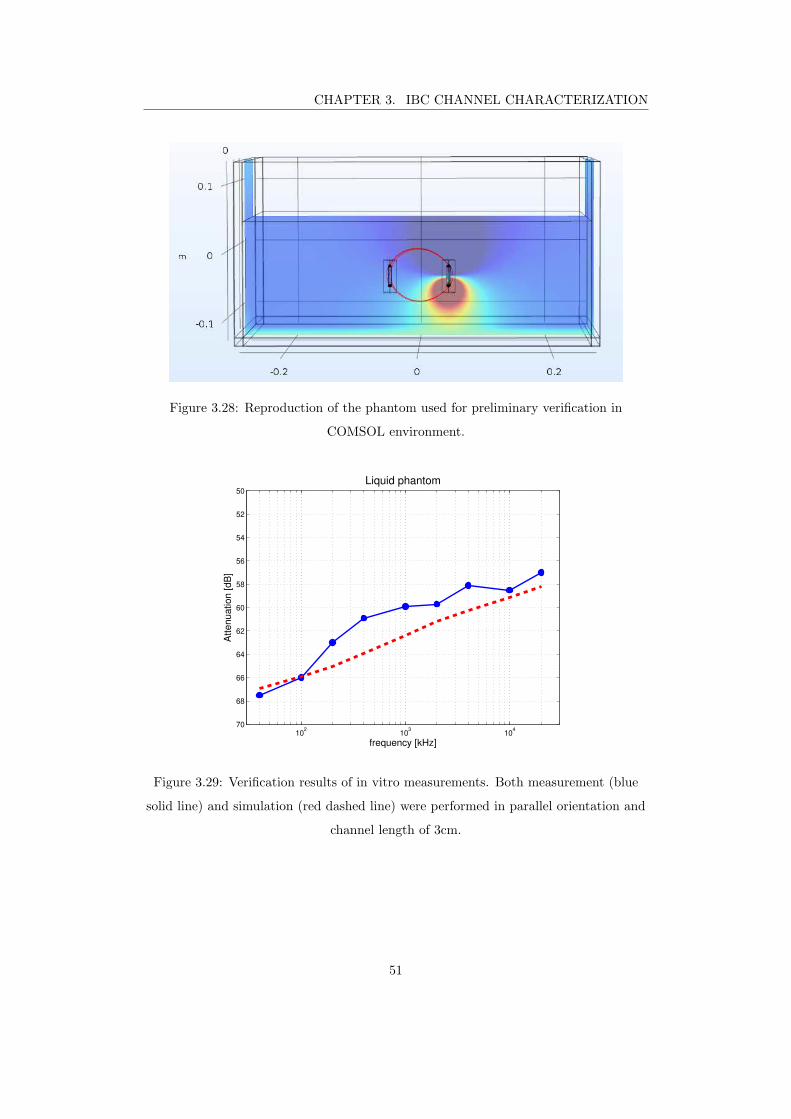
CHAPTER 3. IBC CHANNEL CHARACTERIZATION
Figure 3.28: Reproduction of the phantom used for preliminary verification in
COMSOL environment.
102
103
104
50
52
54
56
58
60
62
64
66
68
70
Liquid phantom
frequency [kHz]
Att
en
ua
tio
n [
dB
]
Figure 3.29: Verification results of in vitro measurements. Both measurement (blue
solid line) and simulation (red dashed line) were performed in parallel orientation and
channel length of 3cm.
51
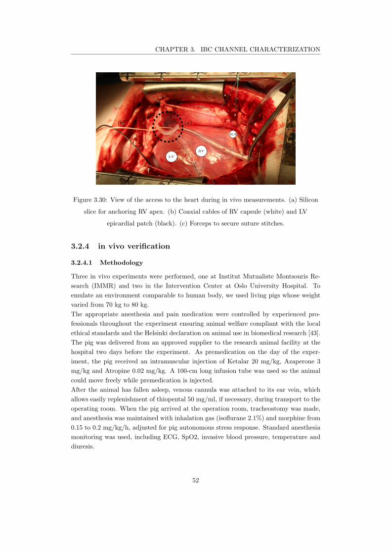
CHAPTER 3. IBC CHANNEL CHARACTERIZATION
(a)(b) (c)
LV
RV
RA
Figure 3.30: View of the access to the heart during in vivo measurements. (a) Silicon
slice for anchoring RV apex. (b) Coaxial cables of RV capsule (white) and LV
epicardial patch (black). (c) Forceps to secure suture stitches.
3.2.4 in vivo verification
3.2.4.1 Methodology
Three in vivo experiments were performed, one at Institut Mutualiste Montsouris Re-
search (IMMR) and two in the Intervention Center at Oslo University Hospital. To
emulate an environment comparable to human body, we used living pigs whose weight
varied from 70 kg to 80 kg.
The appropriate anesthesia and pain medication were controlled by experienced pro-
fessionals throughout the experiment ensuring animal welfare compliant with the local
ethical standards and the Helsinki declaration on animal use in biomedical research [43].
The pig was delivered from an approved supplier to the research animal facility at the
hospital two days before the experiment. As premedication on the day of the exper-
iment, the pig received an intramuscular injection of Ketalar 20 mg/kg, Azaperone 3
mg/kg and Atropine 0.02 mg/kg. A 100-cm long infusion tube was used so the animal
could move freely while premedication is injected.
After the animal has fallen asleep, venous cannula was attached to its ear vein, which
allows easily replenishment of thiopental 50 mg/ml, if necessary, during transport to the
operating room. When the pig arrived at the operation room, tracheostomy was made,
and anesthesia was maintained with inhalation gas (isoflurane 2.1%) and morphine from
0.15 to 0.2 mg/kg/h, adjusted for pig autonomous stress response. Standard anesthesia
monitoring was used, including ECG, SpO2, invasive blood pressure, temperature and
diuresis.
52
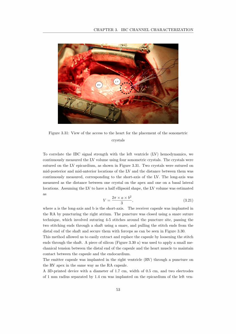
CHAPTER 3. IBC CHANNEL CHARACTERIZATION
LV
RV
Figure 3.31: View of the access to the heart for the placement of the sonometric
crystals
To correlate the IBC signal strength with the left ventricle (LV) hemodynamics, we
continuously measured the LV volume using four sonometric crystals. The crystals were
sutured on the LV epicardium, as shown in Figure 3.31. Two crystals were sutured on
mid-posterior and mid-anterior locations of the LV and the distance between them was
continuously measured, corresponding to the short-axis of the LV. The long-axis was
measured as the distance between one crystal on the apex and one on a basal lateral
locations. Assuming the LV to have a half ellipsoid shape, the LV volume was estimated
as
V =2π × a× b2
3, (3.21)
where a is the long-axis and b is the short-axis. The receiver capsule was implanted in
the RA by puncturing the right atrium. The puncture was closed using a snare suture
technique, which involved suturing 4-5 stitches around the puncture site, passing the
two stitching ends through a shaft using a snare, and pulling the stitch ends from the
distal end of the shaft and secure them with forceps as can be seen in Figure 3.30.
This method allowed us to easily extract and replace the capsule by loosening the stitch
ends through the shaft. A piece of silicon (Figure 3.30 a) was used to apply a small me-
chanical tension between the distal end of the capsule and the heart muscle to maintain
contact between the capsule and the endocardium.
The emitter capsule was implanted in the right ventricle (RV) through a puncture on
the RV apex in the same way as the RA capsule.
A 3D-printed device with a diameter of 1.7 cm, width of 0.5 cm, and two electrodes
of 1 mm radius separated by 1.4 cm was implanted on the epicardium of the left ven-
53
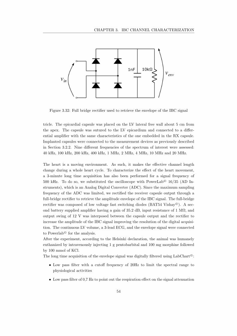
CHAPTER 3. IBC CHANNEL CHARACTERIZATION
Figure 3.32: Full bridge rectifier used to retrieve the envelope of the IBC signal
tricle. The epicardial capsule was placed on the LV lateral free wall about 5 cm from
the apex. The capsule was sutured to the LV epicardium and connected to a differ-
ential amplifier with the same characteristics of the one embedded in the RX capsule.
Implanted capsules were connected to the measurement devices as previously described
in Section 3.2.2. Nine different frequencies of the spectrum of interest were assessed:
40 kHz, 100 kHz, 200 kHz, 400 kHz, 1 MHz, 2 MHz, 4 MHz, 10 MHz and 20 MHz.
The heart is a moving environment. As such, it makes the effective channel length
change during a whole heart cycle. To characterize the effect of the heart movement,
a 3-minute long time acquisition has also been performed for a signal frequency of
500 kHz. To do so, we substituted the oscilloscope with PowerLab© 16/35 (AD In-
struments), which is an Analog Digital Converter (ADC). Since the maximum sampling
frequency of the ADC was limited, we rectified the receiver capsule output through a
full-bridge rectifier to retrieve the amplitude envelope of the IBC signal. The full-bridge
rectifier was composed of low voltage fast switching diodes (BAT54 Vishay©). A sec-
ond battery supplied amplifier having a gain of 35.2 dB, input resistance of 1 MΩ, and
output swing of 12 V was interposed between the capsule output and the rectifier to
increase the amplitude of the IBC signal improving the resolution of the digital acquisi-
tion. The continuous LV volume, a 3-lead ECG, and the envelope signal were connected
to Powerlab© for the analysis.
After the experiment, according to the Helsinki declaration, the animal was humanely
euthanized by intravenously injecting 1 g pentobarbital and 100 mg morphine followed
by 100 mmol of KCl.
The long time acquisition of the envelope signal was digitally filtered using LabChart©:
• Low pass filter with a cutoff frequency of 20Hz to limit the spectral range to
physiological activities
• Low pass filter of 0,7 Hz to point out the respiration effect on the signal attenuation
54
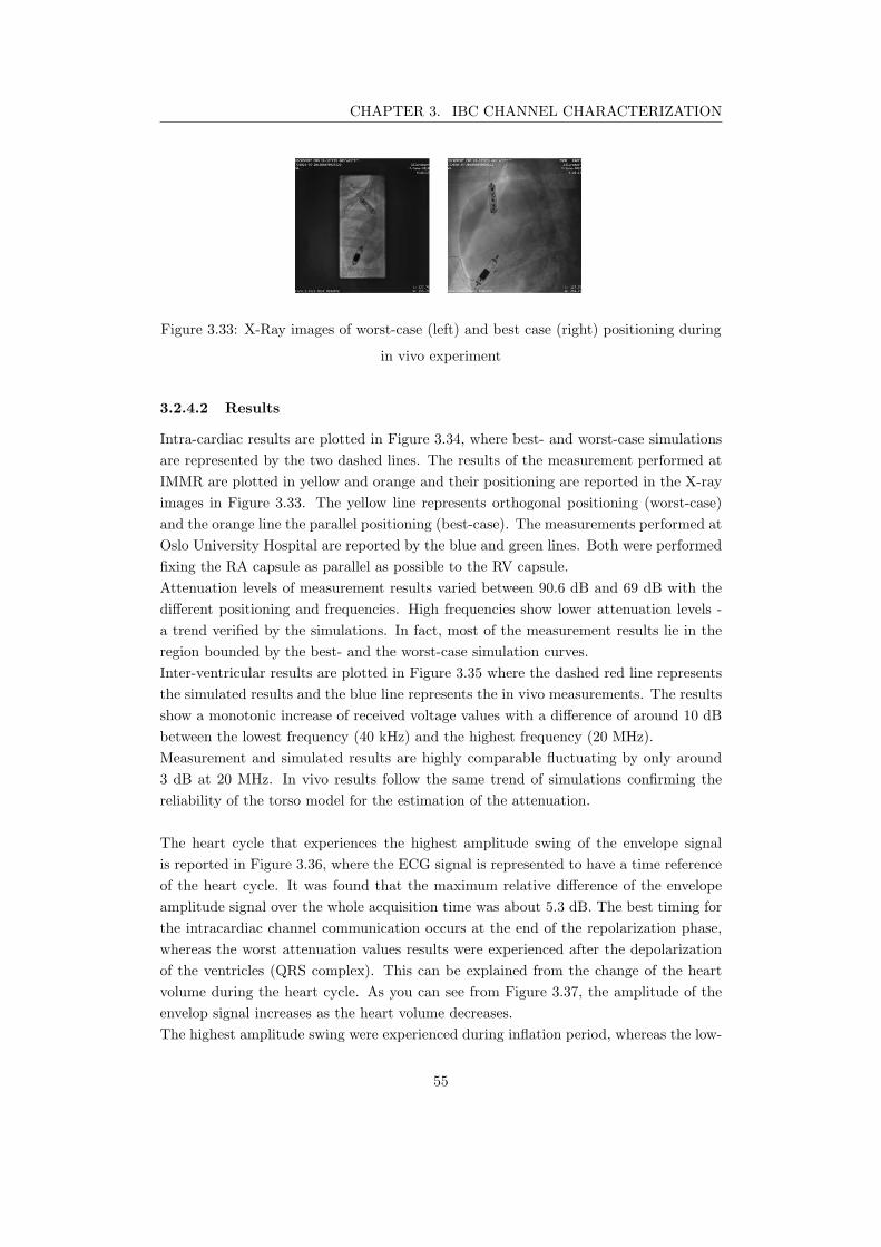
CHAPTER 3. IBC CHANNEL CHARACTERIZATION
Figure 3.33: X-Ray images of worst-case (left) and best case (right) positioning during
in vivo experiment
3.2.4.2 Results
Intra-cardiac results are plotted in Figure 3.34, where best- and worst-case simulations
are represented by the two dashed lines. The results of the measurement performed at
IMMR are plotted in yellow and orange and their positioning are reported in the X-ray
images in Figure 3.33. The yellow line represents orthogonal positioning (worst-case)
and the orange line the parallel positioning (best-case). The measurements performed at
Oslo University Hospital are reported by the blue and green lines. Both were performed
fixing the RA capsule as parallel as possible to the RV capsule.
Attenuation levels of measurement results varied between 90.6 dB and 69 dB with the
different positioning and frequencies. High frequencies show lower attenuation levels -
a trend verified by the simulations. In fact, most of the measurement results lie in the
region bounded by the best- and the worst-case simulation curves.
Inter-ventricular results are plotted in Figure 3.35 where the dashed red line represents
the simulated results and the blue line represents the in vivo measurements. The results
show a monotonic increase of received voltage values with a difference of around 10 dB
between the lowest frequency (40 kHz) and the highest frequency (20 MHz).
Measurement and simulated results are highly comparable fluctuating by only around
3 dB at 20 MHz. In vivo results follow the same trend of simulations confirming the
reliability of the torso model for the estimation of the attenuation.
The heart cycle that experiences the highest amplitude swing of the envelope signal
is reported in Figure 3.36, where the ECG signal is represented to have a time reference
of the heart cycle. It was found that the maximum relative difference of the envelope
amplitude signal over the whole acquisition time was about 5.3 dB. The best timing for
the intracardiac channel communication occurs at the end of the repolarization phase,
whereas the worst attenuation values results were experienced after the depolarization
of the ventricles (QRS complex). This can be explained from the change of the heart
volume during the heart cycle. As you can see from Figure 3.37, the amplitude of the
envelop signal increases as the heart volume decreases.
The highest amplitude swing were experienced during inflation period, whereas the low-
55
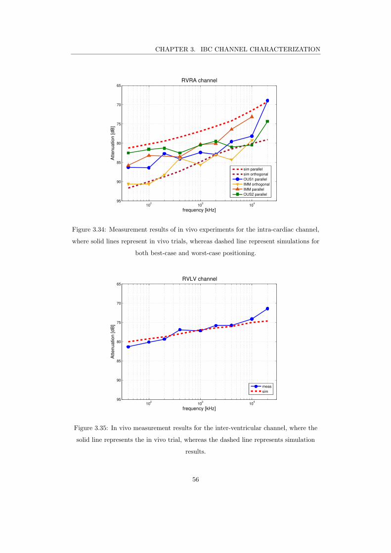
CHAPTER 3. IBC CHANNEL CHARACTERIZATION
102
103
104
65
70
75
80
85
90
95
RVRA channel
frequency [kHz]
Att
en
ua
tio
n [
dB
]
sim parallel
sim orthogonal
OUS1 parallel
IMM orthogonal
IMM parallel
OUS2 parallel
Figure 3.34: Measurement results of in vivo experiments for the intra-cardiac channel,
where solid lines represent in vivo trials, whereas dashed line represent simulations for
both best-case and worst-case positioning.
102
103
104
65
70
75
80
85
90
95
RVLV channel
frequency [kHz]
Att
en
ua
tio
n [
dB
]
meas
sim
Figure 3.35: In vivo measurement results for the inter-ventricular channel, where the
solid line represents the in vivo trial, whereas the dashed line represents simulation
results.
56
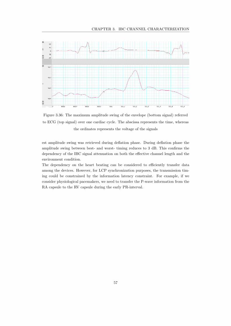
CHAPTER 3. IBC CHANNEL CHARACTERIZATION
Figure 3.36: The maximum amplitude swing of the envelope (bottom signal) referred
to ECG (top signal) over one cardiac cycle. The abscissa represents the time, whereas
the ordinates represents the voltage of the signals
est amplitude swing was retrieved during deflation phase. During deflation phase the
amplitude swing between best- and worst- timing reduces to 3 dB. This confirms the
dependency of the IBC signal attenuation on both the effective channel length and the
environment condition.
The dependency on the heart beating can be considered to efficiently transfer data
among the devices. However, for LCP synchronization purposes, the transmission tim-
ing could be constrained by the information latency constraint. For example, if we
consider physiological pacemakers, we need to transfer the P-wave information from the
RA capsule to the RV capsule during the early PR-interval.
57
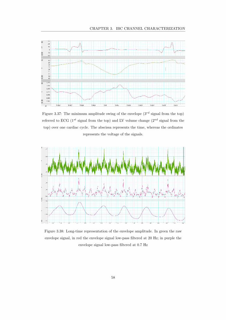
CHAPTER 3. IBC CHANNEL CHARACTERIZATION
Figure 3.37: The minimum amplitude swing of the envelope (3rd signal from the top)
referred to ECG (1st signal from the top) and LV volume change (2nd signal from the
top) over one cardiac cycle. The abscissa represents the time, whereas the ordinates
represents the voltage of the signals.
Figure 3.38: Long-time representation of the envelope amplitude. In green the raw
envelope signal, in red the envelope signal low-pass filtered at 20 Hz; in purple the
envelope signal low-pass filtered at 0.7 Hz
58
CHAPTER 3. IBC CHANNEL CHARACTERIZATION
3.3 Discussion
The simulations performed in this work highlight the need for accurate models to char-
acterize galvanic intra-body communication channels for deep-implant devices. It was
shown that the accurate and the simple geometry models led to different results in
terms of both attenuation and frequency trend. Even though the heart anatomy changes
among the population, accurate model showed to better follow in vivo frequency trends.
Multi-nodal LCP systems need to communicate with different devices set in different
positions leading to completely different channels. We estimated through simulations
the attenuation levels for all the channels involved in a CRT-leadless system.
The attenuation levels of the trans-thoracic channel are much lower than cardiac ones.
The reason is that the surface electrodes can be optimally placed on the body surface
to maximize the differential voltage across the receiver dipole. The mutual orientation
between emitter and receiver strongly impact the signal attenuation. Nevertheless, the
communication must be possible for any implant positioning.
Worst and best-case conditions were identified for the intra-cardiac channel. The at-
tenuation variability according to positioning can be used to set the link margin of the
channel considering the worst-case scenario and design a receiver whose specifications
allow demodulating data either way. For the intra-ventricular channel, it was found that
the link margin reduces at high frequency. The reason is that longer channels experience
higher attenuation and have higher relative benefits of working at frequencies resulting
in higher conductivity of tissues.
The simulation model has been verified using a galvanically isolated measurement system
using capsule prototypes having the same size as the simulated capsules. To verify the
coherence between the simulation environment and the suggested measurement setup,
we compared in-vitro measurements with simulation results. To do so, we have used
an NaCl-solution whose concentration was adapted to follow the frequency trend of the
heart conductivity. This technique allows predicting attenuation difference due to con-
ductivity variation and made possible the verification of the simulation approach, but
it cannot replace in vivo experiment due to the homogeneity of the phantom.
In vivo experiments verified the effect of RA capsule positioning since almost the same
difference was found between worst- and best-case between measurement and simula-
tions. The difference of the pointwise results between in vivo measurement and simula-
tion can be explained by the different morphology of the heart and the error introduced
from the measurement system and the quasi-static approximation.
The evolution of the IBC signals has been monitored over the whole cardiac cycle show-
ing the influence of the movement of the heart to attenuation values. Furthermore, it
was shown that close physiologic changes can impact the propagation of the IBC sig-
nals. In particular, it was shown that the attenuation of the intracardiac channel is also
impacted by the respiration. The lowest attenuation was experienced during inflation
phase, when the lungs are filled with air lowering the overall conductivity of lung tissue
59
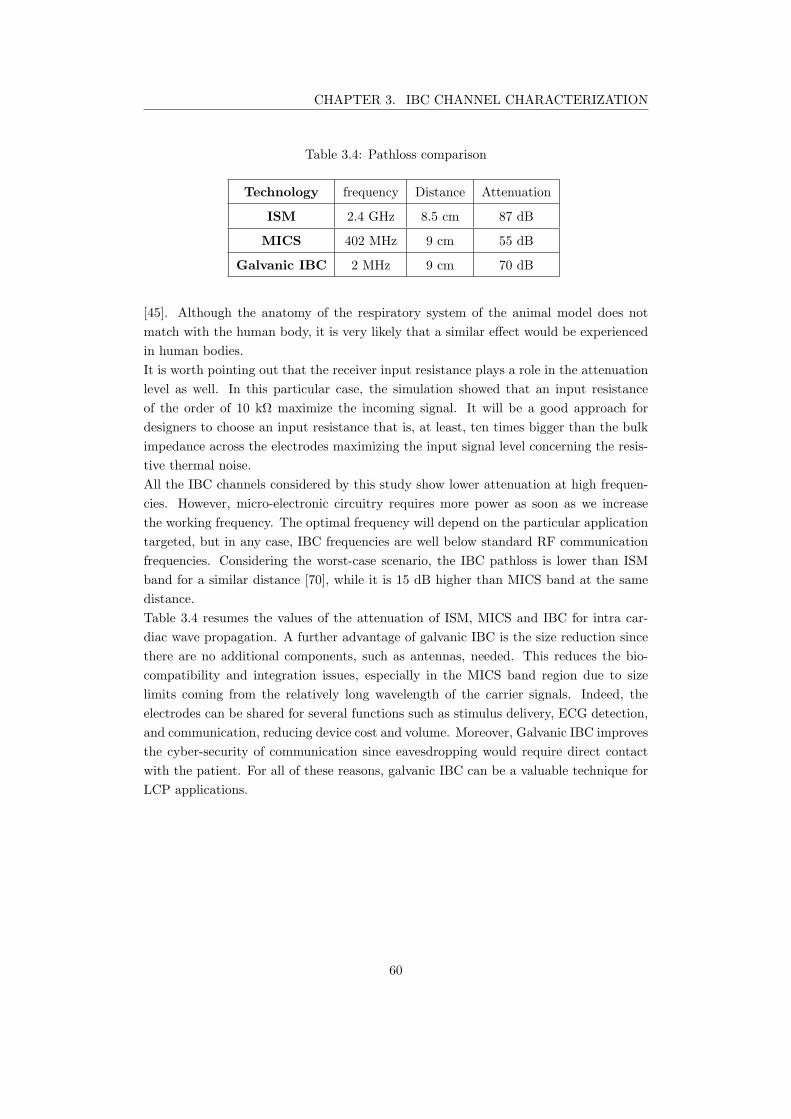
CHAPTER 3. IBC CHANNEL CHARACTERIZATION
Table 3.4: Pathloss comparison
Technology frequency Distance Attenuation
ISM 2.4 GHz 8.5 cm 87 dB
MICS 402 MHz 9 cm 55 dB
Galvanic IBC 2 MHz 9 cm 70 dB
[45]. Although the anatomy of the respiratory system of the animal model does not
match with the human body, it is very likely that a similar effect would be experienced
in human bodies.
It is worth pointing out that the receiver input resistance plays a role in the attenuation
level as well. In this particular case, the simulation showed that an input resistance
of the order of 10 kΩ maximize the incoming signal. It will be a good approach for
designers to choose an input resistance that is, at least, ten times bigger than the bulk
impedance across the electrodes maximizing the input signal level concerning the resis-
tive thermal noise.
All the IBC channels considered by this study show lower attenuation at high frequen-
cies. However, micro-electronic circuitry requires more power as soon as we increase
the working frequency. The optimal frequency will depend on the particular application
targeted, but in any case, IBC frequencies are well below standard RF communication
frequencies. Considering the worst-case scenario, the IBC pathloss is lower than ISM
band for a similar distance [70], while it is 15 dB higher than MICS band at the same
distance.
Table 3.4 resumes the values of the attenuation of ISM, MICS and IBC for intra car-
diac wave propagation. A further advantage of galvanic IBC is the size reduction since
there are no additional components, such as antennas, needed. This reduces the bio-
compatibility and integration issues, especially in the MICS band region due to size
limits coming from the relatively long wavelength of the carrier signals. Indeed, the
electrodes can be shared for several functions such as stimulus delivery, ECG detection,
and communication, reducing device cost and volume. Moreover, Galvanic IBC improves
the cyber-security of communication since eavesdropping would require direct contact
with the patient. For all of these reasons, galvanic IBC can be a valuable technique for
LCP applications.
60
4Ultra-Low-Power transceiver
The characterization of the channel attenuation for Leadless pacemaker applications de-
scribed in Chapter 3 was an essential step for the design of power-optimized transceivers.
Hereafter, we will consider only the synchronization issue of multi-node leadless pace-
makers since it is the most critical communication in terms of average power consump-
tion. Indeed, synchronization among capsules must occur each cardiac cycle to adapt
the timing of the therapy stimuli according to the spontaneous activity of the heart. In
particular, the transceiver must be able to send cardiac event detection information from
one capsule implanted in a first chamber of the patient heart to another capsule that is
implanted in a neighbor chamber of the multi-LCP system. The cardiac event informa-
tion will be used by the receiver capsule to trigger the therapy according to the other
chamber activity. This information must occur each cardiac cycle for the whole device
lifetime; thus it requires an ultra-low-power technique to minimize the power budget
of the wireless communication. In the following section, we specify the constraints of
the intra-cardiac channel for leadless pacemakers using galvanic IBC. Then, we point
out a convenient ultra-low power receiver architecture, the Super-Regenerative Receiver,
which can sustain the high sensitivity constraint that this kind of application requires.
Finally, a CMOS design tailored to fit the specification is proposed.
4.1 Transceiver requirements
In this section, we consider the main characteristics of the transceiver separately, eval-
uating the maximum acceptable values for each of them.
4.1.1 Average current consumption
Leadless Cardiac Pacemakers are limited in size, reducing the battery capacity, which
ranges in [120 - 248]mAh [36, 71]. Nevertheless, LCP lifetime must be ensured for several
years to reduce surgical operation required to replace the exhausted device with a new
61
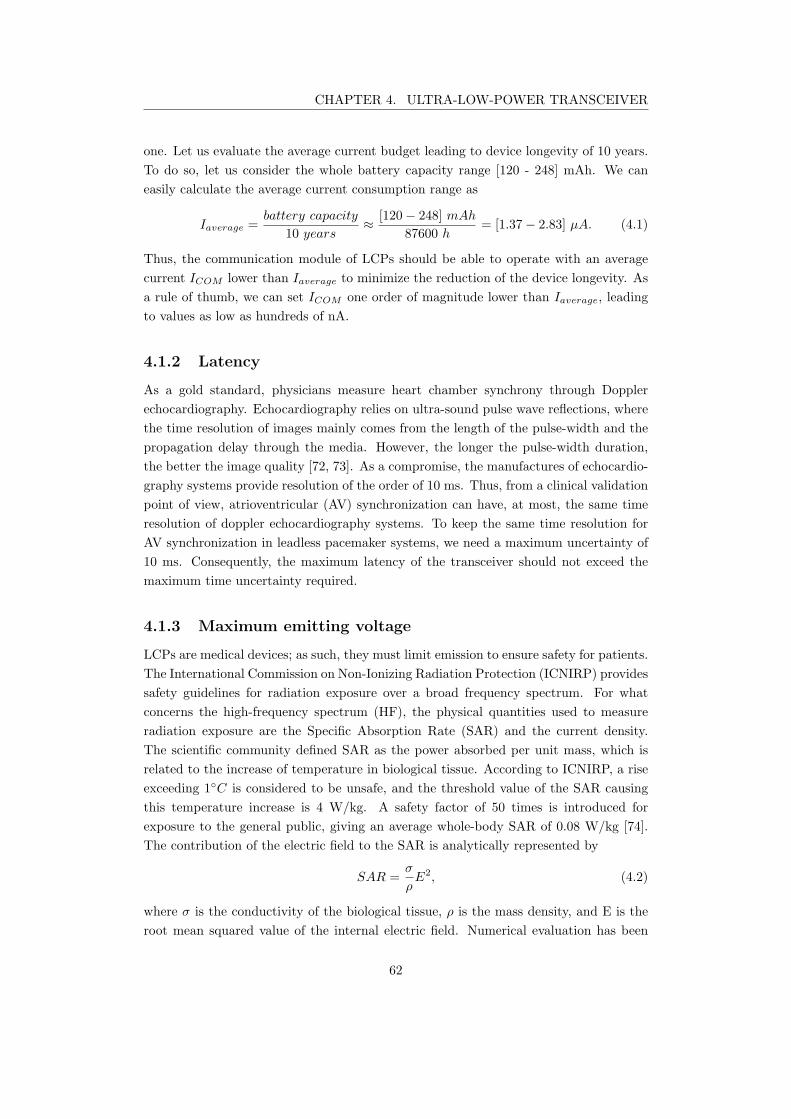
CHAPTER 4. ULTRA-LOW-POWER TRANSCEIVER
one. Let us evaluate the average current budget leading to device longevity of 10 years.
To do so, let us consider the whole battery capacity range [120 - 248] mAh. We can
easily calculate the average current consumption range as
Iaverage =battery capacity
10 years≈
[120− 248] mAh
87600 h= [1.37− 2.83] µA. (4.1)
Thus, the communication module of LCPs should be able to operate with an average
current ICOM lower than Iaverage to minimize the reduction of the device longevity. As
a rule of thumb, we can set ICOM one order of magnitude lower than Iaverage, leading
to values as low as hundreds of nA.
4.1.2 Latency
As a gold standard, physicians measure heart chamber synchrony through Doppler
echocardiography. Echocardiography relies on ultra-sound pulse wave reflections, where
the time resolution of images mainly comes from the length of the pulse-width and the
propagation delay through the media. However, the longer the pulse-width duration,
the better the image quality [72, 73]. As a compromise, the manufactures of echocardio-
graphy systems provide resolution of the order of 10 ms. Thus, from a clinical validation
point of view, atrioventricular (AV) synchronization can have, at most, the same time
resolution of doppler echocardiography systems. To keep the same time resolution for
AV synchronization in leadless pacemaker systems, we need a maximum uncertainty of
10 ms. Consequently, the maximum latency of the transceiver should not exceed the
maximum time uncertainty required.
4.1.3 Maximum emitting voltage
LCPs are medical devices; as such, they must limit emission to ensure safety for patients.
The International Commission on Non-Ionizing Radiation Protection (ICNIRP) provides
safety guidelines for radiation exposure over a broad frequency spectrum. For what
concerns the high-frequency spectrum (HF), the physical quantities used to measure
radiation exposure are the Specific Absorption Rate (SAR) and the current density.
The scientific community defined SAR as the power absorbed per unit mass, which is
related to the increase of temperature in biological tissue. According to ICNIRP, a rise
exceeding 1C is considered to be unsafe, and the threshold value of the SAR causing
this temperature increase is 4 W/kg. A safety factor of 50 times is introduced for
exposure to the general public, giving an average whole-body SAR of 0.08 W/kg [74].
The contribution of the electric field to the SAR is analytically represented by
SAR =σ
ρE2, (4.2)
where σ is the conductivity of the biological tissue, ρ is the mass density, and E is the
root mean squared value of the internal electric field. Numerical evaluation has been
62
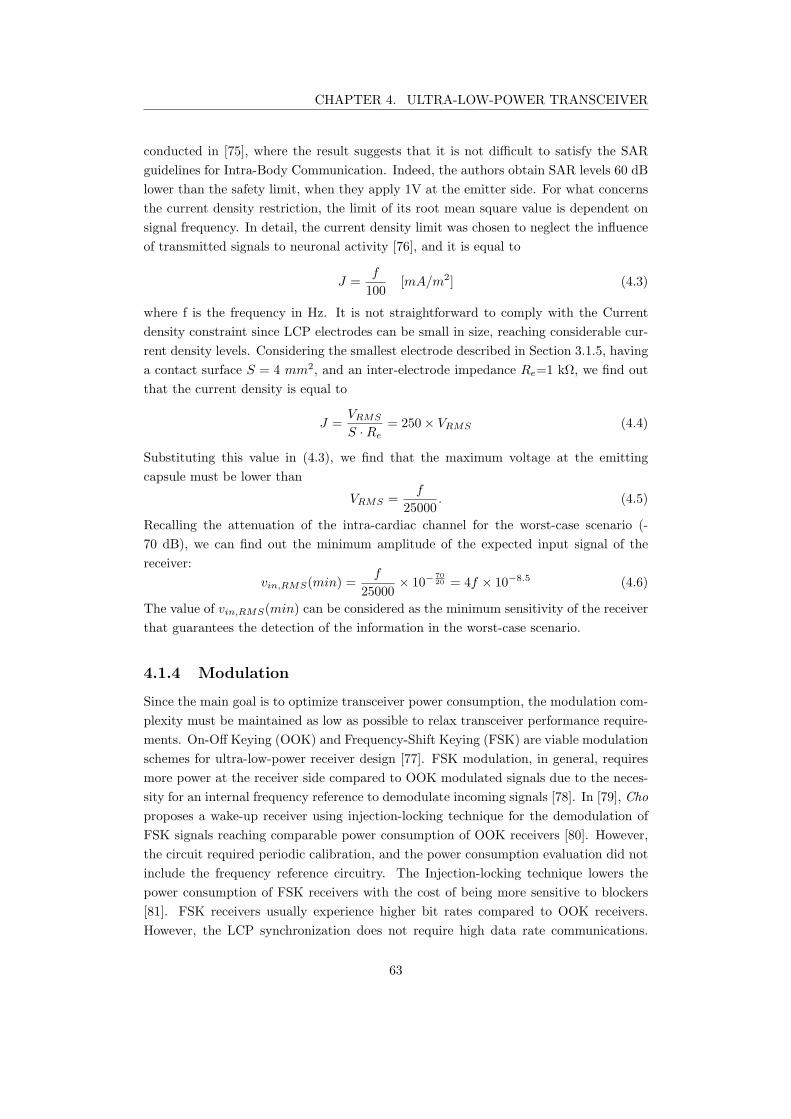
CHAPTER 4. ULTRA-LOW-POWER TRANSCEIVER
conducted in [75], where the result suggests that it is not difficult to satisfy the SAR
guidelines for Intra-Body Communication. Indeed, the authors obtain SAR levels 60 dB
lower than the safety limit, when they apply 1V at the emitter side. For what concerns
the current density restriction, the limit of its root mean square value is dependent on
signal frequency. In detail, the current density limit was chosen to neglect the influence
of transmitted signals to neuronal activity [76], and it is equal to
J =f
100[mA/m2] (4.3)
where f is the frequency in Hz. It is not straightforward to comply with the Current
density constraint since LCP electrodes can be small in size, reaching considerable cur-
rent density levels. Considering the smallest electrode described in Section 3.1.5, having
a contact surface S = 4 mm2, and an inter-electrode impedance Re=1 kΩ, we find out
that the current density is equal to
J =VRMS
S ·Re
= 250× VRMS (4.4)
Substituting this value in (4.3), we find that the maximum voltage at the emitting
capsule must be lower than
VRMS =f
25000. (4.5)
Recalling the attenuation of the intra-cardiac channel for the worst-case scenario (-
70 dB), we can find out the minimum amplitude of the expected input signal of the
receiver:
vin,RMS(min) =f
25000× 10−
70
20 = 4f × 10−8.5 (4.6)
The value of vin,RMS(min) can be considered as the minimum sensitivity of the receiver
that guarantees the detection of the information in the worst-case scenario.
4.1.4 Modulation
Since the main goal is to optimize transceiver power consumption, the modulation com-
plexity must be maintained as low as possible to relax transceiver performance require-
ments. On-Off Keying (OOK) and Frequency-Shift Keying (FSK) are viable modulation
schemes for ultra-low-power receiver design [77]. FSK modulation, in general, requires
more power at the receiver side compared to OOK modulated signals due to the neces-
sity for an internal frequency reference to demodulate incoming signals [78]. In [79], Cho
proposes a wake-up receiver using injection-locking technique for the demodulation of
FSK signals reaching comparable power consumption of OOK receivers [80]. However,
the circuit required periodic calibration, and the power consumption evaluation did not
include the frequency reference circuitry. The Injection-locking technique lowers the
power consumption of FSK receivers with the cost of being more sensitive to blockers
[81]. FSK receivers usually experience higher bit rates compared to OOK receivers.
However, the LCP synchronization does not require high data rate communications.
63
CHAPTER 4. ULTRA-LOW-POWER TRANSCEIVER
Considering that the latency constraint is respected, the cardiac event message reduces
to binary information allowing the communication module to work with a single bit
demodulation. Thus, we preferred the OOK modulation technique to the FSK in order
to reduce the complexity at the emitter side.
4.1.5 Bit Error Rate (BER)
For what concerns the BER, there is not a standard for multi-node pacemaker systems.
We can design the receiver to neglect the probability of the communication loss com-
pared to the probability that sensors miss the atrial depolarization. Sensors can miss
atrial events for several reasons: pacemaker programming problems (improper sensing
threshold), insufficient myocardial voltage signal, lead or pacer failure (fibrosis, frac-
ture), or an electrolyte abnormality [82, 83]. Loss of atrial sensing is 2%-11% among
patients of clinical studies reported in the literature [84]. As a rule of thumb, the error
probability of the communication must be at least ten times lower the probability of
missing atrial detection, leading to a BER of 10−3 for single synchronization bit com-
munication. The error probability of OOK signals is well approximated by the function
expressed in (4.7)
Pe = Q(√
2Eb/N), (4.7)
where Q is the Q-function whose distribution depends on the energy per bit Eb and the
noise amplitude N [85]. Since OOK modulation encodes only one bit per symbol, we
can equate the ratio Eb/N to the signal noise ratio (SNR) and the error probability Pe
to the BER. Thus (4.7) can be rewritten as
BER = Q(√
2SNR). (4.8)
According to (4.8), the SNR must be greater or equal than 10 dB to achieve a BER of
10−3. Recalling that the input signal amplitude can be as low as -84 dBv and considering
a margin of at least 10dB for the receiver noise figure (NF), the maximum input noise
amplitude must be lower than -104dBv.
Let us now evaluate the characteristics of the OOK modulation pulse to find out the
limiting values according to the allowed noise contribution. For the sake of clarity, we
graphically represented the synchronization pulse in Figure 4.1, where Tbit represents
the time duration of a single bit, and TCC is the communication period that can vary
according to the cardiac cycle. We can assume that TCC is infinitely longer than Tbit,
allowing to reducing the time-analysis of the signal to a single pulse. Thus, considering
only the first harmonic of the carrier, the synchronization pulse can be represented in
the time domain as
s(t) =∏
Tbit
2
·cos(2πf0t) (4.9)
where Π is the rectangular function, t is the time variable, and f0 is the carrier frequency
value. Let us now analyze the synchronization signal in the frequency domain S(f).
64
CHAPTER 4. ULTRA-LOW-POWER TRANSCEIVER
Figure 4.1: Example of OOK signal for LCP synchronization
Figure 4.2: Example of OOK signal for LCP synchronization in frequency domain
Applying the convolution theorem of the Fourier transform, we can easily retrieve the
analytical representation of synchronization pulse in the positive frequency domain [86].
F s(t) = S(f) = TbitSinc(πfTbit) ∗ δ(f − f0). (4.10)
For the convolution property of the Dirac function δ(f), we can represent S(f) as a
Sinc signal centered at f0, as depicted in Figure 4.2 We can reasonably approximate
the bandwidth of the synchronization signal to the main lobe of S(f) that is equal to
4 × 1
Tbit
. The IBC channel can be considered as an Additive White Gaussian Noise
channel (AWGN). Under this assumption, we can model the the thermal noise of the
inter-electrode resistance as a voltage source, whose spectral density is
N0 =√
4KB × T ×R×BW (4.11)
where KB is the Boltzmann constant, T is the temperature in kelvin, R is the inter-
electrode resistance and BW is the bandwidth of interest. Considering that the body
temperature is approximately 37C (310,15 K), for R =1 kΩ, the spectral noise density
is
N0 = 4, 13 nV/√Hz = −166, 65 dBv/
√Hz (4.12)
65
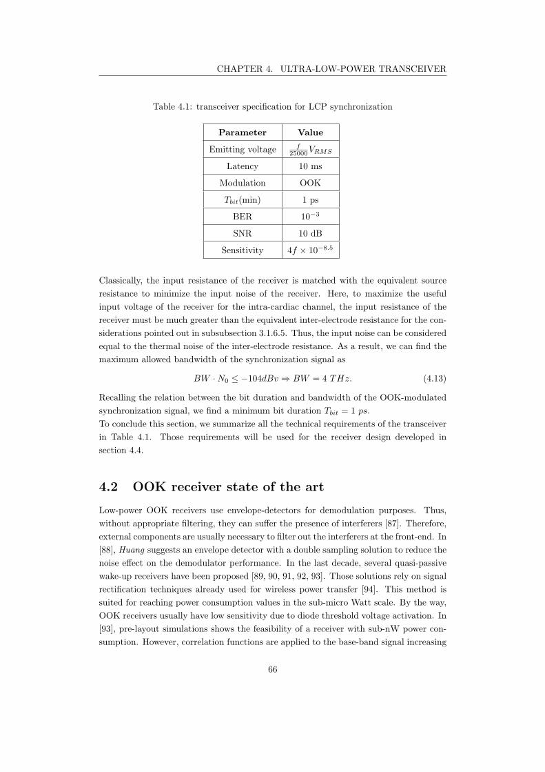
CHAPTER 4. ULTRA-LOW-POWER TRANSCEIVER
Table 4.1: transceiver specification for LCP synchronization
Parameter Value
Emitting voltage f25000
VRMS
Latency 10 ms
Modulation OOK
Tbit(min) 1 ps
BER 10−3
SNR 10 dB
Sensitivity 4f × 10−8.5
Classically, the input resistance of the receiver is matched with the equivalent source
resistance to minimize the input noise of the receiver. Here, to maximize the useful
input voltage of the receiver for the intra-cardiac channel, the input resistance of the
receiver must be much greater than the equivalent inter-electrode resistance for the con-
siderations pointed out in subsubsection 3.1.6.5. Thus, the input noise can be considered
equal to the thermal noise of the inter-electrode resistance. As a result, we can find the
maximum allowed bandwidth of the synchronization signal as
BW ·N0 ≤ −104dBv ⇒ BW = 4 THz. (4.13)
Recalling the relation between the bit duration and bandwidth of the OOK-modulated
synchronization signal, we find a minimum bit duration Tbit = 1 ps.
To conclude this section, we summarize all the technical requirements of the transceiver
in Table 4.1. Those requirements will be used for the receiver design developed in
section 4.4.
4.2 OOK receiver state of the art
Low-power OOK receivers use envelope-detectors for demodulation purposes. Thus,
without appropriate filtering, they can suffer the presence of interferers [87]. Therefore,
external components are usually necessary to filter out the interferers at the front-end. In
[88], Huang suggests an envelope detector with a double sampling solution to reduce the
noise effect on the demodulator performance. In the last decade, several quasi-passive
wake-up receivers have been proposed [89, 90, 91, 92, 93]. Those solutions rely on signal
rectification techniques already used for wireless power transfer [94]. This method is
suited for reaching power consumption values in the sub-micro Watt scale. By the way,
OOK receivers usually have low sensitivity due to diode threshold voltage activation. In
[93], pre-layout simulations shows the feasibility of a receiver with sub-nW power con-
sumption. However, correlation functions are applied to the base-band signal increasing
66
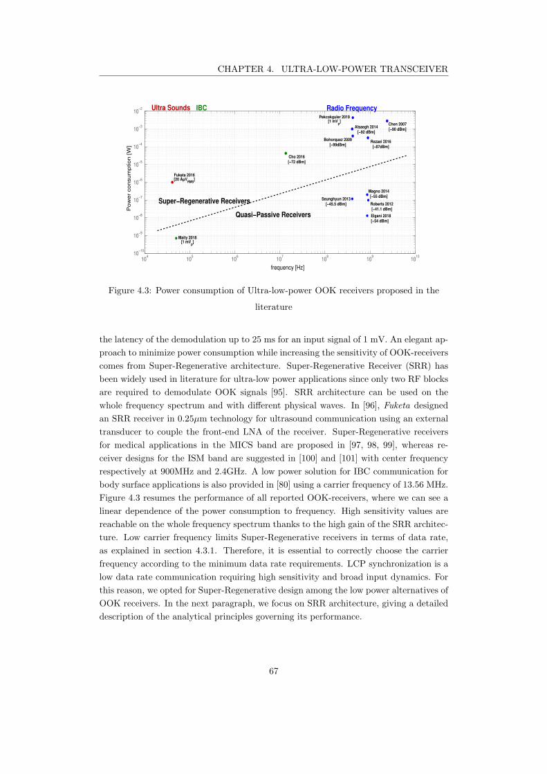
CHAPTER 4. ULTRA-LOW-POWER TRANSCEIVER
104
105
106
107
108
109
1010
10−10
10−9
10−8
10−7
10−6
10−5
10−4
10−3
10−2
frequency [Hz]
Pow
er
consum
ption [W
]
Ultra Sounds Radio Frequency
Pekcokguler 2019[1 mV
p]
Maity 2018[1 mV
p]
Fuketa 2016[20 µV
RMS]
Seunghyun 2013[−45.5 dBm]
IBC
Quasi−Passive Receivers
Super−Regenerative Receivers
Cho 2016[−72 dBm]
Bohorquez 2009[−99dBm]
Alsaegh 2014[−92 dBm]
Rezaei 2016[−87dBm]
Chen 2007[−90 dBm]
Magno 2014[−55 dBm]
Roberts 2012[−41.1 dBm]
Elgani 2018[−54 dBm]
Figure 4.3: Power consumption of Ultra-low-power OOK receivers proposed in the
literature
the latency of the demodulation up to 25 ms for an input signal of 1 mV. An elegant ap-
proach to minimize power consumption while increasing the sensitivity of OOK-receivers
comes from Super-Regenerative architecture. Super-Regenerative Receiver (SRR) has
been widely used in literature for ultra-low power applications since only two RF blocks
are required to demodulate OOK signals [95]. SRR architecture can be used on the
whole frequency spectrum and with different physical waves. In [96], Fuketa designed
an SRR receiver in 0.25µm technology for ultrasound communication using an external
transducer to couple the front-end LNA of the receiver. Super-Regenerative receivers
for medical applications in the MICS band are proposed in [97, 98, 99], whereas re-
ceiver designs for the ISM band are suggested in [100] and [101] with center frequency
respectively at 900MHz and 2.4GHz. A low power solution for IBC communication for
body surface applications is also provided in [80] using a carrier frequency of 13.56 MHz.
Figure 4.3 resumes the performance of all reported OOK-receivers, where we can see a
linear dependence of the power consumption to frequency. High sensitivity values are
reachable on the whole frequency spectrum thanks to the high gain of the SRR architec-
ture. Low carrier frequency limits Super-Regenerative receivers in terms of data rate,
as explained in section 4.3.1. Therefore, it is essential to correctly choose the carrier
frequency according to the minimum data rate requirements. LCP synchronization is a
low data rate communication requiring high sensitivity and broad input dynamics. For
this reason, we opted for Super-Regenerative design among the low power alternatives of
OOK receivers. In the next paragraph, we focus on SRR architecture, giving a detailed
description of the analytical principles governing its performance.
67
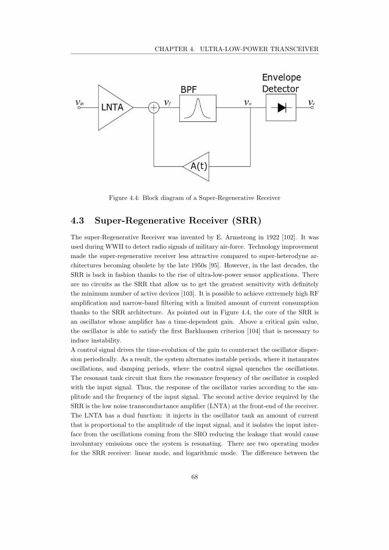
CHAPTER 4. ULTRA-LOW-POWER TRANSCEIVER
Figure 4.4: Block diagram of a Super-Regenerative Receiver
4.3 Super-Regenerative Receiver (SRR)
The super-Regenerative Receiver was invented by E. Armstrong in 1922 [102]. It was
used during WWII to detect radio signals of military air-force. Technology improvement
made the super-regenerative receiver less attractive compared to super-heterodyne ar-
chitectures becoming obsolete by the late 1950s [95]. However, in the last decades, the
SRR is back in fashion thanks to the rise of ultra-low-power sensor applications. There
are no circuits as the SRR that allow us to get the greatest sensitivity with definitely
the minimum number of active devices [103]. It is possible to achieve extremely high RF
amplification and narrow-band filtering with a limited amount of current consumption
thanks to the SRR architecture. As pointed out in Figure 4.4, the core of the SRR is
an oscillator whose amplifier has a time-dependent gain. Above a critical gain value,
the oscillator is able to satisfy the first Barkhausen criterion [104] that is necessary to
induce instability.
A control signal drives the time-evolution of the gain to counteract the oscillator disper-
sion periodically. As a result, the system alternates instable periods, where it instaurates
oscillations, and damping periods, where the control signal quenches the oscillations.
The resonant tank circuit that fixes the resonance frequency of the oscillator is coupled
with the input signal. Thus, the response of the oscillator varies according to the am-
plitude and the frequency of the input signal. The second active device required by the
SRR is the low noise transconductance amplifier (LNTA) at the front-end of the receiver.
The LNTA has a dual function: it injects in the oscillator tank an amount of current
that is proportional to the amplitude of the input signal, and it isolates the input inter-
face from the oscillations coming from the SRO reducing the leakage that would cause
involuntary emissions once the system is resonating. There are two operating modes
for the SRR receiver: linear mode, and logarithmic mode. The difference between the
68
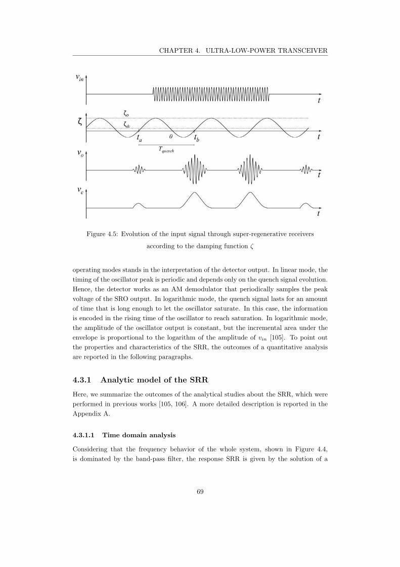
CHAPTER 4. ULTRA-LOW-POWER TRANSCEIVER
Figure 4.5: Evolution of the input signal through super-regenerative receivers
according to the damping function ζ
operating modes stands in the interpretation of the detector output. In linear mode, the
timing of the oscillator peak is periodic and depends only on the quench signal evolution.
Hence, the detector works as an AM demodulator that periodically samples the peak
voltage of the SRO output. In logarithmic mode, the quench signal lasts for an amount
of time that is long enough to let the oscillator saturate. In this case, the information
is encoded in the rising time of the oscillator to reach saturation. In logarithmic mode,
the amplitude of the oscillator output is constant, but the incremental area under the
envelope is proportional to the logarithm of the amplitude of vin [105]. To point out
the properties and characteristics of the SRR, the outcomes of a quantitative analysis
are reported in the following paragraphs.
4.3.1 Analytic model of the SRR
Here, we summarize the outcomes of the analytical studies about the SRR, which were
performed in previous works [105, 106]. A more detailed description is reported in the
Appendix A.
4.3.1.1 Time domain analysis
Considering that the frequency behavior of the whole system, shown in Figure 4.4,
is dominated by the band-pass filter, the response SRR is given by the solution of a
69
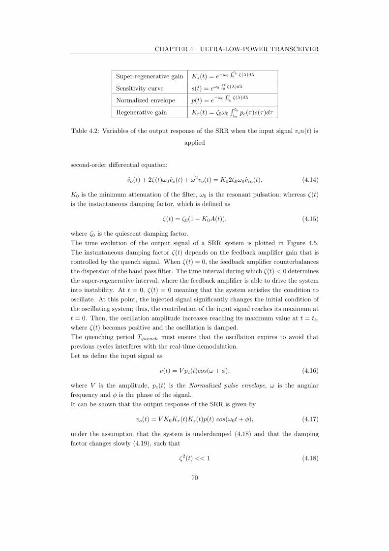
CHAPTER 4. ULTRA-LOW-POWER TRANSCEIVER
Super-regenerative gain Ks(t) = e−ω0
∫ tb
0ζ(λ)dλ
Sensitivity curve s(t) = eω0
∫t
0ζ(λ)dλ
Normalized envelope p(t) = e−ω0
∫t
tbζ(λ)dλ
Regenerative gain Kr(t) = ζ0ω0
∫ tb
tapc(τ)s(τ)dτ
Table 4.2: Variables of the output response of the SRR when the input signal vin(t) is
applied
second-order differential equation:
vo(t) + 2ζ(t)ω0vo(t) + ω2vo(t) = K02ζ0ω0vin(t). (4.14)
K0 is the minimum attenuation of the filter, ω0 is the resonant pulsation; whereas ζ(t)
is the instantaneous damping factor, which is defined as
ζ(t) = ζ0(1−K0A(t)), (4.15)
where ζ0 is the quiescent damping factor.
The time evolution of the output signal of a SRR system is plotted in Figure 4.5.
The instantaneous damping factor ζ(t) depends on the feedback amplifier gain that is
controlled by the quench signal. When ζ(t) = 0, the feedback amplifier counterbalances
the dispersion of the band pass filter. The time interval during which ζ(t) < 0 determines
the super-regenerative interval, where the feedback amplifier is able to drive the system
into instability. At t = 0, ζ(t) = 0 meaning that the system satisfies the condition to
oscillate. At this point, the injected signal significantly changes the initial condition of
the oscillating system; thus, the contribution of the input signal reaches its maximum at
t = 0. Then, the oscillation amplitude increases reaching its maximum value at t = tb,
where ζ(t) becomes positive and the oscillation is damped.
The quenching period Tquench must ensure that the oscillation expires to avoid that
previous cycles interferes with the real-time demodulation.
Let us define the input signal as
v(t) = V pc(t)cos(ω + φ), (4.16)
where V is the amplitude, pc(t) is the Normalized pulse envelope, ω is the angular
frequency and φ is the phase of the signal.
It can be shown that the output response of the SRR is given by
vo(t) = V K0Kr(t)Ks(t)p(t) cos(ω0t+ φ), (4.17)
under the assumption that the system is underdamped (4.18) and that the damping
factor changes slowly (4.19), such that
ζ2(t) << 1 (4.18)
70
CHAPTER 4. ULTRA-LOW-POWER TRANSCEIVER
ζ(t) << ω0 (4.19)
We represented the output response (4.17) using the variables resumed in Table 4.2. As
can be seen, the receiver has an exponential response, boosting very low input signals
up to supply voltage levels.
4.3.1.2 Frequency domain analysis
Let us consider the response to an input with arbitrary frequency
vo(t) = V Kp(t)ω
ω0
∫ tb
tapc(τ)s(τ)cos[(ω − ω0)τ + ω0t+ φ]dτ
∫ tb
tapc(τ)s(τ)dτ
(4.20)
Assuming that pc(t) and s(t) are equal to zero out of the considered interval [ta; tb], we
can define the complex function
ψ(ω) =
∫
∞
−∞
pc(t)s(t)ejωtdt =
[∫
∞
−∞
pc(t)s(t)e−jωtdt
]
∗
= F∗ pc(t)s(t) (4.21)
It can be shown that the frequency response of the SRR is
H(ω) =ω
ω0
ψ(ω − ω0)
ψ(0). (4.22)
Thus, we can rewrite the SRR output as
vo(t) = V Kp(t)|H(ω)|cos[ω0t+ φ+ ∠H(ω)] (4.23)
Note that the frequency response of the Super-Regenerative output is a band-pass filter
centered at the resonance frequency ω0 whose output linearly depends on the amplitude
of the input signal. This analysis is valid as far as the oscillations are small enough
to keep the feedback amplifier in linear region. When the oscillation increases over
an amplitude threshold depending on the characheristics of the feedback amplifier, the
gain A(t) reduces changing the instantaneous damping function. In this condition, the
oscillation can reach saturation before t = tb when the oscillator is quenched and the
output signal is damped out [105].
4.3.1.3 Noise analysis
Performing the time domain analysis using as input signal the noise n(t), we can find
the noise contribution to the output response of the SRR such that
vo,noise(t) = 2ζ0K0Ksp(t)ω0
∫
n(τ)s(τ)sin[ω0(t− τ)]dτ. (4.24)
We can finally express the SNR over a unitary resistance [106]
SNR =V 2
o,signalRMS(t)
E vo,noise(t)=
Eb
(
∫
∞
−∞p(τ)s(τ)dτ
)2
N0
∫
∞
−∞p2(τ)dτ
∫
∞
−∞s2(τ)dτ
, (4.25)
71
CHAPTER 4. ULTRA-LOW-POWER TRANSCEIVER
where
Eb = V 2
in,RMS(t) =1
2V 2
∫∞
−∞
p(τ)dτ. (4.26)
Recalling the Cauchy-Schwartz inequality [85], we can see that the maximum value of
(A.50) is Eb
N0
that occurs when the envelope of the input signal p(t) equals the sensitivity
curve s(t) [106]. For a practical point of view, we can apply an OOK modulated input
with pulse duration that completely covers the sensitivity curve. In such a condition,
we can neglect the contribution of the input envelope achieving the maximum value of
the SNR. It is worth noting that the maximum value of the SNR for the SRR equals
the SNR of standard OOK architectures Eb
N0
4.4 SRR design
In the previous section, we pointed out the main characteristics of the SRR architecture.
A quantitative analysis showed the critical importance of the quench signal on the over-
all response of the system. In particular, the sensitivity of the SRR improves when the
quench signal varies slowly. LCP synchronization does not require high-speed commu-
nications, relaxing the constraint on the quenching frequency. To minimize both power
consumption and chip size, we decided to build the quench signal using the 32 kHz clock
of the LCP device. In this work, we do not consider the implementation of the quench
signal circuitry, which was rather ideally modeled. All the blocks of the SRR repre-
sented in Figure 4.6 were designed using the technology XH018 from XFAB©. XH018 is
a 0.18 µm technology for CMOS design that allows High Voltage applications required
for therapy stimulation. Thus, this technology allows mono-chip integration of all the
functional blocks required by pacemaker devices reducing both the cost and the size of
the whole device production. In the next section, we will give a detailed insight into
the receiver design, considering, first, each block as a standalone component, and then,
describe the performance of the global functioning.
4.4.1 Receiver design
4.4.1.1 The oscillator
Let us start from the core of the Super-Regenerative receiver: the oscillator. Before
dealing with the circuit design, let us remind some theory of oscillators that is essential
to understand the design choices. Oscillators consist of an amplifying stage, a frequency-
selective network, and a positive feedback network. The feedback circuit is required to
sum the output signal to the input signal. Under proper conditions, the positive feedback
system establishes an oscillatory response. Let us consider a generic feedback system,
like the one shown in Figure 4.7. The direct gain of the system is A(jω), whereas β(jω)
is the transfer function of the feedback network.
72
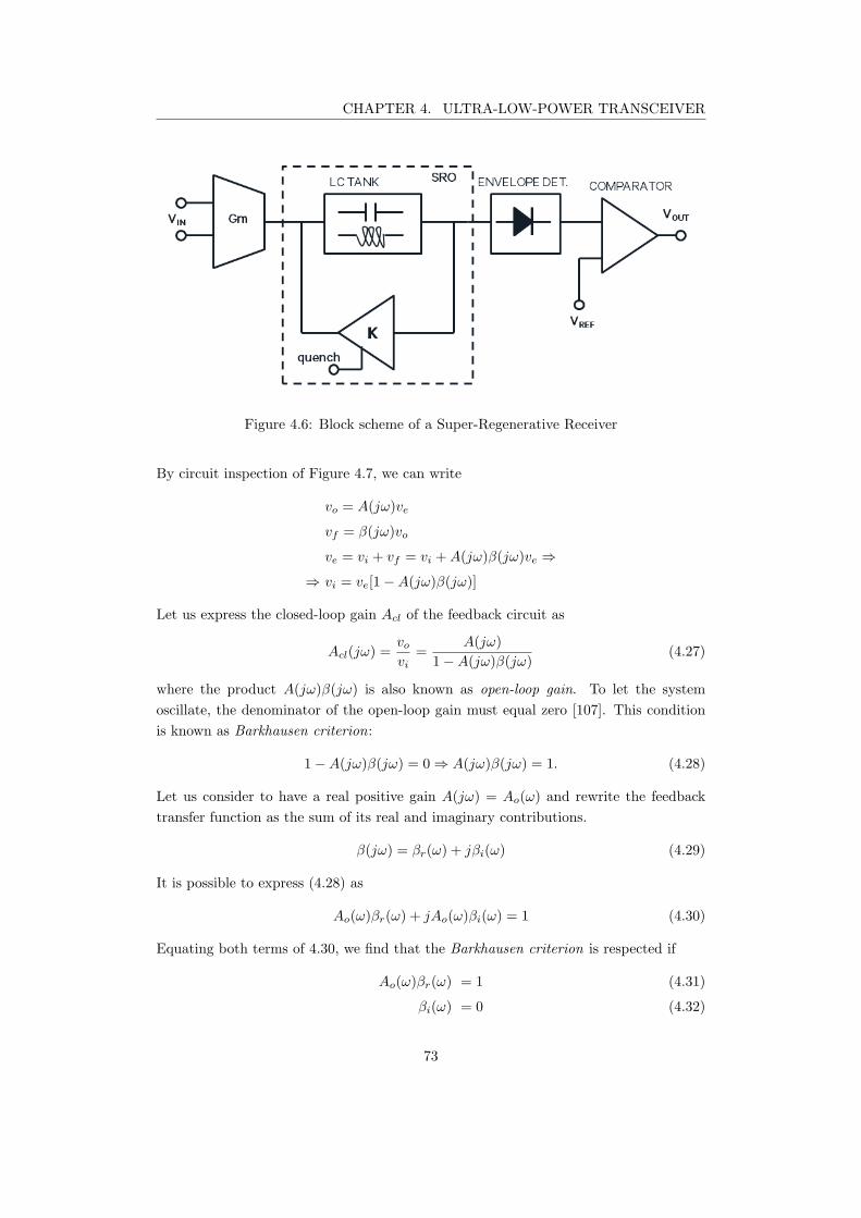
CHAPTER 4. ULTRA-LOW-POWER TRANSCEIVER
Figure 4.6: Block scheme of a Super-Regenerative Receiver
By circuit inspection of Figure 4.7, we can write
vo = A(jω)ve
vf = β(jω)vo
ve = vi + vf = vi +A(jω)β(jω)ve ⇒
⇒ vi = ve[1−A(jω)β(jω)]
Let us express the closed-loop gain Acl of the feedback circuit as
Acl(jω) =vo
vi=
A(jω)
1−A(jω)β(jω)(4.27)
where the product A(jω)β(jω) is also known as open-loop gain. To let the system
oscillate, the denominator of the open-loop gain must equal zero [107]. This condition
is known as Barkhausen criterion:
1−A(jω)β(jω) = 0 ⇒ A(jω)β(jω) = 1. (4.28)
Let us consider to have a real positive gain A(jω) = Ao(ω) and rewrite the feedback
transfer function as the sum of its real and imaginary contributions.
β(jω) = βr(ω) + jβi(ω) (4.29)
It is possible to express (4.28) as
Ao(ω)βr(ω) + jAo(ω)βi(ω) = 1 (4.30)
Equating both terms of 4.30, we find that the Barkhausen criterion is respected if
Ao(ω)βr(ω) = 1 (4.31)
βi(ω) = 0 (4.32)
73
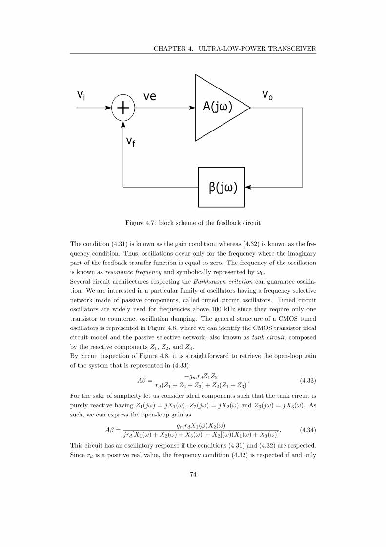
CHAPTER 4. ULTRA-LOW-POWER TRANSCEIVER
Figure 4.7: block scheme of the feedback circuit
The condition (4.31) is known as the gain condition, whereas (4.32) is known as the fre-
quency condition. Thus, oscillations occur only for the frequency where the imaginary
part of the feedback transfer function is equal to zero. The frequency of the oscillation
is known as resonance frequency and symbolically represented by ω0.
Several circuit architectures respecting the Barkhausen criterion can guarantee oscilla-
tion. We are interested in a particular family of oscillators having a frequency selective
network made of passive components, called tuned circuit oscillators. Tuned circuit
oscillators are widely used for frequencies above 100 kHz since they require only one
transistor to counteract oscillation damping. The general structure of a CMOS tuned
oscillators is represented in Figure 4.8, where we can identify the CMOS transistor ideal
circuit model and the passive selective network, also known as tank circuit, composed
by the reactive components Z1, Z2, and Z3.
By circuit inspection of Figure 4.8, it is straightforward to retrieve the open-loop gain
of the system that is represented in (4.33).
Aβ =−gmrdZ1Z2
rd(Z1 + Z2 + Z3) + Z2(Z1 + Z3). (4.33)
For the sake of simplicity let us consider ideal components such that the tank circuit is
purely reactive having Z1(jω) = jX1(ω), Z2(jω) = jX2(ω) and Z3(jω) = jX3(ω). As
such, we can express the open-loop gain as
Aβ =gmrdX1(ω)X2(ω)
jrd[X1(ω) +X2(ω) +X3(ω)]−X2[(ω)(X1(ω) +X3(ω)]. (4.34)
This circuit has an oscillatory response if the conditions (4.31) and (4.32) are respected.
Since rd is a positive real value, the frequency condition (4.32) is respected if and only
74

CHAPTER 4. ULTRA-LOW-POWER TRANSCEIVER
Figure 4.8: Ideal model of single transistor LC-oscillators
if
X1(ω0) +X2(ω0) +X3(ω0) = 0. (4.35)
At ω = ω0, the open-loop gain of the system reduces to
A(jω0)β(jω0) =−gmrdX1(ω0)
X1(ω0) +X3(ω0). (4.36)
Substituting the value of X3(ω0) coming from 4.35 we can rewrite the (4.36) as
A(jω0)β(jω0) =gmrdX1(ω0)
X2(ω0)≥ 1. (4.37)
The open-loop gain (eq. 4.37) must be equal to one to respect the gain condition at the
resonance frequency, and greater to one to initiate the oscillations. The gain condition is
respected if and only if the reactive impedances X1 and X2 have the same sign since the
transconductance gm and the drain resistance rd of the transistor are positive real values.
In opposition, the frequency condition is respected if X3 has opposite sign compared to
X1 and X2. We decide to choose Z1 = C1, Z2 = C2, and Z3 = L to reduce the number
of inductive components. This configuration of the tuned circuit oscillator is known as
Pierce oscillator, where the resonance frequency is
ω0 =1
√
LCeff
(4.38)
Ceff =C1C2
C1 + C2
(4.39)
Moreover, the oscillations can occur if the gain of the amplifier is greater than the
capacitive ratio C1
C2
such that
gmrd ≥C1
C2
(4.40)
75
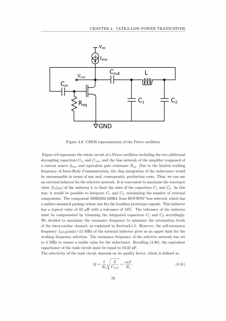
CHAPTER 4. ULTRA-LOW-POWER TRANSCEIVER
Figure 4.9: CMOS representation of the Pierce oscillator
Figure 4.9 represents the whole circuit of a Pierce oscillator including the two additional
decoupling capacitors Cin and Cout, and the bias network of the amplifier composed of
a current source Ibias and equivalent gate resistance Req. Due to the limited working
frequency of Intra-Body Communication, the chip integration of the inductance would
be unreasonable in terms of size and, consequently, production costs. Thus, we can use
an external inductor for the selective network. It is convenient to maximize the reactance
value X3(ω0) of the inductor L to limit the sizes of the capacitors C1 and C2. In this
way, it would be possible to integrate C1 and C2, minimizing the number of external
components. The component SDR0302-820KL from BOURNS™was selected, which has
a surface-mounted package whose size fits the Leadless prototype capsule. This inductor
has a typical value of 82 µH with a tolerance of 10%. The tolerance of the inductor
must be compensated by trimming the integrated capacitors C1 and C2 accordingly.
We decided to maximize the resonance frequency to minimize the attenuation levels
of the intra-cardiac channel, as explained in Section3.1.5. However, the self-resonance
frequency fSFR(min)=12 MHz of the external inductor gives us an upper limit for the
working frequency selection. The resonance frequency of the selective network was set
to 4 MHz to ensure a stable value for the inductance. Recalling (4.38), the equivalent
capacitance of the tank circuit must be equal to 19.32 pF.
The selectivity of the tank circuit depends on its quality factor, which is defined as
Q =1
Rs
√
L
Ceff
=ω0L
Rs
, (4.41)
76

CHAPTER 4. ULTRA-LOW-POWER TRANSCEIVER
where Rs is the stray resistance of the inductor [107]. We can notice that having an
inductance value several orders of magnitude bigger than the equivalent capacitance
leads to very high quality factors increasing the selectivity of the receiver. On the other
hand, a very high selective network requires accurate reactance values that would lead
to a complex trimming network of the capacitors. In order to limit the trimming of the
equivalent capacitor to 1%, leading to a bandwidth of at least 40 KHz, we set the series
resistance of the inductor Rs = 16 Ω. By specification, the maximum stray resistance
of the chosen inductance is 2.10 Ω requiring an additional resistance of 14 Ω. The
additional resistance needing is good news since it can be obtained through the trace
resistance, relaxing the constraint of the layout.
To avoid that the bias network of the common source amplifier degrades the oscillatory
response of the system, we integrated a decoupling capacitor Cin, whose value was
selected to behave as a short circuit at the resonance frequency. The value of Cin must
be sized according to the value of the gate equivalent resistance Req such that the cutoff
frequency of the resulting passive high-pass filter lies at least a decade from ω0.
Cin =10
ω0Req
. (4.42)
For what concerns Cout, let us analyze its effect on the system, studying the poles of
the transfer function. The open-loop gain equation in the Laplace domain considering
Cout is
A(s)β(s) =−gm( 1
LC1C2
)
s3 + s2 C1+Cout
rdC1Cout
+ sC1+C2
LC1C2
+ C1+C2+Cout
rdLC1C2Cout
(4.43)
where s = jω. Let us recall the transfer function H(s) of feedback oscillators
H(s) =A(s)β(s)
1−A(s)β(s). (4.44)
To study the stability of the system, we need to characterize the poles of H(s). To do
so, it is convenient to rewrite the open-loop gain 4.43 in its polynomial form
A(s)β(s) =KN(s)
D(s)(4.45)
where
K =−gm
C1C2L, N(s) = 1
D(s) = s3 + s2C1 + Cout
rdC1Cout
+ sC1 + C2
LC1C2
+C1 + C2 + Cout
rdLC1C2Cout
.
The closed loop gain H(s) can be rewritten according to 4.45
H(s) =KN(s)
D(s)−KN(s)(4.46)
The poles of the system are defined as the values of s for which the denominator equals
zero. Thus, let us focus on the denominator of the closed loop gain D′(s) = D(s) −
77
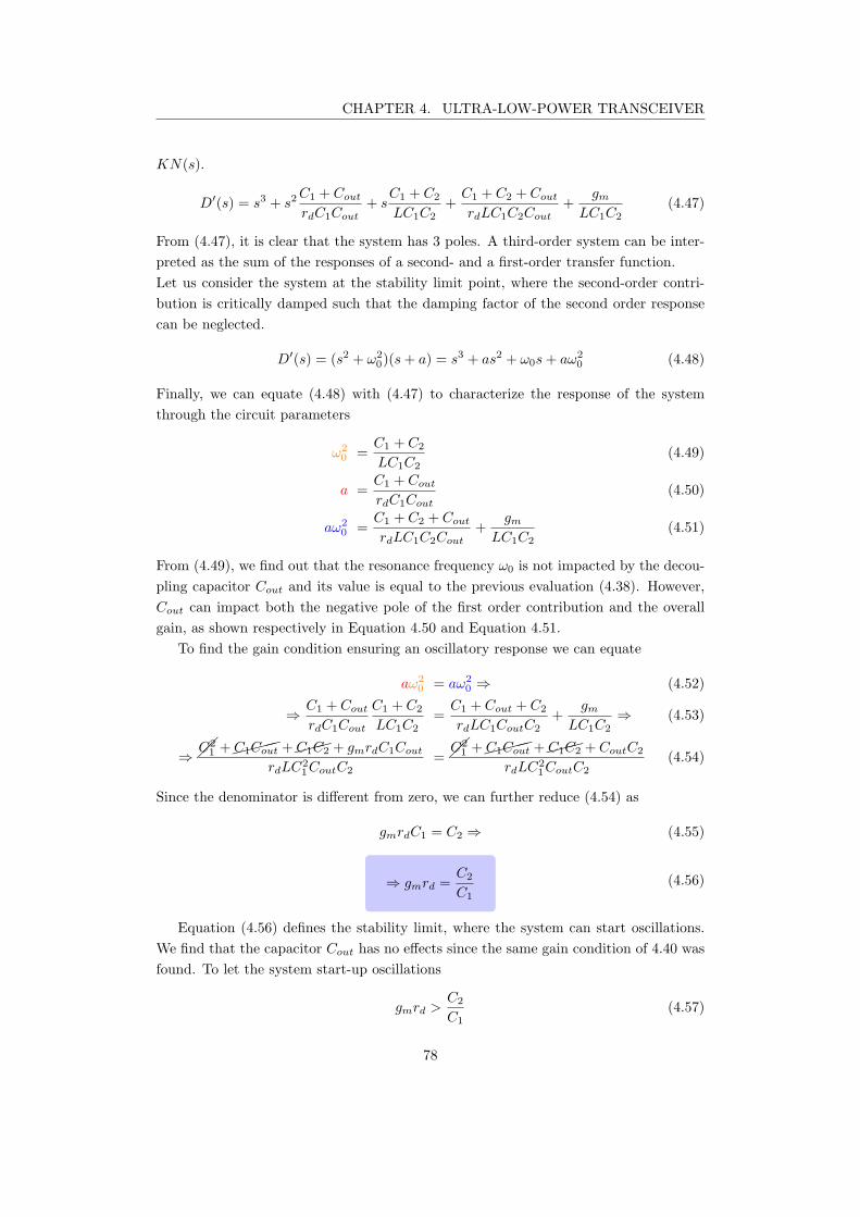
CHAPTER 4. ULTRA-LOW-POWER TRANSCEIVER
KN(s).
D′(s) = s3 + s2C1 + Cout
rdC1Cout
+ sC1 + C2
LC1C2
+C1 + C2 + Cout
rdLC1C2Cout
+gm
LC1C2
(4.47)
From (4.47), it is clear that the system has 3 poles. A third-order system can be inter-
preted as the sum of the responses of a second- and a first-order transfer function.
Let us consider the system at the stability limit point, where the second-order contri-
bution is critically damped such that the damping factor of the second order response
can be neglected.
D′(s) = (s2 + ω2
0)(s+ a) = s3 + as2 + ω0s+ aω2
0(4.48)
Finally, we can equate (4.48) with (4.47) to characterize the response of the system
through the circuit parameters
ω2
0=
C1 + C2
LC1C2
(4.49)
a =C1 + Cout
rdC1Cout
(4.50)
aω2
0=
C1 + C2 + Cout
rdLC1C2Cout
+gm
LC1C2
(4.51)
From (4.49), we find out that the resonance frequency ω0 is not impacted by the decou-
pling capacitor Cout and its value is equal to the previous evaluation (4.38). However,
Cout can impact both the negative pole of the first order contribution and the overall
gain, as shown respectively in Equation 4.50 and Equation 4.51.
To find the gain condition ensuring an oscillatory response we can equate
aω2
0= aω2
0⇒ (4.52)
⇒C1 + Cout
rdC1Cout
C1 + C2
LC1C2
=C1 + Cout + C2
rdLC1CoutC2
+gm
LC1C2
⇒ (4.53)
⇒ C2
1+C1Cout +C1C2 + gmrdC1Cout
rdLC2
1CoutC2
= C2
1+C1Cout +C1C2 + CoutC2
rdLC2
1CoutC2
(4.54)
Since the denominator is different from zero, we can further reduce (4.54) as
gmrdC1 = C2 ⇒ (4.55)
⇒ gmrd =C2
C1
(4.56)
Equation (4.56) defines the stability limit, where the system can start oscillations.
We find that the capacitor Cout has no effects since the same gain condition of 4.40 was
found. To let the system start-up oscillations
gmrd >C2
C1
(4.57)
78
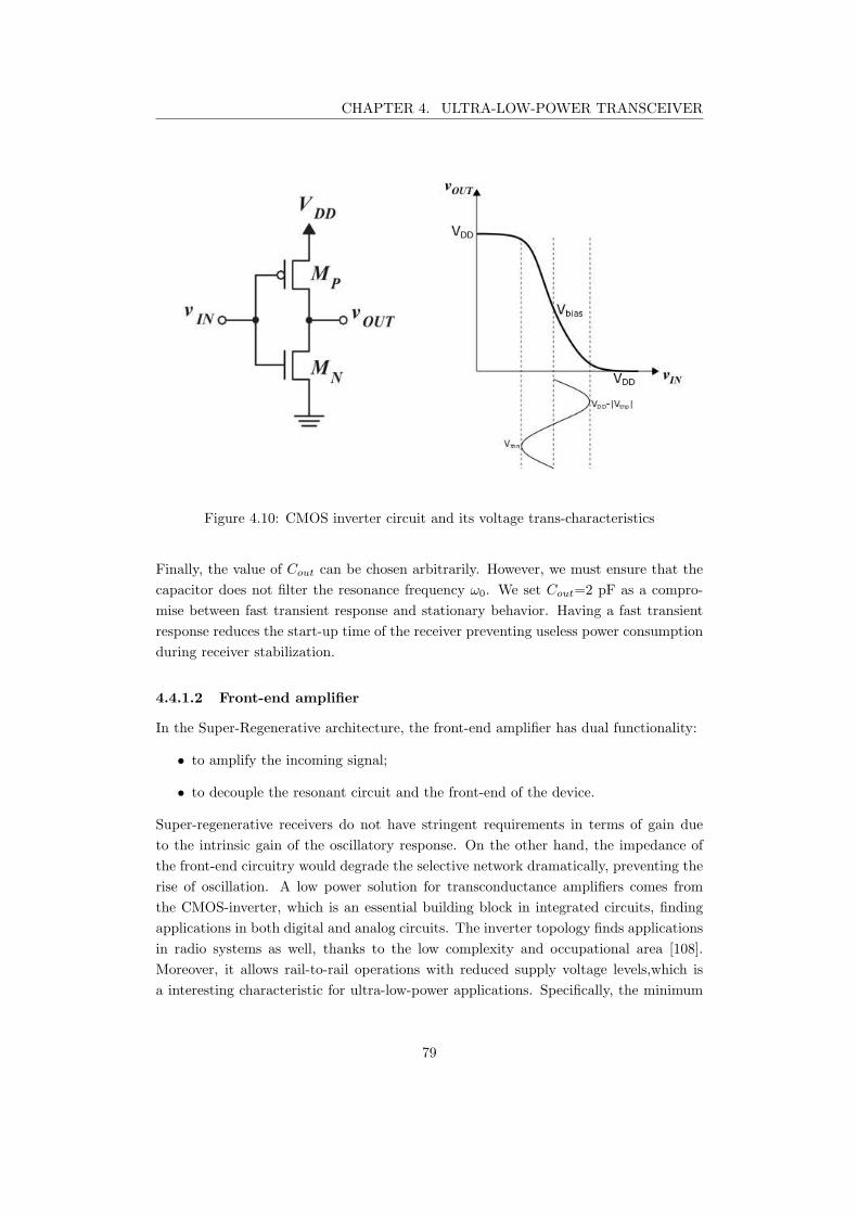
CHAPTER 4. ULTRA-LOW-POWER TRANSCEIVER
Figure 4.10: CMOS inverter circuit and its voltage trans-characteristics
Finally, the value of Cout can be chosen arbitrarily. However, we must ensure that the
capacitor does not filter the resonance frequency ω0. We set Cout=2 pF as a compro-
mise between fast transient response and stationary behavior. Having a fast transient
response reduces the start-up time of the receiver preventing useless power consumption
during receiver stabilization.
4.4.1.2 Front-end amplifier
In the Super-Regenerative architecture, the front-end amplifier has dual functionality:
• to amplify the incoming signal;
• to decouple the resonant circuit and the front-end of the device.
Super-regenerative receivers do not have stringent requirements in terms of gain due
to the intrinsic gain of the oscillatory response. On the other hand, the impedance of
the front-end circuitry would degrade the selective network dramatically, preventing the
rise of oscillation. A low power solution for transconductance amplifiers comes from
the CMOS-inverter, which is an essential building block in integrated circuits, finding
applications in both digital and analog circuits. The inverter topology finds applications
in radio systems as well, thanks to the low complexity and occupational area [108].
Moreover, it allows rail-to-rail operations with reduced supply voltage levels,which is
a interesting characteristic for ultra-low-power applications. Specifically, the minimum
79
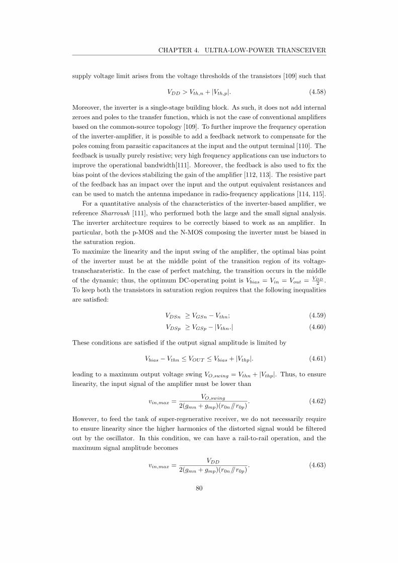
CHAPTER 4. ULTRA-LOW-POWER TRANSCEIVER
supply voltage limit arises from the voltage thresholds of the transistors [109] such that
VDD > Vth,n + |Vth,p|. (4.58)
Moreover, the inverter is a single-stage building block. As such, it does not add internal
zeroes and poles to the transfer function, which is not the case of conventional amplifiers
based on the common-source topology [109]. To further improve the frequency operation
of the inverter-amplifier, it is possible to add a feedback network to compensate for the
poles coming from parasitic capacitances at the input and the output terminal [110]. The
feedback is usually purely resistive; very high frequency applications can use inductors to
improve the operational bandwidth[111]. Moreover, the feedback is also used to fix the
bias point of the devices stabilizing the gain of the amplifier [112, 113]. The resistive part
of the feedback has an impact over the input and the output equivalent resistances and
can be used to match the antenna impedance in radio-frequency applications [114, 115].
For a quantitative analysis of the characteristics of the inverter-based amplifier, we
reference Sharroush [111], who performed both the large and the small signal analysis.
The inverter architecture requires to be correctly biased to work as an amplifier. In
particular, both the p-MOS and the N-MOS composing the inverter must be biased in
the saturation region.
To maximize the linearity and the input swing of the amplifier, the optimal bias point
of the inverter must be at the middle point of the transition region of its voltage-
transcharateristic. In the case of perfect matching, the transition occurs in the middle
of the dynamic; thus, the optimum DC-operating point is Vbias = Vin = Vout = VDD
2.
To keep both the transistors in saturation region requires that the following inequalities
are satisfied:
VDSn ≥ VGSn − Vthn; (4.59)
VDSp ≥ VGSp − |Vthn.| (4.60)
These conditions are satisfied if the output signal amplitude is limited by
Vbias − Vthn ≤ VOUT ≤ Vbias + |Vthp|. (4.61)
leading to a maximum output voltage swing VO,swing = Vthn + |Vthp|. Thus, to ensure
linearity, the input signal of the amplifier must be lower than
vin,max =VO,swing
2(gmn + gmp)(r0n//r0p). (4.62)
However, to feed the tank of super-regenerative receiver, we do not necessarily require
to ensure linearity since the higher harmonics of the distorted signal would be filtered
out by the oscillator. In this condition, we can have a rail-to-rail operation, and the
maximum signal amplitude becomes
vin,max =VDD
2(gmn + gmp)(r0n//r0p). (4.63)
80
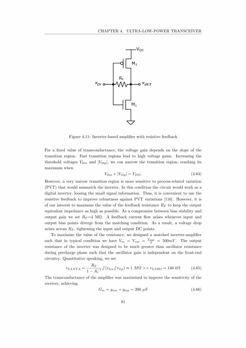
CHAPTER 4. ULTRA-LOW-POWER TRANSCEIVER
Figure 4.11: Inverter-based amplifier with resistive feedback
For a fixed value of transconductance, the voltage gain depends on the slope of the
transition region. Fast transition regions lead to high voltage gains. Increasing the
threshold voltages Vthn and |Vthp|, we can narrow the transition region, reaching its
maximum when
Vthn + |Vthp| = VDD. (4.64)
However, a very narrow transition region is more sensitive to process-related variation
(PVT) that would mismatch the inverter. In this condition the circuit would work as a
digital inverter, loosing the small signal information. Thus, it is convenient to use the
resistive feedback to improve robustness against PVT variations [116]. However, it is
of our interest to maximize the value of the feedback resistance RF to keep the output
equivalent impedance as high as possible. As a compromise between bias stability and
output gain we set RF=4 MΩ. A feedback current flow arises whenever input and
output bias points diverge from the matching condition. As a result, a voltage drop
arises across RF , tightening the input and output DC points.
To maximize the value of the resistance, we designed a matched inverter-amplifier
such that in typical condition we have Vin = Vout = VDD
2= 500mV . The output
resistance of the inverter was designed to be much greater than oscillator resistance
during precharge phase such that the oscillator gain is independent on the front-end
circuitry. Quantitative speaking, we set
r0,LNTA =RF
1−A−1v
//(r0,n//r0,p) ≈ 1 MΩ >> r0,SRO = 140 kΩ (4.65)
The transconductance of the amplifier was maximized to improve the sensitivity of the
receiver, achieving
Gm = gmn + gmp = 200 µS (4.66)
81
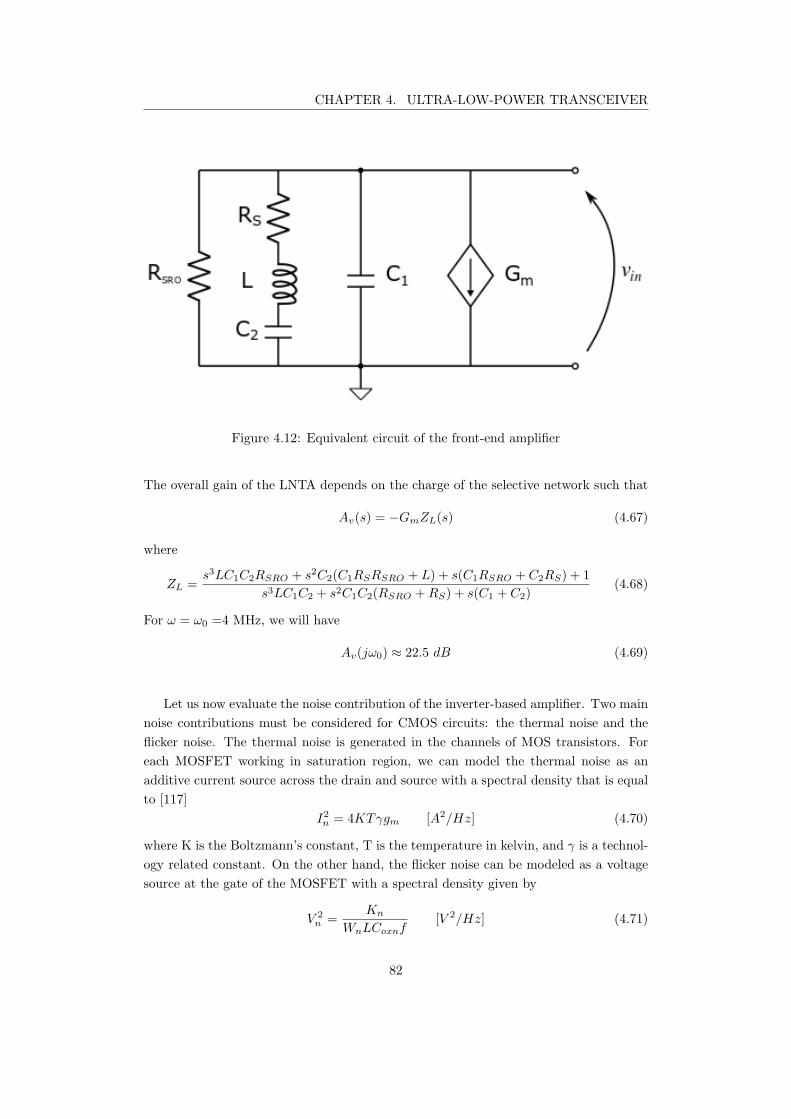
CHAPTER 4. ULTRA-LOW-POWER TRANSCEIVER
Figure 4.12: Equivalent circuit of the front-end amplifier
The overall gain of the LNTA depends on the charge of the selective network such that
Av(s) = −GmZL(s) (4.67)
where
ZL =s3LC1C2RSRO + s2C2(C1RSRSRO + L) + s(C1RSRO + C2RS) + 1
s3LC1C2 + s2C1C2(RSRO +RS) + s(C1 + C2)(4.68)
For ω = ω0 =4 MHz, we will have
Av(jω0) ≈ 22.5 dB (4.69)
Let us now evaluate the noise contribution of the inverter-based amplifier. Two main
noise contributions must be considered for CMOS circuits: the thermal noise and the
flicker noise. The thermal noise is generated in the channels of MOS transistors. For
each MOSFET working in saturation region, we can model the thermal noise as an
additive current source across the drain and source with a spectral density that is equal
to [117]
I2n = 4KTγgm [A2/Hz] (4.70)
where K is the Boltzmann’s constant, T is the temperature in kelvin, and γ is a technol-
ogy related constant. On the other hand, the flicker noise can be modeled as a voltage
source at the gate of the MOSFET with a spectral density given by
V 2
n =Kn
WnLCoxnf[V 2/Hz] (4.71)
82
CHAPTER 4. ULTRA-LOW-POWER TRANSCEIVER
Figure 4.13: Testbench of the ideal front-end amplifier
where Kn is a process related constant, and f is the frequency of operation. Since in our
application the signal is centered at 4 MHz, we can neglect the flicker noise contribution.
Starting from this assumption, we can find the noise factor of the inverter. Considering
that the signal to be amplified has an equivalent resistance Rs with noise power
Nin = 4KTRin, (4.72)
the total noise at the output node, for ZL << Rout, is equal to
Nout(s) = (4KTγgmn + 4KTγgmp)Z2
L(s) + 4KTRin(gmn + gmp)2Z2
L(s) (4.73)
We can quantify the contribution of the front-end amplifier through the Noise Factor
(NF), which is defined as the ratio between the total output noise and the output noise
due to the input source [103]. Such that,
NF = 1 +(4KTγgmn + 4KTγgmp)
4KTRin(gmn + gmp)2(4.74)
We can see from (4.74) that the larger the transconductances, the lower is the noise
factor of the inverter-amplifier. However, the total output noise increases boosting the
gain of the amplifier, as seen in (4.73). By the way, the selectivity of the equivalent load
seen by the amplifier strongly reduces the noise contribution.
83
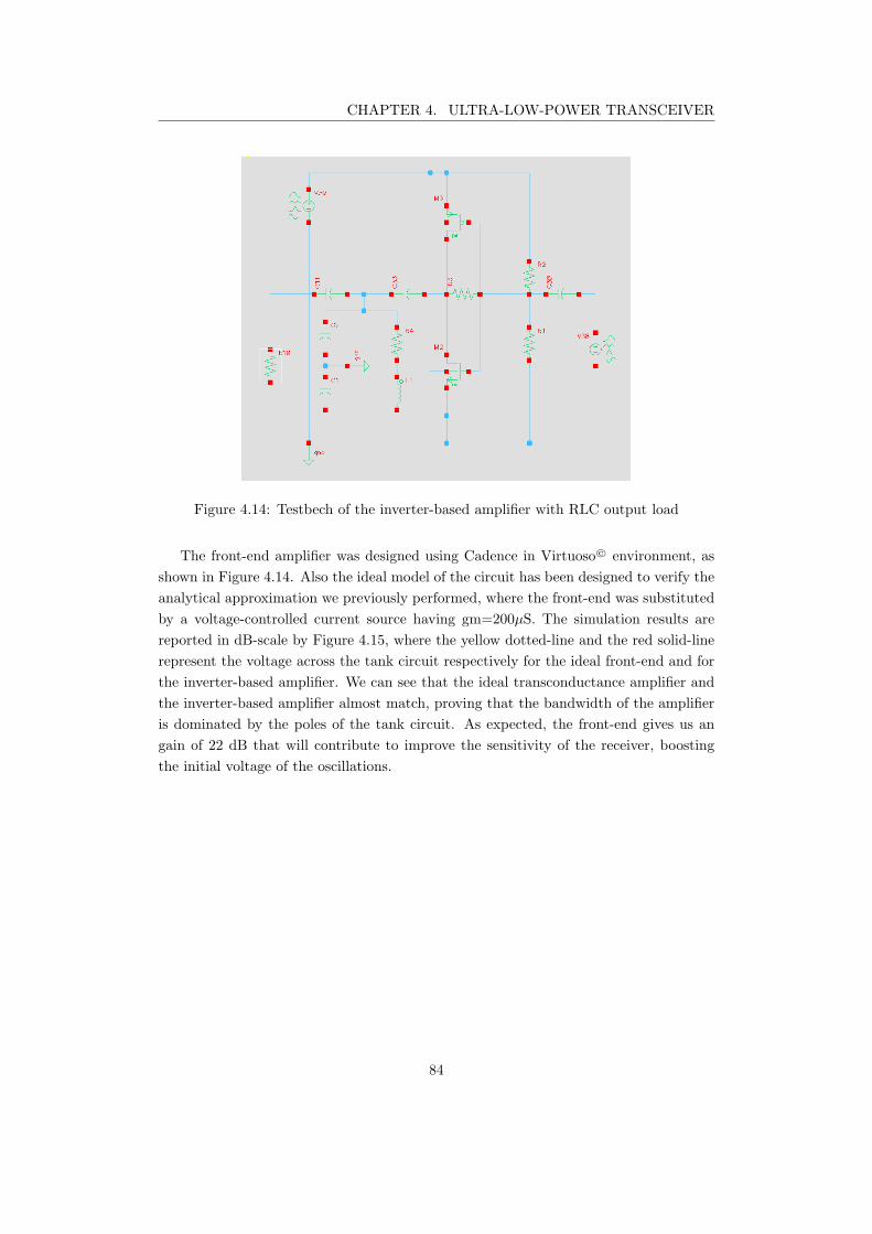
CHAPTER 4. ULTRA-LOW-POWER TRANSCEIVER
Figure 4.14: Testbech of the inverter-based amplifier with RLC output load
The front-end amplifier was designed using Cadence in Virtuoso© environment, as
shown in Figure 4.14. Also the ideal model of the circuit has been designed to verify the
analytical approximation we previously performed, where the front-end was substituted
by a voltage-controlled current source having gm=200µS. The simulation results are
reported in dB-scale by Figure 4.15, where the yellow dotted-line and the red solid-line
represent the voltage across the tank circuit respectively for the ideal front-end and for
the inverter-based amplifier. We can see that the ideal transconductance amplifier and
the inverter-based amplifier almost match, proving that the bandwidth of the amplifier
is dominated by the poles of the tank circuit. As expected, the front-end gives us an
gain of 22 dB that will contribute to improve the sensitivity of the receiver, boosting
the initial voltage of the oscillations.
84
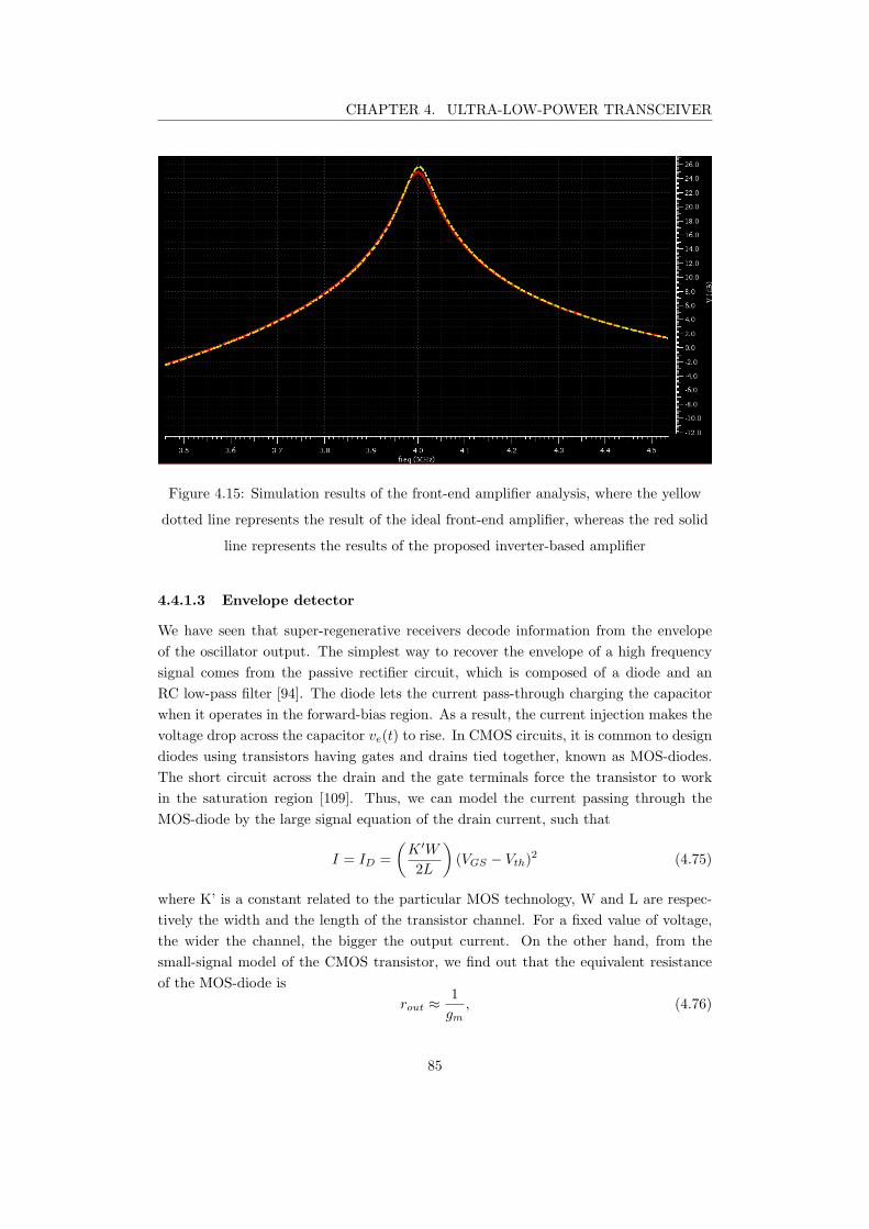
CHAPTER 4. ULTRA-LOW-POWER TRANSCEIVER
Figure 4.15: Simulation results of the front-end amplifier analysis, where the yellow
dotted line represents the result of the ideal front-end amplifier, whereas the red solid
line represents the results of the proposed inverter-based amplifier
4.4.1.3 Envelope detector
We have seen that super-regenerative receivers decode information from the envelope
of the oscillator output. The simplest way to recover the envelope of a high frequency
signal comes from the passive rectifier circuit, which is composed of a diode and an
RC low-pass filter [94]. The diode lets the current pass-through charging the capacitor
when it operates in the forward-bias region. As a result, the current injection makes the
voltage drop across the capacitor ve(t) to rise. In CMOS circuits, it is common to design
diodes using transistors having gates and drains tied together, known as MOS-diodes.
The short circuit across the drain and the gate terminals force the transistor to work
in the saturation region [109]. Thus, we can model the current passing through the
MOS-diode by the large signal equation of the drain current, such that
I = ID =
(
K ′W
2L
)
(VGS − Vth)2 (4.75)
where K’ is a constant related to the particular MOS technology, W and L are respec-
tively the width and the length of the transistor channel. For a fixed value of voltage,
the wider the channel, the bigger the output current. On the other hand, from the
small-signal model of the CMOS transistor, we find out that the equivalent resistance
of the MOS-diode is
rout ≈1
gm, (4.76)
85
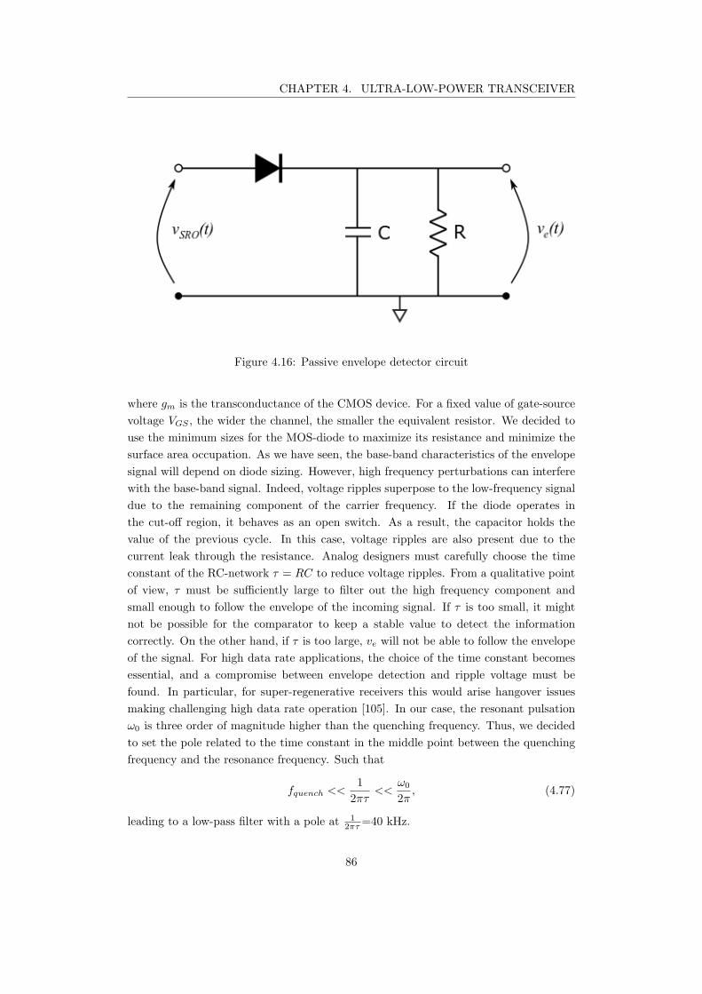
CHAPTER 4. ULTRA-LOW-POWER TRANSCEIVER
Figure 4.16: Passive envelope detector circuit
where gm is the transconductance of the CMOS device. For a fixed value of gate-source
voltage VGS , the wider the channel, the smaller the equivalent resistor. We decided to
use the minimum sizes for the MOS-diode to maximize its resistance and minimize the
surface area occupation. As we have seen, the base-band characteristics of the envelope
signal will depend on diode sizing. However, high frequency perturbations can interfere
with the base-band signal. Indeed, voltage ripples superpose to the low-frequency signal
due to the remaining component of the carrier frequency. If the diode operates in
the cut-off region, it behaves as an open switch. As a result, the capacitor holds the
value of the previous cycle. In this case, voltage ripples are also present due to the
current leak through the resistance. Analog designers must carefully choose the time
constant of the RC-network τ = RC to reduce voltage ripples. From a qualitative point
of view, τ must be sufficiently large to filter out the high frequency component and
small enough to follow the envelope of the incoming signal. If τ is too small, it might
not be possible for the comparator to keep a stable value to detect the information
correctly. On the other hand, if τ is too large, ve will not be able to follow the envelope
of the signal. For high data rate applications, the choice of the time constant becomes
essential, and a compromise between envelope detection and ripple voltage must be
found. In particular, for super-regenerative receivers this would arise hangover issues
making challenging high data rate operation [105]. In our case, the resonant pulsation
ω0 is three order of magnitude higher than the quenching frequency. Thus, we decided
to set the pole related to the time constant in the middle point between the quenching
frequency and the resonance frequency. Such that
fquench <<1
2πτ<<
ω0
2π, (4.77)
leading to a low-pass filter with a pole at 1
2πτ=40 kHz.
86
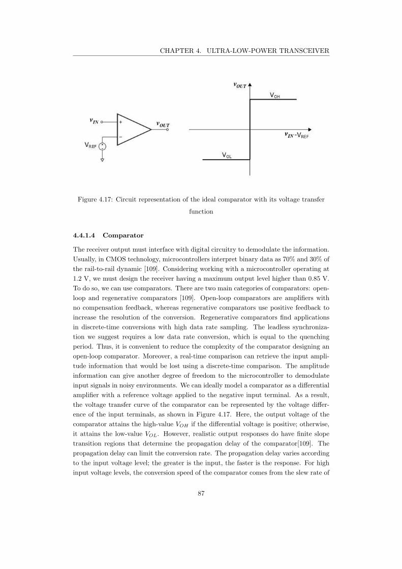
CHAPTER 4. ULTRA-LOW-POWER TRANSCEIVER
Figure 4.17: Circuit representation of the ideal comparator with its voltage transfer
function
4.4.1.4 Comparator
The receiver output must interface with digital circuitry to demodulate the information.
Usually, in CMOS technology, microcontrollers interpret binary data as 70% and 30% of
the rail-to-rail dynamic [109]. Considering working with a microcontroller operating at
1.2 V, we must design the receiver having a maximum output level higher than 0.85 V.
To do so, we can use comparators. There are two main categories of comparators: open-
loop and regenerative comparators [109]. Open-loop comparators are amplifiers with
no compensation feedback, whereas regenerative comparators use positive feedback to
increase the resolution of the conversion. Regenerative comparators find applications
in discrete-time conversions with high data rate sampling. The leadless synchroniza-
tion we suggest requires a low data rate conversion, which is equal to the quenching
period. Thus, it is convenient to reduce the complexity of the comparator designing an
open-loop comparator. Moreover, a real-time comparison can retrieve the input ampli-
tude information that would be lost using a discrete-time comparison. The amplitude
information can give another degree of freedom to the microcontroller to demodulate
input signals in noisy environments. We can ideally model a comparator as a differential
amplifier with a reference voltage applied to the negative input terminal. As a result,
the voltage transfer curve of the comparator can be represented by the voltage differ-
ence of the input terminals, as shown in Figure 4.17. Here, the output voltage of the
comparator attains the high-value VOH if the differential voltage is positive; otherwise,
it attains the low-value VOL. However, realistic output responses do have finite slope
transition regions that determine the propagation delay of the comparator[109]. The
propagation delay can limit the conversion rate. The propagation delay varies according
to the input voltage level; the greater is the input, the faster is the response. For high
input voltage levels, the conversion speed of the comparator comes from the slew rate of
87
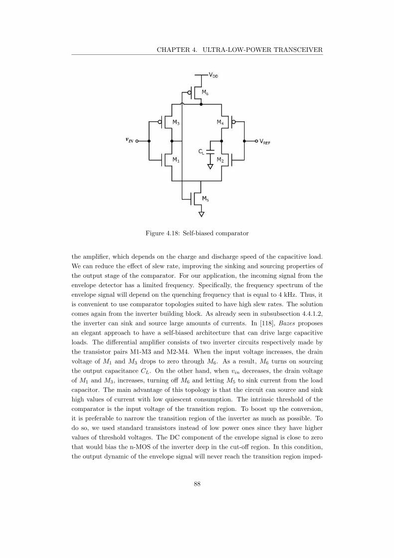
CHAPTER 4. ULTRA-LOW-POWER TRANSCEIVER
Figure 4.18: Self-biased comparator
the amplifier, which depends on the charge and discharge speed of the capacitive load.
We can reduce the effect of slew rate, improving the sinking and sourcing properties of
the output stage of the comparator. For our application, the incoming signal from the
envelope detector has a limited frequency. Specifically, the frequency spectrum of the
envelope signal will depend on the quenching frequency that is equal to 4 kHz. Thus, it
is convenient to use comparator topologies suited to have high slew rates. The solution
comes again from the inverter building block. As already seen in subsubsection 4.4.1.2,
the inverter can sink and source large amounts of currents. In [118], Bazes proposes
an elegant approach to have a self-biased architecture that can drive large capacitive
loads. The differential amplifier consists of two inverter circuits respectively made by
the transistor pairs M1-M3 and M2-M4. When the input voltage increases, the drain
voltage of M1 and M3 drops to zero through M6. As a result, M6 turns on sourcing
the output capacitance CL. On the other hand, when vin decreases, the drain voltage
of M1 and M3, increases, turning off M6 and letting M5 to sink current from the load
capacitor. The main advantage of this topology is that the circuit can source and sink
high values of current with low quiescent consumption. The intrinsic threshold of the
comparator is the input voltage of the transition region. To boost up the conversion,
it is preferable to narrow the transition region of the inverter as much as possible. To
do so, we used standard transistors instead of low power ones since they have higher
values of threshold voltages. The DC component of the envelope signal is close to zero
that would bias the n-MOS of the inverter deep in the cut-off region. In this condition,
the output dynamic of the envelope signal will never reach the transition region imped-
88
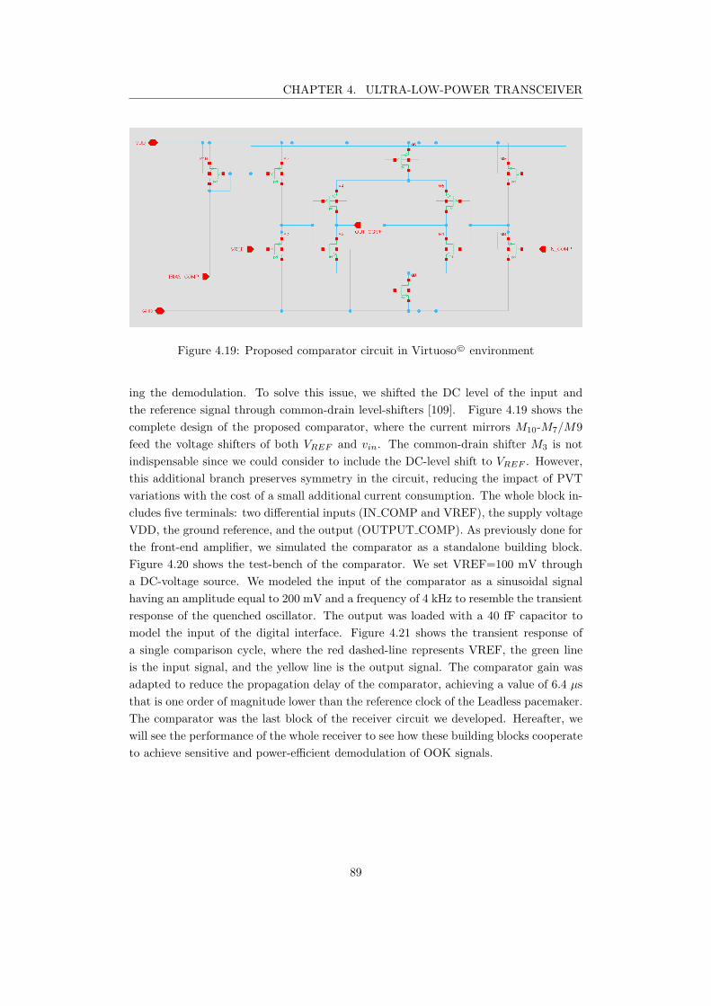
CHAPTER 4. ULTRA-LOW-POWER TRANSCEIVER
Figure 4.19: Proposed comparator circuit in Virtuoso© environment
ing the demodulation. To solve this issue, we shifted the DC level of the input and
the reference signal through common-drain level-shifters [109]. Figure 4.19 shows the
complete design of the proposed comparator, where the current mirrors M10-M7/M9
feed the voltage shifters of both VREF and vin. The common-drain shifter M3 is not
indispensable since we could consider to include the DC-level shift to VREF . However,
this additional branch preserves symmetry in the circuit, reducing the impact of PVT
variations with the cost of a small additional current consumption. The whole block in-
cludes five terminals: two differential inputs (IN COMP and VREF), the supply voltage
VDD, the ground reference, and the output (OUTPUT COMP). As previously done for
the front-end amplifier, we simulated the comparator as a standalone building block.
Figure 4.20 shows the test-bench of the comparator. We set VREF=100 mV through
a DC-voltage source. We modeled the input of the comparator as a sinusoidal signal
having an amplitude equal to 200 mV and a frequency of 4 kHz to resemble the transient
response of the quenched oscillator. The output was loaded with a 40 fF capacitor to
model the input of the digital interface. Figure 4.21 shows the transient response of
a single comparison cycle, where the red dashed-line represents VREF, the green line
is the input signal, and the yellow line is the output signal. The comparator gain was
adapted to reduce the propagation delay of the comparator, achieving a value of 6.4 µs
that is one order of magnitude lower than the reference clock of the Leadless pacemaker.
The comparator was the last block of the receiver circuit we developed. Hereafter, we
will see the performance of the whole receiver to see how these building blocks cooperate
to achieve sensitive and power-efficient demodulation of OOK signals.
89
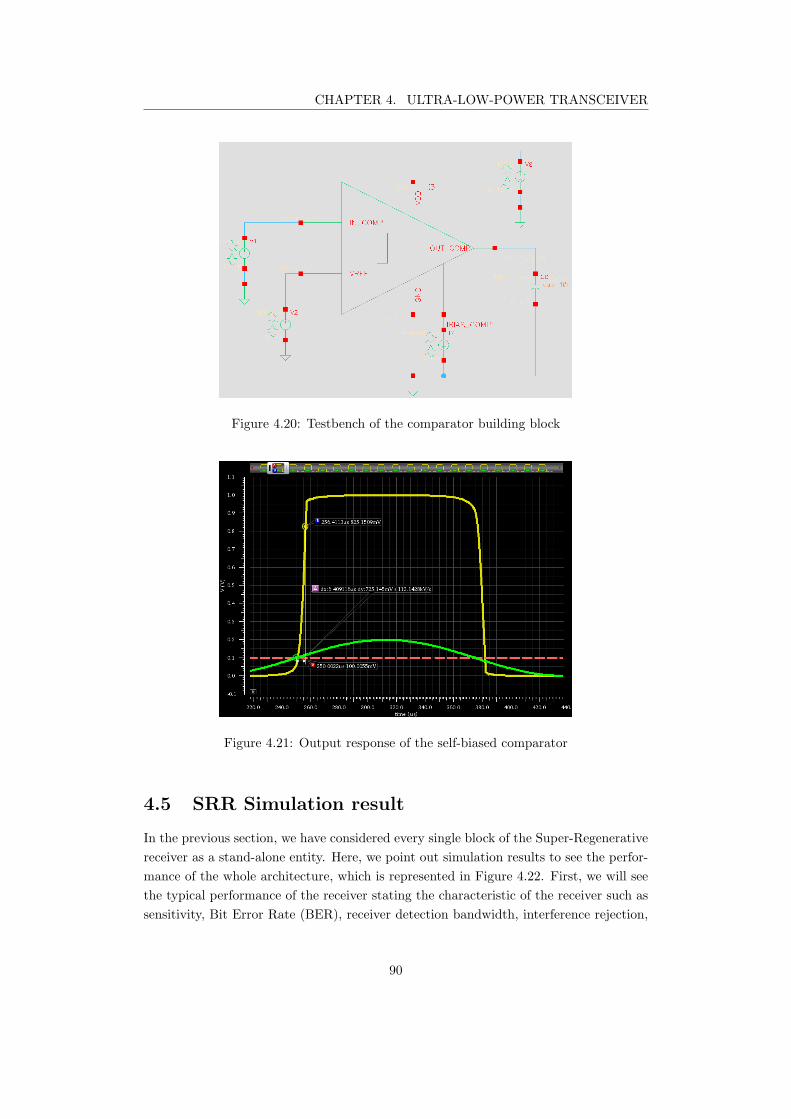
CHAPTER 4. ULTRA-LOW-POWER TRANSCEIVER
Figure 4.20: Testbench of the comparator building block
Figure 4.21: Output response of the self-biased comparator
4.5 SRR Simulation result
In the previous section, we have considered every single block of the Super-Regenerative
receiver as a stand-alone entity. Here, we point out simulation results to see the perfor-
mance of the whole architecture, which is represented in Figure 4.22. First, we will see
the typical performance of the receiver stating the characteristic of the receiver such as
sensitivity, Bit Error Rate (BER), receiver detection bandwidth, interference rejection,
90
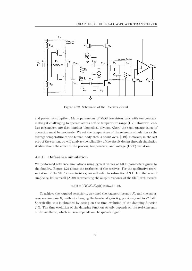
CHAPTER 4. ULTRA-LOW-POWER TRANSCEIVER
Figure 4.22: Schematic of the Receiver circuit
and power consumption. Many parameters of MOS transistors vary with temperature,
making it challenging to operate across a wide temperature range [117]. However, lead-
less pacemakers are deep-implant biomedical devices, where the temperature range of
operation must be moderate. We set the temperature of the reference simulation as the
average temperature of the human body that is about 37C [119]. However, in the last
part of the section, we will analyze the reliability of the circuit design through simulation
studies about the effect of the process, temperature, and voltage (PVT) variation.
4.5.1 Reference simulation
We performed reference simulations using typical values of MOS parameters given by
the foundry. Figure 4.24 shows the testbench of the receiver. For the qualitative repre-
sentation of the SRR characteristics, we will refer to subsection 4.3.1. For the sake of
simplicity, let us recall (A.32) representing the output response of the SRR architecture:
vo(t) = V K0KrKsp(t)cos(ω0t+ φ).
To achieve the required sensitivity, we tuned the regenerative gain Kr and the super-
regenerative gain Ks without changing the front-end gain K0, previously set to 22.5 dB.
Specifically, this is obtained by acting on the time evolution of the damping function
ζ(t). The time evolution of the damping function strictly depends on the real-time gain
of the oscillator, which in turn depends on the quench signal.
91
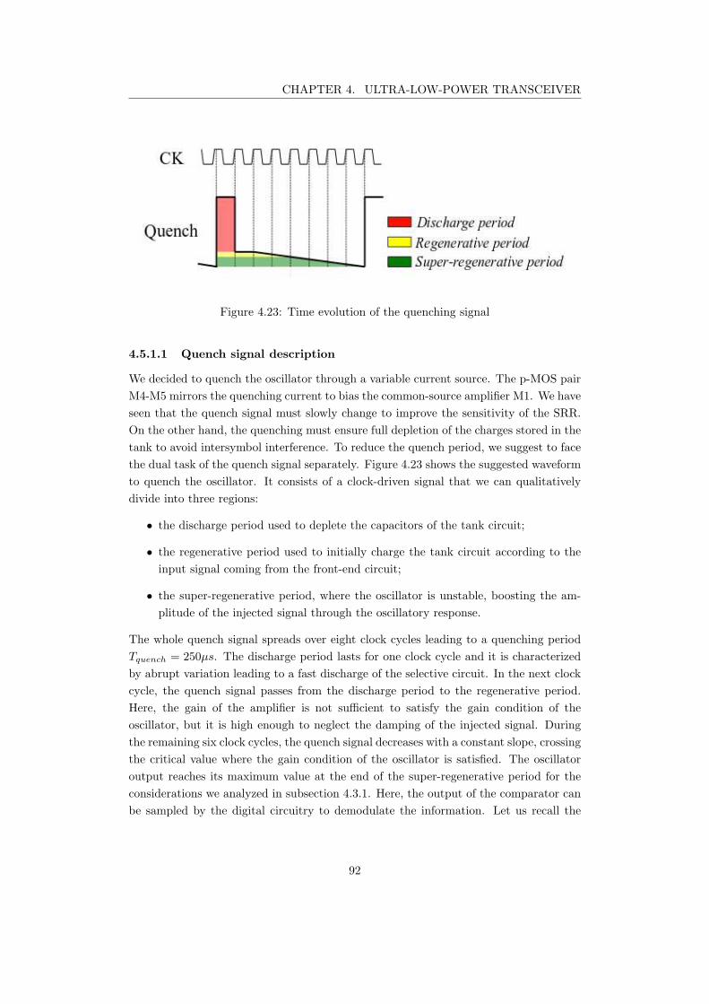
CHAPTER 4. ULTRA-LOW-POWER TRANSCEIVER
Figure 4.23: Time evolution of the quenching signal
4.5.1.1 Quench signal description
We decided to quench the oscillator through a variable current source. The p-MOS pair
M4-M5 mirrors the quenching current to bias the common-source amplifier M1. We have
seen that the quench signal must slowly change to improve the sensitivity of the SRR.
On the other hand, the quenching must ensure full depletion of the charges stored in the
tank to avoid intersymbol interference. To reduce the quench period, we suggest to face
the dual task of the quench signal separately. Figure 4.23 shows the suggested waveform
to quench the oscillator. It consists of a clock-driven signal that we can qualitatively
divide into three regions:
• the discharge period used to deplete the capacitors of the tank circuit;
• the regenerative period used to initially charge the tank circuit according to the
input signal coming from the front-end circuit;
• the super-regenerative period, where the oscillator is unstable, boosting the am-
plitude of the injected signal through the oscillatory response.
The whole quench signal spreads over eight clock cycles leading to a quenching period
Tquench = 250µs. The discharge period lasts for one clock cycle and it is characterized
by abrupt variation leading to a fast discharge of the selective circuit. In the next clock
cycle, the quench signal passes from the discharge period to the regenerative period.
Here, the gain of the amplifier is not sufficient to satisfy the gain condition of the
oscillator, but it is high enough to neglect the damping of the injected signal. During
the remaining six clock cycles, the quench signal decreases with a constant slope, crossing
the critical value where the gain condition of the oscillator is satisfied. The oscillator
output reaches its maximum value at the end of the super-regenerative period for the
considerations we analyzed in subsection 4.3.1. Here, the output of the comparator can
be sampled by the digital circuitry to demodulate the information. Let us recall the
92
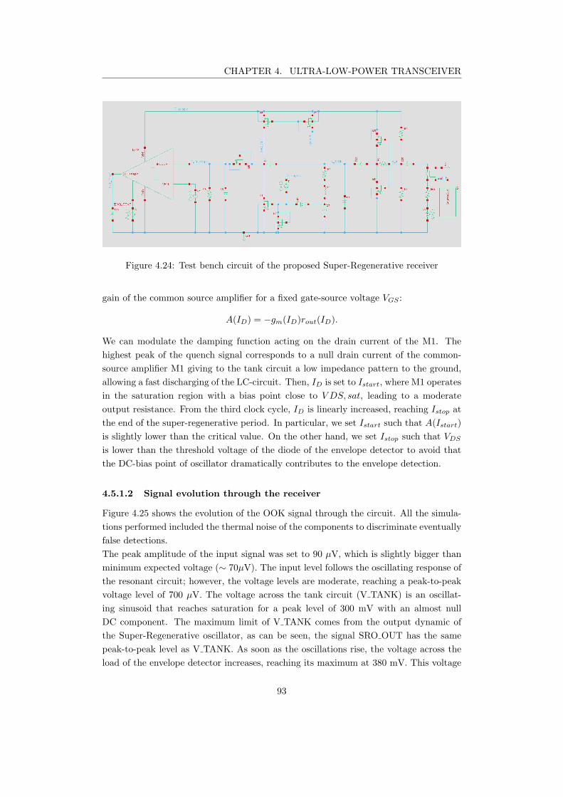
CHAPTER 4. ULTRA-LOW-POWER TRANSCEIVER
Figure 4.24: Test bench circuit of the proposed Super-Regenerative receiver
gain of the common source amplifier for a fixed gate-source voltage VGS :
A(ID) = −gm(ID)rout(ID).
We can modulate the damping function acting on the drain current of the M1. The
highest peak of the quench signal corresponds to a null drain current of the common-
source amplifier M1 giving to the tank circuit a low impedance pattern to the ground,
allowing a fast discharging of the LC-circuit. Then, ID is set to Istart, where M1 operates
in the saturation region with a bias point close to V DS, sat, leading to a moderate
output resistance. From the third clock cycle, ID is linearly increased, reaching Istop at
the end of the super-regenerative period. In particular, we set Istart such that A(Istart)
is slightly lower than the critical value. On the other hand, we set Istop such that VDS
is lower than the threshold voltage of the diode of the envelope detector to avoid that
the DC-bias point of oscillator dramatically contributes to the envelope detection.
4.5.1.2 Signal evolution through the receiver
Figure 4.25 shows the evolution of the OOK signal through the circuit. All the simula-
tions performed included the thermal noise of the components to discriminate eventually
false detections.
The peak amplitude of the input signal was set to 90 µV, which is slightly bigger than
minimum expected voltage (∼ 70µV). The input level follows the oscillating response of
the resonant circuit; however, the voltage levels are moderate, reaching a peak-to-peak
voltage level of 700 µV. The voltage across the tank circuit (V TANK) is an oscillat-
ing sinusoid that reaches saturation for a peak level of 300 mV with an almost null
DC component. The maximum limit of V TANK comes from the output dynamic of
the Super-Regenerative oscillator, as can be seen, the signal SRO OUT has the same
peak-to-peak level as V TANK. As soon as the oscillations rise, the voltage across the
load of the envelope detector increases, reaching its maximum at 380 mV. This voltage
93
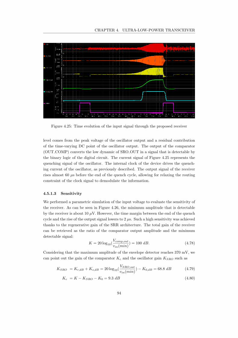
CHAPTER 4. ULTRA-LOW-POWER TRANSCEIVER
Figure 4.25: Time evolution of the input signal through the proposed receiver
level comes from the peak voltage of the oscillator output and a residual contribution
of the time-varying DC point of the oscillator output. The output of the comparator
(OUT COMP) converts the low dynamic of SRO OUT in a signal that is detectable by
the binary logic of the digital circuit. The current signal of Figure 4.25 represents the
quenching signal of the oscillator. The internal clock of the device drives the quench-
ing current of the oscillator, as previously described. The output signal of the receiver
rises almost 60 µs before the end of the quench cycle, allowing for relaxing the routing
constraint of the clock signal to demodulate the information.
4.5.1.3 Sensitivity
We performed a parametric simulation of the input voltage to evaluate the sensitivity of
the receiver. As can be seen in Figure 4.26, the minimum amplitude that is detectable
by the receiver is about 10 µV. However, the time margin between the end of the quench
cycle and the rise of the output signal lowers to 2 µs. Such a high sensitivity was achieved
thanks to the regenerative gain of the SRR architecture. The total gain of the receiver
can be retrieved as the ratio of the comparator output amplitude and the minimum
detectable signal:
K = 20 log10(Vcomp,out
vin(min)) = 100 dB. (4.78)
Considering that the maximum amplitude of the envelope detector reaches 370 mV, we
can point out the gain of the comparator Kc and the oscillator gain KSRO such as
KSRO = Kr,dB +Ks,dB = 20 log10(VSRO,sat
vin(min))−K0,dB = 68.8 dB (4.79)
Kc = K −KSRO −K0 = 9.3 dB (4.80)
94
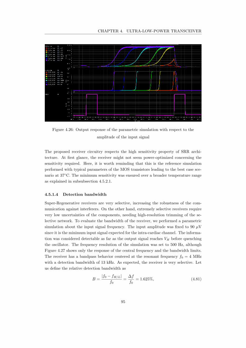
CHAPTER 4. ULTRA-LOW-POWER TRANSCEIVER
Figure 4.26: Output response of the parametric simulation with respect to the
amplitude of the input signal
The proposed receiver circuitry respects the high sensitivity property of SRR archi-
tecture. At first glance, the receiver might not seem power-optimized concerning the
sensitivity required. Here, it is worth reminding that this is the reference simulation
performed with typical parameters of the MOS transistors leading to the best case sce-
nario at 37C. The minimum sensitivity was ensured over a broader temperature range
as explained in subsubsection 4.5.2.1.
4.5.1.4 Detection bandwidth
Super-Regenerative receivers are very selective, increasing the robustness of the com-
munication against interferers. On the other hand, extremely selective receivers require
very low uncertainties of the components, needing high-resolution trimming of the se-
lective network. To evaluate the bandwidth of the receiver, we performed a parametric
simulation about the input signal frequency. The input amplitude was fixed to 90 µV
since it is the minimum input signal expected for the intra-cardiac channel. The informa-
tion was considered detectable as far as the output signal reaches VH before quenching
the oscillator. The frequency resolution of the simulation was set to 500 Hz, although
Figure 4.27 shows only the response of the central frequency and the bandwidth limits.
The receiver has a bandpass behavior centered at the resonant frequency f0 = 4 MHz
with a detection bandwidth of 13 kHz. As expected, the receiver is very selective. Let
us define the relative detection bandwidth as
B =|f0 − fH/L|
f0=
∆f
f0= 1.625%, (4.81)
95
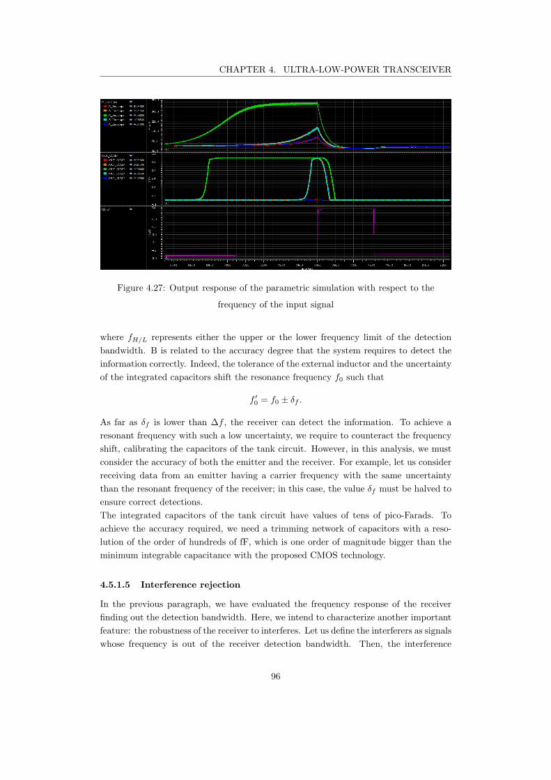
CHAPTER 4. ULTRA-LOW-POWER TRANSCEIVER
Figure 4.27: Output response of the parametric simulation with respect to the
frequency of the input signal
where fH/L represents either the upper or the lower frequency limit of the detection
bandwidth. B is related to the accuracy degree that the system requires to detect the
information correctly. Indeed, the tolerance of the external inductor and the uncertainty
of the integrated capacitors shift the resonance frequency f0 such that
f ′
0= f0 ± δf .
As far as δf is lower than ∆f , the receiver can detect the information. To achieve a
resonant frequency with such a low uncertainty, we require to counteract the frequency
shift, calibrating the capacitors of the tank circuit. However, in this analysis, we must
consider the accuracy of both the emitter and the receiver. For example, let us consider
receiving data from an emitter having a carrier frequency with the same uncertainty
than the resonant frequency of the receiver; in this case, the value δf must be halved to
ensure correct detections.
The integrated capacitors of the tank circuit have values of tens of pico-Farads. To
achieve the accuracy required, we need a trimming network of capacitors with a reso-
lution of the order of hundreds of fF, which is one order of magnitude bigger than the
minimum integrable capacitance with the proposed CMOS technology.
4.5.1.5 Interference rejection
In the previous paragraph, we have evaluated the frequency response of the receiver
finding out the detection bandwidth. Here, we intend to characterize another important
feature: the robustness of the receiver to interferes. Let us define the interferers as signals
whose frequency is out of the receiver detection bandwidth. Then, the interference
96
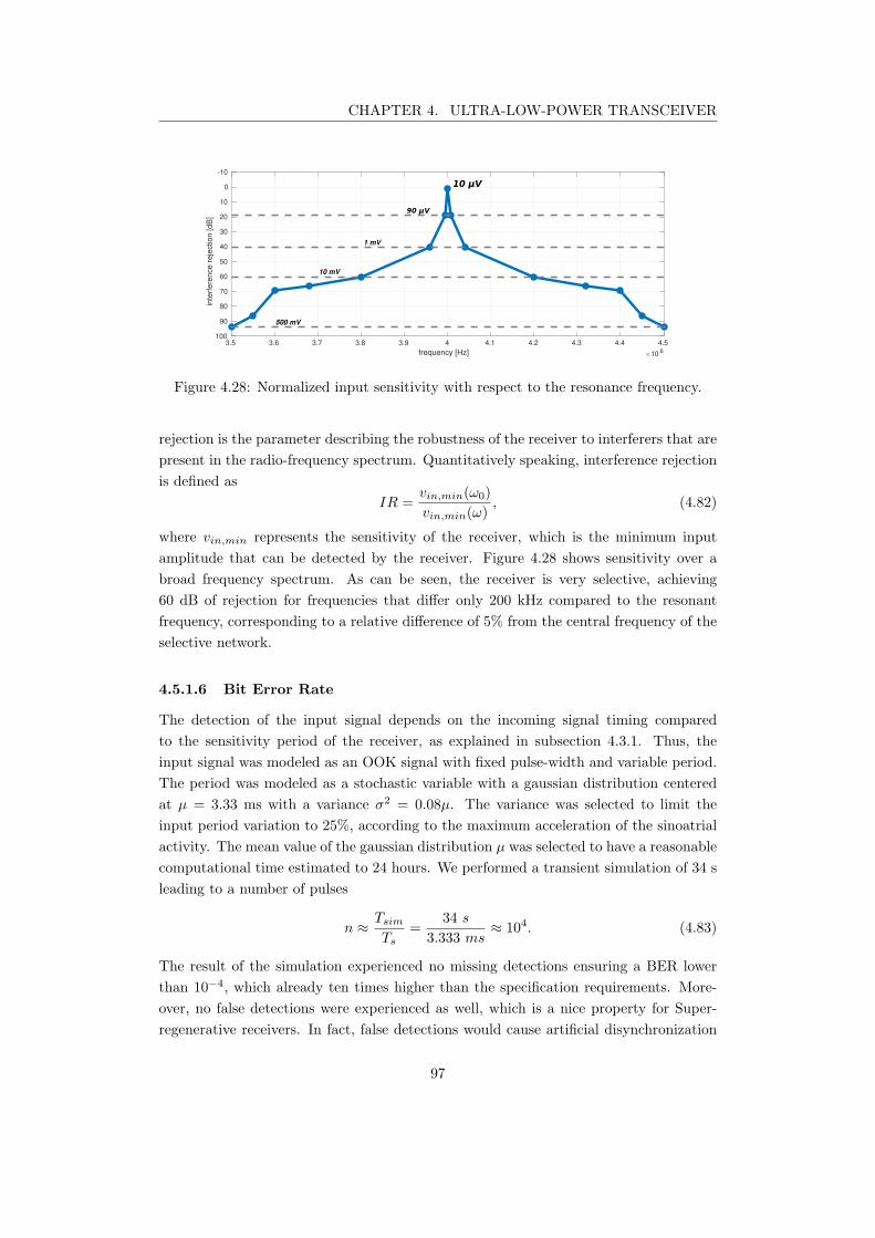
CHAPTER 4. ULTRA-LOW-POWER TRANSCEIVER
3.5 3.6 3.7 3.8 3.9 4 4.1 4.2 4.3 4.4 4.5
frequency [Hz] 10 6
-10
0
10
20
30
40
50
60
70
80
90
100
inte
rfere
nce r
eje
ction [dB
]
1 mV
10 mV
500 mV
Figure 4.28: Normalized input sensitivity with respect to the resonance frequency.
rejection is the parameter describing the robustness of the receiver to interferers that are
present in the radio-frequency spectrum. Quantitatively speaking, interference rejection
is defined as
IR =vin,min(ω0)
vin,min(ω), (4.82)
where vin,min represents the sensitivity of the receiver, which is the minimum input
amplitude that can be detected by the receiver. Figure 4.28 shows sensitivity over a
broad frequency spectrum. As can be seen, the receiver is very selective, achieving
60 dB of rejection for frequencies that differ only 200 kHz compared to the resonant
frequency, corresponding to a relative difference of 5% from the central frequency of the
selective network.
4.5.1.6 Bit Error Rate
The detection of the input signal depends on the incoming signal timing compared
to the sensitivity period of the receiver, as explained in subsection 4.3.1. Thus, the
input signal was modeled as an OOK signal with fixed pulse-width and variable period.
The period was modeled as a stochastic variable with a gaussian distribution centered
at µ = 3.33 ms with a variance σ2 = 0.08µ. The variance was selected to limit the
input period variation to 25%, according to the maximum acceleration of the sinoatrial
activity. The mean value of the gaussian distribution µ was selected to have a reasonable
computational time estimated to 24 hours. We performed a transient simulation of 34 s
leading to a number of pulses
n ≈
Tsim
Ts
=34 s
3.333 ms≈ 104. (4.83)
The result of the simulation experienced no missing detections ensuring a BER lower
than 10−4, which already ten times higher than the specification requirements. More-
over, no false detections were experienced as well, which is a nice property for Super-
regenerative receivers. In fact, false detections would cause artificial disynchronization
97
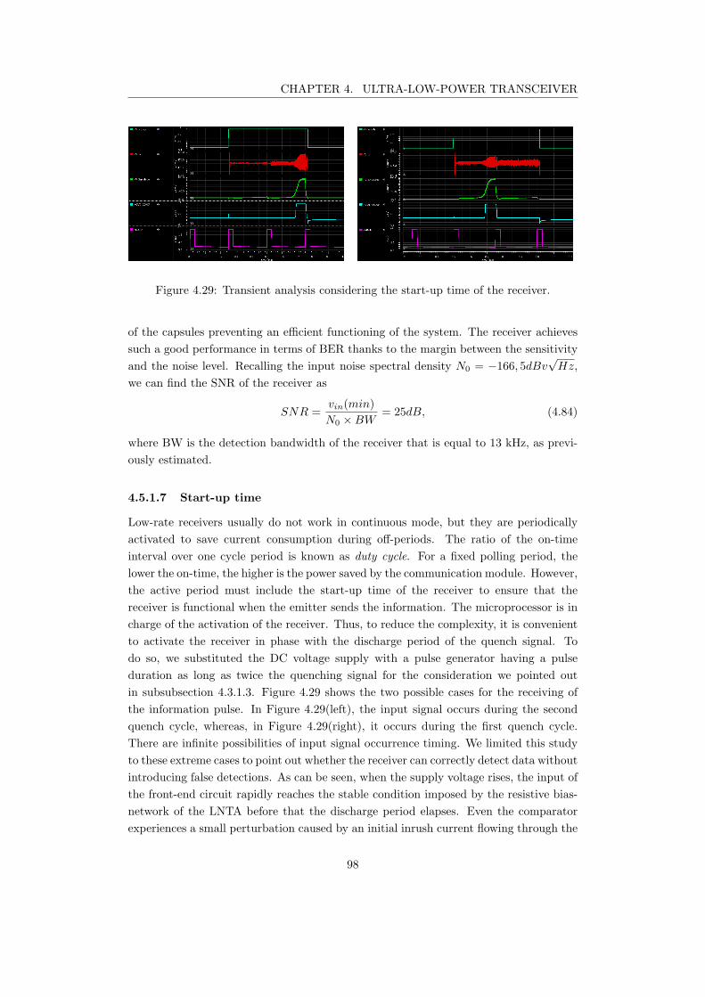
CHAPTER 4. ULTRA-LOW-POWER TRANSCEIVER
Figure 4.29: Transient analysis considering the start-up time of the receiver.
of the capsules preventing an efficient functioning of the system. The receiver achieves
such a good performance in terms of BER thanks to the margin between the sensitivity
and the noise level. Recalling the input noise spectral density N0 = −166, 5dBv√Hz,
we can find the SNR of the receiver as
SNR =vin(min)
N0 ×BW= 25dB, (4.84)
where BW is the detection bandwidth of the receiver that is equal to 13 kHz, as previ-
ously estimated.
4.5.1.7 Start-up time
Low-rate receivers usually do not work in continuous mode, but they are periodically
activated to save current consumption during off-periods. The ratio of the on-time
interval over one cycle period is known as duty cycle. For a fixed polling period, the
lower the on-time, the higher is the power saved by the communication module. However,
the active period must include the start-up time of the receiver to ensure that the
receiver is functional when the emitter sends the information. The microprocessor is in
charge of the activation of the receiver. Thus, to reduce the complexity, it is convenient
to activate the receiver in phase with the discharge period of the quench signal. To
do so, we substituted the DC voltage supply with a pulse generator having a pulse
duration as long as twice the quenching signal for the consideration we pointed out
in subsubsection 4.3.1.3. Figure 4.29 shows the two possible cases for the receiving of
the information pulse. In Figure 4.29(left), the input signal occurs during the second
quench cycle, whereas, in Figure 4.29(right), it occurs during the first quench cycle.
There are infinite possibilities of input signal occurrence timing. We limited this study
to these extreme cases to point out whether the receiver can correctly detect data without
introducing false detections. As can be seen, when the supply voltage rises, the input of
the front-end circuit rapidly reaches the stable condition imposed by the resistive bias-
network of the LNTA before that the discharge period elapses. Even the comparator
experiences a small perturbation caused by an initial inrush current flowing through the
98
CHAPTER 4. ULTRA-LOW-POWER TRANSCEIVER
output capacitor. However, the voltage level is small and cannot induce false detection.
4.5.1.8 Power consumption
Last but not least, we report the power consumption of the receiver. By definition, the
power consumption of the circuit is given by the root mean square product between the
supply voltage and the total current drawn. The supply voltage of the receiver is fixed
and equal to 1 V. On the other hand, the current varies over time due to the current-
driven quenching of the oscillator. Thus, the active power consumption of the proposed
circuit can be found as
Pactive = Vsupply · IRMS = 18.25 µW, (4.85)
where IRMS is the root mean square current drawn by the supply voltage generator.
Here, we characterized the typical performances of the receiver through reference sim-
ulations. In the next subsection, we will evaluate how the receiver performances are
impacted by PVT variations.
4.5.2 Process, voltage and temperature (PVT) variation
So far, we characterized the performance of the suggested receiver for typical conditions.
However, CMOS components vary with the fabrication process, supply voltage, and
ambient temperature. We denote these effects by PVT and design circuits such that
their performance is acceptable for a specified range of PVT variations [117]. Those
effects are tested separately to point out the effect of each variation over the typical
performance of the receiver.
4.5.2.1 Temperature
The temperature dependence of MOS transistors is mainly related to the changes in
the charge mobility and the threshold voltage [120, 121]. As a result, the drain current
of transistors varies accordingly. The following equation quantifies the drain current
considering temperature effect [109]:
ID(T ) =K
2
W
L
(
T
T0
)
−1.5
[VGS − Vth0 − α(T − T0)]2, (4.86)
where T0 is the reference temperature in Kelvin, Vth0 = Vth(T0), and α is an empirical
coefficient that is positive for p-MOS and negative for n-MOS devices. Thus, to eval-
uate the effect of temperature variation, we launched a parametric analysis for a set
of temperatures ranging in [27C - 50C]. We limited the analysis to such a moderate
temperature range since the application targets deep-implant devices where the envi-
ronment temperature must not extremely vary from 37C. In particular, we considered
as low temperature limit the room temperature of 300K (27C) to have a reference
99
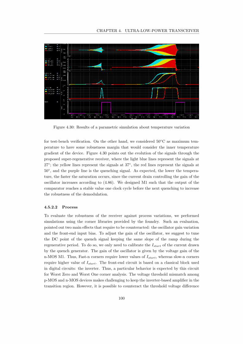
CHAPTER 4. ULTRA-LOW-POWER TRANSCEIVER
Figure 4.30: Results of a parametric simulation about temperature variation
for test-bench verification. On the other hand, we considered 50C as maximum tem-
perature to have some robustness margin that would consider the inner temperature
gradient of the device. Figure 4.30 points out the evolution of the signals through the
proposed super-regenerative receiver, where the light blue lines represent the signals at
27; the yellow lines represent the signals at 37, the red lines represent the signals at
50, and the purple line is the quenching signal. As expected, the lower the tempera-
ture, the faster the saturation occurs, since the current drain controlling the gain of the
oscillator increases according to (4.86). We designed M1 such that the output of the
comparator reaches a stable value one clock cycle before the next quenching to increase
the robustness of the demodulation.
4.5.2.2 Process
To evaluate the robustness of the receiver against process variations, we performed
simulations using the corner libraries provided by the foundry. Such an evaluation,
pointed out two main effects that require to be counteracted: the oscillator gain variation
and the front-end input bias. To adjust the gain of the oscillator, we suggest to tune
the DC point of the quench signal keeping the same slope of the ramp during the
regenerative period. To do so, we only need to calibrate the Istart of the current drawn
by the quench generator. The gain of the oscillator is given by the voltage gain of the
n-MOS M1. Thus, Fast-n corners require lower values of Istart, whereas slow-n corners
require higher value of Istart. The front-end circuit is based on a classical block used
in digital circuits: the inverter. Thus, a particular behavior is expected by this circuit
for Worst Zero and Worst One corner analysis. The voltage threshold mismatch among
p-MOS and n-MOS devices makes challenging to keep the inverter-based amplifier in the
transition region. However, it is possible to counteract the threshold voltage difference
100
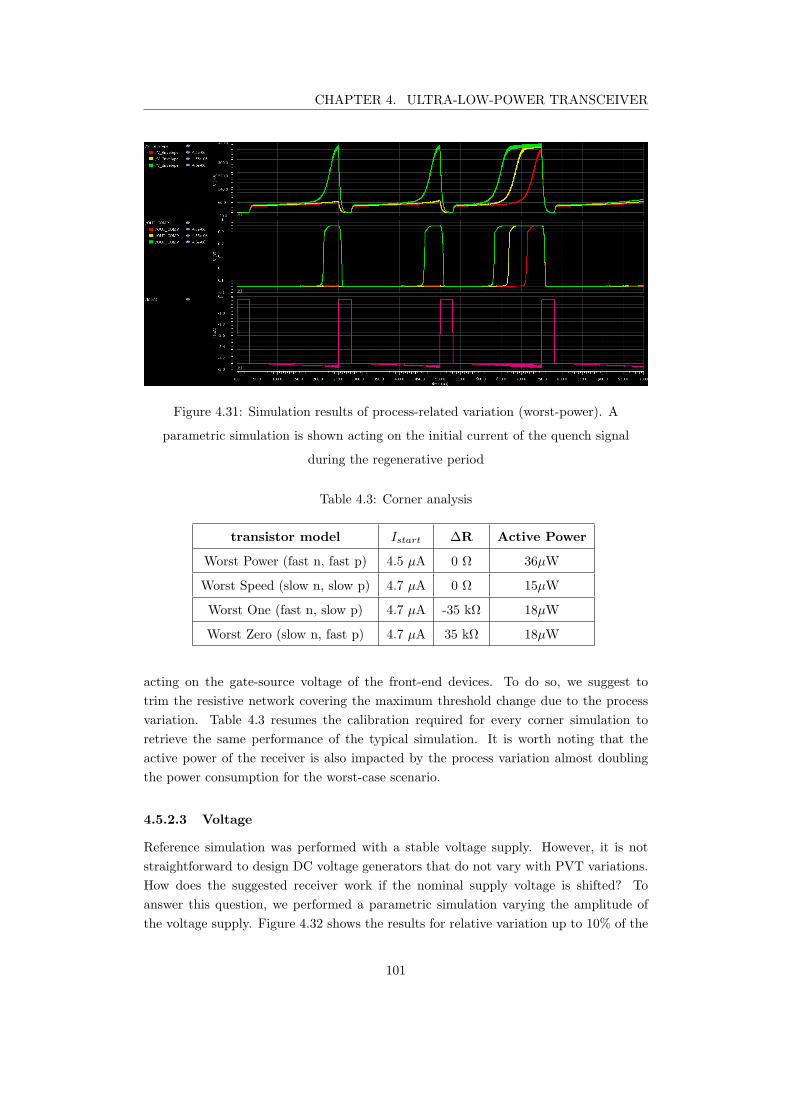
CHAPTER 4. ULTRA-LOW-POWER TRANSCEIVER
Figure 4.31: Simulation results of process-related variation (worst-power). A
parametric simulation is shown acting on the initial current of the quench signal
during the regenerative period
Table 4.3: Corner analysis
transistor model Istart ∆R Active Power
Worst Power (fast n, fast p) 4.5 µA 0 Ω 36µW
Worst Speed (slow n, slow p) 4.7 µA 0 Ω 15µW
Worst One (fast n, slow p) 4.7 µA -35 kΩ 18µW
Worst Zero (slow n, fast p) 4.7 µA 35 kΩ 18µW
acting on the gate-source voltage of the front-end devices. To do so, we suggest to
trim the resistive network covering the maximum threshold change due to the process
variation. Table 4.3 resumes the calibration required for every corner simulation to
retrieve the same performance of the typical simulation. It is worth noting that the
active power of the receiver is also impacted by the process variation almost doubling
the power consumption for the worst-case scenario.
4.5.2.3 Voltage
Reference simulation was performed with a stable voltage supply. However, it is not
straightforward to design DC voltage generators that do not vary with PVT variations.
How does the suggested receiver work if the nominal supply voltage is shifted? To
answer this question, we performed a parametric simulation varying the amplitude of
the voltage supply. Figure 4.32 shows the results for relative variation up to 10% of the
101
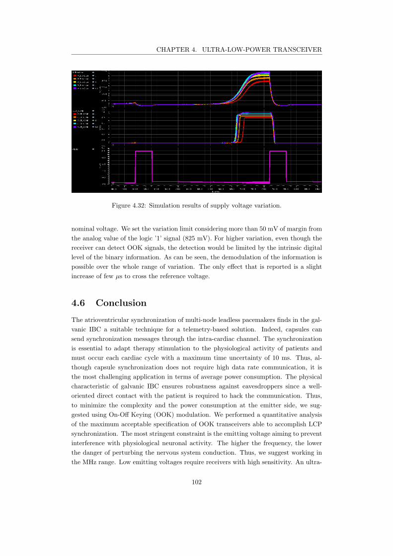
CHAPTER 4. ULTRA-LOW-POWER TRANSCEIVER
Figure 4.32: Simulation results of supply voltage variation.
nominal voltage. We set the variation limit considering more than 50 mV of margin from
the analog value of the logic ’1’ signal (825 mV). For higher variation, even though the
receiver can detect OOK signals, the detection would be limited by the intrinsic digital
level of the binary information. As can be seen, the demodulation of the information is
possible over the whole range of variation. The only effect that is reported is a slight
increase of few µs to cross the reference voltage.
4.6 Conclusion
The atrioventricular synchronization of multi-node leadless pacemakers finds in the gal-
vanic IBC a suitable technique for a telemetry-based solution. Indeed, capsules can
send synchronization messages through the intra-cardiac channel. The synchronization
is essential to adapt therapy stimulation to the physiological activity of patients and
must occur each cardiac cycle with a maximum time uncertainty of 10 ms. Thus, al-
though capsule synchronization does not require high data rate communication, it is
the most challenging application in terms of average power consumption. The physical
characteristic of galvanic IBC ensures robustness against eavesdroppers since a well-
oriented direct contact with the patient is required to hack the communication. Thus,
to minimize the complexity and the power consumption at the emitter side, we sug-
gested using On-Off Keying (OOK) modulation. We performed a quantitative analysis
of the maximum acceptable specification of OOK transceivers able to accomplish LCP
synchronization. The most stringent constraint is the emitting voltage aiming to prevent
interference with physiological neuronal activity. The higher the frequency, the lower
the danger of perturbing the nervous system conduction. Thus, we suggest working in
the MHz range. Low emitting voltages require receivers with high sensitivity. An ultra-
102
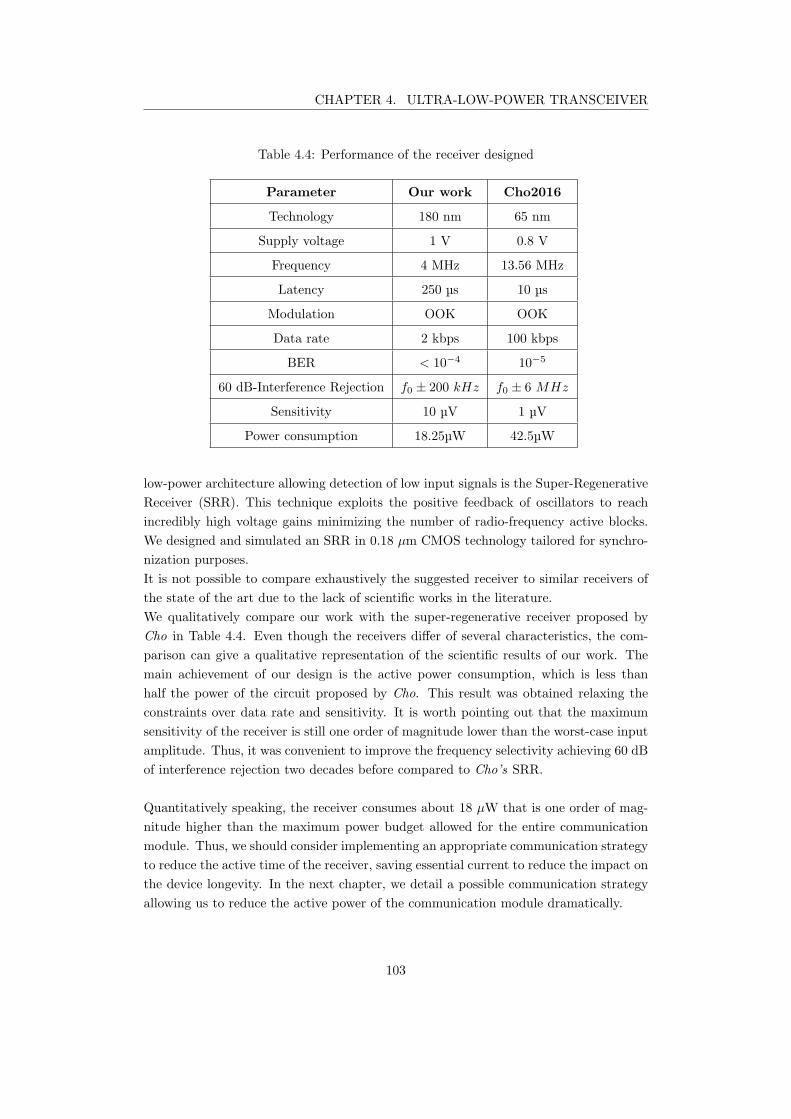
CHAPTER 4. ULTRA-LOW-POWER TRANSCEIVER
Table 4.4: Performance of the receiver designed
Parameter Our work Cho2016
Technology 180 nm 65 nm
Supply voltage 1 V 0.8 V
Frequency 4 MHz 13.56 MHz
Latency 250 µs 10 µs
Modulation OOK OOK
Data rate 2 kbps 100 kbps
BER < 10−4 10−5
60 dB-Interference Rejection f0 ± 200 kHz f0 ± 6 MHz
Sensitivity 10 µV 1 µV
Power consumption 18.25µW 42.5µW
low-power architecture allowing detection of low input signals is the Super-Regenerative
Receiver (SRR). This technique exploits the positive feedback of oscillators to reach
incredibly high voltage gains minimizing the number of radio-frequency active blocks.
We designed and simulated an SRR in 0.18 µm CMOS technology tailored for synchro-
nization purposes.
It is not possible to compare exhaustively the suggested receiver to similar receivers of
the state of the art due to the lack of scientific works in the literature.
We qualitatively compare our work with the super-regenerative receiver proposed by
Cho in Table 4.4. Even though the receivers differ of several characteristics, the com-
parison can give a qualitative representation of the scientific results of our work. The
main achievement of our design is the active power consumption, which is less than
half the power of the circuit proposed by Cho. This result was obtained relaxing the
constraints over data rate and sensitivity. It is worth pointing out that the maximum
sensitivity of the receiver is still one order of magnitude lower than the worst-case input
amplitude. Thus, it was convenient to improve the frequency selectivity achieving 60 dB
of interference rejection two decades before compared to Cho’s SRR.
Quantitatively speaking, the receiver consumes about 18 µW that is one order of mag-
nitude higher than the maximum power budget allowed for the entire communication
module. Thus, we should consider implementing an appropriate communication strategy
to reduce the active time of the receiver, saving essential current to reduce the impact on
the device longevity. In the next chapter, we detail a possible communication strategy
allowing us to reduce the active power of the communication module dramatically.
103
5Communication strategy
A multi-nodal leadless pacemaker system requires a communication network between
the devices implanted in different heart chambers. The communication link aims to
send physiological information such as EGM-event detections to deliver a synchronized
therapy. Wireless communication approaches are power demanding reducing battery
lifetime, which is a critical issue in permanent implants with limited battery capacity.
In the previous chapter, we have seen that the Super-Regenerative Receiver can be an
attractive solution for IBC intra-cardiac communication to demodulate low amplitude
input signals. However, the active current drawn of the proposed circuit is still too high
for continuous-time usage. Indeed, there is a need for smart strategies to reduce the duty
cycle of the receiver and, consequently, its average power consumption. This chapter
deals with a communication strategy for AV synchronization. The suggested algorithm
is driven by the detection of the P-wave and can considerably reduce the power con-
sumption of the receiver. According to clinical studies [122], the physiological heart rate
does not accelerate by more than [25-35] % from beat to beat. Standard pacemakers
have also the possibility to set a parameter for the beat to beat deceleration, which
we will refer to as ∆pos. ∆pos reduces the artificial depolarization of cardiomyocytes
and ranges from [0-30] % of the heart rate. Considering both the physiological accel-
eration and the allowed deceleration of the atrial activity, we find out that the P-wave
information variability ranges in a time-window that varies from 25% and 65% of the
heart-cycle duration. Even though we consider to turn on the receiver only during this
amount of time, its power consumption would be extremely high compared to the LCP
power budget.
5.1 Communication protocol description
In a healthy heart, the stimulation impulse propagates from the sinoatrial node of the
RA to the ventricles, as described in chapter 2. However, electrical dysfunctions of
104
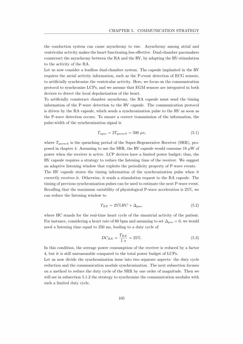
CHAPTER 5. COMMUNICATION STRATEGY
the conduction system can cause asynchrony to rise. Asynchrony among atrial and
ventricular activity makes the heart functioning less effective. Dual-chamber pacemakers
counteract the asynchrony between the RA and the RV, by adapting the RV-stimulation
to the activity of the RA.
Let us now consider a leadless dual-chamber system. The capsule implanted in the RV
requires the atrial activity information, such as the P-event detection of ECG sensors,
to artificially synchronize the ventricular activity. Here, we focus on the communication
protocol to synchronize LCPs, and we assume that EGM sensors are integrated in both
devices to detect the local depolarization of the heart.
To artificially counteract chamber asynchrony, the RA capsule must send the timing
information of the P-wave detection to the RV capsule. The communication protocol
is driven by the RA capsule, which sends a synchronization pulse to the RV as soon as
the P-wave detection occurs. To ensure a correct transmission of the information, the
pulse-width of the synchronization signal is
Tsync = 2Tquench = 500 µs, (5.1)
where Tquench is the quenching period of the Super-Regenerative Receiver (SRR), pro-
posed in chapter 4. Assuming to use the SRR, the RV capsule would consume 18 µW of
power when the receiver is active. LCP devices have a limited power budget; thus, the
RV capsule requires a strategy to reduce the listening time of the receiver. We suggest
an adaptive listening window that exploits the periodicity property of P-wave events.
The RV capsule stores the timing information of the synchronization pulse when it
correctly receives it. Otherwise, it sends a stimulation request to the RA capsule. The
timing of previous synchronization pulses can be used to estimate the next P-wave event.
Recalling that the maximum variability of physiological P-wave acceleration is 25%, we
can reduce the listening window to
TRX = 25%HC +∆pos, (5.2)
where HC stands for the real-time heart cycle of the sinoatrial activity of the patient.
For instance, considering a heart rate of 60 bpm and assuming to set ∆pos = 0, we would
need a listening time equal to 250 ms, leading to a duty cycle of
DCRX =TRX
1 s= 25%. (5.3)
In this condition, the average power consumption of the receiver is reduced by a factor
4, but it is still unreasonable compared to the total power budget of LCPs.
Let us now divide the synchronization issue into two separate aspects: the duty cycle
reduction and the communication module synchronization. The next subsection focuses
on a method to reduce the duty cycle of the SRR by one order of magnitude. Then we
will see in subsection 5.1.2 the strategy to synchronize the communication modules with
such a limited duty cycle.
105
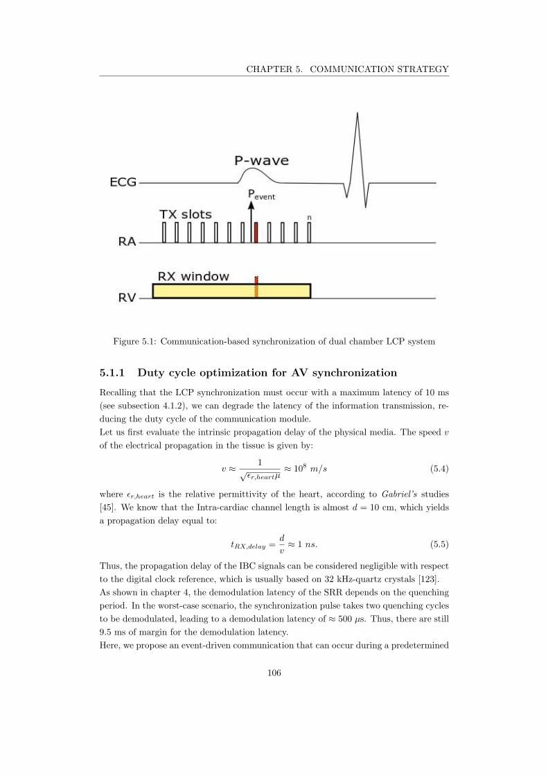
CHAPTER 5. COMMUNICATION STRATEGY
Figure 5.1: Communication-based synchronization of dual chamber LCP system
5.1.1 Duty cycle optimization for AV synchronization
Recalling that the LCP synchronization must occur with a maximum latency of 10 ms
(see subsection 4.1.2), we can degrade the latency of the information transmission, re-
ducing the duty cycle of the communication module.
Let us first evaluate the intrinsic propagation delay of the physical media. The speed v
of the electrical propagation in the tissue is given by:
v ≈1
√ǫr,heartµ
≈ 108 m/s (5.4)
where ǫr,heart is the relative permittivity of the heart, according to Gabriel’s studies
[45]. We know that the Intra-cardiac channel length is almost d = 10 cm, which yields
a propagation delay equal to:
tRX,delay =d
v≈ 1 ns. (5.5)
Thus, the propagation delay of the IBC signals can be considered negligible with respect
to the digital clock reference, which is usually based on 32 kHz-quartz crystals [123].
As shown in chapter 4, the demodulation latency of the SRR depends on the quenching
period. In the worst-case scenario, the synchronization pulse takes two quenching cycles
to be demodulated, leading to a demodulation latency of ≈ 500 µs. Thus, there are still
9.5 ms of margin for the demodulation latency.
Here, we propose an event-driven communication that can occur during a predetermined
106
CHAPTER 5. COMMUNICATION STRATEGY
Figure 5.2: Sub-block representation of the emitter time-window
period. The basic concept is to map the physiologic period where the P-wave can occur
into periodic sub-blocks where the communication can be enabled.
It is worth reminding that the P-wave acceleration is relative to the real-time heart rate.
Thus, the number of sub-blocks must be adapted to the heart rate as well.
The time-window is composed of n periodic slots, covering the whole physiological time-
window for both the emitter (RA capsule) and the receiver (RV capsule). Let us first
consider the emitting slots of the RA capsule, represented in Figure 5.2. Each slot is
equally spaced in time by Tslot and have duration pulse equal to Tbit. When the RA
capsule detects the P-wave, it will use the first possible emitting slot of the TX window
to send the synchronization pulse to the RV capsule. As previously said, Tbit = 500 µs;
then, to respect the latency constraint, the value of Tslot must be lower or equal to 9.5 ms.
On the other hand, the RV capsule maps the physiological time-window into the same
number of sub-blocks n, as depicted in Figure 5.3. Each sub-blocks is composed of a
SLEEP-period and an ON-period. During the SLEEP-period, the main microcontroller
of the device turns off the receiver, whereas, during the ON-period, it keeps it active.
The ON-period must cover the starting time of the receiver, considering an appropriate
margin to ensure the correct detection of the synchronization pulse. The number of slots
n is given as the first integer number coming from the ratio between the physiological
P-wave time-window and a single sub-block period (Tsub), as described by:
n =TRX
Tsub
=25%HC +∆pos
TSleep + TON
(5.6)
For example, if we consider having a heartbeat rate of 60 bpm with ∆pos = 0, the total
physiological period is equal to 250 ms. Then, setting Tsleep = 9 ms and TON = 1 ms,
leads to n=25, reducing the overall listening time to 25 ms. Thus, the average power
consumption of the receiver lowers of one order of magnitude, reaching an average current
drawn of 450 nA. To further reduce receiver consumption during heartbeat acceleration,
the receiver of the RV capsule could be disabled once the synchronization signal is
received.
107
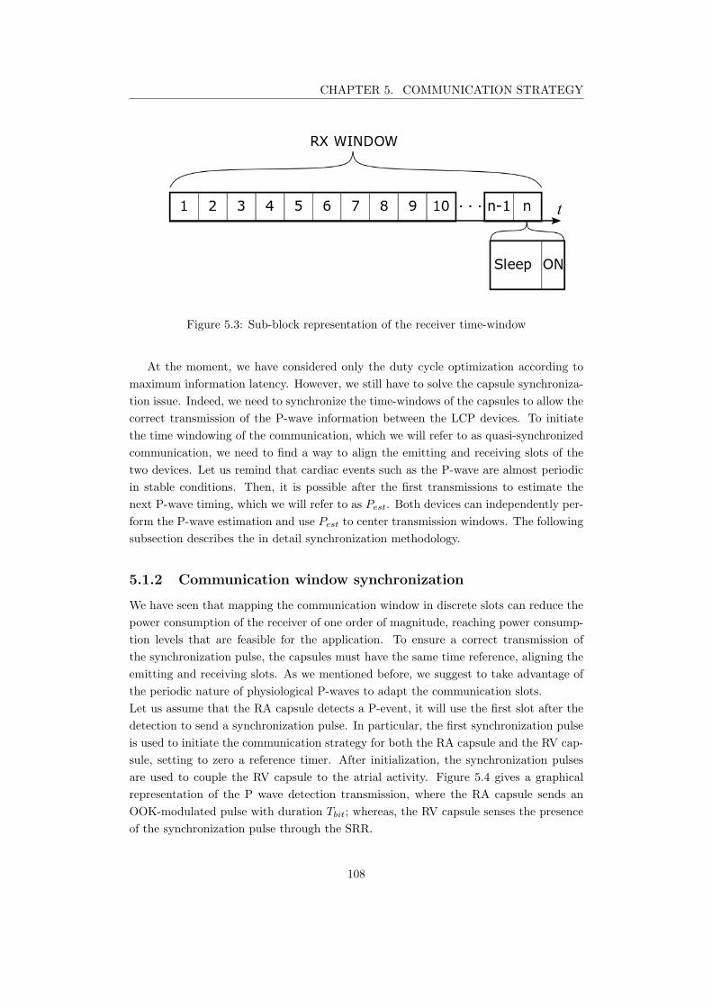
CHAPTER 5. COMMUNICATION STRATEGY
Figure 5.3: Sub-block representation of the receiver time-window
At the moment, we have considered only the duty cycle optimization according to
maximum information latency. However, we still have to solve the capsule synchroniza-
tion issue. Indeed, we need to synchronize the time-windows of the capsules to allow the
correct transmission of the P-wave information between the LCP devices. To initiate
the time windowing of the communication, which we will refer to as quasi-synchronized
communication, we need to find a way to align the emitting and receiving slots of the
two devices. Let us remind that cardiac events such as the P-wave are almost periodic
in stable conditions. Then, it is possible after the first transmissions to estimate the
next P-wave timing, which we will refer to as Pest. Both devices can independently per-
form the P-wave estimation and use Pest to center transmission windows. The following
subsection describes the in detail synchronization methodology.
5.1.2 Communication window synchronization
We have seen that mapping the communication window in discrete slots can reduce the
power consumption of the receiver of one order of magnitude, reaching power consump-
tion levels that are feasible for the application. To ensure a correct transmission of
the synchronization pulse, the capsules must have the same time reference, aligning the
emitting and receiving slots. As we mentioned before, we suggest to take advantage of
the periodic nature of physiological P-waves to adapt the communication slots.
Let us assume that the RA capsule detects a P-event, it will use the first slot after the
detection to send a synchronization pulse. In particular, the first synchronization pulse
is used to initiate the communication strategy for both the RA capsule and the RV cap-
sule, setting to zero a reference timer. After initialization, the synchronization pulses
are used to couple the RV capsule to the atrial activity. Figure 5.4 gives a graphical
representation of the P wave detection transmission, where the RA capsule sends an
OOK-modulated pulse with duration Tbit; whereas, the RV capsule senses the presence
of the synchronization pulse through the SRR.
108
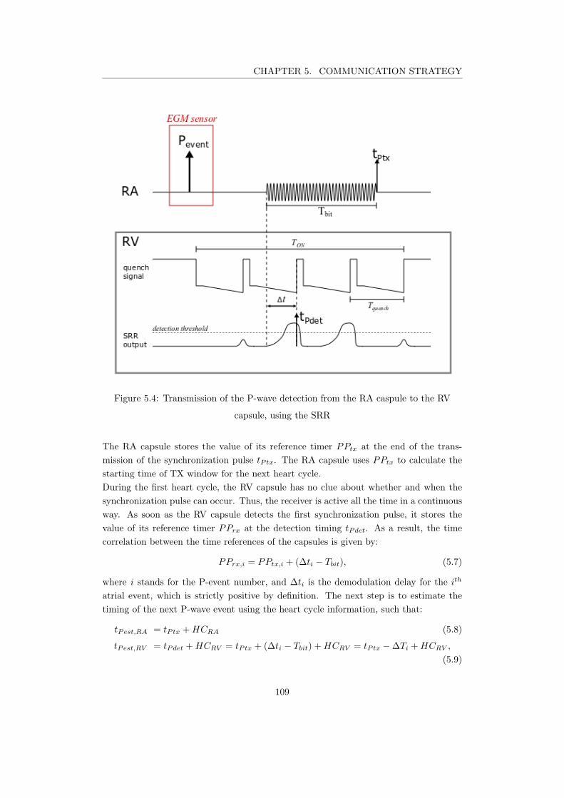
CHAPTER 5. COMMUNICATION STRATEGY
Figure 5.4: Transmission of the P-wave detection from the RA caspule to the RV
capsule, using the SRR
The RA capsule stores the value of its reference timer PPtx at the end of the trans-
mission of the synchronization pulse tPtx. The RA capsule uses PPtx to calculate the
starting time of TX window for the next heart cycle.
During the first heart cycle, the RV capsule has no clue about whether and when the
synchronization pulse can occur. Thus, the receiver is active all the time in a continuous
way. As soon as the RV capsule detects the first synchronization pulse, it stores the
value of its reference timer PPrx at the detection timing tPdet. As a result, the time
correlation between the time references of the capsules is given by:
PPrx,i = PPtx,i + (∆ti − Tbit), (5.7)
where i stands for the P-event number, and ∆ti is the demodulation delay for the ith
atrial event, which is strictly positive by definition. The next step is to estimate the
timing of the next P-wave event using the heart cycle information, such that:
tPest,RA = tPtx +HCRA (5.8)
tPest,RV = tPdet +HCRV = tPtx + (∆ti − Tbit) +HCRV = tPtx −∆Ti +HCRV ,
(5.9)
109
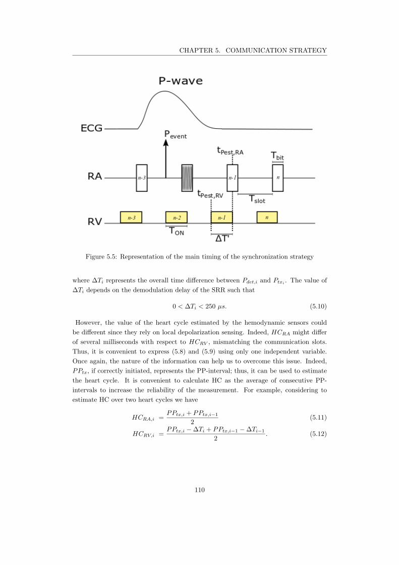
CHAPTER 5. COMMUNICATION STRATEGY
Figure 5.5: Representation of the main timing of the synchronization strategy
where ∆Ti represents the overall time difference between Pdet,i and Ptxi. The value of
∆Ti depends on the demodulation delay of the SRR such that
0 < ∆Ti < 250 µs. (5.10)
However, the value of the heart cycle estimated by the hemodynamic sensors could
be different since they rely on local depolarization sensing. Indeed, HCRA might differ
of several milliseconds with respect to HCRV , mismatching the communication slots.
Thus, it is convenient to express (5.8) and (5.9) using only one independent variable.
Once again, the nature of the information can help us to overcome this issue. Indeed,
PPtx, if correctly initiated, represents the PP-interval; thus, it can be used to estimate
the heart cycle. It is convenient to calculate HC as the average of consecutive PP-
intervals to increase the reliability of the measurement. For example, considering to
estimate HC over two heart cycles we have
HCRA,i =PPtx,i + PPtx,i−1
2(5.11)
HCRV,i =PPtx,i −∆Ti + PPtx,i−1 −∆Ti−1
2. (5.12)
110
CHAPTER 5. COMMUNICATION STRATEGY
Substituting (5.11) and (5.12) respectively in (5.8) and (5.9), the calculation of tPest
resumes to:
tPest,RA(i+1) = tPtx,i +PPtx,i + PPtx,i−1
2=
3PPtx,i + PPtx,i−1
2(5.13)
tPest,RV (i+1) = (tPtx,i −∆Ti) +(PPtx,i −∆Ti) + (PPtx,i−1 −∆Ti−1)
2=
= tPest,RA(i+1) −3∆Ti +∆Ti−1
2= tPest,RA(i+1) −∆T ′
i+1, (5.14)
where ∆T ′ represents the overall time difference due to the demodulation latency.
For the sake of simplicity, let us consider the worst-case scenario, for which ∆Ti = Ti−1 =
250µs. In such a condition, the value of ∆T ′ = 500 µs. Considering a synchronization
pulse with time duration Tbit = 500µs, the RX window requires sub-blocks with TON =
∆T ′ to ensure that the synchronization pulse totally covers at least one quench cycle of
the SRR.
5.2 Algorithms for communication based dual cham-
ber LCP system
In this section, all the algorithms used to implement the synchronization strategy are
detailed. The RV capsule algorithm and the RA capsule one are considered as separate
entities to resemble the real case scenario. Here, we assume that the devices can detect
local depolarization events since all pacemakers embed hemodynamic sensors such as
electrogram (EGM). The algorithms reuse the timing of previous synchronization signals
to estimate the value of Pest and align the communication slots.
5.2.1 Synchronization algorithm of the RA capsule
Let us first consider the RA routine, represented in Figure 5.6. The device starts in
the initialization phase to retrieve programmed information from the microcontroller.
Moreover, during the initialization phase, the registers used for timing estimation can
be reset. After the initialization step, the first synchronization events are sent asyn-
chronously with a delay time less than 10 ms for the consideration previously reported.
The microcontroller periodically checks the value of a counter to decide if the algorithm
can move to the quasi-synchronized routine. If the value of the counter is less than
init, the algorithm stays in the asynchronous routine; otherwise, it moves to the quasi-
synchronized routine. The first step of the quasi-synchronized routine is the evaluation
of the expected timing of the next P-wave (tPest). The value of tPest is updated each
cardiac cycle as described in the previous section. Hereafter, we directly reference the
labels of the algorithm steps of Figure 5.6 for the sake of clarity.
Moving forward through the algorithm, the detection of the P-wave is checked out (α)
111
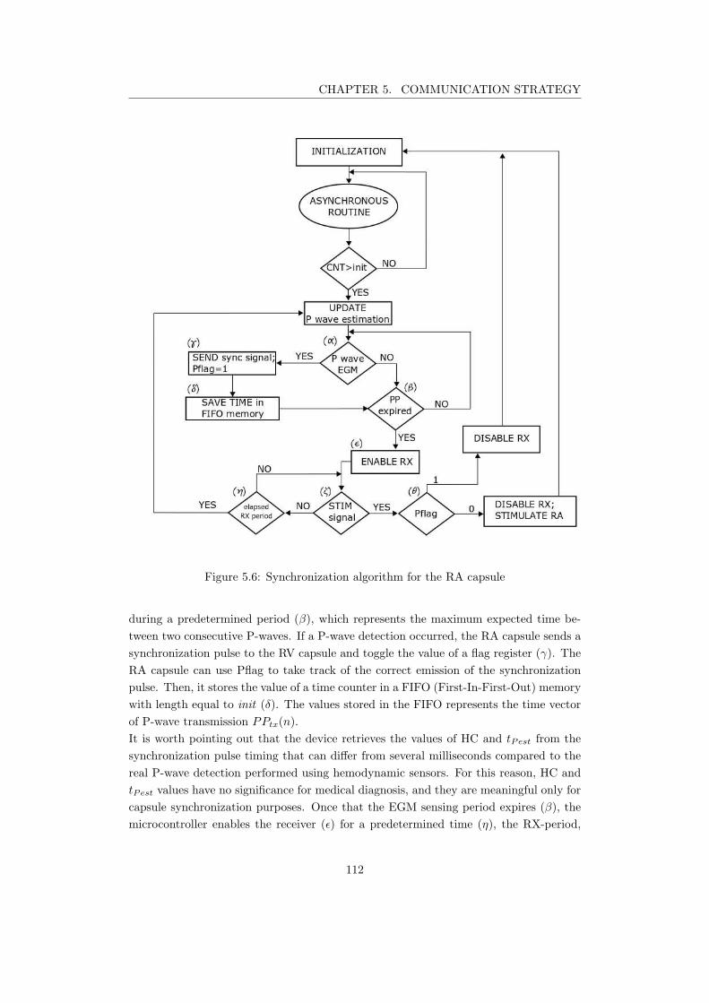
CHAPTER 5. COMMUNICATION STRATEGY
Figure 5.6: Synchronization algorithm for the RA capsule
during a predetermined period (β), which represents the maximum expected time be-
tween two consecutive P-waves. If a P-wave detection occurred, the RA capsule sends a
synchronization pulse to the RV capsule and toggle the value of a flag register (γ). The
RA capsule can use Pflag to take track of the correct emission of the synchronization
pulse. Then, it stores the value of a time counter in a FIFO (First-In-First-Out) memory
with length equal to init (δ). The values stored in the FIFO represents the time vector
of P-wave transmission PPtx(n).
It is worth pointing out that the device retrieves the values of HC and tPest from the
synchronization pulse timing that can differ from several milliseconds compared to the
real P-wave detection performed using hemodynamic sensors. For this reason, HC and
tPest values have no significance for medical diagnosis, and they are meaningful only for
capsule synchronization purposes. Once that the EGM sensing period expires (β), the
microcontroller enables the receiver (ǫ) for a predetermined time (η), the RX-period,
112
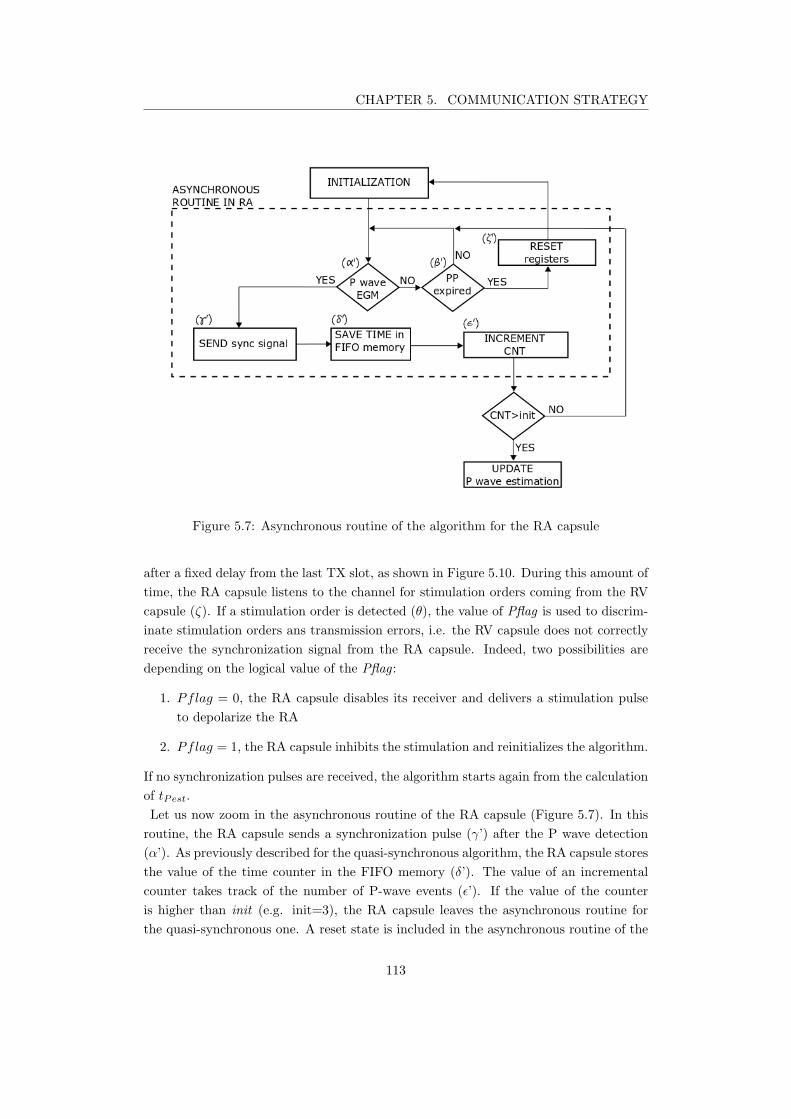
CHAPTER 5. COMMUNICATION STRATEGY
Figure 5.7: Asynchronous routine of the algorithm for the RA capsule
after a fixed delay from the last TX slot, as shown in Figure 5.10. During this amount of
time, the RA capsule listens to the channel for stimulation orders coming from the RV
capsule (ζ). If a stimulation order is detected (θ), the value of Pflag is used to discrim-
inate stimulation orders ans transmission errors, i.e. the RV capsule does not correctly
receive the synchronization signal from the RA capsule. Indeed, two possibilities are
depending on the logical value of the Pflag :
1. Pflag = 0, the RA capsule disables its receiver and delivers a stimulation pulse
to depolarize the RA
2. Pflag = 1, the RA capsule inhibits the stimulation and reinitializes the algorithm.
If no synchronization pulses are received, the algorithm starts again from the calculation
of tPest.
Let us now zoom in the asynchronous routine of the RA capsule (Figure 5.7). In this
routine, the RA capsule sends a synchronization pulse (γ’) after the P wave detection
(α’). As previously described for the quasi-synchronous algorithm, the RA capsule stores
the value of the time counter in the FIFO memory (δ’). The value of an incremental
counter takes track of the number of P-wave events (ǫ’). If the value of the counter
is higher than init (e.g. init=3), the RA capsule leaves the asynchronous routine for
the quasi-synchronous one. A reset state is included in the asynchronous routine of the
113
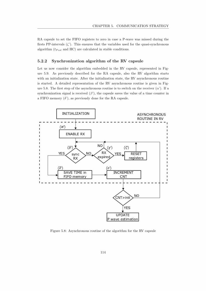
CHAPTER 5. COMMUNICATION STRATEGY
RA capsule to set the FIFO registers to zero in case a P-wave was missed during the
firsts PP-intervals (ζ’). This ensures that the variables used for the quasi-synchronous
algorithm (tPest and HC) are calculated in stable conditions.
5.2.2 Synchronization algorithm of the RV capsule
Let us now consider the algorithm embedded in the RV capsule, represented in Fig-
ure 5.9. As previously described for the RA capsule, also the RV algorithm starts
with an initialization state. After the initialization state, the RV asynchronous routine
is started. A detailed representation of the RV asynchronous routine is given in Fig-
ure 5.8. The first step of the asynchronous routine is to switch on the receiver (α’). If a
synchronization signal is received (β’), the capsule saves the value of a time counter in
a FIFO memory (δ’), as previously done for the RA capsule.
Figure 5.8: Asynchronous routine of the algorithm for the RV capsule
114
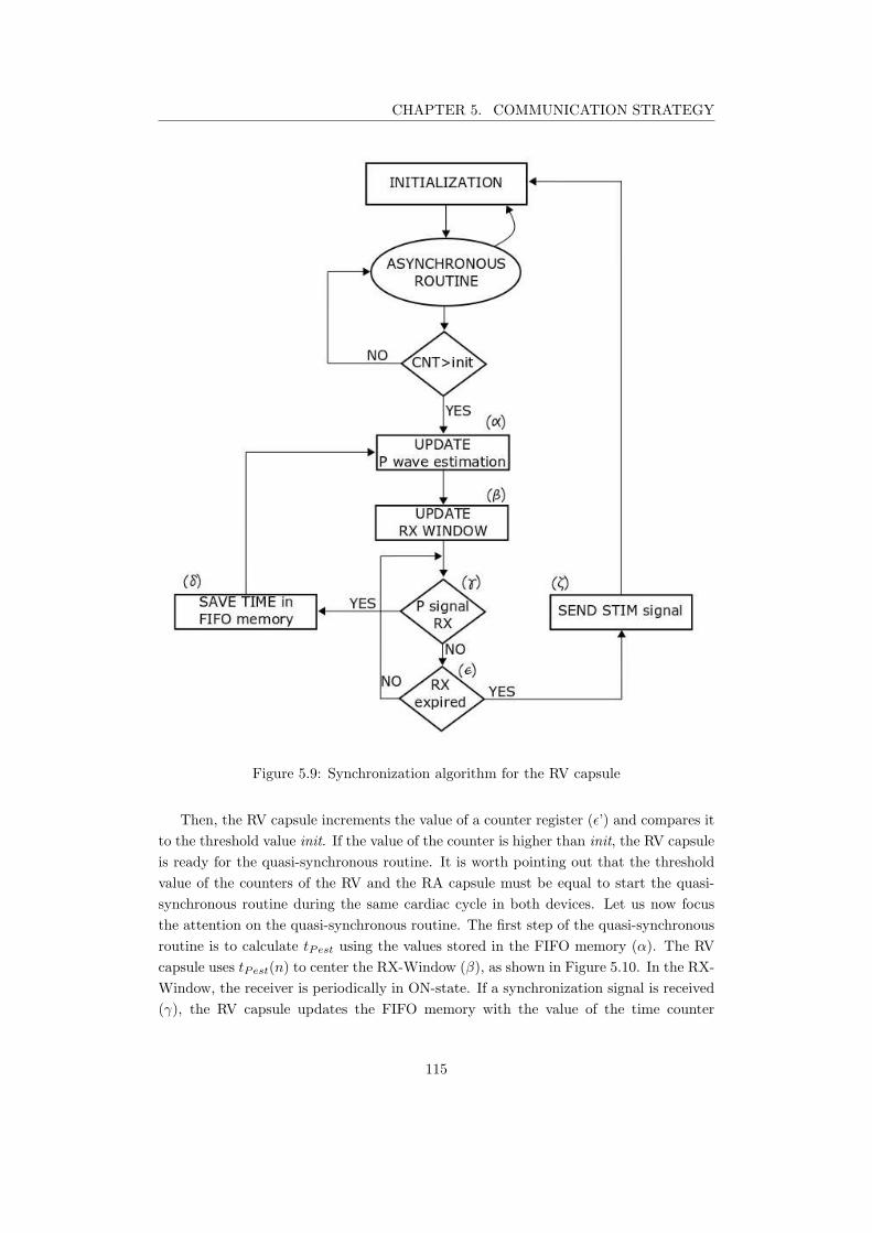
CHAPTER 5. COMMUNICATION STRATEGY
Figure 5.9: Synchronization algorithm for the RV capsule
Then, the RV capsule increments the value of a counter register (ǫ’) and compares it
to the threshold value init. If the value of the counter is higher than init, the RV capsule
is ready for the quasi-synchronous routine. It is worth pointing out that the threshold
value of the counters of the RV and the RA capsule must be equal to start the quasi-
synchronous routine during the same cardiac cycle in both devices. Let us now focus
the attention on the quasi-synchronous routine. The first step of the quasi-synchronous
routine is to calculate tPest using the values stored in the FIFO memory (α). The RV
capsule uses tPest(n) to center the RX-Window (β), as shown in Figure 5.10. In the RX-
Window, the receiver is periodically in ON-state. If a synchronization signal is received
(γ), the RV capsule updates the FIFO memory with the value of the time counter
115
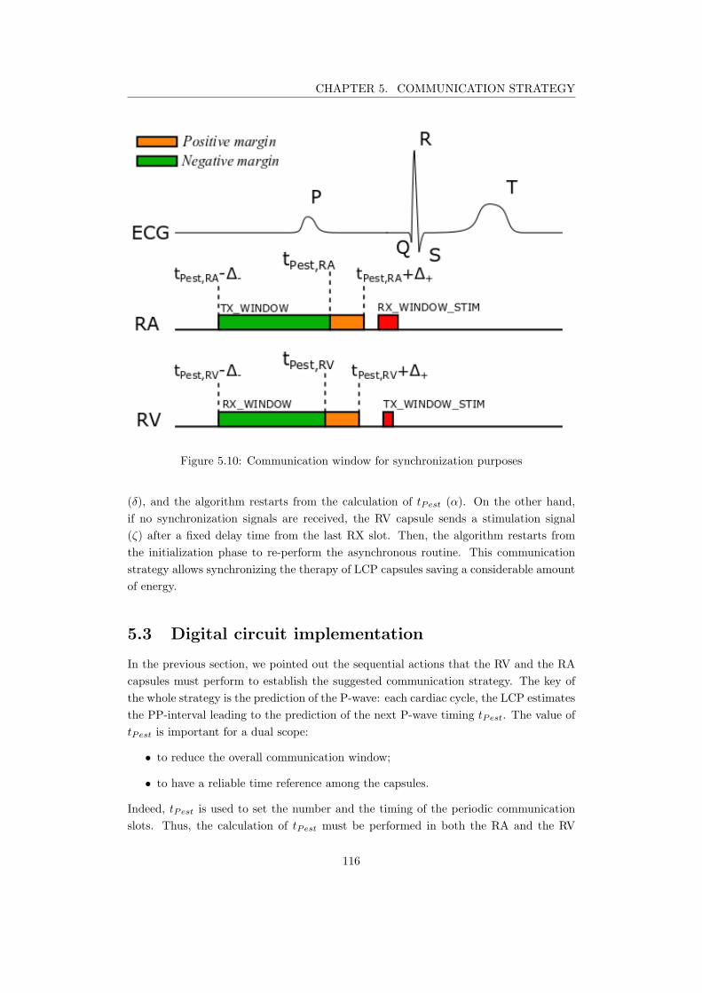
CHAPTER 5. COMMUNICATION STRATEGY
Figure 5.10: Communication window for synchronization purposes
(δ), and the algorithm restarts from the calculation of tPest (α). On the other hand,
if no synchronization signals are received, the RV capsule sends a stimulation signal
(ζ) after a fixed delay time from the last RX slot. Then, the algorithm restarts from
the initialization phase to re-perform the asynchronous routine. This communication
strategy allows synchronizing the therapy of LCP capsules saving a considerable amount
of energy.
5.3 Digital circuit implementation
In the previous section, we pointed out the sequential actions that the RV and the RA
capsules must perform to establish the suggested communication strategy. The key of
the whole strategy is the prediction of the P-wave: each cardiac cycle, the LCP estimates
the PP-interval leading to the prediction of the next P-wave timing tPest. The value of
tPest is important for a dual scope:
• to reduce the overall communication window;
• to have a reliable time reference among the capsules.
Indeed, tPest is used to set the number and the timing of the periodic communication
slots. Thus, the calculation of tPest must be performed in both the RA and the RV
116
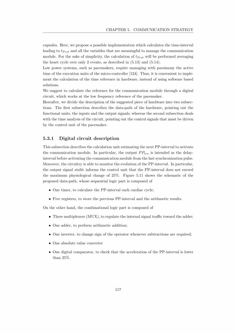
CHAPTER 5. COMMUNICATION STRATEGY
capsules. Here, we propose a possible implementation which calculates the time-interval
leading to tPest and all the variables that are meaningful to manage the communication
module. For the sake of simplicity, the calculation of tPest will be performed averaging
the heart cycle over only 2 events, as described in (5.13) and (5.14).
Low power systems, such as pacemakers, require managing with parsimony the active
time of the execution units of the micro-controller [124]. Thus, it is convenient to imple-
ment the calculation of the time reference in hardware, instead of using software based
solutions.
We suggest to calculate the reference for the communication module through a digital
circuit, which works at the low frequency reference of the pacemaker.
Hereafter, we divide the description of the suggested piece of hardware into two subsec-
tions. The first subsection describes the data-path of the hardware, pointing out the
functional units, the inputs and the output signals; whereas the second subsection deals
with the time analysis of the circuit, pointing out the control signals that must be driven
by the control unit of the pacemaker.
5.3.1 Digital circuit description
This subsection describes the calculation unit estimating the next PP-interval to activate
the communication module. In particular, the output PPtrx is intended as the delay-
interval before activating the communication module from the last synchronization pulse.
Moreover, the circuitry is able to monitor the evolution of the PP-interval. In particular,
the output signal stable informs the control unit that the PP-interval does not exceed
the maximum physiological change of 25%. Figure 5.11 shows the schematic of the
proposed data-path, whose sequential logic part is composed of
• One timer, to calculate the PP-interval each cardiac cycle;
• Five registers, to store the previous PP-interval and the arithmetic results.
On the other hand, the combinational logic part is composed of
• Three multiplexers (MUX), to regulate the internal signal traffic toward the adder;
• One adder, to perform arithmetic addition;
• One inverter, to change sign of the operator whenever subtractions are required;
• One absolute value converter
• One digital comparator, to check that the acceleration of the PP-interval is lower
than 25%.
117
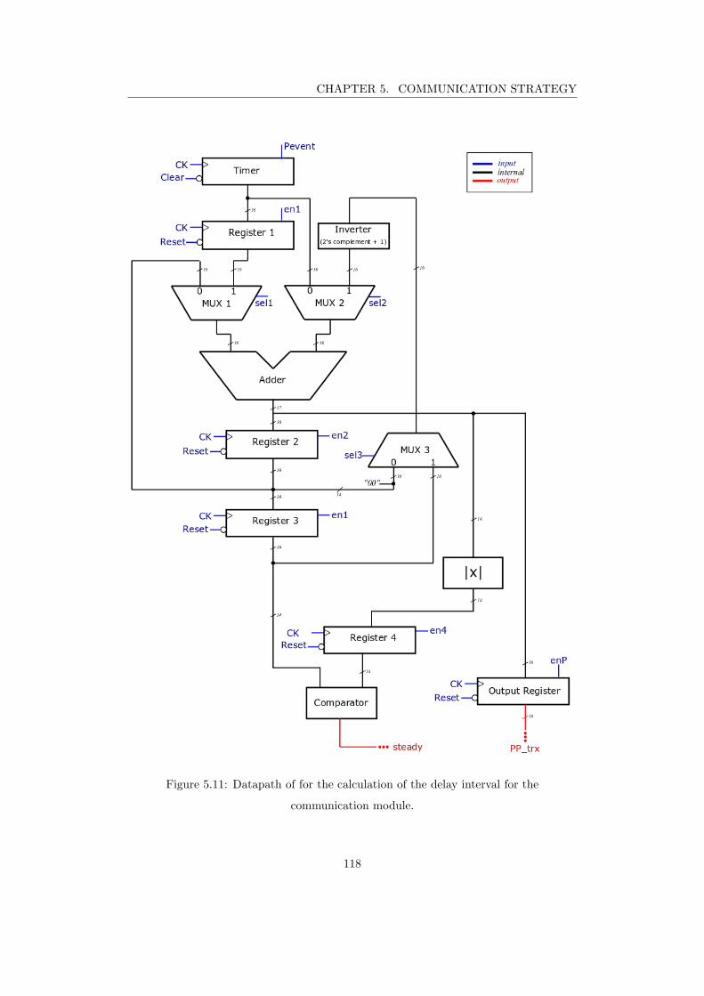
CHAPTER 5. COMMUNICATION STRATEGY
Figure 5.11: Datapath of for the calculation of the delay interval for the
communication module.
118
CHAPTER 5. COMMUNICATION STRATEGY
Let us focus on each functional block to understand its role for the evaluation of the
output signals.
The timer was designed as a 16-bit up-counter that increments its value at each cardiac
cycle, limiting the maximum acceptable PP-interval to
PPmax = TCK × 216 ≈ 2 s, (5.15)
which is an acceptable limit for the application since it would lead to heart rates of
≈ 30 bpm, which is lower than the minimum physiological heart rate of athletes at rest
(40 bpm) [125].
Register 1 stores the value of the timer to keep track of the PP-interval for the next
cardiac cycle. The adder has two 16-bit inputs and a 17-bit output to prevent overflow
issues. The output of the adder is connected to three different blocks: the register 2,
the absolute value converter, and the output register. Register 2 stores the 16 Most-
Significant Bits (MSB) of the adder output. This operation allows storing the average
of the sum directly. Indeed, register 2 is used to evaluate the average of the heart cycle
such as
HC =PPtx,l + PPtx,l−1
2,
where PPtx,l and PPtx,l−1 are the P-wave intervals stored respectively in the timer and
in register 1.
Register 3 stores the output of register 2 to keep track of the HC during the next event.
To verify that the patient heart rate is in stable condition, we must check that the P-wave
acceleration respects the physiological limit of 25%. To do so, the combinational logic
performs the difference between the two last heart cycles that are stored in register 3 and
register 2. The absolute value of this operation ∆PP is stored in register 4. Once that
register 3 is updated, the digital comparator checks that the time difference between
the last two PP-intervals is lower than 25%, comparing ∆PP and the 14 MSB of the
register 3. The heart rate stability information is encoded on the signal stable that
interfaces the control unit directly. Finally, the delay interval PPtrx for the RX window
is calculated as
PPtrx = PPi − 25%Pi = 75%Pi (5.16)
The output register stores the value of PPest, which is used by the control unit to
manage the activation of the communication module.
To control the whole circuitry, the data-path requires 10 input signals:
1. CK, a 32 kHz clock;
2. Reset, a global signal to clear all the registers;
3. Clear, to reinitialize the timer.
4. Pevent, an enabling signal for the timer;
5. en1, to enable register 1 and register 3;
119
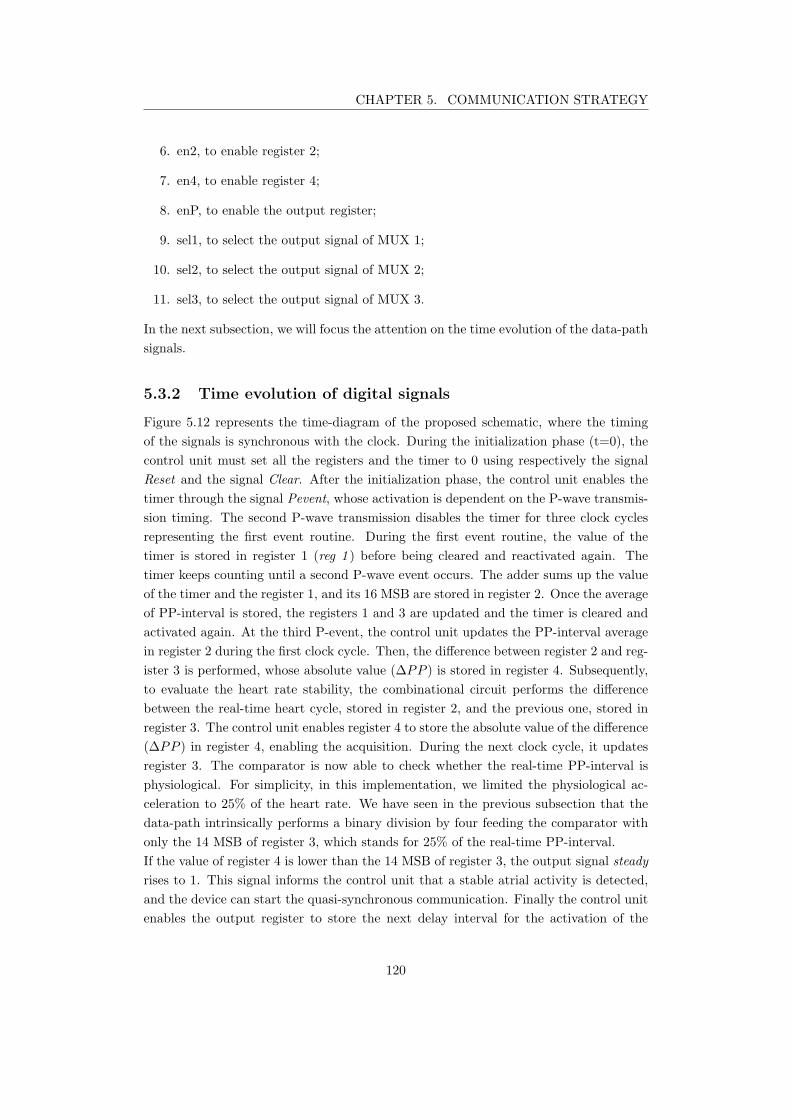
CHAPTER 5. COMMUNICATION STRATEGY
6. en2, to enable register 2;
7. en4, to enable register 4;
8. enP, to enable the output register;
9. sel1, to select the output signal of MUX 1;
10. sel2, to select the output signal of MUX 2;
11. sel3, to select the output signal of MUX 3.
In the next subsection, we will focus the attention on the time evolution of the data-path
signals.
5.3.2 Time evolution of digital signals
Figure 5.12 represents the time-diagram of the proposed schematic, where the timing
of the signals is synchronous with the clock. During the initialization phase (t=0), the
control unit must set all the registers and the timer to 0 using respectively the signal
Reset and the signal Clear. After the initialization phase, the control unit enables the
timer through the signal Pevent, whose activation is dependent on the P-wave transmis-
sion timing. The second P-wave transmission disables the timer for three clock cycles
representing the first event routine. During the first event routine, the value of the
timer is stored in register 1 (reg 1 ) before being cleared and reactivated again. The
timer keeps counting until a second P-wave event occurs. The adder sums up the value
of the timer and the register 1, and its 16 MSB are stored in register 2. Once the average
of PP-interval is stored, the registers 1 and 3 are updated and the timer is cleared and
activated again. At the third P-event, the control unit updates the PP-interval average
in register 2 during the first clock cycle. Then, the difference between register 2 and reg-
ister 3 is performed, whose absolute value (∆PP ) is stored in register 4. Subsequently,
to evaluate the heart rate stability, the combinational circuit performs the difference
between the real-time heart cycle, stored in register 2, and the previous one, stored in
register 3. The control unit enables register 4 to store the absolute value of the difference
(∆PP ) in register 4, enabling the acquisition. During the next clock cycle, it updates
register 3. The comparator is now able to check whether the real-time PP-interval is
physiological. For simplicity, in this implementation, we limited the physiological ac-
celeration to 25% of the heart rate. We have seen in the previous subsection that the
data-path intrinsically performs a binary division by four feeding the comparator with
only the 14 MSB of register 3, which stands for 25% of the real-time PP-interval.
If the value of register 4 is lower than the 14 MSB of register 3, the output signal steady
rises to 1. This signal informs the control unit that a stable atrial activity is detected,
and the device can start the quasi-synchronous communication. Finally the control unit
enables the output register to store the next delay interval for the activation of the
120
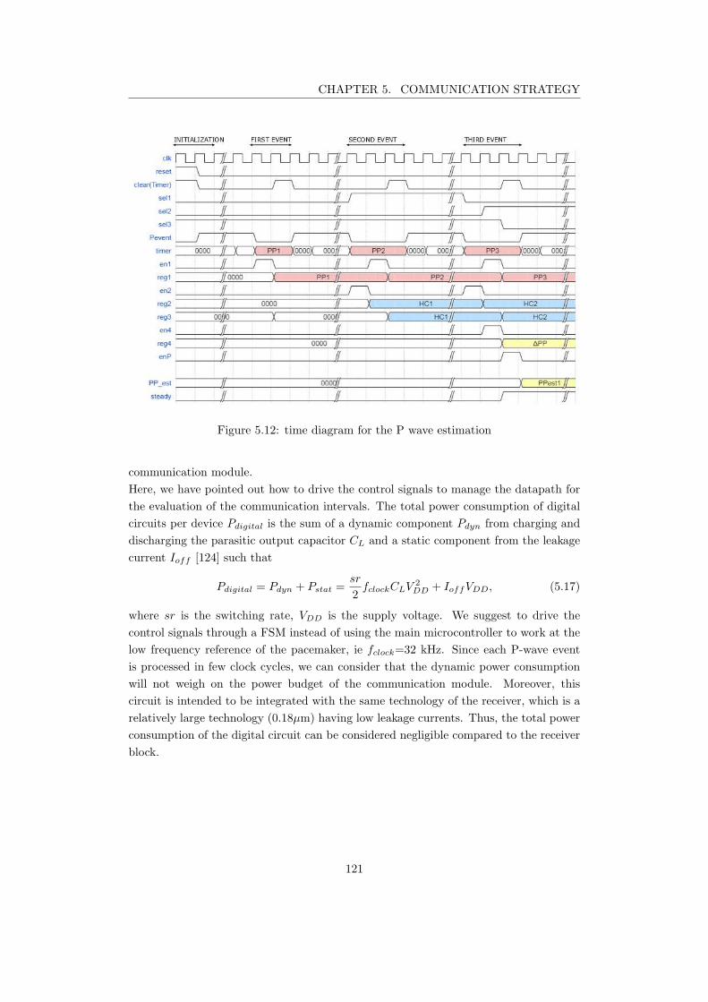
CHAPTER 5. COMMUNICATION STRATEGY
Figure 5.12: time diagram for the P wave estimation
communication module.
Here, we have pointed out how to drive the control signals to manage the datapath for
the evaluation of the communication intervals. The total power consumption of digital
circuits per device Pdigital is the sum of a dynamic component Pdyn from charging and
discharging the parasitic output capacitor CL and a static component from the leakage
current Ioff [124] such that
Pdigital = Pdyn + Pstat =sr
2fclockCLV
2
DD + IoffVDD, (5.17)
where sr is the switching rate, VDD is the supply voltage. We suggest to drive the
control signals through a FSM instead of using the main microcontroller to work at the
low frequency reference of the pacemaker, ie fclock=32 kHz. Since each P-wave event
is processed in few clock cycles, we can consider that the dynamic power consumption
will not weigh on the power budget of the communication module. Moreover, this
circuit is intended to be integrated with the same technology of the receiver, which is a
relatively large technology (0.18µm) having low leakage currents. Thus, the total power
consumption of the digital circuit can be considered negligible compared to the receiver
block.
121
CHAPTER 5. COMMUNICATION STRATEGY
5.4 Discussion
In chapter 4, we proposed an ultra-low power solution tailored for the intra-cardiac chan-
nel. However, the sensitivity requirement limited the minimum power consumption of
the receiver. Even though the receiver consumption was reduced by more than a factor
2 compared to state of the art, the active power consumption of the circuitry prevents a
continuous-time functioning of the communication module. The time variability of the
P-wave signal makes standard pollings of the receiver insufficient. In this chapter, we
suggested a simple solution to reduce the average power consumption down to 2% of
its active power. The stochastic nature of the physiologic P-wave does depend on its
previous value. In particular, PP-intervals should not exceed a beat-to-beat accelera-
tion of [25-35]%. Physicians consider Sinoatrial activity accelerations faster than 25%
as supraventricular tachyarrhythmia events. In this case, AV synchronization must be
avoided preventing a dangerous ventricular tachyarrhythmia.
The proposed algorithm tracks previous PP-intervals to map sub-windows over the whole
physiological variability period. Thanks to this method, we can synchronize heart cham-
bers in a power efficient way. The active power consumption adapts to the heart rate
making the average power consumption constant over time.
Thanks to the reduction of the duty cycle, the receiver achieves an average power con-
sumption as low as 340 nW. To guarantee the same longevity of a single chamber LCP,
for example 10 years, we would need an additive charge equal to
Q(mAh) =Iav
10× 365× 24≈ 30 mAh (5.18)
The effort of this slight increase in battery capacity is rewarded with a continuous-time
AV-synchrony, improving the hemodynamic of patients [126].
Pacemaker patients can experience supraventricular arrhythmia. In one embodiment of
the proposed strategy, the right atrium capsule can send a disable message to decouple
the functioning of the right ventricle capsule. In this condition, the right ventricle
device works as a standard VVI pacemaker. The RA capsule monitors the evolution of
the atrial arrhythmia event using standard hemodynamic sensors such as EGM. When
the RA capsule detects the reestablishment of physiological atrial activity, it restores
the AV-synchrony using an enabling message.
122
6Conclusions and Future work
In this chapter, we review the main results of this doctoral thesis to take stock. A
summary of the results is given in the section 6.1, followed by the future works, in
section 6.2, necessary to develop the suggested system. Finally, we report the scientific
contributions in section 6.3.
6.1 Summary of the main results
The main objective of this PhD project was to propose a power optimized solution for
the synchronization of multi-node leadless pacemakers.
Among all radio-frequency communications, the galvanic Intra-Body Communication
(IBC) seems to be tailored for leadless pacemaker applications. The advantages of IBC
are:
1. ultra-low power requirement;
2. no additional antenna is required;
3. minimal risk of eavesdropping.
However, little work has been done about the IBC channel characterization for in-body
communications since the IBC signal propagation is impacted by several factors, making
difficult a pathloss analytical generalization. Thus, it was necessary to estimate the
channel loss and point out the sensitivity requirements of the receiver.
To do so, we performed numerical simulations using a customized torso model, pointing
out the voltage attenuation of IBC signals over a wide frequency domain [40 kHz -
20 MHz]. We focused on the main channels involved for LCP applications:
• the Intra-cardiac channel, defined as the communication channel between the RV
capsule and the RA capsule;
123
CHAPTER 6. CONCLUSIONS AND FUTURE WORK
• the Inter-ventricular channel, defined as the communication channel between the
RV capsule and the epicardial surface of the LV;
• the Trans-thoracic channels, defined as the communication channel between the
LCPs implanted in the heart and the body surface.
The simulation results showed that trans-thoracic channels experience the lowest atten-
uation, thanks to the possibility to place patch electrodes in an optimized positioning,
leading to large inter-electrode distance and optimal orientation with respect to the im-
plant device. The trans-thoracic channel is essential for programming the device and to
retrieve data during patient follow-ups. However, these events are rare; thus, if properly
managed, they will not weigh on the power budget of the LCP.
The attenuation of the Inter-ventricular channel ranges from 45 dB to 80 dB accord-
ing to the channel length and the working frequency. The Inter-ventricular channel is
intended to be used to share information among the RV capsule and an epicardial pace-
maker fixed to the external wall of the LV.
The orientation of the capsules plays a key-role in the attenuation of IBC signals: the
more aligned the lower the attenuation. However, the placement of the LCP must pri-
oritize the optimization of the therapy, which can vary among the patient population.
Thus, the attenuation of the intra-cardiac channel was estimated for both the worst-
and the best-case condition. The intra-cardiac channel attenuation ranges from 72 dB
to 55 dB, according to orientation and frequency. For capsules of fixed lengths, the
orientation is the most effective variable, leading to an almost constant gap of 10 dB
between the worst- and the best-case, over the whole spectrum under analysis. As fore-
seen by Bereuter et al. [20], the intra-cardiac channel experiences lower attenuation in
the MHz-range thanks to the higher conductivity of the biological tissues.
This trend was confirmed through three in-vivo tests using capsules of the same size
than those of the simulation. To do so, we prototyped a measurement system, which
was verified and validated through in-vitro experiments. For the verification, we sug-
gested a low-cost procedure using a NaCl-solution, whose concentration was changed to
follow the conductivity of the heart over frequency. The results were validated through
numerical simulations.
Thanks to the in-vivo trials, we were also able to see the relative change of the atten-
uation with respect to physiological activities such as respiration and heart beating.
For what concerns respiration, the lowest attenuation was experienced during inflation;
whereas for the heart cycle, we found that it is convenient to communicate during the
ventricular repolarization (T-wave).
However, multi-node leadless pacemakers must be synchronized with the atrial activity
of the heart (P-wave) to better reproduce a physiological heart functioning. Thus, the
RA capsule must rather send a synchronization message to the other devices during the
PR-interval.
We decided to focus our studies on the intra-cardiac channel that is the essential mile-
stone toward multi-chamber leadless systems.
124
CHAPTER 6. CONCLUSIONS AND FUTURE WORK
In the first part of chapter 4, we pointed out the transceiver constraints, consider-
ing the safety radiation guidelines provided by the International Commission on Non-
Ionizing Radiation Protection (ICNIRP). The maximum allowed current density lin-
early increases with frequency. However, the power consumption of integrated circuits
increases with frequency as well. Thus, we faced the low emission constraint designing
a receiver with very high sensitivity property.
We identified a suitable ultra-low-power architecture for the receiver that could over-
come the high sensitivity constraint: the Super-Regenerative Receiver (SRR). The SRR
is particularly appealing since it can achieve extremely high gains with the lowest num-
ber of high-frequency blocks. A SRR was designed in 0.18 µm CMOS technology. The
receiver was tailored for the synchronization of LCPs, achieving 18 µW of estimated
active power. Simulation studies showed a robust design against the noise, achieving a
Bit Error Rate lower than 0.01% of events with a sensitivity of -100 dBv.
Nevertheless, the active power consumption of the receiver prevents the LCP listening
to the communication channel continuously. Thus, we acted on the optimization of the
listening time of the receiver to reduce its impact on the device longevity. In chapter 5,
we proposed an adaptive communication strategy allowing to reduce the receiver cycle
time down to 2%. As a result, we have a receiver that can detect a synchronization
pulse at each cardiac cycle, consuming only 340 nW of the LCP power budget. The
additional power required by the receiver can be compensated over ten years increasing
the battery charge capacity of 30 mAh, which is the 25% of the capacity of the LCP
currently on the market.
This work led to the first power-optimized solution for communication-based LCP syn-
chronization.
6.2 Future works
This work aggregates very different studies that were essential for the conception of
an IBC-system for leadless pacemaker applications: channel characterization, ultra-low-
power circuit, synchronization strategy; thus, there are aspects of the particular studies
that could not be exhaustively covered by this work. Hereafter, we identify the future
works that should be assessed to finalize and optimize our suggested solutions.
The characterization of the channels was tailored on a capsule prototype with length
of 33 mm and diameter of 6.4 mm. More simulations should be performed to quantify
the effect of the capsule length in terms of channel attenuation. Such a study can lead
to an optimal LCP sizing as the compromise between low communication losses and
mechanical constraints.
In this study, we used to inject IBC signals electrodes designed for therapy delivery to
reduce the complexity of the LCP design. However, it is possible that sightly lower
attenuation can be reached optimizing electrode size [127]. Moreover, with larger elec-
125
CHAPTER 6. CONCLUSIONS AND FUTURE WORK
trodes come lower current densities, relaxing the constraint of the emitting voltage. This
consideration is essential whenever IBC transceivers must work with limited carrier fre-
quencies since the safety guidelines are more stringent at lower frequencies.
Furthermore, other in-vivo experiments should be performed to better characterize the
environment noise and interferers, leading to a more accurate BER prediction.
Moreover, the same approach of channel characterization can be adopted for other im-
plantable applications adapting the model to the particular sizing and positioning of the
transducers.
In this work, an ultra-low-power receiver respecting all the specifications of our case
of study was presented. As described in chapter 4, process-related variations must be
counteracted, designing a calibration system for the receiver. Post-layout simulations
must be performed to validate the results before the circuit integration. Then, the circuit
should be tested using external signals to validate our results. These preliminary tests
are intended to validate the performance of the super-regenerative receiver according to
the proposed quenching signal. Once a correct operation of the suggested architecture is
verified, a complete version of the transceiver must be designed. In particular, a stable
signal generator is needed to quench the receiver, and a high-efficiency emitting circuitry
must be designed.
The strategy suggested in this work can drastically reduce the power consumption for
the synchronization of multi-node LCP systems. Multi-node LCP systems were chosen
as the main application platform of our studies. However, the synchronization strategy
can be adopted by any couple of devices including LCP implanted in the RV and another
device that can detect the P-wave such as subcutaneous devices (i.e. Loop recorders,
Subcutaneous-ICD). To validate the strategy, I suggest to synthesize the hardware and
the controlling signals of the proposed technique in an FPGA. Then, in vivo experiments
must be performed to evaluate how close the system is to a perfect atrioventricular syn-
chronization.
6.3 Scientific contribution and publications
This work demonstrated the feasibility of a communication-based synchronization for
Leadless Cardiac Pacemaker (LCP) through the Galvanic Intra-Body Communication
(IBC). The system was analyzed from scratch, from the characterization of the channels
to the drafting of the transceiver requirements. These requirements were used to design
an ultra-low-power receiver in 0.18 µm CMOS technology to analyze the power budget
required by this kind of solutions. The power budget of the receiver was amortized
using an adaptable communication strategy leading to a power-efficient synchronization
protocol.
The results of this work led to the submission of two patents to the french patent institute
126

CHAPTER 6. CONCLUSIONS AND FUTURE WORK
(INPI) [128][129]:
• M.Maldari. Systeme medical implantable pour mesurer un parametre physiologique,
PA122168FR, 2019.
• M.Maldari. Systeme pour realiser une mesure d’impedance cardiographie, PA126089FR,
2019.
• M.Maldari. Procede et systeme de communication entre plusieurs dispositifs medicaux
implantables, PA127465FR, 2020.
From what concerns the dissemination of this work, one international conference article
[130], and one journal article [131] were published so far:
• M. Maldari, K. Amara, I. Rattalino, C. Jabbour, and P. Desgreys. Human Body
Communication channel characterization for leadless cardiac pacemakers, 25th
IEEE International Conference on Electronic Circuits (ICECS), 2018.
• M. Maldari, M. Albatat, J. Bergsland, Y. Haddab, C. Jabbour, and P. Desgreys.
Wide frequency characterization of intra-body communication for leadless pace-
makers, IEEE Transaction on Biomedical Engineering, 2020.
Another conference paper concurring to article extension selection is under submission.
Furthermore, two works without acts were presented:
• M. Maldari. Human Body Communication for leadless pacemaker applications,
International Micro-electronics Assembly and Packaging Society (iMAPS) Lyon,
2017.
• Mirko Maldari, Karima Amara, Chadi Jabbour, Patricia Desgreys. Human Body
Communication channel modeling for leadless cardiac pacemaker applications, GDR
SOC2 Paris, 2018.
127

Bibliography
[1] Plonsey Malmivuo, Jaakko Malmivuo, and Robert Plonsey. Bioelectromagnetism:
principles and applications of bioelectric and biomagnetic fields. Oxford University
Press, USA, 1995.
[2] J. L. Winter. Ecg educator blog, [online] available: https://ecg-
educator.blogspot.com/2016/02/atrial-rhythms.html, 2016.
[3] Elaine Nicpon Marieb and Katja Hoehn. Human anatomy & physiology. Pearson
education, 2007.
[4] Shaan Khurshid, Seung Hoan Choi, Lu-Chen Weng, Elizabeth Y Wang, Ludovic
Trinquart, Emelia J Benjamin, Patrick T Ellinor, and Steven A Lubitz. Frequency
of cardiac rhythm abnormalities in a half million adults. Circulation: Arrhythmia
and Electrophysiology, 11(7):e006273, 2018.
[5] R. E. Kirkfeldt et al. Risk factors for lead complications in cardiac pacing:
a population-based cohort study of 28,860 danish patients. Heart Rhythm,
8(10):1622–1628, 2011.
[6] R. E. Kirkfeldt et al. Complications after cardiac implantable electronic device
implantations: an analysis of a complete, nationwide cohort in denmark. European
heart journal, 35(18):1186–1194, 2013.
[7] M. S. Kiviniemi et al. Complications related to permanent pacemaker therapy.
Pacing and clinical electrophysiology, 22(5):711–720, 1999.
[8] M. R. Sohail et al. Risk factor analysis of permanent pacemaker infection. Clinical
Infectious Diseases, 45(2):166–173, 2007.
[9] E. O. Udo et al. Incidence and predictors of short-and long-term complications in
pacemaker therapy: the followpace study. Heart Rhythm, 9(5):728–735, 2012.
128
CHAPTER 6. CONCLUSIONS AND FUTURE WORK
[10] Wilhelm Fischer and Philippe Ritter. Cardiac pacing in clinical practice. Springer
Science & Business Media, 2012.
[11] Marc A Miller, Petr Neuzil, Srinivas R Dukkipati, and Vivek Y Reddy. Lead-
less cardiac pacemakers: back to the future. Journal of the American College of
Cardiology, 66(10):1179–1189, 2015.
[12] A. E. Epstein et al. Acc/aha/hrs 2008 guidelines for device-based therapy of car-
diac rhythm abnormalities: a report of the american college of cardiology/ameri-
can heart association task force on practice guidelines (writing committee to revise
the acc/aha/naspe 2002 guideline update for implantation of cardiac pacemakers
and antiarrhythmia devices) developed in collaboration with the american associa-
tion for thoracic surgery and society of thoracic surgeons. Journal of the American
College of Cardiology, 51(21):e1–e62, 2008.
[13] M Albatat, J Bergsland, H Arevalo, HH Odland, P Bose, PS Halvorsen, and
I Balasingham. Technological and clinical challenges in lead placement for cardiac
rhythm management devices. Annals of Biomedical Engineering, pages 1–21, 2019.
[14] M. S. Wegmuller. Intra-body communication for biomedical sensor networks. PhD
thesis, ETH Zurich, 2007.
[15] D. Das et al. Enabling covert body area network using electro-quasistatic human
body communication. Scientific reports, 9(1):4160, 2019.
[16] Thoams Guthrie Zimmerman. Personal area networks: near-field intrabody com-
munication. IBM systems Journal, 35(3.4):609–617, 1996.
[17] M. A. Callejon et al. Galvanic coupling transmission in intrabody communica-
tion: A finite element approach. IEEE Transactions on Biomedical Engineering,
61(3):775–783, 2014.
[18] Y. Song et al. The simulation method of the galvanic coupling intrabody commu-
nication with different signal transmission paths. IEEE Transactions on Instru-
mentation and Measurement, 60(4):1257–1266, 2011.
[19] S. Maity et al. Bio-physical modeling, characterization, and optimization of
electro-quasistatic human body communication. IEEE Transactions on Biomedi-
cal Engineering, 66(6):1791–1802, 2018.
[20] L. Bereuter et al. Fundamental characterization of conductive intracardiac commu-
nication for leadless multisite pacemaker systems. IEEE transactions on biomedical
circuits and systems, 13(1):237–247, 2019.
[21] M.A. Callejon et al. Measurement issues in galvanic intrabody communication:
Influence of experimental setup. IEEE Transactions on Biomedical Engineering,
62(11):2724–2732, 2015.
129
CHAPTER 6. CONCLUSIONS AND FUTURE WORK
[22] Lukas Bereuter, Mirco Gysin, Thomas Kueffer, Martin Kucera, Thomas Nieder-
hauser, Jurg Fuhrer, Paul Heinisch, Adrian Zurbuchen, Dominik Obrist, Hildegard
Tanner, et al. Leadless dual-chamber pacing: a novel communication method
for wireless pacemaker synchronization. JACC: Basic to Translational Science,
3(6):813–823, 2018.
[23] Lukas Bereuter, Thomas Niederhauser, Martin Kucera, Dominic Loosli, Immanuel
Steib, Marcel Schildknecht, Adrian Zurbuchen, Fabian Noti, Hildegard Tanner,
Tobias Reichlin, et al. Leadless cardiac resynchronization therapy: An in vivo
proof-of-concept study of wireless pacemaker synchronization. Heart rhythm,
16(6):936–942, 2019.
[24] NTNU. Wireless in-body environment communication (wibec), 2017. [online] avail-
able: https://www.ntnu.edu/wibec, 2017.
[25] Frank Henry Netter, Sharon Colacino, et al. Atlas of human anatomy. Ciba-Geigy
Corporation, 1989.
[26] Glauco Ambrosi, Giuseppe Anastasi, Dario Cantino, S Capitani, P Castano,
FR Donato, AT Franzi, E Gaudio, R Geremia, M Gulisano, et al. Anatomia
dell’uomo. Seconda Edizione edi-ermes, 2001.
[27] Comunita europee. Istituto statistico. Health Statistics: Atlas on Mortality in the
European Union. Office for official publications of the European Communities,
2009.
[28] Baris Akdemir, Hirad Yarmohammadi, M Chadi Alraies, and Wayne O Adkisson.
Premature ventricular contractions: Reassure or refer? Cleveland Clinic journal
of medicine, 83(7):525, 2016.
[29] Julia Vogler, Gunter Breithardt, and Lars Eckardt. Bradyarrhythmias and con-
duction blocks. Revista Espanola de Cardiologıa (English Edition), 65(7):656–667,
2012.
[30] Carlos A Morillo, Amitava Banerjee, Pablo Perel, DavidWood, and Xavier Jouven.
Atrial fibrillation: the current epidemic. Journal of geriatric cardiology: JGC,
14(3):195, 2017.
[31] Mark A Crandall, David J Bradley, Douglas L Packer, and Samuel J Asirvatham.
Contemporary management of atrial fibrillation: update on anticoagulation and
invasive management strategies. In Mayo Clinic Proceedings, volume 84, pages
643–662. Elsevier, 2009.
[32] Ashish Shukla and Anne B Curtis. Avoiding permanent atrial fibrillation: treat-
ment approaches to prevent disease progression. Vascular health and risk manage-
ment, 10:1, 2014.
130
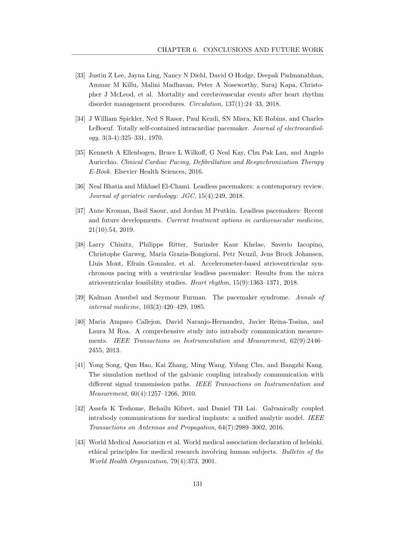
CHAPTER 6. CONCLUSIONS AND FUTURE WORK
[33] Justin Z Lee, Jayna Ling, Nancy N Diehl, David O Hodge, Deepak Padmanabhan,
Ammar M Killu, Malini Madhavan, Peter A Noseworthy, Suraj Kapa, Christo-
pher J McLeod, et al. Mortality and cerebrovascular events after heart rhythm
disorder management procedures. Circulation, 137(1):24–33, 2018.
[34] J William Spickler, Ned S Rasor, Paul Kezdi, SN Misra, KE Robins, and Charles
LeBoeuf. Totally self-contained intracardiac pacemaker. Journal of electrocardiol-
ogy, 3(3-4):325–331, 1970.
[35] Kenneth A Ellenbogen, Bruce L Wilkoff, G Neal Kay, Chu Pak Lau, and Angelo
Auricchio. Clinical Cardiac Pacing, Defibrillation and Resynchronization Therapy
E-Book. Elsevier Health Sciences, 2016.
[36] Neal Bhatia and Mikhael El-Chami. Leadless pacemakers: a contemporary review.
Journal of geriatric cardiology: JGC, 15(4):249, 2018.
[37] Anne Kroman, Basil Saour, and Jordan M Prutkin. Leadless pacemakers: Recent
and future developments. Current treatment options in cardiovascular medicine,
21(10):54, 2019.
[38] Larry Chinitz, Philippe Ritter, Surinder Kaur Khelae, Saverio Iacopino,
Christophe Garweg, Maria Grazia-Bongiorni, Petr Neuzil, Jens Brock Johansen,
Lluis Mont, Efrain Gonzalez, et al. Accelerometer-based atrioventricular syn-
chronous pacing with a ventricular leadless pacemaker: Results from the micra
atrioventricular feasibility studies. Heart rhythm, 15(9):1363–1371, 2018.
[39] Kalman Ausubel and Seymour Furman. The pacemaker syndrome. Annals of
internal medicine, 103(3):420–429, 1985.
[40] Maria Amparo Callejon, David Naranjo-Hernandez, Javier Reina-Tosina, and
Laura M Roa. A comprehensive study into intrabody communication measure-
ments. IEEE Transactions on Instrumentation and Measurement, 62(9):2446–
2455, 2013.
[41] Yong Song, Qun Hao, Kai Zhang, Ming Wang, Yifang Chu, and Bangzhi Kang.
The simulation method of the galvanic coupling intrabody communication with
different signal transmission paths. IEEE Transactions on Instrumentation and
Measurement, 60(4):1257–1266, 2010.
[42] Assefa K Teshome, Behailu Kibret, and Daniel TH Lai. Galvanically coupled
intrabody communications for medical implants: a unified analytic model. IEEE
Transactions on Antennas and Propagation, 64(7):2989–3002, 2016.
[43] World Medical Association et al. World medical association declaration of helsinki.
ethical principles for medical research involving human subjects. Bulletin of the
World Health Organization, 79(4):373, 2001.
131
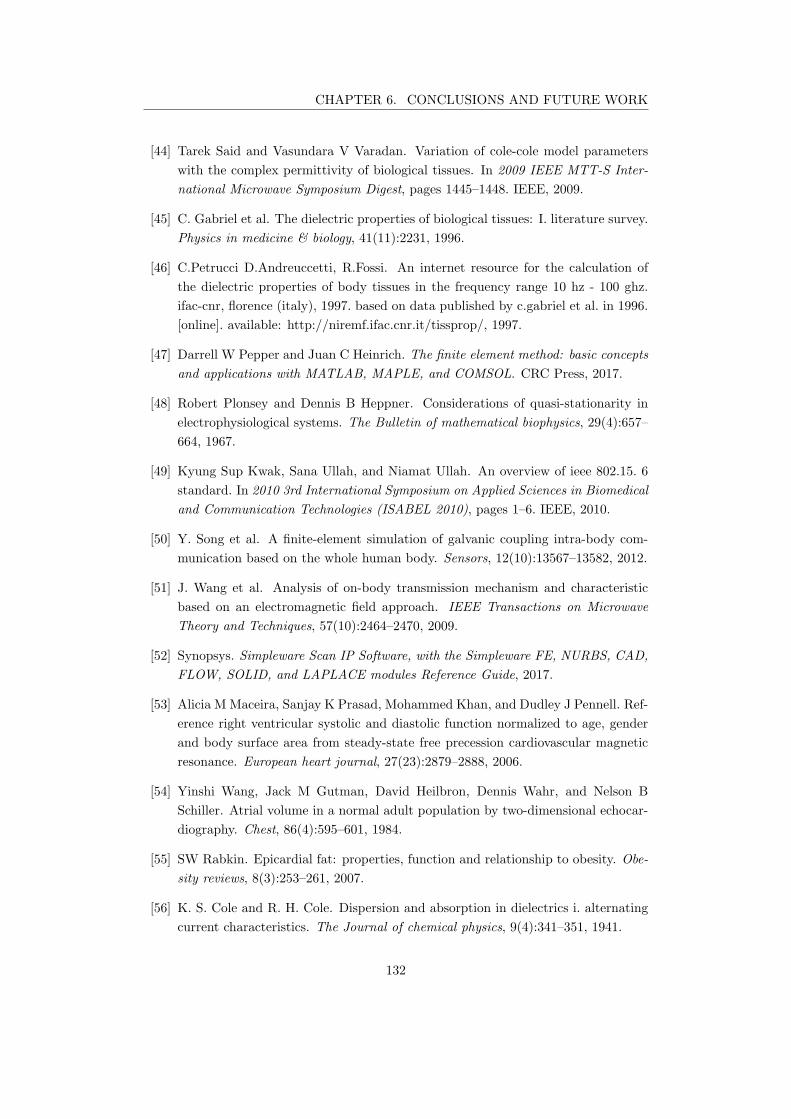
CHAPTER 6. CONCLUSIONS AND FUTURE WORK
[44] Tarek Said and Vasundara V Varadan. Variation of cole-cole model parameters
with the complex permittivity of biological tissues. In 2009 IEEE MTT-S Inter-
national Microwave Symposium Digest, pages 1445–1448. IEEE, 2009.
[45] C. Gabriel et al. The dielectric properties of biological tissues: I. literature survey.
Physics in medicine & biology, 41(11):2231, 1996.
[46] C.Petrucci D.Andreuccetti, R.Fossi. An internet resource for the calculation of
the dielectric properties of body tissues in the frequency range 10 hz - 100 ghz.
ifac-cnr, florence (italy), 1997. based on data published by c.gabriel et al. in 1996.
[online]. available: http://niremf.ifac.cnr.it/tissprop/, 1997.
[47] Darrell W Pepper and Juan C Heinrich. The finite element method: basic concepts
and applications with MATLAB, MAPLE, and COMSOL. CRC Press, 2017.
[48] Robert Plonsey and Dennis B Heppner. Considerations of quasi-stationarity in
electrophysiological systems. The Bulletin of mathematical biophysics, 29(4):657–
664, 1967.
[49] Kyung Sup Kwak, Sana Ullah, and Niamat Ullah. An overview of ieee 802.15. 6
standard. In 2010 3rd International Symposium on Applied Sciences in Biomedical
and Communication Technologies (ISABEL 2010), pages 1–6. IEEE, 2010.
[50] Y. Song et al. A finite-element simulation of galvanic coupling intra-body com-
munication based on the whole human body. Sensors, 12(10):13567–13582, 2012.
[51] J. Wang et al. Analysis of on-body transmission mechanism and characteristic
based on an electromagnetic field approach. IEEE Transactions on Microwave
Theory and Techniques, 57(10):2464–2470, 2009.
[52] Synopsys. Simpleware Scan IP Software, with the Simpleware FE, NURBS, CAD,
FLOW, SOLID, and LAPLACE modules Reference Guide, 2017.
[53] Alicia M Maceira, Sanjay K Prasad, Mohammed Khan, and Dudley J Pennell. Ref-
erence right ventricular systolic and diastolic function normalized to age, gender
and body surface area from steady-state free precession cardiovascular magnetic
resonance. European heart journal, 27(23):2879–2888, 2006.
[54] Yinshi Wang, Jack M Gutman, David Heilbron, Dennis Wahr, and Nelson B
Schiller. Atrial volume in a normal adult population by two-dimensional echocar-
diography. Chest, 86(4):595–601, 1984.
[55] SW Rabkin. Epicardial fat: properties, function and relationship to obesity. Obe-
sity reviews, 8(3):253–261, 2007.
[56] K. S. Cole and R. H. Cole. Dispersion and absorption in dielectrics i. alternating
current characteristics. The Journal of chemical physics, 9(4):341–351, 1941.
132
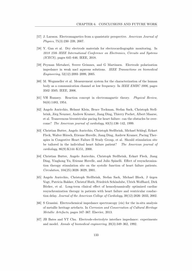
CHAPTER 6. CONCLUSIONS AND FUTURE WORK
[57] J. Larsson. Electromagnetics from a quasistatic perspective. American Journal of
Physics, 75(3):230–239, 2007.
[58] Y. Gan et al. Dry electrode materials for electrocardiographic monitoring. In
2018 25th IEEE International Conference on Electronics, Circuits and Systems
(ICECS), pages 645–646. IEEE, 2018.
[59] Peyman Mirtaheri, Sverre Grimnes, and G Martinsen. Electrode polarization
impedance in weak nacl aqueous solutions. IEEE Transactions on biomedical
Engineering, 52(12):2093–2099, 2005.
[60] M. Wegmueller et al. Measurement system for the characterization of the human
body as a communication channel at low frequency. In IEEE EMBC 2006, pages
3502–3505. IEEE, 2006.
[61] VH Rumsey. Reaction concept in electromagnetic theory. Physical Review,
94(6):1483, 1954.
[62] Angelo Auricchio, Helmut Klein, Bruce Tockman, Stefan Sack, Christoph Stell-
brink, Jorg Neuzner, Andrew Kramer, Jiang Ding, Thierry Pochet, Albert Maarse,
et al. Transvenous biventricular pacing for heart failure: can the obstacles be over-
come? The American journal of cardiology, 83(5):136–142, 1999.
[63] Christian Butter, Angelo Auricchio, Christoph Stellbrink, Michael Schlegl, Eckart
Fleck, Walter Horsch, Etienne Huvelle, Jiang Ding, Andrew Kramer, Pacing Ther-
apies in Congestive Heart Failure II Study Group, et al. Should stimulation site
be tailored in the individual heart failure patient? The American journal of
cardiology, 86(9):K144–K151, 2000.
[64] Christian Butter, Angelo Auricchio, Christoph Stellbrink, Eckart Fleck, Jiang
Ding, Yinghong Yu, Etienne Huvelle, and Julio Spinelli. Effect of resynchroniza-
tion therapy stimulation site on the systolic function of heart failure patients.
Circulation, 104(25):3026–3029, 2001.
[65] Angelo Auricchio, Christoph Stellbrink, Stefan Sack, Michael Block, J urgen
Vogt, Patricia Bakker, Christof Huth, Friedrich Schondube, Ulrich Wolfhard, Dirk
Bocker, et al. Long-term clinical effect of hemodynamically optimized cardiac
resynchronization therapy in patients with heart failure and ventricular conduc-
tion delay. Journal of the American College of Cardiology, 39(12):2026–2033, 2002.
[66] S Grassini. Electrochemical impedance spectroscopy (eis) for the in-situ analysis
of metallic heritage artefacts. In Corrosion and Conservation of Cultural Heritage
Metallic Artefacts, pages 347–367. Elsevier, 2013.
[67] JB Bates and YT Chu. Electrode-electrolyte interface impedance: experiments
and model. Annals of biomedical engineering, 20(3):349–362, 1992.
133
CHAPTER 6. CONCLUSIONS AND FUTURE WORK
[68] Ramon Pallas-Areny and John G Webster. Common mode rejection ratio in dif-
ferential amplifiers. IEEE Transactions on Instrumentation and Measurement,
40(4):669–676, 1991.
[69] D. H. Gadani et al. Effect of salinity on the dielectric properties of water.
NISCAIR-CSIR, India, 2012.
[70] P. Bose et al. Rf channel modeling for implant-to-implant communication and
implant to subcutaneous implant communication for future leadless cardiac pace-
makers. IEEE Transactions on Biomedical Engineering, 65(12):2798–2807, 2018.
[71] Brian D McCauley and Antony F Chu. Leadless cardiac pacemakers: the next
evolution in pacemaker technology. Rhode Island Medical Journal, 100(11):31–34,
2017.
[72] Alexander Ng and Justiaan Swanevelder. Resolution in ultrasound imaging. Con-
tinuing Education in Anaesthesia Critical Care & Pain, 11(5):186–192, 2011.
[73] Parisa Gifani, Hamid Behnam, and Zahra Alizadeh Sani. A new method for
pseudo-increasing frame rates of echocardiography images using manifold learning.
Journal of medical signals and sensors, 1(2):107, 2011.
[74] International Commission on Non-Ionizing Radiation Protection et al. Icnirp state-
ment on the “guidelines for limiting exposure to time-varying electric, magnetic,
and electromagnetic fields (up to 300 ghz)”. Health physics, 97(3):257–258, 2009.
[75] Jianqing Wang and Qiong Wang. Body area communications: channel modeling,
communication systems, and EMC. John Wiley & Sons, 2012.
[76] magnetic Guidelines for limiting exposure to time-varying electric and electromag-
netic fields (up to 300 GHz). International commission on non-ionizing radiation
protection. Health Phys, 74:494–522, 1998.
[77] Maarten Lont, Dusan Milosevic, and Arthur van Roermund. Wake-up receiver
based ultra-low-power WBAN. Springer, 2014.
[78] Long Yan, Joonsung Bae, Seulki Lee, Taehwan Roh, Kiseok Song, and Hoi-Jun
Yoo. A 3.9 mw 25-electrode reconfigured sensor for wearable cardiac monitoring
system. IEEE Journal of Solid-State Circuits, 46(1):353–364, 2010.
[79] Hyunwoo Cho, Joonsung Bae, and Hoi-Jun Yoo. A 37.5 µw body channel commu-
nication wake-up receiver with injection-locking ring oscillator for wireless body
area network. IEEE Transactions on Circuits and Systems I: Regular Papers,
60(5):1200–1208, 2013.
[80] Hyunwoo Cho, Hyunki Kim, Minseo Kim, Jaeeun Jang, Yongsu Lee, Kyuho Jason
Lee, Joonsung Bae, and Hoi-Jun Yoo. A 79 pj/b 80 mb/s full-duplex transceiver
134
CHAPTER 6. CONCLUSIONS AND FUTURE WORK
and a 42.5µw 100 kb/s super-regenerative transceiver for body channel communi-
cation. IEEE journal of solid-state circuits, 51(1):310–317, 2015.
[81] Joonsung Bae and Hoi-Jun Yoo. A 45µw injection-locked fsk wake-up receiver
with frequency-to-envelope conversion for crystal-less wireless body area network.
IEEE Journal of Solid-State Circuits, 50(6):1351–1360, 2015.
[82] Majid Haghjoo. Pacing system malfunction: evaluation and troubleshooting. Mod-
ern Pacemakers–Present and Future. Rijeka: InTech, pages 367–80, 2011.
[83] Payam Safavi-Naeini and Mohammad Saeed. Pacemaker troubleshooting: com-
mon clinical scenarios. Texas Heart Institute Journal, 43(5):415–418, 2016.
[84] VAN CMC CAMPEN, CAREL C DE COCK, Jeroen Huijgens, and Cees A Visser.
Clinical relevance of loss of atrial sensing in patients with single lead vdd pace-
makers. Pacing and Clinical Electrophysiology, 24(5):806–809, 2001.
[85] Upamanyu Madhow. Fundamentals of digital communication. Cambridge Univer-
sity Press, 2008.
[86] Claudio Canuto and Anita Tabacco. Mathematical analysis II, volume 85.
Springer, 2015.
[87] John Oetting. A comparison of modulation techniques for digital radio. IEEE
Transactions on communications, 27(12):1752–1762, 1979.
[88] Xiongchuan Huang, Simonetta Rampu, Xiaoyan Wang, Guido Dolmans, and
Harmke De Groot. A 2.4 ghz/915mhz 51µw wake-up receiver with offset and
noise suppression. In 2010 IEEE International Solid-State Circuits Conference-
(ISSCC), pages 222–223. IEEE, 2010.
[89] A Elgani, M Magno, F Renzini, Luca Perilli, E Franchi Scarselli, Antonio Gnudi,
Roberto Canegallo, G Ricotti, and Luca Benini. Nanowatt wake-up radios:
Discrete-components and integrated architectures. In 2018 25th IEEE Interna-
tional Conference on Electronics, Circuits and Systems (ICECS), pages 793–796.
IEEE, 2018.
[90] Michele Magno and Luca Benini. An ultra low power high sensitivity wake-up radio
receiver with addressing capability. In 2014 IEEE 10th International Conference
on Wireless and Mobile Computing, Networking and Communications (WiMob),
pages 92–99. IEEE, 2014.
[91] Seunghyun Oh, Nathan E Roberts, and David D Wentzloff. A 116nw multi-band
wake-up receiver with 31-bit correlator and interference rejection. In Proceedings
of the IEEE 2013 Custom Integrated Circuits Conference, pages 1–4. IEEE, 2013.
135
CHAPTER 6. CONCLUSIONS AND FUTURE WORK
[92] Nathan E Roberts and David DWentzloff. A 98nw wake-up radio for wireless body
area networks. In 2012 IEEE Radio Frequency Integrated Circuits Symposium,
pages 373–376. IEEE, 2012.
[93] Shovan Maity, David Yang, Baibhab Chatterjee, and Shreyas Sen. A sub-nw wake-
up receiver for human body communication. In 2018 IEEE Biomedical Circuits
and Systems Conference (BioCAS), pages 1–4. IEEE, 2018.
[94] Fei Yuan. CMOS circuits for passive wireless microsystems. Springer Science &
Business Media, 2010.
[95] Brian Otis and Jan Rabaey. Ultra-low power wireless technologies for sensor net-
works. Springer Science & Business Media, 2007.
[96] Hiroshi Fuketa, Shinichi O’uchi, and Takashi Matsukawa. A 0.3-v 1-muw super-
regenerative ultrasound wake-up receiver with power scalability. IEEE Transac-
tions on Circuits and Systems II: Express Briefs, 64(9):1027–1031, 2016.
[97] Samar Alsaegh, Sherif AS Mohamed, and Yiannos Manoli. Design of 1mwcmos
ook super-regenerative receiver for 402–405mhz medical applications. In 2014
IEEE International Symposium on Circuits and Systems (ISCAS), pages 1400–
1403. IEEE, 2014.
[98] Jose L Bohorquez, Anantha P Chandrakasan, and Joel L Dawson. A 350 µw cmos
msk transmitter and 400µw ook super-regenerative receiver for medical implant
communications. IEEE Journal of Solid-State Circuits, 44(4):1248–1259, 2009.
[99] Naci Pekcokguler, Gunhan Dundar, and Catherine Dehollain. Analysis, modeling
and design of a cmos super-regenerative receiver for implanted medical devices
under square and sinusoidal quench signals. Integration, 67:1–7, 2019.
[100] Vahid Dabbagh Rezaei, Stephen J Shellhammer, Mohamed Elkholy, and Kamran
Entesari. A fully integrated 320 pj/b ook super-regenerative receiver with- 87 dbm
sensitivity and self-calibration. In 2016 IEEE Radio Frequency Integrated Circuits
Symposium (RFIC), pages 222–225. IEEE, 2016.
[101] Jia-Yi Chen, Michael P Flynn, and John P Hayes. A fully integrated auto-
calibrated super-regenerative receiver in 0.13− µm cmos. IEEE Journal of Solid-
state circuits, 42(9):1976–1985, 2007.
[102] Edwin H Armstrong. Some recent developments of regenerative circuits. Proceed-
ings of the Institute of Radio Engineers, 10(4):244–260, 1922.
[103] Thomas H Lee. The design of CMOS radio-frequency integrated circuits. Cam-
bridge university press, 2003.
[104] Andrei Grebennikov. RF and microwave transistor oscillator design. John Wiley
& Sons, 2007.
136
CHAPTER 6. CONCLUSIONS AND FUTURE WORK
[105] F Xavier Moncunill-Geniz, Pere Pala-Schonwalder, and Orestes Mas-Casals. A
generic approach to the theory of superregenerative reception. IEEE Transactions
on Circuits and Systems I: regular papers, 52(1):54–70, 2005.
[106] Prakash E Thoppay, Catherine Dehollain, and Michel J Declercq. Noise analysis in
super-regenerative receiver systems. In 2008 Ph. D. Research in Microelectronics
and Electronics, pages 189–192. IEEE, 2008.
[107] Guillermo Gonzalez. Foundations of oscillator circuit design. Artech House Nor-
wood, 2007.
[108] Miguel A Martins, Pui-In Mak, and Rui P Martins. A 0.02-to-6ghz sdr balun-lna
using a triple-stage inverter-based amplifier. In 2012 IEEE International Sympo-
sium on Circuits and Systems, pages 472–475. IEEE, 2012.
[109] Phillip E Allen and Douglas R Holberg. CMOS analog circuit design. Elsevier,
2011.
[110] Gyu-Seob Jeong, Hankyu Chi, Kyungock Kim, and Deog-Kyoon Jeong. A 20-gb/s
1.27 pj/b low-power optical receiver front-end in 65nm cmos. In 2014 IEEE Inter-
national Symposium on Circuits and Systems (ISCAS), pages 1492–1495. IEEE,
2014.
[111] Sherif M Sharroush. Design of the cmos inverter-based amplifier: A quantitative
approach. International Journal of Circuit Theory and Applications, 47(7):1006–
1036, 2019.
[112] Skawrat Wangtaphan and Varakorn Kasemsuwan. A high performance thermal
noise-canceling transimpedance-based differential amplifier. In TENCON 2009-
2009 IEEE Region 10 Conference, pages 1–4. IEEE, 2009.
[113] Ahmad Yarahmadi and Abumoslem Jannesari. Two-path inverter-based low noise
amplifier for 10–12 ghz applications. Microelectronics journal, 50:76–82, 2016.
[114] Ivy Lo, Olga Boric-Lubecke, and Victor Lubecke. 0.25 µm cmos dual feedback
wide-band uhf low noise amplifier. In 2007 IEEE/MTT-S International Microwave
Symposium, pages 1059–1062. IEEE, 2007.
[115] Stanley BT Wang, Ali M Niknejad, and Robert W Brodersen. A sub-mw 960-
mhz ultra-wideband cmos lna. In 2005 IEEE Radio Frequency integrated Circuits
(RFIC) Symposium-Digest of Papers, pages 35–38. IEEE, 2005.
[116] Jun-Young Park, Ji-Young Lee, Cheong-Ki Yeo, and Tae-Yeoul Yun. Analysis and
optimization of a resistive-feedback inverter lna. Microwave and Optical Technol-
ogy Letters, 60(5):1143–1151, 2018.
[117] Behzad Razavi. Design of analog CMOS integrated circuits. McGraw-Hill Educa-
tion, 2017.
137
CHAPTER 6. CONCLUSIONS AND FUTURE WORK
[118] Mel Bazes. Two novel fully complementary self-biased cmos differential amplifiers.
IEEE Journal of Solid-State Circuits, 26(2):165–168, 1991.
[119] James S Hutchison, Roxanne E Ward, Jacques Lacroix, Paul C Hebert, Marcia A
Barnes, Desmond J Bohn, Peter B Dirks, Steve Doucette, Dean Fergusson, Ronald
Gottesman, et al. Hypothermia therapy after traumatic brain injury in children.
New England Journal of Medicine, 358(23):2447–2456, 2008.
[120] Donald B Estreich and Robert W Dutton. Modeling latch-up in cmos integrated
circuits. IEEE Transactions on computer-aided design of integrated circuits and
systems, 1(4):157–162, 1982.
[121] Simon M Sze and Kwok K Ng. Physics of semiconductor devices. John wiley &
sons, 2006.
[122] L Geroux, M Limousin, and S Cazeau. Clinical performances of a new
mode switch function based on a statistical analysis of the atrial rhythm.
Herzschrittmachertherapie und Elektrophysiologie, 10(1):S15–S21, 1999.
[123] H. Elmqvist. Stimulateur cardiaques intelligents et consommation d’energie. CAR-
DIOSTIM80, pages 206–213, 1980.
[124] Anantha P Chandrakasan, Samuel Sheng, and Robert W Brodersen. Low-power
cmos digital design. IEICE Transactions on Electronics, 75(4):371–382, 1992.
[125] American Heart Association et al. All about heart rate (pulse). Retrieved from,
2012.
[126] Anthony C Pearson, Denise L Janosik, Robert M Redd, Thomas A Buckingham,
Arthur J Labovitz, and Denise Mrosek. Hemodynamic benefit of atrioventricular
synchrony: prediction from baseline doppler-echocardiographic variables. Journal
of the American College of Cardiology, 13(7):1613–1621, 1989.
[127] S. Maity et al. Characterization of human body forward path loss and variability
effects in voltage-mode hbc. IEEE Microwave and Wireless Components Letters,
28(3):266–268, 2018.
[128] Mirko Maldari. Systeme pour realiser une mesure d’impedance cardiographie,
PA126089FR., 2019.
[129] Mirko Maldari. Systeme medical implantable pour mesurer un parametre physi-
ologique, PA122168FR., 2019.
[130] Mirko Maldari, Karima Amara, Ismael Rattalino, Chadi Jabbour, and Patricia
Desgreys. Human body communication channel characterization for leadless car-
diac pacemakers. In 2018 25th IEEE International Conference on Electronics,
Circuits and Systems (ICECS), pages 185–188. IEEE, 2018.
138

CHAPTER 6. CONCLUSIONS AND FUTURE WORK
[131] M. Maldari, M. Albatat, Bergsland, J., Y. Haddab, C. Jabbour, and P. Desgreys.
Wide frequency characterization of intra-body communication for leadless pace-
makers. IEEE Transactions on Biomedical Engineering, 2020.
[132] Roger Grimshaw. Nonlinear ordinary differential equations. Routledge, 2017.
[133] Martin Braun and Martin Golubitsky. Differential equations and their applica-
tions, volume 4. Springer, 1983.
139

Appendices
140
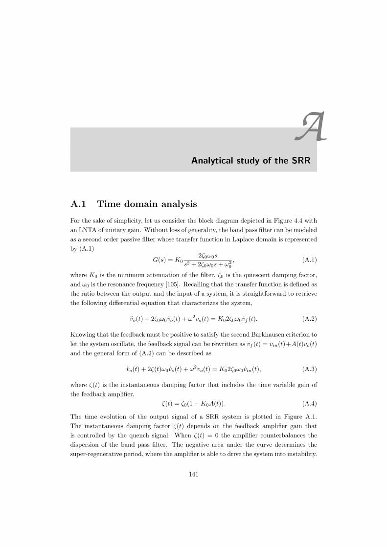
AAnalytical study of the SRR
A.1 Time domain analysis
For the sake of simplicity, let us consider the block diagram depicted in Figure 4.4 with
an LNTA of unitary gain. Without loss of generality, the band pass filter can be modeled
as a second order passive filter whose transfer function in Laplace domain is represented
by (A.1)
G(s) = K0
2ζ0ω0s
s2 + 2ζ0ω0s+ ω2
0
, (A.1)
where K0 is the minimum attenuation of the filter, ζ0 is the quiescent damping factor,
and ω0 is the resonance frequency [105]. Recalling that the transfer function is defined as
the ratio between the output and the input of a system, it is straightforward to retrieve
the following differential equation that characterizes the system,
vo(t) + 2ζ0ω0vo(t) + ω2vo(t) = K02ζ0ω0vf (t). (A.2)
Knowing that the feedback must be positive to satisfy the second Barkhausen criterion to
let the system oscillate, the feedback signal can be rewritten as vf (t) = vin(t)+A(t)vo(t)
and the general form of (A.2) can be described as
vo(t) + 2ζ(t)ω0vo(t) + ω2vo(t) = K02ζ0ω0vin(t), (A.3)
where ζ(t) is the instantaneous damping factor that includes the time variable gain of
the feedback amplifier,
ζ(t) = ζ0(1−K0A(t)). (A.4)
The time evolution of the output signal of a SRR system is plotted in Figure A.1.
The instantaneous damping factor ζ(t) depends on the feedback amplifier gain that
is controlled by the quench signal. When ζ(t) = 0 the amplifier counterbalances the
dispersion of the band pass filter. The negative area under the curve determines the
super-regenerative period, where the amplifier is able to drive the system into instability.
141
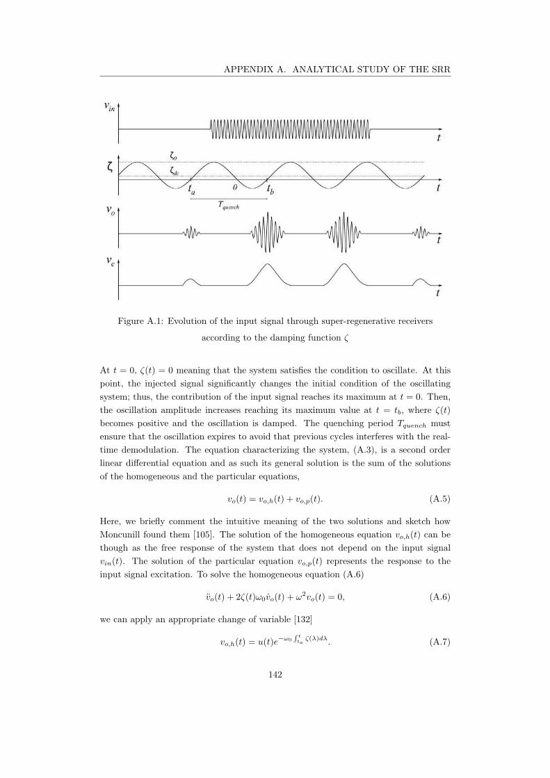
APPENDIX A. ANALYTICAL STUDY OF THE SRR
Figure A.1: Evolution of the input signal through super-regenerative receivers
according to the damping function ζ
At t = 0, ζ(t) = 0 meaning that the system satisfies the condition to oscillate. At this
point, the injected signal significantly changes the initial condition of the oscillating
system; thus, the contribution of the input signal reaches its maximum at t = 0. Then,
the oscillation amplitude increases reaching its maximum value at t = tb, where ζ(t)
becomes positive and the oscillation is damped. The quenching period Tquench must
ensure that the oscillation expires to avoid that previous cycles interferes with the real-
time demodulation. The equation characterizing the system, (A.3), is a second order
linear differential equation and as such its general solution is the sum of the solutions
of the homogeneous and the particular equations,
vo(t) = vo,h(t) + vo,p(t). (A.5)
Here, we briefly comment the intuitive meaning of the two solutions and sketch how
Moncunill found them [105]. The solution of the homogeneous equation vo,h(t) can be
though as the free response of the system that does not depend on the input signal
vin(t). The solution of the particular equation vo,p(t) represents the response to the
input signal excitation. To solve the homogeneous equation (A.6)
vo(t) + 2ζ(t)ω0vo(t) + ω2vo(t) = 0, (A.6)
we can apply an appropriate change of variable [132]
vo,h(t) = u(t)e−ω0
∫t
taζ(λ)dλ
. (A.7)
142

APPENDIX A. ANALYTICAL STUDY OF THE SRR
In this way, the first derivative of the homogeneous solution can be written as
vo,h(t) = (u(t)− ω0ζ(t)u(t))e−ω0
∫t
taζ(λ)dλ
. (A.8)
Iterating the derivative we can find also the second order term of (A.3)
vo,h(t) = (u(t)− 2ω0ζ(t)u(t) + [(ω0ζ(t))2− ω0ζ(t)]u)e
−ω0
∫t
taζ(λ)dλ
. (A.9)
Substituting the variable and its derivatives in (A.3) we find a easiest representation
known as Hill equation
u(t) + ω20
(
1− ζ2(t)−ζ(t)
ω0
)
u(t) = 0. (A.10)
It is possible to decrease the complexity of the solution on top of two reasonable as-
sumptions:
• The system is underdamped, hence it is able to give an oscillatory response at any
time during the period Tquench.
• The damping factor changes slowly, that is usually respected in super-regenerative
systems to improve sensitivity [100].
Mathematically speaking, we are assuming that
ζ2(t) << 1 (A.11)
ζ(t) << ω0 (A.12)
It is worth pointing out that the assumption A.11 implies that the modulus of the
instantaneous quality factor must be kept high enough over the whole Tquench. Thanks
to those assumptions, we can reformulate (A.10) as
u(t) + ω20u(t) = 0, (A.13)
whose solution is
u(t) = 2ℜ
V1ejω0t
= V1ejω0t + V ∗
1 e−jω0t. (A.14)
Substituting A.14 in A.7 we can find the general solution of the homogeneous differential
equation
vo,h(t) = e−ω0
∫t
taζ(λ)dλ2ℜ
V1ejω0t
. (A.15)
The solution of the particular equation can be found using the method of variation of
parameters. The basic principle of this method is to use convenient solutions of the
homogeneous equation to find a solution of the particular equation [133]. In particular,
this method uses the principle that linear combinations of solutions of a differential
equation are themselves solution of differential equations. In this way, we can write the
particular solution as
vo,p(t) = 2ℜ[
V2(t)b(t)] = V2(t)b(t) + V ∗
2 (t)b∗(t), (A.16)
143
APPENDIX A. ANALYTICAL STUDY OF THE SRR
where b(t) is the base of the solution of the homogeneous equation
b(t) = e−ω0
∫t
taζ(λ)dλ
ejω0t. (A.17)
Assuming that V2(t) respects the following conditions
V2(t)b(t) + V ∗
2 (t)b∗(t) = 0 (A.18)
V2(t)b(t) + V ∗
2 (t)b∗(t) = 2K0ζ0ω0v(t) (A.19)
the solution of the particular equation is provided by integrating
V2(t) = −jK0ζ0v(t)
b(t)(A.20)
and it is equal to
V2(t) = −jK0ζ0
∫ t
ta
v(τ)
b(τ)dτ = −jK0ζ0
∫ t
ta
v(τ)eω0
∫τ
taζ(λ)dλ
e−jω0τdτ. (A.21)
Now we can substitute the equation of V2(t) and b(t) in A.16 and get the solution of the
particular equation,
vo,p(t) = e−ω0
∫t
taζ(λ)dλ2ℜ
−jK0ζ0
∫ t
ta
v(τ)eω0
∫τ
taζ(λ)dλ
e−jω0(τ−t)dτ
. (A.22)
The particular solution vo,p(t) can be used to interpret the system reaction to the input
signal v(t). It is shown that the output response depends on the derivative of the input
signal amplitude rather than the signal amplitude itself. The first exponential term
defines the behavior of the quenched oscillator of the SRR. Depending on the sign of
the instantaneous damping factor ζ(λ), the system output may be either attenuated (for
ζ > 0) or amplified (for ζ < 0). For the sake of clarity, Let us consider the distribution
of ζ depicted in Figure A.1. In the time range [0; tb] ⊆ Tquench, ζ has negative values,
and becomes positive right after tb. Thus, we can define the Super-Regenerative gain
Ks and the Normalized envelope of the SRO p(t) as
Ks = e−ω0
∫ tb
0ζ(λ)dλ (A.23)
p(t) = e−ω0
∫t
tbζ(λ)dλ
. (A.24)
For low input signals v(t), we can consider that the first exponential in (A.16) dominates
over the second term of the equation. Hence, the Sensitivity curve is defined as
s(t) = eω0
∫t
0ζ(λ)dλ (A.25)
Using (A.25), (A.23), and (A.24), it is possible to rewrite the homogenous and the
particular solution of the differential equation as
vo,h(t) = |V1|p(t)cos(ω0t+ ∠V1) (A.26)
vo,p(t) = 2ζ0K0Ksp(t)
∫
v(τ)s(τ)sin[ω0(t− τ)]dτ. (A.27)
144
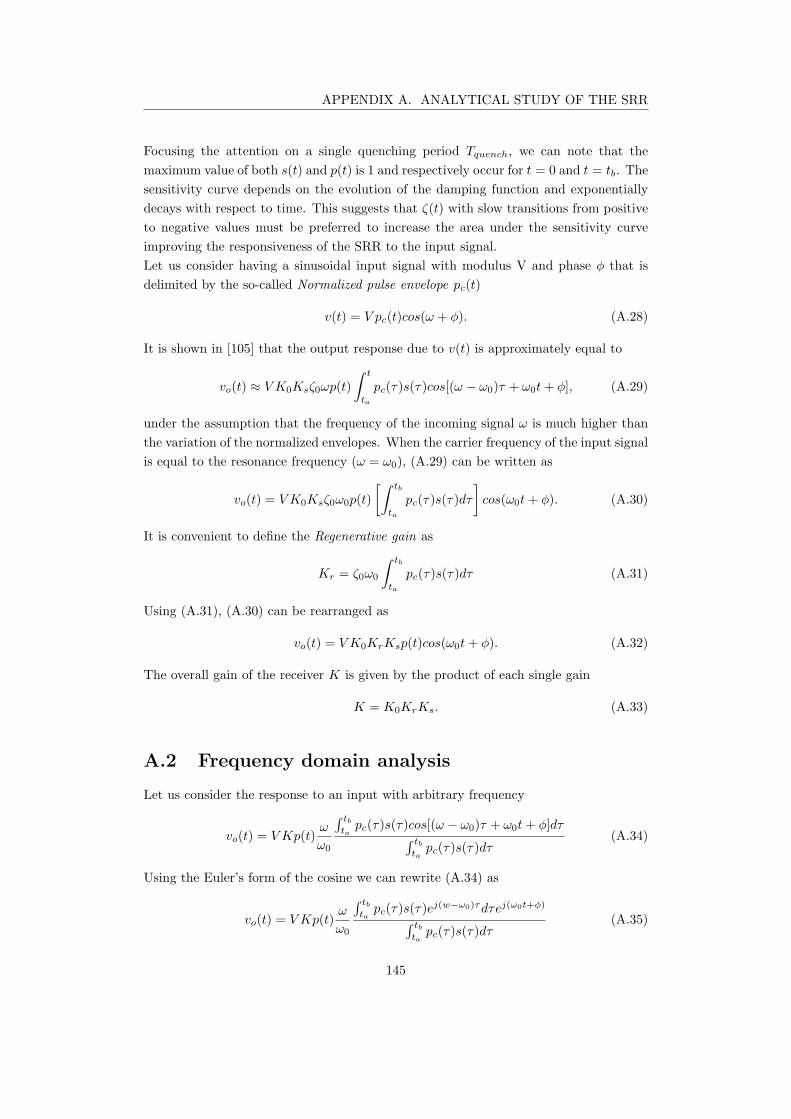
APPENDIX A. ANALYTICAL STUDY OF THE SRR
Focusing the attention on a single quenching period Tquench, we can note that the
maximum value of both s(t) and p(t) is 1 and respectively occur for t = 0 and t = tb. The
sensitivity curve depends on the evolution of the damping function and exponentially
decays with respect to time. This suggests that ζ(t) with slow transitions from positive
to negative values must be preferred to increase the area under the sensitivity curve
improving the responsiveness of the SRR to the input signal.
Let us consider having a sinusoidal input signal with modulus V and phase φ that is
delimited by the so-called Normalized pulse envelope pc(t)
v(t) = V pc(t)cos(ω + φ). (A.28)
It is shown in [105] that the output response due to v(t) is approximately equal to
vo(t) ≈ V K0Ksζ0ωp(t)
∫ t
ta
pc(τ)s(τ)cos[(ω − ω0)τ + ω0t+ φ], (A.29)
under the assumption that the frequency of the incoming signal ω is much higher than
the variation of the normalized envelopes. When the carrier frequency of the input signal
is equal to the resonance frequency (ω = ω0), (A.29) can be written as
vo(t) = V K0Ksζ0ω0p(t)
[∫ tb
ta
pc(τ)s(τ)dτ
]
cos(ω0t+ φ). (A.30)
It is convenient to define the Regenerative gain as
Kr = ζ0ω0
∫ tb
ta
pc(τ)s(τ)dτ (A.31)
Using (A.31), (A.30) can be rearranged as
vo(t) = V K0KrKsp(t)cos(ω0t+ φ). (A.32)
The overall gain of the receiver K is given by the product of each single gain
K = K0KrKs. (A.33)
A.2 Frequency domain analysis
Let us consider the response to an input with arbitrary frequency
vo(t) = V Kp(t)ω
ω0
∫ tb
tapc(τ)s(τ)cos[(ω − ω0)τ + ω0t+ φ]dτ
∫ tb
tapc(τ)s(τ)dτ
(A.34)
Using the Euler’s form of the cosine we can rewrite (A.34) as
vo(t) = V Kp(t)ω
ω0
∫ tb
tapc(τ)s(τ)e
j(w−ω0)τdτej(ω0t+φ)
∫ tb
tapc(τ)s(τ)dτ
(A.35)
145
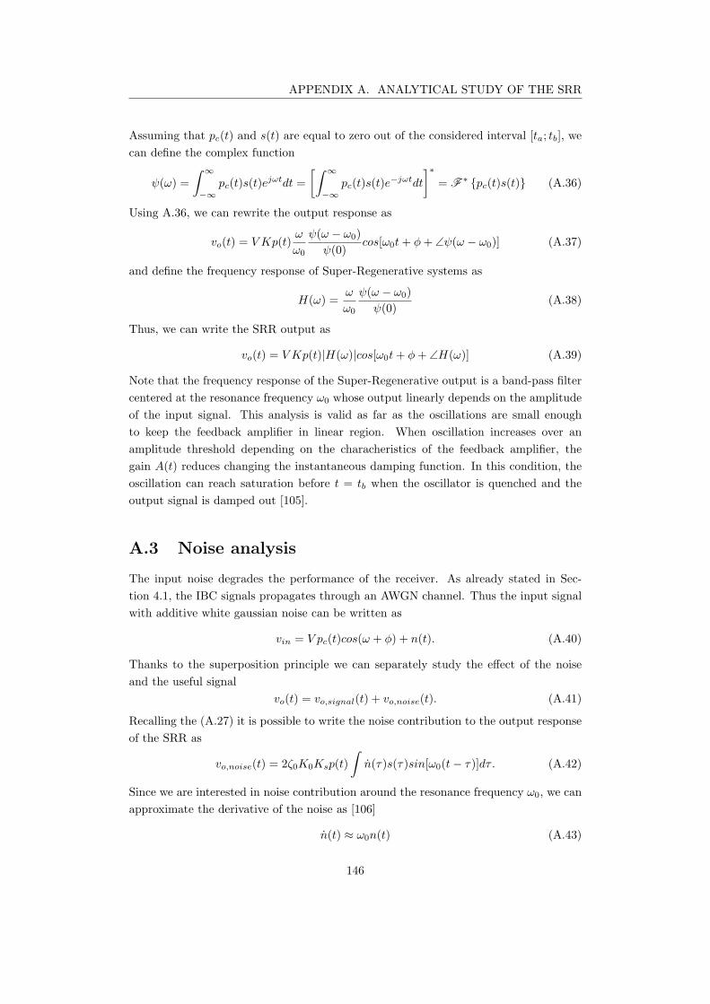
APPENDIX A. ANALYTICAL STUDY OF THE SRR
Assuming that pc(t) and s(t) are equal to zero out of the considered interval [ta; tb], we
can define the complex function
ψ(ω) =
∫
∞
−∞
pc(t)s(t)ejωtdt =
[∫
∞
−∞
pc(t)s(t)e−jωtdt
]
∗
= F∗ pc(t)s(t) (A.36)
Using A.36, we can rewrite the output response as
vo(t) = V Kp(t)ω
ω0
ψ(ω − ω0)
ψ(0)cos[ω0t+ φ+ ∠ψ(ω − ω0)] (A.37)
and define the frequency response of Super-Regenerative systems as
H(ω) =ω
ω0
ψ(ω − ω0)
ψ(0)(A.38)
Thus, we can write the SRR output as
vo(t) = V Kp(t)|H(ω)|cos[ω0t+ φ+ ∠H(ω)] (A.39)
Note that the frequency response of the Super-Regenerative output is a band-pass filter
centered at the resonance frequency ω0 whose output linearly depends on the amplitude
of the input signal. This analysis is valid as far as the oscillations are small enough
to keep the feedback amplifier in linear region. When oscillation increases over an
amplitude threshold depending on the characheristics of the feedback amplifier, the
gain A(t) reduces changing the instantaneous damping function. In this condition, the
oscillation can reach saturation before t = tb when the oscillator is quenched and the
output signal is damped out [105].
A.3 Noise analysis
The input noise degrades the performance of the receiver. As already stated in Sec-
tion 4.1, the IBC signals propagates through an AWGN channel. Thus the input signal
with additive white gaussian noise can be written as
vin = V pc(t)cos(ω + φ) + n(t). (A.40)
Thanks to the superposition principle we can separately study the effect of the noise
and the useful signal
vo(t) = vo,signal(t) + vo,noise(t). (A.41)
Recalling the (A.27) it is possible to write the noise contribution to the output response
of the SRR as
vo,noise(t) = 2ζ0K0Ksp(t)
∫
n(τ)s(τ)sin[ω0(t− τ)]dτ. (A.42)
Since we are interested in noise contribution around the resonance frequency ω0, we can
approximate the derivative of the noise as [106]
n(t) ≈ ω0n(t) (A.43)
146

APPENDIX A. ANALYTICAL STUDY OF THE SRR
Substituting (A.43) in (A.42) we find
vo,noise(t) = 2ζ0K0Ksp(t)ω0
∫
n(τ)s(τ)sin[ω0(t− τ)]dτ. (A.44)
Recalling signal theory, we can express the energy of a signal as its auto-correlation in
the origin. Thus, we can use (A.44) to calculate the energy of the output noise as
E vo,noise(t) = (2ζ0K0Ksp(t)ω0)2
∫∞
−∞
∫∞
−∞
E n(t)s(τ)s∗(τ ′)sin[ω0(t− τ)]sin[ω0(t− τ ′)]dτdτ ′.
(A.45)
Knowing that AWGN signals have a pointwise distribution of their spectral energy, wecan rewrite (A.45) as
Evo,noise(t) = (2ζ0K0Ksp(t)ω0)2
∫∞
−∞
∫∞
−∞
N0
2δ0(τ − τ
′)s(τ)s
∗(τ
′)sin[ω0(t − τ)]sin[ω0(t − τ
′)]dτdτ
′
= (2ζ0K0Ksp(t)ω0)2N0
∫∞
−∞
s2(τ)sin(ω0t − τ)dτ ≈ (ζ0K0Ksp(t)ω0)
2N0
∫∞
−∞
s2(τ)dτ.
(A.46)
Then, we can express the output signal power over a unitary resistance as the mean
square value described in (A.47)
V 2o,signalRMS(t) =
1
2
(
V ζ0K0Ksp(t)
∫ ∞
−∞
pc(τ)s(τ)dτ
)2
. (A.47)
We can finally express the SNR over a unitary resistance [106]
SNR =V 2o,signalRMS(t)
E vo,noise(t)=
V 2(
∫∞
−∞pc(τ)s(τ)dτ
)2
2N0
∫∞
−∞s2(τ)dτ
. (A.48)
It is convenient to represent the SNR with respect to the ratio of between the energy
per bit Eb and the doubled sided noise power spectral density N0. Knowing that
Eb = V 2in,RMS(t) =
1
2V 2
∫ ∞
−∞
p2c(τ)dτ (A.49)
yields to
SNR =Eb
(
∫∞
−∞pc(τ)s(τ)dτ
)2
N0
∫∞
−∞p2c(τ)dτ
∫∞
−∞s2(τ)dτ
. (A.50)
Recalling the Cauchy-Schwartz inequality [85], we can see that the maximum value of
(A.50) is Eb
N0
that occurs when the envelope of the input signal p(t) equals the sensitivity
curve s(t) [106]. For a practical point of view, we can apply an OOK modulated input
with pulse duration that completely covers the sensitivity curve. In such a condition,
we can neglect the contribution of the input envelope achieving the maximum value of
the SNR. It is worth noting that the maximum value of the SNR for the SRR equals
the SNR of standard OOK architectures Eb
N0
147
Copyright © 2022 FDOKUMEN