Engineering Fracture Mechanics 110 (2013) 270–280

Contents lists available at ScienceDirect

Engineering Fracture Mechanics

journal homepage: www.elsevier .com/locate /engfracmech

Design based on ductile–brittle transition temperature for API5L X65 steel used for dense CO2 transport

0013-7944/$ - see front matter � 2013 Elsevier Ltd. All rights reserved.http://dx.doi.org/10.1016/j.engfracmech.2013.08.009

⇑ Corresponding author.E-mail addresses: capelle@enim.fr, capelle@hotmail.fr (J. Capelle).

J. Capelle a,⇑, J. Furtado b, Z. Azari a, S. Jallais b, G. Pluvinage a

a LaBPS – Ecole Nationale d’Ingenieurs de Metz et Université Paul Verlaine Metz, 1 route d’Ars Laquenexy, 57078 Metz, Franceb Air Liquide R&D, 1, chemin de la Porte des Loges, BP 126, 78354-Les Loges-en-Josas, Jouy-en-Josas, France

a r t i c l e i n f o

Article history:Received 10 July 2012Received in revised form 1 August 2013Accepted 10 August 2013Available online 23 August 2013

Keywords:Transition temperaturePipe steel API 5L X65ConstraintT-stressCO2 transportation

a b s t r a c t

Safe and reliable transport of dense carbon dioxide by pipes needs a careful choice of theconstitutive pipe materials to prevent brittle crack propagation after ductile or brittlefailure initiation. So the material must remain ductile at this temperature; its ductile–brittle transition temperature has to be lower than �80 �C minus a margin. This tempera-ture is not a material characteristic but depends on specimen geometry, loading rate andloading mode, i.e. on constraints. Constraints can be estimated by different parameters:stress triaxiality, Q factor or T-stress. Constraints in a pipe under pressure are close to thosegiven by a tensile specimen.

� 2013 Elsevier Ltd. All rights reserved.

1. Introduction

Carbon dioxide is an odorless, colorless gas which forms naturally in the atmosphere at room temperature, withconcentrations of approximately 0.037%. According to temperature and pressure, CO2 is present in 3 distinct states. CO2 isin a supercritical phase with temperatures higher than 31.1 �C and pressures higher than 7.38 MPa (values of the criticalpoint). For conditions of temperature and pressure lower than these values, CO2 will be in a gas, liquid or solid state.

Beyond its critical point, carbon dioxide enters a phase called supercritical. The liquid–gas equilibrium curve is cut at thelevel of the critical point, ensuring for the supercritical phase a continuum of the physicochemical properties without phasetransformation. CO2 is then a dense phase such as a liquid but exhibiting transport properties (viscosity, diffusion) close tothose of a gas. Supercritical carbon dioxide is used as a green solvent, the extracts being free from solvent trace. In this form,it is useful, in particular:

� For extraction of chemical or biological compounds.� For purification of chemical compounds.� For transport and storage for geological sequestration of carbon dioxide.

Dense CO2 transport is mainly performed by pipeline. Only in the United States the existing national CO2 pipelineinfrastructure dedicated primarily to deliver CO2 for enhanced oil recovery (EOR) comprises 3900 miles, and an extendednational CO2 pipeline system is forecasted with the implementation of carbon dioxide capture and storage (CCS)-derived

Nomenclature

TK27 transition temperature for Charpy V testTK50 transition temperature at half the jump between brittle and ductile plateauTK100 fracture toughness transition temperatureTs service temperatureTt transition temperatureRTi reference temperatureMAT Minimum Allowable TemperatureCET Critical Exposure TemperatureTstruct structure or component transition temperatureRe yield stressRm ultimate strengthA% elongation at failureKCV Charpy energyKJc fracture toughnessHV hardnessRl

e yield stress thresholdRel,d yield stress threshold in dynamicRl

m ultimate strength thresholdRml,d ultimate strength threshold in dynamicW widthB thicknessa notch depthL constraint factorPGY load at general yieldingPmax maximum loadUc energy for fracture initiationKmin fracture toughness thresholdLmc crack lengthT T-stressrxx stress in the direction xxryy stress in the direction yyKI stress intensity factorfij(h) angular functiondij symbol of Kronecker’s determinantA3 transferability parameterXef effective distanceref effective stressX (r) relative stress gradientryy (r) crack opening stressU (r) weight functionTef effective T-stress

J. Capelle et al. / Engineering Fracture Mechanics 110 (2013) 270–280 271

emission reductions. The entire system could be comprised between 11,000 and 23,000 additional miles dedicated CO2 pipe-line before 2050 and dependent upon the hypothetical climate stabilization policies adopted [1].

As shown on Fig. 1, transport of CO2 in dense state presents a high potential for auto-refrigeration due to depressurisation,either during operations or due to equipment failure (e.g., a safety relief valve sticks open).

The concept of brittle–ductile transition temperature was discovered during the Second World War, because of the rup-ture of Liberty ships at sea. The ductile–brittle transition temperature (DBTT), nil ductility temperature (NDT), or nil ductilitytransition temperature (NDTT) of a metal represents the point at which the fracture energy passes below a pre-determinedvalue [3].

Design against brittle fracture considers that the material exhibits at service temperature, a sufficient ductility to preventcleavage initiation and sudden fracture with an important elastic energy release. Concretely, this means that service temper-ature Ts is higher than transition temperature Tt:

Ts � Tt ð1Þ

Service temperature is conventionally defined by codes or laws according to the country where the structure or the com-ponent is built or installed. For examples, in France, a law published in July 1974 indicates that service temperature in Franceis �20 �C.

Fig. 1. Phase diagram of CO2 hypercritical domain [2].

272 J. Capelle et al. / Engineering Fracture Mechanics 110 (2013) 270–280

A Fracture Mechanics based design ensures that stress intensity factor for design is lower than admissible fracturetoughness and fracture toughness is greater than 100 MPa

pm (i.e. the reglementary service temperature defined is above

the reference temperature). This additional criterion is expressed by:

Ts � RTti þ DT ð2Þ

where DT is the uncertainty on reference temperature. This reference temperature RTi varies according to codes (RTNDT orRTT100):

RTNDT ¼ TNDT

RTT100 ¼ T100 þ 19:4 �C

In ASME API 579 [4], this approach is slightly different, and it is based on Critical Exposure Temperature (CET) and Min-imum Allowable Temperature (MAT). The Critical Exposure Temperature (CET) is defined as the lowest (coldest) metal tem-perature derived from either the operating or atmospheric conditions at the maximum credible coincident combination ofpressure and supplemental loads that result in primary stresses greater than 55 MPa. The Minimum Allowable Temperature(MAT) is the lowest (coldest) allowable metal temperature for a given material and thickness based on its resistance to brittlefracture. It may be a single temperature, or an envelope of allowable operating temperatures as a function of pressure. TheMAT is derived from mechanical design information, materials specifications, and/or materials data. Design is based on thefollowing criterion:

CET �MAT ð3Þ

In this paper, a selected pipeline steel API 5L X65 is controlled by several mechanical tests in order to check if the materialis eligible for dense CO2 transportation. The material has to satisfy a design based on transition temperature with a servicetemperature Ts equal to �80 �C minus a DT, where DT is a safety margin estimated to 8 �C [4]. Due to the fact that differentfracture tests give different transition temperatures, the choice of the most adequate test to provide a value close to the‘‘structure or component’’ transition temperature Tstruct is an open question. In addition, traditional design is based on tran-sition temperature given by Charpy tests. Thus, it is necessary to know the degree of conservatism of this approach. For thispurpose, three transition temperatures have been determined:

� Transition temperature for elastic to elastoplastic behavior in tension Tt.� Brittle to ductile transition temperature for Charpy V test TK27.� Fracture toughness transition temperature T100.

It is generally admitted that fracture resistance is sensitive to constraint. Consequently transition temperatures are af-fected as well. In order to evaluate the sensitivity to constraint of the abovementioned transition temperature, each transi-tion temperature has been expressed as a function of T-stress [5], which is often used as a constraint parameter anddetermined by a master curve. This master curve allows determining the structure transition temperature (Tstruct) and con-sequently the degree of conservatism of each abovementioned transition temperature.

2. Material, standard characterization

The investigated material is a pipeline steel API 5L X65 grade supplied as seamless tube with wall thickness equal to19 mm and external diameter of 355 mm. The typical chemical composition is given in Table 1, mechanical properties atroom temperature are given in Table 2, and microstructure in Fig. 2.

Table 1Typical chemical composition of pipe steel API 5L X65 (wt%) [6].

C Si Mn P S Mo Ni Al Cu V Nb

Min. 0.05 0.15 1.00 – – – – 0.01 – – –Max. 0.14 0.35 1.50 0.020 0.005 0.25 0.25 0.04 0.080 0.080 0.040

Table 2Mechanical properties of pipe steel API 5L X65 at 20 �C.

Yield stress Re

(MPa)Ultimate strength Rm

(MPa)Elongation at failure A(%)

Charpy energy KCV

(J)Fracture toughness KJc

(MPp

am)Hardness(HV)

465.5 558.6 10.94 285.2 280 205

Fig. 2. Microstructure of pipeline steel API 5L X65 (�100, nital etching).

J. Capelle et al. / Engineering Fracture Mechanics 110 (2013) 270–280 273

3. Evaluation of DBTT by three different methods

3.1. Transition temperature for elastic to elastoplastic behavior in tension Tt

Tensile tests at very low temperature exhibits brittle fracture and ductile failure at high temperature. At very low tem-perature, fracture always occurs at yield stress. This phenomenon was proven by compressive tests where no failure occurs,but yield stress is easily determined. When test temperature reaches transition temperature, failure occurs with plasticity atultimate stress. In other words, transition temperature is defined when ultimate strength is equal to yield stress. Plasticity isa thermal activated process and yield stress decreases exponentially with temperature according to the followingrelationship:

Re ¼ Rle þ AExpð�BTÞ ð4Þ

where Rle is a threshold, A and B are constants and T is temperature in Kelvin.

Fig. 3. Evolution of static and dynamic yield stress and ultimate strength versus temperature for API 5L X65 pipeline steel.

Table 3Values of constants of Eqs. (3) and (4) for API 5L X65 pipeline steel for static loading.

Rle (MPa) A (MPa) B (T�1) Rl

m (MPa) C (MPa) D (T�1)

434 1910 �0.01405 507 843 �0.0094

274 J. Capelle et al. / Engineering Fracture Mechanics 110 (2013) 270–280

Similarly the ultimate strength decreases to temperature according to:

Table 4Values

Rel,d

541

Rm ¼ Rlm þ CExpð�DTÞ ð5Þ

where Rlm is a threshold, C and D are constants. Tensile tests have been performed on standard specimens in a temperature

range [120–293 K] with a strain rate of about 10�3 s�1 [7]. Stress–strain diagrams have been recorded and the (static) yieldstress and ultimate strength determined. Values of yield stress Re, and ultimate strength Rm are reported on Fig. 3. Data arefitted with Eqs. (4) and (5). Values of Rl

e , Rlm and constants A, B, C, D are reported in Table 3. Yield stress value at 0 K is

independent of loading rate and equal to 2320 MPa. This value is generally considered as equal to cleavage stress. Transitiontemperature is determined as the intersection of two curves at temperature 150 K.

Dynamic yield stress (strain rate 102 s�1) is determined by the method of instrumented Charpy impact test [8]. The loadversus time diagram is recorded and the load at general yielding PGY is evaluated (see Fig. 4). Fracture energy is defined onload displacement diagram until load at initiation, which is different from maximum load. Dynamic yield stress is thenobtained using the Green and Hundy solution [9]:

PGY ¼ LReðW � aÞ2B

4Wð6Þ

where W is specimen’s width, B thickness, a is notch depth, and L is the constraint factor with a value of L = 1.31.Results are fitted with Eqs. (4) and (5) and values of constants are reported in Table 4. One notes that higher loading rate

leads to higher yield stress and transition temperature. Similarly, dynamic ultimate strength is obtained from maximum loadPmax using following equation:

Pmax ¼ LRmðW � aÞ2B

4Wð7Þ

3.2. Brittle to ductile transition temperature for Charpy V test TK27

However, despite the introduction during the 1960s of Fracture Mechanics tests to measure fracture resistance of mate-rials, the practice of the Charpy impact test remains. It always gives a simple and inexpensive method to classify materials by

Fig. 4. Instrumented Charpy impact test. Definitions of load at general yielding, maximum load and energy for fracture initiation Uc.

of constants of Eqs. (3) and (4) for API 5L X65 pipe steel for dynamic loading.

(MPa) Ad (MPa) Bd (T�1) Rml,d (MPa) Cd (MPa) Dd (T�1)

1802 �0.0012226 658 691 0.010276

J. Capelle et al. / Engineering Fracture Mechanics 110 (2013) 270–280 275

their resistance to brittle fracture. The current trend is also to use these tests to measure fracture toughness and ductiletearing strength. The comparison of the two methods requires taking into account two major differences:

� Charpy test uses a notched sample, and fracture mechanics tests use a pre-cracked specimen (but a pre-cracked Charpyspecimens may also be used).� Charpy tests are dynamic tests, although the conventional fracture mechanics tests are static ones.

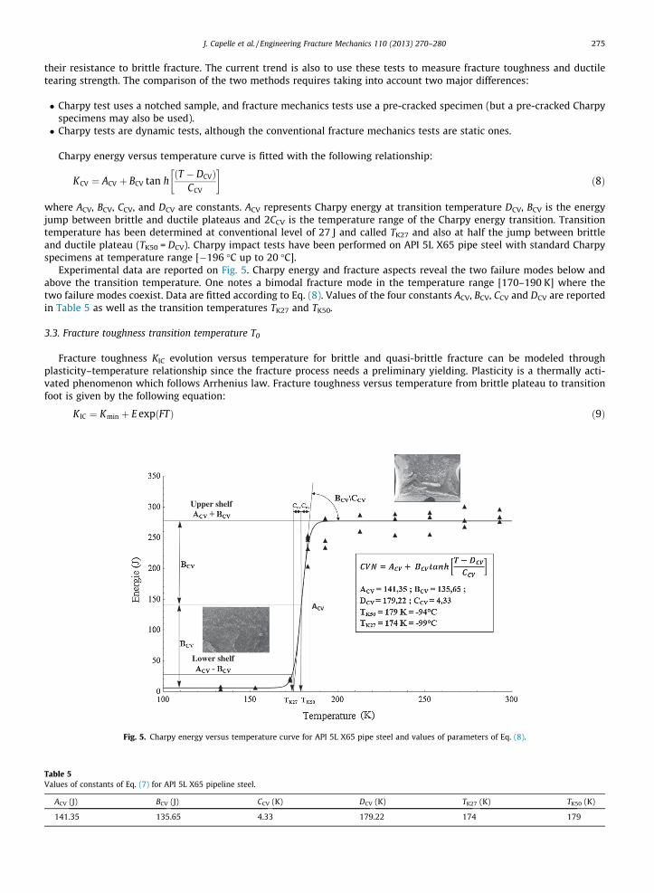
Charpy energy versus temperature curve is fitted with the following relationship:

Table 5Values

ACV (

141.

KCV ¼ ACV þ BCV tan hT � DCVð Þ

CCV

� �ð8Þ

where ACV, BCV, CCV, and DCV are constants. ACV represents Charpy energy at transition temperature DCV, BCV is the energyjump between brittle and ductile plateaus and 2CCV is the temperature range of the Charpy energy transition. Transitiontemperature has been determined at conventional level of 27 J and called TK27 and also at half the jump between brittleand ductile plateau (TK50 = DCV). Charpy impact tests have been performed on API 5L X65 pipe steel with standard Charpyspecimens at temperature range [�196 �C up to 20 �C].

Experimental data are reported on Fig. 5. Charpy energy and fracture aspects reveal the two failure modes below andabove the transition temperature. One notes a bimodal fracture mode in the temperature range [170–190 K] where thetwo failure modes coexist. Data are fitted according to Eq. (8). Values of the four constants ACV, BCV, CCV and DCV are reportedin Table 5 as well as the transition temperatures TK27 and TK50.

3.3. Fracture toughness transition temperature T0

Fracture toughness KIC evolution versus temperature for brittle and quasi-brittle fracture can be modeled throughplasticity–temperature relationship since the fracture process needs a preliminary yielding. Plasticity is a thermally acti-vated phenomenon which follows Arrhenius law. Fracture toughness versus temperature from brittle plateau to transitionfoot is given by the following equation:

K IC ¼ Kmin þ E expðFTÞ ð9Þ

Fig. 5. Charpy energy versus temperature curve for API 5L X65 pipe steel and values of parameters of Eq. (8).

of constants of Eq. (7) for API 5L X65 pipeline steel.

J) BCV (J) CCV (K) DCV (K) TK27 (K) TK50 (K)

35 135.65 4.33 179.22 174 179

276 J. Capelle et al. / Engineering Fracture Mechanics 110 (2013) 270–280

Kmin is the fracture toughness threshold, E and F are constants and T is the temperature in Kelvin. Transition temperaturecalled T0 is defined conventionally for a fracture toughness of 100 MPa

pm.

The statistical effect of specimen size on KIC in the transition range is taken into account using the weakest-link theory[9–11] applied to a three-parameter Weibull distribution of fracture toughness values. With the threshold toughness K0

equal to 20 MPap

m, the cumulative distribution function is given by Eq. (10). Note that the thickness of the componenthas been implicitly accounted for in this equation through the parameter Lmc:

Fmc ¼ 1� exp � Lmc

25:4KJc � 20K0 � 20

� �4" #

ð10Þ

where Lmc is the crack length (mm) used in the master curve. For a through crack, Lmc is the total crack length; for internalcrack, Lmc is twice the total crack length; and for a surface crack, Lmc is twice the thickness.

Statistical methods are used to predict the transition toughness curve and specified tolerance limits for 1 T specimens ofthe tested material. The standard deviation of the data distribution is a function of Weibull slope and median KJc [10,11]:

KJcðmedianÞ ¼ 30þ 70 exp 0:019ðT � T0Þ½ � ð11Þ

in which T0 is the temperature associated with the fracture toughness value of 100 MPap

m. T0 is a characteristic parameterof the material which depends on loading rate. If fracture toughness is plotted versus the reduced temperature (T–T0), thematerial curve is then independent of the loading rate.

Fig. 7. (a) CT specimen geometry and (b) CT specimen Txx and Tzz distributions ahead crack tip.

Fig. 6. Evolution of fracture toughness versus temperature for API 5L X65 pipeline steel.

Table 6Different values of transition temperature T0.

T0.1 (�C) T0.2 (�C)

�128 �117

J. Capelle et al. / Engineering Fracture Mechanics 110 (2013) 270–280 277

Fracture toughness tests have been performed according to standard with CT specimens in the temperature range [128–293 K]. Geometry of the specimen is given in Fig. 7a. Fracture toughness data are plotted versus temperature in K and fittedaccording to Eq. (9) from the brittle plateau to transition regime in Fig. 6.

Transition temperature T0 is obtained according to two methods, which are reported in Table 6:

� T0.1 after fitting experimental data and determining the corresponding temperature to KJc = 100 MPap

m.� T0.2 using the following empirical relationship in Eq. (12) between transition temperatures TK27 and T0.

T0;2 ¼ TK27 � 18 �C ð12Þ

4. Results analysis and discussion. Effect of stress constraint on DBTT

A pragmatic, engineering approach to assess the fracture integrity of cracked or notched structures requires that con-straints in the test specimen approximate that of the structure to provide an ‘‘effective’’ toughness for use in a structuralintegrity assessment. Constraint effect can be represented by stress triaxiality, Q parameter [11,12] or T-stress [13]. Hereconstraint is measured by T-stress which is defined by:

T ¼ ðrxx � ryyÞy¼0;h¼0 ð13Þ

However, stress distribution is different for a crack and a notch. The elastic stress field in a region surrounding the cracktip can be characterized by the following solution [14]:

rij ¼KIffiffiffiffiffiffiffiffiffi2prp fijðhÞ þ Tdxidxj þ A3

ffiffiffiffiffiffiffiffiffi2prp

þ OðrÞ ð14Þ

where KI is the stress intensity factor, fij(h) is the angular function, dij is the symbol of Kronecker’s determinant. A polar coor-dinate system (r, h) with an origin at the crack tip is used. The second term is called the T-stress. The value of T is constant,with the stress acting parallel to the crack line in the direction xx of the crack extension with a magnitude proportional to thegross stress. In the third term, A3 is sometimes used as a transferability parameter like the T-stress. The non-singular term Trepresents a tension (or compression) stress. Positive T-stress strengthens the level of crack tip stress triaxiality and leads tohigh crack tip constraint while negative T-stress leads to a loss of constraint. Therefore, the T-stress can be considered as aconstraint crack tip parameter.

The volumetric method [3] is employed to calculate the notch fracture toughness and to estimate the effective T-stressahead of the notch tip. It is assumed, according to the meso-fracture principle, that the fracture process requires a physicalvolume. This assumption is supported by the fact that fracture resistance is affected by the loading mode, specimen geom-etry and scale effect. To explain these effects, it is necessary to take into account the stress value and the stress gradient in allneighboring points within the fracture process volume. This volume is assumed to be quasi-cylindrical with a fracture pro-cess zone of similar shape. The diameter of this cylinder is called the ‘‘effective distance’’. By computing the average value ofthe opening stress within this zone, the fracture stress can be estimated. This procedure leads to a local fracture criterionbased on two parameters, namely, the effective distance Xef and the effective stress ref. The minimum point of the relativestress gradient in the bi-logarithmic diagram is conventionally taken into account as the relevant effective distance. The min-imum value of the relative stress gradient X is written as follows:

XðrÞ ¼ 1ryyðrÞ

@ryyðrÞ@r

ð15Þ

Here, X(r) and ryy(r) are the relative stress gradient and the maximum principal stress or the crack opening stress, respec-tively. The relative stress gradient depicts the severity of the stress concentration around the notch tip. The effective stress isdefined as the average of the weighted stress within the fracture process zone:

ref ¼1

Xef

Z Xd

0ryyðrÞUðrÞdr ð16Þ

where ref, Xef, ryy(r) and U(r) are the effective stress, effective distance, maximum principal stress and weight function,respectively.

278 J. Capelle et al. / Engineering Fracture Mechanics 110 (2013) 270–280

The unit weight function and Peterson weight function are the simplest definitions of weight function U(r). The unitweight function deals with the average stress and Peterson weight function gives the stress value at a specific distance; itis not required to compute numerical integration.

Due to the fact that the effective T-stress in the fracture process zone is not constant, it is also assumed to be determinedby averaging the T-stress distribution over the effective distance according to a line method (Eq. (17)):

Tef ¼1

Xef

Z Xef

0TxxðrÞUðrÞdr ð17Þ

where TxxðrÞ ¼ rxxðrÞ � ryyðrÞ� �

h¼0Several methods have been proposed in the literature to determine the T-stress for cracked specimen (Chao et al. [15],

Ayatollahi et al. [16], and Wang [17]). Here, the stress difference method (SDM) proposed by Yang and Ravi-Chandar [18]is used. In this method, the T-stress is evaluated from stress distribution computed by finite element method. The T-stressis equal to the difference between the opening stress and the stress acting parallel to the crack plane. rxx was calculated byfinite element method in the direction h = 180� (i.e., in the crack rear back direction), and the T-stress was defined as thevalue of rxx in region where this value is constant.

Stress distribution ahead of crack tip has been computed for CT specimens by finite element method using ABAQUS code.In addition, T-stress is determined by the stress difference method. For each test, critical load has been chosen at transitiontemperature at which brittle fracture is assumed under linear elastic behavior. The considered T-stress value is the effectivevalue given by Eq. (17) for CT specimens.

The use of Charpy V TK27 or TK50 transition temperature as reference temperature needs to introduce a correction due tothe fact that this test is made at a loading rate of about 10 s�1 and consequently higher than the loading rate correspondingto a static loading (10�3 s�1).

An empirical relationship between transition Tt and yield stress Re, proposed by Barsom and Rolfe [19] is used.

Tt ¼ 0:17Re � 125ðK;MPaÞ ð18Þ

Knowing transition temperature for Charpy Test Tt,d, (171 K) it is easy to know the equivalent static transition temperatureTt,s by reporting dynamic yield stress (661 MPa) at this temperature into modify Eq. (18):

DTt ¼ 0:17ðRe;dðTt;dÞ � Re;sðTt;sÞÞ ð19Þ

This equation is solved knowing relationship between static yield stress and temperature by dichotomy method, Eq. (4).For API X65, the shift in transition temperature is 10 �C. This corrected transition temperature is reported in Fig. 8.In this paper the stress difference (rxx–ryy) is called T, however the use of a cracked, a notched. For smooth specimen T

has another definition and based on strain difference:

T ¼ E � ðexx � eyyÞ ð20Þ

Table 7 summarizes values of T-stress and associated transition temperature.Transition temperatures obtained with the 3different specimens are plotted against temperature and reported in Fig. 8. One notes a linear increase of transition temper-ature with T-stress according to the following relationship:

Fig. 8. Evolution of transition temperature with effective T-stress (Tef).

Table 7Specimen geometry T-stress and associated transition temperature.

Specimen Charpy CT Tensile

Tef (MPa) �230.8 �330 �510Transition temperature (K) 171 156 123

Fig. 9. Estimation of component transition temperature from the master curve (Tt = f (constraint)).

J. Capelle et al. / Engineering Fracture Mechanics 110 (2013) 270–280 279

Tt ¼ 0:13Tef þ 195 ð21Þ

where Tt is the transition temperature in Kelvin and Tef the effective T-stress in MPa. Transition temperature is not intrinsic tomaterial. It decreases with loss of constraint and the choice of TK27 as reference temperature in Eq. (8) is the mostconservative.

Fig. 8 allowed to determine a transition temperature relative to the investigated component, i.e., a transition temperaturecorresponding to the same constraint as the component at failure. For that purpose, it is necessary to obtain the ‘‘materialmaster curve’’ which is the relationship between fracture toughness and constraint and effective T-stress (Tef) at critical pres-sure for a test according to the procedure described in [20].

Transition temperature of component has then been determined for pipe steel made in API 5L X52 with 610 mm diameterand 5.8 mm thickness equal to. This pipe exhibits a surface notch with a notch angle j = 0, a notch radius r = 0.25 mm and anotch depth (a) to thickness (t) ratio equal to a/t = 0.5. Loading curve Kap = f (T) has been computed by finite element assum-ing elastic behavior, the steel is considered as brittle at transition temperature. This loading curve Kap = f (T) intercept thematerial master curve at point (Tef , Kc) figure.

The obtained value of Tef is �495 MPa. In this procedure, we have used the available data in order to have a cheaper andfaster procedure. To take into account this uncertainty, it is better to estimate the constraint range �450 MPa and �550 MPa.

The average component transition temperature Tcomp is deduced from the master curve and evaluated to 150 K (seeFig. 9). This temperature is lower than TK27 transition temperature of 24 K; this value represents the degree of conservatismof using transition temperature deduced from Charpy specimens. The safety temperature range between the depressurisa-tion temperature plus a temperature allowance and the component temperature is 35 K, which is enough, allowing to con-sider that API 5L X65 could be used for dense CO2 transportation.

5. Conclusion

In order to select a steel for transportation of dense CO2, transition temperatures Tt (from tensile test), TK27 and TK50 (fromCharpy test)and TK100 (from fracture mechanics test) have been determined on an API 5L X65 steel. These transition temper-atures have been reported versus a constraint parameter, e.g. T-stress, in a master curve. Differences between differentbrittle–ductile transition temperatures and temperature corresponding to T-stress acting in a pipe submitted to internalpressure on the master curve, give an estimation of the conservatism of the chosen transition temperature.

Based on this methodology the selected API 5L X65 pipeline steel could be used for dense CO2 transportation since theexperimental and calculated transition temperatures are lower than the expected �80 �C following a rapid decompressionof dense CO2 pipeline rupture. The most conservative transition temperature was obtained by Charpy impact test TK27, whichis lower than depressurisation temperature plus a temperature allowance.

280 J. Capelle et al. / Engineering Fracture Mechanics 110 (2013) 270–280

Acknowledgements

This research is part of the France Nord project, which has been selected by the ADEME’S Demonstrator Funds (The FrenchEnvironment Agency), implemented following the ‘‘Grenelle de l’Environnement’’. Authors thank Dr. Hadj Meliani for deter-mination by computing of T-stress values, Mr. Mansour Haithem for participating in the test performance, and Vallourec &Mannesmann Tubes for providing a seamless tube sample of API 5L X65 pipeline steel.

References

[1] Dooley JJ, Dahowski RT, Davidson CL. Comparing existing pipeline networks with the potential scale of future U.S. CO2 pipeline networks. EnergyProcedia 2009;1:1595–602.

[2] Eldevik F, Graver B, Torbergsen LE, Saugerud OT. Development of a guideline for safe, reliable and cost efficient transmission of CO2 in pipelines. EnergyProcedia 2009;5:1579–85.

[3] Pluvinage G. In: Pluvinage G, Elwany M, editors. General approaches of pipeline defect assessment in safety. Reliability and risks associated with water,oil and gas pipelines. Springer; 2007. p. 1–22.

[4] API 579-1/ASME FFS-1. Fitness for service. Houston: American Society of Mechanical Engineers; 2007.[5] Hadj Meliani M, Matvienko YG, Pluvinage G. Corrosion defect assessment on pipes using limit analysis and notch fracture mechanics. Engng Fail Anal

2011;18:271–83.[6] Kloster G, Probst-Hein M. X65 steel for seamless line pipe and risers for on- and offshore projects. Vallourec and Mannesmann Tubes, Düsseldorf; 2012.

[accessed on 08.06.12] <www.vmtubes.com>.[7] AFNOR standard: NF EN 10002-1. Matériaux métalliques. Essai de traction. Saint Denis La Pleine: Association Française de Normalisation; 1990.[8] AFNOR standard: NF EN ISO 14556. Acier. Essai de flexion par choc sur éprouvette Charpy à entaille en V. Méthode d’essai instrumentée. Saint Denis La

Pleine: Association Française de Normalisation; 2001.[9] Green AP, Hundy BB. Initial plastic yielding in notch bend tests. J Mech Phys Solids 1956;4:128–44.

[10] ASTM E1921-11a. Standard test method for determination of reference temperature, T0 for ferritic steels in the transitionrange. Philadelphia: American Society for Testing and Materials; 2003.

[11] Ruggieri C, Gao X, Dodds RH. Transferability of elastic–plastic fracture toughness using the Weibull stress approach: significance of parametercalibration. Engng Fract Mech 2000;67:101–17.

[12] Henry BS, Luxmore AR. The stress triaxiality constraint and the Q-value as a ductile fracture parameter. Engng Fract Mech 1997;57:375–90.[13] Betegon C, Hancock JW. Two parameter characteristics of elastic–plastic crack-tip fields. J Appl Mech 1991;58:101–4.[14] Williams ML. Stress singularity resulting from various boundary conditions in angular corners of plates in extension. J Appl Mech 1952;19:526–8.[15] Chao YJ, Zhang X. Constraint effect in: Brittle Fracture. In: 27th National, symposium on fatigue and fracture. ASTM STP 1296. Piascik RS, Newman Jr.,

JC, Dowling DE. American Society for Testing and Materials, Philadelphia; 1997. p. 41–60.[16] Ayatollahi MR, Pavier MJ, Smith DJ. Determination of T-stress from finite element analysis for mode I and mixed mode I/II loading. Int J Fract

1998;91:283–98.[17] Wang X. Elastic stress solutions for semi-elliptical surface cracks in infinite thickness plates. Engng Fract Mech 2003;70:731–56.[18] Yang B, Ravi-Chandar K. Evaluation of elastic T-stress by the stress difference method. Engng Fract Mech 1999;64:589–605.[19] Barsom JM, Rolfe ST. Correlation between KIC and Charpy V-notch test results in the transition temperature range. Impact Testing Met ASTM STP

1970;466:281.[20] Hadj Meliani M, Matvienko YG, Pluvinage G. Two-parameter fracture criterion (Kq,v–Tef,c) based on notch fracture mechanics. Int J Fract

2011;167:173–82.