IN DEGREE PROJECT COMPUTER SCIENCE AND ENGINEERING,SECOND CYCLE, 30 CREDITS

, STOCKHOLM SWEDEN 2021

Design and implementation of embedded system for chl-a fluorescence detection

ANARGYROS KATSOGRIDAKIS

KTH ROYAL INSTITUTE OF TECHNOLOGYSCHOOL OF ELECTRICAL ENGINEERING AND COMPUTER SCIENCE

KTH Royal Institute of Technology

School of Electrical Engineering and Computer Science

Design and implementation of

embedded system for chlorophyll-a

fluorescence detection

Anargyros Katsogridakis

Author: Anargyros Katsogridakis, anakat@kth.se

Examiner: Mark T. Smith, msmith@kth.se

Supervisor: Fei Ye, feiy@kth.se

Host company: Cybercom AB

Swedish title: Design och implementering av inbyggt system för klorofyll-a

fluorescens detektering

ii

Abstract

Over the last decades, the effects of climate change have become increasingly evident

across natural environments. Apart from other areas, climate change poses a serious

threat on water quality.

More specifically, it is expected that the effects of global warming around the world will

severely limit our ability to control the spread and occurrence of Harmful Algal Blooms

(HABs) in the future. A HAB episode is characterised by rapid proliferation of algal

biomass which can cause major implications on the environment, the ecosystems, on

human health, the economy, and societies overall. One way of detecting the presence

of algae is to determine the chlorophyll-a concentration levels in water.

This project proposes an embedded system for early algae detection in water samples

by means of chl-a fluorometry. The system makes use of a constructed sensor to detect

chl-a fluorescence emission. Two versions of the sensor were designed and

implemented, both of which were calibrated and then tested. Afterwards, the results

were presented, and the system’s performance was evaluated and discussed.

Lastly, it was concluded that the performance of the system was adequate for detecting

a 50 µg/L limit of chl-a concentration, however, careful testing of the site is required

for field applications in samples of natural water.

Keywords

Embedded systems, Microcontrollers, Harmful algal bloom, Climate change, chl-a

fluorescence

iii

Sammanfattning

Under de senaste decennierna har effekterna av klimatförändringar blivit allt tydligare

i naturliga miljöer. Förutom andra områden utgör klimatförändringarna ett allvarligt

hot mot vattenkvaliteten.

I synnerhet förväntas effekterna av global uppvärmning över hela världen begränsa vår

förmåga att kontrollera spridningen och förekomsten av skadliga algblomningar

(HAB) i framtiden. En HAB-episod kännetecknas av snabb spridning av algbiomassa

som kan orsaka stora konsekvenser för miljön, ekosystemen, människors hälsa,

ekonomin och samhället i stort. Ett sätt att upptäcka förekomsten av alger är att

bestämma klorofyll-a-koncentrationsnivåerna i vatten.

Detta projekt föreslår ett inbyggt system för tidig algedetektering i vattenprover med

hjälp av chl-a fluorometri. Systemet använder en konstruerad sensor för att detektera

chl-a-fluorescensemission. Två versioner av sensorn designades och implementerades,

båda kalibrerades och testades sedan. Därefter presenterades resultaten och systemets

prestanda utvärderades och diskuterades.

Slutligen drogs slutsatsen att systemets prestanda var tillräcklig för att detektera 50

µg/L-gräns för chl-a-koncentration, men noggrann testning av platsen krävs för

fältapplikationer i prover av naturligt vatten.

Nyckelord

Inbyggda system, mikrokontroller, skadlig algblomning, klimatförändring, chl-a-

fluorescens

iv

Acknowledgements

First of all, I would like to thank Dr. Joydeep Dutta for being kind enough to assist this

project by providing access to laboratory equipment and also for providing the chl-a

analytical standard used in this study. Without his invaluable contribution this thesis

would not have been possible to complete.

Moreover, I want to thank my supervisor Dr. Fei Ye for his advice and guidance during

the process of conducting the experiments in the chemistry lab, for testing and

calibrating the constructed system. Lastly, I would like to thank my friends, Federica,

Panos and Yiota for answering my questions during this study, for sharing their

scientific knowledge with me and for their overall support in this effort.

Stockholm, February 2021

Anargyros Katsogridakis

v

Table of Contents

Chapter 1. Introduction ........................................................................... 1

1.1. Background ............................................................................................................ 1

1.2. Problem statement................................................................................................ 2

1.3. Purpose ................................................................................................................. 2

1.4. Goal ....................................................................................................................... 3

1.5. Benefits, Ethics and Sustainability ....................................................................... 3

Chapter 2. Background ............................................................................ 4

2.1. Climate Crisis ........................................................................................................ 4

2.2. Climate Change and Water Quality ..................................................................... 5

2.3. Harmful Algal Blooms .......................................................................................... 7

2.3.1. Toxicity ........................................................................................................... 8

2.3.2. Effects on nature ............................................................................................ 8

2.3.3. Economic impacts .......................................................................................... 9

2.3.4. Causes ........................................................................................................... 11

2.3.5. Studying HABs .............................................................................................. 12

2.4. HAB Detection..................................................................................................... 13

2.5. Chlorophyll-a fluorescence ................................................................................. 17

Chapter 3. Method ................................................................................. 21

3.1. Assumptions and specifications .......................................................................... 21

3.2. Design #1 ............................................................................................................ 23

3.2.1. Component selection .................................................................................... 23

3.2.2. Building the device....................................................................................... 26

3.3. Design #2 ............................................................................................................. 31

3.3.1. Component selection .................................................................................... 32

3.3.2. Building the device....................................................................................... 32

3.4. 3D printing ......................................................................................................... 35

3.5. Algorithm ............................................................................................................ 39

3.6. Experiments ....................................................................................................... 42

3.6.1. Calibration .................................................................................................... 42

3.6.2. Turbidity ...................................................................................................... 47

vi

3.6.3. Water samples .............................................................................................. 48

3.6.4. Data variance ............................................................................................... 49

Chapter 4. Results ................................................................................. 50

4.1. Results ................................................................................................................. 50

4.1.1. Calibration .................................................................................................... 50

4.1.2. Turbidity ....................................................................................................... 59

4.1.3. Water samples ...............................................................................................61

4.2. Data analysis ...................................................................................................... 63

4.2.1. Calibration .................................................................................................... 63

4.2.2. Turbidity ...................................................................................................... 67

4.2.3. Water samples .............................................................................................. 68

Chapter 5. Discussion and Conclusion ................................................... 69

5.1. Discussion ........................................................................................................... 69

5.2. Conclusion ........................................................................................................... 71

5.3. Future Work ....................................................................................................... 72

References .............................................................................................73

vii

List of Figures

Figure 1: Combined absorption and emission spectrum of chlorophyll-a in visible

wavelengths [56]. .......................................................................................................... 18

Figure 2: The relaxation procedures of fluorescence and phosphorescence are

presented and compared in an Jablonski energy diagram [60]. ..................................19

Figure 3: Indicative block diagram of the proposed device. ........................................ 23

Figure 4: Raspberry Pi v2.1 camera module. ............................................................... 24

Figure 5: 16x2 LCD screen used with Raspberry Pi. .................................................... 27

Figure 6: Booklet of optical filters (left) and spectrum of selected red filter (right). .. 28

Figure 7: Typical application of KA317 voltage regulator. ........................................... 28

Figure 8: LED mounting base and heat sink................................................................ 29

Figure 9: Circuit schematic of the designed LED driver and the isolation circuit. ..... 30

Figure 10: Block diagram of the device setup. .............................................................. 31

Figure 11: The Arduino Mega 2560 microcontroller board. ........................................ 33

Figure 12: Circuit schematic for the interface of LDR with the microcontroller. ........ 34

Figure 13: Block diagram of the improved version of the device. ................................ 35

Figure 14: 3D model of the enclosure's base which includes the camera and cuvette

holder. ........................................................................................................................... 36

Figure 15: LED and LDR holders. ................................................................................ 36

Figure 16: 3D models of the top part of the enclosure. ................................................ 37

Figure 17: 3D printed enclosure. .................................................................................. 37

Figure 18: Connectivity of sensor components. ........................................................... 38

Figure 19: Flow chart of algorithm for design #1. ........................................................ 39

Figure 20: Histogram of one of the samples (left) and the corresponding calculated

CDF (right). ................................................................................................................... 40

Figure 21: Flowchart of algorithm for design #2. ......................................................... 41

Figure 22: Variable volume pipettes used for preparing the samples for calibration. 44

Figure 23: Stock solutions covered with aluminium foil to protect them from light,

and glass vial of pure chl-a analytical standard. .......................................................... 45

Figure 24: Samples of known chl-a concentration. ..................................................... 45

Figure 25: The calibration procedure with LS 55 fluorescence spectrometer and the

designed sensor. ........................................................................................................... 46

Figure 26: Samples prepared with known mass of suspended particulate matter. .... 47

Figure 27: Turbid sample in 1cm path length cuvette. ................................................ 48

Figure 28: Locations of water sample collection. ........................................................ 48

Figure 29: Investigation of peak excitation wavelength of chl-a samples used for the

device's calibration. The current graph was produced from data collected from the

sample with highest chl-a concentration of 400 µg/L. The same response with lower

intensity was recorded from all samples with lower chl-a concentration. Solid lines

represent the dominant wavelength range of the LED with the correspondent colour,

while the dashed line represents the peak wavelength. ............................................... 50

viii

Figure 30: Locating the peak wavelength of fluorescence emission of samples used for

calibration using the LS-55 instrument. The current graph was produced from data

collected from the sample with highest chl-a concentration of 400 µg/L. The same

response with lower intensity was recorded from all samples with lower chl-a

concentration. ................................................................................................................ 51

Figure 31: Correlated measurements of chl-a sample solutions between the Design #1

of the constructed device (y-axis) and LS-55 fluorescence spectrometer (x-axis). ..... 52

Figure 32: Fluorescence emission intensity of chl-a samples measured from the

constructed device (design #1) plotted with the chl-a concentration of the samples (x

axis). .............................................................................................................................. 53

Figure 33: Fluorescence emission intensity of prepared samples measured from LS-

55 fluorescence spectrometer with the excitation wavelength set at 425nm. ............. 55

Figure 34: Correlated measurements of chl-a sample solutions between the Design #2

of the constructed device (y-axis) and LS-55 fluorescence spectrometer (x-axis). ..... 56

Figure 35: Fluorescence emission intensity of chl-a samples measured from the

constructed device (design #2) plotted with the chl-a concentration of the samples (x

axis). .............................................................................................................................. 57

Figure 36: Fluorescence emission intensity of prepared samples measured from LS-

55 fluorescence spectrometer with the excitation wavelength set at 448nm. ............. 59

Figure 37: Optimal linear response of Design #1 of the proposed device. .................. 64

Figure 38: Optimal linear response of Design #2 of the proposed device. ................. 66

Figure 39: Emission spectrum of water sample #8 which caused strong interference

to the constructed sensor.............................................................................................. 69

ix

List of Tables

Table 1: Settings used on the Perkin Elmer LS-55 fluorescence spectrometer

instrument to capture the fluorescence emission intensity data. ................................ 46

Table 2: Data captured from Perkin Elmer LS-55 fluorescence spectrometer for the

produced samples of chl-a with an excitation wavelength of 425nm. ......................... 54

Table 3: Data captured from Perkin Elmer LS-55 fluorescence spectrometer for the

produced samples of chl-a with an excitation wavelength of 448nm. ........................ 58

Table 4: Measurements of samples with varying turbidity from Design #1 (violet

LED) of the constructed device. Data of fluorescence were acquired from the camera

and absorption data were collected from the LDR sensor. .......................................... 60

Table 5: Measurements of samples with varying turbidity from Design #2 (blue LED)

of the constructed device. Data of fluorescence were acquired from the camera and

absorption data were collected from the LDR sensor. ..................................................61

Table 6: Comparing the fluorescence intensity captured from Design #1 (violet LED)

of our constructed device and the LS-55 fluorescence spectrometer. ......................... 62

Table 7: Comparing the fluorescence intensity captured from Design #2 (blue LED) of

our constructed device and the LS-55 fluorescence spectrometer. ............................. 62

Table 8: Overview of calibration results for both versions of the proposed device and

both the excitation wavelengths used on the LS-55 fluorescence spectrometer. ........ 67

Table 9: Cost of each component used to construct the fluorescence sensor. ............ 72

1

Chapter 1. Introduction

1.1. Background

Over the last decades, the problem of climate change has affected ecosystems and

societies with increasingly adverse effects. One of the negative impacts of this

phenomenon is on water quality. Rising temperatures across the globe as well as the

increasing frequency of extreme precipitation events provide fertile ground for rapid

proliferation of algae and cyanobacteria in coastal and lake waters [1].

The microscopic planktonic algae found in the oceans are a critical part of many

ecosystems as they are food source to many fish species. In most cases, the proliferation

of phytoplankton algae, often referred to as an algal bloom, is beneficial for

aquaculture. However, there are also cases where an algal bloom can have negative

effects causing severe economic losses to aquaculture, fisheries and tourism operations

as well as having major environmental and human health impacts [2].

Algal blooms usually occur naturally during spring and summer months in lakes and

coastal water bodies. However, climate change is now causing them to appear more

and more early in the year, more frequently and in higher magnitude. A Harmful Algal

Bloom (HAB) contains organisms that can severely lower oxygen levels in natural

waters, killing the marine life. HABs can also contain cyanobacteria, which is a species

of algae that produces toxins (cyanotoxins) dangerous both for fish and humans.

Human exposure to cyanotoxins can cause illness with various degrees of severity, and

in extreme cases can lead to death.

It is clear that HABs are detrimental to water quality and can cause severe damages

and socioeconomic problems which cost millions to be repaired. Much of that cost

comes from commercial fisheries through fishing closures applied, increase of fish

prices and from public health through medical expenses and hospitalization of patients

[3]. Moreover, HAB episodes have a negative impact on tourism due to the reduction

of recreational experiences of visitors near the beaches. Lastly, monitoring and

management expenses are also increased due to water sampling and water treatments

to remove toxins, among other actions.

2

1.2. Problem statement

Various technologies such as deep learning and computer vision have been exploited

to detect HABs through remote sensing [4]. However, these techniques do not have the

capability to detect the formation of harmful algal blooms at an early stage where

further spreading can be prevented so that water quality is maintained in safe levels.

It is a fact that algae and cyanobacteria are microorganisms that are capable of

photosynthesis and therefore contain chlorophyll. Photosynthesis alters the properties

of a water body and many techniques can be used to detect them. Multiple sensor

modules are available that can measure parameters which provide crucial information

regarding the state of a water body. Some of these important parameters are water

temperature, dissolved oxygen levels, pH and chlorophyll-a concentration levels.

Chlorophyll-a, more specifically, can be found in all species of algae. This substance

has the property of fluorescence, meaning that once excited with a certain wavelength

of blue light it emits lower energy photons of red light as the molecule returns to a non-

excited state. Chlorophyll-a fluorescence is well investigated and commonly used as an

estimator for algal biomass indicating the state of a marine water body, e.g.,

oligotrophic, mesotrophic or eutrophic [5].

However, up until now the existing systems for chlorophyll-a fluorescence sensing are

either too expensive to be implemented at many locations or not portable. Professional

fluorometers are commercially available and can be submersible in water, but their

maintenance cost is often too high which introduces limitations in their practical use.

From the above, it is obvious that there is crucial need for a system which can sense

water fluorescence and that is portable, affordable and self-sustainable so that it can

be easily deployed and used in multiple locations without the need of expertise

knowledge. The research question for this project is as follows:

Can an embedded system successfully detect the level of chlorophyll-a concentration

in a sample of water?

1.3. Purpose

The purpose of the current project is to construct device that will allow measurements

of the marine realm by the general public. This will allow for considerably more

measurements of water quality conditions being collected, both in quantity and

frequency in water bodies located near the proposed device. This in turn can lead to

more effective maintenance of the water quality from the state by taking actions to

protect it and therefore achieving considerably increased safety for all society.

Moreover, the collected data can be shared and utilised for HAB forecasting.

3

1.4. Goal

The goal of this project is the design and implementation of an embedded system

containing a custom fluorescence sensor for chlorophyll-a. This sensor must be able to

detect at least 50ug.L-1 chlorophyll-a concentration in a water sample (cuvette). As

defined in the guidelines for Water Quality from the World Health Organisation

(WHO) such levels of chlorophyll-a pose a moderate to high health alert to recreational

waters [6], [7].

1.5. Benefits, Ethics and Sustainability

• The method of chl-a fluorometry utilised in this project is non-invasive and is

characterised by low energy footprint.

• This project promotes sustainable development by suggesting solutions for

monitoring and maintaining water quality by means of low-cost electronics.

• The current thesis promotes ways to act towards mitigating the negative effects

of climate change and global warming to society through technology.

4

Chapter 2. Background

This chapter will present the literature review for this problem as well as the related

work. Moreover, theoretical aspects regarding the approach used in this study will

be analysed.

2.1. Climate Crisis

Climate crisis is undoubtedly a threat nowadays and its impacts can be detrimental to

society in multiple ways [8], [9]. Global warming refers to the long-term rise in the

Earth’s surface temperatures mainly caused by human activity. According to the

Intergovernmental Panel on Climate Change (IPCC) Fifth Assessment Report it has

been concluded that “it is extremely likely that human influence has been the dominant

cause of the observed warming since the mid-20th century” [10]. Climate crisis is a term

describing global warming and climate change occurring because of greenhouse gas

emissions and their consequences.

The causes of global warming effect have been attributed to fossil fuel combustion such

as coal and oil, as well as to the clearing of land for agriculture and to deforestation.

These activities tend to increase the concentration of greenhouse gases (GHG) in

Earth’s atmosphere. Those gases include water vapor, carbon dioxide (CO2), methane,

nitrous oxide and chlorofluorocarbons (CFC’s) which are synthetic compounds of

entirely industrial origin. GHG’s have the property of trapping heat coming from the

sun in the atmosphere and block it from escaping back toward space. Therefore, higher

GHG concentrations expand the greenhouse effect which occurs naturally on Earth

[11].

The consequences of this phenomenon affect the natural environment, ecosystems and

human societies in various complex and interdependent ways.

• Rising sea levels – inundation of coastal cities

• More frequent and more extreme weather events such as precipitation,

hurricanes, floods and unprecedented heatwaves

• Expansion of deserts

• Ocean acidification threat for marine life survival

• Retreat of glaciers, permafrost and sea ice – the arctic is expected to be ice free

during summers within a few years.

• Droughts and wildfires

5

• Extinction of species, collapse of ecosystems, loss of biodiversity including coral

reef systems

• Human health & security: food insecurity poses the risk of higher malnutrition

rates, insufficient fresh water supply in many areas, extreme weather

• Social and economic changes: migration, negative effects on economic growth

in developing countries, destruction of local nature in all parts of the world

2.2. Climate Change and Water Quality

From what was mentioned above it can be concluded that climate crisis is a

phenomenon affecting all kinds of ecosystems on earth, including human life.

Therefore, it is no surprise that global warming has severe negative effects on aquatic

ecosystems and water quality. Over the past decades a great amount of scientific

attention has been focused around investigating how the aquatic environment is

transformed by climate change and in what ways this affects marine life and water

quality.

According to the literature, increased temperatures, increased frequency of

precipitation events and increased occurrence of flooding are the predominant factors

that pose a threat to water quality across the globe [12], [13]. Other effects include

acidification, deoxygenation and stratification of water bodies with severe negative

impacts to their overall health [14], [15]. Coastal waters have experienced progressive

temperature increase that is expected to intensify within the coming century. At the

same time, increased precipitation events and flooding can in turn cause a drastic

increase to the input of important nutrients, such as phosphorus and nitrogen, in a

water body [10], [16]. This can lead to the eutrophication of a water body.

The Trophic State Index (TSI) is a classification system that is used to rate the

biological productivity of a water body, or in other words the amount of biological

species such as algae, plants, fish, or birds they can sustain. Eutrophication is defined

as the presence of excess nutrients in lakes, rivers, or coastal waters. According to the

TSI system, a water body state can be described as oligotrophic, mesotrophic or

eutrophic [17]. Defining the water body state is of high importance as it can serve as an

indication of water quality [18].

The nutrients causing eutrophication are mainly phosphorus and nitrogen and they

enter aquatic ecosystems through the air, surface water or groundwater.

Eutrophication can occur naturally (natural eutrophication) but this phenomenon is

often dramatically intensified due to human factors (cultural or anthropogenic

eutrophication) [19]. Natural eutrophication can be described as the addition, flow,

and accumulation of nutrients into water bodies and has been taking place on the

6

planet for thousands of years. On the other hand, cultural eutrophication is defined as

the process of speeding up natural eutrophication because of human activity. It is a fact

that altering of the nutrient input in water bodies can be attributed to anthropogenic

factors for the most part [20]. The most significant sources of anthropogenic nutrient

input in water bodies are the following:

• Erosion and leaching from agricultural areas where fertilizers are used

• Sewage runoffs from urban environments

• Wastewater from industrial environments

• Atmospheric deposition of nitrogen due to combustion

More specifically, artificial fertilizers are especially rich in nitrogen content and their

demand over the last decades has risen exponentially. This is because of the need to

cover the nutritional demands of the sky-rocketing human population. All of the factors

mentioned above are well documented and studied, and it has been shown that they

already have severe implications to water quality causing it to diminish sharply [21].

On top of this situation, human-induced global warming is at the same time affecting

water bodies in its own way intensifying the problem even further. As mentioned

above, climate change is also the root cause of events such as flooding and change in

precipitation patterns which result in altering of the nutrient load ending up

accumulating into lakes and coastal waters [22].

This kind of transformation of aquatic ecosystems which is a result of a wide range of

factors, involves consequences. More specifically, scientists have found a clear

correlation between nutrient enrichment in a water body due to cultural

eutrophication, i.e. the one occurring from anthropogenic factors, and the formation

of algal blooms [23]. Algae are tiny microorganisms that are naturally present in water

but under suitable conditions they can proliferate at a significant rate. In that case algal

blooms appear. Blue-green algae is a species of algae which often favoured to develop

over other species in culturally eutrophic water bodies and estuaries and can be highly

toxic. In literature, an event like this is referred to as a harmful algal bloom (HAB)

episode [24], [25].

Over the past few decades that climate change effects have become evident, it has also

been observed that meanwhile the frequency of harmful algal blooms has increased at

an alarming rate worldwide [16]. Up to this point there is no clear link between the two

events, meaning that scientists have not yet managed to prove that climate change is

directly affecting the increased occurrence of toxic algal blooms in coastal and lake

waters across the globe [1].

In contrast, extensive research has focused on studying the effects of climate change in

marine ecosystems and combining these findings with the present scientific knowledge

of how toxic algal blooms are formed and what affects their growth and prevalence

[26], [8]. In their publication, environmental scientists K.H. Havens and H.W. Pearl

are warning that “because of climate change, we are at a crossroad with regard to

control of harmful algal blooms, and must aggressively tackle the problem before it

7

becomes so difficult that in many ecosystems we are faced with the option of allowing

these micro-organisms to go unchecked” [27]. According to studies it is underlined

that it is extremely likely that climate change will affect our ability to control HAB

episodes in the future and also that in many cases to the extent which it may prove

impossible to do so [1], [28], [29], [30].

Climate change is a pressing issue and there is a need to act now to protect the

environment so that the negative consequences are minimised or even avoided. More

specifically, when it comes to water quality maintenance and ensuring its safe use and

consumption across the globe, there is an urgent need for innovative and sustainable

solutions regarding HAB detection so that the control of their expansion can be

achieved successfully in the future.

2.3. Harmful Algal Blooms

As mentioned in the previous section, a Harmful Algal Bloom (HAB) can be described

as the accumulation of algal biomass in a water body which has negative effects on the

marine ecosystem, the local economy, as well as on human health. The microscopic

planktonic algae found in the oceans is a critical part of many ecosystems since they

are food source to multiple fish species. In many cases, the proliferation of

phytoplankton algae can be beneficial for aquaculture and fisheries operations [2].

However, excessive algal growth leading up to a HAB event can induce severe

socioeconomic impacts.

HABs are a problem characterised by extraordinary diversity and complexity both

when considering the factors influencing or causing their appearance and regarding

their impacts on society. Moreover, it has been observed that over the past decades the

amount of reported HAB events in coastal waters has increased dramatically.

According to the World Resources Institute (WRI), the number of dead zones caused

by the so-called “red-tides”, which are a type of HAB event that discolours the water,

has increased from 10 in 1960 to more than 450 in 1980 and is still growing [31]. It is

worth noting that “HAB” is an umbrella term that can also include cases of macroalgae

which are non-toxic species of seaweed that can grow out of control and cause major

ecological impacts. Furthermore, some HABs are not algae but rather prokaryotic

photosynthetic bacteria (cyanobacteria) or even small protists that do not

photosynthesize but feed on other organisms.

A reasonable question that may arise is in what ways HABs can actually cause harm.

The harmful impacts of HAB events can be identified in two main categories. First of

all, a HAB event can refer to cases where the accumulated algal biomass becomes so

excessive that may affect other types of marine life under the same environment.

Furthermore, during a HAB event, algae can become the dominant species within an

ecosystem in terms of population, at the expense of other organisms’ survival, therefore

8

disrupting an ecosystem’s balance and its ability to maintain healthy populations.

Apart from that, HABs can also be harmful due to their production of toxins which can

cause illness or death to humans and animals [32].

2.3.1. Toxicity

It is a fact that HABs are able to produce quite an extensive variety of toxins for which

there are currently no antidotes available. In marine ecosystems only 2% of

phytoplankton species are harmful or toxic and most of the toxins are produced mainly

from the dinoflagellates and diatom algal species [33]. The most common way they

can harm humans is through the ingestion of contaminated shellfish or fish that

contain accumulated algal toxins and are consumed by people or other animals. Most

of these toxins are temperature-stable and therefore remain unaffected by cooking.

Multiple illnesses have been reported out of which some of the most common include

paralytic shellfish poisoning (PSP), amnesic shellfish poisoning (ASP) and neurotoxic

shellfish poisoning (NSP). Moreover, the toxins can cause respiratory problems to

humans when they are aerosolised. In extreme cases deaths have also been reported.

In addition, these toxins can directly kill shellfish, fish and harm other species of

marine wildlife [34].

In freshwater environments such as lakes, ponds, reservoirs, rivers, and estuaries,

most HAB events can be attributed to cyanobacteria (also known as “blue-green” algae)

which form the so-called cyano-HABs. Cyanobacteria can also occur in marine waters,

even though this case is less common. As opposed to marine HAB events, it is a fact

that most cyanobacterial blooms occur locally and pose a major threat since up to 50%

of cyano-HABs are toxic [35]. Human exposure to cyanotoxins can cause substantial

health implications with symptoms ranging from asthma or severe skin irritation to

liver and kidney damage as well as paralysis. Lastly, exposure to toxins released from

cyanobacteria has been linked with the occurrence of neurodegenerative diseases such

as amyotrophic lateral sclerosis (ALS) and Parkinson’s disease as well as chronic

tumour promotion [36].

2.3.2. Effects on nature

A HAB event can have multiple negative effects on a natural ecosystem. To begin with,

some HABs can cause harm because of the natural shape and form of the

microorganisms that they consist of. For example, some species of algae contain

physical structures such as spines that get caught into gills of various marine wildlife.

This can cause irritation and ultimately in suffocation of fish [32].

9

However, the primary way in which HABs cause harm is through excessively high

biomass accumulation. An event like this may induce severe environmental damages.

More specifically, once algae accumulates it consumes very large amounts of the

oxygen present in the water body during photosynthesis. Even worse, once the

microalgae die off and then decompose in the water, then the bacterial degradation of

their biomass consumes even greater amounts of oxygen. This can lead to the water

body entering a state of severe oxygen depletion, also known as hypoxia. In extreme

cases, most or all of the oxygen can disappear from a water body leaving it completely

anoxic.

As a result, a hypoxic or anoxic water environment can no longer sustain any kind of

marine life, therefore creating the so-called dead zones. In these areas, no fish, plants

or birds are able to survive. In addition, it is particularly important to highlight that

dead zones often occur in extensive areas of water that can cover up to thousands of

square kilometres.

As an example, researchers from the Baltic Sea Centre (Stockholm University)

reported that over the past century the dead zones in the Baltic sea have grown from

approximately 5,000km2 to more than 60,000km2 in recent years [37]. Judging by the

enormous size and geographical extent that a HAB event can cover it is made clear that

the impacts on wildlife are equally profound. It is not uncommon that a bloom’s

appearance can cause mass die-offs of fish that would otherwise be farmed for human

consumption, thus leading to tremendous economic losses to local economies [34].

Moreover, an event of high algal biomass accumulation is a type of HAB that is

responsible for causing visible water discoloration. The water can appear more turbid

and also may turn green, brown, blue, yellow, or even red depending on the species of

algae that has grown. Another negative effect involves problems with the water’s taste

and odour. Furthermore, once algae has grown out of control it tends to pile up and

float at the water surface. This layer of algal biomass can thus block the sunlight from

entering the water. As a result the submerged vegetation that remains underwater is

shaded and ends up dying off [32]. Moreover, in case toxins are released from the

bloom they can cause illness or death directly to marine wildlife as well as land wildlife

if they come in contact with the contaminated water by swimming or drinking. Lastly,

it is worth noting that once a HAB event occurs it can last from a few days up to many

months.

2.3.3. Economic impacts

It is clear that HAB episodes can seriously impair water quality in both freshwater and

marine environments with significant consequences on a socioeconomic level as well

as on public health. This is because millions of people around the world depend on

freshwater or marine water for acquiring resources and services whose availability

largely depends on the protection of water bodies and their overall health. The effects

10

a HAB event can have on a society can be classified in four main categories: public

health, fisheries operations, tourism and recreation, monitoring and management.

First of all, as far as HAB impacts on public health are concerned, it is a fact that toxins

produced by harmful algae can cause human illness with various degrees of severity.

This of course involves costs for the public health sector in the form of hospitalisation,

medical treatments, investigation for diagnosis as well as emergency transportation.

Many of those cases can be attributed to food poisoning through seafood consumption

or exposure to waters which contain harmful toxins. Moreover, even more negative

effects are introduced in cases where a HAB event causes the contamination of

freshwater environments which serve as drinking water reservoirs. It has been

estimated that the annual cost to the USA public health sector due to the health impacts

of marine toxins and pathogens are up to 900 million US dollars [38].

Secondly, when it comes to fisheries operations, as it was mentioned in previous

sections HAB episodes can cover extended areas of water and cause mass fish die-offs

of enormous size. Moreover, toxins released by algae can contaminate fish and shellfish

causing closure of fish trades. As a result, the cost of seafood products may increase

considerably and may also lead to a decline in purchases from consumers due to

reluctance. In addition, aquaculture facilities are adversely affected because of the fact

that the cultivated organisms are most often kept in confined areas where a HAB event

occurrence might prove disastrous. For this reason, aquaculture industries also invest

more into safeguarding their commercial activities which introduces even more costs.

All the above factors result in major monetary losses in the fish market [32], [34].

Thirdly, tourism and recreation industries are also affected by HAB episode

appearances. A bloom can significantly deteriorate water quality by not only creating

displeasing odours when algae decomposes but also alter the taste in the water and

cause its discoloration. Fishing closures that may occur also apply to recreational

fishing, and beaches or lakes may no longer be suitable or safe for swimming or other

recreational purposes. Therefore, accumulated algae can induce an overall decline in

amusement and recreational experiences near coastal waters and lakes. Local

economies that depend on this kind of activities such as hotels, restaurants, rental of

apartments etc, are affected adversely with severe economic losses [3]. More

specifically, studies have shown that in the US the monetary losses due to freshwater

eutrophication were estimated at 1.16 billion US dollars per year [39].

Lastly, monitoring and management expenses are inevitably increased in case of a

bloom occurrence. These can involve costs regarding monitoring programmes for

regular water sampling to determine phytoplankton biomass content. In addition,

sampling may be necessary to detect levels of harmful toxins that can be present in the

water in case algal biomass is found to exceed safe limits. Also, the presence of toxins

needs to be assessed in seafood such as shellfish to ensure there is no contamination

before they are placed on the market. Other expenses involve the water treatment

performed for the removal of toxins from water bodies that serve as drinking water

reservoirs. Moreover, costly actions are needed to reverse or halt further algae growth

once a bloom has been detected, or to investigate the causes that the bloom appeared

in the first place [40].

11

To sum up, HAB occurrence causes severe damages that can cost millions to repair.

The estimation of these costs can be difficult because in many parts of the world the

records of incidences are incomplete. Therefore, there is a need to develop new or

advance the already existing techniques for HAB detection. This would allow for the

collection of valuable data which would pave new ways for mitigating the negative

impacts more effectively.

2.3.4. Causes

According to the literature, there is a vast range of factors that influence both the

occurrence of a HAB episode as well as the extent of its negative impacts. For this

reason, it often proves very difficult to accurately determine the exact conditions or

events that lead to the establishment of a bloom population. Although HABs have

received significant attention in terms of studies and research, the underlying reasons

for their appearance, the ability to predict them and the means to mitigate them often

remain questions to be answered [32].

However, there is scientific knowledge on what factors can promote rapid proliferation

of algae in a more general perspective. Firstly, it is a fact that the primary element

which can determine algae growth is the level of nutrients present in a water body. As

mentioned in section 2.2, in case a water body is enriched with nutrients then this is a

phenomenon called eutrophication and the compounds responsible for it are mainly

nitrogen and phosphorus. The presence of excess nutrients can promote and support

the reproduction of algae and cyanobacteria [41]. Therefore, cultural as well as natural

eutrophication are both states that can dramatically increase the susceptibility of a

water body to a HAB episode occurrence. Cultural eutrophication occurs because of

human activities such as: urban and industrial runoff accumulating in lakes and coastal

waters, atmospheric deposition of nitrogen due to combustion or leaching and erosion

form agricultural areas where fertilizers are used. Moreover, climate crisis plays a big

role nowadays in natural eutrophication with profound changes in precipitation

patterns and increased occurrence of flooding [21]. The combined effect of these

phenomena can sharply intensify the problem and lead to even more extensive HAB

episodes with devastating environmental impacts [30].

Apart from the above, we could say that climate conditions are ultimately the decisive

factor when it comes to algal growth by controlling parameters such as temperature,

nutrients and light. One of the main parameters which regulates algae proliferation is

water temperature. Different species of algae thrive in different temperature

conditions. For example, temperatures above 25 degrees Celsius are optimal for the

growth of cyanobacteria which appear most often in freshwater environments. Other

types of algae have a lower optimal growth temperature of approximately 15 degrees

Celsius [41]. However, studies have shown that harmful cyanobacteria tend to adapt

rapidly to new climate conditions due to rising CO2 levels in earth’s atmosphere which

gives a significant competitive advantage over other algal species [9]. Moreover,

12

occurrence of higher water temperatures earlier in the year due to global warming

allows for earlier algae growth [42]. Therefore, climate change provides fertile ground

for HAB events to appear more and more early in the year, more frequently and in

higher magnitude.

Furthermore, other factors that promote the proliferation of algae include light, water

currents or stable conditions, water turbidity as well as food-chain dynamics within an

ecosystem. To begin with, algae needs a source of intermittent light to survive through

photosynthesis. This condition is met below the water surface where the exposure to

light varies over daytime and night-time. Some species of algae such as cyanobacteria

can thrive in low light conditions while others cannot. In addition, low water turbidity

allows for more light to penetrate the water and in this way promotes algal

reproduction, while the opposite is true for high turbidity [34]. Also, another

anthropogenic factor that can benefit algae growth is the reduction of the grazer’s

population. Overfishing of fish and shellfish that feed on phytoplankton species can

lead to the emergence of a bloom [32].

Moreover, it is important to note that when it comes to HAB events, it is often the case

that the area of initiation is different than the area where the bloom ends up expanding

and therefore causing the most problems. According to the literature, large-scale

circulation systems in the ocean are able to not only generate a bloom by mixing

nutrients from the sediment towards the water surface, but also transport it over great

distances of thousands of kilometres. As a result, a bloom can be initiated deep in the

ocean, but end up taking over a nearshore location. Even then, algae can still be

transported hundreds or even thousands of kilometres along the coast under the

influence of currents produced by wind [32]. Then, the eventual size of the

accumulated algal biomass depends on the level which the right environmental

conditions are met at the areas where the bloom is located.

On the other hand, stable water conditions can provide fertile ground for algae

proliferation as well. This case refers mostly to freshwater environments such as lakes,

or water reservoirs but also applies to semi-enclosed coastal systems such as estuaries

and fjords. These types of water bodies offer prolonged periods of suitable conditions

for algal cells to thrive and therefore a bloom can occur. Lastly, water bodies that have

a retentive nature, do not mix and tend to become thermally stratified, meaning that

the cooler water column remains at the bottom while the upper layer becomes warmer

and stable. This is another factor that promotes algal proliferation and is expected to

intensify because of global warming [41], [30].

2.3.5. Studying HABs

A major challenge in the study and research of HAB events is introduced by the

immense diversity of species, ecosystems and impacts that are involved and whose

effects are intertwined with each other. As a result, it is very difficult to define a single

13

set of conditions or approach for mitigation that can be generalised to all HAB events

[43]. Moreover, it has been observed that the same species of algae can have widely

different impacts in different regions. For example, the same species can be toxic in

one location and non-toxic in another. This property of harmful algae has been

attributed to substantial genetic diversity, documented within the same species.

Evidence indicates that only some of the genotypes bloom under a set of conditions

[32]. However, more and more scientists agree that there is an urgent need for

protecting the public through successful HAB modelling, prediction, and forecasting.

2.4. HAB Detection

As mentioned in previous chapters, there is a dire need for development of new

innovative technologies that can both aid data collection regarding HAB events as well

as improve our ability to detect them. The current section will present information

regarding the properties of algae that can be utilised in order to sense their presence in

a water body and also illustrate latest technologies that have been employed for these

purposes.

As far as the ways to detect algae are concerned, it is a fact that algae are

microorganisms that perform photosynthesis. This is a process that alters the

properties of a water environment in multiple ways. Firstly, like most plants, due to

photosynthesis algae produce oxygen during daytime and they consume oxygen over

the night. Therefore, the dissolved oxygen levels in a water body fluctuate over the

course of the day because of the presence of algae [44]. Moreover, a by-product of

photosynthesis is the removal of carbon dioxide from the water. However, CO2 is

slightly acidic and thus the overall acidity of water declines, which in turn leads to an

observable increase in pH values. A pH value greater than 8.0 is a strong indication of

massive amounts of algae photosynthesizing [45]. Furthermore, temperature is also

another parameter which influences algae growth and oxygen levels in a water body.

When water has higher temperature its capacity to hold dissolved oxygen decreases

[44]. In addition, warmer water most often promotes algae proliferation but that is also

dependent on the species. It can be concluded that high water temperature increases

the risk of a HAB event occurrence.

The alterations in temperature, pH and dissolved oxygen mentioned above are easily

observable with plenty of low cost and high performing sensors available in the market.

Despite that, it is true that algae may not be the only organisms present in a water

environment that perform photosynthesis. Consequently, observed changes may stem

from different aquatic plants, submerged vegetation, or seaweed rather than algae.

Hence, measurements of pH and dissolved oxygen can serve as an indication for the

potential presence of algae but cannot guarantee it. The same is true for the monitoring

14

of temperature which can only provide information regarding whether the right

conditions for a bloom are met in a given water area.

Other ways to determine the presence of algae in water include the detection of specific

chemical compounds in a water column that are present in algae. A key chemical

pigment that is necessary for photosynthesis and is present in all species of algae is

chlorophyll-a (chl-a). Chl-a is commonly used as a general indicator of phytoplankton

biomass [7]. Moreover, species of cyanobacteria that are highly toxic often contain

another compound called phycocyanin (PC), so the presence of PC is a marker for a

Cyano-HAB formation. Both chl-a and PC can be detected by using optical techniques

because of their unique properties regarding light absorption, reflectance and

fluorescence [46]. Furthermore, harmful toxins as well as analysis of algal biomass can

be directly detected through sampling and laboratory testing using traditional

methods.

However, it is a fact that traditional biochemical analysis methods are highly laborious,

require usage of expensive equipment, involve high costs and are unable to provide an

overview of a HAB event regarding the spatial information of a bloom. This introduces

difficulties in the application of these techniques for consistent monitoring of HABs at

a larger scale [47]. A different approach is that of remote sensing. Remote sensing has

the advantage that it allows the collection of data over large geographical areas while

being capable of achieving monitoring over extended periods of time. Imaging

techniques that can be utilised for algae sensing include multispectral imaging,

hyperspectral imaging, spectral reflectance measurements as well as computer vision

and machine learning [5].

The authors of [4] developed a computer vision algorithm that is able to process images

of water bodies and determine the presence or not of an algal bloom. To achieve that

multiple machine learning models that can serve as object detectors were trained,

tested and compared. The models used as input images captured from cameras

mounted on aerial, aquatic or ground based platforms and were able to detect and

locate blooms in real time based on this data. The images were true colour RGB images,

meaning that only reflectance data from floating algae were exploited. A significant

advantage of this implementation is that the algorithm can be applied on multiple

vehicles or platforms that contain a camera such as Unmanned Aerial Vehicles (UAVs),

Unmanned Surface Vehicles (USVs), aircrafts or submergible devices. Moreover, this

application is capable of providing important information regarding the extent of the

water area that bloom has occupied and also calculate the results with accuracy,

efficiency, low resource requirements and in real-time.

A sensor based approach for remote sensing of algae detection is described in [48]

where a multispectral camera was employed. A multispectral camera contains an extra

channel that can detect near-infrared (NIR) wavelengths in addition to the already

existing red, green and blue (RGB) channels in true colour cameras. The information

obtained from the NIR spectral band is often used for monitoring and detecting

vegetation, since plants show a high reflectance of ambient light in infrared

15

wavelengths. Likewise, algae have the same property and another important aspect is

that water does not reflect IR frequencies and therefore a distinction can be made. In

this application the acquired data regarding the reflectance of a river were collected

and algal biomass was then calculated using mathematical transformations. The

results were calibrated and tested with findings from laboratory analysis of water

samples from the river both when it was clear during a bloom occurrence.

Another interesting application is that of UAV based remote sensing of cyanobacterial

blooms using hyperspectral imaging in [49]. This implementation made use of a

hyperspectral imaging sensor mounted on a drone. The sensor had a wavelength range

between 400 and 1000nm which corresponds to all visible light as well as near-infrared

(NIR) frequencies. This type of sensor supports a considerably higher number of

channels, approximately 270, compared to the conventional RGB cameras that only

support 3. Moreover, it can achieve very high spectral resolution of only 2nm. These

features allow for a very detailed analysis of the light reflected by a water body that

make it possible to distinguish the fluctuations in the spectral information of important

chemical pigments present in water such as chlorophyll-a and phycocyanin. According

to the reflectance data collected in specific wavelengths the levels of chl-a and PC can

then be estimated with known mathematical formulas and algorithms. The results

showed good resolution regarding the concentration levels of the two chemicals,

however the precision was considerably low making the data less reliable. Lastly, the

usage of this type of sensor clearly is advantageous given the capabilities it offers but it

also introduces high costs to the overall system.

It is worth noting that similar modules are used by satellites that offer considerable

potential in HAB detection and magnitude measurement over time. More specifically,

data are used from the Medium Resolution Imaging Spectrometer (MERIS) which is a

five-camera spectrometer instrument on board a European Space Agency’s (ESA)

satellite, namely Envisat [50]. Moreover, the Moderate Resolution Imaging

Spectroradiometer (MODIS) is another instrument aboard NASA’s Terra and Aqua

satellites. Terra and Aqua MODIS are viewing the Earth’s surface every 1 to 2 days and

collect data in 36 spectral bands [51].

However, although remote sensing technologies offer significant advantages regarding

acquiring both critical spatial information as well as temporal information of algal

blooms, it is a fact that these techniques do not allow early detection of a HAB event.

Remote sensing is a suitable option for HAB monitoring after a bloom has occurred for

large scale monitoring, but even in that case bad weather conditions (rain, fog, clouds)

can prevent data collection. On the other hand, early warning of algae growth enables

quick investigation for potential presence of harmful toxins and gives time to plan and

apply necessary actions before the bloom becomes unmanageable. Therefore,

techniques that perform continuous algae monitoring allow better mitigation of HABs,

saving of time and costs on HAB mitigation and most importantly secure water quality

to ensure public health and safety.

16

An example of a system capable of continuous monitoring for algae from the literature

can be found in [52]. The authors designed a microcontroller-based wireless sensor

using an Arduino and a Raspberry Pi that was called CyanoSense and aimed to detect

the presence of cyanobacterial blooms. CyanoSense could connect to a cloud

infrastructure where the acquired data is uploaded and can be further processed. The

system was developed with an initial goal to maintain cost-effectiveness, low footprint

and low energy requirements. The device utilised a solar panel as its power source, so

low power consumption was important for the system to remain operational under

cloudy weather conditions. As far as algae detection is concerned, a spectroradiometer

(hyperspectral) sensor was used to detect the reflectivity of the water surface in specific

wavelengths. In this way the chlorophyll-a concentration levels as well as the

phycocyanin levels can be estimated by using mathematical transformations.

Moreover, the spectrometer was mounted on a servo motor since it was necessary that

scanning of both the sunlight intensity and its reflection by the water was implemented

(upwelling and downwelling). Lastly, a GSM cellular module was employed on the

Raspberry Pi to establish connection with the cloud infrastructure and enable

transmission of the continuously acquired spectral data. It is worth noting that the

overall cost of this device was approximately 2000 US dollars with the hyperspectral

sensor accounting for ¾ of the costs at about ~1500 US dollars.

Another system suitable for early algae detection is presented in [53]. The authors of

this article describe how they developed a custom made in situ optical sensor to detect

phytoplankton in water using low-cost electronics. The method makes use of the

fluorescence property of chlorophyll-a, so it practically functions as a in situ

fluorometer. Although in situ fluorometers are commercially available, their high retail

price, usually above 3000 US dollars, limits their use significantly so there is a

considerable need for low-cost alternatives. This device was based on an Arduino

microcontroller and it used a waterproof case that contained the sensor components

and could be submerged in water. The custom fluorometer employed a LED as the

excitation source for chl-a and a photodiode with an attached lens and an appropriate

optical filter as the detector to capture the fluorescence signal. The data was captured

and processed from the Arduino and the overall system utilised a 9V battery as a power

supply component. Furthermore, the system could keep a log of all the measurements

in an SD card where they were stored for further process. The sensor was calibrated

using both extracted chlorophyll-a from spinach leaves and with live phytoplankton

cells. In addition, a commercial in situ fluorometer was used to cross calibrate the

sensor readings. Lastly, the results of two overnight deployments of the constructed

device along with the commercial fluorometer in a river estuary were presented. The

sensor exhibited a strong linear response to chl-a concentration with good accuracy in

low concentration values and the overall cost of the device was approximately 150 US

dollars which is surprisingly low.

Apart from the above, an additional system that can detect early algae growth is

described in [54]. In the article, a low-cost adapter for mobile phones named

SmartFluo is presented. The device is intended to perform measurements of

17

chlorophyll-a concentration in a small water sample by using the fluorescence

property. Therefore, a custom sensor for chl-a fluorescence measurements is designed.

The smartphone adapter is a 3D printed construction that can house a water sample,

the sensor components, and a battery, while it can be attached on a mobile phone. A

LED was used as the excitation component and the smartphone camera with

appropriate filtering was used for capturing the fluorescence signal. Moreover, the

custom sensor was calibrated using chl-a analytical standard and cross calibrated with

a laboratory fluorescence spectrometer to validate the results. In addition, the system

includes an application for mobile phones where communication and control over the

sensor could be established from any user. However, the device did not calculate the

resulting chl-a concentration but rather focused on data collection and storage on an

online database. Hence, the results were computed remotely by means of an algorithm

that received as an input the captured imaged from SmartFluo. As far as the

performance of the smartphone adapter is concerned, strong linear correlation was

found between chl-a concentration in a given sample and the fluorescence signal

measured from the sensor with a good precision. Last but not least, the total cost spent

for the device construction was below 80EUR.

In conclusion, the current project aims to advance on the techniques for early algae

detection mentioned above. More particularly, the goal is to design a cost-effective

device characterised by ease of use from non-expert users and is compact and portable.

For this reason, out of all the explored options for HAB detection from the literature

review, the custom-made sensor for chlorophyll-a concentration was selected as the

most suitable alternative in terms of cost, performance potential and usability.

2.5. Chlorophyll-a fluorescence

Chlorophyll-a is a light harvesting pigment that can be found in all species of algae.

This substance has the property of fluorescence which will be further explained in the

current section. Chlorophyll-a fluorescence is well investigated and commonly used as

a proxy for algal biomass estimation as well as an indication for a marine body’s trophic

state index [5]. The uniqueness of the emitted fluorescence signal from chlorophyll-a

has made chl-a fluorometry a major tool in biological oceanography for monitoring

temporal fluctuations and for mapping the spatial distribution of phytoplankton

biomass. This technique is known for more than 50 years [55].

A solution containing chl-a has distinct optical properties depending on the light

sources it is illuminated from. Moreover, Figure 1 is showing the absorption spectrum

of the fluorophore in the wavelength range of visible electromagnetic radiation. From

18

the graph it is clear that chl-a absorbs light in the blue and red parts of the visible

spectrum. The energy of a photon is derived from the following formula:

𝐸 = ℎ𝑓 =ℎ

𝜆 Equation 1

where E represents the photon’s energy, h is Planck’s constant, f is frequency and λ is

the wavelength of a given photon. From Equation 1 we can derive that wavelength is

inversely proportional to a photon’s energy, meaning that higher wavelength photons

have less energy. Back to Figure 1, in the absorption spectrum of the chlorophyll-a

molecule we can see that the red light absorption peaks around 662nm. This is the peak

with the lowest energy in the spectrum and it corresponds to the energy gap needed for

the molecule to transition from the ground state (zero energy) to its first excited state.

Figure 1: Combined absorption and emission spectrum of chlorophyll-a in visible wavelengths [56].

To better understand this, the Jablonski diagram presented on Figure 2 can be helpful.

A molecule’s ground energy state is annotated as S0 on the graph while the first excited

state is S1. Moreover, on Figure 1 it is shown that the blue absorption band is centred

around 430nm for chl-a and this second peak correspond to the molecule’s second

excited state, annotated as S2 on Figure 2 energy diagram. It is important to note that

each electronic state in reality consists of multiple substates that have to do with

different molecular vibrational energy levels. This explains the peaks occurring in wide

wavebands rather than distinct vertical lines.

Once the molecule absorbs a photon with energy equal or higher than hfblue, then it

transitions to its second excited state. From that point, the energy is released back to

the environment and there is a number of different pathways that the electrons can

follow to return back to the relaxed state. From the second excited state, the molecule

can transition to the first excited state by following many small vibrational states while

the energy dissipates as heat. However, when it reaches the first excited state there are

19

two different options to get to the ground energy state. The molecule will either re-emit

a lower energy photon back to the environment or transition to the relaxed state

through thermal decay.

In case a photon re-emission occurs then this phenomenon is called fluorescence. For

chl-a the emission peak is located at approximately 668nm with a considerably smaller

peak appearing at 710nm, as seen in Figure 1 [57]. The quantum yield (φ) of

fluorescence is defined by the following formula:

𝜑 = 𝑝ℎ𝑜𝑡𝑜𝑛𝑠 𝑒𝑚𝑖𝑡𝑡𝑒𝑑

𝑝ℎ𝑜𝑡𝑜𝑛𝑠 𝑎𝑏𝑠𝑜𝑟𝑏𝑒𝑑 Equation 2

Quantum yield represents the fraction of light that will be emitted back at a lower

energy. This figure is usually between 1 to 3 percent for chl-a, meaning that the

remaining absorbed photons lead to thermal decay or other photochemical processes

that consume this energy (quenching) [58]. Although from Equation 2 a linear

relationship between chl-a concentration and the observed fluorescence emission

intensity is expected, in practice this is often not the case. Studies have also reported

strong variability of 𝜑 in nature that can range between 0,5 to 5 percent [59].

Figure 2: The relaxation procedures of fluorescence and phosphorescence are presented and compared in an Jablonski energy diagram [60].

Variations in quantum yield can be caused by many factors that can decrease the

fluorescence intensity observed. One example in the case of algal pigments is

photochemical quenching which occurs when the energy from the absorbed photons is

consumed through chemical processes such as photosynthesis. Another effect that

20

lowers the fluorescence intensity is non-photochemical quenching which occurs in

plants and algae. This is a property that photosynthetic organisms have where once

exposed to high light intensities after being in the dark, the energy harvested from

photons over time is gradually dissipated as heat to the environment until a plateau

level of minimum fluorescence is reached. However, if the light pulse is fast enough

then the fluorescence maximum can be observed. The time to reach the maximum is

approximately 100ms and commercial fluorometers have an illumination time of up to

several seconds. Lastly, since algal pigments and chl-a can absorb photons of the same

wavelength as the ones emitted by fluorescence a deviation from the linearity is

expected in high concentrations. This is called the self-shading effect [58], [59].

In the literature, a mathematical model has been developed to describe the variations

of chl-a fluorescence quantum yield in natural water conditions [61]. According to the

model, the relationship between the fluorescence flux and chl-a concentration can be

expressed by the following equation:

𝐹 = 𝑃𝐴𝑅 ∗ [𝑐ℎ𝑙 𝑎] ∗ 𝑎 ∗ 𝑄𝑎 ∗ 𝜑 Equation 3

where PAR stands for photosynthetically available radiation of wavelengths between

400nm and 700nm, [chl-a] is the chl-a concentration, a is the absorption coefficient of

phytoplankton, Qa is the intracellular reabsorption factor and φ is the quantum yield

of chl-a. This model facilitates the estimation of the expected fluorescence flux of chl-

a in nature.

Apart from the internal optical properties of algal pigments, it is a fact that other factors

can cause variation of the fluorescence flux output observed in natural water

conditions. One example is water turbidity that can result in backscattering of light and

therefore causing implications when attempting to detect it. Another important factor

is that the excitation as well as the emission peaks of the fluorescence effect exhibit a

shift towards more red wavelengths (to the right) when chl-a is present in live

organisms. This shift is most often a 10nm difference from the laboratory values of the

pure chl-a pigment but there are cases that it is even higher than that.

21

Chapter 3. Method

This chapter will present in detail the methods and tools that will be used for

investigating the research question. A detailed description of the constructed devices

will be presented in terms of the components they will consist of, the reasons that they

were selected and how they were put together. Moreover, the experimental setup used

to calibrate and test the performance of the sensor will be clearly outlined.

3.1. Assumptions and specifications

As mentioned in the previous chapter, the current project aims to the design of an

embedded system that will be able to detect the content of chlorophyll-a concentration

in a water sample under observation. The sensor that will be designed will make use of

the fluorescence property of chlorophyll-a. Therefore, requirements need to be

specified for a custom fluorescence sensor design to detect a specific fluorophore

pigment which is chl-a.

First of all, to move forward with the specifications of this device it is necessary to

clarify that this implementation will be based on certain assumptions. Considering

Equation 3, if PAR is constant, meaning that fluorescence is not triggered from

daylight or direct sunlight but rather from a constant light source, then we can assume

that the product 𝑎 ∗ 𝑄𝑎 ∗ 𝜑 is also constant [57]. Therefore, this study will aim to

explore if a linear response from the sensor is possible to be achieved by a low-cost

embedded system. In addition, to have a source of constant light intensity this

implementation will observe collected small samples of water or other solutions

outside the water body. More specifically, in order to completely avoid any kind of

interference from ambient light the water sample and all the sensor components need

to be placed into a dark enclosure where any light from the outside is blocked.

A fluorescence sensor must contain an excitation source to trigger the fluorescence on

the observed sample solution and a detector to determine the resulting fluorescence

intensity. The performance of a sensor like this depends mainly on 3 factors. These can

be defined as shown below:

1. The intensity of the excitation source.

2. The quantum yield of the pigment under examination, which is an inherent

optical property.

3. The sensitivity of the detector that collects the fluorescence signal.

22

In particular, the device to be designed should consist of several parts whose

specifications can be described as follows:

• Power supply system that can provide sufficient energy to the microcontroller,

its peripherals, as well as all the components of the sensor.

• A component to establish interaction with users, such that a user can be notified

that a measurement process has started and that the measurement process is

completed.

• An excitation source that is able to trigger fluorescence emission on chl-a. This

should be a light source of wavelengths at 460nm or lower (blue, violet, or ultra-

violet).

• A detection component that can capture light of wavelengths between 650nm

and 700nm (visible red colour) and block the wavelengths of the excitation

source.

• A microcontroller that can:

o Control the sensor components:

▪ Toggle the excitation source by software.

▪ Capture, process and save the data from the detection unit.

• RAM capacity enough to store at least triplicate

measurements.

• Memory that allows storage of multiple collected data

o Control the UI components to interact with the user.

• An electronic circuit which:

o interfaces the excitation source with the microcontroller

o provides the excitation source with constant power

• An enclosure that blocks ambient light and where all sensor components along

with the sample under investigation can be placed.

With the above components in place we can expect to obtain a system ready to detect

fluorescence of chl-a in a sample. For the purpose of the current project, two different

versions of a designed fluorescence sensor will be presented. The second version will

attempt to improve the performance of the initial design by applying refinements that

could mitigate the error according to the theoretical background and the literature

review.

23

3.2. Design #1

For this project, the design of the custom fluorescence sensor will be microcontroller-

based. Therefore, a system will be developed where the sensor components will be

controlled by software running from the MCU. On Figure 3 a block diagram of the

proposed system is presented.

Figure 3: Indicative block diagram of the proposed device.

The sensor consists of the excitation source and the detector, both of which need to be

placed in a dark enclosure that blocks ambient light. Furthermore, the power supply

for this system is another important part that needs to be carefully selected. Lastly, to

make the system easy to use for non-experienced users a simple UI needs to be utilised

to establish interaction with the user and usability.

3.2.1. Component selection

Excitation source

For the excitation source, a light source capable of providing with enough light

intensity at specific wavelengths to trigger the fluorescence effect is needed. This

functionality can be implemented by using a Light Emitting Diode (LED). As a

requirement, it is necessary that the chosen LED emits light consisting of wavelengths

that are close to the second absorption peak of chl-a molecule (see Figure 1), which is

located at approximately 430nm. In addition, the spectrum of the emitted radiation

from the LED needs to include only wavelengths near the wavelength of interest.

24

After a research on the market, it was found that the specifications listed above were

fulfilled by the violet high-power LED from LUMILEDS (Luxeon C colour line). This

component emits visible light where the dominant wavelengths are located between

420nm and 430nm and the peak wavelength is at 425nm. Moreover, according to its

datasheet, the LED has a radiometric power of 595mW when driven with a forward

constant current of 350mA which is sufficient for our application. The maximum

current it can drive is 1225mA as specified from the manufacturer. This LED cannot be

driven in reverse bias [62]. This product’s cost was 30SEK.

Detector

For the current project it was decided that a camera module will be used as the detector

for our design. Commercial camera sensors are able to detect wavelengths of light

between 650nm and 700nm. Therefore, this study will also explore the feasibility of

using a low-cost camera to detect chl-a fluorescence. After investigating the properties

and features of several available camera modules available on the market, the one that

was most suitable to our application was selected.

The first module that was considered was the Arduino OV7670 camera [63]. This is a

low-cost 0,3-megapixel CMOS camera with a maximum resolution of 640x480 VGA.

The communication between the camera and the MCU is established through I2C

(Inter-Integrated Circuit) serial communication protocol. It can be configured and

used with various microcontrollers such as Arduino, STM32, ARM, FPGA’s etc.

Although this camera module is capable of detecting light in the wavelengths of interest

for chl-a fluorescence emission, the low resolution limits the component’s capability to

effectively differentiate between various red intensities in a dark environment. High-

resolution images were preferred for this functionality.

Figure 4: Raspberry Pi v2.1 camera module.

25

Another module that was considered was the Raspberry Pi camera v1.3. This board

package includes an OmniVision 5647 camera that can support a 5-megapixel image

as well as 1080p HD video recording at 30fps. The maximum resolution for a still

picture is 2592 x 1944 and it comes with a focus lens attached onboard. The component

is lightweight and very small in size making ideal for mobile applications. Moreover,

the board can be easily connected to a Raspberry Pi through a 15 pin ribbon cable to

the dedicated 15 pin Camera Serial Interface (CSI) which allows for very high data

transfer rates.

However, a newer version of the Raspberry Pi camera is also available. This is the v2.1

camera module which includes a Sony IMX219 sensor with an onboard focus lens. This

board exhibits improved performance compared to the previous version supporting up

to 8-megapixel pictures with a still image resolution of 3280 x 2464 pixels. Moreover,

it supports 1080p HD video capture at 30fps and is suitable for portable applications

due to its small size and weight. It interfaces with the Raspberry Pi through the CSI

which was designed specifically for interfacing with cameras. Since the cost difference

was very low between the two last options, the RPi v2.1 camera module was selected

for this application. The cost of the component was 350SEK.

Microcontroller

An Arduino Mega 2560 board was considered for the current project. This is a basic 8-

bit microcontroller based on the ATmega2560 processor with a maximum clock

frequency at 16MHz. The board supports 16 analog input channels, 54 digital

input/output pins where 15 of them can be used as PWM outputs, and 4 UART

interfaces for serial communication. When it comes to memory, the MCU has an 8KB

SRAM as well as a 4KB EEPROM modules. These specifications indicate that this

component is not suitable for an application that requires the capture, storage and

processing of high-resolution images. That is because high-resolution images usually

take up more than 1MB of space in memory which is far higher than the RAM capacity

of the Arduino board. Therefore, this component is not compatible with a detector that

is able to capture data of high quality. Another drawback of the Arduino is that

although the memory can be extended by adding external ones, the processor’s

maximum clock speed would still make the image processing very slow.

Another component that was considered for our system’s microcontroller was the

Raspberry Pi 3B. The raspberry pi is a compact-sized computer that can be plugged

into a monitor and be used with a standard keyboard and mouse. It supports a Unix-

based operating system (Raspbian) but can also mimic the functionality of a

microcontroller by being configured to boot directly from a script. Raspberry Pi model

3B has the following specifications:

• Quad Core 1.2GHz Broadcom BCM2837 64bit CPU

• 1GB RAM

• BCM43438 wireless LAN and Bluetooth Low Energy (BLE) on board

26

• 100 Base Ethernet

• 40-pin extended GPIO

• 4 USB 2 ports

• 4 Pole stereo output and composite video port

• Full size HDMI

• CSI camera port for connecting a Raspberry Pi camera

• DSI display port for connecting a Raspberry Pi touchscreen display

• Micro SD port for loading your operating system and storing data

• Upgraded switched Micro USB power source up to 2.5A

From the specifications above we can see that the Raspberry Pi has a high RAM

capacity that allows for storage and processing of multiple high-resolution images at

once, and therefore meets the needs of this project. Moreover, the microSD port

facilitates the extension of memory for further storage of data. This product was

selected for the current application since it fulfils the requirements regarding RAM and

memory capacity.

As for the memory extension, a 32GB microSD card (SanDisk Ultra) was mounted to

the board. The Raspberry Pi needs an operating system to function which has a

minimum requirement of 16GB space. This would be sufficient for our application,

however due to the small cost difference 32GB were selected to allow for storage of

more data from measurements.

3.2.2. Building the device

Microcontroller

To set up the Raspberry Pi a 32GB microSD card (SanDisk Ultra) was used where the

Raspbian OS was loaded and installed on our system. After this step, some important

packages needed to be installed such as python and necessary software libraries like

matplotlib, OpenCV, as well as some drivers for raspberry pi. More specifically the

installed software packages are as follows:

• Rasbian OS

• Python 3.7.3

• OpenCV2 package

• Matplotlib package

• Numpy and math packages

• PiCamera driver package

The camera module was connected to the board through the 15-pin ribbon cable on the

CSI interface and control through software was established by installing the

corresponding libraries on Python. The focus lens was adjusted appropriately by

mechanically turning it and testing the output by capturing images of small objects

27

placed in known small distances. It was found that the shortest distance where the

camera could capture clear images was 4cm. So, this would be the distance of the

camera from our sample under examination.

Moreover, an LCD screen was connected and configured to use with the Raspberry Pi

to establish the device’s usability. A 16x2 LCD screen was selected for this purpose. The

component’s cost was 130SEK. The screen is mounted on a board with 16 GPIO pins

that can be connected to any MCU board and control the peripheral. More specifically

the component had 8 data pins which were connected directly to the MCU’s digital

GPIO pins, 2 pins for power supply of 5V and ground which was provided directly from

the Raspberry Pi and 3 pins that controlled the screen’s brightness through a

potentiometer. Lastly, driver libraries were written on Python to easily program the

LCD screen to output any message.

Figure 5: 16x2 LCD screen used with Raspberry Pi.

Detector

The Raspberry Pi camera v2.1 module will be used as our system’s detector. However,

there is a need to ensure that the detector will only collect information regarding the

fluorescence emission intensity and that interference from the excitation source or

ambient light is blocked. The solution for blocking ambient light is placing the sensor

components in a dark enclosure which will be 3D modelled and then printed according

to the dimensions of the sensor parts. However, to avoid interference from the LED

that is used as an excitation source, it is required that we use another component that

selectively blocks light of specific wavelengths.

28

Figure 6: Booklet of optical filters (left) and spectrum of selected red filter (right).

For this purpose, an optical filter can be utilised. The Roscolux optical filter booklet

was selected and purchased. The package contains a selection of 200 filters that allow

the transmission of different light frequencies. For the current project we want to

capture the wavelengths of chl-a fluorescence emission which is close to 670nm.

Therefore, the appropriate red filter was selected which is shown in Figure 6. The #19

filter effectively allows the transmission of wavelengths between 620nm and 700nm

while at the same time blocks all wavelengths that correspond to the violet colour

emitted from the excitation source which are between 420nm and 430nm. Lastly, the

cost for this component was 150SEK.

LED driver

As mentioned in the previous section, the excitation source must emit adequate radiant

power of light frequencies close to the wavelength of interest which is 430nm. To

achieve this, the LED was supplied with power from a constant current source of

300mA.

Figure 7: Typical application of KA317 voltage regulator.

29

To design a constant current source, it was decided that a voltage regulator would be

used. For this purpose, the standard KA317 linear voltage regulator was selected. This

component has a maximum input-output differential voltage of 40V and a maximum

output current of 2,2A which makes it suitable for our application. A typical usage of

the component can be seen in Figure 7.

The output voltage is calculated using the following formula:

𝑉𝑜 = 1.25𝑉 (1 +𝑅2

𝑅1) + 𝐼𝑎𝑑𝑗𝑅2 Equation 4

Where the term 𝐼𝑎𝑑𝑗𝑅2 can be considered negligible. If we set R2 to 0 ohms then the

output voltage is equal to the dropout voltage of the component which is 1,25V

regardless of the input voltage. Therefore, since this dropout voltage is constant, we

can construct a constant current source by placing a resistor in series with the voltage

regulator. The output current can be derived from the following equation:

𝐼𝑜 =1.25𝑉

𝑅=> 𝑅 =

1.25𝑉

𝐼𝑜 Equation 5

Since we want the current to be 300mA the resistor value that we need to place is 4Ω.

In order to provide the LED driver with enough power, a 15V battery was used as a

power supply. Lastly, to ensure the safe operation of the circuit and avoid overheating

of the voltage regulator, a heat sink was attached to it with thermal tape.

Moreover, the LED was too small to be soldered directly and apart from that a heat

sink was required for its safe operation. For this reason, the setup shown in Figure 8

was used. The LED was first soldered appropriately to a mounting base where it was

easier to attach cables on, and then the mounting based was attached to a heat sing

with double-sided thermal tape.

Figure 8: LED mounting base and heat sink.

However, it was still necessary to control the LED functionality through software,

meaning that it was required to be connected to the microcontroller. This was not

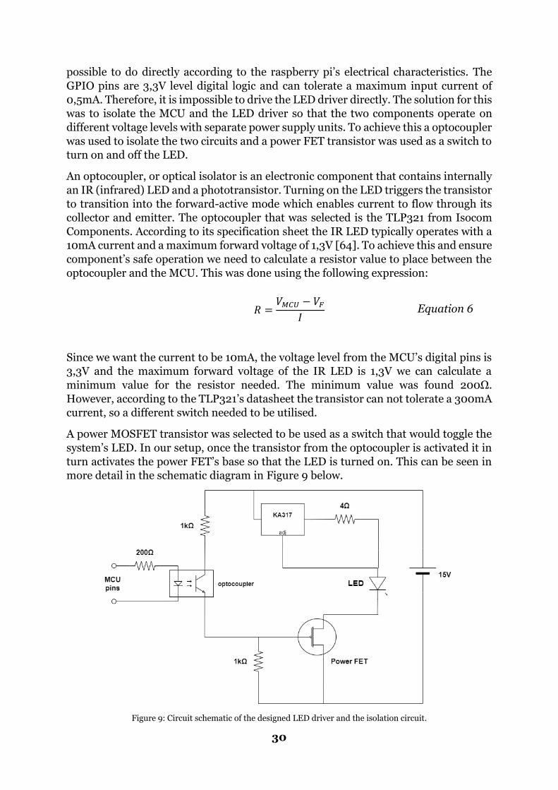
30

possible to do directly according to the raspberry pi’s electrical characteristics. The

GPIO pins are 3,3V level digital logic and can tolerate a maximum input current of

0,5mA. Therefore, it is impossible to drive the LED driver directly. The solution for this

was to isolate the MCU and the LED driver so that the two components operate on

different voltage levels with separate power supply units. To achieve this a optocoupler

was used to isolate the two circuits and a power FET transistor was used as a switch to

turn on and off the LED.

An optocoupler, or optical isolator is an electronic component that contains internally

an IR (infrared) LED and a phototransistor. Turning on the LED triggers the transistor

to transition into the forward-active mode which enables current to flow through its

collector and emitter. The optocoupler that was selected is the TLP321 from Isocom

Components. According to its specification sheet the IR LED typically operates with a

10mA current and a maximum forward voltage of 1,3V [64]. To achieve this and ensure

component’s safe operation we need to calculate a resistor value to place between the

optocoupler and the MCU. This was done using the following expression:

𝑅 =𝑉𝑀𝐶𝑈 − 𝑉𝐹

𝐼 Equation 6

Since we want the current to be 10mA, the voltage level from the MCU’s digital pins is

3,3V and the maximum forward voltage of the IR LED is 1,3V we can calculate a

minimum value for the resistor needed. The minimum value was found 200Ω.

However, according to the TLP321’s datasheet the transistor can not tolerate a 300mA

current, so a different switch needed to be utilised.

A power MOSFET transistor was selected to be used as a switch that would toggle the

system’s LED. In our setup, once the transistor from the optocoupler is activated it in

turn activates the power FET’s base so that the LED is turned on. This can be seen in

more detail in the schematic diagram in Figure 9 below.

Figure 9: Circuit schematic of the designed LED driver and the isolation circuit.

31

Power Supply

As mentioned in the previous section a 15V battery was used to provide power to the

LED driver. An additional power supply of 5V and current of 2A was used to power the

Raspberry pi through its USB port. A more detailed view of the setup can be seen in the

block diagram in Figure 10.

Figure 10: Block diagram of the device setup.

3.3. Design #2

As an attempt to improve the performance of the custom fluorescence sensor, several

additions were made to the initial setup.

Frist of all, according to the theory chl-a fluorescence exhibits some differences in its

properties when in living cells. More specifically, chl-a fluorescence in living cells

occurs in longer wavelengths than when it is dissolved in an organic solvent. This is

true both for the excitation peak and the emission peaks. As mentioned in the previous

chapter, usually a shift of approximately 10nm towards the red wavelengths occurs.

Therefore, the expected excitation peak in a water sample would be closer to 440nm

and the emission peak near 680nm [65], [57]. For this reason, an additional high-

power LED needs to be selected.

Furthermore, water turbidity is another factor that may cause implications and be a

source of error in our measurements. To cope with this, an appropriate component will

be selected and added to our system’s design.

32

3.3.1. Component selection

Excitation source

The LED that was selected is the royal blue LED from Luxeon Rebel series (Philips

Lumileds). This component emits visible light where the dominant wavelengths are

located between 440nm and 460nm and the peak wavelength is at 447,5nm. Moreover,

according to its datasheet, the LED has a radiometric power of 500mW when driven

with a forward constant current of 350mA which is sufficient for our application. The

maximum current it can drive is 1000mA as specified from the manufacturer. This

LED cannot be driven in reverse bias [66]. The product’s cost was 30SEK.

Turbidity sensing

For detecting high levels of turbidity in our sample solution a Light Dependent Resistor

(LDR) will be utilised. More specifically, the GL55 photoresistor is a type of resistor

that varies its value when exposed to different intensities of light. The sensor will be

used for measuring how much light can pass through the water sample. The excitation

source will be used the light source to implement this functionality.

According to the device’s specification sheet it shows a peak in its sensitivity when

illuminated by light at wavelengths between 550nm and 600nm (yellow – orange

visible light) [67]. This means that wen used with our system’s light sources (both the

violet and blue LED) the GL55 photoresistor will not perform optimally. However, it’s

response will still be tested and evaluated through experiments.

3.3.2. Building the device

Microcontroller

To establish control of the LDR sensor an analog input on the microcontroller was

needed. However, the Raspberry Pi does not support analog input since it does not

have an Analog-to-Digital Converter (ADC). To solve this issue, it was decided that an

Arduino Mega 2560 board would be used along with the Raspberry Pi to make use of

the analog pins that it contains.

33

Figure 11: The Arduino Mega 2560 microcontroller board.

The Arduino Mega 2560 is a microcontroller board based on the ATmega2560

processor. More detailed specifications have been presented in section 3.2.1. The clock

speed of 16MHz is considered to provide with enough computational power to execute

the task of collecting measurements from the LDR sensor. Moreover, the Arduino

board supports up to 16 analog channels which makes it ideal for our application. It is

important to note that the Arduino does provide more features than necessary for the

current application and that an external Analog-to-Digital converter could be used with

the Rasberry pi instead, however the functionality would remain the same in both cases

and the system’s performance is not affected. Consequently, due to the availability of

the Arduino and the limited budget for this project, the Arduino board was used.

Furthermore, it was decided that the easiest way to power the Arduino was from one

of the USB ports on the Raspberry Pi. This configuration has the advantage that the

USB connection can supply the Arduino board with power and can also be used for

UART serial communication at the same time. Therefore, the collected data can be

directly transferred and saved to the Raspberry Pi SD card.

Detector

Since the red optical filter we are using for the camera is allowing a band of wavelengths

between 620nm and 700nm it is suitable for capturing the fluorescence emission with

a peak at approximately 680nm. Therefore, no different approach needs to be followed

in this case.

LED driver

To drive the blue LED a similar circuit was used as presented in Figure 9. However,

since the blue LED provides with less radiometric power than the violet LED at 350mA

constant current, it was decided to use a higher current value of 400mA. This was

34

achieved recalculating the value of the resistor placed after the voltage regulator

according to Equation 5. For this purpose, a 3Ω resistor was the suitable value.

In addition, to collect data from the LDR sensor it was necessary to establish control of

the LED from the Arduino board as well. This was achieved by connecting an additional

isolation circuit with another optocoupler chip in parallel with the existing one that

was connected to the Raspberry Pi. It is worth mentioning that the Arduino digital pins

operate at a 5V digital level as opposed to the Raspberry Pi which operates in 3,3V. For

this reason, to ensure the safe operation of the internal IR LED of the optocoupler a

new value for the resistor needed to be calculated according to Equation 6. The lowest

value for this resistor was found to be 370Ω.

LDR driver

The circuit shown in Figure 12 was used to interface the LDR sensor with the Arduino

microcontroller. A voltage divider was set up by using a 10kΩ resistor in series with the

variable photoresistor. Lastly, the output of the circuit was connected to one of the

analog pins of the Arduino MCU.

Figure 12: Circuit schematic for the interface of LDR with the microcontroller.

Power supply

As mentioned in the previous section it was decided that the Arduino MCU will be

powered and controlled from the Raspberry Pi board through a USB interface. A block

diagram of the system after the design improvements were applied is presented in

Figure 13.

35

Figure 13: Block diagram of the improved version of the device.

3.4. 3D printing

For the current project it was decided that the enclosure where all the sensor parts,

including the sample under examination would be placed, would be 3D modelled and

then 3D printed according to the model. For this purpose, an open source 3D modelling

software was used, namely Blender 2.80.

The sample solutions that fluorescence measurements are taken from are placed in a

standard cuvette of 1cm path length. A cuvette is a test tube used in chemistry that is

especially designed for optical analysis. They can be made of plastic, glass or quartz

material and they are considered 100% transparent in the wavelengths we are working

with. In the 3D model that was created a holder for a cuvette was designed according

to the dimensions of the small liquid container.

Moreover, a holder for the Raspberry Pi camera was designed. By adjusting the camera

lens’ focus, it was found that the minimal distance from an object in order to capture a

clear image was 4cm. Therefore, the camera was placed in 4cm distance from the

cuvette. The 3D model of the base of the enclosure which includes the camera and

cuvette holder can be seen in Figure 14. In addition, two holders for the LED’s were

modelled according to the dimensions of the heat sink. In the same model some space

was created to place the LDR sensors. These parts can be seen in Figure 15. The

LED/LDR holders where placed across the two sides of the cuvette, assuming that the

36

side facing the camera is the front side. This arrangement can be seen in detail on

Figure 14.

Figure 14: 3D model of the enclosure's base which includes the camera and cuvette holder.

Figure 15: LED and LDR holders.

The top part of the enclosure was designed to have an opening at which a cuvette can

be easily inserted. Furthermore, on the sides openings were created for the cables as

well as an opening at the back for the ribbon cable to connect the camera to our

microcontroller. The 3D models of this part can be seen in Figure 16.

37

Figure 16: 3D models of the top part of the enclosure.

For the 3D printer, PLA filament material in black colour was used to 3D print the

models that were designed. Black colour was necessary to ensure blocking of ambient

light. The resulting printed enclosure parts can be seen in Figure 17.

Figure 17: 3D printed enclosure.

Lastly, the designed system is presented below in Figure 18.

38

Figure 18: Connectivity of sensor components.

39

3.5. Algorithm

Figure 19: Flow chart of algorithm for design #1.

To configure and control all the sensor components for design #1, scripts were written

in Python and run on the Raspberry Pi board. With the LED driver setup that we are

using, control of the LED is established through a digital pin from the microcontroller.

A flow chart of the procedure can be seen in Figure 19.

As far as capturing images of the samples is concerned, it was necessary to place some

wait time between turning on the LED and using the camera so that the sensor adapts

to the new light conditions. It was found that 400msec was sufficient for the camera

sensor to output stable images. Moreover, during initialisation of the camera

component its settings were configured. The white balance was set to “Daylight” mode,

the exposure was set to 0 while the shutter speed was 320msec. To capture the sample

40

images, the full sensor mode was utilised meaning that the maximum supported

resolution was used which is 3280 x 2464 pixels.

After the sensor calibration was completed, a Region Of Interest (ROI) was selected

that gave a stable colour output in varying intensities of fluorescence emission. This

was done to avoid edge effects from the cuvette where light is reflected and can

introduce error to the measurements. The selected ROI had a size of 440 x 1560 pixels.

Moreover, it was decided that the images of the samples would be captured in

triplicates and then averaged to minimize the error. According to the literature when

designing a fluorescence sensor the usage of a blank measurement indicating the zero

emission level is of high importance [57]. Therefore, the blank image was subtracted

from the averaged measurement image. Afterwards, the ROI was extracted from the

resulting averaged and blank corrected image. The rest of the image processing took

place with this smaller image.

The next step in processing the collected image data was to split the channels of the

RGB image. Since our interest is the detection of red emission, the red channel contains

all the information that is useful to this application. In addition, when taking

measurements of samples, it was noticed that small areas of high light intensity could

appear in the image due to bubbles or particles on the container. To eliminate this, a

normalization of the data was applied. This was done through calculating the

histogram of each image and then from that calculating the Cumulative Distribution

Function (CDF) for each pixel value, which ranges from 0 to 255 in standard 8-bit RGB

images. These graphs were plotted using Python’s matplotlib library and a relevant

example can be seen in Figure 20.

Figure 20: Histogram of one of the samples (left) and the corresponding calculated CDF (right).

From the CDF, the 0,997 point of the graph, the corresponding pixel intensity was

selected and then truncated for the whole image. This means that any pixel containing

a value higher than the 0,997 intensity is replaced by the 0,997 value, therefore

smoothening the scattered peaks in the image. Lastly, the mean pixel intensity for the

41

red channel is calculated and from this value we can easily calculate the corresponding

chl-a concentration in the sample using the calibration results.

Figure 21: Flowchart of algorithm for design #2.

42

A flow chart of the algorithm for the 2nd version of our designed sensor is presented in

Figure 21. The main difference is that after collecting measurements regarding the

sample’s fluorescence emission using the LED and camera, the Raspberry Pi is

configured to send a command to the Arduino microcontroller. This command triggers

the collection of measurements from the LDR sensor through the analog pin. 10

measurements are obtained and then averaged to minimize the error. If the result is

found to exceed a limit set for turbidity, the sample is rejected and a relevant message

to the user is displayed on the LCD screen. If that is not the case, then the chl-a

concentration is calculated in a similar way as in design #1.

3.6. Experiments

This section will demonstrate the experiments conducted to calibrate the sensor as

well as the tests to determine the device’s performance.

3.6.1. Calibration

After the device was constructed, the next step was to calibrate the sensor. To do this,

measurements from the developed sensor will be compared to measurements of the

same samples collected from benchtop fluorometer, namely the Perkin Elmer LS-55

Fluorescence Spectrometer.

The Perkin Elmer LS-55 offers flexibility and reliability in a wide range of research,

including fluorescence, phosphorescence, and chemi- or bio-luminescence. As a

standard accessory the LS-55 includes a single cell sample holder that can

accommodate 1cm path length cuvettes. Furthermore, the device uses a pulsed Xenon

lamp as a source of excitation as well as a photomultiplier as a detector. The

instrument contains 2 monochromators, one for the detector and one for the excitation

source. By using this instrument, the inserted sample can be illuminated in the

wavelength range of 200nm to 800nm and the emission spectra can be recorded from

200nm to 900nm. The device has a wavelength accuracy of ±1 nm and a wavelength

reproducibility of 0,5nm. Moreover, the device contains excitation slits 2.5-15 nm and

emission slits 2.5-20 nm which can be varied and controlled by software in 0.1 nm

increments. Excitation and emission monochromators can be independently or

synchronously scanned, while the pre-scan mode is ideal for precise locating of

excitation and emission peaks [68].

To calibrate and evaluate the performance of our designed system the same samples

will be measured by both the LS 55 lab instrument and our custom fluorescence sensor

43

and the results will be compared. To calibrate the sensor, solutions with known

concentration of chl-a were produced and measured from both devices. To prepare the

solutions, 1mg of chl-a analytical standard was used which was in powder form.

According to the substance’s safety data sheet, the substance should be stored in -18 oC

and in dark conditions since it is light sensitive, meaning that it degrades when exposed

to light for prolonged time. Moreover, the pigment is not classified as acutely toxic, is

not corrosive or irritant to the skin and in general, no special conditions are required

to handle this chemical [69].

The solvent used to dilute the chl-a solution was acetone, since the substance cannot

be solved in water.

It was decided that the sensor would be calibrated in a range of chl-a concentrations

between 0 µg/L to 400 µg/L. In addition, different steps were used in the various

sample solutions that were used. More specifically, we used concentrations of chl-a

ranging from:

• 1 µg/L to 10 µg/L with a step of 1 µg/L

• 10 µg/L to 30 µg/L with a step of 5 µg/L

• 30 µg/L to 50 µg/L with a step of 10 µg/L

• 50 µg/L to 300 µg/L with a step of 50 µg/L

• 300 µg/L to 400 µg/L with a step of 100 µg/L.

This resulted in a total of 22 samples being prepared including the blank sample which

consisted of pure acetone.

To perform the calibration of the sensor we first needed to prepare all the solutions to

be measured. In order to calculate the volumes that should be transferred from one

solution to another to achieve the concentration we aim for, the following formula was

used:

𝑀1𝑉1 = 𝑀2𝑉2 Equation 7

where M stands for chl-a concentration and V stands for volume. In Equation 7, we

solve for V1 so that we calculate the volume that needs to be extracted from a stock

solution with concentration M1 into the sample solution to achieve the wanted

concentration M2. The samples used in this study would be observed through cuvettes

of 1cm path length. The cuvette can be filled with 4mL solution, but it is not

recommended to fill it 100% to avoid spilling and due to safety concerns. For this

reason, we prepared 4mL of solution for each sample but used 3,5mL in the cuvette to

collect measurements. Therefore, the sample volume is always V2 = 4mL.

According to our calculations, to prepare samples for all the concentrations that we

want to test, 3 stock solutions of 10mL volume needed to be prepared with the following

concentration of chl-a:

44

Stock solution Chl-a concentration Volume

1 MS1 = 1000 µg/L VS1 = 10mL

2 MS2 = 100 µg/L VS2 = 10mL

3 MS3 = 10 µg/L VS3 = 10mL

In order to make the stock solutions we first needed to dilute the pure chl-a pigment

which came in powder form. To do that, the pure chl-a powder was removed from its

storage space and was put to a dark fume hood and left for 1 hour to reach room

temperature. This was an important step to get more accurate fluorescence results.

Afterwards, 1 mL of acetone was added in the vial of the pure substance and it was

properly shaken to dilute completely. To ensure that all the solution would be fully

transferred to a new test tube, a glass single use pipette was used. To achieve a

concentration of 1mg/10mL = 100 mg/L, 9mL of solvent were added and mixed

thoroughly. From this step it was possible to prepare all 3 stock solutions and our

samples to be tested.

For the procedure of serial dilution, adjustable volume pipettes were used that are

shown in Figure 22. These pipettes can be used with single use tips and can be

configured to transfer a fixed volume from a solution. For each pipette the volume

range that can be transferred without error is specified. For this project, 3 different

pipettes were used with volume ranges 0,5 – 5 mL, 100 – 1000 µL, and 10 – 100 µL.

To test the functionality of these instruments, tap water was used that was then

weighed on a high precision scale. After correctness of the results was verified, we could

move forward to perform the serial dilution.

Figure 22: Variable volume pipettes used for preparing the samples for calibration.

45

Figure 23: Stock solutions covered with aluminium foil to protect them from light, and glass vial of pure chl-a analytical standard.

After the stock solutions were prepared, they were covered with aluminium foil to

prevent exposure to light, as seen in Figure 23. The next step was to prepare all the

4mL samples for our testing. The samples were temporarily stored in 4mL glass vials

with plastic cap. Each sample was mixed properly to avoid introducing error in our

measurements. Moreover, the samples were also covered with aluminium foil to

protect them for high light intensities. The samples can be seen in Figure 24.

Figure 24: Samples of known chl-a concentration.

46

Lastly, each of the samples was transferred to a quartz cuvette of 1cm path length and

measured from both the Perkin Elmer LS 55 Fluorescence Spectrometer and our

designed fluorescence sensor. The calibration setup is presented in Figure 25.

Figure 25: The calibration procedure with LS 55 fluorescence spectrometer and the designed sensor.

Using the LS 55 fluorescence spectrometer, the excitation peak of the solution under

test was investigated through scanning the excitation wavelengths while maintaining a

stable emission wavelength. Furthermore, for each sample we observed the

fluorescence through performing emission scanning while maintaining a fixed

excitation wavelength. The excitation wavelength was set according to the peak

wavelength emitted from each LED that we used on our designed system. The results

were collected and analysed using Python’s matplotlib library. The settings used on the

LS-55 instrument were as follows:

Violet LED Blue LED

Excitation 425 nm 448 nm

Emission scan 650 nm – 700 nm 650 nm – 700 nm

Scan speed 1000 nm/min 1000 nm/min

Excitation slit 10 nm 10 nm

Emission slit 10 nm 10 nm

Table 1: Settings used on the Perkin Elmer LS-55 fluorescence spectrometer instrument to capture the fluorescence emission intensity data.

47

3.6.2. Turbidity

To evaluate the sensor’s response to turbidity, solutions which contained known mass

of suspended particulate matter were prepared. To achieve this, bentonite clay was

used with deionized water. Deionized water is pure H2O meaning that there are no free

particles or ions within it. Moreover, according to literature studies, the average

particle size of bentonite powder is no greater than 40µm [70], which in turn means

that the settling time due to gravity (sedimentation) is higher than 2,5 minutes [71].

For the purpose of this experiment, each sample is used for less than 20 seconds, and

therefore the gravity sedimentation time can be considered zero, meaning that all

particulate matter remains suspended for the duration of our measurements.

As far as the experiment process is concerned, firstly a small amount of bentonite clay

was weighed with a high-precision scale. The mass was found 1,2 mg. To achieve a

concentration of 1 g/L, 12mL of deionized water were added to the test tube. From that

point serial dilution was performed to prepare 4mL samples of varying mass of

suspended particulate matter (see Figure 26). All of the samples were properly mixed

to avoid introducing error to the measurements. Moreover, measurements were taken

from a new blank sample as well which consisted of pure deionized water.

Figure 26: Samples prepared with known mass of suspended particulate matter.

According to the literature, a mass of suspended particulate matter of over 50 g.m-3 is

rarely found in coastal water environments. However, in this experiment

concentrations up to 1000 g.m-3 were tested. The samples were prepared with a step of

10 g.m-3 between 0 and 100 g.m-3, then concentrations of 250, 500, 750 and lastly 1000

g.m-3 were tested.

48

Figure 27: Turbid sample in 1cm path length cuvette.

To determine the turbidity level of the sample, 10 measurements were captured from

the LDR sensor which were then averaged. The averaged value of the blank sample (0

g.m-3) is used as a reference to indicate zero turbidity value. The blank value is

deducted from each measurement and the results are analysed for varying levels of

turbidity.

3.6.3. Water samples

Figure 28: Locations of water sample collection.

To further test the response of the sensor, samples were collected from coastal and lake

water bodies around Stockholm area. The samples were measured from both the

49

designed sensor and the LS-55 fluorescence spectrometer lab instrument and the

results were compared. The locations at which samples were collected can be seen in

Figure 28. No blank samples were used for this data acquisition.

3.6.4. Data variance

To determine the variance of the output data, in all of the experiments conducted, each

sample was measured 3 times for both Design #1 and Design #2. Therefore, all

calibration data were collected in triplicate for each sample from both the constructed

device and the LS-55 instrument. Similarly, for the turbidity testing, measurements

were captured 3 times for each prepared sample from both versions of the proposed

device. Lastly, for the water sample testing all samples were measured 3 times from

both our constructed sensor and the LS-55 fluorescence spectrometer.

50

Chapter 4. Results

In this section, the results of the current study will be presented, and the data will be

analysed.

4.1. Results

4.1.1. Calibration

The excitation wavelength of the chl-a solutions used for the calibration of our device

was investigated using the Perkin Elmer LS-55 fluorescence spectrometer. To extract

this data the emission wavelength was kept stable, while an excitation scan was

performed in wavelengths ranging from 350 nm to 550 nm. The result is shown in

Figure 29. With solid violet lines the dominant wavelengths of the violet LED used in

this study are annotated, while the peak wavelength is annotated with a dashed line.

The dominant wavelength range of the blue LED are marked with solid blue lines, and

the blue LED’s peak wavelength is annotated with a dashed blue line.

Figure 29: Investigation of peak excitation wavelength of chl-a samples used for the device's calibration. The current graph was produced from data collected from the sample with highest chl-a concentration of 400 µg/L. The same response with lower intensity was recorded from all samples with lower chl-a concentration. Solid lines represent the dominant wavelength range of the LED with the correspondent colour, while the dashed line represents the peak wavelength.

51

Moreover, the emission wavelength of the samples used for calibration was located

using the LS-55 instrument. To obtain this data, the excitation wavelength was kept

stable and an emission scan was performed in wavelengths ranging from 650 nm to

700 nm. The results are shown in Figure 30.

Figure 30: Locating the peak wavelength of fluorescence emission of samples used for calibration using the LS-55 instrument. The current graph was produced from data collected from the sample with highest chl-a concentration of 400 µg/L. The same response with lower intensity was recorded from all samples with lower chl-a concentration.

To ensure the validity of our study, the linear response of fluorescence emission

intensity from all the samples used was explored using the LS-55 fluorescence

spectrometer. Data were collected in triplicate and their variance was found. Lastly, it

is worth noting that the 30 µg/L sample was excluded from all the calculations to

determine the performance since it was corrupted during the experiment process.

Design #1

As explained in the previous chapter, to calibrate our device we will compare

measurements from samples with known chl-a concentration between our device and

the LS-55 instrument. The results for Design #1 of the constructed device are presented

in Figure 31. The x-axis represents the fluorescence emission intensity of the samples

at the peak wavelength of 670 nm as measured from the LS-55 spectrometer, while the

y axis represents the measured red intensity from our constructed device.

52

Since fluorescence emission is typically represented in relative units, the constructed

device’s output was normalized to facilitate repeatability of the results. The zero value

represents the measurement of the blank sample (0 µg/L chl-a), while 1 represents the

highest recorded value at 400 µg/L chl-a concentration. More specifically, the blank

measurement was found 5,388 (digital number) and the highest measurement was

found 162,465 (digital number).

Moreover, the variance of each measurement point is represented in the graph with

error bars on the y-axis. The highest variance was recorded at the sample with a chl-a

concentration of 200 µg/L with a value of 0,0418 (normalised red intensity). Lastly,

the mean variance of all the measurement points was found to be 0,0061 (normalised

red intensity).

Figure 31: Correlated measurements of chl-a sample solutions between the Design #1 of the constructed device (y-axis) and LS-55 fluorescence spectrometer (x-axis).

53

In the following graph in Figure 32, the fluorescence emission intensity of Design #1 of

our constructed device is plotted with the actual chl-a concentration of the samples

being examined.

Figure 32: Fluorescence emission intensity of chl-a samples measured from the constructed device (design #1) plotted with the chl-a concentration of the samples (x axis).

From Figure 32, it was found that the maximum data variance from Design #1 of the

proposed device, was recorded at the sample with 200 µg/L Chl-a concentration with

a value of 0,0418 (normalised red intensity). Moreover, the average variance of all the

data points was computed and found at 0,006 (normalised red intensity).

Furthermore, the data collected from the laboratory instrument LS-55 were collected

in triplicate in order to determine important parameters of the device under the

selected settings (see Table 1) that were applied for the purpose of the experiment. For

calibrating Design #1 of our constructed device, the excitation wavelength was set at

425nm. The captured data and their respective variance are presented in Table 2 below.

54

Chl-a concentration (µg/L)

Intensity at 670nm [Rel. Units]

0 0,072 ± 0,023 1 1,711 ± 0,106 2 2,673 ± 0,138 3 4,861 ± 0,183 4 6,366 ± 0,077 5 7,564 ± 0,066 6 8,803 ± 0,347 7 10,733 ± 0,118 8 11,689 ± 0,194 9 14,086 ± 0,130

10 14,526 ± 0,287 15 21,376 ± 0,321 20 28,301 ± 0,374 25 35,343 ± 0,710 30 50,342 ± 1,129 40 67,730 ± 0,943 50 83,915 ± 2,416

100 157,874 ± 0,742 150 232,657 ± 2,443 200 313,472 ± 2,102 250 407,384 ± 2,149 300 456,398 ± 1,154 400 631,207 ± 0,472

Table 2: Data captured from Perkin Elmer LS-55 fluorescence spectrometer for the produced samples of chl-a with an excitation wavelength of 425nm.

From Table 2, we can see that the highest recorded variance has a value of 2,443 (Rel.

Units) and corresponds to the sample with 150 µg/L chl-a concentration, while the

average data variance was computed and found at 0,723 (Rel. Units).

Lastly, the data collected from the LS-55 instrument with an excitation wavelength of

425nm are presented in a graphical way in Figure 33 below.

55

Figure 33: Fluorescence emission intensity of prepared samples measured from LS-55 fluorescence spectrometer with the excitation wavelength set at 425nm.

Design #2

As explained in the previous chapter, to calibrate our device we will compare

measurements from samples with known chl-a concentration between our device and

the LS-55 instrument. The results for the blue LED, which is part of Design #2 of the

constructed system are presented in Figure 34. The x-axis represents the fluorescence

emission intensity of the samples at the peak wavelength of 670 nm as measured from

the LS-55 spectrometer, while the y axis represents the measured red intensity from

our constructed device.

Since fluorescence emission is typically represented in relative units, the constructed

device’s output was normalized to facilitate repeatability of the results. The zero value

represents the measurement of the blank sample (0 µg/L chl-a), while 1 represents the

highest recorded value at 400 µg/L chl-a concentration. More specifically, the blank

measurement resulted in a value of 3,422 (digital number) while the highest

measurement was found 115,278 (digital number).

Moreover, the variance of each measurement point is represented in the graph with

error bars on the y-axis. The highest variance was recorded at the sample with a chl-a

concentration of 200 µg/L with a value of 0,0435 (normalised red intensity). Lastly,

the mean variance of all the measurement points was found to be 0,0091 (normalised

red intensity).

56

Figure 34: Correlated measurements of chl-a sample solutions between the Design #2 of the constructed device (y-axis) and LS-55 fluorescence spectrometer (x-axis).

In the following graph presented in Figure 35, the fluorescence emission intensity of

Design #2 of our constructed device is plotted with the actual chl-a concentration of

the samples being examined.

57

Figure 35: Fluorescence emission intensity of chl-a samples measured from the constructed device (design #2) plotted with the chl-a concentration of the samples (x axis).

From Figure 35, it was found that the maximum data variance from Design #1 of the

proposed device, was recorded at the sample with 300 µg/L Chl-a concentration with

a value of 0,0435 (normalised red intensity). Moreover, the average variance of all the

data points was computed and found at 0,009 (normalised red intensity).

Furthermore, the data collected from the laboratory instrument LS-55 were collected

in triplicate in order to determine important parameters of the device under the

selected settings (see Table 1) that were applied for the purpose of the experiment. For

calibrating Design #2 of our constructed device, the excitation wavelength was set at

448nm. The captured data and their respective variance are presented in Table 2

below.

58

Chl-a concentration (µg/L)

Intensity at 670nm [Rel. Units]

0 0,130 ± 0,084 1 0,460 ± 0,029 2 0,608 ± 0,025 3 1,105 ± 0,035 4 1,558 ± 0,047 5 1,852 ± 0,099 6 2,249 ± 0,107 7 2,709 ± 0,184 8 3,053 ± 0,051 9 3,689 ± 0,028 10 3,237 ± 0,261 15 4,930 ± 0,231 20 6,398 ± 0,060 25 7,834 ± 0,254 30 13,141 ± 0,121 40 15,028 ± 0,200 50 17,046 ± 0,221

100 34,558 ± 0,681 150 47,946 ± 0,555 200 70,371 ± 0,345 250 88,963 ± 0,941 300 100,832 ± 0,442 400 135,807 ± 0,397

Table 3: Data captured from Perkin Elmer LS-55 fluorescence spectrometer for the produced samples of chl-a with an excitation wavelength of 448nm.

From Table 2, we can see that the highest recorded variance has a value of 0,941 (Rel.

Units) and corresponds to the sample with 150 µg/L chl-a concentration, while the

average data variance was computed and found at 0,235 (Rel. Units).

Lastly, the data collected from the LS-55 instrument with an excitation wavelength of

448nm are presented in a graphical way in Figure 36 below.

59

Figure 36: Fluorescence emission intensity of prepared samples measured from LS-55 fluorescence spectrometer with the excitation wavelength set at 448nm.

4.1.2. Turbidity

Design #1

Samples of varying turbidity were measured from Design #1 of the constructed device

(violet LED) and results regarding the captured red channel intensity and the LDR

sensor were recorded. The red intensity values found from the device were normalized

between the minimum and maximum values recorded. The minimum value represents

the blank measurement (deionized water - pure H2O) which was found at 4,356 (digital

number). The maximum value was found at the sample with the highest suspended

particulate matter concentration, at 31,112 (digital number).

As far as the response from the LDR sensor, the data was captured in triplicate and the

result of each data point and their respective variance were documented. The values

were extracted directly from the Arduino’s analog-to-digital converter as analog values.

Also, to make data more readable the difference from our zero (blank) measurement is

shown on a separate column for each of the samples. The figures are presented in Table

4 below.

60

Turbidity (gm-3)

Normalized red intensity Device #1

LDR readings (analog value)

LDR difference from blank measurement

10 0,0071 ± 0,018 1019,8 ± 0,1 0,1

20 0,0232 ± 0,009 1019,5 ± 0,4 0.4

30 0.0148 ± 0.008 1019,8 ± 0,4 0.1

40 0.0626 ± 0.028 1020,0 ± 0,0 0

50 0.0369 ± 0.014 1019,6 ± 0,3 0.3

60 0.0395 ± 0.015 1019,7 ± 0,2 0.2

70 0.0456 ± 0,009 1019,6 ± 0,3 0.3

80 0.0645 ± 0.015 1020,0 ± 0,3 0

90 0.0455 ± 0.015 1019,8 ± 0,1 0.2

100 0.0474 ± 0.008 1020,0 ± 0,0 0

250 0.1914 ± 0.024 1019,7 ± 0,2 0.3

500 0.2796 ± 0.005 1019,4 ± 0,2 0.5

750 0,6574 ± 0.033 1019,1 ± 0,5 0.8

1000 0.9999 ± 0.060 1018,8 ± 0,1 1.1

Table 4: Measurements of samples with varying turbidity from Design #1 (violet LED) of the constructed device. Data of fluorescence were acquired from the camera and absorption data were collected from the LDR sensor.

The highest variance from the LDR sensor was 0,5 (analog value) and it corresponds

to the 750 gm-3 sample. Lastly, the average variance of the LDR data was computed

and found at 0,25 (analog value).

Design #2

Samples of varying turbidity were measured from Design #2 of the constructed device

(blue LED) and results regarding the captured red channel intensity and the LDR

sensor were documented. The red intensity values found from the device were

normalized between the minimum and maximum values recorded. The minimum

value represents the blank measurement (deionized water - pure H2O) which was

found at 2,401 (digital number). The maximum value was found at the sample with the

highest suspended particulate matter concentration, at 17,105 (digital number).

As far as the response from the LDR sensor, the data was captured in triplicate and the

result of each data point and their respective variance were documented. The values

were extracted directly from the Arduino’s analog-to-digital converter as analog values.

Also, to make data more readable the difference from our zero (blank) measurement is

61

shown on a separate column for each of the samples. The figures are presented in Table

5 below.

Turbidity (gm-3)

Normalized red intensity Device #2

LDR readings (analog value)

LDR difference from blank measurement

10 0.0072 ± 0.029 1022,5 ± 0,1 0

20 0.0329 ± 0.018 1022,4 ± 0,2 0.1

30 0.0237 ± 0.025 1022,2 ± 0,1 0.3

40 0.0719 ± 0.006 1022,3 ± 0,3 0.3

50 0.0537 ± 0.017 1022,3 ± 0,3 0.2

60 0.0610 ± 0.021 1022,5 ± 0,4 0

70 0.0448 ± 0,021 1022,2 ± 0,1 0.3

80 0.0805 ± 0.023 1022,0 ± 0,5 0.5

90 0.0743 ± 0.007 1022,2 ± 0,1 0.5

100 0.0776 ± 0.019 1022,5 ± 0,4 0.3

250 0.1674 ± 0.021 1022,1 ± 0,2 0.5

500 0.3506 ± 0.006 1022,1 ± 0,2 0.5

750 0.6221 ± 0.020 1021,8 ± 0,2 0.7

1000 0.9999 ± 0.048 1021,5 ± 0,1 1.0

Table 5: Measurements of samples with varying turbidity from Design #2 (blue LED) of the constructed device. Data of fluorescence were acquired from the camera and absorption data were collected from the LDR sensor.

The highest variance from the LDR sensor was 0,5 (analog value) and it corresponds

to the 80 gm-3 sample. Lastly, the average variance of the LDR data was computed

and found at 0,20 (analog value).

4.1.3. Water samples

Design #1

Water samples were measured from both the Design #1 (violet LED) of the constructed

device and the LS-55 fluorescence spectrometer. The results are presented in Table 6.

62

Sample number Red intensity

(digital number)

Intensity at 670nm from LS-55 [Rel. units]

1 8,43 ± 0,35 0,856 ± 0,043

2 18,67 ± 0,56 1,907 ± 0,066

3 8,39 ± 0,25 1,825 ± 0,154

4 8,80 ± 0,14 1,453 ± 0,083

5 9,77 ± 0,97 0,735 ± 0,236

6 13,07 ± 0,43 2,127 ± 0,151

7 14,94 ± 0,20 2,369 ± 0,118

8 20,94 ± 0,63 2,790 ± 0,139

9 8,92 ± 0,11 1,326 ± 0,041

10 8,83 ± 0,90 1,050 ± 0,104

Table 6: Comparing the fluorescence intensity captured from Design #1 (violet LED) of our constructed device and the LS-55 fluorescence spectrometer.

Design #2

Water samples were measured from both the Design #2 (blue LED) of the constructed

device and the LS-55 fluorescence spectrometer. The results are presented in Table 7.

Sample number Red intensity

(digital number)

Intensity at 670nm from LS-55 [Rel. units]

1 10,94 ± 1,91 1,129 ± 0,084

2 32,04 ± 1,02 1,262 ± 0,159

3 11,33 ± 0,62 1,695 ± 0,122

4 11,01 ± 0,54 1,707 ± 0,054

5 10,99 ± 0,96 1,269 ± 0,127

6 18,49 ± 0,29 1,536 ± 0,142

7 23,47 ± 0,75 1,824 ± 0,071

8 32,32 ± 1,51 2,483 ± 0,059

9 11,86 ± 0,31 1,014 ± 0,198

10 11,01 ± 2,42 0,745 ± 0,121

Table 7: Comparing the fluorescence intensity captured from Design #2 (blue LED) of our constructed device and the LS-55 fluorescence spectrometer.

63

4.2. Data analysis

4.2.1. Calibration

After investigating the excitation peak location for our prepared chl-a samples, the

excitation peak was found at 432 nm as seen in Figure 29. This is a deviation of 2 nm

towards the red wavelengths from the value of 430 nm which was found in the

literature and can be considered negligible.

Furthermore, in Figure 29 the dominant and peak wavelengths of the blue and violet

LED’s used in our custom fluorescence sensor are annotated. We can see clearly that

the violet LED can provide more effective excitation of the chl-a samples since it emits

wavelengths closer to the peak excitation wavelength. From this, we can expect a higher

quantum yield value which in turn leads to a significantly higher fluorescence emission

intensity. Subsequently, the blue LED emits radiation with a peak wavelength at 447,5

nm which is not optimal for the excitation of pure chl-a pigment. Therefore, the

fluorescence emission intensity observed in Design #2 where the blue LED is used as

an excitation source is expected to be substantially decreased.

Moreover, after investigating the fluorescence emission peak location for our prepared

chl-a samples, the emission peak was found at 670 nm as seen in Figure 30. This is a

deviation of 2 nm from the value of 668 nm which was found in the literature and can

be considered negligible. The same deviation of 2 nm was also observed on the

excitation peak which is another factor that confirms the correctness of our

measurements.

Design #1

The results of the cross calibration between Design #1 of the constructed device and

the LS-55 fluorescence spectrometer are presented in Figure 31. Moreover, the

fluorescence intensity measurements form Design #1 were plotted against the actual

chl-a concentrations of the prepared samples in Figure 32.

From the graphs we can see that the sensor does not successfully capture the linear

correlation between chl-a concentration and fluorescence intensity in the prepared

samples in low chl-a concentrations. More specifically, in chl-a concentrations between

1 to 40 µg/L, a linear regression was applied in the cross-correlated measurements of

Figure 31. A positive correlation was observed which, however, indicated noticeably

high error values with an RMSE of approximately R2 = 0,737. Moreover, polynomial

regression was applied to the measurements in both graphs with an RMSE of R2 =

0.996 in both cases. On Figure 32, the polynomial fit represents the sensitivity curve

of the sensor readings correlated with chl-a concentration of the samples.

Furthermore, as far as concentrations ranging from 50 to 300 µg/L are concerned, a

linear regression model showed positive correlation with the reference measurements

64

from the LS-55 instrument in Figure 31 with an RMSE value of R2 = 0.976. Lastly, the

linear regression applied on the same range in Figure 32 where the sensor response to

chl-a concentration was plotted, showed a positive correlation with an R2 of 0.989.

In order to determine the performance of our constructed device, conclusions will be

drawn based on the results observed regarding the variance of the collected data. The

highest variance that was recorded represents the resolution of the designed sensor

which has a value of 0,048 (normalized red intensity). Furthermore, the sensor’s

precision is computed by the average variance of all the measured data points. As a

result, the precision was found to have a value of 0,006 (normalized red intensity).

According to this data, we can exclude measurements that were found to have a

difference in red intensity smaller than the resolution and observe the response of the

sensor more accurately. The results are shown in Figure 37 below.

Figure 37: Optimal linear response of Design #1 of the proposed device.

From Figure 37 we can see strong linear response with a positive correlation of R2 =

0.99 in the chl-a concentration range between 20 µg/L and 250 µg/L. Considering the

sensor’s resolution the lower detection limit is set to 20 µg/L of chl-a. Moreover,

according to the linear response observed, the red intensity resolution value

corresponds to a smallest range of chl-a that can be detected that was found to be 16,6

µg/L. For the upper detection limit, this is set to 250 µg/L of chl-a since our next

measurement (i.e. 300µg/L) diverged greatly from the linear response of lower

concentration measurements. Lastly, the sensor’s accuracy within its dynamic range

was found to be ±0,020 (normalized red intensity) which corresponds to ±6,2% of the

signal.

In addition, in Figure 33 the known chl-a concentration of the prepared samples was

plotted against the fluorescence emission intensity at the peak wavelength of 670 nm

65

as measured from the LS-55 fluorescence spectrometer. As mentioned in the previous

chapter, for calibrating Design #1 of the proposed device, the excitation wavelength

was set at 425nm. In the acquired data, a least squares linear regression model was

applied that had a root mean square error (RMSE) of R2 > 0.99 showing a significant

positive correlation with chlorophyll-a concentration. This result validates the

correctness of the prepared samples since strong linearity between the fluorescence

emission and chl-a concentration is observed.

As far as the performance of the LS-55 fluorometer is concerned, the highest variance

that was recorded corresponds to the resolution of the instrument for the settings that

were selected. More specifically, the resolution had a value of 2,443 (Rel. Units) which

in turn shows that the smallest range of chl-a fluorescence emission that can be

detected reliably is 1,6 µg/L. Therefore, the lower detection limit of LS-55 when using

an excitation wavelength of 425nm is set at 2 µg/L, while the upper detection limit is

our maximum measurement of 400 µg/L. Moreover, the precision of LS-55 was

calculated as the average of the variance found from all the data points which was found

to have a value of 0,723 (Rel. Units). Lastly, the accuracy of LS-55 was found to have a

value of ±2,9 which corresponds to 5,5% of the signal.

Design #2

The results of the cross calibration between Design #2 of the constructed device and

the LS-55 fluorescence spectrometer are presented in Figure 34. Moreover, the

fluorescence intensity measurements form Design #2 were plotted against the actual

chl-a concentrations of the prepared samples in Figure 35.

From the graphs we can see that the Design #2 of the constructed sensor does not

successfully capture the linear correlation between chl-a concentration and

fluorescence emission intensity in the prepared samples. A polynomial regression

model was applied to the measurements in both graphs with an RMSE of R2 = 0.984

in the cross-correlated measurements and R2 = 0,982 on Figure 35. Furthermore, as

far as the sensor response to lower chl-a concentrations between 1 to 30 µg/L is

concerned, linear regression was applied in the cross correlated measurements of

Figure 31. A positive correlation was observed which indicated significantly high error

values with an RMSE of R2 = 0,69. However, in chl-a concentrations ranging from 50

up to 300 µg/L another linear regression was applied. In that case, a strongly positive

correlation was found with an RMSE value of R2 > 0,99 in both graphs.

In order to determine the performance of our constructed device, conclusions will be

drawn based on the results observed regarding the variance of the collected data. The

highest variance that was recorded represents the resolution of the designed sensor

which has a value of 0,0435 (normalized red intensity). Furthermore, the sensor’s

precision is computed by the average variance of all the measured data points. As a

result, the precision was found to have a value of 0,009 (normalized red intensity).

According to this data, we can exclude measurements that were found to have a

66

difference in red intensity smaller than the resolution and observe the response of the

sensor more accurately. The results are shown in Figure 38 below.

Figure 38: Optimal linear response of Design #2 of the proposed device.

From Figure 38 we can see strong linear response with a positive correlation of R2 =

0.9988 in the chl-a concentration range between 20 µg/L and 300 µg/L. Considering

the sensor’s resolution the lower detection limit is set to 20 µg/L of chl-a. Moreover,

according to the linear response observed, the red intensity resolution value

corresponds to a smallest range of chl-a that can be detected that was found to be 15,5

µg/L. For the upper detection limit, this is set to 300 µg/L of chl-a since our next

measurement (i.e. 400µg/L) diverged greatly from the linear response of lower

concentration measurements. Lastly, the sensor’s accuracy within its dynamic range

was found to be ±0,007 (normalized red intensity) which corresponds to ±2% of the

signal.

In addition, in Figure 36 the known chl-a concentration of the prepared samples was

plotted against the fluorescence emission intensity at the peak wavelength of 670 nm

as measured from the LS-55 fluorescence spectrometer. As mentioned in the previous

chapter, for calibrating Design #1 of the proposed device, the excitation wavelength

was set at 448nm. In the acquired data, a least squares linear regression model was

applied that had a root mean square error (RMSE) of R2 > 0.99 showing a significant

positive correlation with chlorophyll-a concentration. This result validates the

correctness of the prepared samples since strong linearity between the fluorescence

emission and chl-a concentration is observed.

As far as the performance of the LS-55 fluorometer is concerned, the highest variance

that was recorded corresponds to the resolution of the instrument for the settings that

67

were selected. More specifically, the resolution had a value of 0,941 (Rel. Units) which

in turn shows that the smallest range of chl-a fluorescence emission that can be

detected reliably is 2,8 µg/L. Therefore, the lower detection limit of LS-55 when using

an excitation wavelength of 425nm is set at 3 µg/L, while the upper detection limit is

our maximum measurement of 400 µg/L. Moreover, the precision of LS-55 was

calculated as the average of the variance found from all the data points which was found

to have a value of 0,235 (Rel. Units). Lastly, the accuracy of LS-55 was found to have a

value of ±0,8 (Rel. Units).

An overview of the results can be found in Table 8 below.

Design #1 LS-55 excitation at 425nm

Normalized red intensity

Chl-a concentration

(µg/L)

Intensity at 670nm (Rel. units)

Chl-a concentration

(µg/L)

Dynamic range 0,234 - 0,833 20 - 250 0,072 - 631,208 2 - 400

Resolution 0,048 16,6 2,443 1,6

Precision 0,006 2,1 0,723 0,5

Accuracy ±6,2% ±6,9 ±5,5% ±1,8

Design #2 LS-55 excitation at 448nm

Normalized red intensity

Chl-a concentration

(µg/L)

Intensity at 670nm (Rel. units)

Chl-a concentration

(µg/L)

Dynamic range 0,223 - 0,917 20 - 300 0,130 - 135,807 3 - 400

Resolution 0,0435 15,5 0,941 2,8

Precision 0,009 3,2 0,235 0,7

Accuracy ±2,0% ±2,5 ±7,2% ±2,3

Table 8: Overview of calibration results for both versions of the proposed device and both the excitation wavelengths used on the LS-55 fluorescence spectrometer.

4.2.2. Turbidity

For Design #1, the results recorded in Table 4 show that the LDR sensor’s resolution

was found at 0,5 (average analog level) according to the maximum data variance.

Moreover, the LDR sensor has a precision of 0,25 according to the averaged data

variance. From this information we can conclude that the LDR sensor can detect turbid

samples with a resolution of 750gm-3 (suspended particulate matter concentration)

68

which showed a difference from the blank measurement greater than 0,5 (analog

value).

Similar results were observed for Design #2, shown in Table 5. More specifically, the

LDR sensor’s resolution was found at 0,5 (average analog level) according to the

maximum data variance. Moreover, the LDR sensor has a precision of 0,20 according

to the averaged data variance. From this information we can conclude that the LDR

sensor can detect turbid samples with a resolution of 750gm-3 (suspended particulate

matter concentration) which showed a difference from the blank measurement greater

than 0,5 (analog value).

For both Design #1 and Design #2, from the results in Table 4 and Table 5 respectively,

we can see that turbidity levels characterised by suspended particulate matter

concentration between 10 and 100 gm-3 give readings of red intensity very similar to

the blank since they are all less than 0,08 (normalised red intensity). However, we can

see that for mass of particulate matter over 250 gm-3 the back-scattered light from the

excitation source affects the readings of our detector in both Design #1 and Design #2.

For both versions of the design, the interference is rather small for concentrations up

to 500 gm-3 but is considerably high in concentrations from 750 to 1000 gm-3.

4.2.3. Water samples

First of all, the results from both device #1 and device #2, seen in Table 6 and Table 7

respectively, indicate that no fluorescence emission was detected from the LS-55

fluorescence spectrometer in any of the samples. The highest intensity found at 670

nm had a value of approximately 2,8 which is considerably low to indicate the presence

of a fluorescence peak. Moreover, the emission scan in all cases was performed between

650 nm and 700 nm with the same settings used in Table 1, and from this data no

emission peak was found. Therefore, it can be concluded that all the sensor readings

from the water samples can be attributed to noise. More specifically, it was observed

that the interference in sample numbers 2, 7 and 8 was found to be substantially high

in both design #1 and design #2.

69

Chapter 5. Discussion and Conclusion

5.1. Discussion

From the results in the previous chapter, several conclusions regarding the device

functionality can be drawn.

First of all, as far as the excitation source is concerned, as observed from the calibration

results, the violet LED in Design #1 was more optimal for yielding fluorescence from

the prepared samples of pure chl-a. On the contrary, the blue LED in Design #2

resulted in a decreased fluorescence emission intensity from the samples of

approximately 6 times lower than the violet LED. This can be confirmed from the

maximum intensity measured from the LS-55 fluorescence spectrometer in the results

of Table 2 and Table 3 respectively.

Figure 39: Emission spectrum of water sample #8 which caused strong interference to the constructed sensor.

Furthermore, in the water samples that were tested no fluorescence peak was found in

wavelengths between 650 nm and 700 nm, so there is no indication that chl-a was

present in the samples. However, strong interference caused the constructed sensor to

measure significantly high values of red intensity. In the way the system was designed,

the sensor cannot differentiate between specific wavelengths but rather calculates

70

average red intensity from the radiation that passes the red filter placed in front of the

detector and reaches the camera sensor.

The filter used in this application allows wavelengths between 620 nm and 700 nm. By

analysing the emission spectrum of the samples that caused strong interference it was

found that another fluorescence peak was present in wavelengths just below 600 nm

whose tail stretched up to 670 nm approximately as seen in Figure 39. This light

intensity can be attributed to non-chlorophyll Coloured Dissolved Organic Matter

(CDOM) present in the samples. Therefore, the wavelengths between 620 nm and 650

nm that are not blocked by the optical filter decrease the system’s performance

significantly by introducing error to the measurements. Lastly, the noise from the

measurements that did not account to interference from CDOM can be eliminated by

using a blank correction.

In addition, when it comes to the sensor’s response to turbidity, it was found that turbid

water with a mass of suspended particulate matter up to 100 gm-3 does not introduce

significant error to the fluorescence emission measurements. Literature studies have

confirmed that a particulate matter concentration higher than 100 gm-3 is rarely found

in coastal and lake water bodies [72]. In concentrations higher than 500 gm-3 the

backscattering of the excitation light towards the detector caused interference

introducing error to the measurements. Despite that, it was found that the LDR sensor

is able to detect very high turbidity values above 750 gm-3 which can be useful for

rejecting false samples.

It is important to note that the calibration conducted in this study is not an absolute

one. From the literature, we know that the quantum yield of a pure chl-a pigment is

25% regardless of the solvent used [73]. However, in natural water conditions this

figure is expected to be lower, most usually between 1-3% as explained in section 2.5.

Moreover, as mentioned in section 3.1, this design was based on the assumption that

the linearity of the fluorescence emission signal is preserved in natural water

conditions. Therefore, the experiments conducted will determine if the device is able

to detect the linear relationship between chl-a concentration and fluorescence intensity

and its performance. Once these results are evaluated, in order for the device to be

applied in the field, a new field calibration is necessary. This can be easily done by

collecting samples of water from the area where the device will be used and map the

chl-a content to the fluorescence intensity calculated from the sensor.

According to our results, the constructed sensor showed unstable readings of

fluorescence intensity in chl-a concentrations below 20 µg/L for both design #1 and

design #2. This can be attributed to the fact that the sensor’s resolution in both Design

#1 and #2 was found to have a value over 15 µg/L of chl-a concentration. This restricted

the lower detection limit to 20 µg/L for both versions of the constructed device.

Moreover, when comparing the performance between the two versions of the device,

we can say that Design #1 and Design #2 exhibited a similar response with Design #2

performing marginally better. Despite the significant drop in fluorescence emission

intensity in Design #2, it was seen that Design #2 had a slightly improved performance

71

overall. More specifically, according to the data from Table 8 Design #2 was found to

have a higher resolution than Design #1, significantly increased accuracy but decreased

precision. Moreover, the dynamic range of Design #2 was increased by 50 µg/L of chl-

a concentration in the upper range.

The drop that was observed in the performance of Design #1 can be attributed to the

fact that the fluorescence intensity when using the violet LED as an excitation source,

was excessively high for the sensor to be able to capture the linear response effectively.

This outcome was expected according to the theoretical background, since various

phenomena such as the self-shading effect can cause the fluorescence intensity to

diverge from linearity in high concentrations of the fluorophore. As a result, this

explains the decrease in accuracy that was recorded in Design #2. Furthermore, we can

conclude that the decreased fluorescence intensity in the case of Design #2 affected

mainly the sensor’s precision which exhibited a decrease.

From the above findings, we can conclude that the designed sensor was able to achieve

the goal of this project which was the detection of a 50 µg/L level of chl-a concentration

in the experiments that were conducted. However, it is important to note that the

decreased quantum yield of chl-a fluorescence is natural water conditions will shift the

50 µg/L level to lower intensities where the sensor’s response was found to be highly

unstable. Moreover, the quantum yield of chl-a in natural water exhibits significant

variability which may also introduce problems. For this reason, for field applications

careful selection and testing of the specific site where the device is intended to be used

is necessary.

5.2. Conclusion

In conclusion, as far as HAB detection is concerned, it is a fact that the device presented

in the current thesis is characterised by low spatial resolution since it is only able to

implement measurements in a limited area of water. However, the system’s total cost,

presented in Table 9, is considerably low. The cost of the proposed device is

comparable to the low-cost implementations that were described in chapter 2.4,

however it is substantially lower than commercial fluorimeters that may cost at least 6

times more. The fact that the system is cost-effective allows for multiple devices to be

constructed and deployed in various locations. This approach would improve the

limitation in spatial resolution.

Moreover, another drawback of this design is that the temporal resolution with regard

to HAB detection is dependent on users and the frequency in which they make use of

it and contribute to data collection. Lastly, another limitation is the fact that the

quantum yield of in vivo chl-a fluorescence can exhibit strong variability which can

have adverse implications in the sensitivity of the sensor.

72

Component Cost (SEK)

Raspberry Pi 3B 450

Arduino Mega 2560 500

RPi camera v2.1 350

LCD screen 130

Memory card 200

PLA filament (3D printing) 50

Violet LED 20

Thermal tape 5

Heat sink for LED 80

Mounting base 40

Optical filter booklet 150

Voltage Regulator 10

Heat sink 10

FET switch 10

Resistors (various) 20

Total 2 025

Table 9: Cost of each component used to construct the fluorescence sensor.

5.3. Future Work

Some ideas for future work on this project include:

• Further testing of the device with improved detector that shows higher

sensitivity in wavelengths between 650 nm and 700 nm. Testing and comparing

different kind of detectors could be an option.

• Improve the design so that field calibration parameters can be configured and

updated remotely through establishing wireless communication.

• Improve de design so that detection of multiple fluorophores can be detected in

the water. For example, phycocyanin determination in water samples can serve

as an indicator of cyanobacterial HABs which can be toxic in many cases.

• Improve the device to implement fluorescence spectroscopy by using multiple

excitation sources and optical filters to perform fluorescence scanning in

various wavelength ranges. This can help in the determination of fluorophore

dissolved organic matter (fDOM) content in water which can be analysed

further to indicate water quality levels.

73

References

[1] M. L. Wells et al., “Harmful algal blooms and climate change: Learning from the past and present to forecast the future,” Harmful Algae, vol. 49, pp. 68–93, 2015.

[2] G. M. Hallegraeff, “Harmful algal blooms in the Australian region,” Mar. Pollut. Bull., vol. 25, no. 5–8, pp. 186–190, 1992.

[3] I. Sanseverino, D. Conduto, L. Pozzoli, S. Dobricic, and T. Lettieri, Algal bloom and its economic impact. 2016.

[4] A. Samantaray, B. Yang, J. E. Dietz, and B.-C. Min, “Algae Detection Using Computer Vision and Deep Learning,” 2018.

[5] V. Klemas, “Remote sensing of algal blooms: An overview with case studies,” J. Coast. Res., vol. 28, no. 1 A, pp. 34–43, 2012.

[6] I. Falconer et al., “Safe levels and safe practices,” Toxic Cyanobacteria in Water, pp. 155–178, 1999.

[7] J. a. Hambrook Berkman and M. G. Canova, “Algal Biomass Indicators,” U.S. Geol. Surv. TWRI B. 9 Biol. Indic., vol. 0, pp. 1–86, 2007.

[8] B. W. Brooks et al., “Are harmful algal blooms becoming the greatest inland water quality threat to public health and aquatic ecosystems?,” Environ. Toxicol. Chem., vol. 35, no. 1, pp. 6–13, 2016.

[9] G. Sandrini et al., “Rapid adaptation of harmful cyanobacteria to rising CO2,” Proc. Natl. Acad. Sci. U. S. A., vol. 113, no. 33, pp. 9315–9320, 2016.

[10] IPCC, Climate change 2014: Synthesis report, vol. 9781107025. 2014.

[11] “Causes | Facts – Climate Change: Vital Signs of the Planet.” [Online]. Available: https://climate.nasa.gov/causes/. [Accessed: 05-Feb-2020].

[12] X. H. Xia, Q. Wu, X. L. Mou, and Y. J. Lai, “Potential impacts of climate change on the water quality of different water bodies,” J. Environ. Informatics, vol. 25, no. 2, pp. 85–98, 2015.

[13] C. H. Chang, L. Y. Cai, T. F. Lin, C. L. Chung, L. Van Der Linden, and M. Burch, “Assessment of the impacts of climate change on the water quality of a small deep reservoir in a humid-subtropical climatic region,” Water (Switzerland), vol. 7, no. 4, pp. 1687–1711, 2015.

[14] C. D. G. Harley et al., “The impacts of climate change in coastal marine systems,” Ecol. Lett., vol. 9, no. 2, pp. 228–241, 2006.

[15] S. C. Doney et al., “Climate change impacts on marine ecosystems,” Ann. Rev. Mar. Sci., vol. 4, pp. 11–37, 2012.

[16] C. J. Gobler, O. M. Doherty, T. K. Hattenrath-Lehmann, A. W. Griffith, Y. Kang, and R. W. Litaker, “Ocean warming since 1982 has expanded the niche of toxic algal blooms in the North Atlantic and North Pacific oceans,” Proc. Natl. Acad. Sci. U. S. A., vol. 114, no. 19, pp. 4975–4980, 2017.

74

[17] “Learn More About Trophic State Index (TSI) - Lake.WaterAtlas.org.” [Online]. Available: http://www.lake.wateratlas.usf.edu/shared/learnmore.asp?toolsection=lm_tsi. [Accessed: 29-Aug-2020].

[18] “Eutrophication and Water Pollution - Water Pollution.” [Online]. Available: https://www.water-pollution.org.uk/eutrophication-and-water-pollution/. [Accessed: 29-Aug-2020].

[19] “What causes eutrophication? - Coastal Wiki.” [Online]. Available: http://www.coastalwiki.org/wiki/What_causes_eutrophication%3F. [Accessed: 31-Aug-2020].

[20] D. J. Conley et al., “Ecology - Controlling eutrophication: Nitrogen and phosphorus,” Science (80-. )., vol. 323, no. 5917, pp. 1014–1015, 2009.

[21] V. N. De Jonge, M. Elliott, and E. Orive, “Causes, historical development, effects and future challenges of a common environmental problem: Eutrophication,” Hydrobiologia, vol. 475–476, pp. 1–19, 2002.

[22] “SGEF-189/SG127: Effects of Climate Change on the Eutrophication of Lakes and Estuaries.” [Online]. Available: https://edis.ifas.ufl.edu/sg127. [Accessed: 05-Feb-2020].

[23] R. W. Drenner, “Eutrophication and recovery in experimental lakes: implications for lake management.,” Ecol. Appl., vol. 7, no. 2, pp. 897–899, 1997.

[24] “Eutrophication: Causes, Consequences, and Controls in Aquatic Ecosystems | Learn Science at Scitable.” [Online]. Available: https://www.nature.com/scitable/knowledge/library/eutrophication-causes-consequences-and-controls-in-aquatic-102364466/. [Accessed: 05-Sep-2020].

[25] J. Heisler et al., “Eutrophication and harmful algal blooms: A scientific consensus,” Harmful Algae, vol. 8, no. 1, pp. 3–13, 2008.

[26] S. K. Moore et al., “Impacts of climate variability and future climate change on harmful algal blooms and human health,” Environ. Heal. A Glob. Access Sci. Source, vol. 7, no. SUPPL. 2, pp. 1–12, 2008.

[27] K. E. Havens and H. W. Paerl, “Climate Change at a Crossroad for Control of Harmful Algal Blooms,” Environmental Science and Technology, vol. 49, no. 21. American Chemical Society, pp. 12605–12606, 03-Nov-2015.

[28] H. W. Paerl et al., “Mitigating cyanobacterial harmful algal blooms in aquatic ecosystems impacted by climate change and anthropogenic nutrients,” Harmful Algae, vol. 54. Elsevier B.V., pp. 213–222, 2016.

[29] A. W. Griffith and C. J. Gobler, “Harmful algal blooms: A climate change co-stressor in marine and freshwater ecosystems,” Harmful Algae, vol. 91, no. March, p. 101590, 2020.

[30] P. M. Glibert, “Harmful algae at the complex nexus of eutrophication and climate change,” Harmful Algae, vol. 91, Jan. 2020.

[31] “WRI - Eutrophication & Hypoxia.” [Online]. Available: https://www.wri.org/media/maps/eutrophication/fullscreen.html. [Accessed:

75

14-Sep-2020].

[32] P. M. Glibert, D. M. Anderson, P. Gentien, E. Granéli, and K. Sellner, “The Global, Complex Phenomena of Harmful Algal Blooms,” Oceanography, vol. 18, no. 2, pp. 136–147, 2005.

[33] T. J. Smayda, “Harmful algal blooms: Their ecophysiology and general relevance to phytoplankton blooms in the sea,” Limnol. Oceanogr., vol. 42, no. 5 II, pp. 1137–1153, 1997.

[34] S. McGowan, Algal Blooms. Elsevier Inc., 2016.

[35] A. Fristachi et al., “Occurrence of Cyanobacterial Harmful Algal Blooms Workgroup Report,” 2008.

[36] W. Holtcamp, “The Emerging Science of BMAA: Do cyanobacteria contribute to neurodegenerative disease?,” Environ. Health Perspect., vol. 120, no. 3, pp. a110–a116, 2012.

[37] “10-fold increase of ‘dead zones’ in the Baltic Sea - Stockholm University Baltic Sea Centre.” [Online]. Available: https://www.su.se/ostersjocentrum/english/research/marine-modelling-baltic-nest-institute/10-fold-increase-of-dead-zones-in-the-baltic-sea-1.173139. [Accessed: 16-Sep-2020].

[38] E. P. Ralston, H. Kite-Powell, and A. Beet, “An estimate of the cost of acute health effects from food-and water-borne marine pathogens and toxins in the USA,” 2011.

[39] W. K. Dodds et al., “Eutrophication of U. S. freshwaters: Analysis of potential economic damages,” Environ. Sci. Technol., vol. 43, no. 1, pp. 12–19, 2009.

[40] D. M. Anderson, P. Hoagland, Y. Kaoru, and A. W. White, “Economic impacts from harmful algal blooms (HABs) in the United States,” Natl. Ocean. Atmos. Adm. Norman OK Natl. Sev. Storms Lab, no. September, p. No. WHOI-2000-11, 2000.

[41] “What causes algal blooms? | Center for Earth and Environmental Science.” [Online]. Available: http://www.cees.iupui.edu/research/algal-toxicology/bloomfactors. [Accessed: 21-Nov-2019].

[42] Y. Xu, Q. Cai, L. Ye, and M. Shao, “Asynchrony of spring phytoplankton response to temperature driver within a spatial heterogeneity bay of Three-Gorges Reservoir, China,” Limnologica, vol. 41, no. 3, pp. 174–180, 2011.

[43] C. R. Anderson, S. K. Moore, M. C. Tomlinson, J. Silke, and C. K. Cusack, Living with Harmful Algal Blooms in a Changing World: Strategies for Modeling and Mitigating Their Effects in Coastal Marine Ecosystems. Elsevier Inc., 2015.

[44] “Louisiana Fisheries - Fact Sheets.” [Online]. Available: https://www.lsu.edu/seagrantfish/resources/factsheets/algae.htm. [Accessed: 23-Sep-2020].

[45] “NC DEQ: Algal Blooms.” [Online]. Available: https://deq.nc.gov/about/divisions/water-resources/water-resources-data/water-sciences-home-page/ecosystems-branch/algal-blooms. [Accessed:

76

23-Sep-2020].

[46] S. G. H. Simis, S. W. M. Peters, and H. J. Gons, “Remote sensing of the cyanobacterial pigment phycocyanin in turbid inland water,” Limnol. Oceanogr., vol. 50, no. 1, pp. 237–245, 2005.

[47] K. Shi, Y. Zhang, B. Qin, and B. Zhou, “Remote sensing of cyanobacterial blooms in inland waters: present knowledge and future challenges,” Sci. Bull., vol. 64, no. 20, pp. 1540–1556, 2019.

[48] H.-M. Kim et al., “Application of Unmanned Aerial Vehicle Imagery for Algal Bloom Monitoring in River Basin,” Int. J. Control Autom., vol. 9, no. 12, pp. 203–220, 2016.

[49] Y. S. Kwon, J. C. Pyo, Y. H. Kwon, H. Duan, K. H. Cho, and Y. Park, “Drone-based hyperspectral remote sensing of cyanobacteria using vertical cumulative pigment concentration in a deep reservoir,” Remote Sens. Environ., vol. 236, no. November 2019, p. 111517, 2020.

[50] S. Mishra, R. P. Stumpf, B. A. Schaeffer, P. J. Werdell, K. A. Loftin, and A. Meredith, “Measurement of Cyanobacterial Bloom Magnitude using Satellite Remote Sensing,” Sci. Rep., vol. 9, no. 1, pp. 1–17, 2019.

[51] “MODIS Web.” [Online]. Available: https://modis.gsfc.nasa.gov/about/. [Accessed: 05-Oct-2020].

[52] V. Boddula, L. Ramaswamy, and D. Mishra, “CyanoSense: A Wireless Remote Sensor System Using Raspberry-Pi and Arduino with Application to Algal Bloom,” Proc. - 2017 IEEE 6th Int. Conf. AI Mob. Serv. AIMS 2017, pp. 85–88, 2017.

[53] T. Leeuw, E. S. Boss, and D. L. Wright, “In situ measurements of phytoplankton fluorescence using low cost electronics,” Sensors (Switzerland), vol. 13, no. 6, pp. 7872–7883, 2013.

[54] A. Friedrichs, J. A. Busch, H. J. van der Woerd, and O. Zielinski, “SmartFluo: A method and affordable adapter to measure chlorophyll a fluorescence with smartphones,” Sensors (Switzerland), vol. 17, no. 4, pp. 1–14, 2017.

[55] C. J. Lorenzen, “A method for the continuous measurement of in vivo chlorophyll concentration,” Deep. Res., vol. 13, pp. 223–227, 1966.

[56] “leipner photosynthesis consulting - applications - ozone damage.” [Online]. Available: https://www.photosynthesis.ch/fluorescence.htm. [Accessed: 08-Oct-2020].

[57] M. Babin, C. S. Roesler, and J. J. Cullen, “Real-time coastal observing systems for marine ecosystem dynamics and harmful algal blooms : theory, instrumentation and modelling,” in Oceanographic methodology series, United Nations Educational, Scientific and Cultural Organization: Paris, France, 2008, pp. 237–280.

[58] J. T. O. Kirk, Light and photosynthesis in aquatic ecosystems, 3rd ed. Cambridge University Press: Cambridge UK., 2011.

[59] K. Maxwell and G. N. Johnson, “Chlorophyll fluorescence - A practical guide,” J. Exp. Bot., vol. 51, no. 345, pp. 659–668, 2000.

77

[60] “Fluorescence, Phosphorescence.” [Online]. Available: https://www.azooptics.com/Article.aspx?ArticleID=1326. [Accessed: 05-Oct-2020].

[61] P. Falkowski and D. A. Kiefer, “Chlorophyll a fluorescence in phytoplankton: Relationship to photosynthesis and biomass,” J. Plankton Res., vol. 7, no. 5, pp. 715–731, 1985.

[62] Datasheet, “LUXEON C Color Line.” Lumileds, 2019.

[63] Datasheet, “OV7670/OV7171 CMOS VGA (OmniPixel ® ) CAMERACHIPTM Sensor Omnivision.” OmniVision Technologies, pp. 1–43, 2006.

[64] Datasheet, “High Density Mounting Phototransistor Optically Coupled Isolators TLP321, TLP321-2, TLP321-4,” no. 01429. Isocom Components, pp. 3–6.

[65] J. B. Thomas and W. F. G. Flight, “Fluorescence responses of chlorophyll in vivo to treatment with acetone,” BBA - Spec. Sect. Biophys. Subj., vol. 79, no. 3, pp. 500–510, 1964.

[66] Datasheet, “LUXEON Rebel.” Philips Lumileds.

[67] Datasheet, “GL55 Series.” CdS photoresistor manual.

[68] J. Dutta, “Perkin Elmer LS 55 User Manual.” personal communication. [Obtained: 25-Apr-2020].

[69] “Safety Data Sheet, Chlorophyll a.” Carl Roth, 2019.

[70] Z. Vryzas, D. I. Gerogiorgis, Y. Wubulikasimu, and V. C. Kelessidis, “Understanding the Temperature Effect on the Rheology of Water-Bentonite Suspensions,” Nord. Polym. Days Nord. Rheol. Conf., no. May, p. 11, 2016.

[71] C. J. Lentfer, M. M. Cotter, and W. E. Boyd, “Particle settling times for gravity sedimentation and centrifugation: A practical guide for Palynologists,” J. Archaeol. Sci., vol. 30, no. 2, pp. 149–168, 2003.

[72] E. Boss et al., “Comparison of inherent optical properties as a surrogate for particulate matter concentration in coastal waters,” Limnol. Oceanogr. Methods, vol. 7, no. NOV, pp. 803–810, 2009.

[73] L. S. Forster and R. Livingston, “The absolute quantum yields of the fluorescence of chlorophyll solutions,” J. Chem. Phys., vol. 20, no. 8, pp. 1315–1320, 1952.

TRITA-EECS-EX-2021:57

www.kth.se