Deriving terrestrial cloud top pressure from photopolarimetry of reflected light

*Corresponding author.

Journal of Quantitative Spectroscopy &Radiative Transfer 64 (2000) 173}199

Note

Deriving terrestrial cloud top pressure fromphotopolarimetry of re#ected light

Willem Jan J. Knibbe!, Johan F. de Haan!,*, Joop W. Hovenier!,

Daphne M. Stam!,", Robert B.A. Koelemeijer", Piet Stammes"! Department of Physics and Astronomy, Free University, Amsterdam, Netherlands

" Royal Netherlands Meteorological Institute, De Bilt, Netherlands

Abstract

The linear polarization of sunlight re#ected by cloudy areas on Earth is sensitive to the cloud top pressureas a result of molecular scattering above the clouds. We consider the derivation of cloud top pressures usingpolarimetric data from satellites or aircraft. The inversion method used is based on adding/doublingcalculations and a Newton}Raphson iteration scheme developed earlier to analyze the polarization of theplanet Venus. A modi"cation of the adding/doubling scheme is presented and used. This approach reducesthe execution time for multiple scattering calculations with about an order of magnitude. Two di!erentatmospheric models were used. The "rst model includes multiple scattering by a cloud layer of sphericalwater drops and a higher layer of molecules and spherical aerosol particles, whereas in the second model there#ection by the cloud layer is approximated by that of a Lambertian surface and the aerosols in the higherlayer are ignored, thereby reducing the necessary computer time by about two orders of magnitude. Usingsimulated observations, the errors in derived cloud top pressures due to the approximations made in thesecond model are compared with those due to measurement errors. For a "rst application of our method toreal measurements we used some photopolarimetric data obtained over the Atlantic Ocean by the GlobalOzone Monitoring Experiment (GOME). It is shown that for the data considered the second model leads toerrors in derived cloud top pressures which are typically smaller than 80 mb. The measurement errors in theGOME polarization observations at about 355 and 490 nm lead to errors in derived cloud top pressureswhich are typically smaller than 100 and 200 mb, respectively, so that the second model is su$cientlyaccurate to derive cloud top pressures from these observations. It also appears that the measurements atabout 355 nm are more suited to derive cloud top pressures than those at about 490 nm. If more precisemeasurements are made, a more realistic model, such as our "rst model, will be required. ( 1999 Publishedby Elsevier Science Ltd. All rights reserved.

Keywords: Radiative transfer; Polarization; Satellite remote sensing; Clouds

0022-4073/99/$ - see front matter ( 1999 Published by Elsevier Science Ltd. All rights reserved.PII: S 0 0 2 2 - 4 0 7 3 ( 9 8 ) 0 0 1 3 5 - 6

1. Introduction

Knowledge of cloud top pressure on a global scale is important for climatological studies [1}3].Such knowledge can be obtained by interpreting observations made by aircraft or Earth-orbitingsatellites. The main purpose of this paper is to present an approach for using satellite photo-polarimetry data to deduce cloud top pressures.

Various methods that are currently used for determining terrestrial cloud top pressures employonly photometric data. As examples, we mention the following methods. Infrared radiance datamay be converted to e!ective cloud top temperatures, and these to cloud top pressures, usingvertical temperature and pressure pro"les. This method was used by Liao et al. [4] in a comparisonwith a di!erent method that uses solar occultation measurements. In the latter method, theobserved variation with altitude of the atmospheric extinction of sunlight is used to determinecloud top pressures. Di!erential absorption methods, using, e.g., CO

2absorption [5, 6], or

O2

absorption [7, 8], employ the relationship between the cloud top pressure and the columndensity of absorbing gas above a cloud. Other ways to infer cloud top pressures use, e.g.,stereoscopic imagery [9, 10], or rotational Raman scattering [11].

Using only photometric data, cloud top pressures as deduced with di!erent methods may welldi!er by 100 mb, or more, as indicated by the comparisons of Liao et al. [4], Joiner and Bhartia[11] and Wu [12]. Therefore, it is only natural to investigate if the accuracy may be improved byconsidering the polarization of the radiation. The e!ectiveness of polarimetry as a tool for studyingplanetary atmospheres was convincingly demonstrated by the interpretation of Hansen andHovenier [13] of Earthbound observations of Venus which were obtained by Dollfus, [14], Co!eenand Gehrels [15] and Dollfus and Co!een [16]. Since then, polarimetry has been applied to studyvarious planets in the solar system (e.g., for studies of Venus Refs. [17}22]). Clouds on Earth werestudied using polarimetry by, e.g., Co!een [23], Egan et al. [24, 25] and Goloub et al. [26]. Theseworks indicate the potential of aircraft and satellite polarimetry for investigations of terrestrialclouds. The investigations which are reported in this paper were performed in view of current andfuture satellite instruments that are capable of obtaining terrestrial polarimetry data, such asPOLDER [27], launched in August 1996 on board of the ADEOS satellite, and EOSP [28] whichis scheduled for the EOS mission. In particular, the approach presented in this paper can be usedfor a comprehensive analysis of photopolarimetry data that are now being obtained by the GlobalOzone Monitoring Experiment (GOME) [29], launched in April 1995 as part of the ERS-2mission. The main purpose of this instrument is to take spectra of the radiation re#ected by Earth.It also performs polarization measurements, but these are only intended for correcting the radiancemeasurements. More polarimetry data will be obtained by SCIAMACHY [30] which is scheduledfor the ENVISAT mission to be launched in 1999, and GOME-2, which is scheduled for theMETOP mission to be launched around 2000. The measurement errors of these measurements willprobably grow smaller due to advances in technology and improved calibration procedures.Therefore an appreciable part of this paper is devoted to sensitivity studies.

In this paper, we employ both photometric and polarimetric data. Analogously to the di!erentialabsorption methods mentioned above, the relationship between the cloud top pressure and thecolumn density of scattering gas above a cloud may be employed for determining cloud toppressures from polarimetric data. Scattering of light by molecules is namely strongly polarizing atscattering angles near 903, compared to scattering by clouds.

W.J.J. Knibbe et al. / Journal of Quantitative Spectroscopy & Radiative Transfer 64 (2000) 173}199174

The feasibility of determining the cloud top pressure of Venus using the in#uence of molecularscattering on the polarization has been demonstrated by Hansen and Hovenier [13], Lane [17],Kawabata et al. [19], Sato et al. [20] and Knibbe et al. [22]. The inversion method which waspresented by Knibbe et al. [22] for deriving atmospheric properties from satellite observations isalso employed in the present paper. With this method, the results of multiple scattering calculationsare used in a Newtonian iteration scheme. Knibbe et al. [22] used this method to determine hazeoptical thicknesses and absorption optical thicknesses, as well as cloud top pressures, for theVenusian atmosphere. It is investigated in the present paper whether the same method may be usedto derive cloud top pressures from terrestrial photopolarimetric data.

Although this paper is focused on deriving cloud top pressures from satellite photopolarimetry,our method can also be used for aircraft observations. Aircraft polarimetry data have been used byGoloub et al. [26] to derive cloud top pressures. They employed approximative relations forscattering above the cloud, which can analytically be inverted. Our method for determining cloudtop pressures di!ers from theirs mainly in two senses: (1) our method is a more generally applicablemethod, because it can be extended to determine other atmosphere properties; (2) we take fullaccount of multiple scattering above the clouds.

Model calculations for this paper were performed with the adding/doubling algorithm. Even withthis e$cient algorithm, calculations of the radiance and state of polarization of light re#ected byterrestrial clouds require large amounts of computational labor, of the order of hours or even days onIBM RS/6000 computers, due to the strong forward scattering of cloud particles. We were able toreduce this labor by about an order of magnitude by developing a modi"cation of theadding/doubling algorithm, as outlined in the Appendix. However, still a large amount of computa-tional labor is required to compute the multiple scattering by terrestrial clouds. Further reducing thislabor is desirable to facilitate analyzing large quantities of accurate satellite photopolarimetry data. Inorder to investigate if model simpli"cations may be used for further reducing this labor, we performeda sensitivity study to chart the in#uences of model simpli"cations on derived cloud top pressures. In thissensitivity study, we employed two atmosphere models. The "rst model (called cloud model) includesmultiple scattering by a homogeneous cloud layer of spherical water droplets, and a higher homogene-ous layer of molecules and spherical aerosol particles. In the second model (called surface model) there#ection properties of the cloud layer are approximated by those of a Lambertian surface, and aerosolscattering in the higher layer is ignored. Thus, the possible presence of multilayered clouds, as well as iceparticles is not taken into account. Whereas the cloud model provides a more realistic description ofscattering by a cloudy atmosphere than the surface model, calculations with the surface model requireabout two orders of magnitude less computer time than those with the cloud model.

Our approach is not restricted to data of a particular aircraft or satellite. However, if in this paperchoices had to be made for speci"c values of parameters or variables, we have sometimes chosenvalues relevant for a solution of photopolarimetric data obtained over the Atlantic Ocean by GOME[29]. This was motivated by our wish to apply our approach to at least some real measurements.

2. Speci5cation of atmosphere models

Determination of cloud top pressures with our approach requires model calculations of theradiance and linear polarization of sunlight re#ected by model atmospheres. For these calculations,

W.J.J. Knibbe et al. / Journal of Quantitative Spectroscopy & Radiative Transfer 64 (2000) 173}199 175

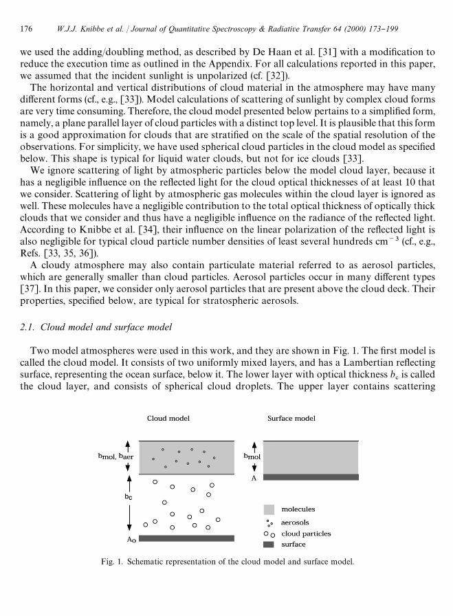
Fig. 1. Schematic representation of the cloud model and surface model.

we used the adding/doubling method, as described by De Haan et al. [31] with a modi"cation toreduce the execution time as outlined in the Appendix. For all calculations reported in this paper,we assumed that the incident sunlight is unpolarized (cf. [32]).

The horizontal and vertical distributions of cloud material in the atmosphere may have manydi!erent forms (cf., e.g., [33]). Model calculations of scattering of sunlight by complex cloud formsare very time consuming. Therefore, the cloud model presented below pertains to a simpli"ed form,namely, a plane parallel layer of cloud particles with a distinct top level. It is plausible that this formis a good approximation for clouds that are strati"ed on the scale of the spatial resolution of theobservations. For simplicity, we have used spherical cloud particles in the cloud model as speci"edbelow. This shape is typical for liquid water clouds, but not for ice clouds [33].

We ignore scattering of light by atmospheric particles below the model cloud layer, because ithas a negligible in#uence on the re#ected light for the cloud optical thicknesses of at least 10 thatwe consider. Scattering of light by atmospheric gas molecules within the cloud layer is ignored aswell. These molecules have a negligible contribution to the total optical thickness of optically thickclouds that we consider and thus have a negligible in#uence on the radiance of the re#ected light.According to Knibbe et al. [34], their in#uence on the linear polarization of the re#ected light isalso negligible for typical cloud particle number densities of least several hundreds cm~3 (cf., e.g.,Refs. [33, 35, 36]).

A cloudy atmosphere may also contain particulate material referred to as aerosol particles,which are generally smaller than cloud particles. Aerosol particles occur in many di!erent types[37]. In this paper, we consider only aerosol particles that are present above the cloud deck. Theirproperties, speci"ed below, are typical for stratospheric aerosols.

2.1. Cloud model and surface model

Two model atmospheres were used in this work, and they are shown in Fig. 1. The "rst model iscalled the cloud model. It consists of two uniformly mixed layers, and has a Lambertian re#ectingsurface, representing the ocean surface, below it. The lower layer with optical thickness b

#is called

the cloud layer, and consists of spherical cloud droplets. The upper layer contains scattering


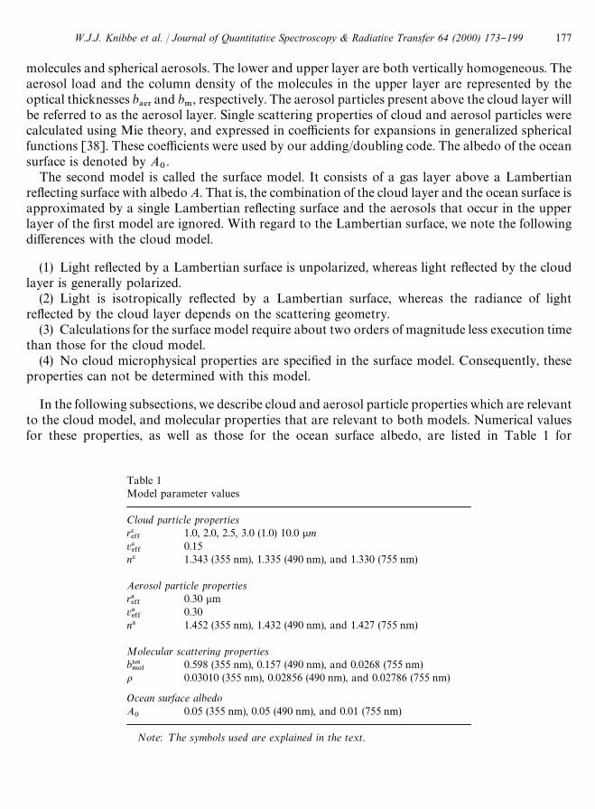
Table 1Model parameter values

Cloud particle propertiesr#%&&

1.0, 2.0, 2.5, 3.0 (1.0) 10.0 lmv#%&&

0.15n# 1.343 (355 nm), 1.335 (490 nm), and 1.330 (755 nm)

Aerosol particle propertiesr!%&&

0.30 lmv!%&&

0.30n! 1.452 (355 nm), 1.432 (490 nm), and 1.427 (755 nm)

Molecular scattering propertiesb505.0-

0.598 (355 nm), 0.157 (490 nm), and 0.0268 (755 nm)o 0.03010 (355 nm), 0.02856 (490 nm), and 0.02786 (755 nm)

Ocean surface albedoA

00.05 (355 nm), 0.05 (490 nm), and 0.01 (755 nm)

Note: ¹he symbols used are explained in the text.

molecules and spherical aerosols. The lower and upper layer are both vertically homogeneous. Theaerosol load and the column density of the molecules in the upper layer are represented by theoptical thicknesses b

!%3and b

., respectively. The aerosol particles present above the cloud layer will

be referred to as the aerosol layer. Single scattering properties of cloud and aerosol particles werecalculated using Mie theory, and expressed in coe$cients for expansions in generalized sphericalfunctions [38]. These coe$cients were used by our adding/doubling code. The albedo of the oceansurface is denoted by A

0.

The second model is called the surface model. It consists of a gas layer above a Lambertianre#ecting surface with albedo A. That is, the combination of the cloud layer and the ocean surface isapproximated by a single Lambertian re#ecting surface and the aerosols that occur in the upperlayer of the "rst model are ignored. With regard to the Lambertian surface, we note the followingdi!erences with the cloud model.

(1) Light re#ected by a Lambertian surface is unpolarized, whereas light re#ected by the cloudlayer is generally polarized.

(2) Light is isotropically re#ected by a Lambertian surface, whereas the radiance of lightre#ected by the cloud layer depends on the scattering geometry.

(3) Calculations for the surface model require about two orders of magnitude less execution timethan those for the cloud model.

(4) No cloud microphysical properties are speci"ed in the surface model. Consequently, theseproperties can not be determined with this model.

In the following subsections, we describe cloud and aerosol particle properties which are relevantto the cloud model, and molecular properties that are relevant to both models. Numerical valuesfor these properties, as well as those for the ocean surface albedo, are listed in Table 1 for


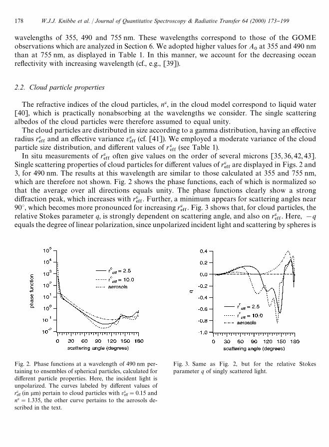
Fig. 2. Phase functions at a wavelength of 490 nm per-taining to ensembles of spherical particles, calculated fordi!erent particle properties. Here, the incident light isunpolarized. The curves labeled by di!erent values ofrceff (in lm) pertain to cloud particles with vc

eff"0.15 andn#"1.335, the other curve pertains to the aerosols de-scribed in the text.

Fig. 3. Same as Fig. 2, but for the relative Stokesparameter q of singly scattered light.

wavelengths of 355, 490 and 755 nm. These wavelengths correspond to those of the GOMEobservations which are analyzed in Section 6. We adopted higher values for A

0at 355 and 490 nm

than at 755 nm, as displayed in Table 1. In this manner, we account for the decreasing oceanre#ectivity with increasing wavelength (cf., e.g., [39]).

2.2. Cloud particle properties

The refractive indices of the cloud particles, n#, in the cloud model correspond to liquid water[40], which is practically nonabsorbing at the wavelengths we consider. The single scatteringalbedos of the cloud particles were therefore assumed to equal unity.

The cloud particles are distributed in size according to a gamma distribution, having an e!ectiveradius r#

%&&and an e!ective variance v#

%&&(cf. [41]). We employed a moderate variance of the cloud

particle size distribution, and di!erent values of r#%&&

(see Table 1).In situ measurements of r#

%&&often give values on the order of several microns [35, 36, 42, 43].

Single scattering properties of cloud particles for di!erent values of r#%&&

are displayed in Figs. 2 and3, for 490 nm. The results at this wavelength are similar to those calculated at 355 and 755 nm,which are therefore not shown. Fig. 2 shows the phase functions, each of which is normalized sothat the average over all directions equals unity. The phase functions clearly show a strongdi!raction peak, which increases with r#

%&&. Further, a minimum appears for scattering angles near

903, which becomes more pronounced for increasing r#%&&

. Fig. 3 shows that, for cloud particles, therelative Stokes parameter q, is strongly dependent on scattering angle, and also on r#

%&&. Here, !q

equals the degree of linear polarization, since unpolarized incident light and scattering by spheres is


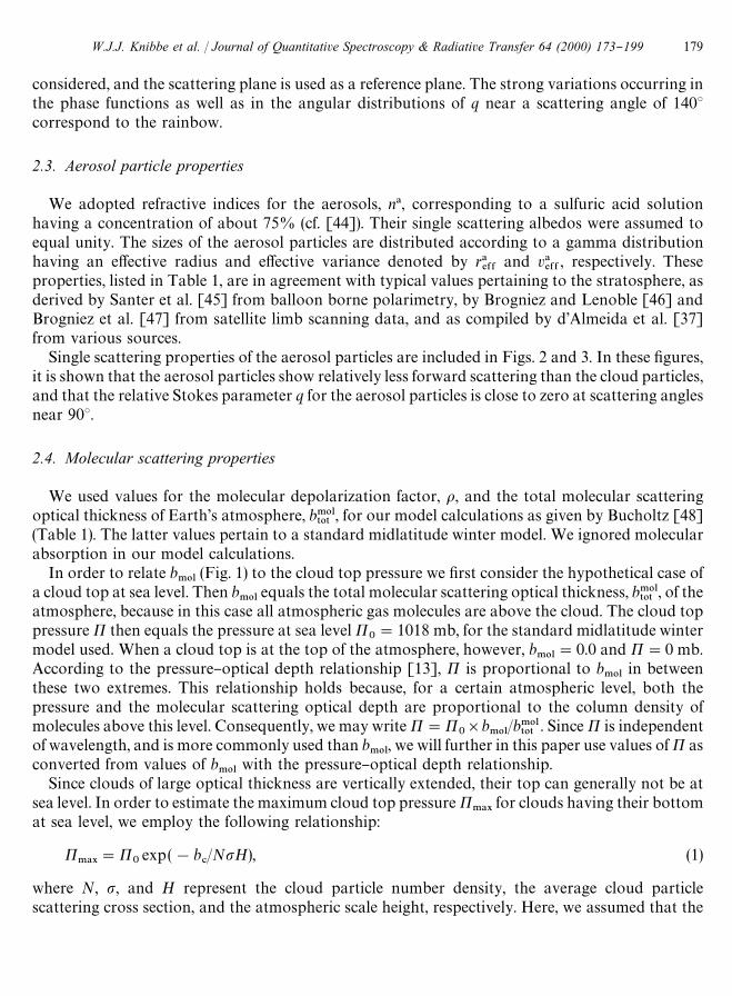
considered, and the scattering plane is used as a reference plane. The strong variations occurring inthe phase functions as well as in the angular distributions of q near a scattering angle of 1403correspond to the rainbow.

2.3. Aerosol particle properties

We adopted refractive indices for the aerosols, n!, corresponding to a sulfuric acid solutionhaving a concentration of about 75% (cf. [44]). Their single scattering albedos were assumed toequal unity. The sizes of the aerosol particles are distributed according to a gamma distributionhaving an e!ective radius and e!ective variance denoted by r!

%&&and v!

%&&, respectively. These

properties, listed in Table 1, are in agreement with typical values pertaining to the stratosphere, asderived by Santer et al. [45] from balloon borne polarimetry, by Brogniez and Lenoble [46] andBrogniez et al. [47] from satellite limb scanning data, and as compiled by d'Almeida et al. [37]from various sources.

Single scattering properties of the aerosol particles are included in Figs. 2 and 3. In these "gures,it is shown that the aerosol particles show relatively less forward scattering than the cloud particles,and that the relative Stokes parameter q for the aerosol particles is close to zero at scattering anglesnear 903.

2.4. Molecular scattering properties

We used values for the molecular depolarization factor, o, and the total molecular scatteringoptical thickness of Earth's atmosphere, b.0-

505, for our model calculations as given by Bucholtz [48]

(Table 1). The latter values pertain to a standard midlatitude winter model. We ignored molecularabsorption in our model calculations.

In order to relate b.0-

(Fig. 1) to the cloud top pressure we "rst consider the hypothetical case ofa cloud top at sea level. Then b

.0-equals the total molecular scattering optical thickness, b.0-

505, of the

atmosphere, because in this case all atmospheric gas molecules are above the cloud. The cloud toppressure P then equals the pressure at sea level P

0"1018 mb, for the standard midlatitude winter

model used. When a cloud top is at the top of the atmosphere, however, b.0-

"0.0 and P"0 mb.According to the pressure}optical depth relationship [13], P is proportional to b

.0-in between

these two extremes. This relationship holds because, for a certain atmospheric level, both thepressure and the molecular scattering optical depth are proportional to the column density ofmolecules above this level. Consequently, we may write P"P

0]b

.0-/b.0-

505. Since P is independent

of wavelength, and is more commonly used than b.0-

, we will further in this paper use values of P asconverted from values of b

.0-with the pressure}optical depth relationship.

Since clouds of large optical thickness are vertically extended, their top can generally not be atsea level. In order to estimate the maximum cloud top pressure P

.!9for clouds having their bottom

at sea level, we employ the following relationship:

P.!9

"P0exp(!b

#/NpH), (1)

where N, p, and H represent the cloud particle number density, the average cloud particlescattering cross section, and the atmospheric scale height, respectively. Here, we assumed that the


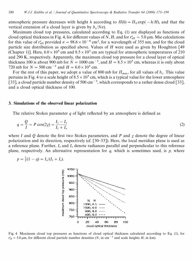
Fig. 4. Maximum cloud top pressures as functions of cloud optical thickness calculated according to Eq. (1), forrceff"5.0 lm, for di!erent cloud particle number densities (N, in cm~3 and scale heights H, in km).

atmospheric pressure decreases with height h according to P(h)"P0exp(!h/H), and that the

vertical extension of a cloud layer is given by b#/Np).

Maximum cloud top pressures, calculated according to Eq. (1) are displayed as functions ofcloud optical thickness in Fig. 4, for di!erent values of N, H, and for r#

%&&"5.0 lm. Mie calculations

for this value of r#%&&

provided p"98.6]10~8 cm2, for a wavelength of 355 nm, and for the cloudparticle size distribution as speci"ed above. Values of H were used as given by Houghton [49(Chapter 1)]. Here, 6.0]105 cm and 8.5]105 cm are typical for atmospheric temperatures of 210and 290 K, respectively. Apparently, the maximum cloud top pressure for a cloud layer of opticalthickness 100 is about 900 mb for N"1000 cm~3, and H"8.5]105 cm, whereas it is only about720 mb for N"500 cm~3 and H"6.0]105 cm.

For the rest of this paper, we adopt a value of 800 mb for P.!9

, for all values of b#. This value

pertains in Fig. 4 to a scale height of 8.5]105 cm, which is a typical value for the lower atmosphere[33], a cloud particle number density of 500 cm~3, which corresponds to a rather dense cloud [33],and a cloud optical thickness of 100.

3. Simulations of the observed linear polarization

The relative Stokes parameter q of light re#ected by an atmosphere is de"ned as

q"QI"P cos(2s)"

Il!I

rIl#I

r

(2)

where I and Q denote the "rst two Stokes parameters, and P and s denote the degree of linearpolarization and its direction, respectively (cf. [50}53]). Here, the local meridian plane is used asa reference plane. Further, I

land I

rdenote radiances parallel and perpendicular to this reference

plane, respectively. An alternative representation for q, which is sometimes used, is p, where

p"12(1!q)"I

r/(I

l#I

r).


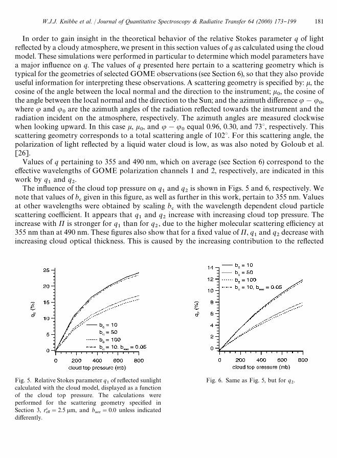
Fig. 5. Relative Stokes parameter q1of re#ected sunlight

calculated with the cloud model, displayed as a functionof the cloud top pressure. The calculations wereperformed for the scattering geometry speci"ed inSection 3, rc

eff"2.5 lm, and b!%3

"0.0 unless indicateddi!erently.

Fig. 6. Same as Fig. 5, but for q2.

In order to gain insight in the theoretical behavior of the relative Stokes parameter q of lightre#ected by a cloudy atmosphere, we present in this section values of q as calculated using the cloudmodel. These simulations were performed in particular to determine which model parameters havea major in#uence on q. The values of q presented here pertain to a scattering geometry which istypical for the geometries of selected GOME observations (see Section 6), so that they also provideuseful information for interpreting these observations. A scattering geometry is speci"ed by: k, thecosine of the angle between the local normal and the direction to the instrument; k

0, the cosine of

the angle between the local normal and the direction to the Sun; and the azimuth di!erence u!u0,

where u and u0

are the azimuth angles of the radiation re#ected towards the instrument and theradiation incident on the atmosphere, respectively. The azimuth angles are measured clockwisewhen looking upward. In this case k, k

0, and u!u

0equal 0.96, 0.30, and 733, respectively. This

scattering geometry corresponds to a total scattering angle of 1023. For this scattering angle, thepolarization of light re#ected by a liquid water cloud is low, as was also noted by Goloub et al.[26].

Values of q pertaining to 355 and 490 nm, which on average (see Section 6) correspond to thee!ective wavelengths of GOME polarization channels 1 and 2, respectively, are indicated in thiswork by q

1and q

2.

The in#uence of the cloud top pressure on q1

and q2

is shown in Figs. 5 and 6, respectively. Wenote that values of b

#given in this "gure, as well as further in this work, pertain to 355 nm. Values

at other wavelengths were obtained by scaling b#

with the wavelength dependent cloud particlescattering coe$cient. It appears that q

1and q

2increase with increasing cloud top pressure. The

increase with P is stronger for q1

than for q2, due to the higher molecular scattering e$ciency at

355 nm than at 490 nm. These "gures also show that for a "xed value of P, q1

and q2

decrease withincreasing cloud optical thickness. This is caused by the increasing contribution to the re#ected


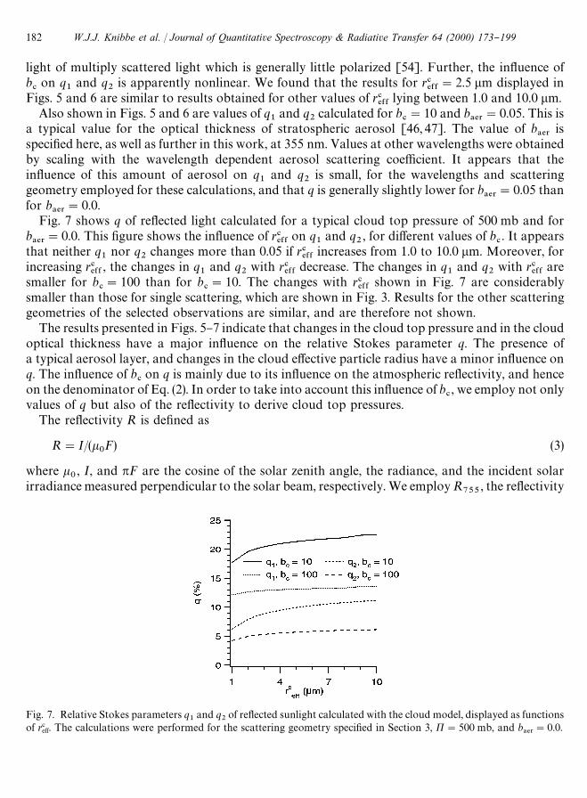
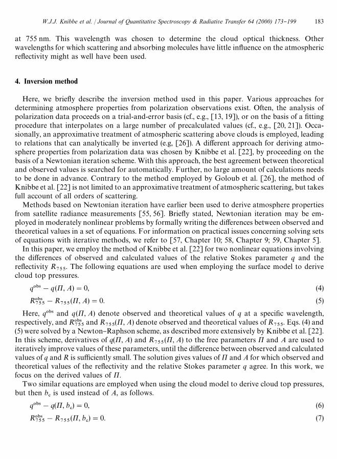
Fig. 7. Relative Stokes parameters q1and q

2of re#ected sunlight calculated with the cloud model, displayed as functions

of rceff. The calculations were performed for the scattering geometry speci"ed in Section 3, P"500 mb, and b

!%3"0.0.

light of multiply scattered light which is generally little polarized [54]. Further, the in#uence ofb#on q

1and q

2is apparently nonlinear. We found that the results for r#

%&&"2.5 lm displayed in

Figs. 5 and 6 are similar to results obtained for other values of r#%&&

lying between 1.0 and 10.0 lm.Also shown in Figs. 5 and 6 are values of q

1and q

2calculated for b

#"10 and b

!%3"0.05. This is

a typical value for the optical thickness of stratospheric aerosol [46, 47]. The value of b!%3

isspeci"ed here, as well as further in this work, at 355 nm. Values at other wavelengths were obtainedby scaling with the wavelength dependent aerosol scattering coe$cient. It appears that thein#uence of this amount of aerosol on q

1and q

2is small, for the wavelengths and scattering

geometry employed for these calculations, and that q is generally slightly lower for b!%3

"0.05 thanfor b

!%3"0.0.

Fig. 7 shows q of re#ected light calculated for a typical cloud top pressure of 500 mb and forb!%3

"0.0. This "gure shows the in#uence of r#%&&

on q1

and q2, for di!erent values of b

#. It appears

that neither q1

nor q2

changes more than 0.05 if r#%&&

increases from 1.0 to 10.0 lm. Moreover, forincreasing r#

%&&, the changes in q

1and q

2with r#

%&&decrease. The changes in q

1and q

2with r#

%&&are

smaller for b#"100 than for b

#"10. The changes with r#

%&&shown in Fig. 7 are considerably

smaller than those for single scattering, which are shown in Fig. 3. Results for the other scatteringgeometries of the selected observations are similar, and are therefore not shown.

The results presented in Figs. 5}7 indicate that changes in the cloud top pressure and in the cloudoptical thickness have a major in#uence on the relative Stokes parameter q. The presence ofa typical aerosol layer, and changes in the cloud e!ective particle radius have a minor in#uence onq. The in#uence of b

#on q is mainly due to its in#uence on the atmospheric re#ectivity, and hence

on the denominator of Eq. (2). In order to take into account this in#uence of b#, we employ not only

values of q but also of the re#ectivity to derive cloud top pressures.The re#ectivity R is de"ned as

R"I/(k0F) (3)

where k0, I, and pF are the cosine of the solar zenith angle, the radiance, and the incident solar

irradiance measured perpendicular to the solar beam, respectively. We employ R755

, the re#ectivity


at 755 nm. This wavelength was chosen to determine the cloud optical thickness. Otherwavelengths for which scattering and absorbing molecules have little in#uence on the atmosphericre#ectivity might as well have been used.

4. Inversion method

Here, we brie#y describe the inversion method used in this paper. Various approaches fordetermining atmosphere properties from polarization observations exist. Often, the analysis ofpolarization data proceeds on a trial-and-error basis (cf., e.g., [13, 19]), or on the basis of a "ttingprocedure that interpolates on a large number of precalculated values (cf., e.g., [20, 21]). Occa-sionally, an approximative treatment of atmospheric scattering above clouds is employed, leadingto relations that can analytically be inverted (e.g, [26]). A di!erent approach for deriving atmo-sphere properties from polarization data was chosen by Knibbe et al. [22], by proceeding on thebasis of a Newtonian iteration scheme. With this approach, the best agreement between theoreticaland observed values is searched for automatically. Further, no large amount of calculations needsto be done in advance. Contrary to the method employed by Goloub et al. [26], the method ofKnibbe et al. [22] is not limited to an approximative treatment of atmospheric scattering, but takesfull account of all orders of scattering.

Methods based on Newtonian iteration have earlier been used to derive atmosphere propertiesfrom satellite radiance measurements [55, 56]. Brie#y stated, Newtonian iteration may be em-ployed in moderately nonlinear problems by formally writing the di!erences between observed andtheoretical values in a set of equations. For information on practical issues concerning solving setsof equations with iterative methods, we refer to [57, Chapter 10; 58, Chapter 9; 59, Chapter 5].

In this paper, we employ the method of Knibbe et al. [22] for two nonlinear equations involvingthe di!erences of observed and calculated values of the relative Stokes parameter q and there#ectivity R

755. The following equations are used when employing the surface model to derive

cloud top pressures.

q0"4!q (P, A)"0, (4)

R0"4755

!R755

(P, A)"0. (5)

Here, q0"4 and q(P, A) denote observed and theoretical values of q at a speci"c wavelength,respectively, and R0"4

755and R

755(P, A) denote observed and theoretical values of R

755. Eqs. (4) and

(5) were solved by a Newton}Raphson scheme, as described more extensively by Knibbe et al. [22].In this scheme, derivatives of q(P, A) and R

755(P, A) to the free parameters P and A are used to

iteratively improve values of these parameters, until the di!erence between observed and calculatedvalues of q and R is su$ciently small. The solution gives values of P and A for which observed andtheoretical values of the re#ectivity and the relative Stokes parameter q agree. In this work, wefocus on the derived values of P.

Two similar equations are employed when using the cloud model to derive cloud top pressures,but then b

#is used instead of A, as follows.

q0"4!q(P, b#)"0, (6)

R0"4755

!R755

(P, b#)"0. (7)


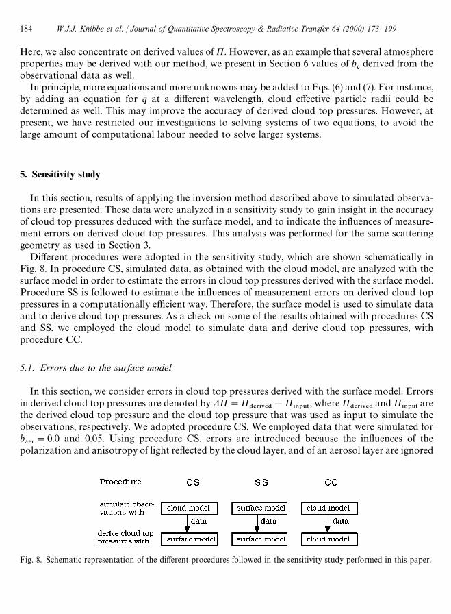
Fig. 8. Schematic representation of the di!erent procedures followed in the sensitivity study performed in this paper.

Here, we also concentrate on derived values of P. However, as an example that several atmosphereproperties may be derived with our method, we present in Section 6 values of b

#derived from the

observational data as well.In principle, more equations and more unknowns may be added to Eqs. (6) and (7). For instance,

by adding an equation for q at a di!erent wavelength, cloud e!ective particle radii could bedetermined as well. This may improve the accuracy of derived cloud top pressures. However, atpresent, we have restricted our investigations to solving systems of two equations, to avoid thelarge amount of computational labour needed to solve larger systems.

5. Sensitivity study

In this section, results of applying the inversion method described above to simulated observa-tions are presented. These data were analyzed in a sensitivity study to gain insight in the accuracyof cloud top pressures deduced with the surface model, and to indicate the in#uences of measure-ment errors on derived cloud top pressures. This analysis was performed for the same scatteringgeometry as used in Section 3.

Di!erent procedures were adopted in the sensitivity study, which are shown schematically inFig. 8. In procedure CS, simulated data, as obtained with the cloud model, are analyzed with thesurface model in order to estimate the errors in cloud top pressures derived with the surface model.Procedure SS is followed to estimate the in#uences of measurement errors on derived cloud toppressures in a computationally e$cient way. Therefore, the surface model is used to simulate dataand to derive cloud top pressures. As a check on some of the results obtained with procedures CSand SS, we employed the cloud model to simulate data and derive cloud top pressures, withprocedure CC.

5.1. Errors due to the surface model

In this section, we consider errors in cloud top pressures derived with the surface model. Errorsin derived cloud top pressures are denoted by DP"P

$%3*7%$!P

*/165, where P

$%3*7%$and P

*/165are

the derived cloud top pressure and the cloud top pressure that was used as input to simulate theobservations, respectively. We adopted procedure CS. We employed data that were simulated forb!%3

"0.0 and 0.05. Using procedure CS, errors are introduced because the in#uences of thepolarization and anisotropy of light re#ected by the cloud layer, and of an aerosol layer are ignored


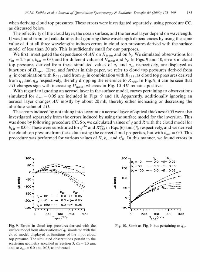
Fig. 9. Errors in cloud top pressures derived with thesurface model from observations of q

1simulated with the

cloud model, displayed as functions of the input cloudtop pressure. The simulated observations pertain to thescattering geometry speci"ed in Section 3, rc

eff"2.5 lm,and to b

!%3"0.0 and 0.05, as indicated.

Fig. 10. Same as Fig. 9, but pertaining to q2.

when deriving cloud top pressures. These errors were investigated separately, using procedure CC,as discussed below.

The re#ectivity of the cloud layer, the ocean surface, and the aerosol layer depend on wavelength.It was found from test calculations that ignoring these wavelength dependencies by using the samevalue of A at all three wavelengths induces errors in cloud top pressures derived with the surfacemodel of less than 20 mb. This is su$ciently small for our purposes.

We "rst investigated the dependence of DP on P*/165

and on b#. We simulated observations for

r#%&&"2.5 lm, b

!%3"0.0, and for di!erent values of P

*/165and b

#. In Figs. 9 and 10, errors in cloud

top pressures derived from these simulated values of q1

and q2, respectively, are displayed as

functions of P*/165

. Here, and further in this paper, we refer to cloud top pressures derived fromq1in combination with R

755, and from q

2in combination with R

755, as cloud top pressures derived

from q1

and q2, respectively, thereby dropping the reference to R

755. In Fig. 9, it can be seen that

DP changes sign with increasing P*/165

, whereas in Fig. 10 DP remains positive.With regard to ignoring an aerosol layer in the surface model, curves pertaining to observations

simulated for b!%3

"0.05 are included in Figs. 9 and 10. Apparently, additionally ignoring anaerosol layer changes DP mostly by about 20 mb, thereby either increasing or decreasing theabsolute value of DP.

The errors induced by not taking into account an aerosol layer of optical thickness 0.05 were alsoinvestigated separately from the errors induced by using the surface model for the inversion. Thiswas done by following procedure CC. So, we calculated values of q and R with the cloud model forb!%3

"0.05. These were substituted for q0"4 and R0"4755

in Eqs. (6) and (7), respectively, and we derivedthe cloud top pressure from these data using the correct cloud properties, but with b

!%3"0.0. This

procedure was performed for various values of P, b#, and r#

%&&. In this manner, we found errors in


Fig. 11. Errors in cloud top pressures derived with the surface model from observations of q1

and q2

simulated with thecloud model, displayed as functions of rc

eff . The simulated observations pertain to the scattering geometry speci"ed insection 3, %

*/165"500 mb, and b

!%3"0.0.

the derived cloud top pressure that increased from a few millibars for low cloud top pressures, tovalues not exceeding 40 mb for P"800 mb.

Next, we investigated the dependence of the errors in derived cloud top pressures on cloude!ective particle radius, using again procedure CS. Fig. 11 shows errors DP in cloud top pressuresderived from observations simulated for a typical cloud top pressure of 500 mb, for di!erent valuesof b

#and r#

%&&. Apparently, DP changes more rapidly with r#

%&&for 1 lm(r#

%&&(3 lm than for

3 lm(r#%&&(10 lm. We found a similar variation of DP with r#

%&&for other cloud top pressures.

Lastly, we adopted procedure CC in a particular way to estimate the in#uence on derived cloudtop pressures of ignoring only the polarization of light re#ected by the cloud layer, but taking intoaccount the anisotropy of this re#ected light. For this purpose, simulations of q and R wereperformed with the cloud model for various values of b

#, P

*/165and for r#

%&&"2.5 lm. Then, cloud

top pressures were derived with the cloud model, using the correct cloud properties, but nowassuming that the light scattered by the cloud particles is unpolarized. Errors DP in derived cloudtop pressures were found to be signi"cant, namely about 40 mb for P

*/165"500 mb, and about

100 mb for P*/165

"800 mb. These errors were found generally to increase with increasing cloudtop pressure.

From the results presented in Figs. 9}11, we conclude the following. The errors in cloud toppressures derived with the surface model strongly depend on the cloud top pressure. At 500 and800 mb, they are at most about 50 and 130 mb, respectively, for cloud top pressures derived fromq1, and at most about 100 and 130 mb for cloud top pressures derived from q

2, respectively. The

errors also depend signi"cantly on the cloud optical thickness. There is, however, generally lessvariation of the errors with cloud e!ective particle radius. This variation is strongest whenr#%&&

increases from 1 to about 3 lm, and less when r#%&&

increases from 3 to 10 lm. It was found thaterrors in cloud top pressures derived with the surface model are not only due to ignoring theanisotropic re#ection of light by a cloud layer, but also due to ignoring the polarization of lightre#ected by a cloud layer.


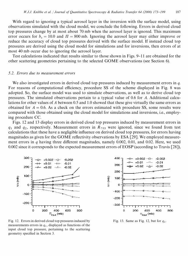
Fig. 12. Errors in derived cloud top pressures induced bymeasurements errors in q

1, displayed as functions of the

input cloud top pressure, pertaining to the scatteringgeometry speci"ed in Section 3.

Fig. 13. Same as Fig. 12, but for q2.

With regard to ignoring a typical aerosol layer in the inversion with the surface model, usingobservations simulated with the cloud model, we conclude the following. Errors in derived cloudtop pressures change by at most about 70 mb when the aerosol layer is ignored. This maximumerror occurs for b

#"10.0 and P"800 mb. Ignoring the aerosol layer may either improve or

reduce the accuracy of cloud top pressures derived with the surface model. If instead cloud toppressures are derived using the cloud model for simulations and for inversions, then errors of atmost 40 mb occur due to ignoring the aerosol layer.

Test calculations indicated that results similar to those shown in Figs. 9}11 are obtained for theother scattering geometries pertaining to the selected GOME observations (see Section 6).

5.2. Errors due to measurement errors

We also investigated errors in derived cloud top pressures induced by measurement errors in q.For reasons of computational e$ciency, procedure SS of the scheme displayed in Fig. 8 wasadopted. So, the surface model was used to simulate observations, as well as to derive cloud toppressures. The simulated observations pertain to a typical value of 0.6 for A. Additional calcu-lations for other values of A between 0.5 and 1.0 showed that these give virtually the same errors asobtained for A"0.6. As a check on the errors estimated with procedure SS, some results werecompared with those obtained using the cloud model for simulations and inversions, i.e., employ-ing procedure CC.

Figs. 12 and 13 display errors in derived cloud top pressures induced by measurement errors inq1

and q2, respectively. Measurement errors in R

755were ignored, since we found from test

calculations that these have a negligible in#uence on derived cloud top pressures, for errors havingmagnitudes as given for the GOME re#ectivity observations by ESA [29]. We employed measure-ment errors in q having three di!erent magnitudes, namely 0.002, 0.01, and 0.02. Here, we used0.002 since it corresponds to the expected measurement errors of EOSP (according to Travis [28]),


which is developed to obtain high accuracy data. Errors of 0.01 and 0.02 were used since these aretypical for the observations performed by GOME (according to Aben et al. [60]). We note thatGOME was not intended for conducting polarimetry, but was designed to measure polarizationproperties of the re#ected light in order to improve the accuracy of the radiance measurements.Future improvements in the processing of GOME observations might lead to a reduction inmeasurement errors in q to at most 0.01. It appears from Figs. 12 and 13 that DP due tomeasurement errors increases with P

*/165. Further, except for cloud top pressures close to 800 mb,

measurement errors in q2

have a larger in#uence on derived cloud top pressures than those in q1.

The in#uences of measurement errors estimated with the surface model were compared within#uences estimated with the cloud model. For this purpose, procedure CC was adopted. Simula-tions of q

1and q

2were performed for various values of r#

%&&, b

#, and b

!%3. Then, we added arti"cial

measurement errors to the simulated values of q, and determined the cloud top pressure with thecloud model, using the correct values of rc

eff , b#, and b

!%3. It was found that the resulting errors were

mostly larger than those derived with the surface model, by a few tens of millibars.We conclude that measurement errors in q

1of 0.002, 0.01, and 0.02 maximally induce errors in

derived cloud top pressures of about 20, 100, and 200 mb, occurring for P"800 mb. If q2

isemployed, the maximum errors are about 20, 110, and 230 mb, respectively, and also occur forP"800 mb. These errors were estimated using the surface model for simulations and inversions.We note that we deduced errors which are larger by several tens of millibars when the cloud modelwas used instead of the surface model. It appears that equal measurement errors in q

1and q

2induce

about the same maximum errors in derived cloud top pressures. However, the errors in derivedcloud top pressures decrease faster with decreasing P

*/165for q

1than for q

2. Typically, measure-

ment errors of 0.02 in q1

and q2

induce errors in the derived cloud top pressure smaller than 100and 200 mb, respectively. Test calculations indicated that similar results are obtained for the otherscattering geometries pertaining to the selected GOME observations.

6. Analysis of GOME photopolarimetry data

For a "rst application of our approach to real measurements some observations over theAtlantic Ocean obtained by GOME on 23 July 1995 were analyzed. In this section, afterintroducing the instrument and the observations, we present results of this analysis. No validationof the derived cloud top pressures is available. They are, however, presented for two reasons: (1) toinvestigate if cloud top pressures derived from observations of q in di!erent wavelength bands areconsistent given the accuracy of the measurements, and (2) to examine the usefulness of the resultsobtained with the surface model. These issues will be discussed in Section 7.

6.1. GOME photopolarimetry data

The Global Ozone Monitoring Experiment (GOME) is a grating spectrometer on board ofERS-2. Comprehensive information on GOME may be found in Guyenne and Readings [61] andESA [29]. ERS-2 has been launched in April 1995 and #ies in a sun-synchronous orbit at analtitude of 780 km, with a local equator crossing time of 10 :30 AM for the descending node. Theorbital period is about 100 min. The spectral measurements of GOME are aimed at remote sensing


of atmospheric trace gases, especially ozone. The observations are performed at viewing zenithangles between 03 and 313. The pixels that we analyzed correspond to areas of about 80]40 km2on the Earth's surface.

Three polarimetric channels have been added to the spectrometric channels. The polarimetricmeasurements are needed to correct the spectrometric readouts for the polarization of theincoming light. We did not use the third channel because its e!ective wavelength of about 700 nm istoo large for molecules to have a signi"cant e!ect on the polarization of the re#ected light. Thee!ective wavelengths of the three polarimetric channels are determined in #ight, using themeasured spectral distribution of the incoming light and the wavelength dependence of the detectorsensitivity. For observations made over the Atlantic Ocean on 23 July 1995, the e!ectivewavelengths are between 352 and 358 nm for the "rst channel and between 489 and 491 nm for thesecond channel. The bandwidths of these channels are about 100 and 200 nm, respectively.

We applied two selection criteria to the observations made on 23 July 1995 in orbit 1337, whichwere processed with version 0.7 of the GOME data processor. (1) In order to obtain observationsin cloudy areas we demanded a re#ectivity of at least 0.5 at 755 nm. This re#ectivity corresponds toa cloud optical thickness of about 10 when considering an overcast pixel. Because the selectedpixels are located over the ocean, which has a surface re#ectivity less than 0.1, high re#ectivitiesmust be due to the presence of clouds, unless the ocean surface is covered by ice. The lattersituation, however, is unlikely at the latitudes of the selected pixels. Moreover, it may expectedly berecognized by "nding estimates of P close to the pressure at sea level. (2) A single scattering anglebetween 703 and 1103, so that the in#uence of Rayleigh scattering on the linear polarization is large.Using these two criteria, we found 20 pixels, which were numbered according to the increasing timelapse of the observations.

In order to obtain more information of the observed areas, we inspected simultaneous collocateddata obtained by the Along Track Scanning Radiometer-2 (ATSR-2), which is an extended versionof ATSR [62, 63]. ATSR-2, which is also on board of ERS-2, measures radiances in di!erentwavelength bands in the visible and infrared part of the spectrum, with a spatial resolution of about1]1 km2. The infrared radiances were converted into brightness temperatures, ¹

", using a Planck

curve.We employed ATSR-2 observations obtained in the wavelength band centered at 660 nm to

estimate the fractions of the observed regions covered by optically thick clouds. An ATSR-2 pixelwas assumed to be covered by such clouds if its re#ectivity is at least 0.4 at 660 nm. From thisinspection we found that the GOME pixels 1}16 are almost completely covered by optically thickclouds. The cloud cover is about 50% for pixels 17}19, and about 30% for pixel 20. We excludedtherefore pixels 17}20 from our selection.

The di!erence between the brightness temperatures determined from ATSR-2 observations inthe 11 and 12 lm bands, ¹

"(11 lm) and ¹

"(12 lm), respectively, was used to estimate the portions

of the observed areas covered by optically thin clouds, such as cirrus clouds, above a main clouddeck. The principles for using this di!erence are described by, e.g., Stephens [64], and has been usedby Koelemeijer et al. [65]. We considered optically thin clouds to be present in an ATSR-2 pixelwhen ¹

"(11 lm)!¹

"(12 lm)'2 K. This inspection indicated that pixels 1}16 are for signi"cant

portions covered by optically thin clouds. As a result the derived cloud top pressure will not beprecisely the pressure of the top of the main cloud deck but it will be biased towards lowerpressures.


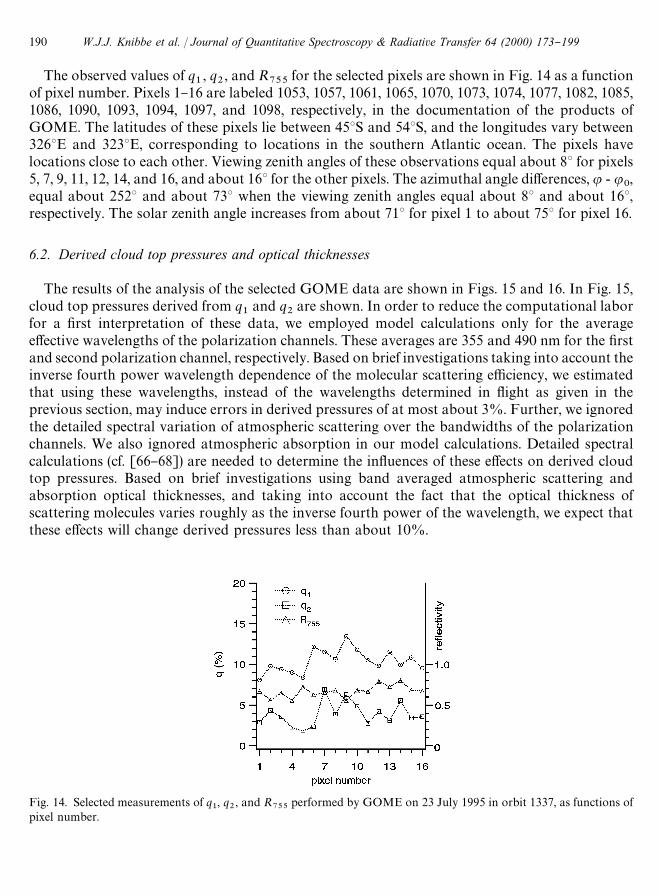
Fig. 14. Selected measurements of q1, q

2, and R

755performed by GOME on 23 July 1995 in orbit 1337, as functions of

pixel number.

The observed values of q1, q

2, and R

755for the selected pixels are shown in Fig. 14 as a function

of pixel number. Pixels 1}16 are labeled 1053, 1057, 1061, 1065, 1070, 1073, 1074, 1077, 1082, 1085,1086, 1090, 1093, 1094, 1097, and 1098, respectively, in the documentation of the products ofGOME. The latitudes of these pixels lie between 453S and 543S, and the longitudes vary between3263E and 3233E, corresponding to locations in the southern Atlantic ocean. The pixels havelocations close to each other. Viewing zenith angles of these observations equal about 83 for pixels5, 7, 9, 11, 12, 14, and 16, and about 163 for the other pixels. The azimuthal angle di!erences, u - u

0,

equal about 2523 and about 733 when the viewing zenith angles equal about 83 and about 163,respectively. The solar zenith angle increases from about 713 for pixel 1 to about 753 for pixel 16.

6.2. Derived cloud top pressures and optical thicknesses

The results of the analysis of the selected GOME data are shown in Figs. 15 and 16. In Fig. 15,cloud top pressures derived from q

1and q

2are shown. In order to reduce the computational labor

for a "rst interpretation of these data, we employed model calculations only for the averagee!ective wavelengths of the polarization channels. These averages are 355 and 490 nm for the "rstand second polarization channel, respectively. Based on brief investigations taking into account theinverse fourth power wavelength dependence of the molecular scattering e$ciency, we estimatedthat using these wavelengths, instead of the wavelengths determined in #ight as given in theprevious section, may induce errors in derived pressures of at most about 3%. Further, we ignoredthe detailed spectral variation of atmospheric scattering over the bandwidths of the polarizationchannels. We also ignored atmospheric absorption in our model calculations. Detailed spectralcalculations (cf. [66}68]) are needed to determine the in#uences of these e!ects on derived cloudtop pressures. Based on brief investigations using band averaged atmospheric scattering andabsorption optical thicknesses, and taking into account the fact that the optical thickness ofscattering molecules varies roughly as the inverse fourth power of the wavelength, we expect thatthese e!ects will change derived pressures less than about 10%.


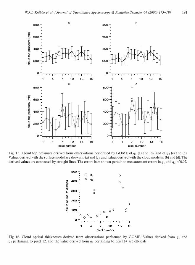
Fig. 15. Cloud top pressures derived from observations performed by GOME of q1

(a) and (b), and of q2

(c) and (d).Values derived with the surface model are shown in (a) and (c), and values derived with the cloud model in (b) and (d). Thederived values are connected by straight lines. The errors bars shown pertain to measurement errors in q

1and q

2of 0.02.

Fig. 16. Cloud optical thicknesses derived from observations performed by GOME. Values derived from q1

andq2

pertaining to pixel 12, and the value derived from q1

pertaining to pixel 14 are o!-scale.


The cloud top pressures shown were obtained with the surface model and the cloud model. Forthe cloud model, we adopted r#

%&&"5.0 lm and b

!%3"0.0. As additional information, values of

b#derived with the cloud model are displayed in Fig. 16. This exempli"es the possibility to derive

other cloud properties with our inversion method.Concerning q

1, cloud top pressures derived with the surface model and the cloud model di!er

less than 50 mb for all pixels, with the highest cloud top pressures generally derived with the surfacemodel. Regarding q

2, cloud top pressures deduced with the surface model are between 50 and

100 mb higher than those derived with the cloud model, for all pixels. Typically, for both channels,di!erences between cloud top pressures derived with the surface and cloud model are less than80 mb.

With regard to the cloud top pressures derived with the cloud model, it appears that, for allpixels, values of P derived from q

1and q

2di!er on average about 150 mb. Some values derived

from q1

are larger and other values are smaller than those derived from q2. Similar di!erences

appear between cloud top pressures derived from q1and q

2with the surface model. It appears from

Fig. 15 that the error bars for q1

are much smaller than those for q2. Therefore, the GOME

polarization channel at 355 nm is better suited for deriving cloud top pressures than the channel at490 nm.

Additional calculations, for other values of r ceff , and also for b

!%3"0.05, resulted in derived cloud

top pressures that di!er generally less than 50 mb from the results shown in Fig. 15.The derived cloud optical thicknesses, displayed in Fig. 16, are less than 100, except for pixels 5,

11, 12, 13, 14 and 16. Apparently, there is no correlation between derived values of P and b#. Values

of the cloud optical thickness for pixel 12 derived from q1

and q2, as well as for pixel 14 derived

from q1, are even larger than 500, and thus o!-scale in this "gure. Such unrealistic magnitudes may

be caused by the fact that ice clouds have been observed, whereas we employed single scatteringproperties of liquid water droplets in the interpretation of the observations [69]. The presence ofice clouds may also introduce errors in cloud top pressures derived with the cloud model, but thishas not been investigated.

7. Discussion and conclusions

The work described in this paper was performed to present an approach for using the in#uenceof molecular scattering above clouds on the linear polarization of re#ected sunlight to derivecloud top pressures. For that purpose, a method to determine cloud top pressures was appliedto simulated and observed data concerning the re#ectivity and the relative Stokes parameter q.Two di!erent atmosphere models were used, called the cloud model and the surface model,respectively.

Simulated data were employed to estimate errors in derived cloud top pressures due tomeasurement errors and to the simpli"cations of the second model compared to the "rst model.Table 2 lists such errors pertaining to a typical cloud top pressure of 500 mb and a maximum cloudtop pressure of 800 mb. The estimates listed in Table 2 were obtained for a scattering geometry(k"0.96, k

0"0.30, and u!u

0"733) that is typical for the scattering geometries of the selected

GOME observations that we analyzed. It appears that the in#uence on derived cloud top pressuresof measurement errors in q

1is generally smaller than that of measurement errors in q

2. For this


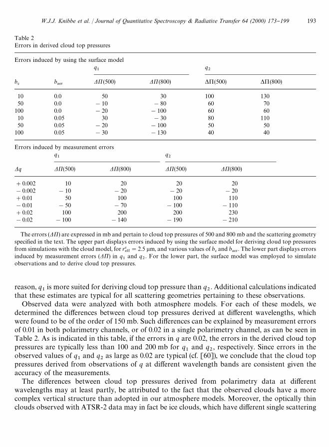
Table 2Errors in derived cloud top pressures

Errors induced by using the surface modelq1

q2

b#

b!%3

DP(500) DP(800) *%(500) *%(800)

10 0.0 50 30 100 13050 0.0 !10 !80 60 70

100 0.0 !20 !100 60 6010 0.05 30 !30 80 11050 0.05 !20 !100 50 50

100 0.05 !30 !130 40 40

Errors induced by measurement errorsq1

q2

Dq DP(500) DP(800) DP(500) DP(800)

#0.002 10 20 20 20!0.002 !10 !20 !20 !20#0.01 50 100 100 110!0.01 !50 !70 !100 !110#0.02 100 200 200 230!0.02 !100 !140 !190 !210

The errors (DP) are expressed in mb and pertain to cloud top pressures of 500 and 800 mb and the scattering geometryspeci"ed in the text. The upper part displays errors induced by using the surface model for deriving cloud top pressuresfrom simulations with the cloud model, for r#

%&&"2.5 lm, and various values of b

#and b

!%3. The lower part displays errors

induced by measurement errors (DP) in q1

and q2. For the lower part, the surface model was employed to simulate

observations and to derive cloud top pressures.

reason, q1

is more suited for deriving cloud top pressure than q2. Additional calculations indicated

that these estimates are typical for all scattering geometries pertaining to these observations.Observed data were analyzed with both atmosphere models. For each of these models, we

determined the di!erences between cloud top pressures derived at di!erent wavelengths, whichwere found to be of the order of 150 mb. Such di!erences can be explained by measurement errorsof 0.01 in both polarimetry channels, or of 0.02 in a single polarimetry channel, as can be seen inTable 2. As is indicated in this table, if the errors in q are 0.02, the errors in the derived cloud toppressures are typically less than 100 and 200 mb for q

1and q

2, respectively. Since errors in the

observed values of q1

and q2

as large as 0.02 are typical (cf. [60]), we conclude that the cloud toppressures derived from observations of q at di!erent wavelength bands are consistent given theaccuracy of the measurements.

The di!erences between cloud top pressures derived from polarimetry data at di!erentwavelengths may at least partly, be attributed to the fact that the observed clouds have a morecomplex vertical structure than adopted in our atmosphere models. Moreover, the optically thinclouds observed with ATSR-2 data may in fact be ice clouds, which have di!erent single scattering


properties than adopted in the cloud model. More accurate polarimetry data are needed toinvestigate the e!ects of these clouds on the polarization of re#ected light. We note that investiga-tions taking into account the detailed wavelength dependence of atmospheric scattering andabsorption over the wavelength bands of the polarization channels may improve the accuracy ofcloud top pressures derived from GOME polarimetry data.

For most of the observations considered, cloud top pressures derived with a model that accountsfor multiple scattering by cloud particles di!er less than 80 mb from results derived assumingLambert re#ection by a cloud (see Section 6). Because this di!erence is generally less than errorsdue to measurement errors, we conclude that assuming Lambert re#ection is su$cient to derivecloud top pressures from these observations. In this manner, the computational labor may bereduced by at least two orders of magnitude. However, the anisotropy and polarization of lightre#ected by the cloud layer needs to be taken into account in order to analyze more accurateobservations, such as to be expected from EOSP (cf. Table 2). This is also required for accuratedetermination of additional cloud properties, such as the cloud optical thickness. In the latter case,further research is needed to improve the e$ciency of radiative transfer codes, so that they becomemore suited for operational use.

Acknowledgements

We are indebted to ESA for making the GOME data used in this work available to us; these dataare a pre-release for scienti"c investigators. It is a pleasure to express our gratitude to L.D. Travisfor many helpful discussions and useful comments on an earlier version of this paper. We gratefullyacknowledge stimulating discussions with C.V.M. van der Mee about the topic described in theAppendix of this paper. This work has been supported in part by a Columbia University researchprogram funded by NASA Goddard Institute for Space Studies.

Appendix. A method for faster adding/doubling calculations

Here, we present a method that was developed to reduce the execution time of adding/doublingcalculations, and to increase the user friendliness of our code. It is based on the requirement thatsecond-order scattering is treated with a prescribed accuracy. This requirement is used to adjust thenumerical integrations for the nadir angles for successive Fourier terms. The method reduces theexecution time for calculations for terrestrial clouds with about an order of magnitude. In ourdescription, we closely follow the terminology of De Haan et al. [31].

In the adding/doubling method, the azimuth dependence of each function is expanded ina Fourier series. For each term in such an expansion, adding and doubling is performed usingGauss}Legendre integration (cf., e.g., [58]) for the nadir angles. These integrations have beenimplemented as multiplications of supermatrices. The dimensions of these matrices are propor-tional to the number of Gaussian division points employed. Generally, most of the execution timeof the adding/doubling method is spent in these matrix multiplications. Therefore, the executiontime depends approximately cubically on the number of Gaussian division points used for theintegrations.


The number of Gaussian division points needed for a certain accuracy used to be determined bytrial-and-error, which becomes rather time consuming when a single calculation takes severalhours. In order to increase the user friendliness of our code, we developed a scheme to automati-cally determine the number of division points needed for a certain accuracy. Then, we realized thatthis scheme could be applied to each Fourier component, in order to determine for each termseparately how many division points are needed. This signi"cantly reduces the execution time,since the required number of division points appeared to decrease for higher terms.

The following expression is used in our scheme:

P1

~1

Zm (u, u@)Zm (u@, uA)du@"M0

+l/m

22l#1

(al1)2Pl

m,0(u)Pl

m,0(uA) (A.1)

where Zm denotes the mth Fourier component of the one}one element of the phase matrix, u, u@, anduA denote direction cosines, M

0is determined using Eq. (138) of De Haan et al. [31], al

1denotes the

l-th expansion coe$cient of the one-one element of the scattering matrix, and Plm,0

denotesa generalized spherical function. These quantities are extensively described by De Haan et al. [31].Eq. (A.1) was obtained using the expansion of Zm in generalized spherical functions (Eq. (66) of DeHaan et al. [31]), and the orthogonality of the generalized spherical functions.

Using the symmetry relations given by Hovenier [70], and considering u40 and uA50, whichcorresponds to the directions of scattered light traveling upwards and illumination from above,respectively, we may write

P1

~1

Zm (u, u@)Zm (u@, uA)du@"P1

0

Zm(!k, k@)Zm (k@, kA)dk@

#P1

0

Zm (k, k@)Zm (!k@, kA)dk@ (A.2)

where k"Du D . It is now demanded that for a certain accuracy e we have

KN+i/1

Zm(!k, ki)Zm (k

i, kA)w

i#

N+i/1

Zm(k, ki)Zm(!k

i, kA)w

i

!

M0

+l/m

22l#1

(al1)2Pl

m,0(k)Pl

m,0(kA) K(e (A.3)

where N is the number of Gaussian division points, and kiand w

idenote the division points and

weights of the Gauss}Legendre integration. For each Fourier term m and "xed values of k and kA,the number of Gaussian division points N is chosen as the minimal even number for whichcondition (A.3) holds.

The integral in Eq. (A.1) represents the core of the problem of numerically integrating secondorder scattering. In Eq. (A.1), namely, the attenuation of light in the atmosphere described byexponential functions that is a part of the complete description of second order scattering (cf., e.g.,[71]) is ignored, but these are smooth functions that are not di$cult to integrate numerically.Using condition (A.3), we demand that numerical integration is performed with an accuracyepsilon, for each Fourier term. Single scattering shows a more complicated angular behavior thansecond order scattering [54, 72]. However, single scattering is in our code not calculated by


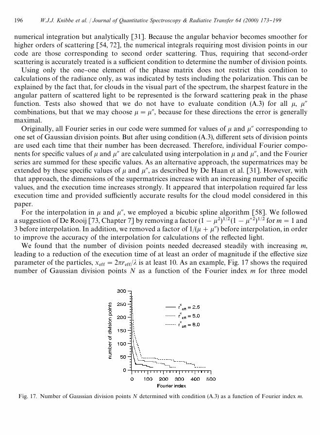
Fig. 17. Number of Gaussian division points N determined with condition (A.3) as a function of Fourier index m.

numerical integration but analytically [31]. Because the angular behavior becomes smoother forhigher orders of scattering [54, 72], the numerical integrals requiring most division points in ourcode are those corresponding to second order scattering. Thus, requiring that second-orderscattering is accurately treated is a su$cient condition to determine the number of division points.

Using only the one}one element of the phase matrix does not restrict this condition tocalculations of the radiance only, as was indicated by tests including the polarization. This can beexplained by the fact that, for clouds in the visual part of the spectrum, the sharpest feature in theangular pattern of scattered light to be represented is the forward scattering peak in the phasefunction. Tests also showed that we do not have to evaluate condition (A.3) for all k, kAcombinations, but that we may choose k"kA, because for these directions the error is generallymaximal.

Originally, all Fourier series in our code were summed for values of k and kA corresponding toone set of Gaussian division points. But after using condition (A.3), di!erent sets of division pointsare used each time that their number has been decreased. Therefore, individual Fourier compo-nents for speci"c values of k and kA are calculated using interpolation in k and kA, and the Fourierseries are summed for these speci"c values. As an alternative approach, the supermatrices may beextended by these speci"c values of k and kA, as described by De Haan et al. [31]. However, withthat approach, the dimensions of the supermatrices increase with an increasing number of speci"cvalues, and the execution time increases strongly. It appeared that interpolation required far lessexecution time and provided su$ciently accurate results for the cloud model considered in thispaper.

For the interpolation in k and kA, we employed a bicubic spline algorithm [58]. We followeda suggestion of De Rooij [73, Chapter 7] by removing a factor (1!k2)1@2(1!kA2)1@2 for m"1 and3 before interpolation. In addition, we removed a factor of 1/(k#kA) before interpolation, in orderto improve the accuracy of the interpolation for calculations of the re#ected light.

We found that the number of division points needed decreased steadily with increasing m,leading to a reduction of the execution time of at least an order of magnitude if the e!ective sizeparameter of the particles, x

%&&"2nr

%&&/j is at least 10. As an example, Fig. 17 shows the required

number of Gaussian division points N as a function of the Fourier index m for three model


calculations as determined by using condition (A.3). They pertain to calculations of the Stokesparameters of re#ected light, ignoring the circular polarization of light, for the cloud model withb#"100, P"0 mb, b

!%3"0.0, v#

%&&"0.15 and r#

%&&"2.5, 5.0, and 8.0 lm, respectively. All three

calculations were performed for epsilon"0.001, and pertain to a wavelength of 355 nm. Theexecution times were reduced by factors of about 12, 18, and 28 for calculations pertaining torceff"2.5, 5.0, and 8.0 lm, respectively. Total execution times for these calculations using condition

(A.3) equaled about 6, 50, and 234 min, respectively, on an IBM RS/6000 58H computer.

References

[1] Houghton JT, Jenkins GJ, Ephraums JJ, editors. Climate change. The IPCC Scienti"c Assessment, Cambridge:Cambridge Univ. Press, 1990.

[2] Peixoto JP, Oort AH, Physics of climate, New York: American Institute of Physics, 1992.[3] Hansen J, Rossow W, Carlson B, Lacis A, Travis L, Del Genio A, Fung I, Cairns B, Mishchenko M, Sato M.

Low-cost long-term monitoring of global climate forcings and feedbacks, Climatic change 1995;31:247}71.[4] Liao X, Rossow WB, Rind D. Comparison between SAGE II and ISCCP high-level clouds 2. Locating cloud tops.

J Geophys Res 1995;100:1137}47.[5] Smith WL, Platt CMR. Comparison of satellite deduced cloud heights with indications from radiosonde and

ground}based laser measurements, J Appl Meteorol 1978;17:1796}802.[6] Menzel WP, Smith WL, Stewart TR. Improved cloud motion wind vector and altitude assignment using VAS.

J Appl Meteorol 1983;22:377}84.[7] Fischer J, Grassl H. Detection of cloud-top height from backscattered radiances within the oxygen A band, Part I,

Theoretical study, J Appl Meteorol 1991;30:1245}59.[8] Fischer J, Cordes W, Schmitz-Pei!er A, Renger W, Morl P. Detection of cloud-top height from backscattered

radiances within the oxygen A band, Part II, Measurements. J Appl Meteorol 1991;30:1260}7.[9] Shenk WE, Holuband RJ, Ne! RA. Stereographic cloud analysis from Apollo photographs over a cold front, Bull

Am Meteorol Soc 1975;56:4}16.[10] Prata AJ, Turner PJ. Cloud top height determination using ATSR Data, Remote Sensing Environ 1997;59:1}13.[11] Joiner J, Bhartia PK. The determination of cloud pressures from rotational Raman scattering in satellite

backscatter ultraviolet measurements. J Geophys Res 1995;100:23 019}26.[12] Wu ML. Remote Sensing of cloud}top pressures using re#ected solar radiation in the oxygen A-band, J Climate

Appl Meteorol 1985;24:539}46.[13] Hansen JE, Hovenier JW. Interpretation of the polarization of Venus, J Atmos Sci 1974;31:1137}60.[14] Dollfus A. Contribution au Colloque Caltech-JPL sur la Lune et les Planetes: Venus, Proc Caltech-JPL Lunar and

Planetary Conf, JPL TM 33-266, 1966:187}202.[15] Co!een DL, Gehrels T. Wavelength dependence of the polarization. XV. Observations of Venus, Astron

J 1969;74:433}45.[16] Dollfus A, Co!een DL. Polarization of Venus. I. Disk observations, Astron Astrophys 1970;8:251}66.[17] Lane WA. Wavelength dependence of the polarization. XXXV. Vertical structure of scattering layers above the

visible Venus clouds. Astron J 1979;84:683}91.[18] Santer R, Herman M. Wavelength dependence of the polarization. XXXVIII. Analysis of ground-based observa-

tions of Venus, Astron J 1979;84:1802}10.[19] Kawabata K, Co!een DL, Hansen JE, Lane WA, Makoto S, Travis LD. Cloud and haze properties from Pioneer

Venus polarimetry. J Geophys Res 1980;85:8129}40.[20] Sato M, Travis LD, Kawabata K. Photopolarimetry analysis of the Venus atmosphere in polar regions. Icarus

1996;124:569}85.[21] Knibbe WJJ, De Haan JF, Hovenier JW, Travis LD. A biwavelength analysis of Pioneer Venus polarization

observations. J Geophys Res 1997;102:10945}58.


[22] Knibbe WJJ, De Haan JF, Hovenier JW, Travis LD. Interpretation of temporal variations of the polarization ofVenus as observed by Pioneer Venus orbiter. J Geophys Res 1998;103:8557}74.

[23] Co!een DL. Polarization and scattering characteristics in the atmospheres of Earth, Venus, and Jupiter. J Opt SocAmer 1979;69:1051}64.

[24] Egan WG, Johnson WR, Whitehead VS. Terrestrial polarization imagery from the Space Shuttle: characterizationand interpretation. Appl Opt 1991;30:435}42.

[25] Egan WG, Israel S, Sidran M, Hindman EE, Johnson WR, Whitehead VS. Optical properties of continental hazeand orographic clouds based on Space Shuttle polarimetric observations. Appl Opt 1993;32:6841}52.

[26] Goloub P, Deuze JL, Herman M, Fouquart Y. Analysis of the POLDER polarization measurements performedover cloud covers. IEEE Trans Geosci Remote Sensing 1994;32:78}88.

[27] Deschamps PY, Breon FM, Leroy M, Podaire A, Bricaud A, Buriez JC, Seze G. The POLDER mission: instrumentcharacteristics and scienti"c objectives. IEEE Trans Geosci Remote Sensing 1994;32:598}615.

[28] Travis LD. Earth observing scanning polarimeter. In: Hansen JE, Rossow W, Fung I, editors. Long termmonitoring of global climate forcings and feedbacks. NASA Conference Publication 3234. 1992:40}6.

[29] ESA, GOME users manual, ESA SP-1182, 1995.[30] Burrows JP, Chance KV, Van Dop H, Fishman J, Fredericks JE, Geary JC, Johnson T, Harris GW, Isaksen ISA,

Moortgat EK, Muller C, Perner D, Platt U, Pommereau JP, Roche H, Roeckner E, Schneider W, Simon P,Sundquist H, Vercheval J, SCIAMACHY* a european proposal for atmospheric remote Sensing from the ESApolar platform. Max Planck Institut fuK r Chemie, D-6500, Mainz, Germany, 1988.

[31] De Haan JF, Bosma PB, Hovenier JW. The adding method for multiple scattering calculations of polarized light.Astron Astrophys 1987;183:371}91.

[32] Sten#o JO. Solar magnetic "elds, Dordrecht. The Netherlands: Kluwer Academic Publishers, 1994.[33] Wallace JM, Hobbs PV. Atmospheric science. Orlando: Academic Press, 1977.[34] Knibbe WJJ, De Haan JF, Hovenier JW, Travis LD. Derivation of cloud properties from biwavelength polariza-

tion measurements. Proc Soc Photo Opt Instr Engng 1995;2582:244}52.[35] Radke LF, Hobbs PV. Humidity and particle "elds around some small cumulus clouds. J Atmos Sci

1991;48:1190}3.[36] Gillani NV, Schwartz SE, Leaitch WR, Strapp JW, Isaac GA. Field observations in continental stratiform

clouds: partitioning of cloud particles between droplets and unactivated interstitial aerosols. J Geophys Res1995;100:18687}706.

[37] d'Almeida GA, Koepke P, Shettle EP. Atmospheric aerosols: global climatology and radiative characteristics.Hampton Va: Deepak Publishing, 1991.

[38] De Rooij WA, Van der Stap CCAH. Expansion of Mie scattering matrices in generalized spherical functions.Astron Astrophys 1984;131:237}48.

[39] Lenoble J. Atmospheric radiative transfer. Hampton Va: Deepak Publishing, 1993.[40] Hale GM, Querry MR. Optical constants of water in the 200-nm to 200-micrometer wavelength region. Appl Opt

1973;12:555}63.[41] Hansen, J. E. and Travis, L. D., Light scattering in planetary atmospheres, Space Sci. Rev 1974, 16, 527-610.[42] Liou KN. Radiation and cloud processes in the atmosphere. Oxford: Oxford Univ. Press, 1992.[43] Martin GM, Johnson DW, Spice A. The measurement and parametrization of e!ective radius of droplets in warm

stratocumulus clouds. J Atmos Sci 1994;51:1823}42.[44] Palmer KF, Williams D. Optical constants of sulfuric acid; application to the clouds of Venus? Appl Opt

1975;14:208}19.[45] Santer R, Herman M, Tanre D, Lenoble J. Characterization of stratospheric aerosol from polarization measure-

ments. J Geophys Res 1988;93:14 209}21.[46] Brogniez C, Lenoble J. Analysis of 5-year aerosol data from the Stratospheric Aerosol and Gas Experiment II.

J Geophys Res 1991;96:15 479}97.[47] Brogniez C, Santer R, Diallo BS, Herman M, Lenoble J, Comparative observations of stratospheric aerosols by

ground-based lidar, balloon-borne polarimeter, and satellite solar occultation. J Geophys Res 1992;97:20805}23.[48] Bucholtz A. Rayleigh-scattering calculations for the terrestrial atmosphere. Appl Opt 1995;34:2765}73.[49] Houghton JT. The physics of atmospheres. Cambridge: Cambridge Univ. Press, 1986.


[50] Chandrasekhar S. Radiative transfer. New York: Oxford Univ. Press, 1950. (Also New York: Dover, 1960)[51] Van de Hulst HC. Light scattering by small particles. New York: Wiley, 1957. (Also New York: Dover, 1981)[52] Bohren CF, Hu!man DR. Absorption and scattering of light by small particles, New York: Wiley, 1983.[53] Hovenier JW, Van der Mee CVM. Fundamental relationships relevant to the transfer of polarized light in

a scattering atmosphere. Astron Astrophys 1983;128:1}16.[54] Hansen JE, Hovenier JW. The doubling method applied to multiple scattering of polarized light. JQSRT

1971;11:809}12.[55] Rodgers CD. Retrieval of atmospheric temperature and composition from remote measurements of thermal

radiation. Rev Geophys Space Phys 1976;14:609}24.[56] Houghton JT, Taylor FW, Rodgers CD. Remote sounding of atmospheres. Cambridge: Cambridge Univ. Press,

1984.[57] Hildebrand FB. Introduction to numerical analysis, New York: Dover, 1974.[58] Press WH, Teukolsky SA, Vetterling WT, Flannery BP. Numerical recipes. Cambridge: Cambridge Univ. Press,

1992.[59] Stoer J, Bulirsch R. Introduction to numerical analysis. New York: Springer, 1993.[60] Aben I, Stam DM, Stammes P. Polarisation validation method applied to GOME measurements. In: Smith WL,

Stamnes K, IRS'96: Current problems in atmospheric radiation. Hampton, VA: Deepak Publ., 1997:506}9.[61] Guyenne TD, Readings C. Global ozone monitoring experiment. ESA Interim Science Report SP-1151, 1993.[62] Delder"eld J, Llewellyn-Jones DT, Bernard R, De Javel Y, Williamson EJ, Mason I, Pick DR, Barton IJ. The along

track scanning radiometer (ATSR) for ERS-1. In Proc Soc Photo Opt Instr Engng 1986;589:114}20.[63] Edwards T, Browning R, Delder"eld J, Lee DJ, Lidiard KA, Milborrow RS, McPherson PH, Peskett SC, Toplis

GM, Taylor HS, Mason I, Mason G, Smith A, Stringer S. The along track scanning radiometer measurement of seasurface temperature from ERS-1. J British Interplanetary Soc 1990;43:160}80.

[64] Stephens GL. Remote sensing of the lower atmosphere. Oxford: Oxford Univ. Press, 1994.[65] Koelemeijer RBA, Feijt AJ, Hulshof A, Van Lammeren A. Cloud properties from the KNMI cloud detection system

compared with LITE Proc Meteorol Satellite Data Users' Conf, Winchester, UK, 1995;377}84.[66] Goody RM, Yung YL. Atmospheric radiation, Oxford: Oxford Univ Press, 1989.[67] Lacis AA, Oinas V. A description of the correlated k-distribution method for modeling nongray gaseous

absorption, thermal emission, and multiple scattering in vertically inhomogeneous atmospheres, J Geophys Res1991;96:9027}63.

[68] Stam DM, Stammes P, Hovenier JW, De Haan JF. The correlated k-distribution method for polarised light In:Smith WL, Stamnes K, editors. IRS'96: current problems in atmospheric radiation. Hampton, VA: Deepak Publ.,1997;830}3.

[69] Mishchenko MI, Rossow WB, Macke A, Lacis AA. Sensitivity of cirrus cloud albedo, bidirectional re#ectance andoptical thickness retrieval accuracy to ice particle shape. J Geophys Res 1996;101:16973}85.

[70] Hovenier JW. Symmetry relationships for scattering of polarized light in a slab of randomly oriented particles.J Atmos Sci 1969;26:488}99.

[71] Hovenier JW. Multiple scattering of polarized light in planetary atmospheres. Astron Astrophys 1971;13:7}29.[72] Wauben WMF, De Haan JF, Hovenier JW. Low orders of scattering in a plane-parallel homogeneous atmosphere.

Astron Astrophys 1993;276:589}602.[73] De Rooij WA. Re#ection and transmission of polarized light by planetary atmospheres, PhD thesis, Free Univ of

Amsterdam, Amsterdam, The Netherlands, 1985.


Deriving terrestrial cloud top pressure from photopolarimetry of reflected light

Documents

Transcript of Deriving terrestrial cloud top pressure from photopolarimetry of reflected light