Deriving a light use efficiency model from eddy covariance flux

data for predicting daily gross primary production across biomes

Wenping Yuan a,b, Shuguang Liu c,d,*, Guangsheng Zhou a,**, Guoyi Zhou e,Larry L. Tieszen f, Dennis Baldocchi g, Christian Bernhofer h, Henry Gholz i,

Allen H. Goldstein j, Michael L. Goulden k, David Y. Hollinger l, Yueming Hu m,Beverly E. Law n, Paul C. Stoy o,p, Timo Vesala q, Steven C. Wofsy r

other AmeriFlux collaboratorsa Laboratory of Quantitative Vegetation Ecology, Institute of Botany, The Chinese Academy of Sciences (CAS), 20 Nanxincun,

Xiangshan, Haidian District, Beijing 100093, Chinab Graduate School of the CAS, Beijing 100039, China

c SAIC, U.S. Geological Survey Center for Earth Resources Observation and Science, Sioux Falls, SD 57198, USAd Geographic Information Science Center of Excellence, South Dakota State University, Brookings, SD 57007, USA

e South China Botanic Garden, CAS, Guangzhou, Chinaf U.S. Geological Survey Center for Earth Resources Observation and Science, Sioux Falls, SD 57198, USA

g Ecosystem Sciences Division, Department of Environmental Science, Policy and Management, 137 Mulford Hall,

University of California, Berkeley, CA 94720, USAh Technische Universitaet Dresden, 01062 Dresden, Germany

i Long Term Ecological Research Program, Division of Environmental Biology, National Science Foundation,

4201 Wilson Boulevard, Arlington, VA 22230, USAj Department of Environmental Science, Policy & Management, University of California at Berkeley,

137 Mulford Hall, 3114 Berkeley, CA 94720-3114, USAk Department of Earth System Science, University of California, Irvine, California 92697-3100, USA

l USDA Forest Service NE Research Station, Durham, NH 03824, USAm South China Agricultural University, Guangzhou 510642, China

n College of Forestry, Oregon State University, Corvallis, OR 97331, USAo Nicholas School of the Environment and Earth Sciences, Box 90328, Duke University, Durham, NC 27708, USA

p University Program in Ecology, Duke University, Durham, NC 27708, USAq Department of Physical Sciences, University of Helsinki, P.O. Box 64, FIN-00014 Helsinki, Finland

r Division of Applied Sciences, Department of Earth and Planetary Sciences, Harvard University, Cambridge, MA, USA

Received 17 July 2006; received in revised form 2 December 2006; accepted 8 December 2006

www.elsevier.com/locate/agrformet

Agricultural and Forest Meteorology 143 (2007) 189–207

Abstract

The quantitative simulation of gross primary production (GPP) at various spatial and temporal scales has been a major challenge

in quantifying the global carbon cycle. We developed a light use efficiency (LUE) daily GPP model from eddy covariance (EC)

measurements. The model, called EC-LUE, is driven by only four variables: normalized difference vegetation index (NDVI),

photosynthetically active radiation (PAR), air temperature, and the Bowen ratio of sensible to latent heat flux (used to calculate

* Corresponding author at: SAIC, U.S. Geological Survey Center for Earth Resources Observation and Science, Sioux Falls, SD 57198, USA.

Tel.: +1 605 594 6168; fax: +1 605 594 6529.

** Corresponding author.

E-mail addresses: sliu@usgs.gov (S. Liu), gszhou@ibcas.ac.cn (G. Zhou).

0168-1923/$ – see front matter # 2007 Elsevier B.V. All rights reserved.

doi:10.1016/j.agrformet.2006.12.001

W. Yuan et al. / Agricultural and Forest Meteorology 143 (2007) 189–207190

moisture stress). The EC-LUE model relies on two assumptions: First, that the fraction of absorbed PAR (fPAR) is a linear function

of NDVI; Second, that the realized light use efficiency, calculated from a biome-independent invariant potential LUE, is controlled

by air temperature or soil moisture, whichever is most limiting. The EC-LUE model was calibrated and validated using 24,349 daily

GPP estimates derived from 28 eddy covariance flux towers from the AmeriFlux and EuroFlux networks, covering a variety of

forests, grasslands and savannas. The model explained 85% and 77% of the observed variations of daily GPP for all the calibration

and validation sites, respectively. A comparison with GPP calculated from the Moderate Resolution Imaging Spectroradiometer

(MODIS) indicated that the EC-LUE model predicted GPP that better matched tower data across these sites. The realized LUE was

predominantly controlled by moisture conditions throughout the growing season, and controlled by temperature only at the

beginning and end of the growing season. The EC-LUE model is an alternative approach that makes it possible to map daily GPP

over large areas because (1) the potential LUE is invariant across various land cover types and (2) all driving forces of the model can

be derived from remote sensing data or existing climate observation networks.

# 2007 Elsevier B.V. All rights reserved.

Keywords: Gross primary production; Light use efficiency; Eddy covariance; EC-LUE model; Evaporative fraction; NDVI

1. Introduction

Predicting the gross primary productivity (GPP) of

terrestrial ecosystems has been a major challenge in

quantifying the global carbon cycle (Canadell et al.,

2000). Among all the predictive methods, the light use

efficiency (LUE) model may have the most potential to

adequately address the spatial and temporal dynamics

of GPP because of its theoretical basis and practicality

(Running et al., 2000). The LUE model is built upon

two fundamental assumptions (Running et al., 2004):

(1) that ecosystem GPP is directly related to absorbed

photosynthetically active radiation (APAR) through

LUE, where LUE is defined as the amount of carbon

produced per unit of APAR and (2) that realized LUE

may be reduced below its theoretical potential value by

environmental stresses such as low temperatures or

water shortages (Landsberg, 1986). The general form of

the LUE model is:

GPP ¼ fPAR� PAR � emax � f (1)

where PAR is the incident photosynthetically active

radiation (MJ m�2) per time period (e.g., day or month),

fPAR is the fraction of PAR absorbed by the vegetation

canopy, emax is the potential LUE (g C m�2 MJ�1

APAR) without environment stress, and f is a scalar

varying from 0 to 1 and represents the reduction of

potential LUE under limiting environmental conditions,

the multiplication of emax and f is realized LUE.

Independently and as a part of integrated ecosystem

models, the LUE approach has been used to estimate

GPP and net primary production (NPP) at various

spatial and temporal scales (Potter et al., 1993; Prince

and Goward, 1995; Landsberg and Waring, 1997; Coops

et al., 2005; Running et al., 2000; Xiao et al., 2004; Law

and Waring, 1994a).

The CASA model (Potter et al., 1993) combines

AVHRR satellite data, monthly temperature, precipita-

tion, soil attributes, and a biome-independent potential

LUE of 0.389 g C m�2 MJ�1 APAR to estimate global

terrestrial NPP.

The Global Production Efficiency Model (GLO-

PEM) (Prince and Goward, 1995) simulates both global

GPP and global NPP by retrieving APAR directly from

satellite data, along with environmental variables that

affect the utilization of APAR.

The 3-PG model (Physiological Principles in Pre-

dicting Growth) (Landsberg and Waring, 1997) calcu-

lates forest GPP from APAR and LUE, and takes into

consideration the effects of freezing temperatures, soil

drought, atmospheric vapor pressure deficits, soil

fertility, carbon allocation, and stand age. A model

output is NPP, where the NPP/GPP ratio is assumed to be

fairly constrained (Waring et al., 1998). A spatial version

of 3-PG, is based on spatially derived climatology, soil

surveys, and remote sensing estimates of fPAR.

MODIS-GPP algorithms (Running et al., 1999,

2000) also rely heavily on the LUE approach, with

inputs from MODIS LAI/fPAR (MOD15A2), land

cover, and biome-specific climatologic data from

NASA’s Data Assimilation Office. Light use efficiency

(e) is calculated from two factors: the biome-specific

maximum conversion efficiency emax, a multiplier that

reduces the conversion efficiency when cold tempera-

tures limit plant function, and a second multiplier that

reduces the maximum conversion efficiency when

vapor pressure deficit (VPD) is high enough to inhibit

photosynthesis. It is assumed that soil water deficit co-

varies with VPD and that VPD will account for drought

stress. The GPP algorithm was tested with flux datasets

from a range of biomes (Heinsch et al., 2006).

In the Vegetation Production Model (VPM) (Xiao

et al., 2004), the potential LUE is affected by

W. Yuan et al. / Agricultural and Forest Meteorology 143 (2007) 189–207 191

temperature, land surface moisture condition and leaf

phenology. The model C-Fix (Veroustraete et al., 2002)

is driven by temperature, radiation and fPAR.

Although these LUE models have been used to

estimate global or regional patterns of GPP or NPP, the

LUE values on which they are based need to be

calibrated rigorously because they greatly impact the

accuracy of the model. The C-Fix model assumes a

value of 1.1 g C m�2 MJ�1 APAR as the invariant

realized LUE value for the calculation of GPP, while

other models are based on the concept of potential LUE

regulated by environmental conditions (Table 1). GLO-

PEM calculates the potential light use efficiency for C3

plants (Table 1), while the potential LUE value for C4

plants is fixed at 2.76 g C m�2 MJ�1 APAR. The

MODIS-GPP algorithm relies on BIOME-BGC to

compute the LUE of the MODIS-GPP product based

on the standard global 1-km biome classification for

Earth Observation Systems. Some LUE models apply a

value for universal mean realized LUE taken from the

literature sources as model inputs for various ecosys-

tems, but some research suggests that realized LUE is

not a universal constant (Russell et al., 1989).

Another important parameter in the LUE model is

fPAR. In general, fPAR can be derived from remotely

sensed data because of the connection between

absorbed solar energy and satellite-derived spectral

indices of vegetation (Myneni and Williams, 1994).

This connection is usually realized by the implementa-

tion of Beer’s law that defines light absorption as a

Table 1

The structure and inputs of common light use efficiency models

Model eg or en (g C m�2 MJ�1 APAR) e

Net primary production

CASA en = e0 � Ts � SM

Gross primary production

GLO-PEM eg = e0 � Ts � SM � VPD 5

eg = e0 � Ts � SM � VPD

MODIS-PSN eg = e0 � Ts � VPD

3-PG eg = e0

VPM eg = e0 � Ts �W

eg = e0 � Ts �W

C-Fix model eg = e0

EC-LUE eg = e0 � Ts � SM

NPP = en � fPAR � PAR or GPP = eg � fPAR � PAR, where en is realized

regulation scales for light use efficiency include: temperature (Ts), soil moist

content (W). e0 is the potential light use efficiency in a few models.a For C3 plants, and a is quantum yield.b For C4 plants.c For 11 standard global biome classes.d For forest ecosystems.e For evergreen needleleaf forests.f For moist tropical evergreen forests. An approximate conversion of 4.6 be

factor of leaf area index (Bondeau et al., 1999; Running

et al., 2004). A few studies have also shown that fPAR is

linearly related to the normalized difference vegetation

index (NDVI) across different biomes (Ruimy and

Saugier, 1994; Myneni and Williams, 1994; Law and

Waring, 1994b). It would be very useful if the linear

relationship between fPAR and NDVI could be

implemented in the LUE model to address the spatial

and temporal variability of GPP.

Eddy covariance (EC) measurements recorded by

the increasing number of EC towers offer the best

opportunity for estimating GPP and developing LUE

models. The concurrent measurements of meteorolo-

gical variables such as temperature and vapor pressure,

as well as water balance variables including evapo-

transpiration and soil water status, provide unprece-

dented datasets for investigating the dynamics and

driving variables of GPP. The CO2 EC flux data now

play a growing role in evaluating process- and satellite-

based models (Law et al., 2000b). The network of EC

towers (e.g., AmeriFlux) now covers a wide range of

biomes in contrast to most previous efforts, which

focused on individual sites or biomes (van Wijk and

Bouten, 2002; Xiao et al., 2005a,b; Braswell et al.,

2005; Williams et al., 2005; Dufrene et al., 2005). It is of

clear value to understand the similarities and differences

of GPP across time, space and biomes. The overarching

goal of this study is to develop a LUE model (EC-LUE)

for predicting daily GPP across biomes based on EC

flux data. Specific objectives are to (1) derive consistent

0 (g C m�2 MJ�1 APAR) Reference

0.389 Potter et al. (1993)

5.2aa Prince and Goward (1995)

2.76b Prince and Goward (1995)

0.604–1.259c Running et al. (2000)

1.8d Landsberg and Waring (1997)

2.208e Xiao et al. (2005a)

2.484f Xiao et al. (2005b)

1.1 Veroustraete et al. (2002)

2.14 This study

light use efficiency for calculating NPP, and eg for GPP. Downward

ure index (SM), water vapor pressure deficit (VPD) and canopy water

tween MJ (106 J) and mol PPFD (Aber et al., 1996) is used in this study.

W. Yuan et al. / Agricultural and Forest Meteorology 143 (2007) 189–207192

daily GPP values from EC flux measurements collected

from various forests, grasslands, and savannas, (2)

develop a LUE model and optimize the parameters

based on daily GPP estimates from EC measurements

across biomes, (3) compare EC-LUE GPP predictions

with MODIS products, and (4) investigate the major

controlling factors of GPP during the growing season

across major biomes.

2. Methods and materials

2.1. Description of the EC-LUE model

The algorithms for calculating fPAR and realized

LUE, two important variables in the EC-LUE model

(Eq. (1)), are described below. APAR combines the

meteorological constraint of how much sunlight reaches

a site with the ecological constraint of the amount of

leaf area absorbing the solar energy, thus avoiding many

complexities of canopy micrometeorology and carbon

balance theory. Using a radiative transfer model,

Myneni and Williams (1994) found a linear relationship

between fPAR and NDVI for a large set of different

vegetation-soil-atmosphere conditions:

fPAR ¼ a� NDVIþ b (2)

where a and b are empirical constants. The intercept of

the relationship between fPAR and NDVI is generally

negative, and the ratio of a to b indicates bare soil NDVI

when fPAR is zero. In our study, a and b are set to 1.24

and �0.168 according to Sims et al. (2005), and NDVI

is obtained directly from 1-km MODIS data.

The magnitude of LUE and its relationship to

controlling factors are of crucial importance in the EC-

LUE model. It is assumed in the EC-LUE model that a

universal invariant potential LUE (emax, g C m�2 MJ�1

APAR) exists across all the sites and biomes. The

potential LUE is reduced by non-optimal temperature or

water stress:

e ¼ emax �minðT s;W sÞ (3)

where Ts and Ws are the downward-regulation scalars

for the respective effects of temperature and moisture on

LUE of vegetation. Ts and Ws vary between 0 and 1 with

smaller values indicating a stronger negative impact.

Min denotes the minimum value of Ts and Ws. It should

be noticed that in Eq. (3) we assumed that the impacts of

temperature and moisture on LUE follow Liebig’s law,

i.e., LUE is only affected by the most limiting factor at

any given time. Most other approaches assume that the

impacts of temperature and moisture are multiplicative.

Ts is estimated based on the equation developed for

the Terrestrial Ecosystem Model (TEM) (Raich et al.,

1991):

T s ¼ðT � TminÞðT � TmaxÞ

½ðT � TminÞðT � TmaxÞ� � ðT � ToptÞ2(4)

where Tmin, Tmax and Topt are minimum, maximum and

optimum air temperature (8C) for photosynthetic activ-

ity, respectively. If air temperature falls below Tmin or

increases beyond Tmax, Ts is set to zero. In this study,

Tmin and Tmax are set to 0 and 40 8C, respectively, while

Topt will be determined using nonlinear optimization.

Defining a function for quantifying the control of

moisture availability on plant photosynthesis (Ws) has

long been a challenge. Traditionally, soil moisture (Potter

et al., 1993) and vapor pressure deficit (VPD) (Running

et al., 2000) have been used to define the response

function. However, these variables have their weak-

nesses. For example, it is difficult to characterize soil

moisture conditions over large areas from either

modeling or remote sensing. This limits the predictive

power of any spatial GPP model that relies on soil

moisture. On the other hand, VPD is not a good indicator

of the spatial heterogeneity of soil moisture conditions

across the landscape (e.g., slope versus valley) and it is

not likely to be linearly related to soil water availability

for which it is often used as a proxy. Here, we explore an

alternative approach that uses the evaporative fraction

(EF) to define the impact of moisture on photosynthesis:

EF ¼ LE

LEþ H(5)

where LE is EC-measured latent heat flux (W m�2), and

H is sensible heat flux (W m�2). The Bowen ratio (b) is

the ratio of energy available for sensible heating to

energy available for latent heating (Lewis, 1995) and is

related to EF by:

EF ¼ 1

bþ 1(6)

In this study, the water stress factor Ws equals EF. EF is a

very good indicator of soil or vegetation moisture con-

ditions because decreasing amounts of energy partitioned

into latent heat flux suggests a stronger moisture limita-

tion. A number of studies have used EF to represent

moisture conditions of ecosystems (Kurc and Small,

2004; Zhang et al., 2004; Suleiman and Crago, 2004).

In addition, EF can be derived from remotely sensed

vegetation indices and land surface temperature products

from satellites such as AVHRR and MODIS (Venturini

et al., 2004), a major advantage of this approach.

W. Yuan et al. / Agricultural and Forest Meteorology 143 (2007) 189–207 193

2.2. EC flux data

The EC flux data used in this study were downloaded

from the AmeriFlux Internet site (http://public.ornl.gov/

ameriflux; AmeriFlux, 2001) and EuroFlux site (http://

www.fluxnet.ornl.gov/fluxnet/index.cfm; Valentini,

2003). Twenty-eight EC flux tower sites were included

in this study (Table 2), from five major terrestrial

biomes: deciduous broadleaf forest, mixed forest,

evergreen needleleaf forest, grassland and savanna.

Detailed information on the vegetation, climate, and

soils at these sites is available at the AmeriFlux and

EuroFlux Internet sites.

Eddy covariance systems directly measure net

ecosystem exchange (NEE) rather than GPP. In order

to estimate GPP, it is necessary to estimate daytime

respiration (Rd):

GPP ¼ Rd � NEEd (7)

Table 2

Name, location, annual mean temperature (AMT), annual precipitation (AP)

and validation

Site Latitude, longitude Vegetation type

Model calibration sites

Morgan Monroe 39.328N, 86.418W Deciduous broadleaf forest

Sarrebourg 48.678N, 7.088E Deciduous broadleaf forest

Duke Hardwood 35.978N, 79.108W Deciduous broadleaf forest

Donaldson 29.758N, 82.168W Evergreen needleleaf forest

Metolius Young 44.448N, 121.578W Evergreen needleleaf forest

Metolius 44.498N, 121.628W Evergreen needleleaf forest

Howland Forest 45.208N, 68.748W Evergreen needleleaf forest

Tharandt 50.978N, 13.638E Evergreen needleleaf forest

Boreas NSA 55.878N, 98.488W Evergreen needleleaf forest

Walnut River 37.528N, 96.868W Grassland

Sylvania 46.248N, 89.358W Mixed forest

Vaira Ranch 38.418N, 120.958W Grassland

Model validation sites

Goodwin Creek 34.258N, 89.978W Deciduous broadleaf forest

Willow Creek 45.918N, 90.088W Deciduous broadleaf forest

Austin Cary 29.738N, 82.228W Evergreen needleleaf forest

Blodgett Forest 38.898N, 120.638W Evergreen needleleaf forest

Boreas NSA 1930 55.918N, 98.528W Evergreen needleleaf forest

Boreas NSA 1963 55.918N, 98.388W Evergreen needleleaf forest

Boreas NSA 1981 55.868N, 98.498W Evergreen needleleaf forest

Metolius Mid 44.458N, 121.568W Evergreen needleleaf forest

Hyytiala 61.858N, 24.288E Evergreen needleleaf forest

Niwot Ridge 40.038N, 105.558W Evergreen needleleaf forest

Duke Pine 35.988N, 79.098W Evergreen needleleaf forest

Fort Peck 48.318N, 105.108W Grassland

Duke Grass 35.978N, 79.098W Grassland

Lost Creek 46.088N, 89.988W Mixed forest

UMBS 45.568N, 84.718W Mixed forest

Tonzi Ranch 38.438N, 120.978W Savanna

where NEEd is daytime NEE. Daytime ecosystem

respiration Rd is usually estimated by using daytime

temperature and an equation describing the temperature

dependence of respiration, and the latter is usually

developed from nighttime NEE measurements. Night-

time NEE represents nighttime respiration (autotrophic

and heterotrophic) because plants do not photosynthe-

size at night. The following model (Marshall and Bis-

coe, 1980; Falge et al., 2002; Saito et al., 2005) was used

to describe the effects of temperature on night-time

NEE:

NEEnight ¼ g � ekT (8)

where NEEnight is night-time ecosystem respiration, T is

average air temperature at night time. The parameters g

and k were determined using nonlinear optimization.

Eq. (8) and daytime temperature were subsequently

used to estimate daytime respiration (Rd). Because

nighttime CO2 flux can be underestimated by eddy

, and other characteristics of the study sites used for model calibration

AMT

(8C)

AP

(mm)

Stand age

(year)

Reference

12.42 1030.5 60–90 Schmid et al. (2000)

9.20 820 30 Granier et al. (2000)

14.35 1154 80–100 Pataki and Oren (2003)

21.70 1330 11–13 Gholz and Clark (2002)

7.68 403 15 Law et al. (2000a)

8.37 577 250 and 50 Law et al. (2000b)

6.65 523–1032 95–140 Hollinger et al. (1999, 2004)

7.50 824 140 Kramer et al. (2002)

�3.55 420 120 and 90 Goulden et al. (1998)

13.10 1045.4 Song et al. (2005)

6.14 408 1–350 Desai et al. (2005)

15.90 498 Baldocchi et al. (2004)

16.10 700–1800

5.13 703 60–80 Bolstad et al. (2004)

21.70 1330 81 Gholz and Clark (2002)

10.40 1290 6–7 Goldstein et al. (2000)

�2.88 499.82 76 Goulden et al. (2006)

�2.87 502 43 Goulden et al. (2006)

�2.86 500.34 Goulden et al. (2006)

7.00 418 56 Law et al. (2004)

3.50 640 30 Kramer et al. (2002)

2.40 800 100 Monson et al. (2002)

14.35 1154 17 Stoy et al. (2006)

5.13 500

14.35 1154 Novick et al. (2004)

5.02 648.5 Davis et al. (2003)

6.20 750 90 Curtis et al. (2005)

15.4 494 Baldocchi et al. (2004)

W. Yuan et al. / Agricultural and Forest Meteorology 143 (2007) 189–207194

covariance measurements under stable conditions (Bal-

docchi, 2003), the data included in this study were

limited to conditions when the friction velocity (u*)

exceeded 0.25 m s�1. On average, 48% of the nighttime

data was rejected due to insufficient turbulence. The

data rejected varied among sites from 76% (Duke

hardwood) to 16% (Boreas 1930). Although many

variants of Eq. (8) have been proposed (Wang et al.,

2003; Gilmanov et al., 2005), our results indicated that

Eq. (8) was the most reliable and robust across all sites

because regressions of other methods sometimes tended

to yield unstable parameters.

MODIS data used in the model were MODIS ASCII

subset data generated with Collection 4 or later

algorithms, and were downloaded directly from the

AmeriFlux web site. MODIS NDVI 16-day composites

at 1-km spatial resolution were the basis for calculating

the fPAR for the flux sites. Only the NDVI values of the

pixel containing the tower were used. Quality control

(QC) flags, which signal cloud contamination in each

pixel, were examined to screen and reject NDVI data of

insufficient quality. Daily NDVI values were derived

from two consecutive 16-day composites by linear

interpretation.

2.3. Nonlinear optimization and statistical analysis

The nonlinear regression procedure (Proc NLIN) in

the Statistical Analysis System (SAS, SAS Institute

Inc., Cary, NC, USA) was applied to two calculations:

(1) to determine the parameter values in the equation

describing the temperature dependence of ecosystem

respiration (i.e., Eq. (8)), and (2) to optimize the values

for Topt and emax in the EC-LUE model across all the

calibration sites.

Four metrics were used to evaluate the performance

of the EC-LUE model in this study, including these

four:

(1) T

he coefficient of determination, R2, representing

how much variation in the observations was

explained by the model.

(2) A

bsolute predictive error (PE), quantifying the

difference between simulated and observed values.

(3) R

elative predictive error (RPE), computed as:

RPE ¼ S� O

O� 100 (9)

where S and O are mean simulated and mean

observed values, respectively.

(4) K

endall’s coefficient of rank correlation t (Kanji,

1999), which was used to quantify the agreement

between the simulated and estimated from EC

measurements seasonal patterns of GPP. The

Kendall coefficient measured the tendency coher-

ence between predicted and observed GPP by

comparing the ranks assigned to successive pairs. If

Oj � Oi and Sj � Si have the same sign (i.e., positive

or negative), the pair would be concordant.

Otherwise, the pair would be discordant. With n

observations, we can form n (n � 1)/2 pairs. Let C

stand for the number of concordant pairs and D

stand for the number of discordant pairs, then the

Kendall concordance coefficient can be calculated

as follows:

t ¼ C � D

nðn� 1Þ=2(10)

From the definition, it can be seen that the Kendall

coefficient varies from �1 (when C = 0) to 1 (when

D = 0). A preponderance of concordant pairs would

result in a value close to 1, indicating a strong

positive relationship between the seasonal patterns

of observed and simulated GPP; a preponderance of

discordant pairs would result in a negative value

close to �1, indicating a strong negative relation-

ship between the seasonal patterns.

3. Results

3.1. Model calibration

Twelve sites were selected to develop the EC-LUE

model. These sites spanned from the subtropical to

boreal regions, covered several dominant natural

ecosystem types including: evergreen needleleaf

forest, mixed forest, deciduous broadleaf forest,

grassland and savanna (Table 2). The calibrated values

for optimal temperature (Topt) and potential LUE

(emax) were 20.33 8C and 2.14 g C m�2 MJ�1 APAR,

respectively.

Fig. 1 shows the range of predicted GPP and

estimated GPP from EC measurements at the 12

calibration sites. Collectively, the EC-LUE model

explained about 85% of the variation of daily GPP

estimated across all these sites (Fig. 2). There were no

significant systematic errors in model predictions.

Individually, the coefficients of determination (R2)

varied from 0.63 at Donaldson site to 0.93 at the Walnut

River site, with all of them being statistically significant

at p < 0.05 (Table 3). Although the EC-LUE model

explained significant amounts of GPP variability at the

individual sites, large differences between predicted

W. Yuan et al. / Agricultural and Forest Meteorology 143 (2007) 189–207 195

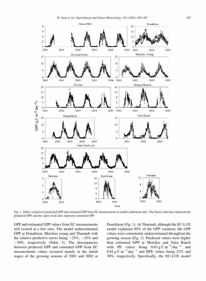
Fig. 1. Daily variation of predicted GPP and estimated GPP from EC measurements at model calibration sites. The black solid lines represent the

predicted GPP, and the open circle dots represent estimated GPP.

GPP and estimated GPP values from EC measurements

still existed at a few sites. The model underestimated

GPP at Donaldson, Metolius young and Tharandt with

the relative predictive errors being �25%, �25% and

�30%, respectively (Table 3). The discrepancies

between predicted GPP and estimated GPP from EC

measurements values occurred mainly in the initial

stages of the growing seasons of 2001 and 2002 at

Donaldson (Fig. 1). At Tharandt, although the EC-LUE

model explained 89% of the GPP variation, the GPP

values were consistently underestimated throughout the

growing season (Fig. 1). Predicted values were higher

than estimated GPP at Metolius and Vaira Ranch

with PE values being 0.63 g C m�2 day�1 and

0.81 g C m�2 day�1 and RPE values being 22% and

38%, respectively. Specifically, the EC-LUE model

W. Yuan et al. / Agricultural and Forest Meteorology 143 (2007) 189–207196

Fig. 2. Predicted vs. the estimated GPP at the model calibration sites

in Table 1. The short dash line is 1:1 line and the solid line is linear

regression line.

overestimated GPP during the mid-growing season at

Metolius (Fig. 1). At the other seven sites, the EC-LUE

model gave good predictions with RPE values lower

than 20% (Table 3).

The predicted GPP and estimated GPP from EC

measurements time series at the calibration sites

demonstrated distinct seasonal cycles and matched

well (Fig. 1). At most sites, GPP values were near zero

in the winter season because low temperature and frozen

soil inhibited photosynthetic activities. The evergreen

needleleaf forest at Donaldson still maintains high

ecosystem production in winter because it is located at

low latitude with adequate temperature. The starting

and end dates of the predicted GPP and estimated GPP

from EC measurements agreed well across all sites. The

average Kendall’s correlation coefficient for the 12

calibration sites was 0.91, indicating strong seasonal

concordance between the simulated and estimated GPP

from EC measurements (Table 3).

3.2. Model validation

We added 16 sites, including various ecosystem

types, to check the performance of the EC-LUE model

(Table 2). The EC-LUE model successfully predicted

the magnitudes and seasonal variations of the estimated

GPP from EC measurements at these new sites (Fig. 3).

Model performance was similar to that at the calibration

sites and explained 77% of the GPP variations across all

16 sites (Fig. 4). No significant systematic errors were

found in the EC-LUE model across the validation sites.

At individual sites, the EC-LUE model explained 59–

96% of the GPP variability with no apparent biases in

any one biome (Table 3).

However, large differences between predicted and

estimated GPP still existed in a few sites, including the

three Boreas NSA burn sites, Lost Creek, Fort Peck and

Tonzi Ranch. At the three Boreas NSA burn sites, the

RPE varied from�44% to�23%. Predicted GPP values

were higher than estimated GPP at Fort Peck, Lost

Creek and Tonzi Ranch with RPE values of 41%, 46%

and 31%, respectively. At the other 10 sites, the RPE

values were lower than 15%.

The predicted seasonal patterns as well as beginning

and end of growing seasons agreed well with the

estimated values from EC measurements at all validation

sites (Fig. 3). The average Kendall’s correlation

coefficient from the 16 validation sites was 0.88,

indicating that predicted GPP had a strong seasonal

coherence with estimated GPP from EC measurements.

3.3. Comparison with the MODIS-GPP product

The MOD17 GPP products were level-4, 1-km

global data collections, downloaded from the FLUX-

NET sites directly. We compared results generated from

the EC-LUE model and MODIS-GPP products at 28

sites. The EC-LUE results were summed over 8-day

periods to match the time scale of MODIS-GPP

products. Comparison was performed only when all

three estimates of GPP were available: estimated GPP

from FLUXNET sites, predicted GPP by the EC-LUE

model and MODIS-GPP products.

Overall, the EC-LUE model performed better than the

MODIS algorithms at these sites according to the values

of R2, PE and RPE (Table 4). The EC-LUE model could

explain 82% of the variation in the 8-day GPP compared

with just 44% by the MODIS-GPP product (Fig. 5). The

PE values of the EC-LUE model and MODIS-GPP were

significantly correlated with the estimated GPP from EC

measurements (Fig. 5). However, it is apparent that the

correlation of EC-LUE was strongly affected by one

extreme value (GPP = 66.69 at Donaldson). Without this

point, PE values of the EC-LUE model were independent

of estimated GPP from EC measurements. As to the RPE

values, significant correlation with the estimated GPP

from EC measurements was only found in the MODIS-

GPP product. However, the slopes of EC-LUE in the

regression equation of PE and RPE with estimated GPP

from EC measurements were closer to zero, with lower

R2 and intercepts that were comparable to the MODIS-

GPP product. Overall, the EC-LUE model offered better

predictions of GPP than the MODIS-GPP product.

W. Yuan et al. / Agricultural and Forest Meteorology 143 (2007) 189–207 197

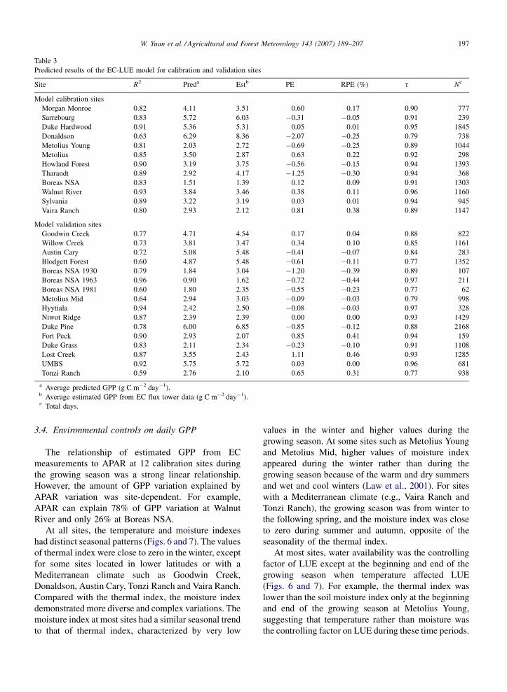
Table 3

Predicted results of the EC-LUE model for calibration and validation sites

Site R2 Preda Estb PE RPE (%) t Nc

Model calibration sites

Morgan Monroe 0.82 4.11 3.51 0.60 0.17 0.90 777

Sarrebourg 0.83 5.72 6.03 �0.31 �0.05 0.91 239

Duke Hardwood 0.91 5.36 5.31 0.05 0.01 0.95 1845

Donaldson 0.63 6.29 8.36 �2.07 �0.25 0.79 738

Metolius Young 0.81 2.03 2.72 �0.69 �0.25 0.89 1044

Metolius 0.85 3.50 2.87 0.63 0.22 0.92 298

Howland Forest 0.90 3.19 3.75 �0.56 �0.15 0.94 1393

Tharandt 0.89 2.92 4.17 �1.25 �0.30 0.94 368

Boreas NSA 0.83 1.51 1.39 0.12 0.09 0.91 1303

Walnut River 0.93 3.84 3.46 0.38 0.11 0.96 1160

Sylvania 0.89 3.22 3.19 0.03 0.01 0.94 945

Vaira Ranch 0.80 2.93 2.12 0.81 0.38 0.89 1147

Model validation sites

Goodwin Creek 0.77 4.71 4.54 0.17 0.04 0.88 822

Willow Creek 0.73 3.81 3.47 0.34 0.10 0.85 1161

Austin Cary 0.72 5.08 5.48 �0.41 �0.07 0.84 283

Blodgett Forest 0.60 4.87 5.48 �0.61 �0.11 0.77 1352

Boreas NSA 1930 0.79 1.84 3.04 �1.20 �0.39 0.89 107

Boreas NSA 1963 0.96 0.90 1.62 �0.72 �0.44 0.97 211

Boreas NSA 1981 0.60 1.80 2.35 �0.55 �0.23 0.77 62

Metolius Mid 0.64 2.94 3.03 �0.09 �0.03 0.79 998

Hyytiala 0.94 2.42 2.50 �0.08 �0.03 0.97 328

Niwot Ridge 0.87 2.39 2.39 0.00 0.00 0.93 1429

Duke Pine 0.78 6.00 6.85 �0.85 �0.12 0.88 2168

Fort Peck 0.90 2.93 2.07 0.85 0.41 0.94 159

Duke Grass 0.83 2.11 2.34 �0.23 �0.10 0.91 1108

Lost Creek 0.87 3.55 2.43 1.11 0.46 0.93 1285

UMBS 0.92 5.75 5.72 0.03 0.00 0.96 681

Tonzi Ranch 0.59 2.76 2.10 0.65 0.31 0.77 938

a Average predicted GPP (g C m�2 day�1).b Average estimated GPP from EC flux tower data (g C m�2 day�1).c Total days.

3.4. Environmental controls on daily GPP

The relationship of estimated GPP from EC

measurements to APAR at 12 calibration sites during

the growing season was a strong linear relationship.

However, the amount of GPP variation explained by

APAR variation was site-dependent. For example,

APAR can explain 78% of GPP variation at Walnut

River and only 26% at Boreas NSA.

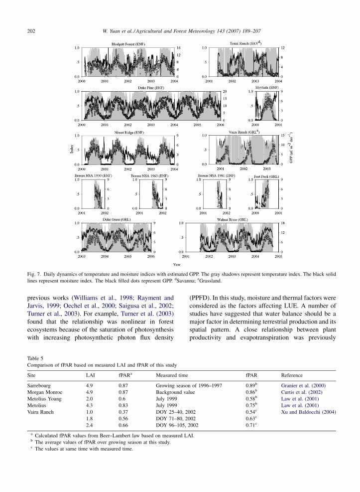
At all sites, the temperature and moisture indexes

had distinct seasonal patterns (Figs. 6 and 7). The values

of thermal index were close to zero in the winter, except

for some sites located in lower latitudes or with a

Mediterranean climate such as Goodwin Creek,

Donaldson, Austin Cary, Tonzi Ranch and Vaira Ranch.

Compared with the thermal index, the moisture index

demonstrated more diverse and complex variations. The

moisture index at most sites had a similar seasonal trend

to that of thermal index, characterized by very low

values in the winter and higher values during the

growing season. At some sites such as Metolius Young

and Metolius Mid, higher values of moisture index

appeared during the winter rather than during the

growing season because of the warm and dry summers

and wet and cool winters (Law et al., 2001). For sites

with a Mediterranean climate (e.g., Vaira Ranch and

Tonzi Ranch), the growing season was from winter to

the following spring, and the moisture index was close

to zero during summer and autumn, opposite of the

seasonality of the thermal index.

At most sites, water availability was the controlling

factor of LUE except at the beginning and end of the

growing season when temperature affected LUE

(Figs. 6 and 7). For example, the thermal index was

lower than the soil moisture index only at the beginning

and end of the growing season at Metolius Young,

suggesting that temperature rather than moisture was

the controlling factor on LUE during these time periods.

W. Yuan et al. / Agricultural and Forest Meteorology 143 (2007) 189–207198

Fig. 3. Daily variation of predicted GPP and estimated GPP from EC measurements at model test sites. The black solid lines represent predicted

GPP, and the open circle dots represent estimated GPP.

W. Yuan et al. / Agricultural and Forest Meteorology 143 (2007) 189–207 199

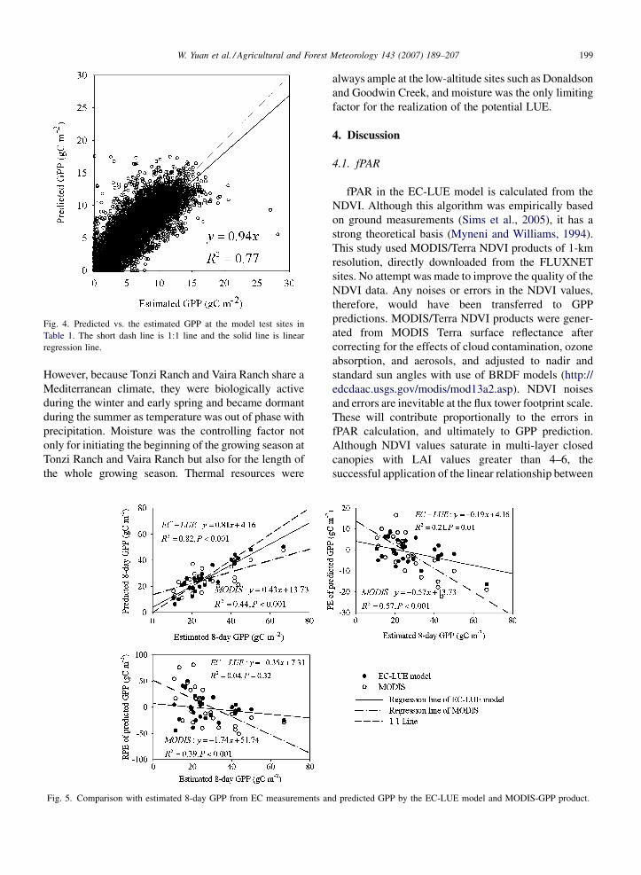
Fig. 4. Predicted vs. the estimated GPP at the model test sites in

Table 1. The short dash line is 1:1 line and the solid line is linear

regression line.

However, because Tonzi Ranch and Vaira Ranch share a

Mediterranean climate, they were biologically active

during the winter and early spring and became dormant

during the summer as temperature was out of phase with

precipitation. Moisture was the controlling factor not

only for initiating the beginning of the growing season at

Tonzi Ranch and Vaira Ranch but also for the length of

the whole growing season. Thermal resources were

Fig. 5. Comparison with estimated 8-day GPP from EC measurements an

always ample at the low-altitude sites such as Donaldson

and Goodwin Creek, and moisture was the only limiting

factor for the realization of the potential LUE.

4. Discussion

4.1. fPAR

fPAR in the EC-LUE model is calculated from the

NDVI. Although this algorithm was empirically based

on ground measurements (Sims et al., 2005), it has a

strong theoretical basis (Myneni and Williams, 1994).

This study used MODIS/Terra NDVI products of 1-km

resolution, directly downloaded from the FLUXNET

sites. No attempt was made to improve the quality of the

NDVI data. Any noises or errors in the NDVI values,

therefore, would have been transferred to GPP

predictions. MODIS/Terra NDVI products were gener-

ated from MODIS Terra surface reflectance after

correcting for the effects of cloud contamination, ozone

absorption, and aerosols, and adjusted to nadir and

standard sun angles with use of BRDF models (http://

edcdaac.usgs.gov/modis/mod13a2.asp). NDVI noises

and errors are inevitable at the flux tower footprint scale.

These will contribute proportionally to the errors in

fPAR calculation, and ultimately to GPP prediction.

Although NDVI values saturate in multi-layer closed

canopies with LAI values greater than 4–6, the

successful application of the linear relationship between

d predicted GPP by the EC-LUE model and MODIS-GPP product.

W. Yuan et al. / Agricultural and Forest Meteorology 143 (2007) 189–207200

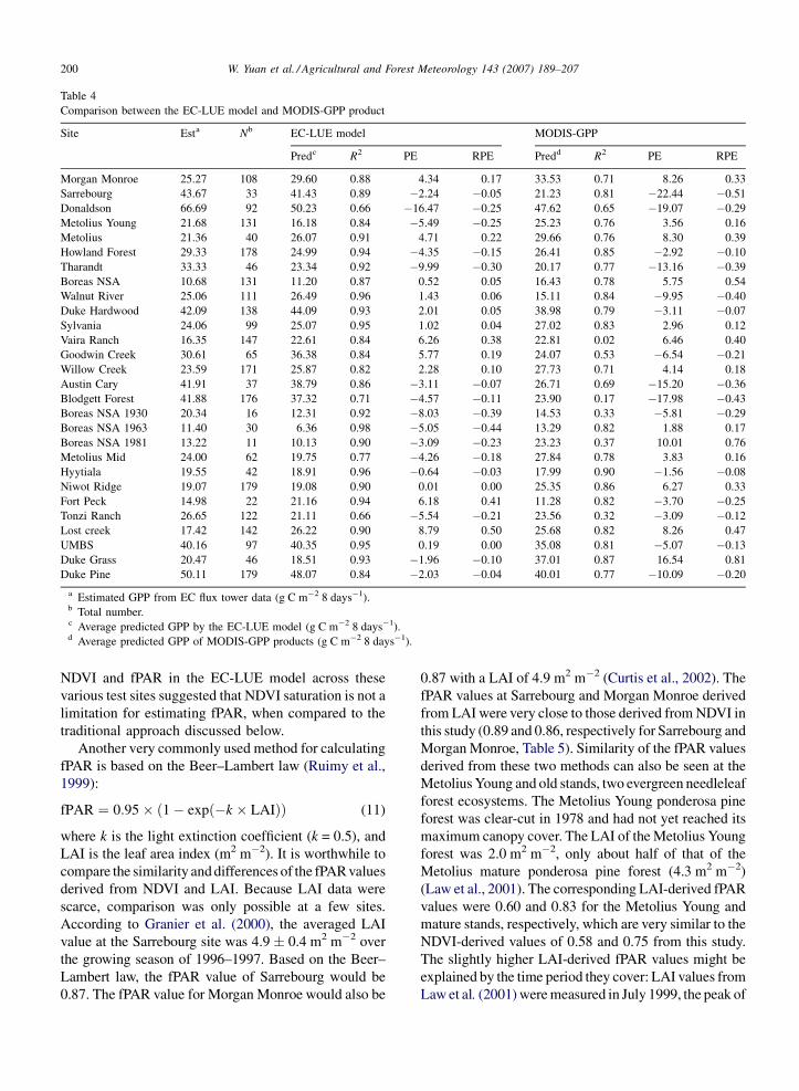
Table 4

Comparison between the EC-LUE model and MODIS-GPP product

Site Esta Nb EC-LUE model MODIS-GPP

Predc R2 PE RPE Predd R2 PE RPE

Morgan Monroe 25.27 108 29.60 0.88 4.34 0.17 33.53 0.71 8.26 0.33

Sarrebourg 43.67 33 41.43 0.89 �2.24 �0.05 21.23 0.81 �22.44 �0.51

Donaldson 66.69 92 50.23 0.66 �16.47 �0.25 47.62 0.65 �19.07 �0.29

Metolius Young 21.68 131 16.18 0.84 �5.49 �0.25 25.23 0.76 3.56 0.16

Metolius 21.36 40 26.07 0.91 4.71 0.22 29.66 0.76 8.30 0.39

Howland Forest 29.33 178 24.99 0.94 �4.35 �0.15 26.41 0.85 �2.92 �0.10

Tharandt 33.33 46 23.34 0.92 �9.99 �0.30 20.17 0.77 �13.16 �0.39

Boreas NSA 10.68 131 11.20 0.87 0.52 0.05 16.43 0.78 5.75 0.54

Walnut River 25.06 111 26.49 0.96 1.43 0.06 15.11 0.84 �9.95 �0.40

Duke Hardwood 42.09 138 44.09 0.93 2.01 0.05 38.98 0.79 �3.11 �0.07

Sylvania 24.06 99 25.07 0.95 1.02 0.04 27.02 0.83 2.96 0.12

Vaira Ranch 16.35 147 22.61 0.84 6.26 0.38 22.81 0.02 6.46 0.40

Goodwin Creek 30.61 65 36.38 0.84 5.77 0.19 24.07 0.53 �6.54 �0.21

Willow Creek 23.59 171 25.87 0.82 2.28 0.10 27.73 0.71 4.14 0.18

Austin Cary 41.91 37 38.79 0.86 �3.11 �0.07 26.71 0.69 �15.20 �0.36

Blodgett Forest 41.88 176 37.32 0.71 �4.57 �0.11 23.90 0.17 �17.98 �0.43

Boreas NSA 1930 20.34 16 12.31 0.92 �8.03 �0.39 14.53 0.33 �5.81 �0.29

Boreas NSA 1963 11.40 30 6.36 0.98 �5.05 �0.44 13.29 0.82 1.88 0.17

Boreas NSA 1981 13.22 11 10.13 0.90 �3.09 �0.23 23.23 0.37 10.01 0.76

Metolius Mid 24.00 62 19.75 0.77 �4.26 �0.18 27.84 0.78 3.83 0.16

Hyytiala 19.55 42 18.91 0.96 �0.64 �0.03 17.99 0.90 �1.56 �0.08

Niwot Ridge 19.07 179 19.08 0.90 0.01 0.00 25.35 0.86 6.27 0.33

Fort Peck 14.98 22 21.16 0.94 6.18 0.41 11.28 0.82 �3.70 �0.25

Tonzi Ranch 26.65 122 21.11 0.66 �5.54 �0.21 23.56 0.32 �3.09 �0.12

Lost creek 17.42 142 26.22 0.90 8.79 0.50 25.68 0.82 8.26 0.47

UMBS 40.16 97 40.35 0.95 0.19 0.00 35.08 0.81 �5.07 �0.13

Duke Grass 20.47 46 18.51 0.93 �1.96 �0.10 37.01 0.87 16.54 0.81

Duke Pine 50.11 179 48.07 0.84 �2.03 �0.04 40.01 0.77 �10.09 �0.20

a Estimated GPP from EC flux tower data (g C m�2 8 days�1).b Total number.c Average predicted GPP by the EC-LUE model (g C m�2 8 days�1).d Average predicted GPP of MODIS-GPP products (g C m�2 8 days�1).

NDVI and fPAR in the EC-LUE model across these

various test sites suggested that NDVI saturation is not a

limitation for estimating fPAR, when compared to the

traditional approach discussed below.

Another very commonly used method for calculating

fPAR is based on the Beer–Lambert law (Ruimy et al.,

1999):

fPAR ¼ 0:95� ð1� expð�k � LAIÞÞ (11)

where k is the light extinction coefficient (k = 0.5), and

LAI is the leaf area index (m2 m�2). It is worthwhile to

compare the similarity and differences of the fPAR values

derived from NDVI and LAI. Because LAI data were

scarce, comparison was only possible at a few sites.

According to Granier et al. (2000), the averaged LAI

value at the Sarrebourg site was 4.9� 0.4 m2 m�2 over

the growing season of 1996–1997. Based on the Beer–

Lambert law, the fPAR value of Sarrebourg would be

0.87. The fPAR value for Morgan Monroe would also be

0.87 with a LAI of 4.9 m2 m�2 (Curtis et al., 2002). The

fPAR values at Sarrebourg and Morgan Monroe derived

from LAI were very close to those derived from NDVI in

this study (0.89 and 0.86, respectively for Sarrebourg and

Morgan Monroe, Table 5). Similarity of the fPAR values

derived from these two methods can also be seen at the

Metolius Young and old stands, two evergreen needleleaf

forest ecosystems. The Metolius Young ponderosa pine

forest was clear-cut in 1978 and had not yet reached its

maximum canopy cover. The LAI of the Metolius Young

forest was 2.0 m2 m�2, only about half of that of the

Metolius mature ponderosa pine forest (4.3 m2 m�2)

(Law et al., 2001). The corresponding LAI-derived fPAR

values were 0.60 and 0.83 for the Metolius Young and

mature stands, respectively, which are very similar to the

NDVI-derived values of 0.58 and 0.75 from this study.

The slightly higher LAI-derived fPAR values might be

explained by the time period they cover: LAI values from

Law et al. (2001) were measured in July 1999, the peak of

W. Yuan et al. / Agricultural and Forest Meteorology 143 (2007) 189–207 201

Fig. 6. Daily dynamics of temperature and moisture indices with estimated GPP. The gray shadows represent temperature index. The black solid

lines represent moisture index. The black filled dots represent GPP. aDeciduous broadleaf forest; bMixed forest; cEvergreen needleleaf forest.

the growing season, while the NDVI-derived values were

based on the mean NDVI value over the entire growing

season. The fPAR values of grasslands and savannas were

lower than those of forest ecosystems because of lower

canopy cover. The fPAR values were 0.57 for Walnut

River, 0.62 for Vaira Ranch, and 0.47 for Tonzi Ranch.

The seasonal trend of the fPAR values at Vaira Ranch

found in this study was similar to that found by Xu and

Baldocchi (2004).

4.2. Environmental controls on daily GPP

Our study’s finding of a strong linear relationship

between daily GPP and APAR at all sites differs from

W. Yuan et al. / Agricultural and Forest Meteorology 143 (2007) 189–207202

Fig. 7. Daily dynamics of temperature and moisture indices with estimated GPP. The gray shadows represent temperature index. The black solid

lines represent moisture index. The black filled dots represent GPP. dSavanna; eGrassland.

previous works (Williams et al., 1998; Rayment and

Jarvis, 1999; Oechel et al., 2000; Saigusa et al., 2002;

Turner et al., 2003). For example, Turner et al. (2003)

found that the relationship was nonlinear in forest

ecosystems because of the saturation of photosynthesis

with increasing photosynthetic photon flux density

Table 5

Comparison of fPAR based on measured LAI and fPAR of this study

Site LAI fPARa Measured time

Sarrebourg 4.9 0.87 Growing seaso

Morgan Monroe 4.9 0.87 Background va

Metolius Young 2.0 0.6 July 1999

Metolius 4.3 0.83 July 1999

Vaira Ranch 1.0 0.37 DOY 25–40, 2

1.8 0.56 DOY 71–80, 2

2.4 0.66 DOY 96–105,

a Calculated fPAR values from Beer–Lambert law based on measured Lb The average values of fPAR over growing season at this study.c The values at same time with measured time.

(PPFD). In this study, moisture and thermal factors were

considered as the factors affecting LUE. A number of

studies have suggested that water balance should be a

major factor in determining terrestrial production and its

spatial pattern. A close relationship between plant

productivity and evapotranspiration was previously

fPAR Reference

n of 1996–1997 0.89b Granier et al. (2000)

lue 0.86b Curtis et al. (2002)

0.58b Law et al. (2001)

0.75b Law et al. (2001)

002 0.54c Xu and Baldocchi (2004)

002 0.63c

2002 0.71c

AI.

W. Yuan et al. / Agricultural and Forest Meteorology 143 (2007) 189–207 203

shown by Rosenzweig (1968), and mean annual

precipitation was used to estimate NPP of those

ecosystems that are not limited by low temperature

(Lieth, 1975). Plant-available water appears to be the

dominant control on leaf area index and NPP of the

forests in the northwestern United States (Gholz, 1982).

Stephenson (1990) and Neilson et al. (1992) illustrated

the high correlation between the distribution of North

American plant formations and water-balance para-

meters. In our study, we used evaporative fraction (EF) to

evaluate moisture availability to plants. At most sites,

water availability was the controlling factor of LUE for

the entire growing season except at the beginning and the

end when temperature was controlling in some ecosys-

tems (Figs. 6 and 7), a result consistent with a number of

phenological studies. In boreal ecosystems, there was a

very good relationship between accumulated tempera-

ture summed above a given threshold and the timing of

bud break (Hannerz, 1999; Linkosalo, 2000). Some

authors have also stressed the role of soil temperature as

the prime factor determining the timing of the onset of

boreal, deciduous forests and temperate conifer photo-

synthesis (Schwarz et al., 1997; Jarvis and Linder, 2000;

Baldocchi et al., 2005). Chen et al. (2005) found that the

spatial patterns of beginning and end dates of growing

season correlated significantly with the spatial patterns of

mean air temperatures in spring and autumn, respec-

tively, in temperate eastern China, and temperature

during the growing season usually did not reach the level

that incurred strong negative temperature effects on

photosynthesis. In our study, temperature index had little

impact on GPP during the growing season, in agreement

with field observations (Polley et al., 1992; Bassow and

Bazzaz, 1998).

We found that under the Mediterranean climate (e.g.,

Tonzi Ranch and Vaira Ranch), soil moisture was the

dominant control factor during the growing season and

temperature only occasionally limited the LUE after

germination in the winter. These results were consistent

with field phenological observations at Tonzi Ranch and

Vaira Ranch that closely followed soil moisture fluctua-

tions (Xu and Baldocchi, 2004). These authors found that

grass seed germination normally occurs in the autumn, 1

week after a major rain event with total precipitation of at

least 15 mm. After germination, due to low soil and air

temperature and occasional frosts, the grasses undergo a

period of slow vegetative growth in the wintertime.

4.3. Realized light use efficiency (LUE)

Light use efficiency was the primary controlling

factor in the LUE model for predicting GPP. Large

discrepancies have arisen in previous studies because

realized LUE has been determined using inconsistent

methods due to different research objectives. LUE has

represented the total NPP or aboveground NPP in most

studies, but rarely to GPP (Gower et al., 1999).

Whichever method is used, LUE is calculated as:

LUE ¼ P

APAR(12)

where P may be NPP, aboveground NPP or GPP. If either

NPP or aboveground NPP is chosen, there would be

several effects on LUE variability. First, some photo-

synthates are immediately used for maintenance and

growth respiration, and respiration has a different depen-

dence on temperature and factors other than LUE (Gower

et al., 1999). Hunt (1994) found that published LUE

values ranged from 0.2 to 1.5 g C MJ�1 for woody

vegetation, and hypothesized that this was the result of

respiration from the 6% to 27% of living cells in the

sapwood of woody stems. Second, the exclusion of

important components of production (e.g., understory,

ground cover, and fine roots) was an important source of

error in most LUE estimates (Gower et al., 1999). Most

LUE estimates were based on aboveground components

of the overstory layer because few measurements of

belowground primary production are available. Biomass

allocation to belowground ranges from 20% to 75% of

NPP in terrestrial biomes and therefore cannot be

ignored. Many researchers calculate total NPP from

measured aboveground primary production. However,

the task of estimating the allocation fraction between

aboveground and belowground primary production is

complicated because of the limited understanding of

the physiological controls on allocation constraints (Frie-

dlingstein et al., 1999). The fraction of total NPP allo-

cated to root production differs among plant functional

groups, different environmental conditions, and with

forest age (Law et al., 2001). Eddy covariance flux towers

offer the best opportunity for estimating GPP at the

ecosystem scale, and improving the calculation of

LUE from GPP and APAR. In this study, GPP estimates

from EC measurements were used to calculate realized

LUE based on Eqs. (1) and (12).

Our study indicated that the mean daily realized LUE

during the growing season was lowest at the boreal forest

sites, highest at the deciduous broadleaf forests, and

intermediate at the grasslands and mixed forests. This

pattern was consistent with other studies (e.g., Turner

et al., 2003; Gower et al., 1999). The LUE of deciduous

forest ecosystems was highest because of ample thermal

resources and moisture. For example, average air

temperature and annual precipitation from 1999 to

W. Yuan et al. / Agricultural and Forest Meteorology 143 (2007) 189–207204

2003 were 12.42 8C and 1030.5 mm at Morgan Monroe,

respectively (http://www.modis.ornl.gov/modis/index.

cfm). The LUE values, 0.62 g C m�2 MJ�1 APAR for

Metolius Mid, 0.68 g C m�2 MJ�1 APAR for Metolius

Young and 0.86 g C m�2 MJ�1 APAR for Metolius-old,

were lower than the realized LUE at other sites because

most of the precipitation in the region occurred between

October and June, with the summer months lacking

effective precipitation (normally 0 � 20 mm July

through August) (Law et al., 2001). The values of EF

were lower during the growing season than in the

wintertime at these sites (Figs. 6 and 7), consistent with

the precipitation pattern. In general, grasslands are

sensitive to soil drought (Nouvellon et al., 2000), but in

this study, the LUE value at Walnut River was

1.38 g C m�2 MJ�1 APAR, second only to the LUE

values of deciduous forest ecosystems. The higher LUE

value at Walnut River was probably related to the

presence of C4 plants (http://www.modis.ornl.gov/

modis/index.cfm) that can maintain a given rate of

photosynthesis with less water and nitrogen compared to

C3 plants (Chapin et al., 2002).

5. Summary

The light use efficiency (LUE) daily GPP model

developed in this study, with a biome-independent

invariant potential LUE, relies on only four driving

variables: PAR, NDVI, air temperature, and evaporative

fraction. Model calibration and validation at 28

FLUXNET sites in North America and Europe

suggested that the model was robust and reliable across

biomes and geographic regions. Comparison with

MODIS-GPP suggested that the EC-LUE model offered

better GPP predictions. The model can be a good

candidate for mapping GPP at the regional to global

scales because it is independent of land cover types, and

all driving variables can be retrieved from satellites or

standard weather observation networks. The suitability

of the EC-LUE model for crop systems should be

investigated in the future. In addition, the causes of

large errors at several FLUXNET sites should be

analyzed especially with regard to the quality of the

input data such as NDVI.

Acknowledgments

This paper benefited from comments from Eugene

Fosnight, John Hutchison, Bruce Wylie and several

anonymous reviewers. We gratefully acknowledge the

financial support from U.S. Geological Survey (the

Geographic Analysis and Monitoring Program and the

Earth Surface Dynamics Program) and NASA Earth

Science Enterprise (grant LUCC99-0022-0035). Liu’s

work was partially performed under U.S. Geological

Survey contract 03CRCN0001. This work was also

jointly supported by NKBRSF (No. G2006CB400502),

National Natural Science Foundation of China (No.

40231018), and the Chinese Academy of Sciences (Nos.

KSCX2- SW-133) and by the Office of Science (BER),

U.S. Department of Energy.

References

Aber, J.D., Reich, P.B., Goulden, M.L., 1996. Extrapolating leaf CO2

exchange to the canopy: a generalized model of forest photo-

synthesis compared with measurements by eddy correlation.

Oecologia 106, 257–265.

AmeriFlux, 2001. http://public.ornl.gov/ameriflux/Participants/Sites/

Map/index.cfm.

Baldocchi, D.D., 2003. Assessing the eddy covariance technique for

evaluating carbon dioxide exchange rates of ecosystems: past,

present and future. Global Change Biol. 9, 479–492.

Baldocchi, D.D., Black, T.A., Curtis, P.S., Falge, E., Fuentes, J.D.,

Granier, A., Gu, L., Knohl, A., Pilegaard, K., Schmid, H.P.,

Valentini, R., Wilson, K., Wofsy, S., Xu, L., Yamamoto, S.,

2005. Predicting the onset of net carbon uptake by deciduous

forests with soil temperature and climate data: a synthesis of

FLUXNET data. Int. J. Biometeorol. 49 (6), 377–387.

Baldocchi, D.D., Xu, L.K., Kiang, N., 2004. How plant functional-

type, weather, seasonal drought, and soil physical properties alter

water and energy fluxes of an oak-grass savanna and an annual

grassland. Agric. For. Meteorol. 123 (1/2), 13–39.

Bassow, S.L., Bazzaz, F.A., 1998. How environmental conditions

affect canopy leaf-level photosynthesis in four deciduous tree

species. Ecology 79, 2660–2675.

Bolstad, P.V., Davis, K.J., Martin, J., Cook, B.D., Wang, W., 2004.

Component and whole-system respiration fluxes in northern

deciduous forests. Tree Physiol. 24 (5), 493–504.

Bondeau, A., Kicklighter, D.W., Kaduk, J., The Participants of the

Potsdam NPP Model Intercomparison, 1999. Comparing global

models of terrestrial net primary productivity (NPP): importance

of vegetation structure on seasonal NPP estimates. Global Change

Biol. 5, 35–45.

Braswell, B.H., Sacks, W.J., Linder, E., Schimel, D.S., 2005. Estimat-

ing diurnal to annual ecosystem parameters by synthesis of a

carbon flux model with eddy covariance net ecosystem exchange

observations. Global Change Biol. 11, 335–355.

Canadell, J.G., Mooney, H.A., Baldocchi, D.D., Berry, J.A., Ehler-

inger, B., Field, C.B., Gower, S.T., Hollinger, D.Y., Hunt, J.E.,

Jackson, R.B., Running, S.W., Shaver, G.R., Steffen, W., Trum-

bore, S.E., Valentini, R., Bond, B.Y., 2000. Carbon metabolism of

the terrestrial biosphere: a multi-technique approach for improved

understanding. Ecosystems 3, 115–130.

Chapin, M.C., Matson, P.A., Mooney, H.A. (Eds.), 2002. Principles

of Terrestrial Ecosystem Ecology. Springer-Verlag, New York,

Berlin, Heidelberg, p. 102.

Chen, X.Q., Hu, B., Yu, R., 2005. Spatial and temporal variation of

phonological growing season and climate change impacts in

temperature eastern China. Global Change Biol. 11, 1118–1130.

Coops, N.C., Waring, R.H., Law, B.E., 2005. Assessing the past and

future distribution and productivity of ponderosa pine in the

W. Yuan et al. / Agricultural and Forest Meteorology 143 (2007) 189–207 205

pacific northwest using a process model, 3-PG. Ecol. Model. 183,

107–124.

Curtis, P.S., Hanson, P.J., Bolstad, P., Barford, C., Randolph, J.C.,

Schmid, H.P., Wilson, K.B., 2002. Biometric and eddy-covariance

based estimates of annual carbon storage in five eastern North

American deciduous forests. Agric. For. Meteorol. 113, 3–19.

Curtis, P.S., Vogel, C.S., Gough, C.M., Schmid, H.P., Su, H.B.,

Bovard, B.D., 2005. Respiratory carbon losses and the carbon-

use efficiency of a northern hardwood forest, 1999–2003. New

Phytol. 167, 437–456.

Davis, K.J., Bakwin, P.S., Yi, C.X., Berger, B.W., Zhao, C., Teclaw,

R.M., Isebrands, J.G., 2003. The annual cycles of CO2 and H2O

exchange over a northern mixed forest as observed from a very tall

tower. Global Change Biol. 9, 1278–1293.

Desai, A.R., Bolstad, P.V., Cook, B.D., Davis, K.J., Carey, E.V., 2005.

Comparing net ecosystem exchange of carbon dioxide between an

old-growth and mature forest in the upper Midwest, USA. Agric.

For. Meteorol. 128, 33–55.

Dufrene, E., Davi, H., Francois, C., Le Maire, G., Le Dantec, V.,

Granier, A., 2005. Modelling carbon and water cycles in a beech

forest. Part I. Model description and uncertainty analysis on

modelled NEE. Ecol. Model. 85, 407–436.

Falge, E., Baldocchi, D., Tenhunen, J., Aubinet, M., Bakwin, P.,

Berbigier, P., Bernhofer, C., Burba, G., Clement, R., Davis, K.J.,

Elbers, J.A., Goldstein, A.H., Grelle, A., Granier, A., Guo-

mundsson, J., Hollinger, D., Kowalski, A.S., Katul, G., Law,

B.E., Malhi, Y., Meyers, T., Monson, R.K., 2002. Seasonality of

ecosystem respiration and gross primary production as derived

from FLUXNET measurements. Agric. For. Meteorol. 113, 53–

74.

Friedlingstein, P., Joel, G., Field, C.B., Fung, I.Y., 1999. Toward an

allocation scheme for global terrestrial carbon models. Global

Change Biol. 5, 755–770.

Gholz, H.L., Clark, K.L., 2002. Energy exchange across a chronose-

quence of slash pine forests in Florida. Agric. For. Meteorol. 112

(2), 87–102.

Gholz, H.Z., 1982. Environmental limits on aboveground net primary

production, leaf area and biomass in vegetation zones in the Pacific

Northwest. Ecology 63, 469–481.

Gilmanov, T.G., Tieszen, L.L., Wylie, B.K., Flanagan, L., Frank, A.,

Meyers, T., 2005. Integration of CO2 flux and remotely-sensed

data for primary production and ecosystem respiration analyses in

the Northern Great Plains: potential for quantitative spatial extra-

polation. Global Ecol. Biogeogr. 14, 271–292.

Goldstein, A.H., Hultman, N.E., Fracheboud, J.M., Bauer, M.R.,

Panek, J.A., Xu, M., Qi, Y., Guenther, A.B., Baugh, W., 2000.

Effects of climate variability on the carbon dioxide, water, and

sensible heat fluxes above a ponderosa pine plantation in the Sierra

Nevada (CA). Agric. For. Meteorol. 101, 113–129.

Goulden, M.L., Wofsy, S.C., Harden, J.W., Trumbore, S.E., Crill,

P.M., Gower, S.T., Fries, T., Daube, B.C., Fan, S.M., Sutton, D.J.,

Bazzaz, A., Munger, J.W., 1998. Sensitivity of boreal forest carbon

balance to soil thaw. Science 279 (5348), 214–217.

Goulden, M.L., Winston, G.C., McMillan, A.M.S., Litvak, E.E., Read,

E.L., Rocha, A.V., Elliot, J.R., 2006. An eddy covariance mesonet

to measure the effect of forest age on land-atmosphere exchange.

Global Change Biol. 12 (11), 2146–2162.

Gower, S.T., Kucharik, C.J., Norman, J.M., 1999. Direct and indirect

estimation of leaf area index, fAPAR, and net primary production

of terrestrial ecosystems. Remote Sens. Environ. 70, 29–51.

Granier, A., Ceschia, C., Damesin, C., Dufrene, E., Epron, D., Gross,

P., Lebaube, S., Dantec, V.L.E., Goff, N.L.E., Lemoine, D., Lucot,

E., Ottorini, J.M., Pontailler, J.Y., Saugier, S., 2000. The carbon

balance of a young Beech forest. Funct. Ecol. 14, 312–325.

Hannerz, M., 1999. Evaluation of temperature models for predicting

bud burst in Norway spruce. Can. J. For. Res. 29, 1–11.

Heinsch, F.A., Zhao, M., Running, S.W., Kimball, J.S., Nemani, R.R.,

Davis, K.J., Bolstad, P.V., Cook, B.D., Desai, A.R., Ricciuto,

D.M., Law, B.E., Oechel, W.C., Kwon, H., Luo, H., Wofsy,

S.C., Dunn, A.L., Munger, J.W., Baldocchi, D.D., Xu, L., Hol-

linger, D.Y., Richardson, A.D., Stoy, P.C., Siqueira, M.B.S.,

Monson, R.K., Burns, S.P., Flanagan, L.B., 2006. Evaluation of

remote sensing based terrestrial production from MODIS using

AmeriFlux eddy tower flux network observations. IEEE Trans.

Geosci. Remote Sens. 44, 1908–1925.

Hollinger, D.Y., Aber, J., Dail, B., Davidson, E.A., Goltz, S.M.,

Hughes, H., Leclerc, M.Y., Lee, J.T., Richardson, A.D., Rodrigues,

C., Scott, N.A., Achuatavarier, D., Walsh, J., 2004. Spatial and

temporal variability in forest-atmosphere CO2 exchange. Global

Change Biol. 10, 1689–1706.

Hollinger, D.Y., Goltz, S.M., Davidson, E.A., Lee, J.T., Tu, K.,

Valentine, H.T., 1999. Seasonal patterns and environmental con-

trol of carbon dioxide and water vapour exchange in an ecotonal

boreal forest. Global Change Biol. 5, 891–902.

Hunt, E.R., 1994. Relationship between woody biomass and PAR

conversion efficiency for estimating net primary production from

NDVI. Int. J. Remote Sens. 15, 1725–1730.

Jarvis, P., Linder, S., 2000. Constraints to growth of boreal forests.

Nature 405, 904–905.

Kanji, G.K., 1999. 100 Statistical Tests. SAGE Publications, London.

Kramer, K., Leinonen, I., Bartelink, H.H., Berbigier, P., Borghetti, M.,

Bernhofer, C., Cienciala, E., Dolman, A.J., Froer, O., Gracia, C.A.,

Granier, A., Grunwald, T., Hari, P., Jans, W., Kellomaki, S.,

Loustau, D., Magnani, F., Markkanen, T., Matteucci, G., Mohren,

G.M.J., Moors, E., Nissinen, A., Peltola, H., Sabate, S., Sanchez,

A., Sontag, M., Valentini, R., Vesala, T., 2002. Evaluation of six

process-based forest growth models using eddy-covariance mea-

surements of CO2 and H2O fluxes at six forest sites in Europe.

Global Change Biol. 8, 213–230.

Kurc, S.A., Small, E.E., 2004. Dynamics of evapotranspiration in

semiarid grassland and shrubland ecosystems during the summer

monsoon season, central New Mexico. Water Resour. Res. 40,

W09305, doi:10.1029/2004WR003068.

Landsberg, J.J., 1986. Physiological Ecology of Forest Production.

Academic Press, London, pp. 165–178.

Landsberg, J.J., Waring, R.H., 1997. A generalised model of forest

productivity using simplified concepts of radiation-use efficiency,

carbon balance and partitioning. For. Ecol. Manage. 95, 209–228.

Law, B.E., Thornton, P.E., Irvine, J., Anthoni, P.M., Tuy, S.V., 2001.

Carbon storage and fluxes in ponderosa pine forests at different

developmental stages. Global Change Biol. 7, 755–777.

Law, B.E., Turner, D., Campbell, J., Sun, O.J., Van Tuyl, S., Ritts,

W.D., Cohen, W.B., 2004. Disturbance and climate effects on

carbon stocks and fluxes across Western Oregon USA. Global

Change Biol. 10, 1429–1444.

Law, B.E., Waring, R.H., 1994a. Combining remote sensing and

climatic data to estimate net primary production across Oregon.

Ecol. Appl. 4, 717–728.

Law, B.E., Waring, R.H., 1994b. Remote sensing of leaf area index

and radiation intercepted by understory vegetation. Ecol. Appl. 4,

272–279.

Law, B.E., Williams, M., Anthoni, P.M., Baldocchi, D.D., Unsworth,

M.H., 2000a. Measuring and modelling seasonal variation of

carbon dioxide and water vapour exchange of a Pinus ponderosa

W. Yuan et al. / Agricultural and Forest Meteorology 143 (2007) 189–207206

forest subject to soil water deficit. Global Change Biol. 6, 613–

630.

Law, B.E., Waring, R.H., Anthoni, P.M., Aber, J.D., 2000b. Measure-

ments of gross and net ecosystem productivity and water vapour

exchange of a Pinus ponderosa ecosystem, and an evaluation of

two generalized models. Global Change Biol. 6 (2), 155–168.

Lewis, J.M., 1995. The story behind the Bowen ratio. Bull. Am.

Meteorol. Soc. 76, 2433–2443.

Lieth, H., 1975. Modeling the primary productivity of the world. In:

Lieth, H., Whittaker, R.H. (Eds.), Primary Productivity of the

Biosphere. Springer-Verlag, New York, pp. 237–262.

Linkosalo, T., 2000. Mutual regularity of spring phenology of some

boreal tree species: predicting with other species and phonological

models. Can. J. For. Res. 30, 667–673.

Marshall, B., Biscoe, P.V., 1980. A model of C3 leaves describing the

dependence of net photosynthesis on irradiance. J. Exp. Bot. 31,

29–39.

Monson, R.K., Turnipseed, A.A., Sparks, J.P., Harley, P.C., Scott-

Denton, L.E., Sparks, K., Huxman, T.E., 2002. Carbon sequestra-

tion in a high-elevation, subalpine forest. Global Change Biol. 8,

459–478.

Myneni, R.B., Williams, D.L., 1994. On the relationship between

FAPAR and NDVI. Remote Sens. Environ. 49, 200–221.

Neilson, R.P., King, C.A., Koerper, E., 1992. Toward a rule-based

biome model. Landscape Ecol. 7, 27–43.

Nouvellon, Y., Seen, D.L., Verma, S.G., 2000. Time course of radia-

tion use efficiency in a shortgrass ecosystem: consequences for

remotely sensed estimation of primary production. Remote Sens.

Environ. 71, 43–55.

Novick, K.A., Stoy, P.C., Katul, G.G., Ellsworth, D.E., Siqueira, M.B.S.,

Juang, J., Oren, R., 2004. Carbon dioxide and water vapor exchange

in a warm temperate grassland. Oecologia 138, 259–274.

Oechel, W.C., Vourlitis, G.L., Verfailier, J., Crawford, T., Brooks, S.,

Dumas, E., Hope, A., Stow, D., Boynton, B., Nosov, V., Zulueta,

R., 2000. A scaling approach for quantifying the net CO2 flux of

the Kuparuk river basin, Alaska. Global Change Biol. 6, 160–173.

Pataki, D.E., Oren, R., 2003. Species differences in stomatal control of

water loss at the canopy scale in a mature bottomland deciduous

forest. Adv. Water Resour. 26, 1267–1278.

Polley, H.W., Norman, J.M., Arkebauer, T.J., Walter-Shea, E.A., Gree-

gor, D.H., Bramer, B., 1992. Leaf gas exchange of Andropogon

gerardii Vitman, Panicum virgatum L. and Sorghastrum mutans (L.)

Nash in a tallgrass prairie. J. Geophys. Res. 97, 18837–18844.

Potter, C.B., Randerson, J.T., Field, C.B., Matson, P.A., Vitousek,

P.M., Mooney, H.A., Klooster, S.A., 1993. Terrestrial ecosystem

production: a process model based on global satellite and surface

data. Global Biogeochem. Cycle 7, 811–841.

Prince, S.D., Goward, S.N., 1995. Global primary production: a

remote sensing approach. J. Biogeogr. 22, 815–835.

Raich, J.W., Rastetter, E.B., Melillo, J.M., Kicklighter, D.W., Steudler,

P.A., Peterson, B.J., Grace, A.L., Moore, B., Vorosmarty, C.J.,

1991. Potential net primary productivity in South America: appli-

cation of a global model. Ecol. Appl. 1, 399–429.

Rayment, M.B., Jarvis, P.G., 1999. Seasonal gas exchange of black

spruce using an automatic branch bag system. Can. J. For. Res. 29,

1528–1538.

Rosenzweig, M.L., 1968. Net primary productivity of terrestrial

communities: prediction from climatological data. Am. Nat.

102, 67–74.

Ruimy, A., Kergoat, L., Bondeau, A., The Participants of the Potsdam

NPP Model Intercomparison, 1999. Comparing global models of

terrestrial net primary productivity (NPP): analysis of differences

in light absorption and light-use efficiency. Global Change Biol. 5,

56–64.

Ruimy, A., Saugier, B., 1994. Methodology for the estimation of

terrestrial net primary production from remotely sensed data. J.

Geophys. Res. 97, 18515–18521.

Running, S.W., Nemani, R., Glassy, J.M., Thornton, P.E., 1999.

MODIS daily photosynthesis (PSN) and annual net primary

production (NPP) product (MOD17), algorithm theoretical basis

document, version 3.0. In: http://modis.gsfc.nasa.gov/.

Running, S.W., Nemani, R.R., Heinsch, F.A., Zhao, M.S., Reeves, M.,

Hashimoto, H., 2004. A continuous satellite-derived measure of

global terrestrial primary production. Bioscience 54, 547–560.

Running, S.W., Thornton, P.E., Nemani, R., Glassy, J.M., 2000. Global

terrestrial gross and net primary productivity from the earth

observing system. In: Sala, O.E., Jackson, R.B., Mooney, H.A.

(Eds.), Methods in Ecosystem Science. Springer-Verlag, New

York, pp. 44–57.

Russell, G., Jarvis, P.G., Monteith, J.L., 1989. Absorption of radiation

by canopies and stand growth. In: Russell, G., Marshall, B., Jarvis,

P.G. (Eds.), Plant Canopies: Their Growth, Form and Function.

Cambridge Univ. Press, Cambridge, pp. 21–39.

Saigusa, N., Yamamotoa, S., Murayamaa, S., Kondoa, H., Nishi-

murab, N., 2002. Gross primary production and net ecosystem

exchange of a cool-temperate deciduous forest estimated by the

eddy covariance method. Agric. For. Meteorol. 112, 203–215.

Saito, M., Miyata, A., Nagai, H., Yamada, T., 2005. Seasonal variation

of carbon dioxide exchange in rice paddy field in Japan Tomoyasu

Yamada. Agric. For. Meteorol. 135, 93–109.

Schmid, H.P., Grimmond, C.S.B., Cropley, F., Offerle, B., Su, H.B.,

2000. Measurements of CO2 and energy fluxes over a mixed

hardwood forest in the mid-western United States. Agric. For.

Meteorol. 103 (4), 357–374.

Schwarz, P.A., Fahey, T.J., Dawson, T.E., 1997. Seasonal air and soil

temperature effects on photosynthesis in red spruce (Picea rubens)

saplings. Tree Physiol. 17, 187–194.

Sims, D.A., Rahman, A.F., Cordova, V.D., Baldocchi, D.D., Flanagan,

L.B., Goldstein, A.H., Hollinger, D.Y., Misson, L., Monson, R.K.,

Schmid, H.P., Wofsy, S.C., Xu, L.K., 2005. Midday values of gross

CO2 flux and light use efficiency during satellite overpasses can be

used to directly estimate eight-day mean flux. Agric. For.

Meteorol. 131, 1–12.

Song, J., Liao, K., Coulter, R.L., Lesht, B.M., 2005. Climatology of

the low-level jet at the southern Great Plains atmospheric Bound-

ary Layer Experiments site. J. Appl. Meteorol. 44, 1593–1606.

Stephenson, N.L., 1990. Climate control of vegetation distribution: the

role of the water balance. Am. Nat. 135, 649–670.

Stoy, P.C., Katul, G.G., Siqueira, M.B.S., Juang, J.Y., Novick, K.A.,

Oren, R., 2006. An evaluation of methods for partitioning eddy

covariance-measured net ecosystem exchange into photosynthesis

and respiration. Agric. For. Meteorol. 141, 2–18.

Suleiman, A., Crago, R., 2004. Hourly and daytime evapotranspiration

from grassland using radiometric surface temperatures. Agron. J.

96, 384–390.

Turner, D.P., Urbanski, S., Bremer, D., Wofsy, S.C., Meyers, T.,

Gower, S.T., Gregory, M., 2003. A cross-biome comparison of

daily light-use efficiency for gross primary production. Global

Change Biol. 9, 385–395.

Valentini, R. (Ed.), 2003. Fluxes of Carbon, Water and Energy of

European Forests, Springer Verlag, Heidelberg, pp. 260.

van Wijk, M.T., Bouten, W.M.T., 2002. Simulating daily and half-

hourly fluxes of forest carbon dioxide and water vapor exchange

with a simple model of light and water use. Ecosystems 5, 597–610.

W. Yuan et al. / Agricultural and Forest Meteorology 143 (2007) 189–207 207

Venturini, V., Bisht, G., Islam, S., Jiang, L., 2004. Comparison of

evaporative fractions estimated from AVHRR and MODIS sensors

over South Florida. Remote Sens. Environ. 93, 77–86.

Veroustraete, F., Sabbe, H., Eerens, H., 2002. Estimation of carbon

mass fluxes over Europe using the C-Fix model and Euroflux data.

Remote Sens. Environ. 83, 376–399.

Wang, Q., Tenhunen, J., Falge, E., Bernhofer, C.H., Granier, A.,

Vesala, T., 2003. Simulation and scaling of temporal variation

in gross primary production for coniferous and deciduous tempe-

rate forests. Global Change Biol. 10, 37–51.

Waring, R.H., Landsberg, J.J., Williams, M., 1998. Net primary

production of forests: a constant fraction of gross primary

production? Tree Physiol. 18, 129–134.

Williams, M., Malhi, Y., Nobre, D., Rastetter, E.B., Grace, J., Pereira,

M.G.P., 1998. Seasonal variation in net carbon exchange and

evapotranspiration in a Brazilian rain forest: a modeling analysis.

Plant Cell Environ. 21, 935–968.

Williams, M., Schwarz, P.A., Law, B., Irvine, J., Kurpius, M.R., 2005.

An improved analysis of forest carbon dynamics using data

assimilation. Global Change Biol. 11, 89–105.

Xiao, X.M., Zhang, Q.Y., Braswell, B., Urbanski, S., Boles, S., Wofsy,

S., Moore, B., Ojima, D., 2004. Modeling gross primary produc-

tion of temperate deciduous broadleaf forest using satellite images

and climate data. Remote Sens. Environ. 91, 256–270.

Xiao, X.M., Zhang, Q.Y., Hollinger, D., Aber, J., Moore, B., 2005a.

Modeling gross primary production of an evergreen needleleaf

forest using MODIS and climate data. Ecol. Appl. 15 (3), 954–

969.

Xiao, X.M., Zhang, Q.Y., Saleska, S., Hutyra, L., Camargo, P.,

Wofsy, S., Frolking, S., Boles, S., Keller, M., Moore, B.,

2005b. Satellite-based modeling of gross primary production

in a seasonally moist tropical evergreen forest. Remote Sens.

Environ. 94, 105–122.

Xu, L.K., Baldocchi, D.D., 2004. Seasonal variation in carbon dioxide

exchange over a Mediterranean annual grassland in California.

Agric. For. Meteorol. 123, 79–96.

Zhang, Y.Q., Liu, C.M., Yu, Q., Shen, Y.J., Kendy, E., Kondoh, A.,

Tang, C.Y., Sun, H.Y., 2004. Energy fluxes and the Priestley-

Taylor parameter over winter wheat and maize in the North China

Plain. Hydrol. Process. 18, 2235–2246.