Deriving Information from Sampling and Diving

1

Deriving information from sampling and diving

Michele Lombardi C

[email protected],Alma Mater StudiorumUniversita di BolognaV.le Risorgimento 2, 40136, Bologna, Italy

Michela [email protected],Alma Mater StudiorumUniversita di BolognaV.le Risorgimento 2, 40136, Bologna, Italy

Andrea [email protected] - Campus of Cesena,Alma Mater StudiorumUniversita di BolognaVia Venezia 52, 47023, Cesena, Italy

Alessandro [email protected] EuropePlace de l’Universite 16, 1348, Louvain-La-Neuve,Belgium

Keywords: Constraint Satisfaction Problem, Sampling, Diving, Solution Counting, Heuristics Eval-uation

Abstract. We investigate the impact of information extracted fromsamplinganddiving on the so-lution of Constraint Satisfaction Problems (CSP). A sampleis a complete assignment of variables tovalues taken from their domain according to a given distribution. Diving consists in repeatedly per-forming depth first search attempts with random variable andvalue selection, constraint propagationenabled and backtracking disabled; each attempt is called adive and, unless a feasible solution isfound, it is a partial assignment of variables (whereas a sample is a –possibly infeasible– completeassignment). While the probability of finding a feasible solution via sampling or diving is negligibleif the problem is difficult enough, samples and dives are veryfast to generate and, intuitively, evenwhen they are infeasible, they can provide some statisticalinformation on search space structure.The aim of this paper is to understand to what extent it is possible to support the CSP solving pro-cess with information derived from sampling and diving. In particular, we are interested in extractingfrom samples and dives precise indications on the quality ofindividual variable-value assignmentswith respect to feasibility. We formally prove that even uniform sampling could provide preciseevaluation of the quality of single variable-value assignments; as expected, this requires huge sam-ple sizes and is therefore not useful in practice. On the contrary, diving is much better suited forassignment evaluation purposes. We undertake a thorough experimental analysis on a collection ofPartial Latin Square and Car Sequencing instances to assessthe quality of information provided bydives. Dive features are identified and their impact on search is evaluated. Results show that divingprovides information that can be fruitfully exploited.

CCorresponding author

2 author / short title

1. Introduction

Exploiting information collected during search is often one of the key components for the successfulsolution of Constraint Satisfaction Problems (CSPs). In this work, we address the issue of formallystudying to what extent it is possible to extract information from two kinds of sampling techniques,namely random sampling and diving. In particular, we are interested in extracting precise indications onhow good/bad are individual variable-value assignments, with a focus oninformation regarding problemfeasibility.

The collected information can be used for designing search heuristics, for partitioning domains indecomposition based search [10], for over-filtering unpromising valuesfrom variable domains, or fordefining suitable local moves to repair an infeasible assignment.

In this paper, we will call asamplean assignment of variables to values taken from their domains.In case of random samples, variables and values are chosen according to a uniform distribution. Adive,on the contrary, is obtained by tree search in which a variable and a value inits domain are randomlychosen and after each assignment propagation filters out values proved to be infeasible with the currentpartial assignments. We will limit our discussion to samples and dives collected at the root node (in apre-processing phase of the search) and to uniform distributions.

We will first define a formal probabilistic model that makes it possible to estimate through sam-pling the probability that the problem remains feasible after a specific event occurs, such as a singlevariable-value assignment. This study shows that it is possible to extract valuable information from ran-dom sampling in a sound theoretical framework. Nevertheless, in the case of large-size instances, thisapproach has the drawback that a good estimation of the variable-value assignment probability can beachieved only at the price of huge sample sizes.

As a second step, we will show how to extract dive features to measure thepotential feasibilityand infeasibility of single variable-value assignments, using Partial Latin Square completion and CarSequencing as sample problems [8]. Parameters such as the average dive length and the number ofvariable-value occurrences enable us to extract pieces of information on the quality of single variable-value assignments. Experimental results show that some of the features extracted from dives are veryinformative, having accuracy (w.r.t. to feasibility) comparable to or better than a state-of-the-art heuristicused in Impact Based Search [17].

To the best of our knowledge, a formal analysis of this kind has not yet been published in the lit-erature, except for our introductory work on this subject [14]. This paper substantially extends andcompletes our previous work by adding further experimental evaluations mainly concerning(i) the cor-relation between the real solution density (computed by exhaustive enumeration) and parameters derivedfrom diving by defining a set of error rate indicators;(ii) the complementarity of the diving parameters;(iii) the effect of different propagation algorithms on diving parameters;(iv) the use of diving parametersinto a search strategy and their comparison with impact based search;(v) experimentations on a newproblem domain, that is the Car Sequencing problem.

The remainder of the paper is organized as follows: in Sect.2, we provide an overview of relatedwork. In Sect.3, we present a formal model for evaluating the quality of information provided by sam-pling and delineating the limits of its applicability. In Sect.4, we define diving and themain featureswhich will be considered in the experimental analysis presented in Sect.5. Finally, in Sect.6 we summa-rize the main results of this contribution and we outline directions for further research.

author / short title 3

2. Related work

Uniform sampling of solutions has been recently studied by Gogate and Dechter in [4]. Their approachuses a randomized backtracking procedure guided by a heuristic computed through generalized beliefpropagation. In order to avoid the rejection problem (ending up to an infeasible solution) they systemati-cally search for a feasible solution using a standard backtracking procedure. In a follow-up work [5] theyadded a second re-sampling phase that gives approximation guaranteesthat the distribution of sampledsolutions converges to the uniform distribution.

Gomes et al. in [7] also propose an algorithm for sampling solutions of SAT problems. They iter-atively add streamlining constraints to the SAT formula to reduce the set of solutions (possibly to onlyone) and they return one solution chosen uniformly at random. Our approach mainly differs from thetwo described above in the fact that we sample assignments that can be either(very unlikely) feasible orinfeasible whereas they sample only feasible solutions (thus with an exponential computational effort).

Knuth proposed in 1975 [12] an estimator of a search tree based on random probing of the searchspace, exploiting the branching factor at each node of the search tree.

In [2], Boussemart et al. propose a conflict-driven variable ordering heuristic: they extend the conceptof variable degree integrating a simple but effective learning technique that takes into account failures.Basically, each constraint has a weight associated that is increased by one each time the constraint leadsto a failure (i.e. a domain wipe-out). Grimes and Wallace in [9] employ random dives (referred to asprobes) to initialize the process. Nevertheless, during the diving phase,they do not collect any explicitinformation regarding variable assignments and dive lengths.

Ruml proposes in [20] to use adaptive probes to iteratively learn the search strategy to be employedin exploring a search tree. In constraint satisfaction problems, he measures the quality of a dive in termsof the number of instantiated variables (dive length). The algorithm then adaptively adjusts the heuristicused for the following dives.

In [1] random dives are used to initialize an elite set of partial solutions where the number of assignedvariables is taken as a quality measure. An elite solution is then randomly chosento provide heuristicguidance. Note that the heuristic is based solely on a single elite (partial) solution whereas our approachtries to infer general information from the whole set of partial solutions.

Refalo in [17] proposes a heuristic (known as Impact Based Search) that estimates the effort of thesearch as the proportional reduction of the Cartesian product of the variable domains after a variableinstantiation. This estimation (referred to asimpact) is initialized at the beginning of the search througha dichotomic search in which each variable domain is iteratively split into two sub-domains.

As an interesting connection, in the following we cite some approaches that share the same aim ofthis paper, i.e., deriving measures on the quality of individual variable-value assignments with respectto feasibility. Hsu et al. [11] apply a Belief Propagation algorithm within an Expectation Maximizationframework (EMBP) in order to approximate variable biases (or marginals),i.e., the probability that avariable takes a given value in a solution. Even though the approach is general, they derive formulas forcomputing and updating the variable biases only for thealldifferent constraint and they experimentedon the Partial Latin Square problem. The computation of variable biases is time-consuming but they showthat the heuristic is effective even when it is employed only in the top part of the search tree. That workhas been recently extended by Le Bras et al. in [13]; the contribution is twofold: firstly, they generalizeHsu et al.’s method to tackle any global constraint; secondly, they leverage the same method to considerthe problem model as an individual (likely NP-Hard) constraint. Unfortunately, previous works do not


assess the quality of the derived estimates w.r.t. exact probabilities.Finally, Zanarini et al. [21] employs counting algorithm at the constraint level to find an exact or

approximate probability of a given variable-value pair to be in a solution of a constraint. The estimatesare exploited to guide the search and they attain promising results on some benchmark problems. Nev-ertheless, the information extracted by this approach is focused on individual constraints rather than onthe whole problem as we do in this study.

We point out that in none of the methods described above systematic statistic measures are extractedfrom the random dives; in fact, our approach can be thought as beingorthogonal to the described ones,as the emphasis is on evaluating the feasibility related information extracted fromsamples and divesrather than on providing a top quality heuristic. As a consequence, the method we propose can be easilyintegrated in most of the mentioned frameworks.

3. Uniform Sampling

In this section, we study the quality of information that samples can provide on individual variable-value assignments. A formal model is defined in terms of probability that the problem at hand remainsfeasible after a variable-value assignment. This analytical model makes it possible to formally expressthe information provided by sampling and the relation between number of samplesand informationaccuracy.

Definition 3.1. Assume we are given aCSP = (X,D,C) whereX = X1, . . . Xn is the set ofvariables,D = D1, . . . Dn the set of domains andC = c1, . . . ck the set of constraints. Asamplesis an element of the Cartesian product of the domains of all problem variables,s ∈

∏ni=1Di. Constraints

are not taken into account in the definition ofs. A uniform, or random, sampleis a sample taken w.r.t. auniform distribution over

∏ni=1Di.

The idea is that by sampling the search space randomly, either we find a solution to the problem,and we are done, or we collect only infeasible samples. In the second case, we can try to measure thefeasibility or infeasibility degree of single variable-value assignments. Suppose to model the samplegeneration problem as a stochastic variable with sample spaceΩ =

∏

iDi. In this context the setF offeasible solutions and the set of infeasible solutionsI are events, such thatF ∪ I = Ω, F ∩ I = ∅ andP (F ) (resp.P (I)) is the probability of a random sample to be feasible (resp. infeasible).

Now, letA0, A1, . . . Am be a set of events we want to evaluate; one possible event can be a singlevariable-value assignment, another can be the removal of a value from a domain. We want to estimatethe probability the problem is still feasible after the event occurs. For example, let us consider theproblem of choosing a valuev from the domain of a variableXi, as it would be done by a value selectionheuristic; we want the problem to remain feasible after the assignment. More formally, given a thresholdvalueθ ∈ [0, 1), we wantP (F | Xi = v) > θ; that is, we want the probability to randomly pick afeasible solution containingXi = v to be greater than the specified threshold. As in this work we aremostly concerned with problem feasibility, a single variable assignmentXi = v is considered better thanXj = u if it has a greater value for the probabilityP (F | Xi = v). So, we need a way to estimate theconditional probabilityP (F | Xi = v): this can be done by using probability theory results [15]. From


the Bayes theorem we know that:

P (F | Xi = v) =P (F )P (Xi = v | F )

P (Xi = v)

whereP (Xi = v | F ) is the probability thatXi = v in a randomfeasiblesolution. ProbabilityP (Xi =v), instead, is defined on the entire sample space and thereforeP (Xi = v) = 1/|Di|, where|Di| is thecardinality of the domain ofXi. Therefore, in order to identify good assignments we only need a way tocomputeP (F )P (Xi = v | F ). For doing this, we consider another result in probability theory whichstates that, given a set of eventsB0, B1, . . . such thatBi ∩Bj = ∅ for eachi 6= j and

⋃

iBi = Ω, and anarbitrary eventA:

P (A) =∑

j

P (Bj)P (A | Bj)

The eventA in our case is the assignmentXi = v, while eventsBj areF and I, that have emptyintersection:

P (Xi = v) = P (F )P (Xi = v | F ) + P (I)P (Xi = v | I)

hence:P (F )P (Xi = v | F ) = P (Xi = v)− P (I)P (Xi = v | I)

Note that the probabilityP (Xi = v | I) can be estimated by generating a number of infeasiblesolutions and counting the occurrences of theXi = v assignment. Indeed, since in principle we randomlysample the whole spaceF ∪ I, alsoI is randomly sampled. Thus, by counting the frequency of variable-value assignments restricted to the infeasible samples, by definition of conditional probability, we doestimateP (Xi = v | I). Therefore:

P (F | Xi = v) =P (F )P (Xi = v | F )

P (Xi = v)

=P (Xi = v)− P (I)P (Xi = v | I)

P (Xi = v)

= 1− P (I)1

P (Xi = v)P (Xi = v | I)

Finally, sinceP (Xi = v) = 1/|Di|:

P (F | Xi = v) = 1− P (I) |Di| P (Xi = v | I) (1)

whereP (I) is an unknown, problem dependent, constant factor which has no contribution when used tocompare assignments. Note that domain size does influence the evaluation of the assignments. Formula(1) provides us with a way to evaluate assignments of single values to single variables; the result can begeneralized to take into account a generic eventA and thus target other search strategies as well.

Unfortunately, formula (1) is useless in most practical cases: this is due to the sample size neededto get good probability approximations, especially when there are few feasible solutions. The samplesize can be computed with the following formula, used to bound the absolute error on the fraction of apopulation (for example our solutions) satisfying a specific condition (for exampleXi = v):

n = zαp(1− p)

δ2


wherep is a rough estimate of the probability that a random chosen solution satisfies thecondition,δ isthe absolute error we allow and thezα parameter depends on the confidence level we want to achieve. Forexample in a Partial Latin Square instance of order 25, with around 2000 feasible solutions and averagedomain size of 4, in order to get a confidence interval of 10% with a 95% confidence level we need thefollowing sample size:

n = 4×P (Xi = v|I)P (Xi 6= v|I)

(0.1× 2000/2525)2≃ 4×

0.25× 0.75

(0.1× 2000/2525)2≃ 1.48× 1065

where 4 is the value of thezα parameter for a 95% confidence level,P (Xi = v|I) is estimated to beroughly 0.25 since the average domain size is 4, we want an absolute errorof around 10% (0.1) and theorder of magnitude of the probability of a feasible solution is (2000/2525).

Although not often applicable in most of the practical cases, formula (1) is based on a valid proba-bilistic model which can be used to draw insightful conclusions. First of all, we proved that a relationexists between the occurrence of a single assignmentXi = v in infeasiblesolutions and infeasiblesolutions; this fact could sound counterintuitive, because at a first sight one might think that infeasibleassignments do not provide any piece of information. Second, we provedthat domain size influences thechoice of the best variable.

In the next section, we introduce diving as an alternative way of extracting information. We will seethat statistics computed over features of dives, which can be collected farmore efficiently than samples,provide high quality information to the search process.

4. Diving

The main difference between dives and samples is that, in the construction ofdives, constraints are takeninto account. In the literature, dives are often referred to as probes. Intuitively, a dive collects variableassignments (derived both from branching decisions and from propagation) up to a failure. We do notinclude the choice that causes failure, so that the dive is in general a consistent (depending on the chosenpropagation algorithms) partial assignment.

First, we have to clarify when we consider that a constraintcj is consistent after some variables areassigned. Suppose we have a set of variablesX1, . . . , Xn with domainsD1, . . . Dn. A partial assignmenton a subset ofm variablesγ = (Xi1 = vi1, . . . , Xim = vim) is consistentif all the constraints mention-ing assigned variablesXi1, . . . Xim are consistent. A constraintcj is consistent if, after propagating theeffects of the assignment, the not yet instantiated variables appearing in theconstraints have a non emptydomain. We refer to the constraintcj subject to the assignmentγ to ascj |γ . Clearly, some assignedvariables may not appear in the constraint. In this case the assignment has no effect. More formally:

Definition 4.1. Given aCSP = (X,D,C) whereX = X1, . . . Xn is the set of variables,D =D1, . . . Dn the set of domains andC = c1, . . . ck the set of constraints. Adiveγ is an assignmentof (some) variables to values(Xi1 = vi1, . . . Xim = vim) wherem ≤ n such that for each problemconstraintcj , cj |γ is consistent.1

1Any form of local consistency can be considered, although it is likely to have an impact both on the quality of the informationextracted and on the performance of the dive generation.


For example, let be given a problem with ten variablesX1, . . . X10. The first four variablesX1, X2,X3, X4 have a domain containing values from 1 to 4, while the remaining variablesX5, . . . X10 have adomain from 1 to 10. Suppose we have a constraintcj = alldifferent([X1, X2, X3, X4]), for whichGAC in enforced;cj is consistent with the assignmentX1 = 1, X2 = 2, X5 = 7, X7 = 8 since, af-ter propagation, values 3 and 4 are left inX3 andX4 domains. We refer to this instantiated constraintascj |X1=1,X2=2,X5=7,X7=8. Clearly, the assignmentsX5 = 7, X7 = 8 have no effect on the constraint.

In our experiments, we consider a special case of dives built as follows. We visit the search tree bychoosing randomly at each node a variable and choosing randomly a valuein its domain. Propagation isactivated, so as to remove inconsistent values from variable domains. Possibly, some variables becomeinstantiated due to propagation. As soon as a failure occurs, we retract the last assignment and wemaintain the consistent set of assignments up to that point. Hence, assignmentsin a dive are derived bothby branching choices and by propagation.

For example, let us consider again the problem with ten variablesX1, . . . X10. Now the first threevariablesX1, X2, X3, have a domain containing values from 1 to 4, variableX4 has a domain containingvalues 3 and 4, while the remaining variablesX5, . . . X10 have a domain from 1 to 10. Suppose againwe have analldifferent constraintc1 = alldifferent([X1, X2, X3, X4]) (with GAC) and otherproblem constraintsc2, . . . ck. Suppose we perform tree search by randomly selecting variables andvalues in this orderX1 = 4, X2 = 2, X5 = 7, X7 = 8. After the assignmentX1 = 4, the propagationof thealldifferent constraint instantiates alsoX4 = 3. This assignment is part of the dive. Then,X2 = 2 produces the assignmentX3 = 1. Suppose now thatX5 = 7 is consistent with other problemconstraints, whileX7 = 8 produces a failure. The dive is therefore:X1 = 4, X2 = 2, X5 = 7, X4 =3, X3 = 1.

We want to infer from dives some parameters which measure how good/badare single variable-valueassignments. In particular, as the focus is on the ability of a search heuristicto keep the problem feasible,for a given variableXi, an assignmentXi = v is considered “better” than an assignmentXi = u if it ispart of more feasible solutions.

Our considerations are motivated by two basic conjectures: first, if a variable-value pairXi = vis part of many feasible solutions, then it is likely to occur inlonger partial assignments; second, if avariable-value pairXi = v is part of many feasible solutions, then it is likely to occur inmanypartialassignments. After preliminary experiments we decided to focus on two features based on the aboveconjectures: the average dive depth (ADD) and the number of occurrences of a given single assignment(OCC ). Given aCSP = (X,D,C) and a set of random divesΓ, theaverage dive depthof an assignmentXi = vi is:

ADD(Xi, vi) =1

|ΓXi=vi |

∑

γ∈ΓXi=vi

|dom(γ)|

whereΓXi=vi is the set of dives containing the assignmentXi = vi and dom(γ) is the set of variablesassigned in diveγ. In practiceADD is simply the sample average of the depth of all dives containing agiven variable-value pair. With the same notation, thenumber of occurrencesas a dive feature is definedas:

OCC (Xi, vi) = |ΓXi=vi |

The following section presents a thorough experimental analysis on the quality of information pro-vided by dives and its relation with the kind of propagation used.


5. Experimental analysis

We performed experiments on 60 Partial Latin Square instances and on reduced-size versions of 9 wellknown Car Sequencing instances2, with the primary aim to evaluate the extent of the correlation betweendive features and the actual quality of the single variable assignments (density in feasible solutions).

The experimental setting consists of two parts. In the first part, we collectedall the useful statisticsconcerning dive features and actual frequency of variable-value pairs in the feasible solutions. In detail,for each instance we performed the following operations:

A. We computed the actual occurrence frequency of each variable-value pair in the feasible solutions.This evaluation was done via complete enumeration;

B. we collected a number of dives and we used them to extract theADD andOCC features;

C. we evaluated the variable-value rankings obtained by usingADD andOCC against those obtainedby looking at the actual occurrence densities.

The second part of the analysis consists of five groups of experiments performed in order to:

(1) assess the correlation between the dive based scores and the actual densities;

(2) investigate the complementarity of the information provided by different dive features;

(3) estimate the effect of the enforced consistency level on the dive features;

(4) evaluate, on a single-variable basis, the accuracy of a pairwise comparison of the values in thedomain, according to the feature provided scores.

(5) assess the effectiveness of the proposed features in guiding actual search runs.

In the following, the adopted models and the instance generation process are detailed for the twotarget problems. The results attained in each of the five groups of experiments follow.

5.1. Partial Latin Square completion problem

A Partial Latin Square (PLS) of ordern is an×n matrix wheren numbers (e.g.,0, . . . n−1) occur onceper each row and column; completing a partially filled matrix to a full Latin Square isan NP-completeproblem [3]. If the matrix is interpreted as a multiplicative table, then the described structure matchesthat of Quasi-group in mathematics; hence Latin Square completion problems are sometimes referred toas Quasi-group Completion Problems (QCP).

Randomly generated QCP/PLS instances were shown to exhibit an extremely rapid switch betweenthe under-constrained and the over-constrained region (formally, a phase transition [8]) for a given per-centage of pre-filled cells. Instances in the phase transition tend to be the hardest to solve.

2Detailed analysis results are available from http://ai.unibo.it/people/MicheleLombardi


For PLS problems of ordern, we adopt a classical CP model, basedn2 integer variablesXij withdomain1, . . . n:

alldifferent([Xi,1, . . . Xi,n]) ∀i = 1 . . . n (2)

alldifferent([X1,j, . . . Xn,j]) ∀j = 1 . . . n (3)

Xi,j ∈ 1, . . . n

Where constraints (2) refer to rows and (3) refer to columns. We generated 60 instances3, followingthe method described in [6]; all instances were designed to be in the phase transition, i.e. having 41%of holes for instances of this size. Unless explicitly specified, GeneralizedArc Consistency (GAC) wasalways enforced on thealldifferent constraints. The size of the instances must be sufficiently highto make them not too easy, and sufficiently low to allow complete enumeration; after preliminary test wedecided to fixed the PLS size (order) to 25.

5.2. Car Sequencing

The Car Sequencing (CS) problem has been originally proposed in [16]and it is now part of the bench-mark suite CSPLib4. The problem consists in defining an ordering of cars to be produced in an assemblyline; the cars differ on the basis of the needed option set to assembly (air-conditioning, sun-roof, and soon). Letk be the number of different configurations,n1, . . . , nk are the number of cars for each con-figuration that need to be produced (withn =

∑

1,...,k nk); each configuration is described by the set ofoptions that includes. Each option is installed in a different station of the assembly line, however stationshave limited capacity and can only process a certain percentage of cars passing along. In particular, eachoptionoj ∈ O can be present in at mostuoj cars out ofwoj consecutive cars in order to avoid stalling theassembly line. For example, a given option may be installed in no more than 3 carsout of any consecutivesequence of size 5 of cars.

The task is to find a suitable order of cars such that no stalling of the assemblyline occurs and thenumber of cars produced for each configuration is attained. The problem can be modeled as follows:

gcc([X1, . . . Xn], [n1, . . . , nk], [n1, . . . , nk]) (4)

sequence([O1,j, . . . On,j], uoj , woj) ∀oj ∈ O (5)

Oi,j = confj[Xi] ∀i = 1 . . . n, ∀j = 1 . . . |O| (6)

Oi,j ∈ 0, 1

Xi ∈ 1, . . . k

VariableXi represents thei− th car of the sequence; variableOi,j tells whether thei− th car producedhas optionj or not. Consistency between the variablesX andO is maintained by channeling constraints(6): the array elementconfj[k] is equal to one iff configurationk has optionj. Note that variablesO arebinary and bounding them all directly defines also variablesX; in the remainder of the paper, we willconsider the setO as the main branching variables.

3The target PLS instances are available at http://ai.unibo.it/people/MicheleLombardi4www.csplib.org


Constraint (4) enforces to produce the needed quantity of cars for each configuration; thesequenceconstraints (5) ensure that the assembly line does not stall by forbidding each option to overcome itsmaximum production capacity. In the experiments, GAC is always enforced on thegcc and on thesequence constraint.

In order to enumerate all the solutions, we used 9 instances derived by [18]5. Those instances sharethe samesequence constraints as they respective originals but have lower number of cars tobe produced(n = 30) and the minimum required number of cars for each configuration is modified.Moreover, unliketheir original versions, all the resulting reduced-size instances are feasible. Similarly to the PLS case, thetweaks are motivated by the need to make the target instances non-trivial, but still amenable for completeenumeration.

5.3. Correlation with the actual densities

To evaluate the features proposed, we enumerated all the solutions of the problem instances and com-puted the densities for each variable-value pair. Formally, the density of a valuevj in the domain ofvariableXi is defined as:

ρ(Xi, vj) =|SXj=vi |

|S|

whereS is the set of all feasible solutions of the problem andSXj=vi ⊆ S is the set of solutionshavingXj = vi. In the following, we also use the notationρ(vj) for ρ(Xi, vj), omitting the targetvariable when it is clear from the context. We instead writeσ(Xi, vj) (or simplyσ(vj)) to denote thescore given to the pair(Xi, vj) by eitherACC, OCC or IMP feature (IMP will be explained later on).Intuitively, we wish the scoreσ(Xi, vj) to provide as much information as possible about the actualdensity of the assignmentXi = vj in feasible solutions.

The correlation between the score and the actual occurrence density was evaluated by defining a setof error rate indicatorsand measuring their value at the root node. The main idea is that the evaluationresults for the root should extend to the rest of the search space (of course with some approximation);this comes as a consequence of the fact that the root node is a search node, like any other node in thesearch tree. The evaluation consists of the following steps:

1. collecting sets of (a fixed number of) dives;

2. computing the error rate indicators for each variable in each instance;

3. extracting statistics for each instance (mean and standard deviation of theerror ratesover all thevariablesandover all the sets of divesfrom step 1);

4. extracting statistics for all instances (mean and standard deviation for themean error rates of eachinstance);

In step 1, we repeated the process with different number of dives, namely 500, 1000 and 2000. Foreach of such numbers, we collected 30 sets of dives per instance, usingdifferent seeds for the randomgenerator; overall, the number of sets of dives for each instance is therefore3× 30. In step 3, mean and

5The target CS instances are available at http://ai.unibo.it/people/MicheleLombardi


standard deviation are computed over the pool of data available for each instance, where each variableoccurs several times (one per dive set) with different scores.

The error rate indicator computed for the considered dive features arecompared with the error rateindicator value corresponding to: (A) the value selection heuristics used inImpact Based Search (IMP),and (B) the baseline heuristics consisting in the choice of a value for each variable uniformly at random(RND). In particular, Impact Based Search suggests to branch on the variable that has the highest impact(i.e., the amount of reduction of the search space by branching on the variable) and to accord preferenceto values having thelowest impact. Variable and value impacts are extracted in a preliminary step viaa fully deterministic process based on domain dichotomization (see [17]), thenerror based indicatorsare extracted analogously to theOCCandADD dive features. In contrast, error rates for random valueselection are computed analytically.

The error rate indicators are discussed extensively in the following; all of them representerror prob-abilities (hence the lower the better) and refer to a specific step of an hypothetic search process. Table 1and Table 2 respectively report the results of this first evaluation over the PLS and CS instances.

5.3.1. Branching/filtering indicators

Thenot max max indicator assumes a branching process based on the selection of single value for thetarget variable; in detail, the value with the highest score is chosen, in the hope that it matches the highestactual density in feasible solutions. Ties are broken by choosing a value uniformly at random; in casethere is more than one value with highest density, it is sufficient for the chosen value to be among thehighest density ones.

In detail, the error rate indicator denotes the probability that a value chosenat random among thosewith the bestscoredoes not have the highestactual densityin the feasible solutions. For the consideredvariable, letσ(vi) be the score assigned to valuevi by the heuristics; similarly, letρ(vi) be the corre-sponding density in the feasible solutions (number of occurrences/numberof feasible solutions). Thenthis error probability is given by:

not max max = 1−|vi | σ(vi) = maxvj∈D(σ(vj)) ∧ ρ(vi) = maxvj∈D(ρ(vj))|

|vi | σ(vi) = maxvj∈D(σ(vj))|

wheremaxj(σ(vj)) is the maximum score assigned by the dive feature to valuesvj in the domain of thetarget variable; similarly,maxj(ρ(vj)) is the maximum density in feasible solutions.

Thenot max good indicator is similar in spirit; a valuevi for the target variable is chosen as in theprevious case, but here we just requirevi to have a “good” density in the feasible solutions. A densityis considered “good” if it is greater than or equal to the average density (i.e. the inverse of the variabledomain cardinality). Formally, letD be the domain of the target variable, then valuevi has good densityiff ρ(vi) ≥ 1

|D| . Next, thenot max good indicator can be defined as:

not max good = 1−|vi | σ(vi) = maxvj∈D(σ(vj)) ∧ ρ(vi) ≥

1|D||

|vi | σ(vi) = maxvj∈D(σ(vj))|

In case all values in the variable domainD have the same density, they are all considered good (as nobetter value could be chosen). The twonot maxindicators can be useful, for example, if we plan to usedives to design a value selection heuristics.


Thenot min min andnot min bad indicators are the counterparts ofnot max max andnot max good ;they measure the probability that, for a given variable, a value chosen according to the minimum score haslowest density (resp. bad density). A density is considered “bad” ifρ(vi) ≤

1|D| ; hence, ifρ(vi) = 1

|D| ,the value density is consideredbothgood and bad. Thenot min indicators can be used, for instance, ifwe plan to use the dives to filter out the least promising values.

The analytical value of all the branching/filtering indicators for the baselineheuristics is obtainedby assuming the reference heuristics gives no information at all, so that allvalues rank equally goodand equally bad. In such a situation the error probabilities only depend on the distribution of feasiblesolutions in the target instance.

5.3.2. DBS based indicators

Indicatorsnone good good andnone bad bad refer to a Decomposition Based Search process [10],where domains are tentatively classified into a “good” and a “bad” set, before actual assignments begin.Here, a value is classified as good if its score is greater then or equal to theaverage for the target variable;similarly, a value is classified as bad if its score is lower than or equal to the average. Note that a valuecan be both good and bad at the same time. In the context of DBS, a critical failure correspond to (A)missing in the “good” set all the values having actual good density or (B) missing in the “bad” set all thevalues with actual bad density.

Thenone good good indicator reports when, for a target variable, a type (A) failure occurs; the aver-age of the indicator over a set of variables is the probability to make such a mistake. Thenone bad bad

indicator is the counterpart for type (B) failures. Formally, a valuevi is considered to have good score if

σ(vi) ≥∑

vi∈D σ(vi)

|D| :

none good good =

1 if

vi | σ(vi) ≥

∑vj∈D σ(vj)

|D| ∧ ρ(vi) ≥1|D|

= ∅

0 otherwise

none bad bad =

1 if

vi | σ(vi) ≤

∑vj∈D σ(vj)

|D| ∧ ρ(vi) ≤1|D|

= ∅

0 otherwise

Note that in case the heuristic gives no information on a variable, the described DBS process includes allvalues both in the “good” and in the “bad”; in this situation bothnonegoodgoodandnonegoodgoodare 0 even if the heuristics performance has obviously been bad. In the following, the reader will benotified whenever such situation has non negligible effect on the error rate value.

More in general, the DBS process involves the identification of multiple good/bad values; the generalaccuracy of such a classification is assessed by the last two indicators. Given a target variable,good bad

is the probability of a false positive classification, i.e. the probability that a value not having gooddensityreceives a goodscore. The density of a valuevi is considered “not good” iffρ(vi) < 1

D, hence

the concept differs from that ofbad density (ρ(vi) ≤ 1D

). Similarly, bad good is the probability of a


Table 1. Performance indicators and correlation for the dive features on the PLS instancesdi

ves

num

not

max

max

not

max

good

not

min

min

not

min

bad

none

good

good

none

bad

bad

good

bad

bad

good

ADD

500 .62(.03) .50(.06) .45(.16) .20(.02) .20(.05) .08(.01) .53(.06) .23(.03)

1000 .58(.03) .45(.07) .43(.15) .18(.02) .18(.06) .07(.01) .50 (.06) .22(.03)

2000 .53(.03) .40(.08) .41(.15) .17(.02) .16(.06) .06(.01) .47(.07) .20(.03)

OCC

500 .42(.05) .29(.09) .39(.14) .15(.02) .17(.08) .04(.01) .32(.09) .20(.02)

1000 .41(.05) .28(.10) .37(.14) .13(.02) .17(.09) .04(.01) .31(.09) .19(.02)

2000 .40(.05) .28(.10) .36(.13) .12(.02) .16(.09) .03(.01) .31(.09) .19(.02)

IMP — .47(.05) .34(.09) .39(.13) .16(.03) .21(.09) .05(.01) .38(.08) .22(.03)

RND — .74(.01) .64(.04) .61(.17) .36(.04) .42(.06) .17(.03) .74(.11) .74(.11)

false negative classification. Formally:

good bad =

∣

∣

∣

∣

vi | σ(vi) ≥

∑vj∈D σ(vj)

|D| ∧ ρ(vi) <1|D|

∣

∣

∣

∣

∣

∣

∣

∣

vi | σ(vi) ≥

∑vj∈D σ(vj)

|D|

∣

∣

∣

∣

bad good =

∣

∣

∣

∣

vi | σ(vi) ≤

∑vj∈D σ(vj)

|D| ∧ ρ(vi) >1|D|

∣

∣

∣

∣

∣

∣

∣

∣

vi | σ(vi) ≤

∑vj∈D σ(vj)

|D|

∣

∣

∣

∣

The random value of thenonegoodgood indicator(resp. nonebad bad indicator) is the probabilityto miss all good density (resp. bad density) values by randomly partitioning thedomain in two equallysized sets; such probability is analytically computed. The random value forgoodbadandbad goodisthe probability of a misprediction, assuming a single value is classified as good/bad with 50% chance.

5.3.3. Discussion of the results

As mentioned, Table 1 reports results for the PLS instances; the first valuein each cell is the mean of theindicator, while the standard deviation (over the pool of instances) followsbetween round brackets. Anaverage dive for the PLS instances counts around 55-65 bound variables.

As a first remark, observe that the selected indicatorsdo provide information about the feasibility ofvariable-value pairs, as bothADD andOCCdominateRND. There is sharp dominance relation betweentheOCC, IMP andADD features. In particular,OCCbeatsIMP over all the error rate indicators, alreadyfor quite small number of dives; this comes quite unexpected and raises a strong interest in using thefeature to guide avalueselection heuristic (although selecting highest density values does not give anyperformance guarantee in principle); this is investigated in Section 5.7. Conversely, the more complexADD feature provides definitely lower quality feasibility information.


Next, one has to observe values of the standard deviations; since the error rate values over the poolof instance do not have Gaussian distribution, usual statistical relations regarding the amount of value inthe interval[µ − 2σ, µ + 2σ] (whereµ andσ respectively are the mean and the standard deviation) donot hold. However, the very low values show how all the features tend to report consistent performanceover the pool of PLS instances.

The number of collected dives has in principle a strong effect on the qualityof any dive based tech-nique. Interestingly, as one can see, theOCC feature is almost no sensible at all to the number ofcollected dives (at least not with the considered sample sizes). Conversely, the performance ofADD

increases more sensibly and the number of dives grows. Note no number of dives is reported forIMPandRND, as their computation does not involve a dive collection step.

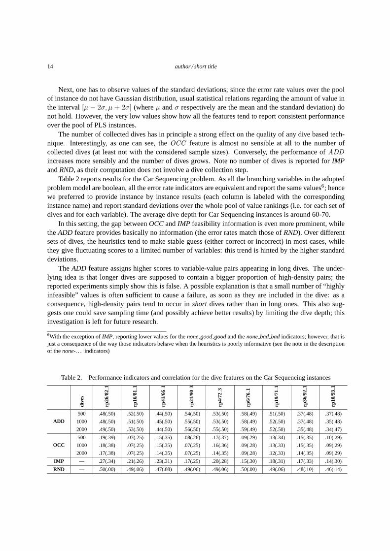
Table 2 reports results for the Car Sequencing problem. As all the branching variables in the adoptedproblem model are boolean, all the error rate indicators are equivalentand report the same values6; hencewe preferred to provide instance by instance results (each column is labeled with the correspondinginstance name) and report standard deviations over the whole pool of value rankings (i.e. for each set ofdives and for each variable). The average dive depth for Car Sequencing instances is around 60-70.

In this setting, the gap betweenOCCandIMP feasibility information is even more prominent, whiletheADD feature provides basically no information (the error rates match those ofRND). Over differentsets of dives, the heuristics tend to make stable guess (either correct or incorrect) in most cases, whilethey give fluctuating scores to a limited number of variables: this trend is hinted by the higher standarddeviations.

TheADD feature assigns higher scores to variable-value pairs appearing in longdives. The under-lying idea is that longer dives are supposed to contain a bigger proportionof high-density pairs; thereported experiments simply show this is false. A possible explanation is that a small number of “highlyinfeasible” values is often sufficient to cause a failure, as soon as they are included in the dive: as aconsequence, high-density pairs tend to occur inshort dives rather than in long ones. This also sug-gests one could save sampling time (and possibly achieve better results) by limitingthe dive depth; thisinvestigation is left for future research.

6With the exception ofIMP, reporting lower values for thenonegoodgoodand thenonebad bad indicators; however, that isjust a consequence of the way those indicators behave when the heuristics is poorly informative (see the note in the descriptionof thenone-. . . indicators)

Table 2. Performance indicators and correlation for the dive features on the Car Sequencing instances

dive

s

rp26

/82

1

rp16

/81

1

rp41

/66

1

rp21

/90

3

rp4/

723

rp6/

761

rp19

/71

1

rp36

/92

1

rp10

/93

1

ADD

500 .48(.50) .52(.50) .44(.50) .54(.50) .53(.50) .58(.49) .51(.50) .37(.48) .37(.48)

1000 .48(.50) .51(.50) .45(.50) .55(.50) .53(.50) .58(.49) .52(.50) .37(.48) .35(.48)

2000 .49(.50) .53(.50) .44(.50) .56(.50) .55(.50) .59(.49) .52(.50) .35(.48) .34(.47)

OCC

500 .19(.39) .07(.25) .15(.35) .08(.26) .17(.37) .09(.29) .13(.34) .15(.35) .10(.29)

1000 .18(.38) .07(.25) .15(.35) .07(.25) .16(.36) .09(.28) .13(.33) .15(.35) .09(.29)

2000 .17(.38) .07(.25) .14(.35) .07(.25) .14(.35) .09(.28) .12(.33) .14(.35) .09(.29)

IMP — .27(.34) .21(.26) .23(.31) .17(.25) .20(.28) .15(.30) .18(.31) .17(.33) .14(.30)

RND — .50(.00) .49(.06) .47(.08) .49(.06) .49(.06) .50(.00) .49(.06) .48(.10) .46(.14)


Table 3. Correlation of the dive features on the PLS instances

not

max

max

not

max

good

not

min

min

not

min

bad

none

good

good

none

bad

bad

good

bad

bad

good

OCC/ADD .15(.08) .11(.08) .26(.09) .25(.06) .13(.10) .23(.13) .16(.09) .34(.09)

OCC/IMP .54(.06) .49(.08) .39(.07) .38(.07) .44(.10) .49(.16) .56(.07) .58(.07)

ADD/IMP .03(.07) .01(.07) .09(.08) .10(.05) .03(.07) .12(.11) .04(.07) .20(.09)

Table 4. Correlation of the dive features on the Car Sequencing instances

rp26

/82

1

rp16

/81

1

rp41

/66

1

rp21

/90

3

rp4/

723

rp6/

761

rp19

/71

1

rp36

/92

1

rp10

/93

1

OCC/ADD -0.19(.06) -0.08(.06) -0.14(.06) -0.04(.04) -0.16(.07) -0.28(.03) -0.26(.06) -0.05(.06) -0.13(.06)

OCC/IMP .64(.02) .27(.04) .61(.01) .35(.02) .46(.03) .71(.03) .65(.03) .72(.02) .73(.02)

ADD/IMP -0.48(.05) -0.56(.07) -0.43(.05) -0.47(.05) -0.36(.07) -0.34(.05) -0.49(.05) -0.16(.05) -0.21(.05)

5.4. Complementarity of different dive features

A naturally arising question concerns the possible correlation of the described dive features; in case theyare found to provide complementary information, one has the opportunity to exploit such complemen-tarity to increase the detection accuracy. We therefore performed a second set of experiments with thepurpose to evaluate the correlation between errors made by pairs of different heuristics. In details:

1. we fixed the number of collected dives to 2000;

2. for each instance, we considered the 30 sets of dives collected in the experiments of Section 5.3;

3. we evaluated the Pearson’sr coefficient for the values of all error rate indicators for each instanceand set of dives;

4. we averaged over the sets of dives (then on the set of instances, for the PLS problem).

We recall the Pearson’sr coefficient (see [19]) ranges in[−1, 1] and evaluates the extent of a linearcorrelation between two random variables; hence,r close to 1 denotes a strong direct linear correlationandr close to -1 denotes a strong linear inverse correlation (r close to 0 may hint at poor correlation, buttechnically provides no information, as a non-linear relation may exist).

Table 3 and Table 4 respectively report the correlation analysis results for the PLS and Car Sequenc-ing instances; as in Section 5.3, the Pearson’s correlation for each error rate indicator is reported for thePLS (and the standard deviations are computed over the pool of instances), while instance by instancedata is shown for the Car Sequencing (and the standard deviations are computed over the sets of dives).

The most relevant result in both cases is the relatively high linear correlation betweenOCCandIMP,pointing out thatOCC and IMP tend to make the same mistakes (in terms of feasibility), withOCCsimply failing less often. On the contrary, no reliable conclusion onADD can be drawn on the PLS, asthe r coefficient values are too close to 0. An interesting negative correlation seems to exist between


ADD andIMP on the Car Sequencing instances, opening perspectives for the combined use of the twoheuristics.

5.5. Effect of the consistency level

As pointed out in Sect.4, dives depend on the actual propagation algorithmused. Therefore, we per-formed a set of experiments to investigate the effect of the propagation andlocal consistency on thequality of the feasibility information. As basically all the considered heuristics (included impacts) relyon propagation and diving as a mean to extract information, by weakening the consistency level one mayexpected a performance drop-off. Table 5 and Table 6 show the resultsfor this evaluation; in particular,we reported the same indicators as in Tables 1 and 2, with the number of collected dives fixed to 2000;Arc Consistency (AC, rather then the strongest consistency level allowed by the solver) is enforced onall the global constraints (alldifferent, gcc, sequence).

On the PLS instances, the performance of all the considered heuristics decreases on average by 5%-10%, with IMP andOCC being the most sensitive to the achieved consistency level. Conversely, theADD feature is subjected to a less sensible performance drop-off and appears to be more robust w.r.t.propagation. This could be appealing for problems involving complex constraints, for which effectivefiltering algorithms are not available or not efficient enough.

The situation appears to be completely different on the Car Sequencing instances; here, whileIMPsuffers a limited performance loss when switching to arc consistency, both the dive base heuristics (OCCandADD) appear to get no penalty and even report some slightly better results in somecases. Thisphenomenon is likely connected to the type of branching variables (all binary) and its investigation is leftas part of future research.

5.6. Evaluation of the value ranking, on a single variable basis

From a different perspective, the feasibility information can be assessed by evaluating therankingpro-vided for the values in each variable’s domain by the dive features and bythe actual densities. Thismethod provides an order-based measure of the correlation between the actual occurrence frequency infeasible solutions of variable-value pairs, and their score provided byADD , OCC or IMP .

In particular, for each variableXi we computed the number of correctly classified pairs of values

Table 5. Performance indicators for the dive features on PLS, with arc consistency on thealldifferent con-straints

dive

snu

m

not

max

max

not

max

good

not

min

min

not

min

bad

none

good

good

none

bad

bad

good

bad

bad

good

ADD 2000 .56(.03) .45(.07) .45(.16) .20(.03) .19(.06) .07(.01) .52(.07) .23(.03)

OCC 2000 .52(.04) .40(.082) .43(.16) .18(.03) .19(.07) .05(.01) .46(.07) .22(.03)

IMP — .52(.04) .41(.08) .43(.16) .18(.03) .19(.07) .06(.02) .47(.07) .22(.03)


vj , vk. A pair vi, vj is correctly classified by theADD (resp.OCC , IMP ) feature if:

ρ(Xi, vj) ≤ ρ(Xi, vk) ∧ ADD(Xi, vj) ≤ ADD(Xi, vk)

or

ρ(Xi, vj) > ρ(Xi, vk) ∧ ADD(Xi, vj) > ADD(Xi, vk)

whereρ(Xi, vj) denotes the density of the pairXi, vj within feasible solutions. We considered for thisof experiments the PLS instances only; for each of them:

1. we counted the number of correctly classified pairs for each variable domain;

2. the number was normalized over the total number of pairs for the variable;

3. the computed value is averaged over all the 30 sets of samples;

4. the resulting mean values are averaged over all the variables in the problem;

5. the resulting mean values are averaged over all the 60 instances in the set.

Table 7 provides the results for this evaluation, conducted on the PLS instances only with 2000,4000 and 8000 as number of collected dives. Themean andstdv rows report the mean and the standarddeviation for the number of correctly classified values (CC) over the set of instances. Here, theIMP

heuristic is the one matching more closely the ranking provided by actual densities. Nevertheless, onecan see how bothADD andOCC have definitely comparable performance, even outperforming impactsin a minor number of instances (reported in row> IMP ).

5.7. Effectiveness in guiding search

Finally, we performed tests in order to assess the actual performance onecould get by using dive featuresto guide search. The main issue here is that choosing the values with the highest density in feasiblesolutions gives in principle no guarantee to obtain the best results; hence (A) the actual relevance ofvariable-value pair density has to be assessed and (B) the reliability of the error rate indicators in pre-dicting search performance must be evaluated. In other words, the main focus is on how predictablethe results are, rather than on the absolute performance. In particular, for the first 10% variables in theproblem:

• the branching variable is selected according to a predefined criterion (i.e.maximum impact), toallow a fair comparison;

Table 6. Performance indicators and correlation for the dive features on the Car Sequencing instances

dive

s

rp26

/82

1

rp16

/81

1

rp41

/66

1

rp21

/90

3

rp4/

723

rp6/

761

rp19

/71

1

rp36

/92

1

rp10

/93

1

ADD 2000 .44(.50) .46(.50) .54(.50) .56(.50) .64(.47) .58(.49) .49(.50) .56(.50) .50(.50)

OCC 2000 .16(.37) .05(0.23) .18(0.38) .08(.28) .16(.37) .10(.31) .12(.33) .16(.36) .11(.31)

IMP — .31(.34) .25(.30) .24(.29) .21(.26) .23(.27) .21(.34) .21(.34) .21(.34) .21(0.35)


Table 7. Correlation between the ranking provided by dive features and actual densities

IMP ADD OCC

dives — 2000 4000 8000 2000 4000 8000

CCmean .518 .497 .498 .498 .498 .501 .505stdv .024 .018 .015 .013 .026 .023 .023

> IMP — 8 9 9 13 14 16

• a value is assigned according to the dive scorescollected at the root node; this choice was forced,as extracting dives at every search node would make an extensive evaluation impractical.

Once at least 10% problem variables are bound, the problem is resolvedvia a default heuristics (impactsfor Car Sequencing, min size domain for the PLS). The main drawback of using scores collected only atthe root node is that density information may be compromised along the search:for example the highestdensity valuevj of a variableXi may become the lowest one due to a branching decision. Restrictingthe use of dive related scores to the first 10% variables compensates forthe fact that dives are collectedat the root node only.

Table 8 and Table 9 show the result of this evaluation, respectively for thePLS and Car Sequencingproblems. In detail:

1. each instance was solved once with a default search heuristics, usedas a reference (dynamic im-pacts for Car Sequencing, min size domain for the PLS);

2. each instance was solved once by using actual densities to select values for the first 10% variables;

3. each instance was solved once by using impact (extracted at the root node) to select values for thefirst 10% variables;

4. each instance was solved 10 times (with different seeds and number of dives fixed to 2000) byusingOCC to select values for the first 10% variables;

In Table 8 instances are grouped by increasing solution time when performing selection based on densi-ties. For each heuristics we report the mean solution time and fails (and corresponding standard devia-tions) over the pool of instances. As one can see, selecting value with highoccurrence frequency in thefeasible solution enables considerable improvements, as pointed out by the lower solution times in theDENScolumns.IMP andOCChave similar performance, withOCCdoing a little better on average; thiswas indeed predicted by the values of the error rate indicators and provides some experimental supportfor their relevance.

Table 8. Performance statistics on actual search runs for the PLS instancesDEFAULT DENS IMP OCC

time fails time fails time fails time fails

45.9(84.1) 117K (219K) .2(.2) 466(439) 44.1(69.3) 111K(180K) 16.4(29.3) 40K(71K)19.5(33.5) 53K(98K) .8(.2) 2K(481) 15.8(16.6) 41K(43K) 30.8(50.6) 82K(136K)

334.2(841.2) 874K(2M) 1.9(.3) 4K(1K) 206.4(561.5) 522K(1M) 219.2(542.1) 559K(1M)157.5(272.4) 398K(693K) 4.1(1.0) 10K(2K) 69.0(86.7) 170K(210K) 56.5(86.7) 137K(209K)72.5(121.6) 197K(336K) 15.2(9.7) 40K(26K) 110.4(197.2) 299K(543K) 88.7(131.8) 235K(352K)

139.0(121.9) 365K(328K) 72.9(25.5) 192K(71K) 179.5(313.0) 506K(953K) 99.2(75.9) 256K(191K)


Table 9. Performance statistics on actual search runs for Car Sequencing

DEFAULT DENS IMP OCCinst time fails time fails time fails time fails

rp10/93-1 .58 425 .57 425 .58 425 .57(.01) 421(4)rp16/81-1 .89 768 .78 579 .78 579 .77(.01) 580(2)rp19/71-1 .68 541 .61 465 .62 465 .62(.02) 487(22)rp21/90-3 1.05 1081 .79 721 .78 721 .79(.01) 730(17)rp26/82-1 .76 622 .67 552 .64 505 1.25(.47) 1298(599)rp36/92-1 .56 415 .57 451 .57 451 .56(.01) 447(4)rp41/66-1 .67 540 .59 444 .59 444 .59(.01) 596(15)rp4/72-3 .62 598 .59 577 .6 577 .61(.02) 474(27)rp6/76-1 .65 651 .54 511 .54 482 .54(.03) 512(50)

Results for Car Sequencing are shown in Table 9 instance by instance. Note that, to limit the numberof solutions and enable enumeration, we had to resort to smaller problems with 30 cars; as a consequence,solution time differences are much less marked. Nevertheless, using exactdensities for the first searchchoices seems to bring some benefit over the default heuristics. Interestingly, impacts at the root node(column IMP) provides slightly better results compared toOCC, suggesting for this kind of problemother factors (e.g. ability to exploit propagation) play a more important role than matching the highestdensities.

6. Conclusion and discussion of future research lines

In the presented paper we have defined a sound theoretical frameworkfor studying the informationthat can be derived from sampling and diving. In particular, we discussed information concerning thefeasibility of variable-value pairs. The extracted information can be used toguide search, or to performdecomposition or to overfilter unpromising values.

A statistical model has been presented that shows that uniform sampling canin principle be infor-mative, but, to be used in practice, it needs huge sample sizes for inferringprecise indications. Divinginstead can be used for this purpose also in practical cases. We have identified dive features and experi-mented them on Partial Latin Square and Car Sequencing problems.

We have defined a set of performance indicators to evaluate the effectiveness of each dive featuresin providing information about the problem variables. The correlation between dive-driven parametersand assignment density in feasible solutions has been measured. Additionalexperiments have been per-formed aimed at applying a statistical analysis to measure the complementarity of thefeatures presentedand the effect of different consistency levels on the quality of such features. Finally, we performed a lastset of experiments by using the identified dive features to actually guide a search process.

A state of the art impact based heuristic was used as a comparison reference throughout the paper.A byproduct of this work is the definition of a statistically sound method for evaluating variable-valueselection heuristics.

This work is an attempt to get a better understanding of the search process. Despite the availabilityof so many methods for the solution of CSPs, the study of the impact on the search efficiency of keysearch components, such as propagation, branching schema, ability to keep the problem feasible duringbranching has received poor attention. For this reason, the understanding of CP search behavior by means


of statistics and formal methods is a crucial and very appealing research topic.The presented work goes is such a direction: it suggests ideas about general evaluation processes,

and points out the importance and investigates the limits of maintaining feasibility during search. Manyquestions remain open and are subject of on-going research. We plan todevise new dive features to becompared with current ones. Second, we are investigating the relations between dive-derived informationand backbones and backdoors; on the one hand, to understand whichlevel of accuracy we can reach forsuch critical variables, and on the other hand to see whether dives can help in their identification. More ingeneral, finding a formal model for some well-known CP search processes is a tough, but very appealing,objective.

Other important issues we are considering are the evaluation of the approach on other problems, theestimation of variables by means of dive-driven information, to detect the most critical ones or those forwhich we have the highest level of confidence. Finally, we plan to devise techniques to make the divingprocess more efficient, and to get precise problem information (for evaluation purpose) without resortingto complete enumeration.

References

[1] Beck, J. C.: Solution-Guided Multi-Point ConstructiveSearch for Job Shop Scheduling,Journal of ArtificialIntelligence Research, 29, 2007, 49–77.

[2] Boussemart, F., Hemery, F., Lecoutre, C., Sais, L.: Boosting Systematic Search by Weighting Constraints,Proc. of ECAI, Ios Pr Inc, 2004, ISBN 1586034529.

[3] Colbourn, C. J.: The Complexity Of Completing Partial Latin Squares,Discrete Applied Mathematics, 8(1),1984, 25–30.

[4] Gogate, V., Dechter, R.: A New Algorithm For Sampling CSPSolutions Uniformly At Random, in:Princi-ples and Practice of Constraint Programming - CP 2006(F. Benhamou, Ed.), vol. 4204 ofLecture Notes inComputer Science, Springer-Verlag Berlin Heidelberg, Germany, 2006, 711–715.

[5] Gogate, V., Dechter, R.: Approximate Counting by Sampling the Backtrack-free Search Space,Proc. ofAAAI, AAAI Press, 2007, ISBN 978-1-57735-323-2.

[6] Gomes, C., Shmoys, D.: Completing Quasigroups Or Latin Squares: A Structured Graph Coloring Problem,Proc. of the COLOR, 2002.

[7] Gomes, C. P., Sabharwal, A., Selman, B.: Near-Uniform Sampling Of Combinatorial Spaces Using XORConstraints,Advances In Neural Information Processing Systems, 19, 2007, 481.

[8] Gomes, C. P., Shmoys, D. B.: Approximations And Randomization To Boost CSP Techniques,Annals ofOperations Research, 130(1), 2004, 117–141.

[9] Grimes, D., Wallace, R. J.: Learning To Identify Global Bottlenecks In Constraint Satisfaction Search,20thInternational FLAIRS conference, 2007.

[10] van Hoeve, W., Milano, M.: Decomposition Based Search-A theoretical and experimental evaluation,Arxivpreprint cs/0407040, 2004.

[11] Hsu, E. I., Kitching, M., Bacchus, F., Mcllraith, S. A.:Using Expectation Maximization to Find LikelyAssignments for Solving CSP’S,Proc. of AAAI, 22, Menlo Park, CA; Cambridge, MA; London; AAAIPress; MIT Press; 1999, 2007.


[12] Knuth, D.: Estimating The Efficiency Of Backtrack Programs,Mathematics of computation, 29(129), 1975,121–136, ISSN 0025-5718.

[13] Le Bras, R., Zanarini, A., Pesant, G.: Efficient GenericSearch Heuristics within the EMBP Framework,Proceedings of the 15th international conference on Principles and practice of constraint programming,Springer-Verlag, 2009, ISBN 3642042430.

[14] Lombardi, M., Milano, M., Roli, A., Zanarini, A.: Deriving information from sampling and diving, in:Emergent Perspectives in Artificial Intelligence – AI*IA 2009 (R. Serra, R. Cucchiara, Eds.), vol. 5883 ofLecture Notes in Computer Science, Springer-Verlag Berlin Heidelberg, Germany, 2009, 82–91.

[15] Papoulis, A., Pillai, S. U., A, P., SU, P.:Probability, Random Variables, And Stochastic Processes, McGraw-Hill New York, 1965.

[16] Parrello, B., Kabat, W., Wos, L.: Job-Shop Scheduling Using Automated Reasoning: A Case Study Of TheCar-Sequencing Problem,Journal of Automated Reasoning, 2(1), 1986, 1–42, ISSN 0168-7433.

[17] Refalo, P.: Impact-Based Search Strategies for Constraint Programming, in:Principles and Practice ofConstraint Programming - CP 2004(M. Wallace, Ed.), vol. 3258 ofLecture Notes in Computer Science,Springer-Verlag Berlin Heidelberg, Germany, 2004, 557–571.

[18] Regin, J.-C., Puget, J.-F.: A Filtering Algorithm for GlobalSequencing Constraints, in:Principles andPractice of Constraint Programming - CP 1997(G. Smolka, Ed.), vol. 1330 ofLecture Notes in ComputerScience, Springer-Verlag Berlin Heidelberg, Germany, 1997, 32–46.

[19] Rodgers, J. L., Nicewander, W. A.: Thirteen Ways to Lookat the Correlation Coefficient,The AmericanStatistician, 42(1), 1988, pp. 59–66, ISSN 00031305.

[20] Ruml, W.: Adaptive Tree Search, Ph.D. Thesis, Harvard University Cambridge, Massachusetts, 2002.

[21] Zanarini, A., Pesant, G.: Solution Counting Algorithms For Constraint-Centered Search Heuristics,Con-straints, 14(3), 2009, 392–413.

Deriving Information from Sampling and Diving

Documents

Transcript of Deriving Information from Sampling and Diving