The Interaction Between Inflection and Derivation in English and MSA
Upload
independentresearcherCategory
view
2download
0
RESEARCH ARTICLE1010022014WR015643
Derivation of lowland riparian wetland deposit architectureusing geophysical image analysis and interface detectionJ E Chambers1 P B Wilkinson1 S Uhlemann12 J P R Sorensen3 C Roberts4 A J Newell3W O C Ward15 A Binley6 P J Williams3 D C Gooddy3 G Old4 and L Bai5
1Geophysical Tomography Team British Geological Survey Nottingham UK 2ETH-Swiss Federal Institute of TechnologyInstitute of Geophysics Zurich Switzerland 3Groundwater Science British Geological Survey Wallingford UK 4Centre forEcology and Hydrology Wallingford UK 5School of Computer Science University of Nottingham Nottingham UK6Lancaster Environment Centre Lancaster University Lancaster UK
Abstract For groundwater-surface water interactions to be understood in complex wetland settings thearchitecture of the underlying deposits requires investigation at a spatial resolution sufficient to characterizesignificant hydraulic pathways Discrete intrusive sampling using conventional approaches provides insuffi-cient sample density and can be difficult to deploy on soft ground Here a noninvasive geophysical imagingapproach combining three-dimensional electrical resistivity tomography (ERT) and the novel application ofgradient and isosurface-based edge detectors is considered as a means of illuminating wetland deposit archi-tecture The performance of three edge detectors were compared and evaluated against ground truth datausing a lowland riparian wetland demonstration site Isosurface-based methods correlated well with intrusivedata and were useful for defining the geometries of key geological interfaces (ie peatgravels and gravelsChalk) The use of gradient detectors approach was unsuccessful indicating that the assumption that thesteepest resistivity gradient coincides with the associated geological interface can be incorrect These findingsare relevant to the application of this approach in settings with a broadly layered geology with strata of con-trasting resistivities In addition ERT revealed substantial structures in the gravels related to the depositionalenvironment (ie braided fluvial system) and a complex distribution of low-permeability putty Chalk at thebedrock surfacemdashwith implications for preferential flow and variable exchange between river and ground-water systems These results demonstrate that a combined approach using ERT and edge detectors can pro-vide valuable information to support targeted monitoring and inform hydrological modeling of wetlands
1 Introduction
Groundwater-dependent ecosystems are significant in terms of their hydrological and biogeochemical func-tioning and as a vital habitat with considerable biodiversity and productivity However these systems areparticularly sensitive to environmental change [eg Klove et al 2011] and this is acknowledged in currentlegislation (eg US Clean Water Act European Union Water Framework Directive and Habitats Directiveand the Ramsar convention) resulting in a drive to characterize their functioning and understand therequirements for their sustainable management Specifically establishing hydrological functioning is essen-tial as a precursor to successful management [Zedler 2000] controlling flora [Baldwin 2001] fauna [Ausdenet al 2001] and biogeochemical cycling [McClain et al 2003]
Wetland hydrology can be notoriously spatially complex as a result of heterogeneity within the subsurface[Holden et al 2002 Holden and Burt 2003] However subsurface investigations are typically spatiallyrestricted to a limited number of core samples [eg Andersen 2004] given the inaccessibility of many sitesdue to ecological sensitivity inundation andor the associated costs of drillings Geophysical investigationsprovide a means of achieving spatial coverage noninvasively to characterize the subsurface architecture ofsites in order to improve our hydrological understanding
This study considers the use of three-dimensional (3-D) electrical resistivity tomography (ERT) Crucially thisapproach has the potential to provide high-resolution volumetric subsurface information with minimalimpact to the ecosystem ERT involves the measurement of potential differences resulting from applied cur-rents using arrays of electrodes at the ground surface or within boreholes an inverse problem is then
Key Points Subsurface wetland architecture is
characterized using 3-D resistivityimaging Edge detectors for resistivity image
analysis are compared Resistivity models illuminate
structures relevant to hydrologicalfunctioning
Correspondence toJ E Chambersjonathanchambersbgsacuk
CitationChambers J E et al (2014) Derivationof lowland riparian wetland depositarchitecture using geophysical imageanalysis and interface detection WaterResour Res 50 5886ndash5905doi1010022014WR015643
Received 3 APR 2014
Accepted 26 JUN 2014
Accepted article online 30 JUN 2014
Published online 16 JUL 2014
CHAMBERS ET AL VC 2014 American Geophysical Union All Rights Reserved 5886
Water Resources Research
PUBLICATIONS
solved to produce spatial or volumetric models of the subsurface resistivity distribution from the measureddata [eg Loke et al 2013] It is a rapidly developing technique that is being increasingly applied to geolog-ical and hydrological investigations due to its sensitivity to a range of material and fluid properties includingclay content [eg Shevnin et al 2007] porosity [eg Jackson et al 1978] water content [eg Zhou et al2001] salinity [eg Singha and Gorelick 2006] and temperature [eg Hayley et al 2007]
In the context of wetland investigations ERT has only been applied in relatively few studies Most of thesestudies describe the application of two-dimensional (2-D) ERT for characterizing subsurface geology [Slaterand Reeve 2002 Comas et al 2004 Crook et al 2008 Karan et al 2013] salinity distribution [Heagle et al2013] and the detection of thermal anomalies associated with groundwater-surface water interactions[Musgrave and Binley 2011]
Far fewer wetland studies deal with the use of 3-D ERT perhaps due to the greater difficulty of surveydesign execution and data processing However 3-D ERT is clearly the more appropriate method for thecharacterization of complex geologies for which the 2-D assumption is violated resulting in significant inac-curacies in 2-D ERT models [eg Chambers et al 2002 Loke et al 2013] Mansoor and Slater [2007] appliedon-water 3-D ERT to the investigation of a shallow water wetland (Kearney Freshwater Marsh USA) wherethe resistivity structure of the wetlands sediments was illuminated and used to identify pollution pathwaysfrom local landfills Riddell et al [2010] deployed 3-D ERT surveys to develop a conceptual model of wetlandforming processes in an upland setting (Manalana South Africa) ERT was shown to be particularly effectivein revealing the distribution of clay plugs within the broader sandy deposit which exerted a major controlon the hydrological functioning of the wetland To date there are no studies exploring the use of 3-D ERTfor subsurface characterization in lowland riparian wetlands
Emerging theoretical developments in the analysis of ERT images are also highly relevant to this study Inparticular it is postulated that automated approaches to extracting interfaces from 3-D ERT images [egChambers et al 2012 Ward et al 2014] will be valuable for delineating key interfaces within the subsurfaceHowever there are very few studies for which automated edge detection has been validated in field set-tings with good ground truth In this case where spatially dense probe data has defined the thickness ofthe surficial peat and alluvium deposits the opportunity exists to quantitatively assess the performance ofedge detectors for the characterization of broadly layered geological structure
The aim is therefore to apply for the first time the latest developments in 3-D ERT image analysis to improveour understanding of the subsurface architecture of lowland riparian wetland depositsmdashthereby providinga foundation on which to further elucidate groundwater-surface water interactions Specific objectivesinclude (1) validation of image analysis approaches (derivative and isosurface methods) for interface detec-tion using 3-D ERT against a high-resolution control data set (ie intrusive peat depth probing) and (2)reconstruction of the lithostratigraphic architecture of the deposits underlying the wetland including allu-vial fluvial and bedrock lithologies
2 Site Description
21 Location and BackgroundThe site considered here is a wetland located on the River Lambourn immediately upstream of the villageof Boxford Berkshire UK (Figure 1) The Lambourn and its associated wetlands comprise some of the leastimpacted Chalk river systems in Britain therefore providing a reference laboratory against which to com-pare other similar sites The River and wetland are designated as Sites of Special Scientific Interest (SSSI)due to the habitats they provide for aquatic and terrestrial flora and fauna
Land adjacent to the current study site has been a focus of previous research which indicated a complexgeological system and hydrogeological regime [Prior and Johnes 2002 Wheater et al 2007 Allen et al2010 Lapworth et al 2009] with the geology exerting a major control on groundwater-surface water inter-actions However the local stratigraphic and lithologic structure remains poorly understood Promisinglynearby 2-D ERT investigations have successfully demonstrated its use for delineating key subsurface litholo-gies [Crook et al 2008 Musgrave and Binley 2011] Nevertheless the challenge remains of understandingthe geological complexities at the site to understand the controls on groundwater-surface water interactionwithout disturbing the delicate ecosystem
Water Resources Research 1010022014WR015643
CHAMBERS ET AL VC 2014 American Geophysical Union All Rights Reserved 5887
22 Geologyand GeomorphologyThe River Lambourn flows SEalong a mostly linear valleyincised into the Chalk of theBerkshire Downs (Figure 1)The Boxford site is located inthe lower part of the RiverLambourn at one of two con-spicuous valley bends (Figure1) The Upper Cretaceous Chalkof the Berkshire Downs is up to252 m thick with a very shallowdip to the south east awayfrom the steep escarpmentwhich marks its northernboundary The Chalk is under-lain by a thin layer of UpperGreensand (Lower Cretaceous)in hydraulic continuity andsealed beneath by mudrocksof Jurassic age A range of Qua-ternary and younger superficialdeposits partially cover theChalk including Clay-with-flintson interfluves and river terracedeposits head and alluvium onvalley floors [Aldiss et al 2010]
At Boxford the River Lambournis cut into the Seaford Chalk
formation (Upper Chalk) a uniform soft to medium-hard chalk with many flint nodules and a few laterallycontinuous tabular flints and clay-rich chalks [Woods and Aldiss 2004] The Chalk bedding dips at low angles(1ndash2) across the river valley from NW to SE Boreholes drilled at the site along the northern margin of thevalley show that the River Lambourn and its floodplain is separated from the Chalk by up to 75 m of riverterrace deposits and alluvium [Allen et al 2010] Such river terrace deposits and alluvium are common inChalk valleys The river terrace deposits are primarily coarse-grained gravels with typically 50 of clastsranging from 25 to 100 mm in size The sand silt and clay do not generally comprise more than 5 of thedeposit although locally thin beds of sandy gravel are developed The gravels are typically 3ndash4 m thickalthough there is local thickening and thinning which suggests an irregular erosion surface on the top ofthe Chalk The gravels are composed predominantly of rounded flint clasts however the basal 1ndash2 m oftenincludes a high proportion of reworked chalk material which may have been incorporated into the river ter-race deposits during downcutting and erosion The chalk clasts are often highly degraded and may have asignificant hydrogeological impact by occluding porosity and significantly reducing the permeability of thegravels adjacent to the underlying chalk In addition the upper part of the Chalk is commonly of a structure-less lsquolsquoputtyrsquorsquo type which has a much lower permeability than less weathered fissured Chalk [Younger 1989]In the subsequent hydrogeological discussion the term lsquolsquogravelsrsquorsquo is used to encompass the arenaceousmainly coarse-grained lithologies forming the river terrace deposits The gravels are overlain by a heteroge-neous cover of sands silts clays peat and tufa which are 1ndash2 m thick and underlie the modern floodplainsurface (Figure 1) The contact with the underlying gravels is abrupt and undulating with localized thicken-ing of the peaty alluvial deposits in narrow linear depressions which may result from the infill of river chan-nels associated with the underlying gravels
By analogy with detailed studies of the fluvial stratigraphy in downstream parts of the river system on theRiver Kennet [Collins et al 2006] the River Lambourn and its deposits at Boxford developed in three mainstages The chalk and flint gravels which form the lower part of the valley fill were probably deposited in
Figure 1 Geological map of Boxford and the surrounding area Inset map (top right) showsthe location of the study area at the national scale The study area is defined by the blackand white dashed line and the location of the Crook et al [2008] cross-borehole ERT surveyis shown as a black line
Water Resources Research 1010022014WR015643
CHAMBERS ET AL VC 2014 American Geophysical Union All Rights Reserved 5888
high-energy bed load channels during the Late Pleistocene (Devensian) when the Berkshire Downs formedpart of a periglacial environment south of the main British ice sheets [Murton and Belshaw 2011] The riverhydrology was dominated by nival regimes with high spring and summer runoff [Collins et al 2006] and lim-ited water infiltration to the porous chalk bedrock because of permafrost The high-energy rivers carved anextensive network of valleys most of which are now dry under the modern temperate climate Rates ofweathering and erosion would have been enhanced by frost heave and brecciation [Murton 1996] and thepresent-day linear form of the River Lambourn could indicate the importance of joints and fractures in control-ling chalk weathering erosion and valley development [Goudie 1990] The cover of peat and alluvium accu-mulated in low-energy rivers and wetlands under the temperate climate of the Holocene [Collins et al 2006]As with the present day Chalk streams rivers and wetlands were probably fed primarily by groundwater sup-ply from the Chalk aquifer Over the last few centuries the river and wetland at Boxford has entered its thirdmajor development stage with significant anthropogenic modification associated with the creation of a watermeadow system This involved the construction of channels and ponds for farming and recreation
23 Hydrology and HydrogeologyThe water meadow would historically have been managed as pastureland A network of channels is shownon historic maps (1882) and it is likely that these would have been used for controlled flooding or lsquolsquofloatingrsquorsquoof the water meadows in the winter to protect them from frost and encourage early growth of the vegeta-tion [eg Everard 2005] The site has not been grazed for a number of years and many of the historic chan-nels do not appear on current maps (Figure 1)
The hydrogeological functioning of the wetland is likely to depend on a number of factors The site islocated on the major Chalk aquifer and therefore groundwater flows are likely to be important also thelocation of the wetland in a valley bottom would normally indicate a groundwater discharge zone In addi-tion the River Lambourn flows through the site potentially providing a major control on local groundwaterheads as well as a focus for groundwater discharge (or recharge) However this potentially simple valleybottom hydraulic system is made much more complex by the presence of heterogeneous river terrace grav-els and wetland peat and other alluvium and the surface water system is complicated by the presence ofwetland drainage channels [Grapes et al 2006]
Investigations at an adjacent riverside study site [Allen et al 2010] have revealed a complex pattern ofgroundwater-surface water interactions involving both influent and effluent relationships between the riverand underlying gravels and with groundwater flow in the Chalk occurring under and transverse to the riverSignificantly at this study site the gravels were found to be mainly hydraulically separate from the ChalkThe study indicated that lithological knowledge was crucial to understanding the groundwater flow dynam-ics and the relationship between groundwater and surface water and the same is likely to be true to aneven greater degree at the adjacent wetland site given the presence of the peat overlying the gravels It isthe complexity of the site geology and its impact on groundwater-surface water interactions that is themain driver for the 3-D geophysical characterization of the deposit structure
3 Intrusive Methodology
The peat and alluvium depth was determined by pushing a 6 mm diameter steel rod to the contact betweenthe penetrable peat and impenetrable gravels This was undertaken at 2815 points with an approximate gridresolution of 5 m 3 5 m (Figure 2a) The peat depth exceeded the rod length at six locations where it wasassumed to be 186 m deep (which was the maximum depth of investigation of the metal rod) The ground levelwas surveyed at each point using the combination of a real-time kinematic (RTK) GPS and a Total Station
Drilling was undertaken using a small crawler-mounted Dando Terrier percussion rig at three locations across thestudy site (Figure 2) Cores were recovered using a hollow stem auger in U100 tubes for logging and analysis
4 Geophysical Methodology
41 ERT Survey Design and Data CollectionThe 3-D ERT surveys were carried out in both the southern and northern sections of the wetland (Figure 2)A single survey covering both areas simultaneously was not possible due to the presence of significant
Water Resources Research 1010022014WR015643
CHAMBERS ET AL VC 2014 American Geophysical Union All Rights Reserved 5889
obstructions in the centralregion including a stream(Figure 2) and maturevegetation Dense vegetationprevented 3-D ERT surveysbetween late spring andautumn and so the surveyswere carried out in early spring(southern area) and winter(northern area) 2012 outsideof the growing seasons for thesedge and other vegetationthat covered much of the openareas of the wetland Groundconditions during the survey ofthe southern area were goodwith moist but firm groundconditions with little standingwater During the northern sur-vey ground conditions werevery soft with shallow stand-ing water covering much ofthe area
The southern wetland surveycovered an area of approxi-mately 15 hectares and com-prised 21 parallel survey linesand two crosscutting linespositioned at either end of theprimary survey lines with theaim of improving model reso-lution in low-sensitivity regionstoward the edges of the modelspace (Figure 2b) Likewise thenorthern survey extendedacross an area of approxi-mately 16 hectares and com-prised 15 parallel survey lineswith an additional three surveylines positioned at the ends ofthe primary survey lines againwith the aim of improvingmodel resolution in these areas(Figure 2b) In both areas thelengths of the survey lineswere constrained by site condi-tions and therefore varied sig-nificantly for the southern arealines lengths of the primary
parallel lines varied from 90 to 177 m and for the northern area between 159 and 189 m All of the surveylines used a 3 m electrode spacing and for the sets of primary parallel survey lines a line spacing of 6 mThe line spacing was limited to 6 m (ie two along-line electrode spacings) to minimize artifacts in theresulting images associated with the use of a single line orientation [Gharibi and Bentley 2005] The dipole-dipole array was used with dipole sizes (a) of 3 6 9 and 12 m and dipole separations (n) of 1a to 8a with a
171800
171850
171900
171950
172000
172050
172100
172150
172200
Nor
thin
g[m
]
BHN
BHS1
BHS2
442750 442800 442850 442900 442950Easting [m]
BHN
BHS1
BHS2
171800
171850
171900
171950
172000
172050
172100
172150
172200
Nor
thin
g[m
]
(a)
(b)
x
y
x
y
Figure 2 Annotated maps of the Boxford study site showing (a) intrusive sample locationsand (b) ERT electrode positions and survey areas (blue shading)
Water Resources Research 1010022014WR015643
CHAMBERS ET AL VC 2014 American Geophysical Union All Rights Reserved 5890
full set of both normal andreciprocal measurements Thedipole-dipole array was chosenfor good resolving capabilitiesand because it effectivelyexploits multichannel data col-lection and enables efficientmeasurement of reciprocalcombinations Further explana-tion of survey design is givenin Appendix A For a normalfour-electrode measurement oftransfer resistance the recipro-cal is found by exchanging thecurrent and potential dipolesand in the absence of nonlin-
ear effects should give the same result Reciprocal error is defined here as the percentage standard error inthe average of the forward and reciprocal measurements which provides a robust means of assessing dataquality [Binley et al 1996 Wilkinson et al 2012] Measurements were made using an eight-channel AGISuperSting R8 and 64-way switch box with multicore cables attached to stainless steel rod electrodes Amaximum injection current of 500 mA was applied
42 Data Processing Inversion and VisualizationContact resistances averaged 395 X (standard deviation (SD) 130 X) and 292 X (SD 50 X) for the southernand northern areas respectively Analysis of reciprocal errors indicated very good data quality (Figure 3)95 of the 20563 measurement pairs (normal and reciprocal) collected during the southern area survey fellbelow the 5 reciprocal error (RE) threshold while 995 of the 23164 measurement pairs collected duringthe northern area survey had reciprocal errors falling below the 5 RE threshold Measurements with areciprocal error of more than 5 were removed the remaining reciprocal pairs were averaged and thereciprocal errors were used to weight the data during the inversion The slightly lower contact resistancesand hence slightly better reciprocal errors observed in the northern area are probably the result of wetterground conditions and more electrically conductive surficial deposits
Both data sets were inverted using a regularized least squares optimization method [Loke and Barker 1996]An L2-norm was applied to the model and an L1-norm was used on the data with a cutoff factor of 005[Loke et al 2003 Farquharson and Oldenburg 1998] The selection of constraints is discussed in Appendix AThe forward problem was solved using a finite element method in which node positions were adjusted toallow the observed topographic variations to be incorporated The aim of the inversion process is to calcu-late a model (or image) that satisfies the observed data A starting model is produced ie a homogeneoushalf-space with resistivity equal to the mean of the measured apparent resistivities for which a response iscalculated and compared to the measured data The starting model is then modified in such a way as toreduce the mean absolute misfit between the model response and the measured data This process contin-ues iteratively until acceptable convergence between the calculated and measured data is achieved Theresulting northern area resistivity model consisted of 45 cells in the x direction 74 cells in the y directionand 15 layers in the z direction resulting in a total of 48180 model cells acceptable convergence wasachieved after six iterations as indicated by a root mean square (RMS) misfit error of 103 The southernarea model comprised 61 cells in the x direction 54 in the y direction and 15 in the z direction resulting in47700 model cell a RMS misfit error of 108 was observed after five iterations
43 Interface DetectionThree different methods were used to detect interfaces within the 3-D inverted ERT models The firstassumes that the interface is located at the elevation of the steepest gradient on the resistivity-elevationcurve q(z) (eg Figure 4) and is therefore referred to as the lsquolsquosteepest gradient methodrsquorsquo (SGM) [Chamberset al 2012 2013] Similar approaches have previously been applied to 2-D ERT images by Nguyen et al[2005] Hsu et al [2010] and Bouchedda et al [2012] Here the SGM uses linear interpolation of finite
0
10
20
30
40
50
60
70
0001 001 01 1 10 100 1000
Re
la
ve
fre
qu
en
cy
(
)
Reciprocal error ()
North
South
0
Figure 3 Distributions of reciprocal errors for the northern and southern 3-D ERT surveys
Water Resources Research 1010022014WR015643
CHAMBERS ET AL VC 2014 American Geophysical Union All Rights Reserved 5891
difference estimates of the second derivative to find the point where 2qz2 5 0 which implicitly assumesfor simplicity that the interfaces are close to horizontal
The second method assumes that the interface is represented in the inverted ERT image by a resistivity iso-surface This method requires the location of the interface to be known through an independent measure-ment (ie borehole or penetration test) at one or more points in the subsurface (hence being referred to asthe lsquolsquoknown interface methodrsquorsquo KIM) The isosurface value is then assumed to be the average of the modelresistivities at those points [Chambers et al 2013] and the surface is calculated by trilinear interpolation ofthe resistivity model q(x y z) Since a single resistivity value is used to characterize a surface this method isonly applicable where a clear layered structure is present
The third method also uses resistivity isosurfaces to identify interfaces however the isosurface values aredetermined from the statistical properties of the image rather than intrusive data The probability distribu-tion of resistivity values within the image is characterized using kernel density estimation to identify dis-tinct populations of resistivity values associated with separate units (Table 1) [Chambers et al 2012] A fuzzyc-means clustering method is then used to assign each cell within the image to its most likely populationthereby identifying the resistivity values that characterize the boundaries between the populations [Wardet al 2014] These values are used as in the KIM method above to calculate the isosurfaces representingthe geological interfaces This is referred to as the lsquolsquoclustering methodrsquorsquo (CLS)
5 Results and Discussion
51 Surface Topography and Intrusive InvestigationsSurface elevations recorded during the peat probing indicate a remarkably flat surface across the northernand southern areas with a height variation of little more than 1 m A general increase in surface elevation tothe north is observed as is some indication of relict channel structures (particularly in the northern area)defined by sinuous linear features (Figure 5a)
0 50 100 150 200Resistivity (Ohmm)
BT
BB
BHS1
75
80
85
90
0 50 100 150 200
Ele
vatio
n (m
AO
D)
Resistivity (Ohmm)
BT
BB
BHN
KIMgt09KIM
CLSSGM
KIM_baseCLS_baseSGM baseResistivity (Ohmm)
Seaford Chalk Formation
Peat amp AlluviumBeenham Grange Gravel Member
Core loss
KeyGeology Interfaces and model resistivities
BT
BB
BHS2
Figure 4 Resistivity data as a function of elevation given as mAOD at surface positions corresponding to BHN and BHS1 The interfacesfor the peat and alluviumgravel and the gravelChalk derived using CLS KIM KIMgt 09 and SGM methods are indicated Borehole logsfor BHN BHS1 and BHS2 are shown
Water Resources Research 1010022014WR015643
CHAMBERS ET AL VC 2014 American Geophysical Union All Rights Reserved 5892
The peat forms a clear channel structure acrossthe two survey areas However it is generallythicker and more extensive in the northernarea (Figure 5c) The plot of peat base eleva-tions (Figure 5b) indicates that the peat andalluvium is occupying a topographic low on thesurface of the gravels
Two of the boreholes BHN and BHS1 werelocated within the peat channel in the northernand southern areas respectively (Figure 5)Both show a substantial thickness of peat over-lying several meters of gravel overlying chalkbedrock (Figure 4) Drilling was hampered byrefusals caused by coarse material close to the
interface between the gravels and chalk which was probably related to the presence of lag deposits BHS2was located toward the south eastern margin of the southern area (Figures 2 and 5) and comprised approxi-mately 1 m of peat and alluvium overlyinglt 02 m sand and gravel a mixture of chalk and gravel (08 m)and chalk bedrock which became firmer with depth In all of the boreholes the surficial peat depositincluded thin layers of clay which was consistently observed at between 01 and 03 m below ground levelThis layer was also observed in several other hand dug pits across the site
52 ERT521 Model DescriptionA 3-D visualization of the northern and southern ERT models is shown in Figure 6 The most electrically con-ductive (lt50 Xm) and resistive (gt150 Xm) values are shown as solid volumes along with a number of verti-cal sections The lithostratigraphy revealed by the boreholes is clearly displayed in the resistivity modelsThe most conductive materials are peat and alluvium which span both areas in the form of a channel
442750 442800 442850 442900 442950Easting [m]
171800
171850
171900
171950
172000
172050
172100
172150
172200
Nor
thin
g[m
]
BHN
BHS1
885
89
895
90
905
91
Surface elevation[m AOD]
(a)
442750 442800 442850 442900 442950Easting [m]
BHN
BHS1
885
89
895
90
905
91
Peat base elevation[m AOD]
(b)
442750 442800 442850 442900 442950Easting [m]
Peat thickness [m](c)
Peat filledchannel
BHN
BHS1
0
05
1
15
2
BHS2 BHS2 BHS2
Figure 5 Boxford study site (a) ground surface elevations derived from real-time kinematic GPS surveys and (b) peat base elevations (c) Peat thicknesses determined from intrusiveprobe surveys
Table 1 Centroid Resistivities and Interpreted Associated Litholo-gies for the Northern and Southern Areas Resistivity Models
Centroid Resistivity (Xm) Material Type
Northern Area35 Peat54 Weathered chalk98 Chalkgravels164 Chalk256 GravelsSouthern Area49 Peat72 Weathered chalk102 Chalkgravels126 Chalk183 Gravels
Water Resources Research 1010022014WR015643
CHAMBERS ET AL VC 2014 American Geophysical Union All Rights Reserved 5893
structure across the surface of the models which is also consistent with the intrusive investigations Themost resistive materials are the gravels which particularly in the southern area thin markedly to the westThis thinning can also be seen in the horizontal (Figure 7) and vertical (Figure 8) sections extracted from the3-D model In the south western corner of the southern area the gravels appear to be effectively absentwith peat and alluvium directly overlying chalkmdashan observation corroborated by BHS2 that indicates verysubstantial thinning of gravel in this area The gravel also displays very significant heterogeneity appearingto show a braided structure particularly in the western area where it thins Chalk resistivities are intermedi-ate between the peat and alluvium and the gravels but display an increase in resistivity with depth (Figure8) although this increase is highly variable and not consistent across the site
522 Edge DetectionTo determine the resistivity value for the KIM isosurface the average resistivity value at the intrusive samplepoints was found by trilinear interpolation of the model resistivities at the intrusive sample points Since theelectrode spacing used in the surveys was 3 m and the thickness of the peat was typically lt2 m it wasuncertain whether the peat base could be resolved accurately from the resistivity models where the peatlayer was thinner than one model cell Since the top layer of model cells was 09 m thick it was decidedalso to examine an isosurface determined by the average of the interpolated resistivity values for only thosesamples taken where the peat was gt09 m thick (referred to as the KIMgt 09 isosurface) The results of thepeat base interface detection are shown in Figure 9 for the CLS KIM and KIMgt 09 methods plotted aspeat thickness to aid comparisons with the probe-derived peat base data (Figure 5c) The SGM results arenot shown as they consistently overestimated the depth of the interface by more than 12 m indicatingthat the steepest gradient in the resistivity models was not located at the peat base interface The resultsgiven in Figure 9 show the peat channel extending from north to south across the two models with a gen-erally broader and thicker distribution of peat in the north There is a good degree of consistency betweenthe CLS KIM and KIMgt 09 approaches with the main difference being that the CLS method produced athinner peat layer particularly in the north
N
Resistivity [Ohmm]
3 11 36 100 270 630
Gravels(redorange)
Braided structurewithin gravels
Seaford Chalk Formation(orangeyellow) withweathered uppersurface (bluegreen)
Gravels (redorange)thinning to West
Peat (blue) channel
Peat channel 30 m
Figure 6 Three-dimensional resistivity model of the northern and southern Boxford survey areas Solid volumes shown for resistivities ofless than 50 Xm (blues peat) and above 150 Xm (orange gravels)
Water Resources Research 1010022014WR015643
CHAMBERS ET AL VC 2014 American Geophysical Union All Rights Reserved 5894
The interfaces recovered for the base of the gravels (or top of the chalk) are shown in Figures 9dndash9f In thiscase the results from the three approaches (CLS KIM and SGM) are generally consistent In the north area aclear south-eastern trending channel or scour feature can be observed on the eastern boundary The
171800
171850
171900
171950
172000
172050
172100
172150
172200
Nor
thin
g[m
]
(a)
442750 442800 442850 442900 442950Easting [m]
(b)
442750 442800 442850 442900 442950Easting [m]
Resistivity[Ohmm]
3
11
36
100
270
630
Resistivity[Ohmm]
3
11
36
100
270
630
BHN
BHS1
BHN
Gravels (redorange)thinning to West
PEAT
PEAT
GRAVELS
TOPSOILALLUVIUM
PEAT
TOPSOILALLUVIUM
PEAT
GRAVELS
Peat filledchannel
Line ofsection N
Line ofsection S
Line ofsection N
Line ofsection S
442750 442800 442850 442900 442950Easting [m]
(c)Resistivity[Ohmm]
3
11
36
100
270
630
Gravels (redorange)thinning to West
Line ofsection N
BHN
GRAVELS
Line ofsection S
BHS2 BHS2
CHALK
GRAVELS
CHALK
Braided structurewithin gravels
BHS1
GRAVELS
BHS1
BHS2
Ground surface level 86 m AOD 82 m AOD
Figure 7 Horizontal sections through the 3-D resistivity models (a) surface (b) 86 mAOD and (c) 82 mAOD The black dashed lines show the interfaces between the peat and alluviumand gravels and the gravels and Chalk The white dashed lines indicate major braided structures within the gravels and lineations within the weathered region of the Chalk
90
80
70
Ele
vatio
n (m
AO
D)
0 20 6040 80Horizontal distance (m)West East
90
80
70
Ele
vatio
n (m
AO
D)
0 20 6040 80 100Horizontal distance (m)West East
Line of section N
Line of section S
GRAVELS
CHALK
PEATPEAT
GRAVELS
CHALK
PEATGravels thinning
to West
Resistivity [Ohmm]
3 11 36 100 270 630
Line of section82m AOD
Line of section82m AOD
Figure 8 Vertical sections through the 3-D resistivity models (a) north and (b) south
Water Resources Research 1010022014WR015643
CHAMBERS ET AL VC 2014 American Geophysical Union All Rights Reserved 5895
southern area interfaces all show the base of the gravels deepening to the east The gravel base detectedby KIM does not show the interface extending much beyond 442800mE This is because the isosurface forthe resistivity at the known interface did not extend beyond this point This is probably due to the thinningof the gravels to the west and the failure of this approach to resolve a very thin (lt1 m) gravel layer at thisdepth
171800
171850
171900
171950
172000
172050
172100
172150
172200
Nor
thin
g[ m
]
(d)
442750 442800 442850 442900 442950Easting [m]
(e)
442750 442800 442850 442900 442950Easting [m]
Gravels deepento East
GRAVELS
442750 442800 442850 442900 442950Easting [m]
(f)
Gravels deepento East
171800
171850
171900
171950
172000
172050
172100
172150
172200
Nor
thin
g[m
]
(a) (b)
Braided structurewithin gravels
PEAT
GRAVELS
GRAVELS
TOPSOILALLUVIUM
PEAT
Peat filledchannel
(c)GRAVELS
CHALK
GRAGRAGRAGRAGRAGRAGRAAGRGGGGRARAGRAGRAGRAGGRAGRAGGGGRGGGRGRGGGRAGGGRAGRAGGRAGGGGGGRGRG
VELSVELSVELSVELSVELSVELLVELSVELSVELSVELSVELSVELSVELSVELSVELSVELSVEVELSVELSELS
VELSVELSELSSELSELS
VELSVELSSSELSS
VS
ELSSSEELSSS
AAAAAAAAAA
CCCCCCCHALKCHALKCCHALKCCCCHALKCHALKCHALKCHALKCCHALKCCCCHCCHALKCCCCHALKCC LCCGGGGGGGGGGGGRAGGGGGGGGGGGGGGGGGG VELSLLAA
PPPEPEPEPEPEAAAAP AAAPPEP AAAEAAP TTTTTTTTTTTTTTTTTTTAAAAAAAAAAA
TOPSOILALLUVIUM
PEATAA
BBBBBraidBraidBBraidBraidBraidBraidBraidBraidBraidBBBBBraidBraidBraidBraidBBraiddBraidBBraidBraidBBBBB dBBBraiddBBBBBBraidB edededededededededededdd dd steddeddeeddeddeddddedededddddd ructurewwiwitwithwithwithiwiwitwitwitwitwwitwwithwiwithwitwithwiwitwitwitwiwitwiwwwiwiwwwwi n gran gn gn g vels
GGGGGGGRGRRRARAGGGGRRRAGGGGGGG ARAARAGGGGRRRARAGGGGRAGGGGGGRGGGGGG ARAGG AGG VEVEVEVEVELSELSELELSELELVELSEAAAAAAA
BHS1
PEATPEAT
PEAT
BHN BHN
BHS1 BHS1
BHN
PEATPEAT
PEAT
PEAT
PEAT
PEAT
GRAGRAGRAGRAGRAAVELSVELSVELSVELSVELSVELSVELSVE SAAAAA
BHN
BHS1
BHN
BHS1BHS1
BHN
Gravels deepento East
Channel
Channel
Channel
Peat thickness [m]
0
05
1
15
2
Base of sandand gravel [m AOD]
78
80
82
84
86
Base of sandand gravel [m AOD]
78
80
82
84
86
Base of sandand gravel [m AOD]
78
80
82
84
86
Peat thickness [m]
0
05
1
15
2
Peat thickness [m]
0
05
1
15
2
BHS2 BHS2 BHS2
BHS2 BHS2 BHS2
CLS KIM KIMgt09
CLS KIM SGM
Figure 9 Peat and alluviumgravels interface recovered using (a) CLS (b) KIM and (c) KIMgt 09 and the gravelChalk interface recovered using (d) CLS (e) KIM and (f) SGM
Water Resources Research 1010022014WR015643
CHAMBERS ET AL VC 2014 American Geophysical Union All Rights Reserved 5896
6 Discussion
61 Performance of Edge DetectorsComparison with the intrusive probe-derived peat thickness is a useful means of assessing the performanceof the edge detection algorithms As the peat thickness probing was a direct sampling technique it isassumed to be generally more reliable than indirect methods such as ERT and hence constitutes a data setagainst which the ERT-derived edge detectors can be tested However it should be noted that the intrusiveprobing has a limitation false depths could potentially arise due to the probe-striking coarse-grained mate-rial entrained within the peat and alluvium
The scatter plots in Figure 10 show the correlation between the intrusive (horizontal axes) and ERT-derived peat thicknesses (vertical axes) The best fit lines are shown in green with upper and lower 95confidence limits shown in purple and red respectively The thin black lines indicate the hypothetical 11relationship where the ERT thickness equals the probe thickness Eight plots are shown for each area giv-ing the results for the CLS KIM KIMgt 09 and SGM methods for two scenarios comparison of derivedthicknesses at all intrusive points (no suffix) and comparison of derived thicknesses only at points wherethe ERT method gave a thickness value (NZ suffix) The mean differences between the intrusively derivedthickness and those determined using the CLS KIM and KIMgt 09 methods indicate that the ERT-basededge detectors on average underestimate peat thicknesses to a greater or lesser degree This is becausethe ERT electrode spacing and measurement scheme used here and therefore also the edge detectorswere unable to resolve the very thin surface layers of peat and alluvium It can be seen from both Figure9 which shows spatial plots of peat thickness and the scatter plots in Figures 10a 10c 10e 10i 10k and10m that for peat thicknesses of less than 1 m the edge detectors tended to return a thickness of 0 mthereby skewing the mean difference toward negative values (Table 2) and the best fits away from the11 lines (Figure 10) This is shown clearly in Figure 9 where areas outside of the channel structure arecharacterized by an absence of peat (ie dark blues) This occurs because where the peat is thin theretends to be no isosurface at the derived resistivity value Essentially the ERT survey was unable to imagethe peat in these regions due to the size of the electrode spacing The correlation between the intrusiveand ERT thicknesses improves if only the points where the ERT-based methods return a nonzero thicknessare included (NZ suffix Figures 10b 10d 10f 10j 10l and 10n) When this is done the best fits movemuch closer to the 11 lines although in no case does it fall fully within the 95 confidence interval ofthe best fit (it is closest in the case of the KIMgt 09 results in the southern area) This improvement in theERT-derived thicknesses can be seen qualitatively in Figure 9 where the areas of thicker peat (gt1 m) cor-relate well with the intrusive probe-derived peat thicknesses in terms of spatial distribution andthickness
In both areas the SGM effectively failed to detect the peat surface with very substantial overestimates ofmean peat depth of 128 and 166 m for the southern and northern areas respectively The steepest resistiv-ity gradient was not coincident with the edge of the deposit typically falling one or two model blocksbelow the true location of the interface This observation is consistent with previous work [eg Chamberset al 2013 Hirsche et al 2008 Meads et al 2003] where the steepest gradient in resistivity images is signifi-cantly offset from associated interface depths It is possible to improve the results of the SGM slightly by cal-culating the gradients of the data on a log scale but this only reduces the discrepancy by 014 m for thesouthern area and 035 m for the northern area The likely reason for the majority of the offset is a combina-tion of the thinness of the peat layer compared to the electrode spacing and the use of a 5 times greaterdamping factor in the inversion process in the uppermost model layer The latter was applied to reducebanding effects caused by the use of parallel 2-D data electrode lines to acquire the majority of the data[Loke et al 2013 Gharibi and Bentley 2005] only a few perpendicular lines were acquired due to constraintson survey time The greater damping factor in the upper layer does not affect the KIM methods to the sameextent because the isosurface is derived from the average model resistivity which includes the effects ofthe damping at the known interface points These results emphasize the very significant challenges inusing ERT to detect thin surface layers with a thickness less than that of the uppermost layer of cells of theresistivity model (which in this case was 09 m) In particular the results in Figure 10 suggest that for futureanalysis reliable resolution of surface layers with a thickness of less than one third of electrode spacingshould not be expected The failure of the SGM in this case also highlights the need for intrusive data to val-idate and assess the geophysical results
Water Resources Research 1010022014WR015643
CHAMBERS ET AL VC 2014 American Geophysical Union All Rights Reserved 5897
0
05
15
1
2
0 05 151 2
25
3
35
0 05 151 2
0
05
15
1
20
05
15
1
20
05
15
1
2
Thickness - probe (m)
Thic
knes
s - E
RT
(m)
Thic
knes
s - E
RT
(m)
Thic
knes
s - E
RT
(m)
Thic
knes
s - E
RT
(m)
Thickness - probe (m)0 05 151 2 0 05 151 2
Thickness - probe (m)Thickness - probe (m)
CLS CLS (NZ)
KIM
KIMgt09
SGM
KIM (NZ)
KIMgt09 (NZ)
SGM (NZ)
CLS CLS (NZ)
KIM
KIMgt09
SGM
KIM (NZ)
KIMgt09(NZ)
SGM (NZ)
Southern Area Northern Area
a) b)
c) d)
e) f)
g)
i)
h)
j)
k) l)
m) n)
o) p)
Figure 10 Scatter plots showing peat depths derived from ERT images versus intrusive probe-derived peat depths for the southern area determined using (a b) CLS (c d) KIM (e f)KIMgt 09 and (g h) SGM (indashp) Corresponding plots for the northern area Plots with no suffix show all data including points where a peat-alluviumgravel interface could not be deter-mined from the ERT-based method (thicknessndashERT 5 0 m) Plots with the (NZ) suffix show only data for which thicknessndashERT was nonzero Best fit and 11 lines are shown by green andblack lines respectively Purple and red lines indicate upper and lower 95 confidence limits of best fits
Water Resources Research 1010022014WR015643
CHAMBERS ET AL VC 2014 American Geophysical Union All Rights Reserved 5898
For the deeper interface between the gravels and chalk the geophysical edge detectors produced broadlysimilar results No ground truth data with the exception of the three boreholes is available to assess therespective performances of the three methods However two factors would suggest that the KIM might bemore reliable The first is that it performed best at defining the interface between the peat and gravel andsecond it is the only approach that incorporates direct observations of the interface (ie the borehole usedto determine the interface location) into the interpretation
Survey design in this case was a compromise between resolution depth of investigation and coveragerates and was informed by the need to provide information on the deeper deposits (ie gravels and the topof the Chalk) as well as the peat and alluvium Had the sole target been the peat and alluvium and theirinterface with the gravels survey design would have been modified to better resolve the very near surfacedeposits by reducing electrode and line spacings
62 Lithostratigraphy and Deposit Architecture621 ChalkThe Chalk is represented in the model by a considerable range of resistivities from a few tens to a few hun-dreds of Xm This variability is displayed in both the near surface and at depth However a strong trend ofincreasing resistivity with depth is observed which is associated with the weathering of the Chalk The vari-ability observed in the Chalk below the weathered zone is strikingly similar to that observed by Crook et al[2008] in a cross-borehole section approximately 200 m to the south west of the northern area (Figure 11)and is probably related to fracture systems and compositional changes such as the occurrence of flintsHowever Chalk in the weathered zone has been altered by brecciation [eg Murton 1996] and the forma-tion of clay-rich (and hence electrically conductive [eg Shevnin et al 2007]) putty chalk [Younger 1989]The presence of putty chalk at the site is confirmed in the boreholes This is consistent with observations byCrook et al [2008] at an adjacent site where weathered chalk with a resistivity in the range of 10ndash75 Xmwas observed during borehole investigations The weathered chalk is seen in the northern and southern 3-D ERT models as a mantle of highly variable thickness (approximately 1ndash10 m) at the top of the ChalkAlthough putty chalk is more commonly associated with interfluves it has been previously observedbeneath river valleys In particular Younger [1989] considers the formation of putty chalk in this setting inthe Reading area of the Thames Valley in the vicinity of the study site described here He proposes a modelfor its formation in periglacial conditions involving annual freeze-thaw causing pulverization of Chalkbeneath minor channels leading to putty chalk formations at the gravelChalk interface This would accountfor the highly variable nature of the putty chalk distribution including the features in the top of the Chalkwith a similar distribution and orientation to the apparent braid structures observed in the overlying gravels(Figure 7c)
622 GravelChalk InterfaceThe gravelChalk interface appears to generally deepen to the north and east (81 m AOD) (eg Figures 7band 8) which is consistent with deeper scouring of the bedrock at the bend in the river where the coursechanges sharply from east to south Conversely the interface is shallowest to the southwest (86 m AOD)
Table 2 Comparison Between Edge Detector and Intrusive Probe-Derived Peat Thickness
Southern Area Northern Area
MeanDifference (m)
Mean AbsoluteDifference (m)
RMSDifference (m)
MeanDifference (m)
Mean AbsoluteDifference (m)
RMSDifference (m)
CLSa 2033 048 054 2071 073 079KIMb 2004 049 054 2024 040 051KIMgt 09c 2048 053 059 2039 047 059SGMd 128 128 132 166 166 169CLS (NZ) 011 027 034 2042 046 055KIM (NZ) 033 042 050 2004 025 035KIMgt 09 (NZ) 2006 024 033 2014 027 037SGM (NZ) 129 129 133 166 166 170
aClusteringbKnown interface methodcKnown interface methods using pear depths greater than 09 mdSteepest gradient method
Water Resources Research 1010022014WR015643
CHAMBERS ET AL VC 2014 American Geophysical Union All Rights Reserved 5899
The smaller scale lateral vari-ability (meter to tens of meter)could indicate small-scale ero-sional structures or incisedchannels parallel and subparal-lel to the river course The larg-est such structure can be seenon the eastern margin of thenorthern area running south-southeast
623 GravelThe geophysical results indi-cate thicker and more continu-ous gravels in the northernarea which is closer to thepresent-day river course andoutside of the bend in the val-ley where deeper scouringappears to have occurredAgain gravel thicknesses in
this area are consistent with those observed by Crook et al [2008] (Figure 11) In the southern area the grav-els are very much more variable and can be seen to thin markedly toward their western limits the gravelsare either very thin or absent along the western margin of the model which is corroborated by BHS2 Thegravels display a very strong internal braided or anastomosing structure which is most apparent wherethey thin to the south-west of the study area This is consistent with the terrace gravels from this regiondescribed by Murton and Belshaw [2011] which were up to 5 m thick comprising sheets of sand and gravelwith small-cut and fill structures in multiple channels along with less common massive gravels that cutdown through the underlying terraces deposits and upon occasions the bedrock
The variability in the resistivities of the gravels will be influenced by lithological variability (ie variable claycontent) and variations in porosity To date intrusive sampling in the vicinity of the study area has shownthat the fines content (ie silt and clay-sized particles) of the gravels is very low Particle size analysis recov-ered from core in the north of the study area revealed fines content in the main body of the gravel to be inthe range of 02ndash1 only increasing near to the interface with the Chalk and including the occasional thinlayer of Chalk fines Likewise a nearby borehole (2 km down river) in the same formation described by Goz-zard [1981] records a fines content of 2ndash3 in the main body of the gravels with an increase observed to13 within 06 m of the Chalk bedrock Given the very low fines content (of which only a proportion will beclay sized) and the likelihood that the fines fraction will be predominantly Chalk-derived (and hence lowactivitycation exchange capacity) it is assumed that the resistivity variations observed in the main body ofthe gravels are primarily a function of porosity rather than conduction on clay mineral surfaces For the sedi-ment types considered here it is likely that porosity will increase with both grain size and the degree of sort-ing [Nelson 1994 Pryor 1973 Shepherd 1989] Archie [1942] demonstrates that for saturated porous mediaas porosity increases the proportion of pore fluid increases resulting in a decrease in resistivity Conse-quently well sorted and more porous gravels will display a lower resistivity than poorly sorted lower-porosity gravels In the absence of surface conductivity the relationship between bulk resistivity (qt) andporosity () is given as
qt52mqw
where m is the cementation exponent and qw is the pore fluid resistivity For the gravels at this study site itis reasonable to assume that m 5 15 [Jackson et al 1978 2007] The average pore fluid resistivity in thegravels is known to be 22 Xm Therefore according to Archie bulk resistivities of between 700 and 100Xm respectively which are very close to maximum and minimum resistivities associated with the gravelswould result in a porosity range of between 01 and 04 which is consistent with the ranges observed in
River channelBH-D BH-ENorth South
0
10Dep
th (m
)
Distance (m)0 10 20
Resistivity [Ohmm]
3 11 36 100 270 630
GRAVELS
CHALK (WEATHERED)
CHALKFLINTS
Figure 11 Cross-borehole ERT model [after Crook et al 2008] Borehole and surface electro-des are indicated as black dots The key for the geological logs of boreholes BH-D and BH-Eis given in Figures 1 and 4 The location of the cross-hole section is shown in Figure 1
Water Resources Research 1010022014WR015643
CHAMBERS ET AL VC 2014 American Geophysical Union All Rights Reserved 5900
similar sedimentary settings [Frings et al 2011 Pryor 1973] It is likely that the lower porosities would beassociated with the finest and most poorly sorted sediments and the highest with well-sorted gravels[Nelson 1994]
624 Peat and AlluviumThe deposits of peat and alluvium cover most of the study site as indicated by the intrusive survey and thelayer of lower resistivity observed across the top of the northern and southern resistivity models (Figure 7a)The thickest deposits occupy a channel-like structure defined by a topographic low on the surface of thegravels Unlike the thin (lt09 m) peat and alluvium in other areas of the site these deeper channel filldeposits have been well resolved by the KIM and CLS edge detectors
63 Implications for Hydrology and HydrogeologyThe distribution of low-permeability putty chalk as indicated by the ERT surveys aids our understanding ofthe potential groundwater exchange between the gravels and the Chalk Upwelling groundwater from theChalk bedrock into the gravels is more likely to occur where the weathered low-permeability zone is thinnest(Figure 12) This observation supports the contention of Allen et al [2010] that the interaction between thegravels and underlying Chalk is highly variable However the variability displayed in the weathered zone ofthe Chalk appears to take a similar form to the braided structures seen in the gravels This supports the modelof putty chalk formation put forward by Younger [1989] who postulated the preferentially formation of puttychalk beneath minor channels which in this case would be at the scale of individual channel braids Spatialand volumetric imaging techniques such as ERT are able to spatially characterize these structures at a resolu-tion more appropriate to the scale of heterogeneity unlike intrusive techniques such as drilling
The distribution of the gravels has a strong directional component (ie structures aligned with the directionof the water course) and given the likely relationship between resistivity distribution and porosity andhence permeability [Nelson 1994] this has significant implications for groundwater flow through the systemdue to directional permeability [Pryor 1973] In particular preferential flow is likely to occur in well-sortedhigh-porosity units of the gravels running parallel or subparallel to the current river course with less poten-tial for flow perpendicular to the river
It is also likely that the interactions between the river and the gravels will vary significantly depending onthe porosity and permeability of the gravels intersecting the river producing complex flows at a range ofscales [Allen et al 2010] Again well-sorted high-porosity and permeability gravels (hypothetically charac-terized by lower resistivities) are likely to provide preferential flow pathways [Pryor 1973] associated with agreater degree of exchange between surface and groundwaters
7 Conclusions
Volumetric analysis of the architecture of complex deposits underlying a lowland riparian wetland has beendemonstrated using 3-D ERT Gradient and isosurface-based edge detectors were used to automaticallyextract key lithostratigraphic interfaces from the resistivity models the peat and alluviumgravels interfaceand the gravelsChalk interface Assessment of the edge detectors was achieved with reference to a spatiallydense intrusive data set of peat thickness Three edge detectors were applied to the images and the results
EastWest RiverLambourn
Beenham GrangeGravel MemberAlluvium - peat silt clay
QUATERNARYSeaford Chalk Formationweathered lsquoputtyrsquo chalk
Seaford Chalk Formationunweathered
UPPER CRETACEOUS
Braided sand and gravelChannel - peat amp clay layers
Gravel lag deposits
Preferential flow
Erosional surface
Upwelling groundwater
250 m
15 m PreferentialflowDeeply
weatheredchalk
Figure 12 Schematic vertical section through the Boxford research site
Water Resources Research 1010022014WR015643
CHAMBERS ET AL VC 2014 American Geophysical Union All Rights Reserved 5901
were compared with the intrusive data using the complete set of samples and the subset comprising depthsgreater than the thickness of the first model layer At the 95 confidence level there was no combination ofedge detector and data set that was consistent with a 11 relationship between the ERT-derived and intru-sively determined peat thicknesses This implies that each ERT edge detection method exhibited a statisticallysignificant bias with respect to the intrusive data This bias was least for isosurfaces based on the intrusivedata and was improved by restricting analysis to the subset greater than the thickness of the uppermost ERTmodel layer The fuzzy clustering analysis performed slightly less well but considerably better than thegradient-based method which failed to correctly resolve the peat and alluviumgravels interface even inregions of thicker peat This was due to the peatrsquos relative thinness compared to the electrode spacing andthe need to apply greater damping to the top model layer to reduce inversion artifacts caused by the parallel2-D data acquisition It is likely that the resolution of the shallow peat would have been improved if a full setof orthogonal lines could have been acquired [Gharibi and Bentley 2005] in which case the gradient edgedetector would probably have performed better This suggests that the fundamental assumption of SGM thatthe steepest gradient will be coincident with the interface must be considered carefully in light of the modeldiscretization and inversion constraints For a broadly layered geology with relatively homogeneous strata ofcontrasting resistivities these results support previous findings [Chambers et al 2013] that isosurfaces cali-brated by intrusive data provide the best estimate of interface location In the absence of intrusive data clus-tering techniques may still give reasonable results Gradient-based detectors can be useful where strata areheterogeneous [Chambers et al 2012] but are unlikely to perform well in regions of the model where resolu-tion is lower (eg in heavily damped areas or regions further from the electrodes)
ERT identified significant heterogeneity in terms of both thickness and internal structure of the depositsand this would not have been appreciated with necessarily more spatially restricted intrusive methods Peatthickness varied between 0 and 2 m with the thicker deposits occupying a channel structure across the sur-face of the gravels Likewise sand and gravel thickness varied from 0 to 7 m with upper and lower surfacesdisplaying significant variations in elevation These variations along with the heterogeneity within the grav-els and Chalk will have significant implications for our understanding of groundwater-surface water interac-tions at the site In particular the highly variable weathered zone at the top of the Chalk comprising low-permeability putty chalk will exert significant controls on groundwater flows between the Chalk and grav-els Likewise the strong directional element in the resistivity and hence porosity distribution of the gravelsis likely to be associated with a directional permeability that will strongly influence flows through the grav-els and interactions between the river and groundwater
Three-dimensional ERT has proved to be a highly efficient approach to characterizing the geology associ-ated with this wetland site The resources required for the geophysical surveys were similar in terms of thefield time required to the intrusive surveys but have produced a data set with significantly richer informa-tion (ie a volumetric data set which reveals the architecture of the deposits underlying the wetland to adepth of approximately 25 m) which will be able to guide the development of hydrological and hydrogeo-logical models of the site and subsequent ecological management of the site Detailed understanding ofthe hydrological functioning of such complex groundwater-dependent ecosystems is essential for theirmanagement conservation and possible restoration and in particular in understanding the implications offuture environmental change
Appendix A Survey Design and Inversion Constraints
The design of the survey had to balance the requirement for good resolution of the near surface peatdeposits which would suggest smaller electrode spacings against the competing needs to cover the areasof interest in a reasonable time and to reconstruct the architecture of the deeper underlying deposits andbedrock which would give a preference for larger spacings An electrode spacing of 3 m was eventuallychosen since this gave a maximum line length of 189 m with 64 electrodes and a maximum depth-of-investigation using the dipole-dipole array of 27 m At the same time using the standard model discreti-zation in the inversion code (Res3DInv Geotomo Software wwwgeotomosoftcom) this still placed 2ndash3 ver-tical model cells within the typical thickness of the peat layer
Similarly the constraints placed on the resistivity model during the inversion had to be carefully consideredIn many circumstances an L1 model constraint [Loke et al 2003] is preferred when investigating lithological
Water Resources Research 1010022014WR015643
CHAMBERS ET AL VC 2014 American Geophysical Union All Rights Reserved 5902
boundaries since it favorssharp changes in resistivity Butin this case although the peatboundary was expected to besharp other interfaces of inter-est within the region (egbetween the gravels and thechalk) had a gradational char-acter In addition the use of anL1 constraint tends to alignresistivity boundaries to modelcell edges which can causeunrealistic step-like changeswith position when an inter-face is subhorizontal This isparticularly pronounced if thelithological layers being investi-gated are thin (such as thepeat layer here) On balancean L2 model constraint wastherefore thought to providethe best compromise
The effects of these decisions are demonstrated here using synthetic models Data were generated for a sin-gle line of 64 electrodes spaced at 3 m using dipole-dipole configurations with a 5 3 6 9 12 m and n 5 1ndash8 The forward models were one-dimensional and comprised a layer of peat between 01 and 30 m thick (in01 m increments) with resistivity q 5 15 Xm underlain by a layer of gravel with q 5 200 Xm so that thetotal thickness of peat and gravel was 50 m This was in turn underlain by chalk bedrock with q 5 100 XmThe data were inverted using Res2DInv with the same model discretization damping factors and data con-straint used in the 3-D inversions Both L1 and L2 model constraints were applied and results were simu-lated for the situations where all peat interface depths were considered (KIM) and where only interfacedepths greater than 09 m were used (KIMgt 09)
The resistivity at the interface depth was determined for each inverted model To reflect site conditions aweighted average of these was calculated with the weighting taken to be the frequency with which thatdepth was observed in the real peat probe data set (eg for a modeled peat depth of 11 m the proportion ofpeat depths observed in the range 105ndash115 m was 0098) The weighted average was used as the resistivityvalue to determine the depth to the interface This was calculated for the four combinations of L1 or L2 modelconstraints and all depths (KIM) or depths gt09 m (KIMgt 09) The results were L1 KIM qint 5 355 Xm L1KIMgt 09 qint 5 274 Xm L2 KIM qint 5 375 Xm L2 KIMgt 09 qint 5 307 Xm The interface depths at theseresistivity values are shown in Figure A1 The depths derived from the L1 model show a somewhat step-likedependence against the true depth whether they were determined using the KIM or KIMgt 09 resistivity Incontrast the L2 model depths vary more smoothly with the true depth This is due to the effect mentionedabove of the L1 constraint preferring to place the interface on model cell boundaries The RMS errors betweenthe model-derived and true depths were L1 KIM 0246 m L1 KIMgt 09 0283 m L2 KIM 0276 m L2 KIMgt 090130 m For the survey geometry and lithological architecture at this site these results show that using an L2model constraint with intrusive data only from depths greater than the first model block gives the bestapproximation when using isoresistivity contours to determine the peat interface location
ReferencesAldiss D T et al (2010) Geology of the Newbury District and Part of the Abingdon District Br Geol Surv Nottingham U KAllen D J W G Darling D C Gooddy D J Lapworth A J Newell A T Williams D Allen and C Abesser (2010) Interaction between
groundwater the hyporheic zone and a Chalk stream A case study from the River Lambourn UK Hydrogeol J 18(5) 1125ndash1141 doi101007s10040-010-0592-2
Andersen H E (2004) Hydrology and nitrogen balance of a seasonally inundated Danish floodplain wetland Hydrol Processes 18(3) 415ndash434 doi101002hyp1277
Figure A1 Model-derived depths as a function of true interface depth
AcknowledgmentsThis paper is published with thepermission of the Executive Director ofthe British Geological Survey (NERC)Data used to generate the resistivitymodels are archived by the BritishGeological Survey and are availablefrom the authors
Water Resources Research 1010022014WR015643
CHAMBERS ET AL VC 2014 American Geophysical Union All Rights Reserved 5903
Archie G E (1942) The electrical resistivity log as an aid in determining some reservoir characteristics Trans AIME 146 54ndash62Ausden M W J Sutherland and R James (2001) The effects of flooding lowland wet grassland on soil macroinvertebrate prey of breed-
ing wading birds J Appl Ecol 38(2) 320ndash338 doi101046j1365-2664200100600xBaldwin A H M S Egnotovich and E Clarke (2001) Hydrologic change and vegetation of tidal freshwater marshes Field greenhouse
and seed-bank experiments Wetlands 21(4) 519ndash531 doi1016720277-5212(2001)021[0519hcavot]20co2Binley A B Shaw and S Henry-Poulter (1996) Flow pathways in porous media Electrical resistance tomography and dye staining image
verification Meas Sci Technol 7(3) 384ndash390 doi1010880957-023373020Bouchedda A M Chouteau A Binley and B Giroux (2012) 2-D joint structural inversion of cross-hole electrical resistance and ground
penetrating radar data J Appl Geophys 78 52ndash67 doi101016jjappgeo201110009Chambers J E R D Ogilvy O Kuras J C Cripps and P I Meldrum (2002) 3D electrical imaging of known targets at a controlled environ-
mental test site Environ Geol 41(6) 690ndash704 doi101007s00254-001-0452-4Chambers J E et al (2012) Bedrock detection beneath river terrace deposits using three-dimensional electrical resistivity tomography
Geomorphology 177 17ndash25 doi101016jgeomorph201203034Chambers J E P B Wilkinson S Penn P I Meldrum O Kuras M H Loke and D A Gunn (2013) River terrace sand and gravel deposit
reserve estimation using three-dimensional electrical resistivity tomography for bedrock surface detection J Appl Geophys 93 25ndash32doi101016jjappgeo201303002
Collins P E F P Worsley D M Keith-Lucas and I M Fenwick (2006) Floodplain environmental change during the Younger Dryas andHolocene in Northwest Europe Insights from the lower Kennet Valley south central England Palaeogeogr Palaeoclimatol Palaeoecol233(1ndash2) 113ndash133 doi101016jpalaeo200509014
Comas X L Slater and A Reeve (2004) Geophysical evidence for peat basin morphology and stratigraphic controls on vegetationobserved in a Northern Peatland J Hydrol 295(1ndash4) 173ndash184 doi101016jjhydrol2004303008
Crook N A Binley R Knight D A Robinson J Zarnetske and R Haggerty (2008) Electrical resistivity imaging of the architecture of sub-stream sediments Water Resour Res 44 W00D13 doi1010292008WR006968
Everard M (2005) Water Meadows 289 pp Forrest Text Ceredigion U KFarquharson C G and D W Oldenburg (1998) Non-linear inversion using general measures of data misfit and model structure Geophys
J Int 134(1) 213ndash227 doi101046j1365-246x199800555xFrings R M H Schuettrumpf and S Vollmer (2011) Verification of porosity predictors for fluvial sand-gravel deposits Water Resour Res
47 W07525 doi1010292010WR009690Gharibi M and L R Bentley (2005) Resolution of 3-D electrical resistivity images from inversions of 2-D orthogonal lines J Environ Eng
Geophys 10(4) 339ndash349 doi102113JEEG104339Goudie A (1990) The Landforms of England and Wales Basil Blackwell Oxford U KGozzard J R (1981) The sand and gravel resources of the country around Newbury Berkshire Part 1 around Newbury Description of 1
25000 sheet SU46 and parts of SU36 37 and 47 [and] Part 2 North-east of Newbury Description of 125000 sheet SU57 Mineral Assess-ment Report 59 Institute of Geological Sciences Her Majestyrsquos Stationary Office (HMSO) London U K
Grapes T R C Bradley and G E Petts (2006) Hydrodynamics of floodplain wetlands in a chalk catchment The River Lambourn UK JHydrol 320(3ndash4) 324ndash341 doi101016jjhydrol200507028
Hayley K L R Bentley M Gharibi and M Nightingale (2007) Low temperature dependence of electrical resistivity Implications for nearsurface geophysical monitoring Geophys Res Lett 34 L18402 doi1010292007GL031124
Heagle D M Hayashi and G van der Kamp (2013) Surface-subsurface salinity distribution and exchange in a closed-basin prairie wetlandJ Hydrol 478 1ndash14 doi101016jjhydrol201205054
Hirsch M L R Bentley and P Dietrich (2008) A comparison of electrical resistivity ground penetrating radar and seismic refraction resultsat a river terrace site J Environ Eng Geophys 13(4) 325ndash333 doi102113JEEG134325
Holden J and T P Burt (2003) Runoff production in blanket peat covered catchments Water Resour Res 39(7) 1191 doi1010292002WR001956
Holden J T P Burt and M Vilas (2002) Application of ground-penetrating radar to the identification of subsurface piping in blanket peatEarth Surf Processes Landforms 27(3) 235ndash249 doi101002esp316
Hsu H L B J Yanites C C Chen and Y G Chen (2010) Bedrock detection using 2D electrical resistivity imaging along the Peikang Rivercentral Taiwan Geomorphology 114(3) 406ndash414 doi101016jgeomorph200908004
Jackson P D D Taylor-Smith and P N Stanford (1978) Resistivity-porosity-particle shape relationships for marine sands Geophysics43(6) 1250ndash1268 doi10119011440891
Jackson P D J F Williams M A Lovell A Camps C Rochelle and A E Milodowski (2007) An investigation of the exponent in Archiersquosequation Comparing numerical modeling with laboratory data Towards characterising disturbed samples from the Cascadia MarginIODP Expedition 311 in Society of Petrophysicists and Well Log Analysts (SPWLA) 49th Annual Logging Symposium 10 pp SPWLAEdinburgh
Karan S P Engesgaard M C Looms T Laier and J Kazmierczak (2013) Groundwater flow and mixing in a wetland-stream system Fieldstudy and numerical modeling J Hydrol 488 73ndash83 doi101016jjhydrol201302030
Klove B et al (2011) Groundwater dependent ecosystems Part I Hydroecological status and trends Environ Sci Policy 14(7) 770ndash781doi101016jenvsci201104002
Lapworth D J D C Gooddy D Allen and G H Old (2009) Understanding groundwater surface water and hyporheic zone biogeochemi-cal processes in a Chalk catchment using fluorescence properties of dissolved and colloidal organic matter J Geophys Res 114G00F02 doi1010292009JG000921
Loke M H and R D Barker (1996) Practical techniques for 3D resistivity surveys and data inversion Geophys Prospect 44(3) 499ndash523doi101111j1365-24781996tb00162x
Loke M H I Ackworth and T Dahlin (2003) A comparison of smooth and blocky inversion methods in 2D electrical imaging surveysExplor Geophys 34 182ndash187
Loke M H J E Chambers D F Rucker O Kuras and P B Wilkinson (2013) Recent developments in the direct-current geoelectrical imag-ing method J Appl Geophys 95 135ndash156 doi101016jjappgeo201302017
Mansoor N and L Slater (2007) Aquatic electrical resistivity imaging of shallow-water wetlands Geophysics 72(5) F211ndashF221 doi10119012750667
McClain M E et al (2003) Biogeochemical hot spots and hot moments at the interface of terrestrial and aquatic ecosystems Ecosystems6 301ndash312 doi101007s10021-003-0161-9
Water Resources Research 1010022014WR015643
CHAMBERS ET AL VC 2014 American Geophysical Union All Rights Reserved 5904
Meads L N L R Bentley and C A Mendoza (2003) Application of electrical resistivity imaging to the development of a geologic model for aproposed Edmonton landfill site Canadian Geotechnical Journal 40(3) 551ndash558 doi101139t03-017
Murton J B (1996) Near-surface brecciation of chalk Isle of Thanet south-east England A comparison with ice-rich brecciated bedrocks in Can-ada and Spitsbergen Permafrost Periglacial Processes 7(2) 153ndash164 doi 101002(sici)1099-1530(199604)72lt153aid-ppp215gt30co2-7
Murton J B and R K Belshaw (2011) A conceptual model of valley incision planation and terrace formation during cold and arid perma-frost conditions of Pleistocene southern England Quat Res 75(2) 385ndash394 doi101016jyqres201010002
Musgrave H and A Binley (2011) Revealing the temporal dynamics of subsurface temperature in a wetland using time-lapse geophysicsJ Hydrol 396(3ndash4) 258ndash266 doi101016jjhydrol201011008
Nelson P H (1994) Permeability-porosity relationships in sedimentary rocks Log Anal 35(3) 38ndash62Nguyen F S Garambois D Jongmans E Pirard and M H Loke (2005) Image processing of 2D resistivity data for imaging faults J Appl
Geophys 57(4) 260ndash277 doi101016jjappgeo200502001Prior H and P J Johnes (2002) Regulation of surface water quality in a Cretaceous Chalk catchment UK An assessment of the relative
importance of instream and wetland processes Sci Total Environ 282 159ndash174 doi101016s0048-9697(01)00950-0Pryor W A (1973) Permeability-porosity patterns and variations in some Holocene sand bodies Am Assoc Pet Geol Bull 57(1) 162ndash189Riddell E S S A Lorentz and D C Kotze (2010) A geophysical analysis of hydro-geomorphic controls within a headwater wetland in a
granitic landscape through ERI and IP Hydrol Earth Syst Sci 14(8) 1697ndash1713 doi105194hess-14-1697-2010Shepherd R G (1989) Correlations of permeability and grain-size Ground Water 27(5) 633ndash638 doi101111j1745-65841989tb00476xShevnin V A Mousatov A Ryjov and O Delgado-Rodriquez (2007) Estimation of clay content in soil based on resistivity modelling and
laboratory measurements Geophys Prospect 55(2) 265ndash275 doi101111j1365-2478200700599xSingha K and S M Gorelick (2006) Hydrogeophysical tracking of three-dimensional tracer migration The concept and application of
apparent petrophysical relations Water Resour Res 42 W06422 doi1010292005WR004568Slater L D and A Reeve (2002) Investigating peatland stratigraphy and hydrogeology using integrated electrical geophysics Geophysics
67(2) 365ndash378 doi10119011468597Ward W O C P B Wilkinson J E Chambers L S Oxby and L Bai (2014) Distribution-based fuzzy clustering of Electrical Resistivity
Tomography images for interface detection Geophysical Journal International 197(1) 310ndash321 doi101093gjiggu006Wheater H S D Peach and A Binley (2007) Characterising groundwater-dominated lowland catchments The UK Lowland Catchment
Research Programme (LOCAR) Hydrol Earth Syst Sci 11(1) 108ndash124 doi105194hess-11-108-2007Wilkinson P M H Loke P I Meldrum J E Chambers O Kuras D A Gunn and R D Ogilvy (2012) Practical aspects of applied optimised
survey design for electrical resistivity tomography Geophys J Int 189(1) 428ndash440 doi101111j1365-246X201205372xWoods M A and D T Aldiss (2004) The stratigraphy of the Chalk Group of the Berkshire Downs Proc Geol Assoc 115 249ndash265 doi
101016S0016-7878(04)80006-3Younger P L (1989) Devensian periglacial influences on the development of spatially-variable permeability in the Chalk of southeast Eng-
land Q J Eng Geol 22(4) 343ndash354 doi101144gslqjeg19890220407Zedler J B (2000) Progress in wetland restoration ecology Trends Ecol Evol 15(10) 402ndash407 doi101016s0169-5347(00)01959-5Zhou Q Y J Shimada and A Sato (2001) Three-dimensional spatial and temporal monitoring of soil water content using electrical resis-
tivity tomography Water Resour Res 37(2) 273ndash285 doi1010292000WR900284
Water Resources Research 1010022014WR015643
CHAMBERS ET AL VC 2014 American Geophysical Union All Rights Reserved 5905
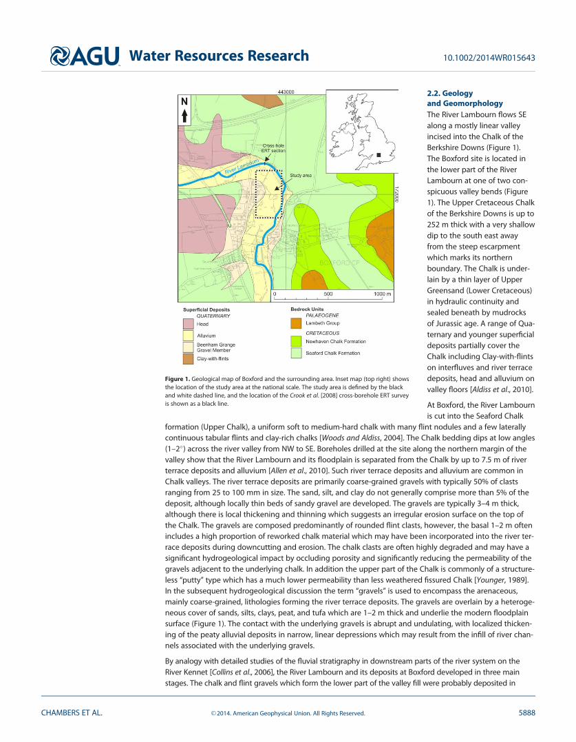
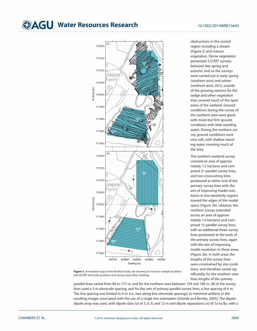
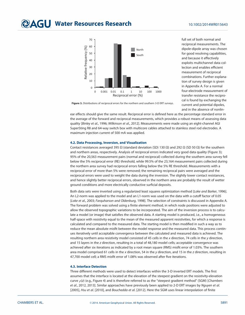
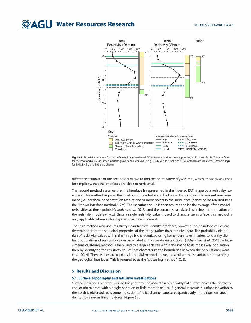
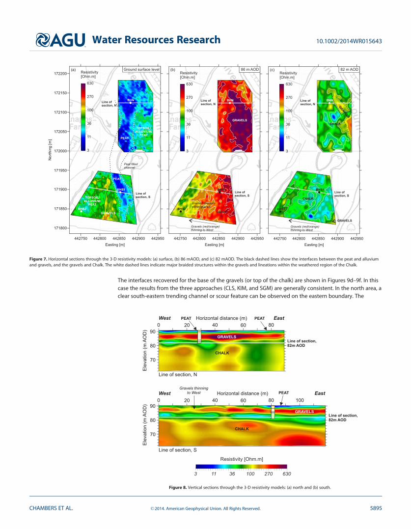
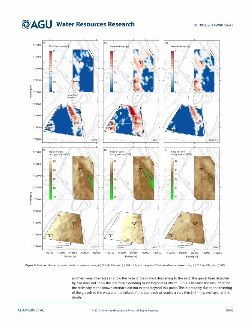
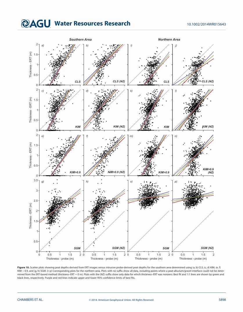
0
05
15
1
2
0 05 151 2
25
3
35
0 05 151 2
0
05
15
1
20
05
15
1
20
05
15
1
2
Thickness - probe (m)
Thic
knes
s - E
RT
(m)
Thic
knes
s - E
RT
(m)
Thic
knes
s - E
RT
(m)
Thic
knes
s - E
RT
(m)
Thickness - probe (m)0 05 151 2 0 05 151 2
Thickness - probe (m)Thickness - probe (m)
CLS CLS (NZ)
KIM
KIMgt09
SGM
KIM (NZ)
KIMgt09 (NZ)
SGM (NZ)
CLS CLS (NZ)
KIM
KIMgt09
SGM
KIM (NZ)
KIMgt09(NZ)
SGM (NZ)
Southern Area Northern Area
a) b)
c) d)
e) f)
g)
i)
h)
j)
k) l)
m) n)
o) p)
Figure 10 Scatter plots showing peat depths derived from ERT images versus intrusive probe-derived peat depths for the southern area determined using (a b) CLS (c d) KIM (e f)KIMgt 09 and (g h) SGM (indashp) Corresponding plots for the northern area Plots with no suffix show all data including points where a peat-alluviumgravel interface could not be deter-mined from the ERT-based method (thicknessndashERT 5 0 m) Plots with the (NZ) suffix show only data for which thicknessndashERT was nonzero Best fit and 11 lines are shown by green andblack lines respectively Purple and red lines indicate upper and lower 95 confidence limits of best fits
Water Resources Research 1010022014WR015643
CHAMBERS ET AL VC 2014 American Geophysical Union All Rights Reserved 5898
For the deeper interface between the gravels and chalk the geophysical edge detectors produced broadlysimilar results No ground truth data with the exception of the three boreholes is available to assess therespective performances of the three methods However two factors would suggest that the KIM might bemore reliable The first is that it performed best at defining the interface between the peat and gravel andsecond it is the only approach that incorporates direct observations of the interface (ie the borehole usedto determine the interface location) into the interpretation
Survey design in this case was a compromise between resolution depth of investigation and coveragerates and was informed by the need to provide information on the deeper deposits (ie gravels and the topof the Chalk) as well as the peat and alluvium Had the sole target been the peat and alluvium and theirinterface with the gravels survey design would have been modified to better resolve the very near surfacedeposits by reducing electrode and line spacings
62 Lithostratigraphy and Deposit Architecture621 ChalkThe Chalk is represented in the model by a considerable range of resistivities from a few tens to a few hun-dreds of Xm This variability is displayed in both the near surface and at depth However a strong trend ofincreasing resistivity with depth is observed which is associated with the weathering of the Chalk The vari-ability observed in the Chalk below the weathered zone is strikingly similar to that observed by Crook et al[2008] in a cross-borehole section approximately 200 m to the south west of the northern area (Figure 11)and is probably related to fracture systems and compositional changes such as the occurrence of flintsHowever Chalk in the weathered zone has been altered by brecciation [eg Murton 1996] and the forma-tion of clay-rich (and hence electrically conductive [eg Shevnin et al 2007]) putty chalk [Younger 1989]The presence of putty chalk at the site is confirmed in the boreholes This is consistent with observations byCrook et al [2008] at an adjacent site where weathered chalk with a resistivity in the range of 10ndash75 Xmwas observed during borehole investigations The weathered chalk is seen in the northern and southern 3-D ERT models as a mantle of highly variable thickness (approximately 1ndash10 m) at the top of the ChalkAlthough putty chalk is more commonly associated with interfluves it has been previously observedbeneath river valleys In particular Younger [1989] considers the formation of putty chalk in this setting inthe Reading area of the Thames Valley in the vicinity of the study site described here He proposes a modelfor its formation in periglacial conditions involving annual freeze-thaw causing pulverization of Chalkbeneath minor channels leading to putty chalk formations at the gravelChalk interface This would accountfor the highly variable nature of the putty chalk distribution including the features in the top of the Chalkwith a similar distribution and orientation to the apparent braid structures observed in the overlying gravels(Figure 7c)
622 GravelChalk InterfaceThe gravelChalk interface appears to generally deepen to the north and east (81 m AOD) (eg Figures 7band 8) which is consistent with deeper scouring of the bedrock at the bend in the river where the coursechanges sharply from east to south Conversely the interface is shallowest to the southwest (86 m AOD)
Table 2 Comparison Between Edge Detector and Intrusive Probe-Derived Peat Thickness
Southern Area Northern Area
MeanDifference (m)
Mean AbsoluteDifference (m)
RMSDifference (m)
MeanDifference (m)
Mean AbsoluteDifference (m)
RMSDifference (m)
CLSa 2033 048 054 2071 073 079KIMb 2004 049 054 2024 040 051KIMgt 09c 2048 053 059 2039 047 059SGMd 128 128 132 166 166 169CLS (NZ) 011 027 034 2042 046 055KIM (NZ) 033 042 050 2004 025 035KIMgt 09 (NZ) 2006 024 033 2014 027 037SGM (NZ) 129 129 133 166 166 170
aClusteringbKnown interface methodcKnown interface methods using pear depths greater than 09 mdSteepest gradient method
Water Resources Research 1010022014WR015643
CHAMBERS ET AL VC 2014 American Geophysical Union All Rights Reserved 5899
The smaller scale lateral vari-ability (meter to tens of meter)could indicate small-scale ero-sional structures or incisedchannels parallel and subparal-lel to the river course The larg-est such structure can be seenon the eastern margin of thenorthern area running south-southeast
623 GravelThe geophysical results indi-cate thicker and more continu-ous gravels in the northernarea which is closer to thepresent-day river course andoutside of the bend in the val-ley where deeper scouringappears to have occurredAgain gravel thicknesses in
this area are consistent with those observed by Crook et al [2008] (Figure 11) In the southern area the grav-els are very much more variable and can be seen to thin markedly toward their western limits the gravelsare either very thin or absent along the western margin of the model which is corroborated by BHS2 Thegravels display a very strong internal braided or anastomosing structure which is most apparent wherethey thin to the south-west of the study area This is consistent with the terrace gravels from this regiondescribed by Murton and Belshaw [2011] which were up to 5 m thick comprising sheets of sand and gravelwith small-cut and fill structures in multiple channels along with less common massive gravels that cutdown through the underlying terraces deposits and upon occasions the bedrock
The variability in the resistivities of the gravels will be influenced by lithological variability (ie variable claycontent) and variations in porosity To date intrusive sampling in the vicinity of the study area has shownthat the fines content (ie silt and clay-sized particles) of the gravels is very low Particle size analysis recov-ered from core in the north of the study area revealed fines content in the main body of the gravel to be inthe range of 02ndash1 only increasing near to the interface with the Chalk and including the occasional thinlayer of Chalk fines Likewise a nearby borehole (2 km down river) in the same formation described by Goz-zard [1981] records a fines content of 2ndash3 in the main body of the gravels with an increase observed to13 within 06 m of the Chalk bedrock Given the very low fines content (of which only a proportion will beclay sized) and the likelihood that the fines fraction will be predominantly Chalk-derived (and hence lowactivitycation exchange capacity) it is assumed that the resistivity variations observed in the main body ofthe gravels are primarily a function of porosity rather than conduction on clay mineral surfaces For the sedi-ment types considered here it is likely that porosity will increase with both grain size and the degree of sort-ing [Nelson 1994 Pryor 1973 Shepherd 1989] Archie [1942] demonstrates that for saturated porous mediaas porosity increases the proportion of pore fluid increases resulting in a decrease in resistivity Conse-quently well sorted and more porous gravels will display a lower resistivity than poorly sorted lower-porosity gravels In the absence of surface conductivity the relationship between bulk resistivity (qt) andporosity () is given as
qt52mqw
where m is the cementation exponent and qw is the pore fluid resistivity For the gravels at this study site itis reasonable to assume that m 5 15 [Jackson et al 1978 2007] The average pore fluid resistivity in thegravels is known to be 22 Xm Therefore according to Archie bulk resistivities of between 700 and 100Xm respectively which are very close to maximum and minimum resistivities associated with the gravelswould result in a porosity range of between 01 and 04 which is consistent with the ranges observed in
River channelBH-D BH-ENorth South
0
10Dep
th (m
)
Distance (m)0 10 20
Resistivity [Ohmm]
3 11 36 100 270 630
GRAVELS
CHALK (WEATHERED)
CHALKFLINTS
Figure 11 Cross-borehole ERT model [after Crook et al 2008] Borehole and surface electro-des are indicated as black dots The key for the geological logs of boreholes BH-D and BH-Eis given in Figures 1 and 4 The location of the cross-hole section is shown in Figure 1
Water Resources Research 1010022014WR015643
CHAMBERS ET AL VC 2014 American Geophysical Union All Rights Reserved 5900
similar sedimentary settings [Frings et al 2011 Pryor 1973] It is likely that the lower porosities would beassociated with the finest and most poorly sorted sediments and the highest with well-sorted gravels[Nelson 1994]
624 Peat and AlluviumThe deposits of peat and alluvium cover most of the study site as indicated by the intrusive survey and thelayer of lower resistivity observed across the top of the northern and southern resistivity models (Figure 7a)The thickest deposits occupy a channel-like structure defined by a topographic low on the surface of thegravels Unlike the thin (lt09 m) peat and alluvium in other areas of the site these deeper channel filldeposits have been well resolved by the KIM and CLS edge detectors
63 Implications for Hydrology and HydrogeologyThe distribution of low-permeability putty chalk as indicated by the ERT surveys aids our understanding ofthe potential groundwater exchange between the gravels and the Chalk Upwelling groundwater from theChalk bedrock into the gravels is more likely to occur where the weathered low-permeability zone is thinnest(Figure 12) This observation supports the contention of Allen et al [2010] that the interaction between thegravels and underlying Chalk is highly variable However the variability displayed in the weathered zone ofthe Chalk appears to take a similar form to the braided structures seen in the gravels This supports the modelof putty chalk formation put forward by Younger [1989] who postulated the preferentially formation of puttychalk beneath minor channels which in this case would be at the scale of individual channel braids Spatialand volumetric imaging techniques such as ERT are able to spatially characterize these structures at a resolu-tion more appropriate to the scale of heterogeneity unlike intrusive techniques such as drilling
The distribution of the gravels has a strong directional component (ie structures aligned with the directionof the water course) and given the likely relationship between resistivity distribution and porosity andhence permeability [Nelson 1994] this has significant implications for groundwater flow through the systemdue to directional permeability [Pryor 1973] In particular preferential flow is likely to occur in well-sortedhigh-porosity units of the gravels running parallel or subparallel to the current river course with less poten-tial for flow perpendicular to the river
It is also likely that the interactions between the river and the gravels will vary significantly depending onthe porosity and permeability of the gravels intersecting the river producing complex flows at a range ofscales [Allen et al 2010] Again well-sorted high-porosity and permeability gravels (hypothetically charac-terized by lower resistivities) are likely to provide preferential flow pathways [Pryor 1973] associated with agreater degree of exchange between surface and groundwaters
7 Conclusions
Volumetric analysis of the architecture of complex deposits underlying a lowland riparian wetland has beendemonstrated using 3-D ERT Gradient and isosurface-based edge detectors were used to automaticallyextract key lithostratigraphic interfaces from the resistivity models the peat and alluviumgravels interfaceand the gravelsChalk interface Assessment of the edge detectors was achieved with reference to a spatiallydense intrusive data set of peat thickness Three edge detectors were applied to the images and the results
EastWest RiverLambourn
Beenham GrangeGravel MemberAlluvium - peat silt clay
QUATERNARYSeaford Chalk Formationweathered lsquoputtyrsquo chalk
Seaford Chalk Formationunweathered
UPPER CRETACEOUS
Braided sand and gravelChannel - peat amp clay layers
Gravel lag deposits
Preferential flow
Erosional surface
Upwelling groundwater
250 m
15 m PreferentialflowDeeply
weatheredchalk
Figure 12 Schematic vertical section through the Boxford research site
Water Resources Research 1010022014WR015643
CHAMBERS ET AL VC 2014 American Geophysical Union All Rights Reserved 5901
were compared with the intrusive data using the complete set of samples and the subset comprising depthsgreater than the thickness of the first model layer At the 95 confidence level there was no combination ofedge detector and data set that was consistent with a 11 relationship between the ERT-derived and intru-sively determined peat thicknesses This implies that each ERT edge detection method exhibited a statisticallysignificant bias with respect to the intrusive data This bias was least for isosurfaces based on the intrusivedata and was improved by restricting analysis to the subset greater than the thickness of the uppermost ERTmodel layer The fuzzy clustering analysis performed slightly less well but considerably better than thegradient-based method which failed to correctly resolve the peat and alluviumgravels interface even inregions of thicker peat This was due to the peatrsquos relative thinness compared to the electrode spacing andthe need to apply greater damping to the top model layer to reduce inversion artifacts caused by the parallel2-D data acquisition It is likely that the resolution of the shallow peat would have been improved if a full setof orthogonal lines could have been acquired [Gharibi and Bentley 2005] in which case the gradient edgedetector would probably have performed better This suggests that the fundamental assumption of SGM thatthe steepest gradient will be coincident with the interface must be considered carefully in light of the modeldiscretization and inversion constraints For a broadly layered geology with relatively homogeneous strata ofcontrasting resistivities these results support previous findings [Chambers et al 2013] that isosurfaces cali-brated by intrusive data provide the best estimate of interface location In the absence of intrusive data clus-tering techniques may still give reasonable results Gradient-based detectors can be useful where strata areheterogeneous [Chambers et al 2012] but are unlikely to perform well in regions of the model where resolu-tion is lower (eg in heavily damped areas or regions further from the electrodes)
ERT identified significant heterogeneity in terms of both thickness and internal structure of the depositsand this would not have been appreciated with necessarily more spatially restricted intrusive methods Peatthickness varied between 0 and 2 m with the thicker deposits occupying a channel structure across the sur-face of the gravels Likewise sand and gravel thickness varied from 0 to 7 m with upper and lower surfacesdisplaying significant variations in elevation These variations along with the heterogeneity within the grav-els and Chalk will have significant implications for our understanding of groundwater-surface water interac-tions at the site In particular the highly variable weathered zone at the top of the Chalk comprising low-permeability putty chalk will exert significant controls on groundwater flows between the Chalk and grav-els Likewise the strong directional element in the resistivity and hence porosity distribution of the gravelsis likely to be associated with a directional permeability that will strongly influence flows through the grav-els and interactions between the river and groundwater
Three-dimensional ERT has proved to be a highly efficient approach to characterizing the geology associ-ated with this wetland site The resources required for the geophysical surveys were similar in terms of thefield time required to the intrusive surveys but have produced a data set with significantly richer informa-tion (ie a volumetric data set which reveals the architecture of the deposits underlying the wetland to adepth of approximately 25 m) which will be able to guide the development of hydrological and hydrogeo-logical models of the site and subsequent ecological management of the site Detailed understanding ofthe hydrological functioning of such complex groundwater-dependent ecosystems is essential for theirmanagement conservation and possible restoration and in particular in understanding the implications offuture environmental change
Appendix A Survey Design and Inversion Constraints
The design of the survey had to balance the requirement for good resolution of the near surface peatdeposits which would suggest smaller electrode spacings against the competing needs to cover the areasof interest in a reasonable time and to reconstruct the architecture of the deeper underlying deposits andbedrock which would give a preference for larger spacings An electrode spacing of 3 m was eventuallychosen since this gave a maximum line length of 189 m with 64 electrodes and a maximum depth-of-investigation using the dipole-dipole array of 27 m At the same time using the standard model discreti-zation in the inversion code (Res3DInv Geotomo Software wwwgeotomosoftcom) this still placed 2ndash3 ver-tical model cells within the typical thickness of the peat layer
Similarly the constraints placed on the resistivity model during the inversion had to be carefully consideredIn many circumstances an L1 model constraint [Loke et al 2003] is preferred when investigating lithological
Water Resources Research 1010022014WR015643
CHAMBERS ET AL VC 2014 American Geophysical Union All Rights Reserved 5902
boundaries since it favorssharp changes in resistivity Butin this case although the peatboundary was expected to besharp other interfaces of inter-est within the region (egbetween the gravels and thechalk) had a gradational char-acter In addition the use of anL1 constraint tends to alignresistivity boundaries to modelcell edges which can causeunrealistic step-like changeswith position when an inter-face is subhorizontal This isparticularly pronounced if thelithological layers being investi-gated are thin (such as thepeat layer here) On balancean L2 model constraint wastherefore thought to providethe best compromise
The effects of these decisions are demonstrated here using synthetic models Data were generated for a sin-gle line of 64 electrodes spaced at 3 m using dipole-dipole configurations with a 5 3 6 9 12 m and n 5 1ndash8 The forward models were one-dimensional and comprised a layer of peat between 01 and 30 m thick (in01 m increments) with resistivity q 5 15 Xm underlain by a layer of gravel with q 5 200 Xm so that thetotal thickness of peat and gravel was 50 m This was in turn underlain by chalk bedrock with q 5 100 XmThe data were inverted using Res2DInv with the same model discretization damping factors and data con-straint used in the 3-D inversions Both L1 and L2 model constraints were applied and results were simu-lated for the situations where all peat interface depths were considered (KIM) and where only interfacedepths greater than 09 m were used (KIMgt 09)
The resistivity at the interface depth was determined for each inverted model To reflect site conditions aweighted average of these was calculated with the weighting taken to be the frequency with which thatdepth was observed in the real peat probe data set (eg for a modeled peat depth of 11 m the proportion ofpeat depths observed in the range 105ndash115 m was 0098) The weighted average was used as the resistivityvalue to determine the depth to the interface This was calculated for the four combinations of L1 or L2 modelconstraints and all depths (KIM) or depths gt09 m (KIMgt 09) The results were L1 KIM qint 5 355 Xm L1KIMgt 09 qint 5 274 Xm L2 KIM qint 5 375 Xm L2 KIMgt 09 qint 5 307 Xm The interface depths at theseresistivity values are shown in Figure A1 The depths derived from the L1 model show a somewhat step-likedependence against the true depth whether they were determined using the KIM or KIMgt 09 resistivity Incontrast the L2 model depths vary more smoothly with the true depth This is due to the effect mentionedabove of the L1 constraint preferring to place the interface on model cell boundaries The RMS errors betweenthe model-derived and true depths were L1 KIM 0246 m L1 KIMgt 09 0283 m L2 KIM 0276 m L2 KIMgt 090130 m For the survey geometry and lithological architecture at this site these results show that using an L2model constraint with intrusive data only from depths greater than the first model block gives the bestapproximation when using isoresistivity contours to determine the peat interface location
ReferencesAldiss D T et al (2010) Geology of the Newbury District and Part of the Abingdon District Br Geol Surv Nottingham U KAllen D J W G Darling D C Gooddy D J Lapworth A J Newell A T Williams D Allen and C Abesser (2010) Interaction between
groundwater the hyporheic zone and a Chalk stream A case study from the River Lambourn UK Hydrogeol J 18(5) 1125ndash1141 doi101007s10040-010-0592-2
Andersen H E (2004) Hydrology and nitrogen balance of a seasonally inundated Danish floodplain wetland Hydrol Processes 18(3) 415ndash434 doi101002hyp1277
Figure A1 Model-derived depths as a function of true interface depth
AcknowledgmentsThis paper is published with thepermission of the Executive Director ofthe British Geological Survey (NERC)Data used to generate the resistivitymodels are archived by the BritishGeological Survey and are availablefrom the authors
Water Resources Research 1010022014WR015643
CHAMBERS ET AL VC 2014 American Geophysical Union All Rights Reserved 5903
Archie G E (1942) The electrical resistivity log as an aid in determining some reservoir characteristics Trans AIME 146 54ndash62Ausden M W J Sutherland and R James (2001) The effects of flooding lowland wet grassland on soil macroinvertebrate prey of breed-
ing wading birds J Appl Ecol 38(2) 320ndash338 doi101046j1365-2664200100600xBaldwin A H M S Egnotovich and E Clarke (2001) Hydrologic change and vegetation of tidal freshwater marshes Field greenhouse
and seed-bank experiments Wetlands 21(4) 519ndash531 doi1016720277-5212(2001)021[0519hcavot]20co2Binley A B Shaw and S Henry-Poulter (1996) Flow pathways in porous media Electrical resistance tomography and dye staining image
verification Meas Sci Technol 7(3) 384ndash390 doi1010880957-023373020Bouchedda A M Chouteau A Binley and B Giroux (2012) 2-D joint structural inversion of cross-hole electrical resistance and ground
penetrating radar data J Appl Geophys 78 52ndash67 doi101016jjappgeo201110009Chambers J E R D Ogilvy O Kuras J C Cripps and P I Meldrum (2002) 3D electrical imaging of known targets at a controlled environ-
mental test site Environ Geol 41(6) 690ndash704 doi101007s00254-001-0452-4Chambers J E et al (2012) Bedrock detection beneath river terrace deposits using three-dimensional electrical resistivity tomography
Geomorphology 177 17ndash25 doi101016jgeomorph201203034Chambers J E P B Wilkinson S Penn P I Meldrum O Kuras M H Loke and D A Gunn (2013) River terrace sand and gravel deposit
reserve estimation using three-dimensional electrical resistivity tomography for bedrock surface detection J Appl Geophys 93 25ndash32doi101016jjappgeo201303002
Collins P E F P Worsley D M Keith-Lucas and I M Fenwick (2006) Floodplain environmental change during the Younger Dryas andHolocene in Northwest Europe Insights from the lower Kennet Valley south central England Palaeogeogr Palaeoclimatol Palaeoecol233(1ndash2) 113ndash133 doi101016jpalaeo200509014
Comas X L Slater and A Reeve (2004) Geophysical evidence for peat basin morphology and stratigraphic controls on vegetationobserved in a Northern Peatland J Hydrol 295(1ndash4) 173ndash184 doi101016jjhydrol2004303008
Crook N A Binley R Knight D A Robinson J Zarnetske and R Haggerty (2008) Electrical resistivity imaging of the architecture of sub-stream sediments Water Resour Res 44 W00D13 doi1010292008WR006968
Everard M (2005) Water Meadows 289 pp Forrest Text Ceredigion U KFarquharson C G and D W Oldenburg (1998) Non-linear inversion using general measures of data misfit and model structure Geophys
J Int 134(1) 213ndash227 doi101046j1365-246x199800555xFrings R M H Schuettrumpf and S Vollmer (2011) Verification of porosity predictors for fluvial sand-gravel deposits Water Resour Res
47 W07525 doi1010292010WR009690Gharibi M and L R Bentley (2005) Resolution of 3-D electrical resistivity images from inversions of 2-D orthogonal lines J Environ Eng
Geophys 10(4) 339ndash349 doi102113JEEG104339Goudie A (1990) The Landforms of England and Wales Basil Blackwell Oxford U KGozzard J R (1981) The sand and gravel resources of the country around Newbury Berkshire Part 1 around Newbury Description of 1
25000 sheet SU46 and parts of SU36 37 and 47 [and] Part 2 North-east of Newbury Description of 125000 sheet SU57 Mineral Assess-ment Report 59 Institute of Geological Sciences Her Majestyrsquos Stationary Office (HMSO) London U K
Grapes T R C Bradley and G E Petts (2006) Hydrodynamics of floodplain wetlands in a chalk catchment The River Lambourn UK JHydrol 320(3ndash4) 324ndash341 doi101016jjhydrol200507028
Hayley K L R Bentley M Gharibi and M Nightingale (2007) Low temperature dependence of electrical resistivity Implications for nearsurface geophysical monitoring Geophys Res Lett 34 L18402 doi1010292007GL031124
Heagle D M Hayashi and G van der Kamp (2013) Surface-subsurface salinity distribution and exchange in a closed-basin prairie wetlandJ Hydrol 478 1ndash14 doi101016jjhydrol201205054
Hirsch M L R Bentley and P Dietrich (2008) A comparison of electrical resistivity ground penetrating radar and seismic refraction resultsat a river terrace site J Environ Eng Geophys 13(4) 325ndash333 doi102113JEEG134325
Holden J and T P Burt (2003) Runoff production in blanket peat covered catchments Water Resour Res 39(7) 1191 doi1010292002WR001956
Holden J T P Burt and M Vilas (2002) Application of ground-penetrating radar to the identification of subsurface piping in blanket peatEarth Surf Processes Landforms 27(3) 235ndash249 doi101002esp316
Hsu H L B J Yanites C C Chen and Y G Chen (2010) Bedrock detection using 2D electrical resistivity imaging along the Peikang Rivercentral Taiwan Geomorphology 114(3) 406ndash414 doi101016jgeomorph200908004
Jackson P D D Taylor-Smith and P N Stanford (1978) Resistivity-porosity-particle shape relationships for marine sands Geophysics43(6) 1250ndash1268 doi10119011440891
Jackson P D J F Williams M A Lovell A Camps C Rochelle and A E Milodowski (2007) An investigation of the exponent in Archiersquosequation Comparing numerical modeling with laboratory data Towards characterising disturbed samples from the Cascadia MarginIODP Expedition 311 in Society of Petrophysicists and Well Log Analysts (SPWLA) 49th Annual Logging Symposium 10 pp SPWLAEdinburgh
Karan S P Engesgaard M C Looms T Laier and J Kazmierczak (2013) Groundwater flow and mixing in a wetland-stream system Fieldstudy and numerical modeling J Hydrol 488 73ndash83 doi101016jjhydrol201302030
Klove B et al (2011) Groundwater dependent ecosystems Part I Hydroecological status and trends Environ Sci Policy 14(7) 770ndash781doi101016jenvsci201104002
Lapworth D J D C Gooddy D Allen and G H Old (2009) Understanding groundwater surface water and hyporheic zone biogeochemi-cal processes in a Chalk catchment using fluorescence properties of dissolved and colloidal organic matter J Geophys Res 114G00F02 doi1010292009JG000921
Loke M H and R D Barker (1996) Practical techniques for 3D resistivity surveys and data inversion Geophys Prospect 44(3) 499ndash523doi101111j1365-24781996tb00162x
Loke M H I Ackworth and T Dahlin (2003) A comparison of smooth and blocky inversion methods in 2D electrical imaging surveysExplor Geophys 34 182ndash187
Loke M H J E Chambers D F Rucker O Kuras and P B Wilkinson (2013) Recent developments in the direct-current geoelectrical imag-ing method J Appl Geophys 95 135ndash156 doi101016jjappgeo201302017
Mansoor N and L Slater (2007) Aquatic electrical resistivity imaging of shallow-water wetlands Geophysics 72(5) F211ndashF221 doi10119012750667
McClain M E et al (2003) Biogeochemical hot spots and hot moments at the interface of terrestrial and aquatic ecosystems Ecosystems6 301ndash312 doi101007s10021-003-0161-9
Water Resources Research 1010022014WR015643
CHAMBERS ET AL VC 2014 American Geophysical Union All Rights Reserved 5904
Meads L N L R Bentley and C A Mendoza (2003) Application of electrical resistivity imaging to the development of a geologic model for aproposed Edmonton landfill site Canadian Geotechnical Journal 40(3) 551ndash558 doi101139t03-017
Murton J B (1996) Near-surface brecciation of chalk Isle of Thanet south-east England A comparison with ice-rich brecciated bedrocks in Can-ada and Spitsbergen Permafrost Periglacial Processes 7(2) 153ndash164 doi 101002(sici)1099-1530(199604)72lt153aid-ppp215gt30co2-7
Murton J B and R K Belshaw (2011) A conceptual model of valley incision planation and terrace formation during cold and arid perma-frost conditions of Pleistocene southern England Quat Res 75(2) 385ndash394 doi101016jyqres201010002
Musgrave H and A Binley (2011) Revealing the temporal dynamics of subsurface temperature in a wetland using time-lapse geophysicsJ Hydrol 396(3ndash4) 258ndash266 doi101016jjhydrol201011008
Nelson P H (1994) Permeability-porosity relationships in sedimentary rocks Log Anal 35(3) 38ndash62Nguyen F S Garambois D Jongmans E Pirard and M H Loke (2005) Image processing of 2D resistivity data for imaging faults J Appl
Geophys 57(4) 260ndash277 doi101016jjappgeo200502001Prior H and P J Johnes (2002) Regulation of surface water quality in a Cretaceous Chalk catchment UK An assessment of the relative
importance of instream and wetland processes Sci Total Environ 282 159ndash174 doi101016s0048-9697(01)00950-0Pryor W A (1973) Permeability-porosity patterns and variations in some Holocene sand bodies Am Assoc Pet Geol Bull 57(1) 162ndash189Riddell E S S A Lorentz and D C Kotze (2010) A geophysical analysis of hydro-geomorphic controls within a headwater wetland in a
granitic landscape through ERI and IP Hydrol Earth Syst Sci 14(8) 1697ndash1713 doi105194hess-14-1697-2010Shepherd R G (1989) Correlations of permeability and grain-size Ground Water 27(5) 633ndash638 doi101111j1745-65841989tb00476xShevnin V A Mousatov A Ryjov and O Delgado-Rodriquez (2007) Estimation of clay content in soil based on resistivity modelling and
laboratory measurements Geophys Prospect 55(2) 265ndash275 doi101111j1365-2478200700599xSingha K and S M Gorelick (2006) Hydrogeophysical tracking of three-dimensional tracer migration The concept and application of
apparent petrophysical relations Water Resour Res 42 W06422 doi1010292005WR004568Slater L D and A Reeve (2002) Investigating peatland stratigraphy and hydrogeology using integrated electrical geophysics Geophysics
67(2) 365ndash378 doi10119011468597Ward W O C P B Wilkinson J E Chambers L S Oxby and L Bai (2014) Distribution-based fuzzy clustering of Electrical Resistivity
Tomography images for interface detection Geophysical Journal International 197(1) 310ndash321 doi101093gjiggu006Wheater H S D Peach and A Binley (2007) Characterising groundwater-dominated lowland catchments The UK Lowland Catchment
Research Programme (LOCAR) Hydrol Earth Syst Sci 11(1) 108ndash124 doi105194hess-11-108-2007Wilkinson P M H Loke P I Meldrum J E Chambers O Kuras D A Gunn and R D Ogilvy (2012) Practical aspects of applied optimised
survey design for electrical resistivity tomography Geophys J Int 189(1) 428ndash440 doi101111j1365-246X201205372xWoods M A and D T Aldiss (2004) The stratigraphy of the Chalk Group of the Berkshire Downs Proc Geol Assoc 115 249ndash265 doi
101016S0016-7878(04)80006-3Younger P L (1989) Devensian periglacial influences on the development of spatially-variable permeability in the Chalk of southeast Eng-
land Q J Eng Geol 22(4) 343ndash354 doi101144gslqjeg19890220407Zedler J B (2000) Progress in wetland restoration ecology Trends Ecol Evol 15(10) 402ndash407 doi101016s0169-5347(00)01959-5Zhou Q Y J Shimada and A Sato (2001) Three-dimensional spatial and temporal monitoring of soil water content using electrical resis-
tivity tomography Water Resour Res 37(2) 273ndash285 doi1010292000WR900284
Water Resources Research 1010022014WR015643
CHAMBERS ET AL VC 2014 American Geophysical Union All Rights Reserved 5905
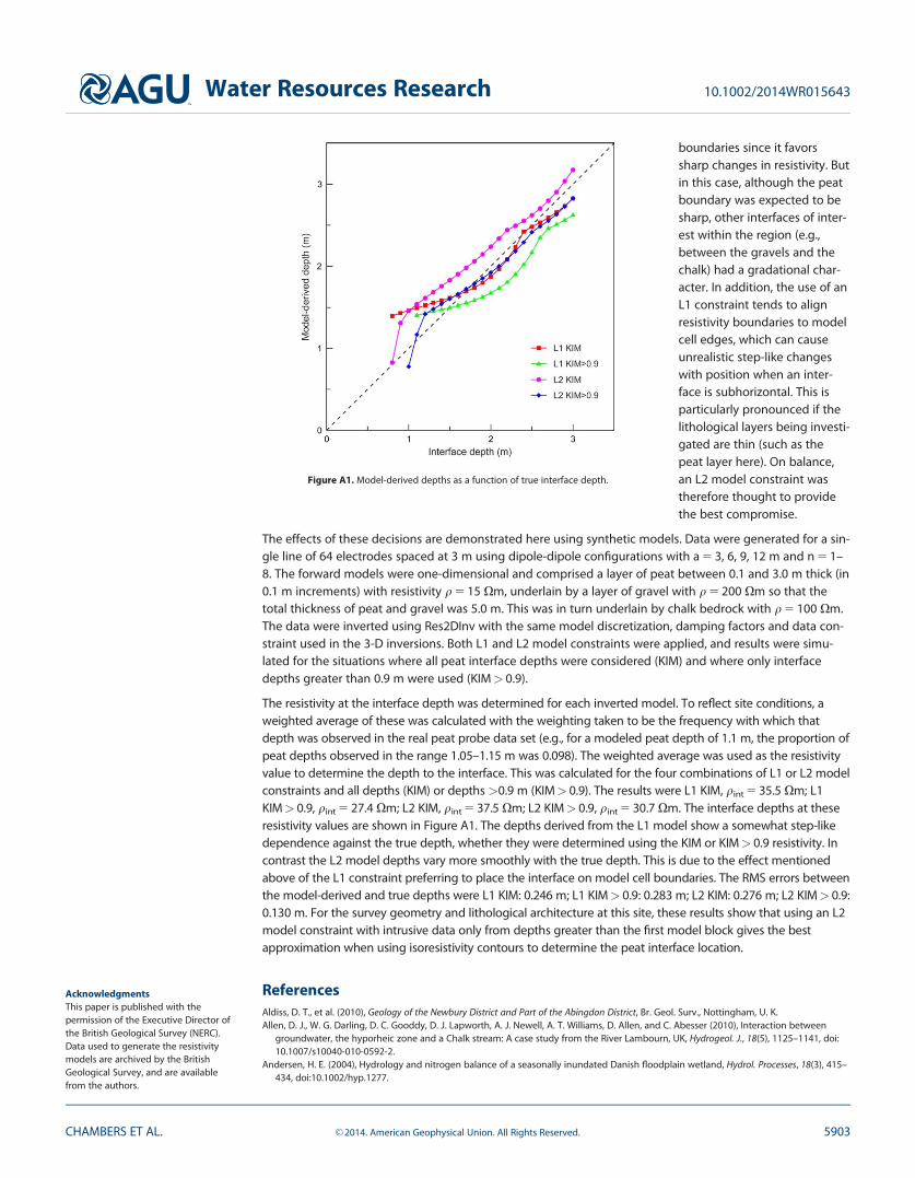
Copyright © 2022 FDOKUMEN