Depth-to-the-bottom optimization for magnetic data inversion: Magnetic structure of the Latium...

Depth-to-the-bottom optimization for magnetic data

inversion: Magnetic structure of the Latium volcanic

region, Italy

F. Caratori Tontini,1 L. Cocchi,2 and C. Carmisciano1

Received 13 October 2005; revised 14 June 2006; accepted 17 July 2006; published 17 November 2006.

[1] We present an algorithm for the linear inversion of two-dimensional (2-D) surfacemagnetic data to obtain 3-D models of the susceptibility of the source. The forward modelis discretized by a mesh of prismatic cells with constant magnetization that allows therecovery of a complete 3-D generating source. As the number of cells are normally greaterthan the amount of available data, we have to solve an underdetermined linear inverseproblem. A Tikhonov regularization of the solution is introduced as a depth-weightingfunction adapted from Li and Oldenburg (1996) to close the source toward the bottom.The main novelty of this method is a first-stage optimization that gives information aboutthe depth to the bottom of the generating source. This parameter permits both theevaluation of the appropriate vertical extension of the mesh and the definition of the shapeof the regularizing depth-weighting distribution. After discussing the performance of thismethod by showing the results of various synthetic tests, we invert the magnetic anomaliesof the volcanic edifices in the Latium region in central Italy to define their 3-D sourcedistribution.

Citation: Caratori Tontini, F., L. Cocchi, and C. Carmisciano (2006), Depth-to-the-bottom optimization for magnetic data inversion:

Magnetic structure of the Latium volcanic region, Italy, J. Geophys. Res., 111, B11104, doi:10.1029/2005JB004109.

1. Introduction

[2] The quantitative estimation of the physical parametersof the source generating an observed potential-field anom-aly is an inverse problem. Functionals relating a particulardistribution of magnetic susceptibility to the observedanomaly are usually not analytically invertible, and further-more, even after linearization, the number of unknownsoften exceeds the number of observations. Inverse problemsof this kind are characterized by instability and nonunique-ness of the solution [Tikhonov and Arsenin, 1977; Tarantola,1987; Menke, 1989]. The theoretical or inherent ambiguityhas been known since Gauss’ epoch as a trivial conse-quence of the Laplace equation [Blakely, 1995]. Algebraicambiguity is another major concern.We follow the frequentlyused procedure that consists of subdividing the regionpresumably containing the source into a set of prismaticvolume pixels (voxels). The relationship connecting themagnetization of each voxel with the observed datumis thus linear and can be represented by a sensitivitymatrix. This matrix is always rank deficient: thus it has amultidimensional null-space. The solution of this problemis an affine space of vectors, in the sense that a particularsolution can be perturbed by a vector that spans the null-

space of the matrix (also called its annihilator) withoutchanging the resulting anomaly. Experimental ambiguityfinally, comes from geological or experimental noise inthe data that always affects the resolution of the modeland may generate spurious sources. All of the aboveconsiderations apply to inversions for density perturba-tions from gravity anomalies as well as to inversions formagnetic susceptibility from magnetometer observations,on which we focus mainly in this paper.[3] We recall that the forward model may be unable to

represent the source exactly. In the case of a sphericalsource meshed by prismatic voxels the problem is one ofincompatibility of the system of equations rather thanambiguity. As a consequence of these ambiguities andincompatibilities ‘‘optimal solutions’’ may arise at anydepth, which accounts for the widely perceived notion thatpotential-field data lack depth resolution and that the inversemodeling often yields solutions that are too shallow. Toobtain realistic models additional information has to beintroduced, known as ‘‘a priori’’ information, in the statis-tical (Bayesian) sense, or as regularization in the sensedefined by Tikhonov and Arsenin [1977]. These approacheshave been interpreted as different alternatives [Scales andSnieder, 1997], but they may in fact be compatible undercertain restrictive assumptions [Ho-Liu et al., 1989;Yanovskaya and Ditmar, 1990; Simons et al., 2002].[4] Several approaches that deal with the problems of

nonuniqueness of potential-field inversion exist [Boulangerand Chouteau, 2001; Silva et al., 2001]. Minimization ofthe total volume [Last and Kubik, 1983] or of the moment

JOURNAL OF GEOPHYSICAL RESEARCH, VOL. 111, B11104, doi:10.1029/2005JB004109, 2006ClickHere

for

FullArticle

1Stazione di Geofisica Marina, Istituto Nazionale di Geofisica eVulcanologia, Fezzano, Italy.

2Dipartimento Scienze della Terra Geologiche-Ambientali, Universita diBologna, Bologna, Italy.

Copyright 2006 by the American Geophysical Union.0148-0227/06/2005JB004109$09.00

B11104 1 of 17

http://dx.doi.org/10.1029/2005JB004109

of inertia [Guillen and Menichetti, 1984] of the sourceallows the recovery of compact models by avoiding disper-sion of the source. Barbosa and Silva [1994] obtainedcompactness along several axes by introducing ‘‘a priori’’information about the axis length. Caratori Tontini et al.[2003] developed a model based on the envelope of thesource by using a set of three-dimensional (3-D) Gaussianfunctions. Fedi and Rapolla [1999] studied a multilayer 3-Ddata set, obtaining solutions at the correct depth by studyingalso the vertical variations of the magnetic field. In this veinwe also note the work of Jacobsen [1987] and Pedersen[1991], who concluded that ‘‘the difference of the fieldsupward continued to different levels represents the bestestimate of the field from the depth interval which is halfof the upward continued height interval’’.[5] In their very interesting paper, Li and Oldenburg

[1996] introduced a depth-weighting function to counteractthe spatial decay of the kernel function with depth, givingincreasing weight to voxels at increasing depths. Togetherwith global smoothness constraints these authors obtainedcompact solutions and reduced the dispersion of the sourcealong the three spatial directions, recovering thus a modelwith a ‘‘minimum structure’’. Depth-weighting has givenmeaningful results and has been applied successfully intoother inversion algorithms [Pilkington, 1997; Boulangerand Chouteau, 2001; Portniaguine and Zhdanov, 2002;Zhdanov, 2002; Pignatelli et al., 2006], since it allows theuser to obtain solutions at the correct depths even in the caseof vertically dislocated sources.[6] Our work is built on the study of Li and Oldenburg

[1996]. The guidelines we adopted were mainly dictated bythe requirement of a straightforward and easy-to-use algo-rithm, with good performance in terms of execution timesand robustness in the presence of noise. This is particularlyuseful for direct real-time applications during the surveyexecution, where we have few information about the sourceand the data quality is not fully enhanced. The easiness ofimplementation is particularly suitable for anyone interestedto reproduce or to increase the capability of the method. Tothis aim we introduce a depth weighting of the model normwithout additional constraints in order to reduce to aminimum level the amount of required ‘‘a priori’’ informa-tion. This allows the user to get fast first-order approxima-tion solutions which can show, however, importantinformation about the susceptibility distribution, the struc-tural trends of the source and the depth distribution,especially concerning the bottom characterization. Thischoice allows the transformation of the problem into a‘‘free’’ inversion with a new sensitivity matrix, increasingthe numerical performance of the method.[7] We will show that the inverse models are pushed

toward the bottom of the mesh, even if the relative depthsbetween sources are preserved. Depth-weighting alone isthus unable to give a solution with a correct depth to thebottom (DTB) of the source, and additional informationshould be added. As far as we know, the exact introductionof the DTB parameter in the framework of 3-D linearinversion has not been directly treated by previous methods,while often the depth to the top is properly found whenusing a standard depth-weighting distribution. Resolvingthe DTB, however, is important not only because it maydefine the magnetic basement, but also because it permits

the definition of an appropriate mesh for the inversion withminimum vertical extent. We thus modify the depth-shapedistribution in the regularization matrix by combining adepth-weighting function, based on a power law decay, witha function that allows the closure of the solutions at aconsistent bottom depth. In other words, our method finds aregularization matrix that depends on one parameter relatedto the DTB of the source.[8] Moreover enough information is contained in the data

itself to find this parameter by the preliminary minimizationof a new norm of the solution, which we introduce in thispaper. In practice we have adopted a regularization whichuses the minimum amount of ‘‘a priori’’ information neededfor an essential characterization of the source, especially interms of depth-shape and susceptibility distribution, lettingthe algorithm being sufficiently fast and easy to use, butalso flexible, to be upgraded by additional constraints oroptimization improvements if needed by the user. Thisdemonstrates also that when the Tikhonov regularizationis adapted with a meaningful depth function, potential-fielddata can provide DTB information without imposing addi-tional constraints or requiring more ‘‘a priori’’ information.We show the above on the basis of synthetic tests and alsoby inverting the magnetic anomalies of the volcanic centersof Latium in central Italy.

2. Inverse Model

[9] We group the observations into a column vector d,while the parameters that are the target of the inversion areidentified by the vector p that consists of the magneticsusceptibility of each voxel, within a 3-D mesh gridpresumably containing the true source. The elements ofthe vector p are ordered in function of increasing depth, inthe direction of the layers of the mesh. The linear forwardmodel is expressed in the following equation

d ¼ K � p; ð1Þ

where K is the sensitivity matrix that expresses thecontribution of a single voxel of the mesh to a particularobserved datum. The column index j of Kij indicates thecontribution of the jth prismatic voxel of the mesh to the ithobservation, i.e., the magnetic field generated in the spatialposition of the ith observation by the jth prismatic voxel, asif the voxel was uniformly magnetized. This matrix isevaluated according to Bhattacharyya [1964], who derivedanalytical relationships for the magnetic field generated by arectangular prism. The magnetic theory being linear, thefield at the spatial position of the ith observation is given bythe sum of all the contributions of each jth voxel weightedwith its specific susceptibility pj, as in equation (1). As wewill see, we look for two main sets of parameters: apreliminary optimization step gives the DTB of the source,while the final result is the 3-D spatial distribution of thesusceptibility p.[10] We introduce further the hypothesis of induced

magnetization, namely that the ambient geomagnetic fieldhas the same direction as the source magnetization. This is awell-justified hypothesis since many anomalies are gener-ated by sources whose magnetization is induced by theambient field itself. Otherwise an average remanent mag-

B11104 CARATORI TONTINI ET AL.: DEPTH-TO-THE-BOTTOM OPTIMIZATION

2 of 17

B11104

netization direction has to be properly evaluated and intro-duced in the sensitivity matrix [Helbig, 1963; Claerbout,1976; Andersen and Pedersen, 1979].[11] The linear operator K has a multidimensional null-

space. The solution thus has to be regularized [Tikhonov andArsenin, 1977]. To this aim we adopt the very useful set ofMatlab routines developed by Hansen [1994]. The optimalsolution popt minimizes the misfit between the observeddata and the anomaly generated by the recovered model in achi-square sense, with the additional constraint of minimiz-ing also a particular regularizing norm:

popt ¼ arg min jK � p� dj2 þ l2jL � pj2n o� �

; ð2Þ

where L is a square matrix, whose dimension equals thenumber of unknown parameters. The Lagrange multiplier lshould represent a compromise between data fitting andnorm of the solution. Large values of l generate verycompact solutions at the expense of a large chi-square normthat indicates poor data fit; instead lower values of lgenerate solutions that, while fitting very well the data, inmany cases are far from the true model. We choose theoptimal l value according to the L curve principle [Lawsonand Hanson, 1974; Hansen and O’Leary, 1993]. TheL curve is a plot of log jL � pj2 versus log jK � p � dj2. Thiscurve is L shaped, with the optimal l in a distinct corner,that is, the point of maximum curvature.

[12] An example of this particular behavior can be seen inFigure 1, where we show the L curve that corresponds tothe inversion of the synthetic anomaly of Figure 2. Weannounce in advance that this inversion was performed byusing n = 400 data. In proximity of the optimal l = 12.9491the chi-square norm c2 is 420, and thus the reduced chi-square norm (c2/n) is 1.05, indicating a good fit. Quantita-tively speaking this result translates into a significance levelof 75%, i.e., the probability that a value of c2 at least aslarge as 420 will be obtained within a large number ofexperiments. These results allow thus the interpretation ofthe optimal l value as a good balance between data fittingand norm of the solution.[13] A common practice in inverse problems is to identify

L with the identity matrix. This corresponds to finding theminimum L2 norm solution of the linear problem. Li andOldenburg [1996] showed that in potential-field inversionthis is unsatisfactory since the solution tends to be clusteredtoward the top of the mesh, where low values of density ormagnetization can fit the observed data very well. Wedesign a regularization matrix L that generates solutionsat a consistent depth. Li and Oldenburg [1996] corrected theradial decay of the kernel by using an empirical functionthat simulates the decay of the magnetic field with depth.Following them, we assume a diagonal form for L, such that

L zð Þij� Freg zð Þdij; ð3Þ

Figure 1. L curve obtained inverting the synthetic anomaly of Figure 2. Along the curve are drawn thel values. The corner of the curve, that is, the maximum curvature point, corresponds to the optimal l =12.9491. This value, as can be seen in this qualitative figure, represents a good compromise between datafitting and small norm of the solution. The chi-square norm is 420. Having inverted 400 data, weobtained a reduced chi-square norm 1.05 that corresponds to a significance level of 75%.


3 of 17

B11104

where dij is the Kronecker symbol and Freg(z) indicates thefunction expressing the contribution of a horizontal layer ofthe mesh at the depth z, normalized to its maximum over alldepths. The first-order approximation of the function Freg(z)is

Freg zð Þ l3=2z

z3=2; ð4Þ

where lz is the vertical extension of the mesh, and the depthz is measured from the top of the mesh to the center of the

layer to avoid singularities in equation (4). As shown by Liand Oldenburg [1996] the choice of the depth function isempirical. In particular, the use of a greater exponent inequation (4) flattens the solution too much toward thebottom of the mesh, without preserving the vertical ratiosbetween depths of separate sources. Lower values of thesame exponent instead produce too shallow results. Byusing equations (3) and (4) we next define

p � L�1 zð Þ � p0; ð5Þ

which emphasizes the deep layers of the mesh given theincreasing values of L�1(z) with depth. Being diagonal andhaving nonzero values on the diagonal L(z) is invertible,and equation (2) takes on the following form

p0opt ¼ arg min fjK � L�1 � p0 � dj2 þ l2jp0j2� o� �

: ð6Þ

Practically the solution of equation (6) is obtained by asimple SVD decomposition that gives the minimum L2

norm solution of a problem with a new sensitivity matrixK � L�1. The correctness of equation (6) is simplyestablished by the following steps

min jK � L�1 � p0 � dj2 þ l2jp0j2n o

¼

min jK � L�1 � p0 � dj2 þ l2jL � L�1 � p0j2n o

¼

min jK � p� dj2 þ l2jL � pj2n o

; ð7Þ

where having used equation (5) together with the identitymatrix in the form of L�1 � L, we show that the processis equivalent to finding a solution that gives emphasis togreater depths as in equation (2). Equation (7) agreeswith the results of Boulanger and Chouteau [2001] and

Figure 2. Synthetic anomaly generated by a compositeprismatic model. The inducing field is assumed having aninclination of 60�, a declination of 0�, and a magnitude of46,000 nT. The anomaly is calculated by a grid of 20 � 20points. Random Gaussian noise with a standard deviation of3% of the data amplitude has been added to the data.

Figure 3. Central section showing the result of the inversion of the anomaly of Figure 1 by using apower law decay regularization matrix. The true source is represented by the thick boxes and has asusceptibility of 0.3 (SI). The recovered model is far from the true model, since it tends to flatten thesolution toward the bottom of the mesh. Nevertheless, it seems to resemble the depth ratios of the truemodel, in the sense that a shallower source is found where the upper prism is located.


4 of 17

B11104

Pignatelli et al. [2006], where the sensitivity matrix hasbeen directly corrected by multiplying it with a powerlaw function that increases with depth. We find theminimum L2 norm solution p0opt, and finally the correctvector popt � L�1(z) � p0opt.[14] As it turns out, this regularization is insufficient,

even if in the case of vertically dislocated sources itpreserves the difference in depth. In Figure 2 we show themagnetic anomaly generated by a source made of twoprismatic bodies buried at different depths, while Figure 3shows a vertical northward oriented cross section with theresult of the inversion compared with the true sources. Wehave inverted 20 � 20 data contaminated by randomGaussian noise with a standard deviation of 3% of the dataamplitude by using a mesh of 20 � 20 � 10 voxels centeredunder the anomaly. We show only the relevant central crosssection since the source is characterized by a strike lengthalong the y axis of 1000 m. The recovered solution is farfrom the true model because the chosen regularization tendsto put the maxima of the magnetization toward the bottomof the mesh. However, the shape of the solution has acertain resemblance to the ratios of depths between the realsources.[15] Our solution is now to introduce a correction term

in the regularization that allows the exact evaluation of thedepth to the bottom of the solution. We correct thus theregularization matrix by closing it toward the bottom ofthe mesh according to the following equation:

L�1 zð Þij � F�1reg zð Þ � B zð Þ � dij; ð8Þ

where the function B(z) should contain the DTB informa-tion. This function B too, is empirical, and we introduce itby practical considerations.

3. Fermi Function

[16] The choice of B(z) is dictated by the requirementthat it preserves the power law decay of the regularizationmatrix at depths shallower than the DTB of the generat-ing source. This property is really essential to obtain thecorrect depth-to-the-top ratios. Below the DTB of thegenerating source we should obtain instead a negligiblesolution. The function B(z) should thus have a constantunitary value at shallow depths and should annihilateitself at depths greater than the DTB of the generating

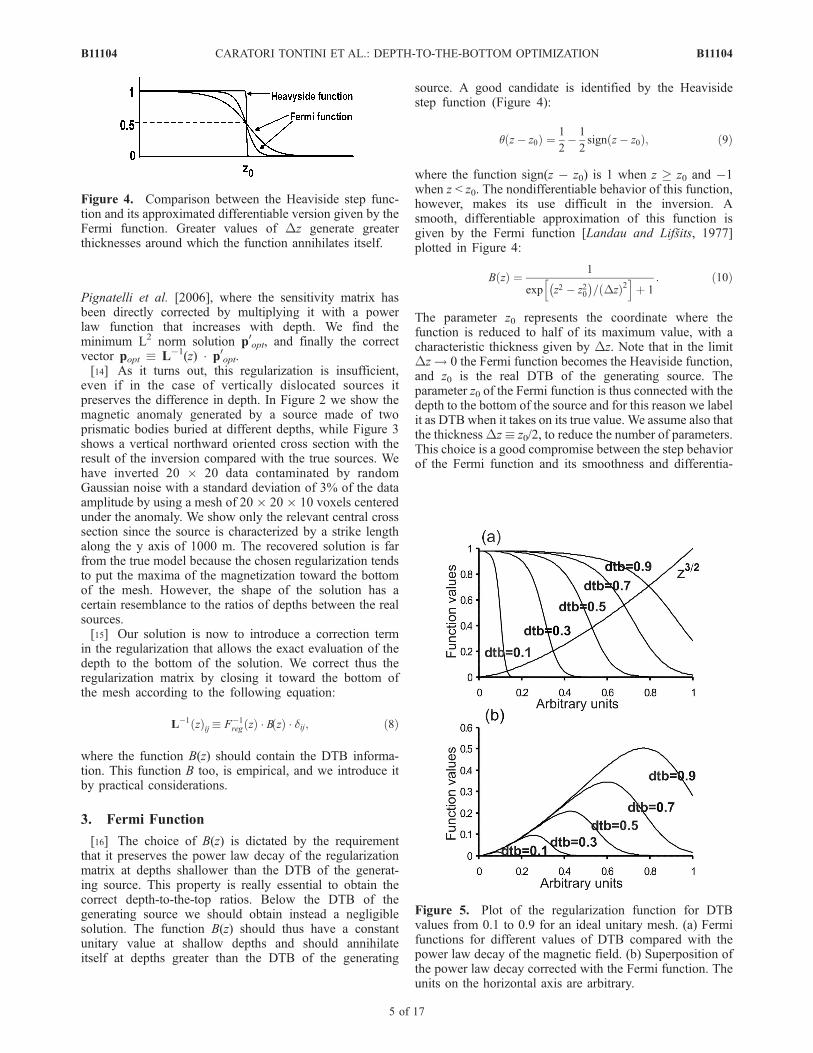
source. A good candidate is identified by the Heavisidestep function (Figure 4):

q z� z0ð Þ ¼ 1

2� 1

2sign z� z0ð Þ; ð9Þ

where the function sign(z � z0) is 1 when z z0 and �1when z < z0. The nondifferentiable behavior of this function,however, makes its use difficult in the inversion. Asmooth, differentiable approximation of this function isgiven by the Fermi function [Landau and Lifsits, 1977]plotted in Figure 4:

B zð Þ ¼ 1

exp z2 � z20� �

= Dzð Þ2h i

þ 1: ð10Þ

The parameter z0 represents the coordinate where thefunction is reduced to half of its maximum value, with acharacteristic thickness given by Dz. Note that in the limitDz! 0 the Fermi function becomes the Heaviside function,and z0 is the real DTB of the generating source. Theparameter z0 of the Fermi function is thus connected with thedepth to the bottom of the source and for this reason we labelit as DTB when it takes on its true value. We assume also thatthe thicknessDz� z0/2, to reduce the number of parameters.This choice is a good compromise between the step behaviorof the Fermi function and its smoothness and differentia-

Figure 4. Comparison between the Heaviside step func-tion and its approximated differentiable version given by theFermi function. Greater values of Dz generate greaterthicknesses around which the function annihilates itself.

Figure 5. Plot of the regularization function for DTBvalues from 0.1 to 0.9 for an ideal unitary mesh. (a) Fermifunctions for different values of DTB compared with thepower law decay of the magnetic field. (b) Superposition ofthe power law decay corrected with the Fermi function. Theunits on the horizontal axis are arbitrary.


5 of 17

B11104

bility. The final version of the inverse regularization matrixis thus

L�1 zð Þij�z3=2

l3=2z exp z2 � z20

� �= z0=2ð Þ2

h iþ 1

� � � dij: ð11Þ

This choice can be understood also in terms of a statisticalapproach of the Bayesian kind [Tarantola and Valette, 1982].As shown by Yanovskaya and Ditmar [1990] and Simons etal. [2002] there is a connection between numerical regular-ization, for example by the Tikhonov method, and statisticaladdition of ‘‘a priori’’ information. In the Bayesian approachin particular, the vector of model parameters p is distributedaccording to a Gaussian probability density function

r pð Þ / exp � 1

2pt � C�1

p � p

; ð12Þ

where Cp is the ‘‘a priori’’ model covariance matrix. Asshown by Simons et al. [2002], the choice of a particularregularizationmatrixL induces the same choice for themodelcovariance matrix

C�1p ¼ L: ð13Þ

By analyzing the behavior with depth z of the regularizationmatrix L(z), expressed in equation (11), we can conclude thatthe ‘‘a priori’’ probability distribution function r(p) isdrastically suppressed outside of the depth range defined bythe Fermi function, i.e., for depths greater than z0. This allowsthe activation of layers shallower than z0 during the inversion.[17] Figure 5 shows the shape of the Fermi function at

various values of DTB, together with the effects of thedecay factor of equation (4), evaluated on a unitary mesh.Figure 6 shows the matrix L�1 with these characteristics forparticular values of DTB. Each block represents the contri-bution of L�1 for a layer of the mesh, organized atincreasing depths, as the vector p. The choice of a regular-ization matrix of this kind introduces some importantcharacteristics within the inverted model. Particularly itdescribes a compact body along the vertical dimension,with a bottom depth given by the chosen DTB value. Thischoice generates some specific physical features in thesolution, thereby reducing the ambiguity domain towardobtaining a model which is characterized by a thicknesssufficient to close the source toward its bottom at a depthgiven by DTB. Actually the DTB value, if it is introducedby the user, represents a strong ‘‘a priori’’ information,which may generate realistic solutions.[18] In the following section we will demonstrate that

the parameter DTB can be estimated in a stable way from thedata. The data itself thus can provide information about thedepth to the bottom of the source. We will test and applythe inversion algorithm also on a case with sources atdifferent depths and horizontal locations.

4. Determining the Regularization ParameterDTB: Synthetic Tests

[19] The choice of different values of DTB allows theclosure of the solution at different bottom depths: larger

values of z0 generate deeper sources. In Figure 7 we haveinverted the field generated by a synthetic source describedby a prism at a given depth in the range z 2 [300;700] m.Different inversions have been performed by using differentvalues of the DTB parameters. The mesh was made of 20 �20 � 10 cubic voxels centered about the anomaly, with acell size of 100 m. The data have been again contaminatedby random Gaussian noise. As we can see from Figure 7 weobtain solutions that are placed at different depths accordingto the values of DTB. The optimal value of DTB, repre-sented by the plots where maximal magnetization values areplaced inside the synthetic prism, is ideally located around700 m, in good agreement with the depth to the bottomof the true source. It is interesting to highlight that thereduced chi-square norm c2/n (not to be confused with themagnetic susceptibility c that goes by the same symbol) forFigures 7a –7f) was always close to 1, indicating a good fitindependently from the chosen DTB value, while obviouslythe L2 norm increases as DTB increases, since more layersare activated by the inversion algorithm.[20] At this level, however, we still need a method to

determine the DTB parameter z0 of equation (11) from theanomaly data set. The DTB represents the bottom of thesource, which provides meaningful information in manygeological settings, as in the definition of the magneticbasement or the Curie temperature. Estimation of thisparameter is commonly done by analyzing the long-wavelength field of the magnetic anomaly in the Fourierdomain [Bhattacharyya and Leu, 1975; Shuey et al., 1977;Connard et al., 1983; Blakely, 1988; Okubo and Matsunaga,1994; Maus et al., 1997]. The DTB parameter is alsoimportant in the definition of the optimal dimension of themesh to invert the anomaly data. While the horizontalgeometry of the mesh can be decided upon by analyzingthe horizontal shape of the anomaly, the vertical extension ismore problematic and an optimal choice of it allows areduction of the number of layers, increasing the numericalperformance of the inversion itself.[21] If an optimal value of the DTB parameter exists, it

should manifest itself in the data, for example by minimizingor maximizing some function. This approach resembles theL curve method for evaluating the optimal l of equation (2).In that case a set of preliminary inversions at various lwas performed, and the optimal value was obtained bymaximizing the curvature of the resulting plot of log jL � pj2versus log jK � p � dj2. In the case of equation (11), weseek a particular function showing a well-defined stationarypoint for the optimal value of z0. The functionals commonlyused as additional bounds in the inversion methods (i.e., thechi-square norm, different Ln norms of the solution, theoptimal l parameter, the volume and the moment of inertiaof the source) typically show monotonic behaviors withDTB. This can be easily understood for the chi-square normor for the volume and moment of inertia of the source,because putting magnetized cells at the upper layers of themesh allows us to obtain very good solution in terms of datafitting with a small number of magnetized cells, whichpractically means models with small volume or moment ofinertia. The same reasons explain the behavior of thevarious Ln norms, because the upper layers of the meshcan be magnetized with low susceptibility values causingsmall norms of the solutions [Oldenburg and Li, 2003;


6 of 17

B11104

Figure

6.

Plotsofdifferentregularizationmatricesforvalues

ofDTBfrom

100to

600m

forthemeshofthemodel

of

Figure

3.Eachblock

ofthematrixrepresentsalayerofthemeshsince

thedatahavebeenorganized

into

adepth-descending

order.


7 of 17

B11104

Strykowski and Boschetti, 2003]. These functionals are thususeful during the inversion itself to obtain constrainedmodels, but they cannot give information about the optimalDTB of equation (11).[22] On the basis of numerical experiments, we found

instead a norm of the model that gave meaningful results.The chosen regularization has a power law decay of 3/2with depth for the first layers of the mesh, until the Fermidecay function is negligible. From this point of view thefollowing N norm of the solution appears as a goodcandidate

Nz0 ¼ZV

jcz0rð Þj

z3=2dV ; ð14Þ

where V is the volume of the mesh, r indicates the positioninside of this volume, and the magnetic susceptibility cz0 isobtained by the inversion at a determined z0. This quantityhas been evaluated for different z0 values and then plotted asa function of z0. The plot of this norm, having been testedby a large number of synthetic models, shows minimumvalues in proximity of a value of DTB that is close to theactual bottom depth of the source. Among the differentsolutions, each minimizing at the same time a misfitfunction and a regularizing functional characterized by adepth decay with a power law of 3/2, the optimal solution ischaracterized by the global minimum value of N norm. Thisnorm is not completely empirical, since susceptibility anddepth decay of the field are both present. The search for a

Figure 7. Results of inversions of the synthetic model of a prism buried at depth from 300 to 700 m.The magnetic susceptibility of the true source is 0.3 (SI). For each subplot the horizontal axis is north (m),while the vertical axis indicates the depth (m). The recovered models are evaluated by using differentDTB parameters drawn in each subplot. In particular, Figure 7f indicates the result obtained by a powerlaw regularization without the Fermi function effect, which corresponds to an infinite value of DTB. Therecovered models show that the solution is shifted toward greater values of depth as the DTB parameterincreases.


8 of 17

B11104

minimum ratio between the numerator given by suscept-ibility and the denominator given by the depth decayprevents the source clustering at shallow depths, where z�3/2

assumes large values, while the term jcz0(r)j avoids alsothe existence of large susceptibility values, as happens whenthe best fitting solution is obtained at a depth larger than thetrue one.[23] Before showing some synthetic tests to confirm these

hypotheses, we summarize the main steps of the inversionmethod which proceeds as follows:[24] 1. We define the mesh grid for the inversion with the

straightforward prerequisite of enclosing the source. At thislevel the vertical extension of the mesh or the cell size of thegrid is not so essential, since it can be optimized afterhaving minimized the N norm. However, using a large meshwill ensure the proper closure of the source;[25] 2. We run a set of fast preliminary inversions with a

regularization matrix defined in equation (11) aimed atminimizing the N norm of the solution in terms of z0.The optimal DTB is found as the z0 which minimizes theN norm;[26] 3. The final inversion is performed with the obtained

DTB that replaces z0 in the regularization matrix of equation(11). The mesh grid at this level can be redefined, forexample by neglecting layers deeper than DTB and increas-ing the number of layers shallower than DTB by reducingtheir thicknesses;[27] 4. The recovered model is evaluated graphically in

three dimensions, together with the statistical informationpertaining to the chi-square optimization.[28] Following this procedure we have inverted synthetic

models of prisms with a thickness of 300 m, buried atdifferent depths, with bottoms at every 50 m from 400 to650 m. The inversions were performed by using the samemesh of the test of Figure 3. The preliminary analysis basedon evaluation of minima of the N norm is shown in Figure 8,together with the true depth of the source that is represented

by the linear trend. The error associated to the DTB valueis estimated in the following way:[29] 1. We fit a polynomial function of order 6 to a

discrete set of data of the N norm as a function of z0;[30] 2. We evaluate the error DN of the N norm as the

average difference between the observed N norm and itsinterpolated value on the discrete points used to build thecurve;[31] 3. The minimization algorithm of the N norm pro-

ceeds by a Golden Section search and stops when sometolerance value of the N norm is assumed: as this tolerancevalue we choose the DN value calculated above;[32] 4. The value of DN becomes a corresponding error

Dd in the DTB value, by using the corresponding values onthe N norm curve.[33] Figure 9 shows the recovered models from the

inversion performed by the DTB values shown as legendin each single plot. They are in good agreement. Onceagain, that the reduced chi-square norm c2/n was alwaysclose to 1, indicating a good and significant fit. The closingfunction also has the effect of reducing the L2 norm of thesolutions, so that in the final analysis for each separate casethe L2 norm was practically unchanged. The susceptibilityvalues are slightly underestimated as the depth increases,since, obviously, the source is less accurately detected, butthe distribution is peaked about the true center of the sourceand the structural trends of susceptibility are effectivelydetermined. These results indicate that besides a correctDTB, our algorithm has given also a good approximation ofthe true susceptibility distribution.[34] We now turn to studying the behavior of the N norm

when moving from its optimal value, by analyzing Figure 7,where the true DTB parameter is 700 m. It is intuitivelyunderstandable that the regularization of equation (11)allows the inversion to activate vertical levels with depthshallower than z0, but drastically suppresses layers at depthgreater than z0. The shallower solutions (Figures 7a and 7b)are characterized by a finite total susceptibility Si jcij,whose value is not as much decreased as the increase ofthe average depth effect (Table 1). The large depth factorz�3/2 plays the dominant role generating a large N norm.Increasing the value of z0 > 700 m, as in Figures 7e and 7f,we note that cells placed inside of the true source maintainapproximately the same susceptibility values, since theregularization permits to activate layers at a depth lowerthan z0. This effect, which is recognizable also in thenumerical results of Table 1, is essential to preserve datafitting without altering the misfit function too much. Greatervalues of z0, however, allow the inversion to activate deeperlayers, that do not contribute effectively to the predictedanomaly, but surely increase the N norm with a rate differentthan that which is given by the increase of the average deptheffect as in Figures 7a and 7b. The optimal DTB is theminimum point at which this transition of behavior happens.[35] This can be seen both by analyzing the numerical

results of Table 1, and the example of Figure 10, which wasobtained from another synthetic test, in which we study theasymmetric shape of the N norm around its minimum. Weshow in fact the application of this method to a morecomplex test, made of three separate sources at differentdepths. The inducing field is assumed to have an inclination

Figure 8. Plot of the minima of the N norm for the sourcesof Figure 9 with their error bars, compared with the trueDTB represented by the linear trend.


9 of 17

B11104

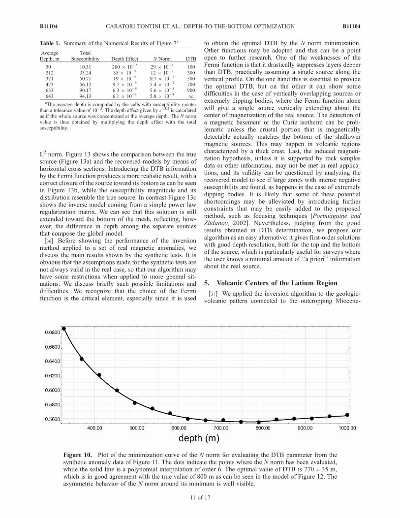
of 45�, a declination of 45� and a magnitude of 40,000 nT.The magnetic anomaly map can be seen in Figure 11 wherethe distinct anomalies of each of the separate sources thatcompose the model are overlapped. We used a mesh madeof 20 � 20 � 10 voxels to invert the grid made of 20 � 20data, to which we added Gaussian noise with a standarddeviation of 3% of the data amplitude. In Figure 10 weshow the plot of the N norm that gives a value of the DTB =770 ± 35 m. This value is in good agreement with the truevalue which is at 800 m. We have performed the inversionof the anomaly of Figure 11 by using the recovered DTB =770 m, and DTB = 1 that corresponds to using only a

power law regularization matrix. The corresponding Lcurves are shown in Figure 12, where Figure 12a indicatesthe solution at the correct DTB, while Figure 12b indicatesthe solution without DTB. The reduced chi-square normfor the model in Figure 12a is 0.55, while for the model inFigure 12b it is 0.49. The significance level of Figure 12a isthus 96% and 97% for Figure 12b, indicating a good fit inboth cases. The L2 norm of Figure 12b, approximately1050, is instead considerably larger than the L2 norm ofFigure 12a at about 370, indicating that the deeper layers ofthe solution Figure 12b do not contribute effectively to fitthe inverted anomaly, and generate a solution with a large

Figure 9. Results of inversions of synthetic models of prisms buried at different depths from 400 to650 m every 50 m and relative DTB parameters. The magnetic susceptibility of the true source is 0.3 (SI).For each subplot the horizontal axis is north (m), while the vertical axis indicates the depth (m). Therecovered models are in good agreement with the true sources, and the values of DTB reflect the actualvalues of the bottom depths of each prism. These values were obtained by minimization of the N norm.


10 of 17

B11104

L2 norm. Figure 13 shows the comparison between the truesource (Figure 13a) and the recovered models by means ofhorizontal cross sections. Introducing the DTB informationby the Fermi function produces a more realistic result, with acorrect closure of the source toward its bottom as can be seenin Figure 13b, while the susceptibility magnitude and itsdistribution resemble the true source. In contrast Figure 13cshows the inverse model coming from a simple power lawregularization matrix. We can see that this solution is stillextended toward the bottom of the mesh, reflecting, how-ever, the difference in depth among the separate sourcesthat compose the global model.[36] Before showing the performance of the inversion

method applied to a set of real magnetic anomalies, wediscuss the main results shown by the synthetic tests. It isobvious that the assumptions made for the synthetic tests arenot always valid in the real case, so that our algorithm mayhave some restrictions when applied to more general sit-uations. We discuss briefly such possible limitations anddifficulties. We recognize that the choice of the Fermifunction is the critical element, especially since it is used

to obtain the optimal DTB by the N norm minimization.Other functions may be adopted and this can be a pointopen to further research. One of the weaknesses of theFermi function is that it drastically suppresses layers deeperthan DTB, practically assuming a single source along thevertical profile. On the one hand this is essential to providethe optimal DTB, but on the other it can show somedifficulties in the case of vertically overlapping sources orextremely dipping bodies, where the Fermi function alonewill give a single source vertically extending about thecenter of magnetization of the real source. The detection ofa magnetic basement or the Curie isotherm can be prob-lematic unless the crustal portion that is magneticallydetectable actually matches the bottom of the shallowermagnetic sources. This may happen in volcanic regionscharacterized by a thick crust. Last, the induced magneti-zation hypothesis, unless it is supported by rock samplesdata or other information, may not be met in real applica-tions, and its validity can be questioned by analyzing therecovered model to see if large zones with intense negativesusceptibility are found, as happens in the case of extremelydipping bodies. It is likely that some of these potentialshortcomings may be alleviated by introducing furtherconstraints that may be easily added to the proposedmethod, such as focusing techniques [Portniaguine andZhdanov, 2002]. Nevertheless, judging from the goodresults obtained in DTB determination, we propose ouralgorithm as an easy alternative: it gives first-order solutionswith good depth resolution, both for the top and the bottomof the source, which is particularly useful for surveys wherethe user knows a minimal amount of ‘‘a priori’’ informationabout the real source.

5. Volcanic Centers of the Latium Region

[37] We applied the inversion algorithm to the geologic-volcanic pattern connected to the outcropping Miocene-

Figure 10. Plot of the minimization curve of the N norm for evaluating the DTB parameter from thesynthetic anomaly data of Figure 11. The dots indicate the points where the N norm has been evaluated,while the solid line is a polynomial interpolation of order 6. The optimal value of DTB is 770 ± 35 m,which is in good agreement with the true value of 800 m as can be seen in the model of Figure 12. Theasymmetric behavior of the N norm around its minimum is well visible.

Table 1. Summary of the Numerical Results of Figure 7a

AverageDepth, m

TotalSusceptibility Depth Effect N Norm DTB

50 10.31 280 � 10�5 29 � 10�3 100212 33.24 35 � 10�5 12 � 10�3 300321 50.71 19 � 10�5 9.7 � 10�3 500473 56.12 9.7 � 10�5 5.4 � 10�3 700633 90.17 6.3 � 10�5 5.6 � 10�3 900643 94.13 6.1 � 10�5 5.8 � 10�3 1aThe average depth is computed by the cells with susceptibility greater

than a tolerance value of 10�3. The depth effect given by z�3/2 is calculatedas if the whole source was concentrated at the average depth. The N normvalue is thus obtained by multiplying the depth effect with the totalsusceptibility.


11 of 17

B11104

Quaternary magmatism of the Latium Region in Italy. Thevolcanoes of the Northern Latium Center are located on theTyrrhenian margin of Italy westward of the compressionalfront of the Apennine-Maghrebian chain. The magmaticpattern shows a NW-SE trend and covers four singularvolcanics complexes (toward SE): Vulsini, Vico, Sabatiniand Albani. The volcanism of the Latium area begun in thePleistocene (about 0.6–0.4 Ma) [Serri et al., 2001] andreached its end around 0.1 Ma. The Albani system had morerecent activity since 0.02 Ma [Marra et al., 2004].These volcanic structures are the northwestern evidenceof the potassic-ultrapotassic Roman Magmatic Province[Washington, 1906]. The potassic-ultrapotassic magmatismof the Latium region is strongly connected with the Tertiarycompressional system and is related to intense block fault-ing and rifting developed between Upper Miocene andPresent in the western side of the Apennine chain [Beccaluvaet al., 1991]. The geochemical features of the Latium areaare related to the undersaturated chemistry of the othermagmatic centers of the central Italy (Campanian Region–Vulture). They are connected with distinct enrichment of themantle sources [Serri, 1990; Serri et al., 2001]. Figure 14shows the magnetic anomaly pattern of the Latium region,located near Rome. This map derives from the digitaldatabase of the aeromagnetic anomaly field of Italy of theOil Company Eni Exploration and Production Division. Theanomaly field, after the standard leveling, has been obtainedby DGRF (Definitive Geomagnetic Reference Model) sub-

Figure 12. L curves coming from the inversion of the anomaly of Figure 11 (a) in the case ofDTB = 770 m and (b) with DTB = 1. The chi-square norm of the model in Figure 12a is slightly largerthan that of Figure 12b, but the L2 norm is considerably larger in the case of Figure 12b, showing that thedeep layers do not contribute effectively to fit the observed anomaly.

Figure 11. Synthetic anomaly generated by a compositeprismatic model. The inducing field is assumed to have aninclination of 45�, a declination of 45�, and a magnitude of40,000 nT. The anomaly is calculated by a grid of 20 � 20points. Random Gaussian noise with a standard deviation of3% of the data magnitude has been added to the data.


12 of 17

B11104

traction for the geomagnetic epoch 1979.0. The data wererecorded at an observation level of 1460 m, the projection isa transverse Mercator with reference latitude at 0�, referencelongitude at 14�, false east at 1,500,000 m and false north at0 m [Caratori Tontini et al., 2004].[38] The boxes in Figure 14 indicate three distinct anoma-

lies that have been separately inverted by our algorithm.These anomalies are interpreted to be magnetic signatures ofthe magmatism of the region. The Vulsini complex isrepresented by anomaly A, the Vico-Sabatini anomaly isenclosed by the box B, while C is the anomaly of the Albanicomplex. The very similarity of these anomalies as regardstheir amplitude and typical wavelengths allows the extractionof these anomalies from the relatively flat background, and

suggests a common nature. The induced magnetizationhypothesis is justified because of the young age of thisvolcanic complex, whose origin is more recent than the lastpolarity inversion, so that if remanent magnetization ispresent it is aligned with the ambient-inducing field [Marraet al., 2004]. Each separate anomaly, gridded with a cell sizeof 1.5 km, has been inverted by our algorithm by using ameshcentered under the anomaly made of 30 � 30 � 15 voxels.The vertical extension of the mesh sizes from 500 m abovesea level to 13,500 m below sea level. The DTB analysisyielded a common value of 12.0 ± 0.6 km for anomalies Aand C, while anomaly B showed a DTB = 10.1 ± 0.5 km.Figure 15 shows the results of the inversions by horizontalcross sections that allow comparison between the sources.

Figure 13. Recovered model from inversion of synthetic anomaly data of Figure 11 represented byhorizontal cross sections at various depths. The data were inverted by using a mesh of 20 � 20 � 10voxels, centered about the anomaly of Figure 11, thus extending from 0 to 2000 m for each horizontaldirection and from 0 to 1000 m for the vertical axis. (a) True susceptibility model, (b) recovered modelwith DTB = 770 m, and (c) recovered model with DTB = 1 that corresponds to using only a power lawdecay regularization matrix. Figures 13b and 13c are similar for the first cross sections, but while themodel in Figure 13b is closed toward its bottom at the correct depth, the solution in Figure 13c appearsstill pushed toward the bottom of the mesh.


13 of 17

B11104

The geometry and extension of the sources in the deeplayers is typical for this kind of magmatic chambers that arecharacterized by a circular shape. Typical rise-up structuresare evident in the shallow sections, converging at depthinto four isolated magmatic chambers. It is interesting tocompare the outcropping evidence of these volcanic struc-tures with our recovered model. To this aim we haveprojected the first horizontal cross section over the topo-graphic shaded relief (Figure 16). This section ranges from500 m above sea level to 500 m below sea level and iscompatible with the maximum topographic relief of 460 m.The susceptibility is located over topographic highsconnected with the outcropping volcanic edifices. The

recovered susceptibility values are in the range 0–10�3

black which is dimensionless in SI units. These values are ingood agreement with rock samples from this area [Porrecaet al., 2003]. Some ring-shaped susceptibility patternsmoreover identify the border of the rims that in this regionare evident in the form of volcanic lakes. These caldericstructures are well visible in Figure 16. This is an importantcharacteristic of this volcanic region, since the calderizationprocess tends sometimes to change the magnetic features ofrocks because of the collapse of the main conduit that altersthe susceptibility pattern. This is mainly due to a mixingwith terrigenous sediments with very low susceptibilityvalues. The separate structures recovered by our model

Figure 14. Magnetic pattern of the investigated volcanic structures of the Latium region at anobservation level of 1460 m. Three magnetic anomalies, indicated by the boxes A, B, and C, wereisolated and inverted. The solid black line represents the Italian coastline, and westward is the TyrrhenianSea. The map is a transverse Mercator projection with reference latitude at 0�, reference longitude at 14�,false east at 1,500,000 m, and false north at 0 m.


14 of 17

B11104

show similar susceptibility values and geometries, suggest-ing that probably they have a deep common mantle originthat during rise up has been differentiated according to themodel of Figure 15.

6. Conclusions

[39] We have developed an inversion algorithm formagnetic data by inserting a depth-weighting function intothe model regularization function, modified from Li and

Oldenburg [1996]. We have transformed this problem into asimple ‘‘free’’ inversion with minimization of an L2 norm,increasing the numerical performance of the algorithm thatthus is particularly effective for fast applications. The depth-weighting function depends on one parameter that isconnected with the depth to the bottom of the source andallows the closure of the source toward its bottom at aconsistent depth. We have shown how this DTB parametercan be found from the data by a first inversion step.Synthetic tests have been performed to ascertain the reli-

Figure 15. Recovered model from inversion of the system of anomalies of the Roman MagmaticProvince shown in Figure 13. Each inversion has been performed by using a mesh of 30 � 30 � 15voxels centered under the anomaly. The global horizontal extension of each cross section is east =[1300,1420] km and north = [4600,4740] km. The coordinate system is the same as Figure 12.


15 of 17

B11104

ability of the method and a set of three anomalies ofvolcanic origin in Italy have been inverted, obtaining amodel that is in good agreement with the available geolog-ical information and the topographic evidence of the region.[40] While we have shown examples of magnetic anoma-

lies, a similar algorithm has been successfully tested ongravity data, provided an appropriate change of parameters.We have shown examples of optimization curves to evaluatethe depth-to-the-bottom parameter, but this procedure isembedded in the algorithm itself by a fast preliminaryanalysis. Some limitations have also been discussed in orderto highlight possible future improvements. The methodallows the user to obtain realistic models and can be alsoused to have a quantitative evaluation of the DTB of thesource even for large-scale anomalies, for example in Curiedepth or magnetic basement evaluation. When possible andif it is allowed by the crustal regime of the investigatedregion, we can extract a set of windowed subanomalies andseparately analyze them to find a DTB for each anomaly.The global superposition of the DTBs can thus provide amap of the magnetic basement. In conclusion, this is apromising method, which we are working on extending tomore complex source geometries.

[41] Acknowledgments. We thank Eni Exploration and ProductionDivision and particularly I. Giori for the use of the magnetic data. We areindebted to AE F.J. Simons for his significant help in improving the level ofthis work, and we thank Erwan Thebault and an unknown reviewer for theiruseful comments. P. C. Hansen is particularly appreciated for having madeavailable the Matlab routines for regularization tools that have been used in

the algorithm (www.imm.dtu.dk/�pch). Finally, we thank Lynden Croninfor having corrected the English style. F.C.T. wishes to dedicate this paperto his little Riccardo.

ReferencesAndersen, F. H., and L. B. Pedersen (1979), Some relations betweenpotential fields and the strength and center of their sources, Geophys.Prospect., 27, 761–774.

Barbosa, V. C. F., and J. B. C. Silva (1994), Generalized compact gravityinversion, Geophysics, 59, 57–68.

Beccaluva, L., P. Di Girolamo, and G. Serri (1991), Petrogenesis and tec-tonic setting of the Roman Volcanic Province, Lithos, 26, 191–221.

Bhattacharyya, B. K. (1964), Magnetic anomalies due to prism-shapedbodies with arbitrary polarization, Geophysics, 29, 517–531.

Bhattacharyya, B. K., and L. K. Leu (1975), Analysis of magnetic anoma-lies over Yellowstone National Park: Mapping Curie point isothermalsurface for geothermal reconnaissance, J. Geophys. Res., 80, 4461–4465.

Blakely, R. J. (1988), Curie temperature isotherm analysis and tectonicimplications of aeromagnetic data from Nevada, J. Geophys. Res., 93,11,817–11,832.

Blakely, R. J. (1995), Potential Theory in Gravity and Magnetic Applica-tions, Cambridge Univ. Press, New York.

Boulanger, O., and M. Chouteau (2001), Constraints in 3D gravity inver-sion, Geophys. Prospect., 49, 265–280.

Caratori Tontini, F., O. Faggioni, N. Beverini, and C. Carmisciano (2003),Gaussian envelope for 3D geomagnetic data inversion, Geophysics, 68,996–1007.

Caratori Tontini, F., P. Stefanelli, I. Giori, O. Faggioni, and C. Carmisciano(2004), The revised aeromagnetic anomaly map of Italy, Ann. Geophys.,47, 1547–1555.

Claerbout, J. F. (1976), Fundamentals of Geophysical Data ProcessingWith Applications to Petroleum Prospecting, McGraw-Hill, New York.

Connard, G., R. Couch, and M. Gemperle (1983), Analysis of aeromagneticmeasurements form the Cascade Range in central Oregon, Geophysics,48, 376–390.

Fedi, M., and A. Rapolla (1999), 3-D inversion of gravity and magneticdata with depth resolution, Geophysics, 64, 452–460.

Guillen, A., and V. Menichetti (1984), Gravity and magnetic inversion withminimization of a specific functional, Geophysics, 49, 1354–1360.

Hansen, P. C. (1994), Regularization tools: A Matlab package for analysisand solution of discrete ill-posed problems, Numer. Algorithms, 6, 1–35.

Hansen, P. C., and D. P. O’Leary (1993), The use of the L-curve in theregularization of discrete ill-posed problems, SIAM J. Sci. Comput., 14,1487–1503.

Helbig, K. (1963), Some integrals of magnetic anomalies and their relationto the parameters of the disturbing body, Z. Geophys., 29, 81–96.

Ho-Liu, P., J.-P. Montagner, and H. Kanamori (1989), Comparison of itera-tive back-projection inversion and generalized inversion without blocks:Case studies in attenuation tomography, Geophys. J. Int., 97, 19–29.

Jacobsen, B. H. (1987), A case for upward continuation as a standardseparation filter for potential field maps, Geophysics, 52, 1138–1148.

Landau, L. D.. and E. M. Lifsits (1977), Statistical Physics, MIR, Moscow.Last, B. J., and K. Kubik (1983), Compact gravity inversion, Geophysics,48, 713–721.

Lawson, C. L., and R. J. Hanson (1974), Solving Least Squares Problems,Prentice-Hall, Upper Saddle River, N. J.

Li, Y., and D. W. Oldenburg (1996), 3-D inversion of magnetic data,Geophysics, 61, 394–408.

Marra, F., J. Taddeucci, C. Freda, W. Marzocchi, and P. Scarlato (2004),Recurrence of volcanic activity along the Roman Comagmatic Province(Tyrrhenian margin of Italy) and its tectonic significance, Tectonics, 23,TC4013, doi:10.1029/2003TC001600.

Maus, S., D. Gordon, and D. Fairhead (1997), Curie-temperature depthestimation using a self-similar magnetization model, Geophys. J. Int.,129, 163–168.

Menke, W. (1989), Geophysical Data Analysis: Discrete Inverse Theory,Elsevier, New York.

Okubo, Y., and T. Matsunaga (1994), Curie point depth in northeast Japanand its correlation with regional thermal structure and seismicity, J. Geo-phys. Res., 99, 22,363–22,371.

Oldenburg, D. W., and Y. Li (2003), Discussion on ‘‘3-D inversion ofgravity and magnetic data with depth resolution’’, Geophysics, 68,400–403.

Pedersen, L. B. (1991), Relations between potential fields and some equiva-lent sources, Geophysics, 56, 961–971.

Pignatelli, A., I. Nicolosi, and M. Chiappini (2006), An alternative 3Dsource inversion method for magnetic anomalies with depth resolution,Ann. Geophys, in press.

Pilkington, M. (1997), 3-D magnetic imaging using conjugate gradients,Geophysics, 62, 1132–1142.

Figure 16. First cross section of the recovered model ofFigure 14 projected over the shaded topographic relief ofthe region investigated by the inversion algorithm. The firstsection of Figure 14 describes actually outcroppingstructures since it is evaluated from 500 m above sea levelto 500 m below sea level.


16 of 17

B11104

Porreca, M., M. Mattei, G. Giordano, D. De Rita, and R. Funiciello (2003),Magnetic fabric and implications for pyroclastic flow and lahar emplace-ment, Albano maar, Italy, J. Geophys. Res., 108(B5), 2264, doi:10.1029/2002JB002102.

Portniaguine, O., and M. S. Zhdanov (2002), 3-D magnetic inversionwith data compression and image focusing, Geophysics, 67, 1532–1541.

Scales, J. A., and R. Snieder (1997), To Bayes or not to Bayes?, Geophy-sics, 62, 1045–1046.

Serri, G. (1990), Neogene-Quaternary magmatism of the Tyrrhenian region:Characterization of the magma sources and geodynamic implications,Mem. Soc. Geol. It., 41, 219–242.

Serri, G., F. Innocenti, and P. Manetti (2001), Magmatism from Mesozoicto Present: Petrogenesis, time-space distribution and geodynamicimplications, in Anatomy of an Orogen: The Apennines and AdjacentMediterranean Basins, edited by G. B. Vai, and I. P. Martini, pp. 77–103, Springer, New York.

Shuey, R. T., D. K. Schellinger, A. C. Tripp, and L. B. Alley (1977), Curiedepth determination from aeromagnetic spectra, Geophys. J.R. Astron.Soc., 50, 75–101.

Silva, J. B. C., W. E. Medeiros, and V. C. F. Barbosa (2001), Potential-fieldinversion: Choosing the appropriate technique to solve a geological pro-blem, Geophysics, 66, 511–520.

Simons, F. J., R. D. van der Hilst, J.-P. Montagner, and A. Zielhuis (2002),Multimode Rayleigh wave inversion for heterogeneity and azimuthal

anisotropy of the Australian upper mantle, Geophys. J. Int., 151, 738–754.

Strykowski, G., and F. Boschetti (2003), Discussion on ‘‘3-D inversion ofgravity and magnetic data with depth resolution’’, Geophysics, 68, 403–405.

Tarantola, A. (1987), Inverse Problem Theory, Elsevier, New York.Tarantola, A., and B. Valette (1982), Generalized nonlinear inverse problemssolved using the least squares criterion, Rev. Geophys., 20, 219–232.

Tikhonov, A. N., and V. Y. Arsenin (1977), Solutions of Ill-Posed Problems,Winston, Washington, D. C.

Washington, H. S. (1906), The Roman Comagmatic Region, 199 pp., Car-negie Inst., Washington, D. C.

Yanovskaya, T. B., and P. G. Ditmar (1990), Smoothness criteria in surfacewave tomography, Geophys. J. Int., 102, 63–72.

Zhdanov, M. S. (2002), Geophysical Inverse Theory and RegularizationProblems, Elsevier, New York.

��F. Caratori Tontini and C. Carmisciano, Stazione di Geofisica Marina,

Istituto Nazionale di Geofisica e Vulcanologia, via Pezzino Basso 2,I-19020 Fezzano (SP), Italy. ([email protected]; [email protected])L. Cocchi, Dipartimento Scienze della Terra Geologiche-Ambientali,

Universita di Bologna, P.zza Porta S. Donato 1, I-40126 Bologna, Italy.([email protected])


17 of 17

B11104

Depth-to-the-bottom optimization for magnetic data inversion: Magnetic structure of the Latium...

Documents

Transcript of Depth-to-the-bottom optimization for magnetic data inversion: Magnetic structure of the Latium...