Dependent component analysis for blind restoration of images degraded by turbulent atmosphere

Corresponding author:

Dr. Jenny Q. Du

Department of Electrical and Computer Engineering

Mississippi State University

Mississippi State, MS 39762

phone: 662-325-2035

fax: 662-325-2298

e-mail: [email protected]

1

Dependent Component Analysis for Blind Restoration of Images

Degraded by Turbulent Atmosphere

Qian Du 1, Ivica Kopriva 2

1 Department of Electrical and Computer Engineering

Mississippi State University, MS 39762, USA

2 Division of Laser and Atomic Research and Development, Rudjer Bošković Institute

Bijenička cesta 54, P.O. Box 180, 10002 Zagreb, Croatia

Abstract

In our previous research, we applied independent component analysis (ICA) for the

restoration of image sequences degraded by atmospheric turbulence. The original high-resolution

image and turbulent sources were considered independent sources from which the degraded

image is composed of. Although the result was promising, the assumption of source

independence may not be true in practice. In this paper, we propose to apply the concept of

dependent component analysis (DCA), which can relax the independence assumption, to image

restoration. In addition, the restored image can be further enhanced by employing a recently

developed Gabor-filter-bank-based single channel blind image deconvolution algorithm. Both

simulated and real data experiments demonstrate that DCA outperforms ICA, resulting in the

flexibility in the use of adjacent image frames. The contribution of this research is to convert the

2

original multi-frame blind deconvolution problem into blind source separation problem without

the assumption on source independence; as a result, there is no a priori information, such as

sensor bandwidth, point-spread-function, or statistics of source images, that is required.

Keywords: Atmospheric turbulence; Image restoration; Independent component analysis;

Dependent component analysis.

1. Introduction

Atmospheric turbulence is an inevitable problem in long-distance ground-based and space-based

imaging. The optical effects of atmospheric turbulence arise from random inhomogeneities in the

temperature distribution of the atmosphere. A consequence of these temperature inhomogeneities

is non-stationary random distribution of the refraction index of the atmosphere [1]. Atmospheric

turbulence can make distant objects being viewed through a sensor (e.g., a digital camera or

video recorder) to appear blurred. Also, the time-varying nature of the turbulence can make the

appearance of objects to wave in a slow quasi-periodic fashion. When a target is small and

moving, its actual location becomes very difficult to estimate. This phenomenon greatly hinders

accurate target detection, tracking, classification, and identification.

Numerous methods have been developed to mitigate the atmospheric turbulence effects.

Three broad classes of techniques used to correct turbulence effects are: 1) pure post-processing

techniques, which use specialized image processing algorithms; 2) adaptive optics techniques,

which afford a mechanical means of sensing and correcting for turbulence effects; and 3) hybrid

methods, which combine the elements of post-processing techniques and adaptive optics

techniques. Each of these techniques has performance limitation as well as hardware and

3

software requirements. In our research, due to its low cost, we focus on the development of pure

post-processing techniques to correct atmospheric turbulence. Quite a few algorithms in this

aspect have been developed in the past twenty years. These algorithms fall into two major

categories: those adopting explicit or implicit ways to measure the perturbations induced on the

wavefront by the atmosphere, and those using no wavefront information to construct the

underlying image formation characteristics of the atmosphere. Wavefront reference algorithms

include the guides (natural or artificial) and deconvolution from optical measurements of the

wavefront entering the telescope, while reference-less algorithms do not need such guides. In our

research, we are interested in the no-reference techniques because no optical measurements are

required. This also makes real time or near-real time implementation possible and simple for

many national defense related applications.

Current image restoration techniques for atmospheric turbulence correction employ the well-

known linear image formation model , where the degraded image

is obtained by convolving the original high-resolution image with the point-

spread-function (PSF) (i.e., PSF models the degradation caused by atmospheric

turbulence) [2]. Due to the space- and time-varying nature of atmospheric turbulence, the PSF

should be changed with pixel location and time t. However, for the purpose of simplicity

and mathematical tractability, most techniques assume that PSF is unchanged with space and

time. In other words, they are space- and time-invariant restoration approaches.

To relax the unrealistic assumption of a space- and time-invariant PSF, we introduced the

Blind Source Separation (BSS) technique to achieve the restoration of image sequences [3].

Instead of using the linear convolutive degradation model and estimating the PSF, we considered

each spatial turbulence pattern as one physical source, the original high-resolution image of the

4

object as another source, and then the degraded low-resolution image was the result from the

linear combination of these sources. This leads to the model at the component level written as

(1)

where contributions from the high-resolution object image and individual turbulence patterns

between time tn and the reference time t0, i.e. tn = tn t0, are contained in the unknown

mixing matrix coefficients anm, which depend on some physical constants [3]. The component

level model (1) can be generalized to a multi-frame model in a matrix form as

(2)

where is a matrix of the blurred image frames with each row representing a blurred

image frame, is an unknown basis or mixing matrix, and is a matrix of the

source images. Here, N represents the number of frames whereas each frame is treated as one

measurement, M denotes the number of source images, and T = PQ stands for the number of

pixels in each image (P and Q are image spatial dimensions). It is assumed that each image

frame has been transformed into a vector by a row or column stacking procedure. It is also

assumed that motion effects, if present, are compensated in advance.

BSS can be applied on (2) to extract the high-resolution object image without the prior

knowledge or estimation of PSF. The most successful solution of the BSS problem is achieved

through independent component analysis (ICA). It solves the BSS problem by imposing a

constraint on extracted sources to be non-Gaussian (at most one source is allowed to be

Gaussian) and statistically independent from each other [4]. One of popular ICA algorithms,

referred to as Joint Approximate Dia-gonalization of Eigenmatrices (JADE), was adopted due to

5

its robustness, wherein the statistical dependence among data samples was measured by the

fourth-order cross-cumulants [5].

However, it has been argued that the assumption of source independence may not be true in

many situations. For instance, the atmospheric turbulence components may be correlated

spatially and temporally. Sources may be at least partially statistically dependent due to the fact

that multi-frame image model adopted in [3] and used herein assumes all the sources are emitted

from the same space-time location (x, y, t0). Thus, in this paper, we will propose the use of

dependent component analysis (DCA) for image restoration, which does not require sources to

be independent. Both simulated and real data experiments demonstrate that DCA outperforms

ICA under this circumstance. In addition, DCA can be employed to further sharpen the restored

image to achieve super-resolution.

In summary, the contribution of this research is to convert the original multi-frame blind

deconvolution problem into BSS problem without the assumption on source independence; as a

result, no a priori information or assumption on sensor bandwidth, PSF, or statistics of source

images is required.

2. Derivation of DCA algorithms

Few papers in the literature discuss the problem of DCA [6]. Here we adopt some previous

studies conducted in [7][8]. The basic idea behind DCA is to find a transform T that can improve

the statistical independence between the sources but leave the basis matrix unchanged, i.e.,

. (3)

Because the sources after this transformation will be less statistically dependent, any standard

ICA algorithm, such as JADE, derived for the original BSS problem can be used to learn the

6

basis matrix A. Once the basis matrix A is estimated, the sources S can be recovered by applying

the pseudo-inverse of A on the multi-frame image G in (2).

Examples of linear transforms that possess such a required invariance property and generate

less dependent sources include: 1) highpass filtering, 2) innovation, and 3) wavelet transforms.

Highpass filtering (HP)

A highpass filter, such as the Butterworth highpass filter, is applied to preprocess the observed

signals G, followed by a standard ICA algorithm, such as JADE, on the filtered data in order to

learn the mixing matrix A. This is motivated by the fact that highpass filtered signals are usually

more independent than original signals that include low frequency components. Meanwhile, this

approach is computationally very efficient, making it attractive for DCA problems with

statistically dependent sources. In this case the transform T in Eq. (3) is the highpass filtering

operator that can be seen as a special case of the filter bank approach [9][10].

Innovation (IN)

Another computationally efficient approach is based on the use of innovation. The arguments for

using innovation are that they are usually more independent from each other and more non-

Gaussian than original processes [11]. The innovation process is referred to as prediction error

[12], which is defined as:

(4)

where sm(r i) is the i-th sample of a source process sm(r) at location (r i) and b’s are prediction

coefficients. em(r) represents the new information that sm(r) has but is not contained in the past l

7

samples. It is proved in [11] that if G and S follow the linear mixture model (2) their innovation

processes and (in matrix form) follow the same model as well, i.e.,

. (5)

In this case the transform T in Eq. (3) is the linear prediction operator. Temporal decorrelation

based preprocessing algorithm [23] can be seen as an extension of the presented innovation

based DCA algorithm. It is the same as the presented method when the model is linear but the

algorithm in [23] works in the case of post-nonlinear mixture as well.

Subband decomposition independent component analysis (SDICA)

The SDICA approach assumes that wideband source signals can be dependent but some of their

narrowband sub-components are less dependent [9][10]. Thus, SDICA extends applicability of

standard ICA through the relaxation of the independence assumption. In this case, the transform

T in Eq. (3) is any kind of filter-bank-like transform used to implement the sub-band

decomposition scheme.

A wavelet transform-based approach to SDICA was developed in [8][13] to obtain adaptive

subband decomposition of wideband signals through a computationally efficient implementation

in a form of iterative filter bank. Computationally efficient small cumulant-based approximation

of mutual information is used for automated selection of the subband with the least dependent

components, to which an ICA algorithm is applied. The potential disadvantage of this approach

is high computational complexity if 2D wavelet transform is used for image decomposition.

Hence, a reformulation can be accomplished based on dual tree complex wavelets [14]. Dual tree

complex wavelets are approximately computationally as efficient as decimated wavelet packets

but as accurate as the shift-invariant wavelet packet approach [15][16].

8

3. Algorithms for comparison

Other BSS approaches that can deal with statistically dependent sources include: independent

subspace analysis (ISA) [24][25], nonnegative matrix and tensor factorization (NMF/NTF) [27-

30], and the blind Richardson-Lucy (BRL) algorithm [33-36], which are used for comparison

purpose in this paper. They are briefly described as follows.

Independent Subspace Analysis

ISA assumes that the source signal space is composed of a number of subspaces. Signals

contained in the same subspace are mutually dependent while signals contained in different

subspaces are independent. When each subspace contains one component only, the ISA becomes

ICA. The practical difficulty with the ISA approach is in choosing a scheme necessary to

partition the source signal space into the subspaces with the required property. For instance, it is

not obvious how to choose the number of subspaces as well as the number of signals contained

in each subspace.

In the multi-frame blind deconvolution problem treated in this paper we decompose the

signal space into two subspaces: one that contains one image representing an approximation of

the object and the other that contains images related to the turbulence patterns. Here, we present

in the sequel brief derivation of the ISA algorithm [25], which is based on the concept of multi-

dimensional ICA [24] that follows the same model in (2). It is assumed that components

are divided into K tuples where components contained in the same tuple are dependent and

components contained in different tuples are independent (in other words, tuples correspond to

subspaces). It is also assumed in [25] that the joint probability density function (pdf) of a

particular subspace is spherically symmetric; hence, it can be expressed as the sum of squares of

9

, where k denotes the subspace index and dk denotes the dimension of the kth subspace

such that . It is further assumed sparse representation, which may be in agreement

with data representation adopted in our approach due to the fact that turbulence patterns are

expected to be sparse. Under these assumptions the following gradient update for de-mixing

matrix W is obtained (i.e., WGS)

(6)

where k(m) denotes the index of the subspace to which wm belongs and z denotes the whitened

data (whitening is applied to data matrix in ISA in the same way as in standard ICA) [26].

Nonnegative Matrix and Tensor Factorization

Unlike ICA, NMF/NTF algorithms do not impose statistical independence or non-

Gaussianity requirements on the sources. NMF/NTF algorithms may yield physically useful

solutions by imposing the nonnegativity, sparseness or smoothness constraints on the sources

[27-30]. In [27], the NMF algorithm was first derived to minimize two cost functions: the

squared Euclidean distance and the Kullback-Leibler divergence. Using a gradient descent

approach the resulting multiplicative algorithms converged very slowly. In addition, the lack of

additional constraints prevents NMF algorithms [27] from yielding a unique decomposition.

Generalization of the NMF algorithms [27] has been done in [28-30]. The gradient-based NMF

algorithm with a sparseness constraint being incorporated into the cost function leads to the

regularized alternating least square (RALS) algorithm [28]:

(7)

10

where the regularization terms S and A enforce sparse solutions for A and S, respectively. If

constraints are chosen as and , the regularization terms help

regularize the pseudo-inverse when the normal matrices ATA and SST are ill-conditioned.

Assume and for positive entries in A and S, which occurs at

stationary points. Then

(8)

where k denotes iteration index, ( )+ is Moore-Penrose inverse, and is a small constant (10-9) to

enforce positive entries. Regularization terms help avoid local minima and are implemented as

(in the experiments 0=20 and =10). We employ constraints if there

is a priori information about the sparseness of either A or S; otherwise, we set both

regularization terms to zero. This algorithm is referred to as the NMF algorithm in this paper.

Extension of this approach, known as local ALS, to 3D tensor factorization is given in [29],

which is referred to as the NTF algorithm in this paper. In this case G and S in model (2) become

3D tensors: and . Unlike a majority of NTF/NMF algorithms that estimate

the source matrix/tensor globally, the local ALS algorithm [29] performs it at the source level:

(9)

where IM is an MM identity matrix, is a sparseness constraint that regulates sparseness of

the mth source, am represents the mth column of A , , and []+=max{,}

11

(e.g., =10-16). Regularization constant changes as a function of the iteration index as

(with 0 = 100 and = 0.02 in the experiments). Note that sparseness

constraint imposed on source tensors affects the final result ( = 0.05 in the experiment).

Blind Richardson-Lucy (BRL) algorithm

BRL algorithm [33][34] was originally derived for non-blind single frame deconvolution of

astronomical images. It has been later formulated in [35] for blind deconvolution, and then

modified by an iterative restoration algorithm in [36]. To briefly introduce BRL algorithm we

need to write a single frame image gn, n {1,…,N}, in the lexicographical notation:

(10)

where (BRL needs to employ a PSF function whose matrix version is

H). The observed image vector gn and the original image vector s are obtained by a stacking

procedure. The matrix H is a block-Toeplitz matrix [31]. It absorbs itself into the blurring kernel

h(x,y) by assuming that at least its size is known. The block-Toeplitz structure of H can be

further approximated by a block-circular structure. This approximation introduces small

degradations at image boundaries, but enables the expression of Eq. (10) with the circular

convolution. The algorithm can be implemented in the block adaptive fashion:

(11)

where denotes component-wise multiplication, denotes component-wise division, i and k

are internal and main iteration indices, respectively. Note that although H is blindly estimated

from the observed image, its size must be either known or estimated a priori.

12

4. DCA for single image enhancement

After a high-resolution frame is reconstructed, its quality can be further improved using a

sharpening approach in a post-processing step. In general, it is difficult to conduct image

sharpening based on a single-frame image only, due to the lack of additional information. It is

easier if more observations are available about the scene, and image details can be extracted from

these observations. Here, we investigate a single-frame multi-channel image enhancement

approach [13]. A 2D Gabor filter bank can be employed to realize multi-channel filtering,

considered as multiple observations for ICA or DCA [13]. After the multi-channel version of the

original image is generated, an ICA or DCA algorithm can be applied to extract an enhanced

image. The multi-channel linear mixture model of an observed image, in the form of (2), has in

[13] been obtained under a special assumption that source signals are the original high-resolution

source image and its higher order spatial derivatives. Note that this special class of sources is

mutually statistically dependent, [17], and a DCA algorithm is a better choice than an ICA

algorithm to fulfill image enhancement.

5. No-reference image quality assessment

In order to objectively evaluate image quality after restoration, automatic assessment is needed.

When desired high-resolution image is available, quality assessment can simply be achieved by

comparing the restored image with desired image using a certain criterion, such as signal-to-

noise ratio (SNR). However, in many practical situations the desired image is not available.

Thus, quality assessment becomes “no-reference”. Here we introduce two “no-reference”

metrics: the area under the magnitude of the 1D the Fourier transform along a chosen line in the

image and the Laplacian operator.

13

The power spectrum-based image quality metric has been proposed in [21][22] due to the

invariance of power spectra of arbitrary scenes. It has been proposed as a substitute for

subjective image assessment in situations when naturally occurring targets are not available and

when re-imaging of the same scene for comparison purpose (via mean square error) is not

possible. Most importantly the power spectrum metric can be easily incorporated into a human

visual system model [21][22]. In this paper, instead of calculating power spectrum-based image

quality metric in an absolute sense, we compare one-dimensional power spectrums of images

restored by various algorithms. When the power spectrum is normalized to unit gain at the DC

component, the area under it corresponds to the level of details contained in the image:

(12)

where corresponds with half of the sampling frequency and represents magnitude of

the discrete Fourier transform (DFT) of a chosen line in the image. An image with better quality

of restored details should have a larger PSA.

The Laplacian operator is an approximation to the second derivative of brightness I(x,y) in

direction x and y, can be applied:

. (13)

It is actually a spatial highpass filter. It yields a larger response to a point than to a line. An

image with turbulence is typically comprised of points varying in brightness, and the Laplacian

operator will emphasize these points. A metric based on Laplacian operator is [18]

(14)

which takes the average of second-order derivatives of pixels in the entire image. An image with

better quality should have a smaller I4.

14

6. Experiments

6.1 Computer simulation

In order to perform comparative performance analysis and demonstrate performance consistency

of the DCA algorithms in solving blind deconvolution problem, we created four degraded

frames. They were obtained by convolving the original image shown in Fig. 1(a) (with 128128

pixels) using a Gaussian kernel-based PSFs, i.e.

(15)

where Cn and n represent a normalization constant and standard deviation associated with the

nth frame, respectively.

We point out that Gaussian kernel-based PSFs are commonly used to simulate the long-term

exposure to atmospheric turbulence [31][32]. Standard deviations used to generate four PSFs in

this experiment were randomly chosen as [1.8535 2.1909 2.2892 1.9624]. Fig. 1(b) shows one of

the four blurred frames. Fig. 2 shows the result obtained by DCA (IN-JADE) algorithm. Based

on the adopted data representation one image (i.e., Fig. 2(b)) corresponds with the object, while

the rest of images correspond with turbulence patterns. Fig. 3 shows the restored images using

various algorithms. In terms of visual perception, the best performance is achieved by innovation

and HPF based DCA algorithms. Note that performance of the BRL algorithm is modest despite

the fact that radius of the degradation kernel had to be estimated. To quantify the performance,

Table 1 lists the values using the two no-reference image quality metrics: PSA metric given by

Eq. (12) and I4 metric given by Eq. (14). Note that better performance corresponds to a larger

PSA value and a smaller I4 value. In this regard it appears that DCA algorithms based on

15

innovation, HP filtering, and wavelet transform performed the best. This is in agreement with the

visual impression discussed previously.

6.2 Real data experiment 1

An image sequence of the Washington Monument is used in the experiment, which is the same

as in [3]. Note that the frames with 10-frame spacing were used in [3]. In Figs. 4-12, we

compared the performance of the ICA (i.e., JADE) algorithm and the three DCA algorithms in

nine cases with different fashions in frame selection. The number of Givens rotations was used to

evaluate the computational complexity, and the Laplacian metric I4 was adopted to evaluate the

image quality.

Case 1: using 5 consecutive frames (Fig. 4)

In this case, the observations were obviously dependent. So the JADE algorithm yielded a poor

result. The three DCA algorithms provided better performance, but the result could be further

improved. This may be because the number of frames (i.e., observations) was not large enough

to accommodate all the sources existing (the number of components that can be extracted is up-

bounded by the number of frames).


In this case, the observations were strongly dependent. So the JADE algorithm yielded an even

poorer result. Compared to Case 1, the three DCA algorithms provided better performance with

the number of frames (i.e., observations) being increased.


The phenomenon was similar to that in Case 2. The performance of the JADE algorithm became

worse, and the performance of the three DCA algorithms became better.

16


The phenomenon was similar to that in Case 2. The performance of the JADE algorithm became

even worse, and the performance of the three DCA algorithms became even better.

Case 5: using 25 frames with 2-frames spacing (Fig. 8)

In this case, the observations became less dependent. But the performance of the three DCA

algorithms was still better than that of the JADE algorithm.


In this case, the observations became more independent. The performance of the JADE

algorithm became much better, and the performance of the three DCA algorithms remained

unchanged.


It is similar to Case 6 but more frames were used. The performance of the JADE algorithm

became worse again due to the increase of the number of frames; the performance of the three

DCA algorithms was slightly improved.


In this case, the observations became quite independent. The performance of the JADE algorithm

became much better; the performance of the three DCA algorithms remained unchanged.


In this case, the observations became very independent. So the performance of the JADE

algorithm was improved; the performance of the three DCA algorithms remained unchanged.

17

The observations in Cases 1-9 can be summarized as follows.

1) When the original JADE is applied, use of consecutive frames causes the difficulty in source

separation; it has to use the frames with spacing; increasing the number of frames even

worsens the situation.

2) The proposed DCA algorithms can relax the constraints on frame selection, greatly

simplifying future hardware implementation.

3) Among the three DCA algorithms, the one using innovation provides the best reconstruction

result (due to the smallest I4 values in most cases).

4) Among the three DCA algorithms, the SDICA requires the least computation time (due to the

smallest number of Givens rotations in most cases).

5) The three DCA algorithms may yield better results than the original ICA even when the ICA

performs well.

Note that increasing the frame spacing results in more independent observations.

Consequently, the mixing matrix A is better conditioned. This certainly improves the

performance of the ICA algorithm. However, the performance of the DCA algorithms is not

influenced much by this strategy due to its capability of handling source dependence. However,

if spacing is increased too much, then the slow quasi-periodic variation of turbulence can make

the measurements more linearly dependent, which will degrade the ICA performance again.

Hence, DCA algorithms can significantly relax the constraints on the selection of frames and the

number of frames to be used in the restoration process.

The data in Case 1, which includes five consecutive frames, were used for comparative

performance analysis with other methods capable to separate dependent sources. The PSA and I4

were calculated for the restored images obtained from these methods. As shown in Table 2, it is

18

confirmed that ISA, NMF, NTF, and BRL could not compete with the three DCA methods.

Within the three DCA methods, those using innovation and HP filtering provided the best results.

Fig. 13 shows an original image obtained after restoration with the previously described

DCA approach. Fig. 14 shows the 16 versions (real and imaginary) obtained after 2D Gabor

filtering where two spatial frequencies and four orientations were used [13]. Then there were 17

channels available for the further processing.

The 17 channels ought to be processed by DCA, because the high-resolution image and its

spatial derivatives are statistically dependent [13][17]. One extracted source will be the final

sharpened image. In order to automatically extract the finally enhanced image, predictability

metric is adopted as the selection criteria. Predictability metric of an extracted image s(n) is

defined as:

(16)

where V reflects the extent to which s(n) is predicted by a long term moving average and U

reflects the extent to which s(n) is predicted by a short term moving average [19][20].

Because the deconvolution method [13] extracts source image and its spatial derivatives, the true

source image should be the most predictable and its derivatives should be less predictable. In

other words, the algorithm automatically chooses the source with the lowest F value as the final

sharpened image.

Fig. 15(a) shows the result when the wavelet transform was applied for DCA (i.e., SDICA).

Obviously, the final result was s1. Fig. 16(b) shows the result when the innovation was applied

for DCA. Obviously, the final result was still s1. Comparing the s1 in Fig. 15(b) with the s1 in Fig.

15(a), it implies that the result obtained by innovation was better because it looked more natural,

19

and the enhancement around the window area was obvious. Results shown on Fig. 15(a) and

Fig. 15(b) were obtained when four sources were extracted using JADE, i.e., it had been assumed

that in addition to the high-resolution image its three spatial derivatives existed in the linear

mixture model of the multi-channel single frame image. If only one source was assumed, the

result looked even better as shown in Fig. 15(c). By comparing Fig. 15(b) and Fig. 15(c) with

Fig. 13, we can see that the image is significantly enhanced with sharpened edges and enhanced

details such as the area around the window.

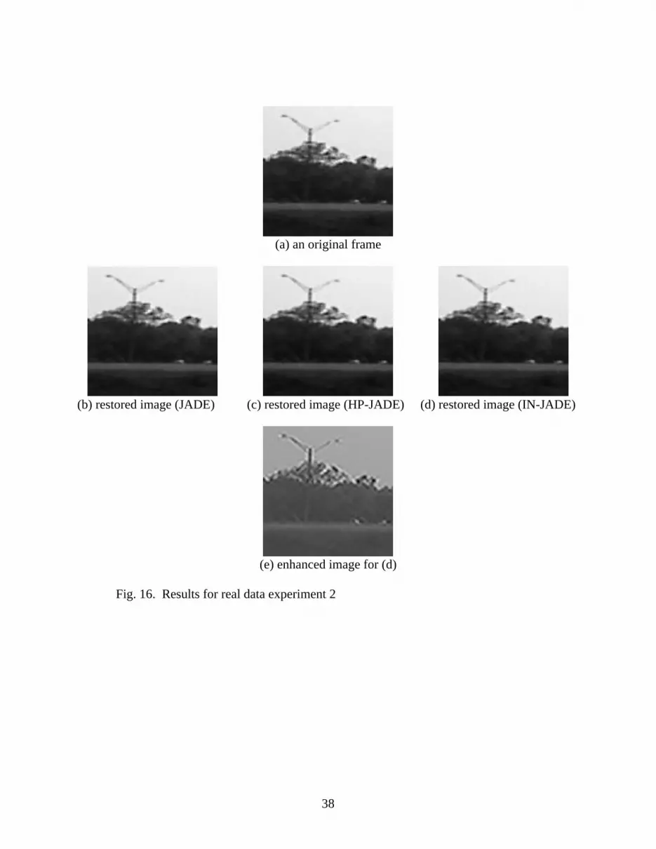
6.3 Real data experiment 2

To further investigate the performance of the DCA algorithms, 10 consecutive frames with

108108 pixels were used in the second experiment. One of degraded frames was shown in Fig.

16(a). The restored images using JADE, IN-JADE, and HP-JADE were shown in Fig. 16(b)-(d),

where the improvement is evident around road lamps. Fig. 16(e) is the enhancement result for

the image in Fig. 16(d) using the multi-channel filtering approach in Section 4, where the details

in tree profile and road lamp were highlighted.

Table 3 lists the image quality assessment results for all the methods. We can see that ICA

(JADE) performed well in this case, and SDICA did not perform as well as ICA. However, IN-

JADE and HP-JADE still outperformed the ICA. All these methods provided better results than

ISA, NMF, NTF, and BRL.

7. Conclusion

In our previous research, we applied ICA for the restoration of image sequences degraded by

atmospheric turbulence. The degraded image was assumed to be composed of the original high-

resolution image and turbulent sources that exist at the same space-time location (x,y,t0). The

20

assumption made on the high-resolution image and turbulent sources is that they are mutually

statistically independent despite the fact that they are emitted from the same space-time location

(x,y,t0). Although the result was promising, the assumption of source independence may not be

true in practice. To make the ICA result acceptable, we need to select frames with certain

spacing. This leads to problems in real-time or near real-time implementation. In this paper, we

propose to apply DCA, which can relax this requirement. The experimental results using

simulated and real data demonstrate that DCA can significantly improve the restoration

performance, without imposing any requirement on the selection of frames to be used in the

restoration process. They outperform other algorithms that can be applied to dependent sources.

Among the three DCA algorithms we discuss here, the ones based on innovation and highpass

filtering yield the better results and the SDICA based on wavelet packet requires the smallest

computational times. In addition to that, the restored image can be further sharpened through a

post-processing step with a single-frame multi-channel blind deconvolution method based on 2D

Gabor-filter bank and DCA. It is noteworthy that DCA performs similarly to ICA when the

assumption of source independence is satisfied.

References

[1] M. C. Roggemann, B. Welsh, Turbulence Effects on Imaging Systems, CRC Press, Boca

Raton, 1996.

[2] S. C. Park, M. K. Park, M. G. Kang, Super-resolution image reconstruction: A technical

overview, Signal Processing Magazine 20 (2003) 21-36.

21

[3] I. Kopriva, Q. Du, H. Szu, W. Wasylkiwskyj, Independent component analysis approach to

image sharpening in the presence of atmospheric turbulence, Optics Communications 233

(2004) 7-14.

[4] A. Hyvarinen, J. Karhunen, E. Oja, Independent Component Analysis, John Wiley & Sons,

2001.

[5] J. F. Cardoso, A. Souloumiac, Blind beamforming for non-Gaussian signals, IEE-Proc. F

140 (1993) 362-370.

[6] A. K. Barros, The independence assumption: dependent component analysis, in: Advances

in Independent Component Analysis, Springer, London, 2000.

[7] I. Kopriva. Blind Signal Deconvolution as an Instantaneous Blind Separation of Statistically

Dependent Sources, Lecture Notes in Computer Science 4666, pp. 504-511, Springer-

Verlag, Proceedings of the Seventh International Conference on Independent Component

Analysis and Blind Source Separation, eds. M.E. Davies et al., London, UK, September 9-

12, 2007.

[8] I. Kopriva, D. Seršić, Wavelet packets approach to blind separation of statistically

dependent sources, Neurocomputing 71(2008) 1642-1655.

[9] A. Cichocki, P. Georgiev, Blind source separation algorithms with matrix constraints,

IEICE Transactions on Fundamentals of Electronics, Communications and Computer

Sciences E86-A (2003) 522-531.

[10] T. Tanaka, A. Cichocki, Subband decomposition independent component analysis and new

performance criteria, in: Proc. IEEE Int. Conf. on Acoustics, Speech and Signal Processing

(ICASSP 2004), Montreal, Canada, 2004, pp. 541-544.

22

[11] A. Hyvärinen, Independent component analysis for time-dependent stochastic processes, in:

Proceedings of the International Conference on Artificial Neural Networks (ICANN’98),

pp. 541-546, Skovde, Sweden, 1998.

[12] S. J. Orfanidis, Optimum Signal Processing – An Introduction, 2nd ed. MacMillan

Publishing Comp., New York, 1988.

[13] I. Kopriva, Approach to blind image deconvolution by multiscale subband decomposition

and independent component analysis, Journal of Optical Society of America A 24 (2007)

973-983.

[14] I. Kopriva, D. Seršić, Robust Blind Separation of Statistically Dependent Sources Using

Dual Tree Wavelets, in: Proceedings of the 2007 IEEE International Image Processing

Conference, Vol. I, pp. 433-436, San Antonio, TX, USA, September 16-19, 2007.

[15] N. G. Kingsbury, Complex wavelets for shift invariant analysis and filtering of signals,

Appl. Comput. Harmon. Anal. 10 (2001) 234-253.

[16] W. Selesnick, R. G. Baraniuk, N.G. Kingsbury, The dual-tree complex wavelet transform,

Signal Processing Magazine 22 (2005) 123-151.

[17] M. B. Priestley, Stochastic Differentiability, in: Spectral Analysis and Time Series, London:

Academic Press, 1981, pp.153-154.

[18] J. C. Russ, The Image Processing Handbook, CRC Press, Boca Raton, 1992.

[19] J. V. Stone, Blind source separation using temporal predictability, Neural

Computation 13 (2001) 1559-1574.

[20] J. V. Stone, Blind deconvolution using temporal predictability, Neurocomputing 49 (2002)

79-86.

23

[21] N. B. Hill, B. H. Bouzas, Objective Image Quality Measure Derived from Digital Image

Power Spectra, Opt. Eng. 31 (1992) 813-825.

[22] J. A. Saghri, P. S. Cheatham, A. Habibi, Image quality measure based on human visual

system model, Opt. Eng. 28 (1989) 813-818.

[23] J. Karvanen, T. Tanaka, Temporal Decorrelation as Preprocessing for Linear and Post-

nonlinear ICA, in C.G. Puntonet and A. Prieto (Eds.): ICA 2004, LNCS 3195, pp. 774-781,

2004.

[24] J.-F. Cardoso, Multidimensional independent component analysis, in Proceedings of the

1998 IEEE International Conference on Acoustics, Speech and Signal Processing, Seattle,

WA, USA.

[25] A. Hyvärinen, P. Hoyer, Emergence of Phase- and Shift-Invariant Features by

Decomposition of Natural Images into Independent Feature Subspaces, Neural Computation

12 (2000) 1705-1720.

[26] http://www.cs.helsinki.fi/u/phoyer/software.html.

[27] D. D. Lee, H. S. Seung, Learning the parts of objects by non-negative matrix factorization,”

Nature 401 - 6755 (1999) 788-791.

[28] A. Cichocki, R. Zdunek, S. Amari, Csiszár’s Divergences for Non-negative Matrix

Factorization: Family of New Algorithms, LNCS 3889 (2006) 32-39

[29] A. Cichocki, R. Zdunek, S.I. Amari, Hierarchical ALS Algorithms for Nonnegative Matrix

Factorization and 3D Tensor Factorization, LNCS 4666 (2007) 169-176.

[30] A. Cichocki, R. Zdunek, S. Amari, Nonnegative Matrix and Tensor Factorization, IEEE Sig.

Proc. Mag. 25 (2008) 142-145.

[31] R. L. Lagendijk, J. Biemond, Iterative Identification and Restoration of Images, KAP, 1991.

24

[32] P. Campisi, K. Egiazarian, editors, Blind Image Deconvolution p. 8-9, CRC Press, Boca

Raton, 2007.

[33] W.H. Richardson, Bayesian-based iterative method of image restoration, J.Opt.Soc. Am. 62

(1972) 55-59.

[34] L. B. Lucy, An iterative technique for rectification of observed distribution, Astron. J. 79

(1974) 745-754.

[35] D. A. Fish, A. M. Brinicombe, E. R. Pike, J. G. Walker, Blind deconvolution by means of

the Richardson-Lucy algorithm, J. Opt. Soc. Am. A 12 (1995) 58-65.

[36] D. S. C. Biggs, M. Andrews, Acceleration of iterative image restoration algorithms, Applied

Optics 36 (1997) 1766-1775.

25

List of table captions

Table 1. No-reference quality assessment for the restored images in the computer simulation.

Table 2. No-reference quality assessment for the restored images in real data experiment 1.


List of figure captions

Fig. 1. (a) original image and (b) a degraded image used in computer simulation.

Fig. 2. Four source images obtained from DCA (IN-JADE) algorithm: (a), (c), and (d)

correspond to turbulence patterns, (b) corresponds to the restored image.

Fig. 3. Images restored from four simulated blurred frames using (a) ICA (JADE), (b) DCA

(IN-JADE), (c) DCA (HP-JADE), (d) DCA (SDICA), (e) ISA, (f) NMF, (g) NTF, and

(h) BRL algorithms.

Fig. 4. Restored images from ICA and three DCA algorithms when using 5 consecutive frames.

Fig. 5. Restored images from ICA and three DCA algorithms when using 10 consecutive

frames.


frames.


frames.

Fig. 8. Restored images from ICA and three DCA algorithms when using 25 frames with 2-

frames spacing.


frames spacing.

26


frames spacing.


frames spacing.


frames spacing.

Fig. 13. A reconstructed frame for further enhancement.

Fig. 14. Multi-channel version of the original image in Fig. 13 produced by the 2D Gabor filter

bank with two spatial frequencies and four orientations.

Fig. 15. Image enhancement for Fig. 13 using single-frame multi-channel filtering.

Fig. 16. Results for real data experiment 2.

27

Table 1. No-reference quality assessment for the restored images in computer simulation.

ICA(JADE)

DCA (IN-JADE)

DCA(HP-JADE)

DCA (SDICA)

ISA NMF NTF BRL

PSA 3.53 3.90 4.44 3.18 2.87 3.44 2.45 2.66

I4 6.18 2.56 3.66 2.79 4.08 5.21 2.54 3.60


ICA(JADE)

DCA (IN-JADE)

DCA(HP-JADE)

DCA (SDICA)

ISA NMF NTF BRL

PSA 2.74 2.74 2.76 2.73 1.61 2.69 2.73 2.23

I4 2.06 1.63 1.63 1.82 3.53 2.10 9.10 7.29


ICA(JADE)

DCA (IN-JADE)

DCA(HP-JADE)

DCA (SDICA)

ISA NMF NTF BRL

PSA 6.71 6.99 7.11 5.27 3.94 5.20 3.69 2.63

I4 2.56 2.52 2.56 3.57 5.26 5.19 4.38 5.19

28

(a) (b)

Fig. 1. (a) original image and (b) a degraded image used in computer simulation.

29

(a) (b)

(c) (d)

Fig. 2. Four source images obtained from DCA (IN-JADE) algorithm: (a), (c), and (d)

correspond to turbulence patterns, (b) corresponds to the restored image.

30

(a) (b) (c)

(d) (e) (f)

(g) (h)

Fig. 3. Images restored from four simulated blurred frames using (a) ICA (JADE), (b) DCA (IN-

JADE), (c) DCA (HP-JADE), (d) DCA (SDICA), (e) ISA, (f) NMF, (g) NTF, and (h) BRL

algorithms.

31

JADE HP-JADE IN-JADE SDICAGivens Rotation: (44) (30) (32) (59)Laplacian Metric: (2.0580) (1.6284) (1.6260) (1.8220)






32

JADE HP-JADE IN-JADE SDICAGivens Rotation: (51746) (33355) (36922) (46)Laplacian Metric: (3.4932) (1.3928) (1.3756) (1.5200)Fig. 7. Restored images from ICA and three DCA algorithms when using 50 consecutive frames.

JADE HP-JADE IN-JADE SDICAGivens Rotation: (5364) (9492) (8368) (44)Laplacian Metric: (2.8660) (1.3664) (1.3600) (1.4560)Fig. 8. Restored images from ICA and three DCA algorithms when using 25 frames with 2-frames spacing.


Fig. 9. Restored images from ICA and three DCA algorithms when using 10 frames with 5-frames spacing.

33

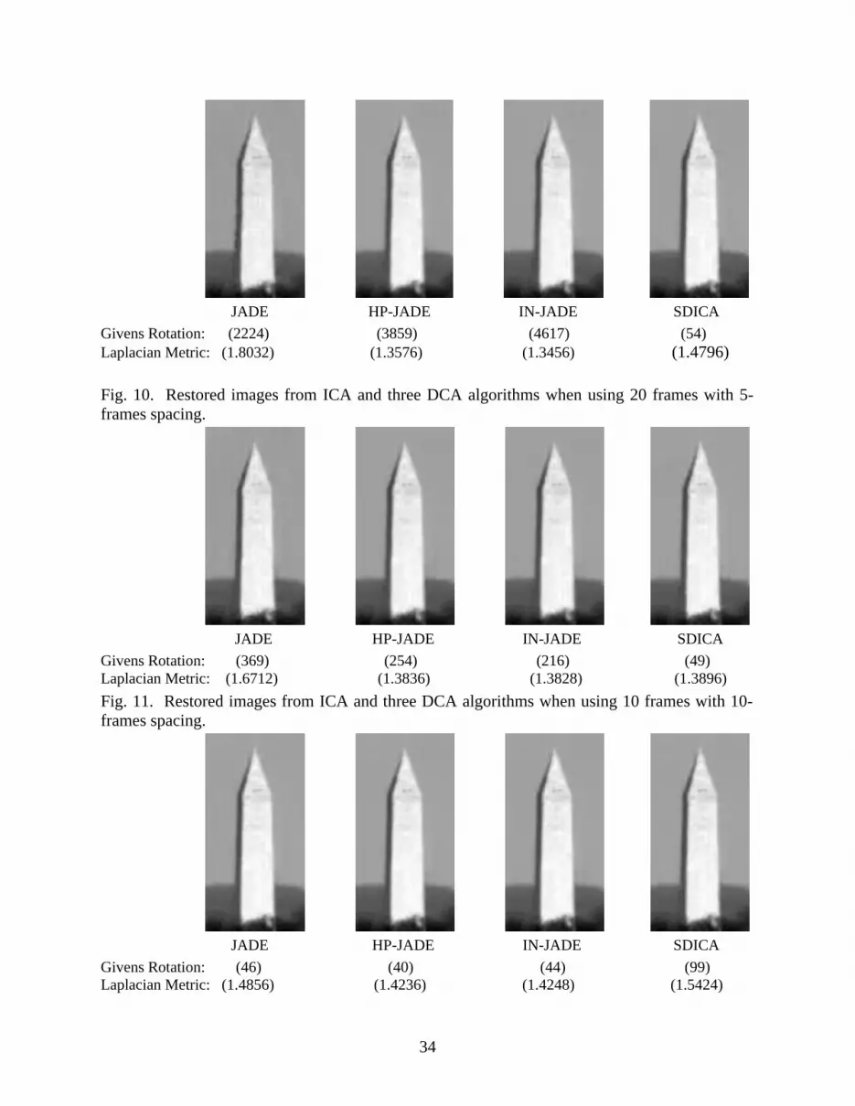
JADE HP-JADE IN-JADE SDICAGivens Rotation: (2224) (3859) (4617) (54)Laplacian Metric: (1.8032) (1.3576) (1.3456) (1.4796) Fig. 10. Restored images from ICA and three DCA algorithms when using 20 frames with 5-frames spacing.

JADE HP-JADE IN-JADE SDICAGivens Rotation: (369) (254) (216) (49)Laplacian Metric: (1.6712) (1.3836) (1.3828) (1.3896)Fig. 11. Restored images from ICA and three DCA algorithms when using 10 frames with 10-frames spacing.


34

Fig. 12. Restored images from ICA and three DCA algorithms with 20-frames spacing.

Fig. 13. A reconstructed frame for further enhancement.

35

Fig. 14. Multi-channel version of the original image in Fig. 13 produced by the 2D Gabor filter bank with two spatial frequencies and four orientations.

36

s1 s2 s3 s4

Predictability Metric: (2.4874) (2.8756) (2.7367) (2.6140)

(a) Gabor + Wavelet + ICA (4 sources)

s1 s2 s3 s4

Predictability Metric: (2.0453) (2.7177) (2.8131) (2.1752)

(b) Gabor + Innovation + ICA (4 sources)

(c) Gabor + Innovation + ICA (1 source)

Fig. 15. Image enhancement for Fig. 13 using single-frame multi-channel filtering.

37

(a) an original frame

(b) restored image (JADE) (c) restored image (HP-JADE) (d) restored image (IN-JADE)

(e) enhanced image for (d)

Fig. 16. Results for real data experiment 2

38

Dependent component analysis for blind restoration of images degraded by turbulent atmosphere

Documents

Transcript of Dependent component analysis for blind restoration of images degraded by turbulent atmosphere