G.PULLAIAH COLLEGE OF ENGINEERING AND TECHNOLOGY: KURNOOL DEPARTMENT OF ELECTRICAL AND ELECTRONICS ENGINEERING

CLASS/SEM: IV.B.Tech I-SEM SUB: UTILISATION OF ELECTRICAL ENERGY

UNIT-IV BASIC TERMS AND DEFINITIONS:

Scheduled speed =

Average speed

Crest speed Maximum speed attained by the train during time of run.

Trapezoidal speed

time curve Vm=

√

To find α, β = [

α

] =

Where Vavg =

=Accelaration =Vm/t1, β= Braking Retardation = Vm/t3

k=[

] ; T=Total time of run in sec

Dead weight It is the total weight of train to be propelled by the locomotive. It is denoted

by ‘W’.

Accelerating weight It is the effective weight of train that has angular acceleration due to the

rotational inertia including the dead weight of the train. It is denoted by

‘We’. This effective train is also known as accelerating weight. The effective

weight of the train will be more than the dead weight. Normally, it is taken

as 5–10% of more than the dead weight.

Adhesive weight The total weight to be carried out on the drive in wheels of a locomotive is

known as adhesive weight.

Coefficientof

adhesion

It is defined as the ratio of the tractive effort required to propel the wheel

of alocomotive to its adhesive weight.

CONCEPTS

INTRODUCTION

The movement of trains and their energy consumption can be most conveniently studied by means of

the speed–distance and the speed–time curves. The motion of any vehicle may be at constant speed or

it may consist of periodic acceleration and retardation. The speed–time curves have significant

importance in traction. If the frictional resistance to the motion is known value, the energy required for

motion of the vehicle can be determined from it. Moreover, this curve gives the speed at various time

instants after the start of run directly.

TYPES OF SERVICES

There are mainly three types of passenger services, by which the type of traction system has to be

selected, namely:

1. Main line service.

2. Urban or city service.

3. Suburban service.

MAIN LINE SERVICES

In the main line service, the distance between two stops is usually more than 10 km. High balancing

speeds should be required. Acceleration and retardation are not so important.

URBAN SERVICE

In the urban service, the distance between two stops is very less and it is less than 1 km. It requires high

average speed for frequent starting and stopping.

SUBURBAN SERVICE

In the suburban service, the distance between two stations is between 1 and 8 km. This service requires

rapid acceleration and retardation as frequent starting and stopping is required.

SPEED–TIME AND SPEED–DISTANCE CURVES FOR DIFFERENT SERVICES

The curve that shows the instantaneous speed of train in kmph along the ordinate and time in seconds

along the abscissa is known as ‘speed–time’ curve. The curve that shows the distance between two

stations in km along the ordinate and time in seconds along the abscissa is known as ‘speed–distance’

curve. The area under the speed–time curve gives the distance travelled during, given time internal and

slope at any point on the curve toward abscissa gives the acceleration and retardation at the instance,

out of the two speed–time curve is more important.

SPEED–TIME CURVE FOR MAIN LINE SERVICE

Typical speed–time curve of a train running on main line service is shown in Fig.It mainly consists of the

following time periods:

1. Constant accelerating period.

2. Acceleration on speed curve.

3. Free-running period.

4. Coasting period.

5. Braking period.

Fig.4.1. Speed–time curve for mainline service

Constant Acceleration

During this period, the traction motor accelerate from rest. The curve ‘OA’ represents the constant

accelerating period. During the instant 0 to T1, the current is maintained approximately constant and

the voltage across the motor is gradually increased by cutting out the starting resistance slowly moving

from one notch to the other.

Acceleration On Speed-Curve

During the running period from T1 to T2, the voltage across the motor remains constant and the current

starts decreasing, this is because cut out at the instant ‘T1’. According to the characteristics of motor, its

speed increases with the decrease in the current and finally the current taken by the motor remains

constant. This period is shown by the curve ‘AB’.

Free-Running Or Constant-Speed Period

The train runs freely during the period T2 to T3 at the speed attained by the train at the instant ‘T2’.

During this speed, the motor draws constant power from the supply lines. This period is shown by the

curve BC.

Coasting Period

This period is from T3 to T4, i.e., from C to D. At the instant ‘T3’ power supply to the traction, the motor

will be cut off and the speed falls on account of friction, windage resistance, etc. During this period, the

train runs due to the momentum attained at that particular instant. The rate of the decrease of the

speed during coasting period is known as coasting retardation. Usually, it is denoted with the symbol

‘βc’.

Braking Period

Braking period is from T4 to T5, i.e., from D to E. At the end of the coasting period, i.e., at ‘T4’ brakes are

applied to bring the train to rest. During this period, the speed of the train decreases rapidly and finally

reduces to zero. In main line service, the free-running period will be more, the starting and braking

periods are very negligible, since the distance between the stops for the main line service is more than

10 km.

SPEED–TIME CURVE FOR SUBURBAN SERVICE

In suburban service, the distance between two adjacent stops for electric train is lying between 1 and 8

km. In this service, the distance between stops is more than the urban service and smaller than the main

line service. The typical speed–time curve for suburban service is shown in Fig.

Fig.4.2.Typical speed–time curve for suburban service

The speed–time curve for urban service consists of three distinct periods. They are:

1. Acceleration.

2. Coasting.

3. Retardation.

For this service, there is no free-running period. The coasting period is comparatively longer since the

distance between two stops is more. Braking or retardation period is comparatively small. It requires

relatively high values of acceleration and retardation. Typical acceleration and retardation values are

lying between 1.5 and 4 kmphp and 3 and 4 kmphp, respectively.

SPEED–TIME CURVE FOR URBAN OR CITY SERVICE

The speed–time curve urban or city service is almost similar to suburban service and is shown in Fig.4.3.

Fig.4.3.Typical speed–time curve for urban service

In this service also, there is no free-running period. The distance between two stop is less about 1 km.

Hence, relatively short coasting and longer braking period is required.. The acceleration for the urban

service lies between 1.6 and 4 kmphp. The coasting retardation is about 0.15 kmphp and the braking

retardation is lying between 3 and 5 kmphp. Some typical values of various services are shown in Table.

Table : 4.1.Types of services

Average speed

It is the mean of the speeds attained by the train from start to stop, i.e., it is defined as the ratio of the

distance covered by the train between two stops to the total time of run. It is denoted with ‘Va’. where

Va is the average speed of train in kmph, D is the distance between stops in km, and T is the actual time

of run in hours

Schedule speed

The ratio of the distance covered between two stops to the total time of the run including the time for

stop is known as schedule speed. It is denoted with the symbol ‘Vs’, where Ts is the schedule time in

hours.

Schedule time

It is defined as the sum of time required for actual run and the time required for stop.

i.e., Ts = Trun + Tstop.

FACTORS AFFECTING THE SCHEDULE SPEED OF A TRAIN

The factors that affect the schedule speed of a train are:

1. Crest speed.

2. The duration of stops.

3. The distance between the stops.

4. Acceleration.

5. Braking retardation.

Crest Speed

It is the maximum speed of train, which affects the schedule speed as for fixed acceleration, retardation,

and constant distance between the stops. If the crest speed increases, the actual running time of train

decreases. For the low crest speed of train it running so, the high crest speed of train will increases its its

schedule speed.

Duration of Stops

If the duration of stops is more, then the running time of train will be less; so that, this leads to the low

schedule speed. Thus, for high schedule speed, its duration of stops must be low.

Distance between the stop. If the distance between the stops is more, then the running time of the train

is less; hence, the schedule speed of train will be more.

Acceleration

If the acceleration of train increases, then the running time of the train decreases provided the distance

between stops and crest speed is maintained as constant. Thus, the increase in acceleration will increase

the schedule speed.

Breaking Retardation

High breaking retardation leads to the reduction of running time of train. These will cause high schedule

speed provided the distance between the stops is small.

SIMPLIFIED TRAPEZOIDAL AND QUADRILATERAL SPEED TIME CURVES

Simplified speed–time curves gives the relationship between acceleration, retardation average

speed, and the distance between the stop, which are needed to estimate the performance of a service

at different schedule speeds. So that, the actual speed–time curves for the main line, urban, and

suburban services are approximated to some from of the simplified curves. These curves may be of

either trapezoidal or quadrilateral shape.

ANALYSIS OF TRAPEZOIDAL SPEED–TIME CURVE

Trapezoidal speed–time curve can be approximated from the actual speed–time curves of different

services by assuming that:

o The acceleration and retardation periods of the simplified curve is kept same as to that of the actual

curve.

o The running and coasting periods of the actual speed–time curve are replaced by the constant periods.

This known as trapezoidal approximation, a simplified trapezoidal speed–time curve is shown in fig,

Fig. 4.3.Trapezoidal speed–time curve

Calculations from the trapezoidal speed–time curve

Let D be the distance between the stops in km, T be the actual running time of train in second, α be the

acceleration in km/h/sec, β be the retardation in km/h/sec, Vm be the maximum or the crest speed of

train in km/h, and Va be the average speed of train in km/h. Area under the trapezoidal speed–time

curve gives the total distance between the two stops (D).

∴ The distance between the stops (D) = area under triangle OAE + area of rectangle ABDE + area of

triangle DBC = The distance travelled during acceleration + distance travelled during free running period

+ distance travelled during retardation.

The distance travelled during acceleration = average speed during accelerating period × time for

acceleration

The distance travelled during free-running period = average speed × time of free running

The distance travelled during retardation period = average speed × time for retardation

The distance between the two stops is:

The distance between the two stops is:

ANALYSIS OF QUADRILATERAL SPEED–TIME CURVE

Quadrilateral speed–time curve for urban and suburban services for which the distance

between two stops is less. The assumption for simplified quadrilateral speed–time curve is the initial

acceleration and coasting retardation periods are extended, and there is no free-running period.

Simplified quadrilateral speed–timecurve is shown in Fig.

Fig. 4.4.Quadrilateral speed–time curve

Let V1 be the speed at the end of accelerating period in km/h, V2 be the speed at the end of coasting

retardation period in km/h, and βc be the coasting retardation in km/h/sec.

Time for acceleration,

Time for coasting period,

Time period for braking retardation period,

Total distance travelled during the running period D:

= the area of triangle PQU + the area of rectangle UQRS + the area of triangle TRS.= (the distance

travelled during acceleration + the distance travelled during coasting retardation + the distance travelled

during breaking retardation). But, the distance travelled during acceleration = average speed × time for

Acceleration

The distance travelled during coasting retardation =

The distance travelled during breaking retardation = average speed × time for breaking retardation

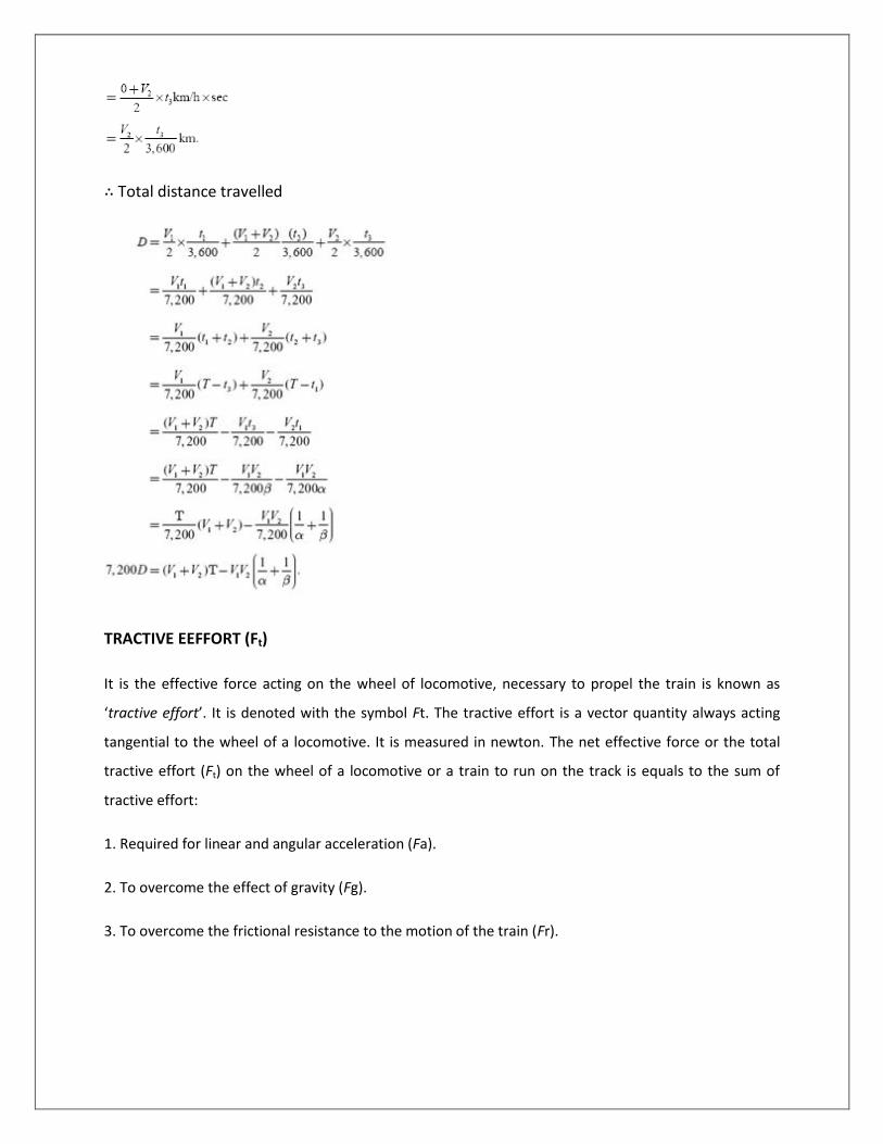
∴ Total distance travelled

TRACTIVE EEFFORT (Ft)

It is the effective force acting on the wheel of locomotive, necessary to propel the train is known as

‘tractive effort’. It is denoted with the symbol Ft. The tractive effort is a vector quantity always acting

tangential to the wheel of a locomotive. It is measured in newton. The net effective force or the total

tractive effort (Ft) on the wheel of a locomotive or a train to run on the track is equals to the sum of

tractive effort:

1. Required for linear and angular acceleration (Fa).

2. To overcome the effect of gravity (Fg).

3. To overcome the frictional resistance to the motion of the train (Fr).

MECHANICS OF TRAIN MOVEMENT

The essential driving mechanism of an electric locomotive is shown in Fig. The electric locomotive

consists of pinion and gear wheel meshed with the traction motor and the wheel of the locomotive.

Here, the gear wheel transfers the tractive effort at the edge of the pinion to the driving wheel.

Fig.4.5. Driving mechanism of electric locomotives

Let T is the torque exerted by the motor in N-m, Fp is tractive effort at the edge of the pinion in

Newton,Ft is the tractive effort at the wheel, D is the diameter of the driving wheel, d1 and d2 are the

diameter of pinion and gear wheel, respectively, and η is the efficiency of the power transmission for

the motor to the driving axle.

The tractive effort at the edge of the pinion transferred to the wheel of locomotive is

the tractive effort required for train propulsion is: Ft = Fa + Fg + Fr, where Fa is the force required for

linear and angular acceleration, Fg is the force required to overcome the gravity, and Fr is the force

required to overcome the resistance to the motion.

Force required for linear and angular acceleration (Fa)

According to the fundamental law of acceleration, the force required to accelerate the motion of the

body is given by: Force = Mass × acceleration F = ma.

Let the weight of train be ‘W ’ tons being accelerated at ‘α’ kmphps:

Equation

Equation holds good only if the accelerating body has no rotating parts.Owing to the fact that the train

has rotating parts such as motor armature, wheels, axels, and gear system. Hence, these parts need to

be given angular acceleration at the same time as the whole train is accelerated in linear direction.

∴ The tractive effort required-for linear and angular acceleration is:

Tractive effort required to overcome the train resistance (Fr)

When the train is running at uniform speed on a level track, it has to overcome the opposing force due

to the surface friction, i.e., the friction at various parts of the rolling stock, the fraction at the track, and

also due to the wind resistance. The magnitude of the frictional resistance depends upon the shape,

size, and condition of the track and the velocity of the train, etc.

Let ‘r’ is the specific train resistance in N/ton of the dead weight and ‘W’ is the dead weight in ton.

Tractive effort required to overcome the effect of gravity (Fg)

When the train is moving on up gradient as shown in Fig., the gravity component of the dead weight

opposes the motion of the train in upward direction. In order to prevent this opposition, the tractive

effort should be acting in upward direction.

∴ The tractive effort required to overcome the effect of gravity:

Fig.4.6.Train moving on up gradient

From above Equations

+ve sign for the train is moving on up gradient.

–ve sign for the train is moving on down gradient.

This is due to when the train is moving on up a gradient, the tractive effort showing Equation will be

required to oppose the force due to gravitational force, but while going down the gradient, the same

force will be added to the total tractive effort.

∴ The total tractive effort required for the propulsion of train Ft = Fa + Fr ± Fg:

SPECIFIC ENERGY CONSUMPTION

The energy input to the motors is called the energy consumption. This is the energy consumed by

various parts of the train for its propulsion. The energy drawn from the distribution system should be

equals to the energy consumed by the various parts of the train and the quantity of the energy required

for lighting, heating, control, and braking. This quantity of energy consumed by the various parts of train

per ton per kilometer is known as specific energy consumption. It is expressed in watt hours per ton per

km.

Determination of specific energy output from simplified speed–time curve

Energy output is the energy required for the propulsion of a train or vehicle is mainly for accelerating

the rest to velocity ‘Vm’, which is the energy required to overcome the gradient and track resistance to

motion. Energy required for accelerating the train from rest to its crest speed ‘Vm'

Energy required for overcoming the gradient and tracking resistance to motion

Energy required for overcoming the gradient and tracking resistance:

where Ft′ is the tractive effort required to overcome the gradient and track resistance, W is the dead

weight of train, r is the track resistance, and G is the percentage gradient.

FACTORS AFFECTING THE SPECIFIC ENERGY CONSUMPTION

Factors that affect the specific energy consumption are given as follows.

Distance between stations

From equation specific energy consumption is inversely proportional to the distance between stations.

Greater the distance between stops is, the lesser will be the specific energy consumption. The typical

values of the specific energy consumption is less for the main line service of 20–30 W-hr/ton-km and

high for the urban and suburban services of 50–60 W-hr/ton-km.

Acceleration and retardation

For a given schedule speed, the specific energy consumption will accordingly be less for more

acceleration and retardation.

Maximum speed

For a given distance between the stops, the specific energy consumption increases with the increase in

the speed of train.

Gradient and train resistance

From the specific energy consumption, it is clear that both gradient and train resistance are proportional

to the specific energy consumption. Normally, the coefficient of adhesion will be affected by the running

of train, parentage gradient, condition of track, etc. for the wet and greasy track conditions. The value of

the coefficient of adhesion is much higher compared to dry and sandy conditions.

Important Questions

1. Explain the factors affecting Specific Energy Consumption

2. Determine of Specific Energy Output from Simplified Speed–Time Curve

3. Write about Mechanics of Train movement.

4. Explain analysis of Quadrilateral and Trapezoidal Speed–Time curves.

5. Write about factors affecting the Schedule Speed of a train

6. Explain the Speed–Time and Speed–Distance Curves for different services