UNIT 3 - gpcet

131

UNIT 3

BASIC TRAVERSAL

AND SEARCH TECHNIQUES

Search means finding a path or traversal between a start node and one of a set of

goal nodes. Search is a study of states and their transitions.

Search involves visiting nodes in a graph in a systematic manner, and may or may

not result into a visit to all nodes. When the search necessarily involved the

examination of every vertex in the tree, it is called the traversal.

Techniques for Traversal of a Binary Tree:

A binary tree is a finite (possibly empty) collection of elements. When the binary tree

is not empty, it has a root element and remaining elements (if any) are partitioned

into two binary trees, which are called the left and right subtrees.

There are three common ways to traverse a binary tree:

1. Preorder

2. Inorder

3. postorder

In all the three traversal methods, the left subtree of a node is traversed before the

right subtree. The difference among the three orders comes from the difference in the

time at which a node is visited.

Inorder Traversal:

In the case of inorder traversal, the root of each subtree is visited after its left subtree

has been traversed but before the traversal of its right subtree begins. The steps for

traversing a binary tree in inorder traversal are:

1. Visit the left subtree, using inorder. 2. Visit the root.

3. Visit the right subtree, using inorder.

The algorithm for preorder traversal is as follows:

treenode = record {

Type data; //Type is the data type of data.

Treenode *lchild; treenode *rchild; }

132

algorithm inorder (t) // t is a binary tree. Each node of t has three fields: lchild, data, and rchild.

{

if t 0 then

{ inorder (t lchild);

visit (t); inorder (t rchild);

}

}

Preorder Traversal:

In a preorder traversal, each node is visited before its left and right subtrees are

traversed. Preorder search is also called backtracking. The steps for traversing a

binary tree in preorder traversal are:

1. Visit the root.

2. Visit the left subtree, using preorder.

3. Visit the right subtree, using preorder.


Algorithm Preorder (t)

// t is a binary tree. Each node of t has three fields; lchild, data, and rchild.

{

if t 0 then {

visit (t); Preorder (t lchild);

Preorder (t rchild); }

}

Postorder Traversal:

In a postorder traversal, each root is visited after its left and right subtrees have been

traversed. The steps for traversing a binary tree in postorder traversal are:

1. Visit the left subtree, using postorder.

2. Visit the right subtree, using postorder

3. Visit the root.


Algorithm Postorder (t)

// t is a binary tree. Each node of t has three fields : lchild, data, and rchild.

{

if t 0 then {

Postorder (t lchild);

Postorder (t rchild);

visit(t); }

}

133

Examples for binary tree traversal/search technique:

Example 1:

Traverse the following binary tree in pre, post and in-order.

Bi n a ry T re e P re, P o st a n d In- o rd er T ra v ers in g

Example 2:

Traverse the following binary tree in pre, post, inorder and level order.

Bi n a ry T re e P re, P o st , In o rd er a n d l ev e l o rd er T ra v ers in g

Example 3:


Bi n a ry T re e P re, P o st , In o rd er a n d lev e l o rd er T ra v ers in g

A

B C

D E F

G H I

Preord eri ng of t he

vertices: A, B, D, C, E, G,

F, H, I.

Post ord eri ng of t he vertices:

D, B, G, E, H, I, F, C, A.

Inord eri ng of t he

vertices: D, B, A, E, G,

C, H, F, I

A

B C

D E F

G H I

• P reo rde r t ra v e rs a l y ie lds: A, B, D, C , E, G , F , H, I

• Posto rde r t ra v e rs a l y ie lds: D, B, G , E, H, I, F , C , A

• Ino rde r t ra v e rs a l y ie lds: D, B, A, E, G , C , H, F , I

• Le v e l o rde r t ra v e rs a l y ie lds:

A, B, C , D, E, F , G , H, I

P

F S

B H R Y

G T Z

W

• P reo rde r t ra v e rs a l y ie lds: P , F , B, H, G , S, R, Y, T, W , Z

• Posto rde r t ra v e rs a l y ie lds:

B, G , H, F , R, W , T, Z, Y, S, P

• Ino rde r t ra v e rs a l y ie lds: B, F , G , H, P , R, S, T, W , Y, Z

• Le v e l o rde r t ra v e rs a l y ie lds:

P , F , S, B, H, R, Y, G , T, Z, W

134

Example 4:


Bi n a ry T re e P re, P o st , In o rd er a n d l ev e l o rd er T ra v ers in g

Example 5:


Bi n a ry T re e P re, P o st , In o rd er a n d l ev e l ord er T ra v ers in g

Techniques for graphs:

Given a graph G = (V, E) and a vertex V in V (G) traversing can be done in two ways.

1. Depth first search

2. Breadth first search

3. D-search (Depth Search)

2

7 5

2 6 9

5 11 4

• P reo rde r t ra v e rs a l y ie lds: 2, 7 , 2 , 6 , 5 , 11 , 5 , 9 , 4

• Posto rde r t ra v a rs a l y ie lds:

2, 5 , 11 , 6 , 7 , 4 , 9 , 5 , 2

• Ino rde r t ra v a rs a l y ie lds: 2, 7 , 5 , 6 , 11 , 2 , 5 , 4 , 9

• Le v e l o rde r t ra v e rs a l y ie lds: 2, 7 , 5 , 2 , 6 , 9 , 5 , 11 , 4

A

B C

D E

G H

K L M

• Preo rde r t rav e rs al y ie lds: A, B, D, G , K, H, L, M , C , E

• Posto rde r t rav ars al y ie lds: K, G , L, M , H, D, B, E, C , A

• Ino rde r t rav ars al y ie lds: K, G , D, L, H, M , B, A, E, C

• Le v e l o rde r t rav e rs al y ie lds:

A, B, C , D, E, G , H, K, L, M

135

Depth first search:

With depth first search, the start state is chosen to begin, then some successor of the

start state, then some successor of that state, then some successor of that and so on,

trying to reach a goal state.

If depth first search reaches a state S without successors, or if all the successors of a state S have been chosen (visited) and a goal state has not get been found, then it “backs up” that means it goes to the immediately previous state or predecessor formally, the state whose successor was „S‟ originally.

For example consider the figure. The circled letters are state and arrows are

branches.

ST A RT

G OA L

Suppose S is the start and G is the only goal state. Depth first search will first visit S,

then A then D. But D has no successors, so we must back up to A and try its second

successor, E. But this doesn‟t have any successors either, so we back up to A again.

But now we have tried all the successors of A and haven‟t found the goal state G so

we must back to „S‟. Now „S‟ has a second successor, B. But B has no successors, so

we back up to S again and choose its third successor, C. C has one successor, F. The

first successor of F is H, and the first of H is J. J doesn‟t have any successors, so we

back up to H and try its second successor. And that‟s G, the only goal state. So the

solution path to the goal is S, C, F, H and G and the states considered were in order

S, A, D, E, B, C, F, H, J, G.

Disadvantages:

1. It works very fine when search graphs are trees or lattices, but can get

struck in an infinite loop on graphs. This is because depth first search can

travel around a cycle in the graph forever.

To eliminate this keep a list of states previously visited, and never permit

search to return to any of them.

2. One more problem is that, the state space tree may be of infinite depth, to

prevent consideration of paths that are too long, a maximum is often placed on the depth of nodes to be expanded, and any node at that depth is treated as if it had no successors.

3. We cannot come up with shortest solution to the problem.

D

A

E

J

S B

H G

C F K

I

136

Time Complexity:

Let n = |V| and e = |E|. Observe that the initialization portion requires (n) time.

Since we never visit a vertex twice, the number of times we go through the loop is at

most n (exactly n assuming each vertex is reachable from the source). As, each

vertex is visited at most once. At each vertex visited, we scan its adjacency list once.

Thus, each edge is examined at most twice (once at each endpoint). So the total

running time is O (n + e).

Alternatively,

If the average branching factor is assumed as „b‟ and the depth of the solution as „d‟, and maximum depth m ≥ d.

The worst case time complexity is O(bm ) as we explore bm nodes. If many solutions

exists DFS will be likely to find faster than the BFS.

Space Complexity:

We have to store the nodes from root to current leaf and all the unexpanded siblings

of each node on path. So, We need to store bm nodes.

Breadth first search:

Given an graph G = (V, E), breadth-first search starts at some source vertex S and

“discovers" which vertices are reachable from S. Define the distance between a vertex

V and S to be the minimum number of edges on a path from S to V. Breadth-first

search discovers vertices in increasing order of distance, and hence can be used as an

algorithm for computing shortest paths (where the length of a path = number of

edges on the path). Breadth-first search is named because it visits vertices across the

entire breadth.

To illustrate this let us consider the following tree:

ST A RT

G OA L

Breadth first search finds states level by level. Here we first check all the immediate

successors of the start state. Then all the immediate successors of these, then all the

immediate successors of these, and so on until we find a goal node. Suppose S is the

start state and G is the goal state. In the figure, start state S is at level 0; A, B and C

are at level 1; D, e and F at level 2; H and I at level 3; and J, G and K at level 4. So

breadth first search, will consider in order S, A, B, C, D, E, F, H, I, J and G and then

stop because it has reached the goal node.

Breadth first search does not have the danger of infinite loops as we consider states

in order of increasing number of branches (level) from the start state.

D

A

E

J

S B

H G

C F K

I

137

One simple way to implement breadth first search is to use a queue data structure

consisting of just a start state. Any time we need a new state, we pick it from the

front of the queue and any time we find successors, we put them at the end of the

queue. That way we are guaranteed to not try (find successors of) any states at level

„N‟ until all states at level „N – 1‟ have been tried.

Time Complexity:

The running time analysis of BFS is similar to the running time analysis of many graph

traversal algorithms. Let n = |V| and e = |E|. Observe that the initialization portion

requires (n) time. Since we never visit a vertex twice, the number of times we go

through the loop is at most n (exactly n, assuming each vertex is reachable from the

source). So, Running time is O (n + e) as in DFS. For a directed graph the analysis is

essentially the same.

Alternatively,

If the average branching factor is assumed as „b‟ and the depth of the solution as „d‟.

In the worst case we will examine 1 + b + b2 + b3 + . . . + bd = (bd + 1 - 1) / (b –1) =

O(bd ).

In the average case the last term of the series would be bd / 2. So, the complexity is

still O(bd)

Space Complexity:

Before examining any node at depth d, all of its siblings must be expanded and

stored. So, space requirement is also O(bd).

Depth First and Breadth First Spanning Trees:

BFS and DFS impose a tree (the BFS/DFS tree) along with some auxiliary edges

(cross edges) on the structure of graph. So, we can compute a spanning tree in a

graph. The computed spanning tree is not a minimum spanning tree. Trees are much

more structured objects than graphs. For example, trees break up nicely into

subtrees, upon which subproblems can be solved recursively. For directed graphs the

other edges of the graph can be classified as follows:

Back edges: (u, v) where v is a (not necessarily proper) ancestor of u in the tree.

(Thus, a self-loop is considered to be a back edge).

138

2 3

Forward edges: (u, v) where v is a proper descendent of u in the tree.

Cross edges: (u, v) where u and v are not ancestors or descendents of one another (in fact, the edge may go between different trees of the forest).

Depth first search and traversal:

Depth first search of undirected graph proceeds as follows. The start vertex V is

visited. Next an unvisited vertex 'W' adjacent to 'V' is selected and a depth first

search from 'W' is initiated. When a vertex 'u' is reached such that all its adjacent

vertices have been visited, we back up to the last vertex visited, which has an

unvisited vertex 'W' adjacent to it and initiate a depth first search from W. The search

terminates when no unvisited vertex can be reached from any of the visited ones.

Let us consider the following Graph (G):

G ra p h

The adjacency list for G is:

V ert e x

1

2

1

4

5

3 1 6 7

4

2

8

5

2

8

6 3 8

7 3 8

8

4

5

6

7

If the depth first is initiated from vertex 1, then the vertices of G are visited in the order: 1, 2, 4, 8, 5, 6, 3, 7. The depth first spanning tree is as follows:

1

2 3

4 5 6 7

8

139

De p t h F i rst S p a n n in g T re e

The spanning trees obtained using depth first searches are called depth first spanning

trees. The edges rejected in the context of depth first search are called a back edges.

Depth first spanning tree has no cross edges.

Breadth first search and traversal:

Starting at vertex 'V' and marking it as visited, BFS differs from DFS in that all

unvisited vertices adjacent to V are visited next. Then unvisited vertices adjacent to

there vertices are visited and so on. A breadth first search beginning at vertex 1 of

the graph would first visit 1 and then 2 and 3.

Bre a dt h F irst S p a n n in g T re e

Next vertices 4, 5, 6 and 7 will be visited and finally 8. The spanning trees obtained

using BFS are called Breadth first spanning trees. The edges that were rejected in the

breadth first search are called cross edges.

Articulation Points and Biconnected Components:

Let G = (V, E) be a connected undirected graph. Consider the following definitions:

Articulation Point (or Cut Vertex): An articulation point in a connected graph is a

vertex (together with the removal of any incident edges) that, if deleted, would break

the graph into two or more pieces..

Bridge: Is an edge whose removal results in a disconnected graph.

Biconnected: A graph is biconnected if it contains no articulation points. In a

biconnected graph, two distinct paths connect each pair of vertices. A graph that is

not biconnected divides into biconnected components. This is illustrated in the

following figure:

1

2 3

4 5 6 7

8

1

2 3

4 5 6 7

8

140

Articulation Points and Bridges

Biconnected graphs and articulation points are of great interest in the design of

network algorithms, because these are the “critical" points, whose failure will result in

the network becoming disconnected.

Let us consider the typical case of vertex v, where v is not a leaf and v is not the root. Let w1, w2, . . . . . . . wk be the children of v. For each child there is a subtree of the DFS tree rooted at this child. If for some child, there is no back edge going to a proper ancestor of v, then if we remove v, this subtree becomes disconnected from the rest of the graph, and hence v is an articulation point.

On the other hand, if every one of the subtree rooted at the children of v have back

edges to proper ancestors of v, then if v is removed, the graph remains connected

(the back edges hold everything together). This leads to the following:

Observation 1: An internal vertex v of the DFS tree (other than the root) is an articulation point if and only if there is a subtree rooted at a child of v such that there is no back edge from any vertex in this subtree to a proper ancestor of v.

Observation 2: A leaf of the DFS tree is never an articulation point, since a leaf will not have any subtrees in the DFS tree.

Thus, after deletion of a leaf from a tree, the rest of the tree remains

connected, thus even ignoring the back edges, the graph is connected after

the deletion of a leaf from the DFS tree.

Observation 3: The root of the DFS is an articulation point if and only if it has two or more children. If the root has only a single child, then (as in the case of leaves) its removal does not disconnect the DFS tree, and hence cannot disconnect the graph in general.

Biconnecte

d Component

s

Articulation Point

Bridge

141

Articulation Points by Depth First Search:

Determining the articulation turns out to be a simple extension of depth first search. Consider a depth first spanning tree for this graph.

Observations 1, 2, and 3 provide us with a structural characterization of which

vertices in the DFS tree are articulation points.

Deleting node E does not disconnect the graph because G and D both have dotted

links (back edges) that point above E, giving alternate paths from them to F. On the

other hand, deleting G does disconnect the graph because there are no such alternate

paths from L or H to E (G‟s parent).

A vertex „x‟ is not an articulation point if every child „y‟ has some node lower in the

tree connect (via a dotted link) to a node higher in the tree than „x‟, thus providing an

alternate connection from „x‟ to „y‟. This rule will not work for the root node since

there are no nodes higher in the tree. The root is an articulation point if it has two or

more children.

Depth First Spanning Tree for the above graph is:

By using the above observations the articulation points of this graph are:

A : because it connects B to the rest of the graph. H : because it connects I to the rest of the graph. J : because it connects K to the rest of the graph.

G : because the graph would fall into three pieces if G is deleted.

Biconnected components are: {A, C, G, D, E, F}, {G, J, L, M}, B, H, I and K

A H I

B C G

J K

D

E

F L M

142

This observation leads to a simple rule to identify articulation points. For each is

define L (u) as follows:

L (u) = min {DFN (u), min {L (w) w is a child of u}, min {DFN (w) (u, w)

is a back edge}}.

L (u) is the lowest depth first number that can be reached from „u‟ using a path of

descendents followed by at most one back edge. It follows that, If „u‟ is not the root

then „u‟ is an articulation point iff „u‟ has a child „w‟ such that:

L (w) ≥ DFN (u)

6.6.2. Algorithm for finding the Articulation points:

Pseudocode to compute DFN and L.

Algorithm Art (u, v)

// u is a start vertex for depth first search. V is its parent if any in the depth first

// spanning tree. It is assumed that the global array dfn is initialized to zero and that // the global variable num is initialized to 1. n is the number of vertices in G. {

dfn [u] := num; L [u] := num; num := num + 1;

for each vertex w adjacent from u do {

if (dfn [w] = 0) then {

Art (w, u); // w is unvisited. L [u] := min (L [u], L [w]);

}

else if (w v) then L [u] := min (L [u], dfn [w]);

}

}

6.6.1. Algorithm for finding the Biconnected Components:

Algorithm BiComp (u, v)

// u is a start vertex for depth first search. V is its parent if any in the depth first // spanning tree. It is assumed that the global array dfn is initially zero and that the

// global variable num is initialized to 1. n is the number of vertices in G. {

dfn [u] := num; L [u] := num; num := num + 1; for each vertex w adjacent from u do {

if ((v w) and (dfn [w] < dfn [u])) then add (u, w) to the top of a stack s;

if (dfn [w] = 0) then {

if (L [w] > dfn [u]) then {

write (“New bicomponent”);

repeat {

Delete an edge from the top of stack s; Let this edge be (x, y); Write (x, y);

} until (((x, y) = (u, w)) or ((x, y) = (w, u)));

}

143

8 6

1 1 5 7

4 6 2 7

3 3 8 1 0

1 0 9 5

BiComp (w, u); // w is unvisited.

L [u] := min (L [u], L [w]); }

else if (w v) then L [u] : = min (L [u], dfn [w]);

}

}

6.7.1. Example:

For the following graph identify the articulation points and Biconnected components:

2 9

4

4

Grap h

Dept h Fi rst Sp an ni ng Tree

To identify the articulation points, we use:

L (u) = min {DFN (u), min {L (w) w is a child of u}, min {DFN (w) w is a vertex

to which there is back edge from u}}

L (1) = min {DFN (1), min {L (4)}} = min {1, L (4)} = min {1, 1} = 1


L (3) = min {DFN (3), min {L (10), L (9), L (2)}} = = min {3, min {L (10), L (9), L (2)}} = min {3, min {4, 5, 1}} = 1

L (10) = min {DFN (10)} = 4

L (9) = min {DFN (9)} = 5

L (2) = min {DFN (2), min {L (5)}, min {DFN (1)}} = min {6, min {L (5)}, 1} = min {6, 6, 1} = 1

L (5) = min {DFN (5), min {L (6), L (7)}} = min {7, 8, 6} = 6

L (6) = min {DFN (6)} = 8

L (7) = min {DFN (7), min {L (8}, min {DFN (2)}}

= min {9, L (8) , 6} = min {9, 6, 6} = 6

L (8) = min {DFN (8), min {DFN (5), DFN (2)}}

1 1

2 4

3 3

1 0 5 9 6 2

7 5

8 6 7 9

8 1 0

144

= min {10, min (7, 6)} = min {10, 6} = 6

Therefore, L (1: 10) = (1, 1, 1, 1, 6, 8, 6, 6, 5, 4)

Finding the Articulation Points:

Vertex 1: Vertex 1 is not an articulation point. It is a root node. Root is an articulation

point if it has two or more child nodes.

Vertex 2: is an articulation point as child 5 has L (5) = 6 and DFN (2) = 6, So, the condition L (5) = DFN (2) is true.

Vertex 3: is an articulation point as child 10 has L (10) = 4 and DFN (3) = 3,

So, the condition L (10) > DFN (3) is true.

Vertex 4: is not an articulation point as child 3 has L (3) = 1 and DFN (4) = 2,

So, the condition L (3) > DFN (4) is false.

Vertex 5: is an articulation point as child 6 has L (6) = 8, and DFN (5) = 7, So, the condition L (6) > DFN (5) is true.

Vertex 7: is not an articulation point as child 8 has L (8) = 6, and DFN (7) = 9,

So, the condition L (8) > DFN (7) is false.

Vertex 6, Vertex 8, Vertex 9 and Vertex 10 are leaf nodes.

Therefore, the articulation points are {2, 3, 5}.

Example:


1

2

G ra p h

D F S s p a n ni n g T re e

1 4

2 3 7 8

5 6

1

2 3 3

4 5 5 6 4 6

7 7

8 8

145

V ert e x

1 2

2 1 3

3 2 5 6 4

4 3 7 8

5

3

6 3

7 4 8

8 4 7

Adj ac e nc y List





L (3) = min {DFN (3), min {L (4), L (5), L (6)}} = min {3, min {6, 4, 5}} = 3

L (4) = min {DFN (4), min {L (7)} = min {6, L (7)} = min {6, 6} = 6

L (5) = min {DFN (5)} = 4

L (6) = min {DFN (6)} = 5

L (7) = min {DFN (7), min {L (8)}} = min {7, 6} = 6

L (8) = min {DFN (8), min {DFN (4)}} = min {8, 6} = 6

Therefore, L (1: 8) = {1, 2, 3, 6, 4, 5, 6, 6}


Check for the condition if L (w) > DFN (u) is true, where w is any child of u.

Vertex 1: Vertex 1 is not an articulation point.

It is a root node. Root is an articulation point if it has two or more child

nodes.

Vertex 2: is an articulation point as L (3) = 3 and DFN (2) = 2.

So, the condition is true

Vertex 3: is an articulation Point as:

I. L (5) = 4 and DFN (3) = 3

II. L (6) = 5 and DFN (3) = 3 and

III. L (4) = 6 and DFN (3) = 3

So, the condition true in above cases

146

2 4 5

Vertex 4: is an articulation point as L (7) = 6 and DFN (4) = 6. So, the condition is true

Vertex 7: is not an articulation point as L (8) = 6 and DFN (7) = 7.

So, the condition is False

Vertex 5, Vertex 6 and Vertex 8 are leaf nodes.

Therefore, the articulation points are {2, 3, 4}.

Example:


1 1

2 2

3 3

4 4

5 5 7 8

Graph 6 6 Depth First

Spanning Tree

7 8

DFN (1: 8) = {1, 2, 3, 4, 5, 6, 8, 7}

V ert e x

1

2

1

3

3 2 4 7

4 1 3 5 6 7 8

5 1 4 6

6 4 5 8

7 3 4

8

4

6

Adj ac e nc y List



L (1) = min {DFN (1), min {L (2)}}

= min {1, L (2)} = 1

L (2) = min {DFN (2), min {L (3)}} = min {2, L (3)} = min{2, 1}= 11

5

1

6

2 4

8

3

7

161

L (3) = min {DFN (3), min {L (4)}} = min {3, L (4)} = min {3, L (4)}

= min {3, 1} = 1

L (4) = min {DFN (4), min {L (5), L (7)}, min {DFN (1)}} = min {4, min {L (5), L (7)}, 1} = min {4, min {1, 3}, 1} = min {4, 1, 1} = 1

L (5) = min {DFN (5), min {L (6)}, min {DFN (1)}} = min {5, L (6), 1}

= min {5, 4, 1} = 1

L (6) = min {DFN (6), min {L (8)}, min {DFN (4)}} = min(6, L (8), 4}

= min(6, 4, 4} = 4



Therefore, L (1: 8) = {1, 1, 1, 1, 1, 4, 3, 4}


Check for the condition if L (w) > DFN (u) is true, where w is any child of u.

Vertex 1: is not an articulation point.

It is a root node. Root is an articulation point if it has two or more child nodes.

Vertex 2: is not an articulation point. As L (3) = 1 and DFN (2) = 2.

So, the condition is False.

Vertex 3: is not an articulation Point as L (4) = 1 and DFN (3) = 3.

So, the condition is False.

Vertex 4: is not an articulation Point as:

L (3) = 1 and DFN (2) = 2 and

L (7) = 3 and DFN (4) = 4

So, the condition fails in both cases.

Vertex 5: is not an Articulation Point as L (6) = 4 and DFN (5) = 6.


Vertex 6: is not an Articulation Point as L (8) = 4 and DFN (6) = 7.


Vertex 7: is a leaf node.

Vertex 8: is a leaf node.

So they are no articulation points.

162

BACKTRACKING

General Method:

Backtracking is used to solve problem in which a sequence of objects is chosen from a specified set so that the sequence satisfies some criterion. The desired solution is expressed as an n-tuple (x1, . . . . , xn) where each xi Є S, S being a finite set.

The solution is based on finding one or more vectors that maximize, minimize, or satisfy a criterion function P (x1, . . . . . , xn). Form a solution and check at every step if this has any chance of success. If the solution at any point seems not promising, ignore it. All solutions requires a set of constraints divided into two categories: explicit and implicit constraints.

Definition 1: Explicit constraints are rules that restrict each xi to take on values only

from a given set. Explicit constraints depend on the particular instance I of problem being solved. All tuples that satisfy the explicit constraints define a possible solution space for I.

Definition 2: Implicit constraints are rules that determine which of the tuples in the

solution space of I satisfy the criterion function. Thus, implicit

constraints describe the way in which the xi‟s must relate to each other.

For 8-queens problem:

Explicit constraints using 8-tuple formation, for this problem are S= {1, 2, 3, 4, 5, 6, 7, 8}.

The implicit constraints for this problem are that no two queens can be the

same (i.e., all queens must be on different columns) and no two queens can

be on the same diagonal.

Backtracking is a modified depth first search of a tree. Backtracking algorithms

determine problem solutions by systematically searching the solution space for the

given problem instance. This search is facilitated by using a tree organization for the

solution space.

Backtracking is the procedure where by, after determining that a node can lead to

nothing but dead end, we go back (backtrack) to the nodes parent and proceed with

the search on the next child.

A backtracking algorithm need not actually create a tree. Rather, it only needs to

keep track of the values in the current branch being investigated. This is the way we

implement backtracking algorithm. We say that the state space tree exists implicitly

in the algorithm because it is not actually constructed.

163

Terminology:

Problem state is each node in the depth first search tree.

Solution states are the problem states „S‟ for which the path from the root node to „S‟ defines a tuple in the solution space.

Answer states are those solution states for which the path from root node to s

defines a tuple that is a member of the set of solutions.

State space is the set of paths from root node to other nodes. State space tree is the

tree organization of the solution space. The state space trees are called static trees.

This terminology follows from the observation that the tree organizations are

independent of the problem instance being solved. For some problems it is

advantageous to use different tree organizations for different problem instance. In

this case the tree organization is determined dynamically as the solution space is

being searched. Tree organizations that are problem instance dependent are called

dynamic trees.

Live node is a node that has been generated but whose children have not yet been generated.

E-node is a live node whose children are currently being explored. In other words, an

E-node is a node currently being expanded.

Dead node is a generated node that is not to be expanded or explored any further.

All children of a dead node have already been expanded.

Branch and Bound refers to all state space search methods in which all children of

an E-node are generated before any other live node can become the E-node.

Depth first node generation with bounding functions is called backtracking. State

generation methods in which the E-node remains the E-node until it is dead, lead to

branch and bound methods.

Planar Graphs:

When drawing a graph on a piece of a paper, we often find it convenient to permit

edges to intersect at points other than at vertices of the graph. These points of

interactions are called crossovers.

A graph G is said to be planar if it can be drawn on a plane without any crossovers;

otherwise G is said to be non-planar i.e., A graph is said to be planar iff it can be

drawn in a plane in such a way that no two edges cross each other.

Example:

the following graph can be redrawn without

crossovers as follows:

a

e b

d c

a

e b

d c

164

Bipartite Graph:

A bipartite graph is a non-directed graph whose set of vertices can be portioned into

two sets V1 and V2 (i.e. V1 U V2 = V and V1 ∩ V2 = ø) so that every edge has one end in V1 and the other in V2. That is, vertices in V1 are only adjacent to those in V2 and vice- versa.

Example:

a b c a c e

The graph is bipartite. We can redraw it as

d e f b d f

The vertex set V = {a, b, c, d, e, f} has been partitioned into V1 = {a, c, e} and V2 = {b, d, f}. The complete bipartite graph for which V1 = n and V2 = m is denoted Kn,m.

N-Queens Problem:

Let us consider, N = 8. Then 8-Queens Problem is to place eight queens on an 8 x 8

chessboard so that no two “attack”, that is, no two of them are on the same row,

column, or diagonal.

All solutions to the 8-queens problem can be represented as 8-tuples (x1, . . . . , x8), where xi is the column of the ith row where the ith queen is placed.

The explicit constraints using this formulation are Si = {1, 2, 3, 4, 5, 6, 7, 8}, 1 < i < 8. Therefore the solution space consists of 88 8-tuples.

The implicit constraints for this problem are that no two xi‟s can be the same (i.e., all queens must be on different columns) and no two queens can be on the same diagonal.

This realization reduces the size of the solution space from 88 tuples to 8! Tuples.

The promising function must check whether two queens are in the same column or diagonal:

Suppose two queens are placed at positions (i, j) and (k, l) Then:

Column Conflicts: Two queens conflict if their xi values are identical.

Diag 45 conflict: Two queens i and j are on the same 450 diagonal if:

i – j = k – l.

This implies, j – l = i – k

Diag 135 conflict:

i + j = k + l.

This implies, j – l = k – i

164

Therefore, two queens lie on the same diagonal if and only if:

j - l = i – k

Where, j be the column of object in row i for the ith queen and l be the column of object in row „k‟ for the kth queen.

To check the diagonal clashes, let us take the following tile configuration:

In this example, we have:

i 1 2 3 4 5 6 7 8

xi 2 5 1 8 4 7 3 6

Let us consider for the

case whether the queens on 3rd row and 8th row

are conflicting or not. In this case (i, j) = (3, 1) and (k, l) = (8, 6). Therefore:

j - l = i – k 1 - 6 = 3 – 8

5 = 5

In the above example we have, j - l = i – k , so the two queens are attacking.

This is not a solution.

Example:

Suppose we start with the feasible sequence 7, 5, 3, 1.

Step 1:

Add to the sequence the next number in the sequence 1, 2, . . . , 8 not yet

used.

Step 2:

If this new sequence is feasible and has length 8 then STOP with a solution. If

the new sequence is feasible and has length less then 8, repeat Step 1.

Step 3:

If the sequence is not feasible, then backtrack through the sequence until we

find the most recent place at which we can exchange a value. Go back to Step

1.

*

*

*

*

*

*

*

*

*

*

*

*

165

1 2 3 4 5 6 7 8 Remarks

7 5 3 1

7 5 3 1* 2* j - l = 1 – 2 = 1

i – k = 4 – 5 = 1

7 5 3 1 4

7* 5 3 1 4 2* j - l = 7 – 2 = 5

i – k = 1 – 6 = 5

7 5 3* 1 4 6* j - l = 3 – 6 = 3

i – k = 3 – 6 = 3

7 5 3 1 4 8

7 5 3 1 4* 8 2* j - l = 4 – 2 = 2

i – k = 5 – 7 = 2

7 5 3 1 4* 8 6* j - l = 4 – 6 = 2

i – k = 5 – 7 = 2

7 5 3 1 4 8 Backtrack

7 5 3 1 4 Backtrack

7 5 3 1 6

7* 5 3 1 6 2* j - l = 1 – 2 = 1

i – k = 7 – 6 = 1

7 5 3 1 6 4

7 5 3 1 6 4 2

7 5 3* 1 6 4 2 8* j - l = 3 – 8 = 5

i – k =3 – 8 = 5

7 5 3 1 6 4 2 Backtrack

7 5 3 1 6 4 Backtrack

7 5 3 1 6 8

7 5 3 1 6 8 2

7 5 3 1 6 8 2 4 SOLUTION

* indicates conflicting queens.

On a chessboard, the solution will look like:

*

*

*

*

*

*

*

*

166

4 – Queens Problem:

Let us see how backtracking works on the 4-queens problem. We start with the root

node as the only live node. This becomes the E-node. We generate one child. Let us

assume that the children are generated in ascending order. Let us assume that the

children are generated in ascending order. Thus node number 2 of figure is generated

and the path is now (1). This corresponds to placing queen 1 on column 1. Node 2

becomes the E-node. Node 3 is generated and immediately killed. The next node

generated is node 8 and the path becomes (1, 3). Node 8 becomes the E-node.

However, it gets killed as all its children represent board configurations that cannot

lead to an answer node. We backtrack to node 2 and generate another child, node 13.

The path is now (1, 4). The board configurations as backtracking proceeds is as

follows:

(a) (b) (c) (d)

(e) (f) (g) (h)

The above figure shows graphically the steps that the backtracking algorithm goes

through as it tries to find a solution. The dots indicate placements of a queen, which

were tried and rejected because another queen was attacking.

In Figure (b) the second queen is placed on columns 1 and 2 and finally settles on

column 3. In figure (c) the algorithm tries all four columns and is unable to place the

next queen on a square. Backtracking now takes place. In figure (d) the second

queen is moved to the next possible column, column 4 and the third queen is placed

on column 2. The boards in Figure (e), (f), (g), and (h) show the remaining steps that

the algorithm goes through until a solution is found.

1

1

. . 2

1

2

. . . .

1

2

. 3

1

2

3

. . . .

1

1

. . . 2

1

2

3

. . 4

167

Complexity Analysis:

1 n n2 n3 . . . . . . . . . . . nn

nn 1 1 n 1

For the instance in which n = 8, the state space tree contains:

88 1 1 = 19, 173, 961 nodes 8 1

Program for N-Queens Problem:

# include <stdio.h> # include <conio.h>

# include <stdlib.h>

int x[10] = {5, 5, 5, 5, 5, 5, 5, 5, 5, 5};

place (int k) {

int i; for (i=1; i < k; i++) {

if ((x [i] == x [k]) || (abs (x [i] – x [k]) == abs (i - k))) return (0);

}

return (1); }

nqueen (int n) {

int m, k, i = 0;

x [1] = 0; k = 1;

while (k > 0) {

x [k] = x [k] + 1;

while ((x [k] <= n) && (!place (k))) x [k] = x [k] +1;

if(x [k] <= n) {

if (k == n) {

}

else

}

} else

{

}

k--;

i++;

printf (“\ncombination; %d\n”,i); for (m=1;m<=n; m++) printf(“row = %3d\t column=%3d\n”, m, x[m]); getch();

k++;

x [k]=0;

return (0);

168

} main ()

{

}

int n;

clrscr ();

printf (“enter value for N: “); scanf (“%d”, &n); nqueen (n);

Output:

Enter the value for N: 4

Combination: 1

Row = 1 column = 2

Combination: 2

3

Row = 2 column = 4 1 Row = 3 column = 1 4

Row = 4 column = 3 2

For N = 8, there will be 92 combinations.

Sum of Subsets:

Given positive numbers wi, 1 ≤ i ≤ n, and m, this problem requires finding all subsets of wi whose sums are „m‟.

All solutions are k-tuples, 1 ≤ k ≤ n.

Explicit constraints:

xi Є {j | j is an integer and 1 ≤ j ≤ n}.

Implicit constraints:

No two xi can be the same.

The sum of the corresponding wi‟s be m.

xi < xi+1 , 1 ≤ i < k (total order in indices) to avoid generating multiple instances of the same subset (for example, (1, 2, 4) and (1, 4, 2) represent the same subset).

A better formulation of the problem is where the solution subset is represented by an n-tuple (x1, . . . . . , xn) such that xi Є {0, 1}.

The above solutions are then represented by (1, 1, 0, 1) and (0, 0, 1, 1).

For both the above formulations, the solution space is 2n distinct tuples.

For example, n = 4, w = (11, 13, 24, 7) and m = 31, the desired subsets are (11, 13, 7) and (24, 7).

169

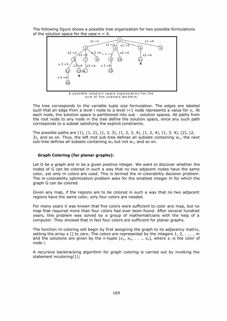
The following figure shows a possible tree organization for two possible formulations

of the solution space for the case n = 4.

A p o s s ib le s o lu t io n s p ac e o rg a n is at io n f or t h e

s u m of t h e s u b s et s pro b le m.

The tree corresponds to the variable tuple size formulation. The edges are labeled such that an edge from a level i node to a level i+1 node represents a value for xi. At each node, the solution space is partitioned into sub - solution spaces. All paths from the root node to any node in the tree define the solution space, since any such path corresponds to a subset satisfying the explicit constraints.

The possible paths are (1), (1, 2), (1, 2, 3), (1, 2, 3, 4), (1, 2, 4), (1, 3, 4), (2), (2,

3), and so on. Thus, the left mot sub-tree defines all subsets containing w1, the next sub-tree defines all subsets containing w2 but not w1, and so on.

Graph Coloring (for planar graphs):

Let G be a graph and m be a given positive integer. We want to discover whether the

nodes of G can be colored in such a way that no two adjacent nodes have the same

color, yet only m colors are used. This is termed the m-colorabiltiy decision problem.

The m-colorability optimization problem asks for the smallest integer m for which the

graph G can be colored.

Given any map, if the regions are to be colored in such a way that no two adjacent

regions have the same color, only four colors are needed.

For many years it was known that five colors were sufficient to color any map, but no

map that required more than four colors had ever been found. After several hundred

years, this problem was solved by a group of mathematicians with the help of a

computer. They showed that in fact four colors are sufficient for planar graphs.

The function m-coloring will begin by first assigning the graph to its adjacency matrix, setting the array x [] to zero. The colors are represented by the integers 1, 2, . . . , m and the solutions are given by the n-tuple (x1, x2, . . ., xn), where xi is the color of node i.

A recursive backtracking algorithm for graph coloring is carried out by invoking the statement mcoloring(1);

x 1 =1 1

x 1 =3

x 1 =4 x 1 =2

2 3 4 5

x 2 =2 x 2 =3

x 2 =4 x 2 =3

x 2 =4 x 2 =4

6 7

x 3 =4 x 3 =4

13 14

S

8 9 10

x 3 =3

12

x 4 =4

16

x 3 =4

15

11

S

170

Algorithm mcoloring (k) // This algorithm was formed using the recursive backtracking schema. The graph is // represented by its Boolean adjacency matrix G [1: n, 1: n]. All assignments of // 1, 2, . . . . . , m to the vertices of the graph such that adjacent vertices are assigned // distinct integers are printed. k is the index of the next vertex to color.

{ repeat { // Generate all legal assignments for x[k].

NextValue (k); // Assign to x [k] a legal color.

If (x [k] = 0) then return; // No new color possible If (k = n) then // at most m colors have been

// used to color the n vertices. write (x [1: n]); else mcoloring (k+1);

} until (false);

}

Algorithm NextValue (k) // x [1] , . . . . x [k-1] have been assigned integer values in the range [1, m] such that // adjacent vertices have distinct integers. A value for x [k] is determined in the range // [0, m].x[k] is assigned the next highest numbered color while maintaining distinctness

// from the adjacent vertices of vertex k. If no such color exists, then x [k] is 0. {

repeat {

x [k]: = (x [k] +1) mod (m+1) // Next highest color.

If (x [k] = 0) then return; // All colors have been used

for j := 1 to n do

{ // check if this color is distinct from adjacent colors if ((G [k, j] 0) and (x [k] = x [j]))

// If (k, j) is and edge and if adj. vertices have the same color.

then break; }

if (j = n+1) then return; // New color found

} until (false); // Otherwise try to find another color.

}

Example:

Color the graph given below with minimum number of colors by backtracking using state space tree.

1 2

3 x1

1 2 2 3 1 3 1 2 x2

4 3 1 3 1 2 2 3 1 2 2 3 1 3

x3

Gra p h

2 3 2 2 3 3 1 3 1 3 1 3 1 1 2 2 1 2 x4

A 4- n o d e gra p h a n d a l l p o s s ib le 3-c o l ori n g s

171

Hamiltonian Cycles:

Let G = (V, E) be a connected graph with n vertices. A Hamiltonian cycle (suggested by William Hamilton) is a round-trip path along n edges of G that visits every vertex once and returns to its starting position. In other vertices of G are visited in the order v1, v2, . . . . . , vn+1, then the edges (vi, vi+1) are in E, 1 < i < n, and the vi are distinct expect for v1 and vn+1, which are equal. The graph G1 contains the Hamiltonian cycle 1, 2, 8, 7, 6, 5, 4, 3, 1. The graph G2 contains no Hamiltonian cycle.

Two graphs to illustrate Hamiltonian cycle

The backtracking solution vector (x1, . . . . . xn) is defined so that xi represents the ith visited vertex of the proposed cycle. If k = 1, then x1 can be any of the n vertices. To avoid printing the same cycle n times, we require that x1 = 1. If 1 < k < n, then xk can be any vertex v that is distinct from x1, x2, . . . , xk–1 and v is connected by an edge to kx-1. The vertex xn can only be one remaining vertex and it must be connected to both xn-1 and x1.

Using NextValue algorithm we can particularize the recursive backtracking schema to

find all Hamiltonian cycles. This algorithm is started by first initializing the adjacency

matrix G[1: n, 1: n], then setting x[2: n] to zero and x[1] to 1, and then executing

Hamiltonian(2).

The traveling salesperson problem using dynamic programming asked for a tour that

has minimum cost. This tour is a Hamiltonian cycles. For the simple case of a graph

all of whose edge costs are identical, Hamiltonian will find a minimum-cost tour if a

tour exists.

Algorithm NextValue (k) // x [1: k-1] is a path of k – 1 distinct vertices . If x[k] = 0, then no vertex has as yet been // assigned to x [k]. After execution, x[k] is assigned to the next highest numbered vertex

// which does not already appear in x [1 : k – 1] and is connected by an edge to x [k – 1]. // Otherwise x [k] = 0. If k = n, then in addition x [k] is connected to x [1]. {

repeat

{

x [k] := (x [k] +1) mod (n+1); // Next vertex. If (x [k] = 0) then return; If (G [x [k – 1], x [k]] 0) then { // Is there an edge?

for j := 1 to k – 1 do if (x [j] = x [k]) then break; // check for distinctness.

If (j = k) then // If true, then the vertex is distinct. If ((k < n) or ((k = n) and G [x [n], x [1]] 0)) then return;

} } until (false);

}

1 2 3 4 1 2 3

8 7 6 5 5 4

Graph G1 Graph G2

172

Algorithm Hamiltonian (k) // This algorithm uses the recursive formulation of backtracking to find all the Hamiltonian

// cycles of a graph. The graph is stored as an adjacency matrix G [1: n, 1: n]. All cycles begin

// at node 1. {

repeat { // Generate values for x [k].

NextValue (k); //Assign a legal Next value to x [k]. if (x [k] = 0) then return;

if (k = n) then write (x [1: n]); else Hamiltonian (k + 1)

} until (false);

}

0/1 Knapsack:

Given n positive weights wi, n positive profits pi, and a positive number m that is the knapsack capacity, the problem calls for choosing a subset of the weights such that:

wi

1 i n

xi m and pi 1 i n

xi is maximized.

The xi‟s constitute a zero–one-valued vector.

The solution space for this problem consists of the 2n distinct ways to assign zero or

one values to the xi‟s.

Bounding functions are needed to kill some live nodes without expanding them. A

good bounding function for this problem is obtained by using an upper bound on the

value of the best feasible solution obtainable by expanding the given live node and

any of its descendants. If this upper bound is not higher than the value of the best

solution determined so far, than that live node can be killed.

We continue the discussion using the fixed tuple size formulation. If at node Z the values of xi, 1 < i < k, have already been determined, then an upper bound for Z can be obtained by relaxing the requirements xi = 0 or 1.

(Knapsack problem using backtracking is solved in branch and bound chapter)

7.8 Traveling Sale Person (TSP) using Backtracking:

We have solved TSP problem using dynamic programming. In this section we shall

solve the same problem using backtracking.

Consider the graph shown below with 4 vertices.

A graph for TSP

The solution space tree, similar to the n-queens problem is as follows:

1 30

2

5

6 10

4

3 20

4

173

We will assume that the starting node is 1 and the ending node is obviously 1. Then

1, {2, … ,4}, 1 forms a tour with some cost which should be minimum. The vertices

shown as {2, 3, …. ,4} forms a permutation of vertices which constitutes a tour. We

can also start from any vertex, but the tour should end with the same vertex.

Since, the starting vertex is 1, the tree has a root node R and the remaining nodes

are numbered as depth-first order. As per the tree, from node 1, which is the live

node, we generate 3 braches node 2, 7 and 12. We simply come down to the left

most leaf node 4, which is a valid tour {1, 2, 3, 4, 1} with cost 30 + 5 + 20 + 4 = 59.

Currently this is the best tour found so far and we backtrack to node 3 and to 2,

because we do not have any children from node 3. When node 2 becomes the E-

node, we generate node 5 and then node 6. This forms the tour {1, 2, 4, 3, 1} with

cost 30 + 10 + 20 + 6 = 66 and is discarded, as the best tour so far is 59.

Similarly, all the paths from node 1 to every leaf node in the tree is searched in a

depth first manner and the best tour is saved. In our example, the tour costs are

shown adjacent to each leaf nodes. The optimal tour cost is therefore 25.

1

2 7 12

3 5 8 10 13 15

4 6 9 11 14 16

UNIT 3 - gpcet

Documents

Transcript of UNIT 3 - gpcet