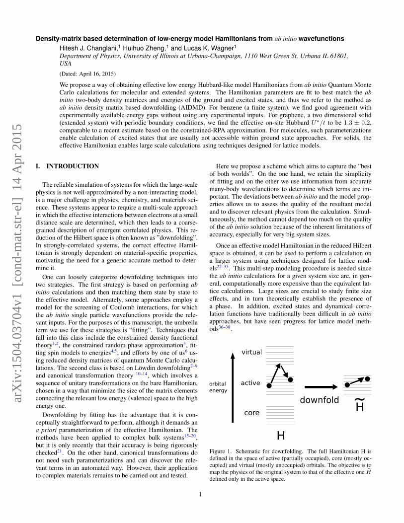
Density-matrix based determination of low-energy model Hamiltonians from ab initio wavefunctionsHitesh J. Changlani,1 Huihuo Zheng,1 and Lucas K. Wagner1

Department of Physics, University of Illinois at Urbana-Champaign, 1110 West Green St, Urbana IL 61801,USA

(Dated: April 16, 2015)

We propose a way of obtaining effective low energy Hubbard-like model Hamiltonians from ab initio Quantum MonteCarlo calculations for molecular and extended systems. The Hamiltonian parameters are fit to best match the abinitio two-body density matrices and energies of the ground and excited states, and thus we refer to the method asab initio density matrix based downfolding (AIDMD). For benzene (a finite system), we find good agreement withexperimentally available energy gaps without using any experimental inputs. For graphene, a two dimensional solid(extended system) with periodic boundary conditions, we find the effective on-site Hubbard U∗/t to be 1.3 ± 0.2,comparable to a recent estimate based on the constrained-RPA approximation. For molecules, such parameterizationsenable calculation of excited states that are usually not accessible within ground state approaches. For solids, theeffective Hamiltonian enables large scale calculations using techniques designed for lattice models.

I. INTRODUCTION

The reliable simulation of systems for which the large-scalephysics is not well-approximated by a non-interacting model,is a major challenge in physics, chemistry, and materials sci-ence. These systems appear to require a multi-scale approachin which the effective interactions between electrons at a smalldistance scale are determined, which then leads to a coarse-grained description of emergent correlated physics. This re-duction of the Hilbert space is often known as ”downfolding”.In strongly-correlated systems, the correct effective Hamil-tonian is strongly dependent on material-specific properties,motivating the need for a generic accurate method to deter-mine it.

One can loosely categorize downfolding techniques intotwo strategies. The first strategy is based on performing abinitio calculations and then matching them state by state tothe effective model. Alternately, some approaches employ amodel for the screening of Coulomb interactions, for whichthe ab initio single particle wavefunctions provide the rele-vant inputs. For the purposes of this manuscript, the umbrellaterm we use for these strategies is ”fitting”. Techniques thatfall into this class include the constrained density functionaltheory1,2, the constrained random phase approximation3, fit-ting spin models to energies4,5, and efforts by one of us6 us-ing reduced density matrices of quantum Monte Carlo calcu-lations. The second class is based on Lowdin downfolding7–9

and canonical transformation theory 10–14, which involves asequence of unitary transformations on the bare Hamiltonian,chosen in a way that minimize the size of the matrix elementsconnecting the relevant low energy (valence) space to the highenergy one.

Downfolding by fitting has the advantage that it is con-ceptually straightforward to perform, although it demands ana priori parameterization of the effective Hamiltonian. Themethods have been applied to complex bulk systems15–20,but it is only recently that their accuracy is being rigorouslychecked21. On the other hand, canonical transformations donot need such parameterizations and can discover the rele-vant terms in an automated way. However, their applicationto complex materials remains to be carried out and tested.

Here we propose a scheme which aims to capture the ”bestof both worlds”. On the one hand, we retain the simplicityof fitting and on the other we use information from accuratemany-body wavefunctions to determine which terms are im-portant. The deviations between ab initio and the model prop-erties allows us to assess the quality of the resultant modeland to discover relevant physics from the calculation. Simul-taneously, the method cannot depend too much on the qualityof the ab initio solution because of the inherent limitations ofaccuracy, especially for very big system sizes.

Once an effective model Hamiltonian in the reduced Hilbertspace is obtained, it can be used to perform a calculation ona larger system using techniques designed for lattice mod-els22–35. This multi-step modeling procedure is needed sincethe ab initio calculations for a given system size are, in gen-eral, computationally more expensive than the equivalent lat-tice calculations. Large sizes are crucial to study finite sizeeffects, and in turn theoretically establish the presence ofa phase. In addition, excited states and dynamical corre-lation functions have traditionally been difficult in ab initioapproaches, but have seen progress for lattice model meth-ods36–38.

core

virtual

active

downfold

H

H~orbitalenergy

Figure 1. Schematic for downfolding. The full Hamiltonian H isdefined in the space of active (partially occupied), core (mostly oc-cupied) and virtual (mostly unoccupied) orbitals. The objective is tomap the physics of the original system to that of the effective one Hdefined only in the active space.

1

arX

iv:1

504.

0370

4v1

[co

nd-m

at.s

tr-e

l] 1

4 A

pr 2

015

In this paper, we demonstrate a downfolding method thatuses data from ab initio quantum Monte Carlo techniquesto derive an effective coarse-grained Hamiltonian. Thismethod, which we call non-eigenstate ab initio density ma-trix downfolding (N-AIDMD), uses many-body simulationsof non-eigenstates to fit an effective low-energy Hamiltonian.We demonstrate that the method can use wave functions ofmedium quality to derive highly accurate effective Hamiltoni-ans. Along with a few simple examples, we downfold benzenefrom a 30-electron problem to a 6-electron one and show thatthe resulting Hamiltonian reproduces the experimental spec-trum well. We also show that the method works for extendedsystems, by applying it to graphene.

II. METHODS

In the present section we discuss the methods we used togenerate our ab initio data. While most of our discussion isspecific to QMC, the quantities used can also be calculatedin almost any other wavefunction-based quantum chemistrymethod.

A. Variational and Fixed Node Diffusion QuantumMonte Carlo

Ab initio Quantum Monte Carlo comprises of a suite ofmethods that efficiently sample the phase space ofN electronseach moving in 3-dimensional real space. When the wave-function as a function of 3N coordinates is known, the phasespace can be sampled with variational Monte Carlo (VMC)using Metropolis algorithms. For ground state calculations,the Diffusion Monte Carlo (DMC) method, based on imagi-nary time evolution of the Schroedinger equation, is formallyexact but in practice limited by the numerical sign problem.This problem ceases to exist if one knew the exact locationof the nodes (zeroes) of the many-body wavefunction. Thus,the optimal strategy for very accurate calculations is to gen-erate a good trial wavefunction, and optimize its parametersto minimize its variational energy. Then, we use this wave-function to ”fix the nodes” (which may only approximatelycorrespond to the exact nodes) and perform a DMC calcula-tion under this constraint. This last variant is called the fixednode DMC (FN-DMC) method and is known to be very accu-rate for a large variety of systems. While some more detailsare discussed here, we refer the interested reader to Ref.39 foran exhaustive review of concepts and applications. All theab initio QMC calculations were carried out with the QWalkpackage40.

A typical QMC calculation was carried out as follows.First, we perform DFT calculations with the B3LYP41 or PBEfunctionals42 using GAMESS43 for molecules or CRYSTAL44

for solids. The lowest energy DFT orbitals provide the Slater

determinant part of the trial wavefunction. For molecules, amulti-determinantal wavefunction is generated by performinga configuration interaction with singles and doubles excita-tioncs (CISD) from the reference Slater determinant. Oncethis is done, a Jastrow factor is introduced, resulting in theansatz,

ψT (r1, r2, ....rN ) = J∑i

diDi (1)

When we desire eigenstates, the full wavefunction (i.e. pa-rameters in the Jastrow J and the coefficients di of the deter-minants Di are optimized to get the best possible variationalenergy within the ansatz chosen) using a technique introducedby Umrigar and coworkers45 with an efficient implementationby Clark et al.46.

The variational energy is calculated via Metropolis sam-pling of |ψT |2,

EVMC ≡〈ψT |H|ψT 〉〈ψT |ψT 〉

=

´|ψT (R)|2HψT (R)

ψT (R) dR´|ψT (R)|2dR

(2)

where R is a compact notation for the 3-N coordinates(r1, r2, ....rN ) and HψT (R)/ψT (R) is the ”local energy”.With this trial wavefunction we perform FN-DMC to calcu-late the energy using the mixed (or projected) estimator,

EDMC ≡〈ψT |H|ψ〉〈ψ|ψT 〉

=

´ψT (R)ψ(R)HψT (R)

ψT (R) dR´ψT (R)ψ(R)dR

(3)

where ψ ≡ exp(−βH)ψT is obtained by a stochastic projec-tion of ψT under the constraint that ψ and ψT have the samesign everywhere.

We now discuss measurements in the QMC methods. For ageneric operator O the pure (VMC) and mixed estimators arecomputed as,

〈O〉VMC ≡〈ψT |O|ψT 〉〈ψT |ψT 〉

〈O〉mix ≡〈ψT |O|ψ〉〈ψT |ψ〉

(4)

The mixed estimator of an operator is equal to the pure estima-tor only in two limits; (1) when ψT is the exact wavefunctionor (2) when the operator commutes with the Hamiltonian. Inmore general situations, higher accuracy can be obtained withthe extrapolated estimator47 for eigenstates,

〈O〉extrap = 2〈O〉mix − 〈O〉VMC (5)

For near-eigenstates, all these estimators must approach thesame value; in practice, this may not be the case when veryhigh accuracy is needed.

We will construct effective Hamiltonians using the two-body reduced density matrix (2-RDM) elements:

2

ρijkl ≡ 〈c†i c†jclck〉 =

∑a 6=b

ˆφ∗k(r′a)φ∗l (r

′b)φi(ra)φj(rb)Ψ

∗(R′′ab) Ψ(R)dr′adr′bdR, (6)

where R′′ab = (r1, r2, r′a..., r

′b, ....rN ) is the set of coordinates

with the many-body wavefunction and φi(r) are pre-decidedone-particle wavefunctions (orbitals) indexed by compact la-bel i(j, k, l) which accounts for space and spin. The mixedestimator equivalent of Eq. (6) is obtained like that for theenergy. More details of this computation have been previ-ously discussed elsewhere by one of us6. The chosen set oforbitals is often localized on the atoms; this property makes itconvenient to derive Hubbard-like models. We explain theirconstruction next.

B. Localized orbitals

Localized orbitals often provide an intuitive way of under-standing an electronic system in terms of electron hops andon-site or inter-site repulsions. Thus, many works have beendevoted to this subject; ranging from the Linearized Muffin-Tin Orbital (LMTO) method48 to the maximally localizedWannier function construction49. Orbital localization has alsobeen widely discussed in the quantum chemistry literature.

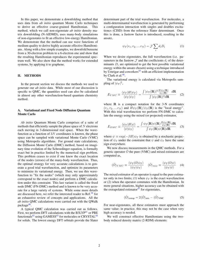
Figure 2. (Left) One of the six symmetry equivalent π orbitals inthe benzene molecule obtained by localizing three bonding and threeanti-bonding orbitals. The 1-RDM computed within QMC confirmsthat the 1s-like and the 2p − σ orbitals (not shown) are close tofully occupied. Hence only the half filled π orbitals are used to fit aHubbard-like Hamiltonian. (Right) Representative localized orbitalsfor the 4× 4 unit cell of graphene.

The idea is to first select a set of orbitals in a certain energywindow. For solids these correspond to bands close to theFermi level, and for molecules these are partially occupied or-bitals which constitute the active space. Then, a unitary trans-formation is performed to optimize a pre-decided metric forlocalization. In this work, we minimize the spread,

S =∑n

(〈φn|r2|φn〉 − 〈φn|r|φn〉2

)(7)

where φn(r) are the desired localized orbitals related to thechosen set of orbitals Φi(r) by a unitary transformation,φn(r) =

∑i UniΦi(r)

For some systems, as we will see in the case of benzeneand graphene, it is necessary to include unoccupied orbitals to

get well-localized orbitals of the right symmetry50. Thus theconstruction of localized orbitals is not a black-box procedureand may need adaptations based on the specifics of the system.

C. Lattice model calculations

The lattice model calculations for Hubbard models of ben-zene and graphene at half-filling were carried out with a com-bination of our own codes and the freely available QUESTdeterminantal Quantum Monte Carlo package51. For the hon-eycomb lattice half-filled Hubbard model, the determinantalQMC method is sign problem free and the results are exact upto statistical errors. A time step of 0.1 was chosen and β (theimaginary time) was set to 20 for every calculation. Measure-ments were performed for 5000 sweeps, with an additional2000 sweeps being used for equilibration.

III. CRITERIA FOR A LOW ENERGY EFFECTIVEHAMILTONIAN

Our aim is to obtain a low energy effective Hamiltonian de-fined in the active space of electrons. In this basis, the criteriaany effective low energy model Hamiltonian must satisfy are:

(a) The reduced density matrices (RDM) of the ground andexcited states obtained from the ab initio calculation mustmatch with that of the model calculation.

(b) The energy spectra of the ab initio and model systemsmust match in the energy window of interest.

(c) The model must be detailed enough to capture the essen-tial physics and yet simple enough to avoid overparame-terization and overfitting.

The concept of matching RDMs [criterion (a)] has previ-ously appeared in related contexts8,52,53 and in work by oneof us6. Most physical properties, such as the charge andspin structure factors, are functions of the 2-RDM. Since itis computationally expensive to calculate high-order RDMs,we use the matching condition only on the 2-RDM, ρijkl ≡〈c†i c

†jclck〉 where i, j, k, l are orbital indices (including space

and spin). This criterion automatically ensures that the com-bined number of electrons occupying the orbitals is equal tothose in the model Hamiltonian. If any input state does nothave the expected electron number in the active space, it cannot be described by the effective Hamiltonian.

The importance of excited state energies used in the fitting[criterion (b)] is highlighted by the fact that the wavefunc-tions, and their corresponding two-body density matrices, areinvariant to many kinds of terms that enter the Hamiltonian.

3

For example, the transformation,

H ′ → H + αS2 + βn+ γS2n (8)

is, by construction, consistent with all the 2-RDM data forany α, β, γ for systems which have definite spin symmetryand particle number. Imposing certain physical constraints onthe form of the interactions can reduce the need for this crite-rion. To give a concrete example, consider wavefunction datagenerated from the ground state of an unfrustrated HeisenbergHamiltonian in a bipartite lattice54, H = J

∑〈i,j〉 Si · Sj .

where 〈i, j〉 refer to nearest neighbor pairs. Then adding αS2

gives the same reduced density matrices for the ground state,as long as α is small enough to not cause energy crossingsi.e. not make an original excited state the new ground state.This additional term has the effect of introducing long-rangeHeisenberg couplings. Moreover, the effective Hamiltonian isnot unique; the Lieb-Mattis model55 H = SA · SB (whereA(B) and SA(B) refer to the sublattice and correspondingspin), is also known to reproduce the low-energy limit ofthe Heisenberg model. Thus, imposing the requirement thatthe Hamiltonian has the nearest-neighbor form constrains αto zero and picks one particular model. Similar argumentsshould apply to extended Hubbard models in homogenoussystems where a physical constraint is that the density-densityinteraction must decrease monontonically with distance be-tween orbitals.

IV. AB INITIO DENSITY MATRIX BASEDDOWNFOLDING (AIDMD) PROCEDURES

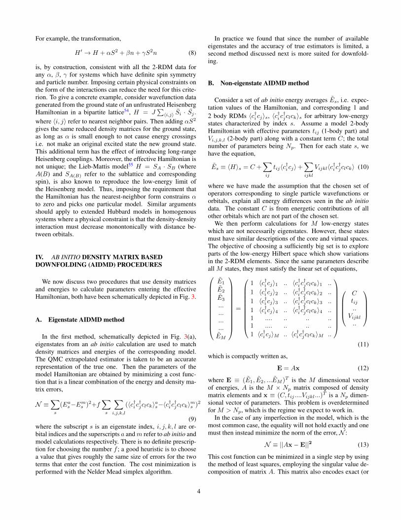
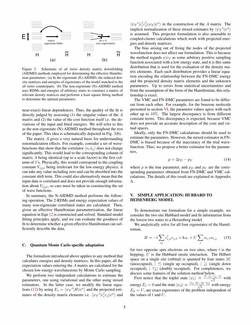
We now discuss two procedures that use density matricesand energies to calculate parameters entering the effectiveHamiltonian, both have been schematically depicted in Fig. 3.

A. Eigenstate AIDMD method

In the first method, schematically depicted in Fig. 3(a),eigenstates from an ab initio calculation are used to matchdensity matrices and energies of the corresponding model.The QMC extrapolated estimator is taken to be an accuraterepresentation of the true one. Then the parameters of themodel Hamiltonian are obtained by minimizing a cost func-tion that is a linear combination of the energy and density ma-trix errors,

N ≡∑s

(Eas−Ems )2+f∑s

∑i,j,k,l

(〈c†i c†jclck〉

as−〈c

†i c†jclck〉

ms )2

(9)where the subscript s is an eigenstate index, i, j, k, l are or-bital indices and the superscripts a andm refer to ab initio andmodel calculations respectively. There is no definite prescrip-tion for choosing the number f ; a good heuristic is to choosea value that gives roughly the same size of errors for the twoterms that enter the cost function. The cost minimization isperformed with the Nelder Mead simplex algorithm.

In practice we found that since the number of availableeigenstates and the accuracy of true estimators is limited, asecond method discussed next is more suited for downfold-ing.

B. Non-eigenstate AIDMD method

Consider a set of ab initio energy averages Es, i.e. expec-tation values of the Hamiltonian, and corresponding 1 and2 body RDMs 〈c†i cj〉s, 〈c

†i c†jclck〉s for arbitrary low-energy

states characterized by index s. Assume a model 2-bodyHamiltonian with effective parameters tij (1-body part) andVi,j,k,l (2-body part) along with a constant term C; the totalnumber of parameters being Np. Then for each state s, wehave the equation,

Es ≡ 〈H〉s = C +∑ij

tij〈c†i cj〉+∑ijkl

Vijkl〈c†i c†jclck〉 (10)

where we have made the assumption that the chosen set ofoperators corresponding to single particle wavefunctions ororbitals, explain all energy differences seen in the ab initiodata. The constant C is from energetic contributions of allother orbitals which are not part of the chosen set.

We then perform calculations for M low-energy stateswhich are not necessarily eigenstates. However, these statesmust have similar descriptions of the core and virtual spaces.The objective of choosing a sufficiently big set is to exploreparts of the low-energy Hilbert space which show variationsin the 2-RDM elements. Since the same parameters describeall M states, they must satisfy the linear set of equations,

E1

E2

E3

...

...

...

...

EM

=

1 〈c†i cj〉1 .. 〈c†i c†jclck〉1 ..

1 〈c†i cj〉2 .. 〈c†i c†jclck〉2 ..

1 〈c†i cj〉3 .. 〈c†i c†jclck〉3 ..

1 〈c†i cj〉4 .. 〈c†i c†jclck〉4 ..

1 .... .. .. ..1 .... .. .. ..

1 〈c†i cj〉M .. 〈c†i c†jclck〉M ..

Ctij..

Vijkl..

(11)

which is compactly written as,

E = Ax (12)

where E ≡ (E1, E2, ...EM )T is the M dimensional vectorof energies, A is the M × Np matrix composed of densitymatrix elements and x ≡ (C, tij ....Vijkl...)

T is a Np dimen-sional vector of parameters. This problem is overdeterminedfor M > Np, which is the regime we expect to work in.

In the case of any imperfection in the model, which is themost common case, the equality will not hold exactly and onemust then instead minimize the norm of the error, N :

N ≡ ||Ax−E||2 (13)

This cost function can be minimized in a single step by usingthe method of least squares, employing the singular value de-composition of matrix A. This matrix also encodes exact (or

4

match eigenstate RDMs

H H~

E Ax = E(non eigenstates)

H H~(a) (b)

Figure 3. Schematic of ab initio density matrix downfolding(AIDMD) methods employed for determining the effective Hamilto-nian parameters. (a) In the eigenstate (E)-AIDMD, the reduced den-sity matrices and energies of eigenstates of the model matched to theab initio counterparts. (b) The non-eigenstate (N)-AIDMD methoduses RDMs and energies of arbitrary states to construct a matrix ofrelevant density matrices and performs a least square fitting methodto determine the optimal parameters.

near-exact) linear dependences. Thus, the quality of the fit isdirectly judged by assessing (1) the singular values of the Amatrix and (2) the value of the cost function itself i.e. the de-viations of the input and fitted energies. We will refer to thisas the non eigenstate (N)-AIDMD method throughout the restof the paper. This idea is schematically depicted in Fig. 3(b).

The matrix A gives a very natural basis for understandingrenormalization effects. For example, consider a set of wave-functions that show that the correlator 〈ninj〉 does not changesignificantly. This would lead to the corresponding column ofmatrix A being identical (up to a scale factor) to the first col-umn of 1’s. Physically, this would correspond to the couplingconstant Vijji being irrelevant for the low-energy physics; itcan take any value including zero and can be absorbed into theconstant shift term. This could also alternatively mean that theinput data is correlated and does not provide enough informa-tion about Vijji, so care must be taken in constructing the setof wave functions.

In summary, the N-AIDMD method performs the follow-ing operation. The 2-RDMs and energy expectation values ofmany non-eigenstate correlated states are calculated. Then,given an effective Hamiltonian parameterization, the linearequation in Eqn 12 is constructed and solved. Standard modelfitting principles apply, and we can evaluate the goodness offit to determine whether a given effective Hamiltonian can suf-ficiently describe the data.

C. Quantum Monte Carlo specific adaptation

The formalism introduced above applies to any method thatcalculates energies and density matrices. In this paper, all theexpectation values entering theAmatrix are calculated for thechosen low-energy wavefunctions by Monte Carlo sampling.

We perform two independent calculations to estimate theparameters, one using variational and the other using mixedestimators. In the latter case, we modify the linear equa-tions (12) by using Es = 〈ψT s|H|ψs〉 and the projected esti-mates of the density matrix elements i.e. 〈ψT s|c†i cj |ψs〉 and

〈ψT s|c†i c†jclck|ψs〉 in the construction of the A matrix. The

implicit normalization of these mixed estimates by 〈ψT s|ψs〉is assumed. This projector formulation is also amenable tocoupled-cluster calculations which work with projected ener-gies and density matrices.

The bias arising out of fixing the nodes of the projectedwavefunction does not affect our formulation. This is becausethe method regards ψψT as some arbitrary positive samplingfunction associated with a low energy state, and it is this samedistribution that is used for the evaluation of the density ma-trix elements. Each such distribution provides a linear equa-tion encoding the relationship between the FN-DMC energyand the projected density matrix elements and the unknownparameters. Up to errors from statistical uncertainities andfrom the assumption of the form of the Hamiltonian, this rela-tionship is exact.

The VMC and FN-DMC parameters are found to be differ-ent from each other. For example, for the benzene moleculepresented in section VI, the parameter values agree with eachother up to 10%. The largest discrepancy is from differentconstant terms. This discrepancy is expected, because VMCdoes not provide an accurate description of the core and vir-tual spaces.

Ideally, only the FN-DMC calculations should be used toestimate the parameters. However, the mixed estimator in FN-DMC is biased because of the inaccuracy of the trial wave-function. Thus, we propose a better estimator for the parame-ters,

p = 2pD − pV (14)

where p is the true parameter, and pD and pV are the corre-sponding parameters obtained from FN-DMC and VMC cal-culations. The details of this result are explained in AppendixA.

V. SIMPLE APPLICATION: HUBBARD TOHEISENBERG MODEL

To demonstrate our formalism for a simple example, weconsider the two site Hubbard model and fit information fromthe lowest two states to a Heisenberg model.

We analytically solve for all four eigenstates of the Hamil-tonian,

H = −t∑ij

c†i,σcj,σ + h.c. + U∑i

ni,↑ni,↓ (15)

for two opposite spin electrons on two sites, where t is thehopping, U is the Hubbard onsite interaction. The Hilbertspace on a single site (orbital) is spanned by four states |0〉(unoccupied), | ↑〉 (single up occupied), | ↓〉 (single downoccupied), | ↑↓〉 (doubly occupied). For completeness, wediscuss some features of the solution method below.

First notice that the triplet state |ψt〉 ≡ |↑ ↓〉−|↓ ↑〉√2

with

energyEt = 0 and the state |ψd〉 ≡ |↑↓ 0〉−|0 ↑↓〉√2

with energyEd = U , are exact eigenstates of the problem independent ofthe values of t and U .

5

To get the other two states, write the Hamiltonian inthe basis of |ψs〉 ≡ 1√

2(| ↑ ↓〉+ | ↓ ↑〉) and |ψd

′〉 ≡

1√2

(| ↑↓ 0〉+ |0 ↑↓〉),

H =

(0 −2t−2t U

)(16)

Then diagonalizing it, we get the energies to be,

E± =U ±

√U2 + 16t2

2(17)

The lowest energy corresponds to the singlet, E− and thecorresponding eigenvector is

|ψ−〉 =2t√

4t2 + E−2|ψs〉 −

E−√4t2 + E−

2|ψd

′〉 (18)

with the next excited state being the triplet |ψt〉.We choose the Heisenberg form to fit to

H = C + JS1 · S2 (19)

To determine the parametersC and J , form the 2×2Amatrixwith the lowest two energy states,(

E−Et

)=

(1 1

4+(E−/t)2

1 −3/4

)(CJ

)(20)

Using derived values of Es and Et = 0, we get,

J =Es(4 + (E−/t)

2)

4 + 34 (E−/t)2

(21)

which to lowest order in t/U is J = −4t2/U .Observe that the correlator for 〈Si · Sj〉 is not exactly 1/4

but only approximately so. This is expected since the fluc-tuations from the high-energy states are not exactly zero, ifit were, it would be equivalent to exactly block-diagonalizingthe Hamiltonian. This exact block diagonalization is not pos-sible in general, unless it is also accompanied with a changein the low energy degrees of freedom entering the model.

If we now rotate the two low energy eigenstates and definethe orthogonal linear combinations,

|ψ′

1〉 = p|ψ−〉+ q|ψt〉 (22)

|ψ′

2〉 = q|ψ−〉 − p|ψt〉 (23)

and calculate their energies and construct the correspondingAmatrix, we get J to be independent of p and q. This propertyis desirable as the method does not hinge on the requirementof eigenstates as inputs.

In terms of canonical transformations (here equivalent tosecond order perturbation theory), the matrix element of theeffective Hamiltonian between the singly occupied states is,

〈↑↓ |H| ↓↑〉 =∑n

〈↑↓ |H|n〉〈n|H| ↓↑〉0− En

=−2t2

U(24)

Since this matrix element must equal J/2 in the Heisenbergmodel we arrive at the same result, namely J = −4t2/U 56.

VI. APPLICATION TO A MOLECULE: BENZENE

We show the workings of the described AIDMD methodsfor the benzene molecule. Our choice of system is motivatedby the simplicity of the system (one band model and presenceof many symmetries) and the availability of experimental en-ergies to compare to.

DFT calculations were first performed in the TZVP ba-sis with Burkatzki-Filippi-Dolg pseudopotentials57, using themolecular geometry that corresponds to a B3LYP optimizedcalculation. These serve as a starting point for the QMC cal-culations, discussed in the Methods section. In the chargeneutral sector, there are a total of 30 electrons (15 ↑ and 15↓ for the spin-singlet state) and our objective is to downfoldthis system to an effective one with 6 electrons (3↑, 3 ↓).

The model Hamiltonian is defined in the space of six πorbitals; a representative localized orbital has been shown inFig. 2. These orbitals were obtained by localizing the highestthree occupied B3LYP orbitals from the S = 0 ground stateDFT calculation and the lowest three unoccupied orbitals withπ orbital symmetry, a well established procedure in the litera-ture50. The overall phase of these orbitals is adjusted to enableuse of parameter symmetries directly when fitting.

Appendix A discusses the QMC data used for fitting andthe initial pre-processing to determine the eligibility of statesthat can be described by a six-π orbital Hamiltonian.

A. On-site Hubbard model

We consider the Hubbard model for six orbitals of benzene,given by Eq. (15), where the notation t is the nearest-neighborhopping andU∗ will be used for the effective on-site Coulombrepulsion. We will discuss multiple ways of using reduceddensity matrix elements to estimate these parameters.

1. Hubbard U∗/t from the E-AIDMD method

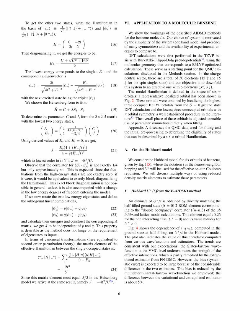
An estimate of U∗/t is obtained by directly matching thehalf-filled ground state (S = 0) 2-RDM element correspond-ing to the ”double occupancy” correlator (〈n↑n↓〉) of the abinitio and lattice-model calculations. This element equals 0.25for the non interacting case (U∗ = 0) and its value reduces forU∗ > 0.

Fig. 4 shows the dependence of 〈n↑n↓〉, computed in theground state at half filling, on U∗/t in the Hubbard model.The plot also indicates the value of this correlator computedfrom various wavefunctions and estimators. The trends areconsistent with our expectations; the Slater-Jastrow wave-function at the VMC level underestimates the strength of theeffective interactions, which is partly remedied by the extrap-olated estimator from FN-DMC. However, the bias (system-atic error) is expected to be large because of the considerabledifference in the two estimates. This bias is reduced by themultideterminantal-Jastrow wavefunction we employed; thedifference between the variational and extrapolated estimatoris about 5%.

6

0.0 0.5 1.0 1.5 2.0U ∗ /t

0.180.190.200.210.220.230.240.25

⟨ n 0,↑n

0,↓⟩

HubbardSJ-VMCSJ-ExtCISDJ-VMCCISDJ-Ext

Figure 4. Double occupancy of the π orbital of benzene as a functionof U∗/t, computed in the half filled ground state. Comparisons aremade with the values from the variational (pure) and extrapolatedestimators obtained from the ab initio QMC calculation with Slater-Jastrow and CISD-Jastrow wavefunctions.

The value of U∗/t is found to be extremely sensitive to theprecise value of the double occupancy, a change of a few per-cent (i.e. from 0.24 to 0.20) changes our estimate from ≈ 0.3to 1.3 (i.e. a factor of almost 4). In general, this observationsuggests that it is crucial to look at various other elements ofthe 2-RDM and to look at alternate ways of estimating Hub-bard parameters.

2. Hubbard U∗/t from the N-AIDMD method

As mentioned previously, the idea of matching density ma-trix elements is useful only for comparing exact eigenstates.However, it is difficult to construct eigenstates with very highaccuracy in the ab initio calculations and at times also for theequivalent model for large system sizes. This is why we ap-peal to the N-AIDMD method, introduced and explained inSec. IV B, which is relatively insensitive to the nature of thestates input to the method. For charge-neutral benzene, weconstruct the A matrix by taking various states in a 10 eV en-ergy window above the ground state using VMC and DMCmethods.

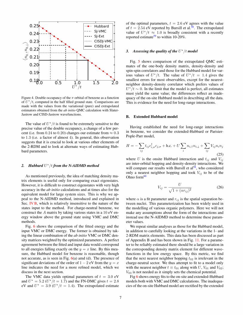
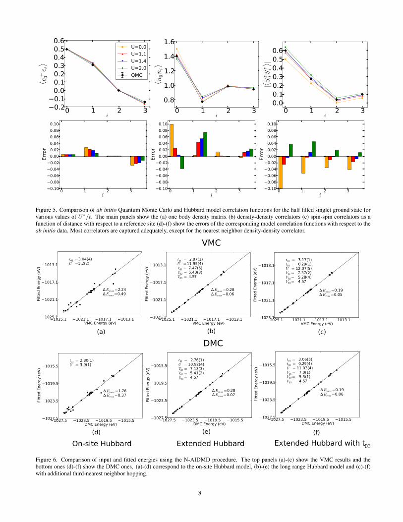
Fig. 6 shows the comparison of the fitted energy and theinput VMC or DMC energy. The former is obtained by tak-ing the linear combination of the ab initio VMC or DMC den-sity matrices weighted by the optimized parameters. A perfectagreement between the fitted and input data would correspondto all energies falling exactly on the y = x line. By this mea-sure, the Hubbard model for benzene is reasonable, thoughnot accurate, as is seen in Fig. 6(a) amd (d). The presence ofsignificant deviations of the order of 1− 2 eV from the y = xline indicates the need for a more refined model, which wediscuss in the next section.

The VMC data yields optimal parameters of t = 3.0 eVand U∗ = 5.2 (U∗/t = 1.7) and the FN-DMC gives t = 2.8eV and U∗ = 3.9 (U∗/t = 1.4). The extrapolated estimate

of the optimal parameters, t = 2.6 eV agrees with the valueof t = 2.54 eV reported by Bursill et al.58. The extrapolatedvalue of U∗/t ≈ 1.0 is broadly consistent with a recentlyreported estimate59 to within 10-20%.

3. Assessing the quality of the U∗/t model

Fig. 5 shows comparison of the extrapolated QMC esti-mates of the one-body density matrix, density-density andspin-spin correlators and those for the Hubbard model for var-ious values of U∗/t. The value of U∗/t = 1.4 gives thesmallest errors for most observables, except for the nearest-neighbor density-density correlator which prefers values ofU∗/t ∼ 0. In the limit that the model is perfect, all estimatesmust yield the same value; the differences reflect an inade-quacy of the on-site Hubbard model in describing all the data.This is evidence for the need for long-range interactions.

B. Extended Hubbard model

Having established the need for long-range interactionsin benzene, we consider the extended-Hubbard or Parisier-Pople-Parr model,

H = −∑ij

tijc†i,σcj,σ + h.c. + U

∑i

ni,↑ni,↓ +∑ij

Vijninj

(25)where U is the onsite Hubbard interaction and tij and Vijare inter-orbital hopping and density-density interactions. Wewill compare our results with Bursill et al58, who consideredonly a nearest neighbor hopping and took Vij to be of theOhno form60

Vij =U√

1 + (αrij)2(26)

where α is a fit parameter and rij is the spatial separation be-tween nuclei. This parameterization has been widely used inthe modelling of various organic polymers. Here we will notmake any assumptions about the form of the interactions andinstead use the N-AIDMD method to determine these param-eter values.

We repeat similar analyses as those for the Hubbard model,in addition to carefully looking at the variations in the 1- and2-RDM matrix elements. This data has been discussed as partof Appendix B and has been shown in Fig. 11. For a parame-ter to be reliably estimated there should be a large variation inthe corresponding density matrix element for different wave-functions in the low energy space. By this metric, we findthat the next nearest neighbor hopping t02 is irrelevant in thecharge-neutral sector. We thus attempt to fit to a model onlywith the nearest neighbor t ≡ t01 along with U , V01 and V02;V03 is not needed as it simply sets the chemical potential.

Fig 6 shows energy fits to the on-site and extended-Hubbardmodels both with VMC and DMC calculations. The inadequa-cies of the on-site Hubbard model are rectified by the extended

7

0 1 2 3i

0.20.10.00.10.20.30.40.50.6

⟨ c+ 0c i⟩

U=0.0U=1.1U=1.4U=2.0QMC

0 1 2 3i

0.8

1.0

1.2

1.4

1.6

⟨ n 0ni⟩

0 1 2 3i

0.00.10.20.30.40.50.6

|⟨ Sz 0Sz i

⟩ |

0 1 2 3i

0.100.080.060.040.020.000.020.040.060.080.10

Erro

r

0 1 2 3i

0.100.080.060.040.020.000.020.040.060.080.10

Erro

r

0 1 2 3i

0.100.080.060.040.020.000.020.040.060.080.10

Erro

r

Figure 5. Comparison of ab initio Quantum Monte Carlo and Hubbard model correlation functions for the half filled singlet ground state forvarious values of U∗/t. The main panels show the (a) one body density matrix (b) density-density correlators (c) spin-spin correlators as afunction of distance with respect to a reference site (d)-(f) show the errors of the corresponding model correlation functions with respect to theab initio data. Most correlators are captured adequately, except for the nearest neighbor density-density correlator.

1025.1 1021.1 1017.1 1013.1VMC Energy (eV)

1025.1

1021.1

1017.1

1013.1

Fitt

ed E

nerg

y (

eV

)

t01 =3.04(4)U =5.2(2)

∆Emax=2.24∆Erms=0.49

1025.1 1021.1 1017.1 1013.1VMC Energy (eV)

1025.1

1021.1

1017.1

1013.1

Fitt

ed E

nerg

y (

eV

)

t01 = 2.87(1)U =11.95(4)V01 = 7.47(5)V02 = 5.40(3)V03 = 4.57

∆Emax=0.28∆Erms=0.06

1025.1 1021.1 1017.1 1013.1VMC Energy (eV)

1025.1

1021.1

1017.1

1013.1

Fitt

ed E

nerg

y (

eV

)t01 = 3.17(1)t03 = 0.29(1)U = 12.07(5)V01 = 7.37(2)V02 = 5.28(4)V03 = 4.57

∆Emax=0.19∆Erms=0.05

VMC

1027.5 1023.5 1019.5 1015.5DMC Energy (eV)

1027.5

1023.5

1019.5

1015.5

Fitt

ed E

nerg

y (

eV

)

t01 = 2.80(1)U = 3.9(1)

∆Emax=1.76∆Erms=0.37

1027.5 1023.5 1019.5 1015.5DMC Energy (eV)

1027.5

1023.5

1019.5

1015.5

Fitt

ed E

nerg

y (

eV

)

t01 = 2.76(1)U = 10.92(4)V01 = 7.13(3)V02 = 5.41(2)V03 = 4.57

∆Emax=0.28∆Erms=0.07

1027.5 1023.5 1019.5 1015.5DMC Energy (eV)

1027.5

1023.5

1019.5

1015.5

Fitt

ed E

nerg

y (

eV

)

t01 = 3.06(5)t03 = 0.29(4)U = 11.03(4)V01 = 7.0(1)V02 = 5.3(1)V03 = 4.57

∆Emax=0.19∆Erms=0.06

DMC

On-site Hubbard Extended Hubbard Extended Hubbard with t03

(a) (b) (c)

(d) (e) (f)

Figure 6. Comparison of input and fitted energies using the N-AIDMD procedure. The top panels (a)-(c) show the VMC results and thebottom ones (d)-(f) show the DMC ones. (a)-(d) correspond to the on-site Hubbard model, (b)-(e) the long range Hubbard model and (c)-(f)with additional third-nearest neighbor hopping.

8

4 5 6 7 8Expt Gap (eV)

4

5

6

7

8M

odel

Gap

(eV)

VMC paramsDMC paramsExtrap. params

(a)

4 5 6 7 8Expt Gap (eV)

4

5

6

7

8

Mod

el G

ap (e

V)

Hubbard modelPPP-Ohno [Ref 58]PPPPPP with t03

(b)

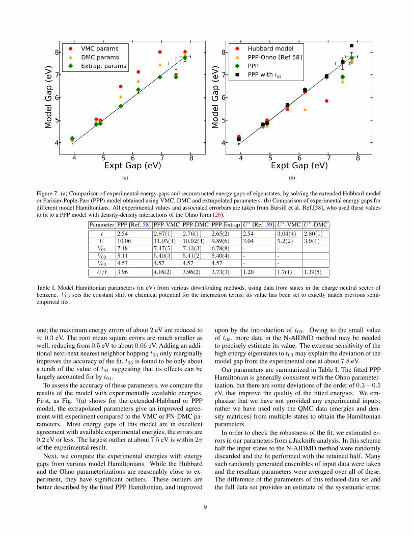
Figure 7. (a) Comparison of experimental energy gaps and reconstructed energy gaps of eigenstates, by solving the extended Hubbard modelor Parisier-Pople-Parr (PPP) model obtained using VMC, DMC and extrapolated parameters. (b) Comparison of experimental energy gaps fordifferent model Hamiltonians. All experimental values and associated errorbars are taken from Bursill et al. Ref.[58], who used these valuesto fit to a PPP model with density-density interactions of the Ohno form (26).

Parameter PPP [Ref. 58] PPP-VMC PPP-DMC PPP-Extrap U∗ [Ref. 59] U∗-VMC U∗-DMCt 2.54 2.87(1) 2.76(1) 2.65(2) 2.54 3.04(4) 2.80(1)U 10.06 11.95(4) 10.92(4) 9.89(6) 3.04 5.2(2) 3.9(1)V01 7.18 7.47(5) 7.13(3) 6.78(8) - -V02 5.11 5.40(3) 5.41(2) 5.40(4) - -V03 4.57 4.57 4.57 4.57 - -U/t 3.96 4.16(2) 3.96(2) 3.73(3) 1.20 1.7(1) 1.39(5)

Table I. Model Hamiltonian parameters (in eV) from various downfolding methods, using data from states in the charge neutral sector ofbenzene. V03 sets the constant shift or chemical potential for the interaction terms; its value has been set to exactly match previous semi-empirical fits.

one; the maximum energy errors of about 2 eV are reduced to≈ 0.3 eV. The root mean square errors are much smaller aswell, reducing from 0.5 eV to about 0.06 eV. Adding an addi-tional next-next nearest neighbor hopping t03 only marginallyimproves the accuracy of the fit, t03 is found to be only abouta tenth of the value of t01 suggesting that its effects can belargely accounted for by t01.

To assess the accuracy of these parameters, we compare theresults of the model with experimentally available energies.First, as Fig. 7(a) shows for the extended-Hubbard or PPPmodel, the extrapolated parameters give an improved agree-ment with experiment compared to the VMC or FN-DMC pa-rameters. Most energy gaps of this model are in excellentagreement with available experimental energies, the errors are0.2 eV or less. The largest outlier at about 7.5 eV is within 2σof the experimental result.

Next, we compare the experimental energies with energygaps from various model Hamiltonians. While the Hubbardand the Ohno parameterizations are reasonably close to ex-periment, they have significant outliers. These outliers arebetter described by the fitted PPP Hamiltonian, and improved

upon by the introduction of t03. Owing to the small valueof t03, more data in the N-AIDMD method may be neededto precisely estimate its value. The extreme sensitivity of thehigh energy eigenstates to t03 may explain the deviation of themodel gap from the experimental one at about 7.8 eV.

Our parameters are summarized in Table I. The fitted PPPHamiltonian is generally consistent with the Ohno parameter-ization, but there are some deviations of the order of 0.3− 0.5eV, that improve the quality of the fitted energies. We em-phasize that we have not provided any experimental inputs;rather we have used only the QMC data (energies and den-sity matrices) from multiple states to obtain the Hamiltonianparameters.

In order to check the robustness of the fit, we estimated er-rors in our parameters from a Jacknife analysis. In this schemehalf the input states to the N-AIDMD method were randomlydiscarded and the fit performed with the retained half. Manysuch randomly generated ensembles of input data were takenand the resultant parameters were averaged over all of these.The difference of the parameters of this reduced data set andthe full data set provides an estimate of the systematic error,

9

which we report in table I. The other source of errors is fromstatistical noise, which in the present case was found to bemuch smaller than the systematic error.

VII. APPLICATION TO A SOLID: GRAPHENE

As an application of the AIDMD methods to solid mate-rials, we consider graphene, a 2D solid of carbon atoms ar-ranged on a honeycomb lattice. Graphene is has great poten-tial technological applications, which has spurred much workdevoted to understanding it thoroughly61. In addition, therehave been several proposals for engineering exotic phasesin graphene62–64. That said, it is only recently that system-atic studies to estimate the role of electron-electron interac-tions20,59,65 have been carried out. While some of its long-distance properties appear to be adequately described by atight-binding model, the short range features, crucial for phe-nomena such as magnetism, require more refined modeling.

0.0 0.5 1.0 1.5 2.0U ∗ /t

0.18

0.19

0.20

0.21

0.22

0.23

0.24

0.25

⟨ n 0,↑n

0,↓⟩

2x24x46x68x8SJ-VMCSJ-DMCExtrapcRPA

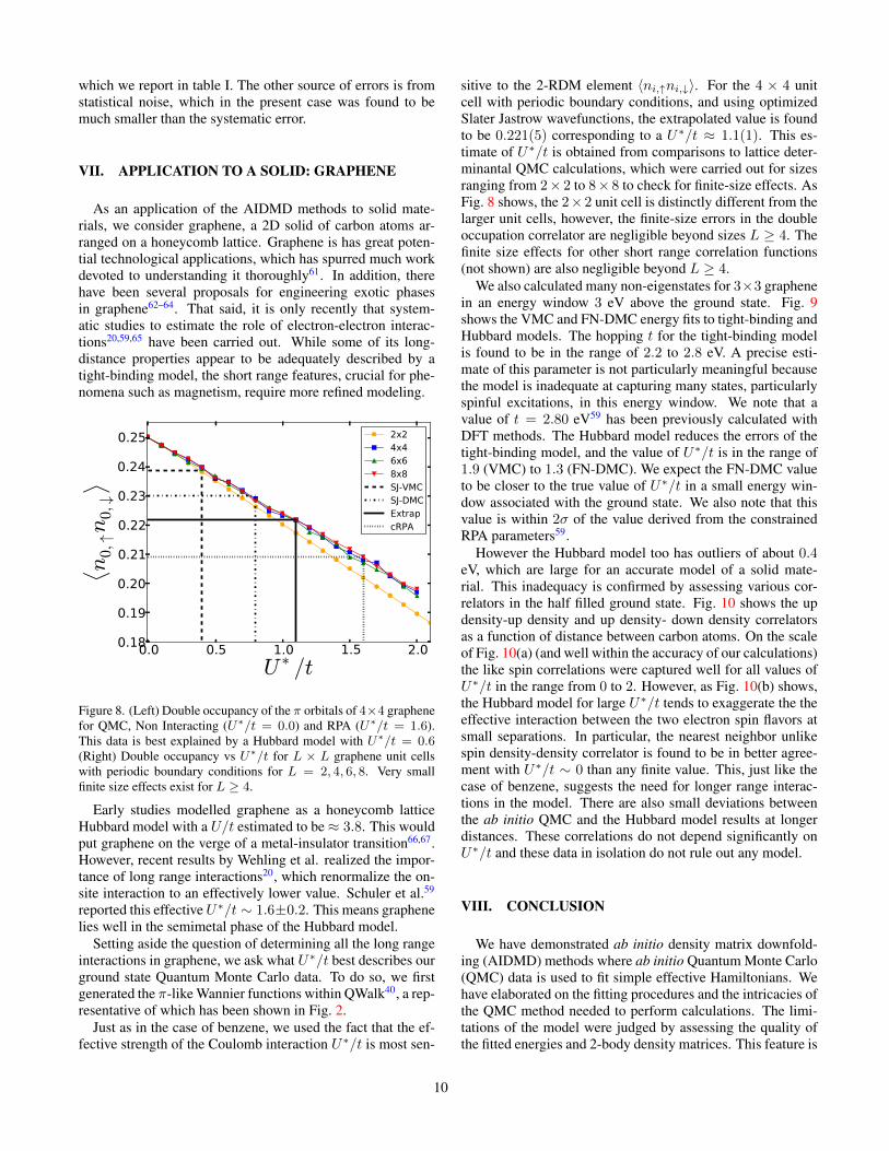
Figure 8. (Left) Double occupancy of the π orbitals of 4×4 graphenefor QMC, Non Interacting (U∗/t = 0.0) and RPA (U∗/t = 1.6).This data is best explained by a Hubbard model with U∗/t = 0.6(Right) Double occupancy vs U∗/t for L × L graphene unit cellswith periodic boundary conditions for L = 2, 4, 6, 8. Very smallfinite size effects exist for L ≥ 4.

Early studies modelled graphene as a honeycomb latticeHubbard model with a U/t estimated to be≈ 3.8. This wouldput graphene on the verge of a metal-insulator transition66,67.However, recent results by Wehling et al. realized the impor-tance of long range interactions20, which renormalize the on-site interaction to an effectively lower value. Schuler et al.59

reported this effectiveU∗/t ∼ 1.6±0.2. This means graphenelies well in the semimetal phase of the Hubbard model.

Setting aside the question of determining all the long rangeinteractions in graphene, we ask what U∗/t best describes ourground state Quantum Monte Carlo data. To do so, we firstgenerated the π-like Wannier functions within QWalk40, a rep-resentative of which has been shown in Fig. 2.

Just as in the case of benzene, we used the fact that the ef-fective strength of the Coulomb interaction U∗/t is most sen-

sitive to the 2-RDM element 〈ni,↑ni,↓〉. For the 4 × 4 unitcell with periodic boundary conditions, and using optimizedSlater Jastrow wavefunctions, the extrapolated value is foundto be 0.221(5) corresponding to a U∗/t ≈ 1.1(1). This es-timate of U∗/t is obtained from comparisons to lattice deter-minantal QMC calculations, which were carried out for sizesranging from 2× 2 to 8× 8 to check for finite-size effects. AsFig. 8 shows, the 2×2 unit cell is distinctly different from thelarger unit cells, however, the finite-size errors in the doubleoccupation correlator are negligible beyond sizes L ≥ 4. Thefinite size effects for other short range correlation functions(not shown) are also negligible beyond L ≥ 4.

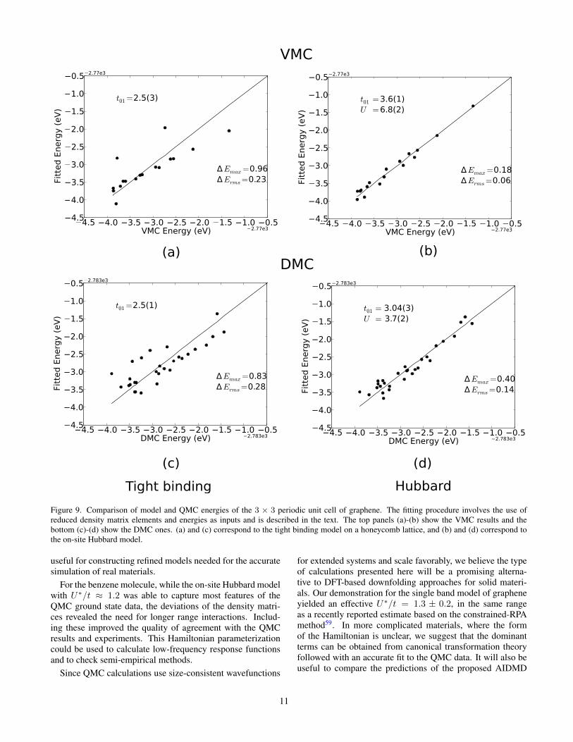
We also calculated many non-eigenstates for 3×3 graphenein an energy window 3 eV above the ground state. Fig. 9shows the VMC and FN-DMC energy fits to tight-binding andHubbard models. The hopping t for the tight-binding modelis found to be in the range of 2.2 to 2.8 eV. A precise esti-mate of this parameter is not particularly meaningful becausethe model is inadequate at capturing many states, particularlyspinful excitations, in this energy window. We note that avalue of t = 2.80 eV59 has been previously calculated withDFT methods. The Hubbard model reduces the errors of thetight-binding model, and the value of U∗/t is in the range of1.9 (VMC) to 1.3 (FN-DMC). We expect the FN-DMC valueto be closer to the true value of U∗/t in a small energy win-dow associated with the ground state. We also note that thisvalue is within 2σ of the value derived from the constrainedRPA parameters59.

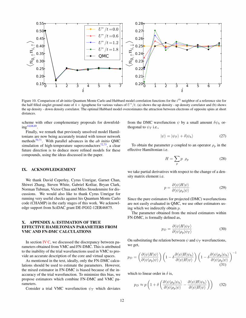
However the Hubbard model too has outliers of about 0.4eV, which are large for an accurate model of a solid mate-rial. This inadequacy is confirmed by assessing various cor-relators in the half filled ground state. Fig. 10 shows the updensity-up density and up density- down density correlatorsas a function of distance between carbon atoms. On the scaleof Fig. 10(a) (and well within the accuracy of our calculations)the like spin correlations were captured well for all values ofU∗/t in the range from 0 to 2. However, as Fig. 10(b) shows,the Hubbard model for large U∗/t tends to exaggerate the theeffective interaction between the two electron spin flavors atsmall separations. In particular, the nearest neighbor unlikespin density-density correlator is found to be in better agree-ment with U∗/t ∼ 0 than any finite value. This, just like thecase of benzene, suggests the need for longer range interac-tions in the model. There are also small deviations betweenthe ab initio QMC and the Hubbard model results at longerdistances. These correlations do not depend significantly onU∗/t and these data in isolation do not rule out any model.

VIII. CONCLUSION

We have demonstrated ab initio density matrix downfold-ing (AIDMD) methods where ab initio Quantum Monte Carlo(QMC) data is used to fit simple effective Hamiltonians. Wehave elaborated on the fitting procedures and the intricacies ofthe QMC method needed to perform calculations. The limi-tations of the model were judged by assessing the quality ofthe fitted energies and 2-body density matrices. This feature is

10

4.5 4.0 3.5 3.0 2.5 2.0 1.5 1.0 0.5DMC Energy (eV) 2.783e3

4.5

4.0

3.5

3.0

2.5

2.0

1.5

1.0

0.5

Fitt

ed E

nerg

y (

eV

)

2.783e3

t01 =2.5(1)

∆Emax=0.83∆Erms=0.28

4.5 4.0 3.5 3.0 2.5 2.0 1.5 1.0 0.5DMC Energy (eV) 2.783e3

4.5

4.0

3.5

3.0

2.5

2.0

1.5

1.0

0.5

Fitt

ed E

nerg

y (

eV

)

2.783e3

t01 = 3.04(3)U = 3.7(2)

∆Emax=0.40∆Erms=0.14

4.5 4.0 3.5 3.0 2.5 2.0 1.5 1.0 0.5VMC Energy (eV) 2.77e3

4.5

4.0

3.5

3.0

2.5

2.0

1.5

1.0

0.5

Fitt

ed

Energ

y (

eV

)

2.77e3

t01 =2.5(3)

∆Emax=0.96∆Erms=0.23

4.5 4.0 3.5 3.0 2.5 2.0 1.5 1.0 0.5VMC Energy (eV) 2.77e3

4.5

4.0

3.5

3.0

2.5

2.0

1.5

1.0

0.5

Fitt

ed E

nerg

y (

eV

)

2.77e3

t01 =3.6(1)U =6.8(2)

∆Emax=0.18∆Erms=0.06

VMC

DMC(a) (b)

(c) (d)

Tight binding Hubbard

Figure 9. Comparison of model and QMC energies of the 3 × 3 periodic unit cell of graphene. The fitting procedure involves the use ofreduced density matrix elements and energies as inputs and is described in the text. The top panels (a)-(b) show the VMC results and thebottom (c)-(d) show the DMC ones. (a) and (c) correspond to the tight binding model on a honeycomb lattice, and (b) and (d) correspond tothe on-site Hubbard model.

useful for constructing refined models needed for the accuratesimulation of real materials.

For the benzene molecule, while the on-site Hubbard modelwith U∗/t ≈ 1.2 was able to capture most features of theQMC ground state data, the deviations of the density matri-ces revealed the need for longer range interactions. Includ-ing these improved the quality of agreement with the QMCresults and experiments. This Hamiltonian parameterizationcould be used to calculate low-frequency response functionsand to check semi-empirical methods.

Since QMC calculations use size-consistent wavefunctions

for extended systems and scale favorably, we believe the typeof calculations presented here will be a promising alterna-tive to DFT-based downfolding approaches for solid materi-als. Our demonstration for the single band model of grapheneyielded an effective U∗/t = 1.3 ± 0.2, in the same rangeas a recently reported estimate based on the constrained-RPAmethod59. In more complicated materials, where the formof the Hamiltonian is unclear, we suggest that the dominantterms can be obtained from canonical transformation theoryfollowed with an accurate fit to the QMC data. It will also beuseful to compare the predictions of the proposed AIDMD

11

0 1 2 3 4 5 6 7i

0.15

0.20

0.25

0.30

0.35

0.40

0.45

0.50

0.55⟨ n 0,↑

ni,↑⟩

U ∗ /t=0.0

U ∗ /t=0.6

U ∗ /t=1.2

U ∗ /t=1.8

QMC

0 1 2 3 4 5 6 7i

0.20

0.21

0.22

0.23

0.24

0.25

0.26

0.27

0.28

⟨ n 0,↑ni,↓⟩

Figure 10. Comparison of ab initio Quantum Monte Carlo and Hubbard model correlation functions for the ith neighbor of a reference site forthe half filled singlet ground state of 4× 4graphene for various values of U∗/t. (a) shows the up density - up density correlator and (b) showsthe up density - down density correlator. The optimal Hubbard model overestimates the attraction between electrons of opposite spins at shortdistances.

scheme with other complementary proposals for downfold-ing14,68,69.

Finally, we remark that previously unsolved model Hamil-tonians are now being accurately treated with tensor networkmethods70,71. With parallel advances in the ab initio QMCsimulation of high-temperature superconductors72,73, a clearfuture direction is to deduce more refined models for thesecompounds, using the ideas discussed in the paper.

IX. ACKNOWLEDGEMENT

We thank David Ceperley, Cyrus Umrigar, Garnet Chan,Shiwei Zhang, Steven White, Gabriel Kotliar, Bryan Clark,Norman Tubman, Victor Chua and Miles Stoudenmire for dis-cussions. We would also like to thank Cyrus Umrigar forrunning very useful checks against his Quantum Monte Carlocode (CHAMP) in the early stages of this work. We acknowl-edge support from SciDAC grant DE-FG02-12ER46875.

X. APPENDIX A: ESTIMATION OF TRUEEFFECTIVE HAMILTONIAN PARAMETERS FROMVMC AND FN-DMC CALCULATIONS

In section IV C, we discussed the discrepancy between pa-rameters obtained from VMC and FN-DMC. This is attributedto the inability of the trial wavefunctions used in VMC to pro-vide an accurate description of the core and virtual spaces.

As mentioned in the text, ideally, only the FN-DMC calcu-lations should be used to estimate the parameters. However,the mixed estimator in FN-DMC is biased because of the in-accuracy of the trial wavefunction. To minimize this bias, wepropose estimators which combine FN-DMC and VMC pa-rameters.

Consider a trial VMC wavefunction ψT which deviates

from the DMC wavefunction ψ by a small amount δψh or-thogonal to ψT i.e.,

|ψ〉 = |ψT 〉+ δ|ψh〉 (27)

To obtain the parameter p coupled to an operator ρp in theeffective Hamiltonian i.e.

H =∑p

p ρp (28)

we take partial derivatives with respect to the change of a den-sity matrix element i.e.

p =∂〈ψ|H|ψ〉∂〈ψ|ρp|ψ〉

(29)

Since the pure estimators for projected (DMC) wavefunctionsare not easily evaluated in QMC, we use other estimators us-ing which we indirectly obtain p.

The parameter obtained from the mixed estimators withinFN-DMC, is formally defined as,

pD =∂〈ψ|H|ψT 〉∂〈ψ|ρp|ψT 〉

(30)

On substituting the relation between ψ and ψT wavefunctions,we get,

pD =

(∂〈ψ|H|ψ〉∂〈ψ|ρp|ψ〉

)(1− δ ∂〈ψ|H|ψh〉

∂〈ψ|H|ψ〉

)(1− δ ∂〈ψ|ρp|ψh〉

∂〈ψ|ρp|ψ〉

)−1(31)

which to linear order in δ is,

pD ≈ p(

1 + δ

(∂〈ψ|ρp|ψh〉∂〈ψ|ρp|ψ〉

− ∂〈ψ|H|ψh〉∂〈ψ|H|ψ〉

))(32)

12

A similar expression for parameters obtained from VMCcalculations,

pV =∂〈ψT |H|ψT 〉∂〈ψT |ρp|ψT 〉

(33)

is derived and leads to the result,

pV ≈ p(

1 + 2δ

(∂〈ψ|ρp|ψh〉∂〈ψ|ρp|ψ〉

− ∂〈ψ|H|ψh〉∂〈ψ|H|ψ〉

))(34)

where we have used the hermiticity of the Hamiltonian H andthe operator ρp.

On combining equations (32) and (34), to leading order inδ we get,

p = 2pD − pV +O(δ2) (35)

As expected, all estimates are consistent with each other in thelimit of exact wavefunctions.

XI. APPENDIX B: QMC DATA FOR THE BENZENEMOLECULE

Table II shows the QMC data for several eigenstates ofbenzene. Most of these states along with many other non-eigenstates constitute our data set for fitting a model.

The calculations confirm the general expectation that sig-nificant energy gains are obtained by improving wavefunc-tions going from the single-Slater-Jastrow form to the multi-determinantal-Jastrow form (the determinants being selectedfrom a CISD calculation). Moreover, the DMC calculationsimprove total energies significantly; typically, the DMC val-ues are 2− 3 eV lower than the corresponding VMC value.

The total electron count from the one-body density matrixis assessed to verify the validity of fitting to a six-π orbitalHamiltonian. Table II shows that for charge-neutral benzene,the singlet state (S = 0) has up and down electron counts of2.96 each, which are close to the expected values of 3,3. Forthe S = 2 state, roughly 9 eV above the ground state, the de-viations were slightly larger; the summed occupation numberswere 4.92 and 1.0 in comparison to the expected values of 5and 1. Since there is a slight deviation of these numbers fromintegers, we rescale the one and two body density matrices byfactors (all slightly greater than 1) that correctly accounts forsum rules for each individual state used in the AIDMD meth-ods.

However, for the S = 3 state, the electron occupation num-bers deviate signficantly from the corresponding value in themodel; almost by one integer. This indicates that the S = 3state is inadequately described by the proposed Hamiltonianand hence can not be used in the fitting procedure. This de-viation is not completely unexpected since this state is ∼ 17eV above the ground state and a potential high-energy state.Said differently, the active space at this energy scale is con-siderably different from that assumed for the ground state andits low-energy excitations. Thus, this QMC data suggests thatit is only reasonable for the effective Hamiltonian concept to

hold only in an energy window of the order of 10 eV abovethe ground state.

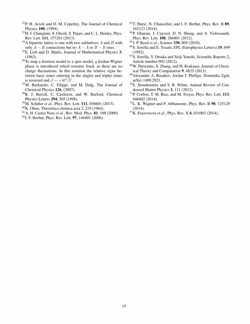
We now assess some aspects of our non-eigenstate data. Forthe N-AIDMD method, we desire large variations in the den-sity matrix elements for different wavefunctions in the low-energy space, in order to accurately estimate the Hamiltonianparameters. Fig. 11 shows these variations for all relevantdensity-matrix elements (within FN-DMC) that were neededfor estimating the parameters of the extended Hubbard model.t02 was found to be irrelevant, as the summed density matrixelements coupling to it were found to not vary significantly(not shown in the plot).

REFERENCES

1E. Pavarini et al., Phys. Rev. Lett. 87, 047003 (2001).2O. K. Andersen and T. Saha-Dasgupta, Phys. Rev. B 62,R16219 (2000).

3F. Aryasetiawan et al., Phys. Rev. B 70, 195104 (2004).4H. O. Jeschke, F. Salvat-Pujol, and R. Valentı, Phys. Rev. B88, 075106 (2013).

5N. S. Fedorova, C. Ederer, N. A. Spaldin, A. Scaramucci,arXiv:1412.3702.

6L. K. Wagner, The Journal of Chemical Physics 138, 094106(2013).

7K. F. Freed, Accounts of Chemical Research 16, 137 (1983).8S. Q. Zhou and D. M. Ceperley, Phys. Rev. A 81, 013402(2010).

9S. Ten-no, The Journal of Chemical Physics 138, (2013).10S. D. Głazek and K. G. Wilson, Phys. Rev. D 48, 5863

(1993).11F. Wegner, Annalen der Physik 506, 77 (1994).12S. R. White, The Journal of Chemical Physics 117, (2002).13T. Yanai and G. K.-L. Chan, The Journal of Chemical

Physics 124, (2006).14T. J. Watson Jr., G. K-L Chan, arXiv:1502.04698.15M. Hirayama, T. Miyake, and M. Imada, Phys. Rev. B 87,

195144 (2013).16K. Nakamura, Y. Yoshimoto, Y. Nohara, and M. Imada,

Journal of the Physical Society of Japan 79, 123708 (2010).17F. Nilsson, R. Sakuma, and F. Aryasetiawan, Phys. Rev. B

88, 125123 (2013).18F. Aryasetiawan, K. Karlsson, O. Jepsen, and U.

Schonberger, Phys. Rev. B 74, 125106 (2006).19E. P. Scriven and B. J. Powell, Phys. Rev. Lett. 109, 097206

(2012).20T. O. Wehling et al., Phys. Rev. Lett. 106, 236805 (2011).21Hiroshi Shinaoka, Rei Sakuma, Philipp Werner, Matthias

Troyer, arXiv:1410.1276.22S. R. White, Phys. Rev. Lett. 69, 2863 (1992).23A. Gendiar, N. Maeshima, and T. Nishino, Prog. Theor.

Phys. 110, 691 (2003).24G. Vidal, Phys. Rev. Lett. 101, 110501 (2008).25F. Verstraete, V. Murg, and J. Cirac, Advances in Physics 57,

143 (2008).26H. J. Changlani, J. M. Kinder, C. J. Umrigar, and G. K.-L.

Chan, Phys. Rev. B 80, 245116 (2009).

13

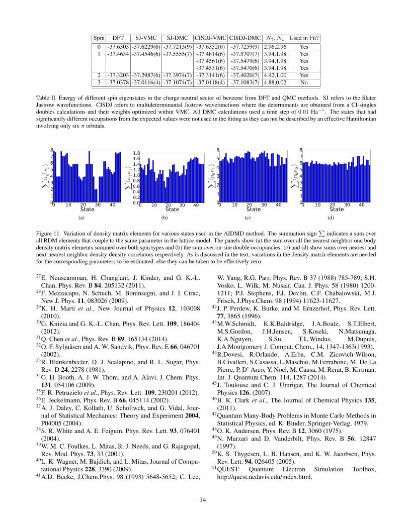
Spin DFT SJ-VMC SJ-DMC CISDJ-VMC CISDJ-DMC N↑, N↓ Used in Fit?0 -37.6303 -37.6229(6) -37.7213(9) -37.6352(6) -37.7259(9) 2.96,2.96 Yes1 -37.4634 -37.4546(6) -37.5555(7) -37.4814(6) -37.5707(7) 3.94,1.98 Yes

-37.4561(6) -37.5479(6) 3.94,1.98 Yes-37.4531(6) -37.5470(6) 3.94,1.98 Yes

2 -37.3203 -37.2987(6) -37.3974(7) -37.3141(6) -37.4020(7) 4.92,1.00 Yes3 -37.0378 -37.0116(4) -37.1074(7) -37.0118(4) -37.1083(7) 4.88,0.02 No

Table II. Energy of different spin eigenstates in the charge-neutral sector of benzene from DFT and QMC methods. SJ refers to the SlaterJastrow wavefunctions. CISDJ refers to multideterminantal Jastrow wavefunctions where the determinants are obtained from a CI-singlesdoubles calculations and their weights optimized within VMC. All DMC calculations used a time step of 0.01 Ha−1. The states that hadsignificantly different occupations from the expected values were not used in the fitting as they can not be described by an effective Hamiltonianinvolving only six π orbitals.

0 10 20 30 40State

012345678

∑ ⟨c 0c 1⟩

(a)

0 10 20 30 40State

0.00.20.40.60.81.01.21.41.61.8

∑ ⟨n↑n

↓⟩

(b)

0 10 20 30 40State

0123456

∑ ⟨n

0n

1

⟩(c)

0 10 20 30 40State

012345678

∑ ⟨n

0n

2

⟩

(d)

Figure 11. Variation of density matrix elements for various states used in the AIDMD method. The summation sign∑

indicates a sum overall RDM elements that couple to the same parameter in the lattice model. The panels show (a) the sum over all the nearest neighbor one bodydensity matrix elements summed over both spin types and (b) the sum over on-site double occupancies. (c) and (d) show sums over nearest andnext-nearest neighbor density-density correlators respectively. As is discussed in the text, variations in the density matrix elements are neededfor the corresponding parameters to be estimated, else they can be taken to be effectively zero.

27E. Neuscamman, H. Changlani, J. Kinder, and G. K.-L.Chan, Phys. Rev. B 84, 205132 (2011).

28F. Mezzacapo, N. Schuch, M. Boninsegni, and J. I. Cirac,New J. Phys. 11, 083026 (2009).

29K. H. Marti et al., New Journal of Physics 12, 103008(2010).

30G. Knizia and G. K.-L. Chan, Phys. Rev. Lett. 109, 186404(2012).

31Q. Chen et al., Phys. Rev. B 89, 165134 (2014).32O. F. Syljuasen and A. W. Sandvik, Phys. Rev. E 66, 046701

(2002).33R. Blankenbecler, D. J. Scalapino, and R. L. Sugar, Phys.

Rev. D 24, 2278 (1981).34G. H. Booth, A. J. W. Thom, and A. Alavi, J. Chem. Phys.

131, 054106 (2009).35F. R. Petruzielo et al., Phys. Rev. Lett. 109, 230201 (2012).36E. Jeckelmann, Phys. Rev. B 66, 045114 (2002).37A. J. Daley, C. Kollath, U. Schollwck, and G. Vidal, Jour-

nal of Statistical Mechanics: Theory and Experiment 2004,P04005 (2004).

38S. R. White and A. E. Feiguin, Phys. Rev. Lett. 93, 076401(2004).

39W. M. C. Foulkes, L. Mitas, R. J. Needs, and G. Rajagopal,Rev. Mod. Phys. 73, 33 (2001).

40L. K. Wagner, M. Bajdich, and L. Mitas, Journal of Compu-tational Physics 228, 3390 (2009).

41A.D. Becke, J.Chem.Phys. 98 (1993) 5648-5652; C. Lee,

W. Yang, R.G. Parr, Phys. Rev. B 37 (1988) 785-789; S.H.Vosko, L. Wilk, M. Nusair, Can. J. Phys. 58 (1980) 1200-1211; P.J. Stephens, F.J. Devlin, C.F. Chabalowski, M.J.Frisch, J.Phys.Chem. 98 (1994) 11623-11627.

42J. P. Perdew, K. Burke, and M. Ernzerhof, Phys. Rev. Lett.77, 3865 (1996).

43M.W.Schmidt, K.K.Baldridge, J.A.Boatz, S.T.Elbert,M.S.Gordon, J.H.Jensen, S.Koseki, N.Matsunaga,K.A.Nguyen, S.Su, T.L.Windus, M.Dupuis,J.A.Montgomery J. Comput. Chem., 14, 1347-1363(1993).

44R.Dovesi, R.Orlando, A.Erba, C.M. Zicovich-Wilson,B.Civalleri, S.Casassa, L.Maschio, M.Ferrabone, M. De LaPierre, P. D’ Arco, Y. Noel, M. Causa, M. Rerat, B. Kirtman.Int. J. Quantum Chem. 114, 1287 (2014).

45J. Toulouse and C. J. Umrigar, The Journal of ChemicalPhysics 126, (2007).

46B. K. Clark et al., The Journal of Chemical Physics 135,(2011).

47Quantum Many-Body Problems in Monte Carlo Methods inStatistical Physics, ed. K. Binder, Springer-Verlag, 1979.

48O. K. Andersen, Phys. Rev. B 12, 3060 (1975).49N. Marzari and D. Vanderbilt, Phys. Rev. B 56, 12847

(1997).50K. S. Thygesen, L. B. Hansen, and K. W. Jacobsen, Phys.

Rev. Lett. 94, 026405 (2005).51QUEST: Quantum Electron Simulation Toolbox,

http://quest.ucdavis.edu/index.html.

14

52P. H. Acioli and D. M. Ceperley, The Journal of ChemicalPhysics 100, (1994).

53H. J. Changlani, S. Ghosh, S. Pujari, and C. L. Henley, Phys.Rev. Lett. 111, 157201 (2013).

54A bipartite lattice is one with two sublattices A and B withonly A−B connections but no A−A or B −B ones.

55E. Lieb and D. Mattis, Journal of Mathematical Physics 3,(1962).

56To map a fermion model to a spin model, a Jordan-Wignerphase is introduced which remains fixed, as there are nocharge fluctuations. In this notation the relative signs be-tween basis states entering in the singlet and triplet statesis reversed and J = +4t2/U .

57M. Burkatzki, C. Filippi, and M. Dolg, The Journal ofChemical Physics 126, (2007).

58R. J. Bursill, C. Castleton, and W. Barford, ChemicalPhysics Letters 294, 305 (1998).

59M. Schuler et al., Phys. Rev. Lett. 111, 036601 (2013).60K. Ohno, Theoretica chimica acta 2, 219 (1964).61A. H. Castro Neto et al., Rev. Mod. Phys. 81, 109 (2009).62I. F. Herbut, Phys. Rev. Lett. 97, 146401 (2006).

63T. Duric, N. Chancellor, and I. F. Herbut, Phys. Rev. B 89,165123 (2014).

64P. Ghaemi, J. Cayssol, D. N. Sheng, and A. Vishwanath,Phys. Rev. Lett. 108, 266801 (2012).

65J. P. Reed et al., Science 330, 805 (2010).66S. Sorella and E. Tosatti, EPL (Europhysics Letters) 19, 699

(1992).67S. Sorella, Y. Otsuka and Seiji Yunoki, Scientific Reports 2,

Article number:992 (2012).68W. Purwanto, S. Zhang, and H. Krakauer, Journal of Chem-

ical Theory and Computation 9, 4825 (2013).69Alexander A. Rusakov, Jordan J. Phillips, Dominika Zgid,

arXiv:1409.2921.70E. Stoudenmire and S. R. White, Annual Review of Con-

densed Matter Physics 3, 111 (2012).71P. Corboz, T. M. Rice, and M. Troyer, Phys. Rev. Lett. 113,

046402 (2014).72L. K. Wagner and P. Abbamonte, Phys. Rev. B 90, 125129

(2014).73K. Foyevtsova et al., Phys. Rev. X 4, 031003 (2014).

15