This content has been downloaded from IOPscience. Please scroll down to see the full text.

Download details:

IP Address: 130.202.25.98

This content was downloaded on 21/01/2015 at 16:31

Please note that terms and conditions apply.

Branched Hamiltonians and supersymmetry

View the table of contents for this issue, or go to the journal homepage for more

2014 J. Phys. A: Math. Theor. 47 145201

(http://iopscience.iop.org/1751-8121/47/14/145201)

Home Search Collections Journals About Contact us My IOPscience

Journal of Physics A: Mathematical and Theoretical

J. Phys. A: Math. Theor. 47 (2014) 145201 (14pp) doi:10.1088/1751-8113/47/14/145201

Branched Hamiltonians andsupersymmetry

T L Curtright1 and C K Zachos2

1 Department of Physics, University of Miami, Coral Gables, FL 33124-8046, USA2 High Energy Physics Division, Argonne National Laboratory, Argonne,IL 60439-4815, USA

E-mail: curtright@miami.edu and zachos@anl.gov

Received 2 December 2013, revised 3 February 2014Accepted for publication 20 February 2014Published 21 March 2014

AbstractSome examples of branched Hamiltonians are explored both classically andin the context of quantum mechanics, as recently advocated by Shapere andWilczek. These are in fact cases of switchback potentials, albeit in momentumspace, as previously analyzed for quasi-Hamiltonian chaotic dynamical systemsin a classical setting, and as encountered in analogous renormalization groupflows for quantum theories which exhibit RG cycles. A basic two-worlds model,with a pair of Hamiltonian branches related by supersymmetry, is consideredin detail.

Keywords: Hamiltonian, multi-valued, quantum, switchbackPACS numbers: 03.65.Fd, 11.30.−j, 04.60.Nc, 04.60.Pp

(Some figures may appear in colour only in the online journal)

1. Introduction

Multi-valued Hamiltonians have appeared in at least two contexts. Most recently, they haveresulted from Legendre transforming Lagrangians whose velocity dependence is not convex[1, 2], which invariably leads to a Riemann surface phase-space structure, with multiply-branched Hamiltonians, and to interesting topological issues [3, 4]. Previously, they havearisen in the continuous interpolation of discrete time dynamical systems, particularly thosesystems that exhibited chaotic behavior, where they could be incorporated in a canonical‘quasi-Hamiltonian’ formalism [5–8].

Moreover, by analogy with quasi-Hamiltonian systems, renormalization groupflows that exhibit cycles have also been shown to be governed by multi-valued β

functions [9, 10].

1751-8113/14/145201+14$33.00 © 2014 IOP Publishing Ltd Printed in the UK 1

J. Phys. A: Math. Theor. 47 (2014) 145201 T L Curtright and C K Zachos

We consider here several simple Lagrangian models that lead to double-valuedHamiltonian systems, to illuminate ‘two-worlds theory.’ We begin with an example wherethe velocity dependence of L is given by a Gaussian. This example illustrates many genericfeatures of branched Hamiltonians, in addition to its more specific peculiarities. In particular,as a quantum system the Gaussian model is not amenable to solution in closed form, so we turnto a different class of models where analytic results can be obtained. One of the models in thisclass is tailored so as to have a pair of Hamiltonians that comprise a supersymmetric quantummechanical system [11]. This facilitates obtaining analytic results as well as numerical studyof this special model.

2. A Gaussian model with momentum switchbacks

For an interesting example, consider a non-convex v-dependent Gaussian Lagrangian:

L(x, v) = C

(1 − exp

(− 1

2Cmv2

))− V (x), (1)

p(v) = ∂L

∂v= mv exp

(− 1

2Cmv2

). (2)

Most of what can be said about this model can be stated at the classical level. L is a unionof three convex functions defined on the three v intervals (−∞,−√

C/m], [−√C/m,

√C/m]

and [√

C/m,∞). The width parameter C sets the energy scale. When plotted versus v, thekinetic energy of the model has the classic shape of a fedora hat profile.

-4 -2 0 2 4

0.5

1.0

1.5

z

K.E./C

Kinetic energy, (1 + mv2

C )e− 12

mv2C , versus z ≡ v

√m/C, for the Gaussian model.

For this model, v and p always have the same sign, and clearly −∞ � v � +∞. However,due to the Gaussian suppression in v, the momentum p is confined to a finite interval, as givenby the maximum and minimum of (2), namely, p(v)|v=±√

C/m = ±√mC/e.

Moreover, there are two values for H at every value of p ∈ (−√mC/e,

√mC/e). To see

this double-valued H, we invert (2) to obtain

v(p) = ±√

−C

mLambertW

(− p2

mC

), (3)

2

J. Phys. A: Math. Theor. 47 (2014) 145201 T L Curtright and C K Zachos

where both real branches of the negatively-valued Lambert function, for negative argument,are allowed. Thus the Hamiltonian, H(x, p) = pv(p) − L(x, v(p)), as a function of positionand momentum, is

H(x, p) =√

Cp2

m

⎛⎜⎜⎝±

√−LambertW

(− p2

mC

)± 1√

−LambertW(− p2

mC

)⎞⎟⎟⎠ − C + V (x)

= V (x) + 1

2mp2 + 1

8Cm2p4 + 5

48m3C2p6 + O(p8), (4)

where the low momentum expansion is valid near p = 0 for the upper, principal branch of theLambert function.

Now, since there are two real branches for both the square-root function and the Lambertfunction, we might expect four values for H at any given momentum. However, the square-root and LambertW branches are always correlated, as is evident upon considering the(p(v), H(x, p(v))) curve in parametric form on the (p, H) plane, using v as the parameter, sothat the Gaussian model’s Hamiltonian is only double-valued for all p ∈ (−√

mC/e,√

mC/e).This is shown in the following figure for V (x) = 0. Note the Hamiltonian curve closes, as afunction of p, with three cusps.

-0.6 -0.4 -0.2 0.2 0.4 0.6

-1.0

-0.5

H/C

z

The real branches of H/C versus z ≡ p/√

mC ∈ [−1/√

e, 1/√

e] ≈ [−0.61, 0.61].

While only double-valued, H is clearly the union of three convex functions, definedon three overlapping momentum intervals: H−, H0 and H+ for p ∈ [−√

mC/e, 0],[−√

mC/e,√

mC/e], and [0,√

mC/e], as displayed in the figure in blue, orange, and green,respectively.

Classical trajectories for this model, given a specific choice forV (x), evince the switchbackpotential phenomena discussed at length in [6], only here in momentum rather than positionspace.

For instance, selecting the harmonic potential, V (x) = C + 12 mω2x2, it is straightforward

to plot trajectory curves in terms of either (x, v) or (x, p). Some explicit (x, p) phase spacetrajectories for various fixed energies are plotted below (for 1

2 mω2 = 1 = C). More informationis available online3, where trajectories are also shown on the (x, v) configuration surface (acylinder, actually).

3 http://server.physics.miami.edu/curtright/MiamiFedoraTrajectories.pdf

3

J. Phys. A: Math. Theor. 47 (2014) 145201 T L Curtright and C K Zachos

When moving on a trajectory governed by one branch of H, a classical particle willencounter one of the Hamiltonian cusps in finite time, in general, and then bounce (switch) tobe governed by another branch of H. Because of this switching, trajectories may intersect andcross in the figure. This cannot happen for a system governed by a single-valued Hamiltonian,as is well-known, but it is allowed when different Hamiltonian branches are governing themotion for the different curves that cross. A system governed by a multi-valued Hamiltonianusually does exhibit this novel feature. We have called such trajectories ‘quasi-Hamiltonian’flows in our earlier work [6].

The unified three-fold structure of H brings to mind some previous theories exhibitingtriality [12], along with supersymmetry. However, to our knowledge the Gaussianmodel above shows no compelling signs of supersymmetry. Still, it would be quiteinteresting to find a simple, three-Hamiltonian, single-particle quantum system, basedon a single unifying Lagrangian, that could be partitioned into pairs of supersymmetricHamiltonians, with state-linking operators of a type familiar from supersymmetric quantummechanics.

In the following sections, we will analyze a different model with a double-valuedHamiltonian that does exhibit supersymmetry. But first some preliminaries. The Gaussianmodel does not readily admit analytic, closed form results when quantized, even with sosimple a potential as V (x) = C + 1

2 mω2x2, so we turn to a class of models where exactquantum results can be more easily obtained.

-2 -1 1 2

-1

1

x

p

Gaussian model phase space trajectories for E = 2/√

e ≈ 1.21, E = 3/2 and E = 2are shown in black, blue, and purple, respectively, and also for E = 0.800, 1.001 and1.100, in sienna, orange, and red, respectively. The black curves constitute a separatrix.The outer, black, cusped curve is approached from within by trajectories whose E isincreased from 0 to 2/

√e, while the inner, black oval is approached not only from

without by the cusped, triangular trajectories, as E is decreased to 2/√

e, but also fromwithin by bounded, closed oval orbits, as E is increased from 1 to 2/

√e.

4

J. Phys. A: Math. Theor. 47 (2014) 145201 T L Curtright and C K Zachos

3. A class of double-valued Hamiltonians

For positive integer k, consider4

L = C(v − 1)2k−12k+1 − V (x) with C ≡ 2k + 1

2k − 1

(1

4

) 22k+1

> 0. (5)

For real v we take the 1/(2k+1) roots to be real, such that (v−1)1

2k+1 ≷ 0 for v ≷ 1. By doingthis we are in fact taking the real parts of two different branches of the analytic 1/(2k + 1)

roots as a function of complex v. We do this solely to have a real, single-valued Lagrangianfunction for all real v.

So far as we can tell, there is no particularly compelling reason not to draw on morethan one branch of an analytic function of v so long as only one branch is encountered at anygiven real v, or at least that would seem to be true for classical dynamics. We will discuss theconsequences this choice for L has for the quantum dynamics in the following, especially forthe case k = 1.

-1

0

1L+V

3211- v

The k = 1 case, L + V = C(v − 1)13 .

For v near zero, we then have L ≈ C(−1+v 2k−12k+1 +v2 2k−1

(2k+1)2 +O(v3)). Of these terms, thefirst is innocuous, the second would give a boundary contribution to the action and thereforenot effect the equations of motion, and the third is the usual v2 kinetic structure:

A =∫ t2

t1

L dt

≈ C

(t2 − t1 + 2k − 1

2k + 1(x(t2) − x(t1)) + 2k − 1

(2k + 1)2

∫ t2

t1

v2 dt +∫ t2

t1

O(v3) dt

)

−∫ t2

t1

V (x) dt. (6)

So this action would yield the usual Newtonian classical equations of motion for small v. Onthe other hand, for large velocities, the v dependence is more elaborate, leading (for finite,positive integer k) to a non-convex function of velocity, whose curvature ∂2L/∂v2 flips sign atjust one point, namely, v = 1.

Thus, the function L may be thought of a single pair of convex functions judiciouslypieced together. The non-convexity of L has the effect of making the kinetic energy, and

4 This class of models could be generalized to L = C(v − c)n/m −V (x) for any fixed c and C, and for any odd integern and odd integer m. There seems to be no real gain or simplification achieved by doing so, except perhaps for thechoice c = 0.

5

J. Phys. A: Math. Theor. 47 (2014) 145201 T L Curtright and C K Zachos

hence the Hamiltonian, a double-valued function of p. For any positive integer k, we find twobranches for H,

H± = p ± 1

4k − 2

(1√p

)2k−1

+ V (x). (7)

This follows from

p = ∂L/∂v =(

1

4

) 22k+1 1

[(v − 1)2]1/2k+1, (8)

whose inverse v (p) is double-valued,

v±(p) ≡ 1 ∓ 1

4

(1√p

)2k+1

. (9)

The pair of Hamiltonians in (7) are then obtained by taking the Legendre transform withrespect to each of the two v branches,

H±(x, p) = pv±(p) − L, (10)

where we have used L(x, p) = ∓ 14

2k+12k−1 ( 1√

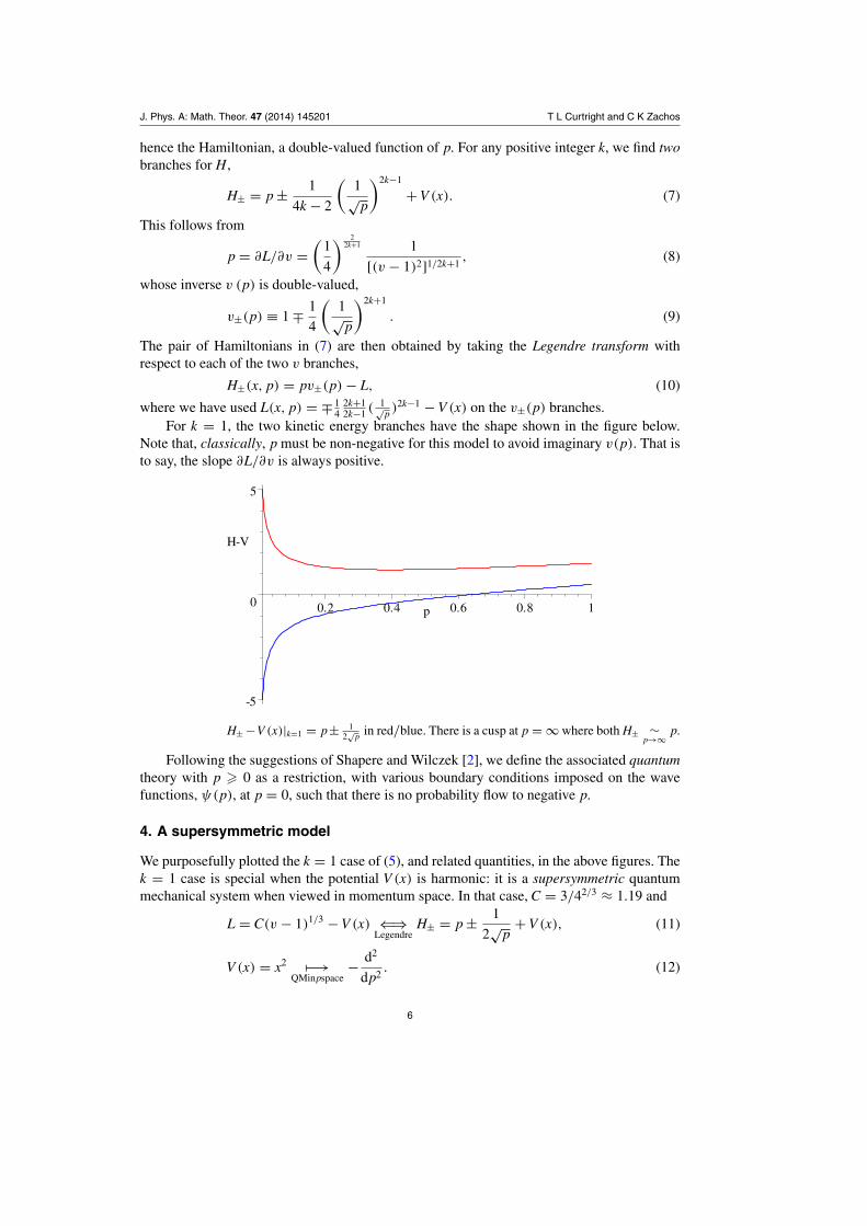
p )2k−1 − V (x) on the v±(p) branches.For k = 1, the two kinetic energy branches have the shape shown in the figure below.

Note that, classically, p must be non-negative for this model to avoid imaginary v(p). That isto say, the slope ∂L/∂v is always positive.

-5

0

5

H-V

0.2 0.4 0.6 0.8 1p

H± −V (x)|k=1 = p± 12√

p in red/blue. There is a cusp at p = ∞ where both H± ∼p→∞

p.

Following the suggestions of Shapere and Wilczek [2], we define the associated quantumtheory with p � 0 as a restriction, with various boundary conditions imposed on the wavefunctions, ψ(p), at p = 0, such that there is no probability flow to negative p.

4. A supersymmetric model

We purposefully plotted the k = 1 case of (5), and related quantities, in the above figures. Thek = 1 case is special when the potential V (x) is harmonic: it is a supersymmetric quantummechanical system when viewed in momentum space. In that case, C = 3/42/3 ≈ 1.19 and

L = C(v − 1)1/3 − V (x) ⇐⇒Legendre

H± = p ± 1

2√

p+ V (x), (11)

V (x) = x2 �−→QMinpspace

− d2

dp2. (12)

6

J. Phys. A: Math. Theor. 47 (2014) 145201 T L Curtright and C K Zachos

4.1. Quantum features

The momentum space pair of QM Hamiltonian operators for this case is therefore expressiblein the standard form for a supersymmetric pair,

H± = − d2

dp2+ w2

0(p) ± w′0(p) =

(d

dp± w0(p)

) (− d

dp± w0(p)

), (13)

where w0(p) = √p. This has the interesting feature that the true—square-integrable—ground

state of the system is non-vanishing for only one of the branches, namely, H−.As an algebraic system, for p � 0, the two Hamiltonians are related in a familiar fashion by

H− = a†a, H+ = aa† = H− + [a, a†] = H− + 1/√

p, (14)

a ≡ d

dp+ √

p, a† ≡ − d

dp+ √

p, [a, a†] = 1√p. (15)

Both energy spectra are non-negative given either Dirichlet or Neumann boundary conditionsat p = 0.5

The zero-energy ground state of H− is given by

aψ0(p) = 0, ψ0(p) = N0 exp

(−2

3p3/2

), N0 = 61/6√

�(

23

) ≈ 1.16 . (16)

This obeys the boundary condition ψ ′0(0) = 0 �= ψ0(0), and is normalized such that∫ ∞

0 |ψ0(p)|2 dp = 1.On the other hand, the zero-energy state for H+, namely, φ(x) = exp(+ 2

3 p3/2), is notadmissible, because it has infinite norm.

The higher energy states are degenerate, with H±ψ(±) = Eψ(±) eigenstates for E > 0mutually related by

ψ(+)E = 1√

Eaψ

(−)E , ψ

(−)E = 1√

Ea†ψ

(+)E , (17)

so as to have equal norms. In particular the first excited state for H− is degenerate with thelowest energy state for H+, with E1 = 1.89379, as determined by numerical analysis.

All this conforms with well-known expectations for general supersymmetric QM. Dueto the restriction p � 0, there is perhaps an interesting wrinkle here, albeit previouslyencountered for the supersymmetric simple harmonic oscillator (but normally expressed interms of ψ(x)): the degenerate H± eigenfunctions obey different boundary conditions atp = 0. If one is Dirichlet, the other is Neumann. This follows from the mutual relationsbetween ψ

(±)E and the fact that a and a† reduce to ±d/dp when acting on nonsingular

functions at p = 0. For example, the first H− excited state and its degenerate H+ partnereigenstate satisfy ψ

(−)E1

|p=0 = 0 = dψ(+)E1

/dp|p=0, while for the next excited states,dψ

(−)E2

/dp|p=0 = 0 = ψ(+)E2

|p=0, etc.Flipping the boundary conditions actually has a practical benefit due to the 1/

√p

singularity in both H±: it is more straightforward to perform an accurate numerical computationof the energy eigenvalue using the boundary condition ψE (0) = 0 �= ψ ′

E (0) than it is using thecondition ψE (0) �= 0 = ψ ′

E (0). The degeneracy of the eigenfunctions permits one to alwayschoose the ψE (0) = 0 condition, along with the corresponding H+ or H−.

These higher energy states may be thought of as a single nontrivial state defined on aunified covering space—a double covering of the half-line R+ by R—obtained by unfolding

5 There is a subtlety here. Strictly, a† is not the adjoint of a. For states subject to Neumann conditions, ψ |p=0 �=0 = ψ ′|p=0, there are non-vanishing boundary contributions at p = 0:

∫ ∞0 (ψ2(a†ψ∗

1 ) − ψ∗1 (aψ2)) dp = ψ∗

1 ψ2|p=0.Nevertheless, it is still true for ψ satisfying either Neumann or Dirichlet conditions that 〈H−〉 = ∫ ∞

0 |aψ |2 dp � 0and 〈H+〉 = ∫ ∞

0 |a†ψ |2 dp � 0, because for such states, ψ∗(aψ)|p=0 = 0 = ψ∗(a†ψ)|p=0.

7

J. Phys. A: Math. Theor. 47 (2014) 145201 T L Curtright and C K Zachos

the two Hamiltonian branches to obtain a single H [2] globally defined on R. However, as isclear from the preceding discussion, the true ground state of the system isψ0(p) ∪ 0 on theunfolded space. The latter, somewhat unusual feature is possible because the two Hamiltonianson the half-lines join together in a cusp at p = ∞, where ψ0 and all its derivatives vanish. Sotoo vanish all the higher ψ

(±)E and all their derivatives at p = ∞.

For this reason, it would be excusable not to have thought of the degenerate eigenstateson the half-line as two branches of a single function. However, the unified two-worlds pictureprovided by joining them together on a covering real line, with Neumann and Dirichletboundary conditions at opposite ends, is a more compelling point of view, in our opinion.Perhaps more importantly, this omniscient view of the two-worlds system becomes naturalwhen the common Lagrangian underpinning both H± is considered.

Self-adjointness of H and probability flow. For arbitrary superpositions of momentum spacewave functions, ψ = ∑

n cnψn, with each of the ψn obeying either Dirichlet or Neumannboundary conditions, the Hamiltonians are real but not self-adjoint. While the behavior atp = ∞ is sufficiently benign for all normalizable linear combinations of energy eigenfunctions,the behavior at p = 0 could be a problem since∫ ∞

0((H±χ∗)ψ − χ∗(H±ψ)) dp = ψ

d

dpχ∗

∣∣∣∣p=0

− χ∗ d

dpψ

∣∣∣∣p=0

, (18)

and this does not necessarily vanish. To avoid this and ensure self-adjointness of H, asuperselection rule may be imposed [13]: the Hilbert space may be partitioned into Dirichletand Neumann solutions, H = HD ⊕ HN , while allowing no mixing of the two. Thus,superpositions of only Dirichlet or only Neumann wave functions are permitted, but linearcombinations of both are not.

While restrictive, this rule nevertheless retains the novel double-valued Hamiltonianfeature of the model. Both branches of H± are operative on each of HD and HN . Linearcombinations of progressively higher energy levels that alternate between H− and H+eigenstates, i.e. ψ = ∑

n bnψ(−)En

+cnψ(+)En+1

, maintain the self-adjointness of H, while requiringboth H± for their time evolution.

The same superselection rule guarantees conservation of probability at p = 0. Wavepackets in either HD or HN will not transport probability to negative p.

4.2. Classical features

It is also instructive to survey essential features of the classical trajectories for the model. TheEuler–Lagrange equations are

dv

dt= 9

Cx 3√

(v − 1)5 (19)

where 9/C = 3 × 42/3 ≈ 7. 56. So we immediately see there are special solutions: v = 1 forany initial x results in v(t) = 1 for all t. Therefore, for any x(0),

x(t) = x(0) + t. (20)

More generally, if v > 1 at any time, then it will remain so for all t, the force does notrestore, and x will grow with t, faster than exponential in fact. In this case the time it takes forx to go to ∞ is finite. But if v < 1 at any time, it will remain so for all t, the force is restoring,and the solution oscillates, albeit nonlinearly.

Classically, energy conservation along a given configuration space trajectory may beexpressed as constant E where

E(x, v) = x2 + C

3

3 − 2v

3√

(v − 1)2. (21)

8

J. Phys. A: Math. Theor. 47 (2014) 145201 T L Curtright and C K Zachos

Note that this E is single-valued as a function of v, even though H±(x, v) = vp±(v)− L(x, v)

is double-valued as a function of v.How can this be? It is possible just because the two branches of H±(x, v) appear on

opposite sides of v = 1, and not for the same value of v. That is to say, it all comes backto our choice for the cube roots on the real line. By taking L real for both v > 1 and forv < 1, we have in fact used two different branches of the analytic cube root function definedfor complex z. However, with our construction, we encounter only one branch of this analyticfunction, and hence one value of L, at any given real value of v. The story is different for thetwo Hamiltonians, H±(x, p), where we encounter both branches for every p > 0.

Upon detailed inspection of constant E(x, v) curves on the (x, v) plane, one finds that,for E < C, there are only open trajectories with v > 1, and all these escape to x = ∞ in finitetimes, in which case only H−(x, p) is operative; while for E � C, on the (x, v) plane there arenot only open, unbounded trajectories, for all v > 1, as governed again by H−(x, p), but alsoclosed, bounded trajectories, for all v < 1, as governed by H+(x, p).

Hence for E � C classical trajectories exist in which both H+ and H− are operative.This should be compared with the existence of admissible wave functions for both H± withidentical energy eigenvalues E > C.

In fact, the E < C classical situation provides intuition that is in accord with the featuresof the quantum ground state. For E < C, there are no classical trajectories (whether openand unbounded, or closed and bounded) in the v < 1 region governed by H+(x, p). ForE < C, rather, there are only unbounded classical trajectories in the v > 1 region governed byH−(x, p). Hence, for E < C, a path integral of exp(iA/�) would encounter no stationary pointsif restricted to trajectories in the v < 1 region. Moreover, there is an infinite, impenetrableE barrier separating classical solutions with v < 1 from those with v > 1, as is evident inthe figure below. This would suggest there are no admissible wave functions for E < C withsupport in the region v < 1. Or, in terms of p, for energy less than C, there would be noadmissible ψ(p) energy eigenstates governed by H+. This heuristic argument is in agreementwith the quantum features of the model.

-2

0

4

E

-5 5 v

E(x, v) as given by (21) is clearly minimized on the (x, v) plane along the line x = 0,and less obviously for v < 1 at v = 0. This is evident in a graph of E(x, v)|x=0 versus v.The minimum for v < 1 is at the (x, v) origin, where E(0, 0) = C = 3

42/3 ≈ 1.19. Thered dots on the E axis are the lowest two energy eigenvalues for the quantized model,namely, E0 = 0 and E1 = 1.89379.

9

J. Phys. A: Math. Theor. 47 (2014) 145201 T L Curtright and C K Zachos

Perhaps these classical features underpinning the quantized model become clearer uponconsidering trajectories as constant energy curves in (x, p) phase space. Several representativeexamples are shown in the next figure (more details are available online)6. Two energiesshown in the figure allow both open, unbounded trajectories, and closed, bounded orbits,namely, for E = 1.2 and E = 1.4. As noted in the previous figure, there is a critical energy,E = C = 3

42/3 ≈ 1. 19, below which bounded orbits do not occur.When bounded orbits do exist, their turning points are given by x = ±√

E − C,corresponding to v = 0 in (21). However, at these turning points the momentum does notvanish, being given instead by p = C/3 = 1

42/3 ≈ 0.397, as indicated by the horizontal lightgray line in the figure.

-2 -1 0 1 2

1

2

x

p

Supersymmetric model phase space trajectories are shown for various energies:E = −0.5 in blue-green, E = 0 in blue, E = 0.5 in purple, E = 1 in black, E = 1.2 insienna, and E = 1.4 in red.

It is important to note in the figure the counter-intuitive feature that p > 0 even when v � 0.Moreover, the phase space curves also exhibit quasi-Hamiltonian flow [6], as mentioned abovefor the Gaussian model: trajectories can cross each other on this (x, p) phase space plot. Thisis allowed when different Hamiltonian branches are governing the motion for the differentcurves that cross. That is to say, just like H, the trajectories are actually on two differentbranches of a phase space Riemann surface.

5. Deforming the supersymmetric Hamiltonians

Here we implement a deformation procedure [14, 15] to construct a family of related butmodified Hamiltonians through the use of general solutions to the Riccati equation as obtainedfrom particular solutions.

6 http://server.physics.miami.edu/curtright/SuperDuperTrajectories.pdf

10

J. Phys. A: Math. Theor. 47 (2014) 145201 T L Curtright and C K Zachos

In addition to the square-integrable zero-energy solution of H−ψ = 0, as given by(d

dp+ √

p

)ψ(p) = 0 i.e. ψ(p) = exp(−2p3/2/3), (22)

the factorized Hamiltonian method may be used to construct another square-integrablesolution, for a modified Hamiltonian, from the non-square-integrable zero-energy solutionof H+φ = 0, as given by(

d

dp− √

p

)φ(p) = 0 i.e. φ(p) = exp(2p3/2/3). (23)

The construction involves the general solution of the Riccati equation V− = w2 − w′, asobtained from the particular one used above, w0(p) = √

p. This general solution involves thenon-square-integrable φ, and a single constant of integration, κ . Thus

wκ(p) = w0(p) − d

dpln

(1 + κ

∫ p

0e2

∫ s0 w0(u) du ds

)

= w0(p) − κe2∫ p

0 w0(u) du

1 + κ∫ p

0 e2∫ s

0 w0(u) du ds. (24)

For the case at hand, this comes down to

wκ(p) = √p − κe4p3/2/3

1 + κg(p)(25)

= √p − κe4p3/2/3 + κ2e4p3/2/3g(p) + O(κ3), (26)

g(p) ≡∫ p

0e4s3/2/3 ds = pe

43 p

32

1 F1

(1; 5/3;−4

3p

32

). (27)

So the subleading terms in this κ-deformation involve a confluent hypergeometric function(incomplete gamma). Note that w0(p) = wκ(p)|κ=0. Also note that w2

κ − w′κ = p − 1

2√

p forany κ .

Now, a zero-energy eigenfunction of H− constructed from the general wκ is not square-integrable (except in the case κ = 0). However, a new square-integrable solution for a modifiedHamiltonian H+(κ) can be constructed.

For any κ > 0 this solution is

φ0(p, κ ) = κe∫ p

0 w0(u) du

1 + κ∫ p

0 e2∫ s

0 w0(u) du ds, (28)

where it is significant that the exponent in the numerator is one half that in wκ . For the presentcase this is

φ0(p, κ ) = κe23 p

32

1 + κg(p). (29)

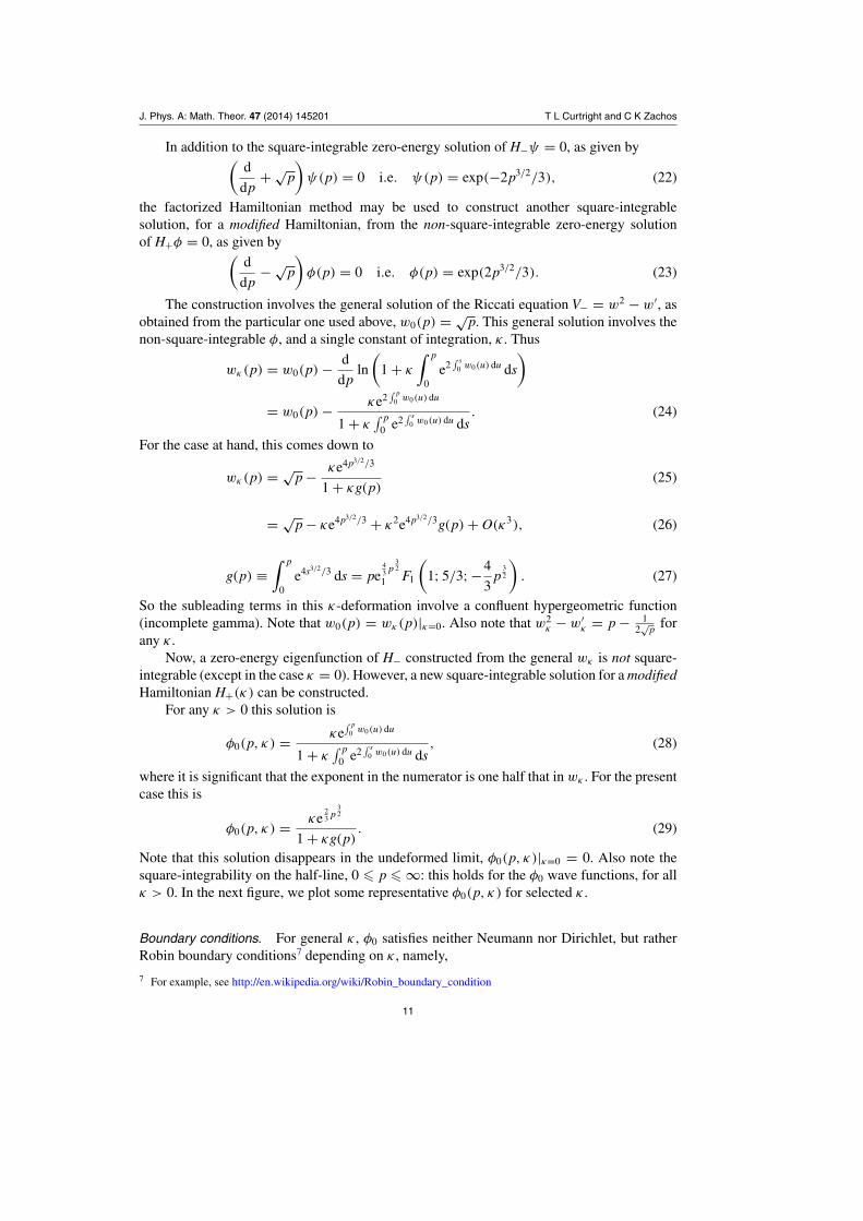
Note that this solution disappears in the undeformed limit, φ0(p, κ )|κ=0 = 0. Also note thesquare-integrability on the half-line, 0 � p � ∞: this holds for the φ0 wave functions, for allκ > 0. In the next figure, we plot some representative φ0(p, κ ) for selected κ .

Boundary conditions. For general κ , φ0 satisfies neither Neumann nor Dirichlet, but ratherRobin boundary conditions7 depending on κ , namely,

7 For example, see http://en.wikipedia.org/wiki/Robin_boundary_condition

11

J. Phys. A: Math. Theor. 47 (2014) 145201 T L Curtright and C K Zachos

κφ0(0, κ ) + dφ0(0, κ )/dp = 0. (30)

This follows from φ0(0, κ ) = κ, dφ0(0, κ )/dp = −κ2.

0

1

phi

1 2 3 4 5 p

φ0(p, κ ) for κ = 1, 1/2, 1/4 and 1/8, in red, blue, orange, and green, respectively.Note that φ0(p, 0) = 0.

Of course, it is better to write the derivative of φ0 at all values of p � 0 as a linear nullequation: (

d

dp− wκ(p)

)φ0(p, κ ) = 0. (31)

In this form it is clear that φ0(p, κ ) is a square-integrable zero-energy solution of a κ-dependentclass of Hamiltonians involving the general wκ(p):

H+(κ) = −(

d

dp+ wκ(p)

) (d

dp− wκ(p)

)

= − d2

dp2+ p + 1

2√

p− 4κ

√pe4p3/2/3

1 + κg(p)+ 2κ2e8p3/2/3

(1 + κg(p))2. (32)

Note, then, that H+(κ)|κ=0 = H+, the initial undeformed Hamiltonian, as given in equation(13).

By way of comparison, H−(κ) = −( ddp − wκ(p))( d

dp + wκ(p)) does not participatein this deformation, as it is actually independent of κ , and identical to the previous H− inequation (13). As mentioned earlier, in this case the κ-dependent zero-energy eigenfunctionsof H−, as given by exp(− ∫ p

0 wκ(s) ds), are not square-integrable except for κ = 0.That is to say, the true ground state of H− is indeed unique, and proportional

to exp(−2p3/2/3). The normalization of the true ground state is finite and given by∫ ∞0 exp(−4p3/2/3) dp = 1

61/3 �( 23 ) ≈ 0.745. On the other hand, it is informative to check

that exp(− ∫ p0 wκ(s) ds) is not square integrable for κ > 0, where

wκ(p) = √p − κe4p3/2/3

1 + κg(p). (33)

To see this, it is sufficient just to plot wκ for a few values of κ and infer the general result.For any κ > 0, it is evident from the figure below that wκ becomes negative and grows

in magnitude for large enough p, asymptoting toward a common κ-independent function

12

J. Phys. A: Math. Theor. 47 (2014) 145201 T L Curtright and C K Zachos

in the limit of large p. Thus we have∫ p

0 wκ(u) du < 0 for p sufficiently large, and hence∫ ∞0 exp(−2

∫ p0 wκ(s) ds) dp will diverge.

-2

0

2

w

1 2 3 4 5 p

wκ(p) for κ = 1, 1/2, 1/4 and 1/8, in red, blue, orange, and green, respectively, alongwith w0(p) = √

p in black.

The large p behavior of wκ(p) for κ �= 0 may be seen analytically from the asymptoticbehavior of (27), which gives

g(p) ∼p→∞

1

2

e43 p

32

√p

(1 + 1

2p32

+ O

(1

p3

)), wκ (p) ∼

p→∞√

p

(−1 + 1

p32

+ O

(1

p3

)).

(34)

As was the case for the undeformed model, there are some technical issues associatedwith probability flow and self-adjointness of the Hamiltonians when κ �= 0. We are content toleave these issues as exercises for the interested reader.

6. Discussion

As emphasized by Shapere and Wilczek, ‘many worlds’ systems with branched Hamiltoniansare by no means rare, in theory. Here, we have displayed some simple unified Lagrangianprototype systems which, by virtue of non-convexity in their velocity dependence, branch intodouble-valued (but still self-adjoint) Hamiltonians.

We have outlined a Gaussian model whose branches lie on a compact, closed momentummanifold with coalescing cusps at finite p, as a preliminary step in the search for asupersymmetric model with similar properties. We then discussed a class of models withdouble-valued Hamiltons, one of which has the canonical structure of a supersymmetric pairof Hamiltonians. We have surveyed the spectral and boundary condition linkages involvedacross the respective branches for this supersymmetric model, in a uniform framework, byutilizing the eigenstate-linking supercharge ladder operators (but which are not Grassmannand which do not commute with the two Hamiltonians).

These particular branched Hamiltonians—although living in ‘two worlds’—arenevertheless paired by supercharges into a uniform Darboux isospectral system, in the verysame Hilbert space; and yet they are inexorably separated, in some analogy to fermionic

13

J. Phys. A: Math. Theor. 47 (2014) 145201 T L Curtright and C K Zachos

and bosonic sectors, as the respective dynamical intervals only connect at p = ∞. In thisrespect, this particular supersymmetric system differs from more typical constructions givenby Shapere and Wilczek, which exhibit similar operator branching structures but connect forfinite p.

Acknowledgments

This work was supported in part by NSF Award PHY-1214521; and in part, the submittedmanuscript has been created by UChicago Argonne, LLC, Operator of Argonne NationalLaboratory. Argonne, a US Department of Energy Office of Science laboratory, is operatedunder contract no. DE-AC02-06CH11357. The US Government retains for itself, and othersacting on its behalf, a paid-up nonexclusive, irrevocable worldwide license in said article toreproduce, prepare derivative works, distribute copies to the public, and perform publicly anddisplay publicly, by or on behalf of the Government. TLC was also supported in part by aUniversity of Miami Cooper Fellowship.

References

[1] Shapere A and Wilczek F 2012 Branched quantization Phys. Rev. Lett. 109 200402[2] Shapere A and Wilczek F 2012 Classical time crystals Phys. Rev. Lett. 109 160402[3] Shapere A D, Wilczek F and Xiong Z 2012 Models of topology change arXiv:1210.3545 [hep-th][4] Wilczek F 2012 Quantum time crystals Phys. Rev. Lett. 109 160401[5] Curtright T L and Zachos C K 2009 Evolution profiles and functional equations J. Phys. A: Math.

Theor. 42 485208[6] Curtright T L and Zachos C K 2010 Chaotic maps, Hamiltonian flows, and holographic methods

J. Phys. A: Math. Theor. 43 445101[7] Curtright T L and Veitia A 2011 Logistic map potentials Phys. Lett. A 375 276–82[8] Curtright T L 2011 Potentials unbounded below SIGMA 7 042[9] Curtright T L and Zachos C K 2011 Renormalization group functional equations Phys. Rev.

D 83 065019[10] Curtright T L, Jin X and Zachos C K 2012 RG flows, cycles, and c-theorem folklore Phys. Rev.

Lett. 108 131601[11] Witten E 1982 Supersymmetry and Morse theory J. Differ. Geom. 17 661–92

Witten E 1982 Constraints on supersymmetry breaking Nucl. Phys. B 202 253–316[12] Shankar R 1981 Solvable models with selftriality in statistical mechanics and field theory Phys.

Rev. Lett. 46 379[13] Wigner E P 1952 Die messung quantenmechanischer operatoren Z. Phys. 133 101–8

Wick G C, Wightman A S and Wigner E P 1952 The intrinsic parity of elementary particles Phys.Rev. 88 101–5

Wick G C, Wightman A S and Wigner E P 1970 Superselection rule for charge Phys. Rev.D 1 3267–9

[14] Mielnik B 1984 Factorization method and new potentials with the oscillator spectrum J. Math.Phys. 25 3387–9

[15] Rosas-Ortiz J O 1999 On the factorization method in quantum mechanics Proc. Int. Workshop onSymmetries in Quantum Mechanics and Quantum Optics (Burgos, Spain) ed A Ballesteroset al (Burgos: Servicio de Publicaciones de la Universidad de Burgos) pp 285–99(arXiv:quant-ph/9812003)

14