SHADES OF HYPERBOLICITY FOR HAMILTONIANS

MARIO BESSA, JORGE ROCHA, AND MARIA JOANA TORRES

Abstract. We prove that a Hamiltonian system H ∈ C2(M,R) is globally hyperbolicif any of the following statements holds: H is robustly topologically stable; H is stablyshadowable; H is stably expansive; and H has the stable weak specification property.Moreover, we prove that, for a C2-generic Hamiltonian H, the union of the partiallyhyperbolic regular energy hypersurfaces and the closed elliptic orbits, forms a densesubset of M . As a consequence, any robustly transitive regular energy hypersurface of aC2-Hamiltonian is partially hyperbolic. Finally, we prove that stably weakly shadowableregular energy hypersurfaces are partially hyperbolic.

Keywords: Hamiltonian vector field, structural stability, dominated splitting, elliptic closed orbits.

2000 Mathematics Subject Classification: Primary: 37J10, 37D30; Secondary: 70H05.

1. Introduction and a tour along the main results

The Hamiltonian functions H : M → R on symplectic 2n-dimensional manifolds Mform a central subclass of all continuous-time dynamical systems generated by the 2ndifferential equations known as the Hamilton equations qi = ∂piH and pi = −∂qiH, where(qi, pi) ∈ M and i = 1, .., n. Their relevance follows from the vast range of applicationsthroughout several branches of mathematics. Actually, the laws of mathematical physicsare mostly expressed in terms of differential equations, and a well studied and successfulsubclass of these differential equations, whose solutions keep invariant a given symplecticform, are the Hamiltonian equations (see [1, 4]).

Stable properties of Hamiltonians, i.e. those properties that are shared by slightly per-turbed systems of these continuous-time systems are a fundamental problem in describingthe dynamics in the space of all Hamiltonians. Among them the structurally stable pro-perty, introduced in the mid 1930s by Andronov and Pontrjagin, plays a fundamental role.Roughly speaking it means that under small perturbations the dynamics are topologicallyequivalent. Smale’s program in the early 1960s aimed to prove the (topological) generi-city of structurally stable systems. Although Smale’s program was proved to be wrongone decade later, it played a fundamental role in the theory of dynamical systems andraised the problem of characterizing structural stability as being essentially equivalent to

Date: January 9, 2014.1

arX

iv:1

212.

4874

v1 [

mat

h.D

S] 1

9 D

ec 2

012

2 M. BESSA, J. ROCHA, AND M. J. TORRES

uniform hyperbolicity. In [16] the authors characterized the structurally stable Hamil-tonian systems as the Anosov ones. The characterization of structurally stable systems,using topological and geometric dynamical properties, has been one of the main object ofinterest in the global qualitative theory of dynamical systems, in the last 40 years. Thepurpose of one of our main results (see Theorem 1) is, thus, to give a characterization ofthe structurally stable Hamiltonians by making use of the notions of topological stability,shadowing, expansiveness and specification. These properties although they seem quitedifferent they are intertconnected with uniformly hyperbolic demeanor.

Anosov systems, and thus, structurally stable Hamiltonians, are topologically stable,expansive and satisfy the shadowing property. But the converse is not true. There areexamples of systems far from the structurally stable ones that are topologically stable1,that are expansive (see Example 3.1), and that satisfy the shadowing property (see [60]and also the symplectic curious example of existence of shadowing of transition chains ofseveral invariant tori alternating with Birkhoff zones of instability [32]).

Therefore, the problem on the relationship between structural stability and topologicaland geometric properties of the system is not trivial. The passage to C2-interiors of setsof Hamiltonians that have these properties developed in the present work became oneeffective approach to the solution of this problem. A property is C2-stable if once theproperty holds for a C2-Hamiltonian it also holds for every C2-nearby Hamiltonian. Letus explain the dynamical properties that we deal with and state Theorem 1.

The shadowing of a given set of points which are an “almost orbit” of some system by atrue orbit appears in many branches of dynamical systems and is quite often related withhyperbolicity. Actually, the computational estimates, fitted with a certain error of orbits,are meaningless if they cannot be realized by genuine orbits of the given system, and, inthis sense, are mere pixel inaccuracy typical of the computational framework. Despite thefact that shadowable systems can be non hyperbolic the stability of shadowing goes a longway when proving hyperbolicity. We refer the work developed in [8, 31, 38, 47, 52, 57]both for flows and diffeomorphisms and in dissipative and conservative contexts. Here wewill prove that stability of shadowing is equivalent to hyperbolicity.

The notion of topological stability (see the precise definition in §3.1), grew parallel tothe theory of structural stability, and was first introduced by Walters in ([56]) whenproving that Anosov diffeomorphisms are topologically stable. Then, Nitecki proved thattopological stability was a necessary condition to get Axiom A plus strong transversality(see [44]). In the late 1970’s ([50]), Robinson proved that Morse-Smale flows are topologi-cally stable, and in the mid 1980’s, Hurley obtained necessary conditions for topologicalstability (see [35, 36, 37]). Here we generalize the results for flows in [18, 41]) to the

1It is immediate that the topological stability is invariant by conjugacy. Moreover, by a result ofGogolev (see [33]) the existence of a conjugacy between two maps where one of which is Anosov is notsufficient to guarantee that the other is Anosov.

SHADES OF HYPERBOLICITY FOR HAMILTONIANS 3

Hamiltonian context (see also [19]) which says that robust topologically stable vectorfields are hyperbolic.

A dynamical system is said to be expansive when, in brief terms, if two points stay nearfor future and past iterates, then they must be equal. We can say, in a general scope, thatthe system has sensitivity to the initial conditions, because, when different, two pointsmust be separated by forward or backward iteration. This notion was first developed inthe 1950’s (see [58]) and, in the flow context, initialized by the studies of Bowen andWalters (see [28]). In this paper we generalize the recent results in [31, 40, 54] by provingthat the stability of expansiveness is equivalent to hyperbolicity.

The concept of weak specification although intricate (see §3.5) is quite well summarizedin simple words, for diffeomorphisms, in [30, page 193]: “The weak specification means thatwhenever there are two pieces of orbits fn(x1) : a1 ≤ n ≤ b1 and fn(x2) : a2 ≤ n ≤ b2,they may be approximated up to ε by one single orbit - the orbit of x - provided that thetime for switching from the first piece of orbit to the second (namely a2−b1) and the timefor switching back (namely p− (b2 − a1))2 are larger than K(ε), this number K(ε) beingindependent of the pieces of orbit, and in particular independent of their length.”Several authors obtained hyperbolicity from the hypothesis that the system has the stablespecification property (see [6, 53]). We point out that their arguments were supported ona change of index argument in the hyperbolic closed orbits. However, in the symplecticsetting such situation is impossible to happen because the index is constant and equal ton− 1. Here we obtain similar results for Hamiltonians using a new symplectic approach.

Summarizing, in Theorem 1, we prove that a Hamiltonian is globally hyperbolic (Anosov)if any of the following properties is stable: topological stability, shadowing, expansiveness,and specification. Thus, we call these properties shades of hyperbolicity. The proof is adirect consequence of the following. First, we refer that it was recently proved that astar Hamiltonian is Anosov (see Theorem 2, proved in [10] for n = 2 and generalized bythe authors in [16] for n ≥ 2). We recall that a Hamiltonian is a star Hamiltonian if theproperty of having all periodic orbits of hyperbolic type is stable. Finally, we prove, inTheorem 3, that the stability of any of the shade properties just described implies thatthe Hamiltonian is a star system.

Dynamical systems exhibiting dense orbits are called transitive. Informally speakingthis means that the whole manifold is indecomposable. Those systems for which thisproperty remains valid for any perturbation are called robustly transitive. Since the pi-oneering work of Mane (see [39]) several other results were obtained guaranteeing thatrobust transitivity, with respect to C1-topology, implies a certain form of hyperbolicity(see e.g. [5, 17, 26, 27, 34, 55]). Here, and as a direct consequence a dichotomy thatwe discuss in the sequel, we shall prove that robustly transitive Hamiltonians are par-tially hyperbolic. Moreover, we shall prove that stably ergodic Hamiltonians are partiallyhyperbolic.

2The number p is any number greater or equal than K(ε) + b2 − a1.

4 M. BESSA, J. ROCHA, AND M. J. TORRES

The shadowing property in the weak sense first appear in the paper by Corless andPilyugin (see [29]) when related to the genericity (with respect to the C0-topology) ofshadowing among homeomorphisms. In simple terms weak shadowing allows that the“almost orbits” may be approximated by true orbits if one forgets the time parameteri-zation and consider only the distance between the orbit and the “almost orbit” as twosubsets in the manifold. There exist dynamical systems without the weak shadowing(see [46, Example 2.12]) and dynamical systems satisfying the weak shadowing but notthe shadowing property ([46, Example 2.13]. In the present paper we generalize a recentresult (see [20, 21]) for the setting of Hamiltonians. More precisely, we obtain partialhyperbolicity under the hypothesis of stable weak shadowing (see Theorem 6).

Generic properties of Hamiltonians, i.e. those properties that are shared by a countableintersection of open and dense subsets of these continuous-time systems, are thus of greatimportance and interest since they give us the typical behavior, in Baire’s category sense,that one could expect from a wide class of systems (cf. [10, 11, 12, 13, 16, 43, 49]). Thereare obvious constraints to the amount of information we can obtain from a certain clusterof generic systems. Howsoever, it is of great importance and utility to learn that a givensystem can be slightly perturbed in order to obtain a system whose global and localdynamics we understand quite well.

Questions concerning the generic behaviour of Hamiltonians were first raised by Robin-son (see [49]). One of our main generic results (see Theorem 5) is the generalizationof a result stated in [43] by Newhouse and proved in [13] for the 4-dimensional context(or a weak 2n-dimensional version): C2-generic Hamiltonians are of hyperbolic type orelse exhibit dense 1-elliptic closed orbits. We prove that most Hamiltonians, from thegeneric viewpoint, have only two types of well-differentiated behavior: partial hyperbo-licity (chaotic type, cf. [25]) or else lots of elliptic closed orbits (KAM type, cf. [59]).Of course that, in the 4-dimensional case, 1-elliptic closed orbits are totally elliptic and,moreover, partial hyperbolicity is actually hyperbolicity. See ([13]) for a detailed proofof this result. It is still an open and quite interesting question to know if these type ofresults hold for mechanic systems (see [14, §8]).

With respect to the discrete-time case, in [43], it was obtained that C1-generic symplec-tomorphisms in surfaces are Anosov (uniformly hyperbolic) or else the elliptic points aredense. Long after Newhouse’s proof, Arnaud (see [2]) proved the 4-dimensional version ofthis result, namely that C1-generic symplectomophisms are Anosov, partially hyperbolicor have dense elliptic periodic points. Finally, Saghin and Xia ([51]) proved the sameresult but for any dimension completing the program for the discrete case. In this paper,and among other issues, we developed, in Theorem 4, the approach for the continuous-timecase of Saghin-Xia’s theorem.

We emphasize that in this paper we are restricted to the C2-topology for Hamiltoniansand to the C1-topology for the associated vector field, since our proofs use several technicalresults which are proved for this topology (see the perturbation results in §5).

SHADES OF HYPERBOLICITY FOR HAMILTONIANS 5

2. Hamiltonian systems

2.1. The Hamiltonian framework. Let (M,ω) be a symplectic manifold, where M isa 2n-dimensional (n ≥ 2), compact, boundaryless, connected and smooth Riemannianmanifold, endowed with a symplectic form ω. A Hamiltonian is a real-valued Cr functionon M , 2 ≤ r ≤ ∞. We denote by Cr(M,R) the set of Cr-Hamiltonians on M . Fromnow on, we shall restrict to the C2-topology, and thus we set r = 2. Associated withH, we have the Hamiltonian vector field XH defined by ω(XH(p), u) = ∇Hp(u), for allu ∈ TpM , which generates the Hamiltonian flow X t

H . Observe that H is C2 if and onlyif XH is C1 and that, since H is continuous and M is compact, Sing(XH) 6= ∅, whereSing(XH) denotes the singularities of XH or, in other words, the critical points of H orthe equilibria of X t

H . Let R(H) = M \ Sing(XH) stands for the set of regular points.A scalar e ∈ H(M) ⊂ R is called an energy of H and the pair (H, e) is called Hamil-

tonian level. An energy hypersurface EH,e is a connected component of H−1(e), calledenergy level set, and it is regular if it does not contain singularities. Observe that a regu-lar energy hypersurface is a X t

H-invariant, compact and (2n − 1)-dimensional manifold.The energy level set H−1(e) is said regular if any energy hypersurface of H−1(e) isregular. If H−1(e) is regular, then H−1(e) is the union of a finite number of energyhypersurfaces. Finally, a Hamiltonian level (H, e) is said regular if the energy level setH−1(e) is regular.

A Hamiltonian system is a triple (H, e, EH,e), where H is a Hamiltonian, e is an energyand EH,e is a regular connected component of H−1(e).

Fixing a small neighbourhood W of a regular EH,e, there exist a small neighbourhood

U of H and ε > 0 such that, for all H ∈ U and e ∈ (e− ε, e + ε), H−1(e) ∩W = EH,e.We call EH,e the analytic continuation of EH,e.

In the space of Hamiltonian systems we consider the topology generated by a funda-mental systems of neighbourhoods. Given a Hamiltonian system (H, e, EH,e) we say thatV is a neighbourhood of (H, e, EH,e) if there exist a small neighbourhood U of H and ε > 0

such that for all H ∈ U and e ∈ (e− ε, e+ ε) one has that the analytic continuation EH,eof EH,e is well-defined.

Since the symplectic form ω is non-degenerate, given H ∈ C2(M,R) and p ∈ M , weknow that ∇Hp = 0 is equivalent to XH(p) = 0. Therefore, the extreme values of aHamiltonian H are exactly the singularities of the associated Hamiltonian vector fieldXH .

Given a Hamiltonian level (H, e), let Ω(H|EH,e) be the set of non-wandering points of

H on the energy hypersurface EH,e, that is, the points x ∈ EH,e such that, for everyneighborhood U of x in EH,e, there is τ > 0 such that Xτ

H(U) ∩ U 6= ∅.By Liouville’s Theorem, the symplectic manifold (M,ω) is also a volume manifold (see,

for example, [1]). This means that the 2n-form ωn = ω ∧ n... ∧ ω (wedging n-times) isa volume form and induces a measure µ on M , which is called the Lebesgue measureassociated to ωn. Notice that the measure µ on M is invariant by the Hamiltonian flow.

6 M. BESSA, J. ROCHA, AND M. J. TORRES

So, given a regular Hamiltonian level (H, e), we induce a volume form ωEH,eon each energy

hypersurface EH,e ⊂ H−1(e), where for all p ∈ EH,e:ωEH,e

: TpEH,e × TpEH,e × TpEH,e −→ R(u, v, w) 7−→ ωn(∇Hp, u, v, w)

The volume form ωEH,eis X t

H-invariant. Hence, it induces an invariant volume measureµEH,e

on EH,e which is a finite measure, since any energy hypersurface is compact. Observethat, under these conditions, we have that µEH,e

-a.e. x ∈ EH,e is recurrent, by the PoincareRecurrence Theorem.

2.2. Transversal linear Poincare flow and hyperbolicity. Let us begin with thedefinition of the transversal linear Poincare flow. After, we state some results using thislinear flow. Consider a Hamiltonian vector field XH and a regular point x in M and lete = H(x). Define Nx := Nx ∩TxH−1(e), where Nx = (RXH(x))⊥ is the normal fiber atx, RXH(x) stands for the flow direction at x, and TxH

−1(e) = Ker∇Hx is the tangentspace to the energy level set. Thus, Nx is a (2n− 2)-dimensional bundle.

Definition 2.1. The transversal linear Poincare flow associated to H is given by

ΦtH(x) : Nx → NXt

H(x)

v 7→ ΠXtH(x) DXH

tx(v),

where ΠXtH(x) : TXt

H(x)M → NXtH(x) denotes the canonical orthogonal projection.

Observe that Nx is ΦtH(x)-invariant. It is well-known (see e.g. [1]) that, given a regular

point x ∈ EH,e, then ΦtH(x) is a linear symplectomorphism for the symplectic form ωEH,e

,that is, ωEH,e

(u, v) = ωEH,e(Φt

H(x) u,ΦtH(x) v), for any u, v ∈ Nx.

For any symplectomorphism, in particular for ΦtH(x), we have the following result.

Theorem 2.1. (Symplectic eigenvalue theorem, [1]) Let f be a symplectomorphism in M ,p ∈ M and σ an eigenvalue of Dfp of multiplicity m. Then 1/σ is an eigenvalue of Dfpof multiplicity m. If σ is non real, then σ and 1/σ are also eigenvalues of Dfp. Moreover,the multiplicity of the eigenvalues +1 and −1, if they occur, is even.

The proof of the following result can be found in [12, Section 2.3].

Lemma 2.2. Take a Hamiltonian H ∈ C2(M,R) and let Λ be an X tH-invariant, regular

and compact subset of M . Then, Λ is uniformly hyperbolic for X tH if and only if the

induced transversal linear Poincare flow ΦtH is uniformly hyperbolic on Λ.

So, we can define a uniformly hyperbolic set as follows.

Definition 2.2. Let H ∈ C2(M,R). An X tH-invariant, compact and regular set Λ ⊂ M

is uniformly hyperbolic if NΛ admits a ΦtH-invariant splitting N s

Λ⊕N uΛ such that there

is ` > 0 satisfying

SHADES OF HYPERBOLICITY FOR HAMILTONIANS 7

‖Φ`H(x)|N s

x‖ ≤ 1

2and ‖Φ−`H (X`

H(x))|Nu

X`H

(x)‖ ≤ 1

2, for any x ∈ Λ.

We remark that the constant 12

can be replaced by any constant θ ∈ (0, 1) with thedetriment of changing the value of `.

Given x ∈ R(H), we say that x is a periodic point of the Hamiltonian H if X tH(x) = x

for some t. The smallest t0 > 0 satisfying the condition above is called period of x; inthis case, we say that the orbit of x is a closed orbit of period t0. Accordingly withDefinition 2.2, a periodic point x is hyperbolic if there exists a splitting of the normalsubbundle N along the orbit of x that satisfies the condition above.

Now, we state the definition of dominated splitting, by using the transversal linearPoincare flow.

Definition 2.3. Take H ∈ C2(M,R) and let Λ be a compact, X tH-invariant and regular

subset of M . Consider a ΦtH-invariant splitting N = N 1 ⊕ · · · ⊕ N k over Λ, for 1 ≤ k ≤

2n−2, such that all the subbundles have constant dimension. This splitting is dominatedif there exists ` > 0 such that, for any 0 ≤ i < j ≤ k,

‖Φ`H(x)|N i

x‖ · ‖Φ−`H (X`

H(x))|N j

X`H

(x)

‖ ≤ 1

2, ∀ x ∈ Λ.

Finally, we state the definition of partial hyperbolicity, of the transversal linear Poincareflow.

Definition 2.4. Take H ∈ C2(M,R) and let Λ be a compact, X tH-invariant and regular

subset of M . Consider a ΦtH-invariant splitting N = N u ⊕ N c ⊕ N s over Λ such that

all the subbundles have constant dimension and at least two of them are non-trivial. Thissplitting is partially hyperbolic if there exists ` > 0 such that,

(1) N u is uniformly hyperbolic and expanding;(2) N s is uniformly hyperbolic and contracting and(3) N u `-dominates N c and N c `-dominates N s.

In general, along this paper, we consider these three structures defined in a set Λ whichis the whole energy level.

Remark 2.1. It was proved in [22] that, in the symplectic world, the existence of a do-minated splitting implies partial hyperbolicity. More precisely, If N u⊕N 2 is a dominatedsplitting, with dimN u ≤ dimN 2, then N 2 splits invariantly as N 2 = N c ⊕ N s, withdimN s = dimN u. Furthermore, the splitting N u ⊕ N c ⊕ N s is dominated, N u is uni-formly expanding, and N s is uniformly contracting. In conclusion, N u ⊕ N c ⊕ N s ispartially hyperbolic.

8 M. BESSA, J. ROCHA, AND M. J. TORRES

3. Shade properties: topological stability, shadowing, weak shadowing,expansiveness, specification, transitivity and ergodicity

In this section we describe the dynamical properties that we shall deal with in thesequel.

3.1. Topological stability. Let (H, e, EH,e) and (H, e, EH,e) be Hamiltonians systems;

we say that (H, e, EH,e) is semiconjugated to (H, e, EH,e) if there exist a continuous andonto map h : EH,e → EH,e and a continuous real map τ : EH,e × R→ R such that:

(a) for any x ∈ EH,e, τx : R → R is an orientation preserving homeomorphism whereτ(x, 0) = 0 and

(b) for all x ∈ EH,e and t ∈ R we have h(X tH

(x)) = Xτ(x,t)H (h(x)).

We say that the Hamiltonian system (H, e, EH,e) is topologically stable if for any ε > 0,

there exists δ > 0 such that for any Hamiltonian system (H, e, EH,e) such that H is δ-

C1-close to H and e ∈ (e − δ, e + δ), there exists a semiconjugacy from (H, e, EH,e) to(H, e, EH,e), i.e., there exists h : EH,e → EH,e and τ : EH,e × R → R satisfying (a) and(b) above, and d(h(x), x) < ε for all x ∈ EH,e. Observe that the notion of topologicallystability does not define an equivalence relation. Furthermore, the set of systems semi-conjugated to a given Hamiltonian system may not be an open set. This motivates thefollowing definition. We say that (H, e, EH,e) is robustly topologically stable if there exists

a neighbourhood V of (H, e, EH,e) such that any (H, e, EH,e) ∈ V is topologically stable.

3.2. The shadowing property. Let (H, e, EH,e) be a Hamiltonian system. Let us fix realnumbers δ, T > 0. We say that a pair of sequences ((xi), (ti))i∈Z (xi ∈ EH,e, ti ∈ R, ti ≥ T )is a (δ, T )-pseudo-orbit of H if d(X ti

H(xi), xi+1) < δ for all i ∈ Z. For the sequence (ti)i∈Zwe write S(n) = t0 + t1 + . . .+ tn−1 if n ≥ 0, and S(n) = −(tn + . . .+ t−2 + t−1) if n < 0,where S(0) = t0 + t−1 = 0. Let x0 ? t denote a point on a (δ, T )-chain t units time fromx0. More precisely, for t ∈ R,

x0 ? t = Xt−S(i)H (xi) if S(i) ≤ t < S(i+ 1).

Simple examples show that, in the case of a flow, it is unnatural to require in the defini-tion of shadowing the closeness of points of a pseudo-orbit and its shadowing exact orbitcorresponding to the same instants of time, as it is posed in the shadowing problem fordiffeomorphisms. We need to reparametrize the exact shadowing orbit. By Rep we denotethe set of all increasing homemorphisms α : R→ R, called reparametrizations, satisfying

α(0) = 0. Fixing ε > 0, we define the set Rep(ε) =α ∈ Rep :

∣∣∣α(t)t− 1∣∣∣ < ε, t ∈ R

.

When we choose a reparametrization α in the previous set, we want α to be taken arbi-trarily close to identity. A (δ, T )-pseudo-orbit ((xi), (ti))i∈Z is ε-shadowed by some orbit of

H if there is z ∈ EH,e and a reparametrization α ∈ Rep(ε) such that d(Xα(t)H (z), x0 ?t) < ε,

for every t ∈ R.

SHADES OF HYPERBOLICITY FOR HAMILTONIANS 9

The Hamiltonian system (H, e, EH,e) is said to have the shadowing property if, for anyε > 0 there exist δ, T > 0 such that any (δ, T )-pseudo-orbit ((xi), (ti))i∈Z is ε-shadowedby some orbit of H.

We say that the Hamiltonian system (H, e, EH,e) is stably shadowable if there exists a

neighbourhood V of (H, e, EH,e) such that any (H, e, EH,e) ∈ V has the shadowing property.

3.3. The weak shadowing property. We recall the following definition of weakly sha-dowable systems that was introduced in [29] in connection with the problem of genericityof shadowing. Given a Hamiltonian system (H, e, EH,e) and δ, T > 0, a (δ, T )-pseudo-orbit((xi), (ti))i∈Z is weakly ε-shadowed by some orbit of H if there exists z ∈ EH,e such thatxii∈Z ⊂ Bε(O(z)).

The Hamiltonian system (H, e, EH,e) is said to have the weak shadowing property if, forany ε > 0 there exist δ, T > 0 such that any (δ, T )-pseudo-orbit ((xi), (ti))i∈Z is weaklyε-shadowed by some orbit of H.

We say that the Hamiltonian system (H, e, EH,e) is stably weakly shadowable if there

exists a neighbourhood V of (H, e, EH,e) such that any (H, e, EH,e) ∈ V has the weakshadowing property.

3.4. The expansiveness property. Let (H, e, EH,e) be a Hamiltonian system. We saythat (H, e, EH,e) is expansive if, for any ε > 0, there is δ > 0 such that if x, y ∈ EH,e satisfy

d(X tH(x), X

α(t)H (y)) ≤ δ, for any t ∈ R and for some continuous map α : R → R with

α(0) = 0, then y = XsH(x), where |s| ≤ ε.

This definition asserts that any two points whose orbits remain indistinguishable, upto any continuous time displacement, must be in the same orbit.

Observe that the reparametrization α is not assumed to be close to identity and thatthe expansiveness property does not depend on the choice of the metric on M .

We say that the Hamiltonian system (H, e, EH,e) is stably expansive if there exists a

neighbourhood V of (H, e, EH,e) such that any (H, e, EH,e) ∈ V has the expansivenessproperty.

The next example, point to us by Pedro Duarte, shows that expansiveness can coexistwith elliptic orbits.

Example 3.1. Consider the Hamiltonian with 1-degree of freedom given by H(x, y) =x3 − 3xy2. The associated Hamiltonian vector field if XH(x, y) = (−6xy, 3y2 − 3x2) (formore details see [4, Appendix 7]). The origin is a degenerated singularity of the vectorfield. However, our system exhibits a symmetry; the rotation by 2π

3centered in (0, 0) keeps

invariant the phase portrait (see Figure 1). Hence, we can keep the same dynamics asthe one in the figure and turn the origin into an elliptic fixed point inducing a rotation ofangle 2π

3. Observe that, locally, the system is expansive despite the fact that we are in the

presence of an elliptic point.

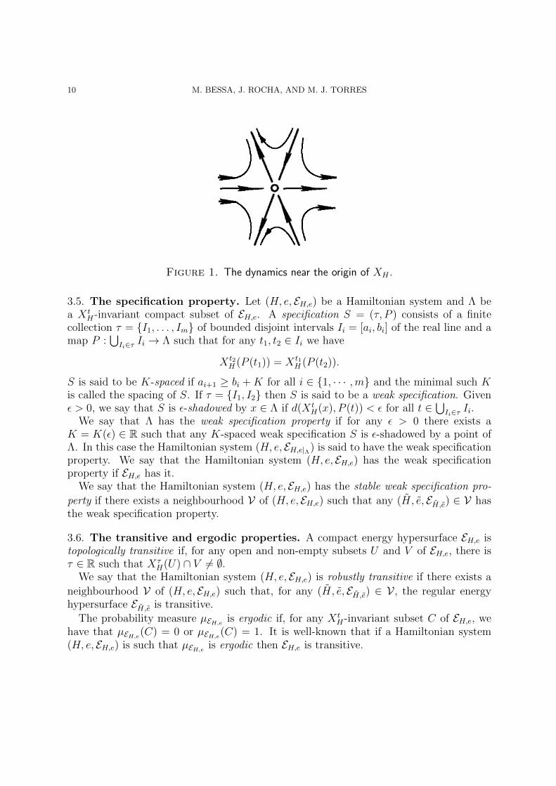
10 M. BESSA, J. ROCHA, AND M. J. TORRES

Figure 1. The dynamics near the origin of XH .

3.5. The specification property. Let (H, e, EH,e) be a Hamiltonian system and Λ bea X t

H-invariant compact subset of EH,e. A specification S = (τ, P ) consists of a finitecollection τ = I1, . . . , Im of bounded disjoint intervals Ii = [ai, bi] of the real line and amap P :

⋃Ii∈τ Ii → Λ such that for any t1, t2 ∈ Ii we have

X t2H (P (t1)) = X t1

H (P (t2)).

S is said to be K-spaced if ai+1 ≥ bi +K for all i ∈ 1, · · · ,m and the minimal such Kis called the spacing of S. If τ = I1, I2 then S is said to be a weak specification. Givenε > 0, we say that S is ε-shadowed by x ∈ Λ if d(X t

H(x), P (t)) < ε for all t ∈⋃Ii∈τ Ii.

We say that Λ has the weak specification property if for any ε > 0 there exists aK = K(ε) ∈ R such that any K-spaced weak specification S is ε-shadowed by a point ofΛ. In this case the Hamiltonian system (H, e, EH,e|Λ) is said to have the weak specificationproperty. We say that the Hamiltonian system (H, e, EH,e) has the weak specificationproperty if EH,e has it.

We say that the Hamiltonian system (H, e, EH,e) has the stable weak specification pro-

perty if there exists a neighbourhood V of (H, e, EH,e) such that any (H, e, EH,e) ∈ V hasthe weak specification property.

3.6. The transitive and ergodic properties. A compact energy hypersurface EH,e istopologically transitive if, for any open and non-empty subsets U and V of EH,e, there isτ ∈ R such that Xτ

H(U) ∩ V 6= ∅.We say that the Hamiltonian system (H, e, EH,e) is robustly transitive if there exists a

neighbourhood V of (H, e, EH,e) such that, for any (H, e, EH,e) ∈ V , the regular energyhypersurface EH,e is transitive.

The probability measure µEH,eis ergodic if, for any X t

H-invariant subset C of EH,e, wehave that µEH,e

(C) = 0 or µEH,e(C) = 1. It is well-known that if a Hamiltonian system

(H, e, EH,e) is such that µEH,eis ergodic then EH,e is transitive.

SHADES OF HYPERBOLICITY FOR HAMILTONIANS 11

We say that the Hamiltonian system (H, e, EH,e) with H ∈ C3(M,R), is stably ergodic

if there exists a neighbourhood V of (H, e, EH,e) such that, for any (H, e, EH,e) ∈ V with

H ∈ C3(M,R), the probability measure µEH,eis ergodic.

4. Precise statement of the results

A Hamiltonian system (H, e, EH,e) is Anosov if EH,e is uniformly hyperbolic for theHamiltonian flow X t

H associated to H.Our first main result states that the stability of any of the properties: topological

stability, shadowing, expansiveness, and specification guarantees global hyperbolicity:

Theorem 1. Let (H, e, EH,e) be a Hamiltonian system. If any of the following statementshold:

(1) (H, e, EH,e) is robustly topologically stable;(2) (H, e, EH,e) is stably shadowable;(3) (H, e, EH,e) is stably expansive;(4) (H, e, EH,e) has the stable weak specification property,

then (H, e, EH,e) is Anosov.

It is well-known from classical hyperbolic dynamics that Anosov implies shadowing,expansiveness and topological stability. With respect to weak specification the issueis more subtle. For instance, mixing Anosov flows satisfy the specification property.However, we consider the following example:

Example 4.1. (Non-mixing Anosov suspension flow) Let be given an Anosov diffeo-morphism in a surface Σ, f : Σ → Σ, and a ceiling function h : Σ → R+ satisfyingh(x) ≥ β > 0 for all x ∈ Σ. We consider the space Mh ⊆ Σ× R+ defined by

Mh = (x, t) ∈ Σ× R+ : 0 ≤ t ≤ h(x)with the identification between the pairs (x, h(x)) and (f(x), 0). The flow defined on Mh

by Ss(x, r) = (fn(x), r+ s−∑n−1

i=0 h(f i(x))) is an Anosov suspension flow, where n ∈ N0,is uniquely defined by the condition

n−1∑i=0

h(f i(x)) ≤ r + s <

n∑i=0

h(f i(x)).

If we choose f(x) = 1, then the suspension flow cannot be topologically mixing. To seethis just observe that the integer iterates of Σ× (0, 1/2) are disjoint from Σ× (1/2, 1).

A Hamiltonian system (H, e, EH,e) is a Hamiltonian star system if there exists a neigh-

bourhood V of (H, e, EH,e) such that, for any (H, e, EH,e) ∈ V , the correspondent regularenergy hypersurface EH,e has all the closed orbits hyperbolic.

12 M. BESSA, J. ROCHA, AND M. J. TORRES

The next result was proved in [10], for n = 2, and recently generalized by the authorsin [16], for n ≥ 2.

Theorem 2. If (H, e, EH,e) is a Hamiltonian star system, then (H, e, EH,e) is Anosov.

Thus, Theorem 1 is a direct consequence of Theorem 2 and Theorem 3.

Theorem 3. Let (H, e, EH,e) be a Hamiltonian system. If any of the following statementshold:

(a) (H, e, EH,e) is robustly topologically stable;(b) (H, e, EH,e) is stably shadowable;(c) (H, e, EH,e) is stably expansive;(d) (H, e, EH,e) has the stable weak specification property,

then (H, e, EH,e) is a Hamiltonian star system.

It is interesting to note that the specification property implies the topologically mixingproperty (see Lemma 6.2). Moreover, we also note that recently it was proved (see [11])that C2-generically Hamiltonian systems are topologically mixing. Clearly, topologicallymixing implies transitivity, thus C2-stable weak specification implies C2-stable transiti-vity.

Given 1 ≤ k ≤ n − 1, we recall that a k-elliptic closed orbits has 2k simple non-realeigenvalues of the transversal linear Poincare flow (see Definition 2.1) at the period ofnorm one, and its remaining eigenvalues of norm different from one. In particular, whenk = n − 1, (totally) elliptic closed orbits have all eigenvalues at the period of norm one,simple and non-real.

Partial hyperbolicity guarantees the decomposition of the normal bundle at energylevels into three invariant subbundles such that, the dynamics is uniformly expandingin one direction, uniformly contracting the other direction and central in the remainingdirection (cf. Definition 2.4). If the central subbundle is trivial the system is Anosov.

A regular energy hypersurface is far from partially hyperbolic if it is not in the closure(w.r.t. the C2-topology) of partially hyperbolic surfaces. Notice that, by structuralstability, the union of partially hyperbolic energies is open ([10]). Moreover, partiallyhyperbolic hypersurfaces do not contain elliptic closed orbits. Now, we state the followingmain result:

Theorem 4. Given an open subset U ⊂ M , if a C2-Hamiltonian has a regular energyhypersurface, far from partially hyperbolic, intersecting U , then it can be C2-approximatedby a C∞-Hamiltonian having a closed elliptic orbit intersecting U .

The previous result generalizes the result stated in [43, Theorem 6.2] and provedin [13]. As an almost direct consequence, we arrive at the Newhouse-Arnaud-Saghin-Xia dichotomy for 2n-dimensional (n ≥ 2) Hamiltonians ([2, 43, 51]). Recall that, for aC2-generic Hamiltonian, all but finitely many points are regular.

SHADES OF HYPERBOLICITY FOR HAMILTONIANS 13

Theorem 5. For a C2-generic Hamiltonian H ∈ C2(M,R) the union of the partiallyhyperbolic regular energy hypersurfaces and the closed elliptic orbits, forms a dense subsetof M .

At this point it is worth to recall the 4-dimensional result that motivated the proof of theHamiltonian version of Franks’ lemma (see §5 and Theorem 5.2). Therese Vivier showedin [55] that any robustly transitive regular energy surface of a C2-Hamiltonian is Anosov.See also ([34]) for the symplectomorphisms case. It is easy to see that our results implythe multidimensional version of Vivier’s theorem. In fact, if a regular energy hypersurfaceEH,e of a C2-Hamiltonian H is far from partial hyperbolicity, then, by Theorem 4, thereexists a C2-close C∞-Hamiltonian with an elliptic closed orbit on a nearby regular energyhypersurface. This invalidates the chance of robust transitivity for H according to aKAM-type criterium (see [55, Corollary 9]). The same argument shows that the presenceof a regular energy hypersurface EH,e of a C2-Hamiltonian H which is far from partialhyperbolicity invalidates the chance of stable ergodicity.

Corollary 1. Let (H, e, EH,e) be a robustly transitive Hamiltonian system. Then EH,e ispartially hyperbolic.

Corollary 2. Let (H, e, EH,e) be a stably ergodic Hamiltonian system. Then EH,e is par-tially hyperbolic.

Finally, we obtain the following result that states that any robustly weakly shadowableregular energy hypersurface of a C2-Hamiltonian is partially hyperbolic.

Theorem 6. Let (H, e, EH,e) be a stably weakly shadowable Hamiltonian system. ThenEH,e is partially hyperbolic.

5. Perturbation lemmas

In this section we present three key perturbation results for Hamiltonians that we shalluse in the sequel. The first one (Theorem 5.1) is a version of the C1-pasting lemma (see [5,Theorem 3.1]) for Hamiltonians. Actually, in the Hamiltonian setting, the proof of thisresult is much more simple (see [11]). The second perturbation result (Theorem 5.2), dueto Vivier, is a version of Franks’s lemma for Hamiltonians (see [55, Theorem 1]). Roughlyspeaking, it says that we can realize a Hamiltonian corresponding to a given perturbationof the transversal linear Poincare flow. The last perturbation result (Theorem 5.3) is aHamiltonian suspension theorem (see [15, Theorem 3]), specially useful for the conversionof perturbative results between symplectomorphisms and Hamiltonian flows. Indeed, ifwe perturb the Poincare map of a periodic orbit, there is a nearby Hamiltonian realizingthe new map.

Theorem 5.1. (Pasting lemma for Hamiltonians) Fix H ∈ Cr(M,R), 2 ≤ r ≤ ∞, andlet K be a compact subset of M and U a small neighbourhood of K. Given ε > 0, there

14 M. BESSA, J. ROCHA, AND M. J. TORRES

exists δ > 0 such that if H1 ∈ C l(M,R), for 2 ≤ l ≤ ∞, is δ-Cminr,l-close to H on Uthen there exist H0 ∈ C l(M,R) and a closed set V such that:

• K ⊂ V ⊂ U ;• H0 = H1 on V ;• H0 = H on U c;• H0 is ε-Cminr,l-close to H.

Let x ∈ M be a regular point of a Hamiltonian H and define the arc X[t1,t2]H (x) =

X tH(x), t ∈ [t1, t2]. Given a transversal section Σ to the flow at x, a flowbox associated

to Σ is defined by F(x) = X[−τ1,τ2]H (Σ), where τ1, τ2 are chosen small such that F(x) is a

neighborhood of x foliated by regular orbits.

Theorem 5.2. (Franks’ lemma for Hamiltonians) Take H ∈ Cr(M,R), 2 ≤ r ≤ ∞,ε > 0, τ > 0 and x ∈ M . Then, there exists δ > 0 such that for any flowbox F(x) of an

injective arc of orbit X[0,t]H (x), with t ≥ τ , and a transversal symplectic δ-perturbation Ψ

of ΦtH(x), there is H0 ∈ C`(M,R) with ` = max2, k − 1 satisfying:

• H0 is ε-C2-close to H;• Φt

H0(x) = Ψ;

• H = H0 on X[0,t]H (x) ∪ (M\F(x)).

Consider a Hamiltonian system (H, e, EH,e) and a periodic point p ∈ EH,e with periodπ. At p consider a transversal Σ ⊂ M to the flow, i.e. a local (2n − 1)-submanifold forwhich XH is nowhere tangencial. Define the 2n− 2 symplectic submanifold

Σ = Σ ∩ EH,e.Thus, for any x ∈ Σ

TxEH,e = TxΣ⊕ RXH(x).

Let U ⊂ M be some open neighbourhood of p and V = U ∩ Σ. The Poincare (section)map f : V → Σ is the return map of X t

H to Σ. It is given by

f(x) = Xτ(x)H (x), x ∈ V,

where τ is the return time to Σ defined implicitely by the relation Xτ(x)H (x) ∈ Σ and

satisfying τ(p) = π. In addition, p is a fixed point of f . Notice that one needs to assumethat U is a small neighbourhood of p. Thus, f is a C1-symplectomorphism between Vand its image. Moreover, any two Poincare section maps of the same closed orbit areconjugate by a symplectomorphism.

Theorem 5.3. (Hamiltonian suspension) Let H ∈ C∞(M,R) with Poincare map f at aperiodic point p. Then, for any ε > 0 there is δ > 0 such that for any symplectomorphismf0 being δ-C3-close to f , there is a Hamiltonian H0 ε-C

2-close with Poincare map f0.

SHADES OF HYPERBOLICITY FOR HAMILTONIANS 15

6. Hyperbolicity versus stable shades (proof of Theorem 3)

We shall start by a key lemma that states that the presence of a non-hyperbolic periodicpoint p for a Hamiltonian H ensures the existence of an Hamiltonian H1, arbitrarily C2-close to H, exhibiting a continuum of periodic points close to p.

Consider a Hamiltonian system (H, e, EH,e) and a periodic point p ∈ EH,e with periodπ. Let Σc

p denote a submanifold of Σ, associated to p, such that TpΣcp ⊕ RXH(x) =

N cp⊕RXH(x), where N c

p denotes the subspace of Np associated with norm-one eigenvaluesof Φπ

H(p).

Lemma 6.1. (Explosion of periodic orbits) Let (H, e, EH,e) be a Hamiltonian system andlet p ∈ EH,e be a non-hyperbolic periodic point. Then, there exists a Hamiltonian system(H1, e1, EH1,e1), arbitrarily close to (H, e, EH,e), such that H1 has a non-hyperbolic periodicpoint q ∈ EH1,e1, close to p, and such that every point in a small neighborhood of q, in Σc

q,is a periodic point of H1.

Proof. Let (H, e, EH,e) be a Hamiltonian system and let p ∈ EH,e be a non-hyperbolicperiodic point of period π. If H ∈ C∞(M,R), take H0 = H, otherwise we use the Pastinglemma for Hamiltonians (Theorem 5.1) to obtain a Hamiltonian H ∈ C∞(M,R) suchthat H is arbitrarily C2-close to H and such that H has a periodic point p, close to p,with period π close to π. We observe that p may not be the analytic continuation of pand this is precisely the case when 1 is an eigenvalue of Φπ

H(p). If p is not hyperbolic, takeH0 = H. If p is hyperbolic then, since H is arbitrarily C2-close to H, the distance betweenthe spectrum of Φπ

H(p) and S1 can be taken arbitrarily close to zero (weak hyperbolicity).

Now, we are in position to apply Frank’s lemma for Hamiltonians (Theorem 5.2) to obtaina new Hamiltonian H0 ∈ C∞(M,R), C2-close to H and having a non-hyperbolic periodicpoint q close to p.

Clearly, the Poincare map f0 at q, associated to the Hamiltonian flow X tH0

, is a C∞ localsymplectomorphism. In order to go on with the argument and obtain the Hamiltonian H1,the first step is to use the Weak pasting lemma for symplectomorphisms [5, Lemma 3.9]to change the Poincare map f0 by its derivative. In this way we get a symplectomorphismf1, arbitrarily C∞-close to f0, such that (in the local canonical coordinates mentioned in[42] and given by Darboux’s theorem) f1 is linear and equal to Df0 in a neighbourhoodof the periodic non-hyperbolic periodic point q.

Next, we use the Hamiltonian suspension theorem (Theorem 5.3) to realize f1, i.e., inorder to obtain a Hamiltonian H1 ∈ C∞(M,R) such that f1 is linear and equal to Df0 ina neighbourhood of the non-hyperbolic periodic point q.

Moreover, the existence of an eigenvalue, λ, with modulus equal to one is associated to asymplectic invariant two-dimensional subspace E contained in the subspaceN c

q , associatedto norm-one eigenvalues. Furthermore, up to a perturbation using again the Hamiltoniansuspension theorem, λ can be taken rational, thus creating periodic points related withE. This argument can be repeated for each norm-one eigenvalue, if necessary (see the

16 M. BESSA, J. ROCHA, AND M. J. TORRES

proof of ([16, Theorem 2]) for the details). This ensures the existence of a Hamiltoniansystem (H1, e1, EH1,e1) arbitrarily close to (H, e, EH,e) such that q ∈ EH1,e1 , and of a smallneighborhood of q in Σc

q composed of periodic points.

Remark 6.1. Let (H1, e1, EH1,e1) and q ∈ EH1,e1 be given by Lemma 6.1. We observe thatthe proof of Lemma 6.1 guarantees that (H1, e1, EH1,e1) is such that the Poincare map f1 atq associated to X t

H1is a linear map (in the local canonical coordinates mentioned above).

This fact will be implicitly used in the proofs of (a), (b) and (c) of Theorem 3 and in theproof of Proposition 8.1.

Now we are in position to prove item (a) of Theorem 3.

Proof. Given a robustly topologically stable Hamiltonian system (H, e, EH,e), we provethat all its periodic orbits in EH,e are hyperbolic; from this it follows that (H, e, EH,e) is aHamiltonian star system.

By contradiction, let us assume that there exists a robustly topologically stable Hamil-tonian system (H, e, EH,e) having a non-hyperbolic periodic point p ∈ EH,e. If followsfrom Lemma 6.1 that there exists a robustly topologically stable Hamiltonian system(H1, e1, EH1,e1), arbitrarily close to (H, e, EH,e), and there exists a non-hyperbolic periodicpoint q ∈ EH1,e1 of H1 for which every point in a small neighborhood of q, in Σc

q, is aperiodic point of H1.

Finally, we approximate (H1, e1, EH1,e1) by (H2, e2, EH2,e2), also robustly topologicallystable, such that q is an hyperbolic periodic point or an isolated k-elliptic periodicpoint (for H2). This is a contradiction because (H2, e2, EH2,e2) is semiconjugated to(H1, e1, EH1,e1), although there is an H1-orbit (different from q) contained in a small neigh-bourhood of q and the same cannot occur for H2 because q is a hyperbolic periodic pointor an isolated k-elliptic periodic point of H2.

Let us now prove item (b) of Theorem 3.

Proof. Given a stably shadowable Hamiltonian system (H, e, EH,e), we prove that all itsperiodic orbits in EH,e are hyperbolic; from this it follows that (H, e, EH,e) is a Hamiltonianstar system.

By contradiction, let us assume that there exists a stably shadowable Hamiltoniansystem (H, e, EH,e) having a non-hyperbolic periodic point p ∈ EH,e. It follows fromLemma 6.1 that there exists a stably shadowable Hamiltonian system (H1, e1, EH1,e1),arbitrarily close to (H, e, EH,e), and there exists a non-hyperbolic periodic point q ∈ EH1,e1

of H1 for which every point, say in a ξ-neighborhood of q, in Σcq, is a periodic point of H1.

Since (H1, e1, EH1,e1) has the shadowing property fixing ε ∈ (0, ξ4), there exist δ ∈ (0, ε)

and T > 0 such that every (δ, T )-pseudo-orbit ((xi), (ti))i∈Z is ε-shadowed by some orbitof H1.

SHADES OF HYPERBOLICITY FOR HAMILTONIANS 17

Let x0 = q. Take y ∈ Σcq such that d(q, y) = 3ξ

4> 2ε and fix δ ∈ (0, ε) sufficiently

small. We construct a bi-infinite sequence of points ((xi), (ti))i∈Z with xi ∈ Σcq such that

((xi), (ti))i∈Z is a (δ, T )-pseudo orbit for some T > 0. For fixed k ∈ Z, let xk = y. Thereexist xi ∈ Σc

q, i ∈ Z, such that:

• xi = x0 and ti = π for i ≤ 0;• d(xi, xi−1) < δ and ti = π for 1 ≤ i ≤ k;• xi = xk and ti = π for i > k.

Observe that we are considering that the return time at the transversal section is thesame and equal to π. Clearly, it is not exactly equal to π, however it is as close to π as wewant by just decreasing the ξ-neighborhood. Therefore, ((xi), (π))i∈Z is a (δ, T )-pseudo-orbit for some T > 0 such that π ≥ T .

By the shadowing property, there is a point z ∈ EH,e and a reparametrization α ∈ Rep(ε)

such that d(Xα(t)H1

(z), x0 ? t) < ε, for every t ∈ R. Hence, cannot have forward/backwardexpansion and so, z ∈ Σc

q. However, since (H1, e1, EH1,e1) has the shadowing property andx0 ? kπ = xk, we have that

d(q, y) ≤ d(q,Xα(kπ)H1

(z)) + d(Xα(kπ)H1

(z), xk) < 2ε,

which is a contradiction.

Now we prove item (c) of Theorem 3.

Proof. Given a stably expansive Hamiltonian system (H, e, EH,e), we prove that all itsperiodic orbits are hyperbolic; from this it follows that (H, e, EH,e) is a Hamiltonian starsystem.

By contradiction, let us assume that there exists a stably expansive Hamiltonian system(H, e, EH,e) having a non-hyperbolic periodic point p ∈ EH,e. If follows from Lemma 6.1that there exists a stably expansive Hamiltonian system (H1, e1, EH1,e1), arbitrarily closeto (H, e, EH,e), and there exists a non-hyperbolic periodic point q ∈ EH1,e1 of period π ofH1 for which every point in a small neighborhood of q, in Σc

q, is a periodic point of H1

with period close to π.Finally, we just have to pick two points x, y ∈ Σc

q sufficiently close in order to obtaind(X t

H1(x), X t

H1(y)) < δ for all t ∈ R. It is clear that (H1, e1, EH1,e1) can not be expansive

which is a contradiction and Theorem 3 (c) is proved.

To prove Theorem 3 (d), we shall start by deducing some consequences of the weakspecification property. Let us first recall that a compact energy hypersurface EH,e of aHamiltonian (H, e, EH,e) is topologically mixing if, for any open and non-empty subsets ofEH,e, say U and V , there is τ ∈ R such that X t

H(U) ∩ V 6= ∅, for any t ≥ τ . The firstlemma is a particular case of [6, Lemma 3.1].

Lemma 6.2. If a Hamiltonian system (H, e, EH,e) has the weak specification property,then EH,e is topologically mixing.

18 M. BESSA, J. ROCHA, AND M. J. TORRES

Let (H, e, EH,e) be a Hamiltonian system and let p ∈ EH,e be a periodic point of pe-riod π such that the spectrum of Φπ

H(p) outside the unit circle is a non-empty set. LetS0(H, p) stand for the spectrum outside the unit circle. Observe that this set containsboth eigenvalues with modulus greater than one and smaller than one.

We define the strong stable and stable manifolds of p as:

W ss(p) = y ∈ EH,e : limt→+∞

d(X tH(y), X t

H(p)) = 0

andW s(O(p)) =

⋃t∈R

W ss(X tH(p)),

where O(x) stands for the orbit of x. For small ε > 0, the local strong stable manifold isdefined as

W ssε (p) = y ∈ EH,e; d(X t

H(y), X tH(p)) < ε if t ≥ 0.

By the stable manifold theorem, there exists an ε = ε(p) > 0 such that

W ss(p) =⋃t≥0

X−tH (W ssε (X t

H(p))).

Analogous definitions hold for unstable manifolds.Next result is an adaptation of [6, Theorem 3.3].

Lemma 6.3. If a Hamiltonian system (H, e, EH,e) has the weak specification property,then for every distinct periodic points p, q ∈ EH,e such that S0(H, p) 6= ∅ and S0(H, q) 6= ∅,we have that W u(O(p)) ∩W s(O(q)) 6= ∅.

Proof. We denote by ε(p) the size of the local strong unstable manifold of p and byε(q) the size of the local strong stable manifold of q. Let ε = minε(p), ε(q), and letK = K(ε) be given by the weak specification property. If t > 0 then take I1 = [0, t] andI2 = [K+ t,K+2t]. Now define P (s) = Xs−t

H (p) if s ∈ I1 and P (s) = Xs−K−tH (q) if s ∈ I2.

Note that this is a K-spaced weak specification.So, there exists xt which shadows this weak specification:

d(XsH(xt), P (s)) ≤ ε if s ∈ I1 ∪ I2.

Using the change of variable u = t− s, for every u ∈ [0, t] we have:

d(X−uH (X tH(xt)), X

−uH (p)) = d(X t−u

H (xt), X−uH (p)) ≤ ε

and using u = s−K − t, for every u ∈ [0, t] we have

d(XuH(XK+t

H (xt)), XuH(q)) ≤ ε.

If yt = X tH(xt) then we can assume that yt → y. And taking limits in the previous

inequalities we obtain

d(X−uH (y), X−uH (p)) ≤ ε for every u ≥ 0, and

d(XuH(XK

H (y)), XuH(q)) ≤ ε for every u ≥ 0.

SHADES OF HYPERBOLICITY FOR HAMILTONIANS 19

The first one says that y ∈ W uuε (p) ⊂ W u(O(p)) and the second one says that XK

H (y) ∈W ssε (q), hence y ∈ W s(O(p)).

Proposition 6.4. If (H, e, EH,e) satisfies the stable weak specification property, then EH,eis partially hyperbolic. In particular, due to Remark 2.1, if n = 2, then EH,e is hyperbolic.

Proof. The proof is by contradiction; let us assume there exists a Hamiltonian system(H, e, EH,e) that has the stable weak specification property and such that EH,e is not par-tially hyperbolic. Then, by Theorem 4, there exists a C2-close C∞-Hamiltonian H0 withan elliptic closed orbit on a nearby regular energy hypersurface EH0,e0 . This invalidatesthe chance of mixing for EH0,e0 according to a KAM-type criterium (see [55, Corollary 9]),which contradicts Lemma 6.2.

We recall that a Hamiltonian system (H, e, EH,e) is a Kupka-Smale Hamiltonian systemif (see [49]):

(1) the union of the hyperbolic and k-elliptic closed orbits (1 ≤ k ≤ n− 1) in EH,e isdense in EH,e;

(2) the intersection of W s(O(p)) with W u(O(q)) is transversal, for any closed orbitsO(p) and O(q).

Lemma 6.5. Let (H, e, EH,e) be a Hamiltonian system satisfying the stable weak specifica-tion property and let V be a neighbourhood of (H, e, EH,e) such that any (H0, e0, EH0,e0) ∈ Vhas the weak specification property. Then, every Kupka-Smale Hamiltonian system in Vhas all periodic points of hyperbolic type.

Proof. Let V be a neighbourhood of (H, e, EH,e) as in the hypothesis of the lemma. Letp, q ∈ EH0,e0 be two periodic points of a Kupka-Smale Hamiltonian system (H0, e0, EH0,e0) ∈V and suppose, by contradiction, that p is a non-hyperbolic periodic point. Then,dimW u(O(p)) < (2n−2)/2 and, therefore, dimW u(O(p))+dimW s(O(q)) < 2n−2. Since,the stable/unstable manifolds intersect in a tranversal way, we must have W u(O(p)) ∩W s(O(q)) = ∅. But this contradicts Lemma 6.3.

Remark 6.2. Fix some Hamiltonian system (H, e, EH,e) such that EH,e has a k-ellipticclosed orbit, 1 ≤ k ≤ n− 1. We get that the analytic continuation of EH,e, EH,e, has stilla k-elliptic closed orbit (its analytic continuation). Therefore, the set of Hamiltoniansexhibiting k-elliptic (1 ≤ k ≤ n− 1) closed orbits is open in C2(M,R) (see e.g. [49]).

Lemma 6.6. Let (H, e, EH,e) be a Hamiltonian system and let p ∈ EH,e be a non-hyperbolicperiodic point. Then, there exists (H0, e0, EH0,e0), arbitrarily close to (H, e, EH,e), such that(H0, e0, EH0,e0) is a Kupka-Smale Hamiltonion system exhibiting 1-elliptic periodic points.

Proof. Let (H, e, EH,e) be a Hamiltonian system with a non-hyperbolic periodic pointp ∈ EH,e. As the boundary of the Anosov Hamiltonian systems has no isolated points(see [16, Corollary 1]), it follows from Newhouse dicothomy for Hamiltonians [43, 13] thatH can be C2-approximated by a Hamiltonian exhibiting 1-elliptic periodic points. Since,

20 M. BESSA, J. ROCHA, AND M. J. TORRES

by Remark 6.2, 1-elliptic periodic points are stable, it follows from Robinson’s version ofthe Kupka-Smale theorem (see [49]) that there exists a Kupka-Smale Hamiltonian system(H0, e0, EH0,e0), arbitrarily close to (H, e, EH,e), such that H0 has a 1-elliptic periodic pointin EH0,e0 .

Now we are in position to prove item (d) of Theorem 3.

Proof. Given a Hamiltonian system (H, e, EH,e) satisfying the stable weak specificationproperty, we prove that all its periodic orbits are hyperbolic; from this it follows that(H, e, EH,e) is a Hamiltonian star system.

By contradiction, let us assume that there exists a Hamiltonian system (H, e, EH,e)satisfying the stable weak specification property and having a non-hyperbolic periodicpoint p ∈ EH,e. Let V be a neighbourhood of (H, e, EH,e) such that the weak specifi-cation property is verified. Using Lemma 6.6 there exists a Kupka-Smale Hamiltonian(H0, e0, EH0,e0) ∈ V such that H0 has a non-hyperbolic periodic point which contradictsLemma 6.5.

7. Partial hyperbolicity versus dense elliptic orbits (proof ofTheorems 4 and 5)

7.1. Proof of Theorem 5. A Hamiltonian system (H, e, EH,e) is partially hyperbolic ifEH,e is partially hyperbolic. Let PH2

ω(M) ⊂ C2(M,R) denote the subset of partiallyhyperbolic Hamiltonians 3.

Fix H ∈ PH2ω(M) and let e ∈ H(M) be an energy such that the subset H−1(e)

has a partial hyperbolic component EH,e. For any H arbitrarilly C2-close to H and earbitrarially close to e, we get that the analytic continuation of EH,e, EH,e, is still partiallyhyperbolic. Thus, in other words, partial hyperbolicity is an open property. The proofis similar to the openness of the hyperbolicity done in [10] and mainly uses cone fieldarguments.

The proof of Theorem 5 is a consequence of Theorem 4.

Proof. Consider the set

G = C2(M,R)×Mendowed with the product topology associated to the C2-topology in C2(M,R) and withthe topology inherited by the Riemannian structure in M . Given p ∈ M , let EH,e be theenergy surface passing through p. As we mention before the subset

PH := (H, p) ∈ G : EH,e is a partially hyperbolic regular energy hypersurface

is open. Let PH be its closure (w.r.t. the C2-topology) with complement N = G \ PH.

3Observe that, due to Remark 2.1, if n = 2, then PH2ω(M) is equal to the Anosov Hamiltonian systems.

SHADES OF HYPERBOLICITY FOR HAMILTONIANS 21

Given ε > 0 and an open set U ⊂ N , define the subset O(U , ε) of pairs (H, p) ∈ U forwhich H has a closed elliptic orbit intersecting the (2n−1)-dim ball B(p, ε)∩EH,e. This ispossible due to Theorem 4. It follows from Theorem 4 and the fact that (totally)-ellipticorbits are stable (Remark 6.2), that O(U , ε) is dense and open in U .

Let (εk)k∈N0 be a positive sequence such that εk→0 when k → 0. Then, define recursivelythe sequence of dense and open sets U0 = N and Uk = O(Uk−1, εk−1), k ∈ N. Notice that⋂k∈N Uk is the set of pairs (H, p) yielding the property that p is accumulated by closed

elliptic orbits for H.Finally, the above implies that, for each k ∈ N, PH ∪ Uk is open and dense in G, and

F :=⋂k∈N

(PH ∪ Uk) = PH ∪⋂k∈N

Uk

is residual. By [24, Proposition A.7], we write

F =⋃H∈R

H ×MH ,

where R is C2-residual in C2(M,R) and, for each H ∈ R, MH is a residual subset of M ,having the following property: if H ∈ R and p ∈MH , then EH,e is partially hyperbolic orp is accumulated by closed elliptic orbits.

7.2. Proof of Theorem 4. We begin by considering the following result which is a kindof closing lemma of strong type.

Lemma 7.1. For any homoclinic point z associated to the periodic hyperbolic point xof H ∈ C∞(M,R), there exists an arbitrarily small C2-perturbation of H supported in asmall neighborhood of x such that z becomes a periodic point.

Proof. By [51, Lemma 10], for any homoclinic point z associated to the periodic hyperbolicpoint x of f ∈ Diff3

ω(M2n−2), there exists an arbitrarily small C3 perturbation of f ,

f ∈ Diff3ω(M2n−2), supported in a small neighborhood of x such that z becomes a periodic

point.Since periodic points are dense in the homoclinic class, we can choose a periodic point

p close to x. We consider the Poincare map of H in a small transversal section at x anddefine it as the symplectic map f obtained in [51, Lemma 10]. Finally, the Hamiltonianssuspension theorem (Theorem 5.3), gives the perturbation required in the statement ofthe lemma.

Take H ∈ C2(M,R). Since the time-1 map of any tangent flow derived from a Hamil-tonian vector field is measure preserving, we obtain a version of Oseledets’ theorem ([45])

22 M. BESSA, J. ROCHA, AND M. J. TORRES

for Hamiltonian systems. Thus, there exists a decomposition Nx = N 1x ⊕N 2

x ⊕· · ·⊕Nk(x)x

called Oseledets splitting and, for 1 ≤ i ≤ k(x) ≤ 2n, there are well defined real numbers

λi(H, x) = limt→±∞

1

tlog ‖Φt

H(x) · vi‖, ∀vi ∈ Eix \ 0,

called the Lyapunov exponents associated to H and x. Since we are dealing with Hamil-tonian systems (which imply the volume-preserving property), we obtain that

k(x)∑i=1

λi(H, x) = 0. (7.1)

Notice that the spectrum of the symplectic linear map ΦtH is symmetric with respect to

the x-axis and to the unit circle. In fact, if σ ∈ C is an eigenvalue with multiplicity m sois σ−1, σ and σ−1 keeping the same multiplicity (cf. Theorem 2.1). Consequently, in theHamiltonian context the Lyapunov exponents come in pairs and, for all i ∈ 1, ..., n− 1,we have

λi(H, x) = −λ2n−i−1(H, x) := −λi(H, x). (7.2)

Therefore, not counting the multiplicity and abreviating λ(H, x) = λ(x), we have theincreasing set of real numbers,

λ1(x) ≥ λ2(x) ≥ ... ≥ λn−1(x) ≥ 0 ≥ −λn−1(x) ≥ ... ≥ −λ2(x) ≥ −λ1(x),

or simply

λ1(x) ≥ λ2(x) ≥ ... ≥ λn−1(x) ≥ 0 ≥ λ ˆn−1(x) ≥ ... ≥ λ2(x) ≥ λ1(x).

Associated to the Lyapunov exponents we have the Oseledets decomposition

TxM = N 1(x)⊕N 2(x)⊕ ...⊕N n−1(x)⊕N ˆn−1(x)⊕ ...⊕N 2(x)⊕N 1(x). (7.3)

When all Lyapunov exponents are equal to zero, we say that the Oseledets splittingis trivial. The vector field direction RXH(x) is trivially an Oseledets’s direction withzero Lyapunov exponent and its “symplectic conjugate” is the direction transversal to theenergy level.

Remark 7.1. Let p ∈M be a closed orbit for X tH of period π. Then, λi = π−1 log |σi| are

the Lyapunov exponents, where σi are the eigenvalues of ΦπH(p). Moreover, the Oseledets

decomposition is defined by the eigendirections. Observe that eigenvalues can be complexand Lyapunov exponents are real numbers.

Define Λi(x) = λ1(x) + λ2(x) + ...+ λi(x) which represents the top exponential growthof the i-dimensional volume corresponding to the evolving of Φt

H(x) (for details see [3,§3.2.3]).

The main principle that makes the argument for the proof of our results possible is thefollowing one due to Mane:

SHADES OF HYPERBOLICITY FOR HAMILTONIANS 23

Mane principle: In the absence of a dominated splitting some perturbation of ΦtH , by

rotating its solutions, can be done in order to lower the Lyapunov exponents associated tothe splitting without domination.

Actually, the ideas presented here are based on the now well-known Mane seminal ideasof mixing different Oseledets directions in order to decay its expansion rates and wasdeeply explored in [7, 9, 12, 23, 51, 55]. This is the content of the following two lemmas.We observe that our notation with respect to the order of the Lyapunov exponents isinverted when compared to the one used in [51], however, the proofs follows equally. Werecall that a splitting E ⊕ F has index k if dim(E) = k. In our case the index is thedimension of the Oseledets subspace associated to the exponents λ1,...,λi−1.

Lemma 7.2. Let H ∈ C2(M,R), x ∈ EH,e a hyperbolic periodic point for X tH and

λi−1(H, x) − λi(H, x) > δ where δ > 0. Moreover, we assume that H does not havean `-dominated splitting of index i− 1. Then, there exist H0, such that ‖H −H0‖ < ε(`)and y ∈ EH0,e0 a hyperbolic periodic point of H0, arbitrarilly close to x, such that:

Λi−1(H0, y) < Λi−1(H, x)− δ

2. (7.4)

Proof. The proof follows the same lines of the one in [51, Proposition 9]. Let us recallthe main steps: First, by [11, Corollary 3.9], we know that there is a residual set R inC2(M,R) such that, for any H ∈ R, there is an open and dense set S(H) in H(M)such that if e ∈ S(H) then any energy hypersurface of H−1(e) is a homoclinic class.Actually, we can make a small perturbation on the Hamiltonian and on the energy inorder to obtain that, given any hyperbolic periodic point x of H, the set of its homoclinicrelated points, Hx, is dense on EH,e. Moreover, we can do these perturbations arbitrarilysmall to guarantee that we still do not have `-dominated splitting of index i − 1 for theanalytic continuation of x.

Second, using the spectral gap hypothesis on x, i.e, λi−1(H, x) − λi(H, x) > δ, wecan spread this property to Hx by defining subbundles E and F of NHx , where E isassociated to Lyapunov exponents greater or equal than λi−1 and F is associated toLyapunov exponents less or equal than λi. Since the dominated splitting can be extendedto the closure (see [25]), if E `-dominates F in Hx, then it can be extended to the wholeenergy hypersurface which is a contradiction.

Third, we use the lack of dominated splitting on E ⊕ F (say E does not `-dominatesF ) to send directions in E into directions in F by small C2 local perturbations along thesegment of the orbit of a homoclinic point z. To put into operation Mane’s principle wemust use Theorem 5.2 several times. This will imply the desire inequalities (7.4) for thehomoclinic point z.

Finally, we just have to use Lemma 7.1 to obtain a small perturbation that makes zperiodic.

24 M. BESSA, J. ROCHA, AND M. J. TORRES

As an almost immediate consequence of Lemma 7.2, we obtain (see [51, Corollary 11]):

Lemma 7.3. Let H ∈ C2(M,R) and EH,e be an energy hypersurface without a dominatedsplitting of index i − 1. Then, there exists H0 arbitrarilly close to H such that H0 has aclosed orbit p with λi(p) = λi−1(p).

Now we give the highlights of the proof since we follow closely [51, §7].

Proof. Let be given an open subset U ⊂M and let H be a C2-Hamiltonian with a far frompartially hyperbolic regular energy hypersurface intersecting U . We will prove that H canbe C2-approximated by a C∞-Hamiltonian H0 having a closed elliptic orbit through U .

By Remark 2.1, the existence of a dominated splitting implies partial hyperbolicity.Thus, if some energy hypersurface EH,e intersects U and is not partially hyperbolic, thenEH,e does not have a dominated splitting at any fiber decomposition of the normal sub-bundle N that we consider.

Observe that ε-close to H we have that all systems have energy hypersurfaces far frombeing `ε-dominated. By contradiction, we assume that the systems is “far” from havingelliptic closed orbits, i.e., arbitrarily close to H there are no elliptic closed orbits insidethe intersection of a regular energy hypersurface and U . Thus, all closed orbits have somepositive Lyapunov exponent λ.

Then, Lemma 7.2 is used several times to create a sequence of Hamiltonians C2-converging to H with a Lyapunov exponent at the closed orbits passing throughout Uless than rλ, where r ∈ (0, 1) but close to 1 which is a contradiction.

8. Weak shadowing (proof of Theorem 6)

The next result says, in brief terms, that if a Hamiltonian system can be perturbedin order to create elliptic points, then for small perturbations an iterate of the Poincaremap associated to the elliptic point is the identity. This prevents the weak shadowingproperty.

Proposition 8.1. Let (H, e, EH,e) be a stably weakly shadowable Hamiltonian system.Then, there exists a neighbourhood V of (H, e, EH,e) such that any (H0, e0, EH0,e0) ∈ Vdoes not have elliptic points in EH0,e0.

Proof. Let V be a neighbourhood of (H, e, EH,e) such that any Hamiltonian system in Vis weakly shadowable. By contradiction, let us assume that (H0, e0, EH0,e0) ∈ V has anelliptic point q ∈ EH0,e0 of period π. It follows from Lemma 6.1 and from the stability ofelliptic points (see Remark 6.2) that there exists a Hamiltonian system (H1, e1, EH1,e1) ∈ Vsuch that every point in a ξ-neighborhood of q, in Σc

q, is a periodic point. But, since inthe current setting, q is elliptic, we have that Σc

q = Σq and, therefore, as f1 is linear,there exists m > 0 such that fm1 is the identity map in a ξ-neighborhood of q. In orderto simplify our arguments, let us suppose that m = 1. Since H1 has the weak shadowing

SHADES OF HYPERBOLICITY FOR HAMILTONIANS 25

property fixing ε ∈ (0, ξ4), there exists δ ∈ (0, ε) and T > 0 such that every (δ, T )-pseudo-

orbit ((xi), (ti))i∈Z is weakly ε-shadowed by a trajectory O(z).Let x0 = q. Take y ∈ Σq such that d(q, y) = 3ξ

4> 2ε and fix δ ∈ (0, ε) sufficiently

small. We construct a bi-infinite sequence of points ((xi), (ti))i∈Z with xi ∈ Σq such that((xi), (ti))i∈Z is a (δ, T )-pseudo orbit for some T > 0. For fixed k ∈ Z, let xk = y. Thereexist xi ∈ Σq, i ∈ Z such that:

• xi = x0 and ti = π for i ≤ 0;• d(xi, xi−1) < δ and ti = π for 1 ≤ i ≤ k;• xi = xk and ti = π for i > k.

Observe that we are considering that the return time at the transversal section is thesame and equal to π. Clearly, it is not exactly equal to π, however it is as close to π as wewant by just decreasing the ξ-neighborhood. Therefore, ((xi), (π))i∈Z is a (δ, T )-pseudo-orbit for some T > 0 such that π ≥ T .

By the weakly shadowing property, there is a point z ∈ EH,e such that xii∈Z ⊂Bε(O(z)). Without loss of generality, we may assume that z ∈ B(x0, ε). Since H1 isweakly shadowable, we have that for some τ = nπ,

d(x0, xk) ≤ d(x0, z) + d(z, xk) = d(x0, z) + d((XτH1

(z), xk) < 2ε,

which is a contradiction.

Finally, the proof of Theorem 6 is a consequence of Theorem 4 and Proposition 8.1.

Proof. Let (H, e, EH,e) be a stably weakly shadowable Hamiltonian system and suppose,by contradiction, that EH,e is not partially hyperbolic. Then, by Theorem 4, there existsa C2-close C∞-Hamiltonian H0 with an elliptic closed orbit on a nearby regular energyhypersurface EH0,e0 and this contradicts Proposition 8.1.

Acknowledgements

JR was partially funded by European Regional Development Fund through the pro-gramme COMPETE and by the Portuguese Government through the FCT under theproject PEst-C/MAT/UI0144/2011.

MJT was partially financed by FEDER Funds through “Programa Operacional Factoresde Competitividade - COMPETE” and by Portuguese Funds through FCT - “Fundacaopara a Ciencia e a Tecnologia”, within the Project PEst-C/MAT/UI0013/2011.

JR was partially supported by the FCT- “Fundacao para a Ciencia e a Tecnologia”,project PTDC/MAT/099493/2008.

References

[1] R. Abraham and J.E. Marsden, Foundations of Mechanics. The Benjamin/Cummings PublishingCompany. Advanced Book Program, 2nd edition (1980).

26 M. BESSA, J. ROCHA, AND M. J. TORRES

[2] M.-C. Arnaud, The generic symplectic C1-diffeomorphisms of four-dimensional symplectic man-ifolds are hyperbolic, partially hyperbolic or have a completely elliptic periodic point, Ergod. Th.& Dynam. Sys., 22 (6) (2002), 1621–1639.

[3] L. Arnold, Random Dynamical Systems. Springer-Verlag, New York, 1998.[4] V. I. Arnol’d, Mathematical Methods of Classical Mechanics, GTM, 2nd edition, Springer, 1989.[5] A. Arbieto and C. Matheus, A pasting lemma and some applications for conservative systems,

Ergod. Th. & Dynam. Sys., 27 (2007), 1399–1417.[6] A. Arbieto, L. Senos, and T. Sodero, The specification property for flows from the robust and

generic view point, Jr. Diff. Eq., 253 (6) (2012), 1893–1909.[7] M. Bessa, The Lyapunov exponents of generic zero divergence-free three-dimensional vector fields.

Erg. Th. & Dyn. Syst., 27 (6) (2007), 1445–1472.[8] M. Bessa, C1-stably shadowable conservative diffeomorphisms are Anosov. Preprint ArXiv 2011.[9] M. Bessa and J. Rocha, Contributions to the geometric and ergodic theory of conservative flows.

Erg. Th. & Dyn. Syst., (at press) Available on CJO2012 doi:10.1017/etds.2012.110.[10] M. Bessa, C. Ferreira and J. Rocha, On the stability of the set of hyperbolic closed orbits of a

Hamiltonian, Math. Proc. Cambridge Philos. Soc., 149 (2) (2010), 373–383.[11] M. Bessa, C. Ferreira and J. Rocha, Generic Hamiltonian Dynamics, Preprint ArXiv 2012.[12] M. Bessa and J. Lopes Dias, Generic Dynamics of 4-Dimensional C2 Hamiltonian Systems, Com-

mun. in Math. Phys., 281 (2008), 597–619.[13] M. Bessa and J. Lopes Dias, Hamiltonian elliptic dynamics on symplectic 4-manifolds, Proc.

Amer. Math. Soc., 137 (2009), 585–592.[14] M. Bessa and J. Lopes Dias, Generic Hamiltonian dynamical systems: an overview. Dynamics,

Games and Science- Vol. I, 123–138, Springer Proceedings in Mathematics 2011.[15] M. Bessa and J. Lopes Dias, Creation of homoclinic tangencies in Hamiltonians by the suspension

of Poincare sections. Preprint ArXiv 2011 arXiv:1107.4286.[16] M. Bessa, J. Rocha and M. J. Torres, Hyperbolicity and Stability for Hamiltonian flows. Jr. Diff.

Eq., 254 (1) (2013), 309–322.[17] M. Bessa and J. Rocha, On C1-robust transitivity of volume-preserving flows, Jr. Diff. Eq., 245

(2008), 3127–3143.[18] M. Bessa and J. Rocha, Topological stability for conservative systems, Jr. Diff. Eq., 250 (10)

(2011), 3960–3966.[19] M. Bessa and J. Rocha, A remark on the topological stability of symplectomorphisms, Applied

Mathematics Letters, 25 (2) (2012), 163–165.[20] M. Bessa, M. Lee, S. Vaz, Stable weakly shadowable volume-preserving systems are volume-

hyperbolic. Preprint ArXiv 2012.[21] M. Bessa and S. Vaz, Stably weakly shadowing symplectic maps are partially hyperbolic. Preprint

ArXiv 2012.[22] J. Bochi and M. Viana, Lyapunov exponents: How frequently are dynamical systems hyperbolic?,

in Modern Dynamical Systems and Applications, 271–297, Cambridge Univ. Press, Cambridge,2004.

[23] J. Bochi and M. Viana, The Lyapunov exponents of generic volume-preserving and symplecticmaps. Annals of Mathematics, 161 (2005), 1423–1485.

[24] J. Bochi and B. Fayad, Dichotomies between uniform hyperbolicity and zero Lyapunov exponentsfor SL(2, R) cocycles. Bull. Braz. Math. Soc., 37 (2006), 307–349.

[25] C. Bonatti, L. Dıaz and M. Viana, Dynamics beyond uniform hyperbolicity (Springer-Verlag, NewYork, 2005, 288–289).

SHADES OF HYPERBOLICITY FOR HAMILTONIANS 27

[26] C. Bonatti, L. Dıaz and E. Pujals, A C1-generic dichotomy for diffeomorphisms: Weak forms ofhyperbolicity or infinitely many sinks or sources, Annals Math., 158 (2) (2003), 355–418.

[27] C. Bonatti, N. Gourmelon and T. Vivier, Perturbations of the derivative along periodic orbits,Ergod. Th. & Dynam. Sys., 26 (5) (2006), 1307–1337.

[28] R. Bowen and P. Walters, Expansive one-parameter flows, Jr. Diff. Eq., 12 (1972), 180–193.[29] R. M. Corless and S. Yu. Pilyugin, Approximate and real trajectories for generic dynamical sys-

tems, J. Math. Anal. Appl., 189 (1995), 409–423.[30] M. Denker, C. Grillenberger and K. Sigmund, Ergodic Theory on Compact Spaces, Lecture Notes

in Math. 527 (Springer-Verlag, Berlin, 1976).[31] C. Ferreira, Shadowing, expansiveness and stability of divergence-free vector fields,

arXiv:1011.3546.[32] M. Gidea, and C. Robinson, Shadowing orbits for transition chains of invariant tori alternating

with Birkhoff zones of instability, Nonlinearity 20 (5) (2007), 1115–1143.[33] A. Gogolev, Diffeomorphisms Holder conjugate to Anosov diffeomorphisms, Ergod. Th. & Dynam.

Sys., 30 (2010), 441–456.[34] V. Horita and A. Tahzibi, Partial hyperbolicity for symplectic diffeomorphisms Ann. I. H.

Poincare–AN, 23 (2006), 641–661.[35] M. Hurley, Fixed points of topologically stable flows, Trans. Amer. Math. Soc., 294 (2) (1986),

625–633.[36] M. Hurley, Consequences of topological stability, Jr. Diff. Eq., 54 (1) (1984), 60–72.[37] M. Hurley, Combined structural and topological stability are equivalent to Axiom A and the strong

transversality condition, Ergod. Th. & Dynam. Sys., 4 (1) (1984), 81–88.[38] K. Lee, K. Sakai, Structural stability of vector fields with shadowing, Jr. Diff. Eq., 232 (2007),

303–313.[39] R. Mane, An ergodic closing lemma, Ann. of Math., 116 (3) (1982), 503–540.[40] K. Moriyasu, K. Sakai and W. Sun, C1-stably expansive flows, Jr. Diff. Eq., 213 (2) (2005),

352–367.[41] K. Moriyasu, K. Sakai and N. Sumi, Vector fields with topological stability, Trans. Amer. Math.

Soc., 353 8 (2001), 3391–3408.[42] J. Moser and E. Zehnder, Notes on Dynamical Systems, in Courant Lectures Notes in Mathemat-

ics, vol.12, AMS, Providence, RI (2005).[43] S. Newhouse, Quasi-elliptic periodic points in conservative dynamical systems, Amer. J. Math.,

99 (5) (1977), 1061–1087.[44] Z. Nitecki, On semi-stability for diffeomorphisms, Invent. Math., 14 (1971), 83–122.[45] V.I. Oseledets, A multiplicative ergodic theorem: Lyapunov characteristic number for dynamical

systems, Trans. Moscow Math. Soc., 19 (1968), 197–231.[46] S. Yu. Pilyugin, Shadowing in Dynamical Systems. Lecture Notes in Math., 1706, Springer-Verlag,

Berlin, 1999.[47] S. Yu. Pilyugin, Shadowing in structurally stable flows, Jr. Diff. Eq., 140 (1977), 283-265.[48] S. Yu. Pilyugin, and S. B. Tikhomirov, Lipschitz shadowing implies structural stability, Nonlin-

earity, 23 (2010), 2509–2515.[49] C. Robinson, Generic properties of conservative systems I and II. Amer. J. Math., 92 (1970),

562–603.[50] C. Robinson, Stability theorems and hyperbolicity in dynamical systems, Rocky Mountain J. Math.,

7 (3) (1977), 425–437.[51] R. Saghin and Z. Xia, Partial Hyperbolicity or dense elliptical periodic points for C1-generic

symplectic diffeomorphisms. Trans. Amer. Math. Soc., 358 (11) (2006), 5119–5138.

28 M. BESSA, J. ROCHA, AND M. J. TORRES

[52] K. Sakai, C1-stably shadowable chain components. Ergod. Th. & Dynam. Sys., 28 (3) (2008),987–1029.

[53] K. Sakai, N. Sumi and K. Yamamoto, Diffeomorphisms satisfying the specification property, Proc.Amer. Math. Soc., 138 (1) (2010), 315–321.

[54] L. Senos, Generic Bowen-expansive flows, Bull Braz Math Soc, 43 (1) (2012), 59–71.[55] T. Vivier, Robustly transitive 3-dimensional regular energy surfaces are Anosov. Ins-

titut de Mathematiques de Bourgogne, Dijon, Preprint 412 (2005). http://math.u-bourgogne.fr/topo/prepub/pre05.html.

[56] P. Walters, Anosov diffeomorphisms are topologically stable, Topology, 9 (1970), 71–78.[57] X. Wen, S. Gan and L. Wen, C1-stably shadowable chain components are hyperbolic, Jr. Diff. Eq.,

246 (2009), 340–357.[58] R. F. Williams, A note on unstable homeomorphisms, Proc. Amer. Math. Soc., 6 (1955), 308–309.[59] J. C. Yoccoz, Travaux de Herman sur les Tores invariants, Asterisque, 206 Exp: 754 (4) (1992),

311–344.[60] G. C. Yuan and J. A. Yorke, An open set of maps for which every point is absolutely nonshadowable,

Proc. Amer. Math. Soc., 128 (3) (2000), 909–918.

Departamento de Matematica, Universidade da Beira Interior, Rua Marques d’Avilae Bolama, 6201-001 Covilha, Portugal.

E-mail address: bessa@fc.up.pt

Departamento de Matematica, Universidade do Porto, Rua do Campo Alegre, 687,4169-007 Porto, Portugal

E-mail address: jrocha@fc.up.pt

CMAT, Departamento de Matematica e Aplicacoes, Universidade do Minho, Campus deGualtar, 4700-057 Braga, Portugal

E-mail address: jtorres@math.uminho.pt