University of Calgary

PRISM: University of Calgary's Digital Repository

Graduate Studies Legacy Theses

2005-08

Hairs, Textures, and Shades: Improving the Realism

of Plant Models Generated with L-Systems

Fuhrer, Martin

Fuhrer, M. (2005). Hairs, Textures, and Shades: Improving the Realism of Plant Models Generated

with L-Systems (Unpublished master's thesis). University of Calgary, Calgary, AB.

doi:10.11575/PRISM/17902

http://hdl.handle.net/1880/50345

master thesis

University of Calgary graduate students retain copyright ownership and moral rights for their

thesis. You may use this material in any way that is permitted by the Copyright Act or through

licensing that has been assigned to the document. For uses that are not allowable under

copyright legislation or licensing, you are required to seek permission.

Downloaded from PRISM: https://prism.ucalgary.ca

THE UNIVERSITY OF CALGARY

Hairs, Textures, and Shades: Improving the Realism of Plant Models

Generated with L-Systems

by

Martin Fuhrer

A THESIS

SUBMITTED TO THE FACULTY OF GRADUATE STUDIES

IN PARTIAL FULFILLMENT OF THE REQUIREMENTS FOR THE

DEGREE OF MASTER OF SCIENCE

DEPARTMENT OF COMPUTER SCIENCE

CALGARY, ALBERTA

August, 2005

c© Martin Fuhrer 2005

THE UNIVERSITY OF CALGARY

FACULTY OF GRADUATE STUDIES

The undersigned certify that they have read, and recommend to the Faculty of Graduate

Studies for acceptance, a thesis entitled “Hairs, Textures, and Shades: Improving the

Realism of Plant Models Generated with L-Systems” submitted by Martin Fuhrer in partial

fulfillment of the requirements for the degree of Master of Science.

Supervisor,Dr. Przemyslaw PrusinkiewiczDepartment of Computer Science

Co-supervisor,Dr. Brian WyvillDepartment of Computer Science

Dr. Mario Costa SousaDepartment of Computer Science

Gerald HushlakDepartment of Art

Date

ii

Abstract

High-quality, realistic visualization of plant models is a long-standing goal in computer

graphics. Plants are often modeled using L-systems. Strings of symbols generated by the

L-systems may be interpreted graphically as drawing commands to a rendering system.

In this research, techniques for improving the appearance of plants generated from L-

systems are proposed. A method of incorporating dynamic material specifications in L-

system strings is presented, along with shading and lighting considerations for leaves and

petals. Texture mapping of generalized cylinders is revisited in order to properly fit leaf

and petal textures onto surfaces, and procedural methods for generating venation patterns

and translucent rims on these surfaces are introduced. Finally, a method of generating

hairs and controlling their parameters with L-systems is proposed. The importance of

these techniques is illustrated in numerous state-of-the-art plant renderings.

iii

Acknowledgments

The rewarding task of pursuing research and writing a Masters thesis has depended on the

generous support of numerous individuals and organizations, and I wish to sincerely thank

everyone involved.

My supervisor, Dr. Przemyslaw Prusinkiewicz, has provided invaluable guidance and

experience during my studies. His undergraduate graphics course inspired me to pursue

research in the modeling and rendering of plants, and the journey has been most fulfilling.

My co-supervisor, Dr. Brian Wyvill, encouraged me to undertake research as well and

provided thoughtful feedback for my work. The renderings of plant models would not have

been possible without the help of Dr. Henrik Wann Jensen, who supplied the Dali renderer

and offered first-rate support. Gentlemen, it has been an honour to work with you!

Day to day life in the Jungle lab has been enriched by the cooperation, enthusiasm,

and good humor of my fellow students. Their insights and comments regarding my work

have been truly helpful, and their companionship during spare-time activities ranging from

movie nights to hiking trips have rounded out the academic experience. I’d especially like to

thank Adam Runions for providing high-order venation patterns that contributed greatly

to the appearance of several synthetic plant images in this thesis.

My research has been generously funded by the Natural Sciences and Engineering

Research Council of Canada (NSERC), the Informatics Circle of Research Excellence

(iCORE), the Province of Alberta, and the University of Calgary. I wish to thank Dr.

Przemyslaw Prusinkiewicz for providing further financial support.

Finally, I would like to thank my parents for their strong support, care, and under-

standing during my term as a Masters student. Though health has taken unfortunate

turns for each of us during this period, we managed to face any challenges with optimism

and anticipation for more scenic trails ahead.

To my parents, Hans and Lilo.

v

Table of Contents

Approval Page ii

Abstract iii

Acknowledgments iv

Table of Contents vi

List of Tables viii

List of Figures ix

1 Introduction 11.1 Problem Statement . . . . . . . . . . . . . . . . . . . . . . . . . . . . . . . 11.2 Contributions . . . . . . . . . . . . . . . . . . . . . . . . . . . . . . . . . . 21.3 Thesis Overview . . . . . . . . . . . . . . . . . . . . . . . . . . . . . . . . . 3

2 L-Systems 42.1 Topology . . . . . . . . . . . . . . . . . . . . . . . . . . . . . . . . . . . . . 42.2 Geometry . . . . . . . . . . . . . . . . . . . . . . . . . . . . . . . . . . . . 72.3 Rendering . . . . . . . . . . . . . . . . . . . . . . . . . . . . . . . . . . . . 102.4 The Turtle Dispatcher . . . . . . . . . . . . . . . . . . . . . . . . . . . . . 11

3 Rendering Fundamentals 123.1 Radiometry . . . . . . . . . . . . . . . . . . . . . . . . . . . . . . . . . . . 123.2 Light-Material Interactions . . . . . . . . . . . . . . . . . . . . . . . . . . . 143.3 Rendering . . . . . . . . . . . . . . . . . . . . . . . . . . . . . . . . . . . . 18

4 Dynamic Specification of Materials 224.1 Shaders . . . . . . . . . . . . . . . . . . . . . . . . . . . . . . . . . . . . . 224.2 Rendering Limitations in L-systems . . . . . . . . . . . . . . . . . . . . . . 244.3 Requirements . . . . . . . . . . . . . . . . . . . . . . . . . . . . . . . . . . 264.4 Material Modules . . . . . . . . . . . . . . . . . . . . . . . . . . . . . . . . 274.5 Example: Color Gradient on a Cylinder . . . . . . . . . . . . . . . . . . . . 304.6 Shade Trees . . . . . . . . . . . . . . . . . . . . . . . . . . . . . . . . . . . 324.7 Implementation . . . . . . . . . . . . . . . . . . . . . . . . . . . . . . . . . 36

5 Illuminating and Shading Plants 405.1 Light Scattering in Leaf Layers . . . . . . . . . . . . . . . . . . . . . . . . 405.2 Diffuse and Specular Reflectance . . . . . . . . . . . . . . . . . . . . . . . 415.3 Translucency . . . . . . . . . . . . . . . . . . . . . . . . . . . . . . . . . . 43

5.3.1 Shadows . . . . . . . . . . . . . . . . . . . . . . . . . . . . . . . . . 45

vi

5.3.2 Fuzzy Translucency . . . . . . . . . . . . . . . . . . . . . . . . . . 465.4 Sky Illumination and Light Penetration . . . . . . . . . . . . . . . . . . . . 475.5 A Leaf and Petal Shader . . . . . . . . . . . . . . . . . . . . . . . . . . . . 52

6 Texturing Surfaces 576.1 Setting up Texture Space . . . . . . . . . . . . . . . . . . . . . . . . . . . . 57

6.1.1 Tileable versus Non-Repeating Textures . . . . . . . . . . . . . . . 576.1.2 Fitting Textures on Bezier Patches . . . . . . . . . . . . . . . . . . 586.1.3 Tiling Textures on Generalized Cylinders . . . . . . . . . . . . . . . 586.1.4 Fitting Textures on Generalized Cylinders . . . . . . . . . . . . . . 60

6.2 Procedural Textures . . . . . . . . . . . . . . . . . . . . . . . . . . . . . . 636.2.1 Translucent Outlines . . . . . . . . . . . . . . . . . . . . . . . . . . 646.2.2 Venation Systems . . . . . . . . . . . . . . . . . . . . . . . . . . . . 656.2.3 Ray Traced Parallel Veins . . . . . . . . . . . . . . . . . . . . . . . 676.2.4 Particle Vein Systems . . . . . . . . . . . . . . . . . . . . . . . . . 75

7 Plant Hairs 787.1 Background . . . . . . . . . . . . . . . . . . . . . . . . . . . . . . . . . . . 787.2 Hair generation . . . . . . . . . . . . . . . . . . . . . . . . . . . . . . . . . 81

7.2.1 Distribution of the attachment points . . . . . . . . . . . . . . . . . 817.2.2 Hair modeling and placement . . . . . . . . . . . . . . . . . . . . . 83

7.3 Control of Hair Parameters . . . . . . . . . . . . . . . . . . . . . . . . . . . 857.3.1 Density . . . . . . . . . . . . . . . . . . . . . . . . . . . . . . . . . 877.3.2 Size . . . . . . . . . . . . . . . . . . . . . . . . . . . . . . . . . . . 887.3.3 Orientation . . . . . . . . . . . . . . . . . . . . . . . . . . . . . . . 887.3.4 Placement probability . . . . . . . . . . . . . . . . . . . . . . . . . 897.3.5 Hair Material . . . . . . . . . . . . . . . . . . . . . . . . . . . . . . 90

7.4 Results . . . . . . . . . . . . . . . . . . . . . . . . . . . . . . . . . . . . . . 90

8 Conclusions and Future Work 97

A A Recipe for Leaf Venation Textures in Photoshop 100

B Additions to cpfg 107

Bibliography 112

vii

List of Tables

2.1 Turtle modules . . . . . . . . . . . . . . . . . . . . . . . . . . . . . . . . . 8

3.1 Symbols and terminology . . . . . . . . . . . . . . . . . . . . . . . . . . . . 18

4.2 Material module tokens . . . . . . . . . . . . . . . . . . . . . . . . . . . . . 29

5.1 Illumination and translucency settings for lilac . . . . . . . . . . . . . . . . 52

7.1 Hair modules . . . . . . . . . . . . . . . . . . . . . . . . . . . . . . . . . . 85

viii

List of Figures

1.1 Prairie crocus in nature . . . . . . . . . . . . . . . . . . . . . . . . . . . . . 2

2.1 Derivation in an L-system . . . . . . . . . . . . . . . . . . . . . . . . . . . 52.2 Turtle coordinate frame . . . . . . . . . . . . . . . . . . . . . . . . . . . . 82.3 Generalized cylinder segment . . . . . . . . . . . . . . . . . . . . . . . . . 92.4 Material table . . . . . . . . . . . . . . . . . . . . . . . . . . . . . . . . . . 10

3.1 Solid angle . . . . . . . . . . . . . . . . . . . . . . . . . . . . . . . . . . . . 133.2 Radiance . . . . . . . . . . . . . . . . . . . . . . . . . . . . . . . . . . . . . 153.3 Light-material interactions . . . . . . . . . . . . . . . . . . . . . . . . . . . 163.4 BRDF . . . . . . . . . . . . . . . . . . . . . . . . . . . . . . . . . . . . . . 173.5 Direct and Indirect Illumination . . . . . . . . . . . . . . . . . . . . . . . . 193.6 Path tracing . . . . . . . . . . . . . . . . . . . . . . . . . . . . . . . . . . . 21

4.1 Red Phong material . . . . . . . . . . . . . . . . . . . . . . . . . . . . . . . 244.2 Avalanche lily . . . . . . . . . . . . . . . . . . . . . . . . . . . . . . . . . . 254.3 Shader file . . . . . . . . . . . . . . . . . . . . . . . . . . . . . . . . . . . . 284.4 Cylinder with varying specular intensity . . . . . . . . . . . . . . . . . . . 304.5 Shader data types . . . . . . . . . . . . . . . . . . . . . . . . . . . . . . . . 334.6 Lupine leaf shade tree . . . . . . . . . . . . . . . . . . . . . . . . . . . . . 344.7 Lupine . . . . . . . . . . . . . . . . . . . . . . . . . . . . . . . . . . . . . . 354.8 Leaf material for Dali . . . . . . . . . . . . . . . . . . . . . . . . . . . . . . 374.9 Implementation of dynamically defined materials . . . . . . . . . . . . . . . 38

5.1 Cross-section of leaf blade . . . . . . . . . . . . . . . . . . . . . . . . . . . 415.2 Poplar leaves with frontlighting and backlighting . . . . . . . . . . . . . . . 425.3 Translucency and transparency . . . . . . . . . . . . . . . . . . . . . . . . 435.4 Rendered leaf . . . . . . . . . . . . . . . . . . . . . . . . . . . . . . . . . . 445.5 Translucency in nature . . . . . . . . . . . . . . . . . . . . . . . . . . . . . 465.6 Sampling objects for fuzzy translucency . . . . . . . . . . . . . . . . . . . . 475.7 Poppies with backlighting and frontlighting . . . . . . . . . . . . . . . . . . 485.8 Indirect lighting on a lilac . . . . . . . . . . . . . . . . . . . . . . . . . . . 495.9 Daytime illumination . . . . . . . . . . . . . . . . . . . . . . . . . . . . . . 505.10 Comparison of lilac under various lighting conditions . . . . . . . . . . . . 515.11 Leaf BDF shader description . . . . . . . . . . . . . . . . . . . . . . . . . . 53

6.1 Tiling of bark with varying aspect ratios . . . . . . . . . . . . . . . . . . . 596.2 Computing texture coordinates on a semi-sphere . . . . . . . . . . . . . . . 606.3 Texture space on a petal . . . . . . . . . . . . . . . . . . . . . . . . . . . . 616.4 Two-pass approach for texture mapping a generalized cylinder . . . . . . . 626.5 Translucent edges . . . . . . . . . . . . . . . . . . . . . . . . . . . . . . . . 646.6 Translucent edges and veins on leaves . . . . . . . . . . . . . . . . . . . . . 666.7 Bands and vein regions . . . . . . . . . . . . . . . . . . . . . . . . . . . . . 68

ix

6.8 Branching point . . . . . . . . . . . . . . . . . . . . . . . . . . . . . . . . . 696.9 Shade tree used to render a daylily leaf in Dali. . . . . . . . . . . . . . . . 726.10 Production for setting material properties . . . . . . . . . . . . . . . . . . 726.11 Daylily leaves . . . . . . . . . . . . . . . . . . . . . . . . . . . . . . . . . . 736.12 Hyacinth . . . . . . . . . . . . . . . . . . . . . . . . . . . . . . . . . . . . . 746.13 Poplar leaves. . . . . . . . . . . . . . . . . . . . . . . . . . . . . . . . . . . 766.14 Trillium flower . . . . . . . . . . . . . . . . . . . . . . . . . . . . . . . . . . 77

7.1 Fuzz on Nankin cherry boughs . . . . . . . . . . . . . . . . . . . . . . . . . 797.2 Mapping of point-diffusion texture onto cylinder . . . . . . . . . . . . . . 827.3 Template hairs . . . . . . . . . . . . . . . . . . . . . . . . . . . . . . . . . 847.4 Modifying hair properties according to longitudinal position . . . . . . . . 877.5 Modifying hair properties according to transverse position . . . . . . . . . 897.6 Placement probability . . . . . . . . . . . . . . . . . . . . . . . . . . . . . 907.7 Nankin cherry branches . . . . . . . . . . . . . . . . . . . . . . . . . . . . . 917.8 Fern croziers . . . . . . . . . . . . . . . . . . . . . . . . . . . . . . . . . . . 927.9 Oriental poppy frond . . . . . . . . . . . . . . . . . . . . . . . . . . . . . . 947.10 Oriental poppy . . . . . . . . . . . . . . . . . . . . . . . . . . . . . . . . . 957.11 Prairie crocus . . . . . . . . . . . . . . . . . . . . . . . . . . . . . . . . . . 96

A.1 Unprocessed veins . . . . . . . . . . . . . . . . . . . . . . . . . . . . . . . . 101A.2 Layer mask . . . . . . . . . . . . . . . . . . . . . . . . . . . . . . . . . . . 103A.3 Vein bump maps . . . . . . . . . . . . . . . . . . . . . . . . . . . . . . . . 105A.4 Arrangement of layers . . . . . . . . . . . . . . . . . . . . . . . . . . . . . 106A.5 Final vein texture and bump map . . . . . . . . . . . . . . . . . . . . . . . 106

B.1 Hair axis file format . . . . . . . . . . . . . . . . . . . . . . . . . . . . . . . 111

x

List of Algorithms

1 Material modules . . . . . . . . . . . . . . . . . . . . . . . . . . . . . . . . 312 Lupine L-system . . . . . . . . . . . . . . . . . . . . . . . . . . . . . . . . 363 BDF shader for plants . . . . . . . . . . . . . . . . . . . . . . . . . . . . . 544 Parallel venation function . . . . . . . . . . . . . . . . . . . . . . . . . . . 715 Adjusting hair properties according to position . . . . . . . . . . . . . . . . 86

xi

Chapter 1

Introduction

Plant growth surrounds us. In the form of mighty trees, colorful flowers, or slender blades

of grass, plants dominate many outdoor environments. Because plants contribute to the

visual richness of a scene, either as foreground or background elements, it is desirable to

generate realistic-looking plants for computer graphics applications.

The prairie crocus in Figure 1.1 is an example of a plant modeling and rendering chal-

lenge. Hairs along the stems, leaves, and sepals lend the crocus a soft and fuzzy appearance.

Translucency in the violet sepals (commonly confused as petals [95]) permits light from the

stamens to seep through the surface, generating a soft yellow glow. Subtle venation pat-

terns are visible on the surface of the sepals. The color along the finger-like leaves changes

gradually from green to a slightly-browned tip. Shadow areas below the sepals appear dark-

ened, but do not conceal details completely. All these effects are important considerations

when attempting to improve the realism of a synthetic plant model.

1.1 Problem Statement

L-systems, because of their ability to compactly describe branching structures, are com-

monly used for the modeling of plants. In the quest for realistic computer generated images,

modeling is only one stage of the process. Equally important are rendering considerations

that lend the plant model a convincing appearance. While L-systems encode geometric

information in a string, they have not traditionally provided a comprehensive means of

encoding rendering information. In addition, applications that deal with realistic synthe-

sis of plants require models that can handle details textured onto or protruding from the

surface, such as veins and hairs. Modeling plants from a purely geometric standpoint us-

1

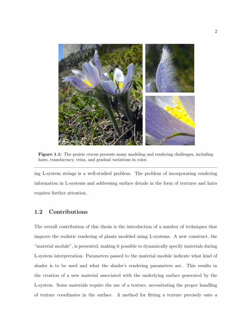
2

Figure 1.1: The prairie crocus presents many modeling and rendering challenges, includinghairs, translucency, veins, and gradual variations in color.

ing L-system strings is a well-studied problem. The problem of incorporating rendering

information in L-systems and addressing surface details in the form of textures and hairs

requires further attention.

1.2 Contributions

The overall contribution of this thesis is the introduction of a number of techniques that

improve the realistic rendering of plants modeled using L-systems. A new construct, the

“material module”, is presented, making it possible to dynamically specify materials during

L-system interpretation. Parameters passed to the material module indicate what kind of

shader is to be used and what the shader’s rendering parameters are. This results in

the creation of a new material associated with the underlying surface generated by the

L-system. Some materials require the use of a texture, necessitating the proper handling

of texture coordinates in the surface. A method for fitting a texture precisely onto a

3

generalized cylinder is presented, taking into account the contour of the cylinder to avoid

non-uniform spacing of the texture coordinates. These texture coordinates are used as the

basis of procedural shaders for generating translucent edges and parallel venation patterns,

whose parameters can be encoded in the L-system string via material modules. Texture

mapping of more complex venation patterns with bump mapping is also examined. In order

to properly shade the plant surfaces, a simple shader for leaves and petals is introduced.

This shader takes into account translucency and reflective properties of plant surfaces.

Finally, a method for generating hairs that protrude from the surface of the plant mesh is

introduced. Numerous synthetic plants modeled with cpfg [31, 80, 78, 81] and rendered

with Dali [36] are included throughout the thesis to illustrate the importance of the new

techniques.

1.3 Thesis Overview

Chapter 2 contains background information about L-systems and their implementation

using turtle geometry. An overview of rendering is presented in Chapter 3, both from

a theoretical and an applied standpoint. The shortcomings of specifying materials in L-

system implementations is discussed in Chapter 4, followed by a proposed solution involving

material modules. To achieve more realistic shading of plant surfaces, effective use of

skylight illumination and implementation of a leaf-and-petal shader is discussed in Chapter

5. Information about leaf structure and light interactions with plant tissues is used as a

basis of the shader. In Chapter 6, texture mapping of generalized cylinders is discussed, and

procedurally-based venation shaders are introduced as a means of adding surface detail to

leaves and petals. The incorporation of hairs into plant models generated using L-systems

is discussed in Chapter 7, along with a method for mapping hairs onto generalized cylinder

surfaces and controlling hair parameters. Finally, Chapter 8 contains a discussion of results

and probes future directions for research in realistic plant rendering.

Chapter 2

L-Systems

L-systems, named after their founder Aristid Lindenmayer [52], provide an elegant means

of modeling the development of plants. At the heart of L-systems is a string-rewriting

mechanism, which allows individual symbols in a string to be replaced by strings of new

symbols. A symbol can be used to denote a cell or organ in a plant, and the replacement

of the symbol by a successor sub-string may represent cell division or growth of plant

structure. L-systems provide a means of characterizing the topology of a plant at every

stage of its growth. Geometric aspects may be considered by interpreting L-systems using

turtle geometry [74]. Programs that implement L-systems and turtle geometry can associate

symbols and optional parameters with drawing commands, making it possible to visualize

plant structures. This section begins by describing L-systems at the topological level. We

then describe the implementation-specific details of L-systems for controlling geometry and

rendering properties.

2.1 Topology

L-systems compactly describe the topology or overall structure of plants [81]. The position

of symbols in an L-system string corresponds to the relative locations of plant organs.

The initial string of symbols is known as the axiom. As plants grow, new organs emerge,

resulting in more complex plant structure. At every time step, L-systems generate new

sequences of symbols by applying various productions or rewriting rules to a string. The

preceding string may be the axiom or a descendant string resulting from the previous

application of productions. The newly generated string, in turn, is passed back to the set

of productions at the next time step.

4

5

(a)

ab aa b a

b a a b aa b a b a a b a

(b)

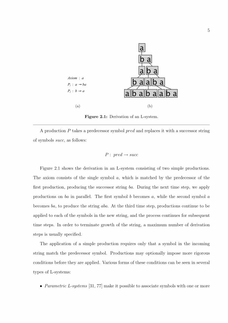
Figure 2.1: Derivation of an L-system.

A production P takes a predecessor symbol pred and replaces it with a successor string

of symbols succ, as follows:

P : pred → succ

Figure 2.1 shows the derivation in an L-system consisting of two simple productions.

The axiom consists of the single symbol a, which is matched by the predecessor of the

first production, producing the successor string ba. During the next time step, we apply

productions on ba in parallel. The first symbol b becomes a, while the second symbol a

becomes ba, to produce the string aba. At the third time step, productions continue to be

applied to each of the symbols in the new string, and the process continues for subsequent

time steps. In order to terminate growth of the string, a maximum number of derivation

steps is usually specified.

The application of a simple production requires only that a symbol in the incoming

string match the predecessor symbol. Productions may optionally impose more rigorous

conditions before they are applied. Various forms of these conditions can be seen in several

types of L-systems:

• Parametric L-systems [31, 77] make it possible to associate symbols with one or more

6

parameters. A symbol together with parameters is known as a module. Productions

may use these parameters to evaluate a boolean condition β. The predecessor will be

replaced with the successor only if the boolean condition evaluates to true:

P : pred block1 β block2 → succ

The optional blockn statements are used to calculate variables that can be used in the

condition or as new parameters for modules. The first block is executed prior to the

evaluation of the condition, while the second block is executed only if the condition

turns out true.

• Context-sensitive L-systems [52, 81] apply productions based on the context of the

predecessor in relation to neighbouring symbols in the string. The predecessor must

occur immediately after a matching left context lc and immediately before a matching

right context rc in order for the production to proceed:

P : lc < pred > rc → succ

• Stochastic L-systems [81] make it possible to specify the probability prob that a

production will be applied:

P : pred → succ : prob

These various types of L-systems are not mutually exclusive, and a single production may

utilize a combination of boolean, context-sensitive, and stochastic conditions. For example,

the following production

A(x) < B(y) > C(z) : m = x + 1m > z n = z − 1) → A(m)B(n) : 0.5

replaces module B with the module string AB, provided that B occurs between modules A

and C, and variable m is greater than parameter z. Furthermore, should these conditions be

7

met, a stochastic evaluation will determine whether or not the production will be applied.

If the production is applied, the newly computed variables m and n are used as parameters

for the modules in the resulting string.

The repetitive application of productions results in an ever-changing string, representing

a sequential ordering of symbols and modules. Plant structure, however, is rarely purely

sequential because of branching. In order to characterize branching in a string of symbols,

bracketed notation is utilized. Two specially defined symbols delimit a branch in a string

[52]:

[ Left bracket begins a branch.

] Right bracket ends a branch.

Pairs of brackets can be nested to an arbitrary degree, to represent higher-order branching

structures. The entire string segment between a left and right bracket, including all nested

brackets, describes a branch. The string segment between a left and right bracket, excluding

all nested brackets and strings therein, describes the branch axis.

2.2 Geometry

While topological considerations help define an abstract model of a structure, the geometric

treatment of L-systems makes it possible to use quantitative data for constructing and

visualizing a structure. As we move from the realm of theory to geometric implementation,

certain symbols in an L-system string serve as drawing commands for a LOGO-style turtle

[1, 90, 74]. In parametric L-systems, modules include parameters that provide quantitative

information for manipulating the turtle.

The turtle defines a right-handed local coordinate frame consisting of three orthogonal

vectors: heading−→H , left

−→L , and up

−→U (see Figure 2.2). The turtle moves forward in discrete

steps along its heading vector. By reorienting the coordinate frame at every step, the turtle

8

H\→

/L

−+

U→

→

^&

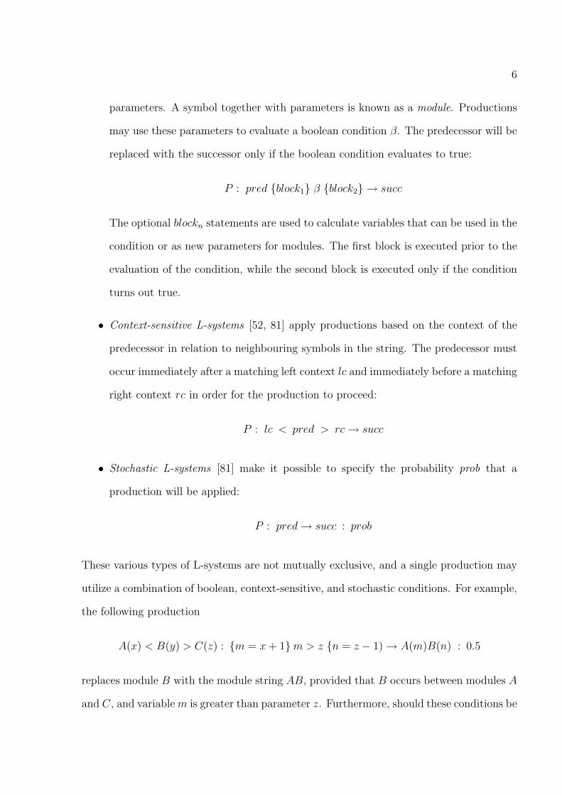
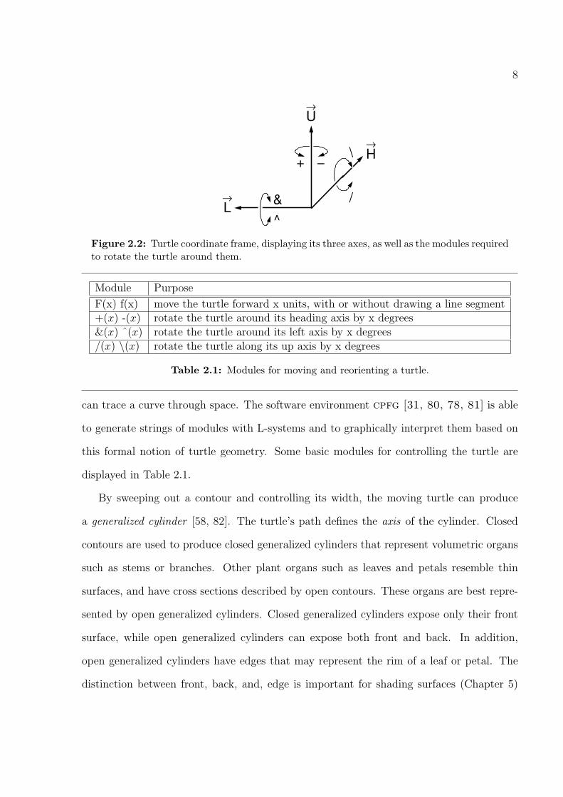
Figure 2.2: Turtle coordinate frame, displaying its three axes, as well as the modules requiredto rotate the turtle around them.

Module Purpose

F(x) f(x) move the turtle forward x units, with or without drawing a line segment+(x) -(x) rotate the turtle around its heading axis by x degrees&(x) ˆ(x) rotate the turtle around its left axis by x degrees/(x) \(x) rotate the turtle along its up axis by x degrees

Table 2.1: Modules for moving and reorienting a turtle.

can trace a curve through space. The software environment cpfg [31, 80, 78, 81] is able

to generate strings of modules with L-systems and to graphically interpret them based on

this formal notion of turtle geometry. Some basic modules for controlling the turtle are

displayed in Table 2.1.

By sweeping out a contour and controlling its width, the moving turtle can produce

a generalized cylinder [58, 82]. The turtle’s path defines the axis of the cylinder. Closed

contours are used to produce closed generalized cylinders that represent volumetric organs

such as stems or branches. Other plant organs such as leaves and petals resemble thin

surfaces, and have cross sections described by open contours. These organs are best repre-

sented by open generalized cylinders. Closed generalized cylinders expose only their front

surface, while open generalized cylinders can expose both front and back. In addition,

open generalized cylinders have edges that may represent the rim of a leaf or petal. The

distinction between front, back, and, edge is important for shading surfaces (Chapter 5)

9

Tk

Bk

AkMk

(a)

MkAk

Tk

Bk

(b)

Figure 2.3: Diagram of the kth segment of (a) an open generalized cylinder and (b) a closedgeneralized cylinder. The outer edges of the open segment and seam of the closed segmentare shown in red. Tk and Bk are the length (or circumference) of the top and bottom rims ofthe segment, respectively. The length of the axis is denoted Ak. The mid-arc of a cylinder isa line segment joining the midpoint of the top rim and bottom rim. The length of the mid-arcis denoted Mk.

and placing hairs (Chapter 7).

Generalized cylinders are polygonized into sequences of connected segments, where each

segment corresponds to a step taken by the turtle [58]. These segments consist in turn of

a strip of quadrilateral faces that approximate the cylinder shape defined by the contour.

In the actual implementation, each quadrilateral face may consist of two joined triangles,

but for the purpose of discussion, we will assume that each face is a quadrilateral. A

quadrilateral strip for an open cylinder segment has a top and bottom rim running between

the strip’s two outer edges. On a closed cylinder segment, these edges are joined along a

seam. Cylinder segments with open and closed contours are shown in Figure 2.3, along

with several measurements.

cpfg provides several modules to manipulate generalized cylinders [58]. The module

@Gs begins a generalized cylinder, @Gc instructs the turtle to sweep out a cylinder segment

during its next step, and @Ge ends the cylinder. The contour tracing out the generalized

cylinder can be scaled by a factor of s using the module !(s).

10

Figure 2.4: The material table and material properties as seen in the medit editor [19].

Certain lobed structures cannot be modeled by generalized cylinders, and are more

easily modeled using Bezier patches. The module ˜(p, s) places a Bezier patch p, and scales

it by factor s.

2.3 Rendering

Using the modules discussed thus far, it is possible to construct a geometric mesh of a plant

or its constituent organs. For realistic visualization, we must be able to shade the mesh.

This can be achieved by introducing several modules for rendering purposes.

Surface materials can be specified with the module ; (x). The parameter x indexes a

table with material presets (Figure 2.4). The material presets used by cpfg are all based

on the Phong model [9]. For each material, ambient, diffuse, and specular colors can be

defined, along with values for shininess and transparency.

Plant surfaces rarely have one solid color. Normally, there are subtle color gradations

along a stem or leaf. Gradations can be simulated by defining a range of gradually changing

materials in the color table, and changing the color index for every successive generalized

cylinder along the plant organ. However, even gradations cannot capture more complex

surface features, such as venation patterns or bark. For these purposes, texture mapping

11

is desirable, and cpfg can index a texture x using the module @Tx(x) [58, 59]. cpfg will

either overlay or blend the texture with the current material. The use of texture mapping

to add more detail to plants is discussed further in Chapter 6.

2.4 The Turtle Dispatcher

In order to visualize the results of an L-system, the drawing commands issued by symbols

or modules need to be sent to a rendering system. The actions defined by these drawing

commands are sufficiently high-level that a variety of rendering systems can be supported.

For every renderer, all that is required is a rendering interpreter that translates turtle com-

mands into function calls or statements supported by the renderer. cpfg provides a turtle

dispatcher interface, consisting of virtual function headers for every drawing command. A

rendering interpreter must implement each of these functions. When cpfg interprets an

L-system and encounters a particular drawing command, it calls the corresponding function

for the currently active interpreter. Conceptually, a turtle command has been issued, and

the rendering interpreter intercepts the command. For example, if cpfg is currently ren-

dering to OpenGL, the ; (x) module will trigger a “change material” command, which gets

dispatched to the material function in cpfg’s OpenGL interpreter in order to issue a glMa-

terial() call. When real-time rendering systems such as OpenGL are employed, the drawing

commands are immediately carried out, producing graphical results in a framebuffer. Of-

fline rendering systems, such as Dali and Renderman, require the rendering commands to

be written to a file which is processed at a later time when the renderer is invoked.

Chapter 3

Rendering Fundamentals

In order to synthesize realistic images in computer graphics, it is essential to simulate the

proper passage of light through a scene and to model interactions with materials when

light strikes a surface. After a discussion of terminology related to light propagation, we

will examine light-material interactions and examine the progression of rendering systems

toward global illumination solutions.

3.1 Radiometry

The body of work concerned with the measurement of radiant energy transfer is known as

radiometry. While the field of radiometry covers the entire spectrum of radiant energy from

radio waves to gamma rays, in image synthesis we are concerned in particular with visible

light. This section presents some of the important terminology introduced by radiometry.

Light is often described in terms of wave-particle duality [3]. Certain characteristics

of light, such as interference, diffraction, and polarization, can only be described by wave

phenomena. On the other hand, a particle analogy is required to explain the photoelectric

effect, whereby electrons are ejected from a surface upon the application of light. This dual

nature makes it necessary to describe light in terms of both waves and particles.

Light travels as packets of energy called photons, which have a particular wavelength

λ. The energy eλ of a photon can be computed through the use of Planck’s constant h and

the speed of light c:

eλ =hc

λ(3.1)

12

13

r = 1

ω

r = 1

Θ

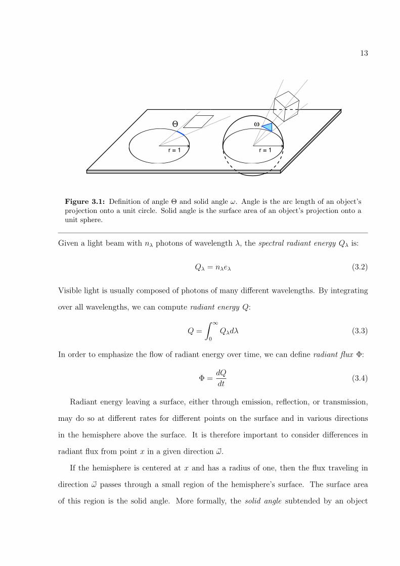
Figure 3.1: Definition of angle Θ and solid angle ω. Angle is the arc length of an object’sprojection onto a unit circle. Solid angle is the surface area of an object’s projection onto aunit sphere.

Given a light beam with nλ photons of wavelength λ, the spectral radiant energy Qλ is:

Qλ = nλeλ (3.2)

Visible light is usually composed of photons of many different wavelengths. By integrating

over all wavelengths, we can compute radiant energy Q:

Q =

∫ ∞

0

Qλdλ (3.3)

In order to emphasize the flow of radiant energy over time, we can define radiant flux Φ:

Φ =dQ

dt(3.4)

Radiant energy leaving a surface, either through emission, reflection, or transmission,

may do so at different rates for different points on the surface and in various directions

in the hemisphere above the surface. It is therefore important to consider differences in

radiant flux from point x in a given direction ~ω.

If the hemisphere is centered at x and has a radius of one, then the flux traveling in

direction ~ω passes through a small region of the hemisphere’s surface. The surface area

of this region is the solid angle. More formally, the solid angle subtended by an object

14

from a point x is defined to be the surface area of the projection of the object onto a unit

sphere centered at x. A solid angle is a generalization of the concept of an angle in two

dimensions to three dimensions (Figure 3.1). Angles are measured in radians, and solid

angles in steradians (sr). In the same way that the angle subtended by an enclosing circle

is 2π rad (the circumference of a circle), the solid angle subtended by an enclosing sphere

is 4π sr (the surface area of a sphere).

Radiance L is the radiant flux per unit area perpendicular to the direction of travel,

per unit solid angle:

L(x, ~ω) =d2Φ

cos θ dA d~ω(3.5)

Conceptually, radiance is a measure of the number of photons arriving at or leaving from

a small area in a particular direction (Figure 3.2). Spectral radiance Lλ is a measure of

radiance for photons of a certain wavelength λ (i.e. light of a particular color).

If we integrate radiance over all directions, we are able to compute radiosity B, the flux

leaving a point x, and irradiance E, the flux arriving at a point x:

B(x) = E(x) =dΦ

dA(3.6)

Radiance, radiosity, and irradiance are important entities in computer graphics, as they

provide a means of expressing light transfer between light sources and objects. We shall

now consider what happens when light actually hits an object.

3.2 Light-Material Interactions

Light traveling toward an object consists of photons of particular wavelengths. The col-

oration of this light, as perceived by a viewer, depends on the photons’ wavelengths, while

the intensity of the light depends on the number of photons. When light strikes the object’s

surface, the photons interact with the material in different ways.

15

Θ

dω Ln

dA

Figure 3.2: Definition of radiance L. Radiance is radiant flux per unit projected area dAper unit solid angle d~ω.

A material can be thought of as a volumetric collection of small particles suspended

in a medium [71] (Figure 3.3). If these particles are packed tightly together, an incoming

photon is unable to penetrate the material and will reflect directly from the surface. If

the particles are loosely packed, the photon may pass partially through the medium before

colliding with a particle. During a photon-particle collision, the photon may be selectively

absorbed depending on its wavelength [3]. The net effect is that more photons of certain

wavelengths are absorbed than photons of other wavelengths, and the color of the light

changes. A photon may undergo several successive collisions with particles before emerging

from a different point on the surface; this phenomenon is called subsurface scattering.

Alternatively, light may completely miss particles, retaining its original color but emerging

with a reduced intensity, due to photon absorption in the medium.

Interactions between photons and materials result in reflected or transmitted light hav-

ing a different radiance than incoming light. Calculating this change in radiance is an

important step for determining the appearance of a surface. In general, the outgoing radi-

ance Lo in direction ~ω from point x on a surface can be computed as follows:

Lo(x, ~ω) = Le(x, ~ω) + Lr(x, ~ω) + Lt(x, ~ω) (3.7)

where Le is emitted radiance, Lr is reflected radiance, and Lt is transmitted radiance.

16

(a) (b) (c)

Figure 3.3: Light-material interactions shown in cross-section. Photons striking the materialmay follow one of several paths. In (a), a photon is reflected at the surface after a singlecollision with a particle. In (b), a photon penetrates the material and subsurface scatteringtakes place due to collisions with multiple particles. In (c), no particle collisions take place.

Emitted radiance need only be considered if the material emits energy, as in the case of a

heated element or phosphorous compound. For materials that do not emit energy, only the

reflected and transmitted radiance terms are of interest.

The reflected radiance depends on all the incoming radiance Li arriving from various

directions ~ω′ within the hemisphere Ω above the surface:

Lr(x, ~ω) =

∫Ω

fr(x, ~ω′, ~ω)Li(x, ~ω′)(~ω′ · ~n)d~ω′ (3.8)

The term (~ω′ · ~n) is required according to Lambert’s Law, which states that a light source

directly above a surface delivers the most radiance, while radiance gradually decreases as

a light source sets toward the surface’s horizon. The incoming radiance must be scaled

by the factor fr to account for energy absorbed by the surface. This factor is known as

the BRDF (Bidirectional Reflectance Distribution Function) [66], if we assume that light

arrives and leaves at the same point on a surface.

Formally, a BRDF is the ratio of reflected radiance to irradiance:

fr(x, ~ω′, ~ω) =dLr(x, ~ω)

dEi(x, ~ω′)(3.9)

and has units of sr−1. In this way, a BRDF can be considered to be a density function,

describing the attenuation of radiance per unit steradians. The function can be visualized

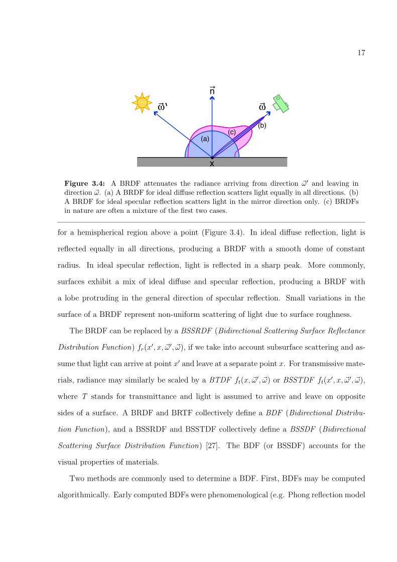
17

ω‘ ωn

x

(a)(c)

(b)

Figure 3.4: A BRDF attenuates the radiance arriving from direction ~ω′ and leaving indirection ~ω. (a) A BRDF for ideal diffuse reflection scatters light equally in all directions. (b)A BRDF for ideal specular reflection scatters light in the mirror direction only. (c) BRDFsin nature are often a mixture of the first two cases.

for a hemispherical region above a point (Figure 3.4). In ideal diffuse reflection, light is

reflected equally in all directions, producing a BRDF with a smooth dome of constant

radius. In ideal specular reflection, light is reflected in a sharp peak. More commonly,

surfaces exhibit a mix of ideal diffuse and specular reflection, producing a BRDF with

a lobe protruding in the general direction of specular reflection. Small variations in the

surface of a BRDF represent non-uniform scattering of light due to surface roughness.

The BRDF can be replaced by a BSSRDF (Bidirectional Scattering Surface Reflectance

Distribution Function) fr(x′, x, ~ω′, ~ω), if we take into account subsurface scattering and as-

sume that light can arrive at point x′ and leave at a separate point x. For transmissive mate-

rials, radiance may similarly be scaled by a BTDF ft(x, ~ω′, ~ω) or BSSTDF ft(x′, x, ~ω′, ~ω),

where T stands for transmittance and light is assumed to arrive and leave on opposite

sides of a surface. A BRDF and BRTF collectively define a BDF (Bidirectional Distribu-

tion Function), and a BSSRDF and BSSTDF collectively define a BSSDF (Bidirectional

Scattering Surface Distribution Function) [27]. The BDF (or BSSDF) accounts for the

visual properties of materials.

Two methods are commonly used to determine a BDF. First, BDFs may be computed

algorithmically. Early computed BDFs were phenomenological (e.g. Phong reflection model

18

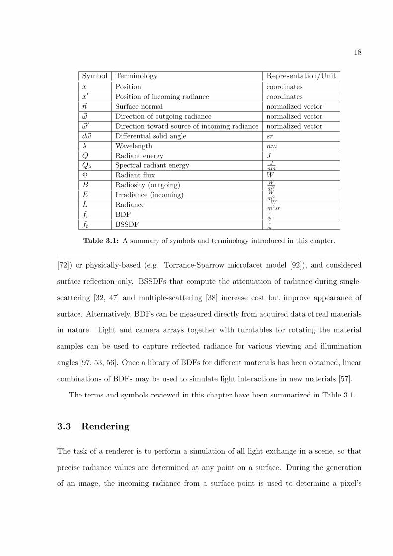
Symbol Terminology Representation/Unit

x Position coordinatesx′ Position of incoming radiance coordinates~n Surface normal normalized vector~ω Direction of outgoing radiance normalized vector~ω′ Direction toward source of incoming radiance normalized vectord~ω Differential solid angle sr

λ Wavelength nm

Q Radiant energy J

Qλ Spectral radiant energy Jnm

Φ Radiant flux W

B Radiosity (outgoing) Wm2

E Irradiance (incoming) Wm2

L Radiance Wm2sr

fr BDF 1sr

ft BSSDF 1sr

Table 3.1: A summary of symbols and terminology introduced in this chapter.

[72]) or physically-based (e.g. Torrance-Sparrow microfacet model [92]), and considered

surface reflection only. BSSDFs that compute the attenuation of radiance during single-

scattering [32, 47] and multiple-scattering [38] increase cost but improve appearance of

surface. Alternatively, BDFs can be measured directly from acquired data of real materials

in nature. Light and camera arrays together with turntables for rotating the material

samples can be used to capture reflected radiance for various viewing and illumination

angles [97, 53, 56]. Once a library of BDFs for different materials has been obtained, linear

combinations of BDFs may be used to simulate light interactions in new materials [57].

The terms and symbols reviewed in this chapter have been summarized in Table 3.1.

3.3 Rendering

The task of a renderer is to perform a simulation of all light exchange in a scene, so that

precise radiance values are determined at any point on a surface. During the generation

of an image, the incoming radiance from a surface point is used to determine a pixel’s

19

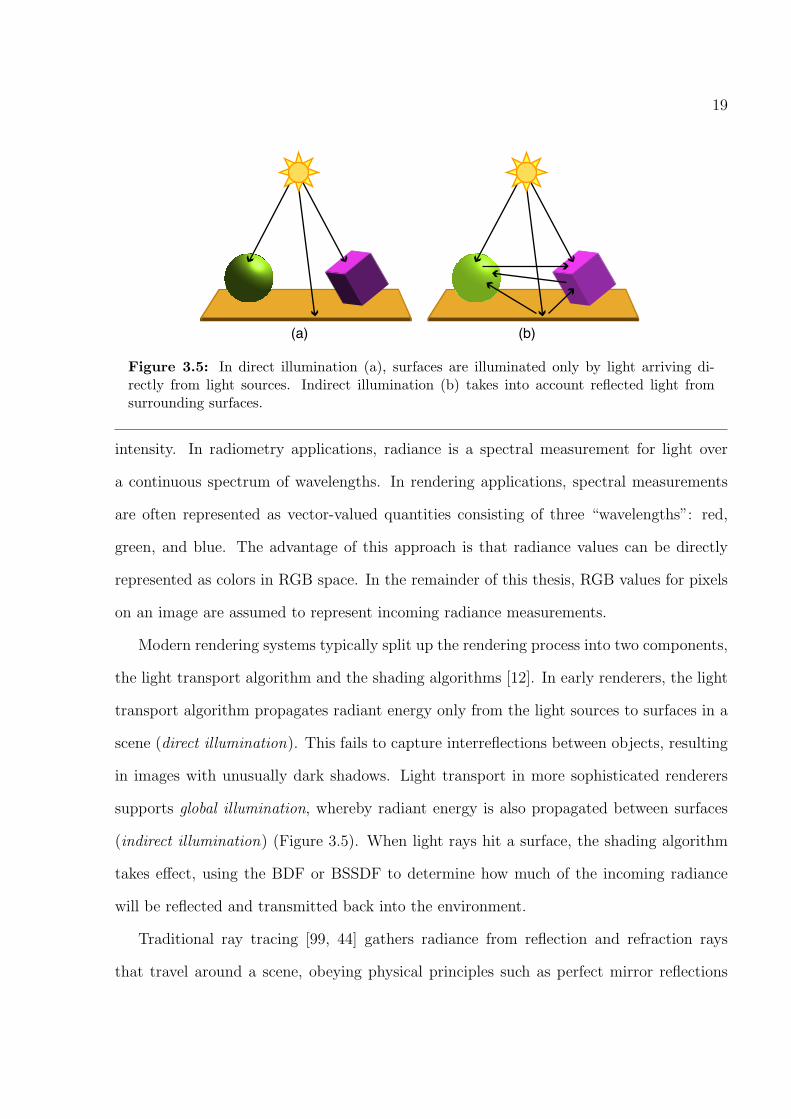
(a) (b)

Figure 3.5: In direct illumination (a), surfaces are illuminated only by light arriving di-rectly from light sources. Indirect illumination (b) takes into account reflected light fromsurrounding surfaces.

intensity. In radiometry applications, radiance is a spectral measurement for light over

a continuous spectrum of wavelengths. In rendering applications, spectral measurements

are often represented as vector-valued quantities consisting of three “wavelengths”: red,

green, and blue. The advantage of this approach is that radiance values can be directly

represented as colors in RGB space. In the remainder of this thesis, RGB values for pixels

on an image are assumed to represent incoming radiance measurements.

Modern rendering systems typically split up the rendering process into two components,

the light transport algorithm and the shading algorithms [12]. In early renderers, the light

transport algorithm propagates radiant energy only from the light sources to surfaces in a

scene (direct illumination). This fails to capture interreflections between objects, resulting

in images with unusually dark shadows. Light transport in more sophisticated renderers

supports global illumination, whereby radiant energy is also propagated between surfaces

(indirect illumination) (Figure 3.5). When light rays hit a surface, the shading algorithm

takes effect, using the BDF or BSSDF to determine how much of the incoming radiance

will be reflected and transmitted back into the environment.

Traditional ray tracing [99, 44] gathers radiance from reflection and refraction rays

that travel around a scene, obeying physical principles such as perfect mirror reflections

20

and Snell’s Law. Every time a ray hits an object, shadow rays are spawned to sample

light sources directly and check for impeding objects. The algorithm is recursive, allowing

rays to follow reflected and refracted paths to an arbitrary depth. Objects, reflections,

and shadows in the resulting images appear very crisp, to the extent that they no longer

look natural. By splitting a ray into multiple rays and using stochastic sampling to find

the average radiance, distribution ray tracing [14, 13] made it possible to render fuzzy

phenomena such as gloss, translucency, depth of field, and motion blur. Multiple shadow

rays could be used to sample area light sources, producing soft shadows.

Early ray tracing techniques did not simulate illumination due to diffuse reflections

from surroundings. The problem was simultaneously addressed in two publications [29, 67]

through the use of finite elements. The surfaces in a scene are subdivided into tiles, and

exchanged radiant energy between tiles is computed by solving a system of linear equa-

tions. This technique is the foundation of radiosity methods, which make it possible to

compute view independent global illumination solutions. However, radiosity methods are

costly for complex models with many tiles and non-diffuse surfaces. Taking inspiration

from distribution ray tracing, Kajiya [40] proposed the use of stochastic sampling to gather

reflected radiance from surrounding surfaces in ray tracing methods. Because of the re-

cursive nature of ray tracing, the number of sampling rays increases exponentially as the

depth of reflections increases. To prevent this situation, Kajiya presented a solution called

path tracing (Figure 3.6). Whenever a ray hits a surface, only a single stochastic ray is

chosen to estimate the indirect illumination.

Pixels in an image produced by path tracing must be supersampled to ensure that suffi-

cient stochastic paths have been followed for a reasonable estimation of reflected radiance.

If too few paths are followed, variances in the estimates result in noisy images. For scenes

with complex illumination, pixels may need to be sampled with hundreds or thousands of

paths to produce acceptable images. Photon mapping [35] considerably improves perfor-

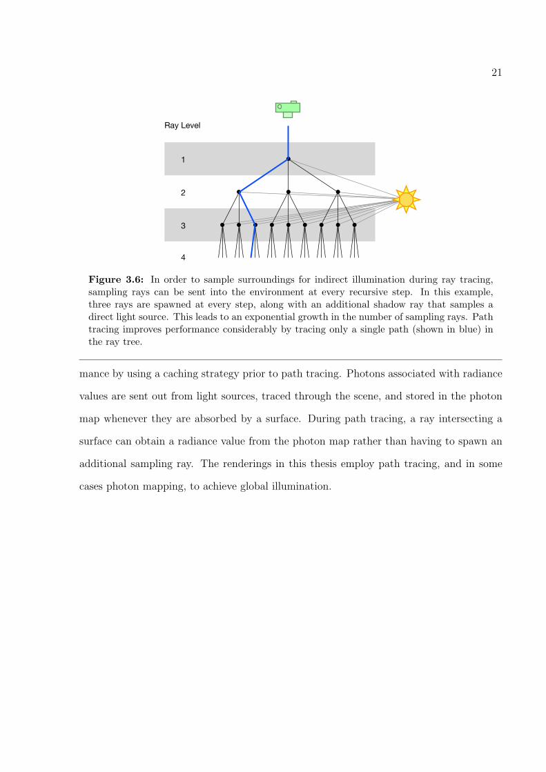
21

2

3

4

1

Ray Level

Figure 3.6: In order to sample surroundings for indirect illumination during ray tracing,sampling rays can be sent into the environment at every recursive step. In this example,three rays are spawned at every step, along with an additional shadow ray that samples adirect light source. This leads to an exponential growth in the number of sampling rays. Pathtracing improves performance considerably by tracing only a single path (shown in blue) inthe ray tree.

mance by using a caching strategy prior to path tracing. Photons associated with radiance

values are sent out from light sources, traced through the scene, and stored in the photon

map whenever they are absorbed by a surface. During path tracing, a ray intersecting a

surface can obtain a radiance value from the photon map rather than having to spawn an

additional sampling ray. The renderings in this thesis employ path tracing, and in some

cases photon mapping, to achieve global illumination.

Chapter 4

Dynamic Specification of Materials

This chapter discusses two concepts that lie at the heart of rendering techniques: shaders

and materials. The current deficiencies in support for shaders and materials in the realm

of L-systems are outlined and discussed. The dynamic specification of materials and their

parameters in the context of L-systems is then proposed.

4.1 Shaders

The process of rendering involves shading surfaces so that they assume a desired appear-

ance. Just as there is literally an endless variation of possible surface appearances, shading

algorithms are limited only by the imagination of the shader writer. Whether the goal is

to create a realistic backlit arbour of leaves or an artistic charcoal rendition of a flower, the

act of shading a surface requires computing intensity values for pixels in the final image.

A shader is a subroutine that defines a BDF or BSSDF so that the outgoing radiance

from a point on a surface can be computed based on incoming radiance. Early renderers

[100] compiled shader subroutines directly into the codebase, making it difficult to extend a

renderer with new shaders. Cook [12] recognized shaders as independent, modular entities

that could be separated from the light transport algorithm of the renderer. Many rendering

programs subsequently provided support for their own shading languages [94, 68, 55, 87]

and allowed shaders to be compiled and loaded as independent modules.

Each shader requires a set of appearance parameters [12] used by the BDF calculation.

Appearance parameters can by varying or uniform [33]. Varying parameters may change

for every point that requires shading. Examples of varying parameters include the shading

normal and uv -coordinates. Shaders typically obtain the varying parameters directly from

22

23

the renderer. Uniform appearance parameters remain constant wherever a shader is applied.

They are typically supplied by the user, and specify properties such as diffuse color, specular

color, and translucency. A uniform appearance parameter does not imply a uniform surface

appearance. For example, the endpoint colors of a gradient may be uniform appearance

parameters, but the shader can interpolate between these colors to generate a surface that

appears anything but uniform.

In this thesis, we call the list of uniform appearance parameters along with their data

types a shader description. The shader description separates the list of parameters required

by the shader from the underlying implementation.

This high-level treatment of shaders is useful, since shaders are typically not compatible

between rendering systems. One notable exception is the family of rendering systems

based on the Renderman interface [94], making it possible to write a single shader that

works under multiple systems. However, many other rendering systems either provide a

built-in set of shaders or provide their own custom shading language or API for building

shaders. While these shaders cannot be swapped between systems because of varying

implementations, their shader descriptions are often very similar. For example, Phong

shaders that require a diffuse color and a specular color, along with a specular highlight

coefficient, can have an identical shader description, even though the shaders may be locked

into their rendering system at an implementation level.

When all of the uniform parameters in a shader description have been specified, they

are said to be bound [33], and a shader instance, or material, has been created (see Figure

4.1). In this way, shaders and materials are analogous to the concept of classes and objects

in object-oriented programming languages. Shaders provide the engine for generating a

class of surface appearances, and they have a clearly defined shader description (similar to

a class interface). Materials, similarly to objects, add the specific parameters required to

produce a particular surface. In the same way that a class interface is designed to hide

24

color ambientcolor phong

color diffusecolor specular

0.2 0 0

int coefficient0.5 0.5 0.5

1 0 0

100

red material

Figure 4.1: A material is formed when a shader’s appearance parameters are bound tospecific values. This diagram depicts a reflective, red material based on a Phong shaderin the Dali renderer. The blue box is the shader description, which lists the appearanceparameters and indicates that the Phong shader returns a color.

the complexity of a class’ implementation from the user, shader descriptions indicate what

values must be supplied, without requiring detailed knowledge of how these values are used

in the shader’s rendering calculations.

4.2 Rendering Limitations in L-systems

In order to visualize an L-system model, the modules in an L-system string must be graph-

ically interpreted. Rendering may take place in real-time, if technologies such as OpenGL

[87] are used, or it may be deferred for high-quality, offline rendering. If a real-time system

is used, L-system modules and their parameters must be immediately translated into ren-

dering instructions and passed via memory to the renderer. For offline rendering systems,

these instructions are usually written to a file whose format conforms to the renderer’s

specifications. The file is then processed by the renderer at a later time.

What is the nature of the rendering instructions? Besides setting up camera and lighting

information, they describe two key pieces of information about the model. First, they

specify the geometry of the model, by defining various transformations and describing

surfaces in the form of polygonal meshes or parametric surfaces. Second, the instructions

specify the materials that are used to shade various parts of the model.

L-systems have traditionally been used as a modeling tool [75, 79, 58, 82, 43], and conse-

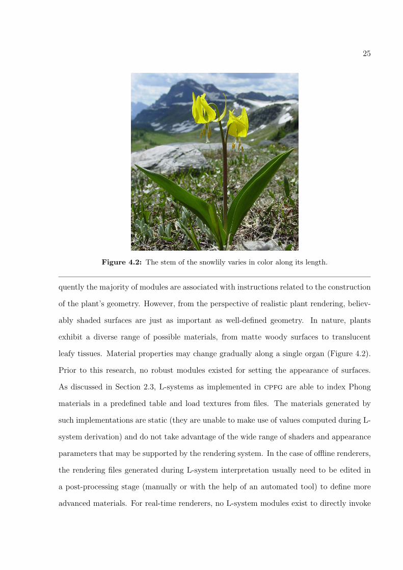
25

Figure 4.2: The stem of the snowlily varies in color along its length.

quently the majority of modules are associated with instructions related to the construction

of the plant’s geometry. However, from the perspective of realistic plant rendering, believ-

ably shaded surfaces are just as important as well-defined geometry. In nature, plants

exhibit a diverse range of possible materials, from matte woody surfaces to translucent

leafy tissues. Material properties may change gradually along a single organ (Figure 4.2).

Prior to this research, no robust modules existed for setting the appearance of surfaces.

As discussed in Section 2.3, L-systems as implemented in cpfg are able to index Phong

materials in a predefined table and load textures from files. The materials generated by

such implementations are static (they are unable to make use of values computed during L-

system derivation) and do not take advantage of the wide range of shaders and appearance

parameters that may be supported by the rendering system. In the case of offline renderers,

the rendering files generated during L-system interpretation usually need to be edited in

a post-processing stage (manually or with the help of an automated tool) to define more

advanced materials. For real-time renderers, no L-system modules exist to directly invoke

26

a desired shader with specific parameters. In short, a new mechanism is required to allow

L-system models to provide detailed information about materials. Together, geometry and

material parameters serve to comprehensively describe the visual nature of a plant within

an L-system.

4.3 Requirements

Several requirements should be met when specifying new materials from an L-system.

• Support for arbitrary shaders. It should be possible to specify any shader sup-

ported by a rendering system. Shader descriptions provide a high-level interface

between the L-system and the shaders of the underlying rendering system.

• Support for multiple appearance parameters. Because shaders may require

anywhere from zero to several dozen appearance parameters, it should be possible to

specify an arbitrary number of parameters for a new material.

• Dynamic declarations. It should be possible to generate new materials on the

fly, using parameters that are calculated during the derivation of the L-system. A

predefined table of static materials, such as the material table used by cpfg, is not

sufficient by itself, although it could be used in conjunction with dynamic material

declarations.

• Compatibility with multiple rendering systems. Because a single L-system can

be used to generate plant models for several rendering systems, it must be possible

to indicate which systems the materials are targeted toward.

The overall goal is to be able to specify any material at any point during L-system inter-

pretation, for any supported rendering system. The solution found during the course of

this research is presented in the remaining sections.

27

4.4 Material Modules

In order to specify a new material dynamically, it must be specified within the L-system.

Variables computed during L-system derivation can then be utilized as parameters for the

material. We define a material module to provide information about the new material.

Two important parameters are s, the name of the shader, and p = p1, p2, . . . , pn, the set

of appearance parameters:

@Mt(s, p)

The number and types of parameters that a particular shader can accept is provided by

a shader description. A shader file containing a list of shader descriptions is parsed prior to

L-system interpretation. Each shader description specifies the name of the shader, followed

by a list of uniform appearance parameter names and their data types. For this research,

the following data types have been used: int, float, string, color, vector, and shader 1. The

first three data types reflect their counterparts in programming languages such as C++

and Java. Color and vector are three-element arrays of floats, which can be used for RGB

values or normals. The shader data type references shaders, and is useful for shade tree

constructs (see Section 4.6). Each appearance parameter can optionally be given a default

value, to be utilized if no corresponding parameter is specified in the L-system material

module.

Because an L-system can generate rendering instructions for multiple rendering systems,

shader descriptions in the shader file must be associated with specific renderers. During

graphical interpretation of the L-system string, only those shader descriptions associated

with the target rendering system (i.e. the rendering system being used to graphically view

the L-system model) are utilized. In the cpfg shader file, a list of renderers is prepended

to each shader description (Figure 4.3). A shader description without a renderer list is

1Parameter values for L-system modules in cpfg are not typed. These values need to be cast to theappropriate data types required by the appearance parameters.

28

DALI lambert color diffuse;;

RIB matte float Ka = 0.2; float Kd = 0.8; color 'color' = 0.6 0.4 0;;

RAYSHADE DALI phong color ambient = 0.2 0 0; color diffuse = 1 0 0; color specular = 0.5 0.5 0.5;;

OPENGL GL color ambient; color diffuse; color specular; int coefficient;;

Figure 4.3: Sample shader descriptions in a cpfg shader file. Keywords are shown inblue. Each shader description is associated with one or more compatible renderers. Of thetwo Lambertian shaders, lambert will only be used by Dali, and matte will only be usedby Renderman. Phong is supported by Rayshade and Dali. The GL shader descriptionis targeted specifically for OpenGL. The appearance parameters for matte and phong areassociated with default values. Shader or parameter names that conflict with keywords mustbe placed in quotes.

automatically associated with all renderers. When a material module is encountered in

the L-system, rendering instructions for the material are generated only if the shader is

supported by the target rendering system. If the shader is supported, rendering instructions

for the new material are generated; otherwise, the material module is skipped.

Different renderers usually support shaders that perform identical or similar appearance

calculations. Sometimes the shader descriptions are identical. For example, Dali and

Rayshade [48] support Phong shaders with three appearance parameters specifying a color:

ambient, diffuse, and specular. The shader file in Figure 4.3 illustrates how a single Phong

shader description can be used for both renderers. More often, shader descriptions differ

slightly, and two separate entries are required. For example, Dali and Renderman both

support Lambertian shaders. In Renderman, the shader is called matte, and requires three

appearance parameters: Ka (ambient reflectance term), Kd (diffuse reflectance term), and

29

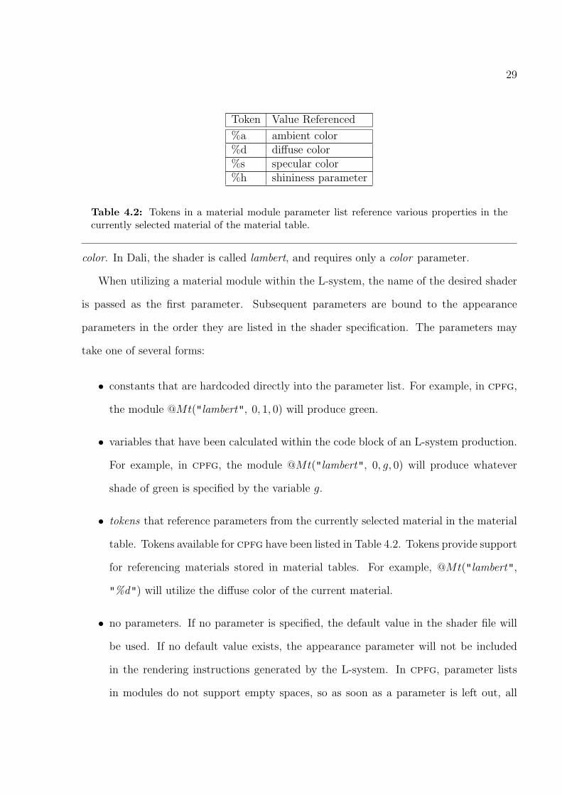
Token Value Referenced

%a ambient color%d diffuse color%s specular color%h shininess parameter

Table 4.2: Tokens in a material module parameter list reference various properties in thecurrently selected material of the material table.

color. In Dali, the shader is called lambert, and requires only a color parameter.

When utilizing a material module within the L-system, the name of the desired shader

is passed as the first parameter. Subsequent parameters are bound to the appearance

parameters in the order they are listed in the shader specification. The parameters may

take one of several forms:

• constants that are hardcoded directly into the parameter list. For example, in cpfg,

the module @Mt("lambert", 0, 1, 0) will produce green.

• variables that have been calculated within the code block of an L-system production.

For example, in cpfg, the module @Mt("lambert", 0, g, 0) will produce whatever

shade of green is specified by the variable g.

• tokens that reference parameters from the currently selected material in the material

table. Tokens available for cpfg have been listed in Table 4.2. Tokens provide support

for referencing materials stored in material tables. For example, @Mt("lambert",

"%d") will utilize the diffuse color of the current material.

• no parameters. If no parameter is specified, the default value in the shader file will

be used. If no default value exists, the appearance parameter will not be included

in the rendering instructions generated by the L-system. In cpfg, parameter lists

in modules do not support empty spaces, so as soon as a parameter is left out, all

30

0.2

0.4

0.6

0.8

1.0

x

y 0.00.00.20.40.60.8

(a) (b)

Figure 4.4: An OpenGL snapshot (b) of the cylinder produced by the L-system in Algorithm1, making use of material modules to change material properties. The function (a) was usedto compute the intensity of the specular component along the length of the cylinder.

subsequent parameters must also be left out. For example, using the matte shader in

Figure 4.3, it is possible to write @Mt("matte", 1, 0.5) to use the default parameter

for color, but attempting to use the default parameter for ambient reflectance as well,

by writing @Mt("matte", , 0.5), would produce an error.

4.5 Example: Color Gradient on a Cylinder

To demonstrate the use of material modules, we will generate the Phong-shaded cylinder

shown in Figure 4.4. The cylinder gradually changes color from green to red, and has a

specular highlight just past its midsection. The L-system in Algorithm 1 produces the

cylinder. The first two lines set the cylinder length and the turtle’s step size. The axiom

on line 3 loads a static material from the table, adjusts the cylinder width, and begins

the cylinder with @Gs. The production B repeatedly advances the turtle and draws a

generalized cylinder segment @Gc (line 13) as long as the current position is less than the

total axis length (line 4). For every step, we calculate the relative distance traveled by

the turtle (line 6). In lines 7 and 8, values for red and green are set proportionally and

inversely proportionally to the turtle’s relative distance along the cylinder axis. A value

for specular color is computed from a function in line 9. The material module in line 11

31

Algorithm 1 This L-system draws a generalized cylinder with changing Phong parametersfor every turtle step.

1. #define l 100 /* length of axis */

2. #define ∆s 1 /* turtle step */

3. Axiom: ;(1) !(40) @Gs B(0)

4. B(s): s ≤ l

5.

6. relativeDistance = s/l;

7. r = relativeDistance;

8. g = 1− relativeDistance;

9. s = func(1, relativeDistance);

10. −→

11. @Mt("GL", "%a", r, g, 0, s, s, s, "%h")

12. @Mt("phong", "%a", r, g, 0, s, s, s)

13. f(∆s) @Gc B(s + ∆s)

14. B(s): s ≥ l −→ @Ge

specifies the GL shader declared in the shader file in Figure 4.3. The ambient and specular

coefficient properties are specified using tokens, which reference the material loaded in the

axiom. The diffuse color and specular colors are dynamically specified using the variables

from lines 7 - 9. According to the shader file, the material based on the GL shader will

only be generated if OpenGL is used, so another material module has been added on line

12. This module references the Phong shader description for Dali and Rayshade, so the

cylinder’s materials will also be generated if the L-system is graphically interpreted for

either of these offline renderers.

32

4.6 Shade Trees

While simple shaders such as phong and matte require only several appearance parame-

ters, complex shaders may easily require several dozen parameters that are passed through

a complex rendering calculation. In order to increase the maintainability of a complex

shader, it can be decomposed into smaller modular units or sub-shaders that perform

nested operations. Sub-shaders operate conceptually like shaders, in that they generate

a value based on input from appearance parameters. In this thesis, a sub-shader whose

appearance parameters are bound to values is termed a sub-material.

Sub-shaders constituting a shader can be arranged as a shade tree [12]. Nodes in the

tree represent sub-shaders. Each sub-shader returns a value that can be bound to an

appearance parameter in the parent node. The root node must produce a radiance value in

order to generate a pixel in the final image. Leaves of the tree represent parameter values.

A node together with its leaves represents a sub-material.

Appearance parameters can now be obtained via explicit values, or from the value

returned by a sub-shader. The appearance parameters of some types of shaders require

not just a value, but a reference to the sub-shader itself. These appearance parameters are

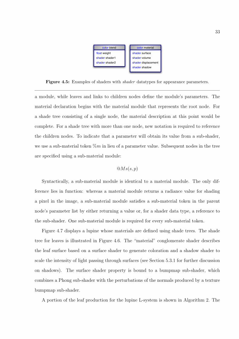
associated with the shader data type. Two example shaders with shader parameters (see

Figure 4.5) are:

• blend shaders : A blend shader blends together the results of two shaders, based on

the value of a weight parameter.

• conglomerate shaders : A conglomerate shader is a collection of several different types

of shaders that function in parallel. Many rendering systems permit the use of a

surface shader, volume shader, displacement shader, and shadow shader for a single

material.

A shade tree is specified in an L-system using preorder traversal. Each node is declared as

33

shader shader1

color blend

shader shader2

float weightshader volume

color material

shader displacement

shader surface

shader shadow

Figure 4.5: Examples of shaders with shader datatypes for appearance parameters.

a module, while leaves and links to children nodes define the module’s parameters. The

material declaration begins with the material module that represents the root node. For

a shade tree consisting of a single node, the material description at this point would be

complete. For a shade tree with more than one node, new notation is required to reference

the children nodes. To indicate that a parameter will obtain its value from a sub-shader,

we use a sub-material token %m in lieu of a parameter value. Subsequent nodes in the tree

are specified using a sub-material module:

@Ms(s, p)

Syntactically, a sub-material module is identical to a material module. The only dif-

ference lies in function: whereas a material module returns a radiance value for shading

a pixel in the image, a sub-material module satisfies a sub-material token in the parent

node’s parameter list by either returning a value or, for a shader data type, a reference to

the sub-shader. One sub-material module is required for every sub-material token.

Figure 4.7 displays a lupine whose materials are defined using shade trees. The shade

tree for leaves is illustrated in Figure 4.6. The “material” conglomerate shader describes

the leaf surface based on a surface shader to generate coloration and a shadow shader to

scale the intensity of light passing through surfaces (see Section 5.3.1 for further discussion

on shadows). The surface shader property is bound to a bumpmap sub-shader, which

combines a Phong sub-shader with the perturbations of the normals produced by a texture

bumpmap sub-shader.

A portion of the leaf production for the lupine L-system is shown in Algorithm 2. The

34

shader shadow

color material

shader surface

shader 'shader'

color bumpmap

shader bump

color ambient

color phong

color diffusecolor specularint coefficient

int project

vector texture_bumpmap_normal

string texture

float bump_scaleint wrap

color shadow_scale

color scale

float specular_scale

Figure 4.6: A simple shade tree used to render lupine leaves in Dali.

shade tree for leaf materials is shown in lines 10 to 14. The sub-material modules have

been indented to reflect the traversal of the shade tree.

Materials parameters are dynamically specified using positional information. Organ

features frequently vary as a function of position on a plant. While positional information

was previously used to adjust geometric features [82], here it is used to influence rendering

parameters. The lupine’s stem and leaf color have been set as a function of position along

the plant’s axis, with lower leaves appearing yellowish. As we move upward along the plant,

we adjust the leaf coloration to increasingly deeper shades of green. We give young leaves

near the top of the lupine a waxier appearance by adjusting specular highlight coefficient

and specular scale of the surface material. Bump mapping gives the leaves a slightly

wrinkled appearance. The height of the simulated bumps produced by bump mapping is

gradually decreased as we move upward along the plant. The material properties for the

flowers have been similarly adjusted according to positional information. The rendering

instructions for one of the leaf materials generated by the L-system is shown in Figure 4.8.

35

Figure 4.7: Lupine. Rendering properties such as color, specularity, and bump mapping arecontrolled through the use of material modules.

36

Algorithm 2 A snippet from the lupine L-system, illustrating the use of the shade treein Figure 4.6 to construct materials. The leaf rendering parameters are based on the leaf’sdistance from the base of the plant.

1. Leaf(relativeDistance): 0 ≤ relativeDistance ≤ 1

2.

3. r = func(RED, relativeDistance);

4. g = func(GREEN, relativeDistance);

5. b = func(BLUE, relativeDistance);

6. bumpiness = 2.3− 2× relativeDistance;

7. coefficient = 20− relativeDistance× 18;

8. specular scale = 0.2 + 0.8× relativeDistance;

9. −→

10. @Mt(”material”, ”%m”, ”%m”)

11. @Ms(”bumpmap”, ”%m”, ”%m”)

12. @Ms(”texture bumpmap normal”, ”bumpy.png”, 3, bumpiness, 1)

13. @Ms(”phong”, 0, 0, 0, r, g, b, ”%s”, coefficient , specular scale)

14. @Ms(”shadow scale”, 0.2, 0.25, 0.2)

15. . . .

4.7 Implementation

An outline of the implementation of dynamically generated materials in cpfg is pictured

in Figure 4.9. When cpfg is run, it generates graphical output for a target rendering

system, whether it be a realtime system (OpenGL) or an offline system (Dali, Rayshade,

Renderman, etc.). cpfg must provide the instructions for generating new materials in the

the target rendering system.

An L-system file describing a plant model along with material specifications is given to

37

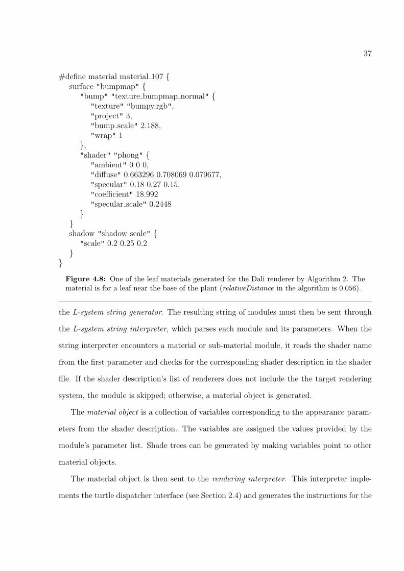
#define material material 107 surface "bumpmap"

"bump" "texture bumpmap normal" "texture" "bumpy.rgb","project" 3,"bump scale" 2.188,"wrap" 1

,"shader" "phong"

"ambient" 0 0 0,"diffuse" 0.663296 0.708069 0.079677,"specular" 0.18 0.27 0.15,"coefficient" 18.992"specular scale" 0.2448

shadow "shadow scale"

"scale" 0.2 0.25 0.2

Figure 4.8: One of the leaf materials generated for the Dali renderer by Algorithm 2. Thematerial is for a leaf near the base of the plant (relativeDistance in the algorithm is 0.056).

the L-system string generator. The resulting string of modules must then be sent through

the L-system string interpreter, which parses each module and its parameters. When the

string interpreter encounters a material or sub-material module, it reads the shader name

from the first parameter and checks for the corresponding shader description in the shader

file. If the shader description’s list of renderers does not include the the target rendering

system, the module is skipped; otherwise, a material object is generated.

The material object is a collection of variables corresponding to the appearance param-

eters from the shader description. The variables are assigned the values provided by the

module’s parameter list. Shade trees can be generated by making variables point to other

material objects.

The material object is then sent to the rendering interpreter. This interpreter imple-

ments the turtle dispatcher interface (see Section 2.4) and generates the instructions for the

38

Shader File

Turtle String

Material Library

Material Object

Target Renderer

…@Mt() @Ms()…

OPENGL DALI •••RAYSHADE

Shading Instructions

RIB

L-system File

L-systemString

Generator

L-systemStringParser

RenderingInterpreter

Figure 4.9: Implementation of dynamically defined materials in cpfg

target rendering system. The “create material” function in the turtle dispatcher interface

is called. This function must use information in the material object to generate shading

instructions for the renderer. If cpfg is rendering to OpenGL, these instructions will con-

sist of “glMaterial” function calls. If it is rendering to an offline system, the instructions

will be written to a file conforming to the renderer’s specifications. Finally, the surface of

the model can be shaded with the new material.

The material object can optionally be compared against a library of all previously

generated materials. If the material does not exist in this material library, it is added to

the library and a new material is generated by the rendering interpreter. If the material

already exists, no new material is generated and the string parser moves on to the next

module. This feature is useful to prevent redundant material definitions for rendering

interpreters that output a rendering file. Suppose that a production containing a material

module with constant parameters is repeatedly called. Normally, the rendering interpreter

will write a new, albeit redundant, material description to the file for each material module.

By using a material library, we ensure that the material is only written once.

39

Whenever support for a new rendering system is added to cpfg, the “create material”

function in the new rendering interpreter must be implemented. cpfg can currently render

to several offline systems, but only supports one real-time system (OpenGL), and does not

make use of real-time shaders. Future work would involve selecting real-time shaders via

material modules to change the appearance of a real-time rendered plant.

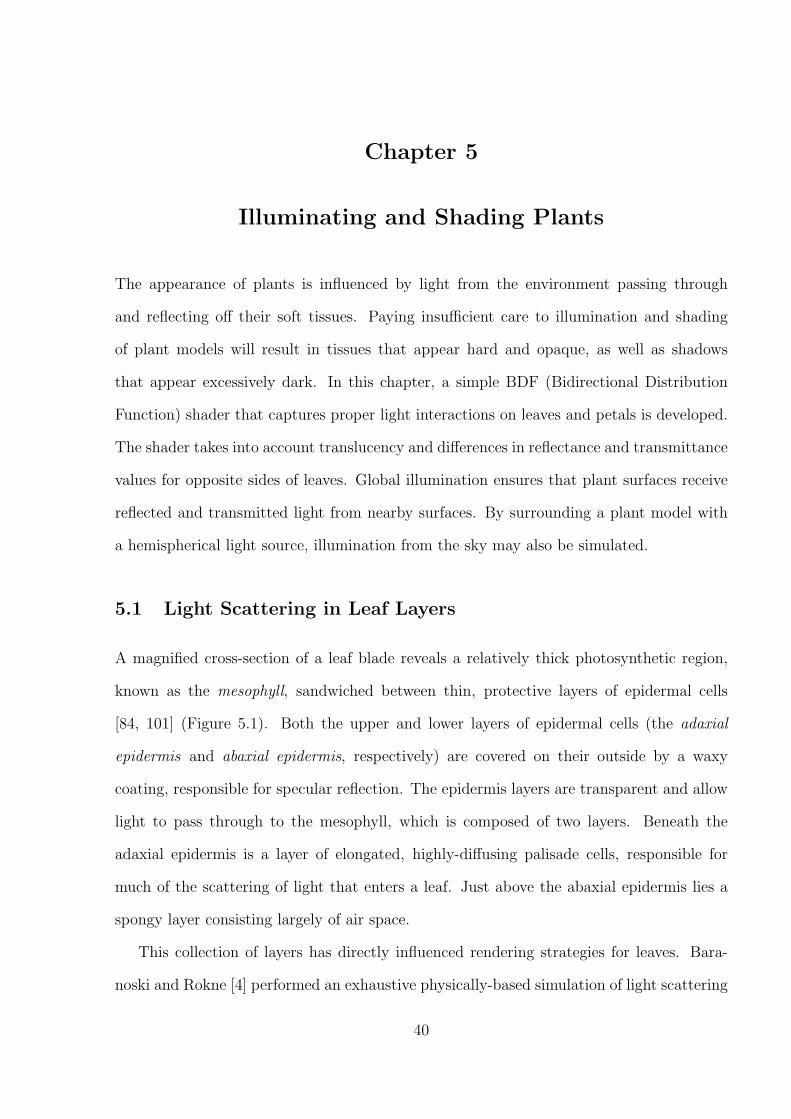
Chapter 5

Illuminating and Shading Plants

The appearance of plants is influenced by light from the environment passing through

and reflecting off their soft tissues. Paying insufficient care to illumination and shading

of plant models will result in tissues that appear hard and opaque, as well as shadows

that appear excessively dark. In this chapter, a simple BDF (Bidirectional Distribution

Function) shader that captures proper light interactions on leaves and petals is developed.

The shader takes into account translucency and differences in reflectance and transmittance

values for opposite sides of leaves. Global illumination ensures that plant surfaces receive

reflected and transmitted light from nearby surfaces. By surrounding a plant model with

a hemispherical light source, illumination from the sky may also be simulated.

5.1 Light Scattering in Leaf Layers

A magnified cross-section of a leaf blade reveals a relatively thick photosynthetic region,

known as the mesophyll, sandwiched between thin, protective layers of epidermal cells

[84, 101] (Figure 5.1). Both the upper and lower layers of epidermal cells (the adaxial

epidermis and abaxial epidermis, respectively) are covered on their outside by a waxy

coating, responsible for specular reflection. The epidermis layers are transparent and allow

light to pass through to the mesophyll, which is composed of two layers. Beneath the

adaxial epidermis is a layer of elongated, highly-diffusing palisade cells, responsible for

much of the scattering of light that enters a leaf. Just above the abaxial epidermis lies a

spongy layer consisting largely of air space.

This collection of layers has directly influenced rendering strategies for leaves. Bara-

noski and Rokne [4] performed an exhaustive physically-based simulation of light scattering

40

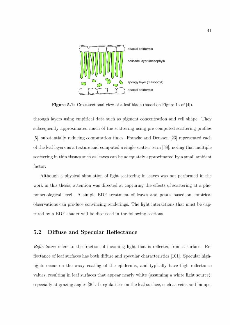
41

adaxial epidermis

abaxial epidermis

palisade layer (mesophyll)

spongy layer (mesophyll)

Figure 5.1: Cross-sectional view of a leaf blade (based on Figure 1a of [4]).

through layers using empirical data such as pigment concentration and cell shape. They

subsequently approximated much of the scattering using pre-computed scattering profiles

[5], substantially reducing computation times. Franzke and Deussen [23] represented each

of the leaf layers as a texture and computed a single scatter term [38], noting that multiple

scattering in thin tissues such as leaves can be adequately approximated by a small ambient

factor.

Although a physical simulation of light scattering in leaves was not performed in the

work in this thesis, attention was directed at capturing the effects of scattering at a phe-

nomenological level. A simple BDF treatment of leaves and petals based on empirical

observations can produce convincing renderings. The light interactions that must be cap-

tured by a BDF shader will be discussed in the following sections.

5.2 Diffuse and Specular Reflectance

Reflectance refers to the fraction of incoming light that is reflected from a surface. Re-

flectance of leaf surfaces has both diffuse and specular characteristics [101]. Specular high-

lights occur on the waxy coating of the epidermis, and typically have high reflectance

values, resulting in leaf surfaces that appear nearly white (assuming a white light source),

especially at grazing angles [30]. Irregularities on the leaf surface, such as veins and bumps,

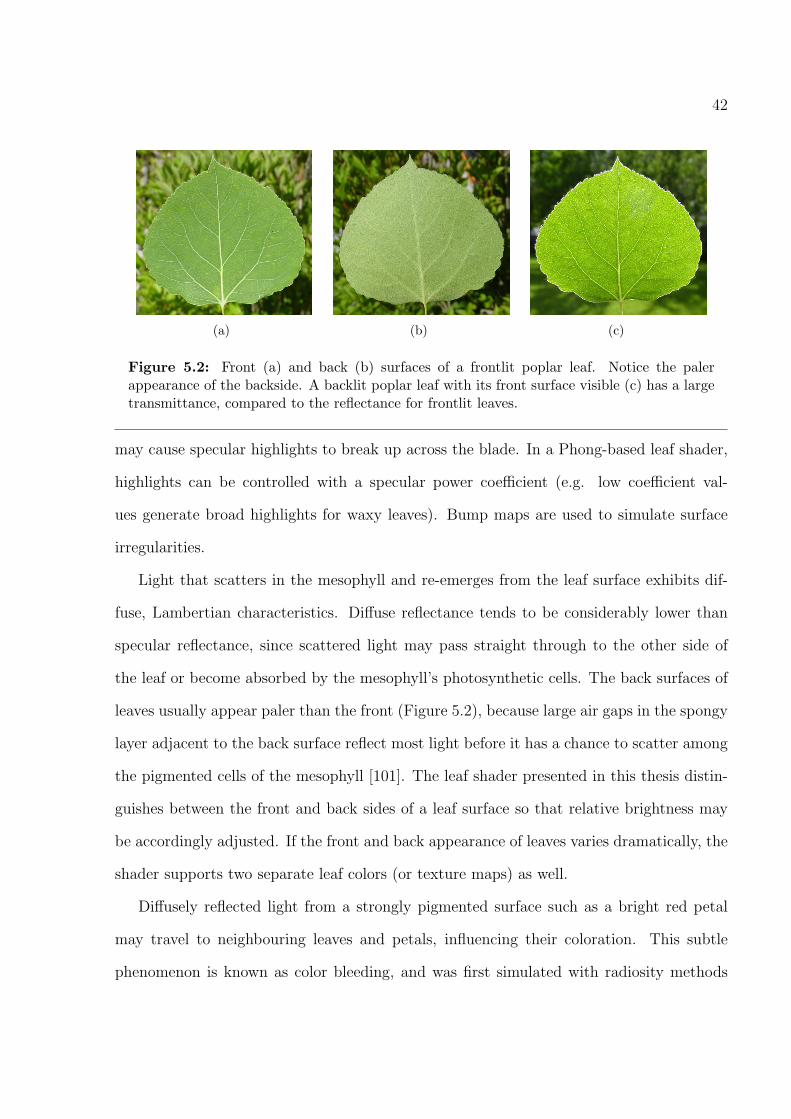
42

(a) (b) (c)

Figure 5.2: Front (a) and back (b) surfaces of a frontlit poplar leaf. Notice the palerappearance of the backside. A backlit poplar leaf with its front surface visible (c) has a largetransmittance, compared to the reflectance for frontlit leaves.

may cause specular highlights to break up across the blade. In a Phong-based leaf shader,

highlights can be controlled with a specular power coefficient (e.g. low coefficient val-

ues generate broad highlights for waxy leaves). Bump maps are used to simulate surface

irregularities.

Light that scatters in the mesophyll and re-emerges from the leaf surface exhibits dif-

fuse, Lambertian characteristics. Diffuse reflectance tends to be considerably lower than

specular reflectance, since scattered light may pass straight through to the other side of

the leaf or become absorbed by the mesophyll’s photosynthetic cells. The back surfaces of

leaves usually appear paler than the front (Figure 5.2), because large air gaps in the spongy

layer adjacent to the back surface reflect most light before it has a chance to scatter among

the pigmented cells of the mesophyll [101]. The leaf shader presented in this thesis distin-

guishes between the front and back sides of a leaf surface so that relative brightness may

be accordingly adjusted. If the front and back appearance of leaves varies dramatically, the

shader supports two separate leaf colors (or texture maps) as well.

Diffusely reflected light from a strongly pigmented surface such as a bright red petal

may travel to neighbouring leaves and petals, influencing their coloration. This subtle

phenomenon is known as color bleeding, and was first simulated with radiosity methods

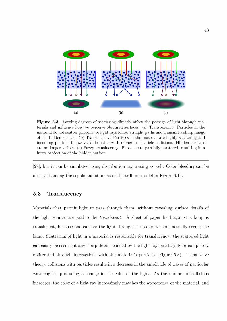
43

(a) (b) (c)

Figure 5.3: Varying degrees of scattering directly affect the passage of light through ma-terials and influence how we perceive obscured surfaces. (a) Transparency: Particles in thematerial do not scatter photons, so light rays follow straight paths and transmit a sharp imageof the hidden surface. (b) Translucency: Particles in the material are highly scattering andincoming photons follow variable paths with numerous particle collisions. Hidden surfacesare no longer visible. (c) Fuzzy translucency: Photons are partially scattered, resulting in afuzzy projection of the hidden surface.

[29], but it can be simulated using distribution ray tracing as well. Color bleeding can be

observed among the sepals and stamens of the trillium model in Figure 6.14.

5.3 Translucency

Materials that permit light to pass through them, without revealing surface details of

the light source, are said to be translucent. A sheet of paper held against a lamp is

translucent, because one can see the light through the paper without actually seeing the

lamp. Scattering of light in a material is responsible for translucency: the scattered light

can easily be seen, but any sharp details carried by the light rays are largely or completely

obliterated through interactions with the material’s particles (Figure 5.3). Using wave

theory, collisions with particles results in a decrease in the amplitude of waves of particular

wavelengths, producing a change in the color of the light. As the number of collisions

increases, the color of a light ray increasingly matches the appearance of the material, and

44

Figure 5.4: Leaf rendered with frontlighting and backlighting. Specular highlights onlyappear on the frontlit surface, and the backlit surface appears more emissive due to thegreater transmittance than reflectance value for leaves.

any resemblance to the appearance of the object or light source the ray originally left is

lost. If the particles are highly scattering, light emerging from the translucent material has

a diffuse nature. Without any scattering, translucency reduces to transparency, whereby

light passes through a surface in a straight path, producing a sharp image. Interactions

with particles in the transparent surface may still result in light attenuation and tinting of

the light’s color (e.g. sunglasses).

Most leaves and petals are translucent due to the scattering of light in the mesophyll as

light passes from one side of a surface to another. Transmittance refers to the fraction of

incoming light that is transmitted through a surface. Transmittance values for leaves are

typically higher than reflectance values [101], with the interesting consequence that leaves

usually appear brighter when backlit than when frontlit (Figure 5.2). The increased inter-

action of light with the mesophyll layer gives some backlit leaves a more deeply saturated

surface color. Our leaf shader simulates these effects by adjusting the value and saturation

of diffuse color under frontlighting and backlighting. The diffuse nature of transmitted light

means that backlit surfaces do not exhibit specular highlights, so specular calculations may

be ignored in that case (Figure 5.4).

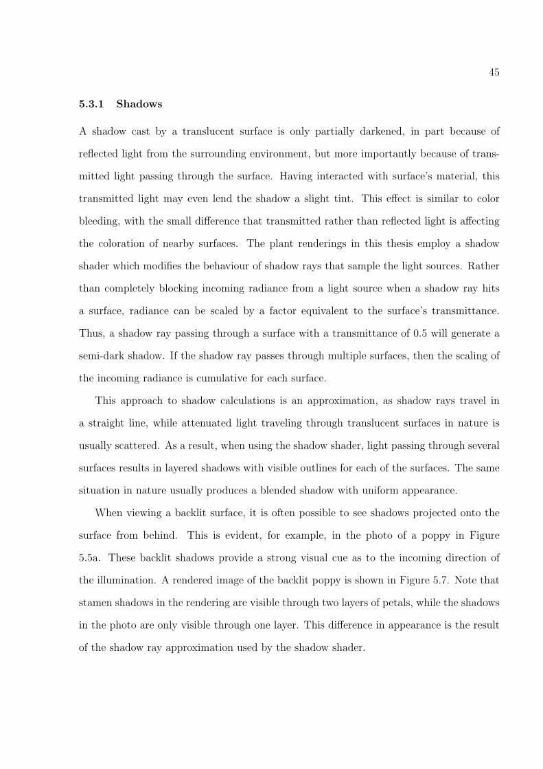
45

5.3.1 Shadows

A shadow cast by a translucent surface is only partially darkened, in part because of

reflected light from the surrounding environment, but more importantly because of trans-

mitted light passing through the surface. Having interacted with surface’s material, this

transmitted light may even lend the shadow a slight tint. This effect is similar to color

bleeding, with the small difference that transmitted rather than reflected light is affecting

the coloration of nearby surfaces. The plant renderings in this thesis employ a shadow

shader which modifies the behaviour of shadow rays that sample the light sources. Rather

than completely blocking incoming radiance from a light source when a shadow ray hits

a surface, radiance can be scaled by a factor equivalent to the surface’s transmittance.

Thus, a shadow ray passing through a surface with a transmittance of 0.5 will generate a

semi-dark shadow. If the shadow ray passes through multiple surfaces, then the scaling of

the incoming radiance is cumulative for each surface.

This approach to shadow calculations is an approximation, as shadow rays travel in

a straight line, while attenuated light traveling through translucent surfaces in nature is

usually scattered. As a result, when using the shadow shader, light passing through several

surfaces results in layered shadows with visible outlines for each of the surfaces. The same

situation in nature usually produces a blended shadow with uniform appearance.

When viewing a backlit surface, it is often possible to see shadows projected onto the

surface from behind. This is evident, for example, in the photo of a poppy in Figure

5.5a. These backlit shadows provide a strong visual cue as to the incoming direction of

the illumination. A rendered image of the backlit poppy is shown in Figure 5.7. Note that

stamen shadows in the rendering are visible through two layers of petals, while the shadows

in the photo are only visible through one layer. This difference in appearance is the result

of the shadow ray approximation used by the shadow shader.

46

(a) (b)

Figure 5.5: Translucency in nature. (a) Backlit shadows on the petals of a poppy. (b) Fuzzytranslucency can be observed where thin, semi-transparent petals overlap.

5.3.2 Fuzzy Translucency

If a leaf or petal is transparent enough for transmitted light rays not to scatter completely,

it becomes possible to see partial details of obscured surfaces (Figure 5.3). In this thesis,

this phenomenon is referred to as fuzzy translucency, to distinguish it from translucency

where scattering is complete and no details are visible through the blade. The flower petals

in Figure 5.5b exhibit fuzzy translucency. The effect is subtle, and is easily overpowered

by specular highlights or if adjacent petals lie too far apart.

To simulate fuzzy translucency, a physically-based shader would trace the paths of pho-

tons as they travel through a material and collide with particles. Because this process is

computationally expensive, our leaf shader achieves the same visual effect using distribu-

tion ray tracing [14]. When a ray passes through a translucent surface, secondary rays

distributed about the main ray are spawned to gather radiance within a conical region

behind the surface. The opening angle of the cone controls the amount of fuzziness. Small

angles focus the secondary rays within a narrow region, resulting in more distinct images

visible through the surface. Larger angles result in radiance from a wider region being

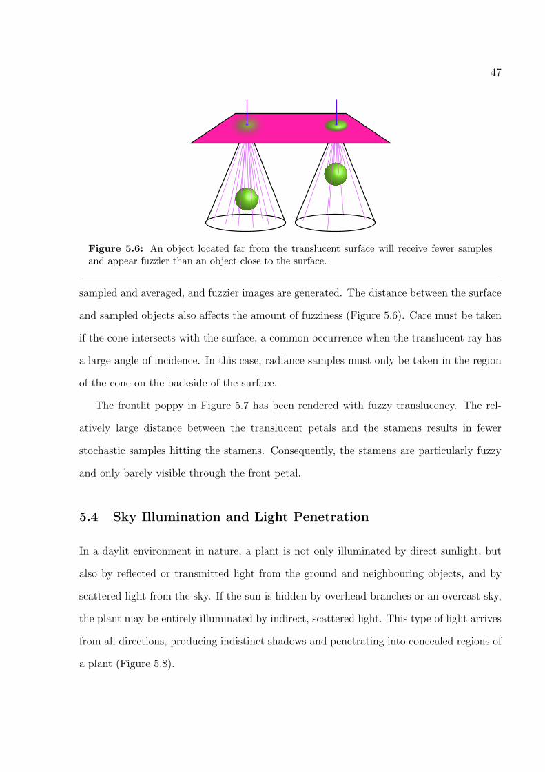
47

Figure 5.6: An object located far from the translucent surface will receive fewer samplesand appear fuzzier than an object close to the surface.

sampled and averaged, and fuzzier images are generated. The distance between the surface

and sampled objects also affects the amount of fuzziness (Figure 5.6). Care must be taken

if the cone intersects with the surface, a common occurrence when the translucent ray has

a large angle of incidence. In this case, radiance samples must only be taken in the region

of the cone on the backside of the surface.

The frontlit poppy in Figure 5.7 has been rendered with fuzzy translucency. The rel-

atively large distance between the translucent petals and the stamens results in fewer

stochastic samples hitting the stamens. Consequently, the stamens are particularly fuzzy

and only barely visible through the front petal.

5.4 Sky Illumination and Light Penetration

In a daylit environment in nature, a plant is not only illuminated by direct sunlight, but

also by reflected or transmitted light from the ground and neighbouring objects, and by

scattered light from the sky. If the sun is hidden by overhead branches or an overcast sky,

the plant may be entirely illuminated by indirect, scattered light. This type of light arrives

from all directions, producing indistinct shadows and penetrating into concealed regions of

a plant (Figure 5.8).

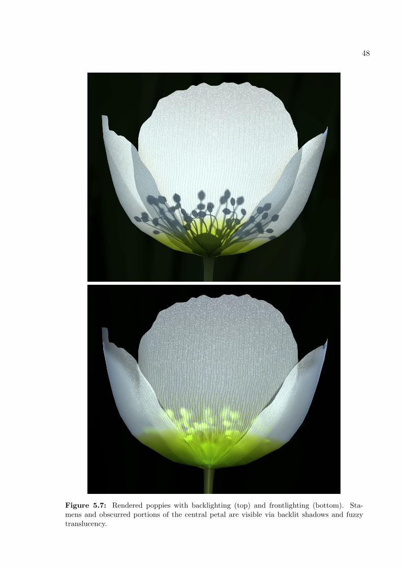
48

Figure 5.7: Rendered poppies with backlighting (top) and frontlighting (bottom). Sta-mens and obscurred portions of the central petal are visible via backlit shadows and fuzzytranslucency.

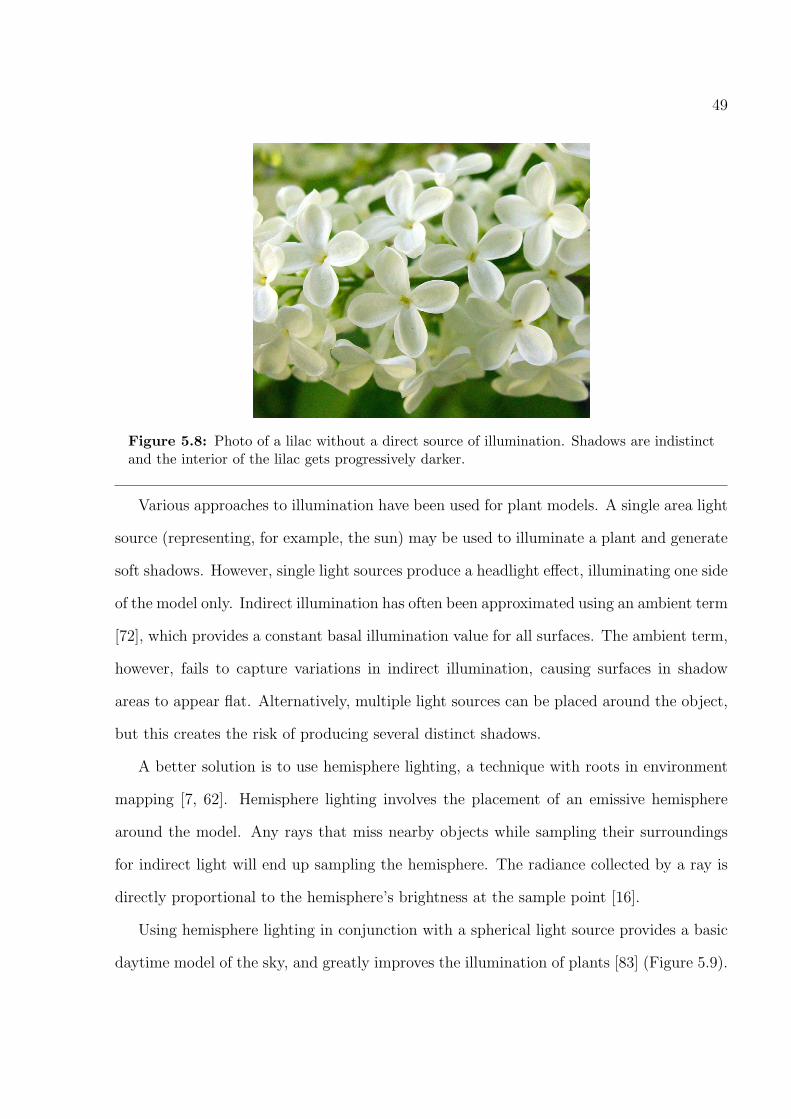
49

Figure 5.8: Photo of a lilac without a direct source of illumination. Shadows are indistinctand the interior of the lilac gets progressively darker.

Various approaches to illumination have been used for plant models. A single area light

source (representing, for example, the sun) may be used to illuminate a plant and generate

soft shadows. However, single light sources produce a headlight effect, illuminating one side

of the model only. Indirect illumination has often been approximated using an ambient term

[72], which provides a constant basal illumination value for all surfaces. The ambient term,

however, fails to capture variations in indirect illumination, causing surfaces in shadow

areas to appear flat. Alternatively, multiple light sources can be placed around the object,

but this creates the risk of producing several distinct shadows.

A better solution is to use hemisphere lighting, a technique with roots in environment

mapping [7, 62]. Hemisphere lighting involves the placement of an emissive hemisphere

around the model. Any rays that miss nearby objects while sampling their surroundings

for indirect light will end up sampling the hemisphere. The radiance collected by a ray is

directly proportional to the hemisphere’s brightness at the sample point [16].

Using hemisphere lighting in conjunction with a spherical light source provides a basic

daytime model of the sky, and greatly improves the illumination of plants [83] (Figure 5.9).

50

Figure 5.9: Illuminating a plant model in daylight conditions. The model is illuminatedby light arriving directly from a spherical light source representing the sun (yellow arrows),and also by reflected light from the ground and neighbouring objects (red arrows) and byscattered light from the sky (blue arrows).

Light arriving from the simulated sky penetrates into shaded regions of the plant. This

light penetration is further enhanced by taking into account interreflected light between

surfaces, as per a full global illumination simulation. In this research, point samples from

photographs of the sky have been taken to determine the coloration of the hemisphere

lighting. Alternatively, color values that take into account turbidity due to haze or smoke

may be computed [73]. Illumination on an overcast day can be simulated by removing any

direct light sources and employing a hemisphere with a solid shade of gray. This allows us

to capture the same soft, indistinct shadows seen in nature.

Figure 5.10 displays several images of lilac inflorescences rendered under various lighting

conditions and with different material settings, recorded in Table 5.1. Traditional ray

tracing, taking into account direct illumination only, was used for the top two lilac images.

The position of the spherical light source above and to the right of the lilac results in very

dark shadows, obliterating most of the model (Figure 5.10a). An ambient constant term

was used to simulate global illumination in Figure 5.10b, brightening the shadow areas.

However, these shadow regions appear uniform, as variations in reflected and transmitted

51

(a) (b)

(d)

(f)(e)

(c)

Figure 5.10: Lilac inflorescences. Refer to Table 5.1 for rendering settings.

52

Figure Global Illumination Sphere Light Skylight Translucency Transparency Cone Angle

5.10a no yes no 0 0 05.10b no (ambient term) yes no 0 0 05.10c yes yes no 0.8 0.25 155.10d yes no yes 0.8 0.25 155.10e yes yes yes 0.8 0 05.10f yes yes yes 0.8 0.25 15

Table 5.1: Illumination and translucency settings for lilac. The translucency settings arebased on the leaf and petal shader appearance parameters in Figure 5.11.

illumination are not captured.

Details in the shadow regions are noticeably improved in the remaining images, where

full global illumination has been applied. The petals in Figure 5.10c exhibit slight trans-

parency and fuzzy translucency, allowing radiance from the spherical light source to pen-

etrate into the interior of the model. The lilac in Figure 5.10d is illuminated solely by

skylight, resulting in non-distinct shadows and a gradual falloff in the amount of light

reaching interior regions. The lilacs in Figures 5.10e and 5.10f are illuminated both by

a spherical light source and skylight, with fuzzy translucency for petals turned off in the

former case.

5.5 A Leaf and Petal Shader

In this section, the leaf and petal BDF shader developed during this research is described.

The appearance parameters for the shader are listed in Figure 5.11. The shader is based

on the Phong illumination model [72], and includes parameters for diffuse color, specular

color, and specular power (the coefficient for controlling the size of the specular highlight).

The value and saturation parameters are used to change the respective properties for dif-

fuse color, based on an HSV (hue/saturation/value) color space [39], in order to simulate

differences in color intensities under frontlighting and backlighting (as in Figure 5.4).

Two important parameters are translucency and transparency, which are used to de-

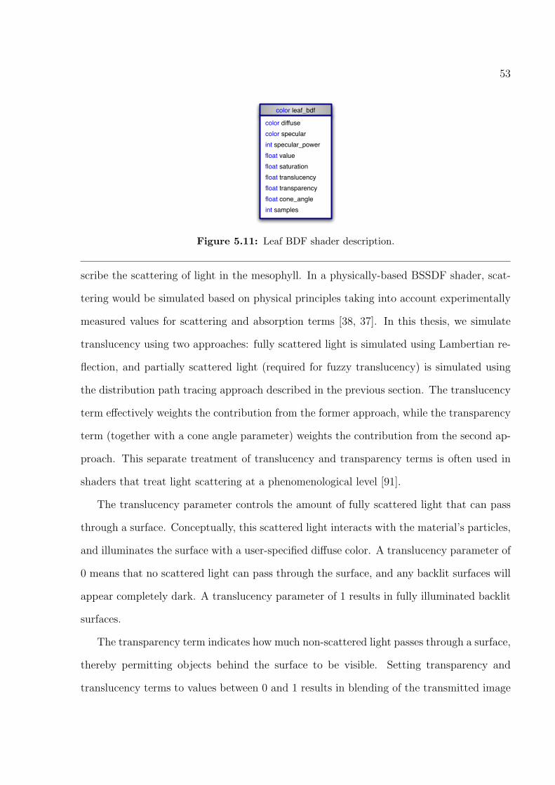
53

color specular

color leaf_bdf

color diffuse

int specular_power

float translucencyfloat transparencyfloat cone_angleint samples

float valuefloat saturation

Figure 5.11: Leaf BDF shader description.

scribe the scattering of light in the mesophyll. In a physically-based BSSDF shader, scat-

tering would be simulated based on physical principles taking into account experimentally

measured values for scattering and absorption terms [38, 37]. In this thesis, we simulate

translucency using two approaches: fully scattered light is simulated using Lambertian re-

flection, and partially scattered light (required for fuzzy translucency) is simulated using

the distribution path tracing approach described in the previous section. The translucency

term effectively weights the contribution from the former approach, while the transparency

term (together with a cone angle parameter) weights the contribution from the second ap-

proach. This separate treatment of translucency and transparency terms is often used in

shaders that treat light scattering at a phenomenological level [91].

The translucency parameter controls the amount of fully scattered light that can pass

through a surface. Conceptually, this scattered light interacts with the material’s particles,

and illuminates the surface with a user-specified diffuse color. A translucency parameter of

0 means that no scattered light can pass through the surface, and any backlit surfaces will

appear completely dark. A translucency parameter of 1 results in fully illuminated backlit

surfaces.

The transparency term indicates how much non-scattered light passes through a surface,

thereby permitting objects behind the surface to be visible. Setting transparency and

translucency terms to values between 0 and 1 results in blending of the transmitted image

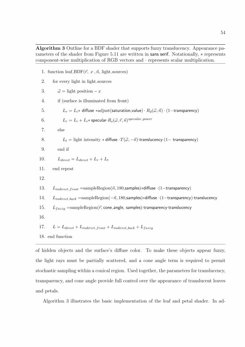
54

Algorithm 3 Outline for a BDF shader that supports fuzzy translucency. Appearance pa-rameters of the shader from Figure 5.11 are written in sans serif. Notationally, ∗ representscomponent-wise multiplication of RGB vectors and · represents scalar multiplication.

1. function leaf BDF(~r, x , ~n, light sources)

2. for every light in light sources

3. ~ω = light position− x

4. if (surface is illuminated from front)

5. Lr = Li∗ diffuse ∗adjust(saturation,value) ·Rd(~ω, ~n) · (1−transparency)

6. Lr = Li + Li∗ specular·Rs(~ω,~r, ~n)specular power

7. else

8. Lt = light intensity ∗ diffuse ·T (~ω,−~n)·translucency·(1− transparency)

9. end if

10. Ldirect = Ldirect + Lr + Lt

11. end repeat

12.

13. Lindirect front =sampleRegion(~n, 180,samples)∗diffuse ·(1−transparency)

14. Lindirect back =sampleRegion(−~n, 180,samples)∗diffuse ·(1−transparency)·translucency

15. Lfuzzy =sampleRegion(~r, cone angle, samples)·transparency·translucency

16.

17. L = Ldirect + Lindirect front + Lindirect back + Lfuzzy

18. end function

of hidden objects and the surface’s diffuse color. To make these objects appear fuzzy,

the light rays must be partially scattered, and a cone angle term is required to permit

stochastic sampling within a conical region. Used together, the parameters for translucency,

transparency, and cone angle provide full control over the appearance of translucent leaves

and petals.

Algorithm 3 illustrates the basic implementation of the leaf and petal shader. In ad-

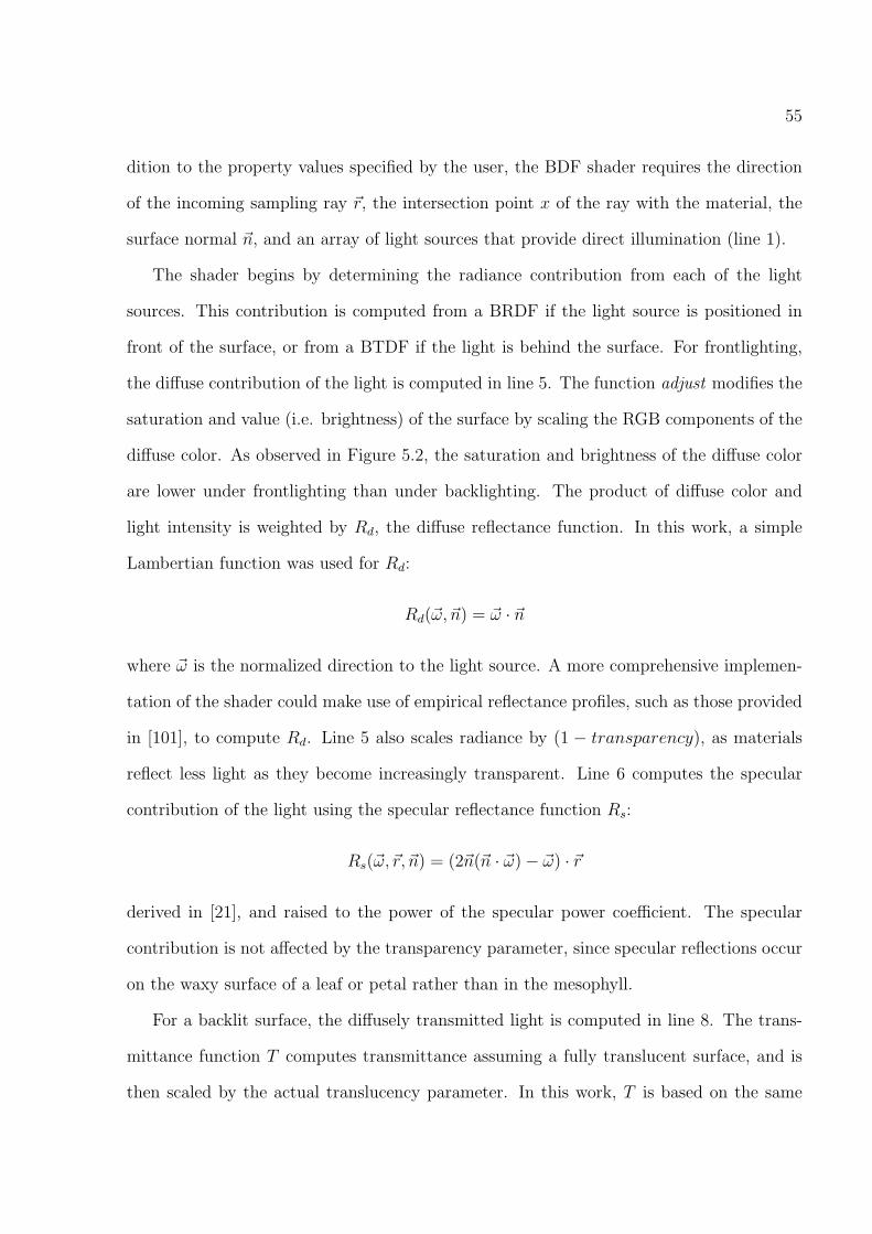
55

dition to the property values specified by the user, the BDF shader requires the direction

of the incoming sampling ray ~r, the intersection point x of the ray with the material, the

surface normal ~n, and an array of light sources that provide direct illumination (line 1).

The shader begins by determining the radiance contribution from each of the light

sources. This contribution is computed from a BRDF if the light source is positioned in

front of the surface, or from a BTDF if the light is behind the surface. For frontlighting,

the diffuse contribution of the light is computed in line 5. The function adjust modifies the

saturation and value (i.e. brightness) of the surface by scaling the RGB components of the

diffuse color. As observed in Figure 5.2, the saturation and brightness of the diffuse color

are lower under frontlighting than under backlighting. The product of diffuse color and

light intensity is weighted by Rd, the diffuse reflectance function. In this work, a simple

Lambertian function was used for Rd:

Rd(~ω, ~n) = ~ω · ~n

where ~ω is the normalized direction to the light source. A more comprehensive implemen-

tation of the shader could make use of empirical reflectance profiles, such as those provided

in [101], to compute Rd. Line 5 also scales radiance by (1 − transparency), as materials

reflect less light as they become increasingly transparent. Line 6 computes the specular

contribution of the light using the specular reflectance function Rs:

Rs(~ω,~r, ~n) = (2~n(~n · ~ω)− ~ω) · ~r

derived in [21], and raised to the power of the specular power coefficient. The specular

contribution is not affected by the transparency parameter, since specular reflections occur

on the waxy surface of a leaf or petal rather than in the mesophyll.

For a backlit surface, the diffusely transmitted light is computed in line 8. The trans-

mittance function T computes transmittance assuming a fully translucent surface, and is

then scaled by the actual translucency parameter. In this work, T is based on the same

56

Lambertian function used for diffuse reflectance Rd. Finally, the radiance must once again

be scaled by (1 − transparency), to account for the visibility of hidden objects that may

be seen through the surface.

Next, indirect light contributions are computed (lines 13 - 15). Path tracing is used to

stochastically sample the surroundings for incoming radiance. A cone centered around a

particular direction vector is used as the sampling region. The shader’s samples parameter

indicates how many times the region is sampled. Indirect radiance is gathered from the

front side of the surface in line 13. An opening angle of 180 degrees centered about the

surface normal effectively sets up a hemispherical sampling region. Indirect radiance from

the back side of the surface is similarly computed in line 14, except that the sampling region

is centered around −~n, and the radiance is scaled by the surface’s translucency.

Line 15 computes the radiance contribution due to transparency, allowing objects behind

the surface to be seen. The region behind the surface is stochastically sampled around ~r

using cone angle as the opening angle, in order to produce the fuzzy translucency effect.

Finally, line 17 sums up the radiance due to direct and indirect illumination for point

x on the surface.

Chapter 6

Texturing Surfaces

Texturing is an important facet of realistic rendering, significantly increasing the amount

of detail visible on a model. This chapter discusses the texturing of generalized cylinders,

and introduces several procedural methods for generating textures, particularly venation

patterns.

6.1 Setting up Texture Space

Texture mapping [11, 7] is a common computer graphics technique to create the illusion of

complexity on an otherwise barren surface. A texture map is a rectangular digital image

of the desired surface appearance. The map has texture coordinates u and v, ranging from

0 to 1 along the image’s width and height respectively. The texture is mapped onto an

object by associating points on the surface of the object with points in the texture space.

This mapping from 3D space to 2D space (R3 → R2) requires that a 2D parameterization

of the object’s surface be found.

The following sections examine some of the methods that have been used for texture-

mapping various surfaces used in L-system modeling, and introduce a modified method for

computing texture coordinates on generalized cylinders.

6.1.1 Tileable versus Non-Repeating Textures

Some types of textures prepared for plant surfaces are tileable. Stems and branches have

traditionally made use of tileable textures for bark [8], since many bark patterns have

a semi-repetitive nature. The texture’s edges must be specially prepared so that there

are no visual discontinuities along seams during tiling. More recently, synthesis of bark

57

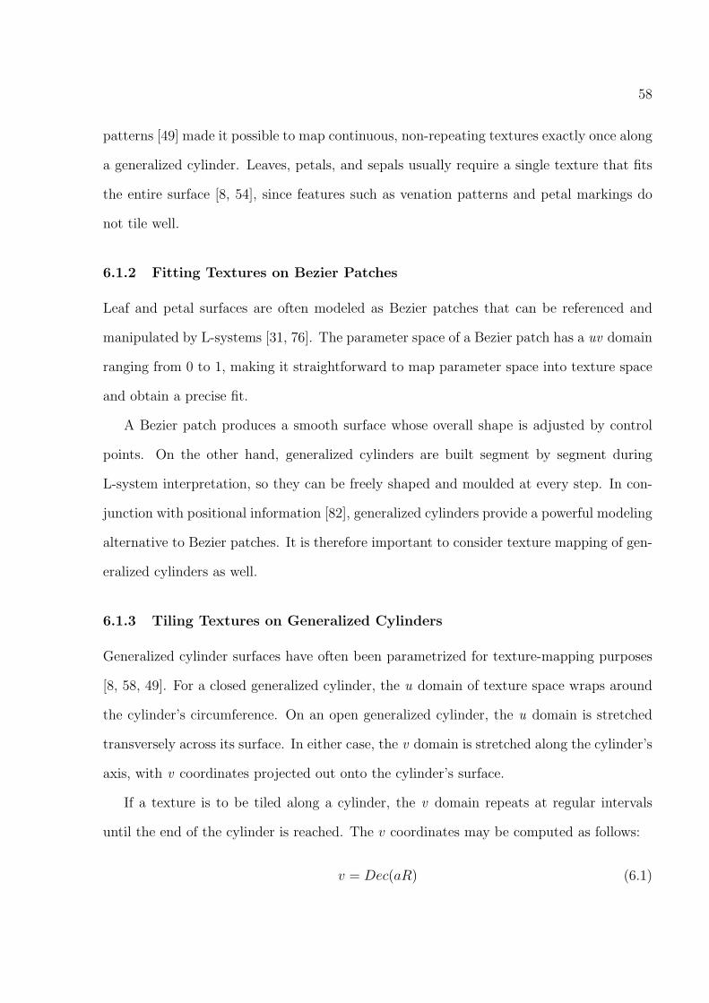
58

patterns [49] made it possible to map continuous, non-repeating textures exactly once along

a generalized cylinder. Leaves, petals, and sepals usually require a single texture that fits

the entire surface [8, 54], since features such as venation patterns and petal markings do

not tile well.

6.1.2 Fitting Textures on Bezier Patches

Leaf and petal surfaces are often modeled as Bezier patches that can be referenced and

manipulated by L-systems [31, 76]. The parameter space of a Bezier patch has a uv domain

ranging from 0 to 1, making it straightforward to map parameter space into texture space

and obtain a precise fit.

A Bezier patch produces a smooth surface whose overall shape is adjusted by control

points. On the other hand, generalized cylinders are built segment by segment during

L-system interpretation, so they can be freely shaped and moulded at every step. In con-

junction with positional information [82], generalized cylinders provide a powerful modeling

alternative to Bezier patches. It is therefore important to consider texture mapping of gen-

eralized cylinders as well.

6.1.3 Tiling Textures on Generalized Cylinders

Generalized cylinder surfaces have often been parametrized for texture-mapping purposes

[8, 58, 49]. For a closed generalized cylinder, the u domain of texture space wraps around

the cylinder’s circumference. On an open generalized cylinder, the u domain is stretched

transversely across its surface. In either case, the v domain is stretched along the cylinder’s

axis, with v coordinates projected out onto the cylinder’s surface.

If a texture is to be tiled along a cylinder, the v domain repeats at regular intervals

until the end of the cylinder is reached. The v coordinates may be computed as follows:

v = Dec(aR) (6.1)

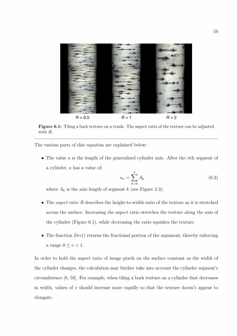
59

R = 0.5 R = 1 R = 2

Figure 6.1: Tiling a bark texture on a trunk. The aspect ratio of the texture can be adjustedwith R.

The various parts of this equation are explained below:

• The value a is the length of the generalized cylinder axis. After the nth segment of

a cylinder, a has a value of:

an =n∑

k=0

Ak (6.2)

where Ak is the axis length of segment k (see Figure 2.3).

• The aspect ratio R describes the height-to-width ratio of the texture as it is stretched

across the surface. Increasing the aspect ratio stretches the texture along the axis of

the cylinder (Figure 6.1), while decreasing the ratio squishes the texture.

• The function Dec() returns the fractional portion of the argument, thereby enforcing

a range 0 ≤ v < 1.

In order to hold the aspect ratio of image pixels on the surface constant as the width of

the cylinder changes, the calculation may further take into account the cylinder segment’s

circumference [8, 58]. For example, when tiling a bark texture on a cylinder that decreases

in width, values of v should increase more rapidly so that the texture doesn’t appear to

elongate.

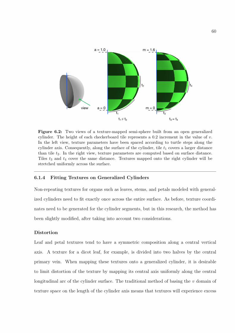
60

a = 1.0

a = 0

m = 1.6

m = 0

t2

t1 t3

t4

t1 ≠ t2 t3 = t4

view

Figure 6.2: Two views of a texture-mapped semi-sphere built from an open generalizedcylinder. The height of each checkerboard tile represents a 0.2 increment in the value of v.In the left view, texture parameters have been spaced according to turtle steps along thecylinder axis. Consequently, along the surface of the cylinder, tile t1 covers a larger distancethan tile t2. In the right view, texture parameters are computed based on surface distance.Tiles t3 and t4 cover the same distance. Textures mapped onto the right cylinder will bestretched uniformly across the surface.

6.1.4 Fitting Textures on Generalized Cylinders

Non-repeating textures for organs such as leaves, stems, and petals modeled with general-

ized cylinders need to fit exactly once across the entire surface. As before, texture coordi-

nates need to be generated for the cylinder segments, but in this research, the method has

been slightly modified, after taking into account two considerations.

Distortion

Leaf and petal textures tend to have a symmetric composition along a central vertical

axis. A texture for a dicot leaf, for example, is divided into two halves by the central

primary vein. When mapping these textures onto a generalized cylinder, it is desirable

to limit distortion of the texture by mapping its central axis uniformly along the central

longitudinal arc of the cylinder surface. The traditional method of basing the v domain of

texture space on the length of the cylinder axis means that textures will experience excess

61

a

m

(a)

(b) (c) (d)

Figure 6.3: Texture mapped petal. (a) View of the petal from the side, with mid-arc m andaxis a of the generalized cylinder illustrated. The texture map is shown in (b). The v domainof texture space on the petal in (c) is stretched along a, while on petal (d) it is stretchedalong m. The texture is excessively stretched in (c) where the petal surface angles outwardfrom the axis.

stretching if the surface angles outward from the axis (Figure 6.2).

A solution devised in this research is to compute v based on the length of the mid-arc

of the generalized cylinder (see Figure 2.3). Equation 6.1 is modified as follows:

v = Dec(mR) (6.3)

where m is the length of the mid-arc. The value of m after the nth segment of a generalized

cylinder is:

mn =n∑

k=0

Mk (6.4)

where Mk is the mid-arc length of segment k. Figure 6.3 compares the texture mapping of

a petal based on use of the cylinder axis versus the mid-arc.

Tile Factor

Because our goal is to fit textures exactly once on the surface, we should be able to say

directly that a texture is to be tiled once, rather than having to specify an aspect ratio.

A tile factor indicates how many times a texture should be tiled along a cylinder, and is

inversely related to aspect ratio.

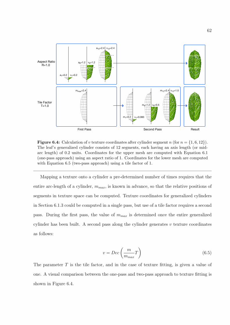
62

v1=0.2

v6=1.2

v12=2.4

m1=0.2

m6=1.2

m12=2.4

v1=0.083

v6=0.5

v12=1.0

R=1.0

T=1.0

a12=2.4

a1=0.2

a6=1.2

First Pass Second Pass Result

Aspect Ratio

Tile Factor

mmax=2.4

Figure 6.4: Calculation of v texture coordinates after cylinder segment n (for n = 1, 6, 12).The leaf’s generalized cylinder consists of 12 segments, each having an axis length (or mid-arc length) of 0.2 units. Coordinates for the upper mesh are computed with Equation 6.1(one-pass approach) using an aspect ratio of 1. Coordinates for the lower mesh are computedwith Equation 6.5 (two-pass approach) using a tile factor of 1.

Mapping a texture onto a cylinder a pre-determined number of times requires that the

entire arc-length of a cylinder, mmax, is known in advance, so that the relative positions of

segments in texture space can be computed. Texture coordinates for generalized cylinders

in Section 6.1.3 could be computed in a single pass, but use of a tile factor requires a second

pass. During the first pass, the value of mmax is determined once the entire generalized

cylinder has been built. A second pass along the cylinder generates v texture coordinates

as follows:

v = Dec

(m

mmax

T

)(6.5)

The parameter T is the tile factor, and in the case of texture fitting, is given a value of

one. A visual comparison between the one-pass and two-pass approach to texture fitting is

shown in Figure 6.4.

63

6.2 Procedural Textures

Leaves and petals display such a wide diversity of colors and patterns that many different

textures are required to properly capture the desired appearance of plant models. These

textures can be obtained directly from nature using flatbed scanners [54] or photographs

[8], provided that flat specimens are readily available. Alternatively, an artist may create

a texture from scratch, adding the exact splotches, gradients, specks, and striations seen

on the real surface. These methods of generating textures can be time-consuming, espe-

cially when multiple versions of a texture are required to capture the variability of surface

appearances in nature. The process of obtaining textures can be shortened by making use

of procedurally generated textures to produce specific features.

Procedural textures [70, 18] are created mathematically, permitting details to be gen-

erated in a resolution-independent manner from a set of user-adjustable parameters. The

texture is generated using a procedural function that accepts a set of coordinates and imme-

diately computes a value (or set of values) for this point. The value is typically interpreted

as a color, but may also be used for many other purposes, for example to perturb normals or

displace surfaces. When used with 3D coordinates, procedural textures can generate solid

textures such as those seen on sculpted marble [69]. In this section, we are concerned with

generating details on parameterized leaf and petal surfaces, so we will use 2D procedural

textures computed as a function of texture coordinates.

By building a shader around a procedural texture algorithm, it is possible to specify

the texture’s parameters from within an L-system using material modules. In this way,

unique textures can easily be specified and generated for every single leaf or petal on

a plant. Because procedural functions are able to specify a texture value for any given

coordinate, this type of shader is well suited for point sampling (i.e. ray tracing). This

section introduces shaders for generating translucent outlines and parallel venation patterns

based on 2D functions.

64

Figure 6.5: Daylily leaves are rimmed by translucent edges.

6.2.1 Translucent Outlines

When illuminated from behind, some leaves and petals display a bright fringe of light along

their edges. During the course of this work, the effect has been observed in two types of

situations: light shining through thin, translucent tissue rimming the edges (Figure 6.5),

or light scattering among short hairs or fuzz along the edges (Figure 7.1). The former case

is discussed below; the latter case is covered in Chapter 7.

A trivial way to simulate translucent edges is to paint them directly onto a texture. The

texture is then mapped onto a blade, and the entire surface rendered as a single material.

This method is problematic, since the translucent edges have different light transmission

and scattering properties than the rest of the blade. In this work, the blade is partitioned

into two regions of separate materials. The edge region is rendered with a highly translucent

material, while the central portion of the blade is rendered with a different material.

The edge regions typically have a constant width around the entire perimeter of the

surface. Texture space can be used to define these regions. A leaf modeled as an open

generalized cylinder has a varying width controlled by a function, as well as a u domain

in texture space varying from zero to one, from one edge to another. An absolute width

65

wabs for the translucent outlines can be specified and converted into a width wtex in the u

domain of texture space. The width of the outline in texture space varies inversely with the

leaf’s width function Fwidth , so wtex at a distance l along the axis of the leaf is computed

as:

wtex =wabs

Fwidth(l)

An outline shader handles the partitioning of a leaf blade during ray tracing (pictured

as a sub-shader node in the shade tree in Figure 6.9). The shader requires parameters for

outline width and the surface’s width function. It returns a value of zero or one, indicating

if the ray intersecting the blade hit the edge or central region, and may optionally return a

value between zero and one to simulate a transition from one region to another. By passing

this value to a blend shader, the appropriate materials for either region may be chosen or

blended together. Figure 6.6 illustrates the outline shader at work.

Because the outline width is measured in a transverse direction along the u domain

rather than perpendicularly to the edge, the outline will appear to shrink if the edge angles

sharply outward from the leaf’s axis (for example, at the base of a leaf where the stem

joins the blade). Translucent outlines tend to be narrow strips, so shrinkage in the outline

width is often visually negligible.

6.2.2 Venation Systems

One of the most striking features on leaves and petals is the venation system. Leaf and petal

veins are a conspicuous component of the vascular system, which serves to distribute nutri-

ents throughout the entire plant [26]. Procedural generation of veins is an especially attrac-

tive goal for computer graphics because of the time-consuming process of hand-modeling,

scanning, or photographing multiple vein patterns for a plant model.

Many varieties of veins and vein patterns exist. These have been extensively categorized

in work by Melville [60] and Hickey [34]. Individual veins belong to a particular vein order,

66

Figure 6.6: The entire surface of the leaf in (a) is a single texture map renderered witha uniform material. The edge regions and veins in the remaining leaves are procedurallygenerated, and use materials with different translucency properties than the rest of the blade.The checkerboard pattern is visible through the edge regions in (b) due to fuzzy translucency.Parallel venation with translucency has been added in (c) and includes branching in (d).

depending on their relative width and location on a blade. Primary or first-order veins

are dominant veins originating at the base of a leaf. Secondary veins typically branch from

the primary veins, and are noticeably thinner. Further branching results in tertiary and

higher-order veins, which tend to form areoles, closed polygonal islets that often contain

free-ending veins [65]. Veins of various orders are arranged in different ways depending on

the type of leaf. Monocots, or grass-like leaves, typically display parallelodromous venation,

with several primary veins emerging from the base and running in a more or less parallel

fashion (e.g. daylily leaves in Figure 6.5). Dicots, or broad, stalked leaves, may also feature

parallelodromous venation, but more commonly bear a pinnate pattern, with secondary

veins emerging laterally from a single primary vein (e.g. poplar leaves in Figure 5.2).

While Hickey’s vein classifications have been directed primarily at leaves, similar patterns

can be found on petals as well.

67

Various methods have been utilized to generate procedural vein patterns. Genetic al-

gorithms have been used to construct L-systems that approximate pinnate patterns with

primary and secondary veins on dicot leaves [86]. Higher order venation has been simulated

using a cellular texture basis function that partitions texture space between feature line

segments [10]. More recently, structured particle systems have been used to model complex

venation systems [85, 88]; these will be further discussed in Section 6.2.4.

6.2.3 Ray Traced Parallel Veins

This section introduces a shader for generating parallelodromous venation. The shader is

based on a procedural texture that takes advantage of the mesh’s texture coordinates to

generate the vein pattern. Parameters for the vein shader include the number of veins, the

number of times the veins will branch, and vein width. For a set of uv-coordinates, the

shader returns a value indicating whether a vein has been hit.

Veins in the shader are represented as binary tree structures. A parent vein may branch

into two child veins. We refer to a pair of child veins as siblings. For any vein, it is possible

to traverse the tree to find the vein’s parent, sibling, or children.

During an initialization phase, the shader divides texture space into a grid of rows and

columns (Figure 6.7). Each column is called a vein region. A single vein passes through

every vein region. If the vein branches, the vein region is split into two additional vein

regions, one for each child vein. Each row is called a band, and a new band is added every

time a vein branches. A pattern with no branching veins requires only one band. If the

pattern includes branching, the branch points are set at non-uniform intervals along the

path of veins.

Two aspects of the vein shader will now be examined in detail: generation of the veins,

and divergence of veins at the branch points.

68

Vein Regions (vn)

Band

s (b

n)

b3

b2

b1

b0

v0 v1 v2

v3 v4

v5 v6

v7 v8

vein region

shoulder region

vein

controlpoint

Figure 6.7: To generate parallel veins with branches, texture space is partitioned into bandsconsisting of rows of vein regions. A vein region contains a single vein, whose path is influencedby a series of control points lying within a shoulder region.

Vein Generation

The shader’s base vein width parameter indicates the width of veins at the base of the

texture. This width is gradually reduced as veins pass through the v domain toward the

top of the texture. Because the width parameter is given in object space, it must be

converted to a width in texture space, wtex, using the same method as outlined in Section

6.2.1.

A vein has a transverse location l given as a u coordinate in texture space. The vein’s

lower and upper bounds are l − wtex

2and l + wtex

2, respectively. Rays hitting the surface

within these bounds will generate a vein.

In a straightforward implementation, the vein location is constant for the entire length

of the vein, producing a perfectly straight path along the entire v domain in texture space.

Veins in nature, however, usually follow a slightly wavy path. For a more natural appear-

ance, our implementation jitters the vein location at uniform intervals of v. Each jittered

point (l, v) forms a control point, and lies within a shoulder region that demarcates the path

followed by the vein (Figure 6.8). By using the control points to guide an approximating

spline, a vein with a smooth, wavy appearance is generated. Approximating splines with

69

transitionregion

bandregion

bandregion

vein region vein region

a

b

vein region

tend

tstart

Figure 6.8: A branching point is followed by a transition region, permitting the child veinsto settle into their new vein regions. Without a transition region, the child veins wouldcontinue to follow the spline paths indicated in violet.

convex-hull property ensure that the veins remain within the shoulder region. B-splines [6]

have been used for the parallel veins in Figure 6.6.

Branching Points

When a parent vein splits into child veins, two new vein regions are produced. If the child

veins are rendered without regard for the branching point, they will continue to follow their

wavy spline path centered in their respective vein regions without merging together (Figure

6.8). The solution is to define a transition region which spans a portion of the v domain at

the start of a new vein region. The length of the transition region determines how quickly

the child veins diverge from their parent.

Conceptually, transition regions operate by shifting u coordinates in texture space of

one vein region toward the vein region occupied by the sibling vein. This is achieved in

practise by adding an offset to the u coordinate of any ray intersection point (uray, vray) in

a transition region. The offset, uoffset, depends on the relative location of the intersection

point within the transition region. If the intersection point lies at the start of the transi-

tion region, its u coordinate is offset by the difference between the child vein’s transverse

70

location, lchild, and the parent vein’s transverse location at the branching point, lparent.

If the intersection point lies at the end of the transition region, its u coordinate remains

unchanged. For any intersection points between these extremes, the offset is weighted by a

cubic polynomial that creates a smooth transition. The surface is then queried at the new

coordinates (uray + uoffset, vray) to test for intersection with a vein.

Figure 6.8 illustrates the offset added to two intersection points, a and b, within the

transition region. Because the offset on point a does not place the point in the violet vein

path, no vein hit takes place. The offset on point b places the point directly inside the

violet vein path, so a vein hit is considered to take place.

Algorithm

The function indicating if the ray intersecting the surface hits a vein is displayed in Algo-

rithm 4. Two binary searches (lines 2 and 3) are performed using the ray intersections’s

texture coordinates to determine in which band and vein region the ray landed.

Lines 4 to 7 add an offset to the intersection’s u coordinate if the ray landed within the

vein region’s transition region. The u coordinate, whether offset or not, is next compared

against the boundaries of the shoulder region (line 8). If u exists outside the boundaries,

the ray intersection most definitely does not hit a vein. If u exists within the shoulder

region, the vein’s transverse location is computed based on the spline defining the vein

path (line 9). The vein’s lower and upper bounds are then computed (line 10). If the

ray intersecton occurs within these bounds, a vein hit is confirmed. While line 12 of the

algorithm simply returns a value of 1, the implementation used for this research generates

a weighted value that can be used for various purposes during rendering. For example, by

returning a value of 1 for the center of the vein and increasingly smaller weights toward

the vein’s edges, a vein can be rendered with soft edges. As well, fading veins are rendered

by returning increasingly smaller weights as the tip of a blade is approached.

The binary searches are the slowest part of the algorithm, requiring a runtime of

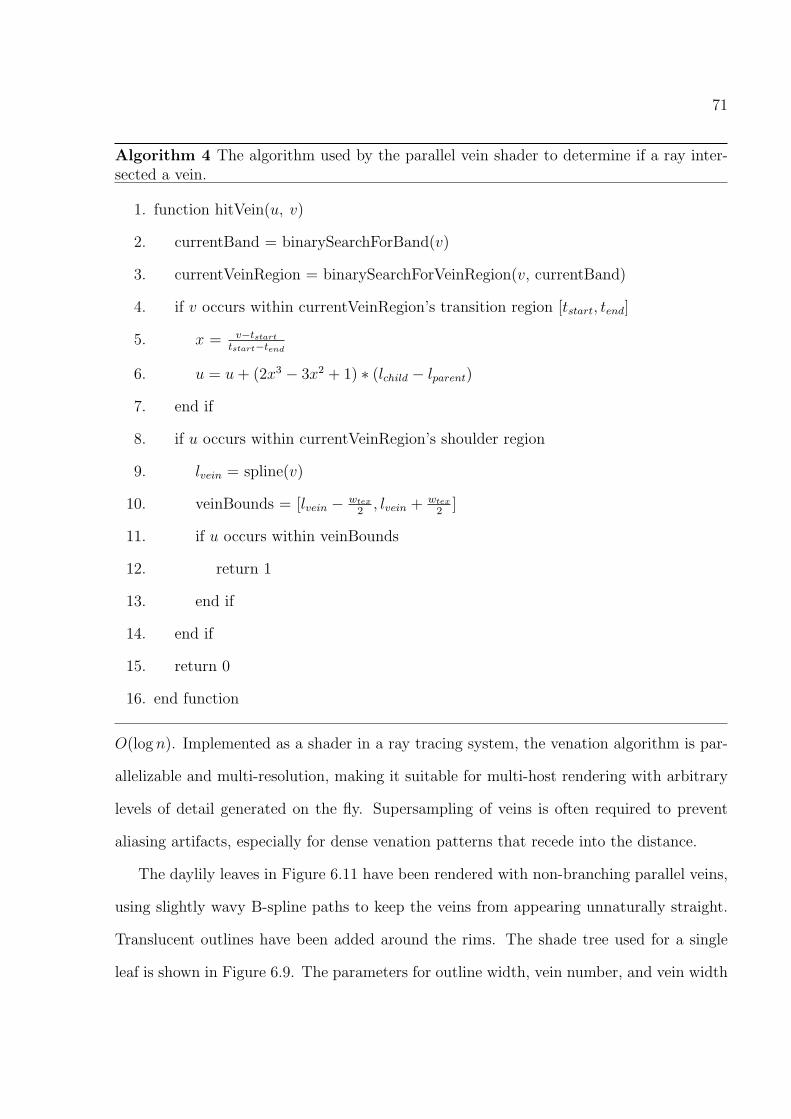
71

Algorithm 4 The algorithm used by the parallel vein shader to determine if a ray inter-sected a vein.

1. function hitVein(u, v)

2. currentBand = binarySearchForBand(v)

3. currentVeinRegion = binarySearchForVeinRegion(v, currentBand)

4. if v occurs within currentVeinRegion’s transition region [tstart, tend]

5. x = v−tstart

tstart−tend

6. u = u + (2x3 − 3x2 + 1) ∗ (lchild − lparent)

7. end if

8. if u occurs within currentVeinRegion’s shoulder region

9. lvein = spline(v)

10. veinBounds = [lvein − wtex

2, lvein + wtex

2]

11. if u occurs within veinBounds

12. return 1

13. end if

14. end if

15. return 0

16. end function

O(log n). Implemented as a shader in a ray tracing system, the venation algorithm is par-

allelizable and multi-resolution, making it suitable for multi-host rendering with arbitrary

levels of detail generated on the fly. Supersampling of veins is often required to prevent

aliasing artifacts, especially for dense venation patterns that recede into the distance.

The daylily leaves in Figure 6.11 have been rendered with non-branching parallel veins,

using slightly wavy B-spline paths to keep the veins from appearing unnaturally straight.

Translucent outlines have been added around the rims. The shade tree used for a single

leaf is shown in Figure 6.9. The parameters for outline width, vein number, and vein width

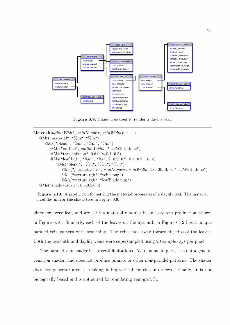
72

shader shadow

color material

shader surface

color shadow_scale

color scale

shader shader1

color blend

shader shader2

float weight

string width_function

float outline

float outline_width

float transmittance

color transmission

color diffuse

color shader1

color blend

color shader2

float weight

float vein_width

float parallel_veins

int vein_number

float vein_shouldersfloat jitter_frequencyint max_branchingfloat transition_lengthstring width_function

color texture_rgb

string filename

color texture_rgb

string filename

color specular

color leaf_bdf

color diffuse

int specular_power

float translucencyfloat transparencyfloat cone_angleint samples

float valuefloat saturation

Figure 6.9: Shade tree used to render a daylily leaf.

Material(outlineWidth, veinNumber , veinWidth): 1 −→@Mt("material", "%m", "%m")

@Ms("blend", "%m", "%m", "%m")@Ms("outline", outlineWidth, "leafWidth.func")@Ms("transmission", 0.6,0.94,0.1, 0.5)@Ms("leaf bdf", "%m", "%s", 2, 0.9, 0.9, 0.7, 0.2, 10, 4)

@Ms("blend", "%m", "%m", "%m")@Ms("parallel veins", veinNumber , veinWidth, 1.6, 20, 0, 0, "leafWidth.func")@Ms("texture rgb", "veins.png")@Ms("texture rgb", "leafBlade.png")

@Ms("shadow scale", 0.5,0.5,0.5)

Figure 6.10: A production for setting the material properties of a daylily leaf. The materialmodules mirror the shade tree in Figure 6.9.

differ for every leaf, and are set via material modules in an L-system production, shown

in Figure 6.10. Similarly, each of the leaves on the hyacinth in Figure 6.12 has a unique

parallel vein pattern with branching. The veins fade away toward the tips of the leaves.

Both the hyacinth and daylily veins were supersampled using 20 sample rays per pixel.

The parallel vein shader has several limitations. As its name implies, it is not a general

venation shader, and does not produce pinnate or other non-parallel patterns. The shader

does not generate areoles, making it impractical for close-up views. Finally, it is not

biologically based and is not suited for simulating vein growth.

73

Figure 6.11: Daylily leaves.

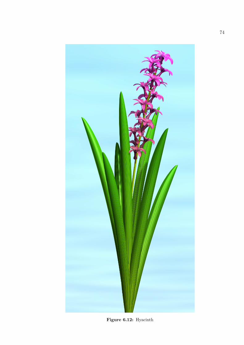
74

Figure 6.12: Hyacinth

75

6.2.4 Particle Vein Systems

A much larger variety of vein patterns has been achieved in previous research through the

use of particle systems. The changing state of particle systems over time has been used

to simulate physiological processes that drive the formation of veins. Rodkaew et al. [85]

modeled veins by spreading particles across a leaf blade. During simulation, the particles

migrate toward the base of the blade, but at the same time are attracted to each other,

forming branching paths that resemble primary and secondary veins. Runions et al. [88],

taking inspiration from the plant hormone auxin, adopted a biologically-based approach to

vein formation. Initial vein nodes placed at the base of a leaf grow toward sources of auxin

distributed in the leaf blade. The formation of new veins reciprocally affects the placement

of new sources of auxin. Over a period of time, this feedback loop results in intricate vein

patterns.

While the patterns produced by Runions are procedurally generated, the algorithm

does not permit point sampling in texture space without first having generated the entire

texture. Unlike the parallel venation algorithm, the textures cannot be generated on the

fly and their resolution must be decided upon prior to rendering. To use a venation pattern

for rendering, the pre-generated texture must be loaded from a file or memory, processed in

an image editor, and texture-mapped onto a surface. Five unique vein textures have been

prepared in this way for the leaves on the backlit twig in Figure 6.13. High order venation

is visible in the petals of the trillium flower in Figure 6.14. Bump mapping has been used

to simulate the troughs formed by the veins. Veins on the front sides of petals are usually

indented into the surface [65, 101], so a negative scaling value for the height of the bumps

has been used. Appendix A describes in detail how to prepare textures and bump maps

from the raw venation patterns generated by Runions’ method.

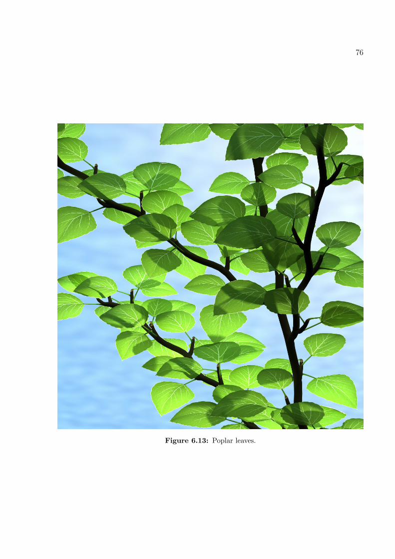
76

Figure 6.13: Poplar leaves.

77

Figure 6.14: Trillium flower

Chapter 7

Plant Hairs

Hairs are a common element of many different plants. Leaves, shoots, and stems covered

in hair must be properly modeled and rendered to generate photorealistic plants [24]. This

chapter presents a novel method of generating hairy plants from L-systems1.

7.1 Background

From a biological perspective, plant hairs are representative of trichomes, which also include

such structures as scales, warts, and spines [93]. The appearance of trichomes varies from

the pronounced scales covering young fern fronds to the fine hairs covering some leaves.

These fine hairs are often perceived as “fuzz”, and give rise to a characteristic soft glow

around backlit surfaces, as illustrated in Figure 7.1. This phenomenon has been termed

asperity scattering [46].

The mechanisms of trichome distribution on their underlying surfaces are an interesting

problem in developmental biology, and have recently been studied from a molecular per-

spective (e.g. [51, 89]). Trichome placement is controlled by a signaling mechanism that

prevents the formation of new organs too close to each other, and in this respect it is related

to the placement of organs in phyllotactic patterns around plant stems [51]. Functionally,

plant hairs and related structures play a variety of roles. For example, they may shade

the plant surface from excessive exposure to sunlight, decrease the loss of water through

transpiration, or ward off hungry insects or herbivores [93].

Modeling of hairs has been extensively investigated in the context of human hair and

animal fur. Kajiya and Kay [41] approached fur rendering using texels, three dimensional

1This chapter is an edited version of the work presented in [24].

78

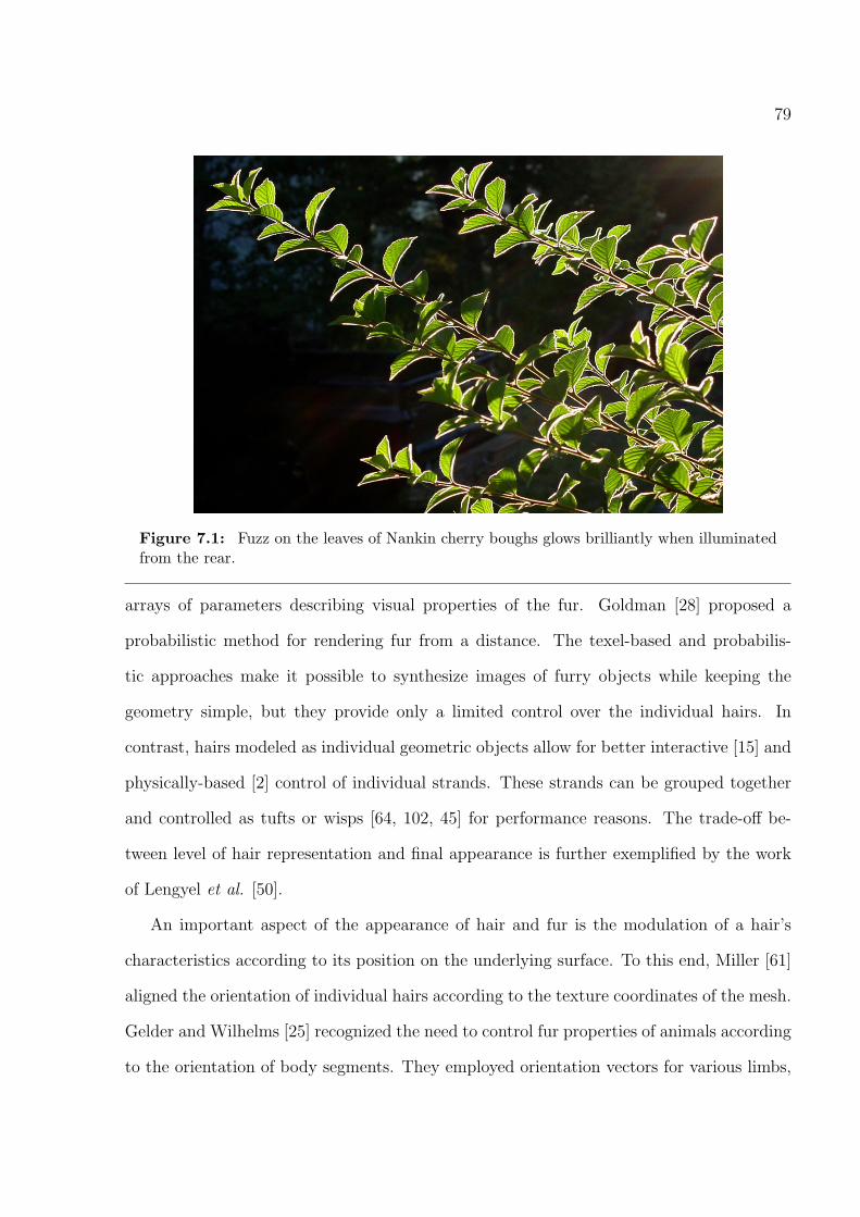
79

Figure 7.1: Fuzz on the leaves of Nankin cherry boughs glows brilliantly when illuminatedfrom the rear.

arrays of parameters describing visual properties of the fur. Goldman [28] proposed a

probabilistic method for rendering fur from a distance. The texel-based and probabilis-

tic approaches make it possible to synthesize images of furry objects while keeping the

geometry simple, but they provide only a limited control over the individual hairs. In

contrast, hairs modeled as individual geometric objects allow for better interactive [15] and

physically-based [2] control of individual strands. These strands can be grouped together

and controlled as tufts or wisps [64, 102, 45] for performance reasons. The trade-off be-

tween level of hair representation and final appearance is further exemplified by the work

of Lengyel et al. [50].

An important aspect of the appearance of hair and fur is the modulation of a hair’s

characteristics according to its position on the underlying surface. To this end, Miller [61]

aligned the orientation of individual hairs according to the texture coordinates of the mesh.

Gelder and Wilhelms [25] recognized the need to control fur properties of animals according

to the orientation of body segments. They employed orientation vectors for various limbs,

80

but encountered difficulties describing orientation in areas such as the head and thoracic

region. Lengyel et al. [50] oriented fur according to vector fields placed on meshes, and

made use of an interactive combing tool to further style fur according to the modeler’s

taste. Fleisher et al. [20] explored the problem of positioning and orienting small elements

(‘cellular particles’) across surfaces of different topologies. They described a number of

strategies to tackle the problem, and illustrated their techniques by covering surfaces with

scales and thorns.

Fowler et al. [22] proposed the first method aimed at placing elements visually related

to hairs on the surfaces of plants. This method exploited phyllotactic patterns to position

and orient spines on cacti and achenes (fruits) on the receptacle of goatsbeard.

The modeling of plant hairs must take into consideration several phenomena. Properties

of plant hairs may vary continuously between different locations on a plant and develop-

mental stages of plant organs. For example, hair density may be greater in young leaves,

and drop off as the leaves become older. Fully mature leaves often lose all the hairs on

their front and back surfaces, but maintain hairs along their edges. Hairs may be aligned

in specific directions, depending on their position. Hairs on opposite sides of the same

surface may be different from each other. In addition, there is much diversity in the shape

of individual hairs: given any patch of hairy surface, it is common to see a mixture of hairs

that are straight and curly, or long and short.

To account for these phenomena, we propose to model plants with hairs using a method

with the following characteristics:

• Geometric representation of hairs. Individual hairs are specified as generalized

cylinders, which are simplified to connected line segments during interactive modeling.

This makes it possible to control the shape of hairs and their distribution across

a surface in fine detail. This geometric approach is computationally efficient (e.g.

plants with hairs can be previewed at interactive rates), because the density of hairs

81

on plants is typically low in comparison to human hair or animal fur. In addition,

fewer line segments are required since plant hairs are often relatively short.

• The use of positional information. Many aspects of plant architecture can con-

veniently be characterized using functions of position along plant axes [82]. This

technique is extended to plant hairs, so that hair parameters along the length and

breadth of plant organs may be changed.

• The framework of L-systems with turtle interpretation. In addition to being

a general method for modeling plant architecture, L-systems lend themselves well to

the local control of hair attributes such as length, radius, curvature, and density of

placement. L-system modules are used for this purpose. The turtle used to interpret

L-system strings also provides a convenient frame of reference [82] for orienting hairs

along plant organs such as stems, leaves, and petals.

7.2 Hair generation

The process of hair generation involves several steps. First, the hair distribution on the

underlying surface is determined. Individual hairs must then be modeled, and an instance

of a pre-determined hair placed at every attachment point.

7.2.1 Distribution of the attachment points

In the extensively studied case of trichome distribution on the leaves of Arabidopsis thaliana,

the individual trichomes are spaced in a semi-regular manner, preserving a minimum dis-

tance from each other. The underlying morphogenetic process is believed to be of the

reaction-diffusion type [51]. Instead of simulating this process, we approximate its out-

come as a Poisson-disk pattern generated using the point diffusion algorithm proposed by

Mitchell [63]. Comparisons of images indicate that trichome distribution patterns (shown,

82

h

tm

tn

Figure 7.2: The point-diffusion texture is mapped onto the generalized cylinder segment(unfolded, curling into the page) in scan-line fashion, starting at the lower left corner andending at the upper right corner. The mapping of the tm × tn texture is indicated by thedashed lines. Density of the hair is controlled by scaling the texture according to positionalinformation.

for example, in [51]) are visually indistinguishable from Poisson-disk patterns (as illustrated

in [63]).

Point diffusion can be viewed as a texture generation algorithm that computes a texture

value (on or off) and a diffusion value at every grid element. This computation is based on

previously computed diffusion values stored in a neighborhood of four adjacent elements,

one to the immediate left and three in the row above. Point diffusion can be applied in

two ways for distributing hairs: on-the-fly or using texture mapping. The former approach

involves continuously generating the distribution pattern as the surfaces are produced. The

resulting seamless pattern is ideal for offline rendering purposes, but too slow to compute

during interactive modeling. We therefore preferably use the texture mapping method,

whereby a single point-diffusion texture is repeatedly tiled along the surface of the plant

organ. As the neighborhood used to compute the points in Mitchell’s algorithm wraps

around the vertical edges of the texture, vertical seams are barely visible. Horizontal seams

are more conspicuous; in practice, however, once hairs have been placed and oriented, the

seams are not noticeable.

The point-diffusion texture is a function τ(u, v) → 0, 1, where a returned value of 1

83

indicates an attachment point for a hair. We have found that a texture of size 100 × 100

results in visually acceptable hair distribution patterns. The texture-mapping technique

is illustrated in Figure 7.2. Although it introduces distortions (shear of the texture) when

applied to generalized cylinders with a rapidly changing circumference or width, we have

found the resulting artifacts visually negligible.

7.2.2 Hair modeling and placement

Hairs on a single plant come in many different shapes and sizes. While it is not feasible to

model the shape of every hair individually, it is possible to capture the overall diversity of

a hairy surface by modeling several different template hairs and instancing them multiple

times. During this research, hairs were modeled as curved generalized cylinders constructed

using simple L-systems (Figure 7.3). These hair L-systems are independent from the L-

system used to generate the whole plant. We control the hair curvature with functions for

tilt, twist, and pitch to rotate the turtle along its up, left, and heading vectors, respectively

[82]. The number of segments used to approximate each hair depends on its curvature:

relatively straight hairs can be reasonably modeled with three turtle steps, while twisted

hairs may require seven or more steps. The number of individual hairs to model depends

on the nature of the plant’s hairy surface: for most of the models in this chapter, three to

five different hairs properly capture the varied appearance of a hairy surface.

A hair is stored as a sequence of vertices describing the position of the turtle at every

step. Whenever a hair is instanced, its vertices are connected together. During real-time

rendering in cpfg, the vertices are connected by antialiased line segments, which are stored

in a display list to improve performance. During high-quality offline rendering, the vertices

are joined by cylindrical primitives. Each hair is assumed to have a constant radius.

When placing a hair on the front or back side of a generalized cylinder, we set the

hair’s orientation by aligning the axis of its first segment with the hair direction vector

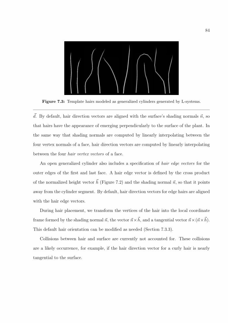
84

Figure 7.3: Template hairs modeled as generalized cylinders generated by L-systems.

~d. By default, hair direction vectors are aligned with the surface’s shading normals ~n, so

that hairs have the appearance of emerging perpendicularly to the surface of the plant. In

the same way that shading normals are computed by linearly interpolating between the

four vertex normals of a face, hair direction vectors are computed by linearly interpolating

between the four hair vertex vectors of a face.

An open generalized cylinder also includes a specification of hair edge vectors for the

outer edges of the first and last face. A hair edge vector is defined by the cross product

of the normalized height vector ~h (Figure 7.2) and the shading normal ~n, so that it points

away from the cylinder segment. By default, hair direction vectors for edge hairs are aligned

with the hair edge vectors.

During hair placement, we transform the vertices of the hair into the local coordinate

frame formed by the shading normal ~n, the vector ~n×~h, and a tangential vector ~n×(~n×~h).

This default hair orientation can be modified as needed (Section 7.3.3).

Collisions between hair and surface are currently not accounted for. These collisions

are a likely occurrence, for example, if the hair direction vector for a curly hair is nearly

tangential to the surface.

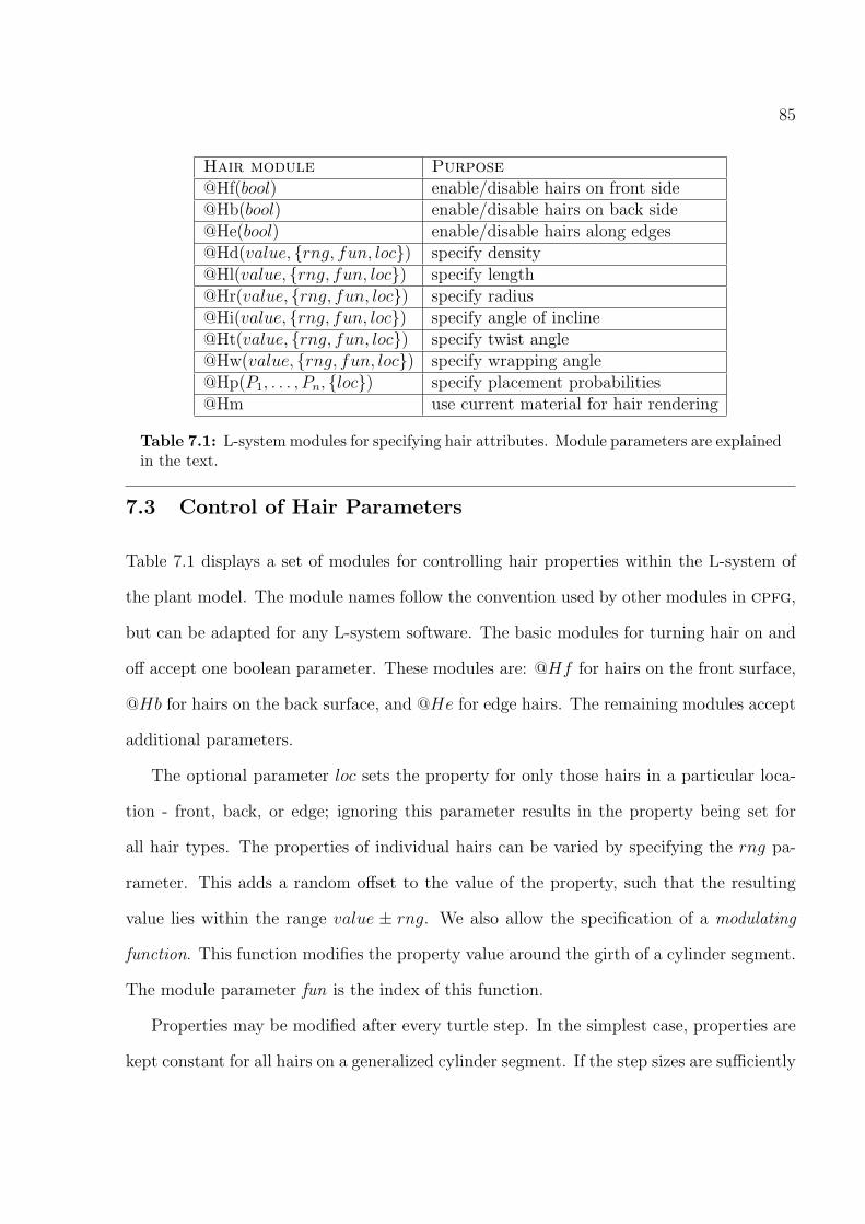
85

Hair module Purpose@Hf(bool) enable/disable hairs on front side@Hb(bool) enable/disable hairs on back side@He(bool) enable/disable hairs along edges@Hd(value, rng, fun, loc) specify density@Hl(value, rng, fun, loc) specify length@Hr(value, rng, fun, loc) specify radius@Hi(value, rng, fun, loc) specify angle of incline@Ht(value, rng, fun, loc) specify twist angle@Hw(value, rng, fun, loc) specify wrapping angle@Hp(P1, . . . , Pn, loc) specify placement probabilities@Hm use current material for hair rendering

Table 7.1: L-system modules for specifying hair attributes. Module parameters are explainedin the text.

7.3 Control of Hair Parameters

Table 7.1 displays a set of modules for controlling hair properties within the L-system of

the plant model. The module names follow the convention used by other modules in cpfg,

but can be adapted for any L-system software. The basic modules for turning hair on and

off accept one boolean parameter. These modules are: @Hf for hairs on the front surface,

@Hb for hairs on the back surface, and @He for edge hairs. The remaining modules accept

additional parameters.

The optional parameter loc sets the property for only those hairs in a particular loca-

tion - front, back, or edge; ignoring this parameter results in the property being set for

all hair types. The properties of individual hairs can be varied by specifying the rng pa-

rameter. This adds a random offset to the value of the property, such that the resulting

value lies within the range value ± rng. We also allow the specification of a modulating

function. This function modifies the property value around the girth of a cylinder segment.

The module parameter fun is the index of this function.

Properties may be modified after every turtle step. In the simplest case, properties are

kept constant for all hairs on a generalized cylinder segment. If the step sizes are sufficiently

86

Algorithm 5 This L-system describes the change in hair properties for length,incline, anddensity along the length of a generalized cylinder. The probability of two types of hairs isalso being set at everystep, and changes as we move along the cylinder (the straight hairsbecome more likely near the right end).The resulting image is displayed in Figure 7.4.

1. #define l 10 /* length of axis */

2. #define ∆s1 /* turtle step */

3. Axiom: @Gs @Hf(1) B(0)

4. B(s): s ≤ l

5.

6. relativeDistance = s/l;

7. len = func(1, relativeDistance);

8. inc = func(2, relativeDistance);

9. den = func(3, relativeDistance);

10. −→

11. @Hl(len) @Hi(inc) @Hd(den)

12. @Hp(relativeDistance, 1− relativeDistance)

13. f(∆s) @Gc B(s + ∆s)

14. B(s): s ≥ l −→ @Ge

small, the sudden transition of properties from segment to segment is nearly invisible, but

if the step sizes increase, visual discontinuities may become apparent. To eliminate this

artifact, properties may be interpolated across segments.

Algorithm 5 presents a sample L-system used to generate the cylinder pictured in Figure

7.4. We set the total length and step size in lines 1 and 2, and begin the generalized

cylinder with module @Gs in the axiom of line 3. The module @Hf turns on the hairs.

The production B repeatedly advances the turtle and draws a generalized cylinder segment

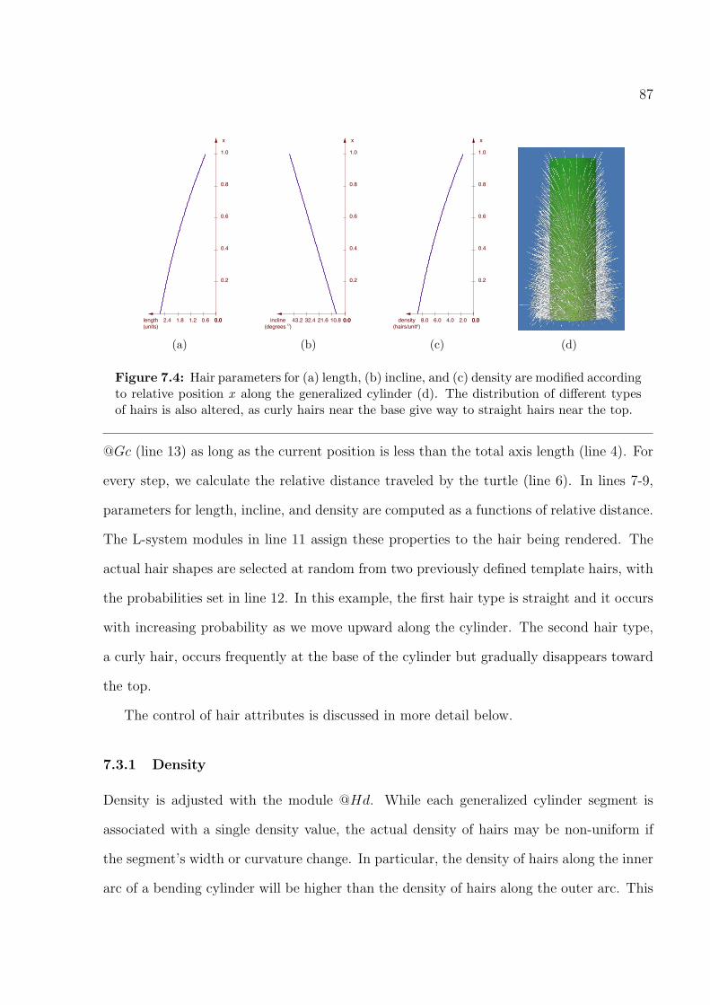
87

0.2

0.4

0.6

0.8

1.0

x

length(units)

0.00.00.61.21.82.4

(a)

0.2

0.4

0.6

0.8

1.0

x

incline(degrees ο)

0.00.010.821.632.443.2

(b)

0.2

0.4

0.6

0.8

1.0

x

density(hairs/unit2)

0.00.02.04.06.08.0

(c) (d)

Figure 7.4: Hair parameters for (a) length, (b) incline, and (c) density are modified accordingto relative position x along the generalized cylinder (d). The distribution of different typesof hairs is also altered, as curly hairs near the base give way to straight hairs near the top.

@Gc (line 13) as long as the current position is less than the total axis length (line 4). For

every step, we calculate the relative distance traveled by the turtle (line 6). In lines 7-9,

parameters for length, incline, and density are computed as a functions of relative distance.

The L-system modules in line 11 assign these properties to the hair being rendered. The

actual hair shapes are selected at random from two previously defined template hairs, with

the probabilities set in line 12. In this example, the first hair type is straight and it occurs

with increasing probability as we move upward along the cylinder. The second hair type,

a curly hair, occurs frequently at the base of the cylinder but gradually disappears toward

the top.

The control of hair attributes is discussed in more detail below.

7.3.1 Density

Density is adjusted with the module @Hd. While each generalized cylinder segment is

associated with a single density value, the actual density of hairs may be non-uniform if

the segment’s width or curvature change. In particular, the density of hairs along the inner

arc of a bending cylinder will be higher than the density of hairs along the outer arc. This

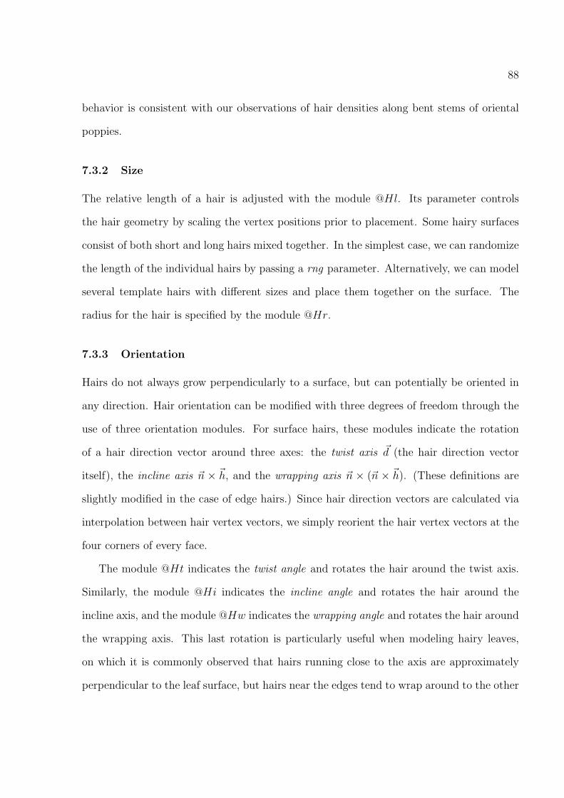
88

behavior is consistent with our observations of hair densities along bent stems of oriental

poppies.

7.3.2 Size

The relative length of a hair is adjusted with the module @Hl. Its parameter controls

the hair geometry by scaling the vertex positions prior to placement. Some hairy surfaces

consist of both short and long hairs mixed together. In the simplest case, we can randomize

the length of the individual hairs by passing a rng parameter. Alternatively, we can model

several template hairs with different sizes and place them together on the surface. The

radius for the hair is specified by the module @Hr.

7.3.3 Orientation

Hairs do not always grow perpendicularly to a surface, but can potentially be oriented in

any direction. Hair orientation can be modified with three degrees of freedom through the

use of three orientation modules. For surface hairs, these modules indicate the rotation

of a hair direction vector around three axes: the twist axis ~d (the hair direction vector

itself), the incline axis ~n × ~h, and the wrapping axis ~n × (~n × ~h). (These definitions are

slightly modified in the case of edge hairs.) Since hair direction vectors are calculated via

interpolation between hair vertex vectors, we simply reorient the hair vertex vectors at the

four corners of every face.

The module @Ht indicates the twist angle and rotates the hair around the twist axis.

Similarly, the module @Hi indicates the incline angle and rotates the hair around the

incline axis, and the module @Hw indicates the wrapping angle and rotates the hair around

the wrapping axis. This last rotation is particularly useful when modeling hairy leaves,

on which it is commonly observed that hairs running close to the axis are approximately

perpendicular to the leaf surface, but hairs near the edges tend to wrap around to the other

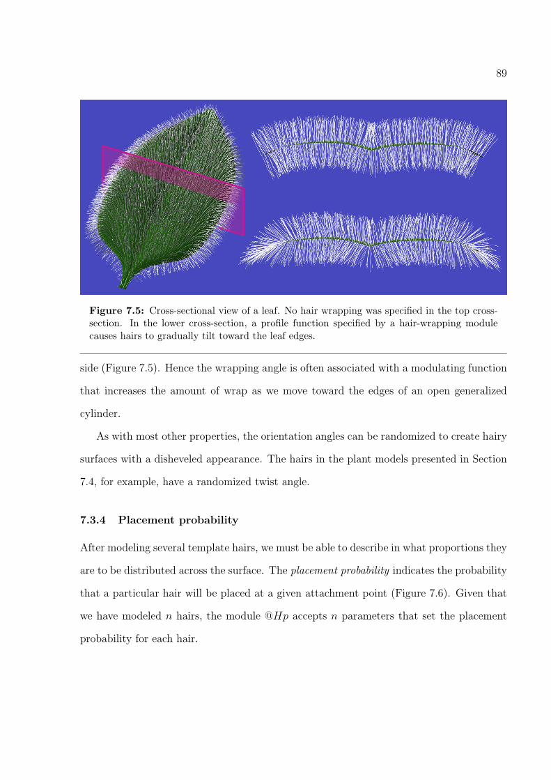
89

Figure 7.5: Cross-sectional view of a leaf. No hair wrapping was specified in the top cross-section. In the lower cross-section, a profile function specified by a hair-wrapping modulecauses hairs to gradually tilt toward the leaf edges.

side (Figure 7.5). Hence the wrapping angle is often associated with a modulating function

that increases the amount of wrap as we move toward the edges of an open generalized

cylinder.

As with most other properties, the orientation angles can be randomized to create hairy

surfaces with a disheveled appearance. The hairs in the plant models presented in Section

7.4, for example, have a randomized twist angle.

7.3.4 Placement probability

After modeling several template hairs, we must be able to describe in what proportions they

are to be distributed across the surface. The placement probability indicates the probability

that a particular hair will be placed at a given attachment point (Figure 7.6). Given that

we have modeled n hairs, the module @Hp accepts n parameters that set the placement

probability for each hair.

90

Straight: 0.2Curly: 0.8

Straight: 0.8Curly: 0.2

Figure 7.6: The distribution of template hairs can be controlled by assigning placementprobability values. In the left image, straight hairs dominate, while in the right image, curlyhairs dominate.

7.3.5 Hair Material

Material modules were introduced in Section 4.4 as a method of specifying materials for

the surface of a plant. Hairs growing from the surface typically have very different material

properties than the surface, so it is necessary to specify hair materials separately. The

module @Hm uses the material from the last material module for the purpose of shading

hairs. Hairs continue to be shaded with this same material until the next occurrence of

@Hm.

7.4 Results

This section presents several plant models that display different types of hairs. All the

images were rendered using a Monte Carlo ray-tracer capable of simulating translucency and

rendering hairs. The plants are visualized against solid backgrounds to better emphasize

the appearance of the hairs. Hair shading is achieved with a slightly modified Kajiya model

[41] that accounts for backscattering (light scattered back in the general direction of the

light source), similar to the model proposed by Goldman [28]. Each model is illuminated

with a single spherical light source and a hemispherical skylight.

The leaves and branches of Nankin cherries are covered in a velvety fuzz that is barely

visible under normal frontlighting. Under the influence of direct backlighting, however, the

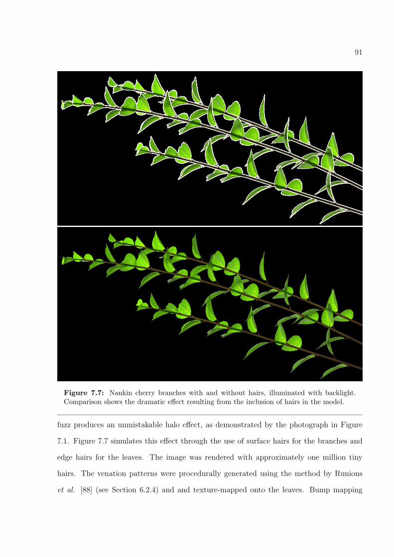
91

Figure 7.7: Nankin cherry branches with and without hairs, illuminated with backlight.Comparison shows the dramatic effect resulting from the inclusion of hairs in the model.

fuzz produces an unmistakable halo effect, as demonstrated by the photograph in Figure

7.1. Figure 7.7 simulates this effect through the use of surface hairs for the branches and

edge hairs for the leaves. The image was rendered with approximately one million tiny

hairs. The venation patterns were procedurally generated using the method by Runions

et al. [88] (see Section 6.2.4) and and texture-mapped onto the leaves. Bump mapping

92

Figure 7.8: A photograph and a model of fern croziers.

lends the veins a sense of depth, while diffuse transmission of light is used to simulate the

translucency in the leaves.

In contrast to the delicate hairs of the Nankin cherry, the fern croziers shown in Figure

7.8 are characterized by relatively large scales. The model captures changes in the length

and density of scales along and around the stem.

Oriental poppies are covered in pronounced white hairs that resemble bristles but are

soft to the touch. New leaves growing at the tips of fronds have a very dense covering

of hairs, but the density decreases as the leaves age. At a certain point, the leaves lose

all their front and back hairs, but retain edge hairs (see Figure 7.9). A fully grown (but

not yet flowering) oriental poppy, with approximately 120,000 hairs, is displayed in Figure

7.10. The hair length from the base to the tip of a frond has been gradually decreased, and

shorter hairs have been used for the backside of leaves. A hair wrapping function around

93

the leaves has also been used. While a mixture of straight and curved hairs were used for

most of the plant, the placement probability for straight hairs on the bud was set to 1, and

the hairs were tilted such that they became almost tangent to the surface of the bud.

In the introduction for thesis, the wild crocus (Figure 1.1) was presented as a modeling

and rendering challenge, not only for its wispy hairs, but also for the fuzzy translucency

and subtle venation patterns of its violet sepals. A synthetic model of the crocus containing

65,000 hairs is shown in Figure 7.11. Hair length and orientation have been varied along

the surface of the sepals and finger-like leaves. Three different template hairs have been

used for the model. Fuzzy translucency and procedurally generated parallel veins have been

added to the sepals. The gradual browning of the leaves toward their tips is achieved by

altering color parameters with material modules. Indirect lighting provided by the skylight

produces subtle variations in illumination, especially where the leaves join the stem. In

short, the rendered crocus is a culmination of most of the techniques presented in this

research.

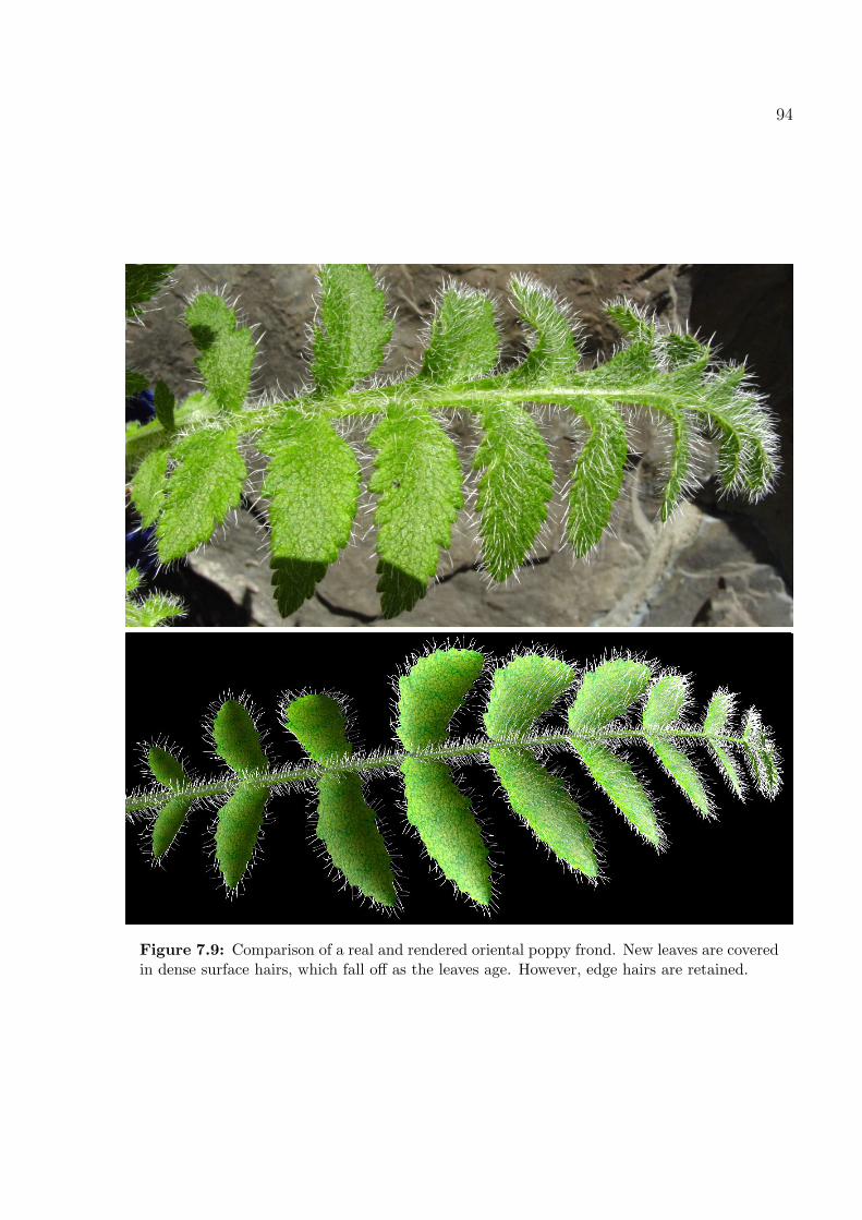
94

Figure 7.9: Comparison of a real and rendered oriental poppy frond. New leaves are coveredin dense surface hairs, which fall off as the leaves age. However, edge hairs are retained.

95

Figure 7.10: Oriental poppy

96

Figure 7.11: Prairie crocus

Chapter 8

Conclusions and Future Work

This research has focused on improving the realism of plants generated with L-systems.

Several approaches were taken toward this goal. A method of incorporating dynamic ma-

terial specifications in L-systems has been proposed, making it possible to use material

modules to generate plant models with a large variety of surface appearances. Global illu-

mination and shading of plant surfaces, with a particular emphasis on translucency, have

been discussed, taking into account observed light interactions with real leaves and petals.

The fitting of textures onto generalized cylinder surfaces generated by L-systems has made

it possible to map surface features onto leaves and petals. This research presented procedu-

ral methods for generating translucent outlines and venation patterns, whose parameters

can be specified in the L-system with material modules. Finally, a method for generating

hairs on plants was presented. Local hair parameters can be controlled using modules, in

conjunction with orientation information inherent to L-systems.

The results of these approaches have contributed to increased realism in the field of

plant rendering, demonstrated through the inclusion of numerous state-of-the-art render-

ings throughout this thesis. Improving the appearance of plants generated with L-systems

is an incremental process, and there are many topics that require further exploration as

part of future work:

• Implementation of material modules in L+C. Material modules implemented

in cpfg often require long parameter lists, making it difficult to determine which

value is associated with which appearance parameter. Furthermore, the ordering of

the parameters lists is rigid, and must conform to the order in which the parameters

are listed in the corresponding shader definition. The L+C modeling language [42] is

97

98

a formalism for expressing L-systems based on the C programming language. Using

this language, it would be possible to express materials using C data structures,

or structs, whose typed data elements would represent appearance parameters. By

linking together structs into a shade tree, the entire tree could then be passed as a

single parameter to a material module.

• Real-time dynamic specification of materials. Rendering libraries such as

OpenGL are increasingly making use of real-time shaders that allow materials to

be created and selected on the fly. While our discussion has focused predominantly

on use of material modules for offline rendering systems, they could also be used, for

example, to alternate between a real-time translucency shader for tissues and a hair

shader for fuzz as a user is interactively rotating a plant model.

• Subsurface scattering rendering techniques. Donner and Jensen [17] recently

presented a BDF that uses an efficient multiple dipole approximation to simulate

scattering in thin surfaces with multiple layers, such as leaves. Scattering in thicker,

volumetric organs such as soft stems would further benefit from a full BSSDF treat-

ment. It would be interesting to further explore these advanced rendering techniques

on full plant models.

• Enhanced parallel venation shader. The shader implemented for this research

does not simulate the fusing of veins commonly observed at the tips of monocot

leaves [65]. This functionality could be added by changing the vein representation

from binary trees to cyclic graphs.

• Multiscale modeling based on biological simulations. Our approach to mod-

eling plants with hair is purely phenomenological: we use a Poisson distribution to

position hairs on their supporting surfaces, and reproduce the shape of individual

hairs according to their observed appearance. It may be interesting, at least from a

99

biological perspective, to simulate the underlying morphogenetic processes according

to current biological theories and hypotheses.

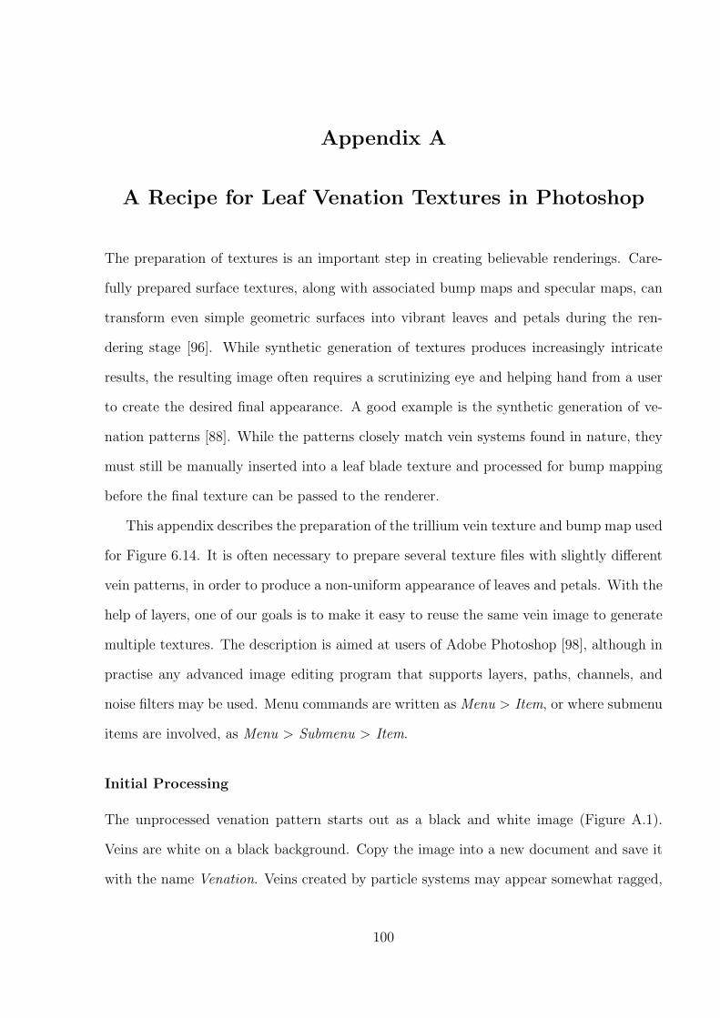
Appendix A

A Recipe for Leaf Venation Textures in Photoshop

The preparation of textures is an important step in creating believable renderings. Care-

fully prepared surface textures, along with associated bump maps and specular maps, can

transform even simple geometric surfaces into vibrant leaves and petals during the ren-

dering stage [96]. While synthetic generation of textures produces increasingly intricate

results, the resulting image often requires a scrutinizing eye and helping hand from a user

to create the desired final appearance. A good example is the synthetic generation of ve-

nation patterns [88]. While the patterns closely match vein systems found in nature, they

must still be manually inserted into a leaf blade texture and processed for bump mapping

before the final texture can be passed to the renderer.

This appendix describes the preparation of the trillium vein texture and bump map used

for Figure 6.14. It is often necessary to prepare several texture files with slightly different

vein patterns, in order to produce a non-uniform appearance of leaves and petals. With the

help of layers, one of our goals is to make it easy to reuse the same vein image to generate

multiple textures. The description is aimed at users of Adobe Photoshop [98], although in

practise any advanced image editing program that supports layers, paths, channels, and

noise filters may be used. Menu commands are written as Menu > Item, or where submenu

items are involved, as Menu > Submenu > Item.

Initial Processing

The unprocessed venation pattern starts out as a black and white image (Figure A.1).

Veins are white on a black background. Copy the image into a new document and save it

with the name Venation. Veins created by particle systems may appear somewhat ragged,

100

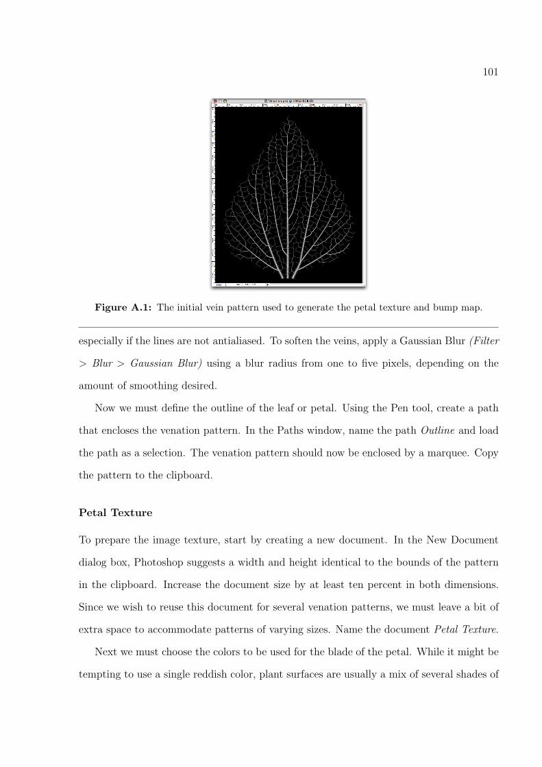
101

Figure A.1: The initial vein pattern used to generate the petal texture and bump map.

especially if the lines are not antialiased. To soften the veins, apply a Gaussian Blur (Filter

> Blur > Gaussian Blur) using a blur radius from one to five pixels, depending on the

amount of smoothing desired.

Now we must define the outline of the leaf or petal. Using the Pen tool, create a path

that encloses the venation pattern. In the Paths window, name the path Outline and load

the path as a selection. The venation pattern should now be enclosed by a marquee. Copy

the pattern to the clipboard.

Petal Texture

To prepare the image texture, start by creating a new document. In the New Document

dialog box, Photoshop suggests a width and height identical to the bounds of the pattern

in the clipboard. Increase the document size by at least ten percent in both dimensions.

Since we wish to reuse this document for several venation patterns, we must leave a bit of

extra space to accommodate patterns of varying sizes. Name the document Petal Texture.

Next we must choose the colors to be used for the blade of the petal. While it might be

tempting to use a single reddish color, plant surfaces are usually a mix of several shades of

102

color. For the trillium, blending together two shades of maroon produces a more believable

surface. In the Layers window, set the name of the existing layer to Blade Color 1. Prepare

the first shade of maroon (e.g. RGB 180, 8, 57 ) and fill the entire layer with the color.

Create another layer named Blade Color 2, and fill it with a second shade of maroon (e.g.

RGB 108, 2, 32 ).

Now create a layer mask for Blade Color 2. The idea is to fill the mask with a black and

white noise texture. Black areas hide the maroon in the top layer (Blade Color 2), white

areas hide the maroon in the lower layer (Blade Color 1 ), and grey areas blend together

the colors to varying degrees.

In the Channels window, make your mask visible and hide all other channels. Set the

foreground and background colours to black and white respectively. Generate a billowy

effect by choosing Filter > Render > Clouds. Add specks by choosing Filter > Noise >

Add Noise. For noise parameters, use 40% for amount and select the uniform distribution

and monochromatic options. Soften the noise with a Gaussian Blur, using a pixel radius

of about 3. The mask should now appear as in Figure A.2-a. Turn on the RGB channel to

see the mask in action (Figure A.2b).

Finally, we need to add the veins. Create a new layer with the title Vein Color. Pick

a deep shade of maroon (RGB 35, 0, 6 works well) to make the veins stand out, and fill

the layer. We want the Vein Color layer to show through the vein patterns, and the Blade

Color layers to appear between the veins. To achieve this, create a new layer mask and

copy the vein pattern from the Venation document. In the Channels window, paste the

veins into the Vein Color Mask channel. Switching back to the Layers window, the stack

of layers and layer masks should appear as in Figure A.4a.

Select Edit > Copy Merged to copy all visible layers together, and paste the final image

texture into a new document (Figure A.5a).

By reusing the Petal Texture document as a kind of template, creating new vein textures

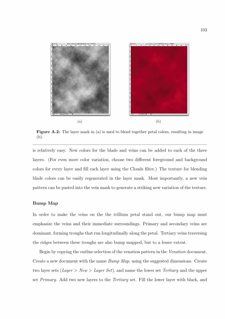
103

(a) (b)

Figure A.2: The layer mask in (a) is used to blend together petal colors, resulting in image(b).

is relatively easy. New colors for the blade and veins can be added to each of the three

layers. (For even more color variation, choose two different foreground and background

colors for every layer and fill each layer using the Clouds filter.) The texture for blending

blade colors can be easily regenerated in the layer mask. Most importantly, a new vein

pattern can be pasted into the vein mask to generate a striking new variation of the texture.

Bump Map

In order to make the veins on the the trillium petal stand out, our bump map must

emphasize the veins and their immediate surroundings. Primary and secondary veins are

dominant, forming troughs that run longitudinally along the petal. Tertiary veins traversing

the ridges between these troughs are also bump mapped, but to a lesser extent.

Begin by copying the outline selection of the venation pattern in the Venation document.

Create a new document with the name Bump Map, using the suggested dimensions. Create

two layer sets (Layer > New > Layer Set), and name the lower set Tertiary and the upper

set Primary. Add two new layers to the Tertiary set. Fill the lower layer with black, and

104

paste the venation pattern into the upper layer. Repeat for the Primary set: add two new

layers, filled with solid black and the venation pattern, respectively. At this point, the

Layers window should appear as in Figure A.4b. Command-click or Control-click on one

of the venation layers to create an outline selection of the petal, and save this selection to

a channel (Select > Save Selection). For now, hide the Tertiary set, as we will first create

the bump maps for the primary and secondary veins.

Our goal is to generate gradients around the vein paths, in order to simulate the inden-

tation of veins in the petal. Select the Magic Wand tool, and set Tolerance to a low value

(below 20 is fine) and uncheck Contiguous. Click anywhere in a black region between the

veins to select the entire blade, excluding veins. Press delete to remove these black regions

(nothing will appear to change, as deleting black regions will only expose the black layer

below). Invert the selection to capture the veins, and fill the selection with solid white.

We can now use the layer stroke effect (Layer > Layer Style > Stroke) to make the

veins bumpy. Set Fill Type to Gradient and Style to Shape Burst. Create a new gradient

to reflect the falloff from the veins to the petal blade. Adjust the size slider to set how far

the falloff extends. The bump map should appear as in Figure A.4a.

Now we can turn our attention to primary and secondary veins. Make the Primary set

visible. In order to remove the tertiary veins from the venation layer, repeatedly apply a

Gaussian Blur and Levels adjustment to tighten up the veins. These operations should be

performed in small increments to prevent the veins from breaking up. For example, each

Gaussian Blur should not have a pixel radius greater than two. For each Levels adjustment,

set the left input slider to a value between 10 and 100. Once the tertiary veins fade out

completely, use the Eraser tool to remove any disjoint veins. As before, use the Magic

Wand to select the black blade regions and clear them. Then invert the selection and fill

the veins with white.

Apply the layer stroke effect to the primary and secondary veins. Set the size slider

105

(a) (b)

Figure A.3: Bump maps for the a) tertiary veins b) primary/secondary veins

to a considerably larger value than the one used for tertiary veins, in order to emphasize

the dominant troughs formed by the primaries and secondaries. Figure A.4b illustrates the

resulting bump map.

Finally, set the opacity value of the Primary set to about 50%, to allow the veins from

the Tertiary set to show through. You can continue to tweak the stroke effects in each of

the layer sets until you are happy with the bump map. Load the outline selection you had

saved earlier (Select > Load Selection), and copy the bump map into a new image (Figure

A.5a).

Generating new bump maps tends to be more tedious than generating new image tex-

tures, because each new venation pattern must be carefully processed to extract the pri-

mary, secondary, and tertiary veins. Hence, a new bump map must be created from scratch

for each venation pattern. While bump maps will not have much effect on leaves or petals

that are rendered in the distance, they are definitely worth the effort to generate for close-up

shots.

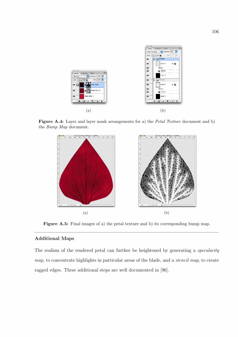
106

(a) (b)

Figure A.4: Layer and layer mask arrangements for a) the Petal Texture document and b)the Bump Map document.

(a) (b)

Figure A.5: Final images of a) the petal texture and b) its corresponding bump map.

Additional Maps

The realism of the rendered petal can further be heightened by generating a specularity

map, to concentrate highlights in particular areas of the blade, and a stencil map, to create

ragged edges. These additional steps are well documented in [96].

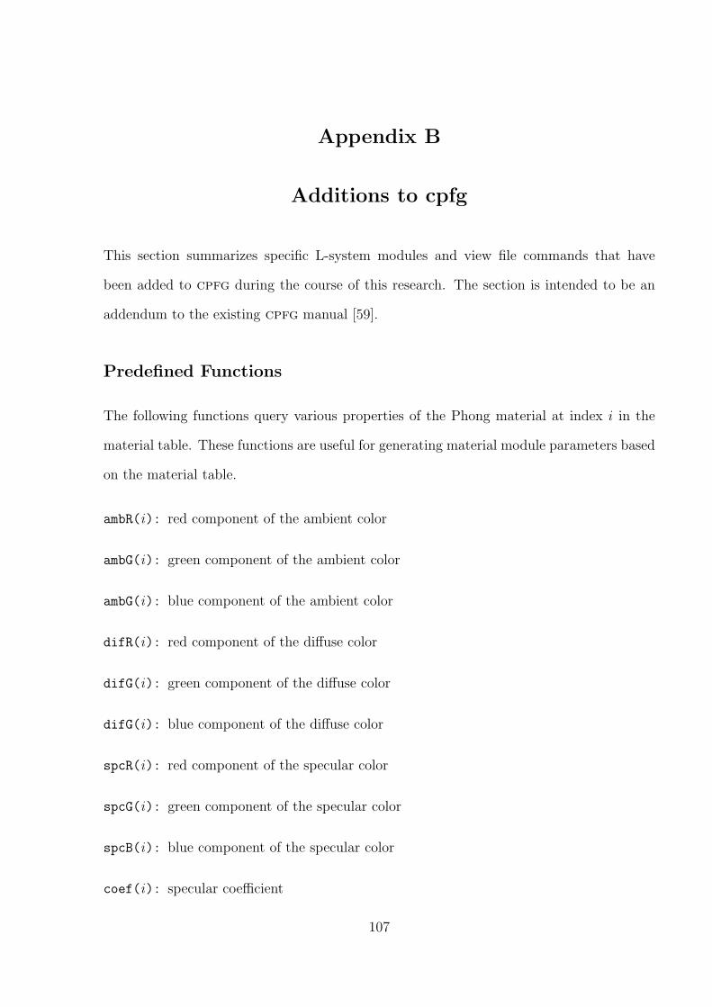
Appendix B

Additions to cpfg

This section summarizes specific L-system modules and view file commands that have

been added to cpfg during the course of this research. The section is intended to be an

addendum to the existing cpfg manual [59].

Predefined Functions

The following functions query various properties of the Phong material at index i in the

material table. These functions are useful for generating material module parameters based

on the material table.

ambR(i): red component of the ambient color

ambG(i): green component of the ambient color

ambG(i): blue component of the ambient color

difR(i): red component of the diffuse color

difG(i): green component of the diffuse color

difG(i): blue component of the diffuse color

spcR(i): red component of the specular color

spcG(i): green component of the specular color

spcB(i): blue component of the specular color

coef(i): specular coefficient

107

108

Interpreted Modules

Interpreted modules are the building blocks of strings in the L-system file. Several new

modules have been specified for materials and hairs.

Dynamically Specified Materials

New materials may now be specified during L-system interpretation using the following

modules:

@Mt("shader", value1, . . . ,valuen): The material module specifies a new material,

based on the shading model shader and using parameters valuen. shader is the name

of the shader specified as a string, and its corresponding shader description must

be included in the shader file. The value parameters may be int, float, or string,

depending on the parameter types specified by the shading model. Value parameters

may also consist of material table tokens (%a, %d, %s, %h) that substitute values

from the current material in the material table (see Table 4.2), or sub-material tokens

(%m) used for building shade trees. Materials specified by material modules form

the root node of a shade tree.

@Ms("shader", value1, . . . ,valuen): The sub-material module specifies a new sub-

material, based on the shading model shader and using parameters valuen. Sub-

materials function like materials, except that they form the child nodes of a shade

tree. Sub-material modules are referenced by a parent (sub)material via the sub-

material token (%m).

Hairs

Hair modules control the appearance of hair on the surface of a generalized cylinder mesh.

@Hf(bool): Enables or disables hairs on the front side of the mesh. bool can be on or off.

109

@Hb(bool): Enables or disables hairs on the back side of the mesh. bool can be on or off.

@He(bool): Enables or disables hairs along the edges of the mesh. bool can be on or off.

@Hd(value, rng, fun, loc): Specifies the density of hairs. A value of 1 will generate a

single hair on a cylinder with a width and circumference of one.

@Hl(value, rng, fun, loc): Specifies the length of hairs.

@Hr(value, rng, fun, loc): Specifies the radius of hairs.

@Hi(value, rng, fun, loc): Specifies the incline angle of hairs along the generalized cylin-

der.

@Ht(value, rng, fun, loc): Specifies the twist angle along the hair’s axis.

@Hw(value, rng, fun, loc): Specifies the wrapping angle of hairs around the generalized

cylinder.

@Hp(P1, ..., Pn, loc): Specifies the placement probability for each template hair.

The optional parameters are explained below:

loc Sets the property for hairs in a particular location of the surface: front (0), back (1),

or edge (2)

fun Index to a modulating function that modifies value around the girth of a cylinder.

The function is specified in the view file.

rng Specifies the maximum bounds for varying the properties of individual hairs. The

property will be a random value within the range value± rng

110

View File

The view file contains various drawing, viewing, and rendering parameters. The following

new parameters may now be included in view file:

Textures

Two new subcommands for specifying texture files exist:

I: When present, makes the texture file invisible during OpenGL rendering. This is useful

for forcing the generation of texture coordinates on a mesh without displaying a

texture.

T: tiles Indicates how many times the texture should be tiled from start to tip of a general-

ized cylinder. If both T: and R: are specified, the last subcommand takes dominance.

M: mapping Indicates how v coordinates are mapped along a generalized cylinder. mapping

may be a, for incrementing coordinates at uniformly intervals along the cylinder axis,

or s, for placing coordinates uniformly along the cylinder surface.

Dynamically Specified Materials

material modules: state Determines whether or not to use material modules. state can

be on or off.

shader: filename Specifies the name of the shader file containing shader descriptions. All

material module parameters used in the L-system are validated against these shader

descriptions.

Hairs

hair: axis file1[:probability1] . . . axis filen[:probabilityn] Specifies the hair axis files to

be used for generating hairs (Figure B.1). Each axis file may optionally be associated

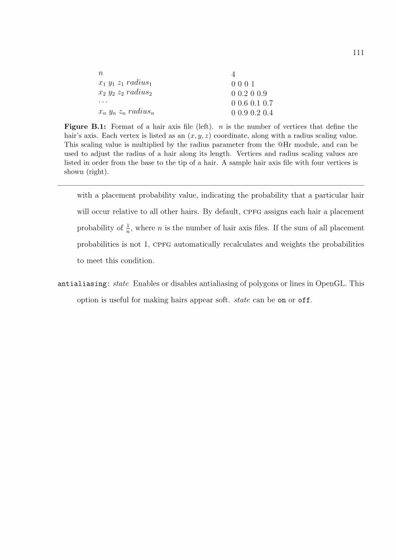
111

nx1 y1 z1 radius1

x2 y2 z2 radius2

· · ·xn yn zn radiusn

40 0 0 10 0.2 0 0.90 0.6 0.1 0.70 0.9 0.2 0.4

Figure B.1: Format of a hair axis file (left). n is the number of vertices that define thehair’s axis. Each vertex is listed as an (x, y, z) coordinate, along with a radius scaling value.This scaling value is multiplied by the radius parameter from the @Hr module, and can beused to adjust the radius of a hair along its length. Vertices and radius scaling values arelisted in order from the base to the tip of a hair. A sample hair axis file with four vertices isshown (right).

with a placement probability value, indicating the probability that a particular hair

will occur relative to all other hairs. By default, cpfg assigns each hair a placement

probability of 1n, where n is the number of hair axis files. If the sum of all placement

probabilities is not 1, cpfg automatically recalculates and weights the probabilities

to meet this condition.

antialiasing: state Enables or disables antialiasing of polygons or lines in OpenGL. This

option is useful for making hairs appear soft. state can be on or off.

Bibliography

[1] H. Abelson and A. DiSessa. Turtle Geometry: The Computer as a Medium for

Exploring Mathematics. MIT Press, Cambridge, MA, 1981.

[2] K. Anjyo, Y. Usami, and T. Kurihara. A simple method for extracting the natural

beauty of hair. In Proceedings of SIGGRAPH ’92, pages 111–120, 1992.

[3] G. B. Arfken, D. F. Griffing, D. C. Kelly, and J. Priest. University Physics. Harcourt

Brace Jovanovich, San Diego, 2nd edition, 1989.

[4] G. Baranoski and J. Rokne. An algorithmic reflectance and transmittance model for

plant tissue. Computer Graphics Forum 16, 16:141–150, 1997.

[5] G. Baranoski and J. Rokne. Efficiently simulating scattering of light by leaves. The

Visual Computer, 17:491–505, 2001.

[6] R. Bartels, J. Beatty, and B. Barsky. An introduction to splines for use in computer

graphics and geometric modeling. Morgan Kaufmann, Los Altos, CA, 1987.

[7] J. F. Blinn and M. E. Newell. Texture and reflection in computer generated images.

Communications of the ACM, 19(10):542–547, October 1976.

[8] J. Bloomenthal. Modeling the mighty maple. In Proceedings of SIGGRAPH ’85,

pages 305–311, 1985.

[9] P. Bui-Tong. Illumination for computer generated pictures. In Communications of

the ACM, volume 18, pages 311–317, June 1975.

[10] T. Burge. A branching cellular texture basis function. In SIGGRAPH 2000 Technical

Sketch, 2000.

112

113

[11] E. Catmull. A subdivision algorithm for computer display of curved surfaces. PhD

thesis, University of Utah, Salt Lake City, UT, December 1974.

[12] R. L. Cook. Shade trees. In Proceedings of SIGGRAPH ’84, pages 223–231, 1984.

[13] R. L. Cook. Stochastic sampling in computer graphics. ACM Transactions on Graph-

ics, 5(1):51–72, 1986.

[14] R. L. Cook, T. Porter, and L. Carpenter. Distributed ray tracing. In Proceedings of

SIGGRAPH ’84, pages 137–145, 1984.

[15] A. Daldegan, N. Thalmann, T. Kurihara, and D. Thalmann. An integrated system

for modeling, animating and rendering hair. In Computer Graphics Forum, pages

211–221, 1993.

[16] P. Debevec. Image-based lighting. IEEE Computer Graphics and Applications,

22(2):26–34, March/April 2002.

[17] C. Donner and H. W. Jensen. Light diffusion in multi-layered translucent materials.

In Proceedings of SIGGRAPH ’05, 2005.

[18] D. Ebert, K. Musgrave, D. Peachey, K. Perlin, and S. Worley. Texturing and Model-

ing: A Procedural Approach. Academic Press, San Diego, CA, 1994.

[19] P. Federl. Vlab documentation. Website, 1999. www.algorithmicbotany.org/vlab.

[20] K. W. Fleischer, D. H. Laidlaw, B. L. Currin, and A. H. Barr. Cellular texture

generation. In Proceedings of SIGGRAPH ’95, pages 239–248, 1995.

[21] J. D. Foley, A. van Dam, S. K. Feiner, and J. F. Hughes. Computer Graphics:

Principles and Practice. Addison-Wesley, Reading, Massachusetts, 2nd edition, 1997.

114

[22] D. R. Fowler, P. Prusinkiewicz, and J. Battjes. A collision-based model of spiral

phyllotaxis. In Proceedings of SIGGRAPH ’92, pages 361–368, 1992.

[23] O. Franzke and O. Deussen. Rendering plant leaves faithfully. In Proceedings of the

SIGGRAPH 2003 Conference on Sketches, page 1, 2003.

[24] M. Fuhrer, H. W. Jensen, and P. Prusinkiewicz. Modeling hairy plants. In Proceed-

ings of Pacific Graphics ’04, pages 217–236, 2004.

[25] A. V. Gelder and J. Wilhelms. An interactive fur modeling technique. In Proceedings

of Graphics Interface ’97, pages 181–188, 1997.

[26] E. M. Gifford and A. S. Foster. Morphology and Evolution of Vascular Plants. W.

H. Freeman and Company, New York, 1996.

[27] A. S. Glassner. Principles of Digital Image Synthesis. Morgan Kaufmann, San Fran-

cisco, 1995.

[28] D. Goldman. Fake fur rendering. In Proceedings of SIGGRAPH ’97, pages 127–134,

1997.

[29] C. M. Goral, K. E. Torrance, D. P. Greenberg, and B. Battaile. Modeling the in-

teraction of light between diffuse surfaces. In Proceedings of SIGGRAPH ’84, pages

213–222, 1984.

[30] L. Grant. Diffuse and specular characteristics of leaf reflectance. Remote Sensing

Environment, 22:309–322, 1987.

[31] J.S. Hanan. Parametric L-systems and their application to the modelling and visual-

ization of plants. PhD thesis, University of Regina, June 1992.

[32] P. Hanrahan and W. Krueger. Reflection from layered surfaces due to subsurface

scattering. In Proceedings of SIGGRAPH ’93, volume 165-174, 1993.

115

[33] P. Hanrahan and J. Lawson. A language for shading and lighting calculations. In

Proceedings of SIGGRAPH ’90, pages 289–298, 1990.

[34] L. J. Hickey. A revised classification of the architecture of dicotyledonous leaves. In

C. R. Metcalfe and L. Chalk, editors, Anatomy of the dicotyledons, volume 1, pages

25–39. Clarendon Press, 1979.

[35] H. W. Jensen. Realistic Image Synthesis Using Photon Mapping. A K Peters, Natick,

Massachusetts, 2001.

[36] H. W. Jensen. Dali rendering system. Software, 2004.

[37] H. W. Jensen and J. Buhler. A rapid hierarchical rendering technique for translucent

materials. In Proceedings of SIGGRAPH ’02, pages 576–581, 2002.

[38] H. W. Jensen, S. R. Marschner, M. Levoy, and P. Hanrahan. A practical model for

subsurface light transport. In Proceedings of SIGGRAPH ’01, pages 511–518, 2001.

[39] G. H. Joblove and D. P. Greenberg. Color spaces for computer graphics. In Proceed-

ings of SIGGRAPH ’78, pages 20–25, 1978.

[40] J. T. Kajiya. The rendering equation. In Proceedings of SIGGRAPH ’86, pages

143–150, 1986.

[41] J. T. Kajiya and T. L. Kay. Rendering fur with three dimensional textures. In

Proceedings of SIGGRAPH ’89, pages 271–280, 1989.

[42] R. Karwowski and P. Prusinkiewicz. Design and implementation of the l+c modeling

language. Electronic Notes in Theoretical Computer Science, 86(2):19, 2003.

[43] R. Karwowski and P. Prusinkiewicz. The L-system-based plant-modeling environ-

ment l-studio 4.0. In Proceedings of the 4th International Workshop on Functional-

Structural Plant Models, pages 403–405, 2004.

116

[44] D. S. Kay. Transparency, refraction, and ray tracing for computer synthesized images.

Master’s thesis, Cornell University, Ithaca, NY, January 1979.

[45] T.-Y. Kim and U. Neumann. Interactive multiresolution hair modeling and editing.

In Proceedings of SIGGRAPH ’02, pages 620–629, 2002.

[46] J. Koenderink and S. Pont. The secret of velvety skin. Machine vision and applica-

tions, 14:260–268, 2003.

[47] A. A. Kokhanovsky. On the determination of the refractive index of strongly ab-

sorbing particles dispersed in a non-absorbing host medium. Journal of Physics D:

Applied Physics, 32:825–831, 1999.

[48] C. Kolb and R. Bogart. Rayshade 4.0. Open source software, 1991.

[49] S. Lefebvre and F. Neyret. Synthesizing bark. In Proceedings of the 13th Eurographics

workshop on Rendering Rendering, pages 105–116, 2002.

[50] J. Lengyel, E. Praun, A. Finkelstein, and H. Hoppe. Real-time fur over arbitrary

surfaces. In Proceedings of the ACM Symposium on Interactive 3D Graphics, pages

227–232, 2001.

[51] O. Leyser and S. Day. Mechanisms in plant development. Blackwell, Oxford, 2003.

[52] A. Lindenmayer. Mathematical models for cellular interaction in development, Parts

I and II. Journal of Theoretical Biology, 18:280–315, 1968.

[53] R. Lu, J. J. Koenderink, and A. M. Kappers. Optical properties (bidirectional re-

flectance distribution functions) of velvet. Applied Optics, 37(25):5974–5984, 1998.

[54] K. Maritaud. Rendu realiste d’arbres vus de pres en images de synthese images de

synthese. PhD thesis, University de Limoges, France, December 2003.

117

[55] W. R. Mark, R. S. Glanville, K. Akeley, and M. J. Kilgard. Cg: a system for pro-

gramming graphics hardware in a C-like language. ACM Transactions on Graphics,

22(3):896–907, 2003.

[56] S. Marschner, S. Westin, E. Lafortune, and K. Torrance. Image-based BRDF mea-

surement. Applied Optics, 39(16):2592–2600, 2000.

[57] W. Matusik. Homogeneous isotropic BRDFs. Realistic Materials in Computer

Graphics SIGGRAPH ’05 Course Notes, 2005.

[58] R. Mech. Modeling and simulation of the interactions of plants with the environment

using L-systems and their extensions. PhD thesis, University of Calgary, October

1997.

[59] R. Mech. CPFG version 3.4 user’s manual, 1998. Manuscript, Department of Com-

puter Science, University of Calgary.

[60] R. Melville. The terminology of leaf architecture. Taxon, 25(5/6):549–561, 1976.

[61] G. Miller. From wire-frame to furry animals. In Proceedings of Graphics Interface

’88, pages 138–146, 1988.

[62] G. S. Miller and C. R. Hoffman. Illumination and reflection maps: Simulated objects

in simulated and real environments. In SIGGRAPH ’84 Course Notes for Advanced

Computer Graphics Animation, 1984.

[63] D. P. Mitchell. Generating antialiased images at low sampling densities. In Proceed-

ings of SIGGRAPH ’87, pages 65–72, 1987.

[64] M. Nakajima, S. Saruta, and H. Takahashi. Hair image generating algorithm using

fractional hair model. In Signal Processing: Image Communication 9, pages 267–273,

1997.

118

[65] T. Nelson and N. Dengler. Leaf vascular pattern formation. The Plant Cell, 9:1121–

1135, July 1997.

[66] F. E. Nicodemus, J. C. Richmond, J. J. Hsia, I. W. Ginsberg, and T. Limperis.

Geometric considerations and nomenclature for reflectance. NBS Monograph 160,

1977.

[67] T. Nishita and E. Nakamae. Continuous tone representation of three-dimensional

objects taking account of shadows and interreflection. In Proceedings of SIGGRAPH

’85, pages 23–30, 1985.

[68] M. Olano and A. Lastra. A shading language on graphics hardware: The pixelflow

shading system. In Proceedings of SIGGRAPH ’98, pages 156–168, 1998.

[69] D. R. Peachey. Solid texturing of complex surfaces. In Proceedings of SIGGRAPH

’85, pages 279–286, 1985.

[70] K. Perlin. An image synthezier. In Proceedings of SIGGRAPH ’85, pages 287–296,

1985.

[71] M. Pharr. Layered media for surface shaders. Advanced RenderMan SIGGRAPH

’02 Course Notes, 2002.

[72] B. T. Phong. Illumination for computer generated pictures. Communications of the

ACM, 18(6):311–317, June 1975.

[73] A. J. Preetham, P. Shirley, and B. Smits. A practical analytic model for daylight. In

Proceedings of SIGGRAPH ’99, pages 91–100, 1999.

[74] P. Prusinkiewicz. Graphical applications of L-systems. In Proceedings of Graphics

Interface ’86, pages 247–253, 1986.

119

[75] P. Prusinkiewicz. Modelling and visualization of biological structures. In Proceedings

of Graphics Interface ’93, pages 128–137, May 1993.

[76] P. Prusinkiewicz, M. Hammel, and E. Mjolsness. Animation of plant development.

In Proceedings of SIGGRAPH ’93, pages 351–360, 1993.

[77] P. Prusinkiewicz and J. Hanan. Visualization of botanical structures and processes

using parametric L-systems. In D. Thalmann, editor, Scientific Visualization and

Graphics Simulation, pages 183–201, Chichester, 1990. J. Wiley Sons.

[78] P. Prusinkiewicz, J. Hanan, and R. Mech. An L-system-based Plant Modeling Lan-

guage, 2000. Lecture Notes in Computer Science 1779, pages 395–410. Springer-

Verlag, Berlin.

[79] P. Prusinkiewicz, M. James, and R. Mech. Synthetic topiary. In Proceedings of

SIGGRAPH ’94, pages 351–358, 1994.

[80] P. Prusinkiewicz, R. Karwowski, R. Mech, and J. Hanan. L-studio/cpfg: A software

system for modeling plants. In M. Nagl, A. Schurr, and M. Munch, editors, Applica-

tions of graph transformation with industrial relevance, Lecture Notes in Computer

Science 1779, pages 457–464. Springer-Verlag, Berlin, 2000.

[81] P. Prusinkiewicz and A. Lindenmayer. The algorithmic beauty of plants. Springer-

Verlag, New York, 1990.

[82] P. Prusinkiewicz, L. Mundermann, R. Karwowski, and B. Lane. The use of positional

information in the modeling of plants. In Proceedings of SIGGRAPH ’01, pages 289–

300, 2001.

[83] X. Qin, E. Nakamae, K. Tadamura, and Y. Nagai. Fast photo-realistic rendering of

trees in daylight. Computer Graphics Forum, 22(3):243–252, 2003.

120

[84] V. Raghavan. Developmental Biology of Flowering Plants. Springer-Verlag, New

York, 2000.

[85] Y. Rodkaew, S. Siripant, C. Lursinsap, and P. Chongstitvatana. An algorithm for

generating vein images for realistic modeling of a leaf. In Proceedings of the In-

ternational Conference on Computational Mathematics and Modeling, pages 73–78,

2002.

[86] Y. Rodkaew, S. Siripant, C. Lursinsap, P. Chongstitvatana, T. Fujimoto, and

N. Chiba. Modeling leaf shapes using L-systems and genetic algorithms. In Pro-

ceedings of NICOGRAPH ’02, pages 1–6, Japan, April 2002.

[87] R. J. Rost, D. Baldwin, and R. Rost. The OpenGL shading language. Technical

Report Language Version 1.10, 3Dlabs, Inc., April 30, 2004.

[88] A. Runions, M. Fuhrer, B. Lane, A. Rolland-Lagan, P. Federl, and P. Prusinkiewicz.

Modeling and visualization of leaf venation patterns. In Proceedings of SIGGRAPH

’05, pages 702–711, 2005.

[89] A. Schnittger, U. Folkers, B. Schwab, G. Jurgens, and M. Hulskamp. Generation of a

spacing pattern: The role of TRIPTYCHON in trichome patterning in Arabidopsis.

Plant Cell, 11:1105–1116, 1999.

[90] A. L. Szilard and R. E. Quinton. An interpretation for DOL systems by computer

graphics. The Science Terrapin, 4:8–13, 1979.

[91] N. Tatarchuk and C. Brennan. Simulation of iridescence and translucency on thin

surfaces. In ShaderX 2: Shader Programming Tips and Tricks with DirectX 9, pages

1–11. Worldwide Publishing, 2003.

[92] K. E. Torrance and E. M. Sparrow. Theory for off-specular reflection from roughened

surfaces. Journal of Optical Society of America, 57(9):1105–1114, 1967.

121

[93] J. C. Uphof. Plant hairs. Gebruder Borntraeger, Berlin, 1962.

[94] S. Upstill. The Renderman Companion. Addison-Wesley, Reading, Massachusetts,

1990.

[95] F. R. Vance, J. R. Jowsey, J. S. McLean, and F. A. Switzer. Wildflowers Across the

Prairies. Greystone Books, 3rd edition, 1999.

[96] F. Vitale. Surfacing: Half the battle. In Mastering 3D Graphics: Digital Botany and

Creepy Insects, pages 147–165. John Wiley and Sons, 2000.

[97] G. J. Ward. Measuring and modeling anisotropic reflection. In Proceedings of SIG-

GRAPH ’92, pages 265–272, 1992.

[98] J. Warnock and C. Geschke. Adobe Photoshop CS. Commercial Software, 2003.

www.adobe.com/photoshop.

[99] T. Whitted. An improved illumination model for shaded display. Communications

of the ACM, 23(6):343–349, June 1980.

[100] T. Whitted and D. M. Weimer. A software testbed for the development of 3D raster

graphics systems. ACM Transactions on Graphics, pages 43–58, 1982.

[101] J. T. Woolley. Reflectance and transmittance of light by leaves. Plant Physiology,

47:656–662, 1971.

[102] X. D. Yang, Z. Xu, T. Wang, and J. Yang. The cluster hair model. Graphical Models,

62(2):85–103, 2000.