Delft University of Technology Ecological Interface Design for ...
Upload
khangminh22Category
view
0download
0
Delft University of Technology
Tourism’s impact on climate change and its mitigation challenges
How can tourism become ‘climatically sustainable’?
Peeters, Paul
DOI10.4233/uuid:615ac06e-d389-4c6c-810e-7a4ab5818e8dPublication date2017Document VersionFinal published version
Citation (APA)Peeters, P. (2017). Tourism’s impact on climate change and its mitigation challenges: How can tourismbecome ‘climatically sustainable’? DOI: 10.4233/uuid:615ac06e-d389-4c6c-810e-7a4ab5818e8d
Important noteTo cite this publication, please use the final published version (if applicable).Please check the document version above.
CopyrightOther than for strictly personal use, it is not permitted to download, forward or distribute the text or part of it, without the consentof the author(s) and/or copyright holder(s), unless the work is under an open content license such as Creative Commons.
Takedown policyPlease contact us and provide details if you believe this document breaches copyrights.We will remove access to the work immediately and investigate your claim.
This work is downloaded from Delft University of Technology.For technical reasons the number of authors shown on this cover page is limited to a maximum of 10.

514727-L-bw-peeters514727-L-bw-peeters514727-L-bw-peeters514727-L-bw-peetersProcessed on: 20-10-2017Processed on: 20-10-2017Processed on: 20-10-2017Processed on: 20-10-2017 PDF page: 1PDF page: 1PDF page: 1PDF page: 1
Tourism’s impact on climate change and its mitigation challenges
How can tourism become ‘climatically sustainable’?
Paul Peeters

514727-L-bw-peeters514727-L-bw-peeters514727-L-bw-peeters514727-L-bw-peetersProcessed on: 20-10-2017Processed on: 20-10-2017Processed on: 20-10-2017Processed on: 20-10-2017 PDF page: 2PDF page: 2PDF page: 2PDF page: 2
I dedicate this study to my beloved Trudi
514727-L-bw-peeters514727-L-bw-peeters514727-L-bw-peeters514727-L-bw-peetersProcessed on: 20-10-2017Processed on: 20-10-2017Processed on: 20-10-2017Processed on: 20-10-2017 PDF page: 3PDF page: 3PDF page: 3PDF page: 3
Tourism’s impact on climate change and its mitigation challenges
How can tourism become ‘climatically sustainable’?
Proefschrift
ter verkrijging van de graad van doctoraan de Technische Universiteit Delft,
op gezag van de Rector Magnificus Prof. Ir. K. Ch. A. M. Luybenvoorzitter van het College van Promoties,
in het openbaar te verdedigen op woensdag 15 november om 12:30 uur
Door
Paulus Maria PEETERSHBO ingenieur VliegtuigbouwkundeGeboren te Alkemade, Nederland

514727-L-bw-peeters514727-L-bw-peeters514727-L-bw-peeters514727-L-bw-peetersProcessed on: 20-10-2017Processed on: 20-10-2017Processed on: 20-10-2017Processed on: 20-10-2017 PDF page: 4PDF page: 4PDF page: 4PDF page: 4
This dissertation has been approved by the promotors: Prof. Dr. Ir. W. A. H. Thissen and prof. Dr. V. R. van der Duim copromotor: Dr. Ir. C. E. van Daalen
Composition of the doctoral committee:Rector Magnificus chairmanProf. Dr. Ir. W. A. H. Thissen Delft University of TechnologyProf. Dr. V. R. Van der Duim Wageningen University & ResearchDr. Ir. C. E. Van Daalen Delft University of Technology
Independent members:Prof. Dr. V. Grewe Delft University of TechnologyProf. Dr. G. P. van Wee Delft University of TechnologyProf. Dr. H. B. J. Leemans Wageningen University & ResearchProf. Dr. J-P. Ceron University of Limoges, France
ISBN: 978-94-028-0812-4Photos: Paul PeetersLayout and design: Thomas van der Vlis, www.persoonlijkproefschrift.nlPrinting: Ipskamp Printing, www.proefschriften.netOnline: https://www.cstt.nl/userdata/documents/Peeters-PhD2017-Thesis.pdfCopyright © 2017 by Paul Peeters
All rights reserved. No part of this publication may be reproduced, stored in a retrieval system or transmitted, in any form or by any means, electronic, mechanical, photocopying, recording or otherwise, without the prior permission in writing from the proprietor.

514727-L-bw-peeters514727-L-bw-peeters514727-L-bw-peeters514727-L-bw-peetersProcessed on: 20-10-2017Processed on: 20-10-2017Processed on: 20-10-2017Processed on: 20-10-2017 PDF page: 5PDF page: 5PDF page: 5PDF page: 5
Contents
1. INTRODUCTION1.1. A thesis about tourism, transport and climate change1.2. Definitions1.3. Climatically sustainable development of tourism1.4. The knowledge gaps1.5. Research problem and questions1.6. Intermezzo: the early model studies
2. The GTTMdyn Model2.1. Introduction to the GTTMdyn
2.2. Behavioural model suite2.3. The other GTTMdyn model units2.4. Calibration2.5. Policy measures
3. Model testing and model limitations3.1. Introduction3.2. Historical data comparison3.3. Comparison with other studies3.4. Extreme values test3.5. A selection of model behaviour tests3.6. Face validation: expert policy strategies3.7. Limitations of the models
4. GTTMdyn results and policy scenarios4.1. Introduction: scenarios and strategies4.2. GTTMdyn Reference Scenario4.3. The effects of individual policy measures4.4. The Freiburg policy scenarios4.5. Climatically sustainable policy scenarios4.6. Conclusion: climatically sustainable development of tourism
5. DISCUSSION AND CONCLUSIONS5.1. Introduction: a decade of research5.2. Answers to the research questions5.3. The study’s contributions to theory, methods and modelling5.4. Reflection on the results5.5. Reflection on tourism and sustainable development5.6. A final word
1718242530394049505966808893949597
101107113114121122122130137142164167168170172174182191

514727-L-bw-peeters514727-L-bw-peeters514727-L-bw-peeters514727-L-bw-peetersProcessed on: 20-10-2017Processed on: 20-10-2017Processed on: 20-10-2017Processed on: 20-10-2017 PDF page: 6PDF page: 6PDF page: 6PDF page: 6
ReferencesSummary
IntroductionThe GTTMdyn modelGTTMdyn results and policy scenariosConclusion
SamenvattingInleidingHet GTTMdyn
GTTMdyn resultaten en beleidsstrategieënConclusie
AcknowledgementsShort Curriculum Vitæ
AnnexesAnnex I. reprints of published papers
Reprint Annex I. Tourism Transport, Technology andCarbon Dioxide Emissions Reprint Annex II.Tourism travel under climate change mitigation constraints Reprint Annex III. The emerging global tourism geography - an environmental sustainability perspective Reprint Annex IV. Developing a long-term global tourism transport model using a behavioural approach
Annex II. definitions Annex III. Links to full description of GTTMdyn and a working version of the model
195221222224225226229230232233235239243
247248
249
272
284
316338
340

514727-L-bw-peeters514727-L-bw-peeters514727-L-bw-peeters514727-L-bw-peetersProcessed on: 20-10-2017Processed on: 20-10-2017Processed on: 20-10-2017Processed on: 20-10-2017 PDF page: 7PDF page: 7PDF page: 7PDF page: 7
List of Figures
Figure 1.1: Timeline and main milestones and publications of my research.Figure 1.2: Schematic overview of the three metrics.Figure 1.3: Treemap of tourism and transport data.Figure 1.4: Distribution of tourism trips and CO2 emissions for transport
per transport mode and main tourism market. Source: GTTMadv.Figure 1.5: Landscape of CO2 emissions growth for a variety of policy
assumptions.Figure 1.6: Overview of results for the three ‘hand-made’ scenarios using
the manual version of GTTMadv.Figure 1.7: Result of the automated backcasting scenarios based on the
GTTMadv.Figure 2.1: Global overview of models and submodels for the GTTMdyn.Figure 2.2: Schematic overview of the behavioural model of the GTTMdyn.Figure 2.3: Global income equity scenarios given in the global GINI
coefficient.Figure 2.4: GDP per capita development in the four SRES scenarios.Figure 2.5: Global CO2 emissions scenarios for Medium UN population
growth.Figure 2.6: The effect of stage distance (flight sector distance) on the
emission factor of aviation.Figure 2.7: Emission factors for new aircraft and the weighted average for
the fleet.Figure 2.8: Relationship between historically known and GTTMdyn-calculated
global number of tourist trips.Figure 2.9: historical car fleet and calibrated model (left) and base run car
fleet as projected by the GTTMdyn until the end of the twenty-first century (right).
Figure 2.10: Overview of the fit to the history of the mutual trips–transport mode–distance choice model.
Figure 2.11: Comparing historical and modelled global air fleet.Figure 2.12: Difference in fleet historical and modelled age distribution in
2007.Figure 2.13: Historical global airport capacity and results of the GTTMdyn
simulation.Figure 2.14: The interaction between airport and air seat capacity limits and
air seat occupancy goal and modelled air seat occupation.Figure 2.15: Optimum cruise speed reduction for Air transport to reach the
maximum cumulative CO2 emissions reduction over the period 2015-2100.
222835
41
42
44
455661
6767
69
74
74
81
82
8485
86
87
88
90

514727-L-bw-peeters514727-L-bw-peeters514727-L-bw-peeters514727-L-bw-peetersProcessed on: 20-10-2017Processed on: 20-10-2017Processed on: 20-10-2017Processed on: 20-10-2017 PDF page: 8PDF page: 8PDF page: 8PDF page: 8
Figure 3.1: Assumed development of the share of passenger-related Air transport CO2 emissions in total aviation emissions.
Figure 3.2: Comparing Air transport emissions from the GTTMdyn with those published by Sausen and Schumann (2000).
Figure 3.3: Comparing the GTTMdyn with scenarios published in the scientific literature (Owen & Lee, 2006).
Figure 3.4: Overview of the results of the GTTMbas, GTTMadv and GTTMdyn for trips (upper left), transport (upper right) and annual CO2 emis-sions (lower).
Figure 3.5: Overview of the annual CO2 emissions as a function of contextual scenarios.
Figure 3.6: Relative impacts of population, GDP/capita and equity on tourism system annual CO2 emissions in 2100.
Figure 3.7: Overview of some structural properties of the GTTMdyn-defined tourism system.
Figure 3.8: Overview of the development of distance decay over time for the Reference Scenario.
Figure 3.9: Time decay for the Reference Scenario for 1950, 2015 and 2100.
Figure 3.10: Overview of the pattern of modal split development for 1950, 2000 and for the Reference Scenario 2050 and 2100 as a func-tion of the average distance one way (km) for each distance class.
Figure 3.11: The distribution of trips over distance classes and modes in the Economic Mitigation policy scenario.
Figure 3.12: Endogenous transport growth and modal shift in the GTTMdyn.Figure 4.1: a graphical overview of the main time series for the Reference
Scenario.Figure 4.2: Overview of the results for a hypothetical scenario with a flat
population development, GDP and equity development between 2015 and 2100.
Figure 4.3: Global travel speed for each transport mode and global average.Figure 4.4: The impact of the different equity of income assumptions on
global tourism’s CO2 emissions.Figure 4.5: Impact of different global CO2 emissions mitigation assumptions
on global tourism’s CO2 emissions.Figure 4.6: The annual CO2 emissions for the context scenarios of the
tourism system and the two global emission reduction scenarios.Figure 4.7: Example of the policy-effectiveness graph.
95
97
98
99
103
104
105
108
109
110
111112
123
125127
127
128
129131

514727-L-bw-peeters514727-L-bw-peeters514727-L-bw-peeters514727-L-bw-peetersProcessed on: 20-10-2017Processed on: 20-10-2017Processed on: 20-10-2017Processed on: 20-10-2017 PDF page: 9PDF page: 9PDF page: 9PDF page: 9
Figure 4.8: Overview of the effect of the maximum policy measures on CO2 emissions in 2100 and revenues as a fraction of the Reference Scenario in 2100 (Reference Scenario = 1.0), calculated using the GTTMdyn.
Figure 4.9: the relationship between the fraction of CO2 emissions and the fraction of revenues (Reference Scenario = 1.0).
Figure 4.10: Overview of the emissions for the six policy strategies applied at their limits to achieve maximum emission reduction.
Figure 4.11: Overview of the six ‘maximum’ policy strategies (groups of policy measures within a certain ‘theme’), scaled from 0.0 to 1.0 for a range of system variables.
Figure 4.12: Overview of the impact of the Freiburg workshop experts’ policy scenarios on CO2 emissions.
Figure 4.13: Overview of the impact of the Freiburg workshop experts’ policy scenarios on total transport volume.
Figure 4.14: a diagram showing the performance of the Freiburg workshop experts’ policy scenarios for tourism economy and volume and environmental impacts.
Figure 4.15: Overview of the ‘ICAO Ambition’ policy scenario results.Figure 4.16: Total revenues and biofuel (algae) subsidies for the ‘ICAO
Subsidised’ policy scenario (1990 USD).Figure 4.17: The three ICAO policy scenarios’ performance with regard to
sectoral and environmental criteria.Figure 4.18: Results for the Maximum Modal Shift policy scenario.Figure 4.19: Overview of the Ultimate Mitigation policy scenario.Figure 4.20: Overview of the Ultimate Mitigation policy scenario and its
delayed and early variants.Figure 4.21: Emission pathways for the three Ultimate Mitigation policy sce-
narios, contrasted with the Paris-Agreed and Paris-Aspired global emission pathways.
Figure 4.22: The carbon tax path assumed in the Economic Mitigation policy scenario.
Figure 4.23: Overview of the results of the ‘Economic Mitigation’ policy scenario.
Figure 4.24: Overview of the ‘Economic Mitigation’ scenario plus its variants.Figure 4.25: Overview of the performance of the ‘Economic Mitigation’ policy
scenario, including its variants and robustness tests.Figure 4.26: Comparing the distribution of total trips over the 60 distance-
transport mode segments for the Reference Scenario and the Economic Mitigation policy scenario for the year 2100.
133
134
135
136
140
140
141145
146
147150151
152
153
154
156157
158
159

514727-L-bw-peeters514727-L-bw-peeters514727-L-bw-peeters514727-L-bw-peetersProcessed on: 20-10-2017Processed on: 20-10-2017Processed on: 20-10-2017Processed on: 20-10-2017 PDF page: 10PDF page: 10PDF page: 10PDF page: 10
Figure 4.27: Comparing the travel time decay for the Reference Scenario in 2015 and 2100 and the Economic Mitigation policy scenario in 2100.
Figure 4.28: Overview of the GTTMdyn projected development of the number of trips and distances travelled between 2015 and 2100 for both the Reference Scenario and the Economic Mitigation policy scenario.
Figure 4.29: Overview of the development of cost per pkm and average return distance per trip in the Economic Mitigation policy scenario.
Figure 4.30: Overview of the development of emission factors for transport, accommodation and overall per trip for the Reference and Eco-nomic Mitigation policy scenarios (index 2015 = 1.0).
Figure 4.31: Development of emissions and revenues in the policy scenario.Figure 4.32: Overview of the final set of policy scenarios.Figure 5.1: Annual revenues from tourism in the Reference Scenario (left
pane) and the Economic Mitigation policy scenario (right pane).Figure 5.2: The effect of the power-to-liquid technology based on the data
provided by (Schmidt & Weindorf, 2016).
159
160
161
161162163
176
180

514727-L-bw-peeters514727-L-bw-peeters514727-L-bw-peeters514727-L-bw-peetersProcessed on: 20-10-2017Processed on: 20-10-2017Processed on: 20-10-2017Processed on: 20-10-2017 PDF page: 11PDF page: 11PDF page: 11PDF page: 11
List of tables
Table 1.1: Overview of the main definitions and concepts used in my study.Table 1.2: Criteria for the minimum` climatically sustainable development of
tourism case.Table 1.3: Overview of the main pre-2007 knowledge gaps regarding global
tourism transport systems and modelling.Table 1.4 Results of the first CO2 emissions inventory of global tourism (ex-
cluding same-day visitors). Source: (UNWTO-UNEP-WMO, 2008).Table 2.1: Overview of the main GTTMdyn Powersim™ Studio submodels
(which are shaded green), their purpose and the main inputs and outputs.
Table 2.2: the GTTMdyn boundary chart as suggested by Sterman (2000, p. 97).
Table 2.3: The coefficients used in the PV model.Table 2.4: Coefficients a, b and of equation (12) for calculating the abate-
ment costs per ton of CO2 emissions reduction (based on net societal costs given by (IPCC, 2007b)).
Table 2.5: Overview of biofuel properties as assumed in GTTMdyn.Table 2.6: Calibrated values for the parameters determining trip generation.
See equation (1).Table 2.7: Car fleet model calibration parameters.Table 2.8: Calibration objectives and final values for the mutual trips–
transport mode - distance choice model.Table 2.9: Calibrated parameters of the mutual trips - transport mode–dis-
tance choice model.Table 2.10: Overview of calibration values for air fleet growth.Table 2.11: airport capacity model calibration values.Table 3.1: extracting passenger share from aviation-related emissions of CO2.Table 3.2: Comparing GTTMdyn CO2 emissions with historical data as pub-
lished in the literature.Table 3.3: Some comparisons with other scenarios for passenger Air
transport CO2 emissions in 2050.Table 3.4: Overview of outcomes and conclusions per GTTM version.Table 3.5: Overview of socio-economic scenarios in the GTTMdyn.Table 3.6: Overview of the results of the extreme values test for the GTTM.Table 4.1: Overview of past (1900), current (2000) and future (2100)
characteristics of the tourism and transport system, comparing ‘simple exponential extrapolation’ with the results of the GTTMdyn.
Table 4.2: Overview for all of the contextual scenarios for the sustainability metrics.
24
30
38
40
54
5863
7779
8081
82
83848695
96
98100102106
126
130

514727-L-bw-peeters514727-L-bw-peeters514727-L-bw-peeters514727-L-bw-peetersProcessed on: 20-10-2017Processed on: 20-10-2017Processed on: 20-10-2017Processed on: 20-10-2017 PDF page: 12PDF page: 12PDF page: 12PDF page: 12
Table 4.3: Overview of policy measures and variables, the default value and the minimum and maximum allowed in the GTTMdyn.
Table 4.4: Overview of climatically sustainable development for all policy strategies.
Table 4.5: Overview of the Freiburg expert policy measures and policy scenarios.
Table 4.6: Overview of all the Freiburg workshop policy scenarios for climati-cally sustainable development.
Table 4.7: Overview of the climatically sustainable development of the three ICAO policy scenarios.
Table 4.8: Inputs for the ‘Ultimate Modal shift’ policy scenario.Table 4.9: Overview of inputs for the Ultimate and the Economic Mitigation
policy scenario.Table 4.10: Overview of the climatically sustainable development for the final
set of policy scenarios.Table 4.11: Overview of all context and policy scenarios calculated with
the GTTMdyn showing the performance necessary to obtain the climatically sustainable development of tourism.
131
136
138
142
147148
154
163
165

514727-L-bw-peeters514727-L-bw-peeters514727-L-bw-peeters514727-L-bw-peetersProcessed on: 20-10-2017Processed on: 20-10-2017Processed on: 20-10-2017Processed on: 20-10-2017 PDF page: 13PDF page: 13PDF page: 13PDF page: 13
List of Abbreviations
Abbreviation Description
1990 USD US Dollar value in the year 1990; this is the standard monetary unit in GTTMdyn
ATC Air traffic control
CAEP Committee on Aviation Environmental Protection
CORSIA Carbon Offsetting and Reduction Scheme
CS-25 Certification Specifications Large Aeroplanes
FAR 25 Federal Aviation Regulations Part 25: Airworthiness Standards: Transport Category Airplanes
FQD European Union Fuel Quality Directive
GDP Gross Domestic Product
GINI Factor indicating equity of income
GTTD2005 Global Tourism and Transport database for the year 2005
GTTD2010 Global Tourism and Transport database for the year 2010
GTTM Global tourism and Transport Model
GTTMD Global tourism and Transport Model Database, a suite of Microsoft Excel files that were specially prepared to be used as input for the GTTMdyn
HSR High-speed rail
IATA International Air Transport Association
ICAO International Civil Aviation Organisation
IEA International Energy Agency
LDC Least Developed Country
LOS Length of Stay
OECD Organisation for Economic Co-operation and Development
pkm passenger kilometre
ppm parts per million
PtL Power-to-liquid
PV Psychological Value
RED European Union Renewable Energy Directive
RF Radiative Forcing
RFI Radiative Forcing Index
RFS2 U.S. Renewable Fuels Standard
SAF Sustainable Alternative Fuels
SAR Specific Air Range (kilometre of flight per kg of fuel burn)
SDM System dynamics model
SEM Standard Economic Model
skm seat kilometre
TRL Technology Readiness Level
UIC International Union of Railways
UN United Nations

514727-L-bw-peeters514727-L-bw-peeters514727-L-bw-peeters514727-L-bw-peetersProcessed on: 20-10-2017Processed on: 20-10-2017Processed on: 20-10-2017Processed on: 20-10-2017 PDF page: 14PDF page: 14PDF page: 14PDF page: 14
Abbreviation Description
UNEP UN Environment (former United Nations Environmental Programme)
UNFCCC United Nations Framework Convention on Climate Change
UNWTO United Nations World Tourism Organisation
USD United States Dollar
VFR Visiting Friends and Relatives
vkm Vehicle-kilometre
WMO World Meteorological Organisation
WTO World Tourism organisation (Before circa 2010 when it changed to UNWTO)

514727-L-bw-peeters514727-L-bw-peeters514727-L-bw-peeters514727-L-bw-peetersProcessed on: 20-10-2017Processed on: 20-10-2017Processed on: 20-10-2017Processed on: 20-10-2017 PDF page: 15PDF page: 15PDF page: 15PDF page: 15

514727-L-bw-peeters514727-L-bw-peeters514727-L-bw-peeters514727-L-bw-peetersProcessed on: 20-10-2017Processed on: 20-10-2017Processed on: 20-10-2017Processed on: 20-10-2017 PDF page: 16PDF page: 16PDF page: 16PDF page: 16

514727-L-bw-peeters514727-L-bw-peeters514727-L-bw-peeters514727-L-bw-peetersProcessed on: 20-10-2017Processed on: 20-10-2017Processed on: 20-10-2017Processed on: 20-10-2017 PDF page: 17PDF page: 17PDF page: 17PDF page: 17
Chapter 1
Introduction
1

514727-L-bw-peeters514727-L-bw-peeters514727-L-bw-peeters514727-L-bw-peetersProcessed on: 20-10-2017Processed on: 20-10-2017Processed on: 20-10-2017Processed on: 20-10-2017 PDF page: 18PDF page: 18PDF page: 18PDF page: 18
18
1.1. A thesis about tourism, transport and climate change
1.1.1 Tourism and transportTourism is often thought to be a typically twentieth-century phenomenon, but this idea requires correction. Tourism, in its broadest sense of people travelling and staying outside of their normal environment, was already common during the Roman Empire (Perrottet, 2002), and it has been a constant factor of human culture ever since. For example, it has been in the form of trade, in religion (pilgrimage), and in education and status (the Grand Tour) (Anderson, 2000; Bates, 1911; Towner, 1985, 1995). Nevertheless, the scale of modern mass tourism is unprecedented. Whereas in 1950 the United Nations World Tourism Organisation (UNWTO) recorded 25 million international tourists, in 2014 it reported 1,133 million (UNWTO, 2016c). As the number of domestic tourists is about five to six times greater than the number of international tourists (UN-WTO, 2016c), the number of tourists (i.e. return trips) totalled between six to seven billion in 2014. Over the past 65 years, there has been a nearly continuous growth of between 3 and 4% per year. The 2014 export value of international tourism is estimated at some $1.5 trillion, with the wider tourism industry1 having a 9% share of the global economy. Growth is projected to continue, rising as high as 1,800 million internation-al arrivals in 2030 (UNWTO, 2011). The future of tourism was studied in various ways. Hall (2005b) devotes a qualitative chapter to the future of tourism, suggesting that space tourism might represent the final leap for the sector. Yeoman (2008) takes a more quantitative approach, providing 2030 projections for international tourism that are comparable to the UNWTO. Yeoman (2012) extends his earlier projections (Yeoman, 2008) to 4,173 million international arrivals in 2050. The ‘grey literature’ also provides some future studies (Bosshart & Frick, 2006; TUI UK, 2004), which are all dedicated to international tourism. All assume continued strong growth and focus mainly on economic and social trends. In some cases, the impact of the changing global environment (like climate change) is mentioned as a potential factor that will shape tourism in the future.
Although tourism is reliant on transport (Peeters, 2005; Prideaux, 2001), surprisingly little has been pub-lished on the development of tourism transport volumes, modal split and economic and ecological effects. Knowledge about the volume and modal split of current global tourism transport is sparse and fragmented, or, as Lohmann and Duval (2014) observe about the combined tourism and the transport research fields: “It remains, despite strong and illuminating contributions over the past few decades, a comparatively under-studied topic in either field.” The best documented is Air transport, which has a 54% share of trips in inter-national tourism (UNWTO, 2016c), but less than 20% of total (domestic plus international) tourism (Peeters, 2005). Boeing (2016) expects the global airliner fleet to more than double to 45,240 aircraft between 2015 and 2035. Airbus (2016) envisages comparable growth but with lower numbers of aircraft overall: 18,020 in 2015 and 37,710 in 2035. Even faster growth is expected of passenger kilometres (pkm), from 6,600 billion pkm in 2015 to 16,000 billion pkm (Airbus, 2016) or even 17,000 billion pkm in 2035, according to Boeing (2016). Tourism researchers often do not assess the development of Other transport modes like private cars, trains, buses, ferries and cruise ships. A possible reason for the lack of interest in tourism transport from origin markets to destinations is that most tourism studies limit the scope of their research to the destination (Hall, 2005a). The destination is a level which excludes the (environmental, economic and behavioural) im-pact of transport between the normal place of residence and the destination. But transport researchers, like for instance Schäfer and Victor (1999), who discuss the future of global passenger transport for all modes,
1 This number includes indirect and induced economic effects. The direct share is about 4.3% (WTTC, 2014).
Chapter 1

514727-L-bw-peeters514727-L-bw-peeters514727-L-bw-peeters514727-L-bw-peetersProcessed on: 20-10-2017Processed on: 20-10-2017Processed on: 20-10-2017Processed on: 20-10-2017 PDF page: 19PDF page: 19PDF page: 19PDF page: 19
19
fail to consider tourism as a travel motive. In my study, I include transport and distance travelled in the tourism system. Integrating tourism and transport is an essential aspect of the ideas underlying this study.
1.1.2 Climate change in tourism researchIt was only in 2002 that Gössling (2002) made an initial attempt to quantify tourism’s contribution to the changing global environment, including climate change, and he concluded that it was significant. Four years later, Gössling and Hall (2006, p. 317) observed that “mobility lies at the heart of global anthropogenic envi-ronmental change, with tourism being a significant contributor to such change even though it promotes itself as being environmentally friendly and a key factor in species conservation through ‘ecotourism’.” Higham and Hall (2005, p. 304) show that (at least up to 2005) “the tourism and hospitality industry response to climate change issues has largely been one of denial” and that the “industry itself must demonstrate a commitment to assessing and responding to its own contribution to climate change” (Higham & Hall, 2005, p. 306). Inventories of aviation’s contribution to climate change have a much longer history (Baughcum, Henderson, & Tritz, 1996; Penner, Lister, Griggs, Dokken, & McFarland, 1999; Vedantham & Oppenheimer, 1998), but none of these specifically refer to tourism transport, although most passenger air transport falls within the wider UNWTO definition of tourism (see 1.4.2).
The relationship between tourism and climate (not climate change) was studied as early as 1936, with a paper by Selke (1936) cited by Scott, Jones, and McBoyle (2006). However, it was not exactly a ‘hot topic’ with only fourteen papers about tourism and climate or weather published between 1936 and 1970 (Scott et al., 2006). Scott et al. (2006) further show that this increased to 38 papers per decade in the period 1970-1980 and 74 per decade in the period 1980-2000. Between 2000 and 2006, 198 papers related to climate, weather and tourism were published. A substantial share of the papers published after 1980 discussed the impact of climate change on tourism and travel (e.g. Wall, 1998). It was not until the late 1990s, however, that papers appeared whose focus was tourism’s impact on climate change (e.g. Bach & Gössling, 1996), the main subject of this thesis. Also, the reports issued by the International Panel on Climate Change (IPCC) ignored this interest in tourism as a potentially important ‘vector of climate change’ (Cabrini, Simpson, & Scott, 2009). The first IPCC Assessment Report published in 1990 did not even mention tourism and the second one only referred to the impact of climate change on tourism’s development (Scott, Hall, & Gössling, 2012b). The IPCC special report on aviation (Penner et al., 1999) was the first UN report to discuss a significant share of the tourism industry - Air transport - albeit without acknowledging aviation to be a part of tourism. At the same time, the tourism and travel sector seemed unaware of the issue and mainly considered itself to be a ‘victim’ of climate change. The 2000s marked a shift in interest by researchers and the sector in tourism’s role in climate change. The First International Conference on Climate Change and Tourism, Djerba (Tunisia), 11-13 April 2003 (WTO, 2003), cautiously acknowledged that tourism’s contribu-tion to climate change might be relevant. Since then, research interest has gained volume from, on average, only 0.9% of all publications in the tourism domain in the 1990s to 2.6% in the 2000s and up to 3.4% in the 2010-2016 period (based on my own search using the search term [“climate change” AND tourism] on Scopus in February 2017). Since 2003, results of the study described in this thesis have contributed to the scientific literature (among which, the four papers in Annex I).
1
Introduction

514727-L-bw-peeters514727-L-bw-peeters514727-L-bw-peeters514727-L-bw-peetersProcessed on: 20-10-2017Processed on: 20-10-2017Processed on: 20-10-2017Processed on: 20-10-2017 PDF page: 20PDF page: 20PDF page: 20PDF page: 20
20
1.1.3 Motivation and timeline of the studyThe idea for, or better yet, the necessity of an integrated global tourism and transport model to assess cli-mate change emerged in 2007 during an OECD workshop in Paris. Daniel Scott, Stefan Gössling, Bas Ame-lung, Susanne Becken, Jean-Paul Ceron, Ghislain Dubois, Murray Simpson and I were asked by the World Tourism Organisation (UNWTO) to draft a status report on the relationships between tourism and climate change. I was responsible for the chapter titled ‘Emissions from Tourism: Status and Trends’ (Chapter 11 of UNWTO-UNEP-WMO, 2008) as well as a section on the future contribution to climate change of tourism in Chapter 12. Initially, the idea was to give an overview of case studies involving tourism and transport emis-sions, which is in line with the common practice in tourism research (Xiao & Smith, 2006). In environmental studies, a meta-analysis of case studies has proven helpful to developing knowledge at a more general level (Rudel, 2008). However, it was impossible to answer highly relevant questions for policymakers about the role and share of tourism’s emissions in global climate change and the primary mechanisms causing its continued growth, based on case studies only. Therefore, I pressed the guidance group of the study to agree to a full CO2 emissions inventory of all tourism (including domestic tourism) and to use a simple constant exponential growth model for projecting current emissions for a medium-term future. This model formed the first of a series of my three global tourism and transport models (GTTM):1. GTTMbas is a MS-Excel-based model that features constant exponential growth to explore medium-
term future scenarios. Several publications describe this model, and its results (Dubois, Ceron, Peeters, & Gössling, 2011; Peeters, 2007; Peeters & Dubois, 2010; UNWTO-UNEP-WMO, 2008). See a summary of the approach and its results in Section 1.6.1.
2. GTTMadv is still an exponential development model based on constant coefficients without feedback loops, but programmed in system dynamics software Powersim™ Studio 7. This software enabled me to use the optimisation feature of Powersim™. A description of this model and its results can be found in Reprint Annex II and an additional paper (Dubois et al., 2011). See the results in sections 1.6.2 and 1.6.3.
3. GTTMdyn represents the dynamic global tourism and transport model, including full feedback and non-linear behaviour, modelled in Powersim™ Studio 10. Reprint Annex IV, a reprint of (Peeters, 2013) provides the model set-up. For a description of the model, see chapters 2 and 3 and the results of a range of model runs in Chapter 4.
During the 2000s and 2010s, the tourism sector became aware of its problematic relationship with climate change, but, as tourism research scholars identified at that time, “there is little incentive for proactive mitigation across the sector” (Prideaux, McKercher, & McNamara, 2012, p. 170). The tourism sector does acknowledge that solutions are needed. However, it simultaneously sets strong conditions for such solu-tions: “the challenges of climate change should not be about sacrifice but about opportunity” (Lipman, DeLacy, Vorster, Hawkins, & Jiang, 2012, p. L336), and “there should be a healthy aviation industry, even when we have achieved the low-carbon world of the future” (Lipman et al., 2012, p. L336). From the context of this statement, it is clear that a ‘healthy’ aviation sector is one that continues to grow. These statements raise the question of just how realistic it is to combine unlimited Air transport with a low carbon future and why specifically ‘aviation’ must have unlimited growth to support a healthy tourism sector. To answer these questions, one needs to assess and understand the development of tourism, the effects of policy measures ranging from technological improvements to taxes, subsidies or growth-restricting legislation and the im-
Chapter 1
514727-L-bw-peeters514727-L-bw-peeters514727-L-bw-peeters514727-L-bw-peetersProcessed on: 20-10-2017Processed on: 20-10-2017Processed on: 20-10-2017Processed on: 20-10-2017 PDF page: 21PDF page: 21PDF page: 21PDF page: 21
21
pacts of these on the tourism industry. My first research objective has been to fill this knowledge gap. In this thesis, the main operational question I try to answer is ‘How can the global tourism sector develop in a climatically sustainable way? To answer this question, I have to define what ‘climatically sustainable de-velopment of tourism’ is (see Section 1.3) and gain insight into the main drivers of tourism growth and how this growth affects climate change and potential policy strategies to mitigate these impacts. To that end, I will explore the global tourism and transport system by developing and running a global model (the GTTMdyn).
As shown in Figure 1.1, I began my research in 2007 when I wrote Chapter 11 and parts of Chapter 12 of the UN World Tourism Organisation (UNWTO) report on tourism and climate change (UNWTO-UNEP-WMO, 2008). Before that time, only two studies (Bigano, Hamilton, & Tol, 2005; Gössling, 2002) had attempted to calculate tourism’s share of global CO2 emissions with varying results. The ‘Policy dialogue’ was a large stakeholder meeting attended by UNWTO and UNEP and organised by Consultancy TEC Marseille. At this oc-casion, the UNWTO commissioned the UNWTO status report on tourism and climate change (UNWTO-UNEP-WMO, 2008), providing me with the opportunity to start working on the first CO2 emissions inventory of global tourism. For this research, I developed the first version of the basic GTTMbas, a constant exponential-growth spreadsheet model. The statistical office of UNWTO generated the core dataset for global tourism and (mainly Air) transport, now including not only detailed international tourism and aviation data but also global domestic tourism and some transport volume estimates. We presented the results of the draft report to the sector at the 2nd International Conference on Tourism and Climate Change, Davos, 1-3 October 2007, organised by UNWTO2.
2 See http://sdt.unwto.org/en/event/2nd-international-conference-tourism-and-climate-change.
Two workshops held in Aix-en-Provence and Brussels were pivotal in the development of the GTTMbas and the GTTMadv. These models explore a range of scenarios, and we published them in two papers (Dubois et al., 2011; Peeters & Dubois, 2010). The two years following the development of the GTTMadv model al-lowed me to generate additional general insights and some theory toward the system dynamics needed to programme GTTMdyn and resulted in two more papers (Peeters, 2010b; Peeters & Landré, 2012). The presentation given in Freiburg in 2012 of the first draft of the GTTMdyn model helped to shape the behavioural part of the model further and culminated in a paper (Peeters, 2013), later also republished as a book chapter (Peeters, 2014). During another workshop held in Freiburg, June 2016, the model went through a process of face validation, and the delegates developed several scenarios. The basic GTTMdyn model‘s ability to generate a broad range of contextual scenarios formed the quantitative basis of several papers in 2015 and 2016 (Gössling & Peeters, 2015; Peeters, 2016; Scott, Gössling, Hall, & Peeters, 2016a). The next section will provide some definitions and a conceptual framework of the study and the model.
Most of the text of this thesis involves a description of the GTTMdyn and the results of analyses based on it. I discuss the results of the analyses using the GTTMbas and GTTMadv models in Section 1.6. In the remain-der of Chapter 1, I will describe several definitions (1.2), a definition of ‘climatically sustainable development of tourism’ (1.3) and a range of knowledge gaps I had to fill to do my study (1.4), which shapes my research objectives and questions (1.5). Section 1.6 provides an overview of the early work we published in several papers and book chapters (Peeters, 2010b; Peeters & Dubois, 2010; Peeters & Landré, 2012) and which are reprinted in Reprint Annex I through to Reprint Annex III. De following section (1.1.4) describes the further report set-up.
1
Introduction

514727-L-bw-peeters514727-L-bw-peeters514727-L-bw-peeters514727-L-bw-peetersProcessed on: 20-10-2017Processed on: 20-10-2017Processed on: 20-10-2017Processed on: 20-10-2017 PDF page: 22PDF page: 22PDF page: 22PDF page: 22
22
Policy dialogue on tourism, transport and climatechange, Paris, 17-04-2007
UNWTO Tourism and Climate ChangeConference, Davos, 03-10-2007
Workshop, Aix-en-Provence, 23-03-2008
Workshop, Brussels, 23-04-2008
Presentation behavioural model ,Freiburg, 29-06-2012
Workshop Freiburg, 29-06-2016
Thesis Defence, Delft
Dubois, Ceron, Peeters, & Gössling (2011)
Peeters (2010b)
Peeters & Dubois (2010)
Gössling & Peeters (2015)
Peeters (2016)
Scott, Gössling, Hall, & Peeters (2016a)
Peeters (2013)
Figure 1.1: Timeline and main milestones and publications of my research.
Chapter 1

514727-L-bw-peeters514727-L-bw-peeters514727-L-bw-peeters514727-L-bw-peetersProcessed on: 20-10-2017Processed on: 20-10-2017Processed on: 20-10-2017Processed on: 20-10-2017 PDF page: 23PDF page: 23PDF page: 23PDF page: 23
23
1.1.4 Guide to the reader of this reportChapters 1 through 5 provide a full report of my thesis, of which the four reprinted published papers in Reprint Annex I through Reprint Annex IV form an integral part. The remainder of chapter 1 provides basic information like definitions (1.2), an explanation of what my understanding of ‘climatically sustainable de-velopment’ of tourism (1.3), the knowledge gaps I had to overcome to do the study (1.4) and the research question (1.5). The final section (1.6) of chapter 1 discusses the results of three early modelling studies with GTTMbas and GTTMadv. Chapter 2 describes the GTTMdyn, its requirements and general layout (2.1), followed by a description of the main model suite that governs tourist transport behaviour (2.2). Section 2.3 provides a detailed description of additional model units, 2.4 the calibration of the model to the history of tourism between 1900 and 2005 and 2.5 a description of the modelling of policy measures in GTTMdyn. Sections 2.2 and 2.3 are partly based on the three theoretical papers reprinted in Reprint Annex I (Peeters, 2010b), Reprint Annex III (Peeters & Landré, 2012) and Reprint Annex IV (Peeters, 2013). Chapter 3 describes four ways of validating GTTMdyn: historical validation (3.2), scenario validation (3.3), extreme values validation, including a wide range of socio-economic contextual scenarios (3.4), and face validation (3.6). Chapter 4 explores tourism’s future starting with a description of the Reference Scenario 2100 (4.2), followed by the effects of 24 individual policy measures (4.3). Section 4.4 describes seven workshop-based suggestions for policy scenarios, and Section 4.5 contains my exploration of low carbon emission futures for the tourism sector. Finally, Chapter 5 provides answers to the research questions (5.2) and an overview of my study’s contributions to our knowledge and understanding of the tourism transport system and its role in climate change (5.3). Section 5.4 reflects on the limitations of the models and study (3.7) and the role of (un)known unknowns in technological development (5.4.2) and policies (5.4.3). Section 5.5 discusses the role of tour-ism in sustainable development. The thesis closes with a personal reflection on the study results (5.6).
Because my thesis is rather long, I like to provide some guidance to the reader to how to quickly get acquainted with its key results or to find specific information:
· 1.1.1 introduction to tourism and transport· 1.1.2 introduction to the relationship between climate change and tourism· 1.1.3 outline of the study· 1.2 definitions· 1.4.4 research gaps· 1.5 research questions· 2.1.2 model requirements· 2.1.6 overview of the model· 2.3.1 background global context scenarios· 4.2.1 and 4.2.5 Reference scenario and context scenario sustainability· 4.3.3 effects of policy strategies· 4.5.6 main policy scenario results· 4.6 Climatically sustainable development of tourism· 5.2 answers to the research questions· 5.4 reflection on the results· 5.5 reflection on tourism and sustainable development; and
1
Introduction

514727-L-bw-peeters514727-L-bw-peeters514727-L-bw-peeters514727-L-bw-peetersProcessed on: 20-10-2017Processed on: 20-10-2017Processed on: 20-10-2017Processed on: 20-10-2017 PDF page: 24PDF page: 24PDF page: 24PDF page: 24
24
certain topics easily. Also you may find it helpful to consult Figure 2.1 to find the section numbers describing certain GTTMdyn model parts and Figure 2.2 for sections describing elements of the behavioural model of GTTMdyn.
1.2. Definitions
This study uses concepts like tourism, transport, climate change, scenarios and sustainable development. Because different scientific disciplines define these concepts in various ways, I provide a set of definitions in Table 1.1 as I understand them and have applied them in my study. Table 1.1 provides a summary of the most relevant definitions and concepts for this thesis, and I would like to invite the reader to read these definitions carefully. Annex II provides a full overview of definitions of visitor, usual environment, sustainable development, sustainable tourism, radiative forcing, background scenario, problem owners and backcasting scenario.
Table 1.1: Overview of the main definitions and concepts used in my study. Note: for the concept of ‘dangerous climate change’, refer to section 1.3.2.
Concept Definition Comment/reference
Tourist “A visitor (domestic, inbound or outbound) is classified as a tourist (or overnight visitor) if his/her trip includes an overnight stay.”
UNWTO (2016a, pp. 531-532).
Tourism Tourism is the sum of economic activities serving the demand of all tourists for any purpose other than to be employed by a resident entity in the country or place visited or for military purposes.
Based on UNWTO (2016a).
Global Tourism System
The global tourism system comprises tourists travelling from a tourism-generating geographical region through a transit route region to a tourist destination region. The tourism sector pro-vides hospitality, leisure, transport and financial, insurance and other travel-related services and operates within an environment of physical, cultural, social, economic, political and technical elements with which it interacts.
I base this definition on Leiper (1979); Leiper (1990), as cited by Cooper (2008).
Climate change “Climate change means a change of climate which is attributed directly or indirectly to human activity that alters the composi-tion of the global atmosphere and which is in addition to natural climate variability observed over comparable time periods.”
United Nations (1992).
Climatically sus-tainable develop-ment of global tourism
A tourism system develops in a climatically sustainable way when it does not compromise the agreed global CO2 emissions pathway and cumulative CO2 emissions budget considered necessary to keep the temperature rise below 2 °C, as agreed in Paris (UNFCCC, 2015).
My definition.
Emission factor An emission factor is the amount of emissions (COP2 in most cases) per unit of activity, product or service. Common emission factors in my thesis are those representing the emissions per guest-night, per vehicle-kilometre, per seat-kilometre and per passenger-kilometre.
Based on the information on page 15 of EEA (2013).
Chapter 1

514727-L-bw-peeters514727-L-bw-peeters514727-L-bw-peeters514727-L-bw-peetersProcessed on: 20-10-2017Processed on: 20-10-2017Processed on: 20-10-2017Processed on: 20-10-2017 PDF page: 25PDF page: 25PDF page: 25PDF page: 25
25
Concept Definition Comment/reference
Scenario “A scenario is a coherent, internally consistent and plausible description of a possible future state of the world.”
IPCC (2007a, p. 145).
Contextual sce-nario
“Contextual scenarios provide images of possible future envi-ronments of the […] system to be taken into account.”
Enserink et al. (2010, p. 125).
Reference Sce-nario
A contextual scenario assuming medium population and high economic growth and ‘business-as-usual’ technological devel-opment (i.e. energy efficiency and infrastructure) meant as a reference case to demonstrate the impacts of policy measures.
My definition.
Policy measure A single coherent intervention in a system’s exogenous vari-ables, representing an action completed by policymakers.
My definition.
Policy strategy A set of different policy measures for a certain policy domain (e.g. Taxes and Subsidies).
My definition.
Policy scenario A policy scenario describes “possible developments of the problem or system itself, where the problem owner or poli-cymaker can influence the choices that give direction to the development.”
Enserink et al. (2010).
Throughout this thesis, I have tried to as much as possible utilise contemporary concepts within the disci-plines of tourism, transport and climate research. However, one matter complicates this: in the early stages of my research, while working on the basic and advanced version of the GTTM models, I sometimes used deviating terms and definitions. I published these definitions in reviewed journals and books, four of which are reprinted in Reprint Annex I. Therefore, in some cases, Table 1.1 indicates the same definition for two different terms (or concepts). For instance, the terms ‘contextual scenario’ and ‘background scenario’ are used to describe the same concept.
1.3. Climatically sustainable development of tourism
1.3.1 Planetary boundariesMy study of mitigating tourism’s climate change is inspired by, and thus part of, the broader discussion about the sustainable development of tourism (e.g. Bramwell & Lane, 1993; Butler, 1999). To be able to evaluate the ‘sustainability’ of tourism’s development, I needed a set of metrics and criteria that could evalu-ate the tourism system’s performance. An issue with ‘sustainable development’ is that “the concept is not value-free” (Butler, 1999, p. 10). To minimise bias, I defined a relatively wide range of criteria sets. As Table 1.1 shows, the overall definition was coined by the World Commission on Environment and Development (1987, p. 43). This definition mainly tells us that each generation should fulfil its needs in such a way that the earth and its resources are conserved so following generations can still ‘meet their own needs’. This WECD report develops the idea by explaining two ‘key concepts’ (World Commission on Environment and Development, 1987, p. 43):
priority should be given; and
ability to meet present and future needs.”
1
Introduction

514727-L-bw-peeters514727-L-bw-peeters514727-L-bw-peeters514727-L-bw-peetersProcessed on: 20-10-2017Processed on: 20-10-2017Processed on: 20-10-2017Processed on: 20-10-2017 PDF page: 26PDF page: 26PDF page: 26PDF page: 26
26
The concept of ‘limitations’ is further defined as being “sustainable development must not endanger the natural systems that support life on Earth: the atmosphere, the waters, the soils and the living beings” (World Commission on Environment and Development, 1987, pp. 44-45). Recently, the idea of limitations due to global unsustainability has been defined by Rockstrom et al. (2009) as “planetary boundaries within which we expect that humanity can operate safely.” Griggs et al. (2013) argue that “the stable functioning of Earth systems - including the atmosphere, oceans, forests, waterways, biodiversity and biogeochemical cycles - is a prerequisite for a thriving global society.” In 2015, the concept of planetary boundaries was further refined and, for climate change, shows a planetary boundary of CO2 concentration in the atmosphere should be set at 350 ppm (parts per million), with an uncertainty range of 350-450 ppm, while the level was 398.5 ppm in 2015 (Steffen et al., 2015). The politically agreed planetary boundary in terms of CO2 emis-sions is set by the UNFCCC (2015) with the objective of avoiding ‘dangerous climate change’ (see 1.3.2). I define ‘climatically unsustainable development’ as any development that violates this planetary boundary. Climatic sustainability is not a function of how the CO2 emissions are distributed over nations, regions, indi-viduals or sectors, but it is defined as the total budget, which is the total cumulative CO2 emissions between 2015 and 2100. The budget should not exceed the politically agreed planetary boundary, and keep the CO2 concentration more or less below the 450 ppm defined by Steffen et al. (2015). This brings me to the issue of how to define ‘climatically sustainable development of tourism’. By trying to define sustainable develop-ment for just one sector, the question of the distribution of the CO2 emissions becomes a relevant aspect of the definition. Trying to extract the concept from contemporary sustainable tourism literature is problematic as Buckley (2012) found that of “5,000 relevant publications, very few attempt to evaluate the entire global tourism sector in terms which reflect global research in sustainable development.” In other words, I need to develop my own framework to assess the ‘climatic sustainability’ of tourism development, as described in the following two sections.
1.3.2 Dangerous climate change Given that ‘avoiding dangerous climate change’ is a key assumption in my thesis and needs to be defined, I will first devote some words to explaining how to define this. The definition for this term was initially devel-oped by the Framework Convention on Climate Change (UNFCCC), which was signed at the United Nations Conference on Environment and Development in Rio de Janeiro in 1992 (Parry, Carter, & Hulme, 1996) and operationalised and developed in many later publications (Hansen et al., 2015; Parry, Lowe, & Hanson, 2008; Schellnhuber, Cramer, Nakicenovic, Wigley, & Yohe, 2006; Seneviratne, Donat, Pitman, Knutti, & Wilby, 2016). Though policymakers generally tend to emphasise reducing emissions by a certain percentage and year, the basic challenge is to keep long-term global cumulative emissions within a certain limit. This has re-cently been set at limits that vary between 470 and 1270 Gton CO2 (Rogelj et al., 2016). Though Hansen et al. (2013) set it at a much lower value (about 130 Gton C, which is 477 Gton CO2), Seneviratne et al. (2016) pro-pose a global value of some 850 Gton C (including cumulative emissions since 1870), meaning about 350 Gton C (1,284 Gton CO2) budget left. I have chosen to assume about 1000 Gton CO2 for the 2 °C temperature rise limit (the Paris-Agreed goal) and about 600 Gton CO2 for the 1.5 °C (the Paris-Aspired goal). With that in mind, I took the emission paths published by IIASA (2015) and corrected these so that negative emissions were avoided without changing the cumulative emissions. In this way, I defined the two Paris goals in terms of two emission paths. The IIASA (2015) associates 450 ppm with 1.5 °C, and 480 ppm with 2 °C.
Chapter 1

514727-L-bw-peeters514727-L-bw-peeters514727-L-bw-peeters514727-L-bw-peetersProcessed on: 20-10-2017Processed on: 20-10-2017Processed on: 20-10-2017Processed on: 20-10-2017 PDF page: 27PDF page: 27PDF page: 27PDF page: 27
27
1.3.3 Metrics To operationalise the ‘climatically sustainable development of tourism’, firstly, one needs a metric for meas-uring the impact of tourism on climate change. I have defined the following three metrics that jointly provide a static measure of tourism’s contribution in the future, a cumulative (budget) measure and a measure that at a certain moment in the future tourism does not derail the global CO2 emissions pathway agreed in Paris:
Em-2100 (%): the percentage of global tourism’s CO2 emissions per year of the Paris-Agreed projected emissions per year, both in 2100; this criterion tells us to what extent tourism can reduce its emissions below the globally accepted level;Budget (%): the percentage of global tourism’s accumulated CO2 emissions of the global Paris-Agreed (to keep temperature anomaly below 2 °C) accumulated CO2 emissions between 2015 and 2100. This figure gives an indication of the share taken by the tourism sector in using the globally available carbon budget; andDeficiency (%): the percentage of global tourism’s cumulative CO2-emissions deficiency of the Paris-Agreed CO2 emissions budget for the 2015-2100 period. This indicator (see definition below) shows whether tourism makes it impossible to attain the Paris-Agreed emissions pathway. When it is more than 0%, the global pathway becomes impossible3.
Figure 1.2 provides a graphical overview of the elements that make up the three metrics. The Em-2100 is the percentage of tourism emissions in 2100 (represented by the red arrow) of the global Paris-Agreed emissions (the blue arrow). In this example, the tourism emissions are much higher than the Paris-Agreed emissions, and thus the share is 380%. The ‘budget’ metric is the percentage of the reddish plus yellow area (tourism’s cumulative emissions between 2015 and 2100) of the blue and the reddish area (the cumulative global emissions between 2015 and 2100). The deficit is the yellow area, and thus the of cumulative amount emissions by which tourism exceeds the globally agreed emission pathway. Note that this is the minimum deficiency, as it assumes that tourism emissions will stay below the global emissions. The above means that emissions of all non-tourism sectors will have to become zero in 2072, where the ‘yellow’ deficiency starts to emerge.
3 Theoretically, the Paris pathway is still attainable in case the tourism or other sectors have anticipated the situation by implementing additional emission reductions before the deficiency occurs.
1
Introduction

514727-L-bw-peeters514727-L-bw-peeters514727-L-bw-peeters514727-L-bw-peetersProcessed on: 20-10-2017Processed on: 20-10-2017Processed on: 20-10-2017Processed on: 20-10-2017 PDF page: 28PDF page: 28PDF page: 28PDF page: 28
28
Figure 1.2: Schematic overview of the three metrics. The graph shows the global emissions budget (combined blue and reddish shape area), the tourism deficiency (yellow shape area) as a percentage of the global budget, the total cumulative tourism emissions (reddish plus yellow shape area) and the Em-2100 (red arrow size as a percentage of the length of the blue arrow; in this example, much higher than 100%). The vertical axis indicates annual CO2 emis-sions in Mton/year. Note: the Reference Scenario shows tourism-related emissions only.
1.3.4 CriteriaTo judge sustainability, a criterion for ‘climatically sustainable development of tourism’ is needed. Such a criterion is difficult to determine because facts and values both play a role. While at the global level, for a more or less closed system like earth, setting ‘planetary boundaries’ has been shown to make sense, this is far more complex to accomplish for earth subsystems. Is tourism development only sustainable when it exactly follows the global annual emissions reduction percentage every year? Or should it contribute in efficiency terms, thus reducing emissions along a pathway dictated by the global average emissions per € revenues, or per full-time labour position or any other socio-economic parameter? Or is it reasonable to take account of the costs to mitigate, which varies per sector? In that case, the significant challenges to improving aviation’s emission factors4 (Peeters, Higham, Kutzner, Cohen, & Gössling, 2016) could be an argument for allowing tourism to follow a slower than average emission reduction path. Directly related to the three metrics is the question: What is a sustainable level for tourism’s percentage of CO2 emissions in 2100, for its share of the total CO2 budget, and for its CO2-emissions deficiency? And how should these three metrics be combined? Should all three be satisfied or can shortcomings in one be compensated by better compliance by others?
This kind of discussion is the domain of ‘moral philosophy’, which Broome (2012) applied to climate change and ‘ethics in a warming world’, including the fair distribution of the burdens of reducing emissions. Broome (2012) argues that a general rule of fairness is that “when some good is to be divided among people who need or want it, each person should receive a share that is proportional to the claim she has to the good.” For instance, in case of dividing food among people, the most hungry may claim to get relatively more than those who are well fed. But in case of emission reduction, the criterion is less obvious. Therefore, I have created four sets of criteria (see Table 1.2) that apply a range of different levels of ‘fairness’. The lower
4 An emission factor is defined as the amount of emissions (CO2 in most cases) per unit of activity, product or service. Common emission factors in my thesis are those representing the emissions per guest-night, per vehicle-kilometre, per seat-kilometre and per passenger-kilometre.
Chapter 1

514727-L-bw-peeters514727-L-bw-peeters514727-L-bw-peeters514727-L-bw-peetersProcessed on: 20-10-2017Processed on: 20-10-2017Processed on: 20-10-2017Processed on: 20-10-2017 PDF page: 29PDF page: 29PDF page: 29PDF page: 29
29
limit is set by assuming that other sectors have to reduce their emissions ‘immediately’ to zero, thus leaving 100% of the budget for the tourism sector. I defined this as ‘weak contribution to climatically sustainable de-velopment’. It is more difficult to find a ‘fair’ distribution of emissions. Den Elzen, Lucas, and Vuuren (2005) argue there are four key equity principles that may be used for the distribution over nations: “(1) Egalitarian, i.e. all human beings have equal rights in the ‘use’ of the atmosphere; (2) Sovereignty, i.e. all countries have the right to use the atmosphere, and current emissions constitute a ‘status-quo right’; (3) Responsibility, i.e. the greater the contribution to the problem, the greater the share of the user in mitigation/economic burden; and (4) Capability: The greater the capacity to act or ability to pay, the greater the share in the mitigation/economic burden” (den Elzen et al., 2005, p. 2139). The sovereignty principle does make sense and can be translated into the ‘current’ or, in the case of the CO2 budget, the unmitigated share in the reference case. This provides us with the ‘fair emissions-based shares’. The strongest set, ‘fair economics-based shares’, follows the responsibility principle, where tourism’s shares of CO2 emissions in 2100 of total cumulative CO2 emissions between 2015-2100 (the budget) proportional to its share in the economy. This means, tourism will improve its current worse than average eco-efficiency - kg of CO2 per € revenue - (Gössling et al., 2005) to get closer to the average of the global economy. Finally, the ‘capability principle’ may lead to the conclu-sion that tourism may be allotted a larger share of emissions than most other sectors because tourism depends partly on Air transport for which technological and efficiency measures are more limited than for most other sectors (Peeters, 2010b; Peeters & Middel, 2007). Therefore, to define the ‘fair emissions-based shares corrected for technology’ set of criteria, I have multiplied the ‘fair emissions-based shares’ by a fac-tor of 3.0. This is a rather arbitrary value, which is mainly meant to illustrate the potential consequences of distributing the mitigation burden in this way. Furthermore, this set of criteria allows a 1% deficiency, under the assumption that tourism may help other sectors to reduce total emissions and thus initially provide for an additional CO2 budget that compensates for the deficiency of 1% of the total budget (this is 10 Gtons CO2). The condition for this is that tourism will take its responsibility before the deficiency starts to develop somewhere in 2070. Table 1.2 provides an overview of the criteria sets and definitions.
1
Introduction

514727-L-bw-peeters514727-L-bw-peeters514727-L-bw-peeters514727-L-bw-peetersProcessed on: 20-10-2017Processed on: 20-10-2017Processed on: 20-10-2017Processed on: 20-10-2017 PDF page: 30PDF page: 30PDF page: 30PDF page: 30
30
Table 1.2: Criteria for the minimum climatically sustainable development of tourism case. The ‘criterion’ is the level below which sustainability exists.
Metric (%) Criterion Reasoning
Weak contribution to climatically sustainable devel-opment
The guiding principle is that tourism should not compro-mise the Paris-Agreed 2 °C emissions path. So tourism can take up to 100% without causing deficiency (0%). No ‘fair share’ criterion. Total emissions in 2100 <100%
Total emissions budget for 2015-2100 <100%
Deficiency 2015-2100 0%
Fair emissions-based shares The guiding principle is that tourism should reduce its emissions to a level proportional to its reference-scenario emissions share in a business-as-usual global scenario. For budget share the cumulative emissions share for 2015-2100, has been taken.
Total emissions in 2100 <13.8%
Total emissions budget 2015-2100 <7.5%
Deficiency 2015-2100 0%
Fair economics-based shares The guiding principle is that tourism should reduce its emissions to a level proportional to its economic share. Economic share here is defined as tourism revenues divided by global GDP in the Reference Scenario. For budget share, the cumulative economic share of 2015-2100 has been taken.
Total emissions in 2100 <2.9%
Total emissions budget for 2015-2100 <3.4%
Deficiency 2015-2100 0%
Fair emissions-based shares corrected for technology The guiding principle is to account for the physical impossibility for the aviation sector to reduce its emis-sions significantly through efficiency measures. I use the fair emissions shares times 3.0 and a small allowance for deficiency.
Total emissions in 2100 <41.4%
Total emissions budget for 2015-2100 <22.5%
Deficiency 2015-2100 <1%
1.4. The knowledge gaps
In Section 1.1.3, I introduced the three versions of the global tourism and transport model (GTTMbas, GTTMadv and GTTMdyn), which is the main tool for assessing tourism’s impact on climate change and for exploring systemic changes and policies to mitigate these effects. To develop a model like the GTTM, one needs to have a theoretical understanding of how the system’s components depend on each other and behave both individually and as a system, but also how the system reacts to exogenous inputs. With regard to the GTTM, the global tourism system comprises tourists travelling from a tourism-generating geographical region through a transit route to a tourist destination region. The tourism sector provides hospitality, leisure, transport, financial, insurance and other travel-related services, and operates within an environment of physical, cultural, social, economic, political and technical elements with which it interacts (see Table 1.1). Exogenous to the tourism and transport system are global economic growth (measured as income per capita and income distribution), demographic growth, technological developments (e.g. fuel efficiency of aircraft and cars), taxes, subsidies, investments in high-speed rail (HSR) and airports, and legislative poli-cies (for details, see Table 2.2). Endogenous to the tourism and transport system is the number of tourist trips, guest nights, distribution of trips over distances and transport modes, tourism-sector revenues and environmental costs used. When starting this PhD study in 2007, there were major gaps regarding suitable and directly applicable theory, data and scenario modelling.
Chapter 1

514727-L-bw-peeters514727-L-bw-peeters514727-L-bw-peeters514727-L-bw-peetersProcessed on: 20-10-2017Processed on: 20-10-2017Processed on: 20-10-2017Processed on: 20-10-2017 PDF page: 31PDF page: 31PDF page: 31PDF page: 31
31
1.4.1 The theoretical gapTo be able to calculate a system’s emissions, one needs an understanding of where and how these emis-sions arise in the system. The total emissions of a system (during a day, a year, throughout its lifetime) are calculated by multiplying the volume of the use of the system’s elements (e.g. nights in accommodation, kilometres travelled by each transport mode) by the appropriate emission factors for these elements and then summing all these emissions. To develop the GTTM, I needed a global and integrated theory of tour-ism and transport. Both ‘global’ and ‘integrated’, however, are problematic. While some attempts have been made to develop a ‘theory of everything in tourism’, the conclusion was that this is not possible due to the “complexity and plasticity of the phenomena known collectively as tourism” (Smith & Lee, 2010, p. 3). In tourism studies, a common theoretical approach is to develop a ‘grand narrative’ (e.g. Kellner, 1988). Such a narrative is rich in details and full of original lines of thought, but it is hard to translate into a few general rules that can be used for modelling a global tourism and transport system. Can these theories even answer simple - or simplistic - questions like ‘Why do people travel?’ According to Moscardo (2015, p. 72) this question was answered in sociological terms by MacCannell (1976) for he “argued that tourism was a feature of modern societies in which alienated individuals sought to bring meaning to their lives through the discovery of others.” Moscardo (2015) identifies two approaches in research: the ‘lists approach’ and the ‘Maslow approach’. The ‘lists approach’ simply lists all kinds of motivations and assesses the shares of these categories among tourists. This dichotomy is generally troublesome because these approaches confuse different levels of analysis and are incomplete (Moscardo, 2015). For instance, travel motives are often confused with destination choice only, thus ignoring the question of all the other reasons and motives for why people travel. Maslow’s pyramid distinguishes between deficiency needs (survival needs like food, safety and relationships) and growth needs, which develop one’s self-esteem. Travel is mainly located in these upper parts of the pyramid. Most travel motivation theory bypasses the question of why some people do not travel at all and implicitly assumes that “people will travel if they can” (Moscardo, 2015, p. 79). There is also a group of people who, owing to societal pressures, still elect to travel though they personally would prefer not to. Moscardo (2015) concludes, “A more complete study of tourist motivation would require us to consider the costs as well as the benefits of tourism,” which, incidentally, is a common approach in most transport theories. Overall, current mainstream tourism theory delivers an amalgamate of very different, rather specific and sometimes incompatible approaches that are beset by complexity. This perceived com-plexity has led to ‘troubles’ with tourism theory (Franklin & Crang, 2001). Tourism theory is based in a large number of case studies, lacking meta-studies. Tourism research seems obsessed with ever more detailed classifications. McKercher (2015, p. 87) observes, “Sometimes we academics make life more complicated than it need be” and “because we ignore the simple, we also miss out on some profound observations that can open doors to innovative research areas.” I hope to contribute to some extent to such an innovation. Rather than a ‘grand narrative’, for me, a theory is “a plausible or scientifically acceptable general principle or body of principles offered to explain phenomena” (Merriam-Webster, 2017). Therefore, I hope some of the ‘general rules’ I have formulated for the world tourism and transport system model may inspire to develop new grand narratives.
The second issue with tourism theory is its weak integration with transport theories. Though tourism obviously depends on transport - moving from home to a destination is part of the very definition of a tour-ist - the disciplines of tourism and transport have never really come together as the “transport aspects of tourism is a neglected field of studies” (Prideaux, 2001, p. 92). Transport’s role in tourism was recognised
1
Introduction

514727-L-bw-peeters514727-L-bw-peeters514727-L-bw-peeters514727-L-bw-peetersProcessed on: 20-10-2017Processed on: 20-10-2017Processed on: 20-10-2017Processed on: 20-10-2017 PDF page: 32PDF page: 32PDF page: 32PDF page: 32
32
in the early days of tourism research (Miossec, 1976; Williams & Zelinsky, 1970), but was subsequently never fully developed (Pearce, 1995). Most current textbooks on tourism management and economics view transport as a derived demand, with cost expressed in terms of time and money (e.g. Cooper, 2008), with only few exemptions (e.g. Hall, 2005b). For Car transport, Hannam, Butler, and Paris (2014, p. 175) observe that “tourism’s dynamic relationship with automobilities has frequently resided on the periphery of tour-ism research.” Conversely, transport research strongly focuses on commuting and business travel, almost entirely ignoring tourism-related research (Lumsdon & Page, 2004). Furthermore, transport studies often consider daily transport, not transport for over-night travel, thus generally ignoring tourists and long distance transport. The gaps in tourism and transport research cause a lack of well-defined tourism flows in transport models and data and the overlooking of transport in tourism studies (Peeters, Szimba, & Duijnisveld, 2007a). In the 2000s, the ‘new mobilities paradigm’ emerged in sociology (Sheller & Urry, 2006). This concept is highly qualitative and theoretical, and not easily applied in, for instance, modelling.
An additional weakness of tourism studies is their focus on destinations (Butler, 2006; Lozano, Gómez, & Rey-Maquieira, 2005; Mitchell & Murphy, 1991; Pearce, 1995; Pike, 2005). Hall (2006) argues that the widely cited ‘tourism area life cycle’ theory (TALC, see Butler, 1980) would have greatly benefitted from a more geographical approach because aspects such as distance, travel time and costs may have a much larger impact on the number of arrivals than socio-economic characteristics of the visitors or issues with over-crowding and the ability of the residents to cope with high numbers of tourists. To develop an inte-grated global tourism and transport model, I needed to extend elements of contemporary tourism geography so that it integrates tourism transport, including the role of infrastructure, transport, cost and speed and distance (Peeters & Landré, 2012); see also the reprint in Reprint Annex III.
1.4.2 Gaps in definitions and data
The nation-state: domestic versus internationalMany tourism studies and the global tourism data provided, for example, by UNWTO (2016a) use the
nation-state as their geographical scale. This geographical scale is problematic for several reasons. A na-tion is not a very uniform entity as, for instance, the largest nation; Russia, and the smallest; Vatican City, differ by 7.5 orders of magnitude in land area and 5.5 orders of magnitude regarding population. Tourism in countries with such large differences seem incomparable regarding, for instance, domestic distances travelled and shares of ‘international’ and ‘domestic’ trips. Add to this a strong bias in tourism studies to ‘international tourism’, and it will be clear that tourism flows and tourist behaviour become very difficult to study. For instance, it leads to misconceptions such as the idea that Europe is the most important tourism destination (UNWTO, 2008b, 2009). This statement is incorrect given that, for instance, the number of do-mestic tourists in China, 1.6 billion (National Bureau of Statistics of China, 2009), exceeds the number, 0.8 billion, of combined domestic and international intra-European visitors (Peeters et al., 2007a).
Also, the behavioural characteristics of tourism for different countries cannot be usefully compared based on international tourism alone, because the nations’ different scales mean that virtually all tourist trips by citizens of Monaco will be ‘international’, while most trips by Australians are ‘domestic’. Based solely on international tourism, one could easily conclude that nearly 100% of Australian tourists use Air transport for their trips, while tourists from Monaco use a range of transport modes, while in both cases the car is most likely the most important mode of transport for all tourists together. When utilising this kind of
Chapter 1

514727-L-bw-peeters514727-L-bw-peeters514727-L-bw-peeters514727-L-bw-peetersProcessed on: 20-10-2017Processed on: 20-10-2017Processed on: 20-10-2017Processed on: 20-10-2017 PDF page: 33PDF page: 33PDF page: 33PDF page: 33
33
nation-state-based data, one will not be able to make a valid comparison between the travel behaviour of Monegasques and Australians in terms of trip frequency, the average length of stay, spending per trip, modal choice and distances travelled.
The divide between domestic and international tourism has caused an overvaluation of international tourism, which is relatively easy to measure, while the harder to measure domestic tourism represents a much larger volume (Pearce, 1995). Also, it has resulted in an overvaluation of Air transport‘s share of and importance for tourism. For European tourism transport, Peeters et al. (2007a) show that the car is the backbone of tourism, not the aircraft. Many textbooks only discuss air travel, ignoring more abundantly used modes (e.g. Dwyer, Forsyth, & Dwyer, 2010).
DefinitionsTourism transport data are a prerequisite for assessing environmental effects (Gössling, 2002; Høyer, 1999; Peeters et al., 2007a). The first problem pertains to the definitions used in tourism studies in comparison to transport studies. The UNWTO provides the following set of definitions (UNWTO, 2016a, pp. 531-532). Firstly, a visitor is defined as “a traveller taking a trip to a destination outside his/her usual environment, for less than a year, for any purpose (business, leisure or ‘other personal purpose’) other than to be employed by a resident entity in the country or place visited.” The usual environment of an individual is defined as “the geographical area (though not necessarily a contiguous one) within which an individual conducts his/her regular life routines.” Defined in this way, tourism involves all visitors including excursionists and same-day returns. For the 2008 UNWTO report (UNWTO-UNEP-WMO, 2008), UNWTO estimated the number to be approximately 5 billion in 2005, but also found that data for excursionists are scarce and require strong assumptions regarding their travel behaviour, distances they cover, transport modes they use and even their very number. Defining the number of tourists is also hampered because of the wide range of different defini-tions used in the national statistics that feed the international UNWTO statistics. The UK Office for National Statistics recommends defining same-day visitors, or excursionists, by setting a limit to the minimum time of the total trip (from leaving home to arriving back again) at three hours. The US long-distance travel statis-tics (Office of Highway Policy Information, 1998) use a different definition and assume a minimum distance of 75 or 100 miles travelled from home, but no overall time limit. The UN recommends that “each country define the precise meaning of what is termed regular and frequent in the context of its tourism statistics” (UN Department of Economic and Social Affairs, 2010, p. 12) in the context of determining what the ‘usual environment’ is and when a traveller becomes a visitor, because she or he travels to a destination outside his usual environment. This room for vastly different definitions is problematic.
Often, the word ‘tourism’ causes confusion as, for instance, transport researchers associate it with holidays only, tourism researchers consider it as all over-night visitors, and leisure researchers may not rec-ognise their same-day visitors as part of their studies at all. I have chosen to follow UNWTO for the definition of tourism in terms of the visitor that UNWTO labels as a ‘tourist’: “A visitor (domestic, inbound or outbound) is classified as a tourist (or overnight visitor) if his/her trip includes an overnight stay.”
In summary, in this thesis tourism is the sum of economic activities serving the demand of all tourists staying for between one night and one year outside their usual environment for any purpose other than to be employed by a resident entity in the country or place visited. This definition means it includes not only holiday travel but also visiting friends and relatives (VFR), business trips, visiting conferences and events and both domestic and international. In 2014, holiday travel accounted for 53% of all international arrivals,
1
Introduction

514727-L-bw-peeters514727-L-bw-peeters514727-L-bw-peeters514727-L-bw-peetersProcessed on: 20-10-2017Processed on: 20-10-2017Processed on: 20-10-2017Processed on: 20-10-2017 PDF page: 34PDF page: 34PDF page: 34PDF page: 34
34
while 27% was VFR motivated and 14% was for business purposes, with 6% undefined (UNWTO, 2016c). For domestic tourism, the shares of tourist motives are not reported at the global level. Ignoring same-day visitors may overlook about 10% of CO2 emissions as published by UNWTO-UNEP-WMO (2008).
In transport research, ‘tourism’ is often not included or defined in a way that is compatible with tour-ism research (Peeters et al., 2007a). TEN-STAC, a large European-transport model, disperses tourism flows over different segments (TEN-STAC, 2003). They define holidays by a two-night limit, business travel has no overnight limit but is defined as ‘inter-regional’ and visiting friends and relatives is part of the ‘private’ travel segment, which also includes same-day visits. Peeters et al. (2007a) created a database by combining UNWTO data with those from TEN-STAC, thus providing a relatively detailed tourism-transport data model. This model facilitated the study of the impact of European tourism transport on the environment, of which the results are published in Peeters, van Egmond, and Visser (2004).
Data There are two issues concerning global tourism and transport data: only a small share of all tourists world-wide is systematically reported and these data exclude transport attributes like transport mode and kilome-tres travelled. The UNWTO provides the most accessible global tourism data in their annual Compendium of Tourism Statistics (e.g. UNWTO, 2016a). However, these tourism statistics are incomplete regarding do-mestic tourism, almost ignoring between 5 to 6 billion domestic tourists (UNWTO, 2014) or about 83-86% of combined domestic and international tourists. Another caveat is the lack of outbound data. These are not systematically measured, though recently UNWTO has begun providing outbound statistics per country of destination (UNWTO, 2016b). UNWTO calculated these by summing all of the arrivals reported by every country, per country of origin. However, many destinations have aggregated arrivals to regions (e.g. ‘rest of Africa’), or simply have underreported their arrivals per country, which limits the accuracy of the outbound data at the individual country level.
A further serious data gap is the lack of transport data. Becken and Lennox (2012, p. 135) state that “global interactions within the tourism sector (e.g. substitution between destination countries) are not well accounted for” because of “current limitations of global datasets.” Global tourism statistics fail to provide the transport modal split and distances travelled from origin to destination. The aggregated mode shares for international tourism - 52% Air transport, 40% by road including cars, taxis, buses and coaches, 2% by rail and 6% by water in 2012 (UNWTO, 2014) - are insufficient to calculate CO2 emissions as it is unclear which distances tourists cover by these modes and because it does not include domestic trips. Figure 1.3 shows a ‘treemap’ of the tourism sector in terms of number of trips (left panel) and number of passenger kilometres (pkm) travelled between the home and the destination (right panel), (including same-day visitors). What the treemap shows is the tiny green-shaded share of international trips that are covered by more or less consistent data. Most of the red-shaded area, representing the scope of the GTTM, is not covered by consistent data. Furthermore, contemporary tourism and transport statistics only remotely cover the green dashed-line circumvented area and fail to provide data about tourism transport volumes.
Chapter 1

514727-L-bw-peeters514727-L-bw-peeters514727-L-bw-peeters514727-L-bw-peetersProcessed on: 20-10-2017Processed on: 20-10-2017Processed on: 20-10-2017Processed on: 20-10-2017 PDF page: 35PDF page: 35PDF page: 35PDF page: 35
35
Figure 1.3: Treemap of tourism and transport data. A treemap is a visual method for displaying hierarchical data that uses nested rectangles for the elements (all trips are on the left, and all passenger-kilometres are at the right). Each rectangle has an area proportional to the shares of the number of trips (in the left half) and the volume of passenger kilometres (in the right half) that it represents. These shares, which are for 2005 and Sda-Dom-Car (same-day visitors, domestic, car), clearly represent the largest share of trips, while To-Int-Air (international air-based tourists) represents the largest volume of passenger kilometres. The shares are further divided over same-day visitors (Sda), tourists (To), domestic (Dom), international (Int) and the three transport modes: Air, Car and Other. The transport mode is also used to shade the areas (yellow shading). The green-shaded and lined shapes indicate the full (continuous line) or remote (dashed line) availability of data. The red-lined shape indicates the scope of data required for the GTTMdyn.
Mode choice is an important determinant of any CO2 emissions inventory because of the different emission factors between transport modes. However, the most important determinant is ‘distance travelled’. Data about distances travelled by tourists are not directly collected by tourism or transport statistical offices. For international tourism, distances can be derived by calculating the great circle distance (e.g. as provided by Swartz, 2010) between the ‘centre’ of each country. A centre can be the population-weighted centre of gravity, the main international airport or the capital city. The best way to define the distances depends on the country pair studied. Whatever the method to pinpoint the centre, these distances need to be corrected for ‘detours’ because cars, trains, ferries and aircraft never follow a straight line. Also, a correction is required in the case of large cross-border volumes between neighbouring countries, because the majority of such trips will originate and terminate within these border regions, therefore, in most cases involving much shorter distances than would be estimated based on the two centre points of the neighbouring countries. I have tried this approach twice. During the first attempt, together with my colleague Martin Landré, we created a Global Tourism and Transport Database for 2005 (GTTD2005), which revealed a global international tourism distance of 3,720 billion passenger kilometres (pkm) (Peeters & Landré, 2012), see also the reprint in Re-
1
Introduction

514727-L-bw-peeters514727-L-bw-peeters514727-L-bw-peeters514727-L-bw-peetersProcessed on: 20-10-2017Processed on: 20-10-2017Processed on: 20-10-2017Processed on: 20-10-2017 PDF page: 36PDF page: 36PDF page: 36PDF page: 36
36
print Annex III. For the second attempt, a master student developed a more advanced method for inputting a series of UNWTO data from the 2001-2010 period (Janssen, 2012) into a GTTD2010. This data revealed 7% higher distances for international tourism in 2005 (4,013 billion pkm) as in the GTTD2005. One difference appeared to be the larger detour factors for aviation applied in the newer study, based on a range of real flight examples that were not available in 2005. Additional national data also revealed some underestimates in the GTTD2005 regarding detours, neighbouring country distances and the location of the centres of entrances to countries. In principle, I could have tried to work with the GTTD2010. However, the data in the GTTD2010 are still far from detailed enough to estimate a conventional transport model using a common approach like the ‘four-stage’ model (Bates, 2008), where trip generation, distribution and mode-choice are combined, including assigning travellers to transport networks. At a global level, a network-based approach becomes far too detailed and complex and is difficult to develop reliably. I will elaborate more on modelling in the next section.
1.4.3 Gaps in scenarios Global tourism modelling is a much-neglected trade in tourism research (Prideaux et al., 2012). Most of the literature published is based on national or regional studies e.g. New Zealand (Becken & Lennox, 2012), France (Ceron & Dubois, 2007), Europe (Peeters et al., 2007a), Australia (Walker, Greiner, McDonald, & Lyne, 1999), Cyprus (Georgantzas, 2001), and a Chinese lake area (Guo et al., 2001). In the early 2000s, the Ham-burg Tourism Model (Bigano, Hamilton, Lau, Tol, & Zhou, 2004; Bigano et al., 2005) was the only example of a global tourism model. This econometric model was initially developed for assessing the effect of climate change on tourism (Bigano, Hamilton, Maddison, & Tol, 2006) but was later also used for evaluating the impact of climate mitigation policies on aviation (Mayor & Tol, 2007, 2010b). The UNWTO also occasionally uses an econometric model to generate a global tourism projection (UNWTO, 2011; WTO, 2000b). Some model-based scenario studies exist (Bosshardt, Ulli-Beer, Gassmann, & Wokaun, 2006; Hamilton, Maddison, & Tol, 2005; Nordin, 2005; Scott & Gössling, 2015; TUI UK, 2004; Yeoman, 2012), but all of these studies lack the detail about transport modes and distances needed to assess the impact of tourism on climate change. On a regional level, very few studies deal with tourism’s contribution to climate change except for instance for the EU by Peeters et al. (2007a) and for France by Dubois and Ceron (2007). Scenarios for global transport and climate change are more common (e.g. Åkerman, 2005; Azar, Lindgren, & Andersson, 2003; Boeing, 2007; Hawksworth, 2006; Kelly, Haider, & Williams, 2007; Moriarty & Honnery, 2004; Olsthoorn, 2001; Schäfer, 1998; Schäfer & Jacoby, 2005, 2006; Schäfer & Victor, 2000; Vedantham & Oppenheimer, 1998; Wiederkehr, 1999), but none of these studies specifically deal with tourism transport. The above-mentioned list of studies describes the pre-2007 situation, thus before the start of my research I presented in this thesis. Several colleagues and I published a range of papers that were all based on work for my PhD thesis (e.g. Dubois et al., 2011; Gössling & Peeters, 2015; Peeters & Dubois, 2010; Scott et al., 2016a; UN-WTO-UNEP-WMO, 2008). The IPCC publishes global emissions inventories (e.g. IPCC, 2000, 2007b, 2007d, 2014c), but these inventories are not suitable for extracting the impact of tourism, because tourism IPCC does not recognise it as an individual sector. The IPCC considers it as part of an amalgamate of elements of contemporary economic sectors like transport and services industries (Gössling, 2013).
An important choice for scenario development is the ‘appropriate timescale’. I have chosen a time span
Chapter 1

514727-L-bw-peeters514727-L-bw-peeters514727-L-bw-peeters514727-L-bw-peetersProcessed on: 20-10-2017Processed on: 20-10-2017Processed on: 20-10-2017Processed on: 20-10-2017 PDF page: 37PDF page: 37PDF page: 37PDF page: 37
37
of 100 years, i.e. up to 2100. Most tourism projections span from fifteen to twenty years (e.g. Berkhout, Berkhout, Girigorie, & Kotzebue, 2005; Forum for the Future, 2009; Schwaninger, 1984; UNWTO, 2011; WTO, 1998), even though some published tourism and climate change scenarios have used wider time horizons between 2050 and 2100 (e.g. Ceron & Dubois, 2007; Mayor & Tol, 2010b; Müller & Weber, 2007). I chose this 100-year time horizon for the following reasons. Firstly, transport infrastructure life cycles (rail, airports and new aircraft types) are measured in centuries rather than decades (Grübler, 1990), causing both political decision-making and long-term socio-economic behaviour to be locked-in by the significant sunk cost of those infrastructure investments. Secondly, climate responses to socio-economic changes can take anywhere from decades up to centuries to manifest (Tokarska, Gillett, Weaver, Arora, & Eby, 2016). Global climate mitigation scenarios adopt time horizons of 2100 (Girod, van Vuuren, & Deetman, 2012; Girod, Wiek, Mieg, & Hulme, 2009; IPCC, 2000; Rogelj et al., 2011) or as late as 2300 (Moss et al., 2010; Tokarska et al., 2016). As I will show later, a time horizon that extends to 2050 would tell us that tourism CO2 emissions grow exponentially, while the time horizon that extends to 2100 shows this development to flatten at the end of the twenty-first century. A consequence of adopting this long time horizon is that I will need to calibrate and test the model over a more or less similar historical period (e.g. van Vuuren, Strengers, & De Vries, 1999) to capture the long phased life cycles of infrastructure. This consequence means a historical calibration of the twentieth century, a period that witnessed an entirely new mode of transport: air travel. The aircraft entered the tourism and transport system in the 1920s, requiring the GTTM to accommodate the emergence of a completely new transport mode.
1.4.4 Overview of the gapsTable 1.3 provides an overview of the theoretical, data and modelling gaps. The colours indicate the size of the gap. Chapter 2 describes the ways to overcome the gaps. Table 1.3 illustrates the shortcomings of the integration of tourism and transport in data, theory, models and scenarios. This situation may partly be the result of a lack of cooperation between the tourism and transport research communities, the substantial differences between definitions and general assumptions, modelling and research traditions and data. This situation provided me the opportunity to add to our knowledge and understanding of the tourism system, its impacts on climate change and ways to mitigate these impacts.
1
Introduction

514727-L-bw-peeters514727-L-bw-peeters514727-L-bw-peeters514727-L-bw-peetersProcessed on: 20-10-2017Processed on: 20-10-2017Processed on: 20-10-2017Processed on: 20-10-2017 PDF page: 38PDF page: 38PDF page: 38PDF page: 38
38
Table 1.3: Overview of the main pre-2007 knowledge gaps regarding global tourism transport systems and modelling.
Theory and definitions
Global tourism theory A large body of case studies that provide empirics for a range of theories (grand narratives); but no meta-studies to generate a set of global, generalised rules that I need for the GTTMdyn.
Tourism economics theory Destination centred and ignoring transport.
Tourist behaviour theory Ignores transport, except mobilities work by Sheller and Urry (2006), which is not quantitatively operationalised to be helpful for underpinning a generalised global model.
High-level (aggregation) relationship between number of trips and socio-economic variables
One national reference (Mulder et al., 2007) and one international one (Bigano et al., 2004) show a linear relationship: Trips/year = f(GDP/capita).
Tourism classification Based on an international/domestic nexus that is not helpful for understanding tourism mobility
Tourism transport modal choice theory Some ideas from transport geography
Global tourism data
Arrivals Nights Distance Mode choice
International per nation Yes No No No
Domestic per nation Some No No No
International total Yes Some No Some
Domestic total Yes Some No No
Tourism-transport models and scenarios
Global tourism trip models Hamburg Model (Bigano et al., 2004; Bigano et al., 2005)
Global tourism transport models Hamburg model (Bigano et al., 2004; Bigano et al., 2005), econometric
Global tourism scenarios Several, but ignoring transport and/or domestic with medium-length time horizons of, at most, a couple of decades.
Global tourism transport scenarios None
Legend
Available
Available to a certain extent
Not available
Chapter 1

514727-L-bw-peeters514727-L-bw-peeters514727-L-bw-peeters514727-L-bw-peetersProcessed on: 20-10-2017Processed on: 20-10-2017Processed on: 20-10-2017Processed on: 20-10-2017 PDF page: 39PDF page: 39PDF page: 39PDF page: 39
39
1.5. Research problem and questions
As discussed in 1.1.3, the prevailing view in the tourism sector is that unlimited tourism (transport) growth can be reconciled with avoiding dangerous climate change. However, pre-2007 evidence neither supported nor contradicted this view because global tourism and transport data were incomplete and global tourism transport models did not exist at the time, excepting the ‘Hamburg Model’ (Bigano et al., 2004; Bigano et al., 2005). After 2007, growing evidence contradicts this view, based in part on research I was involved in (Gössling & Peeters, 2015; Peeters & Dubois, 2010; Scott, Peeters, & Gössling, 2010; UNWTO-UNEP-WMO, 2008), but including many valuable contributions from colleagues in the field (e.g. Ceron & Dubois, 2007; Dickinson & Lumsdon, 2010; Mayor & Tol, 2010a). Gössling (2002) had already hinted at the problematic aspects of unlimited tourism growth. But it was only with the first results of my PhD study (Peeters & Dubois, 2010; UNWTO-UNEP-WMO, 2008) that it became apparent that tourism’s CO2 emissions may even outpace the globally reduced emissions in scenarios assuming to avoid dangerous climate change during the sec-ond half of the twenty-first century (Scott et al., 2010). The overarching social issue connected with this situation consists of the conflict between the desire of many for unlimited travel and the conflicting desire of many who want to avoid dangerous climate change. The emission pathway toward avoiding dangerous climate change has become better defined through the international policy goals established by the 2015 Paris Agreement (UNFCCC, 2015). Therefore, one may formulate the social problem as follows: ‘the tourism sector can potentially cause the UNFCCC Paris Agreement to fail if it continues its current growth patterns without significant mitigation measures’.
My research’s main operational question (see Section 1.1.3) is ‘How to reconcile long-term CO2 emis-sions of the global tourism sector with the internationally agreed ambition to avoid dangerous climate change, as agreed upon by UNFCCC in Paris, December 2015 UNFCCC (2015)?’ Based on the definition of ‘climatically sustainable development of tourism’ (see Section 1.3), this question translates to ‘How can the global tourism sector develop in a climatically sustainable way?’ To answer this operational question, I need to answer the following main research question:
Which mechanisms drive the development of global tourism and its CO2 emissions, and what are the potential effects and consequences of the policy strategies to mitigate these emissions?
Every model represents a simplification of reality and describes a well-defined part of the world (Sterman, 2000). Because my models cover the tourism and transport system, which is part of larger systems of earth and humanity, there will be three kinds of mechanisms and associated variables. The first kind includes those variables and mechanisms that are part of the model (endogenous). The second kind is formed by variables that are external to it, but which do affect the model (exogenous, e.g. input variables). Finally, some variables are ignored (excluded variables). In all cases, the choice lies with the modeller, so even excluded variables may, in the real world, affect the behaviour of the system, but they are ignored by the modeller to avoid too high complexity or because of a lack of data or knowledge. See Section 2.1.5 for further details regarding the scope of the GTTMdyn. Bearing in mind that I need to define the endogenous mechanism and
1
Introduction
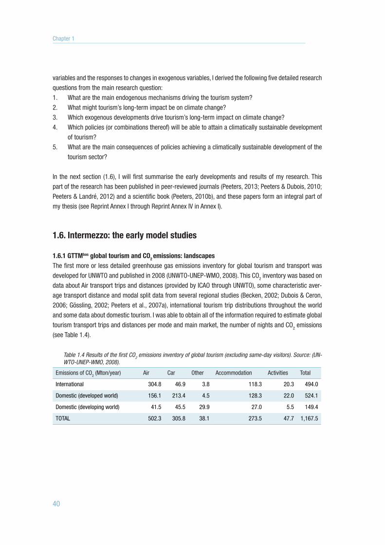
514727-L-bw-peeters514727-L-bw-peeters514727-L-bw-peeters514727-L-bw-peetersProcessed on: 20-10-2017Processed on: 20-10-2017Processed on: 20-10-2017Processed on: 20-10-2017 PDF page: 40PDF page: 40PDF page: 40PDF page: 40
40
variables and the responses to changes in exogenous variables, I derived the following five detailed research questions from the main research question: 1. What are the main endogenous mechanisms driving the tourism system?2. What might tourism’s long-term impact be on climate change?3. Which exogenous developments drive tourism’s long-term impact on climate change?4. Which policies (or combinations thereof) will be able to attain a climatically sustainable development
of tourism?5. What are the main consequences of policies achieving a climatically sustainable development of the
tourism sector?
In the next section (1.6), I will first summarise the early developments and results of my research. This part of the research has been published in peer-reviewed journals (Peeters, 2013; Peeters & Dubois, 2010; Peeters & Landré, 2012) and a scientific book (Peeters, 2010b), and these papers form an integral part of my thesis (see Reprint Annex I through Reprint Annex IV in Annex I).
1.6. Intermezzo: the early model studies
1.6.1 GTTMbas global tourism and CO2 emissions: landscapesThe first more or less detailed greenhouse gas emissions inventory for global tourism and transport was developed for UNWTO and published in 2008 (UNWTO-UNEP-WMO, 2008). This CO2 inventory was based on data about Air transport trips and distances (provided by ICAO through UNWTO), some characteristic aver-age transport distance and modal split data from several regional studies (Becken, 2002; Dubois & Ceron, 2006; Gössling, 2002; Peeters et al., 2007a), international tourism trip distributions throughout the world and some data about domestic tourism. I was able to obtain all of the information required to estimate global tourism transport trips and distances per mode and main market, the number of nights and CO2 emissions (see Table 1.4).
Table 1.4 Results of the first CO2 emissions inventory of global tourism (excluding same-day visitors). Source: (UN-WTO-UNEP-WMO, 2008).
Emissions of CO2 (Mton/year) Air Car Other Accommodation Activities Total
International 304.8 46.9 3.8 118.3 20.3 494.0
Domestic (developed world) 156.1 213.4 4.5 128.3 22.0 524.1
Domestic (developing world) 41.5 45.5 29.9 27.0 5.5 149.4
TOTAL 502.3 305.8 38.1 273.5 47.7 1,167.5
Chapter 1

514727-L-bw-peeters514727-L-bw-peeters514727-L-bw-peeters514727-L-bw-peetersProcessed on: 20-10-2017Processed on: 20-10-2017Processed on: 20-10-2017Processed on: 20-10-2017 PDF page: 41PDF page: 41PDF page: 41PDF page: 41
41
The total amount of 1,168 Mton of tourism-related CO2 emissions in 2005 represents a 4.6% share of global emissions5. Of the fifteen different segments distinguished (from ‘international Air transport’ to ‘developing world domestic activities’), international Air transport generates 305 Mton, the largest share (26%). Includ-ing domestic tourism, Air transport is responsible for 502 Mton (43%) of CO2 emissions and all transport for 846 Mton (72.5%). The majority of the remaining emissions is caused by accommodation (20%), leaving about 7.5% for activities, which represents the emissions caused by excursions, touring, visiting museums, festivals and other tourist attractions and holding meetings (e.g. for business travel). Figure 1.4 shows the inequality of the distribution of tourism and CO2 emissions over both the main tourism markets and the main transport modes. Whereas international tourism accounts for about 16% of all tourism trips, it generates 42% of emissions. Because about 5% of international tourists originate from the least-developed countries, we found that the developed world is responsible for some 70% of all tourism CO2 emissions, when as-signed to regions of origin (based on data from Peeters & Eijgelaar, 2014).
Although 2005’s tourism could be described as a “non-negligible contributor to climate change” (UN-WTO-UNEP-WMO, 2008, p. 27), the more important issue is the continued growth of this contribution. In the UNWTO-UNEP-WMO (2008) report, I show that by 2035 tourism’s CO2 emissions will have grown by more than 160% with respect to 2005, equivalent to an average rate of 3.2% per year. This finding is the result of UNWTO international tourism arrival projections (WTO, 2000a) extended to 2035, Air transport data (IATA, 2009b) and expert opinions about development of domestic tourism, length of stay, shares of transport modes and transport distances travelled.
Figure 1.4: Distribution of tourism trips and CO2 emissions for transport per transport mode and main tourism market. Source: GTTMadv.
In their book ‘Shaping the next 100 years’, Lempert, Popper, and Bankes (2003) propose ‘landscaping’ as part of robust policymaking. Landscaping is visualising the effects of a range of policy combinations on the development of the system. Peeters and Dubois (2010) use the GTTMadv to provide an example of exploring tourism mitigation policies. The landscape is composed of 70 scenarios as combinations of ten levels of volume changes (i.e. changes in the assumed growth factors for transport volume per transport mode and global market) combined with seven assumed rates of change of efficiency (CO2 emission factors) of three
5 This is lower than the 4.9% share cited in UNWTO-UNEP-WMO (2008) because the latter includes same-day visitors.
1
Introduction

514727-L-bw-peeters514727-L-bw-peeters514727-L-bw-peeters514727-L-bw-peetersProcessed on: 20-10-2017Processed on: 20-10-2017Processed on: 20-10-2017Processed on: 20-10-2017 PDF page: 42PDF page: 42PDF page: 42PDF page: 42
42
transport modes, and accommodation and tourist activities separated for the developing and developed world. Tables 8 and 9 of Peeters and Dubois (2010), see Reprint Annex II, provide the detailed assumptions. The results are based on the GTTMbas exponential model. The technological improvement assumptions were added to the baseline scenario and ranged between 1.3%/year for aviation to 2.0%/year for Other transport modes, accommodation and tourist activities. The seven policies varied in the way it combined the addi-tional improvement for each main element (e.g. Air transport, accommodations) of the system. The volume growth changes were defined in absolute terms of % growth per year varying between 0.0%/year to 7.7% and again in different combinations for the various main elements.
Figure 1.5 depicts the resulting scenario landscape for the growth factor of CO2 emissions between 2010 and 2035. Only one combination, Volume_scen_9 plus Tech_scen_6, shows a reduction of the CO2 emissions compared to those in 2005. The results do not provide any solution that could be called ‘sustain-able’, i.e. in line with the 2 °C climate change goal. Of course, assuming larger technological or volume rates of change would improve the results. The ones chosen here were those that the researchers involved, Jean-Paul Ceron, Ghislain Dubois, Stefan Gössling and myself, considered the physical, political and economic limits of what could ultimately be done. Therefore, they were based on our expert judgement.
Figure 1.5: Landscape of CO2 emissions growth for a variety of policy assumptions.
1.6.2 GTTMadv global tourism CO2 emissions: narrative backcastingThe GTTMadv uses the same exponential growth coefficients as GTTMbas. The difference is that the GTTMadv has been programmed in Powersim™ Studio (version 7). Using this software enabled the model not only quickly to assess the effects of a large number of policy and system settings, but also to automate this process using certain objectives (e.g. a specific reduction of emissions while maximising revenues).
The model cannot run without entering background economic and population scenario data. These contextual scenarios in are based on the IPCC SRES scenarios (IMAGE-team, 2006) designated by Dubois
Chapter 1

514727-L-bw-peeters514727-L-bw-peeters514727-L-bw-peeters514727-L-bw-peetersProcessed on: 20-10-2017Processed on: 20-10-2017Processed on: 20-10-2017Processed on: 20-10-2017 PDF page: 43PDF page: 43PDF page: 43PDF page: 43
43
et al. (2011) as A1 (High Growth and Less Crowded6), A2 (Low Growth and Very Crowded), B1 (Medium Growth and Less Crowded) and B2 (Medium Growth and Medium Crowded). Just like GTTMbas, the GTT-Madv distinguishes three main tourism markets (international, domestic developed and domestic developing world), three transport modes (air, car and other) and two other main system elements (accommodation and activities). The user can change the system by setting a total of 42 system ‘growth’ constants. See Dubois et al. (2011) for a detailed description of all the constants that define a scenario run. These constants manipulate the three tourism markets, the trip and distance growth rates of all three transport modes in each of the three tourism markets and the development of CO2 emission factors (a proxy for technological development). The results of a workshop held with Jean-Paul Ceron and Ghislain Dubois, attempting to define scenarios based on storylines and using GTTMadv that will reduce tourism’s emissions by 70% in 2050 compared to 2005, were published by Dubois et al. (2011). This exercise was not to find policies for mitigating tourism’s CO2 emissions, but to describe what the tourism system should look like under a strict mitigation goal. In other words, how many trips and kilometres could fit within the goal? This analysis would merely set the size of the changes required to reduce tourism emissions to a set level and provide the chal-lenge for policies to achieve this. To systemise our efforts, we defined three ‘storylines’:
’Happy Few’ scenario. This scenario is characterised by global cooperation and governance stimulating technological innovation and high mitigation taxes enabled on A1 (high) economic growth. It means that rich people can still travel as much as they want, but many others have to reduce the distances they travel;
’Proximity’ scenario. In this scenario, people are all equal in their basic right to travel, which leads to more general reductions of distances (for everyone). The major difference with the Happy Few scenario, therefore, is that policymakers introduce household carbon budgets, which can be traded up to a certain limit (20%). This trading mechanism will generate even stronger technology developments because the carbon budgets do not allow for high emission technologies and low emission factors thus directly determine the size of the market and the prospects for growth. This development also creates a strong market for an expanding long-distance electric rail transport network and modal shifts from air and car to rail. As we assume limited emission trade, the difference between rich and poor will be far less substantial, and the growth in the number of trips is much larger in developing countries than in developed ones; and
’Global Isolationism’ scenario. This scenario assumes limited global governance and a multi-polar world. Conflicts about resources abound, and the pace of technological innovation slows down due to lack of international cooperation and reduced funds for innovation, development and research in a weak economy, international travel becomes less attractive and even domestic tourism is under pressure. All travel volumes grow much less than in the other scenarios.
The workshop approach - based on the general storyline - was designed stepwise to modify the system parameters, evaluate the results for CO2 emission, revenues and equity and then define the next step, until the maximum emissions reduction was reached within the constraints we felt we had to maintain. The result was that none of the three scenarios reached the 70% emissions reduction with respect to 2005 emissions. Figure 1.6 shows the overall results. In all cases, the number of trips, the number of nights and distances
6 High Growth refers to growth of GDP/capita; Less Crowded refers to a low population growth assumption.
1
Introduction

514727-L-bw-peeters514727-L-bw-peeters514727-L-bw-peeters514727-L-bw-peetersProcessed on: 20-10-2017Processed on: 20-10-2017Processed on: 20-10-2017Processed on: 20-10-2017 PDF page: 44PDF page: 44PDF page: 44PDF page: 44
44
travelled decrease substantially compared to the baseline or the Reference Scenario. The outcomes mean that in this exercise we did not manage to reduce the emissions as far as we would have liked to (between -33% and -42% instead of -70%) and we managed only to do so by significantly constraining the entire tourism sector.
Figure 1.6: Overview of results for the three ‘hand-made’ scenarios using the manual version of GTTMadv.
1.6.3 GTTMadv Global tourism CO2 emissions: automated backcastingBecause of the failure during the workshop to reach the emissions reduction goals in the manual scenario exercise, I used the capacity of Powersim™ Studio 7 to find an optimum objective-based solution. I defined two objectives. The first was once again to reach the 70% CO2-emissions reduction in 2050 with respect to 2005. The second objective was to maximise the net revenues, which was the sum of all revenues for transport, accommodation and activities minus the cost of emissions abatement (see also Section 2.3.5 for a description of the calculation method). The abatement cost method was introduced to avoid the system receiving ‘free’ technological improvements. I disaggregated the original 42 parameters to fourteen by as-suming the growth rates for trips of transport modes to be equal for all markets and that average distances, and the maximum number of trips per capita would not change. I tried the optimisation for each of the four contextual scenarios. Figure 1.7 shows the results regarding the ‘optimum’ modal split of the scenarios. Interestingly, the four contextual scenarios only provided two different optimum solutions based either on very low Air transport shares (in absolute terms about the level of the 1970s) combined with a high share of personal car or a very large rail share and Air transport to be kept at the level of about 2005. In all four sce-narios, the 70% emissions reduction is matched. The parameters were allowed to vary over a larger range
Chapter 1

514727-L-bw-peeters514727-L-bw-peeters514727-L-bw-peeters514727-L-bw-peetersProcessed on: 20-10-2017Processed on: 20-10-2017Processed on: 20-10-2017Processed on: 20-10-2017 PDF page: 45PDF page: 45PDF page: 45PDF page: 45
45
than in the landscape case described in Section 1.6.1. The landscape case was limited due to constraints imposed on the research by the reviewers of the draft versions of the UNWTO report (UNWTO-UNEP-WMO, 2008).
Figure 1.7: Result of the automated backcasting scenarios based on the GTTMadv. Peeters and Dubois (2010), re-printed in Reprint Annex II, published this graph. The scenario names refer to the four different socio-economic contextual scenarios that give rise to different ‘optimum’ solutions.
The GTTMbas shows us that manually defining the tourism sector within constraints set by experts of the UN-WTO (as a proxy for the sector) in terms of technology improvements and volume restrictions failed to generate very significant emissions reductions. Only one of the many scenarios showed an overall reduction of CO2 emissions and only a moderate 16% in 2035 in comparison to 2005. However, also our attempt to manually find scenarios which achieve 70% reduction in 2050, with respect to 2005, failed, even though all four of us were very aware of the need to reduce emissions. This failure to reduce emissions - the second finding with GTTMadv based on the landscape of 70 ‘scenarios’ - may have been because the researchers were not prepared to push changes to wider limits because of presumed and partly unconscious social or political issues to do so. I remember discussions about the ethics of forcing down the volume growth in domestic tourism in develop-ing countries. The third finding was that an automated optimising model had no problems finding solutions for reducing emissions by 70% between 2005 and 2050 while keeping the net revenues of the tourism and transport sector as high as possible. This result is not surprising as the automatic run of the model was allowed to explore the changes over the same range of values, but certainly not hampered by what the researchers initially judged to be ‘realistic’ or ‘ethical’. Also, the model performed several sessions of up to 10,000 runs, enabling it to find a global or local maximum concerning revenues. Even more interesting was the finding that the model’s solutions tended to either keep the volume of flying constant at the 2005 level, combined with a major shift from Car to Other (mainly rail) transport or to maintain the share (not the volume!) of car users as in the Reference Scenario for 2050, but reducing the Air transport volume to the level of the 1970s. The assumed contextual scenario determined the result (see Figure 1.7).
1
Introduction

514727-L-bw-peeters514727-L-bw-peeters514727-L-bw-peeters514727-L-bw-peetersProcessed on: 20-10-2017Processed on: 20-10-2017Processed on: 20-10-2017Processed on: 20-10-2017 PDF page: 46PDF page: 46PDF page: 46PDF page: 46
46
The findings from running the GTTMbas and GTTMadv indicate that technology alone is unable to re-duce the emissions in absolute terms and other volume-related changes need to be strong. To reduce CO2 emissions to the level required to avoid dangerous climate change, major shifts in transport modes and destination choice (less far away) are necessary. This conclusion was drawn within the limitations we set for ourselves regarding the maximum technological development we deemed possible and the maximum reductions of volumes we considered socially desirable. Furthermore, these conclusions were based on constant exponential growth modelling and as such may miss secondary effects and feedbacks that could profoundly influence the long-term future (past 2050). Furthermore, the ‘scenarios’ are based on different system assumptions such as for growth, efficiency, rather than policy measures to achieve such changes in the modelled system. Therefore, the objective of the third version of the model, the GTTMdyn, is to resolve these issues by creating a full-fledged system dynamics model and adding a range of policy measure inputs.
Chapter 1

514727-L-bw-peeters514727-L-bw-peeters514727-L-bw-peeters514727-L-bw-peetersProcessed on: 20-10-2017Processed on: 20-10-2017Processed on: 20-10-2017Processed on: 20-10-2017 PDF page: 47PDF page: 47PDF page: 47PDF page: 47
47
1
Introduction

514727-L-bw-peeters514727-L-bw-peeters514727-L-bw-peeters514727-L-bw-peetersProcessed on: 20-10-2017Processed on: 20-10-2017Processed on: 20-10-2017Processed on: 20-10-2017 PDF page: 48PDF page: 48PDF page: 48PDF page: 48

514727-L-bw-peeters514727-L-bw-peeters514727-L-bw-peeters514727-L-bw-peetersProcessed on: 20-10-2017Processed on: 20-10-2017Processed on: 20-10-2017Processed on: 20-10-2017 PDF page: 49PDF page: 49PDF page: 49PDF page: 49
Chapter 2
The GTTMdyn Model

514727-L-bw-peeters514727-L-bw-peeters514727-L-bw-peeters514727-L-bw-peetersProcessed on: 20-10-2017Processed on: 20-10-2017Processed on: 20-10-2017Processed on: 20-10-2017 PDF page: 50PDF page: 50PDF page: 50PDF page: 50
50
2.1. Introduction to the GTTMdyn
2.1.1 GTTMdyn: rooted in earlier modelsThe GTTMbas and GTTMadv models revealed that tourism’s emissions are likely to significantly increase in the coming decades, which contrasts with the strong mitigation of global CO2 emissions necessary to avoid dangerous climate change (see 1.6). Furthermore, absolute reductions of CO2 emissions are only possible with significant changes to the tourism system: changes regarding distances travelled and transport modes used. Though these models illustrate what a low CO2-emissions tourism sector may look like, it fails to reveal which policies might achieve these changes. The main objective of the GTTMdyn was to be able to apply policy strategies and analyse how these affect global tourism and transport and its CO2 emissions. Another objective was to enable long term systemic analyses of the tourism and transport system, rather than short or medium term projections.
The GTTMadv model allows the researcher to explore what the tourism and transport sector should look like regarding technological efficiency, tourism trip volumes, transport volumes, modal split and length of stay. In contrast, the GTTMdyn model was developed not only to provide a model based on mechanisms rather than growth assumptions and add policy strategies (or measures) as inputs instead of changes in the exponential growth coefficients of the model. Furthermore, it includes several feedbacks in the system that might cause rebound effects for certain measures (e.g. more efficient cars make driving cheaper and increase the volume of Car transport). The GTTMdyn is also designed so that it can be used as a ‘simulator’ by stakeholders, researchers, students or other parties interested in the issue, to explore the development of the tourism system, its impacts on CO2 emissions and the impact of policies to mitigate these emissions.
I chose system dynamics modelling based on the perception that global tourism and transport is a sys-tem. Leiper (1979) suggested decades ago that tourism is indeed a system. Also (Cohen, 1984, p. 382) de-scribes modern tourism as “an ecological, economic, and political system that is complex and global.” More recently, scholars have confirmed that the tourism system is complex, non-linear and dynamic (Lazanski & Kljajić, 2006; Ndou & Petti, 2006; Walker et al., 1999). The non-linearity makes analytical modelling impos-sible as shown by von Bertalanffy (1969, p. 20). Another important characteristic of systems is the existence of feedback loops between system elements (von Bertalanffy, 1969). The tourism transport system does show feedback loops like a ‘mode shift loop’, a ‘cost loop’ and a ‘travel time loop’ like I showed in a book chapter (Peeters, 2010b), reprinted in Reprint Annex I.
So, tourism might be considered a dynamic and complex system (Peeters, 2015). A convenient way to explore such systems is to use systems thinking and system dynamics models (SDMs). System dynamics provides a way to learn about the behaviour of non-linear complex systems (Sterman, 2000). Contrary to most econometric models, system dynamics is based on the assumption of causal relationships, where econometric models normally start with statistical relationships for which causality is not necessarily known nor even in existence. See further my paper (Peeters, 2013) reprinted in Reprint Annex IV. In system-dy-namics models, the ability to accommodate these causal relations allows the study of complex non-linear dynamics that do not have analytical solutions. Early applications can be found in Industrial Dynamics (Forrester, 1961), and the ‘World 2’ model (Forrester, 1971). Meadows and others further developed this model into the ‘World 3’ model used for the iconic ‘Limits to growth’ report (Meadows, Meadows, Randers, & Behrens III, 1972). The goal of the GTTMdyn is to create a global tourism and transport model that enables exploring both the impact of contextual scenarios and policies to generate policy-relevant system outcomes
Chapter 2

514727-L-bw-peeters514727-L-bw-peeters514727-L-bw-peeters514727-L-bw-peetersProcessed on: 20-10-2017Processed on: 20-10-2017Processed on: 20-10-2017Processed on: 20-10-2017 PDF page: 51PDF page: 51PDF page: 51PDF page: 51
51
at appropriate timescales. These considerations generate requirements regarding the time horizon, desired policy inputs and policy-relevant system outcomes.
2.1.2 GTTMdyn requirementsA detailed discussion of the requirements for the behavioural part of GTTMdyn can be found in (Peeters, 2013), reprinted in Reprint Annex III. As shown by the results of the analyses with the GTTMadv, the model needs to be able to accommodate substantial changes. These may be relatively easy to model for tech-nological development that improves energy and emission efficiencies. But for the major emitting part of tourism, the Air transport sector, improving energy efficiency and reducing emission factors is less straight-forward (Chèze, Chevallier, & Gastineau, 2013; Cohen, Higham, Gössling, Peeters, & Eijgelaar, 2016; Peeters et al., 2016; Sgouridis, Bonnefoy, & Hansman, 2010). This lack of development is due to, for instance, very long lead times between the development of new technologies to their wide-spread application in aircraft, trains and both air and rail infrastructure. Furthermore, the model should be able to handle strong behav-ioural changes in response to strong policies, a feature that is hard to achieve with econometric modelling (compare Van Cranenburgh, 2013). These large behavioural changes were the main focus when developing the GTTMdyn. Finally, the very long time horizon may require the emergence of a new major technology, like Air transport during the 1920s. To enable answering the research questions, the following set of require-ments has been deduced for the GTTMdyn, which had to:1. handle both international and domestic tourism, independent of geographical regions;2. handle new transport modes like the emergence of aviation in the 1920s, and eventually space travel
during the twenty-first century;3. be based on mechanisms governing travel behaviour rather than pure econometric/statistical
relationships;4. handle large changes in costs, infrastructure capacity and other main system parameters; and5. provide long-term policy analysis up to the year 2100.
Defining the model in trips per ‘transport mode’ and ‘distance class’ rather than trying to model all flows between and within every country in the world fulfils the first requirement. Global trip generation was based on a linear relationship between GDP/capita and the number of trips per year (Bigano et al., 2004; Peeters & Dubois, 2010; Peeters & Landré, 2012), further explained in Section 2.2.3.
The second requirement - handle the emergence of new products on the market - was solved by using the product adoption and diffusion model proposed by Bass (1969). The Bass adoption and diffusion model assumes product diffusion consists of commercial adoption (advertising) and social adoption (word-of-mouth) mechanisms. The overall sales development of a new product is initially dominated by commercial adoption until social adoption takes over after some time has passed. The third requirement is implemented by using the psychological value (PV) from prospect theory (Kahneman & Tversky, 1979; Kahneman & Tversky, 2000) rather than a utilities-based econometric approach. For the GTTMdyn, the PV is defined as the sum of generalised travel cost (travel cost plus monetarized travel time) and distance (as an attractor). By integrating prospect theory into the framework of the Bass model, the GTTMdyn becomes sensitive to changes in income, population size, travel cost and time, and it is based on mechanisms beyond constant
2
The GTTMdyn Model

514727-L-bw-peeters514727-L-bw-peeters514727-L-bw-peeters514727-L-bw-peetersProcessed on: 20-10-2017Processed on: 20-10-2017Processed on: 20-10-2017Processed on: 20-10-2017 PDF page: 52PDF page: 52PDF page: 52PDF page: 52
52
exponential growth functions. This approach enables the model to follow larger changes in the inputs of income, costs and travel time (fourth requirement). It also allows the model to cover very long time spans (the fifth requirement).
2.1.3 Description of the GTTMdyn The GTTMdyn model has been programmed using the academic version of Powersim™ Studio 10 Academic SR 5, system-dynamics modelling software. It consists of a series of stock and flow constructions. The model runs from 1900 up to 2100. The time step has been set to one year. This time step plays a role in the air fleet model that assumes a shift of all aircraft by one age class for every exact year. Unfortunately, this means the model only runs correctly at this one-year time step.
The model is composed of a series of model units (graphically separated parts of the main model) and mutually interacting sub-models. The model uses a range of data input files (the GTTMDB, a suite of Microsoft Excel files that were specially prepared for the GTTMdyn) and generates both graphical output in the Studio file as well as time-series data outputs into several data files (Microsoft Excel files). The model calculates a range of characteristics for the tourism and transport system, such as number of trips, dis-tances travelled, travel time, number of nights, modal split, revenues, costs (revenues plus additional costs due to policy measures), CO2 emissions and radiative forcing (a measure of the net-energy flux into the atmosphere). The main exogenous inputs for the model were GDP/capita, GINI factor (a measure of income equity), global population, assumptions on transport costs and speed and accommodation costs and some characteristics of car fleet, airport and high-speed rail infrastructure and aircraft in the fleet. These inputs were provided in time series from 1900 up to 2100, with projections starting in 2010.
The scope of GTTMdyn is the tourism and transport system. The tourism system consists of hospitality (accommodation) and service industries providing travel products and services, and MICE (Meetings, Incen-tives and Conventions and Exhibitions) facilities and services (UNWTO, 2012). Furthermore, those parts such as local tourism and leisure-dedicated facilities (museums, zoos and lunar parks), restaurants, cafés, that are used by tourists are also considered part of the tourism system. Regarding transport, all transport that is used by tourists to travel from their normal place of residence to their destinations is regarded as part of the system. For Air transport, this means most of the Air transport industry is included as some 90% of air pas-senger travel is tourism-related (Peeters et al., 2007a). For Car and Other transport modes, global passenger transport’s shares of tourism are more likely approximately 20% (Peeters et al., 2007a). For Other transport (such as rail, bus, ferry), the tourism system includes high-speed rail as that is considered as a potential substitute for Air transport. Moreover, on some major connections like the Eurostar between UK, France and Belgium, it is mainly used by tourists (UNWTO, 2007b). Local transport, i.e. transport at the destination from and to or between temporary places of residence is excluded from GTTMdyn.
Section 4.5 provides an extensive overview of the policy measures and strategies used when exploring the GTTMdyn model. However, to be able to describe the main elements of the model, I provide a summary of them here. The GTTMdyn provides the user with a range of inputs for policy measures. These policy measures have been organised around the following strategies:1. Alternative Fuels: choosing which fuel feedstocks to include, subsidies per chosen feedstock and
maximum land-use available following ‘sustainable’ or ’physical’ criteria;2. Technology: set development (% change per year) of emission factors for the main parts of the
system;
Chapter 2

514727-L-bw-peeters514727-L-bw-peeters514727-L-bw-peeters514727-L-bw-peetersProcessed on: 20-10-2017Processed on: 20-10-2017Processed on: 20-10-2017Processed on: 20-10-2017 PDF page: 53PDF page: 53PDF page: 53PDF page: 53
53
3. Infrastructure: set turboprop desired share, air-fleet scrapping age, investments in high-speed rail and airport capacity limits;
4. Travel Speed policies: maximum aircraft cruise speed, maximum car speed and average speed for Other transport;
5. Taxes and Subsidies: a global carbon tax for the main system elements of choice, ticket tax/subsidy for Air and Other transport and a fuel tax for Cars; and6. Behaviour Change: sets factors for the length of stay, inclination to travel and the value of distance.
Furthermore, the GTTMdyn provides the user with two results screens showing a range of scenario time graphs and a suite of key performance indicators (set-up of the KPIs). In the following section, I will describe the general set-up of the model.
2.1.4 General layout of the GTTMdyn
The GTTMdyn main model has been divided into several model units. A model unit is a part of the main model, but with a specific task. Each model unit has been visually separated from the main model by clustering the model elements in a coloured frame. The submodel units are at a lower level and are connected through ‘global’ variables, which are applied to all layers of the model. These perform a certain dedicated task and are easily copied. For instance, a submodel for implementing the Bass model to Air transport was first developed and then copied twice and adapted for Car respectively Other transport modes. In total, there are 23 model units, partly formal Powersim™ Studio submodels, of which twelve combine to deliver the behavioural model described in Section 2.2. The other models provide infrastructure, fleet capacity and environmental information for the GTTMdyn. Table 2.1 gives an overview of all fourteen model units and nine submodels, their tasks and the main inputs and outputs. The core of the GTTMdyn is formed by the behav-ioural model suite that generates trips and distributes them over the twenty distance classes for three trans-port modes (elements indicated in bold-italic). The other model units generate inputs (global population, car fleet model and biofuel model), feedbacks (accommodation model, infrastructure models and abatement cost model) and provide outputs (energy and emission model and aviation radiative forcing index, RFI).
2
The GTTMdyn Model
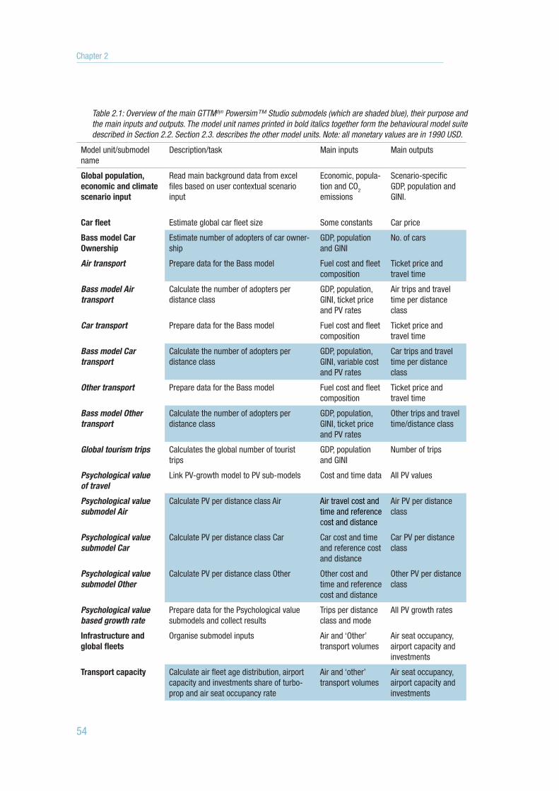
514727-L-bw-peeters514727-L-bw-peeters514727-L-bw-peeters514727-L-bw-peetersProcessed on: 20-10-2017Processed on: 20-10-2017Processed on: 20-10-2017Processed on: 20-10-2017 PDF page: 54PDF page: 54PDF page: 54PDF page: 54
54
Table 2.1: Overview of the main GTTMdyn Powersim™ Studio submodels (which are shaded blue), their purpose and the main inputs and outputs. The model unit names printed in bold italics together form the behavioural model suite described in Section 2.2. Section 2.3. describes the other model units. Note: all monetary values are in 1990 USD.
Model unit/submodel name
Description/task Main inputs Main outputs
Global population, economic and climate scenario input
Read main background data from excel files based on user contextual scenario input
Economic, popula-tion and CO2 emissions
Scenario-specific GDP, population and GINI.
Car fleet Estimate global car fleet size Some constants Car price
Bass model Car Ownership
Estimate number of adopters of car owner-ship
GDP, population and GINI
No. of cars
Air transport Prepare data for the Bass model Fuel cost and fleet composition
Ticket price and travel time
Bass model Air transport
Calculate the number of adopters per distance class
GDP, population, GINI, ticket price and PV rates
Air trips and travel time per distance class
Car transport Prepare data for the Bass model Fuel cost and fleet composition
Ticket price and travel time
Bass model Car transport
Calculate the number of adopters per distance class
GDP, population, GINI, variable cost and PV rates
Car trips and travel time per distance class
Other transport Prepare data for the Bass model Fuel cost and fleet composition
Ticket price and travel time
Bass model Other transport
Calculate the number of adopters per distance class
GDP, population, GINI, ticket price and PV rates
Other trips and travel time/distance class
Global tourism trips Calculates the global number of tourist trips
GDP, population and GINI
Number of trips
Psychological value of travel
Link PV-growth model to PV sub-models Cost and time data All PV values
Psychological value submodel Air
Calculate PV per distance class Air Air travel cost and time and reference cost and distance
Air PV per distance class
Psychological value submodel Car
Calculate PV per distance class Car Car cost and time and reference cost and distance
Car PV per distance class
Psychological value submodel Other
Calculate PV per distance class Other Other cost and time and reference cost and distance
Other PV per distance class
Psychological value based growth rate
Prepare data for the Psychological value submodels and collect results
Trips per distance class and mode
All PV growth rates
Infrastructure and global fleets
Organise submodel inputs Air and ‘Other’ transport volumes
Air seat occupancy, airport capacity and investments
Transport capacity Calculate air fleet age distribution, airport capacity and investments share of turbo-prop and air seat occupancy rate
Air and ‘other’ transport volumes
Air seat occupancy, airport capacity and investments
Chapter 2

514727-L-bw-peeters514727-L-bw-peeters514727-L-bw-peeters514727-L-bw-peetersProcessed on: 20-10-2017Processed on: 20-10-2017Processed on: 20-10-2017Processed on: 20-10-2017 PDF page: 55PDF page: 55PDF page: 55PDF page: 55
55
Model unit/submodel name
Description/task Main inputs Main outputs
Accommodation Calculate the length of stay (LOS), nights and revenues
LOS rate fraction per year
Number of nights, accommodation and revenues
Energy and emissions Calculate accommodation emission factor; share turboprop; organise input/output transport emissions
Historical/policy assumptions
Emission factors for accommodation and Other transport
Emissions submodel Calculate air and car emission factors per mode and energy source
Historical/policy assumptions
Air and car emission factors
Aviation RFI Calculate aviation radiative forcing and ra-diative forcing index (RF, respectively RFI).
Global (tourism) emissions
RF, RFI
Biofuel Calculate the markets for five biofuel feedstocks
Cost and subsidies for biofuels; global land-use restric-tion
Shares of kerosene and biofuels
Abatement cost Calculate the abatement cost for CO2 emis-sions reductions
Relative change in CO2 emission factors
Abatement cost for accommodation and transport modes
Figure 2.1 provides an overview of the GTTMdyn model units and their main relationships. The main drivers of the model are the external data inputs for global population size, average GDP/capita, and income equality – represented by the GINI coefficient – from the context scenario and a suite of user-defined policy strategy inputs. GINI is a measure of equality of income distribution (Gini, 1912; Rasche, Gaffney, Koo, & Obst, 1980). The arrows in the model indicate data flows. The car fleet model was created because the portion of the population that lacks access to a car will (logically) not be able to use one frequently. Therefore, the car fleet model reduces the share of potential adopters of tourist trips by car. The ‘Behavioural model suite’ governs all three transport modes.
2
The GTTMdyn Model

514727-L-bw-peeters514727-L-bw-peeters514727-L-bw-peeters514727-L-bw-peetersProcessed on: 20-10-2017Processed on: 20-10-2017Processed on: 20-10-2017Processed on: 20-10-2017 PDF page: 56PDF page: 56PDF page: 56PDF page: 56
56
Figure 2.1: Global overview of models and submodels for the GTTMdyn. Arrows represent data flows, not causal relationships. The italic numbers between brackets refer to the section that describes the model element. Figure 2.2 explains the Behavioural model suite in greater detail. The GTTMDB data files provide the external data (see section 2.1.3 for information about GTTMDB).
In the following sections, I will zoom in on the additional model units. In each case, I will include the sub-models associated with the respective units (e.g. section 2.3.3 on infrastructure model units includes the Transport capacity submodel).
2.1.5 Scope of the modelTable 2.2 shows the endogenous, exogenous and excluded elements of the GTTMdyn. One notable exclusion is the discount rate. Though there is an ongoing discussion about (social) discounting in environmental modelling, including ethical issues (Aaheim, 2010; Dasgupta, 2008; Hourcade, Ambrosi, & Dumas, 2009), I tend to follow the line of argument chosen by Stern (2006). See further discussion under the Economics subheading in Section 3.7. Other excluded elements include road and conventional rail infrastructure be-
Chapter 2
514727-L-bw-peeters514727-L-bw-peeters514727-L-bw-peeters514727-L-bw-peetersProcessed on: 20-10-2017Processed on: 20-10-2017Processed on: 20-10-2017Processed on: 20-10-2017 PDF page: 57PDF page: 57PDF page: 57PDF page: 57
57
cause the majority of this infrastructure is built for purposes other than tourism. As argued in section 1.4.2, same-day visitors are also excluded. Also, I excluded local transportation i.e. transport during a tourist trip taken from or between temporary places of residence, because of a lack of data at the global level. Finally, I excluded tourist activities and services because of an insurmountable gap in data at the global level and because these tend to represent only a small share of all tourism revenues (about 10% according to UNWTO-UNEP-WMO, 2008). The main endogenous elements in the GTTMdyn are abatement costs, number of trips and distances trav-elled, aircraft and car fleet sizes, aircraft-fleet age distribution, airport investments, airport capacity, high-speed rail network capacity, CO2 emissions, radiative forcing, tourism revenues and expenditures, biofuel prices (only in case land-use restrictions develop), (bio)fuel shares and technological developments for energy efficiencies and emission factors such as the function of carbon cost. Major exogenous drivers of the model include (Table 2.2 provides the details):1. socio-economic growth in terms of GDP/capita, equity (GINI factor) and global population;2. global climate mitigation scenario determining global CO2 emissions and the global cost of CO2:
Unlimited (>4.5 °C), Moderate (3.3 °C), Paris Agreed (2.0 °C) and Paris Aspired (1.5 °C);3. baseline technology development in terms of energy efficiency, emission factors, transport speed and
aircraft utility; 4. baseline costs for accommodation, basic biofuels costs, car fuel, aircraft tickets, Other transport
tickets and high-speed rail investments; and5. some internal system ‘goals’ like for the aircraft seat occupancy rate, airport capacity occupancy and
share of turboprops.
2
The GTTMdyn Model

514727-L-bw-peeters514727-L-bw-peeters514727-L-bw-peeters514727-L-bw-peetersProcessed on: 20-10-2017Processed on: 20-10-2017Processed on: 20-10-2017Processed on: 20-10-2017 PDF page: 58PDF page: 58PDF page: 58PDF page: 58
58
Table 2.2: the GTTMdyn boundary chart as suggested by Sterman (2000, p. 97).
Endogenous: Exogenous: Excluded:
(Bio)fuel sharesAbatement costAircraft fleet average ageAircraft fleet sizeAircraft flightsAircraft seat occupancyAirport capacityAirport capacity model coefficientsAirport investmentsAverage distance per modeBass models’ coefficientsBiofuel cost after applying land-use restrictionsCar price (up to 1990)CO2 emissionsEmission factors as a function of CO2 tax.Global number of trips per transport mode and distance classHigh-speed rail network lengthHigh-speed rail shareModal sharesPsychological ValuesPV models coefficientsRadiative Forcing and RFIShare electric Car transportShare electric Other transportTechnology development as function of CO2 emissions costsTourism revenuesTravel timesTurboprop shareValue of Travel Time
Accommodation cost per nightAir transport ticket priceAir, Car (bio)fuel pricesAircraft average block speedAircraft average seat capacityAircraft average seat-occupancy rate goalAircraft average utility (hours/year)Aircraft delivery delay timeAircraft retirement rateAirport-capacity occupancy rate goalAirport investment delay timeAirport maximum operational life of infrastructure Average length of stayBaseline technology and energy/emission efficienciesBasic trends for all emission coefficientsBiofuel basic costBiofuel maximum land useCar acquisition priceCar speedGDP/capitaGlobal CO2 emissions and concentrationGlobal populationHigh-speed rail infrastructure invest-mentsIncome equity (GINI)Other conventional and high-speed rail speedOther transport ticket priceTravel time constraintsTurboprop share goal
Discount rate (equivalent to assumed zero)Normal (non-high speed) rail and all road infrastructureSame-day visitorsTourist activities (like museums, lunar parks, skiing facilities,) Tourist services (such as tour operators, travel agencies)Food services (restaurants and the like) to the extent that these are not part of the accommoda-tion carbon-emission factorsLocal transportation (i.e. trans-port during a tourist trip taken from or between temporary places of residence)
2.1.6 Summary of the model descriptionOne thing makes GTTMdyn different from other transport and tourism models: the idea to ignore the geo-graphical distribution of destinations and source markets, but to define the global tourism markets entirely by transport mode and distance class. I assumed sixty markets: three transport modes times twenty dis-tance classes. The behavioural model suite forms the core of the GTTMdyn. The first step in this suite is the global tourism trip model that calculates global tourism trips as a function of average GDP/capita, the GINI factor as a proxy for income distribution to determine the share of the population that took a maximum of five trips per year and population size. Cost is not part of the equation because changes in costs can easily be compensated for by the large range of choices for different destinations, transport modes, seasons and length of stay that tourists can make. Higher costs will cause them to travel differently, not less often. This causality is an important feature of the GTTMdyn Behavioural model suite, which determines the distribution over the sixty markets. The global trips and, again, GDP, GINI and population, feed into the Bass models that determine the share of the population that is a potential customer for each of the 60 markets. Then
Chapter 2

514727-L-bw-peeters514727-L-bw-peeters514727-L-bw-peeters514727-L-bw-peetersProcessed on: 20-10-2017Processed on: 20-10-2017Processed on: 20-10-2017Processed on: 20-10-2017 PDF page: 59PDF page: 59PDF page: 59PDF page: 59
59
the potential adopters ‘flow’ into adopters (people that decide to make a trip in a certain class) through a Bass model construction with a commercial and a social adoption pathway. The first is important to get a new product adopted and determines the (generally very low coefficient) shares of early adopters. The social adoption - word-of-mouth mechanism - provides a growth rate depending on the size of the group of potential adopters and a coefficient. In both the commercial coefficient and the social coefficient, the utility enters the equation and the two coefficients are not constants as in the original Bass models. This utility is value of distance minus the sum of integrated travel costs (time plus monetary). From this, I calculated the psychological value based on prospect theory and thus including ‘framing’ (a reference point for cost or travel time consists of a mix of the ‘personal choice’ and the alternative choices), change-orientation (marginal costs and benefits count, not the absolute levels), loss aversion and diminishing sensitivity with increasing changes in utility levels. Based on prospect theory, the utilities adapted per market segment (the distance-mode ones) are used in an exponential function to calculate the probability of choice for each of the 60 markets. The probabilities are used as a coefficient for the ‘commercial adoption’, calibrated with one overall factor for all of the markets. The ‘social adoption coefficient’ is calculated from the first derivative of the probability. Furthermore, I defined a ‘dominance factor’ that governs the effect of large markets creating their own additional attraction due to social conformity or peer pressure.
The infrastructure submodel includes the aircraft fleet and airport capacity model units. Airport capac-ity normally follows demand from the global aircraft fleet and the latter follows the global demand for trips by air. However, the fleet supply-demand submodel is cyclic, because of significant delay times between changing demand and new aircraft orders. For the GTTMdyn, the fleet consists of 50 aircraft age classes. All newly ordered aircraft enter the fleet into the one-year-old aircraft bin and jump every year to the next bin. This procedure was developed because the emission factor of aircraft continuously declines in a non-linear way and the cyclic behaviour causes rather uneven improvements for the fleet average emission factor. Fast growth will improve the average; fast decline will deteriorate it. Because Air transport also causes highly significant non-CO2 climate impacts, a radiative-forcing model unit calculates the impacts on RF. For non-air transport and accommodation, CO2 emissions are based on average emission factors, accounting for the share of electric cars, electric rail and high-speed rail. For details about the abatement cost, biofuel, accom-modation, car ownership and several other minor model units, please refer to the appropriate sections under Section 2.3. The GTTMDB set of Excel files that directly feed into the GTTMdyn providing all data.
2.2. Behavioural model suite
2.2.1 IntroductionThe underlying theory of the GTTMdyn has been described in published papers, reprinted in annexes to this thesis. Peeters (2010b), Reprint Annex I, describes the dynamics between tourism development and transport technology. Technological development from horse-drawn carriages in the eighteenth century, to steam trains in the nineteenth century up to the jet age in the twentieth century has led to a remarkable increase in both the capacity and speed of tourist travel. This development has an endogenous systemic cause, i.e., the transport system will, if politically unchecked and within physical and technological bounds, forever tend to increase speed, decrease cost and grow in capacity and volume. The GTTMdyn theoreti-cal background has been presented by Peeters (2013) and supplemental information in Reprint Annex IV.
2
The GTTMdyn Model

514727-L-bw-peeters514727-L-bw-peeters514727-L-bw-peeters514727-L-bw-peetersProcessed on: 20-10-2017Processed on: 20-10-2017Processed on: 20-10-2017Processed on: 20-10-2017 PDF page: 60PDF page: 60PDF page: 60PDF page: 60
60
Peeters and Dubois (2010), see Reprint Annex II, describe the GTTMbas and GTTMadv models, but they also provide the tourism-trip generation module. The same source describes the basic emission factors used in GTTM for transport modes and accommodation and the method to calculate ‘abatement costs’. These costs are important to account for the cost of reducing emissions and are based on the work by Nordhaus (2008) and data from IPCC (2007b). Furthermore, the significant gaps in theory combining tourism and transport required a newly integrated ‘tourism and transport geography’, which I developed with Martin Landré and reprinted in Reprint Annex III (Peeters & Landré, 2012). This integrated geography provides the relationship between travel speed and distance travelled for the three transport modes and some data for the distance class-based behavioural model. Peeters (2013), reprinted in Reprint Annex IV gives a detailed description of data and methods used to estimate worldwide domestic-tourism volume and a detailed description of the behavioural model.
2.2.2 Behavioural model overviewSeveral global transport models use constant elasticities for price, time or substitution (e.g. Schäfer, 2012). However, published elasticities differ over an extensive range of values, even for the same kind of behav-iour, such as the choice between Air and Car transport (Oum, Waters, & Fu, 2008). At lower spatial scales, a common approach in transport modelling is to model trip distribution and modal choice as (multinomial) logit models (Bates, 2008). Such models determine the probability of choice for each alternative using an exponential function of utility (Morley, 1994; Papatheodorou, 2006). Both kinds of models find their main assumptions in the Standard Economic Model (SEM, see Sanfey, Rilling, Aronson, Nystrom, & Cohen, 2003; Wilkinson, 2008). However, the validity of SEM is highly disputed (Wilkinson, 2008). Alternatives have been developed including evolutionary economics (Dopfer, 2005), ecological economics (Daly & Farley, 2004) and, more directly applicable to choice behaviour models, prospect theory (Kahneman & Sugden, 2005; Kahne-man & Tversky, 1979). As the psychological mechanisms deviate from the axioms of SEM, models based on SEM may be less suitable to describe long-term and substantial changes. Elasticities, the main feature in SEM, are not likely to be constant over long time periods, nor over significant changes and are rather sta-tistical artefacts, failing to describe the psychological mechanism underneath the revealed behaviour (see further Peeters, 2013). Therefore, I decided to adopt prospect theory as an alternative to the usual definitions of utilities commonly used in SEM-based transport models.
As I had abandoned the idea of examining all travel relations worldwide, I created a problem: the model no longer assumed ‘destinations’. That assumption, naturally, made it impossible to find the market ‘attrac-tion’ of each destination in the world, for each specific market. Without such an attraction and with only costs for travel, essentially no one would choose to travel. Therefore, I hypothesised that physical distance could be a proxy for attraction as well. I tested this with several student classes at NHTV by asking students to select one free, one-week beach holiday from a set of four with just one parameter varying: the dis-tance. And always I find a strong positive relationship between the distance of a destination and its choice frequency. Unfortunately, little research has been published on this topic. One study assumes that tourists “believe that vacationing at far away or exotic destinations makes them happier” (Ram, Nawijn, & Peeters, 2013, p. 1023). Diana (2008) hints at ‘intrinsic utilities’ related to distance, but does not operationalise the idea. Another explanation for the ‘value’ of distance was suggested by (Pappas, 2014, p. 390) who found that “distance is the fundamental factor expressing social status.” So, the overall utility in my model is composed of a negative value for the generalised cost (travel cost plus monetarized travel time) and the
Chapter 2

514727-L-bw-peeters514727-L-bw-peeters514727-L-bw-peeters514727-L-bw-peetersProcessed on: 20-10-2017Processed on: 20-10-2017Processed on: 20-10-2017Processed on: 20-10-2017 PDF page: 61PDF page: 61PDF page: 61PDF page: 61
61
positive value for distance. Figure 2.2 provides an overview of the behavioural model in GTTMdyn. The behavioural model consists
of a trip generation model, Bass models, psychological value (PV) models and PV-growth models for each transport mode. A detailed description of the GTTMdyn is given by (Peeters, 2013) as reprinted in Reprint Annex IV, but in the following sections, I will summarise the theoretical background and algorithms for the main elements.
Figure 2.2: Schematic overview of the behavioural model of the GTTMdyn. PVij is the psychological value, Pij the prob-ability of choice and the trip growth rate for all modes ‘i’ and distance classes ‘j’. The GINI factor determines the share of potential adopters and the strength of adoption growth. The numbers between brackets refer to the section describing the element.
2
The GTTMdyn Model

514727-L-bw-peeters514727-L-bw-peeters514727-L-bw-peeters514727-L-bw-peetersProcessed on: 20-10-2017Processed on: 20-10-2017Processed on: 20-10-2017Processed on: 20-10-2017 PDF page: 62PDF page: 62PDF page: 62PDF page: 62
62
2.2.3 Trip generation The trip generation model provides the total number of tourist trips based on a partially linear relationship between GDP/capita and the number of trips per year (Bigano et al., 2004; Peeters & Dubois, 2010; Peeters & Landré, 2012). The non-linearity is due to the existence of a maximum number of trips above a certain GDP/capita level (Mulder et al., 2007). The equation for trips per capita tT in a particular year and for a spe-cific economy (GDP/capita) is:
With Ccy and αcy constants fitted from data, GDPcap is GDP/capita and the maximum number of trips per capita. The coefficients are respectively 0.2888 trips/capita, 0.00005832 trips/capita/$ and 5.0 trips/capita. The maximum number of trips per capita is reached at a GDP/capita of $80,780/capita, measured in ‘1990 USD’, the currency used for all data in the GTTMdyn. This equation provides the average trip intensity for a population group, e.g. all people with an income ranging between $40,000 and $45,000 per capita per year. Individual rates may vary considerably. For individual European countries, the inhabitants who do not travel at all may vary between 15% and 75% (Eurostat, 2011). At the other end, some people may be described as ‘addicted’ to travel (Cohen, Higham, & Cavaliere, 2011). The consequence of the partial non-linearity of the relationship is that I need to know the distribution of the population over income classes. This distribution has been estimated based on the GINI factor, and an analytical method explained in the supplemental file number 1 of Peeters (2013) in Reprint Annex IV.
2.2.4 Product diffusion: Bass modelsBass (1969) introduced a type of product diffusion model that could handle the introduction of an entirely new product. It defines potential adopters, adopters, innovators and imitators. The innovators are potential adopters that acquire the products based on commercial advertising, while imitators do so because of social pressure from those who have already adopted the product. The growth rate of adoptions is defined as:
with the growth rate of the number of adopters between time t and t+1, the number of potential adopters, Nt the number of adopters at time t, cc the commercial adoption coefficient and cs the social adoption coefficient (Maier, 1998). For the GTTMdyn model, the total population and the potential adopters’ share of this population vary over time, while in most existing Bass studies the population is assumed to be constant. Because of the very long time span that GTTMdyn needs to cover, I have included the birth rates of non-adopters and the death rates of non-adopters, adopters and potential adopters1. Furthermore, the prop-
1 At first sight, one might expect that young children will simply follow the travel practices of their parents, but it has been found that young children form a strong deterrent for travel, thus negatively influencing travel by the whole family (Apostolopoulos, Sönmez, & Timothy, 2001). Therefore, I chose not to make new-borns to be direct adopters.
(1)
(2)
Chapter 2

514727-L-bw-peeters514727-L-bw-peeters514727-L-bw-peeters514727-L-bw-peetersProcessed on: 20-10-2017Processed on: 20-10-2017Processed on: 20-10-2017Processed on: 20-10-2017 PDF page: 63PDF page: 63PDF page: 63PDF page: 63
63
erties of the product - a certain transport mode distance-class combination - are not constant over the long time spans in the GTTMdyn. Therefore, in the GTTMdyn the coefficient cs is not taken as a constant, but as the growth factor derived from the development of the psychological value of all modes i and distance classes j, an approach also proposed by Maier (1998). For the GTTMdyn, I assume the number of potential adopters to be a function of a population with sufficient income to travel. The ‘sufficient income’ is defined as an income high enough to exceed a certain maximum fraction spent. This maximum share varies per transport mode.
2.2.5 The Psychological ValueFor their ‘prospect theory’, Kahneman and Tversky (1979) modified ‘expected utility’ into ‘psychological value’ (PV). The PV introduces four complexities to the constant utility definition. Framing: which illustrates that people base choices on a reference point, such as their current income. This framing is change-ori-ented, meaning that choices are made based on marginal changes - gains or losses - to the current state. Further, x% loss is valued higher than x% gain, which is defined as loss aversion. Finally, for diminishing sensitivity, it is assumed that the marginal PV reduces with the increasing magnitude of the changes. The PV function follows a power law (Kahneman & Tversky, 1979; Timmermans, 2010):
with vij the psychological value for gain or loss of attribute xijn with ij indicating the alternative (i is mode and j distance class), n the specific attribute (distance attraction or generalised cost) and λ the loss aversion factor. The gain equation accounts for values of xijn > 0 and the loss equation for xijn < 0 (therefore, there is a minus sign before the λ). The power law coefficients α and β by definition have a value between 0.0 and 1.0 and a λ larger than 1.0. Van de Kaa (2010) found a value of 2.0 for λ based on twenty experiments, which is slightly lower than the range 2.0-2.5 given by Kahneman (2003). Furthermore, al-Nowaihi, Bradley, and Dhami (2008) show that α and β should be equal. For distance, I assume λ to be a bit larger than for cost and time because I suspect that it is socially and mentally much easier for people to take a holiday further away compared to last year’s than to take one that is closer. The ‘travel career ladder’ (Ryan, 1998) may provide some evidence into this direction. Table 2.3 provides the values that I used.
Table 2.3: The coefficients used in the PV model.
Psych Value kinds Alpha Beta Lambda Index n
PV for distance 0.4 0.4 -2.5 1
PV for generalised (monetary plus time) cost 0.5 0.5 -2.0 2
(3)
2
The GTTMdyn Model

514727-L-bw-peeters514727-L-bw-peeters514727-L-bw-peeters514727-L-bw-peetersProcessed on: 20-10-2017Processed on: 20-10-2017Processed on: 20-10-2017Processed on: 20-10-2017 PDF page: 64PDF page: 64PDF page: 64PDF page: 64
64
I have defined the reference point as an ‘aspiration level’, as suggested by Van de Kaa (2010, p. 307). For travel, I assume the aspirational level will be determined by “social norms [that] are also heavily related to herding behaviour and social pressure” Metcalfe and Dolan (2012, p. 505) or will be simplified by “what the peers from the own social-economic class do.” Therefore, I have chosen the reference point for trans-port mode i as a weighted average of transport for this mode i and the average of all transport modes and distance markets. The weight factor was defined as the ‘own mode only reference factor’, and calibrated for each mode i (see Section 2.4) to govern what share of the perceived reference is determined by the transport mode i and the average one (eq. (5)). For instance, in case of Air transport, the reference distance for each distance class is the ‘air only reference factor’ (calibrated at 0.497) times the average distance of all Air transport plus one minus the ‘air only reference factor’ times the average distance for all transport modes together. For further details, please refer to Reprint Annex IV (Peeters, 2013).
2.2.6 The attributes for generalised costFor the GTTMdyn, I use ‘generalised cost’ as the input for PV. The generalised cost is the sum of the money cost and travel time cost. The first is ticket price (including taxes) per mode and distance class for Air and Other transport modes and fuel cost per distance class for car use. The travel time cost is the value of travel time (VoTT), founded on 2005 values given by Roman, Espino, and Martin (2007) and the assumption that VoTT is decreasing at half the rate of the growth in income (Gunn, 2008). For each attribute n (1 = distance, 2 = generalised cost), the normalised attribute value xijn for mode i and distance class j is calculated using the following equation:
where uijn is the absolute value of distance (n=1) or generalised cost (n=2) and is the reference value which is a mix of the average for all transport mode-market combinations and governed by the weight of ‘own mode only factor’ ζi. csign is a factor that determines the sign of the attribute value; it is +1 for n=1 and -1 for n=2. For further details, see Reprint Annex IV.
2.2.7 The PV-growth modelThe PV-growth model delivers the growth rates of social adoption and the choice probabilities used in the commercial adoption parts of the Bass model. The psychological value vij is calculated for each transport mode i and distance class j using the power law as given in equation (3) and summing for distance (n=1) and generalised cost (n=2):
(4)
(5)
Chapter 2

514727-L-bw-peeters514727-L-bw-peeters514727-L-bw-peeters514727-L-bw-peetersProcessed on: 20-10-2017Processed on: 20-10-2017Processed on: 20-10-2017Processed on: 20-10-2017 PDF page: 65PDF page: 65PDF page: 65PDF page: 65
65
in which is a weighting factor between generalised cost (always 1.0) and distance (the distance weights are calibrated for each mode i). The probability of each alternative market ij is calculated using the multino-mial logit model (Nijkamp, Reggiani, & Tsang, 2004):
where Pij is the probability of choosing an alternative with transport mode i and distance class j, vij the direct utility associated with mode i and distance class j.
The growth rate (fraction per year) per market ij is calculated as follows:
with tij being travel time constraints (a value between 0 and 1, see further down), a calibration factor that fits the probabilities to ‘normal’ growth rates, Pij the first derivative for time, and the domi-nance growth factor. I introduced the dominance factor because the GTTMdyn must handle large changes in transport mode choice causing ‘the winner takes all’ effects (Lee & O’Connor, 2003). Basically these effects indicate that products with equal attributes but different market shares profit from this ‘market dominance’ and will have different attractions in the way that a high share increases attraction over a small share (Lee & O’Connor, 2003). I modelled this effect by adding an additional growth rate to the dominant transport mode per distance market at the cost of the growth rate of the smallest market. The dominance factor is calculated as follows:
with ɛfit, an overall dominance factor (calibrated, see Section 2.4.4), and ψj a discrete factor for each trans-port mode which is 1 for the mode with the largest market, 0 for the middle market and -1 for the smallest market. Furthermore, is the number of adopters per mode i and distance class j and the overall global growth of the number of tourism trips.
Finally, I have integrated the psychological value calculations in the Bass models. For this, I assumed that the probabilities Pij govern the commercial part of the Bass model and the growth rates µij the social part as shown in the following equation:
(6)
(7)
(8)
(9)
(10)
2
The GTTMdyn Model

514727-L-bw-peeters514727-L-bw-peeters514727-L-bw-peeters514727-L-bw-peetersProcessed on: 20-10-2017Processed on: 20-10-2017Processed on: 20-10-2017Processed on: 20-10-2017 PDF page: 66PDF page: 66PDF page: 66PDF page: 66
66
Whereas the equation above determines how the number of trips is estimated and distributed over the 60 tourism markets (modes i times distance classes j), the GTTMdyn requires a range of additional components that govern the development of, for instance, infrastructure, transport fleets, cost of travel, energy efficiency and emissions. The following section describes the GTTMdyn model itself. For brevity, I have combined the description of the theory of these components with the description of their data inputs and modelling.
2.3. The other GTTMdyn model units
2.3.1 Global population, economic and climate scenariosA spreadsheet enters the historical and future socio-economic data into the GTTMdyn via. The sole purpose of the model unit is to read this MS Excel database and input the economic and population variables into the GTTMdyn model in accordance with the scenario selected by the user. The main socio-economic inputs are GDP per capita, global population development and the global GINI coefficient, which is a measure of income distribution (Gini, 1912; Rasche et al., 1980). See ‘Supplementary file 1: background data and theory’ of Peeters (2013) in Reprint Annex IV for further details about GINI and how this was used to isolate a share of the population with an income above a certain level. The four SRES scenarios (IMAGE-team, 2006; IPCC, 2000) provide GDP per capita development. These data are given as the global average GDP/capita in 1990 Geary-Khamis USD. Geary-Khamis USD is used to provide a global currency for all nations, so the of national currency conversions are based on ‘real GDP’ measured as ‘purchase power parity’ (Maddison, 2007, 2010). Geary and Khamis developed this widely adopted method for performing the conversion, hence the name (see also Summers & Heston, 1991). UN data and projections for 1950-2100 (United Nations, 2011) present the global population scenarios. The first half of the twentieth century has been exponentially interpolated from a 1900 point given by the Limits to Growth update (Meadows, Meadows, & Randers, 2004) and the start of the UN data (1950) by assuming a constant population growth rate. The historical GINI coefficients have been estimated using a range of published data (Atkinson & Brandolini, 2010; Bourguignon & Mor-risson, 2002; Dowrick & Akmal, 2003; Korzeniewicz & Moran, 1996; Milanovic, 2002; O’Rourke, 2001; Pinkovskiy & Sala-i-Martin, 2010).
Figure 2.3 provides the assumptions for the global income equity development (GINI) for the four SRES scenarios and three additional options that can be combined with the each of the four SRES scenarios, replacing the scenario ‘default equity development’.
Chapter 2

514727-L-bw-peeters514727-L-bw-peeters514727-L-bw-peeters514727-L-bw-peetersProcessed on: 20-10-2017Processed on: 20-10-2017Processed on: 20-10-2017Processed on: 20-10-2017 PDF page: 67PDF page: 67PDF page: 67PDF page: 67
67
Figure 2.3: Global income equity scenarios given in the global GINI coefficient.
Figure 2.4: GDP per capita development in the four SRES scenarios.
An additional task in this model unit is to assign background CO2 emissions scenarios. These emissions are necessary to calculate tourism’s share of global emissions, global emission budgets for certain climate-mitigation scenarios and radiative forcing. I assumed four global background climate-mitigation scenarios:1. Unlimited (4.5 °C);2. Moderate (3.3 °C);3. Paris Agreed (2.0 °C); and4. Paris Aspired (1.5 °C).
2
The GTTMdyn Model

514727-L-bw-peeters514727-L-bw-peeters514727-L-bw-peeters514727-L-bw-peetersProcessed on: 20-10-2017Processed on: 20-10-2017Processed on: 20-10-2017Processed on: 20-10-2017 PDF page: 68PDF page: 68PDF page: 68PDF page: 68
68
The GTTMdyn scenarios have been modified from IIASA Greenhouse Gas Initiative (GGI) data (IIASA, 2015) representing the new IPCC scenarios (Moss et al., 2010). Figure 2.5 shows historical and future CO2 emis-sions in Gton CO2. The four ‘unlimited’ climate change scenarios depend on the economic assumptions. Thus they differ for the contextual scenarios A1, A2, B1 and B2. The three mitigation scenarios are ‘goal-seeking’ scenarios that follow a path to reach the temperature anomaly goal in parentheses behind the scenario’s name. Therefore, these scenarios are the same for all economic backgrounds. As the economic scenarios were taken from IMAGE-team (2006) and combined with population scenarios from a different source United Nations (2011), a correction was applied that assumed the per capita CO2 emissions to be economically determined, thus assuming that global emissions will be linearly proportional to population. The emissions data from the GGI could not be used directly because the dataset had some shortcomings. Firstly, the data did not contain the A1 scenario. I generated A1 data from the A2 series by using the fraction A1/A2 from an older data series (IMAGE-team, 2006). Another issue was the ‘negative emissions’ caused by a large carbon sequestration assumption at the end of the century for the two Paris climate scenarios. The GTTMdyn uses annual global emission reductions to estimate ‘shadow costs’ for CO2 emissions, which then accelerate abatement technology to reduce emission factors in the climate-mitigation contextual scenarios. This procedure is not valid for carbon sequestering. Furthermore, the options for the massive sequester-ing of CO2 directly from the atmosphere are uncertain (van Vuuren et al., 2013), even though a brand-new technology has been announced by Nature Climate Change (2017) that is the first to perform carbon capture at a reasonable cost of $30/ton CO2. However, the latest IPCC report generally excludes scenarios assuming negative emissions of more than 20 Gton CO2/year (IPCC, 2014c). Therefore, I corrected the annual emis-sions taken from the IIASA datasets for mitigation pathways by assuming the initial emission reductions to be greater than in the GGI, while keeping the total amount of the emissions, the CO2 budget, constant per context scenario starting in 2030. For this, I applied an exponential emission curve reduction between 2030 and 2100 that initially falls below the GGI data but keeps total emissions positive up to 2100 and has comparable cumulative overall emissions between 2030 and 2100. The exponential coefficient was -0.04 for the Paris-Agreed and -0.06 for the Paris-Aspired scenario.
Chapter 2

514727-L-bw-peeters514727-L-bw-peeters514727-L-bw-peeters514727-L-bw-peetersProcessed on: 20-10-2017Processed on: 20-10-2017Processed on: 20-10-2017Processed on: 20-10-2017 PDF page: 69PDF page: 69PDF page: 69PDF page: 69
69
Figure 2.5: Global CO2 emissions scenarios for Medium UN population growth. For other population scenarios, the emissions are assumed to change proportionally with population.
2.3.2 Car fleetThe car-fleet model unit provides the total number of private cars. This fleet size is necessary to determine the potential car adopters. Though it may seem that now ‘everyone has a car’, this was certainly not the case in 1900 and, actually, still is not the case nor will it be in the long term. In 1900 there were 11,000 cars in the world (Banks, 2009) and by 2000 approximately 587 million (Schäfer, 1998). In 2000 the global population accounted for 6.2 billion cars, so less than 0.1 car per capita (United Nations, 2011).
The car fleet is also based on a Bass model, with income as a limitation for purchasing a car and income distribution used to determine the share of the population able to afford one. I used the same method as was described in Section 2.2.4. An interesting case is the car-acquisition price development. While for the other sectors in GTTMdyn, like Air transport, I assumed an exponential decline of the per kilometre cost of tickets, for the car I found an elegant price development method based on the ‘status’ effect of cars. The idea is inspired by Grübler, Nakicenovic, and Victor (1999) and Hopkins and Kornienko (2006). It assumes that the change in car ownership is directly related to its status and that status will increase the price of cars (i.e. the willingness to pay extra for status). Status used to play an important role in the desire for car ownership (Wright & Egan, 2000), but this role is changing and probably declining with new generations of car owners and users (Delbosc & Currie, 2013). Therefore, I have added a ‘tip-over’ year, set at 1990, where the mecha-nism of status car influence stops and the car price becomes almost stable in real $ terms.
2.3.3 Infrastructure and global fleetsThe ‘Infrastructure and global fleets’ model unit only handles the inputs and outputs of the Transport capac-ity submodel. This submodel calculates the size of the global aircraft fleet, airport capacity and investments and high-speed rail investments and capacity share.
2
The GTTMdyn Model

514727-L-bw-peeters514727-L-bw-peeters514727-L-bw-peeters514727-L-bw-peetersProcessed on: 20-10-2017Processed on: 20-10-2017Processed on: 20-10-2017Processed on: 20-10-2017 PDF page: 70PDF page: 70PDF page: 70PDF page: 70
70
Aircraft fleetAir transport demand drives the global aircraft fleet development, supported by a range of data from the GTTMDB. The fleet is a stock variable with ‘Fleet growth’ as inflow and ‘Fleet scrap flow’ as outflow. The var-iable driving fleet growth, the ‘aircraft fleet growth rate’ is the difference between the actual and the desired seat occupation times a calibration factor. The ‘desired seat occupation’ for the model is the seat occupancy measured up to 2008 (ATA, 1950; IATA, 1957, 1961, 1971, 1981, 2000, 2009b) with one estimate for 2033 (Airbus, 2014). Between 2033 and 2100, the seat occupation rate assumed to remain constant at 79%.
The aircraft-fleet growth rate translates into an aircraft delivery (and an aircraft scrap rate, in case of a negative growth rate). The delivery rate is the current fleet size times the aircraft-fleet growth rate plus all aircraft replaced due to aircraft scraps/retirements. The scrap rate is a combination of a retirement curve and eventual policy-enforced retirements due to limited global airport capacity. The retirement curve (actu-ally the share of aircraft, per age class, that is expected to retire) is derived from FESG (2008).
To calculate the occupancy rate from Air transport volume (passenger-kilometre) and the fleet size requires a number of assumptions: the average size of the aircraft, the annual utility (flight hours) and the average speed of the aircraft. The average aircraft capacity (number of seats) between 1900 and 2013 is based on data from Airbus (2007); ATA (1950); Boeing (2014). After 2013, the number of seat per aircraft is assumed slowly to continue growing linearly from 171 seats to 220 in 2100. Several sources (Hudson & Pettifer, 1979, p. 37; IATA, 1961, p. 5; 1971, 1981; 2000, p. 17; 2009b, p. 93) provide information about aircraft average block speed2. In this way, many periods are covered by data, but missing data have been interpolated linearly. Between 2000 and 2100, the average speed is not expected to develop much - as-suming supersonic aircraft will not develop significantly. So, I assumed a linear extrapolation based on the changes between 1980 and 1994, which causes the block speed to rise from 612 km/h in 2000 to 635 km/h in 2100. The utility of the aircraft is measured in terms of flights/aircraft/year and has been based on data from IATA (IATA, 1961, 1971, 1981, 2000, 2009b). I only took the operational portion of the fleet and ignored all aircraft that were parked. Typically, those aircraft end up scrapped or are entered into operations again on a temporary basis, not significant for the GTTMdyn results. Seat occupation is kilometre based and determined by dividing total air-transport demand (pkm) by total air-transport seat-km capacity (skm). The latter is the total fleet times average seat capacity times aircraft utility (flight hrs/year) times aircraft average block speed (km/hr).
A 50 elements array, with each element representing one year of age class defines the stock variable (or level in Powersim™ Studio) for aircraft fleet. Every year, all aircraft from age class n flow to age class n+1 (for instance, all aircraft in the ten-years-old age class in 2000 will flow to the eleven-years-old age class in 2001). The first class (0 to 1 year old) is filled with the entire ‘Fleet growth’, and the ‘older’ aircraft are re-moved using the retirement curve shares per age class. This procedure enabled the accurate accounting for the effects of an aircraft’s design age on its efficiency. As shown by Peeters and Middel (2007) and Peeters (2010b) aircraft become more fuel-efficient over time. This improvement does not occur at a constant rate but diminishes over time. To account for this, I assigned a specific year-of–acquisition-related emission factor for each age class of aircraft. In this way, I was able to account, for instance, for the effect that in times of fast fleet growth, the emission factor will improve as the average fleet age goes down. In times of
2 ‘Block’ refers to the overall flight time between releasing the wheel block at the gate, so the moment the aircraft starts to move up to replacing the blocks at the gate of destination, i.e. the moment the aircraft stops moving.
Chapter 2

514727-L-bw-peeters514727-L-bw-peeters514727-L-bw-peeters514727-L-bw-peetersProcessed on: 20-10-2017Processed on: 20-10-2017Processed on: 20-10-2017Processed on: 20-10-2017 PDF page: 71PDF page: 71PDF page: 71PDF page: 71
71
low growth, the fleet will age and emission factors, on average, will slow their ‘natural’ decline. Note that in this way I ignored the cyclic way new aircraft types come onto the market staying for one or two decades before being replaced by a newer, more efficient, type. Meaning I assumed this process to be continuous.
Share of turbopropsA small section of the fleet model determines the share of turboprops in the global fleet. Again, the model calculates the share as a stock-and-flow system with a ‘Turboprop capacity growth’ inflow and ‘Turboprop capacity decrease’ outflow. A turboprop-share constant corrects the global fleet aircraft delivery per year. This constant calibrated at 0.542% so as GTTMdyn delivers the known number of turboprops in 2014 of 2,880 aircraft (ATR, 2014). The overall share of turboprops varies between 5% and 14% between 1940 and 2014. After 2014, the constant is ignored and share is determined by the desired (goal) share set by the user of the GTTMdyn, with a default of 10%. The share of transport capacity is approximately an order of magnitude smaller than utility, size and speed, and all are significantly lower for a turboprop aircraft than for an average jet.
Airport capacityThe airport capacity model follows the fleet size by investing in airport capacity as soon as the ‘airport ca-pacity occupancy’ rises above 0.60. This value is based on data for Frankfurt Airport (Gelhausen, Berster, & Wilken, 2013) showing 0.63 to be a value in that case. For very busy airports, they find a factor of up to 0.7. A world average will certainly be lower, but not by much, as most air traffic goes through large high-traffic airports, best represented by this value of 0.6. The actual airport capacity is a stock variable with a positive flow only when the actual airport capacity use is higher than desired (the 0.6) and an airport investment delay of five years. These two parameters are set through calibration (see Section 2.4.6). I also applied a de-lay of five years, which served as a calibration factor. This delay means that investments in airport capacity lag behind capacity use by five years. Furthermore, I assume that airport facilities have on average lifetime of 50 years, after which new investments are necessary. Therefore, I reduce the airport capacity with the inflow but with a 50-year delay. In addition, the GTTMdyn provides a policy strategy by deliberately reducing airport capacity against demand growth. If this policy is in force, there will be an additional outflow keeping the airport capacity near to this ‘airport capacity goal’. Of course, this means that demand for capacity will become too high and, as soon as that situation arises, the growth of the fleet will be limited by reduced aircraft sales and, if the fleet is still too large, by the additional scrapping of aircraft.
For policy information, I calculated the total investment in airports by multiplying the capacity growth flow, which is measured in additional flights/year times the capacity cost of 1 flight. IATA expects that the next two decades requires worldwide an investment of $1 trillion (IATA, 2012). With 23 million flights in 2011 (based on the GTTMdyn), a doubling of this number expected between 2012 and 2031 (Boeing, 2012), the $1 trillion and assuming an airport occupation rate of 0.6 this amounts to $25,800 (2011 USD) investments per capacity flight. This amount translates to $15,270 in 1990 USD based on a conversion factor from Sahr (2011).
High-speed railA second task of the Transport capacity submodel is to determine the share of high-speed rail based on global investments. I did not find many references for the cost of 1 km of double track high-speed rail, but
2
The GTTMdyn Model

514727-L-bw-peeters514727-L-bw-peeters514727-L-bw-peeters514727-L-bw-peetersProcessed on: 20-10-2017Processed on: 20-10-2017Processed on: 20-10-2017Processed on: 20-10-2017 PDF page: 72PDF page: 72PDF page: 72PDF page: 72
72
€18 million in 2005 seemed a reasonable value (Campos & de Rus, 2009). This number was translated into 1990 USD to be $15.31 million/km. Based on historical data (Ollivier, Bullock, Jin, & Zhou, 2014; UIC, 2008, 2012, 2015; World Bank Group, 2008) for HSR, track development investments up to 2015 were extracted. After 2015, the investment per year is determined by the GTTMdyn user. The default here is an amount that can maintain the 2015 level of HSR network. The basic development of HSR track length is now total invest-ment divided by investment per km per year as a growth factor to a stock of HSR network length. This stock is depleted by maintenance replacements of the tracks assuming a lifetime of 60 years. So the outflow is essentially the same as inflow due to investments, but with a 60-year time delay. The share of HSR traffic is based on the length of the network times a constant capacity use factor of 20 million pkm/km track (UIC, 2012, p. 19). The share of HSR in the total of Other transport has been limited to 70% based on network data from several railway companies, such as the French SNCF, Spanish RENFE and South Korean KORAIL that varied between 18% and 64% (UIC, 2015). Furthermore, Other transport also contains large shares of bus, coaches, ferries and other more exotic modes of transport. Therefore, once reaching 70%, the growth of the share is stopped and the volume is forced to follow the growth of the Other transport volume.
2.3.4 Accommodation modelThe accommodation model translates the number of trips into the number of nights by multiplying trips with the length of stay (LOS). Historically, the LOS has been declining almost continuously, as best I can tell from the scarce data available. The default LOS has been calculated using a constant rate of decline between the 1900-2100 period, which was calibrated to follow almost exactly the more complex exponential function provided by Gössling and Peeters (2015). Some historical and two extrapolated values include 7.27 in 1900, 5 in 1975 (WTO, 1979), 4.21 in 2005 (UNWTO-UNEP-WMO, 2008) and an extrapolation to 3.62 in 2035 (UNWTO-UNEP-WMO, 2008) and 2.62 in 2100 (Gössling & Peeters, 2015). The coefficient of the exponen-tial growth of LOS that best fits the assumed reduction of LOS between 2035 and 2100 was found to be -0.0051/year. The model user can adjust this rate for scenarios starting at the year 2015.
2.3.5 Emissions and abatement cost modelsThe emissions are calculated by multiplying an emission factor by the volume (guest nights, passenger kilo-metres) for each part of the tourism system. Therefore, by multiplying the average CO2 emissions per pas-senger kilometre of the private car times the total distance covered by the car, I obtain the total emissions for car use. Of course, I distinguish the four main subsystems: Air, Car, Other transport and Accommodation. I have distinguished the following emission factors:1. Air: piston-powered aircraft, jet aircraft, turboprop aircraft;2. Car: non-electric, electric;3. Other: steam, non-electric, electric, conventional, high-speed rail; and4. Accommodation.
The following subsections will describe the basic historical and estimated emission factors. Besides these basic factors, there are two ways that the GTTMdyn can modify the emission factors. The first is by directly assuming a certain accelerated technological progress as a policy strategy defined by the model user. The second one occurs in case of higher costs for CO2 when a carbon tax is assumed. This tax can be a dedi-cated policy strategy, but it will also occur in contextual scenarios assuming climate mitigation measures.
Chapter 2

514727-L-bw-peeters514727-L-bw-peeters514727-L-bw-peeters514727-L-bw-peetersProcessed on: 20-10-2017Processed on: 20-10-2017Processed on: 20-10-2017Processed on: 20-10-2017 PDF page: 73PDF page: 73PDF page: 73PDF page: 73
73
Using a global average abatement cost function, each contextual scenario with mitigation will have to increase carbon cost up to a certain level to accomplish the goal temperature of 3.3 °C, 2.0 °C respectively 1.5 °C global climate-mitigation scenarios. The total additional carbon cost is then used to estimate the technological improvements using the inverted abatement curves (efficiency improvement as a function of abatement cost) for all different technologies (i.e. jet aircraft, cars, electric trains). These costs also depend on the unlimited emissions, which are a function of economic growth. Peeters and Dubois (2010) (see Re-print Annex II) describe how abatement costs are calculated.
AirThe aircraft energy efficiency factors (MJ/pkm) between 1900 and 2005 were obtained from Peeters and Middel (2007). As Peeters and Middel provide two estimates (IPCC and LEE3) I have chosen the average of the two, as that represents a reasonable average for the fleet consisting of the wide-body (IPCC) and the narrow-body aircraft (LEE). The emission factors are added annually to an array variable with values for each age class by shifting every simulation year all values back one year. In this way, the oldest aircraft (age class 50, which means 50 years old) have the lowest energy efficiency. The share of jet aircraft is also taken from Peeters and Middel (2007). The switch occurred in less than ten years, partly because of the strong growth of aviation during the 1950s and 1960s.
The fleet emission factor is a simple multiplication of the fleet array with the energy factors array times an emission factor for gasoline or kerosene. These two emission factors are rather close (the piston age only lasted for a short period with low volumes at the beginning of the Air transport era, so I only assumed a minor difference due to using kerosene as the basis for both combustion heats). From EPA (2004), I find 19.33 kg C/Mbtu, which translates to 0.06723 kg CO2/MJ. However, another correction was necessary: the emission factors vary greatly with distance because for short flights the relatively inefficient take-off and climb sections dominate the efficiency. At long distances, efficiency tends to deteriorate again due to the effect of the need for additional fuel, adding weight and thus adding fuel consumption in the earlier stages of the flight. The distance correction is based on UNWTO-UNEP-WMO (2008), which has the shape depicted in Figure 2.6.
3 Peeters and Middel (2007) estimated two trend lines for the historical improvement of aircraft fuel efficiency. One is based on fuel efficiency data for long aircraft published in the “Aviation and the global atmosphere; a special report of IPCC working groups I and III” (Penner et al., 1999) and designated ‘IPCC’. The other, indi-cated by ‘LEE’, is based on efficiency data for all kinds of passenger jet aircraft published by Lee, Lukachko, Waitz, and Schäfer (2001).
2
The GTTMdyn Model

514727-L-bw-peeters514727-L-bw-peeters514727-L-bw-peeters514727-L-bw-peetersProcessed on: 20-10-2017Processed on: 20-10-2017Processed on: 20-10-2017Processed on: 20-10-2017 PDF page: 74PDF page: 74PDF page: 74PDF page: 74
74
Figure 2.6: The effect of stage distance (flight sector distance) on the emission factor of aviation (index lowest emis-sion factor is 1.0).
I also added an inefficiency factor for wind (1.05) and ATC + detours (1.10) based on Peeters and Williams (2009) and, finally, I calibrated the total emissions with a factor of 1.15 to data taken from Lee et al. (2009) for 2005 and Sausen and Schumann (2000) for 1995. The turboprop share of the fleet was assumed to be used for the shortest distance classes and was assumed to save an average 10% when compared to jets (Peeters, 2010a; Ryerson & Ge, 2014; Ryerson & Hansen, 2010). The overall effect of the Air transport emissions for the GTTMdyn model is shown in Figure 2.7. The unweighted fleet average lags behind the new aircraft emission factors. The GTTMdyn model uses, of course, the weighted average emission factor.
Figure 2.7: Emission factors for new aircraft and the weighted average for the fleet. This weighting was done with respect to the shares of aircraft in each age class. The relatively sudden switch from efficient piston-powered aircraft to less efficient jets causes the little ‘bump’ in the 1950s.
CarFirstly, I describe the fossil-fuel-based fuel efficiency of cars. Many car fuel-efficiency data are given in
Chapter 2

514727-L-bw-peeters514727-L-bw-peeters514727-L-bw-peeters514727-L-bw-peetersProcessed on: 20-10-2017Processed on: 20-10-2017Processed on: 20-10-2017Processed on: 20-10-2017 PDF page: 75PDF page: 75PDF page: 75PDF page: 75
75
terms of kg fuel per km and kg empty weight. I only found such time series as far back as 1975, which was much shorter than for aviation, where I found statistics going back the 1920s. It was only for the Ford T that I found a rough reference to its fuel consumption in 1910 (Ford Motor Company, 2012). As cars in the US differ greatly regarding empty weight and resulting fuel consumption and power ratios compared to cars in Europe, I have created two time series and used the average. US data were obtained from the EPA (2008) and EU data from Zachariadis (2006). All data between 1910 and 1975 have been interpolated linearly and the data from the 1900-1910 period was extrapolated with the same trend as for the period 1910-1975. For the future, car fuel efficiency (per kg and km) is assumed to decline by 0.55% per year. For car weight, I assumed that the 1,782 kg in 2011 would continue increasing to the end of the century, but only by 11% in 2100 in comparison to 2011.
For electric cars, there is no need to go back in history, as the share of electric cars is nearly zero up to the GTTMdyn policy scenario start year of 2015. The average emission factor was calculated using data for German electric cars (Jochem, Babrowski, & Fichtner, 2015) and was 0.11 kg/vkm (vehicle kilometre). After 2015, the GTTMdyn user may specify an ultimate electricity decarbonisation goal and rate as part of the contextual scenario. The default setting is a 50% reduction that is ultimately achieved in 2100, but exponentially, so by 2050 the reduction is already at 40%. The share of electric cars used in tourism in the future is assumed to be approximately 10% by 2050 and is almost constant up to 2100. This rough estimate is based on rather vague statements by (IPCC, 2014c, p. 634), such as the “rapid increase in use likely over next decade from a small base, so only a small impact likely in short-term” and “significant replacement of ICE-powered LDVs” for the long term, but only to develop in the event of strong global mitigation. The user can change both the rate of change as well as the desired share. Finally, I needed the average car-occupancy rate to find the emissions per pkm. This has been estimated at 2.21 persons per car as cited in (UNWTO-UNEP-WMO, 2008).
Other transportIn 1900, the majority of Other transport was rail-based or involved horse-drawn coaches. Rail started to develop as a tourism transport mode starting in 1840 (Dickinson & Lumsdon, 2010), while the motor coach, what I now consider a bus, emerged only in 1905. Therefore, in 1900, Other transport was almost exclu-sively rail, which was steam based. The average energy efficiency for steam locomotives is rather low at 3% in 1900, and approximately 10% in 1960 (Lawyer, 2008). I estimated the transition from steam to electric and diesel to have primarily occurred between the years 1950 and 1960, based on data provided by Grübler (1990, p. 124). The current (2005) rail emission factor (coal-based electricity) is 0.025 kg CO2/pkm (UNWTO-UNEP-WMO, 2008). The 1900 railway emission factor is calculated to be 0.417 kg CO2/pkm, which is the current rail emission factor multiplied by current electricity production efficiency (0.5) and divided by the 1900 steam efficiency (0.03). For the rail emission factor in 1950, whereby steam engines have attained 10% efficiency, the emission factor is 0.125 kg CO2/pkm. Between 1950 and 1960, I assume that the factor will exponentially go down to the current value. For the future, I assume a default annual Other transport modes, thus including rail, with an efficiency gain of 0.5%. However, Other transport also includes coaches, buses, public transport and ferries. My estimate is that the non-electric rail portion of Other transport and excluding high-speed rail (which is 99% electric) takes about 50% of total conventional rail plus road-based public transport volume (pkm) (Peeters & Dubois, 2010). Based on the above I defined the total Other trans-port electric share by 0.5*(1-’HSR share’)+’HSR share’. The HSR share is calculated as described in Section
2
The GTTMdyn Model

514727-L-bw-peeters514727-L-bw-peeters514727-L-bw-peeters514727-L-bw-peetersProcessed on: 20-10-2017Processed on: 20-10-2017Processed on: 20-10-2017Processed on: 20-10-2017 PDF page: 76PDF page: 76PDF page: 76PDF page: 76
76
2.3.3. The development of both electric and non-electric efficiency also depends on the global-climate scenario ‘carbon cost development’ and, of course, the policy set by the GTTMdyn user.
AccommodationThe emissions per night for 2005 were calculated based on the GTTMadv, which gave values of 19 kg/night for western domestic and international and 4 kg/night for non-western domestic, equating to 13.9 kg/night on average (Peeters & Dubois, 2010), reprinted in Reprint Annex II. As I have no data from the past about accommodation emissions, I assume these emissions were constant from 1900 onwards. There will have been improvements in efficiency but also increases in the luxury level of the hotels and shifts from camping to more luxury accommodation forms. These will all have had a mixed impact on the emissions per night. From 2015 onwards, I assume the political pressure exerted on accommodation enforces a 0.5% improve-ment per year as a default. The user can adjust this factor, and it is also affected by global carbon costs as determined by the global-mitigating climate scenario.
Abatement costsGenerally, one cannot simply improve the efficiency or reduce the CO2 emissions of an activity without rais-ing the cost. The “abatement cost function assumes that abatement costs are proportional to global output and a polynomial function of the reduction rate” of emissions (Nordhaus, 2008, p. 42). As abatement costs can be significant with respect to revenues, I have included them in the GTTMdyn. The method is based on the one presented by Peeters and Dubois (2010) (see also Reprint Annex II). Nordhaus (2008, p. 205) suggests an ‘allometric power curve’ to calculate Cab (the abatement cost in 1990 USD per ton of CO2):
In this equation, μ is the overall reduction of the emission factor as a fraction of the emission factor without abatement (between 0 and 1), a and b are parameters and χ is a coefficient. I used Findgraph software version 1.942 (Vasilyev, 2004) to estimate the two parameters and the coefficient for each GTTMdyn emis-sion factor (e.g. for jet aircraft, fossil fuel car and accommodation) using both net societal costs per ton for absolute emission reduction potentials published by IPCC . Equation (11) gives us the overall abatement cost to achieve a certain improvement in the emission factor, independent of the time span used to do so. The problem now is that I want to know the cost of the effort for all emissions avoided in year t, which is the cost sunk into the lifetime of, for instance, the car (it was more expensive because of the use of advanced technologies in the engine) to be paid every year again. The amount of all emissions avoided in a certain year t in the GTTMdyn require the calculation of the annual abatement per year, but for the varying value of μ and, thus, varying abatement costs. Therefore, to find the average cost per ton saved up to a certain year t, I integrated equation (11), divided by the value of μ in year t with respect to year t=0, and solved it using a standard integral solution:
(11)
(12)
Chapter 2

514727-L-bw-peeters514727-L-bw-peeters514727-L-bw-peeters514727-L-bw-peetersProcessed on: 20-10-2017Processed on: 20-10-2017Processed on: 20-10-2017Processed on: 20-10-2017 PDF page: 77PDF page: 77PDF page: 77PDF page: 77
77
The abatement cost at year t now is the average cost per ton of emissions avoided up to the year t times the total amount of emissions avoided in year t with respect to t=0. Table 2.4 gives the values I used, which have been converted from 2005 EUR to 1990 USD from Peeters and Dubois (2010) and corrected because the data given in the second column of Table 3 in Peeters and Dubois (2010) is not for the parameter b but for .
Table 2.4: Coefficients a, b and c of equation (12) for calculating the abatement costs per ton of CO2 emissions reduc-tion (based on net societal costs given by (IPCC, 2007b)).
Tourism system element a ($/kg CO2) b ($/kg CO2) χAccommodation -0.1030 0.6507 1.455
Car 0.0 0.7359 2.585
Air 0.0 0.7359 1.552
Other (electric part) 0.13 0.7359 10.39
Other (non-electric part) 0.0 0.7359 1.552
The abatement costs are all calculated from the starting year for the scenarios (the user can select that year; its default is 2015). Thus, the GTTMdyn calculates the emissions reduction rate µ starting at this scenario start year.
2.3.6 Radiative forcing modelThe radiative forcing (RF) model is based on the model developed by Peeters and Williams (2009). It relates aviation’s annual CO2 emissions per year with the non-CO2 effects of aviation (mainly emissions at high altitudes, contrails and contrail-induced cirrus clouds). The cumulative emissions add to the atmospheric concentration of CO2. Both elements are translated into radiative forcing (RF) before being summed. The effect of this method is that the CO2-related RF is a function of cumulative CO2 emissions, while the non-CO2 RF is directly proportional to the annual CO2 emissions. The above means that the Air transport growth rate has an impact on the shares of RF for CO2 and non-CO2 emissions. See section 3.2 in Peeters, Williams, and Gössling (2007b) for further details.
2.3.7 Alternative fuels modelThe aviation sector proposes alternative fuels as one of the main pillars for mitigating aviation’s emissions (ATAG, 2011; IATA, 2015; ICAO, 2014). However, biofuels are also a subject of much debate (McManners, 2016; Rosillo-Calle, Thrän, Seiffert, & Teelucksingh, 2012) due to a range of potential issues like ecological, agricultural, water, resources, socio-economic or land use. There is also debate about the effectiveness of biofuel: life-cycle emissions are reported to be at most reduced to 40% of the emissions of fossil fuel kero-sene (Alternative Fuels Task Force, 2015). Regulation by both US (RFS2) and (EU RED/FQD) renewable jet fuels’ life-cycle GHG emissions set effectiveness at 35%, 50% or 60% below conventional fuel, depending on when the production facility began operating. In addition, there are concerns about the amount that can be produced within the physical land-use constraints of the earth and within sustainability constraints. For
2
The GTTMdyn Model

514727-L-bw-peeters514727-L-bw-peeters514727-L-bw-peeters514727-L-bw-peetersProcessed on: 20-10-2017Processed on: 20-10-2017Processed on: 20-10-2017Processed on: 20-10-2017 PDF page: 78PDF page: 78PDF page: 78PDF page: 78
78
the GTTMdyn, I have operationalised this through a maximum of land use of 13,300 Mha as a ‘physical’ limit and 446 Mha as a ‘sustainable’ limit (World Bank Group, 2010). Furthermore, I assumed that the share of all global biofuel used by aviation would be limited and would be smaller in case global mitigation becomes tougher and other sectors increasingly claim their shares of biofuels. The following maximum shares for aviation biofuels have been assumed: 1. Unmitigated: 40%;2. Moderate: 30%;3. Paris Agreed: 20%; and4. Paris Aspired: 10%.
Finally, there is a cost issue as most biofuels seem to be more expensive than fossil-fuel-based kerosene. An additional issue is that, depending on the mitigation scenario, fossil fuel is likely to become cheaper. From the large number of biofuel stocks, I selected a limited number (five). I did not include new tech-nologies like Sun-to-Fuel (IATA, 2015; Mallapragada, Singh, Curteanu, & Agrawal, 2013) or the equivalent Power-to-Liquid (PtL, see Schmidt & Weindorf, 2016) in GTTMdyn. This was due to practical reasons, as information only very recently was published. At the time of developing the GTTMdyn biofuel submodel, these technologies were still at a technology readiness level (TRL, see Mankins, 1995) of somewhere between 2 (technology concept and/or application formulated) and 3 (analytical and experimental critical function and/or characteristic proof of concept). Schmidt and Weindorf (2016, p. 24) show tentatively that PtL might be as efficient as switchgrass, thus, not very different from contemporary alternative fuels. Therefore, it is hard to realistically assess its properties like cost, efficiency and land use, even though IATA (2015) seems rather optimistic about the development toward TRL 8 (Actual system ‘flight proven’ through successful mission operations). Therefore, the alternative fuel model is based on:
five typical and highly different biofuels (algae, Jatropha, camellia, switchgrass and palm oil); a current and future cost curve; the user may define a five-point subsidy curve for the future; net CO2 emissions for atmosphere per kg fuel and including changes in land-use and forestry-related
(LUCF) emissions; and the land-use limiting factor (physical or sustainable).
The biofuel model determines the market shares of the five biofuel feedstocks and oil based on the cost per kg, after taxes and subsidies. Depending on the mix, the weighted averages of cost and effect (emissions reduction at LC level) will be calculated as well as the area necessary for generating the total amount of fuel. This land use provides a negative feedback in the model if it nears the land available globally (physical or sustainable at the choice of the user of the model). The market share model is based on a supplementary file from Agusdinata, Zhao, Ileleji, and DeLaurentis (2011, p. 8):
where MSi is the market share of biofuel i and the cost of biofuel i. LT is a coefficient between 2 and 12. High values that cause feedstocks with low production costs will get a proportionately higher market
(13)
Chapter 2

514727-L-bw-peeters514727-L-bw-peeters514727-L-bw-peeters514727-L-bw-peetersProcessed on: 20-10-2017Processed on: 20-10-2017Processed on: 20-10-2017Processed on: 20-10-2017 PDF page: 79PDF page: 79PDF page: 79PDF page: 79
79
share. For the GTTMdyn, this was set at six as suggested by Agusdinata et al. (2011, p. 8). The model is a simple flow and stock system where the flow per biofuel is based on the difference between actual and ‘desired’ market as calculated with equation (13) divided by a time lag constant of twenty years. Table 2.5 provides an overview of the data used to set the properties of the five biofuels based on a range of sources (Agusdinata et al., 2011; Alternative Fuels Task Force, 2015; Heraghty et al., 2013; Krammer, Dray, & Köhler, 2013; Mortimer, 2011; Quinn & Davis, 2014; Rosillo-Calle et al., 2012; Ross, 2013; Shonnard, Williams, & Kalnes, 2010; Stratton, 2010, p. 107; World Bank Group, 2010). I have omitted waste-based feedstock for biofuels for a range of reasons and uncertainties. Firstly, there are problems with providing enough waste to satisfy more than a couple of percent of the fuel demand (e.g. for Australia see Heraghty et al., 2013); problems that will increase when other sectors reduce their emissions by reducing waste. Agricultural resi-due is another feedstock that is considered available at no environmental cost, but it will be limited due to a range of problems as listed by Lal (2005, p. 575) “even a partial removal (30–40%) of crop residue from land can exacerbate soil erosion hazard, deplete the SOC pool4, accentuate emission of CO2 and other GHGs from soil to the atmosphere and exacerbate the risks of global climate change.” Using frying oils is another option that occasionally occurs in the literature, but, if one examines some numbers, for example, for the Netherlands this would only supply about two days of flying from its main airport per year5. Table 2.5 shows the biofuel properties assumed for the GTTMdyn biofuel model.
Table 2.5: Overview of biofuel properties as assumed in GTTMdyn.
Item Algae Jatropha Camelina Switchgrass Palm Oil
Cost (1990 USD/kg) 2015-2050
1.96-1.27 2.35-1.88 0.404-0.346 0.577-0.808 0.484-0.862
LC (part LUC) % fossil kerosene (89 g/MJ)
78% 42% 63% 66% 61%
Yield (kg/ha/year) 16,440 779 2,727 4,869 3,486
Sustainable land (Mha) 446 446 446 446 446
Max land (Mha) 13,300 13,300 13,300 13,300 13,300
4 SOC stands for Soil Organic Carbon.5 Based on the 23,000 tons of frying oil mentioned on http://www.ecosupporter.nl/welke-afvalstromen/fritu-
urvet-inzamelen and the circa 3.5 Mton of kerosene bunkers at Schiphol (van der Maas et al., 2010).
2
The GTTMdyn Model

514727-L-bw-peeters514727-L-bw-peeters514727-L-bw-peeters514727-L-bw-peetersProcessed on: 20-10-2017Processed on: 20-10-2017Processed on: 20-10-2017Processed on: 20-10-2017 PDF page: 80PDF page: 80PDF page: 80PDF page: 80
80
2.4. Calibration
2.4.1 IntroductionThe model has been calibrated against time-series data for the period 1900 to 2005 (in the case of the air-fleet age distribution, 2007 was chosen because of availability of data for that particular year). These data and the calibration have been described by Peeters (2013). However, due to testing, some changes have been made to the model and the assumptions, necessitating the recalibration of the model. Therefore, the calibration data published by Peeters (2013), see reprint in Reprint Annex IV, are not exactly equal to the ones finally used and described in this section. The calibration has been performed on the following submodels:1. Global trips model;2. Car fleet;3. Mutual trips-transport mode-distance choice model;4. Air fleet; and 5. Airport capacity model.
For calibration purposes, I used the evolutionary optimisation module of Powersim™ Studio 10 (see Hansen, 2006 for background information). The Powersim™ procedure modifies the calibration parameters until reaching certain objective conditions. For the calibration, I used the constants to calibrate as decision vari-ables and the error compared to historical data as the objective. These errors comprise the deviation from the entire historical simulation period by summing the square of the error fractions for each year between the years 1900 and 2005 and the final error in 2005. The latter ensures that the model represents the 2005 base year simulation as best as possible. Although there are several feedbacks within and between the sub-models and model units, these are mainly at work in case strong policies have been assumed. Therefore, I did not need to iteratively calibrate the models when keeping the above order of calibration. In the following sections, I will discuss the calibration of the five model units mentioned above.
2.4.2 Global trip modelThe global number of trips is calculated from the distribution of GDP/capita as a function of the GINI coef-ficient, assuming a linear relationship between GDP/capita and number of trips per capita per year with a maximum of five trips/capita/year (Peeters, 2013). See Figure 2.8 for the calibrated GTTMdyn result com-pared to history. The original coefficients for the linear relationship between GDP/capita and number of trips per year were estimated for three global markets: international, domestic-in-developed countries and domestic-in-developing countries (Peeters & Dubois, 2010). Because the GTTMdyn no longer distinguishes between domestic international nor between developing and developed countries, new values have been found such that the total number of trips calculated by GTTMdyn for 2005 arrives at the total number of trips provided by (UNWTO-UNEP-WMO, 2008) of 4.75 billion. Also, the trips per USD rate has been converted to 1990 USD. Table 2.6 gives the resulting parameters and coefficient.
Table 2.6: Calibrated values for the parameters determining trip generation. See equation (1).
Tourism market Ϲcy (trips/capita/year) αcy (trips/$) (trips/capita/year)
Total trips 0.2888 0.00005832 5.0
τT max
Chapter 2

514727-L-bw-peeters514727-L-bw-peeters514727-L-bw-peeters514727-L-bw-peetersProcessed on: 20-10-2017Processed on: 20-10-2017Processed on: 20-10-2017Processed on: 20-10-2017 PDF page: 81PDF page: 81PDF page: 81PDF page: 81
81
Figure 2.8: Relationship between historically known and GTTMdyn-calculated global number of tourist trips.
2.4.3 Car fleet modelI calibrated the car fleet model for the two Bass model parameters (commercial effectiveness and social adoption) and the car acquisition factor for personal income (see Table 2.7). The latter parameter was estimated by Lescaroux (2010, p. 13) to be 0.81 but, after calibration, I found it to be 1.277 for the global population. The difference may be caused by the fact that Lescaroux (2010) based his analyses on 64 countries, while my calibration covers all the countries in the world. Because of the 1930s crisis and Second World War, I have artificially reduced car fleet growth as calculated from the model between 1930 and 1945 by between 30 and 95%.
Table 2.7: Car fleet model calibration parameters.
Parameter Calibrated value
Car acquisition cost fraction of personal income 1.277
Car fleet commercial effectiveness 0.006660
Car fleet social adoption fraction 0.03999
Figure 2.9 shows how the fleet model compares with history. The GTTMdyn is only a bit optimistic about the global fleet development during the last decade. Though a growing body of literature points at the existence of ‘peak car’ or ‘peak travel’ in developed countries, at the global population level my model only shows such phenomena emerging very late in the twenty-first century as shown by the flattening of the green line in the right graph of Figure 2.9.
2
The GTTMdyn Model

514727-L-bw-peeters514727-L-bw-peeters514727-L-bw-peeters514727-L-bw-peetersProcessed on: 20-10-2017Processed on: 20-10-2017Processed on: 20-10-2017Processed on: 20-10-2017 PDF page: 82PDF page: 82PDF page: 82PDF page: 82
82
Figure 2.9: historical car fleet and calibrated model (left) and base run car fleet as projected by the GTTMdyn until the end of the twenty-first century (right).
2.4.4 Mutual trips-transport mode-distance choice modelThe calibration of this submodel unit is based on 22 parameters that were simultaneously calibrated to find the best solution for eleven objectives. The calibration of the 22 parameters and eleven objectives has to be done simultaneously because all three transport modes mutually influence each other through the reference psychological value and the dominance effect. This connectedness makes it difficult to calibrate each one individually without a lengthy iteration. The calibration objectives were the cumulative error in trips and distances and the final 2005 number of trips and total distance for all three transport modes except for Other transport, where the cumulative distance error was omitted due to too significant uncertainties in the historical values that showed too large irregularities. The calibrated values are reported in Table 2.9 and the objectives in Table 2.8. These values are different from the ones provided in Supplementary File 2 of my paper (Peeters, 2013), reprinted in Reprint Annex IV, because of small changes to the model and its inputs and historical data since 2012. The cumulative objectives all consist of the sum of the absolute fraction of deviations from history (i.e. (model - history)/model) for the entire historical period of 105 years. Basically, ‘<50’ means the annual deviation is, on average, 5%.
Table 2.8: Calibration objectives and final values for the mutual trips–transport mode - distance choice model.
Name Value Limit
Air cumulative average distance error 13.3 <25
Air trips cumulative error 54.72 <50
Car cumulative average distance error 18.32 <30
Car trips cumulative error 29.62 <50
Objective Air distance error in 2005 0.09 <0.06
Objective Air trips error in 2005 0.03 <0.03
Objective Car distance error in 2005 0.02 <0.03
Objective Car trips error in 2005 0.06 <0.03
Objective Other distance error in 2005 0.02 <0.03
Objective Other trips error in 2005 0.03 <0.03
Other cumulative trips error 7.13 <15
Chapter 2

514727-L-bw-peeters514727-L-bw-peeters514727-L-bw-peeters514727-L-bw-peetersProcessed on: 20-10-2017Processed on: 20-10-2017Processed on: 20-10-2017Processed on: 20-10-2017 PDF page: 83PDF page: 83PDF page: 83PDF page: 83
83
Table 2.9: Calibrated parameters of the mutual trips - transport mode–distance choice model.
Parameter Calibrated value
Air only reference factor
Air Potential adopters share 0.2602
Air PV distance weight 1.550*)
Air social adoption factor 5.000*)
Air ticket cost fraction of personal income 0.3733
Air transport commercial effectiveness 0.004629
Car only reference factor 0.5728
Car Potential adopters share 0.03910
Car PV distance weight 1.328
Car social adoption factor 5.086
Car ticket cost fraction of personal income 0.1050
Car transport commercial effectiveness 0.003325
Dominance fit factor 0.001932
Growth fit Air 0.01605
Growth fit Car 0.03707
Growth fit Other 0.03132
Other only reference factor 0.4137
Other Potential adopters share 0.3486
Other PV distance weight 1.939
Other social adoption factor 2.137
Other ticket cost fraction of personal income 0.2151
Other transport commercial effectiveness 0.004686
*) Note: these two values were slightly adjusted by hand to keep the model fit with history accurate after small changes in the model were implemented after the calibration run.
Figure 2.10 gives an overview of the calibrated results. The model is a good fit for trips and distance for car and air and is reasonable for Other transport. The average distance for Car transport deviates relatively much as this is the quotient of two deviating numbers that deviate in different directions (one too high, the other too low); exaggerating the deviation of the quotient.
2
The GTTMdyn Model

514727-L-bw-peeters514727-L-bw-peeters514727-L-bw-peeters514727-L-bw-peetersProcessed on: 20-10-2017Processed on: 20-10-2017Processed on: 20-10-2017Processed on: 20-10-2017 PDF page: 84PDF page: 84PDF page: 84PDF page: 84
84
Figure 2.10: Overview of the fit to the history of the mutual trips–transport mode–distance choice model.
2.4.5 Air fleetThe fleet model is a relatively simple Air transport demand-following model in which delayed growth is trig-gered by an average seat-occupancy goal of 75% over the long term. Six calibration parameters define the fleet model. These consist of two multipliers, one for the direct growth effect of a deviation from the ‘desired’ seat occupancy and one for the price effect of high occupancy. A maximum fleet growth rate and maximum fleet decline rate limit the development rates. Furthermore, two factors determining the delay between the seat occupation signal and actual fleet growth and a multiplier determining the difference between aircraft acquisition and scrapping reaction of airlines. See Table 2.10 for calibrated values.
Table 2.10: Overview of calibration values for air fleet growth.
Parameter Calibrated value
Air fleet growth global factor (multiplier setting the strength of the effect of seat occupation deviation from goal)
1.676
Air fleet max decline (maximum air fleet reduction in one year) 0.4010
Air fleet max growth (maximum air fleet growth in one year) 0.4217
Air seat occupation strength effect (multiplier setting the price effect of a global seat occupation deficit)
3.632
Chapter 2

514727-L-bw-peeters514727-L-bw-peeters514727-L-bw-peeters514727-L-bw-peetersProcessed on: 20-10-2017Processed on: 20-10-2017Processed on: 20-10-2017Processed on: 20-10-2017 PDF page: 85PDF page: 85PDF page: 85PDF page: 85
85
Parameter Calibrated value
Air transport acquisition delay fit factor (coefficient used to determine the growth rate of aircraft acquisition delays caused by increasing waiting lists with manufacturers)
2.197
Air transport acquisition max delay (maximum aircraft acquisition delay time in years) 5.000
Airline acquisition sensitivity factor IN (multiplier on the aircraft delivery flow to the fleet) 0.6729
The criteria for calibration are the fleet size in 2007 (see Figure 2.11) and total deviation of the age distribu-tion in 2007 (see Figure 2.12). Although the aircraft ‘acquisition waves’ are about five years out of phase with history, the pattern is the same. Though this phase shift may seem a substantial deficiency, one needs to consider that the GTTMdyn develops the aircraft fleet endogenously from 1920 onwards, based just on passenger travel demand. Aircraft orders are highly volatile (see e.g. Dray, 2013), so a small deviation in the fleet development, both in the model and in reality, immediately translate into large changes in the number of orders. As Figure 2.11 shows, the GTTMdyn fleet development lags behind a couple of years when compared to historical fleet data, which may be responsible for most of the five-year difference in phase. The aircraft age distribution is an important variable in determining the overall fleet emission factor as the difference between the newest and the oldest aircraft can be more than a factor of two. The five-year phase difference is less important considering the GTTMdyn has a time horizon of nine decades.
Figure 2.11: Comparing historical and modelled global air fleet.
Table 2.10: continued
2
The GTTMdyn Model

514727-L-bw-peeters514727-L-bw-peeters514727-L-bw-peeters514727-L-bw-peetersProcessed on: 20-10-2017Processed on: 20-10-2017Processed on: 20-10-2017Processed on: 20-10-2017 PDF page: 86PDF page: 86PDF page: 86PDF page: 86
86
Figure 2.12: Difference in fleet historical and modelled age distribution in 2007 (vertical axis shows the fraction of the fleet for each particular age between 1 and 50 on the horizontal axis).
2.4.6 Airport capacity modelThe challenge developing the airport capacity model was that global airport capacity data simply do not exist. Therefore, I assumed that the system determining global airport capacity would tend to minimise investments for a given demand, especially due to the deregulation of airlines and the de-politicisation of airport infrastructure that has transpired since the 1970s. Before that time, airports were more likely to be built as prestige objects, rather than out of necessity to accommodate demand (e.g. Simmons & Caruana, 2001). Therefore, the airport model is calibrated based on minimising air capacity cumulative error for a longer period in GTTMdyn 1970-2100 in a way to set the parameters to follow demand efficiently. The airport capacity model has been calibrated by three variables. Table 2.11 gives the resulting calibration values, and the resulting fit of the GTTMdyn airport capacity model is depicted in Figure 2.13.
Table 2.11: airport capacity model calibration values.
Airport calibration factor Value
Airport investment delay (year) 5.0
Airport investment fit factor 2.031
Airport occupancy goal 0.600
Chapter 2

514727-L-bw-peeters514727-L-bw-peeters514727-L-bw-peeters514727-L-bw-peetersProcessed on: 20-10-2017Processed on: 20-10-2017Processed on: 20-10-2017Processed on: 20-10-2017 PDF page: 87PDF page: 87PDF page: 87PDF page: 87
87
Figure 2.13: Historical global airport capacity and results of the GTTMdyn simulation. Note: the model assumes a goal of using 60% of airport capacity, hence the difference between the two lines.
At certain points in history (in the 1970s), airport capacity fails to follow demand. In the GTTMdyn simulation, such failing airport capacity restricts flights and the development of the aircraft fleet. Subsequently, the fail-ing aircraft fleet capacity restricts Air transport demand initially by instituting Air transport price increases, however, in case these increases are unable to balance demand and supply, by using a ‘hard’ demand reduction factor. See Figure 2.14 for the interaction between the airport and air fleet limitations and seat occupancy goals and levels. The purple line gives the ‘airport capacity growth limit’, which limits air fleet growth due to a reluctance by airlines to invest in aircraft in case global airport capacity is deficient. The red line in Figure 2.14 provides the ‘Air seat occupancy growth price effect’, a factor by which the price of air travel is divided raising it in case of supply shortages with airlines. Historically, such capacity deficiencies have occurred three times: in 1935, 1943 and 1952, the latter coinciding with the end of the piston-powered aircraft era and a rapid transition to jet aircraft. The blue line in Figure 2.14 indicates the goal for seat occu-pancy, which is the real seat occupancy up to 2010 and then kept constant. Finally, the green line indicates the extent to which the GTTMdyn is able to follow the historical and future goal line.
2
The GTTMdyn Model

514727-L-bw-peeters514727-L-bw-peeters514727-L-bw-peeters514727-L-bw-peetersProcessed on: 20-10-2017Processed on: 20-10-2017Processed on: 20-10-2017Processed on: 20-10-2017 PDF page: 88PDF page: 88PDF page: 88PDF page: 88
88
Figure 2.14: The interaction between airport and air seat capacity limits and air seat occupancy goal and modelled air seat occupation. The vertical axis shows the values of the different parameters.
2.5. Policy measures
As the objective of the GTTMdyn is to provide inputs for policymakers and stakeholders concerning mitigating tourism’s CO2 emissions, the model provides the user with a range of policy measures that are divided over six policy strategies, with measures grouped within a certain theme. The policy strategies include Alterna-tive Fuels, Technology, Infrastructure, Taxes and Subsidies, Travel Speed and Behavioural Assumptions (see overview in Table 4.3 in Section 4.3). Each policy strategy contains between two and six specific policy measures. The aim of the first strategy is for the aviation sector to switch to alternative fuels. The aviation sector consistently suggests implementing this policy (ATAG, 2010; IATA, 2009a, 2013b, 2015). Up to 2003, the discussion centred around choosing between liquid hydrogen and biofuels (Azar et al., 2003), but more recently the interest in hydrogen has faded. The aviation sector strongly prefers biofuels because it offers a range of advantages. The most obvious being that biofuels can provide kerosene with the same properties as fossil-based kerosene: making it a so-called ‘drop-in’ alternative (IATA, 2015). This drop-in alternative would avoid the need for a new airport-fuel infrastructure or strongly modified aircraft and engines. Accom-modating hydrogen will require huge investments in all three (Kivits, Charles, & Ryan, 2010). I have chosen five typical biofuels - micro-algae, Jatropha, camellia, palm oil and switchgrass - with varying properties (see Section 2.3.7 for further details). The GTTMdyn user can select one or more feedstocks to produce biofuel from and assign a subsidy trajectory per biofuel feedstock. A goal of the aviation sector is the sus-tainable production of biofuels. The sector even defines biofuels as SAF or ‘sustainable aviation fuels’ (IATA, 2015). Sustainable land use is one of the main sustainability issues in the mass production of biofuels (Af-fuso & Hite, 2013). The World Bank Group (2010) has calculated the land available for biofuels, designating the land as either ‘physically’ available or ‘sustainably’ available. The ‘physically’ available constraint refers to the sum of every piece of land technically suitable for biofuel production, while ‘sustainably’ available refers to the cumulative land area that recognises sustainability requirements, such as not competing with food or degrading ecosystems. The GTTMdyn user has the option to explore the physical and the sustainable availability of land for biofuels; both options limit the total volume of biofuels produced per year.
The second policy strategy is technology. Technology is considered to be a main ‘pillar’ for sustainable development of the aviation sector (ICAO, 2014), but also for Other transport modes (EEA, 2011) and accom-
Chapter 2

514727-L-bw-peeters514727-L-bw-peeters514727-L-bw-peeters514727-L-bw-peetersProcessed on: 20-10-2017Processed on: 20-10-2017Processed on: 20-10-2017Processed on: 20-10-2017 PDF page: 89PDF page: 89PDF page: 89PDF page: 89
89
modation (Chong & Ricaurte, 2015). The user can select additional technological improvement for the four main elements of the tourism system, Air, Car, Other transport and Accommodation, and two parameters determining the extent and rate of a change to electric cars. It is not easy to set maximum levels for these policy measures. The aviation sector thrives on fuel efficiency; consequently, current aircraft are relatively close to the best technology available. I have taken the average of the IPCC and LEE curves proposed by Peeters and Middel (2007) as the autonomous baseline development, which means that a maximum reduc-tion of fuel consumption per seat kilometre (skm) of 42% by 2100, as compared to 2005, is possible. The more optimistic IPCC curve is based on long-haul aircraft only, which have better options for improving fuel efficiency. For 2100, Peeters and Middel (2007) show a 53% reduction of fuel per skm in comparison to 2005. Assuming this is the maximum achievable, the additional reduction of the emission factor for new aircraft turns out to be 0.269%/year, limiting the policy input.
For the car industry, I used data provided by Creutzig, McGlynn, Minx, and Edenhofer (2011) about fuel efficiency standards in the US, China and the EU. It appears these can reduce specific fuel consumption by 2.9-3.2%/year (see also Scenario input calculations.xlsx). At present, however, standards are only planned up to 2020 (EU), so it is uncertain what policies will be taken in the long term up to the year 2100. I consider 3.5%/year to be a maximum. For Other transport, McCollum and Yang (2009) assume a maximum of 1.6% per year for rail between 1990 and 2050. In China, a range of policy measures achieved an 87% reduction in specific emissions between 1975 and 2007 (IPCC, 2014c, p. 614), which is approximately 6%/year. Because the measures China has taken also involved a switch from diesel (and even steam) to electric power, I have chosen to limit the development to 2.5% per year (IPCC, 2014c, p. 614). For accommodation, many highly effective technologies exist (IPCC, 2014c). Oddly enough, the accommodation sector is not at the forefront of reducing energy consumption or using alternative energy sources (Melissen, Cavagnaro, Damen, & Düweke, 2015) and many other sustainability aspects. So, I also elected for a maximum of 2.5% per year.
Infrastructure is the third policy strategy and comprises two air fleet measures, high-speed rail invest-ments and an airport capacity measure. The first air fleet measure is to increase the share of turboprops (Horton, 2010) as these are normally more efficient. The second aircraft fleet measure is to stimulate the early scrapping of old, less efficient aircraft (Schafer, Evans, Reynolds, & Dray, 2016). High-speed rail is considered more efficient and as a decent candidate to replace short-haul flights (Kamga & Yazici, 2014). The last infrastructure measure - capping the slot capacity of airports - could be viable as global aviation’s growth is already endangered by capacity constraints, partly caused by noise and local air-quality legislation (Gelhausen et al., 2013). But climate change is not considered a serious measure by, for instance, (Forsyth, 2008, p. 8) who claims that “airport use is only weakly related to emissions, and that the leakage effect is likely to be substantial (passengers will travel by car to more distant airports).” Also Schäfer and Waitz (2014, p. 4), who suggests that “capacity constraints at key airports would mainly shift the traffic away from more congested toward less constrained airports and affect the growth in total traffic only marginally.” Though this might be true for capping a selection of airports, logic dictates this would not be true in case a worldwide cap was assumed, as in GTTMdyn. Therefore, long-term scenario studies do mention this capacity option. For instance, Evans (2010) devotes a large share of his thesis to airport capacity constraints because of environmental limitations and Vorster, Ungerer, and Volschenk (2012, p. 17) suggest to “suppress growth in airport infrastructure.”
The fourth policy strategy, Taxes and Subsidies, is commonly proposed, though taxes are not popular within the industry (e.g. IATA, 2006). In the scientific literature, there is wide consensus that taxing CO2
2
The GTTMdyn Model

514727-L-bw-peeters514727-L-bw-peeters514727-L-bw-peeters514727-L-bw-peetersProcessed on: 20-10-2017Processed on: 20-10-2017Processed on: 20-10-2017Processed on: 20-10-2017 PDF page: 90PDF page: 90PDF page: 90PDF page: 90
90
emissions for transport will be the most economically efficient way to reduce emissions (Keen, Perry, & Strand, 2012; Pagoni & Psaraki-Kalouptsidi, 2016; Rothengatter, 2010; Van Cranenburgh, 2013). But there are also concerns about the effectiveness of this approach (Mayor & Tol, 2010a; Tol, 2007). However, these concerns mainly criticise the low level of existing taxes causing these to be ineffective. The GTTMdyn offers five different options for taxing or subsidising emissions. A global carbon tax ($/ton CO2) can be applied to a (user) selection of the main elements of the tourism system and taxes (or subsidy, when negative) can be applied to the ticket price or fuel cost in the case of Car transport for each transport mode. Although these are commonly applied measures, a fuel tax on cars and tax or subsidy on Other transport do present an is-sue, as both are mainly used for non-tourism purposes, so such a tax is hardly the responsibility of tourism.
The fifth policy strategy, which comprises transport speed measures, is mainly inspired by the increas-ingly popular ‘slow tourism’ idea (Dickinson & Lumsdon, 2010; Lumsdon & McGrath, 2010). Slow tourism was initially framed as an answer to the ever-growing transport speed and distances to mitigate climate change. Here too the slowness of travel at the destination is viewed as the core element, even if a fast and long-haul flight is required to get to that destination (see many examples in Fullagar, Markwell, & Wilson, 2012). Out of these three measures, two of them change the operational speed of cars and Other transport and one measure changes the cruise speed of aircraft. This latter has been chosen because reducing the cruise speed initially involves a reduction of emissions per pkm, but below a certain point this reduction reverses into a relatively strong increase because the aircraft is then flying far beyond its optimised design speed (Peeters, 2000). Furthermore, in the GTTMdyn, the reduced speed will increase travel time and thus increase the negative part of the psychological value, thereby reducing volume growth. Therefore, there is an optimum cruise-speed reduction, and a strategy has been calculated that maximises the cumulative CO2 emissions reduction, which also implies a strong initial speed reduction (see Figure 2.15).
Figure 2.15: Optimum cruise speed reduction for Air transport to reach the maximum cumulative CO2 emissions reduction over the period 2015-2100.
A final policy strategy affects the desire to travel. This ‘behavioural’ policy strategy comprises the rate of change of length of stay, the strength of the desire to travel, i.e. the factor governing the slope in the linear relationship of trips/capita/year as a function of GDP/capita (see Section 2.2.3) and the desire for distance
Chapter 2

514727-L-bw-peeters514727-L-bw-peeters514727-L-bw-peeters514727-L-bw-peetersProcessed on: 20-10-2017Processed on: 20-10-2017Processed on: 20-10-2017Processed on: 20-10-2017 PDF page: 91PDF page: 91PDF page: 91PDF page: 91
91
(i.e. a factor on the distance coefficient used in the psychological value calculations; see Section 2.2.5). Such measures have not been further defined, but they could be in the area of ‘de-marketing’, for example, applying marketing techniques to reduce demand for certain products (Higham, Cohen, Peeters, & Gössling, 2013; Peeters, Gössling, & Lane, 2009) or even more general social changes like a strong increase in envi-ronmental awareness and reduced consumerism. 2
The GTTMdyn Model

514727-L-bw-peeters514727-L-bw-peeters514727-L-bw-peeters514727-L-bw-peetersProcessed on: 20-10-2017Processed on: 20-10-2017Processed on: 20-10-2017Processed on: 20-10-2017 PDF page: 92PDF page: 92PDF page: 92PDF page: 92

514727-L-bw-peeters514727-L-bw-peeters514727-L-bw-peeters514727-L-bw-peetersProcessed on: 20-10-2017Processed on: 20-10-2017Processed on: 20-10-2017Processed on: 20-10-2017 PDF page: 93PDF page: 93PDF page: 93PDF page: 93
Chapter 3
Model testing and model limitations

514727-L-bw-peeters514727-L-bw-peeters514727-L-bw-peeters514727-L-bw-peetersProcessed on: 20-10-2017Processed on: 20-10-2017Processed on: 20-10-2017Processed on: 20-10-2017 PDF page: 94PDF page: 94PDF page: 94PDF page: 94
94
3.1. Introduction
“There is no such thing as an absolutely valid model” (Love & Back, 2000). Therefore, the role of validation and model testing is generally seen as a way to ‘build confidence’ (Ford, 1999; Forrester & Senge, 1980) in the model and its ability to provide insights in the real world system (Sargent, 2005). The question is not ‘Is the model valid?’, but ‘Is the model useful?’ (Ford, 1999, p. 284). Put simply, “The significance of a model depends on how well it serves its purpose” (Forrester, 1961, p. 115). Two philosophies exist about model validation. The more traditional, deterministic school assumes a model is either valid or not. The second by the more ’relativist, functional and holistic‘ school assumes models “are not true or false, but lie somewhere on a continuum of usefulness” (Ford, 1999, p. 288). For this study, I tend to follow the functionalist approach as there is “no such thing as an absolute valid model” (Love & Back, 2000, p. 2). Validation of the GTTMdyn has been a continuous process from the very beginning, encompassing several different tests, checks and methods (Sterman, 2000). The following confidence-building approaches proposed by Ford (1999); For-rester (1961); Love and Back (2000) were applied to the GTTMdyn (to a certain extent and not all in the order given below):1. verification: a process of testing whether the model is correct in terms of units and algorithms and
whether it behaves as ‘expected’. This kind of validation has been performed continuously while building the GTTMdyn. Powersim™ Studio automatically checks variable units, and I checked the algorithms checked by hand. Furthermore, I tested each new element of the model against expected behaviour within the normal range of input values;
2. historical comparison with other studies: the GTTMdyn has been calibrated using a range of major variables (like the number of trips per transport mode and distance class), for which the fit is shown to be reasonable over the 1900-2005 period. Historical validation furthermore has been tested for some outcomes, mainly CO2 emissions and revenues (see Section 3.2);
3. scenario comparison: some comparisons are also made with existing future studies (see Section 3.3);
4. extreme behaviour has been tested in two ways. Firstly, by ‘logically’ testing to demonstrate GTTMdyn behaviour for a wide range of contextual scenario assumptions (see Section 4.2) and secondly, by exploring the model behaviour under unreasonable assumptions for policy inputs (see Section 3.4); and
5. model behaviour test: this test explores certain expected behaviour from the ‘behavioural model suite’, specifically regarding the development of the distribution of trips over transport modes, travel distance and travel time classes. This test connects to the expected behaviour of distance and time decay as proposed by Peeters and Landré (2012), Reprint Annex III (see 3.5).
6. Face validity: different approaches are described from third-party expert evaluation of the conceptual model (Sargent, 2005). Face validation comprises a common sense test by, for instance, checking whether variables do become negative where they cannot be negative (Ford, 1999). It also checks whether the model behaves in ‘scenarios’ as expected by external experts (Heijkoop, 2005; Love & Back, 2000). By way of a ‘face validation light’, I did organise a workshop with tourism and transport experts to discuss the model and policy measures (see 3.6).
Chapter 3

514727-L-bw-peeters514727-L-bw-peeters514727-L-bw-peeters514727-L-bw-peetersProcessed on: 20-10-2017Processed on: 20-10-2017Processed on: 20-10-2017Processed on: 20-10-2017 PDF page: 95PDF page: 95PDF page: 95PDF page: 95
95
3.2. Historical data comparison
As the GTTMdyn has been calibrated using historical data for tourism trips and distances, it is not legitimate to ‘validate’ the resulting fit. However, based on the distribution of trips over transport modes and distance classes, it is certainly possible to gain confidence in the environmental submodels and model units by com-paring CO2 emissions generated by the GTTMdyn with those found in the literature. Unfortunately, the only figures in the literature for all tourism are based on my own GTTMbas and GTTMadv. So I can only compare the GTTMdyn emissions of Air transport, which is the main source of tourism’s CO2 emissions. However, com-paring aviation emissions with other published data is difficult because CO2 emissions studies for tourism-related global aviation are relatively rare and typically include general, freight and military aviation. For this latter problem, I found the passenger share for 1990 and 2002 (see Table 3.1).
Table 3.1: extracting passenger share from aviation-related emissions of CO2.
Year Share What Source
1990 56.6% Passenger share Based on Vedantham and Oppenheimer (1998)
2002 79.3% Passenger share Based on Eyers et al. (2004, p. 51)
When comparing my study with the literature, I corrected my data with the passenger shares as shown in Figure 3.1. As the share of CO2 assigned to passenger transport shifted from 57% to almost 80% within a short time, it does not make sense to take the steep line in between the two as a constant rate of change. Therefore, I have chosen to use the two published points as constants before 1990 respectively after 2002, with linearly interpolating between the 1990 and 2002 points. So all scenarios are run with an assumed 80% passenger transport share of all aviation CO2 emissions.
Figure 3.1: Assumed development of the share of passenger-related Air transport CO2 emissions in total aviation emissions. Note: about 90% of passengers are tourists.
Furthermore, GTTMdyn corrects Air transport emissions with a factor accommodating for wind (1.05) and ATC and detours (1.10), arriving overall at 1.155 (Peeters & Williams, 2009). Table 3.2 compares GTTMdyn-simulated CO2 emissions with values from the literature (Eyers et al., 2004; Gössling, 2002; Lee et al., 2010; Lee et al., 2009; Sausen & Schumann, 2000; Simone, Stettler, & Barrett, 2013; UNWTO-UNEP-WMO, 2008).
3
Model testing and limitations

514727-L-bw-peeters514727-L-bw-peeters514727-L-bw-peeters514727-L-bw-peetersProcessed on: 20-10-2017Processed on: 20-10-2017Processed on: 20-10-2017Processed on: 20-10-2017 PDF page: 96PDF page: 96PDF page: 96PDF page: 96
96
Only Gössling (2002) provides a full CO2 emissions inventory for tourism, which has a total that is relatively close to GTTMdyn, but for which the individual compartments (accommodation and Air transport) vary greatly when compared to the GTTMdyn. In hindsight, some assumptions by Gössling (2002) appear to have been less accurate.
Table 3.2: Comparing GTTMdyn CO2 emissions with historical data as published in the literature.
Variable (Mton CO2) Year From literature
GTTMdyn GTTM/history
Reference
Global air emissions1 2005 581 552 95% Lee et al. (2009)
Global air emissions2 1995 374 373 100% Sausen and Schumann (2000)
Cumulative Air transport emissions 1940-19953
1995 8,415 6,545 78% Eyers et al. (2004)
Air emissions FAST 1990 332 316 95% Lee et al. (2010)
Air emissions NASA/Boeing 1992 360 348 97% Lee et al. (2010)
Air emissions NASA/Boeing 2005 430 552 128% Simone et al. (2013)
Air emissions Quantify 1999 480 475 99% Simone et al. (2013)
Air emissions AERO2K4 2000 493 449 91% Simone et al. (2013)
Air emissions AEDT 2002 550 478 87% Simone et al. (2013)
Air emissions Lee et al. 2010, low estimate
2004 569 548 96% Lee et al. (2010)
Air emissions Lee et al. 2010, high estimate
2004 708 548 77% Lee et al. (2010) cited in Simone et al. (2013)
Air emissions US EIA 2005 733 552 75% Simone et al. (2013)
Air emissions AEIC 2005 571 552 97% Simone et al. (2013)
Air emissions AEDT 2006 595 541 91% Simone et al. (2013)
Air emissions5 2001 173 455 268% Gössling (2002)
Car emissions 2001 680 200 29% Gössling (2002)
Other transport 2001 108 35 32% Gössling (2002)
Accommodation emissions 2001 80.5 247 307% Gössling (2002)
Tourism sector emissions 2001 1,105 938 85% Gössling (2002)
Notes:1) Lee includes freight, non-tourism and private aviation. This is corrected for using the factor Pax_share_2005 = 79.3%.2) Corrected history for shares of passenger from total aviation using a passenger fraction of 0.6607, which is based on
interpolation from Pax_share_1990 at 56.6% to Pax_share_2002 at 79.3%.
3) The mismatch is mainly caused by the emissions between 1940 and 1982. The emissions between 1940 and 1960 were estimated by Eyers et al., (2004), using a fixed backward growth assumption of 8%, while my model shows fluctuations. However, the Air transport volume was larger in history than in the GTTMdyn, so that also caused a difference. Furthermore, it seems Eyers et al., (2004) is a bit better in sync with the Air transport data from other sources (see the comparison with historical data for transport), where also the crisis in the 1970s caused a discontinuity.
4) Between 180-224.5) Corrected for the CO2e conversion applied by Gössling (a factor of 2.7). The main difference is the strong underestimation
of Air transport volume, estimated by Gössling to be 1,179 billion pkm, while for the GTTM, this was 3,413 billion pkm.
Chapter 3

514727-L-bw-peeters514727-L-bw-peeters514727-L-bw-peeters514727-L-bw-peetersProcessed on: 20-10-2017Processed on: 20-10-2017Processed on: 20-10-2017Processed on: 20-10-2017 PDF page: 97PDF page: 97PDF page: 97PDF page: 97
97
Figure 3.2 compares an emissions timeline for the years 1940-1995 taken from Sausen and Schumann (2000) with the results of the GTTMdyn. Sausen and Schumann (2000) show higher volumes between 1945 and 1980. Sausen and Schumann (2000) derived their data from fuel production reported by the Interna-tional Energy Agency in 1991 (IEA, 1991) for the years 1960 to 1995 (between 1990 and 1995 apparently extrapolated). These data were incomplete as they did not cover all the countries in the world up to 1970, and the data are missing several years. Sausen and Schumann (2000) corrected and completed their data by personally contacting several experts and by multiplying the total for the incomplete data by a factor of 1.4. Furthermore, the IEA data will include all aviation bunker fuels, including military and private aviation. The data are also based on refinery sales and, owing to storage, in some cases the amount burnt may have deviated. Finally, the data between 1940 and 1960 were calculated backwards using a constant exponential growth coefficient of 8%. The fit between 1980 and 1995 as well as in the 1940s is rather good, but in between the difference is relatively large.
Figure 3.2: Comparing Air transport emissions from the GTTMdyn with those published by Sausen and Schumann (2000).
3.3. Comparison with other studies
3.3.1 GTTMdyn and Air transport studiesOne way to build confidence in the GTTMdyn model’s behaviour is by comparing its results with the results of other scenario studies and long-term models. As stated before, no such studies exist for the entire tourism system, but several studies can be consulted for elements of the system. For instance, the development of Air transport CO2 emissions and the accompanying impact on climate change have been well researched and published. As shown in Table 3.3, the results of the GTTMdyn compare relatively well with those from other studies, showing both higher and lower emissions for the medium (2050) and the long (2100) term. The variation in literature data, even historical data, is considerable. The data Owen and Lee (2006) provide differ greatly compared to, for instance, the data released by Boeing. While Boeing (2013) found 4,043 billion pkm for the volume of Air transport in 2005, Owen and Lee (2006) found only 3,304 billion pkm. When I multiply the data from Owen and Lee (2006) with the ratio 4043/3304, the result is somewhat low in comparison to the GTTMdyn estimate for the time span 2005 and 2020, but it is a better fit at the end of the projection (2100).
3
Model testing and limitations

514727-L-bw-peeters514727-L-bw-peeters514727-L-bw-peeters514727-L-bw-peetersProcessed on: 20-10-2017Processed on: 20-10-2017Processed on: 20-10-2017Processed on: 20-10-2017 PDF page: 98PDF page: 98PDF page: 98PDF page: 98
98
Table 3.3: Some comparisons with other scenarios for passenger Air transport CO2 emissions in 2050.
What Year From the literature GTTMdyn GTTMdyn/
literature Source
Air CO2-emissions median estimate from a range of scenarios
2050 2,296 2,077 91% (Gudmundsson & Anger, 2012)
Air CO2 emissions (Mton) 2050 1,978 2,077 105% (Dessens, Anger, Barker, & Pyle, 2014)
Factor 2050/2006 CO2 emissions 2050 4.8 3.8 80% (Unger, Zhao, & Dang,
2013, p. 642)
Air CO2 emissions (Mton) 2050 2,500 2,077 83% (Lee et al., 2010)
Air CO2 emissions (Mton) 2050 2,296 2,077 91% (Gudmundsson & Anger,
2012)
SRES A1 2100 4,019 4,394 109% (Owen, Lee, & Lim, 2010)
SRES A2 2100 2,394 3,425 143% (Owen et al., 2010)
Figure 3.3 shows that the Reference Scenario of the GTTMdyn follows a relatively high level of Air transport emissions compared to some of the scenarios published by Owen and Lee (2006). At the same time, how-ever, a wider range of contextual scenarios provides more or less the same range as Owen and Lee (2006). One explanation for slightly higher air emissions being generated by the GTTMdyn could be that almost all of the scenario studies assume that the fuel efficiency in aviation will have a constant rate of annual improve-ment. This assumption contrasts the way I modelled this rate assuming it to slow down over time (Peeters & Middel, 2007), thus generating higher emissions toward 2050.
Figure 3.3: Comparing the GTTMdyn with scenarios published in the scientific literature (Owen & Lee, 2006).
3.3.2 The Reference Scenarios for all three GTTMsThe three GTTM models differ greatly in terms of their complexity, approach, interface and output. It is interesting to explore whether the conclusions differ depending on the model used, and if so, whether these variations are caused by the differences in modelling or just by developing knowledge. Let us first compare the differences in outcomes. Figure 3.4 shows the differences between the two baseline scenarios in the GTTMbas and GTTMadv and the reference Scenario in the GTTMdyn. The largest difference concerns the development of the number of trips. The two baseline scenarios compare rather well because they are
Chapter 3

514727-L-bw-peeters514727-L-bw-peeters514727-L-bw-peeters514727-L-bw-peetersProcessed on: 20-10-2017Processed on: 20-10-2017Processed on: 20-10-2017Processed on: 20-10-2017 PDF page: 99PDF page: 99PDF page: 99PDF page: 99
99
based on the same set of assumptions for economic growth (both A1 from IMAGE-team, 2006), while the Reference Scenario for the GTTMdyn assumes the lower growth B1 income development. However, the B1 variant in the GTTMadv still does not match the results of the GTTMdyn. The main difference between the trip modules is that the GTTMbas and the GTTMadv both use the average population GDP/capita to calculate the trips per capita for three different travel groups (international, domestic rich countries and domestic poor countries) which differ in assumed maximum number of trips per capita. In contrast, the GTTMdyn includes the income distribution by calculating the exact share of the population limited by the maximum trips per capita. Such a procedure is likely to put a larger constraint on the trips per capita values. Another differ-ence is a soft coupling between the length of stay development and trip growth in the GTTMadv (Peeters & Dubois, 2010), reprinted in Reprint Annex II, which may slightly strengthen the baseline trip development. The GTTMbas baseline is simply an exponential function based on growth factors proposed by WTO (2000b). The calculated transport volumes of all baselines and the Reference Scenario are much closer. This result shows that the average trip distance develops faster in the GTTMdyn than in the two earlier models because the same overall distance is generated with a far lower number of trips. Because the GTTMbas assumes a constant growth factor for transport volume per transport mode, independent of the number of trips, while the GTTMdyn uses an advanced utility model based on cost and travel time for distributing trips over modes and distance classes, the differences come as no big surprise. It is not possible to tell which of the models performs best. However, the evidence for reasonable estimates of the transport mode growth factors per global tourism market (international, domestic rich and domestic poor) was thin, while the GTTMdyn provides a better representation of the psychological transport decision mechanisms and is firmly based in the de-velopments of the twentieth century. When developing the GTTMdyn, my objective was for the model to be based on mechanisms, not constant exponential growth, so it would be better equipped to run reliably until the long-term time horizons. The difference between the two constant exponential growth and the system dynamics model demonstrates that the modelling method matters. The flattening of the Reference Scenario in the second half of the century also makes more sense to me than the enormously expanded travel dis-tances that the early models would generate up to 2100.
Figure 3.4: Overview of the results of the GTTMbas, GTTMadv and GTTMdyn for trips (upper left), transport (upper right) and annual CO2 emissions (lower). GTTMdyn shows the Reference Scenario, which has the more moderate economic growth of the B1 scenario as compared to the A1 used in GTTMbas and GTTMadv.
3
Model testing and limitations

514727-L-bw-peeters514727-L-bw-peeters514727-L-bw-peeters514727-L-bw-peetersProcessed on: 20-10-2017Processed on: 20-10-2017Processed on: 20-10-2017Processed on: 20-10-2017 PDF page: 100PDF page: 100PDF page: 100PDF page: 100
100
3.3.3 Consequences of the differences in the GTTMs for conclusionsComparing the conclusions and recommendations drawn from the three models reveals both differences and constants. Table 3.4 provides an overview of the different results of the three model studies.
Table 3.4: Overview of outcomes and conclusions per GTTM version.
GTTMbas GTTMadv GTTMdyn
Reference UNWTO-UNEP-WMO (2008)
Peeters and Dubois (2010) (this thesis)
Ability to reduce CO2 emissions
13% in 2035 compared to 2005 CO2 emissions
70% reduction in 2050 compared to 2005
Up to 82% reduction in 2100 compared to 2005.
Changes required to achieve the above reduc-tion.
Strong decline of Air trans-port growth and distances and considerable potential for promoting domestic tourism and neighbouring countries tourism.
Major shifts in transport modes and destination choice (less far away).
Limit to airport slot capac-ity, high taxes, maximum possible technology, sustainable and subsidised biofuels, substantial high-speed rail investments and a modest change assumed in behavioural coefficients.
Role of high-speed rail Not specified. Optimum share calculated based on highest net tour-ism sector revenues: very high in two low population scenarios, very low in two high population scenarios.
Boosts overall transport distance by about 10-15% in climatically sustainable scenarios. HSR appears to be not a major, but a significant component of solutions.
Air transport growth restriction
No growth from 2005 onwards.
Strong reduction in volume required if car share kept; zero growth with a strong shift to Other transport.
A strong reduction in volume.
Role of technology Cannot make tourism develop climatically sustainable
Cannot make tourism develop climatically sustainable
Cannot make tourism develop climatically sustainable
Role of economic meas-ures
N/A N/A Significant part of the solution toward climati-cally sustainable tourism development
Role of biofuels N/A N/A Part of the solution to-wards climatically sustain-able tourism development
The key outcome from all three models is that Air transport volume cannot grow or has to reduce, even when assuming maximum efficiency improvements and a strong shift to rail. However, the evidence for the conclusion that global Air transport volume needs to be reduced during the twenty-first century is more extensive in the GTTMdyn because it has a broader suite of measures that have been tested for their individual and collective effectiveness. These measures range from taxes and subsidies to subsidising bio-fuel feedstocks, changing operational speeds, investing in alternative transport modes, de-growing airport capacity and assuming changes in behavioural coefficients. The latter encompasses specifically a reduced inclination to travel and reduced value of distance. The GTTMbas and GTTMadv provided insights into how the
Chapter 3

514727-L-bw-peeters514727-L-bw-peeters514727-L-bw-peeters514727-L-bw-peetersProcessed on: 20-10-2017Processed on: 20-10-2017Processed on: 20-10-2017Processed on: 20-10-2017 PDF page: 101PDF page: 101PDF page: 101PDF page: 101
101
tourism system might have to change to achieve significant emission reductions, but not which policies could lead to such a change. The GTTMdyn fills this gap to some extent. The impact of taxes and subsidies and investments in high-speed rail or a cap on airport slot capacity are examples of real policy measures, i.e. they are the kind of measures governments can take. Nonetheless, some GTTMdyn modelled measures are not policy measures, but rather the desired outcome of these measures. This is the case for the technol-ogy measures, which all assume the adoption of certain undefined policies that will cause the industry to improve energy efficiency or reduce emissions. Still, the efficiency improvements are user-guided assump-tions in the GTTMdyn. Uptake of new technology requires a regulation or tax policy that incentivises the sector to apply that technology. Only carbon cost provides such an incentive and, by applying abatement costs, this has been accounted for in the model. Also the ‘behavioural measures’ provide the user with an option to change some of the main calibrated behavioural parameters, rather than a direct policy of for instance campaigns to change behaviour.
3.4. Extreme values test
3.4.1 IntroductionAnother way to test a system dynamics model is to evaluate its robustness to extreme conditions (Ster-man, 2000). For the GTTMdyn
, I have tested this in two ways: extreme contextual scenario inputs (3.4.2) and extreme values for all policy measures (3.4.3). Extreme values testing cannot prove the validity of a model, but it does help to show its general behaviour, the quality of the logic behind its algorithms and assumptions, whether it has been properly programmed, its limitations toward the range of inputs it can handle and its general usefulness. I will first discuss the range of contextual scenario assumptions the GTTMdyn user may choose from (3.4.2). Section 3.4.3 deals with extreme policy measures. These extremes go much further than the reasonable policy measure user bounds described in 4.3.
3.4.2 Contextual scenariosThe GTTMdyn provides potentially 192 contextual scenarios as every combination of four economic, three demographic, four equity and four climate mitigation options. These choices provide an opportunity not only to test a large range of contextual scenarios but also how the GTTMdyn behaves. Furthermore, this section provides information about the wide range of future emission pathways and allows for general conclusions about these projections. GDP per capita development is taken from four SRES scenarios (A1, A2, B1 and B2) provided by IMAGE-team (2006).
3
Model testing and limitations

514727-L-bw-peeters514727-L-bw-peeters514727-L-bw-peeters514727-L-bw-peetersProcessed on: 20-10-2017Processed on: 20-10-2017Processed on: 20-10-2017Processed on: 20-10-2017 PDF page: 102PDF page: 102PDF page: 102PDF page: 102
102
Table 3.5: Overview of socio-economic scenarios in the GTTMdyn.
Name Global economy Global population Equity Climate mitigation
A1_High_Def_Unl High growth (A1) High growth Def in scenario Unlimited
A1_Medium_Def_Unl High growth (A1) Medium growth Def in scenario Unlimited
A1_Low_Def_Unl High growth (A1) Low growth Def in scenario Unlimited
A2_High_Def_Unl Stagnation (A2) High growth Def in scenario Unlimited
A2_Medium_Def_Unl Stagnation (A2) Medium growth Def in scenario Unlimited
A2_Low_Def_Unl Stagnation (A2) Low growth Def in scenario Unlimited
B1_High_Def_Unl Medium growth (B1)
High growth Def in scenario Unlimited
B1_Medium_Def_Unl (Reference 2100)
Medium growth (B1)
Medium growth Def in scenario Unlimited
B1_Low_Def_Unl Medium growth (B1)
Low growth Def in scenario Unlimited
B2_High_Def_Unl Low growth (B2) High growth Def in scenario Unlimited
B2_Medium_Def_Unl Low growth (B2) Medium growth Def in scenario Unlimited
B2_Low_Def_Unl Low growth (B2) Low growth Def in scenario Unlimited
Test_FLAT_Con_Unl FLAT FLAT Constant Unlimited
Test_Max_Inc_Unl High growth (A1) C Fertility Increased Unlimited
Table 3.5 presents an overview of the contextual scenarios tested. In this section, I will initially look at the twelve combinations of the four economic growth and the three population growth assumptions. Figure 3.5 shows the large range of tourism’s CO2 emissions between 1990 and 2100 as a function of the twelve scenarios. The GTTMdyn can handle a vast range of scenarios including two extreme cases. The extreme up-per case (the blue line in Figure 3.5) consists of a combination of the A1 high economic growth plus the UN ‘constant fertility’ i.e. the global population rate of growth is kept constant after 2010 (United Nations, 2011), increasing income equity and globally unmitigated mitigation climate change (4.5 °C). The lower case con-sists of flat population and GDP growth, decreasing income equity and ambitious global mitigations (Paris Aspired to keep the temperature rise below 1.5 °C). The Paris Aspired scenario is assumed because that will increase carbon cost and thus additionally reduce tourism’s transport volume - not the number of trips - and emissions. Again, no problems occur, and emissions reduced as expected. Ignoring the two extreme cases, the final emissions per year vary between 2.4 Gton CO2 in the low growth B2 plus low population growth scenario up to 8.3 Gton CO2 in the high growth A1, high population growth scenario. The 2100 reference scenario is, at 5.2 Gton CO2, just a bit below the middle. The specific variation of the scenarios makes sense, as in all cases the economic scenarios, from low to high, follow the order of A2, B2, B1, A1 - the same as the GDP/capita growth provides. In addition, for a given economic scenario, the lowest population growth generates the lowest emissions, followed by the medium and the high population growth.
Chapter 3

514727-L-bw-peeters514727-L-bw-peeters514727-L-bw-peeters514727-L-bw-peetersProcessed on: 20-10-2017Processed on: 20-10-2017Processed on: 20-10-2017Processed on: 20-10-2017 PDF page: 103PDF page: 103PDF page: 103PDF page: 103
103
Figure 3.5: Overview of the annual CO2 emissions as a function of contextual scenarios. Scenario names: A1, B1, A2 and B2 refer to economic growth in the IPCC SRES scenarios (IPCC, 2000), Low, Medium, High and Cfert refer to population growth (Cfert means ‘constant fertility’, United Nations, 2011). Inc, Def and Decr refer to an increasing, default or decreasing equality of income distribution, where default varies with SRES economic scenario, and Unl, Pas refer to unlimited (non-mitigated) global climate change; respectively Paris Aspired global mitigation. FLAT_FLAT refers to a scenario with constant GDP/capita and size of the population after 2015.
An interesting question is which of the main contextual scenario determining factors (population, GDP/capita and equity) affects emissions the most? Figure 3.6 shows the fraction of the size of the global population, the GDP/capita and the equity - expressed as 1/GINI) - as a fraction of the value for the Reference Scenario 2100 in comparison to the fraction of CO2 emissions. The GTTMdyn shows a genuine proportional relationship with the population. The proportional relationship makes sense as the trips’ submodel is a simple function of GDP/capita, which means that, given the GDP/capita and GINI factor, the number of trips only varies with global population size (see 2.2.3). The effect of GDP/capita is less than proportional, while that of equity is greater than proportional. Though this may be counter-intuitive, it does make sense. Increasing GDP/capita does increase the number of trips, but only to a certain maximum number per capita and per year. So further increasing GDP/capita, while keeping all else equal, including GINI, causes the tourism growth to level off. The more than proportional effect of equity is harder to explain. It occurs in the lower ranges of change in the GINI factor and becomes proportional in the higher range. The equity line is constructed with a constant average GDP/capita, which means that increasing equity will increase the lowest incomes and decrease the highest incomes for a given constant average of income. The effect of increasing the lowest incomes is that the share of the population able to participate in tourism increases quickly. The reduced highest incomes are still largely able to participate, perhaps at a slightly lower frequency, in case the income reduces to the five trips per year limit of about $70,000 per capita per year. One will see thus two effects at the low-income end: an increasing share of the population that is able to participate, an increasing number of trips per capita and the increased use of faster transport modes and thus an increase in the distance and emissions per trip. When equity increases further, the effect of participation will start to fade because, at a certain point, most people will be able to participate in tourism and all transport modes. From that point onwards, the increase becomes more or less proportional to the equity increase.
3
Model testing and limitations

514727-L-bw-peeters514727-L-bw-peeters514727-L-bw-peeters514727-L-bw-peetersProcessed on: 20-10-2017Processed on: 20-10-2017Processed on: 20-10-2017Processed on: 20-10-2017 PDF page: 104PDF page: 104PDF page: 104PDF page: 104
104
Figure 3.6: Relative impacts of population, GDP/capita and equity on tourism system annual CO2 emissions in 2100.
I also found that the contextual scenario’s effect on emissions is almost entirely caused by the volume of the number of trips and transport distances while structural variables, like the emissions per trip, emissions per pkm, average distance, and revenues per trip show little variation (<10%, see Figure 3.7). The revenues per trip made slight gains, average distance increased significantly while the emissions per trip, were best (lowest) at the end of the 1950s. This discontinuity coincides with the introduction of the jet aircraft. This ‘jet age’ facilitated both high transport speeds and low costs, but also relatively high emissions per passenger kilometre. The emissions per trip show a marked discontinuity in 1960, where the decline between 1900 and 1960 turns into a sharp increase coinciding with the introduction of the jet aircraft. Only in 2015 is there another turning point for which the emissions per trip become more or less constant. The causes are manifold: further improved emissions factors, further reducing length of stay, slowing down of the rate of increase of average distance, to name a few. The development in aviation toward much faster (and cheaper) transport thus may have had a very strong impact on both the emissions per trip and the eco-efficiency (emissions per $ revenue). The average return distance has always been increasing, its rate of increase starting relatively low high period 1900-1920, then down to less than 1.5% a year and quickly rising again after 1930, the moment when Air transport started to gain some market share.
Chapter 3

514727-L-bw-peeters514727-L-bw-peeters514727-L-bw-peeters514727-L-bw-peetersProcessed on: 20-10-2017Processed on: 20-10-2017Processed on: 20-10-2017Processed on: 20-10-2017 PDF page: 105PDF page: 105PDF page: 105PDF page: 105
105
Figure 3.7: Overview of some structural properties of the GTTMdyn-defined tourism system. All values account for the whole tourism system (e.g. average distance for all three modes). The different lines represent all 23 context scenarios but show little variation.
Concluding, the GTTMdyn is able to accommodate a large range of contextual scenarios without encountering technical problems. Furthermore, both the twelve basic contextual scenarios and the two extreme contex-tual scenarios produce reasonable outputs.
3.4.3 Extreme policy valuesWhile building the model, I continuously tested it with ‘reasonable’ values, which I considered interesting to evaluate with the GTTMdyn. For instance, the carbon tax impact was tested up to $1,000/kg CO2, a value at the very high end of what the literature discusses. In this section, I explore the behaviour of GTTMdyn for extreme values beyond the ‘reasonable ones’. Table 3.6 displays all of the extreme value tests and the limits beyond which the model crashes or its results become erroneous. For the future, a recommended investiga-tion would be to find the causes of the model crashes occurring under the extreme value assumptions. The resulting insight would help to make the model even more robust. All of the extreme values were beyond, often far beyond, the operational range of the GTTMdyn, so there will be no limitations to its use and the pre-sented results in chapter 4 are unlikely to be affected. The main exception is the ‘airport maximum capacity’ policy variable, which due to unreliable model behaviour cannot be reduced much more than below 10 million slots per year, while there is scope to explore lower values.
3
Model testing and limitations

514727-L-bw-peeters514727-L-bw-peeters514727-L-bw-peeters514727-L-bw-peetersProcessed on: 20-10-2017Processed on: 20-10-2017Processed on: 20-10-2017Processed on: 20-10-2017 PDF page: 106PDF page: 106PDF page: 106PDF page: 106
106
Table 3.6: Overview of the results of the extreme values test for the GTTM. All tested values were policy measures, excepting the model parameter TIMESTEP.
Policy measure Extreme value Result
Biofuel subsidies 10^9 % Smooth changeover to biofuels. No effect on transport demand as the subsidy is not programmed to change prices.
Car efficiency improvement change per year
-100 %/year Achieving more than 100% reduction per year is impossible: the result is that all car emissions disappear in one year.
Car electric share goal 1.0 (100%) The 1.0 is the largest meaningful value, and the model reacts normally. Higher values result in negative car emissions. The user is not allowed a value >1.0.
Car electric share goal < 0.01 (1%) This value causes the GTTMdyn to crash. A slightly different algorithm in the ‘Car electric share rate’ variable solves this, but it very slightly changes the baseline emission pathways as well. So, this was left as is.
Car share electric rate of change
3.0 The maximum value the model can take. A higher value causes the GTTMdyn to crash, also with the newer algorithm. The user is allowed a maximum of 1.0.
Air additional efficiency change
-200%/year Oscillations start and at -250% per year the model crashes. Physical limit is -100%/year.
Other efficiency rate of change
-195%/year Oscillations start at -200% per year, and these become very large at larger negative values. The GTTMdyn does not crash. Physical lower than -100%/year does not make sense.
Accommodation efficiency rate of change
-100%/year This value is the physical limit. Higher values result in increasing-ly sharp oscillations and below -195%/year, the oscillations get out of hand, but the model does not crash until -100,000%/year.
Turboprop desired fleet share
1,000,000% No problems: the model reaches 100% turboprop.
Maximum aircraft scrap age
0 years Oscillation develops, but the model works normally at a lower emission efficiency (for just new aircraft). Very high values of up to 109 have no impact.
High-speed rail investment per year
$1020/year The model runs but generates negative CO2 emissions. Up to $1014 the Other transport emissions stay positive. The current global GDP is $0.8*1014.
Airport slot capacity limit $107/year Lower values cause the model to crash, so the user is not al-lowed to set lower values.
Global CO2 tax $105/kg Up to $104/kg, no problems, at $105/kg the model crashes.
Ticket tax Air transport 104 % Up to 103 %, no problems, at 104 % the model crashes.
Global fuel tax car 105 % Up to 104 %, no problems, at 105 % the model crashes.
Global ticket tax other 1020 % Up to 1020 %, there are no problems.
All three ticket/fuel subsidies
-100% The model runs, but the calculation of tourism revenues crashes due to dividing by zero at exactly -100%.
Global air cruise speed change
100% The model runs at double speed, but emissions become very high with an initial peak. At -30%, there are no problems. Bear in mind that the current jet aircraft are unable to fly faster than 10% of the current cruise speeds because of the speed of sound and no slower than -30% because it becomes difficult to stay aloft.
Global car speed factor 106 % No issues found. Results in a strong modal shift to car use, as expected.
Chapter 3

514727-L-bw-peeters514727-L-bw-peeters514727-L-bw-peeters514727-L-bw-peetersProcessed on: 20-10-2017Processed on: 20-10-2017Processed on: 20-10-2017Processed on: 20-10-2017 PDF page: 107PDF page: 107PDF page: 107PDF page: 107
107
Policy measure Extreme value Result
Global Other speed factor 106 % No problems: it results in a moderate modal shift to the use of Other transport.
Length of stay rate of change
+1.0/year Normal behaviour with a growing number of nights and accom-modation emissions and the revenues increased to extreme levels.
Length of stay rate of change
-1.0/year Normal behaviour, reducing all nights and accommodation emis-sions to zero at scenario start. Lower values result in negative accommodation numbers, but the user inputs are restricted to much smaller values.
Desire to travel 1000 This value poses no problems.
Desire to travel .01 The first value (in 2015) cannot be reduced below 0.5 as the model crashes below that. After that, it is no problem to reduce the value gradually to 0.01 in 2100.
Attraction of distance 100 The model runs, but, above 10, a further increase of the attraction of distance does not increase the distances, but rather reduces the increase.
Attraction of distance 0 As expected, this results in a significant reduction of distances and emissions.
TIMESTEP <1 year The aircraft fleet model is only modelled to run with the TIMESTEP set at 1 year. With values lower than 1 year for TIMESTEP, all air fleet calculations stop functioning, causing Air transport to become zero; at higher values, the model stops running.
Overall, there is certainly scope for ‘cleaning’ the issues revealed by the results of the extreme values test. However, as the model still works well within the reasonable limits of its intended use, it is likely that these issues might not deteriorate the usability of the model. At least it has not provided suspect responses to ‘reasonable’ inputs.
3.5. A selection of model behaviour tests
3.5.1 Distance and time decayPeeters and Landré (2012) show some general characteristics in tourism transport, like distance decay and travel time decay (see also Reprint Annex III). To explore whether the GTTMdyn inhibits such behaviour, Figure 3.8 shows the number of trips as a function of the average one-way distance for the twenty distance classes, drawn as a continuous line for the Reference Scenario, starting in 1950 with 50-year intervals up to 2100. The distribution in 1950 sharply followed a distance decay, but in later years, some discontinuities in the lower distance ranges do emerge. These are most likely caused by the mixing of the three transport modes with one mode that is characterised by five to ten times higher operation speed than the other two modes. This transport travel speed difference has a significant impact on differences in travel time costs and causes, at a certain distance, the cost of (flying) a longer distance becomes lower than (driving) shorter distances. In reality, there are also several discontinuities in the international tourism distance decay curve as shown by McKercher (2008); McKercher, Chan, and Lam (2008). However, these discontinuities appear at a much higher distance (about 6000 km) and are probably related to the irregularities of the distribution of
3
Model testing and limitations

514727-L-bw-peeters514727-L-bw-peeters514727-L-bw-peeters514727-L-bw-peetersProcessed on: 20-10-2017Processed on: 20-10-2017Processed on: 20-10-2017Processed on: 20-10-2017 PDF page: 108PDF page: 108PDF page: 108PDF page: 108
108
wealth over the globe. In this case, the economically and culturally strong relationship between two medium distance bodies of the global economy, the US and the Europe, causes the high levels of trips at the 6000 km range. In the GTTMdyn, geographic distributions have been ignored and thus will not be the cause of the irregularity.
Our study on the distance and travel time decay for Dutch holidaymakers makes a case for travel time decay over distance decay (Peeters & Landré, 2012), see also Reprint Annex III. With distances greater than 2,000 km, the market is served almost exclusively by Air transport, and above that distance, the distance decay becomes more regular. However, another effect is discernible: distance decay is far less strong in 2050 and certainly in 2100. The possibility of travelling the entire length of the world (18,000 km) has be-come more and more ‘doable’ due to the speed of jet aircraft and the combination of higher incomes and reduced prices, filling up the long-haul segments of the market. The second reason is that the curve is cut off at 18,000 km simply because the world is finite, thus cutting-off the original ‘long tail’.
Figure 3.8: Overview of the development of distance decay over time for the Reference Scenario. The figure shows that while distance decay did exist in 1950, it became irregular over time. Note that this graph shows the patterns, but not the absolute distance decay because the bin sizes vary from narrow at the lower distances to wide at the longer distances. The dots show the bin means.
Chapter 3

514727-L-bw-peeters514727-L-bw-peeters514727-L-bw-peeters514727-L-bw-peetersProcessed on: 20-10-2017Processed on: 20-10-2017Processed on: 20-10-2017Processed on: 20-10-2017 PDF page: 109PDF page: 109PDF page: 109PDF page: 109
109
Figure 3.9: Time decay for the Reference Scenario for 1950, 2015 and 2100. The desire to travel further combined with the limitation to the maximum distance that earth allows us to travel (some 18,000 km), causes in 2100 a concentration of trips at the high end of the tail. The bins are equally sized from 0-5 hours, 5-10 hours, etc., but the dots are placed at the real average travel time per bin.
Figure 3.9 shows that the time decay curve acquires a ‘fat tail’ in 2100. Also this fat tail is likely caused by the finite size of the earth. At the short distance side of the curve, the definition of tourism reduces the num-ber of trips, because at very short distances it is difficult to get ‘out of the usual environment’. In the 1950s, travel speed was low and longer distances very expensive, so it makes sense that the usual environment was much smaller and that true time decay is shown in that year. Concluding, the relatively weak distance decay and clearer time decay (see Figure 3.9) which are also found in the literature are represented by the behavioural model of the GTTMdyn.
3.5.2 Transport mode and distance class distributionI have looked at the development of modes over distance classes. Figure 3.10 shows the results. Note that the distance classes are unevenly distributed with most of them covering short haul travel and only few medium and long haul. In 1950, the car’s importance increased and distances boosted above 200 km one way. By 2000, air travel has established a significant market for the middle distances up to 2,500 km and enabled the development of long-haul travel. In the GTTMdyn, long-haul travel is exclusively for Air transport, though high-speed rail captures a bit of the market up to 4,000 km one way.
3
Model testing and limitations

514727-L-bw-peeters514727-L-bw-peeters514727-L-bw-peeters514727-L-bw-peetersProcessed on: 20-10-2017Processed on: 20-10-2017Processed on: 20-10-2017Processed on: 20-10-2017 PDF page: 110PDF page: 110PDF page: 110PDF page: 110
110
Figure 3.10: Overview of the pattern of modal split development for 1950, 2000 and for the Reference Scenario 2050 and 2100 as a function of the average distance one way (km) for each distance class. The distance classes are concentrated at the lower end, with only a few for the distances above 4,000 km one way. The graphs have different vertical scales for the number of trips. Note that the bins are unequally sized as shown by their lower-upper limits on the horizontal axis.
Another test is to explore how the GTTMdyn behaves under strong policy measures. The Economic Mitigation policy scenario (see details in 4.5.5) is such a scenario that assumes not only high taxes on air tickets and carbon emissions but also a significant level of investments in high-speed rail infrastructure and a world-wide cap on airport slot capacity. It also assumes a reduced attraction of distance and a slightly reduced inclination to travel, but at the same time a slower reduction in the length of stay. This causes the overall number of nights to remain as in the Reference Scenario. Figure 3.11 shows that the distance decay is partly restored compared to the Reference Scenario case. The slot capacity restriction sweeps away most of Air transport and the heavy investments in high-speed rail create a market for much longer distances for high-speed rail travel, though I am unsure whether distances of up to 9,000 km one way would be able to capture
Chapter 3

514727-L-bw-peeters514727-L-bw-peeters514727-L-bw-peeters514727-L-bw-peetersProcessed on: 20-10-2017Processed on: 20-10-2017Processed on: 20-10-2017Processed on: 20-10-2017 PDF page: 111PDF page: 111PDF page: 111PDF page: 111
111
the market indicated in Figure 3.11. Economically, it makes more sense that the scarce slots at airports will be allocated to long-haul flights at the cost of short-haul flights, where there are more abundant alternative transport modes. The GTTMdyn does not capture such a development. The reason may be that there is a kind of maximum travel time that prevents the majority of people from travelling longer than a certain time; a time that could be about 30 hours as indicated for 2015 in Figure 3.10. The GTTMdyn assumes the value of travel time to be independent of the trip travel time, i.e. equal regardless of whether the travel time amounts to a couple of hours or up to longer than two days, the maximum observed in the GTTMdyn. As no research has been conducted on this topic, it remains speculation if such a limit exists and, if so, at what level.
Figure 3.11: The distribution of trips over distance classes and modes in the Economic Mitigation policy scenario. This scenario assumes high investments in high-speed rail, a limitation to airport slot capacity and high taxation of aviation and carbon emissions (see Section4.5.5 for additional information). Note that the distance bins on the horizontal axis do not follow an equal distribution.
To summarise, the GTTMdyn does provide the kind of distance decay, time decay and modal-split distribu-tions over time one would expect, and maintains them long into the future, though the long-haul ‘tail’ becomes rather thick, due to the limitation of earth’s maximum distances.
3
Model testing and limitations

514727-L-bw-peeters514727-L-bw-peeters514727-L-bw-peeters514727-L-bw-peetersProcessed on: 20-10-2017Processed on: 20-10-2017Processed on: 20-10-2017Processed on: 20-10-2017 PDF page: 112PDF page: 112PDF page: 112PDF page: 112
112
3.5.3 Endogenous mechanisms of growth
Results of GTTMdyn with all exogenous variables set constant between 2015 and 2100.
Same as in the first column, but with the distance attrac-tion factor set at 0.0.
Figure 3.12: Endogenous transport growth and modal shift in the GTTMdyn. The two graphs on the left show the out-come when all exogenous variables are set to constants between the years 2015 and 2100. Also, the right graphs as-sume the distance attraction factor to be zero. The grey lines indicated with an * give the Reference Scenario values.
A significant exogenous variable that causes the tendency of the GTTMdyn to increase distance is the ‘at-traction of distance’ factor, as the two graphs at the right of Figure 3.12 reveal. In most transport models, ‘distance’ is an intermediary variable that translates into time and monetary costs and therefore causes a tendency for short distance trips to be preferred over long ones. However, in the GTTMdyn, the assumption is that the further away a destination, the higher its attraction. Upon looking more closely at the transport vol-ume (upper right graph in Figure 3.12), however, it appears that even with the distance attraction set at zero, transport volume continues to increase slowly up to approximately 2035, after which it becomes exactly constant. It is difficult to say where this delayed effect comes from, without performing a further in-depth analysis with the GTTMdyn. The same accounts for the continued modal shift that is even more significant when the distance attraction is set at zero, rather than at its calibrated value. One could speculate that the effect is caused by the complicated interplay between the psychological value of each transport mode and distance class and the reference value, which is a mixture of the average cost and travel time values for all modes and distance classes and a varying share per mode of the ‘own mode’ average. For instance, this share, the ‘mode only reference factor’ (see Table 2.9) is 0.41 for Other transport, means that 41% of the cost and travel time of Other transport determines the reference value for Other transport travellers, with the remaining 59% by the average of Car and Air transport. For Air, the ‘mode only reference factor’ is 0.48
Chapter 3

514727-L-bw-peeters514727-L-bw-peeters514727-L-bw-peeters514727-L-bw-peetersProcessed on: 20-10-2017Processed on: 20-10-2017Processed on: 20-10-2017Processed on: 20-10-2017 PDF page: 113PDF page: 113PDF page: 113PDF page: 113
113
and for Car 0.57. Furthermore, this connectivity combines with some delayed feedback loops for airport and rail infrastructure and air fleet capacity, which together may be responsible for the small shifts that continue after 2015 due to the global mode distribution being relatively far from its equilibrium. However, this is all mere speculation without more extensively testing GTTMdyn.
3.6. Face validation: expert policy strategies
Face validation (Heijkoop, 2005) comprises a technique described by Forrester (1961), where the model results are presented to and discussed by a group of experts (Love & Back, 2000). The experts assess whether they consider the model results and the reaction to policy measures to be ‘reasonable’. To facilitate ‘face validation’, a workshop was organised as part of the ‘Desirable transport futures’ third international workshop in the Black Forest of Freiburg, Germany held, 28 June - 1 July 2016 in Kirchzarten. Twenty-two tourism and transport experts from Germany, Switzerland, the United Kingdom, the Netherlands, Austria, Belgium, Canada and New Zealand visited the international workshop. The GTTM workshop was an op-tional programme element attended by ten attendees from the United Kingdom, Israel, Germany, Belgium, the Netherlands and Canada. Just before the workshop, as part of the regular conference programme, I presented the results of the GTTMdyn policy strategies. The workshop’s programme consisted of a short in-troduction to the GTTMdyn model, some example runs and background information followed by a discussion and an attempt by the attendees to define input for their own policy strategy. For the latter, the attendees were asked to fill in a form with their preferred policy measures. They were free to follow their own strategy and policy goals, for example, to minimise emissions or maximise revenues, or any other goal of their own choice. After the workshop, each workshop attendees suggested policy measures were implemented in the GTTMdyn. Section 4.4 shows that the experts had different goals, but they were not always able to achieve these goals with the GTTMdyn generally because of misconceptions caused by the complexity of the task to set over 20 highly different policy measures, that often caused contradicting effects for the tourism system and its emissions.
The discussion kicked off with questions about how the model works. We discussed, for instance, whether a life-cycle assessment is part of the model. In general, the GTTMdyn does not account for LCA aspects, except for the production of oil-based fuels and biofuels. The reason is that LCA emissions for aircraft are <1% of operational emissions and for trains and cars less than 10% (Åkerman, 2011). Another question generating discussion was why the GTTMdyn ignores a range of technological revolutions in Air transport, such as electric aircraft, propfans, blended wing bodies, full active laminar flow and even low-energy nuclear reaction (LENR) aircraft (Wells et al., 2014). Furthermore, attendees questioned whether rebounds were taken into account. For instance, when automobiles are made more fuel-efficient, car travel will become cheaper; therefore, demand will show additional growth, negating part of the emission reduc-tions gained from the efficiency improvement. Of course, the GTTMdyn includes many such rebounds, like for Car and Air transport. Some of the GTTMdyn
’s responses to policy measures generated surprise. This shown by GTTMdyn’s behaviour that both slowing Air transport beyond a certain point (10%) or taxing Car transport would increase emissions (see Section 4.5). Finally, there was a methodological discussion concerning the use of scenarios and the role of a storyline to determine the input variables.
3
Model testing and limitations

514727-L-bw-peeters514727-L-bw-peeters514727-L-bw-peeters514727-L-bw-peetersProcessed on: 20-10-2017Processed on: 20-10-2017Processed on: 20-10-2017Processed on: 20-10-2017 PDF page: 114PDF page: 114PDF page: 114PDF page: 114
114
The workshop demonstrated that the GTTMdyn description and results generated a range of questions, which could all be answered to the satisfaction of the experts. The consensus was that the model behaviour and outcomes made sense. Besides policy strategies, there were suggestions for ‘true’ scenario building that is based on a certain storyline that consistently details developments for, among others, policies, soci-ety, technology and the economy. The experts’ policy strategies, further presented in section 4.4, illustrated the tension between the sector’s growth paradigm and reducing emissions. Moderate strategies do perform relatively well regarding economics and growth, but, at the same time, they do not substantially reduce emissions.
3.7. Limitations of the models
A model is always a simplification of reality, and the three GTTMs are no exception. Models suffer from theoretical and methodological uncertainty and errors, a lack of appropriate data, aggregation, simplifica-tion, flawed assumptions and limitations to their validity over time and input ranges. Furthermore, scenario studies based on such models suffer from uncertain estimates of future exogenous variables, known un-knowns (technology that is known to exist at a low-technology readiness level, but for which it is unknown when and to what extent it will become practically available), and unknown unknowns (technologies or de-velopments that have no name yet, but which may emerge in the future). See further Lempert et al. (2003); Schwartz (1996). I will discuss some of these unknowns in Section 5.4.2. For long-term policy analyses, the uncertainties are significant and are prone to aberrations (Lempert et al., 2003). Indeed, one simply cannot know the long-term future. However, many decisions taken today may have long-lasting impacts, for decades and sometimes up to the end of this century and beyond. How can one take such decisions without regret? The main source for long-term impacts and ‘lock-in’ effects are decisions on infrastructure. Most of the underground systems in cities like Paris, London, Moscow and New York were built more than a century ago, yet they still determine how people travel through these cities. The same is also true for many railway lines, roads, harbours and airports. For instance, current high-speed rail infrastructure invest-ments in China may have a significant impact up to the end of the twenty-first century (Fu, Zhang, & Lei, 2012). Apart from infrastructure, there are also long-term effects of aircraft and train fleet developments. For both the development of new types now takes over a decade, while the trains and aircraft will be in production for two to three decades and will be in use for up to five decades. Decisions to develop or not to develop certain technology will leave a footprint until the end of the twenty-first century, including a carbon footprint. Even more challenging for policymakers is the slow response of the climate system to changing emissions. Consequently, scenarios of one or two decades are less relevant because the success or failure of mitigation efforts can only be proven after a century has passed. Therefore, it is difficult to discuss tour-ism’s contribution to climate change and mitigation effects without having a long-term view on what may happen. The need to apply a very long time horizon, of course, introduces much uncertainty and it limits its interpretations. In the following section, I discuss the most important limitations to the results generated by the GTTMdyn: model structural (ignored feedbacks), informational (lack of data), scope (simplifications) and the modelling approach (economics).
Chapter 3

514727-L-bw-peeters514727-L-bw-peeters514727-L-bw-peeters514727-L-bw-peetersProcessed on: 20-10-2017Processed on: 20-10-2017Processed on: 20-10-2017Processed on: 20-10-2017 PDF page: 115PDF page: 115PDF page: 115PDF page: 115
115
3.7.1 Ignored feedbacksMy choices between endogenous and exogenous variables and parameters in the GTTMdyn may cause some feedback mechanisms to be overlooked. For instance, the impact of climate change on the global economy is designated as an exogenous variable, while it likely feeds back into the tourism system in a way that could reduce economic growth (Stern, 2006), thereby slowing down tourism development. Also, it may affect income distribution (Mutter, 2010; Skidmore & Toya, 2002), which decreases equity and thus decreases the development of tourism. Therefore, when tourism causes additional climate change, this negative feedback will cause a slowdown in tourism growth and its contribution to climate change. This feedback may cause a (likely small) overestimation of tourism’s impact on the climate in unmitigated scenarios.
Another ignored feedback is the effect that a growing tourism economy may exert on technological in-novation and development in tourism. When the sector shows healthy growth and profits, it will be able to invest more in technology, particularly in technologies that save energy and reduce emissions. A declining sector will not have the same capacity to do this. This feedback loop may consist of two loops, one innova-tion loop that might increase tourism’s growth and one efficiency loop that might reduce the emission fac-tors (see also Peeters (2010b), reprinted in Reprint Annex I). The impact on CO2 emissions will probably not be large, also because of another balancing loop in which emissions reductions will further reduce the costs of tourism (transport) and thereby increase its volume growth, which partly counters the gain in efficiency. The GTTMdyn version ignores this loop, except for the car. Finally, basic prices for using cars and rail and air tickets are exogenous. In a real-world economy, these would be determined by demand and supply. I only modelled endogenous price increases in a few cases as a response to supply shortages caused by a policy (airport and concomitant air fleet capacity limitations causes increased ticket prices). For the other modes, Car and Other, such feedbacks were ignored. Because transport markets are often low profit (for instance in the airline sector, IATA, 2013a) the effect will not be large because prices will stay close to the real costs.
3.7.2 Insufficient dataAs shown in Figure 1.3 in Section 1.4.2, under the subheading ‘Data’, only approximately 20% of all global tourism trips are systematically recorded. Tourism transport is not specifically measured, but there is in-formation about the major transport volume, which is Air transport. International tourism trips have been measured since the 1950s; aviation data goes as far back as the full history of aviation, though with dif-ferent coverage throughout the world. Data that goes further back to 1900, are particularly scarce. I used various strategies to solve these problems (see chapters 1 and 2). These comprised an in-depth literature study with all manner of sources while acquiring some data points and interpolating the data in between. Furthermore, I applied ‘rules of thumb’ when generating data. For instance, the initial average distance and distance distribution for each transport mode were based on an assumed relationship between average distance and average speed and a power curve describing distance distribution, which was developed by Peeters and Landré (2012), see Reprint Annex III. I also applied several checks and balances when interpret-ing historical data and creating the time series for trips and distances with which the GTTMdyn had been calibrated. For instance, the generated tourism transport volumes were checked to be sure they represented the expected small shares of known transport volumes per mode. Apart from tourism and transport volumes, the prices, fuel efficiency, emission factors and operational factors (like aircraft utility or car seat occupa-tion rates) were also required. I reviewed all the time series for internal consistency. Still, much uncertainty exists about the historical reconstruction of tourism and tourism transport and the time series are most
3
Model testing and limitations

514727-L-bw-peeters514727-L-bw-peeters514727-L-bw-peeters514727-L-bw-peetersProcessed on: 20-10-2017Processed on: 20-10-2017Processed on: 20-10-2017Processed on: 20-10-2017 PDF page: 116PDF page: 116PDF page: 116PDF page: 116
116
likely not always accurate. The estimated historical growth rates could have been systematically too large or too small, probably cause the model to provide too high or too low future estimates. I examined parts of the tourism system; specifically the total tourism numbers and Air transport volumes for both trip numbers and passenger kilometres, in comparison with a range of existing studies (see Section 3.3). This examina-tion showed that the GTTMdyn was within the varying results of other studies. The calibrated model does reproduce the twentieth-century developments reasonably well, but this cannot prove it does so for the right reasons. This uncertainty, of course, may have consequences for calculations involving the future of tourism in the GTTMdyn. These consequences are unknown.
3.7.3 Model simplificationsLike every model, the GTTMs are based on simplifications of the systems that they describe. In this section, I will only discuss the GTTMdyn, whose main simplifications include the trip-generation assumptions, the as-sumption of 60 global tourism ‘markets’, and the assumptions with regard to the travel choice process (the behavioural model). Also, the emissions modelling of accommodations, Car transport and Other transport are simplifications, as explained in this section. Furthermore, the scope of the model sets limitations to its use as well. The restriction of tourism to over-night visitors, thus ignoring same-day visitors, may have consequences for results and conclusions. In this section, I will explore the consequences of trip genera-tion, global markets, restriction to overnight visitors and simplifications in the emissions model, as they are likely the most important aspects concerning tourism and transport volume development and the impact on emissions.
The trip-generation assumption consists of a direct, linear relationship between the number of trips and GDP per capita, but with a limit of five trips per capita per year (see Section 2.2.3). The non-linearity caused by the maximum number of trips/capita/year makes the distribution of income over the population relevant for estimating the share of the population above the GDP/capita that is limited. To that end, I developed a reverse calculation based on the GINI factor for global income distribution, detailed in Section 2.2.3 and by Peeters (2013), see Reprint Annex IV. The limitation of the assumed relationship between GDP/capita and trips/capita is that the GTTMdyn is unable to represent a total collapse of the tourism sector, that is, of the vol-ume of tourist trips. Although there is some anecdotal evidence that tourism continues even during periods of global conflict, scenarios with great international conflicts will not be represented well by GTTMdyn. The trip-generating model only determines the number of trips the global population will make, but not where they go, for what purposes and by what transport modes. For the GTTMdyn, the global number of trips itself is highly significant: without it, the distribution over transport modes and travel distances cannot be made. The above raises two questions: What will the impact be if the relationship used results in the wrong shape (not linear), and what if the shape is right, but the coefficients are wrong? The coefficient between trips/capita and GDP/capita directly affects the number of trips for the share of the population below the limiting income. A 1% error in this coefficient will generate a 1% error in the model outcome. More interesting is the assump-tion of the linear form and the maximum, which is based on empirical work by Mulder et al. (2007) but was not included by the single other paper assuming a linear income to the number of trips relationship (Bigano et al., 2004). The maximum means that with almost any income distribution, the relationship between aver-age GDP/capita and trips/capita per year is not linear but concave and down increasing. So the long-term decoupling of the global tourism trips volume from GDP/capita growth revealed by the GTTMdyn is logical. The GTTMdyn coefficients were calibrated on the limited data available for global tourism trips between 1900
Chapter 3

514727-L-bw-peeters514727-L-bw-peeters514727-L-bw-peeters514727-L-bw-peetersProcessed on: 20-10-2017Processed on: 20-10-2017Processed on: 20-10-2017Processed on: 20-10-2017 PDF page: 117PDF page: 117PDF page: 117PDF page: 117
117
and 2005. Certainly, the number of tourism trips at the start of the twentieth century is extremely uncertain, although it is most likely low. The 2005 data are far better known and empirically based development, more or less exponential growth, is considered not uncommon for consumption goods over the past century (e.g. Grübler, 1990), as long as no substitution enters the market. The latter has not been the case for tourism arrivals sec. The model is sensitive to the maximum value. When this maximum number of trips/capita is set at six instead of five (+20%), total tourism emissions increase by 9.8%. An unlimited per capita number of trips would nearly double emissions. This doubling would mean that the results of the GTTMdyn are no longer compatible with other long-term scenarios, such as those described in Section 3.3, or the coefficient determining the relationship between GDP and number of trips would need to be much lower than what has been suggested by both Mulder et al. (2007) and Bigano et al. (2004).
A more complex undertaking was finding the distances involved in the global-tourist trips and the dis-tribution over transport modes. The data gaps for tourist transport were extreme, and data was essentially unavailable. Some global data about transportation are available, but this information is not specified for travel by tourists and is only detailed for Air transport. The international portion of the relevant transport volumes was created using international statistics for tourist travel between countries and assuming a cer-tain average distance based on the distances between capitals and between each country, as explained in Peeters and Landré (2012) and reprinted in Reprint Annex III. The average distance is corrected for in case of high volumes of trips between border regions or in case of eccentrically positioned capitals. This data contained over 12,000 relations and distances. There is no detailed data available for domestic tourism. The estimated overall number of domestic trips is based on the global trips generation model unit and subtract-ing the known international trips. For the average domestic travel distance, I used a relationship between the surface area of a country as developed by Peeters and Landré (2012), see reprinted in Reprint Annex III. This relationship allowed me to fill 60 tourist travel ‘markets’ for the model’s base year 2005, comprising twenty distance classes for each of the three main transport modes: air, car and other. The main drawback to the model’s accuracy may come from the relatively small number of distance classes accommodating distances varying between less than 100 km up to 19,000 km one way. An even distribution would create the shortest distance class to contain all trips up to almost 1,000 km one-way. So, the transport modes Car transport and Other transport would only be included in two classes, as the trip numbers become very low above 2,000 km. To avoid this, I chose to distribute the classes in far shorter distances in the short-haul market and much further apart for the medium and long-haul segments, where modal choice plays no role. The overall distance is derived by multiplying the number of trips in a distance class with the average distance defined for the distance class. Because changing the number of classes would involve a major modelling effort, no test has been done to verify the impact on resolution and accuracy.
The apparent disadvantage of the 60 distance-mode markets approach is that the GTTMdyn cannot pro-vide data about the geographic distribution of arrivals and departures, nor about domestic or international trips. It also fails to say anything about travel to developing or developed countries. Overall, the accuracy of the calculations is not affected, apart from the resolution effect discussed previously. More important limitations to this approach include the kind of measures that can be simulated. Those measures that do differentiate within the least developed, developing and developed countries, or between domestic and international tourism, will require further analysis or adding modules to GTTMdyn.
The ‘emissions submodel’ is fairly detailed for aviation, including the dynamic relationship between overall emission factors and fleet age. However, it is relatively simple for other elements of the tourism
3
Model testing and limitations

514727-L-bw-peeters514727-L-bw-peeters514727-L-bw-peeters514727-L-bw-peetersProcessed on: 20-10-2017Processed on: 20-10-2017Processed on: 20-10-2017Processed on: 20-10-2017 PDF page: 118PDF page: 118PDF page: 118PDF page: 118
118
system (Car, Other transport and Accommodation). The consequence of these simplifications is that, for instance, the GTTMdyn cannot accommodate measures affecting certain car types or fuels, except for the division between cars driven by fossil fuels and by electric power. Of course, because of this simplification, the output of the GTTMdyn does not differentiate between different types of cars, fuels used and the many types of Other transport. The overall emissions for Air transport, well over half of the total tourism emissions in 2015 and increasing to 70-90% up to 2100, does not appear to be affected because the results calculated with the GTTMdyn compare relatively well with the estimates published in the wider literature (see sections 3.2 and 3.3).
As regards the number of visitors, the same-day visitor sector - those going for a day’s hike, shopping or attending a daytime meeting, without staying overnight – are excluded from GTTMdyn. UNWTO-UNEP-WMO (2008) estimated this number at five billion for 2005. However, there is a great deal of uncertainty about this figure, due to a wide range of different definitions in the national statistics that feed the international UNWTO statistics (see the section ‘Definitions’ in 1.4.2). The overall CO2 emissions caused by same-day visitors were estimated to be 133 Mton, which is about 11% of the total tourism sector. About 11 Mton is caused by same-day visitors using aviation. The latter is important because the main challenge of mitigating tourism’s CO2 emissions is down to aviation, and 11 Mton accounted for 2% of all tourism-related aviation emissions in 2005. The conclusions based on the GTTMdyn are therefore unlikely to be different if same-day visitors are included.
Chapter 3

514727-L-bw-peeters514727-L-bw-peeters514727-L-bw-peeters514727-L-bw-peetersProcessed on: 20-10-2017Processed on: 20-10-2017Processed on: 20-10-2017Processed on: 20-10-2017 PDF page: 119PDF page: 119PDF page: 119PDF page: 119
119
3
Model testing and limitations

514727-L-bw-peeters514727-L-bw-peeters514727-L-bw-peeters514727-L-bw-peetersProcessed on: 20-10-2017Processed on: 20-10-2017Processed on: 20-10-2017Processed on: 20-10-2017 PDF page: 120PDF page: 120PDF page: 120PDF page: 120

514727-L-bw-peeters514727-L-bw-peeters514727-L-bw-peeters514727-L-bw-peetersProcessed on: 20-10-2017Processed on: 20-10-2017Processed on: 20-10-2017Processed on: 20-10-2017 PDF page: 121PDF page: 121PDF page: 121PDF page: 121
Chapter 4
GTTMdyn results and policy scenarios

514727-L-bw-peeters514727-L-bw-peeters514727-L-bw-peeters514727-L-bw-peetersProcessed on: 20-10-2017Processed on: 20-10-2017Processed on: 20-10-2017Processed on: 20-10-2017 PDF page: 122PDF page: 122PDF page: 122PDF page: 122
122
4.1. Introduction: scenarios and strategies
The literature provides wide-ranging definitions of scenarios (Bradfield, Wright, Burt, Cairns, & van Der Heijden; Schwartz, 1996). Firstly, it is important to understand that a scenario does not forecast the future, but rather provides a coherent and plausible (not likely) future state of the world, or, in my case, the tour-ism system. Scenarios are commonly divided into groups based on the dichotomies ‘exploratory’ versus ‘normative’, and ‘quantitative’ versus ‘qualitative’ (Gordon, 1992; Prideaux, Laws, & Faulkner, 2003; van Notten, Rotmans, van Asselt, & Rothman, 2003). Exploratory scenarios are plausible scenarios based on a coherent set of assumptions, also referred to as ‘what if’ scenarios. By contrast, normative scenarios start with a ‘desired future’ and try to determine the policy measures (e.g. a carbon tax) and assumptions (such as a faster rate of fuel efficiency improvement per year for aircraft) that can be taken now to reach such a desired state. Often, the term ‘backcasting’ is used to describe this process (Prideaux et al., 2003, p. 476). Backcasting is often applied in environmental studies that explore the sustainable development of complex systems (Dreborg, 1996). The other scenario division axis is quantitative versus qualitative. Quanti-tative scenarios use models and simulations to describe the future based on underlying relationships, while qualitative scenarios are narrative and exploit methods like the Delphi method or brainstorming. In my work, all scenarios are based on the GTTMdyn and thus are quantitative, even though in some cases narratives have been used to define the scenario. For further background to the scenario method, please consult our paper (Peeters & Dubois, 2010), reprinted in Reprint Annex II.
This chapter starts by describing the Reference Scenario (4.2). This scenario is more or less based on ‘middle-of-the-road’ assumptions for parameters like population, the economy, global climate mitigation and ‘business-as-usual’ policies. It also shows behaviour somewhere in the middle of the entire set of con-textual scenarios, which were introduced in 3.3. Section 4.3 explores the effects of a range of policy meas-ures. Section 4.4 discusses the experimental scenarios developed during the workshop held in Freiburg. Section 4.5 presents and discusses a range of policy strategies, including those suggested by the experts who attended the workshop (see also Section 3.6).
4.2. GTTMdyn Reference Scenario
4.2.1 General descriptionThe Reference Scenario is a specific contextual scenario that is meant to be ‘middle of the road’, which is used as a reference when comparing different policies and futures. It is not meant to be used as a forecasted most likely future. The Reference scenario assumes the IPCC SRES B1 economic growth (IMAGE-team, 2006) and Medium UN population growth (United Nations, 2011) as well as no specific mitigation policies and default B1 equity development. Figure 4.1 gives a graphical overview of the output of the GTTMdyn or the Reference Scenario.
Chapter 4

514727-L-bw-peeters514727-L-bw-peeters514727-L-bw-peeters514727-L-bw-peetersProcessed on: 20-10-2017Processed on: 20-10-2017Processed on: 20-10-2017Processed on: 20-10-2017 PDF page: 123PDF page: 123PDF page: 123PDF page: 123
123
Figure 4.1: a graphical overview of the main time series for the Reference Scenario. In the lower left graph, the expenditures and revenues are equal, causing expenditures not to be shown. The grey lines indicated with an * give the Reference Scenario values. CO2 emissions are the annual emissions.
4
GTTMdyn results and policy scenarios

514727-L-bw-peeters514727-L-bw-peeters514727-L-bw-peeters514727-L-bw-peetersProcessed on: 20-10-2017Processed on: 20-10-2017Processed on: 20-10-2017Processed on: 20-10-2017 PDF page: 124PDF page: 124PDF page: 124PDF page: 124
124
Based on the Reference Scenario, the following observations can be made:1. tourism growth is large measured in number of trips, distances (pkm) travelled, revenues and CO2
emissions between 1900 and 2100. The main cause will be the combined increase of population and income. However, a scenario assuming constant population, GDP and income equity (Figure 4.2) shows that only the number of trips become exactly constant, while the distances continue to grow and the transport modes continue to shift from ‘car’ to ‘air’ and ‘other’. CO2 emissions become nearly constant. The transport mode and distance class shifts are caused by reducing ticket costs and increasing speed for both Air and Other transport modes between 2015 and 2100;
2. the growth was exponential in the twentieth century, but it appears to flatten during the 21st century. Apparently, tourism follows an S-shaped curve over the two centuries considered in the GTTMdyn. The reduced growth in the second half of the twenty-first century is mainly caused by the assumed slowing down of the world population in the Reference Scenario;
3. tourism revenues and CO2 emissions both follow the same growth pattern, but revenues grow slightly faster than emissions (by a factor 5.25 and 4.49, respectively);
4. for annual CO2 emissions, the role of Air transport continues to increase from almost 50% in 2005 up to 76% in 2100;
5. a fast increase of investments in high-speed rail, airports and emissions abatement (technological development of efficiency), these amounts are an order of magnitude lower than the total revenues for the sector. The HSR investment bump between 2000 and 2015 is entirely caused by the sharp rise in investments in China; and
6. the private car has formed the backbone of tourism transport since about the 1990s, and it continues to do so as measured by the number of trips. However, in terms of transport volume (pkm), Air transport has occupied the largest share of tourism transport since the 1990s.
4.2.2 GrowthIn 1900, tourism was limited to a 640 million trips with an average length of stay of 7.3 nights (adding to a total of 4.6 billion nights). For nearly all of these trips, tourists travelled by either train, bus or ferry, aircraft did not exist, and cars were not yet common. Tourists covered a total of 130 billion passenger kilometres (pkm), averaging a one-way distance of slightly more than 100 km. Transport and accommodation gener-ated a rather roughly estimated 118 Mton of CO2 emissions, which represented a 2.6% share of the global emissions in 1900 as indicated by the IIASA (2015). The twentieth century saw a sharp rise in the growth of tourism. By 2000, the volume of trips had increased to 6.3 times the volume of trips taken in 1900 (a 530% increase), and the number of nights increased by a factor of 3.8. The substantial growth, however, is shown by tourism transport (pkm), which increased by a factor of 51.4 (5,040%). The effect on CO2 emissions was an increase to 930 Mton in 2000, thus by a factor of 7.9. Based on these findings it is concluded that the ‘trip emissions’ per night - thus the sum of all accommodation and transport emissions divided by the length of stay - increased substantially, while those per trip rose only slightly and those travelled per kilometre decreased substantially.
Chapter 4

514727-L-bw-peeters514727-L-bw-peeters514727-L-bw-peeters514727-L-bw-peetersProcessed on: 20-10-2017Processed on: 20-10-2017Processed on: 20-10-2017Processed on: 20-10-2017 PDF page: 125PDF page: 125PDF page: 125PDF page: 125
125
Figure 4.2: Overview of the results for a hypothetical scenario with a flat population development, GDP and equity development between 2015 and 2100. The grey lines indicated with an * give the Reference Scenario values. Emis-sions represent the annual CO2 emissions.
4
GTTMdyn results and policy scenarios

514727-L-bw-peeters514727-L-bw-peeters514727-L-bw-peeters514727-L-bw-peetersProcessed on: 20-10-2017Processed on: 20-10-2017Processed on: 20-10-2017Processed on: 20-10-2017 PDF page: 126PDF page: 126PDF page: 126PDF page: 126
126
Table 4.1: Overview of past (1900), current (2000) and future (2100) characteristics of the tourism and transport system, comparing ‘simple exponential extrapolation’ with the results of the GTTMdyn. The years 1900 and 2000 are based on data and the year 2100 is based on either the extrapolation or the GTTMdyn.
1900 2000 Historical average growth factor (%/year)
2100constant historical exponent extrapolation1)
2100GTTM Reference Scenario
Average growth factor %/year GTTMdyn
pkm (109) 130 6,687 4.02% 343,900 81,900 2.54%
trips (106) 638 4,051 1.87% 25,700 20,020 1.61%
average one-way distance (km)
102 825 2.11% 6,686 2,044 0.91%
nights (106) 4,625 17,590 1.34% 66,900 52,100 1.09%
LOS (nights per trip) 7.25 4.34 -0.51% 2.60 2.602) -0.51%
CO2 (Mton) 118 930 2.08% 7,308 5,162 1.73%
Average transport emission factor (kg/pkm)
0.4165 0.1025 -1.39% 0.0252 0.0573 -0.58%
1) In this column, the value is calculated by assuming the historic average growth rate (e.g. 4.025% for pkm) continues over the entire2015 to 2100 period (e.g. 1.042^(2100-2015) as the overall growth factor. This illustrates how such ‘simplistic’ but not uncommon methods may fail to account for the many feedbacks and S-curve like relationships. 2) In the GTTMdyn, the decline in the length of stay is assumed to continue as observed historically.
Using the numbers shown above, I also may break down the tourism and transport system into a number of single historical growth percentages per year, allowing me to assess what would happen if I assume these were constant through the end of the twenty-first century. Table 4.1 shows the result in the column ‘2100 constant historical exponent extrapolation’. The twenty-first century with just over 4% per year growth of tourism transport, the historical rate, would result in 343.9 trillion pkm. However, the GTTM indicates a significantly lower growth in both the average and total distances travelled by people (‘GTTM Reference Scenario’). This is mainly because in the past, the introduction of the car and, even more so, the jet aircraft, increased travel speed from an average of about 80 km/hr to over 200 km/hr in 2015 and 344 km/hr in 2100 (see Figure 4.3). The major change occurred during the twentieth century, levelling off during the twenty-first century. If supersonic flight or space travel develops during the twenty-first century, there is a chance that distances would again increase much faster, provided such fast transport be available at comparable costs to current flights. Also, the rise in the number of trips and CO2 emissions is lower than the simple exponential extrapolation suggests, but the difference is more moderate at 21%, respectively, 29% less. Interestingly, the average transport emission factor will improve far less than it has done in the past. This lack of development is mainly caused by the increasingly slowing trend of aviation efficiency because this sector is approaching the limits posed by the laws of thermodynamics, aerodynamics and materials science, as explained by Peeters (2010b), reprinted in Reprint Annex I.
Chapter 4

514727-L-bw-peeters514727-L-bw-peeters514727-L-bw-peeters514727-L-bw-peetersProcessed on: 20-10-2017Processed on: 20-10-2017Processed on: 20-10-2017Processed on: 20-10-2017 PDF page: 127PDF page: 127PDF page: 127PDF page: 127
127
Figure 4.3: Global travel speed for each transport mode and global average.
4.2.3 Effects of population, GDP and GINIThe relationship between climate change and equity is diverse. It is known that, measured as a percentage of GDP, developing countries tend to be more affected by the damage caused by climate change than devel-oped countries (Tol, Downing, Kuik, & Smith, 2004). For instance, while the US would suffer climate damages in the range of 0.5% of GDP at 2.5 °C, with the same rise in temperature, Africa would face climate damages of 3.9% and India would face damages as high as 4.9% of GDP, in comparison to a situation without climate change. The contribution to climate change, certainly the total historical contribution to radiative forcing, is mainly caused by the minority of rich people causing a “robust double inequity between responsibility and vulnerability for most climate-sensitive sectors” (Füssel, 2010, p. 597). My literature review did not reveal studies on the impact of reducing inequity on CO2 emissions. Also, the subject is not mentioned in seminal papers like Griggs et al. (2013), although Nilsson, Griggs, and Visbeck (2016) hint at it. The GTTMdyn allows users to analyse the impact of higher or lower equity in income distribution on tourism’s CO2 emissions. Figure 4.4 displays the results.
Figure 4.4: The impact of the different equity of income assumptions on global tourism’s CO2 emissions.
4
GTTMdyn results and policy scenarios

514727-L-bw-peeters514727-L-bw-peeters514727-L-bw-peeters514727-L-bw-peetersProcessed on: 20-10-2017Processed on: 20-10-2017Processed on: 20-10-2017Processed on: 20-10-2017 PDF page: 128PDF page: 128PDF page: 128PDF page: 128
128
An increase in equity, even when GDP and population are kept equal, also increases emissions. The reason for this is likely the relationship between GDP/capita and the number of trips, which shows a linear relation-ship up to a certain level. Therefore, the equity effect is stronger when it involves increasing equity coming from a situation of low equity as opposed to coming from a situation that already has relatively high equity (see also Figure 3.6 in Section 3.4.2). Interestingly, this effect is not mentioned Nilsson et al. (2016) in a recent assessment of the relationships between the latest UN Sustainability Development Goals.
4.2.4 Effects of global climate mitigation scenariosGlobal mitigation is typically considered to be accompanied by some form of higher global carbon cost (Rogelj, McCollum, Reisinger, Meinshausen, & Riahi, 2013). Of course, such an increased carbon cost would affect the tourism system as well. This higher carbon cost would impact both the distances travelled and mode choice, as well as the efficiency improvements gained through technology. Figure 4.5 shows the impact, where stronger global mitigation efforts lead to lower tourism CO2 emissions. I added one special case: strong global mitigation (Paris Aspiration at 1.5 °C) while excluding the aviation sector to illustrate the effects of the current inability of the global community to include aviation in global climate policies. Such an exclusion would halve the emissions reduction effect. The four global mitigation scenarios are Unlimited (the default causing >4.5 °C temperature anomaly), Moderate (3.3 °C temperature anomaly), Paris Agreed (2.0 °C temperature anomaly) and Paris Aspired (1.5 °C temperature anomaly).
Figure 4.5: Impact of different global CO2 emissions mitigation assumptions on global tourism’s CO2 emissions.
4.2.5 Sustainability metrics reference and contextual scenariosAs outlined in sections 1.3.3 and 1.3.4, three metrics and four sustainability criteria sets have been pro-posed. First, Figure 4.6 shows the tourism-transport system’s annual CO2 emissions for the context sce-narios and the Paris agreed and aspired global emission pathways. Somewhere between 2050 and 2080, the context scenario CO2 emissions start to exceed the global sustainable emissions. Such an exceedance has implications for the climatically sustainable development of global tourism as shown below.
Chapter 4

514727-L-bw-peeters514727-L-bw-peeters514727-L-bw-peeters514727-L-bw-peetersProcessed on: 20-10-2017Processed on: 20-10-2017Processed on: 20-10-2017Processed on: 20-10-2017 PDF page: 129PDF page: 129PDF page: 129PDF page: 129
129
Figure 4.6: The annual CO2 emissions for the context scenarios of the tourism system and the two global emission reduction scenarios representing the 2 °C and 1.5 °C temperature-anomaly goals agreed in Paris, 2015.
Table 4.2 provides an overview of the results for all contextual scenarios, including the Reference Scenario. The latter fails to attain sustainability for all of the criteria sets and on all metrics, except for a weak con-tribution to climatically sustainable development. A ‘do nothing’ policy on tourism would mean that tourism could be labelled ‘climatically sustainable’ solely for a weak contribution to the set of criteria for the two lowest emissions contextual scenarios. Note that the ‘Flat-Flat’ scenario is not very likely as it assumes global population growth to immediately stop. Independent of the set of criteria, the two lowest growth sce-narios do not result in an emissions deficiency and in the fair emissions share set (corrected for technology), the CO2 budget criterion is also met, but the emissions share in 2100 is not. The overall conclusion is that none of the contextual scenarios result in a climatically sustainable development of tourism, and they often severely fail the criteria for the medium- to high-growth scenarios.
4
GTTMdyn results and policy scenarios

514727-L-bw-peeters514727-L-bw-peeters514727-L-bw-peeters514727-L-bw-peetersProcessed on: 20-10-2017Processed on: 20-10-2017Processed on: 20-10-2017Processed on: 20-10-2017 PDF page: 130PDF page: 130PDF page: 130PDF page: 130
130
Table 4.2: Overview for all of the contextual scenarios for the sustainability metrics. The numbers show the metric values and the colours the criteria (‘green’ means the emissions comply with the criterion, and ‘red’ means the emis-sions fail the criterion; the darker the red, the more severe the failure).
4.3. The effects of individual policy measures
4.3.1 Policy effectiveness indicatorsFrom the many indicators available for evaluating the performance of policy measures, strategies and sce-narios, I have chosen the following six. The first three describe tourism sector performance, and the last three describe environmental performance:1. number of trips: offering an indication of the total volume of tourism;2. number of nights: which is more of a proxy for the total trip time enjoyed by tourists;3. after-tax revenues: this indicator is a proxy for the direct economic earnings of the tourism sector.
Because I use the after-tax figure for revenues, high tax rates do not add to the income of the tourism sector;
4. reduction of radiative forcing: includes the effect of contrail-induced cirrus, compared to the Reference Scenario in 2100;
5. reduction of CO2 emissions in 2100: compared to the Reference Scenario; and6. reduction of the cumulative emissions between 2015 and 2100: as a share of the Paris-Agreed
global cumulative CO2 budget between 2015 and 2100.
Chapter 4

514727-L-bw-peeters514727-L-bw-peeters514727-L-bw-peeters514727-L-bw-peetersProcessed on: 20-10-2017Processed on: 20-10-2017Processed on: 20-10-2017Processed on: 20-10-2017 PDF page: 131PDF page: 131PDF page: 131PDF page: 131
131
The above indicators mean that in all cases the larger the value, the better the scenario performs. For all graphs like Figure 4.7, this means that the larger the area circumvented by the line through the six indicator points, the better the performance of the scenario it depicts.
Figure 4.7: Example of the policy-effectiveness graph. The Reference Scenario scores a 1.0 for all sector-develop-ment-related indicators and a zero for the environmental ones. The indicator for the volume effects is calculated as a fraction of the Reference Scenario in 2100, hence a 1.0 three times. The environmental effects are determined as a fraction reduction of the Reference Scenario emissions, hence a 0.0 for all three indicators. A score of, for instance, 0.3 for an environmental indicator means a 30% reduction with respect to the total impact of the Reference Scenario.
The above indicators provide a relatively complete picture of both the tourism sector’s socio-economic performance (growth, free travel and revenues) and the environmental climate-related effects of measures. It contains the final emissions in 2100, the radiative forcing in 2100 that is partly based on the accumulation of CO2 from tourism and the cumulative emissions themselves as a share of global emissions as agreed at the Paris Agreement (UNFCCC, 2015). So scenarios that provide early effects moving toward the year 2100 will perform better on that parameter than scenarios that show a long delay in emissions reductions, even if they arrive at the same emission level in 2100.
4.3.2 Individual measuresThis section begins with an exploration of the effects of each policy measure. Table 4.3 presents a full overview of the 24 measures, the six categories and their default and extreme settings. The user limits have been set to be reasonable (see also the discussion in Section 2.5) so that the model can handle them without producing errors. In some cases, a maximum has been set for what is considered a physical limit (e.g. for Air transport an additional fuel efficiency improvement of 0.27% as explained in Section 2.5).
Table 4.3: Overview of policy measures and variables, the default value and the minimum and maximum allowed in the GTTMdyn. The default is the value used for the Reference Scenario and all other contextual scenarios, except for the ‘global (tourism) carbon tax’, which rises above zero in the case of global mitigation contextual scenarios (3.3 °C, 2.0 °C and 1.5 °C).
Code Description Category Default Min Max
PA01 Land-use capacity Alt. fuels Physical Sustainable Physical
4
GTTMdyn results and policy scenarios

514727-L-bw-peeters514727-L-bw-peeters514727-L-bw-peeters514727-L-bw-peetersProcessed on: 20-10-2017Processed on: 20-10-2017Processed on: 20-10-2017Processed on: 20-10-2017 PDF page: 132PDF page: 132PDF page: 132PDF page: 132
132
Code Description Category Default Min Max
PA02 Biofuels that may be used Alt. fuels None None all
PA03 Biofuel subsidies per biofuel feedstock time curve Alt. fuels 0% 0% 90%
PT01 Car efficiency change, per year Technology -0.55%/yr -3.5%/yr +2.0%/yr
PT02 Share of electric cars policy goal (fraction of fleet) Technology 0.1 0.0 1.0
PT03 Factor determining rate of introduction of e-cars Technology 0.15 0.0 1.0
PT04 Air additional efficiency improvement Technology 00%/yr -0.2686%/yr 00%/yr
PT05 Other transport efficiency per year change Technology -0.5%/yr -2.5%/yr 0.0%/yr
PT06 Accommodation efficiency per year change Technology -0.5%/yr -2.5%/yr 0.0%/yr
PI01 Turboprop desired share of fleet Infra 10% 0% 100%
PI02 Maximum aircraft scrap age Infra 50 yr 20 yr 50 yr
PI03 High-speed rail investments (109 1990 USD/year) Infra 10.2-26.4 0 200
PI04 Global airport capacity limit (slots /year) Infra 500*10^6 10*10^6 500*10^6
PF01 Global (tourism) carbon tax (1990 USD/ton CO2) Tax & Sub $0 $0 $1000
PF02 Carbon tax for air, car, other and accommodation Tax & Sub Yes No Yes
PF03 Global ticket tax Air transport (– is subsidy) Tax & Sub 0% -50% +200%
PF04 Global ticket tax Car transport (– is subsidy) Tax & Sub 0% -50% +200%
PF05 Global ticket tax for Other transport (– is subsidy) Tax & Sub 0% -50% +200%
PS01 Global aircraft cruise speed reduction factor Speed 0% -30% 0%
PS02 Global operational ‘car speed’ change policy factor
Speed 0% -30% +30%
PS03 Global operational Other transport speed factor Speed 0% -30% +30%
PB01 Rate of change of the length of stay (night/trip/year)
Behaviour -0.0051 -0.006 +0.0015
PB02 Marketing policy desire to travel (trips/capita/year)
Behaviour 1 0.75 1.20
PB03 Marketing policy attraction of distance Behaviour 1 0.20 1.20
Figure 4.8 shows the maximum effect of applying each measure at the maximum rate prescribed by the GTTMdyn. Some measures are having an adverse effect, like the maximum air cruise speed or subsidy for Air transport. In some instances, the model user might sacrifice some emissions to retain certain economic per-formances. For example, the user could subsidise Other transport in an attempt to keep the overall level of revenues for the tourism and transport system close to the Reference Scenario, even though such subsidies may cause additional volume and CO2 emissions. The effects of these measures on CO2 emissions in 2100 with respect to the Reference Scenario range from a 60% reduction in a global airport slot capacity limit up to a 25% increase for decreasing air cruise speed by 30%. Subsidising Air transport by 50% generates 19% additional CO2 emissions and a policy aiming at stimulating travel, not uncommon in many countries, may result in up to 13% higher CO2 emissions.
Table 4.3: continued
Chapter 4

514727-L-bw-peeters514727-L-bw-peeters514727-L-bw-peeters514727-L-bw-peetersProcessed on: 20-10-2017Processed on: 20-10-2017Processed on: 20-10-2017Processed on: 20-10-2017 PDF page: 133PDF page: 133PDF page: 133PDF page: 133
133
Figure 4.8: Overview of the effect of the maximum policy measures on CO2 emissions in 2100 and revenues as a fraction of the Reference Scenario in 2100 (Reference Scenario = 1.0), calculated using the GTTMdyn.
Regarding CO2 emissions reductions, very high taxes on air tickets (200%), a $1,000/ton CO2 tax (including air) manage to reduce CO2 emissions in 2100 by more than 20%, with respect to the Reference Scenario in 2100. Bear in mind that a reduction of 71% in 2100 is required to maintain emissions at the 2015 level 2015 and 67% to maintain emissions at the 2020 level, the ‘carbon neutral growth’ goal of IATA/ICAO (ICAO, 2014). Cutting off airport capacity at ten million flights globally achieves the greatest emissions reduction (60% in 2100). Biofuels may reduce emissions by up to 28%, but only by assuming an unsustainable level of land-use (see definition in Section 2.3.7). A sustainable level of land use would only allow for a 4% reduc-tion in emissions without subsidies and 12% if algae are heavily subsidised at 90%. Individual technology measures, improving fuel efficiency, generate between 1% (improving Other transport) and 13% (improving Air transport). Taxing car use has the effect of increasing emissions, which is caused by a shift from Car to Air transport and at the same time a shift to larger distance classes. The same happens when Car transport’s speed is reduced.
4
GTTMdyn results and policy scenarios

514727-L-bw-peeters514727-L-bw-peeters514727-L-bw-peeters514727-L-bw-peetersProcessed on: 20-10-2017Processed on: 20-10-2017Processed on: 20-10-2017Processed on: 20-10-2017 PDF page: 134PDF page: 134PDF page: 134PDF page: 134
134
Figure 4.9: the relationship between the fraction of CO2 emissions and the fraction of revenues (Reference Scenario = 1.0).
Finally, the policy strategy of implementing behavioural changes, summarised as ‘marketing policies’, have a significant impact. Reducing the desire for travel by 25% does reduce the CO2 emissions by just under 18%. Not 25%, because a part of the global population will be at their maximum number of trips per year (five) and will not be affected by such marketing campaigns; their travel desire is constrained by time rather than their willingness to travel. This finding is illustrated by the fact that a 20% increase in the desire to travel increases emissions by 13%, again less than the 20% one might expect. Lowering the attraction for distance factor by 80% reduces emissions by 27%, and increasing distance attraction by 20% increases emissions by 7%. Changing the rate of change for length of stay has a relatively small effect on emissions (between a reduction of 1% and an increase of 7%), although the difference is mainly caused by the uneven increase (+0.0015 nights/year) and decrease (-0.006 nights/year) of the rate of change compared to the default of -0.0051/year.
Figure 4.9 shows the effect of measures on tourism’s revenues as a function of the effect of measures on CO2 emissions in 2100, both as a fraction of the Reference Scenario values. I have split the measures into those that only affect behaviour (LOS, desire to travel and attraction of distance) and the other measures. I made this distinction because the behavioural policy measures are not measures pure sang because they only change the calibrated assumptions of the (behavioural) model cluster for the GTTMdyn. This finding contrasts with the other policy measures for which context variables are assumed, such as infrastructure investments, taxes, subsidies, speed regulations and measures affecting technology developments. Inter-estingly, all measures that affect emissions between 0.75 (a 25% decline in emissions) and 1.1 (a 10% increase in emissions) have a small impact on revenues. Outside this range, the revenues decline at about 0.55 times the decline of CO2 emissions and increase by about 0.75 times the increase of CO2 emissions. It is an important finding for policymakers that the GTTMdyn demonstrates that many policy measures which achieve a small to moderate (25%) reduction in CO2 emissions, have no impact on revenues but that the more effective measures reduce CO2 emissions stronger than the loss of revenues thy cause. This finding means that the effective measures assessed with the GTTMdyn improve the tourism sector’s eco-efficiency (kg CO2/$ revenues).
Chapter 4

514727-L-bw-peeters514727-L-bw-peeters514727-L-bw-peeters514727-L-bw-peetersProcessed on: 20-10-2017Processed on: 20-10-2017Processed on: 20-10-2017Processed on: 20-10-2017 PDF page: 135PDF page: 135PDF page: 135PDF page: 135
135
4.3.3 Results per policy strategyA ‘policy strategy’ is a group of individual policy measures that share a common theme (e.g. Taxes and Sub-sidies). Figure 4.10 shows the CO2 emissions development over time for each policy strategy, which is set at the most effective level that the GTTMdyn allows the user to select. Of course, the results depend strongly on these limits. The limits are set within physical and technical constraints to a level several times stronger than the level currently being applied or discussed, in ‘real world’ politics. Therefore, the results shown are considered the upper limits of what the measure can technically achieve, without taking into account all kinds of political or societal constraints. The policy strategies seem to fall into three levels of maximum effectiveness. The least effective policy strategy is a change in travel speed. Its relatively low impact is mainly caused by the fact that reducing Air transport speed beyond about 7% increases the CO2 emissions of current jet aircraft. Alternative fuels (based on the unsustainable land-use assumption, thus causing competition with food production and a significant loss of natural ecosystems), technology and behaviour show moderate effects. The most effective policy measures are Infrastructure and Taxes and Subsidies.
Figure 4.10: Overview of the emissions for the six policy strategies applied at their limits to achieve maximum emis-sion reduction. Note that the ‘alternative fuels’ policy strategy assumes physical land-use space, not sustainable.
Figure 4.11 shows a radar plot for the six indicators, defined in section 4.3.1, as a fraction of the Reference Scenario in 2100. The red dotted line indicates the Reference Scenario 2100. As expected, the Reference Scenario achieves a score of 1.0 for the economic and volume indicators and 0.0 (no reduction) for the en-vironmental indicators. The Taxes and Subsidies policy ranks best for CO2 emissions in 2100 and the share of the Paris-Agreed emissions budget. Infrastructure ranks best for radiative forcing. The lowest scores are obtained by the policy strategy involving ‘speed’ measures, while ‘alternative fuels’ comes next, which spe-cifically fails to reduce RF significantly. The cause of this is that alternative fuels do reduce CO2-related RF, but fail to change non-CO2-related RF of aviation, which is four to five times as large as the CO2-related por-tion (RFI is 4.7). The policy strategies of Technology and Behaviour have a moderate effect, while Technology specifically fails again regarding RF. This reduced impact on RF is caused by the fact that high efficiency mainly reduces non-aviation emissions and thus fails to reduce aviation RF, which takes the largest share of all tourism-related RF. Taxes and Subsidies, Alternative Fuels, Technology and Speed all perform almost
4
GTTMdyn results and policy scenarios

514727-L-bw-peeters514727-L-bw-peeters514727-L-bw-peeters514727-L-bw-peetersProcessed on: 20-10-2017Processed on: 20-10-2017Processed on: 20-10-2017Processed on: 20-10-2017 PDF page: 136PDF page: 136PDF page: 136PDF page: 136
136
equivalent to the Reference Scenario. Infrastructure reduces revenues and the measures in the Behaviour policy strategy reduce all aspects of the sector.
Figure 4.11: Overview of the six ‘maximum’ policy strategies (groups of policy measures within a certain ‘theme’), scaled from 0.0 to 1.0 for a range of system variables. The indicator shows the volume effects as a fraction of the Reference Scenario in 2100. The environmental effects are measured as fraction reduction of the Reference Sce-nario 2100 CO2 emissions, radiative forcing and budget share. Therefore, the Reference Scenario score is zero for all three environmental indicators. A score of 0.3 means a 30% reduction with respect to the environmental impact of the Reference Scenario. A 100% reduction would mean that the environmental impacts were reduced to zero. Note: alternative fuels assume physical, not sustainable land-use space.
Finally, I have tested the effects of the policy strategies on the climatically sustainable development under the Reference Scenario. Table 4.4 shows that none of the policy strategies enables the climatically sustain-able development of tourism. Taxes and Subsidies and Infrastructure, however, do come relatively close.
Table 4.4: Overview of climatically sustainable development for all policy strategies. The numbers show the metric values and the colours the criteria (‘green’ means the emissions comply with the criterion, and ‘red’ means the emis-sions fail the criterion; the darker the red, the more severe the failure).
Chapter 4

514727-L-bw-peeters514727-L-bw-peeters514727-L-bw-peeters514727-L-bw-peetersProcessed on: 20-10-2017Processed on: 20-10-2017Processed on: 20-10-2017Processed on: 20-10-2017 PDF page: 137PDF page: 137PDF page: 137PDF page: 137
137
The following are the general conclusions of this assessment of the policy measures and policy strategies:1. most individual policy measures, even at a strong implementation level, have a minor effect on the
emissions;2. the most effective measures are taxes and infrastructural restrictions. Alternative fuels (at unsustainable
land-use levels), technological and behavioural measures have a more moderate impact on emission reductions, while speed measures have almost no effect. However, this finding depends greatly on the maximum levels set for the measures. Assuming, for instance, moderate levels for a carbon tax (e.g. $30/ton CO2) would render this tax almost ineffective, while the maximum of $1,000/ton CO2 has a significant effect;
3. some measures have counter-intuitive effects: both tax and speed-limiting measures directed at Car transport generate small increases in emissions. Reducing the cruise speed of air travel needs to be done carefully, as the maximum decrease of 30% GTTMdyn allows the user would significantly increase the emissions. In Section 2.5, I show that there is an optimum application path of cruise speed reduction over time (see Figure 2.15), which would reduce CO2 emissions by 8-9%;
4. individual measures (excluding those in the behavioural policy strategy), show minimal effects on tourism revenues up to reductions of approximately 25%. It is only when stronger measures are applied that revenues start to be penalised, but at a slower rate than the rate of emissions reduction;
5. in general, all of the measures that reduce emissions also improve the tourism system’s overall eco-efficiency (kg CO2/€ revenue), because the reductions in emissions are higher than the losses in revenues; and
6. none of the policy strategies appears able to fulfil any of the four criteria sets for climatically sustainable development. Some prudence is required here, as the GTTMdyn allows for a certain maximum application of measures, such as a maximum ticket tax of 200% and the maximum annual technological improvements that are considered physically or technically possible. Higher levels may be able to reach the environmental goal.
4.4. The Freiburg policy scenarios
Before presenting my final policy scenarios in Section 4.5, I would like to review the policy scenarios pro-posed by seven of the Freiburg workshop attendees (see Section 3.6 for a description of this workshop). The workshop attendees all received a form listing the 24 policy measures that also indicated the default (Reference Scenario) values and the maximum and minimum options that can be chosen. Based on the at-tendees’ choices, I have added names to the policy scenarios, as shown in Table 4.5. The ‘Dark World’ and ‘Random’ policy scenarios were named by the two workshop attendees who developed them. The ‘Transport Expert’ scenario was suggested by the transport-policy expert. ‘Slow travel’ came from an expert in slow transport modes. The ‘Balanced Mitigation’ scenario proposed balanced measures between environmental effects and sector interests. ‘Strong Mitigation’ used the environmental impact as the guiding principle, while ‘Prudent Mitigation’ applied all measures more or less in between default and maximum. The idea of ‘Dark World’ was to include some measures that might not reduce, but could potentially increase CO2 emissions (e.g. the physical limit for biofuels, but no subsidies and the assumption that cars will improve their efficiency much less than indicated by the default). The ‘Random’ scenario was indeed completed at
4
GTTMdyn results and policy scenarios
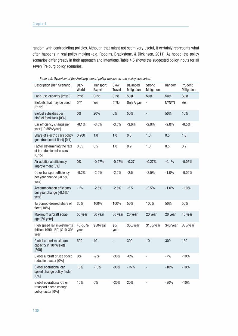
514727-L-bw-peeters514727-L-bw-peeters514727-L-bw-peeters514727-L-bw-peetersProcessed on: 20-10-2017Processed on: 20-10-2017Processed on: 20-10-2017Processed on: 20-10-2017 PDF page: 138PDF page: 138PDF page: 138PDF page: 138
138
random with contradicting policies. Although that might not seem very useful, it certainly represents what often happens in real policy making (e.g. Robbins, Brackstone, & Dickinson, 2011). As hoped, the policy scenarios differ greatly in their approach and intentions. Table 4.5 shows the suggested policy inputs for all seven Freiburg policy scenarios.
Table 4.5: Overview of the Freiburg expert policy measures and policy scenarios.
Description [Ref. Scenario] Dark World
Transport Expert
Slow Travel
Balanced Mitigation
Strong Mitigation
Random Prudent Mitigation
Land-use capacity [Phys.] Phys Sust Sust Sust Sust Sust Sust
Biofuels that may be used [5*No]
5*Y Yes 5*No Only Algae - NYNYN Yes
Biofuel subsidies per biofuel feedstock [0%]
0% 20% 0% 50% - 50% 10%
Car efficiency change per year [-0.55%/year]
-0.1% -3.5% -3.5% -3.0% -2.0% -2.0% -0.5%
Share of electric cars policy goal (fraction of fleet) [0.1]
0.200 1.0 1.0 0.5 1.0 0.5 1.0
Factor determining the rate of introduction of e-cars [0.15]
0.05 0.5 1.0 0.9 1.0 0.5 0.2
Air additional efficiency improvement [0%]
0% -0.27% -0.27% -0.27 -0.27% -0.1% -0.05%
Other transport efficiency per year change [-0.5%/year]
-0.2% -2.5% -2.5% -2.5 -2.5% -1.0% -0.05%
Accommodation efficiency per year change [-0.5%/year]
-1% -2.5% -2.5% -2.5 -2.5% -1.0% -1.0%
Turboprop desired share of fleet [10%]
30% 100% 100% 50% 100% 50% 50%
Maximum aircraft scrap age [50 year]
50 year 30 year 30 year 20 year 20 year 20 year 40 year
High speed rail investments (billion 1990 USD) [$10-30/year]
40-50 $/year
$50/year $0/year
$50/year $100/year $40/year $35/year
Global airport maximum capacity in 10^6 slots [500]
500 40 - 300 10 300 150
Global aircraft cruise speed reduction factor [0%]
0% -7% -30% -6% - -7% -10%
Global operational car speed change policy factor [0%]
10% -10% -30% -15% - -10% -10%
Global operational Other transport speed change policy factor [0%]
10% 0% -30% 20% - -20% -10%
Chapter 4

514727-L-bw-peeters514727-L-bw-peeters514727-L-bw-peeters514727-L-bw-peetersProcessed on: 20-10-2017Processed on: 20-10-2017Processed on: 20-10-2017Processed on: 20-10-2017 PDF page: 139PDF page: 139PDF page: 139PDF page: 139
139
Description [Ref. Scenario] Dark World
Transport Expert
Slow Travel
Balanced Mitigation
Strong Mitigation
Random Prudent Mitigation
Global (tourism) carbon tax (1990 USD) [$0/ton]
$20/ton $100/ton $1000/ton
250 1000/ton $50 $30/ton
Tourism carbon tax applied to air, car, other, accom-modation [all yes]
Yes except air/car
Yes Yes Air only Yes Yes all Yes
Global ticket tax Air transport (+ is tax and - is subsidy) [0%]
10% + 200% 100% 200% +50% 0%
Global ticket tax Car transport (+ is tax and - is subsidy) [0%]
30% + 200% 100% 200% +50% 0%
Global ticket tax Other transport (+ is tax and - is subsidy) [0%]
5% - 200% -80% 200% -10% 0%
Rate of change of length of stay (night/trip/year) [-0.0051]
-0.1 -0.0051 - - 0.0015 0.0015 -0.0051
Marketing policy that changes the desire to travel (trips per capita per year) [1.0]
1.0 0.75 - 0.8 .75 1.2 1.0
Marketing policy that factors in the attraction of distance [1.0]
1.1 0.2 0.2 0.2 .20 1.2 0.8
All expert policy scenarios significantly reduced the emissions, as shown in Figure 4.12, even the ‘Dark World’ and ‘Random’ policy scenarios, which did not particularly aim to do so. Interestingly, these ‘Random’ and ‘Dark World’ policy scenarios had almost the same effect on emissions. That these two still obtain emission reductions can partly be explained by the fact that the two experts both applied some additional technological efficiency improvements. The instability in the ‘Random’ scenario was caused by the twenty-year aircraft scrap limit set for the policy scenario. This setting, which was much lower than the default, tends to amplify the business cycle for the aircraft fleet. Such instability might also occur in the real world because a regulatory twenty-year scrap age poses an additional constraint to fleet operations, depriving fleet dispatchers and planners of one of their options for matching Air transport demand. The two next best scenarios in terms of emission reductions are the ‘Slow Travel’ and ‘Prudent Mitigation’ policy scenarios. The ‘Slow Travel’ policy scenario aimed at minimising transport. For instance, all transport was heavily taxed, and investments in high-speed rail were discontinued. Still, airport capacity was allowed to keep pace with demand. A decision to restrict airport capacity would have been in line with a ‘slow travel’ approach. This approach shows that some assistance may be required for using the GTTMdyn. The ‘Reasonable Meas-ures’ policy scenario applies most of the policy measures, but it does so in a moderate way. Two other close policy scenarios in terms of emission reductions were the ‘Balanced Mitigation’ and ‘Transport Expert’ policy scenarios. Both of these show emissions becoming more or less flat. Although, at the end of this century, the ‘Transport Expert’ policy scenario reduces emissions a bit more. The tourist expert and the transport
4
GTTMdyn results and policy scenarios

514727-L-bw-peeters514727-L-bw-peeters514727-L-bw-peeters514727-L-bw-peetersProcessed on: 20-10-2017Processed on: 20-10-2017Processed on: 20-10-2017Processed on: 20-10-2017 PDF page: 140PDF page: 140PDF page: 140PDF page: 140
140
expert obtained equal results but using slightly different approaches. Finally, the most effective mitigation was obtained by the ‘Strong Mitigation’ policy scenario. This policy scenario would reduce CO2 emissions by some 70% in 2100, in comparison to 2000.
Figure 4.12: Overview of the impact of the Freiburg workshop experts’ policy scenarios on CO2 emissions.
Considering that emissions are but one way to evaluate the policy scenarios, in Figure 4.13, I show the impacts on total transport volume. Regarding transport, the ‘Random’ policy scenario increased its growth above the transport volume in the Reference Scenario. For both the ‘Dark World’ and the ‘Prudent Mitiga-tion’ scenarios the transport volume kept growing only slightly less than in the Reference Scenario. Medium reduction of transport growth was obtained in the ‘Slow Travel’, ‘Balanced Mitigation’ and ‘Transport Expert’ scenarios, while a strong reduction, but still growth, was found for the ‘Strong Mitigation’ scenario.
Figure 4.13: Overview of the impact of the Freiburg workshop experts’ policy scenarios on total transport volume.
Figure 4.14 shows the fractions of the Reference Scenario, indexed for six criteria. The most remarkable policy scenario was ‘Random’, which increased tourism and tourism transport volume while reducing CO2
Chapter 4

514727-L-bw-peeters514727-L-bw-peeters514727-L-bw-peeters514727-L-bw-peetersProcessed on: 20-10-2017Processed on: 20-10-2017Processed on: 20-10-2017Processed on: 20-10-2017 PDF page: 141PDF page: 141PDF page: 141PDF page: 141
141
emissions by approximately 25% in comparison to the Reference Scenario in 2100 (see Figure 4.13). Ap-parently, randomly changing policy measures tends to result in emissions reductions. This result, of course, may partly be caused by the fact that the GTTMdyn is designed to assess mitigation of emissions, thus the set of measures implemented aim to reduce emissions, though some may increase them. At the other end of the scale, ’Strong Mitigation’ performs best for the environment and, although it reduces the number of trips, it assumed an increase in the length of stay, thereby keeping revenue losses low. The ‘Prudent Mitigation’ and ‘Slow Travel’ policy scenarios had a limited impact on emissions, but for different reasons. ‘Slow Travel’ aims at both strong technology, and taxes, but no investments in high-speed rail, alternative fuels, and it has an Air transport cruise-speed limitation that reduces aircraft fuel efficiency. ‘Prudent Mitigation’ applies nearly every policy, but all in a prudent way. ‘Slow Travel’ reduces radiative forcing better than ‘Prudent mitigation’; most likely because of the very high tax on air tickets assumed in the first policy scenario and the failure of the biofuels to effectively reduce RF in the second one. The two remaining policy scenarios, ‘Transport Expert’ and ‘Balanced Mitigation’, perform better for the environment, but they are not as good for the sector as both partly rely on reducing tourism volume and its concomitant revenues.
Figure 4.14: a diagram showing the performance of the Freiburg workshop experts’ policy scenarios for tourism economy and volume and environmental impacts. The indicator shows the effects of volume as a fraction of the Reference Scenario in 2100 and the effects on the environment as a fraction of the reduction of the emissions in the Reference Scenario 2100. Therefore, the Reference Scenario score is zero for all three environmental indicators. A score of 0.3 translates into a 30% reduction with respect to the environmental impact of the Reference Scenario.
As shown in Table 4.6, only the ‘Strong Mitigation’ scenario achieves a climatically sustainable development of tourism when evaluated against the two weakest sets of criteria. However, even this policy scenario failed to reach a fair economic or emissions share in 2100.
4
GTTMdyn results and policy scenarios

514727-L-bw-peeters514727-L-bw-peeters514727-L-bw-peeters514727-L-bw-peetersProcessed on: 20-10-2017Processed on: 20-10-2017Processed on: 20-10-2017Processed on: 20-10-2017 PDF page: 142PDF page: 142PDF page: 142PDF page: 142
142
Table 4.6: Overview of all the Freiburg workshop policy scenarios for climatically sustainable development. The numbers show the metric values and the colours the criteria (‘green’ means the emissions comply with the criterion, and ‘red’ means the emissions fail the criterion; the darker the red, the more severe the failure).
The workshop demonstrates the following:1. it is not a highly complex operation to develop policy scenarios with the GTTMdyn, as such, it can be
performed by scholars from various disciplines (ranging from transport to tourism and sociology to engineering), and it can provide widely differing policy scenarios within a couple of hours;
2. the approaches to how to mitigate tourism’s long-term contribution to climate change varied considerably, but all of the policy scenarios achieved some emissions reductions in comparison to the Reference Scenario. It may be that most of the policy measures included in the GTTMdyn aim at emission reductions, thereby providing the user with a biased set of measures;
3. the policy scenarios aimed at maximising mitigation still delivered mixed effects. Only a combination of strong measures was able to obtain a climatically sustainable development of tourism. Other policy scenarios, inspired by a theme (for example, ‘slow travel’) suffered from not including all of the opportunities to reduce emissions.; and
4. without a reduction of tourism transport volumes (pkm), there is, within the capabilities and limitations of the GTTMdyn, no way to reach any level of a climatically sustainable development of tourism, including the criteria set ‘weak contribution to climatically sustainable development’.
4.5. Climatically sustainable policy scenarios
4.5.1 Policy scenario development strategyWith the experience of the workshop in mind, I explored policy strategies further. The first step was to examine the policies that the tourism and transport sector have already implemented and to assess their effectiveness with the GTTMdyn. The tourism sector, however, does not appear to be very influential at miti-gation (Hall, Scott, & Gössling, 2013; Scott & Becken, 2010; Scott, Hall, & Gössling, 2016b; Scott et al.,
Chapter 4

514727-L-bw-peeters514727-L-bw-peeters514727-L-bw-peeters514727-L-bw-peetersProcessed on: 20-10-2017Processed on: 20-10-2017Processed on: 20-10-2017Processed on: 20-10-2017 PDF page: 143PDF page: 143PDF page: 143PDF page: 143
143
2010). For example, it does not play a role in developing electric cars (Gössling, 2015), does not particularly promote or develop rail-based tourism (e.g. Albalate & Fageda, 2016) and it does not have a strategy to achieve zero-emissions accommodation by a certain year (Melissen, 2013; Melissen et al., 2015). The only subsector that has a global strategy is the international aviation industry that has decided to implement measures from 2020 onwards to reduce its carbon footprint (Cames, Graichen, & Pulles, 2016a). The agreed actions consist of a CO2 standard and a global emissions offsetting system. Also, the international aviation industry has announced its ambition to have sustainable alternative fuels (SAF). Aviation emits the majority of tourism’s emissions, so it is certainly worthwhile to explore the ICAO ambition and test its effectiveness. From there, I have explored if more is needed to achieve a climatically sustainable development of tourism, preferably against criteria that are stronger than the ‘weak contribution to climatically sustainable develop-ment’. One approach could be a strong modal shift from Car transport and Air transport to Other transport, as shown with the GTTMadv (see Section 1.6.4). Therefore, I started developing an ‘Ultimate Modal Shift’ policy scenario, which I present in Section 4.5.3). Unfortunately, this approach did not deliver the desired climatically sustainable development of tourism, just as the ‘Slow Travel’ policy scenario from the Freiburg workshop failed to accomplish. It was clear that a stronger approach was required. The ‘Ultimate Mitiga-tion’ policy scenario is the result of that strategy (see Section 4.5.4). It aims to reduce the emissions as far as the GTTMdyn allows the user. Based on the ‘Ultimate Mitigation’ policy scenario, I tested the role of early versus delayed action on climate change. There is a debate about this issue, in which some urge a quick mitigation effort (Schaeffer, Kram, Meinshausen, van Vuuren, & Hare, 2008; Stern, 2006), while others argue for delayed action (Nordhaus, 2008). To contribute to this debate, I tested a ‘Delayed Mitigation’ policy scenario, assuming that the measures would be taken after 2050 and would only be fully deployed in 2100. Moreover, I also tested an ‘Early Mitigation’ policy scenario, where measures are taken immediately in 2015 but assumed to decline to no measures by mid-century. Section 4.5.4 discusses both. Though the ‘Ultimate Mitigation’ policy scenario certainly obtained climatically sustainable development, this was achieved at the cost of losing nearly half of the tourism sector’s revenues. Therefore, my next step was to transform ‘Ultimate Mitigation’ into ‘Economic Mitigation’. The objective of this policy scenario was to preserve the economic potential of the tourism sector as projected in the Reference Scenario while securing most of the emission reductions achieved in ‘Ultimate Mitigation’ (see Section 4.5.5). ‘Economic Mitigation’ can be considered the most balanced answer to the question of what climatically sustainable tourism would look like during this century. I tested the robustness of the ‘Economic Mitigation’ policy scenario for several contextual scenarios (see also Section 4.5.5). Section 4.5.6 provides an overview of all of these results and discusses the differences between the policy scenarios.
4.5.2 Mitigation proposed by the aviation sector As Air transport has the largest and much increasing share of emissions and poses the biggest problem for mitigating emissions, I dedicated a special scenario to the ambitions proposed by the aviation sector. Several sector brochures (IATA, 2013b; ICAO, 2014) published these ambitions. The basic ambitions include additional efficiency through the development and implementation of a CO2 standard for various aircraft categories (ICAO, 2012) and global market-based measures (GMBM), which would require the sector to buy emission permits from outside of the aviation sector (ICAO, 2013). Global market-based measures were agreed upon at the end of 2016 and were subsequently labelled as the Carbon Offsetting and Reduction Scheme (CORSIA, ICAO, 2016). Furthermore, biofuels form an important part of the ambition for carbon-
4
GTTMdyn results and policy scenarios

514727-L-bw-peeters514727-L-bw-peeters514727-L-bw-peeters514727-L-bw-peetersProcessed on: 20-10-2017Processed on: 20-10-2017Processed on: 20-10-2017Processed on: 20-10-2017 PDF page: 144PDF page: 144PDF page: 144PDF page: 144
144
neutral growth (ICAO, 2013). The basic international measure for Air transport is the 2016 ICAO CO2 standard. This standard distin-
guishes between existing - in production - aircraft types like the Boeing B737-800 and new aircraft types. The ‘in production’ aircraft types are defined as those that have received their type certificate before 2020; the ‘new’ aircraft types are type certified after that date. To assess whether an aircraft type complies with the CO2 standard, a metric value (MV) was developed. The MV is the specific air range at cruise flight (kg fuel per aircraft km) divided by a floor-area-based correction factor for size. Furthermore, several ‘stringency levels’ were defined. These consist of a curve showing MV as a function of maximum take-off weight of the aircraft type. An aircraft type needs to show its MV to be below this line for the type’s (certified) maximum take-off weight to comply with the standard. The stringency lines differ for different groups of aircraft types. All aircraft of an ‘in production’ type need to comply with a lower level than ‘new types’. Furthermore, if an ‘in production’ type fails the standard, it has the time up to make the type to comply, for instance by improving parts of the aircraft. If by 2028, the aircraft type does still not comply with this level, it has to go out of production. New aircraft types are aircraft certified after 2020 that need to comply from the date of their certification. The MV level varies for different aircraft categories and over the maximum take-off weight (Cames et al., 2016a; Grote, Williams, & Preston, 2014; ICAO, 2014).
The effect of the CO2 standard agreed in February 2016 could potentially result in cumulative savings of 0.6 Gton of emissions between 2020 and 2040 (The White House, 2016). The GTTMdyn’s cumulative emissions for 2020-2040 are in the Reference Case 45.9 Gtons CO2, which means the standard may save an overall 1.30% (or -0.0704 %/year). As part of the process, ICAO defined ten different stringency options (SO) for the CO2 standard. The maximum possible effectiveness for the fuel standard is estimated by MDG and FESG (2015)1 to be approximately 1.2 Gton saved between the years 2020 and 2040. This amount is the equivalent of 2.62% of Air transport’s cumulative emissions (equivalent to -0.1325 %/year) over the 20-year period. This rate of improvement is assumed in the ‘ICAO Ambition’ as the CO2 standard effectiveness through the end of this century, assuming the stringencies are regularly – and soon - upgraded to enforce further fuel efficiency improvements.
The global market-based measures, implemented as CORSIA, will have two effects: the offset of climate effects by buying credits on the carbon market and an increase in the cost of flying. Because the offsets are created outside the scope of the GTTMdyn, no emission reductions have initially been accounted. However, at the end of this section, I have added a short assessment of what the effects might be. The cost effect has been accommodated in the following results.
Several aviation sector reports (ATAG, 2010; IATA, 2013b, 2015) assume that biofuels will become a major component of the aviation sector’s mitigation strategy. The ambition for the global sector ranges from 20 to 50% emissions reduction (Scott et al., 2016b). The aviation sector aims at sustainably produced biofu-els. For instance, (IATA, 2015, pp. author-year) consistently uses the term SAF (Sustainable Alternative Fuel). Therefore, in this policy scenario, I assume the application of a sustainable land-use limit. Also, I assume there will be no subsidy for biofuels because it is a sector strategy. Summarised, I ‘optimistically’ assume that an ICAO CO2-standard will result in a 0.133% additional technological improvement over the long term, a 1% ticket tax for Air transport as a proxy for the cost of CORSIA and the maximum sustainable application of biofuels without subsidies. Without subsidies, only the biofuel feedstock camellia will gain a share of the market. Figure 4.15 gives an overview of the main results.
1 This is a confidential paper in possession of the author.
Chapter 4

514727-L-bw-peeters514727-L-bw-peeters514727-L-bw-peeters514727-L-bw-peetersProcessed on: 20-10-2017Processed on: 20-10-2017Processed on: 20-10-2017Processed on: 20-10-2017 PDF page: 145PDF page: 145PDF page: 145PDF page: 145
145
Figure 4.15: Overview of the ‘ICAO Ambition’ policy scenario results. The grey lines indicated with an * give the Reference Scenario values.
4
GTTMdyn results and policy scenarios

514727-L-bw-peeters514727-L-bw-peeters514727-L-bw-peeters514727-L-bw-peetersProcessed on: 20-10-2017Processed on: 20-10-2017Processed on: 20-10-2017Processed on: 20-10-2017 PDF page: 146PDF page: 146PDF page: 146PDF page: 146
146
The CO2 emissions growth between 2005 and 2100 declines from 374% in the Reference Scenario in 2100 to 323% in the ‘ICAO Ambition’ policy scenario. Tourism’s share of the cumulative Paris-Agreed CO2 budget (2 °C) goes down from 28.5% in the Reference Scenario 2100 to 26.3%.
Biofuels have a limited effect because, without subsidies, only camellia will be available on the market, and this product rather quickly faces sustainable land-use limitations. Subsidies for biofuels are considered inevitable, according to Heraghty et al. (2013). Algae have the highest yield per hectare, so a scenario with subsidised algae might achieve a higher reduction in emissions. Indeed, the emissions will reduce more in 2100, although there will still be a considerable growth, 285%, between 2005 and 2100. Tourism’s share of the Paris-Agreed CO2 budget will reduce to 24.2%. However, this will only be possible at a high subsidy burden that might amount to some two trillion dollars by 2100 (1990 USD), as shown by the purple line in Figure 4.16. I did not explore further whether a lower subsidy rate (it has been defined at 90% for the entire 2015 to 2100 period) would have the same effect.
Figure 4.16: Total revenues and biofuel (algae) subsidies for the ‘ICAO Subsidised’ policy scenario (1990 USD).
Of course, it is legitimate to question whether governments would need to pay the entire subsidy burden. To simulate what would happen if the subsidy of biofuels was compensated by a ticket tax so that the policy scenario would become budget neutral for the government over the entire 2015-2100 period, I developed ‘ICAO Ambition Budget Neutral’. The additional cost for the sector, which translates into higher costs for travellers, achieves an additional reduction of CO2 emissions in 2100 as compared to the Reference Sce-nario. The growth of CO2 emissions between 2005 and 2100 subsequently reduces to 256% and the share of tourism of the total Paris-Agreed budget reduces to 23.5%.
Chapter 4
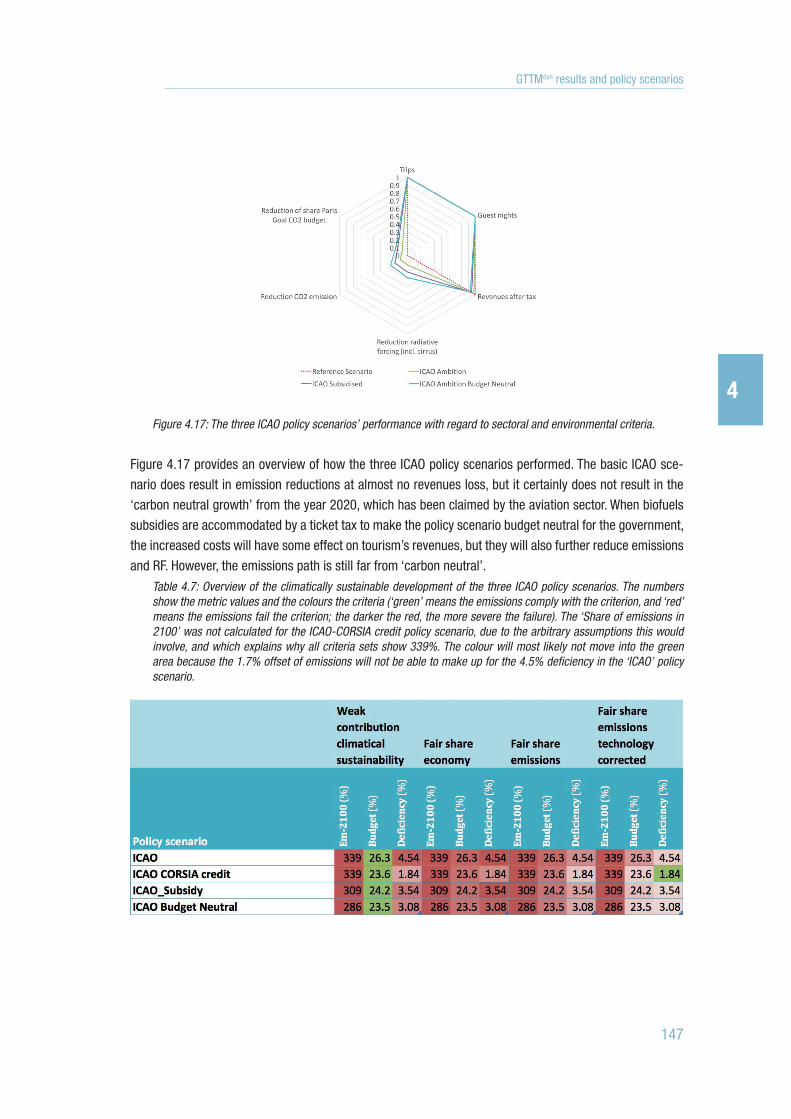
514727-L-bw-peeters514727-L-bw-peeters514727-L-bw-peeters514727-L-bw-peetersProcessed on: 20-10-2017Processed on: 20-10-2017Processed on: 20-10-2017Processed on: 20-10-2017 PDF page: 147PDF page: 147PDF page: 147PDF page: 147
147
Figure 4.17: The three ICAO policy scenarios’ performance with regard to sectoral and environmental criteria.
Figure 4.17 provides an overview of how the three ICAO policy scenarios performed. The basic ICAO sce-nario does result in emission reductions at almost no revenues loss, but it certainly does not result in the ‘carbon neutral growth’ from the year 2020, which has been claimed by the aviation sector. When biofuels subsidies are accommodated by a ticket tax to make the policy scenario budget neutral for the government, the increased costs will have some effect on tourism’s revenues, but they will also further reduce emissions and RF. However, the emissions path is still far from ‘carbon neutral’.
Table 4.7: Overview of the climatically sustainable development of the three ICAO policy scenarios. The numbers show the metric values and the colours the criteria (‘green’ means the emissions comply with the criterion, and ‘red’ means the emissions fail the criterion; the darker the red, the more severe the failure). The ‘Share of emissions in 2100’ was not calculated for the ICAO-CORSIA credit policy scenario, due to the arbitrary assumptions this would involve, and which explains why all criteria sets show 339%. The colour will most likely not move into the green area because the 1.7% offset of emissions will not be able to make up for the 4.5% deficiency in the ‘ICAO’ policy scenario.
4
GTTMdyn results and policy scenarios

514727-L-bw-peeters514727-L-bw-peeters514727-L-bw-peeters514727-L-bw-peetersProcessed on: 20-10-2017Processed on: 20-10-2017Processed on: 20-10-2017Processed on: 20-10-2017 PDF page: 148PDF page: 148PDF page: 148PDF page: 148
148
One of ICAO’s measures, the CORSIA scheme, relies entirely on offsetting. However, the effects of offsetting are subject to fierce debate (see Section 5.5.1). One problem with offsetting is that substantial uncertainty exists about its effectiveness. Cames et al. (2016b, p. 11) found from an investigation of 5,655 projects that these projects delivered a total of 4,829 Mton CO2 CERs (Certified Emission Credits). However, “85% of the projects covered in this analysis and 73% of the potential 2013-2020 Certified Emissions Reduction (CER) supply have a low likelihood that emission reductions are additional and are not over-estimated. Only 2% of the projects and 7% of potential CER supply have a high likelihood of ensuring that emission reductions are additional and are not over-estimated.” If I assume that aviation can find effective offsets and manages to reduce global emissions between 2021 and 2075 and follow the main CORSIA rules of only additional emissions from international aviation and including some exemptions, this would amount to be about 27 Gton CO2, the equivalent of 2.7% of the Paris-Agreed budget. Tourism’s share of the 2100 Paris-Agreed emissions would decrease a bit, depending on the distribution of the saved budget (the 27 Gton) over the years 2075-2100, but it would be unlikely to reach the ‘green’ region. In comparison with the relatively weak ‘fair share emissions’ set of criteria, tourism would achieve sustainability for the deficiency, but not for the two other criteria.
4.5.3 Ultimate Modal shiftWith the GTTMadv, I found that a strong modal shift might be one of the two optimum solutions for the sus-tainable development of tourism without harming the tourism sector’s economy (Peeters & Dubois, 2010). Therefore, I developed the ‘Ultimate Modal Shift’ policy scenario, which was based mainly on the idea that a combination of faster and cheaper Other transport as well as taxing the competitors (car and air) could be the primary mechanism to achieve this. I based the policy measures entirely on maximising the share of Other transport without considering the impact on CO2 emissions. Table 4.8 displays the policy measures. The global ticket tax on cars was designed to maximise the modal shift, meaning it to be less than the maxi-mum level allowed in the GTTMdyn. For the other policy measures, I have set the measures to the maximum allowed by the GTTMdyn input limits.
Table 4.8: Inputs for the ‘Ultimate Modal shift’ policy scenario. The inputs are equally divided between 2015 and 2100 into intervals of 21.5 years, rounded to the whole year. Money values are in 1990 USD. A negative tax means a ‘subsidy’.
Year 2015 2036 2057 2078 2100
High-speed rail investment (billion $/year) 200 200 200 200 200
Global carbon tax in $/ton CO2 (excluding Other transport)
1,000 1,000 1,000 1,000 1,000
Global ticket tax on air (%) 200 200 200 200 200
Global ticket tax on car (%) 35 64 190 171 110
Global ticket tax on Other transport (%) -80 -80 -80 -80 -80
Other transport average speed increase (%) 30 30 30 30 30
Car transport average speed increase (%) -30 -30 -30 -30 -30
Figure 4.18 shows the large effects on modal shift of the Ultimate Modal Shift policy. In this scenario the tax on air tickets, the subsidy of rail tickets, and the large investments in high-speed rail combine to more
Chapter 4

514727-L-bw-peeters514727-L-bw-peeters514727-L-bw-peeters514727-L-bw-peetersProcessed on: 20-10-2017Processed on: 20-10-2017Processed on: 20-10-2017Processed on: 20-10-2017 PDF page: 149PDF page: 149PDF page: 149PDF page: 149
149
than double the share of Other transport in terms of the number of trips and more than quadruple the share of transport distances travelled. Overall, the number of trips and distances are similar to the Reference Scenario. Total CO2-emissions growth in 2100 declines to 68% for 2005. This policy scenario increases the overall revenues (after tax) of the tourism sector, but it increases expenditures by tourists much more, as they will have to pay the taxes on aviation, car use and carbon. The subsidisation of Other transport does not compensate at all for this. The investment in high-speed rail is assumed to jump from its 2015 value of some $10 million to an estimated $200 million (all in 1990 USD).
4.5.4 Ultimate Mitigation policy scenarioIn this scenario, I have tried to find the limits of mitigation by systematically setting all policy measures to the ‘reducing CO2 emissions most’ setting. To do so, I ignored the possible negative impacts on the sector. Alternative fuel measures included a 90% subsidy on all five feedstocks and a physical land-use limit, all technologies were set at their limits, with maximum investment in high-speed rail, airport slot capacity at its minimum, 100% desired turboprop fleet and a 20-year maximum aircraft age. All taxes were set to their maximum because this kind of a policy gains the highest reduction in CO2 emissions. Operationally, the air cruise speed was set at -6%, car speed at -30% and other speed at +30%. Finally, the length of stay was reduced to follow the highest decline rate available (-0.2%/year), and the desire to travel and attraction of distance were set to their minimum. This policy scenario was the first to actually reduce emissions in 2100, in comparison to 2005. The CO2 emissions reduction in 2100 amounts to 83%. Tourism’s share of the Paris-Agreed CO2 emissions budget goes down from the 28.5% in the Reference Scenario to 3.6%. At the same time, however, the tourism sector’s revenues growth prospects will more than halved from a growth of 428% for the 2005-2100 period in the Reference Scenario to 204% and the number of trips from 336% to 226%. An overview of all policy measures is given in Table 4.9 in section 4.5.5. Figure 4.19 presents the main characteristics of the policy scenario.
4
GTTMdyn results and policy scenarios

514727-L-bw-peeters514727-L-bw-peeters514727-L-bw-peeters514727-L-bw-peetersProcessed on: 20-10-2017Processed on: 20-10-2017Processed on: 20-10-2017Processed on: 20-10-2017 PDF page: 150PDF page: 150PDF page: 150PDF page: 150
150
Figure 4.18: Results for the Maximum Modal Shift policy scenario. The grey lines indicated with an * give the Refer-ence Scenario values. Emissions represent the annual CO2 emissions.
Chapter 4

514727-L-bw-peeters514727-L-bw-peeters514727-L-bw-peeters514727-L-bw-peetersProcessed on: 20-10-2017Processed on: 20-10-2017Processed on: 20-10-2017Processed on: 20-10-2017 PDF page: 151PDF page: 151PDF page: 151PDF page: 151
151
Figure 4.19: Overview of the Ultimate Mitigation policy scenario. The grey lines indicated with an * give the Reference Scenario values. Emissions represent the annual CO2 emissions.
4
GTTMdyn results and policy scenarios

514727-L-bw-peeters514727-L-bw-peeters514727-L-bw-peeters514727-L-bw-peetersProcessed on: 20-10-2017Processed on: 20-10-2017Processed on: 20-10-2017Processed on: 20-10-2017 PDF page: 152PDF page: 152PDF page: 152PDF page: 152
152
As mentioned in Section 4.5.1, there is an ongoing debate about whether it makes sense to take immediate action, as advocated, for instance, by Stern (2006) or to follow the most optimised path for the economy, which typically includes delayed measures as proposed by Nordhaus (2008); Nordhaus (2007). To test this, I took the ‘Ultimate Mitigation’ policy scenario and created a ‘Delayed Mitigation’ policy scenario by start-ing a smooth transition from no measures to the full ‘Ultimate Mitigation’ level in the second half of the twenty-first century. For the ‘Early Mitigation’ policy scenario, I applied a reverse approach (starting with the ‘Ultimate Mitigation’ measures in 2015 and declining these smoothly to the Reference Scenario values by the middle of the twenty-first century. Figure 4.20 and Figure 4.21 show the performance of the three variants of the Ultimate Mitigation policy scenario. The results of the GTTMdyn show that the finding by Nor-dhaus (2008) performs technically far worse than the early adoption of measures, although both perform substantially worse than the continuous mitigation efforts assumed for ‘Ultimate Mitigation’. Nordhaus as-sumed high discount rates and concluded that delayed action might be the economically optimum policy. The GTTMdyn does not assume a discount rate nor an economic optimisation, but it does look at what is physically required (in terms of emission reductions) to avoid dangerous climate change. The main differ-ences between early mitigation and delayed mitigation are a much smaller reduction of the CO2 budget in the case of delayed action and a much higher cost in terms of the revenues of delayed action. This finding thus rather contrasts with the conclusion drawn by Nordhaus (2008).
Figure 4.20: Overview of the Ultimate Mitigation policy scenario and its delayed and early variants.
There is also another issue: the impact of delay on policy freedom future policymakers will have. Let us con-sider a policymaker living in the 2050s, and assume that, by then, the impact of climate change is heavily felt in terms of ‘natural’ disasters, human suffering and unprecedented migration of climate refugees. The population will probably demand strong measures to correct the situation. In the early mitigation scenario, policymakers in 2050, even though the impacts already will be less severe, would still have the option to follow more or less the Ultimate Mitigation policy scenario and avoid the worst effects of climate change. Under the delayed scenario, causing the most severe impacts of climate change, policymakers would have no other option than to satisfy the public with too late mitigation measures, which would be both very costly and mostly ineffective in terms of achieving climatically sustainable development.
Chapter 4

514727-L-bw-peeters514727-L-bw-peeters514727-L-bw-peeters514727-L-bw-peetersProcessed on: 20-10-2017Processed on: 20-10-2017Processed on: 20-10-2017Processed on: 20-10-2017 PDF page: 153PDF page: 153PDF page: 153PDF page: 153
153
Figure 4.21: Emission pathways for the three Ultimate Mitigation policy scenarios, contrasted with the Paris-Agreed and Paris-Aspired global emission pathways.
Often, the marginal effect of a measure diminishes with its increasing level of application, which means that relaxing the economically most disadvantageous measures may only marginally increase the overall emissions, while significantly reducing the burden on the sector or the tourist. Therefore, I developed an ‘Economic Mitigation’ policy scenario, which is presented in the next section.
4.5.5 Economic Mitigation policy scenario
Rationale and assumptions‘Economic Mitigation’ is intended to be mitigation that avoids the most eco-inefficient measures, in an at-tempt to reduce the effects on the tourism sector, while maintaining as much as possible of the maximum emissions reduction obtained in the Ultimate Mitigation scenario. Therefore, I started with this Ultimate Miti-gation scenario and relaxed successive measures to improve the sector performance without overly dete-riorating the emissions reduction. The following steps were taken (see the green-shaded cells in Table 4.9):1. the policies targeting behavioural change were relaxed: the assumed reduction of trips was relaxed
from -20% to -5%, the rate of change of LOS went down from -0.0020%/year to -0.0002%/year, and the attraction of distance was reduced to 50% instead of 80%;
2. by increasing Other transport speed to 30%, there is a slight additional shift to Other transport, which generates additional revenues from tickets;
3. in the ‘Ultimate Mitigation’ scenario, the global carbon tax was set at its maximum of $1,000/ton CO2 for all transport modes and accommodation. By trial and error, I found that the same emissions reduction could be achieved with a relaxed carbon tax pathway (see Figure 4.22);
4
GTTMdyn results and policy scenarios

514727-L-bw-peeters514727-L-bw-peeters514727-L-bw-peeters514727-L-bw-peetersProcessed on: 20-10-2017Processed on: 20-10-2017Processed on: 20-10-2017Processed on: 20-10-2017 PDF page: 154PDF page: 154PDF page: 154PDF page: 154
154
Figure 4.22: The carbon tax path assumed in the Economic Mitigation policy scenario;
4. in the ‘Ultimate Mitigation’ scenario, all ticket taxes were set at their maximum limit (200%). However, it appears that the assumed taxes for Car and Other transport only generate 1% additional emissions reduction while it reduces revenues by 9% up to a value slightly higher than the 2100 level of the Reference Scenario; and
5. I also assumed 100% turboprop and a 20-year maximum age of jet airliners in the ‘Ultimate Mitigation’ policy scenario. Both are far from the developing practices, so I relaxed these two measures to 40% and 30 years, which only had a very slight impact on emissions or revenues, but helps to keep better to current aviation practices.
Table 4.9: Overview of inputs for the Ultimate and the Economic Mitigation policy scenario. The relaxed measures are shaded green.
Description Reference 2100
Ultimate Mitigation
Economic Mitigation
Land-use capacity Physical Physical Sustainable
Biofuels that may be used Five times ‘no’
Yes Yes
Biofuel subsidies per biofuel feedstock (%) 0 90 90
Car efficiency change (% per year) -0.55 -3.50 -3.50
Share of electric cars policy goal (fraction of fleet) 0.1 1 1
Factor determining the rate of introduction of electric cars 0.15 1 1
Air additional efficiency improvement (%/year) 0 -0.27 -0.27
Other transport efficiency per year change (%/year) -0.50 -2.50 -2.50
Accommodation efficiency per year change (%/year) -0.50 -2.50 -2.50
Turboprop desired share of fleet (%) 10 100 40
Maximum aircraft age operational (year) 50 20 30
High-speed rail investments time curve (billion 1990 USD/year) $10-29 $200 $200
Chapter 4

514727-L-bw-peeters514727-L-bw-peeters514727-L-bw-peeters514727-L-bw-peetersProcessed on: 20-10-2017Processed on: 20-10-2017Processed on: 20-10-2017Processed on: 20-10-2017 PDF page: 155PDF page: 155PDF page: 155PDF page: 155
155
Description Reference 2100
Ultimate Mitigation
Economic Mitigation
Global airport maximum capacity in million flights/year 5003 10 10
Global aircraft cruise speed reduction factor (%) 0 -6 0
Global operational car speed change policy factor (%) 0 0 0
Global operational Other transport speed change (%) 0 0 30
Global (tourism) carbon tax (1990 USD/ton CO2) $0 $1,000 $90-450
Tourism carbon tax applied to all modes and accommodation Yes Yes Yes
Global ticket tax Air transport (+ is a tax and - is a subsidy; %) 0 200 200
Global ticket tax Car transport (+ is a tax and - is a subsidy; %) 0 200 0
Global ticket tax Other transport (+ is a tax and - is a subsidy; %) 0 200 0
Rate of change of the length of stay (night/trip/year) -0.0051 -0.0060 -0.0006
Marketing policy that factors the desire to travel 1 0.75 0.95
Marketing policy that factors the attraction-of-distance curve 1 0.2 0.5
Global results of the Economic Mitigation scenarioFigure 4.23 shows details of the ‘Economic Mitigation’ scenario. Total tourism revenues are now equal to the Reference Scenario, though there is a shift from transport revenues to accommodation revenues. The number of trips increases between 2005 and 2100 by over 313%, slightly less than the 336% in the Refer-ence Scenario 2100. Over the same period, transport distances now grow by 355%, much less than in the Reference Scenario (877%), but the number of nights increases by 273% instead of 168%. In 2100, the CO2 emissions will reduce by 72% compared to 2005 and by 94% compared to the Reference Scenario. Com-pared to ‘Ultimate Mitigation’, ‘Economic Mitigation’ results in 65% more CO2 emissions in 2100 and a 36% higher CO2 budget between the years 2015 and 2100. Tourism’s share of global RF reduces from 14.7% in the Reference Scenario to 1.8% in the ‘Economic Mitigation’ policy scenario.
2
3 Proxy for ‘unlimited’ Air transport capacity. In 2015, the slot capacity was about 30 million in the Reference Scenario 2100.
4
GTTMdyn results and policy scenarios
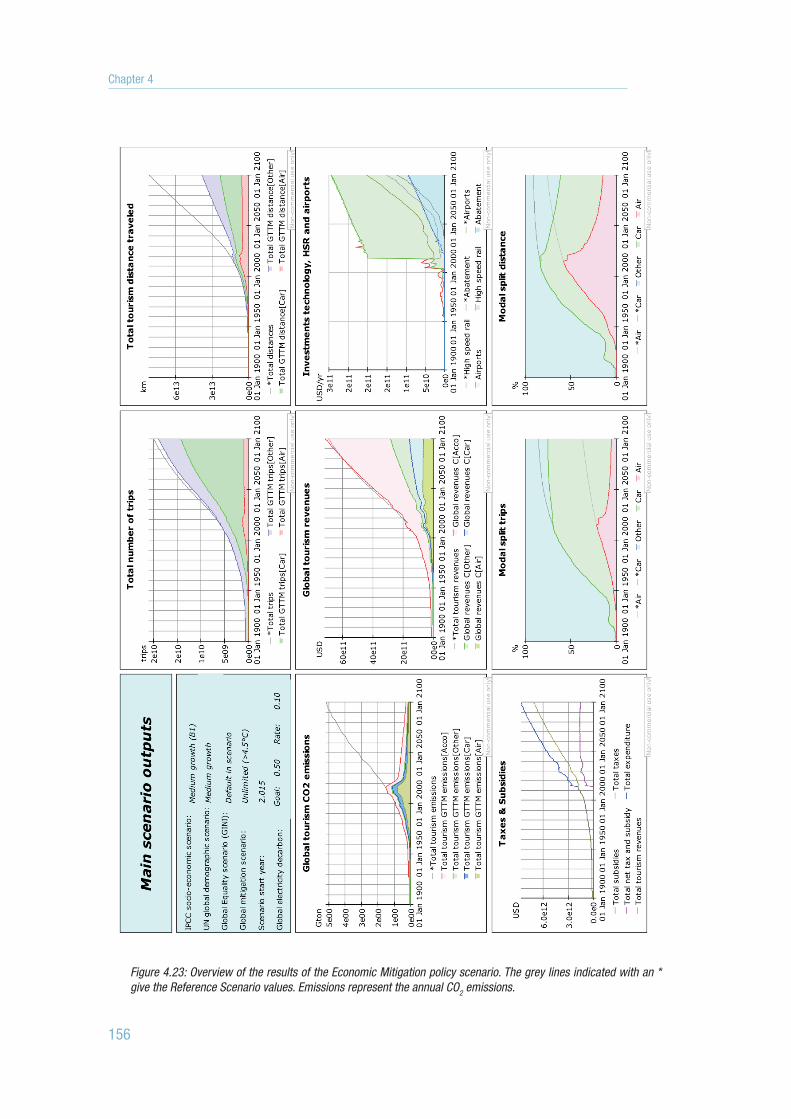
514727-L-bw-peeters514727-L-bw-peeters514727-L-bw-peeters514727-L-bw-peetersProcessed on: 20-10-2017Processed on: 20-10-2017Processed on: 20-10-2017Processed on: 20-10-2017 PDF page: 156PDF page: 156PDF page: 156PDF page: 156
156
Figure 4.23: Overview of the results of the Economic Mitigation policy scenario. The grey lines indicated with an * give the Reference Scenario values. Emissions represent the annual CO2 emissions.
Chapter 4

514727-L-bw-peeters514727-L-bw-peeters514727-L-bw-peeters514727-L-bw-peetersProcessed on: 20-10-2017Processed on: 20-10-2017Processed on: 20-10-2017Processed on: 20-10-2017 PDF page: 157PDF page: 157PDF page: 157PDF page: 157
157
The Economic Mitigation policy scenario is characterised by a strong modal shift, but less than in the Ulti-mate Mitigation policy scenario. Still, the level of the measures (taxes) and certainly the airport slot restric-tion will not make this policy scenario very popular with the aviation and tourism sectors. The slot restriction was introduced to restrict Air transport in a regulatory way through partly existing legislation (see section 2.5). The same effect could be achieved by restricting the global airliner fleet capacity through international agreements. The latter would, for instance, be a bit like the legislation that is designed to prevent overfishing (European Union, 2016).
It is most likely difficult to implement such a capacity restriction. The question is how important the slot-capacity restriction policy measure is to attain climatically sustainable tourism development. To test this, I created an Economic Mitigation’ policy scenario without the slot restriction: ‘Unlimited Economic Mitigation’. Also, I tested the robustness of the Economic Mitigation policy scenario under the highest and lowest growth contextual scenarios. Figure 4.24 shows the CO2 emissions pathways. Without the slot ca-pacity limit (‘Unlimited Economic Mitigation’), the emissions pathway becomes almost flat, ending in 2100 at roughly the level of 2003. Another result of this policy scenario will be that the Paris-Aspired (1.5 °C) emissions pathway becomes impossible and the Paris-Agreed (2° C) emissions pathway very unlikely, cer-tainly if tourism growth is higher than anticipated in the Reference Scenario. Figure 4.24 also demonstrates that the Economic Mitigation policy scenario is robust regardless of the growth of the global population and economy. It keeps the emissions well below the Paris-Agreed line, although in 2100, the Paris-Aspired line is only possible when the world economy and population are developing less prosperous than expected in the Reference Scenario. However, the airport capacity slot specifically is important for the robustness of the policy scenario. When no slot capacity limit is assumed, high global economic and population growth will cause the Paris Agreement to become impossible by 2095, and tourism’s emissions of will not be declin-ing by the end of this century. Note that the Paris emissions pathways are assumed not to change with the extremes of the contextual scenarios.
Figure 4.24: Overview of the ‘Economic Mitigation’ scenario plus its variants.
4
GTTMdyn results and policy scenarios

514727-L-bw-peeters514727-L-bw-peeters514727-L-bw-peeters514727-L-bw-peetersProcessed on: 20-10-2017Processed on: 20-10-2017Processed on: 20-10-2017Processed on: 20-10-2017 PDF page: 158PDF page: 158PDF page: 158PDF page: 158
158
Figure 4.25 provides the resulting performance for all Economic Mitigation policy scenario variants. Inter-estingly, when assuming a low growth context scenario, the difference between Economic Mitigation and Unlimited Economic Mitigation, thus without the slot capacity limit, becomes minimal. Overall, it appears that the unlimited growth of aviation makes it very unlikely that tourism will stay within the Paris-Agreed (2 °C) emissions pathway. Any form of capacity restraint, whether it is a slot capacity at airports or a global fleet capacity limit, requires further study regarding the legal basis to introduce it and its environmental, economical, practical and social impacts. My study hints at relatively small economic (net revenues) and social (ability to travel) impacts.
Figure 4.25: Overview of the performance of the ‘Economic Mitigation’ policy scenario, including its variants and robustness tests.
Market distributions in the Economic Mitigation policy scenarioThe distribution of trips over the 60 market segments (distance-transport mode) shows a marked difference between the Reference Scenario and Economic Mitigation policy scenario (see Figure 4.26). In the Economic Mitigation policy scenario, the distribution of air travel follows more or less the same pattern as in the Refer-ence Scenario, with a peak at around 4,000 km one way, but its shares are far less. The car takes over most of these trips at up to 2,400 km one-way, from where (high-speed) rail acquires much larger shares than in the reference case.
Chapter 4

514727-L-bw-peeters514727-L-bw-peeters514727-L-bw-peeters514727-L-bw-peetersProcessed on: 20-10-2017Processed on: 20-10-2017Processed on: 20-10-2017Processed on: 20-10-2017 PDF page: 159PDF page: 159PDF page: 159PDF page: 159
159
Figure 4.26: Comparing the distribution of total trips over the 60 distance-transport mode segments for the Ref-erence Scenario and the Economic Mitigation policy scenario for the year 2100. Note that the distance bins are unevenly distributed.
Figure 4.27 shows the time-decay curves for both scenarios to be relatively equal, with a shift toward shorter travel times at the low end. Note that the total number of trips to be distributed in the Economic Mitigation policy scenario is 5% less than in the Reference Scenario.
Figure 4.27: Comparing the travel time decay for the Reference Scenario in 2015 and 2100 and the Economic Miti-gation policy scenario in 2100. The bins are equally sized from 0-5 hours, 5-10 hours, and so forth but the dots are placed at the real average travel time per bin.
What these two figures show is that the main differences between the two scenarios are found in the modal choice, and the far smaller share of distances travelled above approximately 2,500 km. There are no significant changes in terms of travel time, though the share of greater than 20 hours one way is about 18% higher in the Economic Mitigation policy scenario than it is in the Reference Scenario. In that sense, the world presented in the Economic Mitigation policy scenario has some characteristics of a ‘slow travel’ scenario (Dickinson & Lumsdon, 2010).
4
GTTMdyn results and policy scenarios

514727-L-bw-peeters514727-L-bw-peeters514727-L-bw-peeters514727-L-bw-peetersProcessed on: 20-10-2017Processed on: 20-10-2017Processed on: 20-10-2017Processed on: 20-10-2017 PDF page: 160PDF page: 160PDF page: 160PDF page: 160
160
Consequences of the Economic Mitigation policy scenario for the tourism sectorThe main differences between the ‘Economic Mitigation’ policy scenario and the Reference Scenario are a strong shift from Air transport to Other transport modes (high speed and conventional) and a significantly lower average distance per trip. Figure 4.28 shows that Air transport will see volumes reduced (with 22% trips and 24% distances) compared to 2015, which means that, in 2100, the access to Air transport - net-work density and frequencies - will be comparable to that in the 2000s. Air transport will become very ex-pensive due to three effects: the carbon tax, a 200% ticket tax and the effect of the slot capacity restriction on the ticket price. All in all, the price will be almost six times higher (per passenger kilometres) than in 2015 and up to nine times the cost in 2100, compared to the Reference Scenario (see Figure 4.29). Of course, this higher price will impede access to Air transport for less wealthy people.
Figure 4.28: Overview of the GTTMdyn projected development of the number of trips and distances travelled between 2015 and 2100 for both the Reference Scenario and the Economic Mitigation policy scenario.
The dependence on Air transport reduces in the Economic Mitigation policy scenario (the share goes down from 22% in 2015 to 5% in 2100). Furthermore, measured in terms of the number of trips, the car share is 70% in 2100 for the Economic Mitigation scenario, up from 48% in 2015. The share of Other transport will decline from 30% in 2015 to 25%, but it becomes stable at the end of the century. In terms of distances, the picture is different. Overall, the distance travelled will increase by a factor of 4.6 over 2005, which is sig-nificantly less than the growth ratio of 9.8 in the Reference Scenario. Air transport goes down from a share of total passenger kilometres of 58% in 2015 to 14% in 2100 (76% in 2100 in the Reference Scenario). Car transport increases from 26% to 47% (16% in the Reference Scenario) and Other transport increases from 16% to 39% (9% in 2100 in the Reference Scenario). The medium-haul segment is dominated more by high-speed rail. The average speed of tourism transport will decline from 239 km/hr in 2015 to 189 km/hr (up to 344 km/hr in the Reference Scenario) in 2100, which is the level of 2002.
Chapter 4

514727-L-bw-peeters514727-L-bw-peeters514727-L-bw-peeters514727-L-bw-peetersProcessed on: 20-10-2017Processed on: 20-10-2017Processed on: 20-10-2017Processed on: 20-10-2017 PDF page: 161PDF page: 161PDF page: 161PDF page: 161
161
Figure 4.29: Overview of the development of cost per pkm and average return distance per trip in the Economic Mitigation policy scenario.
The average distance will not increase compared to the situation in 2015, while in the Reference Scenario it will almost double between the 2015-2100 period (see Figure 4.29). The average distance can only stay constant due to a redistribution of tourists in the Economic Mitigation policy scenario, as compared to the Reference Scenario.
Figure 4.30: Overview of the development of emission factors for transport, accommodation and overall per trip for the Reference and Economic Mitigation policy scenarios (index 2015 = 1.0).
The sector also needs to invest in more efficient technology, which requires significant funding (multi-billion). Figure 4.30 shows the efficiency improvements in both the Reference and the Economic Mitigation policy scenarios.
4.5.6 Overview of the policy scenariosFigure 4.31 provides an overview of the emissions for all policy scenarios. The ‘Worst Case’ scenario shows a large increase in emissions in comparison to the Reference Scenario for socio-economic development. The ICAO policy scenarios do not reduce emissions in an absolute sense, but they do slow down their growth. The main impact comes from assuming the implementation of SAF (sustainable alternative fuels). However, this is not backed by legislation. So, the internationally agreed ICAO policies will have even less of an impact on the global emissions from tourism. I disregard the emission credits that may be bought through ICAO’s CORSIA scheme because these fall outside the model’s scope and because Figure 4.31 clearly shows that the CORSIA offsetting proposal becomes increasingly meaningless after 2050, due to insufficient remaining emissions available for offsets (the two Paris-Agreed global emissions pathways come close to or even lower than the tourism emissions pathway). I may consider the ICAO scenarios to
4
GTTMdyn results and policy scenarios

514727-L-bw-peeters514727-L-bw-peeters514727-L-bw-peeters514727-L-bw-peetersProcessed on: 20-10-2017Processed on: 20-10-2017Processed on: 20-10-2017Processed on: 20-10-2017 PDF page: 162PDF page: 162PDF page: 162PDF page: 162
162
be ’techno-fixes’. Additional technological development for Other transport modes and accommodation will improve the effectiveness of this scenario for the whole tourism sector. The ‘Ultimate Modal Shift’ policy scenario almost achieves flat emissions growth. This scenario is not sufficient without additional measures. Such additional measures have been added in the ‘Ultimate Mitigation’ policy scenario, which does reduce emissions significantly; however, this is partly at the cost of the growth perspective of the tourism sector (see Figure 4.32). The ‘Economic Mitigation’ policy scenario mitigated much of these issues with growth, but it still performs almost equal on the environmental indicators.
Figure 4.31: Development of emissions and revenues in all policy scenarios.
Figure 4.32 shows the effects of the five policy scenarios on the six evaluation indicators. The figure shows that the Economic Mitigation policy scenario combines the tourism-sector growth of the Reference Scenario 2100 with the environmental performance of the ‘Ultimate Mitigation’ policy scenarios. The ICAO policy scenarios have only a minor impact on the tourism sector’s growth perspective, but they also exert only a small environmental impact. The ‘Ultimate Modal Shift’ policy scenario would benefit the tourism sector’s revenues and deliver moderate environmental improvements, but by itself, it would fail to achieve climati-cally sustainable development of tourism that fits within the Paris-Agreed 2.0 °C goal (UNFCCC, 2015).
Table 4.10 shows the climatic sustainability of the final set of policy scenarios. Only the Ultimate Mitigation and the Economic Mitigation policy scenarios achieve climatically sustainable development. For the two weakest criteria sets, climatically sustainable development is almost reached for the ‘fair emissions-based shares’ criteria set, though they largely fail the ‘fair economics-based shares’ set. The Economic Mitigation policy scenario is vulnerable to very high tourism growth that far exceeds the Reference Scenario, for which it might partly fail the ‘fair emissions-based shares corrected for technology’ criteria set. ‘fair emissions-based shares’ sustainability may be obtained for budget and deficiency, while ‘fair economics-based shares’ only shows a ’green’ for the deficiency criterion. The conclusion is that the Economic Mitigation policy sce-nario enables keeping a normal economic development of tourism - though with a much less grown volume of (Air) transport - while taking a fair share of the global emissions mitigation burden.
Chapter 4

514727-L-bw-peeters514727-L-bw-peeters514727-L-bw-peeters514727-L-bw-peetersProcessed on: 20-10-2017Processed on: 20-10-2017Processed on: 20-10-2017Processed on: 20-10-2017 PDF page: 163PDF page: 163PDF page: 163PDF page: 163
163
Figure 4.32: Overview of the final set of policy scenarios.
Table 4.10: Overview of the climatically sustainable development for the final set of policy scenarios. The numbers show the metric values and the colours the criteria (‘green’ means the emissions comply with the criterion, and ‘red’ means the emissions fail the criterion; the darker the red, the more severe the failure). Note: the ICAO CORSIA credit policy scenario has not been calculated for ‘Share of emissions in 2100’ (the value 339 in the column Em-2100) due to arbitrary assumptions that would be involved. However, the colour will most likely not get into the green area be-cause the 1.7% offset emissions will not be able to make good for the 4.5% deficiency in the ‘ICAO’ policy scenario.
4
GTTMdyn results and policy scenarios

514727-L-bw-peeters514727-L-bw-peeters514727-L-bw-peeters514727-L-bw-peetersProcessed on: 20-10-2017Processed on: 20-10-2017Processed on: 20-10-2017Processed on: 20-10-2017 PDF page: 164PDF page: 164PDF page: 164PDF page: 164
164
4.6. Conclusion: climatically sustainable development of tourism
The question of whether tourism is developing in a climatically sustainable direction can be answered with a firm ‘no’ based on the analyses from the GTTM modelling suite. None of the contextual scenarios shows a decrease in emissions by the end of the twenty-first century, and all of them exceed the three criteria for sustainability for almost all of the criteria sets (see Section 1.3). Only the two lowest growth contextual scenarios obtain a ‘weak contribution to climatically sustainable development’. This finding means that they stay within 100% of the global CO2 emissions in 2100 and the global cumulative CO2 emissions for the 2015-2100 period, as defined by the Paris-Agreed (2 °C) emissions pathway (UNFCCC, 2015) for all sectors together. The policy strategies, which are combinations of policy measures for a certain category, such as ‘alternative fuels’ or ‘technology’, fail to achieve climatically sustainable development for all four criteria sets. Even the most stringent mitigation scenarios fail to comply with all of the criteria for a climatically sustainable development of tourism. Specifically, the most stringent ‘fair economics-based shares’ criteria set is not reached in any scenario for the criterion ‘final emissions in 2100’, nor for the Cumulative CO2 Budget metric. Only the Ultimate Mitigation and Economic Mitigation policy scenarios fully comply with the ‘fair emissions-based shares corrected for technology’ criteria set. This requirement allows tourism to take three times the emissions share that it would take in a global 4 °C Reference Scenario (so the share of the tourism Reference Scenario in an unmitigated context scenario for all sectors). The allowance is made because of tourism’s technological solutions, specifically for Air transport, have far less potential than for most other sectors.
The overall conclusion is that climatically sustainable development of tourism is nearly impossible to achieve, and it would only be possible if the sector were allowed to take on a significantly lower portion of the mitigation burden. The main causes for this are the combination of the increase in the number of trips to five times the volume in 2005 and the growth of transport volume to nearly ten times the 2005 volume. Finally, it has become clear that a ‘business-as-usual’ development of tourism volume will render the Paris-Agreed goals unattainable, even if all other sectors mitigate their emissions to zero before 2070.
Chapter 4
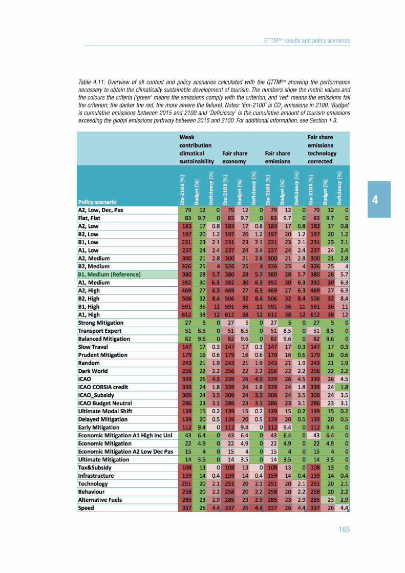
514727-L-bw-peeters514727-L-bw-peeters514727-L-bw-peeters514727-L-bw-peetersProcessed on: 20-10-2017Processed on: 20-10-2017Processed on: 20-10-2017Processed on: 20-10-2017 PDF page: 165PDF page: 165PDF page: 165PDF page: 165
165
Table 4.11: Overview of all context and policy scenarios calculated with the GTTMdyn showing the performance necessary to obtain the climatically sustainable development of tourism. The numbers show the metric values and the colours the criteria (‘green’ means the emissions comply with the criterion, and ‘red’ means the emissions fail the criterion; the darker the red, the more severe the failure). Notes: ‘Em-2100’ is CO2 emissions in 2100, ‘Budget’ is cumulative emissions between 2015 and 2100 and ‘Deficiency’ is the cumulative amount of tourism emissions exceeding the global emissions pathway between 2015 and 2100. For additional information, see Section 1.3.
4
GTTMdyn results and policy scenarios

514727-L-bw-peeters514727-L-bw-peeters514727-L-bw-peeters514727-L-bw-peetersProcessed on: 20-10-2017Processed on: 20-10-2017Processed on: 20-10-2017Processed on: 20-10-2017 PDF page: 166PDF page: 166PDF page: 166PDF page: 166

514727-L-bw-peeters514727-L-bw-peeters514727-L-bw-peeters514727-L-bw-peetersProcessed on: 20-10-2017Processed on: 20-10-2017Processed on: 20-10-2017Processed on: 20-10-2017 PDF page: 167PDF page: 167PDF page: 167PDF page: 167
Chapter 5
Discussion and conclusions

514727-L-bw-peeters514727-L-bw-peeters514727-L-bw-peeters514727-L-bw-peetersProcessed on: 20-10-2017Processed on: 20-10-2017Processed on: 20-10-2017Processed on: 20-10-2017 PDF page: 168PDF page: 168PDF page: 168PDF page: 168
168
5.1. Introduction: a decade of research
My doctoral study extended over a long period, from 2007 to 2017. A period which was rather dynamic for global climate policy: from the technically failing Kyoto Protocol (Rosen, 2015), and the political failure of the UNFCCC meeting in Copenhagen (Daniel, 2010) to the breakthrough UNFCCC meeting in Paris, 2015 (UNFCCC, 2015). In addition, within both tourism research communities and the tourism sector, awareness of the climate mitigation problem has transitioned from a negating position to one of acknowledgement (see Section 1.1). The problem is that in a business-as-usual scenario, before the end of the twenty-first century, the tourism sector would result in higher emissions than the emissions required for all of the sectors com-bined to avoid ‘dangerous climate change’, a condition exceeding a temperature rise of 2 °C. This dangerous climate change would mean that, whatever efforts all of the other sectors put into mitigating their emissions, the tourism sector on its own would still cause global emissions to exceed the CO2 emissions budget to keep the temperature anomaly below 2 °C. The objective of my study was to deepen the understanding of tourism’s contribution to climate change and to form ideas of how to mitigate this impact against the context of the global climate policy.
The research approach I adopted was a modelling study that started with an emissions inventory and delivered three Global Tourism and Transport Models (GTTM). The basic GTTMbas was a constant exponential growth model, which enabled some extrapolations through 2035. The advanced GTTMadv was programmed with system dynamics software, while still being a constant exponential growth model. It explored the future up to the year 2050. The third model, the dynamic GTTMdyn, is a system dynamics model that runs up to 2100 and is based on mechanisms for the combined tourism and tourism-transport sectors. In all of the models, tourism is defined as the sum of economic activities serving the demand of all tourists for any purpose other than to be employed by a resident entity in the country or place visited or for military pur-poses. A tourist is a visitor staying at least one night and no more than one year outside his or her normal environment. This definition means that not only holidaymakers are ‘tourists’, but travellers visiting friends and relatives (VFR) and business travellers as well. It also means that both international and domestic tour-ists are included. Furthermore, the hospitality sector, including accommodation, restaurants, and so forth, most of passenger Air transport and a significant share of high-speed rail are an integral part of the tour-ism and transport system and endogenous to the GTTM. Most Car transport and public transport including conventional rail transport are used for non-tourism purposes, so these sectors are not full subsystems in the system and the GTTM, though, of course, the tourism-related costs, revenues, emissions and transport volumes are included.
I will explain some important concepts to promote a better understanding of the following text. If you are familiar with these, my advice is to skip the remainder of this section and continue with section 5.2. A ‘policy measure’ is a single intervention in the system that represents an action by policymakers (e.g. implement-ing a ticket tax). A ‘policy strategy’ is a set of policy measures within a theme (e.g. Taxes and Subsidies). For a ‘contextual scenario’, I mean a background scenario composed of a set of economic, demographic and technological developments, but assuming business-as-usual for policies. The Reference Scenario is a special contextual scenario that describes a ‘middle-of-the-road’ contextual scenario (medium GDP/capita growth, medium population growth and moderate technological innovation). A ‘policy scenario’ describes the response of the model to a set of policy measures (a policy strategy).
Six criteria are used to evaluate policy and contextual scenarios, three of which represent the tourism
Chapter 5

514727-L-bw-peeters514727-L-bw-peeters514727-L-bw-peeters514727-L-bw-peetersProcessed on: 20-10-2017Processed on: 20-10-2017Processed on: 20-10-2017Processed on: 20-10-2017 PDF page: 169PDF page: 169PDF page: 169PDF page: 169
169
sector’s socio-economic performance and three the environmental performance. To evaluate the results of policy measures, strategies and scenarios, I defined ‘climatically sustainable development of tourism’. The metrics are CO2 emissions in 2100, and, for the period 2015 and 2100, cumulative CO2 emissions and a CO2 emissions deficiency1. Furthermore, I defined three levels of criteria for sustainability. Ranging from weak to strong, these are ‘weak contribution to climatically sustainable development’, ‘fair share emissions technology corrected’, ‘fair share emissions ‘ and ‘fair share economy’. See Section 1.3.4 for definitions of these terms.
My study made a two-fold contribution to the global tourism and climate change mitigation discussion: the first comprehensive and detailed CO2 emissions inventory and the first global tourism mitigation scenar-ios. In 2007, I developed the GTTMbas, which already roughly showed that unlimited growth in tourism is very unlikely to fit within a global scenario aiming that climate change goes beyond 2 °C temperature rise. With the GTTMbas, seventy ‘scenarios’ were evaluated by assuming different assumptions to the development of tourism volume (i.e. a shift in mode transport choice and a change in the average distance) and technology (i.e. the impact of technology on CO2 emission factors). This work revealed 69 combinations with increased CO2 emissions in 2035 and only one combination with reduced emissions compared to the CO2 emissions in 2010. As presented in Section 1.6.2, using a narrative scenario approach in the GTTMadv did generate better-performing scenarios, though with a 30-40% reduction in emissions in 2050 compared to 2005 that was still short of 70%, which was at the time of the study (2009-2010) considered a ‘sustainable’ level. With an automated backcasting method added to the GTTMadv (section 1.6.3), I developed four scenarios that reduced tourism’s 2005 CO2 emissions by 70% in 2050. The four scenarios differed only in assump-tions for the contextual scenario economic and demographic growth. Interestingly, two distinct solutions were found, depending on the contextual scenario for global economic growth and global population. The basic dichotomy was the modal split of tourism transport. Either it showed some reduction of Air transport combined with a large shift from Car transport to Other transport, or it resulted in a strong reduction of Air transport to the level of the 1970s combined with the current shares of Car and Other transport. Both the GTTMbas and GTTMadv distinguished between domestic and international tourism and some geographically dispersed regions in the world (developed and developing). The GTTMdyn fully departed from this ‘geographi-cal’ approach and assumed the global market to be divided into 60 markets based on all combinations of three transport modes and twenty distance classes.
Section 5.2 deals with the answers to the research questions, followed by a section (5.3) describing what my study has contributed to our knowledge and understanding of the tourism and transport system and its role in climate change. These sections are followed by a reflection on the results in section 5.4, including a discussion of the limitations of the study (5.4.1), technological (un)known unknowns (5.4.2), and policies (5.4.3). The thesis finishes with some research and policy recommendations and a personal reflection on the results (5.5).
1 Deficiency means the cumulative overshoot of emissions of the tourism sector compared to the Paris-Agreed emission pathway. See further 1.3.3.
5
Discussion and conclusions

514727-L-bw-peeters514727-L-bw-peeters514727-L-bw-peeters514727-L-bw-peetersProcessed on: 20-10-2017Processed on: 20-10-2017Processed on: 20-10-2017Processed on: 20-10-2017 PDF page: 170PDF page: 170PDF page: 170PDF page: 170
170
5.2. Answers to the research questions
The main operational question of my research is ‘How can the global tourism sector develop in a climatically sustainable way?’ This operational question has been translated into the following general two-part research question: ‘Which mechanisms drive the development of global tourism and its CO2 emissions, and what are the potential effects and consequences of the policy strategies to mitigate these emissions?’ Based on this general question, five detailed research questions were derived, which I will try to answer in the remainder of this section.
1. What are the main endogenous mechanisms driving the tourism system? The assumption of distance attraction forms the main endogenous driver for the increase of transport
volume and average distance per trip. I tested this phenomenon by running the GTTMdyn with all exogenous variables such as global population size, GDP/capita, equity of income, fuel efficiency, average travel speed, transport prices and investments in high-speed rail set at a constant level between 2015 and 2100 (see Section 3.5.3). This analysis revealed there was still an increase in the distance travelled and a shift in modal split for transport volume, measured as passenger kilometres, to Other (rail, public transport and coach) at the cost of air and car shares. The only way to make the GTTMdyn show stable trips between 2015 and 2100 was to assume the distance attraction factor to be zero (see Figure 3.12 in Section 3.5.3). However, the share of Other transport’s volume (pkm) still increases, though now only at the cost of car share. I did not find a satisfactory explanation for this model behaviour. The ‘distance attraction’ may be an indication that some tourists do indeed seek adventurous and ‘exotic’ distant destinations as proposed by Plog (1974). Though Plog’s model has been tested and refuted for travel behaviour, it was validated for ‘desired’ behaviour (Litvin, 2006). This validation means a potential market exists for longer travel distances, which will develop as soon as the opportunity arises, and ravel cost and time becomes within reach for more people, a development supported by the GTTMdyn.
2. What might tourism’s long-term impact be on climate change? Based on the broad range of contextual scenarios run with the GTTMdyn, an initial conclusion is that
tourism’s contribution to CO2 emissions and climate change is very likely to increase for the remainder of the twenty-first century. I base this conclusion on the result that none of the contextual scenarios, which cover wide-ranging combinations of economic and population growth together with business-as-usual technology-driven efficiency improvements, show a reduction in emissions between 2015 and 2100. Figure 3.5 (see Section 3.4.2) shows that, out of twelve contextual scenarios, only three scenarios show some decline in emissions in the last decades of the twenty-first century, but all end with higher emissions in 2100 than in 2015. All other contextual scenarios show a continuous increase in emissions.
A second conclusion is that tourism will most likely develop in a climatically unsustainable way. This is shown in Table 4.2, in which only the A2 lowest economic growth, low population growth, decreasing income equity and Paris Aspiration (inducing high carbon cost) contextual scenario shows a ‘weak contribution to climatically sustainable development’.
Chapter 5

514727-L-bw-peeters514727-L-bw-peeters514727-L-bw-peeters514727-L-bw-peetersProcessed on: 20-10-2017Processed on: 20-10-2017Processed on: 20-10-2017Processed on: 20-10-2017 PDF page: 171PDF page: 171PDF page: 171PDF page: 171
171
3. Which exogenous developments drive tourism’s long-term impact on climate change? The main exogenous drivers of tourism growth include GDP/capita, population growth and equity
of income. Trips/capita is assumed a linear, continuously increasing function of GDP/capita, up to a certain level of GDP/capita, after which the number of trips is kept constant. Therefore, economic growth directly drives the number of tourist trips but in a non-linear way, also depending on income distribution. Also, not surprisingly, the total number of trips is exactly proportional to the size of the global population, all other variables being equal. More surprising was the strength of the third main driver: equity of income (see Figure 3.6 in Section 3.4.2 for the results for CO2 emissions). The GTTMdyn shows that increasing equity, all other parameters constant, causes an increase in emissions that, for low equity, is more than proportional, but develops approximately proportionally at the higher end of the equity scale. The improving fuel efficiency of cars will directly cause increased growth because of lower fuel costs. This effect is not accounted for in the Air and Other transport ticket prices because these are market driven, rather than being cost driven. A feedback loop between travel speed and modal shift toward faster modes will enforce any exogenous parameter-driven shifts to higher speed modes (air, high-speed rail). Also, an increase in distances for Air transport will reduce the per pkm ticket price and increase average speed due to the greater share of high-speed cruising in long flights, both combined with the value of distance stimulating to travel longer distances. Another exogenous driver for tourism transport growth2 is the historical continuous reduction of transport prices in business-as-usual scenarios. Though a small part of this may be caused by the continually improving fuel efficiency of Air transport, there are many other factors at work. These are the increased seat densities, higher aircraft productivity, continuously increasing speed, accelerated by the introduction of the jet aircraft in the 1960s, and improved maintenance, which increases the flight hours per year, reducing cost. Furthermore, the more recent widespread introduction of low-cost carriers has vastly reduced ticket prices, again shifting modes from slow and relatively expensive surface-based transport modes to fast and relatively cheap Air transport. For the future, after 2015, most of these developments are assumed to slow down.
4. Which policies (or combinations thereof) will be able to attain the climatically sustainable development of tourism?
The most climatically sustainable policy scenario was ‘Ultimate Mitigation’, which assumes all measures set at their maximum CO2 emissions saving levels. However, this scenario suffers from a more than 40% loss of revenues in 2100 compared to the Reference Scenario. Therefore, I developed a better balanced policy scenario - the ‘Economic Mitigation’ - which reduced some of the most severe measures with only small losses for the emission mitigation potential. The Economic Mitigation policy scenario obtained the same tourism sector revenues as the Reference Scenario. This scenario’s main measures included technology (fuel or emissions efficiency) improved to the maximum assumed possible, biofuels subsidised up to 90%, Air transport taxed by 200% on the
2 Not for tourism volume growth in terms of trips because, in the GTTMdyn, the number of trips is directly and exclusively governed by GDP/capita and independent of the cost of a trip. This is reasonable because GDP/capita is a relatively strong proxy for lifestyle, while the cost of travel varies over several orders of magnitude, providing people with many opportunities to save on cost in case, for instance, taxes would increase the cost of travel.
5
Discussion and conclusions

514727-L-bw-peeters514727-L-bw-peeters514727-L-bw-peeters514727-L-bw-peetersProcessed on: 20-10-2017Processed on: 20-10-2017Processed on: 20-10-2017Processed on: 20-10-2017 PDF page: 172PDF page: 172PDF page: 172PDF page: 172
172
ticket price and a moderate carbon tax rising from $90/ton CO2 (1990 USD) in 2015 to $450/ton CO2 in 2100, applied to all transport modes and accommodation. Furthermore, some behavioural change was assumed (50% less attraction of distance, 5% less inclination to travel and a slower reduction in the length of stay). The latter assumptions help to reduce transport distances, while still improving revenues from accommodation through a longer stay for each trip. Though the two most effective policy strategies are tax policies and infrastructural measures, it is imperative to combine these with technology, biofuels and a regulatory restriction on Air transport growth (in my study, I assumed a reduced global airport slot capacity, but other options could be explored as well). Though the individual policy strategies did not provide climatically sustainable tourism development, combining different policy strategies did enable some policy scenarios to achieve a climatically sustainable development of tourism.
5. What are the main consequences of policies achieving a climatically sustainable development of the tourism sector?
The main differences between the ‘Economic Mitigation’ policy scenario and the Reference Scenario are a strong shift from Air transport to Other transport modes (high speed and conventional) and a strong shift from the long distance markets to medium and short distance ones causing a significantly lower average distance per trip. Air transport will see reduced volumes (with 22% trips and 24% distances) compared to 2015, which means that in 2100 access to Air transport - network and frequencies - will be comparable to that in the 2000s. Air transport will become very expensive due to three effects: the carbon tax, a 200% ticket tax and the effect of the slot capacity restriction on the ticket price. Overall, the price will be almost six times higher (per passenger kilometre) than in 2015 and as much as nine times the cost in 2100, compared to the Reference Scenario. Of course, this higher price will hinder access to Air transport for less wealthy people, but tourism will still be accessible by most people through Car and Other transport modes.
5.3. The study’s contributions to theory, methods and modelling
This section lists my main contributions to theory, methods and modelling. The following new theoretical assumptions and theory are applied:
not by the attractiveness of destinations, cost of travel and the availability of specific transport infrastructure, which all only determine the distribution of trips over tourism markets, but not the total number of trips;
destinations;
theory for transport (integrated monetary and time-cost based) with the non-linearities of prospect theory’s ‘psychological values’. This integration includes the idea that the prospect-theory-based ‘reference value’ of cost is not only based on the ‘personal’ transport mode (for instance, for air
Chapter 5

514727-L-bw-peeters514727-L-bw-peeters514727-L-bw-peeters514727-L-bw-peetersProcessed on: 20-10-2017Processed on: 20-10-2017Processed on: 20-10-2017Processed on: 20-10-2017 PDF page: 173PDF page: 173PDF page: 173PDF page: 173
173
travellers based on the cost and travel time averages of air travel); and
by transport geographers.
The following are innovative methods developed for the GTTMdyn:
(Rohde, 2009), a ‘reverse’ equation has been derived that provides the share of the population above a certain threshold income level for a given average income. This reverse equation is used to determine the share of potential adopters of the global population per transport mode and distance class in the Bass models;
theory. Specifically the novel time decay idea is applied to fill in the initial trip distribution over distance classes;
a method to divide the global tourism market, including the major share of domestic tourism trips, into 60 market combinations of transport mode and distance class. This approach allowed me to avoid the serious biases existing in contemporary tourism studies about the role of Air transport (overestimated), international tourism (overestimated), public transport and Car transport (both underestimated and the first one often ignored) and domestic tourism (often ignored);a method to allow the introduction of a new product, i.e. transport mode, by applying ‘Bass models’ for adoption and the diffusion of the product; the only user assumption is the year of the introduction on the market;a behavioural model based on causal relationships rather than the more common statistical relationships assumed in many econometric models, thus enabling very large changes in travel time and monetary costs of travel;
2 emissions in the year 2005;a database with a century of historical data for the main variables describing tourism, tourism transport, its cost and travel-time parameters and its impacts on CO2 emissions; and
contemporary method like a constant reduction of fuel consumption per year, but also takes into account that the rate itself slowly diminishes over time (Peeters & Middel, 2007). This submodel almost perfectly matches the historical data, while constant rate-of-change models show either a very poor fit to the data or require re-setting the rate of change of efficiency at several points in history, which are exogenous to the models (and often rather arbitrary).
Regarding modelling, the GTTMdyn stands apart because, at least within tourism modelling, it:
calibrated for a 105-year period (1900-2005) of historical data;
5
Discussion and conclusions

514727-L-bw-peeters514727-L-bw-peeters514727-L-bw-peeters514727-L-bw-peetersProcessed on: 20-10-2017Processed on: 20-10-2017Processed on: 20-10-2017Processed on: 20-10-2017 PDF page: 174PDF page: 174PDF page: 174PDF page: 174
174
portion of the model) and, for instance, future space travel;
improvements in emission factors;
an important input for calculating the emission factor of air travel; and
or investments in high-speed rail and airport infrastructure.
5.4. Reflection on the results
5.4.1 Limitations to the studyThe results of my study run into several limitations. In Section 3.7.3, I explored the consequences of model-ling choices for trip generation, global market structure, restriction of the model’s scope to overnight visitors and simplifications in the emissions model being the most important with respect to tourism and transport volume development and impact on emissions. Other restrictions originate from the theoretical, data and scenario knowledge gaps identified in Section 1.4. Finally, the GTTMdyn is not an economic model; therefore, the data it generates on economic impacts may be relatively crude. In this section, I will explore the model’s limitations, which are mainly caused by theoretical gaps, the data gap limitations and the limitations caused by the (lack of) economic modelling.
Model limitationsMost of the model’s limitations were caused by gaps in the theoretical knowledge. A practical and suitable theory of global tourism trip generation was not available. Based on only two sources, one global and one for the Netherlands, a linear relationship between trips/capita/year and GDP/capita has been assumed in-cluding a certain maximum number of trips/capita/year. The slope of this linear equation was almost equal for the two sources that provide one. The maximum number of trip/capita/year was measured for the Dutch population. The assumption that the total number of tourist trips was a simple and fixed function of GDP/capita - and thus income distribution - means that the quality and cost of destinations and tourism transport did not affect the global tourism economy. This may very well be true for a large range of those qualities, but the GTTMdyn obviously will be unable to represent the case of almost no tourism transport or a very low quality of tourist destinations being provided, limiting the ability of the model to assess extreme sector-restricting policy measures.
The idea to create sixty transport mode/distance class markets to describe tourism deprived the GTT-Mdyn of the ability to provide insights into the geographical and motivational distribution of tourism and whether it is domestic or international. For the CO2 emissions and overall volumes of tourism and transport, this was not essential, but it did cause some issues for the link with contemporary tourism research. On the one hand, this non-geographical approach prevented the study from directly assessing, for instance, the impact of the Economic Mitigation scenario on developed and developing countries. On the other hand, parts of the studies for this thesis helped to assess such issues (e.g. Peeters & Eijgelaar, 2014).
Several simplifying assumptions were made for the emissions model. The results of the GTTMdyn for avi-ation emissions, the main source of emissions, paired relatively well with the extrapolations and scenarios
Chapter 5

514727-L-bw-peeters514727-L-bw-peeters514727-L-bw-peeters514727-L-bw-peetersProcessed on: 20-10-2017Processed on: 20-10-2017Processed on: 20-10-2017Processed on: 20-10-2017 PDF page: 175PDF page: 175PDF page: 175PDF page: 175
175
published by other scholars. The main restrictions of the GTTMdyn regarding emissions were the technology policies that, for Car transport and Other transport and accommodation, assumed rather arbitrarily chosen exponential improvements in fuel efficiency and shifts toward the use of electricity. Though the prospects for electrification and decarbonising buildings and both Car transport and Other transport are considered relatively good, the maximum policies assumed in the GTTMdyn scenarios for the Ultimate and Economic Mitigation policy scenarios may have been a bit too optimistic. For the long time horizon (85 years), this may have mainly affected the CO2 budget for tourism, but it had a far lesser impact on the final emissions in 2100, because the rates do more affect the year in the future these elements of tourism become zero emis-sions, rather than the final emissions in 2100. The assumptions for Air transport, causing the main share of emissions, were better founded in scientific knowledge.
Data limitationsSystematic counts for the global volume of tourism exist for international arrivals since the 1950s and an-nually published by UNWTO (e.g. UNWTO, 2008a). For several years, portions of the counts for domestic tourism arrivals were also published, but these were always covering a minority of countries with many years even missing completely. Domestic tourism always has made up the largest share of tourism, though it has gradually declined to its approximately 80% share in 2005. The GTTMdyn coefficients were calibrated based on the limited data for global tourism trips between 1900 and 2005. By applying the GDP/capita trips equation and some other methods to fill these data gaps, the historical data from 1900 to 2005 were sur-rounded in uncertainty. However, the overall picture seems unlikely to be way off. For instance, it is unlikely that tourism was a mass phenomenon at the beginning of the twentieth century, but it is still certain tourism did exist and most was domestic. The first large seaside resorts did develop at the end of the nineteenth century (Walton, 2009). The 2005 data point is far more accurate. The shape of the development, more or less exponential growth, is considered not uncommon for consumption goods over the past century (e.g. Grübler, 1990). Such curves hold as long no substitution has entered the market, which, for ‘tourism arrivals’ has not been the case.
A more severe issue was the lack of data about transport modes used in tourism, and the distances tourists travelled. However, again, it was not likely that the data I used for calibration were significantly wrong because they were also verified against reasonable travel speeds and times. Once more, the calibra-tion year, 2005, was better covered by empirics, so the uncertainty centred more on the coefficients govern-ing the model dynamics than on the absolute values in 2005 the beginning of the projections in the GTTMdyn. The initial (1900-1950) emission data were also based on little and often anecdotal information. For exam-ple, the fuel efficiency of the car in 1910 was entirely based on one reference that mentioned mileage per gallon for the iconic T-Ford. However, these historical emissions did play almost no role in the calibration of the behavioural model, which is governed by a mix of cumulative errors and the 2005 reference point. . At the same time, the future emissions, at least for Air transport, were comparable with projections published by other researchers, based on other models.
Economics The GTTMdyn is not an economic model, but a behavioural model. Most prices are exogenous, excepting some feedbacks that delivered additional price rises in case of constraints for aircraft fleet and airport slot capacity. Still, it does provide simple cost and revenue calculations, but it ignores discount rates. It also
5
Discussion and conclusions

514727-L-bw-peeters514727-L-bw-peeters514727-L-bw-peeters514727-L-bw-peetersProcessed on: 20-10-2017Processed on: 20-10-2017Processed on: 20-10-2017Processed on: 20-10-2017 PDF page: 176PDF page: 176PDF page: 176PDF page: 176
176
does not look at maximising the present values of investments or other common economic variables. It has the disadvantage of being disconnected from economic studies and is likely missing some (second-order) economic effects connected with, for instance, returns on investments. This disconnectedness means that losses or profits are not part of the model and collapses of entire subsectors of tourism cannot occur within the GTTMdyn. So, in case airport slot capacity is restricted, the possibility that the entire Air transport sector collapses is not a possible outcome of the model. The effect of this on the conclusions is likely not very large, because in the climatically sustainable scenarios, where collapse might be imminent, the share of Air transport is low anyway compared to the Reference Scenario. Furthermore, there is another mechanism that may preserve the aviation sector from global bankruptcy. GTTMdyn includes the effect of airport capacity con-straints on ticket prices. In slot-constrained scenarios, these will increase from $0.04/pkm to $0.10/pkm. This price increase would lend some resilience to the aviation industry to be able to cope with the loss of growth and sunk cost of investments in new aircraft programmes and over-capacity of the fleet. The impact of these higher prices may even help to improve the profitability of the remaining airports and airlines. At the same time, for the aircraft manufacturers the cancellation of many of the aircraft now on order with aircraft manufacturers may produce adverse effects like over-production, slack prices and the need to lay-off many employees in a short time. Figure 5.1 shows that in the Economic Mitigation scenario, aviation will maintain its overall revenues more or less at the level of 2015. But growth will now benefit other parts of the tourism sector and is divided over Car transport, Other transport and accommodation, which all grow faster than in the Reference Scenario.
Figure 5.1: Annual revenues from tourism in the Reference Scenario (left pane) and the Economic Mitigation policy scenario (right pane).
Another approach is that the GTTMdyn ignores discount rates as it does not have a model element to cal-culate returns on investments, discounted revenues or savings or net-present-value calculations. It simply shows the taxes, subsidies, investments, costs and revenues for each year in a constant currency unit (1990 USD). This assumption ignores the discount rate or, more precise, assumes it to be zero, more or less fol-lowing Stern (2006), who proposes that discounting for long-term - intergenerational - policy-supporting scenario studies should be set low or at zero. One reason for discounting costs and damages in the future is the assumption that income will always be higher in the future, and consequently, a given amount of costs and damages will be felt less (Hourcade et al., 2009). This reduced valuation of a given amount of money would mean that costs taken now to save damages in the future will show less economic efficiency, because the saved damages in the future are valued less (Chancel & Piketty, 2015), causing inequality
Chapter 5

514727-L-bw-peeters514727-L-bw-peeters514727-L-bw-peeters514727-L-bw-peetersProcessed on: 20-10-2017Processed on: 20-10-2017Processed on: 20-10-2017Processed on: 20-10-2017 PDF page: 177PDF page: 177PDF page: 177PDF page: 177
177
between current and future generations. Another reason to apply discounting is that consumers appreci-ate current costs more than they do future costs, and thus will lend greater weight to current costs than to future costs when making decisions (e.g. Schäfer & Jacoby, 2006). This weighing, of course, is important in models that describe consumer behaviour in response to measures, like my PV and Bass models do. But such discounts are ‘perceived costs’, not the real costs felt by future generations. The behavioural model of GTTMdyn‘ is calibrated on the basis of revealed collective behaviour, and thus it implicitly does include utility discount rates. But in my opinion, it would be wrong to discount future costs and benefits (like the abate-ment costs and tourism revenues) based solely on such perceived values of current consumers because the real (undiscounted) costs that are felt by consumers in the future by then will, of course, be ‘current’ (e.g. supported to some extent by Dasgupta, 2008). In other words, to base a long-term policy decision, like investing in infrastructure, on current perceived consumer costs would rather distort the view on the long-term future and the costs perceived by the people living in said future.
5.4.2 Technology: the (un)known unknowns
IntroductionWhen I present the results of my study, invariably the audience raises the issue of technological solutions that they feel have been wrongfully neglected. These technologies are seen as a kind of ‘silver bullet’ solving all problems at once. The most commonly mentioned technologies include power-to-liquid fuels (Schmidt & Weindorf, 2016), electric flight (The Economist, 2015), solar flight (Wise, 2015), the Hyperloop (Spacex, 2017) and space travel (Walter, 2010). None of these technologies is part of the GTTMdyn, though, with vary-ing degrees of effort, it is possible to add most of these options to the GTTMdyn. I will discuss some of these options and explain why they cannot be part of the solution to the climatically unsustainable development of tourism. More generally, the aviation discussion suffers from a discourse of technology optimism, which is an “enduring but flawed promise of sustainable aviation” that “may result in inaction that continues to delay much-needed progress in climate policy for aviation” (Peeters et al., 2016, p. 30). In other words, hoping for technological solutions will delay volume and growth-related policies, which are inevitable as shown by my study if the Paris Agreed emission path is taken as goal. In addition, while many of the proposed technolo-gies do improve aircraft fuel efficiency, they do so slowly and evolutionarily, which is already part of the pro-jected improvements that have also been assumed in the GTTMdyn (see Section 2.3.5). Examples are laminar flow (a way to significantly reduce aerodynamic skin friction drag forces acting on flying aircraft, which has first been proposed in the 1920s and since then applied initially on glider aircraft and more recently also on airliners), carbon fibres (material to reduce the weight of aircraft increasingly applied since the 1960s), and high bypass engines (implemented first time in the 1970s as a way to improve engine efficiency and reduce engine noise). All of these technologies continue to improve the fuel efficiency of (jet) aircraft. Therefore, they are all part of the business-as-usual development in aviation. In the following sections, I discuss five of the proposed silver bullet technologies: electric flight, solar flight, power-to-liquid alternative fuels, the Hyperloop and space tourism.
Electric flightAirbus is experimenting with a small electric aircraft that can now fly approximately less than 20 minutes on its battery power, including taxiing, take-off, climbing, cruising, descending and landing (Tegler, 2016).
5
Discussion and conclusions

514727-L-bw-peeters514727-L-bw-peeters514727-L-bw-peeters514727-L-bw-peetersProcessed on: 20-10-2017Processed on: 20-10-2017Processed on: 20-10-2017Processed on: 20-10-2017 PDF page: 178PDF page: 178PDF page: 178PDF page: 178
178
The aircraft is 350 kg (45%) heavier than the same type of aircraft with a piston engine, mainly due to the battery weight. Some experts (Evation, 2017) believe a nine-seat aircraft flying stretches of up to 965 km could be viable by 2030. Some sources claim that current battery densities should increase by at least a factor of ten, which in itself would take nearly 30 years if the rule of thumb holds (Moore, 2014)3. However, Moore (2014) also observes that there are several significant advantages to integrating electric propulsion into a wing. Furthermore, electric engines have an energy efficiency of almost 100%, while current turbo-fans only achieve 35% (Torenbeek, 2013) and turboprops might achieve 40%. These improvements would require batteries to improve their kWhr/kg performance by a factor of four at least. At the recent rate of 8% per year improvement, this would still take more than fifteen years. As soon as the battery is available, the clean-sheet design of the electric airliner, initially most likely for the smaller short-haul aircraft, will be a major challenge as almost every major part of the aircraft will need to be changed or newly developed. This also includes current aircraft safety regulations like FAR 25 (US) and CS-25 (EU). Such a challenging clean-sheet design will take between fifteen and twenty years to mature to its first delivery, which would bring us to the second half of the twenty-first century. The Delayed Mitigation policy scenario shows that this will be too late to make climatically sustainable tourism possible. The National Academies of Sciences Engineering and Medicine (2016) consider a hybrid form of turbo-electric propulsion to have some prob-ability to become operational for single-aisle airliners (relatively small and short-haul) within a time frame of 30 years. Although such a hybrid approach may lay the foundation for electric flight, the downside is that CO2 emissions per passenger kilometre will be reduced by about 20-30%, which is insufficient to make Air transport climatically sustainable.
Solar flightSolar flight, however, is a different matter. My own bachelor’s thesis was an attempt to design solar-pow-ered aircraft (Peeters, 1980). For this thesis, I first designed a solar plane that could fly on its solar power for two hours with a single pilot during a sunny summer’s day in the Netherlands. Of course, the aircraft could extend its flight using thermals. My second design was for an ultra-light aircraft with a range of up to 657 km at 51° north latitude on a sunny summer day and only carrying the pilot. The third design involved an aircraft for scientific exploration of the ozone layer - a hot topic in the 1980s - that could potentially carry 2.5 kg of equipment continuously by slowly climbing during the day and slowly descending during the night. A 27.5 kg battery was installed to help overcome the nights. Such aircraft are still under study, albeit at a much smaller scale, but they are not operational (Noth, 2008). The main issues with solar flight are the low energy density (kW/m2) of solar radiation, combined with the problem of sunless periods during the day and even the year. A Fokker-50 turboprop airliner has a wing area of 70 m2, a total engine power of 3,728 kW, which translates to a power loading during cruise flight (my guess is at about 70% of maximum power) of 37 kW/m2. The sun delivers a maximum of 1 kW/hr, assuming 100% solar cell efficiency. Currently, solar cells reach some 20-25% energy efficiency (Cheng, Pascoe, Huang, & Peng, 2016; IPCC, 2011). Therefore, even midday on a sunny day in summer, the energy density of the sun fails by a factor of 150 for this size of a Fokker-50 aircraft. Modern jets have even higher wing-loadings and thus power loadings. Solar cells that are 100% efficient - a theoretical impossibility - may reduce the gap to a factor of 40, but this is still in-
3 This Moore is not of Moore’s law which states that every eighteen months, the CPU calculation speed and data storage capacity will double (Fettweis & Zimmermann, 2008).
Chapter 5

514727-L-bw-peeters514727-L-bw-peeters514727-L-bw-peeters514727-L-bw-peetersProcessed on: 20-10-2017Processed on: 20-10-2017Processed on: 20-10-2017Processed on: 20-10-2017 PDF page: 179PDF page: 179PDF page: 179PDF page: 179
179
surmountable. Solar flight that directly captures the sun’s energy on the aircraft’s wings and that maintains a mass transport system with speeds significantly higher than those for conventional rail and the comfort that is currently offered by airlines is physically impossible. Of course, the Solar Impulse, a one-seat aircraft with a wingspan exceeding that of the Boeing B747-4000 ‘jumbo jet’ did recently manage to fly around the world in over 23 days of flying (550 flight hours). However, its creators acknowledged that ‘‘solar planes will never replace fuel-powered commercial flights” (Peeters et al., 2016, p. 37).
Power-to-liquid alternative fuelsAnother technology often mentioned is producing kerosene by power-to-liquid (PtL Schmidt & Weindorf, 2016). The basic idea is to use sustainable energy sources like wind, solar and hydro to create liquid fuels directly from CO2 in the atmosphere (Schmidt & Weindorf, 2016). The yield per hectare (for solar or wind power) would be about 19,750 kg/ha, compared to 16,440 kg/ha for algae-based biofuels. An advantage of solar energy is the assumption that approximately 33% of land with solar cells is fully occupied, while for wind energy, only 3% of the land is directly covered access roads and the foundations of the wind turbines. So, PtL would be three to thirty times as land-efficient as the best performing biofuel known, assuming the non-directly occupied space is effectually used for other purposes. The cost is estimated at $1.6 per kg compared to $0.8 for kerosene, both estimates for 2050 (Schmidt & Weindorf, 2016). The CO2 lifecycle emis-sions per MJ will be in the range of 11-28 kg CO2/MJ, compared to 87 kg CO2/MJ for kerosene and some 25-35 CO2/MJ for many biofuels. Assuming a 50% subsidy, sustainable global land-use and a mix of 50% solar and wind energy to calculate land-use, the effect on emissions potentially is strong as shown in Figure 5.2. The technology is at a readiness level of between 5 and 8 (technology validated in an industrial setting to be system complete and qualified), though a plant in Iceland did produce five million litres of methanol in 2015 (Schmidt & Weindorf, 2016). Technology to convert methanol to kerosene does exist. However, the non-zero emissions of PtL still limit its capacity to act as the ‘silver bullet’ that will solve the mitigation is-sues for the sector, but it may help to relax the airport slot restriction, allowing more flights in the long-term future than is the case in the Economic Mitigation scenario. Another issue is whether we really can find the very large areas where wind and solar power integrate for 100% with other land-uses, without compromis-ing these uses. Or in other words: is there enough solar and wind power left to power aviation entirely on PtL technology? The answer requires an additional study.
5
Discussion and conclusions

514727-L-bw-peeters514727-L-bw-peeters514727-L-bw-peeters514727-L-bw-peetersProcessed on: 20-10-2017Processed on: 20-10-2017Processed on: 20-10-2017Processed on: 20-10-2017 PDF page: 180PDF page: 180PDF page: 180PDF page: 180
180
Figure 5.2: The effect of the power-to-liquid technology based on the data provided by (Schmidt & Weindorf, 2016). The emissions are annual CO2 emissions. The grey line denoted with an * shows the emissions in the Reference Scenario.
HyperloopAnother frequently mentioned idea is the Hyperloop (Spacex, 2017). The idea is to build very long tubes that are near vacuum and ‘shoot’ 28-seat ‘pods’ through them at high speeds and virtually no aerodynamic drag. The system is specifically designed for distances up to 1,500 km, as the authors of the study believe that supersonic flight will cover longer distances in the future. KiM (2016) assessed the technology and concluded it to be far too weakly founded to become a game-changer in long-distance transport, if at all possible. Also there are serious flaws with respect to transport capacity (van Goeverden, Milakis, & Janic, 2017). However, even if it were possible, this solution also suffers from the very long lead times to design the technology, build the hundreds of thousands of kilometres of tubes and to take over aviation. Moreover, so far no reliable data has been published about the energy efficiency of this system, specifically the energy necessary to maintain the tubes’ vacuum, which very likely is high.
Space tourismSpace travel is proposed as a new type of excursion (Duval & Hall, 2015) and a novel way to travel from A to B (Walter, 2010). The energy required for space travel differs greatly from air travel. Where for Air transport, every additional kilometre will add to the energy use, for space travel, after lift-off and the climb into orbit, no further energy is required except, depending on the type of spacecraft, during landing for the braking speed. However, the energy for launch and getting into orbit can be considerable. The energy required to launch the reusable Space Shuttle was 45,360 GJ for lifting a maximum of nine passengers (space limited) or 25 tons of payload (weight limited) into orbit (how-green-is, 2017). Although 25 tons is equivalent to some 170 pas-sengers, including furniture, passenger equipment and luggage based on data given by Torenbeek (1982), the Space Shuttle was about the same size as a 100-seat DC-9, but with a pressurised cabin that occupied a much smaller share of the fuselage than in a normal aircraft. So potentially 50 to 100 passengers could be accommodated in a design dedicated to transportation. A flight from London (UK) to Perth (Australia) will create about two tons of CO2 emissions, which would translate to 28 GJ using the kerosene emission factor
Chapter 5

514727-L-bw-peeters514727-L-bw-peeters514727-L-bw-peeters514727-L-bw-peetersProcessed on: 20-10-2017Processed on: 20-10-2017Processed on: 20-10-2017Processed on: 20-10-2017 PDF page: 181PDF page: 181PDF page: 181PDF page: 181
181
provided by Zijlema (2009). On a per passenger-flight basis, the Space Shuttle would need about 30 times the amount of energy that a modern aircraft requires for a single flight. I do not see how newer spacecraft technology could compensate these almost two orders of magnitude higher energy levels. However, even if these higher energy levels somehow could be compensated, another issue to emerge is the prospect of a three-hour transfer from London to Sydney, which would make even day returns feasible. Such an increase in speed by a factor of five to six may give strong incentives for additional growth in the tourism transport volume and, by extension, emissions. Overall, it is concluded that the idea of space travel would amplify tourism’s climatically sustainability issues.
5.4.3 PoliciesWhy would tourism, as a sector, take measures to mitigate its CO2 emissions? Scott (2011) argues that “how tourism responds to climate change is absolutely critical to the sustainability of tourism and should the sector retreat from climate change engagement, it would be to its substantial detriment.” One reason to engage in mitigation could be the real threats to many elements of tourism that unmitigated climate change poses (Scott, Gössling, & Hall, 2012a). These impacts comprise “temporal and geographic shifts in tourism demand” and “environmental change and destination competitiveness within three major market segments (winter sports tourism, coastal tourism and nature-based tourism)” (Scott et al., 2012a, p. 213). So far, these climate threats to tourism have not given rise to strong tourism mitigation policy. The tourism sector, and certainly the aviation part of it, assumes that others will solve the problem as shown by the CORSIA compensation scheme developed by ICAO. However, simply expecting other sectors to solve the mitigation issue poses risks to the sector. The first reason to take action is that global mitigation, if following the 2015 Paris Agreement would, based on the GTTMdyn calculations, potentially increase costs for tourists by about 10-15% due to (carbon) taxes and abatement cost and damage growth of the sector. The second reason for strong mitigation is the fact that the impacts on nature, economic growth, health, and international tensions of unmitigated climate change may severely impact tourism. Current popular destinations such as the Mediterranean may simply become too dry and hot for tourism (Nicholls & Amelung, 2008), winter sports may sharply decline (Agrawala, 2007) or ecosystems could be destroyed, which are one of the most important resources for nature-based tourism (Scott et al., 2012a). The third reason to engage in and sup-port strong mitigation policies within the tourism sector is the moral duty to do so. As clearly shown by this thesis, failing to mitigate tourism’s - specifically aviation’s - emissions will render the global Paris-Agreed target of 2 °C unattainable. Enterprises in tourism highly value actions taken for the environment, viewing these actions as the “morally the right thing to do” (Coles, Zschiegner, & Dinan, 2012, p. 15). As shown in this thesis, the success of mitigating climate change ultimately lies in the hands of the tourism sector. This knowledge should pose a strong moral imperative.
However, why is the tourism sector not taking powerful actions and, indeed, is often lobbying not to take action when it comes to most of the policy measures suggested in my Economic Mitigation policy scenario? Most likely this has to do with being afraid of the uncertainty imposed by strong mitigation (van den Bergh, 2017) and probably conflicting stakeholder interests within the sector, as was shown to be an issue for coastal management (Nursey-Bray et al., 2013). In tourism, the aviation sector has a strong self-interest to avoid the discussion about effective mitigation as that could result in lower volume growth or even volume decline. On the other hand, the rail sector would have much to gain from a strong mitigation policy for tour-ism. The tourism sector itself (the enterprises in hospitality and travel services) would remain indifferent so
5
Discussion and conclusions
514727-L-bw-peeters514727-L-bw-peeters514727-L-bw-peeters514727-L-bw-peetersProcessed on: 20-10-2017Processed on: 20-10-2017Processed on: 20-10-2017Processed on: 20-10-2017 PDF page: 182PDF page: 182PDF page: 182PDF page: 182
182
long as the volume of arrivals is not reduced. Unfortunately, the voices of those suffering from mitigation policies like the aviation sector seem much louder than the voices of those who would benefit.
An obvious sector to initiate a determined action is the hospitality sector (e.g. accommodation, restau-rants). The tourism sector bears total responsibility for hospitality and its emissions. Furthermore, the hospi-tality sector is lagging behind compared to housing and utility buildings (Melissen, 2013), where proven zero emissions technology is available (e.g. Mohamed, Hasan, & Sirén, 2014), thus providing ample opportunity to improve the environmental performance. The next sectors that would benefit enormously from a strong tourism mitigation policy is the rail sector, both conventional and high-speed. Unfortunately, the tourism and rail sectors have lost interest in each other (Rehman Khan, Qianli, SongBo, Zaman, & Zhang, 2017). In light of the strong modal shift required in the climatically sustainable policy scenarios presented in this study, rail and tourism regaining interest in each other would provide a significant opportunity to combine mitiga-tion with economic growth (compare Delaplace, Bazin, Pagliara, & Sposaro, 2014). Additionally, Lumsdon and Page (2004) propose that rail travel can be a positive experience for tourists, an advantage above Air transport or Car transport. The Chinese understand the vital link between rail and tourism (Chen & Haynes, 2015) and, in a very short time span, they have created an extensive and well-used high-speed rail network (Ollivier et al., 2014).
The most ‘exotic’ and toughest policy to implement in the Economic Mitigation policy scenario is the reduction of airport slot capacity or any equivalent air travel capacity constraint. The idea of volume restric-tions is not entirely new. For instance, in many cases, noise regulations restrict airport growth (Graham & Guyer, 1999). In other sectors, production-capacity constraining regulations for environmental reasons can be found in livestock (Cardwell, 1997) and fisheries (Pauly et al., 2002). Some lessons may be learned from these experiences.
The travel services sector, like tour operators and travel agencies, may have a key solution within their power: ‘carbon management’ (CSTT, 2016). A Dutch tour operator, Sawadee, tried to implement this by making detailed calculations of its carbon footprints for all of its travel products. These were then used to assess the development of their product portfolio with an eye to reducing the CO2 emissions per product and changing the product portfolio to include products that were more eco-efficient. Because the eco-efficiency of different travel products varies by an order of magnitude (Gössling et al., 2005), the sector certainly has many opportunities to improve its average, without any economic damage. However, tour operators and travel agencies often calculate carbon footprints just for the purpose of informing the traveller (Gössling & Buckley, 2014) or to sell carbon offsets (Eijgelaar, 2011). The above brings the discussion to the last large stakeholder, the tourist. Unfortunately, there is an overwhelming amount of research showing that tourists do not change behaviour without strong changes in supply (Alcock et al., 2017; Cohen, Higham, Peeters, & Gössling, 2014b; Font & Hindley, 2016).
5.5. Reflection on tourism and sustainable development
5.5.1 Climatically sustainable tourismThe question as to whether tourism is developing in a climatically sustainable direction can be answered with a firm ‘no’ based on the analyses from the GTTM modelling suite. None of the contextual scenarios
Chapter 5

514727-L-bw-peeters514727-L-bw-peeters514727-L-bw-peeters514727-L-bw-peetersProcessed on: 20-10-2017Processed on: 20-10-2017Processed on: 20-10-2017Processed on: 20-10-2017 PDF page: 183PDF page: 183PDF page: 183PDF page: 183
183
complies with the three criteria for sustainability. This finding means that tourism will preclude reaching the Paris-Agreed goal of keeping global temperature below 2 °C (UNFCCC, 2015). Current international poli-cies only pertain to international Air transport and provide marginal reductions of emissions. The ‘Economic Mitigation policy scenario’ suggested in this thesis can be considered as coming close to attaining climati-cally sustainable tourism development, but only when the tourism sector is allowed to take a, compared to all other sectors combined, relatively large share of the total CO2 budget available under the 2015 Paris Agreement.
The impacts of ‘dangerous’ climate change, i.e. an average global temperature rise of over 2 °C, are potentially severe and could destroy communities, lead to a large-scale loss of life, cause increased health risks and damage ecosystems and economies (IPCC, 2014a, 2014b; Lehmann, Coumou, & Frieler, 2015; Moore & Diaz, 2015). The above issues contrast with a sentiment among proponents of the tourism sector that posit that “tourism, if appropriately planned and managed, is fundamentally a good thing” (Sharpley, 2015, p. 195). Note that the above statement is based on industry discourses, not necessarily the personal view of Sharpley. Such claims about the ‘fundamental good’ of tourism centre around two themes. The first is tourism’s role in alleviating poverty, as “there is no other industry that can have such a universal impact on economic development and the escape from poverty” (Lipman et al., 2012, p. L180). The second theme is nature conservation, because “ecotourism should be recognised as a specific green growth element and an important beacon for the sector: it is particularly important for developing countries and should be factored into both conservation strategies and development funding” (Lipman et al., 2012, p. L365). A large share of the sustainable tourism discourse centres around forms of tourism like pro-poor tourism that aims to allevi-ate poverty (United Nations, 2014; WTO, 2005) and ecotourism that aims to preserve nature and ecosystems (Wood, 2002). In most cases, pro-poor tourism and ecotourism involve tourists from countries with a high GDP-per-capita, who are travelling long distances to destinations in developing countries, which generates above average CO2 emissions per tourist arrival. The impact of this long-haul Air transport is acknowledged as the ‘Achilles heel’ of sustainable tourism (e.g. Butler, 2015), but the international community does not appear to be trying to find solutions. My study shows that tourism cannot become climatically sustainable if it does not develop away from long and medium-haul air travel. Even though the total share of long-haul trips covering more than 6,000 km one way are small even though increasing (1.5% in 2000, 5.1% in 2050 and 8.8% in 2100), these trips are a dominate source of CO2 emissions causing 24% of all tourism’s CO2 emissions in 2015 and 45% in 2100. In the climatically sustainable Economic Mitigation scenario, there will still be significant long-haul tourism, but this will certainly not be enough to significantly alleviate poverty or conserve nature by long-haul West-South tourism.
My experience at conferences, United Nations workshop meetings, ICAO CAEP discussions and within the Dutch ‘sustainable tourism world’ is that there is an ‘emotional’ opposition to discuss alternatives for long-haul tourism in relation to poverty alleviation and nature conservation. For instance, the United Nations (2014, p. 2) suggests that “sustainable tourism, including ecotourism, represents an important driver of sustainable economic growth and decent job creation, that it can have a positive impact on income genera-tion and education, and thus on the fight against poverty and hunger.” However, it fails to mention climate change as a potential limitation to the environmental sustainability of these drivers. In the international arena, the idea that Air transport cannot grow unlimited in a climatically sustainable tourism world is not acknowledged and is not part of the solutions being offered for other sustainability issues. The failure to
5
Discussion and conclusions

514727-L-bw-peeters514727-L-bw-peeters514727-L-bw-peeters514727-L-bw-peetersProcessed on: 20-10-2017Processed on: 20-10-2017Processed on: 20-10-2017Processed on: 20-10-2017 PDF page: 184PDF page: 184PDF page: 184PDF page: 184
184
acknowledge the key problem will likely cause those solutions to fail. For instance, in June 2002, UNWTO and UNCTAD joined efforts to implement the ST-EP (Sustainable Tourism - Eliminating poverty) project. The project “seeks to refocus and incentivise Sustainable Tourism - social, economic and ecological - to make it a primary tool for Eliminating Poverty in the world’s poorest countries” (WTO, 2006, p. 15). Language like ‘eliminate poverty’ and ‘primary tool’ leads to overly optimistic expectations of the opportunities of sustainable tourism and may hamper effective international policymaking. The idea has been widely used by tourism-promoting organisations that call for “tourism to be integrated in all development and poverty reduction strategies” and for the “recognition of the interrelationship of aviation and tourism as well as the need to increase air service access to poor countries” (Koumelis, 2007, pp. 1-2). One should at least consider that the current contribution of tourism to poverty alleviation is minimal, and, far more importantly, cannot grow substantially based on west-south tourism travel as clearly explained by Nawijn, Peeters, and Van der Sterren (2008), who show that to double the income of the 2.7 billion poor people would require sixty times current Air transport volume and cause humanities CO2 emissions to triple. Even small contribu-tions of West-South tourism to alleviate poverty will have a significant increase of climate change. Where long-haul tourism will not provide much of a solution to poverty alleviation and nature conversation, several alternative approaches may exist that are rarely considered: 1. one may approach this problem from a different angle. One could pose the question, for instance,
whether pro-poor tourism necessarily needs long-haul travel. The exclusion of regional and domestic tourism in the pro-poor debate was noted already by Ashley, Boyd, and Goodwin (2000) and Goodwin (2009), but this has largely been ignored by the majority of the professional and scientific literature. In a paper published in 2014 (Peeters & Eijgelaar, 2014), we have shown that a strong reduction of the distances travelled (a limit of up to 1500 kilometre per trip one way) would indeed impair the revenues in some small and remote least developed countries (LDCs). But it would also benefit other LDCs that are not in a geographically remote location, because of a shift from long-haul arrivals to medium and short-haul ones and a new balance between outbound and inbound travel;
2. another approach could be to use a share of the billions of carbon and ticket tax revenues to alleviate poverty in those small remote LDCs that are disproportionally affected by the tourism climate-mitigation measures. Such funds could be purely subsistence subsidies, but also investments in creating an economy that is not based on high carbon emissions and has a long-term future. These funds run into the trillions of USD (e.g. see Figure 4.23 in Section 4.5.5); and
3. the aviation growth-curbing policies suggested in this study, the airport slots restrictions and taxes, may exempt the LDCs. Such an exemption is part of ICAO’s proposed offsetting scheme (CORSIA). Challenging is to avoid misuse of this sympathetic idea. The problem may be how to avoid current massive long-haul west-to-west markets simply starting to fly with a transfer in LDCs, causing additional emissions without significantly benefiting the LDCs? One way to avoid this issue might be to allocate slot capacity strictly on a per capita basis for each country. This approach would keep the global slot capacity cap, allow most LDCs to experience some growth still, while all developed countries would have significant de-growth.
5.5.2 Policy recommendationsOften the tourism and aviation sectors cooperate very closely. Far more closely than tourism cooperates
Chapter 5

514727-L-bw-peeters514727-L-bw-peeters514727-L-bw-peeters514727-L-bw-peetersProcessed on: 20-10-2017Processed on: 20-10-2017Processed on: 20-10-2017Processed on: 20-10-2017 PDF page: 185PDF page: 185PDF page: 185PDF page: 185
185
with, for instance, the automotive, shipping and railway sectors. This lack of cooperation is unfortunate from the perspective of sustainable tourism development. The current share of Air transport in tourism trips is about 20% (including domestic tourism). This fact means that 80% of tourism is largely neglected by the tourism sector. The idea that most tourism depends on Air transport is caused by another bias in tourism’s data, research and discourses, the strong focus on international tourism, while 80% of tourism is domestic. These biased conceptions are problematic in the context of mitigating climate change, as the distances for domestic tourism, on average, are about 75% shorter (based on data from UNWTO-UNEP-WMO, 2008) and CO2 emissions. These two biases are highly relevant when one seeks to develop a future such as the one described by the Economic Mitigation policy scenario. The majority of tourism trips only generate a small share of its emissions, and thus changes are at the ‘tails’ of the distribution of tourism, not at its core. With that in mind, the following recommendations for policymakers and stakeholders have been derived:1. The UNFCCC could take over the supervising responsibility for climate policies for international aviation
from the ICAO. The ICAO’s two climate measures, fuel standards and CORSIA, are both ineffective and it is too late for them to contribute significantly to a solution for the climate problem. The role of the ICAO should be to develop the technical expertise and facilitate the technical discussions of measures, but the goals and the form of measures cannot be left to the ICAO itself as the organisation is - and should because of its role in flight safety regulations - fully entangled with the aviation sector. Therefore, ICAO will not be able, nor should it be asked, to discuss capacity restrictions or de-growth in aviation. Restricting airport slots is a crude way to reduce the growth of Air transport. Including the carbon footprint or the total amount of bunker fuels sold within the slot allowance may help make the measure more efficient.
2. Another measure could be to restrict global fleet capacity, but as airlines are increasingly international, the equal distribution of capacity will become a major issue. One that is not hampering airport slots capacity as it is clear in which country such airports are located. Lessons may be learned from, for instance, fisheries that do have fleet capacity restrictions in place (European Union, 2016). One lesson is that reducing fleet capacity is a viable form of policy, even international. Conversely, the fishing industry has a stronger incentive to act because of its very resource - fish - is directly at risk when the capacity is not reduced. For aviation, this feedback loop is rather weak.
3. Governments may try to stimulate the air and rail transport sectors to integrate into one ‘high-speed’ or ‘long-distance’ travel sector. Much of the technologies and skills, like aerodynamics, lightweight construction, electronics, yield management, passenger flow management, network development and punctuality are aspects of the core business in the Air transport sector and are sometimes not as well developed in the current rail industry. Such a strategy would help the Air transport sector to overcome the zero-growth assumed in the Economic Mitigation policy scenario, by growing in rail transport. Some corporations, like Bombardier, are already involved in both manufacturing trains and aircraft.
4. Governments should enable and encourage the tourism sector to connect closely to the rail and public transport sectors by creating knowledge platforms, designing tourism products and forging economic and political bonds. A tiny village in Austria, Werfenweng, proved the concept of an all-out ‘no-car’ tourism policy (Orsi & Geneletti, 2014; Thaler, 2004) to be highly effective. Switzerland accomplishes this at the country level.
5. UN bodies, such as the UNWTO and the UNEP, are invited critically to review their positions in the pro-poor and ecotourism discourses. These discourses, though likely with the best of intentions, could also
5
Discussion and conclusions

514727-L-bw-peeters514727-L-bw-peeters514727-L-bw-peeters514727-L-bw-peetersProcessed on: 20-10-2017Processed on: 20-10-2017Processed on: 20-10-2017Processed on: 20-10-2017 PDF page: 186PDF page: 186PDF page: 186PDF page: 186
186
act as a form of greenwashing and an excuse to promote unlimited Air transport growth (Gössling & Peeters, 2007; Peeters et al., 2016), which may seriously hamper efficient policymaking in the domain of climate mitigation of tourism and Air transport.
6. The tourism sector could promote and facilitate carbon management for all tourism businesses and destination management organisations. A global assessment of the development of the tourism’s carbon footprint could inform international policymakers about progress. The last (and only) United Nations publication with a global tourism CO2 emissions assessment is the one for 2005 issued by UNWTO-UNEP-WMO (2008). Such reports are also rare in tourism at lower spatial scales. An example is the Dutch holidaymaker’s footprint annually published by Eijgelaar, Peeters, de Bruijn, and Dirven (2015). At the private-sector level, carbon disclosure is a necessary starting point for reducing emissions. Some large tour operators and airlines are providing carbon disclosure (Scott et al., 2016b). In the Netherlands, the tour operator branch organisation ANVR has issued a carbon calculator, Carmacal, that is an award-winning instrument to assess the carbon footprint of tour operator travel products in high detail (CSTT, 2016). Carmacal enables carbon management, which tour operators can use to reduce their products’ carbon footprint, shift their portfolio development toward lower carbon emission products, include eco-efficiency in portfolio development, measure CO2 emissions against company reduction goals and communicate about emissions with customers and the wider public.
7. Global and national tourism organisations should set concrete and quantitative CO2 emissions goals in line with the Paris-Agreed (2 °C) pathway and draft plans to meet those goals.
8. Governments may consider a policy to enable, stimulate or even enforce the accommodation sector towards zero-emissions to be reached by about 2035. The technologies do exist, and the costs are compensated by energy savings, so it would mainly involve removing barriers like the lack of awareness of opportunities and cost savings and management cultures that prevent such changes.
9. All tourism’s emissions, including international travel, should become part of emission trading schemes like the EU ETS. Such schemes are a far more effective way to reduce emissions than the voluntary offsetting markets that ICAO uses for its CORSIA programme. The main issues with voluntary offsets are the ’additionality’ requirement of offsetting projects and an overestimation of their CO2 savings. Additionality is not an issue in the capped trading system and the assessment of the total emissions is less complicated to calculated as well.
10. Currently, NGOs do not have many means to place political or societal pressure on aviation. The main reason is that the public does not have access to accurate emissions data for aircraft at the airline and aircraft type level, let alone specific fights. Currently, this information is classified, which means that the emission efficiency of aircraft cannot play a proper role in the public debate nor policymaking or competition in air travel. Governments, for instance the European Commission, could enforce the industry to disclose the exact fuel consumption data of all certified aircraft, certainly when the new ICAO fuel standard is introduced. This standard is based on three specific air range (SAR) measurements, a measure which represents the distance the aircraft can fly on one kg of fuel. Public access to the SAR values will provide NGOs and consumer organisations with a powerful instrument to encourage airlines to renew fleets, deploy aircraft in a fuel-efficient way and to increase the number of seats per aircraft. Also, it will place pressure on aircraft manufacturers to transition more quickly to
Chapter 5

514727-L-bw-peeters514727-L-bw-peeters514727-L-bw-peeters514727-L-bw-peetersProcessed on: 20-10-2017Processed on: 20-10-2017Processed on: 20-10-2017Processed on: 20-10-2017 PDF page: 187PDF page: 187PDF page: 187PDF page: 187
187
new and more fuel-efficient aircraft type.11. Just improving efficiency is not sufficient to move tourism to climatically sustainable development.
Both NGOs and the aviation industry may have to shift the discussion toward improving eco-efficiency (kg CO2/€ revenues or profit) and away from fuel efficiency. Such a shift in the discussion means the debate about growth would centre on revenues or profit growth rather than transport volume growth (pkm). The fuel-efficiency centred discussion may cause some NGOs to believe low-cost carriers (LCCs) are the solution for sustainable development because most have low emissions per passenger kilometre (Li, Kwan, & Rutherford, 2015). However, in this way, one would fail to acknowledge that LCCs were responsible for the strong growth of Air transport volumes, even during the global economic crisis of 2008 (e.g. for South-East Asia as shown by Bowen Jr, 2016). And it is this volume growth that has far outpaced fuel efficiency improvement in the aviation sector (Peeters & Middel, 2007). Some NGOs are aware of this dilemma. For instance, the German organisation Atmosfair has separated LCCs from the analysis performed by main carriers to measure ‘climate efficiency’, claiming that these two groups are too different (Atmosfair, 2014). My recommendation to both types of airlines is to explore strategically the consequences of an Economic Mitigation scenario, which may provide options for a combination of still increasing revenues while reducing transport volume. Such a high ‘eco-efficiency’ aviation scenario may serve the richest part of the global population at far higher prices than LCCs now provide. NGOs would benefit from a discussion about an Economic Mitigation scenario by realising that there is a tension between mitigating climate change and increasing equity in income, which is demonstrated in this thesis. Likely, it is inevitable to accept that once again flying becomes more elitist. This development might be easier to accept knowing that flying is already elitist, with about 97-98% of the global population in 2005 flying less than once a year and most of the people not flying at all (Peeters, Gössling, & Becken, 2006).
5.5.3 Future researchBased on the study, I will provide a shortlist of research opportunities classified either as research with the GTTMdyn and research as a follow-up on my study. Apart from additional research, organising GTTMdyn -based workshops with stakeholders like large tour operators, hotel chains, international bodies and NGOs is a way to familiarise them with the difficulties of mitigating tourism’s climate impacts and how to achieve climati-cally sustainable tourism development. My recommendations for research are limited to research topics that are currently rarely researched, if at all. To progress, it seems best to mainly perform applied science-based research, answering ‘how to’ questions and developing practical solutions. However, some more theoretical approaches are necessary to understand the mechanisms behind tourism’s development better. I have, there-fore, divided the recommendations into theory development, research methods (filling methodological and data gaps) and policy research (developing concrete policy instruments). Theoretical research (better understanding of the behaviour of tourists and stakeholders in the sector) recommendations are listed below.1. One of the main hypotheses underpinning the GTTMdyn is the ‘value of distance’ idea in the behavioural
model suite. Measuring this value, if it indeed exists, could be accomplished by using both revealed and stated preference surveys and discrete choice models. Part of such a study should include not only the value of distance but also the value of time and the cost perception of tourism transport and assessing whether such coefficients vary with the overall trip-transport travel time (the en route time). The GTTMdyn did not limit the travel time, by a lack of empirics about such a limit. If such a limit exists,
5
Discussion and conclusions
514727-L-bw-peeters514727-L-bw-peeters514727-L-bw-peeters514727-L-bw-peetersProcessed on: 20-10-2017Processed on: 20-10-2017Processed on: 20-10-2017Processed on: 20-10-2017 PDF page: 188PDF page: 188PDF page: 188PDF page: 188
188
and it is surpassed in the outcomes of the GTTMdyn, then the model could be updated and would probably better represent the trip distribution at the long-haul end of the tourism trip distribution over distance classes. Again, stated preference surveys combined with in-depth interviews could reveal such limits and their role.
2. Business travel comprises about a quarter of all trips and takes likely an even higher share of transport volume and emissions. The 2008 financial crisis induced a strong decline in business travel, far more than leisure travel, and it is important to understand why this was the case. The reduction was immediate and significant, and it cannot be easily explained as being caused by the bankruptcy of some larger financial corporations (banks). Therefore, it is important to understand the role of business travel in commercial activities better. Potential research questions could pertain to what role, for instance, personal preferences have in travel, and the role of travel in building status within a company and how these compare to the economic arguments for business travel like selling products, visiting potential customers, creating projects and products. Also, the role of ICT solutions could be better assessed, both for their ability to provide equal qualities of meetings as live ones, their impact on labour and financial resource efficiency (saving time and money), and the impact on the environment (ICT also causes CO2 emissions and energy use).
3. The GTTMdyn assumes a linear relationship between GDP per capita and trips/year/capita, capped by a limit of about five trips. This hypothesis is based on just two references and is fundamental to the GTTMs. Research could be statistical, attempting to test the hypothesis of the linearity (or another form, if appropriate) and the limit. The ideal study would require a global and extensive tourism survey database, preferably longitudinal because that would allow not only for the static relationship to be studied, but also whether it holds for individuals with changing incomes. The database should include domestic tourism. But a meta-study assessing all relevant national databases would be a good start as well.
4. The Economic Mitigation policy scenario requires a shift away from long-haul and medium-haul to medium-haul and short-haul travel. Therefore, it is highly important to understand the destination choice process. Destination choice is experienced by travel agencies and tour operators as a ‘given’. These enterprises do not feel responsible for this choice, just for facilitating it. The role of the supply side in consumer behaviour is currently under-researched. One way to research this is by combining a detailed analysis of the travel career from a long-term longitudinal holiday survey, like the Dutch CVO (continuous holiday survey) with an additional survey and in-depth interviews. My hypothesis is that deep motivations to travel are not born in ‘a genetically determined desire’ to see for instance Ayers Rock, the Great Wall of China or Mount Everest, but more in something like the desire to get out of daily routine and environment, to be in close contact with relatives and friends and to experience cultural or natural heritage (in principle, not specific ones). Still, the desire to see Ayers Rock, etc. is real, but only after an initial choice process. A second hypothesis, therefore, is that the specific desire (to see Ayers Rock or the Great Wall of China) is a social construct. If that is the case, it could be susceptible to change, even rapid, in case necessity presents itself. Severe infrastructure restrictions like a global restriction on airport slots potentially can be such a necessity. This hypothesis may seem to contradict with the large body of research showing that individuals are unwilling to change their (flying) habits. However, such research is invariably conducted within the social context of the subjects: most of their
Chapter 5

514727-L-bw-peeters514727-L-bw-peeters514727-L-bw-peeters514727-L-bw-peetersProcessed on: 20-10-2017Processed on: 20-10-2017Processed on: 20-10-2017Processed on: 20-10-2017 PDF page: 189PDF page: 189PDF page: 189PDF page: 189
189
peers are frequent flyers, just as they are themselves. I do not know any research that first posed to the subjects, that all their peers in their social networks would have abandoned flying already. If you confront subjects with such a future situation, they will likely be more willing to abandon flying, then in the common case, where they assume all their peers just keep flying. Consequently, the results of current studies are biased toward maintaining the status quo and miss opportunities for (societal) change because they ignore the dynamic s in social pressure.
5. One way to gain a better insight into the deeper psychological motivations for current travel practices, including long distances and the high shares of Air transport, is by way of an experiment. Such an experiment would comprise confronting subjects with two environments: require them to prioritise behavioural changes with the objective to reduce personal carbon footprints as one set and another one to do the same, but then with a pre-set, quantitative reduction goal. Some preliminary, not yet published, research by TEC Consultants in Marseille shows a significant difference between the stated preferences between these two experimental situations. The free choice case invariably places a very low priority on ‘flying less’. However, the second one, with a fixed personal carbon footprint reduction goal, appears to place a high priority on ‘flying less’, simply because the goal cannot be achieved in any other way.
6. At the technology level, further study to the application and global consequences of PtL fuel production may provide insights in the opportunities this technology offers to produce sustainable alternative fuels and maybe relieve the slot capacity constraint in the Economic Mitigation policy scenario.
Research instruments (filling methodological and data gaps):1. Both national and international statistics bureaus need to start including transport mode and distance
data within their tourism statistics. These statistics also should provide both international and domestic tourists, at the same level of detail, which is currently not often the case. The large gaps in our understanding of tourism travel behaviour seriously impair fact-based, efficient and innovative governance. Some large global tourism surveys do exist, (e.g. IPK International, 2016), but these are way too costly to be accessed by scientists. The UNWTO, issuing annual international tourism arrivals data, could further update the requirements to the data delivered by national tourism statistical offices. These requirements should extend the data to include domestic tourism and start including transport mode and transport distance for both international and domestic tourism.
2. An additional approach to the data issues might be to carry out GPS-based research on a large global community of volunteers who use personal online, GPS-enabled devices to share their whereabouts while travelling. Alternatively, ‘big data’ sources may be explored as well, which would fill in much of the unknown data about travel. Even when only the geographic coordinates and times are registered, much can be learned from such a database because the distances travelled and transport modes used can be estimated fairly accurately from such data.
Policy research (develop concrete policy instruments):1. The outcome of my study is clear: without a legislative restriction on air travel, there is no chance
to develop tourism climatically sustainable. However, what is the best way to accomplish this? I suggested a slot capacity limit, but one could also try to reach the same reduction by a global fleet capacity limit, or, more directly, a bunker fuel cap. The main issue here is the ability of national
5
Discussion and conclusions

514727-L-bw-peeters514727-L-bw-peeters514727-L-bw-peeters514727-L-bw-peetersProcessed on: 20-10-2017Processed on: 20-10-2017Processed on: 20-10-2017Processed on: 20-10-2017 PDF page: 190PDF page: 190PDF page: 190PDF page: 190
190
governments to accomplish such a limit. Airports always fall under national and regional legislation, while airline fleets may be possessed by international airline corporations or global lessors and are more difficult for national governments to regulate. Even though slot management in Europe is bound to EU guidelines, the quest for a revision does exist (Haylen & Butcher, 2017). This quest is mainly inspired by economic considerations like the current system failing to allocate slots to the airlines making most value out of the slots, but in a revision the value of CO2 emission could be taken on board. Another way to reduce flights is to create a global system of ‘tradable air-miles’ and distribute these on a per capita basis to all people in the world. An approach to such research could be based on stakeholder engagement and expert groups and involve environmental politics, transport economics, climate science (specifically for assessing the radiative forcing impacts of measures) and international studies.
2. Currently, the international travel emissions of aviation are excluded from the obligatory annual UNFCCC country reports on emissions. Aviation bunker fuels are registered, but these are not included when comparing the development of emissions against the goals set in Paris (UNFCCC, 2015). Practical political research, through expert meetings, and panels may help to establish solutions for the distributional aspects of allocating international air travel emissions to certain countries. These could potentially be based on departures, arrivals, bunkers and all of the CO2 emitted within the national territories. This topic was a major issue at the CORSIA negotiations at ICAO (ICAO, 2016).
3. The role of rail transport in tourism deserves an in-depth study. National governments often have large stakes in managing national railway companies, causing their priorities to be far more directed at domestic transport than international transport. Still, both rail and tourism could strongly benefit from a much stronger cooperation that is comparable with or even exceeds the existing cooperation between Air transport and tourism. The shares of tourists’ rail use vary by an order of magnitude between countries. For instance, in Europe, Switzerland has about a 20% tourist trip share (rail plus other public transport) while many other European countries only manage to attract shares in the range of 1-5%. One main problem appears to be that rail companies place a low priority on leisure and tourism transport and focus instead on commuting and parts of business travel. Research should be twofold. The first part could try to understand why people elect to travel by rail or why they do not, even when the transport is high quality and reasonably priced. Such qualitative and quantitative research should not only include current rail travellers but also and potential rail users in the domain of tourism. The second part of such research could try to improve the understanding of why rail-transport marketing departments and product developers fail to engage with the tourism markets. Hypothetically, the overlooking of these markets could be due to the financial relationships (subsidies) forged with governments, who prioritise commuting and are mainly interested in infrastructure capacity requirements rather than overall travel needs. However, railway management culture should not be ruled out as a cause. Also, the management culture within the tourism sector, which is pro-air, not pro-rail and only partly pro-car, could be further researched.
Chapter 5

514727-L-bw-peeters514727-L-bw-peeters514727-L-bw-peeters514727-L-bw-peetersProcessed on: 20-10-2017Processed on: 20-10-2017Processed on: 20-10-2017Processed on: 20-10-2017 PDF page: 191PDF page: 191PDF page: 191PDF page: 191
191
5.6. A final word
When I began my research career in tourism fifteen years ago, I had no idea what tourism was, what the discourses in tourism were nor the sustainability issues. Coming as I did from an aircraft engineering back-ground and with a research career in sustainable transport scenario research, some ‘culture shocks’ were waiting for me. The first was possibly the realisation that tourism is not equivalent to ‘holidaymakers’ – or even middle-aged, slightly heavy men in shorts at the beach - but included almost everyone who is travelling and staying at least one night not at home. Often, when I have the opportunity at an international conference to talk about my work to colleagues from outside the tourism sector, my audience is quite surprised when I suggest that most of the people in the room could be labelled as a ‘tourist’. For some reason, the word ‘tourist’ is not appreciated. This sentiment is a pity because the entire tourism and travel sector functions as one system, even though within the system there is considerable variation in the travel motives and forms. From a systems point of view, the same main elements are needed: transport, infrastructure, accommoda-tion, hospitality, attractions, meeting places and travel, financial and insurance services. Moreover, often the different kinds of tourists use the same accommodation, aircraft, trains, roads and travel services like insur-ance. And what is even more, many tourists take on different faces, even within one trip. Just think of the Dutch businesswoman who takes her husband on a business trip to New York, with the business meeting or conference on the first day, changing into a typical leisure tourist in the evening, dining with her partner and taking on an additional day to the trip to become again another kind of tourist when she visits family living near New York, before travelling back by KLM in a Boeing 747-400 full of both business and leisure travellers. Therefore, business travellers, holidaymakers, visitors of friends and relatives: they all form part of the same inextricable tourism system. Consequently, they are all part of my GTTM models in this study.
A second surprise came when I learned that tourism studies had largely ignored the transport element of tourism and reduced this element to the capacity of the airport at a destination, the cost of a ticket or the capacity of parking lots. Furthermore, 80% of all tourists - domestic over-night visitors - were largely ignored in both tourism statistics and a majority of the tourism studies. Finally, most tourism scholars and many tourism business schools take the destination as the starting point for their studies and research. However, can one fully understand tourism solely from the point of view of the destination? I believe this is impossible. Moreover, as we show in Peeters and Eijgelaar (2014), the preoccupation with international tourism and destination-centred approaches to tourism causes serious flaws in understanding what would happen if Air transport were to become limited. Of course, such limitations traditionally are not really on the minds of tourism researchers or their clients, but, as shown by my research in this thesis, they are inextri-cable for the climatically sustainable development of tourism.
Which brings me to the third surprise I encountered all those years ago: the discourse in sustainable tourism research. Essential questions like ‘What is the environmental impact of global tourism?’ were hardly being asked, let alone answered, with at that time the sole exemption being the paper published by Stefan Gössling (2002). So I eagerly seized the opportunity to do just that when I got an opportunity through EU funding, and in cooperation with PriceWaterhouseCoopers. This study (Peeters et al., 2004; Peeters & van Halen, 2004) revealed that tourism transport in the EU caused many environmental issues but that by far the most substantial was climate change. Therefore, I decided to concentrate my work at the NHTV Centre for Sustainability, Tourism and Transport in that direction and dedicated this thesis to it.
5
Discussion and conclusions

514727-L-bw-peeters514727-L-bw-peeters514727-L-bw-peeters514727-L-bw-peetersProcessed on: 20-10-2017Processed on: 20-10-2017Processed on: 20-10-2017Processed on: 20-10-2017 PDF page: 192PDF page: 192PDF page: 192PDF page: 192
192
The outcome of my thesis is straightforward and clear: the expected volume growth of Air transport for tourism is impossible to reconcile with the ambition to keep the global temperature anomaly within 2 °C, as agreed in Paris in 2015. Individual stakeholders in the industry and policymakers could decide to start working on it, instead of devoting their energy to negating the issue as too often is still the case. The mitiga-tion task is still not included in most discourses about sustainable tourism. Believing in magical technolo-gies (Peeters et al., 2016), and assuming that others will solve the problem of tourism’s climate impacts (offsetting, CORSIA) negates the sheer size of tourism’s environmental consequences. It also renders global problems such as poverty and ecosystem degradation hostage to promoting flying even more (e.g. Lipman et al., 2012). In this way, the tourism sector does a disservice to itself, being a victim of climate change as well, and the global community. That is both unnecessary and unfortunate for humanity and for the tourism sector itself. The narrow view on tourism (as international, mainly Air transport and destination centred) deprives the sector of a view on viable solutions like rail travel, domestic tourism and short-haul tourism. These alternatives are good options to help maintain a healthy tourism economy, while making it climatically sustainable, but are not yet part of the tourism sector mind-set. I hope, with this study, to have contributed to correcting this situation and to help the sector to engage effectively with climatically sustainable develop-ment. I find it difficult to envision how tourism could ever be labelled as developing in a ‘sustainable’ way or as contributing to sustainable development as assumed by several high-level United Nations bodies, as long as it is not climatically sustainable. Just imagine, in 2070, talking to your great-grandchildren, who ask you, “Why do we have millions of climate refugees because of those awful floods, famines and diseases? Why did half of the species on earth disappear, and why do I know glaciers only from pictures? As that really because your generation did not want to control its addiction to flying long-haul distances, seeking to arrive at a paradise that now has truly been destroyed?” What would your answer be?
Chapter 5

514727-L-bw-peeters514727-L-bw-peeters514727-L-bw-peeters514727-L-bw-peetersProcessed on: 20-10-2017Processed on: 20-10-2017Processed on: 20-10-2017Processed on: 20-10-2017 PDF page: 193PDF page: 193PDF page: 193PDF page: 193
193
5
Discussion and conclusions

514727-L-bw-peeters514727-L-bw-peeters514727-L-bw-peeters514727-L-bw-peetersProcessed on: 20-10-2017Processed on: 20-10-2017Processed on: 20-10-2017Processed on: 20-10-2017 PDF page: 194PDF page: 194PDF page: 194PDF page: 194

514727-L-bw-peeters514727-L-bw-peeters514727-L-bw-peeters514727-L-bw-peetersProcessed on: 20-10-2017Processed on: 20-10-2017Processed on: 20-10-2017Processed on: 20-10-2017 PDF page: 195PDF page: 195PDF page: 195PDF page: 195
References

514727-L-bw-peeters514727-L-bw-peeters514727-L-bw-peeters514727-L-bw-peetersProcessed on: 20-10-2017Processed on: 20-10-2017Processed on: 20-10-2017Processed on: 20-10-2017 PDF page: 196PDF page: 196PDF page: 196PDF page: 196
196
Aaheim, A. (2010). The determination of optimal climate policy. Ecological Economics, 69, 562–568.
Affuso, E., & Hite, D. (2013). A Model for Sus-tainable Land Use in Biofuel Production: An Application to the State of Alabama. Energy Economics, 37, 29–39.
Agrawala, S. (Ed.). (2007). Climate Change in the European Alps: Adapting Winter Tourism and Natural Hazards Management Complete Edition-ISBN 9264031685 (Vol. 2007). Paris: OECD.
Agusdinata, D. B., Zhao, F., Ileleji, K., & DeLaurentis, D. (2011). Life Cycle Assessment of Potential Biojet Fuel Production in the United States. Environmental Science & Technology, 45(21), 9133-9143.
Airbus. (2007). Flying by nature. Global market forecast 2007-2026. Paris: Airbus S.A.S.
Airbus. (2014). Flying on demand. Global market forecast 2014-2033. Paris: Airbus S.A.S.
Airbus. (2016). Flying on demand. Global market forecast 2016-2036. Mapping Demand. Paris: Airbus S.A.S.
Åkerman, J. (2005). Sustainable air transport - on track in 2050. Transportation Research - D, 10(2), 111–126.
Åkerman, J. (2011). The role of high-speed rail in mitigating climate change - The Swedish case Europabanan from a life cycle perspective. Transportation Research Part D: Transport and Environment, 16(3), 208-217.
al-Nowaihi, A., Bradley, I., & Dhami, S. (2008). A note on the utility function under prospect theory. Economics Letters, 99(2), 337-339.
Albalate, D., & Fageda, X. (2016). High speed rail and tourism: Empirical evidence from Spain. Transportation Research Part A: Policy and Practice, 85, 174-185.
Alcock, I., White, M. P., Taylor, T., Coldwell, D. F., Gribble, M. O., Evans, K. L., Corner, A., Vardou-lakis, S., & Fleming, L. E. (2017). ‘Green’ on the ground but not in the air: Pro-environmental attitudes are related to household behaviours but not discretionary air travel. Global Environ-mental Change, 42, 136-147.
Alternative Fuels Task Force. (2015). Methodology to quantify life cycle emissions from alterna-tive jet fuels in a global market based measure (CONFIDENTIAL) (No. CAEP/10 -IP/12). Mon-treal: ICAO/CAEP.
Anderson, M. (2000). The struggle for free travel. Britons abroad and the origin of tourism 1814-1858. Unpublished PhD, Stanford University, Stanford.
Apostolopoulos, Y., Sönmez, S., & Timothy, D. J. (Eds.). (2001). Women as producers and Consumers of Tourism in developing regions. . Westport, CT: Praeger Publishers.
Ashley, C., Boyd, C., & Goodwin, H. (2000). Pro-poor tourism: putting poverty at the heart of the tourism agenda. Natural Resource Perspec-tives, 51, 1-6.
ATA. (1950). Air transport facts and figures (No. 11th edition). Washington: Air Transport As-sociation of America.
ATAG. (2010). The right flightpath to reduce avia-tion emissions. Geneva: ATAG.
ATAG. (2011). Powering the future of flight. The six easy steps to growing a viable aviation biofuels industry (No. web version). Geneva: Air Transport Action Group (ATAG).
Atkinson, A. B., & Brandolini, A. (2010). On Analyz-ing the World Distribution of Income. The World Bank Economic Review, 24(1), 1-37.
Atmosfair. (2014). atmosfair Airline Index 2014. Berlin: atmosfair.
ATR. (2014). Regional turboprop market outlook 2014-2033 (No. ATR Dc/E - June 2014). Blagnac: ATR.

514727-L-bw-peeters514727-L-bw-peeters514727-L-bw-peeters514727-L-bw-peetersProcessed on: 20-10-2017Processed on: 20-10-2017Processed on: 20-10-2017Processed on: 20-10-2017 PDF page: 197PDF page: 197PDF page: 197PDF page: 197
197
Azar, C., Lindgren, K., & Andersson, B. A. (2003). Global energy scenarios meeting stringent CO2 constraints - cost effective fuel choices in the transportation sector Energy Policy, 31, 961-976.
Bach, W., & Gössling, S. (1996). Klimaökologische Auswirkungen des Flugverkehrs. Geographis-che Rundschau, 48, 54-59.
Banks, A. S. (2009). Cross-national time-series data archive. Jerusalem, Israel: Databanks International.
Bass, F. M. (1969). A New Product Growth for Model Consumer Durables. Management Science, 15(5), 215-227.
Bates, E. S. (1911). Touring in 1600. London: Century.
Bates, J. (2008). History of demand modelling. In D. A. Hensher & K. J. Button (Eds.), Handbook of transport modelling (Vol. 1, pp. 11-34). Amsterdam: Elsevier.
Baughcum, S. L., Henderson, S. C., & Tritz, T. G. (1996). Scheduled civil aircraft emission inventories for 1976 and 1984: Database de-velopment and analysis (No. NASA CR-4722). Washington: NASA.
Becken, S. (2002). Energy use in the New Zealand tourism sector. Doctoral thesis Lincoln Univer-sity.
Becken, S., & Lennox, J. (2012). Implications of a long-term increase in oil prices for tourism. Tourism Management, 33(1), 133-142.
Berkhout, P., Berkhout, E., Girigorie, L., & Kotzebue, C. (2005). Turistika: modelscenario’s 2005-2012. Tussentijds verslag behorende bij de workshop 6 oktober 2005. Amsterdam: SEO Economisch Onderzoek.
Bigano, A., Hamilton, J. M., Lau, M., Tol, R. S. J., & Zhou, Y. (2004). A global database of domestic and international tourist numbers at national and subnational level (No. Working Paper FNU-54). Hamburg: Research Unit Sustainability and Global Change, Hamburg University and Centre for Marine and Atmospheric Science.
Bigano, A., Hamilton, J. M., Maddison, D. J., & Tol, R. S. J. (2006). Predicting tourist flows under scenarios of climate change. An editorial comment on Gössling and Hall (2006). Climatic Change, 79, 175-180.
Bigano, A., Hamilton, J. M., & Tol, R. S. J. (2005). The impact of climate change on domestic and international tourism: a simulation study (No. Working Paper FNU-58). Hamburg: Re-search Unit Sustainability and Global Change, Hamburg University and Centre for Marine and Atmospheric Science.
Boeing. (2007). Current market outlook 2007. How will you travel through life? Seattle: Boeing Commercial Airplanes. Marketing.
Boeing. (2012). Current market outlook 2012-2031. Seattle: Boeing Commercial Airplanes. Marketing.
Boeing. (2013). Current market outlook 2013-2032. Seattle: Boeing Commercial Airplanes. Marketing.
Boeing. (2014). Current market outlook 2014-2033. Seattle: Boeing Commercial Airplanes. Marketing.
Boeing. (2016). Current market outlook 2016-2035. Seattle: Boeing Commercial Airplanes. Marketing.
Bosshardt, M., Ulli-Beer, S., Gassmann, F., & Wokaun, A. (2006, July 23-27, 2006 ). Conseptualising the substitution processes of technological change in the Swiss car fleet. Paper presented at the The 24th International Conference of the System Dynamics Society, Nijmegen, The Netherlands.
References
514727-L-bw-peeters514727-L-bw-peeters514727-L-bw-peeters514727-L-bw-peetersProcessed on: 20-10-2017Processed on: 20-10-2017Processed on: 20-10-2017Processed on: 20-10-2017 PDF page: 198PDF page: 198PDF page: 198PDF page: 198
198
Bosshart, D., & Frick, K. (2006). The future of leisure travel – trend study (No. ISBN 3-7184-7032-2). Zurich: Gottlieb Duttweiler Institute.
Bourguignon, F. ß., & Morrisson, C. (2002). Inequal-ity among World Citizens: 1820-1992. The American Economic Review, 92(4), 727-744.
Bowen Jr, J. T. (2016). “Now everyone can fly”? Scheduled airline services to secondary cities in Southeast Asia. Journal of Air Transport Management, 53, 94-104.
Bradfield, R., Wright, G., Burt, G., Cairns, G., & van Der Heijden, K. (2005). The origins and evolution of scenario techniques in long range business planning. Futures, 37, 795–812.
Bramwell, B., & Lane, B. (1993). Sustainable Tour-ism: An Evolving Global Approach. Journal of Sustainable Tourism, 1(1), 1-5.
Broome, J. (2012). Climate matters. Ethics in a warming world. New York, N.Y.: W. W. Norton & Company.
Buckley, R. (2012). Sustainable tourism: Research and reality. Annals of Tourism Research, 39(2), 528–546.
Butler, R. (2015). Sustainable tourism: Paradoxes, inconsistencies and a way forward. In M. Hughes, D. Weaver & C. Pforr (Eds.), The practice of sustainable tourism: Resolving the paradox (pp. 66-80). London: Routledge.
Butler, R. W. (1980). The concept of a tourist area cycle of evolution: implications for manage-ment of resources. The Canadian Geographer/Le Géographe canadien, 24(1), 5-12.
Butler, R. W. (1999). Sustainable tourism: A state�of�the�art review. Tourism Geographies, 1(1), 7-25.
Butler, R. W. (Ed.). (2006). The tourism area life cycle, Conceptual and theoretical issues. Vol. 2 (Vol. 2). Clevedon: Channel View Press.
Cabrini, L., Simpson, M., & Scott, D. (2009). From Davos to Copenhagen and Beyond: Advanc-ing Tourism’s Response to Climate Change. UNWTO Background Paper. Madrid: UNWTO.
Cames, M., Graichen, J., & Pulles, J. W. (2016a). Issues at stake at the 10th session of the ICAO Committee on Aviation Environmental Protec-tion (CAEP/10) (No. PE 569.991). Brussels: European Parliament.
Cames, M., Harthan, R. O., Füssler, J. r., Lazarus, M., Lee, C. M., Erickson, P., & Spalding-Fecher, R. (2016b). How additional is the Clean Devel-opment Mechanism? Analysis of the applica-tion of current tools and proposed alternatives (No. CLlMA.B.3/SERl2013/0026r). Berlin: Öko-Institut.
Campos, J., & de Rus, G. (2009). Some stylized facts about high-speed rail: A review of HSR experiences around the world. Transport Policy, 16(1), 19-28.
Cardwell, M. (1997). Common Agricultural Policy Quotas and the Environment. Drake Law Review, 45, 71-81.
Ceron, J. P., & Dubois, G. (2007). Limits to Tourism? A Backcasting Scenario for Sustainable Tour-ism Mobility in 2050. Tourism and Hospitality Planning & Development, 4(3), 191 - 209.
Chancel, L., & Piketty, T. (2015). Carbon and inequality: from Kyoto to Paris. Trends in the global inequality of carbon emissions (1998-2013) & prospects for an equitable adaptation fund. Paris, France: Paris School of Economics.
Chen, Z., & Haynes, K. E. (2015). Impact of high-speed rail on international tourism demand in China. Applied Economics Letters, 22(1), 57-60.
Cheng, Y.-b., Pascoe, A., Huang, F., & Peng, Y. (2016). Print flexible solar cells. Nature, 539(7630), 488-489.
Chèze, B., Chevallier, J., & Gastineau, P. (2013). Will technological progress be sufficient to stabilize CO2 emissions from air transport in the mid-term? Transportation Research Part D: Transport and Environment, 18, 91-96.

514727-L-bw-peeters514727-L-bw-peeters514727-L-bw-peeters514727-L-bw-peetersProcessed on: 20-10-2017Processed on: 20-10-2017Processed on: 20-10-2017Processed on: 20-10-2017 PDF page: 199PDF page: 199PDF page: 199PDF page: 199
199
Chong, H., & Ricaurte, E. E. (2015). Hotel Sustain-ability Benchmarking Tool 2015: Energy, Water, and Carbon. Ithaca, NY: @e Center for Hospitality Research.
Cohen, E. (1984). The Sociology of Tourism: Ap-proaches, Issues, and Findings. Annual Review of Sociology, 10, 373-392.
Cohen, S. A., Higham, J., Gössling, S., Peeters, P. M., & Eijgelaar, E. (2016). Finding effective pathways to sustainable mobility: Bridging the science-policy gap. Journal of Sustainable Tourism, 24(3), 317-334.
Cohen, S. A., Higham, J. E., Peeters, P. M., & Gössling, S. (2014a). Understanding and gov-erning sustainable tourism mobility: Psycho-logical and behavioural approaches: Routledge.
Cohen, S. A., Higham, J. E., Peeters, P. M., & Gössling, S. (2014b). Why tourism mobility behaviours must change. In S. A. Cohen, J. E. Higham, S. Gössling & P. Peeters (Eds.), Understanding and governing sustainable tour-ism mobility: Psychological and behavioural approaches (pp. 1-12). London: Routledge.
Cohen, S. A., Higham, J. E. S., & Cavaliere, C. T. (2011). Binge flying: Behavioural addiction and climate change. Annals of Tourism Research, 38(3), 1070-1089.
Coles, T., Zschiegner, A.-K., & Dinan, C. (2012). Cli-mate change mitigation policy and the tourism sector: perspectives from the South West of England. Journal of Policy Research in Tourism, Leisure and Events, 5(1), 1-27.
Cooper, C. (2008). Tourism: principles and practice. Harlow (UK): Pearson Education Limited.
Creutzig, F., McGlynn, E., Minx, J., & Edenhofer, O. (2011). Climate policies for road transport re-visited (I): Evaluation of the current framework. Energy Policy, 39(5), 2396-2406.
CSTT. (2016). CARMACAL - carbon management tool for tour operators. Retrieved 20-04-2016, 2016, from http://www.cstt.nl/carmacal
Daly, H. E., & Farley, J. (2004). Ecological econom-ics. Principles and Applications. Washington (DC): Island Press.
Daniel, B. (2010). The Copenhagen Climate Change Conference: A Postmortem. The American Journal of International Law, 104(2), 230-240.
Dasgupta, P. (2008). Discounting climate change. Journal of Risk and Uncertainty, 37(2), 141-169.
Delaplace, M., Bazin, S., Pagliara, F., & Sposaro, A. (2014). High Speed Railway System and the tourism market: between accessibility, image and coordination tool. Paper presented at the 54th European Regional Science Association Congress.
Delbosc, A., & Currie, G. (2013). Causes of Youth Licensing Decline: A Synthesis of Evidence. Transport Reviews, 33(3), 271-290.
den Elzen, M., Lucas, P., & Vuuren, D. v. (2005). Abatement costs of post-Kyoto climate re-gimes. Energy Policy, 33(16), 2138-2151.
Dessens, O., Anger, A., Barker, T., & Pyle, J. (2014). Effects of decarbonising international shipping and aviation on climate mitigation and air pollution. Environmental Science & Policy, 44, 1-10.
Diana, M. (2008). Making the “primary utility of travel” concept operational: A measurement model for the assessment of the intrinsic utility of reported trips. Transportation Research Part A: Policy and Practice, 42(3), 455-474.
Dickinson, J., & Lumsdon, L. (2010). Slow Travel and Tourism. London: Earthscan.
Dopfer, K. (Ed.). (2005). The evolutionary founda-tions of economics. Cambridge: Cambridge University Press.
Dowrick, S., & Akmal, M. (2003 of Conference, May 2003). Contradictory trends in global income inequality: a tale of two biases. Paper
References

514727-L-bw-peeters514727-L-bw-peeters514727-L-bw-peeters514727-L-bw-peetersProcessed on: 20-10-2017Processed on: 20-10-2017Processed on: 20-10-2017Processed on: 20-10-2017 PDF page: 200PDF page: 200PDF page: 200PDF page: 200
200
presented at the Inequality, Poverty and Human Well-being, Helsinki.
Dray, L. (2013). An analysis of the impact of aircraft lifecycles on aviation emissions mitigation poli-cies. Journal of Air Transport Management(In press).
Dreborg, K. H. (1996). Essence of backcasting. Futures, 28(9), 813-828.
Dubois, G., & Ceron, J. P. (2006). Tourism/leisure greenhouse gas emissions forecasts for 2050: factors for change in France. Journal of Sus-tainable Tourism, 14(2), 172-191.
Dubois, G., & Ceron, J. P. (2007). How heavy will the burden be? Using scenario analysis to as-sess future tourism greenhouse gas emissions. In P. M. Peeters (Ed.), Tourism and climate change mitigation. Methods, greenhouse gas reductions and policies (Vol. AC 6, pp. 189-207). Breda: NHTV.
Dubois, G., Ceron, J. P., Peeters, P. M., & Gössling, S. (2011). The future tourism mobility of the world population: emission growth versus climate policy Transportation Research - A, 45(10), 1031-1042.
Duval, D. T., & Hall, C. M. (2015). Sustainable space tourism. New destinations, new challenges. In C. M. Hall, S. Gössling & D. Scott (Eds.), The Routledge handbook of tourism and sustain-ability (pp. 450-459). Abingdon: Routledge.
Dwyer, L., Forsyth, P., & Dwyer, W. (2010). Tourism Economics and Policy. Bristol (UK): Channel View Publications.
EEA. (2011). Laying the foundations for greener transport. TERM 2011: transport indicators tracking progress towards environmental targets in Europe (No. EEA Report No 7/2011). Copenhagen: European Environmental Agency.
EEA. (2013). EMEP/EEA air pollutant emission in-ventory guidebook 2013. Technical guidance to prepare national emission inventories (No. EEA Technical report No 12/2013). Luxembourg: European Environment Agency.
Eijgelaar, E. (2011). Voluntary Carbon Offsets a Solution for Reducing Tourism Emissions? Assessment of Communication Aspects and Mitigation Potential. European Journal of Transport and Infrastructure Research, 11(3), 281-296.
Eijgelaar, E., Peeters, P. M., de Bruijn, K., & Dirven, R. (2015). Travelling large in 2014. The carbon footprint of Dutch holidaymakers in 2014 and the development since 2002 (No. ISBN: 978-90-819011-7-8). Breda: NHTV University for Applied Sciences in collaboration with NBTC-NIPO Research.
Enserink, B. (2003). Creating a Scenariologic – Design and Application of a Repeatable Methodology. In Proceedings of the 36th IEEE Annual Hawaii International Conference on System Sciences, Collaboration Systems and Technology Track, sub-group GSS Patterns of Use: Repeatable thinkLets and Methods. Hawaii: IEEE.
Enserink, B., Hermans, L., Kwakkel, j., Thissen, W., Koppenjan, J., & Bots, P. (2010). Policy Analysis of Multi-stakeholder Systems. The Hague: Uitgeverij Lemma.
EPA. (2004). Unit conversions, emissions factors, and other reference data Retrieved 11-09-2012, from www.epa.gov/cpd/pdf/brochure.pdf
EPA. (2008). Light-Duty Automotive Technology and Fuel Economy Trends: 1975 Through 2008 (No. EPA420-R-08-015). Washington DC: United States Environmental Protection Agency.
European Union. (2016). Facts and figures on the Common Fisheries Policy. Basic statistical data 2016 Edition (No. ISBN 978-92-79-60972-5). Luxembourg: European Union.
Eurostat. (2011). Tourism Satellite Accounts (TSA) in Europe (No. KS-RA-10-031-EN-N). Luxem-bourg: Eurostat.
Evans, A. (2010). Simulating airline operational responses to environmental constraints. Univercity of Cambridge, Cambridge.

514727-L-bw-peeters514727-L-bw-peeters514727-L-bw-peeters514727-L-bw-peetersProcessed on: 20-10-2017Processed on: 20-10-2017Processed on: 20-10-2017Processed on: 20-10-2017 PDF page: 201PDF page: 201PDF page: 201PDF page: 201
201
Evation. (2017). Alice Commuter. Retrieved 29-09-2017, from http://www.eviation.co/alice/
Eyers, C. J., Norman, P., Middel, J., Plohr, M., Mi-chot, S., Atkinson, K., & Christou, R. A. (2004). AERO2K global aviation emissions inventories for 2002 and 2025. Farnborough (UK): QinetiQ Ltd.
FESG. (2008). Steering group meeting. Agenda Item 3: Forecasting and Economic Analysis Support Group (FESG) FESG CAEP/8 Traffic and fleet forecasts (No. CAEP-SG/20082-IP/02). Montreal: ICAO.
Fettweis, G., & Zimmermann, E. (2008). ICT energy consumption-trends and challenges. Paper presented at the Proceedings of the 11th International Symposium on Wireless Personal Multimedia Communications.
Font, X., & Hindley, A. (2016). Understanding tourists’ reactance to the threat of a loss of freedom to travel due to climate change: a new alternative approach to encouraging nuanced behavioural change. Journal of Sustainable Tourism, 1-17.
Ford, A. (1999). Modeling the environment. An introduction to system dynamics modeling of environmental systems. Washington, D.C.: Island Press.
Ford Motor Company. (2012). Model T Facts. Re-trieved 13-03-2012, 2012
Forrester, J. (1961). Industrial dynamics. Cam-bridge (MA): MIT press.
Forrester, J. W. (1971). World dynamics. Cambridge, Massachusetts: Wright-Allen Press, Inc.
Forrester, J. W., & Senge, P. M. (1980). Tests for building confidence in system dynamics models. TIMS Studies in the Management Sci-ences, 14, 209-228.
Forsyth, P. (2008). The impact of climate change policy on competition in the air transport industry (No. Discussion Paper No. 2008-18). Clayton, Vic, 3800: Monash University.
Forum for the Future. (2009). Tourism 2023 - creating a sustainable tourism industry. Four scenarios, a vision and a strategy for UK outbound tourism and travel. London: Forum for the Future.
Franklin, A., & Crang, M. (2001). The trouble with tourism and travel theory. Tourist Studies, 1(1), 5-22.
Fu, X., Zhang, A., & Lei, Z. (2012). Will China’s airline industry survive the entry of high-speed rail? Research in Transportation Economics, 35(1), 13-25.
Fullagar, S., Markwell, K., & Wilson, E. (2012). Slow tourism: Experiences and mobilities (Vol. 54). Bristol (UK): Channel View Publications.
Füssel, H.-M. (2010). How inequitable is the global distribution of responsibility, capability, and vulnerability to climate change: A compre-hensive indicator-based assessment. Global Environmental Change, 20(4), 597–611.
Gelhausen, M. C., Berster, P., & Wilken, D. (2013). Do airport capacity constraints have a serious impact on the future development of air traffic? Journal of Air Transport Management(0).
Georgantzas, N. C. (2001, July, 2001). Cyprus’ tour-ism. Environment, profitability & sustainability dynamics. Paper presented at the Nineteenth International System Dynamics Conference, Atlanta.
Gini, C. (1912). Variabilità e mutabilità. Reprinted in Memorie di metodologica statistica (Ed. Pizetti E, Salvemini, T). Rome: Libreria Eredi Virgilio Veschi, 1.
Girod, B., van Vuuren, D. P., & Deetman, S. (2012). Global travel within the 2º C climate target. Energy Policy, 45, 152–166.
Girod, B., Wiek, A., Mieg, H., & Hulme, M. (2009). The evolution of the IPCC’s emissions sce-narios. Environmental Science & Policy, 12(2), 103–118.
References

514727-L-bw-peeters514727-L-bw-peeters514727-L-bw-peeters514727-L-bw-peetersProcessed on: 20-10-2017Processed on: 20-10-2017Processed on: 20-10-2017Processed on: 20-10-2017 PDF page: 202PDF page: 202PDF page: 202PDF page: 202
202
Goodwin, H. (2009). Reflections on 10 years of Pro�Poor Tourism. Journal of Policy Research in Tourism, Leisure and Events, 1(1), 90-94.
Gordon, T. J. (1992). The Methods of Futures Research. Annals of the American Academy of Political and Social Science, 522, 25-35.
Gössling, S. (2002). Global environmental con-sequences of tourism. Global environmental change part A, 12(4), 283-302.
Gössling, S. (2013). National emissions from tour-ism: An overlooked policy challenge? Energy Policy, 59, 433–442.
Gössling, S. (2015). Low-carbon and post-carbon travel and destinations. In C. M. Hall, S. Gössling & D. Scott (Eds.), The Routledge handbook of tourism and sustainability (pp. 472-480). Abingdon: Routledge.
Gössling, S., & Buckley, R. (2014). Carbon labels in tourism: Persuasive communication? Journal of Cleaner Production, 111, 358–369.
Gössling, S., & Hall, C. M. (2006). Conclusion. Wake up ... this is serious. In S. Gössling & C. M. Hall (Eds.), Tourism & global environmental change. Ecological, social, economic and political inter-relationships (Vol. 4, pp. 305-320). London: Routledge.
Gössling, S., & Peeters, P. M. (2007). “It does not harm the environment!” An analysis of industry discourses on tourism, air travel and the environment. Journal of Sustainable Tourism, 15(4), 402-417.
Gössling, S., & Peeters, P. M. (2015). Assess-ing tourism’s global environmental impact 1900–2050. Journal of Sustainable Tourism, 23(5), 639-659.
Gössling, S., Peeters, P. M., Ceron, J. P., Dubois, G., Patterson, T., & Richardson, R. B. (2005). The eco-efficiency of tourism. Ecological Econom-ics, 54(4), 417– 434.
Graham, B., & Guyer, C. (1999). Environmental sustainability, airport capacity and European air transport liberalization: irreconcilable goals? Journal of Transport Geography, 7(3), 165-180.
Griggs, D., Stafford-Smith, M., Gaffney, O., Rockstrom, J., Ohman, M. C., Shyamsundar, P., Steffen, W., Glaser, G., Kanie, N., & Noble, I. (2013). Policy: Sustainable development goals for people and planet. Nature, 495(7441), 305-307.
Grote, M., Williams, I., & Preston, J. (2014). Direct carbon dioxide emissions from civil aircraft. Atmospheric Environment, 95, 214-224.
Grübler, A. (1990). The rise and fall of infrastruc-tures. Laxenburg: International Institute for Apllied Systems Analysis.
Grübler, A., Nakicenovic, N., & Victor, D. G. (1999). Dynamics of energy technologies and global change. Energy Policy, 27(5), 247-280.
Gudmundsson, S. V., & Anger, A. (2012). Global car-bon dioxide emissions scenarios for aviation derived from IPCC storylines: A meta-analysis. Transportation Research Part D: Transport and Environment, 17(1), 61-65.
Gunn, H. F. (2008). An introduction to the valua-tion of travel time-savings and losses. In D. A. Hensher & K. J. Button (Eds.), Handbook of transport modelling (Vol. 1, pp. 503-517). Amsterdam: Elsevier.
Guo, H. C., Liu, L., Huang, G. H., Fuller, G. A., Zou, R., & Yin, Y. Y. (2001). A system dynamics approach for regional environmental planning and management: A study for the Lake Erhai Basin. Journal of Environmental Management, 61(1), 93-111.
Hall, C. (2005a). Time, space, tourism and social physics. Tourism Recreation Research, 30(1), 93-98.
Hall, C. M. (2005b). Tourism: Rethinking the social science of mobility. London: Pearson Education Limited.

514727-L-bw-peeters514727-L-bw-peeters514727-L-bw-peeters514727-L-bw-peetersProcessed on: 20-10-2017Processed on: 20-10-2017Processed on: 20-10-2017Processed on: 20-10-2017 PDF page: 203PDF page: 203PDF page: 203PDF page: 203
203
Hall, C. M. (2006). Space-time accessibility and TALC: The role of geographies of spatial interaction and mobility in contributing to an improved understanding of tourism. In R. W. Butler (Ed.), The tourism area life cycle, Con-ceptual and theoretical issues. Vol. 2 (Vol. 2, pp. 83-100). Clevedon: Channel View Press.
Hall, C. M., Scott, D., & Gössling, S. (2013). The Primacy of Climate Change for Sustainable International Tourism. Sustainable Develop-ment, In Press.
Hall, C. M., Scott, D., & Gössling, S. (2015). Tourism and sustainability. Towards agreen(er) tourism economy? In C. M. Hall, S. Gössling & D. Scott (Eds.), The Routledge Handbook of Tourism and Sustainability. Abingdon, Oxon: Routledge.
Hamilton, J. M., Maddison, D. J., & Tol, R. S. J. (2005). Climate change and international tour-ism: A simulation study. Global Environmental Change, 15, 253-266.
Hannam, K., Butler, G., & Paris, C. M. (2014). Devel-opments and key issues in tourism mobilities. Annals of Tourism Research, 44, 171-185.
Hansen, J., Kharecha, P., Sato, M., Masson-Delmotte, V., Ackerman, F., Beerling, D. J., Hearty, P. J., Hoegh-Guldberg, O., Hsu, S.-L., & Parmesan, C. (2013). Assessing “Danger-ous Climate Change”: Required Reduction of Carbon Emissions to Protect Young People, Future Generations and Nature. PLOS ONE, 8(12), e81648.
Hansen, J., Sato, M., Hearty, P., Ruedy, R., Kelley, M., Masson-Delmotte, V., Russell, G., Tseli-oudis, G., Cao, J., Rignot, E., Velicogna, I., Kan-diano, E., von Schuckmann, K., Kharecha, P., Legrande, A. N., Bauer, M., & Lo, K. W. (2015). Ice melt, sea level rise and superstorms: evidence from paleoclimate data, climate modeling, and modern observations that 2 °C global warming is highly dangerous. Atmos. Chem. Phys. Discuss., 15(14), 20059-20179.
Hansen, N. (2006). The CMA evolution strategy: A comparing review. In J. A. Lozano, P. Lar-rañaga, I. Inza & E. Bengoetxea (Eds.), Studies in fuzziness and soft computing: Towards a New Evolutionary Computation (Vol. 192, pp. 75-102). Berlin: Springer-Verlag.
Hawksworth, J. (2006). The World in 2050: Implica-tions of global growth for carbon emissions and climate change policy. London: PriceWa-terhouseCoopers.
Haylen, A., & Butcher, L. (2017). Airport slots (No. Briefing Paper, Number CBP 488).
Heijkoop, G. (2005). Enterprise resource planning systems: turning promises into performance: modeling the business requirements for im-provement of ERP system’s benefit realization. TU Delft, Delft University of Technology, Delft.
Heraghty, B., Elverton, J., Valastro, J., van Ewijk, F., Burgher, L., & Branighan, J. (2013). Feasibility Study of Australian feedstock and production capacity to produce sustainable aviation fuel. Mascot, Australia: Qantas Airways Ltd.
Higham, J., Cohen, S., Peeters, P., & Gössling, S. (2013). Psychological and behavioural approaches to understanding and governing sustainable mobility. Journal of Sustainable Tourism, 21(7), 949–967.
Higham, J., & Hall, C. M. (2005). Making tourism sustainable: The real challenge of climate change? In M. C. Hall & J. Higham (Eds.), Tour-ism, recreation and climate change (Vol. As-pects of Tourism 22, pp. 301-307). Clevedon: Channel View Publications.
Hopkins, E., & Kornienko, T. (2006). Methods of So-cial Comparison in Games of Status. Retrieved 24-07-2006, 2006, from http://homepages.ed.ac.uk/hopkinse//rank.pdf
Horton, G. (2010). Future Aircraft Fuel Efficien-cies—Final Report (No. QINETIQ/10/00473). London: QinetiQ plc.
References

514727-L-bw-peeters514727-L-bw-peeters514727-L-bw-peeters514727-L-bw-peetersProcessed on: 20-10-2017Processed on: 20-10-2017Processed on: 20-10-2017Processed on: 20-10-2017 PDF page: 204PDF page: 204PDF page: 204PDF page: 204
204
Hourcade, J.-C., Ambrosi, P., & Dumas, P. (2009). Beyond the Stern Review: Lessons from a risky venture at the limits of the cost-benefit analy-sis. Ecological Economics, 68(10), 2479-2484.
how-green-is. (2017). Energy consumption. Space shuttle mission. Retrieved 18-03-2017, from http://www.how-green-is.co.uk/article.asp?Uname=1009
Høyer, K. G. (1999). Sustainable mobility - the concept and its implications. Unpublished Phd thesis, Roskilde University Centre, Roskilde.
Hudson, K., & Pettifer, J. (1979). Diamonds in the sky: A social history of air travel. London: Bodley Head.
IATA. (1957). World air transport statistics. Mon-treal: International Air transport Association.
IATA. (1961). World air transport statistics 1960 (5th ed.). Montreal-Geneva-London: Interna-tional Air transport Association.
IATA. (1971). World air transport statistics 1970 (15th ed.). Montreal-Geneva-London: Interna-tional Air transport Association.
IATA. (1981). World air transport statistics 1980 (25th ed.). Montreal-Geneva-London: Interna-tional Air transport Association.
IATA. (2000). World air transport statistics 2000 (44th ed.). Montreal-Geneva-London: Interna-tional Air transport Association.
IATA. (2006). IATA urges rejection of French proposal for aviation tax to fund development. Retrieved 26-03-2006, 2006, from http://www.iata.org/pressroom/pr/2006-02-28-02.htm
IATA. (2009a). The IATA Technology Roadmap Report Montreal: IATA.
IATA. (2009b). World air transport statistics (53rd ed.). Montreal-Geneva-London: International Air transport Association.
IATA. (2012). Special report airport cities. Retrieved 21-09-2012, from http://www.iata.org/press-room/airlines-international/april-2012/Pages/special-report-airport-cities.aspx
IATA. (2013a). the air transport value chain (No. IATA Economics Briefing No 10). Montreal: IATA.
IATA. (2013b). IATA Technology Roadmap Montreal: IATA.
IATA. (2015). IATA Sustainable Aviation Fuel Road-map. Geneva: IATA.
ICAO. (2012). Aircraft CO2 emissions standard met-
ric system. ICAO Fact Sheet. from http://www.icao.int/environmental-protection/Documents/CO2 Metric System - Information Sheet.pdf
ICAO. (2013). Report on the Assessment of Market-based Measures (No. Doc 10018). Montreal: ICAO.
ICAO. (2014). 2013 Environmental report. Destina-tion Green. Montreal: ICAO.
ICAO. (2016). 2016 Environmental report. On board a sustainable future. Montreal: ICAO.
IEA. (1991). Oil and Gas Information 1988–1990, 2, rue Andre-Pascal, 75775 Paris Cedex 16, France. Paris: IEA/OECD.
IIASA. (2015). The GGI Scenario Database (Version 2.0). Retrieved 02-05-2015, 2015, from http://www.iiasa.ac.at/Research/GGI/DB/
IMAGE-team. (2006). The IMAGE 2.2 implementa-tion of the SRES scenarios. A comprehensive analysis of emissions, climate change and impacts in the 21st century (No. CD-ROM 500110001 (former 481508018)). Bilthoven: National Institute for Public Health and the Environment.
IPCC. (2000). Special report on emission scenarios (No. ISBN-10: 0521800811 (web version)): International Panel on Climate Change.
IPCC. (2007a). Climate Change 2007: Impacts, adaptation and vulnerability. Working Group II contribution to the Intergovernmental Panel on Climate Change. Fourth Assessment Report. Geneva: International Panel on Climate Change.
IPCC. (2007b). Climate Change 2007: Mitigation of climate change. IPCC Fourth Assessment Report, Working Group III. Geneva: International Panel on Climate Change.

514727-L-bw-peeters514727-L-bw-peeters514727-L-bw-peeters514727-L-bw-peetersProcessed on: 20-10-2017Processed on: 20-10-2017Processed on: 20-10-2017Processed on: 20-10-2017 PDF page: 205PDF page: 205PDF page: 205PDF page: 205
205
IPCC. (2007c). Climate Change 2007: Synthesis report. Cambridge (UK): Cambridge University Press.
IPCC. (2007d). Climate Change 2007: The physical science basis. Working Group I contribution to to the Fourth Assessment Report of the Intergovernmental Panel on Climate Change (No. 978-0-52170596-7). Cambridge (UK): Cambridge University Press.
IPCC. (2011). Special Report on Renewable Energy Sources and Climate Change Mitigation. United Kingdom and New York, NY, USA: Cambridge University Press.
IPCC. (2014a). Climate Change 2014: Impacts, Adaptation, and Vulnerability. Part A: Global and Sectoral Aspects. Contribution of Working Group II to the Fifth Assessment Report of the Intergovernmental Panel on Climate Change. Cambridge UK: Cambridge University Press.
IPCC. (2014b). Climate Change 2014: Impacts, Adaptation, and Vulnerability. Part B: Regional Aspects. Contribution of Working Group II to the Fifth Assessment Report of the Intergovern-mental Panel on Climate Change. Cambridge UK: Cambridge University Press.
IPCC. (2014c). Climate Change 2014: Mitigation of Climate Change. Contribution of Working Group III to the Fifth Assessment Report of the Intergovernmental Panel on Climate Change. Cambridge UK: Cambridge University Press.
IPCC. (2014d). Climate change 2014. Synthesis report. Contribution of Working Groups I, II and III to the Fifth Assessment Report of the Intergovernmental Panel on Climate Change. Geneva, Switzerland: IPCC.
IPK International. (2016). World Travel Monitor® Data. Retrieved 22-10-2016, from http://www.ipkinternational.com/en/world-travel-monitorr/about-world-travel-monitorr/
Janssen, B. (2012). The development of global tourism between 2001-2010. NHTV Breda University of Applied Sciences, Breda.
Jochem, P., Babrowski, S., & Fichtner, W. (2015). Assessing CO2 emissions of electric vehicles in Germany in 2030. Transportation Research Part A: Policy and Practice, 78, 68-83.
Johannsdottir, L. (2014). The Geneva Association framework for climate change actions of insur-ers: a case study of Nordic insurers. Journal of Cleaner Production, 75, 20-30.
Kahneman, D. (2003). Maps of Bounded Rationality: Psychology for Behavioral Economics. Ameri-can Economic Review, 93(5), 1449-1475.
Kahneman, D., & Sugden, R. (2005). Experienced Utility as a Standard of Policy Evaluation. Environmental and Resource Economics, 32(1), 161-181.
Kahneman, D., & Tversky, A. (1979). Prospect theory: An analysis of decision under risk. Econometrica: Journal of the Econometric Society, 47(2), 263-291.
Kahneman, D., & Tversky, A. (Eds.). (2000). Choices, values, and frames. Cambridge: Cambridge University Press.
Kamga, C., & Yazici, M. A. (2014). Achieving envi-ronmental sustainability beyond technological improvements: Potential role of high-speed rail in the United States of America. Transportation Research Part D: Transport and Environment, 31(0), 148-164.
Keen, M., Perry, I., & Strand, J. (2012). Market-based instruments for international aviation and shipping as a source of climate finance (No. WPS5950). Washington DC: World Bank.
Kellner, D. (1988). Postmodernism as Social Theory: Some Challenges and Problems. Theory, Culture & Society, 5(2), 239-269.
Kelly, J., Haider, W., & Williams, P. W. (2007). A Be-havioral Assessment of Tourism Transportation Options for Reducing Energy Consumption and Greenhouse Gases. Journal of Travel Research, 45(3), 297-309.
KiM. (2016). KiM keurt... al tien jaar! The Hague: Kennisinstituut voor Mobiliteitsbeleid.
References
514727-L-bw-peeters514727-L-bw-peeters514727-L-bw-peeters514727-L-bw-peetersProcessed on: 20-10-2017Processed on: 20-10-2017Processed on: 20-10-2017Processed on: 20-10-2017 PDF page: 206PDF page: 206PDF page: 206PDF page: 206
206
Kivits, R., Charles, M. B., & Ryan, N. (2010). A post-carbon aviation future: Airports and the transition to a cleaner aviation sector. Futures, 42(3), 199-211.
Korzeniewicz, R. P., & Moran, T. P. (1996). World-economic trends in the distribution of income, 1965-1992. American Journal of Sociology, 102(3), 1000-1039.
Koumelis, T. (2007). World Tourism Organization: Use Tourism in war on poverty - world leaders urged. Retrieved 05-04-2017, 2017, from http://www.traveldailynews.asia/news/arti-cle/10694
Krammer, P., Dray, L., & Köhler, M. O. (2013). Climate-neutrality versus carbon-neutrality for aviation biofuel policy. Transportation Research Part D: Transport and Environment, 23(0), 64-72.
Lal, R. (2005). World crop residues production and implications of its use as a biofuel. Environ-ment International, 31(4), 575-584.
Lawyer, D. S. (2008). 3.5 1. Steam locomotive efficiency Retrieved 27-12-2016, 2016, from http://www.lafn.org/~dave/trans/energy/fuel-eff-20th-3.html
Lazanski, T. J., & Kljajić, M. (2006). Systems approach to complex systems modelling with special regards to tourism. Kybernetes, 35(7/8), 1048-1058.
Lee, D., Pitari, G., Grewe, V., Gierens, K., Penner, J., Petzold, A., Prather, M., Schumann, U., Bais, A., Berntsen, T., Iachetti, D., Lim, L. L., & Sausen, R. (2010). Transport impacts on atmosphere and climate: Aviation. Atmospheric Environ-ment, 44(37), 4678-4734.
Lee, D. S., Fahey, D. W., Forster, P. M., Newton, P. J., Wit, R. C. N., Lim, L. L., Owen, B., & Sausen, R. (2009). Aviation and global climate change in the 21st century. Atmospheric Environment, 43, 3520-3537.
Lee, J. J., Lukachko, S. P., Waitz, I. A., & Schäfer, A. (2001). Historical and future trends in aircraft performance, cost and emissions. Annual Review Energy Environment, 26, 167-200.
Lee, Y., & O’Connor, G. (2003). New product launch strategy for network effects products. Journal of the Academy of Marketing Science, 31(3), 241-255.
Lehmann, J., Coumou, D., & Frieler, K. (2015). Increased record-breaking precipitation events under global warming. Climatic Change, 132(4), 501-515.
Leiper, N. (1979). The framework of tourism: Towards a definition of tourism, tourist, and the tourist industry. Annals of Tourism Research, 6(4), 390-407.
Leiper, N. (1990). Tourism systems: An interdiscipli-nary perspective: Department of Management Systems, Business Studies Faculty, Massey University Palmerston North.
Lempert, R. J., Popper, S. W., & Bankes, S. C. (2003). Shaping the next one hundred years. New methods for quantitative, long-term policy analysis. Santa Monica (CA): RAND.
Lescaroux, F. (2010). Car Ownership in Relation to Income Distribution and Consumers’ Spending Decisions. Journal of Transport Economics and Policy (JTEP), 44, 207-230.
Li, G., Kwan, I., & Rutherford, D. (2015). U.S. Domestic airline fuel efficiency ranking, 2014. Washington DC: ICCT.
Lipman, G., DeLacy, T., Vorster, S., Hawkins, R., & Jiang, M. (Eds.). (2012). Green Growth and Travelism: letters from leaders (Kindle ed.). Oxford (UK): Goodfellow Publishers LtD.
Litvin, S. W. (2006). Revisiting Plog’s Model of Allocentricity and Psychocentricity... One More Time. Cornell Hotel and Restaurant Administra-tion Quarterly, 47(3), 245-253.

514727-L-bw-peeters514727-L-bw-peeters514727-L-bw-peeters514727-L-bw-peetersProcessed on: 20-10-2017Processed on: 20-10-2017Processed on: 20-10-2017Processed on: 20-10-2017 PDF page: 207PDF page: 207PDF page: 207PDF page: 207
207
Lohmann, G., & Duval, D. T. (2014). Destination morphology: A new framework to understand tourism–transport issues? Journal of Destina-tion Marketing & Management, 3, 133–136.
Love, G., & Back, G. (2000, 6-10 August 2000). Model verification and validation for rapidly developed simulation models: Balancing cost and theory. Paper presented at the Proceed-ings of the 18th international conference of the system dynamics society, Bergen, Norway.
Lozano, J., Gómez, C., & Rey-Maquieira, J. (2005). An analysis of the evolution of tourism destina-tions from the point of view of the economic growth theory (No. Nota di lavore146.2005). Milano: Fondazione Eni Enrico Mattei.
Lumsdon, L., & Page, S. J. (2004). Progress in transport and tourism research: reformulat-ing the transport-tourism interface and future research agendas. In L. Lumsdon & S. J. Page (Eds.), Tourism and Transport. Issues and agenda for the new millennium (First Edition ed., pp. 1-27). Amsterdam: Elsevier.
Lumsdon, L. M., & McGrath, P. (2010). Develop-ing a conceptual framework for slow travel: a grounded theory approach. Journal of Sustain-able Tourism, 19(3), 265–279.
MacCannell, D. (1976). The tourist: a new theory of the leisure class (1999 edition ed.): University of California Press.
Maddison, A. (2007). Contours of the world economy, 1-2030 AD. New York: Oxford Univer-sity Press Inc.
Maddison, A. (2010). Historical Statistics of the World Economy: 1-2008 AD (Publication. Retrieved 02-08-2010, from University of Gro-ningen: http://www.ggdc.net/Maddison/Histori-cal_Statistics/horizontal-file_02-2010.xls
Maier, F. H. (1998). New product diffusion models in innovation management - a system dynamics perspective. System Dynamics Review, 14(4), 285-308.
Mallapragada, D. S., Singh, N. R., Curteanu, V., & Agrawal, R. (2013). Sun-to-Fuel Assessment of Routes for Fixing CO2 as Liquid Fuel. Industrial & Engineering Chemistry Research, 52(14), 5136-5144.
Mankins, J. C. (1995). Technology readiness levels: NASA.
Mayor, K., & Tol, R. S. J. (2007). The impact of the UK aviation tax on carbon dioxide emissions and visitor numbers. Transport Policy, 14(6), 507-513.
Mayor, K., & Tol, R. S. J. (2010a). The impact of European climate change regulations on international tourist markets. Transportation Research Part D: Transport and Environment, 15(1), 26-36.
Mayor, K., & Tol, R. S. J. (2010b). Scenarios of carbon dioxide emissions from aviation. Global Environmental Change, 20(1), 65-73.
McCollum, D., & Yang, C. (2009). Achieving deep reductions in US transport greenhouse gas emissions: Scenario analysis and policy impli-cations. Energy Policy, 37(12), 5580-5596.
McKercher, B. (2008). The implicit effect of distance on tourist behavior: a comparison of short and long haul pleasure tourists to Hong Kong. Travel & Tourism Analysis, 25(3), 367 — 381.
McKercher, B. (2015). Tourism: the quest for the selfish. In T. V. Singh (Ed.), Challenges in Tourism Research (Vol. 70, pp. 87-91). Bristol: Channel View Publications.
McKercher, B., Chan, A., & Lam, C. (2008). The impact of distance on international tourist movements. Journal of Travel Research, 47, 208-224.
McManners, P. J. (2016). Developing policy integrating sustainability: A case study into aviation. Environmental Science & Policy, 57, 86-92.
MDG, & FESG. (2015). CO2 Main Analysis (No. CAEP/10-WP/16). Montreal: ICAO/CAEP.
References

514727-L-bw-peeters514727-L-bw-peeters514727-L-bw-peeters514727-L-bw-peetersProcessed on: 20-10-2017Processed on: 20-10-2017Processed on: 20-10-2017Processed on: 20-10-2017 PDF page: 208PDF page: 208PDF page: 208PDF page: 208
208
Meadows, D. H., Meadows, D. L., & Randers, J. (2004). Limits to Growth. The 30-year update. London: Earthscan Publications Ltd.
Meadows, D. H., Meadows, D. L., Randers, J., & Behrens III, W. W. (1972). The limits to Growth (First Printing ed.). New York: Universe Books, Publishers.
Melissen, F. (2013). Sustainable hospitality: a meaningful notion? Journal of Sustainable Tourism, 21(6), 810-824.
Melissen, F., Cavagnaro, E., Damen, M., & Düweke, A. (2015). Is the hotel industry prepared to face the challenge of sustainable devel-opment? Journal of Vacation Marketing, 1356766715618997.
Merriam-Webster. (2017). Theory. Retrieved 01-03-2017, from https://www.merriam-webster.com/dictionary/theory
Metcalfe, R., & Dolan, P. (2012). Behavioural eco-nomics and its implications for transport. Jour-nal of Transport Geography, 24(0), 503-511.
Milanovic, B. (2002). True world income distribu-tion, 1988 and 1993: First calculation based on household surveys alone. The Economic Journal, 112(476), 51-92.
Miossec, j.-m. (1976). Elements pour une theorie de l’espace touristique. Les cahiers du tour-isme, Serie C(36), 1-63.
Mitchell, L. S., & Murphy, P. E. (1991). Geography and tourism. Annals of Tourism Research, 18(1), 57-70.
Mohamed, A., Hasan, A., & Sirén, K. (2014). Fulfill-ment of net-zero energy building (NZEB) with four metrics in a single family house with different heating alternatives. Applied Energy, 114, 385-399.
Moore, F. C., & Diaz, D. B. (2015). Temperature impacts on economic growth warrant stringent mitigation policy. Nature Climate Change, 5(2), 127-131.
Moore, M. D. (2014). Misconceptions of Electric Aircraft and their Emerging Aviation Markets. Paper presented at the 52nd Aerospace Sci-ences Meeting.
Moriarty, P., & Honnery, D. (2004). Forecasting world transport in the year 2050. International Journal of Vehicle Design, 35(1), 151-165.
Morley, C. L. (1994). Experimental destination choice analysis. Annals of Tourism Research, 21(4), 780-791.
Mortimer, N. D. (2011). Life Cycle Assessment of Refined Vegetable Oil and Biodiesel from Jat-ropha Grown in Dakatcha Woodlands of Kenya. Stocksfield (Northumberland): North Energy Associates Limited.
Moscardo, G. (2015). A journey in search of ‘self’ and the ‘other’. In T. V. Singh (Ed.), Challenges in Tourism Research (Vol. 70, pp. 72-81). Bristol: Channel View Publications.
Moss, R. H., Edmonds, J. A., Hibbard, K. A., Man-ning, M. R., Rose, S. K., van Vuuren, D. P., Carter, T. R., Emori, S., Kainuma, M., Kram, T., Meehl, G. A., Mitchell, J. F. B., Nakicenovic, N., Riahi, K., Smith, S. J., Stouffer, R. J., Thomson, A. M., Weyant, J. P., & Wilbanks, T. J. (2010). The next generation of scenarios for climate change research and assessment. Nature, 463(7282), 747-756.
Mulder, S., Schalekamp, A., Sikkel, D., Zengerink, E., van der Horst, T., & van Velzen, J. (2007). Trendanalyse van het Nederlandse vakantiege-drag van 1969 tot 2040. Vakantiekilometers en hun milieu-effecten zullen spectaculair blijven stijgen. (No. E 4922 18-02-2007). Amsterdam: TNS NIPO.
Müller, H., & Weber, F. (2007, 30.3.-1.4.07). Climate change and tourism – scenarios for the Bernese Oberland in 2030. Paper presented at the 42nd TRC Meeting, Bolzano (I).
Mutter, J. (2010). Disasters widen the rich-poor gap. Nature, 466(7310), 1042-1042.

514727-L-bw-peeters514727-L-bw-peeters514727-L-bw-peeters514727-L-bw-peetersProcessed on: 20-10-2017Processed on: 20-10-2017Processed on: 20-10-2017Processed on: 20-10-2017 PDF page: 209PDF page: 209PDF page: 209PDF page: 209
209
National Academies of Sciences Engineering and Medicine. (2016). Commercial Aircraft Propul-sion and Energy Systems Research: Reducing Global Carbon Emissions (No. ISBN-13: 978-0-309-44096-7). Washington, DC:.
National Bureau of Statistics of China. (2009). China Statistical Yearbook - 2008. Retrieved 12-09-2009, 2009, from http://www.stats.gov.cn/tjsj/ndsj/2008/indexee.htm
Nature Climate Change. (2017). Keeping it clean. Nature Clim. Change, 7(2), 87-87.
Nawijn, J., Peeters, P. M., & Van der Sterren, J. (2008). The ST-EP programme and least devel-oped countries: is tourism the best alternative? In P. M. Burns & M. Novelli (Eds.), Tourism development. Growth, myths and inequalities (pp. 1-10). Wallinford (UK): CABI International.
Ndou, V., & Petti, C. (2006). Approaching tourism as a complex dynamic system: Implications and insights. Paper presented at the Information and communication technologies in tourism, Lausanne.
Nicholls, S., & Amelung, B. (2008). Climate Change and Tourism in Northwestern Europe: Impacts and Adaptation. Tourism Analysis, 13, 21-31.
Nijkamp, P., Reggiani, A., & Tsang, W. F. (2004). Comparative modelling of interregional transport flows: Applications to multimodal European freight transport. European Journal of Operational Research, 155(3), 584-602.
Nilsson, M., Griggs, D., & Visbeck, M. (2016). Policy: Map the interactions between Sustainable Development Goals. Nature, 534, 320-322.
Nordhaus, W. (2008). A question of balance. Weigh-ing the options on global warming policies. New Haven: Yale University Press.
Nordhaus, W. D. (2007). A Review of the Stern Review on the Economics of Climate Change. Journal of Economic Literature, 45(3), 686-702.
Nordin, S. (2005). Tourism of tomorrow. Travel trends and forces of change (No. ISBN 91-974657-7-1). Östersund: ETOUR European Tourism Research Institute.
Noth, A. (2008). Design of solar powered airplanes for continuous flight. Unpublished PhD, ETH Zürich.
Nursey-Bray, M. J., Vince, J., Scott, M., Haward, M., O’Toole, K., Smith, T., Harvey, N., & Clarke, B. (2013). Science into policy? Discourse, coastal management and knowledge. Environmental Science & Policy, In Press.
O’Rourke, K. H. (2001). Globalization and inequal-ity: historical trends (No. NBER Working Paper No. 8339). Cambridge (MA): National Bureau of Economic Research.
Office of Highway Policy Information. (1998). Personal Travel. The Long and the Short of It. Issues involved in analysis using the NPTS and the ATS. Washington, DC
1998: Office of Highway Policy Information.Ojanen, P., Minkkinen, K., & Penttilä, T. (2013). The
current greenhouse gas impact of forestry-drained boreal peatlands. Forest Ecology and Management, 289, 201-208.
Ollivier, G., Bullock, R., Jin, Y., & Zhou, N. (2014). High-Speed Railways in China: A Look at Traffic (No. China Transport Topics No. 11, 93227). Beijing: World Bank Office, Beijing.
Olsthoorn, X. (2001). Carbon dioxide emissions from international aviation: 1950-2050. Jour-nal of Air Transport Management, 7(2), 87-93.
Orsi, F., & Geneletti, D. (2014). Assessing the ef-fects of access policies on travel mode choices in an Alpine tourist destination. Journal of Transport Geography, 39(0), 21-35.
Oum, T. h., Waters, W. G., & Fu, X. (2008). Transport demand elasticities. In D. A. Hensher & K. J. Button (Eds.), Handbook of transport modelling (Vol. 1, pp. 239-255). Amsterdam: Elsevier.
References

514727-L-bw-peeters514727-L-bw-peeters514727-L-bw-peeters514727-L-bw-peetersProcessed on: 20-10-2017Processed on: 20-10-2017Processed on: 20-10-2017Processed on: 20-10-2017 PDF page: 210PDF page: 210PDF page: 210PDF page: 210
210
Owen, B., & Lee, D. S. (2006). Allocation of inter-national aviation emissions from scheduled air traffic – Future cases, 2005 to 2050 (report 3 of 3) (No. CATE-2006-3(C)-3). Manchester: Centre for Air Transport and the Environment (CATE).
Owen, B., Lee, D. S., & Lim, L. (2010). Flying into the Future: Aviation Emissions Scenarios to 2050. Environmental Science & Technology, 44(7), 2255-2260.
Pagoni, I., & Psaraki-Kalouptsidi, V. (2016). The impact of carbon emission fees on passenger demand and air fares: A game theoretic ap-proach. Journal of Air Transport Management, 55, 41-51.
Papatheodorou, A. (2006). Microfoundations of tourist choice. In L. Dwyer & P. Forsyth (Eds.), International handbook on the economics of tourism (pp. 73-88). Cheltenham: Edward Elgar Publishing Limited.
Pappas, N. (2014). The Effect of Distance, Expendi-ture and Culture on the Expression of Social Status Through Tourism. Tourism Planning & Development, 11(4), 387-404.
Parry, M., Lowe, J., & Hanson, C. (2008). The consequences of delayed action on climate change. Retrieved 21-01-2009, 2009, from www3.imperial.ac.uk/pls/portallive/docs/1/53345696.PDF
Parry, M. L., Carter, T. R., & Hulme, M. (1996). What is a dangerous climate change? Global Environmental Change, 6(1), 1-6.
Pauly, D., Christensen, V., Guenette, S., Pitcher, T. J., Sumaila, U. R., Walters, C. J., Watson, R., & Zel-ler, D. (2002). Towards sustainability in world fisheries. Nature, 418(6898), 689-695.
Pearce, D. (1995). Tourism today. A geographical analysis (second edition) (Second ed.). Harlow, Essex (UK): Longman Scientific & Technical.
Peeters, P. (2016). Mitigating aviation’s long term impact on climate change. Paper presented at the Greener aviation conference, Brussels, 11-13 September 2016.
Peeters, P. M. (1980). Vliegtuigen op zonne-energie (Aircraft on solar energy). HTS Haarlem, Haarlem.
Peeters, P. M. (2000). Annex I: Designing aircraft for low emissions. Technical basis for the ESCAPE project. (No. 00.4404.17). Delft: Centrum voor Energiebesparing en Schone Technologie.
Peeters, P. M. (2005). Climate change, leisure-related tourism and global transport. In M. C. Hall & J. Higham (Eds.), Tourism, recreation and climate change (Vol. Aspects of Tourism 22, pp. 247-259). Clevedon: Channel View Publications.
Peeters, P. M. (2007 of Conference, September 27-30, 2007). System dynamic modelling of tourism, transport and climate change. Paper presented at the 16 th Nordic Symposium in Tourism Research, Tourism at Borders, Helsingborg.
Peeters, P. M. (2010a). Gestion de l’énergie Transport aérien et tourisme en Méditerranée. Modélisation: méthodologie et sources de don-nées. Marseille: TEC.
Peeters, P. M. (2010b). Tourism Transport, Technol-ogy, and Carbon Dioxide Emissions. In C. Schott (Ed.), Tourism and the Implications of Climate Change: Issues and Actions (Vol. 3, pp. 67 - 90). Bingley (UK): Emerald.
Peeters, P. M. (2013). Developing a long-term global tourism transport model using a behav-ioural approach: implications for sustainable tourism policy making. Journal of Sustainable Tourism, 21(7), 1049–1069.
Peeters, P. M. (2014). Developing a long-term glob-

514727-L-bw-peeters514727-L-bw-peeters514727-L-bw-peeters514727-L-bw-peetersProcessed on: 20-10-2017Processed on: 20-10-2017Processed on: 20-10-2017Processed on: 20-10-2017 PDF page: 211PDF page: 211PDF page: 211PDF page: 211
211
al tourism transport model using a behavioural approach: implcations for sustainable tourism policy making. In S. A. Cohen, J. E. Higham, S. Gössling & P. Peeters (Eds.), Understanding and governing sustainable tourism mobility: Psychological and behavioural approaches (pp. 184-207). London: Routledge.
Peeters, P. M. (2015). Tourism system. In E. Cater, B. Garrod & J. Lowe (Eds.), The encyclopedia of sustainable tourism (pp. 497-498). Wallingford, UK: Cabi international.
Peeters, P. M., & Dubois, G. (2010). Tourism travel under climate change mitigation constraints. Journal of Transport Geography, 18, 447–457.
Peeters, P. M., & Eijgelaar, E. (2014). Tourism’s climate mitigation dilemma: flying between rich and poor countries. Tourism Management, 40, 15-26.
Peeters, P. M., Gössling, S., & Becken, S. (2006). Innovation towards tourism sustainability: climate change and aviation. Journal of In-novation and Sustainable Development, 1(3), 184-200.
Peeters, P. M., Gössling, S., & Lane, B. (2009). Moving towards low-carbon tourism. New op-portunities for destinations and tour operators. In S. Gössling, C. M. Hall & D. B. Weaver (Eds.), Sustainable tourism futures. Perspectives on systems, restructuring and innovations (Vol. 15, pp. 240-257). New York: Routledge.
Peeters, P. M., Higham, J., Kutzner, D., Cohen, S. A., & Gössling, S. (2016). Are technology myths stalling aviation climate policy? Transportation Research Part D, 44, 30-42.
Peeters, P. M., & Landré, M. (2012). The emerging global tourism geography – an environmental sustainability perspective. Sustainability, 4(1), 42-71.
Peeters, P. M., & Middel, J. (2007). Historical and
future development of air transport fuel ef-ficiency. In R. Sausen, A. Blum, D. S. Lee & C. Brüning (Eds.), Proceedings of an International Conference on Transport, Atmosphere and Climate (TAC); Oxford, United Kingdom, 26th to 29th June 2006 (pp. 42-47). Oberpfaffenhoven: DLR Institut für Physic der Atmosphäre.
Peeters, P. M., Szimba, E., & Duijnisveld, M. (2007a). Major environmental impacts of European tourist transport. Journal of Transport Geography, 15, 83-93.
Peeters, P. M., van Egmond, T., & Visser, N. (2004). European tourism, transport and environment. Final Version. Breda: NHTV CSTT.
Peeters, P. M., & van Halen, C. (2004). MuSTT sus-tainability framework: SII and SIA methods and user guide. Appendix 4. Breda, Utrecht: NHTV; PricewaterhousCoopers.
Peeters, P. M., & Williams, V. (2009). Calculat-ing emissions and radiative forcing: global, national, local, individual. In S. Gössling & P. Upham (Eds.), Climate change and aviation: Issues, challenges and solutions (pp. 69-87). London: Earthscan.
Peeters, P. M., Williams, V., & Gössling, S. (2007b). Air transport greenhouse gas emissions. In P. M. Peeters (Ed.), Tourism and climate change mitigation. Methods, greenhouse gas reduc-tions and policies (Vol. AC 6, pp. 29-50). Breda: NHTV.
Penner, J. E., Lister, D. H., Griggs, D. J., Dokken, D. J., & McFarland, M. (Eds.). (1999). Aviation and the global atmosphere; a special report of IPCC working groups I and III. Cambridge: Cambridge University Press.
Perrottet, T. (2002). Pagan holiday. On the trail of ancient roman tourists. New york: Random House Trade Paperbacks.
Pike, S. (2005). Tourism destination branding com-plexity. Journal of Product & Brand Manage-ment, 14(4), 258-259.
Pinkovskiy, M., & Sala-i-Martin, X. (2010).
References

514727-L-bw-peeters514727-L-bw-peeters514727-L-bw-peeters514727-L-bw-peetersProcessed on: 20-10-2017Processed on: 20-10-2017Processed on: 20-10-2017Processed on: 20-10-2017 PDF page: 212PDF page: 212PDF page: 212PDF page: 212
212
Parametric estimations of the world distribu-tion of income. from http://voxeu.org/index.php?q=node/4508
Plog, S. C. (1974). Why destinations areas fall in popularity. Cornell Hotel and Restaurant Administration Quarterly, 14(4), 55-58.
Prideaux, B. (2001). Links between transport and tourism - past, present and future. In B. Faulkner, G. Moscardo & E. Laws (Eds.), Tour-ism in the 21st century: Lessons from experi-ence (pp. 91-109). London: Continuum.
Prideaux, B., Laws, E., & Faulkner, B. (2003). Events in Indonesia: exploring the limits to formal tourism trends forecasting methods in complex crisis situations. Tourism Management, 24(4), 475-487.
Prideaux, B., McKercher, B., & McNamara, K. E. (2012). Modelling a Tourism Response to Climate Change Using a Four Stage Problem Definition and Response Framework. Asia Pacific Journal of Tourism Research, 18(1-2), 165-182.
Quinn, J. C., & Davis, R. (2014). The potentials and challenges of algae based biofuels: A review of the techno-economic, life cycle, and resource assessment modeling. Bioresource Technol-ogy(0).
Ram, Y., Nawijn, J., & Peeters, P. M. (2013). Happi-ness and limits to sustainable tourism mobility: a new conceptual model. Journal of Sustain-able Tourism, 21(7), 1017–1035.
Rasche, R. H., Gaffney, J., Koo, A. Y. C., & Obst, N. (1980). Functional Forms for Estimating the Lorenz Curve. Econometrica, 48(4), 1061-1062.
Rehman Khan, S. A., Qianli, D., SongBo, W., Zaman,
K., & Zhang, Y. (2017). Travel and tourism competitiveness index: The impact of air transportation, railways transportation, travel and transport services on international inbound and outbound tourism. Journal of Air Transport Management, 58, 125-134.
Robbins, D., Brackstone, J., & Dickinson, J. (2011). Planning Approaches to Achieve a More Sus-tainable Travel Industry for Tourism in the UK - a Case Study. European Journal of Transport and Infrastructure Research, 11(3), 320-333.
Rockstrom, J., Steffen, W., Noone, K., Persson, A., Chapin, F. S., Lambin, E. F., Lenton, T. M., Scheffer, M., Folke, C., Schellnhuber, H. J., Nykvist, B., de Wit, C. A., Hughes, T., van der Leeuw, S., Rodhe, H., Sorlin, S., Snyder, P. K., Costanza, R., Svedin, U., Falkenmark, M., Karlberg, L., Corell, R. W., Fabry, V. J., Hansen, J., Walker, B., Liverman, D., Richardson, K., Crutzen, P., & Foley, J. A. (2009). Planetary Boundaries: Exploring the safe operating space for humanity. Ecology and Society, 14(2), 32.
Rogelj, J., Hare, W., Lowe, J., van Vuuren, D. P., Riahi, K., Matthews, B., Hanaoka, T., Jiang, K., & Meinshausen, M. (2011). Emission pathways consistent with a 2º C global temperature limit. Nature Clim. Change, 1(8), 413-418.
Rogelj, J., McCollum, D. L., Reisinger, A., Mein-shausen, M., & Riahi, K. (2013). Probabilistic cost estimates for climate change mitigation. Nature, 493(7430), 79-83.
Rogelj, J., Schaeffer, M., Friedlingstein, P., Gillett, N. P., van Vuuren, D. P., Riahi, K., Allen, M., & Knutti, R. (2016). Differences between carbon budget estimates unravelled. Nature Clim. Change, 6(3), 245-252.
Rohde, N. (2009). An alternative functional form for estimating the Lorenz curve. Economics Letters, 105(1), 61-63.
Roman, C., Espino, R., & Martin, J. C. (2007). Com-

514727-L-bw-peeters514727-L-bw-peeters514727-L-bw-peeters514727-L-bw-peetersProcessed on: 20-10-2017Processed on: 20-10-2017Processed on: 20-10-2017Processed on: 20-10-2017 PDF page: 213PDF page: 213PDF page: 213PDF page: 213
213
petition of high-speed train with air transport: The case of Madrid-Barcelona. Journal of Air Transport Management, 13(5), 277-284.
Rosen, A. M. (2015). The Wrong Solution at the Right Time: The Failure of the Kyoto Protocol on Climate Change. Politics & Policy, 43(1), 30-58.
Rosillo-Calle, F., Thrän, D., Seiffert, M., & Teeluck-singh, S. (2012). The potential role of biofuels in commercial air transport – biojetfuel. London: IEA Bioenergy Task 40 Sustainable International Bioenergy Trade.
Ross, L. (2013). Eco-skies. The global rush for avia-tion biofuel. Oakland, CA: The Oakland Institute.
Rothengatter, W. (2010). Climate change and the contribution of transport: Basic facts and the role of aviation. Transportation Research Part D: Transport and Environment, 15(1), 5-13.
Rudel, T. K. (2008). Meta-analyses of case studies: A method for studying regional and global environmental change. Global Environmental Change, 18(1), 18-25.
Ryan, C. (1998). The travel career ladder An Ap-praisal. Annals of Tourism Research, 25(4), 936-957.
Ryerson, M. S., & Ge, X. (2014). The role of tur-boprops in China’s growing aviation system. Journal of Transport Geography, 40(0), 133-144.
Ryerson, M. S., & Hansen, M. (2010). The potential of turboprops for reducing aviation fuel consumption. Transportation Research Part D: Transport and Environment, 15(6), 305-314.
Sahr, R. (2011). Inflation Conversion Factors for Dollars 1774 to Estimated 2021. Retrieved 17-01-2012, 2012, from http://oregonstate.edu/cla/polisci/faculty-research/sahr/sahr.htm
Sanfey, A. G., Rilling, J. K., Aronson, J. A., Nystrom, L. E., & Cohen, J. D. (2003). The Neural Basis of Economic Decision-Making in the Ultimatum Game. Science, 300(5626), 1755-1758.
Sargent, R. G. (2005). Verification and validation
of simulation models. Paper presented at the Proceedings of the 37th conference on Winter simulation.
Sausen, R., & Schumann, U. (2000). Estimates of the climate response to aircraft CO
2 and NOx emissions scenarios. Climatic Change, 44, 27-58.
Schaeffer, M., Kram, T., Meinshausen, M., van Vuuren, D. P., & Hare, W. L. (2008). Near-linear cost increase to reduce climate-change risk. Proceedings of the National Academy of Sci-ences, 105(52), 20621-20626.
Schäfer, A. (1998). The global demand for motor-ized mobility. Transportation Research - A, 32(6), 445-477.
Schäfer, A. (2012). Introducing Behavioral Change in Transportation into Energy/Economy/ Envi-ronment Models (No. Policy Research Working Paper 6234). Washington DC: The World Bank.
Schäfer, A., & Jacoby, H. D. (2005). Technology detail in a multisector CGE model: transport under climate policy. Energy Economics, 27(1), 1-24.
Schäfer, A., & Jacoby, H. D. (2006). Vehicle technol-ogy under CO2 constraint: a general equilib-rium analysis. Energy Policy, 34(9), 975-985.
Schäfer, A., & Victor, D. G. (1999). Global passenger travel: implications for carbon dioxide emis-sions. Energy, 24(8), 657-679.
Schäfer, A., & Victor, D. G. (2000). The future mobil-ity of the world population. Transportation Research - A, 34, 171-205.
Schafer, A. W., Evans, A. D., Reynolds, T. G., & Dray, L. (2016). Costs of mitigating CO2 emissions from passenger aircraft. Nature Clim. Change, 6(4), 412-417.
Schäfer, A. W., & Waitz, I. A. (2014). Air transporta-tion and the environment. Transport Policy, 34, 1-4.
Schellnhuber, J., Cramer, W., Nakicenovic, N.,
References

514727-L-bw-peeters514727-L-bw-peeters514727-L-bw-peeters514727-L-bw-peetersProcessed on: 20-10-2017Processed on: 20-10-2017Processed on: 20-10-2017Processed on: 20-10-2017 PDF page: 214PDF page: 214PDF page: 214PDF page: 214
214
Wigley, T., & Yohe, G. (Eds.). (2006). Avoid-ing Dangerous Climate Change Cambridge: Cambridge University Press.
Schmidt, P., & Weindorf, W. (2016). Power-to-Liq-uids. Potentials and Perspectives for the Future Supply of Renewable Aviation Fuel. Dessau-Roßlau: Umwelt Bundesamt.
Schwaninger, M. (1984). Forecasting leisure and tourism - scenario projections for 2000-2010. Tourism Management, 5(4), 250-257.
Schwartz, P. (1996). The art of the long view: Planning for the future in an uncertain world. Chichester (UK): John Wiley & Sons, Ltd.
Scott, D. (2011). Why sustainable tourism must ad-dress climate change. Journal of Sustainable Tourism, 19(1), 17 - 34.
Scott, D., & Becken, S. (2010). Adapting to climate change and climate policy: progress, problems and potentials. Journal of Sustainable Tourism, 18(3), 283 - 295.
Scott, D., & Gössling, S. (2015). What could the next 40 years hold for global tourism? Tourism Recreation Research, 1-17.
Scott, D., Gössling, S., & Hall, C. M. (2012a). Inter-national tourism and climate change. Wiley Interdisciplinary Reviews: Climate Change.
Scott, D., Gössling, S., Hall, C. M., & Peeters, P. M. (2016a). Can tourism be part of the decarbon-ized global economy? The costs and risks of alternate carbon reduction policy pathways. Journal of Sustainable Tourism, 24(1), 52-72.
Scott, D., Hall, C. M., & Gössling, S. (2012b). Tour-ism and climate change. Impacts, adaptation and mitigation. London: Routledge.
Scott, D., Hall, C. M., & Gössling, S. (2016b). A review of the IPCC Fifth Assessment and im-plications for tourism sector climate resilience and decarbonization. Journal of Sustainable Tourism, 24(1), 8-30.
Scott, D., Jones, B., & McBoyle, G. (2006). Climate,
tourism & recreation. A bibliography — 1936 to 2006. Retrieved 06-04-2007, 2007, from http://lib.icimod.org/record/12508/files/676.pdf
Scott, D., Peeters, P. M., & Gössling, S. (2010). Can tourism deliver its ‘aspirational’ greenhouse gas emission reduction targets? Journal of Sustainable Tourism, 18(3), 393 - 408.
Selke, A. C. (1936). Geographic Aspects of the Ger-man Tourist Trade. Economic Geography, 12(2), 205-216.
Seneviratne, S. I., Donat, M. G., Pitman, A. J., Knutti, R., & Wilby, R. L. (2016). Allowable CO2 emis-sions based on regional and impact-related climate targets. Nature, 529(7587), 477-483.
Sgouridis, S., Bonnefoy, P. A., & Hansman, R. J. (2010). Air transportation in a carbon con-strained world: Long-term dynamics of policies and strategies for mitigating the carbon footprint of commercial aviation. Transporta-tion Research Part A: Policy and Practice, 45, 1077–1091.
Sharpley, R. (2015). In defence of tourism. In T. V. Singh (Ed.), Challenges in Tourism Research (Vol. 70, pp. 194-201). Bristol: Channel View Publications.
Sheller, M., & Urry, J. (2006). The new mobilities paradigm. Environment and Planning A, 38, 207-226.
Shonnard, D. R., Williams, L., & Kalnes, T. N. (2010). Camelina�derived jet fuel and diesel: Sustaina-ble advanced biofuels. Environmental Progress & Sustainable Energy, 29(3), 382-392.
Simmons, C., & Caruana, V. (2001). Enterprising Local Government. The Journal of Transport History, 22(2), 126-146.
Simone, N. W., Stettler, M. E. J., & Barrett, S. R. H. (2013). Rapid estimation of global civil aviation emissions with uncertainty quantification. Transportation Research Part D: Transport and Environment, 25(0), 33-41.
Skidmore, M., & Toya, H. (2002). Do natural

514727-L-bw-peeters514727-L-bw-peeters514727-L-bw-peeters514727-L-bw-peetersProcessed on: 20-10-2017Processed on: 20-10-2017Processed on: 20-10-2017Processed on: 20-10-2017 PDF page: 215PDF page: 215PDF page: 215PDF page: 215
215
disasters promote long-run growth? Economic Inquiry, 40(4), 664-687.
Smith, S., & Lee, H. (2010). A typology of ‘theory’ in tourism. In D. G. Pearce & R. W. Butler (Eds.), Tourism Research: A 20-20 Vision (pp. 28-39). Oxford: Goodfellow Publishers Limited.
Spacex. (2017). Hyperloop Alpha. Retrieved 19-02-2017, from http://www.spacex.com/sites/spacex/files/hyperloop_alpha.pdf
Steffen, W., Richardson, K., Rockström, J., Cornell, S. E., Fetzer, I., Bennett, E. M., Biggs, R., Car-penter, S. R., de Vries, W., de Wit, C. A., Folke, C., Gerten, D., Heinke, J., Mace, G. M., Persson, L. M., Ramanathan, V., Reyers, B., & Sörlin, S. (2015). Planetary boundaries: Guiding human development on a changing planet. Science, 347(6223).
Sterman, J. D. (2000). Business dynamics. Systems theory and modeling for a complex world. Boston: Irwin McGraw-Hill.
Stern, N. (2006). The economics of climate change: The Stern review. Cambridge: Cambridge University Press.
Stratton, R. W. (2010). Life cycle assessment of greenhouse gas emissions and non-CO� combustion effects from alternative jet fuels. Unpublished Master, Massachusetts Institute of Technology, Cambridge (MA).
Summers, R., & Heston, A. (1991). The Penn World Table (Mark 5): an expanded set of interna-tional comparisons, 1950-1987. NBER Working Paper(R1562).
Swartz, K. L. (2010). Great Circle Mapper. Re-trieved 22-01-2010, 2010, from http://gc.kls2.com/
Tegler, E. (2016). This Extra 330 is the fastest-climbing electric-powered airplane ever. Re-trieved 19-02-2017, from https://arstechnica.com/cars/2016/12/this-extra-330-is-the-fast-est-climbing-electric-powered-airplane-ever/
TEN-STAC. (2003). Description of the base year
2000 and forecasts 2020, deliverable D3 of the TEN-STAC project funded by the European Commission (DG TREN). Rijswijk: NEA, IWW, COWI, NESTEAR, PWC Italy, TINA, IVT, HERRY and Mkmetric.
Thaler, R. (2004, 4-5 November 2004). Ecotourism needs ecomobility. Problems, strategies and good practices (powerpoint presentation). Pa-per presented at the OECD Workshop Leisure Travel, Tourism Travel and the Environment, Berlin.
The Economist. (2015). Electrifying flight. By using electric and hybrid forms of propulsion, very different-looking aircraft may end up taking to the sky. Retrieved 28-09-2015, from http://www.economist.com/news/science-and-technology/21664944-using-electric-and-hy-brid-forms-propulsion-very-different-looking-aircraft?frsc=dg|d
The White House. (2016). FACT SHEET: U.S. Leader-ship in Securing First-Ever Global Carbon Emissions Standards for Commercial Airplanes. Retrieved 12-08-2016, from https://www.whitehouse.gov/the-press-office/2016/02/08/fact-sheet-us-leadership-securing-first-ever-global-carbon-emissions
Timmermans, H. (2010). On the (ir) relevance of prospect theory in modelling uncertainty in travel decisions. EJTIR, 4(10).
Tokarska, K. B., Gillett, N. P., Weaver, A. J., Arora, V. K., & Eby, M. (2016). The climate response to five trillion tonnes of carbon. Nature Clim. Change, advance online publication.
Tol, R. S., Downing, T. E., Kuik, O. J., & Smith, J. B. (2004). Distributional aspects of climate change impacts. Global Environmental Change, 14(3), 259-272.
Tol, R. S. J. (2007). The impact of a carbon tax on international tourism. Transportation Research Part D: Transport and Environment, 12(2), 129-142.
Torenbeek, E. (1982). Synthesis of subsonic air-
References

514727-L-bw-peeters514727-L-bw-peeters514727-L-bw-peeters514727-L-bw-peetersProcessed on: 20-10-2017Processed on: 20-10-2017Processed on: 20-10-2017Processed on: 20-10-2017 PDF page: 216PDF page: 216PDF page: 216PDF page: 216
216
plane design; An introduction to the prelimi-nary design of subsonic general aviation and transport aircraft, with emphasis on layout, aerodynamic design, propulsion and perfor-mance. Dordrecht: Kluwer Academic Publish-ers.
Torenbeek, E. (2013). Advanced aircraft design. Conceptual design, analysis, and optimization of subsonic civil airplanes. New Jersey: Wiley.
Towner, J. (1985). The grand tour: A key phase in the history of tourism. Annals of Tourism Research, 12(3), 297-333.
Towner, J. (1995). What is tourism’s history? Tour-ism Management, 16(5), 339-343.
TUI UK. (2004). A future-gazing study of how holidays are set to change over the next 20 years. from http://www.hospitalitynet.org/file/152001280.pdf
UIC. (2008). Railway Statistics 2007. Synopsis. Paris: International Union of Railways (UIC).
UIC. (2012). High speed rail Fast track to sustain-able mobility (No. ISBN 978-2-7461-1887-4). Paris: InternatIonal UnIon of raIlways (UIC).
UIC. (2015). Railway Statistics 2014. Synopsis. Paris: International Union of Railways (UIC).
UN Department of Economic and Social Affairs. (2010). International Recommendations for tourism statistics 2008 (No. Series M No. 83/Rev.1). New York: United Nations.
UNFCCC. (2015). Adoption of the Paris Agreement. Proposal by the President. Draft decision -/CP.21 (No. FCCC/CP/2015/L.9/Rev.1). Paris, France: Framework Convention on Climate Change.
Unger, N., Zhao, Y., & Dang, H. (2013). Mid-21st century chemical forcing of climate by the civil aviation sector. Geophysical Research Letters, 40(3), 641-645.
United Nations. (1992). United Nations framework convention on climate change. Rio de Janeiro: UNFCCC.
United Nations. (2011). World Population Prospects:
The 2010 Revision. Retrieved 15-01-2012, 2012, from http://esa.un.org/unpd/wpp/unpp/panel_indicators.htm
United Nations. (2014). Resolution adopted by the General Assembly on 19 December 2014 on the report of the Second Committee (A/69/472) (No. A/RES/69/233). New York: United Nations.
UNWTO. (2007a). Davos declaration. Climate change and tourism responding to global chal-lenges. In UNWTO (Ed.). Madrid: UNWTO.
UNWTO. (2007b). UNWTO World Tourism Barom-eter Volume 5, No. 1 (No. Vol. 5, nr. 1). Madrid: UNWTO.
UNWTO. (2008a). International Tourist Arriv-als, 1950-2007. In Tourism Market Trends, 2007 Edition - Europe (pp. Annex-3). Madrid: UNWTO.
UNWTO. (2008b). Tourism market trends 2006. World overview and tourism topics (No. 2006 Edition). Madrid: World Tourism Organisation.
UNWTO. (2009). UNWTO World Tourism Barometer, Volume 7, No. 2 (No. Vol. 7, nr. 2). Madrid: UNWTO.
UNWTO. (2011). Tourism Towards 2030. Global Overview (No. Advance edition presented at UNWTO 19th General Assembly – 10 October 2011). Madrid: UNWTO.
UNWTO. (2012). MICE Industry. An Asia-Pacific Perspective. Madrid: UNWTO.
UNWTO. (2014). Tourism highlights (No. 2013 Edition). Madrid: World Tourism Organisation (WTO).
UNWTO. (2016a). Compendium of tourism statis-tics. Data 2010-2014. 2016 Edition. Madrid: World Tourism Organisation.
UNWTO. (2016b). Outbound tourism data (calcu-lated on the basis of arrivals data in destina-tion countries). Retrieved 21-07-2016, from http://statistics.unwto.org/content/outbound
UNWTO. (2016c). Tourism highlights (No. 2015

514727-L-bw-peeters514727-L-bw-peeters514727-L-bw-peeters514727-L-bw-peetersProcessed on: 20-10-2017Processed on: 20-10-2017Processed on: 20-10-2017Processed on: 20-10-2017 PDF page: 217PDF page: 217PDF page: 217PDF page: 217
217
Edition). Madrid: World Tourism Organisation (WTO).
UNWTO-UNEP-WMO. (2008). Climate change and tourism: Responding to global challenges. Madrid: UNWTO.
van Cranenburgh, S. (2013). Vacation Travel Behav-iour in a Very Different Future. TU Delft, Delft University of Technology, Delft.
van de Kaa, E. J. (2010). Prospect Theory and Choice Behaviour Strategies: Review and Syn-thesis of Concepts from Social and Transport sciences. EJTIR, 10, 4.
van den Bergh, J. C. J. M. (2017). A third option for climate policy within potential limits to growth. Nature Clim. Change, 7(2), 107-112.
van der Maas, C. W. M., Coenen, P. W. H. G., Zijlema, P. J., Brandes, L. J., Baas, K., van den Berghe, G., van den Bor, G. J., Guis, B., Geilenkirchen, G., te Molder, R., Nijdam, D. S., Peek, C. J., & van der Sluis, S. M. (2010). Greenhouse Gas Emissions in the Netherlands 1990-2008. National Inventory Report 2010 (No. PBL report 500080017 / 2010). Bilthoven: Netherlands Environmental Assessment Agency (PBL).
van Goeverden, C., Milakis, D., & Janic, M. (2017). Performances of the HL (Hyperloop) transport system. 2017 BIVEC-GIBET Transport Research Days.
van Notten, P. W. F., Rotmans, J., van Asselt, M. B. A., & Rothman, D. S. (2003). An updated scenario typology. Futures, 35, 423–443.
van Vuuren, D. P., Deetman, S., van Vliet, J., van den Berg, M., van Ruijven, B. J., & Koelbl, B. (2013). The role of negative CO2 emissions for reaching 2 °C—insights from integrated as-sessment modelling. Climatic Change, 118(1), 15-27.
van Vuuren, D. P., Strengers, B. J., & De Vries, H. J. M. (1999). Long-term perspectives on world metal use--a system-dynamics model. Resources Policy, 25(4), 239-255.
Vasilyev, S. (2004). FindGraph (Version 1.942).
Vancouver: Uniphiz Lab.Vedantham, A., & Oppenheimer, M. (1998). Long-
term Scenarios for Aviation: Demand and Emissions of CO
2 and NOx. Energy Policy, 26(8), 625-641.
von Bertalanffy, L. (1969). General systems theory. Foundations, development, applications. Re-vised edition. New York: Georg Braziller, Inc.
Vorster, S., Ungerer, M., & Volschenk, J. (2012). 2050 Scenarios for Long-Haul Tourism in the Evolving Global Climate Change Regime. Sustainability, 5(1), 1-51.
Walker, P. A., Greiner, R., McDonald, D., & Lyne, V. (1999). The Tourism Futures Simulator: a systems thinking approach. Environmental Modelling and Software, 14(1), 59-67.
Wall, G. (1998). Climate change, tourism and the IPCC. Tourism Recreation Research, 23(2), 65-68.
Walter, P. (2010). From suborbital space tourism to commercial personal spaceflight. Acta Astro-nautica, 66(11–12), 1625-1632.
Walton, J. K. (2009). Prospects in tourism history: Evolution, state of play and future develop-ments. Tourism Management, 30(6), 783-793.
Wells, D. P., McDonald, R., Campbell, R., Chase, A., Daniel, J., Darling, M., Green, C., MacGregor, C., Sudak, P., & Sykes, H. (2014). Low Energy Nuclear Reaction Aircraft-2013 ARMD Seedling Fund Phase I Project (No. NASA/TM–2014-218283). Hampton, Virginia: Langley Research Center.
Wiederkehr, P. (1999). Final report on phase II of the OECD EST project. Volume 1: Synthesis Report (No. 81789). Vienna: OECD.
Wilkinson, N. (2008). An introduction to behavioral economics. New York: Palgrave Macmillan.
Williams, A. V., & Zelinsky, W. (1970). On Some Pat-terns in International Tourist Flows. Economic Geography, 46(4), 549-567.
Wise, J. (2015). Air travel is terrible for the environ-
References

514727-L-bw-peeters514727-L-bw-peeters514727-L-bw-peeters514727-L-bw-peetersProcessed on: 20-10-2017Processed on: 20-10-2017Processed on: 20-10-2017Processed on: 20-10-2017 PDF page: 218PDF page: 218PDF page: 218PDF page: 218
218
ment. Can new tech change that? The New Zealand Herald.
Wood, M. E. (2002). Ecotourism: principles, prac-tices & policies for sustainability. Parijs: UNEP/IES.
World Bank Group. (2008). Railways databases update 2007. Retrieved 29-12-2008, 2008, from http://go.worldbank.org/ME5PTWRLH0
World Bank Group. (2010). Rising Global Interest in Farmland. Can It Yield Sustainable and Equita-ble Benefits? New york: World Bank.
World Commission on Environment and Develop-ment. (1987). Our common future. Oxford: Oxford University Press.
Wright, C., & Egan, J. (2000). De-marketing the car. Transport Policy, 7(4), 287-294.
WTO. (1979). Domestic tourism statistics 1971-1978. Madrid: WTO.
WTO. (1998). Tourism 2020 vision. Executive summary (2nd ed.). Madrid: World Tourism Organisation (WTO).
WTO. (2000a). Tourism 2020 vision. Volume 4. Europe. Madrid: World Tourism Organisation (WTO).
WTO. (2000b). Tourism 2020 vision. Volume 7. Global forecasts and profiles of market seg-ments. Madrid: World Tourism Organisation (WTO).
WTO. (2003, 9/11-04-2003). Climate change and tourism. Proceedings of the 1st International conference on climate change and tourism. Paper presented at the 1st International conference on climate change and tourism, Djerba, Tunisia.
WTO. (2005). Declaration “Harnessing Tourism for the Millennium Development Goals”. Madrid: World Tourism Organisation.
WTO. (2006). The impact of rising oil prices on in-ternational tourism (No. Special Report number 26). Madrid: World Tourism Organisation.
WTTC. (2014). Travel & Tourism Economic impact
2014 World: WTTC.Xiao, H., & Smith, S. L. J. (2006). Case studies in
tourism research: A state-of-the-art analysis. Tourism Management, 27(5), 738-749.
Yeoman, I. (2008). Tomorrow’s Tourist: Scenarios & Trends. Amsterdam: Elsevier Science.
Yeoman, I. (2012). 2050-tomorrow’s tourism (Vol. 55): Channel View Publications.
Zachariadis, T. (2006). On the baseline evolution of automobile fuel economy in Europe. Energy Policy, 34(14), 1773-1785.
Zijlema, P. J. (2009). The Netherlands: list of fuels and standard CO2 emission factors version of January 2016. The Hague: Netherlands Enterprise Agency.

514727-L-bw-peeters514727-L-bw-peeters514727-L-bw-peeters514727-L-bw-peetersProcessed on: 20-10-2017Processed on: 20-10-2017Processed on: 20-10-2017Processed on: 20-10-2017 PDF page: 219PDF page: 219PDF page: 219PDF page: 219
219
References

514727-L-bw-peeters514727-L-bw-peeters514727-L-bw-peeters514727-L-bw-peetersProcessed on: 20-10-2017Processed on: 20-10-2017Processed on: 20-10-2017Processed on: 20-10-2017 PDF page: 220PDF page: 220PDF page: 220PDF page: 220

514727-L-bw-peeters514727-L-bw-peeters514727-L-bw-peeters514727-L-bw-peetersProcessed on: 20-10-2017Processed on: 20-10-2017Processed on: 20-10-2017Processed on: 20-10-2017 PDF page: 221PDF page: 221PDF page: 221PDF page: 221
Summary
Summary

514727-L-bw-peeters514727-L-bw-peeters514727-L-bw-peeters514727-L-bw-peetersProcessed on: 20-10-2017Processed on: 20-10-2017Processed on: 20-10-2017Processed on: 20-10-2017 PDF page: 222PDF page: 222PDF page: 222PDF page: 222
222
Introduction
Background and research questions In 2015, the global community came together in Paris and agreed on a CO2 emissions pathway to avoid a temperature anomaly of more than 2 °C above pre-industrial levels. A significant source of CO2 emissions, the main greenhouse gas causing climate change, is the tourism sector. From research published by the UN-WTO (World Tourism Organisation) in 2008, this contribution to anthropogenic CO2 emissions was found to be significant at 4.9% in 2005 and to increase. These growing emissions contrast with the Paris Agreement goal to obtain a very substantial reduction of global CO2 emissions. This thesis examines what the main drivers for tourism’s CO2 emissions development are. It also indicates what the tourism sector should look like in terms of improved energy efficiencies and volumes of trips, guest-nights, transport distances and transport mode choice to fit a ‘climatically sustainable development’ and what policies may evoke changes toward such a tourism development. The main research question of my thesis is:
‘Which mechanisms drive the development of global tourism and its CO2 emissions, and what are potential effects and consequences of policy strategies to mitigate these emissions?
To measure the effectiveness of mitigation policies, I defined the ‘climatically sustainable development of tourism’ as ‘a tourism system development that does not compromise the agreed global CO2 emissions pathway and cumulative CO2 emissions budget considered necessary to keep the temperature rise below 2 °C’. Climatically sustainable development has been operationalised through three metrics: CO2 emissions in 2100, cumulative CO2 emissions between 2015 and 2100 and the cumulative CO2-deficiency between 2015 and 2100 (see section 1.3.3 for further details). The cumulative deficiency between 2015 and 2100 totals the excess caused by tourism’s emissions in comparison to the globally-agreed reduced CO2 emis-sions pathway. These metrics are evaluated against four sets of criteria, ranging from a weak to a strong contribution from the tourism sector to climatically sustainable development (see section 1.3.4 for details).
Gaps, scope and modelsTo be able to answer the research question, a range of knowledge gaps must be addressed. The first is a lack of understanding about the relationship between tourism and transport. Second, I faced a data gap as only approximately 5% of the tourism and tourism transport volumes is covered by empirical data. The main data gaps relate to domestic tourism (80% of global trips) and almost all transport volume (travelled distance) and mode choice data. A third gap is caused by the lack of a suitable global tourism theory based on a consistent set of definitions for ‘tourism’ and supported by statistics.
This thesis follows the broad definition recommended for tourism statistics by UNWTO. The global tour-ism system comprises tourists travelling from a tourism-generating geographical region through a transit route region to a tourist destination region. Furthermore, the tourism sector comprises enterprises and organisations providing hospitality, leisure and transport and insurance and other travel-related services. All these actors operate within an environment of physical, cultural, social, economic, political and technical elements with which it interacts. A tourist is a visitor who includes an overnight stay in his or her trip. A visi-tor is a traveller who takes a trip to a destination outside of his or her usual environment, for less than a year, and for any purpose (business, leisure or other personal purposes) other than to be employed by a resident

514727-L-bw-peeters514727-L-bw-peeters514727-L-bw-peeters514727-L-bw-peetersProcessed on: 20-10-2017Processed on: 20-10-2017Processed on: 20-10-2017Processed on: 20-10-2017 PDF page: 223PDF page: 223PDF page: 223PDF page: 223
223
entity in the country or place visited. The usual environment of an individual is the geographical area, not necessarily contiguous, within which an individual conducts his or her regular life routines.
To answer the research questions, a modelling approach was chosen, which resulted in three models of increasing complexity and detail. Because of the large knowledge gaps, a system dynamics approach was chosen for the third and most comprehensive model, which is a proven way to gain a deeper understanding of a system’s behaviour under such restricted knowledge. The three global tourism and transport models (GTTM) are:1. The GTTMbas: a MS-Excel-based constant exponential model that features constant exponential
growth to explore medium-term future scenarios up to 2035. 2. The GTTMadv: a constant exponential growth model that runs up to 2050, but is now programmed in
system dynamics software, Powersim™ Studio 7, which includes an optimisation feature to find the most efficient solution for a given emissions reduction.
3. The GTTMdyn: represents the final system dynamics model, including full feedbacks and non-linear behaviour, which is modelled in Powersim™ Studio 10. This model provides the user with a range of policy measures to explore their effects up to the year 2100.
The early model studiesThis thesis focuses on the results obtained with the last model, the GTTMdyn, because the analysis with the other two models are described in a published paper that forms an integral part of the thesis (see Reprint Annex II in Annex I). The GTTMbas provides an initial CO2 emissions inventory for tourism, partly filling the data gap. It reveals that the tourism system generated 1,168 Mton CO2 in 2005, about 4.6%1 of global CO2 emis-sions. International tourism, 16% of all trips, generated 42% of these emissions. In 2005, Air transport was responsible for 43% of tourism’s CO2 emissions, whereas Air transport’s share of trips amounted to 20%. Global accommodation accounts for 20% of tourism’s CO2 emissions. The GTTMbas shows that these emis-sions may increase by an average of 3.3% per year to 3,050 Mton in 2035. After making various assump-tions for growth rates for nine market segments and a range of different technological improvement rates for emission factors in accommodation and transport, I calculated a total of 70 ‘scenarios’. Only one of these scenarios shows a small reduction in emissions in 2035 as compared to 2005 (16%), falling short of the large reductions (approximately 30-40% in 2035) required for climatically sustainable tourism development.
The GTTMadv is essentially the same as the GTTMbas, but it was programmed into system dynamics software and included tourism sector revenues and abatement costs for mitigation. The latter is the cost to achieve a certain reduction in emission factors expressed in cost per ton CO2. Because it has both revenues and costs of mitigation, the GTTMadv was able to find the highest net economic (revenues minus costs) solu-tion for a given emissions reduction target. The target was set at 70% for 2050. The optimisation runs were completed for four context (or background) scenarios, defining global population and economic growth. This revealed two different ‘solutions’: (1) keeping the volume of flying at the 2005 level, combined with a major shift from car to other (mainly rail) transport or (2) keeping the share (not the volume) of car use as in the 2050 reference case and reducing Air transport volume to the 1970s level. The two early models suffered from several drawbacks. The exponential functions made the models unsuitable for very long-term runs (up
1 Because UNWTO includes ‘same-day visitors’ in the tourism sector and I did only include overnight visitors, tourists, this share is slightly lower as the share mentioned by UNWTO (2008).
Summary

514727-L-bw-peeters514727-L-bw-peeters514727-L-bw-peeters514727-L-bw-peetersProcessed on: 20-10-2017Processed on: 20-10-2017Processed on: 20-10-2017Processed on: 20-10-2017 PDF page: 224PDF page: 224PDF page: 224PDF page: 224
224
to 2100), and they failed to accommodate some system feedback loops. They also only showed what had to change for the tourism system to become climatically sustainable, but not how these changes could be achieved by policies. The two early models provided part of the data and insights enabling the development of the GTTMdyn. GTTMdyn was developed to include several feedback loops, to investigate policies for the long term, and to further develop some theoretical concepts. The remainder of my thesis describes the GTTMdyn, its functioning and results and the conclusions, reflections and recommendations based on these results.
The GTTMdyn model
Introduction and model requirementsTourism can be considered a dynamic, complex system. A convenient way to explore such systems is by using systems thinking and system dynamics models (SDMs). System dynamics provides a way to learn about the behaviour of non-linear complex systems. System dynamics is founded on the assumption of causal relationships, whereas for instance econometric models generally start with statistical relationships that do not necessarily have causality. I had to develop a model that could handle both international and domestic tourism, independent of geographical regions (to get around the data gap). The model also had to be able to handle new transport options like the emergence of aviation in the 1920s, to be based on causal mechanisms governing travel behaviour, to be able to handle substantial changes in, for example, price and speed and to facilitate long-term policy analysis up to the year 2100. Solutions to the modelling problem were found in the combination of a range of novel approaches. These are defining 60 global markets for tourism (combinations of twenty distance classes and three transport modes), a product adoption and a diffusion model (the Bass model), the utility function from multinomial logit models and the psychological value defined in prospect theory (behavioural economics).
DescriptionThe GTTMdyn was programmed into the academic version of the Powersim™ Studio 10 SR 5 system dy-namics modelling software. The model is composed of fourteen model units (graphically separated parts of the main model) and nine submodels. Model units take care of estimates for the global population, economy and climate-mitigation scenario inputs based on the user’s choice for a context scenario. Further estimates comprise for instance global emissions and average abatement cost for a given CO2 reduction pathway. Furthermore, these units govern assumptions about technological developments like energy ef-ficiency, costs, infrastructure investments and transport fleet characteristics. These were fed into a cluster of eleven model units, the ‘behavioural suite’, which describes travel behaviour and the distribution of tourists over the 60 markets. The remaining model units calculate car and aircraft fleets, airport and high-speed rail infrastructure, the number of nights, biofuels, abatement costs, CO2 emissions, radiative forcing (a measure of the energy flux into the atmosphere) and tourism revenues. The scope of the GTTMdyn is the tourism and transport system, thus including holiday/leisure, business travel and visiting friends and relatives for all visitors staying at least one night. The entire hospitality sector is included in the tourism system, about 90% of the passenger air-transport sector, and a significant share of the high-speed rail sector. The GTTMDB, a database consisting of a suite of Microsoft Excel files, provides all sorts of data inputs for the GTTMdyn: rang-ing from calibrated model coefficients to context scenario inputs and assumptions.
514727-L-bw-peeters514727-L-bw-peeters514727-L-bw-peeters514727-L-bw-peetersProcessed on: 20-10-2017Processed on: 20-10-2017Processed on: 20-10-2017Processed on: 20-10-2017 PDF page: 225PDF page: 225PDF page: 225PDF page: 225
225
The model calculates the number of trips and nights distributed over the 60 distance-mode markets. The distribution over the markets combined with cost and emission factors and tax and subsidy rates pro-vides distances, revenues, taxes, subsidies and CO2 emissions. The GTTMdyn has been programmed to offer users six policy strategies. The policy strategies are groups of policy measures that centre on the themes ‘Alternative Fuels’, ‘Technology’, ‘Infrastructure and Fleets’, ‘Travel Speed’, ‘Taxes and Subsidies’ and ‘Be-havioural Change’. The GTTMdyn has been calibrated for the period 1900-2005. The behavioural model suite, the part of GTTMdyn that governs the generation of trips and distribution over the 60 markets, is defined by 22 coefficients and calibrated by minimising eleven objective functions of deviations from historical data. Other calibrated model units include car fleet, aircraft fleet, airport capacity and high-speed rail investments. Run-ning the GTTMdyn for the years 1900 to 2005 demonstrates a relatively good fit with historical data for total distance and trips, but sometimes deviates more significantly for the development of the average distance.
GTTMdyn results and policy scenarios
Reference Scenario and growthThe Reference Scenario is a specific context scenario that was intended to be a ‘middle-of-the-road’ sce-nario. It is used as a baseline with which one can compare the effects of policy strategies and scenarios. It is a projection assuming IPCC SRES B1 economic growth and medium UN population development and the default B1 equity development, but it does not include global mitigation policies. The Reference Scenario shows that tourism growth and tourism transport growth were exponential in the twentieth century, but these could flatten in the second half of the twenty-first century. The reduced growth in the second half of the twenty-first century is mainly caused by the assumed slowing down of the world population in the medium-term UN demographic scenario. Tourism increased from 640 million trips in 1900 to 4,700 million in 2000, a factor of 6.3. More striking is the growth of the relevant transport volume by a factor of 51.4 between 1900 and 2000. Despite this enormous growth in transport volume, the CO2 emissions increased by a factor of 7.9, somewhat larger than trip volume, indicating a strong emission factor improvement for all tourism transport.
The Reference Scenario growth is characterised by an increase between 2005 and 2100 in trips (times 4.4, which equals 340% growth), nights (2.7), transport (9.8), revenues (5.3) and CO2 emissions (4.5). Air transport’s share of CO2 emissions will continue to increase from nearly 50% in 2005 to 76% in 2100, while Air transport’s share of trips will increase from 19% in 2005 to 36% in 2100. The private car has been the backbone of global tourism transport since about the 1990s and likely will continue to do so up to 2100. However, in terms of transport volume (pkm), Air transport has taken on the largest share of tourism transport since the 1990s. The Reference Scenario fails all but one climatically sustainable development criterion for all four criteria sets of the three indicators. The exception is the indicator ‘CO2 budget share’ in the weakest criteria set that allows tourism to take the entire global CO2 budget between 2015 and 2100, implying an immediate reduction of all other emissions to zero to be able to reach the Paris Agreed global emission pathway.
Policy measures and strategiesIn the GTTMdyn, the effects of policies and policy strategies on the tourism sector are measured by trips, nights, revenues and three environmental performance indicators: a reduction of CO2 emissions and radia-
Summary

514727-L-bw-peeters514727-L-bw-peeters514727-L-bw-peeters514727-L-bw-peetersProcessed on: 20-10-2017Processed on: 20-10-2017Processed on: 20-10-2017Processed on: 20-10-2017 PDF page: 226PDF page: 226PDF page: 226PDF page: 226
226
tive forcing in 2100, and a reduction of the CO2 budget share for 2015-2100, all in comparison with the Reference Scenario. Additionally, the climatically sustainable development was tested. None of the 24 policy measures could reduce CO2 emissions in 2100 to a level below that of 2015. The effect of policy strategies varies from nearly ineffective for the ‘Operational Speed’ strategy to more or less zero emissions growth for ‘Taxes and Subsidies’ and for ‘Infrastructure’. ‘Alternative Fuels’ and ‘Technology’ could reduce rising emis-sion. None of the strategies attained climatically sustainable tourism development. The overall conclusion is that no ‘silver bullet’ policy measure or strategy exists.
Policy scenariosThe most recent UN policy statement about mitigating tourism’s impact on climate change is the 2007 UNWTO Djerba Declaration (UNWTO, 2007a). However, this declaration only provides recommendations. Only the aviation sector, as a main part of the tourism sector, agreed recently two policy measures: a fuel efficiency (or CO2) standard for new aircraft and an offsetting system for excess emissions both to be introduced between 2020 and 2025. My research shows that these two ICAO policy measures are largely ineffective, even when combined with the international aviation sector’s aspiration to introduce sustainable alternative fuels.
Calculations with the GTTMdyn showed that while CO2 emissions will stop increasing after 2030 in an Ultimate Modal Shift policy scenario, climatically sustainable development will still not be achieved. The Ultimate Mitigation policy scenario, combining all GTTMdyn policy strategies at their maximum strength, did achieve climatically sustainable tourism development, but at the cost of about 40% of the sector’s revenues and 25-30% of its trips and nights. To avoid this economically unsustainable development, the Economic Mitigation policy scenario was developed, which relaxed the measures that were the most harmful to the economy and added some behavioural assumptions (longer length of stay, 5% more trips) to repair revenues at a minimum loss in CO2 emissions reductions. The Economic Mitigation policy scenario combines climati-cally sustainable tourism development with revenues equal to those in the Reference Scenario. The scenario is robust as develops still climatically sustainable when the highest growth context scenario is assumed in-stead of the medium-growth reference context scenario. An important measure in both the Ultimate Mitiga-tion and the Economic Mitigation scenarios is a global cap on airport slots, to artificially reduce Air transport volume beyond what can be reached with ticket and carbon taxes. Removing this cap will cause climatically unsustainable development, showing that unlimited, or even heavily taxed, Air transport growth is not com-patible with the criteria for achieving climatically sustainable tourism development.
Conclusion
The main conclusion of my study is that only a combination of extreme policy measures seems to be able to combine the climatically sustainable development of tourism with a Reference scenario economic develop-ment of tourism. These policy measures cover high taxes on CO2 and air tickets, dedicated investments in efficiency-enhancing technologies and alternative fuels, strong investment in high-speed rail and a policy measure to restrict the growth of Air transport capacity to a level below the 2005-2010 volume. The as-sumed measures will cause ‘smart’ shifts between the 60 markets away from CO2 emissions intensive markets towards low CO2 emissions intensive ones. This conclusion is founded on a model-based evaluation

514727-L-bw-peeters514727-L-bw-peeters514727-L-bw-peeters514727-L-bw-peetersProcessed on: 20-10-2017Processed on: 20-10-2017Processed on: 20-10-2017Processed on: 20-10-2017 PDF page: 227PDF page: 227PDF page: 227PDF page: 227
227
of a wide range of policy strategies and scenarios, which run up to 2100 and build on 24 different policy measures offered by GTTMdyn to the user. Furthermore, some potential additional measures have been explored, such as electric flight and power-to-liquid alternative fuels, but these will be introduced too late and in some cases will fail to achieve the necessary effectiveness to allow Air transport to grow as it does the Reference Scenario and simultaneously to develop tourism in a climatically sustainable manner. The above conclusions show no ‘silver bullet’ exists to solve tourism’s climatically unsustainable development.
The GTTMdyn model shows an endogenous tendency toward larger distances and, surprisingly, to a larg-er share of Other transport modes. The main exogenous drivers of tourism growth (as measured in trips) are economic and population growth and increased income equity. However, increased overall transport speeds for the three transport systems and reduced transport costs caused the total volume of tourism transport (passenger kilometres) to increase at a much higher pace than the number of trips. The increased speeds are caused by the introduction of aircraft in 1920, the higher cruising speeds for aircraft mainly achieved between 1920 and 1970 and higher speeds for conventional and high-speed rail, but also because of the increased density of infrastructure networks and higher frequency of timetables, which reduces detours, transfers and waiting times.
My main contributions to bridging the knowledge gaps and the understanding of the tourism system are the assumptions that the global number of trips is mainly governed by demand and the distribution over the 60 markets by supply. By defining the global number of trips to be a function of income levels and distribution, and the distribution over transport modes and distances travelled to depend on operational travel speed and cost, this demand and distribution have been estimated. Another new idea was assuming a ‘distance attraction’ utility for the tourist behavioural model. Also new is to integrate three theories into the behavioural model: Bass models and Utility and Prospect theories. Furthermore, I delivered the first in-depth and complete emissions inventory of global tourism that fully integrated international and domestic tourism and integrated global and tourism transport into one very long-term model (a century) and reconstructed global tourism and transport development for the entire twentieth century.
Obviously, the before mentioned assumptions and – sometimes weakly tested - ideas come with uncer-tainties and limitations. Nevertheless, I have tested the model outcomes against results from contemporary research and found the GTTMdyn to be in line with these. Also, GTTMdyn offers a range of future projections, which are of the same order of magnitude as from other studies. Therefore, I am confident to provide a general recommendation to all stakeholders involved. My main recommendation is to stop believing in ‘silver bullet’ solutions and to acknowledge that unlimited growth of Air transport can neither be combined with climatically sustainable tourism, nor is essential for a healthy economic development of global tour-ism in particular and the global economy in general. Therefore, tourism and tourism transport products and government legislation and taxation are recommended to be developed accordingly.
Summary

514727-L-bw-peeters514727-L-bw-peeters514727-L-bw-peeters514727-L-bw-peetersProcessed on: 20-10-2017Processed on: 20-10-2017Processed on: 20-10-2017Processed on: 20-10-2017 PDF page: 228PDF page: 228PDF page: 228PDF page: 228

514727-L-bw-peeters514727-L-bw-peeters514727-L-bw-peeters514727-L-bw-peetersProcessed on: 20-10-2017Processed on: 20-10-2017Processed on: 20-10-2017Processed on: 20-10-2017 PDF page: 229PDF page: 229PDF page: 229PDF page: 229
Samenvatting

514727-L-bw-peeters514727-L-bw-peeters514727-L-bw-peeters514727-L-bw-peetersProcessed on: 20-10-2017Processed on: 20-10-2017Processed on: 20-10-2017Processed on: 20-10-2017 PDF page: 230PDF page: 230PDF page: 230PDF page: 230
230
Inleiding
Achtergrond en onderzoeksvragen In 2015 kwamen wereldleiders bijeen in Parijs en spraken af dat de CO2 emissie een afnemend pad moet volgen zodat de temperatuurstijging tot 2° C beperkt blijft. De toeristische sector is een van de bronnen van CO2 emissies, het belangrijkste broeikasgas verantwoordelijk voor klimaatverandering. In 2005 was de bijdrage van toerisme aan alle antropogene CO2 emissies voor 4,9% en dit aandeel is sindsdien verder toe-genomen. Deze groei staat in op gespannen voet met de Parijse klimaatovereenkomst. In mijn proefschrift verken ik welke factoren de groei van CO2 emissies door toerisme veroorzaken en wat de sector zou kunnen doen om deze emissies zodanig te verminderen dat ze binnen de Parijs afspraken passen. Het gaat dan om bijvoorbeeld het verbeteren van de efficiëntie (minder emissies per reis) verminderen van de omvang van het toerisme en de daarvoor afgelegde afstanden en het veranderen van de vervoerwijzekeuze. Ook worden de effecten van concrete politieke maatregelen geanalyseerd. De hoofdvraag van mijn onderzoek is:
Door welke mechanismen groeit het wereldwijde toerisme en de door toerisme veroorzaakte CO2 emis-sies en wat zijn de effecten en consequenties van beleidsstrategieën om deze emissies te mitigeren?
Om de effectiviteit van beleidsstrategieën te meten definieerde ik een ‘klimatologisch duurzame ontwik-keling van toerisme’ als ‘een ontwikkeling van het wereldwijde toerismesysteem zodanig dat het in Parijs afgesproken wereldwijde CO2 emissiereductie pad en het tussen 2015 en 2100 cumulatief beschikbare CO2 emissiebudget om de temperatuurtoename onder de 2° C te houden, niet wordt overschreden’. Dit criterium is geoperationaliseerd door drie meeteenheden waaronder de CO2 emissies in 2100 en de cumulatieve CO2 emissies tussen 2015 en 2100 (zie verder paragraaf 1.3.3). Om de klimatologische duurzaamheid te bepalen zijn deze drie meeteenheden telkens langs vier criteria sets gelegd (zie verder 1.3.4). De criteria sets variëren van een zwakke tot een sterke bijdrage van het toerisme aan het oplossen van het klimaat-probleem.
Hiaten, reikwijdte en modellenOm de onderzoeksvraag te kunnen beantwoorden heb ik gedurende het onderzoek een aantal hiaten in de kennis getracht in te vullen. Het eerste hiaat betreft een beperkt begrip van de werking van het gecom-bineerde toerisme- en vervoersysteem. Het tweede hiaat bestond uit het gebrek aan data. Slechts ongeveer 5% van aantal toeristische reizen en van het aantal daarvoor afgelegde kilometers wordt afgedekt door empirische data. Het gaat om data die het wereldwijde toerisme beschrijven. De belangrijke oorzaak voor het gebrek aan data vormt het geven dat de meeste gegevens alleen over internationaal toerisme worden verzameld waardoor het binnenlandse toerisme (met 80% van alle trips verreweg het grootste aandeel van toerisme) onbelicht blijft. Het derde hiaat heeft te maken met een gebrek aan een theorie of conceptueel model dat het wereldwijde toerisme beschrijft en op basis waarvan een model kan worden geconstrueerd.
In mijn onderzoek pas ik de brede definitie van toerisme toe zoals die door de UNWTO (VN Wereld Toerisme Organisatie) wordt aanbevolen en toegepast in de meeste nationale toerismestatistieken. Een toerist is een bezoeker die ten minste één nacht buitenshuis verblijft. Een bezoeker is iemand die voor welk motief dan ook (zaken, vakantie, bezoek aan vrienden of familie) naar een bestemming reist buiten haar of zijn normale omgeving, en daar maximaal een jaar blijft met uitzondering van mensen die voor een werk-gever op de bestemming werken. Iemands normale omgeving is het geografische, niet noodzakelijkerwijs

514727-L-bw-peeters514727-L-bw-peeters514727-L-bw-peeters514727-L-bw-peetersProcessed on: 20-10-2017Processed on: 20-10-2017Processed on: 20-10-2017Processed on: 20-10-2017 PDF page: 231PDF page: 231PDF page: 231PDF page: 231
231
aaneengesloten, gebied waarin zij of hij haar dagelijks leven slijt. Het wereldtoerismesysteem bestaat uit alle toeristen die vanuit toeristen-genererende geografische gebieden via een transit zone naar bestem-mingszones reizen. De toerisme sector bestaat uit accommodaties, verleners van recreatiediensten maar ook bijvoorbeeld vergaderlocaties, en dienstverleners in horeca, vervoer, verzekeringen en reisproducten. Het wereldtoerismesysteem is verbonden aan een omgeving van fysieke, culturele, sociale, economische, politieke en technische kenmerken van de wereld.
Om de onderzoeksvragen te beantwoorden is gekozen voor een modelmatige aanpak, waarbij uiteinde-lijk drie modellen van toenemende complexiteit zijn gebouwd. Vanwege de grote hiaten in kennis is bij het derde meest complexe model gekozen voor systeem dynamisch modelleren. De systeemdynamica leent zich bij uitstek voor het verkrijgen van diepere inzichten in gecompliceerde systemen, ook wanneer er grote hiaten in kennis en data over het systeem bestaan. Daarvoor ontwikkelde ik drie versies van het Global Tourism and Transport Model (GTTM):
bas is een in MS-Excel geprogrammeerd datamodel met op constante coëfficiënten gebaseerde exponentiële groei en bedoeld om de middellange termijn (2035) te verkennen.
adv gebruikt ook exponentiële groei op basis van constante coëfficiënten, maar is nu geprogrammeerd in Powersim™ Studio, een systeem dynamische modeltaal. GTTMadv is bedoeld voor lange termijn toekomstverkenningen tot 2050.
dyn vormt het volwaardig systeem dynamische model dat de periode 2005-2100 simuleert. Het is gemodelleerd in Powersim™ Studio versie 10. Het in het model beschreven systeem bevat diverse feedback loops en vertoont niet-lineair gedrag en staat de gebruiker toe een reeks beleidsmaatregelen in te zetten en zo te verkennen wat het effect daarvan is over de gehele simulatieperiode.
De eerste twee modellenMijn proefschrift beschrijft voornamelijk het GTTMdyn. De twee eerdere modellen zijn beschreven in een eerder gepubliceerd paper (zie Reprint Annex II in Annex I) en vormt een integraal onderdeel van het proef-schrift. Met het GTTMbas is een eerste analyse gemaakt van de omvang van de CO2 emissies door het wereldtoerisme, waarmee een deel van het ‘data-hiaat’ kon worden ingevuld, met name de omvang van het toerisme en het toeristisch vervoer in de wereld en de CO2 emissies als gevolg daarvan. Daaruit bleek dat in 2005 het wereldtoerisme 1.168 Mton CO2 uitstootte, ofwel 4,6%1 van de totale menselijke CO2 emissies. Het internationale toerisme, 16% van alle reizen, veroorzaakte 42% van de CO2 emissies. Luchtvaart (internatio-naal plus binnenlands) was verantwoordelijk voor 43% van alle toerisme emissies, terwijl het slechts 20% van alle reizen bedient. Accommodaties zijn goed voor 20% van de CO2 emissies van toerisme. Op basis van de basisrun van GTTMbas bleek dat de CO2 emissies van toerisme met gemiddeld 3,3% per jaar zouden kun-nen toenemen tot 3.050 Mton in 2035. Door de aangenomen groeifactoren voor toeristische markten (com-binaties van internationaal, binnenlands in ontwikkelde landen en binnenlands in ontwikkelende landen en de drie vervoerwijzen auto, vliegtuig en ‘overig’) en aannames voor verbeteringen van emissiefactoren voor accommodaties en vervoer berekende ik met behulp van GTTMbas 70 ‘scenario’s’. In 69 van deze scenario’s nemen de CO2 emissie in 2035 fors toe ten opzichte van de emissies in 2005. Slechts één scenario laat een reductie zien en deze reductie is slechts 16% van de CO2 emissies ten opzichte van 2005. Dit is duidelijk
1 Dit aandeel is iets lager dan het door de UNWTO (2008) berekende aandeel van 4,9% omdat ik ben uitgegaan van verblijfstoeristen, terwijl het UNWTO rapport ook dagtoeristen heeft meegenomen.
Samenvatting

514727-L-bw-peeters514727-L-bw-peeters514727-L-bw-peeters514727-L-bw-peetersProcessed on: 20-10-2017Processed on: 20-10-2017Processed on: 20-10-2017Processed on: 20-10-2017 PDF page: 232PDF page: 232PDF page: 232PDF page: 232
232
te weinig vergeleken met de reducties (30-40% in 2035) nodig voor klimatologisch duurzaam toerisme. Het rekenmodel van GTTMadv is in essentie gelijk aan dat van GTTMbas, maar dan geprogrammeerd met
software voor systeemdynamica en uitgebreid met zowel de inkomsten van het toerisme als de abatement cost, kosten van het verminderen van CO2 emissies, of meer precies, de verbetering van de emissiefactoren, uitgedrukt in $/ton CO2. Omdat het GTTMadv zowel de inkomsten uit toerisme als de kosten van mitiga-tie van emissies bevat, was het mogelijk om de economisch meest efficiënte oplossing te bepalen voor een gegeven CO2 emissiereductie doelstelling. Ten behoeve van deze optimalisatie is het doel gesteld op 70% vermindering van CO2 emissies in 2050 ten opzichte van 2005. De optimalisatie runs met het model werden uitgevoerd tegen vier verschillende achtergrondscenario’s voor combinaties van demografische en economische ontwikkelingen. Deze vier optimalisaties leverden niet vier doch maar twee verschillende ‘oplossingen’: (1) luchtvaart blijft gelijk aan het volume in 2005 maar de auto wordt grotendeels ingeruild voor de trein of (2) het aandeel (niet het doorgroeiende volume) van de auto is gelijk in 2050 aan dat in het Referentiescenario, maar de vervoersvolume van de luchtvaart daalt naar het niveau van de jaren zeventig. In essentie dus een keuze tussen auto of luchtvaart. De twee vroege modellen hebben een exponentiële karakter wat de modellen ongeschikt maakt voor de gewenste zeer-lange-termijn verkenningen (tot 2100). Ook ontbreken terugkoppelingen, waarbij de ontwikkeling van sommige systeemparameters een direct of indirect effect kunnen hebben op de ontwikkeling van andere systeemparameters. Bovendien laten ze alleen zien hoe het toerismesysteem moet veranderen in termen van aantallen reizen en verdeling over vervoerwijzen en afstanden om zich klimatologisch duurzaam te kunnen ontwikkelen, maar ontbreken de beleidsmaatregelen om die veranderingen tot stand te brengen. Niettemin vormen de twee vroege modellen de basis voor het GTTMdyn en bieden vooral een goed beeld van de huidige staat van het toerismesysteem en haar invloed op het klimaat en van de belangrijkste oplossingsrichtingen op middellange termijn. De rest van mijn proefschrift beschrijft de ontwikkeling, werking en resultaten van het GTTMdyn en conclusies, reflectie en aanbevelingen gebaseerd daarop.
Het GTTMdyn
Inleiding en modeleisenToerisme kan worden beschouwd als een dynamisch en complex systeem waarover beperkte kennis bestaat. Daarom laat het zich relatief goed verkennen met behulp van systeemdenken en systeem-dynamische modellen (SDM). De systeemdynamica biedt mogelijkheden te leren over het gedrag van niet-lineaire com-plexe systemen. Systeemdynamica is gebaseerd op (veronderstelde) causale verbanden tussen variabelen, terwijl bijvoorbeeld econometrische modellen in het algemeen uitgaan van statistische verbanden die niet noodzakelijkerwijs causaal zijn. De uitdaging was om een model te ontwikkelen dat zowel internationaal als binnenlands toerisme kon verwerken en niet was gebaseerd op geografische eenheden als landen (vanwege het gebrek aan data). Het model moet voorts in staat zijn om het ontstaan van een nieuwe ver-voerwijze te accommoderen zoals bijvoorbeeld in 1920 de opkomst van de luchtvaart of in de toekomst het ruimtetoerisme, uitgaan van causale mechanismen voor reisgedrag, in staat zijn zeer grote veranderingen in bijvoorbeeld reiskosten en –tijden te verwerken en lange termijn analyses van beleidsopties tot 2100 mogelijk maken. Oplossingen zijn gevonden in een combinatie van het vereenvoudigen van de wereldto-erisme markt in 60 deelmarkten (alle combinaties van 20 afstandsklassen en de drie vervoerwijzen auto, vliegtuig en overig), de toepassing van een productadoptie en -diffusiemodel (het Bass model), toepassing

514727-L-bw-peeters514727-L-bw-peeters514727-L-bw-peeters514727-L-bw-peetersProcessed on: 20-10-2017Processed on: 20-10-2017Processed on: 20-10-2017Processed on: 20-10-2017 PDF page: 233PDF page: 233PDF page: 233PDF page: 233
233
van utiliteitsfuncties uit multinomiale logit-modellen en de ‘psychologische waarde’ zoals gedefinieerd door prospect theory uit de gedragseconomie.
BeschrijvingHet GTTMdyn is geprogrammeerd in de academische versie van Powersim™ Studio 10 SR 5 systeem-dyna-mische software. Het model bestaat uit veertien modeleenheden (grafisch gescheiden delen van het model) en negen submodellen. Deze modeleenheden zorgen voor taken als het aanleveren van de wereldbevolking, wereldeconomie en wereldwijde CO2 emissies en de emissiereductiekosten voor een gegeven emissier-eductie pad voor het door de modelgebruiker gekozen achtergrond- of contextscenario. Ook berekenen een aantal van deze modeleenheden en submodellen zaken als technische ontwikkelingen in energie-efficiëntie, kosten, investeringen in infrastructuur en de kenmerken van wagenpark en vliegtuigvloot. Al deze gegevens voeden een set van elf modeleenheden die samen de ‘reisgedragsbundel’ van het model vormen waarmee de verdeling van de toeristen over de zestig markten wordt bepaald. Ten slotte is er een aantal eenheden dat wagenpark en vliegtuigvloot berekent alsmede luchthaven- en hogesnelheidsspoorcapaciteit, het aantal overnachtingen, biobrandstoffen voor luchtvaart, emissiereductiekosten, CO2 emissies, radiative forcing (de netto stralingsbalans van de aardse atmosfeer die de temperatuur op aarde bepaalt) en inkomsten uit toer-isme. De reikwijdte of scope van GTTMdyn is het wereldwijde toerismesysteem inclusief toeristisch vervoer en inclusief vakanties, zakenreizen, en bezoek aan familie en vrienden, maar alleen voor verblijfstoeristen. De gehele accommodatiesector vormt deel van dit systeem, ongeveer 90% van de passagiersluchtvaart en een significant deel van de hogesnelheidstreinpassagiers. De GTTMDB, een database bestaande uit een bundel van MS Excel files, levert allerlei data voor het GTTMdyn zoals gekalibreerde modelcoëfficiënten, invoer voor achtergrondscenario’s en een reeks coëfficiënten gebaseerd op de literatuur.
Het model berekent het aantal trips en nachten verdeeld over de 60 afstand-vervoerwijze deelmarkten. Uit deze verdeling en op basis van een aantal kostenfactoren, emissiefactoren en belasting- en subsidie-tarieven worden afgelegde afstanden, inkomsten, belastingen, subsidies, en CO2 emissies afgeleid. Het GTTMdyn biedt de gebruiker zes beleidsstrategieën. Beleidsstrategieën bestaan uit groepen van beleids-maatregelen rondom de thema’s ‘Alternatieve Brandstoffen’, ‘Techniek’, ‘Infrastructuur en Voertuigvloten’, ‘Snelheden’, ‘Belastingen en Subsidies’ en ‘Gedragsverandering’. Het GTTMdyn is gekalibreerd voor de peri-ode 1900-2005. In totaal 22 kalibratiecoëfficiënten definiëren de ‘gedragsbundel’, het deel dat de verdeling van trips en nachten over de 60 deelmarkten berekend. De waarden van deze coëfficiënten zijn bepaald door voor een elftal doelfuncties de afwijkingen ten opzichte van historische data te minimaliseren. Andere gekalibreerde modeleenheden zijn de autovloot, vliegtuigvloot, luchthavencapaciteit en hogesnelheidstrei-ninvesteringen. De GTTMdyn standaard run over de periode 1900-2005 laat zien dat het aantal reizen en de totale afstanden per vervoerwijze redelijk overeenkomen met historische data, maar met grotere afwijkin-gen voor de gemiddelde afstanden.
GTTMdyn resultaten en beleidsstrategieën
Referentiescenario en groeiHet Referentiescenario is bedoeld als een ‘gemiddelde groei’ contextscenario. Het wordt gebruikt als base-line of referentie waarmee de effecten van beleidsstrategieën en –scenario’s kunnen worden vergeleken. Het Referentiescenario gaat uit van het IPCC SRES B1 scenario voor economische groei, een bijbehorende
Samenvatting

514727-L-bw-peeters514727-L-bw-peeters514727-L-bw-peeters514727-L-bw-peetersProcessed on: 20-10-2017Processed on: 20-10-2017Processed on: 20-10-2017Processed on: 20-10-2017 PDF page: 234PDF page: 234PDF page: 234PDF page: 234
234
default ontwikkeling van inkomensongelijkheid, een VN midden scenario voor de wereldbevolking en het ontbreken van internationaal klimaatmitigatiebeleid. Het Referentiescenario laat zien dat toerisme en toeris-tische vervoer exponentieel groeiden gedurende de gehele twintigste eeuw, en daarna nog enkele decennia, maar dat deze ontwikkeling lijkt af te vlakken na ongeveer 2050. Deze afnemende groei in de tweede helft van de eenentwintigste eeuw is het gevolg van een verwachtte afnemende groei van de wereldbevolking in het VN midden scenario. Toerisme groeide met een factor 6,4 van 640 miljoen reizen in 1900 naar 4.700 miljoen reizen in 2000. Opvallend is dat deze groei tussen 1900 en 2000 gepaard ging met een groei van het vervoer voor toerisme met een factor 51,4. Toch nam de hoeveelheid CO2 emissie, ondanks deze enorme vervoersgroei maar iets sneller toe dan het aantal reizen, namelijk met een factor 7,9. Dit laat zien dat de CO2 emissiefactoren voor toeristische vervoer fors zijn verbeterd tussen 1900 en 2000.
Tussen 2005 en 2100 groeit het toerisme sterk in het Referentiescenario. Het gaat dan om bijvoorbeeld het aantal reizen (met een factor 4,4; een groei met 340%), het aantal overnachtingen (2,7), het aantal passagierskilometers met (9,8), de inkomsten (5,3) en de CO2 emissies (4,5). Het aandeel van luchtvaart in de emissies groeit van bijna 50% in 2005 naar ruim 75% in 2100, terwijl het aandeel reizen per vliegtuig toeneemt van 19% in 2005 naar 36% in 2100. De personenauto vormt de ruggengraat van het wereldwijde toerisme sinds 1990 en blijft die rol vervullen tot ten minste 2100. Echter, gemeten in het aandeel passa-gierskilometers heeft het vliegtuig het grootste aandeel vanaf 1990. Het referentiescenario ontwikkelt zich volgens geen enkele criteria set klimatologisch duurzaam, behalve voor het criterium ‘aandeel CO2 budget’ in de zwakste set, wat inhoudt dat toerisme het volledige CO2 budget tussen 2015 en 2100 zou kunnen verbruiken waardoor het in Parijs afgesproken emissie-pad alleen nog haalbaar is als alle andere sectoren hun emissies vanaf nu naar nul reduceren.
Beleidsmaatregelen en -strategieënIn het GTTMdyn worden de effecten van beleidsmaatregelen en -strategieën op de toerismesector gemeten met drie indicatoren: het aantal reizen, het aantal overnachtingen en de inkomsten. Het effect op het klimaat wordt ook gemeten met drie indicatoren: reductie van CO2 emissies, reductie van de radiative forcing en reductie van het aandeel van toerisme in het totale CO2 budget tussen 2015 en 2100, alles ten opzichte van het Referentiescenario. Ook is getoetst of de ontwikkeling ‘klimatologische duurzaam’ is. Daaruit bleek dat in geen enkel van de 24 door mij doorgerekende context scenario’s de CO2 emissies in 2100 onder het niveau van 2015 zakken. Het effect van beleidsstrategieën varieert van vrijwel nul zoals bij de strategie ‘Snelheden’ tot het afvlakken van de emissies naar een min of meer constante waarde over de periode 2015 tot 2100 voor bijvoorbeeld de strategieën ‘Belastingen en Subsidies’ en voor ‘Infrastructuur en Voertuigv-loten’. Substantiële vermindering van de groei van CO2 emissies is te bereiken met de beleidsstrategieën (niet-duurzame) Alternatieve Brandstoffen en Technologie. Geen enkele beleidsstrategie bereikt klimatolo-gisch duurzame ontwikkeling. Er lijkt geen wondermiddel te bestaan als beleidsmaatregel of -strategie.
Beleidsscenario’sDe meest recente VN uitspraak over het mitigeren van de bijdrage aan klimaatverandering veroorzaakt door het toerisme dateert van 2007: de UNWTO Djerba Declaratie (UNWTO, 2007a). Deze Declaratie heeft slechts de status van aanbeveling. Meer dwingend zijn twee recente beleidsmaatregelen van de internationale luchtvaartsector via de ICAO (International Civil Aviation Organisation): een CO2 standaard voor nieuw te bouwen vliegtuigen en een klimaatcompensatie systeem voor luchtvaartmaatschappijen. Mijn studie laat

514727-L-bw-peeters514727-L-bw-peeters514727-L-bw-peeters514727-L-bw-peetersProcessed on: 20-10-2017Processed on: 20-10-2017Processed on: 20-10-2017Processed on: 20-10-2017 PDF page: 235PDF page: 235PDF page: 235PDF page: 235
235
zien dat deze maatregelen zo goed als ineffectief zijn, zelfs wanneer ze worden gecombineerd met de door de internationale luchtvaartsector voorgenomen ontwikkeling van duurzame alternatieve brandstoffen.
Berekeningen met GTTMdyn laten zien dat in een Ultimate Modal Shift beleidsscenario, waarin maxi-maal wordt ingezet op verandering van vervoerwijzekeuze, de CO2 emissies na 2030 weliswaar niet langer groeien, maar dat nog altijd klimatologisch duurzame ontwikkeling niet wordt bereikt. Het Ultimate Miti-gation beleidsscenario, waarin alle in GTTMdyn gemodelleerde maatregelen worden gecombineerd, bereikt wel klimatologisch duurzame ontwikkeling voor toerisme, maar ten koste van 40% van de economische groei van de toerisme sector en 25-30% van het aantal reizen en overnachtingen in 2100 vergeleken met het Referentiescenario. In een poging deze economisch niet-duurzame ontwikkeling te voorkomen is het Economic Mitigation beleidsscenario ontwikkeld, waarin een aantal van de economisch meest schadelijke maatregelen zijn verzacht tot een niveau waarop het effect op de emissies echt merkbaar wordt. Bovendien is een kleine vermindering van het aantal reizen (met 5%) en verlenging van de verblijfsduur verondersteld, wat het aantal overnachtingen constant houdt maar het vervoersvolume en de CO2 emissies daarvan ver-mindert. Het Economic Mitigation beleidsscenario combineert een klimatologisch duurzame ontwikkeling van de toerisme sector met toerisme inkomsten die vrijwel gelijk zijn aan die in het Referentiescenario. Bo-vendien is dit scenario robuust in die zin dat het deze klimatologische duurzaamheid behoudt ook wanneer het contextscenario met de hoogste economische en demografische groei wordt verondersteld in plaats van het gemiddelde groei scenario in het Referentiescenario. Een belangrijke maatregel in de Ultimate Mitigation en Economic Mitigation beleidsscenario’s vormt een veronderstelde internationale limiet aan het aantal slots op luchthavens. Deze limiet beperkt het volume van vervoer door de lucht verder dan met een tickettaks en een koolstofbelasting mogelijk is. Wanneer deze limiet wordt verwijderd is volgens het GTTMdyn klima-tologisch duurzame ontwikkeling van het toerisme niet langer mogelijk. Dit laat zien dat deze duurzame ontwikkeling gedurende de rest van de eenentwintigste eeuw niet te combineren is met ongelimiteerde groei van de luchtvaart, noch met gangbare maatregelen als belastingen, zelfs wanneer toegepast op een niet-gangbaar hoog niveau.
Conclusie
De hoofdconclusie van mijn studie is dat alleen een combinatie van zware belastingen op CO2 en vliegtick-ets, maximale verbeteringen in energie efficiency en alternatieve energiebronnen voor auto, overig niet-luchtvervoer en accommodaties en een internationaal beleid om de groei van de luchtvaart te beteugelen tot op een niveau van het volume in 2005-2010, zou kunnen leiden tot een klimatologisch duurzame ontwik-keling van het wereldwijde toerisme. Daarbij is het mogelijk de economische groei van de sector gelijk te houden aan een business-as-usual ontwikkeling door vooral binnen het toerismesysteem markten op een slimme manier selectief te laten ontwikkelen en niet eenvoudigweg het toerisme zelf te verkleinen. Deze conclusie is gebaseerd op een evaluatie van een reeks beleidsstrategieën en -scenario’s tot 2100 die met behulp van het GTTMdyn zijn doorgerekend voor combinaties van de 24 beleidsmaatregelen die GTTMdyn de gebruiker biedt. Eerdere modellen, GTTMbas en GTTMadv, lieten vergelijkbare uitkomsten zien maar zonder een vertaalslag naar beleid en voor een aanzienlijk kortere tijdshorizon. Voorts is het potentiële effect van nog een paar extra beleidsmaatregelen getoetst, die niet direct in GTTMdyn zijn opgenomen. Daaronder ele-
Samenvatting

514727-L-bw-peeters514727-L-bw-peeters514727-L-bw-peeters514727-L-bw-peetersProcessed on: 20-10-2017Processed on: 20-10-2017Processed on: 20-10-2017Processed on: 20-10-2017 PDF page: 236PDF page: 236PDF page: 236PDF page: 236
236
ktrisch vliegen en power-to-liquid brandstoffen. Zulke oplossingen hebben wel effecten maar komen te laat en/of met te weinig effectiviteit om klimatologisch duurzame ontwikkeling van toerisme mogelijk te maken onder behoud van haar economische groei zoals voorzien in het Referentiescenario.
Het GTTMdyn biedt ook kansen om de werking van het toerismesysteem te verkennen. De belangrijkste exogene drijfveren voor de groei van het toerisme (gemeten in het aantal trips) zijn de groei van de wereld economie en wereldbevolking en de toename van inkomensgelijkheid. Echter, de toename van de reissnel-heid en de afname van de kosten voor de drie vervoerwijzen per gereisde kilometer waren er de oorzaak van dat het toeristisch vervoer (gemeten in passagiers-kilometers) aanzienlijk harder groeide dan het aantal trips. De toegenomen snelheden worden niet alleen veroorzaakt door de invoering van het vliegtuig in 1920 maar ook door de toenemende snelheid van (hogesnelheids-)treinen en de toegenomen dichtheid van netwerken, alsmaar hogere frequenties van ritten en vluchten, en de verschuiving van trage naar snelle vervoerwijzen. Voorts blijkt bijvoorbeeld de tendens naar grotere afstanden een intrinsieke eigenschap van het modelsysteem te zijn geworden omdat ze ook optreedt wanneer alle exogene prikkels voor groei (zoals economische groei, verandering van inkomensgelijkheid, bevolkingsgroei, technologische ontwikkelingen en veranderingen in prijzen en reissnelheden) tussen 2015 en 2100 constant worden gehouden. Voorts blijkt dat er in zo’n ‘nulgroei scenario’ een tendens naar een groter aandeel van ‘overige’ vervoerwijzen ontstaat in tegenstelling tot de trend in het Referentiescenario.
Om de eerdergenoemde hiaten in de kennis aan te vullen heb ik een aantal innovaties in het model opgenomen. Mijn belangrijkste bijdrage aan het verbeteren van het begrip van het wereldwijde toeris-mesysteem is de aanname dat het aantal toeristische reizen door het inkomen wordt gestuurd maar dat de verdeling van die vraag over de 60 deelmarkten een functie is van het aanbod (kosten en reistijd). De eerste aanname is gebaseerd op de resultaten van slechts één onderzoek en een soortgelijke aanname in een ander toerisme model, dat het aantal reizen een functie is van de gemiddelde hoogte en verdeling van het inkomen per capita, zolang infrastructuuraanbod deze vraag volgt. De verdeling van de reizen over afstandsklassen en vervoerwijzen hangt af van de kosten en reissnelheid van dat vervoer. Een ander nieuw idee voor de werking van het toerismesysteem is de veronderstelling dat afstand zich niet alleen vertaalt in kosten en reistijden, maar dat het ook een attractie, een positieve utility, van zichzelf is. Wanneer men een groep studenten vier identieke gratis reizen aanbiedt die echter op één kenmerk, de reisafstand, sterk ver-schillen dan blijkt de meerderheid voor de langste afstand te kiezen. Dit idee vormt een hypothese onder het model die noodzakelijk bleke te zijn om de enorme toename van de reisafstanden gedurende de afgelopen eeuw in GTTMdyn te kunnen reproduceren. Ook nieuw is het idee om de Bass, Utility en Prospect theorieën te combineren in één model. Voorts leverde ik met mijn studie de eerste gedetailleerde en volledige studie naar de CO2 emissies van het toerisme, integreerde ik toerisme en toeristisch vervoer en internationaal en binnenlands toerisme in één zeer-lange-termijn model en reconstrueerde ik data over de ontwikkeling van het wereldwijde toerisme en toeristisch vervoer en de daardoor veroorzaakte CO2 emissies voor de gehele twintigste eeuw.
Vanzelfsprekend gaan de hierboven genoemde vernieuwingen gepaard met grote onzekerheden en soms ‘sterke’ aannames en als gevolg daarvan onzekerheden in de resultaten van het GTTMdyn, maar te-gelijk heb ik laten zien dat het model de ontwikkeling van het toerisme en het toeristisch vervoer tussen 1900 en 2005 naar behoren representeert. De belangrijkste aanbeveling naar de toerisme sector en daarbij betrokken beleidsmakers is te stoppen met het zoeken naar een ‘wondermiddel’ als oplossing voor de klimatologisch niet-duurzame ontwikkeling van toerisme en te accepteren dat ongelimiteerde groei van de

514727-L-bw-peeters514727-L-bw-peeters514727-L-bw-peeters514727-L-bw-peetersProcessed on: 20-10-2017Processed on: 20-10-2017Processed on: 20-10-2017Processed on: 20-10-2017 PDF page: 237PDF page: 237PDF page: 237PDF page: 237
237
luchtvaart een duurzame ontwikkeling van toerisme onmogelijk maakt. Het goede nieuws is dat ongelimi-teerde groei van luchtvaart ook niet nodig is voor een gezonde economische ontwikkeling van het toerisme. Dat alles zou als uitgangspunt genomen moeten worden bij de ontwikkeling van toeristische producten en wetgeving voor toerisme en, meer nog, toeristisch vervoer als luchtvaart en (hogesnelheids-)treinen.
Samenvatting

514727-L-bw-peeters514727-L-bw-peeters514727-L-bw-peeters514727-L-bw-peetersProcessed on: 20-10-2017Processed on: 20-10-2017Processed on: 20-10-2017Processed on: 20-10-2017 PDF page: 238PDF page: 238PDF page: 238PDF page: 238

514727-L-bw-peeters514727-L-bw-peeters514727-L-bw-peeters514727-L-bw-peetersProcessed on: 20-10-2017Processed on: 20-10-2017Processed on: 20-10-2017Processed on: 20-10-2017 PDF page: 239PDF page: 239PDF page: 239PDF page: 239
Acknowledgements

514727-L-bw-peeters514727-L-bw-peeters514727-L-bw-peeters514727-L-bw-peetersProcessed on: 20-10-2017Processed on: 20-10-2017Processed on: 20-10-2017Processed on: 20-10-2017 PDF page: 240PDF page: 240PDF page: 240PDF page: 240
240
Many people have supported me doing this research the past decade. First of all, I like to thank my (co-)promotors, Wil Thissen, René van der Duim and Els van Daalen for the many inspiring meetings, discussions, suggestions, encouragement and edits to the long text. Among those the repeated advice ‘keep it simple’ from Wil, which I may not always have taken on board as much as I should. And the many comments from René on what my theory was! Most beneficial to build a bridge between the rather different transport and tourism studies. Els’s always pragmatic approach much helped to get the study going. And of course, I want to thank Jaap Lengkeek who started as promotor in 2007 but had to give up due to reaching five years past his emeritus state. Sorry Jaap, entirely my fault, taking a couple of years too long. But thanks for the many good points you raised in the first years of the study!
Then, of course, I like to thank all my dear colleagues at NHTV who contributed directly or indirectly to my research. A special thank you goes to Eke Eijgelaar, who has joined the CSTT in 2008 and has since been a cornerstone for the CSTT. And you are a great guy for discussing many sustainable tourism and greenhouse gas emission mitigation topics, collaborating in projects, travelling to many places in Europe for work and meetings. Also, you are good at writing papers! Your cautious observations often tend to be accurate and to-the-point. You also provided valuable comments on an early version of my thesis, just as Jeroen Nawijn did. Thank you, both! Also, I like to thank Martin Landré, now retired from NHTV but who is still working as a consultant in GIS applications. Martin, thank you for the pleasant way we worked together, the papers we co-authored (including the one in Annex I of this thesis), the amazing bookshop you once showed me in Paris, and the things you taught me about GIS. Also your scientific curiosity, and the many discus-sions we had on the contents. In the first years at NHTV, I often missed such discussions about the content, drowned as I was in matters of organisation and management. You certainly helped to get me going in those early years! Then my gratitude goes to Rianne Nelemans, for her formidable project assistance work, specifically with the award-winning CARMATOP project that developed the first comprehensive international carbon emissions calculator for tour operators. This project was much related to my thesis. And of course, there is my former colleague ‘lector’ Frans Schouten who got me started on scientific publishing when he co-authored a paper about ecological footprints of tourists visiting Amsterdam, my first scientific paper as a first author. Then I like to thank all my current and former colleagues at the CSTT: you are a great group of colleagues to work with! Finally I saw several directors of the NHTV Academy for Tourism coming and going, but all supported this PhD project. Wicher Meijer and Jos van der Sterren, thanks for this!
Many colleagues all over the world did help me directly or indirectly by commenting on presentations or article manuscripts related to my PhD. You all much helped to develop my scientific career, which started in 2002 at NHTV when I was 45. Among them, Stefan Gössling stands out. You immediately saw potential in my initially rather immature and contrarian ideas, and we joined forces in countless papers, presentations and projects. Stefan, you did help to shape my work! Then, of course, I like to thank Ghislain Dubois and Jean-Paul Ceron, not only for their precious contributions to developing the research on tourism, transport and climate change but also for the great hospitality at the small but very productive workshop near Aix-en-Provence in the cold spring of 2009. Never knew so many different kinds of cheeses existed! And then there is Bas Amelung. One of the core initiators of eCLAT, a group of tourism and climate change scientists, was Bas Amelung. ECLAT did not survive, but we still work together! Furthermore, I presented and tested intermediate results of my study several times during the ‘Freiburg workshops’, which were organised three times by Eke, Stefan, James Higham, Scott Cohen and me. Thank you all for the great and positive discus-sions we had and all the work going into getting the workshops right.

514727-L-bw-peeters514727-L-bw-peeters514727-L-bw-peeters514727-L-bw-peetersProcessed on: 20-10-2017Processed on: 20-10-2017Processed on: 20-10-2017Processed on: 20-10-2017 PDF page: 241PDF page: 241PDF page: 241PDF page: 241
241
I am grateful to Bill Hemmings for his trust, even though my views on the sustainable development of air transport often are contrarian to conventional NGO (and industry!) thinking. I remember us sitting in a such a small Brussels cafeteria and him calling out ‘at who’s side are you, Paul? Working for Airbus?’ But we always manage to reach an understanding in the end. More important was that Bill reintroduced me into the aviation sector I had left in 1985, through supporting my membership of several ICAO CAEP working groups. This work provided me with an opportunity to share my ideas about sustainable aircraft design and aircraft performance with the sector. This work had two distinct impacts on my thesis: firstly, it caused some delay, but secondly, it inspired and informed several scenarios presented in my thesis.
Also, I thank all those with whom I wrote papers and chapters or worked together in projects, many of which were relevant to my PhD. In particular a thanks to Daniel Scott, Colin Michael Hall, Susanne Becken, John Broderick, Paul Upham, Carlo Aall, Pieter Piket, Yael Ram, Alice Larkin (previously Bows), Richard Weston, Jo Guiver, Janet Dickinson, Bert van Wee, Anna Scuttari, Les Lumsdon, Cees van Goeverden, Jan Middel, Robert Richardson, Otto Andersen, Kim de Bruin, Frank Bruinsma, Rob Dirven, and Sue Jordan who voluntarily proof-read the 2010 paper I wrote with Ghislain Dubois.
I am very much indebted to my parents, Gerard and Plien, from whom I inherited the curiosity, basic knowledge, and love for nature and our beautiful planet, indispensable to do the kind of scientific work presented in this thesis. Plien and Gerard, thank you for your encouragement and support for my work, even though it caused I sometimes should have visited you more often than I did the past decade. The same ac-counts for my brother Jan and his spouse Ellen and for my sister-in-law Marja and brother-in-law Jaap! You always showed interest in my progress and thereby encourage to keep going. And when I visited my in-laws, they always inquired how the study was going. It is regrettable my father-in-law passed away a couple of years ago and will never see the result.
Last but not least, a very big ‘thank you’ to Trudi for her unremitting and loving support. And her tol-erance! Too often I was nearly visible at home, tucked away in my office and distracted by definitions of ‘levels’, ‘flows’, inexplicable model behaviour, the complexities of writing in English, and the struggle to keep up-to-date with literature and data. Furthermore, Trudi, you were a great help discussing dilemmas I encountered in doing the study, processing some fundamental comments about the study I now and then received, and how to proceed when I got stuck. And also, now and then, you drew me away from my screen and out in the very world I try to help preserve with this work. You have contributed so much to getting the work done. And you also were a great help editing the Dutch Summary and several other texts. Thank you, Trudi! I lovingly dedicate this thesis to you.
Acknowledgdements

514727-L-bw-peeters514727-L-bw-peeters514727-L-bw-peeters514727-L-bw-peetersProcessed on: 20-10-2017Processed on: 20-10-2017Processed on: 20-10-2017Processed on: 20-10-2017 PDF page: 242PDF page: 242PDF page: 242PDF page: 242

514727-L-bw-peeters514727-L-bw-peeters514727-L-bw-peeters514727-L-bw-peetersProcessed on: 20-10-2017Processed on: 20-10-2017Processed on: 20-10-2017Processed on: 20-10-2017 PDF page: 243PDF page: 243PDF page: 243PDF page: 243
Short Curriculum Vitæ

514727-L-bw-peeters514727-L-bw-peeters514727-L-bw-peeters514727-L-bw-peetersProcessed on: 20-10-2017Processed on: 20-10-2017Processed on: 20-10-2017Processed on: 20-10-2017 PDF page: 244PDF page: 244PDF page: 244PDF page: 244
244
Paul Peeters was born in Roelofarendsveen (municipality of Alkemade) on the 11th of July 1957. He studied aircraft engineering at the University of Applied Sciences (HTS) Haarlem and got his degree in 1980. After graduation and military duty he started his career in 1981 as a preliminary aircraft designer at the Prelimi-nary Design department of Fokker Aircraft, Schiphol-Oost, The Netherlands and worked on the early design stages of both Fokker 50 and Fokker 100 types. In 1985 he left Fokker and joined the Dutch Energy Re-search Centre (ECN) in Petten, the Netherlands. There he was involved in wind turbine research and meas-urements. In 1987 he decided not to extend the two-year contract and started work on sustainable transport scenarios with Friends of the Earth (VMD) in Amsterdam between 1987 and 1988. This job then transferred to a consultancy, Werkgroep ‘2duizend in Amersfoort where he continued studies on the sustainable devel-opment of transport in the Netherlands. From 1995 onwards he became an independent consultant, branded ‘Peeters Advies’, working mainly for Dutch ministries and NGO’s and often in collaboration with universities like the TU Delft and the Free University, Amsterdam, but also consultants like NEA (Rijswijk) and TNO (The Hague/Delft). In November 2002 he made a switch to a career as a scientist at NHTV Breda University of Applied Sciences. The leitmotiv in his work has been building policy-relevant scenarios, generally rooted in knowledge from environmental sciences, technology, social science and economics. He (co-)authored 47 scientific papers (between 2002 and 2017) and over 100 professional publications (since 1988), apart from a range of confidential (industry) papers, reports and models.

514727-L-bw-peeters514727-L-bw-peeters514727-L-bw-peeters514727-L-bw-peetersProcessed on: 20-10-2017Processed on: 20-10-2017Processed on: 20-10-2017Processed on: 20-10-2017 PDF page: 245PDF page: 245PDF page: 245PDF page: 245
245
Short Curriculum Vitæ

514727-L-bw-peeters514727-L-bw-peeters514727-L-bw-peeters514727-L-bw-peetersProcessed on: 20-10-2017Processed on: 20-10-2017Processed on: 20-10-2017Processed on: 20-10-2017 PDF page: 246PDF page: 246PDF page: 246PDF page: 246

514727-L-bw-peeters514727-L-bw-peeters514727-L-bw-peeters514727-L-bw-peetersProcessed on: 20-10-2017Processed on: 20-10-2017Processed on: 20-10-2017Processed on: 20-10-2017 PDF page: 247PDF page: 247PDF page: 247PDF page: 247
Annexes

514727-L-bw-peeters514727-L-bw-peeters514727-L-bw-peeters514727-L-bw-peetersProcessed on: 20-10-2017Processed on: 20-10-2017Processed on: 20-10-2017Processed on: 20-10-2017 PDF page: 248PDF page: 248PDF page: 248PDF page: 248
248
Annex I. reprints of published papers
This annex provides a print of one chapter (Peeters, 2010b) and reprints of three papers (Peeters, 2013; Peeters & Dubois, 2010; Peeters & Landré, 2012) that form an integral part of this thesis.

514727-L-bw-peeters514727-L-bw-peeters514727-L-bw-peeters514727-L-bw-peetersProcessed on: 20-10-2017Processed on: 20-10-2017Processed on: 20-10-2017Processed on: 20-10-2017 PDF page: 249PDF page: 249PDF page: 249PDF page: 249
249
Reprint Annex I. Tourism Transport, Technology and Carbon Dioxide Emissions
This annex contains the text of Peeters, P. (2010), Tourism Transport, Technology and Carbon Dioxide Emis-sions. IN Schott, C. (Ed.) Tourism and the Implications of Climate Change: Issues and Actions, 67 - 90. Bingley (UK): Emerald. Tourism Transport, Technology and Carbon Dioxide Emissions. ISSN: 2042-1443/doi:10.1108/S2042-1443(2010)0000003007.
This article is © Emerald Publishing Limited and permission has been granted for this version to appear on https://www.cstt.nl/userdata/documents/Peeters-PhD2017-Thesis.pdf. Emerald does not grant permission for this article to be further copied/distributed or hosted elsewhere without the express permission from Emerald Group Publishing Limited.’
Note: The chapter was awarded with the 2012 Outstanding Author Contribution Award by Emerald Literati Network of Emerald Group Publishing Limited.
Reprints of published papers

514727-L-bw-peeters514727-L-bw-peeters514727-L-bw-peeters514727-L-bw-peetersProcessed on: 20-10-2017Processed on: 20-10-2017Processed on: 20-10-2017Processed on: 20-10-2017 PDF page: 250PDF page: 250PDF page: 250PDF page: 250
250
Chapter 4
Tourism Transport, technology and Carbon dioxide emissions
Paul Peeters Breda University of Applied Sciences, The NetherlandsTechnical university of delft, the NetherlandsWageningen university and Research Centre, The Netherlands
Abridgement: Technological development from horse-drawn carriages to the new Airbus A380 has led to a remarkable increase in both the capacity and speed of tourist travel. This development has an en-dogenous systemic cause and will continue to increase carbon dioxide emissions/energy consumption if left unchecked. Another stream of technological research and development aims at reducing pollution and will reduce emissions per passenger-kilometre, but suffers from several rebound effects. The final impact on energy consumption depends on the strength of the positive and negative feedback in the technology system of tourism transport. However, as the core tourism industry including tour operators, travel agencies, and, accommodation has a strong link with air transport, it is unlikely that technological development without strong social and political control will result in delivering the emission reductions required for avoiding dangerous climate change.
Keywords: tourism transport; technology; energy efficiency; system dynamics; travel time budgets
IntroductionThe impact of tourism on climate change is dominated by the emissions of tourism transport. About 75% of all emissions are accounted for by the transportation of tourists between their homes and destinations (Dubois, Ceron, Peeters and Gössling 2010; Peeters and Dubois 2010; UNWTO- UNEP-WMO 2008:298). In terms of radiative forcing, the measure that directly determines the atmospheric temperature on earth this share could rise to between 81 and 91% (Scott, Peeters and Gössling 2010). Furthermore, it has become clear that the growth of tourism’s contribution to climate change has mainly been caused by growth in tour-ism transport, particularly in terms of longer distances (Peeters and Dubois 2010). These growing emissions are at odds with global climate policies that require strong emission reductions to avoid dangerous climate change (see an overview of this issue in Scott et al 2010). In 2005, 40% of all tourist- kilometres travelled were by air, 41% by private car, and the remainder by train, coach, ferries, and cruise ships. In terms of trips the share of air transport is just 17%, with 49% by car, and 34% by other modes of transport (UNWTO-UNEP-WMO 2008). It is clear that faster transport modes are used over longer distances. Therefore, emissions and radiative forcing caused by these trips follow a different distribution, as shown in Table 1. Clearly, mitigation policies should primarily address the contribution of air transport.

514727-L-bw-peeters514727-L-bw-peeters514727-L-bw-peeters514727-L-bw-peetersProcessed on: 20-10-2017Processed on: 20-10-2017Processed on: 20-10-2017Processed on: 20-10-2017 PDF page: 251PDF page: 251PDF page: 251PDF page: 251
251
CO2 (Mt) Contribution to RF (W/m2)
Transport mode
CO2 emissions RF (excluding cirrus) RF (incl. maximum cirrus)
Air 53% 67% 89%
Car 43% 30% 10%
Other 5% 3% 1%
Table 1: Shares of emissions and radiative forcing of tourism transport in 2005 based on the model used in UNWTO-UNEP-WMO (2008) with updated figures for radiative forcing from Lee et al. (2009).
The objective of this chapter is first to explore the role of transport technology in tourism’s growth and concomitant emissions. This role can be divided into that of transport technology translating into transport quality (like speed, cost, and comfort) and that of improved transport energy efficiency and reduced carbon dioxide (CO2) emissions per passenger-kilometre (pkm). The dual role of technology is subsequently evalu-ated by enlisting conceptual models from the field of system dynamics (Forrester 1961; Sterman 2000). Conceptual models, in this case causal loop diagrams (CLDs), will be drawn to illustrate basic relation-ships between technology, economy, tourism, transport, and energy efficiency/emissions. Some systemic causes for processes underlying current and forecasted emission growth are then identified before energy efficiency enhancing technologies for the main transport modes are discussed in more detail. For a brief introduction to CLDs see Figure 1. A CLD consists of variables and connectors indicated by arrows. The direction and sign of the arrow (+ or —) means that an increase in the independent source variable, keep-ing all other variables equal, will always cause an increase (in form of a “ + ‘’ sign) or a decrease (in form of a “—’’ sign) in the dependent variable. Technology’s role in solving environmental problems is strongly debated. On one hand, technology critics such as Jurgen Habermas pose the argument that technology is the root cause of unsustainable development, while others view technology to be at the heart of any move toward sustainable development (Mulder 2009). The dual role of transport technology in the development of tourism shows both sides of this discussion. Improved speed, cost, and comfort will stimulate the growth of transport and increase emissions, but are countered by new technology that improves energy efficiency. An interesting balancing feedback loop of the (promise of) technological achievements is that it may impede political action outside the technological domain, which is discussed in the concluding section.
Reprints of published papers

514727-L-bw-peeters514727-L-bw-peeters514727-L-bw-peeters514727-L-bw-peetersProcessed on: 20-10-2017Processed on: 20-10-2017Processed on: 20-10-2017Processed on: 20-10-2017 PDF page: 252PDF page: 252PDF page: 252PDF page: 252
252
Figure 1: Example and Nomenclature of Causal Loop Diagrams Some Conventions Apply to CLDs: Positive Relation-ships are Indicated with Arrows with a “ + “ Sign; Negative Relationships are Indicated by Arrows with a ‘’—’’ Sign; Reinforcing Feedback Loops are Indicated with a “ + Balancing Feedback Loops are Indicated with a ‘’—’’; a Loop Follows the Direction of the Arrows and Can be Clockwise or Anticlockwise.
The role of transport technology in tourism developmentThe role of transport technology is unequivocal. “Each new breakthrough in transport technology ... has enabled the traveller to go further, at greater speed, for a cheaper price, and in greater comfort and safety’’ (Prideaux 2000:53). Tourism historians even used transport modes to distinguish between different histori-cal periods (as in Babeau 1885). It is generally assumed that better transport leads to higher volumes of tourists in terms of more trips (Bieger, Wittmer and Laesser 2007). At the destination level this is likely because destinations compete with each other and improved access will generate competitive advantages. However, for global tourism (all destinations together), the accumulated competitive advantage of improved access will be near zero (where one destination gains, the other will lose). This latter observation is im-portant, as insight into the global system is needed to understand tourism’s relationship with the global challenge posed by climate change.
To assess the issue a distinction is made between tourism volume measured in number of trips and transport volume measured in pkm. Based on several studies it appears that, on a global scale, the number of trips/annum/capita is linearly related to gross domestic product (GDP)/capita (Bigano, Hamilton, Lau, Tol and Zhou 2004; Dubois et al 2010; Peeters and Dubois 2010). This means that the global number of trips can be defined as a function of GDP/capita and global population, as shown in the upper right hand part of the CLD in Figure 2. With the number of global trips known, the next question is how much tourism transport it will generate in terms of distance travelled. The distribution of distances determines important characteristics of tourism in terms of domestic and international share, the distribution of tourists over the world, and the transport modes used. The basic behavioural hypotheses used to draw the three primary reinforcing causal loops in Figure 2 are: a significant part of a population has the aspiration to increase their range (to travel longer distances), on a population level the total amount of time spent for actually traveling from home to destinations and back is more or less constant (travel time budget), and the average amount of money spent on transport per year on a population level is a constant share of income.
514727-L-bw-peeters514727-L-bw-peeters514727-L-bw-peeters514727-L-bw-peetersProcessed on: 20-10-2017Processed on: 20-10-2017Processed on: 20-10-2017Processed on: 20-10-2017 PDF page: 253PDF page: 253PDF page: 253PDF page: 253
253
The first hypothesis means that at least a part of the global population has an aspiration to travel longer distances, or in other words, tends to increase the distance travelled when opportunities arise. That distances do increase is clearly shown by the strong growth of the share of long-haul trips during the past decades (UNWTO 2008b), a growth that is often taken for granted in projections such as in WTO (2000). However, it appeared difficult to find empirical evidence to prove an intrinsic desire of (a part of all) tourists to increase their travel distances. Statements may be assumed from the professional world like “desire to see the world’’ (Francis 2008) as a loose indication. A study published in 2000 reveals that the decision to change from normal to long-haul holidays ‘’seems to supply a new and rewarding sense of self”, ‘’because long-haul travel is imagined as providing for the accumulation of experience, which is used to re-narrate and represent self-identity’’ (Desforges 2000:936, 942). Another indirect proof may be derived from the fact that income elasticities for short-haul air travel are lower than for long-haul air travel (Graham 2000), meaning that, if given a chance, people tend to spend more on long-haul than on short-haul travel, thus increasing their travel range. Finally, the nearest proof for the hypothesis is given by Nicolau and Mas (2006), who found that tourists with an interest in better climate or discovering new places are more prepared to travel longer distances then those seeking tranquillity or cultural experiences. In conclusion, the search for longer distances seems to be valid for at least a part of all tourists.
The idea of a travel time budget, the second hypothesis, states that the amount of average time spent on transport is more or less constant at the population level. It was first proposed in the 70s, but has since been developed (Grübler 1990; Hupkes 1977, 1982; Metz 2008; Peters 2006; Schafer 1998, 2000; Schafer and Victor 2000). Of course these ideas encountered critique as well (Levinson and Kumar 1995; Mokhtar-ian and Chen 2004; van Wee, Rietveld and Meurs 2006). Most of these critics discuss what is a definition of ‘’constant’’. Unfortunately some confusion exists about the definition of travel time budget, as most critics seem to believe that a large individual diversity of travel times cannot be combined with a constancy of average travel time at the higher aggregate level of a population. The average travel time budget per day per capita is some 75 minutes and appears to be valid between 1975 and 1995 for citizens living in places like New Delhi suburbs, Tanzania and Ghana villages, Singapore, United Kingdom, Japan, the United States, and the Netherlands (Schafer 2000). A constant population level of travel time budget was also found for cities such as Tianjin (China, 1965/66), Kazanlik (Bulgaria, 1965/66), Sao Paolo (Brazil, 1987), Paris (France, 1976), and Warsaw (Poland, 1993) (Schäfer and Victor 1999).
The third hypothesis, which proposes that travel money budget is a constant share of income, is based on Schäfer’s work (1998, 2000; Schäfer and Victor 1999, 2000). From these studies it appears that total travel money budget is about 10% of total income. However, in this case the constancy holds only true for GDP/capita above US$5,000 (the income refers to the year 1985; in 2010 dollars the amount would be about double). Below this threshold the share appears to be much lower. This constancy is also based on a wide geographical and temporal range of data. Whether the constant travel time and money budget hypotheses also apply to tourism has not been researched, but these apply to different daily travel motives such as commuting, work-related business trips, and leisure (Schäfer 2000).
Reprints of published papers

514727-L-bw-peeters514727-L-bw-peeters514727-L-bw-peeters514727-L-bw-peetersProcessed on: 20-10-2017Processed on: 20-10-2017Processed on: 20-10-2017Processed on: 20-10-2017 PDF page: 254PDF page: 254PDF page: 254PDF page: 254
254
Tourism transportsystem
Travel time budget Money budget
Speed
Transport volume
(pkm)
+
+
Investments in
infrastructure and
vehicles+
Cost per pkm
C
+
-
Population
GDP per capita+
+
Cost loop
Travel time loopSpeed
improvement+
-
Tourism (trips)
+
+
Shift towards fast
mode mix
+
Mode shift loop
Average distance
per trip
+
+Maximum
practical speed
Difference with
maximum
-
-+max speed loop
+
Figure 2: Causal loop diagram representing the basic forces in development of transport systems. Essentially this diagram depicts the full transport system consisting of different transport modes. Clearly all feedback loops point at growth of transport volumes (measured in passenger-kilometres). See Annex A for a short introduction to causal loop diagrams.
Figure 2 shows the CLD for the tourism transport model. Essentially this diagram depicts the full transport system consisting of different transport modes. Clearly all feedback loops point at growth of transport vol-umes (measured in pkm). Endogenous drivers are the development of GDP and population volume (upper right corner of the model), together determining the total number of trips. The average distance is deter-mined by both travel time and money budgets. If people have more money they will be able to acquire more kilometres within the constant time budget. This is valid for the whole population, but not for the individual as they can temporarily change the amount of time and money spent on travel. From “average distance’’ a reinforcing loop boosts the distances travelled (travel time loop). Again, this loop is valid on the level of a population, the whole world, and considers multiyear timescales. If the average distance increases, this will increase the total volume of transport, induce investments in both infrastructure and transport vehicles that, after some time delay (indicated by the double strikethrough lines in the arrows), will improve the speed and thus the average speed. It might seem counter intuitive that more volume can create a higher speed in the system, because, on short-term timescales, volumes that are too high will create congestion and travel delays. However, on a longer timescale the business reaction will be to add infrastructure that will create shortcuts and generally higher quality infrastructure, such as an upgrade from a regional road to a trunk road. For railways, airlines, and bus companies the reaction to higher demand generally is to add capacity, which, when service frequencies are increased, may considerably improve travel times.
Another reinforcing loop runs through cost of transport. With an increase in speed, operational costs generally reduce because productivity is increased faster than per hour operational costs, allowing for a

514727-L-bw-peeters514727-L-bw-peeters514727-L-bw-peeters514727-L-bw-peetersProcessed on: 20-10-2017Processed on: 20-10-2017Processed on: 20-10-2017Processed on: 20-10-2017 PDF page: 255PDF page: 255PDF page: 255PDF page: 255
255
higher number of kilometres to be sold (e.g., compare rail cost given by Litman (2007) and air transport cost by Tsoukalas, Belobaba and Swelbar (2008)). The existence of this cost reduction loop is also shown by the historical development of travel cost for different modes in the USA (Grübler 1990:236). Airlines consist-ently reduced costs between 1930 and 1990, while railway costs reduced between 1875 and 1980, but slowly increased after that, most likely caused by the decline of rail transport volumes creating overcapacity and lower efficiency. A final reinforcing loop runs through a shift from slow to fast transport modes and is initiated by the money budget and thus (substantially) increases the speed of tourists. An increase in aver-age travel distance will increase the share of faster modes (Schafer 2000:20 for the USA and Peeters, van Egmond and Visser 2004 for the European Union (EU)).
The balancing loop is the “max speed loop’’ governed by the practical maximum speed on the network, which varies for different transport systems. For walking it is something like 6km/hr; for running it may be 10- 12km/hr; and for cycling it may reach an average of almost 30 km/hr for a fit cyclist on an infrastruc-ture that is free of obstacles and traffic lights. For the private car an average of 100 km/hr may be reached when covering relatively large distances as in travel between home and destination. Rail will show a lower average than the car except when origin and destination are near stations of an intercity or high-speed rail line. Air transport’s average speed is limited by the current sound barrier of about 1,000 km/hr maximum cruising speed, though practical speeds are much lower due to time delays for check-in and airport access. For example, Schafer and Victor (1999) give an average gate-to-gate transport speed of 600 km/hr. The balancing max speed loop will act in a way that the system will seek to reach this maximum speed goal, but will never reach it.
The diagram shows that new transport systems will be successful only if they offer a higher average speed and at the same time reduce the cost to a competitive level, meaning that the whole transport system is naturally set to achieve ever higher speeds. The next speed revolution may be in supersonic air trans-port or in space travel. “There is a significant portion of the public, who are favourably disposed towards engaging in some form of commercial space tourism flight activity’’ (Crouch, Devinney, Louviere and Islam 2009:451). Space tourism is often thought of as a form of tourism offering a short stay in space itself, but its main asset may be to travel between any places on the globe in a matter of hours (Tkatchova 2006).
Pollution-saving technological change Many studies approach the role of technology in reducing environmental impacts by looking at technologies that enhance fuel efficiency and/or reduce emissions per seat-kilometre (skm) (Chapman 2007; Imperial College Centre for Energy Policy and Technology (ICCEPT) 2002; IEA 2008; IPCC 2007c; Rajan 2006; Schafer, Heywood, Jacoby and Waitz 2009; World Business Council for Sustainable Development (WBCSD) 2004; Yang, McCollum, McCarthy and Leighty 2009). However, for the environment the total amount of emissions is the only important outcome, not fuel efficiency or low emission factors. Only a few of the studies men-tioned above also consider behavioural changes like modal shift or reduced transport volumes (Gilbert and Perl 2008; IEA 2008; IPCC 2007c; Yang et al 2009). Unfortunately in many cases volume growth outpaces the improvement in efficiency. This is most clearly the case in air transport, where a 70% improvement in fuel efficiency of jet aircraft between 1960 and 2000 (Penner, Lister, Griggs, Dokken and McFarland 1999) did not prevent an increase of CO2 emissions with a factor of over 10 (Sausen and Schumann 2000:33). Why does this happen? Figure 3 shows the existence of rebound effects (see also van Dender 2009). Such rebounds occur when better technology makes a product cheaper causing consumption to increase, thereby
Reprints of published papers

514727-L-bw-peeters514727-L-bw-peeters514727-L-bw-peeters514727-L-bw-peetersProcessed on: 20-10-2017Processed on: 20-10-2017Processed on: 20-10-2017Processed on: 20-10-2017 PDF page: 256PDF page: 256PDF page: 256PDF page: 256
256
reducing the overall beneficial effect of the better technology on pollution. New technology may also remove social norms preventing the use of a product because of its unwanted pollution and thus boost demand for it. Figure 3 shows the main efficiency enhancing loop, and a rebound through the emissions loop.
Environmental
attitude
Emissions
Energy consumption
per skm
Transport volume
(pkm)
+
+
+
Investment in energy
efficiency enhancing
technology
-
+
Pollution-saving technology intourism transport
Efficiency loop
Attitude loop
Emissions loop
+
-
Figure 3: Pollution saving conceptual model.
The pollution-saving technology model for tourism transport shown in Figure 3 starts with investment in efficiency enhancing technology that will reduce energy consumption per skm. As this will reduce cost per skm as well, transport volume (pkm) increases. More transport generates funds that can be directed at fur-ther improving technology, creating a reinforcing loop that improves efficiency, but not necessarily reduces total emissions as the transport volume loop is also reinforcing. Which of the two loops has the most impact depends on the specifics of the transport system described by the model. A third relevant loop in this system is the attitude loop, a balancing one because an increase in environmental pressure will tend to increase the willingness to invest in pollution-saving technology, which improves efficiency.
A general transport pollution saving technology modelThe amount of energy required to move a person over a certain distance depends on the physical proper-ties, way of use of the vehicle, and on the properties of the energy conversion. The resulting greenhouse gas (GHG) emissions depend on the energy source or fuel used. The physical properties are governed by the laws of physics, while the energy conversion is the domain of the laws of thermodynamics. It is important to realize that humanity will not be able to change these laws (i.e., perpetual motion simply does not ex-ist). Every movement requires energy input and due to the laws of physics the amount of energy per unit distance and weight (pkm) increases with speed because energy is required to accelerate and to overcome friction and drag (Schäfer et al 2009:103). Generally, all other things being equal, the energy requirement

514727-L-bw-peeters514727-L-bw-peeters514727-L-bw-peeters514727-L-bw-peetersProcessed on: 20-10-2017Processed on: 20-10-2017Processed on: 20-10-2017Processed on: 20-10-2017 PDF page: 257PDF page: 257PDF page: 257PDF page: 257
257
increases proportional to the square of the speed. A zero drag vehicle is not possible as it always has to move through the air and/or overcome tires-to-tarmac (car) or wheels-to-steel (rail) friction. Still, modern cars have a relatively low overall efficiency (the amount of energy dissipated at the wheels divided by the energy content of the fuel burnt) of about 10- 12% (Smil 2008:265). The conversion of energy is governed by the laws of thermodynamics, which indicate that an internal combustion engine’s maximum efficiency will be about 50%. Current practical efficiencies are in the order of 20-30% (Schafer et al 2009:104), but will never reach the ideal 50%.
Air transport is confronted with stronger constraints because the same aerodynamic forces that lift the aircraft also cause induced (lift related) drag. Induced drag is inversely proportional to the wing aspect ratio (the ratio between span and average chord of a wing): the larger the aspect ratio the lower the induced drag (Prandtl 1924; Torenbeek 1982). Only an infinite aspect ratio (and thus wingspan) will reduce the induced drag to zero, but this will increase wing area to infinite as well and thus introduce an infinite friction drag. Practically the aspect ratio is limited to about 40 (for glider planes) and economically at about 12 for airlin-ers, with an increase to about 15 in case fuel prices reach about $1/kg (Peeters 2000). The prospects for very low energy consumption of aircraft are thus practically restricted because speed is required to stay aloft, generating both induced and friction drag. The role of speed and other performance components (e.g., the time to accelerate from 0 to 100 km/hr, spaciousness, comfort, and air conditioning) of transport systems determines the final fuel efficiency. In general it appears that transport systems’ environmental impacts show a positive relation with speed (Peeters, van Asseldonk, van Binsbergen et al 1996).
Physical minimum energy
consumption per skm
Difference of energy
consumption with physical
minimum
-
-
Fractional growth of
energy consumption per
skm
+
Change of energy
consumption per skm
Energy consumption
per skm
+
+
+
Investment in energy
efficiency enhancing
technology
+
Efficiency loop
Physical limits loop
Energy efficiencyenhancing technology
model
Fractional growth
= f (EI/EImin)
F
Figure 4: Conceptual model of energy efficiency enhancing technology for tourism transport
Figure 4 shows the CLD for the energy efficiency enhancing technology model. The efficiency loop repre-sents the link with the general pollution- saving model in Figure 3. Added to this is the physical limits loop that balances the development of efficiency improvements as a function of the ratio to physical limits of technology. The efficiency will never go below these limits regardless of technology. To make this model work it will be necessary to both define the minimum energy consumption per skm, and the relation be-tween the fractional distance to this minimum of the actual energy efficiency and the rate of change of efficiency. There are two ways to implement this relationship. The ideal one would be to model the whole complex relationship between cost and development time as a function of the distance to the minimum energy efficiency. However, due to lack of detailed data on cost of technology development, time to develop
Reprints of published papers

514727-L-bw-peeters514727-L-bw-peeters514727-L-bw-peeters514727-L-bw-peetersProcessed on: 20-10-2017Processed on: 20-10-2017Processed on: 20-10-2017Processed on: 20-10-2017 PDF page: 258PDF page: 258PDF page: 258PDF page: 258
258
technology from the lab to commercial application, etc., a global statistical approach has been followed. Based on historical data of energy efficiency development, a relation between the minimum energy intensity (EI) and the rate of change per year can be fitted to an exponential growth function (the variable linked to the model with an arrow indicated with F from “Function”; see the example for air transport in Figure 6). By adding sensitivity of the exponential growth equation to investments in technology the development may speed up or slow down depending on changes in policies or attitudes.
Strong or weak technologySchumacher (2009) defines weak technology as technology unable to reach a zero environmental im-pact situation, while strong technology completely removes impacts. For transport energy consumption all technology is weak as it is physically impossible to move without using energy. However, when translated to emissions, opportunities exist to reach a state of zero emissions (but generally not zero impacts). This section shows the opportunities for strong emission technology for the main transport modes (air, rail, and road). For these modes it also explores the physical limits to energy efficiency and the technological devel-opment decay when nearing this limit.
Aviation. Most studies present technological trends in terms of a constant annual percentage of ef-ficiency gain. The IPCC special report assumes values between 1.2 and 2.2% efficiency increase per annum (Penner et al 1999). Other authors use the same method and arrive at comparable rates (Green 2003; Lee 2003; Lee, Lukachko, Waitz and Schafer 2001; Pulles, Baarse, Hancox, Middel and van Velthoven 2002). All these studies base the efficiency improvements on historical data.
Figure 5: Energy Intensity (EI) Data for Passenger Aircraft. Source: Author’s graph based on data published by Lee et al (2001) amended with data of post-2000 jets based on data from Peeters et al (2005).
Figure 5 shows the EI per available skm for new aircraft at the year of first delivery. The data for the jets have been taken from Lee et al (2001) and Peeters, Middel, and Hoolhorst (2005). The solid line represents a sigmoidal regression model fitted to the data given by Lee (2001). The EI of the new Airbus A380 is based
514727-L-bw-peeters514727-L-bw-peeters514727-L-bw-peeters514727-L-bw-peetersProcessed on: 20-10-2017Processed on: 20-10-2017Processed on: 20-10-2017Processed on: 20-10-2017 PDF page: 259PDF page: 259PDF page: 259PDF page: 259
259
on the 12% reduction with respect to the B747-400, cited by Bickerstaff (2005). The B787 is taken 20% below any aircraft within the B787 seat capacity class (as indicated by Boeing (2009); the A330-300 has been found as this undefined competitor). The A350 is based on data presented by Finnair (Ihamaki 2009).
It is most likely that aircraft technology is both nearing technical and physical limits. Technical limits relate to the maximum obtainable levels of aircraft lift/drag and weight ratios, and maximum energy density of fuel. Physical limits relate to thermodynamic laws imposing limits on the overall engine efficiency of turbo-jets, which is bound by the product of thermal efficiency (power to the gas stream divided by energy content of the fuel) and the propulsive efficiency (the thrust times flying speed divided by the power to the gas stream; Penner et al 1999). Thermal efficiency can be improved by increasing the overall pressure and temperature ratio in the engine, but levels off at 70%, while the thermal propulsive efficiency is best improved by increasing the bypass ratio (the amount of air flow that passes through the fan, but not through the hot core of the turbine engine divided by the total air flow). The latter is clearly bound by the increase in size and weight of the engine and has currently reached 77%. It may be boosted further to about 90% (Penner et al 1999). This means that the overall efficiency is theoretically bound to 63% (70% times 90%). Current engines reach 40%, leaving a maximum of 30% improvement. For aerodynamics and aircraft struc-ture the limits are also both physical and technical. The physical limits, for example, comprise the inevitable amount of induced drag when using a finite wing (a wing with a practically confined span regarding the maximum space at airports; see discussion in Dalhuijsen and Slingerland 2004) and of skin friction drag when moving shapes through the air. Technical limits are posed by the maximum wingspan and the ac-curacy of the shape of wing sections.
Furthermore, economic forces play a role as aircraft manufacturers optimize their new designs for low operational cost within operational limits as range, take-off, and landing performance (Kroo 2004; Raymer 1992; Torenbeek 1982). Just reducing fuel consumption per payload is not a goal, but a means to achieve economic efficiency. Therefore, if the theoretical minimum EI is approached, it will become increasingly costly and time- consuming to further reduce actual EI. Figure 6 shows the rate of improvement of EI as function of the ratio between actual EI and the physical EImin, assuming a condition of zero for the case EI — EImin and using the data given in Figure 5. The best fit in Figure 6 was found for a theoretical minimum EI of 0.2MJ/skm. However, at rates of change projected by the sigmoidal regression, this value will only be reached at the end of this millennium (the year 3000). In 2100, EI may reduce by 40% with respect to the best aircraft in 2010.
Reprints of published papers

514727-L-bw-peeters514727-L-bw-peeters514727-L-bw-peeters514727-L-bw-peetersProcessed on: 20-10-2017Processed on: 20-10-2017Processed on: 20-10-2017Processed on: 20-10-2017 PDF page: 260PDF page: 260PDF page: 260PDF page: 260
260
Figure 6: Relation between the ratio actual EI and theoretical minimum EImin and the rate of change of EI per year. This relation is used in the general pollution preventing technology model as given in Figure 3.
Road Transport. The development of car energy efficiency differs considerably from the aircraft case. Where aircraft designers have to cope with strong constraints for safety, space, weight, and requirements for payload-range and take-off and landing performance, car designers also have to meet strong psychological requirements from the market regarding maximum speed, acceleration, and the sensation of power and comfort. Therefore, it is not surprising that time series for energy consumption per car kilometre give a wide scatter and lack clear trends (CBS 2009; EPA 2008b; Gallachoir, Howley, Cunningham and Bazilian 2009; Meyer and Wessely 2009; Sprei, Karlsson and Holmberg 2008). Compared to the T-Ford, the current 10 litres per 100 km (for the United States) shows a reduction by 33% or only 0.4%/year on average. For the more recent history several time series have been published showing the improvement of fuel efficiency of passenger cars. In most countries, gains in energy or CO2 emissions efficiency have only been achieved until approximately 1990. For example, the Dutch passenger car fleet average CO2 emissions per pkm reduced by 12% between 1980 and 1990, after which the reduction abruptly stopped up to 2007 (CBS 2009). The cars newly purchased in Ireland between 2000 and 2006 did not gain any energy or emission efficiency, while for all of the EU countries together a fuel consumption reduction of 10% was reached within these years (Gallachoir et al 2009). Gains are reported for Austria, where petrol and diesel cars reduced fuel consumption by 16% and 23%, respectively, between 1990 and 2007. The overall fuel consumption of new cars has been reduced by 25% because there was a strong shift from petrol to the higher efficiency diesels (Meyer and Wessely 2009). The average car fleet EI stayed constant over 1990-2004 in the International Energy Agency (IEA) countries (IEA: EU plus Australia, New Zealand, Norway, Switzerland, Turkey, Canada and USA; IEA 2008:448). For the purchase of new cars the IEA shows a rather diverse picture for the period 1990-2004. There are no gains for the USA, Canada, Australia, and the Netherlands, but strong reductions in France, Italy, Japan, and medium reductions in Germany, Sweden, and the UK (IEA 2008:459). A stepped pattern is found for new cars bought in Sweden, a decrease over 1975-1985, stable between 1985 and 1995, and decrease again until 2002 (Sprei et al 2008).
Sprei et al (2008) analysed the achievements of technology and found that about one-third of the potential technological improvements were not used for reducing fuel consumption and concomitant CO2

514727-L-bw-peeters514727-L-bw-peeters514727-L-bw-peeters514727-L-bw-peetersProcessed on: 20-10-2017Processed on: 20-10-2017Processed on: 20-10-2017Processed on: 20-10-2017 PDF page: 261PDF page: 261PDF page: 261PDF page: 261
261
emissions, but for increasing car performance, weight, and comfort. This leads to a more precise measure of technological achievements in energy efficiency by relating it to the empty weight of cars (Figure 7). Similar developments of weight increases and rather slow EI improvements were seen in other parts of the world (Zachariadis 2006). For Europe a study found a relatively strong improvement of CO2 emissions per vehicle kilometre, while both car weight and engine power increased (Zervas 2010), confirming the trend observed in the United States.
Figure 7: Energy efficiency in miles per gallon and gallons/mile/lb empty weight for new cars purchased in the USA. Clearly the latter measure gives a better idea of the technological achievements (data based on (EPA, 2008)).
Theoretically, the ultimate combustion engine efficiency is 50%, while engines’ current average is 15-30% (Schäfer et al 2009:104). So without alternative power systems cars may reduce energy consumption per weight-kilometre by not more than 50%. In many countries of the world governments try to improve fuel ef-ficiency by setting standards (An and Sauer 2004). These vary widely from just 25 miles per gallon (MPG) for the USA in 2007, through 35 MPG for the state of California (2015) and 49 MPG in Japan (2010), to 52 MPG in the EU (2012). This provides evidence of a very strong cultural element in car fuel efficiency. In relation to tourism transport it should be considered that most distances are relatively large, large amounts of luggage is taken (including objects like skis and bicycles), or heavy caravans are pulled, all requiring relatively heavy, high-powered cars. So even if average fleet standards are met, it remains to be seen if cars and vans used for tourism will meet these standards.
Rail Transport. Scientific information about the development of energy efficiency technology for rail transport is scarce. Even the mitigation report of the IPCC (IPCC 2007c) bases its very short rail section (less than one page out of 851) entirely on the information given on http://www.railway- energy.org (see also Ahrens 2004), a website dedicated to rail energy efficiency technology maintained by International Union of Railways (UIC). Many reduction options given on the website are short-term operational ones with a promise to reduce energy consumption by 10-25% (Lukaszewicz 2004). Very cost-effective measures are also pos-sible as shown by the case of the Dutch railways (NS) that optimized brake energy recuperation settings, saving 1% of the company’s total electricity use with a payback time of just four weeks (Meerman 2004). From these anecdotal samples it can be concluded that energy efficiency has not been very high on the agenda of railway companies. At the same time this means that opportunities to improve energy efficiency are unknown though most likely large and relatively cheap.
Reprints of published papers

514727-L-bw-peeters514727-L-bw-peeters514727-L-bw-peeters514727-L-bw-peetersProcessed on: 20-10-2017Processed on: 20-10-2017Processed on: 20-10-2017Processed on: 20-10-2017 PDF page: 262PDF page: 262PDF page: 262PDF page: 262
262
An important advantage for electric rail transport is that decarbonizing electricity production is much cheaper than decarbonizing combustion engines-based transport. The share of emissions that can be abated at a cost of less than $50/ton CO2
is about 30% for road transport and 12% for air transport, while for electricity production the share is 75% (based on data from IPCC 2007c; see also Peeters and Dubois 2010). Furthermore, electric rail systems are better suited for using sustainable energy sources like solar, hydro, and wind. As electric trains are coupled to the grid, there is no necessity of in-vehicle energy storage and less need for storage on average. Storing and recovering electricity on a vehicle level is expensive and causes efficiency losses. A large-scale storage system may be needed, but that will generally be cheaper. The Swiss Railways have their own hydro plants that power their rail system and have been running on almost zero emissions for over a decade (SBB 2007).
The energy consumption of the trains themselves is relatively low, reducing the demand for sustain-able electricity compared to battery-powered cars. Based on figures given by the French national railway company SNCF (Laurencin, Le Moal and Henry 2004), a traditional Corail train uses only 0.05 MJ/skm, while a Honda Civic Diesel 2.2i-CTDi (a very fuel-efficient car) uses 0.50 MJ/skm (Gilbert and Perl 2008:150), 10 times as much. The much faster French TGV has an energy consumption of approximately 0.13-0.16 MJ/skm. An electric car like the four-seat Mitsubishi Lancer Evolution MIEV has an average energy consump-tion of 0.17 MJ/skm. Note that this is comparing the 80s (rail) technology with the 2010’s (car) technology. Moreover, the electric car system will suffer from energy losses for battery use and is still not a car with current average performance of power, speed, and range, which are specifically relevant for the tourism market. For diesel trains the same kind of technology as for diesel road transport is in principle available. But rail traffic generally takes a much less dynamic course, and because weight and space restrictions are much less constraining than for road transport, there is a tradition to use diesel-electric engines. These engines exhibit the same kind of advantages as hybrid cars like running the diesel engine at its highest efficiency rating and the possibility of recovering braking energy.
It is difficult to find the mechanism determining the development of new technology. In rail transport, and certainly electric rail transport, the energy efficiency that can be attained depends on the interplay of infrastructure and railway operation (the infrastructure must be electrified to drive electric, it must be connected to a grid powered by low carbon electricity production, and it needs a modern traffic guidance and safety system and the ability to recuperate braking energy). Therefore not only energy costs, but also institutional factors such as political will, may play a role as governments will likely keep a large stake in what are traditionally monopolies like rail infrastructure and operations.
Alternative energy sourcesA much discussed technology to reduce GHG emissions is to shift toward non-fossil energy sources. A large share of rail tracks in Europe and increasingly in Asia are electrified (UIC 2007) and use electricity partly generated with hydro, wind, solar, or nuclear power. The electric car could be another application using elec-tricity from the grid instead of petrol or diesel. However, for this application batteries are required that are still expensive, weighty, take relatively long times to charge, may pose a chemical resource and waste prob-lem, and do not provide a range desirable for tourism trips (Nagelhout and Ros 2009). For aircraft an electric option is rather remote (Peeters 2000:section 5.6; Snyder 1998). Though technically feasible, it will require the combination of several technological revolutions like super-cooled electric engines (to prevent them from becoming too heavy), the use of high-speed propellers, and a solution for storing liquefied hydrogen.

514727-L-bw-peeters514727-L-bw-peeters514727-L-bw-peeters514727-L-bw-peetersProcessed on: 20-10-2017Processed on: 20-10-2017Processed on: 20-10-2017Processed on: 20-10-2017 PDF page: 263PDF page: 263PDF page: 263PDF page: 263
263
Until recently the hydrogen economy has been seen as the most viable long-term solution (Azar, Lind-gren and Andersson 2003; Smil 2003). Hydrogen is a fuel, not an energy source, and has an advantage as it burns without generating CO2. It has a high energy density by weight and can be used in fuel cells to generate electricity, emitting just water vapour. Disadvantages are the low energy density by volume (even in liquefied form), the fact that it cannot be used as a direct replacement for petrol or diesel, and the en-ergy required to produce and to liquefy hydrogen. Hydrogen can be produced by hydrolysis of water using electricity, or by dehydrating coal or natural gas. The efficiency of hydrolysis is somewhere between 50 and 80%, but most likely at the lower end; and dehydrating fossil fuels still produces CO2 emissions.
Another mainstream solution is the use of biofuels for road and air transport. At first inspection biofuels seem to be zero GHG emissions, but due to the production and cultivation processes GHGs are still emitted, which can even be in greater amounts than just using fossil fuel (see the case of algae given by Wilson 2009). Biofuels are also rather space intensive. To illustrate this, one Boeing 747-400 flight over 10,000 km consumes about 32,000 gallons of biofuel (141,000 litres or 112 tons), corresponding to 52 ha of Jatropha plantations (based on data given by Smith 2009). In 2005, global consumption of jet fuel was 232 MT (Lee, Fahey, Forster et al 2009). Replacing conventional fuels with biofuels consequently translates into area re-quirements of more than one million km2 (Jatropha). Note that this area would grow by a factor of two within the next 15 years due to the strong growth in air transport. For comparison, one million km2 corresponds roughly to the size of Germany, France, the Netherlands, and Belgium combined. Finding such an immense area for energy crop cultivation would be incredibly difficult politically in the light of current high population densities and projected growth of the world population.
A more space efficient solution might be the use of algae. Algae will deliver about eight times as much fuel per hectare as Jatropha (Smith 2009). As algae grow in water basins it is possible to grow them in any location that has sun and water, even salt water (on coastal wastelands). However, on a life cycle basis algae do not deliver much reduction of GHGs, and actually may cause about 30% more emissions than kerosene (Wilson 2009). The large land, water, nutrients, and process energy requirements will make it difficult to supply all car and air transport fuel in the world, certainly at the growth rate expected in most business-as-usual scenarios (Schafer et al 2009), while at the same time space needs to be reserved for food, leisure, nature, and build-up areas for a global population growing to between 12.5 and 16 billion people (van Vuuren, de Vries, Beusen and Heuberger 2008) by the end of this century. Curiously almost none of the papers about biofuels give information about the overall efficiency of photosynthesis. The theoreti-cal maximum efficiency for plants is estimated to be 3.7% for “C4 plants’’ like maize (Dismukes, Carrieri, Bennette, Ananyev and Posewitz 2008). For algae an energy conversion rate of 3-9% is expected. However, for the whole process up to the liquid fuel an efficiency of 0.5-1.0% for algae seems to be the best attain-able estimate (Dismukes et al 2008: 239). Even with algae, space issues remain. For example, replacing all gasoline in the United States would require a space equal to the current space used for all corn crop in the country (based on Dismukes et al 2008: figure 1).
Conclusion This chapter investigates the role of technological development in the context of GHG emissions from tour-ism transport. It considers if technology is able to solve the growing discrepancy between the current strong growth of tourism transport-related CO2 emissions and the strong reductions required to avoid dangerous climate change. The role of technology in tourism’s contribution to GHG emissions is diverse. Pollution-
Reprints of published papers

514727-L-bw-peeters514727-L-bw-peeters514727-L-bw-peeters514727-L-bw-peetersProcessed on: 20-10-2017Processed on: 20-10-2017Processed on: 20-10-2017Processed on: 20-10-2017 PDF page: 264PDF page: 264PDF page: 264PDF page: 264
264
saving technological change may improve energy efficiency (EI) and reduce the amount of GHG emissions per unit energy, but at the same time the development of transportation technology dedicated to improving range, speed, capacity, comfort, etc. has a strong impact on transport volumes, even for a given number of tourist trips, thus resulting in an increase in emissions. Furthermore efficiency improvements lead to rebound effects like the reduction of operational (fuel) costs and thus increase of transport volume. These three factors may explain why tourism’s overall emissions (and certainly air transport’s emissions) have been growing faster than the overall number of trips.
It has been shown that efficiency measures can never deliver strong (pollution solving) technologies (Schumacher 2009), as 100% efficiency is not feasible due to the laws of physics. As avoiding dangerous climate change requires very strong absolute emission reductions of 80% within 20-40 years, while energy consumption easily doubles or, in the case of tourism, triples within the same time span, efficiency improve-ments of 90- 99% might be required, which is impossible for most technologies, specifically for transport generating most emissions growth. Strong technology for zero emission energy sources will have to play an important role. The best opportunities seem to exist for electric rail transport where the combination of elec-trical power, renewable energy sources like wind, solar, and hydro, and the relatively high energy efficiency of rail systems themselves have already created zero emission rail systems in, for example, Switzerland and Sweden (SBB 2007; SJ 2010). While rail transport has favourable energy efficiency compared to other long distance transport modes used in tourism, it has been found that many opportunities for improvements still exist. Less clear is when and how these will be developed and used. Political will, market forces, and safety considerations seem to be strong forces in the system, making energy efficiency just one of many design constraints.
For air transport the development of fuel efficiency is directed by operating economics and aircraft performance constraints. Inefficient aircraft designs are penalized not only by higher direct operating cost, but also by weaker performance, and therefore aircraft development has followed a long path of continu-ously improving fuel efficiency. But it has also been found that fuel efficiency is reaching its physical limits and current jet aircraft may not become much more fuel efficient. In addition, the development of aircraft technology is also slowing down. The operational use of aircraft, a nontechnical parameter, may have a large impact on the final energy efficiency of air transport. Where low cost carriers generally fly with as many seats per aircraft as possible in a one class layout, many other carriers decrease seat numbers to allow for luxury travel, specifically on long-haul aircraft (see seat layouts on seatguru.com showing British airways highest comfort Boeing 747-400 with just 291 seats, while Air France’s highest density 747-400 flies with 447 seats). But here too, a strong rebound effect exists, as high density seating allows for very low prices, boosting transport volume. This has been shown by the fast emergence of low cost carriers, who are very fuel efficient but have also maintained growth in air transport, even during economic crises.
For cars a clear efficiency improving technological development has been found, though in this case the overall efficiency of the car (energy per vehicle kilometre) may still deteriorate over time. This is caused by the large role of non-commercial and psychological arguments in the market for cars. Generally people buy larger and heavier cars than they really need. Therefore the vehicle efficiency (energy per vehicle kilometre) of newly sold cars can be decreasing while technologically the car still becomes more efficient, as was shown by the continuous improvement of efficiency per kg of empty car weight, while at the same time fuel use per pkm remained almost constant (Figure 7).
Alternative fuels and energy (hydrogen, renewable electricity, and biofuels) have all been shown to be

514727-L-bw-peeters514727-L-bw-peeters514727-L-bw-peeters514727-L-bw-peetersProcessed on: 20-10-2017Processed on: 20-10-2017Processed on: 20-10-2017Processed on: 20-10-2017 PDF page: 265PDF page: 265PDF page: 265PDF page: 265
265
both promising and problematic. The hydrogen economy will only be effective in reducing CO2 emissions if renewable energy sources are very abundant, which they are currently not. Biofuels suffer from both effi-ciency and land use problems and electricity could be used far more effectively for electric rail than for road transport due to cost and technological limitations of battery technology. The latter is specifically important for tourism transport with its typically long distances. The intense discussions about biofuels, electric cars, and aircraft engine efficiency improvements may hamper more effective policies, as Edgerton observes “Calling for new technologies to be developed, in the old-fashioned futuristic way, is a cover for inaction now’’ (Edgerton 2008:1031).
Most obvious is the role of transport speed in the development of the distances tourists cover and thus the environmental pressure caused by tourism transport. The tourism transport technology dynamic system has been shown to be inherently favouring developments toward increasing speed and transport volume (measured in kilometres travelled). Though aircraft have not become much faster since the introduction of jet aircraft, there is mounting evidence that space travel may be the next phase in increased travel speed. This development is most likely devastating for any environmental policy, including climate change mitiga-tion, as it will induce previously unheard of transport volumes.
Finally, the issue remains as to whether the tourism sector has the power to reduce its emissions sub-stantially by transport technology alone. Only air transport can be considered to be a full part of the tourism industry (about 80% of all civil aviation is for tourism, UNWTO-UNEP-WMO 2008), while the automotive and rail industries serve mainly other transport sectors like commuting and daily travel. This biased link between the core tourism industry (tour operators, travel agencies, and accommodation) and one single transport mode (air transport) creates biased ideas about the role of transport in tourism, blocking non-technological solutions as modal shifts and reduced distances per trip. Concluding, it may be stated that technological developments will not reduce the total emissions of tourism transport as the impacts of better efficiency are countered by higher transport volumes. Only in combination with strong social pressure and political action will the emission reductions needed to avoid dangerous climate change be reached.
Reprints of published papers

514727-L-bw-peeters514727-L-bw-peeters514727-L-bw-peeters514727-L-bw-peetersProcessed on: 20-10-2017Processed on: 20-10-2017Processed on: 20-10-2017Processed on: 20-10-2017 PDF page: 266PDF page: 266PDF page: 266PDF page: 266
266
ReferencesAhrens, J. (2004). EVENT and EVENTComTool -
Evaluation of energy efficient technologies for railways - results and perspectives. In UIC (Ed.), Energy efficient railways: “next steps towards sustainable mobility” (pp. 15-19). Paris: UIC.
An, F., & Sauer, A. (2004). Comparison of passenger vehicle fuel economy and greenhouse gas emission standards around the world. Arling-ton: Pew Center on Global Climate Change.
Azar, C., Lindgren, K., & Andersson, B. A. (2003). Global energy scenarios meeting stringent CO2 constraints - cost effective fuel choices in the transportation sector Energy Policy, 31, 961-976.
Babeau, A. (1885). Les voyageurs en France depuis la Renaissance jusqu’la R volution. Paris: Firmin-Didot et Cie.
Bickerstaff, C. (2005 of Conference, 31 May to 1 June 2005). Aircraft Technological Develop-ments. Paper presented at the AERONET III Workshop on Air Transportation Systems, Stockholm.
Bieger, T., Wittmer, A., & Laesser, C. (2007). What is driving the continued growth in demand for air travel? Customer value of air transport. Journal of Air Transport Management, 13, 31-36.
Bigano, A., Hamilton, J. M., Lau, M., Tol, R. S. J., & Zhou, Y. (2004). A global database of domestic and international tourist numbers at national and subnational level (No. Working Paper FNU-54). Hamburg: Research Unit Sustainability and Global Change, Hamburg University and Centre for Marine and Atmospheric Science.
Boeing. (2009). Boeing 787-9 Dreamliner factsheet. Retrieved 14-08-2009, 2009
CBS. (2009). Statline. 2008, from http://statline.cbs.nl/StatWeb/start.asp?LA=nl&DM=SLNL&lp=Search/Search
Chapman, L. (2007). Transport and climate change: A review. Journal of Transport Geography, 15(5), 354-367
Crouch, G. I., Devinney, T. M., Louviere, J. J., & Islam, T. (2009). Modelling consumer choice behaviour in space tourism. Tourism Manage-ment, 30(3), 441-454.
Dalhuijsen, J. L., & Slingerland, R. (2004 of Confer-ence, 5 - 8 January 2004). Preliminary wing optimization for very large transport aircraft with wingspan constraints. Paper presented at the 42nd AIAA Aerospace Sciences Meeting and Exhibit, Reno, Nevada.
van Dender, K. (2009). Energy policy in transport and transport policy. Energy Policy, 37(10), 3854-3862
Desforges, L. (2000). Traveling the world: Identity and Travel Biography. Annals of Tourism Re-search, 27(4), 926-945.
Dismukes, G., Carrieri, D., Bennette, N., Ananyev, G., & Posewitz, M. (2008). Aquatic phototrophs: efficient alternatives to land-based crops for biofuels. Current Opinion in Biotechnology, 19(3), 235-240.
Dubois, G., Ceron, J. P., Peeters, P., & Gössling, S. (2010). The future tourism mobility of the world population: emission growth versus climate policy Transportation Research - A, in press, doi:10.1016/j.tra.2009.1011.1004.
Edgerton, D. (2008). The charge of technology. Nature, 1030-1031.
EPA. (2008). Light-Duty Automotive Technology and Fuel Economy Trends: 1975 Through 2008 (No. EPA420-R-08-015). Washington DC: United States Environmental Protection Agency.
Francis, J. (2008). The future of travel. Retrieved 14-08-2009, 2009, from http://www.geo-graphical.co.uk/Magazine/People/Justin_Fran-cis_-_Dec_08.html

514727-L-bw-peeters514727-L-bw-peeters514727-L-bw-peeters514727-L-bw-peetersProcessed on: 20-10-2017Processed on: 20-10-2017Processed on: 20-10-2017Processed on: 20-10-2017 PDF page: 267PDF page: 267PDF page: 267PDF page: 267
267
Gallachóir, B. P. Ó., Howley, M., Cunningham, S., & Bazilian, M. (2009). How private car purchasing trends offset efficiency gains and the suc-cessful energy policy response. Energy Policy, 37(10), 3790-3802.
Gilbert, R., & Perl, A. (2008). Transport revolutions. Moving people and freight without oil. London: Earthscan.
Graham, A. (2000). Demand for leisure air travel and limits to growth. Journal of Air Transport Management, 6(2), 109-118.
Green, J. E. (2003). Civil aviation and the environ-mental challenge. The Aeronautical Journal, 107(1072), 281-299.
Grübler, A. (1990). The rise and fall of infrastruc-tures. Laxenburg: International Institute for Apllied Systems Analysis.
Hupkes, G. (1977). Gasgeven of afremmen. Toekomstscenario’s voor ons vervoersysteem. Deventer: Kluwer.
Hupkes, G. (1982). The law of constant travel time and trip-rates. Futures, 14(1), 38-46.
ICCEPT. (2002). Assessment of technological op-tions to address climate change. A report for the Prime Minister’s Strategy Unit. London: IC-CEPT Imperial College Centre for Energy Policy and Technology.
IEA. (2008). Energy technology perspectives 2008. Scenarios & strategies to 2050 (No. ISBN 978-92-64-04142-4). Paris: International Energy Agency.
Ihamäki, K. (2009 of Conference, 11-03-2009). En-vironmental issues in the air. Paper presented at the ITB/ Carbon management Berlin.
IPCC. (2007). Climate Change 2007: Mitigation of climate change. IPCC Fourth Assessment Report, Working Group III. Geneva: International Panel on Climate Change.
Kroo, I. (2004, 5-8 January). Innovations in aero-nautics. Paper presented at the 42nd AIAA Aerospace Sciences Meeting and Exhibit, Reno.
Laurencin, C., Le Moal, E., & Henry, P. (2004). Energy consumption and energy efficiency of SNCF state-of-the-art electric motive power units. In UIC (Ed.), Energy efficient railways: “next steps towards sustainable mobility” (pp. 65-68). Paris: UIC.
Lee, D. S., Fahey, D. W., Forster, P. M., Newton, P. J., Wit, R. C. N., Lim, L. L., Owen, B., & Sausen, R. (2009). Aviation and global climate change in the 21st century. Atmospheric Environment, 43, 3520-3537.
Lee, J. (2003). The potential offered by aircraft and engine technologies. In P. Upham, J. Magham, D. Raper & T. Callum (Eds.), Towards sustain-able aviation (pp. 162-178). London: Earthscan Publications Ltd.
Lee, J. J., Lukachko, S. P., Waitz, I. A., & Schäfer, A. (2001). Historical and future trends in aircraft performance, cost and emissions. Annual Review Energy Environment, 26, 167-200.
Levinson, D., & Kumar, A. (1995). Activity, travel, and the allocation of time. Journal of the Amer-ican Planning Association, 61(4), 458ñ470.
Lukaszewicz, P. (2004). SimERT Project. Simlation of energy useage and running time for trains. In UIC (Ed.), Energy efficient railways: “next steps towards sustainable mobility” (pp. 77-81). Paris: UIC.
Meerman, E. (2004). Increased recuperation ef-ficiency above the substation’s no-load voltage in a 1500V DC catenary system. In UIC (Ed.), Energy efficient railways: “next steps towards sustainable mobility” (pp. 99-102). Paris: UIC.
Metz, D. (2008). The limits to travel. How far will we go? London: Earthscan.
Meyer, I., & Wessely, S. (2009). Fuel efficiency of the Austrian passenger vehicle fleet--Analysis of trends in the technological profile and re-lated impacts on CO2 emissions. Energy Policy, 37(10), 3779-3789.
Reprints of published papers

514727-L-bw-peeters514727-L-bw-peeters514727-L-bw-peeters514727-L-bw-peetersProcessed on: 20-10-2017Processed on: 20-10-2017Processed on: 20-10-2017Processed on: 20-10-2017 PDF page: 268PDF page: 268PDF page: 268PDF page: 268
268
Mokhtarian, P. L., & Chen, C. (2004). TTB or not TTB, that is the question: a review and analysis of the empirical literature on travel time (and money) budgets. Transportation Research Part A: Policy and Practice, 38(9-10), 643-675.
Mulder, K. (2009). Technology for environmental problems. In J. Boersema & L. Reijnders (Eds.), Principles of Environmental Sciences (pp. 305-334). Aldershot, UK: Springer.
Nagelhout, D., & Ros, J. P. M. (2009). Elektrisch autorijden - Evaluatie van transities op basis van systeemopties (No. PBL-publicatienummer 500083010). Bilthoven: Planbureau voor de Leefomgeving.
Nicolau, J. L., & Más, F. J. (2006). The influence of distance and prices on the choice of tourist destinations: The moderating role of motiva-tions. Tourism Management, 27(5), 982-996.
Peeters, P. M. (2000). Annex I: Designing aircraft for low emissions. Technical basis for the ESCAPE project. (No. Publ. code: 00.4404.17). Delft: Centrum voor Energiebesparing en Schone Technologie.
Peeters, P. M., van Asseldonk, Y., van Binsbergen, A. J., Van Goeverden, C. D., Schoemaker, T. J. H., Vermijs, R. G. M. M., Rietveld, P., & Rienstra, S. A. (1996). Time to tame our speed? A study of the socio-economic cost and benefits of speed reduction of passenger cars. Primary report. Den Haag: Projectbureau IVVS.
Peeters, P. M., & Dubois, G. (2009). Exploring tour-ism travel under climate change mitigation constraints. Journal of Transport Geography, doi:10.1016/j.jtrangeo.2009.09.003.
Peeters, P. M., van Egmond, T., & Visser, N. (2004). European tourism, transport and environment. Final Version. Breda: NHTV CSTT.
Peeters, P. M., Middel, J., & Hoolhorst, A. (2005). Fuel efficiency of commercial aircraft. An overview of historical and future trends (No. NLR-CR-2005-669). Amsterdam: Peeters Advies/National Aerospace Laboratory NLR.
Penner, J. E., Lister, D. H., Griggs, D. J., Dokken, D. J., & McFarland, M. (Eds.). (1999). Aviation and the global atmosphere; a special report of IPCC working groups I and III. Cambridge: Cambridge University Press.
Peters, P. (2006). Time, innovation and mobilities: travel in technological cultures. London: Taylor & Francis.
Prandtl, L. (1924). Induced drag of multiplanes (No. NACA TN-182): NACA.
Prideaux, B. (2000). The role of the transport system in destination development. Tourism Management, 21(1), 53-63.
Pulles, J. W., Baarse, G., Hancox, R., Middel, J., & van Velthoven, P. F. J. (2002). AERO main report. Aviation emissions and evaluation of reduction options. Den Haag: Ministerie van Verkeer & Waterstaat.
Rajan, S. C. (2006). Climate change dilemma: tech-nology, social change or both? An examination of long-term transport policy choices in the United States. Energy Policy, 34(6), 664-679.
Raymer, D. P. (1992). Aircraft Design: A conceptual approach (second ed.). Washington: AIAA.
Sausen, R., & Schumann, U. (2000). Estimates of the climate response to aircraft CO
2 and NOx emissions scenarios. Climatic Change, 44, 27-58.
SBB. (2007). SBB environmental topics - energy. Retrieved 05-04-2007, 2007, from http://mct.sbb.ch/mct/en/umwelt/umwelt-umweltbere-iche/umwelt-umweltbereiche-energie.htm
Schäfer, A. (1998). The global demand for motor-ized mobility. Transportation Research - A, 32(6), 445-477.
Schäfer, A. (2000). Regularities in travel demand: an international perspective. Journal of Trans-portation and Statistics, 3(3), 1-31.
Schäfer, A., Heywood, J. B., Jacoby, h. D., & Waitz, I. A. (2009). Transportation in a climate-con-strained world. Cambridge, MA: MIT Press.

514727-L-bw-peeters514727-L-bw-peeters514727-L-bw-peeters514727-L-bw-peetersProcessed on: 20-10-2017Processed on: 20-10-2017Processed on: 20-10-2017Processed on: 20-10-2017 PDF page: 269PDF page: 269PDF page: 269PDF page: 269
269
Schäfer, A., & Victor, D. G. (1999). Global passenger travel: implications for carbon dioxide emis-sions. Energy, 24(8), 657-679.
Schäfer, A., & Victor, D. G. (2000). The future mobil-ity of the world population. Transportation Research - A, 34, 171-205.
Schumacher, I. (2009). The dynamics of environ-mentalism and the environment. Ecological Economics, 68(11), 2842-2849.
Scott, D., Peeters, P., & Gössling, S. (2010). Can tourism deliver its ‘aspirational’ greenhouse gas emission reduction targets? Journal of Sustainable Tourism, in press.
SJ. (2010). Carbon dioxide emissions Stockholm - Göteborg: 400 g. Retrieved 16-02-2010, 2010, from http://www.sj.se/sj/jsp/polopoly.jsp?d=260&a=41286&l=en
Smil, V. (2003). Energy at the Crossroads. Global perspectives and uncertanties. Cambridge, Massachusetts: The MIT Press.
Smil, V. (2008). Energy in nature and society. General energetics of complex systems. Cam-bridge, Ma: MIT Press.
Smith, D. (2009 of Conference, 10-12 February 2009). Aviation and the Environment. Dem-onstrating Commitment with Action. Boeing. Paper presented at the ICAO Workshop Aviation and Alternative Fuels, Montreal.
Snyder, C. (1998 of Conference, July 7, 1998). Ze-ro-emissions aircraft? Scenarios for aviation’s growth: opportunities for advanced technology. Paper presented at the NASA Environmental Compatibility Research Workshop III, Monterey, CA.
Sprei, F., Karlsson, S., & Holmberg, J. (2008). Better performance or lower fuel consumption: Tech-nological development in the Swedish new car fleet 1975-2002. Transportation Research Part D: Transport and Environment, 13(2), 75-85.
Sterman, J. D. (2000). Business dynamics. Systems theory and modeling for a complex world. Boston: Irwin McGraw-Hill.
Tkatchova, S. (2006). From space exploration to commercialisation. Delft University of Technol-ogy, Department of Aerospace Engineering, Delft.
Torenbeek, E. (1982). Synthesis of subsonic air-plane design; An introduction to the prelimi-nary design of subsonic general aviation and transport aircraft, with emphasis on layout, aerodynamic design, propulsion and perfor-mance. Dordrecht: Kluwer Academic Publish-ers.
UIC. (2007). International Railways statistics 2005 (No. ISBN 274611223-X). Paris: UIC.
UNWTO. (2008). 2007 Edition Tourism market trends. World overview (No. 2006 Edition). Madrid: World Tourism Organisation.
UNWTO-UNEP-WMO. (2008). Climate change and tourism: Responding to global challenges. Madrid: UNWTO.
van Vuuren, D. P., de Vries, B., Beusen, A., & Heu-berger, P. S. C. (2008). Conditional probabilistic estimates of 21st century greenhouse gas emissions based on the storylines of the IPCC-SRES scenarios. Global Environmental Change, In Press, Corrected Proof(doi:10.1016/j.gloenv-cha.2008.06.001).
van Wee, B., Rietveld, P., & Meurs, H. (2006). Is av-erage daily travel time expenditure constant? In search of explanations for an increase in average travel time. Journal of Transport Geography, 14(2), 109-122.
Wilson, C. (2009 of Conference, 10-12 February 2009). Environmental assessments/initiatives (life cycle assessment, air quality measure-ment; international initiatives). Paper presented at the ICAO Workshop Aviation and Alternative Fuels, Montreal.
World Business Council for Sustainable Develop-ment. (2004). Mobility 2030: Meeting the chal-lenges to sustainability. Geneva: WBCSD.
Reprints of published papers

514727-L-bw-peeters514727-L-bw-peeters514727-L-bw-peeters514727-L-bw-peetersProcessed on: 20-10-2017Processed on: 20-10-2017Processed on: 20-10-2017Processed on: 20-10-2017 PDF page: 270PDF page: 270PDF page: 270PDF page: 270
270
WTO. (2000). Tourism 2020 vision. Volume 7. Glob-al forecasts and profiles of market segments. Madrid: World Tourism Organisation (WTO).
Yang, C., McCollum, D., McCarthy, R., & Leighty, W. (2009). Meeting an 80% reduction in green-house gas emissions from transportation by 2050: A case study in California. Transportation Research Part D: Transport and Environment, 14(3), 147-156
Zachariadis, T. (2006). On the baseline evolution of automobile fuel economy in Europe. Energy Policy, 34(14), 1773-1785.
Zervas, E. (2010). Analysis of the CO2 emissions and of the other characteristics of the Euro-pean market of new passenger cars. 1. Analy-sis of general data and analysis per country. Energy Policy, 38(10), 5413-5425.

514727-L-bw-peeters514727-L-bw-peeters514727-L-bw-peeters514727-L-bw-peetersProcessed on: 20-10-2017Processed on: 20-10-2017Processed on: 20-10-2017Processed on: 20-10-2017 PDF page: 271PDF page: 271PDF page: 271PDF page: 271
271
Reprints of published papers

514727-L-bw-peeters514727-L-bw-peeters514727-L-bw-peeters514727-L-bw-peetersProcessed on: 20-10-2017Processed on: 20-10-2017Processed on: 20-10-2017Processed on: 20-10-2017 PDF page: 272PDF page: 272PDF page: 272PDF page: 272
272
Tourism travel under climate change mitigation constraints
Paul Peeters a,b,c,*, Ghislain Dubois d,1
aNHTV Breda University of Applied Sciences, P.O. Box 3917, 4800 DX Breda, The NetherlandsbDelft University of Technology, The NetherlandscWageningen University, The NetherlandsdC3ED/University of Versailles-Saint-Quentin-en-Yvelines/TEC Consultants, 38 rue Sénac, 13001 Marseille, France
a r t i c l e i n f o
Keywords:TourismTransportClimate changeMitigationScenariosBackcasting
a b s t r a c t
The paper first describes an inventory for 2005 giving the tourism related CO2 emission caused by globaltourism, and presents a 30-year projection and a 45-year simulation. The study found that tourists cause4.4% of global CO2 emissions. Also these emissions are projected to grow at an average rate of 3.2% peryear up to 2035. This increase is problematic as globally a reduction of emissions by 3–6% is requiredto avoid ‘dangerous’ climate change. Using contemporary scenario techniques it appeared difficult to finda future tourist travel system consistent with CO2 emission reductions of up to 70% by 2050 with respectto 2005. Based on the model underlying the 30-year projection, 70 scenarios are presented in a ‘land-scape’ graph exploring the effect of opportunities to reduce the emissions, but this attempt did not reachthe large reductions envisaged. We therefore explored automated scenario generation as a way to definebackcasting scenarios that both reach the emission reduction target and retain the highest possible eco-nomic value for the sector. The main contributions made by this study are (1) in comparing the value ofdifferent ways to approach a (desired) future and (2) giving insight into the kind of structural changesrequired within tourism and tourism transport in case very strong emission reductions are required.Finally the model showed signs of ‘complex’ behaviour.
! 2009 Elsevier Ltd. All rights reserved.
1. Introduction
The fourth Assessment report of the Intergovernmental Panelon Climate Change (IPCC) forecasts that a post-industrial tempera-ture rise is very unlikely to stay below 1.5 "C and likely to riseabove 2 "C (IPCC, 2007c). A change in temperature of over 2 "C isconsidered to be at a ‘dangerous’ level, meaning it may destabilisethe climate system (Hansen et al., 2006; Schellnhuber et al., 2006).Temperature rise projections for 2100 range from 1.5 "C to as muchas 6.4 "C. To avoid ‘dangerous’ climate change, current emissionswill have to be reduced by between 3% (Hansen et al., 2006; Parryet al., 2008b) and 6% per year from 2015 onwards (Parry et al.,2008a). In our paper we will show that current tourism develop-ment is unsustainable with respect to climate change as its emis-sions are projected to grow at over 3% per year, and, ifunrestricted, may even become larger than the global emissionallowance within four decades. Both the sector and governments
need to assess the risks and opportunities associated with futureclimate change and climate policies. So there is a clear need forthorough examination of the future of tourism and tourismtransport.
Scenario development is one of the major tools to inform thepolicy building process (Bradfield et al., 2005). This is especiallytrue in IPCC reports, heavily dependent on scenario studies (IPCC,2000) to deliver data on global greenhouse gas emissions or on cli-mate change impacts. Global tourism scenarios are scarce, withonly four studies found (Bosshardt et al., 2006; Nordin, 2005; TUIUK, 2004; WTO, 2000). Only Bosshart and Frick (2006) and Nordin(2005) mention climate change, but their studies are limited to theimpacts of climate change on tourism. On a regional level, very fewstudies deal with tourism’s contribution to climate change (e.g. forthe EU by Peeters et al., 2007 and for France by Dubois and Ceron,2007). Scenarios for global transport and climate change are morecommon (e.g. Åkerman, 2005; Azar et al., 2003; Boeing, 2007;Hawksworth, 2006; Kelly et al., 2007; Moriarty and Honnery,2004; Olsthoorn, 2001; Schafer, 1998; Schäfer and Jacoby, 2005,2006; Schafer and Victor, 2000; Vedantham and Oppenheimer,1998; Wiederkehr, 1999), but none of these studies deal specifi-cally with tourism transport. Global emission inventories are pub-lished by the IPCC (IPCC, 2000, 2007b, 2007c). These inventoriesare unsuitable to extract the impact of tourism as these inventories
0966-6923/$ - see front matter ! 2009 Elsevier Ltd. All rights reserved.doi:10.1016/j.jtrangeo.2009.09.003
* Corresponding author. Address: NHTV Breda University of Applied Sciences,P.O. Box 3917, 4800 DX Breda, The Netherlands. Tel.: +31 (0)76 5302203; fax: +3176 5302295.
E-mail addresses: [email protected] (P. Peeters), [email protected](G. Dubois).
1 Tel.: +33 (0) 4 91918125.
Journal of Transport Geography 18 (2010) 447–457
Contents lists available at ScienceDirect
Journal of Transport Geography
journal homepage: www.elsevier .com/ locate / j t rangeo
Reprint Annex II. Tourism travel under climate change mitigation constraints
This chapter is a reprint of: Peeters and Dubois (2010) Tourism travel under climate change Mitigation Constraints. Journal of Transport Geography, 18, 447–457. Tourism travel under climate change mitigation constraints.
Reprinted with the kind permission of Ghislain Dubois and Elsevier. The original paper can be found on http://dx.doi.org/10.1016/j.jtrangeo.2009.09.003.

514727-L-bw-peeters514727-L-bw-peeters514727-L-bw-peeters514727-L-bw-peetersProcessed on: 20-10-2017Processed on: 20-10-2017Processed on: 20-10-2017Processed on: 20-10-2017 PDF page: 273PDF page: 273PDF page: 273PDF page: 273
Tourism travel under climate change mitigation constraints
Paul Peeters a,b,c,*, Ghislain Dubois d,1
aNHTV Breda University of Applied Sciences, P.O. Box 3917, 4800 DX Breda, The NetherlandsbDelft University of Technology, The NetherlandscWageningen University, The NetherlandsdC3ED/University of Versailles-Saint-Quentin-en-Yvelines/TEC Consultants, 38 rue Sénac, 13001 Marseille, France
a r t i c l e i n f o
Keywords:TourismTransportClimate changeMitigationScenariosBackcasting
a b s t r a c t
The paper first describes an inventory for 2005 giving the tourism related CO2 emission caused by globaltourism, and presents a 30-year projection and a 45-year simulation. The study found that tourists cause4.4% of global CO2 emissions. Also these emissions are projected to grow at an average rate of 3.2% peryear up to 2035. This increase is problematic as globally a reduction of emissions by 3–6% is requiredto avoid ‘dangerous’ climate change. Using contemporary scenario techniques it appeared difficult to finda future tourist travel system consistent with CO2 emission reductions of up to 70% by 2050 with respectto 2005. Based on the model underlying the 30-year projection, 70 scenarios are presented in a ‘land-scape’ graph exploring the effect of opportunities to reduce the emissions, but this attempt did not reachthe large reductions envisaged. We therefore explored automated scenario generation as a way to definebackcasting scenarios that both reach the emission reduction target and retain the highest possible eco-nomic value for the sector. The main contributions made by this study are (1) in comparing the value ofdifferent ways to approach a (desired) future and (2) giving insight into the kind of structural changesrequired within tourism and tourism transport in case very strong emission reductions are required.Finally the model showed signs of ‘complex’ behaviour.
! 2009 Elsevier Ltd. All rights reserved.
1. Introduction
The fourth Assessment report of the Intergovernmental Panelon Climate Change (IPCC) forecasts that a post-industrial tempera-ture rise is very unlikely to stay below 1.5 "C and likely to riseabove 2 "C (IPCC, 2007c). A change in temperature of over 2 "C isconsidered to be at a ‘dangerous’ level, meaning it may destabilisethe climate system (Hansen et al., 2006; Schellnhuber et al., 2006).Temperature rise projections for 2100 range from 1.5 "C to as muchas 6.4 "C. To avoid ‘dangerous’ climate change, current emissionswill have to be reduced by between 3% (Hansen et al., 2006; Parryet al., 2008b) and 6% per year from 2015 onwards (Parry et al.,2008a). In our paper we will show that current tourism develop-ment is unsustainable with respect to climate change as its emis-sions are projected to grow at over 3% per year, and, ifunrestricted, may even become larger than the global emissionallowance within four decades. Both the sector and governments
need to assess the risks and opportunities associated with futureclimate change and climate policies. So there is a clear need forthorough examination of the future of tourism and tourismtransport.
Scenario development is one of the major tools to inform thepolicy building process (Bradfield et al., 2005). This is especiallytrue in IPCC reports, heavily dependent on scenario studies (IPCC,2000) to deliver data on global greenhouse gas emissions or on cli-mate change impacts. Global tourism scenarios are scarce, withonly four studies found (Bosshardt et al., 2006; Nordin, 2005; TUIUK, 2004; WTO, 2000). Only Bosshart and Frick (2006) and Nordin(2005) mention climate change, but their studies are limited to theimpacts of climate change on tourism. On a regional level, very fewstudies deal with tourism’s contribution to climate change (e.g. forthe EU by Peeters et al., 2007 and for France by Dubois and Ceron,2007). Scenarios for global transport and climate change are morecommon (e.g. Åkerman, 2005; Azar et al., 2003; Boeing, 2007;Hawksworth, 2006; Kelly et al., 2007; Moriarty and Honnery,2004; Olsthoorn, 2001; Schafer, 1998; Schäfer and Jacoby, 2005,2006; Schafer and Victor, 2000; Vedantham and Oppenheimer,1998; Wiederkehr, 1999), but none of these studies deal specifi-cally with tourism transport. Global emission inventories are pub-lished by the IPCC (IPCC, 2000, 2007b, 2007c). These inventoriesare unsuitable to extract the impact of tourism as these inventories
0966-6923/$ - see front matter ! 2009 Elsevier Ltd. All rights reserved.doi:10.1016/j.jtrangeo.2009.09.003
* Corresponding author. Address: NHTV Breda University of Applied Sciences,P.O. Box 3917, 4800 DX Breda, The Netherlands. Tel.: +31 (0)76 5302203; fax: +3176 5302295.
E-mail addresses: [email protected] (P. Peeters), [email protected](G. Dubois).
1 Tel.: +33 (0) 4 91918125.
Journal of Transport Geography 18 (2010) 447–457
Contents lists available at ScienceDirect
Journal of Transport Geography
journal homepage: www.elsevier .com/ locate / j t rangeo

514727-L-bw-peeters514727-L-bw-peeters514727-L-bw-peeters514727-L-bw-peetersProcessed on: 20-10-2017Processed on: 20-10-2017Processed on: 20-10-2017Processed on: 20-10-2017 PDF page: 274PDF page: 274PDF page: 274PDF page: 274
than one consecutive year’ (UNWTO, 2008a, Annex-21). So ‘tour-ism’ includes both ‘tourists’ (i.e. overnight visitors) and ‘same-day’ visitors. This means that not only are holidaymakers included,but also business and visiting friends and relatives tourists, as wellas a share of the leisure daytrips outside the usual environment.Unfortunately this broad definition of tourism is confusing. In mostpublications tourism is defined as overnight visitors and even oftenrestricted to leisure based trips, thus excluding business travel.Same-day visitors are ignored in this study because their levelsare measured by national statistical offices that use different andoften incomparable definitions. Furthermore, in spite of the verylarge numbers of same-day visitors, they contribute only about10% to all tourism related emissions.
Tourist- and tourism transport-related CO2 emissions are de-rived by multiplying emission factors by volumes of transport(passenger-kilometre per transport mode), guest-nights and activ-ities. For the purpose of the 2035 Baseline Scenario, we created, incollaboration with the World Tourism Organisation’s Departmentof Statistics and Economic Measurement of Tourism (UNWTO-DSEMT), a database for trips (i.e. not arrivals, as is common prac-tice in most UNWTO statistics, because one international tripmay account for several arrivals when more than one country isvisited in one trip), and guest-nights, from data published by UN-WTO, IATA and ICAO. Three main markets are distinguished –international, domestic within developed countries (OECD90, seein IMAGE-team, 2006 for a full list) and domestic within other(non-OECD90) countries, as well as three transport mode groups– air, car and other. The database gives estimates of the numberof passenger-kilometres (pkm) and trips per transport mode (air,car, other) and tourist market, as well as the number of guest-nights per market. The modal split measured in number of tripsof surface tourism-related transport divided into car and other(public transport modes like rail, coach and ferries) and distanceper trip were derived as follows:
– For international trips, UNWTO-DSEMT shows 70% of surfacetrips to be by car.
– For domestic tourism we estimated that for 90% of all surfacetrips within OECD90 and 30% within non-OECD90 countriesthe car is used (based on data from Gössling, 2002).
– Average distances for car and other (surface) transport modesfor international and domestic markets within OECD90 coun-tries were taken from the MuSTT study (Peeters et al., 2004).
– Distances travelled for domestic trips within non-OECD90 coun-tries are simply not available. We assumed the averages to be20% less with respect to the OECD90 value because the infra-structure in non-OECD90 countries have much higher sharesof unpaved roads and thus will allow for lower speeds as com-pared to OECD90 countries (based on data from InternationalRoad Federation, 2008) and average travel time budgets percountry are supposed to be equal (e.g. see Schafer, 1998; Scha-fer, 2000; Schafer and Victor, 1999; Schafer and Victor, 2000).
The CO2 emission factors are based on a European scenariostudy (see Peeters et al., 2007). For cars in non-OECD90 countries,however, the average seat occupation was raised from two per carto three per car, assuming that low incomes would lead to moreefficient use of transport. This assumption is backed by data for16 OECD90 and 10 non-OECD90 countries. From this an averageseat occupation of 1.7 appeared for OECD90 and 2.4 for non-OECD90 countries (International Road Federation, 2008) wasfound. We have rounded these to 2 and 3 for tourism purposesrespectively as commuting tends to show much lower occupationrates compared to leisure.
The emission factors for air transport were chosen such that thetotal amount of emissions for tourism corresponds to the most re-
cent air transport emission inventories (Eyers et al., 2004; Kimet al., 2005 (upd. 2006), Kim et al., 2007). For the model we needto subtract the share of emissions allocated to air freight transport.For this we first defined a conversion factor of 160 kg freight asequivalent to one passenger by comparing full payload capacityof passenger and freight versions of the same Aircraft (Peeterset al., 2005; Wit et al., 2002). Interpolation of data for 1997 and2010 shows that 19.5% of all aviation transport volume (i.e. reve-nue ton kilometres) was freight (Pulles et al., 2002).
The emission factors for international and OECD90 domesticmarket accommodations are based on various recent publications(Becken, 2002b; Bohdanowicz and Martinac, 2007; Gössling,2000; Gössling, 2002; UK CEED, 1998). For non-OECD90 domestictrips, we use a much lower figure because most (domestic) touristsin non-OECD90 countries stay at the homes of friends or family andthe emissions per head caused by households in non-OECD90countries are very low (see Watkins, 2006). The assumption of highshares of domestic tourists staying at private addresses is backedby the large difference between the number of domestic trips inthe largest domestic market, China, of 1.2 billion trips in 2005 (Na-tional Bureau of Statistics of China, 2007) and the number ofdomestic nights in hotels and similar establishments, which wasonly 0.3 billion nights. This means at least 70% of domestic tour-ist-nights were not spent at commercial tourist accommodation.
The emissions for tourist activities at the destination (localtransport and leisure activities) were determined by averagelength of stay for the three groups of tourists (international,domestic within OECD90 and domestic within non-OECD90 coun-tries) and data from the literature (i.e. emissions from Becken,2002a; Gössling, 2002 and types of tourism from UNWTO, 2006).Table 1 gives an overview of all emission factors.
2.3. The basic Global Tourism and Transport Model (GTTMbas)
The GTTMbas is an Excel-based model which projects tourismand transport volumes and CO2 emissions in 2035 by extrapolatingthe 2005 Emission Inventory data using constant growth rates forthe number of trips, average distance per trip, length of stay (LOS)and emission factors. All these rates are assumed to be constant forthe whole period 2005–2035 and described by:
Vn ¼ ð1þ dÞn % V0 ð1Þ
with Vn the volume or emission factor in year n, d the annual growthfactor (fraction of the volume) and V0 the volume or emission factorin the base year (in this study 2005). Table 6 in Section 3.2 shows
Table 1Generalised emission factors for transport. Sources: transport (adjusted from Peeterset al., 2007), accommodation (based on Becken, 2002a; Bohdanowicz and Martinac,2007; Gössling, 2000; Gössling, 2002; UK CEED, 1998; Watkins, 2006; see fulldescription in section A2.2.3 of UNWTO-UNEP-WMO, 2008) and activities (Becken,2002a; Gössling, 2002; see also Section 11.1.3 of UNWTO-UNEP-WMO, 2008).
Transport mode (kg CO2/pkm): Emission factorAir (international) 0.124Air (domestic) 0.137Car (international) 0.133Car (dom. OECD90) 0.133Car (dom. non-OECD90) 0.089Other 0.025
Accommodation (kg CO2/night):International 19Domestic OECD90 19Domestic non-OECD90 4
Activities (kg CO2/trip):International 27.0Domestic OECD90 11.3Domestic non-OECD90 2.8
P. Peeters, G. Dubois / Journal of Transport Geography 18 (2010) 447–457 449
are based on contemporary economic sectors, while tourism is notsuch a sector in itself but a composite of parts of other sectors (e.g.transport, leisure industry, hospitality, ITC). This clearly illustratesthe need for both specific emission inventories and scenarios fortourism.
In 2007 the UN World Tourism Organisation (UNWTO), UNEPand the World Meteorological Organisation (WMO) issued a reportabout tourism and climate (UNWTO-UNEP-WMO, 2008). For thisreport the authors developed an emission inventory and 2005–2035 emission scenario (published in Chapter 11 and Section 2.5).In this paper we describe this inventory and these scenarios. How-ever, scenarios, being narrative or model-based (Raskin et al.,2005), often are problematic as they are subject to bias towardsthe ordinary (MacKay and McKiernan, 2004). Scenario builders re-ject the more remote scenarios or those perceived to be unlikelyand generally have difficulties in introducing discontinuities,which hampers the ability to assess risks (van Notten et al.,2005). A specific way out of these problems is to develop system-atic sets of ‘landscapes’ of scenarios reaching all extremes regard-less of probability (see e.g. Lempert et al., 2003). A more generalsolution is to use automated techniques of scenario building,avoiding the many arbitrary or subjective choices to be made whendeveloping just a small number of scenarios.
The first objective of this paper is to fill gaps in knowledgeabout current and future greenhouse gas emissions caused by glo-bal tourism. The second objective is to show what tourism couldlook like in the case of very strong emission reduction goals. Thethird objective is to explore methods beyond the classical scenariomethod using automated backcasting. For the 2035 projection andlandscapes, the Global Tourism and Travel Model, basic version(GTTMbas) was developed. This model assumes constant annualgrowth of its input variables projecting tourism and transport vol-umes and CO2 emissions. For automated backcasting scenario gen-eration, this model has been re-programmed using PowersimStudio 7 system dynamic modelling software into the advancedGTTMadv.
Section two briefly discusses the scenario method and the posi-tion of our global scenarios within this theory. It also describes theassumptions and methods used for the inventories and the modelversions. Section three presents the results of the 2005 emissionsinventory, the projections and the backcasting scenarios. Finally,section four discusses the limitations of the methods presentedto explore the future and presents some conclusions.
2. Methods
2.1. The scenario method
The scientific literature gives a wide range of definitions of sce-narios (Bradfield et al., 2005; Schwartz, 1996). We have adoptedthe definition given by the IPCC for climate scenarios: ‘‘A scenariois a coherent, internally consistent and plausible description of apossible future state of the world. Scenarios are not predictionsor forecasts but are alternative images without ascribed likelihoodsof how the future might unfold” (IPCC, 2007a, p. 145).
The range of scenario types is broad, and scenarios are often di-vided into different groups. One commonly used division distin-guishes four groups by dividing scenarios into combinations ofexploratoryM normative and quantitativeM qualitative projec-tions (Gordon, 1992; Prideaux et al., 2003 and, in other terms,van Notten et al., 2003). Exploratory (plausible) scenarios generallyextrapolate trends or are forms of forecasting, while normative(desirable) scenarios first define a desired future and use backcast-ing to find a way to get to this future (Prideaux et al., 2003, p. 476).The technique of backcasting is useful for studies exploring sus-
tainable development of complex systems, where a specific futuresituation is desired that deviates strongly from continuation of cur-rent trends (e.g. Dreborg, 1996). Quantitative scenarios use a rangeof methods (e.g. models, simulations) to describe the future anddetermine underlying relationships, while qualitative scenarios de-pend on expert judgement (e.g. the Delphi method, brainstorms,narratives). Our 2035 tourism and tourism transport projection isquantitative and explorative and uses the exponential growthGTTMbas model. The 2050 backcasting simulation with theGTTMadv is quantitative and normative as it uses a well-defined fu-ture target for tourism and tourism transport CO2 emissions. Fur-thermore the backcasting exercise differs from the landscapemethod as we used wider ranges for the input variables, we testedthe model against four different economic and demographic back-ground scenarios and we extended the scenario period by 15 yearsto 2050.
Future studies are empirical and output-oriented comprising amultitude of techniques, the choice of which depends on the objec-tives of the study. In the field of transport quantitative results areoften required (Ceron and Dubois, 2007), for example to plan newinfrastructure, while in tourism qualitative results are indispens-able, such as the type of societal change. Ideally, a scenario exerciseshould try to integrate both needs (Raskin et al., 2005): coherentand plausible quantitative results embedded within qualitativestorylines and policy pathways. A challenge for our backcastingexercise is to define a tool allowing a transparent and rigorousexploration of a future situation satisfying several targets (e.g. acertain GHG emission reduction, while maximising tourism reve-nues), for a complex set of variables and factors of change (e.g.technology, infrastructure, the tourism markets, demographics,international context). Contemporary scenarios are often devel-oped in working groups, but present severe limitations:
– At best, if at all, they allow for quantification through laboriousmanual iterations with simple models, consuming largeamounts of time.
– The complex interactions and feedbacks within many systemshamper experts to fully comprehend/control which is a sourceof inconsistency and plain errors.
– More importantly, for such long term scenarios (2050, or even2100, frequently used in the field of climate change), expertsand scientists tend to ignore strong discontinuities or trendsperceived to be unlikely, thus censoring themselves while ven-turing at ‘terra incognita’.
– Finally, the experts may introduce some moral limitations in theprocess blurring the broader picture (e.g. reducing growth ofdomestic travel in developing countries as a possible solution,but dismissed on grounds of equity when done manually).
Therefore, instead of first exploring narratives and qualitativepathways of change for tourism and then quantifying the mostpromising ones, we chose to explore first quantitative automatedbackcasting optimisation. We run this optimisation model thou-sands of times to find the set of input parameters (growth of mar-kets, technological development) that satisfies the goal (a certainreduction of CO2 emissions) and objective (maximum total touristrevenues). In this way we may inform policy makers about struc-tural changes of the tourism sector required to reach the emissiongoal. The next step – to be developed in a follow-up to this paper –will go back to explore and describe the qualitative pathways andpolicies to reach this desired future.
2.2. The 2005 emissions inventory
Tourism is defined as ‘the activities of persons travelling to andstaying in places outside their usual environment for not more
448 P. Peeters, G. Dubois / Journal of Transport Geography 18 (2010) 447–457

514727-L-bw-peeters514727-L-bw-peeters514727-L-bw-peeters514727-L-bw-peetersProcessed on: 20-10-2017Processed on: 20-10-2017Processed on: 20-10-2017Processed on: 20-10-2017 PDF page: 275PDF page: 275PDF page: 275PDF page: 275
than one consecutive year’ (UNWTO, 2008a, Annex-21). So ‘tour-ism’ includes both ‘tourists’ (i.e. overnight visitors) and ‘same-day’ visitors. This means that not only are holidaymakers included,but also business and visiting friends and relatives tourists, as wellas a share of the leisure daytrips outside the usual environment.Unfortunately this broad definition of tourism is confusing. In mostpublications tourism is defined as overnight visitors and even oftenrestricted to leisure based trips, thus excluding business travel.Same-day visitors are ignored in this study because their levelsare measured by national statistical offices that use different andoften incomparable definitions. Furthermore, in spite of the verylarge numbers of same-day visitors, they contribute only about10% to all tourism related emissions.
Tourist- and tourism transport-related CO2 emissions are de-rived by multiplying emission factors by volumes of transport(passenger-kilometre per transport mode), guest-nights and activ-ities. For the purpose of the 2035 Baseline Scenario, we created, incollaboration with the World Tourism Organisation’s Departmentof Statistics and Economic Measurement of Tourism (UNWTO-DSEMT), a database for trips (i.e. not arrivals, as is common prac-tice in most UNWTO statistics, because one international tripmay account for several arrivals when more than one country isvisited in one trip), and guest-nights, from data published by UN-WTO, IATA and ICAO. Three main markets are distinguished –international, domestic within developed countries (OECD90, seein IMAGE-team, 2006 for a full list) and domestic within other(non-OECD90) countries, as well as three transport mode groups– air, car and other. The database gives estimates of the numberof passenger-kilometres (pkm) and trips per transport mode (air,car, other) and tourist market, as well as the number of guest-nights per market. The modal split measured in number of tripsof surface tourism-related transport divided into car and other(public transport modes like rail, coach and ferries) and distanceper trip were derived as follows:
– For international trips, UNWTO-DSEMT shows 70% of surfacetrips to be by car.
– For domestic tourism we estimated that for 90% of all surfacetrips within OECD90 and 30% within non-OECD90 countriesthe car is used (based on data from Gössling, 2002).
– Average distances for car and other (surface) transport modesfor international and domestic markets within OECD90 coun-tries were taken from the MuSTT study (Peeters et al., 2004).
– Distances travelled for domestic trips within non-OECD90 coun-tries are simply not available. We assumed the averages to be20% less with respect to the OECD90 value because the infra-structure in non-OECD90 countries have much higher sharesof unpaved roads and thus will allow for lower speeds as com-pared to OECD90 countries (based on data from InternationalRoad Federation, 2008) and average travel time budgets percountry are supposed to be equal (e.g. see Schafer, 1998; Scha-fer, 2000; Schafer and Victor, 1999; Schafer and Victor, 2000).
The CO2 emission factors are based on a European scenariostudy (see Peeters et al., 2007). For cars in non-OECD90 countries,however, the average seat occupation was raised from two per carto three per car, assuming that low incomes would lead to moreefficient use of transport. This assumption is backed by data for16 OECD90 and 10 non-OECD90 countries. From this an averageseat occupation of 1.7 appeared for OECD90 and 2.4 for non-OECD90 countries (International Road Federation, 2008) wasfound. We have rounded these to 2 and 3 for tourism purposesrespectively as commuting tends to show much lower occupationrates compared to leisure.
The emission factors for air transport were chosen such that thetotal amount of emissions for tourism corresponds to the most re-
cent air transport emission inventories (Eyers et al., 2004; Kimet al., 2005 (upd. 2006), Kim et al., 2007). For the model we needto subtract the share of emissions allocated to air freight transport.For this we first defined a conversion factor of 160 kg freight asequivalent to one passenger by comparing full payload capacityof passenger and freight versions of the same Aircraft (Peeterset al., 2005; Wit et al., 2002). Interpolation of data for 1997 and2010 shows that 19.5% of all aviation transport volume (i.e. reve-nue ton kilometres) was freight (Pulles et al., 2002).
The emission factors for international and OECD90 domesticmarket accommodations are based on various recent publications(Becken, 2002b; Bohdanowicz and Martinac, 2007; Gössling,2000; Gössling, 2002; UK CEED, 1998). For non-OECD90 domestictrips, we use a much lower figure because most (domestic) touristsin non-OECD90 countries stay at the homes of friends or family andthe emissions per head caused by households in non-OECD90countries are very low (see Watkins, 2006). The assumption of highshares of domestic tourists staying at private addresses is backedby the large difference between the number of domestic trips inthe largest domestic market, China, of 1.2 billion trips in 2005 (Na-tional Bureau of Statistics of China, 2007) and the number ofdomestic nights in hotels and similar establishments, which wasonly 0.3 billion nights. This means at least 70% of domestic tour-ist-nights were not spent at commercial tourist accommodation.
The emissions for tourist activities at the destination (localtransport and leisure activities) were determined by averagelength of stay for the three groups of tourists (international,domestic within OECD90 and domestic within non-OECD90 coun-tries) and data from the literature (i.e. emissions from Becken,2002a; Gössling, 2002 and types of tourism from UNWTO, 2006).Table 1 gives an overview of all emission factors.
2.3. The basic Global Tourism and Transport Model (GTTMbas)
The GTTMbas is an Excel-based model which projects tourismand transport volumes and CO2 emissions in 2035 by extrapolatingthe 2005 Emission Inventory data using constant growth rates forthe number of trips, average distance per trip, length of stay (LOS)and emission factors. All these rates are assumed to be constant forthe whole period 2005–2035 and described by:
Vn ¼ ð1þ dÞn % V0 ð1Þ
with Vn the volume or emission factor in year n, d the annual growthfactor (fraction of the volume) and V0 the volume or emission factorin the base year (in this study 2005). Table 6 in Section 3.2 shows
Table 1Generalised emission factors for transport. Sources: transport (adjusted from Peeterset al., 2007), accommodation (based on Becken, 2002a; Bohdanowicz and Martinac,2007; Gössling, 2000; Gössling, 2002; UK CEED, 1998; Watkins, 2006; see fulldescription in section A2.2.3 of UNWTO-UNEP-WMO, 2008) and activities (Becken,2002a; Gössling, 2002; see also Section 11.1.3 of UNWTO-UNEP-WMO, 2008).
Transport mode (kg CO2/pkm): Emission factorAir (international) 0.124Air (domestic) 0.137Car (international) 0.133Car (dom. OECD90) 0.133Car (dom. non-OECD90) 0.089Other 0.025
Accommodation (kg CO2/night):International 19Domestic OECD90 19Domestic non-OECD90 4
Activities (kg CO2/trip):International 27.0Domestic OECD90 11.3Domestic non-OECD90 2.8
P. Peeters, G. Dubois / Journal of Transport Geography 18 (2010) 447–457 449
are based on contemporary economic sectors, while tourism is notsuch a sector in itself but a composite of parts of other sectors (e.g.transport, leisure industry, hospitality, ITC). This clearly illustratesthe need for both specific emission inventories and scenarios fortourism.
In 2007 the UN World Tourism Organisation (UNWTO), UNEPand the World Meteorological Organisation (WMO) issued a reportabout tourism and climate (UNWTO-UNEP-WMO, 2008). For thisreport the authors developed an emission inventory and 2005–2035 emission scenario (published in Chapter 11 and Section 2.5).In this paper we describe this inventory and these scenarios. How-ever, scenarios, being narrative or model-based (Raskin et al.,2005), often are problematic as they are subject to bias towardsthe ordinary (MacKay and McKiernan, 2004). Scenario builders re-ject the more remote scenarios or those perceived to be unlikelyand generally have difficulties in introducing discontinuities,which hampers the ability to assess risks (van Notten et al.,2005). A specific way out of these problems is to develop system-atic sets of ‘landscapes’ of scenarios reaching all extremes regard-less of probability (see e.g. Lempert et al., 2003). A more generalsolution is to use automated techniques of scenario building,avoiding the many arbitrary or subjective choices to be made whendeveloping just a small number of scenarios.
The first objective of this paper is to fill gaps in knowledgeabout current and future greenhouse gas emissions caused by glo-bal tourism. The second objective is to show what tourism couldlook like in the case of very strong emission reduction goals. Thethird objective is to explore methods beyond the classical scenariomethod using automated backcasting. For the 2035 projection andlandscapes, the Global Tourism and Travel Model, basic version(GTTMbas) was developed. This model assumes constant annualgrowth of its input variables projecting tourism and transport vol-umes and CO2 emissions. For automated backcasting scenario gen-eration, this model has been re-programmed using PowersimStudio 7 system dynamic modelling software into the advancedGTTMadv.
Section two briefly discusses the scenario method and the posi-tion of our global scenarios within this theory. It also describes theassumptions and methods used for the inventories and the modelversions. Section three presents the results of the 2005 emissionsinventory, the projections and the backcasting scenarios. Finally,section four discusses the limitations of the methods presentedto explore the future and presents some conclusions.
2. Methods
2.1. The scenario method
The scientific literature gives a wide range of definitions of sce-narios (Bradfield et al., 2005; Schwartz, 1996). We have adoptedthe definition given by the IPCC for climate scenarios: ‘‘A scenariois a coherent, internally consistent and plausible description of apossible future state of the world. Scenarios are not predictionsor forecasts but are alternative images without ascribed likelihoodsof how the future might unfold” (IPCC, 2007a, p. 145).
The range of scenario types is broad, and scenarios are often di-vided into different groups. One commonly used division distin-guishes four groups by dividing scenarios into combinations ofexploratoryM normative and quantitativeM qualitative projec-tions (Gordon, 1992; Prideaux et al., 2003 and, in other terms,van Notten et al., 2003). Exploratory (plausible) scenarios generallyextrapolate trends or are forms of forecasting, while normative(desirable) scenarios first define a desired future and use backcast-ing to find a way to get to this future (Prideaux et al., 2003, p. 476).The technique of backcasting is useful for studies exploring sus-
tainable development of complex systems, where a specific futuresituation is desired that deviates strongly from continuation of cur-rent trends (e.g. Dreborg, 1996). Quantitative scenarios use a rangeof methods (e.g. models, simulations) to describe the future anddetermine underlying relationships, while qualitative scenarios de-pend on expert judgement (e.g. the Delphi method, brainstorms,narratives). Our 2035 tourism and tourism transport projection isquantitative and explorative and uses the exponential growthGTTMbas model. The 2050 backcasting simulation with theGTTMadv is quantitative and normative as it uses a well-defined fu-ture target for tourism and tourism transport CO2 emissions. Fur-thermore the backcasting exercise differs from the landscapemethod as we used wider ranges for the input variables, we testedthe model against four different economic and demographic back-ground scenarios and we extended the scenario period by 15 yearsto 2050.
Future studies are empirical and output-oriented comprising amultitude of techniques, the choice of which depends on the objec-tives of the study. In the field of transport quantitative results areoften required (Ceron and Dubois, 2007), for example to plan newinfrastructure, while in tourism qualitative results are indispens-able, such as the type of societal change. Ideally, a scenario exerciseshould try to integrate both needs (Raskin et al., 2005): coherentand plausible quantitative results embedded within qualitativestorylines and policy pathways. A challenge for our backcastingexercise is to define a tool allowing a transparent and rigorousexploration of a future situation satisfying several targets (e.g. acertain GHG emission reduction, while maximising tourism reve-nues), for a complex set of variables and factors of change (e.g.technology, infrastructure, the tourism markets, demographics,international context). Contemporary scenarios are often devel-oped in working groups, but present severe limitations:
– At best, if at all, they allow for quantification through laboriousmanual iterations with simple models, consuming largeamounts of time.
– The complex interactions and feedbacks within many systemshamper experts to fully comprehend/control which is a sourceof inconsistency and plain errors.
– More importantly, for such long term scenarios (2050, or even2100, frequently used in the field of climate change), expertsand scientists tend to ignore strong discontinuities or trendsperceived to be unlikely, thus censoring themselves while ven-turing at ‘terra incognita’.
– Finally, the experts may introduce some moral limitations in theprocess blurring the broader picture (e.g. reducing growth ofdomestic travel in developing countries as a possible solution,but dismissed on grounds of equity when done manually).
Therefore, instead of first exploring narratives and qualitativepathways of change for tourism and then quantifying the mostpromising ones, we chose to explore first quantitative automatedbackcasting optimisation. We run this optimisation model thou-sands of times to find the set of input parameters (growth of mar-kets, technological development) that satisfies the goal (a certainreduction of CO2 emissions) and objective (maximum total touristrevenues). In this way we may inform policy makers about struc-tural changes of the tourism sector required to reach the emissiongoal. The next step – to be developed in a follow-up to this paper –will go back to explore and describe the qualitative pathways andpolicies to reach this desired future.
2.2. The 2005 emissions inventory
Tourism is defined as ‘the activities of persons travelling to andstaying in places outside their usual environment for not more
448 P. Peeters, G. Dubois / Journal of Transport Geography 18 (2010) 447–457

514727-L-bw-peeters514727-L-bw-peeters514727-L-bw-peeters514727-L-bw-peetersProcessed on: 20-10-2017Processed on: 20-10-2017Processed on: 20-10-2017Processed on: 20-10-2017 PDF page: 276PDF page: 276PDF page: 276PDF page: 276
the tourist industry to the world economy. The net contribution tothe economy is defined by the sum of tourism and tourism trans-port revenues and CO2 abatement costs.
Revenues per tourist-night differ for the three market segmentsand the three transport modes. In addition, the length of stay hassome impact on revenues per day, as generally the daily spendingof tourists decreases with increasing LOS. This has been modelledas follows:
Ri ¼ LOSi " r0i þ ari " LOSi! "
þX3
m¼1
rmi " !dmi ð4Þ
and
R ¼ Vt "X3
i¼1
ri ð5Þ
with ri the revenues per tourist for market i, r0i the revenues for aone night trip, ari the rate of change of revenues per extra night,rmi the revenues for transport mode m (1 = air, 2 = car, 3 = other),!dmi the average return distance per transport mode and market iand LOSi the length of stay for market i. R represents the total rev-enues of the global tourist industry. Values for r0i and ari are basedon data from the 2005 Dutch Continuous Holiday Survey (CVO),while revenues for transport per passenger-kilometre were definedusing data from UNWTO, World Bank, IATA and other sources (e.g.IATA, 2008a; IATA, 2008b; UNWTO, 2008a, 2008b; World BankGroup, 2008a, 2008b, 2008c).
The net revenues are equated by subtracting the emissionabatement cost from the revenues as found with Eq. (4). Nordhaussuggests the general abatement cost development has the form ofan ‘allometric power curve’ (see Nordhaus, 2008, p. 205):
C ¼ aþ b " lc ð6Þ
In this equation l is the reduction of the emission factor as afraction of current emission factor (between 0 and 1) and C is theabatement cost in US$ per ton of CO2. We used Findgraph (softwareversion 1.942, Vasilyev, 2004) to estimate the parameters a, b and cusing data on 2030 net (societal) costs per ton and absolute emis-sion reduction potentials published by IPCC (2007b). The averagecosts are calculated by integrating (6), dividing by the value of l,and solved using a standard integral solution:
C ¼ aþ bc þ 1
" lc ð7Þ
The total abatement cost at year T is the average cost per tonof avoided emissions times total amount of avoided emissions.Hence, based on Eq. (7) and assuming Et the total emissions attime t, the following expression for total abatement costs isfound:
C ¼ C " Ei "l
1& l
# $ð8Þ
The literature gives abatement costs in US$ for 2005, whichhave been converted to 2005 € using an average conversion rateof 0.80379 €/$ (based on UNWTO, 2008a, Annex-25). Table 3 givesthe values for the coefficients of Eq. (7) for accommodation, activ-ities and transport; ‘activities’ are assumed to be equal to cartransport.
3. Results
3.1. The 2005 inventory
Table 4 shows the number of arrivals and trips for worldwideinternational and domestic tourists (excluding same-day visitors).The table also shows that the global share of air transport in alltourist trips is relatively small (17%). However for individual mar-ket segments like inter-regional travel between Europe, the Amer-icas, Asia, the Pacific, Africa and the Middle East, air travel accountsfor 92% of tourist trips. Globally, these long haul trips account forjust 2.5% of all tourist trips (domestic and international, all trans-port modes). Another important finding is that domestic tourismtrips outnumber international trips by more than a factor 5. Thisfinding is based on a range of national statistics. For OECD90 coun-tries domestic tourism has been extrapolated from data for the EU(Peeters et al., 2007), USA (UNWTO, 2006) and Australia (Austra-lian Bureau of Statistics, 2007) for all countries. For non-OECD90countries data for the main domestic markets (Indian Tour Opera-tors Promotion Council, 2009; Ministry of Culture and Tourism,2005; Ministry of Tourism, 2004; National Bureau of Statistics ofChina, 2007; Prom Perú, 2004a; Prom Perú, 2004b; TourismAuthority, 2006; UNWTO, 2007) were used as a base to estimateall domestic tourism within this part of the world.
CO2 emissions amount to 1170 Mton CO2 for global tourist trips(thus excluding same-day visitors), which equal 4.4% of total hu-man CO2 emissions in 2005 (7.2 Gton C according to IPCC, 2007c,or 26,400 Mton CO2). Total 2005 CO2 emissions for tourism (thusincluding same-day visitors) is estimated at 1302 Mton, which isalmost 5% of global emissions. Table 5 shows that most touristemissions are caused by transport (72%). Also, air transport aloneproduces 43% of total CO2 emissions but is only used in 17% ofthe total number of tourist trips.
Table 2Baseline values for the parameters determining trip generation.
Tourism market Ccy acy Tmax
International &0.0042 0.00002003 1.2Domestic OECD90 0.5382 0.00005427 4.8Domestic non-OECD90 0.2544 0.00005326 4.8
Table 3Coefficients a, b and c of Eq. (7) for calculating abatement costs per ton of CO2
emission reduction (based on net societal costs given by IPCC, 2007b).
a (€/ton CO2) b (€/ton CO2) c (–)
Accommodation &123.9 318.8 1.455Activities 0.0 246.8 2.585Car 0.0 246.8 2.585Air 0.0 346.8 1.552Other (electric part) 0.13 77.7 10.390Other (non-electric part) 0.0 246.8 1.552
Table 4Approximate tourism and transport volumes 2005. The number of trips and nights fordomestic tourism are coincidentally equally divided over OECD90 and non-OECD90countries. Source: UNWTO Department of Statistics and Economic Measurement ofTourism (UNWTO-UNEP-WMO, 2008, Annex 1).
Total Of which:
International Domestic
OECD90 Non-OECD90
Nights (bln) 19.87 6.17 6.85 6.85Trips (bln) 4.75 0.75 2.00 2.00Car 2.32 0.29 1.46 0.57Air 0.82 0.34 0.38 0.10Other modes 1.61 0.12 0.16 1.33Share for air (%) 17 45 19 5
Distances (bln pkm) 7908 3077 2841 1990Car 2462 344 1605 513Air 3924 2585 1058 281Other modes 1522 148 178 1196Share for air (%) 50 84 37 14
P. Peeters, G. Dubois / Journal of Transport Geography 18 (2010) 447–457 451
the growth rates d for transport distances (pkm) and tourist vol-umes (nights and trips).
The d’s are kept constant for the whole 2005–2035 period. TheGTTMbas therefore has two limitations: the time horizon and theconsistency of the results. It is felt the 30-year period for the2035 Baseline Scenario represents the maximum time span forassuming constant growth factors. Countries like China or India,for example, have recently shown very high tourism growth rates(National Bureau of Statistics of China, 2007), but these growthrates will most likely fall to much lower levels within 30 years(e.g. Yeoman, 2008, p. 48).
Regarding the second issue, data consistency, problems arisespecifically when combining growth rates for the number of tripsand those for transport volume (passenger-kilometres), as a differ-ence in these rates will change the average distance per trip, with-out a consistent change in infrastructure or travel speed. Therefore,growth rates not given by the literature have been chosen in such away that the average distances will change in consistent ways forthe 2035 Baseline Scenario.
2.4. The advanced Global Tourism and Transport Model (GTTMadv)
The GTTMbas model described above is programmed in Excel,which made it a convenient tool for assessing scenarios manually.We have re-programmed the GTTMbas into the GTTMadv usingPowersim Studio 7 software (SR 10). Powersim Studio 7 includesan evolutionary optimisation module, which allows the user to findsets of input values (the growth factors for trips, LOS, transport vol-ume and energy efficiency) for a given goal (in this paper, the goalis a predefined target for CO2 emissions while maximising thetourism economy). This module is based on a Co-Variance Matrix(CMA) evolutionary algorithm (see Hansen, 2006; Hansen andOstermeier, 2001). Furthermore we added a more advance tripgeneration module to the model.
2.4.1. Trip generationDeviating from the original GTTMbas, the GTTMadv does not
make use of constant exponential growth factors for tourismgrowth, but uses a ‘trip generation model’. This model is basedon the assumption that there is a positive continuous linear rela-tionship between GDP per capita and the annual number of tripsper capita (TC) up to a certain maximum (see e.g. Mulder et al.,2007). This works out as:
TC ¼ min TCmax ; Ccy þ acy # GDPcap
! "ð2Þ
In this equation Ccy gives the number of trips at GDP = €0 and acythe number of trips per € GDP/cap. From the data we used for thismodel it appeared that Ccy is small but not zero at zero GDP, asmight be expected. Most likely the relation between GDP and tripnumbers is non-linear at very low GDP’s.
Now we arrive at the following equation for the total number oftrips:
Vt ¼Xn¼3
n¼1
LOS2005nLOStn
# Pn # TCn
# $ð3Þ
where Vt is the total number of tourist trips for t, Pn is the popula-tion for the tourism segment n and TCn is the number of trips percapita per year as found with Eq. (2). LOS2005n and LOStn denotelength of stay (in 2005 and year t respectively, both for tourist seg-ment n). The population and tourism segments are:
& International market, global population (n = 1).& Domestic within OECD90 countries market with OECD90 popu-
lation (n = 2).
& Domestic within non-OECD90 countries market, non-OECD90population (n = 3).
The factor LOS2005n=LOStn is necessary to correct for changes inlength of stay over time since the data given by Mulder et al.(2007) refer to a constant number of trips for a given GDP per ca-pita, while the literature points to a stable travel time (see forexample Hupkes, 1982; Kölbl and Helbing, 2003; Schafer and Vic-tor, 2000). In Fig. 1, the 2005 and 2035 scenario points are secondand third from the left respectively. Compared to a similar relation-ship published previously our estimated number of trips per capitais slightly more shallow (compare Bigano et al., 2004).
The 2035 Baseline Scenario data used are presented in Table 2.These coefficients have been determined by fitting the 2005 and2035 points to the results of the GTTMbas using the SRES A1F sce-nario population and GDP per capita data (Bouwman et al., 2006;IMAGE-team, 2006; IPCC, 2000).
2.4.2. Decisions‘Decisions’ are equivalent to the input of the model, i.e. the vari-
ables the model user at normal manual use may change to gener-ate one projection. The Powersim Studio 7 optimisation moduleautomatically changes the values of decision variables to reach aset of objectives. The GTTMadv optimisation has been based ondecisions for technological development (the constant rate ofchange of emission coefficients for accommodation, activities, airtransport, cars and other transport modes), rate of change of LOS(length of stay), and transport mode and market specific trip gen-eration. For each decision variable a minimum and maximum va-lue was defined to keep the model within perceived reasonablebounds. The technological rate of change was kept between 0%and '4% per year ('6% for other transport modes, where a changeto green electricity might accelerate change). The rate of change ofLOS was kept between '1% and +1% per year. The modes may in-crease additionally with '5% to +5% per year. Finally trip genera-tion is changed through multiplying the default number of tripsacy by a coefficient (one for each market) between 0.6 and 1.1.
2.4.3. ObjectivesThe objective of the GTTMadv backcasting runs is to find a set of
decision values that fulfils the predefined target, i.e. a reduction ofthe CO2 emissions by 70% at the highest possible contribution of
0
1
2
3
4
5
6
0 20000 40000 60000 80000 100000GDP/Cap
Trips/cap/year
InternationalDomestic (OECD90)Domestic (non-OECD90)
2035
2005
2035
2005
Fig. 1. The number of trips/cap/year as based on UNWTO scenarios (UNWTO-UNEP-WMO, 2008) and TNS NIPO maximum (Mulder et al., 2007).
450 P. Peeters, G. Dubois / Journal of Transport Geography 18 (2010) 447–457

514727-L-bw-peeters514727-L-bw-peeters514727-L-bw-peeters514727-L-bw-peetersProcessed on: 20-10-2017Processed on: 20-10-2017Processed on: 20-10-2017Processed on: 20-10-2017 PDF page: 277PDF page: 277PDF page: 277PDF page: 277
the tourist industry to the world economy. The net contribution tothe economy is defined by the sum of tourism and tourism trans-port revenues and CO2 abatement costs.
Revenues per tourist-night differ for the three market segmentsand the three transport modes. In addition, the length of stay hassome impact on revenues per day, as generally the daily spendingof tourists decreases with increasing LOS. This has been modelledas follows:
Ri ¼ LOSi " r0i þ ari " LOSi! "
þX3
m¼1
rmi " !dmi ð4Þ
and
R ¼ Vt "X3
i¼1
ri ð5Þ
with ri the revenues per tourist for market i, r0i the revenues for aone night trip, ari the rate of change of revenues per extra night,rmi the revenues for transport mode m (1 = air, 2 = car, 3 = other),!dmi the average return distance per transport mode and market iand LOSi the length of stay for market i. R represents the total rev-enues of the global tourist industry. Values for r0i and ari are basedon data from the 2005 Dutch Continuous Holiday Survey (CVO),while revenues for transport per passenger-kilometre were definedusing data from UNWTO, World Bank, IATA and other sources (e.g.IATA, 2008a; IATA, 2008b; UNWTO, 2008a, 2008b; World BankGroup, 2008a, 2008b, 2008c).
The net revenues are equated by subtracting the emissionabatement cost from the revenues as found with Eq. (4). Nordhaussuggests the general abatement cost development has the form ofan ‘allometric power curve’ (see Nordhaus, 2008, p. 205):
C ¼ aþ b " lc ð6Þ
In this equation l is the reduction of the emission factor as afraction of current emission factor (between 0 and 1) and C is theabatement cost in US$ per ton of CO2. We used Findgraph (softwareversion 1.942, Vasilyev, 2004) to estimate the parameters a, b and cusing data on 2030 net (societal) costs per ton and absolute emis-sion reduction potentials published by IPCC (2007b). The averagecosts are calculated by integrating (6), dividing by the value of l,and solved using a standard integral solution:
C ¼ aþ bc þ 1
" lc ð7Þ
The total abatement cost at year T is the average cost per tonof avoided emissions times total amount of avoided emissions.Hence, based on Eq. (7) and assuming Et the total emissions attime t, the following expression for total abatement costs isfound:
C ¼ C " Ei "l
1& l
# $ð8Þ
The literature gives abatement costs in US$ for 2005, whichhave been converted to 2005 € using an average conversion rateof 0.80379 €/$ (based on UNWTO, 2008a, Annex-25). Table 3 givesthe values for the coefficients of Eq. (7) for accommodation, activ-ities and transport; ‘activities’ are assumed to be equal to cartransport.
3. Results
3.1. The 2005 inventory
Table 4 shows the number of arrivals and trips for worldwideinternational and domestic tourists (excluding same-day visitors).The table also shows that the global share of air transport in alltourist trips is relatively small (17%). However for individual mar-ket segments like inter-regional travel between Europe, the Amer-icas, Asia, the Pacific, Africa and the Middle East, air travel accountsfor 92% of tourist trips. Globally, these long haul trips account forjust 2.5% of all tourist trips (domestic and international, all trans-port modes). Another important finding is that domestic tourismtrips outnumber international trips by more than a factor 5. Thisfinding is based on a range of national statistics. For OECD90 coun-tries domestic tourism has been extrapolated from data for the EU(Peeters et al., 2007), USA (UNWTO, 2006) and Australia (Austra-lian Bureau of Statistics, 2007) for all countries. For non-OECD90countries data for the main domestic markets (Indian Tour Opera-tors Promotion Council, 2009; Ministry of Culture and Tourism,2005; Ministry of Tourism, 2004; National Bureau of Statistics ofChina, 2007; Prom Perú, 2004a; Prom Perú, 2004b; TourismAuthority, 2006; UNWTO, 2007) were used as a base to estimateall domestic tourism within this part of the world.
CO2 emissions amount to 1170 Mton CO2 for global tourist trips(thus excluding same-day visitors), which equal 4.4% of total hu-man CO2 emissions in 2005 (7.2 Gton C according to IPCC, 2007c,or 26,400 Mton CO2). Total 2005 CO2 emissions for tourism (thusincluding same-day visitors) is estimated at 1302 Mton, which isalmost 5% of global emissions. Table 5 shows that most touristemissions are caused by transport (72%). Also, air transport aloneproduces 43% of total CO2 emissions but is only used in 17% ofthe total number of tourist trips.
Table 2Baseline values for the parameters determining trip generation.
Tourism market Ccy acy Tmax
International &0.0042 0.00002003 1.2Domestic OECD90 0.5382 0.00005427 4.8Domestic non-OECD90 0.2544 0.00005326 4.8
Table 3Coefficients a, b and c of Eq. (7) for calculating abatement costs per ton of CO2
emission reduction (based on net societal costs given by IPCC, 2007b).
a (€/ton CO2) b (€/ton CO2) c (–)
Accommodation &123.9 318.8 1.455Activities 0.0 246.8 2.585Car 0.0 246.8 2.585Air 0.0 346.8 1.552Other (electric part) 0.13 77.7 10.390Other (non-electric part) 0.0 246.8 1.552
Table 4Approximate tourism and transport volumes 2005. The number of trips and nights fordomestic tourism are coincidentally equally divided over OECD90 and non-OECD90countries. Source: UNWTO Department of Statistics and Economic Measurement ofTourism (UNWTO-UNEP-WMO, 2008, Annex 1).
Total Of which:
International Domestic
OECD90 Non-OECD90
Nights (bln) 19.87 6.17 6.85 6.85Trips (bln) 4.75 0.75 2.00 2.00Car 2.32 0.29 1.46 0.57Air 0.82 0.34 0.38 0.10Other modes 1.61 0.12 0.16 1.33Share for air (%) 17 45 19 5
Distances (bln pkm) 7908 3077 2841 1990Car 2462 344 1605 513Air 3924 2585 1058 281Other modes 1522 148 178 1196Share for air (%) 50 84 37 14
P. Peeters, G. Dubois / Journal of Transport Geography 18 (2010) 447–457 451
the growth rates d for transport distances (pkm) and tourist vol-umes (nights and trips).
The d’s are kept constant for the whole 2005–2035 period. TheGTTMbas therefore has two limitations: the time horizon and theconsistency of the results. It is felt the 30-year period for the2035 Baseline Scenario represents the maximum time span forassuming constant growth factors. Countries like China or India,for example, have recently shown very high tourism growth rates(National Bureau of Statistics of China, 2007), but these growthrates will most likely fall to much lower levels within 30 years(e.g. Yeoman, 2008, p. 48).
Regarding the second issue, data consistency, problems arisespecifically when combining growth rates for the number of tripsand those for transport volume (passenger-kilometres), as a differ-ence in these rates will change the average distance per trip, with-out a consistent change in infrastructure or travel speed. Therefore,growth rates not given by the literature have been chosen in such away that the average distances will change in consistent ways forthe 2035 Baseline Scenario.
2.4. The advanced Global Tourism and Transport Model (GTTMadv)
The GTTMbas model described above is programmed in Excel,which made it a convenient tool for assessing scenarios manually.We have re-programmed the GTTMbas into the GTTMadv usingPowersim Studio 7 software (SR 10). Powersim Studio 7 includesan evolutionary optimisation module, which allows the user to findsets of input values (the growth factors for trips, LOS, transport vol-ume and energy efficiency) for a given goal (in this paper, the goalis a predefined target for CO2 emissions while maximising thetourism economy). This module is based on a Co-Variance Matrix(CMA) evolutionary algorithm (see Hansen, 2006; Hansen andOstermeier, 2001). Furthermore we added a more advance tripgeneration module to the model.
2.4.1. Trip generationDeviating from the original GTTMbas, the GTTMadv does not
make use of constant exponential growth factors for tourismgrowth, but uses a ‘trip generation model’. This model is basedon the assumption that there is a positive continuous linear rela-tionship between GDP per capita and the annual number of tripsper capita (TC) up to a certain maximum (see e.g. Mulder et al.,2007). This works out as:
TC ¼ min TCmax ; Ccy þ acy # GDPcap
! "ð2Þ
In this equation Ccy gives the number of trips at GDP = €0 and acythe number of trips per € GDP/cap. From the data we used for thismodel it appeared that Ccy is small but not zero at zero GDP, asmight be expected. Most likely the relation between GDP and tripnumbers is non-linear at very low GDP’s.
Now we arrive at the following equation for the total number oftrips:
Vt ¼Xn¼3
n¼1
LOS2005nLOStn
# Pn # TCn
# $ð3Þ
where Vt is the total number of tourist trips for t, Pn is the popula-tion for the tourism segment n and TCn is the number of trips percapita per year as found with Eq. (2). LOS2005n and LOStn denotelength of stay (in 2005 and year t respectively, both for tourist seg-ment n). The population and tourism segments are:
& International market, global population (n = 1).& Domestic within OECD90 countries market with OECD90 popu-
lation (n = 2).
& Domestic within non-OECD90 countries market, non-OECD90population (n = 3).
The factor LOS2005n=LOStn is necessary to correct for changes inlength of stay over time since the data given by Mulder et al.(2007) refer to a constant number of trips for a given GDP per ca-pita, while the literature points to a stable travel time (see forexample Hupkes, 1982; Kölbl and Helbing, 2003; Schafer and Vic-tor, 2000). In Fig. 1, the 2005 and 2035 scenario points are secondand third from the left respectively. Compared to a similar relation-ship published previously our estimated number of trips per capitais slightly more shallow (compare Bigano et al., 2004).
The 2035 Baseline Scenario data used are presented in Table 2.These coefficients have been determined by fitting the 2005 and2035 points to the results of the GTTMbas using the SRES A1F sce-nario population and GDP per capita data (Bouwman et al., 2006;IMAGE-team, 2006; IPCC, 2000).
2.4.2. Decisions‘Decisions’ are equivalent to the input of the model, i.e. the vari-
ables the model user at normal manual use may change to gener-ate one projection. The Powersim Studio 7 optimisation moduleautomatically changes the values of decision variables to reach aset of objectives. The GTTMadv optimisation has been based ondecisions for technological development (the constant rate ofchange of emission coefficients for accommodation, activities, airtransport, cars and other transport modes), rate of change of LOS(length of stay), and transport mode and market specific trip gen-eration. For each decision variable a minimum and maximum va-lue was defined to keep the model within perceived reasonablebounds. The technological rate of change was kept between 0%and '4% per year ('6% for other transport modes, where a changeto green electricity might accelerate change). The rate of change ofLOS was kept between '1% and +1% per year. The modes may in-crease additionally with '5% to +5% per year. Finally trip genera-tion is changed through multiplying the default number of tripsacy by a coefficient (one for each market) between 0.6 and 1.1.
2.4.3. ObjectivesThe objective of the GTTMadv backcasting runs is to find a set of
decision values that fulfils the predefined target, i.e. a reduction ofthe CO2 emissions by 70% at the highest possible contribution of
0
1
2
3
4
5
6
0 20000 40000 60000 80000 100000GDP/Cap
Trips/cap/year
InternationalDomestic (OECD90)Domestic (non-OECD90)
2035
2005
2035
2005
Fig. 1. The number of trips/cap/year as based on UNWTO scenarios (UNWTO-UNEP-WMO, 2008) and TNS NIPO maximum (Mulder et al., 2007).
450 P. Peeters, G. Dubois / Journal of Transport Geography 18 (2010) 447–457

514727-L-bw-peeters514727-L-bw-peeters514727-L-bw-peeters514727-L-bw-peetersProcessed on: 20-10-2017Processed on: 20-10-2017Processed on: 20-10-2017Processed on: 20-10-2017 PDF page: 278PDF page: 278PDF page: 278PDF page: 278
has to develop to become sustainable. Working on the likelinessand consistency of pathways is a future step.
Table 10 shows the 70 scenarios2 which result when combiningall Tech and Volume strategies. Only the combination of the twostrongest changes reduces the amount of tourist CO2 emissions tobelow pre-2005 levels (by 16%, highlighted dark grey and boldlylined). Only four scenarios come close to keeping CO2 emissionsmore or less at 2005 levels (highlighted dark grey and thinly lined).Most combinations fail to prevent even a doubling of the 2005 emis-sions (26 combinations highlighted in light grey).
Table 10 makes clear that, considering issues of probability andignoring the details of policy measures, it is almost impossible tofind a tourism future that is physically able to reduce its CO2 emis-sions without challenging the current growth of tourism volume.At the same time, all sectors need to reduce emissions by 50–80% before 2050 to avoid dangerous climate change (Hansenet al., 2006; Parry et al., 2008b).
3.4. Automated backcasting
The objective of the simulations is to find the right set of coef-ficients of the exponential functions defined in the GTTMadv toreach a predefined objective for CO2 emissions in 2050. We ex-tended the time horizon because it is better in line with emissionreduction targets avoiding ‘dangerous’ climate change and becausethe trip generation engine of the model is now attached to the long
term IPCC SRES scenario’s economic and population projectionsand thus no longer a simple exponential growth extrapolation.
We used Powersim Studio 7’s evolutionary optimisation mod-ule to automatically find the optimised set of coefficients. Thismodule needs a target and an optimisation parameter. The targetwas set to a 70% reduction of CO2 emissions in 2050 with respectto 2005 levels. The optimisation parameter used was to maximisetotal net revenues (i.e. tourism plus transport revenues minusabatement costs). The runs were performed for four differentassumptions regarding global economic and demographic develop-ments (scenarios, see Table 11). The simulation limits for the deci-sion variables were kept constant for all four runs. Compared to thelandscapes we set these limits wider because the landscapes weredeveloped for UNWTO, UNEP and WMO, whose referees limitedthe changes to within perceived politically feasible values. How-ever, the limits are comparable with our earlier manual backcast-ing (Dubois et al., in press). In all cases the simulation reachedthe 70% reduction target.
Fig. 3 shows the growth rates for the 2035 Baseline Scenariofound for the four backcasting scenarios each based on one of thefour background growth scenarios. From the figure the followingobservations can be made:
! All four scenarios will have lower growth rates of number oftrips than in the 2035 Baseline Scenario.
! All scenarios show a choice for extended technology, eventhough we attached a price (the abatement costs) to this. Stilltechnological change did not reach the limiting values weassumed.
! For all scenarios the non-OECD90 domestic growth is more orless the same, but OECD90 domestic growth equals the Baselinecase for Low Growth & Very Crowded (A2) and Medium Growth&Medium Crowded (B2), while it is much lower in the two othercases.
! As far as growth for different transport modes is concerned, thefigure shows a dividing for Medium and High Crowded (A2 andB2) and the Less Crowded scenarios (A1 and B1). In A1 and B1car transport is increased at the cost of air transport, while ‘othermodes’ remain constant. In the cases A2 and B2 however, car useis strongly reduced for the benefit of keeping current air trans-port volumes and a very strong growth for ‘other modes’.
The left graph of Fig. 4 shows the modal split for 2005 data andthe four resulting scenarios. Air transport drops from 17% of total
0
500
1000
1500
2000
2500
3000
3500
2005 2035
CO2 e
mis
sion
s (M
ton)
Activities
Accommodation
Other transport
Car transport
Air transport
Fig. 2. CO2 emissions caused by global tourism (excl. same-day visitors).
Table 8Energy efficiency (Tech changes) improvement assumptions (the numbers give theadditional reduction of energy consumption per year with respect to the 2035baseline (e.g. in Tech_1 for air transport the 1% per year is raised to 1.0 + 1.3 = 2.3%reduction).
Air Car Other Accommodations Activities
Tech_0 0 0 0 0 0Tech_1 1.3 0 0 0 0Tech_2 0 2.0 0 0 0Tech_3 0 0 2.0 0 0Tech_4 0 0 0 2.0 2.0Tech_5 1.3 2.0 2.0 0 0Tech_6 1.3 2.0 2.0 2.0 2.0
2 There are 7 Tech scenarios and 10 Volume scenarios; when all combined this is7 " 10 = 70, of which 1 is the Baseline scenario 2035 (the combination of Tech_Scen_0and Volume_Scen_0).
P. Peeters, G. Dubois / Journal of Transport Geography 18 (2010) 447–457 453
3.2. The 2035 Baseline Scenario
The future growth of tourist-related CO2 emissions dependsupon three major parameters. First, the number of tourists is pro-jected to grow exponentially over the next two decades. Accordingto Vision 2020 (WTO, 2000) and more recent reports (e.g. UNWTO,2008a, p. 77, showing actual development to be close to the Visionforecasts), the number of international tourist arrivals will reach1.56 billion by 2020, an increase of 95% compared to 2005 levels(about 800 million arrivals). Current growth rates in domestictourism in India and China, the two most important non-OECD90markets, have been up to 10% per year in recent years (Indian TourOperators Promotion Council, 2009; National Bureau of Statistics ofChina, 2007).
Second, the Vision 2020 project (WTO, 2000) also shows thatthe number of trips of long haul tourism is growing by a factor 2.6between 1990 and 2020, which is much faster than global interna-tional tourism growth (1.95 times) found in the same study. There-fore, average trip distance is increasing, as shown in the EU, wherethe number of trips is projected to grow by 57% between 2000 and2020, while the distances travelled are expected to grow by 122%(Peeters et al., 2007).
Third, there is a trend for more frequent holidays for a shorterlength of stay. Consequently, guest-night numbers are likely to
grow at a slower pace than the number of trips, distances travelledand corresponding CO2 emissions. These three trends translate tothe growth factors given in Table 6.
The ‘expert estimates’ were made in such a way that the resultswere consistent with the known growth rates from the literature.For example the distance growth of OECD90 domestic tourism by‘other modes’ was constrained to a narrow band of reasonableaverage distances in the future for air and car transport and the to-tal number of trips. The average distances are assumed not tochange very much because these are limited by the average speedof the transport system and travel time budget limitations.
Table 7 shows the assumed changes of emission factors. For airtransport a reduction of 27% in 2035 as compared to 2005 has beenused (based on Peeters and Middel, 2007), which translates to justover 1%/year. For cars, a moderate 1% reduction for OECD90 andinternational tourists has been assumed. Better technology andthe desire for higher performance partly counterbalance each other(e.g. Sprei et al., 2008). In non-OECD90 domestic travel, the rate isestimated at 2%/year, higher because it is assumed that the averageage of cars will reduce in these countries. In the accommodationand activities domain, two trends may counterbalance each other:better energy efficiency will reduce emissions, while higher luxurystandards will increase them. It has been assumed that emissionsper night will not change for international and domestic tourismin OECD90 countries, but will grow by 2% per year in non-OECD90domestic tourism, mainly due to a strong shift of private homestays to commercial accommodations with much higher additionalCO2 emissions per night. For activities the improved technologicalefficiency is also more than balanced by increased use of energyconsuming leisure devices.
In the 2035 Baseline Scenario, the extrapolations show tourist-related CO2 emissions may reach 3059 Mton by 2035, up from1170 Mton in 2005 (see also Fig. 2). The number of trips is pro-jected to grow by 179%, guest-nights by 156%, passenger-kilome-tres by 222% and CO2 emissions by 161%. The proportion ofemissions related to aviation may increase from 43% in 2005 to53% by 2035. The share of transport-related CO2 emissions slightlydecreases from 75% to 69% of all tourism emissions according tothese extrapolations.
3.3. Landscapes
The main purpose of this section is to find ‘‘physical changes” tothe tourism transport system that might reduce emissions, ignor-ing policy measures that may be put in place to bring about these‘low emissions futures’ or the likeliness of such changes to emerge.Physical changes are divided into two groups. The first includesimprovements in energy efficiency through technological develop-ment (see Table 8). The second group concerns changes in touristflows, modal shifts, destination shifts and length of stay (the Vol-ume changes, see Table 9). In these latter changes we kept thenumber of nights equal to the 2035 Baseline Scenario except inchanges 1 and 9. This is the first step in a strategy which ultimatelyallows us to assess the effectiveness of policies, and how tourism
Table 5Emissions from global tourism in 2005 (excluding same-day visitors).
CO2 emissions (metric Mton) Transport Accommodation Activities Total
Total Air Car Other
International 370 320 46 4 117 20 507Domestic (OECD90) 363 146 213 5 130 23 516Domestic (non-OECD90) 114 39 46 30 27 6 147Total 847 504 305 38 275 48 1170
Table 6Model assumptions: tourist arrivals and transport volume growth rates (%/year).
Transport volume(pkm)
Accommodation Tourismvolume
Air Car Other Nights Trips
International 5.3a 2.3b 2.0d 4.0b 4.5c
Domestic(OECD90)
3.0a 1.5b 3.7b 1.8b 2.3d
Domestic(non-OECD90)
8.1a 6.0b 0.0d 3.5d 4.0d
a Boeing (2006).b Peeters et al. (2007).c WTO (2000).d Expert estimate.
Table 7CO2 emission efficiency changes.
International Domestic(OECD90)
Domestic(non-OECD90)
Air transport (overallreduction between2005 and 2035 in %)
27 27 27
Specific energy use cartransport (% changeper year)
!1 !1 !2
Other transport (%change per year)
!1 !1 !1
Accommodation (%change per year)
0 0 2
Activities (% change peryear)
1 1 2
452 P. Peeters, G. Dubois / Journal of Transport Geography 18 (2010) 447–457

514727-L-bw-peeters514727-L-bw-peeters514727-L-bw-peeters514727-L-bw-peetersProcessed on: 20-10-2017Processed on: 20-10-2017Processed on: 20-10-2017Processed on: 20-10-2017 PDF page: 279PDF page: 279PDF page: 279PDF page: 279
has to develop to become sustainable. Working on the likelinessand consistency of pathways is a future step.
Table 10 shows the 70 scenarios2 which result when combiningall Tech and Volume strategies. Only the combination of the twostrongest changes reduces the amount of tourist CO2 emissions tobelow pre-2005 levels (by 16%, highlighted dark grey and boldlylined). Only four scenarios come close to keeping CO2 emissionsmore or less at 2005 levels (highlighted dark grey and thinly lined).Most combinations fail to prevent even a doubling of the 2005 emis-sions (26 combinations highlighted in light grey).
Table 10 makes clear that, considering issues of probability andignoring the details of policy measures, it is almost impossible tofind a tourism future that is physically able to reduce its CO2 emis-sions without challenging the current growth of tourism volume.At the same time, all sectors need to reduce emissions by 50–80% before 2050 to avoid dangerous climate change (Hansenet al., 2006; Parry et al., 2008b).
3.4. Automated backcasting
The objective of the simulations is to find the right set of coef-ficients of the exponential functions defined in the GTTMadv toreach a predefined objective for CO2 emissions in 2050. We ex-tended the time horizon because it is better in line with emissionreduction targets avoiding ‘dangerous’ climate change and becausethe trip generation engine of the model is now attached to the long
term IPCC SRES scenario’s economic and population projectionsand thus no longer a simple exponential growth extrapolation.
We used Powersim Studio 7’s evolutionary optimisation mod-ule to automatically find the optimised set of coefficients. Thismodule needs a target and an optimisation parameter. The targetwas set to a 70% reduction of CO2 emissions in 2050 with respectto 2005 levels. The optimisation parameter used was to maximisetotal net revenues (i.e. tourism plus transport revenues minusabatement costs). The runs were performed for four differentassumptions regarding global economic and demographic develop-ments (scenarios, see Table 11). The simulation limits for the deci-sion variables were kept constant for all four runs. Compared to thelandscapes we set these limits wider because the landscapes weredeveloped for UNWTO, UNEP and WMO, whose referees limitedthe changes to within perceived politically feasible values. How-ever, the limits are comparable with our earlier manual backcast-ing (Dubois et al., in press). In all cases the simulation reachedthe 70% reduction target.
Fig. 3 shows the growth rates for the 2035 Baseline Scenariofound for the four backcasting scenarios each based on one of thefour background growth scenarios. From the figure the followingobservations can be made:
! All four scenarios will have lower growth rates of number oftrips than in the 2035 Baseline Scenario.
! All scenarios show a choice for extended technology, eventhough we attached a price (the abatement costs) to this. Stilltechnological change did not reach the limiting values weassumed.
! For all scenarios the non-OECD90 domestic growth is more orless the same, but OECD90 domestic growth equals the Baselinecase for Low Growth & Very Crowded (A2) and Medium Growth&Medium Crowded (B2), while it is much lower in the two othercases.
! As far as growth for different transport modes is concerned, thefigure shows a dividing for Medium and High Crowded (A2 andB2) and the Less Crowded scenarios (A1 and B1). In A1 and B1car transport is increased at the cost of air transport, while ‘othermodes’ remain constant. In the cases A2 and B2 however, car useis strongly reduced for the benefit of keeping current air trans-port volumes and a very strong growth for ‘other modes’.
The left graph of Fig. 4 shows the modal split for 2005 data andthe four resulting scenarios. Air transport drops from 17% of total
0
500
1000
1500
2000
2500
3000
3500
2005 2035
CO2 e
mis
sion
s (M
ton)
Activities
Accommodation
Other transport
Car transport
Air transport
Fig. 2. CO2 emissions caused by global tourism (excl. same-day visitors).
Table 8Energy efficiency (Tech changes) improvement assumptions (the numbers give theadditional reduction of energy consumption per year with respect to the 2035baseline (e.g. in Tech_1 for air transport the 1% per year is raised to 1.0 + 1.3 = 2.3%reduction).
Air Car Other Accommodations Activities
Tech_0 0 0 0 0 0Tech_1 1.3 0 0 0 0Tech_2 0 2.0 0 0 0Tech_3 0 0 2.0 0 0Tech_4 0 0 0 2.0 2.0Tech_5 1.3 2.0 2.0 0 0Tech_6 1.3 2.0 2.0 2.0 2.0
2 There are 7 Tech scenarios and 10 Volume scenarios; when all combined this is7 " 10 = 70, of which 1 is the Baseline scenario 2035 (the combination of Tech_Scen_0and Volume_Scen_0).
P. Peeters, G. Dubois / Journal of Transport Geography 18 (2010) 447–457 453
3.2. The 2035 Baseline Scenario
The future growth of tourist-related CO2 emissions dependsupon three major parameters. First, the number of tourists is pro-jected to grow exponentially over the next two decades. Accordingto Vision 2020 (WTO, 2000) and more recent reports (e.g. UNWTO,2008a, p. 77, showing actual development to be close to the Visionforecasts), the number of international tourist arrivals will reach1.56 billion by 2020, an increase of 95% compared to 2005 levels(about 800 million arrivals). Current growth rates in domestictourism in India and China, the two most important non-OECD90markets, have been up to 10% per year in recent years (Indian TourOperators Promotion Council, 2009; National Bureau of Statistics ofChina, 2007).
Second, the Vision 2020 project (WTO, 2000) also shows thatthe number of trips of long haul tourism is growing by a factor 2.6between 1990 and 2020, which is much faster than global interna-tional tourism growth (1.95 times) found in the same study. There-fore, average trip distance is increasing, as shown in the EU, wherethe number of trips is projected to grow by 57% between 2000 and2020, while the distances travelled are expected to grow by 122%(Peeters et al., 2007).
Third, there is a trend for more frequent holidays for a shorterlength of stay. Consequently, guest-night numbers are likely to
grow at a slower pace than the number of trips, distances travelledand corresponding CO2 emissions. These three trends translate tothe growth factors given in Table 6.
The ‘expert estimates’ were made in such a way that the resultswere consistent with the known growth rates from the literature.For example the distance growth of OECD90 domestic tourism by‘other modes’ was constrained to a narrow band of reasonableaverage distances in the future for air and car transport and the to-tal number of trips. The average distances are assumed not tochange very much because these are limited by the average speedof the transport system and travel time budget limitations.
Table 7 shows the assumed changes of emission factors. For airtransport a reduction of 27% in 2035 as compared to 2005 has beenused (based on Peeters and Middel, 2007), which translates to justover 1%/year. For cars, a moderate 1% reduction for OECD90 andinternational tourists has been assumed. Better technology andthe desire for higher performance partly counterbalance each other(e.g. Sprei et al., 2008). In non-OECD90 domestic travel, the rate isestimated at 2%/year, higher because it is assumed that the averageage of cars will reduce in these countries. In the accommodationand activities domain, two trends may counterbalance each other:better energy efficiency will reduce emissions, while higher luxurystandards will increase them. It has been assumed that emissionsper night will not change for international and domestic tourismin OECD90 countries, but will grow by 2% per year in non-OECD90domestic tourism, mainly due to a strong shift of private homestays to commercial accommodations with much higher additionalCO2 emissions per night. For activities the improved technologicalefficiency is also more than balanced by increased use of energyconsuming leisure devices.
In the 2035 Baseline Scenario, the extrapolations show tourist-related CO2 emissions may reach 3059 Mton by 2035, up from1170 Mton in 2005 (see also Fig. 2). The number of trips is pro-jected to grow by 179%, guest-nights by 156%, passenger-kilome-tres by 222% and CO2 emissions by 161%. The proportion ofemissions related to aviation may increase from 43% in 2005 to53% by 2035. The share of transport-related CO2 emissions slightlydecreases from 75% to 69% of all tourism emissions according tothese extrapolations.
3.3. Landscapes
The main purpose of this section is to find ‘‘physical changes” tothe tourism transport system that might reduce emissions, ignor-ing policy measures that may be put in place to bring about these‘low emissions futures’ or the likeliness of such changes to emerge.Physical changes are divided into two groups. The first includesimprovements in energy efficiency through technological develop-ment (see Table 8). The second group concerns changes in touristflows, modal shifts, destination shifts and length of stay (the Vol-ume changes, see Table 9). In these latter changes we kept thenumber of nights equal to the 2035 Baseline Scenario except inchanges 1 and 9. This is the first step in a strategy which ultimatelyallows us to assess the effectiveness of policies, and how tourism
Table 5Emissions from global tourism in 2005 (excluding same-day visitors).
CO2 emissions (metric Mton) Transport Accommodation Activities Total
Total Air Car Other
International 370 320 46 4 117 20 507Domestic (OECD90) 363 146 213 5 130 23 516Domestic (non-OECD90) 114 39 46 30 27 6 147Total 847 504 305 38 275 48 1170
Table 6Model assumptions: tourist arrivals and transport volume growth rates (%/year).
Transport volume(pkm)
Accommodation Tourismvolume
Air Car Other Nights Trips
International 5.3a 2.3b 2.0d 4.0b 4.5c
Domestic(OECD90)
3.0a 1.5b 3.7b 1.8b 2.3d
Domestic(non-OECD90)
8.1a 6.0b 0.0d 3.5d 4.0d
a Boeing (2006).b Peeters et al. (2007).c WTO (2000).d Expert estimate.
Table 7CO2 emission efficiency changes.
International Domestic(OECD90)
Domestic(non-OECD90)
Air transport (overallreduction between2005 and 2035 in %)
27 27 27
Specific energy use cartransport (% changeper year)
!1 !1 !2
Other transport (%change per year)
!1 !1 !1
Accommodation (%change per year)
0 0 2
Activities (% change peryear)
1 1 2
452 P. Peeters, G. Dubois / Journal of Transport Geography 18 (2010) 447–457

514727-L-bw-peeters514727-L-bw-peeters514727-L-bw-peeters514727-L-bw-peetersProcessed on: 20-10-2017Processed on: 20-10-2017Processed on: 20-10-2017Processed on: 20-10-2017 PDF page: 280PDF page: 280PDF page: 280PDF page: 280
and (2) changes in modal split, number of trips and length of stay.Only one scenario reached an absolute reduction of emissions in2035 with respect to 2005, but none showed the goal of reducingemissions by two-thirds. Also in a previous exercise (Duboiset al., in press), using the GTTMbas to manually develop backcastingscenarios, we did not succeed in reaching the target of reducingemissions by 67% in 2050 compared to 2005. Theoretically thereis no reason why manual backcasting or landscaping could notreach an optimum solution, but the radical changes required com-bined with the issue of author perceived acceptability and practicallimits of model run-time prevented the authors to find the inputthat would satisfy the same optimum solution.
The third finding is that without radical shifts, it seemsimpossible to find a future tourist travel system consistent with
the strong CO2 emission reductions required to avoid dangerousclimate change. This finding is based on the automated backcast-ing we performed with GTTMadv, that shows the radical changesin modal split and distribution of tourists over destinations re-quired and on par with current trends. The backcasting simula-tion approach appears to be promising for future work onsustainable tourism development. Interestingly the relativelysimple model used shows ‘chaotic’ behaviour typical for complexsystems as it is ‘‘non-linear, (. . .) deterministic and unstable inthat it displays sensitivity to initial conditions” (Smith, 2007, p.16).
The findings have important implications for the sustainabledevelopment of tourism. Improvements in technology alone areinsufficient if we want to reach sustainability targets for CO2
-6.00
-4.00
-2.00
0.00
2.00
4.00
6.00
8.00
10.00Baseline growth rates
A1: High Growth & LessCrowded
A2: Low Growth & VeryCrowded
B1: Medium Growth &Less crowded
B2: Medium Growth &Medium crowded
Gro
wth
rate
s (%
)
Trips international Trips domestic OECD90 Trips domestic non-OECD90Trips air Trips car Trips otherEmission factor Air Emission factor Car Emission factor OtherEmission factor Activities Emission factor Accommodations
Fig. 3. Solutions for the four backcasting optimisation runs with GTTMadv, given as growth rates in %/year for the number of trips per tourism market and per transport modeand for the emission reductions (i.e. the amount of technology applied). Note 1: for the growth rates of number of trips the average value between 2005 and 2050 is given asthese are non-linear. Note 2: in all scenarios the CO2 emissions have been reduced by 70% with respect to the emissions in 2005.
0%
10%
20%
30%
40%
50%
60%
70%
80%
90%
100%
Base
200
5
A1: H
igh
Gro
wth
&Le
ss C
row
ded
A2: L
ow G
row
th &
Very
Cro
wde
d
B1: M
ediu
mG
row
th &
Les
scr
owde
d
B2: M
ediu
mG
row
th &
Med
ium
crow
ded
Mod
al s
hare
(%)
Other transportshare (% trips)
Car transport share(% trips)
Air transport share(% trips)
0
0.5
1
1.5
2
2.5
3
3.5
4
4.5
A1: H
igh
Gro
wth
& Le
ss C
row
ded
A2: L
ow G
row
th&
Very
Cro
wde
d
B1: M
ediu
mG
row
th &
Les
scr
owde
d
B2: M
ediu
mG
row
th &
Med
ium
cro
wde
d
Frac
tion
(200
5=1.
0)
LOSInternational
LOS domesticOECD90
LOS domesticnon-OECD90
Total tourist trips
Total-touristnights
Total netrevenues
Fig. 4. Scenario results for modal split (left figure) and LOS, trips, nights and net revenues (right figure).
P. Peeters, G. Dubois / Journal of Transport Geography 18 (2010) 447–457 455
trips to about 2% in A1 and B1 and 7% in A2 and B2. Differences be-tween the scenarios are mainly determined by the split betweencar and ‘other’ transport modes, as the right graph shows. High tripgrowth (A2, B2) results in more public transport use (‘‘other”),while lower trip growth leads to an increase in car use.
The right graph also shows that total net revenues grow by afactor of about 2.5 in all four scenarios, though this growth is ob-tained with different structures (increased length of stay in thetwo low growth scenarios).
4. Conclusions and discussion
This paper had three objectives: (1) describe the current and fu-ture CO2 emissions caused by global tourism, (2) show what tour-ism would look like in the case of very strong emission reductiongoals and (3) explore methods beyond the classical scenario meth-od using automated backcasting. To do so, we first developed anemission inventory for 2005, as well as a 30-year projection. Basedon the model underlying the projection (basic Global Tourism andTransport Model, GTTMbas), 70 scenarios were presented in a ‘land-scape’ graph. Finally, a derivative model (GTTMadv) was developedwith the ability to optimise the tourism system towards a prede-fined emission constraint while maximising net revenues. This
model allowed us to develop four automated backcasting scenar-ios. Both landscape and backcasting scenarios describe just whattourism would look like in a carbon emission restricted future interms of revenues, number of trips and modal split. No policy path-ways or measures are attached to these scenarios.
The study found that overnight tourism represents 4.4% of glo-bal CO2 emissions (including all motives and transport, accommo-dation and activities; for all tourism – also including same-daytrips – this is 4.95%). If we are to avoid dangerous climate change,global CO2 emissions must be reduced by 3–6% per year. Howeverthe 2035 Baseline Scenario yields 3.2% growth in tourist-relatedCO2 emissions between 2005 and 2035, a growth rate that sur-passes the IPCC’s expectations for global CO2 emissions in the high-est SRES growth scenarios (2.5% for CO2 emissions between 2000and 2030; IPCC, 2007b, p. 4). Therefore current tourism sectordevelopment is at odds with serious climate change mitigationpolicies and objectives.
The second finding is that we did not achieve the target emis-sion reduction with the (manual) landscape scenario method. Thisfinding is based on a set of 70 scenarios using a linear growth (i.e.constant growth rates) model for tourist trips, tourist-nights anddifferential growth of the transport volume for the three transportmodes, and assuming mitigation by (1) reducing emission factors
Table 11Overview of GDP and population assumptions (the data and scenario codes are taken from the four SRES scenarios; IMAGE-team, 2006).
Scenario name Global economy Equity Population Poverty
A1: High Growth and Less Crowded Max Max Min MinA2: Low Growth and Very Crowded Min Min Max MaxB1: Medium Growth and Less Crowded Medium Medium Min MinB2: Medium Growth and Medium Crowded Medium Medium Medium Medium
Table 9Volume related change assumptions (the numbers give the factor of change per year; the first row designated with a ‘_0’ gives the 2035 Baseline Scenario assumptions).
Growth rate of total distance travelled Number of trips Nights/trip
International Domestic OECD90 Domestic non-OECD90 Trips LOS
Air Car Other Air Car Other Air Car Other
Volume_0 1.053 1.023 1.020 1.030 1.015 1.037 1.081 1.060 1.000 1.000 0.995Volume_1 1.026 1.023 1.035 1.026 1.015 1.035 1.026 1.060 1.035 1.000 0.995Volume_2 1.053 1.023 1.020 1.030 1.015 1.037 1.038 1.038 1.038 1.000 0.995Volume_3 1.053 1.023 1.020 1.000 1.015 1.072 1.081 1.060 1.000 1.000 0.995Volume_4 1.053 1.023 1.020 1.030 1.000 1.072 1.081 1.060 1.000 1.000 0.995Volume_5 1.025 1.023 1.077 1.030 1.015 1.037 1.081 1.060 1.000 1.000 0.995Volume_6 1.045 1.045 1.045 1.023 1.023 1.023 1.040 1.040 1.040 0.937 0.995Volume_7 1.053 1.023 1.020 1.030 1.015 1.037 1.081 1.060 1.000 0.862 1.005Volume_8 1.026 1.023 1.020 1.015 1.015 1.037 1.040 1.060 1.000 1.000 1.005Volume_9 1.000 1.023 1.050 1.000 1.015 1.040 1.000 1.060 1.024 1.000 1.005Volume_10 1.053 1.000 1.040 1.030 1.000 1.072 1.081 1.000 1.039 1.000 0.995
Table 10Results of the ratio of 2035 CO2 emissions to 2005 emissions for the 70 scenarios. The last two columns give the ratio for total number of trips and nights with respect to the 2035Baseline Scenario.
454 P. Peeters, G. Dubois / Journal of Transport Geography 18 (2010) 447–457

514727-L-bw-peeters514727-L-bw-peeters514727-L-bw-peeters514727-L-bw-peetersProcessed on: 20-10-2017Processed on: 20-10-2017Processed on: 20-10-2017Processed on: 20-10-2017 PDF page: 281PDF page: 281PDF page: 281PDF page: 281
and (2) changes in modal split, number of trips and length of stay.Only one scenario reached an absolute reduction of emissions in2035 with respect to 2005, but none showed the goal of reducingemissions by two-thirds. Also in a previous exercise (Duboiset al., in press), using the GTTMbas to manually develop backcastingscenarios, we did not succeed in reaching the target of reducingemissions by 67% in 2050 compared to 2005. Theoretically thereis no reason why manual backcasting or landscaping could notreach an optimum solution, but the radical changes required com-bined with the issue of author perceived acceptability and practicallimits of model run-time prevented the authors to find the inputthat would satisfy the same optimum solution.
The third finding is that without radical shifts, it seemsimpossible to find a future tourist travel system consistent with
the strong CO2 emission reductions required to avoid dangerousclimate change. This finding is based on the automated backcast-ing we performed with GTTMadv, that shows the radical changesin modal split and distribution of tourists over destinations re-quired and on par with current trends. The backcasting simula-tion approach appears to be promising for future work onsustainable tourism development. Interestingly the relativelysimple model used shows ‘chaotic’ behaviour typical for complexsystems as it is ‘‘non-linear, (. . .) deterministic and unstable inthat it displays sensitivity to initial conditions” (Smith, 2007, p.16).
The findings have important implications for the sustainabledevelopment of tourism. Improvements in technology alone areinsufficient if we want to reach sustainability targets for CO2
-6.00
-4.00
-2.00
0.00
2.00
4.00
6.00
8.00
10.00Baseline growth rates
A1: High Growth & LessCrowded
A2: Low Growth & VeryCrowded
B1: Medium Growth &Less crowded
B2: Medium Growth &Medium crowded
Gro
wth
rate
s (%
)
Trips international Trips domestic OECD90 Trips domestic non-OECD90Trips air Trips car Trips otherEmission factor Air Emission factor Car Emission factor OtherEmission factor Activities Emission factor Accommodations
Fig. 3. Solutions for the four backcasting optimisation runs with GTTMadv, given as growth rates in %/year for the number of trips per tourism market and per transport modeand for the emission reductions (i.e. the amount of technology applied). Note 1: for the growth rates of number of trips the average value between 2005 and 2050 is given asthese are non-linear. Note 2: in all scenarios the CO2 emissions have been reduced by 70% with respect to the emissions in 2005.
0%
10%
20%
30%
40%
50%
60%
70%
80%
90%
100%
Base
200
5
A1: H
igh
Gro
wth
&Le
ss C
row
ded
A2: L
ow G
row
th &
Very
Cro
wde
d
B1: M
ediu
mG
row
th &
Les
scr
owde
d
B2: M
ediu
mG
row
th &
Med
ium
crow
ded
Mod
al s
hare
(%)
Other transportshare (% trips)
Car transport share(% trips)
Air transport share(% trips)
0
0.5
1
1.5
2
2.5
3
3.5
4
4.5
A1: H
igh
Gro
wth
& Le
ss C
row
ded
A2: L
ow G
row
th&
Very
Cro
wde
d
B1: M
ediu
mG
row
th &
Les
scr
owde
d
B2: M
ediu
mG
row
th &
Med
ium
cro
wde
d
Frac
tion
(200
5=1.
0)
LOSInternational
LOS domesticOECD90
LOS domesticnon-OECD90
Total tourist trips
Total-touristnights
Total netrevenues
Fig. 4. Scenario results for modal split (left figure) and LOS, trips, nights and net revenues (right figure).
P. Peeters, G. Dubois / Journal of Transport Geography 18 (2010) 447–457 455
trips to about 2% in A1 and B1 and 7% in A2 and B2. Differences be-tween the scenarios are mainly determined by the split betweencar and ‘other’ transport modes, as the right graph shows. High tripgrowth (A2, B2) results in more public transport use (‘‘other”),while lower trip growth leads to an increase in car use.
The right graph also shows that total net revenues grow by afactor of about 2.5 in all four scenarios, though this growth is ob-tained with different structures (increased length of stay in thetwo low growth scenarios).
4. Conclusions and discussion
This paper had three objectives: (1) describe the current and fu-ture CO2 emissions caused by global tourism, (2) show what tour-ism would look like in the case of very strong emission reductiongoals and (3) explore methods beyond the classical scenario meth-od using automated backcasting. To do so, we first developed anemission inventory for 2005, as well as a 30-year projection. Basedon the model underlying the projection (basic Global Tourism andTransport Model, GTTMbas), 70 scenarios were presented in a ‘land-scape’ graph. Finally, a derivative model (GTTMadv) was developedwith the ability to optimise the tourism system towards a prede-fined emission constraint while maximising net revenues. This
model allowed us to develop four automated backcasting scenar-ios. Both landscape and backcasting scenarios describe just whattourism would look like in a carbon emission restricted future interms of revenues, number of trips and modal split. No policy path-ways or measures are attached to these scenarios.
The study found that overnight tourism represents 4.4% of glo-bal CO2 emissions (including all motives and transport, accommo-dation and activities; for all tourism – also including same-daytrips – this is 4.95%). If we are to avoid dangerous climate change,global CO2 emissions must be reduced by 3–6% per year. Howeverthe 2035 Baseline Scenario yields 3.2% growth in tourist-relatedCO2 emissions between 2005 and 2035, a growth rate that sur-passes the IPCC’s expectations for global CO2 emissions in the high-est SRES growth scenarios (2.5% for CO2 emissions between 2000and 2030; IPCC, 2007b, p. 4). Therefore current tourism sectordevelopment is at odds with serious climate change mitigationpolicies and objectives.
The second finding is that we did not achieve the target emis-sion reduction with the (manual) landscape scenario method. Thisfinding is based on a set of 70 scenarios using a linear growth (i.e.constant growth rates) model for tourist trips, tourist-nights anddifferential growth of the transport volume for the three transportmodes, and assuming mitigation by (1) reducing emission factors
Table 11Overview of GDP and population assumptions (the data and scenario codes are taken from the four SRES scenarios; IMAGE-team, 2006).
Scenario name Global economy Equity Population Poverty
A1: High Growth and Less Crowded Max Max Min MinA2: Low Growth and Very Crowded Min Min Max MaxB1: Medium Growth and Less Crowded Medium Medium Min MinB2: Medium Growth and Medium Crowded Medium Medium Medium Medium
Table 9Volume related change assumptions (the numbers give the factor of change per year; the first row designated with a ‘_0’ gives the 2035 Baseline Scenario assumptions).
Growth rate of total distance travelled Number of trips Nights/trip
International Domestic OECD90 Domestic non-OECD90 Trips LOS
Air Car Other Air Car Other Air Car Other
Volume_0 1.053 1.023 1.020 1.030 1.015 1.037 1.081 1.060 1.000 1.000 0.995Volume_1 1.026 1.023 1.035 1.026 1.015 1.035 1.026 1.060 1.035 1.000 0.995Volume_2 1.053 1.023 1.020 1.030 1.015 1.037 1.038 1.038 1.038 1.000 0.995Volume_3 1.053 1.023 1.020 1.000 1.015 1.072 1.081 1.060 1.000 1.000 0.995Volume_4 1.053 1.023 1.020 1.030 1.000 1.072 1.081 1.060 1.000 1.000 0.995Volume_5 1.025 1.023 1.077 1.030 1.015 1.037 1.081 1.060 1.000 1.000 0.995Volume_6 1.045 1.045 1.045 1.023 1.023 1.023 1.040 1.040 1.040 0.937 0.995Volume_7 1.053 1.023 1.020 1.030 1.015 1.037 1.081 1.060 1.000 0.862 1.005Volume_8 1.026 1.023 1.020 1.015 1.015 1.037 1.040 1.060 1.000 1.000 1.005Volume_9 1.000 1.023 1.050 1.000 1.015 1.040 1.000 1.060 1.024 1.000 1.005Volume_10 1.053 1.000 1.040 1.030 1.000 1.072 1.081 1.000 1.039 1.000 0.995
Table 10Results of the ratio of 2035 CO2 emissions to 2005 emissions for the 70 scenarios. The last two columns give the ratio for total number of trips and nights with respect to the 2035Baseline Scenario.
454 P. Peeters, G. Dubois / Journal of Transport Geography 18 (2010) 447–457
514727-L-bw-peeters514727-L-bw-peeters514727-L-bw-peeters514727-L-bw-peetersProcessed on: 20-10-2017Processed on: 20-10-2017Processed on: 20-10-2017Processed on: 20-10-2017 PDF page: 282PDF page: 282PDF page: 282PDF page: 282
IPCC, 2000. Special report on emission scenarios. International Panel on ClimateChange, ISBN-10: 0521800811 (web version).
IPCC, 2007a. Climate Change 2007: Impacts, adaptation and vulnerability. WorkingGroup II contribution to the Intergovernmental Panel on Climate Change.Fourth Assessment Report. International Panel on Climate Change, Geneva.
IPCC, 2007b. Climate Change 2007: Mitigation of Climate Change. IPCC FourthAssessment Report, Working Group III. International Panel on Climate Change,Geneva.
IPCC, 2007c. Climate Change 2007: The Physical Science Basis. Working Group IContribution to the Fourth Assessment Report of the Intergovernmental Panelon Climate Change. Cambridge University Press, Cambridge (UK). ISBN978-0-52170596-7
Kelly, J., Haider, W., Williams, P.W., 2007. A behavioral assessment of tourismtransportation options for reducing energy consumption and greenhouse gases.Journal of Travel Research 45 (3), 297–309.
Kim, B.Y., Fleming, G.G., Balasubramanian, S., Malwitz, A., Lee, J.J., Waitz, I.A., Klima,K., Locke, M., Holsclaw, C.A., Morales, A., McQueen, E., Gillette, W., 2005 (upd.2006). System for Assessing Aviation’s Global Emissions (SAGE), Version 1.5,Global Aviation Emissions Inventories for 2000 through 2004. FAA-EE-2005-02.Federal Aviation Administration, Washington, DC.
Kim, B.Y., Fleming, G.G., Lee, J.J., Waitz, I.A., Clarke, J.-.P., Balasubramanian, S.,Malwitz, A., Klima, K., Locke, M., Holsclaw, C.A., Maurice, L.Q., Gupta, M.L., 2007.System for assessing Aviation’s Global Emissions (SAGE). Part 1: Modeldescription and inventory results. Transportation Research – D 12, 325–346.
Kölbl, R., Helbing, D., 2003. Energy and scaling laws in human travel behaviour. NewJournal of Physics 5, 48.1–48.12.
Lempert, R.J., Popper, S.W., Bankes, S.C., 2003. Shaping the Next One Hundred Years.New Methods for Quantitative, Long-term Policy Analysis. RAND, Santa Monica(CA).
MacKay, R.B., McKiernan, P., 2004. Exploring strategy context with foresight.European Management Review 1 (1), 69–77.
Ministry of Culture and Tourism, 2005. Tourism in Indonesia. Online documents atURL <http://www.world-tourism.org/tsunami/reports/Serial7.pdf> (17.07.07).
Ministry of Tourism, 2004. India Tourism Statistics 2003. Market Research Division,Ministry of Tourism, Government of India.
Moriarty, P., Honnery, D., 2004. Forecasting world transport in the year 2050.International Journal of Vehicle Design 35 (1), 151–165.
Mulder, S., Schalekamp, A., Sikkel, D., Zengerink, E., van der Horst, T., van Velzen, J.,2007. Trendanalyse van het Nederlandse vakantiegedrag van 1969 tot 2040.Vakantiekilometers en hun milieu-effecten zullen spectaculair blijven stijgen. E4922. TNS NIPO, Amsterdam.
National Bureau of Statistics of China, 2007. China Statistical Yearbook – 2006.Online documents at URL <http://www.stats.gov.cn/tjsj/ndsj/2006/indexee.htm> (25.08.07).
Nordhaus, W., 2008. A Question of Balance. Weighing the Options on GlobalWarming Policies. Yale University Press, New Haven.
Nordin, S., 2005. Tourism of Tomorrow. Travel Trends and Forces of Change. ETOUREuropean Tourism Research Institute, Östersund. ISBN 91-974657-7-1
van Notten, P.W.F., Rotmans, J., van Asselt, M.B.A., Rothman, D.S., 2003. An updatedscenario typology. Futures 35, 423–443.
van Notten, P.W.F., Sleegers, A.M., van Asselt, M.B.A., 2005. The future shocks: ondiscontinuity and scenario development. Technological Forecasting and SocialChange 72 (2), 175–194.
Olsthoorn, X., 2001. Carbon dioxide emissions from international aviation: 1950–2050. Journal of Air Transport Management 7 (2), 87–93.
Parry, M., Lowe, J., Hanson, C., 2008a. The consequences of delayed action on climatechange. Online documents at URL <http://www3.imperial.ac.uk/pls/portallive/docs/1/53345696.PDF> (21.01.09).
Parry, M., Palutikof, J., Hanson, C., Lowe, J., 2008b. Squaring up to reality. NatureReports Climate Change 68.
Peeters, P., Szimba, E., Duijnisveld, M., 2007. Major environmental impacts ofEuropean tourist transport. Journal of Transport Geography 15, 83–93.
Peeters, P.M., van Egmond, T., Visser, N., 2004. European Tourism, Transport andEnvironment. Final Version. NHTV CSTT, Breda.
Peeters, P.M., Middel, J., 2007. Historical and future development of air transportfuel efficiency. In: Sausen, R., Blum, A., Lee, D.S., Brüning, C. (Eds.), Proceedingsof an International Conference on Transport, Atmosphere and Climate (TAC);Oxford, United Kingdom, 26th to 29th June 2006. DLR Institut für Physic derAtmosphäre, Oberpfaffenhoven.
Peeters, P.M., Middel, J., Hoolhorst, A., 2005. Fuel efficiency of commercial aircraft.An overview of historical and future trends. NLR-CR-2005-669. Peeters Advies/National Aerospace Laboratory NLR, Amsterdam.
Prideaux, B., Laws, E., Faulkner, B., 2003. Events in Indonesia: exploring the limits toformal tourism trends forecasting methods in complex crisis situations.Tourism Management 24 (4), 475–487.
Perú, Prom, 2004a. Perú. Perfil de turista extranjero 2003. Prom Perú, Lima.Perú, Prom, 2004b. Perú. Perfil de turista nacional 2003. Prom Perú, Lima.Pulles, J.W., Baarse, G., Hancox, R., Middel, J., van Velthoven, P.F.J., 2002. AERO main
report. Aviation emissions and evaluation of reduction options. Ministerie vanVerkeer & Waterstaat, Den Haag.
Raskin, P., Monks, F., Ribeiro, T., van Vuuren, D., Zurek, M.B., 2005. Global scenariosin historical perspective. In: Carpenter, S.R., Pingali, P.L., Bennett, E.M., Zurek,M.B. (Eds.), Ecosystems and Human Well-being: Scenarios, vol. 2. Island Press,Washington.
Schafer, A., 1998. The global demand for motorized mobility. TransportationResearch – A 32 (6), 445–477.
Schafer, A., 2000. Regularities in travel demand: an international perspective.Journal of Transportation and Statistics 3 (3), 1–31.
Schäfer, A., Jacoby, H.D., 2005. Technology detail in a multisector CGE model:transport under climate policy. Energy Economics 27 (1), 1–24.
Schäfer, A., Jacoby, H.D., 2006. Vehicle technology under CO2 constraint: a generalequilibrium analysis. Energy Policy 34 (9), 975–985.
Schafer, A., Victor, D.G., 1999. Global passenger travel: implications for carbondioxide emissions. Energy 24 (8), 657–679.
Schafer, A., Victor, D.G., 2000. The future mobility of the world population.Transportation Research – A 34, 171–205.
Schellnhuber, J., Cramer, W., Nakicenovic, N., Wigley, T., Yohe, G. (Eds.),2006. Avoiding Dangerous Climate Change. Cambridge University Press,Cambridge.
Schwartz, P., 1996. The art of the long view: planning for the future in an uncertainworld. John Wiley & Sons, Ltd., Chichester (UK).
Smith, L.A., 2007. Chaos. A Very Short Introduction. Oxford University Press, New York.Sprei, F., Karlsson, S., Holmberg, J., 2008. Better performance or lower fuel
consumption: technological development in the Swedish new car fleet 1975–2002. Transportation Research Part D: Transport and Environment 13 (2), 75–85.
Tourism Authority, 2006. Thailand Tourism Statistics Main Page. Online documentsat URL <http://www2.tat.or.th/stat/web/static_index.php> (17.07.07).
TUI UK, 2004. A future-gazing study of how holidays are set to change over the next20 years. Online documents at URL <http://www.hospitalitynet.org/file/152001280.pdf>.
UK CEED, 1998. An Assessment of the Environmental Impacts of Tourism in St Lucia.A Report to British Airways and British Airways Holidays. Report 5/98Cambridge, England: United Kingdom Centre for Economic andEnvironmental Development.
UNWTO, 2006. Tourism Market Trends 2005. World Overview and Tourism Topics.2005 Edition. World Tourism Organisation, Madrid.
UNWTO, 2007. UNWTO World Tourism Barometer. Vol. 5, nr. 1. UNWTO, Madrid.UNWTO, 2008a. Tourism Market Trends 2006. World Overview and Tourism Topics.
2006 Edition. World Tourism Organisation, Madrid.UNWTO, 2008b. Tourism Market Trends. 2007 Edition – Europe. UNWTO, Madrid.UNWTO-UNEP-WMO, 2008. Climate Change and Tourism: Responding to Global
Challenges. UNWTO, Madrid.Vasilyev, S., 2004. FindGraph. 1.942 version. Vancouver, Uniphiz Lab.Vedantham, A., Oppenheimer, M., 1998. Long-term scenarios for aviation: demand
and emissions of CO2 and NOx. Energy Policy 26 (8), 625–641.Watkins, K., 2006. Human Development Report 2006. Beyond Scarcity: Power,
Poverty and the Global Water Crisis. United Nations Development Programme(UNDP), New York. ISBN 0-230-50058-7.
Wiederkehr, P., 1999. Final Report on Phase II of the OECD EST Project. Volume 1:Synthesis Report. 81789. OECD, Vienna.
Wit, R.C.N., Dings, J., Mendes de Leon, P., Thwaites, L., Peeters, P.M., Greenwood, D.,Doganis, R., 2002. Economic incentives to mitigate greenhouse gas emissionsfrom air transport in Europe. 02.4733.10 Delft: CE.
World Bank Group, 2008a. Railways databases update 2007. Online documents atURL <http://go.worldbank.org/ME5PTWRLH0> (29.12.08).
World Bank Group, 2008b. Road Costs Knowledge System (ROCKS) Version 2.3.User’s Guide. The World Bank Group, Washington.
World Bank Group, 2008c. World Bank Road Use Costs Study Results. The WorldBank Group, Washington.
WTO, 2000. Tourism 2020 Vision. Global Forecasts and Profiles of Market Segments.vol. 7. World Tourism Organisation (WTO), Madrid.
Yeoman, I., 2008. Tomorrow’s Tourist: Scenarios & Trends. Elsevier Science,Amsterdam.
P. Peeters, G. Dubois / Journal of Transport Geography 18 (2010) 447–457 457
emissions. To reduce CO2 emissions to the level required to avoiddangerous climate change, major shifts in transport modes anddestination choice (less far away) are necessary. Given tourism’scurrent contribution to CO2 emissions and growth rates in CO2
emissions from tourism and tourism transport, the problem cannotbe solved globally by relying on the reductions made by all othersectors (e.g. Bows et al., 2009).
The results describe how a sustainable tourism system mightlook in the future. It does not give directions for policies thatimplement this situation. The four backcasting scenarios show noeasy solutions. A larger than business-as-usual investment in tech-nology seems efficient in any case. Furthermore, the four scenariosare characterised by either a very strong reduction of current airtransport or a simultaneous reduction of car use and increase ofother modes like rail and coach, while keeping air transport at cur-rent levels (i.e. no growth). Both are politically and socially noteasy to achieve. However, as the impacts of climate change becomemore and more severe and the disastrous character of ‘dangerous’climate change gains more widespread acceptance, a sense of‘emergency’ may lead to much stronger policies not yet consideredfeasible. An example is the modal split of all passenger transport inthe USA during World War II. At the start of the war public trans-port captured just 10% of all traffic, but in 1943–1944 this in-creased to 40% (Gilbert and Perl, 2008, p. 29), because of strongpatriotic communication by the government (e.g. driving alonewas likened to ‘driving with Hitler’).
The main contribution made by this study is in comparing thevalue of different ways to approach the future. In this case, forexample, futures that deviate significantly from the current situa-tion are required. Contemporary forecasting scenarios may causepeople to ‘lock-in’ to the problem, rather than search for a solution(‘it has been forecasted so we cannot escape it’). Explorative tech-niques using qualitative scenarios avoid this problem, but seemmore vulnerable to subjective considerations of likeliness or prob-ability and may lead, to a lesser extent, to the same kind of lock-in.Backcasting (normative) scenarios are shown to be a more usefulway to explore problems, as they are solution-oriented and mayhelp avoid lock-in, and if the scenario input parameters are al-lowed a sufficiently large range.
The next step of this research will be to include policy and sec-tor investment measures and feedback that controls human andcorporate behaviour. The target can be economic (net tourism rev-enues), but also social (access to tourism). Decision variables in-clude pricing policies, emission caps, innovation policies andinvestments in infrastructure (investment by governments andcorporations). Human behaviour will be modelled using general-ised rules. Candidates are travel time and financial budgets (e.g.Schafer and Victor, 2000), the relation between tourist number ofnights and average income, and a general latent urge to travel to‘exotic’ places. This will result in a system dynamics version ofthe model – GTTMdyn – which can be used for evolutionary policyapproaches.
Acknowledgements
We extend our grateful thanks to UNWTO, UNEP and WMO fortheir support and data that helped us create the emission inven-tory and 2035 Baseline scenario. Also we are very grateful for thecritical but constructive comments by Wil Thissen (Delft Univer-sity of Technology, the Netherlands) Jaap Lengkeek (WageningenUniversity and Research, the Netherlands), Stefan Gössling (LundUniversity, Sweden), Jean-Paul Ceron (CRIDEAU Université de Li-moges, France) and two anonymous reviewers. Finally we aregrateful for the help by Rhonda Campbell and Sue Jordan withour struggle to write proper English. Still we take full responsibilityfor the text and contents of this paper.
References
Åkerman, J., 2005. Sustainable air transport – on track in 2050. TransportationResearch – D 10 (2), 111–126.
Australian Bureau of Statistics, 2007. Tourism Satellite Account. NationalInformation and Referral Service, Canberra.
Azar, C., Lindgren, K., Andersson, B.A., 2003. Global energy scenarios meetingstringent CO2 constraints – cost effective fuel choices in the transportationsector. Energy Policy 31, 961–976.
Becken, S., 2002a. Energy Use in the New Zealand Tourism Sector. Doctoral ThesisNew Zealand. Lincoln University.
Becken, S., 2002b. Making tourism in New Zealand energy-efficient – more thanturning off lights. In: Sixth International Conference on Greenhouse Gas ControlTechnologies, 10-2002. Kyoto.
Bigano, A.,Hamilton, J.M., Lau,M., Tol,R.S.J., Zhou,Y., 2004. Aglobaldatabaseofdomesticand international tourist numbers at national and subnational level. WorkingPaper FNU-54.ResearchUnitSustainabilityandGlobalChange,HamburgUniversityand Centre for Marine and Atmospheric Science, Hamburg.
Boeing, 2006. Current Market Outlook 2006. Boeing Commercial Airplanes,Marketing, Seattle.
Boeing, 2007. Current Market Outlook 2007. How Will You Travel Through Life?Boeing Commercial Airplanes, Marketing, Seattle.
Bohdanowicz, P., Martinac, I., 2007. Determinants and benchmarking of resourceconsumption in hotels—Case study of Hilton International and Scandic inEurope. Energy and Buildings 39 (1), 82–95.
Bosshardt, M., Ulli-Beer, S., Gassmann, F., Wokaun, A., 2006. Conseptualising thesubstitution processes of technological change in the Swiss car fleet. In:The 24th International Conference of the System Dynamics Society. TheNetherlands, System Dynamics Society, Nijmegen.
Bosshart, D., Frick, K., 2006. The future of leisure travel – trend study. GottliebDuttweiler Institute, Zurich. ISBN 3-7184-7032-2.
Bouwman, A.F., Kram, T., Klein Goldewijk, K. (Eds.), 2006. Integrated Modelling ofGlobal Environmental Change. An Overview of IMAGE 2.4. Milieu en NatuurPlanbureau, Bilthoven.
Bows, A., Anderson, B., Peeters, P.M., 2009. Air transport, climate change andtourism. Tourism and Hospitality: Planning and Development 6 (1), 7–20.
Bradfield, R., Wright, G., Burt, G., Cairns, G., van Der Heijden, K., 2005. The originsand evolution of scenario techniques in long range business planning. Futures37, 795–812.
Ceron, J.P., Dubois, G., 2007. Limits to tourism? A backcasting scenario forsustainable tourism mobility in 2050. Tourism and Hospitality Planning,Development 4 (3), 191–209.
Dreborg, K.H., 1996. Essence of backcasting. Futures 28 (9), 813–828.Dubois, G., Ceron, J.-P., Peeters, P., Gössling, S., in press. The future tourism mobility
of the world population: emission growth versus climate policy. TransportationResearch – A.
Dubois, G., Ceron, J.P., 2007. How heavy will the burden be? Using scenario analysisto assess future tourism greenhouse gas emissions. In: Peeters, P.M. (Ed.),Tourism and Climate Change Mitigation. Methods, Greenhouse Gas Reductionsand Policies. NHTV, Breda.
Eyers, C.J., Norman, P., Middel, J., Plohr, M., Michot, S., Atkinson, K., Christou, R.A.,2004. AERO2K Global Aviation Emissions Inventories for 2002 and 2025.QinetiQ Ltd., Farnborough (UK).
Gilbert, R., Perl, A., 2008. Transport Revolutions. Moving People and Freight WithoutOil. Earthscan, London.
Gordon, T.J., 1992. The methods of futures research. Annals of the AmericanAcademy of Political and Social Science 522, 25–35.
Gössling, S., 2000. Sustainable tourism development in developing countries: someaspects of energy use. Journal of Sustainable Tourism 8 (5), 410–425.
Gössling, S., 2002. Global environmental consequences of tourism. GlobalEnvironmental Change Part A 12 (4), 283–302.
Hansen, J., Sato, M., Ruedy, R., Kharecha, P., Lacis, A., Miller, R., Nazarenko, L., Lo, K.,Schmidt, G.A., Russell, G., 2006. Dangerous human-made interference withclimate: a GISS modelE study. Atmospheric Chemistry and Physics 7, 2287–2312.
Hansen, N., 2006. The CMA evolution strategy: a comparing review. In: Lozano, J.A.,Larrañaga, P., Inza, I., Bengoetxea, E. (Eds.), Studies in Fuzziness and SoftComputing: Towards a New Evolutionary Computation. Springer-Verlag, Berlin.
Hansen, N., Ostermeier, A., 2001. Completely derandomized self-adaptation inevolution strategies. Evolutionary Computation 9 (2), 159–195.
Hawksworth, J., 2006. The World in 2050: Implications of Global Growth for CarbonEmissions and Climate Change Policy. PriceWaterhouseCoopers, London.
Hupkes,G., 1982. The lawof constant travel timeand trip-rates. Futures 14 (1), 38–46.IATA, 2008a. Business Intelligence Services Fare Tracker. A Special Introductory
Edition 2007. IATA, Montreal.IATA, 2008b. FACT SHEET: Industry Statistics. Online documents at URL <http://
www.iata.org/NR/rdonlyres/8BDAFB17-EED8-45D3-92E2-590CD87A3144/0/FactSheetIndustryFactsDEC2008.pdf> (20.12.08).
IMAGE-team, 2006. The IMAGE 2.2 Implementation of the SRES Scenarios. AComprehensive Analysis of Emissions, Climate Change and Impacts in the 21stCentury. CD-ROM 500110001 (former 481508018). National Institute for PublicHealth and the Environment, Bilthoven.
Indian Tour Operators Promotion Council, 2009. Domestic tourism statistics. Onlinedocuments at URL <http://www.itopc.org/travel-requisite/domestic-tourism-statistics.html> (12.09.09).
International Road Federation, 2008. World road statistics 2008. Data 2001 to 2006.International Road Federation, Geneva.
456 P. Peeters, G. Dubois / Journal of Transport Geography 18 (2010) 447–457

514727-L-bw-peeters514727-L-bw-peeters514727-L-bw-peeters514727-L-bw-peetersProcessed on: 20-10-2017Processed on: 20-10-2017Processed on: 20-10-2017Processed on: 20-10-2017 PDF page: 283PDF page: 283PDF page: 283PDF page: 283
IPCC, 2000. Special report on emission scenarios. International Panel on ClimateChange, ISBN-10: 0521800811 (web version).
IPCC, 2007a. Climate Change 2007: Impacts, adaptation and vulnerability. WorkingGroup II contribution to the Intergovernmental Panel on Climate Change.Fourth Assessment Report. International Panel on Climate Change, Geneva.
IPCC, 2007b. Climate Change 2007: Mitigation of Climate Change. IPCC FourthAssessment Report, Working Group III. International Panel on Climate Change,Geneva.
IPCC, 2007c. Climate Change 2007: The Physical Science Basis. Working Group IContribution to the Fourth Assessment Report of the Intergovernmental Panelon Climate Change. Cambridge University Press, Cambridge (UK). ISBN978-0-52170596-7
Kelly, J., Haider, W., Williams, P.W., 2007. A behavioral assessment of tourismtransportation options for reducing energy consumption and greenhouse gases.Journal of Travel Research 45 (3), 297–309.
Kim, B.Y., Fleming, G.G., Balasubramanian, S., Malwitz, A., Lee, J.J., Waitz, I.A., Klima,K., Locke, M., Holsclaw, C.A., Morales, A., McQueen, E., Gillette, W., 2005 (upd.2006). System for Assessing Aviation’s Global Emissions (SAGE), Version 1.5,Global Aviation Emissions Inventories for 2000 through 2004. FAA-EE-2005-02.Federal Aviation Administration, Washington, DC.
Kim, B.Y., Fleming, G.G., Lee, J.J., Waitz, I.A., Clarke, J.-.P., Balasubramanian, S.,Malwitz, A., Klima, K., Locke, M., Holsclaw, C.A., Maurice, L.Q., Gupta, M.L., 2007.System for assessing Aviation’s Global Emissions (SAGE). Part 1: Modeldescription and inventory results. Transportation Research – D 12, 325–346.
Kölbl, R., Helbing, D., 2003. Energy and scaling laws in human travel behaviour. NewJournal of Physics 5, 48.1–48.12.
Lempert, R.J., Popper, S.W., Bankes, S.C., 2003. Shaping the Next One Hundred Years.New Methods for Quantitative, Long-term Policy Analysis. RAND, Santa Monica(CA).
MacKay, R.B., McKiernan, P., 2004. Exploring strategy context with foresight.European Management Review 1 (1), 69–77.
Ministry of Culture and Tourism, 2005. Tourism in Indonesia. Online documents atURL <http://www.world-tourism.org/tsunami/reports/Serial7.pdf> (17.07.07).
Ministry of Tourism, 2004. India Tourism Statistics 2003. Market Research Division,Ministry of Tourism, Government of India.
Moriarty, P., Honnery, D., 2004. Forecasting world transport in the year 2050.International Journal of Vehicle Design 35 (1), 151–165.
Mulder, S., Schalekamp, A., Sikkel, D., Zengerink, E., van der Horst, T., van Velzen, J.,2007. Trendanalyse van het Nederlandse vakantiegedrag van 1969 tot 2040.Vakantiekilometers en hun milieu-effecten zullen spectaculair blijven stijgen. E4922. TNS NIPO, Amsterdam.
National Bureau of Statistics of China, 2007. China Statistical Yearbook – 2006.Online documents at URL <http://www.stats.gov.cn/tjsj/ndsj/2006/indexee.htm> (25.08.07).
Nordhaus, W., 2008. A Question of Balance. Weighing the Options on GlobalWarming Policies. Yale University Press, New Haven.
Nordin, S., 2005. Tourism of Tomorrow. Travel Trends and Forces of Change. ETOUREuropean Tourism Research Institute, Östersund. ISBN 91-974657-7-1
van Notten, P.W.F., Rotmans, J., van Asselt, M.B.A., Rothman, D.S., 2003. An updatedscenario typology. Futures 35, 423–443.
van Notten, P.W.F., Sleegers, A.M., van Asselt, M.B.A., 2005. The future shocks: ondiscontinuity and scenario development. Technological Forecasting and SocialChange 72 (2), 175–194.
Olsthoorn, X., 2001. Carbon dioxide emissions from international aviation: 1950–2050. Journal of Air Transport Management 7 (2), 87–93.
Parry, M., Lowe, J., Hanson, C., 2008a. The consequences of delayed action on climatechange. Online documents at URL <http://www3.imperial.ac.uk/pls/portallive/docs/1/53345696.PDF> (21.01.09).
Parry, M., Palutikof, J., Hanson, C., Lowe, J., 2008b. Squaring up to reality. NatureReports Climate Change 68.
Peeters, P., Szimba, E., Duijnisveld, M., 2007. Major environmental impacts ofEuropean tourist transport. Journal of Transport Geography 15, 83–93.
Peeters, P.M., van Egmond, T., Visser, N., 2004. European Tourism, Transport andEnvironment. Final Version. NHTV CSTT, Breda.
Peeters, P.M., Middel, J., 2007. Historical and future development of air transportfuel efficiency. In: Sausen, R., Blum, A., Lee, D.S., Brüning, C. (Eds.), Proceedingsof an International Conference on Transport, Atmosphere and Climate (TAC);Oxford, United Kingdom, 26th to 29th June 2006. DLR Institut für Physic derAtmosphäre, Oberpfaffenhoven.
Peeters, P.M., Middel, J., Hoolhorst, A., 2005. Fuel efficiency of commercial aircraft.An overview of historical and future trends. NLR-CR-2005-669. Peeters Advies/National Aerospace Laboratory NLR, Amsterdam.
Prideaux, B., Laws, E., Faulkner, B., 2003. Events in Indonesia: exploring the limits toformal tourism trends forecasting methods in complex crisis situations.Tourism Management 24 (4), 475–487.
Perú, Prom, 2004a. Perú. Perfil de turista extranjero 2003. Prom Perú, Lima.Perú, Prom, 2004b. Perú. Perfil de turista nacional 2003. Prom Perú, Lima.Pulles, J.W., Baarse, G., Hancox, R., Middel, J., van Velthoven, P.F.J., 2002. AERO main
report. Aviation emissions and evaluation of reduction options. Ministerie vanVerkeer & Waterstaat, Den Haag.
Raskin, P., Monks, F., Ribeiro, T., van Vuuren, D., Zurek, M.B., 2005. Global scenariosin historical perspective. In: Carpenter, S.R., Pingali, P.L., Bennett, E.M., Zurek,M.B. (Eds.), Ecosystems and Human Well-being: Scenarios, vol. 2. Island Press,Washington.
Schafer, A., 1998. The global demand for motorized mobility. TransportationResearch – A 32 (6), 445–477.
Schafer, A., 2000. Regularities in travel demand: an international perspective.Journal of Transportation and Statistics 3 (3), 1–31.
Schäfer, A., Jacoby, H.D., 2005. Technology detail in a multisector CGE model:transport under climate policy. Energy Economics 27 (1), 1–24.
Schäfer, A., Jacoby, H.D., 2006. Vehicle technology under CO2 constraint: a generalequilibrium analysis. Energy Policy 34 (9), 975–985.
Schafer, A., Victor, D.G., 1999. Global passenger travel: implications for carbondioxide emissions. Energy 24 (8), 657–679.
Schafer, A., Victor, D.G., 2000. The future mobility of the world population.Transportation Research – A 34, 171–205.
Schellnhuber, J., Cramer, W., Nakicenovic, N., Wigley, T., Yohe, G. (Eds.),2006. Avoiding Dangerous Climate Change. Cambridge University Press,Cambridge.
Schwartz, P., 1996. The art of the long view: planning for the future in an uncertainworld. John Wiley & Sons, Ltd., Chichester (UK).
Smith, L.A., 2007. Chaos. A Very Short Introduction. Oxford University Press, New York.Sprei, F., Karlsson, S., Holmberg, J., 2008. Better performance or lower fuel
consumption: technological development in the Swedish new car fleet 1975–2002. Transportation Research Part D: Transport and Environment 13 (2), 75–85.
Tourism Authority, 2006. Thailand Tourism Statistics Main Page. Online documentsat URL <http://www2.tat.or.th/stat/web/static_index.php> (17.07.07).
TUI UK, 2004. A future-gazing study of how holidays are set to change over the next20 years. Online documents at URL <http://www.hospitalitynet.org/file/152001280.pdf>.
UK CEED, 1998. An Assessment of the Environmental Impacts of Tourism in St Lucia.A Report to British Airways and British Airways Holidays. Report 5/98Cambridge, England: United Kingdom Centre for Economic andEnvironmental Development.
UNWTO, 2006. Tourism Market Trends 2005. World Overview and Tourism Topics.2005 Edition. World Tourism Organisation, Madrid.
UNWTO, 2007. UNWTO World Tourism Barometer. Vol. 5, nr. 1. UNWTO, Madrid.UNWTO, 2008a. Tourism Market Trends 2006. World Overview and Tourism Topics.
2006 Edition. World Tourism Organisation, Madrid.UNWTO, 2008b. Tourism Market Trends. 2007 Edition – Europe. UNWTO, Madrid.UNWTO-UNEP-WMO, 2008. Climate Change and Tourism: Responding to Global
Challenges. UNWTO, Madrid.Vasilyev, S., 2004. FindGraph. 1.942 version. Vancouver, Uniphiz Lab.Vedantham, A., Oppenheimer, M., 1998. Long-term scenarios for aviation: demand
and emissions of CO2 and NOx. Energy Policy 26 (8), 625–641.Watkins, K., 2006. Human Development Report 2006. Beyond Scarcity: Power,
Poverty and the Global Water Crisis. United Nations Development Programme(UNDP), New York. ISBN 0-230-50058-7.
Wiederkehr, P., 1999. Final Report on Phase II of the OECD EST Project. Volume 1:Synthesis Report. 81789. OECD, Vienna.
Wit, R.C.N., Dings, J., Mendes de Leon, P., Thwaites, L., Peeters, P.M., Greenwood, D.,Doganis, R., 2002. Economic incentives to mitigate greenhouse gas emissionsfrom air transport in Europe. 02.4733.10 Delft: CE.
World Bank Group, 2008a. Railways databases update 2007. Online documents atURL <http://go.worldbank.org/ME5PTWRLH0> (29.12.08).
World Bank Group, 2008b. Road Costs Knowledge System (ROCKS) Version 2.3.User’s Guide. The World Bank Group, Washington.
World Bank Group, 2008c. World Bank Road Use Costs Study Results. The WorldBank Group, Washington.
WTO, 2000. Tourism 2020 Vision. Global Forecasts and Profiles of Market Segments.vol. 7. World Tourism Organisation (WTO), Madrid.
Yeoman, I., 2008. Tomorrow’s Tourist: Scenarios & Trends. Elsevier Science,Amsterdam.
P. Peeters, G. Dubois / Journal of Transport Geography 18 (2010) 447–457 457
emissions. To reduce CO2 emissions to the level required to avoiddangerous climate change, major shifts in transport modes anddestination choice (less far away) are necessary. Given tourism’scurrent contribution to CO2 emissions and growth rates in CO2
emissions from tourism and tourism transport, the problem cannotbe solved globally by relying on the reductions made by all othersectors (e.g. Bows et al., 2009).
The results describe how a sustainable tourism system mightlook in the future. It does not give directions for policies thatimplement this situation. The four backcasting scenarios show noeasy solutions. A larger than business-as-usual investment in tech-nology seems efficient in any case. Furthermore, the four scenariosare characterised by either a very strong reduction of current airtransport or a simultaneous reduction of car use and increase ofother modes like rail and coach, while keeping air transport at cur-rent levels (i.e. no growth). Both are politically and socially noteasy to achieve. However, as the impacts of climate change becomemore and more severe and the disastrous character of ‘dangerous’climate change gains more widespread acceptance, a sense of‘emergency’ may lead to much stronger policies not yet consideredfeasible. An example is the modal split of all passenger transport inthe USA during World War II. At the start of the war public trans-port captured just 10% of all traffic, but in 1943–1944 this in-creased to 40% (Gilbert and Perl, 2008, p. 29), because of strongpatriotic communication by the government (e.g. driving alonewas likened to ‘driving with Hitler’).
The main contribution made by this study is in comparing thevalue of different ways to approach the future. In this case, forexample, futures that deviate significantly from the current situa-tion are required. Contemporary forecasting scenarios may causepeople to ‘lock-in’ to the problem, rather than search for a solution(‘it has been forecasted so we cannot escape it’). Explorative tech-niques using qualitative scenarios avoid this problem, but seemmore vulnerable to subjective considerations of likeliness or prob-ability and may lead, to a lesser extent, to the same kind of lock-in.Backcasting (normative) scenarios are shown to be a more usefulway to explore problems, as they are solution-oriented and mayhelp avoid lock-in, and if the scenario input parameters are al-lowed a sufficiently large range.
The next step of this research will be to include policy and sec-tor investment measures and feedback that controls human andcorporate behaviour. The target can be economic (net tourism rev-enues), but also social (access to tourism). Decision variables in-clude pricing policies, emission caps, innovation policies andinvestments in infrastructure (investment by governments andcorporations). Human behaviour will be modelled using general-ised rules. Candidates are travel time and financial budgets (e.g.Schafer and Victor, 2000), the relation between tourist number ofnights and average income, and a general latent urge to travel to‘exotic’ places. This will result in a system dynamics version ofthe model – GTTMdyn – which can be used for evolutionary policyapproaches.
Acknowledgements
We extend our grateful thanks to UNWTO, UNEP and WMO fortheir support and data that helped us create the emission inven-tory and 2035 Baseline scenario. Also we are very grateful for thecritical but constructive comments by Wil Thissen (Delft Univer-sity of Technology, the Netherlands) Jaap Lengkeek (WageningenUniversity and Research, the Netherlands), Stefan Gössling (LundUniversity, Sweden), Jean-Paul Ceron (CRIDEAU Université de Li-moges, France) and two anonymous reviewers. Finally we aregrateful for the help by Rhonda Campbell and Sue Jordan withour struggle to write proper English. Still we take full responsibilityfor the text and contents of this paper.
References
Åkerman, J., 2005. Sustainable air transport – on track in 2050. TransportationResearch – D 10 (2), 111–126.
Australian Bureau of Statistics, 2007. Tourism Satellite Account. NationalInformation and Referral Service, Canberra.
Azar, C., Lindgren, K., Andersson, B.A., 2003. Global energy scenarios meetingstringent CO2 constraints – cost effective fuel choices in the transportationsector. Energy Policy 31, 961–976.
Becken, S., 2002a. Energy Use in the New Zealand Tourism Sector. Doctoral ThesisNew Zealand. Lincoln University.
Becken, S., 2002b. Making tourism in New Zealand energy-efficient – more thanturning off lights. In: Sixth International Conference on Greenhouse Gas ControlTechnologies, 10-2002. Kyoto.
Bigano, A.,Hamilton, J.M., Lau,M., Tol,R.S.J., Zhou,Y., 2004. Aglobaldatabaseofdomesticand international tourist numbers at national and subnational level. WorkingPaper FNU-54.ResearchUnitSustainabilityandGlobalChange,HamburgUniversityand Centre for Marine and Atmospheric Science, Hamburg.
Boeing, 2006. Current Market Outlook 2006. Boeing Commercial Airplanes,Marketing, Seattle.
Boeing, 2007. Current Market Outlook 2007. How Will You Travel Through Life?Boeing Commercial Airplanes, Marketing, Seattle.
Bohdanowicz, P., Martinac, I., 2007. Determinants and benchmarking of resourceconsumption in hotels—Case study of Hilton International and Scandic inEurope. Energy and Buildings 39 (1), 82–95.
Bosshardt, M., Ulli-Beer, S., Gassmann, F., Wokaun, A., 2006. Conseptualising thesubstitution processes of technological change in the Swiss car fleet. In:The 24th International Conference of the System Dynamics Society. TheNetherlands, System Dynamics Society, Nijmegen.
Bosshart, D., Frick, K., 2006. The future of leisure travel – trend study. GottliebDuttweiler Institute, Zurich. ISBN 3-7184-7032-2.
Bouwman, A.F., Kram, T., Klein Goldewijk, K. (Eds.), 2006. Integrated Modelling ofGlobal Environmental Change. An Overview of IMAGE 2.4. Milieu en NatuurPlanbureau, Bilthoven.
Bows, A., Anderson, B., Peeters, P.M., 2009. Air transport, climate change andtourism. Tourism and Hospitality: Planning and Development 6 (1), 7–20.
Bradfield, R., Wright, G., Burt, G., Cairns, G., van Der Heijden, K., 2005. The originsand evolution of scenario techniques in long range business planning. Futures37, 795–812.
Ceron, J.P., Dubois, G., 2007. Limits to tourism? A backcasting scenario forsustainable tourism mobility in 2050. Tourism and Hospitality Planning,Development 4 (3), 191–209.
Dreborg, K.H., 1996. Essence of backcasting. Futures 28 (9), 813–828.Dubois, G., Ceron, J.-P., Peeters, P., Gössling, S., in press. The future tourism mobility
of the world population: emission growth versus climate policy. TransportationResearch – A.
Dubois, G., Ceron, J.P., 2007. How heavy will the burden be? Using scenario analysisto assess future tourism greenhouse gas emissions. In: Peeters, P.M. (Ed.),Tourism and Climate Change Mitigation. Methods, Greenhouse Gas Reductionsand Policies. NHTV, Breda.
Eyers, C.J., Norman, P., Middel, J., Plohr, M., Michot, S., Atkinson, K., Christou, R.A.,2004. AERO2K Global Aviation Emissions Inventories for 2002 and 2025.QinetiQ Ltd., Farnborough (UK).
Gilbert, R., Perl, A., 2008. Transport Revolutions. Moving People and Freight WithoutOil. Earthscan, London.
Gordon, T.J., 1992. The methods of futures research. Annals of the AmericanAcademy of Political and Social Science 522, 25–35.
Gössling, S., 2000. Sustainable tourism development in developing countries: someaspects of energy use. Journal of Sustainable Tourism 8 (5), 410–425.
Gössling, S., 2002. Global environmental consequences of tourism. GlobalEnvironmental Change Part A 12 (4), 283–302.
Hansen, J., Sato, M., Ruedy, R., Kharecha, P., Lacis, A., Miller, R., Nazarenko, L., Lo, K.,Schmidt, G.A., Russell, G., 2006. Dangerous human-made interference withclimate: a GISS modelE study. Atmospheric Chemistry and Physics 7, 2287–2312.
Hansen, N., 2006. The CMA evolution strategy: a comparing review. In: Lozano, J.A.,Larrañaga, P., Inza, I., Bengoetxea, E. (Eds.), Studies in Fuzziness and SoftComputing: Towards a New Evolutionary Computation. Springer-Verlag, Berlin.
Hansen, N., Ostermeier, A., 2001. Completely derandomized self-adaptation inevolution strategies. Evolutionary Computation 9 (2), 159–195.
Hawksworth, J., 2006. The World in 2050: Implications of Global Growth for CarbonEmissions and Climate Change Policy. PriceWaterhouseCoopers, London.
Hupkes,G., 1982. The lawof constant travel timeand trip-rates. Futures 14 (1), 38–46.IATA, 2008a. Business Intelligence Services Fare Tracker. A Special Introductory
Edition 2007. IATA, Montreal.IATA, 2008b. FACT SHEET: Industry Statistics. Online documents at URL <http://
www.iata.org/NR/rdonlyres/8BDAFB17-EED8-45D3-92E2-590CD87A3144/0/FactSheetIndustryFactsDEC2008.pdf> (20.12.08).
IMAGE-team, 2006. The IMAGE 2.2 Implementation of the SRES Scenarios. AComprehensive Analysis of Emissions, Climate Change and Impacts in the 21stCentury. CD-ROM 500110001 (former 481508018). National Institute for PublicHealth and the Environment, Bilthoven.
Indian Tour Operators Promotion Council, 2009. Domestic tourism statistics. Onlinedocuments at URL <http://www.itopc.org/travel-requisite/domestic-tourism-statistics.html> (12.09.09).
International Road Federation, 2008. World road statistics 2008. Data 2001 to 2006.International Road Federation, Geneva.
456 P. Peeters, G. Dubois / Journal of Transport Geography 18 (2010) 447–457

514727-L-bw-peeters514727-L-bw-peeters514727-L-bw-peeters514727-L-bw-peetersProcessed on: 20-10-2017Processed on: 20-10-2017Processed on: 20-10-2017Processed on: 20-10-2017 PDF page: 284PDF page: 284PDF page: 284PDF page: 284
284
Sustainability 2012, 4, 42-71; doi:10.3390/su4010042
sustainability ISSN 2071-1050
www.mdpi.com/journal/sustainability
Article
The Emerging Global Tourism Geography—An Environmental Sustainability Perspective
Paul Peeters * and Martin Landré
NHTV Breda University of Applied Sciences, P.O. Box 3917, 4800 DX Breda, The Netherlands; E-Mail: [email protected]
* Author to whom correspondence should be addressed; E-Mail: [email protected]; Tel.: +31-76-5332203; Fax: +31-76-5332205.
Received: 17 November 2011; in revised form: 13 December 2011 / Accepted: 13 December 2011 / Published: 28 December 2011
Abstract: The current development of tourism is environmentally unsustainable. Specifically, tourism’s contribution to climate change is increasing while other sectors are reducing their greenhouse gas emissions. This paper has two goals: reveal the main structural cause for tourism’s emission growth and show the consequences thereof for (mitigation) policies. It is reasoned that the main cause for tourism’s strong emission growth is the time-space expansion of global tourism behavior. Contemporary tourism theory and geography fail to clearly describe this geographical development, making it difficult to understand this expansion and develop effective policies to mitigate environmental impacts. Therefore, this paper explores some elements of a ‘new tourism geography’ and shows how this may help to better understand the causes of the environmentally unsustainable development of tourism with respect to climate change and devise mitigation policies.
Keywords: tourism; geography; transport; climate change; sustainable development
1. Introduction
If climate change is a proxy for the environmental issues related to tourism, then it has been clearly demonstrated that tourism is developing unsustainably. Several studies have shown that in the 2050s, tourism related greenhouse gas emissions will be larger than global emissions and will surpass the
OPEN ACCESS
Reprint Annex III. The emerging global tourism geography - an environmental sustainability perspective
This chapter is a reprint of Peeters, P. & Landré, M. (2012), The emerging global tourism geography - an environmental sustainability perspective. Sustainability, 4 (1), 42-71. The emerging global tourism geogra-phy - an environmental sustainability perspective.
The article is open access and can be found on http://www.mdpi.com/2071-1050/4/1/42/.

514727-L-bw-peeters514727-L-bw-peeters514727-L-bw-peeters514727-L-bw-peetersProcessed on: 20-10-2017Processed on: 20-10-2017Processed on: 20-10-2017Processed on: 20-10-2017 PDF page: 285PDF page: 285PDF page: 285PDF page: 285
Sustainability 2012, 4, 42-71; doi:10.3390/su4010042
sustainability ISSN 2071-1050
www.mdpi.com/journal/sustainability
Article
The Emerging Global Tourism Geography—An Environmental Sustainability Perspective
Paul Peeters * and Martin Landré
NHTV Breda University of Applied Sciences, P.O. Box 3917, 4800 DX Breda, The Netherlands; E-Mail: [email protected]
* Author to whom correspondence should be addressed; E-Mail: [email protected]; Tel.: +31-76-5332203; Fax: +31-76-5332205.
Received: 17 November 2011; in revised form: 13 December 2011 / Accepted: 13 December 2011 / Published: 28 December 2011
Abstract: The current development of tourism is environmentally unsustainable. Specifically, tourism’s contribution to climate change is increasing while other sectors are reducing their greenhouse gas emissions. This paper has two goals: reveal the main structural cause for tourism’s emission growth and show the consequences thereof for (mitigation) policies. It is reasoned that the main cause for tourism’s strong emission growth is the time-space expansion of global tourism behavior. Contemporary tourism theory and geography fail to clearly describe this geographical development, making it difficult to understand this expansion and develop effective policies to mitigate environmental impacts. Therefore, this paper explores some elements of a ‘new tourism geography’ and shows how this may help to better understand the causes of the environmentally unsustainable development of tourism with respect to climate change and devise mitigation policies.
Keywords: tourism; geography; transport; climate change; sustainable development
1. Introduction
If climate change is a proxy for the environmental issues related to tourism, then it has been clearly demonstrated that tourism is developing unsustainably. Several studies have shown that in the 2050s, tourism related greenhouse gas emissions will be larger than global emissions and will surpass the
OPEN ACCESS

514727-L-bw-peeters514727-L-bw-peeters514727-L-bw-peeters514727-L-bw-peetersProcessed on: 20-10-2017Processed on: 20-10-2017Processed on: 20-10-2017Processed on: 20-10-2017 PDF page: 286PDF page: 286PDF page: 286PDF page: 286
Sustainability 2012, 4 44
presents a distance decay graph for Germany [15]. He also presents schematic graphs showing the relations between distance, travel time and travel cost for different transport modes (p. 37, Figure 12 in [15]). Another early description of tourism geography was published by Williams and Zelinsky in 1970 [16]. They reject a rather basic hypothesis for tourism flows, the ‘hypothesis of indifference’ (p. 556 in [16]), that assumes that if a destination receives X percent of global international tourists, it should receive the same X percent of all departures for each country in the world. This hypothesis fully ignores the role of transportation, distance, cost, and travel time, and it is not surprising that it did not hold against empirical evidence [16]. Williams and Zelinsky also reject the hypothesis of reciprocity, which assumes that a strong tourism flow from A to B will always generate a “reflexive, or counterflow” (p. 564 in [16]). A third hypothesis, the idea that destinations with a lower cost of living will generate the most arrivals, is only partly confirmed by empirical analysis (p. 566 in [16]). Only two hypotheses appear to be valid to them. The first positively relates tourism flows to tourism attraction (e.g., ‘desirable climatic characteristics, scenic attractions, cultural and historical features, sports, shopping facilities, night life’). The second hypothesis positively relates tourism flows to international connectivity (e.g., commercial, business, migration, cultural relations and political linkages) (pp. 564–565 in [16]).
The obvious roles of transport and distance have not been tested because of “the absence of data on points of origin for tourists from large countries (e.g., the United States and Scandinavia) and a similar lack of data for destination points” (pp. 563–564 in [16]). Unfortunately, this theoretical work has not been further developed into a strong theoretical base [14]. An exemption is the tourism area life cycle model [17] that originated in geography but which is often treated in an aspatial fashion [18]. The lack of theoretical progress on spatial interaction properties of tourism has arguably resulted in tourism geography being mainly focused on the development of destinations, while generally ignoring the (places of) demand and the links between the two. This skewed focus has produced a lack of recognition within the wider scientific community of the importance of tourism geography [12,19,20]. Most textbooks on tourism management and economics see transport as a derived demand with a cost in terms of money and time (e.g., [21]). These books often ignore the fact that transport is an intrinsic part of any travel, also mentally (e.g., [22]). Furthermore, these books also ignore the many interactions between the transport system and the (in-)ability of certain destinations and certain forms of tourism to develop. Even some tourism geography texts pay little attention to the role of transport and transport infrastructure [12,14,19]. An exemption forms a textbook by C. Michael Hall [23], that extensively discusses tourism mobility and models taken from transport and behavioral geography.
Climate mitigation studies conclude that policies may increase costs of tourism and reduce its economic growth in case of carbon taxes [24-27] or oil price increases [28], though other studies find no significant impacts [29] or believe that second order effects like a mode shift from aviation to the car, may even increase overall emissions when taxing aviation. Unfortunately, most of these studies fail to include important parts of the tourism system, e.g., by just dealing with air transport or international tourism thus failing to acknowledge shifts to other transport modes, or domestic tourism. For instance, Becken et al. [28] state on page 135 that the main challenge “that global interactions within the tourism sector (e.g., substitution between destination countries) are not well accounted for” because of “current limitations of global datasets”. We provide such a geographical database.
Sustainability 2012, 4 43
global emission ceiling that safeguards against ‘dangerous’ climate change [1-3]. Proposed mitigation of tourism’s greenhouse gas emissions focuses mainly on technological improvements such as improving the energy efficiency of accommodations and transport modes, using low carbon fuels (mainly bio-fuels for aviation and electric cars for road transport), and off-setting the emissions through funding reductions in other sectors [4-6]. Using these measures, the sector envisages reducing total emissions by 50% by 2035 [4], but this ambition is deemed un-realistic [1,7], unless a strong change in tourism transport modes and distances is effected [8,9]. This implies that the trend towards globalization of tourism patterns should be reversed, including reversal of the trends towards travelling farther, more often, for shorter stays and more frequently by air transport.
The aim of this paper is to develop some elements of a ‘new tourism geography’ and, based on this, show the importance of distance in tourism and its sustainable development. The main questions addressed in this paper are the following: (1) if current tourism is developing sustainably; (2) if geographies/studies are well equipped to assist policy makers in creating sustainable tourism development; and (3) how the geography of tourism has to change to develop tourism sustainably? To find answers, first some geographical mechanisms/relations are explored, providing tools to fill in data gaps in global databases of international and domestic tourism flows. This database is used to find the implications of changes in travel distances on greenhouse gas emissions. Transport modes are related to distances as travel over more than 1,500 km tends to be almost exclusively air transport, while at shorter distances all modes compete, though under 200 km air transport’s share approaches zero. Distance is the most important driver for CO2 emissions as at long distances the large volume of travel (passenger kilometers) combines with higher average emissions per pkm.
2. Tourism and Transport Geography
Definitions of geography, range from rather general—“the study of the world, its people, and the interactions between the two” [10]—to more specific—“the study of the earth and its features and of the distribution of life on the earth, including human life and the effects of human activity” [11]). The main elements in these definitions are the interactions between the physical and living world, including humans. Within geography, Williams defines tourism geography as part of human geography [12] but observes that it has never gained a serious position for academic investigation as tourism is considered to be “a fun-related activity” (p. 19 in [12]). According to Mitchell [13], tourism geography has its focus on the spatial and environmental development of destinations, including access, but not specifically mobility. This description corresponds with the assertion that the main element of human (tourism) geography is places that are defined as “not only merely bounded spaces or locations, but … also settings (or locales) in which social relations and identities are constituted and in which is developed a sense of place” (p. 185 in [12]). Currently, the destination seems to be the main focus of tourism geography, which is also clear from the contents of some major texts on tourism geography [12,14].
In 1976, Miossec published a geography-based tourism theory that gave a prominent place to transport [15]. He stressed the role of transport, transport technology, travel time, travel distance and mode choice in destination choice. His mapping of tourism from Germany, France, and the United Kingdom showed clearly that for larger distances the number of trips is lower. On page 19, Miossec

514727-L-bw-peeters514727-L-bw-peeters514727-L-bw-peeters514727-L-bw-peetersProcessed on: 20-10-2017Processed on: 20-10-2017Processed on: 20-10-2017Processed on: 20-10-2017 PDF page: 287PDF page: 287PDF page: 287PDF page: 287
Sustainability 2012, 4 44
presents a distance decay graph for Germany [15]. He also presents schematic graphs showing the relations between distance, travel time and travel cost for different transport modes (p. 37, Figure 12 in [15]). Another early description of tourism geography was published by Williams and Zelinsky in 1970 [16]. They reject a rather basic hypothesis for tourism flows, the ‘hypothesis of indifference’ (p. 556 in [16]), that assumes that if a destination receives X percent of global international tourists, it should receive the same X percent of all departures for each country in the world. This hypothesis fully ignores the role of transportation, distance, cost, and travel time, and it is not surprising that it did not hold against empirical evidence [16]. Williams and Zelinsky also reject the hypothesis of reciprocity, which assumes that a strong tourism flow from A to B will always generate a “reflexive, or counterflow” (p. 564 in [16]). A third hypothesis, the idea that destinations with a lower cost of living will generate the most arrivals, is only partly confirmed by empirical analysis (p. 566 in [16]). Only two hypotheses appear to be valid to them. The first positively relates tourism flows to tourism attraction (e.g., ‘desirable climatic characteristics, scenic attractions, cultural and historical features, sports, shopping facilities, night life’). The second hypothesis positively relates tourism flows to international connectivity (e.g., commercial, business, migration, cultural relations and political linkages) (pp. 564–565 in [16]).
The obvious roles of transport and distance have not been tested because of “the absence of data on points of origin for tourists from large countries (e.g., the United States and Scandinavia) and a similar lack of data for destination points” (pp. 563–564 in [16]). Unfortunately, this theoretical work has not been further developed into a strong theoretical base [14]. An exemption is the tourism area life cycle model [17] that originated in geography but which is often treated in an aspatial fashion [18]. The lack of theoretical progress on spatial interaction properties of tourism has arguably resulted in tourism geography being mainly focused on the development of destinations, while generally ignoring the (places of) demand and the links between the two. This skewed focus has produced a lack of recognition within the wider scientific community of the importance of tourism geography [12,19,20]. Most textbooks on tourism management and economics see transport as a derived demand with a cost in terms of money and time (e.g., [21]). These books often ignore the fact that transport is an intrinsic part of any travel, also mentally (e.g., [22]). Furthermore, these books also ignore the many interactions between the transport system and the (in-)ability of certain destinations and certain forms of tourism to develop. Even some tourism geography texts pay little attention to the role of transport and transport infrastructure [12,14,19]. An exemption forms a textbook by C. Michael Hall [23], that extensively discusses tourism mobility and models taken from transport and behavioral geography.
Climate mitigation studies conclude that policies may increase costs of tourism and reduce its economic growth in case of carbon taxes [24-27] or oil price increases [28], though other studies find no significant impacts [29] or believe that second order effects like a mode shift from aviation to the car, may even increase overall emissions when taxing aviation. Unfortunately, most of these studies fail to include important parts of the tourism system, e.g., by just dealing with air transport or international tourism thus failing to acknowledge shifts to other transport modes, or domestic tourism. For instance, Becken et al. [28] state on page 135 that the main challenge “that global interactions within the tourism sector (e.g., substitution between destination countries) are not well accounted for” because of “current limitations of global datasets”. We provide such a geographical database.
Sustainability 2012, 4 43
global emission ceiling that safeguards against ‘dangerous’ climate change [1-3]. Proposed mitigation of tourism’s greenhouse gas emissions focuses mainly on technological improvements such as improving the energy efficiency of accommodations and transport modes, using low carbon fuels (mainly bio-fuels for aviation and electric cars for road transport), and off-setting the emissions through funding reductions in other sectors [4-6]. Using these measures, the sector envisages reducing total emissions by 50% by 2035 [4], but this ambition is deemed un-realistic [1,7], unless a strong change in tourism transport modes and distances is effected [8,9]. This implies that the trend towards globalization of tourism patterns should be reversed, including reversal of the trends towards travelling farther, more often, for shorter stays and more frequently by air transport.
The aim of this paper is to develop some elements of a ‘new tourism geography’ and, based on this, show the importance of distance in tourism and its sustainable development. The main questions addressed in this paper are the following: (1) if current tourism is developing sustainably; (2) if geographies/studies are well equipped to assist policy makers in creating sustainable tourism development; and (3) how the geography of tourism has to change to develop tourism sustainably? To find answers, first some geographical mechanisms/relations are explored, providing tools to fill in data gaps in global databases of international and domestic tourism flows. This database is used to find the implications of changes in travel distances on greenhouse gas emissions. Transport modes are related to distances as travel over more than 1,500 km tends to be almost exclusively air transport, while at shorter distances all modes compete, though under 200 km air transport’s share approaches zero. Distance is the most important driver for CO2 emissions as at long distances the large volume of travel (passenger kilometers) combines with higher average emissions per pkm.
2. Tourism and Transport Geography
Definitions of geography, range from rather general—“the study of the world, its people, and the interactions between the two” [10]—to more specific—“the study of the earth and its features and of the distribution of life on the earth, including human life and the effects of human activity” [11]). The main elements in these definitions are the interactions between the physical and living world, including humans. Within geography, Williams defines tourism geography as part of human geography [12] but observes that it has never gained a serious position for academic investigation as tourism is considered to be “a fun-related activity” (p. 19 in [12]). According to Mitchell [13], tourism geography has its focus on the spatial and environmental development of destinations, including access, but not specifically mobility. This description corresponds with the assertion that the main element of human (tourism) geography is places that are defined as “not only merely bounded spaces or locations, but … also settings (or locales) in which social relations and identities are constituted and in which is developed a sense of place” (p. 185 in [12]). Currently, the destination seems to be the main focus of tourism geography, which is also clear from the contents of some major texts on tourism geography [12,14].
In 1976, Miossec published a geography-based tourism theory that gave a prominent place to transport [15]. He stressed the role of transport, transport technology, travel time, travel distance and mode choice in destination choice. His mapping of tourism from Germany, France, and the United Kingdom showed clearly that for larger distances the number of trips is lower. On page 19, Miossec

514727-L-bw-peeters514727-L-bw-peeters514727-L-bw-peeters514727-L-bw-peetersProcessed on: 20-10-2017Processed on: 20-10-2017Processed on: 20-10-2017Processed on: 20-10-2017 PDF page: 288PDF page: 288PDF page: 288PDF page: 288
Sustainability 2012, 4 46
of residence’ are used when available. These arrivals are given per country of destination. The number of countries of origin per country of destination distinguished by UNWTO data varies over the destination countries between just a few up to more than 100. Remaining countries of origin are given as aggregates per world region (e.g., ‘Other Europe’, ‘Other South-East Asia’ or ‘Other World’). However, it appears that these ‘other’ places of residence represented just 3% of the total number of arrivals in the database and we have simply removed them instead of trying to redistribute them over the designated regions. In some cases (e.g., Comoros, Libya), no data for 2005 were available, and 2004 data were used instead. Also, corrections (reductions) were applied to flows between neighboring countries where in some cases large numbers of same-day arrivals were incorrectly counted as ‘tourist’ arrivals, largely inflating numbers. We consulted national data for this correction where available. The database contains 12,118 country-pairs for a total of 223 countries with international flows totaling to 735 million, which is 2.6% short of the officially published figure of 755 million for 2005 [40]. Furthermore, the data are presented by using world regions as defined in Figure 1, to create more equal geographic entities as nations.
Figure 1. The world regions (source IMAGE-team [41]).
The UNWTO data fail to provide consistent and complete information about domestic tourism, transport mode and distances travelled. The ‘transport’ element of the GTTD was added by calculating the ‘great circle distance’ between all countries using the “Great Circle Mapper” [42] and the airport codes for the main airport of each country. For country pairs between neighboring countries with at least one very large country, we replaced the airport in the large country with one nearer to the border between the two countries. This correction kept large numbers of arrivals from being assigned to too
Sustainability 2012, 4 45
The most fundamental problem of current tourism geography seems to be the unit of geographical scale. Generally, geographical data are based on the nation. Unfortunately, that causes problems as nations’ sizes in terms of population, land area and economy vary by up to eight orders of magnitude (e.g., Monaco versus China). This problem of differing scales already has been observed in the 1970s [15,16] but has yet to be satisfactorily solved. Derived from this geographical scale problem are two other issues: the divide between international and domestic tourism and the preoccupation with air transport. These two issues lead to many misunderstandings and biases. For instance, the idea that Europe is the most important tourism destination [30,31] is incorrect as China receives annually far more tourists if 1.6 billion domestic tourists [32] were included. The different scales of nations cause that almost all tourist trips by citizens of Monaco are ‘international’, and most trips by Australians are ‘domestic’. But this large seemingly large difference is not representative for the overall difference in travel patters. Most likely, overall travel patterns will be relatively similar in terms of trips, distance distribution, costs and travel times, with the main distinctions being caused by differences in transport infrastructure and the geographical distribution of tourism attractions. More generally, the divide between domestic and international tourism tends to cause an overvaluation of relatively easily measurable international tourism and ignorance of more difficult to measure domestic tourism [14]. Even though UNWTO (United Nations World Tourism Organization) has recently updated the standard of their statistical compendium to include a section on domestic tourism in 2010 (see [33]), this has only resulted in domestic tourism data for just 14 of approximately 210 countries/protectorates recognized in the Tourism Factbook [34].
An important caveat of the focus on international tourism is the overvaluation of the role of aviation in tourism. For example, a recently published advanced tourism-energy model [35] ignores transportation by defining the tourism system in terms of energy system, number of tourists, waste, revenues, and accommodations (supply system) only. Also, a well-known textbook about the tourism economy dedicates only one chapter to aviation [36], and ignores the role of other modes. This is unfortunate as these other modes serve over 80% of all tourism trips in the world [8]. Transport geography is seen as “a sub-discipline of geography concerned about movements of freight, people and information: It seeks to link spatial constraints and attributes with the origin, the destination, the extent, the nature and the purpose of movements” (Rodrigue [37], p. 5). Several concepts from transport geography will be used to overcome the main problems of current tourism theory and geography. In this way, a Global Tourism Transport Database (GTTD, see Section 3) has been developed that covers all tourist trips (international and domestic) and provides information on travel distances. Furthermore, the GTTD not only contains all flows between countries, but also aggregates these to 18 world regions as an alternative to the problematic geographical unit of the ‘nation state’.
3. The GTTD and Elements of a New Tourism Geography
Only a few attempts have been made to create a global tourism flow database; one example is a database developed by Bigano et al. [38]. As this database uses rather old data–—generally 1995 data from the World Resources Institute—NHTV CSTT created one with 2005 as base year: the Global Tourism Transport Database (GTTD), which is based on UNWTO data [39]. In this database, the UNWTO ‘Arrivals of non-resident tourists in all types of accommodation establishments, by country

514727-L-bw-peeters514727-L-bw-peeters514727-L-bw-peeters514727-L-bw-peetersProcessed on: 20-10-2017Processed on: 20-10-2017Processed on: 20-10-2017Processed on: 20-10-2017 PDF page: 289PDF page: 289PDF page: 289PDF page: 289
Sustainability 2012, 4 46
of residence’ are used when available. These arrivals are given per country of destination. The number of countries of origin per country of destination distinguished by UNWTO data varies over the destination countries between just a few up to more than 100. Remaining countries of origin are given as aggregates per world region (e.g., ‘Other Europe’, ‘Other South-East Asia’ or ‘Other World’). However, it appears that these ‘other’ places of residence represented just 3% of the total number of arrivals in the database and we have simply removed them instead of trying to redistribute them over the designated regions. In some cases (e.g., Comoros, Libya), no data for 2005 were available, and 2004 data were used instead. Also, corrections (reductions) were applied to flows between neighboring countries where in some cases large numbers of same-day arrivals were incorrectly counted as ‘tourist’ arrivals, largely inflating numbers. We consulted national data for this correction where available. The database contains 12,118 country-pairs for a total of 223 countries with international flows totaling to 735 million, which is 2.6% short of the officially published figure of 755 million for 2005 [40]. Furthermore, the data are presented by using world regions as defined in Figure 1, to create more equal geographic entities as nations.
Figure 1. The world regions (source IMAGE-team [41]).
The UNWTO data fail to provide consistent and complete information about domestic tourism, transport mode and distances travelled. The ‘transport’ element of the GTTD was added by calculating the ‘great circle distance’ between all countries using the “Great Circle Mapper” [42] and the airport codes for the main airport of each country. For country pairs between neighboring countries with at least one very large country, we replaced the airport in the large country with one nearer to the border between the two countries. This correction kept large numbers of arrivals from being assigned to too
Sustainability 2012, 4 45
The most fundamental problem of current tourism geography seems to be the unit of geographical scale. Generally, geographical data are based on the nation. Unfortunately, that causes problems as nations’ sizes in terms of population, land area and economy vary by up to eight orders of magnitude (e.g., Monaco versus China). This problem of differing scales already has been observed in the 1970s [15,16] but has yet to be satisfactorily solved. Derived from this geographical scale problem are two other issues: the divide between international and domestic tourism and the preoccupation with air transport. These two issues lead to many misunderstandings and biases. For instance, the idea that Europe is the most important tourism destination [30,31] is incorrect as China receives annually far more tourists if 1.6 billion domestic tourists [32] were included. The different scales of nations cause that almost all tourist trips by citizens of Monaco are ‘international’, and most trips by Australians are ‘domestic’. But this large seemingly large difference is not representative for the overall difference in travel patters. Most likely, overall travel patterns will be relatively similar in terms of trips, distance distribution, costs and travel times, with the main distinctions being caused by differences in transport infrastructure and the geographical distribution of tourism attractions. More generally, the divide between domestic and international tourism tends to cause an overvaluation of relatively easily measurable international tourism and ignorance of more difficult to measure domestic tourism [14]. Even though UNWTO (United Nations World Tourism Organization) has recently updated the standard of their statistical compendium to include a section on domestic tourism in 2010 (see [33]), this has only resulted in domestic tourism data for just 14 of approximately 210 countries/protectorates recognized in the Tourism Factbook [34].
An important caveat of the focus on international tourism is the overvaluation of the role of aviation in tourism. For example, a recently published advanced tourism-energy model [35] ignores transportation by defining the tourism system in terms of energy system, number of tourists, waste, revenues, and accommodations (supply system) only. Also, a well-known textbook about the tourism economy dedicates only one chapter to aviation [36], and ignores the role of other modes. This is unfortunate as these other modes serve over 80% of all tourism trips in the world [8]. Transport geography is seen as “a sub-discipline of geography concerned about movements of freight, people and information: It seeks to link spatial constraints and attributes with the origin, the destination, the extent, the nature and the purpose of movements” (Rodrigue [37], p. 5). Several concepts from transport geography will be used to overcome the main problems of current tourism theory and geography. In this way, a Global Tourism Transport Database (GTTD, see Section 3) has been developed that covers all tourist trips (international and domestic) and provides information on travel distances. Furthermore, the GTTD not only contains all flows between countries, but also aggregates these to 18 world regions as an alternative to the problematic geographical unit of the ‘nation state’.
3. The GTTD and Elements of a New Tourism Geography
Only a few attempts have been made to create a global tourism flow database; one example is a database developed by Bigano et al. [38]. As this database uses rather old data–—generally 1995 data from the World Resources Institute—NHTV CSTT created one with 2005 as base year: the Global Tourism Transport Database (GTTD), which is based on UNWTO data [39]. In this database, the UNWTO ‘Arrivals of non-resident tourists in all types of accommodation establishments, by country

514727-L-bw-peeters514727-L-bw-peeters514727-L-bw-peeters514727-L-bw-peetersProcessed on: 20-10-2017Processed on: 20-10-2017Processed on: 20-10-2017Processed on: 20-10-2017 PDF page: 290PDF page: 290PDF page: 290PDF page: 290
Sustainability 2012, 4 48
Figure 2. Relations between GDP and trips per capita for the GTTD and Bigano [38].
3.2. Time and Money Budgets and Speed of Travel
The amount people can travel is limited by time and money constraints: the travel money budget (TMB) and the travel time budget (TTB). The TMB hypotheses says that the share of income spent on transport and travel is constant when measured at the population level, while the TTB hypotheses claims that the average travel time is a constant when measured at the population level. Zahavi [45-47] and, to a lesser extent, Hägerstrand [48], were among the first to suggest these ideas, but they have been developed by others as well [49,50]. There are time budget constraints that have been successfully modeled in travel demand dynamic models [51]. The most extensive recent work on TTBs and TMBs has been published by Schafer [52,53], who also developed a global mobility model including long distance travel [54], inspiring others [55]. Furthermore, Metz [56] and Banister [57] give strong arguments for the existence of TTB and its use in transport policy, including a plea to leave the flawed transport policies paradigm that says that increasing travel speed saves time.
The constancy of the TTB is challenged as it is only found at the highest aggregation level [58]. Most of these critiques start, oddly enough, by disaggregating the population and showing differences in travel time among different population groups. This approach ignores that the ‘constancy’ is assumed to exist only at the population level and not for individuals of small population segments.
Kölbl and Helbing [59] relate travel patterns to the energy exerted by the traveler (the individual energy, not the energy consumption of the vehicles used) and show that this budget is a constant. It shows that all different transport modes follow the same distribution of energy used. Lin et al. [60] study the experience of travel time and find that cognitive distances are systematically underestimated at short ranges (<150 km) and overestimated at long ranges (>250 km). This result may support the idea that travel times are important as short distances of up to 150 km will involve trips near the average daily TTB of 60–70 minutes [52], making the trip ‘feel short’, while distances above 250 km will take much longer making their ‘feel’ to be rather long.
0
1
2
3
4
5
6
7
0 10000 20000 30000 40000 50000 60000 70000 80000
Trip
s pe
r ca
pita
(dom
estic
plu
s in
tern
atio
nal)
per
year
GDP per capita (1995 USD)
Bigano et al., 2004 GTTD
Sustainability 2012, 4 47
large distances. A total of international distances (round-trip) of 3.720 × 10¹² (pkm) was found, or an average one-way distance of 2,531 km. This distance is 23% higher than the only other published global estimate of 2,051 km [2]. Significant uncertainties remain in both sets of numbers.
Finally the GTTD has been enriched with domestic tourism. The methods used for the domestic number of trips are described in Section 3.1, while the estimates for distance travelled are given in Section 3.4. Section 3.2 describes time and money budgets and Section 3.3 distance decay and power curves. Both of these sections give some new (or renewed) elements for tourism geography and are both used for the domestic travel distance estimates in Section 3.4.
3.1. Trips as Function of GDP
Tourism trips per capita appear to be strongly related to GDP per capita (e.g., by Bigano et al. and Peeters et al. [8,38]). We assume that this relation is valid for both international and domestic trips and is linear but with a certain maximum number of trips. Hence, domestic trips for all countries were calculated using the following equations:
(1)
and
(2)
The number of departures per capita are a maximised linear function of GDP per capita (PPP,
purchase power parity) as given by Equation (1). Equation (2) gives the number of domestic tourist arrivals for country i as a function of the total departures from this country minus the (already known) international trips . The coefficients are given in Table 1. GDP data generally were taken
from IMAGE [41] but, in case image did not provide data, also from databases such as the CIA World Factbook [43,44].
Table 1. Baseline values for the parameters determining trip generation (Peeters et al. [8]).
Tourism market Ccy αcy Tmax Total trips 0.2888 0.00007343 5.0
We used this method to estimate domestic tourism. The total global number of trips in the GTTD increased from 3.89 × 10⁹ to 4.625 × 10⁹.
Figure 2 shows a comparison of the results of our method with the results from the method by Bigano et al. [38]. Our result is just 2.6% lower than the formerly published number of tourist trips of 4.75 × 10¹² [2]. The equation given by Bigano et al. would underestimate this total of 4.750 × 10¹² by about 17%.

514727-L-bw-peeters514727-L-bw-peeters514727-L-bw-peeters514727-L-bw-peetersProcessed on: 20-10-2017Processed on: 20-10-2017Processed on: 20-10-2017Processed on: 20-10-2017 PDF page: 291PDF page: 291PDF page: 291PDF page: 291
Sustainability 2012, 4 48
Figure 2. Relations between GDP and trips per capita for the GTTD and Bigano [38].
3.2. Time and Money Budgets and Speed of Travel
The amount people can travel is limited by time and money constraints: the travel money budget (TMB) and the travel time budget (TTB). The TMB hypotheses says that the share of income spent on transport and travel is constant when measured at the population level, while the TTB hypotheses claims that the average travel time is a constant when measured at the population level. Zahavi [45-47] and, to a lesser extent, Hägerstrand [48], were among the first to suggest these ideas, but they have been developed by others as well [49,50]. There are time budget constraints that have been successfully modeled in travel demand dynamic models [51]. The most extensive recent work on TTBs and TMBs has been published by Schafer [52,53], who also developed a global mobility model including long distance travel [54], inspiring others [55]. Furthermore, Metz [56] and Banister [57] give strong arguments for the existence of TTB and its use in transport policy, including a plea to leave the flawed transport policies paradigm that says that increasing travel speed saves time.
The constancy of the TTB is challenged as it is only found at the highest aggregation level [58]. Most of these critiques start, oddly enough, by disaggregating the population and showing differences in travel time among different population groups. This approach ignores that the ‘constancy’ is assumed to exist only at the population level and not for individuals of small population segments.
Kölbl and Helbing [59] relate travel patterns to the energy exerted by the traveler (the individual energy, not the energy consumption of the vehicles used) and show that this budget is a constant. It shows that all different transport modes follow the same distribution of energy used. Lin et al. [60] study the experience of travel time and find that cognitive distances are systematically underestimated at short ranges (<150 km) and overestimated at long ranges (>250 km). This result may support the idea that travel times are important as short distances of up to 150 km will involve trips near the average daily TTB of 60–70 minutes [52], making the trip ‘feel short’, while distances above 250 km will take much longer making their ‘feel’ to be rather long.
0
1
2
3
4
5
6
7
0 10000 20000 30000 40000 50000 60000 70000 80000
Trip
s pe
r ca
pita
(dom
estic
plu
s in
tern
atio
nal)
per
year
GDP per capita (1995 USD)
Bigano et al., 2004 GTTD
Sustainability 2012, 4 47
large distances. A total of international distances (round-trip) of 3.720 × 10¹² (pkm) was found, or an average one-way distance of 2,531 km. This distance is 23% higher than the only other published global estimate of 2,051 km [2]. Significant uncertainties remain in both sets of numbers.
Finally the GTTD has been enriched with domestic tourism. The methods used for the domestic number of trips are described in Section 3.1, while the estimates for distance travelled are given in Section 3.4. Section 3.2 describes time and money budgets and Section 3.3 distance decay and power curves. Both of these sections give some new (or renewed) elements for tourism geography and are both used for the domestic travel distance estimates in Section 3.4.
3.1. Trips as Function of GDP
Tourism trips per capita appear to be strongly related to GDP per capita (e.g., by Bigano et al. and Peeters et al. [8,38]). We assume that this relation is valid for both international and domestic trips and is linear but with a certain maximum number of trips. Hence, domestic trips for all countries were calculated using the following equations:
(1)
and
(2)
The number of departures per capita are a maximised linear function of GDP per capita (PPP,
purchase power parity) as given by Equation (1). Equation (2) gives the number of domestic tourist arrivals for country i as a function of the total departures from this country minus the (already known) international trips . The coefficients are given in Table 1. GDP data generally were taken
from IMAGE [41] but, in case image did not provide data, also from databases such as the CIA World Factbook [43,44].
Table 1. Baseline values for the parameters determining trip generation (Peeters et al. [8]).
Tourism market Ccy αcy Tmax Total trips 0.2888 0.00007343 5.0
We used this method to estimate domestic tourism. The total global number of trips in the GTTD increased from 3.89 × 10⁹ to 4.625 × 10⁹.
Figure 2 shows a comparison of the results of our method with the results from the method by Bigano et al. [38]. Our result is just 2.6% lower than the formerly published number of tourist trips of 4.75 × 10¹² [2]. The equation given by Bigano et al. would underestimate this total of 4.750 × 10¹² by about 17%.

514727-L-bw-peeters514727-L-bw-peeters514727-L-bw-peeters514727-L-bw-peetersProcessed on: 20-10-2017Processed on: 20-10-2017Processed on: 20-10-2017Processed on: 20-10-2017 PDF page: 292PDF page: 292PDF page: 292PDF page: 292
Sustainability 2012, 4 49
Unfortunately, global travel time data for tourism travel are non-existent. Therefore, a relationship between travel distance and travel is suggested to impute speed to the most common travel modes, as already proposed by Miossec in the 1970s [15]. Using the Mobility Survey Netherlands (MON [61]), Figure 3 has been constructed. MON contains detailed data for 200,000 trips per year generated by 60,000 subjects. The focus of this survey is daily transport and most long international trips are missed. However, it is assumed that the way tourists use transport modes will not fundamentally differ from daily travel. The measured travel speeds were best represented (i.e., highest R2) by the power law model given by Equation (3), where V is the speed in km/hr, d the distance in km and CV and b1 are the model constants estimated with PASW Statistics 18.0.
(3)
For the modes private boat, ferry, sea- and river-cruise, and local public transport (bus, tram), we assumed a constant speed because the number of trips in MON was too low or the scatter was too large to accurately calculate the speed. For cycling and walking we assume that these also have a constant speed independent of distance. Figure 3 shows the result.
Figure 3. Transport speeds per transport mode as modeled from the MON database [61]. Power curve fit: (a) logarithmic plot for all distances; (b) linear plot for 0–1500 km.
(a)

514727-L-bw-peeters514727-L-bw-peeters514727-L-bw-peeters514727-L-bw-peetersProcessed on: 20-10-2017Processed on: 20-10-2017Processed on: 20-10-2017Processed on: 20-10-2017 PDF page: 293PDF page: 293PDF page: 293PDF page: 293
Sustainability 2012, 4 50
Figure 3. Cont.
(b)
The train data are based on conventional speed trains (less than 180 km/hr maximum speed). MON does not include high speed rail data, but we expect these will show comparable or better average speeds on trips up to 1,500 km.
3.3. Distance Decay and Power Curves
Early attempts to develop tourism geography [15,16,62] related transport system qualities such as cost, distance and speed to travel patterns in a conceptual manner, were inspired by gravity models. These models assume transport flows to be proportional to the ‘masses’ of origin and destination and inversely proportional to the distance between them [23,63-66], where distance is defined as a mix of physical distance, cost, travel time and discomfort. This idea is closely related to the ‘distance decay’ [62,64,67-69] theory that assumes the frequency of trips to be inversely proportional to physical distance. Distance decay has even been formulated as the ‘first law of geography’ (p. 236 in Tobler [68]), which says that “everything is related to everything else, but near things are more related than distant things”. Only a few authors have published distance decay for tourism [62,70-74].
For global travel, McKercher [71] finds a surprisingly good fit for 2002 international arrivals, with just a small secondary maximum for the distance class between 5,001 and 6,000 km. For 2005, our GTTD shows the same maximum at 5,500 km and two more at 9,500 km and at 16,500 km (see Figure 4). The maximum at 5,500 km is mainly caused by transatlantic travel (63% between Europe and North America), while the maximum at 16,500 km shows most (79%) traffic between Oceania with either Europe or the USA. The 9,500 km maximum has no specific origin.

514727-L-bw-peeters514727-L-bw-peeters514727-L-bw-peeters514727-L-bw-peetersProcessed on: 20-10-2017Processed on: 20-10-2017Processed on: 20-10-2017Processed on: 20-10-2017 PDF page: 294PDF page: 294PDF page: 294PDF page: 294
Sustainability 2012, 4 51
Figure 4. Distance decay and power curve for international arrivals in 2005 (data per nation; source: GTTD).
Many phenomena in nature and society follow a bell shaped probability curve (e.g., the weight distribution of people, which has a clear average and reduced probability the farther away from this average). However, there is also a class of phenomena that follow a much different probability curve that has a very high probability at one end of the range of occurrences and very low at the other end. These power curve probabilities are often suggested for varying physical, natural, economic and social phenomena [75-81]. Examples of phenomena following a power distribution are earthquakes [75], the number of species in general [79], the use of words [77] and the distribution of wealth [82]. Generally, power curves do not cover the whole dataset but only from a certain minimum cut-off value of the phenomenon. Newman et al. [79] mention seven mechanisms in phenomena that may generate power curves in nature of which at least one, the random walk, may be applicable to tourism travel. The random walk literally means that the amount of time before a subject that makes random moves returns to his original position has a power probability (very frequent short times and very infrequent long times). These random walks, also called ‘Lévy Flights’ [83,84] have been shown to occur in human travel [85,86]. They are also shown [87,88] and disputed [89] for foraging animals. Section 4.1 highlights Lévy Flights for Dutch travel and Section 4.2 for global travel.
3.4. Country Size and Domestic Tourism Travel Distances
The average distance domestic tourists travel will mainly be a function of the size of the country and to some extent the quality of the infrastructure. Based on data from the MuSTT study [90] we drafted a relation between the average domestic distance and the size (the area of land surface in km2) and fitted a curve to these data (see also Figure 5):
(4)
where di is the average domestic one-way distance in km and Ai is the country’s land area in km2. The factor εq is an indicator of the quality of the road network, which we consider to be of a better quality in
y = 2E+13x-1.626 R² = 0.86989
1.0E+04
1.0E+05
1.0E+06
1.0E+07
1.0E+08
1.0E+09
1.0E+10
0 5000 10000 15000 20000
Num
ber
of tr
ips
per
dist
ance
cla
ss
Average distance (km, one-way)

514727-L-bw-peeters514727-L-bw-peeters514727-L-bw-peeters514727-L-bw-peetersProcessed on: 20-10-2017Processed on: 20-10-2017Processed on: 20-10-2017Processed on: 20-10-2017 PDF page: 295PDF page: 295PDF page: 295PDF page: 295
Sustainability 2012, 4 52
developed countries, enabling higher travel speeds. To be consistent with former work, we set εq to 1.0 for developed countries, designated OECD90 in the IMAGE models [41] and 0.8 for all other countries.
Figure 5. Relation between land area (km2) and average one-way distance for domestic tourism (source: [90]).
With the method described above, we know the number of domestic trips and the average distance travelled at the scale of nations. This information increases the total distance travelled in the world from 3.72 × 10¹² billion pkm to 11.36 × 10¹² billion. The new distance decay results for global tourism are given in Figure 6.
Figure 6. Distance decay and power curve for global tourism (domestic and international; data per nation; source: GTTD).
y = 1.6792x0.4387 R² = 0.83756
0
100
200
300
400
500
600
700
0 100000 200000 300000 400000 500000 600000
Ave
rage
dom
estic
one
-way
dis
tanc
e (k
m)
Total country land area (km2)
y = 3E+15x-2.169 R² = 0.89261
1.0E+04
1.0E+05
1.0E+06
1.0E+07
1.0E+08
1.0E+09
1.0E+10
0 5000 10000 15000 20000
Num
ber
of tr
ips
per
dist
ance
cla
ss
Average distance (km 1-way)

514727-L-bw-peeters514727-L-bw-peeters514727-L-bw-peeters514727-L-bw-peetersProcessed on: 20-10-2017Processed on: 20-10-2017Processed on: 20-10-2017Processed on: 20-10-2017 PDF page: 296PDF page: 296PDF page: 296PDF page: 296
Sustainability 2012, 4 54
Clearly the ‘power curve’ fit improved (see Figure 7), although it appears to be following two separate power curves: one in the domestic domain of distances and the other in the medium to long haul international domain. Without better national tourism data it remains unclear if the imputed domestic distance class distribution is realistic.
Figure 7. Distance decay for global domestic and international tourism flows from the final GTTD with large domestic data points redistributed (smoothed).
4. Tourism Geographies: Towards Sustainable Development
In Section 4.1 the Dutch case will be introduced, as The Netherlands seems the only country with a sufficiently detailed database for Dutch outbound tourism (excluding business). This database includes information about the time and duration of the trip, transport modes, spending, and (imputed) distances. This information is needed to give some statistical evidence for the ideas presented in Section 3. In Section 4.2 we return to the global level of analysis. Some of the findings from the Dutch case are applied globally, and the flaws in contemporary global tourism geography, which is based on international travel, are discussed.
4.1. Dutch Holiday Travel
Dutch holidaymakers travel all over the world. Figure 8 is based on data from the Dutch Continuous Holiday Survey (CVO [91]) and shows all 104 of the largest international flows. The CVO survey distinguishes 299 destinations with a high resolution at short distances (e.g., at the province level in The Netherlands, Belgium, UK, Germany and France). Travel distances were calculated based on the great circle distances to these destinations [42]. These distances were increased by a certain factor per transport mode to accommodate for detours (see the Travelling Large report [92] for further details about the methods used). Furthermore, travel times were generated that are based on average travel speeds as a function of distance (see Section 3.2).
y = 1E+16x-2.28 R² = 0.93293
1.0E+04
1.0E+05
1.0E+06
1.0E+07
1.0E+08
1.0E+09
1.0E+10
0 5000 10000 15000 20000
Num
ber
of tr
ips
per
dist
ance
cla
ss
Average distance (km one-way)
Sustainability 2012, 4 53
All domestic trips ended up in one of the first two distance classes. This distorts the figure, as, domestic trips will also be distributed in the same way as international trips, thus with most trips in the lower distance classes and fewer trips for medium to, in the largest countries, even for long haul trips. In the GTTD, the 15 largest domestic flows (0.1% of all data points in GTTD) represent 61% of all trips. Therefore, we have redistributed the 13 largest (all domestic) data points plus two additional large points that are in geographically large countries (Australia and Canada). These 15 data points represent 60.3% of all trips in the GTTD. For this analysis we assumed a power curve distribution for one-way distance classes with averages of 200, 400 and so forth up till 7,000 km. The power curve is as follows:
(5)
where nT is the number of tourists, d is the average distance of a distance class, C is a constant and µ is the power coefficient. The minimum value dmin is defined by the following relation between C and this minimum value [78]:
(6)
We used Equation (6) and the ‘known’ average value and maximum distance (measured using the Google Maps distance tool) to find a value for µ using Excel’s Solve add-in and fitting the trip numbers per distance class to the total known domestic trips. Table 2 shows the results. Note that the power law exponents are relatively low with the exception of France. Further research is needed on this issue.
Table 2. Overview of the power law constants for the 15 countries with the largest domestic tourism demand.
Distance (km, one-way distance) Country µ
Maximum Minimum Average
Australia 1.123 3,600 800 1,757 Brazil 1.303 4,300 400 1,286 Canada 1.155 5,200 600 1,908 China 1.394 5,000 400 1,342 France 2.698 1,200 400 536 Germany 1.260 1,000 200 399 India 1.235 3,500 200 813 Indonesia 1.682 5,300 200 654 Italy 1.781 1,200 400 610 Japan 1.731 2,500 200 469 Mexico 1.408 3,300 200 679 Pakistan 1.612 1,800 200 450 Russia 1.269 6,000 600 1,971 United Kingdom 1.884 1,300 200 343 United States 1.175 7,000 400 1,902

514727-L-bw-peeters514727-L-bw-peeters514727-L-bw-peeters514727-L-bw-peetersProcessed on: 20-10-2017Processed on: 20-10-2017Processed on: 20-10-2017Processed on: 20-10-2017 PDF page: 297PDF page: 297PDF page: 297PDF page: 297
Sustainability 2012, 4 54
Clearly the ‘power curve’ fit improved (see Figure 7), although it appears to be following two separate power curves: one in the domestic domain of distances and the other in the medium to long haul international domain. Without better national tourism data it remains unclear if the imputed domestic distance class distribution is realistic.
Figure 7. Distance decay for global domestic and international tourism flows from the final GTTD with large domestic data points redistributed (smoothed).
4. Tourism Geographies: Towards Sustainable Development
In Section 4.1 the Dutch case will be introduced, as The Netherlands seems the only country with a sufficiently detailed database for Dutch outbound tourism (excluding business). This database includes information about the time and duration of the trip, transport modes, spending, and (imputed) distances. This information is needed to give some statistical evidence for the ideas presented in Section 3. In Section 4.2 we return to the global level of analysis. Some of the findings from the Dutch case are applied globally, and the flaws in contemporary global tourism geography, which is based on international travel, are discussed.
4.1. Dutch Holiday Travel
Dutch holidaymakers travel all over the world. Figure 8 is based on data from the Dutch Continuous Holiday Survey (CVO [91]) and shows all 104 of the largest international flows. The CVO survey distinguishes 299 destinations with a high resolution at short distances (e.g., at the province level in The Netherlands, Belgium, UK, Germany and France). Travel distances were calculated based on the great circle distances to these destinations [42]. These distances were increased by a certain factor per transport mode to accommodate for detours (see the Travelling Large report [92] for further details about the methods used). Furthermore, travel times were generated that are based on average travel speeds as a function of distance (see Section 3.2).
y = 1E+16x-2.28 R² = 0.93293
1.0E+04
1.0E+05
1.0E+06
1.0E+07
1.0E+08
1.0E+09
1.0E+10
0 5000 10000 15000 20000
Num
ber
of tr
ips
per
dist
ance
cla
ss
Average distance (km one-way)

514727-L-bw-peeters514727-L-bw-peeters514727-L-bw-peeters514727-L-bw-peetersProcessed on: 20-10-2017Processed on: 20-10-2017Processed on: 20-10-2017Processed on: 20-10-2017 PDF page: 298PDF page: 298PDF page: 298PDF page: 298
Sustainability 2012, 4 56
Figure 9. Trip distribution for distance travelled (a) and travel time (b) by Dutch holidaymakers (source: CVO [91]).
(a)
(b)
Based on calculations of the carbon footprint of Dutch holidaymakers between 2005 and 2010, we found an increase in carbon emissions from holidaymakers, except for a dip in the economic crisis year 2009. Both the growth and ‘dip’ are associated with the share of air travel and the average distance travelled; the number of trips was almost constant, giving support to the idea that travel time is more or less a constant. Thus, distance is the dependent and travel speed the independent variable. Both of these variables are strongly related in 2009 for length of stay, cost per day and travel speed (Pearson correlation in bivariate of distance is highest for average speed (0.818), followed by cost per day (0.464) and length of stay (0.402). The carbon footprint calculations include technological energy efficiency improvements calculated for air transport based on Peeters and Middel [97] and measured by the Dutch Statistical Office (CBS) for other transport modes in the Netherlands [98]. As speed and
y = 4E+13x-2.06 R² = 0.711
1.0E+03
1.0E+04
1.0E+05
1.0E+06
1.0E+07
1.0E+08
1.0E+02 1.0E+03 1.0E+04 1.0E+05
Num
ber
of tr
ips/
year
Return distance (km)
y = 6E+09x-2.68 R² = 0.940
1.0E+02
1.0E+03
1.0E+04
1.0E+05
1.0E+06
1.0E+07
1.0E+08
1.0E+00 1.0E+01 1.0E+02 1.0E+03
Freq
uenc
y (t
rips
)
Total travel time (hr)
Sustainability 2012, 4 55
Figure 8. Dutch holiday makers 104 largest international flows for 2009. Background shading gives the total distance (pkm) travelled to the destination country, while the wedge width is a measure of the number of trips.
We tested the distribution frequency of trips per distance class (in classes of 1,000 km one-way distance from 0 up to 20,000 km) and found a power law best represented (largest R2, though still just 0.71) and a coefficient of 2.06. Most of the scatter appears in the tail of the distribution, where numbers per class are low (see Figure 9(a)). This result gives some support for the power law relation of tourism travel by Dutch holidaymakers, but the result is much weaker than for the global case as shown in Figure 7.
When a TTB is a valid proposition, it might be that travel time is the quantity measured by the human brain, acting as a reference to humans’ travel decisions. In that case, the power law for travel time should result in a better fit than for travel distance. Figure 9(b) shows that total travel time has a much better power curve relation than distance (exponent of 2.685 and R2 = 0.94). The idea that travel time is the main parameter in travel decisions has support in the literature concerning the TTB [45,49,50,56,57,93]. Kölbl et al. [59] tried to find a physical mechanism for TTB and found it in canonical energy use during travel. The idea that travel time might be related to daily energy use has been convincingly found for animals, as exemplified by the airborne time and energy use of kestrels [94-96]. For example, it appears that kestrels have a rather constant activity pattern with approximately 1 hour daily of flight/hunting, except during breeding season when this time increases to approximately 4 hours. However, 4 hours is still far short of the maximum activity time the birds physically could achieve. When the number of chicks in the nest is manipulated, those kestrels confronted with more chicks than they chose to raise showed a much lower survival rate the next season. This reduction might be a strong evolutionary mechanism that creates daily energy constancy of which daily movement (flight) is a derivative, giving support to Kölbl et al. [59].

514727-L-bw-peeters514727-L-bw-peeters514727-L-bw-peeters514727-L-bw-peetersProcessed on: 20-10-2017Processed on: 20-10-2017Processed on: 20-10-2017Processed on: 20-10-2017 PDF page: 299PDF page: 299PDF page: 299PDF page: 299
Sustainability 2012, 4 56
Figure 9. Trip distribution for distance travelled (a) and travel time (b) by Dutch holidaymakers (source: CVO [91]).
(a)
(b)
Based on calculations of the carbon footprint of Dutch holidaymakers between 2005 and 2010, we found an increase in carbon emissions from holidaymakers, except for a dip in the economic crisis year 2009. Both the growth and ‘dip’ are associated with the share of air travel and the average distance travelled; the number of trips was almost constant, giving support to the idea that travel time is more or less a constant. Thus, distance is the dependent and travel speed the independent variable. Both of these variables are strongly related in 2009 for length of stay, cost per day and travel speed (Pearson correlation in bivariate of distance is highest for average speed (0.818), followed by cost per day (0.464) and length of stay (0.402). The carbon footprint calculations include technological energy efficiency improvements calculated for air transport based on Peeters and Middel [97] and measured by the Dutch Statistical Office (CBS) for other transport modes in the Netherlands [98]. As speed and
y = 4E+13x-2.06 R² = 0.711
1.0E+03
1.0E+04
1.0E+05
1.0E+06
1.0E+07
1.0E+08
1.0E+02 1.0E+03 1.0E+04 1.0E+05
Num
ber
of tr
ips/
year
Return distance (km)
y = 6E+09x-2.68 R² = 0.940
1.0E+02
1.0E+03
1.0E+04
1.0E+05
1.0E+06
1.0E+07
1.0E+08
1.0E+00 1.0E+01 1.0E+02 1.0E+03
Freq
uenc
y (t
rips
)
Total travel time (hr)

514727-L-bw-peeters514727-L-bw-peeters514727-L-bw-peeters514727-L-bw-peetersProcessed on: 20-10-2017Processed on: 20-10-2017Processed on: 20-10-2017Processed on: 20-10-2017 PDF page: 300PDF page: 300PDF page: 300PDF page: 300
Sustainability 2012, 4 58
thin inter-regional flows. Also, tourism is now more attached to the richer parts of the world, and the ‘special’ position of Europe has almost been lost.
Figure 11. Global map of all flows between and within the IMAGE regions in 2005. The flows are measured in arrivals and include international and domestic tourists (income per capita for 2003 in 2000 USD; source GTTD).
4.3. Mitigating Climate Change by Reducing Tourism Transport
As shown in the literature, a large gap exists between emission reduction goals and mitigation options, such as improved technology, energy efficiency and switching from air and car transport to low-carbon transport modes (e.g., coach and train) [1,2,7,99]. The main, but not only, problem is that the growth in aviation volume outpaces the benefits of technological efficiency improvements [100-102]. One way to achieve substantial absolute emission reductions often suggested is to switch aviation to biofuels [103-105]. However, there are doubts about the life cycle reductions to be achieved with alternative fuels and problems such as space use, conflicts with food production, and potential loss of biodiversity [106]. It also appears that initially promising biofuels as Jatropha seeds [103], depend greatly on where the seeds are planted [107] and may have serious environmental, social and economic problems associated with them [108-112]. Some researchers recommend using caution when suggesting biofuels such as Jatropha will contribute to large scale greenhouse gas emission reductions [111,113]. In addition, technological solutions have, historically, often not lived up to their expectations [7,114,115].
These problems mean that another solution appears inevitable: decoupling transport volume growth from tourism growth, or, in other words, reducing the average distance people travel per tourist day [116,117]. Figure 12 shows Lorenz curves based on the GTTD for the relation between the share of trips and the share of total distance travelled, with trips ordered from short to long distances. The point labels show the ‘cut-off distance’ for the case of the fully developed GTTD, including the 15 largest domestic flows redistributed over different distance classes. For example, the ‘2000 km’ point
Sustainability 2012, 4 57
concomitant distance growth is a strong driver for carbon footprint growth, it is necessary to explore what impacts distance restrictions might have on global tourism.
4.2. Global Tourism Flows
Figure 10 shows a geography based map on nations for the 168 most important relations of the 12,000 plus relations in the GTTD. These flows represent 90% of all international trips. Clearly, international tourism is not evenly distributed over the world, and there is a strong bias to the more developed parts of the world. Figure 10 also shows the ‘fatter’ wedges are those at shorter distances between large countries (such as the USA and its neighbors).
Figure 10. The main international tourist flows in 2005 and income per capita (for 2003 in 2000 USD; based on GTTD).
Many developing countries in Africa, Asia and Latin America do not show any international arrivals because their international tourism flows do not belong to the 168 largest flows we selected. This map also reinforces the perception that Europe is the most important (international) tourism destination.
However, these impressions are incorrect due to some serious caveats underlying the use of only international flows, as outlined in Section 3. First, international flows represent only 17% of all tourism trips as they ignore the 3.89 billion domestic trips (see Section 3.1). Second, international flows are based on flows between very uneven geographic entities, nation states, which are the main cause of the high density of flows in Europe and relatively small flows in North America and Asia. Therefore, we introduced a geographical division of the world that is based on the IPCC scenarios and gives a fairly equal mix of global population, economy and surface area [41].
Figure 11 uses the GTTD to show all of the relations between 17 out of the 18 world regions (Antarctica has no data) for both international and domestic tourism. This map looks rather different from the one in Figure 10. The short but thick intra-regional flows now dominate over the numerous
514727-L-bw-peeters514727-L-bw-peeters514727-L-bw-peeters514727-L-bw-peetersProcessed on: 20-10-2017Processed on: 20-10-2017Processed on: 20-10-2017Processed on: 20-10-2017 PDF page: 301PDF page: 301PDF page: 301PDF page: 301
Sustainability 2012, 4 58
thin inter-regional flows. Also, tourism is now more attached to the richer parts of the world, and the ‘special’ position of Europe has almost been lost.
Figure 11. Global map of all flows between and within the IMAGE regions in 2005. The flows are measured in arrivals and include international and domestic tourists (income per capita for 2003 in 2000 USD; source GTTD).
4.3. Mitigating Climate Change by Reducing Tourism Transport
As shown in the literature, a large gap exists between emission reduction goals and mitigation options, such as improved technology, energy efficiency and switching from air and car transport to low-carbon transport modes (e.g., coach and train) [1,2,7,99]. The main, but not only, problem is that the growth in aviation volume outpaces the benefits of technological efficiency improvements [100-102]. One way to achieve substantial absolute emission reductions often suggested is to switch aviation to biofuels [103-105]. However, there are doubts about the life cycle reductions to be achieved with alternative fuels and problems such as space use, conflicts with food production, and potential loss of biodiversity [106]. It also appears that initially promising biofuels as Jatropha seeds [103], depend greatly on where the seeds are planted [107] and may have serious environmental, social and economic problems associated with them [108-112]. Some researchers recommend using caution when suggesting biofuels such as Jatropha will contribute to large scale greenhouse gas emission reductions [111,113]. In addition, technological solutions have, historically, often not lived up to their expectations [7,114,115].
These problems mean that another solution appears inevitable: decoupling transport volume growth from tourism growth, or, in other words, reducing the average distance people travel per tourist day [116,117]. Figure 12 shows Lorenz curves based on the GTTD for the relation between the share of trips and the share of total distance travelled, with trips ordered from short to long distances. The point labels show the ‘cut-off distance’ for the case of the fully developed GTTD, including the 15 largest domestic flows redistributed over different distance classes. For example, the ‘2000 km’ point
Sustainability 2012, 4 57
concomitant distance growth is a strong driver for carbon footprint growth, it is necessary to explore what impacts distance restrictions might have on global tourism.
4.2. Global Tourism Flows
Figure 10 shows a geography based map on nations for the 168 most important relations of the 12,000 plus relations in the GTTD. These flows represent 90% of all international trips. Clearly, international tourism is not evenly distributed over the world, and there is a strong bias to the more developed parts of the world. Figure 10 also shows the ‘fatter’ wedges are those at shorter distances between large countries (such as the USA and its neighbors).
Figure 10. The main international tourist flows in 2005 and income per capita (for 2003 in 2000 USD; based on GTTD).
Many developing countries in Africa, Asia and Latin America do not show any international arrivals because their international tourism flows do not belong to the 168 largest flows we selected. This map also reinforces the perception that Europe is the most important (international) tourism destination.
However, these impressions are incorrect due to some serious caveats underlying the use of only international flows, as outlined in Section 3. First, international flows represent only 17% of all tourism trips as they ignore the 3.89 billion domestic trips (see Section 3.1). Second, international flows are based on flows between very uneven geographic entities, nation states, which are the main cause of the high density of flows in Europe and relatively small flows in North America and Asia. Therefore, we introduced a geographical division of the world that is based on the IPCC scenarios and gives a fairly equal mix of global population, economy and surface area [41].
Figure 11 uses the GTTD to show all of the relations between 17 out of the 18 world regions (Antarctica has no data) for both international and domestic tourism. This map looks rather different from the one in Figure 10. The short but thick intra-regional flows now dominate over the numerous

514727-L-bw-peeters514727-L-bw-peeters514727-L-bw-peeters514727-L-bw-peetersProcessed on: 20-10-2017Processed on: 20-10-2017Processed on: 20-10-2017Processed on: 20-10-2017 PDF page: 302PDF page: 302PDF page: 302PDF page: 302
Sustainability 2012, 4 60
Figure 13. Impacts of distance cut-off on global tourism flows. Income per capita for 2003 in 2000 USD. (a) Unrestricted tourism flows, inter- and intraregional. Trips: 4.625 × 10⁹, Distance: 11.360 × 10¹² pkm; (b) Cut-off distance 6000 km, inter-and intraregional. Trips: 4.625 × 10⁹, Distance: 9.482 × 10¹² pkm, Distance reduction: 16.5%; (c) Cut-off distance 3000 km, inter-and intraregional. Trips: 4.625 × 10⁹, Distance: 7.286 × 10¹² pkm, Distance reduction: 35.9%; (d) Cut-off distance 1500 km, inter-and intraregional. Trips: 4.625 × 10⁹, Distance: 5.370 × 10¹² pkm, Distance reduction: 52.7%.
(a)
(b)

514727-L-bw-peeters514727-L-bw-peeters514727-L-bw-peeters514727-L-bw-peetersProcessed on: 20-10-2017Processed on: 20-10-2017Processed on: 20-10-2017Processed on: 20-10-2017 PDF page: 303PDF page: 303PDF page: 303PDF page: 303
Sustainability 2012, 4 60
Figure 13. Impacts of distance cut-off on global tourism flows. Income per capita for 2003 in 2000 USD. (a) Unrestricted tourism flows, inter- and intraregional. Trips: 4.625 × 10⁹, Distance: 11.360 × 10¹² pkm; (b) Cut-off distance 6000 km, inter-and intraregional. Trips: 4.625 × 10⁹, Distance: 9.482 × 10¹² pkm, Distance reduction: 16.5%; (c) Cut-off distance 3000 km, inter-and intraregional. Trips: 4.625 × 10⁹, Distance: 7.286 × 10¹² pkm, Distance reduction: 35.9%; (d) Cut-off distance 1500 km, inter-and intraregional. Trips: 4.625 × 10⁹, Distance: 5.370 × 10¹² pkm, Distance reduction: 52.7%.
(a)
(b)

514727-L-bw-peeters514727-L-bw-peeters514727-L-bw-peeters514727-L-bw-peetersProcessed on: 20-10-2017Processed on: 20-10-2017Processed on: 20-10-2017Processed on: 20-10-2017 PDF page: 304PDF page: 304PDF page: 304PDF page: 304
Sustainability 2012, 4 62
Figure 14. Average emission factors and standard deviation based scatter (source: [119]).
5. Conclusion and Discussion
This paper answered three questions: (1) is current tourism developing sustainably; (2) are current geographies/studies well equipped to assist policy makers in creating sustainable tourism development; and (3) how may the geography of tourism have to change to develop tourism sustainably. In short, the answers are: (1) tourism is not developing sustainably with respect to climate change; (2) the way in which current tourism geography is applied gives incomplete and sometimes misleading information to policy makers; and (3) sustainable development of tourism is impossible without substantial reductions of global travel distances in combination with a strong modal shift and additional improvements in energy efficiency in both transport and accommodations. These conclusions were reached by further developing older ideas from tourism geography and integrating them with some elements of transport geography; ‘New’ approaches include a focus on travel distance and travel time, the inclusion of all tourism (international and domestic) and a reconsideration of the nation as a basis for tourism flow data.
The first conclusion is founded in the literature [1-3,8,9]. Tourism related emissions are expected to continue to grow through the end of this century, and emission reductions of more than 80% are required to avoid ‘dangerous’ climate change. The main drivers for the environmentally unsustainable development of tourism are the increasing number of tourism trips and, on top of that, an increase of average travel speed caused by an increasing use of air transport, and resulting in an increase of average distances travelled. By 2050, tourism may cause all of the CO2 emissions globally allowable within a scenario that assumes preventing ‘dangerous climate change’. This projection includes assumptions about improved technology but excludes a significant role of biofuels because the prospects for biofuels are generally estimated to be higher than can be realized in the short to medium term. The role of transport speed has been shown in the boost of distances travelled, that grow faster than the number of tourist-nights. A sustainable tourism sector should somehow embrace the idea of decoupling its growth from the growth of transport. The sector must somehow get away from the
0
0.05
0.1
0.15
0.2
0.25
0-749 1500-2249 3000-3749 4500-5249 6000-6749
Em
issi
on fa
ctor
(kg
CO
2/pkm
)
Distance class (km roundtrip)
Sustainability 2012, 4 61
Figure 13. Cont.
(c)
(d)
Figure 13 shows the results for cut-off distances of 6,000, 3,000 and 1,500 km (one-way) distance, in terms of distance reductions of the travel pattern on global maps. Distance reductions vary between 16.5% for a 6,000 km cut-off distance to and 52.7% for 1,500 km one-way cut-off distance. These cut-offs produce is substantial reductions of distances. However, the reduction of emissions may even be stronger as average emissions are some 20% lower for return distances below 2,500 km (see Figure 14). More importantly, the opportunities for emission reductions also improve greatly for the same short haul trips as the lowest attainable emission factors drop by 50–60% compared to return distances above 5,000 km. To achieve such larger reductions, strong transport mode shifts will be needed.

514727-L-bw-peeters514727-L-bw-peeters514727-L-bw-peeters514727-L-bw-peetersProcessed on: 20-10-2017Processed on: 20-10-2017Processed on: 20-10-2017Processed on: 20-10-2017 PDF page: 305PDF page: 305PDF page: 305PDF page: 305
Sustainability 2012, 4 62
Figure 14. Average emission factors and standard deviation based scatter (source: [119]).
5. Conclusion and Discussion
This paper answered three questions: (1) is current tourism developing sustainably; (2) are current geographies/studies well equipped to assist policy makers in creating sustainable tourism development; and (3) how may the geography of tourism have to change to develop tourism sustainably. In short, the answers are: (1) tourism is not developing sustainably with respect to climate change; (2) the way in which current tourism geography is applied gives incomplete and sometimes misleading information to policy makers; and (3) sustainable development of tourism is impossible without substantial reductions of global travel distances in combination with a strong modal shift and additional improvements in energy efficiency in both transport and accommodations. These conclusions were reached by further developing older ideas from tourism geography and integrating them with some elements of transport geography; ‘New’ approaches include a focus on travel distance and travel time, the inclusion of all tourism (international and domestic) and a reconsideration of the nation as a basis for tourism flow data.
The first conclusion is founded in the literature [1-3,8,9]. Tourism related emissions are expected to continue to grow through the end of this century, and emission reductions of more than 80% are required to avoid ‘dangerous’ climate change. The main drivers for the environmentally unsustainable development of tourism are the increasing number of tourism trips and, on top of that, an increase of average travel speed caused by an increasing use of air transport, and resulting in an increase of average distances travelled. By 2050, tourism may cause all of the CO2 emissions globally allowable within a scenario that assumes preventing ‘dangerous climate change’. This projection includes assumptions about improved technology but excludes a significant role of biofuels because the prospects for biofuels are generally estimated to be higher than can be realized in the short to medium term. The role of transport speed has been shown in the boost of distances travelled, that grow faster than the number of tourist-nights. A sustainable tourism sector should somehow embrace the idea of decoupling its growth from the growth of transport. The sector must somehow get away from the
0
0.05
0.1
0.15
0.2
0.25
0-749 1500-2249 3000-3749 4500-5249 6000-6749
Em
issi
on fa
ctor
(kg
CO
2/pkm
)
Distance class (km roundtrip)
Sustainability 2012, 4 61
Figure 13. Cont.
(c)
(d)
Figure 13 shows the results for cut-off distances of 6,000, 3,000 and 1,500 km (one-way) distance, in terms of distance reductions of the travel pattern on global maps. Distance reductions vary between 16.5% for a 6,000 km cut-off distance to and 52.7% for 1,500 km one-way cut-off distance. These cut-offs produce is substantial reductions of distances. However, the reduction of emissions may even be stronger as average emissions are some 20% lower for return distances below 2,500 km (see Figure 14). More importantly, the opportunities for emission reductions also improve greatly for the same short haul trips as the lowest attainable emission factors drop by 50–60% compared to return distances above 5,000 km. To achieve such larger reductions, strong transport mode shifts will be needed.

514727-L-bw-peeters514727-L-bw-peeters514727-L-bw-peeters514727-L-bw-peetersProcessed on: 20-10-2017Processed on: 20-10-2017Processed on: 20-10-2017Processed on: 20-10-2017 PDF page: 306PDF page: 306PDF page: 306PDF page: 306
Sustainability 2012, 4 64
A final methodological finding came from the analysis of the detailed Dutch holidaymaker data. It appeared that a ‘Levy Flight’ might be at work for travel time rather than travel distance. If that result is the case, this means that indeed travel speed will be the main or even the only parameter determining total distances travelled. Thus, effective mitigation policies should take reducing speed as a starting point, something also proposed by proponents of ‘slow travel’, although partly for different reasons [123,126,127]. It is recommended that further development of the approach to tourism geography as described above is necessary with the aims to better understand the mechanisms causing environmentally unsustainable development of tourism and to make the case for using reduced transport speeds as a policy to improve sustainable development.
In many discussions about reducing tourism transport because of its environmental impacts, there is reference to the detrimental effects of such measures on developing countries because the economy of such countries (e.g., small island nations) depends significantly on tourism. These ideas are based on a general notion that tourists always need to travel long distances to many of these developing countries and that reductions in long haul travel will always result in a reduction of the local tourism industry. However, these notions are based on an erroneous view of global tourism, which ignores most tourism trips (domestic) and assumes that a trip not taken for one destination will be lost for the whole tourism sector. Exclusion of domestic tourism causes an exaggeration of the impacts on tourism flows as including domestic tourism would dilute the impact on trips by a factor of up to 5. The idea that trips made impossible will be lost for the whole tourism sector is typical for destination-based thinking. Indeed it is correct for a specific destination. However, the incentive to travel does not depend on one specific destination, but on availability of time and income of the tourist. This means that such trips will redistribute to other destination, which thus will benefit from the measure.
Finally, our work has importance for the other, non-environmental, aspects of sustainability, such as the economic and social elements. Although we concentrated on environmental sustainability, it seems obvious that discussions about economic distribution effects and cross-cultural impacts would also likely benefit from a clear understanding of global tourism flows and the drivers causing them. Our recommendation is to do more research in establishing the economic and socio-cultural flows caused by tourism and then proceed to assess the positive and negative impacts.
Acknowledgments
First, we thank Jeroen Nawijn and Nina Delbressine for their advice and work on some statistics used for this paper. Also, we are indebted to Michael Hall and Stefan Gössling for asking us to write this paper and for their very constructive comments on a draft version of this paper and assistance with writing proper English. Finally we thank the two anonymous reviewers for their constructive comments.
Conflict of Interest
The authors declare no conflict of interest.
Sustainability 2012, 4 63
highest speed transport modes or put more effort into selling other properties of travel than the shortest travel time.
To answer the second question it has been shown that a spatially-based theoretical approach to tourism geography had been founded already by the 1970s, but that a lack of operationalization at the global level and the use of flawed global tourism data [33], though being a useful starting point, led to knowledge gaps and misleading information. First, all domestic tourism, approximately 80% of all global trips, is not included. Second, the data takes the nation as the basis for measurement. This basis is unfortunate as nations vary by up to eight orders of magnitude in size (geographic, population, economic), which means that data points are not consistent (e.g., compare domestic travel within China with that within Monaco, both of which are an equal record in a nation based global database). Finally, almost all tourism databases fail to provide origin-destination data and thus exclude transport volumes. We developed the GTTD using the UNWTO data for international arrivals, additional EU and Dutch data, and some known and novel general relationships or ‘rules of thumb’. A linear relationship between tourist trips and GDP per capita delivered the number of domestic trips, while domestic distances were extracted from the relation between the size of a country and the average distance of domestic tourism found for EU tourism. The possible existence of a power law describing the trip frequency as function of travel distance, related to the phenomenon of distance decay, allowed for redistribution of the largest domestic markets (e.g., China, the USA) over several distance classes. Although distance decay has been demonstrated by some authors for international tourism, detailed data for Dutch holidaymakers revealed that travel time (total in-transport time) follows the power law much better than travel distance. To find this result, the relation between travel distance and average travel speed for a range of transport modes has been found from another Dutch database that describes daily mobility. Figure 3 is the first published figure to use such data, although the idea for such relations stems at least from the 1970s [15]. Finally the problem of the nation as unit of measure, has been tackled by introducing the 18 SRES world regions, which are more even and differ by less than one order of magnitude in size. Ideally, a global database should be based on standardized areas (e.g., 100 × 100 km2) containing data at the origin destination level for the number of trips, transport modes, distances, and spending habits. However, such a database may reach prohibitive sizes with current computer technology [120]. Interestingly, such tourism models might be coupled to down-scaled climate models, though some climatologists doubt the accuracy of these detailed models [120].
The GTTD is based on a large set of estimates and assumptions that create uncertainty about its validity. Therefore, we recommend the start of a new line of research on the intersection of tourism and transport geography to substantiate or reject the hypotheses about travel time and distance power laws, trip generation, and accessibility. However, the conclusion of this study, that sustainable tourism will not be achieved without somehow decoupling tourism growth from tourism transport volume growth has wide support [8,9,121-125]. A reduction of tourism trip one-way distances to below 1,500 km, affecting 20–25% of all trips, may reduce total travel distance by 57% and emissions by approximately 65%. Such reductions would also allow for a modal shift from air (and car) to rail and coach, enabling a total reduction of emissions of up to 90% with current technology and at current trip numbers. This two-pronged (combined transport volume reduction and a shift to more efficient transport modes) improvement of sustainability has thus far been ignored by most scholars and policy-makers but, as we have shown in the methodological sections of this paper, probably on flawed grounds.

514727-L-bw-peeters514727-L-bw-peeters514727-L-bw-peeters514727-L-bw-peetersProcessed on: 20-10-2017Processed on: 20-10-2017Processed on: 20-10-2017Processed on: 20-10-2017 PDF page: 307PDF page: 307PDF page: 307PDF page: 307
Sustainability 2012, 4 64
A final methodological finding came from the analysis of the detailed Dutch holidaymaker data. It appeared that a ‘Levy Flight’ might be at work for travel time rather than travel distance. If that result is the case, this means that indeed travel speed will be the main or even the only parameter determining total distances travelled. Thus, effective mitigation policies should take reducing speed as a starting point, something also proposed by proponents of ‘slow travel’, although partly for different reasons [123,126,127]. It is recommended that further development of the approach to tourism geography as described above is necessary with the aims to better understand the mechanisms causing environmentally unsustainable development of tourism and to make the case for using reduced transport speeds as a policy to improve sustainable development.
In many discussions about reducing tourism transport because of its environmental impacts, there is reference to the detrimental effects of such measures on developing countries because the economy of such countries (e.g., small island nations) depends significantly on tourism. These ideas are based on a general notion that tourists always need to travel long distances to many of these developing countries and that reductions in long haul travel will always result in a reduction of the local tourism industry. However, these notions are based on an erroneous view of global tourism, which ignores most tourism trips (domestic) and assumes that a trip not taken for one destination will be lost for the whole tourism sector. Exclusion of domestic tourism causes an exaggeration of the impacts on tourism flows as including domestic tourism would dilute the impact on trips by a factor of up to 5. The idea that trips made impossible will be lost for the whole tourism sector is typical for destination-based thinking. Indeed it is correct for a specific destination. However, the incentive to travel does not depend on one specific destination, but on availability of time and income of the tourist. This means that such trips will redistribute to other destination, which thus will benefit from the measure.
Finally, our work has importance for the other, non-environmental, aspects of sustainability, such as the economic and social elements. Although we concentrated on environmental sustainability, it seems obvious that discussions about economic distribution effects and cross-cultural impacts would also likely benefit from a clear understanding of global tourism flows and the drivers causing them. Our recommendation is to do more research in establishing the economic and socio-cultural flows caused by tourism and then proceed to assess the positive and negative impacts.
Acknowledgments
First, we thank Jeroen Nawijn and Nina Delbressine for their advice and work on some statistics used for this paper. Also, we are indebted to Michael Hall and Stefan Gössling for asking us to write this paper and for their very constructive comments on a draft version of this paper and assistance with writing proper English. Finally we thank the two anonymous reviewers for their constructive comments.
Conflict of Interest
The authors declare no conflict of interest.
Sustainability 2012, 4 63
highest speed transport modes or put more effort into selling other properties of travel than the shortest travel time.
To answer the second question it has been shown that a spatially-based theoretical approach to tourism geography had been founded already by the 1970s, but that a lack of operationalization at the global level and the use of flawed global tourism data [33], though being a useful starting point, led to knowledge gaps and misleading information. First, all domestic tourism, approximately 80% of all global trips, is not included. Second, the data takes the nation as the basis for measurement. This basis is unfortunate as nations vary by up to eight orders of magnitude in size (geographic, population, economic), which means that data points are not consistent (e.g., compare domestic travel within China with that within Monaco, both of which are an equal record in a nation based global database). Finally, almost all tourism databases fail to provide origin-destination data and thus exclude transport volumes. We developed the GTTD using the UNWTO data for international arrivals, additional EU and Dutch data, and some known and novel general relationships or ‘rules of thumb’. A linear relationship between tourist trips and GDP per capita delivered the number of domestic trips, while domestic distances were extracted from the relation between the size of a country and the average distance of domestic tourism found for EU tourism. The possible existence of a power law describing the trip frequency as function of travel distance, related to the phenomenon of distance decay, allowed for redistribution of the largest domestic markets (e.g., China, the USA) over several distance classes. Although distance decay has been demonstrated by some authors for international tourism, detailed data for Dutch holidaymakers revealed that travel time (total in-transport time) follows the power law much better than travel distance. To find this result, the relation between travel distance and average travel speed for a range of transport modes has been found from another Dutch database that describes daily mobility. Figure 3 is the first published figure to use such data, although the idea for such relations stems at least from the 1970s [15]. Finally the problem of the nation as unit of measure, has been tackled by introducing the 18 SRES world regions, which are more even and differ by less than one order of magnitude in size. Ideally, a global database should be based on standardized areas (e.g., 100 × 100 km2) containing data at the origin destination level for the number of trips, transport modes, distances, and spending habits. However, such a database may reach prohibitive sizes with current computer technology [120]. Interestingly, such tourism models might be coupled to down-scaled climate models, though some climatologists doubt the accuracy of these detailed models [120].
The GTTD is based on a large set of estimates and assumptions that create uncertainty about its validity. Therefore, we recommend the start of a new line of research on the intersection of tourism and transport geography to substantiate or reject the hypotheses about travel time and distance power laws, trip generation, and accessibility. However, the conclusion of this study, that sustainable tourism will not be achieved without somehow decoupling tourism growth from tourism transport volume growth has wide support [8,9,121-125]. A reduction of tourism trip one-way distances to below 1,500 km, affecting 20–25% of all trips, may reduce total travel distance by 57% and emissions by approximately 65%. Such reductions would also allow for a modal shift from air (and car) to rail and coach, enabling a total reduction of emissions of up to 90% with current technology and at current trip numbers. This two-pronged (combined transport volume reduction and a shift to more efficient transport modes) improvement of sustainability has thus far been ignored by most scholars and policy-makers but, as we have shown in the methodological sections of this paper, probably on flawed grounds.

514727-L-bw-peeters514727-L-bw-peeters514727-L-bw-peeters514727-L-bw-peetersProcessed on: 20-10-2017Processed on: 20-10-2017Processed on: 20-10-2017Processed on: 20-10-2017 PDF page: 308PDF page: 308PDF page: 308PDF page: 308
Sustainability 2012, 4 66
20. Gössling, S.; Hall, C.M. Conclusion. Wake up ... This is serious. In Tourism & Global Environmental Change. Ecological, Social, Economic and Political Interrelationships, Gössling, S., Hall, C.M., Eds.; Routledge: London, UK, 2006; Volume 4, pp. 305-320.
21. Cooper, C. Tourism: Principles and Practice; Pearson Education Limited: Harlow, UK, 2008. 22. Budd, L.C.S. On being aeromobile: Airline passengers and the affective experiences of flight.
J. Transp. Geogr. 2011, 19, 1010-1016. 23. Hall, C.M. Tourism: Rethinking the Social Science of Mobility; Pearson Education Limited:
London, UK, 2005. 24. Mayor, K.; Tol, R.S.J. The impact of european climate change regulations on international tourist
markets. Transp. Res. Part D 2010, 15, 26-36. 25. Veryard, D. Study of International Visitor Flows and Greenhouse Gas Emissions for a Template
to Examine the Impact on Apec Economies of Future Market-Based Measures Applying to International Transport; GHD Meyrick: Canberra, Australia, 2009.
26. Mayor, K.; Tol, R.S.J. The impact of the UK aviation tax on carbon dioxide emissions and visitor numbers. Transp. Policy 2007, 14, 507-513.
27. Gössling, S.; Peeters, P.; Scott, D., Consequences of climate policy for international tourist arrivals in developing countries. Third World Q. 2008, 29, 873-901.
28. Becken, S.; Lennox, J. Implications of a long-term increase in oil prices for tourism. Tour. Manag. 2012, 33, 133-142.
29. Anger, A. Including aviation in the european emissions trading scheme: Impacts on the industry, CO2 emissions and macroeconomic activity in the EU. J. Air Transp. Manag 2010, 16, 100-105.
30. UNWTO. 2007 Edition Tourism Market Trends. World Overview; 2006 Ed.; World Tourism Organisation: Madrid, Spain, 2008.
31. UNWTO. UNWTO World Tourism Barometer; UNWTO: Madrid, Spain, 2009; Volume 7, nr. 2. 32. China Statistical Yearbook—2008. National Bureau of Statistics of China: Beijing, China,
2008. Available online: http://www.stats.gov.cn/tjsj/ndsj/2008/indexee.htm (accessed on 12 Septermber 2009).
33. UNWTO World Statistics Day; UNWTO World Tourism Organization: Madrid, Spain. Available online: http://statistics.unwto.org/en/content/world-statistics-day (accessed on 22 October 2011).
34. UNWTO. Compendium of tourism statistics (2005–2009); UNWTO: Madrid, Spain, 2011. Available online: http://www.wtoelibrary.org/content/v486k6/?v=search (accessed on 28 July 2011).
35. Xu, J.; Yao, L.; Mo, L. Simulation of low-carbon tourism in world natural and cultural heritage areas: An application to Shizhong district of Leshan city in China. Energy Policy 2011, 39, 4298-4307.
36. Dwyer, L.; Forsyth, P.; Dwyer, W. Tourism Economics and Policy; Channel View Publications: Bristol, UK, 2010.
37. Rodrigue, J.P.; Comtois, C.; Slack, B. The Geography of Transport Systems; Routledge: London, UK, 2006.
Sustainability 2012, 4 65
References and Notes
1. Scott, D.; Peeters, P.; Gössling, S. Can tourism deliver its ‘aspirational’ greenhouse gas emission reduction targets? J. Sustain. Tour. 2010, 18, 393-408.
2. UNWTO-UNEP-WMO. Climate Change and Tourism: Responding to Global Challenges; UNWTO: Madrid, Spain, 2008.
3. Bows, A.; Anderson, B.; Peeters, P.M. Air transport, climate change and tourism. Tour. Hosp. Plan. Dev. 2009, 6, 7-20.
4. World Travel&Tourism Council (WTTC). Climate Change. A Joint Approach to Addressing the Challenge; WTTC: London, UK, 2010.
5. Chiesa, T.; Gautam, A. Towards a Low Carbon Travel & Tourism Sector; World Economic Forum: Geneva, Switzerland, 2009.
6. Cabrini, L.; Simpson, M.; Scott, D. From Davos to Copenhagen and Beyond: Advancing Tourism’s Response to Climate Change; Unwto Background Paper; UNWTO: Madrid, Spain, 2009.
7. Gössling, S.; Hall, C.M.; Peeters, P.; Scott, D. The future of tourism: Can tourism growth and climate policy be reconciled? A climate change mitigation perspective. Tour. Recreat. Res. 2010, 35, 119-130.
8. Peeters, P.M.; Dubois, G. Tourism travel under climate change mitigation constraints. J. Transp. Geogr. 2010, 18, 447-457.
9. Dubois, G.; Ceron, J.P.; Peeters, P.; Gössling, S. The future tourism mobility of the world population: Emission growth versus climate policy. Transp. Res. A 2011, 45, 1031-1042.
10. Geography World What is Geography? Definition of Geography on the Web. Geography World, 2011. Available online: http://geographyworldonline.com/definition.html (accessed on 20 June 2011).
11. Geography; Answers.com: Jerusalem, Israel, 2011. Available online: http://www.answers. com/geography (accessed on20 June 2011).
12. Williams, S. Tourism Geography: A New Synthesis, 2nd ed.; Taylor & Francis: London, UK, 2009. 13. Mitchell, L.S.; Murphy, P.E. Geography and tourism. Ann. Tour. Res. 1991, 18, 57-70. 14. Pearce, D. Tourism Today. A Geographical Analysis, 2nd ed.; Longman Scientific & Technical:
Essex, UK, 1995; p. 202. 15. Miossec, J.-M. Elements pour une theorie de l’espace touristique. Les Cahiers du Tourisme
1976, Serie C, 1-63. 16. Williams, A.V.; Zelinsky, W. On some patterns in international tourist flows. Econ. Geogr.
1970, 46, 549-567. 17. Butler, R.W. The concept of a tourist area cycle of evolution: Implications for management of
resources. Can. Geogr. 1980, 24, 5-12. 18. Hall, C.M. Space-time accessibility and talc: The role of geographies of spatial interaction and
mobility in contributing to an improved understanding of tourism. In The Tourism Area Life Cycle, Conceptual and Theoretical Issues; Butler, R.W., Ed.; Channel View Press: Clevedon, UK, 2006; volume 2, pp. 83-100.
19. Hall, C.; Page, S. The geography of Tourism and Recreation: Environment, Place and Space, 2nd ed.; Routeledge: London, UK, 2002; p. 399.

514727-L-bw-peeters514727-L-bw-peeters514727-L-bw-peeters514727-L-bw-peetersProcessed on: 20-10-2017Processed on: 20-10-2017Processed on: 20-10-2017Processed on: 20-10-2017 PDF page: 309PDF page: 309PDF page: 309PDF page: 309
Sustainability 2012, 4 66
20. Gössling, S.; Hall, C.M. Conclusion. Wake up ... This is serious. In Tourism & Global Environmental Change. Ecological, Social, Economic and Political Interrelationships, Gössling, S., Hall, C.M., Eds.; Routledge: London, UK, 2006; Volume 4, pp. 305-320.
21. Cooper, C. Tourism: Principles and Practice; Pearson Education Limited: Harlow, UK, 2008. 22. Budd, L.C.S. On being aeromobile: Airline passengers and the affective experiences of flight.
J. Transp. Geogr. 2011, 19, 1010-1016. 23. Hall, C.M. Tourism: Rethinking the Social Science of Mobility; Pearson Education Limited:
London, UK, 2005. 24. Mayor, K.; Tol, R.S.J. The impact of european climate change regulations on international tourist
markets. Transp. Res. Part D 2010, 15, 26-36. 25. Veryard, D. Study of International Visitor Flows and Greenhouse Gas Emissions for a Template
to Examine the Impact on Apec Economies of Future Market-Based Measures Applying to International Transport; GHD Meyrick: Canberra, Australia, 2009.
26. Mayor, K.; Tol, R.S.J. The impact of the UK aviation tax on carbon dioxide emissions and visitor numbers. Transp. Policy 2007, 14, 507-513.
27. Gössling, S.; Peeters, P.; Scott, D., Consequences of climate policy for international tourist arrivals in developing countries. Third World Q. 2008, 29, 873-901.
28. Becken, S.; Lennox, J. Implications of a long-term increase in oil prices for tourism. Tour. Manag. 2012, 33, 133-142.
29. Anger, A. Including aviation in the european emissions trading scheme: Impacts on the industry, CO2 emissions and macroeconomic activity in the EU. J. Air Transp. Manag 2010, 16, 100-105.
30. UNWTO. 2007 Edition Tourism Market Trends. World Overview; 2006 Ed.; World Tourism Organisation: Madrid, Spain, 2008.
31. UNWTO. UNWTO World Tourism Barometer; UNWTO: Madrid, Spain, 2009; Volume 7, nr. 2. 32. China Statistical Yearbook—2008. National Bureau of Statistics of China: Beijing, China,
2008. Available online: http://www.stats.gov.cn/tjsj/ndsj/2008/indexee.htm (accessed on 12 Septermber 2009).
33. UNWTO World Statistics Day; UNWTO World Tourism Organization: Madrid, Spain. Available online: http://statistics.unwto.org/en/content/world-statistics-day (accessed on 22 October 2011).
34. UNWTO. Compendium of tourism statistics (2005–2009); UNWTO: Madrid, Spain, 2011. Available online: http://www.wtoelibrary.org/content/v486k6/?v=search (accessed on 28 July 2011).
35. Xu, J.; Yao, L.; Mo, L. Simulation of low-carbon tourism in world natural and cultural heritage areas: An application to Shizhong district of Leshan city in China. Energy Policy 2011, 39, 4298-4307.
36. Dwyer, L.; Forsyth, P.; Dwyer, W. Tourism Economics and Policy; Channel View Publications: Bristol, UK, 2010.
37. Rodrigue, J.P.; Comtois, C.; Slack, B. The Geography of Transport Systems; Routledge: London, UK, 2006.
Sustainability 2012, 4 65
References and Notes
1. Scott, D.; Peeters, P.; Gössling, S. Can tourism deliver its ‘aspirational’ greenhouse gas emission reduction targets? J. Sustain. Tour. 2010, 18, 393-408.
2. UNWTO-UNEP-WMO. Climate Change and Tourism: Responding to Global Challenges; UNWTO: Madrid, Spain, 2008.
3. Bows, A.; Anderson, B.; Peeters, P.M. Air transport, climate change and tourism. Tour. Hosp. Plan. Dev. 2009, 6, 7-20.
4. World Travel&Tourism Council (WTTC). Climate Change. A Joint Approach to Addressing the Challenge; WTTC: London, UK, 2010.
5. Chiesa, T.; Gautam, A. Towards a Low Carbon Travel & Tourism Sector; World Economic Forum: Geneva, Switzerland, 2009.
6. Cabrini, L.; Simpson, M.; Scott, D. From Davos to Copenhagen and Beyond: Advancing Tourism’s Response to Climate Change; Unwto Background Paper; UNWTO: Madrid, Spain, 2009.
7. Gössling, S.; Hall, C.M.; Peeters, P.; Scott, D. The future of tourism: Can tourism growth and climate policy be reconciled? A climate change mitigation perspective. Tour. Recreat. Res. 2010, 35, 119-130.
8. Peeters, P.M.; Dubois, G. Tourism travel under climate change mitigation constraints. J. Transp. Geogr. 2010, 18, 447-457.
9. Dubois, G.; Ceron, J.P.; Peeters, P.; Gössling, S. The future tourism mobility of the world population: Emission growth versus climate policy. Transp. Res. A 2011, 45, 1031-1042.
10. Geography World What is Geography? Definition of Geography on the Web. Geography World, 2011. Available online: http://geographyworldonline.com/definition.html (accessed on 20 June 2011).
11. Geography; Answers.com: Jerusalem, Israel, 2011. Available online: http://www.answers. com/geography (accessed on20 June 2011).
12. Williams, S. Tourism Geography: A New Synthesis, 2nd ed.; Taylor & Francis: London, UK, 2009. 13. Mitchell, L.S.; Murphy, P.E. Geography and tourism. Ann. Tour. Res. 1991, 18, 57-70. 14. Pearce, D. Tourism Today. A Geographical Analysis, 2nd ed.; Longman Scientific & Technical:
Essex, UK, 1995; p. 202. 15. Miossec, J.-M. Elements pour une theorie de l’espace touristique. Les Cahiers du Tourisme
1976, Serie C, 1-63. 16. Williams, A.V.; Zelinsky, W. On some patterns in international tourist flows. Econ. Geogr.
1970, 46, 549-567. 17. Butler, R.W. The concept of a tourist area cycle of evolution: Implications for management of
resources. Can. Geogr. 1980, 24, 5-12. 18. Hall, C.M. Space-time accessibility and talc: The role of geographies of spatial interaction and
mobility in contributing to an improved understanding of tourism. In The Tourism Area Life Cycle, Conceptual and Theoretical Issues; Butler, R.W., Ed.; Channel View Press: Clevedon, UK, 2006; volume 2, pp. 83-100.
19. Hall, C.; Page, S. The geography of Tourism and Recreation: Environment, Place and Space, 2nd ed.; Routeledge: London, UK, 2002; p. 399.

514727-L-bw-peeters514727-L-bw-peeters514727-L-bw-peeters514727-L-bw-peetersProcessed on: 20-10-2017Processed on: 20-10-2017Processed on: 20-10-2017Processed on: 20-10-2017 PDF page: 310PDF page: 310PDF page: 310PDF page: 310
Sustainability 2012, 4 68
58. Mokhtarian, P.L.; Chen, C. TTB or not TTB, that is the question: A review and analysis of the empirical literature on travel time (and money) budgets. Transp. Res. Part A 2004, 38, 643-675.
59. Kölbl, R.; Helbing, D. Energy and scaling laws in human travel behaviour. New J. Phys. 2003, 5, 48:1-48:12.
60. Lin, C.-H.; Morais, D.B. The spatial clustering effect of destination distribution on cognitive distance estimates and its impact on tourists’ destination choices. Travel Tour. Mark. 2009, 25, 382-397.
61. Projectteam MON. Mobiliteitsonderzoek Nederland 2005. Het Onderzoek; Ministerie van Verkeer en Waterstaat, Rijkswaterstaat Adviesdienst Verkeer en Vervoer: Den Haag, The Netherlands, 2006.
62. Mitchell, L.S. Tourism research in the united states: A geographic perspective. GeoJournal 1984, 9, 5-15.
63. Fotheringham, A.S. Spatial structure and distance-decay parameters. Ann. Assoc. Am. Geogr. 1981, 71, 425-436.
64. Wilson, A.G. The use of entropy maximising models, in the theory of trip distribution, mode split and route split. J. Transp. Econ. Policy 1969, 111, 108-126.
65. Ravenstein, E.G. The laws of migration. Second paper. J. R. Stat. Soc. 1889, 52, 241-305. 66. Ravenstein, E.G. The laws of migration. J. Stat. Soc. Lond. 1885, 48, 167-235. 67. Eldridge, J.D.; Jones, J.P. Warped space: A geography of distance decay. Prof. Geogr. 1991, 43,
500-511. 68. Tobler, W.R. A computer movie simulating urban growth in the Detroit region. Econ. Geogr.
1970, 46, 234-240. 69. Tobler, W. Thirty five years of computer cartograms. Ann. Assoc. Am. Geogr. 2004, 94, 58-73. 70. Mckercher, B.; Lew, A. Distance decay and the impact of effective tourism exclusion zones on
international travel flows. J. Travel Res. 2003, 42, 159-165. 71. McKercher, B.; Chan, A.; Lam, C. The impact of distance on international tourist movements.
J. Travel Res. 2008, 47, 208-224. 72. Smith, S. US vacation travel patterns: Correlates of distance decay and the willingness to travel.
Leis. Sci. 1985, 7, 151-174. 73. Christaller, W. Some considerations of tourism location in Europe: The peripheral
regions-underdeveloped countries-recreation areas. Papers Reg. Sci. 1964, 12, 95-105. 74. Hall, C. Time, space, tourism and social physics. Tour. Recreat. Res. 2005, 30, 93-98. 75. Ball, P. Critical Mass; Farrar, Strauss and Giroux: New York, NY, USA, 2004. 76. Banerjee, A.; Yakovenko, V.M. Universal patterns of inequality. New J. Phys. 2010, 12, 075032. 77. Clauset, A.; Shalizi, C.R.; Newman, M.E.J. Power-law distributions in empirical data. SIAM Rev.
2009, 51, 661-703. 78. James, A.; Plank, M.J. On fitting power laws to ecological data. Arxiv Prepr. 2007,
arXiv:0712.0613v1. 79. Newman, M. Power laws, Pareto distributions and Zipf’s law. Contemp. Phys. 2005, 46, 323-351. 80. Sornette, D. Critical Phenomena in Natural Sciences: Chaos, Fractals, Selforganization, and
Disorder: Concepts and Tools, 2nd ed.; Springer: Berlin, Germany, 2006.
Sustainability 2012, 4 67
38. Bigano, A.; Hamilton, J.M.; Lau, M.; Tol, R.S.J.; Zhou, Y. A Global Database of Domestic and
International Tourist Numbers at National and Subnational Level; Working Paper FNU-54; Research Unit Sustainability and Global Change, Hamburg University and Centre for Marine and Atmospheric Science: Hamburg, Germany, 2004.
39. UNWTO. Compendium of Tourism Statistics (2007 Edition); World Tourism Organisation: Madrid, Spain, 2007.
40. UNWTO. UNWTO World Tourism Barometer (English Version); UNWTO: Madrid, Spain, 2011; volume 9, pp. 1-57.
41. IMAGE-team. The IMAGE 2.2 Implementation of the SRES Scenarios. A Comprehensive Analysis of Emissions, Climate Change and Impacts in the 21st Century; CD-ROM 500110001 (former 481508018); National Institute for Public Health and the Environment: Bilthoven, The Netherlands, 2006.
42. Swartz, K.L. Great Circle Mapper; 2010. Available online: http://gc.kls2.com/ (accessed on 22 January 2010).
43. Central Intelligence Agency (CIA). The World Factbook 2005; ISSN 1553-8133; CIA: Washington, DC, USA, 2005.
44. Central Intelligence Agency (CIA). The World Factbook 2008; ISSN 1553-8133; CIA: Washington, DC, USA, 2008.
45. Zahavi, Y.; Talvitie, A. Regularities in travel time and money expenditures. Transp. Res. Record 1980, 750, 13-19.
46. Zahavi, Y.; Lang, P.J. Traveltime Budgets and Mobility in Urban Areas; US Department of Transportation: Washington, DC, USA, 1974.
47. Zahavi, Y. The Unified Mechanism of Travel (UMOT) Model; 1976. Available online: http://www.surveyarchive.org/Zahavi/TheUMOTModel.pdf (accessed on 9 November 2011).
48. Hägerstrand, T. What about people in regional science? Papers Reg. Sci. 1970, 24, 6-21. 49. Levinson, D.; Kumar, A. Activity, travel, and the allocation of time. J. Am. Plan. Assoc. 1995,
61, 458-470. 50. Hupkes, G. The law of constant travel time and trip-rates. Futures 1982, 14, 38-46. 51. Arentze, T.A.; Timmermans, H.J.P. A dynamic model of time-budget and activity generation:
Development and empirical derivation. Transp. Res. Part C 2011, 19, 242-253. 52. Schäfer, A. Regularities in travel demand: An international perspective. J. Transp. Stat. 2000, 3,
1-31. 53. Schäfer, A. The global demand for motorized mobility. Transp. Res. A 1998, 32, 445-477. 54. Schäfer, A.; Victor, D.G. The future mobility of the world population. Transp. Res. A 2000, 34,
171-205. 55. Shu-wei, Z.; Ke-jun, J.; De-shun, L. Macro-level transport modal split model: Theory and
application in China. In Proceedings of International Conference on Management Science and Engineering, ICMSE’06, Lille, France, 5–7 October 2006; pp. 2033-2038.
56. Metz, D. The Limits to Travel. How Far will We Go? Earthscan: London, UK, 2008; p. 164. 57. Banister, D. The trilogy of distance, speed and time. J. Transp. Geogr. 2011, 19, 950-959.

514727-L-bw-peeters514727-L-bw-peeters514727-L-bw-peeters514727-L-bw-peetersProcessed on: 20-10-2017Processed on: 20-10-2017Processed on: 20-10-2017Processed on: 20-10-2017 PDF page: 311PDF page: 311PDF page: 311PDF page: 311
Sustainability 2012, 4 68
58. Mokhtarian, P.L.; Chen, C. TTB or not TTB, that is the question: A review and analysis of the empirical literature on travel time (and money) budgets. Transp. Res. Part A 2004, 38, 643-675.
59. Kölbl, R.; Helbing, D. Energy and scaling laws in human travel behaviour. New J. Phys. 2003, 5, 48:1-48:12.
60. Lin, C.-H.; Morais, D.B. The spatial clustering effect of destination distribution on cognitive distance estimates and its impact on tourists’ destination choices. Travel Tour. Mark. 2009, 25, 382-397.
61. Projectteam MON. Mobiliteitsonderzoek Nederland 2005. Het Onderzoek; Ministerie van Verkeer en Waterstaat, Rijkswaterstaat Adviesdienst Verkeer en Vervoer: Den Haag, The Netherlands, 2006.
62. Mitchell, L.S. Tourism research in the united states: A geographic perspective. GeoJournal 1984, 9, 5-15.
63. Fotheringham, A.S. Spatial structure and distance-decay parameters. Ann. Assoc. Am. Geogr. 1981, 71, 425-436.
64. Wilson, A.G. The use of entropy maximising models, in the theory of trip distribution, mode split and route split. J. Transp. Econ. Policy 1969, 111, 108-126.
65. Ravenstein, E.G. The laws of migration. Second paper. J. R. Stat. Soc. 1889, 52, 241-305. 66. Ravenstein, E.G. The laws of migration. J. Stat. Soc. Lond. 1885, 48, 167-235. 67. Eldridge, J.D.; Jones, J.P. Warped space: A geography of distance decay. Prof. Geogr. 1991, 43,
500-511. 68. Tobler, W.R. A computer movie simulating urban growth in the Detroit region. Econ. Geogr.
1970, 46, 234-240. 69. Tobler, W. Thirty five years of computer cartograms. Ann. Assoc. Am. Geogr. 2004, 94, 58-73. 70. Mckercher, B.; Lew, A. Distance decay and the impact of effective tourism exclusion zones on
international travel flows. J. Travel Res. 2003, 42, 159-165. 71. McKercher, B.; Chan, A.; Lam, C. The impact of distance on international tourist movements.
J. Travel Res. 2008, 47, 208-224. 72. Smith, S. US vacation travel patterns: Correlates of distance decay and the willingness to travel.
Leis. Sci. 1985, 7, 151-174. 73. Christaller, W. Some considerations of tourism location in Europe: The peripheral
regions-underdeveloped countries-recreation areas. Papers Reg. Sci. 1964, 12, 95-105. 74. Hall, C. Time, space, tourism and social physics. Tour. Recreat. Res. 2005, 30, 93-98. 75. Ball, P. Critical Mass; Farrar, Strauss and Giroux: New York, NY, USA, 2004. 76. Banerjee, A.; Yakovenko, V.M. Universal patterns of inequality. New J. Phys. 2010, 12, 075032. 77. Clauset, A.; Shalizi, C.R.; Newman, M.E.J. Power-law distributions in empirical data. SIAM Rev.
2009, 51, 661-703. 78. James, A.; Plank, M.J. On fitting power laws to ecological data. Arxiv Prepr. 2007,
arXiv:0712.0613v1. 79. Newman, M. Power laws, Pareto distributions and Zipf’s law. Contemp. Phys. 2005, 46, 323-351. 80. Sornette, D. Critical Phenomena in Natural Sciences: Chaos, Fractals, Selforganization, and
Disorder: Concepts and Tools, 2nd ed.; Springer: Berlin, Germany, 2006.
Sustainability 2012, 4 67
38. Bigano, A.; Hamilton, J.M.; Lau, M.; Tol, R.S.J.; Zhou, Y. A Global Database of Domestic and
International Tourist Numbers at National and Subnational Level; Working Paper FNU-54; Research Unit Sustainability and Global Change, Hamburg University and Centre for Marine and Atmospheric Science: Hamburg, Germany, 2004.
39. UNWTO. Compendium of Tourism Statistics (2007 Edition); World Tourism Organisation: Madrid, Spain, 2007.
40. UNWTO. UNWTO World Tourism Barometer (English Version); UNWTO: Madrid, Spain, 2011; volume 9, pp. 1-57.
41. IMAGE-team. The IMAGE 2.2 Implementation of the SRES Scenarios. A Comprehensive Analysis of Emissions, Climate Change and Impacts in the 21st Century; CD-ROM 500110001 (former 481508018); National Institute for Public Health and the Environment: Bilthoven, The Netherlands, 2006.
42. Swartz, K.L. Great Circle Mapper; 2010. Available online: http://gc.kls2.com/ (accessed on 22 January 2010).
43. Central Intelligence Agency (CIA). The World Factbook 2005; ISSN 1553-8133; CIA: Washington, DC, USA, 2005.
44. Central Intelligence Agency (CIA). The World Factbook 2008; ISSN 1553-8133; CIA: Washington, DC, USA, 2008.
45. Zahavi, Y.; Talvitie, A. Regularities in travel time and money expenditures. Transp. Res. Record 1980, 750, 13-19.
46. Zahavi, Y.; Lang, P.J. Traveltime Budgets and Mobility in Urban Areas; US Department of Transportation: Washington, DC, USA, 1974.
47. Zahavi, Y. The Unified Mechanism of Travel (UMOT) Model; 1976. Available online: http://www.surveyarchive.org/Zahavi/TheUMOTModel.pdf (accessed on 9 November 2011).
48. Hägerstrand, T. What about people in regional science? Papers Reg. Sci. 1970, 24, 6-21. 49. Levinson, D.; Kumar, A. Activity, travel, and the allocation of time. J. Am. Plan. Assoc. 1995,
61, 458-470. 50. Hupkes, G. The law of constant travel time and trip-rates. Futures 1982, 14, 38-46. 51. Arentze, T.A.; Timmermans, H.J.P. A dynamic model of time-budget and activity generation:
Development and empirical derivation. Transp. Res. Part C 2011, 19, 242-253. 52. Schäfer, A. Regularities in travel demand: An international perspective. J. Transp. Stat. 2000, 3,
1-31. 53. Schäfer, A. The global demand for motorized mobility. Transp. Res. A 1998, 32, 445-477. 54. Schäfer, A.; Victor, D.G. The future mobility of the world population. Transp. Res. A 2000, 34,
171-205. 55. Shu-wei, Z.; Ke-jun, J.; De-shun, L. Macro-level transport modal split model: Theory and
application in China. In Proceedings of International Conference on Management Science and Engineering, ICMSE’06, Lille, France, 5–7 October 2006; pp. 2033-2038.
56. Metz, D. The Limits to Travel. How Far will We Go? Earthscan: London, UK, 2008; p. 164. 57. Banister, D. The trilogy of distance, speed and time. J. Transp. Geogr. 2011, 19, 950-959.

514727-L-bw-peeters514727-L-bw-peeters514727-L-bw-peeters514727-L-bw-peetersProcessed on: 20-10-2017Processed on: 20-10-2017Processed on: 20-10-2017Processed on: 20-10-2017 PDF page: 312PDF page: 312PDF page: 312PDF page: 312
Sustainability 2012, 4 70
100. Lee, D.; Pitari, G.; Grewe, V.; Gierens, K.; Penner, J.; Petzold, A.; Prather, M.; Schumann, U.; Bais, A.; Berntsen, T. Transport impacts on atmosphere and climate: Aviation. Atmos. Environ. 2010, 44, 4678-4734.
101. Åkerman, J. Sustainable air transport—On track in 2050. Transp. Res. D 2005, 10, 111-126. 102. Peeters, P.; Williams, V.; de Haan, A. Technical and management reduction potentials. In
Climate Change and Aviation: Issues, Challenges and Solutions, Gössling, S., Upham, P., Eds. Earthscan: London, UK, 2009; pp. 293-307.
103. Air Transport Action Group (ATAG). Powering the Future of Flight. The Six Easy Steps to Growing a Viable Aviation Biofuels Industry; web version; ATAG: Geneva, Switzerland, 2011.
104. The Air Transport Association (IATA). The IATA Technology Roadmap Report; IATA: Montreal, Canada, 2009.
105. Aviation Global Deal Group: A Sectoral Approach to Addressing International Aviation Emissions; Discussion note 2.0, 9 June 2009; AGD: London, UK, 2009. Available online: http://www.agdgroup.org/pdfs/090609_AGD_Discussion_Note_2.0.pdf (accessed on 22 December 2009).
106. ICAO. Comparison of life cycle GHG emissions from select alternative jet fuels, caaf/09-ip/6. In Conference on Aviation and Alternative Fuels, ICAO: Rio de Janeiro, Brazil, 2009.
107. Bailis, R.E.; Baka, J.E. Greenhouse gas emissions and land use change from Jatropha curcas-based jet fuel in Brazil. Environ. Sci. Technol. 2010, 44, 8684-8691.
108. Ariza-Montobbio, P.; Lele, S. Jatropha plantations for biodiesel in Tamil Nadu, India: Viability, livelihood trade-offs, and latent conflict. Ecol. Econ. 2010, 70, 189-195.
109. Findlater, K.M.; Kandlikar, M. Land use and second-generation biofuel feedstocks: The unconsidered impacts of Jatropha biodiesel in Rajasthan, India. Energy Policy 2011, 39, 3404-3413.
110. Gerbens-Leenes, W.; Hoekstra, A.Y.; van der Meer, T.H. The water footprint of bioenergy. Proc. Natl. Acade. Sci. USA 2009, 106, 10219-10223.
111. Kant, P.; Wu, S. The extraordinary collapse of Jatropha as a global biofuel. Environ. Sci. Technol. 2011, 45, 7114-7115.
112. Sanderson, K. Wonder weed plans fail to flourish. Nature 2009, 461, 328-329. 113. Achten, W.; Verchot, L.; Franken, Y.; Mathijs, E.; Singh, V.; Aerts, R.; Muys, B. Jatropha
bio-diesel production and use. Biomass Bioenergy 2008, 32, 1063-1084. 114. Edgerton, D. The Shock of the Old; Profile Books Ltd.: London, UK, 2007. 115. Edgerton, D. The charge of technology. Nature 2008, 455, 1030-1031. 116. Hall, C.M. Degrowing tourism: Décroissance, sustainable consumption and steady-state tourism.
Anatolia 2009, 20, 46-61. 117. Hall, C.M. Changing paradigms and global change: From sustainable to steady-state tourism.
Tour. Recreat. Res. 2010, 35, 131-143. 118. OECD. Oecd Tourism Trends and Policies 2010; ISBN 978-92-64-07742-3; OECD: Paris,
France, 2010. 119. De Bruijn, K.; Dirven, R.; Eijgelaar, E.; Peeters, P. Travelling Large in 2010. The Carbon
Footprint of Dutch Tourism in 2010 and Developments Since 2002; NHTV University for Applied Sciences in collaboration with NBTC-NIPO Research: Breda, The Netherlands, 2011, in press.
Sustainability 2012, 4 69
81. Stanley, H.E.; Amaral, L.A.N.; Buldyrev, S.V.; Gopikrishnan, P.; Plerou, V.; Salinger, M.A. Self-organized complexity in economics and finance. Prod. Natl. Acad. Sci. USA 2002, 99, 2561-2565.
82. Coelho, R.; Richmond, P.; Barry, J.; Hutzler, S. Double power laws in income and wealth distributions. Phys. A 2008, 387, 3847-3851.
83. Mandelbrot, B.B. Fractals and Scaling in Finance: Discontinuity, Concentration, Risk; Springer Verlag: New York, NY, USA, 1997.
84. Mandelbrot, B. The variation of certain speculative prices. J. Bus. 1963, 36, 394-419. 85. Brockmann, D.; Hufnagel, L.; Geisel, T. The scaling laws of human travel. Nature 2006, 439,
462-465. 86. Gonzalez, M.C.; Hidalgo, C.A.; Barabasi, A.-L. Understanding individual human mobility
patterns. Nature 2008, 453, 779-782. 87. Humphries, N.E.; Queiroz, N.; Dyer, J.R.M.; Pade, N.G.; Musyl, M.K.; Schaefer, K.M.;
Fuller, D.W.; Brunnschweiler, J.M.; Doyle, T.K.; Houghton, J.D.R.; et al. Environmental context explains Lévy and Brownian movement patterns of marine predators. Nature 2010, 465, 1066-1069.
88. Viswanathan, G.M. Ecology: Fish in Lévy-flight foraging. Nature 2010, 465, 1018-1019. 89. James, A.; Plank, M.J.; Edwards, A.M. Assessing Lévy walks as models of animal foraging. J. R.
Soc. Interface 2011, in press. 90. Peeters, P.M.; van Egmond, T.; Visser, N. European Tourism, Transport and Environment. Final
version; NHTV CSTT: Breda, The Netherlands, 2004. 91. NBTC-NIPO. Continu Vakantie Onderzoek (continuous holiday survey); NBTC-NIPO:
Amsterdam, The Netherlands, 2011. Available online: http://www.nbtcniporesearch.nl/nl/ Home/Producten-en-diensten/cvo.htm (accessed on 5 July 2011).
92. De Bruijn, K.; Dirven, R.; Eijgelaar, E.; Peeters, P. Travelling Large in 2009. The Carbon Footprint of Dutch Holidaymakers in 2009 and the Development Since 2002; NHTV University for Applied Sciences in collaboration with NBTC-NIPO Research: Breda, The Netherlands, 2010.
93. Nicolau, J.L.; Más, F.J. The influence of distance and prices on the choice of tourist destinations: The moderating role of motivations. Tour. Manag. 2006, 27, 982-996.
94. Daan, S.; Deerenberg, C.; Dijkstra, C. Increased daily work precipitates natural death in the Kestrel. J. Anim. Ecol. 1996, 539-544.
95. Masman, D.; Daan, S.; Dijkstra, C. Time allocation in the Kestrel (falco tinnunculus), and the principle of energy minimization. J. Anim. Ecol. 1988, 411-432.
96. Masman, D.; Dijkstra, C.; Daan, S.; Bult, A.; Reyer, U. Energetic limitation of avian parental effort: Field experiments in the Kestrel (falco tinnunculus). J. Evol. Biol. 1989, 2, 435-455.
97. Peeters, P.M.; Middel, J. Historical and Future Development of Air Transport Fuel Efficiency. In Proceedings of an International Conference on Transport, Atmosphere and Climate (tac), Oxford, UK, 26–29 June 2006, Sausen, R., Blum, A., Lee, D.S., Brüning, C., Eds.; DLR Institut für Physic der Atmosphäre: Oberpfaffenhoven, Germany, 2007; pp. 42-47.
98. CBS Statline; CBS: The Hague, The Netherlands, 2011. Available online: http://statline.cbs.nl/ StatWeb/start.asp?LA=nl&DM=SLNL&lp=Search/Search (accessed on 1 Septermber 2011).
99. Mayor, K.; Tol, R.S.J. Scenarios of carbon dioxide emissions from aviation. Glob. Environ. Change 2010, 20, 65-73.

514727-L-bw-peeters514727-L-bw-peeters514727-L-bw-peeters514727-L-bw-peetersProcessed on: 20-10-2017Processed on: 20-10-2017Processed on: 20-10-2017Processed on: 20-10-2017 PDF page: 313PDF page: 313PDF page: 313PDF page: 313
Sustainability 2012, 4 70
100. Lee, D.; Pitari, G.; Grewe, V.; Gierens, K.; Penner, J.; Petzold, A.; Prather, M.; Schumann, U.; Bais, A.; Berntsen, T. Transport impacts on atmosphere and climate: Aviation. Atmos. Environ. 2010, 44, 4678-4734.
101. Åkerman, J. Sustainable air transport—On track in 2050. Transp. Res. D 2005, 10, 111-126. 102. Peeters, P.; Williams, V.; de Haan, A. Technical and management reduction potentials. In
Climate Change and Aviation: Issues, Challenges and Solutions, Gössling, S., Upham, P., Eds. Earthscan: London, UK, 2009; pp. 293-307.
103. Air Transport Action Group (ATAG). Powering the Future of Flight. The Six Easy Steps to Growing a Viable Aviation Biofuels Industry; web version; ATAG: Geneva, Switzerland, 2011.
104. The Air Transport Association (IATA). The IATA Technology Roadmap Report; IATA: Montreal, Canada, 2009.
105. Aviation Global Deal Group: A Sectoral Approach to Addressing International Aviation Emissions; Discussion note 2.0, 9 June 2009; AGD: London, UK, 2009. Available online: http://www.agdgroup.org/pdfs/090609_AGD_Discussion_Note_2.0.pdf (accessed on 22 December 2009).
106. ICAO. Comparison of life cycle GHG emissions from select alternative jet fuels, caaf/09-ip/6. In Conference on Aviation and Alternative Fuels, ICAO: Rio de Janeiro, Brazil, 2009.
107. Bailis, R.E.; Baka, J.E. Greenhouse gas emissions and land use change from Jatropha curcas-based jet fuel in Brazil. Environ. Sci. Technol. 2010, 44, 8684-8691.
108. Ariza-Montobbio, P.; Lele, S. Jatropha plantations for biodiesel in Tamil Nadu, India: Viability, livelihood trade-offs, and latent conflict. Ecol. Econ. 2010, 70, 189-195.
109. Findlater, K.M.; Kandlikar, M. Land use and second-generation biofuel feedstocks: The unconsidered impacts of Jatropha biodiesel in Rajasthan, India. Energy Policy 2011, 39, 3404-3413.
110. Gerbens-Leenes, W.; Hoekstra, A.Y.; van der Meer, T.H. The water footprint of bioenergy. Proc. Natl. Acade. Sci. USA 2009, 106, 10219-10223.
111. Kant, P.; Wu, S. The extraordinary collapse of Jatropha as a global biofuel. Environ. Sci. Technol. 2011, 45, 7114-7115.
112. Sanderson, K. Wonder weed plans fail to flourish. Nature 2009, 461, 328-329. 113. Achten, W.; Verchot, L.; Franken, Y.; Mathijs, E.; Singh, V.; Aerts, R.; Muys, B. Jatropha
bio-diesel production and use. Biomass Bioenergy 2008, 32, 1063-1084. 114. Edgerton, D. The Shock of the Old; Profile Books Ltd.: London, UK, 2007. 115. Edgerton, D. The charge of technology. Nature 2008, 455, 1030-1031. 116. Hall, C.M. Degrowing tourism: Décroissance, sustainable consumption and steady-state tourism.
Anatolia 2009, 20, 46-61. 117. Hall, C.M. Changing paradigms and global change: From sustainable to steady-state tourism.
Tour. Recreat. Res. 2010, 35, 131-143. 118. OECD. Oecd Tourism Trends and Policies 2010; ISBN 978-92-64-07742-3; OECD: Paris,
France, 2010. 119. De Bruijn, K.; Dirven, R.; Eijgelaar, E.; Peeters, P. Travelling Large in 2010. The Carbon
Footprint of Dutch Tourism in 2010 and Developments Since 2002; NHTV University for Applied Sciences in collaboration with NBTC-NIPO Research: Breda, The Netherlands, 2011, in press.
Sustainability 2012, 4 69
81. Stanley, H.E.; Amaral, L.A.N.; Buldyrev, S.V.; Gopikrishnan, P.; Plerou, V.; Salinger, M.A. Self-organized complexity in economics and finance. Prod. Natl. Acad. Sci. USA 2002, 99, 2561-2565.
82. Coelho, R.; Richmond, P.; Barry, J.; Hutzler, S. Double power laws in income and wealth distributions. Phys. A 2008, 387, 3847-3851.
83. Mandelbrot, B.B. Fractals and Scaling in Finance: Discontinuity, Concentration, Risk; Springer Verlag: New York, NY, USA, 1997.
84. Mandelbrot, B. The variation of certain speculative prices. J. Bus. 1963, 36, 394-419. 85. Brockmann, D.; Hufnagel, L.; Geisel, T. The scaling laws of human travel. Nature 2006, 439,
462-465. 86. Gonzalez, M.C.; Hidalgo, C.A.; Barabasi, A.-L. Understanding individual human mobility
patterns. Nature 2008, 453, 779-782. 87. Humphries, N.E.; Queiroz, N.; Dyer, J.R.M.; Pade, N.G.; Musyl, M.K.; Schaefer, K.M.;
Fuller, D.W.; Brunnschweiler, J.M.; Doyle, T.K.; Houghton, J.D.R.; et al. Environmental context explains Lévy and Brownian movement patterns of marine predators. Nature 2010, 465, 1066-1069.
88. Viswanathan, G.M. Ecology: Fish in Lévy-flight foraging. Nature 2010, 465, 1018-1019. 89. James, A.; Plank, M.J.; Edwards, A.M. Assessing Lévy walks as models of animal foraging. J. R.
Soc. Interface 2011, in press. 90. Peeters, P.M.; van Egmond, T.; Visser, N. European Tourism, Transport and Environment. Final
version; NHTV CSTT: Breda, The Netherlands, 2004. 91. NBTC-NIPO. Continu Vakantie Onderzoek (continuous holiday survey); NBTC-NIPO:
Amsterdam, The Netherlands, 2011. Available online: http://www.nbtcniporesearch.nl/nl/ Home/Producten-en-diensten/cvo.htm (accessed on 5 July 2011).
92. De Bruijn, K.; Dirven, R.; Eijgelaar, E.; Peeters, P. Travelling Large in 2009. The Carbon Footprint of Dutch Holidaymakers in 2009 and the Development Since 2002; NHTV University for Applied Sciences in collaboration with NBTC-NIPO Research: Breda, The Netherlands, 2010.
93. Nicolau, J.L.; Más, F.J. The influence of distance and prices on the choice of tourist destinations: The moderating role of motivations. Tour. Manag. 2006, 27, 982-996.
94. Daan, S.; Deerenberg, C.; Dijkstra, C. Increased daily work precipitates natural death in the Kestrel. J. Anim. Ecol. 1996, 539-544.
95. Masman, D.; Daan, S.; Dijkstra, C. Time allocation in the Kestrel (falco tinnunculus), and the principle of energy minimization. J. Anim. Ecol. 1988, 411-432.
96. Masman, D.; Dijkstra, C.; Daan, S.; Bult, A.; Reyer, U. Energetic limitation of avian parental effort: Field experiments in the Kestrel (falco tinnunculus). J. Evol. Biol. 1989, 2, 435-455.
97. Peeters, P.M.; Middel, J. Historical and Future Development of Air Transport Fuel Efficiency. In Proceedings of an International Conference on Transport, Atmosphere and Climate (tac), Oxford, UK, 26–29 June 2006, Sausen, R., Blum, A., Lee, D.S., Brüning, C., Eds.; DLR Institut für Physic der Atmosphäre: Oberpfaffenhoven, Germany, 2007; pp. 42-47.
98. CBS Statline; CBS: The Hague, The Netherlands, 2011. Available online: http://statline.cbs.nl/ StatWeb/start.asp?LA=nl&DM=SLNL&lp=Search/Search (accessed on 1 Septermber 2011).
99. Mayor, K.; Tol, R.S.J. Scenarios of carbon dioxide emissions from aviation. Glob. Environ. Change 2010, 20, 65-73.

514727-L-bw-peeters514727-L-bw-peeters514727-L-bw-peeters514727-L-bw-peetersProcessed on: 20-10-2017Processed on: 20-10-2017Processed on: 20-10-2017Processed on: 20-10-2017 PDF page: 314PDF page: 314PDF page: 314PDF page: 314
Sustainability 2012, 4 71
120. Kerr, R.A. Vital details of global warming are eluding forecasters. Science 2011, 334, 173-174. 121. Kallis, G. In defence of degrowth. Ecol. Econ. 2011, 70, 873-880. 122. Peeters, P. Transport technology, tourism and climate change. In Tourism and the Implications of
Climate Change: Issues and Actions, Schott, C., Ed.; Emerald: Bingley, UK, 2010; Volume 3, pp. 67-90.
123. Dickinson, J.E. Adapting tourism for a lower carbon future: A slow travel approach. In Transport and Tourism. Challenges, Issues and Conflicts. Proceedings of the Travel and Tourism Research Association Europe, Annual Conference, Rotterdam; Breda, The Netherlands, 22–24 April 2009; Landré, M., Ed.; TTRA: Breda, The Netherlands, 2009; pp. 32-45.
124. Peeters, P.; Szimba, E.; Duijnisveld, M. Major environmental impacts of european tourist transport. J. Transp. Geogr. 2007, 15, 83-93.
125. Hall, C.M. Policy learning and policy failure in sustainable tourism governance: From first- and second-order to third-order change? J. Sustain. Tour. 2011, 19, 649-671.
126. Lumsdon, L.M.; McGrath, P. Developing a conceptual framework for slow travel: A grounded theory approach. J. Sustain. Tour. 2010, 19, 265-279.
127. Dickinson, J.; Lumsdon, L. Slow Travel and Tourism; Earthscan: London, UK, 2010.
© 2012 by the authors; licensee MDPI, Basel, Switzerland. This article is an open access article distributed under the terms and conditions of the Creative Commons Attribution license (http://creativecommons.org/licenses/by/3.0/).

514727-L-bw-peeters514727-L-bw-peeters514727-L-bw-peeters514727-L-bw-peetersProcessed on: 20-10-2017Processed on: 20-10-2017Processed on: 20-10-2017Processed on: 20-10-2017 PDF page: 315PDF page: 315PDF page: 315PDF page: 315
Sustainability 2012, 4 71
120. Kerr, R.A. Vital details of global warming are eluding forecasters. Science 2011, 334, 173-174. 121. Kallis, G. In defence of degrowth. Ecol. Econ. 2011, 70, 873-880. 122. Peeters, P. Transport technology, tourism and climate change. In Tourism and the Implications of
Climate Change: Issues and Actions, Schott, C., Ed.; Emerald: Bingley, UK, 2010; Volume 3, pp. 67-90.
123. Dickinson, J.E. Adapting tourism for a lower carbon future: A slow travel approach. In Transport and Tourism. Challenges, Issues and Conflicts. Proceedings of the Travel and Tourism Research Association Europe, Annual Conference, Rotterdam; Breda, The Netherlands, 22–24 April 2009; Landré, M., Ed.; TTRA: Breda, The Netherlands, 2009; pp. 32-45.
124. Peeters, P.; Szimba, E.; Duijnisveld, M. Major environmental impacts of european tourist transport. J. Transp. Geogr. 2007, 15, 83-93.
125. Hall, C.M. Policy learning and policy failure in sustainable tourism governance: From first- and second-order to third-order change? J. Sustain. Tour. 2011, 19, 649-671.
126. Lumsdon, L.M.; McGrath, P. Developing a conceptual framework for slow travel: A grounded theory approach. J. Sustain. Tour. 2010, 19, 265-279.
127. Dickinson, J.; Lumsdon, L. Slow Travel and Tourism; Earthscan: London, UK, 2010.
© 2012 by the authors; licensee MDPI, Basel, Switzerland. This article is an open access article distributed under the terms and conditions of the Creative Commons Attribution license (http://creativecommons.org/licenses/by/3.0/).

514727-L-bw-peeters514727-L-bw-peeters514727-L-bw-peeters514727-L-bw-peetersProcessed on: 20-10-2017Processed on: 20-10-2017Processed on: 20-10-2017Processed on: 20-10-2017 PDF page: 316PDF page: 316PDF page: 316PDF page: 316
316
Reprint Annex IV. Developing a long-term global tourism transport model using a behavioural approach
This chapter is a reprint of Peeters, P. (2013), Developing a long-term global tourism transport model using a behavioural approach: implications for sustainable tourism policymaking. Journal of Sustainable Tourism, 21 (7), 1049–1069.
This is an accepted manuscript of an article published by Taylor & Francis in Journal of Sustainable Tourism on the 19th of September 2013, available at http://www.tandfonline.com/doi/abs/10.1080/09669582.2013.828732.

514727-L-bw-peeters514727-L-bw-peeters514727-L-bw-peeters514727-L-bw-peetersProcessed on: 20-10-2017Processed on: 20-10-2017Processed on: 20-10-2017Processed on: 20-10-2017 PDF page: 317PDF page: 317PDF page: 317PDF page: 317
Journal of Sustainable Tourism, 2013Vol. 21, No. 7, 1049–1069, http://dx.doi.org/10.1080/09669582.2013.828732
Developing a long-term global tourism transport model usinga behavioural approach: implications for sustainable tourism policymaking
Paul M. Peetersa,b,c,*
aCentre for Sustainable Tourism and Transport, NHTV Breda University of Applied Sciences, Mgr.Hopmansstraat 1, Breda 4817 JT, The Netherlands; bFaculty of Technology, Policy andManagement, Delft University of Technology, Delft, The Netherlands; cEnvironmental Sciences,Wageningen University, Wageningen, The Netherlands
(Received 12 January 2013; accepted 18 July 2013)
This paper explores the creation and use of a long-term global tourism transport modelfor private and public sector tourism policy makers. Given that technology is unlikelyto reduce tourism transport’s impact on climate change sufficiently to avoid seriousdangers, behavioural change is necessary. The model presented here helps policy makersand the tourism sector evaluate behavioural change measures. Such tools to assess long-term (up to a century) policy impacts do not currently exist. Projecting behaviouralchange over such long periods is difficult with contemporary economic modelling. Thispaper’s model is founded in psychological economics theory and mechanisms at work inproduct diffusion. It describes the tourism system based on identifiable mechanisms andnot on statistical relations with only current validity. It delivers global numbers of tripsand distances travelled per transport mode as a function of transport cost, travel time,population and income distribution. The model is based on theories including productinnovation theory (Bass model) and prospect theory (psychological value). It has beensuccessfully calibrated to tourism development between 1900 and 2005 and testedagainst future low and high growth economic and demographic scenario combinations.Implications for tourism travel and climate change are discussed.
Keywords: tourism transport; travel behaviour; prospect theory; utility; behaviouraleconomics; bass diffusion
Introduction
Tourism emits 5% of anthropogenic carbon dioxide emissions of which about 75% is causedby tourism transport (Scott, Peeters, & Gossling, 2010). If historic developments continue,it will be very difficult for tourism to significantly reduce its emissions to a sustainable level(Scott et al., 2010). Technology-based efficiency improvements have so far been outpacedby volume and demand growth (Cheze, Gastineau, & Chevallier, 2011; Owen, Lee, & Lim,2010; Sgouridis, Bonnefoy, & Hansman, 2010). Therefore, changes in demand and travelbehaviour will be inevitable to achieve sustainable tourism development with respect toclimate change. Further, most current tourism studies cover only international trips, just16% of all global tourism trips (Peeters & Dubois, 2010). Finally, a long-term horizonis needed, up to at least the year 2100 in most climate scenarios (Girod, van Vuuren, &Deetman, 2012; Girod, Wiek, Mieg, & Hulme, 2009; IPCC, 2000; Rogelj et al., 2011) andeven up to 2300 (Moss et al., 2010). The main reasons for such a long-term focus in climate
∗Email: [email protected]
C⃝ 2013 Taylor & Francis
Dow
nloa
ded
by [N
HTV
Inte
rnat
iona
le H
oges
choo
l] at
02:
43 2
6 Se
ptem
ber 2
013

514727-L-bw-peeters514727-L-bw-peeters514727-L-bw-peeters514727-L-bw-peetersProcessed on: 20-10-2017Processed on: 20-10-2017Processed on: 20-10-2017Processed on: 20-10-2017 PDF page: 318PDF page: 318PDF page: 318PDF page: 318
1050 P.M. Peeters
change scenarios are the “long-term (decades to centuries) trends in energy- and land-usepatterns” and because of “the slow response of the climate system (centuries) to changingconcentrations of greenhouse gases” (Moss et al., 2010, p. 748). Most existing tourismdemand models (Lim, 1997) and many tourism scenario studies cover only time horizonsof 15–20 years (e.g. Forum for the Future, 2009; Schwaninger, 1984; UNWTO, 2011; WTO,1998). Only a few studies take wider horizons, all dedicated to tourism and climate change(Ceron & Dubois, 2007; Mayor & Tol, 2010; Muller & Weber, 2007). Suitable system-based models for global tourism do not exist. Econometric models find increasing validityproblems when describing longer-term futures; the coefficients defining such models arestatistically derived, but not necessarily founded in the real world mechanisms of behaviour.
This paper’s goal is to create a tourism travel behaviour model founded in systemdynamics, product diffusion and psychological mechanisms. System dynamics can modelsystems that lack data, proven theoretical foundations, and need longer simulation periods(Sterman, 2000). The paper explores a way to develop a novel tourism behaviour modelthat describes travel behaviour in terms of trips and distances travelled per transport modeat the global scale. Tourism’s CO2 emissions are, for a given level of technology, deter-mined by trip numbers, distances travelled and transport mode (Peeters & Dubois, 2010).Therefore the model must provide estimates of trip numbers and distances per transportmode. Important model inputs are travel cost, travel time, income distribution, GDP/capitaand population. Secondary inputs are transport infrastructure and technology that will af-fect both travel cost and travel time. The behavioural model has been created and testedwith a dynamic version of the Global Tourism Transport Model (GTTMdyn). Two versionsof GTTMdyn preceded the dynamic version: a basic version, GTTMbas programmed withExcel, with linear extrapolations and an advanced version, GTTMadv, programmed in Pow-ersim Studio (version 7), mainly based on linear projections but with automatic scenariogeneration capabilities used for back-casting towards certain emission goals. The GTTMbas
and GTTMadv models are described by Dubois, Ceron, Peeters, and Gossling (2011) andPeeters and Dubois (2010).
The ultimate goal of the GTTMdyn model is to provide insights into the impacts oftourism on greenhouse gas emissions and the effectiveness of policies to mitigate thoseemissions. The model will cover the period up to the year 2100. A consequence of that longtime span is that we will need to calibrate the model over a similar period, i.e. from 1900to 2005. The model must be able to handle the development of a completely new transportmode, civil air transport, that became available from c. 1920 (Ananthasayanam, 2003).Furthermore, GTTMdyn should be able to handle a wide range of policies governing travelcost, time or speed, infrastructure capacity and psychological factors in decision-makingprocesses of tourists (Schafer, 2012). The long-term and the global character of GTTMdyn
forms a challenging combination to the behavioural (demand) part of the model (Schafer,2012).
A common approach in transport modelling is the “four-stage” model (Bates, 2008).The stages are trip generation, trip distribution, modal split and assignment to the gridor infrastructure. In GTTMdyn we need the trip generation, distribution and mode-choicestages, but not the grid assignment stage, as detailed global networks are not defined in themodel for the main transport modes. In most transport models trip generation is a functionof population characteristics including income, age, household and trip properties such asmotive. Generalised cost (a combination of cost and monetised travel time and sometimesdiscomfort) is ideally taken into account, but often ignored (Bates, 2008). Trip distributionand modal choice generally are modelled as (multinomial) logit models (Bates, 2008).Multinomial logit models are used in many studies for tourism demand (Huybers, 2003;
Dow
nloa
ded
by [N
HTV
Inte
rnat
iona
le H
oges
choo
l] at
02:
43 2
6 Se
ptem
ber 2
013
514727-L-bw-peeters514727-L-bw-peeters514727-L-bw-peeters514727-L-bw-peetersProcessed on: 20-10-2017Processed on: 20-10-2017Processed on: 20-10-2017Processed on: 20-10-2017 PDF page: 319PDF page: 319PDF page: 319PDF page: 319
Journal of Sustainable Tourism 1051
Lyons, Mayor, & Tol, 2009; Nicolau, 2008) and tourism transport demand (Bieger, Wittmer,& Laesser, 2007; Pettebone et al., 2011). Such models determine the probability of choicefor each alternative using an exponential function of utility (Morley, 1994; Papatheodorou,2006).
Another line of modelling is based on the use of constant elasticity for travel cost andtravel time (Schafer, 2012). Schafer (2012) shows that most large-scale transport modelsuse a constant elasticity of substitution (CES) or price elasticity as the basic demandfunction, and in some cases, additionally, a logit type of model to govern distributionof trips over transport modes. Distances are generally determined from distances between(world) regions as given by Schafer (2012, p. 31). The problem with elasticity-based modelsis that elasticities are more a statistical artefact than a factor that represents any specific“psychological” behaviour. Elasticities differ when taken over different time periods andgeneral validity is low which is shown by the very wide range of values obtained fromdifferent studies for the same kind of behaviour, e.g. choice between air and car transport(Oum, Waters, & Fu, 2008).
The kinds of modelling described above are founded in the standard economic model(SEM). The main axioms of SEM are that economic agents make rational decisions, aremotivated by utility maximisation, are purely selfish, ignore the impact on others’ utility,are Bayesian probability operators, have consistent time preferences (i.e. the discountrate is constant over time) and consider all income and assets to be completely fungibleor freely interchangeable (Wilkinson, 2008, p. 5). Mounting criticism of SEM claimsthat almost none of the above axioms seems to be valid in the real world and resultin different strands of thinking like behavioural economics (Wilkinson, 2008) includingprospect theory (Kahneman & Tversky, 1979), evolutionary economics (Dopfer, 2005) andecological economics (Daly & Farley, 2004). It seems risky, specifically in the context of asystems model for a long-term analysis, to ignore known discrepancies in human economicbehaviour. Therefore, the behavioural model of GTTMdyn has been founded on insightsfrom prospect theory (Kahneman, 2011; Kahneman & Tversky, 1979) as will be furtherelaborated in the next section.
The model
An overview of GTTMdyn
The GTTMdyn is a system dynamics simulation model programmed by Powersim Studio9.2. System dynamic models (SDM) are based on stock and flow structures, e.g. the numberof adopters of a certain product is the result of the flow from potential adopters to adopters(Forrester, 1971; Sterman, 2000). Another basic characteristic of SDM is the ability to easilyadd feedback loops like the effect that adopters may have on the awareness of potentialadopters of the existence of the product. This makes it suitable to construct models beyondnormal economic equilibrium modelling. SDM is often used where there is a lack of basictheory, lack of detailed data, complexity and flawed cognitive maps (e.g. ignoring >80%of trips – those that are domestic – in most tourism studies), all of which play a role in theassessment of long-term tourism behaviour (Sterman, 2000).
From the introduction, the requirements for the GTTMdyn demand model are that itis:
(1) able to handle both international and domestic tourism trips independent of geo-graphical regions,
Dow
nloa
ded
by [N
HTV
Inte
rnat
iona
le H
oges
choo
l] at
02:
43 2
6 Se
ptem
ber 2
013

514727-L-bw-peeters514727-L-bw-peeters514727-L-bw-peeters514727-L-bw-peetersProcessed on: 20-10-2017Processed on: 20-10-2017Processed on: 20-10-2017Processed on: 20-10-2017 PDF page: 320PDF page: 320PDF page: 320PDF page: 320
1052 P.M. Peeters
(2) able to handle completely new choice options (like the emergence of aviation in the1920s),
(3) based on psychological mechanisms governing travel behaviour rather than pureeconometric/statistical relations,
(4) able to show effects of long term policies changing travel cost, travel time, infras-tructure capacity and psychological factors in choice behaviour, and
(5) able to deliver long term policy analysis from 1900–2100 (Lempert, Popper, &Bankes, 2003).
The first requirement is fulfilled by defining the model in trips per transport mode anddistance class rather than trying to model all flows between and within all countries inthe world. Global trip generation is based on global income distribution and populationsize (Peeters & Landre, 2012). The second requirement is solved by choosing a productdiffusion model as the core of the behavioural model, as proposed by Bass (1969). The“Bass diffusion model” assumes that new product diffusion starts with commercial adoptioncaused by commercial activities and is then gradually taken over by a social adoption (word-to-mouth) mechanism until the market is saturated. In GTTMdyn the number of potentialadopters, the “reservoir” that commercial adoption acts upon, is a function of global incomedistribution. The third requirement is implemented by using the psychological value (PV)from prospect theory rather than linear utilities. In GTTMdyn the PV of generalised travelcost (cost plus weighted time) and distance (as attractor) is used. Choice probabilities areestimated using PV in the exponential form of multinomial logit models (Bates, 2008;Ortuzar & Willumsen, 2011; Papatheodorou, 2006). These probabilities and PVs providethe Bass model with growth factors for, respectively, commercial and social adoption. Inthis way the Bass model is made sensitive to changes in income, population size, travel costand time and thus, all social–economic scenarios and policies affecting these parameters(fourth requirement). As we have made both the Bass models more dynamic, accountingfor long-term changes in income and population, and have founded the behaviour modelmore in psychological theory, we feel GTTMdyn is well equipped to fulfil requirement fiveas well.
Figure 1 shows the general layout of the behavioural model in GTTMdyn (thus, not thewhole GTTMdyn which is much more complex). The main (sub-)models are:
(1) A global Trip generation model which calculates global number of trips as afunction of GDP/capita distribution (Peeters & Landre, 2012). The GDP andpopulation data are exogenous from several historic databases and future sce-narios (see supplementary data file 1 to the web-based version of this paper atwww.tandfonline.com/JOST).
(2) Three Bass models, one per transport mode. The diffusion of transport modes isbased on a Bass model approach (Bass, 1969, 2004; Bass, Krishnan, & Jain, 1994).Each Bass model delivers the distribution of trips over distance class for its transportmode.
(3) Based on the Bass model output, three PV models, one for each transport mode,calculate the PV per mode and distance class law (Kahneman & Tversky, 1979;Timmermans, 2010) based on generalised cost (weighted money plus weightedtime) and distance within some constraints (e.g. infrastructure and fleet capacityand travel time constraints).
(4) The PV values are fed to the PV based growth model. This model calculates growthfactors proportional to the PV values of each market i, j, and the probability of
Dow
nloa
ded
by [N
HTV
Inte
rnat
iona
le H
oges
choo
l] at
02:
43 2
6 Se
ptem
ber 2
013

514727-L-bw-peeters514727-L-bw-peeters514727-L-bw-peeters514727-L-bw-peetersProcessed on: 20-10-2017Processed on: 20-10-2017Processed on: 20-10-2017Processed on: 20-10-2017 PDF page: 321PDF page: 321PDF page: 321PDF page: 321
Journal of Sustainable Tourism 1053
Figure 1. Overview of the GTTMdyn behavioural model. Note: The complete GTTMdyn will be farmore complex including infrastructure, car ownership, environmental impacts, and economic andother modules. In this paper we describe only the behavioural part of the GTTMdyn. PVij is thepsychological value, Pij the probability of choice and µtripi j
the trip growth rate all for mode i anddistance class j.
Dow
nloa
ded
by [N
HTV
Inte
rnat
iona
le H
oges
choo
l] at
02:
43 2
6 Se
ptem
ber 2
013

514727-L-bw-peeters514727-L-bw-peeters514727-L-bw-peeters514727-L-bw-peetersProcessed on: 20-10-2017Processed on: 20-10-2017Processed on: 20-10-2017Processed on: 20-10-2017 PDF page: 322PDF page: 322PDF page: 322PDF page: 322
1054 P.M. Peeters
choice of each of the 60 markets (Morley, 1994; Nijkamp, Reggiani, & Tsang,2004; Papatheodorou, 2006).
The model has a typical feedback structure: the Bass model delivers the trips distri-bution, which delivers input for the PV model, that again feeds into the PV based growthmodel and back to the Bass model. System dynamic modelling is pre-eminently suitablefor such modelling problems.
The GTTMdyn behavioural model has the following main characteristics:
• Inputs: global GDP/capita, income distribution, global population, travel cost pertransport mode and distance class, and travel time per transport mode and distanceclass. Indirectly inputs for instance for infrastructure and transport technology in-vestments will affect both cost and travel time and thus, tourism travel behaviour.
• The main outputs are trips per mode i and distance class j. The distribution overdistance classes delivers an estimate of the average and total distance travelled.
• Transport modes are air, car and other (mainly rail and coach and including high-speed rail).
• The distance classes are defined in a way that the average distance per classincreases according to an exponential function to accommodate a much higherresolution at short distances and still keep the total number of distance classeslow: 50–100, 100–125, 125–175, 175–225, 225–300, 300–400, 400–525, 525–675,675–900, 900–1175, 1175–1550, 1550–2025, 2025–2650, 2650–3500, 3500–4600,4600–6025, 6025–7925, 7925–10425, 10425–13700, 13700–∞. The second dis-tance class may look a little narrow, but the main parameter used in GTTMdyn is theaverage distance per class; the class limits do not play a role in the model, except incalibrating to historic data.
• All monetary data have been set to US 1990$ using conversion rates from Pele (2012)and Sahr (2011).
The following section describes all models. A summary of equations and list of symbolscan be found in the supplementary data file 1 to the web-based version of this paper atwww.tandfonline.com/JOST.
The trip generation model
The trip generation model provides the total number of tourist trips for every simulationyear. Several authors show that the decision to travel is more or less independently taken,i.e. not weighted extensively to spending on other goods or services (Papatheodorou, 2006;van Raaij, 1986). This means that trip generation is more or less exclusively determined byincome (with GDP/capita as proxy) and is independent of the cost of tourism trips. The latteris obvious as the tourism product has a very wide range of costs, allowing people always toadapt. Bigano, Hamilton, Lau, Tol, and Zhou (2004), Peeters and Landre (2012) and Peetersand Dubois (2010) show the existence of a single linear relation between GDP/capita andthe number of trips per capita. Furthermore, some evidence from the Netherlands (Mulderet al., 2007) shows the existence of a maximum number of trips per capita, where other thanfinancial constraints become limiting (most likely time constraints). The general equationfor trips per capita τT in a particular year and for a specific economy (GDP/capita) is:
τT = max!τTmax , Ccy + αcy × GDPcap
"(1)
Dow
nloa
ded
by [N
HTV
Inte
rnat
iona
le H
oges
choo
l] at
02:
43 2
6 Se
ptem
ber 2
013

514727-L-bw-peeters514727-L-bw-peeters514727-L-bw-peeters514727-L-bw-peetersProcessed on: 20-10-2017Processed on: 20-10-2017Processed on: 20-10-2017Processed on: 20-10-2017 PDF page: 323PDF page: 323PDF page: 323PDF page: 323
Journal of Sustainable Tourism 1055
Table 1. Baseline values for the parameters determining trip generation (source: Peeters & Landre,2012).
Tourism market Ccy αcy τTmax
Total trips 0.2888 0.00005832 5.0
Note: The value of αcy is re-calibrated to global tourism data for 2005 given by (UNWTO-UNEP-WMO, 2008)because of inclusion of a maximum number of trips for a share of the population above the limit – values forincome in US 1990$.
with Ccy and αcy constants fitted from data, GDPcap is GDP/capita and τTmax the maximumnumber of trips per capita. The coefficients are given in Table 1.
The income above which the maximum number of trips per capita occurs is derivedfrom Equation (1),
GDPcapthr= τTmax − Ccy
αcy(2)
and is $80,780/capita in US 1990$, the currency used for all data in GTTMdyn.The overall average number of trips per capita now is found from the average GDP/capita
below GDPcapthrand the share of the population above GDPcapthr
times the maximum numberof trips.
Product diffusion: Bass models
In contemporary economic models growth is generally defined in terms of a growth factorper year times the existing volume. However, this creates a problem when a new productis introduced to the market meaning the growth factor is multiplied with a zero market,preventing the market to emerge. To handle such new products diffusion Bass (1969) intro-duced the “Bass model” by defining potential adopters, adopters, innovators and imitators.The innovators are potential adopters that acquire the product independently of the num-ber of existing adopters, while imitators do so because of existing adopters. Bass modelsassume commercial growth to be driven by advertising and marketing and social adoptionby word-of-mouth mechanisms from adopters to potential adopters. The growth rate ofadoptions is defined as
nat+1 = cc × Npt + cs ×Nt × Npt
Nt + Npt
(3)
with nat+1 as the growth rate of adoptions at time t + 1, Npt the number of potential adopters,Nt the number of adoptions at time t, cc the commercial adoption coefficient and cs thesocial adoption coefficient (Maier, 1998). According to Rich (2008), cs represents botha contact rate between adopters and potential adopters and a success coefficient of suchcontacts. Generally, these are considered to be constants and are taken into one coefficientcs.
In many Bass model applications, the two coefficients and the sum of potential adoptersand adopters are constants. In GTTMdyn this is not the case, because on the long timescales that GTTMdyn runs, the idea of a constant population of potential adopters andadopters is not valid: almost all people living at the start of a simulation run will have
Dow
nloa
ded
by [N
HTV
Inte
rnat
iona
le H
oges
choo
l] at
02:
43 2
6 Se
ptem
ber 2
013

514727-L-bw-peeters514727-L-bw-peeters514727-L-bw-peeters514727-L-bw-peetersProcessed on: 20-10-2017Processed on: 20-10-2017Processed on: 20-10-2017Processed on: 20-10-2017 PDF page: 324PDF page: 324PDF page: 324PDF page: 324
1056 P.M. Peeters
died by the end of the run a century later. Furthermore, the properties of the product –a certain transport-mode–distance-class combination – is certainly not constant over suchlong time spans. Therefore, in GTTMdyn the coefficient cs is not taken as a constant,but as the growth factor derived from the development of the PV for all modes i anddistance classes j, an approach also proposed by Maier (1998). Secondly, the number ofpotential adopters is restricted by financial or other constraints (Rich, 2008). In GTTMdyn
we assume the number of potential adopters per market (the 60 transport-mode–distance-class combinations) to be a function of population with sufficient income to acquire thetravel. For this we defined “sufficient income” as a fraction of income of the average ticketcost for a certain market. These coefficients are determined by calibrating the model (seesection discussing Calibration). A common measure for income distribution is the Ginicoefficient (Gini, 1912). Gini measures the deviation from a fully equal income distributionas given by the Lorenz curve (Koo, Quan, & Rasche, 1981). With a Gini coefficient of 0all incomes are equal, while a coefficient of 1.0 means only one person of the populationearns all income. Several authors published historic Gini coefficient time series (Atkinson &Brandolini, 2010; Bourguignon & Morrisson, 2002; Dowrick & Akmal, 2003; Korzeniewicz& Moran, 1996; Milanovic, 2002; O’Rourke, 2001; Pinkovskiy & Sala-i-Martin, 2010). Animportant novelty in the GTTMdyn is an algorithm that calculates the share of the populationabove a certain limiting income for given a Gini coefficient. A description of this methodcan be found in the supplementary data file 1 to the web-based version of this paper atwww.tandfonline.com/JOST.
There are three Bass models in GTTMdyn, one for each transport mode. In these Bassmodels the commercial and social “constants” are linked to the psychological value PV foreach mode i and distance class j combination.
nat+1i j= cci × Pi j × Npti j
+ csi νi j ×Nti j × Npti j
Nti j + Npti j
(4)
with Pij as the probability of choice of alternative ij (see Equation (10)) and ν ij the PV ofalternative ij (see Equation (9)).
The Psychological Value model
Introduction
The SEM often uses expected utility as its base for modelling discrete choices, even thoughit has been known since the 1950s that there are problems with the axioms (al-Nowaihi,Bradley, & Dhami, 2008). Expected utility is calculated as a linear weighted summation ofall attributes of each choice alternative (see e.g. Nijkamp et al., 2004; Ortuzar & Willumsen,2011). Therefore, Kahneman and Tversky (1979) modified “expected utility” into “PV”.Van de Kaa (2010) gives an overview of the differences between prospect theory andexpected utility theory of which the most relevant for our study are:
(1) Framing: people base choices on a reference point and value increases of a utilityas gains and a decrease of utility as losses.
(2) Change-oriented framing: choices are not made referring to the current state, butbased on marginal changes – gains or losses – to the current state.
(3) Loss aversion: a certain loss is valued higher than a gain of the same magnitude.
Dow
nloa
ded
by [N
HTV
Inte
rnat
iona
le H
oges
choo
l] at
02:
43 2
6 Se
ptem
ber 2
013

514727-L-bw-peeters514727-L-bw-peeters514727-L-bw-peeters514727-L-bw-peetersProcessed on: 20-10-2017Processed on: 20-10-2017Processed on: 20-10-2017Processed on: 20-10-2017 PDF page: 325PDF page: 325PDF page: 325PDF page: 325
Journal of Sustainable Tourism 1057
Figure 2. The reference point is at the origin of the axes, gains are valued less than losses, gains arepositive and losses negative, and both values diminish with deviation from the reference point (basedon Kahneman & Tversky, 1979, p. 279).
(4) Diminishing sensitivity: “The marginal value of both gains and losses generallydecreases with their magnitude” (Kahneman & Tversky, 1979, p. 278).
Based on the above assumptions, Figure 2 shows the differences regarding loss aversionand diminishing sensitivity between expected utility and prospect theory. The sharp changein slope at the origin represents loss aversion. The deviation of the expected utility linerepresents the diminishing sensitivity.
The PV function follows a power law (Kahneman & Tversky, 1979; Timmermans,2010):
vingain = xαin
andvinloss = −λ × xβ
in
(5)
with vin as the PV of attribute xin with i indicating the alternative, n the attribute and λ theloss aversion factor. The gain equation accounts for values of xin ≥ 0 and the loss equationfor xin < 0 (therefore the minus sign before λ). The power law coefficients α and β havea value between 0.0 and 1.0 and λ larger than 1.0. Van de Kaa (2010) found a value of2.0 for λ based on 20 experiments, which is slightly lower than the range 2.0–2.5 given byKahneman (2003). Furthermore, al-Nowaihi et al. (2008) show formally the validity of theequation, but also that α and β should be equal.
Often it is assumed that the current situation of a person, e.g. in the current travel fromthe Netherlands to the south of France at 1100 km, can be considered to be the referencestate, i.e. this 1100 km. However, there is evidence that the reference point is better framedas an aspiration level (Kahneman & Tversky, 1979; Van de Kaa, 2010, p. 307). For GTTMdyn
Dow
nloa
ded
by [N
HTV
Inte
rnat
iona
le H
oges
choo
l] at
02:
43 2
6 Se
ptem
ber 2
013

514727-L-bw-peeters514727-L-bw-peeters514727-L-bw-peeters514727-L-bw-peetersProcessed on: 20-10-2017Processed on: 20-10-2017Processed on: 20-10-2017Processed on: 20-10-2017 PDF page: 326PDF page: 326PDF page: 326PDF page: 326
1058 P.M. Peeters
we have chosen to take the reference point for each attribute as a mix of the PV averagevalues per transport mode (a proxy for own reference) and for all 60 markets (a proxy for thegeneral aspiration level). A coefficient between 0 and 1 governs how much of the perceivedreference is determined by the own transport mode (air in the case of the PV calculated forair transport) and by the average over all transport modes (the latter when the factor is 0).This coefficient is one of the calibration variables.
The attributes
The most frequently used independent parameters in tourism economic modelling areincome, relative prices and transport cost (Lim, 1997). In transport modelling the mainindependents are generalised cost (the weighted sum of travel cost and time and often someother transport resistances like discomfort) and attractors like the sizes of the population,work forces and economies at the origin and destination (Bates, 2008). In GTTMdyn weonly use travel cost and travel time as generalised costs. GTTMdyn does not define originsand destinations, thus, it is not possible to define attraction in this way. Our hypothesis isthat in tourism travel, physical distance can be used as a proxy for attraction, meaning thata further away destination, all other (perceived) properties equal, is more attractive than acloser destination. Frandberg and Vilhelmson (2011, p. 1236) find that individuals try toincrease “spatial reach, presenting people with new opportunities”, which is valid for “thetransnational and global levels”, thus pointing to a positive value of distance. The desireto travel further away is acknowledged indirectly by Mitchell (1984, p. 11) as increasedtravel is explained as the result of reduced constraints “as more and more people in theurban-industrial economies of the world have the time and financial ability to engage in longdistance travel”. The perception of distance as a factor enhancing the tourism experiencehas been shown to – conceptually – be a driver towards travelling longer distances (Ram,Nawijn, & Peeters, 2013).
The generalised cost is calculated using the value of travel time (VoTT) for the threemain transport modes based on the values given by Roman, Espino, and Martin (2007).Table 2 gives the values used in GTTMdyn. However, VoTT is not constant over time (Gunn,2008) as VoTT decreases at half the rate of growth of income. This has been implementedin GTTMdyn assuming an elasticity of −0.5 for VoTT with respect to income. Again allVoTT values are converted to US 1990$ using conversion rates from Pele (2012) and Sahr(2011).
For each attribute n (1 = generalised cost, 2 = distance), the normalised attribute valuexijn is calculated using the following equation:
xi jn = csign ×!υi jn − υrefni
"
υrefni
(6)
υrefni= ζi × υi + (1 − ζi ) × υall (7)
where υ ijn is the distance (n = 1) or generalised cost (n = 2), υrefnithe reference value which
is a mix of average υall for all transport-mode–market combinations and υi is governed bythe weight of mode i’s only reference factor ζi ; csign is a factor that determines the sign ofthe attribute value: it is +1 for n = 1 and −1 for n = 2.
Dow
nloa
ded
by [N
HTV
Inte
rnat
iona
le H
oges
choo
l] at
02:
43 2
6 Se
ptem
ber 2
013

514727-L-bw-peeters514727-L-bw-peeters514727-L-bw-peeters514727-L-bw-peetersProcessed on: 20-10-2017Processed on: 20-10-2017Processed on: 20-10-2017Processed on: 20-10-2017 PDF page: 327PDF page: 327PDF page: 327PDF page: 327
Journal of Sustainable Tourism 1059
Table 2. Value of travel time as based on data given by Roman et al. (2007).
Transport mode €2004 1990$ (Geary–Khamis) Assumptions
Air 12.69 10.92 Assumed the average ofone-third is business andof two-thirds is economyclass
Car 12.05 10.38 On average three personsper car (for tourism)
Other (ex-HST) 11.45 9.86 Average conventional railand bus
HST 14 12.05 As in Roman et al. (2007)
OtherVoTT2004$ = αHST × 14.00 + (αHST − 1) × 11.45andVoTT1990$ = αHST × 12.05 + (αHST − 1) × 9.86
Weighted sum of HST(share is αHST) and other(non-HST)
Notes: (1) The conversion from € to $ is taken from Pele (2012), the conversion from 2004 to 1990 $ is based onSahr (2011).(2) HST refers to high-speed train.
The PV based growth model
The growth model
The PV based growth model delivers the growth rates for social adoption and the choiceprobabilities used in the commercial adoption parts of the Bass model. The psychologicalvalue vij is calculated for each transport mode i and distance class j using the power lawgiven by Fishburn and Kochenberger (1979) and Timmermans (2010), and making use ofEquation (5).
vi j = if
!
xi jn ≥ 0,
2"
n=1
ωPVin × xαi jn,−λ ×
2"
n=1
ωPVin × xαi jn
#
(8)
in which ωPVin is a weighting factor between the generalised cost (always 1.0) and distance(the distance weights are calibrated per mode i between 0.2 and 5.0).
The probability of each alternative market ij is calculated using the following multino-mial logit model (Nijkamp et al., 2004):
Pi j = eνi j
I,J$i=1, j=1
eνi j
(9)
where Pij is the probability of choosing an alternative with transport mode i and distanceclass j, ν ij the direct utility associated with option i and j is the normal exponent.
The probability of each alternative is used as the base for the commercial adoptionfactor cc of Equation (4). The growth µtripsi j
per market ij is calculated as follows:
µtripsi j= τi j ×
%Cfiti j × νi j + &µtrips + &µtripsdom
&(10)
with τi j as travel time constraints (values between 0 and 1, see further down), Cfiti j acalibration factor that fits the PVs to “normal” growth rates, &µtrips a factor that equals the
Dow
nloa
ded
by [N
HTV
Inte
rnat
iona
le H
oges
choo
l] at
02:
43 2
6 Se
ptem
ber 2
013
514727-L-bw-peeters514727-L-bw-peeters514727-L-bw-peeters514727-L-bw-peetersProcessed on: 20-10-2017Processed on: 20-10-2017Processed on: 20-10-2017Processed on: 20-10-2017 PDF page: 328PDF page: 328PDF page: 328PDF page: 328
1060 P.M. Peeters
error of the average trip growth rate from Equation (10) and the calculated growth rate withEquation (10), both of the previous year, and !µtripsdom
the dominance growth factor (seefurther down) from Equations (11) and (12).
Market dominance and compromise
As the behavioural model of GTTMdyn must handle large changes in transport-mode choice,there is a particular effect that might become important, which is “market dominance andmarket compromise”. The attraction of certain markets appears to be not only a functionof its direct attributes but also of its position within choices and the size of the market(Simonson, 1989). The first effect is coined as the “compromise” effect, in which a productwith “middle” attributes has more attraction at the cost of product with more extremeattributes. The latter effect is known as the “market dominance attraction”. Part of this effectis caused by a reduction of abandon rates, because that entails “extremely large switchingcosts that deter consumers from adopting new alternatives even if they are superior” (Lee &O’Connor, 2003). But dominant products also have a higher attraction as a choice for sucha dominant product is more easily justified towards one’s peers (Simonson, 1989). Thiseffect is modelled by formulating an additional growth to the dominant transport mode perdistance market at the cost of the growth of the smallest market, where a reduction growth isapplied. The latter keeps the overall growth at the level given by the trip generation model.The dominance growth/decline is calculated as follows:
For the mode with highest share,
!µtripsdom= cfitdom × µtrips × σtmmax (11)
For the lowest mode share,
!µtripsdom= −cfitdom × µtrips × σtmmin (12)
where !µtripsdomis the growth added to overall trip growth, cfitdom a constant “dominance fit
factor”, µtrips the average growth of all trips, and σtmmax the highest and σtmmin the lowestshare of the three transport modes (per distance class). The calibrated cfitdom is 0.1797. Thisadditional rate of growth is added to the social adoption part of the Bass model as it is apart of social mechanisms.
Constraints
Many economic and behavioural models, including discrete choice models, assume thechoice to be limited by “physical” constraints of time and money (Papatheodorou, 2006).The money constraint is accounted for by the Bass model’s limiting income assumption.So the main constraint is travel time. Very long distances with surface transport modesare blocked by travel time constraints. From the Dutch continuous holiday survey (CVO,NBTC-NIPO, 2011) we have calculated the occurrence of return travel times and founddifferent constraints per transport mode. The lower end of the last bin with significantnumbers of trips was chosen as the start of limiting travel times. This appeared to be52 hours (return trip time) for both air and car and 42 hours for rail and bus/coach. Weassume that a restriction of the growth factors will start at this limiting travel time with factor1.0 (no restriction), linearly going down to 0.0 at 25% above the limiting time (these 52 or
Dow
nloa
ded
by [N
HTV
Inte
rnat
iona
le H
oges
choo
l] at
02:
43 2
6 Se
ptem
ber 2
013

514727-L-bw-peeters514727-L-bw-peeters514727-L-bw-peeters514727-L-bw-peetersProcessed on: 20-10-2017Processed on: 20-10-2017Processed on: 20-10-2017Processed on: 20-10-2017 PDF page: 329PDF page: 329PDF page: 329PDF page: 329
Journal of Sustainable Tourism 1061
42 hours). These time constraints are applied directly to the growth rates and probabilities.So the following constraints are applied:
• Air transport shortest distance class (50–100 km) is always set to zero.• Air transport maximum return travel time constraint is set between 52 at 1.0 and
linearly down to 0.0 at 65 hours.• Car transport maximum return travel time constraint is set between 52 at 1.0 and
linearly down to 0.0 at 65 hours.• Other transport maximum return travel time constraint is set between 42 at 1.0 and
linearly down to 0.0 at 52.5 hours.
Calibration
The behavioural model of GTTMdyn as described above has been calibrated to historicaldata over the period 1900–2005 (see supplementary data file 1 to the web-based version ofthis paper at www.tandfonline.com/JOST).
For calibration we used the evolutionary optimisation module of Powersim Studio 9(see Hansen, 2006 for background information). This Powersim procedure requires thedefinition of objectives (the values of model output desired) and decisions, the variablesthat the module may change to reach the objective. For calibration we defined the objectiveto reduce the error between number of trips and distances per transport mode as calculatedby the model and the historical data below a certain (low) value. The errors are calculated ina cumulative way by summing the square of the error fractions for each year between 1900and 2005. Because of the mounting uncertainty going back into history and to achieve agood fit for the year 2005, the starting year for future simulations, we have weighted recenterrors higher than errors further back in history. This is achieved by calculating the squareof the fraction of the error with respect to the final value in 2005 and not the historic valuefor each year. As all three transport modes show considerable growth between 1900 and2005, this effectively weighs the errors of the final years above the errors of the early years.One problem occurred with the cumulative error for the distance for other modes. Afterextensive testing with cumulative errors only, it appeared either the other final distancewas far out of the 2005 historic value or the calibration found no solution with reasonablylow errors set for all trip and distance errors within the maximum of 1000 optimisationcycles allowed (involving some 13000 model runs). Therefore, the distance error for othertransport modes has been based on the 2005 value only and not the cumulative error. Table 3shows the six objective variables (the squared errors), the limit value (maximum calibrationvalue) and the final calibration value. The calibration requires all error values to be belowthe limit value. The final calibration was found after some 300 cycles and 4000 model runs.
Table 3. The limiting and final values for the objective variables.
Error (objective) Limit Calibrated value
Air cumulative distance error 0.15 0.15Air cumulative trip error 0.15 0.14Car cumulative distance error 0.25 0.18Car cumulative trip error 0.10 0.10Other distance error in 2005 0.05 0.05Other cumulative trip error 0.50 0.49
Dow
nloa
ded
by [N
HTV
Inte
rnat
iona
le H
oges
choo
l] at
02:
43 2
6 Se
ptem
ber 2
013

514727-L-bw-peeters514727-L-bw-peeters514727-L-bw-peeters514727-L-bw-peetersProcessed on: 20-10-2017Processed on: 20-10-2017Processed on: 20-10-2017Processed on: 20-10-2017 PDF page: 330PDF page: 330PDF page: 330PDF page: 330
1062 P.M. Peeters
The decisions are the calibration coefficients in the model governing its behaviour.Each calibration coefficient needs a minimum and maximum value between which theoptimisation module tries to find a solution that fulfils the objective. A too narrow searchrange of values will cause some of the decisions to get “stuck” at the minimum or maximumvalue and thus prevent a most optimal solution. A too wide range may cause the modelto crash during the calibration. As can be seen in Table 1 (see the supplementary file 2 inthe web-based version of this paper at www.tandfonline.com/JOST), none of the decisionsis limited by the search range. Each transport mode is defined by six decision variables.The dominance fit factor governs the “dominance fit” for all transport modes in one singlenumber (see Table 1 in the supplementary file 2 in the web-based version of this paper atwww.tandfonline.com/JOST).
Results and discussion
Fit to historic data
The main result of the calibration is given in Figure 3. The fit is generally good, as shownby the lines following the shaded areas rather well. Only the sharp distance reduction forair transport after 2001 is not well represented by the model. This may have been causedmainly due to the 9/11 attacks in the USA; such international conflicts are not taken intoaccount by GTTMdyn, though a special input variable (a so-called X-factor per mode i) isavailable to temper or boost growth in certain years.
The fit to the total number of trips is automatically achieved as the sum of the trips forall three Bass models is each simulation step corrected towards the total trips calculatedby the trip generation model. So it is the fit of the distribution of both trips and distancesand the total distance that tells us something about the quality of the model, not the totalnumber of trips.
Figure I (see supplementary file 2 in the web-based version of this paper at www.tandfonline.com/JOST) shows more detailed results of the calibration for each transport
Figure 3. Main results after calibration: left figure gives number of trips per transport mode, rightfigure the total distance travelled in tourism. The shaded areas give the model output, the solid linesgive the historic data. Note: The word “cumulative” in the variable names has no meaning in thecontext of these figures.
Dow
nloa
ded
by [N
HTV
Inte
rnat
iona
le H
oges
choo
l] at
02:
43 2
6 Se
ptem
ber 2
013

514727-L-bw-peeters514727-L-bw-peeters514727-L-bw-peeters514727-L-bw-peetersProcessed on: 20-10-2017Processed on: 20-10-2017Processed on: 20-10-2017Processed on: 20-10-2017 PDF page: 331PDF page: 331PDF page: 331PDF page: 331
Journal of Sustainable Tourism 1063
mode both for number of trips and distances. The fit is good for trips for both aviation andcar. Model results for other transport modes follow some of the relatively strong changes in,for instance, the 1940s, though overall fit is less impressive. For distance the fit is relativelygood again for car, a bit less for air, ending relatively high and relatively low for othertransport. The latter may be caused by our choice to set the error objective to the error in2005 only, not the cumulative error.
Model scenarios behaviour
Figure II (see supplementary file 2 in the web-based version of this paper at www.tandfonline.com/JOST) shows how the calibrated GTTMdyn behaves for scenarios up tothe year 2100. The scenarios are based on GDP per capita from the IntergovernmentalPanel on Climate Change Special Report: Emissions Scenarios (IPCC SRES) scenarios A1and A2 (IMAGE-team, 2006), and low, medium and high population growth as projectedby the United Nations (2011) and assumptions about the development of Gini fitting thedescription of the A1 (less equal) and A2 (more equal) scenarios (IPCC, 2000). The firstscenario (A1/medium population), a kind of baseline scenario, shows the number of trips toincrease to almost 21 billion by 2100, four times the current 5.0 billion. Distances travelledwill increase to 74 trillion passenger kilometres (pkm) from the current level of 8 trillion,almost nine times as much. The lowest tourism growth will occur in A2 (low economicgrowth/low population growth) and just double the total number of trips in 2100 to 9.4 bil-lion, while the distances will reach 29 trillion pkm, 3.5 times the current levels. The A1/highpopulation growth sets the highest tourism growth at 32.5 billion trips (almost seven timesthe current volume) and 116 trillion pkm (15 times the current transport volume). So the“playing field” in business-as-usual scenarios is growth of trips by two to seven times, witha much stronger increase of distance travelled by a factor of 3.5 to 15.
The GTTMbas and GTTMadv projected 26 trillion pkm in 2035 based on simple ex-ponential growth (Dubois et al., 2011; Peeters & Dubois, 2010), even a little higher thanthe GTTMdyn figure of 24 trillion pkm for A1/high population scenario. In 2050 GTTMdyn
projects, based on the A1/medium population scenario, 36.2 trillion pkm, 65% of which isair transport – which seems a little low compared to the c.37 trillion for high speed modesonly (air and rail, mainly tourism) given by Schafer and Victor (2000). The A1/high popu-lation scenario comes in at c. 41 trillion pkm, of which 26.7 trillion pkm is air transport andthus, again lower than the scenario given by Schafer and Victor (2000). GTTMdyn comparesbetter with the aviation industry’s projections. Boeing (2012) projects a total of 13.7 trillionpkm by air in 2031 and Airbus (2012) expects air transport to be at 12.7 trillion pkm by2031, which positions GTTMdyn in the middle with 13.3 trillion pkm. Tourism-dedicatedlong-term scenarios are scarce in contemporary literature and generally incomplete. Forinstance, Mayor and Tol (2010) suggest that transport will increase by a factor of 16 by2100, but this is for international aviation only. GTTMdyn projects aviation pkm will in-crease by 2100 by a factor of almost 17 for all air transport (international plus domestic)for the A1/medium population scenario.
Concluding, the projections of GTTMdyn behavioural demand model are within theorder of magnitude of the few other long-term projections now available. Furthermore, themodel behaves as expected with different economic and demographic projections. Also, itis interesting to see that low economic growth increases the share of other transport modesand apparently affects mainly air and car. Another observation is that air transport willdominate pkm volumes in all scenarios, but mostly in the high economic-growth scenarios.
Dow
nloa
ded
by [N
HTV
Inte
rnat
iona
le H
oges
choo
l] at
02:
43 2
6 Se
ptem
ber 2
013

514727-L-bw-peeters514727-L-bw-peeters514727-L-bw-peeters514727-L-bw-peetersProcessed on: 20-10-2017Processed on: 20-10-2017Processed on: 20-10-2017Processed on: 20-10-2017 PDF page: 332PDF page: 332PDF page: 332PDF page: 332
1064 P.M. Peeters
Discussion
GTTMdyn was successfully calibrated to time-series data from 1900 to 2005 and its pro-jections are comparable to the few existing projections found in the literature. Still, theGTTMdyn has several weaknesses. For instance, the trip generation model is relativelysimple and straightforward and only driven by population growth, income growth anddistribution. The latter is an important innovation in GTTMdyn, which has not been im-plemented before in the “simple” way based on the Gini coefficient. Current literaturegives some support for our hypotheses that trip generation is mainly income-driven and notcost-driven, but more research is necessary here.
The Bass model adopters are corrected for the death rate of people (assuming adoptersalso die and thus reduce the adopter population), but not for birth rate. The latter couldbe argued to be necessary because new-borns automatically become a part of the adoptersgroup as tourism travel is often a family-based activity. But this is only valid until thechildren start living on their own, developing their own habits, lifestyles and limited bytheir own income and time constraints. As this would result in a rather small growth factor,we decided to ignore it. Tests revealed the difference to be very small, which is caused bythe trip generation model that governs the total number of trips.
The cost of tourism trips consists of travel cost along with cost for lodging, etc. To be ableto travel, at least some accommodation costs are involved. In GTTMdyn the limiting incomeis solely based on the cost of travel. So there is an argument to include accommodation costswhen calculating the potential adopters population’s lower-limit income. GTTMdyn ignoresaccommodation costs because they differ over a very wide range, from almost zero (privatehomes of friends and relatives and wild camping) to the very high cost of luxury hotels. Soaccommodation cost is probably not the limiting factor for people to start travelling; it ismainly transport cost.
A final problem with this kind of model is the long time span (over two centuries) theycover. Of course there is no way to “predict” the future with any model and certainly notover such long time spans and for travel behaviour that varies within less than a year at theindividual level. On the other hand, a model with a time horizon of 15–20 years would reduceuncertainties but not be very helpful to analyse the impacts of climate mitigation policies ontourism’s sustainability as the response times of the tourism–climate system are too long tobe assessed on such a relatively short time scale. Therefore, system dynamics as a modellingenvironment has been chosen for GTTMdyn. The objective of system dynamics is not toproject the future but to learn how complex systems based on cause–effect relations andincluding feedback loops behave under different assumptions (Sterman, 2000). A systemdynamics model that best avoids purely statistical relationships uses “real” mechanisms incause–effect relationships. Therefore, in the GTTMdyn behavioural model we have chosennot to use the commonly applied SEM but to use prospect theory which is more based onknown psychological mechanisms for the distribution of trips over the 60 tourism travelmarkets. The latter is important as these psychological, even neurological mechanisms canbe assumed to be more or less constant for humans, or at least change only slowly, while theparameters for economic models, like price elasticities, are shown to be neither constantover time, nor a property of the “brains” of humans. Finally, the diffusion of products hasbeen split into a commercial and a social effect behaving in different ways and thus betterrepresenting “real” mechanisms.
Conclusion
This paper seeks to describe a tourism travel behaviour model able to describe long-termdevelopments. To do so the behavioural model of the GTTMdyn has been founded partly
Dow
nloa
ded
by [N
HTV
Inte
rnat
iona
le H
oges
choo
l] at
02:
43 2
6 Se
ptem
ber 2
013

514727-L-bw-peeters514727-L-bw-peeters514727-L-bw-peeters514727-L-bw-peetersProcessed on: 20-10-2017Processed on: 20-10-2017Processed on: 20-10-2017Processed on: 20-10-2017 PDF page: 333PDF page: 333PDF page: 333PDF page: 333
Journal of Sustainable Tourism 1065
in psychological mechanisms (prospect theory, Kahneman & Tversky, 1979) rather thanstandard economic theory. Only global trip generation is a statistical model assuming ba-sically a linear relation between GDP/capita and trips/capita/year. The model distinguishesthree transport modes and twenty distance classes: psychological mechanisms have beenused to distribute trips over these modes and classes. This method has delivered globaltourism travel distances. The model is able to reproduce the large increase in trip distancesover the period 1900–2005 just by the growth differences occurring from the differencesin PVs between different distance classes and transport modes. A novel idea to accomplishthis is to assume attraction in the utility-function-based PV to be distance itself: the longerthe distance to a destination, all other attributes equal, the more attractive this destinationbecomes. The successful calibration shows this method works as expected.
Another challenge was to have the model successfully introduce a new transport mode(aviation) during its calibration runs between 1900 and 2005. This was accomplished byusing the Bass product diffusion model (Bass, 1969) that makes a distinction between com-mercial adoption and social adoption, the former allowing a market to develop from zero.The main conclusion is that, using the classical economic ideas of utility maximisationas the driver for tourism travel choice behaviour, but modified with ideas from psycho-logical economics, specifically prospect theory, and applied in a system dynamics modelenvironment, is fit to reproduce the development of revealed tourism travel behaviour be-tween 1900 and 2005. Also the model behaved in a stable and reasonable way for scenarioscombining different economic growth, population growth and income distribution devel-opments. Most of these projections fall in line with the few projections of global tourismtransport found in the literature. Of course the validity of the projections cannot be provenand the reproduction of the past only shows that the model can be calibrated to these pastdevelopments, which does not necessarily validate the model. The model was calibratedthrough 19 coefficients that define the model’s behaviour. Of course each simulation is alsoinformed by input variables like population growth, GDP/capita, income distribution andcost and speed of three transport modes and differentiated to distance class for speed andin the case of aviation also for cost.
A couple of long-term scenario runs reveal that GTTMdyn compares reasonably withprojections found in the literature. The same scenario runs also show that tourism isnot likely to be able to reduce its carbon dioxide emissions without very strong policyinterventions. Even in the unlikely lowest growth scenario, total transport increases by afactor of 3.6, requiring technological solutions to reduce emission factors for transportof more than 70% to just keep emissions at current levels. This might be possible, butthe most recent population estimates point rather to a high population growth than a lowone. In the highest growth scenario tourism transport increases by a factor 14.5, requiringemission factors to be reduced by 93% to keep emissions level. This is most likely prohibitive(Peeters, 2010), emphasising the need for policies changing demand for tourism and tourismtransport, specifically the development of distances travelled. GTTMdyn promises to becomean instrument to explore such policies in more detail.
AcknowledgementsI would like to thank Bert van Wee, Els van Daalen, Wil Thissen, Jaap Lengkeek and two anonymousreviewers for their very valuable comments on various drafts of this paper.
Notes on contributorPaul Peeters is an associate professor specialised in the impacts of tourism on the environment andspecifically on climate change. His publications cover a wide range of topics like global and regional
Dow
nloa
ded
by [N
HTV
Inte
rnat
iona
le H
oges
choo
l] at
02:
43 2
6 Se
ptem
ber 2
013

514727-L-bw-peeters514727-L-bw-peeters514727-L-bw-peeters514727-L-bw-peetersProcessed on: 20-10-2017Processed on: 20-10-2017Processed on: 20-10-2017Processed on: 20-10-2017 PDF page: 334PDF page: 334PDF page: 334PDF page: 334
1066 P.M. Peeters
tourism and climate scenarios, system dynamic approaches to tourism, tourism transport mode choiceand modal shift, policy making and transport technological developments. He is responsible for theNHTV Centre for Sustainable Tourism & Transport (www.cstt.nl) and a group of six researchers atNHTV Breda University of Applied Sciences, The Netherlands.
ReferencesAirbus. (2012). Navigating the future. Global market forecast 2012–2031. Paris: Airbus S.A.S.al-Nowaihi, A., Bradley, I., & Dhami, S. (2008). A note on the utility function under prospect theory.
Economics Letters, 99(2), 337–339.Ananthasayanam, M.R. (2003). Pattern of progress of civil transport airplanes during the twentieth
century. Paper presented at the AIAA Atmospheric Flight Mechanics Conference and Exhibit,Austin, Texas, USA.
Atkinson, A.B., & Brandolini, A. (2010). On analyzing the world distribution of income. The WorldBank Economic Review, 24(1), 1–37.
Bass, F.M. (1969). A new product growth for model consumer durables. Management Science, 15(5),215–227.
Bass, F.M. (2004). Comments on “A new product growth for model consumer durables”: The Bassmodel. Management Science, 50(12), 1833–1840.
Bass, F.M., Krishnan, T.V., & Jain, D.C. (1994). Why the Bass model fits without decision variables.Marketing Science, 13(3), 203–223.
Bates, J. (2008). History of demand modelling. In D.A. Hensher & K.J. Button (Eds.), Handbook oftransport modelling (Vol. 1, pp. 11–34). Amsterdam: Elsevier.
Bieger, T., Wittmer, A., & Laesser, C. (2007). What is driving the continued growth in demand forair travel? Customer value of air transport. Journal of Air Transport Management, 13, 31–36.
Bigano, A., Hamilton, J.M., Lau, M., Tol, R.S.J., & Zhou, Y. (2004). A global database of domesticand international tourist numbers at national and subnational level (Working Paper No. FNU-54). Hamburg: Research Unit Sustainability and Global Change, Hamburg University and Centrefor Marine and Atmospheric Science.
Boeing. (2012). Current market outlook 2012–2031. Seattle, WA: Boeing Commercial Airplanes.Bourguignon, F.ß., & Morrisson, C. (2002). Inequality among world citizens: 1820–1992. The Amer-
ican Economic Review, 92(4), 727–744.Ceron, J.P., & Dubois, G. (2007). Limits to tourism? A backcasting scenario for sustainable tourism
mobility in 2050. Tourism and Hospitality Planning & Development, 4(3), 191–209.Cheze, B., Gastineau, P., & Chevallier, J. (2011). Forecasting world and regional aviation jet fuel
demands to the mid-term (2025). Energy Policy, 39, 5147–5158.Daly, H.E., & Farley, J. (2004). Ecological economics. Principles and Applications. Washington, DC:
Island Press.Dopfer, K. (Ed.). (2005). The evolutionary foundations of economics. Cambridge: Cambridge Uni-
versity Press.Dowrick, S., & Akmal, M. (2003). Contradictory trends in global income inequality: A tale of two
biases. Paper presented at the Conference on Inequality, Poverty and Human Well-being, Helsinki,Finland.
Dubois, G., Ceron, J.P., Peeters, P., & Gossling, S. (2011). The future tourism mobility of theworld population: Emission growth versus climate policy. Transportation Research - A, 45(10),1031–1042.
Fishburn, P.C., & Kochenberger, G.A. (1979). Two-piece von neumann-morgenstern utility functions.Decision Sciences, 10(4), 503–518.
Forrester, J.W. (1971). World dynamics. Cambridge, MA: Wright-Allen Press.Forum for the Future. (2009). Tourism 2023 - creating a sustainable tourism industry. Four scenarios,
a vision and a strategy for UK outbound tourism and travel. London: Author.Frandberg, L., & Vilhelmson, B. (2011). More or less travel: Personal mobility trends in the Swedish
population focusing gender and cohort. Journal of Transport Geography, 19(6), 1235–1244.Gini, C. (1912). Variabilita e mutabilita [Variability and mutability]. In E. Pizetti & T. Salvemini
(Eds.), Rome: Libreria Eredi Virgilio Veschi, as repr. in Memorie di metodologica statistica[Memoirs of statistical methodology], p. 1.
Girod, B., van Vuuren, D.P., & Deetman, S. (2012). Global travel within the 2◦C climate target.Energy Policy, 45, 152–166.
Dow
nloa
ded
by [N
HTV
Inte
rnat
iona
le H
oges
choo
l] at
02:
43 2
6 Se
ptem
ber 2
013

514727-L-bw-peeters514727-L-bw-peeters514727-L-bw-peeters514727-L-bw-peetersProcessed on: 20-10-2017Processed on: 20-10-2017Processed on: 20-10-2017Processed on: 20-10-2017 PDF page: 335PDF page: 335PDF page: 335PDF page: 335
Journal of Sustainable Tourism 1067
Girod, B., Wiek, A., Mieg, H., & Hulme, M. (2009). The evolution of the IPCC’s emissions scenarios.Environmental Science & Policy, 12(2), 103–118.
Gunn, H.F. (2008). An introduction to the valuation of travel time-savings and losses. In D.A. Hensher& K.J. Button (Eds.), Handbook of transport modelling (Vol. 1, pp. 503–517). Amsterdam:Elsevier.
Hansen, N. (2006). The CMA evolution strategy: A comparing review. In J.A. Lozano, P. Larranaga,I. Inza & E. Bengoetxea (Eds.), Studies in fuzziness and soft computing: Towards a New Evolu-tionary Computation (Vol. 192, pp. 75–102). Berlin: Springer-Verlag.
Huybers, T. (2003). Domestic tourism destination choices - a choice modelling analysis. InternationalJournal of Tourism Research, 5(6), 445–459.
IMAGE-team. (2006). The IMAGE 2.2 implementation of the SRES scenarios. A comprehensiveanalysis of emissions, climate change and impacts in the 21st century (No. CD-ROM 500110001(former 481508018)). Bilthoven: National Institute for Public Health and the Environment.
IPCC. (2000). Special report on emission scenarios (No. ISBN-10: 0521800811 (web version)):International Panel on Climate Change.
Kahneman, D. (2003). Maps of bounded rationality: Psychology for behavioral economics. AmericanEconomic Review, 93(5), 1449–1475.
Kahneman, D. (2011). Thinking, fast and slow. London: Allen Lane.Kahneman, D., & Tversky, A. (1979). Prospect theory: An analysis of decision under risk. Econo-
metrica: Journal of the Econometric Society, 47(2), 263–291.Koo, A.Y.C., Quan, N.T., & Rasche, R. (1981). Identification of the Lorenz curve by Lorenz coefficient.
Review of World Economics, 117(1), 125–135.Korzeniewicz, R.P., & Moran, T.P. (1996). World-economic trends in the distribution of income,
1965–1992. American Journal of Sociology, 102(3), 1000–1039.Lee, Y., & O’Connor, G. (2003). New product launch strategy for network effects products. Journal
of the Academy of Marketing Science, 31(3), 241–255.Lempert, R.J., Popper, S.W., & Bankes, S.C. (2003). Shaping the next one hundred years. New
methods for quantitative, long-term policy analysis. Santa Monica, CA: RAND.Lim, C. (1997). Review of international tourism demand models. Annals of Tourism Research, 24(4),
853–849.Lyons, S., Mayor, K., & Tol, R.S.J. (2009). Holiday destinations: Understanding the travel choices of
Irish tourists. Tourism management, 30(5), 683–692.Maier, F.H. (1998). New product diffusion models in innovation management - a system dynamics
perspective. System Dynamics Review, 14(4), 285–308.Mayor, K., & Tol, R.S.J. (2010). Scenarios of carbon dioxide emissions from aviation. Global
Environmental Change, 20(1), 65–73.Milanovic, B. (2002). True world income distribution, 1988 and 1993: First calculation based on
household surveys alone. The Economic Journal, 112(476), 51–92.Mitchell, L.S. (1984). Tourism research in the United States: A geographic perspective. GeoJournal,
9(1), 5–15.Morley, C.L. (1994). Experimental destination choice analysis. Annals of Tourism Research, 21(4),
780–791.Moss, R., Edmonds, J., Hibbard, K., Manning, M., Rose, S., van Vuuren, D., . . . Wilbanks, T.J. (2010).
The next generation of scenarios for climate change research and assessment. Nature, 463(7282),747–756.
Mulder, S., Schalekamp, A., Sikkel, D., Zengerink, E., van der Horst, T., & van Velzen, J. (2007).Trendanalyse van het Nederlandse vakantiegedrag van 1969 tot 2040. Vakantiekilometers en hunmilieu-effecten zullen spectaculair blijven stijgen. (No. E 4922 18–02-2007). Amsterdam: TNSNIPO.
Muller, H., & Weber, F. (2007). Climate change and tourism – Scenarios for the Bernese Oberland in2030. Paper presented at the 42nd TRC Meeting, Bolzano, Italy.
NBTC-NIPO. (2011). ContinuVakantieOnderzoek (continuous holiday survey). Retrieved fromhttp://www.nbtcniporesearch.nl/nl/Home/Producten-en-diensten/cvo.htm
Nicolau, J.L. (2008). Characterizing tourist sensitivity to distance. Journal of Travel Research, 47(1),43–52.
Nijkamp, P., Reggiani, A., & Tsang, W.F. (2004). Comparative modelling of interregional transportflows: Applications to multimodal European freight transport. European Journal of OperationalResearch, 155(3), 584–602.
Dow
nloa
ded
by [N
HTV
Inte
rnat
iona
le H
oges
choo
l] at
02:
43 2
6 Se
ptem
ber 2
013

514727-L-bw-peeters514727-L-bw-peeters514727-L-bw-peeters514727-L-bw-peetersProcessed on: 20-10-2017Processed on: 20-10-2017Processed on: 20-10-2017Processed on: 20-10-2017 PDF page: 336PDF page: 336PDF page: 336PDF page: 336
1068 P.M. Peeters
O’Rourke, K.H. (2001). Globalization and inequality: Historical trends (NBER Working Paper No.8339). Cambridge, MA: National Bureau of Economic Research.
Ortuzar, J.D., & Willumsen, L.G. (2011). Modelling transport (4th ed.). Chichester: John Wiley &Sons.
Oum, T.h., Waters, W.G., & Fu, X. (2008). Transport demand elasticities. In D.A. Hensher &K.J. Button (Eds.), Handbook of transport modelling (Vol. 1, pp. 239–255). Amsterdam:Elsevier.
Owen, B., Lee, D.S., & Lim, L. (2010). Flying into the future: Aviation emissions scenarios to 2050.Environmental Science & Technology, 44(7), 2255–2260.
Papatheodorou, A. (2006). Microfoundations of tourist choice. In L. Dwyer & P. Forsyth (Eds.),International handbook on the economics of tourism (pp. 73–88). Cheltenham: Edward Elgar.
Peeters, P. (2010). Tourism transport, technology, and carbon dioxide emissions. In C. Schott (Ed.),Tourism and the implications of climate change: Issues and actions (Vol. 3, pp. 67–90). Bingley:Emerald.
Peeters, P.M., & Dubois, G. (2010). Tourism travel under climate change mitigation constraints.Journal of Transport Geography, 18, 447–457.
Peeters, P., & Landre, M. (2012). The emerging global tourism geography – an environmentalsustainability perspective. Sustainability, 4(1), 42–71.
Pele, L. (2012). Historical rates. Retrieved from http://fxtop.com/en/historates.php?MA=1Pettebone, D., Newman, P., Lawson, S.R., Hunt, L., Monz, C., & Zwiefka, J. (2011). Estimating
visitors’ travel mode choices along the Bear Lake Road in Rocky Mountain National Park.Journal of Transport Geography, 19(6), 1210–1221.
Pinkovskiy, M., & Sala-i-Martin, X. (2010). Parametric estimations of the world distribution ofincome. Retrieved from http://voxeu.org/index.php?q=node/4508
Ram, Y., Nawijn, J., & Peeters, P. (2013). Happiness and limits to sustainable tourism mobility: Anew conceptual model. Journal of Sustainable Tourism, 21(7).
Rich, E. (2008). Management fads and information delays: An exploratory simulation study. Journalof Business Research, 61(11), 1143–1151.
Rogelj, J., Hare, W., Lowe, J., van Vuuren, D. P., Riahi, K., Matthews, B., . . . Meinshausen, M. (2011).Emission pathways consistent with a 2◦C global temperature limit. Nature Climate Change, 1(8),413–418.
Roman, C., Espino, R., & Martin, J.C. (2007). Competition of high-speed train with air transport:The case of Madrid-Barcelona. Journal of Air Transport Management, 13(5), 277–284.
Sahr, R. (2011). Inflation conversion factors for dollars 1774 to estimated 2021. Retrieved fromhttp://oregonstate.edu/cla/polisci/faculty-research/sahr/sahr.htm
Schafer, A. (2012). Introducing behavioral change in transportation into en-ergy/economy/environment models (Policy Research Working Paper No. 6234). Washington,DC: The World Bank.
Schafer, A., & Victor, D.G. (2000). The future mobility of the world population. TransportationResearch - A, 34, 171–205.
Schwaninger, M. (1984). Forecasting leisure and tourism - scenario projections for 2000–2010.Tourism Management, 5(4), 250–257.
Scott, D., Peeters, P., & Gossling, S. (2010). Can tourism deliver its “aspirational” greenhouse gasemission reduction targets? Journal of Sustainable Tourism, 18(3), 393–408.
Sgouridis, S., Bonnefoy, P.A., & Hansman, R.J. (2010). Air transportation in a carbon constrainedworld: Long-term dynamics of policies and strategies for mitigating the carbon footprint ofcommercial aviation. Transportation Research Part A: Policy and Practice, 45(10), 1077–1091.
Simonson, I. (1989). Choice based on reasons: The case of attraction and compromise effects. Journalof Consumer Research, 16(2), 158–174.
Sterman, J.D. (2000). Business dynamics. Systems theory and modeling for a complex world. Boston:Irwin McGraw-Hill.
Timmermans, H. (2010). On the (ir) relevance of prospect theory in modelling uncertainty in traveldecisions. EJTIR, 4(10).
United Nations. (2011). World population prospects: The 2010 revision. Retrieved fromhttp://esa.un.org/unpd/wpp/unpp/panel_indicators.htm
UNWTO. (2011, October). Tourism towards 2030. Global overview: Advance edition presented atUNWTO 19th General Assembly, Madrid, Spain.
Dow
nloa
ded
by [N
HTV
Inte
rnat
iona
le H
oges
choo
l] at
02:
43 2
6 Se
ptem
ber 2
013

514727-L-bw-peeters514727-L-bw-peeters514727-L-bw-peeters514727-L-bw-peetersProcessed on: 20-10-2017Processed on: 20-10-2017Processed on: 20-10-2017Processed on: 20-10-2017 PDF page: 337PDF page: 337PDF page: 337PDF page: 337
Journal of Sustainable Tourism 1069
UNWTO-UNEP-WMO. (2008). Climate change and tourism: Responding to global challenges.Madrid: UNWTO.
Van de Kaa, E.J. (2010). Prospect theory and choice behaviour strategies: Review and synthesis ofconcepts from social and transport sciences. EJTIR, 10, 4.
van Raaij, W.F. (1986). Consumer research on tourism mental and behavioral constructs. Annals ofTourism Research, 13(1), 1–9.
Wilkinson, N. (2008). An introduction to behavioral economics. New York: Palgrave Macmillan.WTO. (1998). Tourism 2020 vision. Executive summary (2nd ed.). Madrid: Author.
Dow
nloa
ded
by [N
HTV
Inte
rnat
iona
le H
oges
choo
l] at
02:
43 2
6 Se
ptem
ber 2
013

514727-L-bw-peeters514727-L-bw-peeters514727-L-bw-peeters514727-L-bw-peetersProcessed on: 20-10-2017Processed on: 20-10-2017Processed on: 20-10-2017Processed on: 20-10-2017 PDF page: 338PDF page: 338PDF page: 338PDF page: 338
338
Annex II. definitions
Table II-1: Overview of the main definitions and concepts used in my study. Note: for more information on the concept of ‘dangerous climate change’, refer to section 1.3.2.
Concept Definition Comment/reference
Visitor A visitor is defined as “a traveller taking a trip to a destination outside his/her usual environment, for less than a year, for any purpose (business, leisure or other personal purpose) other than to be employed by a resident entity in the country or place visited”. The usual environment of an individual is defined “as the geographical area (though not necessarily a contiguous one) within which an individual conducts his/her regular life routines.”
(UNWTO, 2016a, pp. 531-532)
Tourist “A visitor (domestic, inbound or outbound) is classified as a tourist (or overnight visitor) if his/her trip includes an overnight stay.”
(UNWTO, 2016a, pp. 531-532)
Tourism Tourism is the sum of economic activities serving the demand of all tourists for any purpose other than to be employed by a resident entity in the country or place visited or for military purposes.
Based on UNWTO (2016a). The difference is that UN-WTO uses ‘visitors’ instead of ‘tourists’, thus including same-day visitors.
Global tourism system
The global tourism system comprises tourists travelling from a tourism-generating geographical region through a transit route region to a tourist destination region, the tourism sector providing hospitality, leisure, transport and financial, insur-ance and other travel-related services, and operating within an environment of physical, cultural, social, economic, political and technical elements with which it interacts.
The definition is based on Leiper (1979); Leiper (1990) cited by Cooper (2008).
Climate change “Climate change in IPCC usage refers to a change in the state of the climate that can be identified (e.g. using statistical tests) by changes in the mean and/or the variability of its properties, and that persists for an extended period, typically decades or longer. It refers to any change in climate over time, whether due to natural variability or as a result of human activity. This usage differs from that in the United Nations Framework Convention on Climate Change (UNFCCC), where climate change refers to a change of climate that is attributed directly or indirectly to hu-man activity that alters the composition of the global atmosphere and that is in addition to natural climate variability observed over comparable time periods”.The UNFCCC definition is “Climate change means a change of climate which is attributed directly or indirectly to human activity that alters the composition of the global atmosphere and which is in addition to natural climate variability observed over comparable time periods.”
(IPCC, 2007c, p. 30)”. (United Nations, 1992, p. 7)
Radiative Forcing (RF)
“RF is the change in energy flux caused by a driver (such as greenhouse gases) and is calculated at the tropopause or at the top of the atmosphere.”
(IPCC, 2014d, p. 126)
Sustainable devel-opment
“Sustainable development is development that meets the needs of the present without compromising the ability of future genera-tions to meet their own needs.”
(World Commission on Environment and Develop-ment, 1987, p. 43)
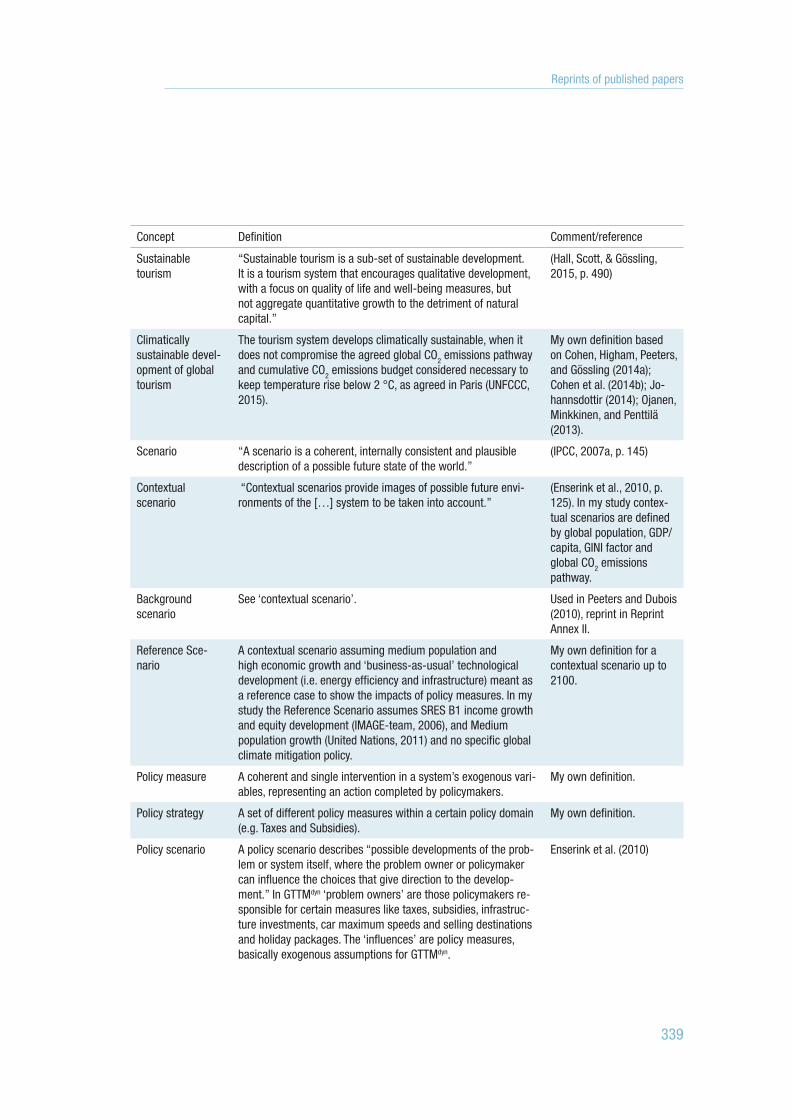
514727-L-bw-peeters514727-L-bw-peeters514727-L-bw-peeters514727-L-bw-peetersProcessed on: 20-10-2017Processed on: 20-10-2017Processed on: 20-10-2017Processed on: 20-10-2017 PDF page: 339PDF page: 339PDF page: 339PDF page: 339
339
Concept Definition Comment/reference
Sustainable tourism
“Sustainable tourism is a sub-set of sustainable development. It is a tourism system that encourages qualitative development, with a focus on quality of life and well-being measures, but not aggregate quantitative growth to the detriment of natural capital.”
(Hall, Scott, & Gössling, 2015, p. 490)
Climatically sustainable devel-opment of global tourism
The tourism system develops climatically sustainable, when it does not compromise the agreed global CO2 emissions pathway and cumulative CO2 emissions budget considered necessary to keep temperature rise below 2 °C, as agreed in Paris (UNFCCC, 2015).
My own definition based on Cohen, Higham, Peeters, and Gössling (2014a); Cohen et al. (2014b); Jo-hannsdottir (2014); Ojanen, Minkkinen, and Penttilä (2013).
Scenario “A scenario is a coherent, internally consistent and plausible description of a possible future state of the world.”
(IPCC, 2007a, p. 145)
Contextual scenario
“Contextual scenarios provide images of possible future envi-ronments of the […] system to be taken into account.”
(Enserink et al., 2010, p. 125). In my study contex-tual scenarios are defined by global population, GDP/capita, GINI factor and global CO2 emissions pathway.
Background scenario
See ‘contextual scenario’. Used in Peeters and Dubois (2010), reprint in Reprint Annex II.
Reference Sce-nario
A contextual scenario assuming medium population and high economic growth and ‘business-as-usual’ technological development (i.e. energy efficiency and infrastructure) meant as a reference case to show the impacts of policy measures. In my study the Reference Scenario assumes SRES B1 income growth and equity development (IMAGE-team, 2006), and Medium population growth (United Nations, 2011) and no specific global climate mitigation policy.
My own definition for a contextual scenario up to 2100.
Policy measure A coherent and single intervention in a system’s exogenous vari-ables, representing an action completed by policymakers.
My own definition.
Policy strategy A set of different policy measures within a certain policy domain (e.g. Taxes and Subsidies).
My own definition.
Policy scenario A policy scenario describes “possible developments of the prob-lem or system itself, where the problem owner or policymaker can influence the choices that give direction to the develop-ment.” In GTTMdyn ‘problem owners’ are those policymakers re-sponsible for certain measures like taxes, subsidies, infrastruc-ture investments, car maximum speeds and selling destinations and holiday packages. The ‘influences’ are policy measures, basically exogenous assumptions for GTTMdyn.
Enserink et al. (2010)
Reprints of published papers

514727-L-bw-peeters514727-L-bw-peeters514727-L-bw-peeters514727-L-bw-peetersProcessed on: 20-10-2017Processed on: 20-10-2017Processed on: 20-10-2017Processed on: 20-10-2017 PDF page: 340PDF page: 340PDF page: 340PDF page: 340
340
Concept Definition Comment/reference
Backcasting scenario
A backcasting scenario shows “a wanted or unwanted normative future situation and how to reach this situation through our policies.”
Enserink (2003);
Annex III. Links to full description of GTTMdyn and a working version of the model
Please find on a full print of the GTTMdyn model including equations on:https://www.cstt.nl/userdata/documents/Peeters-PhD2017-GTTMdyn-model-description.pdf.A fully operational GTTMdyn model including installations manual and data files can be found on:https://www.cstt.nl/userdata/documents/Peeters-PhD2017-GTTMdyn-model-software-data.zip.In case of difficulties to download these files or problems locating them, please contact me on [email protected] or on [email protected].

514727-L-bw-peeters514727-L-bw-peeters514727-L-bw-peeters514727-L-bw-peetersProcessed on: 20-10-2017Processed on: 20-10-2017Processed on: 20-10-2017Processed on: 20-10-2017 PDF page: 341PDF page: 341PDF page: 341PDF page: 341
341
Reprints of published papers

514727-L-bw-peeters514727-L-bw-peeters514727-L-bw-peeters514727-L-bw-peetersProcessed on: 20-10-2017Processed on: 20-10-2017Processed on: 20-10-2017Processed on: 20-10-2017 PDF page: 342PDF page: 342PDF page: 342PDF page: 342
Copyright © 2022 FDOKUMEN