applied sciences

Article

Defrosting of Air-Source Heat Pumps: Effect of RealTemperature Data on Seasonal Energy Performance forDifferent Locations in Italy

Eugenia Rossi di Schio * , Vincenzo Ballerini, Matteo Dongellini and Paolo Valdiserri

�����������������

Citation: Rossi di Schio, E.; Ballerini,

V.; Dongellini, M.; Valdiserri, P.

Defrosting of Air-Source Heat Pumps:

Effect of Real Temperature Data on

Seasonal Energy Performance for

Different Locations in Italy. Appl. Sci.

2021, 11, 8003. https://doi.org/

10.3390/app11178003

Academic Editor: Takahiko Miyazaki

Received: 29 July 2021

Accepted: 23 August 2021

Published: 29 August 2021

Publisher’s Note: MDPI stays neutral

with regard to jurisdictional claims in

published maps and institutional affil-

iations.

Copyright: © 2021 by the authors.

Licensee MDPI, Basel, Switzerland.

This article is an open access article

distributed under the terms and

conditions of the Creative Commons

Attribution (CC BY) license (https://

creativecommons.org/licenses/by/

4.0/).

Department of Industrial Engineering DIN, Alma Mater Studiorum—University of Bologna,Viale Risorgimento 2, I-40136 Bologna, Italy; vincenzo.ballerini2@unibo.it (V.B.);matteo.dongellini@unibo.it (M.D.); paolo.valdiserri@unibo.it (P.V.)* Correspondence: eugenia.rossidischio@unibo.it

Featured Application: The present analysis provides evidence on the importance of the correctevaluation of the defrosting cycles in the determination of the SCOP of ASHPs.

Abstract: In this paper, dynamic simulations of the seasonal coefficient of performance (SCOP) ofAir-Source Heat Pumps will be presented by considering three different heat pump systems coupledwith the same building located in three different Italian municipalities: S. Benedetto del Tronto (42◦58′

North, 13◦53′ East), Milan (45◦28′ North, 9◦10′ East), and Livigno (46◦28′ North, 10◦8′ East). Dynamicsimulations were conducted by employing the software package TRNSYS and by considering realweather data (i.e., outdoor air temperature and humidity as well as solar radiation) referring to thethree abovementioned cities for a period of 8 years (2013–2020) and collected from on-site weatherstations. Attention has been paid to the modeling of the heat pump defrost cycles in order to evaluatetheir influence on the unit’s seasonal performance. Results show that, when referring to differentyears, the thermal energy demand displays huge variations (in some cases it can even double itsvalue), while the effective SCOP is characterized by scarce variability. Sensible variations in SCOPvalues are achieved for Livigno.

Keywords: air-source heat pumps; SCOP; heat pump seasonal performance; defrosting; realweather data

1. Introduction

As is well known, nowadays, a significative amount of greenhouse gas emissions comefrom burning fossil fuels. In the U.S. [1] and in Europe [2], natural gas is widely employedfuel for residential heating. Indeed, technology and politics are trying to find and promotesolutions to reduce or eliminate fossil fuels in order to achieve decarbonization goals,including net zero greenhouse gas emissions at 2050 [3]. An answer can be given by electricheating [4], and low-cost electric heating devices, such as resistive elements, are alreadycommonly available. However, as is well known, heat pumps are thermodynamicallymore efficient than electric resistances, and nowadays, the heat pump market is increasingquickly [5–7].

Air-Source Heat Pumps (ASHPs) are indeed especially effective for space heatingin temperate and mild climates, and therefore could be particularly effective in Italy.A general analysis of the Italian energy system is reported in [8] and focuses on the possibleenergy, economic, and environmental effects of the use of individual heat pumps for winterspace heating.

In the literature, many papers have investigated the Seasonal Coefficient of Perfor-mance (SCOP) of ASHPs, which are usually based on standard climatic data of cities/regionsbased on a Test Reference Year (TRY). Reference years can be constructed starting from

Appl. Sci. 2021, 11, 8003. https://doi.org/10.3390/app11178003 https://www.mdpi.com/journal/applsci

Appl. Sci. 2021, 11, 8003 2 of 15

hourly meteorological data taken from series lasting at least 10 years, according to theprocedure reported in the standard ISO 15927-4 [9]. However, effective ambient temper-ature varies every year, and recently, climate change seems to lead to significant yearlyvariations. Indeed, the use of TRY might underestimate, or overestimate the effectiveenergy performance of ASHP systems [10].

A well-known issue that characterizes ASHPs is the frost build-up on the externalheat exchanger during winter operation and the need to remove it. In fact, in certainweather conditions such as temperature and relative humidity, if the surface temperatureof the evaporator coil is below the air dew point temperature and the water freezing point,ice deposits on it, causing a general degradation of the performance of the air-sourceheat pump. The reduction of HP performance is due to the reduction of the evaporatorheat transfer coefficient, which is mainly for two reasons: the ice layer reduces the airflow through the heat exchanger, and the ice layer also acts as an insulant on the coilsurface [11]. Ice build-up on a heat exchanger is a transient phenomenon, characterizedby three different stages, as proposed by Guo et al. in [12]: the frost layer growth rate inthe first stage increases with time; in the second stage, depending on the relative humidityvalue, the frost thickness growth rate decreases with time or remains invariable; and finally,in the third stage, the frost layer thickness rapidly increases with time. Some papersinvestigate the importance of temperature and relative humidity for frost build-up on theevaporator of the heat pump. In [13], Zhu et al. developed a frosting map (temperature–relative humidity) to guide defrosting control for air-source heat pumps, obtaining threedifferent zones in the frosting region representing different frosting levels from severe tomild. The proposed map can be used to avoid mal-defrosting and to improve defrostingefficiency. In some papers, frosting/defrosting is taken into account, such as, for instance,in [13–16], from a numerical or an experimental point of view. Reported papers mainlyinvestigate the ASHP, and papers dealing with ground coupled exchangers do not considerthe possible effect of natural convection in the soil [17]. Moreover, as far as the authors areconcerned, papers that numerically investigate the defrosting inverse cycle do not take intoaccount the effect of real climate data.

Recently, the authors have analysed the effect of real climate data on the seasonalcoefficient of performance of ASHPs [10]. In the present paper, a transient analysis isperformed in order to evaluate how experimental climate data affect the occurrenceof defrosting cycles in ASHPs if compared with the test reference year standard cli-mate data. In the current study, three Italian cities, characterized by different climates,are considered as reference case studies, the same building is investigated, and the influ-ence of real meteorological data, taken from different years, on the heat pump SCOP isevaluated. The analysis is conducted by employing the dynamic software TRNSYS.

2. Setting of the Analysis

This section describes the used data and the main features of the analysis setting.In particular, we focus on real weather open data, paying attention to the relative humidityas well as on the description of the building under investigation and on the choice of theinverter ASHPs.

2.1. Weather Data

Weather open data were collected for three Italian cities belonging to different climaticzones and that are characterized by different standard heating seasons, according to Italian law,DPR 412/1993. In Table 1 the main data of the selected locations are shown. In detail, Milan andLivigno are located in northern Italy and are classified as climatic zones E and F, respectively;San Benedetto del Tronto is located in central Italy and is classified as climatic zone D. Opendata are collected considering a period of 8 years (2013–2020) from Arpa Lombardia for Milanand Livigno and from the online platform SIRMIP Marche for San Benedetto del Tronto [18,19].Weather stations considered in this paper are, “Milano Lambrate” (45◦30′ North, 9◦15′ East,

Appl. Sci. 2021, 11, 8003 3 of 15

altitude 120 m), “Livigno La Vallaccia” (46◦28′ North, 10◦11′ East, altitude 2650 m) and “SanBenedetto” (13◦53′ North, 42◦55′ East, altitude 6 m), respectively.

Table 1. Climatic zone and standard heating season for Milano, Livigno, and San Benedetto delTronto, according to Italian law, DPR 412/1993.

Town Climatic Zone Heating Season

Milan E 15 October–15 AprilLivigno F 1 January–31 December

San Benedetto del Tronto D 1 November–15 April

With reference to Milan and Livigno, hourly data of temperature, humidity ra-tio, solar radiation, precipitation, wind speed, and wind direction were downloaded.For San Benedetto del Tronto, a lower number of climatic variables are available: for thisreason, only hourly values for the temperature, humidity ratio, and solar radiation weredownloaded. Nonetheless, with the abovementioned, data detailed dynamic simulationscan be performed as well.

According to the authors’ opinion, the quality of the data were good for almost thetotality of the downloaded years for each location, except for San Benedetto del Tronto.For this municipality, 2018 is characterized by a strong lack of data: temperature data aremissing for about 58% of the season, and there are no affordable data available for thehumidity ratio or solar radiation. Therefore, effective climatic data for S. Benedetto delTronto related to year 2018 were not considered.

However, as discussed, climate data were mostly complete; moreover, the availabilityof experimental radiation data integrating the outside air temperature helped to moreaccurately simulate the behavior of the building and its energy balance.

Standard test reference years were created by means of Meteonorm v. 7.2 [20] for thethree cities mentioned above. The TRY created for Livigno was then corrected, consideringthe influence of altitude on air temperature, using the correlation proposed by UNI 10349-2014 [21]:

tH = tREF −∆z178

, (1)

where tH is the corrected temperature, ∆z (m) is the difference between the altitude ofthe two places considered, and tREF is the temperature of the lower place. The correlationis introduced because of the altitude difference between the meteorological station thatcollects weather data in Livigno and the altitude set in Meteonorm (Livigno 1850 m,meteorological station 2650 m). With reference to the humidity ratio, a correction referringto altitude is also introduced, as suggested in [22], considering a linear decrease of humidityratio, i.e.,

HRH = HRREF − 0.0041∆z, (2)

where HRH is the corrected humidity ratio, and HRREF is the humidity ratio of the lower place.Moreover, for Milano, simulations considering the test reference year proposed by the

Italian Thermotechnical Committee CTI [23] were performed as well.For all of the considered years, the values of the real heating degree days (HDD)

are determined for each location, as shown in Figure 1, considering a reference temperaturefor its definition of 20 ◦C (according to DPR 412/93) and the reference period as prescribedby the UNI 11300/1 norm (from 15 October to 15 April for Milan, from 1 November to15 April for San Benedetto del Tronto, and from 5 October to 22 April for Livigno).This figure shows important variation in HDD from a year to another for all of thetowns considered. For example, if we focus our attention on San Benedetto del Tronto,the maximum value is 1846 for the year 2013, and the minimum value is 1515 for the year2014, corresponding to an increase of 11% and a decrease of 9% with respect to the standardTRY value, respectively.

Appl. Sci. 2021, 11, 8003 4 of 15

Appl. Sci. 2021, 11, x FOR PEER REVIEW 4 of 16

For example, if we focus our attention on San Benedetto del Tronto, the maximum value is 1846 for the year 2013, and the minimum value is 1515 for the year 2014, corresponding to an increase of 11% and a decrease of 9% with respect to the standard TRY value, respectively.

Figure 1. Heating degree days for the selected locations and the considered years.

2.2. Building In order to present general results that have not been influenced by the characteristics

of a specific building, a building derived from the reference building proposed by IEA [24] was considered in this work. The simulated building was a two-floor family house characterized by a space heating demand of 45 kWh/m2y in the standard climate of Strasburg. The total floor area of the building considered in the simulations was 360 m2, and the main building envelope thermal properties are presented in Table 2; in Figure 2, the 3D model of the building is sketched.

Table 2. Geometrical and thermo-physical data of the building envelope components. [25].

Envelope Component Thickness (m) U-Value (W/m2K) Ground floor 0.385 0.241

Floor 0.185 0.235 Roof 0.285 0.694

Internal wall 0.200 0.885 External wall 0.318 0.364

Figure 1. Heating degree days for the selected locations and the considered years.

2.2. Building

In order to present general results that have not been influenced by the characteristicsof a specific building, a building derived from the reference building proposed by IEA [24]was considered in this work. The simulated building was a two-floor family house charac-terized by a space heating demand of 45 kWh/m2y in the standard climate of Strasburg.The total floor area of the building considered in the simulations was 360 m2, and the mainbuilding envelope thermal properties are presented in Table 2; in Figure 2, the 3D model ofthe building is sketched.

Table 2. Geometrical and thermo-physical data of the building envelope components. [25].

Envelope Component Thickness (m) U-Value (W/m2K)

Ground floor 0.385 0.241Floor 0.185 0.235Roof 0.285 0.694

Internal wall 0.200 0.885External wall 0.318 0.364

Appl. Sci. 2021, 11, x FOR PEER REVIEW 4 of 16

For example, if we focus our attention on San Benedetto del Tronto, the maximum value is 1846 for the year 2013, and the minimum value is 1515 for the year 2014, corresponding to an increase of 11% and a decrease of 9% with respect to the standard TRY value, respectively.

Figure 1. Heating degree days for the selected locations and the considered years.

2.2. Building In order to present general results that have not been influenced by the characteristics

of a specific building, a building derived from the reference building proposed by IEA [24] was considered in this work. The simulated building was a two-floor family house characterized by a space heating demand of 45 kWh/m2y in the standard climate of Strasburg. The total floor area of the building considered in the simulations was 360 m2, and the main building envelope thermal properties are presented in Table 2; in Figure 2, the 3D model of the building is sketched.

Table 2. Geometrical and thermo-physical data of the building envelope components. [25].

Envelope Component Thickness (m) U-Value (W/m2K) Ground floor 0.385 0.241

Floor 0.185 0.235 Roof 0.285 0.694

Internal wall 0.200 0.885 External wall 0.318 0.364

Figure 2. 3D model of the building.

Appl. Sci. 2021, 11, 8003 5 of 15

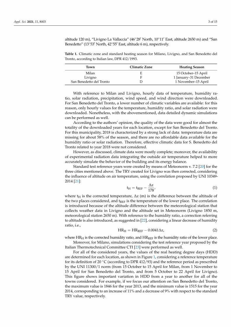
The air change rate due to infiltration was considered to be 0.3 h−1 for all of thethermal zones, and all of the windows were double pane characterized by a 4-16-4 mmconstruction and were filled with Argon gas. The frame was 15% of the total area of thewindow (total area of the glass and frame), and the overall transmittance of the windowwas U-window = 1.5 W/m2K. The window arrangement is shown in Table 3.

Table 3. Window arrangements of the considered building.

Orientation Total Windows Area (m2)

North 14East 20West 20South 30

Gains due to inhabitants and thermal gains caused by electric equipment were con-sidered variable during the day, as shown in Figure 3. The thermal gain caused by asingle inhabitant was divided in two parts: 20 W was considered the convective part ofthe thermal gain, and 40 W was the radiative part. The thermal gains due to electricalequipment were subdivided in half between the convective and radiative parts instead.For any parameter not explicitly mentioned in this section, the value proposed by IEATask 44 for SFH45 was employed and not was not explicitly reported here for the sake ofbrevity [24].

Appl. Sci. 2021, 11, x FOR PEER REVIEW 5 of 16

Figure 2. 3D model of the building.

The air change rate due to infiltration was considered to be 0.3 h−1 for all of the thermal zones, and all of the windows were double pane characterized by a 4-16-4 mm construction and were filled with Argon gas. The frame was 15% of the total area of the window (total area of the glass and frame), and the overall transmittance of the window was U-window = 1.5 W/m2K. The window arrangement is shown in Table 3,

Table 3. Window arrangements of the considered building.

Orientation Total Windows Area (m2) North 14 East 20 West 20 South 30

Gains due to inhabitants and thermal gains caused by electric equipment were considered variable during the day, as shown in Figure 3. The thermal gain caused by a single inhabitant was divided in two parts: 20 W was considered the convective part of the thermal gain, and 40 W was the radiative part. The thermal gains due to electrical equipment were subdivided in half between the convective and radiative parts instead. For any parameter not explicitly mentioned in this section, the value proposed by IEA Task 44 for SFH45 was employed and not was not explicitly reported here for the sake of brevity. [24]

Obviously, the building considered in this study hasa different thermal load, depending on its location. In Table 4, the building design thermal load is reported as a function of the design temperature of the different locations.

In the present paper, the software package TRNSYS was used to model the building, and in particular, the multizone building TRNSYS type 56 [26,27].

Figure 3. Thermal gain profiles due to inhabitants and electrical equipment over a period of 24 h.

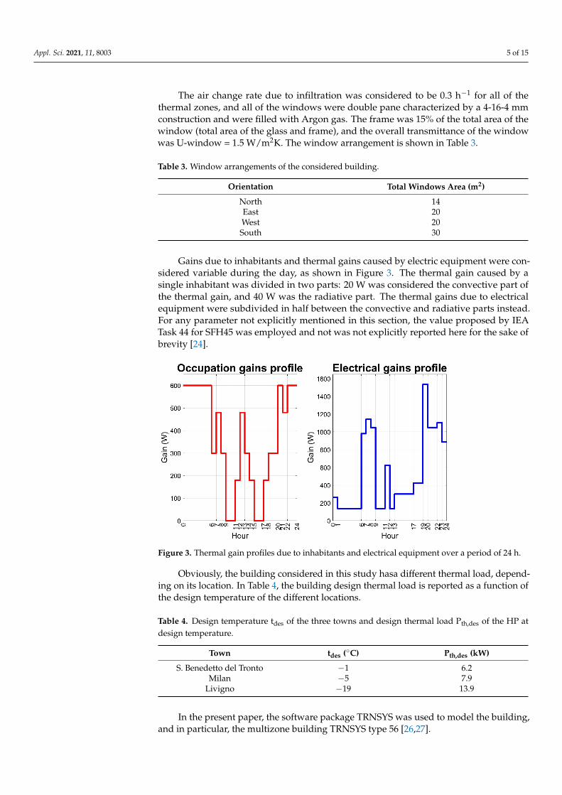
2.3. Heat Pumps A total of three different inverter ASHPs (Unit 1, 2, and 3) were investigated. Unit 1

was coupled to the building placed in San Benedetto del Tronto, Unit 2 and Unit 3 were couples to the buildings located in Milan and in Livigno, respectively. The three heat pumps were characterized by the same coefficient of performance (COP) values, represented in Figure 4 as a function of outdoor air temperature and for different compressor inverter frequencies. The modulation range of the inverter was between 23

Figure 3. Thermal gain profiles due to inhabitants and electrical equipment over a period of 24 h.

Obviously, the building considered in this study hasa different thermal load, depend-ing on its location. In Table 4, the building design thermal load is reported as a function ofthe design temperature of the different locations.

Table 4. Design temperature tdes of the three towns and design thermal load Pth,des of the HP atdesign temperature.

Town tdes (◦C) Pth,des (kW)

S. Benedetto del Tronto −1 6.2Milan −5 7.9

Livigno −19 13.9

In the present paper, the software package TRNSYS was used to model the building,and in particular, the multizone building TRNSYS type 56 [26,27].

Appl. Sci. 2021, 11, 8003 6 of 15

2.3. Heat Pumps

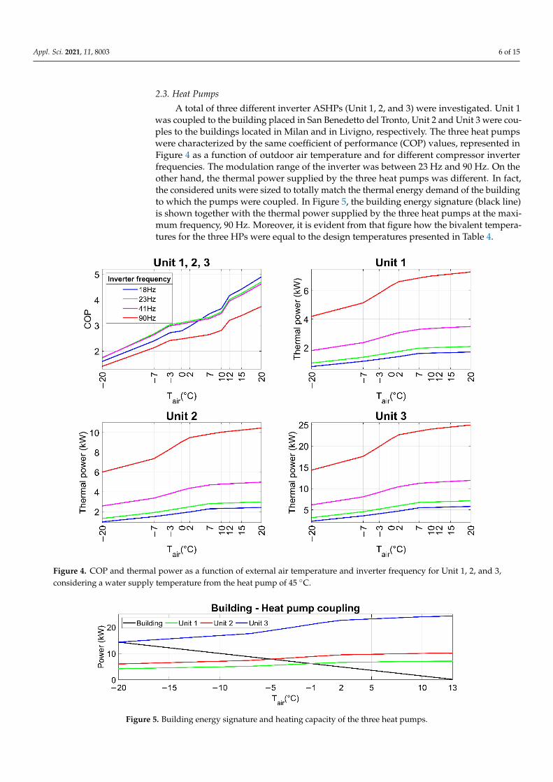
A total of three different inverter ASHPs (Unit 1, 2, and 3) were investigated. Unit 1was coupled to the building placed in San Benedetto del Tronto, Unit 2 and Unit 3 were cou-ples to the buildings located in Milan and in Livigno, respectively. The three heat pumpswere characterized by the same coefficient of performance (COP) values, represented inFigure 4 as a function of outdoor air temperature and for different compressor inverterfrequencies. The modulation range of the inverter was between 23 Hz and 90 Hz. On theother hand, the thermal power supplied by the three heat pumps was different. In fact,the considered units were sized to totally match the thermal energy demand of the buildingto which the pumps were coupled. In Figure 5, the building energy signature (black line)is shown together with the thermal power supplied by the three heat pumps at the maxi-mum frequency, 90 Hz. Moreover, it is evident from that figure how the bivalent tempera-tures for the three HPs were equal to the design temperatures presented in Table 4.

Appl. Sci. 2021, 11, x FOR PEER REVIEW 6 of 16

Hz and 90 Hz. On the other hand, the thermal power supplied by the three heat pumps was different. In fact, the considered units were sized to totally match the thermal energy demand of the building to which the pumps were coupled. In Figure 5, the building energy signature (black line) is shown together with the thermal power supplied by the three heat pumps at the maximum frequency, 90 Hz. Moreover, it is evident from that figure how the bivalent temperatures for the three HPs were equal to the design temperatures presented in Table 4.

Figure 4. COP and thermal power as a function of external air temperature and inverter frequency for Unit 1, 2, and 3, considering a water supply temperature from the heat pump of 45 °C.

Table 4. Design temperature tdes of the three towns and design thermal load Pth,des of the HP at design temperature.

Town tdes (°C) Pth,des (kW) S. Benedetto del Tronto −1 6.2

Milan −5 7.9 Livigno −19 13.9

Figure 5. Building energy signature and heating capacity of the three heat pumps.

2.4. Heating System

Figure 4. COP and thermal power as a function of external air temperature and inverter frequency for Unit 1, 2, and 3,considering a water supply temperature from the heat pump of 45 ◦C.

Appl. Sci. 2021, 11, x FOR PEER REVIEW 6 of 16

Hz and 90 Hz. On the other hand, the thermal power supplied by the three heat pumps was different. In fact, the considered units were sized to totally match the thermal energy demand of the building to which the pumps were coupled. In Figure 5, the building energy signature (black line) is shown together with the thermal power supplied by the three heat pumps at the maximum frequency, 90 Hz. Moreover, it is evident from that figure how the bivalent temperatures for the three HPs were equal to the design temperatures presented in Table 4.

Figure 4. COP and thermal power as a function of external air temperature and inverter frequency for Unit 1, 2, and 3, considering a water supply temperature from the heat pump of 45 °C.

Table 4. Design temperature tdes of the three towns and design thermal load Pth,des of the HP at design temperature.

Town tdes (°C) Pth,des (kW) S. Benedetto del Tronto −1 6.2

Milan −5 7.9 Livigno −19 13.9

Figure 5. Building energy signature and heating capacity of the three heat pumps.

2.4. Heating System

Figure 5. Building energy signature and heating capacity of the three heat pumps.

Appl. Sci. 2021, 11, 8003 7 of 15

2.4. Heating System

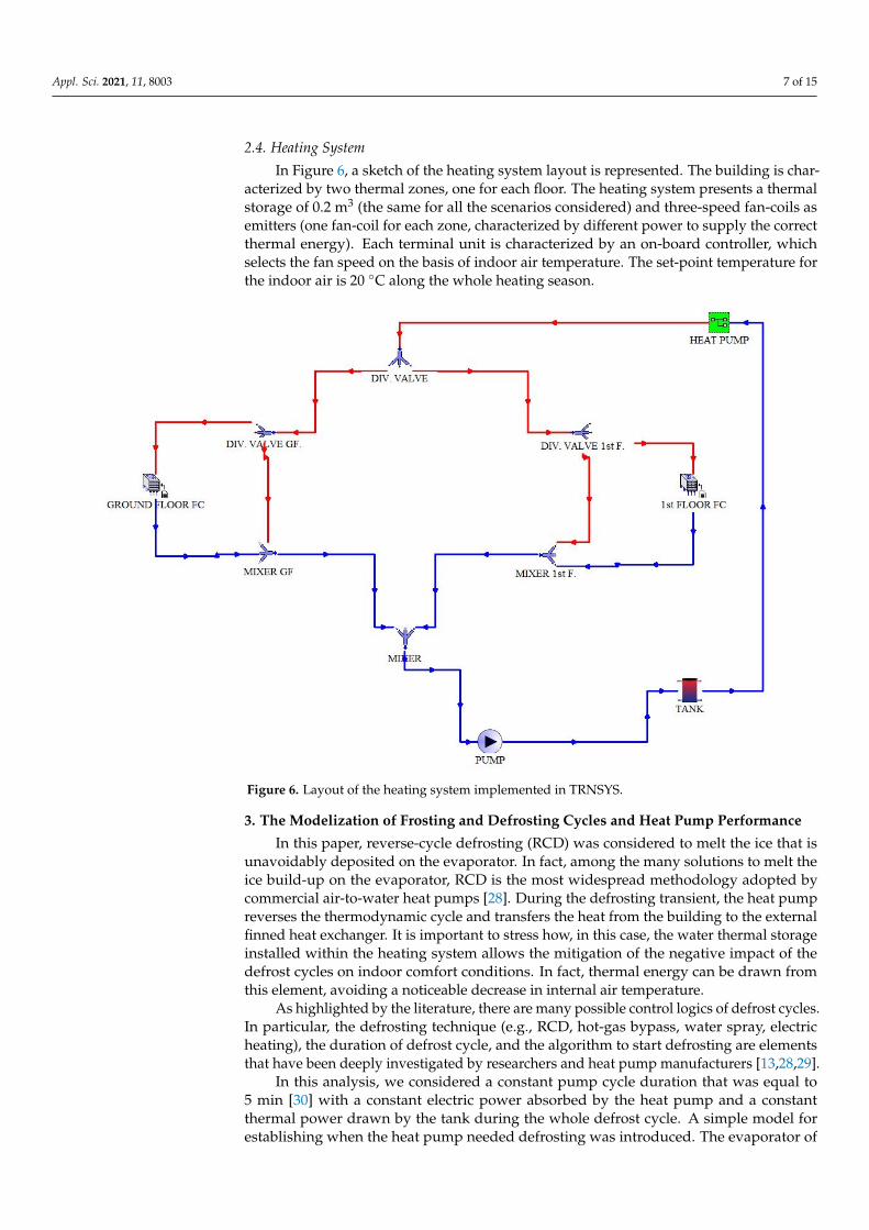
In Figure 6, a sketch of the heating system layout is represented. The building is char-acterized by two thermal zones, one for each floor. The heating system presents a thermalstorage of 0.2 m3 (the same for all the scenarios considered) and three-speed fan-coils asemitters (one fan-coil for each zone, characterized by different power to supply the correctthermal energy). Each terminal unit is characterized by an on-board controller, whichselects the fan speed on the basis of indoor air temperature. The set-point temperature forthe indoor air is 20 ◦C along the whole heating season.

Appl. Sci. 2021, 11, x FOR PEER REVIEW 7 of 16

In Figure 6, a sketch of the heating system layout is represented. The building is characterized by two thermal zones, one for each floor. The heating system presents a thermal storage of 0.2 m3 (the same for all the scenarios considered) and three-speed fan-coils as emitters (one fan-coil for each zone, characterized by different power to supply the correct thermal energy). Each terminal unit is characterized by an on-board controller, which selects the fan speed on the basis of indoor air temperature. The set-point temperature for the indoor air is 20 °C along the whole heating season.

Figure 6. Layout of the heating system implemented in TRNSYS.

3. The Modelization of Frosting and Defrosting Cycles and Heat Pump Performance In this paper, reverse-cycle defrosting (RCD) was considered to melt the ice that is

unavoidably deposited on the evaporator. In fact, among the many solutions to melt the ice build-up on the evaporator, RCD is the most widespread methodology adopted by commercial air-to-water heat pumps [28]. During the defrosting transient, the heat pump reverses the thermodynamic cycle and transfers the heat from the building to the external finned heat exchanger. It is important to stress how, in this case, the water thermal storage installed within the heating system allows the mitigation of the negative impact of the defrost cycles on indoor comfort conditions. In fact, thermal energy can be drawn from this element, avoiding a noticeable decrease in internal air temperature.

As highlighted by the literature, there are many possible control logics of defrost cycles. In particular, the defrosting technique (e.g., RCD, hot-gas bypass, water spray, electric heating), the duration of defrost cycle, and the algorithm to start defrosting are elements that have been deeply investigated by researchers and heat pump manufacturers. [13,28,29]

In this analysis, we considered a constant pump cycle duration that was equal to 5 min [30] with a constant electric power absorbed by the heat pump and a constant thermal power drawn by the tank during the whole defrost cycle. A simple model for establishing when the heat pump needed defrosting was introduced. The evaporator of the machine was considered as a black box (an open thermodynamic system), as shown in Figure 7. The air stream entered the evaporator in conditions expressed by Subscript 1 and exited in the conditions expressed by Subscript 2. The term mw (kg/s) represents the mass flow

Figure 6. Layout of the heating system implemented in TRNSYS.

3. The Modelization of Frosting and Defrosting Cycles and Heat Pump Performance

In this paper, reverse-cycle defrosting (RCD) was considered to melt the ice that isunavoidably deposited on the evaporator. In fact, among the many solutions to melt theice build-up on the evaporator, RCD is the most widespread methodology adopted bycommercial air-to-water heat pumps [28]. During the defrosting transient, the heat pumpreverses the thermodynamic cycle and transfers the heat from the building to the externalfinned heat exchanger. It is important to stress how, in this case, the water thermal storageinstalled within the heating system allows the mitigation of the negative impact of thedefrost cycles on indoor comfort conditions. In fact, thermal energy can be drawn fromthis element, avoiding a noticeable decrease in internal air temperature.

As highlighted by the literature, there are many possible control logics of defrost cycles.In particular, the defrosting technique (e.g., RCD, hot-gas bypass, water spray, electricheating), the duration of defrost cycle, and the algorithm to start defrosting are elementsthat have been deeply investigated by researchers and heat pump manufacturers [13,28,29].

In this analysis, we considered a constant pump cycle duration that was equal to5 min [30] with a constant electric power absorbed by the heat pump and a constantthermal power drawn by the tank during the whole defrost cycle. A simple model forestablishing when the heat pump needed defrosting was introduced. The evaporator of

Appl. Sci. 2021, 11, 8003 8 of 15

the machine was considered as a black box (an open thermodynamic system), as shown inFigure 7. The air stream entered the evaporator in conditions expressed by Subscript 1 andexited in the conditions expressed by Subscript 2. The term mw (kg/s) represents the massflow rate of water condensed on the heat exchanger that may freeze. The symbol t refers tothe temperature, x refers to the vapor quality, and h refers to the specific enthalpy of theair stream. All of the parameters associated with Entry State 1 are known since they referto the conditions of the outdoor ambient air. Using the psychrometric formula proposedby [31]:

h = 1.006t + x(2501 + 1.84t), (3)

the enthalpy h1 (kJ/kg) as well as the dew point temperature tDP (◦C) can be calculatedand given by

tDP =4030.183

16.6536− ln(

psat1000

) − 235, (4)

psat = 1000 exp(

16.6536− 4030.183t + 235

)(5)

where psat (Pa) is the saturation vapor pressure of the water vapor available in the air atthe conditions expressed by Subscript 1. The vapor quality of the mixture at the dew pointcan be calculated as well, by means of the relation

xDP = 0.622ϕpsat

ptot −ϕpsat, (6)

where ϕ is the relative humidity (in this case ϕ = 1) and ptot (Pa) is the atmospheric pressureat the altitude of the selected location.

Appl. Sci. 2021, 11, x FOR PEER REVIEW 9 of 16

Figure 7. Evaporator of the HP considered as a “black box”.

In [11], the authors simulated the RCD using time-dependent functions for electric and thermal power during the defrosting phase; a similar analysis can only be made if a huge amount of data are available from the manufacturer or if long-term experiments are conducted on a specific heat pump. Referring to the three heat pumps that are be investigated in this paper, the electric power input of the heat pump and the thermal power taken from the water tank are considered as constants along the defrost cycle. Their values are shown in Table 5. Furthermore, additional details on the choice of both the values for the electric power and the thermal power are given in Figure 8. In detail, we assume for the same energy for the whole defrost cycle as well as the same electric energy input for each different HP, as proposed in [11]. In particular, the thermal and electric power trends along a generic defrost cycle are reported in Figure 8, according to the model proposed in [11]. The thermal power trend is modelled with two parabolic branches, while the electric power is modeled with two linear functions. In the same figure, the thermal and electric power considered in this analysis are reported, i.e., two constant functions during the whole defrost cycle of 300 s. In Figure 8, the surfaces below the lines are equal to both, with reference to the thermal power (a) and to the electric power (b). Moreover, the duration of the defrost cycle is taken as in [11] and corresponds to a mean time used by the manufacturers on their control systems.

The air mass processed by the heat pumps is assumed to be a linearly increasing function of the thermal power of the machine, according to data given by a manufacturer [32]: used data refer to heat pumps characterized by a nominal thermal power ranging from 4.7 kW to 31 kW. The values of the air mass processed by the three HPs considered are presented in Table 5 and were obtained applying a linear interpolation on the abovementioned data given by the HPs’ manufacturers.

In Figure 9, the defrost control implemented in TRNSYS is shown through a flowchart diagram. It can be noticed that the defrost phase only starts if two conditions are simultaneously satisfied: (1) the enthalpy of the air at evaporator outlet is lower than the enthalpy at the dew point; (2) the HP is turned on.

Table 5. Thermal power drawn from the building by the heat pump during a defrost cycle, Pth,def, electric power absorbed by the machine during defrost, Pel,def, and air mass, ma, processed by the evaporator of the machine.

Heat Pump Pth,def (kW) Pel,def (kW) ma (kg/s) Unit 1 4.59 1.17 1.65 Unit 2 6.57 1.67 2.11 Unit 3 15.68 3.99 4.22

Figure 7. Evaporator of the HP considered as a “black box”.

Equations (4) and (6) allow the air enthalpy at the dew point to be obtained, namely

hDP = 1.006tDP + xDP(2501 + 1.84tDP). (7)

The air enthalpy at the dew point gives information about the moisture formation(and subsequently, the possible frost formation) on the evaporator of the heat pump: if theair enthalpy at the outdoor heat exchanger outlet in Condition 2 is lower than hDP, frostformation on the heat exchanger may occur, and the defrost cycle has to start after a certaininterval. The enthalpy h2 of the air stream at the outlet of the evaporator can be calculatedapproximately (neglecting the enthalpy of the of the water that condenses on the finnedcoil) by applying an energy balance to the heat exchanger:

h2 = h1 −Qevma

, (8)

where Qev (kW) is the thermal power exchanged with the outdoor air by the machine’sevaporator, and ma (kg/s) is the air mass flow rate exiting the evaporator (also, in this

Appl. Sci. 2021, 11, 8003 9 of 15

case, the air mass flow rate exiting the evaporator is the same the one that enters the heatexchanger whenever the mass of water condensed on the evaporator may be neglected).Typically, the quantity of air processed by a heat pump is a parameter given in the technicaldatasheet of the unit, and the term Qev can be calculated applying an energy balance to thewhole heat pump. In fact, the unit works by extracting the power Qev from the evaporator,thus providing the thermal power Pth to the condenser and absorbing the electric powerPel. Hence

Qev = Pth

(1− 1

COP

), (9)

where COP is the coefficient of performance of the HP, defined as the ratio between thermalpower Pth and electric power Pel.

This simple model of a RCD can be easily implemented in TRNSYS with no additionaldata on the heat pump evaporator, using only technical data from the heat pump datasheet.

In [11], the authors simulated the RCD using time-dependent functions for electricand thermal power during the defrosting phase; a similar analysis can only be made ifa huge amount of data are available from the manufacturer or if long-term experimentsare conducted on a specific heat pump. Referring to the three heat pumps that are beinvestigated in this paper, the electric power input of the heat pump and the thermalpower taken from the water tank are considered as constants along the defrost cycle. Theirvalues are shown in Table 5. Furthermore, additional details on the choice of both thevalues for the electric power and the thermal power are given in Figure 8. In detail, weassume for the same energy for the whole defrost cycle as well as the same electric energyinput for each different HP, as proposed in [11]. In particular, the thermal and electricpower trends along a generic defrost cycle are reported in Figure 8, according to the modelproposed in [11]. The thermal power trend is modelled with two parabolic branches, whilethe electric power is modeled with two linear functions. In the same figure, the thermaland electric power considered in this analysis are reported, i.e., two constant functionsduring the whole defrost cycle of 300 s. In Figure 8, the surfaces below the lines are equalto both, with reference to the thermal power (a) and to the electric power (b). Moreover,the duration of the defrost cycle is taken as in [11] and corresponds to a mean time used bythe manufacturers on their control systems.

Table 5. Thermal power drawn from the building by the heat pump during a defrost cycle, Pth,def,electric power absorbed by the machine during defrost, Pel,def, and air mass, ma, processed by theevaporator of the machine.

Heat Pump Pth,def (kW) Pel,def (kW) ma (kg/s)

Unit 1 4.59 1.17 1.65Unit 2 6.57 1.67 2.11Unit 3 15.68 3.99 4.22

The air mass processed by the heat pumps is assumed to be a linearly increasing func-tion of the thermal power of the machine, according to data given by a manufacturer [32]:used data refer to heat pumps characterized by a nominal thermal power ranging from4.7 kW to 31 kW. The values of the air mass processed by the three HPs considered are pre-sented in Table 5 and were obtained applying a linear interpolation on the abovementioneddata given by the HPs’ manufacturers.

In Figure 9, the defrost control implemented in TRNSYS is shown through a flowchartdiagram. It can be noticed that the defrost phase only starts if two conditions are simulta-neously satisfied: (1) the enthalpy of the air at evaporator outlet is lower than the enthalpyat the dew point; (2) the HP is turned on.

Appl. Sci. 2021, 11, 8003 10 of 15

Appl. Sci. 2021, 11, x FOR PEER REVIEW 10 of 16

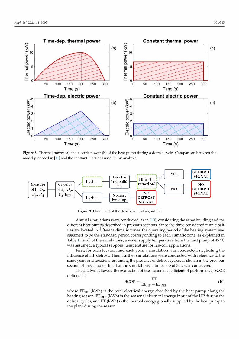
Figure 8. Thermal power (a) and electric power (b) of the heat pump during a defrost cycle. Comparison between the model proposed in [11] and the constant functions used in this analysis.

Figure 9. Flow chart of the defrost control algorithm.

Annual simulations were conducted, as in [10], considering the same building and the different heat pumps described in previous sections. Since the three considered municipalities are located in different climatic zones, the operating period of the heating system was assumed to be the standard period corresponding to each climatic zone, as explained in Table 1. In all of the simulations, a water supply temperature from the heat pump of 45 °C was assumed, a typical set-point temperature for fan-coil applications.

First, for each location and each year, a simulation was conducted, neglecting the influence of HP defrost. Then, further simulations were conducted with reference to the same years and locations, assuming the presence of defrost cycles, as shown in the previous section of this chapter. In all of the simulations, a time step of 30 s was considered.

The analysis allowed the evaluation of the seasonal coefficient of performance, SCOP, defined as SCOP = ETEE + EE (10)

where EEHP (kWh) is the total electrical energy absorbed by the heat pump along the heating season, EEDEF (kWh) is the seasonal electrical energy input of the HP during the defrost cycles, and ET (kWh) is the thermal energy globally supplied by the heat pump to the plant during the season.

4. Results and Discussion In Figure 10, the number of defrost cycles are reported for every year considered in

the simulations. The HP placed in Milan performs more defrost cycles than the units

Figure 8. Thermal power (a) and electric power (b) of the heat pump during a defrost cycle. Comparison between themodel proposed in [11] and the constant functions used in this analysis.

Appl. Sci. 2021, 11, x FOR PEER REVIEW 10 of 16

Figure 8. Thermal power (a) and electric power (b) of the heat pump during a defrost cycle. Comparison between the model proposed in [11] and the constant functions used in this analysis.

Figure 9. Flow chart of the defrost control algorithm.

Annual simulations were conducted, as in [10], considering the same building and the different heat pumps described in previous sections. Since the three considered municipalities are located in different climatic zones, the operating period of the heating system was assumed to be the standard period corresponding to each climatic zone, as explained in Table 1. In all of the simulations, a water supply temperature from the heat pump of 45 °C was assumed, a typical set-point temperature for fan-coil applications.

First, for each location and each year, a simulation was conducted, neglecting the influence of HP defrost. Then, further simulations were conducted with reference to the same years and locations, assuming the presence of defrost cycles, as shown in the previous section of this chapter. In all of the simulations, a time step of 30 s was considered.

The analysis allowed the evaluation of the seasonal coefficient of performance, SCOP, defined as SCOP = ETEE + EE (10)

where EEHP (kWh) is the total electrical energy absorbed by the heat pump along the heating season, EEDEF (kWh) is the seasonal electrical energy input of the HP during the defrost cycles, and ET (kWh) is the thermal energy globally supplied by the heat pump to the plant during the season.

4. Results and Discussion In Figure 10, the number of defrost cycles are reported for every year considered in

the simulations. The HP placed in Milan performs more defrost cycles than the units

Figure 9. Flow chart of the defrost control algorithm.

Annual simulations were conducted, as in [10], considering the same building and thedifferent heat pumps described in previous sections. Since the three considered municipali-ties are located in different climatic zones, the operating period of the heating system wasassumed to be the standard period corresponding to each climatic zone, as explained inTable 1. In all of the simulations, a water supply temperature from the heat pump of 45 ◦Cwas assumed, a typical set-point temperature for fan-coil applications.

First, for each location and each year, a simulation was conducted, neglecting theinfluence of HP defrost. Then, further simulations were conducted with reference to thesame years and locations, assuming the presence of defrost cycles, as shown in the previoussection of this chapter. In all of the simulations, a time step of 30 s was considered.

The analysis allowed the evaluation of the seasonal coefficient of performance, SCOP,defined as

SCOP =ET

EEHP + EEDEF(10)

where EEHP (kWh) is the total electrical energy absorbed by the heat pump along theheating season, EEDEF (kWh) is the seasonal electrical energy input of the HP during thedefrost cycles, and ET (kWh) is the thermal energy globally supplied by the heat pump tothe plant during the season.

Appl. Sci. 2021, 11, 8003 11 of 15

4. Results and Discussion

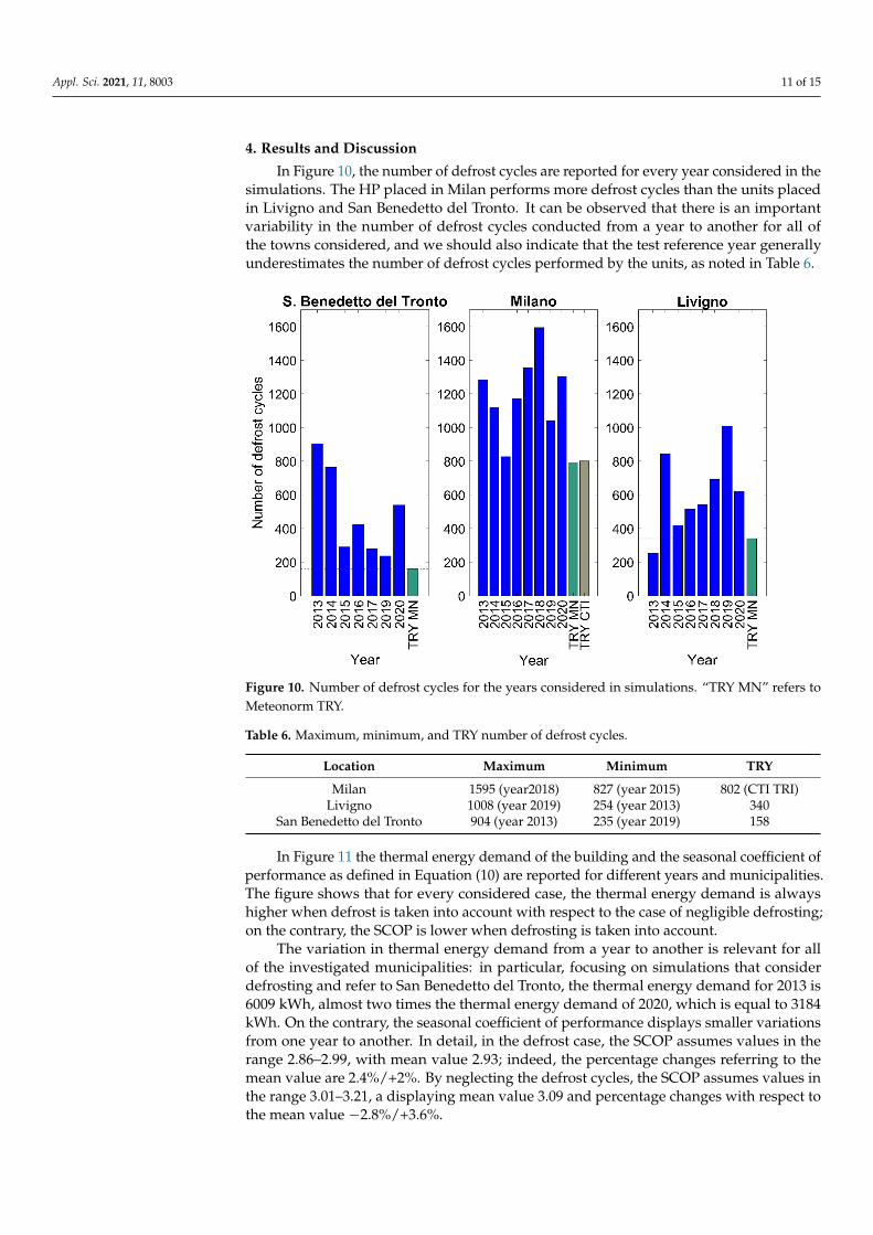
In Figure 10, the number of defrost cycles are reported for every year considered in thesimulations. The HP placed in Milan performs more defrost cycles than the units placedin Livigno and San Benedetto del Tronto. It can be observed that there is an importantvariability in the number of defrost cycles conducted from a year to another for all ofthe towns considered, and we should also indicate that the test reference year generallyunderestimates the number of defrost cycles performed by the units, as noted in Table 6.

Appl. Sci. 2021, 11, x FOR PEER REVIEW 11 of 16

placed in Livigno and San Benedetto del Tronto. It can be observed that there is an important variability in the number of defrost cycles conducted from a year to another for all of the towns considered, and we should also indicate that the test reference year generally underestimates the number of defrost cycles performed by the units, as noted in Table 6.

Figure 10. Number of defrost cycles for the years considered in simulations. “TRY MN” refers to Meteonorm TRY.

In Figure 1,1 the thermal energy demand of the building and the seasonal coefficient of performance as defined in Equation (10) are reported for different years and municipalities. The figure shows that for every considered case, the thermal energy demand is always higher when defrost is taken into account with respect to the case of negligible defrosting; on the contrary, the SCOP is lower when defrosting is taken into account.

The variation in thermal energy demand from a year to another is relevant for all of the investigated municipalities: in particular, focusing on simulations that consider defrosting and refer to San Benedetto del Tronto, the thermal energy demand for 2013 is 6009 kWh, almost two times the thermal energy demand of 2020, which is equal to 3184 kWh. On the contrary, the seasonal coefficient of performance displays smaller variations from one year to another. In detail, in the defrost case, the SCOP assumes values in the range 2.86–2.99, with mean value 2.93; indeed, the percentage changes referring to the mean value are 2.4%/+2%. By neglecting the defrost cycles, the SCOP assumes values in the range 3.01–3.21, a displaying mean value 3.09 and percentage changes with respect to the mean value −2.8%/+3.6%.

Concerning the test reference year defined through Meteonorm for San Benedetto del Tronto, the thermal energy demand of the building is overestimated in both cases, with or without defrost (thermal energy demand is lower with respect to the TRY predictions for 5 years out of 7); conversely, SCOP values obtained from the test reference year are in accordance with the values obtained from the simulations that considered real weather data from the different years.

Considering Milan, Figure 11 shows, as for the case of San Benedetto del Tronto, important variations of the thermal energy demand from one year to another (considering

Figure 10. Number of defrost cycles for the years considered in simulations. “TRY MN” refers toMeteonorm TRY.

Table 6. Maximum, minimum, and TRY number of defrost cycles.

Location Maximum Minimum TRY

Milan 1595 (year2018) 827 (year 2015) 802 (CTI TRI)Livigno 1008 (year 2019) 254 (year 2013) 340

San Benedetto del Tronto 904 (year 2013) 235 (year 2019) 158

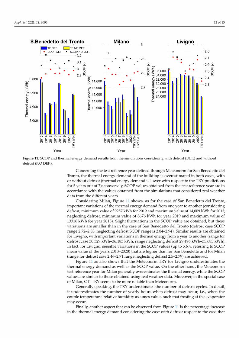
In Figure 11 the thermal energy demand of the building and the seasonal coefficient ofperformance as defined in Equation (10) are reported for different years and municipalities.The figure shows that for every considered case, the thermal energy demand is alwayshigher when defrost is taken into account with respect to the case of negligible defrosting;on the contrary, the SCOP is lower when defrosting is taken into account.

The variation in thermal energy demand from a year to another is relevant for allof the investigated municipalities: in particular, focusing on simulations that considerdefrosting and refer to San Benedetto del Tronto, the thermal energy demand for 2013 is6009 kWh, almost two times the thermal energy demand of 2020, which is equal to 3184kWh. On the contrary, the seasonal coefficient of performance displays smaller variationsfrom one year to another. In detail, in the defrost case, the SCOP assumes values in therange 2.86–2.99, with mean value 2.93; indeed, the percentage changes referring to themean value are 2.4%/+2%. By neglecting the defrost cycles, the SCOP assumes values inthe range 3.01–3.21, a displaying mean value 3.09 and percentage changes with respect tothe mean value −2.8%/+3.6%.

Appl. Sci. 2021, 11, 8003 12 of 15

Appl. Sci. 2021, 11, x FOR PEER REVIEW 12 of 16

defrost, minimum value of 9257 kWh for 2019 and maximum value of 14,009 kWh for 2013; neglecting defrost, minimum value of 8676 kWh for year 2019 and maximum value of 13316 kWh for year 2013). Slight fluctuations in the SCOP value are obtained, but these variations are smaller than in the case of San Benedetto del Tronto (defrost case SCOP range 2.72–2.83, neglecting defrost SCOP range is 2.84–2.94). Similar results are obtained for Livigno, with important variations in thermal energy from a year to another (range for defrost case 30,329 kWh–36,183 kWh, range neglecting defrost 29,496 kWh–35,685 kWh). In fact, for Livigno, sensible variations in the SCOP values (up to 5.6%, referring to SCOP mean value of the years 2013–2020) that are higher than for San Benedetto and for Milan (range for defrost case 2.46–2.71 range neglecting defrost 2.5–2.79) are achieved.

Figure 11 as also shows that the Meteonorm TRY for Livigno underestimates the thermal energy demand as well as the SCOP value. On the other hand, the Meteonorm test reference year for Milan generally overestimates the thermal energy, while the SCOP values are similar to those obtained using real weather data. Moreover, in the special case of Milan, CTI TRY seems to be more reliable than Meteonorm.

Generally speaking, the TRY understimates the number of defrost cycles. In detail, it underestimates the number of yearly hours when defrost may occur, i.e., when the couple temperature–relative humidity assumes values such that frosting at the evaporator may occur.

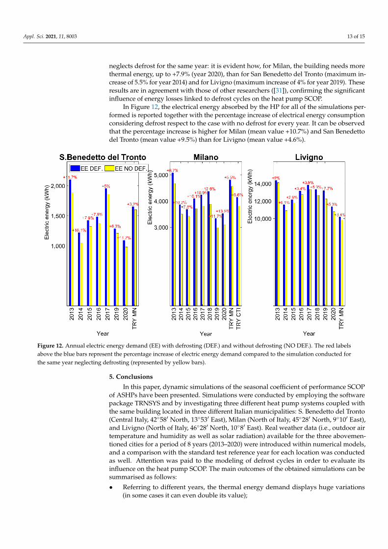
Finally, another aspect that can be observed from Figure 11 is the percentage increase in the thermal energy demand considering the case with defrost respect to the case that neglects defrost for the same year: it is evident how, for Milan, the building needs more thermal energy, up to +7.9% (year 2020), than for San Benedetto del Tronto (maximum increase of 5.5% for year 2014) and for Livigno (maximum increase of 4% for year 2019). These results are in agreement with those of other researchers ([31]), confirming the significant influence of energy losses linked to defrost cycles on the heat pump SCOP.

In Figure 12, the electrical energy absorbed by the HP for all of the simulations performed is reported together with the percentage increase of electrical energy consumption considering defrost respect to the case with no defrost for every year. It can be observed that the percentage increase is higher for Milan (mean value +10.7%) and San Benedetto del Tronto (mean value +9.5%) than for Livigno (mean value +4.6%).

Figure 11. SCOP and thermal energy demand results from the simulations considering with defrost (DEF.) and without defrost (NO DEF.).

Figure 11. SCOP and thermal energy demand results from the simulations considering with defrost (DEF.) and withoutdefrost (NO DEF.).

Concerning the test reference year defined through Meteonorm for San Benedetto delTronto, the thermal energy demand of the building is overestimated in both cases, withor without defrost (thermal energy demand is lower with respect to the TRY predictionsfor 5 years out of 7); conversely, SCOP values obtained from the test reference year are inaccordance with the values obtained from the simulations that considered real weatherdata from the different years.

Considering Milan, Figure 11 shows, as for the case of San Benedetto del Tronto,important variations of the thermal energy demand from one year to another (consideringdefrost, minimum value of 9257 kWh for 2019 and maximum value of 14,009 kWh for 2013;neglecting defrost, minimum value of 8676 kWh for year 2019 and maximum value of13316 kWh for year 2013). Slight fluctuations in the SCOP value are obtained, but thesevariations are smaller than in the case of San Benedetto del Tronto (defrost case SCOPrange 2.72–2.83, neglecting defrost SCOP range is 2.84–2.94). Similar results are obtainedfor Livigno, with important variations in thermal energy from a year to another (range fordefrost case 30,329 kWh–36,183 kWh, range neglecting defrost 29,496 kWh–35,685 kWh).In fact, for Livigno, sensible variations in the SCOP values (up to 5.6%, referring to SCOPmean value of the years 2013–2020) that are higher than for San Benedetto and for Milan(range for defrost case 2.46–2.71 range neglecting defrost 2.5–2.79) are achieved.

Figure 11 as also shows that the Meteonorm TRY for Livigno underestimates thethermal energy demand as well as the SCOP value. On the other hand, the Meteonormtest reference year for Milan generally overestimates the thermal energy, while the SCOPvalues are similar to those obtained using real weather data. Moreover, in the special caseof Milan, CTI TRY seems to be more reliable than Meteonorm.

Generally speaking, the TRY understimates the number of defrost cycles. In detail,it underestimates the number of yearly hours when defrost may occur, i.e., when thecouple temperature–relative humidity assumes values such that frosting at the evaporatormay occur.

Finally, another aspect that can be observed from Figure 11 is the percentage increasein the thermal energy demand considering the case with defrost respect to the case that

Appl. Sci. 2021, 11, 8003 13 of 15

neglects defrost for the same year: it is evident how, for Milan, the building needs morethermal energy, up to +7.9% (year 2020), than for San Benedetto del Tronto (maximum in-crease of 5.5% for year 2014) and for Livigno (maximum increase of 4% for year 2019). Theseresults are in agreement with those of other researchers ([31]), confirming the significantinfluence of energy losses linked to defrost cycles on the heat pump SCOP.

In Figure 12, the electrical energy absorbed by the HP for all of the simulations per-formed is reported together with the percentage increase of electrical energy consumptionconsidering defrost respect to the case with no defrost for every year. It can be observedthat the percentage increase is higher for Milan (mean value +10.7%) and San Benedettodel Tronto (mean value +9.5%) than for Livigno (mean value +4.6%).

Appl. Sci. 2021, 11, x FOR PEER REVIEW 13 of 16

Figure 12. Annual electric energy demand (EE) with defrosting (DEF.) and without defrosting (NO DEF.). The red labels above the blue bars represent the percentage increase of electric energy demand compared to the simulation conducted for the same year neglecting defrosting (represented by yellow bars).

Table 6. Maximum, minimum, and TRY number of defrost cycles.

Location Maximum Minimum TRY Milan 1595 (year2018) 827 (year 2015) 802 (CTI TRI)

Livigno 1008 (year 2019) 254 (year 2013) 340 San Benedetto del Tronto 904 (year 2013) 235 (year 2019) 158

Figure 12. Annual electric energy demand (EE) with defrosting (DEF.) and without defrosting (NO DEF.). The red labelsabove the blue bars represent the percentage increase of electric energy demand compared to the simulation conducted forthe same year neglecting defrosting (represented by yellow bars).

5. Conclusions

In this paper, dynamic simulations of the seasonal coefficient of performance SCOPof ASHPs have been presented. Simulations were conducted by employing the softwarepackage TRNSYS and by investigating three different heat pump systems coupled withthe same building located in three different Italian municipalities: S. Benedetto del Tronto(Central Italy, 42◦58′ North, 13◦53′ East), Milan (North of Italy, 45◦28′ North, 9◦10′ East),and Livigno (North of Italy, 46◦28′ North, 10◦8′ East). Real weather data (i.e., outdoor airtemperature and humidity as well as solar radiation) available for the three abovemen-tioned cities for a period of 8 years (2013–2020) were introduced within numerical models,and a comparison with the standard test reference year for each location was conductedas well. Attention was paid to the modeling of defrost cycles in order to evaluate itsinfluence on the heat pump SCOP. The main outcomes of the obtained simulations can besummarised as follows:

• Referring to different years, the thermal energy demand displays huge variations(in some cases it can even double its value);

Appl. Sci. 2021, 11, 8003 14 of 15

• On the contrary, the SCOP displays small variations with respect to its mean value.SCOP also displays small variations considering defrost vs. no defrost cases (Table 7);

• SCOP values obtained from the test reference year often tend to overestimate orunderestimate the SCOP value, and in the special case of Milan, CTI TRY seems to bemore reliable than Meteonorm;

• The electrical energy absorbed by the HP considering defrost is higher with respectto the case with no defrost for every year; it can be observed that the percentageincrease is higher for Milan (mean value +10.7%) and San Benedetto del Tronto (meanvalue +9.5%) than for Livigno (mean value 4.6%). Indeed, if one neglects the effect ofdefrosting, there is a tendency to underestimate the electric energy consumption ofthe HP up to 10%.

Table 7. Maximum and mean SCOP decrease considering defrost vs. no defrost cases; obtained fromthe dynamic simulations considering real climatic data.

Location Maximum Decrease Mean Decrease

Milan 5.2% 4.1%Livigno 3.4% 1.9%

San Benedetto del Tronto 9% 5.4%

To sum up, frosting/defrosting cycles have to be taken into account in order tocorrectly evaluate the electric energy consumption of a HP. The use of TRY instead of realdata tends to underestimate the number of defrosting cycles, and a revision of TRY shouldhelp manufacturers and technicians.

Author Contributions: Data curation, V.B., M.D. and P.V.; Methodology, E.R.d.S., V.B., M.D. and P.V.;Supervision, M.D.; Validation, E.R.d.S. and P.V.; Visualization, V.B. and M.D.; Writing—original draft,E.R.d.S., V.B., M.D. and P.V.; Writing—review & editing, E.R.d.S., V.B., M.D. and P.V. All authors haveread and agreed to the published version of the manuscript.

Funding: This research received no external funding.

Conflicts of Interest: The authors declare no conflict of interest.

References1. U.S. Energy Information Agency. 2015 Residential Energy Consumption Survey—CE4.1 (2018). Available online: https://www.

eia.gov/consumption/residential/data/2015/ (accessed on 12 October 2020).2. Pezzutto, S.; Croce, S.; ZambottI, S.; Kranzl, L.; Novelli, A.; Zambelli, P. Assessment of the Space Heating and Domestic Hot

Water Market in Europe—Open Data and Results. Energies 2019, 12, 1760. [CrossRef]3. EU 2050 long term strategy. Available online: https://ec.europa.eu/clima/policies/strategies/2050_en (accessed on 28 July 2021).4. Dennis, K.; Colburn, K.; Lazar, J. Environmentally beneficial electrification: The dawn of ‘emissions efficiency’. Electr. J. 2016, 29,

52–58. [CrossRef]5. Kaufman, N.; Sandalow, D.; Rossi di Schio, C.; Higdon, J. Decarbonizing Space Heating with Air Source Heat Pumps.

Available online: https://www.energypolicy.columbia.edu/research/report/decarbonizing-space-heating-air-source-heat-pumps (accessed on 28 July 2021).

6. Nowak, T. Heat Pumps—Integrating Technologies to Decarbonise Heating and Cooling; European Heat Pump Association: Brussels,Belgium, 2018.

7. Nowak, T. EHPA Market Report and Statistics Outlook 2019; European Heat Pump Association (EHPA): Brussels, Belgium, 2019.8. Bianco, V.; Marchitto, A.; Scarpa, F.; Tagliafico, L.A. Heat pumps for buildings heating: Energy, environmental, and economic

issues. Energy Environ. 2018, 31, 116–129. [CrossRef]9. ISO. UNI EN ISO 15927-4:2005, Hygrothermal Performance of Buildings—Calculation and Presentation of Climatic Data—Part 4: Hourly

Data for Assessing the Annual Energy Use for Heating and Cooling; ISO: Geneva, Switzerland, 2005.10. Ballerini, V.; Dongellini, M.; di Schio, E.R.; Valdiserri, P. Effect of real temperature data on the seasonal coefficient of per-formance

of air source heat pumps. In Proceedings of the UIT 38th UIT International Conference, Online, 21–22 June 2021.11. Dongellini, M.; Piazzi, A.; De Biagi, F.; Morini, G.L. The modelling of reverse defrosting cycles of air-to-water heat pumps with

TRNSYS. E3S Web Conf. 2019, 111, 01063. [CrossRef]12. Guo, X.-M.; Chen, Y.-G.; Wang, W.-H.; Chen, C.-Z. Experimental study on frost growth and dynamic performance of air source

heat pump system. Appl. Therm. Eng. 2008, 28, 2267–2278. [CrossRef]

Appl. Sci. 2021, 11, 8003 15 of 15

13. Zhu, J.; Sun, Y.; Wang, W.; Deng, S.S.; Ge, Y.; Li, L. Developing a new frosting map to guide defrosting control for air-source heatpump units. Appl. Therm. Eng. 2015, 90, 782–791. [CrossRef]

14. Wang, W.; Zhang, S.; Li, Z.; Sun, Y.; Deng, S.; Wu, X. Determination of the optimal defrosting initiating time point for an ASHPunit based on the minimum loss coefficient in the nominal output heating energy. Energy 2020, 191, 116505. [CrossRef]

15. Huang, W.; Zhang, T.; Ji, J.; Xu, N. Numerical study and experimental validation of a direct-expansion solar-assisted heat pumpfor space heating under frosting conditions. Energy Build. 2019, 185, 224–238. [CrossRef]

16. Mengjie, S.; Shengchun, L.; Shiming, D.; Zhili, S.; Huaxia, Y. Experimental investigation on reverse cycle defrosting perfor-manceimprovementfor an ASHP unit evenly adjusting the refrigerant distribution in its outdoor coil. Appl. Therm. Eng. 2017, 114,611–620.

17. Di Schio, E.R.; Lazzari, S.; Abbati, A. Natural convection effects in the heat transfer from a buried pipeline. Appl. Therm. Eng.2016, 102, 227–233. [CrossRef]

18. Arpa Lombardia. Available online: https://www.arpalombardia.it/Pages/Meteorologia/Richiesta-dati-misurati.aspx (accessedon 28 July 2021).

19. Marche Protezione Civile. Available online: http://app.protezionecivile.marche.it/sol/indexjs.sol?lang=it (accessed on28 July 2021).

20. Remund, J.; Müller, S.; Schmutz, M.; Barsotti, D.; Studer, C.; Cattin, R. Meteonorm Handbook Part I-II; METEOTEST: Fabrikstrasse,Switzerland, 2020.

21. Heating and Cooling of Buildings. Climatic Data; UNI 10349, UNI Italian Company: Milan, Italy, 2014.22. Turgut, E.T.; Usanmaz, Ö. An Analysis of Altitude Wind and Humidity based on Long-term Radiosonde Data. Anadolu Univ. J.

Sci. Technol. Appl. Sci. Eng. 2016, 17, 830. [CrossRef]23. Italian Thermotecnical Committee. Available online: http://try.cti2000.it/ (accessed on 28 July 2021).24. Dott, R.; Haller, M.; Ruschenburg, J.; Ochs, F.; Bony, J. IEA-SHC Task 44 Subtask C Technical Report: The Reference Frame-work

for System Simulations of the IEA SHC Task 44/HPP Annex 38: Part B: Buildings and Space Heat Load. 2013. Availableonline: https://www.semanticscholar.org/paper/The-Reference-Framework-for-System-Simulations-of-%2F-Dott-Haller/d3638ed65daa87f131266e19cd08aaed2eb43b46 (accessed on 28 July 2021).

25. Dongellini, M.; Valdiserri, P.; Naldi, C.; Morini, G.L. The Role of Emitters, Heat Pump Size, and Building Massive EnvelopeElements on the Seasonal Energy Performance of Heat Pump-Based Heating Systems. Energies 2020, 13, 5098. [CrossRef]

26. Klein, S.A.; Duffie, A.J.; Mitchell, J.C.; Kummer, J.P.; Thornton, J.W.; Bradley, D.E.; Arias, D.A.; Beckman, W.A.; Braun, J.E.TRNSYS 17: A Transient System Simulation Program; University of Wisconsin: Madison, WI, USA, 2010.

27. Klein, S.A.; Duffie, A.J.; Mitchell, J.C.; Kummer, J.P.; Thornton, J.W.; Bradley, D.E.; Arias, D.A.; Beckman, W.A.; Braun, J.E.TRNSYS 17—A TRaNsient SYstem Simulation Program, User Manual. Multizone Building Modeling with Type 56 and TRNBuild.Version 17.1; University of Wisconsin: Madison, WI, USA, 2010.

28. Song, M.; Deng, S.S.; Dang, C.; Mao, N.; Wang, Z. Review on improvement for air source heat pump units during frosting anddefrosting. Appl. Energy 2018, 211, 1150–1170. [CrossRef]

29. Buick, T.R.; McMullan, J.T.; Morgan, R.; Murray, R.B. Ice detection in heat pumps and coolers. Int. J. Energy Res. 1978, 2, 85–98.[CrossRef]

30. Vocale, P.; Morini, G.L.; Spiga, M. Influence of Outdoor Air Conditions on the Air Source Heat Pumps Performance.Energy Procedia 2014, 45, 653–662. [CrossRef]

31. ASHRAE. American Society of Heating, Refrigerating and Air-Conditioning Engineers 2001 ASHRAE Handbook of Fundamentals Atlanta;ASHRAE: Atlanta, GA, USA, 2001.

32. Galletti. Available online: https://www.galletti.com/ (accessed on 28 July 2021).