Walter Grassi - Heat Pumps - randolphtoom introduction

Green Energy and Technology

Walter Grassi

Heat PumpsFundamentals and Applications

Green Energy and Technology

More information about this series at http://www.springer.com/series/8059

Walter Grassi

Heat PumpsFundamentals and Applications

123

Walter GrassiDepartment of Energy, Systems, Territoryand Construction Engineering

University of PisaPisaItaly

ISSN 1865-3529 ISSN 1865-3537 (electronic)Green Energy and TechnologyISBN 978-3-319-62198-2 ISBN 978-3-319-62199-9 (eBook)DOI 10.1007/978-3-319-62199-9

Library of Congress Control Number: 2017946625

© Springer International Publishing AG 2018This work is subject to copyright. All rights are reserved by the Publisher, whether the whole or partof the material is concerned, specifically the rights of translation, reprinting, reuse of illustrations,recitation, broadcasting, reproduction on microfilms or in any other physical way, and transmissionor information storage and retrieval, electronic adaptation, computer software, or by similar or dissimilarmethodology now known or hereafter developed.The use of general descriptive names, registered names, trademarks, service marks, etc. in thispublication does not imply, even in the absence of a specific statement, that such names are exempt fromthe relevant protective laws and regulations and therefore free for general use.The publisher, the authors and the editors are safe to assume that the advice and information in thisbook are believed to be true and accurate at the date of publication. Neither the publisher nor theauthors or the editors give a warranty, express or implied, with respect to the material contained herein orfor any errors or omissions that may have been made. The publisher remains neutral with regard tojurisdictional claims in published maps and institutional affiliations.

Printed on acid-free paper

This Springer imprint is published by Springer NatureThe registered company is Springer International Publishing AGThe registered company address is: Gewerbestrasse 11, 6330 Cham, Switzerland

Preface

Heat pumps are a quite effective means to look forward to the enhancement ofenergy efficiency and savings. It is a very broad subject, and therefore, it is almostimpossible to include all the related features in a unique volume. Far from beingexhaustive, this volume is aimed at providing a detailed overview of the main topicsthat any professional needs to know, before either employing such machines in hisdesigns or evaluating their energy performances.

After a general description of the world market, the thermodynamic basicprinciples of heat pumps are recalled, emphasizing the effects of the internal andexternal irreversibilities on the heat pumps’ performances. The main componentsare analyzed, also concerning their reciprocal interactions and those with thethermal environment they are in contact with.

In fact, heat pumps are complex systems which, in turn, interact with othercomplex systems constituted, on the one hand, by the indoor environment (internalsource) and, on the other, by the outdoor environment (external source).

Some details about the most used refrigerants are then provided, together withtheir thermophysical data. This is done with regard to the fluids used both in thecompression and in the absorption heat pumps.

Hybrid systems and 2-pipe and 4-pipe multipurpose systems are discussed,which constitute a very interesting technology for running thermal plant in anoptimal way.

The text tries to give an organic set of information and methods. Some numericalexamples are provided for each treated subject, together with links and videos tohelp its understanding.

Besides, products existing on market are often mentioned to give the interestedreader a feel for the present status of technological application.

According to the long experience gained by the author, this book can be usefulto engineers involved in the field of building thermal installations and to studentsapproaching this matter in energy engineering courses.

Pisa, Italy Walter Grassi

v

Contents

1 The Fundamentals . . . . . . . . . . . . . . . . . . . . . . . . . . . . . . . . . . . . . . . . . 11.1 General Features . . . . . . . . . . . . . . . . . . . . . . . . . . . . . . . . . . . . . . . 11.2 Working Principles . . . . . . . . . . . . . . . . . . . . . . . . . . . . . . . . . . . . . 3References. . . . . . . . . . . . . . . . . . . . . . . . . . . . . . . . . . . . . . . . . . . . . . . . 14

2 Types of Compression Heat Pumps and Their MainComponents . . . . . . . . . . . . . . . . . . . . . . . . . . . . . . . . . . . . . . . . . . . . . . 152.1 Main Components of Compression Heat Pumps. . . . . . . . . . . . . . . 152.2 Compressor. . . . . . . . . . . . . . . . . . . . . . . . . . . . . . . . . . . . . . . . . . . 162.3 Expansion Valve. . . . . . . . . . . . . . . . . . . . . . . . . . . . . . . . . . . . . . . 382.4 The Liquid Receiver . . . . . . . . . . . . . . . . . . . . . . . . . . . . . . . . . . . . 442.5 Evaporator and Condenser . . . . . . . . . . . . . . . . . . . . . . . . . . . . . . . 462.6 Economizer and Vapor Injection . . . . . . . . . . . . . . . . . . . . . . . . . . 552.7 The Four Way Reversing Valve . . . . . . . . . . . . . . . . . . . . . . . . . . . 592.8 Engine Driven Heat Pumps (GHP) . . . . . . . . . . . . . . . . . . . . . . . . . 602.9 Carbon Dioxide Heat Pumps . . . . . . . . . . . . . . . . . . . . . . . . . . . . . 65References. . . . . . . . . . . . . . . . . . . . . . . . . . . . . . . . . . . . . . . . . . . . . . . . 70

3 Absorption Heat Pumps . . . . . . . . . . . . . . . . . . . . . . . . . . . . . . . . . . . . 733.1 The Operating Principle . . . . . . . . . . . . . . . . . . . . . . . . . . . . . . . . . 733.2 Some Features of Water–Ammonia Mixtures . . . . . . . . . . . . . . . . . 77References. . . . . . . . . . . . . . . . . . . . . . . . . . . . . . . . . . . . . . . . . . . . . . . . 88

4 Operating Conditions . . . . . . . . . . . . . . . . . . . . . . . . . . . . . . . . . . . . . . 894.1 Full Load and Partial Load Operation, the Balance Point . . . . . . . . 894.2 Comparison Among the Different Types of Heat Pump . . . . . . . . . 1044.3 Further Features of Heat Pumps Operation . . . . . . . . . . . . . . . . . . . 107

vii

5 The Refrigerants . . . . . . . . . . . . . . . . . . . . . . . . . . . . . . . . . . . . . . . . . . 1135.1 Properties of Some Refrigerants . . . . . . . . . . . . . . . . . . . . . . . . . . . 1175.2 Lubricating Oils . . . . . . . . . . . . . . . . . . . . . . . . . . . . . . . . . . . . . . . 1235.3 Table and Graphs of Some Refrigerants . . . . . . . . . . . . . . . . . . . . . 125References. . . . . . . . . . . . . . . . . . . . . . . . . . . . . . . . . . . . . . . . . . . . . . . . 143

6 The External Sources: Water and Ground . . . . . . . . . . . . . . . . . . . . . 1456.1 Ground Water . . . . . . . . . . . . . . . . . . . . . . . . . . . . . . . . . . . . . . . . . 1456.2 Surface Water . . . . . . . . . . . . . . . . . . . . . . . . . . . . . . . . . . . . . . . . . 1476.3 Ground . . . . . . . . . . . . . . . . . . . . . . . . . . . . . . . . . . . . . . . . . . . . . . 1476.4 The Ground Thermal Response . . . . . . . . . . . . . . . . . . . . . . . . . . . 151References. . . . . . . . . . . . . . . . . . . . . . . . . . . . . . . . . . . . . . . . . . . . . . . . 154

7 The Hybrid and Multipurpose Systems . . . . . . . . . . . . . . . . . . . . . . . . 1577.1 The Hybrid System. . . . . . . . . . . . . . . . . . . . . . . . . . . . . . . . . . . . . 1577.2 The Multipurpose System. . . . . . . . . . . . . . . . . . . . . . . . . . . . . . . . 160References. . . . . . . . . . . . . . . . . . . . . . . . . . . . . . . . . . . . . . . . . . . . . . . . 166

8 Additional Thermodynamic Remarks . . . . . . . . . . . . . . . . . . . . . . . . . 1678.1 Thermodynamic Cycle . . . . . . . . . . . . . . . . . . . . . . . . . . . . . . . . . . 1678.2 First and Second Principles of Thermodynamics . . . . . . . . . . . . . . 1688.3 Phase Change of Pure Substances . . . . . . . . . . . . . . . . . . . . . . . . . 172References. . . . . . . . . . . . . . . . . . . . . . . . . . . . . . . . . . . . . . . . . . . . . . . . 175

viii Contents

Chapter 1The Fundamentals

Abstract This chapter, at first, provides a synthetic picture of the present spread ofheat pumps over the world market, also quoting some of the main producers. Themost common types are shortly described too. In addition the thermodynamicfundamentals of their working principle are dealt with and the effect of irre-versibilities on the heat pumps performances is stressed. The contribution of thedifferent components to these irreversibilities is shortly illustrated together with thatintroduced by the unavoidable temperature difference between the evolving fluidand the external sources.

1.1 General Features

Heat pumps are an effective means of energy production in several fields of moderntechnology. To have an idea of the present situation we can refer to [1]. It reports aEuropean market increase of 3.5% in 2014 with respect to 2013. Even if somecountries recorded a decrease of the sold units, it was largely compensated by thetop 10 markets led by France, Spain and Finland. In particular France (leadingcountry) followed by Italy and Sweden reached more than hundred thousand unitssold per year, while Finland, Germany, Norway and Spain exceeded fifty thousandof annual sold units.

A fast increase of using heat pumps for sanitary water production is taking placeboth as stand alone units (heat pump and water storage tank in the same casing) oras heat pumps with separate tanks.

Air has been and is the most diffused heat source so far, while larger heat pumpsare increasingly employed for industrial and commercial uses, and for districtheating. Air is still used, but also geothermal and hydrothermal sources are oftenemployed. In some cases heat is provided by waste waters. To have a short insighton the more general state of the art in the world we can refer to [2].

It reports an increase of the world heat pump market of 7.2% by volume in 2013with about two million units, jointly due to a recovery in Europe and to a strongincrease of heat pump heaters in the USA. In terms of value in 2013 there was a

© Springer International Publishing AG 2018W. Grassi, Heat Pumps, Green Energy and Technology,DOI 10.1007/978-3-319-62199-9_1

1

decrease of 6.5% with respect to 2012, mainly due to an increasing competitionamong providers and a sale decrease of large power units. In 2013 heat pumpheaters had a large diffusion with a market growth of 26.5%. Anyway this growthmainly occurred outside Europe, where air—water heat pumps and split systemsdominated the market with small capacity machines, at the expenses of monoblocsystems (sale decreased by 2%). Just the opposite occurred in China where theselatter’s sales grew by around 14% and the worldwide increase is about 5%.Geothermal heat pumps performed poorly in 2013. High initial investment costsand lack of appropriate political support act as the major drawbacks. Despite of thisthey recorded a 5% increase in China and in the USA, while decreased by 1% inEurope. On the other hand, exhaust air heat pumps with heat recovery for energysaving in buildings are an emerging technology, in particular in Scandinavia, and isexpected to expand at least in Northern Europe. Furthermore it is the case to stresshow CO2 heat pumps had a significant rise in commercial and residential appli-cations due to their environmental friendly features.

At present, the major segments of market [3] are located in seven main regions:North America, South America, Eastern Europe, Western Europe, Asia Pacific,Japan and Middle East and Africa. Asia Pacific market is the fastest growing, whileEurope holds the largest share at present. Reference [3] also pinpoints some of themajor global market players in: Viessmann Group, Danfoss Group Global, CarrierCorporation, the Glen Dimplex Group, StiebelEltron, Bosch ThermotechnikGmbH, Panasonic Corporation, Mitsubishi Electric, NIBE energy systems,Geothermal International Ltd (GI), DeLonghi-Climaveneta, Airwell Group, andEnertech Group.

Heat Pumps are classified according to several characteristic features. A first oneconsists in the type of their thermodynamic cycle and therefore in nature of fluidsthey use. On the basis of this we talk about vapor compression and absorption heatpumps. The former follow a traditional inverse thermodynamic cycle and use acompressor driven either by an electric motor or an engine. The used refrigerantshave to be (at least should be) environment friendly, inert, chemically stable, neitherflammable nor toxic, with low freezing temperatures and compatible with lubri-cating oils.

Absorption heat pumps do not have a mechanical compressor. They use amixture of two fluids with a different vapor pressure. The more volatile oneevaporates and, then, recombines with the less volatile. The most common mixturesare water and lithium-bromide and water and ammonia.

We can further differentiate heat pumps according to the type of source they heatexchangers interact with. The final fluid to be heated or cooled is the indoor air inmost of the residential uses. The fluid flowing in heating, or cooling, devices can bethe refrigerant itself (generally in case of short circuits) and we speak of directexpansion systems. Otherwise water is used to this aim, exchanging heat with therefrigerant in the heat pump heat exchangers.

The most common outdoor heat source is air, but also surface water (rivers, lakesand sea), ground water and even the ground itself.

2 1 The Fundamentals

Lastly heat pumps can be used for sanitary water production only or to bothheating and sanitary water production. Often they are used in combination with abackup device (boiler for winter heating). In this case we speak of hybrid systems.

1.2 Working Principles

First of all let us define a physical quantity useful to easily identify the thermo-dynamic performances of any thermodynamic cycle: the equivalent heat exchangeaverage temperature, Tm,eq (K). Consider any transformation taking a system frompoint A to point B, as in Fig. 1.1a. The above temperature is equal to the ratiobetween the exchanged heat (subtended area by curve AB) and the entropy dif-ference between B and A:

Tm;eq ¼R BA Tds

sB � sA

Doing so, it is possible to reduce a transformation to an isotherm where the actualheat exchange takes place. If now we refer to Fig. 1.1b and consider path AB wecan see how segment A1 contributes with a lower Tm,eq than 12 and segment 2Bcontributes with a higher value of the same temperature. Therefore a thermody-namic cycle can be divided into equivalent Carnot sub-cycles at least for a pre-liminary estimation of its performances. This is one more reason to refer to thistheoretical cycle in order to supply basic elements to enhance the understanding ofsome fundamental concepts concerning heat pumps.1

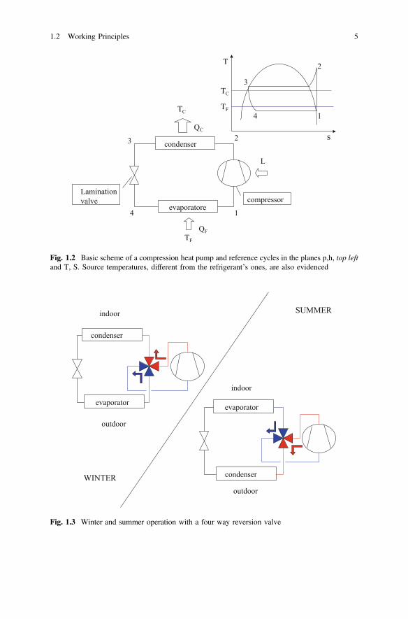
In the simplest configuration for residential uses a heat pump consists of anoutdoor unit, containing compressor and a heat exchanger working as an evaporatorin winter and a condenser in summer, and an indoor unit with another heatexchanger complementary to the previous one (condenser in winter and evaporatorin summer). If subscripts C and F respectively indicate the hot and cold sources, thefollowing relations hold (Figs. 1.2 and 1.3)2:

First Principle of Thermodynamics

QC þQF ¼ L ðQC\0; L\0ÞSecond Principle of ThermodynamicsQC

TCþ QF

TFþ Sg ¼ 0

1Bear in mind we have referred to reversible transformations, while real transformations are notsuch. In particular lamination is absolutely irreversible, so that we can only say (if adiabatic) itsfinal enthalpy is equal to its initial one and not isenthalpic.2Q > 0 if it is supplied to the system following the cycle and <0 if it exits from the system. Work Lis always negative in inverse cycles as it is supplied to the system.

1.1 General Features 3

Q is the heat exchanged with thermal sources, T their thermodynamic temperature(K) and Sg the amount of produced entropy. This is due to existing irreversibilitiesboth internal (e.g., friction losses in fluid motion, in mechanical devices etc.) andexternal, as the temperature jump between evolving fluid and thermal sources.

From the first relation we obtain that QF > 0 (supplied to cycle), L < 0 (suppliedto cycle), QC < 0 and, in addition |QC| > |QF|. It means that heat exchanged with thewarmer source (indoor environment in winter and outdoor environment in summer)is larger than the one with the colder source. If a heat pump is used both in winterand summer, the net total energy exchange with the external source may approachzero, depending on the durations of the winter and summer periods. It is afavourable phenomenon for the external environment once the external source canaccumulate and return this energy close to the user, as it occurs for geothermal heatpumps. Nevertheless the mechanical energy is provided to the heat pump all alongthe period of operation and the heat exchanged with the indoor environment has tobe considered as the produced “useful effect”.

A coefficient of performance, COP, is defined to characterize heat pumps per-formances as the ratio of heat exchanged with indoor environment and the

S

A

B

m,eq

SA SB

B

A

2 1

SSA SB

θ

θ

θ

(a)

(b)

Fig. 1.1 On top theequivalent heat exchangeaverage temperature. At thebottom the contributions tothis temperature of differentsegment of a transformation


condenser

evaporatorecompressor

Laminationvalve

ΤF

ΤC

L

QC

QF

ΤC

ΤF

Τ

s

1

1

2

2

3

3

4

4

Fig. 1.2 Basic scheme of a compression heat pump and reference cycles in the planes p,h, top leftand T, S. Source temperatures, different from the refrigerant’s ones, are also evidenced

condenser

evaporator

condenser

evaporator

indoor

indoor

outdoor

outdoorWINTER

SUMMER

Fig. 1.3 Winter and summer operation with a four way reversion valve

1.2 Working Principles 5

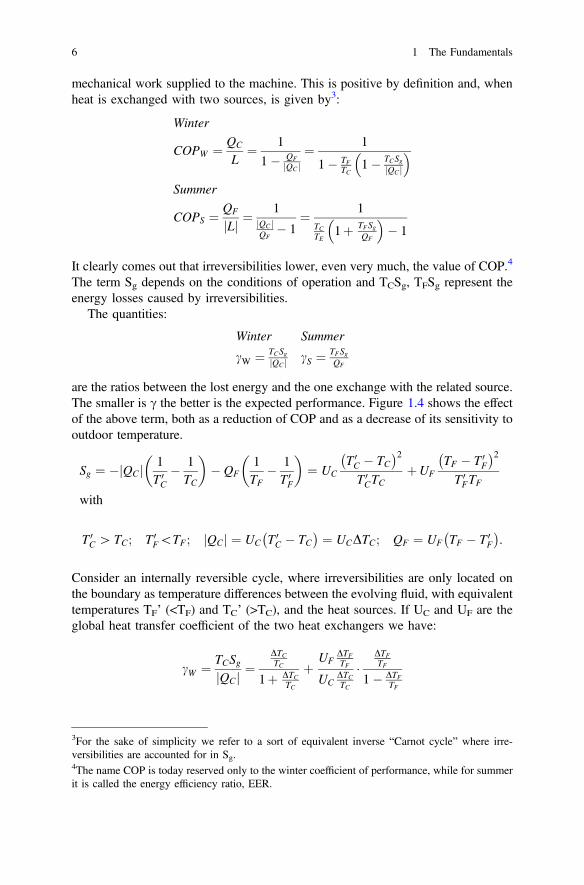
mechanical work supplied to the machine. This is positive by definition and, whenheat is exchanged with two sources, is given by3:

Winter

COPW ¼ QC

L¼ 1

1� QFQCj j

¼ 1

1� TFTC

1� TCSgQCj j

� �

Summer

COPS ¼ QF

Lj j ¼1

QCj jQF

� 1¼ 1

TCTE

1þ TFSgQF

� �� 1

It clearly comes out that irreversibilities lower, even very much, the value of COP.4

The term Sg depends on the conditions of operation and TCSg, TFSg represent theenergy losses caused by irreversibilities.

The quantities:

Winter Summer

cW ¼ TCSgQCj j cS ¼ TFSg

QF

are the ratios between the lost energy and the one exchange with the related source.The smaller is c the better is the expected performance. Figure 1.4 shows the effectof the above term, both as a reduction of COP and as a decrease of its sensitivity tooutdoor temperature.

Sg ¼ � QCj j 1T 0C� 1TC

� �� QF

1TF

� 1T 0F

� �¼ UC

T 0C � TC

� �2T 0CTC

þUFTF � T 0

F

� �2T 0FTF

with

T 0C [ TC; T 0

F\TF ; QCj j ¼ UC T 0C � TC

� � ¼ UCDTC; QF ¼ UF TF � T 0F

� �.

Consider an internally reversible cycle, where irreversibilities are only located onthe boundary as temperature differences between the evolving fluid, with equivalenttemperatures TF’ (<TF) and TC’ (>TC), and the heat sources. If UC and UF are theglobal heat transfer coefficient of the two heat exchangers we have:

cW ¼ TCSgQCj j ¼

DTCTC

1þ DTCTC

þ UFDTFTF

UCDTCTC

�DTFTF

1� DTFTF

3For the sake of simplicity we refer to a sort of equivalent inverse “Carnot cycle” where irre-versibilities are accounted for in Sg.4The name COP is today reserved only to the winter coefficient of performance, while for summerit is called the energy efficiency ratio, EER.


cS ¼TFSgQF

¼DTFTF

1� DTFTF

þ UCDTCTC

UFDTFTF

�DTCTC

1þ DTCTC

For a preliminary evaluation of the above quantities we can refer to the followingvalues for an air/air heat pump:

Seasons TF (°C) TC (°C)

Winter 7 20

Summer 27 35

For the sake of simplicity, we can suppose UC = UF = U and DTC = DTF = DT(remember T is expressed in °C and T in K) and thus (see the trends in Fig. 1.5):

Winter (indoor temperature, TC =20°C)

0

10

20

30

40

50

60

-10 -8 -6 -4 -2 0 2 4 6 8 10 12 14TF (ºC)

TC (ºC)

CO

P

γ=0

γ=0.01

γ=0.05

γ=0.1

γ=0.2

Summer (indoor temperature, TF=24°C)

0102030405060708090

100

27 29 31 33 35 37 39 41 43 45 47 49

CO

P

γ=0γ=0.01γ=0.05γ=0.1

(a)

(b)

Fig. 1.4 Trend of COP in winter (a) and summer (b) versus outdoor temperature for severalvalues of c


cW ¼DTTC

1þ DTTC

þDTTFDTTC

�DTTF

1� DTTF

cS ¼DTTF

1� DTTF

þDTTCDTTF

�DTTC

1þ DTTC

What has been said so far emphasizes some basic thermodynamic aspects affectingthe performances of a heat pump operating between two thermal sources. Of coursereferring to an equivalent inverse Carnot cycle is a convenient simplification tounderstand the fundamental working principles of this type of machine. Anyway,before going forward, it is the case to stress the main differences between the abovereference scheme and the real behavior. They can be listed as follows (Fig. 1.6).

• Fluids actually used can keep their temperatures reasonably constant as theyundergo a phase change. Due to the close link between temperature and pressurein these transformations, a constant pressure is needed to have a constanttemperature. This could be only achieved by neglecting friction losses in heatexchangers. In addition, due to the nature of some refrigerants, temperaturechanges occur also at constant pressure (Glide) as we will see in the following.Furthermore superheated vapor discharging from the compressor is cooleddown, before reaching the saturated condition. Energy subtracted in this phasein a dedicated de-superheater is sometimes employed for different uses fromambient heating as the production of hot sanitary water. In the end liquid exitingfrom evaporator generally has some superheating to avoid liquid inlet into thecompressor as well as liquid from evaporator is slightly subcooled not to havevapor in the expansion valve.

• The expansion valve causes an unavoidable irreversibility, because it is notconvenient to recover energy from the related pressure difference.

• Compressor is characterized by friction losses, is not adiabatic and so on. Allthis leads to define the so called isentropic efficiency.

00,010,020,030,040,050,060,070,080,09

0,10,11

0 1 2 3 4 5 6 7 8 9 10 11 12 13 14 15ΔT

γwinter

summer

Fig. 1.5 Trends of c versus DT in summer and winter


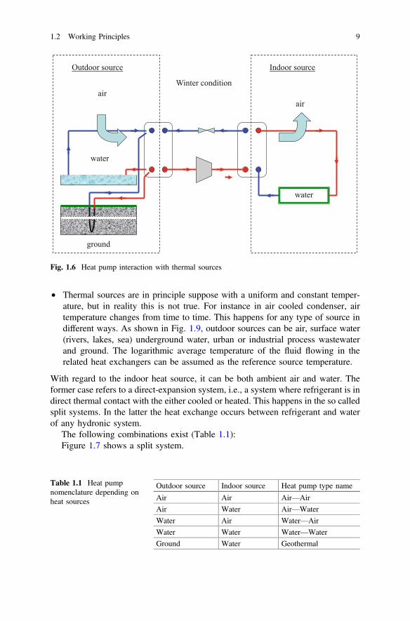
• Thermal sources are in principle suppose with a uniform and constant temper-ature, but in reality this is not true. For instance in air cooled condenser, airtemperature changes from time to time. This happens for any type of source indifferent ways. As shown in Fig. 1.9, outdoor sources can be air, surface water(rivers, lakes, sea) underground water, urban or industrial process wastewaterand ground. The logarithmic average temperature of the fluid flowing in therelated heat exchangers can be assumed as the reference source temperature.

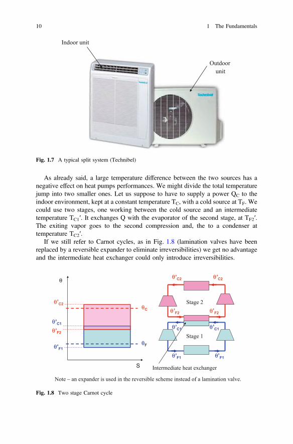
With regard to the indoor heat source, it can be both ambient air and water. Theformer case refers to a direct-expansion system, i.e., a system where refrigerant is indirect thermal contact with the either cooled or heated. This happens in the so calledsplit systems. In the latter the heat exchange occurs between refrigerant and waterof any hydronic system.

The following combinations exist (Table 1.1):Figure 1.7 shows a split system.

Outdoor source Indoor source

airair

water

water

ground

Winter condition

Fig. 1.6 Heat pump interaction with thermal sources

Table 1.1 Heat pumpnomenclature depending onheat sources

Outdoor source Indoor source Heat pump type name

Air Air Air—Air

Air Water Air—Water

Water Air Water—Air

Water Water Water—Water

Ground Water Geothermal


As already said, a large temperature difference between the two sources has anegative effect on heat pumps performances. We might divide the total temperaturejump into two smaller ones. Let us suppose to have to supply a power QC to theindoor environment, kept at a constant temperature TC, with a cold source at TF. Wecould use two stages, one working between the cold source and an intermediatetemperature TC1′. It exchanges Q with the evaporator of the second stage, at TF2′.The exiting vapor goes to the second compression and, the to a condenser attemperature TC2′.

If we still refer to Carnot cycles, as in Fig. 1.8 (lamination valves have beenreplaced by a reversible expander to eliminate irreversibilities) we get no advantageand the intermediate heat exchanger could only introduce irreversibilities.

Outdoor unit

Indoor unit

Fig. 1.7 A typical split system (Technibel)

θ

θC

S

θ C2

θFθ F1

θ F2

θ C1

Stage 1

Stage 2

θ F1 θ F1

θ C1θ C1

θ C2 θ C2

θ F2 θ F2

Note – an expander is used in the reversible scheme instead of a lamination valve.

Intermediate heat exchanger

’

’’

’’ ’

’ ’

’ ’

’ ’

Fig. 1.8 Two stage Carnot cycle


Just as an example we describe the relations holding for a two stage cycle.Figure 1.9 refers to the temperature enthalpy plane to point out the varioustemperatures.

Example 1.1 With reference to Fig. 1.9 we designate with subscript 1 thequantities referring to the lower temperature stage and with subscript 2 thosereferring to the higher temperature stage. If mk (k = 1 or 2) is the mass flowrate, h the enthalpy, QC the heat delivered to the indoor environment and Lk

(k = 1 or 2) the compression work for each simple cycle we get:Stage 2

QC ¼ m2 hf � hg� �

L2 ¼ m2 he � hf� �

and

COP stage 2ð Þ ¼ hf � hg� �he � hf� �

Stage 1

Qc;1 ¼ m1 hf � he� �

And the compression work

L1 ¼ m1 ha � hbð Þ L2 ¼ m2 he � hf� �

L ¼ L1 þ L2

θ θ

S S

a

b

c

d

e

f

g

h

f’

b’

Cycle 1

Cycle 2

Fig. 1.9 Double stage cycle


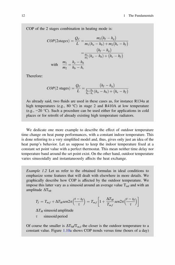
COP of the 2 stages combination in heating mode is:

COPð2stagesÞ ¼ QC

L¼ m2 hf � hg

� �m1 ha � hbð Þþm2 he � hf

� �

¼ hf � hg� �

m1m2

ha � hbð Þþ he � hf� �

withm1

m2¼ he � hh

hb � hc

Therefore:

COPð2 stagesÞ ¼ QC

L¼ hf � hg

� �he�hhhb�hc

ha � hbð Þþ he � hf� �

As already said, two fluids are used in these cases as, for instance R134a athigh temperatures (e.g., 80 °C) in stage 2 and R410A at low temperature(e.g., −20 °C). Such a procedure can be used either for applications in coldplaces or for retrofit of already existing high temperature radiators.

We dedicate one more example to describe the effect of outdoor temperaturetime change on heat pump performances, with a constant indoor temperature. Thisis done referring to a very simplified model and, thus, gives only just an idea of theheat pump’s behavior. Let us suppose to keep the indoor temperature fixed at aconstant set point value with a perfect thermostat. This mean neither time delay nortemperature band around the set point exist. On the other hand, outdoor temperaturevaries sinusoidally and instantaneously affects the heat exchange.

Example 1.2 Let us refer to the obtained formulas in ideal conditions toemphasize some features that will dealt with elsewhere in more details. Wegraphically describe how COP is affected by the outdoor temperature. Weimpose this latter vary as a sinusoid around an average value Tmf and with anamplitude DTM.

Tf ¼ Tm;f þDTMsen2pt � t0s

� �¼ Tm;f 1þ DTM

Tm;fsen2p

t � t0s

� ��

DTM sinusoid amplitude

s sinusoid period

Of course the smaller is DTM/Tm,f the closer is the outdoor temperature to aconstant value. Figure 1.10a shows COP trends versus time (hours of a day)


in the cases of Tm,f = 8 °C e DTM = 5 °C (rhombs) and Tm,f = 10 °C eDTM = 1 °C (square). In Fig. 1.10b the ratio of the instantaneous COP to theone, COP(Tm,f), calculated at the average temperature, Tm,f, is reported versusthe ratio between the temperature and its average daily value, Tm,f.

This stresses the influence of the outdoor heat source. As above said, in thefirst case we refer to outdoor air, while in the second case the outdoor sourcemight be water with a higher average temperature value and a lower tem-perature fluctuation. All this, herein evidenced for a single day, has a muchgreater importance if referred to seasonal performances.

To account for this a seasonal COP is used (SCOP), defined as the ratiobetween the useful energy supplied during the related season and the energythat has to be provided to the heat pump to obtain this useful energy.

05

1015202530354045

outdoor souce air outdoor source water

00,20,40,60,8

11,21,41,61,8

0 1 2 3 4 5 6 7 8 9 10 11 12 13 14 15 16 17 18 19 20 21 22 23

0,98 0,985 0,99 0,995 1 1,005 1,01 1,015 1,02Tf/Tmf

CO

P/C

OP

(Tm

f)

outdoor source: air outdoor source: water

time (hour)

CO

P

(a)

(b)

Fig. 1.10 a COP versus time in case of outdoor sources air (rhombs) and water (squares), b Ratioof instantaneous COP and COP(Tm,f) calculated at the average temperature, Tm,f versus T/Tm,f


References

1. European Heat Pumps Market and Statistics 2015 by EHPA.2. Growth in the world heat pump market August 2014 https://www.bsria.com/news/article/

growth-in-the-world-heat-pump-market/.3. Heat Pumps Market: Global Industry Analysis and Opportunity Assessment 2015–2025. http://

www.futuremarketinsights.com/reports/heat-pumps-market.


https://www.bsria.com/news/article/growth-in-the-world-heat-pump-market/

https://www.bsria.com/news/article/growth-in-the-world-heat-pump-market/

http://www.futuremarketinsights.com/reports/heat-pumps-market

http://www.futuremarketinsights.com/reports/heat-pumps-market

Chapter 2Types of Compression Heat Pumpsand Their Main Components

Abstract The main components of compression heat pumps are treated herein.Their salient features, working principles and roles are dealt with, stressing theircontribution to heat pumps operation and efficiency. Furthermore, products existingon the market are often referred to in order to allow the interested reader to have, atleast, a rough idea of the available equipment, nowadays. Engine driven heatpumps, also named Gas Heat Pumps (GHP) are described in addition to the mostcommonly used electric heat pumps (EHP). Except for the driving motor, GHPsdiffer from EHPs both from the thermodynamic point of view, as they interact withthree heat sources (they are a three-thermal-system), and for the possibility of usingheat recovered by engine cooling. Last but not least, part of this chapter is devotedto describe CO2 heat pumps, due their peculiarity. In fact carbon dioxide has a verylow critical temperature and, thus, they operate in hyper-critical condensions inmost cases. Due to this a gas cooler is employed instead of a classical condenser.

2.1 Main Components of Compression Heat Pumps

From the scheme we have referred to so far, it clearly comes out that the maincomponents of compression heat pumps are:

• the compressor, that keeps the right pressure drop between evaporator andcondenser to maintain the proper phase change temperatures to interact with theexternal (to the HP) sources;

• the expansion valve, irreversibly taking the refrigerant from the condenserpressure to the one of the evaporator;

• the condenser, where the superheated vapor coming from the compressor isde-superheated, first, then condensed to liquid with some degree of sub coolingto prevent vapor from entering the expansion valve;

• the evaporator, where the mixture coming from the expansion device vaporizes.The exiting vapor can be either saturated (wet evaporator) or superheated (dryevaporator). In the former case a proper device (separator) is needed to preventliquid from entering the compressor. In the latter case the vapor leaving theevaporator has a superheat of few degrees Celsius for the same purpose.


15

2.2 Compressor

Heat pumps mainly adopt volumetric compressors. They may be both reciprocatingand rotary compressors. We will refer to the former ones to describe the mainfeatures of this type of device.

2.2.1 Reciprocating Compressor and Basic Concepts

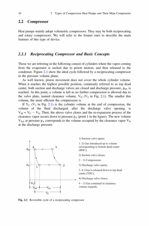
Those we are referring in the following consist of cylinders where the vapor comingfrom the evaporator is sucked due to piston motion, and then released to thecondenser. Figure 2.1 show the ideal cycle followed by a reciprocating compressorin the pressure volume plane.

As well known, piston movement does not cover the whole cylinder volume.When it reaches the highest possible position, commonly referred to as top deadcenter, both suction and discharge valves are closed and discharge pressure, pM, isreached. At this point, a volume is left as no further compression is allowed due tothe valve plate, named clearance volume, VN (V4 in Fig. 2.1). The smaller thisvolume, the more efficient the compression is.

If VC (V3 in Fig. 2.1) is the cylinder volume at the end of compression, thevolume of the fluid discharged, after the discharge valve opening, isVM = VC − VN. Then, the above valve closes and the re-expansion process of theclearance vapor occurs down to pressure pA (point 1 in the figure). The new volumeVNA at pressure pA corresponds to the volume occupied by the clearance vapor VN

at the discharge pressure.

VA

VN

VNA VAS

pM

pA1 2

3 4

1) Suction valve opens;

1 -2) Gas introduced up to volume corresponding to bottom dead center (BDC);

2) Suction valve closes;

2 – 3) Compression;

3) Discharge valve opens;

3 -4 ) Gas is released down to top dead center (TDC);

4) Discharge valve closes;

4 – 1) Gas contained in clearance volume expands.

Fig. 2.1 Reversible cycle of a reciprocating compressor

16 2 Types of Compression Heat Pumps and Their Main Components

The suction valve opens at pressure pA (BTD bottom dead center) and vaporenters the compressor. The volume VA = V2 − VN is the theoretical volume thatcould be sucked and VAS = V2 − VAN = VA − (VAN − VN) is the actual volumesucked by the compressor. The ratio VAS/VA is named the compressor volumetricefficiency.

Example 2.1 Let us consider the isentropic compression of an ideal gas, in acylinder with a clearance volume VN. Let us identify with VA the availablevolume at suction and with pA, TA, pB, and TB respectively the pressures andtemperatures (K) at the suction and discharge points.

The number of moles, nN, contained in the clearance volume is

nN ¼ pMVN

RTM

At suction, in the absence of clearance volume the numbers of moles thatcould be sucked would be:

nA ¼ pAVA

RTA

Actually (in the presence of clearance volume) we can suck a number ofmoles, nAS, equal to the difference between these latter diminished by thenumber of moles contained in the clearance volume.

nAS ¼ nA � nN ¼ pAVA

RTA� pAVNA

RTA¼ pAVAS

RTA

The volumetric efficiency, ηv, of the compressor is:

gv ¼VAS

VA¼ 1þ VN

VA1� b1=k� �

where b = pM/pA is the barometric compression ratio (simply called compressionratio) and k is the ratio between the gas specific heats or, more in general thepolytrophic exponent. The clearance volume commonly varies between 2 and 5%of VA. Thus, if we assume a value of 5% and k = 1.4, values can be calculated bythe following formula:

gv ¼ 1þ 0:05 1� b0:714� �

2.2 Compressor 17

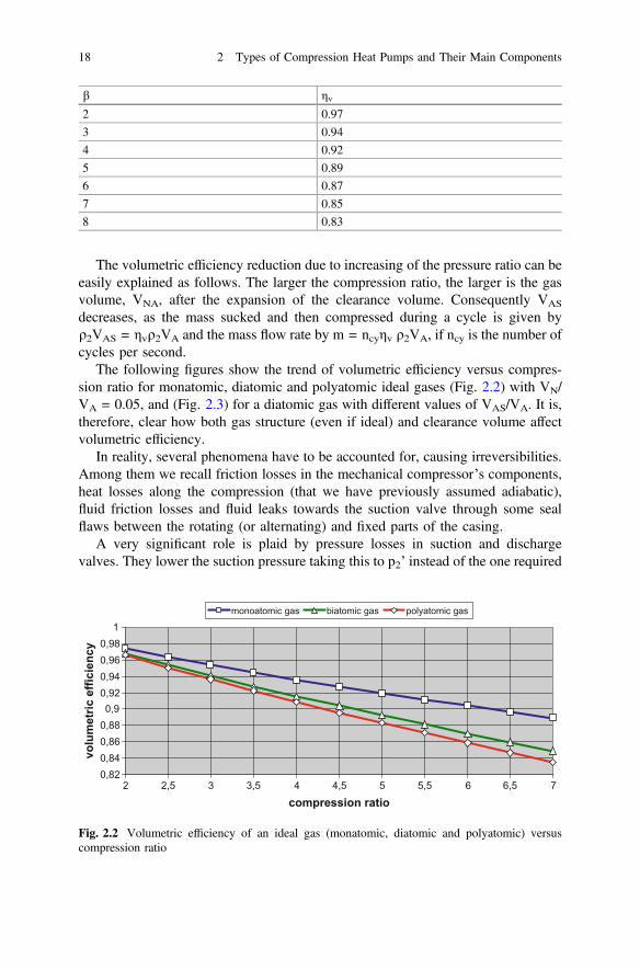
b ηv2 0.97

3 0.94

4 0.92

5 0.89

6 0.87

7 0.85

8 0.83

The volumetric efficiency reduction due to increasing of the pressure ratio can beeasily explained as follows. The larger the compression ratio, the larger is the gasvolume, VNA, after the expansion of the clearance volume. Consequently VAS

decreases, as the mass sucked and then compressed during a cycle is given byq2VAS = ηvq2VA and the mass flow rate by m = ncyηv q2VA, if ncy is the number ofcycles per second.

The following figures show the trend of volumetric efficiency versus compres-sion ratio for monatomic, diatomic and polyatomic ideal gases (Fig. 2.2) with VN/VA = 0.05, and (Fig. 2.3) for a diatomic gas with different values of VAS/VA. It is,therefore, clear how both gas structure (even if ideal) and clearance volume affectvolumetric efficiency.

In reality, several phenomena have to be accounted for, causing irreversibilities.Among them we recall friction losses in the mechanical compressor’s components,heat losses along the compression (that we have previously assumed adiabatic),fluid friction losses and fluid leaks towards the suction valve through some sealflaws between the rotating (or alternating) and fixed parts of the casing.

A very significant role is plaid by pressure losses in suction and dischargevalves. They lower the suction pressure taking this to p2’ instead of the one required

0,820,840,860,880,9

0,920,940,960,98

1

2 2,5 3 3,5 4 4,5 5 5,5 6 6,5 7

compression ratio

monoatomic gas biatomic gas polyatomic gas

volu

met

ric e

ffici

ency

Fig. 2.2 Volumetric efficiency of an ideal gas (monatomic, diatomic and polyatomic) versuscompression ratio


by the heat exchange with the cold source p2 = pA, and cause the discharge pressureto be increased (to a value p3’) instead of the one required by the heat exchangewith the hot source, p3 = pM.

There exist some other reasons (see also the screw and scroll compressors)causing a difference between the pressures actually imposed by compressor andthose imposed by external thermal sources. The actual pressure ratio occurring inthe compressor, p3’/p2’ = b’, is called the internal compressor ratio and may bedifferent from the previously defined b = p3/p2, also named the external compressorratio. The above mentioned phenomena contribute to modify the volumetric effi-ciency and the work achievable.

All this leads to introduce the isentropic efficiency, qc, defined as the ratio of theideal enthalpy difference between discharge and suction, Δh, and the actual one,Δh’ (Fig. 2.4).

qc ¼DhDh0

¼ h3 � h2ðh30 � h3MÞþ ðh3M � h2AÞþ ðh2A � h2Þ

In the case where external compression ratio is equal to the internal one, the worksupplied to compressor in the presence of friction (la) is given by:

l ¼ �Z3M2

vdp� la ¼ cp T2 � T3Mð Þ ¼ cpT2 1� pMpA

� �p�1p

" #

Points 3 M and 2A respectively are at the same pressures as 3 and 2, p is theexponent of the real adiabatic transformation, and the work is negative as suppliedto the system and T the absolute temperature (K).

Recalling that, on the polytrophic 2’-3’1

0,6

0,7

0,8

0,9

1

2 2,5 3 3,5 4 4,5 5 5,5 6 6,5 7

VN/VA=0,01 VN/VA=0,05 VN/VA=0,1

compression ratio

volu

met

ric e

ffici

ency

Fig. 2.3 Volumetric efficiency versus compression ratio for various VN/VA

1Remember we are referring to an equivalent reversible transformation.

2.2 Compressor 19

Z3M2

Tds ¼ la

We can display friction losses on the plane T, s as the area underneath the curve2−3 M. Area 2−3−3 M represents the energy related to the compressed gas heatingup:

Areað2� 3� 3MÞ ¼Z3M2

Tds� la ¼ cpðT3M � T2Þ � la

This phenomenon is called “thermal recovery”.

p

v

pA

pM

2

3 3M

3’

2’

2A

pA

pM

p3’

p2’

Τ

S

2

3’

3

3M

2A

2’

p

h

pM

pA2

3

3’

2’

Δh Δh’

Ideal transf.

Real transf.

2A

3M

Fig. 2.4 Ideal and real compression in the planes p,h, p,v and T,S


To better describe the compressor technical features, a hydraulic efficiency isdefined as:

qy ¼lþ lal

¼ � R 3M2 vdp

cpT2 1� pMpA

� �p�1p

� ¼p

p�1 pAv2 1� pMpA

� �p�1p

� k

k�1 pAv2 1� pMpA

� �p�1p

�

¼p

p�1k

k�1

¼ pkk � 1p� 1

Such a parameter does not depend on compression ratio. Once the hydraulic orpolytropic efficiency2 is known, the exponent of the polytropic curve can beobtained and viceversa. Therefore the isentropic efficiency can be written as:

qc ¼h2 � h3h2 � h3M

¼ T3 � T2T3M � T2

¼ bk�1k � 1

b1qy

k�1k � 1

; b ¼ pMpA

It decreases with the compression ratio and depends on the type of fluid through k,ratio between the specific heats at constant pressure and volume. After recalling thatk = 1.4 for standard air, some values of this parameter are given in Table 2.1 forfour gas used in heat pumps.

Figure 2.5 shows the theoretical trend (calculated here in) of the isentropicefficiency versus the compression ratio at constant values of the hydraulic effi-ciency, with k = 1.11 (continuous line), and k = 1.29 (dotted line).

As already said, the pressure existing in the compressor, both at suction anddischarge, is not the same as the one present in the circuit just before the suction andafter the discharge. Therefore we introduced two compression ratios the internal, b’,and the external, b, ones.

Three different cases can occur, for reciprocating, screw and scroll compressors,as follows.

Table 2.1 Values ofk = cp/cv for somerefrigerants

Fluid k T (°C) p (bar)

NH3 1.31 0 1

CO2 1.29 27 1

R134a 1.11 30 1

R437 1.15 25 1

2The name “hydraulic efficiency” refers to the fact that the thermal recovery is negligible in thehydraulic machines, so that this efficiency is equal to 1. This parameter is also called “the poly-tropic efficiency” because a reference reversible polytropic is usually considered, with an averageexponent equal to that of the actual transformation.

2.2 Compressor 21

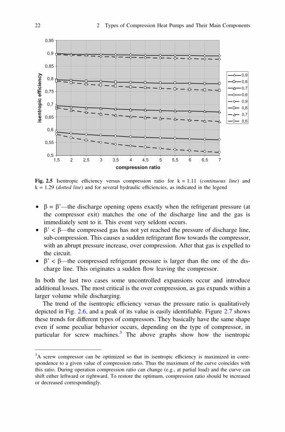
• b = b’—the discharge opening opens exactly when the refrigerant pressure (atthe compressor exit) matches the one of the discharge line and the gas isimmediately sent to it. This event very seldom occurs.

• b’ < b—the compressed gas has not yet reached the pressure of discharge line,sub-compression. This causes a sudden refrigerant flow towards the compressor,with an abrupt pressure increase, over compression. After that gas is expelled tothe circuit.

• b’ < b—the compressed refrigerant pressure is larger than the one of the dis-charge line. This originates a sudden flow leaving the compressor.

In both the last two cases some uncontrolled expansions occur and introduceadditional losses. The most critical is the over compression, as gas expands within alarger volume while discharging.

The trend of the isentropic efficiency versus the pressure ratio is qualitativelydepicted in Fig. 2.6, and a peak of its value is easily identifiable. Figure 2.7 showsthese trends for different types of compressors. They basically have the same shapeeven if some peculiar behavior occurs, depending on the type of compressor, inparticular for screw machines.3 The above graphs show how the isentropic

0,5

0,55

0,6

0,65

0,7

0,75

0,8

0,85

0,9

0,95

1,5 2 2,5 3 3,5 4 4,5 5 5,5 6 6,5 7compression ratio

isen

trop

ic e

ffici

ency 0,9

0,80,70,60,90,80,70,6

Fig. 2.5 Isentropic efficiency versus compression ratio for k = 1.11 (continuous line) andk = 1.29 (dotted line) and for several hydraulic efficiencies, as indicated in the legend

3A screw compressor can be optimized so that its isentropic efficiency is maximized in corre-spondence to a given value of compression ratio. Thus the maximum of the curve coincides withthis ratio. During operation compression ratio can change (e.g., at partial load) and the curve canshift either leftward or rightward. To restore the optimum, compression ratio should be increasedor decreased correspondingly.


efficiency could also increase with a reduction of the compression ratio.Furthermore the typical trends of the volumetric efficiency are displayed in the samefigure.

The thermodynamic cycle irreversibilities play a different role on heat pumpsperformances in winter and in summer. In fact, in winter, the useful effect (i.e., theuseful heating output) h2 − h3, increases, due to the increase of the compressionwork, h2′ − h2. Thus the COP changes as below:

0,4

0,45

0,5

0,55

0,6

0,65

0,7

0,75

0,8

0,85

2 2,5 3 3,5 4 4,5 5 5,5 6

compression ratio

isen

trop

ic e

ffici

ency

Fig. 2.6 Typical trend of a compressor isentropic efficiency

compression ratio

compression ratio

isen

tropi

c ef

ficie

ncy

reciprocating

screw scroll

scroll screw

reciprocating

volu

met

ric e

ffici

ency

100%

50%

1 10 20

100%

72%

50%

1 7 10 14 20

Fig. 2.7 Typical trends ofisentropic efficiency (topgraph) and of volumetricefficiency (lower graph)versus compression ratio forreciprocating, screw andscroll compressors

2.2 Compressor 23

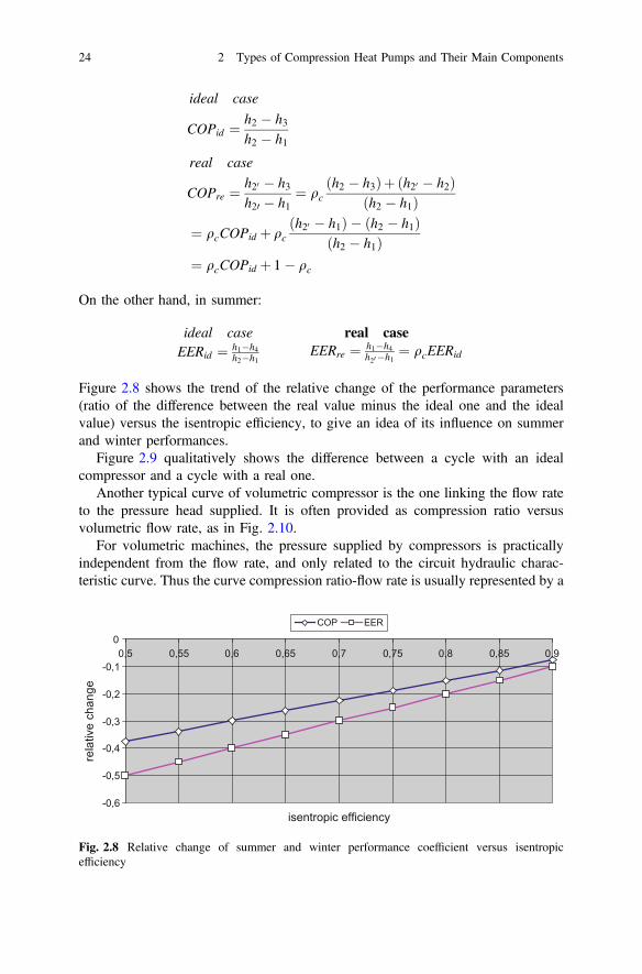
ideal case

COPid ¼ h2 � h3h2 � h1

real case

COPre ¼ h20 � h3h20 � h1

¼ qch2 � h3ð Þþ h20 � h2ð Þ

h2 � h1ð Þ¼ qcCOPid þ qc

h20 � h1ð Þ � h2 � h1ð Þh2 � h1ð Þ

¼ qcCOPid þ 1� qc

On the other hand, in summer:

ideal case real caseEERid ¼ h1�h4

h2�h1EERre ¼ h1�h4

h20�h1¼ qcEERid

Figure 2.8 shows the trend of the relative change of the performance parameters(ratio of the difference between the real value minus the ideal one and the idealvalue) versus the isentropic efficiency, to give an idea of its influence on summerand winter performances.

Figure 2.9 qualitatively shows the difference between a cycle with an idealcompressor and a cycle with a real one.

Another typical curve of volumetric compressor is the one linking the flow rateto the pressure head supplied. It is often provided as compression ratio versusvolumetric flow rate, as in Fig. 2.10.

For volumetric machines, the pressure supplied by compressors is practicallyindependent from the flow rate, and only related to the circuit hydraulic charac-teristic curve. Thus the curve compression ratio-flow rate is usually represented by a

-0,6

-0,5

-0,4

-0,3

-0,2

-0,1

00,5 0,55 0,6 0,65 0,7 0,75 0,8 0,85 0,9

isentropic efficiency

COP EER

rela

tive

chan

ge

Fig. 2.8 Relative change of summer and winter performance coefficient versus isentropicefficiency


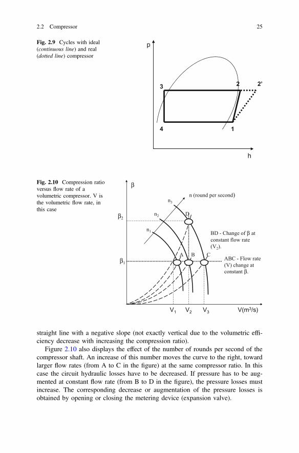
straight line with a negative slope (not exactly vertical due to the volumetric effi-ciency decrease with increasing the compression ratio).

Figure 2.10 also displays the effect of the number of rounds per second of thecompressor shaft. An increase of this number moves the curve to the right, towardlarger flow rates (from A to C in the figure) at the same compressor ratio. In thiscase the circuit hydraulic losses have to be decreased. If pressure has to be aug-mented at constant flow rate (from B to D in the figure), the pressure losses mustincrease. The corresponding decrease or augmentation of the pressure losses isobtained by opening or closing the metering device (expansion valve).

1

23

4

p

h

2’

Fig. 2.9 Cycles with ideal(continuous line) and real(dotted line) compressor

n (round per second)β

V(m3/s)

ABC - Flow rate (V) change at constant β.

BD - Change of β at constant flow rate (V2).

β1

β2

V1 V2 V3

A B C

D

n1

n2

n3

Fig. 2.10 Compression ratioversus flow rate of avolumetric compressor. V isthe volumetric flow rate, inthis case

2.2 Compressor 25

The characteristic number of rounds per minute of compressors may be also verydifferent for the different types. For example, for reciprocating compressors, theyroughly go from a hundred for large and slow compressors with compression ratio2–3, to a thousand for the smallest ones with a compression ratio around 10.

In rotary compressors there might be several thousands rounds per minute.

2.2.2 Screw Compressors

Thanks to the technological progress in heating and cooling applications, rotarycompressors are often employed instead of reciprocating compressors.

Among other things this is due to their smaller size, larger silentness, smoothlyrunning, low vibration and better control and modulation capability. They can beroughly divided in compressors with a single rotating axis (vane and scroll) andwith two rotating axes. Among them we include vane, lobe, screw and scrollcompressors. Vane and scroll compressors have a single shaft (single rotation axis),while the others can have both one and two axes. In general, screw compressorshave two axes, i.e., two screws.

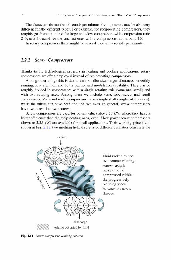
Screw compressors are used for power values above 50 kW, where they have abetter efficiency than the reciprocating ones, even if low power screw compressors(down to 2.25 kW) are available for small applications. Their working principle isshown in Fig. 2.11: two meshing helical screws of different diameters constitute the

volume occupied by fluid

suction

discharge

Fluid sucked by the two counter-rotating screws axially moves and is compressed within the progressively reducing space between the screw threads.

Fig. 2.11 Screw compressor working scheme


compressor rotors. Gas enters at the suction side and moves through the threads asthe screws rotate. They force the gas to the discharge port at the end of the screws,progressively reducing the gas volume.

Generally they have smaller compression ratios (b = 3:4) than the reciprocatingcompressors, they can be used with several stages in series.

The most common configuration consists of a male rotor with four lobes and afemale one with six indentations. Other possible configurations are 3(lobs)/5(in-dentations) and 5/7. Rotor diameters commonly ranges from 12 to 32 mm.

Rotors are located in horizontal cylindrically shaped casings provided withsuction and discharge ports. Lubricating oil is injected on the threads to preventrefrigerant leakages, thanks to the presence of an oil film. It is then recovered in anoil separator located close to the discharge port.

Suction phase begins when the two moving rotors leave the suction port open.Fluid enters the compression region and moves along the screw axes. The suctionport is closed by the engaging rotors and compression starts, with the discharge portclosed.

The ratio, vi, between the initial (suction) and final (discharge) volumes is the socalled “intrinsic volumetric ratio”. Some typical values are 2.2; 2.6; 3.2; 4.4.A given compression ratio corresponds to each vi, depending on refrigerant prop-erties. For a given fluid an optimal (top isentropic efficiency) compression ratio canbe realized, by using an appropriate intrinsic volumetric ratio. What has been saidabove about over and sub compression holds also for this type of compressors.

2.2.3 Vane and Scroll Compressors

Vane and scroll compressors are mainly employed at the lowest power values.Figure 2.12 shows the scheme of a vane compressor. The rotor is eccentricallyplaced with respect to the casing. On this, suction and discharge ports are located,

suction

discharge

Fig. 2.12 Vane compressor working scheme

2.2 Compressor 27

without any valve. Sliding vanes are located on the rotor and pushed against thecylindrical casing by centrifugal forces produced by rotation. They originatechambers with a progressively decreasing volume from suction to discharge.A good continuity of the refrigerant flow is guaranteed, in this case too.

Scroll compressors are basically constituted by two scrolls (spirals), a fixed and amovable one, sketched in Fig. 2.13. The latter is driven by a shaft that makes itorbit (not rotate) about the shaft axis. So, a chamber is formed, compression startsonce the suction port is sealed off, progressively reducing the gas volume betweenthe two scrolls.

Seal between fixed and movable scroll is guaranteed by a lubricating oil film. Asabove said the chamber is in contact with suction, and fluid flows in. After a90°-rotation, the scroll movement closes the suction port, refrigerant stays confinedwithin the two scrolls and gradually compressed until it is released to the dischargeduct.4

As all compressors without suction and discharge valves,5 they have largerisentropic and volumetric efficiencies than the reciprocating ones. They are com-monly inserted in a hermetic shell together with the driving electric motor. A typicalconfiguration is shown in Fig. 2.14.

fixed scroll

Orbiting movable scroll

P

P

high pressure pocket

low pressure pocket

movable scroll

(a) (b)

(c) (d)

discharge duct

Moving spiral, by orbiting on fixed scroll, figures (a) and (b), forms progressively smaller chambers (pockets), as in figures (c) and (d).

Fig. 2.13 Working scheme of scroll compressor

4Videos existing on You-tube may help clarify scroll compressor operation.5Actually, a dynamic discharge valve can be adopted in particular in high pressure ratio appli-cations typical of refrigeration. It is located at the scroll discharge port to prevent entry of highpressure gas into the scroll set during the unloaded state.


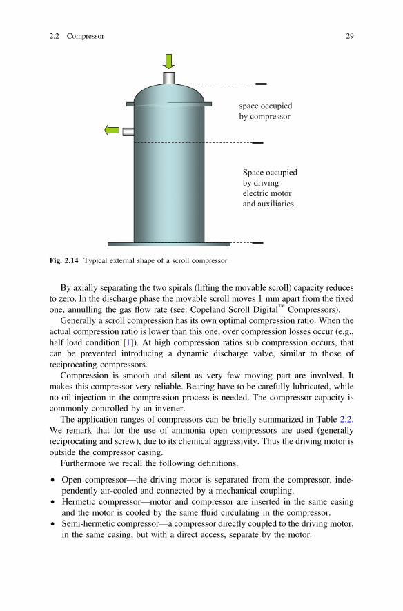
By axially separating the two spirals (lifting the movable scroll) capacity reducesto zero. In the discharge phase the movable scroll moves 1 mm apart from the fixedone, annulling the gas flow rate (see: Copeland Scroll Digital™ Compressors).

Generally a scroll compression has its own optimal compression ratio. When theactual compression ratio is lower than this one, over compression losses occur (e.g.,half load condition [1]). At high compression ratios sub compression occurs, thatcan be prevented introducing a dynamic discharge valve, similar to those ofreciprocating compressors.

Compression is smooth and silent as very few moving part are involved. Itmakes this compressor very reliable. Bearing have to be carefully lubricated, whileno oil injection in the compression process is needed. The compressor capacity iscommonly controlled by an inverter.

The application ranges of compressors can be briefly summarized in Table 2.2.We remark that for the use of ammonia open compressors are used (generallyreciprocating and screw), due to its chemical aggressivity. Thus the driving motor isoutside the compressor casing.

Furthermore we recall the following definitions.

• Open compressor—the driving motor is separated from the compressor, inde-pendently air-cooled and connected by a mechanical coupling.

• Hermetic compressor—motor and compressor are inserted in the same casingand the motor is cooled by the same fluid circulating in the compressor.

• Semi-hermetic compressor—a compressor directly coupled to the driving motor,in the same casing, but with a direct access, separate by the motor.

space occupiedby compressor

Space occupiedby drivingelectric motorand auxiliaries.

Fig. 2.14 Typical external shape of a scroll compressor

2.2 Compressor 29

2.2.4 Control of Compressors’ Operation

Compressors must be enabled to work off their nominal load. The on-off control isthe simplest way to reach this goal, but it is the most energy consuming. In thisway, the reference signal is a set point temperature, TSP, fixed by a thermostat.When this value is exceeded by ΔTSP (depending on thermostat accuracy) thecompressor turns off. It starts again once the temperature achieves the valueTSP − ΔTSP.

In order to keep comfort conditions within the internal environment, ΔTSP

should be as little as possible, but it could cause too many on- offs, thus stressingtoo much both compressor and driving motor during start-up phases. Besides, thiswould produce a COP decrease.

Therefore some techniques have been implemented to work at partial load.In multicylinder6 reciprocating compressor one or more cylinders are made

ineffective. This is done by bypassing fluid from suction to discharge of the cylinderwe want to deactivate, by signals sent to a solenoid valve. So we obtain a stepreduction of the active cylinders number as shown in Table 2.3.

Therefore the number of on-off is reduced. The load to be supplied to thecompressor does not proportionally decrease with the percent of reduction (e.g., a33% reduction may correspond to 40% of the nominal load), as the ineffectivecylinders are anyway operated by the crankshaft, consuming power.

Table 2.2 Main types of compressors

Type Model Capacity(kW)

Refrigerant Application

Reciprocating – Hermetic– Semi hermetic– Open

0.1/3030/250250/50

R134aR404AR407AR407CR717R744

Industrial and commercialrefrigerators, low temperatureindustrial refrigeration

Vane Hermetic 0.75/3 R407CR410AR744

Small refrigerators, portableair-conditioning, split systems

Scroll Hermetic 3.5/90 R407CR410A

Low and medium sizeair-conditioning

Screws – Semihermetic– open

80/8000 R407CR134aR717

Medium and large power airconditioning. Industrialrefrigeration

Single screw – Semi hermetic– Open

100/500 R134aR410A

Medium and large power chillersfor commercial and industrialclimatization

6The multiple cylinder compressor has also the advantage to keep the fluid flow smoother.


A method to obtain a continuous modulation (at least in a given range) consistsin changing the rotation speed of the driving motor (being it an electric motor or aninternal combustion engine).

Electric heat pumps often use an inverter to control the electric motor. Such adevice changes the feeding frequency from lower values than the mains one (50 or60 Hz) to much higher frequencies. The main advantages are: a better achievablecomfort, smoother start up, but, above all, an increase of the instantaneous andseasonal COP. It is even possible to gain a COP increase, respect to the nominalvalue, at a reduced flow rate. This is due to the use of oversized (in this case) heattransfer surfaces in comparison with the design nominal conditions. Thanks to thisthe temperature differences among heat exchangers and thermal sources shrink.

Screw compressors. A typical control employed in screw compressors, using aslide valve, is outlined in Fig. 2.15.7 A slot, parallel to the screws axis, can be

Table 2.3 Active cylinder reduction in a reciprocating compressor

Total number of cylinders Active cylinders Capacity (%) Reduction (%)

4 4 100 no

2 50 50

6 6 100 no

4 67 1/3

2 33 2/3

discharge

suction

slide

oil

volume shaping

amount of fluid to discharge after compression

amount of fluid back to suction

spring

Fig. 2.15 Scheme of a sliding valve for screw compressors. A piston activated by pressurized oilmoves the slide towards suction or away from it, modifying the screw length engaged incompression

7A duct can also be inserted to allow the fluid flow toward the economizer.

2.2 Compressor 31

gradually opened (or closed) by a sliding device. This is activated by the pressureexerted by an oil piston, depending on the actual operation requirements.

The intake pressure acts on the left of the valve and the discharge pressure on theright. The right side contour of the slide is properly shaped to keep the intrinsicvolumetric ratio practically constant within a given range (e.g., 70% of the fullload). So a pretty much constant isentropic efficiency is obtained in the above range.

When the slide is totally shifted to the intake side, the suction volume has itsminimum value and compression takes place all along the screws length. Bymoving rightward (to discharge), the slide increases the suction volume, reducingthe screw length got involved in compression. Thus the flow recirculating back tosuction increases, while the one discharging decreases. As the consequence of thisthe actual sucked volume to be compressed lowers and the compression ratioincreases. Viceversa, if the slide moves to the opposite side.

The slide shift can be either stepwise or continuous, depending on the appli-cation requirements. The use of a continuous shift control is more convenient in thepresence of fully variable loads.

The stepwise configuration generally has four levels (% of the full load):

• 10% minimum level determined by the oil injected in the compressor andcommonly used only for start-up;

• 50%• 75%• 100%, full load.

In some cases both stepwise and continuous controls are feasible on the samecompressor. Several types of the mentioned control method exist. For example: anadditional flow rate bypass at partial loads can be adopted as well as a variablevolumetric ratio, so that the compressor could always operate with the top isen-tropic ratio in correspondence to the required loads.

Referring to Fig. 2.16, let us suppose to have a compressor characterized bycurve 2 (isentropic efficiency vs. compression ratio), with an optimal compressionratio CR2 and constant intrinsic volumetric ratio. CR2 is the most frequentlyoccurring value during daily operation. Anyway load variations can lead to differentcompression ratios, for instance CR1 or CR3. In this case a decrease of isentropicefficiency would occur on curve 2, i.e., if we work at constant volumetric ratio.Thus, in the case of rather frequent load changes, a compressor with a variableintrinsic volumetric ratio is suitable, where the trend of isentropic efficiency versuscompression ratio passes trough CR1 and CR3. Anyway it is always recommendedto contact the manufacturers.

Scroll compressors. Capacity modulation, except for the on-off and variablespeed methods, can be also obtained by axially distancing the movable scroll fromthe fixed one. Meanwhile the compressor keeps on rotating, with no significantpower losses, at list down to a certain degree of modulation. The procedure is thefollowing (at least the one adopted in Digital Scrolls by Copeland): in nominalconditions the movable scroll (lower scroll) is kept in place, keeping the nominalaxial position. The scroll movement is activated by oil pressurized, or depressurized


trough an electric control valve This valve, opens and closes, driven by a digitalsignal, separating the two scrolls axially by one millimeter or restoring the nominalaxial position. When the two scrolls are in the nominal position the compressorworks at full capacity. When they are separated it works at zero capacity.Modulation is achieved by varying the time of full and zero capacities. The cyclesgenerally last from 10 to 30 s. Figure 2.17 shows a digital scroll modulation in a20 s cycle where the compressor operates at full capacity for 8 s and 12 s at zerocapacity.

2.2.5 Inverter Control

Inverter allows for varying the compressor rotation frequency in order to changeflow rate at constant compression ratio and, therefore, at constant volumetric andisentropic efficiencies. The inverter used for a.c. electric motors transforms grid a.c.

80

70

60

50

2,0 2,5 3,0 3,5 4,0 4,5 5,0 5,5 6,0

optimum compression ratios

CR1

CR2CR3

1 2 3

Compression ratio

Isen

tropi

c ef

ficie

ncy

curves with optimized intrinsic volumetric ratio

curve with variable intrinsic volumetric ratio

Fig. 2.16 Trend of isentropic ratio of a screw compressor with optimized intrinsic volumetricratio (curves 1, 2, 3) and with variable intrinsic volume ratio. CR1,2,3 are the points correspondingto top isentropic efficiencies

40% modulationfull load

zero load

Fig. 2.17 Load modulationcycle of a scroll compressor

2.2 Compressor 33

into d.c. voltage. As an output it generates electric pulses, with different amplitudeand frequency, simulating an a.c. voltage. The value of this latter is modulated bychanging the signal amplitude, PMW (Pulse Width Modification), at a fixed fre-quency. The change of frequency of simulated voltage is obtained by varying pulsesfrequency, and, thus, the number of rounds per second of compressors, seeFig. 2.18.

As the input a.c. voltage is converted in a d.c. voltage, at first, also a three-phaseload can be fed by a single-phase voltage input.

The output signal has a harmonic residual, causing electromagnetic noise, whichmay propagate in the surrounding environment.

If V is the voltage applied to the motor, U the magnetic flux, f the frequency andC the torque applied to the rotor, the following relations hold:

V / Ux

P ¼ Cx

C / V2

x/ Uxð Þ2

x2

x ¼ 2pf

Usually the magnetic flux is kept constant to avoid magnetic saturation of the ironnucleus with an increase of parasitic currents and consequent overheating (in her-metic compressors it would cause refrigerant overheating). To this purpose, avoltage proportional to frequency has to be applied and power grows up linearly

Inverter

input output

change of output voltagePWM (Pulse Width Modulation)

low voltage level

high voltage level

change of frequency

t t

t t

Fig. 2.18 Inverter operation


with increasing frequency. The top achievable voltage is the one provided by theelectric grid.

Nevertheless frequency can be further increased, but doing so the relationbetween voltage and frequency is no longer linear and the torque decreases.

In other cases, voltage is kept constant making the magnetic flux diminish, tocompensate iron losses that increase with the frequency squared. Consequentlypower decreases with increasing frequency.

The above two cases are sketched in Fig. 2.19.A better control can be achieved by using the so called “vector inverter, which

can control both active (in phase with voltage) and reactive (90° out of phase)current components. For a better control, device, named “encoder”, may further beadopted. It tracks the turning of motor shafts to generate digital position and motioninformation.

Dynamic power losses depend on the square of feeding voltage and on com-mutation frequency. As an example we report, in Table 2.4, some data related to an

V

V

f

f

C

C

C

C

V=const

constant torque

variable torque

C torqueF frequencyV voltage

Fig. 2.19 Voltage versusfrequency trends and torquebehavior

Table 2.4 Some inverter data

Typical useful mechanical power(kW)

5.5 7.5 11 15 18 … 45

Estimated power losses at nominalload (W)

269 310 447 602 737 … 1636

Efficiency 0.96 0.96 0.96 0.96 0.96 … 0.96

2.2 Compressor 35

electric motor inverter. For a more complete overview of existing products readercan refer to [2] by Danfoss. The inverter efficiency is commonly above 92%.

2.2.6 The Compressor Operation Range

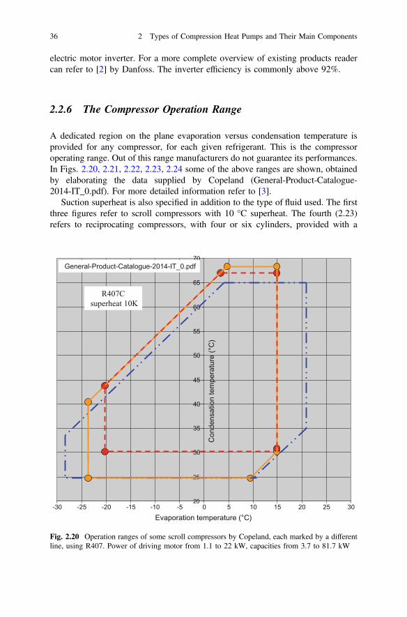
A dedicated region on the plane evaporation versus condensation temperature isprovided for any compressor, for each given refrigerant. This is the compressoroperating range. Out of this range manufacturers do not guarantee its performances.In Figs. 2.20, 2.21, 2.22, 2.23, 2.24 some of the above ranges are shown, obtainedby elaborating the data supplied by Copeland (General-Product-Catalogue-2014-IT_0.pdf). For more detailed information refer to [3].

Suction superheat is also specified in addition to the type of fluid used. The firstthree figures refer to scroll compressors with 10 °C superheat. The fourth (2.23)refers to reciprocating compressors, with four or six cylinders, provided with a

20

25

30

35

40

45

50

55

60

65

70

-30 -25 -20 -15 -10 -5 0 5 10 15 20 25 30

R407Csuperheat 10K

Con

dens

atio

n te

mpe

ratu

re (°

C)

Evaporation temperature (°C)

General-Product-Catalogue-2014-IT_0.pdf

Fig. 2.20 Operation ranges of some scroll compressors by Copeland, each marked by a differentline, using R407. Power of driving motor from 1.1 to 22 kW, capacities from 3.7 to 81.7 kW


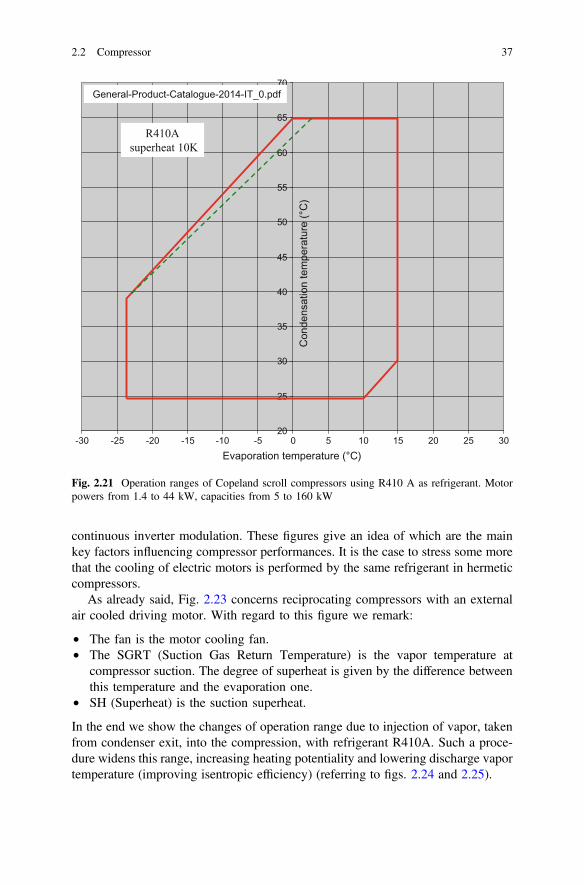
continuous inverter modulation. These figures give an idea of which are the mainkey factors influencing compressor performances. It is the case to stress some morethat the cooling of electric motors is performed by the same refrigerant in hermeticcompressors.

As already said, Fig. 2.23 concerns reciprocating compressors with an externalair cooled driving motor. With regard to this figure we remark:

• The fan is the motor cooling fan.• The SGRT (Suction Gas Return Temperature) is the vapor temperature at

compressor suction. The degree of superheat is given by the difference betweenthis temperature and the evaporation one.

• SH (Superheat) is the suction superheat.

In the end we show the changes of operation range due to injection of vapor, takenfrom condenser exit, into the compression, with refrigerant R410A. Such a proce-dure widens this range, increasing heating potentiality and lowering discharge vaportemperature (improving isentropic efficiency) (referring to figs. 2.24 and 2.25).

20

25

30

35

40

45

50

55

60

65

70

-30 -25 -20 -15 -10 -5 0 5 10 15 20 25 30

R410Asuperheat 10K


Con

dens

atio

n te

mpe

ratu

re (°

C)

Evaporation temperature (°C)

Fig. 2.21 Operation ranges of Copeland scroll compressors using R410 A as refrigerant. Motorpowers from 1.4 to 44 kW, capacities from 5 to 160 kW

2.2 Compressor 37

2.3 Expansion Valve

As above said it is a metering device that feeds refrigerant to the evaporator,lowering its pressure from the condenser value to that of the evaporator, in order tokeep suitable transformations temperatures for heat sources. In simplest applica-tions it is obtained by a fixed bore capillary tube where the total-system chargeflows in any operating condition. It has to be long enough to supply the totalpressure drop at full flow rate and is generally helically coiled.

Of course, such a device is not able to face load variations. Therefore severalsystems allowing for varying the discharge area of the valve according with theactual required load have been employed.

The rationale is quite simple. As a consequence of a reduction of the heatingpower requested by the internal environment and at a constant flow rate, the con-densation phase shifts the outlet point towards larger subcooling in the liquid. Atthe same time the superheat at evaporator exit increases. Both subcooling and

0

5

10

15

20

25

30

35

40

45

50

55

60

65

70

75

80

-25 -20 -15 -10 -5 0 5 10 15 20 25


R134asuperheat 10K

cond

ensa

tion

tem

pera

ture

(°C

)

evaporation temperature (°C)

Fig. 2.22 Operation ranges of Copeland scroll compressors using R134a. Motor powers 1.5 to22 kW, capacity 3.3 to 53.2 kW


superheat increase as larger is the unbalance between the requested and the avail-able power.

It is, therefore, necessary to lower the flow rate in such a case. The valvedischarge area has to be reduced. In many cases the actuating control signal comesfrom a sensor measuring vapor temperature at evaporator exit. This to keep vaporsuperheat at compressor suction fixed at a set-point. In this case we speak ofthermostatic valve and this method is applied in dry evaporators (those where theexiting vapor is superheated).

If Δpv is the valve pressure drop with a mass flow rate m, it can be set forth asKm2, where K is the corresponding flow coefficient. At a reduced flow rate, m’, thevalve partially closes, keeping the pressure drop constant. The new flow coefficient

0

5

10

15

20

25

30

35

40

45

50

55

60

-60 -55 -50 -45 -40 -35 -30 -25 -20 -15 -10 -5 0 5 10


R404A

cond

ensa

tion

tem

pera

ture

(°C

)evaporation temperature (°C)

a

b c

d e

Fig. 2.23 Operation ranges of Copeland™ Stream Digital with Core Sense™ Diagnosticsreciprocating compressors (4–6), with refrigerant R404 A. They use continuous modulation by aninverter from 50 to 100% (4 cylinders) and from 30 to 100% (6 cylinders), with the followingcharacteristics(letters a, b, c, d, e refer to each graph): a 25 °C SGRT at 100% load or 0 °CSGRT + cooling fan, driving motor modulation at 33% (6 cylinders) and 50% (4 cylinders);b 25 °C SGRT with cooling fan and modulation at 33% (6 cylinders) or 50% (4 cylinders); c 0 °CSGRT with cooling fan and modulation at 33% (6 cylinders) or 50% (4 cylinders); d 25 °C SGRTat 100%; e SH > 20 °C at 100%

2.3 Expansion Valve 39

has to become K’ = Δpv/m’2. Both K and K’ are two values of the flow charac-teristic of the installed valve.

Example 2.2 A heat pump, working with R134a8 supplies a nominal heatingload of 10 kW at 44 °C.9 Let us suppose liquid inlet into the expansion valveto be saturated. With data provided in the following Table 2.5 the mass flowrate is:

m ¼ QC

hv � hl¼ 10

158:7¼ 0:063 kg/s

-25

-15

-5

5

15

25

35

45

55

65

75

85

95

105

115

125

-55 -50 -45 -40 -35 -30 -25 -20 -15 -10 -5 0 5 10 15 20 25

cond

ensa

tion

tem

pera

ture

(°C

)


R744 (CO2) superheat 20K


Critical point:

304K (31°C)

7,38MPa (73 bar)

Fig. 2.24 Refers to reciprocating compressors used with carbon dioxide. The graph (continuousline) on the top right regards compression in the hypercritical region, while the lower graph (dottedline) concerns a subcritical compression

8The data are taken from NIST Chemistry Web Book.9We suppose the de-superheating is used for sanitary hot water production. This may occur inoffices, where sanitary water requirements are usually low.


-30 -25 -20 -15 -10 -5 0 5 10 15 20 25 30

R410Asuperheat 10K

Da General-Product-Catalogue-2014-IT_0.pdf

cond

ensa

tion

tem

pera

ture

(°C

)


no vapor injection

dry vapor injection

humid vapor injection.

20

25

30

35

40

45

50

55

60

65

70

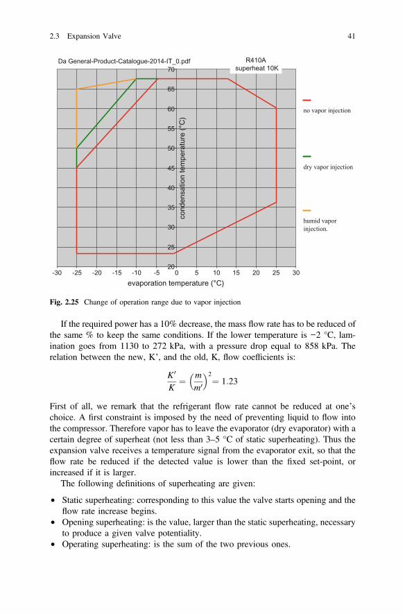
Fig. 2.25 Change of operation range due to vapor injection

If the required power has a 10% decrease, the mass flow rate has to be reduced ofthe same % to keep the same conditions. If the lower temperature is −2 °C, lam-ination goes from 1130 to 272 kPa, with a pressure drop equal to 858 kPa. Therelation between the new, K’, and the old, K, flow coefficients is:

K 0

K¼ m

m0� �2

¼ 1:23

First of all, we remark that the refrigerant flow rate cannot be reduced at one’schoice. A first constraint is imposed by the need of preventing liquid to flow intothe compressor. Therefore vapor has to leave the evaporator (dry evaporator) with acertain degree of superheat (not less than 3–5 °C of static superheating). Thus theexpansion valve receives a temperature signal from the evaporator exit, so that theflow rate be reduced if the detected value is lower than the fixed set-point, orincreased if it is larger.

The following definitions of superheating are given:

• Static superheating: corresponding to this value the valve starts opening and theflow rate increase begins.

• Opening superheating: is the value, larger than the static superheating, necessaryto produce a given valve potentiality.

• Operating superheating: is the sum of the two previous ones.


A liquid separator can be inserted immediately after the evaporator, just to be sureand to have a low superheating. Actually these separators are used in the case of wetevaporators, where no superheating is required to increase efficiency.

A further important parameter is the liquid subcooling at the expansion valveinlet. This is necessary to avoid vapor bubbles formation in the liquid line leading tothe valve that would reduce its performances. A typical minimum subcooling valueis 4 °C.

The expansion valves are generally classified as:

• Constant pressure expansion valve—also improperly called automatic expan-sion valve, it keeps the pressure inside the evaporator constant, no matter whatthe load inside the evaporator is. It does not allow the control of flow ofrefrigerant and, thus, this type of valve is not used when this control is needed.

• Thermal (thermostatic) expansion valve—it controls the amount of refrigerantflow thereby controlling superheating at evaporator outlet. Thermal expansionvalves are often generically referred to as “metering devices”. They areemployed with variable thermal load.

They operate according to the superheating at evaporator exit and to its pressure.This pressure has to be kept below a fixed threshold called MOP (Maximum

Table 2.5 R134a data

°C kPa vl (m3/kg) vv (m

3/kg) hl (kJ/kg) hv − hl (kJ/kg) hv (kJ/kg)

−2 272.2 0.0007684 0.0744 49.17 200.12 249.29

0 292.8 0.0007723 0.0693 51.86 198.60 250.46

2 314.6 0.0007763 0.0647 54.55 197.07 251.62

4 337.7 0.0007804 0.0604 57.25 195.53 252.78

6 362.0 0.0007845 0.0564 59.97 193.95 253.92

8 387.6 0.0007887 0.0528 62.69 192.36 255.05

12 443.0 0.0007975 0.0463 68.19 189.11 257.29

16 504.3 0.0008066 0.0408 73.73 185.74 259.47

20 571.7 0.0008161 0.0360 79.32 182.28 261.60

24 645.8 0.0008261 0.0319 84.98 178.70 263.68

26 685.4 0.0008313 0.0300 87.83 176.87 264.70

28 726.9 0.0008367 0.0283 90.70 175.00 265.69

30 770.2 0.0008421 0.0266 93.58 173.09 266.67

32 815.4 0.0008478 0.0251 96.48 171.16 267.64

34 862.6 0.0008536 0.0237 99.40 169.18 268.58

36 911.9 0.0008595 0.0224 102.33 167.17 269.50

38 963.2 0.0008657 0.0211 105.29 165.12 270.41

40 1016.6 0.0008720 0.0200 108.27 163.01 271.28

42 1072.2 0.0008786 0.0189 111.26 160.88 272.14

44 1130.1 0.0008854 0.0178 114.28 158.69 272.97

48 1252.9 0.0008997 0.0160 120.39 154.16 274.55


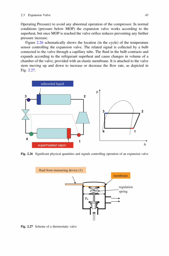
Operating Pressure) to avoid any abnormal operation of the compressor. In normalconditions (pressure below MOP) the expansion valve works according to thesuperheat, but once MOP is reached the valve orifice reduces preventing any furtherpressure increase.

Figure 2.26 schematically shows the location (in the cycle) of the temperaturesensor controlling the expansion valve. The related signal is collected by a bulbconnected to the valve through a capillary tube. The fluid in the bulb contracts andexpands according to the refrigerant superheat and cause changes in volume of achamber of the valve, provided with an elastic membrane. It is attached to the valvestem moving up and down to increase or decrease the flow rate, as depicted inFig. 2.27.

subcooled liquid

superheated vapor

1

2 3

4

1

3

4

p

h

2

Fig. 2.26 Significant physical quantities and signals controlling operation of an expansion valve

membranefluid from measuring device (1)

regulation spring

p4

Fig. 2.27 Scheme of a thermostatic valve


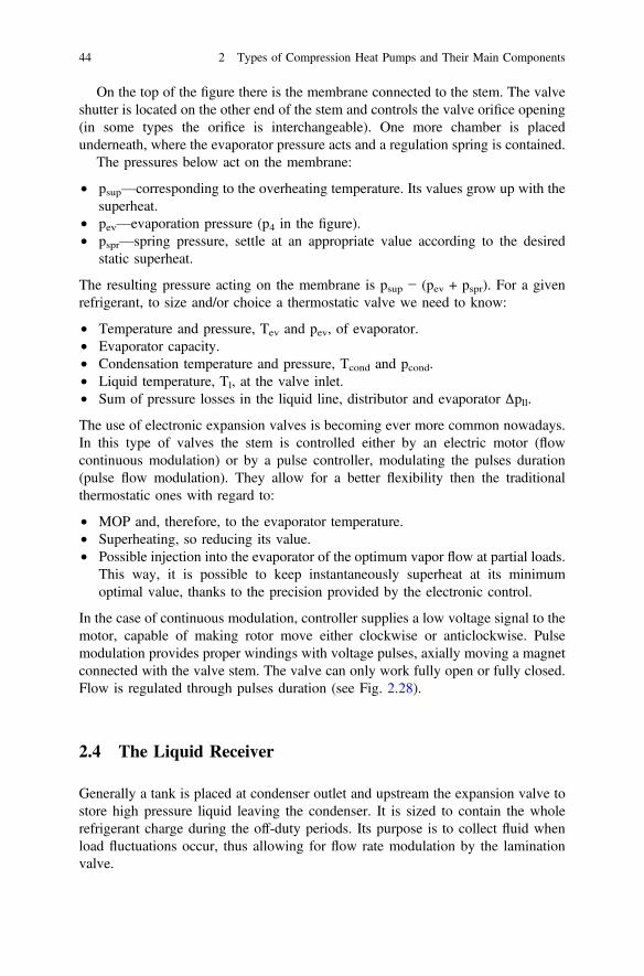
On the top of the figure there is the membrane connected to the stem. The valveshutter is located on the other end of the stem and controls the valve orifice opening(in some types the orifice is interchangeable). One more chamber is placedunderneath, where the evaporator pressure acts and a regulation spring is contained.

The pressures below act on the membrane:

• psup—corresponding to the overheating temperature. Its values grow up with thesuperheat.

• pev—evaporation pressure (p4 in the figure).• pspr—spring pressure, settle at an appropriate value according to the desired

static superheat.

The resulting pressure acting on the membrane is psup − (pev + pspr). For a givenrefrigerant, to size and/or choice a thermostatic valve we need to know:

• Temperature and pressure, Tev and pev, of evaporator.• Evaporator capacity.• Condensation temperature and pressure, Tcond and pcond.• Liquid temperature, Tl, at the valve inlet.• Sum of pressure losses in the liquid line, distributor and evaporator Δpll.

The use of electronic expansion valves is becoming ever more common nowadays.In this type of valves the stem is controlled either by an electric motor (flowcontinuous modulation) or by a pulse controller, modulating the pulses duration(pulse flow modulation). They allow for a better flexibility then the traditionalthermostatic ones with regard to:

• MOP and, therefore, to the evaporator temperature.• Superheating, so reducing its value.• Possible injection into the evaporator of the optimum vapor flow at partial loads.

This way, it is possible to keep instantaneously superheat at its minimumoptimal value, thanks to the precision provided by the electronic control.

In the case of continuous modulation, controller supplies a low voltage signal to themotor, capable of making rotor move either clockwise or anticlockwise. Pulsemodulation provides proper windings with voltage pulses, axially moving a magnetconnected with the valve stem. The valve can only work fully open or fully closed.Flow is regulated through pulses duration (see Fig. 2.28).

2.4 The Liquid Receiver

Generally a tank is placed at condenser outlet and upstream the expansion valve tostore high pressure liquid leaving the condenser. It is sized to contain the wholerefrigerant charge during the off-duty periods. Its purpose is to collect fluid whenload fluctuations occur, thus allowing for flow rate modulation by the laminationvalve.


A scheme of the receiver is illustrated in Fig. 2.29. It is a cylindrical steel tankwith a pipe introducing the refrigerant coming from the condenser and an internaldip tube, ensuring that only 100% of liquid leaves the receiver.

Of course this type of device is not used when a capillary tube is used instead anexpansion valve, as no flow modulation is possible.

flow rate flow rate

time time

Continuous control Pulse control

Fig. 2.28 Control methods of electronic expansion valves

fromcondenser

to laminationFig. 2.29 Liquid receiver

2.4 The Liquid Receiver 45

2.5 Evaporator and Condenser

They can exchange heat with several types of indoor and outdoor sources. There isa widespread use of rather small systems (split systems), where both indoor andoutdoor heat exchangers are cooled by air blown by properly sized axial fans. Inthis case we say we are using an air/air heat pump, in the sense than the refrigerantexchanges heat directly with air on both the heat exchangers. The internal sourcecan also be water of a hydraulic system or sanitary water, while the external sourcecan be water and even ground.

With regard to the type of thermal sources heat pumps can be syntheticallyclassified as:

• Air/Air heat pumps, if both the sources are air.• Air/Water heat pumps, if the outer source is air and the inner one is water, as in

water heating systems.• Water/Water heat pumps, if both the sources are water.

In any case the first word refers to the outer source and the second one to the innersource.

When the heat source/sink is air (air/air or air/water heat pumps) the air cooledheat exchanger mainly consists of a finned tube bundle with rectangular boxheaders on both ends of the tubes. Cooling air is provided by one or more fan.

If refrigerant exchanges heat with water, plate and frame heat exchangers areused. They have corrugated metal plates to transfer heat between the fluids(Fig. 2.30). They may be welded, semiwelded and brazed (most commonly adoptedin heat pumps).

They are high heat transfer efficiency and compact10 heat exchangers.11 Theplates are generally spaced by rubber sealing gaskets (Gasketed Plate HeatExchangers GPHE) and are pressed to form troughs at right angles to the maindirection of flow. Each fluid flows in gaps, each formed by two consecutive plates,1.3–1.5 mm wide.

Plates are compressed together in a rigid frame and form a set of parallelchannels with alternating hot and cold fluids. They can easily be disassembled forcleaning and maintenance purposes as well as for inserting further elements.

The plates can be also brazed (e.g., copper brazed) instead of welded, thusnamed Brazed Plate Heat Exchangers (BPHE). Plates are shaped to promote highlevels of turbulence in order to increase heat transfer efficiency and self-cleaning.

10A heat exchanger compactness is usually based on the value of two parameters: the hydraulicdiameter DH ( the lowest of those employed for the two fluids) and the ratio between the heattransfer area and the volume where fluids flow S/V. The following definitions are given:

• Conventional heat exchangers for DH > 5 mm or S/V < 400 m2/m3.• Compact heat exchangers for 1 < DH(mm) < 5 or S/V > 400.11For a more detailed description of these heat exchanger the interested reader can also refer to [4].


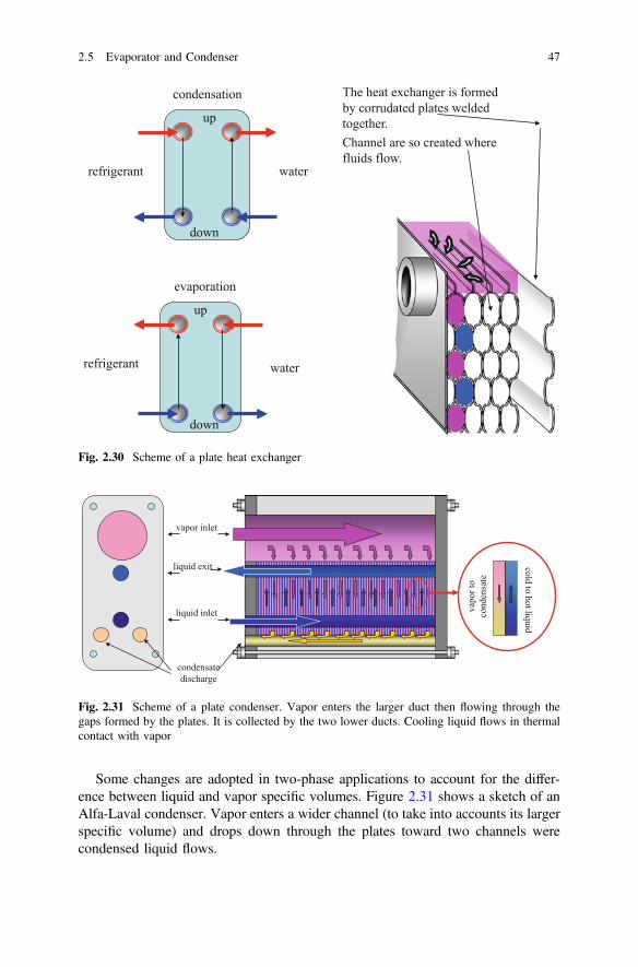
Some changes are adopted in two-phase applications to account for the differ-ence between liquid and vapor specific volumes. Figure 2.31 shows a sketch of anAlfa-Laval condenser. Vapor enters a wider channel (to take into accounts its largerspecific volume) and drops down through the plates toward two channels werecondensed liquid flows.

evaporation

condensation

refrigerant

refrigerant water

water

up

up

down

down

The heat exchanger is formed by corrudated plates welded together. Channel are so created where fluids flow.

Fig. 2.30 Scheme of a plate heat exchangerva

por t

o co

nden

sate

cold to hot liquid

vapor inlet

liquid inlet

liquid exit

condensate discharge

Fig. 2.31 Scheme of a plate condenser. Vapor enters the larger duct then flowing through thegaps formed by the plates. It is collected by the two lower ducts. Cooling liquid flows in thermalcontact with vapor

2.5 Evaporator and Condenser 47

Some features of BPHE for air/water heat pumps from HYDAC International arereported herein just to give some order of magnitude of the main parameters [5]:

Some operating data:

“Operating data Plate material Stainless steel 1.4401 (AISI 316).Braze material Copper (standard), Nickel.Pressures Copper brazed: max. 30 bar (test pressure 45 bar).Nickel braze: max. 10 bar.Use nickel-brazed plate heat exchangers with corrosive fluids: e.g., ammonia,sulphides and sulphates, deionizer or dematerialized water and other fluids onrequest.Temperature range up to +200 °C (freezing point and boiling point must be takeninto consideration).Contamination: the quantity of particles in suspension should be less than10 mg/l…” (Table 2.6).

Capacities ranging from 0.7 to 186 kW are, for example, available for water cooledBPHE condensers and from 0.7 to 141 kW for evaporator, both using R410A, andfrom 0.7 to 176 kW and from 0.7 to 141 kW respectively for condensers andevaporators using R134a.

Tube in tube heat exchangers are also employed, constituted by two coaxialtubes with the inner one corrugated, as shown in Fig. 2.32, to increase the heattransfer area and to promote turbulence. Both heat transfer coefficient andself-cleaning capability increase in so doing. Different heat transfer capacities areavailable. These heat exchangers are often spiral windings shaped to reduce theoccupied room.

Still to give some order of magnitude, few data related to this type of heatexchangers are supplied. For example Packless Industries [6] provides heatexchanger capacities in the range 1.76 kW (1/2 ton12)–105.5 kW(30 tons). Theouter and inner tubes are, in general, respectively made by steel and copper. Thevolume of these spirally wound exchanger is evaluated as the one of a paral-lelepiped (like a box containing them) with sides a and b and height c. For lowercapacities they may be a = 25 cm, b = 17 cm and c ranging from 8 to 10 cm. Forhigher capacities a = 64 cm, b = 51 cm, c = 56 cm or a = 90 cm, b = 31 cm,c = 31 cm. There are also the so called “trombone” heat exchangers, just shaped as

Table 2.6 Size and weightof plate exchangers

Length (mm) Width (mm) Weight (kg)

194 33–101 1.3–2.8

306 34–298 2.5–16.6

613 62–470 15.3–84.8

… … …

12Ton (ton of refrigeration) is an Anglo-Saxon unit: 1 ton = 3.517 kW.


the musical instrument. The sides of the basis are larger than before, but c is in theorder of 5 or 6 cm.

Shell and tube heat exchangers are employed as well. Figure 2.33 shows thescheme of a flooded condenser. Cooling water flows in tubes and refrigerant in theshell. Vapor enters the shell and condenses, in contact with cold tubes,. As anexample Alfa Laval, [6], supplies heat exchangers for R407C and R134a, cooled by

liquid

helical corrugated heat transfer suface.

spiral condenser (Packless Industries)http://www.packless.com/products/condenser-heat-pump-coils-ton.htm

Fig. 2.32 Tube in tube heat exchanger with corrugated surface. On the bottom a spiral condenser(coil)

vapor inlet

condensate exitcooling water inlet

cooling water exit

vapor

liquid

A liquid layer condenses on tubes and falls down.

Fig. 2.33 Shell and tube condenser


water coming from cooling towers, wells, rivers and lakes as well as from industrialprocesses, with condensing power between 60 and 1680 kW.

Heat exchangers are sized for nominal requirements. So that, for instance, vaporexiting the compressor is taken to subcooled liquid to the expansion valve. Whenrefrigerant flow rate is lower than the nominal value, with the same cooling waterflow rate, the region of subcooled liquid refrigerant widens.

As above mentioned, a liquid receiver is placed at condenser exit, aimed atcollecting refrigerant in the case of maintenance and to allow for flow rate mod-ulation, so that only liquid could flow into the lamination valve. Another tank canbe located at evaporator exit (wet evaporators). As stressed before in dry evapo-rators only superheated vapor flows out of the heat exchangers. Thus, there is nodanger for the compressor, but we lose heat transfer efficiency as variable tem-perature region of refrigerant exist in the final part of the evaporator. As a remedy tothis a flooded evaporator is used, where the change of phase ends with no super-heating. A gravity vapor separator is then placed before compressor suction.

Once more we can mention some technical data for the related heat transfercoefficient ranging from 2 to 7 kW/m2K for a corrugated plate evaporator. Similarvalue for condensing micro finned tube with tube diameters up to 9.40 mm [7].

The following data (Table 2.7) for R134a can be roughly obtained by diagrams[8].

Air cooled heat exchangers are basically composed by finned tube bundles.Refrigerant flows in the tubes, often made of copper, and air is blown by fans. Airflow rate can be varied both stepwise (usually three steps) or continuously, by aninverter, according to the requested load.

A typical basic scheme is shown Fig. 2.34.This is the most commonly adopted type for low capacity heat exchangers.

Much more complex devices are employed for larger machines, anyhow workingwith the same operation principle.

Whatever the size, these exchangers may undergo frost formation.

2.5.1 The Effect of Outside Air Humidity and Frosting

The external heat exchanger is generally sized referring to summer conditions,roughly with a temperature difference of 12–15 °C between the flowing refrigerant

Table 2.7 Evaporation data for R134a

Mass flow rate(kg/m2s)

Temperature(°C)

Heat transfer coefficient(kW/m2K)

Vaporquality

200–900 −17.8 5–15 –

400 −18–5 8.5–9.0 –

400 / 6.0–9.0 0.05–0.2

400 – 9.0 >0.2


and the outdoor air. Therefore if the air temperature is 35 °C, condensation takesplace at around 50 °C, and only sensible heat is exchanged.

In winter air flowing to the fins, with an inlet temperature Ti and specific heatcpA, transfers a heat q (J/kg), equal to the difference between the inlet enthalpy, hi,and the outlet one, hu. Then we have:

q ¼ hi � hu ¼ cpA Ti � Tuð Þþ r0ðxi � xuÞTu ¼ Ti � q�r0ðxi�xuÞ½ �

cpAse xi ¼ xuTu ¼ Ti � q

cpA

From the above equations we infer, Ti and q being the same, the outlet air tem-perature Tu is lower for a pure sensible heat exchange (xu = xi) than for a trans-formation with a latent heat exchange (xu 6¼ xi). Figure 2.35 shows, for a givenTi = 5 °C and q = 10 kJ/kg, three transformations starting from different inletrelative humidities (RH): 90% (blue circles), 50% (red circles) and 40% (greencircles). In the usual operating conditions we can affirm that no condensation occursfor a relative humidity lower than 50%, with such air temperature (5 °C).

Example 2.3 To go into more details consider the case with an outdoor airtemperature Ti = 5 °C. By extracting the numerical values from the graph ofFig. 3.32a, we can roughly say that xi = 2.8 g/kg and a dew temperatureTd = −4.6 °C at a relative humidity RH = 50% and xi = 4.8 g/kg andTd = 3.0 °C with RH = 90%.

fins

tubes

variable speed fan

air flow

Fig. 2.34 Heat exchange coil


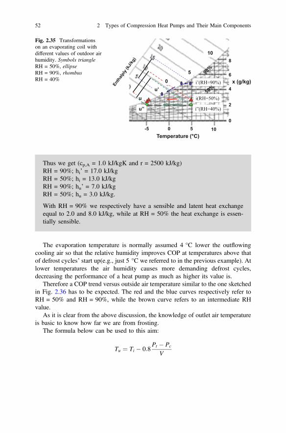
Thus we get (cp,A = 1.0 kJ/kgK and r = 2500 kJ/kg)RH = 90%; hi’ = 17.0 kJ/kgRH = 50%; hi = 13.0 kJ/kgRH = 90%; hu’ = 7.0 kJ/kgRH = 50%; hu = 3.0 kJ/kg.

With RH = 90% we respectively have a sensible and latent heat exchangeequal to 2.0 and 8.0 kJ/kg, while at RH = 50% the heat exchange is essen-tially sensible.

The evaporation temperature is normally assumed 4 °C lower the outflowingcooling air so that the relative humidity improves COP at temperatures above thatof defrost cycles’ start up(e.g., just 5 °C we referred to in the previous example). Atlower temperatures the air humidity causes more demanding defrost cycles,decreasing the performance of a heat pump as much as higher its value is.

Therefore a COP trend versus outside air temperature similar to the one sketchedin Fig. 2.36 has to be expected. The red and the blue curves respectively refer toRH = 50% and RH = 90%, while the brown curve refers to an intermediate RHvalue.

As it is clear from the above discussion, the knowledge of outlet air temperatureis basic to know how far we are from frosting.

The formula below can be used to this aim:

Tu ¼ Ti � 0:8Pt � Pc

V

x (g/kg)4

0

8

10

i’(RH=90%)

i(RH=50%)u u’

i”(RH=40%)u’’

6

2

5 0 -5

10

5 0

Temperature (°C)

Fig. 2.35 Transformationson an evaporating coil withdifferent values of outdoor airhumidity. Symbols triangleRH = 50%, ellipseRH = 90%, rhombusRH = 40%


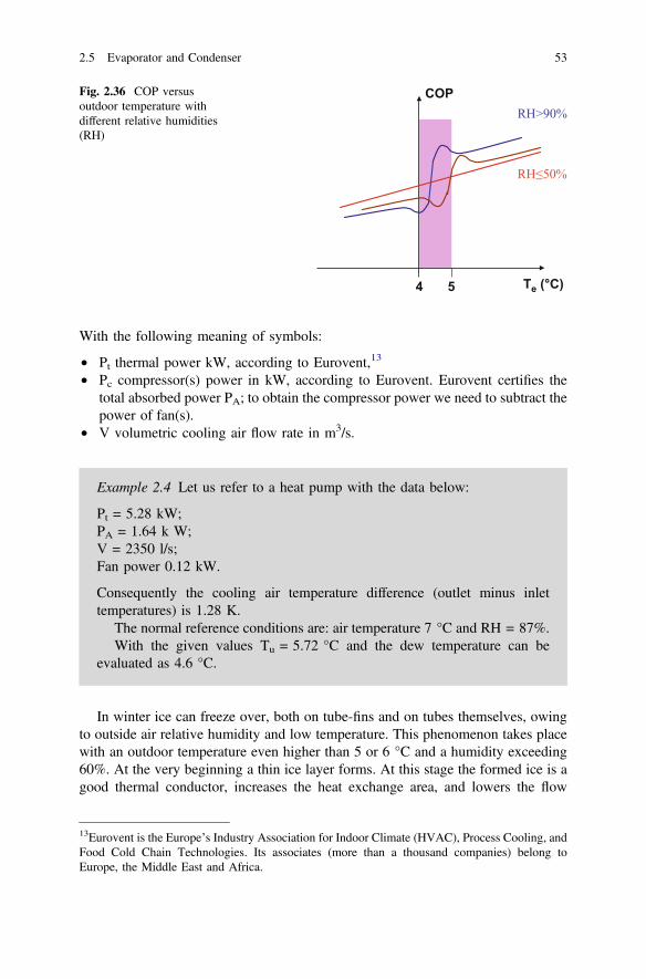
With the following meaning of symbols:

• Pt thermal power kW, according to Eurovent,13

• Pc compressor(s) power in kW, according to Eurovent. Eurovent certifies thetotal absorbed power PA; to obtain the compressor power we need to subtract thepower of fan(s).

• V volumetric cooling air flow rate in m3/s.

Example 2.4 Let us refer to a heat pump with the data below:

Pt = 5.28 kW;PA = 1.64 k W;V = 2350 l/s;Fan power 0.12 kW.

Consequently the cooling air temperature difference (outlet minus inlettemperatures) is 1.28 K.

The normal reference conditions are: air temperature 7 °C and RH = 87%.With the given values Tu = 5.72 °C and the dew temperature can be

evaluated as 4.6 °C.

In winter ice can freeze over, both on tube-fins and on tubes themselves, owingto outside air relative humidity and low temperature. This phenomenon takes placewith an outdoor temperature even higher than 5 or 6 °C and a humidity exceeding60%. At the very beginning a thin ice layer forms. At this stage the formed ice is agood thermal conductor, increases the heat exchange area, and lowers the flow

4 5 Te (°C)

COP

RH≤50%

RH>90%

Fig. 2.36 COP versusoutdoor temperature withdifferent relative humidities(RH)

13Eurovent is the Europe’s Industry Association for Indoor Climate (HVAC), Process Cooling, andFood Cold Chain Technologies. Its associates (more than a thousand companies) belong toEurope, the Middle East and Africa.


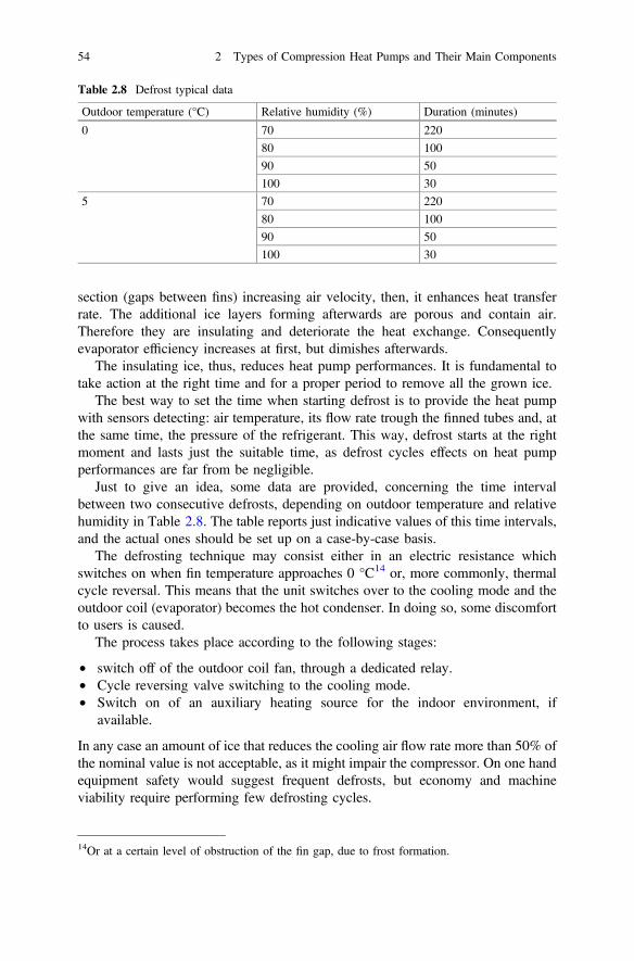
section (gaps between fins) increasing air velocity, then, it enhances heat transferrate. The additional ice layers forming afterwards are porous and contain air.Therefore they are insulating and deteriorate the heat exchange. Consequentlyevaporator efficiency increases at first, but dimishes afterwards.

The insulating ice, thus, reduces heat pump performances. It is fundamental totake action at the right time and for a proper period to remove all the grown ice.

The best way to set the time when starting defrost is to provide the heat pumpwith sensors detecting: air temperature, its flow rate trough the finned tubes and, atthe same time, the pressure of the refrigerant. This way, defrost starts at the rightmoment and lasts just the suitable time, as defrost cycles effects on heat pumpperformances are far from be negligible.

Just to give an idea, some data are provided, concerning the time intervalbetween two consecutive defrosts, depending on outdoor temperature and relativehumidity in Table 2.8. The table reports just indicative values of this time intervals,and the actual ones should be set up on a case-by-case basis.

The defrosting technique may consist either in an electric resistance whichswitches on when fin temperature approaches 0 °C14 or, more commonly, thermalcycle reversal. This means that the unit switches over to the cooling mode and theoutdoor coil (evaporator) becomes the hot condenser. In doing so, some discomfortto users is caused.

The process takes place according to the following stages:

• switch off of the outdoor coil fan, through a dedicated relay.• Cycle reversing valve switching to the cooling mode.• Switch on of an auxiliary heating source for the indoor environment, if

available.

In any case an amount of ice that reduces the cooling air flow rate more than 50% ofthe nominal value is not acceptable, as it might impair the compressor. On one handequipment safety would suggest frequent defrosts, but economy and machineviability require performing few defrosting cycles.

Table 2.8 Defrost typical data

Outdoor temperature (°C) Relative humidity (%) Duration (minutes)

0 70 220

80 100

90 50

100 30

5 70 220

80 100

90 50

100 30

14Or at a certain level of obstruction of the fin gap, due to frost formation.


Several aspects have to be accounted for to optimize defrost start up.

• A first control can be performed on air pressure within the coil, (differentialpressure between inlet and outlet). When this value exceeds a given set pointvalue, the process starts. This type of systems reacts to low pressure difference,so that they might be activated by a wind burst. Therefore a time delay has to beintroduced to verify the permanency of such a pressure drop increase, beforestarting the defrost. Even debris and leaves can cause an improper system action.

• It is also possible to refer to temperature differences. This method is based onthe fact that the usual temperature difference between outdoor and evaporatortemperatures varies in the range 3–9 °C. As ice builds up, this differenceincreases. Defrost starts when a set threshold is exceeded.

• As both the afore said methods revealed not to be always reliable, and alsosomehow costly, at first many manufacturers decided to use a timer in resi-dential applications. So the process started at given time intervals. This is a verysimple method and was the most widespread at least as long as electronics wasintroduced. The timer was coupled to a thermostat measuring air temperature atcoil exit generally set at 3 °C. If air is cooler than this for a given period, say30 min, defrost starts, otherwise it does not. Defrost ends when evaporatortemperature achieves a preset value by manufacturers. This method,timer + thermostat, is the most used in residential buildings also because of itslow cost. A further control based on the pressure difference mentioned abovemay be added so that defrost startup is also influenced by this, when the relatedincrease is about 100 Pa.

An additional method consists in injecting superheated vapor from the compressorinto the evaporator through a dedicated defrosting valve. This is aimed at pre-venting the indoor environment from being cooled, even if some power is anywaysubtracted from it. Other solutions use tanks where thermal energy can be storedand then released to coils, as those using melting salts or ethylene glycolexchanging heat with the condenser de-superheating stage.

In general defrost can affect energy consumption by more than 10%, dependingon the adopted solution. In case of absorption heat pumps some hot fluid (e.g.,ammonia), coming from the generator, can be diverted to the outdoor coil, withoutany cycle reversal. Such a reversal does not even occur in endothermic enginedriven heat pumps. Before ending this paragraph, some features of this type of coilsare provided, see Table 2.9.

2.6 Economizer and Vapor Injection

A way to save energy in the case of a large temperature difference between thermalsources, i.e., large pressure ratio, is injecting vapor into the compressor at anintermediate pressure.


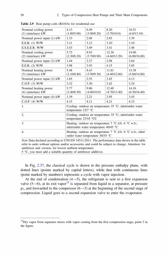
In Fig. 2.37, the classical cycle is drawn in the pressure enthalpy plane, withdotted lines (points marked by capital letters), while that with continuous lines(point marked by numbers) represents a cycle with vapor injection.

At the end of condensation (4!5), the refrigerant is sent to a first expansionvalve (5!6), at its exit vapor15 is separated from liquid in a separator, at pressurep7, and forwarded to the compressor (6!3) at the beginning of the second stage ofcompression. Liquid goes to a second expansion valve to enter the evaporator.

Table 2.9 Heat pump coils (R410A) for residential use

Nominal cooling power(1) (min/max) kW

4.13(1.80/5.00)

6.49(3.00/8.20)

8.20(3.70/10.0)

10.51(4.0/13.10)

Nominal power input (1) kW 1.33 2.08 2.65 3.39

E.E.R. (1) W/W 3.11 3.12 3.10 3.10

E.S.E.E.R. W/W 3.43 3.49 3.41 3.48

Nominal cooling power(2) (min/max) kW

5.72(2.30/0.20)

8.93(3.70/0.90)

12.36(4.60/13.20)

14.00(6.00/16.00)


E.E.R. (2) W/W 3.98 3.93 4.15 3.85

Nominal heating power(3) (min/max) kW

5.48(2.10/0.80)

8.43(3.50/9.30)

11.81(4.40/12.60)

13.38(5.60/14.80)


C.O.P. (3) W/W 3.32 3.30 3.42 3.24

Nominal heating power(4) (min/max) kW

5.77(2.40/6.50)

9.06(4.00/10.0)

12.40(4.70/13.40)

14.16(6.30/16.40)


C.O.P. (4) W/W 4.15 4.11 4.21 4.15

1. Cooling: outdoor air temperature 35 °C; inlet/outlet watertemperature 12/7 °C

2. Cooling: outdoor air temperature 35 °C; inlet/outlet watertemperature 23/18 °CC

3. Heating: outdoor air temperature 7 °C d.b. 6 °C w.b.;inlet/outlet water temperature 40/45 °C

4. Heating: outdoor air temperature 7 °C d.b. 6 °C w.b.; inlet/outlet water temperature 30/35 °C

Note Data declared according to UNI EN 14511:2011. The performance data shown in the tablerefer to units without options and/or accessories and could be subject to change. Attention: forantifreeze unit version, for lowest ambient temperature5 °C, you must add a suitable quantity of antifreeze additives

15Dry vapor from separator mixes with vapor coming from the first compression stage, point 3 inthe figure.


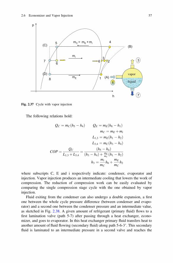
The following relations hold:

QC ¼ mC h5 � h4ð Þ QE ¼ mE h8 � h1ð ÞmC ¼ mE þmi

L1;3 ¼ mE h1 � h2ð ÞL3;4 ¼ mC h3 � h4ð Þ

COP ¼ QC

L1;3 þ L3;4¼ h5 � h4ð Þ

h3 � h4ð Þþ mEmC

h1 � h2ð Þh3 ¼ mi

mCh6 þ mE

mCh2

where subscripts C, E and i respectively indicate: condenser, evaporator andinjection. Vapor injection produces an intermediate cooling that lowers the work ofcompression. The reduction of compression work can be easily evaluated bycomparing the single compression stage cycle with the one obtained by vaporinjection.

Fluid exiting from the condenser can also undergo a double expansion, a firstone between the whole cycle pressure difference (between condenser and evapo-rator) and a second one between the condenser pressure and an intermediate value,as sketched in Fig. 2.38. A given amount of refrigerant (primary fluid) flows to afirst lamination valve (path 5-7) after passing through a heat exchanger, econo-mizer, and goes to evaporator. In this heat exchanger primary fluid transfers heat toanother amount of fluid flowing (secondary fluid) along path 5-6-3’. This secondaryfluid is laminated to an intermediate pressure in a second valve and reaches the

p

h

1

2 6

4 5

6 7

8 (A)

(B) (C)

(D)

mi

mE

mC = mimE +

6

7

3

vapor

liquid

3

Fig. 2.37 Cycle with vapor injection

2.6 Economizer and Vapor Injection 57

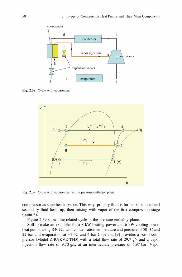
compressor as superheated vapor. This way, primary fluid is further subcooled andsecondary fluid heats up, then mixing with vapor of the first compression stage(point 3).

Figure 2.39 shows the related cycle in the pressure-enthalpy plane.Still to make an example: for a 8 kW heating power and 6 kW cooling power

heat pump, using R407C, with condensation temperature and pressure of 50 °C and22 bar and evaporation at −7 °C and 4 bar Copeland [9] provides a scroll com-pressor (Model ZH09KVE-TFD) with a total flow rate of 29.7 g/s and a vaporinjection flow rate of 9.70 g/s, at an intermediate pressure of 5.97 bar. Vapor

condenser

evaporator

expansion valves

vapor injection

5

6

3

7

3’

1

economizer

compressor

4

Fig. 2.38 Cycle with economizer

p

h

1

23

45

6

7 (A)

(B)(C)

(D)

mi

mE

mC = mimE +

Fig. 2.39 Cycle with economizer in the pressure-enthalpy plane


injection is also employed in screw compressor with a COP claimed increasearound 20%.

This technology is also implemented for sanitary water supply at about 50 °C,even with outdoor temperatures below 0 °C.

In addition scroll compressors exist on the market which can bear liquid, thusallowing for saturated vapor injection, named wet vapor injection, instead of dry orsuperheated vapor. In so doing the operation range of compressors can be widen,but it is generally fixed a top value of time duration of such a type of injection (e.g.,2000 h). The use of wet vapor injection is aimed at limiting the discharge tem-perature, so that it does not exceed a safety value, say around 140 °C. The effect ofvapor injection on compressor operating range has been already shown in Fig. 2.25.

2.7 The Four Way Reversing Valve

The scheme of a cycle reversing valve for reversible heat pumps is drawn inFigs. 2.40 and 2.41. Four ports are placed on it. On top we have the port wherecompressor discharge fluid flows in, high pressure port. Of the three ports placed on

to compressor suction

Winter

from evaporator

to condenser

indoor outdoor

compressor discharge

s

Fig. 2.40 Reversing valve configuration in winter operation mode

2.6 Economizer and Vapor Injection 59

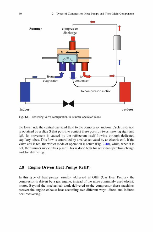
the lower side the central one send fluid to the compressor suction. Cycle inversionis obtained by a slide S that puts into contact these ports by twos, moving right andleft. Its movement is caused by the refrigerant itself flowing through dedicatedcapillary tubes. This flow is controlled by a valve activated by an electric coil. If thevalve coil is fed, the winter mode of operation is active (Fig. 2.40), while, when it isnot, the summer mode takes place. This is done both for seasonal operation changeand for defrosting.

2.8 Engine Driven Heat Pumps (GHP)

In this type of heat pumps, usually addressed as GHP (Gas Heat Pumps), thecompressor is driven by a gas engine, instead of the more commonly used electricmotor. Beyond the mechanical work delivered to the compressor these machinesrecover the engine exhaust heat according two different ways: direct and indirectheat recovering.

to compressor suction

tocondenser

indoor outdoor

Summer

s

compressor discharge

from evaporator

Fig. 2.41 Reversing valve configuration in summer operation mode


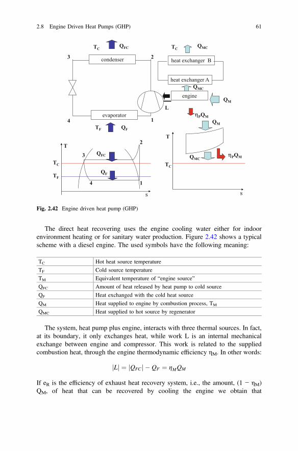
The direct heat recovering uses the engine cooling water either for indoorenvironment heating or for sanitary water production. Figure 2.42 shows a typicalscheme with a diesel engine. The used symbols have the following meaning:

TC Hot heat source temperature

TF Cold source temperature

TM Equivalent temperature of “engine source”

QFC Amount of heat released by heat pump to cold source

QF Heat exchanged with the cold heat source

QM Heat supplied to engine by combustion process, TM

QMC Heat supplied to hot source by regenerator

The system, heat pump plus engine, interacts with three thermal sources. In fact,at its boundary, it only exchanges heat, while work L is an internal mechanicalexchange between engine and compressor. This work is related to the suppliedcombustion heat, through the engine thermodynamic efficiency ηM. In other words:

Lj j ¼ QFCj j � QF ¼ gMQM

If eR is the efficiency of exhaust heat recovery system, i.e., the amount, (1 − ηM)QM, of heat that can be recovered by cooling the engine we obtain that

condenser

evaporator

TCQFC

1

23

4

engine

heat exchanger B

TCQMC

QM

QFTF

TC

TF

T

s

1

2

3

4

s

T

QF

QFC

QM

QMC

TC

L

QMC

ηPQM

ηPQM

heat exchanger A

Fig. 2.42 Engine driven heat pump (GHP)

2.8 Engine Driven Heat Pumps (GHP) 61

QMC = eR(1 − ηM)QM, while the heat released to outdoor environment is (1 − eR)(1 − ηM)QM. Thus the heat exchanged with the hot source is:

Qc ¼ QFC þQMC ¼ QFC þ eRð1� gMÞQM

where the second term on the right hand side of the above equation can be used toproduce hot sanitary water, in summer.

Therefore QC is the “useful” heat we can obtain from an engine driven heatpump in winter.

By applying the first and second Principle of Thermodynamic for ideal condi-tions16 (Carnot cycle), we obtain:

� QCj jTC

þ QF

TFþ QM

TM¼ 0

� QCj j þQF þQM ¼ 0

8<:

The coefficient of performance (see Fig. 2.43), COPMI, in winter is:

COPMI ¼ QCj jQM

¼1TM

� 1TF

1TC

� 1TF

¼ 1� TFTM

� �1

1� TFTC

¼ 1� TFTM

� �COPEI

TC

QFC

QF

TF

QM

TM

QMCideal engine

ideal heat pump

Fig. 2.43 Basic scheme of a GHP with direct heat recovery system

16In this case we can also suppose that the whole exhaust heat, QCM = (1 − ηCarnot)QM, could berecovered.


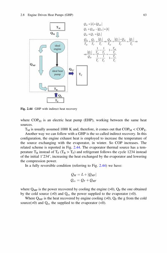
where COPEI is an electric heat pump (EHP), working between the same heatsources.

TM is usually assumed 1000 K and, therefore, it comes out that COPM < COPE.Another way we can follow with a GHP is the so called indirect recovery. In this

configuration, the engine exhaust heat is employed to increase the temperature ofthe source exchanging with the evaporator, in winter. So COP increases. Therelated scheme is reported in Fig. 2.44. The evaporator thermal source has a tem-perature TB instead of TF (TB > TF) and refrigerant follows the cycle 1234 insteadof the initial 1’234’, increasing the heat exchanged by the evaporator and loweringthe compression power.

In a fully reversible condition (referring to Fig. 2.44) we have:

QM ¼ Lþ QMFj jQev ¼ QF þQMF

where QMF is the power recovered by cooling the engine (>0), QF the one obtainedby the cold source (>0) and Qev the power supplied to the evaporator (<0).

Where QMF is the heat recovered by engine cooling (>0), QF the g from the coldsource(>0) and Qev the supplied to the evaporator (<0).

TC

QFC

QF

TF

QM

TM

QMF

ideal engine

ideal heat pump

TB

Fig. 2.44 GHP with indirect heat recovery


The coefficient of performance is:

COP0M ¼ QC

QM¼ QF þQMF þ L

QM

QF þQMF

TB� QCj j

TC¼ 0

Still, with reference to a winter ideal condition, where engine and heat pumprespectively follow a direct and an inverse Carnot cycle and with an ideal regen-erator, the results illustrated below hold.

The mechanical work engine provides to the heat pump is L = ηMQM, where ηMis the Carnot efficiency:

gM ¼ 1� TCTM

QMC ¼ ð1� gMÞQM

While the heat supplied to indoor environment is:

QFC ¼ 1

1� TFTC

!L ¼ 1

1� TFTC

!gMQM

It clearly comes out that heat provided to indoor environment is made up of anamount, QFC, depending on outdoor temperature, TF, and another one, QMC,independent of this temperature. Therefore:

QC ¼ QFC þQMC ¼ 1

1� TFTC

!gPQM þ 1� gPð ÞQM

¼ COPCarnot;inv � 1� �

gCarnot;dir þ 1 �

QM

This relation, once again, stresses that part of this heat does not depend on theoutdoor climate. This part is poor in ideal conditions, due to the high efficiency of aCarnot engine, but this is not in actual cases. Let us refer to the example below.

Example 2.5 Refer to the ideal condition, first. Suppose that TF = 5 °C(278 K), TC = 20 °C (303 K) and TM = 1000 K. The Carnot cycle efficiencyis:

ηM = 0.697andCOP = 12.12


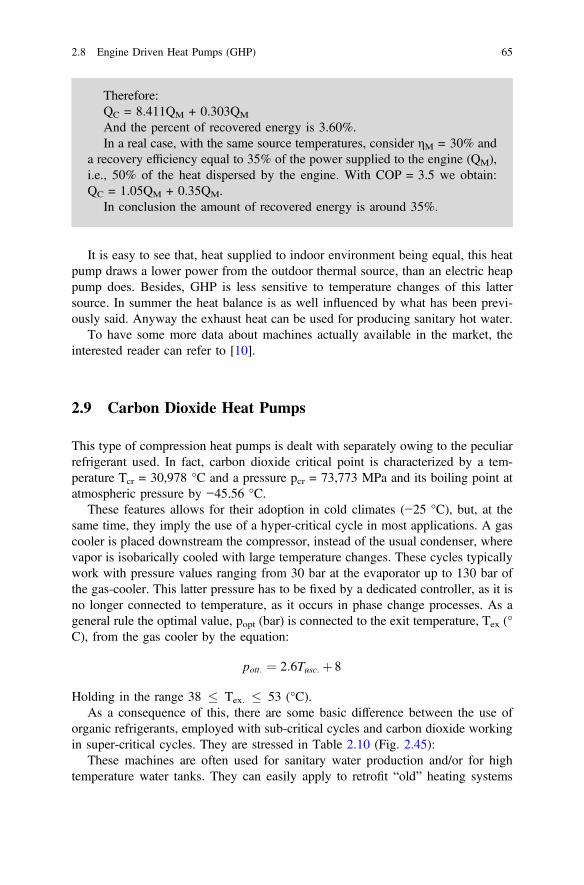
Therefore:QC = 8.411QM + 0.303QM

And the percent of recovered energy is 3.60%.In a real case, with the same source temperatures, consider ηM = 30% and

a recovery efficiency equal to 35% of the power supplied to the engine (QM),i.e., 50% of the heat dispersed by the engine. With COP = 3.5 we obtain:QC = 1.05QM + 0.35QM.

In conclusion the amount of recovered energy is around 35%.

It is easy to see that, heat supplied to indoor environment being equal, this heatpump draws a lower power from the outdoor thermal source, than an electric heappump does. Besides, GHP is less sensitive to temperature changes of this lattersource. In summer the heat balance is as well influenced by what has been previ-ously said. Anyway the exhaust heat can be used for producing sanitary hot water.

To have some more data about machines actually available in the market, theinterested reader can refer to [10].

2.9 Carbon Dioxide Heat Pumps

This type of compression heat pumps is dealt with separately owing to the peculiarrefrigerant used. In fact, carbon dioxide critical point is characterized by a tem-perature Tcr = 30,978 °C and a pressure pcr = 73,773 MPa and its boiling point atatmospheric pressure by −45.56 °C.

These features allows for their adoption in cold climates (−25 °C), but, at thesame time, they imply the use of a hyper-critical cycle in most applications. A gascooler is placed downstream the compressor, instead of the usual condenser, wherevapor is isobarically cooled with large temperature changes. These cycles typicallywork with pressure values ranging from 30 bar at the evaporator up to 130 bar ofthe gas-cooler. This latter pressure has to be fixed by a dedicated controller, as it isno longer connected to temperature, as it occurs in phase change processes. As ageneral rule the optimal value, popt (bar) is connected to the exit temperature, Tex (°C), from the gas cooler by the equation:

pott: ¼ 2:6Tusc: þ 8

Holding in the range 38 � Tex. � 53 (°C).As a consequence of this, there are some basic difference between the use of

organic refrigerants, employed with sub-critical cycles and carbon dioxide workingin super-critical cycles. They are stressed in Table 2.10 (Fig. 2.45):

These machines are often used for sanitary water production and/or for hightemperature water tanks. They can easily apply to retrofit “old” heating systems


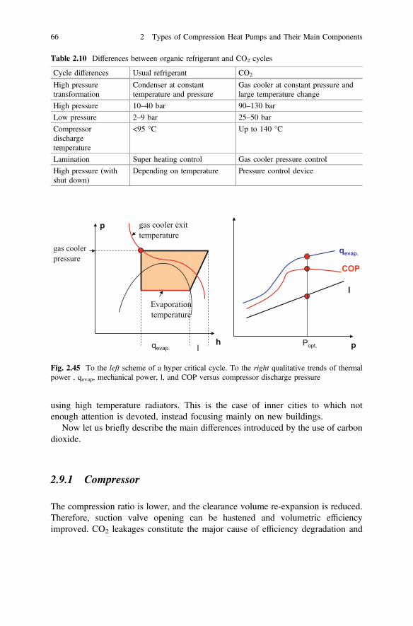
using high temperature radiators. This is the case of inner cities to which notenough attention is devoted, instead focusing mainly on new buildings.

Now let us briefly describe the main differences introduced by the use of carbondioxide.

2.9.1 Compressor

The compression ratio is lower, and the clearance volume re-expansion is reduced.Therefore, suction valve opening can be hastened and volumetric efficiencyimproved. CO2 leakages constitute the major cause of efficiency degradation and

Table 2.10 Differences between organic refrigerant and CO2 cycles

Cycle differences Usual refrigerant CO2

High pressuretransformation

Condenser at constanttemperature and pressure

Gas cooler at constant pressure andlarge temperature change

High pressure 10–40 bar 90–130 bar

Low pressure 2–9 bar 25–50 bar

Compressordischargetemperature

<95 °C Up to 140 °C

Lamination Super heating control Gas cooler pressure control

High pressure (withshut down)

Depending on temperature Pressure control device

gas cooler pressure

gas cooler exit temperature

Evaporation temperature

qevap. l

p

h Popt. p

l

COP

qevap.

Fig. 2.45 To the left scheme of a hyper critical cycle. To the right qualitative trends of thermalpower , qevap, mechanical power, l, and COP versus compressor discharge pressure


must be carefully addressed. Rotary compressors have been added, for smallloads,17 to reciprocating compressors, generally used for large loads,

For commercial, sea and railways refrigeration, Dorin [11] provides a vast rangeof semi-hermetical reciprocating compressors.

Copeland [12] produces scroll compressors with sub critical cycles for lowtemperatures (evaporation between −50 and −25 °C and condensation between −20and 5 °C) coupled with an upper HFC stage. Double stage scroll compressors havebeen designed for high pressures. The related scheme is shown in Fig. 2.46 andworks as follows: fluid exiting the evaporator flows to a first stage, where it iscompressed up to an intermediate pressure value, then it is discharged into com-pressor shell and reaches the second stage, undergoing a further compression. Bothweight and size are lowered in doing so, as the compressor shell stands “only” anintermediate pressure value. In addition leakage losses are reduced as the com-pression ratio is splitted in two stages. Efficiency increases of 15 and 30% arereported respectively for compression ratio of 2 and 4, by choosing a double stagecompressor instead of a single stage one. The related cycle is shown in Fig. 2.47.

2.9.2 Gas Cooler

Tube in tube, plate, micro channel, or plate with micro channels heat exchangers areused as gas coolers. Plate heat exchangers are in particular employed for sanitarywater production. While cooling, carbon dioxide undergoes a large temperature

electric motor

low pressure scroll

high pressure scroll

suction

discharge

Fig. 2.46 Two-stage scroll compressor

17A brochure by Sanyo (SANYO CO2 Heat Pump Water Heater pdf) reports a scroll compressorwith a total length of 217 mm for a 4.5 kW heat pump, dedicated to domestic use.

2.9 Carbon Dioxide Heat Pumps 67

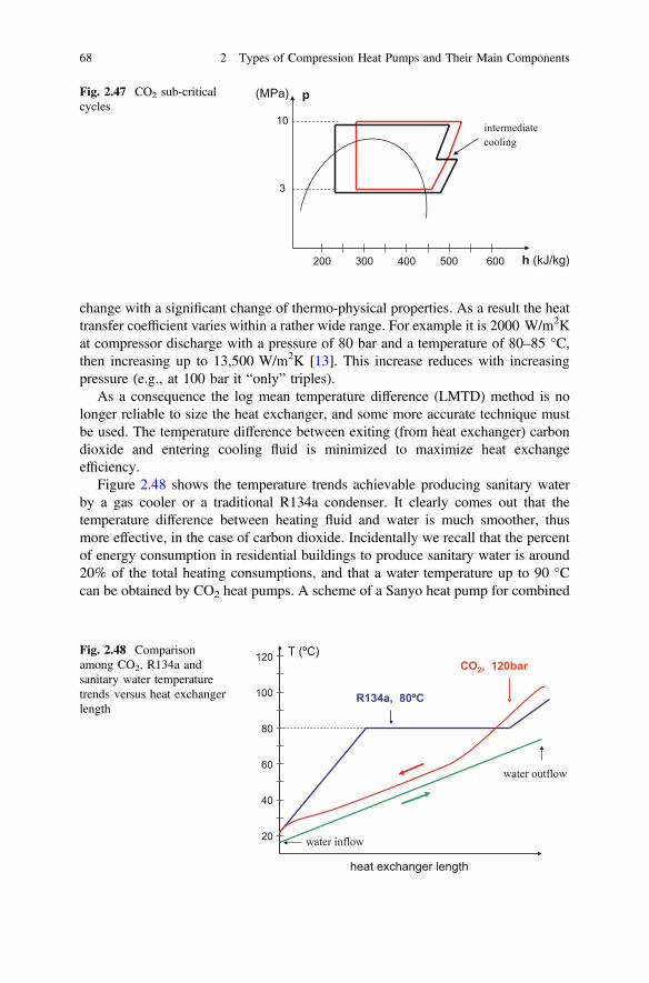
change with a significant change of thermo-physical properties. As a result the heattransfer coefficient varies within a rather wide range. For example it is 2000 W/m2Kat compressor discharge with a pressure of 80 bar and a temperature of 80–85 °C,then increasing up to 13,500 W/m2K [13]. This increase reduces with increasingpressure (e.g., at 100 bar it “only” triples).

As a consequence the log mean temperature difference (LMTD) method is nolonger reliable to size the heat exchanger, and some more accurate technique mustbe used. The temperature difference between exiting (from heat exchanger) carbondioxide and entering cooling fluid is minimized to maximize heat exchangeefficiency.

Figure 2.48 shows the temperature trends achievable producing sanitary waterby a gas cooler or a traditional R134a condenser. It clearly comes out that thetemperature difference between heating fluid and water is much smoother, thusmore effective, in the case of carbon dioxide. Incidentally we recall that the percentof energy consumption in residential buildings to produce sanitary water is around20% of the total heating consumptions, and that a water temperature up to 90 °Ccan be obtained by CO2 heat pumps. A scheme of a Sanyo heat pump for combined

p

h (kJ/kg)

3

10

(MPa)

200 500300 400 600

intermediate cooling

Fig. 2.47 CO2 sub-criticalcycles

20

120

80

60

40

100 R134a, 80ºC

CO2, 120bar

heat exchanger length

T (ºC)

water inflow

water outflow

Fig. 2.48 Comparisonamong CO2, R134a andsanitary water temperaturetrends versus heat exchangerlength


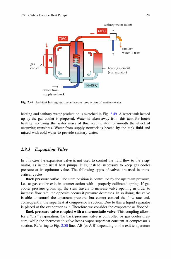
heating and sanitary water production is sketched in Fig. 2.49. A water tank heatedup by the gas cooler is proposed. Water is taken away from this tank for househeating, so using the water mass of this accumulator to smooth the effect ofoccurring transients. Water from supply network is heated by the tank fluid andmixed with cold water to provide sanitary water.

2.9.3 Expansion Valve

In this case the expansion valve is not used to control the fluid flow to the evap-orator, as in the usual heat pumps. It is, instead, necessary to keep gas coolerpressure at its optimum value. The following types of valves are used in trans-critical cycles.

Back pressure valve. The stem position is controlled by the upstream pressure,i.e., at gas cooler exit, in counter-action with a properly calibrated spring. If gascooler pressure grows up, the stem travels to increase valve opening in order toincrease flow rate; the opposite occurs if pressure decreases. In so doing, the valveis able to control the upstream pressure, but cannot control the flow rate and,consequently, the superheat at compressor’s suction. Due to this a liquid separatoris placed at the evaporator exit. Therefore we consider the evaporator as flooded.

Back pressure valve coupled with a thermostatic valve. This coupling allowsfor a “dry” evaporation: the back pressure valve is controlled by gas cooler pres-sure, while the thermostatic valve keeps vapor superheat constant at compressor’ssuction. Referring to Fig. 2.50 lines AB (or A’B’ depending on the exit temperature

sanitary water mixer

heating element (e.g. radiator)

sanitary water to user

water from supply network

70ºC

60ºC

14-45ºC

gas cooler

Fig. 2.49 Ambient heating and instantaneous production of sanitary water

2.9 Carbon Dioxide Heat Pumps 69

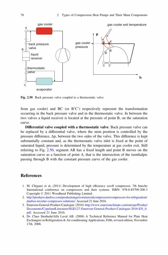
from gas cooler) and BC (or B’C’) respectively represent the transformationoccurring in the back pressure valve and in the thermostatic valve. In between thetwo valves a liquid receiver is located at the pressure of point B, on the saturationcurve.

Differential valve coupled with a thermostatic valve. Back pressure valve canbe replaced by a differential valve, where the stem position is controlled by thepressure difference, Δp, between the two sides of the valve. This difference is keptsubstantially constant and, as the thermostatic valve inlet is fixed at the point ofsaturated liquid, pressure is determined by the temperature at gas cooler exit. Stillreferring to Fig. 2.50, segment AB has a fixed length and point B moves on thesaturation curve as a function of point A, that is the intersection of the isenthalpicpassing through B with the constant pressure curve of the gas cooler.

References

1. M. Chigano et al, (2011) Development of high efficiency scroll compressor, 7th ImecheInternational conference on compressors and their systems. ISBN: 978-0-85709-208-3Copyright © 2011 Woodhead Publishing Limited.

2. http://products.danfoss.com/productrange/commercialcompressors/compressors-for-refrigeration/danfoss-inverter-compressor-solutions/. Accessed 21 June 2016.

3. Emerson-General-Product-Catalogue (2016) http://www.emersonclimate.com/europe/ProductDocuments/CopelandLiterature/SGE127-Emerson-General-Product-Catalogue-2016-EN_0.pdf. Accessed 21 June 2016.

4. Dr. Claes Stenhede/Alfa Laval AB, (2008) A Technical Reference Manual for Plate HeatExchangers in Refrigeration & Air conditioning Applications, Fifth, revised edition, November17th. 2008.

gas cooler pressure

gas cooler exit temperature

p

h

gas cooler

evaporator

back pressure valve

thermostatic valve

liquid receiver

A A’

B B’

C C’

A

B

C

Fig. 2.50 Back pressure valve coupled to a thermostatic valve


http://products.danfoss.com/productrange/commercialcompressors/compressors-for-refrigeration/danfoss-inverter-compressor-solutions/

http://products.danfoss.com/productrange/commercialcompressors/compressors-for-refrigeration/danfoss-inverter-compressor-solutions/

http://www.emersonclimate.com/europe/ProductDocuments/CopelandLiterature/SGE127-Emerson-General-Product-Catalogue-2016-EN_0.pdf



5. Plate Heat Exchangers, Hydac International, http://www.hydac.com.au/MessageForceWebsite/Sites/279/Files/Plate%20coolers.pdf.

6. Packless Industries (2016), Fluid Heat Transfer Coils, Waco, Texas http://www.packless.com/products/condenser-heat-pump-coils-2050.htm. Accessed 21 June 2016.

7. S. Garimella, (2008), Near-Critical/Supercritical Heat Transfer Measurements Of R-410A InSmall Diameter Tube, ARTI Report No. 20120-01, GEORGIA INSTITUTE OFTECHNOLOGY, George W. Woodruff School of Mechanical Engineering Atlanta, GA30332-0405.

8. G.D. Mathur,2008, (2008), Heat Transfer Coefficients And Pressure Gradients For RefrigerantR152a and R134a, Alternate Refrigerant System Symposium, Phoenix, AZ, July 16, 2008.

9. Emerson Climate Technologies & Copeland (2010), Application Engineering Bulletin,AE-1327 R5, 2010. Accessed 21 June 2016.

10. Sanyo, Commercial Gas Heat Pump—Gas Heat Pump—VRF (2011), http://www.marcogaz.org/downloads/GasHeatPumpsWorkshop/3_SANYO_GHP_Introduction_GHPworkshop_2011.pdf. Accessed 21 June 2016.

11. Dorin Innovation. http://www.dorin.com/it/catalogo/SE/HEP/ALLMODELS/H650EP.Accessed21 June 2016.

12. Copeland, General Product Guide 2016 For Refrigeration, Air Conditioning and Heat Pumps.http://www.emersonclimate.com/europe/ProductDocuments/CopelandLiterature/SGE127-Emerson-General-Product-Catalogue-2016-EN_0.pdf. Accessed 21 June 2016.

13. Sanyo, CO2 ECO Water Heaters Energy efficient and environmentally friendly water andspace heating. http://www.airconwarehouse.com/acatalog/SANYO_CO2_ECO_Brochure.pdf.Accessed 21 June 2016.

14. Alfa Laval (2015), CDEW and McDEW shell-and-tube condenser manual, pdf, http://www.alfalaval.ru/globalassets/documents/products/heat-transfer/tubular-heat-exchangers/shell-and-tube-condenser/cdew/alfa-laval-cdew-and-mcdew-shell-and-tube-condenser-manual.pdf.Accessed 21 June 2016.

References 71

http://www.hydac.com.au/MessageForceWebsite/Sites/279/Files/Plate%20coolers.pdf

http://www.hydac.com.au/MessageForceWebsite/Sites/279/Files/Plate%20coolers.pdf

http://www.packless.com/products/condenser-heat-pump-coils-2050.htm

http://www.packless.com/products/condenser-heat-pump-coils-2050.htm

http://www.marcogaz.org/downloads/GasHeatPumpsWorkshop/3_SANYO_GHP_Introduction_GHPworkshop_2011.pdf



http://www.dorin.com/it/catalogo/SE/HEP/ALLMODELS/H650EP



http://www.airconwarehouse.com/acatalog/SANYO_CO2_ECO_Brochure.pdf

http://www.alfalaval.ru/globalassets/documents/products/heat-transfer/tubular-heat-exchangers/shell-and-tube-condenser/cdew/alfa-laval-cdew-and-mcdew-shell-and-tube-condenser-manual.pdf



Chapter 3Absorption Heat Pumps

Abstract Absorption heat pumps are treated in this chapter. Their working prin-ciple is discussed and the difference between them and the compression heat pumpsis described. The method to evaluate their performances is dealt with, and somededicate examples are shown. The behavior of a two component mixture is thenillustrated with a particular reference to water ammonia mixtures and the appro-priate mass and energy balances are evaluated. A short comparison of the ammo-nia–water heat pumps with the water–bromide heat pumps is done. At the end ofthe chapter some table about the water–ammonia mixture are provided, also aimedat giving some order of magnitude of the main quantities playing a role.

3.1 The Operating Principle

This type of heat pump does not make use of a mechanical compressor and operatesaccording to the scheme shown in Fig. 3.1. Its working principle is based on theseparation of the two components of a two fluids mixture: the solute, with a highervapor pressure and the solvent, with a lower vapor pressure. These mixtures aregenerally constituted by water (solute) and lithium bromide (solvent) or ammonia(solute) and water (solvent). Figure 3.1 refers to an ammonia–water machine. Theright side of the scheme (grey) represents the apparatus replacing the compressor.On the left side the classical components of a vapor compression heat pump circuitis sketched: condenser (at pressure pc), expansion valve and evaporator (pressurepe). Pure ammonia flows in these devices. It goes to the condenser coming from agenerator, where it separates from water thanks to the heat supplied either by fuel orrecovered from a waste heat source (process waste heat, engine cooling fluid etc.).

The solution rich in ammonia enters the generator, where a distillation occurs,separating ammonia towards the condenser and a poor solution that goes to anabsorber through a lamination valve. Ammonia coming from the evaporator entersthe absorber, mixes with water (poor solution) and produces an exothermal reac-tion, exchanging the heat QA with a source at temperature TA. Most commonly this


73

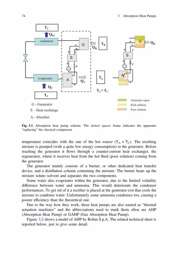
temperature coincides with the one of the hot source (TA = TC). The resultingmixture is pumped (with a quite low energy consumption) to the generator. Beforereaching the generator it flows through a counter-current heat exchanger, theregenerator, where it receives heat from the hot fluid (poor solution) coming fromthe generator.

The generator mainly consists of a burner, or other dedicated heat transferdevice, and a distillation column containing the mixture. The burner heats up themixture solute–solvent and separates the two components.

Some water also evaporates within the generator, due to the limited volatilitydifference between water and ammonia. This would deteriorate the condenserperformances. To get rid of it a rectifier is placed at the generator exit that cools themixture to condense water. Unfortunately some ammonia condenses too, causing apoorer efficiency than the theoretical one.

Due to the way how they work, these heat pumps are also named as “thermalactuation machines” and the abbreviations used to mark them often are AHP(Absorption Heat Pump) or GAHP (Gas Absorption Heat Pump).

Figure 3.2 shows a model of AHP by Robur S.p.A. The related technical sheet isreported below, just to give some detail.

TC

TF

QFC

QF

condenser

evaporator TA

QR

QA

TR

TA = TC

G

S

A

G - GeneratorS – Heat exchange

A - Absorber

S

G

A

Ammonia vapor

Poor solutionRich solution

QR

Fig. 3.1 Absorption heat pump scheme. The dotted square frame indicates the apparatus“replacing” the classical compressor

74 3 Absorption Heat Pumps

Technical sheet of the heat pump in Fig. 3.2.Heating (according to EN 12309-2).Operating point: external air 7 °C, water supplied at 35 °C, Power 37.8 kW,GUE 150%.Operating point: external air 7 °C, water supplied at 50 °C, Power 35.3 kW,GUE 140%.Maximum exit water temperature 60 °C.Dry bulb external temperature: max/min 35/−20 °C.Cooling (according to EN 12309-2).Operating point: external air 35 °C, water supplied at 7 °C, Power 16.9 kW,GUE 67%.Minimum exit water temperature 3 °C.Dry bulb external temperature: max/min 45/0 °C.Nominal electric power standard (82.1 dbA)/silenced (76.1 dbA)0.9/0.93 kW.1

Fig. 3.2 A model of a GAHPby Robur

1These values refer to the sound power according to EN ISO 9614. The calculated GUEs areequivalent to COP = 3.75 with a conversion energy factor equal to 2.5.

3.1 The Operating Principle 75

As above said, the heat released by the absorber is commonly used to heat up theindoor environment (TA = TC). Therefore the heat pump interacts with threethermal sources: the outdoor environment (TF), the indoor environment (TA) andthe device (burner, process water etc.) supplying energy to the generator.

The following equations hold:

QFCj j þ QAj j ¼ QR þQF ) QF ¼ QFCj j þ QAj j � QR

QFCj j þ QAj jTC

¼ QR

TRþ QF

TF) QFCj j þ QAj j

TC¼ QR

TRþ QFCj j þ QAj j � QR

TF

In winter heating:

COPA;W ¼ QFCj j þ QAj jQR

¼1TR� 1

TF1TC

� 1TF

¼ 1� TFTR

1� TFTC

¼ COPA

And in summer cooling:

COPA;S ¼ QF

QR¼ 1� TC

TR

1� TFTC

¼ EERA

Subscript A in the coefficients of performance means absorption, W winter and Ssummer. Once more we recall that EER (Energy Efficiency Ratio) is the name of thecooling coefficient of performance.

The followed cycle is shown in Fig. 3.3 and is usually represented in the planetemperature-pressure, where also the mixture equilibrium curves at differentammonia concentrations are drawn. This is the chart by Duhring and it actuallyreports the logarithm of pressure versus 1/T, even if only p and T appear on thecoordinate axes.

The dotted line on the left represents the condensation, lamination and evapo-ration of pure ammonia. Points C and E respectively correspond to the wholecondensation and evaporation processes, both at constant pressure.

1-2-3-4 mark the cycle followed by liquid. Point 1 corresponds to the solutionrich in ammonia. Ammonia comes from the evaporator and is absorbed in water.From this point the solution is pumped to the generator, after receiving heat fromthe countercurrent flow of the poor solution (coming from the generator) in theregenerator. It enters the generator at point 2, with the same compositions it had inthe absorber. Now most of the ammonia separates leaving a poor solution (lowcontent of ammonia). In Fig. 3.3 the ammonia concentration varies from x = 0.6 tox = 0.2. Then the solution goes to the regenerator and laminates to reach theabsorber (point 4).

Let’s go into more details about the behavior of two component mixtures. Thenon interested reader can skip the next paragraph seamlessly.


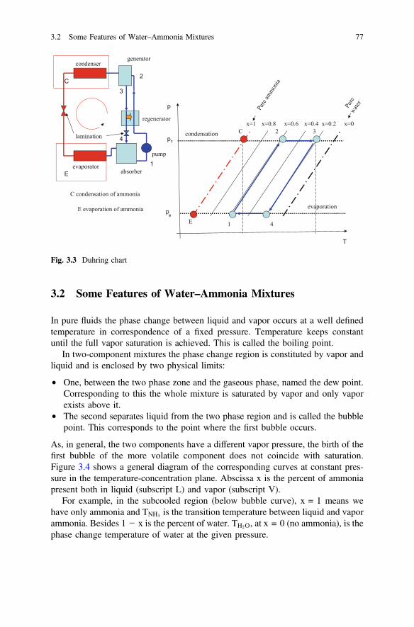
3.2 Some Features of Water–Ammonia Mixtures

In pure fluids the phase change between liquid and vapor occurs at a well definedtemperature in correspondence of a fixed pressure. Temperature keeps constantuntil the full vapor saturation is achieved. This is called the boiling point.

In two-component mixtures the phase change region is constituted by vapor andliquid and is enclosed by two physical limits:

• One, between the two phase zone and the gaseous phase, named the dew point.Corresponding to this the whole mixture is saturated by vapor and only vaporexists above it.

• The second separates liquid from the two phase region and is called the bubblepoint. This corresponds to the point where the first bubble occurs.

As, in general, the two components have a different vapor pressure, the birth of thefirst bubble of the more volatile component does not coincide with saturation.Figure 3.4 shows a general diagram of the corresponding curves at constant pres-sure in the temperature-concentration plane. Abscissa x is the percent of ammoniapresent both in liquid (subscript L) and vapor (subscript V).

For example, in the subcooled region (below bubble curve), x = 1 means wehave only ammonia and TNH3 is the transition temperature between liquid and vaporammonia. Besides 1 − x is the percent of water. TH2O, at x = 0 (no ammonia), is thephase change temperature of water at the given pressure.

x=1 x=0.8 x=0.6 x=0.4 x=0.2 x=0

pc

pe

p

T

condensation

evaporation

C

E

C condensation of ammonia

E evaporation of ammonia

1

4

condenser

evaporator

generator

absorber

regenerator

pump

lamination

C

E1

2

2 3

3

4

Fig. 3.3 Duhring chart

3.2 Some Features of Water–Ammonia Mixtures 77

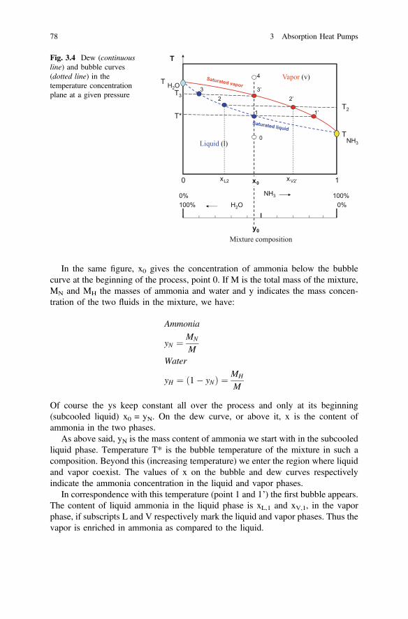
In the same figure, x0 gives the concentration of ammonia below the bubblecurve at the beginning of the process, point 0. If M is the total mass of the mixture,MN and MH the masses of ammonia and water and y indicates the mass concen-tration of the two fluids in the mixture, we have:

Ammonia

yN ¼ MN

MWater

yH ¼ ð1� yNÞ ¼ MH

M

Of course the ys keep constant all over the process and only at its beginning(subcooled liquid) x0 = yN. On the dew curve, or above it, x is the content ofammonia in the two phases.

As above said, yN is the mass content of ammonia we start with in the subcooledliquid phase. Temperature T* is the bubble temperature of the mixture in such acomposition. Beyond this (increasing temperature) we enter the region where liquidand vapor coexist. The values of x on the bubble and dew curves respectivelyindicate the ammonia concentration in the liquid and vapor phases.

In correspondence with this temperature (point 1 and 1’) the first bubble appears.The content of liquid ammonia in the liquid phase is xL,1 and xV,1, in the vaporphase, if subscripts L and V respectively mark the liquid and vapor phases. Thus thevapor is enriched in ammonia as compared to the liquid.

TB

TA

T

NH30%0%

100%100%

Vapor (v)

Liquid (l)

Mixture composition

T

T3

T2T* 1

3’’22

xL2

H2O

y0

NH3

H2OT

xV2’ 10 x0

1’

0

3

4

Fig. 3.4 Dew (continuousline) and bubble curves(dotted line) in thetemperature concentrationplane at a given pressure


Further heating up the fluid to temperature T2:

xV20 ¼ MVN

MV; xL2 ¼ ML

N

ML

MVN þML

N ¼ x0M ! xV20MV þ xL2ML ¼ x0 MV þMLð Þ

ML and MV are the total mass of liquid and vapor in the mixture present at T2.The ratio between liquid and vapor is:

ML

MV¼ xV20 � x0

x0 � xL2

2’ and 2 are intersection between the straight line T = T2 and the dew and bubblecurves. If we go to temperature T3 points 3’ and 3 correspond to the ammoniacontent in vapor and liquid. With a higher temperature (point 4) only superheatedvapor exists.

Example 3.1 Point 0 in Fig. 3.4 is at 11 MPa with x0 = 0.5 with a bubbletemperature T* = 204 °C (point 1). By increasing the temperature toT2 = 230 °C, the vapor ammonia percent in the mixture is xV = 0.7 and theliquid ammonia percent xL = 0.37.

The ratio between the masses of liquid and vapor and yN and yH are:

ML

MV¼ 0:70� 0:50

0:50� 0:37¼ 1:54

MV þ 1:54MV ¼ M

yV ¼ MV

M¼ 1

2:54¼ 0:394

yL ¼ 0:606

The ammonia mass percent in the liquid is 37% of the mixture total mass. Asliquid is the 60.6% of the total mass the ammonia percent in the liquid is22.4% and, thus, 26.6% in the vapor.

At T3 x3 = x0 = 0.5 and ammonia is completely evaporated.

Dew and bubble curves can be drawn in the temperature concentration plane atdifferent pressures as reported in Fig. 3.5 for ammonia water mixtures.

A commonly used plane is the enthalpy concentration plane. Figure 3.6 showsthe dew and bubble curves on such a plane. Enthalpies associated with vapor arealso indicated versus ammonia mass concentration x (water concentration 1 − x).

Both dew and bubble curves’ enthalpies are the sum of these two contributionplus (algebraically) the enthalpy of formation respectively due to ammonia


vaporization in the generator, DhG (>0, being provided to the fluid through andendothermic reaction) and to ammonia absorption in the absorber, DhA (<0 beingsupplied by the fluid through an exothermic reaction).2 The above two quantitiesare also named respectively the heat of desorption and heat of absorption.

For any point of the curves, at a given pressure, we have:

Dew� line

hðxÞ ¼ xVhN;V þð1� xV ÞhH;V þDhG

Bubble� line

hðxÞ ¼ xLhN;L þð1� xLÞhH;L þDhA

x

Dew

cur

ves a

t con

stan

t pr

essu

re

Bubble curves at constant

pressure

0,4 0,5 0,6 0,7 0,8 0,9 1

20

80

60

40

130

0

120

100

160

140T

(°C

)

Fig. 3.5 Dew and bubble curves at different pressures for ammonia water mixture

2This “mixing enthalpy”, Dh, can be calculated by the approximate equation [2]:

Dh ¼ h � xwith

h� ¼ 803:9 � ð1� xmÞ � 929x2mðkJ/kgÞwhere xm is the arithmetic mean of the initial and final concentrations of the transformation.


Subscripts A and G means generator and absorber and N and H ammonia andwater, as usual. Letter x means, here, ammonia vapor concentration on the dewcurve and ammonia liquid concentration on the bubble curve.

The above curves can be drawn for each pressure with different correspondingvalue of the enthalpy of pure water and pure ammonia. At the end of the chaptersome value of temperatures and enthalpies are reported in Tables 3.1, 3.2, 3.3, 3.4to give some orders of magnitude.

Figure 3.7 reports the classical Bosniakovic chart [3].As an example let us consider the transformation occurring in the generator as

reported in Fig. 3.8. Figure 3.9 shows the main flows circulating in the machine.A vapor mass flow rate, m2, exits from it, rich in ammonia with a concentration x2,while a liquid mass flow rate m3, poor in ammonia, x3, leaves it flowing to theabsorber.

Meanwhile a liquid mass flow rate m1 with a concentration x1 enters the gen-erator, coming from the absorber (see Fig. 3.9).

h

x0

0 1

Enthalpy of water vapor

Enthalpy of ammonia vapor

1-x1

NH3 NH3

H2O H2O

hN,V

hH,V hG

P=cost

h N,L

hH,L

B2

D2

Liquid

Vapor

T2

T2

isotherm

Δ

Fig. 3.6 Dew and bubble curves in enthalpy-concentration plane


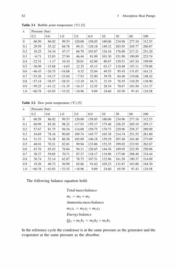
The following balance equation hold:

Total mass balance

m1 ¼ m2 þm3

Ammoniamass balance

m1x1 ¼ m2x2 þm3x3Energy balance

QG þm1h1 ¼ m2h2 þm3h3

In the reference cycle the condenser is at the same pressure as the generator and theevaporator at the same pressure as the absorber.

Table 3.1 Bubble point temperature (°C) [5]

x Pressure (bar)

0.2 0.6 1.0 2.0 6.0 10 30 60 100

0 60.50 86.02 99.53 120.00 158.85 180.06 234.96 277.10 312.53

0.1 29.59 55.22 68.78 89.31 128.18 149.32 203.95 245.77 280.87

0.2 10.25 34.34 47.17 66.70 103.87 124.16 176.80 217.21 251.20

0.3 −6.71 15.83 27.94 46.44 81.89 101.30 151.90 190.89 223.74

0.4 −22.51 −1.17 10.34 28.01 62.00 80.67 129.51 167.24 199.09

0.5 −36.09 −15.68 −4.63 12.35 45.13 63.17 110.48 147.11 178.06

0.6 −46.43 −26.75 −16.08 0.32 32.04 49.53 95.45 131.07 161.21

0.7 −53.26 −34.17 −23.84 −7.93 22.80 39.78 84.40 119.06 148.42

0.8 −57.14 −38.57 −28.53 −13.10 16.71 33.19 76.55 110.29 138.90

0.9 −59.25 −41.12 −31.35 −16.37 12.55 28.54 70.67 103.50 131.37

1.0 −60.78 −43.03 −33.52 −18.96 9.09 24.60 65.50 97.43 124.58

Table 3.2 Dew point temperature (°C) [5]

x Pressure (bar)

0.2 0.6 1.0 2.0 6.0 10 30 60 100

0 60.59 86.02 99.53 120.00 158.85 180.06 234.96 277.10 312.53

0.1 60.99 85.26 98.22 117.93 155.17 175.40 226.25 265.10 295.17

0.2 57.67 81.75 94.54 114.00 150.75 170.73 220.96 258.37 289.09

0.3 54.69 78.16 90.69 109.74 145.77 165.38 214.74 251.55 281.80

0.4 51.53 74.38 86.56 105.09 140.18 159.29 207.48 243.48 273.09

0.5 48.01 70.21 82.01 99.94 133.86 152.35 199.02 233.92 262.67

0.6 43.76 65.43 76.84 94.11 126.65 144.36 189.05 222.50 250.06

0.7 38.27 59.65 70.71 87.27 118.17 134.90 177.00 208.48 234.44

0.8 30.74 52.14 62.87 78.75 107.51 122.96 161.58 190.37 214.09

0.9 19.26 40.72 50.99 65.66 91.62 105.23 131.87 163.80 184.30

1.0 −60.78 −43.03 −33.52 −18.96 9.09 24.60 65.50 97.43 124.58


If we refer to the ratio f = m1/m2 (f > 1), e.g., the ratio between the entering flowrate to the ammonia flow rate circulating in the classical heat pump cycle, the aboveequations become:

Ammoniamass balance

fx1 ¼ x2 þðf � 1Þx3Energy balance

qG þ fh1 ¼ h2 þðf � 1Þh3qG ¼ QG

m2

Table 3.3 Saturated liquid enthalpy of ammonia–water mixture (kJ/kg) [5]

x Pressure (bar)

0.2 0.6 1.0 2.0 6.0 10 30 60 100

0 252.4 359.54 416.44 503.1 670.1 763.78 1012.1 1212.1 1387.5

0.1 55.87 163.19 220.03 306.6 473.6 567.94 820.96 1028.5 1213.3

0.2 −91.72 10.89 65.25 148.1 308.6 399.83 647.03 850.72 1038.1

0.3 −221.5 −122.2 −69.72 10.13 164.6 252.52 491.92 692.80 875.22

0.4 −332.5 −234.0 −182.3 −104.1 46.24 131.40 363.48 558.87 737.08

0.5 −414.7 −315.5 −263.9 −186.4 −38.71 44.46 270.42 460.70 634.65

0.6 −458.5 −358.7 −307.3 −230.3 −84.67 −3.07 217.99 404.05 574.36

0.7 −459.6 −361.1 −310.3 −234.5 −91.39 −11.27 205.75 388.59 556.18

0.8 −421.6 −326.8 −277.8 −204.3 −64.77 13.71 227.16 407.64 573.36

0.9 −355.1 −266.8 −220.6 −150.7 −16.00 60.56 270.61 449.33 613.81

1.0 −274.0 −195.2 −152.9 −87.7 40.80 115.15 321.80 499.15 662.78

Table 3.4 Saturated vapor enthalpy of ammonia-water mixture (kJ/kg) [5]

x Pressure (bar)

0.2 0.6 1.0 2.0 6.0 10 30 60 100

0 2612.2 2655.6 2677.2 2708.1 2758.3 2780.6 2818.9 2828.6 2823.5

0.1 1548.1 1690.4 1766.3 1876.0 2056.1 2138.3 2298.7 2378.2 2419.4

0.2 1359.8 1439.9 1488.7 1567.3 1717.4 1794.5 1961.1 2053.5 2106.3

0.3 1296.3 1349.3 1381.2 1433.8 1541.6 1601.1 1738.8 1819.8 1866.7

0.4 1256.9 1299.7 1323.9 1362.7 1441.2 1485.2 1589.5 1650.6 1682.7

0.5 1227.0 1265.1 1285.8 1317.6 1378.6 1411.7 1487.3 1526.9 1540.1

0.6 1204.9 1240.3 1259.1 1287.1 1337.7 1363.5 1416.8 1436.0 1428.5

0.7 1190.4 1224.0 1241.5 1267.1 1311.1 1332.0 1368.5 1369.4 1341.2

0.8 1182.2 1214.3 1230.8 1254.7 1294.2 1311.7 1335.3 1320.3 1272.5

0.9 1177.7 1208.6 1224.4 1246.9 1282.9 1297.7 1310.7 1281.4 1214.7

1.0 1174.6 1204.4 1219.5 1240.7 1273.5 1286.0 1289.1 1245.5 1158.6


Therefore

f ¼ m1

m2¼ x2 � x3

x1 � x3qG ¼ h2 � h3ð Þþ f h3 � h1ð Þor

QG ¼ m2 h2 � h3ð Þþm1 h3 � h1ð Þ

h (k

cal/k

g)

H (k

J/kg

)

Fig. 3.7 Enthalpy-concentration Bosniakovic chart for an ammonia water mixture. Referencestates: enthalpies of liquid water at 0 °C and of liquid ammonia at −77 °C are zero


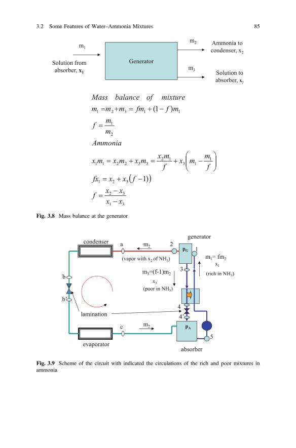
Fig. 3.8 Mass balance at the generator

4’

condenser

evaporator

generator

absorber

lamination

1a

3

5

pG

pA

b

b’

c

m2

m2

(vapor with x2 of NH3) m1= fm2

m3=(f-1)m2

4

(rich in NH3)

(poor in NH3)

x1

x3

2

Fig. 3.9 Scheme of the circuit with indicated the circulations of the rich and poor mixtures inammonia


Thus the heat supplied to the generator, QG, can be seen as composed by twocontributions. The first one, m2(h2 − h3), related to the actual phase change fromliquid to vapor of the fluid going to the condenser. On the other hand the secondone is the enthalpy difference between the fluid leaving and entering the desorber(generator).

Figure 3.10 reports the transformations occurring in the generator.The energy balance at the absorber is:

m2hc þm3h40 ¼ QA þm1h5m2hc þðf � 1Þm2h40 ¼ QA þ fm2h5

Therefore the heat released by the absorber is:

QA ¼ m2hc þðf � 1Þm2h4 � fm2h5 ¼ m2 hc � h4ð Þþ fm2 h4 � h5ð ÞqA ¼ QA

m2¼ hc � h4ð Þþ f h4 � h5ð Þ

Assuming the work done by the pump to be negligible, the lamination isenthalpic(h4 = h4’) and the regenerator adiabatic, we obtain:

f � 1ð Þm2ðh4 � h3Þ ¼ fm2ðh1 � h5Þ

h

T1

T31

3

2

X1 X2X 3

Fig. 3.10 Transformationsoccurring in the generator


And, thus:

f ¼ ðh4 � h3Þðh4 � h3Þþ ðh1 � h5Þ

The energy balance of the whole heat pump accounts for the following quantities.

• QC—heat supplied by condenser (in winter to the indoor source): QC = −|QC|.• QE—heat received by evaporator (in winter by the outdoor source): QE = |QE|.• QG—heat supplied to generator, rectifier included: QG = |QG|.• QA—heat released by absorber: QA = −|QA|.• L—work provided to the solution pump: L = −|L|, commonly not accounted for

in the energy balance being negligible with respect to the other quantities.

Therefore:

� QCj j � QAj j þQG þQE � Lj j ¼ 0

And

COP ¼ QCj j þ QAj jQGj j þ Lj j

The heat released by the absorber can be directly used for space heating in winter.Absorption heat pumps can usually operate with a fluid temperature of a tradi-

tional heating system up to 65 °C (max. return temperature 55 °C) and 70 °C forsanitary water production, as well as with radiant floors and fan coils up to 50 °Cand a return temperature of 45 °C.

As above said, absorption heat pumps also use a mixture of water and lithiumbromide, generally employed for large size air conditioning and refrigerationsystems.

Herein we shortly summarize the plus (�) and minus (►) of these machines withrespect to the ones using the mixture ammonia—water.

• They do not need a rectifier as generator produces a practically pure vapor ofsolute.

► As solute is water they cannot operate below 0 °C► Lithium bromide may crystallize and it stops the heat pump operation.► These heat pumps work at pressures lower than the atmospheric one and

thus they work under vacuum and need proper sealing.

For better details on the subject treated in this chapter the reader is referred to [4].


References

1. http://www.robur.it/area_tecnica/dossier_tecnici/ciclo_frigorifero)o_ad_assorbimento.Accessed July 2016.

2. Manohar Prasad, Refrigeration and Air Conditioning, New Age International Publisher,New Delhi, 2005.

3. Bosniakovic, Technische Thermodynamic, T. Steinkopff, Leipzig, 1935.4. Herold K. E., Radermacher R.,Klein S. A., Absorption Chillers and Heat Pumps, CRC Press,

Boca Raton, FL (USA), 1996.5. Thermodynamic Properties of Ammonia–Water Mixture—Shodhganga shodhganga.inflibnet.

ac.in/bitstream/10603/…/16_appendix.pdf. Accessed May 2017.


http://www.robur.it/area_tecnica/dossier_tecnici/ciclo_frigorifero)o_ad_assorbimento

Chapter 4Operating Conditions

Abstract This chapter describes how to choose the nominal power of a heat pumpin dependence of the load requirement of the user and the local climatic conditions.Furthermore as the performance of a heat pump is obviously affected by the powerrequired, the full load and part load operations are examined and the load factor isintroduced. The chapter describes the methods, provided by the present standards,of evaluating the coefficients of performance and the data the producers have tosupply in order to make such calculations.

4.1 Full Load and Partial Load Operation, the BalancePoint

The heating load required by a building versus the outdoor temperature can beapproximated by a straight line with a negative slope. The trend of the power a heatpump can provide in the same conditions (commonly named capacity) is easilyobtainable as follows. As we already said, heat pumps generally use a volumetriccompressor and, therefore, their mass flow rate depends on their volumetric flowrate (that is rotation speed) and fluid density. The latter increases with rising ofoutdoor temperature, because the evaporation temperature and the related temper-ature increase.

As a consequence of this the supplied power increases and shows a growingtrend with outdoor temperature. In addition COP grows up as sources’ temperaturesget closer.

In summer the required building cooling load grows versus the outdoor tem-perature and solar radiation. In the meantime the sources’ temperatures drift apart,the indoor temperature being kept constant. The net result is a decrease of thecooling capacity and reduction of EER. Thus we have an opposite trend of the twocurves of required and supplied power.

The intersection between the power required by the user and the heat pumpcapacity is named balance point. In winter the power, the heat pump can provide onthe right of the balance point, is progressively larger than the one needed by the


89

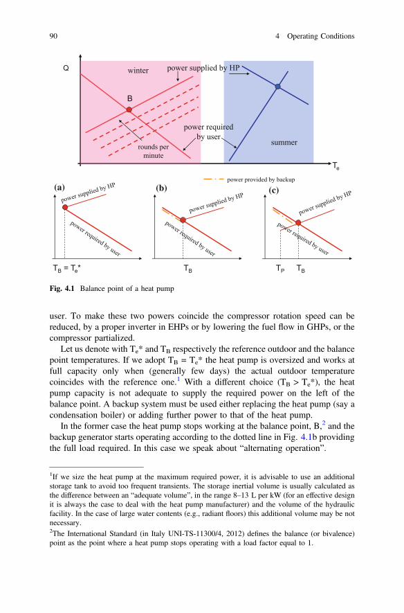
user. To make these two powers coincide the compressor rotation speed can bereduced, by a proper inverter in EHPs or by lowering the fuel flow in GHPs, or thecompressor partialized.

Let us denote with Te* and TB respectively the reference outdoor and the balancepoint temperatures. If we adopt TB = Te* the heat pump is oversized and works atfull capacity only when (generally few days) the actual outdoor temperaturecoincides with the reference one.1 With a different choice (TB > Te*), the heatpump capacity is not adequate to supply the required power on the left of thebalance point. A backup system must be used either replacing the heat pump (say acondensation boiler) or adding further power to that of the heat pump.

In the former case the heat pump stops working at the balance point, B,2 and thebackup generator starts operating according to the dotted line in Fig. 4.1b providingthe full load required. In this case we speak about “alternating operation”.

Q

Te

power required by user

B

winter

summer

power supplied by HP

rounds per minute

TB = Te* TB TB

power provided by backup

TP

(a) (b) (c)

Fig. 4.1 Balance point of a heat pump

1If we size the heat pump at the maximum required power, it is advisable to use an additionalstorage tank to avoid too frequent transients. The storage inertial volume is usually calculated asthe difference between an “adequate volume”, in the range 8–13 L per kW (for an effective designit is always the case to deal with the heat pump manufacturer) and the volume of the hydraulicfacility. In the case of large water contents (e.g., radiant floors) this additional volume may be notnecessary.2The International Standard (in Italy UNI-TS-11300/4, 2012) defines the balance (or bivalence)point as the point where a heat pump stops operating with a load factor equal to 1.

90 4 Operating Conditions

In the latter case an additional power source takes action only supplying thedifference between the user’s power requirement and the power given by the heatpump, down to temperature Tp (Fig. 4.1c). This is the “parallel operation”.

It is necessary to analyze the trend of the outdoor temperature of the location weare interested in. We need to know how many times each value occurs during theperiod we are referring to. For instance we could learn that 0 °C occurs for 40 h, 4 °Cfor 300 h and so on, in winter. To better clarify this, the following example maybe used.

Example 4.1 Let us suppose that a given place has an outdoor referencetemperature equal to Te* (in Italy commonly included in the range 0, −5 °Cand anyway obtainable through the National Standards) and a reference loadQ* in correspondence of the above temperature. In addition let us supposethis temperature occur for a percent p* of the heating season.

If P is the heating period in hours, a temperature Te lower or equal to Te*(Te � Te*) takes place during a time interval p*P. We refer to Fig. 4.2where the cumulative curve p = f(Te) is represented. Temperature Te is on theabscissa and its percent of occurrence, p, in ordinate. For instance at a givenpk correspond temperatures Te � Te,k.

We can divide the seasonal temperature variation TH in n temperaturesub-intervals T = TH/n. If at time tk Te = Te,k, the outdoor temperature will

Fig. 4.2 Cumulative curve of the occurrence of different temperatures versus their percent ofoccurrence

4.1 Full Load and Partial Load Operation, the Balance Point 91

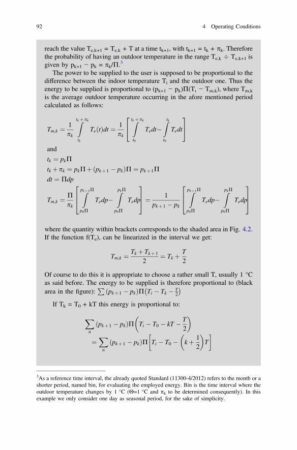
reach the value Te,k+1 = Te,k + T at a time tk+1, with tk+1 = tk + pk. Thereforethe probability of having an outdoor temperature in the range Te,k � Te,k+1 isgiven by pk+1 − pk = pk/P.3

The power to be supplied to the user is supposed to be proportional to thedifference between the indoor temperature Ti and the outdoor one. Thus theenergy to be supplied is proportional to (pk+1 − pk)P(Ti − Tm,k), where Tm,k

is the average outdoor temperature occurring in the afore mentioned periodcalculated as follows:

Tm;k ¼ 1pk

Ztk þ pk

tk

Te tð Þdt ¼ 1pk

Ztk þpk

t0

Tedt�Ztk

t0

Tedt

24

35

and

tk ¼ pkP

tk þ pk ¼ pkPþ pkþ 1 � pkð ÞP ¼ pkþ 1P

dt ¼ Pdp

Tm;k ¼ Ppk

Zpkþ 1P

p0P

Tedp�ZpkP

p0P

Tedp

264

375 ¼ 1

pkþ 1 � pk

Zpkþ 1P

p0P

Tedp�ZpkP

p0P

Tedp

264

375

where the quantity within brackets corresponds to the shaded area in Fig. 4.2.If the function f(Te), can be linearized in the interval we get:

Tm;k ¼ Tk þ Tkþ 1

2¼ Tk þ T

2

Of course to do this it is appropriate to choose a rather small T, usually 1 °Cas said before. The energy to be supplied is therefore proportional to (blackarea in the figure):

Ppkþ 1 � pkð ÞP Ti � Tk � T

2

� �If Tk = T0 + kT this energy is proportional to:

Xn

pkþ 1 � pkð ÞP Ti � T0 � kT � T2

� �

¼Xn

pkþ 1 � pkð ÞP Ti � T0 � kþ 12

� �T

� �

3As a reference time interval, the already quoted Standard (11300-4/2012) refers to the month or ashorter period, named bin, for evaluating the employed energy. Bin is the time interval where theoutdoor temperature changes by 1 °C (H=1 °C and pk to be determined consequently). In thisexample we only consider one day as seasonal period, for the sake of simplicity.


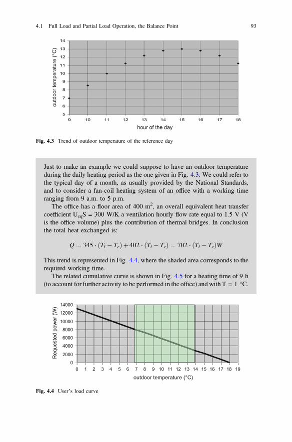
Just to make an example we could suppose to have an outdoor temperatureduring the daily heating period as the one given in Fig. 4.3. We could refer tothe typical day of a month, as usually provided by the National Standards,and to consider a fan-coil heating system of an office with a working timeranging from 9 a.m. to 5 p.m.

The office has a floor area of 400 m2, an overall equivalent heat transfercoefficient UeqS = 300 W/K a ventilation hourly flow rate equal to 1.5 V (Vis the office volume) plus the contribution of thermal bridges. In conclusionthe total heat exchanged is:

Q ¼ 345 � Ti � Teð Þþ 402 � Ti � Teð Þ ¼ 702 � Ti � Teð ÞW

This trend is represented in Fig. 4.4, where the shaded area corresponds to therequired working time.

The related cumulative curve is shown in Fig. 4.5 for a heating time of 9 h(to account for further activity to be performed in the office) and with T = 1 °C.

hour of the day

outd

oor t

empe

ratu

re (°

C)

Fig. 4.3 Trend of outdoor temperature of the reference day

0

2000

4000

6000

8000

10000

12000

14000

0 1 2 3 4 5 6 7 8 9 10 11 12 13 14 15 16 17 18 19

outdoor temperature (°C)

Req

uest

ed p

ower

(W)

Fig. 4.4 User’s load curve


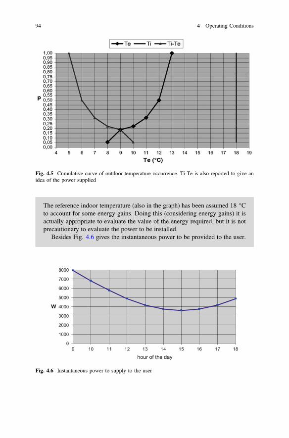
The reference indoor temperature (also in the graph) has been assumed 18 °Cto account for some energy gains. Doing this (considering energy gains) it isactually appropriate to evaluate the value of the energy required, but it is notprecautionary to evaluate the power to be installed.

Besides Fig. 4.6 gives the instantaneous power to be provided to the user.

Fig. 4.5 Cumulative curve of outdoor temperature occurrence. Ti-Te is also reported to give anidea of the power supplied

0

1000

2000

3000

4000

5000

6000

7000

8000

9 10 11 12 13 14 15 16 17 18

W

hour of the day

Fig. 4.6 Instantaneous power to supply to the user


Of course to have a comprehensive evaluation of heat pumps performance thebehaviour of COP4 it is necessary to examine its operation at partial load. To thispurpose manufacturers should provide several kind of information concerning:

• Type of heat pump, also specifying whether it is reversible (heating and cooling)or not.

• Intended use. e.g., only heating (cooling), heating and cooling, mixed heatingand sanitary water, only sanitary water.

• Type of operation: on-off, modulating.• Heat pump thermal sources.• Furthermore manufacturers must provide the full load performances in corre-

spondence of different sources temperatures (EN 14825 and TS 11300). TheStandards give such conditions, reported in Tables 4.1 and 4.2 for sanitary waterproduction.

• Performances at a climatic part load ratio, PLR, other than 1. PLR is supposed togo to zero at an outdoor temperature equal to 16 °C and is defined as:

PLR ¼ Te � 16Tpe � 16

where Te and Tep respectively are the actual outdoor temperature and the reference

outdoor temperature, employed in the system design. For example for Te = 8 °Cand Te

P = 0 °C, PLR = 0.5.Moreover a “second principle efficiency”, η″, is defined as the ratio between

COP in the actual conditions and the ideal one at the same source temperatures.

Table 4.1 Reference temperatures to which manufacturers have to refer to provide performancedata for heating use or mixed use heating and sanitary water production (Tp,c hot sink temperaturein °C)

Temp. (°C)cold source

Tp,c air heating Tp,c water heating Tp,c

sanitarywater

Air

−7 2 7 12 20 35 45 55 45 55

Water

5 10 15 20 35 45 55 45 55

Ground

−5 0 5 10 20 35 45 55 45 55

4(and/or the significant parameter(s) to be considered for the type of heat pump we are using andthe working period we are referring to in the actual use, as stressed in the next paragraph).


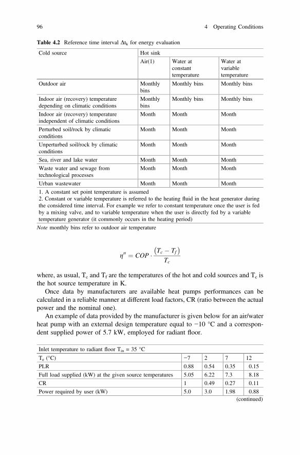
g00 ¼ COP � Tc � Tf� �

Tc

where, as usual, Tc and Tf are the temperatures of the hot and cold sources and Tc isthe hot source temperature in K.

Once data by manufacturers are available heat pumps performances can becalculated in a reliable manner at different load factors, CR (ratio between the actualpower and the nominal one).

An example of data provided by the manufacturer is given below for an air/waterheat pump with an external design temperature equal to −10 °C and a correspon-dent supplied power of 5.7 kW, employed for radiant floor.

Inlet temperature to radiant floor Tin = 35 °C

Te (°C) −7 2 7 12

PLR 0.88 0.54 0.35 0.15

Full load supplied (kW) at the given source temperatures 5.05 6.22 7.3 8.18

CR 1 0.49 0.27 0.11

Power required by user (kW) 5.0 3.0 1.98 0.88(continued)

Table 4.2 Reference time interval Dtk for energy evaluation

Cold source Hot sink

Air(1) Water atconstanttemperature

Water atvariabletemperature

Outdoor air Monthlybins

Monthly bins Monthly bins

Indoor air (recovery) temperaturedepending on climatic conditions

Monthlybins

Monthly bins Monthly bins

Indoor air (recovery) temperatureindependent of climatic conditions

Month Month Month

Perturbed soil/rock by climaticconditions

Month Month Month

Unperturbed soil/rock by climaticconditions

Month Month Month

Sea, river and lake water Month Month Month

Waste water and sewage fromtechnological processes

Month Month Month

Urban wastewater Month Month Month

1. A constant set point temperature is assumed2. Constant or variable temperature is referred to the heating fluid in the heat generator duringthe considered time interval. For example we refer to constant temperature once the user is fedby a mixing valve, and to variable temperature when the user is directly fed by a variabletemperature generator (it commonly occurs in the heating period)

Note monthly bins refer to outdoor air temperature


(continued)

Inlet temperature to radiant floor Tin = 35 °C

COP 3.14 5.39 6.68 4.37

COP(CR = 1) 3.14 3.91 4.51 5.38

Correction factor f = COP(CR = 1)/COP 0.97 1.38 1.48 0.81

Power and COP(CR = 1) at full load for various Tin.

Full load (kW) COP(CR = 1)

Tin = 35 Tin = 45 Tin = 55 Tin = 35 Tin = 45 Tin = 55

−7 5.05 4.91 4.62 3.14 2.54 2.16

2 6.22 5.80 5.44 3.86 2.97 2.35

7 7.30 6.80 6.37 4.59 3.47 2.76

12 8.18 7.94 7.42 5.38 4.09 3.40

Power and COP(CR = 1) at full load for production of sanitary water.

Full load (kW) COP(CR = 1)

Tin = 55 °C

7 6.37 2.76

15 7.90 3.59

20 8.54 3.85

35 8.54 3.81

Parameter η″ (second principle efficiency) is calculated in correspondence of theavailable data (sources temperatures and COP) and evaluated by linear interpolationfor intermediate conditions.

If the above data are not provided, Standard EN14825/2012 gives the followingequation to estimate COP.

Heat pumps air/air, antifreeze/air, water/air:

COP ¼ COPðCR ¼ 1Þ � 1� Cd 1� CRð Þ½ �

If data are not known Cd = 0.25 (ground/air included)Heat pumps air/water, antifreeze/water, water/water:

COP ¼ COPðCR ¼ 1Þ � CRCcCRþ 1� Ccð Þ½ �

If data is not known Cc = 0.9 (ground/water included). For heat pump with inverterno correction is applied in the range of CR from 1 to 0.5. η″ is calculated at theconditions referred to the available data and kept constant in the remaining range.

While addressing the interested reader to the above quoted standard for betterdetails, we refer to Example 4.1 to make an additional one for the sake of clarity.


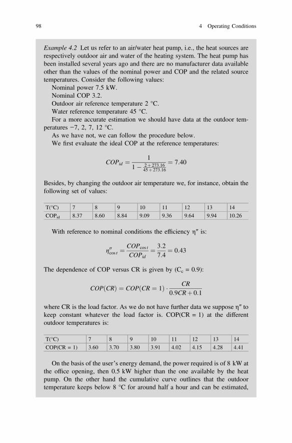
Example 4.2 Let us refer to an air/water heat pump, i.e., the heat sources arerespectively outdoor air and water of the heating system. The heat pump hasbeen installed several years ago and there are no manufacturer data availableother than the values of the nominal power and COP and the related sourcetemperatures. Consider the following values:

Nominal power 7.5 kW.Nominal COP 3.2.Outdoor air reference temperature 2 °C.Water reference temperature 45 °C.For a more accurate estimation we should have data at the outdoor tem-

peratures −7, 2, 7, 12 °C.As we have not, we can follow the procedure below.We first evaluate the ideal COP at the reference temperatures:

COPid ¼ 11� 2þ 273:16

45þ 273:16

¼ 7:40

Besides, by changing the outdoor air temperature we, for instance, obtain thefollowing set of values:

T(°C) 7 8 9 10 11 12 13 14

COPid 8.37 8.60 8.84 9.09 9.36 9.64 9.94 10.26

With reference to nominal conditions the efficiency η″ is:

g00cos t ¼COPcos t

COPid¼ 3:2

7:4¼ 0:43

The dependence of COP versus CR is given by (Cc = 0.9):

COPðCRÞ ¼ COPðCR ¼ 1Þ � CR0:9CRþ 0:1

where CR is the load factor. As we do not have further data we suppose η″ tokeep constant whatever the load factor is. COP(CR = 1) at the differentoutdoor temperatures is:

T(°C) 7 8 9 10 11 12 13 14

COP(CR = 1) 3.60 3.70 3.80 3.91 4.02 4.15 4.28 4.41

On the basis of the user’s energy demand, the power required is of 8 kW atthe office opening, then 0.5 kW higher than the one available by the heatpump. On the other hand the cumulative curve outlines that the outdoortemperature keeps below 8 °C for around half a hour and can be estimated,


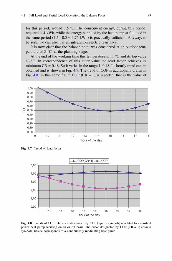
for this period, around 7.5 °C. The consequent energy, during this period,required is 4 kWh, while the energy supplied by the heat pump at full load inthe same period (7.5 � 0.5 = 3.75 kWh) is practically sufficient. Anyway, tobe sure, we can also use an integration electric resistance.

It is now clear that the balance point was considered at an outdoor tem-perature of 8 °C, at the planning stage.

At the end of the working time this temperature is 11 °C and its top value13 °C. In correspondence of this latter value the load factor achieves itsminimum CR = 0.48. So it varies in the range 1–0.48. Its hourly trend can beobtained and is shown in Fig. 4.7. The trend of COP is additionally drawn inFig. 4.8. In this same figure COP (CR = 1) is reported, that is the value of

0,000,100,200,300,400,500,600,700,800,901,00

9 10 11 12 13 14 15 16 17 18

hour of the day

CR

Fig. 4.7 Trend of load factor

0,00

1,00

2,00

3,00

4,00

5,00

9 10 11 12 13 14 15 16 17 18

COP(CR=1) COP

hour of the day

Fig. 4.8 Trends of COP. The curve designated by COP (square symbols) is related to a constantpower heat pump working on an on-off basis. The curve designated by COP (CR = 1) (rhombsymbols) beside corresponds to a continuously modulating heat pump


COP the heat pump would have working at the full load each hour. In thiscase there is not a big difference between the two curves because the loadfactor is not lower than 0.5. For lower CRs this difference is much morepronounced.

Furthermore we show the trends of f = COP/COP (CR = 1) for air/air andair/water heat pumps respectively in Figs. 4.9 and 4.10. The on-off operation isindicated by a continuous line, while symbols represent modulating operationstarting from 30% of the full load. In Example 4.3 we also report the behaviour of amodulating heat pump.

For absorption heat pumps directly fed by a fuel (direct gas fired machines) theeffect of CR is evaluated as follows. As better specified in the next paragraph thecoefficient of performance is now named GUE (Gas Utilization Efficiency), becausethese heat pumps directly use a primary source (fuel) instead of electricity.

The ideal GUE and η″ are expressed as;

GUEid ¼ TcTgen

Tgen � TfTc � Tf

� �

g00 ¼ GUEGUEid

Subscript “gen” means generator.

0,5

0,6

0,7

0,8

0,9

1

1,1

0 0,1 0,2 0,3 0,4 0,5 0,6 0,7 0,8 0,9 1

CR

CO

P/C

OP(

CR

=1)

on/off modulantemodulating

Fig. 4.9 f = COP/COP(CR) versus CR for an air/air heat pump


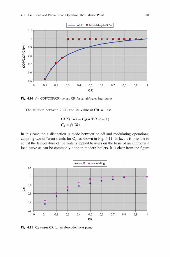
The relation between GUE and its value at CR = 1 is:

GUEðCRÞ ¼ CdGUEðCR ¼ 1ÞCd ¼ f ðCRÞ

In this case too a distinction is made between on-off and modulating operations,adopting two different trends for Cd, as shown in Fig. 4.11. In fact it is possible toadjust the temperature of the water supplied to users on the basis of an appropriateload curve as can be commonly done in modern boilers. It is clear from the figure

0,5

0,6

0,7

0,8

0,9

1

1,1

0 0,1 0,2 0,3 0,4 0,5 0,6 0,7 0,8 0,9 1

CR

CO

P/C

OP(

CR

=1)

on/off modulante f ino al 30%Modulating to 30%

Fig. 4.10 f = COP/COP(CR) versus CR for an air/water heat pump

0,6

0,7

0,8

0,9

1

1,1

0 0,1 0,2 0,3 0,4 0,5 0,6 0,7 0,8 0,9 1

CR

Cd

on-off modulating

Fig. 4.11 Cd versus CR for an absorption heat pump


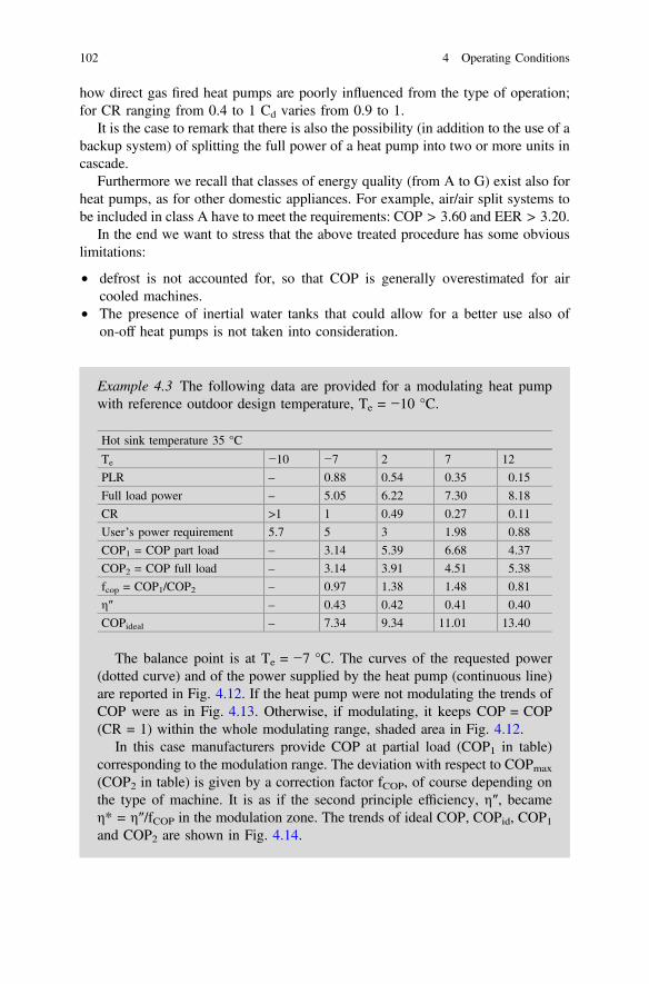
how direct gas fired heat pumps are poorly influenced from the type of operation;for CR ranging from 0.4 to 1 Cd varies from 0.9 to 1.

It is the case to remark that there is also the possibility (in addition to the use of abackup system) of splitting the full power of a heat pump into two or more units incascade.

Furthermore we recall that classes of energy quality (from A to G) exist also forheat pumps, as for other domestic appliances. For example, air/air split systems tobe included in class A have to meet the requirements: COP > 3.60 and EER > 3.20.

In the end we want to stress that the above treated procedure has some obviouslimitations:

• defrost is not accounted for, so that COP is generally overestimated for aircooled machines.

• The presence of inertial water tanks that could allow for a better use also ofon-off heat pumps is not taken into consideration.

Example 4.3 The following data are provided for a modulating heat pumpwith reference outdoor design temperature, Te = −10 °C.

Hot sink temperature 35 °C

Te −10 −7 2 7 12

PLR – 0.88 0.54 0.35 0.15

Full load power – 5.05 6.22 7.30 8.18

CR >1 1 0.49 0.27 0.11

User’s power requirement 5.7 5 3 1.98 0.88

COP1 = COP part load – 3.14 5.39 6.68 4.37

COP2 = COP full load – 3.14 3.91 4.51 5.38

fcop = COP1/COP2 – 0.97 1.38 1.48 0.81

η″ – 0.43 0.42 0.41 0.40

COPideal – 7.34 9.34 11.01 13.40

The balance point is at Te = −7 °C. The curves of the requested power(dotted curve) and of the power supplied by the heat pump (continuous line)are reported in Fig. 4.12. If the heat pump were not modulating the trends ofCOP were as in Fig. 4.13. Otherwise, if modulating, it keeps COP = COP(CR = 1) within the whole modulating range, shaded area in Fig. 4.12.

In this case manufacturers provide COP at partial load (COP1 in table)corresponding to the modulation range. The deviation with respect to COPmax

(COP2 in table) is given by a correction factor fCOP, of course depending onthe type of machine. It is as if the second principle efficiency, η″, becameη* = η″/fCOP in the modulation zone. The trends of ideal COP, COPid, COP1and COP2 are shown in Fig. 4.14.


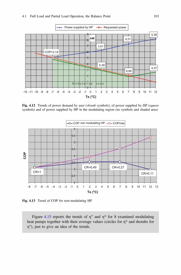
Figure 4.15 reports the trends of η″ and η* for 8 examined modulatingheat pumps together with their average values (circles for η* and rhombs forη″), just to give an idea of the trends.

1

2

33

0

1

22

M o d u l a t i o n z o n e

4

5

6

7

8

9

-12 -11 -10 -9 -8 -7 -6 -5 -4 -3 -2 -1 0 1 2 3 4 5 6 7 8 9 10 11 12

Te (°C)

kW

COP=3,14

5,39

3,91

6,68

4,515,38

4,37

Power supplied by HP Requested power

Fig. 4.12 Trends of power demand by user (rhomb symbols), of power supplied by HP (squaresymbols) and of power supplied by HP in the modulating region (no symbols and shaded area)

2

2,5

3

3,5

4

4,5

5

5,5

6

-8 -7 -6 -5 -4 -3 -2 -1 0 1 2 3 4 5 6 7 8 9 10 11 12 13

Te (°C)

CO

P

COP COPmax

CR=1CR=0,49 CR=0,27

CR=0,11

non modulating HP

Fig. 4.13 Trend of COP for non-modulating HP


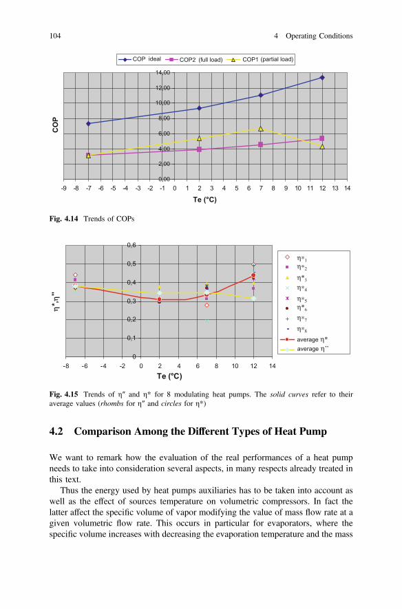
4.2 Comparison Among the Different Types of Heat Pump

We want to remark how the evaluation of the real performances of a heat pumpneeds to take into consideration several aspects, in many respects already treated inthis text.

Thus the energy used by heat pumps auxiliaries has to be taken into account aswell as the effect of sources temperature on volumetric compressors. In fact thelatter affect the specific volume of vapor modifying the value of mass flow rate at agiven volumetric flow rate. This occurs in particular for evaporators, where thespecific volume increases with decreasing the evaporation temperature and the mass

0,00

2,00

4,00

6,00

8,00

10,00

12,00

14,00

-9 -8 -7 -6 -5 -4 -3 -2 -1 0 1 2 3 4 5 6 7 8 9 10 11 12 13 14

Te (°C)

CO

PCOP COP2 COP1ideal (full load) (partial load)

Fig. 4.14 Trends of COPs

Fig. 4.15 Trends of η″ and η* for 8 modulating heat pumps. The solid curves refer to theiraverage values (rhombs for η″ and circles for η*)


flow rate reduces. In addition the air humidity has to be accounted for as it affectsthe heat exchangers’ performance and the defrost cycles.

An appropriate parameter to compare the performances of the different types ofheat pumps has been defined and named P.E.R., Primary Energy Ratio. This is theratio between the useful energy, QUT, delivered to users and the employed primaryenergy, QEP.

For boilers this ratio is larger than unit only for condensation boilers (referring tothe lower calorific value), where it reaches the value of 1.11.

For heat pumps the following considerations hold.Electric heat pumps (EHP)—The primary energy is supplied by the electric

power stations and delivered to heat pumps through the electric power lines system.Therefore it is influenced by the average equivalent efficiency of the system ofavailable power stations, ηCE, and by the equivalent efficiency of the power linessystem, eTR, thus, we have:

power to compressor

L ¼ gMC � gCE � eTRQEP ¼ gMCEelQEP

total efficiency ofelectric system

Eel ¼ gCE � eTR

PEREHP ¼ QUT

QEP¼ gMCEel � QC

L¼ gMCEel � COPEHP

The term ηMC is the efficiency of the set of devices installed between the pointswhere the electric power is delivered to the work L the compressor delivers to thefluid. It includes the efficiencies of the electric motor, of an eventual mechanicalcoupling (motor-compressor), of the inverter and possible other auxiliaries.

Example 4.4 Suppose ηMC = 0.9, the trend of PER versus COP for differentvalues of Eel is reported in Fig. 4.16. This same figure shows the case whenCOP corresponds to a PER larger than unit. The figure also reports the valuesof PER for a traditional boiler with an efficiency of 0.9 and for a condensationboiler with an efficiency of 1.11.

Gas heat pumps (GHP)—By assuming QM = QEP it follows that:

PERGHP ¼ QUT

QEP¼ COPGHP

4.2 Comparison Among the Different Types of Heat Pump 105

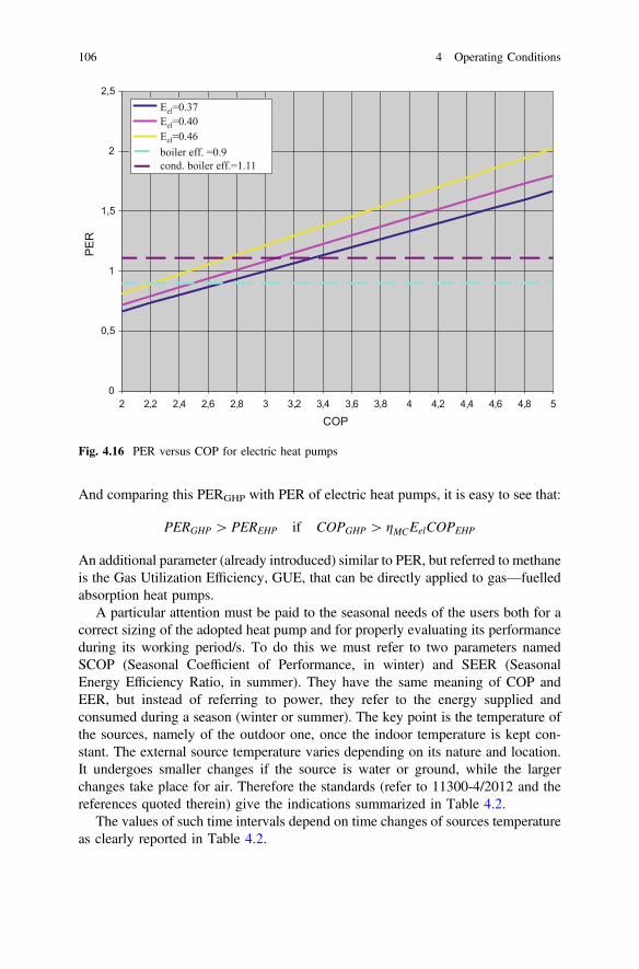
And comparing this PERGHP with PER of electric heat pumps, it is easy to see that:

PERGHP [PEREHP if COPGHP [ gMCEelCOPEHP

An additional parameter (already introduced) similar to PER, but referred to methaneis the Gas Utilization Efficiency, GUE, that can be directly applied to gas—fuelledabsorption heat pumps.

A particular attention must be paid to the seasonal needs of the users both for acorrect sizing of the adopted heat pump and for properly evaluating its performanceduring its working period/s. To do this we must refer to two parameters namedSCOP (Seasonal Coefficient of Performance, in winter) and SEER (SeasonalEnergy Efficiency Ratio, in summer). They have the same meaning of COP andEER, but instead of referring to power, they refer to the energy supplied andconsumed during a season (winter or summer). The key point is the temperature ofthe sources, namely of the outdoor one, once the indoor temperature is kept con-stant. The external source temperature varies depending on its nature and location.It undergoes smaller changes if the source is water or ground, while the largerchanges take place for air. Therefore the standards (refer to 11300-4/2012 and thereferences quoted therein) give the indications summarized in Table 4.2.

The values of such time intervals depend on time changes of sources temperatureas clearly reported in Table 4.2.

0

0,5

1

1,5

2

2,5

2 2,2 2,4 2,6 2,8 3 3,2 3,4 3,6 3,8 4 4,2 4,4 4,6 4,8 5

Eel=0,37Eel=0,40Eel=0,46caldaia rend.=0,9caldaia cond. rend.max

Eel=0.37Eel=0.40Eel=0.46boiler eff. =0.9cond. boiler eff.=1.11

PER

COP

Fig. 4.16 PER versus COP for electric heat pumps


Month is considered when sources temperatures are stable (e.g., water or groundas outdoor source and radiant floor or fan coil for the indoor one). The referencesources’ temperatures are the indoor set point temperature and the average outdoortemperature of the examined month.

Monthly bins are taken into account for larger temperature variations (e.g., air asoutdoor source and/or the indoor temperature is varied to adapt to local climate).Bin is a temperature interval, DTk, and the related bin time interval, Dtj, is theperiod during which temperature varies within DTk. Say we refer to a temperatureTk = 8 °C and DTk = 1 °C (temperature varies within 7.5 °C and 8.5 °C), Dtk isthe time during which temperature keeps within 7.5 and 8.5 °C.

Actually we need to reconstruct the trend of the temperature of the monththrough a normal distribution curve from the local climatic data. On this basis wecan associate a bin time interval, Dtk, to any temperature bin DTk.

The dedicated standard (11300-4/2012) provides a detailed procedure to performthese calculations and the reader is referred to this for any further detail.

In any case to evaluate the heat pump performances the energy consumed byauxiliaries, e.g., circulation pumps and fans, must be taken into account. Forexample in the case of air cooled coils the energy employed by fans must becalculated, as well as the energy consumed by water pumped in and out of heatexchangers.

4.3 Further Features of Heat Pumps Operation

Even if the effects of irreversibilities and of sources temperatures have already beenstressed at the beginning of this text we are going to treat them in a deeper detailand with a more oriented approach to applications.

EUW and EUS commonly designate the useful energy delivered in winter andsummer, i.e., respectively, the enthalpy difference at condenser and evaporator. Ofcourse they depend at first on the phase change bell shaped curve of the employedrefrigerant.

With reference to Fig. 4.17:

EUW ¼ h2 � h3 o EU0W ¼ h20 � h3 ¼ EUI þ h20 � h2

EUS ¼ h1 � h4

Subscript ‘marks the effect of a lower isentropic efficiency of the compressor.

4.2 Comparison Among the Different Types of Heat Pump 107

4.3.1 Change of Compressor’s Isentropic Efficiency

According to Fig. 4.17, a first effect of change of the isentropic efficiency is exertedon the value of EUW and, as a consequence, on COP and EER. If the isentropicefficiency gets poorer the heat exchanged with the user increases in winter, while itkeeps the same in summer with the following effects on COP and EER (subscript‘refer to a lower isentropic efficiency):

COP0 ¼ EU0W

h20 � h1¼ EUW þ h20 � h2ð Þ

h2 � h1 þ h20 � h2ð Þ ¼COPþ h20�h2

h2�h1

1þ h20�h2h2�h1

EER0 ¼ h1 � h4h2 � h1 þ h20 � h2ð Þ ¼

EER

1þ h20�h2h2�h1

If we suppose transformation 1–2 to be ideal, h2′ − h1 = (h2 − h1)/qc, we get:

COP0 ¼ qcEU0

W

h2 � h1ð Þ ¼ qcEUW þ h20 � h1 þ h1 � h2ð Þ

h2 � h1ð Þ ¼ qcCOPþð1� qcÞCOP � COP0

COP¼ 1� qcð Þ 1� 1

COP

� �

EER0 ¼ qc h1 � h4ð Þh2 � h1ð Þ ¼ qcEER

EER� EER0

EER¼ 1� qc

The percent changes of COP and EER are shown in Fig. 4.18. The effect ofdeterioration of isentropic efficiency is larger on EER than on COP.

1

23

4

p

h

2’EUW

EUW

EUS

Fig. 4.17 EUW and EUS.Dotted lines represent a worsecompressor isentropicefficiency


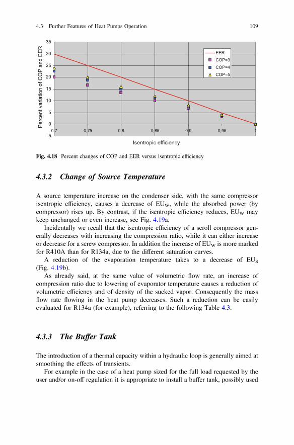
4.3.2 Change of Source Temperature

A source temperature increase on the condenser side, with the same compressorisentropic efficiency, causes a decrease of EUW, while the absorbed power (bycompressor) rises up. By contrast, if the isentropic efficiency reduces, EUW maykeep unchanged or even increase, see Fig. 4.19a.

Incidentally we recall that the isentropic efficiency of a scroll compressor gen-erally decreases with increasing the compression ratio, while it can either increaseor decrease for a screw compressor. In addition the increase of EUW is more markedfor R410A than for R134a, due to the different saturation curves.

A reduction of the evaporation temperature takes to a decrease of EUS

(Fig. 4.19b).As already said, at the same value of volumetric flow rate, an increase of

compression ratio due to lowering of evaporator temperature causes a reduction ofvolumetric efficiency and of density of the sucked vapor. Consequently the massflow rate flowing in the heat pump decreases. Such a reduction can be easilyevaluated for R134a (for example), referring to the following Table 4.3.

4.3.3 The Buffer Tank

The introduction of a thermal capacity within a hydraulic loop is generally aimed atsmoothing the effects of transients.

For example in the case of a heat pump sized for the full load requested by theuser and/or on-off regulation it is appropriate to install a buffer tank, possibly used

-5

0

5

10

15

20

25

30

35

0,7 0,75 0,8 0,85 0,9 0,95 1

EERCOP=3COP=4COP=5

Isentropic efficiency

Perc

ent v

aria

tion

of C

OP

and

EER

Fig. 4.18 Percent changes of COP and EER versus isentropic efficiency

4.3 Further Features of Heat Pumps Operation 109

1

23

4

p

2’3’ 2’’

h

1

23

4

p

h

1’4’

(a)

(b)

Fig. 4.19 Temperatureincrease on the condenser side(a) and temperature decreaseat evaporator (b)

Table 4.3 Properties ofsaturated R134a

T (°C) Pressure (kPa) Density (kg/m3)

Liquid Vapor

−10 200.60 1325.3 10.044

0 292.93 1293.3 14.435

10 414.92 1259.8 20.236

20 572.25 1224.4 27.791

30 771.02 1186.7 37.540

40 1017.61 1146.1 50.072

50 1319.00 1101.8 66.225

60 1682.76 1052.5 87.287

70 2117.34 995.9 115.442

80 2632.97 927.8 155.01

90 3242.87 837.3 217.162


also for sanitary water production, to reduce the number of transients and anyswings.

The volume of this tank is related to the type of plant. We have to refer to an“effective volume” which must allow the heat pump for operating at least during aminimum time requested by compressor (it cannot stop working abruptly).

Thus it is necessary to ensure the availability of an effective volume, Veff,according to the following formula:

Veff ¼ P � 60tmin

qcpDTm3� �

where:

P Heat pump power kW

tmin Minimum working time minutes

q Water density kg/m3

cp Specific heat of water kJ/kgK

DT Evaporator temperature difference K

The minimum time is commonly in the order of 2–5 min.Some reference values are reported in Table 4.4.As a rule of thumb an average plant volume of 15 L per installed kW can be

considered.More in detail the following values can be adopted:

• Ventilation systems (e.g., fan coils): 8 l/kW.• Steel radiators: 11 l/kW.• Cast iron radiators: 14 l/kW.• Floor heating: 23 l/kW.• Central heating of large buildings: 20 l/kW.

Table 4.4 Some proxies of effective volume (by Rossato Group)

DT (°C) 4.0 5.0 6.0

Minimum Optimum Min. Opt. Min. Opt.

7.2 12.7 5.7 10.1 4.8 8.4

4.3 Further Features of Heat Pumps Operation 111

Chapter 5The Refrigerants

Abstract This chapter is dedicated to the most common fluids used in the currentheat pumps’ technology. The main general features and parameters of theserefrigerants are illustrated together with the nomenclature adopted for their classi-fication. In particular the properties of some of the most commonly used fluids(both organic and “natural” as carbon dioxide and ammonia) are reported both asdiagrams and tables.

The history of synthetic refrigerants (pure) starts in the thirties of 1900 in the UnitedStates. At the beginning they were produced from hydrocarbons like ethane, C2H6,and methane, CH4, by halogenation, i.e., by substituting atoms of hydrogen withatoms of chlorine and fluorine. In this case the halogenation was complete, that is allthe atoms of hydrogen were substituted. These products were called chlorofluoro-carbons, CFC. Only in 1974 their negative effects were made clear. In fact, thanks tothe strong and stable bond between chlorine and fluorine, CFCs can last tens of yearsand accumulate in the stratosphere increasing the greenhouse effect and the depletionof the ozone layer (due to chlorine). Therefore their production was shut down in1996 and a partial halogenation process was employed to mitigate the consequencesof the use of refrigerants. The hydro-chlorofluorocarbons, HCFC, were so obtained,with a lighter impact than CFC.

Let us shortly see the meaning of the abbreviations which characterize thesefluids.

Prefix R means refrigerant and the following numbers designate their chemicalcomposition, from left:

• the first digit gives the number of atoms of carbon, C, minus 1 (0 means 1 atomof C, 1 means 2 atoms of C);

• the second digit gives the number of hydrogen, H, atoms plus 1 (2 means 1 atomof H, 3 means 2 atoms of H);

• the third digit gives the number of atoms of fluorine, F;• a letter (a, b, c) following the last digit, indicates the isomer they refer to.


113

R134a (tetrafluoroethane CH2FCF3) is a classical example. In fact it contains twoatoms of carbon, two atoms of hydrogen and three atoms of fluorine and refers tothe isomer a of Fig. 5.1.

This refrigerant has no atoms of chlorine and belongs to the group of the hydrofluorocarbons (HFC), which do not contain chlorine to avoid damages to ozone. Ithas replaced R12 and R114 in heat pumps. Hydro fluorocarbons have not effect onatmospheric ozone but, unfortunately, they act as greenhouse gases and they havelower performances (as refrigerants) than CFCs and HCFCs.

Besides HFCs, that are pure fluids, mixtures of the previously described fluidsmarked by series number 400 and 500 are used. The former fluids (series 400) arenon-azeotropic and the latter (series 500) are azeotropic mixtures.

The mixtures properties depend on the type of component fluids and on theirconcentrations. Generally the transition from liquid to vapor at constant pressureoccurs with a temperature increase, named glide. In the case of zeotropic mixturesboth vapor and liquid compositions change during the process, until their originalcomposition is restored at the end of the phase change. Figure 5.2 shows a phasechange process at constant pressure for these mixtures. The two curves correspondto the saturated vapor (upper line) and the saturated liquid line (lower line).

Let us take a mixture of two components A and B, with boiling temperaturesTA* and TB* (TB* > TA*) at a given pressure. At the beginning its compositioncorresponds to point F with temperature T1. The liquid content (mass of liquiddivided by the mass of the mixture) is equal to l1 and the vapor content v1′. Vaporis richer in A (lower boiling point) and liquid in B. The same happens in anintermediate condition (2-2′, temperature T2) even if with different concentrationsthan before. At temperature T3 the mixture reaches l3′ and v3.

This behavior of zeotropic mixtures may constitute an inconvenient either in thecase of the charge or in the case of a leak of fluid, as it causes the loss of the morevolatile component, thus changing the mixture composition. Fluids of this kind are,for example, R410A and R407C, which has a glide of 7 °C at atmospheric pressureand is not recommended for application where the working cycle is often inverted.R407C has been widely employed as the substitute of R22 in the field of air

C F H

R 134 R 134a

Fig. 5.1 Molecule of R134 and its isomer a (different position of hydrogen and fluorine atoms)

114 5 The Refrigerants

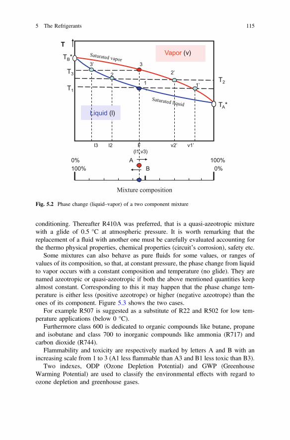
conditioning. Thereafter R410A was preferred, that is a quasi-azeotropic mixturewith a glide of 0.5 °C at atmospheric pressure. It is worth remarking that thereplacement of a fluid with another one must be carefully evaluated accounting forthe thermo physical properties, chemical properties (circuit’s corrosion), safety etc.

Some mixtures can also behave as pure fluids for some values, or ranges ofvalues of its composition, so that, at constant pressure, the phase change from liquidto vapor occurs with a constant composition and temperature (no glide). They arenamed azeotropic or quasi-azeotropic if both the above mentioned quantities keepalmost constant. Corresponding to this it may happen that the phase change tem-perature is either less (positive azeotrope) or higher (negative azeotrope) than theones of its component. Figure 5.3 shows the two cases.

For example R507 is suggested as a substitute of R22 and R502 for low tem-perature applications (below 0 °C).

Furthermore class 600 is dedicated to organic compounds like butane, propaneand isobutane and class 700 to inorganic compounds like ammonia (R717) andcarbon dioxide (R744).

Flammability and toxicity are respectively marked by letters A and B with anincreasing scale from 1 to 3 (A1 less flammable than A3 and B1 less toxic than B3).

Two indexes, ODP (Ozone Depletion Potential) and GWP (GreenhouseWarming Potential) are used to classify the environmental effects with regard toozone depletion and greenhouse gases.

T

A B

0%0%

100%100%

TB* Vapor (v)

Liquid (l)

Mixture composition

TA*

T3T2

T11

3

2 2’

F l2 v2’ v1’l3(l1,v3)

' 1’

3’

Fig. 5.2 Phase change (liquid–vapor) of a two component mixture

5 The Refrigerants 115

ODP is referred to R11, that is a no longer used fluid and to which the value 1 ofthis index is attributed. ODP varies from 0 to 1. Attributing value 1 to a refrigerantmeans that 1 kg of this refrigerant depletes a quantity of ozone equal to thatdepleted by 1 kg of R11. ODP = 0 means that there is no effect on ozone.

GWP refers to the potential contribution to greenhouse effect with respect tocarbon dioxide. It is generally related to the action performed by 1 kg of carbondioxide during hundred years. If a fluid is denoted by an index GWP100 = 1000, itmeans that 1 kg of this fluid causes the same greenhouse effect of 1000 kg ofcarbon dioxide in 100 years.

Unfortunately several fluids with ODP = 0 have high values of GWP100. Valuesof the above parameters for some refrigerants are reported in Table 5.1, as anexample. It has to be emphasized that the “natural” fluid ammonia (R717) has verygood values of both indexes.

The properties of refrigerants can be generally evaluated on the basis of thefollowing features:

• Vapor pressure—it has to be high enough at the actual evaporation temperatureto limit size and costs of compressors, without taking the condenser pressure tooclose to the critical point.

T T

A B B

A 0% 0%

0% 0%100%100%100%

100%

TB

TATA

Vapor (v)

Vapor (v)

Liquid (l)

Liquid (l)

l + v

l + v

TB

(a1) (a2)

(a2) Negative azeotrope (a1) Positive azeotrope Mixture composition Mixture composition

Fig. 5.3 Liquid–vapor phase change of an azeotropic mixture

Table 5.1 Effect of some fluids on ozone and on greenhouse phenomenon

Fluid ODP GWP100 Average life in atmosphere (years)

R11 1 3800 45

R22 0.05 8500 12

R134a 0 1300 14

R290 (propane) 0 20 3

R407C(R32; R125; R134a)

0 1500 (6; 33; 14)

R410A(R32; R125)

0 1700 (6; 33)

R717 0 <1 1


• Critical point—of course it influences the operation field of the heat pump.• Molar mass—as “heavier” is a fluid as lower its volumetric flow rate is, for a

given pipe area. Consequently the components size (pipes, valves.) have toincrease with increasing molar mass. In addition it also affects the compressorspeed as the optimum fluid velocity through a reciprocating compressor’s valvesor from the outflow valves of a screw compressor is proportional to the inverseof the square root of molar mass.

5.1 Properties of Some Refrigerants

The properties of some synthetic refrigerants are dealt with in this paragraphtogether with those of ammonia and carbon dioxide.

First of all we provide some elements of the most commonly used fluids. Forbetter details the interested reader is referred to several sites on the Web as, forexample, [1–3].

R134a. It consists of a single component and has no glide. It has poorer heatexchange characteristics than R22. Thus it requires larger heat exchanger surfaces,for a given temperature difference, and a larger compressor size (around 30%),causing higher costs. It can be used for high water temperatures (above 70 °C), butCOP decreases with increasing this temperature (roughly 3%/K). It is successfullyemployed for commercial refrigeration. In its field of application it has the besttheoretical COP, but not a very good system performance, due to its “low” heatexchange capability and high pressure losses.

R410A. It is a 50% in mass mixture of R32 and R125, with a almost negligibleglide (say 0.11 °C). It is chemically stable and not flammable. It works at pressures50–70% higher than R22 and has better thermo physical properties. It allows abetter compactness of systems, defrost and system reversibility thanks to the almostabsent glide. It usually gives COPs not as good as R134a, but it has better heatexchange properties and lower pressure drops.

R-407C. It is a mixture of R134a, R125 and R32 with a mass percent of,respectively, 52, 25, 23%. It has similar performances as R410A, but has a glidearound 5.5 °C. It is similar to R22 so that it can be easily employed as a goodsubstitute with minor technological changes, like switching from the use of atraditional mineral oil (MO) to polyester oil (POE) necessary with HFCs. But such achoice has two drawbacks: (1) a lower thermodynamic efficiency with respect toR410A and, to a lesser extent, to R22, (2) some operation uncertainty particularlyduring maintenance, due to the fractionation of this ternary mixture. This fluidprovides good performances in commercial systems like medium power refriger-ators and roof tops. The following Figs. 5.4, 5.5 and 5.6 shows the trends of thesaturation curves, p = p(T), and of the evaporation latent heat (enthalpy ofvaporization) of the above discussed fluids.

5 The Refrigerants 117

0

500

1000

1500

2000

2500

3000

3500

4000

-20 -10 0 10 20 30 40 50 60 70 80T(°C)

pression - temperature R407C pression - temperature vapor R407C

pression - temperature R134a pression - temperature liquid R410A

pression - temperature vapor R410A

p(kP

a)

Fig. 5.4 Saturation pressure versus temperature of some refrigerants. Only R407C has a glide

0306090

120150180210240270300330

-100 -70 -40 -10 20 50 80 110

kJ/kg

enthalphy of vaporization R134a enthalpy of vaporization R407Centhalpy of vaporization R410A

T(°C)

Fig. 5.5 Enthalpy of vaporization of some synthetic refrigerants


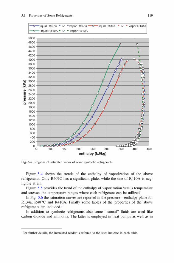
Figure 5.4 shows the trends of the enthalpy of vaporization of the aboverefrigerants. Only R407C has a significant glide, while the one of R410A is neg-ligible at all.

Figure 5.5 provides the trend of the enthalpy of vaporization versus temperatureand stresses the temperature ranges where each refrigerant can be utilized.

In Fig. 5.6 the saturation curves are reported in the pressure—enthalpy plane forR134a, R407C and R410A. Finally some tables of the properties of the aboverefrigerants are included.1

In addition to synthetic refrigerants also some “natural” fluids are used likecarbon dioxide and ammonia. The latter is employed in heat pumps as well as in

0200400600800

100012001400160018002000220024002600280030003200340036003800400042004400460048005000

50 100 150 200 250 300 350 400 450enthalpy (kJ/kg)

pres

sure

(kPa

)liquid R407C vapor R407C liquid R134a vapor R134a liquid R410A vapor R410A

Fig. 5.6 Regions of saturated vapor of some synthetic refrigerants

1For further details, the interested reader is referred to the sites indicate in each table.

5.1 Properties of Some Refrigerants 119

several refrigeration sectors. Carbon dioxide is used in heat pumps mainly suitablefor high temperature uses, as will be later discussed in this text. Ammonia has beenused during almost 130 years, notwithstanding some disadvantages. In fact it istoxic and flammable in air with a percent ranging from 15 to 28%. Furthermore it isnot compatible with copper. It allows lower flow rates than HFCs, as it has a lowmolecular weight and a high enthalpy of vaporization.

The critical point of carbon dioxide corresponds to 30.978 °C and 73.773 MPa,thus at low temperature and high pressure. This fact causes significant changes inthe operation of the heat pumps using it. First of all the condenser is replaced by aheat exchanger using hypercritical gas. Some properties of this fluid are reportedherein both in the saturation zone and in the vapor region.

The trends of the saturation pressure (triangles) and temperature (squares) curvesversus the enthalpy of vaporization are shown in Fig. 5.7.

Figure 5.8 provides the values of the vaporization enthalpy and of the relatedtemperature.

The values of properties referring to the above figures can be found in thefollowing CO2 tables. The same properties are shown in Figs. 5.9 and 5.10 forammonia.

To better stress the working fields of the above discussed fluids the varioussaturation field are respectively illustrated in Figs. 5.11 and 5.12 in the planespressure-enthalpy and temperature-enthalpy.

It is immediately apparent how carbon dioxide needs much higher pressure if thecritical temperature is around 31 °C. Whereby heat pumps using this fluid employ(as already said) a heat exchanger where hypercritic CO2 flows, instead of a usual

-20-15-10-505

1015202530354045505560657075

150 170 190 210 230 250 270 290 310 330 350 370 390 410 430 450

enthalpy of vaporization (kJ/kg)

pres

sure

(MPa

) o te

mpe

ratu

re (°

C)

Fig. 5.7 CO2, trends of saturation pressure (triangle) and temperature (squares) versus enthalpyof vaporization


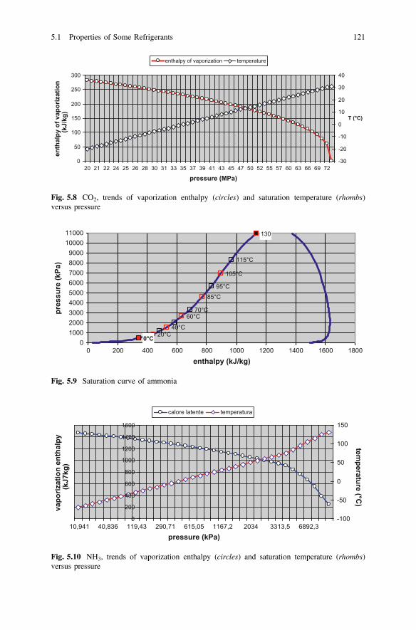
0

50

100

150

200

250

300

20 21 22 24 25 26 28 30 31 33 35 37 39 41 43 45 47 50 52 55 57 60 63 66 69 72-30

-20

-10

0

10

20

30

40

enthalpy of vaporization temperature

pressure (MPa)

enth

alpy

of v

apor

izat

ion

(kJ/

kg)

T (°C)

Fig. 5.8 CO2, trends of vaporization enthalpy (circles) and saturation temperature (rhombs)versus pressure

0°C 20°C40°C

60°C70°C

85°C95°C

105°C

115°C

130

0100020003000400050006000700080009000

1000011000

0 200 400 600 800 1000 1200 1400 1600 1800enthalpy (kJ/kg)

pres

sure

(kPa

)

Fig. 5.9 Saturation curve of ammonia

0

200

400

600

800

1000

1200

1400

1600

203410,941 40,836 119,43 290,71 615,05 1167,2 3313,5 6892,3-100

-50

0

50

100

150

calore latente temperatura

pressure (kPa)

vapo

rizat

ion

enth

alpy

(k

J7kg

)tem

perature (°C)

Fig. 5.10 NH3, trends of vaporization enthalpy (circles) and saturation temperature (rhombs)versus pressure


0,1

10

1000

100000

10 100 1000 10000

R407C R134a R410AR744 R717

pres

sure

(kPa

)

enthalpy (kJ/kg)

Fig. 5.11 Saturation curves of the described refrigerants in the pressure enthalpy plane

0

200

400

600

800

1000

1200

1400

1600

-110 -90 -70 -50 -30 -10 10 30 50 70 90 110 130

en

tha

lpy

(k

J/k

g)

R744 R717 R134a R407C R410A

temperature (°C)

Fig. 5.12 Saturation curves of the described refrigerants in the enthalpy temperature plane


condenser. Carbon dioxide is a cheap and accessible refrigerant as it is abundant innature and a common waste product of several industrial processes. Furthermore, asa “natural fluid”, it does not require specific procedures both for retrieval andmaintenance, as in the case of synthetic refrigerants. It is neither toxic nor flam-mable, but it is heavier than air and its accumulation close to the floors must becarefully avoided.

Ammonia has high values of the vaporization enthalpy and a critical pointcorresponding to 132 °C and 113 bar (11.3 MPa).

In addition to the previously discussed refrigerants we recall fluids like isobutane(R600a) and propane (R290). The former is a hydrocarbon (flammable), has similarthermal properties to R134a and is less expensive. It is used in domestic refriger-ators (except for the USA) and no accident has been reported so far in suchapplications. Furthermore it is compatible with mineral oils. It has been used toreplace R12, thanks to its characteristics.

Propane, flammable too, has similar properties to R22 and is a good substitute ofthis fluid. In fact it has a boiling point of −42 °C at atmospheric pressure andrequires similar operative pressures to R22.

5.2 Lubricating Oils

The main purpose of using a lubricant is to reduce friction, thus, reducing wear ofcompressors’ components. It is necessary to keep the appropriate quantity of oilconstant within a compressor.

The ideal way would be to prevent any leak, but it would imply the adoption ofvery complex and onerous devices. It is preferred to use oils that could circulate inthe cycle, with no drawbacks, provided that the necessary care is paid and thereleased oil gets entirely back to the compressor. Otherwise both insufficientlubrication of the moving parts and detrimental accumulation of oil in heatexchangers may occur.

In optimal conditions (proper choice of oil and correct sizing of tubing) oil isregularly entrained by high pressure vapor from the compressor to the condenser,then to the evaporator trough lamination and, finally, back to the compressor.Sometime manifolds are placed at the compressor(s) suction from which it is sent tothe compressor in the same quantity that left it. In other case a separator isemployed. It is provided with a filter through which vapor flows. The oil containedin the refrigerant is withheld by the filter and deposits on the bottom of the con-tainer. Devices to control the oil level in the compressor crankcase and eventually to


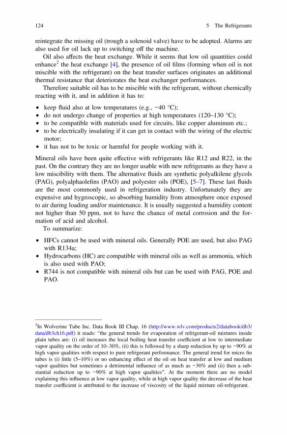
reintegrate the missing oil (trough a solenoid valve) have to be adopted. Alarms arealso used for oil lack up to switching off the machine.

Oil also affects the heat exchange. While it seems that low oil quantities couldenhance2 the heat exchange [4], the presence of oil films (forming when oil is notmiscible with the refrigerant) on the heat transfer surfaces originates an additionalthermal resistance that deteriorates the heat exchanger performances.

Therefore suitable oil has to be miscible with the refrigerant, without chemicallyreacting with it, and in addition it has to:

• keep fluid also at low temperatures (e.g., −40 °C);• do not undergo change of properties at high temperatures (120–130 °C);• to be compatible with materials used for circuits, like copper aluminum etc.;• to be electrically insulating if it can get in contact with the wiring of the electric

motor;• it has not to be toxic or harmful for people working with it.

Mineral oils have been quite effective with refrigerants like R12 and R22, in thepast. On the contrary they are no longer usable with new refrigerants as they have alow miscibility with them. The alternative fluids are synthetic polyalkilene glycols(PAG), polyalphaolefins (PAO) and polyester oils (POE), [5–7]. These last fluidsare the most commonly used in refrigeration industry. Unfortunately they areexpensive and hygroscopic, so absorbing humidity from atmosphere once exposedto air during loading and/or maintenance. It is usually suggested a humidity contentnot higher than 50 ppm, not to have the chance of metal corrosion and the for-mation of acid and alcohol.

To summarize:

• HFCs cannot be used with mineral oils. Generally POE are used, but also PAGwith R134a;

• Hydrocarbons (HC) are compatible with mineral oils as well as ammonia, whichis also used with PAO;

• R744 is not compatible with mineral oils but can be used with PAG, POE andPAO.

2In Wolverine Tube Inc. Data Book III Chap. 16 (http://www.wlv.com/products2/databook/db3/data/db3ch16.pdf) it reads: “the general trends for evaporation of refrigerant-oil mixtures insideplain tubes are: (i) oil increases the local boiling heat transfer coefficient at low to intermediatevapor quality on the order of 10–30%, (ii) this is followed by a sharp reduction by up to −90% athigh vapor qualities with respect to pure refrigerant performance. The general trend for micro fintubes is (i) little (5–10%) or no enhancing effect of the oil on heat transfer at low and mediumvapor qualities but sometimes a detrimental influence of as much as −30% and (ii) then a sub-stantial reduction up to −90% at high vapor qualities”. At the moment there are no modelexplaining this influence at low vapor quality, while at high vapor quality the decrease of the heattransfer coefficient is attributed to the increase of viscosity of the liquid mixture oil-refrigerant.


http://www.wlv.com/products2/databook/db3/data/db3ch16.pdf

http://www.wlv.com/products2/databook/db3/data/db3ch16.pdf

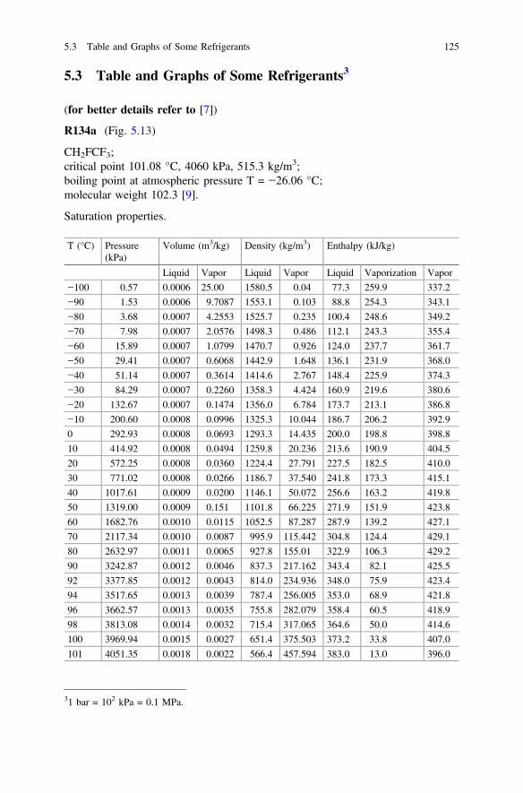
5.3 Table and Graphs of Some Refrigerants3

(for better details refer to [7])

R134a (Fig. 5.13)

CH2FCF3;critical point 101.08 °C, 4060 kPa, 515.3 kg/m3;boiling point at atmospheric pressure T = −26.06 °C;molecular weight 102.3 [9].

Saturation properties.

T (°C) Pressure(kPa)

Volume (m3/kg) Density (kg/m3) Enthalpy (kJ/kg)

Liquid Vapor Liquid Vapor Liquid Vaporization Vapor

−100 0.57 0.0006 25.00 1580.5 0.04 77.3 259.9 337.2

−90 1.53 0.0006 9.7087 1553.1 0.103 88.8 254.3 343.1

−80 3.68 0.0007 4.2553 1525.7 0.235 100.4 248.6 349.2

−70 7.98 0.0007 2.0576 1498.3 0.486 112.1 243.3 355.4

−60 15.89 0.0007 1.0799 1470.7 0.926 124.0 237.7 361.7

−50 29.41 0.0007 0.6068 1442.9 1.648 136.1 231.9 368.0

−40 51.14 0.0007 0.3614 1414.6 2.767 148.4 225.9 374.3

−30 84.29 0.0007 0.2260 1358.3 4.424 160.9 219.6 380.6

−20 132.67 0.0007 0.1474 1356.0 6.784 173.7 213.1 386.8

−10 200.60 0.0008 0.0996 1325.3 10.044 186.7 206.2 392.9

0 292.93 0.0008 0.0693 1293.3 14.435 200.0 198.8 398.8

10 414.92 0.0008 0.0494 1259.8 20.236 213.6 190.9 404.5

20 572.25 0.0008 0.0360 1224.4 27.791 227.5 182.5 410.0

30 771.02 0.0008 0.0266 1186.7 37.540 241.8 173.3 415.1

40 1017.61 0.0009 0.0200 1146.1 50.072 256.6 163.2 419.8

50 1319.00 0.0009 0.151 1101.8 66.225 271.9 151.9 423.8

60 1682.76 0.0010 0.0115 1052.5 87.287 287.9 139.2 427.1

70 2117.34 0.0010 0.0087 995.9 115.442 304.8 124.4 429.1

80 2632.97 0.0011 0.0065 927.8 155.01 322.9 106.3 429.2

90 3242.87 0.0012 0.0046 837.3 217.162 343.4 82.1 425.5

92 3377.85 0.0012 0.0043 814.0 234.936 348.0 75.9 423.4

94 3517.65 0.0013 0.0039 787.4 256.005 353.0 68.9 421.8

96 3662.57 0.0013 0.0035 755.8 282.079 358.4 60.5 418.9

98 3813.08 0.0014 0.0032 715.4 317.065 364.6 50.0 414.6

100 3969.94 0.0015 0.0027 651.4 375.503 373.2 33.8 407.0

101 4051.35 0.0018 0.0022 566.4 457.594 383.0 13.0 396.0

31 bar = 102 kPa = 0.1 MPa.

5.3 Table and Graphs of Some Refrigerants 125

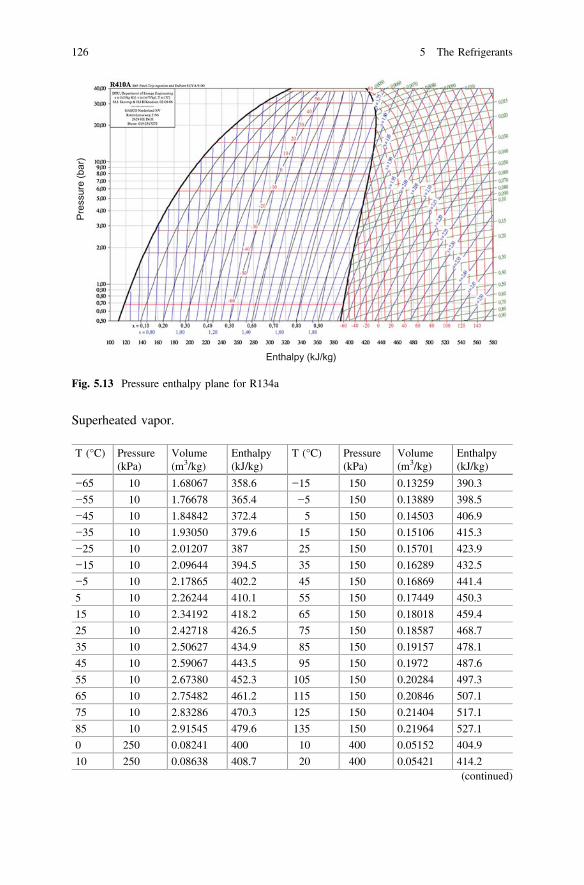
Superheated vapor.


Volume(m3/kg)

Enthalpy(kJ/kg)


Volume(m3/kg)

Enthalpy(kJ/kg)

−65 10 1.68067 358.6 −15 150 0.13259 390.3

−55 10 1.76678 365.4 −5 150 0.13889 398.5

−45 10 1.84842 372.4 5 150 0.14503 406.9

−35 10 1.93050 379.6 15 150 0.15106 415.3

−25 10 2.01207 387 25 150 0.15701 423.9

−15 10 2.09644 394.5 35 150 0.16289 432.5

−5 10 2.17865 402.2 45 150 0.16869 441.4

5 10 2.26244 410.1 55 150 0.17449 450.3

15 10 2.34192 418.2 65 150 0.18018 459.4

25 10 2.42718 426.5 75 150 0.18587 468.7

35 10 2.50627 434.9 85 150 0.19157 478.1

45 10 2.59067 443.5 95 150 0.1972 487.6

55 10 2.67380 452.3 105 150 0.20284 497.3

65 10 2.75482 461.2 115 150 0.20846 507.1

75 10 2.83286 470.3 125 150 0.21404 517.1

85 10 2.91545 479.6 135 150 0.21964 527.1

0 250 0.08241 400 10 400 0.05152 404.9

10 250 0.08638 408.7 20 400 0.05421 414.2(continued)

Enthalpy (kJ/kg)

Pres

sure

(bar

)

Fig. 5.13 Pressure enthalpy plane for R134a


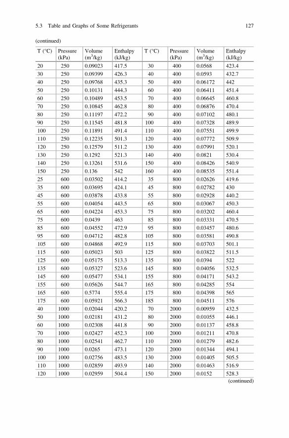
(continued)


Volume(m3/kg)

Enthalpy(kJ/kg)


Volume(m3/kg)

Enthalpy(kJ/kg)

20 250 0.09023 417.5 30 400 0.0568 423.4

30 250 0.09399 426.3 40 400 0.0593 432.7

40 250 0.09768 435.3 50 400 0.06172 442

50 250 0.10131 444.3 60 400 0.06411 451.4

60 250 0.10489 453.5 70 400 0.06645 460.8

70 250 0.10845 462.8 80 400 0.06876 470.4

80 250 0.11197 472.2 90 400 0.07102 480.1

90 250 0.11545 481.8 100 400 0.07328 489.9

100 250 0.11891 491.4 110 400 0.07551 499.9

110 250 0.12235 501.3 120 400 0.07772 509.9

120 250 0.12579 511.2 130 400 0.07991 520.1

130 250 0.1292 521.3 140 400 0.0821 530.4

140 250 0.13261 531.6 150 400 0.08426 540.9

150 250 0.136 542 160 400 0.08535 551.4

25 600 0.03502 414.2 35 800 0.02626 419.6

35 600 0.03695 424.1 45 800 0.02782 430

45 600 0.03878 433.8 55 800 0.02928 440.2

55 600 0.04054 443.5 65 800 0.03067 450.3

65 600 0.04224 453.3 75 800 0.03202 460.4

75 600 0.0439 463 85 800 0.03331 470.5

85 600 0.04552 472.9 95 800 0.03457 480.6

95 600 0.04712 482.8 105 800 0.03581 490.8

105 600 0.04868 492.9 115 800 0.03703 501.1

115 600 0.05023 503 125 800 0.03822 511.5

125 600 0.05175 513.3 135 800 0.0394 522

135 600 0.05327 523.6 145 800 0.04056 532.5

145 600 0.05477 534.1 155 800 0.04171 543.2

155 600 0.05626 544.7 165 800 0.04285 554

165 600 0.5774 555.4 175 800 0.04398 565

175 600 0.05921 566.3 185 800 0.04511 576

40 1000 0.02044 420.2 70 2000 0.00959 432.5

50 1000 0.02181 431.2 80 2000 0.01055 446.1

60 1000 0.02308 441.8 90 2000 0.01137 458.8

70 1000 0.02427 452.3 100 2000 0.01211 470.8

80 1000 0.02541 462.7 110 2000 0.01279 482.6

90 1000 0.0265 473.1 120 2000 0.01344 494.1

100 1000 0.02756 483.5 130 2000 0.01405 505.5

110 1000 0.02859 493.9 140 2000 0.01463 516.9

120 1000 0.02959 504.4 150 2000 0.0152 528.3(continued)


(continued)


Volume(m3/kg)

Enthalpy(kJ/kg)


Volume(m3/kg)

Enthalpy(kJ/kg)

130 1000 0.03058 515 160 2000 0.01575 539.7

140 1000 0.03155 525.6 170 2000 0.01629 551.1

150 1000 0.0325 536.3 180 2000 0.01681 562.6

160 1000 0.03345 547.2 190 2000 0.01733 574.1

170 1000 0.03438 558.1 200 2000 0.01784 587.7

180 1000 0.03531 569.2 210 2000 0.01834 597.4

190 1000 0.03623 580.3 220 2000 0.01883 609.1

90 3000 0.00575 436.1 105 4000 0.00376 433.7

100 3000 0.00665 453.5 115 4000 0.00468 456.8

110 3000 0.00733 468.2 125 4000 0.0053 473.8

120 3000 0.00792 481.8 135 4000 0.0058 488.8

130 3000 0.00845 494.7 145 4000 0.00624 502.8

140 3000 0.00893 507.2 155 4000 0.00664 516.2

150 3000 0.00939 519.4 165 4000 0.00702 529.2

160 3000 0.00982 531.6 175 4000 0.00737 541.9

170 3000 0.01023 543.6 185 4000 0.0077 554.5

180 3000 0.01063 555.6 195 4000 0.00802 567

190 3000 0.01102 567.6 205 4000 0.00884 580.7

200 3000 0.01121 579.6 215 4000 0.00863 591.9

210 3000 0.01176 591.6 225 4000 0.00892 604.3

220 3000 0.01212 603.7 235 4000 0.0092 616.8

230 3000 0.01248 615.8 245 4000 0.00948 629.3

240 3000 0.01283 628 250 4000 0.00962 635.5

R410A (Fig. 5.14)

CH2F2/CHF2CF3 (50% weight);critical point: 72.13 °C, 4926.1 kPa, 488.90 kg/m3;boiling point at atmospheric pressure: T = −51.58 °C;molecular weight: 72.58 [10].


T (°C) Pressure (kPa) Volume (m3/kg) Density (kg/m3) Enthalpy (kJ/kg)

Liquid Vapor Liquid Vapor Liquid Vapor Liquid Vaporization Vapor

−100 3.8 3.7 0.0007 5.3267 1509.0 0.188 63.3 311.4 374.7

−90 8.8 8.8 0.0007 2.3780 1480.7 0.421 75.4 305.0 380.5

−80 18.6 18.5 0.0007 1.1764 1451.7 0.850 87.9 298.3 386.1

−70 36 35.9 0.0007 0.6328 1421.8 1.580 100.7 291.0 391.7

−60 64.8 64.7 0.0007 0.3646 1390.9 2.743 113.8 283.3 397.1

−50 109.7 109.4 0.0007 0.2222 1358.9 4.500 127.3 274.9 402.2(continued)


(continued)


−40 176.2 175.8 0.0008 0.1419 1325.7 7.045 141.1 265.9 407.1

−30 270.8 270.1 0.0008 0.0942 1291.2 10.613 155.3 256.3 411.6

−20 400.7 399.5 0.0008 0.0646 1255.0 15.486 169.8 245.9 415.7

−10 573.9 572.2 0.0008 0.4540 1216.9 22.016 184.7 234.7 419.4

0 799.0 796.5 0.0009 0.0326 1176.7 30.649 200.0 222.5 422.5

10 1085.5 1082 0.0009 0.0328 1133.7 41.977 215.7 209.3 425.1

20 1443.6 1438.8 0.0009 0.0176 1087.2 56.825 232.0 194.8 426.8

30 1884.2 1877.9 0.0010 0.0131 1036.3 76.398 249.1 178.5 427.6

40 2419.3 2411.1 0.0010 0.0098 978.9 102.585 267.1 159.9 427.0

50 3061.3 3051.5 0.0010 0.0072 911.4 138.645 286.9 137.7 424.6

60 3823.3 3813.6 0.0012 0.0052 824.7 191.757 310.3 109.2 419.5

70 4717.5 4713.9 0.0015 0.0032 669.1 308.947 347.3 61.6 408.9

Superheated vapor.

Pres

sure

(bar

)

Enthalpy (kJ/kg)

Fig. 5.14 Pressure enthalpy plane for R410A



Volume(m3/kg)

Enthalpy(kJ/kg)


Volume(m3/kg)

Enthalpy(kJ/kg)

−10 500 0.0532 421.8 0 700 0.0382 425.6

0 500 0.0563 431.5 10 700 0.0406 436

10 500 0.0593 440.9 20 700 0.0429 446

20 500 0.0622 450.2 30 700 0.0451 455.7

30 500 0.065 459.5 40 700 0.0471 465.4

40 500 0.0677 468.7 50 700 0.0492 475

50 500 0.0704 477.9 60 700 0.0511 484.5

60 500 0.073 487.1 70 700 0.053 494

70 500 0.0755 496.4 80 700 0.0549 503.6

80 500 0.078 505.8 90 700 0.0568 513.3

90 500 0.0805 515.2 100 700 0.0586 522.9

100 500 0.083 524.7 110 700 0.0604 532.7

110 500 0.0855 534.3 120 700 0.0622 542.5

120 500 0.0879 544 130 700 0.0639 552.4

130 500 0.0903 553.9 140 700 0.0657 562.4

140 500 0.0927 563.8 150 700 0.0675 572.5

5 800 0.0336 427.9 5 900 0.0291 424.9

15 800 0.0358 438.6 15 900 0.0311 436

25 800 0.0388 453.8 25 900 0.033 446.6

35 800 0.0398 458.8 35 900 0.0348 456.9

45 800 0.0416 468.6 45 900 0.0365 467

55 800 0.0434 478.3 55 900 0.0382 476.9

65 800 0.0451 488 65 900 0.0397 486.7

75 800 0.0468 497.7 75 900 0.0413 496.5

85 800 0.0485 507.4 85 900 0.0428 506.8

95 800 0.0501 517.1 95 900 0.0443 516.1

105 800 0.0517 526.8 105 900 0.0457 526

115 800 0.0533 536.8 115 900 0.0472 535.9

125 800 0.0549 546.7 125 900 0.0486 545.9

135 800 0.0565 556.7 135 900 0.05 556

145 800 0.058 566.8 145 900 0.0514 566.1

155 800 0.0596 577 155 900 0.0479 576.4

– – – – 160 900 0.0479 580.9

10 1000 0.0264 427.6 35 2000 0.0125 431.5

20 1000 0.0283 438.9 45 2000 0.0138 445.9

30 1000 0.03 449.7 55 2000 0.0149 458.8

40 1000 0.0317 460.2 65 2000 0.0158 471

50 1000 0.0332 470.4 75 2000 0.0167 482.6

60 1000 0.0347 480.4 85 2000 0.0176 493.9

70 1000 0.0361 490.4 95 2000 0.0184 504.9(continued)


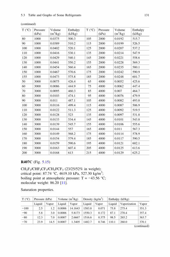
(continued)


Volume(m3/kg)

Enthalpy(kJ/kg)


Volume(m3/kg)

Enthalpy(kJ/kg)

80 1000 0.0375 500.3 105 2000 0.0192 515.7

90 1000 0.0389 510.2 115 2000 0.0199 526.5

100 1000 0.0402 520.1 125 2000 0.0207 537.2

110 1000 0.0416 530.1 135 2000 0.0214 547.9

120 1000 0.0429 540.1 145 2000 0.0221 558.6

130 1000 0.0441 550.2 155 2000 0.0228 569.3

140 1000 0.0454 560.4 165 2000 0.0235 580.1

150 1000 0.0467 570.6 175 2000 0.0242 590.9

155 1000 0.0473 575.8 185 2000 0.0248 601.7

50 3000 0.0075 426.4 65 4000 0.0052 425.6

60 3000 0.0086 444.9 75 4000 0.0062 447.4

70 3000 0.0095 460.3 85 4000 0.007 464.7

80 3000 0.0103 474.1 95 4000 0.0076 479.9

90 3000 0.011 487.1 105 4000 0.0082 493.8

100 3000 0.0116 499.4 115 4000 0.0087 506.9

110 3000 0.0122 511.3 125 4000 0.0092 519.5

120 3000 0.0128 523 135 4000 0.0097 531.8

130 3000 0.0133 534.4 145 4000 0.0101 543.8

140 3000 0.0139 545.7 155 4000 0.0106 555.6

150 3000 0.0144 557 165 4000 0.011 567.3

160 3000 0.0149 568.2 175 4000 0.0114 578.9

170 3000 0.0154 579.4 185 4000 0.0117 590.5

180 3000 0.0159 590.6 195 4000 0.0121 602.1

190 3000 0.0163 607.4 205 4000 0.0125 613.6

200 3000 0.0168 613 215 4000 0.0129 625.2

R407C (Fig. 5.15)

CH2F2/CHF2CF3/CH2FCF3 (23/25/52% in weight);critical point: 87.74 °C, 4619.10 kPa, 527.30 kg/m3;boiling point at atmospheric pressure: T = −43.56 °C;molecular weight: 86.20 [11].



Liquid Vapor Liquid Vapor Liquid Vapor Liquid Vaporization Vapor

−100 2.5 1.2 0.0006 14.1643 1583.8 0.071 75.8 275.4 351.3

−90 5.8 3.0 0.0006 5.8173 1550.3 0.172 87.1 270.4 357.4

−80 12.3 7.0 0.0007 2.6667 1516.6 0.375 98.5 265.2 363.7

−70 23.9 14.5 0.0007 1.3405 1482.7 0.746 110.1 260.0 370.1(continued)


(continued)


−60 43.3 27.9 0.0007 0.7279 1448.5 1.374 122 254.6 376.6

−50 73.8 50.2 0.0007 0.4216 1413.9 2.372 134.2 248.9 383.1

−40 119.7 85.0 0.0007 0.2577 1378.9 3.880 146.6 242.9 389.5

−30 185.5 136.9 0.0007 0.1649 1343.5 6.064 159.6 263.3 395.9

−20 276.8 211.2 0.0008 0.1096 1307.5 9.127 172.4 229.7 402.1

−10 399.6 313.9 0.0008 0.0751 1270.8 13.313 185.9 222.3 408.2

0 560.3 452.0 0.0008 0.0528 1233.2 18.924 200.0 213.9 413.9

10 765.8 632.8 0.0008 0.0380 1194.6 26.338 214.7 204.6 419.3

20 1023.4 864.4 0.0009 0.0277 1154.7 36.052 230.1 194.1 424.1

30 1340.7 1159.9 0.0009 0.0205 1112.9 48.755 246.2 182.1 428.4

40 1725.5 1517.0 0.0009 0.0153 1068.6 65.448 263.4 168.3 431.7

50 2185.9 1959.0 0.0010 0.0114 1020.7 87.701 281.9 152.0 433.9

60 2729.5 2494.4 0.0010 0.0085 966.8 118.255 302.2 132.2 434.4

70 3362.9 3138.8 0.0011 0.0061 902.0 162.80 325.3 106.8 432.1

72 3500.6 3282.6 0.0011 0.0057 886.7 174.415 330.5 100.6 431.1

74 3642 3431.8 0.0011 0.0053 870.1 187.358 335.9 94.0 429.9

76 3786.9 3586.9 0.0012 0.0050 852.0 201.958 341.6 86.7 428.3

78 3935.2 3748.1 0.0012 0.0046 831.6 218.698 347.8 78.6 426.4

79 4010.5 3831.1 0.0012 0.0044 820.3 228.096 351.0 74.2 425.2

Superheated vapor.

Pres

sure

(bar

)

Enthalpy (kJ/kg)

Fig. 5.15 Pressure enthalpy plane for R407C



Volume(m3/kg)

Enthalpy(kJ/kg)


Volume(m3/kg)

Enthalpy(kJ/kg)

−20 200 0.116 402.3 0 400 0.0605 414.8

−10 200 0.1213 410.1 10 400 0.0633 423.1

0 200 0.1265 418 20 400 0.066 431.5

10 200 0.1317 526.1 30 400 0.0688 440

20 200 0.1368 434.3 40 400 0.0715 448.7

30 200 0.142 442.6 50 400 0.0742 457.5

40 200 0.1471 451.2 60 400 0.0768 466.4

50 200 0.1521 459.8 70 400 0.0784 475.5

60 200 0.1572 468.7 80 400 0.0821 484.8

70 200 0.1622 477.6 90 400 0.0847 494.2

80 200 0.1672 486.8 100 400 0.0873 503.7

90 200 0.1723 496.1 110 400 0.0898 513.3

100 200 0.1772 505.5 120 400 0.0924 523.2

110 200 0.1822 515.1 130 400 0.095 533.1

120 200 0.1872 524.8 140 400 0.0975 543.2

130 200 0.1922 534.7 150 400 0.1 553.4

10 600 0.0404 419.8 20 800 0.0304 452.2

20 600 0.0424 428.5 30 800 0.032 434.2

30 600 0.443 437.2 40 800 0.0336 443.3

40 600 0.0462 446.1 50 800 0.0351 452.5

50 600 0.0481 455 60 800 0.0365 461.7

60 600 0.05 464.1 70 800 0.038 471.1

70 600 0.0518 473.4 80 800 0.0394 480.6

80 600 0.0536 482.7 90 800 0.0408 490.2

90 600 0.0555 492.2 100 800 0.0422 499.9

100 600 0.0572 501.8 110 800 0.0436 509.8

110 600 0.059 511.6 120 800 0.045 519.8

120 600 0.0608 521.5 130 800 0.0463 529.9

130 600 0.0625 531.5 140 800 0.0477 540.1

140 600 0.0643 541.7 150 800 0.049 550.5

150 600 0.066 551.9 160 800 0.0503 566.2

160 600 0.0678 562.4 170 800 0.0517 571.6

25 1000 0.0239 426.4 55 2000 0.0115 438.8

35 1000 0.0252 435.7 65 2000 0.0124 451.5

45 1000 0.0266 445.1 75 2000 0.0132 460.8

55 1000 0.0278 454.5 85 2000 0.014 471.5

65 1000 0.0291 464 95 2000 0.0147 482.2

75 1000 0.0303 473.6 105 2000 0.0155 492.9

85 1000 0.0315 483.3 115 2000 0.0161 503.5

95 1000 0.0326 493.1 125 2000 0.0168 514.3(continued)


(continued)


Volume(m3/kg)

Enthalpy(kJ/kg)


Volume(m3/kg)

Enthalpy(kJ/kg)

105 1000 0.0338 503 135 2000 0.0175 525

115 1000 0.0349 513 145 2000 0.0181 535.9

125 1000 0.036 523.1 155 2000 0.0187 546.8

135 1000 0.0372 533.4 165 2000 0.0193 557.8

145 1000 0.0383 543.8 175 2000 0.0199 568.9

155 1000 0.0394 554.3 185 2000 0.0205 580

165 1000 0.0404 564.9 195 2000 0.0211 591.3

175 1000 0.0415 575.6 205 2000 0.0217 602.7

70 3000 0.0068 436 85 4000 0.0046 433.4

80 3000 0.0076 450.1 95 4000 0.0054 451.9

90 3000 0.0083 463 105 4000 0.0061 466.9

100 3000 0.009 475.2 115 4000 0.0066 480.5

110 3000 0.0095 487 125 4000 0.0071 493.5

120 3000 0.0101 498.7 135 4000 0.0076 506.1

130 3000 0.0106 510.2 145 4000 0.008 518.4

140 3000 0.0111 521.7 155 4000 0.0084 530.6

150 3000 0.0107 531.5 165 4000 0.0093 544.2

160 3000 0.0121 544.6 175 4000 0.0097 556.2

170 3000 0.0125 556.1 185 4000 0.0101 568.1

180 3000 0.0129 567.7 195 4000 0.0104 580

190 3000 0.0134 579.3 205 4000 0.0108 592

200 3000 0.0138 590.9 215 4000 0.0111 604

210 3000 0.0142 602.6 225 4000 0.0116 616

220 3000 0.0146 614.4 230 4000 0.0124 623.1

R744

CO2

Critical point: 30.978 °C, 73.773 MPa, 467.51 kg/m3;boiling point at atmospheric pressure: T = −43.56 °C;molecular weight: 44.01 [12].


T (°C) Pressure (MPa) Volume (m3/kg) Enthalpy (kJ/kg)

Liquid Vapor Liquid Vaporization Vapor

−20 19.696 0.000969 0.019343 154.45 282.44 436.89

−19 20.310 0.000974 0.018726 156.61 280.2 436.81

−18 20.938 0.000978 0.018131 158.77 277.93 436.7

−17 21.581 0.000983 0.017557 160.95 275.63 436.58(continued)


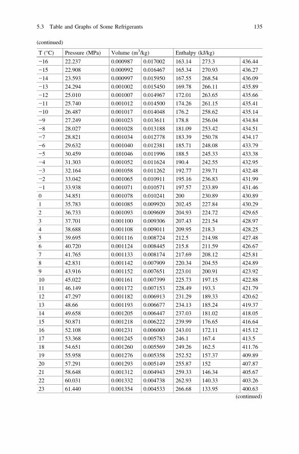
(continued)


−16 22.237 0.000987 0.017002 163.14 273.3 436.44

−15 22.908 0.000992 0.016467 165.34 270.93 436.27

−14 23.593 0.000997 0.015950 167.55 268.54 436.09

−13 24.294 0.001002 0.015450 169.78 266.11 435.89

−12 25.010 0.001007 0.014967 172.01 263.65 435.66

−11 25.740 0.001012 0.014500 174.26 261.15 435.41

−10 26.487 0.001017 0.014048 176.2 258.62 435.14

−9 27.249 0.001023 0.013611 178.8 256.04 434.84

−8 28.027 0.001028 0.013188 181.09 253.42 434.51

−7 28.821 0.001034 0.012778 183.39 250.78 434.17

−6 29.632 0.001040 0.012381 185.71 248.08 433.79

−5 30.459 0.001046 0.011996 188.5 245.33 433.38

−4 31.303 0.001052 0.011624 190.4 242.55 432.95

−3 32.164 0.001058 0.011262 192.77 239.71 432.48

−2 33.042 0.001065 0.010911 195.16 236.83 431.99

−1 33.938 0.001071 0.010571 197.57 233.89 431.46

0 34.851 0.001078 0.010241 200 230.89 430.89

1 35.783 0.001085 0.009920 202.45 227.84 430.29

2 36.733 0.001093 0.009609 204.93 224.72 429.65

3 37.701 0.001100 0.009306 207.43 221.54 428.97

4 38.688 0.001108 0.009011 209.95 218.3 428.25

5 39.695 0.001116 0.008724 212.5 214.98 427.48

6 40.720 0.001124 0.008445 215.8 211.59 426.67

7 41.765 0.001133 0.008174 217.69 208.12 425.81

8 42.831 0.001142 0.007909 220.34 204.55 424.89

9 43.916 0.001152 0.007651 223.01 200.91 423.92

10 45.022 0.001161 0.007399 225.73 197.15 422.88

11 46.149 0.001172 0.007153 228.49 193.3 421.79

12 47.297 0.001182 0.006913 231.29 189.33 420.62

13 48.66 0.001193 0.006677 234.13 185.24 419.37

14 49.658 0.001205 0.006447 237.03 181.02 418.05

15 50.871 0.001218 0.006222 239.99 176.65 416.64

16 52.108 0.001231 0.006000 243.01 172.11 415.12

17 53.368 0.001245 0.005783 246.1 167.4 413.5

18 54.651 0.001260 0.005569 249.26 162.5 411.76

19 55.958 0.001276 0.005358 252.52 157.37 409.89

20 57.291 0.001293 0.005149 255.87 152 407.87

21 58.648 0.001312 0.004943 259.33 146.34 405.67

22 60.031 0.001332 0.004738 262.93 140.33 403.26

23 61.440 0.001354 0.004533 266.68 133.95 400.63(continued)


(continued)


24 62.877 0.001379 0.004327 270.61 127.09 397.7

25 64.342 0.001408 0.004120 274.78 119.65 394.43

26 65.837 0.001440 0.003908 279.26 111.45 390.71

27 67.361 0.001479 0.003690 284.14 102.25 386.39

28 68.918 0.001526 0.003459 289.62 91.58 381.2

29 70.509 0.001589 0.003205 296.07 78.54 374.61

30 72.137 0.001686 0.002898 304.55 60.58 365.13

30.978 73.773 0.002139 0.002139 332.25 0 332.25

Superheated and hyper critical vapor.

P = 2.0 MPa (−19.5 °C) P = 3.0 MPa (−5.55 °C)

T (°C) Volume(m3/kg)

Enthalpy(kJ/kg)


Enthalpy(kJ/kg)

−19.5 0.019033 436.85 −5.55 0.012207 433.61

−10 0.020507 448.58 0 0.012931 442.22

0 0.021926 460 10 0.014082 455.98

10 0.023257 470.84 20 0.015116 468.46

20 0.024526 481.32 30 0.016074 480.2

30 0.025748 491.57 40 0.01698 491.46

40 0.026934 501.65 50 0.017847 502.39

50 0.028091 511.63 60 0.018683 513.09

60 0.029224 521.54 70 0.019495 523.64

70 0.030337 531.41 80 0.020287 534.07

80 0.031434 541.26 90 0.021063 544.42

90 0.032516 551.11 100 0.021824 554.73

100 0.033586 560.97 110 0.022574 565

110 0.034646 570.85 120 0.023313 575.26

120 0.035696 580.76 130 0.024043 585.51

130 0.036738 590.69 140 0.024766 595.77

150 0.038802 610.68 160 0.026191 616.35

160 0.039825 620.73 170 0.026895 626.67

170 0.040842 630.84 – – –

P = 4.0 MPa (5.3 °C) P = 5.0 MPa (14.3 °C)


Enthalpy(kJ/kg)


Enthalpy(kJ/kg)

−5.3 0.008640 427.25 14.3 0.006383 417.66

10 0.009224 436.55 20 0.007110 432.38

20 0.010257 452.99 30 0.008063 451.44

30 0.011141 467.15 40 0.008846 467.13(continued)


(continued)

P = 2.0 MPa (−19.5 °C) P = 3.0 MPa (−5.55 °C)


Enthalpy(kJ/kg)


Enthalpy(kJ/kg)

40 0.011939 480.1 50 0.009538 481.15

50 0.012681 492.31 60 0.010173 494.19

60 0.013382 504.02 70 0.010768 506.59

70 0.014053 515.39 80 0.011334 518.54

80 0.014699 526.51 90 0.011876 530.16

90 0.015326 537.45 100 0.012399 541.55

100 0.015937 548.26 110 0.012907 552.76

110 0.016534 558.97 120 0.013403 563.84

120 0.017120 569.62 130 0.013887 574.82

130 0.017695 580.22 140 0.014363 585.73

140 0.018263 590.8 150 0.014830 596.59

150 0.018823 601.35 160 0.015290 607.41

170 0.019924 622.46 170 0.015745 618.22

P = 6.0 MPa (22.0 °C) P = 7.0 MPa (28.7 °C)


Enthalpy(kJ/kg)


Enthalpy(kJ/kg)

22 0.004742 403.32 28.7 0.003289 376.91

30 0.005833 430.71 30 0.003752 392.71

40 0.006700 451.72 40 0.005050 432.12

50 0.007396 468.57 50 0.005814 453.99

60 0.008006 483.44 60 0.006430 471.53

70 0.008561 497.16 70 0.006969 486.98

80 0.009079 510.11 80 0.007459 501.18

90 0.009569 522.55 90 0.007916 514.57

100 0.010037 534.6 100 0.008347 527.38

110 0.010488 546.36 110 0.008759 539.77

120 0.010924 557.92 120 0.009155 551.85

130 0.011349 569.31 130 0.009537 563.7

140 0.011764 580.59 140 0.009909 575.36

150 0.012170 591.77 150 0.010272 586.88

160 0.012569 602.88 160 0.010627 598.3

170 0.012961 613.94 170 0.010976 609.63

P = 8.0 MPa P = 9.0 MPa


Enthalpy(kJ/kg)


Enthalpy(kJ/kg)

10 0.001107 220.04 10 0.001096 218.97

20 0.001208 246.91 20 0.001186 244.58

30 0.001425 284.04 30 0.001344 276.32

40 0.003599 402.9 40 0.002060 343.78(continued)


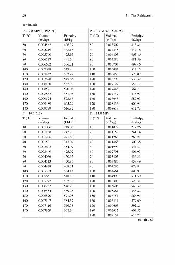
(continued)

P = 2.0 MPa (−19.5 °C) P = 3.0 MPa (−5.55 °C)


Enthalpy(kJ/kg)


Enthalpy(kJ/kg)

50 0.004562 436.37 50 0.003509 413.81

60 0.005219 458.13 60 0.004248 442.78

70 0.005760 475.93 70 0.004807 463.86

80 0.006237 491.69 80 0.005280 481.59

90 0.006672 506.21 90 0.005703 497.46

100 0.007078 519.9 100 0.006092 512.15

110 0.007462 532.99 110 0.006455 526.02

120 0.007828 545.65 120 0.006798 539.32

130 0.008180 557.98 130 0.007127 552.17

140 0.008521 570.06 140 0.007443 564.7

150 0.008852 581.95 150 0.007749 576.97

160 0.009174 593.68 160 0.008046 589.03

170 0.009489 605.29 170 0.008336 600.94

180 0.009799 616.82 180 0.008619 612.73

P = 10.0 MPa P = 11.0 MPa


Enthalpy(kJ/kg)


Enthalpy(kJ/kg)

10 0.001086 218.06 10 0.001078 217.26

20 0.001168 242.7 20 0.001152 241.14

30 0.001296 271.62 30 0.001263 268.21

40 0.001591 313.04 40 0.001463 302.38

50 0.002602 384.07 50 0.001990 354.37

60 0.003449 425.02 60 0.002795 404.93

70 0.004036 450.65 70 0.003405 436.31

80 0.004513 470.85 80 0.003886 459.49

90 0.004928 488.31 90 0.004296 478.8

100 0.005303 504.14 100 0.004661 495.9

110 0.005651 518.88 110 0.004996 511.59

120 0.005977 532.86 120 0.005308 526.31

130 0.006287 546.28 130 0.005603 540.32

140 0.006584 559.28 140 0.005884 553.82

150 0.006870 571.95 150 0.006154 566.91

160 0.007147 584.37 160 0.006414 579.69

170 0.007416 596.58 170 0.006667 592.21

180 0.007679 608.64 180 0.006912 604.55

– – – 190 0.007152 616.72(continued)


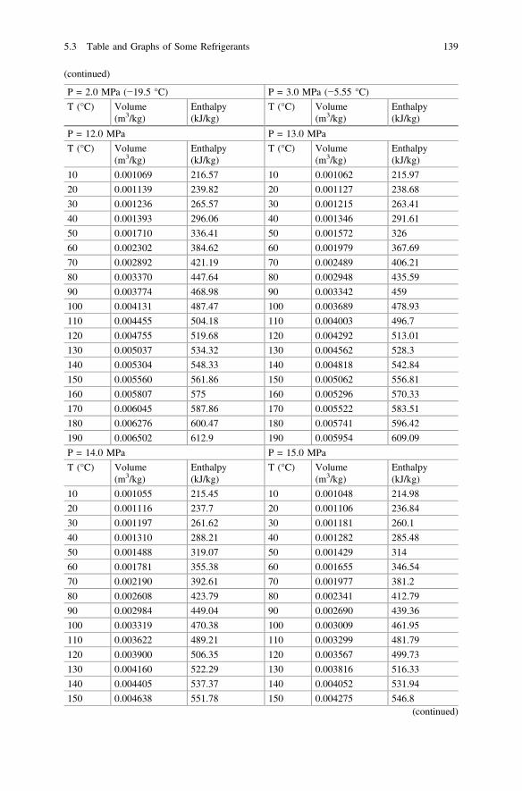
(continued)

P = 2.0 MPa (−19.5 °C) P = 3.0 MPa (−5.55 °C)


Enthalpy(kJ/kg)


Enthalpy(kJ/kg)

P = 12.0 MPa P = 13.0 MPa


Enthalpy(kJ/kg)


Enthalpy(kJ/kg)

10 0.001069 216.57 10 0.001062 215.97

20 0.001139 239.82 20 0.001127 238.68

30 0.001236 265.57 30 0.001215 263.41

40 0.001393 296.06 40 0.001346 291.61

50 0.001710 336.41 50 0.001572 326

60 0.002302 384.62 60 0.001979 367.69

70 0.002892 421.19 70 0.002489 406.21

80 0.003370 447.64 80 0.002948 435.59

90 0.003774 468.98 90 0.003342 459

100 0.004131 487.47 100 0.003689 478.93

110 0.004455 504.18 110 0.004003 496.7

120 0.004755 519.68 120 0.004292 513.01

130 0.005037 534.32 130 0.004562 528.3

140 0.005304 548.33 140 0.004818 542.84

150 0.005560 561.86 150 0.005062 556.81

160 0.005807 575 160 0.005296 570.33

170 0.006045 587.86 170 0.005522 583.51

180 0.006276 600.47 180 0.005741 596.42

190 0.006502 612.9 190 0.005954 609.09

P = 14.0 MPa P = 15.0 MPa


Enthalpy(kJ/kg)


Enthalpy(kJ/kg)

10 0.001055 215.45 10 0.001048 214.98

20 0.001116 237.7 20 0.001106 236.84

30 0.001197 261.62 30 0.001181 260.1

40 0.001310 288.21 40 0.001282 285.48

50 0.001488 319.07 50 0.001429 314

60 0.001781 355.38 60 0.001655 346.54

70 0.002190 392.61 70 0.001977 381.2

80 0.002608 423.79 80 0.002341 412.79

90 0.002984 449.04 90 0.002690 439.36

100 0.003319 470.38 100 0.003009 461.95

110 0.003622 489.21 110 0.003299 481.79

120 0.003900 506.35 120 0.003567 499.73

130 0.004160 522.29 130 0.003816 516.33

140 0.004405 537.37 140 0.004052 531.94

150 0.004638 551.78 150 0.004275 546.8(continued)


(continued)

P = 2.0 MPa (−19.5 °C) P = 3.0 MPa (−5.55 °C)


Enthalpy(kJ/kg)


Enthalpy(kJ/kg)

160 0.004861 565.69 160 0.004488 561.09

170 0.005077 579.2 170 0.004694 574.92

180 0.005285 592.39 180 0.004893 588.4

190 0.005487 605.32 190 0.005085 601.59

200 0.005684 618.05 200 0.005273 614.54

P = 16.0 MPa P = 17.0 MPa


Enthalpy(kJ/kg)


Enthalpy(kJ/kg)

10 0.001042 214.58 10 0.001036 214.23

20 0.001097 236.09 20 0.001089 235.43

30 0.001167 258.79 30 0.001154 257.65

40 0.001258 283.22 40 0.001238 281.32

50 0.001385 310.07 50 0.001350 306.9

60 0.001569 339.95 60 0.001505 334.84

70 0.001826 372.04 70 0.001716 364.75

80 0.002135 402.98 80 0.001977 394.53

90 0.002451 430.23 90 0.002258 421.85

100 0.002750 453.79 100 0.002534 446.04

110 0.003026 474.53 110 0.002794 467.51

120 0.003282 493.22 120 0.003038 486.88

130 0.003521 510.44 130 0.003267 504.68

140 0.003747 526.57 140 0.003483 521.31

150 0.003961 541.87 150 0.003688 537.03

160 0.004166 556.54 160 0.003885 552.06

170 0.004362 570.7 170 0.004073 566.54

180 0.004552 584.46 180 0.004255 580.58

190 0.004736 597.9 190 0.004431 594.27

200 0.004915 611.08 200 0.004602 607.66

P = 18.0 MPa P = 19.0 MPa


Enthalpy(kJ/kg)


Enthalpy(kJ/kg)

10 0.001031 213.93 10 0.001025 213.66

20 0.001081 234.84 20 0.001074 234.33

30 0.001143 256.65 30 0.001133 255.78

40 0.001220 279.68 40 0.001205 278.26

50 0.001321 304.27 50 0.001296 302.04

60 0.001455 330.74 60 0.001415 327.35

70 0.001633 358.88 70 0.001569 354.08

80 0.001855 387.37 80 0.001760 381.34(continued)


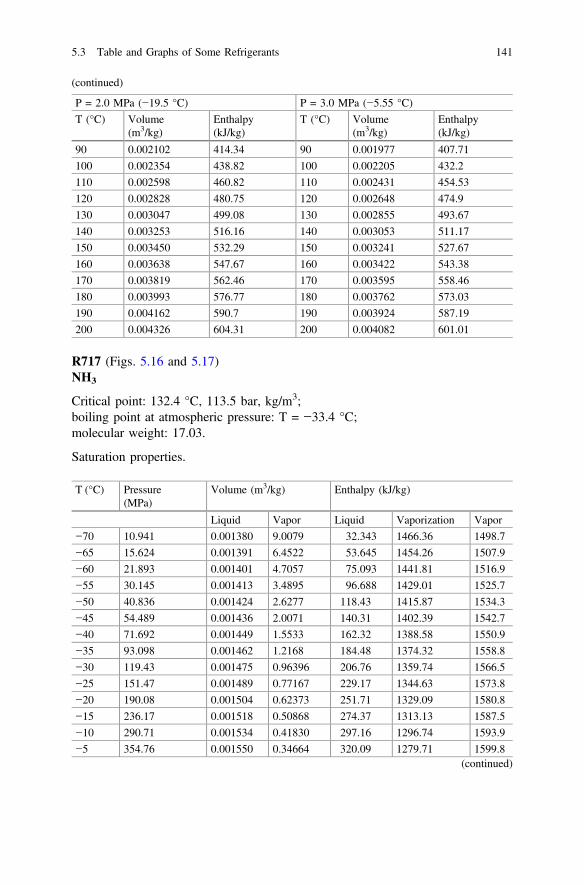
(continued)

P = 2.0 MPa (−19.5 °C) P = 3.0 MPa (−5.55 °C)


Enthalpy(kJ/kg)


Enthalpy(kJ/kg)

90 0.002102 414.34 90 0.001977 407.71

100 0.002354 438.82 100 0.002205 432.2

110 0.002598 460.82 110 0.002431 454.53

120 0.002828 480.75 120 0.002648 474.9

130 0.003047 499.08 130 0.002855 493.67

140 0.003253 516.16 140 0.003053 511.17

150 0.003450 532.29 150 0.003241 527.67

160 0.003638 547.67 160 0.003422 543.38

170 0.003819 562.46 170 0.003595 558.46

180 0.003993 576.77 180 0.003762 573.03

190 0.004162 590.7 190 0.003924 587.19

200 0.004326 604.31 200 0.004082 601.01

R717 (Figs. 5.16 and 5.17)NH3

Critical point: 132.4 °C, 113.5 bar, kg/m3;boiling point at atmospheric pressure: T = −33.4 °C;molecular weight: 17.03.


T (°C) Pressure(MPa)

Volume (m3/kg) Enthalpy (kJ/kg)

Liquid Vapor Liquid Vaporization Vapor

−70 10.941 0.001380 9.0079 32.343 1466.36 1498.7

−65 15.624 0.001391 6.4522 53.645 1454.26 1507.9

−60 21.893 0.001401 4.7057 75.093 1441.81 1516.9

−55 30.145 0.001413 3.4895 96.688 1429.01 1525.7

−50 40.836 0.001424 2.6277 118.43 1415.87 1534.3

−45 54.489 0.001436 2.0071 140.31 1402.39 1542.7

−40 71.692 0.001449 1.5533 162.32 1388.58 1550.9

−35 93.098 0.001462 1.2168 184.48 1374.32 1558.8

−30 119.43 0.001475 0.96396 206.76 1359.74 1566.5

−25 151.47 0.001489 0.77167 229.17 1344.63 1573.8

−20 190.08 0.001504 0.62373 251.71 1329.09 1580.8

−15 236.17 0.001518 0.50868 274.37 1313.13 1587.5

−10 290.71 0.001534 0.41830 297.16 1296.74 1593.9

−5 354.76 0.001550 0.34664 320.09 1279.71 1599.8(continued)


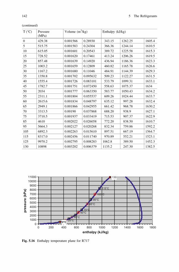
(continued)

T (°C) Pressure(MPa)

Volume (m3/kg) Enthalpy (kJ/kg)

0 429.38 0.001566 0.28930 343.15 1262.25 1605.4

5 515.75 0.001583 0.24304 366.36 1244.14 1610.5

10 615.05 0.001601 0.20543 389.72 1225.58 1615.3

15 728.52 0.001620 0.17461 413.24 1206.26 1619.5

20 857.48 0.001639 0.14920 436.94 1186.36 1623.3

25 1003.2 0.001659 0.12809 460.82 1165.78 1626.6

30 1167.2 0.001680 0.11046 484.91 1144.39 1629.3

35 1350.8 0.001702 0.095632 509.23 1122.27 1631.5

40 1555.4 0.001726 0.083101 533.79 1099.31 1633.1

45 1782.7 0.001751 0.072450 558.63 1075.37 1634

50 2034 0.001777 0.063350 583.77 1050.43 1634.2

55 2311.1 0.001804 0.055537 609.26 1024.44 1633.7

60 2615.6 0.001834 0.048797 635.12 997.28 1632.4

65 2949.1 0.001866 0.042955 661.42 968.78 1630.2

70 3313.5 0.00190 0.037868 688.20 938.9 1627.1

75 3710.5 0.001937 0.033419 715.53 907.37 1622.9

85 4610 0.002022 0.026058 772.20 838.50 1610.7

95 5664.3 0.002127 0.020268 832.34 759.86 1592.2

105 6892.3 0.002263 0.015610 897.51 667.19 1564.7

115 8317.0 0.002456 0.011740 970.89 552.21 1523.1

125 9970.2 0.002795 0.008283 1062.8 389.50 1452.3

130 10898 0.003202 0.006379 1135.2 247.30 1382.5

0°C 20°C40°C

60°C70°C

85°C95°C

105°C

115°C

130

0100020003000400050006000700080009000

1000011000

0 200 400 600 800 1000 1200 1400 1600 1800enthalpy (kJ/kg)

pres

sure

(kPa

)

Fig. 5.16 Enthalpy temperature plane for R717


References

1. https://www.chemours.com/Refrigerants/en_US/products/Suva/Suva134a.html. AccessedOctober 2016.

2. https://www.chemours.com/Refrigerants/en_US/products/Suva/Suva410A.html. AccessedOctober 2016.

3. https://www.chemours.com/Refrigerants/en_US/products/Suva/Suva407A.html. AccessedOctober 2016.

4. M. A. Kardzieski, Effect of refrigerant oil additive on R134a and R123 boiling heat transfer.Performance and related issue for GSA, NISTIR 7132 US Department of Commerce, June2004.

5. http://www.phillips66lubricants.com/documents/industrial/T3_TRI_12390B.pdf. AccessedOctober 2016.

6. http://www.belray.com/synthetic-pao-lubricant-0. Accessed October 2016.7. http://www.refrigerants.com/pdf/NRI-NLPolyolesterSS.pdf. Accessed October 2016.8. 2009 ASHRAE Handbook—Fundamentals (SI) https://app.knovel.com/web/toc.v/cid:

kpASHRAE37/viewerType:toc/root_slug:ashrae-handbook-fundamentals. Accessed October2016.

200210220230240250260270280290300310320330340350360370380390400410420430440450460470480490500510520530540550560570580590600610620630

-20 -10 0 10 20 30 40 50 60 70 80 90 100 110 120 130 140 150 160 170 180 190 200

2 MPa 3 MPa 5 MPa 6 MPa 7 MPa8 MPa 9 MPa 10 MPa 11MPa 12 MPa13 MPa 14 MPa 16 MPa 17 MPa 18 MPA19 MPa saturated liquid saturated vapor

satu

rate

d va

por

T(°C)

Enth

alpy

(kJ/

kg)

Fig. 5.17 Pressure enthalpy plane for R717

References 143

https://www.chemours.com/Refrigerants/en_US/products/Suva/Suva134a.html

https://www.chemours.com/Refrigerants/en_US/products/Suva/Suva410A.html

https://www.chemours.com/Refrigerants/en_US/products/Suva/Suva407A.html

http://www.phillips66lubricants.com/documents/industrial/T3_TRI_12390B.pdf

http://www.belray.com/synthetic-pao-lubricant-0

http://www.refrigerants.com/pdf/NRI-NLPolyolesterSS.pdf

https://app.knovel.com/web/toc.v/cid:kpASHRAE37/viewerType:toc/root_slug:ashrae-handbook-fundamentals

https://app.knovel.com/web/toc.v/cid:kpASHRAE37/viewerType:toc/root_slug:ashrae-handbook-fundamentals

9. https://www.chemours.com/Refrigerants/en_US/assets/downloads/h47751_hfc134a_thermo_prop_eng.pdf. Accessed October 2016.

10. (https://www.chemours.com/Refrigerants/en_US/assets/downloads/h64423_Suva410A_thermo_prop_si.pdf. Accessed October 2016.

11. http://www.mie.uth.gr/ekp_yliko/h56607_Suva407C_thermo_prop_si.pdf. Accessed October2016.

12. https://www.ohio.edu/mechanical/thermo/property_tables/CO2/CO2_TempSat2.html. AccessedOctober 2016.


https://www.chemours.com/Refrigerants/en_US/assets/downloads/h47751_hfc134a_thermo_prop_eng.pdf

https://www.chemours.com/Refrigerants/en_US/assets/downloads/h47751_hfc134a_thermo_prop_eng.pdf

https://www.chemours.com/Refrigerants/en_US/assets/downloads/h64423_Suva410A_thermo_prop_si.pdf

https://www.chemours.com/Refrigerants/en_US/assets/downloads/h64423_Suva410A_thermo_prop_si.pdf

http://www.mie.uth.gr/ekp_yliko/h56607_Suva407C_thermo_prop_si.pdf

https://www.ohio.edu/mechanical/thermo/property_tables/CO2/CO2_TempSat2.html

Chapter 6The External Sources: Water and Ground

Abstract Due to their peculiarities, water and ground are treated as thermalsources, separately, in this chapter. In fact they need appropriate techniques andmust comply with specific rules and standards. The type of used water can derivefrom waterways or, in any case, from surface waters, from underground and fromprocess waste water. The heat exchange with ground is then dealt with and the maintypes of heat exchangers commonly utilized are described both in the case of thehorizontal layout and in the vertical one (borehole heat exchangers).

6.1 Ground Water

Both its withdrawal and re-injection are ruled by legislation on a national and localbasis, due to the particular nature and value of this resource. The usual system usedto employ water consists in one or more well for withdrawal and re-injection, notnecessarily into the same aquifer. These wells must be placed at appropriatereciprocal distances and require a continuous maintenance, that can heavily affectthe management costs. To avoid realizing re-injection wells it is possible either tosend water to waterways or to use it for water supply. This latter solution stronglydepends on the physical and chemical characteristics of the fluid. In any case,designers have to carefully account for the impoverishment of aquifers and for theactual receptivity of waterways, together with their changes of temperature causedby further water injection.

Of course the expertise of a geologist plays a fundamental role in the defining thefeasibility of the project as well as during the sinking process.

At first a detailed analysis must be performed about some basic and imperativeinformation like, for example, the actual availability of the water flow rate1 neededby the plant during its period of operation, the properties of the ground involved bythe facility (both to physically realize wells and to know its thermal response), thedirection of aquifer flow to correctly place the withdrawal and the re-injection wells,and so on.

1As a rule of thumb we can estimate 150–200 l/h as the flow rate to employ for installed kW.


145

From the thermal viewpoint these deep waters allow a constant temperaturesource with a temperature around 10–15 °C.

There are mainly two ways to make this source interact with the heat pump:

• A direct way where water directly exchange heat in the heat exchanger of themachine. This method, more commonly adopted in residential buildings, canonly be employed once the presence of residual salts or of any chemical sub-stance, that could give origin to fouling or other damage, is quite low.

• An indirect way where the heat transfer between water and refrigerant takes placetrough an intermediate heat exchanger, generally a plate heat exchanger. Sodoing the heat pump is hydraulically disconnected from the ground water. Thismethod is normally more reliable, even if the heat transfer efficiency decreases.

The water circuit is provided with proper pumping and filtering systems. Theformer has to withdraw the right flow rate, by a submerged pump, and to release itto the injection well or waterway. The latter is aimed to withhold all those elementsthat could obstruct or damage tubing.

If the aquifer flow velocity is high enough a four well configuration can be usedas shown in Fig. 6.1.

Ground water is used to cool the condenser, in summer. Thus it is taken out fromwell B and sent (warmer) to well C.

At the beginning of the winter season the warm water (previously sent to C)reaches well D. Thus it is withdrawn by well D to exchange heat with the evap-orator and go back to the aquifer trough well A. The distance among wells, both inthe two and four well configurations, has to be sized on the basis of the aquiferwater velocity.

Verso del moto della falda

Verso del moto della falda

EV

COND

EV

COND

ESTATE

INVERNO

Pozzo inattivo

Pozzo caldo

Pozzo freddo

B

A

A

B C

C D

D

SUMMER

WINTERHot well

Coldwell

Inactive well

Aquifer flow direction

Aquifer flow direction

Fig. 6.1 Four well system

146 6 The External Sources: Water and Ground

The use of this type of source has advantages and drawbacks, as usual.Among the advantages there is the high energy efficiency, higher than that of

several other systems, thanks to the level and constancy of the source temperature,and the chance not to use any antifreeze.

Among the drawbacks it is the case to stress the imperative need of performing acareful feasibility study, at least from the hydro geological, economic and regula-tory points of view.

A facility using ground water has been, for instance, built in Milan (Italy) tosupply energy to “Palazzo Lombardia”, seat of the regional government ofLombardia (Italian region). It consists of three heat pumps each of 2 MW, toprovide the whole winter heating power, with 8 withdrawal wells for a total flowrate of 300 l/s and injection in a waterway.

6.2 Surface Water

The use of surface water requires taking care of filtering in order to prevent thepiping system from clogging [1]. If sea water is used, the hydraulic circuits mustemploy materials resistant to saltiness, with some additional cost.

The heat exchanger (tube bundle or coil) can be even directly immersed in water.In this case an appropriate spacing between tubes is employed, generally not lessthan 4 cm, and it has to be properly sheltered against obstruction and impact ofmaterial transported by the water stream.

Most commonly, a flat plate heat exchanger is utilized, where the cooling fluidcan be either the surface water or water circulating in an auxiliary. Once again acareful analysis of the available water quality and quantity and of the influence ofthe released “waste” water on flora and fauna of the waterway must be performed.

For example, district heating systems fed by large heat pumps (generally twostage with centrifugal compressors) of some tens of MW are operating, nowadays,in Stockholm (Nimrod and Vaertan) using seawater, and in Norway (Skojen Vest),using urban waste water. In Paris an installation of about 50 MW, with 8 heatpumps, makes use of river’s water.

Most of them use R134a as refrigerant and heat pumps are provided with doublestage turbo-compressor and can achieve around 90 °C for the hot water to deliver tousers.

6.3 Ground

Heat pumps using either ground or deep waters (ground water) are commonlyreferred to as geothermal heat pumps. Those exchanging heat with ground do notrequire any drainage of water, but use the ground as a heat capacity throughdifferent types of heat exchangers, we are dealing with in the following.

6.1 Ground Water 147

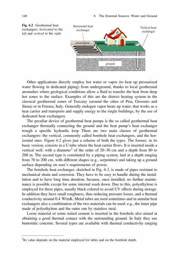
Other applications directly employ hot water or vapor (to heat up pressurizedwater flowing in dedicated piping) from underground, thanks to local geothermalanomalies where geological conditions allow a fluid to transfer the heat from deephot zones to the surface. Examples of this are the district heating system in theclassical geothermal zones of Tuscany (around the cities of Pisa, Grosseto andSiena) or in Ferrara, Italy. Generally endogen vapor heats up water, that works as aheat carrier and transports and supply energy to the single buildings, by the use ofdedicated heat exchangers.

The peculiar device of geothermal heat pumps is the so called geothermal heatexchanger thermally connecting the ground and the heat pump’s heat exchangertrough a specific hydraulic loop There are two main classes of geothermalexchangers: the vertical, commonly called borehole heat exchangers, and the hor-izontal ones. Figure 6.2 gives just a scheme of both the types. The former, in itsbasic version, consists in a U tube where the heat carrier flows. It is inserted inside avertical well, with a diameter2 of the order of 20–30 cm and a depth from 80 to200 m. The second type is constituted by a piping system, laid at a depth rangingfrom 70 to 200 cm, with different shapes (e.g., serpentine) and taking up a groundsurface depending on user’s requirements of power.

The borehole heat exchanger, sketched in Fig. 6.3, is made of pipes resistant tomechanical strain and corrosion. They have to be easy to handle during the instal-lation and to have long time duration, because, once installed, no further mainte-nance is possible except for some internal wash down. Due to this, polyethylene isemployed for these pipes, usually black colored to avoid UV effects during storage.In addition they have small roughness, thus reducing pressure losses, and a thermalconductivity around 0.4 W/mK. Metal tubes are used sometimes and in annular heatexchangers also a combination of the two materials can be used: e.g., the inner pipemade of polyethylene and the outer one by stainless steal.

Loose material or some suited cement is inserted in the borehole also aimed atobtaining a good thermal contact with the surrounding ground. In Italy they usebentonitic concrete. Several types are available with thermal conductivity ranging

Horizontal heat exchanger

Vertical heat exchanger

ground

excavation

Fig. 6.2 Geothermal heatexchangers: horizontal to theleft and vertical to the right

2Its value depends on the material employed for tubes and on the borehole depth.


from 0.7 to 2.3 W/mK. The ground may have very different thermal conductivitiesand capacities depending on its physical nature and water content, which can evenhighly improve its thermal performances. Some data from the German standardVDI464 are reported in Table 6.1 including the average extractable power during agiven time.

These geothermal probes, too, need clearance to be installed as drilling of thewell has to be approved by the competent authority. In any case they have theadvantage not to require water withdrawal from underground. Nevertheless a par-ticular care must be taken to avoid that the excavation put in contact two differentaquifers.

Depending on the power requirements, several probes can be used. In such acase they can interfere from the thermal point of view, thus reducing the perfor-mance of the system. It is necessary to keep a minimum distance among them,depending on their depth, type of ground and so on. As a rule of thumb it is advisedto keep the reciprocal distance not lower than 8–9 m.

Different types of horizontal heat exchangers are also available, which can takeup an appreciable room as shown in Fig. 6.4. The typical patterns are: the classicalserpentine in series and in parallel, linear layouts with one or more pipes placed indedicate trenches, spirals and baskets. The serpentine pattern may have many

filling material (e.g. bentonite)

ground

single U double U

single U annular

annular

bottom ballast

spacers

Fig. 6.3 Typical borehole heat exchanger

6.3 Ground 149

Table 6.1 Properties of several types of ground and related average power per length unit forsingle U borehole heat exchangers

Type of ground Conductivity(W/mK)

Extractable powerin 1800 h (W/m)

Extractable powerin 2400 h (W/m)

Generalvalues

Dry sinter <1.5 25 20

Waterloggedrocks and loose

1.5–3.0 60 50

High thermalconductivityrocks

>3.0 84 70

Specificvalues

Dry gravel andsand

0.4 <25 <20

Waterloggedgravel and sand

1.8–2.4 65–80 55–65

Clay and moistdirt

1.7 35–50 30–40

Limestone 2.8 55–70 45–60

Sandstone 2.3 65–80 55–65

Granite andsimilar

3.4 65–85 55–70

Basalt and similar 1.7 40–65 35–55

Gneiss 2.9 70–85 60–70

series

parallel

linear

A A

Section A-A

spiral

basket

Fig. 6.4 Typical horizontal heat exchanger layouts


different shapes somehow recalling those of radiant floors. Generally it is placed ata depth not higher than 1.5 m and pipes must be located at a minimum reciprocaldistance of 0.5 m, in order not to cause a depletion of the ground from the thermalviewpoint. As a rule of thumb it is possible to obtain around 10 W/m2 with dry soilsand 40 W/m2 with saturated soils. The room taken up on the surface by this type ofheat exchanger depends on the heat pump nominal power, the achievable COP andthe nature of the ground. Just to give an idea the value of this area might range from170 m2 for 5 kW up to 350 m2 for 10 kW.

Basket heat exchangers consist of spirally coiled pipes with either a cylindrical orconical shape. They have a vertical axis with a depth of 1 to 5 m and with differenthorizontal sizes. To them it is usually attributed an average obtainable power duringa standard working period of 1800 h, depending on their actual size. As a rule ofthumb, an average power of about 0.5 kW is assigned to cylindrical baskets with anoverall heat transfer surface of 15 m2. Conical baskets provide larger powers: the“small” ones (height up to 1.4 m, upper diameter 1.9 m and lower diameter 0.9 m)give up to 1 kW, while the “big” ones (height 2.5 m, upper diameter 2 m, lowerdiameter 1.1 m) provide from 1.5 to 2.0 kW. Once again these are only proxies.

Last but not least, geothermal piles have to be mentioned. They are foundationpiles, usually no longer than 40 m, where appropriate heat exchangers are inserted(the interested reader can refer, for example, to [2]). Once bearing piles are adopted,such a solution has the advantage not to require additional excavation costs.A particular attention must be paid to evaluate the most appropriate piles to be usedas geothermal piles. Generally it is the case to choose those located on the outerperimeter of the building, unless large enough ground water flow rates are present.

6.4 The Ground Thermal Response

To give some insight on how ground reacts to air temperature fluctuations, we canrefer to a sinusoidal oscillation around an average value. Let us suppose that thetemperature of the ground surface vary according to the following relation:

Tðx ¼ 0; tÞ ¼ Tm þ T senxt

where Tm is the average value of the surface temperature in the period t0, T itsamplitude and x = 2p/t0. The corresponding temperature profile in the ground isgiven by:

T x; tð Þ ¼ Tm þ T exp � xd

� �sen x t � sð Þ½ �

d ¼ffiffiffiffiffi2ax

r

s ¼ xxd

6.3 Ground 151

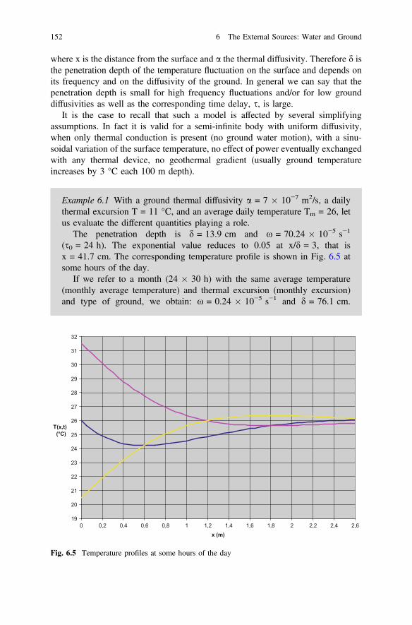
where x is the distance from the surface and a the thermal diffusivity. Therefore d isthe penetration depth of the temperature fluctuation on the surface and depends onits frequency and on the diffusivity of the ground. In general we can say that thepenetration depth is small for high frequency fluctuations and/or for low grounddiffusivities as well as the corresponding time delay, s, is large.

It is the case to recall that such a model is affected by several simplifyingassumptions. In fact it is valid for a semi-infinite body with uniform diffusivity,when only thermal conduction is present (no ground water motion), with a sinu-soidal variation of the surface temperature, no effect of power eventually exchangedwith any thermal device, no geothermal gradient (usually ground temperatureincreases by 3 °C each 100 m depth).

Example 6.1 With a ground thermal diffusivity a = 7 � 10−7 m2/s, a dailythermal excursion T = 11 °C, and an average daily temperature Tm = 26, letus evaluate the different quantities playing a role.

The penetration depth is d = 13.9 cm and x = 70.24 � 10−5 s−1

(s0 = 24 h). The exponential value reduces to 0.05 at x/d = 3, that isx = 41.7 cm. The corresponding temperature profile is shown in Fig. 6.5 atsome hours of the day.

If we refer to a month (24 � 30 h) with the same average temperature(monthly average temperature) and thermal excursion (monthly excursion)and type of ground, we obtain: x = 0.24 � 10−5 s−1 and d = 76.1 cm.

19

20

21

22

23

24

25

26

27

28

29

30

31

32

0 0,2 0,4 0,6 0,8 1 1,2 1,4 1,6 1,8 2 2,2 2,4 2,6x (m)

T(x,t) (°C)

Fig. 6.5 Temperature profiles at some hours of the day


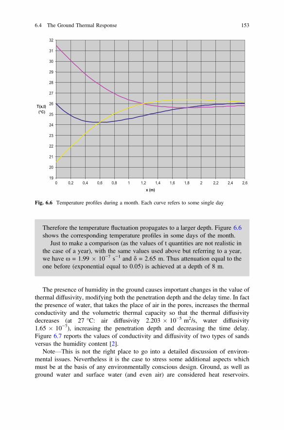
Therefore the temperature fluctuation propagates to a larger depth. Figure 6.6shows the corresponding temperature profiles in some days of the month.

Just to make a comparison (as the values of t quantities are not realistic inthe case of a year), with the same values used above but referring to a year,we have x = 1.99 � 10−7 s−1 and d = 2.65 m. Thus attenuation equal to theone before (exponential equal to 0.05) is achieved at a depth of 8 m.

The presence of humidity in the ground causes important changes in the value ofthermal diffusivity, modifying both the penetration depth and the delay time. In factthe presence of water, that takes the place of air in the pores, increases the thermalconductivity and the volumetric thermal capacity so that the thermal diffusivitydecreases (at 27 °C: air diffusivity 2.203 � 10−5 m2/s, water diffusivity1.65 � 10−7), increasing the penetration depth and decreasing the time delay.Figure 6.7 reports the values of conductivity and diffusivity of two types of sandsversus the humidity content [2].

Note—This is not the right place to go into a detailed discussion of environ-mental issues. Nevertheless it is the case to stress some additional aspects whichmust be at the basis of any environmentally conscious design. Ground, as well asground water and surface water (and even air) are considered heat reservoirs.

19

20

21

22

23

24

25

26

27

28

29

30

31

32

0 0,2 0,4 0,6 0,8 1 1,2 1,4 1,6 1,8 2 2,2 2,4 2,6x (m)

T(x,t) (°C)

Fig. 6.6 Temperature profiles during a month. Each curve refers to some single day

6.4 The Ground Thermal Response 153

Of course ideal reservoirs, with an infinite heat capacity, do not exist in nature. Inreality anytime we interact with them we, at first locally, change their characteristicsFor instance such thermal interactions can modify the reproductive features both ofanimals and vegetation both for water and ground (i.e., they may affect fish, algaeand take to freezing of ground and, where it exists, to the destruction of permafrost).

In addition it is necessary to know the appropriate boundary conditions to adoptin the mathematical models used for designing Just referring only to ground heatexchangers, and depending on their types, it is fundamental to account for the effectof solar radiation, that is the only means to “recharge” the less deep layers of groundafter a winter season and the effect of rain. A sunny ground behaves differently froma ground often subject to rainfalls and it is the case to take this into account also inelaborating the data collected during preliminary tests. Furthermore we recall that theheat transfer to sky is an additional mean to cool soil during summer nights.

Things are even more complex to put the appropriate boundary conditions at theend of borehole heat exchangers and so on.

In any case several studies are been pursued at present to find out a good equi-librium between the induced disturbance and the chance of its proper compensation.

References

1. S. J. Pugh1*, G. F. Hewitt, H. Müller-Steinhagen Fouling during the use of seawater ascoolant- the development of a ‘User Guide’, Refereed Proceedings Heat Exchanger Foulingand Cleaning: Fundamentals and Applications Engineering Conferences International Year2003. http://dc.engconfintl.org/cgi/viewcontent.cgi?article=1001&context=heatexchanger.

0

0,5

1

1,5

2

2,5

3

5 6 7 8 9 10 11 12 13 14 15 16 17 18 19 20% Humidity

Thermal conductiviy, sand density 1600kg/m3

Thermal conductiviy, sand density 1280kg/m3

Thermal diffusivity,sand density 1600kg/m3

Thermal diffusivity, sand density 1280kg/m3

Fig. 6.7 Thermal conductivity (W/mK) and diffusivity (m2/s) versus water content for sands withtwo different densities. (The values of diffusivity have to be multiplied by 10−6)


http://dc.engconfintl.org/cgi/viewcontent.cgi?article=1001&context=heatexchanger

2. N. Batini, A. F. Rotta Loria, P. Conti, D. Testi, W. Grassi, L. Lalou, i Energy and geotechnicalbehaviour of energy piles for different design solutions, Applied Thermal Engineering 86(2015) 199–213.

3. S. P. Kavanaugh, K. Rafferty: “Ground source heat pumps—Design of geothermal systems forcommercial and institutional buildings”, A.S.H.R.A.E. Applications Handbook 1997.

References 155

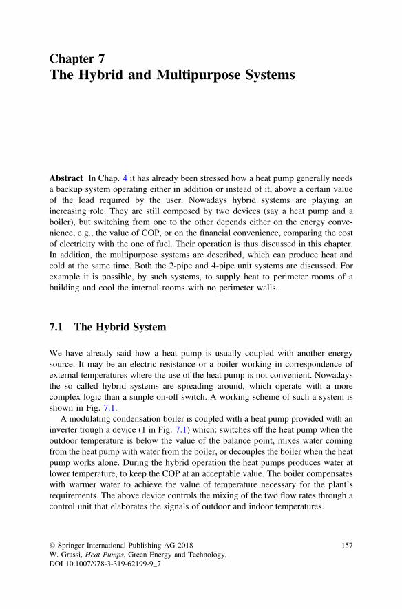
Chapter 7The Hybrid and Multipurpose Systems

Abstract In Chap. 4 it has already been stressed how a heat pump generally needsa backup system operating either in addition or instead of it, above a certain valueof the load required by the user. Nowadays hybrid systems are playing anincreasing role. They are still composed by two devices (say a heat pump and aboiler), but switching from one to the other depends either on the energy conve-nience, e.g., the value of COP, or on the financial convenience, comparing the costof electricity with the one of fuel. Their operation is thus discussed in this chapter.In addition, the multipurpose systems are described, which can produce heat andcold at the same time. Both the 2-pipe and 4-pipe unit systems are discussed. Forexample it is possible, by such systems, to supply heat to perimeter rooms of abuilding and cool the internal rooms with no perimeter walls.

7.1 The Hybrid System

We have already said how a heat pump is usually coupled with another energysource. It may be an electric resistance or a boiler working in correspondence ofexternal temperatures where the use of the heat pump is not convenient. Nowadaysthe so called hybrid systems are spreading around, which operate with a morecomplex logic than a simple on-off switch. A working scheme of such a system isshown in Fig. 7.1.

A modulating condensation boiler is coupled with a heat pump provided with aninverter trough a device (1 in Fig. 7.1) which: switches off the heat pump when theoutdoor temperature is below the value of the balance point, mixes water comingfrom the heat pump with water from the boiler, or decouples the boiler when the heatpump works alone. During the hybrid operation the heat pumps produces water atlower temperature, to keep the COP at an acceptable value. The boiler compensateswith warmer water to achieve the value of temperature necessary for the plant’srequirements. The above device controls the mixing of the two flow rates through acontrol unit that elaborates the signals of outdoor and indoor temperatures.


157

Besides it decouples either the boiler or the heat pump out of the hybrid oper-ation range, on the basis of preset values.

A second device (2 in the figure) deflects the hot water from the plant to thesanitary water reservoir, once its temperature probe measures a lower value than thepreset one. So doing, this unit gives sanitary water the priority.

If both boiler and heat pump have a climatic control as shown in Fig. 7.1, it isnecessary to provide a proper signal to them so that they could operate at theirmaximum temperatures during the sanitary water production.

Of course there are several variants to the discussed scheme. Boiler and heatpump are often connected, in the sanitary water tank, to two different coils: the heatpump to the lower temperature coil and the boiler to higher temperature one.

Furthermore the sanitary water can be produced instantaneously and/or coupledto a thermal solar plant, while the electric power for the heat pump can be providedby a photovoltaic plant.

Pre-assembled units are available on the market for single-family homes, con-tained in a cabinet of limited size.

Figure 7.2 provides a scheme of the operation of such systems. It shows theoperation ranges of the boiler alone, of the hybrid system and of the heat pumpalone versus the outdoor temperature, in abscissa The hour of operation are locatedon the axis of the ordinates, and the symbols refer to North Italy and Central andSouth Italy.

Figure 7.3 shows a type of high efficiency hybrid heat pump for a single-familydwelling (courtesy of Clivet), including an inertial tank for smoothing load

Sanitary water

Outdoor probe

Boiler

Heat pump

Thermal plant

Indoor probe

1

2

Sanitary water

probe

Ever open ways

Fig. 7.1 Scheme of a hybrid system with sanitary water reservoir

158 7 The Hybrid and Multipurpose Systems

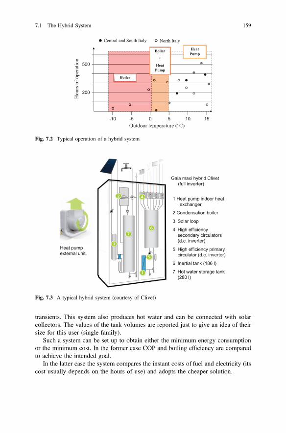
transients. This system also produces hot water and can be connected with solarcollectors. The values of the tank volumes are reported just to give an idea of theirsize for this user (single family).

Such a system can be set up to obtain either the minimum energy consumptionor the minimum cost. In the former case COP and boiling efficiency are comparedto achieve the intended goal.

In the latter case the system compares the instant costs of fuel and electricity (itscost usually depends on the hours of use) and adopts the cheaper solution.

-10 -5 0 5 10 15Outdoor temperature (

500

200

Central and South Italy North Italy

Hou

rs o

f ope

ratio

nBoiler

Boiler

+

Heat Pump

Heat Pump

°C)

Fig. 7.2 Typical operation of a hybrid system

Gaia maxi hybrid Clivet (full inverter)

1 Heat pump indoor heat exchanger.

2 Condensation boiler

3 Solar loop

4 High efficiency secondary circulators (d.c. inverter)

5 High efficiency primary circulator (d.c. inverter)

6 Inertial tank (186 l)

7 Hot water storage tank (280 l)

Heat pumpexternal unit.

Fig. 7.3 A typical hybrid system (courtesy of Clivet)

7.1 The Hybrid System 159

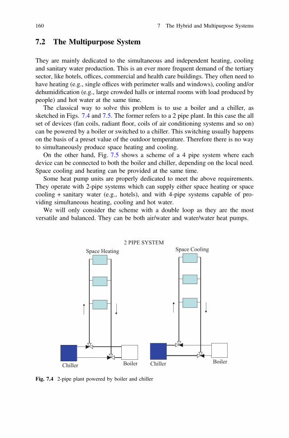
7.2 The Multipurpose System

They are mainly dedicated to the simultaneous and independent heating, coolingand sanitary water production. This is an ever more frequent demand of the tertiarysector, like hotels, offices, commercial and health care buildings. They often need tohave heating (e.g., single offices with perimeter walls and windows), cooling and/ordehumidification (e.g., large crowded halls or internal rooms with load produced bypeople) and hot water at the same time.

The classical way to solve this problem is to use a boiler and a chiller, assketched in Figs. 7.4 and 7.5. The former refers to a 2 pipe plant. In this case the allset of devices (fan coils, radiant floor, coils of air conditioning systems and so on)can be powered by a boiler or switched to a chiller. This switching usually happenson the basis of a preset value of the outdoor temperature. Therefore there is no wayto simultaneously produce space heating and cooling.

On the other hand, Fig. 7.5 shows a scheme of a 4 pipe system where eachdevice can be connected to both the boiler and chiller, depending on the local need.Space cooling and heating can be provided at the same time.

Some heat pump units are properly dedicated to meet the above requirements.They operate with 2-pipe systems which can supply either space heating or spacecooling + sanitary water (e.g., hotels), and with 4-pipe systems capable of pro-viding simultaneous heating, cooling and hot water.

We will only consider the scheme with a double loop as they are the mostversatile and balanced. They can be both air/water and water/water heat pumps.

Chiller Boiler Chiller Boiler

Space Heating Space Cooling2 PIPE SYSTEM

Fig. 7.4 2-pipe plant powered by boiler and chiller


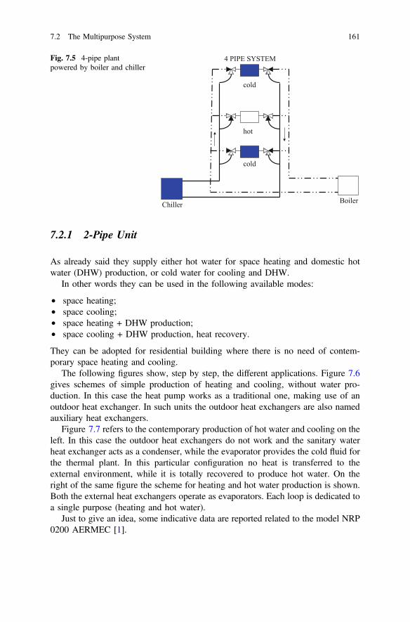
7.2.1 2-Pipe Unit

As already said they supply either hot water for space heating and domestic hotwater (DHW) production, or cold water for cooling and DHW.

In other words they can be used in the following available modes:

• space heating;• space cooling;• space heating + DHW production;• space cooling + DHW production, heat recovery.

They can be adopted for residential building where there is no need of contem-porary space heating and cooling.

The following figures show, step by step, the different applications. Figure 7.6gives schemes of simple production of heating and cooling, without water pro-duction. In this case the heat pump works as a traditional one, making use of anoutdoor heat exchanger. In such units the outdoor heat exchangers are also namedauxiliary heat exchangers.

Figure 7.7 refers to the contemporary production of hot water and cooling on theleft. In this case the outdoor heat exchangers do not work and the sanitary waterheat exchanger acts as a condenser, while the evaporator provides the cold fluid forthe thermal plant. In this particular configuration no heat is transferred to theexternal environment, while it is totally recovered to produce hot water. On theright of the same figure the scheme for heating and hot water production is shown.Both the external heat exchangers operate as evaporators. Each loop is dedicated toa single purpose (heating and hot water).

Just to give an idea, some indicative data are reported related to the model NRP0200 AERMEC [1].

Chiller Boiler

4 PIPE SYSTEM

cold

cold

hot

Fig. 7.5 4-pipe plantpowered by boiler and chiller

7.2 The Multipurpose System 161

.......................................................................................................................................................................................................................................................................................

......................................................................................................................................................................................................................................................................................................................

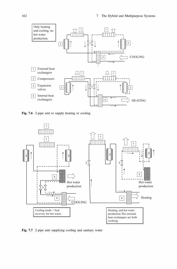
External heat exchangers

Compressors

Internal heatexchangers

............................................................................................................................................................................................................................................................................................................................................................

....................................................................................................................

COOLING

HEATING

1 1

1 1

2 2

2 2

4

3

3

4

1

2

3 Expansion valves

4

Only heating and cooling, no hot water production.

Fig. 7.6 2-pipe unit to supply heating or cooling

1

1

2 2

4

3

5

Heating

1

1

2 2

4

3

COOLING

Hot water production

Hot water production

5

Cooling mode + heat recovery for hot water.

Heating, and hot water production.The external heat exchangers are both working.

3

Fig. 7.7 2-pipe unit supplying cooling and sanitary water


Example 7.1 Cooling system side

Cooling capacity 43 kWTotal input power 14.01 kWEER 3.05

Heating system side

Heating capacity 46 kWTotal input power 13.34 kWCOP 3.47

Heating domestic water side

Heating capacity 46 kWTotal input power 13.44 kWCOP 3.49Water flow rate 7912 l/h

Cooling with heat recovery

Cooling capacity 46 kWRecovered power 58 kWTotal input power 13.45TER 7.72

Reference data

Fluid R410A.

Cooling mode Heating mode Coolingmode + heatrecovery

Evaporator leavingWater temperature7 °C

Condenser leavingWater temperature 45 °C

Heat recoveryleavingWater temperature45 °C

External airtemperature 35 °C

External air temperature 7 °C (drybulb), 6 °C (wet bulb)

Evaporator leavingWater temperature7 °C

DT = 5 °C DT = 5 °C DT = 5 °C

Of course the power recovered from the condensing refrigerant is larger thanthe one from the evaporator due to the compressor’s mechanical workcontribution.

In the preceding example a new quantity is introduced: TER (Total EnergyRatio) that is the ratio between the achievable total useful power (absolute value)and the power to be supplied to the heat pump. Thus, this system works as a


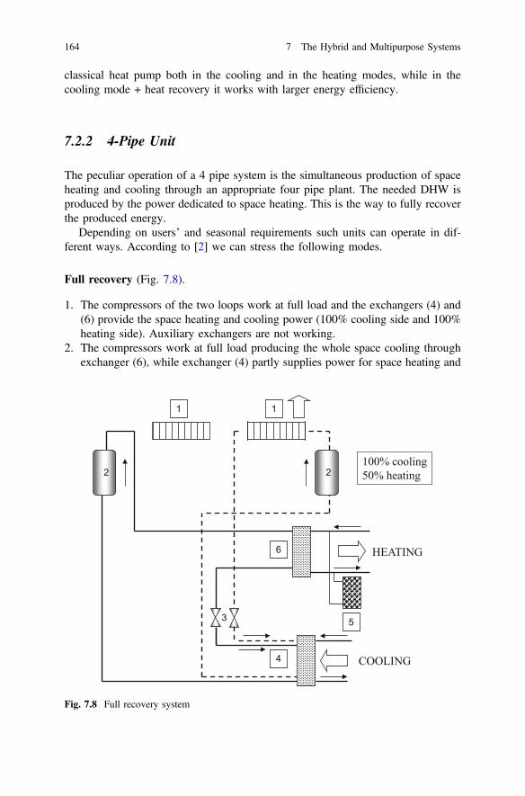
classical heat pump both in the cooling and in the heating modes, while in thecooling mode + heat recovery it works with larger energy efficiency.

7.2.2 4-Pipe Unit

The peculiar operation of a 4 pipe system is the simultaneous production of spaceheating and cooling through an appropriate four pipe plant. The needed DHW isproduced by the power dedicated to space heating. This is the way to fully recoverthe produced energy.

Depending on users’ and seasonal requirements such units can operate in dif-ferent ways. According to [2] we can stress the following modes.

Full recovery (Fig. 7.8).

1. The compressors of the two loops work at full load and the exchangers (4) and(6) provide the space heating and cooling power (100% cooling side and 100%heating side). Auxiliary exchangers are not working.

2. The compressors work at full load producing the whole space cooling throughexchanger (6), while exchanger (4) partly supplies power for space heating and

1 1

2 2

4

3 5

HEATING

COOLING

6

100% cooling 50% heating

Fig. 7.8 Full recovery system


partly for DHW production (100% cooling side and 75% heating side and 100%DHW). Auxiliary heat exchangers are not working.

3. Both compressors work at part load to follow the users’ power requirements forspace heating and cooling (50% cooling side and 50% heating side). Doing soheat exchangers (4) and (6) are oversized and allow achieving better unit per-formances. Auxiliary heat exchangers are not working.

Partial recovery (Fig. 7.9).

4. Both loops contribute either to the whole space cooling or to space cooling(100% cooling and 50% heating or 100% heating and 50% cooling). The twocompressors work at full load but one loop uses the corresponding auxiliary heatexchanger.

Example 7.2 Italy Case Study N°4: Multi-purpose heat pumps for simulta-neous heating and cooling [3].

It reports the data of a 4 pipe multipurpose heat pump operating in thedistrict of Santa Giulia, south of Milan. This district consists of five buildingswith a total area of 4500 m2 of offices, showrooms, restaurant etc. Themonitored unit supplies power to an area of 1500 m2 and uses the groundwater of a very shallow aquifer as external source. Its main features are:

1 1

2 2

4

3 5

HEATING

COOLING

6

3 100% heating 50% cooling

Fig. 7.9 Partial recovery system


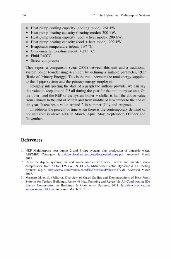
• Heat pump cooling capacity (cooling mode): 261 kW.• Heat pump heating capacity (heating mode): 300 kW.• Heat pump cooling capacity (cool + heat mode): 209 kW.• Heat pump heating capacity (cool + heat mode): 292 kW.• Evaporator temperature in/out: 11/7 °C.• Condenser temperature in/out: 40/45 °C.• Fluid R407C.• Screw compressor.

They report a comparison (year 2007) between this unit and a traditionalsystem boiler (condensing) + chiller, by defining a suitable parameter, REP(Ratio of Primary Energy). This is the ratio between the total energy suppliedto the 4 pipe system and the primary energy employed.

Roughly interpreting the data of a graph the authors provide, we can saythis value to keep around 2.5 all during the year for the multipurpose unit. Onthe other hand the REP of the system boiler + chiller is half the above valuefrom January to the end of March and from middle of November to the end ofthe year. It reaches a value around 2 in summer (July and August).

In addition the percent of time when there is the contemporary demand ofhot and cold is above 40% in March, April, May, September, October andNovember.

References

1. NRP Multipurpose heat pumps 2 and 4 pipe systems plus production of domestic water,AERMEC Catalogue. http://download.aermec.com/docs/opu/dnrpuy.pdf. Accessed March2017.

2. Units for 4-pipe systems, air and water source, with scroll, screw and inverter screwcompressors, from 33 to 1125 kW, INTEGRA, Mitsubishi Electric Hydronic & IT CoolingSystems S.p.A. http://www.climaveneta.com/EN/Download/View/6377.dl. Accessed March2017.

3. Masoero M. et al. (Editors), Overview of Cases Studies and Demonstrations of Heat PumpSystems for Tertiary Buildings, Annex 48 Heat Pumping and Reversible Air Conditioning IEAEnergy Conservation in Buildings & Community Systems, 2011. http://www.ecbcs.org/annexes/annex48.htm. Accessed March 2017.


http://download.aermec.com/docs/opu/dnrpuy.pdf

http://www.climaveneta.com/EN/Download/View/6377.dl

http://www.ecbcs.org/annexes/annex48.htm

http://www.ecbcs.org/annexes/annex48.htm

Chapter 8Additional Thermodynamic Remarks

Abstract This chapter recalls some elements of Thermodynamics that may helpunderstand the theoretical subject dealt with in the text.

8.1 Thermodynamic Cycle

It is a process where the thermodynamic variables (e.g., p, v, T) characteristic of afluid operating in a thermal machine evolve from a given set of values to this sameset, after the fluid has undergone a series of thermodynamic transformations. Thereference cycle is the Carnot cycle with two isentropic (reversible adiabatic trans-formations) and two isotherms. In the former ones the fluid properties changewithout any exchange of heat, i.e., at constant entropy and only a mechanicalexchange of work with the outside environment takes place. In the latter (isotherms)heat is exchanged at constant temperature and the fluid temperatures are the same asthe source’s ones. This is a quite idealized case where the temperature differencebetween fluid and sources is vanishing. In reality:

• of course it is not possible to realize any heat exchange with such a vanishingtemperature difference: it would require an infinite heat transfer surface. Inpractice the smaller is the temperature difference the larger has to be the heattransfer surface.

• To keep a transformation at a constant temperature, i.e., to keep it in equilibriumwith a constant temperature source (reservoir), it is necessary to let it occur withan infinitely slow velocity. This in order to make it go back to its initial tem-perature after any “small” heat exchange.

• The fluid flowing in the machine is subjected to “internal” irreversibilitiescaused by friction (and thus pressure losses) and to “external” irreversibilitiesassociated to the need of a finite temperature difference (between fluid andsource) to realize a heat exchange. In the case of a phase change this also meansthat such a pressure drop causes a temperature decrease.

• There is no way to achieve a perfect adiabatic transformation, due to non perfectinsulation and to internal heat production caused by friction.


167

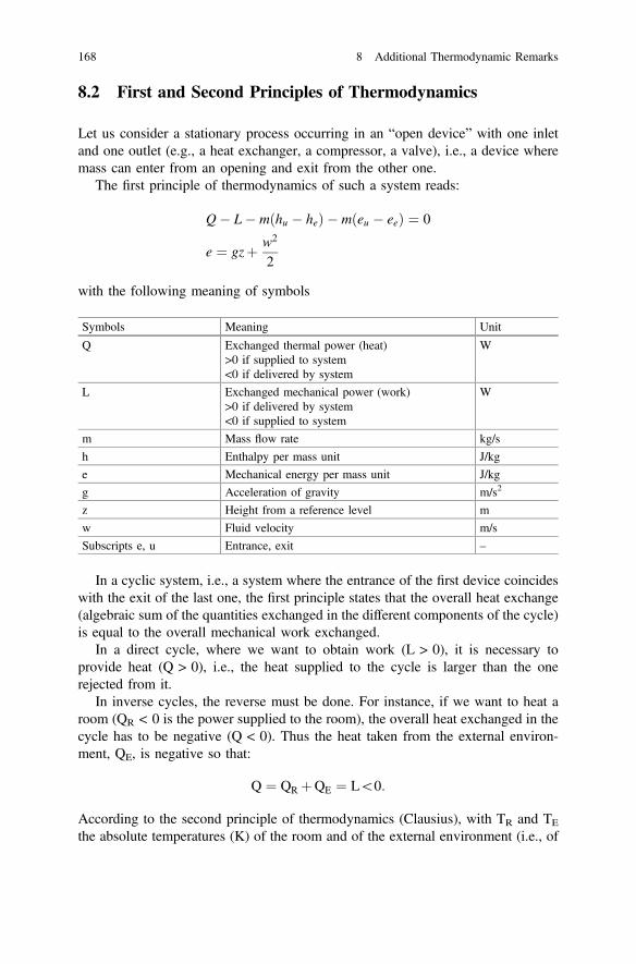
8.2 First and Second Principles of Thermodynamics

Let us consider a stationary process occurring in an “open device” with one inletand one outlet (e.g., a heat exchanger, a compressor, a valve), i.e., a device wheremass can enter from an opening and exit from the other one.

The first principle of thermodynamics of such a system reads:

Q� L� m hu � heð Þ � m eu � eeð Þ ¼ 0

e ¼ gzþ w2

2

with the following meaning of symbols

Symbols Meaning Unit

Q Exchanged thermal power (heat)>0 if supplied to system<0 if delivered by system

W

L Exchanged mechanical power (work)>0 if delivered by system<0 if supplied to system

W

m Mass flow rate kg/s

h Enthalpy per mass unit J/kg

e Mechanical energy per mass unit J/kg

g Acceleration of gravity m/s2

z Height from a reference level m

w Fluid velocity m/s

Subscripts e, u Entrance, exit –

In a cyclic system, i.e., a system where the entrance of the first device coincideswith the exit of the last one, the first principle states that the overall heat exchange(algebraic sum of the quantities exchanged in the different components of the cycle)is equal to the overall mechanical work exchanged.

In a direct cycle, where we want to obtain work (L > 0), it is necessary toprovide heat (Q > 0), i.e., the heat supplied to the cycle is larger than the onerejected from it.

In inverse cycles, the reverse must be done. For instance, if we want to heat aroom (QR < 0 is the power supplied to the room), the overall heat exchanged in thecycle has to be negative (Q < 0). Thus the heat taken from the external environ-ment, QE, is negative so that:

Q ¼ QR þQE ¼ L\0:

According to the second principle of thermodynamics (Clausius), with TR and TE

the absolute temperatures (K) of the room and of the external environment (i.e., of

168 8 Additional Thermodynamic Remarks

the two sources the operating fluid interacts with, they coincide with those of thefluid in a perfectly reversible cycle):

QR

TRþ QE

TE¼ 0 ) QR

QE¼ � TR

TE

As the absolute temperature is positive we easily infer that QR and QE have adifferent sign (QE > 0, being supplied to the machine by the environment).Furthermore if TR > TE, as in winter, |QR| > |QE|. This means that in winter wehave to subtract heat from the external environment and that its value is lower(thanks to the addition of mechanical work) than the one provided to the room.Conversely, in summer, the amount of heat delivered to the environment is higherthan that extracted from the room.

In real conditions, irreversible, the second principle needs to be formulated in adifferent manner. With the same meaning of symbols and indicating with Sg(Sg > 0) the effect of irreversibilities (entropy production):

QR

TRþ QE

TEþ Sg ¼ 0 ) QR ¼ �QE

TRTE

� SgTR

This means that, with the same QE, it is possible to give a lower value of power tothe room or, with the same power, QR, supplied to the room, a higher value ofpower must be subtracted from the environment. Similar conclusions can be drawnin summer.

We already said that irreversibilities can originate either inside the cycle thanoutside it.

Let us shortly deal with the former types. The generalized differential form ofBernoulli’s theorem reads:

dl ¼ �vdp� de� dla

where v, dp, dl, de, dla respectively represent the specific volume, the pressuredifference, the work exchanged during an infinitesimal transformation, the changeof macroscopic energy (kinetic and potential) and the work lost due to friction(dla > 0).

Once the variation of macroscopic energy is negligible the specific workexchanged by a mechanical component (e.g., pump, compressor, and fan) to letfluid flow, can be written:

dl ¼ �vdp� dla

Refer to an inverse cycle where the following components are present:

• a compressor takes the fluid from pressure p1 to pressure p2;• two heat exchangers (for example: one providing heat to the room and the other

extracting heat from the outside);• an expansion valve.

8.2 First and Second Principles of Thermodynamics 169

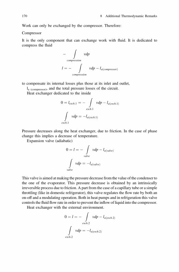
Work can only be exchanged by the compressor. Therefore:

Compressor

It is the only component that can exchange work with fluid. It is dedicated tocompress the fluid

�Z

compression

vdp

l ¼ �Z

compression

vdp� laðcompressorÞ

to compensate its internal losses plus those at its inlet and outlet,la (compressor), and the total pressure losses of the circuit.Heat exchanger dedicated to the inside

0 ¼ lexch:1 ¼ �Z

exch:1

vdp� laðexch:1Þ

Zexch:1

vdp ¼ �laðexch:1Þ

Pressure decreases along the heat exchanger, due to friction. In the case of phasechange this implies a decrease of temperature.

Expansion valve (adiabatic)

0 ¼ l ¼ �Z

valve

vdp� laðvalveÞ

Zvalve

vdp ¼ �laðvalveÞ

This valve is aimed at making the pressure decrease from the value of the condenser tothe one of the evaporator. This pressure decrease is obtained by an intrinsicallyirreversible process due to friction. A part from the case of a capillary tube or a simplethrottling (like in domestic refrigerator), this valve regulates the flow rate by both anon-off and a modulating operation. Both in heat pumps and in refrigeration this valvecontrols the fluid flow rate in order to prevent the inflow of liquid into the compressor.

Heat exchanger with the external environment.

0 ¼ l ¼ �Z

exch:2

vdp� laðexch:2Þ

Zexch:2

vdp ¼ �laðexch:2Þ


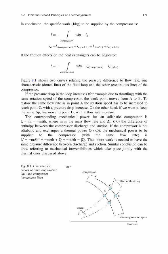
In conclusion, the specific work (J/kg) to be supplied by the compressor is:

l ¼�Z

compressor

vdp� la

la ¼laðcompressorÞ þ laðexch:1Þ þ laðvalveÞ þ laðexch:2Þ

If the friction effects on the heat exchangers can be neglected:

l ¼ �Z

compression

vdp� laðcompressorÞ � laðvalveÞ

Figure 8.1 shows two curves relating the pressure difference to flow rate, onecharacteristic (dotted line) of the fluid loop and the other (continuous line) of thecompressor.

If the pressure drop in the loop increases (for example due to throttling) with thesame rotation speed of the compressor, the work point moves from A to B. Torestore the same flow rate as in point A the rotation speed has to be increased toreach point C, with a pressure drop increase. On the other hand, if we want to keepthe same Dp, we move to point D, with a flow rate increase.

The corresponding mechanical power for an adiabatic compressor isL = ml = −mDh, where m is the mass flow rate and Dh (>0) the difference ofenthalpy between the compressor discharge and suction. If the compressor is notadiabatic and exchanges a thermal power Q (<0), the mechanical power to besupplied to the compressor (with the same flow rate) isL’ = −mDh’ = −mDh + Q = −mDh − |Q|. Thus more work is needed to have thesame pressure difference between discharge and suction. Similar conclusion can bedraw referring to mechanical irreversibilities which take place jointly with thethermal ones discussed above.

Flow rate

Δp

Effect of throttling

Increasing rotation speed

BD

C

A

circuit

compressor

Fig. 8.1 Characteristiccurves of fluid loop (dottedline) and compressor(continuous line)

8.2 First and Second Principles of Thermodynamics 171

Let us compare the mechanical power to supply to a reversible compressor(Q = 0, la = 0) with that to supply to an irreversible one (Q 6¼ 0, la 6¼ 0).

In the former case:

L ¼ Lrev ¼ �mZ

compression

vdp ¼ mlrev ¼ �mDh

In the latter case:

L ¼ �mDh� þQ ¼ Lrev þ La þQ

If the fluid is an ideal gas (Dh = cpDT, pv = RT), and keeping constant the pressuredifference between discharge (pressure p2, temperature T2,rev or T2 respectively inthe reversible and irreversible case) and suction (pressure p1, temperature T1) wehave:

Dhð Þrev¼ � �Z p2

p1

vdp

� �DS¼0

¼ �lrev ¼ lrevj j ¼ cp T2;rev � T1� �

in the reversible case (DS = 0) and

Dhð Þirrev¼Z p2

p1

vdp

� �DS 6¼0

¼ �lrev þ la ¼ lrevj j þ la ¼ cp T2 � T1ð Þ

in the irreversible case.The discharge temperature (enthalpy) in the real case is higher than in the ideal

case, as more work must be provided to keep constant the pressure differencebetween suction and discharge. Therefore:

la ¼ cp T2 � T2;rev� �

The ratio between the difference of enthalpy in reversible and irreversible trans-formations is named the compressor isentropic efficiency, qc.

qc ¼Dhð ÞrevDhð Þirrev

8.3 Phase Change of Pure Substances

A pure substance can exist in different states of matter: solid, liquid or gas.Figure 8.2 shows the regions occupied by the different states in the pressure-temperature plane. Any line marking the border between two regions represent the


phase change occurring at a given couple of values of pressure and temperature. Thecurve separating solid from liquid has a negative slope if the specific volumedecreases, as in the case of water (ice has a larger specific volume than liquid) and apositive slope in the opposite case, as in the case of most pure substances. The pointof connection of the three lines (solid–liquid, liquid–gas and solid–gas) is the socalled triple point, where all the three phases coexist.

The topic dealt with in this volume concerns the fluid state: liquid, saturatedvapor, vapor and gas. Figure 8.3 shows, in a quite schematic form, the aboveregions in the temperature–entropy and pressure–enthalpy planes.

If x is the vapor quality1 of the mixture in the saturated vapor region (va-por + liquid), the enthalpy of a saturated vapor at pressure p2 is:

hðpÞ ¼ ð1� xÞ � hLðpÞþ x � hVðpÞ¼ hLðpÞþ x � ½hV ðpÞ � hLðpÞ� ¼ hLðpÞþ x � rðpÞ

r ¼ hVðpÞ � hLðpÞ

where hL(p) e hV(p) respectively are the enthalpies (J/kg) of saturated liquid andvapor at pressure p, x and (1 − x) are the quantities of vapor and liquid in 1 kg ofmixture and r the latent heat of evaporation (J/kg).

The heat exchanged per kg of mixture during an evaporation from x1 to x2(x2 > x1) is:

qEV ¼ h2 � h1 ¼ ðx2 � x1Þr[ 0

p

T

Ice

Gas

Vapor

Liquid

Critical point

Critical point

Triple point

Fig. 8.2 The phases of apure substance in thepressure–temperature plane

1Ratio between the mass of vapor and the mass of mixture, i.e., the vapor mass in 1 kg of mixture.2Recall that, at constant pressure, the temperature keeps constant as well, during a change of phase.

8.3 Phase Change of Pure Substances 173

Therefore heat has to be supplied to the fluid. In the case of condensation(x2 < x1) it is:

qCOND ¼ h2 � h1 ¼ ðx2 � x1Þr\0

Heat is supplied by the fluid.During both these heat exchanges fluid flows in the ducts of the dedicated heat

exchangers progressively change its quality and decrease its pressure. Figure 8.4

T

s

L. S.V.

G.

V.

Critical point

Critical isotherm p

h

L. S.V.

G.

V.

Critical point

Critical isotherm

isotherm isobar

isobar

G. Gas L. Liquid V. Vapor S.V. Saturated vapor

Fig. 8.3 Two phase region in the temperature-entropy and in the pressure enthalpy planes

Water to be cooled

Evaporating refrigerant

Cold refrigerant, low quality

Large vapor mass originate.

Annular motion: liquid in contact

with wall and vapor “core”.

Super heated vapor

Some two – phase flow regimes during refrigerant evaporation

Fig. 8.4 Sketch of some two–phase flow regimes in an evaporator


qualitatively shows the different two–phase regimes which may occur in an annularheat exchanger during an evaporation. The refrigerant enters with a low quality andthe water to be cooled at a given temperature. Water cools down to the necessarytemperature for space cooling. At the same time the refrigerant quality increases upto 1, then giving origin to superheated vapor in dry evaporators. Qualitatively wemight say that the reverse occurs in condensation. For further details on the subjectthe reader is referred to [1–3].

Table 8.1 reports some characteristic values of the overall heat transfer coeffi-cient for different types of heat exchange.

References

1. Butterworth D. & Hewitt G.F., Two-phase flow and heat transfer, Harwell Series, OxfordUniversity Press, Oxford (UK), 1979.

2. Collier J.G., Thome J.R., Convective Boiling and Condensation, Clarendon Press, Oxford,1994.

3. Hewitt G.F. executive editor, Heat Exchanger Design Handbook 1998, Part 3 Thermal andHydraulic Design of Heat Exchangers, Begell House Inc. New York.

Table 8.1 Indicative values of overall heat transfer coefficients

Heat exchange Typical value (W/m2K) Range

Gas/gas at normal pressure 20 5–50

Gas/gas at high pressione 200 50–500

Gas/liquid 50 10–100

Liquid/liquid in tubular heat exchanger 1000 200–2000

Liquid/liquid in plate heat exchanger 2500 500–5000

Gas cooled condenser 50 10–100

Liquid cooled condenser 3000 500–6000

Gas heated evaporator 50 10–100

Liquid heated evaporator 5000 500–10,000

Note—global heat transfer coefficients ranging from 2000 to 7000 W/m2K, with R410A, havebeen obtained for a corrugated flat plate evaporator

8.3 Phase Change of Pure Substances 175

Walter Grassi - Heat Pumps - randolphtoom introduction

Documents

Transcript of Walter Grassi - Heat Pumps - randolphtoom introduction