arX

iv:1

501.

0114

0v1

[ph

ysic

s.fl

u-dy

n] 6

Jan

201

5

Deformation of a flexible fiber in a viscous flow past an obstacleH. M. López,1, a) J-P. Hulin,2, b) H. Auradou,2, c) and M. V. D’Angelo1, d)

1)Grupo de Medios Porosos, Facultad de Ingeniería, Paseo Colon 850, 1063, Buenos Aires (Argentina),CONICET (Argentina).2)Univ Paris-Sud, CNRS, F-91405. Lab FAST, Bât 502, Campus Univ, Orsay,F-91405 (France).

We study the deformation and transport of elastic fibers in a viscous Hele-Shaw flow with curvedstreamlines. The variations of the global velocity and orientation of the fiber follow closely those ofthe local flow velocity. The ratios of the curvatures of the fibers by the corresponding curvatures ofthe streamlines reflect a balance between elastic and viscous forces: this ratio is shown experimen-tally to be determined by a dimensionless Sperm number Sp combining the characteristic parametersof the flow (transverse velocity gradient, viscosity, fiber diameter/cell gap ratio) and those of thefiber (diameter, effective length, Young’s modulus). For short fibers, the effective length is that ofthe fiber; for long ones, it is equal to the transverse characteristic length of the flow. For Sp . 250,the ratio of the curvatures increases linearly with Sp; For Sp & 250, the fiber reaches the samecurvature as the streamlines.

I. INTRODUCTION

The transport of flexible biological or man made fibers by a flow and their deformation is of interest in viewof their potential applications in many different industrial fields. A first example is the paper industry inwhich the orientation and spatial distributions of the fibers in the flowing pulp must be controlled1,2. Fibersare also widely used by petroleum engineers3 to enhance the proppant transport capabilities of fracturingfluids, or to prevent the backflow of proppant. Other domains of application are civil engineering (specialcements, structural reinforcement), textile engineering, bio engineering and medicine.

In flows at low Reynolds numbers, the deformation of fibers reflects a balance between viscous and elasticstresses and plays often an important part: for instance, these effects are critical for understanding thedynamics of flexible biological filaments4–6, the filtration and cross stream migration of macromoleculesin small channels7–10 and the positioning of bio-fibers in porous media11. In all these applications, theprediction of the motion of the fibers is a difficult fundamental problem, particularly in complex geometriesand inhomogeneous flows where constrictions and obstacles are present: these create complex interactionsbetween the flexible objects, the flowing fluids and the solid walls.

Our interest in these problems is focused on the injectability and transport of long flexible fibers throughfractures in reservoir rocks. In a previous work12, we studied fiber transport by a flow in single narrow modelrough fractures and of its dependence on the fluid velocity, the flexibility of the fiber and the configurationof the aperture field.

The present work is devoted to a quantitative study of the influence of the parameters in the configurationwhere the fiber passes in the vicinity of contact areas or close to regions of low aperture. This situation ismodeled experimentally by means of a Hele-Shaw cell of constant aperture and of width varying with thedistance: this allows one to determine the variations along the flow of the orientation and deformation of theflow lines and of a fiber placed in the flow. More specifically, we seek to relate the variations of the curvatureof the fiber to those of the streamlines, to the velocity gradients and to the geometrical and mechanicalproperties of the fiber.

Most past studies considered the simpler case of flexible fibers in a non confined parallel shear flow13–16

of shear rate (∂v/∂n) (v is the modulus of the local flow velocity and the derivative is taken is the directionperpendicular to the flow lines). In such a configuration, the fiber may rotate about its axis and bucklesabove a threshold value of the Sperm number which characterizes the relative magnitudes of the viscous andelastic forces. and is equal to:

µ(∂v/∂n)ξ4

EI; (1)

a)Electronic mail: lopezhmatias@gmail.comb)Electronic mail: hulin@fast.u-psud.frc)Electronic mail: Harold.Auradou@u-psud.frd)Electronic mail: veronica.dangelo@gmail.com

2

µ is the viscosity, (∂v/∂n) is the shear rate along the fiber, E its Young’s modulus, I its area moment ofinertia (I = πD4/64 for a circular cross section of diameter D) and ξ a characteristic dimension (for instancethe length Lf of the fiber). Other studies dealt with the cross stream migration of a flexible fiber in a parallelPoiseuille flow which is also strongly influenced by buckling8–10. Finally, buckling is also observed above acritical value Sp ∼ 12017) of Sp for fibers approaching a stagnation point18–20. Numerically, slender-bodytheory has been used to model the behavior of an elastic fiber (with one clamped end) in the vicinity of acorner in a curved channel21. In this latter work, the variation with time and the final shape of the filamentwere analyzed in different corner geometries as a function of Sp. Recently, Wexler et al.22 considered a fiberwith one clamped end and initially transverse to a flow confined between two plates (like in the presentcase). In all cases, bending results from the combined effects of the hydrodynamic and viscous forces on thefibers: yet, in Refs. 21 and 22, their resultant is balanced by a force on the attachment point while, in thepresent case of a free fiber, this resultant must be zero, leading to very different shapes of the fibers.

In the following, we characterize first the flow field in the Hele-Shaw cell of varying width by means of dyetracer measurements and of 3D numerical simulations: we study in particular the variations of the velocityalong the streamlines. Then, the local velocity and mean orientation of the fibers are compared to those ofthe fluid velocity at the same location. The curvature κf of the fibers is characterized by its ratio κf/κs

to that of the streamlines: the variations of the extremal values of this ratio on different streamlines arestudied as a function of the diameter D and length Lf of the fiber, of its initial transverse location and ofthe flow velocity. The definition of the Sperm number Sp of the problem allowing one to take into accountthe influence of these different parameters is then discussed and the experimental dependence of κf/κs onSp is analyzed.

II. EXPERIMENTAL PROCEDURE

The experimental setup consists of a Hele Shaw cell placed vertically. Its height and gap are respectivelyL = 280 and H = 2.2 ± 0.1mm (Fig. 1). The upper part of the cell has a Y-shaped section; the top isattached to a fluid bath with a slit at the bottom allowing for the flow of the fluid and the injection of thefibers. The fiber is injected in a funnel-shaped device which permits to select conveniently the location atwhich the fiber is injected. A rounded off step is then cut out of a transparent mylar sheet of thickness equalto H and inserted in the Hele Shaw cell. The mylar is tightly fitted so that no flow is observable between itssurface and the walls of the cell. The height ∆W of the step parallel to the y axis is 30mm and it is locatedin the middle of the cell; the width W (x) of the flow section in the cell is then 70mm in the inlet sectionand is reduced to 40mm at the outlet as shown in the figure. The axis y = 0 corresponds to the boundaryof the mylar sheet at the inlet.

LW(x)

g

x

O

z

y

mylar

sheet

U

H

∆WLf

camera

upperbath

funnelshaped

section

FIG. 1. Experimental setup.

Using a continuous rather than an abrupt variation of the height of the step boundary with the distancefirst minimizes unwanted solid-solid interactions between the fiber and this boundary. Moreover, a continuousvariation of the width of the flow channel with distance is closer to the variation encountered in a real

3

fractured rock. Finally, putting uniform flow sections before and after the step allows one to detect possibleirreversible rotations and deformations of the fiber.

A gear pump produces a downward flow; two Newtonian fluids are used: pure (MiliQ) water, of densityρ = 997 ± 1 kg.m−3 and a viscosity µ ≈ 1mPa.s, and a solution of 70% glycerol by weight in water,of density ρ = 1178 ± 1 kg.m−3 and viscosity µ ≈ 15mPa.s (27oC). The flow rate Q is in the range104 ≤ Q ≤ 2.3× 104mm3.s−1, which corresponds to a characteristic velocity 95 ≤ U ≤ 230 mm.s−1; in thiswork, U is the maximum of the Poiseuille velocity profile (half way between the walls) in the inlet parallel flowsection upstream of the step. Downstream of the step, the velocity is higher by a factor 1.75. For the water-glycerol solution, the corresponding Reynolds number Re = UH/ν is in the range 16 ≤ Re = UH/ν ≤ 40.For water, one has respectively 210 ≤ Re ≤ 500.

The flexible silicone fibers are made using a technique developed in the laboratory. Silicone is forced outof a syringe at an adjustable flow rate by means of a syringe pump. A second pump with a plate attachedto the top is placed below the end of the first one so that the plate moves perpendicular to the flow. Theinjection leaves on the top of the plate thin flexible silicone fibers of constant diameter. The respective valuesof the speeds of the silicone at the outlet of the syringe pump and of the moving plate are very important.In order to obtain fibers of constant diameter, the velocity of the outflow must match approximately that ofthe plate. If the speeds are not well matched, either the stream of silicone buckles or it breaks23. Fibers ofdifferent diameters can be made by using nozzles of different sizes: in the present work, nozzles of diameter300 − 600µm were used. The average D of the diameter over its orientation in the section and the fiberlength is constant within ±0.015mm from a fiber to another; the diameter is constant along the length for agiven orientation within ±0.05mm (D = 0.49mm) and ±0.025mm (D = 0.49mm). In a given section, thevariation of the diameter with its orientation is of the order of ±0.15mm for D = 0.91mm and ±0.02mm forD = 0.49mm. Large fibers become indeed elliptical because they sag under gravity before they polymerize:this effect is prevented by surface tension for D . 0.7mm.

The lengths of the fibers are Lf = 15, 30 and 60mm and, although they are lighter than water (ρf =796 kg.m−3), the tests showed that gravity has little effect on the experimental results. In order to evaluatethe stability of their properties, the silicone fibers were left overnight in different fluids (water, and waterglycerol solutions): no swelling occurred.

In the interpretation of the present experiments, the bending stiffness E I of the fiber plays a major role.In order to measure E I, the fiber is allowed to bend under its own weight with one of its ends clamped in achuck-like device which keeps it locally horizontal; the fiber is placed in front of a dark background in orderto achieve a high optical contrast. The process is repeated for several fiber lengths: 5 ≤ Lf ≤ 80 mm. Thevalues of δx, i.e. the vertical deflection of the tip of the fiber with respect to its position or a zero externalload, and of Lf are determined with an uncertainty of ±20µm by means of an image analysis techniquedeveloped by Semin et al.24. In the present case of a rod bent under its own weight and clamped at one end,the theoretical expression of δx is mL gL4

f/(8E I) where mL g is the force per unit length (i.e. the weight

per unit length). The data were analyzed by plotting the deflection δx as a function of the fourth power L4

of the length. The relationship between these two quantities is linear for δx/L . 0.1; this is the limit of thesmall deflection approximation. The slope of this plot gives the value of E I (See Tab.I).

Fiber Material D (mm) ρ (kg.m−3) E I × 10−8(N.m2)F1 Silicone 0.49 ± 0.015 0.8 0.28 ± 0.04F2 Silicone 0.91 ± 0.015 0.8 0.37 ± 0.04

TABLE I. Physical and mechanical characteristics of the fibers (D, ρ and EI are respectively the diameter (averagedover the length of the fibers and the orientation in a section), the density and the bending stiffness of the fiber).

Experimentally, after the flow is established, the fibers are inserted into the upper inlet with one of theends held by pliers. Three insertion points corresponding to different distances yinlet from the boundary ofthe step at the inlet have been selected (see Fig. 2a). Once the fiber is aligned with the flow, it is releasedand digital images of its subsequent motion in the cell are recorded. In order to improve the contrast, themodel is illuminated from behind by a plane light panel, and images are obtained by means of a digitalcamera at a rate of 30 fps and with a resolution of 1024× 768 pixels (with 1pixel = 0.22mm). Each pictureis then processed digitally in order to determine the instantaneous profile of the fibers.

The velocity of the fiber is determined from the displacement of its geometrical center between twoconsecutive pictures. The deformation of the fiber is characterized quantitatively by adjusting locally theprofile by a polynomial function in order to determine the local slope and the curvature. Only experiments

4

in which fibers are relatively straight and parallel to the flow before reaching the step were considered inthe analysis.

In parallel with these experiments, three dimensional numerical simulations solving the full Navier-Stokesequation by means of the FLUENT™ package have also been carried out. These simulations provide both thecomponents of the velocity and their derivatives with respect to the coordinates x, y and z. The curvatureof the streamlines and the derivative ∂v/∂n of the velocity with respect to distance perpendicular to theselines is then computed by combining the values of these derivatives.

III. EXPERIMENTAL RESULTS

A. Characterization of the flow field

(a)

v (

mm

.s-1

)

400

300

200

15010050 x [mm]

(b)

flow

40

20

0

15010050 x [mm]

y [m

m]

FIG. 2. (a) Visualization of three streamlines by the injection of a dye (continuous lines). Gray region: step obstacle;dotted lines: streamlines computed numerically for the same injection points. (b) Numerical (lines) and experimental(symbols) variation of the fluid velocity v along streamlines corresponding to three injection points located at x = 0and yinlet = 4.5± 1.5mm ((◦), dashed line), 13.5± 2.0mm (△, continuous line) and 21.5± 2.0mm (�, dotted line).The characteristic velocity U upstream of the obstacle is equal to: 230 mm.s−1. Note that the horizontal and verticallength scales in Fig. a are different.

Prior to the injection of the fibers, we have studied the flow velocity variations along the streamlinesstarting at each of the three selected injection points. Experimentally, a stationary flow is first established inthe cell and a stream of dye is then injected at each location (Fig. 2a). The progression of the dye is recordedand analyzed using the procedure described in the previous section. The tip of the dye streak moves at themaximum of the local Poiseuille profile in the gap: this allows one to measure quantitatively the variationof this maximum along the corresponding streamline. The results obtained from these measurements arethen compared to those of the 3D numerical simulations.

Figs. 2a-b show that the experimental and numerical results are in good agreement for both the geometryof the streamlines (a) and the variations of the fluid velocity along them (b). For the most distant streamlines(dotted line and squares in Fig. 2), the velocity increases continuously with distance along x in direct relationwith the decrease of the flow section. The results are different for the two other streamlines: the velocityfirst drops as the fluid reaches the vicinity of the step, then it increases sharply, reaches a maximum rightafter the step and decreases finally towards a constant value. Localized buckling may therefore occur inthese small regions of decreasing velocity.

Fig. 2 corresponds to an upstream velocity U = 230mm.s−1 (in the mid plane between the walls):these numerical simulations were also performed for a velocity 10 times lower. As expected from the HeleShaw approximation, the streamlines of interest at both velocities (and their curvature) are identical withinexperimental error while the velocity components are everywhere proportional to U .

Actually, the deformations of the fibers are not due to the v velocity itself but to its spatial variations(see Section III D). The variations with the distance x of the normalized gradient components (∂v/∂s)/Uand (∂v/∂n)/U parallel and transverse to the velocity are plotted in Figs. 3a-b for the same streamlinesas in Fig. 2b. The parallel component (∂v/∂s)/U has its highest positive value (inducing an extensionalforce) in the region of maximum slope of the streamlines (Fig. 3a); it is instead negative (and produces acompressional force which may induce buckling) at the very beginning and end of the steps. The transversecomponent (∂v/∂n)/U which will be seen to induce deformations of the fiber (see Sec. III C) goes insteadto zero when the slope of the streamlines is highest; (∂v/∂n)/U reaches its maximum positive and negativevalues in the regions of maximum curvature (Fig. 3b). The width of these extrema is of the order of 30mm.

5

50

25

0

-25

2001000

50

25

0

x10-3

2001000

x10-3

x (mm) x (mm)

∂v/∂s ∂v/∂n

(a) (b)

(mm-1)(mm-1)

U U

FIG. 3. Variations as a function of the distance x of the normalized parallel and transverse components (∂v/∂s)/U(a) and (∂v/∂n)/U (b) of the gradient of flow velocity v computed numerically for the same streamlines as in Fig. 2b(the different types of lines have the same meaning as in this latter figure).

Quantitatively, Tab. II lists the minimal (negative) and maximal values (as determined from the numericalsimulations) of the curvature of the line together with the transverse normalized velocity gradient (∂v/∂n)/Uat the same locations; as mentioned above, these values are independent of U . At the distances x = 90 and130mm corresponding to the minimal and maximal velocities along the streamline closest to the obstacle, onefinds respectively: (∂v/∂n) ∼ 0.015U and 0.04U . The experimental values are very close to the numericalones.

Init. location Max. curvature (upstr.) Min. curvature (downstr.)

yinlet κmaxs (1/U)(∂v/∂n) κmin

s (1/U)(∂v/∂n)4.5 0.0144 −0.014 −0.0212 0.03913.5 0.0109 −0.006 −0.011 0.022221.5 0.0077 −0.0034 −0.0066 0.011

TABLE II. Transverse coordinate yinlet (in mm) at inlet, maximum (κmaxs ) and minimum (κmin

s ) curvatures andvelocity gradient (1/U)(∂v/∂n) in mm−1 at the corresponding locations for the three streamlines shown in Fig. 2.

B. Mean velocity and orientation of the fiber

50 100 150x (mm)

200

300

400

Vf ,

v (

mm

.s-1 )

50

25

0

2001000

θf,θs

(a) (b)

x (mm)

(°)

FIG. 4. (a) Experimental variations as a function of the distance x of the flow velocity v measured by the injectionof dye (lines) and of the velocity Vf of the center of mass of a 30mm long fiber of diameter D = 0.49 mm (symbols)along streamlines corresponding to the three same injection points as in Fig. 2. (b) Variation as a function of thedistance x of the local angles with the axis x of the flow velocity (lines) and of the fiber (symbols). Fluid velocityupstream of the obstacles: U = 230mm.s−1. The meaning of the symbols and of the different types of lines is thesame as in Fig. 2b.

We have studied the velocity Vf of the center of mass of fibers of diameters D = 0.49 and 0.91 mmcorresponding to confinement ratios D/H = 0.22 and 0.41 and initially straight and parallel to the flow.In the parallel flow region upstream of the step where v = U , one finds that: Vf = (0.97 ± 0.05)U andVf = (0.87 ± 0.1)U . The ratio Vf/U only depends on the diameter of the fibers and not of their length.

6

Moreover, from Fig. 4a, the velocity Vf remains close to v at all distances along the streamline and not onlyin its parallel part. These results agree with an experimental and numerical study by other authors25 of thetransport of rigid fibers by a Poiseuille flow between parallel flat walls. For the same ratios D/H = 0.22 and0.41, these authors predict that Vf is respectively only 4% and 10% lower than v. Vf is, in addition, thesame for fibers parallel and perpendicular to the flow. This small difference between Vf and v, particularlyfor D/H = 0.22, implies that the friction forces due to the relative motion of the fiber and the walls donot play a major part in the phenomenon. The velocity of the fluid in the center part of the cell gap is,therefore, used as the relevant velocity of the problem.

As the fiber moves along the streamline, it becomes tilted with respect to the vertical axis x as it movesover the step: the variations of the tilt angle θf with the distance x for the three streamlines are plotted inFig. 4, together with those of the local tilt angle θs of the streamline at the same distance. The variationsof θf and θs are very similar, particularly for the two streamlines farthest from the contour of the step. Forthat closest to the contour, instead, the maximum tilt angle of the fiber is slightly lower than that of thestreamline; moreover, θf does not revert exactly to zero after the step. This suggests that a part of the fibermoves into the layer close to the contour where the Hele Shaw approximation of zero 2D vorticity in the(x, y) plane is not valid any more, resulting in a residual rotation. When the fiber happens to be injectedparticularly close to the obstacle, this rotation may be so large that the fiber touches the obstacle: suchexperiments are not included in the present interpretations.

C. Deformations of fibers of constant length

100 125 150x [mm]

20

0

40

y [m

m]

20

0

40

y [m

m]

100 12575 x [mm]

(a) (b)

FIG. 5. Fibers (Lf = 30mm, D = 0.49mm) observed at two particular locations upstream (left) and downstream(right) of the step for three upstream velocities: U = 95mm.s−1 (black), 160mm.s−1 (light gray) and 230mm.s−1

(gray). Streamlines correspond to yinlet = 4.5mm (dashed line) and yinlet = 21.5mm (dotted line). Fluid viscosity:µ = 15mPa.s.

In this section, we compare the deformations of fibers of same length Lf = 30mm at different distances xon a given streamline and for three different values of the mean flow velocity. Fig. 5 displays superimposedimages of fibers of same diameter D = 0.49mm obtained at these different velocities in the regions ofmaximum positive (a) and negative (b) curvature of two different streamlines (these regions are locatedrespectively on the upstream and downstream sides of the step). In case (b), increasing the fluid velocitystrongly increases the curvature of the fiber which becomes of the order of that of the streamline: this isparticularly visible on the streamline closest to the contour of the step. For the other, the curvature isalways similar to that (weaker) of the other streamline. In case (a), the effect of the velocity is still clearclose to the contour but much weaker on the other streamline.

These informations are complemented by Fig. 6 displaying the variation with distance of the curvatureκf of the same fiber as it moves along the streamline corresponding to yinlet = 13.5mm. This variation iscompared for different velocities U to that of the local curvature κs of the streamline: κf reaches extremalvalues at distances x close to those corresponding to the extrema κmax

s and κmins . The minimum of κf

downstream of the obstacle is of the order of the minimum value of κs at all velocities while it is significantlylower and increases with U for the maximum upstream. Up to the end of the step, the curvatures of the fiberand of the streamline follow a similar trend of variation with the distance x, even though the amplitudesare generally different. Farther downstream and at the highest velocity, the curvature of the fiber displaysa second maximum while that of the streamline returns to zero. This may be due to buckling induced by

7

x (mm)

f (x

) (m

m-1

)

κ smax

κsmin

-0.02

-0.01

0

0.01

0.02

200150100500

κ

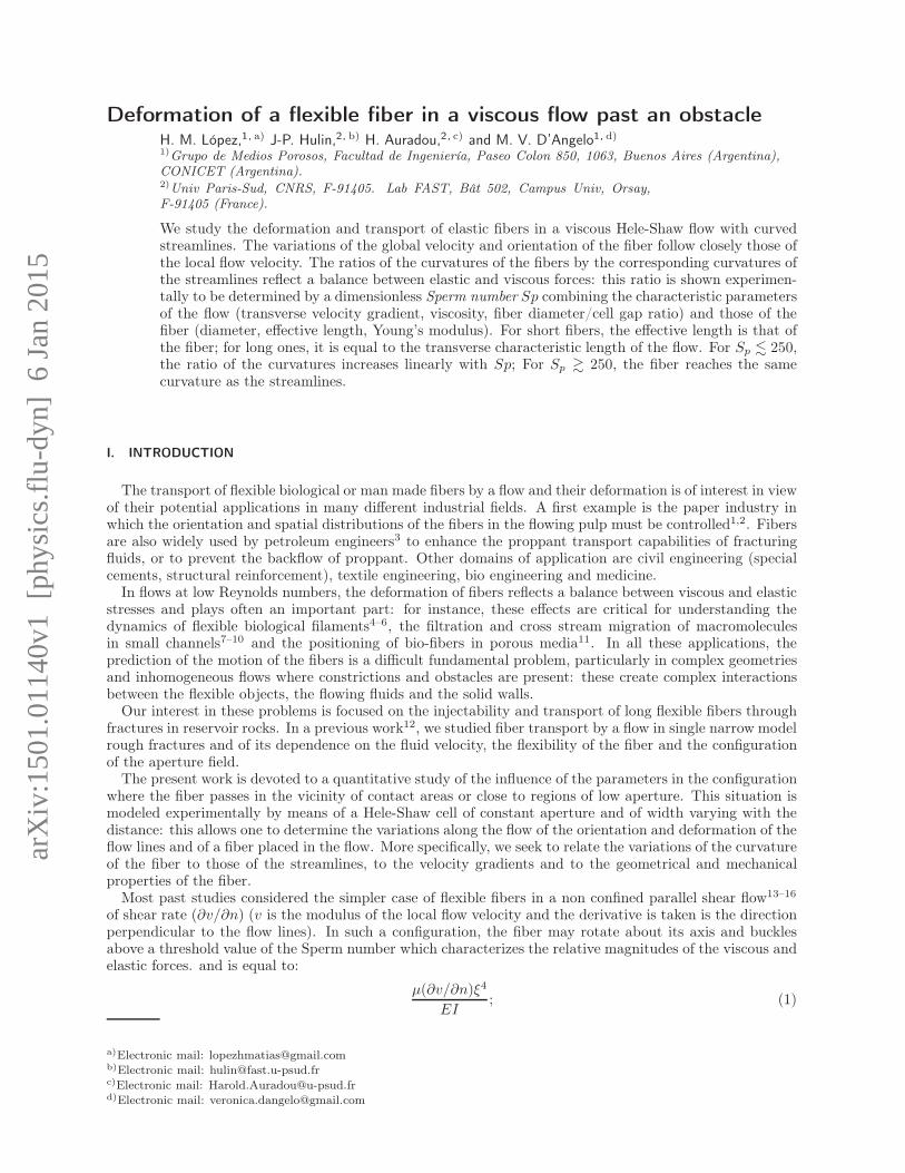
FIG. 6. Curvature κf (mm−1) of a fiber (D = 0.49mm, Lf = 30mm) as a function of the coordinate x of itsgeometrical center for an initial location yinlet = 13.5mm and for flow velocities: (©) U = 95 , (�) 168 and (⋄)230mm.s−1. Continuous line: curvature of the corresponding streamline at the same distance. Fluid viscosity:µ = 15mPa.s. κmax

s , κmins : maximum and minimum curvatures of the streamlines.

the locally negative value of the derivative ∂v/∂s shown in Fig. 3a and resulting in a compressional stresson the fiber just downstream of the step. Figs. 5 and 6 both show therefore that the absolute curvature ofthe fiber increases with the local curvature of the streamlines but depends also of the local flow.

We study now quantitatively the values of these extremal curvatures at different flow rates. Since the flowis laminar, the curvature of the fibers corresponds to a balance between elastic and viscous forces: the latterare induced by local velocity differences between different parts of the fiber and the fluid. These differencesare small compared to the characteristic flow velocity U since the global fiber velocity is close to that of thefluid: the corresponding Reynolds number is also small and the viscous stresses are proportional to thesevelocity contrasts. The relation of the latter to the spatial variations of the velocity and the deformationof the fiber and the streamlines is discussed in Sec. III D but, as a first step, µ∂v/∂n will be chosen as thereference viscous stress: ∂v/∂n is indeed strongly correlated to the variations of the curvature, as shown byFigs. 3 and 6.

1

0.5

0

0.150.10.050 .(∂v/∂n) [Pa]

f /

sκ

κ

µ

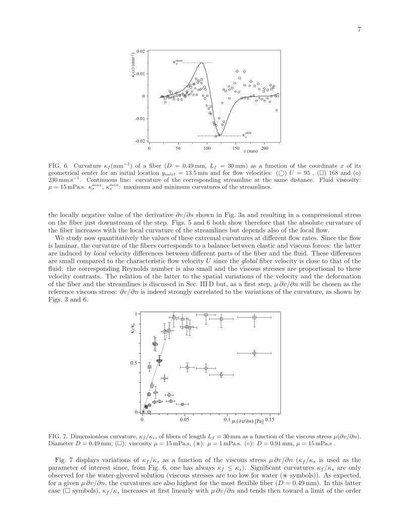
FIG. 7. Dimensionless curvature, κf/κs, of fibers of length Lf = 30mm as a function of the viscous stress µ(∂v/∂n).Diameter D = 0.49mm; (�): viscosity µ = 15mPa.s, (+×): µ = 1mPa.s. (◦): D = 0.91mm, µ = 15mPa.s .

Fig. 7 displays variations of κf/κs as a function of the viscous stress µ∂v/∂n (κf/κs is used as theparameter of interest since, from Fig. 6, one has always κf ≤ κs). Significant curvatures κf/κs are onlyobserved for the water-glycerol solution (viscous stresses are too low for water (+× symbols)). As expected,for a given µ∂v/∂n, the curvatures are also highest for the most flexible fiber (D = 0.49mm). In this lattercase (� symbols), κf/κs increases at first linearly with µ∂v/∂n and tends then toward a limit of the order

8

of 1 (the fiber coincides locally with the streamline). This limit is not reached for the less flexible fibers (◦symbols).

D. Characteristic dimensionless number

In order to collapse the data corresponding to different fibers onto a single master curve, it is necessaryto replace as the horizontal scale µ(∂v/∂n) by a combination including, in addition, the diameter and thelength of the cylinder and the stiffness of its material. As mentioned above, the degree of bending of thefiber reflects a balance between the viscous and elastic forces upon it. The value of the diameter influenceboth of them:

• The curvature κf of a fiber of length Lf submitted to a force q per unit length scales as qL2

f/(E I):

E I is the bending modulus with I = πD4/64. The force necessary to achieve a given curvature scalestherefore as D4.

• In the present case, q is a viscous stress associated to the local relative velocity q also depends on Dthrough the confinement ratio D/H : Increasing D/H results indeed in a stronger blockage of the flownormal to the fiber and, thus, enhances the normal viscous stress. This confinement effect is takeninto account by introducing a factor λ⊥

p (D/H) in the proportionality relation between the viscousstress and both the relative velocity of the fiber and the fluid and the viscosity of the latter. Theinfluence of D/H on the force on fixed circular cylinders in a similar flow geometry has been studiedin Refs. 26–28. For the ratios D/H = 0.22 and 0.41 corresponding to D = 0.49 and 0.91mm, thesestudies provide respective values λ⊥

p = 30 and 73.

As suggested in the previous section, the viscous forces are proportional to the local relative velocitiesof the different parts of the cylinders and the fluid in the regions where the streamlines are curved. Theserelative velocities may be estimated by multiplying ∂v/∂n by the local distance between the ends of thefiber (of curvature κf ) and a streamline of curvature κs: this distance is then of the order of (κs − κf )L

2

f so

that we take: q ∝ λ⊥p µ (κs − κf )L

2

f (∂v/∂n). The factor λ⊥p takes into account the confinement of the flow

Using this expression in the estimation of the curvature κf leads to:

κf

κs − κf

= CSp = Cλ⊥p µL4

f(∂v/∂n)

E I. (2)

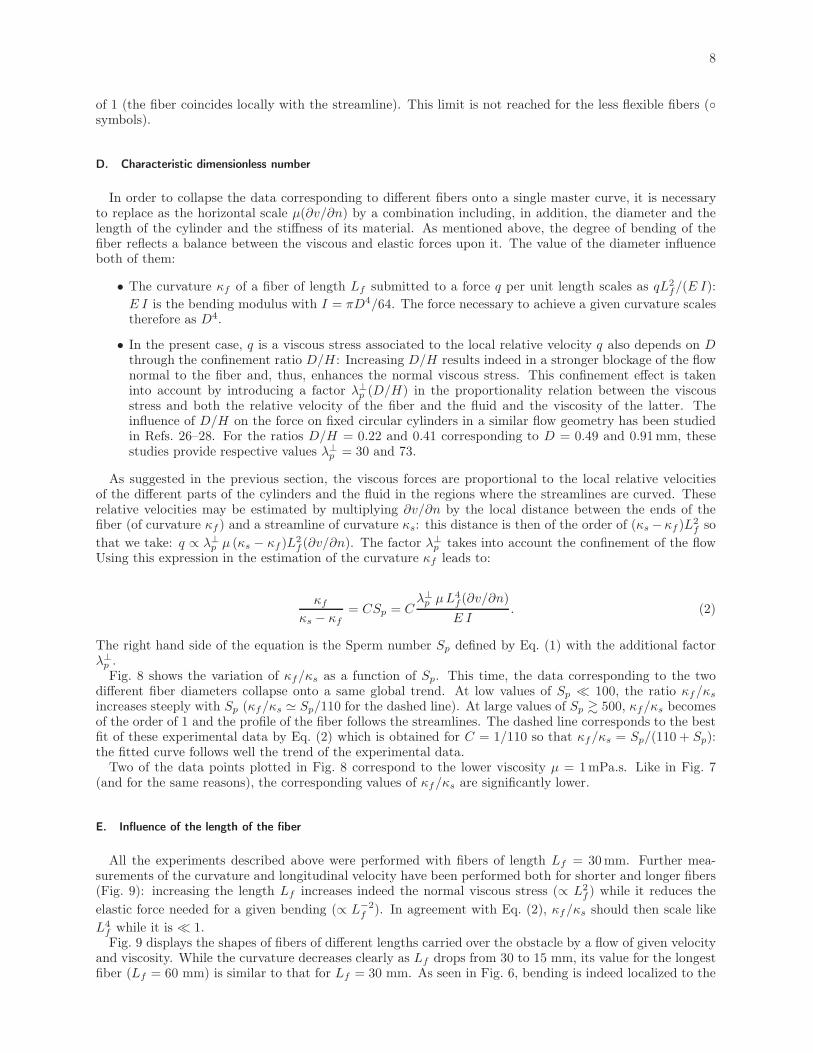
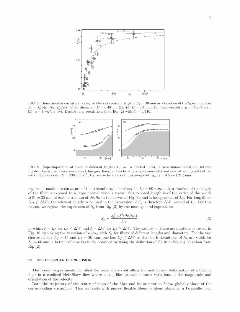
The right hand side of the equation is the Sperm number Sp defined by Eq. (1) with the additional factorλ⊥p .Fig. 8 shows the variation of κf/κs as a function of Sp. This time, the data corresponding to the two

different fiber diameters collapse onto a same global trend. At low values of Sp ≪ 100, the ratio κf/κs

increases steeply with Sp (κf/κs ≃ Sp/110 for the dashed line). At large values of Sp & 500, κf/κs becomesof the order of 1 and the profile of the fiber follows the streamlines. The dashed line corresponds to the bestfit of these experimental data by Eq. (2) which is obtained for C = 1/110 so that κf/κs = Sp/(110 + Sp):the fitted curve follows well the trend of the experimental data.

Two of the data points plotted in Fig. 8 correspond to the lower viscosity µ = 1mPa.s. Like in Fig. 7(and for the same reasons), the corresponding values of κf/κs are significantly lower.

E. Influence of the length of the fiber

All the experiments described above were performed with fibers of length Lf = 30mm. Further mea-surements of the curvature and longitudinal velocity have been performed both for shorter and longer fibers(Fig. 9): increasing the length Lf increases indeed the normal viscous stress (∝ L2

f ) while it reduces the

elastic force needed for a given bending (∝ L−2

f ). In agreement with Eq. (2), κf/κs should then scale like

L4

f while it is ≪ 1.Fig. 9 displays the shapes of fibers of different lengths carried over the obstacle by a flow of given velocity

and viscosity. While the curvature decreases clearly as Lf drops from 30 to 15 mm, its value for the longestfiber (Lf = 60 mm) is similar to that for Lf = 30 mm. As seen in Fig. 6, bending is indeed localized to the

9

1.0

0.5

0

10005000 Sp

f /

sκ

κ

FIG. 8. Dimensionless curvature, κf/κs of fibers of constant length: Lf = 30 mm as a function of the Sperm numberSp = λ⊥

p µ(∂v/∂n)L4

f/EI . Fiber diameter: D = 0.49mm (�, +×), D = 0.91mm (◦); fluid viscosity: µ = 15mPa.s (◦,�), µ = 1 mPa.s (+×). Dashed line: predictions from Eq. (2) with C = 1/110.

75 x [mm] x [mm]

y [m

m]

100

0

20

40

100 125 150

(a) (b)

y [m

m]

0

20

40

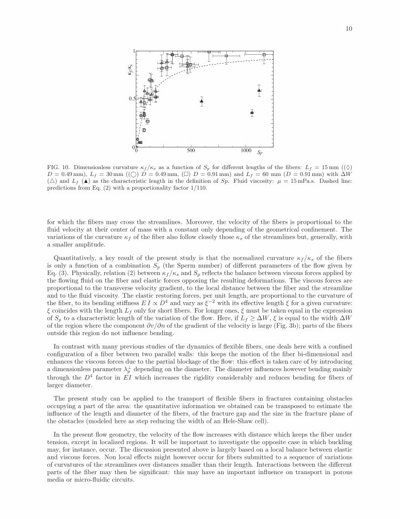
FIG. 9. Superimposition of fibers of different lengths Lf = 15 (dotted lines), 30 (continuous lines) and 60 mm(dashed lines) over two streamlines (thin grey lines) at two locations upstream (left) and downstream (right) of thestep. Fluid velocity: U = 230mm.s−1; transverse locations of injection point: yinlet = 4.5 and 21.5mm

regions of maximum curvature of the streamlines. Therefore, for Lf = 60 mm, only a fraction of the lengthof the fiber is exposed to a large normal viscous stress: this exposed length is of the order of the width∆W ≃ 30 mm of each extremum of ∂v/∂n in the curves of Fig. 3b and is independent of Lf . For long fibers(Lf & ∆W ), the relevant length to be used in the expression of Sp is therefore ∆W instead of Lf . For thisreason, we replace the expression of Sp from Eq. (2) by the more general expression:

Sp =λ⊥

p µ ξ4(∂v/∂n)

E I, (3)

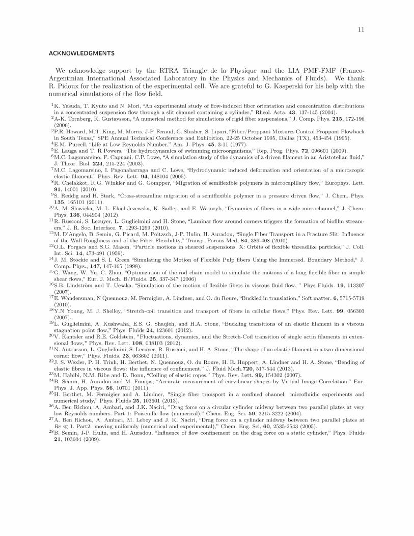
in which ξ = Lf for Lf ≤ ∆W and ξ = ∆W for Lf ≥ ∆W . The validity of these assumptions is tested inFig. 10 displaying the variation of κf/κs with Sp for fibers of different lengths and diameters. For the twoshortest fibers Lf = 15 and Lf = 30 mm, one has Lf ≤ ∆W so that both definitions of Sp are valid; forLf = 60mm, a better collapse is clearly obtained by using the definition of Sp from Eq. (3) (△) than fromEq. (2).

IV. DISCUSSION AND CONCLUSION

The present experiments identified the parameters controlling the motion and deformation of a flexiblefiber in a confined Hele-Shaw flow where a step-like obstacle induces variations of the magnitude andorientation of the velocity.

Both the trajectory of the center of mass of the fiber and its orientation follow globally those of thecorresponding streamline. This contrasts with pinned flexible fibers or fibers placed in a Poiseuille flow,

10

0 500 10000

0.5

1

Sp

f /

sκ

κ

FIG. 10. Dimensionless curvature κf/κs as a function of Sp for different lengths of the fibers: Lf = 15mm ((♦)D = 0.49mm), Lf = 30mm ((©) D = 0.49mm, (�) D = 0.91mm) and Lf = 60 mm (D = 0.91mm) with ∆W(△) and Lf (N) as the characteristic length in the definition of Sp. Fluid viscosity: µ = 15mPa.s. Dashed line:predictions from Eq. (2) with a proportionality factor 1/110.

for which the fibers may cross the streamlines. Moreover, the velocity of the fibers is proportional to thefluid velocity at their center of mass with a constant only depending of the geometrical confinement. Thevariations of the curvature κf of the fiber also follow closely those κs of the streamlines but, generally, witha smaller amplitude.

Quantitatively, a key result of the present study is that the normalized curvature κf/κs of the fibersis only a function of a combination Sp (the Sperm number) of different parameters of the flow given byEq. (3). Physically, relation (2) between κf/κs and Sp reflects the balance between viscous forces applied bythe flowing fluid on the fiber and elastic forces opposing the resulting deformations. The viscous forces areproportional to the transverse velocity gradient, to the local distance between the fiber and the streamlineand to the fluid viscosity. The elastic restoring forces, per unit length, are proportional to the curvature ofthe fiber, to its bending stiffness E I ∝ D4 and vary as ξ−2 with its effective length ξ for a given curvature:ξ coincides with the length Lf only for short fibers. For longer ones, ξ must be taken equal in the expressionof Sp to a characteristic length of the variation of the flow. Here, if Lf ≥ ∆W , ξ is equal to the width ∆Wof the region where the component ∂v/∂n of the gradient of the velocity is large (Fig. 3b); parts of the fibersoutside this region do not influence bending.

In contrast with many previous studies of the dynamics of flexible fibers, one deals here with a confinedconfiguration of a fiber between two parallel walls: this keeps the motion of the fiber bi-dimensional andenhances the viscous forces due to the partial blockage of the flow: this effect is taken care of by introducinga dimensionless parameter λ⊥

p depending on the diameter. The diameter influences however bending mainly

through the D4 factor in EI which increases the rigidity considerably and reduces bending for fibers oflarger diameter.

The present study can be applied to the transport of flexible fibers in fractures containing obstaclesoccupying a part of the area: the quantitative information we obtained can be transposed to estimate theinfluence of the length and diameter of the fibers, of the fracture gap and the size in the fracture plane ofthe obstacles (modeled here as step reducing the width of an Hele-Shaw cell).

In the present flow geometry, the velocity of the flow increases with distance which keeps the fiber undertension, except in localized regions. It will be important to investigate the opposite case in which bucklingmay, for instance, occur. The discussion presented above is largely based on a local balance between elasticand viscous forces. Non local effects might however occur for fibers submitted to a sequence of variationsof curvatures of the streamlines over distances smaller than their length. Interactions between the differentparts of the fiber may then be significant: this may have an important influence on transport in porousmedia or micro-fluidic circuits.

11

ACKNOWLEDGMENTS

We acknowledge support by the RTRA Triangle de la Physique and the LIA PMF-FMF (Franco-Argentinian International Associated Laboratory in the Physics and Mechanics of Fluids). We thankR. Pidoux for the realization of the experimental cell. We are grateful to G. Kasperski for his help with thenumerical simulations of the flow field.

1K. Yasuda, T. Kyuto and N. Mori, “An experimental study of flow-induced fiber orientation and concentration distributionsin a concentrated suspension flow through a slit channel containing a cylinder,” Rheol. Acta. 43, 137-145 (2004).

2A-K. Tornberg, K. Gustavsson, “A numerical method for simulations of rigid fiber suspensions,” J. Comp. Phys. 215, 172-196(2006).

3P.R. Howard, M.T. King, M. Morris, J-P. Feraud, G. Slusher, S. Lipari, “Fiber/Proppant Mixtures Control Proppant Flowbackin South Texas,” SPE Annual Technical Conference and Exhibition, 22-25 October 1995, Dallas (TX), 453-454 (1995).

4E.M. Purcell, “Life at Low Reynolds Number,” Am. J. Phys. 45, 3-11 (1977).5E. Lauga and T. R Powers, “The hydrodynamics of swimming microorganisms,” Rep. Prog. Phys. 72, 096601 (2009).6M.C. Lagomarsino, F. Capuani, C.P. Lowe, “A simulation study of the dynamics of a driven filament in an Aristotelian fluid,”J. Theor. Biol. 224, 215-224 (2003).

7M.C. Lagomarsino, I. Pagonabarraga and C. Lowe, “Hydrodynamic induced deformation and orientation of a microscopicelastic filament,” Phys. Rev. Lett. 94, 148104 (2005).

8R. Chelakkot, R.G. Winkler and G. Gompper, “Migration of semiflexible polymers in microcapillary flow,” Europhys. Lett.91, 14001 (2010).

9S. Reddig and H. Stark, “Cross-streamline migration of a semiflexible polymer in a pressure driven flow,” J. Chem. Phys.135, 165101 (2011).

10A. M. Slowicka, M. L. Ekiel-Jezewska, K. Sadlej, and E. Wajnryb, “Dynamics of fibers in a wide microchannel,” J. Chem.Phys. 136, 044904 (2012).

11R. Rusconi, S. Lecuyer, L. Guglielmini and H. Stone, “Laminar flow around corners triggers the formation of biofilm stream-ers,” J. R. Soc. Interface. 7, 1293-1299 (2010).

12M. D’Angelo, B. Semin, G. Picard, M. Poitzsch, J-P. Hulin, H. Auradou, “Single Fiber Transport in a Fracture Slit: Influenceof the Wall Roughness and of the Fiber Flexibility,” Transp. Porous Med. 84, 389-408 (2010).

13O.L. Forgacs and S.G. Mason, “Particle motions in sheared suspensions. X: Orbits of flexible threadlike particles,” J. Coll.Int. Sci. 14, 473-491 (1959).

14J. M. Stockie and S. I. Green “Simulating the Motion of Flexible Pulp fibers Using the Immersed. Boundary Method,“ J.Comp. Phys., 147, 147-165 (1998).

15G. Wang, W. Yu, C. Zhou, “Optimization of the rod chain model to simulate the motions of a long flexible fiber in simpleshear flows,” Eur. J. Mech. B/Fluids. 25, 337-347 (2006)

16S.B. Lindström and T. Uesaka, “Simulation of the motion of flexible fibers in viscous fluid flow, ” Phys Fluids. 19, 113307(2007).

17E. Wandersman, N Quennouz, M. Fermigier, A. Lindner, and O. du Roure, “Buckled in translation,” Soft matter. 6, 5715-5719(2010).

18Y.N Young, M. J. Shelley, “Stretch-coil transition and transport of fibers in cellular flows,” Phys. Rev. Lett. 99, 056303(2007).

19L. Guglielmini, A. Kushwaha, E.S. G. Shaqfeh, and H.A. Stone, “Buckling transitions of an elastic filament in a viscousstagnation point flow,” Phys. Fluids 24, 123601 (2012).

20V. Kantsler and R.E. Goldstein, "Fluctuations, dynamics, and the Stretch-Coil transition of single actin filaments in exten-sional flows," Phys. Rev. Lett. 108, 038103 (2012).

21N. Autrusson, L. Guglielmini, S. Lecuyer, R. Rusconi, and H. A. Stone, “The shape of an elastic filament in a two-dimensionalcorner flow,” Phys. Fluids. 23, 063602 (2011).

22J. S. Wexler, P. H. Trinh, H. Berthet, N. Quennouz, O. du Roure, H. E. Huppert, A. Lindner and H. A. Stone, “Bending ofelastic fibres in viscous flows: the influence of confinement,” J. Fluid Mech.720, 517-544 (2013).

23M. Habibi, N.M. Ribe and D. Bonn, “Coiling of elastic ropes,” Phys. Rev. Lett. 99, 154302 (2007).24B. Semin, H. Auradou and M. Frano̧is, “Accurate measurement of curvilinear shapes by Virtual Image Correlation,” Eur.

Phys. J. App. Phys. 56, 10701 (2011).25H. Berthet, M. Fermigier and A. Lindner, "Single fiber transport in a confined channel: microfluidic experiments and

numerical study,” Phys. Fluids 25, 103601 (2013).26A. Ben Richou, A. Ambari, and J.K. Naciri, "Drag force on a circular cylinder midway between two parallel plates at very

low Reynolds numbers. Part 1: Poiseuille flow (numerical),” Chem. Eng. Sci. 59, 3215-3222 (2004).27A. Ben Richou, A. Ambari, M. Lebey and J. K. Naciri, “Drag force on a cylinder midway between two parallel plates atRe ≪ 1. Part2: moving uniformly (numerical and experimental),” Chem. Eng. Sci, 60, 2535-2543 (2005).

28B. Semin, J-P. Hulin, and H. Auradou, “Influence of flow confinement on the drag force on a static cylinder,” Phys. Fluids21, 103604 (2009).