Deep NeuralNetworks and Datafor AutomatedDriving

Tim FingscheidtHanno GottschalkSebastian HoubenEditors

Robustness, Uncertainty Quantification, and Insights Towards Safety

Deep Neural Networks and Data for AutomatedDriving

Tim Fingscheidt · Hanno Gottschalk ·Sebastian HoubenEditors

Deep Neural Networksand Data for AutomatedDrivingRobustness, Uncertainty Quantification,and Insights Towards Safety

EditorsTim FingscheidtInstitute for Communications TechnologyTechnische Universität BraunschweigBraunschweig, Germany

Sebastian HoubenSchloss BirlinghovenFraunhofer Institute for Intelligent Analysisand Information Systems IAISSankt Augustin, Germany

Hanno GottschalkFachgruppe Mathematik und InformatikBergische Universität WuppertalWuppertal, Germany

ISBN 978-3-031-01232-7 ISBN 978-3-031-01233-4 (eBook)https://doi.org/10.1007/978-3-031-01233-4

© The Editor(s) (if applicable) and The Author(s) 2022. This book is an open access publication.Open Access This book is licensed under the terms of the Creative Commons Attribution 4.0 InternationalLicense (http://creativecommons.org/licenses/by/4.0/), which permits use, sharing, adaptation, distribu-tion and reproduction in any medium or format, as long as you give appropriate credit to the originalauthor(s) and the source, provide a link to the Creative Commons license and indicate if changes weremade.The images or other third party material in this book are included in the book’s Creative Commons license,unless indicated otherwise in a credit line to the material. If material is not included in the book’s CreativeCommons license and your intended use is not permitted by statutory regulation or exceeds the permitteduse, you will need to obtain permission directly from the copyright holder.The use of general descriptive names, registered names, trademarks, service marks, etc. in this publicationdoes not imply, even in the absence of a specific statement, that such names are exempt from the relevantprotective laws and regulations and therefore free for general use.The publisher, the authors and the editors are safe to assume that the advice and information in this bookare believed to be true and accurate at the date of publication. Neither the publisher nor the authors orthe editors give a warranty, expressed or implied, with respect to the material contained herein or for anyerrors or omissions that may have been made. The publisher remains neutral with regard to jurisdictionalclaims in published maps and institutional affiliations.

Front page picture kindly provided by Jan-Aike Termöhlen and Andreas Bär, © Jan-Aike Termöhlen andAndreas Bär

This Springer imprint is published by the registered company Springer Nature Switzerland AGThe registered company address is: Gewerbestrasse 11, 6330 Cham, Switzerland

Foreword

I am thankful to the editors for sending me a prerelease copy of their book and fortheir kind invitation to write a foreword. I have greatly benefitted by reading thebook and learning fresh ideas shared by distinguished experts from academia as wellas professionals with serious engagement in the development of new generations ofautomobiles and driver assistance systems.

I have been fortunate to enjoy a long academic career pursuing a research agendainvolving a number of topics discussed in the book. These include computer vision,intelligent vehicles and systems, machine learning, and human–robot interactions.For the past two decades, my team and collaborators have focused our explorationson developing human-centered, safe intelligent vehicles and transportation systems.Therefore, I am especially pleased to read this book presenting latest developments,findings, and insights in automated driving with towards safety as a highlighted termin the title and as a thread binding various chapters in the book. Emphasis on safetyas an essential requirement was not always the case in the past. Reports of seriousaccidents involving automobiles with inadequate capabilities for automated drivingare making safety an uncompromising requirement.

However, progress in the field does not occur at a consistent, predictable manneror rate. In the early phase, spanning around 1980–2000, autonomous vehicle researchactivities were mostly limited to a handful of universities and industrial labs. Impor-tant insights and milestones realized during this phase were novel perception andcontrol systems for lane detection, cruise control, and carefully designed demon-strations of “autonomous” highway driving. However, interest and sponsorship ofresearch in the field diminished and real-world deployment was unrealized.

In the next phase of autonomous vehicles research, spanning about mid-2000to 2015, key enabling technologies, such as Global Positioning Systems and cost-effective mass production of sensors (radars, cameras) and embedded processors,not only invigorated serious activities in academic and technical communities, butalso sparked interest and commitments by venture and commercial sectors.

It seemed that this time, our field was on an irreversible forward trajectory. Impor-tant insights and milestones realized during this phase include the introduction ofactive safety systems like dynamic stability control, and practical driver assistance

v

vi Foreword

systems, such as lane keep assistance, collision avoidance, pedestrian protection,panoramic viewing, and other camera-based enhancements. We also started to takenote of the great strides made in the machine learning and computer vision fields.Some of the major limitations encountered in the autonomous vehicles field, suchas “brittle” object detectors trained using traditional, hand-crafted features, seemedresolvable with new developments in machine learning and computer vision.

Topics covered in this book are from the latest phase (from 2015 onwards) ofautonomous vehicle research activities. Authors clearly acknowledge the impor-tant and essential roles of deep neural networks (DNN) and data-driven intelligentsystems in making new contributions. They also recognize that there are unresolvedchallenges laying ahead. More focused research of both analytical and experimentalnature is required. As a long-term proponent of safe, human-centered intelligentvehicles, I appreciate that the book places prominent emphasis on safety, integratedsystems, robustness, performance evaluation, experimentalmetrics, benchmarks, andprotocols. This makes the book very unique and an essential reading for students andscholars from multiple disciplines including engineering, computer/data/cognitivesciences, artificial intelligence, machine learning, and human/machine systems.

This is a very important book, as it deals with a topic surroundedwith great excite-ment, not only in the technical communities, but also in the minds of people at large.With great excitement and wide popular interest in the autonomous driving field,often there is a temptation to overlook or ignore unresolved technical challenges.Given grave consequences of failures of complex systems deployed in the real worldinhabited by humans, designers, engineers, and promoters of autonomous drivingsystems, we need to be most careful and attentive to the topics presented in the book.The editors and authors have done an outstanding job in presenting important themesand carefully selected topics in a systematic, insightful manner. The book identifiespromising avenues for focused research and development, as well as acknowledgesoutstanding challenges yet to be resolved.

I congratulate Prof. Tim Fingscheidt, Prof. Hanno Gottschalk, and Prof. SebastianHouben, for their vision and efforts in organizing an outstanding team of authorswith deep academic and industrial backgrounds in developing this special book. Iam confident that it will prove to be of great value in realizing a new generation ofsafer, smoother, trustworthy automobiles.

La Jolla, CA, USA Mohan M. Trivedi

Mohan M. Trivedi Distinguished Professor of Engineering University of California, San Diego,founding director of the Computer Vision and Robotics Research (CVRR) and the Laboratory forIntelligent and Safe Automobiles (LISA). Fellow IEEE, SPIE, and IAPR.

Preface

This book addresses readers from both academia and industry, since it is written byauthors from both academia and industry. Accordingly, it takes on diverse viewingangles, but keeps a clear focus on machine-learned environment perception inautonomous vehicles. Special interest is on deep neural networks themselves, theirrobustness and uncertainty awareness, the data they are trained on, and, last but notleast, on safety aspects.

The book is also special in its structure. While a first part is an extensive surveyof literature in the field, the second part consists of 14 chapters, each detailing aparticular aspect in the area of interest. This book wouldn’t exist without the large-scale national flagship project KI Absicherung (safe AI for automated driving),with academia, car manufacturers, and suppliers being involved to work towardsrobustness and safety arguments in machine-learned environment perception forautonomous vehicles. I came up with the idea of a book project when I saw a firstdraft of a wonderful survey that was prepared by Sebastian Houben in collaborationwith many partners from the project. My immediate thought was that this shouldnot only be some project deliverable, it should become the core of a book (namely,Part I), appended with a number of novel contributions on specific topics in the field(namely, Part II). Beyond Sebastian Houben, I am happy that Hanno Gottschalkagreed to join the editorial team with his expertise in uncertainty and safety aspects.We thankKIAbsicherung project leader (PL) StephanScholz (Volkswagen),MichaelMock (Scientific PL, Fraunhofer IAIS), and Fabian Hüger (Part PL, Volkswagen)very much, since without their immediate and ongoing support this book projectwouldn’t have come alive. We also thank the many reviewers for the time and energythey put into providing valuable feedback on the initial versions of the book chapters.

But the book reaches beyond the project. There are several contributions fromoutside the project enriching the diversity of views. Aiming at increasing impact, weeditors decided tomake the book an open-access publication. The funds for the open-access publication have been covered by the German Federal Ministry for EconomicAffairs andEnergy (BMWi) in the framework of the “SafeAI forAutomatedDriving”research consortium. Beyond that we are very grateful for the financial support bothfrom Bergische Universität Wuppertal and Technische Universität Braunschweig.

vii

viii Preface

A very special thanks goes to Andreas Bär, TU Braunschweig, for his endlessefforts in running the editorial office, for any extra proofreading, formatting, and forkeeping close contact to all the authors.

Tim Fingscheidt, in the name of the editorial team, jointly with Hanno Gottschalkand Sebastian Houben

Braunschweig, GermanyWuppertal, GermanySankt Augustin, GermanyNovember 2021

Tim FingscheidtHanno GottschalkSebastian Houben

About This Book

An autonomous vehicle must be able to perceive its environment and reactadequately to it. In highly automated vehicles, camera-based perception is increas-ingly performed by artificial intelligence (AI). One of the greatest challenges inintegrating these technologies in highly automated vehicles is to ensure the func-tional safety of the system. Existing and established safety processes cannot simplybe transferred to machine learning methods.

In the nationally funded project KI Absicherung, which is funded by the GermanFederal Ministry for Economic Affairs and Energy (BMWi), 24 partners fromindustry, academia, and research institutions collaborate to set up a stringent safetyargumentation, with which AI-based function modules (AI modules) can be securedand validated for highly automated driving. The project brings together expertsfrom the fields of artificial intelligence and machine learning, functional safety, andsynthetic sensor data generation.

The topics and focus of this book have a large overlap with the field of researchbeing tackled in subproject three of the KI Absicherung project, in which methodsand measures are developed to identify and reduce inherent insufficiencies of the AImodules. We consider such methods and measures to be key elements in supportingthe general safeguarding AI modules in a car.

We gratefully thank the editors of this book as well as Springer Verlag for makingthis research accessible to a broad audience and wish the reader interesting insightsand new research ideas.

Stephan Scholz, Michael Mock, and Fabian Hüger

ix

Introduction

Environment perception for driver assistance systems, highly automated driving, andautonomous driving has seen the same disruptive technology paradigm shift as manyother disciplines: machine learning approaches and along with them deep neuralnetworks (DNNs) have taken over and oftentimes replaced classical algorithms fromsignal processing, tracking, and control theory.

Along with this, many questions arise. Of fundamental interest is the question,how safe an artificial intelligence (AI) system actually is. Part I of this book providesan extensive literature survey introducing various relevant aspects to the reader. Itnot only provides guidance on how to inspect and understand deep neural networks,but also on how to overcome robustness issues or safety problems. Part I will alsoprovide motivations and links to Part II of the book, which features novel approachesin various aspects of deep neural networks in the context of environment perception,such as their robustness and uncertainty awareness, the data they are trained on, and,last but not least, again, it will be about safety.

It all starts from choosing the right data from the right set of sensors, and, veryimportant, the right amount of training data. Chapter “Does Redundancy in AIPerception Systems Help to Test for Super-Human Automated Driving Perfor-mance?” (p. 81) will provide insights into the problem of obtaining statisticallysufficient test data and will discuss this under the assumption of redundant and inde-pendent (sensor) systems. The reader will learn about the curse of correlation inerror occurrences of redundant sub-systems. A second aspect of dataset optimiza-tion is covered in Chapter “Analysis and Comparison of Datasets by LeveragingData Distributions in Latent Spaces” (p. 107). Investigating variational autoencoderlatent space data distributions, it will present a new technique to assess the dissimi-larity of the domains of different datasets. Knowledge about this will help in mixingdiverse datasets in DNN training, an important aspect to keep both training efficiencyand generalization at a high level. When training or inferring on real data, outlierdetection is important and potentially also to learn so far unknown objects. Chapter“Detecting and Learning the Unknown in Semantic Segmentation” (p. 277) presentsa method to detect anomalous objects by statistically analyzing entropy responses insemantic segmentation to suggest new semantic categories. Such method can also be

xi

xii Introduction

used to pre-select diverse datasets for training. Chapter “Optimized Data Synthesisfor DNN Training and Validation by Sensor Artifact Simulation” (p. 127) followsthe path of training with synthetic data, which has high potential, simply becauserich ground truth is available for supervised learning even on sequence data. Theauthors are concerned with intelligent strategies of augmentation and use an appro-priate metric to better match synthetic and real data, thereby increasing performanceof synthetically trained networks.

A second focus area of this book is robustness. Robustness comprises the abilityof a DNN to keep high performance also under adverse conditions such as varyingweather and light conditions, dirt on the sensors, any kind of domain shift, or evenunder adversarial attacks. In Chapter “Improved DNN Robustness by Multi-taskTraining with an Auxiliary Self-Supervised Task” (p. 149), it is shown how intel-ligent multi-task training can be employed to strengthen a semantic segmentationDNN against various noise types and against adversarial attacks. An important aspectis that the supporting task of depth estimation does not require extra ground truthlabels. Among the adversarial attacks, the universal ones are particularly dangerousas they can be applied to any current sensor input. Chapter “Improving Transfer-ability of Generated Universal Adversarial Perturbations for Image Classificationand Segmentation” (p. 171) addresses a way to generate these dangerous attacks bothfor semantic segmentation and for classification tasks, and should not be missed inany test suite for environment perception functions. Obtaining compact and efficientnetworks by compression techniques typically comes along with a degradation inperformance. Not so in Chapter “Joint Optimization for DNN Model Compressionand Corruption Robustness” (p. 405): The authors present a joint pruning and quan-tization framework which yields more robust networks against various corruptions.Mixture-of expert architectures for DNN aggregation can be a suitable means forimproved robustness but also interpretability. Chapter “Evaluating Mixture-of-Ex-perts Architectures for Network Aggregation” (p. 315) also shows that the modelsdeal favorably with out-of-distribution (OoD) objects.

Uncertainty and interpretability are third focus areas of the book. Both conceptsare fundamental towards self-awareness of environment perception for autonomousdriving. In Chapter “Invertible Neural Networks for Understanding Semanticsof Invariances of CNN Representations” (p. 197), invertible neural networks aredeployed to recover invariant representations present in a trained network. Theyallow for a mapping to semantic concepts and thereby interpretation (and manipu-lation) of inner model representations. Confidence calibration, on the other hand, isan important means to obtain reliable confidences for further processing. Chapter“Confidence Calibration for Object Detection and Segmentation” (p. 225) proposesa multivariate calibration approach not only suitable for classification but also forsemantic segmentation and object detection. Also aiming at improved object detec-tion calibration, the authors of Chapter “UncertaintyQuantification forObject Detec-tion: Output- and Gradient-Based Approaches” (p. 251) show that output-based andlearning-gradient-based uncertainty metrics are uncorrelated. This allows advanta-geous combination of both paradigms leading to better overall detection accuracyand to better detection uncertainty estimates.

Introduction xiii

Part II started with safety aspects related to datasets (Chapter “Does Redundancyin AI Perception Systems Help to Test for Super-Human Automated Driving Perfor-mance?”, p. 81). In this fourth focus area, further safety-related aspects are takenup, including validation of networks. To validate environment perception functions,Chapter “AVariational Deep Synthesis Approach for Perception Validation” (p. 359)introduces a novel data generation framework for DNN validation purposes. Theframework allows for effectively defining and testing common traffic scenes. Theauthors of Chapter “The Good and the Bad: Using Neuron Coverage as a DNN Vali-dation Technique” (p. 383) present a useful metric to assess the training regimenand final quality of a DNN. Different forms of neuron coverage are discussedalong with their roots in traditional verification and validation (V&V) methods.Finally, in Chapter “Safety Assurance of Machine Learning for Perception Func-tions” (p. 335), an assurance case is constructed and acceptance criteria for DNNmodels are proposed. Various use cases are covered.

Tim FingscheidtHanno GottschalkSebastian Houben

Contents

Part I Safe AI—An Overview

Inspect, Understand, Overcome: A Survey of Practical Methodsfor AI Safety . . . . . . . . . . . . . . . . . . . . . . . . . . . . . . . . . . . . . . . . . . . . . . . . . . . . . . 3Sebastian Houben, Stephanie Abrecht, Maram Akila,Andreas Bär, Felix Brockherde, Patrick Feifel, Tim Fingscheidt,Sujan Sai Gannamaneni, Seyed Eghbal Ghobadi, Ahmed Hammam,Anselm Haselhoff, Felix Hauser, Christian Heinzemann,Marco Hoffmann, Nikhil Kapoor, Falk Kappel, Marvin Klingner,Jan Kronenberger, Fabian Küppers, Jonas Löhdefink,Michael Mlynarski, Michael Mock, Firas Mualla,Svetlana Pavlitskaya, Maximilian Poretschkin, Alexander Pohl,Varun Ravi-Kumar, Julia Rosenzweig, Matthias Rottmann,Stefan Rüping, Timo Sämann, Jan David Schneider, Elena Schulz,Gesina Schwalbe, Joachim Sicking, Toshika Srivastava,Serin Varghese, Michael Weber, Sebastian Wirkert, Tim Wirtz,and Matthias Woehrle

Part II Recent Advances in Safe AI for Automated Driving

Does Redundancy in AI Perception Systems Help to Testfor Super-Human Automated Driving Performance? . . . . . . . . . . . . . . . . . 81Hanno Gottschalk, Matthias Rottmann, and Maida Saltagic

Analysis and Comparison of Datasets by Leveraging DataDistributions in Latent Spaces . . . . . . . . . . . . . . . . . . . . . . . . . . . . . . . . . . . . . . 107Hanno Stage, Lennart Ries, Jacob Langner, Stefan Otten, and Eric Sax

Optimized Data Synthesis for DNN Training and Validationby Sensor Artifact Simulation . . . . . . . . . . . . . . . . . . . . . . . . . . . . . . . . . . . . . . 127Korbinian Hagn and Oliver Grau

xv

xvi Contents

Improved DNN Robustness by Multi-task Trainingwith an Auxiliary Self-Supervised Task . . . . . . . . . . . . . . . . . . . . . . . . . . . . . . 149Marvin Klingner and Tim Fingscheidt

Improving Transferability of Generated Universal AdversarialPerturbations for Image Classification and Segmentation . . . . . . . . . . . . . 171Atiye Sadat Hashemi, Andreas Bär, Saeed Mozaffari,and Tim Fingscheidt

Invertible Neural Networks for Understanding Semanticsof Invariances of CNN Representations . . . . . . . . . . . . . . . . . . . . . . . . . . . . . . 197Robin Rombach, Patrick Esser, Andreas Blattmann, and Björn Ommer

Confidence Calibration for Object Detection and Segmentation . . . . . . . . 225Fabian Küppers, Anselm Haselhoff, Jan Kronenberger,and Jonas Schneider

Uncertainty Quantification for Object Detection: Output-and Gradient-Based Approaches . . . . . . . . . . . . . . . . . . . . . . . . . . . . . . . . . . . . 251Tobias Riedlinger, Marius Schubert, Karsten Kahl,and Matthias Rottmann

Detecting and Learning the Unknown in Semantic Segmentation . . . . . . . 277Robin Chan, Svenja Uhlemeyer, Matthias Rottmann,and Hanno Gottschalk

Evaluating Mixture-of-Experts Architectures for NetworkAggregation . . . . . . . . . . . . . . . . . . . . . . . . . . . . . . . . . . . . . . . . . . . . . . . . . . . . . . 315Svetlana Pavlitskaya, Christian Hubschneider, and Michael Weber

Safety Assurance of Machine Learning for Perception Functions . . . . . . . 335Simon Burton, Christian Hellert, Fabian Hüger, Michael Mock,and Andreas Rohatschek

A Variational Deep Synthesis Approach for Perception Validation . . . . . 359Oliver Grau, Korbinian Hagn, and Qutub Syed Sha

The Good and the Bad: Using Neuron Coverage as a DNNValidation Technique . . . . . . . . . . . . . . . . . . . . . . . . . . . . . . . . . . . . . . . . . . . . . . 383Sujan Sai Gannamaneni, Maram Akila, Christian Heinzemann,and Matthias Woehrle

Joint Optimization for DNN Model Compression and CorruptionRobustness . . . . . . . . . . . . . . . . . . . . . . . . . . . . . . . . . . . . . . . . . . . . . . . . . . . . . . . 405Serin Varghese, Christoph Hümmer, Andreas Bär, Fabian Hüger,and Tim Fingscheidt

About the Editors

Tim Fingscheidt Chair of Signal Processing and Machine Learning, Institute forCommunicationsTechnology,TechnischeUniversitätBraunschweig,Braunschweig,Germany

Tim Fingscheidt received the Dipl.-Ing. degree in Electrical Engineering in 1993and the Ph.D. degree in 1998 from RWTH Aachen University, Germany, both withdistinction. He joined AT&T Labs, Florham Park, NJ, USA, for a Postdoc in 1998,and Siemens AG, Information and Communication, Munich, Germany, in 1999,heading a team in digital signal processing. After a stay with Siemens CorporateTechnology, Munich, Germany, from 2005 to 2006, he became Full Professor withthe Institute for Communications Technology, Technische Universität (TU) Braun-schweig, Germany, holding the Chair of “Signal Processing andMachine Learning”.His research interests are machine learning methods for robust environment percep-tion, information fusion, signal enhancement, and coding, with applications bothin speech technology and computer vision. He is founder of the TU BraunschweigDeep Learning Lab (TUBS.dll), a graduate student research think tank. Many of hisprojects have beendealingwith automotive applications, such as autonomous driving.In recent years, he has been actively involved in the large-scale national researchprojectsAIValidation,AIDelta Learning, andAIDataTooling, contributing researchin robust semantic segmentation, monocular depth estimation, domain adaptation,corner case detection, and learned image coding. He received numerous national andinternational awards for his publications, among these three CVPR Workshop BestPaper Awards in 2019, 2020, and 2021.

Hanno Gottschalk Professor for Stochastics at the University of Wuppertal,Germany

HannoGottschalk received diploma degrees of Physics andMathematics from theRuhr University of Bochum in 1995 and 1997, respectively. There he also receivedhis Ph.D. in Mathematical Physics under the supervision of Sergio Albeverio in1999. As a fellow of the German Academic Exchange Service (DAAD) he there-after spent a Postdoc year at Università “La Sapienza” in Rome. Returning to theUniversity of Bonn, he led a research project funded by the research council (DFG)

xvii

xviii About the Editors

in 2000–2003, before completing his habilitation in 2003. Acquiring a C2 lecturerposition at the University of Bonn in 2007, he left academia for a 3-year experiencewith Siemens Energy, where he held the position of a core competency owner inprobabilistic design in the field of gas turbine engineering. Returning to academiain 2011, since then he holds a position as a Professor of Stochastics at the Univer-sity of Wuppertal. In 2016, he became spokesperson of the Institute of MathematicalModeling,Analysis andComputationalMathematics (IMACM). In 2018, he foundedthe Interdisciplinary Center of Machine Learning and Data Analytics (IZMD) at theUniversity of Wuppertal as the spokesperson jointly with Anton Kummert and in2020 he became the elected spokesperson of the institute. In the field of computervision, his research is centered around the online detection and reduction of the errorsof artificial intelligence.

Sebastian Houben Senior Data Scientist, Project Lead KI Absicherung, Fraun-hofer Institute for Intelligent Analysis and Information Systems (IAIS), St. Augustin,Germany

Sebastian Houben studied Mathematics and Computer Science in Aachen andHagen working as a scientific staff member at the Institute for Bio and Nanosys-tems at the Helmholtz Center in Jülich, Germany. He received his Ph.D. degree in2015 from the Ruhr University of Bochum, Germany, after which he joined theAutonomous Intelligent Systems Group at the University of Bonn as a PostdoctoralResearcher and was appointed Junior Professor at the University of Bochum in 2017.In early 2020, he took over the project lead KI Absicherung within the FraunhoferInstitute for Intelligent Analysis and Information Systems. He has a strong researchinterest in environment perception for autonomous robots, in particular, in automatedvehicles, and the ramifications from today’s state-of-the-art data-driven approaches.During his Ph.D. studies he has been involved in multiple pre-development projectsfor omnidirectional cameras deployed in advanced driver assistance systems. Heparticipated in several flight robotics challenges, such as the European RoboticsChallenge and theMohamed Bin Zayed International Robotics Challenge, which he,as part of the University Bonn team NimbRo, won in 2017. As of October 2021, hehas been appointed Full Professor with specialization in Autonomous Systems andMachine Learning at the University of Applied Sciences Bonn-Rhein-Sieg.

Safe AI—An Overview

Inspect, Understand, Overcome: ASurvey of Practical Methods for AI Safety

Sebastian Houben, Stephanie Abrecht, Maram Akila, Andreas Bär,Felix Brockherde, Patrick Feifel, Tim Fingscheidt, Sujan Sai Gannamaneni,Seyed Eghbal Ghobadi, Ahmed Hammam, Anselm Haselhoff, Felix Hauser,Christian Heinzemann, Marco Hoffmann, Nikhil Kapoor, Falk Kappel,Marvin Klingner, Jan Kronenberger, Fabian Küppers, Jonas Löhdefink,Michael Mlynarski, Michael Mock, Firas Mualla, Svetlana Pavlitskaya,Maximilian Poretschkin, Alexander Pohl, Varun Ravi-Kumar,Julia Rosenzweig, Matthias Rottmann, Stefan Rüping, Timo Sämann,Jan David Schneider, Elena Schulz, Gesina Schwalbe, Joachim Sicking,Toshika Srivastava, Serin Varghese, Michael Weber, Sebastian Wirkert,Tim Wirtz, and Matthias Woehrle

S. Houben (B) · M. Akila · S. S. Gannamaneni · M. Mock · M. Poretschkin · J. Rosenzweig ·S. Rüping · E. Schulz · J. Sicking · T. WirtzFraunhofer Institute for Intelligent Analysis and Information Systems IAIS, Sankt Augustin,Germanye-mail: sebastian.houben@h-brs.de

M. Akilae-mail: maram.akila@iais.fraunhofer.de

S. S. Gannamanenie-mail: sujan.sai.gannamaneni@iais.fraunhofer.de

M. Mocke-mail: michael.mock@iais.fraunhofer.de

M. Poretschkine-mail: maximilian.poretschkin@iais.fraunhofer.de

J. Rosenzweige-mail: julia.rosenzweig@iais.fraunhofer.de

S. Rüpinge-mail: stefan.rueping@iais.fraunhofer.de

E. Schulze-mail: elena.schulz@iais.fraunhofer.de

J. Sickinge-mail: joachim.sicking@iais.fraunhofer.de

T. Wirtze-mail: tim.wirtz@iais.fraunhofer.de

S. Abrecht · C. Heinzemann · M. WoehrleRobert Bosch GmbH, Gerlingen, Germanye-mail: stephanie.abrecht@de.bosch.com

© The Author(s) 2022T. Fingscheidt et al. (eds.), Deep Neural Networks and Data for Automated Driving,https://doi.org/10.1007/978-3-031-01233-4_1

3

4 S. Houben et al.

Abstract Deployment ofmodern data-drivenmachine learningmethods,most oftenrealized by deep neural networks (DNNs), in safety-critical applications such ashealth care, industrial plant control, or autonomous driving is highly challengingdue to numerous model-inherent shortcomings. These shortcomings are diverse andrange from a lack of generalization over insufficient interpretability and implausiblepredictions to directed attacks bymeans of malicious inputs. Cyber-physical systemsemploying DNNs are therefore likely to suffer from so-called safety concerns, prop-erties that preclude their deployment as no argument or experimental setup can helpto assess the remaining risk. In recent years, an abundance of state-of-the-art tech-niques aiming to address these safety concerns has emerged. This chapter provides astructured and broad overview of them.We first identify categories of insufficienciesto then describe research activities aiming at their detection, quantification, or miti-gation. Our work addresses machine learning experts and safety engineers alike: Theformer ones might profit from the broad range of machine learning topics coveredand discussions on limitations of recent methods. The latter ones might gain insightsinto the specifics of modern machine learning methods. We hope that this contribu-tion fuels discussions on desiderata for machine learning systems and strategies onhow to help to advance existing approaches accordingly.

C. Heinzemanne-mail: christian.heinzemann@de.bosch.com

M. Woehrlee-mail: matthias.woehrle@de.bosch.com

G. SchwalbeContinental AG, Hanover, Germanye-mail: gesina.schwalbe@continental.com

V. Ravi-Kumar · T. SämannValeo S.A., Paris, Francee-mail: varun-ravi.kumar@valeo.com

T. Sämanne-mail: timo.saemann@valeo.com

M. RottmannInterdisciplinary Center for Machine Learning and Data Analytics, University of Wuppertal,Wuppertal, Germanye-mail: rottmann@uni-wuppertal.de

S. WirkertBayerische Motorenwerke AG, Munich, Germanye-mail: sebastian.wa.wirkert@bmwgroup.com

N. Kapoor · J. D. Schneider · S. VargheseVolkswagen AG, Wolfsburg, Germanye-mail: nikhil.kapoor@volkswagen.de

J. D. Schneidere-mail: jan.david.schneider@volkswagen.de

S. Varghesee-mail: john.serin.varghese@volkswagen.de

Inspect, Understand, Overcome: A Survey of Practical Methods for AI Safety 5

1 Introduction

In barely a decade, deep neural networks (DNNs) have revolutionized the field ofmachine learning by reaching unprecedented, sometimes superhuman, performanceson a growing variety of tasks. Many of these neural models have found their way intoconsumer applications like smart speakers, machine translation engines, or contentfeeds. However, in safety-critical systems, where human life might be at risk, theuse of recent DNNs is challenging as various model-immanent insufficiencies areyet difficult to address.

This work summarizes the promising lines of research in how to identify, address,and at least partly mitigate these DNN insufficiencies. While some of the reviewedworks are theoretically grounded and foster the overall understanding of trainingand predictive power of DNNs, others provide practical tools to adapt their devel-opment, training, or predictions. We refer to any such method as a safety mech-anism if it addresses one or several safety concerns in a feasible manner. Theireffectiveness in mitigating safety concerns is assessed by safety metrics [CNH+18,OOAG19, BGS+19, SS20a]. As most safety mechanisms target only a particular

P. Feifel · S. E. Ghobadi · A. HammamOpel Automobile GmbH, Rüsselsheim, Germanye-mail: patrick.feifel@opel-vauxhall.com

S. E. Ghobadie-mail: seyed.eghbal.ghobadi@opel-vauxhall.com

A. Hammame-mail: ahmedmostafa.hammam@opel-vauxhall.com

A. Haselhoff · J. Kronenberger · F. KüppersInstitute of Computer Science, Hochschule Ruhr West, Mülheim, Germanye-mail: anselm.haselhoff@hs-ruhrwest.de

J. Kronenbergere-mail: jan.kronenberger@hs-ruhrwest.de

F. Küpperse-mail: fabian.kueppers@hs-ruhrwest.de

F. Brockherdeumlaut AG, Aachen, Germanye-mail: felix.brockherde@umlaut.com

F. HauserKarlsruhe Institute of Technology, Karlsruhe, Germanye-mail: felix.hauser@kit.edu

T. SrivastavaAudi AG, Ingolstadt, Germanye-mail: toshika.srivastava@audi.de

F. Kappel · F. MuallaZF Friedrichshafen AG, Friedrichshafen, Germanye-mail: falk.kappel@zf.com

6 S. Houben et al.

insufficiency, we conclude that a holistic safety argumentation [BGS+19, SSH20,SS20a, WSRA20] for complex DNN-based systems will in many cases rely on avariety of safety mechanisms.

We structure our reviewof thesemechanisms as follows: Sect. 2 focuses on datasetoptimization for network training and evaluation. It is motivated by the well-knownfact that, in comparison to humans, DNNs perform poorly on data that is structurallydifferent from training data. Apart from insufficient generalization capabilities ofthese models, the data acquisition process and distributional data shifts over timeplay vital roles. We survey potential counter-measures, e.g., augmentation strategiesand outlier detection techniques.

Mechanisms that improve on robustness are described in Sects. 3 and 4, respec-tively. They deserve attention as DNNs are generally not resilient to common per-turbations and adversarial attacks.

Section5 addresses incomprehensible network behavior and reviews mechanismsthat aim at explainability, e.g., a more transparent functioning of DNNs. This isparticularly important from a safety perspective as interpretability might allow fortracing back model failure cases thus facilitating purposeful improvements.

Moreover, DNNs tend to overestimate their prediction confidence, especially onunseen data. Straightforward ways to estimate prediction confidence yield mostly

F. Muallae-mail: firas.mualla@zf.com

S. Pavlitskaya · M. WeberFZI Research Center for Information Technology, Karlsruhe, Germanye-mail: pavlitskaya@fzi.de

M. Webere-mail: weber@fzi.de

A. Bär · T. Fingscheidt · M. Klingner · J. LöhdefinkInstitute for Communcations Technology (IfN), Technische Universität Braunschweig,Braunschweig, Germanye-mail: andreas.baer@tu-bs.de

T. Fingscheidte-mail: t.fingscheidt@tu-bs.de

M. Klingnere-mail: m.klingner@tu-bs.de

J. Löhdefinke-mail: j.loehdefink@tu-bs.de

M. Hoffmann · M. Mlynarski · A. PohlQualityMinds GmbH, München, Germanye-mail: marco.hoffmann@qualityminds.de

M. Mlynarskie-mail: michael.mlynarski@qualityminds.de

A. Pohle-mail: alexander.pohl@qualityminds.de

Inspect, Understand, Overcome: A Survey of Practical Methods for AI Safety 7

unsatisfying results. Among others, this observation fueled research on more sophis-ticated uncertainty estimations (see Sect. 6), redundancy mechanisms (see Sect. 7),and attempts to reach formal verification as addressed in Sect. 8.

At last, many safety-critical applications require not only accurate but also nearreal-time decisions. This is covered by mechanisms on the DNN architecturallevel (see Sect. 9) and furthermore by compression and quantization methods (seeSect. 10).

We conclude this review of mechanism categories with an outlook on the stepsto transfer a carefully arranged combination of safety mechanisms into an actualholistic safety argumentation.

2 Dataset Optimization

The performance of a trained model inherently relies on the nature of the underlyingdataset. For instance, a datasetwith poor variabilitywill hardly result in amodel readyfor real-world applications. In order to approach the latter, data selection processes,such as corner case selection and active learning, are of utmost importance. Theseapproaches can help to design datasets that contain the most important information,while preventing the so-much-desired information from getting lost in an ocean ofdata. For a given dataset and active learning setup, data augmentation techniques arevery common aiming at extracting as much model performance out of the dataset aspossible.

On the other hand, safety arguments also require the analysis of how a modelbehaves on out-of-distribution data, data that contains concepts the model has notencountered during training. This is quite likely to happen as our world is underconstant change, in other words, exposed to a constantly growing domain shift.Therefore, these fields are lately gaining interest, also with respect to perception inautomated driving.

In this section, we provide an overview over anomaly and outlier detection, activelearning, domain shift, augmentation, and corner case detection. The highly relevantproblem of obtaining statistically sufficient test data, even under the assumptionof redundant and independent systems, will then be discussed in Chapter “DoesRedundancy in AI Perception Systems Help to Test for Super-Human AutomatedDriving Performance?” [GRS22]. There it will be shown that neural networks trainedon the same computer vision task show high correlation in error cases, even if trainingdata and other design choices are kept independent.Using different sensormodalities,however, diminishes the problem to some extent.

8 S. Houben et al.

2.1 Outlier/Anomaly Detection

The terms anomaly, outlier, and out-of-distribution (OoD) data detection are oftenused interchangeably in literature and refer to task of identifying data samples thatare not representative of training data distribution. Uncertainty evaluation (cf. Sect. 6)is closely tied to this field as self-evaluation of models is one of the active areas ofresearch for OoD detection. In particular, for image classification problems it hasbeen reported that neural networks often produce high confidence predictions onOoDdata [NYC15, HG17]. The detection of such OoD inputs can either be tackled bypost-processing techniques that adjust the estimated confidence [LLS18, DT18] or byenforcing low confidence on OoD samples during training [HAB19, HMD19]. Evenguarantees that neural networks produce low confidence predictions forOoD samplescan be provided under specific assumptions (cf. [MH20b]).More precisely, this workutilizes Gaussian mixture models that, however, may suffer from high-dimensionaldata and require strong assumptions on the distribution parameters. Some approachesuse generative models like GANs [SSW+17, AAAB18] and autoencoders [ZP17]for outlier detection. The models are trained to learn in-distribution data manifoldsand will produce higher reconstruction loss for outliers.

For OoD detection in semantic segmentation, only a few works have been pre-sented so far. Angus et al. [ACS19] present a comparative study of common OoDdetection methods, which mostly deal with image-level classification. In addition,they provide a novel setup of relevant OoD datasets for this task. Another work trainsa fully convolutional binary classifier that distinguishes image patches from a knownset of classes from image patches stemming from an unknown class [BKOŠ18]. Theclassifier output applied at every pixel will give the per-pixel confidence value foran OoD object. Both of these works perform at pixel level and without any sophisti-cated feature generation methods specifically tailored for the detection of entire OoDinstances. Up to now, outlier detection has not been studied extensively for objectdetection tasks. In [GBA+19], two CNNs are used to perform object detection andbinary classification (benign or anomaly) in a sequential fashion, where the secondCNN takes the localized object within the image as input. From a safety standpoint,detecting outliers or OoD samples is extremely important and beneficial as trainingdata cannot realistically be large enough to capture all situations. Research in this areais heavily entwined with progress in uncertainty estimation (cf. Sect. 6) and domainadaptation (cf. Sect. 2.3). Extending researchworks to segmentation and object detec-tion taskswould be particularly significant for leveraging automated driving research.In addition to safety, OoD detection can be beneficial in other aspects, e.g., whenusing local expert models. Here, an expert model for segmentation of urban drivingscenes and another expert model for segmentation of highway driving scenes canbe deployed in parallel, where an additional OoD detector could act as a trigger onwhich models can be switched. We extend this discussion in Chapter “Detecting andLearning theUnknown in Semantic Segmentation” [CURG22], wherewe investigatethe handling of unknown objects in semantic segmentation. In the scope of semantic

Inspect, Understand, Overcome: A Survey of Practical Methods for AI Safety 9

segmentation, we detect anomalous objects via high-entropy responses and performa statistical analysis over these detections to suggest new semantic categories.

With respect to the approaches presented above, uncertainty-based and generative-model-based OoD detection methods are currently promising directions of research.However, it remains an open question whether they can unfold their potential wellon segmentation and object detection tasks.

2.2 Active Learning

It is widely known that, as a rule of thumb, for the training of any kind of artificialneural network, an increase of training data leads to increased performance. Obtain-ing labeled training data, however, is often very costly and time-consuming. Activelearning provides one possible remedy to this problem: Instead of labeling every datapoint, active learning utilizes a query strategy to request labels from a teacher/an ora-cle which leverage the model performance most. The survey paper by Settles [Set10]provides a broad overview regarding query strategies for active learning methods.However, except for uncertainty sampling and query by committee, most of themseem to be infeasible in deep learning applications up to now. Hence, most of theresearch activities in active deep learning focus on these two query strategies, as weoutline in the following.

It has been shown for image classification [GIG17, RKG18] that labels corre-sponding to uncertain samples can leverage the network’s performance significantlyand that a combination with semi-supervised learning is promising. In both works,uncertainty of unlabeled samples is estimated via Monte Carlo (MC) dropout infer-ence. MC dropout inference and a chosen number of training epochs are executedalternatingly, after performing MC dropout inference, the unlabeled samples’ uncer-tainties are assessed by means of sample-wise dispersion measures. Samples forwhich the DNN model is very uncertain about its prediction are presented to anoracle and labeled.

With respect to object detection, a moderate number of active learning meth-ods has been introduced [KLSL18, RUN18, DCG+19, BKD19]. These approachesinclude uncertainty sampling [KLSL18, BKD19] and query-by-committee meth-ods [RUN18]. In [KLSL18, DCG+19], additional algorithmic features specificallytailored for object detection networks are presented, i.e., separate treatment of thelocalization and classification loss [KLSL18], as well as weak and strong super-vision schemes [DCG+19]. For semantic segmentation, an uncertainty-sampling-based approach has been presented [MLG+18], which queries polygon masks forimage sections of a fixed size (128 × 128). Queries are performed by means of accu-mulated entropy in combination with a cost estimation for each candidate imagesection. Recently, new methods for estimating the quality of a prediction [DT18,RCH+20] as well as new uncertainty quantification approaches, e.g., gradient-basedones [ORG18], have been proposed. It remains an open question whether they aresuitable for active learning. Sincemost of the conducted studies are rather of academic

10 S. Houben et al.

nature, also their applicability to real-life data acquisition is not yet demonstratedsufficiently. In particular, it is not clearwhether the proposed active learning schemes,including the label acquisition, for instance, in semantic segmentation, is suitable tobe performed by human labelers. Therefore, labeling acquisition with a commonunderstanding of the labelers’ convenience and suitability for active learning are apromising direction for research and development.

2.3 Domains

The classical assumption in machine learning is that the training and testing datasetsare drawn from the same distribution, implying that the model is deployed under thesame conditions as it was trained under. However, as it is mentioned in [MTRA+12,JDCR12], for real-world applications this assumption is often violated in the sensethat the training and the testing set stems from different domains having differentdistributions. This poses difficulties for statistical models and the performance willmostly degrade when they are deployed on a domain Dtest , having a different dis-tribution than the training dataset (i.e., generalizing from the training to the testingdomain is not possible). This makes the study of domains not only relevant from themachine learning perspective, but also from a safety point of view.

More formally, there are differing notions of a “domain” in literature. For [Csu17,MD18], a domainD = {X , P(x)} consists of a feature space X ⊂ R

d together witha marginal probability distribution P(x) with x ∈ X . In [BCK+07, BDBC+10], adomain is a pair consisting of a distribution over the inputs together with a labelingfunction. However, instead of a sharp labeling function, it is also widely acceptedto define a (training) domain Dtrain = {(xi , yi )}ni=1 to consist of n (labeled) samplesthat are sampled from a joint distribution P(x, y) (cf. [LCWJ18]).

The reasons for distributional shift are diverse—as are the names to indicate ashift. For example, if the rate of (class) images of interest is different between trainingand testing set this can lead to a domain gap and, result in differing overall error rates.Moreover, as Chen et al. [CLS+18] mention, changing weather conditions and cam-era setups in cars lead to a domain mismatch in applications of autonomous driving.In biomedical image analysis, different imaging protocols and diverse anatomicalstructures can hinder generalization of trained models (cf. [KBL+17, DCO+19]).Common terms to indicate distributional shift are domain shift, dataset shift, covari-ate shift, concept drift, domain divergence, data fracture, changing environments,or dataset bias. References [Sto08, MTRA+12] provide an overview. Methods andmeasures to overcome the problem of domain mismatch between one or more (cf.[ZZW+18]) source domains and target domain(s) and the resulting poor model per-formance are studied in the field of transfer learning and, in particular, its subtopicdomain adaptation (cf. [MD18]). For instance, adapting a model that is trained onsynthetically generated data to work on real data is one of the core challenges, ascan be seen [CLS+18, LZG+19, VJB+19]. Furthermore, detecting when samplesare out-of-domain or out-of-distribution is an active field of research (cf. [LLLS18]

Inspect, Understand, Overcome: A Survey of Practical Methods for AI Safety 11

and Sect. 2.1 as well as Sect. 8.2 for further reference). This is particularly relevantfor machine learning models that operate in the real world: if an automated vehicleencounters some situation that deviates strongly from what was seen during training(e.g., due to some special event like a biking competition, carnival, etc.) this can leadto wrong predictions and thereby potential safety issues if not detected in time.

In Chapter “Analysis and Comparison of Datasets by Leveraging Data Distri-butions in Latent Spaces” [SRL+22], a new technique to automatically assess thediscrepancy of the domains of different datasets is proposed, including domainshift within one target application. The aptitude of encodings generated by differentmachine-learned models on a variety of automotive datasets is considered. In par-ticular, loss variants of the variational autoencoder that enforce disentangled latentspace representations yield promising results in this respect.

2.4 Augmentation

Given the need for big amounts of data to train neural networks, one often runs intoa situation where data is lacking. This can lead to insufficient generalization and anoverfitting to the training data. An overview over different techniques to tackle thischallenge can be found in [KGC17]. One approach to try and overcome this issueis the augmentation of data. It aims at optimizing available data and increasing itsamount, curating a dataset that represents a wide variety of possible inputs duringdeployment. Augmentation can as well be of help when having to work with aheavily unbalanced dataset by creating more samples of underrepresented classes. Abroad survey on data augmentation is provided by [SK19]. They distinguish betweentwo general approaches to data augmentation with the first one being data warpingaugmentations that focus on taking existing data and transforming it in a way thatdoes not affect labels. The other options are oversampling augmentations, whichcreate synthetic data that can be used to increase the size of the dataset.

Examples of some of the most basic augmentations are flipping, cropping, rotat-ing, translating, shearing, and zooming. These are affecting the geometric proper-ties of the image and are easily implemented [SK19]. The machine learning toolkitKeras, for example, provides an easy way of applying them to data using theirImageDataGenerator class [C+15]. Other simple methods include adaptationsin color space that affect properties such as lighting, contrast, and tints, which arecommon variations within image data. Filters can be used to control increased blur orsharpness [SK19]. In [ZZK+20], random erasing is introduced as a method with sim-ilar effect as cropping, aiming at gaining robustness against occlusions. An examplefor mixing images together as an augmentation technique can be found in [Ino18].

The abovementioned methods have in common that they work on the input databut there are different approaches that make use of deep learning for augmentation.An example for making augmentations in feature space using autoencoders can befound in [DT17]. They use the representation generated by the encoder and gener-ate new samples by interpolation and extrapolation between existing samples of a

12 S. Houben et al.

class. The lack of interpretability of augmentations in feature space in combinationwith the tendency to perform worse than augmentations in image space presentsopen challenges for those types of augmentations [WGSM17, SK19]. Adversarialtraining is another method that can be used for augmentation. The goal of adversar-ial training is to discover cases that would lead to wrong predictions. That meansthe augmented images won’t necessarily represent samples that could occur duringdeployment but that can help in achieving more robust decision boundaries [SK19].An example of such an approach can be found in [LCPB18]. Generative modelingcan be used to generate synthetic samples that enlarge the dataset in a useful waywith GANs, variational autoencoders and the combination of both are importanttools in this area [SK19]. Examples for data augmentation in medical context using aCycleGAN [ZPIE17] can be found in [SYPS19] and using a progressively growingGAN [KALL18] in [BCG+18]. Next to neural style transfer [GEB15] that can beused to change the style of an image to a target style, AutoAugment [CZM+19] andpopulation-based augmentation [HLS+19] are two more interesting publications. Inboth, the idea is to search a predefined search space of augmentations to gather thebest selection.

The field of augmenting datasets with purely synthetic images, including relatedwork, is addressed in Chapter “Optimized Data Synthesis for DNN Training andValidation by Sensor Artifact Simulation” [HG22], where a novel approach to applyrealistic sensor artifacts to given synthetic data is proposed. The better overall qualityis demonstrated via established per-image metrics and a domain distance measurecomparing entire datasets. Exploiting this metric as optimization criterion leads toan increase in performance for the DeeplabV3+ model as demonstrated on theCityscapes dataset.

2.5 Corner Case Detection

Ensuring that AI-based applications behave correctly and predictably even in unex-pected or rare situations is amajor concern that gains importance especially in safety-critical applications such as autonomous driving. In the pursuit of more robust AIcorner cases play an important role. The meaning of the term corner case varies inthe literature. Some consider mere erroneous or incorrect behavior as corner cases[PCYJ19, TPJR18, ZHML20]. For example, in [BBLFs19] corner cases are referredto as situations in which an object detector fails to detect relevant objects at rele-vant locations. Others characterize corner cases mainly as rare combinations of inputparameter values [KKB19, HDHH20]. This project adopts the first definition: inputsthat result in unexpected or incorrect behavior of the AI function are defined ascorner cases. Contingent on the hardware, the AI architecture and the training data,the search space of corner cases quickly becomes incomprehensibly large. Whilemanual creation of corner cases (e.g., constructing or re-enacting scenarios) mightbe more controllable, approaches that scale better and allow for a broader and moresystematic search for corner cases require extensive automation.

Inspect, Understand, Overcome: A Survey of Practical Methods for AI Safety 13

One approach to automatic corner case detection is basedon transforming the inputdata. The DeepTest framework [TPJR18] uses three types of image transformations:linear, affine, and convolutional transformations. In addition to these transformations,metamorphic relations help detect undesirable behaviors of deep learning systems.They allow changing the input while asserting some characteristics of the result[XHM+11]. For example, changing the contrast of input frames should not affect thesteering angle of a car [TPJR18]. Input–output pairs that violate those metamorphicrelations can be considered as corner cases.

Among other things, the white-box testing framework DeepXplore [PCYJ19]applies a method called gradient ascent to find corner cases (cf. Sect. 8.1). In theexperimental evaluation of the framework, three variants of deep learning architec-tures were used to classify the same input image. The input image was then changedaccording to the gradient ascent of an objective function that reflected the differencein the resulting class probabilities of the threemodel variants.When the changed (nowartificial) input resulted in different class label predictions by the model variants, theinput was considered as a corner case.

In [BBLFs19], corner cases are detected on video sequences by comparing pre-dicted frames with actual frames. The detector has three components: the first com-ponent, semantic segmentation, is used to detect and locate objects in the input frame.As the second component, an image predictor trained on frame sequences predictsthe actual frame based on the sequence preceding that frame. An error is determinedby comparing the actual with the predicted (i.e., expected) frame, following the ideathat only situations that are unexpected for AI-based perception functions may bepotentially dangerous and therefore a corner case. Both the segmentation and the pre-diction error are then fed into the third component of the detector, which determinesa corner case score that reflects the extent to which unexpected relevant objects areat relevant locations.

In [HDHH20], a corner case detector based on simulations in a CARLA environ-ment [DRC+17] is presented. In the simulated world, AI agents control the vehicles.During simulations, state information of both the environment and the AI agents arefed into the corner case detector. While the environment provides the real vehiclestates, the AI agents provide estimated and perceived state information. Both sourcesare then compared to detect conflicts (e.g., collisions). These conflicts are recordedfor analysis. Several ways of automatically generating and detecting corner casesexist. However, corner case detection is a task with challenges of its own: dependingon the operational design domain including its boundaries, the space of possibleinputs can be very large. Also, some types of corner cases are specific to the AIarchitecture, e.g., the network type or the network layout used. Thus, corner casedetection has to assume a holistic point of view on both model and input, addingfurther complexity and reducing transferability of previous insights.

Although it can be argued that rarity does not necessarily characterize cornercases, rare input data might have the potential of challenging the AI functionality(cf. Sect. 2.1). Another research direction could investigate whether structuring theinput space in a way suitable for the AI functionality supports the detection of cornercases. Provided that the operational design domain is conceptualized as an ontol-

14 S. Houben et al.

ogy, ontology-based testing [BMM18] may support automatic detection. A properlyadapted generatormay specifically select promising combinations of extreme param-eter values and, thus, provide valuable input for synthetic test data generation.

3 Robust Training

Recent works [FF15, RSFD16, BRW18, AW19, HD19, ETTS19, BHSFs19] haveshown that state-of-the-art deep neural networks (DNNs) performing a wide varietyof computer vision tasks, such as image classification [KSH12, HZRS15, MGR+18],object detection [Gir15, RDGF15, HGDG17], and semantic segmentation [CPSA17,ZSR+19, WSC+20, LBS+19], are not robust to small changes in the input.

Robustness of neural networks is an active and open research field that can beconsidered highly relevant for achieving safety in automated driving. Currently, mostof the research is directed toward either improving adversarial robustness [SZS+14](robustness against carefully designedperturbations that aimat causingmisclassifica-tions with high confidence) or improving corruption robustness [HD19] (robustnessagainst commonly occurring augmentations such as weather changes, addition ofGaussian noise, photometric changes, etc.). While adversarial robustness might bemore of a security issue than a safety issue, corruption robustness, on the other hand,can be considered highly safety-relevant.

Equipped with these definitions, we broadly term robust training here as methodsor mechanisms that aim at improving either adversarial or corruption robustnessof a DNN, by incorporating modifications into the architecture or into the trainingmechanism itself.

In this section, we cover three widespread techniques for fostering robustness dur-ing model training: hyperparameter optimization, modification of loss, and domaingeneralization. Additionally, in Chapter “Improved DNN Robustness by Multi-TaskTrainingWith an Auxiliary Self-Supervised Task” [KFs22], an approach for robusti-fication viamulti-task training is presented. Semantic segmentation is combinedwiththe additional target of depth estimation and is proven to show increased robustnesson the Cityscapes and KITTI datasets.

A useful metric to assess the training regimen and final quality of a neural networkis presented in Chapter “The Good and the Bad: Using Neuron Coverage as a DNNValidation Technique” [GAHW22]. The use of different forms of neuron coverageis discussed and juxtaposed with pair-wise coverage on a tractable example that isbeing developed.

Inspect, Understand, Overcome: A Survey of Practical Methods for AI Safety 15

3.1 Hyperparameter Optimization

The final performance of a neural network highly depends on the learning process.The process includes the actual optimization and may additionally introduce trainingmethods such as dropout, regularization, or parametrization of a multi-task loss.

These methods adapt their behavior for predefined parameters. Hence, theiroptimal configuration is a priori unknown. We refer to them as hyperparameters.Important hyperparameters comprise, for instance, the initial learning rate, steps forlearning-rate reduction, learning-rate decay, momentum, batch size, dropout rate,and number of iterations. Their configuration has to be determined according to thearchitecture and task of the CNN [FH19]. The search of an optimal hyperparameterconfiguration is called hyperparameter optimization (HO).

HO is usually described as an optimization problem [FH19]. Thereby, the com-bined configuration space is defined as � = λ1 × λ2 × · · · × λN , according to eachdomainλn . Their individual spaces can be continuous, discrete, categorical, or binary.

Hence, one aims to find an optimal hyperparameter configuration λ� by minimiz-ing an objective functionO (·), which evaluates a trained model F having parametersθ on the validation dataset Dval with the loss J :

λ� = argminλ∈�

O (J, F,θ,Dtrain,Dval) . (1)

This problem statement is widely regarded in traditional machine learning and pri-marily based on Bayesian optimization (BO) in combination with Gaussian pro-cesses. However, a straightforward application to deep neural networks encountersproblems due to a lack of scalability, flexibility, and robustness [FKH18, ZCY+19].To exploit the benefits of BO, many authors proposed different combinations withother approaches. Hyperband [LJD+18] in combination with BO (BOHB) [FKH18]frames the optimization as “[...] a pure exploration non-stochastic infinite-armedbandit problem [...]”. The method of BO for iterative learning (BOIL) [NSO20] iter-atively internalizes collected information about the learning curve and the learningalgorithm itself. The authors of [WTPFW19] introduce the trace-aware knowledgegradient (taKG) as an acquisition function for BO (BO-taKG) which “leveragesboth trace information and multiple fidelity controls”. Thereby BOIL and BO-taKGachieve state-of-the-art performance regarding CNNs outperforming hyperband.

Other approaches such as the orthogonal array tuningmethod (OATM) [ZCY+19]or HO by reinforcement learning (Hyp-RL) [JGST19] turn away from the Bayesianapproaches and offer new research directions.

Finally, the insight that many authors include kernel sizes and number of kernelsand layers in their hyperparameter configuration should be emphasized. More workshould be spent on the distinct integration of HO in the performance estimationstrategy of neural architecture search (cf. Sect. 9.3).

16 S. Houben et al.

3.2 Modification of Loss

There exist many approaches that aim at directly modifying the loss function with anobjective of improving either adversarial or corruption robustness [PDZ18, KS18,LYZZ19, XCKW19, SLC19, WSC+20, SR20]. One of the earliest approaches forimproving corruption robustness was introduced by Zheng et al. [ZSLG16] and iscalled stability training, where they introduce a regularization term that penalizesthe network prediction to a clean and an augmented image. However, their approachdoes not scale to many augmentations at the same time. Janocha et al. [JC17] thenintroduced a detailed analysis on the influence of multiple loss functions to modelperformance as well as robustness and suggested that expectation-based losses tendto work better with noisy data and squared-hinge losses tend to work better for cleandata. Other well-known approaches are mainly based on variations of data augmen-tation [CZM+19, CZSL19, ZCG+19, LYP+19], which can be computationally quiteexpensive.

In contrast to corruption robustness, there exist many more approaches basedon adversarial examples. We highlight some of the most interesting and relevantones here. Mustafa et al. [CWL+19] propose to add a loss term that maximallyseparates class-wise feature map representations, hence increasing the distance fromdata points to the corresponding decision boundaries. Similarly, Pang et al. [PXD+20]proposed the Max-Mahalanobis center (MMC) loss to learn more structured repre-sentations and induce high-density regions in the feature space. Chen et al. [CBLR18]proposed a variation of the well-known cross-entropy (CE) loss that not only max-imizes the model probabilities of the correct class, but, in addition, also minimizesmodel probabilities of incorrect classes. Cisse et al. [CBG+17] constraint the Lips-chitz constant of different layers to be less than one which restricts the error propaga-tion introduced by adversarial perturbations to a DNN. Dezfooli et al. [MDFUF19]proposed to minimize the curvature of the loss surface locally around data points.They emphasize that there exists a strong correlation between locally small curvatureand correspondingly high adversarial robustness.

All of these methods highlighted above are evaluated mostly for image classifi-cation tasks on smaller datasets, namely, CIFAR-10 [Kri09], CIFAR-100 [Kri09],SVHN [NWC+11], and only sometimes on ImageNet [KSH12].Very few approacheshave been tested rigorously on complex safety-relevant tasks, such as object detec-tion, semantic segmentation, etc.Moreover,methods that improve adversarial robust-ness are only tested on a small subset of attack types under differing attack specifi-cations. This makes comparing multiple methods difficult.

In addition, methods that improve corruption robustness are evaluated over astandard dataset of various corruption types which may or may not be relevant to itsapplication domain. In order to assess multiple methods for their effect on safety-related aspects, a thorough robustness evaluation methodology is needed, which islargely missing in the current literature. This evaluation would need to take intoaccount relevant disturbances/corruption types present in the real world (applicationdomain) and have to assess robustness toward such changes in a rigorous manner.

Inspect, Understand, Overcome: A Survey of Practical Methods for AI Safety 17

Without such an evaluation,we run into the risk of beingoverconfident in our network,thereby harming safety.

3.3 Domain Generalization

Domain generalization (DG) can be seen as an extreme case of domain adaptation(DA). The latter is a type of transfer learning, where the source and target tasks are thesame (e.g., shared class labels) but the source and target domains are different (e.g.,another image acquisition protocol or a different background) [Csu17, WYKN20].The DA can be either supervised (SDA), where there is little available labeled datain the target domain, or unsupervised (UDA), where data in the target domain is notlabeled. The DG goes one step further by assuming that the target domain is entirelyunknown. Thus, it seeks to solve the train-test domain shift in general. While DA isalready an established line of research in the machine learning community, DG isrelatively new [MBS13], though with an extensive list of papers in the last few years.

Probably, the first intuitive solution that onemay think of to implement DG is neu-tralizing the domain-specific features. It was shown in [WHLX19] that the gray-levelco-occurrence matrices (GLCM) tend to perform poorly in semantic classification(e.g., digit recognition) but yield good accuracy in textural classification comparedto other feature sets, such as speeded up robust features (SURF) and local binarypatterns (LBP). DG was thus implemented by decorrelating the model’s decisionfrom the GLCM features of the input image even without the need of domain labels.

Besides the aforementioned intensity-based statistics of an input image, it isknown that characterizing image style can be done based on the correlations betweenthe filter responses of a DNN layer [GEB16] (neural style transfer). In [SMK20], thetraining images are enriched with stylized versions, where a style is defined eitherby an external style (e.g., cartoon or art) or by an image from another domain. Here,DG is addressed as a data augmentation problem.

Some approaches [LTG+18, MH20a] try to learn generalizable latent represen-tations by a kind of adversarial training. This is done by a generator or an encoder,which is trained to generate a hidden feature space that maximizes the error of adomain discriminator but at the same time minimizes the classification error of thetask of concern. Another variant of adversarial training can be seen in [LPWK18],where an adversarial autoencoder [MSJ+16] is trained to generate features, which adiscriminator cannot distinguish from random samples drawn from a prior Laplacedistribution. This regularization prevents the hidden space from overfitting to thesource domains, in a similar spirit to how variational autoencoders do not leave gapsin the latent space. In [MH20a], it is argued that the domain labels needed in suchapproaches are not always well-defined or easily available. Therefore, they assumeunknown latent domains which are learned by clustering in a space similar to thestyle-transfer features mentioned above. The pseudo-labels resulting from clusteringare then used in the adversarial training.

18 S. Houben et al.

Autoencoders have been employed for DG not only in an adversarial setup, butalso in the sense of multi-task learning nets [Car97], where the classification taskin such nets is replaced by a reconstruction one. In [GKZB15], an autoencoder istrained to reconstruct not only the input image but also the corresponding images inthe other domains.

In the core of both DA and DG, we are confronted with a distribution matchingproblem. However, estimating the probability density in high-dimensional spacesis intractable. The density-based metrics, such as Kullback–Leibler divergence, arethus not directly applicable. In statistics, the so-called two-sample tests are usuallyemployed to measure the distance between two distributions in a point-wise manner,i.e., without density estimation. For deep learning applications, thesemetrics need notonly to be point-wise but also differentiable. The two-sample testswere approached inthe machine learning literature using (differentiable) K-NNs [DK17], classifier two-sample tests (C2ST) [LO17], or based on the theory of kernel methods [SGSS07].More specifically, the maximum mean discrepancy (MMD) [GBR+06, GBR+12],which belongs to the kernel methods, is widely used for DA [GKZ14, LZWJ17,YDL+17, YLW+20] but also for DG [LPWK18]. Using the MMD, the distancebetween two samples is estimated based on pair-wise kernel evaluations, e.g., theradial basis function (RBF) kernel.

While the DG approaches generalize to domains from which zero shots are avail-able, the so-called zero-shot learning (ZSL) approaches generalize to tasks (e.g., newclasses in the same source domains) for which zero shots are available. Typically, theinput in ZSL is mapped to a semantic vector per class instead of a simple class label.This can be, for instance, a vector of visual attributes [LNH14] or a word embeddingof the class name [KXG17]. A task (with zero shots at training time) can be thendescribed by a vector in this space. In [MARC20], there is an attempt to combineZSL and DG in the same framework in order to generalize to new domains as wellas new tasks, which is also referred to as heterogeneous domain generalization.

Note that most discussed approaches for DG require non-standard handling, i.e.,modifications to models, data, and/or the optimization procedure. This issue posesa serious challenge as it limits the practical applicability of these approaches. Thereis a line of research which tries to address this point by linking DG to other machinelearning paradigms, especially the model-agnostic meta-learning (MAML) [FAL17]algorithm, in an attempt to apply DG in a model-agnostic way. Loosely speaking,a model can be exposed to simulated train-test domain shift by training on a smallsupport set to minimize the classification error on a small validation set. This can beseen as an instance of a few-shot learning (FSL) problem [WYKN20]. Moreover, theprocedure can be repeated on other (but related) FSL tasks (e.g., different classes)in what is known as episodic training. The model transfers its knowledge from onetask to another task and learns how to learn fast for new tasks. Thus, this can be seenas a meta-learning objective [HAMS20] (in a FSL setup). Since the goal of DG isto adapt to new domains rather than new tasks, several model-agnostic approaches[LYSH18, BSC18, LZY+19, DdCKG19] try to recast this procedure in a DG setup.

Inspect, Understand, Overcome: A Survey of Practical Methods for AI Safety 19

4 Adversarial Attacks

Over the last few years, deep neural networks (DNNs) consistently showed state-of-the-art performance across several vision-related tasks. While their superior per-formance on clean data is indisputable, they show a lack of robustness to certaininput patterns, denoted as adversarial examples [SZS+14]. In general, an algorithmfor creating adversarial examples is referred to as an adversarial attack and aims atfooling an underlying DNN, such that the output changes in a desired and maliciousway. This can be carried out without any knowledge about the DNN to be attacked(black-box attack) [MDFF16, PMG+17], or with full knowledge about the param-eters, architecture, or even training data of the respective DNN (white-box attack)[GSS15, CW17a, MMS+18]. While initially being applied on simple classificationtasks, some approaches aim at finding more realistic attacks [TVRG19, JLS+20],which particularly pose a threat to safety-critical applications, such as DNN-basedenvironment perception systems in autonomous vehicles. Altogether, this motivatedthe research in finding ways of defending against such adversarial attacks [GSS15,GRCvdM18, MDFUF19, XZZ+19]. In this section, we introduce the current state ofresearch regarding adversarial attacks in general, more realistic adversarial attacksclosely related to the task of environment perception for autonomous driving, andstrategies for detecting or defending adversarial attacks. We conclude each sectionby clarifying current challenges and research directions.

4.1 Adversarial Attacks and Defenses

The term adversarial examplewas first introduced by Szegedy et al. [SZS+14]. Fromthere on, many researchers tried to find new ways of crafting adversarial exam-ples more effectively. Here, the fast gradient sign method (FGSM) [GSS15], Deep-Fool [MDFF16], least-likely class method (LLCM) [KGB17a, KGB17b], C&W[CW17b], momentum iterative fast gradient sign method (MI-FGSM) [DLP+18],and projected gradient descent (PGD) [MMS+18] are a few of the most famousattacks so far. In general, these attacks can be executed in an iterative fashion, wherethe underlying adversarial perturbation is usually bounded by some norm and isfollowing additional optimization criteria, e.g., minimizing the number of changedpixels.

Thementioned attacks can be further categorized as image-specific attacks, wherefor each image a new perturbation needs to be computed. On the other hand, image-agnostic attacks aim at finding a perturbation, which is able to fool an underlyingDNN on a set of images. Such a perturbation is also referred to as a universal adver-sarial perturbation (UAP). Here, the respective algorithm UAP [MDFFF17], fastfeature fool (FFF) [MGB17], and prior driven uncertainty approximation (PD-UA)[LJL+19] are a few honorable mentions. Although the creation process of a univer-sal adversarial perturbation typically relies on a white-box setting, they show a high

20 S. Houben et al.

transferability across models [HAMFs22]. This allows for black-box attacks, whereone model is used to create a universal adversarial perturbation, and another modelis being attacked with the beforehand-created perturbation. Universal adversarialperturbations are investigated in more detail in Chapter “Improving Transferabilityof Generated Universal Adversarial Perturbations for Image Classification and Seg-mentation” [HAMFs22], where a way to construct these perturbations on the task ofimage classification and segmentation is presented. In detail, the low-level featureextraction layer is attacked via an additional loss term to generate universal adver-sarial perturbations more effectively. Another way of designing black-box attacksis to create a surrogate DNN, which mimics the respective DNN to be attackedand thus can be used in the process of adversarial example creation [PMG+17]. Onthe contrary, some research has been done to create completely incoherent images(based on evolutionary algorithms or gradient ascent) to fool an underlying DNN[NYC15]. Different from that, another line of work has been proposed to alter onlysome pixels in images to attack a respective model. Here [NK17] has used opti-mization approaches to perturb some pixels in images to produce targeted attacks,aiming at a specific class output, or non-targeted attacks, aiming at outputting a classdifferent from the network output or the ground truth. This can be extended up tofinding one pixel in the image to be exclusively perturbed to generate adversarialimages [NK17, SVS19]. The authors of [BF17, SBMC17, PKGB18] proposed totrain generative models to generate adversarial examples. Given an input image andthe target label, a generative model is trained to produce adversarial examples forDNNs. However, while the produced adversarial examples look rather unrealistic toa human, they are able to completely deceive a DNN.

The existence of adversarial examples not only motivated research in finding newattacks, but also in finding defense strategies to effectively defend these attacks. Espe-cially for safety-critical applications, such as DNN-based environment perceptionfor autonomous driving, the existence of adversarial examples needs to be handledaccordingly. Similar to adversarial attacks, one can categorize defense strategies intotwo types: model-specific defense strategies and model-agnostic defense strategies.The former refers to defense strategies, where the model of interest is modified incertain ways. The modification can be done on the architecture, training procedure,training data, ormodel weights. On the other hand, model-agnostic defense strategiesconsider the model to be a black box. Here, only the input or the output is accessi-ble. Some well-known model-specific defense strategies include adversarial training[GSS15, MMS+18], the inclusion of robustness-oriented loss functions during train-ing [CLC+19, MDFUF19, KYL+20], removing adversarial patterns in features bydenoising layers [HRF19, MKH+19, XWvdM+19], and redundant teacher-studentframeworks [BHSFs19, BKV+20]. Majority of model-agnostic defense strategiesprimarily focus on various kinds of (gradient masking) pre-processing strategies[GRCvdM18, BFW+19, GR19, JWCF19, LLL+19, RSFM19, TCBZ19]. The ideais to remove the adversary from the respective image, such that the image is trans-formed from the adversarial space back into the clean space.

Nonetheless, Athalye et al. [ACW18] showed that gradient masking alone is nota sufficient criterion for a reliable defense strategy. In addition, detection and out-of-

Inspect, Understand, Overcome: A Survey of Practical Methods for AI Safety 21

distribution techniques have also been proposed asmodel-agnostic defense strategiesagainst adversarial attacks. Here, the Mahalanobis distance [LLLS18] or area underthe receiver operating characteristic curve (AUROC) and area under the precision-recall curve (AUPR) [HG17] are used to detect adversarial examples. The authorsof [HG17, LLLS17, MCKBF17], on the other hand, proposed to train networks todetect, whether the input image is out-of-distribution or not.

Moreover, Feinman et al. [FCSG17] proved that adversarial attacks usually pro-duce high uncertainty on the output of the DNN. As a consequence, they proposed touse the dropout technique to estimate uncertainty on the output to identify a possibleadversarial attack. Regarding adversarial attacks, majority of the listed attacks aredesigned for image classification. Only a few adversarial attacks consider tasks thatare closely related to autonomous driving, such as bounding box detection, seman-tic segmentation, instance segmentation, or even panoptic segmentation. Also, themajority of the adversarial attacks rely on a white-box setting, which is usually notpresent for a potential attacker. Especially universal adversarial perturbations haveto be considered as a real threat due to their high model transferability. Generallyspeaking, the existence of adversarial examples has not been thoroughly studied yet.An analytical interpretation is still missing, but could help in designing more maturedefense strategies.

Regarding defense strategies, adversarial training is still considered as one of themost effectiveways of increasing the robustness of aDNN.Nonetheless, while adver-sarial training is indeed effective, it is rather inefficient in terms of training time. Inaddition,model-agnostic defenses should be favored as once being designed, they canbe easily transferred to different models. Moreover, as most model-agnostic defensestrategies rely on gradient-masking and it has been shown that gradient-masking isnot a sufficient property for a defense strategy, newways of designingmodel-agnosticdefenses should be taken into account. Furthermore, out-of-distribution and adversar-ial attacks detection or even correctionmethods have been a new trend for identifyingattacks. However, as the environment perception system of an autonomous drivingvehicle could rely on various information sources, including LiDAR, optical flow,or depth from a stereo camera, techniques of information fusion should be furtherinvestigated to mitigate or even eliminate the effect of adversarial examples.

4.2 More Realistic Attacks

We consider the following two categories of realistic adversarial attacks: (1) image-level attacks, which not only fool a neural network but also pose a provable threat toautonomous vehicles and (2) attacks which have been applied in a real world or in asimulation environment, such as car learning to act (CARLA) [DRC+17].

Some notable examples in the first category of attacks include attacks on semanticsegmentation [MCKBF17] or person detection [TVRG19].

In the second group of approaches, the attacks are specifically designed to survivereal-world distortions, including different distances, weather and lighting conditions,

22 S. Houben et al.

as well as camera angles. For this, adversarial perturbations are usually concentratedin a specific image area, called adversarial patch. Crafting an adversarial patchinvolves specifying a patch region in each training image, applying transformationsto the patch, and iteratively changing the pixel values within this region to maximizethe network prediction error. The latter step typically relies on an algorithm, pro-posed for standard adversarial attacks, which aim at crafting invisible perturbationswhile misleading neural networks, e.g., C&W [CW17b], Jacobian-based saliencymap attack (JSMA) [PMG+17], and PGD [MMS+18].

The first printable adversarial patch for image classification was described byBrown et al. [BMR+17]. Expectation over transformations (EOT) [AEIK18] is one ofthe influential updates to the original algorithm—it permits to robustify patch-basedattacks to distortions and affine transformations. Localized and visible adversarialnoise (LaVAN) [KZG18] is a further method to generate much smaller patches (up to2% of the pixels in the image). In general, fooling image classification with a patchis a comparatively simple task, because adversarial noise can mimic an instance ofanother class and thus lower the prediction probability for a true class.

Recently, patch-based attacks for a more tricky task of object detection have beendescribed [LYL+19, TVRG19]. Also, Lee and Kolter [LK19] generate a patch usingPGD [MMS+18], followed by EOT applied to the patch. With this approach, alldetections in an image can be successfully suppressed, even without any overlapof a patch with bounding boxes. Furthermore, several approaches for generating anadversarial T-shirt have been proposed, including [XZL+20, WLDG20].

DeepBillboard [ZLZ+20] is the first attempt to attack end-to-end driving mod-els with adversarial patches. The authors propose to generate a single patch for asequence of input images to mislead four steering models, including DAVE-2 in adrive-by scenario.

Apart from physical feasibility, inconspicuousness is crucial for a realistic attack.Whereas adversarial patches usually look like regions of noise, several works haveexplored attacks with an inconspicuous patch. In particular, Eykholt et al. [EEF+18]demonstrate the vulnerability of road sign classification to the adversarial pertur-bations in the form of only black and white stickers. In [BHG+19], an end-to-enddriving model is attacked in CARLA by painting of black lines on the road. Also,Kong and Liu [KGLL20] use a generative adversarial network to get a realistic bill-board to attack an end-to-end driving model in a drive-by scenario. In [DMW+20], amethod to hide visible adversarial perturbations with customized styles is proposed,which leads to adversarial traffic signs that look unsuspicious to a human. Currentresearch mostly focuses on attacking image-based perception of an autonomousvehicle. Adversarial vulnerability of further components of an autonomous vehicle,e.g., LiDAR-based perception, optical flow, and depth estimation, has only recentlygained attention. Furthermore, most attacks consider only a single component of anautonomous driving pipeline, the question whether the existing attacks are able topropagate to further pipeline stages has not been studied yet. The first work in thisdirection [JLS+20] describes an attack on object detection and tracking. The eval-uation is, however, limited to a few clips, where no experiments in the real world

Inspect, Understand, Overcome: A Survey of Practical Methods for AI Safety 23

have been performed. Overall, the research on realistic adversarial attacks, especiallycombined with physical tests, is currently in the starting phase.

5 Interpretability

Neural networks are, by their nature, black boxes and therefore intrinsically hard tointerpret [Tay06]. Due to their unrivaled performance, they still remain first choicefor advanced systems even in many safety-critical areas, such as level 4 automateddriving. This is why the research community has invested considerable effort tounhinge the black-box character and make deep neural networks more transparent.

We can observe three strategies that provide different viewpoints toward this goalin the state of the art. First is the most direct approach of opening up the black boxand looking at intermediate representations. Being able to interpret individual layersof the system facilitates interpretation of the whole. The second approach tries toprovide interpretability by explaining the network’s decisions with pixel attributions.Aggregated explanations of decisions can then lead to interpretability of the systemitself. Third is the idea of approximating the network with interpretable proxies tobenefit from the deep neural networks performance while allowing interpretation viasurrogate models. Underlying all aspects here is the area of visual analytics.

There exists earlier research in the medical domain to help human experts under-stand and convince them of machine learning decisions [CLG+15]. Legal require-ments in the finance industry gave rise to interpretable systems that can justify theirdecisions.Anadditional driver for interpretability researchwas the concern forCleverHans predictors [LWB+19].

5.1 Visual Analytics

Traditional data science has developed a huge tool set of automated analysis processesconducted by computers, which are applied to problems that are well defined in thesense that the dimensionality of input and output as well as the size of the dataset theyrely on is manageable. For those problems that in comparison are more complex,the automation of the analysis process is limited and/or might not lead to the desiredoutcome. This is especially the casewith unstructured data like image or video data inwhich the underlying information cannot directly be expressed by numbers. Rather,it needs to be transformed to some structured form to enable computers to performsome task of analysis. Additionally, with an ever-increasing amount of various typesof data being collected, this “information overload” cannot solely be analyzed byautomatic methods [KAF+08, KMT09].

Visual analytics addresses this challenge as “the science of analytical reasoningfacilitated by interactive visual interfaces” [TC05]. Visual analytics therefore doesnot only focus on either computationally processing data or visualizing results but

24 S. Houben et al.

coupling both tightlywith interactive techniques. Thus, it enables an integration of thehuman expert into the iterative visual analytics process: through visual understand-ing and human reasoning, the knowledge of the human expert can be incorporatedto effectively refine the analysis. This is of particular importance, where a stringentsafety argumentation for complex models is required. With the help of visual analyt-ics, the line of argumentation can be built upon arguments that are understandablefor humans. To include the human analyst efficiently into this process, a possibleguideline is the visual analytics mantra by Keim: “Analyze first, show the important,zoom, filter and analyze further, details on demand” [KAF+08].1

The core concepts of visual analytics therefore rely on well-designed interactivevisualizations, which support the analyst in the tasks of, e.g., reviewing, understand-ing, comparing, and inferring not only the initial phenomenon or data but also thecomputational model and its results itself with the goal of enhancing the analyticalprocess. Driven by various fields of application, visual analytics is amultidisciplinaryfield with a wide variety of task-oriented development and research. Recent workhas been done in several areas: depending on the task, there exist different pipelineapproaches to create whole visual analytics systems [WZM+16]; the injection ofhuman expert knowledge into the process of determining trends and patterns fromdata is the focus of predictive visual analytics [LCM+17, LGH+17]; enabling thehuman to explore high-dimensional data [LMW+17] interactively and visually (e.g.,via dimensionality reduction [SZS+17]) is a major technique to enhance the under-standability of complex models (e.g., neural networks); the iterative improvementand the understanding of machine learning models is addressed by using interac-tive visualizations in the field of general machine learning [LWLZ17], or the otherway round: using machine learning to improve visualizations and guidance basedon user interactions [ERT+17]. Even more focused on the loop of simultaneouslydeveloping and refining machine learning models is the area of interactive machinelearning, where the topics of interface design [DK18] and the importance of users[ACKK14, SSZ+17] are discussed. One of the current research directions is usingvisual analytics in the area of deep learning [GTC+18, HKPC18, CL18]. However,due to the interdisciplinarity of visual analytics, there are still open directions andongoing research opportunities.

Especially in the domain of neural networks and deep learning, visual analyticsis a relatively new approach in tackling the challenge of explainability and inter-pretability of those often called black boxes. To enable the human to better interactwith the models, research is done in enhancing the understandability of complexdeep learning models and their outputs with the use of proper visualizations. Otherresearch directions attempt to achieve improving the trustability of the models, giv-ing the opportunity to inspect, diagnose, and refine the model. Further, possible areasfor research are online training processes and the development of interactive systemscovering the whole process of training, enhancing, and monitoring machine learningmodels. Here, the approach of mixed guidance, where system-initiated guidance is

1 Extending the original visualization mantra by Shneiderman “Overview first, filter and zoom,details on demand” [Shn96].

Inspect, Understand, Overcome: A Survey of Practical Methods for AI Safety 25

combined with user-initiated guidance, is discussed among the visual analytics com-munity as well. Another challenge and open question is creating ways of comparingmodels to examinewhichmodel yields a better performance, given specific situationsand selecting or combining the best models with the goal of increasing performanceand overall safety.

5.2 Intermediate Representations

In general, representation learning [BCV13] aims to extract lower dimensional fea-tures in latent space from higher dimensional inputs. These features are then used asan effective representation for regression, classification, object detection, and othermachine learning tasks. Preferably, latent features should be disentangled, meaningthat they represent separate factors found in the data that are statistically indepen-dent. Due to their importance in machine learning, finding meaningful intermediaterepresentations has long been a primary research goal. Disentangled representationscan be interpreted more easily by humans and can, for example, be used to explainthe reasoning of neural networks [HDR18].

Among the longer knownmethods for extracting disentangled representations areprincipal component analysis (PCA) [FP78, JC16], independent component analysis[HO00], and nonnegative matrix factorization [BBL+07]. PCA is highly sensitiveto outliers and noise in the data. Therefore, more robust algorithms were proposed.In [SBS12] already a small neural network was used as an encoder and the algo-rithm proposed in [FXY12] can deal with high-dimensional data. Some robust PCAalgorithms are provided with analytical performance guarantees [XCS10, RA17,RL19].

A popularmethod for representation learningwith deep networks is the variationalautoencoder (VAE) [KW14]. An important generalization of the method is the β-VAE variant [HMP+17], which improved the disentanglement capability [FAA18].Later analysis added to the theoretical understanding of β-VAE [BHP+18, SZYP19,KP20]. Compared to standard autoencoders, VAEs map inputs to a distribution,instead of mapping them to a fixed vector. This allows for additional regularizationof the training to avoid overfitting and ensure good representations. In β-VAEs, thetrade-off between reconstruction quality and disentanglement can be fine-tuned bythe hyperparameter β.

Different regularization schemes have been suggested to improve the VAEmethod. Among them are Wasserstein autoencoders [TBGS19, XW19], attributeregularization [PL20], and relational regularization [XLH+20]. Recently, a connec-tion between VAEs and nonlinear independent component analysis was established[KKMH20] and then expanded [SRK20].

Besides VAEs, deep generative adversarial networks can be used to constructlatent features [SLY15, CDH+16, MSJ+16]. Other works suggest centroid encoders[GK20] or conditional learning of Gaussian distributions [SYZ+21] as alternativesto VAEs. In [KWG+18], concept activation vectors are defined as being orthogonal

26 S. Houben et al.

to the decision boundary of a classifier. Apart from deep learning, entirely new archi-tectures, such as capsule networks [SFH17], might be used to disassemble inputs.

While many different approaches for disentangling exist, the feasibility of thetask is not clear yet and a better theoretical understanding is needed. The disentan-gling performance is hard to quantify, which is only feasible with information aboutthe latent ground truth [EW18]. Models that overly rely on single directions, singleneurons in fully connected networks, or single feature maps in CNNs have the ten-dency to overfit [MBRB18]. According to [LBL+19], unsupervised learning does notproduce good disentangling and even small latent spaces do not reduce the samplecomplexity for simple tasks. This is in direct contrast to newer findings that show adecreased sample complexity for more complex visual downstream tasks [vLSB20].So far, it is unclear if disentangling improves the performance of machine learningtasks.

In order to be interpretable, latent disentangled representations need to be alignedwith human understandable concepts. In [EIS+19], training with adversarial exam-ples was used and the learned representations were shown to be more aligned withhuman perception. For explainable AI, disentangling alone might not be enough togenerate interpretable output, and additional regularization could be needed.

In Chapter “Invertible Neural Networks for Understanding Semantics of Invari-ances of CNNRepresentations” [REBO22], a new approach is presented, which aimsat extracting invariant representations that are present in a trained network. To thisend, invertible neural networks are deployed to recover these invariances and to mapthem to accessible semantic concepts. These concepts allow for both interpretation ofan inner model representation and means to carefully manipulate them and examinethe effect on the prediction.

5.3 Pixel Attribution

The non-linearity and complexity of DNNs allow them to solve perception problems,such as detecting a pedestrian, that cannot be specified in detail. At the same time,the automatic extraction of features given in an input image and the mapping to therespective prediction is counterintuitive and incomprehensible for humans, whichmakes it hard to argue safety for a neural-network-based perception task. Featureimportance techniques are currently predominantly used to diagnose the causes ofincorrect model behaviors [BXS+20]. So-called attribution maps are a visual tech-nique to express the relationship between relevant pixels in the input image and thenetwork’s prediction. Regions in an image that contain relevant features are high-lighted accordingly. Attribution approaches mostly map to one of three categories.

Gradient-based and activation-based approaches (such as [SVZ14, SDBR14,BBM+15, MLB+17, SCD+20, STK+17, SGK19] among others) rely on the gradientof the prediction with respect to the input. Regions that were most relevant for theprediction are highlighted. Activation-based approaches relate the feature maps ofthe last convolutional layer to output classes.

Inspect, Understand, Overcome: A Survey of Practical Methods for AI Safety 27

Perturbation-based approaches [ZF14, FV17, ZCAW17, HMK+19] suggestmanipulating the input. If the prediction changes significantly, the input may hold apossible explanation at least.

While gradient-based approaches are oftentimes faster in computation,perturbation-based approaches are much easier to interpret. As many studies haveshown [STY17, AGM+20], there is still a lot of research to be done before attributionmethods are able to robustly provide explanations for model predictions, in partic-ular, erroneous behavior. One key difficulty is the lack of an agreed-upon definitionof a good attribution map including important properties. Even between humans,it is hard to agree on what a good explanation is due to its subjective nature. Thislack of ground truth makes it hard or even impossible to quantitatively evaluate anexplanation method. Instead, this evaluation is done only implicitly. One typical wayto do this is the axiomatic approach. Here a set of desiderata of an attribution methodare defined, on which different attribution methods are then evaluated. Alternatively,different attribution methods may be compared by perturbing the input features start-ing with the ones deemed most important and measuring the drop in accuracy of theperturbed models. The best method will result into the greatest overall loss in accu-racy as the number of inputs are omitted [ACÖG17]. Moreover, for gradient-basedmethods it is hard to assess if an unexpected attribution is caused by a poorly per-forming network or a poorly performing attribution method [FV17]. How to copewith negative evidence, i.e., the object was predicted because a contrary clue in theinput image was missing, is an open research question. Additionally, most methodswere shown on classification tasks until now. It remains to be seen how they canbe transferred to object detection and semantic segmentation tasks. In the case ofperturbation-based methods, the high computation time and single-image analysisinhibit widespread application.

5.4 Interpretable Proxies

Neural networks are capable of capturing complicated logical (cor)relations. How-ever, this knowledge is encoded on a sub-symbolic level in the formof learnedweightsand biases, meaning that the reasoning behind the processing chain cannot be directlyread out or interpreted by humans [CCO98]. To explain the sub-symbolic process-ing, one can either use attribution methods (cf. Sect. 5.3), or lift this sub-symbolicrepresentation to a symbolic one [GBY+18], meaning amore interpretable one. Inter-pretable proxies or surrogate models try to achieve the latter: the DNN behavior isapproximated by a model that uses symbolic knowledge representations. Symbolicrepresentations can be linear models like local interpretable model-agnostic explana-tions (LIME) [RSG16] (proportionality), decision trees (if-then chains) [GBY+18],or loose sets of logical rules. Logical connectors can simply be AND and OR butalso more general ones like at-least-M-of-N [CCO98]. The expressiveness of anapproach refers to the logic that is used: Boolean-only versus first-order logic, andbinary versus fuzzy logic truth values [TAGD98]. Other than attribution methods (cf.

28 S. Houben et al.

Sect. 5.3), these representations can capture combinations of features and (spatial)relations of objects and attributes. As an example, consider “eyes are closed” asexplanation for “person asleep”: attribution methods only could mark the location ofthe eyes, dismissing the relations of the attributes [RSS18]. All mentioned surrogatemodel types (linear, set of rules) require interpretable input features in order to beinterpretable themselves. These features must either be directly obtained from theDNN input or (intermediate) output, or automatically be extracted from the DNNrepresentation. Examples for extraction are the super-pixeling used in LIME for inputfeature detection, or concept activation vectors [KWG+18] for DNN representationdecoding.

Quality criteria and goals for interpretable proxies are [TAGD98]: accuracy of thestandalone surrogate model on unseen examples, fidelity of the approximation by theproxy, consistency with respect to different training sessions, and comprehensibilitymeasured by the complexity of the rule set (number of rules, number of hierarchicaldependencies). The criteria are usually in conflict and need to be balanced: Betteraccuracy may require a more complex, thus less expressive set of rules.

Approaches for interpretable proxies differ in the validity range of the representa-tions: Some aim for surrogates that are only valid locally around specific samples, likein LIME [RSG16] or in [RSS18] via inductive logic programming. Other approachestry to be more globally approximate aspects of the model behavior. Another cate-gorization is defined by whether full access (white box), some access (gray box), orno access (black box) to the DNN internals is needed. One can further differentiatebetween post hoc approaches that are applied to a trained model, and approachesthat try to integrate or enforce symbolic representations during training. Post hocmethods cover the wide field of rule extraction techniques for DNNs. The inter-ested reader may refer to [AK12, Hai16]. Most white- and gray-box methods tryto turn the DNN connections into if-then rules that are then simplified, like donein DeepRED [ZLMJ16]. A black-box example is validity interval analysis [Thr95],which refines or generalizes rules on input intervals, either starting from one sampleor a general set of rules. Enforcement of symbolic representations can be achievedby enforcing an output structure that provides insights to the decision logic, such astextual explanations or a rich output structure allowing investigation of correlations[XLZ+18]. An older discipline for enforcing symbolic representations is the field ofneural-symbolic learning [SSZ19]. The idea is based on a hybrid learning cycle inwhich a symbolic learner and a DNN iteratively update each other via rule insertionand extraction. The comprehensibility of global surrogate models suffers from thecomplexity and size of concurrent DNNs. Thus, stronger rule simplification meth-ods are required [Hai16]. The alternative direction of local approximations mostlyconcentrates on linear models instead of more expressive rules [Thr95, RSS18]. Fur-thermore, balancing of the quality objectives is hard since available indicators forinterpretability may not be ideal. And lastly, applicability is heavily infringed bythe requirement of interpretable input features. These are usually not readily avail-able from input (often pixel level) or DNN output. Supervised extraction approachesvary in their fidelity, and unsupervised ones do not guarantee to yield meaningful orinterpretable results, respectively, such as the super-pixel clusters of LIME.

Inspect, Understand, Overcome: A Survey of Practical Methods for AI Safety 29

6 Uncertainty

Uncertainty refers to the view that a neural network is not conceived as a deterministicfunction but as a probabilistic function or estimator, delivering a random distributionfor each input point. Ideally, the mean value of the distribution should be as close aspossible to the ground-truth value of the function being approximated by the neuralnetwork and the uncertainty of the neural network refers to its variance when beingconsidered as a random variable, thus allowing to derive a confidence with respectto the mean value. Regarding safety, the variance may lead to estimations aboutthe confidence associated with a specific network output and opens the option fordiscarding network outputs with insufficient confidence.

There are roughly two broad approaches for training neural networks as proba-bilistic functions: parametric approaches [KG17] and Bayesian neural networks onthe one hand, such as [BCKW15], where the transitions along the network edges aremodeled as probability distributions, and ensemble-based approaches on the otherhand [LPB17, SOF+19], wheremultiple networks are trained and considered as sam-ples of a common output distribution. Apart from training as probabilistic function,uncertainty measures have been derived from single, standard neural networks bypost-processing on the trained network logits, leading, for example, to calibrationmeasures (cf. e.g., [SOF+19]).

6.1 Generative Models

Generative models belong to the class of unsupervised machine learning models.From a theoretical perspective, these are particularly interesting, because they offer away to analyze and model the density of data. Given a finite datasetD independentlydistributed according to some distribution p(x), x ∈ D, generative models aim toestimate or enable sampling from the underlying density p(x) in a model F(x,θ).The resultingmodel can be used for data indexing [Wes04], data retrieval [ML11], forvisual recognition [KSH12], speech recognition and generation [HDY+12], languageprocessing [KM02, CE17], and robotics [Thr02]. Following [OE18], we can groupgenerative models into two main classes:

• Cost function-based models, such as autoencoder [KW14, Doe16], deep beliefnetworks [Hin09], and generative adversarial networks [GPAM+14, RMC15,Goo17].

• Energy-based models [LCH+07, SH09], where the joint probability density ismodeled by an energy function.

Besides these deep learning approaches, generative models have been studied inmachine learning in general for quite some time (cf. [Fry77, Wer78, Sil86, JMS96,She04, Sco15, Gra18]). A very prominent example of generative networks isGaussian process [WR96, Mac98, WB98, Ras03] and their deep learning exten-sions [DL13, BHLHL+16] as generative models.

30 S. Houben et al.

An example of a generative model being employed for image segmentation uncer-tainty estimation is the probabilistic U-Net [KRPM+18]. Here a variational autoen-coder (VAE) conditioned on the image is trained to model uncertainties. Samplesfrom theVAEare fed into a segmentationU-Netwhich can thus give different resultsfor the same image. This was tested in context of medical images, where inter-raterdisagreements lead to uncertain segmentation results and Cityscapes segmentation.For the Cityscapes segmentation, the investigated use case was label ambiguity (e.g.,is a BMWX7 a car or a van) using artificially created, controlled ambiguities. Resultsshowed that the probabilistic U-Net could reproduce the segmentation ambiguitymodes more reliably than competing methods, such as a dropout U-Net which isbased on techniques elaborated in the next section.

6.2 Monte Carlo Dropout

Awidely used technique to estimate model uncertainty isMonte Carlo (MC) dropout[GG16] that offers a Bayesian motivation, conceptual simplicity, and scalability toapplication-size networks. This combination distinguishes MC dropout from com-peting Bayesian neural network (BNN) approximations (e.g., [RBB18, BCKW15],see Sect. 6.3). However, these approaches and MC dropout share the same goal: toequip neural networks with a self-assessment mechanism that detects unknown inputconcepts and thus potential model insufficiencies.

On a technical level, MC dropout assumes prior distributions on network acti-vations, usually independent and identically distributed (i.i.d.) Bernoulli distri-butions. Model training with iteratively drawn Bernoulli samples, the so-calleddropout masks, then yields a data-conditioned posterior distribution within the cho-sen parametric family. It is interesting to note that this training scheme was usedearlier—independent from an uncertainty context—for better model generalization[SHK+14]. At inference, sampling provides estimates of the input-dependent outputdistributions. The spread of these distributions is then interpreted as the predictionuncertainty that originates from limited knowledge of model parameters. Borrowing“frequentist” terms, MC dropout can be considered as an implicit network ensemble,i.e., as a set of networks that share (most of) their parameters.

In practice, MC dropout requires only a minor modification of the optimizationobjective during training and multiple, trivially parallelizable forward passes duringinference. The loss modification is largely agnostic to network architecture and doesnot cause substantial overhead. This is in contrast to the sampling-based inferencethat increases the computational effort massively—by estimated factors of 20–100compared to networks without MC dropout. A common practice is therefore the useof last-layer dropout [SOF+19] that reduces computational overhead to estimatedfactors of 2–10. Alternatively, analytical moment propagation allows sampling-freeMC dropout inference at the price of additional approximations (e.g., [PFC+19]).Further extensions of MC dropout target the integration of data-inherent (aleatoric)

Inspect, Understand, Overcome: A Survey of Practical Methods for AI Safety 31

uncertainty [KG17] and tuned performance by learning layer-specific dropout rateusing concrete relaxations [GHK17].

The quality ofMC dropout uncertainties is typically evaluated using negative log-likelihood (NLL), expected calibration error (ECE) and its variants (cf. Sect. 6.6) andby considering correlations between uncertainty estimates and model errors (e.g.,AUSE [ICG+18]). Moreover, it is common to study how useful uncertainty esti-mates are for solving auxiliary tasks like out-of-distribution classification [LPB17]or robustness w.r.t. adversarial attacks.

MC dropout is a working horse of safe ML, being used with various networks andfor a multitude of applications (e.g., [BFS18]). However, several authors pointed outshortcomings and limitations of the method: MC dropout bears the risk of overconfi-dent false predictions ([Osb16]), offers less diverse uncertainty estimates comparedto (the equally simple and scalable) deep ensembles ([LPB17], see Sect. 7.1), andprovides only rudimentary approximations of true posteriors.

Relaxing these modeling assumptions and strengthening the Bayesian motivationofMCdropout is therefore an important research avenue. Further directions for futurework are the development of semantic uncertainty mechanisms (e.g., [KRPM+18]),improved local uncertainty calibrations, and a better understanding of the outlinedsampling-free schemes to uncertainty estimation.

6.3 Bayesian Neural Networks

As the name suggests, Bayesian neural networks (BNNs) are inspired by a Bayesianinterpretation of probability (for an introduction cf. [Mac03]). In essence, it rests onBayes’ theorem,

p(a|b)p(b) = p(a, b) = p(b|a)p(a) ⇒ p(a|b) = p(b|a)p(a)

p(b), (2)

stating that the conditional probability density function (PDF) p(a|b) for a givenb may be expressed in terms of the inverted conditional PDF p(b|a). For machinelearning, where one intends tomake predictions y for unknown x given some trainingdata D, this can be reformulated into

y = NN(x|θ) with p(θ|D) = p(D|θ)p(θ)

p(D). (3)

ThereinNNdenotes a conventional (deep) neural network (DNN)withmodel param-eters θ, e.g., the set of weights and biases. In contrast to a regular DNN, the weightsare given in terms of a probability distribution p(θ|D) turning also the output y ofa BNN into a distribution. This allows to study the mean μ = 〈y1〉 of the DNN for agiven x as well as higher moments of the distribution, typically the resulting varianceσ2 = 〈(y − μ)2〉 is of interest, where

32 S. Houben et al.

⟨yk

⟩ =∫NN(x|θ)k p(θ|D) dθ . (4)

While μ yields the output of the network, the variance σ2 is a measure for theuncertainty of themodel for the prediction at the given point. Central to this approachis the probability of the data given the model, here denoted by p(D|θ), as it is the keycomponent connectingmodel and training data. Typically, the prior distribution p(D)

is “ignored” as it only appears as a normalization constantwithin the averages, see (4).In the cases where the data D is itself a distribution due to inherent uncertainty, i.e.,presence of aleatoric risk [KG17], such a concept seems natural. However, Bayesianapproaches are also applicable for all other cases. In those, loosely speaking, thelikelihood ofθ is determined via the chosen loss function (for the connection betweenthe two concepts cf. [Bis06]).

On this general level, Bayesian approaches are broadly accepted and also finduse for many other model classes besides neural networks. However, the loss sur-faces of DNNs are known for their high dimensionality and strong non-convexity.Typically, there are abundant parameter combinations θ that lead to (almost) equallygood approximations to the training dataD with respect to a chosen loss. This makesan evaluation of p(θ|D) for DNNs close to impossible in full generality. At least no(exact) solutions for this case exist at the moment. Finding suitable approximationsto the posterior distribution p(θ|D) is an ongoing challenge for the construction ofBNNs. At this point we only summarize two major research directions in the field.One approach is to assume that the distribution factorizes. While the full solutionwould be a joint distribution implying correlations between different weights (etc.),possibly even across layers, this approximation takes each element of θ to be inde-pendent form the others. Although this is a strong assumption, it is often made, inthis case, parameters for the respective distributions of each element can be learnedvia training (cf. [BCKW15]). The second class of approaches focuses on the regionof the loss surface around the minimum chosen for the DNN. As discussed, theloss relates to the likelihood and quantities such as the curvature at the minimum,therefore directly connected to the distribution of θ. Unfortunately, already usingthis type of quantities requires further approximations [RBB18]. Alternatively, theconvergence of the training process may be altered to sample networks close tothe minimum [WT11]. While this approach contains information about correlationsamong the weights, it is usually restricted to a specific minimum. For a non-Bayesianapproach taking into account several minima, see deep ensembles in Sect. 7.1. BNNsalso touch other concepts such as MC dropout (cf. [GG16] and Sect. 7.1), or priornetworks, which are based on a Bayesian interpretation but use conventional DNNswith an additional (learned) σ output [MG18].

Inspect, Understand, Overcome: A Survey of Practical Methods for AI Safety 33

6.4 Uncertainty Metrics for DNNs in Frequentist Inference

Classical uncertainty quantificationmethods in frequentist inference aremostly basedon the outputs of statistical models. Their uncertainty is quantified and assessed,for instance, via dispersion measures in classification (such as entropy, probabil-ity margin, or variation ratio), or confidence intervals in regression. However, thenature of DNN architectures [RDGF15, CPK+18] and the cutting-edge applicationstackled by those (e.g., semantic segmentation, cf. [COR+16]) open the way towardmore elaborate uncertainty quantification methods. Besides the mentioned classi-cal approaches, intermediate feature representations within a DNN (cf. [CZYS19,OSM19]) or gradients according to self-affirmation that represent re-learning stress(see [ORG18]) reveal additional information. In addition, in case of semantic seg-mentation, the geometry of a prediction may give access to further information,cf. [MRG20, RS19, RCH+20]. By the computation of statistics of those quanti-ties as well as low-dimensional representations thereof, we obtain more elaborateuncertainty quantification methods specifically designed for DNNs that can help usto detect misclassifications and out-of-distribution objects (cf. [HG17]). Featuresgripped during a forward pass of a data point x through a DNN F can be consideredlayer-wise, i.e., F�(x) after the �-th layer. These can be translated into a handfulof quantities per layer [OSM19] or further processed by another DNN that aims atdetecting errors [CZYS19]. While, in particular, [OSM19] presents a proof of con-cept on small-scale classification problems, their applicability to large-scale datasetsand problems, such as semantic segmentation and object detection, remains open.

The development for gradient-based uncertainty quantificationmethods [ORG18]is guided by one central question: if the present prediction was true, how much re-learning would this require. The corresponding hypothesis is that wrong predictionswould be more in conflict with the knowledge encoded in the deep neural networkthan correct ones, therefore causing increased re-learning stress. Given a predictedclass

y = argmaxs∈S

F(x) (5)

we compute the gradient of layer � corresponding to the predicted label. That is,given a loss function J , we compute

∇� J (y, x,θ) (6)

via backpropagation. The obtained quantities can be treated similarly to the caseof forward pass features. While this concept seems to be prohibitively expensivefor semantic segmentation (at least when calculating gradients for each pixel of themultidimensional output y), its applicability to object detection might be feasible, inparticular, with respect to offline applications. Gradients are also of special interestin active learning with query by expected model change (cf. [Set10]).

In the context of semantic segmentation, geometrical information on segments’shapes as well as neighborhood relations of predicted segments can be taken into

34 S. Houben et al.

account alongside with dispersion measures. It has been demonstrated [RS19,MRG20, RCH+20] that the detection of errors in an in-distribution setting stronglybenefits from geometrical information. Recently, this has also been considered inscenarios under moderate domain shift [ORF20]. However, its applicability to out-of-distribution examples and to other sensors than the camera remains subject tofurther research.

The problem of realistically quantifying uncertainty measures will be taken upin Chapter “Uncertainty Quantification for Object Detection: Output- and Gradi-ent-based Approaches” [RSKR22]. Here output-based and learning-gradient-baseduncertainty metrics for object detection will be examined, showing that they arenon-correlated. Thus, a combination of both paradigms leads, as is demonstrated,to a better object detection uncertainty estimate and by extension to a better overalldetection accuracy.

6.5 Markov Random Fields

Although deep neural networks are currently the state of the art for almost all com-puter vision tasks, Markov random fields (MRF) remain one of the fundamentaltechniques used for many computer vision tasks, specifically image segmentation[LWZ09, KK11]. MRFs hold its power in the essence of being able to model depen-dencies between pixels in an image.With the use of energy functions,MRFs integratepixels into models relating between unary and pair-wise pixels together [WKP13].Given the model, MRFs are used to infer the optimal configuration yielding thelowest energy using mainly maximum a posteriori (MAP) techniques. Several MAPinference approaches are used to yield the optimal configuration such as graph cuts[KRBT08] and belief propagation algorithms [FZ10]. However, as with neural net-works, MAP inference techniques result in deterministic point estimates of the opti-mal configuration without any sense of uncertainty in the output. To obtain uncertain-ties on results fromMRFs, most of the work is directed toward modeling MRFs withGaussian distributions. Getting uncertainties fromMRFswith Gaussian distributionsis possible by two typical methods: either approximatemodels are inferred to the pos-terior, from which sampling is easy or the variances can be estimated analytically, orapproximate sampling from the posterior is used. Approximate models include thoseinferred using variational Bayesian (VB) methods, like mean-field approximations,and using Gaussian process (GP) models enforcing a simplified prior model [Bis06,LUAD16]. Examples of approximate sampling methods include traditional Markovchain Monte Carlo (MCMC) methods like Gibbs sampling [GG84]. Some recenttheoretical advances propose the perturb-and-MAP framework and a Gumbel per-turbation model (GPM) [PY11, HMJ13] to exactly sample from MRF distributions.Another line of work has also been proposed, where MAP inference techniquesare used to estimate the probability of the network output. With the use of graphcuts, [KT08] try to estimate uncertainty using the min-marginals associated withthe label assignments of a random field. Here, the work by Kohli and Torr [KT08]

Inspect, Understand, Overcome: A Survey of Practical Methods for AI Safety 35

was extended to show how this approach can be extended to techniques other thangraph cuts [TA12] or compute uncertainties on multi-label marginal distributions[STP17]. A current research direction is the incorporation of MRFs with deep neuralnetworks, along with providing uncertainties on the output [SU15, CPK+18]. Thiscan also be extended to other forms of neural networks such as recurrent neural net-works to provide uncertainties on segmentation of streams of videos with extendingdependencies of pixels to previous frames [ZJRP+15, LLL+17].

6.6 Confidence Calibration

Neural network classifiers output a label Y ∈ Y on a given input x ∈ D with anassociated confidence P . This confidence can be interpreted as a probability of cor-rectness that the predicted label matches the ground-truth label Y ∈ Y . Therefore,these probabilities should reflect the “self-confidence” of the system. If the empiricalaccuracy for any confidence level matches the predicted confidence, a model is calledwell calibrated. Therefore, a classification model is perfectly calibrated if

P(Y = Y |P = p)︸ ︷︷ ︸

accuracy given p

= p︸︷︷︸

confidence

∀p ∈ [0, 1] (7)

is fulfilled [GPSW17]. For example, assume 100 predictions with confidence valuesof 0.9.We call themodel well calibrated if 90 out of these 100 predictions are actuallycorrect. However, recent work has shown that modern neural networks tend to be toooverconfident in their predictions [GPSW17]. The deviation of a model to the perfectcalibration can be measured by the expected calibration error (ECE) [NCH15]. It ispossible to recalibrate models as a post-processing step after classification. One wayto get a calibration mapping is to group all predictions into several bins by theirconfidence. Using such a binning scheme, it is possible to compute the empiricalaccuracy for certain confidence levels, as it is known for a long time already inreconstructing confidence outputs for Viterbi decoding [HR90]. Common methodsare histogrambinning [ZE01], isotonic regression [ZE02], ormore advancedmethodslike Bayesian binning into quantiles (BBQ) [NCH15] and ensembles of near-isotonicregression (ENIR) [NC16]. Anotherway to get a calibrationmapping is to use scalingmethods based on logistic regression like Platt scaling [Pla99], temperature scaling[GPSW17], and beta calibration [KSFF17].

In the setting of probabilistic regression, amodel is calibrated if 95%of the true tar-get values are below or equal to a credible level of 95% (so-called quantile-calibratedregression) [GBR07, KFE18, SDKF19]. A regression model is usually calibratedby fine-tuning its predicted CDF in a post-processing step to match the empiricalfrequency. Common approaches utilize isotonic regression [KFE18], logistic andbeta calibration [SKF18], as well as Gaussian process models [SKF18, SDKF19] tobuild a calibration mapping. In contrast to quantile-calibrated regression, [SDKF19]

36 S. Houben et al.

have recently introduced the concept of distribution calibration, where calibrationis applied on a distribution level and naturally leads to calibrated quantiles. Recentwork has shown that miscalibration in the scope of object detection also depends onthe position and scale of a detected object [KKSH20]. The additional box regressionoutput is denoted by R with A as the size of the used box encoding. Furthermore,if we have no knowledge about all anchors of a model (which is a common case inmany applications), it is not possible to determine the accuracy. Therefore, Küpperset al. [KKSH20] use the precision as a surrogate for accuracy and propose that anobject detection model is perfectly calibrated if

P(M = 1|P = p, Y = y, R = r)︸ ︷︷ ︸

precision given p,y,r

= p︸︷︷︸

confidence

∀p ∈ [0, 1], y ∈ Y, r ∈ RA (8)

is fulfilled, where M = 1 denotes a correct prediction that matches a ground-truthobject with a chosen IoU threshold andM = 0 denotes amismatch, respectively. Theauthors propose the detection-expected calibration error (D-ECE) as the extensionof the ECE to object detection tasks in order to measure miscalibration also bymeans of the position and scale of detected objects. Other approaches try to fine-tunethe regression output in order to obtain more reliable object proposals [JLM+18,RTG+19] or to add a regularization term to the training objective such that trainingyields models that are both well performing and well calibrated [PTC+17, SSH19].

In Chapter “Confidence Calibration for Object Detection and Segmentation”[KHKS22], an extension of the ECE for general multivariate learning problems, suchas object detection or image segmentation, will be discussed. In fact, the proposedmultivariate confidence calibration is designed to take additional information intoaccount, such as bounding boxes or shape descriptors. It is shown that this extendedcalibration reduces the calibration error as expected but also has a positive bearingon the quality of segmentation masks.

7 Aggregation

From a high-level perspective, a neural network is based on processing inputs andcoming to some output conclusion, e.g., mapping incoming image data onto classlabels. Aggregation or collection of non-independent information on either the inputor output side of this network function canbeused as a tool to leverage its performanceand reliability. Starting with the input, any additional “dimension” to add data can beof use. For example, in the context of automated vehicles, this might be input fromany further sensor measuring the same scene as the original one, e.g., stereo camerasor LiDAR. Combining those sensor sets for prediction is commonly referred to assensor fusion [CBSW19]. Staying with the example, the scene will be monitoredconsecutively providing a whole (temporally ordered) stream of input information.This may be used either by adjusting the network for this kind of input [KLX+17] or

Inspect, Understand, Overcome: A Survey of Practical Methods for AI Safety 37

in terms of a post-processing step, in which the predictions are aggregated by somemeasure of temporal consistency.

Another more implicit form of aggregation is training the neural network onseveral “independent” tasks, e.g., segmentation and depth regression. Although theindividual task is executed on the same input, the overall performance can still benefitfrom the correlation among all given tasks. We refer to the discussion on multi-tasknetworks in Sect. 9.2. By extension, solving the same task in multiple different wayscan be beneficial for performance and provide a measure of redundancy. In thissurvey, we focus on single-task systems and discuss ensemble methods in the nextsection and the use of temporal consistency in the one thereafter.

7.1 Ensemble Methods

Training a neural network is optimizing its parameters to fit a given training dataset.The commonly used gradient-based optimization schemes cause convergence in a“nearby” local minimum. As the loss landscapes of neural networks are notoriouslynon-convex [CHM+15], various locally optimal model parameter sets exist. Theselocal optimadiffer in the degree of optimality (“deepness”), qualitative characteristics(“optimal for different parts of the training data”), and their generalizability to unseendata (commonly referred to by the geometrical terms of “sharpness” and “flatness”of minima [KMN+17]).

A single trained network corresponds to one local minimum of such a loss land-scape and thus captures only a small part of a potentially diverse set of solutions.Network ensembles are collections of models and therefore better suited to reflectthis multi-modality. Various modeling choices shape a loss landscape: the selectedmodel class and its meta-parameters (like architecture and layer width), the trainingdata and the optimization objective. Accordingly, approaches to diversify ensemblecomponents range from combinations of different model classes over varying train-ing data (bagging) to methods that train and weight ensemble components to makeup for the flaws of other ensemble members (boosting) [Bis06].

Given the millions of parameters of application-size networks, ensembles of NNsare resource-demanding w.r.t. computational load, storage, and runtime during train-ing and inference. This complexity increases linearly with ensemble size for naïveensembling. Several approaches were put forward to reduce some dimensions of thiscomplexity: snapshot ensembles [HLP+17] require only one model optimizationwith a cyclical learning-rate schedule leading to an optimized training runtime. Theresulting training trajectory passes through several local minima. The correspondingmodels compose the ensemble. On the contrary, model distillation [HVD14] tacklesruntime at inference. They “squeeze” an NN ensemble into a single model that isoptimized to capture the gist of the model set. However, such a compression goesalong with reduced performance compared to the original ensemble.

Several hybrids of single model and model ensemble exist: multi-head networks[AJD18] share a backbone network that provides inputs to multiple prediction net-

38 S. Houben et al.

works. Another variant is mixture-of-expert model that utilizes a gating network toassign inputs to specialized expert networks [SMM+17]. Multi-task networks (cf.Sect. 9.2) and Bayesian approximations of NNs (cf. Sects. 6.2 and 6.3) can be seenas implicit ensembles.

NN ensembles (or deep ensembles) are not only used to boost model quality.They pose the frequentist’s approach to estimating NN uncertainties and are stateof the art in this regard [LPB17, SOF+19]. The emergent field of federated learn-ing is concerned with the integration of decentrally trained ensemble components[MMR+17] and safety-relevant applications of ensembling range from automateddriving [Zha12] to medical diagnostics [RRMH17]. Taking this safe-ML perspec-tive, promising research directions comprise a more principled and efficient compo-sition of model ensembles, by application-driven diversification as well as improvedtechniques to miniaturize ensembles and by gaining a better understanding of meth-ods like model distillation. In the long run, better designed, more powerful learningsystems might partially reduce the need for combining weaker models in a networkensemble.

In Chapter “Evaluating Mixture-of-Expert Architectures for Network Aggrega-tion” [PHW22], the advantages and drawbacks of mixture-of-experts architectureswith respect to robustness, interpretability, and overall test performance will be dis-cussed. Two state-of-the-art architectures are investigated, obtaining, sometimes sur-passing, baseline performance.What ismore, themodels exhibit improved awarenessfor OoD data.

7.2 Temporal Consistency

The focus of previous DNN development for semantic segmentation has been onsingle-image prediction. This means that the final and intermediate results of theDNN are discarded after each image. However, the application of a computer visionmodel often involves the processing of images in a sequence, i.e., there is a temporalconsistency in the image content between consecutive frames (for a metric, cf.,e.g., [VBB+20]). This consistency has been exploited in previous work to increasequality and reduce computing effort. Furthermore, this approach offers the potentialto improve the robustness of DNN prediction by incorporating this consistency asa priori knowledge into DNN development. The relevant work in the field of videoprediction can be divided into two major approaches:

1. DNNs are specially designed for video prediction. This usually requires trainingfrom scratch and the availability of training data in a sequence.

2. A transformation from single prediction DNNs to video prediction DNNs takesplace. Usually no training is required, i.e., the existing weights of the model canbe used unaltered.

The first set of approaches often involves conditional random fields (CRF) and itsvariants. CRFs are known for their use as post-processing step in the prediction of

Inspect, Understand, Overcome: A Survey of Practical Methods for AI Safety 39

semantic segmentation, in which their parameters are learned separately or jointlywith the DNN [ZJRP+15]. Another way to use spatiotemporal features is to include3D convolutions, which add an additional dimension to the conventional 2D convo-lutional layer. Tran et al. [TBF+15] use 3D convolution layers for video recognitiontasks, such as action and object recognition. One further approach to use spatial andtemporal characteristics of the input data is to integrate long short-term memory(LSTM) [HS97], a variant of the recurrent neural network (RNN). Fayyaz et al.[FSS+16] integrate LSTM layers between the encoder and decoder of their convo-lutional neural network for semantic segmentation. The significantly higher GPUmemory requirements and computational effort are disadvantages of this method.More recently, Nilsson and Sminchisescu [NS18] deployed gated recurrent units,which generally require significantly less memory. An approach to improve tem-poral consistency of automatic speech recognition outputs is known as a posterior-in-posterior-out (PIPO) LSTM “sequence enhancer”, a postfilter which could beapplicable to video processing as well [LSFs19]. A disadvantage of the describedmethods is that sequential data for training must be available, which may be limitedor show a lack of diversity.

The second class of approaches has the advantage that it is model independentmost of the time. Shelhamer et al. [SRHD16] found that the deep feature mapswithin the network change only slightly with temporal changes in video content.Accordingly, [GJG17] calculate the optical flow of the input images from time stepst = 0 and t = −1 and convert it into the so-called transform flow which is used totransform the feature maps of the time step t = −1 so that an aligned representationto the feature map t = 0 is achieved. Sämann et al. [SAMG19] use a confidence-based combination of feature maps from previous time steps based on the calculatedoptical flow.

8 Verification and Validation

Verification and validation is an integral part of the safety assurance for any safety-critical systems.As of the functional safety standard for automotive systems [ISO18],verificationmeans to determine whether given requirements are met [ISO18, 3.180],such as performance goals. Validation, on the other side, tries to assess whether thegiven requirements are sufficient and adequate to guarantee safety [ISO18, 3.148],e.g., whether certain types of failures or interactions simply were overlooked. Thelatter is usually achieved via extensive testing in real operation conditions of theintegrated product. This differs from the notion of validation used in the machinelearning community in which it usually refers to simple performance tests on aselected dataset. In this section,wewant to concentrate on general verification aspectsfor deep neural networks.

Verification as in the safety domain encompasses (manual) inspection and analysisactivities, and testing. However, the contribution of single processing steps withina neural network to the final behavior can hardly be assessed manually (compared

40 S. Houben et al.

to the problem of interpretability in Sect. 5). Therefore, we here will concentrateon different approaches to verification testing, i.e., formal testing and black-boxmethods.

The discussion on how to construct an assurance case and how to derive suitableacceptance criteria for ML models in the scope of autonomous driving, as well ashow to determine and acquire sufficient evidences for such an assurance case is pro-vided in Chapter “Safety Assurance of Machine Learning for Perception Functions”[BHH+22]. The authors look into several use cases on how to systematically obtainevidences and incorporate them into a structured safety argumentation.

In Chapter “A Variational Deep Synthesis Approach for Perception Validation”[GHS22], a novel data generation framework is introduced, aiming at validating per-ception functions, in particular, in the context of autonomous driving. The frameworkallows for effectively defining and testing common traffic scenes. Experiments areperformed for pedestrian detection and segmentation in versatile urban scenarios.

8.1 Formal Testing

Formal testing refers to testing methods that include formalized and formally ver-ifiable steps, e.g., for test data acquisition, or for verification in the local vicinityof test samples. For image data, local testing around valid samples is usually morepractical than fully formal verification: (safety) properties are not expected to holdon the complete input space but only on the much smaller unknown lower dimen-sional manifold of real images [WGH19]. Sources of such samples can be real onesor generated ones using an input space formalization or a trained generative model.

Coverage criteria for the data samples are commonly used for two purposes: (a)deciding when to stop testing or (b) identifying missing tests. For CNNs, there areat least three different approaches toward coverage: (1) approaches that establishcoverage based on a model with semantic features of the input space [GHHW20],(2) approaches trying to semantically cover the latent feature space of neural net-work or a proxy network (e.g., an autoencoder) [SS20a], and (3) approaches tryingto cover neurons and their interactions, inspired by classical software white-boxanalysis [PCYJ19, SHK+19].

Typical types of properties to verify are simple test performance, local stability(robustness), a specific structure of the latent spaces like embedding of semanticconcepts [SS20b], andmore complex logical constraints on inputs and outputs, whichcan be used for testing when fuzzified [RDG18]. Most of these properties requirein-depth semantic information about the DNN inner workings, which is often onlyavailable via interpreting intermediate representations [KWG+18], or interpretableproxies/surrogates (cf. Sect. 5.4), which do not guarantee fidelity.

There exist different testing and formal verification methods from classical soft-ware engineering that have already been applied to CNNs. Differential testing asused by DeepXPlore [PCYJ19] trains n different CNNs for the same task using inde-pendent datasets and compares the individual prediction results on a test set. This

Inspect, Understand, Overcome: A Survey of Practical Methods for AI Safety 41

allows to identify inconsistencies between the CNNs but no common weak spots.Data augmentation techniques start from a given dataset and generate additionaltransformed data. Generic data augmentation for images like rotations and transla-tion is state of the art for training but may also be used for testing. Concolic testingapproaches incrementally grow test suites with respect to a coverage model to finallyachieve completeness. Sun et al. [SWR+18] use an adversarial input model based onsome norm (cf. Sect. 4.1), e.g., an L p-norm, for generating additional images arounda given image using concolic testing. Fuzzing generates new test data constrainedby an input model and tries to identify interesting test cases, e.g., by optimizingwhite-box coverage mentioned above [OOAG19]. Fuzzing techniques may also becombined with the differential testing approach discussed above [GJZ+18]. In allthese cases, it needs to be ensured that the image as well as its meta-data remainsvalid for testing after transformation. Finally, proving methods surveyed by Liu et al.[LAL+20] try to formally prove properties on a trained neural network, e.g., based onsatisfiability modulo theories (SMT). These approaches require a formal characteri-zation of an input space and the property to be checked, which is hard for non-trivialproperties like contents of an image.

Existing formal testing approaches can be quite costly to integrate into testingworkflows: differential testing and data augmentation require several inferences perinitial test sample; concolic and fuzzy testing apply an optimization to each giventest sample, while convergence toward the coverage goals is not guaranteed; also,the iterative approaches need tight integration into the testing workflow; and lastly,proving methods usually have to balance computational efficiency against the pre-cision or completeness of the result [LAL+20]. Another challenge of formal testingis that machine learning applications usually solve problems for which no (formal)specification is possible. This makes it hard to find useful requirements for testing[ZHML20] and properties that can be formally verified. Even partial requirements,such as specification of useful input perturbations, specified corner cases, and valu-able coverage goals, are typically difficult to identify [SS20a, BTLFs20].

8.2 Black-Box Methods

In machine learning literature, neural networks are often referred to as black boxesdue to the fact that their internal operations and their decision-making are not com-pletely understood [SZT17], hinting at a lack of interpretability and transparency.However, in this survey, we consider a black box to be a machine learning model towhich we only have Oracle (query) access [TZJ+16, PMG+17]. That means we canquery the model to get input–output pairs, but we do not have access to the specificarchitecture (or weights, in case of neural networks). As [OAFS18] describes, blackboxes are increasingly widespread, e.g., health care, autonomous driving, or ML asa service in general, due to proprietary, privacy, or security reasons. As deployingblack boxes gains popularity, so do methods that aim to extract internal information,such as architecture and parameters, or to find out, whether a sample belongs to the

42 S. Houben et al.

training dataset. These include model extraction attacks [TZJ+16, KTP+20], mem-bership inference attacks [SSSS17], general attempts to reverse-engineer the model[OAFS18], or to attack it adversarially [PMG+17]. Protection and counter-measuresare also actively researched: Kesarwani et al. [KMAM18] propose a warning systemthat estimates how much information an attacker could have gained from queries.Adi et al. [ABC+18] use watermarks for models to prevent illegal re-distribution andto identify intellectual property.

Many papers in these fields make use of so-called surrogate, avatar, or proxymodels that are trained on input–output pairs of the black box. In case the black-box output is available in soft form (e.g., logits), distillation as first proposed by[HVD14] can be applied to train the surrogate (student) model. Then, any white-boxanalysis can be performed on the surrogates (cf. e.g., [PMG+17]) to craft adversarialattacks targeted at the black box. More generally, (local) surrogates, as, for example,in [RSG16], can be used to (locally) explain its decision-making. Moreover, thesetechniques are also of interest if one wants to compare or test black-box models (cf.Sect. 8.1). This is the case, among others, in ML marketplaces, where you wish tobuy a pre-trained model [ABC+18], or if you want to verify or audit that a third-partyblack-box model obeys regulatory rules (cf. [CH19]).

Another topic of active research is so-called observers. The concept of observersis to evaluate the interface of a black-box module to determine if it behaves asexpected within a given set of parameters. The approaches can be divided intomodel-explaining and anomaly-detecting observers. First, model explanation meth-ods answer the question of which input characteristic is responsible for changes atthe output. The observer is able to alter the inputs for this purpose. If the input of themodel under test evolves only slightly but the output changes drastically, this can be asignal that the neural network is misled, which is also strongly related to adversarialexamples (cf. Sect. 4). Hence, the reason for changes in the classification result via theinput can be very important. In order to figure out in which region of an input imagethe main reason for the classification is located, [FV17] “delete” information fromthe image by replacing regions with generated patches until the output changes. Thisreplaced region is likely responsible for the decision of the neural network. Buildingupon this, [UEKH19] adapt the approach to medical images and generate “deleted”regions by a variational autoencoder (VAE). Second, anomaly-detecting observersregister input and output anomalies, either examining input and output independentlyor as an input–output pair, and predict the black-box performance in the current sit-uation. In contrast to model-explaining approaches, this set of approaches has highpotential to be used in an online scenario since it does not need to modify the modelinput. Themaximummean discrepancy (MMD) [BGR+06]measures the domain gapbetween two data distributions independently from the application and can be used toraise a warning if input or output distributions during inference deviate too stronglyfrom their respective training distributions. Another approach is using a GAN-basedautoencoder [LFK+20] to perform a domain shift estimation where the Wassersteindistance is used as domain mismatch metric. This metric can also be evaluated byuse of a casual time-variant aggregation of distributions during inference time.

Inspect, Understand, Overcome: A Survey of Practical Methods for AI Safety 43

9 Architecture

In order to solve a specific task, the architecture of a CNN and its building blocksplay a significant role. Since the early days of using CNNs in image processing, whentheywere applied to handwriting recognition [LBD+89] and the later breakthrough ingeneral image classification [KSH12], the architecture of the networks has changedradically. Did the term of deep learning for these first convolutional neural networksimply a depth of approximately four layers, their depth increased significantly duringthe last years and new techniques had to be developed to successfully train andutilize these networks [HZRS16]. In this context, new activation functions [RZL18]as well as new loss functions [LGG+17] have been designed and new optimizationalgorithms [KB15] were investigated.

With regard to the layer architecture, the initially alternating repetition of convo-lution and pooling layers as well as their characteristics have changed significantly.The convolution layers made the transition from a few layers with often large filtersto many layers with small filters. A further trend was then the definition of entiremodules, which were used repeatedly within the overall architecture as so-callednetwork in network [LCY14].

In areas such as automated driving, there is also a strong interest in the simulta-neous execution of different tasks within one single convolutional neural networkarchitecture. This kind of architecture is called multi-task learning (MTL) [Car97]and can be utilized in order to save computational resources and at the same timeto increase performance of each task [KTMFs20]. Within such multi-task networks,usually one shared feature extraction part is followed by one separate so-called headper task [TWZ+18].

In each of these architectures, manual design using expert knowledge plays amajor role. The role of the expert is the crucial point here. In recent years, however,there have also been great efforts to automate the process of finding architectures fornetworks or, in the best case, to learn them. This is known under the name neuralarchitecture search (NAS).

9.1 Building Blocks

Designing a convolutional neural network typically includes a number of designchoices. The general architecture usually contains a number of convolutional andpooling layers which are arranged in a certain pattern. Convolutional layers arecommonly followed by a nonlinear activation function. The learning process is basedon a loss function which determines the current error and an optimization functionthat propagates the error back to the single convolution layers and its learnableparameters.

When CNNs became state of the art in computer vision [KSH12], they wereusually built using a few alternating convolutional and pooling layers having a few

44 S. Houben et al.

fully connected layers in the end. It turned out that better results are achieved withdeeper networks and so the number of layers increased [SZ15] over the years. Todeal with these deeper networks, new architectures had to be developed. In a firststep, to reduce the number of parameters, the convolutional layers with partly largefilter kernels were replaced by several layers with small 3 × 3 kernels. Today, mostarchitectures are based on the network-in-network principle [LCY14], where morecomplex modules are used repeatedly. Examples of such modules are the inceptionmodule from GoogleNet [SLJ+15] or the residual block from ResNet [HZRS16].While the inceptionmodule consists ofmultiple parallel strings of layers, the residualblocks are based on the highway network [SGS15], whichmeans that they can bypassthe original information and the layers in between are just learning residuals. WithResNeXt [XGD+17] and Inception-ResNet [SIVA17] there already exist twonetworks that combine both approaches. For most tasks, it turned out that replacingthe fully connected layers by convolutional layers is much more convenient mak-ing the networks fully convolutional [LSD15]. These so-called fully convolutionalnetworks (FCN) are no longer bound to fixed input dimensions. Note that with theavailability of convolutional long short-term memory (ConvLSTM) structures alsofully convolutional recurrent neural networks (FCRNs) became available for fullyscalable sequence-based tasks [SCW+15, SDF+20].

Inside the CNNs, the rectified linear unit (ReLU) has been the most frequentlyused activation function for a long time. However, since this function suffers fromproblems related to the mapping of all negative values to zero like the vanishinggradient problem, new functions have been introduced in recent years. Examples arethe exponential linear unit (ELU), swish [RZL18], and the non-parametric linearlyscaled hyperbolic tangent (LiSHT) [RMDC19]. In order to be able to train a networkconsisting of these different building blocks, the loss function is the most crucialpart. This function is responsible for how and what the network ultimately learnsand how exactly the training data is applied during the training process to makethe network train faster or perform better. So the different classes can be weightedin a classification network with fixed values or so-called α-balancing according totheir probability of occurrence. Another interesting approach is weighting trainingexamples according to their easiness for the current network [LGG+17, WFZ19].For multi-task learning also weighting tasks based on their uncertainty [KGC18] orgradients [CBLR18] can be done as further explained in Sect. 9.2. A closer look onhow a modification of the loss function might affect safety-related aspects is givenin Sect. 3, Modification of Loss.

9.2 Multi-task Networks

Multi-task learning (MTL) in the context of neural networks describes the process ofoptimizing several tasks simultaneously by learning a unified feature representation[Car97, RBV18, GHL+20, KBFs20] and coupling the task-specific loss contribu-tions, thereby enforcing cross-task consistency [CPMA19, LYW+19, KTMFs20].

Inspect, Understand, Overcome: A Survey of Practical Methods for AI Safety 45

Unified feature representation is usually implemented by sharing the parametersof the initial layers inside the encoder (also called feature extractor). It not onlyimproves the single tasks by more generalized learned features but also reduces thedemand for computational resources at inference. Not an entirely new network hasto be added for each task but only a task-specific decoder head. It is essential toconsider the growing amount of visual perception tasks in automated driving, e.g.,depth estimation, semantic segmentation,motion segmentation, and object detection.While the parameter sharing can be soft, as in cross stitch [MSGH16] and sluicenetworks [RBAS18], or hard [Kok17, TWZ+18], meaning ultimately sharing theparameters, the latter is usually preferred due to its straightforward implementationand lower computational complexity during training and inference.

Compared to implicitly coupling tasks via a shared feature representation, thereare often more direct ways to optimize the tasks inside cross-task losses jointly. Itis only made possible as, during MTL, there are network predictions for severaltasks, which can be enforced to be consistent. As an example, sharp depth edgesshould only be at class boundaries of semantic segmentation predictions. Often bothapproaches to MTL are applied simultaneously [YZS+18, CLLW19] to improve aneural network’s performance as well as to reduce its computational complexity atinference.

While the theoretical expectations for MTL are quite clear, it is often challengingto find a good weighting strategy for all the different loss contributions as there is notheoretical basis on which one could choose such a weighting with early approacheseither involving heuristics or extensive hyperparameter tuning. The easiest way tobalance the tasks is to use uniform weight across all tasks. However, the lossesfrom different tasks usually have different scales, and uniformly averaging themsuppresses the gradient from tasks with smaller losses. Addressing these problems,Kendall et al. [KGC18] propose to weigh the loss functions by the homoscedasticuncertainty of each task. One does not need to tune the weighting parameters ofthe loss functions by hand, but they are adapted automatically during the trainingprocess. Concurrently Chen et al. [CBLR18] propose GradNorm, which does notexplicitly weigh the loss functions of different tasks but automatically adapts thegradient magnitudes coming from the task-specific network parts on the backwardpass. Liu et al. [LJD19] proposed dynamic weight average (DWA), which uses anaverage of task losses over time to weigh the task losses.

9.3 Neural Architecture Search

In the previous sections, we sawmanually engineeredmodifications of existing CNNarchitectures proposed by ResNet [HZRS16] or Inception [SLJ+15]. They areresults of human design and showed their ability to improve performance. ResNetintroduces a skip connection in building blocks and Inception makes use ofits specific inception module. Hereby, the intervention by an expert is crucial. The

46 S. Houben et al.

approach of neural architecture search (NAS) aims to automate this time-consumingand manual design of neural network architectures.

NAS is closely related to hyperparameter optimization (HO), which is describedin Sect. 3, hyperparameter optimization. Originally, both tasks were solved simul-taneously. Consequently, the kernel size or number of filters were seen as addi-tional hyperparameters. Nowadays, the distinction between HO and NAS should bestressed. The concatenation of complex building blocks or modules cannot be accu-rately described with single parameters. This simplification is no longer suitable.

To describe the NAS process, the authors of [EMH19b] define three steps: (1)definition of search space, (2) search strategy, and (3) performance estimation strat-egy.

Majority of search strategies take advantageof theNASNet search space [ZVSL18]which arranges various operations, e.g., convolution, pooling within a single cell.However, other spaces based on a chain or multi-branch structure are possible[EMH19b]. The search strategy comprises advancedmethods from sequentialmodel-based optimization (SMBO) [LZN+18], Bayesian optimization [KNS+18],evolutionary algorithms [RAHL19, EMH19a], reinforcement learning [ZVSL18,PGZ+18], and gradient descent [LSY19, SDW+19]. Finally, the performance esti-mation describes approximation techniques due to the impracticability of multipleevaluation runs. For a comprehensive survey regarding the NAS process, we referto [EMH19b]. Recent research has shown that reinforcement learning approachessuch as NASNet-A [ZVSL18] and ENAS [PGZ+18] are partly outperformed by evo-lutionary algorithms, e.g., AmoebaNet [RAHL19] and gradient-based approaches,e.g., DARTS [LSY19].

Each of these approaches focuses on different optimization aspects. Gradient-basedmethods are applied to a continuous search space and offer faster optimization.On the contrary, the evolutionary approach LEMONADE [EMH19a] enables multi-object optimization by considering the conjunction of resource consumption andperformance as the two main objectives. Furthermore, single-path NAS [SDW+19]extends the multi-path approach of former gradient-based methods and proposesthe integration of “over-parameterized superkernels”, which significantly reducesmemory consumption.

The focus of NAS is on the optimized combination of humanly predefined CNNelements with respect to objectives such as resource consumption and performance.NAS offers automation, however, the realization of the objectives is strongly limitedby the potential of the CNN elements.

10 Model Compression

Recent developments in CNNs have resulted in neural networks being the state of theart in computer vision tasks like image classification [KSH12, HZRS15, MGR+18],object detection [Gir15, RDGF15, HGDG17], and semantic segmentation [CPSA17,ZSR+19, LBS+19, WSC+20]. This is largely due to the increasing availability of

Inspect, Understand, Overcome: A Survey of Practical Methods for AI Safety 47

hardware computational power and an increasing amount of training data. We alsoobserve a general upward trend of the complexities of the neural networks along withtheir improvement in state-of-the-art performance. These CNNs are largely trainedon back-end servers with significantly higher computing capabilities. The use ofthese CNNs in real-time applications is inhibited due to the restrictions on hardware,model size, inference time, and energy consumption. This led to an emergence ofa new field in machine learning, commonly termed as model compression. Modelcompression basically implies reducing the memory requirements, inference times,and model size of DNNs to eventually enable the use of neural networks on edgedevices. This is tackled by different approaches, such as network pruning (identifyingweights or filters that are not critical for network performance),weight quantizations(reducing the precision of the weights used in the network), knowledge distillation(a smaller network is trained with the knowledge gained by a bigger network), andlow-rank factorization (decomposing a tensor into multiple smaller tensors). In thissection, we introduce some of these methods for model compression and discuss inbrief the current open challenges and possible research directions with respect to itsuse in automated driving applications.

In Chapter “Joint Optimization for DNN Model Compression and CorruptionRobustness” [VHB+22], the concept of both pruning and quantization on the appli-cation of semantic segmentation in autonomous driving is elucidated, while at thesame time robustifying the model against corruptions in the input data. An improvedperformance and robustness for a state-of-the-art model for semantic segmentationis demonstrated.

10.1 Pruning

Pruning has been used as a systematic tool to reduce the complexity of deep neuralnetworks. The redundancy in DNNs may exist on various levels, such as the indi-vidual weights, filters, and even layers. All the different methods for pruning try totake advantage of these available redundancies on various levels. Two of the initialapproaches for neural networks proposed weight pruning in the 1990s as a way ofsystematically damaging neural networks [CDS90, Ree93]. As these weight prun-ing approaches do not aim at changing the structure of the neural network, theseapproaches are called unstructured pruning. Although there is reduction in the sizeof the network when it is saved in sparse format, the acceleration depends on theavailability of hardware that facilitates sparse multiplications. As pruning filters andcomplete layers aim at exploiting the available redundancy in the architecture orstructure of neural networks, these pruning approaches are called structured prun-ing. Pruning approaches can also be broadly classified into: data-dependent anddata-independent methods. Data-dependent methods [LLS+17, LWL17, HZS17]make use of the training data to identify filters to prune. Theis et al. [TKTH18] andMolchanov et al. [MTK+17] propose a greedy pruning strategy that identifies theimportance of feature maps one at a time from the network and measures the effect

48 S. Houben et al.

of removal of the filters on the training loss. This means that filters corresponding tothose feature maps that have least effect on training loss are removed from the net-work. Within data-independent methods [LKD+17, HKD+18, YLLW18, ZQF+18],the selection of CNNfilters to be pruned are based on the statistics of the filter values.Li et al. [LKD+17] proposed a straightforward method to calculate the rank of filtersin a CNN. The selection of filters are based on the L1-norm, where the filter with thelowest norm is pruned away. He et al. [HZS17] employ a least absolute shrinkageand selection operator (LASSO) regression-based selection of filters to minimize theleast squares reconstruction.

Although the abovementioned approaches demonstrated that a neural networkcan be compressed without affecting the accuracy, the effect on robustness is largelyunstudied. Dhillon et al. [DAL+18] proposed pruning a subset of activations andscaling up the survivors to show improved adversarial robustness of a network. Linet al. [LGH19] quantize the precision of the weights after controlling the Lipschitzconstant of layers. This restricts the error propagation property of adversarial per-turbations within the neural network. Ye et al. [YXL+19] evaluated the relationshipbetween adversarial robustness and model compression in detail and show that naivecompression has a negative effect on robustness. Gui et al. [GWY+19] co-optimizerobustness and compression constraints during the training phase and demonstrateimprovement in the robustness along with reduction in the model size. However,these approaches havemostly been tested on image classification tasks and on smallerdatasets only. Their effectiveness on safety-relevant automated driving tasks, suchas object detection and semantic segmentation, is not studied and remains an openresearch challenge.

10.2 Quantization

Quantization of a random variable x having a probability density function p(x) is theprocess of dividing the range of x into intervals, each is represented using a singlevalue (also called reconstruction value), such that the following reconstruction erroris minimized:

I∑

i=1

∫ bi+1

bi

(qi − x)2 p(x)dx, (9)

where bi is the left-side border of the i-th interval, qi is its reconstruction value, andI is the number of intervals, e.g., I = 8 for a 3-bit quantization. This definition canbe extended to multiple dimensions as well.

Quantization of neural networks has been around since the 1990s [Guo18], how-ever, with a focus in the early days on improving the hardware implementations ofthese networks. In the deep learning literature, a remarkable application of quanti-zation combined with unstructured pruning can be found in the approach of deepcompression [HMD16], where one-dimensional k-means is utilized to cluster the

Inspect, Understand, Overcome: A Survey of Practical Methods for AI Safety 49

weights per layer and thus finding the I cluster centers (qi values in (9)) iteratively.This procedure conforms to an implicit assumption that p(x) has the same spreadinside all clusters. Deep compression can reduce the network size needed for imageclassification by a factor of 35 for AlexNet and a factor of 49 for VGG-16withoutany loss in accuracy. However, as pointed out in [JKC+18], these networks fromthe early deep learning days are over-parameterized and a less impressing com-pression factor is thus expected when the same technique is applied to lightweightarchitectures, such as MobileNet and SequeezeNet. For instance, consideringSqueezeNet (50 times smaller than AlexNet), the compression factor of deepcompression without accuracy loss drops to about 10.

Compared to scalar quantization used in deep compression, there were attempts toexploit the structural information by applying variants of vector quantization of theweights [GLYB14, CEL20, SJG+20]. Remarkably, in the latter (i.e., [SJG+20]), thereconstruction error of the activations (instead of the weights) is minimized in orderto find an optimal codebook for the weights, as the ultimate goal of quantization isto approximate the network’s output not the network itself. This is performed in alayer-by-layer fashion (as to prevent error accumulation) using activations generatedfrom unlabeled data.

Other techniques [MDSN17, JKC+18] apply variants of so-called “linear” quan-tization, i.e., the quantization staircase has a fixed interval size. This paradigmconforms to an implicit assumption that p(x) in (9) is uniform and is thus alsocalled uniform quantization. The uniform quantization is widely applied both in spe-cialized software packages, such as Texas Instruments Deep LearningLibrary (automotive boards) [MDS+18], and in general-purpose libraries, such asTensorflow Lite. The linearity assumption enables practical implementations,as the quantization and dequantization can be implemented using a scaling factorand an intercept, whereas no codebook needs to be stored. In many situations, theintercept can be omitted by employing a symmetric quantization mapping. More-over, for power of 2 ranges, the scaling ends up being a bit-wise shift operator, wherequantization and dequantization differ only in the shift direction. It is also straight-forward to apply this scheme dynamically, i.e., for each tensor separately using atensor-specific multiplicative factor. This can be easily applied not only to filters(weight tensors) but also to activation tensors (see, for instance, [MDSN17]).

Unless the scale factor in the linear quantization is assumed constant by con-struction, it is computed based on the statistics of the relevant tensor and can bethus sensitive to outliers. This is known to result in a low-precision quantization. Inorder to mitigate this issue, the original range can be clipped and thus reduced tothe most relevant part of the signal. Several approaches are proposed in the literaturefor finding an optimal clipping threshold: simple percentile analysis of the origi-nal range (e.g., clipping 2% of the largest magnitude values), minimizing the meansquared error between the quantized and original range in the spirit of (9) [BNS19],or minimizing the Kullback–Leibler divergence between the original and the quan-tized distributions [Mig17]. While the clipping methods trade off large quantizationerrors of outliers against small errors of inliers [WJZ+20], other methods tackle the

50 S. Houben et al.

outliers problem using a different trade-off, see, for instance, the outlier channelsplitting approach in [ZHD+19].

An essential point to consider when deciding for a quantization approach for agiven problem is the allowed or intended interaction with the training procedure.The so-called post-training quantization, i.e., quantization of a pre-trained network,seems to be attractive from a practical point of view: no access to training data isrequired and the quantization and training toolsets can be independent from eachother. On the other hand, the training-aware quantization methods often yield higherinference accuracy and shorter training times. The latter is a serious issue for largecomplicated models which may need weeks to train on modern GPU clusters. Thetraining-aware quantization canbe implementedby inserting fakequantizationopera-tors in the computational graph of the forward pass during training (simulated quan-tization), whereas the backward pass is done as usual in floating-point resolution[JKC+18]. Other approaches [ZWN+18, ZGY+19] go a step further by quantizingthe gradients as well. This leads to much lower training time, as the time of the oftencomputationally expensive backward pass is reduced. The gradient’s quantization,however, is not directly applicable as it requires the derivative of the quantizationfunction (staircase-like), which is zero almost everywhere. Luckily, this issue canbe handled by employing a straight-through estimator [BLC13] (approximating thequantization function by an identity mapping). There are also other techniques pro-posed recently to mitigate this problem [UMY+20, LM19].

11 Discussion

We have presented an extensive overview of approaches to effectively handle safetyconcerns accompanying deep learning: lack of generalization, robustness, explain-ability, plausibility, and efficiency. It has been described which lines of researchwe deem prevalent, important, and promising for each of the individual topics andcategories into which the presented methods fall.

The reviewedmethods alonewill not provide safe-ML systems as such and neitherwill their future extensions. This is due to the limitations of quantifying complex real-world contexts. A complete and plausible safety argumentation will, thus, requiremore than advances in methodology and theoretical understanding of neural networkproperties and training processes. Apart from methodological progress, it will benecessary to gain practical experience in using the presented methods to gatherevidence for overall secure behavior, using this evidence to construct a tight safetyargument, and testing its validity in various situations.

In particular, each autonomously acting robotic systemwith state-of-the-art deep-learning-based perception and non-negligible actuation may serve as an object ofstudy and is, in fact, in need of this kind of systematic reasoning before being trans-ferred to widespread use or even market entry. We strongly believe that novel scien-tific insights, the potential market volume, and public interest will drive the arrivalof reliant and trustworthy AI technology.

Inspect, Understand, Overcome: A Survey of Practical Methods for AI Safety 51

Acknowledgements The research leading to these results is fundedby theGermanFederalMinistryfor Economic Affairs and Energy within the project “Methoden und Maßnahmen zur Absicherungvon KI-basierten Wahrnehmungsfunktionen für das automatisierte Fahren (KI Absicherung)”. Theauthors would like to thank the consortium for the successful cooperation.

References

[AAAB18] S. Akcay, A. Atapour-Abarghouei, T.P. Breckon, Ganomaly: semi-supervisedanomaly detection via adversarial training, in Proceedings of the Asian Confer-ence on Computer Vision (ACCV), Perth, WA, Australia (2018), pp. 622–637

[ABC+18] Y. Adi, C. Baum, M. Cisse, B. Pinkas, J. Keshet, Turning your weakness into astrength: watermarking deep neural networks by backdooring, in Proceedings ofthe USENIX Security Symposium, Baltimore, MD, USA (2018), pp. 1615–1631

[ACKK14] S. Amershi, M. Cakmak, W.B. Knox, T. Kulesza, Power to the people: the role ofhumans in interactive machine learning. AI Mag. 35(4), 105–120 (2014)

[ACÖG17] M. Ancona, E. Ceolini, C. Öztireli, M.H. Gross, A unified view of gradient-basedattribution methods for deep neural networks (2017), pp. 1–11. arXiv:1711.06104

[ACS19] M.Angus, K. Czarnecki, R. Salay, Efficacy of pixel-level OODdetection for seman-tic segmentation (2019), pp. 1–13. arXiv:1911.02897

[ACW18] A. Athalye, N. Carlini, D. Wagner, Obfuscated gradients give a false sense of secu-rity: circumventing defenses to adversarial examples, in Proceedings of the Inter-national Conference on Machine Learning (ICML), Stockholm, Sweden (2018),pp. 274–283

[AEIK18] A. Athalye, L. Engstrom, A. Ilyas, K. Kwok, Synthesizing robust adversarial exam-ples, in Proceedings of the International Conference onMachine Learning (ICML),Stockholm, Sweden (2018), pp. 284–293

[AGM+20] J. Adebayo, J. Gilmer,M.Muelly, I.J. Goodfellow,M. Hardt, B. Kim, Sanity checksfor saliency maps (2020), pp. 1–30. arXiv:1810.03292

[AJD18] S. Arık, H. Jun, G. Diamos, Fast spectrogram inversion using multi-head convolu-tional neural networks. IEEE Signal Proc. Lett. 26(1), 94–98 (2018)

[AK12] M.G.Augasta,T.Kathirvalavakumar,Rule extraction fromneural networks – a com-parative study, in Proceedings of the International Conference on Pattern Recog-nition, Informatics and Medical Engineering (PRIME), Salem, India (2012), pp.404–408

[AW19] A. Azulay, Y. Weiss, Why do deep convolutional networks generalize so poorly tosmall image transformations? (2019), pp. 1–25. arXiv:1805.12177

[BBL+07] M.W. Berry, M. Browne, A.N. Langville, V.P. Pauca, R.J. Plemmons, Algorithmsand applications for approximate nonnegative matrix factorization. Comput. Stat.& Data Anal. 52(1), 155–173 (2007)

[BBLFs19] J.-A. Bolte, A. Bär, D. Lipinski, T. Fingscheidt, Towards corner case detection forautonomous driving, in Proceedings of the IEEE Intelligent Vehicles Symposium(IV), Paris, France (2019), pp. 438–445

[BBM+15] S. Bach, A. Binder, G. Montavon, F. Klauschen, K.-R. Müller, W. Samek, OnPixel-wise explanations for non-linear classifier decisions by layer-wise relevancepropagation. PLOS ONE 10(7), 1–46 (2015)

[BCG+18] C. Bowles, L. Chen, R. Guerrero, P. Bentley, R.N. Gunn, A. Hammers, D.A. Dickie,M. del C. Valdés Hernández, J.M. Wardlaw, D. Rueckert, GAN augmentation:augmenting training data using generative adversarial networks (2018), pp. 1–12.arXiv:1810.10863

[BCK+07] J. Blitzer, K. Crammer, A. Kulesza, F. Pereira, J. Wortman, Learning bounds fordomain adaptation, in Proceedings of the Conference on Neural Information Pro-cessing Systems (NIPS/NeurIPS), Vancouver, BC, Canada (2007), pp. 129–136

52 S. Houben et al.

[BCKW15] C. Blundell, J. Cornebise, K. Kavukcuoglu, D.Wierstra, Weight uncertainty in neu-ral networks, in Proceedings of the International Conference on Machine Learning(ICML), Lille, France (2015), pp. 1613–1622

[BCV13] Y. Bengio, A. Courville, P. Vincent, R. Learning, A review and new perspectives.IEEE Trans. Pattern Anal. Mach. Intell. (TPAMI) 35(8), 1798–1828 (2013)

[BDBC+10] S. Ben-David, J. Blitzer, K. Crammer, A. Kulesza, F. Pereira, J. Vaughan, A theoryof learning from different domains. Mach. Learn. 79(1), 151–175 (2010)

[BF17] S. Baluja, I. Fischer, Adversarial transformation networks: learning to generateadversarial examples (2017), pp. 1–13. arXiv:1703.09387

[BFS18] A. Bhattacharyya, M. Fritz, B. Schiele, Long-term on-board prediction of peoplein traffic scenes under uncertainty, in Proceedings of the IEEE/CVF Conferenceon Computer Vision and Pattern Recognition (CVPR), Salt Lake City, UT, USA(2018), pp. 4194–4202

[BFW+19] Y. Bai, Y. Feng, Y. Wang, T. Dai, S.-T. Xia, Y. Jiang, Hilbert-based generativedefense for adversarial examples, in Proceedings of the IEEE International Con-ference on Computer Vision (ICCV), Seoul, Korea (2019), pp. 4784–4793

[BGR+06] K.M. Borgwardt, A. Gretton, M.J. Rasch, H.-P. Kriegel, B. Schölkopf, A.J. Smola,Integrating structured biological data by kernel maximummean discrepancy. Bioin-formatics 22(14), 49–57 (2006)

[BGS+19] S. Burton, L. Gauerhof, B.B. Sethy, I. Habli, R. Hawkins, Confidence argumentsfor evidence of performance in machine learning for highly automated drivingfunctions, in Proceedings of the International Conference on Computer Safety,Reliability, and Security (SAFECOMP), Toulouse, France (2019), pp. 365–377

[BHG+19] A. Boloor, X. He, C. Gill, Y. Vorobeychik, X. Zhang, Simple physical adversarialexamples against end-to-end autonomous driving models, in Proceedings of theIEEE International Conference on Embedded Software and Systems (ICESS), LasVegas, NV, USA (2019), pp. 1–7

[BHH+22] S. Burton, C. Hellert, F. Hüger, M. Mock, A. Rohatschek, Safety assurance ofmachine learning for perception functions, in Deep Neural Networks and Data forAutomatedDriving –Robustness, UncertaintyQuantification, and Insights TowardsSafety, eds. by T. Fingscheidt, H. Gottschalk, S. Houben (Springer, Berlin, 2022),pp. 365–387

[BHLHL+16] T. Bui, D. Hernández-Lobato, J. Hernandez-Lobato, Y. Li, R. Turner, Deep gaussianprocesses for regression using approximate expectation propagation, inProceedingsof the International Conference onMachine Learning (ICML), NewYork, NY,USA(2016), pp. 1472–1481

[BHP+18] C.P. Burgess, I. Higgins, A. Pal, L.Matthey, N.Watters, G. Desjardins, A. Lerchner,Understanding Disentangling in β-VAE (2018), pp. 1–11. arXiv:1804.03599

[BHSFs19] A. Bär, F. Hüger, P. Schlicht, T. Fingscheidt, On the robustness of redundant teacher-student frameworks for semantic segmentation, in Proceedings of the IEEE/CVFConference on Computer Vision and Pattern Recognition (CVPR)Workshops, LongBeach, CA, USA (2019), pp. 1380–1388

[Bis06] C.M. Bishop, Pattern Recognition and Machine Learning (Springer, Berlin, 2006)[BKD19] C.A. Brust, C. Käding, J. Denzler, Active learning for deep object detection, in

Proceedings of the International Joint Conference on Computer Vision, Imagingand Computer Graphics Theory and Applications (VISIGRAPP), Prague, CzechRepublic (2019), pp. 181–190

[BKOŠ18] P. Bevandic, I. Krešo, M. Oršic, S. Šegvic, Discriminative out-of-distribution detec-tion for semantic segmentation (2018), pp. 1–18. arXiv:1808.07703

[BKV+20] A. Bär, M. Klingner, S. Varghese, F. Hüger, P. Schlicht, T. Fingscheidt, Robustsemantic segmentation by redundant networks with a layer-specific loss contribu-tion and majority vote, in Proceedings of the IEEE/CVF Conference on ComputerVision and Pattern Recognition (CVPR) Workshops (2020), pp. 1348–1358, VirtualConference

Inspect, Understand, Overcome: A Survey of Practical Methods for AI Safety 53

[BLC13] Y. Bengio, N. Léonard, A.C. Courville, Estimating or propagating gradients throughstochastic neurons for conditional computation (2013), pp. 1–12. arXiv:1308.3432

[BMM18] G. Bagschik, T. Menzel, M. Maurer, Ontology based scene creation for the devel-opment of automated vehicles, in Proceedings of the IEEE Intelligent VehiclesSymposium (IV), Changshu, China (2018), pp. 1813–1820

[BMR+17] T.B. Brown, D. Mané, A. Roy, M. Abadi, J. Gilmer, Adversarial patch, in Proceed-ings of the Conference on Neural Information Processing Systems (NIPS/NeurIPS)Workshops, Long Beach, CA, USA (2017), pp. 1–6

[BNS19] R. Banner, Y. Nahshan, D. Soudry, Post training 4-bit quantization of convolutionalnetworks for rapid-deployment, in Proceedings of the Conference on Neural Infor-mation Processing Systems (NIPS/NeurIPS), Vancouver, BC, Canada (2019), pp.7948–7956

[BRW18] C. Bunne, L. Rahmann, T. Wolf, Studying invariances of trained convolutionalneural networks (2018), pp. 1–7. arXiv:1803.05963

[BSC18] Y. Balaji, S. Sankaranarayanan, R. Chellappa, MetaReg: towards domain gener-alization using meta-regularization, in Proceedings of the Conference on NeuralInformation Processing Systems (NIPS/NeurIPS), Montréal, QC, Canada (2018),pp. 1006–1016

[BTLFs20] J. Breitenstein, J.-A. Termöhlen, D. Lipinski, T. Fingscheidt, Systematization ofcorner cases for visual perception in automated driving, in Proceedings of the IEEEIntelligent Vehicles Symposium (IV) (2020), pp. 1257–1264. Virtual Conference

[BXS+20] U. Bhatt, A. Xiang, S. Sharma, A. Weller, A. Taly, Y. Jia, J. Ghosh, R. Puri,J.M.F. Moura, P. Eckersley, Explainable machine learning in deployment, in Pro-ceedings of the ACM Conference on Fairness, Accountability, and Transparency(FAccT/FAT*), Barcelona, Spain (2020), pp. 648–657

[C+15] F. Chollet et al., Keras (2015). Accessed 18 Nov 2021[Car97] R. Caruana, Multitask learning. Mach. Learn. 28(1), 41–75 (1997)[CBG+17] M. Cisse, P. Bojanowski, E. Grave, Y. Dauphin, N. Usunier, Parseval networks:

improving robustness to adversarial examples, in Proceedings of the InternationalConference on Machine Learning (ICML), Sydney, NSW, Australia (2017), pp.854–863

[CBLR18] Z. Chen, V. Badrinarayanan, C.-Y. Lee, A. Rabinovich, GradNorm: gradient nor-malization for adaptive loss balancing in deep multitask networks, in Proceedingsof the International Conference onMachine Learning (ICML), Stockholm, Sweden(2018), pp. 794–803

[CBSW19] L. Caltagirone, M. Bellone, L. Svensson, M. Wahde, LiDAR-camera fusion forroad detection using fully convolutional neural networks. Robot. Auton. Syst. 111,125–131 (2019)

[CCO98] A.I. Cristea, P.D. Cristea, T. Okamoto, N.N.K. Extraction, Revue Roumaine desSciences Techniques. Série Électrotechnique et Énergétique 43(1), 1–14 (1998)

[CDH+16] X. Chen, Y. Duan, R. Houthooft, J. Schulman, I. Sutskever, P. Abbeel, InfoGAN:interpretable representation learning by information maximizing generative adver-sarial nets, in Proceedings of the Conference on Neural Information ProcessingSystems (NIPS/NeurIPS), Barcelona, Spain (2016), pp. 2172–2180

[CDS90] Y.L. Cun, J.S. Denker, S.A. Solla, Optimal brain damage, in Proceedings of theConference on Neural Information Processing Systems (NIPS/NeurIPS), Denver,CO, USA (1990), pp. 598–605

[CE17] R. Cotterell, J. Eisner, Probabilistic typology: deep generative models of vowelinventories (2017), pp. 1–11. arXiv:1705.01684

[CEL20] Y. Choi, M. El-Khamy, J. Lee, Universal deep neural network compression. IEEEJ. Select. Topics Signal Proc. 14(4), 715–726 (2020)

[CH19] J. Clark, G.K. Hadfield, Regulatory markets for AI safety (2019), pp. 1–23.arXiv:2001.00078

54 S. Houben et al.

[CHM+15] A. Choromanska, M. Henaff, M. Mathieu, G.B. Arous, Y. LeCun, The loss surfacesof multilayer networks, inProceedings of the International Conference on ArtificialIntelligence and Statistics (AISTATS), San Diego, CA, USA (2015), pp. 192–204

[CL18] J. Choo, S. Liu, Visual analytics for explainable deep learning (2018), pp. 1–10.arXiv:1804.02527

[CLC+19] H.-Y. Chen, J.-H. Liang, S.-C. Chang, J.-Y. Pan, Y.-T. Chen, W. Wei, D.-C. Juan,Improving adversarial robustness via guided complement entropy, in Proceedingsof the IEEE International Conference on Computer Vision (ICCV), Seoul, Korea(2019), pp. 4881–4889

[CLG+15] R. Caruana, Y. Lou, J. Gehrke, P. Koch, M. Sturm, N. Elhadad, Intelligible modelsfor healthcare: predicting pneumonia risk and hospital 30-day readmission, in Pro-ceedings of the ACM SIGKDD International Conference on Knowledge Discoveryand Data Mining (KDD), Sydney, NSW, Australia (2015), pp. 1721–1730

[CLLW19] P.-Y. Chen, A.H. Liu, Y.-C. Liu, Y.-C.F.Wang, Towards scene understanding: unsu-pervised monocular depth estimation with semantic-aware representation, in Pro-ceedings of the IEEE/CVFConference onComputer Vision andPattern Recognition(CVPR), Long Beach, CA, USA (2019), pp. 2624–2632

[CLS+18] Y. Chen, W. Li, C. Sakaridis, D. Dai, L. Van Gool, Domain adaptive faster R-CNNfor object detection in the wild, in Proceedings of the IEEE/CVF Conference onComputer Vision andPattern Recognition (CVPR), Salt LakeCity, UT,USA (2018),pp. 3339–3348

[CNH+18] C.-H.Cheng,G.Nührenberg, C.-H.Huang,H.Ruess, H.Yasuoka, Towards depend-ability metrics for neural networks, in Proceedings of the ACM/IEEE InternationalConference on Formal Methods and Models for System Design (MEMOCODE),Beijing, China (2018), pp. 43–46

[COR+16] M.Cordts,M.Omran, S. Ramos, T. Rehfeld,M.Enzweiler, R. Benenson,U. Franke,S. Roth, B. Schiele, The Cityscapes dataset for semantic urban scene understanding,in: Proceedings of the IEEE/CVF Conference on Computer Vision and PatternRecognition (CVPR), Las Vegas, NV, USA (2016), pp. 3213–3223

[CPK+18] L.-C. Chen, G. Papandreou, I. Kokkinos, K.Murphy, A.L. Yuille, DeepLab: seman-tic image segmentation with deep convolutional nets, atrous convolution, and fullyconnected CRFs. IEEE Trans. Pattern Anal. Mach. Intell. (TPAMI) 40(4), 834–848(2018)

[CPMA19] V. Casser, S. Pirk, R. Mahjourian, A. Angelova, Depth prediction without the sen-sors: leveraging structure for unsupervised learning from monocular videos, inProceedings of the AAAI Conference on Artificial Intelligence, Honolulu, HI, USA(2019), pp. 8001–8008

[CPSA17] L.-C. Chen, G. Papandreou, F. Schroff, H. Adam, Rethinking Atrous convolutionfor semantic image segmentation (2017), pp. 1–14. arXiv:1706.05587

[Csu17] G. Csurka, Domain adaptation for visual applications: a comprehensive survey, inDomain Adaptation in Computer Vision Applications, ed. by G. Csurka (Springer,Berlin, 2017), pp. 1–35

[CURG22] R. Chan, S. Uhlemeyer, M. Rottmann, H. Gottschalk, Detecting and learning theunknown in semantic segmentation, in Deep Neural Networks and Data for Auto-mated Driving – Robustness, Uncertainty Quantification, and Insights TowardsSafety, ed. by T. Fingscheidt, H. Gottschalk, S. Houben (Springer, Berlin, 2022),pp. 307–344

[CW17a] N. Carlini, D. Wagner, Adversarial examples are not easily detected: bypassing tendetection methods, in Proceedings of the ACM Workshop on Artificial Intelligenceand Security (AISec), New York, NY, USA (2017), pp. 3–14

[CW17b] N. Carlini, D.A. Wagner, Towards evaluating the robustness of neural networks, inProceedings of the IEEE Symposium on Security and Privacy (SP), San Jose, CA,USA (2017), pp. 39–57

Inspect, Understand, Overcome: A Survey of Practical Methods for AI Safety 55

[CWL+19] H.-Y. Chen, P.-H. Wang, C.-H. Liu, S.-C. Chang, J.-Y. Pan, Y.-T. Chen, W. Wei,D.-C. Juan, Complement objective training, in Proceedings of the InternationalConference on Learning Representations (ICLR), New Orleans, LA, USA (2019),pp. 1–10

[CZM+19] E.D. Cubuk, B. Zoph, D. Mane, V. Vasudevan, Q.V. Le, AutoAugment: learningaugmentation strategies from data, in Proceedings of the IEEE/CVF Conference onComputer Vision and Pattern Recognition (CVPR), Long Beach, CA, USA (2019),pp. 113–123

[CZSL19] E.D. Cubuk, B. Zoph, J. Shlens, Q.V. Le, RandAugment: practical data augmenta-tion with no separate search (2019), pp. 1–13. arXiv:1909.13719

[CZYS19] F. Cheng, H. Zhang, D. Yuan, M. Sun, Leveraging semantic segmentation withlearning-based confidence measure. Neurocomputing 329, 21–31 (2019)

[DAL+18] G. Dhillon, K. Azizzadenesheli, Z. Lipton, J. Bernstein, J. Kossaifi, A. Khanna,A. Anandkumar, Stochastic activation pruning for robust adversarial defense, inProceedings of the International Conference on Learning Representations (ICLR),Vancouver, BC, Canada (2018), pp. 1–13

[DCG+19] S.V. Desai, A.L. Chandra, W. Guo, S. Ninomiya, V.N. Balasubramanian, An adap-tive supervision framework for active learning in object detection, in Proceedingsof the British Machine Vision Conference (BMVC), Cardiff, UK (2019), pp. 1–13

[DCO+19] Q. Dou, C. Chen, C. Ouyang, H. Chen, P.A. Heng, Unsupervised domain adaptationof ConvNets for medical image segmentation via adversarial learning, in DeepLearning and Convolutional Neural Networks for Medical Imaging and ClinicalInformatics, ed. by L. Le, X. Wang, G. Carneiro, L. Yang (Springer, Berlin, 2019),pp. 93–115

[DdCKG19] Q. Dou, D.C. de Castro, K. Kamnitsas, B. Glocker, Domain generalization viamodel-agnostic learning of semantic features, in Proceedings of the Conference onNeural Information Processing Systems (NIPS/NeurIPS), Vancouver, BC, Canada(2019), pp. 6447–6458

[DK17] J. Djolonga, A. Krause, Learning implicit generative models using differentiablegraph tests (2017), pp. 1–16. arXiv:1709.01006

[DK18] J.J. Dudley, P.O. Kristensson, A review of user interface design for interactivemachine learning. ACM Trans. Inter. Intell. Syst. (TIIS) 8(2), 1–37 (2018)

[DL13] A. Damianou, N. Lawrence, Deep Gaussian processes, in Proceedings of the Inter-national Conference on Artificial Intelligence and Statistics (AISTATS), Scottsdale,AZ, USA (2013), pp. 207–215

[DLP+18] Y. Dong, F. Liao, T. Pang, H. Su, J. Zhu, X. Hu, J. Li, Boosting adversarial attackswith momentum, in Proceedings of the IEEE/CVF Conference on Computer Visionand Pattern Recognition (CVPR), Salt Lake City, UT, USA (2018), pp. 9185–9193

[DMW+20] R. Duan, X. Ma, Y. Wang, J. Bailey, A.K. Qin, Y. Yang, Adversarial camouflage:hiding physical-world attacks with natural styles, in Proceedings of the IEEE/CVFConference on Computer Vision and Pattern Recognition (CVPR), Virtual Confer-ence (2020), pp. 1000–1008

[Doe16] C. Doersch, Tutorial on variational autoencoders (2016), pp. 1–23.arXiv:1606.05908

[DRC+17] A. Dosovitskiy, G. Ros, F. Codevilla, A. Lopez, V. Koltun, CARLA: an open urbandriving simulator, in Proceedings of the Conference on Robot Learning CORL,Mountain View, CA, USA (2017), pp. 1–16

[DT17] T. DeVries, G.W. Taylor, Dataset augmentation in feature space, in Proceedingsof the International Conference on Learning Representations (ICLR) Workshops,Toulon, France (2017), pp. 1–12

[DT18] T. DeVries, G.W. Taylor, Learning confidence for out-of-distribution detection inneural networks (2018), pp. 1–12. arXiv:1802.04865

56 S. Houben et al.

[EEF+18] K. Eykholt, I. Evtimov, E. Fernandes, B. Li, A. Rahmati, C. Xiao, A. Prakash, T.Kohno, D. Song, Robust physical-world attacks on deep learning visual classifica-tion, in Proceedings of the IEEE/CVF Conference on Computer Vision and PatternRecognition (CVPR), Salt Lake City, UT, USA (2018), pp. 1625–1634

[EIS+19] L. Engstrom, A. Ilyas, S. Santurkar, D. Tsipras, B. Tran, A. Madry, Adversarialrobustness as a prior for learned representations (2019), pp. 1–25. arXiv:1906.00945

[EMH19a] T.Elsken, J.H.Metzen, F.Hutter, Efficientmulti-objective neural architecture searchvia lamarckian evolution, in Proceedings of the International Conference on Learn-ing Representations (ICLR), New Orleans, LA, USA (2019), pp. 1–23

[EMH19b] T. Elsken, J.H. Metzen, F. Hutter, Neural architecture search: a survey. J. Mach.Learn. Res. 20(55), 1–21 (2019)

[ERT+17] A. Endert, W. Ribarsky, C. Turkay, W. Wong, I. Nabney, I. Díaz Blanco, F. Rossi,The state of the art in integrating machine learning into visual analytics. Comput.Graph. Forum 36(8), 458–486 (2017)

[ETTS19] L. Engstrom, B. Tran, D. Tsipras, L. Schmidt, A rotation and a translation suffice:fooling CNNs with simple transformations, in Proceedings of the InternationalConference on Learning Representations (ICLR), New Orleans, LA, USA (2019),pp. 1–21

[EW18] C. Eastwood, C.K.I.Williams, A framework for the quantitative evaluation of disen-tangled representations, inProceedings of the InternationalConference onLearningRepresentations (ICLR), Vancouver, BC, Canada (2018), pp. 1–15

[FAA18] E. Fertig, A. Arbabi, A.A. Alemi, β-VAEs can retain label information even at highcompression (2018), pp. 1–6. arXiv:1812.02682

[FAL17] C. Finn, P. Abbeel, S. Levine, Model-agnostic meta-learning for fast adaptationof deep networks, in Proceedings of the International Conference on MachineLearning (ICML), Sydney, NSW, Australia (2017), pp. 1126–1135

[FCSG17] R. Feinman, R.R. Curtin, S. Shintre, A.B. Gardner, Detecting adversarial samplesfrom artifacts (2017), pp. 1–9. arXiv:1703.00410

[FF15] A. Fawzi, P. Frossard, Manitest: are classifiers really invariant? (2015), pp. 1–13.arXiv:1507.06535

[FH19] M. Feurer, F. Hutter, Hyperparameter optimization, in Automated Machine Learn-ing: Methods, Systems, Challenges (Springer, Berlin, 2019), pp. 3–33

[FKH18] S. Falkner, A. Klein, F. Hutter, BOHB: robust and efficient hyperparameter opti-mization at scale, in Proceedings of the International Conference on MachineLearning (ICML), Stockholm, Sweden (2018), pp. 1436–1445

[FP78] D.F. Frey, R.A. Pimentel, Principal component analysis and factor analysis, inQuantitative Ethology, ed. by P.W. Colgan (Wiley, New York, 1978), pp. 219–245

[Fry77] M.J. Fryer, A review of some non-parametric methods of density estimation. J. Inst.Math. Appl. 20(3), 335–354 (1977)

[FSS+16] M. Fayyaz, M.H. Saffar, M. Sabokrou, M. Fathy, R. Klette, F. Huang,STFCN: Spatio-temporal FCN for semantic video segmentation (2016), pp. 1–17.arXiv:1608.05971

[FV17] R.C. Fong, A. Vedaldi, Interpretable explanations of black boxes by meaningfulperturbation, in Proceedings of the IEEE International Conference on ComputerVision (ICCV), Venice, Italy (2017), pp. 3429–3437

[FXY12] J. Feng, H. Xu, S. Yan, Robust PCA in high-dimension: a deterministic approach(2012), pp. 1–8. arXiv:1206.4628

[FZ10] P.F. Felzenszwalb, R. Zabih, Dynamic programming and graph algorithms in com-puter vision. IEEE Trans. Pattern Anal. Mach. Intell. (TPAMI) 33(4), 721–740(2010)

[GAHW22] S.S. Gannamaneni, M. Akila, C. Heinzemann, M. Woehrle, The good and the bad:using neuron coverage as a DNN validation technique, in Deep Neural Networksand Data for Automated Driving – Robustness, Uncertainty Quantification, andInsights Towards Safety, ed. by T. Fingscheidt, H. Gottschalk, S. Houben (Springer,Berlin, 2022), pp. 413–433

Inspect, Understand, Overcome: A Survey of Practical Methods for AI Safety 57

[GBA+19] Y.F.A. Gaus, N. Bhowmik, S. Akçay, P.M. Guillén-Garcia, J.W. Barker, T.P.Breckon, Evaluation of a dual convolutional neural network architecture for object-wise anomaly detection in cluttered x-ray security imagery, in Proceedings of theInternational Joint Conference on Neural Networks (IJCNN), Budapest, Hungary(2019), pp. 1–8

[GBR+06] A. Gretton, K.M. Borgwardt, M.J. Rasch, B. Schölkopf, A.J. Smola, A kernelmethod for the two-sample-problem, in Proceedings of the Conference on NeuralInformation Processing Systems (NIPS/NeurIPS), Vancouver, BC, Canada (2006),pp. 513–520

[GBR07] T. Gneiting, F. Balabdaoui, A.E. Raftery, P. Forecasts, Calibration and sharpness.J. R. Stat. Soc.: Ser. B (Stat. Methodol.) 69(2), 243–268 (2007)

[GBR+12] A. Gretton, K.M. Borgwardt, M.J. Rasch, B. Schölkopf, A.J. Smola, A kernel two-sample test. J. Mach. Learn. Res. 13(25), 723–773 (2012)

[GBY+18] L.H. Gilpin, D. Bau, B.Z. Yuan, A. Bajwa, M. Specter, L. Kagal, Explaining expla-nations: an overview of interpretability of machine learning, in Proceedings of theIEEE International Conference on Data Science and Advanced Analytics (DSAA),Turin, Italy (2018), pp. 80–89

[GEB15] L.A. Gatys, A.S. Ecker, M. Bethge, A neural algorithm of artistic style (2015), pp.1–16. arXiv:1508.06576

[GEB16] L.A. Gatys, A.S. Ecker, M. Bethge, Image style transfer using convolutional neuralnetworks, in Proceedings of the IEEE/CVF Conference on Computer Vision andPattern Recognition (CVPR), Las Vegas, NV, USA (2016), pp. 2414–2423

[GG84] S. Geman, D. Geman, Stochastic relaxation, Gibbs distributions, and the Bayesianrestoration of images. IEEE Trans. Pattern Anal. Mach. Intell. (TPAMI) 6(6), 721–741 (1984)

[GG16] Y. Gal, Z. Ghahramani, Dropout as a Bayesian approximation: representing modeluncertainty in deep learning, in Proceedings of the International Conference onMachine Learning (ICML), New York, NY, USA (2016), pp. 1050–1059

[GHHW20] C. Gladisch, C. Heinzemann, M. Herrmann, M. Woehrle, Leveraging combina-torial testing for safety-critical computer vision datasets, in Proceedings of theIEEE/CVFConference on Computer Vision and Pattern Recognition (CVPR)Work-shops (2020), pp. 1314–1321. Virtual Conference

[GHK17] Y. Gal, J. Hron, A. Kendall, Concrete dropout, in Proceedings of the Conference onNeural Information Processing Systems (NIPS/NeurIPS), Long Beach, CA, USA(2017), pp. 3581–3590

[GHL+20] V. Guizilini, R. Hou, J. Li, R. Ambrus, A. Gaidon, Semantically-guided represen-tation learning for self-supervised monocular depth, in Proceedings of the Interna-tional Conference on Learning Representations (ICLR) (2020), pp. 1–14. VirtualConference

[GHS22] O. Grau, K. Hagn, Q.S. Sha, A variational deep synthesis approach for perceptionvalidation, inDeepNeural Networks andData for AutomatedDriving – Robustness,Uncertainty Quantification, and Insights Towards Safety, ed. by T. Fingscheidt, H.Gottschalk, S. Houben (Springer, Berlin, 2022), pp. 389–412

[GIG17] Y. Gal, R. Islam, Z. Ghahramani, Deep Bayesian active learning with image data, inProceedings of the InternationalConference onMachine Learning (ICML), Sydney,NSW, Australia (2017), pp. 1183–1192

[Gir15] R. Girshick, Fast R-CNN, in Proceedings of the IEEE International Conference onComputer Vision (ICCV), Santiago, Chile (2015), pp. 1440–1448

[GJG17] R. Gadde, V. Jampani, P.V. Gehler, Semantic video CNNs through representationwarping, in Proceedings of the IEEE International Conference on Computer Vision(ICCV), Venice, Italy (2017), pp. 4453–4462

[GJZ+18] J. Guo, Y. Jiang, Y. Zhao, Q. Chen, J. Sun, DLFuzz: differential fuzzing testing ofdeep learning systems, in Proceedings of the ACM Joint Meeting on European Soft-ware Engineering Conference and Symposium on Foundations of Software Engi-neering (ESEC/FSE), Lake Buena Vista, FL, USA (2018), pp. 739–743

58 S. Houben et al.

[GK20] T. Ghosh, M. Kirby, Supervised dimensionality reduction and visualization usingcentroid-encoder (2020), pp. 1–25. arXiv:2002.11934

[GKZ14] M. Ghifary, W.B. Kleijn, M. Zhang, Domain adaptive neural networks for objectrecognition, inProceedings of thePacificRim InternationalConference onArtificialIntelligence (PRICA) – Trends in Artificial Intelligence, GoldCoast, QLD,Australia(2014), pp. 898–904

[GKZB15] M. Ghifary, W.B. Kleijn, M. Zhang, D. Balduzzi, Domain generalization for objectrecognition with multi-task autoencoders, in Proceedings of the IEEE InternationalConference on Computer Vision (ICCV), Santiago, Chile (2015), pp. 2551–2559

[GLYB14] Y.Gong, L. Liu,M.Yang, L.D. Bourdev, Compressing deep convolutional networksusing vector quantization (2014), pp. 1–10. arXiv:1412.6115

[Goo17] I. Goodfellow, NIPS 2016 tutorial: generative adversarial networks (2017), pp. 1–57. arXiv:1701.00160

[GPAM+14] I. Goodfellow, J. Pouget-Abadie, M. Mirza, B. Xu, D. Warde-Farley, S. Ozair, A.Courville, Y. Bengio, Generative adversarial nets, in Proceedings of the Conferenceon Neural Information Processing Systems (NIPS/NeurIPS) (2014), pp. 2672–2680

[GPSW17] C. Guo, G. Pleiss, Y. Sun, K.Q. Weinberger, On calibration of modern neuralnetworks, in Proceedings of the International Conference on Machine Learning(ICML), Sydney, NSW, Australia (2017), pp. 1321–1330

[GR19] P. Gupta, E. Rahtu, CIIDefence: defeating adversarial attacks by fusing class-specific image inpainting and image denoising, in Proceedings of the IEEE Interna-tional Conference onComputer Vision (ICCV), Seoul, Korea (2019), pp. 6708–6717

[Gra18] A. Gramacki, Nonparametric Kernel Density Estimation and its ComputationalAspects (Springer, Berlin, 2018)

[GRCvdM18] C. Guo,M. Rana,M. Cissé, L. van derMaaten, Countering adversarial images usinginput transformations, in Proceedings of the International Conference on LearningRepresentations (ICLR), Vancouver, BC, Canada (2018), pp. 1–12

[GRS22] H. Gottschalk, M. Rottmann, M. Saltagic, Does redundancy in AI perception sys-tems help to test for super-human automated driving performance?, inDeep NeuralNetworks and Data for Automated Driving—Robustness, Uncertainty Quantifica-tion, and Insights Towards Safety, ed. by T. Fingscheidt, H. Gottschalk, S. Houben(Springer, Berlin, 2022), pp. 103–128

[GSS15] I. Goodfellow, J. Shlens, C. Szegedy, Explaining and harnessing adversarial exam-ples, in Proceedings of the International Conference on Learning Representations(ICLR), San Diego, CA, USA (2015), pp. 1–11

[GTC+18] R. Garcia, A.C. Telea, B.C. da Silva, J. Tørresen, J.L. Dihl Comba, A task-and-technique centered survey on visual analytics for deep learning model engineering.Comput. & Graph. 77, 30–49 (2018)

[Guo18] Y. Guo, A survey on methods and theories of quantized neural networks (2018),pp. 1–17. arXiv:1808.04752

[GWY+19] S. Gui, H. Wang, H. Yang, C. Yu, Z. Wang, J. Liu, Model compression with adver-sarial robustness: a unified optimization framework, in Proceedings of the Confer-ence on Neural Information Processing Systems (NIPS/NeurIPS), Vancouver, BC,Canada (2019), pp. 1283–1294

[HAB19] M. Hein, M. Andriushchenko, J. Bitterwolf, Why ReLU networks yield high-confidence predictions far away from the training data and how to mitigate theproblem, in Proceedings of the IEEE/CVF Conference on Computer Vision andPattern Recognition (CVPR), Long Beach, CA, USA (2019), pp. 41–50

[Hai16] T. Hailesilassie, Rule extraction algorithm for deep neural networks: a review(2016), pp. 1–6. arXiv:1610.05267

[HAMFs22] A.S. Hashemi, B. Andreas, S. Mozaffari, T. Fingscheidt, Improving transferabilityof generated universal adversarial perturbations for image classification and seg-mentation, inDeepNeural Networks andData for AutomatedDriving—Robustness,Uncertainty Quantification, and Insights Towards Safety, ed. by T. Fingscheidt, H.Gottschalk, S. Houben (Springer, Berlin, 2022), pp. 195–222

Inspect, Understand, Overcome: A Survey of Practical Methods for AI Safety 59

[HAMS20] T.M. Hospedales, A. Antoniou, P. Micaelli, A.J. Storkey, Meta-learning in neuralnetworks: a survey (2020), pp. 1–20. arXiv:2004.05439

[HD19] D. Hendrycks, T. Dietterich, Benchmarking neural network robustness to commoncorruptions and perturbations, in Proceedings of the International Conference onLearning Representations (ICLR), New Orleans, LA, USA (2019), pp. 1–15

[HDHH20] J. Hanhirova, A.Debner,M.Hyyppä, V.Hirvisalo, Amachine learning environmentfor evaluating autonomous driving software (2020), pp. 1–8. arXiv:2003.03576

[HDR18] M. Harradon, J. Druce, B. Ruttenberg, Causal learning and explanation of deepneural networks via autoencoded activations (2018), pp. 1–8. arXiv:1802.00541

[HDY+12] G. Hinton, L. Deng, D. Yu, G.E. Dahl, A.-r. Mohamed, N. Jaitly, A. Senior, V. Van-houcke, P. Nguyen, T.N. Sainath, B. Kingsbury, Deep neural networks for acousticmodeling in speech recognition: the shared views of four research groups. IEEESignal Proc. Mag. 29(6), 82–97 (2012)

[HG17] D. Hendrycks, K. Gimpel, A baseline for detecting misclassified and out-of-distribution examples in neural networks, in Proceedings of the International Con-ference on Learning Representations (ICLR), Toulon, France (2017), pp. 1–12

[HG22] K.Hagn,O.Grau,Optimized data synthesis forDNN training and validation by sen-sor artifact simulation, inDeepNeural Networks andData for AutomatedDriving—Robustness, Uncertainty Quantification, and Insights Towards Safety, ed. by T.Fingscheidt, H. Gottschalk, S. Houben (Springer, Berlin, 2022), pp. 149–170

[HGDG17] K. He, G. Gkioxari, P. Dollár, R. Girshick, Mask R-CNN, in Proceedings of theIEEE International Conference on Computer Vision (ICCV), Venice, Italy (2017),pp. 2980–2988

[Hin09] G.E. Hinton, Deep belief networks. Scholarpedia 4(5), 5947 (2009)[HKD+18] Y. He, G. Kang, X. Dong, Y. Fu, Y. Yang, Soft filter pruning for accelerating deep

convolutional neural networks, in Proceedings of the International Joint Confer-ences on Artificial Intelligence (IJCAI), Stockholm, Sweden (2018), pp. 2234–2240

[HKPC18] F. Hohman, M. Kahng, R. Pienta, D.H. Chau, Visual analytics in deep learning: aninterrogative survey for the next frontiers (2018), pp. 1–20. arXiv:1801.06889

[HLP+17] G.Huang, Y. Li, G. Pleiss, Z. Liu, J.E. Hopcroft, K.Q.Weinberger, Snapshot ensem-bles: train 1, get M for free (2017), pp. 1–14. arXiv:1704.00109

[HLS+19] D. Ho, E. Liang, I. Stoica, P. Abbeel, X. Chen, Population based augmentation:efficient learning of augmentation policy schedules, in Proceedings of the Interna-tional Conference on Machine Learning (ICML), Long Beach, CA, USA (2019),pp. 2731–2741

[HMD16] S. Han, H. Mao, W.J. Dally, Deep compression: compressing deep neural networkwith pruning, trained quantization and huffman coding, in Proceedings of the Inter-national Conference on Learning Representations (ICLR) (2016), pp. 1–14

[HMD19] D. Hendrycks, M. Mazeika, T. Dietterich, Deep anomaly detection with outlierexposure, in Proceedings of the International Conference on Learning Represen-tations (ICLR), New Orleans, LA, USA (2019), pp. 1–18

[HMJ13] T.Hazan, S.Maji, T. Jaakkola,On sampling from theGibbs distributionwith randommaximum a-posteriori perturbations, in Proceedings of the Conference on NeuralInformation Processing Systems (NIPS/NeurIPS), Lake Tahoe, NV, USA (2013),pp. 1268–1276

[HMK+19] L. Hoyer, M. Munoz, P. Katiyar, A. Khoreva, V. Fischer, Grid saliency for contextexplanations of semantic segmentation, inProceedings of the Conference onNeuralInformation Processing Systems (NIPS/NeurIPS), Vancouver, BC, Canada (2019),pp. 6459–6470

[HMP+17] I. Higgins, L.Matthey, A. Pal, C. Burgess, X.Glorot,M.M.Botvinick, S.Mohamed,A. Lerchner, β-VAE: learning basic visual concepts with a constrained variationalframework, in Proceedings of the International Conference on Learning Represen-tations (ICLR), Toulon, France (2017), pp. 1–22

60 S. Houben et al.

[HO00] A. Hyvärinen, E. Oja, Independent component analysis: algorithms and applica-tions. Neural Netw. 13(4–5), 411–430 (2000). (June)

[HR90] J. Huber, A. Rüppel, Zuverlässigkeitsschätzung für die Ausgangssymbole vonTrellis-Decodern. Archiv für Elektronik und Übertragung (AEÜ) (in German),44(1), 8–21 (1990)

[HRF19] Z. He, A.S. Rakin, D. Fan, Parametric noise injection: trainable randomness toimprove deep neural network robustness against adversarial attack, in Proceedingsof the IEEE/CVFConference on Computer Vision and Pattern Recognition (CVPR),Long Beach, CA, USA (2019), pp. 588–597

[HS97] S. Hochreiter, J. Schmidhuber, Long short-term memory. Neural Comput. 9(8),1735–1780 (1997)

[HVD14] G. Hinton, O. Vinyals, J. Dean, Distilling the knowledge in a neural network,in Proceedings of the Conference on Neural Information Processing Systems(NIPS/NeurIPS) Workshops, Montréal, QC, Canada (2014), pp. 1–9

[HZRS15] K. He, X. Zhang, S. Ren, J. Sun, Spatial pyramid pooling in deep convolutionalnetworks for visual recognition. IEEE Trans. Pattern Anal. Mach. Intell. (TPAMI)37(9), 1904–1916 (2015)

[HZRS16] K. He, X. Zhang, S. Ren, J. Sun, Deep residual learning for image recognition, inProceedings of the IEEE/CVF Conference on Computer Vision and Pattern Recog-nition (CVPR), Las Vegas, NV, USA (2016), pp. 770–778

[HZS17] Y. He, X. Zhang, J. Sun, Channel pruning for accelerating very deep neural net-works, in Proceedings of the IEEE International Conference on Computer Vision(ICCV), Venice, Italy (2017), pp. 1398–1406

[ICG+18] E. Ilg, O. Cicek, S. Galesso, A. Klein, O. Makansi, F. Hutter, T. Brox, Uncertaintyestimates and multi-hypotheses networks for optical flow, in Proceedings of theEuropean Conference on Computer Vision (ECCV), Munich, Germany (2018), pp.652–667

[Ino18] H. Inoue, Data augmentation by pairing samples for images classification (2018),pp. 1–8. arXiv:1801.02929

[ISO18] ISO/TC 22/SC 32. ISO 26262-1:RoadVehicles – Functional Safety – Part 1: Vocab-ulary. International Organization for Standardization (ISO) (2018)

[JC16] I.T. Jolliffe, J. Cadima, Principal component analysis: a review and recent develop-ments. Philos. Trans. R. Soc. A: Math. Phys. Eng. Sci. 374(2065), 1–16 (2016)

[JC17] K. Janocha, W.M. Czarnecki, On loss functions for deep neural networks in classi-fication. Schedae Informaticae 25(9), 49–49 (2017)

[JDCR12] M. Joshi, M. Dredze, W.W. Cohen, C.P. Rosé, Multi-domain learning: when dodomains matter?, in Proceedings of the Joint Conference on Empirical Methodsin Natural Language Processing and Computational Natural Language Learning(EMNLP-CoNLL), Jeju Island, Korea (2012), pp. 1302–1312

[JGST19] H.S. Jomaa, J. Grabocka, L. Schmidt-Thieme, Hyp-RL: hyperparameter optimiza-tion by reinforcement learning (2019), pp. 1–17. arXiv:1906.11527

[JKC+18] B. Jacob, S. Kligys, B. Chen, M. Zhu, M. Tang, A.G. Howard, H. Adam, D.Kalenichenko, Quantization and training of neural networks for efficient integer-arithmetic-only inference, in Proceedings of the IEEE/CVF Conference on Com-puter Vision and Pattern Recognition (CVPR), Salt Lake City, UT, USA (2018), pp.2704–2713

[JLM+18] B. Jiang,R. Luo, J.Mao, T.Xiao,Y. Jiang,Acquisition of localization confidence foraccurate object detection, in Proceedings of the European Conference on ComputerVision (ECCV), Munich, Germany (2018), pp. 784–799

[JLS+20] Y. Jia, Y. Lu, J. Shen,Q.A. Chen,H. Chen, Z. Zhong, T.Wei, Fooling detection aloneis not enough: adversarial attack against multiple object tracking, in Proceedingsof the International Conference on Learning Representations (ICLR) (2020), pp.1–11. Virtual Conference

Inspect, Understand, Overcome: A Survey of Practical Methods for AI Safety 61

[JMS96] M.C. Jones, J.S. Marron, S.J. Sheather, A brief survey of bandwidth selection fordensity estimation. J. Amer. Stat. Assoc. 91(433), 401–407 (1996)

[JWCF19] X. Jia, X. Wei, X. Cao, H. Foroosh, ComDefend: an efficient image compressionmodel to defend adversarial examples, in Proceedings of the IEEE/CVF Confer-ence on Computer Vision and Pattern Recognition (CVPR), Long Beach, CA, USA(2019), pp. 6084–6092

[KAF+08] D.Keim,G.Andrienko, J.-D. Fekete, C.Görg, J. Kohlhammer, G.Melançon,Visualanalytics: definition, process, and challenges, in Information Visualization: Human-Centered Issues and Perspectives (Springer, Berlin, 2008), pp. 154–175

[KALL18] T. Karras, T. Aila, S. Laine, J. Lehtinen, Progressive growing of GANs for improvedquality, stability, and variation, in Proceedings of the International Conference onLearning Representations (ICLR), Vancouver, BC, Canada (2018), pp. 1–26

[KB15] D.P. Kingma, J. Ba, ADAM: a method for stochastic optimization, in Proceedingsof the International Conference on Learning Representations (ICLR), San Diego,CA, USA (2015), pp. 1–15

[KBFs20] M. Klingner, A. Bär, T. Fingscheidt, Improved noise and attack robustness forsemantic segmentation by using multi-task training with self-supervised depth esti-mation, in Proceedings of the IEEE/CVF Conference on Computer Vision and Pat-tern Recognition (CVPR) Workshops (2020), pp. 1299–1309. Virtual Conference

[KBL+17] K. Kamnitsas, C. Baumgartner, C. Ledig, V. Newcombe, J. Simpson, A. Kane,D. Menon, A. Nori, A. Criminisi, D. Rueckert, B. Glocker, Unsupervised domainadaptation in brain lesion segmentation with adversarial networks, in Proceedingsof the International Conference on Information Processing in Medical Imaging(IPMI), Boone, NC, USA (2017), pp. 597–609

[KFE18] V. Kuleshov, N. Fenner, S. Ermon, Accurate uncertainties for deep learning usingcalibrated regression, in Proceedings of the International Conference on MachineLearning (ICML), Stockholm, Sweden (2018), pp. 2801–2809

[KFs22] M. Klingner, T. Fingscheidt, Improved DNN robustness by multi-task training withan auxiliary self-supervised task, inDeep Neural Networks andData for AutomatedDriving—Robustness, Uncertainty Quantification, and Insights Towards Safety, ed.by T. Fingscheidt, H. Gottschalk, S. Houben (Springer, Berlin, 2022), pp. 171–194

[KG17] A. Kendall, Y. Gal, What uncertainties do we need in bayesian deep learning forcomputer vision?, in Proceedings of the Conference on Neural Information Pro-cessing Systems (NIPS/NeurIPS) (Long Beach, CA, USA, 2017), pp. 5574–5584

[KGB17a] A.Kurakin, I.Goodfellow, S.Bengio,Adversarial examples in the physicalworld, inProceedings of the International Conference on Learning Representations (ICLR)Workshops (Toulon, France 2017), pp. 1–14

[KGB17b] A. Kurakin, I. Goodfellow, S. Bengio, Adversarial machine learning at scale, inProceedings of the International Conference on Learning Representations (ICLR)(Toulon, France, 2017), pp. 1–17

[KGC17] J. Kukacka, V. Golkov, D. Cremers, Regularization for deep learning: a taxonomy(2017), pp. 1–23. arXiv:1710.10686

[KGC18] A. Kendall, Y. Gal, R. Cipolla,Multi-task learning using uncertainty toweigh lossesfor scene geometry and semantics, in Proceedings of the IEEE/CVF Conference onComputer Vision andPattern Recognition (CVPR), Salt LakeCity, UT,USA (2018),pp. 7482–7491

[KGLL20] Z.Kong, J.Guo,A.Li,C.Liu, PhysGAN:generatingphysical-world-resilient adver-sarial examples for autonomous driving, in Proceedings of the IEEE/CVF Confer-ence on Computer Vision and Pattern Recognition (CVPR) (2020), pp. 14254–14263. Virtual Conference

[KHKS22] F. Küppers, A. Haselhoff, J. Kronenberger, J. Schneider, Confidence calibrationfor object detection and segmentation, in Deep Neural Networks and Data forAutomatedDriving—Robustness,UncertaintyQuantification, and Insights TowardsSafety, ed. by T. Fingscheidt, H. Gottschalk, S. Houben (Springer, Berlin, 2022),pp. 255–282

62 S. Houben et al.

[KK11] P.Krähenbühl,V.Koltun, Efficient inference in fully connectedCRFswithGaussianedge potentials, inProceedings of theConference onNeural InformationProcessingSystems (NIPS/NeurIPS), Granada, Spain (2011), pp. 109–117

[KKB19] P. Koopman, A. Kane, J. Black, Credible autonomy safety argumentation, in Pro-ceedings of the Safety-Critical Systems Symposium (SSS), Bristol, UK (2019), pp.1–27

[KKMH20] I. Khemakhem, D.P. Kingma, R.P. Monti, A. Hyvärinen, Variational autoencodersand nonlinear ICA: a unifying framework (2020), pp. 1–27. arXiv:1907.04809

[KKSH20] F. Küppers, J. Kronenberger, A. Shantia, A. Haselhoff, Multivariate confidencecalibration for object detection, in Proceedings of the IEEE/CVF Conference onComputer Vision and Pattern Recognition (CVPR) Workshops (2020), pp. 1322–1330. Virtual Conference

[KLSL18] C.C. Kao, T.Y. Lee, P. Sen, M.Y. Liu, Localization-aware active learning for objectdetection (2018), pp. 1–35. arXiv:1801.05124

[KLX+17] K. Kang, H. Li, T. Xiao, W. Ouyang, J. Yan, X. Liu, X. Wang, Object detection invideoswith tubelet proposal networks, inProceedings of the IEEE/CVFConferenceon Computer Vision and Pattern Recognition (CVPR), Honolulu, HI, USA (2017),pp. 727–735

[KM02] D. Klein, C.D. Manning, Fast exact inference with a factored model for natural lan-guage parsing, in Proceedings of the Conference on Neural Information ProcessingSystems (NIPS/NeurIPS), Vancouver, BC, Canada (2002), pp. 3–10

[KMAM18] M.Kesarwani, B.Mukhoty, V. Arya, S.Mehta,Model extractionwarning inMLaaSparadigm, in Proceedings of the Annual Computer Security Applications Confer-ence (2018), pp. 371–380

[KMN+17] N.S. Keskar, D.Mudigere, J. Nocedal, M. Smelyanskiy, P.T.P. Tang, On large-batchtraining for deep learning: generalization gap and sharp minima (2017), pp. 1–16.arXiv:1609.04836

[KMT09] D.A. Keim, F. Mansmann, J. Thomas, Visual analytics: how much visualizationand how much analytics? ACM SIGKDD Explor. Newslett. 11(2), 5–8 (2009)

[KNS+18] K. Kandasamy,W. Neiswanger, J. Schneider, B. Póczos, E.P. Xing, Neural architec-ture search with Bayesian optimisation and optimal transport, in Proceedings of theConference on Neural Information Processing Systems (NIPS/NeurIPS), Montréal,QC, Canada (2018), pp. 2020–2029

[Kok17] I. Kokkinos, Ubernet: training a universal convolutional neural network for low-,mid-, and high-level vision using diverse datasets and limited memory, in Proceed-ings of the IEEE/CVF Conference on Computer Vision and Pattern Recognition(CVPR), Honolulu, HI, USA (2017), pp. 5454–5463

[KP20] A. Kumar, B. Poole, On implicit regularization in β-VAEs, in Proceedings of theInternational Conference on Machine Learning (ICML) (2020), pp. 5480–5490

[KRBT08] P. Kohli, J. Rihan, M. Bray, P.H.S. Torr, Simultaneous segmentation and pose esti-mation of humans using dynamic graph cuts. Int. J. Comput. Vis. (IJCV) 79(3),285–298 (2008)

[Kri09] A. Krizhevsky, Object classification experiments. Technical report, Canadian Insti-tute for Advanced Research (2009)

[KRPM+18] S. Kohl, B. Romera-Paredes, C. Meyer, J. De Fauw, J.R. Ledsam, K. Maier-Hein,S.M.A. Eslami, D. Jimenez Rezende, O. Ronneberger, A probabilistic U-Net forsegmentation of ambiguous images, in Proceedings of the Conference on NeuralInformation Processing Systems (NIPS/NeurIPS), Montréal, QC, Canada (2018),pp. 6965–6975

[KS18] H. Kumar, P.S. Sastry, Robust loss functions for learning multi-class classifiers, inProceedings of the IEEE International Conference on Systems, Man, and Cyber-netics (SMC), Miyazaki, Japan (2018), pp. 1–6

[KSFF17] M. Kull, T. Silva Filho, P. Flach, Beta calibration: a well-founded and easily imple-mented improvement on logistic calibration for binary classifiers, in Proceedings

Inspect, Understand, Overcome: A Survey of Practical Methods for AI Safety 63

of the International Conference on Artificial Intelligence and Statistics (AISTATS),Fort Lauderdale, FL, USA (2017), pp. 623–631

[KSH12] A. Krizhevsky, I. Sutskever, G.E. Hinton, ImageNet classification with deep convo-lutional neural networks, in Proceedings of the Conference on Neural InformationProcessing Systems (NIPS/NeurIPS), Lake Tahoe, NV, USA (2012), pp. 1106–1114

[KT08] P. Kohli, P.H.S. Torr, Measuring uncertainty in graph cut solutions. Comput. Vis.Image Underst. 112(1), 30–38 (2008)

[KTMFs20] M. Klingner, J.-A. Termöhlen, J. Mikolajczyk, T. Fingscheidt, Self-supervisedmonocular depth estimation: solving the dynamic object problem by semantic guid-ance, in Proceedings of the European Conference on Computer Vision (ECCV)(2020), pp. 582–600. Virtual Conference

[KTP+20] K. Krishna, G.S. Tomar, A.P. Parikh, N. Papernot, M. Iyyer, Thieves on sesamestreet! Model extraction of BERT-based APIs, in Proceedings of the InternationalConference on Learning Representations (ICLR) (2020), pp. 1–19. Virtual Confer-ence

[KW14] D.P. Kingma, M. Welling, Auto-encoding variational Bayes, in Proceedings of theInternational Conference on Learning Representations (ICLR), Banff, AB, Canada(2014), pp. 1–14

[KWG+18] B. Kim, M. Wattenberg, J. Gilmer, C. Cai, J. Wexler, F. Viegas, R. Sayres, Inter-pretability beyond feature attribution: quantitative testing with concept activationvectors (TCAV), inProceedings of the International Conference onMachine Learn-ing (ICML), Stockholm, Sweden (2018), pp. 2668–2677

[KXG17] E. Kodirov, T. Xiang, S. Gong, Semantic autoencoder for zero-shot learning, inPro-ceedings of the IEEE/CVFConference onComputer Vision andPattern Recognition(CVPR), Honolulu, HI, USA (2017), pp. 4447–4456

[KYL+20] N. Kapoor, C. Yuan, J. Löhdefink, R. Zimmermann, S. Varghese, F. Hüger, N.Schmidt, P. Schlicht, T. Fingscheidt, A self-supervised feature map augmenta-tion (FMA) loss and combined augmentations finetuning to efficiently improvethe robustness of CNNs, in Proceedings of the ACM Computer Science in CarsSymposium (CSCS) (2020), pp. 1–8. Virtual Conference

[KZG18] D.Karmon,D. Zoran,Y.Goldberg, Lavan: localized and visible adversarial noise, inProceedings of the International Conference on Machine Learning (ICML), Stock-holm, Sweden (2018), pp. 2507–2515

[LAL+20] C. Liu, T. Arnon, C. Lazarus, C. Barrett, M.J. Kochenderfer, Algorithms for veri-fying deep neural networks (2020), pp. 1–126. arXiv:1903.06758

[LBD+89] Y. LeCun, B. Boser, J.S. Denker, D. Henderson, R.E. Howard, W. Hubbard, L.D.Jackel, Backpropagation applied to handwritten zip code recognition. Neural Com-put. 1(4), 541–551 (1989)

[LBL+19] F. Locatello, S. Bauer, M. Lucic, G. Raetsch, S. Gelly, B. Schölkopf, O. Bachem,Challenging common assumptions in the unsupervised learning of disentangled rep-resentations, in Proceedings of the International Conference on Machine Learning(ICML), Long Beach, CA, USA (2019), pp. 4114–4124

[LBS+19] J. Löhdefink, A. Bär, N.M. Schmidt, F. Hüger, P. Schlicht, T. Fingscheidt, On low-bitrate image compression for distributed automotive perception: higher peak SNRdoes not mean better semantic segmentation, in Proceedings of the IEEE IntelligentVehicles Symposium (IV), Paris, France (2019), pp. 352–359

[LCH+07] Y. LeCun, S. Chopra, R. Hadsell, M. Ranzato, F.J. Huang, Energy-based models,in Predicting Structured Data, ed. by G. Baklr, T. Hofmann, B. Schölkopf, A.J.Smola, B. Taskar, S.V.N. Vishwanathan (MIT Press, 2007), pp. 191–246

[LCM+17] L. Junhua, W. Chen, Y. Ma, J. Ke, Z. Li, F. Zhang, R. Maciejewski, Recent progressand trends in predictive visual analytics. Front. Comput. Sci. 11(2), 192–207 (2017)

[LCPB18] S. Li, Y. Chen, Y. Peng, L. Bai, Learning more robust features with adversarialtraining (2018), pp. 1–7. arXiv:1804.07757

64 S. Houben et al.

[LCWJ18] M. Long, Z. Cao, J. Wang, M.I. Jordan, Conditional adversarial domain adapta-tion, in Proceedings of the Conference on Neural Information Processing Systems(NIPS/NeurIPS), Montréal, QC, Canada (2018), pp. 1640–1650

[LCY14] M. Lin, Q. Chen, S. Yan, Network in network, in Proceedings of the InternationalConference on Learning Representations (ICLR), Banff, AB, Canada (2014), pp.1–10

[LFK+20] J. Löhdefink, J. Fehrling, M. Klingner, F. Hüger, P. Schlicht, N.M. Schmidt, T.Fingscheidt, Self-supervised domain mismatch estimation for autonomous percep-tion, in Proceedings of the IEEE/CVF Conference on Computer Vision and PatternRecognition (CVPR) Workshops (2020), pp. 1359–1368. Virtual Conference

[LGG+17] T.-Y. Lin, P. Goyal, R. Girshick, K. He, P. Dollar, Focal loss for dense objectdetection, inProceedings of the IEEE International Conference onComputer Vision(ICCV), Venice, Italy (2017), pp. 2980–2988

[LGH+17] L. Yafeng, R. Garcia, B. Hansen, M. Gleicher, R. Maciejewski, The state-of-the-artin predictive visual analytics. Comput. Graph. Forum 36(3), 539–562 (2017)

[LGH19] J. Lin, C. Gan, S. Han, Defensive quantization: when efficiencymeets robustness, inProceedings of the International Conference on Learning Representations (ICLR),New Orleans, LA, USA (2019), pp. 1–15

[LJD+18] L. Li, K.G. Jamieson, G. DeSalvo, A. Rostamizadeh, A. Talwalkar, Hyperband: anovel bandit-based approach to hyperparameter optimization. J. Mach. Learn. Res.18(185), 1–52 (2018)

[LJD19] S. Liu, E. Johns, A.J. Davison, End-to-end multi-task learning with attention, inProceedings of the IEEE/CVF Conference on Computer Vision and Pattern Recog-nition (CVPR), Long Beach, CA, USA (2019), pp. 1871–1880

[LJL+19] H. Liu, R. Ji, J. Li, B. Zhang, Y. Gao, Y. Wu, F. Huang, Universal adversarialperturbation via prior driven uncertainty approximation, inProceedings of the IEEEInternational Conference on Computer Vision (ICCV), Seoul, Korea (2019), pp.2941–2949

[LK19] M. Lee, Z. Kolter, On physical adversarial patches for object detection (2019), pp.1–5. arXiv:1906.11897

[LKD+17] H. Li, A. Kadav, I. Durdanovic, H. Samet, H.P. Graf, Pruning filters for efficientConvNets, in Proceedings of the International Conference on Learning Represen-tations (ICLR), Toulon, France (2017), pp. 1–13

[LLL+17] Z. Liu, X. Li, P. Luo, C.C. Loy, X. Tang, Deep learning markov random field forsemantic segmentation. IEEE Trans. Pattern Anal. Mach. Intell. (TPAMI) 40(8),1814–1828 (2017)

[LLL+19] Z. Liu, Q. Liu, T. Liu, N. Xu, X. Lin, Y. Wang, W. Wen, Feature distillation:DNN-oriented JPEG compression against adversarial examples, in Proceedings ofthe IEEE/CVF Conference on Computer Vision and Pattern Recognition (CVPR),Long Beach, CA, USA (2019), pp. 860–868

[LLLS17] K. Lee, H. Lee, K. Lee, J. Shin, Training confidence-calibrated classifiers for detect-ing out-of-distribution samples (2017), pp. 1–16. arXiv:1711.09325

[LLLS18] K. Lee, K. Lee, H. Lee, J. Shin, A simple unified framework for detecting out-of-distribution samples and adversarial attacks, in Proceedings of the Conference onNeural Information Processing Systems (NIPS/NeurIPS), Montréal, QC, Canada(2018), pp. 7167–7177

[LLS+17] Z. Liu, J. Li, Z. Shen, G. Huang, S. Yan, C. Zhang, Learning efficient convolutionalnetworks through network slimming, in Proceedings of the IEEE InternationalConference on Computer Vision (ICCV), Venice, Italy (2017), pp. 2755–2763

[LLS18] S. Liang, Y. Li, R. Srikant, Enhancing the reliability of out-of-distribution imagedetection in neural networks, in Proceedings of the International Conference onLearning Representations (ICLR), Vancouver, BC, Canada (2018), pp. 1–15

[LM19] Z.G. Liu, M. Mattina, Learning low-precision neural networks without straight-through estimator (STE), in Proceedings of the AAAI Conference on Artificial Intel-ligence, Honolulu, HI, USA (2019), pp. 3066–3072

Inspect, Understand, Overcome: A Survey of Practical Methods for AI Safety 65

[LMW+17] S. Liu, D. Maljovec, B. Wang, P.-T. Bremer, V. Pascucci, Visualizing high-dimensional data: advances in the past decade. IEEE Trans. Vis. Comput. Graph.23(3), 1249–1268 (2017)

[LNH14] C.H. Lampert, H. Nickisch, S. Harmeling, Attribute-based classification for zero-shot visual object categorization. IEEE Trans. Pattern Anal. Mach. Intell. (TPAMI)36(3), 453–465 (2014)

[LO17] D. Lopez-Paz, M. Oquab, Revisiting classifier two-sample tests, in Proceedings ofthe International Conference on Learning Representations (ICLR), Toulon, France(2017), pp. 1–15

[LPB17] B. Lakshminarayanan,A. Pritzel, C. Blundell, Simple and scalable predictive uncer-tainty estimation using deep ensembles, inProceedings of the Conference onNeuralInformation Processing Systems (NIPS/NeurIPS), Long Beach, CA, USA (2017),pp. 6402–6413

[LPWK18] H. Li, S.J. Pan, S. Wang, A.C. Kot, Domain generalization with adversarial featurelearning, in Proceedings of the IEEE/CVF Conference on Computer Vision andPattern Recognition (CVPR), Salt Lake City, UT, USA (2018), pp. 5400–5409

[LSD15] J. Long, E. Shelhamer, T. Darrell, Fully convolutional networks for semantic seg-mentation, in Proceedings of the IEEE/CVF Conference on Computer Vision andPattern Recognition (CVPR), Boston, MA, USA (2015), pp. 3431–3440

[LSFs19] T. Lohrenz, M. Strake, T. Fingscheidt, On temporal context information for hybridBLSTM-based phoneme recognition, inProceedings of the IEEEAutomatic SpeechRecognition and UnderstandingWorkshop (ASRU), Singapore (2019), pp. 516–523

[LSY19] H. Liu, K. Simonyan, Y. Yang, DARTS: differentiable architecture search, in Pro-ceedings of the International Conference on LearningRepresentations (ICLR), NewOrleans, LA, USA (2019), pp. 1–13

[LTG+18] Y. Li, X. Tian, M. Gong, Y. Liu, T. Liu, K. Zhang, D. Tao, Deep domain generaliza-tion via conditional invariant adversarial networks, in Proceedings of the EuropeanConference on Computer Vision (ECCV), Munich, Germany (2018), pp. 647–663

[LUAD16] M. Lê, J. Unkelbach, N. Ayache, H. Delingette, Sampling image segmentations foruncertainty quantification. Med. Image Anal. 34, 42–51 (2016)

[LWB+19] S. Lapuschkin, S. Wäldchen, A. Binder, G. Montavon, W. Samek, K.-R. Müller,Unmasking clever hans predictors and assessing what machines really learn. Nat.Commun. 10(1096), 1–8 (2019)

[LWL17] J.-H. Luo, J. Wu, W. Lin, ThiNet: a filter level pruning method for deep neuralnetwork compression, in Proceedings of the IEEE International Conference onComputer Vision (ICCV), Venice, Italy (2017), pp. 5068–5076

[LWLZ17] S. Liu, X. Wang, M. Liu, J. Zhu, Towards better analysis of machine learningmodels: a visual analytics perspective. Vis. Inf. 1(1), 48–56 (2017)

[LWZ09] M. Li, W. Yan, Q. Zhang, SAR image segmentation based on mixture context andwavelet hidden-class-label Markov random field. Comput. & Math. Appl. 57(6),961–969 (2009)

[LYL+19] X. Liu, H. Yang, Z. Liu, L. Song, H. Li, Y. Chen, DPATCH: an adversarial patchattack on object detectors, in Proceedings of the Workshop on Artificial IntelligenceSafety (SafeAI), Honolulu, HI, USA (2019), pp. 1–8

[LYP+19] R.G. Lopes, D. Yin, B. Poole, J. Gilmer, E.D. Cubuk, Improving robustnesswithout sacrificing accuracy with patch Gaussian augmentation (2019), pp. 1–18.arXiv:1906.02611

[LYSH18] D. Li, Y. Yang, Y.-Z. Song, T.M. Hospedales, Learning to generalize: meta-learningfor domain generalization, in Proceedings of the AAAI Conference on ArtificialIntelligence, New Orleans, LA, USA (2018), pp. 3490–3497

[LYW+19] C. Luo, Z. Yang, P.Wang, Y.Wang,W.Xu, R. Nevatia, A. Yuille, Every pixel counts++: joint learning of geometry and motion with 3D holistic understanding (2019),pp. 1–17. arXiv:1810.06125

66 S. Houben et al.

[LYZZ19] P. Li, J. Yi, B. Zhou, L. Zhang, Improving the robustness of deep neural networksvia adversarial training with triplet loss, in Proceedings of the International JointConferences on Artificial Intelligence (IJCAI), Macau, China (2019), pp. 2909–2915

[LZG+19] Y. Luo, L. Zheng, T. Guan, J. Yu, Y. Yang, Taking a closer look at domain shift:category-level adversaries for semantics consistent domain adaptation, in Proceed-ings of the IEEE/CVF Conference on Computer Vision and Pattern Recognition(CVPR), Long Beach, CA, USA (2019), pp. 2507–2516

[LZN+18] C. Liu, B. Zoph, M. Neumann, J. Shlens, W. Hua, L.-J. Li, L. Fei-Fei, A. Yuille,J. Huang, K. Murphy, Progressive neural architecture search, in Proceedings of theEuropean Conference on Computer Vision (ECCV), Munich, Germany (2018), pp.19–35

[LZWJ17] M. Long, H. Zhu, J.Wang,M.I. Jordan, Deep transfer learning with joint adaptationnetworks, in Proceedings of the International Conference on Machine Learning(ICML), Sydney, NSW, Australia (2017), pp. 2208–2217

[LZY+19] D. Li, J. Zhang, Y. Yang, C. Liu, Y.-Z. Song, T.M. Hospedales, Episodic trainingfor domain generalization, in Proceedings of the IEEE International Conference onComputer Vision (ICCV), Seoul, Korea (2019), pp. 1446–1455

[Mac98] D.J.C. MacKay, Introduction to Gaussian processes, in Neural Networks andMachine Learning. ed. by C.M. Bishop (Springer, Berlin, 1998), pp. 133–166

[Mac03] D.J.C. MacKay, Information Theory, Inference, and Learning Algorithms (Cam-bridge University Press, Cambridge, 2003)

[MARC20] M. Mancini, Z. Akata, E. Ricci, B. Caputo, Towards recognizing unseen categoriesin unseen domains, inProceedings of the European Conference on Computer Vision(ECCV) (2020), pp. 466–483. Virtual Conference

[MBRB18] A.S. Morcos, D.G.T. Barrett, N.C. Rabinowitz, M. Botvinick, On the importanceof single directions for generalization (2018), pp. 1–15. arXiv:1803.06959

[MBS13] K. Muandet, D. Balduzzi, B. Schölkopf, Domain generalization via invariant fea-ture representation, in Proceedings of the International Conference on MachineLearning (ICML), Atlanta, GA, USA (2013), pp. 10–18

[MCKBF17] J.H. Metzen, M. Chaithanya Kumar, T. Brox, V. Fischer, Universal adversarialperturbations against semantic image segmentation, in Proceedings of the IEEEInternational Conference on Computer Vision (ICCV), Venice, Italy (2017), pp.2774–2783

[MD18] W. Mei, W. Deng, D.V.D. Adaptation, A Survey. Neurocomputing 312, 135–153(2018)

[MDFF16] S.-M. Moosavi-Dezfooli, A. Fawzi, P. Frossard, DeepFool: a simple and accuratemethod to fool deep neural networks, in Proceedings of the IEEE/CVF Conferenceon Computer Vision and Pattern Recognition (CVPR), Las Vegas, NV, USA (2016),pp. 2574–2582

[MDFFF17] S.-M. Moosavi-Dezfooli, A. Fawzi, O. Fawzi, P. Frossard, Universal adversarialperturbations, in Proceedings of the IEEE/CVF Conference on Computer Visionand Pattern Recognition (CVPR), Honolulu, HI, USA (2017), pp. 1765–1773

[MDFUF19] S.-M.Moosavi-Dezfooli, A. Fawzi, J. Uesato, P. Frossard, Robustness via curvatureregularization, and vice versa, in Proceedings of the IEEE/CVF Conference onComputer Vision and Pattern Recognition (CVPR), Long Beach, CA, USA (2019),pp. 9078–9086

[MDS+18] M. Mathew, K. Desappan, P.K. Swami, S. Nagori, B.M. Gopinath, Embedded low-power deep learning with TIDL. Technical Report, Texas Instruments (2018)

[MDSN17] M. Mathew, K. Desappan, P.K. Swami, S. Nagori, Sparse, quantized, full frameCNNfor lowpower embeddeddevices, inProceedings of the IEEE/CVFConferenceon Computer Vision and Pattern Recognition (CVPR) Workshops, Honolulu, HI,USA (2017), pp. 328–336

Inspect, Understand, Overcome: A Survey of Practical Methods for AI Safety 67

[MG18] A. Malinin, M. Gales, Predictive uncertainty estimation via prior networks,in Proceedings of the Conference on Neural Information Processing Systems(NIPS/NeurIPS), Montréal, QC, Canada (2018), pp. 7047–7058

[MGB17] K.R. Mopuri, U. Garg, R.V. Babu, Fast feature fool: a data independent approachto universal adversarial perturbations, in Proceedings of the British Machine VisionConference (BMVC), London, UK (2017), pp. 1–12

[MGR+18] D. Mahajan, R. Girshick, V. Ramanathan, K. He, M. Paluri, Y. Li, A. Bharambe, L.van der Maaten, Exploring the limits of weakly supervised pretraining, in Proceed-ings of the European Conference on Computer Vision (ECCV), Munich, Germany(2018), pp. 185–201

[MH20a] T. Matsuura, T. Harada, Domain generalization using a mixture of multiple latentdomains, in Proceedings of the AAAI Conference on Artificial Intelligence, NewYork, NY, USA (2020), pp. 11749–11756

[MH20b] A. Meinke, M. Hein, Towards neural networks that provably know when they don’tknow, in Proceedings of the International Conference on Learning Representations(ICLR) (2020), pp. 1–18. Virtual Conference

[Mig17] S. Migacz, 8-Bit Inference With TensorRT (2017)[MKH+19] A. Mustafa, S. Khan, M. Hayat, R. Goecke, J. Shen, L. Shao, Adversarial defense

by restricting the hidden space of deep neural networks, in Proceedings of the IEEEInternational Conference on Computer Vision (ICCV), Seoul, Korea (2019), pp.3385–3394

[ML11] R. Miotto, G. Lanckriet, A generative context model for semantic music annota-tion and retrieval. IEEE/ACM Trans. Audio Speech Lang. Proc. 20(4), 1096–1108(2011)

[MLB+17] G. Montavon, S. Lapuschkin, A. Binder, W. Samek, K.-R. Müller, Explaining non-linear classification decisions with deep Taylor decomposition. Pattern Recogn.65(5), 211–222 (2017)

[MLG+18] R.Mackowiak, P. Lenz, O. Ghori, F. Diego, O. Lange, C. Rother, CEREALS – cost-effective region-based active learning for semantic segmentation, in Proceedings ofthe British Machine Vision Conference (BMVC), Newcastle, UK (2018), pp. 1–21

[MMR+17] H.B. McMahan, E. Moore, D. Ramage, S. Hampson, B. Agüera y Arcas,Communication-efficient learning of deep networks fromdecentralized data (2017),pp. 1–11. arXiv:1602.05629

[MMS+18] A. Madry, A. Makelov, L. Schmidt, D. Tsipras, A. Vladu, Towards deep learningmodels resistant to adversarial attacks, in Proceedings of the International Con-ference on Learning Representations (ICLR), Vancouver, BC, Canada (2018), pp.1–10

[MRG20] K. Maag, M. Rottmann, H. Gottschalk, Time-dynamic estimates of the reliabilityof deep semantic segmentation networks, in Proceedings of the IEEE InternationalConference on Tools With Artificial Intelligence (ICTAI) (2020), pp. 502–509. Vir-tual Conference

[MSGH16] I. Misra, A. Shrivastava, A. Gupta, M. Hebert, Cross-stitch networks for multi-tasklearning, in Proceedings of the IEEE/CVF Conference on Computer Vision andPattern Recognition (CVPR), Las Vegas, NV, USA (2016), pp. 3994–4003

[MSJ+16] A. Makhzani, J. Shlens, N. Jaitly, I.J. Goodfellow, B. Frey, Adversarial autoen-coders, in Proceedings of the International Conference on Learning Representa-tions (ICLR) Workshops, San Juan, Puerto Rico (2016), pp. 1–16

[MTK+17] P. Molchanov, S. Tyree, T. Karras, T. Aila, J. Kautz, Pruning convolutional neu-ral networks for resource efficient inference, in Proceedings of the InternationalConference on Learning Representations (ICLR), Toulon, France (2017), pp. 1–17

[MTRA+12] J. Moreno-Torres, T. Raeder, R. Alaiz, N. Chawla, F. Herrera, A unifying view ondataset shift in classification. Pattern Recogn. 45(1), 521–530 (2012)

[NC16] M. Naeini, G. Cooper, Binary classifier calibration using an ensemble of near iso-tonic regression models, in Proceedings of the IEEE International Conference onData Mining (ICDM), Barcelona, Spain (2016), pp. 360–369

68 S. Houben et al.

[NCH15] M.P. Naeini, G. Cooper, M. Hauskrecht, Obtaining well calibrated probabilitiesusing bayesian binning, in Proceedings of the AAAI Conference on Artificial Intel-ligence, Austin, TX, USA (2015), pp. 2901–2907

[NK17] N. Narodytska, S. Kasiviswanathan, Simple black-box adversarial attacks on deepneural networks, in Proceedings of the IEEE/CVF Conference on Computer Visionand Pattern Recognition (CVPR)Workshops, Honolulu, HI, USA (2017), pp. 1310–1318

[NS18] D. Nilsson, C. Sminchisescu, Semantic video segmentation by gated recurrent flowpropagation, in Proceedings of the IEEE/CVF Conference on Computer Vision andPattern Recognition (CVPR), Salt Lake City, UT, USA (2018), pp. 6819–6828

[NSO20] V. Nguyen, S. Schulze, M.A. Osborne, Bayesian optimization for iterative learn-ing, in Proceedings of the Conference on Neural Information Processing Systems(NIPS/NeurIPS) (2020), pp. 9361–9371. Virtual Conference

[NWC+11] Y. Netzer, T. Wang, A. Coates, A. Bissacco, B. Wu, A.Y. Ng, Reading digits innatural imageswith unsupervised feature learning, inProceedings of theConferenceon Neural Information Processing Systems (NIPS/NeurIPS) Workshops, Granada,Spain (2011), pp. 1–9

[NYC15] A. Nguyen, J. Yosinski, J. Clune, Deep neural networks are easily fooled: highconfidence predictions for unrecognizable images, inProceedings of the IEEE/CVFConference on Computer Vision and Pattern Recognition (CVPR), Boston, MA,USA (2015), pp. 427–436

[OAFS18] S.J. Oh, M. Augustin, M. Fritz, B. Schiele, Towards reverse-engineering black-box neural networks, in Proceedings of the International Conference on LearningRepresentations (ICLR), Vancouver, BC, Canada (2018), pp. 1–20

[OE18] A. Oussidi, A. Elhassouny, Deep generative models: survey, in Proceedings of theIEEE International Conference on Intelligent Systems andComputer Vision (ISCV),Fez, Morocco (2018), pp. 1–8

[OOAG19] A. Odena, C. Olsson, D. Andersen, I. Goodfellow, TensorFuzz: debugging neuralnetworkswith coverage-guided fuzzing, inProceedings of the InternationalConfer-ence on Machine Learning (ICML), Long Beach, CA, USA (2019), pp. 4901–4911

[ORF20] P. Oberdiek, M. Rottmann, G.A. Fink, Detection and retrieval of out-of-distributionobjects in semantic segmentation, in Proceedings of the IEEE/CVF Conference onComputer Vision and Pattern Recognition (CVPR) (2020), pp. 1331–1340. VirtualConference

[ORG18] P. Oberdiek, M. Rottmann, H. Gottschalk, Classification uncertainty of deep neuralnetworks based on gradient information, in Proceedings of the IAPR TC3Workshopon Artificial Neural Networks in Pattern Recognition (ANNPR), Siena, Italy (2018),pp. 113–125

[Osb16] I.Osband,Risk versus uncertainty in deep learning: bayes, bootstrap and the dangersof dropout, in Proceedings of the Conference on Neural Information ProcessingSystems (NIPS/NeurIPS) Workshops, Barcelona, Spain (2016), pp. 1–5

[OSM19] H. Okamoto, M. Suzuki, Y. Matsuo, Out-of-distribution detection using layerwiseuncertainty in deep neural networks (2019). Accessed 18 Nov 2021

[PCYJ19] K. Pei, Y. Cao, J. Yang, S. Jana, DeepXplore: automated whitebox testing of deeplearning systems. Commun. ACM 62(11), 137–145 (2019)

[PDZ18] T. Pang, C. Du, J. Zhu, Max-Mahalanobis linear discriminant analysis networks, inProceedings of the International Conference on Machine Learning (ICML), Stock-holm, Sweden (2018), pp. 4016–4025

[PFC+19] J. Postels, F. Ferroni, H. Coskun, N. Navab, F. Tombari, Sampling-free epistemicuncertainty estimation using approximated variance propagation, in Proceedingsof the IEEE International Conference on Computer Vision (ICCV), Seoul, Korea(2019), pp. 2931–2940

[PGZ+18] H. Pham,M.Y. Guan, B. Zoph, Q.V. Le, J. Dean, Efficient neural architecture searchvia parameter sharing, in Proceedings of the International Conference on MachineLearning (ICML), Stockholm, Sweden (2018), pp. 4092–4101

Inspect, Understand, Overcome: A Survey of Practical Methods for AI Safety 69

[PHW22] S. Pavlitskaya, C. Hubschneider, M. Weber, Evaluating mixture-of-expert architec-tures for network aggregation, in Deep Neural Networks and Data for AutomatedDriving - Robustness, Uncertainty Quantification, and Insights Towards Safety, ed.by T. Fingscheidt, H. Gottschalk, S. Houben (Springer, Berlin, 2022), pp. 345–364

[PKGB18] O. Poursaeed, I. Katsman, B. Gao, S. Belongie, Generative adversarial perturba-tions, in Proceedings of the IEEE/CVFConference on Computer Vision and PatternRecognition (CVPR), Salt Lake City, UT, USA (2018), pp. 4422–4431

[PL20] A. Pati, A. Lerch, Attribute-based regularization of VAE latent spaces (2020), pp.1–15. arXiv:2004.05485

[Pla99] John Platt, Probabilistic outputs for support vector machines and comparisons toregularized likelihoodmethods, inAdvances in LargeMarginClassifiers. ed. byA.J.Smola, P. Bartlett, B. Schölkopf, D. Schuurmans (MIT Press, Cambridge, 1999),pp. 61–74

[PMG+17] N. Papernot, P. McDaniel, I. Goodfellow, S. Jha, Z.B. Celik, A. Swami, Practicalblack-box attacks against machine learning, in Proceedings of the ACM ASIA Con-ference on Computer and Communications Security (ASIACSS), AbuDhabi, UnitedArab Emirates (2017), pp. 506–519

[PTC+17] G. Pereyra, G. Tucker, J. Chorowski, Ł. Kaiser, G. Hinton, Regularizing neu-ral networks by penalizing confident output distributions (2017), pp. 1–12.arXiv:1701.06548

[PXD+20] T. Pang, K. Xu, Y. Dong, C. Du, N. Chen, J. Zhu, Rethinking softmax cross-entropyloss for adversarial robustness, in Proceedings of the International Conference onLearning Representations (ICLR) (2020), pp. 1–19. Virtual Conference

[PY11] G. Papandreou, A.L. Yuille, Perturb-and-map random fields: using discrete opti-mization to learn and sample from energy models, in Proceedings of the IEEEInternational Conference on Computer Vision (ICCV), Barcelona, Spain (2011),pp. 193–200

[RA17] M. Rahmani, G. Atia, C. Pursuit, Fast, simple, and robust principal componentanalysis. IEEE Trans. Signal Proc. 65(23), 6260–6275 (2017)

[RAHL19] E. Real, A. Aggarwal, Y. Huang, Q.V. Le, Regularized evolution for image classi-fier architecture search, in Proceedings of the AAAI Conference on Artificial Intel-ligence, Honolulu, HI, USA (2019), pp. 4780–4789

[Ras03] C.E. Rasmussen, Gaussian processes in machine learning, in Advanced Lectureson Machine Learning: ML Summer Schools 2003, Canberra, Australia, February2 - 14, 2003, Tübingen, Germany, August 4 - 16, 2003, Revised Lectures, ed. by O.Bousquet, U. von Luxburg, G. Rätsch (Springer, Berlin, 2003), pp. 63–71

[RBAS18] S. Ruder, J. Bingel, I. Augenstein, A. Søgaard, Latent multi-task architecture learn-ing (2018), pp. 1–8. arXiv:1705.08142

[RBB18] H. Ritter, A. Botev, D. Barber, A scalable laplace approximation for neural net-works, inProceedings of the International Conference on LearningRepresentations(ICLR), Vancouver, BC, Canada (2018), pp. 1–15

[RBV18] S.-A. Rebuffi, H. Bilen, A. Vedaldi, Efficient parametrization of multi-domain deepneural networks, in Proceedings of the IEEE/CVF Conference on Computer Visionand Pattern Recognition (CVPR), Salt Lake City, UT, USA (2018), pp. 8119–8127

[RCH+20] M. Rottmann, P. Colling, T.-P. Hack, R. Chan, F. Hüger, P. Schlicht, H. Gottschalk,Prediction error meta classification in semantic segmentation: detection via aggre-gated dispersion measures of softmax probabilities, in Proceedings of the Inter-national Joint Conference on Neural Networks (IJCNN) (2020), pp. 1–9. VirtualConference

[RDG18] S. Roychowdhury, M. Diligenti, M. Gori, Image classification using deep learningandprior knowledge, inProceedings of theACMSIGKDDInternationalConferenceon Knowledge Discovery and Data Mining (KDD), London, UK (2018), pp. 336–343

70 S. Houben et al.

[RDGF15] J. Redmon, S. Divvala, R. Girshick, A. Farhadi, You only look once: unified, real-time object detection, in Proceedings of the IEEE/CVF Conference on ComputerVision and Pattern Recognition (CVPR), Boston, MA, USA (2015), pp. 779–788

[REBO22] R. Rombach, P. Esser, A. Blattmann, B. Ommer, Invertible neural networks forunderstanding semantics of invariances of CNN representations, in Deep NeuralNetworks and Data for Automated Driving – Robustness, Uncertainty Quantifica-tion, and Insights Towards Safety, ed. by T. Fingscheidt, H. Gottschalk, S. Houben(Springer, Berlin, 2022), pp. 223–253

[Ree93] R. Reed, Pruning algorithms - a survey. IEEE Trans. Neural Netw. (TNN) 4(5),740–747 (1993)

[RKG18] M. Rottmann, K. Kahl, H. Gottschalk, Deep Bayesian active semi-supervised learn-ing, inProceedings of the IEEE International Conference onMachine Learning andApplications (ICMLA), Orlando, FL, USA (2018), pp. 158–164

[RL19] M. Rahmani, P. Li, Outlier detection and data clustering via innovation search(2019), pp. 1–18. arXiv:1912.12988

[RMC15] A. Radford, L. Metz, S. Chintala, Unsupervised representation learning with deepconvolutional generative adversarial networks (2015), pp. 1–16. arXiv:1511.06434

[RMDC19] S.K. Roy, S. Manna, S.R. Dubey, B.B. Chaudhuri, LiSHT: non-parametric linearlyscaled hyperbolic tangent activation function for neural networks (2019), pp. 1–11.arXiv:1901.05894

[RRMH17] R. Rasti, H. Rabbani, A. Mehridehnavi, F. Hajizadeh, Macular OCT classificationusing amulti-scale convolutional neural network ensemble. IEEETrans.Med. Imag.37(4), 1024–1034 (2017)

[RS19] M. Rottmann, M. Schubert, Uncertainty measures and prediction quality rating forthe semantic segmentation of nested multi resolution street scene images, in Pro-ceedings of the IEEE/CVFConference onComputer Vision andPattern Recognition(CVPR) Workshops, Long Beach, CA, USA (2019), pp. 1361–1369

[RSFD16] E. Rodner, M. Simon, R.B. Fisher, J. Denzler, Fine-grained recognition in the noisywild: sensitivity analysis of convolutional neural networks approaches, in Proceed-ings of the British Machine Vision Conference (BMVC), York, UK (2016), pp. 1–13

[RSFM19] E. Raff, J. Sylvester, S. Forsyth, M. McLean, Barrage of random transforms foradversarially robust defense, in Proceedings of the IEEE/CVF Conference on Com-puter Vision and Pattern Recognition (CVPR), Long Beach, CA, USA (2019), pp.6528–6537

[RSG16] M.T. Ribeiro, S. Singh, C. Guestrin, “Why should I trust you?”: explaining thepredictions of any classifier, in Proceedings of the ACM SIGKDD InternationalConference on Knowledge Discovery and Data Mining (KDD), New York, NY,USA (2016), pp. 1135–1144

[RSKR22] T. Riedlinger, M. Schubert, K. Kahl, M. Rottmann, Uncertainty quantification forobject detection: output- and gradient-based approaches, in Deep Neural Networksand Data for Automated Driving – Robustness, Uncertainty Quantification, andInsights Towards Safety, ed. by T. Fingscheidt, H. Gottschalk, S. Houben (Springer,Berlin, 2022), pp. 283–306

[RSS18] J. Rabold, M. Siebers, U. Schmid, Explaining black-box classifiers with ILP –empowering LIME with aleph to approximate non-linear decisions with relationalrules, in Proceedings of the International Conference on Inductive Logic Program-ming (ILP), Ferrara, Italy (2018), pp. 105–117

[RTG+19] H. Rezatofighi, N. Tsoi, J.Y. Gwak, A. Sadeghian, I. Reid, S. Savarese, Generalizedintersection over union: a metric and a loss for bounding box regression, in Pro-ceedings of the IEEE/CVFConference onComputer Vision andPattern Recognition(CVPR), Long Beach, CA, USA (2019), pp. 658–666

[RUN18] S. Roy, A. Unmesh, V.P. Namboodiri, Deep active learning for object detection,in Proceedings of the British Machine Vision Conference (BMVC), Newcastle, UK(2018), pp. 1–12

Inspect, Understand, Overcome: A Survey of Practical Methods for AI Safety 71

[RZL18] P. Ramachandran, B. Zoph, Q.V. Le, Searching for activation functions, in Proceed-ings of the International Conference on Learning Representations (ICLR) Work-shops, Vancouver, BC, Canada (2018), pp. 1–13

[SAMG19] T. Sämann, K. Amende, S. Milz, H.-M. Groß, Robust semantic video segmenta-tion through confidence-based feature map warping, in Proceedings of the ACMComputer Science in Cars Symposium (CSCS), Kaiserslautern, Germany (2019),pp. 1–9

[SBMC17] S. Sarkar, A. Bansal, U.Mahbub, R. Chellappa, UPSET and ANGRI: breaking highperformance image classifiers (2017), pp. 1–9. arXiv:1707.01159

[SBS12] P. Sprechmann, A.M. Bronstein, G. Sapiro, Learning robust low-rank representa-tions (2012), pp. 1–15. arXiv:1209.6393

[SCD+20] R.R. Selvaraju, M. Cogswell, A. Das, R. Vedantam, D. Parikh, D. Batra, Grad-CAM: visual explanations from deep networks via gradient-based localization. Int.J. Comput. Vis. (IJCV) 128, 336–359 (2020)

[Sco15] D.W. Scott, Multivariate Density Estimation: Theory, Practice, and Visualization(Wiley, New York, 2015)

[SCW+15] X. Shi, Z. Chen, H. Wang, D.-Y. Yeung, W.K. Wong, W.C. Woo, Convolu-tional LSTM network: a machine learning approach for precipitation nowcast-ing, in Proceedings of the Conference on Neural Information Processing Systems(NIPS/NeurIPS), Montréal, QC, Canada (2015), pp. 802–810

[SDBR14] J.T. Springenberg, A. Dosovitskiy, T. Brox, M. Riedmiller, Striving for simplicity:the all convolutional net (2014), pp. 1–14. arXiv:1412.6806

[SDF+20] M. Strake, B. Defraene, K. Fluyt, W. Tirry, T. Fingscheidt, Fully convolutionalrecurrent networks for speech enhancement, in Proceedings of the IEEE Interna-tional Conference on Acoustics, Speech and Signal Processing (ICASSP) (2020),pp. 6674–6678. Virtual Conference

[SDKF19] H. Song, T. Diethe, M. Kull, P. Flach, Distribution calibration for regression, inProceedings of the International Conference on Machine Learning (ICML), LongBeach, CA, USA (2019), pp. 5897–5906

[SDW+19] D. Stamoulis, R. Ding, D. Wang, D. Lymberopoulos, B. Priyantha, J. Liu, D. Mar-culescu, Single-path NAS: designing hardware-efficient ConvNets in less than 4hours, in Proceedings of the Joint European Conference on Machine Learning andPrinciples and Practice of Knowledge Discovery in Databases (ECML PKDD),Würzburg, Germany (2019), pp. 481–497

[Set10] B. Settles, Active learning literature survey. Technical Report, University ofWisconsin-Madison (2010)

[SFH17] S. Sabour, N. Frosst, G.E. Hinton, Dynamic routing between capsules, in Proceed-ings of the Conference on Neural Information Processing Systems (NIPS/NeurIPS),Long Beach, CA, USA (2017), pp. 3856–3866

[SGK19] A. Shrikumar, P. Greenside, A. Kundaje, Learning important features through prop-agating activation differences (2019), pp. 1–9. arXiv:1704.02685

[SGS15] R.K. Srivastava,K.Greff, J. Schmidhuber, Training very deep networks, inProceed-ings of the Conference on Neural Information Processing Systems (NIPS/NeurIPS),Montréal, QC, Canada (2015), pp. 2377–2385

[SGSS07] A.J. Smola, A. Gretton, L. Song, B. Schölkopf, A Hilbert space embedding fordistributions, in Proceedings of the International Conference Algorithmic LearningTheory (ALT), Sendai, Japan (2007), pp. 13–31

[SH09] R. Salakhutdinov, G. Hinton, Deep Boltzmann machines, in Proceedings of theInternational Conference on Artificial Intelligence and Statistics (AISTATS), Clear-water Beach, FL, USA (2009), pp. 448–455

[She04] S.J. Sheather, Density estimation. Stat. Sci. 19(4), 588–597 (2004)[SHK+14] N. Srivastava, G. Hinton, A. Krizhevsky, I. Sutskever, R. Salakhutdinov, Dropout:

a simple way to prevent neural networks from overfitting. J. Mach. Learn. Res.15(56), 1929–1958 (2014)

72 S. Houben et al.

[SHK+19] Y. Sun, X. Huang, D. Kroening, J. Sharp, M. Hill, R. Ashmore, Structural testcoverage criteria for deep neural networks. ACM Trans. Embed. Comput. Syst.(TECS) 18(5s), 1–23 (2019)

[Shn96] B. Shneiderman, The eyes have it: a task by data type taxonomy for informationvisualizations, in Proceedings of the IEEE Symposium on Visual Languages, Boul-der, CO, USA (1996), pp. 336–343

[Sil86] B.W. Silverman, Density Estimation for Statistics and Data Analysis (Chapmanand Hall/CRC Press, London, 1986)

[SIVA17] C. Szegedy, S. Ioffe, V. Vanhoucke, A.A. Alemi, Inception-v4, Inception-ResNetand the impact of residual connections on learning, in Proceedings of the AAAIConference on Artificial Intelligence, San Francisco, CA, USA (2017), pp. 4278–4284

[SJG+20] P. Stock, A. Joulin, R. Gribonval, B. Graham, H. Jégou, And the bit goes down:revisiting the qunatization of neural networks, in Proceedings of the InternationalConference on Learning Representations (ICLR) (2020), pp. 1–11. Virtual Confer-ence

[SK19] C. Shorten, T.M. Khoshgoftaar, A survey on image data augmentation for deeplearning. J. Big Data 60(6), 1–48 (2019). (July)

[SKF18] H. Song, M. Kull, P. Flach, Non-parametric calibration of probabilistic regression(2018), pp. 1–17. arXiv:1806.07690

[SLC19] I. Seck, G. Loosli, S. Canu, L1-norm double backpropagation adversarial defense,in Proceedings of the European Symposium on Artificial Neural Networks, Com-putational Intelligence and Machine Learning (ESANN), Bruges, Belgium (2019),pp. 1–6

[SLJ+15] C. Szegedy, W. Liu, Y. Jia, P. Sermanet, S. Reed, D. Anguelov, D. Erhan, V.Vanhoucke, A. Rabinovich, Going deeper with convolutions, in Proceedings ofthe IEEE/CVF Conference on Computer Vision and Pattern Recognition (CVPR),Boston, MA, USA (2015), pp. 1–9

[SLY15] K. Sohn, H. Lee, X. Yan, Learning structured output representation using deepconditional generative models, in Proceedings of the Conference on Neural Infor-mation Processing Systems (NIPS/NeurIPS), Montréal, QC, Canada (2015), pp.3483–3491

[SMK20] N. Somavarapu, C.-Y. Ma, Z. Kira, Frustratingly simple domain generalization viaimage stylization (2020), pp. 1–15. arXiv:2006.11207

[SMM+17] N. Shazeer, A. Mirhoseini, K. Maziarz, A. Davis, Q. Le, G. Hinton, J. Dean, Outra-geously large neural networks: the sparsely-gated mixture-of-experts layer (2017),pp. 1–19. arXiv:1701.06538

[SOF+19] J. Snoek, Y. Ovadia, E. Fertig, B. Lakshminarayanan, S. Nowozin, D. Sculley,J. Dillon, J. Ren, Z. Nado, Can you trust your model’s uncertainty? Evaluatingpredictive uncertainty under dataset shift, in Proceedings of the Conference onNeural Information Processing Systems (NIPS/NeurIPS), Vancouver, BC, Canada(2019), pp. 13969–13980

[SR20] S. Saito, S. Roy, Effects of loss functions and target representations on adversarialrobustness, in Proceedings of the Conference on Machine Learning and Systems(MLSys) Workshops, Austin, TX, USA (2020), pp. 1–10

[SRHD16] E. Shelhamer, K. Rakelly, J. Hoffman, T. Darrell, Clockwork convnets for videosegmentation, in Proceedings of the European Conference on Computer Vision(ECCV) Workshops, Amsterdam, The Netherlands (2016), pp. 852–868

[SRK20] P. Sorrenson, C. Rother, U. Köthe, Disentanglement by nonlinear ICA with generalincompressible-flow networks (GIN) (2020), pp. 1–23. arXiv:2001.04872

[SRL+22] H. Stage, L. Ries, J. Langner, S. Otten, E. Sax, Analysis and comparison of datasetsby leveraging data distributions in latent spaces, in Deep Neural Networks andData for AutomatedDriving – Robustness, UncertaintyQuantification, and InsightsTowards Safety, ed. by T. Fingscheidt, H. Gottschalk, S. Houben (Springer, Berlin,2022), pp. 129–148

Inspect, Understand, Overcome: A Survey of Practical Methods for AI Safety 73

[SS20a] G. Schwalbe, M. Schels, A survey on methods for the safety assurance of machinelearning based systems, in Proceedings of the European Congress on EmbeddedReal Time Software and Systems (ERTS), Toulouse, France (2020), pp. 1–10

[SS20b] G. Schwalbe, M. Schels, Concept enforcement and modularization as methodsfor the ISO 26262 safety argumentation of neural networks, in Proceedings ofthe European Congress on Embedded Real Time Software and Systems (ERTS),Toulouse, France (2020), pp. 1–10

[SSH19] S. Seo, P.H. Seo, B. Han, Learning for single-shot confidence calibration in deepneural networks through stochastic inferences, in Proceedings of the IEEE/CVFConference on Computer Vision and Pattern Recognition (CVPR), Long Beach,CA, USA (2019), pp. 9030–9038

[SSH20] T. Sämann, P. Schlicht, F. Hüger, Strategy to increase the safety of a DNN-basedperception for HAD systems (2020), pp. 1–14. arXiv:2002.08935

[SSSS17] R. Shokri, M. Stronati, C. Song, V. Shmatikov, Membership inference attacksagainst machine learning models, in Proceedings of the IEEE Symposium on Secu-rity and Privacy (SP), San Jose, CA, USA (2017), pp. 3–18

[SSW+17] T. Schlegl, P. Seeböck, S.M. Waldstein, U. Schmidt-Erfurth, G. Langs, Unsuper-vised anomaly detection with generative adversarial networks to guide marker dis-covery, in Proceedings of the International Conference on Information Processingin Medical Imaging (IPMI), Boone, NC, USA (2017), pp. 146–157

[SSZ+17] D. Sacha, M. Sedlmair, L. Zhang, J.A. Lee, J. Peltonen, D. Weiskopf, S.C. North,D.A. Keim, W.Y.S.I.W.Y.C. Change, Human-centered machine learning by inter-active visualization. Neurocomputing 268, 164–175 (2017)

[SSZ19] M. Svatos, G. Sourek, F. Zelezny, Revisiting neural-symbolic learning cycle, inProceedings of the International Workshop on Neural-Symbolic Learning and Rea-soning (NeSy), Macao, China (2019), pp. 1–6

[STK+17] D. Smilkov,N. Thorat, B.Kim, F.B.Viégas,M.Wattenberg, SmoothGrad: removingnoise by adding noise (2007), pp. 1–10. arXiv:1706.03825

[Sto08] A.J. Storkey, When training and test sets are different: characterising learningtransfer, in Dataset Shift in Machine Learning, ed. by J. Quiñonero-Candela, M.Sugiyama, A. Schwaighofer, N.D. Lawrence (MIT Press, 2008), pp. 3–28

[STP17] B.Summa, J.Tierny,V.Pascucci,Visualizing theuncertainty of graph-based2Dseg-mentation with min-path stability. Comput. Graph. Forum 36(3), 133–143 (2017)

[STY17] M. Sundararajan, A. Taly, Q. Yan, Axiomatic attribution for deep networks, inProceedings of the InternationalConference onMachine Learning (ICML), Sydney,NSW, Australia (2017), pp. 3319–3328

[SU15] A.G. Schwing, R. Urtasun, Fully connected deep structured networks (2015), pp.1–10. arXiv:1503.02351

[SVS19] J. Su, D.V. Vargas, K. Sakurai, One pixel attack for fooling deep neural networks.IEEE Trans. Evol. Comput. (TEVC) 23(5), 828–841 (2019)

[SVZ14] K. Simonyan, A. Vedaldi, A. Zisserman, Deep inside convolutional networks: visu-alising image classification models and saliency maps, in Proceedings of the Inter-national Conference on Learning Representations (ICLR) Workshops, Banff, AB,Canada (2014), pp. 1–8

[SWR+18] Y. Sun, M. Wu, W. Ruan, X. Huang, M. Kwiatkowska, D. Kroening, Concolictesting for deep neural networks, in Proceedings of the ACM/IEEE InternationalConference onAutomated SoftwareEngineering (ASE),Montpellier, France (2018),pp. 109–119

[SYPS19] V. Sandfort, K. Yan, P. Pickhardt, R. Summers, Data augmentation using generativeadversarial networks (CycleGAN) to improve generalizability in CT segmentationtasks. Sci. Rep. 9(1–9), 16884 (2019)

[SYZ+21] X. Sun, Z. Yang, C. Zhang, G. Peng, K.-V. Ling, Conditional Gaussian distributionlearning for open set recognition (2021), pp. 1–10. arXiv:2003.08823

74 S. Houben et al.

[SZ15] K. Simonyan, A. Zisserman, Very deep convolutional networks for large-scaleimage recognition, in Proceedings of the International Conference on LearningRepresentations (ICLR), San Diego, CA, USA (2015), pp. 1–14

[SZS+14] C. Szegedy, W. Zaremba, I. Sutskever, J. Bruna, D. Erhan, I. Goodfellow, R. Fer-gus, Intriguing properties of neural networks, in Proceedings of the InternationalConference on Learning Representations (ICLR), Banff, AB, Canada (2014), pp.1–10

[SZS+17] D. Sacha, L. Zhang, M. Sedlmair, J.A. Lee, J. Peltonen, D. Weiskopf, S.C. North,D.A. Keim, Visual interaction with dimensionality reduction: a structured literatureanalysis. IEEE Trans. Visual. Comput. Graph. 23(1), 241–250 (2017)

[SZT17] R. Shwartz-Ziv, N. Tishby, Opening the black box of deep neural networks viainformation (2017), pp. 1–19. arXiv:1703.00810

[SZYP19] H. Sikka,W. Zhong, J. Yin, C. Pehlevan, A closer look at disentangling in beta-VAE(2019), pp. 1–8. arXiv:1912.05127

[TA12] D. Tarlow,R.P.Adams,Revisiting uncertainty in graph cut solutions, inProceedingsof the IEEE/CVFConference on Computer Vision and Pattern Recognition (CVPR),Providence, RI, USA (2012), pp. 2440–2447

[TAGD98] A.B. Tickle, R. Andrews, M. Golea, J. Diederich, The truth will come to light:directions and challenges in extracting the knowledge embedded within trainedartificial neural networks. IEEETrans.NeuralNetw. (TNN) 9(6), 1057–1068 (1998)

[Tay06] B.J. Taylor,Methods and Procedures for the Verification and Validation of ArtificialNeural Networks (Springer, Berlin, 2006)

[TBF+15] D. Tran, L. Bourdev, R. Fergus, L. Torresani, M. Paluri, Learning spatiotemporalfeatures with 3D convolutional networks, in Proceedings of the IEEE InternationalConference on Computer Vision (ICCV), Santiago, Chile (2015), pp. 4489–4497

[TBGS19] I. Tolstikhin, O. Bousquet, S. Gelly, B. Schoelkopf, Wasserstein auto-encoders(2019), pp. 1–20. arXiv:1711.01558

[TC05] J.J. Thomas, K.A. Cook, Illuminating the Path: The Research and DevelopmentAgenda for Visual Analytics (IEEE, 2005)

[TCBZ19] R. Theagarajan, M. Chen, B. Bhanu, J. Zhang, ShieldNets: defending againstadversarial attacks using probabilistic adversarial robustness, in Proceedings ofthe IEEE/CVF Conference on Computer Vision and Pattern Recognition (CVPR),Long Beach, CA, USA (2019), pp. 6988–6986

[Thr95] S. Thrun, Extracting rules from artificial neural networks with distributed repre-sentations, in Proceedings of the Conference on Neural Information ProcessingSystems (NIPS/NeurIPS), Denver, CO, USA 1995, pp. 505–512

[Thr02] S. Thrun, Robotic mapping: a survey. Technical report, CarnegieMellon University(2002)

[TKTH18] L. Theis, I. Korshunova, A. Tejani, F. Huszár, Faster gaze prediction with densenetworks and fisher pruning (2018), pp. 1–18. arXiv:1801.05787

[TPJR18] Y. Tian, K. Pei, S. Jana, B. Ray, DeepTest: automated testing of deep-neural-network-driven autonomous cars, in Proceedings of the IEEE/ACM InternationalConference on Software Engineering (ICSE) (2018), pp. 303–314

[TVRG19] S. Thys, W. Van Ranst, T. Goedemé, Fooling automated surveillance cameras:adversarial patches to attack person detection, in Proceedings of the IEEE/CVFConference on Computer Vision and Pattern Recognition (CVPR)Workshops, LongBeach, CA, USA (2019), pp. 49–55

[TWZ+18] M. Teichmann, M. Weber, J.M. Zollner, R. Cipolla, R. Urtasun, MultiNet: real-time joint semantic reasoning for autonomous driving, in Proceedings of the IEEEIntelligent Vehicles Symposium (IV), Changshu, China (2018), pp. 1013–1020

[TZJ+16] F. Tramèr, F. Zhang, A. Juels, M.K. Reiter, T. Ristenpart, Stealing machine learningmodels via prediction APIs, in Proceedings of the USENIX Security Symposium,Austin, TX, USA (2016), pp. 601–618

Inspect, Understand, Overcome: A Survey of Practical Methods for AI Safety 75

[UEKH19] H. Uzunova, J. Ehrhardt, T. Kepp, H. Handels, Interpretable explanations of blackbox classifiers applied on medical images by meaningful perturbations using varia-tional autoencoders, in Proceedings of the SPIE Medical Imaging, San Diego, CA,USA (2019). 1094911

[UMY+20] S. Uhlich, L. Mauch, K. Yoshiyama, F. Cardinaux, J.A. García, S. Tiedemann, T.Kemp, A. Nakamura, Differentiable quantization of deep neural networks (2020),pp. 1–21. arXiv:1905.11452

[VBB+20] S. Varghese, Y. Bayzidi, A. Bär, N. Kapoor, S. Lahiri, J.D. Schneider, N. Schmidt,F. Hüger, P. Schlicht, T. Fingscheidt, Unsupervised temporal consistency met-ric for video segmentation in highly-automated driving, in Proceedings of theIEEE/CVFConference on Computer Vision and Pattern Recognition (CVPR)Work-shops (2020), pp. 1369–1378. Virtual Conference

[VHB+22] S. Varghese, C. Hümmer, A. Bär, F. Hüger, T. Fingscheidt, Joint optimization forDNNmodel compression and corruption robustness, inDeep Neural Networks andData for AutomatedDriving – Robustness, UncertaintyQuantification, and InsightsTowards Safety, ed. by T. Fingscheidt, H. Gottschalk, S. Houben (Springer, Berlin,2022), pp. 435–458

[VJB+19] T.-H. Vu, H. Jain, M. Bucher, M. Cord, P. Perez, ADVENT: adversarial entropyminimization for domain adaptation in semantic segmentation, in Proceedings ofthe IEEE/CVF Conference on Computer Vision and Pattern Recognition (CVPR),Long Beach, CA, USA (2019), pp. 2517–2526

[vLSB20] S. van Steenkiste, F. Locatello, J. Schmidhuber, O. Bachem,Are disentangled repre-sentations helpful for abstract visual reasoning? (2020), pp. 1–14. arXiv:1905.12506

[WB98] C.K.I. Williams, D. Barber, Bayesian classification with Gaussian processes. IEEETrans. Pattern Anal. Mach. Intell. (TPAMI) 20(12), 1342–1351 (1998)

[Wer78] W. Wertz, Statistical Density Estimation: A Survey (Vandenhoeck & Ruprecht,1978)

[Wes04] T.H.-W.Westerveld,Using generative probabilisticmodels formultimedia retrieval.Dissertation, University of Twente (2004)

[WFZ19] M. Weber, M. Fürst, J.M. Zöllner, Automated focal loss for image based objectdetection (2019), pp. 1–9. arXiv:1904.09048

[WGH19] M. Woehrle, C. Gladisch, C. Heinzemann, Open questions in testing of learnedcomputer vision functions for automated driving, in Proceedings of the Interna-tional Conference on Computer Safety, Reliability, and Security (SAFECOMP),Toulouse, France (2019), pp. 333–345

[WGSM17] S.C. Wong, A. Gatt, V. Stamatescu, M.D. McDonnell, Understanding data aug-mentation for classification: when to warp?, in Proceedings of the InternationalConference on Digital Image Computing: Techniques and Applications (DICTA),Gold Coast, QLD, Australia (2017), pp. 1–6

[WHLX19] H. Wang, Z. He, Z.C. Lipton, E.P. Xing, Learning robust representations by pro-jecting superficial statistics out, in Proceedings of the International Conference onLearning Representations (ICLR), New Orleans, LA, USA (2019), pp. 1–16

[WJZ+20] H. Wu, P. Judd, X. Zhang, M. Isaev, P. Micikevicius, Integer quantization fordeep learning inference: principles and empirical evaluation (2020), pp. 1–20.arXiv:2004.09602

[WKP13] C. Wang, N. Komodakis, N. Paragios, M.R.F. Modeling, Inference & learning incomputer vision & image understanding: a survey. Comput. Vis. Image Underst.117(11), 1610–1627 (2013)

[WLDG20] Z. Wu, S.-N. Lim, L. Davis, T. Goldstein, Making an invisibility cloak: real worldadversarial attacks on object detectors, in Proceedings of the European Conferenceon Computer Vision (ECCV) (2020), pp. 1–17. Virtual Conference

[WR96] C.K.I. Williams, C.E. Rasmussen, Gaussian processes for regression, in Proceed-ings of the Conference on Neural Information Processing Systems (NIPS/NeurIPS),Denver, CO, USA (1996), pp. 514–520

76 S. Houben et al.

[WSC+20] J. Wang, K. Sun, T. Cheng, B. Jiang, C. Deng, Y. Zhao, D. Liu, M. Yadong, M. Tan,X. Wang et al., Deep high-resolution representation learning for visual recognition.IEEE Trans. Pattern Anal. Mach. Intell. (TPAMI) 43(10), 3349–3364 (2020)

[WSRA20] O. Willers, S. Sudholt, S. Raafatnia, S. Abrecht, Safety concerns and mitigationapproaches regarding the use of deep learning in safety-critical perception tasks, inProceedings of the International Conference on Computer Safety, Reliability, andSecurity (SAFECOMP) Workshops (2020), pp. 336–350

[WT11] M. Welling, Y.W. Teh, Bayesian learning via stochastic gradient Langevin dynam-ics, in Proceedings of the International Conference on Machine Learning (ICML),Bellevue, WA, USA (2011), pp. 1–11

[WTPFW19] J. Wu, S. Toscano-Palmerin, P.I. Frazier, A.G. Wilson, Practical multi-fidelitybayesian optimization for hyperparameter tuning, in Proceedings of the Confer-ence on Uncertainty in Artificial Intelligence (UAI), Tel Aviv, Israel (2019), pp.1–11

[WYKN20] Y. Wang, Q. Yao, J.T. Kwok, M.N. Lionel, Generalizing from a few examples: asurvey on few-shot learning. ACM Comput. Surv. (CSUR) 53(3), 1–34 (2020)

[WZM+16] X.-M. Wang, T.-Y. Zhang, Y.-X. Ma, J. Xia, W. Chen, A survey of visual analyticpipelines. J. Comput. Sci. Technol. 31(4), 787–804 (2016)

[XCKW19] Y.Xu, P. Cao,Y.Kong,Y.Wang, LDMI : a novel information-theoretic loss functionfor training deep nets robust to label noise, in Proceedings of the Conference onNeural Information Processing Systems (NIPS/NeurIPS), Vancouver, BC, Canada(2019), pp. 6222–6233

[XCS10] H. Xu, C. Caramanis, S. Sanghavi, Robust PCA via outlier pursuit, in Proceedingsof theConference onNeural Information Processing Systems (NIPS/NeurIPS), Van-couver, BC, Canada (2010), pp. 2496–2504

[XGD+17] S. Xie, R. Girshick, P. Dollár, Z. Tu, K. He, Aggregated residual transformations fordeep neural networks, in Proceedings of the IEEE/CVF Conference on ComputerVision andPattern Recognition (CVPR), Honolulu, HI, USA (2017), pp. 1492–1500

[XHM+11] X. Xie, J.W.K. Ho, C. Murphy, G. Kaiser, B. Xu, T.Y. Chen, Testing and validatingmachine learning classifiers by metamorphic testing. Syst. Softw. 84(4), 544–558(2011)

[XLH+20] H. Xu, D. Luo, R. Henao, S. Shah, L. Carin, Learning autoencoders with relationalregularization (2020), pp. 1–18. arXiv:2002.02913

[XLZ+18] T. Xiao, Y. Liu, B. Zhou, Y. Jiang, J. Sun, Unified perceptual parsing for sceneunderstanding, in Proceedings of the European Conference on Computer Vision(ECCV), Munich, Germany (2018), pp. 432–448

[XW19] Y. Xiao, W.Y. Wang, Disentangled representation learning with Wasserstein totalcorrelation (2019), pp. 1–10. arXiv:1912.12818

[XWvdM+19] C. Xie, Y.Wu, L. van derMaaten, A.L. Yuille, K. He, Feature denoising for improv-ing adversarial robustness, in Proceedings of the IEEE/CVF Conference on Com-puter Vision and Pattern Recognition (CVPR), Long Beach, CA, USA (2019), pp.501–507

[XZL+20] K. Xu, G. Zhang, S. Liu, Q. Fan, M. Sun, H. Chen, P.-Y. Chen, Y. Wang, X. Lin,Adversarial T-shirt! evading person detectors in a physical world, in Proceedings ofthe EuropeanConference onComputer Vision (ECCV) (2020), pp. 665–681. VirtualConference

[XZZ+19] C. Xie, Z. Zhang, Y. Zhou, S. Bai, J. Wang, Z. Ren, A.L. Yuille, Improving transfer-ability of adversarial exampleswith input diversity, inProceedings of the IEEE/CVFConference onComputer Vision andPatternRecognition (CVPR), LongBeach, CA,USA (2019), pp. 2730–2739

[YDL+17] H.Yan,Y.Ding, P. Li, Q.Wang,Y.Xu,W.Zuo,Mind the classweight bias:weightedmaximum mean discrepancy for unsupervised domain adaptation, in Proceedingsof the IEEE/CVFConference on Computer Vision and Pattern Recognition (CVPR),Honolulu, HI, USA (2017), pp. 945–954

Inspect, Understand, Overcome: A Survey of Practical Methods for AI Safety 77

[YLLW18] J.Ye,X.Lu, Z. Lin, J.Wang,Rethinking the smaller-norm-less-informative assump-tion in channel pruning of convolution layers, in Proceedings of the InternationalConference on Learning Representations (ICLR), Vancouver, BC, Canada (2018),pp. 1–11

[YLW+20] H. Yan, Z. Li, Q. Wang, P. Li, X. Yong, W. Zuo, Weighted and class-specific max-imum mean discrepancy for unsupervised domain adaptation. IEEE Trans. Multi-media 22(9), 2420–2433 (2020)

[YXL+19] S. Ye, K. Xu, S. Liu, H. Cheng, J.H. Lambrechts, H. Zhang, A. Zhou, K. Ma, Y.Wang, X. Lin, Adversarial robustness vs. model compression, or both?, in Pro-ceedings of the IEEE International Conference on Computer Vision (ICCV), Seoul,Korea (2019), pp. 111–120

[YZS+18] G.Yang,H. Zhao, J. Shi, Z.Deng, J. Jia, SegStereo: exploiting semantic informationfor disparity estimation, in Proceedings of the European Conference on ComputerVision (ECCV), Munich, Germany (2018), pp. 636–651

[ZCAW17] L.M. Zintgraf, T.S. Cohen, T. Adel, M. Welling, Visualizing deep neural networkdecisions: prediction difference analysis (2017), pp. 1–12. arXiv:1702.04595

[ZCG+19] B. Zoph, E.D. Cubuk, G. Ghiasi, T.-Y. Lin, J. Shlens, Q.V. Le, Learning data aug-mentation strategies for object detection (2013), pp. 1–13. arXiv:1906.11172

[ZCY+19] X. Zhang, X. Chen, L. Yao, C. Ge, M. Dong, Deep neural network hyperparame-ter optimization with orthogonal array tuning, in Proceedings of the InternationalConference on Neural Information Processing (ICONIP), Sydney, NSW, Australia(2019), pp. 287–295

[ZE01] B. Zadrozny, C. Elkan, Obtaining calibrated probability estimates from decisiontrees and naive bayesian classifiers, in Proceedings of the International Conferenceon Machine Learning (ICML), Williamstown, MA, USA (2001), pp. 609–616

[ZE02] B. Zadrozny, C. Elkan, Transforming classifier scores into accuratemulticlass prob-ability estimates, in Proceedings of the ACM SIGKDD International Conference onKnowledge Discovery and Data Mining (KDD), Edmonton, AB, Canada (2002),pp. 694–699

[ZF14] M.D. Zeiler, R. Fergus, Visualizing and understanding convolutional networks, inProceedings of the European Conference on Computer Vision (ECCV), Zurich,Switzerland (2014), pp. 818–833

[ZGY+19] F. Zhu, R. Gong, F. Yu, X. Liu, Y. Wang, Z. Li, X. Yang, J. Yan, Towards unifiedINT8 training for convolutional neural network (2019), pp. 1–14. arXiv:1912.12607

[Zha12] B. Zhang, Reliable classification of vehicle types based on cascade classifier ensem-bles. IEEE Trans. Intell. Trans. Syst. (TITS) 14(1), 322–332 (2012)

[ZHD+19] R. Zhao, Y. Hu, J. Dotzel, C. De Sa, Z. Zhang, Improving neural network quan-tization without retraining using outlier channel splitting, in Proceedings of theInternational Conference on Machine Learning (ICML), Long Beach, CA, USA(2019), pp. 7543–7552

[ZHML20] J.M.Zhang,M.Harman, L.Ma,Y.Liu,Machine learning testing: survey, landscapesand horizons. IEEE Trans. Softw. Eng. 1–37 (2020). Early access

[ZJRP+15] S. Zheng, S. Jayasumana, B. Romera-Paredes, V. Vineet, Z. Su, D. Du, C. Huang,P.H.S. Torr, Conditional random fields as recurrent neural networks, in Proceedingsof the IEEE International Conference on Computer Vision (ICCV), Santiago, Chile(2015), pp. 1529–1537

[ZLMJ16] J.R. Zilke, E. LozaMencía, F. Janssen, DeepRED – rule extraction from deep neuralnetworks, in Proceedings of the International Conference on Discovery Science(DS), Bari, Italy (2016), pp. 457–473

[ZLZ+20] H. Zhou, W. Li, Y. Zhu, Y. Zhang, B. Yu, L. Zhang, C. Liu, Deepbillboard: system-atic physical-world testing of autonomous driving systems, in Proceedings of theIEEE/ACM International Conference on Software Engineering (ICSE) (2020), pp.347–358. Virtual Conference

78 S. Houben et al.

[ZP17] C. Zhou, R.C. Paffenroth, Anomaly detection with robust deep autoencoders, inProceedings of the ACM SIGKDD International Conference on Knowledge Dis-covery and Data Mining (KDD), Halifax, NS, Canada (2017), pp. 665–674

[ZPIE17] J.-Y. Zhu, T. Park, P. Isola, A.A. Efros, Unpaired image-to-image translation usingcycle-consistent adversarial networks, in Proceedings of the IEEE InternationalConference on Computer Vision (ICCV), Venice, Italy (2017), pp. 2242–2251

[ZQF+18] H. Zhuo, X. Qian, Y. Fu, H. Yang, X. Xue, SCSP: spectral clustering filter pruningwith soft self-adaption manners (2018), pp. 1–14. arXiv:1806.05320

[ZSLG16] S. Zheng, Y. Song, T. Leung, I. Goodfellow, Improving the robustness of deepneural networks via stability training, in Proceedings of the IEEE/CVF Conferenceon Computer Vision and Pattern Recognition (CVPR), Las Vegas, NV, USA (2016),pp. 4480–4488

[ZSR+19] Y. Zhu,K. Sapra, F.A. Reda,K.J. Shih, S.Newsam,A. Tao, B. Catanzaro, Improvingsemantic segmentation via video propagation and label relaxation, in Proceedingsof the IEEE/CVFConference on Computer Vision and Pattern Recognition (CVPR),Long Beach, CA, USA (2019), pp. 8856–8865

[ZVSL18] B. Zoph, V. Vasudevan, J. Shlens, Q.V. Le, Learning transferable architecturesfor scalable image recognition, in Proceedings of the IEEE/CVF Conference onComputer Vision andPattern Recognition (CVPR), Salt LakeCity, UT,USA (2018),pp. 8697–8710

[ZWN+18] S. Zhou, Y. Wu, Z. Ni, X. Zhou, H. Wen, Y. Zou, DoReFa-Net: training lowbitwidth convolutional neural networks with low bitwidth gradients (2018), pp.1–13. arXiv:1606.06160

[ZZK+20] Z. Zhong, L. Zheng, G. Kang, S. Li, Y. Yang, Random erasing data augmentation,in Proceedings of the AAAI Conference on Artificial Intelligence, New York, NY,USA (2020), pp. 13001–13008

[ZZW+18] H. Zhao, S. Zhang, G. Wu, J.M.F. Moura, J.P. Costeira, G.J. Gordon, Adversarialmultiple source domain adaptation, in Proceedings of the Conference on NeuralInformation Processing Systems (NIPS/NeurIPS), Montréal, QC, Canada (2018),pp. 8568–8579

Open Access This chapter is licensed under the terms of the Creative Commons Attribution 4.0International License (http://creativecommons.org/licenses/by/4.0/), which permits use, sharing,adaptation, distribution and reproduction in any medium or format, as long as you give appropriatecredit to the original author(s) and the source, provide a link to the Creative Commons license andindicate if changes were made.

The images or other third party material in this chapter are included in the chapter’s CreativeCommons license, unless indicated otherwise in a credit line to the material. If material is notincluded in the chapter’s Creative Commons license and your intended use is not permitted bystatutory regulation or exceeds the permitted use, you will need to obtain permission directly fromthe copyright holder.

Recent Advances in Safe AI for AutomatedDriving

Does Redundancy in AI PerceptionSystems Help to Test for Super-HumanAutomated Driving Performance?

Hanno Gottschalk, Matthias Rottmann, and Maida Saltagic

Abstract While automated driving is often advertised with better-than-human driv-ing performance, this chapter reviews that it is nearly impossible to provide directstatistical evidence on the system level that this is actually the case. The amount oflabeled data needed would exceed dimensions of present-day technical and econom-ical capabilities. A commonly used strategy therefore is the use of redundancy alongwith the proof of sufficient subsystems’ performances. As it is known, this strategyis efficient especially for the case of subsystems operating independently, i.e., theoccurrence of errors is independent in a statistical sense. Here, we give some firstconsiderations and experimental evidence that this strategy is not a free ride as theerrors of neural networks fulfilling the same computer vision task, at least in somecases, show correlated occurrences of errors. This remains true, if training data, archi-tecture, and training are kept separate or independence is trained using special lossfunctions. Using data from different sensors (realized by up to five 2D projections ofthe 3DMNIST dataset) in our experiments is more efficiently reducing correlations,however not to an extent that is realizing the potential of reduction of testing datathat can be obtained for redundant and statistically independent subsystems.

H. Gottschalk and M. Rottmann have equal contribution.

H. Gottschalk (B) · M. Rottmann · M. SaltagicSchool of Mathematics and Science and IZMD, University of Wuppertal, Gaußstr. 20,Wuppertal, Germanye-mail: hanno.gottschalk@uni-wuppertal.de

M. Rottmanne-mail: rottmann@uni-wuppertal.de

M. Saltagice-mail: maida.saltagic@gmx.de

© The Author(s) 2022T. Fingscheidt et al. (eds.), Deep Neural Networks and Data for Automated Driving,https://doi.org/10.1007/978-3-031-01233-4_2

81

82 H. Gottschalk et al.

1 Introduction

The final report of the ethics committee on automated and connected driving[FBB+17] at the German Federal Ministry of Transportation and Digital Infrastruc-ture starts with the sentences1 “Partially and fully automated traffic systems servefirst and foremost to improve the safety of all road users. [...] Protecting people takesprecedence over all other utilitarian considerations. The goal is to reduce harm upto complete prevention. The approval of automated systems is only justifiable if, incomparison with human driving performance, they promise at least a reduction ofdamage in the sense of a positive risk balance”. This pronounced statement sets thehighest safety goals. In this chapter, we contemplate the feasibility of a justificationbased on direct empirical evidence.

If it comes to automated driving, the elephant in the room is the outrageous amountof data that is needed to empirically support the safety requirement set up by the ethicscommittee with direct measurement. This chapter, however, is not the elephant’s firstsighting; see, e.g., [KP16], where it is shown that hundreds of millions to billionsof test kilometers are required for statistically valid evidence of better-than-humandriving performance by automated vehicles.While in this chapter the basic statisticalfacts on the measurement of the probability of rare events are revisited and adaptedto a German context, we slightly extend the findings by estimating the data requiredfor testing AI-based perception functionality using optical sensors along with anestimate of the labeling cost for a sufficient test database.

What is new in this chapter is a statistical discussion and preliminary experimentalevidence on redundancy as a potential solution to the aforementioned problem. Thedecomposition of the system into redundant subsystems, each one capable to triggerthe detectionof other roaduserswithout fusionorfiltering, largely reduces the amountof data needed to test each subsystem. However, this is only true if the failure of thesubsystems is statistically independent of the other subsystems. This leads to thequestion of (a) how to measure independence and (b) whether the actual behavior ofneural networks supports the independence assumption.

A study on the role of independence in ensembles of deep neural networks waspresented in [LWC+19], where the goal was rather (1) to improve performanceby selecting ensemble members according to different diversity scores and (2) toobtain robustness against adversarial attacks. In [WLX+20], a number of differentconsensus algorithms, i.e., ensemble voting algorithms, are compared according todifferent evaluation metrics. Also in that work, networks are trained independentlyand selected afterwards.

In our own studies of independence of the occurrence of error events in the predic-tion of neural networks, we provide experiments for classification with deep neuralnetworks on the academic datasets EMNIST [CATvS17], CIFAR10 [Kri09], and 3D-MNIST.2 We consider networks with an increasing degree of diversity with respect totraining data, architecture, and weight initialization. Even the most diverse networks

1 Translated from German.2 https://www.kaggle.com/daavoo/3d-mnist.

Does Redundancy in AI Perception Systems Help to Test … 83

exhibit a Pearson correlation close to 0.60, which clearly contradicts the hypothesisof independence. Also, re-training committees of up to 5 networks with special lossfunctions to increase independence between committee members by far does notachieve the k-out-of-n performance predicted for independent subsystems [Zac92,ME14]. While it is possible to bring the mean correlation down to zero by specialloss functions in the training, this, at least in our preliminary experiments, at the sametime deteriorates the performance of the committeemembers. As themain take-away,redundancy does not necessarily provide a solution to the testing problem.

In this chapter, we do not aim at presenting final results, but only to provide acontribution to an inevitable debate.

Our chapter is organized as follows: In the next section,we evaluate some numbersfrom the traffic by motor vehicles in the last pre-pandemic year in Germany, 2019.In Sect. 3, we recall some basic facts on the statistics of rare events of an entire sys-tem or a system of redundant subsystems. While independent redundant subsystemslargely reduce the amount of data required for testing, we also consider the case ofcorrelated subsystems for which the data requirements scale down less neatly. Also,we discuss the amount of data required to actually prove sufficiently low correla-tion. In Sect. 4, we test neural networks for independence or correlation for simpleclassification problems. Not surprisingly, we find that such neural networks actuallyprovide correlated error schemes, and the system performance falls far behind thetheoretically predicted performance for the error of statistically independent classi-fiers. This holds true even if we train networks to behave independently or feed thenetworks with different (toy) sensors. This demonstrates that independence cannotbe taken for granted and it might be even hard to achieve through training methods.We give our conclusions and provide a brief outlook on other approaches that havethe potential to resolve the issue of outrageous amounts of labeled data for a directassurance case in the final Sect. 5.

2 How Much Data is Needed for Direct Statistical Evidenceof Better-Than-Human Driving?

We focus on the loss of human life as the most important safety requirement. Ourframe of reference is set by the traffic in Germany in the year 2019. For this year,the Federal Ministry of Transport and Digital Infrastructure reports 3,046 fatalitieswhich results in 4.0 fatalities per billion kilometers driven on German streets in totaland 1.1 fatalities per billion kilometers on motorways; see [Ger20, p. 165] for theseand more detailed data.

If we neglect that some accidents do not involve human drivers, that in deadlyaccidents oftentimes more than one person is killed, and that a large number of thosekilled did not cause the fatal accident, we obtain a lower bound of at least 250 millionkilometers driven per fatality caused by the average human driver. Research on howmuch this is underestimating the actual distance is recommended but beyond the

84 H. Gottschalk et al.

scope of this chapter. For an upper bound, we multiply this number by an ad hocsafety factor of 10.

Assuming an average velocity in the range of 50–100km/h, this amounts to anaverage time of about 2.5–50 million hours or 285–5,700 years of permanent drivinguntil the occurrence of a single fatal accident. If a camera sensor works at a framerate of 20–30 fps, (1.8–54)×1011 frames are processed by the AI-system in this time,corresponding to 0.18–5.4 exabyte (1 exabyte = 1 × 1018 bytes) of data, assuming1 megabyte per high-resolution image.

Several factors can be identified that would leverage or discount the amount ofdata required for a direct test of better-than-human safety. We do not claim that ourselection of factors is exhaustive and new ideasmight change the figures in the future.Nevertheless, here we present some factors that certainly are of importance.

First, due to the strong correlation of consecutive frames, the frame rate of 20–30 fps presumably can be reduced for labeled data. Here, we take the approach thatcorrelation probably is high if the automated car has driven less than one meter, butafter 10m driven there is probably not much correlation is left that one could inferthe safety of the automated car and its environment from the fact that it was safe 10mback. At the same time, this approach eliminates the effect of the average travelingspeed.

One could argue further that on many frames, no safety-relevant instance of otherroad users is given and one could potentially avoid labeling such frames. However,from the history of fatal accidents with the involvement of autopilots we learn thatsuch accidents could even be triggered in situations considered to be non-safety-critical from a human perspective; see, e.g., [Nat20]. As direct measurement of safetyshould not be based on assumptions, unless they can be supported by evidence, wedo not suggest introducing a discounting factor as we would have to assume withoutproof thatwe could separate hazardous fromnon-hazardous situations. This of coursedoes not exclude that a refined methodology is developed in the future that is capableto provide this separation and we refer to the extensive literature on corner cases;see, e.g., [BBLFs19, BTLFs20, BTLFs21, HBR+21].

On the other hand, as we will present in Sect. 3, a statistically valid estimate ofthe frequency of rare events requires a leverage factor of at least 3–10 applied onthe average number of frames per incident; see Sect. 3.1 for the details and precisevalues.

Further, in the presence of a clear trend of the reduction of fatalities in streettraffic [Ger20] (potentially, partially due to AI-based assistance systems already), amere reproduction of the present-day level of safety in driving does not seem to besufficient. Without deeper ethical or scientific justification, we assume that humansexpect at least 10–100 times lower failure rate of robots than they would concedethemselves, while at the same time, we recommend further ethical research andpolitical debate on this critical number. Even with a reduction number of 100, theapproximately 30 fatalities due to autonomous vehicles would well exceed the risk

Does Redundancy in AI Perception Systems Help to Test … 85

of being struck by lightning causing ∼4 fatalities per year in Germany,3 which oftenis considered as a generally acceptable risk.

In addition, several failure modes exist aside from AI-based perception that causefatalities in transportation.We thereforemust not reserve the entire cake of acceptablerisk to perception-related errors, only. Instead, here we suggest a fraction of 1

10 to 12

of the entire acceptable risk for perception-related root causes of fatalities. Also atthis place, we recommend more serious research, ethical consideration, and publicdebate.

Drawing all this together, we obtain a total number of frames that ranges from1.50 trillion frames in the best-case scenario to 23,000 trillion frames, or 1.5–23,000exabyte (in the year of reference 2019, the entire Internet contained 33,000 exabyte4

of data). This computation is summarized from Table1.Note that replacing fatalities with injuries reduces the amount of data by roughly

a factor of one hundred (exact number for 2019 4/509) [Ger20].Direct measurement of reliability of an AI-perception system requires labeled

data, and the time to annotate a single frame by a human ranges from a couple ofminutes for bounding box labeling up to 90min for a fully segmented image [Sch19].Working with the span of 5–90min per annotated frame and a span of wages froma minimum wage of 9.19 Euro for Germany in our year of reference 2019 as lowerbound to 15 EUR as upper bound, the cost of labeling a single image ranges from0.775 to 22.5 EUR.

The total cost for labeling of test data to produce direct statistical evidence there-fore ranges from 1.16 trillion in the best case to 51,800 trillion Euro in the worst case.This compares to 3.5 trillion Euro of Germany’s gross domestic product in 2019.

We conclude in agreement with [KP16] that direct and assumption-free statisticalevidence of safety of the AI-based perception function of an automated vehicle thatcomplies with the safety requirements derived from the ethics committee’s finalreport is largely infeasible with the present-day technology.

Certainly, this does not say anything about whether an AI-based system for auto-mated driving actually would be driving better than human. Many experts, includingthe authors, believe it could be, at least in the long run. But the subjective belief oftechnology-loving experts—in the absence of direct evidence—is certainly insuffi-cient to give credibility to the promise of enhanced safety due to automated drivingin the sense of the ethics committee’s introductory statement.

This of course does not exclude that safety arguments which are based on indirectforms of evidence are reasonable and possible, if they are based on assumptionsthat can be and are carefully checked. In fact, in the following, we discuss one suchpotential strategy based on redundancy and report some problems and some progresswith this approach applied to small, academic examples.

3 https://www.vde.com/de/blitzschutz/infos/bitzunfaelle-blitzschaeden#statistik.4 Here, for clarity, we use powers of 10, e.g., 1000, instead of powers of 2, e.g., 1024.

86 H. Gottschalk et al.

Table 1 Factors and numbers that influence the data requirement for a statistically sound assurancecase by direct testing. Safety factors (↑) multiply and reduction factors (↓) divide the number offrames/cost

Description ↑↓ Quantity Quantity Unit Source Frames Frames

LowerBound

UpperBound

LowerBound

UpperBound

Meters tofatalaccident(2019)

2.50 ×1011

2.50 ×1012

m [Ger20]& ad hoc

Metersdrivenper frame

↓ 1 10 m/f ad hocassumption

2.50 ×1010

2.50 ×1012

Factor forstat. evi-dence

↑ 2.99α = 5%

9.21α = 0.01%

factor Sect. 3.1 7.49 × 1010 2.30 ×1013

Add. safetybyautom. driv-ing

↑ 10 100 factor ad hocassumption

7.49 × 1011 2.30 ×1015

Fraction ofperceptionrisk fromtotal risk

↓ 110

12 factor ad hoc

assumption1.50 ×1012

2.30 ×1016

Cost (EUR)lowerbound

Cost (EUR)upperbound

Labelingtimeper frame

↑ 5 90 min [Sch19]& ad hoc

Hourlywages

↑ 9.19 15 EUR/h minimumwage GER2019 & adhoc

Cost perframe

↑ 0.775 22.5 EUR/f 2 rowsabove

Total cost EUR frames×cost perframe

1.16 × 1012 5.18 × 1017

3 Measurement of Failure Probabilities

3.1 Statistical Evidence for Low Failure Probability

In this subsection, we provide the mathematical reasoning for the leverage factor of2.99–9.21 that accounts for statistical evidence. Let us denote by p the actual proba-bility of a fatal accident for one single kilometer of automated driving.We are lookingfor statistical evidence that p ≤ ptol = ftol · phuman, where ftol is a debit factor for

Does Redundancy in AI Perception Systems Help to Test … 87

enhanced safety of robots and multiple technical risks. From Table1, we infer thatftol ∈ [ 1

1000 ,120 ] taking into account the fraction of perception risk from total risk and

the additional safety due to automated driving, cf. Sect. 2. Here, phuman ≈ 1250,000,000

is the (estimated, upper bound) probability of a fatal accident caused by a humandriver per driven kilometer. With p = Nobs

Ntest, we denote the estimated probability of a

fatal accident per kilometer driven for the autonomous vehicle based on the observednumber of fatal accidents Nobs on Ntest kilometers of test driving. We want to testfor the alternative hypothesis H1 that p is below ptol at a level of confidence 1 − αwith α ∈ (0, 1) a small number, e.g., α = 5%, 1%, 0.1%, 0.01% or even smaller. Wethus assume the null hypothesis H0 that p ≥ ptol using that under the null hypothesisNobs ∼ B(Ntest, ptol) is Bernoulli-distributed with probability ptol and Ntest repeti-tions. The exact one-sided Bernoulli test rejects the null hypothesis and accepts H1provided that

1 − α ≤ PN∼B(Ntest,ptol)(N > Nobs) = 1 − PN∼B(Ntest,ptol)(N ≤ Nobs)

= 1 −Nobs∑

j=0

(Ntestj

) (ptol

) j (1 − ptol

)Ntest− j.

(1)

The reasoning behind (1) is the following: Assume H0, i.e., the true probabilityof a fatal accident due to the autonomous vehicle would be higher than ptol. Then,with a high probability of at least 1 − α we would have seen more fatal accidentsthan just Nobs, which we actually observed. This puts us in front of the alternativeto either believe that in our test campaign we just observed an extremely rare eventof probability α, or to discard the hypothesis H0 that the safety requirements are notfulfilled.

Let us suppose for the moment that the outcome of the test campaign is ideal,i.e., no fatal accidents are observed at all, i.e., Nobs = 0. In this ideal case, (1) isequivalent to

α ≥ (1 − ptol

)Ntest ⇔ − ln(α)

Ntest≤ − ln

(1 − ptol

) ≈ ptol, (2)

where we used the first-order Taylor series expansion of the natural logarithm at 1,which is highly precise as ptol is small. Thus, even in the ideal case of zero fatalitiesobserved, Ntest ≥ − ln(α)

ptolis required. For α ranging from 5% to 0.01%, − ln(α)

roughly ranges from 3 (numerical value 2.9976) to 10 (numerical value 9.2103).This explains the back of the envelope estimates in Sect. 2.

Note that the approach of [KP16] differs as it is based on a rate estimate for thePoisson distribution. Nevertheless, as binominal and Poisson distribution for lowprobabilities approximate each other very well, this difference is negligible, as thedifference is essentially proportional to the event of two or more fatal incidents inone kilometer driven.

88 H. Gottschalk et al.

3.2 Test Data for Redundant Systems

Assuming independence of subsystems: Let (x, y) be a pair of random variables,where x ∈ X represents the input data presented to two neural networks h1 andh2, and y ∈ Y denotes the corresponding ground truth label. We assume that (x, y)follows a joint distribution P possessing a corresponding density p. For each neuralnetwork, the event of failure is described by

Fi := {hi (x) = y} , i = 1, 2,

with 1Fi being their corresponding indicator variables that are equal to one for anevent in Fi and zero else. If and only if we assume independence of the events Fi ,we obtain

E[1F1 · 1F2 ] = P(F1 ∩ F2) = P(F1) · P(F2) = E[1F1 ] · E[1F2 ] ,

which implies that the covariance fulfills

COV(1F1 , 1F2) = E[1F1 · 1F2 ] − E[1F1] · E[1F2 ] = 0 .

This is easily extended to n neural networks hi (x), i ∈ I = {1, . . . , n} and theircorresponding failure sets Fi . Under the hypothesis of independence of the familyof events Fi , we obtain

psystem = E

[∏

i∈I1Fi

]=

∏

i∈IP(Fi ) =

∏

i∈Ipsub,i ,

where psystem is the probability of failure of a system of #I = n redundant neuralnetworks working in parallel, where failure is defined as all networks being wrongat the same time [ME14] and psub,i = P(Fi ) is the probability of failure for the i thsubsystem hi (x).

Let us suppose for convenience that the probability for the subsystems hi (x) are allequal, psub,i = psub. Then psystem = pnsub. In order to give evidence that psystem < ptol,

it is thus enough to provide evidence for psub = psub,i < p1ntol for i ∈ I. Subsystem

testing to a confidence of (1 − α) on the system level requires a higher confidenceat the subsystem level, which, by a simple Bonferroni correction [HS16], can beconservatively estimated as (1 − α

n ). Consequently, by (2) the amount of data fortesting the subsystem hi (x) is given by

− ln(

αn

)

Ntest,i> p

1ntol ⇔ Ntest,i > − ln

(αn

)

p1ntol

. (3)

Does Redundancy in AI Perception Systems Help to Test … 89

As p1ntol is much larger than ptol, the amount of testing data required is radically

reduced, even if one employs n separate test sets for all n subsystems. By comparisonof (2) and (3), the factor of reduction is roughly

γn = Ntest

nNtest,i= 1

n p1− 1

ntol

(1 − ln(n)

ln(α)

) .

For example, for n = 2 in the best-case scenario, α = 5%, and ftol = 120 the reduc-

tion factor is γ2 = 28,712, which reduces the corresponding 1.5 × 1012 frames to52.2 million frames. This already is no longer an absolutely infeasible number.For the worst-case scenario, α = 0.01% and ftol = 1

1000 , the reduction factor isγ2 = 232,502, resulting in 98.9 billion frames, which seems out of reach, but not tothe extent of 2.3 × 1016 frames.

Keeping the other values fixed, n = 3 even yields a reduction factor of γ3 =974,672 in the best-case scenario and γ3 = 11,818,614 in the worst-case scenario,resulting in 1,54 million frames in the best and 1,95 billion frames in the worst-case scenario. These numbers look almost realizable, given the economic interestsat stake.

However, the strategybasedon redundant subsystems comeswith a catch. It is onlyapplicable, if the subsystems are independent. But this is an assumption that is notnecessarily true. We therefore investigate what happens, if the errors of subsystemsare not independent.

Assuming no independence of subsystems: In this case, the covariance of the errorindicator variables 1Fi is not equal to zero and can be regarded as a measure ofthe joint variability for the random variables 1Fi . The normalized version of thecovariance is the Pearson correlation

ρ(1F1 , 1F2) = COV(1F1 , 1F2)

σ(1F1) · σ(1F2)∈ [−1, 1],

where σ(1Fi ) = √psub,i (1 − psub,i ) denotes the standard deviation of 1Fi , which is

supposed to be greater than zero for i = 1, 2. The correlation measures the linearrelationship between the random variables 1Fi and takes values±1 if the relationshipbetween the random variables is deterministic.

Let us first consider a system with two redundant subsystems in parallel, hi (x),i = 1, 2, where we however drop the assumption of independence. Then we obtain

psystem = E[1F1 · 1F2 ]= COV(1F1 , 1F2) + E[1F1] · E[1F2 ]= ρ(1F1 , 1F2)

√psub,1(1 − psub,1)

√psub,2(1 − psub,2) + psub,1psub,2.

(4)

90 H. Gottschalk et al.

Assuming again equal failure probabilities for the subsystems psub = psub,1 = psub,2and using 1 − psub ≈ 1 as a good approximation as psub for a safe system is verysmall, we obtain from (4)

psystem ≈ ρ(1F1 , 1F2)psub + p2sub, (5)

i.e., we can only expect a reduction of the frames needed for testing which is compa-rable to the case, where statistical independence holds, if ρ(1F1 , 1F2) is of the samesmall order of magnitude as psub. If, e.g., we assume an extremely weak correlationof ρ(1F1 , 1F2) = 0.01, we can essentially neglect the p2sub-term as psub � 0.01 andrealize that the reduction factor essentially is 1

ρ(1F1 ,1F2 )= 100, only. Thus, even for

such a pretty uncorrelated error scheme, the number of frames required for test-ing would be lower bounded by 1.5 × 1010 to 2.3 × 1014 frames, even neglectingBonferroni correction and independent test sets which make up a multiplication fac-tor B2 = n(1 − log(n)

log(α) ) yielding B2 = 2.46 and B2 = 2.15, respectively. With theseeffects taken into account, we arrive at 36.9 billion frames in the best-case scenarioand 4.94 × 1014 frames in the worst case, where even the lower number of framesseems hardly feasible.

A related computation for n = 3 yields to leading order, using (5) and approxi-mating the complement of small probabilities with one and neglecting terms of orderp2sub,

psystem = E[1F1 · 1F2 · 1F3

]

≈ ρ(1F1∩1F2, 1F3)

√E

[1F1 · 1F2

]psub + E

[1F1 · 1F2

]psub

≈ ρ(1F1∩1F2, 1F3)

√(ρ(1F1 , 1F2)psub + p2sub

)psub

+ (ρ(1F1 , 1F2)psub + p2sub

)psub

≈ ρ(1F1∩1F2, 1F3)

√ρ(1F1 , 1F2)psub .

(6)

If we thus assume that both correlations ρ(1F1∩1F2, 1F3) between the failure of sub-

system h3(x) and the composite redundant subsystem from h3(x) and h2(x) are bothequal to 0.01,we obtain a total reduction factor of roughly 1

ρ(1F1∩1F2,1F3 )

√ρ(1F1 ,1F2 )

=1,000, which still leads to roughly 1.50 × 109 − 2.30 × 1013 frames, even withoutBonferroni correction and independent test sets for subsystems. With both taken intoaccount, the amount of data ranges from 5,04 billion frames in the best-case scenarioto 9.43 × 1013 frames in the worst case, where only the figure obtained in the bestcase, based on problematic choices, seems remotely feasible. However, in the pres-ence of domain shifts in time and location, it seems questionable if the road of testingweakly correlated subsystems is viable (supposed they are weekly correlated).

We also note that correlation coefficients as low as ρ = 0.01 are rarely foundin nature and in addition, it requires empirical testing to provide evidence for a lowcorrelation.The correlationswemeasure inSect. 4 for the case of simple classification

Does Redundancy in AI Perception Systems Help to Test … 91

problems miss this low level by at least an order of magnitude, leading to an extrafactor of at least 10 in the above considerations.

3.3 Data Requirements for Statistical Evidence of LowCorrelation

In the preceding section, we have analyzed that low correlation between subsys-tems efficiently reduces the data required for testing better-than-human safety ofautonomous vehicles. However, to achieve this, e.g., in the case of two redundant

subsystems, the correlation has to be in the order of magnitude of psub = p12tol. Statis-

tical evidence for such a low level of correlation requires data itself. Let us supposethe ideal situation once more that a correlation coefficient is strictly zero ρ = 0 andwe would like to compute the number of pairs of observations of the random vari-ables (1F1 , 1F2) that is needed to prove that ρ is in the order of magnitude psub, asrequired for a decent downscaling of the number of test data frames. In other words,we have to estimate a number of samples needed to provide statistical evidence at a

given significance level α that ρ(1F1 , 1F2) is less than psub = p12tol.

As shown by Raymond Fisher and others, see, e.g., [LL88], the quantity Z =12 log

(1+ρ1−ρ

)is asymptotically normally distributedwith expected value 1

2 log(1+ρ1−ρ

) =0 in our case, where we assumed ρ = 0. The standard deviation is given by

√1

Ntest−3 .

Here, ρ stands for the empirical correlation coefficient of the pair of observations[HS16].

A two-sided confidence interval for a given level of confidence 1 − α for theobserved value z of Z thus is given by

z± = z ± z1− α2

√1

Ntest − 3, (7)

where z1− α2is the 1 − α

2 quantile of the standard normal distribution. Transformingback (7), we obtain lower and upper bounds

ρ± = exp(2z±) − 1

exp(2z±) + 1. (8)

Under our best-case hypothesis ρ = 0, the boundaries z± of the confidence interval

converge to zero; we may apply the δ-rule with the derivative ddz

exp(2z)−1exp(2z)+1

∣∣∣z=0

=4 exp(2z)

(exp(2z)+1)2

∣∣∣z=0

= 1. Let us consider the width W of the confidence interval for ρ for

the best possible outcome obtained for z = 0. By (8) and the δ-rule, asymptotically

for large Ntest it is given by W = 2z1− α2

√1

Ntest−3 . Even if this is the case, to infer

92 H. Gottschalk et al.

that |ρ| ≤ psub with confidence 1 − α, one requires, for the case of two subsystems,

z1− α2

√1

Ntest−3 ≤ psub = p12tol. If Ntest is large, we can neglect the −3 term and obtain

for the best case

Ntest ≈z21− α

2

ptol. (9)

Not unexpectedly, this brings back the bad scaling behavior observed in (2) and therelated problematic data requirements, which are essentially the same as for the non-redundant, direct approach. The numbers for z21− α

2for α = 5%…α = 0.01% range

from 2.706 to 13.831 which essentially confirms the range of roughly 3…10 for thestatistical safety factor obtained from (1) and (2).

4 Correlation Between Errors of Neural Networks inComputer Vision

As of now, deep neural networks (DNNs) for perception tasks are far away frombeingperfect. Motivated by common practices in reliability engineering, redundancy, i.e.,the deployment of multiple system components pursuing the same task in parallel,might be one possible approach toward improving the reliability of a perceptionsystem.

Redundancy can enter into perception systems in many ways. Assume a systemsetup with multiple sensors, e.g., camera, LiDAR, and RaDAR. There are multipleoptions to design a deep-learning-driven perception system processing the differentsensors’ data. A non-exhaustive list of designs may look as follows:

1. Only a single sensor is processed; this is done by a single DNN;2. Only a single sensor is processed; this is done by a committee of DNNs;3. All sensors are processed by a single-sensor-fusing DNN;4. All sensors are processed by a committee of sensor-fusing DNNs;5. Each sensor is processed by a separate DNN; the results are fused afterwards;6. Each sensor is processedby a committee ofDNNs; the results are fused afterwards.

Except for the first design, all other designs incorporate redundancy. Herein, thereare two types of redundancy, redundancy via multiple sensors (all pursuing the sametask of perceiving the environment) and redundancy via multiple DNNs.

Certainly, approach one is only eligible for direct testing, see Sect. 3.1, and thesame is true for the “early fusion” approach 3. All the other approaches could poten-tially benefit from redundancy, if independence or low correlation of the errors can beassumed. Therefore, the degree of independence, which can be understood and quan-tified as the degree of uncorrelatedness, is a quantity of interest for safety and also fortesting; see Sect. 3.2. However, as explained in Sect. 3.2, in order to use redundancyas a part of the solution to the testing problem outlined in Sect. 2, correlation has tobe extremely low.

Does Redundancy in AI Perception Systems Help to Test … 93

For the case of simple DNNs processing the same sensor’s data, we give evidencethat such low correlation in general does not hold. The evidence we find rather pointsin the opposite direction that it is hard to obtain a correlation that is below 0.5, evenif the training datasets and network architecture are kept well separated. On the otherhand, one could try to train DNNs such that their failure events are uncorrelated.

In this section, we show preliminary numerical results on MNIST (handwrittendigits), EMNIST (also containing handwritten letters), and 3D-MNIST for

• training DNNs for independence/less correlated failure events;• the role of different sensors (by viewing 3D-MNIST examples from differentdirections).

Although our findings do not directly apply to physically more diverse sensorslike Camera, LiDAR, and RaDAR, these preliminary results indicate that the inde-pendence of DNN-based perception systems cannot be taken simply for granted,even if different sources of data are employed.

4.1 Estimation of Reliability for Dependent Subsystems

Most commonly, the so-called active parallel connection of n subsystems is used,wherein the entire system (meaning the ensemble of DNNs) is assumed to be func-tional iff at least one subsystem (which corresponds to one committee member hi )is functional. However, the active parallel connection is not the only decision rule ofinterest which can be applied to the committee hi , i = 1, . . . , n. For instance, con-sidering a pedestrian detection performed by a committee hi that detects a pedestrianif at least one of the DNNs does so. For increasing n, we would expect an increasein false positive detections, therefore facing the typical trade-off of false positivesand false negatives. In order to steer this trade-off, we use k-out-of-n systems thatare functional iff at least k out of n components hi are functional, i.e., at most n − kcomponents fail. Hence, we are interested in the event

{n∑

i=1

1Fi < n − k

}

and its probability which is the probability of the k-out-of-n system being functional.The reliability of k-out-of-n system can be expressed analytically in terms of thereliability of its components; see also [Zac92]. For k = 1, this boils down to theactive parallel connection.

If we assume independence of the failure eventsFi and that all networks fail withequal probability P(Fi ) = psub,i = psub, then the probability that at least k-out-of-nnetworks are functional can be calculated via

94 H. Gottschalk et al.

P

⎛

⎝n∑

i=1

1Fi< n − k

⎞

⎠ =n∑

j=k

(nj

)(1 − psub)

j · pn− jsub = 1 − FB(k − 1; n, 1 − psub),

(10)where FB denotes the distribution function of the binomial distribution. This quantityserves as a reference in our experiments.

4.2 Numerical Experiments

In this section, we conduct the first experiments using the datasets EMNIST,CIFAR10, and 3D-MNIST. The original dataset MNIST [LCB98] contains 60,000grayscale images of size 28×28 displaying handwritten digits (10 classes). EMNISTis an extension ofMNIST that contains handwritten digits and characters of the same28×28 resolution. Of that dataset, we only considered the characters (26 classes) ofwhich there are 145,600 available. We used 60,000 images for training, 20,000 forvalidation, and the rest for testing. CIFAR10 contains 60,000 RGB images of size32×32 categorized into 10 classes (from the categories animals and machines). Weused the default split of 50,000 training and 10,000 test examples. We reserved aquarter of the training set for validation. 3D-MNIST contains point clouds living ona 163-lattice. The dataset contains 10,000 training and 2,000 test examples.

We used convolutional DNNs implemented in Keras [C+15] with simple archi-tectures; if not stated otherwise they contain 2 convolutional layers with 32 and 643×3-filters, respectively, each of them followed by a leakyReLU activation and 2×2max pooling, and finally a single dense layer. For training, we used a batch size of256, weight decay of 10−4, and the Adam optimizer [KB15] with default parame-ters, except for the learning rate. We started with a learning rate of 10−2, trained untilstagnation, and repeated that with a learning rate of 10−3.

Reducing correlations with varying training data, architecture, and weight ini-tializers: First, we study to what extent independence can be promoted by varyingthe training data, architecture, and weight initializers in an active parallel systemwith n = 2 DNNs. To this end, we split the training data and validation data intotwo disjoint chunks; consider another network, where we add a third convolutionallayer with 128 filters, again followed by leakyReLU and max pooling, and use theGlorot uniform and Glorot normal initializers with default parameters. For the sakeof brevity, we introduce a short three-bit notation indicating the boolean truth valuescorresponding to the questions

(same data? same architecture? same initializer?). (11)

For instance, 101 stands for two DNNs being trained with the same data, havingdifferent architectures, and using the same initializer. We report results in termsof average accuracy estimating 1

n

∑ni=1(1 − P(Fi )) and joint accuracy estimating

1 − P(⋂n

i=1 Fi ).

Does Redundancy in AI Perception Systems Help to Test … 95

Table 2 Correlation coefficients and average accuracies for EMNIST and CIFAR10. The config-urations read as defined in (11). All runs have been performed 10 times, all numbers are averagedover these 10 runs, and the standard deviation over these 10 runs are given

Configurations EMNIST CIFAR10

ρ(1F1 , 1F2 ) avg. acc. (%) ρ(1F1 , 1F2 ) avg. acc (%)

111 0.71±0.01 91.17±0.05 0.73±0.01 72.27±0.45

110 0.71±0.00 91.17±0.06 0.74±0.01 72.19±0.22

101 0.71±0.01 91.13±0.04 0.74±0.01 72.08±0.43

100 0.71±0.01 91.13±0.05 0.74±0.01 72.14±0.36

011 0.58±0.01 89.65±0.14 0.66±0.02 66.10±0.74

010 0.58±0.01 89.76±0.08 0.65±0.01 66.08±0.35

001 0.57±0.01 89.74±0.07 0.66±0.01 66.29±0.65

000 0.58±0.01 89.62±0.13 0.65±0.01 66.30±0.38

Table2 shows in all cases correlation coefficients much greater than zero. Corre-spondingχ2 tests with significance levelα = 0.05 in all cases rejected the hypothesisthat the DNNs are independent. Noteworthily, varying the initializer or the networkarchitecture barely changes the results while changing the training data seems tohave the biggest impact, clearly reducing the correlation coefficient. A reduction incorrelation also reduces the average performance of the networks. For the sake ofcomparability, all networks were only trained with half of the training data, sinceotherwise the configurations with equal data would have the advantage of workingwith twice the amount of training data compared to the configuration with differenttraining data.

Next, we study in this setting whether we can achieve at least conditional indepen-dence. To this end, we aim at conditioning the difficulty of the task by conditioningto softmax entropy quantiles. More precisely, we compute the entropy of the softmaxdistribution of all data points of both networks. We then sum the entropy values foreach data point over the two networks and group all examples into 8 equally sizedbins according to ascending summed entropy.

Table3 shows that the higher the softmax entropy gets, the less the DNNs failuresare correlated. This goes down to correlation coefficients of 0.25 for EMNIST and0.23 for CIFAR10, when considering the softmax entropy bin no. 8 with the highestentropy values. Still, χ2 tests reveal that the correlations are too strong to assumeindependent failures.

Training two networks for enhanced independence: Since the measures consid-ered so far do not lead to success, we explicitly try to decorrelate the failures of theDNNs. To this end, we incorporate an additional loss function into training, added tothe typically used empirical cross-entropy loss. Let p(y|x, hi ) denote the probabilityestimated by the DNN hi that the class y is the correct one given the input x. Onepossible approach is to explicitly enforce a prediction of h1 different from that of h2

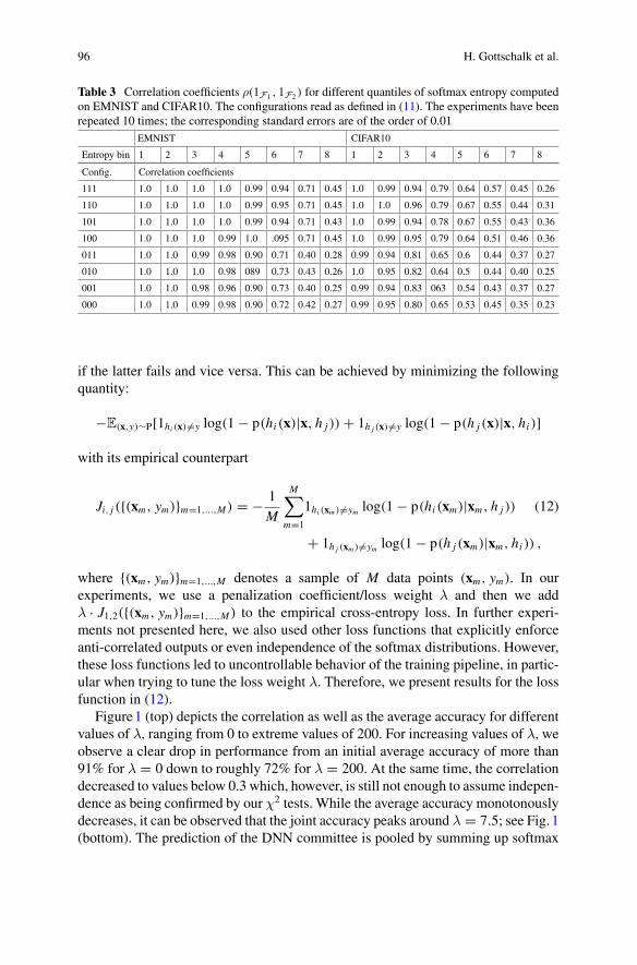
96 H. Gottschalk et al.

Table 3 Correlation coefficients ρ(1F1 , 1F2 ) for different quantiles of softmax entropy computedon EMNIST and CIFAR10. The configurations read as defined in (11). The experiments have beenrepeated 10 times; the corresponding standard errors are of the order of 0.01

EMNIST CIFAR10

Entropy bin 1 2 3 4 5 6 7 8 1 2 3 4 5 6 7 8

Config. Correlation coefficients

111 1.0 1.0 1.0 1.0 0.99 0.94 0.71 0.45 1.0 0.99 0.94 0.79 0.64 0.57 0.45 0.26

110 1.0 1.0 1.0 1.0 0.99 0.95 0.71 0.45 1.0 1.0 0.96 0.79 0.67 0.55 0.44 0.31

101 1.0 1.0 1.0 1.0 0.99 0.94 0.71 0.43 1.0 0.99 0.94 0.78 0.67 0.55 0.43 0.36

100 1.0 1.0 1.0 0.99 1.0 .095 0.71 0.45 1.0 0.99 0.95 0.79 0.64 0.51 0.46 0.36

011 1.0 1.0 0.99 0.98 0.90 0.71 0.40 0.28 0.99 0.94 0.81 0.65 0.6 0.44 0.37 0.27

010 1.0 1.0 1.0 0.98 089 0.73 0.43 0.26 1.0 0.95 0.82 0.64 0.5 0.44 0.40 0.25

001 1.0 1.0 0.98 0.96 0.90 0.73 0.40 0.25 0.99 0.94 0.83 063 0.54 0.43 0.37 0.27

000 1.0 1.0 0.99 0.98 0.90 0.72 0.42 0.27 0.99 0.95 0.80 0.65 0.53 0.45 0.35 0.23

if the latter fails and vice versa. This can be achieved by minimizing the followingquantity:

−E(x,y)∼P[1hi (x)=y log(1 − p(hi (x)|x, h j )) + 1h j (x)=y log(1 − p(h j (x)|x, hi )]

with its empirical counterpart

Ji, j ({(xm, ym)}m=1,...,M) = − 1

M

M∑

m=1

1hi (xm )=ym log(1 − p(hi (xm)|xm, h j )) (12)

+ 1h j (xm )=ym log(1 − p(h j (xm)|xm, hi )) ,

where {(xm, ym)}m=1,...,M denotes a sample of M data points (xm, ym). In ourexperiments, we use a penalization coefficient/loss weight λ and then we addλ · J1,2({(xm, ym)}m=1,...,M) to the empirical cross-entropy loss. In further experi-ments not presented here, we also used other loss functions that explicitly enforceanti-correlated outputs or even independence of the softmax distributions. However,these loss functions led to uncontrollable behavior of the training pipeline, in partic-ular when trying to tune the loss weight λ. Therefore, we present results for the lossfunction in (12).

Figure1 (top) depicts the correlation as well as the average accuracy for differentvalues of λ, ranging from 0 to extreme values of 200. For increasing values of λ, weobserve a clear drop in performance from an initial average accuracy of more than91% for λ = 0 down to roughly 72% for λ = 200. At the same time, the correlationdecreased to values below 0.3 which, however, is still not enough to assume indepen-dence as being confirmed by our χ2 tests. While the average accuracy monotonouslydecreases, it can be observed that the joint accuracy peaks around λ = 7.5; see Fig. 1(bottom). The prediction of the DNN committee is pooled by summing up softmax

Does Redundancy in AI Perception Systems Help to Test … 97

Fig. 1 Study of theinfluence of the loss weightλ on averaged accuracy andjoint accuracy on theEMNIST dataset

probabilities over both DNN class-wise and then selecting the class with maximalsum. The joint accuracy is given by the accuracy of the committee with that deci-sion rule. While the joint accuracy for an ordinarily trained committee with λ = 0is about 93.5%, this can be improved by tenderly decorrelating the DNNs to a cor-relation coefficient around 0.5 which yields an increase of almost 1% point. At thesame time, there is a mild decrease in average accuracy.

Concluding this section, we again study conditional independence for 8 softmaxentropy bins (chosen according to equally distributed softmax entropy quantiles),this time comparing independence trainingλ = 7.5with ordinary trainingλ = 0; seeTable4. We observe a considerable decrease in correlation in bin no. 8 (representingthe highest softmax entropy) for the EMNIST data down to 0.07. In comparison, thedecrease for CIFAR10 is rather mild. However, also this small correlation coefficientof 0.07 is not sufficient for assuming conditional independence.

98 H. Gottschalk et al.

Table 4 Correlation coefficients under independence training for different quantiles of softmaxentropy computed on EMNIST and CIFAR10

EMNIST CIFAR10

Entropy bin 1 2 3 4 5 6 7 8 1 2 3 4 5 6 7 8

λ Correlation coefficients

7.5 1.0 1.0 0.99 0.96 0.90 0.59 0.35 0.07 0.89 0.76 0.63 0.53 0.47 0.39 0.32 0.21

0.0 1.0 1.0 1.0 1.0 0.99 0.95 0.72 0.44 1.0 0.99 0.94 0.80 0.64 0.57 0.42 0.33

Training several networks for independence:Wenowpresent resultswhen trainingan ensemble of n = 5 networks. To this end, we sum up the cross-entropy losses ofthe n = 5 models and add the penalization term

λ · 2

n − 1

n∑

i=2

i−1∑

j=1

Ji, j ({(xm, ym)}m=1...,M) (13)

which is a straightforward combinatorial generalization of the previously usedpenalty term. Therein, λ again denotes the loss weight which varies during ourexperiments.

Besides k-out-of-5 accuracies, we consider also accuracies from single networksand ensemble accuracies. The corresponding ensemble prediction is obtained bysumming up the softmax probabilities (via the class-wise sum over the first k ensem-ble members) and then taking the argmax.

Figure2 depicts the results of our training for independence with 5 models interms of k-out-of-5 accuracy. When stating mean accuracy, this refers to the average

Fig. 2 Experiments with the EMNIST dataset. Left: mean k-out-of-5 accuracy (averaged over 30repetitions) for an ensemble of five networks as a function of the loss weight λ. The solid linesdepict the accuracies of the ensembles trained for independence with loss weight λ, the dashedlines depict baseline ensemble accuracies trained without incorporating the loss from (13). Right:k-out-of-5 accuracy for a single run as a function of the mean correlation (of each network witheach other network)

Does Redundancy in AI Perception Systems Help to Test … 99

Table 5 Correlation coefficients for an ensemble of 5 networks trained on EMNIST for indepen-dence and a baseline ensemblewhere each networkwas trained individually. All results are averagedover 30 runs

Lossweight λ

0 10−1 100 101 102 Baselinemodel

Theoretical

Mean cor-relation

0.70 0.69 0.65 0.53 0.43 0.67 0.00

Singlenetworkaccuracy

k = 1 0.92 0.92 0.91 0.88 0.73 0.91

k = 2 0.92 0.92 0.91 0.91 0.91 0.91

k = 3 0.92 0.92 0.91 0.88 0.60 0.91

k = 4 0.92 0.92 0.91 0.87 0.51 0.91

k = 5 0.92 0.92 0.91 0.85 0.39 0.91

Ensembleaccu-racy/Meank-out-of-5accuracy

k = 1 0.92/0.96 0.92/0.96 0.91/0.96 0.88/0.97 0.73/0.93 0.91/0.96 1.00

k = 2 0.92/0.94 0.92/0.94 0.92/0.94 0.92/0.93 0.91/0.78 0.92/0.94 0.99

k = 3 0.92/0.92 0.92/0.92 0.92/0.92 0.92/0.90 0.90/0.64 0.92/0.92 0.96

k = 4 0.93/0.90 0.93/0.90 0.92/0.89 0.92/0.85 0.90/0.49 0.92/0.90 0.72

k = 5 0.93/0.86 0.93/0.86 0.92/0.84 0.92/0.76 0.90/0.30 0.92/0.85 0.32

of over 30 runs. For a loss weight of λ = 101, we observe in the left panel that the1-out-of-5 accuracy of our independence training is slightly above the accuracy ofthe baseline ensemble which was trained regularly, i.e., each network was trainedindependently. Note that this is different from λ = 0, where all networks are stilltrained jointly with a common loss function which is the sum of the cross-entropylosses. The right-hand panel shows that the 1-out-of-5 accuracy peaks at a meancorrelation (the average correlation over the errors of all networks i < j) of 0.4.Decorrelating the networks’ errors further toward zero-mean correlation is possible,however, the 1-out-of-5 accuracy decreases. The k-out-of-5 accuracy for k > 1 suf-fers even more from decorrelating the networks’ errors. Note that, in practice, 1-out-of-5, e.g., for a pedestrian detection, might additionally suffer from overproductionof false positives and could be impractical. That hypothesis is indeed supported byTable5, which shows that for larger loss weights λ ≥ 1 the individual network accu-racies become heterogeneous. In particular, network 5 suffers from extremely lowaccuracy at λ = 102, which is, however, still far away from zero-mean correlation.For the sake of completeness, we give two examples of correlations between theindividual models since we only reported mean correlations so far; see Fig. 3. Com-paring the right-hand panel with Table5, we see that the well-performing networkno. 2 exhibits comparatively small correlation coefficients with the other networks’errors. Surprisingly, the worse performing models’ errors show higher correlationcoefficients which reveals that in that case they often err jointly on the same input

100 H. Gottschalk et al.

Fig. 3 Correlation coefficients of the networks’ errors for all combinations of 2 out of 5 models.Left: loss weight λ = 10−1. Right: loss weight λ = 102

examples. Additionally, we provide theoretical k-out-of-5 accuracies according to(10) where we choose psub equal to 1 minus the average ensemble accuracy (whichis 92.45%). In particular, the k-out-of-5 accuracies of the ensemble for k = 1 and 2are clearly below the theoretical ones.

We conclude that independence training may help slightly to improve the perfor-mance, however, the benefit seems to be limited when all networks are trained withthe same input. Besides these tests, we considered an additional loss function thatexplicitly penalizes the correlation of the networks’ errors. That approach, being actu-ally more directed toward our goal, even achieved negative correlation coefficients ofthe networks’ errors. It was also able to slightly improve the ensembles’ performancein terms of k-out-of-n accuracy over the baseline, however, this improvement waseven less pronounced than that one reported in this section. Thus, we do not reportthose results here.

Training of independence for different input sensors: In order to conduct furtherexperiments on the scale of the EMNIST and CIFAR10 datasets, we consider the3D-MNIST dataset that provides synthesized 3D representations of handwritten dig-its. We apply rotations around the x-axis with chosen angles. To this end, we create5 rotated variants of the dataset with a randomly chosen but fixed angles θ = aπ/9,a = 1, . . . , 9; see Fig. 4 for an illustrative example. Each of our k = 1, . . . , 5 net-works obtains one of the 5 rotated variants of the data with a given angle θk , and isthen trained. For the baseline, all networks are again trained independently. For inde-pendence training, all networks are trained with common loss functions, as describedpreviously, and the same handwritten digit, however, viewed from a different angleθk , is presented to the network k, k = 1, . . . , 5.

Figure5 shows results of numerical experiments conducted analogously to thosepresented in Fig. 2. Comparing both figures with each other, we observe that thebaseline k-out-of-5 accuracies aremuch lower thanwhen presenting identical imagesto the networks. Indeed, although MNIST classification constitutes a much simpler

Does Redundancy in AI Perception Systems Help to Test … 101

Fig. 4 A 3D-MNIST example data point. Left: original input data. Center: input data rotated byπ/3 along the x-axis. Right: 2D projection of the rotated data, which is obtained by summation andnormalization along the y-axis

Fig. 5 Experiments with the 3D-MNIST dataset. Left: mean k-out-of-5 accuracy (averaged over30 repetitions) for an ensemble of five networks as a function of the loss weight λ. The solid linesdepict the accuracies of the ensembles trained for independence with loss weight λ, the dashedlines depict baseline ensemble accuracies trained without incorporating the loss from (13). Right:k-out-of-5 accuracy for a single run as a function of the mean correlation (of each network witheach other network)

task than classifying the letters from EMNIST; this 3D variant shows much lowerindividual network performances, not only indicated by the left-hand panel of Fig. 5,but also by Table6. On the other hand, the highest mean correlation (obtained forthe loss weight λ = 0) for 3D-MNIST depicted by the right-hand panel of Fig. 5 isbelow 0.3 and therefore much lower than the one depicted by Fig. 2.

Neglecting the reduced performance on 3D-MNIST, these results show that anensemble, wherein each network obtains a different input, can be clearly improvedby increasing the number of ensemble members. The networks only exhibit smallcorrelations among each other. However, it seems that independence training can-not contribute to the performance of the ensemble anymore in the given setup. Itremains open, whether independence training may help in a realistic setting withdifferent sensors for perception in automated driving and networks conducting waymore difficult tasks such as object detection, instance segmentation, semantic seg-mentation, or panoptic segmentation. Note that the correlation strengths reported inour experiments in accordance with Sect. 3 do not suffice to substantially reduce thedata requirements into a feasible regime. Recalling the discussion in Sect. 3.2, even

102 H. Gottschalk et al.

Table 6 Results for an ensemble of 5 networks trained on 3D-MNIST for independence and abaseline ensemble where each network was trained individually. All results are averaged over 30runs

Lossweight λ

0 10−1 100 101 102 Baselinemodel

Theoretical

Mean cor-relation

0.25 0.25 0.24 0.22 0.15 0.24 0.00

Singlenetworkaccuracy

k = 1 0.70 0.70 0.70 0.66 0.38 0.70

k = 2 0.74 0.73 0.74 0.73 0.75 0.75

k = 3 0.73 0.72 0.72 0.67 0.25 0.74

k = 4 0.81 0.80 0.79 0.73 0.17 0.82

k = 5 0.72 0.73 0.71 0.64 0.20 0.74

Ensembleaccu-racy/meank-out-of-5accuracy

k = 1 0.70/0.97 0.70/0.97 0.70/0.97 0.66/0.96 0.38/0.88 0.70/0.97 1.00

k = 2 0.82/0.91 0.82/0.91 0.82/0.91 0.81/0.89 0.77/0.52 0.82/0.92 0.98

k = 3 0.84/0.81 0.84/0.80 0.84/0.80 0.83/0.75 0.78/0.22 0.85/0.82 0.90

k = 4 0.87/0.63 0.86/0.63 0.86/0.62 0.85/0.55 0.79/0.10 0.87/0.65 0.63

k = 5 0.88/0.38 0.88/0.37 0.88/0.37 0.86/0.29 0.79/0.03 0.89/0.39 0.24

if the subsystem performance remained unaffected by independence training, basedon the lowest correlation observed in our experiments, we could at most expect areduction of the required data amount by one order of magnitude.

5 Conclusion and Outlook

Summary andmain take-awaymessages: In this chapter, we argued that obtainingstatistical evidence from brute-force testing leads to the requirement of infeasibleamounts of data. In Sects. 2 and 3, we estimated upper and lower bounds on theamount of data required to test a given perception system with statistical validityfor being significantly safer than a human driver. We restricted our considerationsto fatalities and arrived at data amounts that are infeasible from both storage andlabeling cost perspectives, as already found in [KP16]. In Sect. 3.1, we showed thatperfectly uncorrelated redundant AI perception systems could be used to resolvethe problem. However, as we have seen in Sect. 3.2, redundant subsystems that arenot perfectly uncorrelated require extremely low correlation coefficients betweenerror events produced by neural networks to yield substantial reductions in datarequirement. In Sect. 3.3, we furthermore found the amount of data needed to prove

Does Redundancy in AI Perception Systems Help to Test … 103

a sufficiently low correlation as large as the amount of data needed for the originaltest.

In Sect. 4, we present numerical results on the correlation of redundant subsys-tems. We studied correlation coefficients between error events of redundant neu-ral networks dependent on network architecture, training data, and weight initializ-ers. Furthermore, we trained ensembles of neural networks to become decorrelated.Besides studying correlation coefficients, we considered the system’s performance interms of 1-out-of-n as well as k-out-of-n performance. In the numerical experiments,we obtained correlation coefficients that would allow for a reduction in the amount ofdata required by at most one order of magnitude. For the testing problem, this wouldstill represent an infeasible data requirement. However, redundancy could contributeto a moderate reduction of the amount of data required for testing and potentially becombined with other approaches.

There are alternative approaches to test the safety of perception systems otherthan brute-force testing. Here, we give a short outlook on two of them that are veryactively developed in the research community.

Outlook on testing with synthetic data: One possibility to obtain vast amountsof data for testing is to consider synthetic sources of data. The question of whethersynthetic data can be used for testing has already been addressed, e.g., in [RBK+21].In principle, arbitrary amounts of test data can be created from a driving simulationsuch as CARLA [DRC+17]. The domain shift between synthetic and real data can bebridged with generative adversarial networks (GANs). The latter have been provento be learnable in the large sample limit [BCST20, AGLR21], meaning that forincreasing amounts of data and capacity of the generator and discriminator, thelearned map from synthetic to real data is supposed to converge to the true one.Combining synthetic data and adversarial learning is therefore a promising candidatefor testing DNNs. However, in this setup there remain other gaps to be bridged(number of assets, environmental variability, and infeasibility of the empiricallyrisk-minimizing generator).

Outlook on testing with real data: There exists a number of helpful approachesto estimating the performance of unlabeled data. A DNN of strong performance (orensembles of those) can be utilized to compute pseudo ground truth. The modelto be equipped with an AI perception system can be learned in a teacher-studentfashion [AHKS19, BHSFs19], and the discrepancies between the student modeland the teachers can be compared with errors on a moderate subset with groundtruth, for instance, in terms of correlations of errors and discrepancies. Furthermore,in order to process the vast amounts of recorded data and perform testing moreefficiently, well-performing uncertainty quantification methods [KG17, KRPM+18,RCH+20] in combination with corner case detection methods [BBLFs19, HBR+21]can help to pre-select data for testing. Besides that, many additional approachestoward improving the reliability of DNN exist. However, while a big number of toolsalready exist, their proper application to DNN testing and inference of statisticallyrelevant statements on the system’s safety still require thorough research.

104 H. Gottschalk et al.

These approaches and other upcoming research might be part of the solution tothe testing problem in future.

Concluding remark: As a concluding remark, this chapter does not intend to dis-courage safety arguments, as also conceptualized in this volume. We do not denythe value of empirical evidence in order to, e.g., prove the relative superiority ofone AI system over another with regards to safety. The inherent difficulty to providedirect evidence for the better-than-human safety of automated driving as required bythe ethics committee of the German Ministry of Transportation and Digital Infras-tructure [FBB+17] should not be mistaken as an excuse for a purely experimentalapproach. Bringing automated vehicles to the street without prior risk assessmentimplies that risks would be judged a posteriori based on the experience with a largefleet of automated vehicles.

Suchmatters attain urgency in the light of recent German legislation on the experi-mental usage of automated driving under human supervision5 which only refers to thetechnical equipment for the sensing of automated vehicles, but does not specify theminimal performance for the AI-based perception based on the sensor information.Related regulations in other countries face similar problems.6

The debate on how to ensure a safe transition to automated driving that complieswith high ethical standards, therefore, remains of imminent scientific and publicinterest.

Acknowledgements The authors thank Lina Haidar for support and numerical results in Section4.2. Financial support by the German Federal Ministry of Economic Affairs and Energy (BMWi)via Grant No. 19A19005R as a part of the Safe AI for Automated Driving consortium is gratefullyacknowledged.

References

[AGLR21] H. Asatryan, H. Gottschalk, M. Lippert, M. Rottmann, A convenient infinitedimensional framework for generative adversarial learning, pp. 1–29 (2021).arXiv:2011.12087

[AHKS19] S. Abbasi, M. Hajabdollahi, N. Karimi, S. Samavi, Modeling teacher-studenttechniques in deep neural networks for knowledge distillation, pp. 1–6 (2019).arXiv:1912.13179

[BBLFs19] J.-A. Bolte, A. Bär, D. Lipinski, T. Fingscheidt, Towards corner case detection forautonomous driving, inProceedings of the IEEE Intelligent Vehicles Symposium (IV),pp. 438–445, Paris, France (2019)

[BCST20] G. Biau, B. Cadre, M. Sangnier, U. Tanielian, Some theoretical properties of GANs.Ann. Stat. 48(3), 1539–1566 (2020)

[BHSFs19] A. Bär, F. Hüger, P. Schlicht, T. Fingscheidt, On the robustness of redundant teacher-student frameworks for semantic segmentation, in Proceedings of the IEEE/CVF

5 https://dserver.bundestag.de/btd/19/274/1927439.pdf.6 Framework for Automated Driving System Safety, No. NHTSA-2020-0106, 49 CFR Part 571(Nov. 19, 2020).

Does Redundancy in AI Perception Systems Help to Test … 105

Conference on Computer Vision and Pattern Recognition (CVPR) Workshops, pp.1380–1388, Long Beach, CA, USA (2019)

[BTLFs20] J. Breitenstein, J.-A. Termöhlen, D. Lipinski, T. Fingscheidt, Systematization of cor-ner cases for visual perception in automated driving, in Proceedings of the IEEEIntelligent Vehicles Symposium (IV), pp. 1257–1264, Virtual Conference (2020)

[BTLFs21] J. Breitenstein, J.-A. Termöhlen, D. Lipinski, T. Fingscheidt, Corner cases for visualperception in automated driving: some guidance on detection approaches, pp. 1–8(2021). arXiv:2102.05897

[C+15] F. Chollet, et al. Keras (2015). Accessed 18 Nov 2021[CATvS17] G. Cohen, S. Afshar, J. Tapson, A. van Schaik, EMNIST: an extension of MNIST to

handwritten letters, pp. 1–10 (2017). arXiv:1702.05373[DRC+17] A. Dosovitskiy, G. Ros, F. Codevilla, A. Lopez, V. Koltun, CARLA: an open urban

driving simulator, in Proceedings of the Conference on Robot Learning CORL, pp.1–16, Mountain View, CA, USA (2017)

[FBB+17] U. di Fabio, M. Broy, R.J. Brüngger, U. Eichhorn, A. Grunwald, D. Heckmann, E.Hilgendorf, H. Kagermann, A. Losinger,M. Lutz-Bachmann, A.Markl, K.Müller, K.Nehm, Ethik-Kommission - Automatisiertes und vernetztes Fahren. Technical report,Federal Ministry of Transport and Digital Infrastructure (2017)

[Ger20] German Federal Ministry for Transortation & Infrastructure. Verkehr in Zahlen2020/2021. Deutsches Zentrum für Luft- und Raumfahrt (2020)

[HBR+21] F. Heidecker, J. Breitenstein, K. Rösch, J. Löhdefink, M. Bieshaar, C. Stiller, T.Fingscheidt, B. Sick, An application-driven conceptualization of corner cases forperception in highly automated driving, pp. 1–8 (2021). arXiv:2103.03678

[HS16] J. Hedderich, L. Sachs, Angewandte Statistik (in German) (Springer, Berlin, 2016)[KB15] D.P. Kingma, J. Ba, ADAM: a method for stochastic optimization, in Proceedings

of the International Conference on Learning Representations (ICLR), pp. 1–15, SanDiego, CA, USA (2015)

[KG17] A. Kendall, Y. Gal, What uncertainties do we need in Bayesian deep learning forcomputer vision? inProceedings of theConference onNeural InformationProcessingSystems (NIPS/NeurIPS), pp. 5574–5584, Long Beach, CA, USA (2017)

[KP16] N. Kalra, S.M. Paddock, Driving to safety: how many miles of driving would it taketo demonstrate autonomous vehicle reliability? Transp. Res. Part A: Policy Pract. 94,182–193 (2016)

[Kri09] A. Krizhevsky, Object classification experiments. Technical Report, Canadian Insti-tute for Advanced Research (2009)

[KRPM+18] S. Kohl, B. Romera-Paredes, C. Meyer, J. De Fauw, J.R. Ledsam, K. Maier-Hein,S.M. Ali Eslami, D. Jimenez Rezende, O. Ronneberger, A probabilistic U-Net forsegmentation of ambiguous images, in Proceedings of the Conference on NeuralInformation Processing Systems (NIPS/NeurIPS), pp. 6965–6975, Montréal, QC,Canada (2018)

[LCB98] Y. LeCun, C. Cortes, C.J.C. Burges, The MNIST database of handwritten digits(1998). Assessed 18 Nov 2021

[LL88] G.R. Loftus, E.F. Loftus, Essence of Statistics (Brooks/Cole Publishing Co, Salt LakeCity, 1988)

[LWC+19] L. Liu, W. Wei, K.-H. Chow, M. Loper, E. Gursoy, S. Truex, Y. Wu, Deep neuralnetwork ensembles against deception: ensemble diversity, accuracy and robustness,in Proceedings of the IEEE International Conference on Mobile Ad Hoc and SensorSystems (MASS), pp. 274–282, Monterey, CA, USA (2019)

[ME14] W.Q. Meeker, L.A. Escobar, Statistical Methods for Reliability Data (Wiley, NewYork, 2014)

[Nat20] National Transportation Safety Board NSTB. Collision Between a Sport UtilityVehicle Operating With Partial Driving Automation and a Crash Attenuator (2020).Accessed 18 Nov 2021

106 H. Gottschalk et al.

[RBK+21] J. Rosenzweig, E. Brito, H.-U. Kobialka, M. Akila, N.M. Schmidt, P. Schlicht, J.D.Schneider, F. Hüger, M. Rottmann, S. Houben, T. Wirtz, Validation of simulation-based testing: bypassing domain shift with label-to-image synthesis, pp. 1–8 (2021).arXiv:2106.05549

[RCH+20] M. Rottmann, P. Colling, T.-P. Hack, R. Chan, F. Hüger, P. Schlicht, H. Gottschalk,Prediction error meta classification in semantic segmentation: detection via aggre-gated dispersion measures of softmax probabilities, in Proceedings of the Interna-tional Joint Conference on Neural Networks (IJCNN), pp. 1–9, Virtual Conference(2020)

[Sch19] F.A. Schmidt, Crowdproduktion von Trainingsdaten: Zur Rolle von Online-ArbeitbeimTrainieren autonomer Fahrzeuge, vol. 417 of Study (inGerman) (Hans-Böckler-Stiftung, 2019)

[WLX+20] Y.Wu, L. Liu, Z. Xie, J. Bae, K.-H. Chow,W.Wei, Promoting high diversity ensemblelearning with ensemblebench, in Proceedings of the IEEE International Conferenceon Cognitive Machine Intelligence (CogMI), pp. 208–217, Atlanta, GA, USA (2020)

[Zac92] S. Zacks, Introduction to Reliability Analysis: Probability Models and StatisticalMethods (Springer, Berlin, 1992)

Open Access This chapter is licensed under the terms of the Creative Commons Attribution 4.0International License (http://creativecommons.org/licenses/by/4.0/), which permits use, sharing,adaptation, distribution and reproduction in any medium or format, as long as you give appropriatecredit to the original author(s) and the source, provide a link to the Creative Commons license andindicate if changes were made.

The images or other third party material in this chapter are included in the chapter’s CreativeCommons license, unless indicated otherwise in a credit line to the material. If material is notincluded in the chapter’s Creative Commons license and your intended use is not permitted bystatutory regulation or exceeds the permitted use, you will need to obtain permission directly fromthe copyright holder.

Analysis and Comparison of Datasets byLeveraging Data Distributions in LatentSpaces

Hanno Stage, Lennart Ries, Jacob Langner, Stefan Otten, and Eric Sax

Abstract Automated driving is widely seen as one of the areas, where key innova-tions are driven by the application of deep learning. The development of safe androbust deep neural network (DNN) functions requires newvalidationmethods.A coreinsufficiency of DNNs is the lack of generalization for out-of-distribution datasets.One path to overcome this insufficiency is through the analysis and comparison ofthe domains of training and test datasets. This is important because otherwise, deeplearning cannot advance automated driving. Variational autoencoders (VAEs) areable to extract meaningful encodings from datasets in their latent space. This chapterexamines various methods based on these encodings and presents a broad evalua-tion on different automotive datasets and potential domain shifts, such as weatherchanges or new locations. The used methods are based on the distance to the nearestneighbors between datasets and leverage several network architectures and metrics.Several experiments with different domain shifts on different datasets are conductedand compared with a reconstruction-based method. The results show that the pre-sentedmethods can be a promising alternative to the reconstruction error for detectingautomotive-relevant domain shifts between different datasets. It is also shown thatVAE loss variants that focus on a disentangled latent space can improve the stabilityof the domain shift detection quality. Best resultswere achievedwith nearest neighbormethods using VAE and JointVAE, a VAE variant with a discrete and a continuous

H. Stage (B) · L. Ries · J. Langner · S. Otten · E. SaxFZI Research Center for Information Technology, Haid-und-Neu-Str. 10-14,76131 Karlsruhe, Germanye-mail: stage@fzi.de

L. Riese-mail: ries@fzi.de

J. Langnere-mail: langner@fzi.de

S. Ottene-mail: otten@fzi.de

E. Saxe-mail: sax@fzi.de

© The Author(s) 2022T. Fingscheidt et al. (eds.), Deep Neural Networks and Data for Automated Driving,https://doi.org/10.1007/978-3-031-01233-4_3

107

108 H. Stage et al.

latent space, in combination with a metric based on the well-known z-score, andwith the NVAE, a VAE variant with optimizations regarding reconstruction quality,in combination with the deterministic reconstruction error.

1 Introduction

Artificial intelligence (AI) and deep learning are key enablers in automated driv-ing [RMM21]. One important task in the development of automated cars is theperception of the vehicle environment. While several sensors can be used to solvethis task, the most promising approaches in industry and research rely at least partlyon camera-based perception [RNFP19]. In the perception sub-tasks of object detec-tion and semantic segmentation, deep learning-based approaches already outperformclassical methods [GLGL18, ZZXW19].

However, those deep learning-based approaches suffer from several insufficien-cies. Following Sämann et al., one central insufficiency is the ability to generalizefrom given training data [SSH20]. If the underlying distribution of the input datadiffers from the distribution of the training dataset, the prediction accuracy maydecrease.

In the context of automated driving, a decrease in prediction accuracy can havedramatic consequences, e.g., fatal accidents due to traffic participants which werenot detected, e.g., Uber accident [SSWS19]. One possibility to decrease the proba-bility of these consequences is the optimization of used datasets. A high coverageover all possible situations in the training data is crucial to improve the quality oftrained neural networks. However, since the input spaces (e.g., image data) are veryhigh-dimensional and complex, the rule-based assessment of coverage is not feasi-ble [BLO+17].

Hence, in thiswork, the capabilities of variational autoencoders (VAEs) of extract-ing meaningful distributions from datasets are used to compare different datasets inan unsupervised fashion. Since theVAEworks directlywith rawdata, no assumptionsover relevant dataset dimensions for the comparison are necessary. Additionally, noalready trained perception function is necessary. The underlying data distributionsfound by the VAE are analyzed to find similarities and novelties, using the latentspace of the VAE. This makes it possible to estimate whether a particular datasetis in-domain or out-of-domain of a second dataset, thus allowing the detection ofdomain shifts between datasets.

During early function development, the presented methods can be used to extractdatasets with manageable sizes, still maintaining high coverages over relevant infor-mation in the complete data pool. These smaller datasets lead to faster training andvalidation and allow faster iterations. Moreover, the method can detect an unknowndomain shift between the training, validation, and test datasets, which could leadto wrong conclusions about the performance of the function. In later developmentstages, the dataset comparison enables a prediction, if an already trained function

Analysis and Comparison of Datasets by Leveraging … 109

can be safely used in a different environment. Additionally, for domain shift detec-tions with very high confidences, an online parallel execution of a perception neuralnetwork is thinkable, acting as a warning system for possibly unknown input data.

A domain shift can be caused by a huge variety of factors, some of thempotentiallyunknown to the developer. This makes the application of rule-based approachesimpossible. So, the idea of the presented dataset comparison method is to learn amultivariate distribution for all relevant aspects of one dataset and find useful metricsto compare these distributions. The used metrics in this investigation are related toknown novelty detection techniques for VAEs.

The main contribution of this chapter is the application of various novelty detec-tion methods and various VAE architectures in several experiments, each testing adifferent kind of domain shift. The applied novelty detection methods comprise fivedifferent nearest neighbor approaches applied to the latent spaces. As a benchmark,the reconstruction error is also computed [VGM+20]. The applicability of thesemeth-ods is investigated on three datasets, each providing one or more inherent domainshifts (e.g., weather, location, or daytime). The presented broad evaluation of differ-ent approaches can give insights into the practical application of such approaches inthe development of safe perception functions for automated driving.

2 Related Works

In this section, we provide an overview of related topics. There are various ways touseVAEs for anomaly detection in datasets [AC15, SWXS18, VGM+20]. An et al.compute the reconstruction probability of a given test sample by inspecting severalsamples drawn from the latent distribution of test samples [AC15]. The underlyingassumption is that anomalous data samples have a higher variance and will thereforeshow a lower reconstruction quality. Vasilev et al. propose several methods andmetrics to compute novelty scores usingVAEs [VGM+20]. Theydescribe 19differentmethods for novelty calculation, including latent space-based and reconstruction-based approaches. Their evaluation on a magnetic resonance imaging dataset andon MNIST showed that a variety of metrics outperforms classical approaches suchas nearest neighbor distance or principal component analysis (PCA) in the featurespace.

In the domain of skin disease detection, VAE-based novelty detection methodswere applied by Lu et al. [LX18]. They decompose the VAE loss into the recon-struction term and the KL term and use these as a novelty metric. Their results showbetter performance of the reconstruction-based approaches.

In the automotive domain, the issue of designing meaningful test datasets isaddressed on various levels. Bach et al. address the selection ofwell-adjusted datasetsfor testingwith a visualmethod for time series in recorded real-world data [BLO+17].Langner et al. enhanced this approachwith amethod for dataset design, using the nov-elty detection capabilities of classical autoencoders [LBR+18]. A related approach

110 H. Stage et al.

usesmethods fromnatural language processing (NLP) to describe sequential contextsin automotive datasets, allowing similarity analysis and novelty detection [RSBS20].

These approaches can only indirectly find domain shifts for perception functions,since they are not designed to work in the feature space itself. For the detectionof domain shifts directly in raw data, Löhdefink et al. propose the analysis of thereconstruction error of an autoencoder to predict the quality of a semantic segmen-tation network [LFK+20]. Sundar et al. address the issue of the diversity of auto-motive data by training various β-VAEs using different labels such as weather ordaytime [SRR+20].

There is a lot of research in relation to application domains, proposed metricsand network architectures in the area of dataset analysis with VAEs. However, mostof the related approaches restrict their analysis on datasets with only a few degreesof freedom (e.g., [VGM+20] and [LX18]) or test their method on only one type ofdomain shift (e.g., different locations). In this work, a broad spectrum of approaches(different network architectures, different metrics) were evaluated on three datasetsincluding five different domain shifts.

3 Building Blocks of Our Approach

In this work, four different VAE architectures and five different metrics for anomalydetection are examined on their applicability to compare automotive datasets. Fourmethods use a nearest neighbor approach in the latent space for detection of domainshifts.

In this section, theVAEDNN is introduced.Afterwards, the used novelty detectionmethods are presented, and the section concludes with the explanation for datasetcomparison and domain shift detection.

3.1 Variational Autoencoder DNN

The difference between the original autoencoder and the VAE is that the VAE usesa stochastic model. The VAE consists of a stochastic encoder, a latent space, and astochastic decoder. The general structure of a VAE can be seen in Fig. 1. Simplified,one could say that the VAE transfers the input data into a low-dimensional space tothen reconstruct the input data from this space. The underlying stochastic model isnow explained.

The probabilistic generative model of the VAE pθ(x|z) is a deep neural network(DNN)with network parametersθmapping z into x and is named decoder [VGM+20,Dup18]. This decoder model learns a joint distribution of the data x and a continuouslatent variable z ∈ R

dlat [CHK21]. In other words, the decoder describes the distribu-tion of the decoded variable x given the encoded one z. The inference model of the

Analysis and Comparison of Datasets by Leveraging … 111

trainingdataset

Encoder

σ

μ

latent spaceσ,μ, z ∈ R

dlat

z Decoder

input imagex ∈ I

H×W×Creconstructed image

x ∈ IH×W×C

Fig. 1 Basic variational autoencoder structure, consisting of an encoder to transform data into thelatent space and a decoder to reconstruct images from sampled values z. The encoder receives animage x as input, where H is the height of the image, W is the width of the image, and C is thenumber of color channels

VAE is trained to approximate the posterior distribution qφ(z|x) ∼ N (μ(x), σ2(x))with parameters φ mapping x into z and is named encoder [VGM+20]. The encoderdescribes the distribution of the encoded variable given the decoded one.

The probabilistic generated model and the inference model then give rise to thefirst loss term, since the aim for the input data of the encoder is to be reconstructed bythe decoder. The reconstruction error loss is defined as follows: Eqφ(z|x)[log pθ(x|z)][Dup18]. In order to improve the disentanglement properties of qφ(z|x), the VAE hasa loss optimization that tries to fit qφ(z|x) to p(z) [HMP+17]. This loss optimizationcan be both controlling the capacity of the latent information bottleneck and embody-ing statistical independence. This is achieved by defining p(z) as an isotropic unitGaussian distribution p(z) = N (0, I ) [HMP+17]. In order to train the disentangle-ment in the bottleneck, the VAE uses the Kullback–Leibler (KL) divergence of theapproximate from the true posterior DKL(qφ(z|x)||p(z)). Before we define the lossterm, we introduce the variable β, which serves as a weighting factor. This allows usto define the loss function for the VAE and β-VAE as follows:

J (θ,φ) = Eqφ(z|x)[log pθ(x|z)] − βDKL(qφ(z|x)||p(z)). (1)

The first term of the loss function is the reconstruction error, which is responsi-ble for the VAE encoding the informative latent variable z and allowing the inputdata x to be reconstructed [CHK21]. The second term regulates the posterior dis-tribution by adjusting the distribution of the encoded latent variables qφ(z|x) tothe prior p(z) [CHK21]. If β > 1 is selected, the loss function of the β-VAE asshown in (1) is used, and if β = 1 is selected, (1) breaks down to the standardVAE loss [HMP+17]. The variable β scales the regularization term for the posteriordistribution, with β > 1 enforcing the β-VAE to encode more disentangled latentvariables by matching the encoded latent variables with the prior by higher pressureon DKL(qφ(z|x)||p(z)) [HMP+17, CHK21].

The VAE and β-VAE only use continuous latent variables to model the latentvariable z [CHK21]. The next VAE architecture that we use for our experiments addi-tionally uses discrete variables to disentangle the generative factors of the observeddata [CHK21]. The JointVAE uses the discrete variable c to decode the generative

112 H. Stage et al.

factors of the observed data [Dup18, CHK21]. The loss function of the JointVAE isan extension of the loss function of the β-VAE and results in (2).

J (θ,φ) = Eqφ(z,c|x)[log pθ(x|z, c)] − γ∣∣DKL(qφ(z|x)||p(z)) − Cz

∣∣

− γ∣∣DKL(qφ(c|x)||p(c)) − Cc

∣∣.

(2)

The term DKL(qφ(c|x)||p(c))) is the Kullback–Leibler divergence for the discretelatent variables and DKL(qφ(z|x)||p(z)) is the Kullback–Leibler divergence for thecontinuous latent variables [Dup18]. The variables γ, Cz, and Cc are hyperparame-ters [Dup18]. The hyperparameters Cz and Cc are gradually increased during train-ing and both hyperparameters control the amount of information the model canencode [Dup18]. The hyperparameter γ forces theKL divergence tomatch the capac-ity Cz and Cc. As with the standard VAE, qφ(z, c|x) is the inference model whichmaps x into z and c.

In contrast to β-VAE and JointVAE which are focused on optimized latent spacedistributions, the goal of the NouveauVAE (NVAE) is to reconstruct the best possibleimages [VK21]. Compared to the other used VAEs, the NVAE is a hierarchical VAE.This means that the NVAE has a hierarchical encoder and decoder structure andmultiple latent spaces on different stages. Another special property is that this VAEhas a bidirectional encoder [VK21]. This means that the information does not onlypass from one encoder to the other but also the information from a deeper encoderpassed back to the higher encoder. A focus during the development of the NVAEwasto design expressive neural networks for VAEs [VK21].

In this chapter, the VAE [KW14], β-VAE [HMP+17], JointVAE [Dup18], andNouveau VAE (NVAE) [VK21] are considered for the five experiments.

3.2 Methods for Novelty Detection

Nearest neighbor approaches for novelty detection have the assumption that thedistributions of new and unknown data are different from the distributions of normaldata. So, the latent space distance between a test sample distribution p t and the closestnormal sample can be used as a novelty score. Since latent spaces consist of high-dimensional distributions, the selection of a feasible metric to compute meaningfuldistances is non-trivial. According to Sect. 3.1, the used normal distributions pn aredefined by their parameters μn and σn . As the JointVAE has different latent spaces,for the calculation of the nearest neighbor only the continuous latent space was used.

In this chapter, fivemetrics in the latent space and onemetric in the pixel space areevaluated. The five metrics in the latent space can be further divided into two groups.Group one includes the metrics that only use the means (μ) of the distribution, andmetric group two uses both means (μ) and variance (σ) for the calculation.

First, the metrics from group one are presented that only use means for the cal-culation. The cosine distance is a widely used metric to determine the similarity of

Analysis and Comparison of Datasets by Leveraging … 113

vectors [NB10, Ye11]. Since it is designed for vectors, it can not directly be appliedto distributions. Therefore, only the means μ of the normal distributions are used forcalculating the cosine distance. The cosine distance can be computed by

mcos(pn, pt ) = μnμTt

‖μn‖‖μt‖, (3)

where μn = (μn(δ)) and μt = (μt (δ)) describe the d-dimensional mean vectors oftwo distributions pn and pt , related to a normal and a test sample.

The Euclidean distance is the distance that can be measured with a ruler betweentwo points and is defined as

meuc(pn, pt ) =√√√√

d∑

δ=1

(μn(δ) − μt (δ))2. (4)

Here and in the following definitions, d is the dimensionality of the latent space.The Manhattan distance is inspired by the quadratic layout of Manhattan, New YorkCity, and measures the distance between two vectors as the sum of their components’absolute differences [BR14].

mman(pn, pt ) =d

∑

δ=1

|μn(δ) − μt (δ)|. (5)

The former presented metrics only used the means μ. Next, two metrics are intro-duced that use both means μ and standard deviations σ for the calculation ofthe nearest neighbor. The next metric was defined by the authors of this chapter,using the well-known z-score. From the test samples’ distribution, a vectorial valuezt = (zt (δ)) is sampled. Then the distance is computed via

mzsc(pn, pt ) =d

∑

δ=1

∥∥∥∥

zt (δ) − μn(δ)

σn(δ)

∥∥∥∥

2

, (6)

where the difference between zt and the normal sample meanμn being element-wisedivided by its standard deviation σn . Since we are only interested in the absolutedistance of the distributions, we compute the squared L2 norm. The Bhattacharyyadistance

mbha(pn, pt ) =d

∑

δ=1

1

4· log

(1

4

(σ2n(δ)

σ2t (δ)

+ σ2t (δ)

σ2n(δ)

+ 2

))

+ 1

4

((μn(δ) − μt (δ))

2

σ2n(δ) + σ2

t (δ)

)

,

(7)as proposed by Vasilev et al. [VGM+20], is also tested. The Bhattacharyya distancemeasures the similarity of two distributions [CA79].

114 H. Stage et al.

To consider also a metric which does not use the latent space, the reconstructionerror in the pixel space is considered. Since the VAE is trained only with normal data,the reconstruction quality should decrease, when new data samples are processed.Specifically, we chose the deterministic reconstruction error

mdre(x, x) = ∥∥x − x

∥∥2, (8)

as proposed by Vasilev et al. [VGM+20], since it yielded the best results in theirexperiments.

3.3 Dataset Comparison Approach

In this section, we explain how the methods described in Sect. 3.2 can be leveragedto compare the whole datasets by explaining the data pipeline, also visible in Fig. 2.As starting points of the pipeline, a training dataset Dtr , a validation dataset Dval,which is in the distribution of the training dataset, and a test datasetDdom are needed.Ddom is the dataset, for which the method tests, whether the dataset is in-domainor out-of-domain of the respective training dataset . The presented metrics shouldtherefore be able to separate Dval and Ddom. Dataset Dval most probably will havesingle images with higher novelty scores and Ddom can have already known images.Therefore, the metrics most probably cannot perfectly separate Dval and Ddom. Thisis solved by an analysis of the novelty metric results on a dataset level.

The first step of the pipeline is the training of a VAE with the Dtr dataset. For thenovelty detection, the decoder can be discarded after training. As shown in Fig. 2,the trained encoder can now be used to generate the latent space representations ofDtr , Dval, and Ddom, spanned by the vectors μtr , σtr , μval, σval, μdom, and σdom.

Now, the novelty scores provided in Sect. 3.2 can be applied to every latentspace representation of all data samples in Dval and Ddom. Hence, for the deci-sion, whether Ddom has a large gap to Dval, the novelty scores have to be com-

Dtr

Dval

Ddom

Encoder

μtr ∈ Rtr dl

μval ∈ Rval dl

μdom ∈ Rdom dl

σtr ∈ Rtr dl

σval ∈ Rval dl

σdom ∈ Rdom dl

Distance toTraining Data

Distancesmval, mdom

histogram distancefor mval, mdom

Fig. 2 Approach for dataset comparison based on latent space-based novelty scores. After training,the encoder is used to transform images into their latent space. In this space, different metrics canbe applied to calculate nearest neighbor distances between different datasets. Domain shifts canthen be detected by analyzing the histograms deviations

Analysis and Comparison of Datasets by Leveraging … 115

pared. In case of the nearest neighbor approaches, the resulting novelty scoresmval ={(val1,wval1), . . . , (valn,wvaln )} and mdom = {(dom1,wdom1), . . . , (domn,wdomn )}are represented as a histogram where n ∈ N is the number of buckets, vala anddomb are bucket representatives with 0 < a, b ≤ n, with a, b ∈ N, and wvala , wdomb

being the weights of the bucket [RTG00]. To compare the histograms we use theearth mover’s distance (EMD) [RTG00]. The earth mover’s distance can calculatethe difference between the histogram mval and mdom by calculating the earth amountfab which is to be moved from bucket vala to domb [RTG00]. To calculate the dis-tance, the EMD also needs the ground distance matrix D = (dab), where dab is theground distance between bucket vala and domb [RTG00].With these terms, the EMDcan be defined as follows:

EMD(mval,mdom) =∑n

a=1

∑nb=1 dab fab

∑na=1

∑nb=1 fab

. (9)

Here,∑n

a=1

∑nb=1 dab fab is the flow between mval and mdom, that minimizes the

overall cost with the following constraints [RTG00]:

fab ≥ 0 1 ≤ a ≤ n, 1 ≤ b ≤ n, (10)

n∑

b=1

fab ≤ wvala 1 ≤ a ≤ n, (11)

n∑

a=1

fab ≤ wdomb 1 ≤ b ≤ n, (12)

n∑

a=1

n∑

b=1

fab = min

( n∑

a=1

wvala ,

n∑

b=1

wdomb

)

. (13)

The used histograms are normalized on the x-axis to a range of values between 0 and1. Additionally, the y-axis is also normalized, such that the histogram bars sum to 1.With this normalization, comparability between different experiments is achieved,since the results are independent of absolute metric values and dataset sizes.

For the reconstruction error, the histogram approach is comparable with the dis-tances to the nearest neighbors. The histograms then are definedover the deterministicreconstruction error instead of the latent space distance.

4 Experimental Setup

In this section, first the selection of the datasets is explained. Afterwards, the exper-iments are explained and the hyperparameter values are given. The chapter is con-cluded with the training parameters for the experiments.

116 H. Stage et al.

4.1 Datasets

For the evaluation of our method, we selected different datasets which all havedifferent focuses. The first dataset is the Oxford RobotCar Dataset [MPLN17]. Inthis dataset, the same route was driven multiple times over the time period of 1 year,except for a few small deviations. The special feature of this dataset is that differentweather conditions and seasons were recorded on the same route. This allows variousdomain shift analyses, such as changing weather conditions, e.g., sunny weather vs.snow. In the training, validation, snow test, rain test, and night test data splits thereare 9130, 3873, 4094, 9757, and 9608 images, respectively. For all experiments, thetest split is created to test whether the data is in-domain or out-of-domain.

As a second dataset, the Audi autonomous driving dataset (A2D2) [GKM+20]was used. This dataset is relatively new and was acquired in different German cities.For our evaluation, we compared the images from the city of Gaimersheim with theimages from the city of Munich. The assumption with this dataset is that it showsrelatively little variation because it was recorded in two German cities in the state ofBavaria. Thus, it should result in a very low dataset distance. The small difference isexpected becauseMunich is larger thanGaimersheim, and therefore it is a comparisonbetween an urban and a suburban city. The dataset is divided into training dataset of12550 images, validation dataset of 3138 images, and test dataset of 5490 images.

As a third dataset, the nuScenes dataset [CBL+20] was selected. This datasetwas selected because it was recorded in Boston and Singapore. The interesting pointin the comparison is that there is right-hand traffic in Boston and left-hand trafficin Singapore. A number of 30013 images are used for training, 40152 images forvalidation, and 20512 images for test.

All datasets consist of a number of unconnected video sequences. To avoid similarimages in different datasets splits, the split between Dtr , Dval, and Ddom was donesequence-wise. This ensures, that every scene only occurs in exactly one dataset.Only for the A2D2 dataset, the split between Dtr , Dval was inside the Gaimersheimsequence, resulting in a few very similar images just before and after the split.However, this should not have a big effect, since the similar images take only avery small percentage of the whole dataset.

4.2 Experiments

For the evaluation of our method, we selected three different datasets, which all havea different focus. With these datasets, five different domain shifts were generated.These domain shifts can be seen in Table1.

Thefivedifferent domain shiftswere investigatedwith four differentVAEvariants.Each variant was tested with 6 different metrics, leading to 120 experiments in total.

Experiments 1–3 were performed with the Oxford dataset. For training, imageswere taken on sunny days and as validation data, images were selected that were

Analysis and Comparison of Datasets by Leveraging … 117

Table 1 All our datasets and experiments

Experiment Dataset Dtr Dataset Dval Dataset Ddom

Experiment 1 Oxford Oxford alternate route Snow

Experiment 2 Oxford Oxford alternate route Rain

Experiment 3 Oxford Oxford alternate route Night

Experiment 4 Gaimersheim Gaimersheim (holdout) Munich

Experiment 5 Boston Boston (holdout) Singapore

taken on an alternative route under the same weather conditions. This results in thefollowing experiments for the Oxford dataset. Experiment 1 tests if the latent spacecan be used to distinguish sunny days from snowy days. The second experiment testshow rain can be distinguished from sun, and the third experiment investigates howsunny days differ from night scenes (Fig. 3).

Experiment 4 uses the A2D2 dataset. This experiment only has a very smalldomain shift, since we compare data recorded in the sub-urban area of the smallGerman city Gaimersheim compared to the urban area of Munich. Experiment 5uses the nuScenes dataset. This experiment used images from Boston as trainingdata and, as in Experiment 4, used a holdout of the data as validation data. Imagesfrom Singapore were used as a test set. Since in Singapore also night scenes wererecorded, it has been ensured that no night scenes are in the test dataset.

To allow comparison of the experiments and metrics, baseline experiments wereconducted in addition to the domain shift experiments. This is necessary to find outwhich value themetric has for in-domain data. For this purpose, the validation datasetDval was divided into Dval0 and Dval1 . This makes it possible to define a baseline foreach experiment by setting Dval = Dval0 and Ddom = Dval1 .

4.3 VAE Hyperparameters

To ensure comparability between the VAE, β-VAE, and JointVAE, we used the samelayer architecture and hyperparameters. The goal of this chapter is to be able to givean initial indication of whether a domain shift can be detected with simply chosenhyperparameters. It is to be expected, that with optimization of hyperparameters onmultiple datasets, better results can be achieved.

To evaluate the performance of the presented methods, we have used the standardVAE, β-VAE, JointVAE, and the NVAE. The architecture was the same for the VAE,β-VAE, and the JointVAE. We use five hidden layers with dimensions 32, 64, 128,256, and 512. After the hidden layers, we add three residual blocks. The residualblocks follow a latent space with 100 neurons. Both β and γ were set to 10.5 and theinput size of the images was specified to a format of 512 × 256. For the NVAE, weadopted the architecture from the paper [VK21].

118 H. Stage et al.

0.00 0.25 0.50 0.75 1.000

2

4

Normed distance metric

Normed

numberof

samples

Z-Score based distance

oxford sunoxford rain

0.0 0.2 0.4 0.6 0.8 1.00

2

4

Normed distance metric

Normed

numberof

samples

Cosine distance

oxford sunoxford rain

Fig. 3 These histograms show the results for Experiment 2 and the JointVAE with the z-score andcosine distance. Training was done with the sunny Oxford images (oxford sun), and it was testedif rainy images (oxford rain) are out-of-domain. You can clearly see that the histogram on the leftshows a difference between rain and sun, and the histograms on the right are rather on top of eachother and poorly separated

4.4 Training

The VAE models used for the domain shift analysis were trained and implementedusing Pytorch [PGC+17]. All VAE architectures were trained for 50 epochs witha batch size of 128 images. In addition, a learning rate of 0.0001 in combinationwith the Adam optimizer [KB15] was used. Figure4 shows the original image andthe reconstruction of the different VAEs. The selected image is from the validationdataset.

5 Experimental Results and Discussion

In this section, the results are presented. Section5.1 first explains the results with thenearest neighbor method and after that in Sect. 5.2 the results will be discussed.

5.1 Results

Tomake the results of the different architectures and the differentmetrics comparable,we calculated the ratio of the in-domain data with the out-of-domain data for eachexperiment and architecture. This is done by

Analysis and Comparison of Datasets by Leveraging … 119

(a) original (b) VAE

(c) β-VAE (d) JointVAE

(e) NVAE

Fig. 4 Figure a shows an image from the Oxford validation dataset Dval. Figures b–e show thereconstruction of the VAE architectures used in this chapter. It is clear that the NVAE has the bestreconstruction quality. As expected, the reconstruction of the VAE (b), β-VAE (c), and JointVAE(TheVAEmodelsu) isworse compared to theNVAE.However, there are differences in reconstructionquality of (b)–(d), e.g., in the reconstruction of the JointVAE, compared to the VAE and β-VAE,you can imagine the car on the right edge. However, the fact that the reconstruction is worse is nota problem, because the focus of our method lies on the latent space

QEMD = EMD(Dval,Ddom)

EMD(Dval0 ,Dval1)(14)

and leads to QEMD > 1 for a detected domain shift. The intuition behind this isthat the earth mover’s distance (meaning the distribution of latent space distances)between two in-domain datasets has to be very low,whereas the latent space distancesto out-of-domain data should be higher. The results for the Oxford data can be seenin Tables2, 3, and 4. It can be seen that the NVAE achieves the best results in allexperiments. The reconstruction error works with the NVAE in all three experiments,even if the z-score and the NVAE work slightly better in the rain images.

The values in theA2D2 experiment are lower compared to theOxford values. Thiswas expected, as the domain shift is significantly smaller compared to the Oxforddomain shifts. Different architectures and metrics are close to each other in thisexperiment. The VAE with the z-score has the best result.

In the nuScenes dataset, the ratio is higher than in the A2D2 experiment. For thisexperiment, different combinations are again nearly the same, but the VAE with theManhattan distance is the best.

An important aspect of the experiment results is the stability of results, meaninga combination of architecture and metric should be able to correctly detect everykind of domain shift. For most combinations, this is not fulfilled, as can be seen

120 H. Stage et al.

Table 2 The result of QEMD (14) from Oxford alternate route and Ddom from Oxford snow

Architecture Bhattacharyyadistance

Cosinedistance

Euclideandistance

Manhattandistance

Z-score Reconstructionerror

VAE 1.18 1.49 0.52 0.47 1.01 1.32

β-VAE 7.29 4.12 1.03 0.85 1.95 1.10

JointVAE 3.77 0.50 0.37 0.45 3.00 1.25

NVAE 1.57 1.29 1.23 1.33 0.80 8.92

Table 3 The result of QEMD (14) from Oxford alternate route and Ddom from Oxford rain

Architecture Bhattacharyyadistance

Cosinedistance

Euclideandistance

Manhattandistance

Z-score Reconstructionerror

VAE 1.45 0.77 1.00 1.06 1.01 1.22

β-VAE 1.88 1.24 0.76 0.89 1.72 1.14

JointVAE 1.27 0.68 0.97 1.10 2.52 1.25

NVAE 2.14 0.86 6.08 3.80 5.40 5.00

Table 4 The result of QEMD (14) from Oxford alternate route and Ddom from Oxford night

Architecture Bhattacharyyadistance

Cosinedistance

Euclideandistance

Manhattandistance

Z-score Reconstructionerror

VAE 1.60 1.86 1.55 1.68 1.45 5.88

β-VAE 1.00 2.06 0.69 0.81 1.76 6.74

JointVAE 2.27 1.91 1.54 1.58 2.72 5.83

NVAE 0.00 0.43 0.85 0.60 0.60 10.42

Table 5 The result of QEMD (14) from Gaimersheim (holdout) and Ddom from Munich

Architecture Bhattacharyyadistance

Cosinedistance

Euclideandistance

Manhattandistance

Z-score Reconstructionerror

VAE 0.61 0.41 0.72 0.80 1.76 0.65

β-VAE 0.54 0.28 0.40 0.42 0.68 0.85

JointVAE 0.48 0.32 0.55 0.74 1.31 0.61

NVAE 1.29 1.70 1.31 1.69 1.25 1.57

in Tables2, 3, 4, 5, and 6. One example of this is the VAE with the Bhattacharyyadistance: A combination with values over one in four of the five experiments is given(Tables2, 3, 4, 6), while failing to detect a domain shift for the A2D2 experiment inTable5.

Analysis and Comparison of Datasets by Leveraging … 121

Table 6 The result of QEMD (14) from Boston (holdout) and Ddom from Singapore

Architecture Bhattacharyyadistance

Cosinedistance

Euclideandistance

Manhattandistance

Z-score Reconstructionerror

VAE 3.16 2.49 4.39 4.78 2.50 1.86

β-VAE 1.34 2.42 4.38 4.03 1.87 1.81

JointVAE 1.05 2.19 4.69 4.52 2.97 1.79

NVAE 0.76 2.69 1.43 4.43 1.07 1.32

5.2 Discussion

Since this chapter aims to provide insights into the applicability of latent spacemethods for dataset comparison, some central findings are presented here. One goalwas to use various experiments to find a combination that finds all domain shifts,if possible, irrespective of the extent of the domain shift. To achieve the goal, dif-ferent latent space methods were used, as there are critics who say that a nearestneighbor search does not work in high-dimensional space [AHK01]. In the workof Goos et al. [AHK01], it was said that the Euclidean distance does not work inhigh-dimensional spaces as well, and that the Manhattan distance achieves betterresults. For the NVAE, the latent space dimension of 4096 is significantly higherthan for the other VAE architectures with 100 dimensions. The NVAE has this highnumber of latent space dimensions because we used the parameters from the NVAEpaper [VK21]. The parameters were adopted to achieve the best possible reconstruc-tion without hyperparameter optimization runs. Our results show a similar pattern.The Manhattan distance can work better than the Euclidean distance. However, bothmetrics have the problem that they do not always give reliable results and havemultiple values less than one in the ratio calculation. In addition to investigatingwhether the nearest neighbor method works, we also wanted to find an architectureand metric that works stable, meaning that they are able to correctly detect all testeddomain shifts. Three architectures and two metrics were found that work and areshown graphically in Fig. 5. The three architectures found have in common that theydo not have a ratio with a value smaller than one in all experiments. It can be seenthat the NVAE with the reconstruction error works best with strong domain shifts,resulting in large visual differences between images such as rain, snow, and night. Ifthe domain shifts consist of different locations, resulting in a variety of only smalldataset differences, the z-score with the VAE or JointVAE works better comparedto the NVAE with the reconstruction error. Due to the additional categorical latentspace of the JointVAE, the discrete latent space is built up better. This leads to theJointVAE functioning more stable with the z-score than the VAE. The VAE is sig-nificantly worse with the Oxford dataset and nuScenes. However, in rain and snow,the VAE works not so good, as can be seen in Fig. 5. The ratio 1.01 is so close to thein-domain/out-of-domain boundary that one can say that the VAE should rather notbe used for weather domain shifts. The fact that the JointVAE works better than the

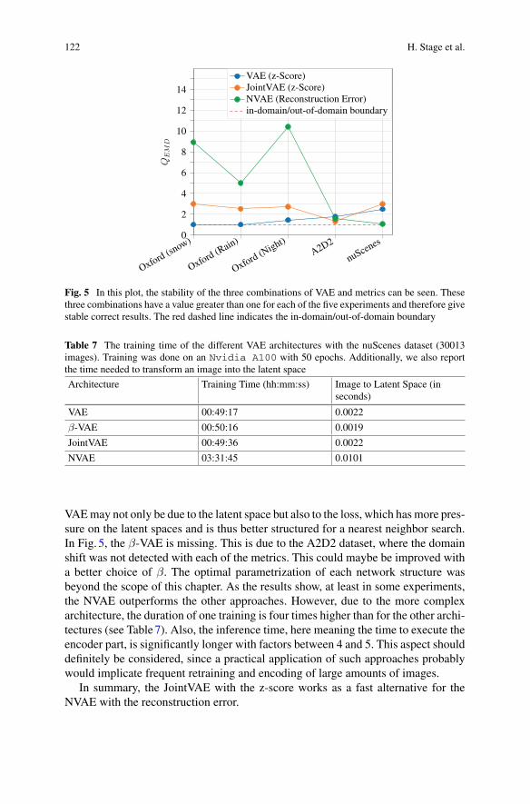
122 H. Stage et al.

Oxford (s

now)

Oxford (R

ain)

Oxford (N

ight)

A2D2

nuScen

es0

2

4

6

8

10

12

14

QEM

D

VAE (z-Score)JointVAE (z-Score)NVAE (Reconstruction Error)in-domain/out-of-domain boundary

Fig. 5 In this plot, the stability of the three combinations of VAE and metrics can be seen. Thesethree combinations have a value greater than one for each of the five experiments and therefore givestable correct results. The red dashed line indicates the in-domain/out-of-domain boundary

Table 7 The training time of the different VAE architectures with the nuScenes dataset (30013images). Training was done on an Nvidia A100 with 50 epochs. Additionally, we also reportthe time needed to transform an image into the latent space

Architecture Training Time (hh:mm:ss) Image to Latent Space (inseconds)

VAE 00:49:17 0.0022

β-VAE 00:50:16 0.0019

JointVAE 00:49:36 0.0022

NVAE 03:31:45 0.0101

VAEmay not only be due to the latent space but also to the loss, which has more pres-sure on the latent spaces and is thus better structured for a nearest neighbor search.In Fig. 5, the β-VAE is missing. This is due to the A2D2 dataset, where the domainshift was not detected with each of the metrics. This could maybe be improved witha better choice of β. The optimal parametrization of each network structure wasbeyond the scope of this chapter. As the results show, at least in some experiments,the NVAE outperforms the other approaches. However, due to the more complexarchitecture, the duration of one training is four times higher than for the other archi-tectures (see Table7). Also, the inference time, here meaning the time to execute theencoder part, is significantly longer with factors between 4 and 5. This aspect shoulddefinitely be considered, since a practical application of such approaches probablywould implicate frequent retraining and encoding of large amounts of images.

In summary, the JointVAE with the z-score works as a fast alternative for theNVAE with the reconstruction error.

Analysis and Comparison of Datasets by Leveraging … 123

6 Conclusions

This chapter investigated whether the latent space of a VAE can be used to finddomain shifts in the (image) context of the automotive industry. One goal was tofind a combination of metrics and VAE architectures that work in general, i.e., fordifferent datasets and domain shifts.

The novelty of our chapter is the different types of VAE used to evaluate the shiftof image data in different datasets and under different conditions.

To find out which combination is the most stable and best compared to the others,we conducted 120 experiments. In these experiments, four different VAE architec-tures were trained with three different datasets and five different domain shifts wereevaluated. The VAE architectures differ in that three of them have the same layerstructure and only the loss changes, and one architecture focuses on reconstructingthe images.

Six different metrics were used to detect the domain shifts, including the recon-struction error and four different nearest neighbor searches.

The most stable results were obtained with the JointVAE and the z-score, andwith the NVAE and the reconstruction error. With “stable results” we mean thatsome ratio of earth movers distances between the histograms of the nearest neighbordistances for in-domain and domain shift data is greater than one for all experiments.The VAE with the z-score was also above one in all experiments, but in the Oxforddataset, it was so minimally above one that this combination of metric and VAEcannot be recommended without limitations. In the experiments, the combinationJointVAE and z-score performed better for more subtle domain shifts like the changeof location, whereas the combination NVAE with reconstruction error performedbetter for visually present domain shifts like snow or rain.

The results of the experiments show that JointVAE with the latent spatial metriccan be an alternative to NVAE with the reconstruction error.

In the current state, it is possible to support the function development with theselection of the best out-of-domain data. This selection can help to select useful datasubsets with all relevant data present.

Better results can be expected if the function for which domain shifts are beingsearched is included in the training. If the information from the function, e.g., innerrepresentations of a neural network is used to build the latent space, a performancedrop of this neural network can probably be predicted better. However, this approachwould be no longer function-agnostic, since it requires an initially trained function.

As a conclusion, the presented methods can be a useful tool to compare andoptimize datasets with only few assumptions and can therefore be one componentin a strategy to develop functions with better generalization capabilities. Yet, fora complete approach, it has to be complemented with other methods such as rule-based or function-specific dataset optimizations tomutually compensate each other’sweaknesses.

124 H. Stage et al.

Acknowledgements The research leading to these results is fundedby theGermanFederalMinistryfor Economic Affairs and Energy within the project “Methoden und Maßnahmen zur Absicherungvon KI-basierten Wahrnehmungsfunktionen für das automatisierte Fahren (KI Absicherung).” Theauthors would like to thank the consortium for the successful cooperation.

References

[AC15] J. An, S. Cho, Variational autoencoder based anomaly detection using reconstructionprobability. Technical report, SNU Data Mining Center (2015)

[AHK01] C. Aggarwal, A. Hinneburg, D. Keim, On the surprising behavior of distancemetrics inhigh dimensional spaces, in Proceedings of the International Conference on DatabaseTheory, pp. 420–434, London, UK (2001)

[BLO+17] J. Bach, J. Langner, S. Otten, E. Sax, M. Holzäpfel, Test scenario selection for system-level verification and validation of geolocation-dependent automotive control systems,inProceedings of the ICE/IEEE International Conference on Engineering, Technologyand Innovation (ITMC), pp. 203–210, Madeira, Portugal (2017)

[BR14] S. Banerjee, A. Roy, Linear Algebra and Matrix Analysis for Statistics (CRC Press,Boca Raton, 2014)

[CA79] G.B. Coleman, H.C. Andrews, Image segmentation by clustering. Proc. IEEE 67(5),773–785 (1979)

[CBL+20] H. Caesar, V. Bankiti, A.H. Lang, S. Vora, V.E. Liong, Q. Xu, A. Krishnan, Y. Pan,G. Baldan, O. Beijbom, nuScenes: a multimodal dataset for autonomous driving, inProceedings of the IEEE/CVFConference onComputerVisionandPatternRecognition(CVPR), pp. 11621–11631, Virtual Conference (2020)

[CHK21] J. Choi, G. Hwang, M. Kang, Discond-VAE: disentangling continuous factors fromthe discrete, pp. 1–14 (2021). arXiv:2009.08039

[Dup18] E. Dupont, Learning disentangled joint continuous and discrete representations, pp.1–16 (2018). arXiv:1804.00104

[GKM+20] J. Geyer, Y. Kassahun, M.Mahmudi, X. Ricou, R. Durgesh, A.S. Chung, L. Hauswald,V.H. Pham, M. Mühlegg, S. Dorn, T. Fernandez, M. Jänicke, S. Mirashi, C. Savani,M. Sturm, O. Vorobiov, M. Oelker, S. Garreis, P. Schuberth, A2D2: Audi autonomousdriving dataset, pp. 1–10 (2020). arXiv:2004.06320

[GLGL18] Y.Y. Guo, T.G. Liu, M.S. Lew, A review of semantic segmentation using deep neuralnetworks. Int. J. Multimed. Inf. Retr. 7(2), 87–93 (2018)

[HMP+17] I. Higgins, L.Matthey, A. Pal, C. Burgess, X. Glorot,M.M. Botvinick, S.Mohamed, A.Lerchner, β-VAE: learning basic visual concepts with a constrained variational frame-work, in Proceedings of the International Conference on Learning Representations(ICLR), pp. 1–22, Toulon, France (2017)

[KB15] D.P. Kingma, J. Ba, ADAM: a method for stochastic optimization, in Proceedingsof the International Conference on Learning Representations (ICLR), pp. 1–15, SanDiego, CA, USA (2015)

[KW14] D.P. Kingma, M. Welling, Auto-encoding variational Bayes, in Proceedings of theInternational Conference on Learning Representations (ICLR), pp. 1–14, Banff, AB,Canada (2014)

[LBR+18] J. Langner, J. Bach, L. Ries, S. Otten, M. Holzäpfel, E. Sax, Estimating the uniquenessof test scenarios derived from recorded real-world-driving-data using autoencoders, inProceedings of the IEEE Intelligent Vehicles Symposium (IV), pp. 1860–1866, Chang-shu, China (2018)

Analysis and Comparison of Datasets by Leveraging … 125

[LFK+20] J. Löhdefink, J. Fehrling, M. Klingner, F. Hüger, P. Schlicht, N.M. Schmidt,T. Fingscheidt, Self-supervised domain mismatch estimation for autonomous percep-tion, in Proceedings of the IEEE/CVF Conference on Computer Vision and PatternRecognition (CVPR) Workshops, pp. 1359–1368, Virtual Conference (2020)

[LX18] Y. Lu, P. Xu, Anomaly detection for skin disease images using variational autoencoder,pp. 1–8 (2018). arXiv:1807.01349

[MPLN17] W.Maddern, G. Pascoe, C. Linegar, P. Newman, 1 year, 1000 km: theOxford RobotCardataset. Int. J. Robot. Res. 36(1), 3–15 (2017)

[NB10] H.V.Nguyen, L.Bai, Cosine similaritymetric learning for face verification, inProceed-ings of the Asian Conference on Computer Vision (ACCV), pp. 709–720, Queenstown,New Zealand (2010)

[PGC+17] A. Paszke, S. Gross, S. Chintala, G. Chanan, E. Yang, Z. DeVito, Z. Lin, A. Desmai-son, L. Antiga, A. Lerer, Automatic differentiation in PyTorch, in Proceedings of theConference on Neural Information Processing Systems (NIPS/NeurIPS) Workshops,pp. 1–4, Long Beach, CA, USA (2017)

[RMM21] M. Rabe, S. Milz, P. Mäder, Development methodologies for safety critical machinelearning applications in the automotive domain: a survey, in Proceedings of theIEEE/CVF Conference on Computer Vision and Pattern Recognition (CVPR) Work-shops, pp. 129–141, Virtual Conference (2021)

[RNFP19] F. Rosique, P.J. Navarro, C. Fernández, A. Padilla, A systematic review of perceptionsystem and simulators for autonomous vehicles research. Sensors 19(3), 1–29 (2019)

[RSBS20] L. Ries, M. Stumpf, J. Bach, E. Sax, Semantic comparison of driving sequences byadaptation of word embeddings, in Proceedings of the IEEE Intelligent TransportationSystems Conference (ITSC), pp. 1–7, Virtual Conference (2020)

[RTG00] Y. Rubner, C. Tomasi, L.J. Guibas, The Earth Mover’s distance as a metric for imageretrieval. Int. J. Comput. Vis. (IJCV) 40, 99–121 (2000)

[SRR+20] V.K. Sundar, S. Ramakrishna, Z. Rahiminasab, A. Easwaran, A. Dubey, Out-of-distribution detection in multi-label datasets using latent space of β-VAE, in Proceed-ings of the IEEE Symposium on Security and Privacy (SP) Workshops, pp. 250–255,Virtual Conference (2020)

[SSH20] T. Sämann, P. Schlicht, F. Hüger, Strategy to increase the safety of a DNN-basedperception for HAD systems, pp. 1–14 (2020). arXiv:2002.08935

[SSWS19] N.A.Stanton, P.M.Salmon,G.H.Walker,M.Stanton,Models andmethods for collisionanalysis: a comparison study based on the Uber collision with a pedestrian. Saf. Sci.120(12), 117–128 (2019)

[SWXS18] J. Sun, X. Wang, N. Xiong, J. Shao, Learning sparse representation with variationalauto-encoder for anomaly detection. IEEE Access 6, 33353–33361 (2018)

[VGM+20] A. Vasilev, V. Golkov, M. Meissner, I. Lipp, E. Sgarlata, V. Tomassini, D.K. Jones,D. Cremers, Q-space novelty detection with variational autoencoders, in Proceedingsof the International Conference on Medical Image Computing & Computer-AssistedIntervention (MICCAI) Workshops, pp. 113–124, Virtual Conference (2020)

[VK21] A. Vahdat, J. Kautz, NVAE: a deep hierarchical variational autoencoder, pp. 1–21(2021). arXiv:2007.03898

[Ye11] J. Ye, Cosine similarity measures for intuitionistic fuzzy sets and their applications.Math. Comput. Modelling 53(1–2), 91–97 (2011)

[ZZXW19] Z.-Q. Zhao, P. Zheng, X. Shou-Tao, W. Xindong, Object detection with deep learning:a review. IEEE Trans. Neural Netw. Learn. Syst. (TNNLS) 30(11), 3212–3232 (2019)

126 H. Stage et al.

Open Access This chapter is licensed under the terms of the Creative Commons Attribution 4.0International License (http://creativecommons.org/licenses/by/4.0/), which permits use, sharing,adaptation, distribution and reproduction in any medium or format, as long as you give appropriatecredit to the original author(s) and the source, provide a link to the Creative Commons license andindicate if changes were made.

The images or other third party material in this chapter are included in the chapter’s CreativeCommons license, unless indicated otherwise in a credit line to the material. If material is notincluded in the chapter’s Creative Commons license and your intended use is not permitted bystatutory regulation or exceeds the permitted use, you will need to obtain permission directly fromthe copyright holder.

Optimized Data Synthesis for DNNTraining and Validation by SensorArtifact Simulation

Korbinian Hagn and Oliver Grau

Abstract Synthetic, i.e., computer-generated imagery (CGI) data is a key compo-nent for training and validating deep-learning-based perceptive functions due to itsability to simulate rare cases, avoidance of privacy issues, and generation of pixel-accurate ground truth data. Today, physical-based rendering (PBR) engines simulatealready a wealth of realistic optical effects but are mainly focused on the humanperception system. Whereas the perceptive functions require realistic images mod-eled with sensor artifacts as close as possible toward the sensor, the training datahas been recorded. This chapter proposes a way to improve the data synthesis pro-cess by application of realistic sensor artifacts. To do this, one has to overcome thedomain distance between real-world imagery and the synthetic imagery. Therefore,we propose a measure which captures the generalization distance of two distinctdatasets which have been trained on the same model. With this measure the data syn-thesis pipeline can be improved to produce realistic sensor-simulated images whichare closer to the real-world domain. The proposed measure is based on the Wasser-stein distance (earth mover’s distance, EMD) over the performance metric meanintersection-over-union (mIoU) on a per-image basis, comparing synthetic and realdatasets using deep neural networks (DNNs) for semantic segmentation. This mea-sure is subsequently used to match the characteristic of a real-world camera for theimage synthesis pipeline which considers realistic sensor noise and lens artifacts.Comparing the measure with the well-established Fréchet inception distance (FID)on real and artificial datasets demonstrates the ability to interpret the generalizationdistance which is inherent asymmetric and more informative than just a simple dis-tance measure. Furthermore, we use the metric as an optimization criterion to adapt asynthetic dataset to a real dataset, decreasing the EMD distance between a syntheticand the Cityscapes dataset from 32.67 to 27.48 and increasing the mIoU of our testalgorithm (DeeplabV3+) from 40.36 to 47.63%.

K. Hagn (B) · O. GrauIntel Deutschland GmbH, Lilienthalstraße 15, 85579 Neubiberg, Germanye-mail: korbinian.hagn@intel.com

O. Graue-mail: oliver.grau@intel.com

© The Author(s) 2022T. Fingscheidt et al. (eds.), Deep Neural Networks and Data for Automated Driving,https://doi.org/10.1007/978-3-031-01233-4_4

127

128 K. Hagn and O. Grau

1 Introduction

Validation of deep neural networks (DNNs) is increasingly resorting towardcomputer-generated imagery (CGI) due to its mitigation of certain issues. First, syn-thetic data can avoid privacy issues found with recordings of members of the publicand, on the other hand, can automatically produce vast amounts of data at high qual-ity with pixel-accurate ground truth data and reliability than costly manually labeleddata.Moreover, simulations allow synthesis of rare cases and the systematic variationand explanation of critical constellations [SGH20]—a requirement for validation ofproducts targeting safety-critical applications, such as automated driving. Here, thecreation of corner cases and scenarios which otherwise could not be recorded in areal-world scenariowithout endangering other traffic participants is the key argumentfor the validation of perceptive AI with synthetic images.

Despite the advantages of CGI methods, training and validation with syntheticimages still have challenges: Training with these images does not guarantee a similarperformance on real-world images and validation is only valid if one can verifythat the found weaknesses in the validation do not stem from the synthetic-to-realdistribution shift seen in the input.

To measure and mitigate this domain shift, metrics have been introduced withvarious applications in the field of domain adaptation or transfer learning. In domainadaptation, the metrics such as FID, kernel inception distance (KID), and maxi-mum mean discrepancy (MMD) are applied to train generative adversarial networks(GANs) to adapt on a target feature space [PTKY09] or to re-create the visual prop-erties of a dataset [SGZ+16]. However, the problem of training and validation withsynthetic imagery is directly related to the predictive performance of a perceptionalgorithm on the target data, and these kinds of metrics struggle to correlate withthe predictive performance [RV19]. Additionally, applications of domain adaptationmethods often resort to specifically trained DNNs, e.g., GANs, which adapt onedomain to the other and therefore add an extra layer of complexity and uncontrol-lability. This is especially unwanted if a validation goal is tested, e.g., to detect allpedestrians, and the domain adaption by a GAN would add additional objects intothe scene (e.g., see [HTP+18]) making it even harder to attribute detected faults ofthe model to certain specifics of the tested scene. Here, the creation of images viaa synthesis process allows to understand domain distance influence factors moredirectly as all parameters are under direct control.

Camera-recorded images inherently show visual imperfections or artifacts, suchas sensor noise, blur, chromatic aberration, or image saturation, as can be seen in animage example from the A2D2 [GKM+20] dataset in Fig. 1. CGI methods, on theother hand, are usually based on idealized models; for example, the pinhole cameramodel [Stu14] which is free of sensor artifacts.

In this chapter, we present an approach to decrease the domain divergence of syn-thetic to real-world imagery for perceptive DNNs by realistically modeling sensorlens artifacts to increase the viability of CGI for training and validation. To achievethis, we first introduce a model of sensor artifacts whose parameters are extracted

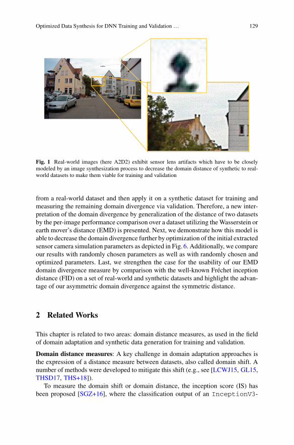
Optimized Data Synthesis for DNN Training and Validation … 129

Fig. 1 Real-world images (here A2D2) exhibit sensor lens artifacts which have to be closelymodeled by an image synthesization process to decrease the domain distance of synthetic to real-world datasets to make them viable for training and validation

from a real-world dataset and then apply it on a synthetic dataset for training andmeasuring the remaining domain divergence via validation. Therefore, a new inter-pretation of the domain divergence by generalization of the distance of two datasetsby the per-image performance comparison over a dataset utilizing theWasserstein orearth mover’s distance (EMD) is presented. Next, we demonstrate how this model isable to decrease the domain divergence further by optimization of the initial extractedsensor camera simulation parameters as depicted in Fig. 6. Additionally, we compareour results with randomly chosen parameters as well as with randomly chosen andoptimized parameters. Last, we strengthen the case for the usability of our EMDdomain divergence measure by comparison with the well-known Fréchet inceptiondistance (FID) on a set of real-world and synthetic datasets and highlight the advan-tage of our asymmetric domain divergence against the symmetric distance.

2 Related Works

This chapter is related to two areas: domain distance measures, as used in the fieldof domain adaptation and synthetic data generation for training and validation.

Domain distance measures: A key challenge in domain adaptation approaches isthe expression of a distance measure between datasets, also called domain shift. Anumber of methods were developed to mitigate this shift (e.g., see [LCWJ15, GL15,THSD17, THS+18]).

To measure the domain shift or domain distance, the inception score (IS) hasbeen proposed [SGZ+16], where the classification output of an InceptionV3-

130 K. Hagn and O. Grau

based [SVI+16] discriminator network trained on the ImageNet dataset [DDS+09]is used. The works of [HRU+17, BSAG21] rely on features extracted from theInceptionV3 network to tune domain adaptation approaches, i.e., the FIDand KID. However, these metrics cannot predict if the classification performanceincreases when adapted data is applied as training data for a discriminator [RV19].

Therefore, tomeasure performance directly, it is essential to train with the adaptedor synthetic data and validate on the target data, i.e., cross-evaluation as done by[RSM+16, WU18, SAS+18].

Performance metrics: The mean intersection-over-union (mIoU) is a widely usedperformance metric for benchmarking semantic segmentation [COR+16, VSN+18].Adaptations and improvements of the mIoU have been proposed which put moreweight on the segmentation contour as in [FMWR18, RTG+19]. Performancemetricsas themIoU are computed over thewhole validation dataset, i.e., the whole confusionmatrix, but there are propositions to apply the mIoU calculation on a per-image basisand compare the resulting empirical distributions [CLP13].

A per-image comparison mitigates several shortcomings of a single evaluationmetric on the whole dataset when used for comparison of classifiers on the samedataset. First, one can distinguish multimodal and unimodal distributions, i.e., strongclassification on one half and weak classification on the other half of a set can leadto the same mean as an average classification on all samples. Second, unimodaldistributions with the same mean but different shape are also indiscernible under asingle dataset averaged metric. This justification led to our choice of a per-image-based mIoUmetric as it allows for deeper investigations which are especially helpfulwhen one wants to understand the characteristics that increase or decrease a domaindivergence.

Sensor simulation for synthetic image training: The use of synthesized data fordevelopment and validation is an accepted technique and has been also suggested forcomputer vision applications (e.g., [BB95]). Recently, specifically for the domain ofdriving scenarios, games engines have been adapted [RHK17, DRC+17].

Although game engines provide a good starting point to simulate environments,they usually only offer a closed rendering set-up with many trade-offs balancingbetween real-time constraints and a subjectively good visual appearance for humanobservers. Specifically the lighting computation in the rendering pipelines is in-transparent. Therefore, it does not produce a physically correct imagery; instead onlya fixed rendering quality (as a function of lighting computation and tone mapping),resulting in output of images having a low dynamic range (LDR) (typically 8-bit perRGB color channel).

Recently, physical-based rendering techniques have been applied to the generationof data for training and validation, like Synscapes [WU18]. For our chapter we usea dataset in high dynamic range (HDR) created with the physical-based BlenderCycles renderer.1 We implemented a customized tone mapping to 8-bit per colorchannel and sensor simulation, as described in the next section.

1 Provided by the KI Absicherung project [KI 20].

Optimized Data Synthesis for DNN Training and Validation … 131

While there is great interest in understanding the domain distance in the area ofdomain adaptation via generative strategies, i.e., GANs, there has been little researchregarding sensor artifact influence on training and validation with synthetic images.Other works [dCCN+16, NdCCP18] add different kinds of sensor noise to theirtraining set and report a degradation of performance, compared to a model trainedwith no noise in the training set, due to training of a harder, i.e., noisier, visual task.Adding noise in training is a common technique for image augmentation and can beseen as a regularization technique [Bis95] to prevent overfitting.

Our task of modeling sensor artifacts for synthetic images extracted from cameraimages is not aimed at improving the generalization through random noise, but totune the parameters of our sensor model to closely replicate the real-world imagesand improve generalization on the target data.

First results of modeling camera effects to improve synthetic data learning onthe perceptive task of bounding box detection have been proposed by [CSVJR18,LLFW20]. Lin et al. [LLFW20] additionally state that generalization is an asymmet-ric measure which should be considered when comparing with symmetric datasetdistance measures from literature. Furthermore, Carlson et al. [CSVJR19] learnedsensor artifact parameters from a real-world dataset and applied the learned parame-ters of their noise sources as image augmentation during training with synthetic dataon the task of bounding box detection. However, contrasting our approach, they applytheir optimization as style loss on a latent feature vector extracted from a VGG-16network trained on ImageNet and evaluate the performance on the task of 2D objectdetection.

3 Methods

Given a synthetic (CGI) dataset of urban street scenes, our goal is to decrease thedomain gap to a real-world dataset for semantic segmentation by realistic sensorartifact simulation. Therefore, we systematically analyze the image sensor artifactsof the real-world dataset and use this extracted parametrization for our sensor artifactsimulation. To compare our synthetic dataset with the real-world dataset we contrivea novel per-image performance-based metric to measure the generalization distancebetween the datasets. We utilize a DeeplabV3+ [CZP+18] semantic segmentationmodel with a ResNet101 [HZRS16] backbone to train and evaluate on the differentdatasets throughout this paper. To show the valuable properties of our measure wecompare it with the established domain distance, i.e., Fréchet inception distance(FID). Lastly, we use ourmeasure as optimization criteria for adapting the parametersof our sensor artifact simulation with the extracted parameters as starting point andshow that we can further decrease the domain distance from synthetic images toreal-world images.

132 K. Hagn and O. Grau

3.1 Sensor Simulation

We implemented a simple sensor model with the principle blocks depicted in Fig. 2:The module expects images in linear RGB space. Rendering engines like BlenderCycles2 can provide these images as results in OpenEXR format.3

We simulate a simple model by applying chromatic aberration, blur, and sensornoise, as additive Gaussian noise (zero mean, variance is a free parameter), followedby a simple exposure control (linear tone mapping), finished by non-linear gammacorrection.

First, we apply blur by a simple box filter with filter size F × F and a chromaticaberration (CA). The CA is approximated using radial distortions (k1, second order),e.g., [CV14], as defined in OpenCV. The CA is implemented as a per channel (red,green, blue) variation of the k1 radial distortion, i.e., we introduce an incremen-tal parameter ca that affects the radial distortions: k1(blue) = −ca; k1(green) =0; k1(red) = +ca. As the next step, we apply Gaussian noise to the input image.

Applying a linear function, the pixel values are then mapped and rounded to thetarget output byte range [0, ..., 255].

The two parameters of the linear mapping are determined by a histogram evalu-ation of the input RGB values of the respective image, imitating an auto exposureof a real camera. In our experiments we have set it to saturate 2% (initially) of thebrightest pixel values, as these are usually values of very high brightness, inducedby sky or even the sun. Values below the minimum or above the set maximum aremapped to 0 or 255, respectively.

In the last step we apply gamma correction to achieve the final processed syntheticimage:

x = (x)γ (1)

The parameter γ is an approximation of the sensor non-linear mapping function.For media applications this is usually γ = 2.2 for the sRGB color space [RD14].However, for industrial cameras, this is not yet standardized and some vendors do

Linear Mapping,Rounding+

NoiseGenerator

Measurement ofHistogram Range

GammaCorrection

Blur,Chromatic Aberration

syntheticimagex

x ∈ [0, ..., 255] "real"imagex

Fig. 2 Sensor artifact simulation

2 https://www.blender.org/.3 https://www.openexr.com/.

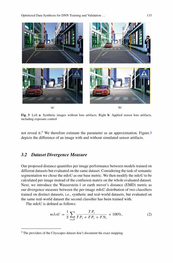
Optimized Data Synthesis for DNN Training and Validation … 133

(a) (b)

Fig. 3 Left a: Synthetic images without lens artifacts. Right b: Applied sensor lens artifacts,including exposure control

not reveal it.4 We therefore estimate the parameter as an approximation. Figure3depicts the difference of an image with and without simulated sensor artifacts.

3.2 Dataset Divergence Measure

Our proposed distance quantifies per image performance between models trained ondifferent datasets but evaluated on the same dataset. Considering the task of semanticsegmentation we chose the mIoU as our base metric. We then modify the mIoU to becalculated per image instead of the confusion matrix on the whole evaluated dataset.Next, we introduce the Wasserstein-1 or earth mover’s distance (EMD) metric asour divergence measure between the per-image mIoU distribution of two classifierstrained on distinct datasets, i.e., synthetic and real-world datasets, but evaluated onthe same real-world dataset the second classifier has been trained with.

The mIoU is defined as follows:

mIoU = 1

S

∑

s∈S

T PsT Ps + FPs + FNs

× 100%, (2)

4 The providers of the Cityscapes dataset don’t document the exact mapping.

134 K. Hagn and O. Grau

with T Ps , FNs , and FPs being the amount of true-positives, false-negatives, andfalse-positives of the sth class over all images of the evaluated dataset.

Here, S = {0, 1, ..., S − 1}, with S = 11, as we use the 11 classes defined inTable1. These classes are the maximal overlap of common classes in the real andsynthetic datasets considered for cross-evaluation and comparison of our measurewith the Fréchet inception distance (FID), as can be seen later in Sect. 4.3, Tables3and 4.

A distribution over the per-image IoU takes the following form:

I oUn = 1

S

∑

s∈S

T Ps,nT Ps,n + FPs,n + FNs,n

× 100%, (3)

where n denotes the nth image in the validation dataset. Here, I oUn is measured in%. We want to compare the distributions of per-image IoU values from two differentmodels; therefore, we apply theWasserstein distance. TheWasserstein distance as anoptimal mass transport metric from [KPT+17] is defined for density distributions pand q where inf denotes the infinium, i.e., lowest transportation cost,�(p, q) denotesthe set containing all joint distributions π, i.e., transportation maps, for (X ,Y ) whichhave the marginals p and q as follows:

Wr (p, q) =(

infπ∈�(p,q)

∫

R×R

|X − Y |rdπ)1/r

. (4)

This distance formulation is equivalent to the following [RTC17]:

Wr (p, q) =(∫ ∞

−∞|P(t) − Q(t)|r

)1/r

dt. (5)

Here P and Q denote the respective cumulative distribution functions (CDFs) of pand q.

In our application we calculate the empirical distributions of p and q, whichsimplifies in this case to the function of the order statistics:

Wr ( p, q) =(

n∑

i=1

| pi − qi |r)1/r

, (6)

where p and q are the empirical distributions of the marginals p and q sorted inascending order. With r = 1 and equal weight distributions we get the earth mover’sdistance (EMD) which, in other words, measures the area between the respectiveCDFs with L1 as ground distance.

We assume a sample size of at least 100 to be enough for the EMD calculation tobe valid, as fewer samples might not guarantee a sufficient sampling of the domains.In our experiments we use sample sizes ≥ 500.

Optimized Data Synthesis for DNN Training and Validation … 135

Table1

Due

todifferencesin

labeld

efinitio

nof

real-w

orld

datasets,the

classmapping

fortraining

andevaluatio

nisdecreasedto

11classesthatarecommon

inallcon

sidereddatasets:A

2D2[G

KM+20

],City

scapes

[COR+16

],BerkeleyDeepDrive

(BDD100K

)[Y

CW+20

],MapillaryVistas(M

V)[N

OBK17

],India

Driving

Dataset(IDD)[V

SN+18

],GTA

V[RVRK16

],ou

rsynthetic

dataset[KI20

],andSy

nscapes[W

U18

]

s0

12

34

56

78

910

Label

road

sidewalk

building

pole

traffic

light

traffic

sign

vegetationsky

human

car

truck

136 K. Hagn and O. Grau

0 20 40 60 80 100mIoU [%]

0.0

0.2

0.4

0.6

0.8

1.0

Cum

ulativecount

Model 6Model 5Model 4Model 3Model 2Model 1

Fig. 4 CDF of ensembles of DeeplabV3+models trained on Cityscapes and evaluated on its val-idation set. Applying the 2-sample Kolmogorov-Smirnov test to each possible pair of the ensemble,we get a minimum p − value > 0.95

The FID is a special case of the Wasserstein-2 distance derived from (6) withp = 2 and p and q being normally distributed, leading to the following definition:

FID = ||µ − µw||2 + tr(� + �w − 2(��w)1/2), (7)

where µ and µw are the means, and � and �w are the covariance matrices of themultivariateGaussian-distributed feature vectors of synthetic and real-world datasets,respectively.

Compared to distance metrics such as the FID which by definition is symmetric,our measure is a divergence, i.e., the distance from dataset A to dataset B can bedifferent to the distance from dataset B to dataset A. Being a divergence also reflectsthe characteristic of a classifier having different generalization distance when trainedon dataset A and evaluated on dataset B or the other way around.

Because the ground measure of the signatures, i.e., the IoU per image, is boundedto 0 ≤ I oUn ≤ 100, the EMDmeasure is then bounded to 0 ≤ EMD ≤ 100r with rbeing theWasserstein norm. For r = 1, themeasure is boundwith 0 ≤ EMD ≤ 100.

To verify whether the per-image IoU of a dataset is a good proxy of a dataset’sdomain distribution, we need to verify that the distribution stays (nearly) constantwhen training from different starting conditions. Therefore, we trained six modelsof the DeeplabV3+ network with the same hyperparameters but different randominitialization on the Cityscapes dataset and evaluated them on the validation setcalculating the mIoU per image. The resulting distributions of each model in theensemble are converted into a CDF as is shown in Fig. 4. To have a stronger empir-ical evidence of the per-image mIoU performance distribution being constant for adataset, we apply the two-sample Kolmogorov-Smirnov test on each pair of distri-

Optimized Data Synthesis for DNN Training and Validation … 137

bution in the ensemble. The resulting p-values are at least > 0.95, hence supportingour hypothesis.

3.3 Datasets

For our sensor parameter optimization experiments we consider two datasets. First,the real-world Cityscapes dataset, which consists of 2,975 annotated images fortraining and 500 annotated images for validation. All images were captured in urbanstreet scenes in German cities. Second, the synthetic dataset provided by the KI-A project [KI 20]. This dataset consists of 21,802 annotated training images and5,164 validation images. The KI-A synthetic dataset comprises urban street scenes,similar to Cityscapes, and suburban to rural street scenes which are characterized byless traffic and less dense house placements, therefore more vegetation and terrainobjects.

4 Results and Discussion

4.1 Sensor Parameter Extraction

As a baseline for our sensor simulation, we analyzed images from the Cityscapestraining data and measured the parameters. Sensor noise was extracted from about10 images with uniformly colored areas ranging from dark to light colors. Chromaticaberration was extracted from 10 images with traffic signs on the outmost edges ofthe image, as can be seen in Fig. 5. The extracted values have been averaged over thecount of images. The starting parameters of our optimization approach are then asfollows: saturation = 2.0%, noise ∼ N (0, 3) , γ = 0.8, F = 4, and ca = 0.08.

4.2 Sensor Artifact Optimization Experiment

Utilizing the EMD as dataset divergence measure and the extracted sensor parame-ters from camera images of Cityscapes, we apply an optimization strategy to itera-tively decrease the gap between the Cityscapes and the synthetic dataset [KI 20]. Foroptimization, we chose to use the trust region reflective (trf) method [SLA+15] asimplemented in SciPy [VGO+20]. The trf is a least-squares minimization methodto find the local minimum of a cost function given certain input variables. The costfunction is the EMD from synthetic model and real-world model predictions on thesame real-world validation dataset. The variables as input to the cost function arethe parameters of the sensor artifact simulation. The trf method has the capability

138 K. Hagn and O. Grau

0 50 100 150horizontal distance [pixel]

30

35

40

intensity

ofRGBchannels

∈[0, 255]

noise in black colored patch

0 10 20 30 40 50horizontal distance [pixel]

50

100

150

200

intensity

ofRGBchannels

∈[0, 255]

horizontal chromatic aberration

0 50 100 150horizontal distance [pixel]

200

205

210

215

intensity

ofRGBchannels

∈[0,255]

noise in white colored patch

0 10 20 30 40vertical distance [pixel]

50

100

150

200

intensity

ofRGBchannels

∈[0,255]

vertical chromatic aberration

Fig. 5 Exemplary manual extraction of sensor parameters from an extracted patch of a Cityscapesimage on a traffic sign in the top right corner. Diagrams clockwise beginning top left: verticalchromatic aberration, noise level on black area, horizontal chromatic aberration, noise level on aplain white area

DtrainKIA

Syntheticimage data

SensorArtifacts

Optimization

DvalCS

Real-worldimage data

EMD

DvalCS

1./7.

2.

3.

4.5.

6.

mIoU [%]

# Im

ages

Earth Mover´s Distance

Synthe c Real World

Fig. 6 Optimization of sensor artifacts to decrease divergence between real and synthetic datasets

of bounding the variables to meaningful ranges. The stop criterion is met when theincrease of parameter step size or decrease of the cost function is below 10−6.

The overall description of our optimization method is depicted in Fig. 6. Step 1:Initial parameters from the optimizationmethod are applied in the sensor artifact sim-ulation to the synthetic images. Step 2: The DeeplabV3+model with ResNet101backbone is pre-trained on 15 epochs on the original unmodified synthetic datasetand finetuned for one epoch on the synthetic dataset with applied sensor artifacts and

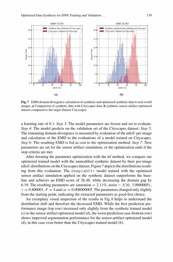
Optimized Data Synthesis for DNN Training and Validation … 139

0 20 40 60 80 100mIoU [%]

0

5

10

15

20

25

30

ImageCount

EMD 32.670

Synthetic data validated on CityscapesCityscapes validated on Cityscapes

(a)

0 20 40 60 80 100mIoU [%]

0

5

10

15

20

25

30

ImageCount

EMD 26.483

Synthetic optimized data validated on CityscapesCityscapes validated on Cityscapes

(b)

Fig. 7 EMD domain divergence calculation of synthetic and optimized synthetic data to real-worldimages. a Comparison of synthetic data with Cityscapes data, b synthetic sensor artifact optimizeddataset compared to the target dataset Cityscapes

a learning rate of 0.1. Step 3: The model parameters are frozen and set to evaluate.Step 4: The model predicts on the validation set of the Cityscapes dataset. Step 5:The remaining domain divergence is measured by evaluation of the mIoU per imageand calculation of the EMD to the evaluations of a model trained on Cityscapes.Step 6: The resulting EMD is fed as cost to the optimization method. Step 7: Newparameters are set for the sensor artifact simulation, or the optimization ends if thestop criteria are met.

After iterating the parameter optimization with the trf method, we compare ouroptimized trained model with the unmodified synthetic dataset by their per-imagemIoUdistributions on theCityscapes dataset. Figure7 depicts the distributions result-ing from this evaluation. The DeeplabV3+ model trained with the optimizedsensor artifact simulation applied on the synthetic dataset outperforms the base-line and achieves an EMD score of 26.48, while decreasing the domain gap by6.19. The resulting parameters are saturation = 2.11%, noise ∼ N (0, 3.0000005) ,γ = 0.800001, F = 4 and ca = 0.008000005. The parameters changed only slightlyfrom the starting point, indicating the extracted parameters as good first choice.

An exemplary visual inspection of the results in Fig. 8 helps to understand thedistribution shift and therefore the decreased EMD. While the best prediction per-formance image (top row) increased only slightly from the synthetic trained model(c) to the sensor artifact optimized model (d), the worst prediction case (bottom row)shows improved segmentation performance for the sensor-artifact-optimized model(d), in this case even better than the Cityscapes trained model (b).

140 K. Hagn and O. Grau

Table2

Performance

results

asper-classmIoU,o

verallmIoU,and

EMDdo

maindivergence

evaluatedon

City

scapes

with

mod

elstrainedon

City

scapes,o

ursynthetic

only,synthetic

with

rand

omparameterized

lens

artifacts,andsynthetic

extractedparameterized

lens

artifactsdatasets.Fo

rthelattertwo,

thereare

mod

elsevaluatedon

City

scapes

with

andwith

outop

timizationof

theparametersforthesensor

lens

artifactsimulation.

The

mod

eltrainedwith

optim

ized

extractedparametersachieves

thehigh

estp

erform

ance

ontheCity

scapes

dataset

Modeltrained

onOptim

ized

road

sidewalk

building

pole

traffic

light

traffic

sign

vegetation

sky

human

car

truck

mIoU

←EMD

→

City

scapes

no97.50

81.21

92.22

54.54

57.28

70.26

92.33

93.98

82.55

93.67

81.62

81.56

–

w/o

artifacts

no60.46

23.51

71.99

10.70

26.00

13.47

75.72

74.70

51.27

34.46

1.74

40.37

32.67

w/rando

martifacts

no77.86

20.56

60.66

8.21

17.83

7.36

72.18

68.21

50.53

74.01

4.68

41.58

30.03

w/extracted

artifacts

no80.65

27.17

66.54

10.43

21.64

11.87

68.82

67.99

59.22

70.06

7.39

44.71

29.84

w/rando

martifacts

yes

82.89

34.69

71.11

11.29

16.66

9.12

69.81

76.77

61.48

79.50

5.30

45.76

26.58

w/extracted

artifacts

yes

79.62

30.30

75.74

16.30

28.31

13.86

78.75

70.88

59.74

64.06

6.42

47.63

26.48

Optimized Data Synthesis for DNN Training and Validation … 141

(a) Original (b) CS Pred (c) Synth Pred (d) Synth Opt Pred

Fig. 8 Top row: Best performance predictions. Bottom row: Worst performance predictions. aOriginal, b Cityscapes-trained model prediction, c synthetically trained model prediction, and dsensor artifact optimized trained model prediction. While top performance increased only slightly,the optimization lead to more robust predictions in worst case, i.e., harder examples

We compare the overall mIoU performance on the Cityscapes datasets betweenmodels trainedwith the initial unmodified synthetic dataset, the synthetic datasetwithrandom initialized lens artifact parameters, and the synthetic dataset with extractedparameters from Cityscapes with the baseline of a model trained on the Cityscapesdataset. Results are listed in Table2 (rows 1–4). Additionally, for the random andthe extracted parameters, we evaluate the performance with initial and optimizedparameters, where the parameters have been optimized by our EMD minimization(rows 5 and 6). While the model without any sensor simulation achieves the low-est overall performance (row 2), the model with random parameter initializationachieves a slightly higher performance (row 3) and is surpassed by the model withthe Cityscapes extracted parameters (row 4). Next, we take the models trained withoptimized parameters into account (rows 5 and 6). Both models outperform all non-optimized experiment settings in terms of overall mIoU, with the model using opti-mized extracted parameters from Cityscapes showing the best overall mIoU (row 6).Concretely, the model trained with optimized random starting parameters achieveshigher performance on classes road, sidewalk, human, and even significantly on thecar class but still falls behind on five of the remaining classes and the overall perfor-mance on the Cityscapes dataset (row 5). Further, the random parameter optimizedmodel took over 22 iterations to converge to its local minimum, whereas the opti-mization of extracted starting parameters only took six iterations until reaching alocal minimum, making it more than three times faster to converge. Furthermore,it is shown that all models with applied sensor lens artifacts outperform the modeltrained without additional lens artifacts.

4.3 EMD Cross-evaluation

To get a deeper understanding of the implications of our EMD score, we evaluate ourEMD results on a range of real-world and synthetic datasets for semantic segmenta-tion. Including real-world datasets A2D2 [GKM+20], Cityscapes (CS) [COR+16],

142 K. Hagn and O. Grau

Table 3 Cross-domain divergence results of models trained on different real-world and syntheticdatasets and evaluated on various validation or test sets of an average size of 1000 images. Thedomain divergence is measured with our proposed EMD measure; boldface values indicate thelowest divergence comparing our synthetic (Synth) and synthetic-optimized (SynthOpt) datasets,whereas underlined values indicate the lowest divergence values over all the datasets. The modeltrained with optimized lens artifacts applied to the synthetic images exhibits a smaller domaindivergence than the model trained without lens artifacts

EMD ↓ A2D2 BDD100K CS GTAV IDD MV SYNS Synth SynthOpt

A2D2 – 18.70 23.46 37.84 20.03 10.72 46.78 34.95 29.32

BDD100K 6.36 – 9.45 22.14 7.26 1.42 36.33 26.43 21.54

CS 10.90 12.09 – 36.42 13.01 4.08 20.62 32.66 26.48

GTAV 33.28 28.37 29.72 – 30.55 23.30 37.53 36.08 32.94

IDD 24.37 19.83 24.71 34.71 – 12.81 46.23 41.64 36.95

MV 10.63 10.36 14.34 28.35 9.20 – 35.97 30.35 27.03

SYNS 25.45 31.46 23.64 45.16 25.12 23.45 – 43.76 43.56

Berkeley Deep Drive (BDD100K) [YCW+20], Mapillary Vistas (MV) [NOBK17],India Driving Dataset (IDD) [VSN+18], as well as synthetic GTAV [RVRK16], oursynthetic (Synth and SynthOpt) [KI 20], and Synscapes (SYNS) [WU18] datasets.In Table3 the results of cross-domain analysis measured with the EMD score aredepicted. The columns denote that a DeeplabV3+ model has been trained on thecorresponding dataset, i.e., the source dataset, whereas the rows denote the datasetsit was evaluated on, i.e., the target datasets. Our optimized synthetic dataset achieveslower EMD scores, shown in boldface, than the synthetic baseline.While the domaindivergencedecrease is highon real datasets, the divergencedecreasedonlymarginallyfor the other synthetic datasets. Inspecting the EMD result on all datasets, the lowestdivergence values are indicated by underline; the MV dataset shows to be closest toall the other evaluated datasets.

To set our measure in relation to established domain distance measures, we cal-culated the FID from each of our considered datasets to one another. The results areshown in Table4. The FID, defined in (7), is the Wasserstein-2 distance of featurevectors from the InceptionV3 [SVI+16] network sampled on the two datasets tobe compared with each other.

Again, boldface values indicate the lowest FID values between the synthetic(Synth) and synthetic-optimized (SynthOpt) datasets, whereas underlined valuesindicate the lowest values of all datasets. Here, only 4 out of the 7 datasets arecloser, measured by the FID, to the synthetic-optimized dataset than to the origi-nal dataset. Furthermore, the FID sees the CS and the SYNS dataset closer to oneanother than the EMD divergence measure, while the MV dataset shows the lowestFID among the other evaluated datasets.

FID and EMD somewhat agree, if we evaluate the distance as minimum per-rowin both tables, that the Mapillary Vistas dataset is in most cases the dataset that isclosest to all other datasets.

Optimized Data Synthesis for DNN Training and Validation … 143

Table 4 Cross-domain distance resultsmeasuredwith the Fréchet inception distance (FID). LowestFID between synthetic (Synth) and synthetic optimized (SynthOpt) datasets are in boldface, whereasthe lowest FID values over all datasets are underlined

FID ↓ A2D2 BDD100K CS GTAV IDD MV SYNS Synth SynthOpt

A2D2 – 60.16 98.46 78.16 58.75 41.84 109.35 116.54 121.55

BDD100K 60.16 – 59.90 62.42 52.15 29.66 74.871 115.51 109.08

CS 98.46 59.90 – 85.81 68.92 59.69 43.87 119.97 112.42

GTAV 78.16 62.42 85.81 – 74.08 51.00 89.62 92.513 92.24

IDD 58.75 52.15 68.92 74.08 – 37.36 64.09 118.06 125.30

MV 41.84 29.66 59.69 51.00 37.36 – 70.24 74.46 78.66

SYNS 109.35 74.87 43.87 89.62 64.09 70.24 – 113.77 108.3

Now, calculating the minimum per-column in both tables, the benefit of ourasymmetric EMD comes to the light. The minimum per-column values of the FIDare unchanged due to the diagonal symmetry of the cross-evaluation matrix stem-ming from the inherent symmetry of the measure. However, the EMD regards theBDD100K as the closest dataset. An intuitive explanation for the different minimumobservations of the EMD is as follows: Training with many images exhibiting dif-ferent geospatial and sensor properties of the Mapillary Vistas dataset covers a verybroad domain and results in good generalization capability and therefore evaluationperformance. Training with any of the other datasets cannot generalize well to thevast domain of Mapillary Vistas but to the rather constrained domain of BDD100K,which consists of lower resolution images with heavy compression artifacts, whereeven a model that has been trained on BDD100K does not generalize well on.

The asymmetric nature of our EMD allows for a more thorough and complexanalysis of dataset discrepancies, when applied to the tasks of visual understanding,e.g., semantic segmentation, which otherwise cannot be captured by inherently sym-metric distance metrics such as FID. Contrasting to [LLFW20], we could with ourevaluation method not identify a consistency between FID and the generalizationdivergence, i.e., our EMD measure.

5 Conclusions

In this chapter, we could demonstrate that by utilizing the performance metric perimage as a proxy distribution for a dataset and the earth mover’s distance (EMD)as a divergence measure between distributions, one can decrease visual differencesof a synthetic dataset through optimization and increase the viability of CGI fortraining and validation purposes of perceptive AI. To reinforce our argument forper-image performance measures as proxy distributions, we showed that training anensemble of a fixedmodelwith different random starting conditions butwith the same

144 K. Hagn and O. Grau

hyperparameters leads to the same per-image performance distributions when theseensemble models are evaluated on the validation set of the training dataset. Whenutilizing synthetic imagery for validation, the domain gap, due to visual differencesbetween real and computer-generated images, is hindering the applicability of thesedatasets. As a step toward decreasing the visual differences, we apply the proposeddivergence measure as a cost function to an optimization which varies the parametersof the sensor artifact simulation, while trying to re-create the sensor artifacts that thereal-world dataset exhibits. As starting point of the sensor artifact parameters, weextracted empirically the values from chosen images of the real-world dataset. Theoptimization improved the visual differencebetween the real-world and the optimizedsynthetic dataset measurably by the EMD and we could show that even when startingwith random initialized parameters we can decrease the EMD and increase the mIoUon the target datasets. When measuring the divergence after parameter optimizationto other real-world and synthetic datasets, we could show that the EMD decreasesfor all considered datasets but when measured by the FID only four of the datasetsare closer. As the EMD is derived from the mIoU per image, it is an indicator ofperformance on the target dataset, whereas the FID fails to relate with performance.Effective minimization of the visual difference between synthetic and real-worlddatasets with the EMD domain divergence measure is one step further toward fullyutilizing CGI for validation of perceptive AI functions.

Acknowledgements The research leading to these results is fundedby theGermanFederalMinistryfor Economic Affairs and Energy within the project “Methoden und Maßnahmen zur Absicherungvon KI-basierten Wahrnehmungsfunktionen für das automatisierte Fahren (KI Absicherung)”. Theauthors would like to thank the consortium for the successful cooperation.

References

[BB95] W. Burger, M.J. Barth, Virtual reality for enhanced computer vision, in J. Rix, S. Haas,J. Teixeira (eds.), Virtual Prototyping: Virtual Environments and the Product DesignProcess (Springer, 1995), pp. 247–257

[Bis95] M. Christopher Bishop, Training with noise is equivalent to Tikhonov regularization.Neural Comput. 7(1), 108–116 (1995)

[BSAG21] M. Binkowski, D.J. Sutherland, M. Arbel, A. Gretton,DemystifyingMMDGANs, Jan.2021, pp. 1–36. arxiv:1801.01401

[CLP13] G. Csurka, D. Larlus, F. Perronnin, What is a good evaluation measure for semanticsegmentation? in Proceedings of the British Machine Vision Conference (BMVC),Bristol, UK, Sept. 2013, pp. 1–11

[COR+16] M. Cordts, M. Omran, S. Ramos, T. Rehfeld, M. Enzweiler, R. Benenson, U. Franke,S. Roth, B. Schiele, The Cityscapes dataset for semantic urban scene understand-ing, in Proceedings of the IEEE/CVF Conference on Computer Vision and PatternRecognition (CVPR), Las Vegas, NV, USA, June 2016, pp. 3213–3223

[CSVJR18] A. Carlson, K.A. Skinner, R. Vasudevan, M. Johnson-Roberson, Modeling cameraeffects to improve visual learning from synthetic data, in Proceedings of the EuropeanConference on Computer Vision (ECCV) Workshops, Munich, Germany, Aug. 2018,pp. 505–520

Optimized Data Synthesis for DNN Training and Validation … 145

[CSVJR19] A. Carlson, K.A. Skinner, R. Vasudevan, M. Johnson-Roberson, Sensor Transfer:Learning Optimal Sensor Effect Image Augmentation for Sim-to-Real Domain Adap-tation, Jan. 2019, pp. 1–8. arxiv:1809.06256

[CV14] V. Chari, A. Veeraraghavan, L. Distortion, Radial distortion, in Computer Vision: AReference Guide. ed. by K. Ikeuchi (Springer, Boston, MA, 2014), pp. 443–445

[CZP+18] L.-C. Chen, Y. Zhu, G. Papandreou, F. Schroff, H. Adam, Encoder-Decoder withatrous separable convolution for semantic image segmentation, in Proceedings of theEuropean Conference on Computer Vision (ECCV), Munich, Germany, Sept. 2018,pp. 833–851

[dCCN+16] G.B.P. da Costa, W.A. Contato, T.S. Nazaré, J.E.S. do Batista Neto, M. Ponti, AnEmpirical Study on the Effects of Different Types of Noise in Image ClassificationTasks, Sept. 2016, pp. 1–6. arxiv:1609.02781

[DDS+09] J. Deng, W. Dong, R. Socher, L.-J. Li, K. Li, F.-F. Li, ImageNet: a large-scale hier-archical image database, in Proceedings of the IEEE/CVF Conference on ComputerVision and Pattern Recognition (CVPR), Miami, FL, USA, June 2009, pp. 248–255

[DRC+17] A. Dosovitskiy, G. Ros, F. Codevilla, A. Lopez, V. Koltun, CARLA: an open urbandriving simulator, in Proceedings of the Conference on Robot Learning CORL, Moun-tain View, CA, USA, Nov. 2017, pp. 1–16

[FMWR18] E. Fernandez-Moral, R. Martins, D. Wolf, P. Rives, A new metric for evaluatingsemantic segmentation: leveraging global and contour accuracy, in Proceedings of theIEEE Intelligent Vehicles Symposium (IV), Changshu, China, June 2018, pp. 1051–1056

[GKM+20] J. Geyer, Y. Kassahun,M.Mahmudi, X. Ricou, R. Durgesh, A.S. Chung, L. Hauswald,V.H. Pham, M. Mühlegg, S. Dorn, T. Fernandez, M. Jänicke, S. Mirashi, C. Savani,M. Sturm, O. Vorobiov, M. Oelker, S. Garreis, P. Schuberth, A2D2: Audi AutonomousDriving Dataset, April 2020, pp. 1–10. arxiv:2004.06320

[GL15] Y. Ganin, V. Lempitsky, Unsupervised domain adaptation by backpropagation, inProceedings of the International Conference on Machine Learning (ICML), Lille,France, July 2015, pp. 1180–1189

[HRU+17] M. Heusel, H. Ramsauer, T. Unterthiner, B. Nessler, S. Hochreiter, GANs trained bya two time-scale update rule converge to a local Nash equilibrium, in Proceedingsof the Conference on Neural Information Processing Systems (NIPS/NeurIPS), LongBeach, CA, USA, Dec. 2017, pp. 6626–6637

[HTP+18] J. Hoffman, E. Tzeng, T. Park, J.-Y. Zhu, P. Isola, K. Saenko, A. Efros, T. Darrell,CyCADA: cycle-consistent adversarial domain adaptation, inProceedings of the Inter-national Conference on Machine Learning (ICML), Stockholm, Sweden, July 2018,pp. 1989–1998

[HZRS16] K. He, X. Zhang, S. Ren, J. Sun, Deep residual learning for image recognition, in Pro-ceedings of the IEEE/CVF Conference on Computer Vision and Pattern Recognition(CVPR), Las Vegas, NV, USA, June 2016, pp. 770–778

[KI 20] KI Absicherung Consortium. KIAbsicherung: Safe AI for AutomatedDriving (2020).Assessed 18 Nov. 2021

[KPT+17] S.Kolouri, S.R. Park,M.Thorpe,D. Slepcev,G.K.Rohde,Optimalmass transport: sig-nal processing and machine-learning applications. IEEE Signal Process. Mag. 34(4),43–59 (2017)

[LCWJ15] M. Long, Y. Cao, J. Wang, M.I. Jordan, Learning transferable features with deepadaptation networks, in Proceedings of the International Conference on MachineLearning (ICML), July 2015, pp. 97–105

[LLFW20] Z. Liu, T. Lian, J. Farrell, B. Wandell, Neural network generalization: the impact ofcamera parameters. IEEE Access 8, 10443–10454 (2020)

[NdCCP18] T.S. Nazaré, G.B.P. da Costa, W.A. Contato, M. Ponti, Deep convolutional neuralnetworks and noisy images, in Proceedings of the Iberoamerican Congress on PatternRecognition (CIARP), Madrid, Spain, Nov. 2018, pp. 416–424

146 K. Hagn and O. Grau

[NOBK17] G. Neuhold, T. Ollmann, S. Rota Bulò, P. Kontschieder, The mapillary vistas datasetfor semantic understanding of street scenes, in Proceedings of the IEEE InternationalConference on Computer Vision (ICCV), Venice, Italy, Oct. 2017, pp. 4990–4999

[PTKY09] S.J. Pan, I.W. Tsang, J.T. Kwok, Q. Yang, Domain adaptation via transfer componentanalysis, in Proceedings of the International Joint Conferences on Artificial Intelli-gence (IJCAI), Pasadena, CA, USA, July 2009, pp. 1187–1192

[RD14] R. Ramanath, M.S. Drew, Color Spaces, in Computer Vision: A Reference Guide. ed.by K. Ikeuchi (Springer, Boston, MA, 2014), pp. 123–132

[RHK17] S.R. Richter, Z. Hayder, V. Koltun, Playing for benchmarks, in Proceedings of theIEEE International Conference on Computer Vision (ICCV), Venice, Italy, Oct. 2017,pp. 2232–2241

[RSM+16] G. Ros, L. Sellart, J. Materzynska, D. Vazquez, A.M. Lopez, The SYNTHIA dataset: alarge collection of synthetic images for semantic segmentation of urban scenes, inPro-ceedings of the IEEE/CVF Conference on Computer Vision and Pattern Recognition(CVPR), Las Vegas, NV, USA, June 2016, pp. 3234–3243

[RTC17] A. Ramdas, N. García Trillos, M. Cuturi, On Wasserstein two sample testing andrelated families of nonparametric tests. Entropy 19(2), 47 (2017)

[RTG+19] H. Rezatofighi, N. Tsoi, J.Y. Gwak, A. Sadeghian, I. Reid, S. Savarese, Generalizedintersectionover union: ametric and a loss for boundingbox regression, inProceedingsof the IEEE/CVF Conference on Computer Vision and Pattern Recognition (CVPR),Long Beach, CA, USA, June 2019, pp. 658–666

[RV19] S.V. Ravuri, O. Vinyals, Seeing is not necessarily believing: limitations of BigGANsfor data augmentation, in: Proceedings of the International Conference on LearningRepresentations (ICLR) Workshops, New Orleans, LA, USA, June 2019, pp. 1–5

[RVRK16] S.R. Richter, V. Vineet, S. Roth, V. Koltun, Playing for data: ground truth from com-puter games, inProceedings of the EuropeanConference onComputer Vision (ECCV),Amsterdam, The Netherlands, Oct. 2016, pp. 102–118

[SAS+18] F.S. Saleh, M.S. Aliakbarian, M. Salzmann, L. Petersson, J.M. Alvarez, Effectiveuse of synthetic data for urban scene semantic segmentation, in Proceedings of theEuropean Conference on Computer Vision (ECCV), Munich, Germany, Sept. 2018,pp. 84–100

[SGH20] Q.S. Sha, O. Grau, K. Hagn, DNN analysis through synthetic data variation, in Pro-ceedings of the ACM Computer Science in Cars Symposium (CSCS), virtual confer-ence, Dec. 2020, pp. 1–10

[SGZ+16] T. Salimans, I. Goodfellow, W. Zaremba, V. Cheung, A. Radford, Xi Chen, ImprovedTechniques for Training GANs, June 2016, pp. 1–10. arxiv:1606.03498

[SLA+15] J. Schulman, S. Levine, P. Abbeel, M. Jordan, P. Moritz, Trust region policy optimiza-tion, in Proceedings of the International Conference on Machine Learning (ICML),Lille, France, July 2015, pp. 1889–1897

[Stu14] P. Sturm, Pinhole Camera Model, in Computer Vision: A Reference Guide. ed. by K.Ikeuchi (Springer, Boston, MA, 2014), pp. 610–613

[SVI+16] C. Szegedy, V. Vanhoucke, S. Ioffe, J. Shlens, Z. Wojna, Rethinking the inceptionarchitecture for computer vision, in Proceedings of the IEEE/CVF Conference onComputer Vision and Pattern Recognition (CVPR), Las Vegas, NV, USA, June 2016,pp. 2818–2826

[THS+18] Y.-H. Tsai, W.-C. Hung, S. Schulter, K. Sohn, M.-H. Yang, M. Chandraker, Learningto adapt structured output space for semantic segmentation, in Proceedings of theIEEE/CVF Conference on Computer Vision and Pattern Recognition (CVPR), SaltLake City, UT, USA, June 2018, pp. 7472–7481

[THSD17] E. Tzeng, J. Hoffman, K. Saenko, T. Darrell, Adversarial discriminative domain adap-tation, in Proceedings of the IEEE/CVF Conference on Computer Vision and PatternRecognition (CVPR), Honolulu, HI, USA, July 2017, pp. 2962–2971

[VGO+20] P. Virtanen, R. Gommers, T.E. Oliphant, M. Haberland, T. Reddy, D. Cournapeau, E.Burovski, P. Peterson, W. Weckesser, J. Bright, S.J. van der Walt, M. Brett, J. Wilson,

Optimized Data Synthesis for DNN Training and Validation … 147

K.J. Millman, N. Mayorov, A.R.J. Nelson, E. Jones, R. Kern, E. Larson, C.J. Carey,l. Polat, Y. Feng, E.W. Moore, J. Vand erPlas, D. Laxalde, J. Perktold, R. Cimrman, I.Henriksen, E.A. Quintero, C.R. Harris, A.M. Archibald, A.H. Ribeiro, F. Pedregosa,P. van Mulbregt, and SciPy 1.0 Contributers. Fundamental algorithms for scientificcomputing in python. SciPy 1.0. Nat. Methods 17, 261–272 (2020)

[VSN+18] G. Varma, A. Subramanian, A. Namboodiri, M. Chandraker, C.V. Jawahar, IDD: ADataset for Exploring Problems of Autonomous Navigation in Unconstrained Envi-ronments, Nov. 2018, pp. 1–9. arxiv:1811.10200

[WU18] M. Wrenninge, J. Unger, Synscapes: A Photorealistic Synthetic Dataset for StreetScene Parsing, Oct. 2018, pp. 1–13. arxiv:1810.08705

[YCW+20] F. Yu, H. Chen, X. Wang, W. Xian, Y. Chen, F. Liu, V. Madhavan, T. Darrell,BDD100K: a diverse driving dataset for heterogeneous multitask learning, in Pro-ceedings of the IEEE/CVF Conference on Computer Vision and Pattern Recognition(CVPR), virtual conference, June 2020, pp. 2636–2645

Open Access This chapter is licensed under the terms of the Creative Commons Attribution 4.0International License (http://creativecommons.org/licenses/by/4.0/), which permits use, sharing,adaptation, distribution and reproduction in any medium or format, as long as you give appropriatecredit to the original author(s) and the source, provide a link to the Creative Commons license andindicate if changes were made.

The images or other third party material in this chapter are included in the chapter’s CreativeCommons license, unless indicated otherwise in a credit line to the material. If material is notincluded in the chapter’s Creative Commons license and your intended use is not permitted bystatutory regulation or exceeds the permitted use, you will need to obtain permission directly fromthe copyright holder.

Improved DNN Robustness by Multi-taskTraining with an AuxiliarySelf-Supervised Task

Marvin Klingner and Tim Fingscheidt

Abstract While deep neural networks for environment perception tasks inautonomous driving systems often achieve impressive performance on clean andwell-prepared images, their robustness under real conditions, i.e., on images beingperturbed with noise patterns or adversarial attacks, is often subject to a significantlydecreased performance. In this chapter,we address this problem for the task of seman-tic segmentation by proposing multi-task training with the additional task of depthestimation with the goal to improve the DNN robustness. This method has a verywide potential applicability as the additional depth estimation task can be trained in aself-supervised fashion, relying only on unlabeled image sequences during training.The final trained segmentation DNN is, however, still applicable on a single-imagebasis during inference without additional computational overhead compared to thesingle-task model. Additionally, our evaluation introduces a measure which allowsfor a meaningful comparison between different noise and attack types. We showthe effectiveness of our approach on the Cityscapes and KITTI datasets, where ourmethod improves the DNN performance w.r.t. the single-task baseline in terms ofrobustness againstmultiple noise and adversarial attack types,which is supplementedby an improved absolute prediction performance of the resulting DNN.

1 Introduction

Motivation: For a safe operation of highly automated driving systems, a reliableperception of the environment is crucial. Various perception tasks such as semanticsegmentation [LSD15], [CPK+18], depth estimation [EPF14], [ZBSL17], or opticalflow estimation [LLKX19] are often implemented by deep neural networks (DNNs).The output of these DNNs is then used to build a model of the environment, which

M. Klingner (B) · T. FingscheidtInstitute for Communications Technology (IfN), Technische Universität Braunschweig,Schleinitzstr. 22, 38106 Braunschweig, Germanye-mail: m.klingner@tu-bs.de

T. Fingscheidte-mail: t.fingscheidt@tu-bs.de

© The Author(s) 2022T. Fingscheidt et al. (eds.), Deep Neural Networks and Data for Automated Driving,https://doi.org/10.1007/978-3-031-01233-4_5

149

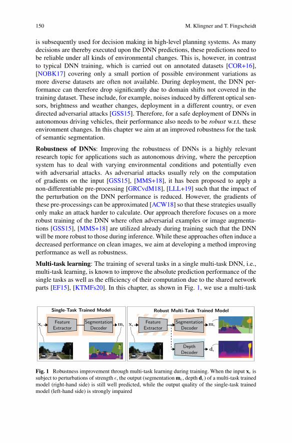
150 M. Klingner and T. Fingscheidt

is subsequently used for decision making in high-level planning systems. As manydecisions are thereby executed upon the DNN predictions, these predictions need tobe reliable under all kinds of environmental changes. This is, however, in contrastto typical DNN training, which is carried out on annotated datasets [COR+16],[NOBK17] covering only a small portion of possible environment variations asmore diverse datasets are often not available. During deployment, the DNN per-formance can therefore drop significantly due to domain shifts not covered in thetraining dataset. These include, for example, noises induced by different optical sen-sors, brightness and weather changes, deployment in a different country, or evendirected adversarial attacks [GSS15]. Therefore, for a safe deployment of DNNs inautonomous driving vehicles, their performance also needs to be robust w.r.t. theseenvironment changes. In this chapter we aim at an improved robustness for the taskof semantic segmentation.

Robustness of DNNs: Improving the robustness of DNNs is a highly relevantresearch topic for applications such as autonomous driving, where the perceptionsystem has to deal with varying environmental conditions and potentially evenwith adversarial attacks. As adversarial attacks usually rely on the computationof gradients on the input [GSS15], [MMS+18], it has been proposed to apply anon-differentiable pre-processing [GRCvdM18], [LLL+19] such that the impact ofthe perturbation on the DNN performance is reduced. However, the gradients ofthese pre-processings can be approximated [ACW18] so that these strategies usuallyonly make an attack harder to calculate. Our approach therefore focuses on a morerobust training of the DNN where often adversarial examples or image augmenta-tions [GSS15], [MMS+18] are utilized already during training such that the DNNwill be more robust to those during inference. While these approaches often induce adecreased performance on clean images, we aim at developing a method improvingperformance as well as robustness.

Multi-task learning: The training of several tasks in a single multi-task DNN, i.e.,multi-task learning, is known to improve the absolute prediction performance of thesingle tasks as well as the efficiency of their computation due to the shared networkparts [EF15], [KTMFs20]. In this chapter, as shown in Fig. 1, we use a multi-task

Single-Task Trained Model

x mFeatureExtractor

SegmentationDecoder

Robust Multi-Task Trained Model

x

d

mFeatureExtractor

DepthDecoder

SegmentationDecoder

Fig. 1 Robustness improvement through multi-task learning during training. When the input xε issubject to perturbations of strength ε, the output (segmentationmε, depth dε) of a multi-task trainedmodel (right-hand side) is still well predicted, while the output quality of the single-task trainedmodel (left-hand side) is strongly impaired

Improved DNN Robustness by Multi-task Training … 151

network for semantic segmentation and depth estimation, for which these propertieshave also been shown in severalworks [KGC18], [KTMFs20]. Particularly,we follow[KBFs20] in focusing on the additional robustness-increasing properties of such amulti-task training. Moreover, it is important to note that the depth estimation canbe trained in a self-supervised fashion, which only requires short unlabeled videosequences and thereby usually does not impose large additional requirements in termsof data. While it was still necessary to manually find a good weighting between thesingle tasks in [KBFs20],we apply theGradNorm taskweighting strategy [CBLR18],which automatically sets and adapts the task weighting according to the task-specifictraining progress. Also, we show the method’s applicability across a wider range ofdatasets.

Comparability of perturbations: Up to now, a wide variety of different possibleadversarial attack and noise types has been proposed [GW08], [GSS15], [CW17],[MMS+18]. However, each of these image perturbations is characterized by its ownset of parameters, e.g., the standard deviation of the Gaussian noise distributionor the maximum noise value for many adversarial attacks. This makes it hard tocompare perturbation strengths in a single mutual evaluation. To better comparethese effects and to be able to draw conclusions between different noise and attacktypes, we employ a measure based on the signal-to-noise ratio, which enables a faircomparison between different perturbation types in terms of strength.

Contributions: To sum up, our contribution with this chapter is threefold. First, wepropose a multi-task learning strategy with the task of self-supervised monoculardepth estimation to improve a DNN’s robustness. Second, we provide a detailedanalysis of the positive effects of this method on DNN performance and robustnessto multiple input perturbations. Third, we employ a general measure for perturbationstrength, thereby making different noise and attack perturbation types comparable.

2 Related Works

In this section, we give an overview of related multi-task learning approaches fordepth estimation and semantic segmentation. Afterward, we discuss methods toimprove the robustness of DNNs focusing on approaches for semantic segmenta-tion.

Multi-task learning The performance of basic perception tasks such as seman-tic segmentation [LSD15] and depth estimation [EF15] has increased significantlyby employing fully convolutional neural networks. Furthermore, these tasks canbe learned jointly in a multi-task learning setup by employing a shared encoder,which was shown to be of mutual benefit for both tasks through the more exten-sively learned scene understanding [EF15], [KGC18]. This could be further facil-itated by combining the loss functions to enforce cross-task consistency duringoptimization [KGC18], [XOWS18], [ZCX+19]. For depth estimation, the research

152 M. Klingner and T. Fingscheidt

focus shifted from supervised to self-supervised training techniques [ZBSL17],[GMAB17], [GMAFB19], due to themore general applicability on unlabeled videos,which are more readily available than labeled datasets. Accordingly, such tech-niques have also been employed in multi-task setups with semantic segmentation[CLLW19], [GHL+20], [NVA19]. Usually, the focus of these works is to improvethe absolute prediction performance of the single involved tasks. Thereby, it wasproposed to exclude the influence of dynamic objects such as cars or pedestrians[KTMFs20], [RKKY+21b], [RKKY+21a] to employ pixel-adaptive convolution forimproved semantic guidance [GHL+20], [RKKY+21b], or to enforce cross-task(edge) consistency between both tasks’ outputs [CLLW19], [ZBL20], [YZS+18],[MLR+19]. The approaches have also been extended from simple pinhole cameramodels to more general fisheye camera models [RKKY+21b], [RKKY+21a]. Forsemantic segmentation, the depth estimation can also be beneficial in unsuperviseddomain adaptation approaches [KTMFs20], [LRLG19], [VJB+19].

In this chapter, we build upon these advances by employing a multi-task learningsetup of self-supervised depth estimation and semantic segmentation as introducedby Klingner et al. [KTMFs20]. However, in contrast to [KTMFs20], we put thefocus rather on the robustness instead of the absolute prediction performance of theresulting semantic segmentation DNN.

Robustness of (semantic segmentation)DNNsWhileDNNs can achieve an impres-sive performance on clean images, their performance is usually not robust w.r.t. addi-tive noise [Bis95], [HK92]. For safety-critical application this is a particularly highrisk, if this noise is calculated in a way that it is nearly not recognizable if added to theimage, but still heavily impairs the performance, as shownby theworks on adversarialexamples by Szegedy et al. [SZS+14]. Consequently, subsequent works developedvarious kinds of targeted and non-targeted perturbations, calculated in an image-specific fashion and optimized to fool the DNN. These adversarial examples rangefrom simple non-iterative methods such as the fast gradient sign method (FGSM)[GSS15] tomore complex iteratively calculatedmethods such as themomentum iter-ative fast gradient signmethod (MI-FGSM) [DLP+18], theCarlini andWagner attack(CW) [CW17], or the projected gradient descent (PGD) method [MMS+18]. Whilethese image-specific attacks may not be a relevant danger in real applications due tothe high computational effort per image, the existence of image-agnostic adversarialperturbations (UAPs) has also been shown, e.g., by prior-driven uncertainty esti-mation (PD-UA) [LJL+19], universal adversarial perturbation (UAP) [MDFFF17],or fast feature fool (FFF) [MGB17]. Although most of these works focus on therather simple task of image classification, the applicability of these attacks to seman-tic segmentation is well known [AMT18], [MGR19], [BLK+21]. Furthermore, theattacks can be designed in a fashion such that the semantic segmentation outputs arecompletely wrong but still appear realistic [ASG+19], [MCKBF17].

The vulnerability of DNNs to different kinds of adversarial attacks has encour-aged research in defense methods, which improve the robustness against these per-turbations. They can be roughly divided into three categories. First, for gradientmasking, the idea is to prevent a potential attacker from calculating the gradients

Improved DNN Robustness by Multi-task Training … 153

[CBG+17], [MMS+18], [PMG+17]. However, Athalye et al. [ACW18] showed thatthe perturbations can be calculated from a different model. Also, they can be calcu-lated in an image-agnostic (universal) fashion [MCKBF17], [MDFFF17], see alsothe Chapter “Improving Transferability of Generated Universal Adversarial Per-turbations for Image Classification and Segmentation” [HAMFs22], such that gra-dient masking methods cannot prevent the network’s vulnerability to adversarialattacks under all conditions. Second, through input transformations, the perturba-tions can be removed from the input image [GRCvdM18], [KBV+21], [LLL+19],e.g., by JPEG image compression [ATT18] or by incorporation of randomness[RSFM19], [XWZ+18]. While this improves the performance on attacked images,these transformations usually impair the performance on clean images, introducingan unfavorable trade-off. Third, redundancy among two or three networks servingthe same task can be exploited, if networks are enforced to reveal some indepen-dence [BHSFs19], [BKV+20]. Fourth, robust training methods can be employedsuch that the DNN is less sensitive to fail because of attacks from the start. Com-mon approaches include, e.g., adversarial training [GSS15], [MMS+18], robustness-oriented loss functions [BHSFs19], [BKV+20], [CLC+19], or self-supervision fromauxiliary tasks [CLC+20], [HMKS19], [ZYC+20] during (pre-)training. Our chapteralso focuses on robustness through self-supervision, where we introduce multi-tasklearning with the auxiliary task of depth estimation as a method to improve a seman-tic segmentation DNN’s robustness, which can be seen as an extension of [KBFs20].Thereby, we achieve an improved performance, while also being more robust andeven introducing a second useful task for scene perception. Compared to [KBFs20],we improve the multi-task learning strategy to reduce the need for manual taskweighting and provide experiments across a wider range of datasets.

3 Multi-task Training Approach

Describing ourmulti-task learning approach,we start by defining our primary seman-tic segmentation task, followed by the auxiliary task of depth estimation. Finally, wedescribe how both tasks are trained in a multi-task learning setup as shown in Fig. 2.

Primary semantic segmentation: Semantic segmentation is defined as the pixel-wise classification of an input image xt = (xt,i ) ∈ GH×W×C at time t, with heightH, width W, number of channels C = 3, and G = {0, 1, ..., 255} (cf. top branch ofFig. 2). Accordingly, for each pixel xt,i ∈ G3 with pixel index i ∈ I = {1, ..., H · W }an output yt,i = (yt,i,s) ∈ I

|S|, I = [0, 1] is predicted, which can be interpreted asthe posterior probabilities that the pixel at index i belongs to a class s ∈ S fromthe set of classes S = {1, 2, ..., |S|}, with the number of classes |S|. The finalpredicted semantic class mt,i ∈ S is determined by applying the argmax operationmt,i = argmaxs∈Syt,i,s . Thereby, the network output yt ∈ I

H×W×|S| is converted to asegmentation mask mt = (mt,i ) ∈ SH×W .

154 M. Klingner and T. Fingscheidt

Fig. 2 Multi-task training setup across domains for the joint learning of depth estimation andsemantic segmentation. While the semantic segmentation is trained on labeled image pairs, thedepth estimation is trained on unlabeled image sequences

As shown in Fig. 2, training of a semantic segmentation network requires groundtruth labels yt ∈ {0, 1}H×W×|S|, which are derived from the ground truth segmenta-tion maskmt ∈ SH×W represented by a one-hot encoding. These are utilized to trainthe network by a cross-entropy loss function as

J segt = − 1

H · W∑

i∈I

∑

s∈Sws yt,i,s · log (

yt,i,s), (1)

wherews are class-wiseweights obtained as outlined in [PCKC16], and yt,i,s ∈ {0, 1}are the single elements from the one-hot encoded ground truth tensor yt = (yt,i,s).

Auxiliary depth estimation: Aiming at a more robust feature representation, weemploy the auxiliary depth estimation task, which can be trained on unlabeled imagesequences, as shown in Fig. 2, bottom part. During training, the depth estimationDNN predicts a depth map dt = (dt,i ) ∈ D

H×W , representing the distance of eachpixel from the camera plane, where D = [dmin, dmax] represents the space of consid-ered depth values constrained between the lower bound dmin and the upper bounddmax. We optimize the depth estimation DNN in a self-supervised fashion by con-sidering two loss terms: First, we make use of the image reconstruction term J ph

t

(photometric loss), which essentially uses the depth estimation in conjunction withthe relative pose between two images, to optimize the camera reprojection modelsbetween two consecutive frames of a video. Second, we apply a smoothness loss termJ smt , allowing high gradients in the depth estimate’s values only in image regions

with high color gradients, such that the total loss can be written as

J deptht = J ph

t + β J smt , (2)

Improved DNN Robustness by Multi-task Training … 155

where β = 10−3 is adopted from previous works [CPMA19], [GMAFB19],[KTMFs20].

To optimize the network, we rely solely on sequential pairs of images xt , xt ′ witht ′ ∈ T ′ = {t−1, t+1}, which are taken from a video. These pairs are passed to anadditional pose network, which predicts the relative poses Tt→t ′ ∈ SE(3) betweenthe image pairs, where SE(3) is the special Euclidean group representing the set of allpossible rotations and translations [Sze10]. The network predicts this transformationin an axis-angle representation such that only the six degrees of freedomare predicted,which are canonically converted to a 4 × 4 matrix for further processing. By lettingthe depth network predict the depth dt , both outputs, i.e., the depth dt and the posesTt→t ′ , can be used to project the image frame xt ′ at time t ′ onto the pixel coordinatesof the image frame xt , which results in two projected images xt ′→t , t ′ ∈ T ′ (for adetailed description, we refer to [KTMFs20]). Conclusively, the reprojection modelcanbeoptimizedbyminimizing the pixel-wise distance between the projected imagesxt ′→t = (xt ′→t,i ) and the actual images xt = (xt,i ) as

J pht = 1

|I|∑

i∈Imint ′∈T ′

(γ

2(1 − SSIMi (xt , xt ′→t )) + (1 − γ)

1

C

∥∥xt,i − xt ′→t,i

∥∥1

).

(3)This so-called minimum reprojection loss or photometric loss [GMAFB19] utilizesa mixture of the structural similarity (SSIM) difference term SSIMi (·) ∈ I, withI = [0, 1], and is computed on 3 × 3 patches of the input, and an L1 difference term‖·‖1 computed over all C = 3 gray value channels. For optimal absolute predictionperformance, the terms are weighted by a factor γ = 0.85, chosen as in previousapproaches [CPMA19], [GMAFB19], [KTMFs20], [YS18]. The depth and posenetworks are then implicitly optimized, as their outputs are the parameters of theprojection model, used to obtain the projected image xt ′→t , whose distance to theactual image xt is minimized by (3).

As the photometric loss J pht does not enforce a relationship in the depth map

between depth values of neighboring pixels, we use a second smoothness loss termJ smt [GMAB17], allowing non-smoothness in the depth map dt only in image loca-

tions with strong color gradients. This loss is computed on the mean-normalizedinverse depth ρt ∈ R

H×W , whose elements can be obtained from the depth map asρt,i = ρt,i

1HW

∑j∈I ρt, j

with ρt,i = 1dt,i

. Thereby, the loss can be formulated as

J smt = 1

|I|∑

i∈I

(|∂h ρt,i | exp

(− 1

C

∥∥∂hxt,i∥∥1

)+ |∂wρt,i | exp

(− 1

C

∥∥∂wxt,i∥∥1

)),

(4)with one-dimensional difference quotients ∂h ρt,i = ∂h ρt,(h,w) = ρt,(h,w) − ρt,(h−1,w)

and ∂wρt,i = ∂wρt,(h,w) = ρt,(h,w) − ρt,(h,w−1) defined with respect to the height andwidth dimensions of the image, respectively. The indices h and w represent the exactpixel position in two dimensions, where h ∈ {2, ..., H} and w ∈ {2, ...,W }, wherewe exclude h = 1 and w = 1 to ensure the existence of a preceding pixel in heightand width dimensions.

156 M. Klingner and T. Fingscheidt

Multi-task learning: To train our model directly in a one-stage fashion withouta pre-trained semantic segmentation network, we choose a multi-task setup with ashared encoder and two task-specific decoder heads as shown in Fig. 2. The decodersfor semantic segmentation and depth estimation are optimized for their respectivetasks according to the losses defined in (1) and (2), respectively, while the encoder isoptimized for both tasks.As in [GL15], [KTMFs20],we let the task-specific gradientsgdeptht and gsegt propagate unscaled in the respective decoders, while their influencewhen reaching the encoder layers during backpropagation are scaled as

gtotalt = λdepthgdeptht + λseggsegt , (5)

where the scalar weight λseg and λdepth determine the weighting between the twotasks. In the other encoder layers, the backpropagation is then executed as usual.By scaling the gradients instead of the losses, the two decoders can learn optimaltask-specific weights, while their influence on the shared encoder can be scaled tothe optimal ratio using (5). Thereby, the encoder does not only learn optimal featuresfor the semantic segmentation task, but can also take profit from the additional dataaccessible by the depth estimation, which can be trained on arbitrary videos.

In this chapter, we compare two kinds of task weightings: First, we apply thegradient weighting (GW) from [KBFs20], where we set λseg = λ and λdepth = 1 − λto scale the influence of both tasks. Here, the hyperparameter λ needs to be tuned tofind the optimal weighting of both tasks. However, the results from [KBFs20] showthat for a badly chosen hyperparameterλ, performance decreases drastically,which iswhy we apply the GradNorm (GN) multi-task learning technique [CBLR18], wherethe scale factors λseg and λdepth are reformulated as learnable parameters λseg(τ ) andλdepth(τ ) which are adapted at each learning step τ . For simplicity, we henceforthabbreviate the tasks with an index k with k ∈ K = {depth, seg}. Thereby, the lossfunction used for optimization of the scale factors, i.e., the task weights, is calculatedas follows:

JGNt (τ ) =

∑

k∈K

∣∣∣G(k)t (τ ) −

( 1

|K |∑

κ∈KG(κ)

t (τ ))

·(r (k)t (τ )

)α ∣∣∣. (6)

It depends on the magnitudeG(k)t (τ ) = ∥∥λ(k)(τ )g(k)t (τ )

∥∥2 of the task-specific gra-

dients g(k)t (τ ) in the last shared layer and the task-specific training rates r (k)t (τ ) =J (k)t (τ ) ·

(1

|K |∑

κ∈K J (κ)t (τ )

)−1with J (k)

t (τ ) = J (k)t (τ ) · (

J (k)t (0)

)−1, depending on

the value of the task-specific losses J (k)t (τ ) taken from (1) and (2) at each step τ in

comparison to their values J (k)t (0) at step τ = 0. These training rates can be inter-

preted as the convergence progress of the single tasks. Note that through the lossfor the scaling factors in (6) a similar and stable convergence speed of both tasksis encouraged, which is essential for a successful multi-task training. The networkis optimized with alternating updates of the scaling factors λ(k)(τ ) by (6) and thenetwork weights by (1) and (2). Although a more stable convergence is generally

Improved DNN Robustness by Multi-task Training … 157

expected, one can still optimize GradNorm (GN) with the hyperparameter α in (6),controlling the restoring force back to balanced training rates. Also, after each step,the task weights are renormalized such that λseg(τ ) + λdepth(τ ) = 1.

4 Evaluation Setup

In this section, we present the input perturbations used to evaluate the model robust-ness, define the perturbation strength, and detail our chosen evaluation metrics.Finally, we provide an overview of our chosen databases and the implementationdetails of our method. The evaluation setup is depicted in Fig. 3.

Image perturbations: After the semantic segmentation network has been trained(either by single-task or multi-task training), we evaluate its robustness during infer-ence by adding a perturbation rε of strength ε to each input image x, yielding aperturbed input image xε = x + rε. For simplicity, we omit the subscript t as theevaluation is carried out on single images. We conduct experiments using two noisetypes and two adversarial attacks, for which we aim at imposing a perturbationstrength ε to make different perturbation types comparable. We measure this com-parable strength by the signal-to-noise ratio (SNR) on the input image xadv, whichis defined as

SNR = E(‖x‖22

)

E(‖rε‖22

) . (7)

Here, E(‖x‖22

)is the expectation value of the sum of the image’s squared gray val-

ues, and E(‖rε‖22

)is the expectation value of the sum of the squared noise pixels. As

E(‖x‖22

)is always equal for different perturbation types, we define the perturbation’s

strength in dependency of E(‖rε‖22

)as

ε =√

1

HWCE

(‖rε‖22). (8)

Fig. 3 Evaluation setup using additive perturbations to evaluate the robustness of a segmentationDNN. As perturbations, we use various noise and attack types to simulate deployment conditions

158 M. Klingner and T. Fingscheidt

We consider Gaussian noise, salt and pepper noise, the fast gradient sign method(FGSM) attack [GSS15], and the projected gradient descent (PGD) attack [KGB17].For Gaussian noise, the perturbation strength can be identified as the standard devi-ation of the underlying Gaussian distribution. For salt and pepper noise, on the otherhand, some pixels are randomly set to 0 or 255. Therefore, first the input is perturbed,then the perturbation is obtained by rε = xε − x, and finally the perturbation strengthis computed by (8).

For the FGSM adversarial attack, the perturbation is calculated according to

xε = x + ε · sign (∇x Jce (y, y (x))) , (9)

where∇x represents the derivative of the loss functionwith respect to the unperturbedimage x, and sign(·) represents the signum function applied to each element ofits vectorial argument. As all elements rε, j of the perturbation rε can only takeon values rε, j = ±ε, j ∈ {1, ..., H · W · C}, the perturbation variance is equal to ε2

when applying (8). We also consider the PGD adversarial attack, due to its moreadvanced attack design, which is optimized over several optimization steps. Thisattack can be interpreted as an iterative version of (9) and allows investigations ofthe network robustness w.r.t. stronger adversarial attacks.

Evaluation metrics: To evaluate DNN performance on a perturbed input image xε,we pass this image to the DNN and generate the output mε, see Fig. 3. The outputquality for a perturbationwith ε > 0 is typicallyworse than the output generated fromclean images xε=0. The absolute segmentation performance can then be obtained bycalculating the mean intersection-over-union metric [EVGW+15] as

mIoUε = 1

|S|∑

s∈S

TPε,s

TPε,s + FPε,s + FNε,s, (10)

where the number of true positives TPε,s , false positives FPε,s , and false negativesFNε,s for each class s are calculated over the entire evaluation subset before theapplication of (10).

As different models may have a different absolute prediction performancemIoUε=0 on clean images, a better performance on perturbed images can either meanthat the model is better in general or more robust. Therefore, we rather compare themIoU ratio

Q = mIoUε

mIoUε=0(11)

obtained from the performance mIoUε on perturbed images with a perturbation ofstrength ε, normalized by the performance on clean images.

Databases: The additional training with the auxiliary task of depth estimation in aself-supervised fashion is applied jointly with the training of the primary semanticsegmentation task. To accomplish this, for training, we always rely on an unlabeledimage sequence dataset (bottom part of Table 1(a)) to train the depth estimation and

Improved DNN Robustness by Multi-task Training … 159

Table 1 (a) Overview on the employed datasets with their respective subsets; (b) the employedimage perturbations used to evaluate the robustness of the DNN (right-hand side)

(a) Databases; number of images

Dataset Symbol Training Validation Test

Cityscapes [COR+16] XCS 2,975 500 1525

KITTI[GLSU13, MG15]

XKIT 28,937 200 200

Cityscapes (seq.)[COR+16]

XCS,seq 83,300 – –

(b) Perturbations

Perturbation Type

Gaussian noise Random noise

Salt and pepper noise Random noise

FGSM [GSS15] Adversarialattack

PGD [KGB17] Adversarialattack

one labeled image dataset (top part of Table 1(a)) to train the semantic segmenta-tion. Both datasets can be from different domains, as [KTMFs20] showed that asuccessful training for both tasks is also possible then. For segmentation training,we use Cityscapes [COR+16] (XCS

train), while for depth estimation training we eitheruse Cityscapes [COR+16] ( XCS,seq

train ) or KITTI [GLSU13] (XKITtrain), with the KITTI

training split defined by [GMAB17]. Note that each image of the Cityscapes seg-mentation dataset contains 19 preceding and 10 succeeding unlabeled image frames,which we use for the depth estimation training. The number of training images forthe depth estimation training splits deviates slightly from the original definitionsdue to the need of a preceding and a succeeding frame. For evaluation, we use thevalidation set from Cityscapes (XCS

val), as the test sets are not publicly available. Wealso evaluate on the training set from the KITTI 2015 Stereo dataset [MG15] (XKIT

val ),which is disjoint from the training split as outlined in [GMAB17].

Implementation details: All models as well as training and evaluation protocolsare implemented in PyTorch [PGM+19] and executed on an NVIDIA TeslaP100 graphics card. Same as [KTMFs20], we choose an encoder-decoder multi-tasknetwork architecture based on a ResNet18 feature extractor [HZRS16] pre-trainedon ImageNet [RDS+15] and two task-specific decoder heads. These heads havean identical architecture except for the last layer: For depth estimation we employa sigmoid output σ ∈ I

H×W , which is converted to depth values in a pixel-wisefashion as 1

aσi+b , where a and b define the depth to the considered range [0.1, 100].The segmentation output logits are comprised of S = |S| feature maps which areconverted to class probabilities via a softmax function. The pose network, which isrequired to train the depth estimation in a self-supervised fashion on videos, utilizesthe same network architecture as in [GMAFB19].

160 M. Klingner and T. Fingscheidt

We resize all images used for depth estimation training to a resolution of 640 ×192, while the images used for segmentation training are resized to 512 × 1024 andcropped to the same resolution. We train the network for 40 epochs using the Adamoptimizer [KB15] with a learning rate of 10−4, which is reduced to 10−5 for the last10 epochs. To ensure fairness, we use batch sizes of 12 and 6 for the single-taskmodel and the two tasks of the multi-task model, respectively. Moreover, gradientscaling (5) is applied at all connections between the encoder and the decoder. Forfurther training details the interested reader is referred to [KTMFs20].

5 Experimental Results and Discussion

In this section, wewill first analyze themulti-task learningmethod w.r.t. the achievedabsolute performance, where we will put the focus on how the performance can beimprovedwithout extensive hyperparameter tuning.Afterwards, the resultingmodelswill be analyzed w.r.t. robustness against common image corruptions such as randomnoise or adversarial attacks.

Absolute performance: While the main focus of this chapter is the improved robust-ness of semantic segmentation DNNs, this robustness improvement should not comeat the price of a significantly decreased absolute performance. In [KBFs20] it wasproposed to scale the gradients using amanually tunable hyperparameter (GW).How-ever, the results from Table 2 show that the absolute performance can decrease sig-nificantly, e.g., for GW (λ = 0.9) on the KITTI dataset (right column in both tables),compared to the single-task baseline. As there is no general way to know which taskweighting is optimal, we propose to use the GradNorm (GN) technique [CBLR18]instead of manual gradient weighting (GW). For this technique we observe that forall considered GN hyperparameters α and on both dataset settings, the GradNormtechnique improves the absolute performance over the single-task baseline. Inter-estingly, for this task weighting strategy, the task weights change over the courseof the learning process. In particular, side experiments showed that the final taskweights at the end of the training process do yield a decreased performance, if theyare used constantly throughout the whole training process. This shows the impor-tance of adapting them in dependence of the task-specific training progresses. Still,optimal performance is sometimes rather reached with manual gradient weighting(e.g., Table 2a), however, for robustness purposes an optimal absolute performanceis not as important as a stable convergence of the multi-task training. We thereforeuse the GradNorm technique (GN) instead of the manual gradient weighting for allfollowing experiments w.r.t. DNN robustness.

Robustness to inputnoise:As a simple next experiment,we compared the robustnessw.r.t. Gaussian input noise between the baseline trained in a single-task fashion andmodels trained in a multi-task fashion with the GradNorm method. The results inTable 3a are obtained for a setting, where the segmentation and depth tasks are trained

Improved DNN Robustness by Multi-task Training … 161

Table 2 Absolute segmentation performance measured by the mIoU [%] metric for models wherethe segmentation is trained on Cityscapes (XCS

train) and the auxiliary depth estimation is either trained

on KITTI (XKITtrain, top) or Cityscapes (X

CS,seqtrain , bottom). We report numbers on the Cityscapes (XCS

val)and KITTI (XKIT

val ) validation sets for manual gradient weighting (GW) and the GradNorm (GN)multi-task training method. Best numbers are in boldface. Second best numbers are underlined

(a) Segmentation: XCStrain, depth: XKIT

train

Method mIoU on XCSval mIoU on XKIT

val

Baseline 63.5 43.0

GW (λ = 0.1) 67.4 49.6

GW (λ = 0.2) 68.9 47.7

GW (λ = 0.5) 67.4 34.7

GW (λ = 0.9) 67.7 29.8

GN (α = 0.2) 66.8 44.0

GN (α = 0.5) 67.0 47.0

GN (α = 1.0) 66.4 48.5

GN (α = 2.0) 65.7 45.6

(b) Segmentation: XCStrain, depth: X

CS,seqtrain

Method mIoU on XCSval mIoU on XKIT

val

Baseline 63.5 43.0

GW (λ = 0.1) 65.8 47.2

GW (λ = 0.2) 66.6 46.0

GW (λ = 0.5) 65.1 44.9

GW (λ = 0.9) 66.1 40.5

GN (α = 0.2) 66.1 46.1

GN (α = 0.5) 67.9 48.3

GN (α = 1.0) 67.1 45.5

GN (α = 2.0) 66.5 48.3

on Cityscapes and KITTI, respectively. We clearly observe that all multi-task models(GN variants) exhibit a higher robustness measured by the mIoU ratio Q (11), e.g.,Q = 27.5% to Q = 33.3% for a perturbation strength of ε = 16, compared to thesingle task baseline (Q = 18.4%). The model variant GN (α = 0.5) is furthermoreshown in Fig. 4. When looking at the curves for the Cityscapes and KITTI validationsets and for both Gaussian and salt and pepper noise, we observe that the multi-taskmodel is consistently either on par or better w.r.t. robustness, measured by the mIoUratio Q.

A slightly different behavior is observed when the auxiliary depth estimationtask is trained on the same dataset as the semantic segmentation task, as shownin Table 3b. Here, for small perturbation strengths (ε ≤ 4), the robustness is stillimproved, however, for larger perturbation strengths, the robustness is either similaror even decreased. This can be interpreted as an indication that the additional data

162 M. Klingner and T. Fingscheidt

Table 3 Robustness to Gaussian input noise measured by the mIoU ratio Q [%] (11) for modelswhere the segmentation is trained on Cityscapes (XCS

train) and the auxiliary depth estimation is either

trained on KITTI (XKITtrain, top) or Cityscapes (X

CS,seqtrain , bottom). Best numbers are in boldface

(a) Segmentation: XCStrain, depth: XKIT

train

ε 0.25 0.5 1 2 4 8 16

Baseline 100.0 99.7 98.6 93.7 75.1 44.7 18.4

GN(α = 0.2)

100.0 99.9 99.0 96.1 85.5 60.8 28.1

GN(α = 0.5)

100.0 99.9 99.6 97.3 87.2 61.9 29.7

GN(α = 1.0)

100.0 100.0 99.5 97.1 88.1 65.4 33.3

GN(α = 2.0)

100.0 99.8 99.2 96.2 86.2 60.7 27.5

(b) Segmentation: XCStrain, depth: X

CS,seqtrain

ε 0.25 0.5 1 2 4 8 16

Baseline 100.0 99.7 98.6 93.7 75.1 44.7 18.4

GN(α = 0.2)

100.0 99.8 99.4 96.8 82.0 45.4 13.0

GN(α = 0.5)

99.9 99.7 99.1 95.3 79.4 41.8 10.2

GN(α = 1.0)

100.0 99.9 99.4 96.3 82.4 42.5 15.6

GN(α = 2.0)

99.8 99.7 99.1 96.2 82.0 44.5 8.0

from another domain is mainly responsible for the robustness improvement ratherthan the additional task itself. However, the self-supervised training technique of theauxiliary task is the precondition for being able to make use of additional unlabeleddata.

Robustness to adversarial attacks: In addition to simple noise conditions, we alsoinvestigate adversarial attacks, where the noise pattern is optimized to fool the net-work. InTable 4we show results on robustnessw.r.t. the FGSMadversarial attack.Weagain observe that when the auxiliary task is trained in a different domain (left-handside), the robustness is significantly improved regardless of the perturbation strength.In contrast to simple noise perturbations, the FGSM attack can degrade performanceeven for very small and visually hard-to-perceive perturbation strengths (ε ≤ 1), forwhich robustness is still improved by our method. Moreover, we again observe thatthe robustness improvement is not as good, when the auxiliary depth task is trainedin the same domain (right-hand side), as here the robustness improvement is not ashigh. For instance, for ε = 8 the robustness improves from Q = 9.6% to Q = 33.4%for the best multi-task model, when the depth is trained out-of-domain, while for in-

Improved DNN Robustness by Multi-task Training … 163

2−2 2−1 20 21 22 23 240

20

40

60

80

100

perturbation strength

mIoUratio

Q[%

]

CS: Multi-taskCS: Single-taskK: Multi-taskK: Single-task

(a) Gaussian noise

2−2 2−1 20 21 22 23 240

20

40

60

80

100

perturbation strength

mIoUratio

Q[%

]

CS: Multi-taskCS: Single-taskK: Multi-taskK: Single-task

(b) Salt and pepper noise

2−2 2−1 20 21 22 23 240

20

40

60

80

100

perturbation strength

mIoUratio

Q[%

]

CS: Multi-taskCS: Single-taskK: Multi-taskK: Single-task

(c) FGSM adversarial attack

2−2 2−1 20 21 22 23 240

20

40

60

80

100

perturbation strength

mIoUratio

Q[%

]

CS: Multi-taskCS: Single-taskK: Multi-taskK: Single-task

(d) PGD adversarial attack

Fig. 4 Robustness to several input perturbation types for models where the segmentation is trainedon Cityscapes (XCS

train) and the auxiliary depth estimation on KITTI (XKITtrain). We report mIoU ratios

Q [%] (11) on the Cityscapes (XCSval) and KITTI (XKIT

val ) validation sets for the GradNorm (α = 0.5)multi-task training method

domain training the improvement is only from Q = 9.6% to Q = 21.8%. Still, for theFGSM attack all multi-taskmodels improve upon the baseline in terms of robustness,showing the general applicability of the GradNormmulti-task learning technique forrobustness improvement.

To also investigate this effect on a wider range of datasets and perturbations,we show robustness results on the Cityscapes and KITTI validation sets and forthe FGSM and PGD adversarial attack in Fig. 4, bottom. For all considered cases,the robustness of the multi-task model GN (α = 0.5) improves upon the single-taskbaseline. We also show qualitative results in Fig. 5 for Gaussian noise (ε = 8.0) andthe FGSM attack (ε = 4.0) for the GN model (α = 0.5), where we also qualitativelyobserve a significant improvement over the single-task baseline.

164 M. Klingner and T. Fingscheidt

Table 4 Robustness to the FGSM adversarial attack measured by the mIoU ratio Q [%] (11) formodels where the segmentation is trained on Cityscapes (XCS

train) and the auxiliary depth estimation

is either trained onKITTI (XKITtrain, top) or Cityscapes (X

CS,seqtrain , bottom). Best numbers are in boldface

(a) Segmentation: XCStrain, depth: XKIT

train

ε 0.25 0.5 1 2 4 8 16

Baseline 63.8 57.0 51.0 43.9 29.6 9.6 2.4

GN(α = 0.2)

73.0 67.2 62.3 58.7 51.2 32.6 14.4

GN(α = 0.5)

70.0 63.4 57.8 53.1 46.4 30.4 12.4

GN(α = 1.0)

70.3 63.9 59.3 55.8 49.2 33.4 13.3

GN(α = 2.0)

72.1 66.1 61.5 57.5 44.5 31.1 14.6

(b) Segmentation: XCStrain, depth: X

CS,seqtrain

ε 0.25 0.5 1 2 4 8 16

Baseline 63.8 57.0 51.0 43.9 29.6 9.6 2.4

GN(α = 0.2)

71.4 65.7 61.0 57.5 46.9 21.8 7.7

GN(α = 0.5)

74.3 66.0 61.1 56.7 44.5 17.7 5.6

GN(α = 1.0)

72.6 66.3 61.5 57.2 40.8 16.4 7.7

GN(α = 2.0)

72.2 66.0 61.5 57.1 44.5 16.2 2.9

Fig. 5 Qualitative result comparison for models where the segmentation is trained on Cityscapes(XCS

train) and the auxiliary depth estimation on KITTI (XKITtrain). We show results for two different

perturbations and compare between the single-task baseline and the GradNorm (α = 0.5) multi-task training method

Improved DNN Robustness by Multi-task Training … 165

6 Conclusions

In this chapter, we show how the robustness of a semantic segmentation DNN can beimproved by multi-task training with the auxiliary task of depth estimation, whichcan be trained in a self-supervised fashion on arbitrary videos. We show this robust-ness improvement across two noise perturbations and two adversarial attacks, wherewe ensure comparability of different perturbations in terms of strength. By makinguse of the GradNorm task weighting strategy, we are able to remove the necessityfor manual tuning of hyperparameters, thereby achieving a stable and easy-to-applyrobustness improvement. Also, we show that in-domain training with the additionaltask of depth estimation already improves robustness to some degree, while out-of-domain training on additional unlabeled data enabled by the self-supervised trainingimproves robustness even further. Moreover, our method is easy-to-apply, induces nocomputational overhead during inference, and even improves absolute performance,which can be of interest for applications such as autonomous driving, virtual reality,or medical imaging as long as additional video data is available. Our method therebydemonstrates various further advantages of multi-task training for semantic segmen-tation, which could be potentially generalizable to various further computer visiontasks.

References

[ACW18] A. Athalye, N. Carlini, D. Wagner, Obfuscated gradients give a false sense of secu-rity: circumventing defenses to adversarial examples, in Proceedings of the Interna-tional Conference on Machine Learning (ICML), Stockholm, Sweden, July 2018,pp. 274–283

[AMT18] A. Arnab, O. Miksik, P.H.S. Torr, On the robustness of semantic segmentation mod-els to adversarial attacks, in Proceedings of the IEEE/CVFConference on ComputerVision and Pattern Recognition (CVPR), Salt Lake City, UT, USA, June 2018, pp.888–897

[ASG+19] F. Assion, P. Schlicht, F. Greßner, W. Günther, F. Hüger, N.M. Schmidt, U.Rasheed, The attack generator: a systematic approach towards constructing adver-sarial attacks, in Proceedings of the IEEE/CVF Conference on Computer Vision andPattern Recognition (CVPR) Workshops, Long Beach, CA, USA, June 2019, pp.1370–1379

[ATT18] A.E. Aydemir, A. Temizel, T.T. Temizel, The Effects of JPEG and JPEG2000Compression on Attacks Using Adversarial Examples, Mar. 2018, pp. 1–4.arxiv:1803.10418

[BHSFs19] A. Bär, F. Hüger, P. Schlicht, T. Fingscheidt, On the robustness of redundant teacher-student frameworks for semantic segmentation, in Proceedings of the IEEE/CVFConference on Computer Vision and Pattern Recognition (CVPR) Workshops, LongBeach, CA, USA, June 2019, pp. 1380–1388

[Bis95] C.M. Bishop, Training with noise is equivalent to Tikhonov regularization. NeuralComput. 7(1), 108–116 (1995)

166 M. Klingner and T. Fingscheidt

[BKV+20] A. Bär, M. Klingner, S. Varghese, F. Hüger, P. Schlicht, T. Fingscheidt, Robustsemantic segmentation by redundant networkswith a layer-specific loss contributionand majority vote, in Proceedings of the IEEE/CVF Conference on Computer Visionand Pattern Recognition (CVPR) Workshops, pp. 1348–1358, virtual conference,June 2020

[BLK+21] A. Bär, J. Löhdefink, N. Kapoor, S.J. Varghese, F. Hüger, P. Schlicht,T. Fingscheidt, The vulnerability of semantic segmentation networks to adversar-ial attacks in autonomous driving: enhancing extensive environment sensing. IEEESignal Process. Mag. 38(1), 42–52 (2021)

[CBG+17] M. Cisse, P. Bojanowski, E. Grave, Y. Dauphin, N. Usunier, Parseval networks:improving robustness to adversarial examples, in Proceedings of the InternationalConference on Machine Learning (ICML), Sydney, NSW, Australia, Aug. 2017, pp.854–863

[CBLR18] Z. Chen, V. Badrinarayanan, C.-Y. Lee, A. Rabinovich, GradNorm: gradient nor-malization for adaptive loss balancing in deep multitask networks, in Proceedingsof the International Conference onMachine Learning (ICML), Stockholm, Sweden,July 2018, pp. 794–803

[CLC+19] H.-Y. Chen, J.-H. Liang, S.-C. Chang, J.-Y. Pan, Y.-T. Chen, W. Wei, D.-C. Juan,Improving adversarial robustness via guided complement entropy, in Proceedingsof the IEEE International Conference on Computer Vision (ICCV), Seoul, Korea,Oct. 2019, pp. 4881–4889

[CLC+20] T. Chen, S. Liu, S. Chang, Y. Cheng, L. Amini, Z. Wang, Adversarial robustness:from self-supervised pre-training to fine-tuning, in Proceedings of the IEEE/CVFConference on Computer Vision and Pattern Recognition (CVPR), virtual confer-ence, June 2020, pp. 699–708

[CLLW19] P.-Y. Chen, A.H. Liu, Y.-C. Liu, Y.-C.F. Wang, Towards scene understanding: unsu-pervised monocular depth estimation with semantic-aware representation, in Pro-ceedings of the IEEE/CVFConference on Computer Vision and Pattern Recognition(CVPR), Long Beach, CA, USA, June 2019, pp. 2624–2632

[COR+16] M. Cordts,M. Omran, S. Ramos, T. Rehfeld,M. Enzweiler, R. Benenson, U. Franke,S. Roth, B. Schiele, The cityscapes dataset for semantic urban scene understand-ing, in Proceedings of the IEEE/CVF Conference on Computer Vision and PatternRecognition (CVPR), Las Vegas, NV, USA, June 2016, pp. 3213–3223

[CPK+18] L.-C.Chen,G. Papandreou, I.Kokkinos,K.Murphy,A.L.Yuille,DeepLab: semanticimage segmentation with deep convolutional nets, atrous convolution, and fullyconnected CRFs. IEEE Trans. Pattern Anal. Mach. Intell. (TPAMI) 40(4), 834–848(2018)

[CPMA19] V. Casser, S. Pirk, R. Mahjourian, A. Angelova, Depth videos, in Proceedings ofthe AAAI Conference on Artificial Intelligence, Honolulu, HI, USA, Jan. 2019, pp.8001–8008

[CW17] N. Carlini, D.A. Wagner, Towards evaluating the robustness of neural networks, inProceedings of the IEEE Symposium on Security and Privacy (SP), San Jose, CA,USA, May 2017, pp. 39–57

[DLP+18] Y. Dong, F. Liao, T. Pang, H. Su, J. Zhu, X. Hu, J. Li, Boosting adversarial attackswith momentum, in Proceedings of the IEEE/CVF Conference on Computer Visionand Pattern Recognition (CVPR), Salt Lake City, UT, USA, June 2018, pp. 9185–9193

[EF15] D. Eigen, R. Fergus, Predicting depth, surface normals and semantic labels with acommon multi-scale convolutional architecture, in Proceedings of the IEEE Inter-national Conference on Computer Vision (ICCV), Santiago, Chile, Dec. 2015, pp.2650–2658

[EPF14] D. Eigen, C. Puhrsch, R. Fergus, Depth map prediction from a single image using amulti-scale deep network, in Proceedings of the Conference on Neural Information

Improved DNN Robustness by Multi-task Training … 167

Processing Systems (NIPS/NeurIPS), Montréal, QC, Canada, Dec. 2014, pp. 2366–2374

[EVGW+15] M. Everingham, L. Van Gool, C.K.I. Williams, J. Winn, A. Zisserman, The pascalvisual object classes challenge: a retrospective. Int. J. Comput. Vis. (IJCV) 111(1),98–136 (2015)

[GHL+20] V. Guizilini, R. Hou, J. Li, R. Ambrus, A. Gaidon, Semantically-Guided represen-tation learning for self-supervised monocular depth, in Proceedings of the Inter-national Conference on Learning Representations (ICLR), virtual conference, Apr.2020, pp. 1–14

[GL15] Y. Ganin, V. Lempitsky, Unsupervised domain adaptation by backpropagation, inProceedings of the International Conference on Machine Learning (ICML), Lille,France, July 2015, pp. 1180–1189

[GLSU13] A. Geiger, P. Lenz, C. Stiller, R. Urtasun, Vision meets robotics: the KITTI dataset.Int. J. Robot. Res. 32(11), 1231–1237 (2013)

[GMAB17] C. Godard, O.M. Aodha, G.J. Brostow, Unsupervised monocular depth estimationwith left-right consistency, in Proceedings of the IEEE/CVF Conference on Com-puter Vision and Pattern Recognition (CVPR), Honolulu, HI, USA, July 2017, pp.270–279

[GMAFB19] C. Godard, O.M. Aodha, M. Firman, G.J. Brostow, Digging into self-supervisedmonocular depth estimation, in Proceedings of the IEEE International Conferenceon Computer Vision (ICCV), Seoul, Korea, Oct. 2019, pp. 3828–3838

[GRCvdM18] C. Guo,M. Rana,M. Cissé, L. van derMaaten, Countering adversarial images usinginput transformations, in Proceedings of the International Conference on LearningRepresentations (ICLR), Vancouver, BC, Canada, Apr. 2018, pp. 1–12

[GSS15] I. Goodfellow, J. Shlens, C. Szegedy, Explaining and harnessing adversarial exam-ples, in Proceedings of the International Conference on Learning Representations(ICLR), San Diego, CA, USA, pp. 1–11 (2015)

[GW08] R.C. Gonzales, R.E. Woods, Digital Image Processing (Prentice Hall, 2008)[HAMFs22] A.S.Hashemi, B.Andreas, S.Mozaffari, T. Fingscheidt, Improving transferability of

generated universal adversarial perturbations for image classification and segmen-tation, in Deep Neural Networks and Data for Automated Driving—Robustness,Uncertainty Quantification, and Insights Towards Safety, ed. by T. Fingscheidt, H.Gottschalk, S. Houben, (Springer, 2022), pp. 195–222

[HK92] L. Holström, P. Koistinen, Using additive noise in backpropagation-training. IEEETrans. Neural Netw. (TNN) 3(1), 24–38 (1992). (January)

[HMKS19] D. Hendrycks, M. Mazeika, S. Kadavath, D. Song, Using self-supervised learningcan improve model robustness and uncertainty, in Proceedings of the Conference onNeural Information Processing Systems (NIPS/NeurIPS), Vancouver, BC, Canada,Dec. 2019, pp. 15637–15648

[HZRS16] K. He, X. Zhang, S. Ren, J. Sun, Deep residual learning for image recognition, inProceedings of the IEEE/CVF Conference on Computer Vision and Pattern Recog-nition (CVPR), Las Vegas, NV, USA, June 2016, pp. 770–778

[KB15] D.P. Kingma, J. Ba, ADAM: a method for stochastic optimization, in Proceedingsof the International Conference on Learning Representations (ICLR), San Diego,CA, USA, May 2015, pp. 1–15

[KBFs20] M.Klingner,A.Bär, T. Fingscheidt, Improvednoise and attack robustness for seman-tic segmentation by using multi-task training with self-supervised depth estimation,inProceedings of the IEEE/CVFConference onComputerVision andPatternRecog-nition (CVPR) Workshops, virtual conference, June 2020, pp. 1299–1309

[KBV+21] N. Kapoor, A. Bär, S. Varghese, J.D. Schneider, F. Hüger, P. Schlicht, T. Fing-scheidt, From a Fourier-domain perspective on adversarial examples to a Wienerfilter defense for semantic segmentation, in Proceedings of the International JointConference on Neural Networks (IJCNN), virtual conference, July 2021, pp. 1–8

168 M. Klingner and T. Fingscheidt

[KGB17] A. Kurakin, I. Goodfellow, S. Bengio, Adversarial examples in the physical world,inProceedings of the International Conference on Learning Representations (ICLR)Workshops, Toulon, France, Apr. 2017, pp. 1–14

[KGC18] A. Kendall, Y. Gal, R. Cipolla, Multi-task learning using uncertainty to weigh lossesfor scene geometry and semantics, in Proceedings of the IEEE/CVF Conference onComputer Vision and Pattern Recognition (CVPR), Salt Lake City, UT, USA, June2018, pp. 7482–7491

[KTMFs20] M. Klingner, J.-A. Termöhlen, J. Mikolajczyk, T. Fingscheidt, Self-Supervisedmonocular depth estimation: solving the dynamic object problem by semantic guid-ance, in Proceedings of the European Conference on Computer Vision (ECCV),virtual conference, Aug. 2020, pp. 582–600

[LJL+19] H. Liu, R. Ji, J. Li, B. Zhang, Y. Gao, Y. Wu, F. Huang, Universal adversarialperturbation via prior driven uncertainty approximation, in Proceedings of the IEEEInternational Conference on Computer Vision (ICCV), Seoul, Korea, Oct. 2019, pp.2941–2949

[LLKX19] P. Liu, M. Lyu, I. King, J. Xu, SelFlow: self-supervised learning of optical flow, inProceedings of the IEEE/CVF Conference on Computer Vision and Pattern Recog-nition (CVPR), Long Beach, CA, USA, June 2019, pp. 4571–4580

[LLL+19] Z. Liu, Q. Liu, T. Liu, N. Xu, X. Lin, Y. Wang, W. Wen, Feature distillation: DNN-Oriented JPEG compression against adversarial examples, in Proceedings of theIEEE/CVF Conference on Computer Vision and Pattern Recognition (CVPR), LongBeach, CA, USA, June 2019, pp. 860–868

[LRLG19] K.-H. Lee, G. Ros, J. Li, A. Gaidon, SPIGAN: privileged adversarial learning fromsimulation, in Proceedings of the International Conference on Learning Represen-tations (ICLR), New Orleans, LA, USA, Apr. 2019, pp. 1–14

[LSD15] J. Long, E. Shelhamer, T. Darrell, Fully convolutional networks for semantic seg-mentation, in Proceedings of the IEEE/CVF Conference on Computer Vision andPattern Recognition (CVPR), Boston, MA, USA, June 2015, pp. 3431–3440

[MCKBF17] J.H. Metzen, M.C. Kumar, T. Brox, V. Fischer, Universal adversarial perturbationsagainst semantic image segmentation, in Proceedings of the IEEE InternationalConference on Computer Vision (ICCV), Venice, Italy, Oct. 2017, pp. 2774–2783

[MDFFF17] S.-M. Moosavi-Dezfooli, A. Fawzi, O. Fawzi, P. Frossard, Universal adversarialperturbations, in Proceedings of the IEEE/CVF Conference on Computer Visionand Pattern Recognition (CVPR), Honolulu, HI, USA, July 2017, pp. 1765–1773

[MG15] M. Menze, A. Geiger, Object scene flow for autonomous vehicles, in Proceedingsof the IEEE/CVF Conference on Computer Vision and Pattern Recognition (CVPR),Boston, MA, USA, June 2015, pp. 3061–3070

[MGB17] K.R. Mopuri, U. Garg, R. Venkatesh Babu, Fast feature fool: a data indepen-dent approach to universal adversarial perturbations, in Proceedings of the BritishMachine Vision Conference (BMVC), London, UK, Sept. 2017, pp. 1–12

[MGR19] K.R. Mopuri, A. Ganeshan, V.B. Radhakrishnan, Generalizable data-free objectivefor crafting universal adversarial perturbations. IEEE Trans. Pattern Anal. Mach.Intell. (TPAMI) 41(10), 2452–2465 (2019)

[MLR+19] Y. Meng, Y. Lu, A. Raj, S. Sunarjo, R. Guo, T. Javidi, G. Bansal, D. Bharadia,SIGNet: semantic instance aided unsupervised 3D geometry perception, in Pro-ceedings of the IEEE/CVFConference on Computer Vision and Pattern Recognition(CVPR), Long Beach, CA, USA, June 2019, pp. 9810–9820

[MMS+18] A. Madry, A. Makelov, L. Schmidt, D. Tsipras, A. Vladu, Towards deep learningmodels resistant to adversarial attacks, in Proceedings of the International Confer-ence on Learning Representations (ICLR), Vancouver, BC, Canada, Apr. 2018, pp.1–10

[NOBK17] G. Neuhold, T. Ollmann, S.R. Bulò, P. Kontschieder, Themapillary vistas dataset forsemantic understanding of street scenes, in Proceedings of the IEEE InternationalConference on Computer Vision (ICCV), Venice, Italy, Oct. 2017, pp. 4990–4999

Improved DNN Robustness by Multi-task Training … 169

[NVA19] J. Novosel, P. Viswanath, B. Arsenali, Boosting semantic segmentation with multi-task self-supervised learning for autonomous driving applications, inProceedings ofthe Conference on Neural Information Processing Systems (NIPS/NeurIPS) Work-shops, Vancouver, BC, Canada, Dec. 2019, pp. 1–11

[PCKC16] A. Paszke, A. Chaurasia, S. Kim, E. Culurciello, ENet: A Deep Neural Net-work Architecture for Real-Time Semantic Segmentation, pp. 1–10, June 2016.arxiv:1606.02147

[PGM+19] A. Paszke, S. Gross, F. Massa, A. Lerer, J. Bradbury, G. Chanan, T. Killeen, Z. Lin,N. Gimelshein, L. Antiga, A. Desmaison et al., PyTorch: an imperative style, high-performance deep learning library, in Proceedings of the Conference on NeuralInformation Processing Systems (NIPS/NeurIPS), Vancouver, BC, Canada, Dec.2019, pp. 8024–8035

[PMG+17] N. Papernot, P. McDaniel, I. Goodfellow, S. Jha, Z.B. Celik, A. Swami, Practicalblack-box attacks against machine learning, in Proceedings of the ACM ASIA Con-ference on Computer and Communications Security (ASIACSS), Abu Dhabi, UAE,Apr. 2017, pp. 506–519

[RDS+15] O. Russakovsky, J. Deng, S. Hao, J. Krause, S. Satheesh, S. Ma, Z. Huang, A.Karpathy, A. Khosla, M. Bernstein, A.C. Berg, L. Fei-Fei, ImageNet large scalevisual recognition challenge. Int. J. Comput. Vis. (IJCV) 115(3), 211–252 (2015)

[RKKY+21a] V.R. Kumar, M. Klingner, S. Yogamani, M. Bach, S. Milz, T. Fingscheidt, P. Mäder,SVDistNet: self-supervised near-field distance estimation on surround view fisheyecameras. IEEE Trans. Intell. Transp. Syst. (TITS) 1–10, June 2021. early access

[RKKY+21b] V.R. Kumar, M. Klingner, S. Yogamani, S. Milz, T. Fingscheidt, P. Mäder, Syn-DistNet: self-supervised monocular fisheye camera distance estimation synergizedwith semantic segmentation for autonomous driving, in Proceedings of the WinterConference on Applications of Computer Vision (WACV), virtual conference, Jan.2021, pp. 61–71

[RSFM19] E. Raff, J. Sylvester, S. Forsyth, M. McLean, Barrage of random transforms foradversarially robust defense, in Proceedings of the IEEE/CVF Conference on Com-puter Vision and Pattern Recognition (CVPR), Long Beach, CA, USA, June 2019,pp. 6528–6537

[Sze10] R. Szeliski. Computer Vision: Algorithms and Applications (Springer, 2010)[SZS+14] C. Szegedy, W. Zaremba, I. Sutskever, J. Bruna, D. Erhan, I. Goodfellow, R. Fer-

gus, Intriguing properties of neural networks, in Proceedings of the InternationalConference on Learning Representations (ICLR), Banff, AB, Canada, Dec. 2014,pp. 1–10

[VJB+19] T.-H. Vu, H. Jain, M. Bucher, M. Cord, P. Perez, ADVENT: adversarial entropyminimization for domain adaptation in semantic segmentation, in Proceedings ofthe IEEE/CVF Conference on Computer Vision and Pattern Recognition (CVPR),Long Beach, CA, USA, June 2019, pp. 2517–2526

[XOWS18] D. Xu, W. Ouyang, X. Wang, N. Sebe, PAD-Net: multi-tasks guided prediction-and-distillation network for simultaneous depth estimation and scene parsing, inProceedings of the IEEE/CVF Conference on Computer Vision and Pattern Recog-nition (CVPR), Salt Lake City, UT, USA, June 2018, pp. 675–684

[XWZ+18] C. Xie, J. Wang, Z. Zhang, Z. Ren, A. Yuille, Mitigating adversarial effects throughrandomization, in Proceedings of the International Conference on Learning Repre-sentations (ICLR), pp. 1–15, Vancouver, BC, Canada, Apr. 2018

[YS18] Z. Yin, J. Shi, GeoNet: unsupervised learning of dense depth, optical flow andcamera pose, in Proceedings of the IEEE/CVF Conference on Computer Vision andPattern Recognition (CVPR), Salt Lake City, UT, USA, June 2018, pp. 1983–1992

[YZS+18] G. Yang, H. Zhao, J. Shi, Z. Deng, J. Jia, SegStereo: exploiting semantic informationfor disparity estimation, in Proceedings of the European Conference on ComputerVision (ECCV), Munich, Germany, Sept. 2018, pp. 636–651

170 M. Klingner and T. Fingscheidt

[ZBL20] S. Zhu, G. Brazil, X. Liu, The edge of depth: explicit constraints between segmen-tation and depth, in Proceedings of the IEEE/CVF Conference on Computer Visionand Pattern Recognition (CVPR), virtual conference, June 2020, pp. 13116–13125

[ZBSL17] T. Zhou, M. Brown, N. Snavely, D.G. Lowe, Unsupervised learning of depth andEgo-Motion from video, in Proceedings of the IEEE/CVF Conference on ComputerVision and Pattern Recognition (CVPR), Honolulu, HI, USA, July 2017, pp. 1851–1860

[ZCX+19] Z. Zhang, Z. Cui, C. Xu, Y. Yan, N. Sebe, J. Yang, Pattern-Affinitive propagationacross depth, surface normal and semantic segmentation, in Proceedings of theIEEE/CVF Conference on Computer Vision and Pattern Recognition (CVPR), LongBeach, CA, USA, June 2019, pp. 4106–4115

[ZYC+20] L.Zhang,M.Yu,T.Chen, Z. Shi, C.Bao,K.Ma,Auxiliary training: towards accurateand robustmodels, inProceedings of the IEEE/CVFConference onComputer Visionand Pattern Recognition (CVPR), virtual conference, June 2020, pp. 372–381

Open Access This chapter is licensed under the terms of the Creative Commons Attribution 4.0International License (http://creativecommons.org/licenses/by/4.0/), which permits use, sharing,adaptation, distribution and reproduction in any medium or format, as long as you give appropriatecredit to the original author(s) and the source, provide a link to the Creative Commons license andindicate if changes were made.

The images or other third party material in this chapter are included in the chapter’s CreativeCommons license, unless indicated otherwise in a credit line to the material. If material is notincluded in the chapter’s Creative Commons license and your intended use is not permitted bystatutory regulation or exceeds the permitted use, you will need to obtain permission directly fromthe copyright holder.

Improving Transferability of GeneratedUniversal Adversarial Perturbationsfor Image Classificationand Segmentation

Atiye Sadat Hashemi, Andreas Bär, Saeed Mozaffari, and Tim Fingscheidt

Abstract Although deep neural networks (DNNs) are high-performance methodsfor various complex tasks, e.g., environment perception in automated vehicles (AVs),they are vulnerable to adversarial perturbations. Recent works have proven the exis-tence of universal adversarial perturbations (UAPs), which, when added to mostimages, destroy the output of the respective perception function. Existing attackmethods often show a low success rate when attacking target models which aredifferent from the one that the attack was optimized on. To address such weak trans-ferability, we propose a novel learning criterion by combining a low-level featureloss, addressing the similarity of feature representations in the first layer of variousmodel architectures, with a cross-entropy loss. Experimental results on ImageNet andCityscapes datasets show that our method effectively generates universal adversarialperturbations achieving state-of-the-art fooling rates across different models, tasks,and datasets. Due to their effectiveness, we propose the use of such novel generatedUAPs in robustness evaluation of DNN-based environment perception functions forAVs.

A. S. Hashemi · A. Bär (B) · T. FingscheidtInstitute for Communications Technology (IfN), Technische Universität Braunschweig,Schleinitzstr. 22, 38106 Braunschweig, Germanye-mail: andreas.baer@tu-bs.de

A. S. Hashemie-mail: atiye.hashemi1991@gmail.com; atiye.hashemi@semnan.ac.ir

T. Fingscheidte-mail: t.fingscheidt@tu-bs.de

A. S. Hashemi · S. MozaffariSemnan University, Campus 1, 35131-19111 Semnan, Irane-mail: mozaffari@semnan.ac.ir; saeed_mozaffari@yahoo.com

S. MozaffariUniversity of Windsor, 401 Sunset Ave, Windsor, ON N9B 3P4, Canada

© The Author(s) 2022T. Fingscheidt et al. (eds.), Deep Neural Networks and Data for Automated Driving,https://doi.org/10.1007/978-3-031-01233-4_6

171

172 A. S. Hashemi et al.

1 Introduction

Reaching desired safety standards quickly is of utmost importance for automatedvehicles (AVs), in particular, for their environment perception module. Recently,growing advancements in deepneural networks (DNNs) gave themeans to researchersfor solving real-world problems, specifically improving the state of the art in envi-ronment perception [GTCM20, NVM+19]. These networks can help AVs in under-standing the environment, such as identifying traffic signs and detecting surroundingobjects, by incorporating many sensors (e.g., camera, LiDAR, and RaDAR) to buildan overall representation of the environment [WLH+20, FJGN20], or even to providean end-to-end control for the vehicle [KBJ+20], see Fig. 1.

A large body of studies has addressed adversarial attacks [SZS+14, MDFF+18]and robustness enhancement [GRM+19, SOZ+18] of DNN architectures. In AVs, itwas shown that adversarial signs could fool a commercial classification system inreal-world driving conditions [MKMW19]. In addition to the vulnerability of imageclassifiers, Arnab et al. [AMT18] extensively analyzed the behavior of semanticsegmentation architectures for AVs and illustrated their susceptibility to adversarialattacks. To reach the high level of automation, defined by the SAE standard J3016[SAE18], car manufacturers have to consider various threats and perturbations tar-geting the AV systems.

In vision-related tasks, adversarial perturbations can be divided into two types:image-dependent (per-instance) adversarial perturbations and universal adversarialperturbations (UAPs). In image-dependent adversarial perturbations, a specific opti-mization has to be performed for each image individually to generate an adversarialexample. In contrast, UAPs are more general perturbations in the sense that an addi-tive single perturbation triggers all the images in a dataset to become adversarialexamples. Therefore, they are much more efficient in terms of computation cost andtime when compared to image-dependent adversarial attacks [CAB+20]. However,while showing a high success rate on the models they are optimized on, they lacktransferability to other models.

In this chapter, we aim to specifically address the vulnerability of image classi-fication and semantic segmentation systems as cornerstones of visual perception inautomated vehicles. In particular, we aim at improving the transferability of task-specific universal adversarial perturbations. Our major contributions are as follows:

First, we present a comprehensive similarity analysis of features from severallayers of different DNN classifiers.

Second, based on these findings, we propose a novel fooling loss function forgenerating universal adversarial perturbations. In particular, we combine the fastfeature fool loss [MGR19], however, focusing on the first layer only, with the cross-entropy loss, to train an attack generatorwith the help of a sourcemodel for generatingtargeted and non-targeted UAPs for any other target model.

Third, we show that our UAPs not only exhibit remarkable transferability acrossmultiple networks trained on the same dataset, but also they can be generated using a

Improving Transferability of Generated Universal Adversarial Perturbations … 173

reduced subset of the training dataset, while still having a satisfactory generalizationpower over unseen data.

Fourth, using our method, we are able to surpass state-of-the-art performance inboth white-box and black-box settings.

Finally, by extensive evaluation of the generated UAPs on various image clas-sification and semantic segmentation models, we demonstrate that our approach isgeneralizable across multiple vision tasks.

The remainder of this chapter is organized as follows. In Sect. 2, we presentsome background and related works. The proposedmethod, alongwithmathematicalnotations, is introduced in Sect. 3. Experimental results on image classification andsemantic segmentation tasks are then presented in Sects. 4 and 5, respectively. Finally,in Sect. 6 we conclude the chapter.

2 Related Works

2.1 Environment Perception for Automated Vehicles

Figure1 gives an overview of the major components comprised within an automatedvehicle: Environment perception, motion planning, and motion control [GR20]. Theenvironment perception module collects data using several sensors to obtain an over-all representation of the surroundings. This information is then processed throughthe motion planning module to calculate a reasonable trajectory, which is executedvia the motion control module at the end. In this chapter, we concentrate on theenvironment perception of automated vehicles.

The environment perception of automated vehicles comprises several sensors,including radiodetection and ranging (RaDAR), light detection and ranging (LiDAR),

Fig. 1 Environment perception and subsequent functions in an automated vehicle (AV), acc. to[GR20]

174 A. S. Hashemi et al.

and camera [RT19]. RaDAR sensors supplement camera vision in times of low visi-bility, e.g., night driving, and are able to improve the detection accuracy [PTWA17].LiDAR sensors are commonly used tomake high-resolutionmaps, and they are capa-ble of detecting obstacles [WXZ20]. The recent rise of deep neural networks puts ahigh interest to camera-based environment perception solutions, e.g., object detectionand classification [ZWJW20], as well as semantic segmentation [RABA18].

In this chapter, we focus on camera-based environment perception with deepneural networks for image classification as well as for semantic segmentation in thecontext of AVs.

2.2 Adversarial Attacks

It is well known that deep neural networks are vulnerable to adversarialattacks [SZS+14].While adversarial attacks for image classificationhavebeenwidelystudied, the influence of these attacks in other applications, such as semantic segmen-tation, has rarely been investigated [AM18, BHSFs19, BZIK20, BKV+20, KBFs20,ZBIK20a, BLK+21]. In this section, we review existing attack methods in both clas-sification and semantic segmentation perception tasks.

There are several possible ways of categorizing an adversarial attack, e.g.,targeted/non-targeted attack, and white-box/black-box attack [HM19]. In a targetedattack, the adversary generates an adversarial example to change the system’s outputto a maliciously chosen target label. In a non-targeted attack, on the other hand,the attacker wants to direct the result to a label that is different from the groundtruth, no matter what it is. It should be noted that in semantic segmentation, targetedattacks can be divided into static and dynamic target segmentation [MCKBF17].Static attacks are similar to the targeted attacks in image classification. Here, theaim is to enforce the model to always output the same target semantic segmentationmask. The dynamic attack follows the objective of replacing all pixels classified witha beforehand chosen target class by its spatial nearest neighbor class. Another way ofattack categorization is based on the attackers’ knowledge of the parameters and thearchitecture of the target model. While a white-box scenario refers to the case whenan attacker has full knowledge about the underlying model, a black-box scenarioimplies that no information about the respective model is available. We address bothtargeted and non-targeted attacks as well as white-box and black-box scenarios inthis chapter.

In the following, we will investigate two types of image-dependent and image-agnostic adversarial perturbations in classification and semantic segmentation mod-els. We will also review the problem of transferability in adversarial attacks.

Image-dependent adversarial perturbations: There are various iterative, non-iterative, and generative methods for crafting image-dependent adversarial exam-ples. Goodfellow et al. [GSS15] introduced the fast gradient sign method (FGSM),one of the first adversarial attacks. FGSM aims at computing the gradients of the

Improving Transferability of Generated Universal Adversarial Perturbations … 175

sourcemodel Swith respect to the (image) input x and a loss J to create an adversarialexample. Iterative FGSM (I-FGSM) [KGB17] iteratively applies FGSMwith a smallstep size, while momentum iterative FGSM [DLP+18] utilizes a momentum-basedoptimization algorithm for stronger adversarial attacks. Another iterative attack isprojected gradient descent (PGD) [MMS+18], where the main difference to I-FGSMis random restarts in the optimization process. Kurakin et al. [KGB17] proposed theleast-likely class method (LLCM), in which the target is set to the least-likely classpredicted by the network. Xiao et al. [XZL+18] introduced the spatial transformattack (STM) for generating adversarial examples. In STM, instead of changing thepixel values in a direct manner, spatial filters are employed to substitute pixel val-ues maliciously. Also, some works [HM19] have employed a generative adversarialnetwork (GAN) [GPAM+14] for generating adversarial examples.

A basic analysis on the behavior of semantic segmentation DNNs against adver-sarial examples was performed by Arnab et al. [AMT18]. They applied three com-monly known adversarial attacks for image classification tasks, i.e., FGSM [GSS15],Iterative-FGSM [KGB17], and LLCM [KGB17], to semantic segmentation modelsand illustrated the vulnerability of this task. There are also some works that concen-trate on sophisticated adversarial attacks that lead to more reasonable outcomes inthe context of semantic segmentation [XDL+18, PKGB18].

Universal adversarial perturbations: Universal adversarial perturbations (UAPs)were firstly introduced by Moosavi-Dezfooli et al. as image-agnostic perturbations[MDFFF17]. Similar to image-dependent adversarial attacks, there are some itera-tive, non-iterative, and generative techniques for creating UAPs. An iterative algo-rithm to generate UAPs for an image classifier was presented in [MDFF+18]. Theauthors provided an analytical analysis of the decision boundary in DNNs basedon geometry and proved the existence of small universal adversarial perturbations.Some researchers focused on generative models that can be trained for generatingUAPs [HD18, RMOGVB18]. Mopuri et al. presented a network for adversary gen-eration (NAG) [RMOGVB18], which builds upon GANs. NAG utilizes fooling anddiversity loss functions tomodel the distribution of UAPs for a DNN image classifier.Moreover, Poursaeed et al. [PKGB18] introduced the generative adversarial pertur-bation (GAP) algorithm for transforming noise drawn from a uniform distribution toadversarial perturbations to conduct adversarial attacks in classification and semanticsegmentation tasks. Metzen et al. [MCKBF17] proposed an iterative algorithm forsemantic segmentation, which led to more realistically looking false segmentationmasks.

Contrary to the previous data-dependent methods, Mopuri et al. [MGR19] intro-duced fast feature fool (FFF), a data-independent algorithm for producing non-targeted UAPs. FFF aims at injecting maximal adversarial energy into each layer ofthe source model S. This is done by the following loss function:

J FFF(r) =L∑

�=1

J FFF� (r), J FFF

� (r) = − log(‖A�(r)‖2), (1)

176 A. S. Hashemi et al.

where A�(r) is the mean of all feature maps of the �-th layer (after the activationfunction in layer �), when only the UAP r is fed into the model. Note that usuallyxadv = x + r, with clean image x, is fed into the model. This algorithm starts witha random r which is then iteratively optimized. For mitigating the absence of datain producing UAPs, Mopuri et al. [MUR18] proposed class impressions (CIs), aform of reconstructed images that are obtained via simple optimization from thesource model. After finding multiple CIs in the input space for each target class,they trained a generator to create UAPs. Recently, Zhang et al. [ZBIK20b] proposeda targeted UAP algorithm using random source images (TUAP-RSI) from a proxydataset instead of the original training dataset.

In this chapter, we follow Poursaeed et al. [PKGB18] by proposing an efficientgenerative approach that focuses on propagating adversarial energy in a sourcemodelto generate UAPs for the task of image classification and semantic segmentation.

Transferability in black-box attacks: The ability of an adversarial example to beeffective against a different, potentially unknown, target model is known as trans-ferability. Researchers have evaluated the transferability of adversarial examples onimage classifiers [MGR19, MDFFF17, PXL+20, LBX+20] and semantic segmen-tation networks [PKGB18, AMT18].

Regarding the philosophy behind transferability, Goodfellow et al. [GSS15]demonstrated that estimating the size of adversarial subspaces is relevant to thetransferability issue. Another potential perspective lies in the similarity of decisionboundaries. Learning substitute models, approximating the decision boundaries oftarget models, is a famous approach to attack an unknown model [PMJ+16]. Wu etal. [WWX+20] considered DNNs with skip connections and found that using moregradients from the skip connections, rather than the residual modules, allows theattacker to craft more transferable adversarial examples. Wei et al. [WLCC18] pro-posed to manipulate feature maps, extracted by a separate feature network, to createmore transferable image-dependent perturbations using a GAN. Li et al. [LBZ+20]introduced a virtual model known as a ghost network to apply feature-level perturba-tions to an existing model to produce a large set of diverse models. They showed thatghost networks, together with a coupled ensemble strategy, improve the transferabil-ity of existing techniques. Wu et al. [WZTE18] empirically investigated the depen-dence of adversarial transferability on model-specific attributes, including modelcapacity, architecture, and test accuracy. They demonstrated that fooling rates heav-ily depend on the similarity of the source model and target model architectures.

In this chapter, we increase the tranferability of generated UAPs by including aloss term inspired by Mopuri et al. [MGR19] focusing on the adversarial energy inearly layers.

Improving Transferability of Generated Universal Adversarial Perturbations … 177

3 Method

3.1 Mathematical Notations

We first introduce notations for image classification and semantic segmentation in anatural domain without attacks and then extend this to the adversarial domain.

Natural Domain: Consider a classifier S trained on a training set Xtrain havingM different classes. This network assigns a label m = S(x) ∈ M = {1, ..., M} toeach input image x from training set Xtrain or test set Xtest. We assume that imagex ∈ I

H×W×C is a clean image, meaning that it contains no adversarial perturbations,with height H , width W , C = 3 color maps, and I = [0, 1]. Each image x is taggedwith a ground truth label m ∈ M.

In semantic segmentation, given an input image x, we assign each pixel witha class label. In this case, the semantic segmentation network S outputs a labelmapm = S(x) ∈ MI for each input image x = (x1, ..., xi , ..., xI ), with I = H × W .Similar to before, each pixel xi ∈ I

C of an image x is tagged with a ground truth labelmi ∈ M, resulting in the ground truth label map m for the entire image x.

Adversarial domain: Let xadv be an adversarial example that belongs to the adver-sarial space of the network; for example, for the network S this space is definedas Xadv

S . In order to have a quasi-imperceptible perturbation r when added to cleanimages to obtain adversarial examples, i.e., xadv = x + r, it is bounded by ‖r‖p ≤ ε,with ε being the supremum of a respective p-norm ‖ · ‖p.

In case of classification networks, for each xadv ∈ XadvS , the purpose of non-

targeted attacks is to obtain S(xadv) �= m. In targeted attacks, the attacker tries toenforce S(xadv) = m �= m, where m denotes the target class the attacker aims at.

In case of semantic segmentation networks, for each xadv ∈ XadvS , in non-targeted

attacks we aim at S(xadv) = m = (mi ) with mi �= mi for all i ∈ I = {1, ..., I }. Onthe other hand, in static targeted attacks, the goal is S(xadv) = m �= m, where mdenotes the target mask of the attacker.

Also, let T be the target model under attack, which is a deep neural network(DNN) with given (frozen) parameters, pretrained on some datasets to perform aspecific environment perception task. We define z as a random variable sampledfrom a distribution, which is fed to a UAP generator G to produce a perturbationr = G(z). Also, J stands for a loss function, which is differentiable with respect tothe network parameters and the input.

3.2 Method Introduction and Initial Analysis

In order to improve the robustness of DNNs for environment perception, knowledgeof sophisticated image-agnostic adversarial attacks is needed, capable of working inboth white-box and black-box fashions.

178 A. S. Hashemi et al.

Fig. 2 Proposed training approach for a UAP generator for non-targeted attacks (label y) andtargeted attacks (y)

In this section, we present our proposed approach to generate UAPs. It buildsupon the adversarial perturbation generator proposed by Poursaeed et al. [PKGB18].Unlike [PKGB18], we focus on a fooling loss function for generating effective UAPsin both white-box and black-box scenarios. We employ a pretrained DNN as thesource model S, which is exposed to UAPs during training the UAP generator. Ourgoal is to find a UAP r by an appropriate loss function, which is able to not onlydeceive the source model S on a training or test dataset Xtrain or Xtest, respectively,but also to effectively deceive a target model T , for which T �= S holds.

Figure2 gives an overview of our UAP generator training methodology. LetG(z) = r be the UAP generator function mapping an unstructured, random multi-dimensional input z ∼ UH×W×C sampled from a prior uniform distributionU = I,onto a perturbation r ∈ I

H×W×C . To obtain a p-norm scaled r, a preliminaryobtained perturbation r′ is bounded by multiplying the generator network raw out-put r′ = G′(z) with min(1, ε

‖G′(z)‖p). Next, the resulting adversarial perturbation r

is added to an image x ∈ Xtrain before being clipped to a valid range of RGB imagepixel values, resulting in an adversarial example xadv. Finally, the generated adver-sarial example xadv is fed to a pretrained source model S to compute the adversarialloss functions based on targeted or non-targeted attack types.

To increase the model transferability of the generated UAPs, we seek similar-ities between different pretrained DNNs to take advantage of this property. Forthis, we selected some state-of-the-art classifiers such as VGG-16, VGG-19 [SZ15],ResNet-18, and ResNet-152 [HZRS16], all pretrained on ImageNet [RDS+15],to investigate their extracted feature maps in different levels. Then, we first measurethe similarity of themean featuremaps of a layer between all networks over the entire

Improving Transferability of Generated Universal Adversarial Perturbations … 179

VGG-16

VGG-19

ResNet-18

ResNet-152

VGG-16

VGG-19

ResNet-18

ResNet-152

0

0.01 0.02

0.02 0.02 0

� = 1

VGG-16

VGG-19

ResNet-18

ResNet-152

0

0.08 0.07

0.27 0.23 0.09

� = 2

VGG-16

VGG-19

ResNet-18

ResNet-152

0.01

0.2 0.15

0.57 0.48 0.12

� = 3

VGG-16

VGG-19

ResNet-18

ResNet-152

0.02

0.71 0.56

0.74 0.59 0.23

� = 4

VGG-16

VGG-19

ResNet-18

ResNet-152

0.04

1.8 1.64

2 1.79 0.56

� = 5

VGG-16

VGG-19

ResNet-18

ResNet-152

0.09

2.37 2.1

2.35 2.08 0.71

� = 6

0.00.20.40.60.81.0

Fig. 3 Mean squared error (MSE) ‖Anet1� (x) − Anet2

� (x)‖22 between the mean of feature represen-tationsA�(x) in layers � ∈ {1, 2, 3, 4, 5, 6} of different DNN classifiers pretrained on the ImageNetdataset. The results are reported for images x from the ImageNet validation dataset. All networksshow a considerable similarity in terms of MSE in the first layer, whereas similarity in later layersis only seen among VGG-16 and VGG-19 [SZ15]

Fig. 4 The layer-wise mean of feature representationsA�(x)within different pretrained classifiers,computed for the first six layers for a random input image x taken from the ImageNet validationdataset. High similarity is observed in the first layers, in the later layers only among the VGG-16and the VGG-19 network

ImageNet [RDS+15] validation set, using the well-known and universally applicablemean squared error (MSE).1 Figure3 displays the resulting heat maps. In addition,Fig. 4 shows the mean of feature representationsA�(x) for these four pretrained clas-sifiers computed for layer � = 1 up to � = 6 (after each activation function) for aselected input image x. Both figures, Figs. 3 and 4, show that the respective networksshare a qualitatively and quantitatively high similarity in the first layer compared toall subsequent layers. Only for close relatives, such as VGG-16 and VGG-19, thissimilarity is found in later layers as well. We thus hypothesize that by applying thefast feature fool loss J FFF

1 (1) only to the first layer of the source model during train-

1 We also evaluated the similarity of featuremaps in different layers by the structural similarity index(SSIM) [WBSS04] and peak signal to noise ratio (PSNR) [HZ10]. The results are very similar toFig. 3.

180 A. S. Hashemi et al.

ing, we not only inject high adversarial energy into the first layer but also increasethe transferability of the generated UAPs.

In the following, we formulate our fooling loss and consider the non-targeted andtargeted attack cases (see Fig. 2).

3.3 Non-targeted Perturbations

In the non-targeted case, we want to fool the source model S so that its predictionS(xadv) differs from the ground truth one-hot representation y. In the simplest andmost sensible possible way, researchers define the negative cross-entropy as thefooling loss for non-targeted attacks, while Poursaeed et al. [PKGB18] proposed thelogarithm of this loss function.

For image classification, we define the generator fooling loss for our non-targetedattacks as

J adv,nontargeted = −α · JCE(S(xadv), y) + (1− α) · J FFF1 (xadv), (2)

where JCE denotes the cross-entropy loss, y = (yμ) ∈ {0, 1}M is the one-hot encod-ing of the ground truth label m for image x, and μ being the class index, such thatm = argmax

μ∈Myμ . Also, let J

FFF1 (xadv) be the fast feature fool loss of layer � = 1 (see

(1)), when xadv is fed to the network S. Further, the cross-entropy loss is defined as

JCE(y, y) = −∑

μ∈Myμ log

(yμ

) = − log (ym) , (3)

wherey = S(xadv) = (yμ) ∈ IM is the network output vector of Swith the predictions

for each classμ. For optimization,we utilizeAdam [KB15] in standard configuration,following [PKGB18].

For semantic segmentation, in (2) y = S(xadv) ∈ IH×W×M and y ∈ {0, 1}H×W×M

holds, and the cross-entropy loss in (3) is changed to

JCE(y, y) = −∑

i∈I

∑

μ∈Myi,μ log

(yi,μ

)

= −∑

i∈Ilog

(yi,mi

),

(4)

with yi,μ, yi,μ being the prediction and ground truth for classμ at pixel i , respectively,and yi,mi being the prediction at pixel i for the ground truth class mi of pixel i .

Improving Transferability of Generated Universal Adversarial Perturbations … 181

3.4 Targeted Perturbations

Different from the non-targeted case, the goal of a targeted one is to let the DNNoutput S(xadv) take on values y defined by the attacker, which usually differ from theground truth (if source target labels align with the ground truth of a particular image,the UAP will output that ground truth label). Hence, the attacker aims to decreasethe cross-entropy loss with respect to a target until the source model S predicts theselected target class with high confidence. As before, we add the fast feature foolloss in the first layer to boost the transferability of the targeted generated UAP.

For image classification, our generator fooling loss for targeted attacks is

J adv,targeted = α · JCE(S(xadv), y) + (1 − α) · J FFF1 (xadv), (5)

where y ∈ {0, 1}M is the one-hot encoding of the target label m �= m. Note that thesign of the cross entropy is flipped compared to the non-targeted case (2). Then,similar to the non-targeted attack, the Adam optimizer is utilized.

If we consider semantic segmentation, the ground truth y in (5) becomes a one-hotencoded semantic segmentation mask y ∈ {0, 1}H×W×M .

4 Experiments on Image Classification

In this section,wewill first describe the dataset, network architectures, and evaluationmetrics, which are used to measure the performance of generated UAPs on imageclassifiers. Afterward, we will analyze the effectiveness of the proposed foolingmethod on state-of-the-art image classifiers and will compare it to other state-of-the-art attack methods.

4.1 Experimental Setup

Dataset: We use the ImageNet dataset [RDS+15], which is a large collection ofhuman-annotated images. For all our experiments, a universal adversarial perturba-tion is computed for a set of 10,000 images taken from the ImageNet training setXtrain

(i.e., 10 images per class) and the results are reported on the ImageNet validation setXval (50,000 images).

Network architectures: There are several design options regarding the architecturechoices for generatorG and source model S. For our generator, we follow [ZPIE17]and [PKGB18] and choose the ResNet generator from [JAFF16], which consistsof some convolution layers for downsampling, followed by some residual blocks,before performing upsampling using transposed convolutions. As topology for thesourcemodel S, we utilize the same set of pretrained image classifiers as for the target

182 A. S. Hashemi et al.

Table 1 Fooling rates (%) of our proposed non-targeted UAPs in white-box attacks, for differentvalues of α and various target classifiers pretrained on ImageNet. Results are reported on a secondtraining set of 10,000 images. The adversarial perturbation is bounded by L∞(r) ≤ ε = 10. Thehighest fooling rates (%) are printed in boldface

α Source Model S = Target Model T Avg

VGG-16 VGG-19 ResNet-18 ResNet-152

0 8.52 8.29 7.24 4.04 7.02

0.6 90.49 93.48 88.93 84.41 89.32

0.7 95.20 93.79 89.16 87.05 91.30

0.8 90.03 93.24 89.07 89.91 90.56

0.9 95.13 92.14 88.34 89.37 91.24

1 92.87 71.88 88.88 85.34 84.74

Table 2 Fooling rates (%) of our proposed non-targeted UAPs in white-box attacks, for varioustarget classifiers pretrained on ImageNet. Results are reported on the ImageNet validation set. Wereport results for two L p norms, namely L2(r) ≤ ε = 2000 and L∞(r) ≤ ε = 10

p ε α Source Model S = Target Model T

VGG-16 VGG-19 ResNet-18 ResNet-152

2 2000 0.7 96.57 94.99 91.85 88.73

∞ 10 0.7 95.70 94.00 90.46 90.40

model T , i.e., VGG-16, VGG-19 [SZ15], ResNet-18, ResNet-152 [HZRS16],and also GoogleNet [SLJ+15].

Evaluation metrics:We use the fooling rate as our metric to assess the performanceof our crafted UAPs on DNN image classifiers [MDFFF17, PKGB18, MUR18,MGR19]. In the case of non-targeted attacks, it is the percentage of input imagesfor which T (xadv) �= T (x) holds. For targeted attacks, we calculate the top-1 targetaccuracy, which can be understood as the percentage of adversarial examples, thatis classified “correctly" as the target class as desired by the attacker.

4.2 Non-Targeted Universal Perturbations

According to Fig. 2, we train our model with the non-targeted fooling loss (2). Fortuning the hyperparameter α, the weight of our novel adversarial loss components,we utilized a second training set of 10,000 random images (again 10 images perclass) taken from the ImageNet training set which is disjoint from both the trainingand the validation dataset. Table1 shows that the best α for non-targeted attacks, onaverage over all model topologies, is α = 0.7.

For white-box attacks, where S = T holds, results on the ImageNet validation setfor two different norms are given in Table2. The maximum permissible L p norm of

Improving Transferability of Generated Universal Adversarial Perturbations … 183

Table 3 Fooling rates (%) of various non-targeted state-of-the-art methods on various target clas-sifiers trained on ImageNet (white-box attacks). The results of other state-of-the-art methods arereported from the respective paper. +For comparison reasons, the average of our method leaves outthe ResNet-18 model results. Highest fooling rates are printed in boldface

p ε Method S = T Avg+

VGG-16 VGG-19 ResNet-18 ResNet-152

∞ *10 FFF 47.10 43.62 - 29.78 40.16

CIs 71.59 72.84 – 60.72 68.38

UAP 78.30 77.80 – 84.00 80.03

GAP 83.70 80.10 – 82.70 82.16

NAG 77.57 83.78 – 87.24 82.86

TUAP-RSI

94.30 94.98 – 90.08 93.12

Ours 95.70 94.00 90.46 90.40 93.36

2 2000 UAP 90.30 84.50 – 88.50 87.76

GAP 93.90 94.90 – 79.50 89.43

Ours 96.57 94.99 91.85 88.73 93.43

Fig. 5 Examples of our non-targeted UAPs and adversarial examples. In a the universal adversarialperturbation is given on the left and eight different adversarial examples are shown on the right,where the L2 norm of the adversarial perturbation is bounded by ε = 2000, i.e., L2(r) ≤ 2000. In bthe respective original images are shown, whereas in c the L∞ norm of the adversarial perturbationis bounded by ε = 10, i.e., L∞(r) ≤ 10, α = 0.7. In these experiments, the source model S isResNet-18 [HZRS16]. The pixel values in UAPs are scaled for better visibility

the perturbations for p = 2 and p = ∞ is set to be ε = 2000 and ε = 10, respec-tively, following [MDFFF17]. As Moosavi-Dezfooli et al. [MDFFF17] pointed out,these values are selected to acquire a perturbation whose norm is remarkably smallerthan the average image norms in the ImageNet dataset to obtain quasi-imperceptibleadversarial examples. The results in Table2 show that the proposed method is suc-cessful in the white-box setting. For the L∞ norm, all reported fooling rate numbers

184 A. S. Hashemi et al.

Table 4 Transferability of our proposed non-targeted UAPs (white-box and black-box attacks).Results are reported in the form of fooling rates (%) for various combinations of source modelsS and target models T , pretrained on ImageNet. The generator is trained to fool the source model(rows), and it is tested on the target model (columns). The adversarial perturbation is bounded byL∞(r) ≤ ε = 10, α = 0.7. ∗The average is computed excluding the easier white-box attacks (maindiagonal)

Target model T Avg∗

VGG-16 VGG-19 ResNet-18 ResNet-152

Sourcemodel S

VGG-16 95.70 86.67 49.98 36.34 57.66

VGG-19 84.77 94.00 47.24 36.46 56.15

ResNet-18 76.49 72.18 90.46 50.46 66.37

ResNet-152 86.19 82.36 76.04 90.40 81.53

are above 90%. To illustrate that our adversarial examples are quasi-imperceptible tohumans, we illustrate some adversarial examples with their respective scaled UAPsin Fig. 5.

In Table3, we compare our proposed approach in generating non-targeted UAPswith state-of-the-art methods, i.e., fast feature fool (FFF, as originally proposed, onall layers) [MGR19], class impressions (CIs) [MUR18], universal adversarial per-turbation (UAP) [MDFFF17], generative adversarial perturbation (GAP) [PKGB18],network for adversary generation (NAG) [RMOGVB18], and targeted UAP-randomsource image (TUAP-RSI) [ZBIK20b]. In these experiments, we again consider thewhite-box setting, i.e., S = T . Our proposed approach achieves a new state-of-the-artperformance on almost all models on both L p norms, being on average 4% absolutebetter in fooling rate with the L2 norm, and at least 0.26% absolute better with theL∞ norm.

In Table4we investigate thewhite-box (S = T ) and black-box (S �= T ) capabilityof our proposed method through various combinations of source and target models.Note that the rightmost column represents an average over the fooling rates in theblack-box settings and thus indicates the transferability of our proposed method.Overall, in thewhite-box andblack-box settings,we achieve fooling rates of over 90%and 55%, respectively. We also compare the transferability of our produced UAPswith the same state-of-the-art methods as before. The results for these experimentsare shown in Table5, where VGG-16, ResNet-152, and GoogleNet are used asthe source model in Table5a–c, respectively. It turns out to be advisable to choose adeep network as the source model (ResNet-152); since then our performance onthe unseen VGG-16 and VGG-19 target models is about 12% absolute better thanearlier state of the art (L∞ norm).

For investigating the generalization power of UAPsw.r.t. unseen data, we evaluatethe influence of the size of the training dataset Xtrain on the quality of UAPs in con-ducting white-box and black-box attacks. Figure6 shows the fooling rates obtainedfor VGG-16 as the target model T , on the ImageNet validation set for different sizes

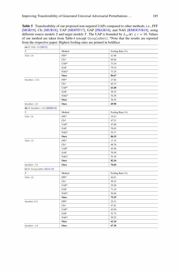
Improving Transferability of Generated Universal Adversarial Perturbations … 185

Table 5 Transferability of our proposed non-targeted UAPs compared to other methods, i.e., FFF[MGR19], CIs [MUR18], UAP [MDFFF17], GAP [PKGB18], and NAG [RMOGVB18], usingdifferent source models S and target models T . The UAP is bounded by L∞(r) ≤ ε = 10. Valuesof our method are taken from Table4 (except GoogleNet). *Note that the results are reportedfrom the respective paper. Highest fooling rates are printed in boldface

(a) S: VGG-16 [SZ15]

T Method Fooling Rate (%)

VGG-19 FFF* 41.98

CIs* 65.64

UAP* 73.10

GAP 79.14

NAG* 73.25

Ours 86.67

ResNet-152 FFF* 27.82

CIs* 45.33

UAP* 63.40

GAP 30.32

NAG* 54.38

Ours 36.34

ResNet-18 Ours 49.98

(b) S: ResNet-152 [HZRS16]

T Method Fooling Rate (%)

VGG-16 FFF* 19.23

CIs* 47.21

UAP* 47.00

GAP 70.45

NAG* 52.17

Ours 86.19

VGG-19 FFF* 17.15

CIs* 48.78

UAP* 45.50

GAP 70.38

NAG* 53.18

Ours 82.36

ResNet-18 Ours 76.04

(c) S: GoogleNet [SLJ+15]

T Method Fooling Rate (%)

VGG-16 FFF* 40.91

CIs* 59.12

UAP* 39.20

GAP 71.14

NAG* 56.40

Ours 75.35

ResNet152 FFF* 25.31

CIs* 47.81

UAP* 45.50

GAP 51.72

NAG* 59.22

Ours 61.24

ResNet-18 Ours 67.30

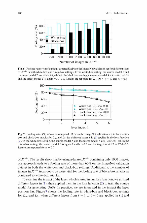
186 A. S. Hashemi et al.

Fig. 6 Fooling rates (%) of our non-targetedUAPs on the ImageNet validation set for different sizesofXtrain in both white-box and black-box settings. In the white-box setting, the source model S andthe targetmodel T areVGG-16, while in the black-box setting, the sourcemodel S isResNet-152and the target model T is again VGG-16. Results are reported for L∞(r) ≤ ε = 10 and α = 0.7

Fig. 7 Fooling rates (%) of our non-targeted UAPs on the ImageNet validation set, in both white-box and black-box attacks for L∞ and L2, for different layers � in (1) applied in the loss function(2). In the white-box setting, the source model S and the target model T are ResNet-18. In theblack-box setting, the source model S is again ResNet-18 and the target model T is VGG-16.Results are reported for α = 0.7

ofXtrain. The results show that by using a datasetXtrain containing only 1000 images,our approach leads to a fooling rate of more than 60% on the ImageNet validationdataset in both the white-box and black-box settings. Additionally, the number ofimages in Xtrain turns out to be more vital for the fooling rate of black-box attacks ascompared to white-box attacks.

To examine the impact of the layer which is used in our loss function, we utilizeddifferent layers in (1), then applied them in the loss function (2) to train the sourcemodel for generating UAPs. In practice, we are interested in the impact the layerposition has. Figure7 shows the fooling rate in white-box and black-box settingsfor L∞ and L2, when different layers from � = 1 to � = 6 are applied in (1) and

Improving Transferability of Generated Universal Adversarial Perturbations … 187

(2). This figure shows that choosing deeper layers leads to a decreasing trend in thefooling rate. Also, this trend is stronger in black-box attacks, where a more than 20%drop in the attack success rate can be observed. This indicates that it is advisable tochoose earlier layers, in particular the first layer, in generating UAPs to obtain bothan optimal fooling rate and transferability.

4.3 Targeted Universal Perturbations

In this section, we apply the targeted fooling loss (5), again withα = 0.7, for trainingthe generator in Fig. 2. We assume the chosen α is appropriate for targeted attacks aswell and thus dispense further investigations. If results are good, then this supportssome robustness w.r.t. the choice of α. Figure8 depicts two examples of our targetedUAPs, some original images and respective adversarial examples. In these exper-iments, the fooling rate (top-1 target accuracy) on the validation set for the targetclass m = 919 (street sign) and m = 920 (traffic light, trafficsignal, stoplight) are 63.2 and 57.83%, respectively, which underlines theeffectiveness of our approach.

For assessing the generalization power of our proposed method across differenttarget classes and comparisonwithGAP [PKGB18],we followedPoursaeed et al. andused 10 randomly sampled classes. The resulting average top-1 target accuracy, whenthe adversarial perturbation is bounded by L∞(r) ≤ ε = 10, is 66.57%, which issignificantly higher than the one reported for GAP [PKGB18] with 52.0%.

Fig. 8 Examples of our targeted UAPs and adversarial examples. In these experiments, the sourcemodel S is VGG-16 [SZ15], with L∞(r) ≤ ε = 10, α = 0.7. The pixel values in UAPs are scaledfor better visibility

188 A. S. Hashemi et al.

Fig. 9 Fooling rates (%) of our targeted UAPs on the ImageNet validation set for different sizesof Xtrain in both white-box and black-box attacks. In the white-box setting, the source modelS and the target model T are VGG-16, while in the black-box setting, the source model S isagain VGG-16 and the target model T is VGG-19. Results are reported for L∞(r) ≤ ε = 10,α = 0.7, and target class m = 847 (tank, army tank, armored combat vehicle,armoured combat vehicle)

To demonstrate the generalization power of our targeted UAPs w.r.t. unseen data,we visualize the attack success rate obtained by the source model VGG-16, in white-box and black-box settings, on the Image-Net validation dataset for different sizesof Xtrain in Fig. 9. For instance, with Xtrain containing 10,000 images, we are ableto fool the target model on over 20% of the images in the ImageNet validation set.It should be noted that training the generator G to produce a single UAP forcingthe target model to output a specific target class m is an extremely challenging task.However, we particularly observe that utilizing 10,000 training images again seemsto be sufficient for a white-box attack.

5 Experiments on Semantic Segmentation

We continue our investigations by applying our method to the task of semanticsegmentation to show its cross-task applicability. We start with the experimentalsetup, followed by an evaluation of non-targeted and targeted attacks.

5.1 Experimental Setup

Dataset: We conduct our experiments on the widely known Cityscapes dataset[COR+16]. It contains pixel-level annotations of 5,000 high-resolution images (2,975training, 500 validation, and 1,525 test images) being captured in urban street scenes.

Improving Transferability of Generated Universal Adversarial Perturbations … 189

Table 6 Themean intersection-over-union (mIoU) (%)of non-targetedUAPmethods on the seman-tic segmentation model FCN-8 pretrained on Cityscapes. Our method is compared with GAP[PKGB18]. In these experiments, both the source model S and the target model T are either thesame, i.e., S = T = FCN-8, or different, i.e., S = ERFNet, T = FCN-8. Parameters are set toL∞(r) ≤ ε, α = 0.7. Best results are printed in boldface

(a) S = T = FCN-8

Method ε

2 5 10 20

GAP 18.1 12.8 4.0 2.1

Ours 16.2 9.8 2.0 0.3

(b) S = ERFNet, T = FCN-8

Method ε

2 5 10 20

GAP 27.3 16.4 7.0 4.3

Ours 26.4 14.8 4.1 1.5

The original images have a resolution of 2048 × 1024 pixels, that we downsampleto 1024 × 512 for our experiments [MCKBF17, PKGB18].

Network architecture: Regarding the architecture of the source model S, we useFCN-8 [LSD15] for white-box attacks, and ERFNet [RABA18] for the black-boxsetting. FCN-8 consists of an encoder part which transforms an input image into alow-resolution semantic representation and a decoder part which recovers the highspatial resolution of the image by fusing different levels of feature representationstogether. ERFNet also consists of an encoder-decoder structure, but without anybypass connections between the encoder and the decoder. Additionally, residualunits are used with factorized convolutions to obtain a more efficient computation.

In our experiments, we consider FCN-8 [LSD15] as our segmentation targetmodel T , and use L∞ norm, to be comparable with [MCKBF17, PKGB18].Evaluationmetrics: To assess the performance of a semantic segmentation network,we used the mean intersection-over-union (mIoU) [COR+16]. It is defined as

mIoU = 1

|M|∑

μ∈M

TPμ

TPμ + FPμ + FNμ, (6)

with classμ ∈ M, class-specific true positives TPμ, false positives FPμ, and false neg-atives FNμ. For assessing the impact of non-targeted adversarial attacks on semanticsegmentation, we compute the mIoU on adversarial examples [AMT18].

190 A. S. Hashemi et al.

To measure the attack success of our targeted attack, we compute the pixelaccuracy (PA) between the prediction m = T (xadv) and the target m [PKGB18].In this chapter, we restrict our analysis to the static target segmentation scenario[MCKBF17] and use the same target mask as in [PKGB18, MCKBF17] (see alsoFig. 11).

5.2 Non-targeted Universal Perturbations

For the non-targeted case, we train our model with the non-targeted adversarial lossfunction (2), where we use (4) as the cross-entropy loss. The maximum permissibleL p norm of the perturbations for p = ∞ is set to ε ∈ {2, 5, 10, 20}. We report resultsfor both ourmethod andGAP [PKGB18] on the Cityscapes validation set in Table6a.It can be observed that across different values for ε our method is superior to GAPin terms of decreasing the mIoU of the underlying target model.

We visualize the effect of the generated non-targeted UAPs in Fig. 10 by illus-trating the original image, the UAP, the resulting adversarial example, the predictionon the original image, the ground truth mask, and the resulting segmentation output.Here, the maximum permissible L p norm of the perturbations p = ∞ is set to ε = 5.

For investigating the transferability of our generated UAPs, we use a UAP opti-mized on ERFNet as the source model S and test it on the target model T beingFCN-8. Table6b reports black-box attack results for our method compared to theattack method GAP [PKGB18]. Our non-targeted UAPs decrease the mIoU of theFCN-8 on the Cityscapes dataset more than GAP [PKGB18] does, in all differentranges of adversarial perturbations (ε ∈ {2, 5, 10, 20}). These results illustrate theeffectivity of the generated perturbation.

5.3 Targeted Universal Perturbations

In the targeted case, we aim at finding a UAP which forces the segmentation sourcemodel S and the segmentation target model T to predict a specific target maskm. We now train our model with the targeted adversarial loss function (5), usingJCE(y, y) according to (4) for the cross-entropy loss. We apply the same target y asin [PKGB18], see m in Fig. 11e.

Figure11 depicts an original image, our generated targeted UAP, the respectiveadversarial example, the prediction on the original image, the target segmentationmask, and the prediction on the adversarial example. The results show that the gen-erated UAP resembles the target mask and is able to fool the FCN-8 in a way that itnow outputs the target segmentation mask.

Improving Transferability of Generated Universal Adversarial Perturbations … 191

Fig. 10 An example of our non-targeted UAPs optimized for the task of semantic segmentation onthe Cityscapes dataset. Results are displayed on the Cityscapes validation set. In these experiments,both the source model S and the target model T are FCN-8, with L∞(r) ≤ ε = 5, α = 0.7. Thepixel values in the UAP are scaled for better visibility

Fig. 11 An example of our targeted UAPs optimized for the task of semantic segmentation on theCityscapes dataset. Results are displayed on the Cityscapes validation set. In these experiments,both the source model S and the target model T are FCN-8, with L∞(r) ≤ ε = 10, α = 0.7. Thepixel values in the UAP are scaled for better visibility

We compare our targeted attack with two state-of-the-art methods in Table 7.While our method performs comparably well as state of the art for weak attacks,in medium to strong attacks we outperform both GAP [PKGB18] and UAP-Seg[MCKBF17].

192 A. S. Hashemi et al.

Table 7 Pixel accuracy (%) of targetedUAPmethods (white-box attack) on the semantic segmenta-tion model FCN-8 pretrained on the Cityscapes training set. Results are reported on the Cityscapesvalidation set. Our method is compared to UAP-Seg [MCKBF17] and GAP [PKGB18]. In theseexperiments, both the source model S and the target model T are FCN-8, with L∞(r) ≤ ε,α = 0.7.Best results are printed in boldface

Method ε

2 5 10 20

GAP 61.2 79.5 92.1 97.2

UAP-Seg 60.9 80.3 91.0 96.3

Ours 61.0 81.8 93.1 97.4

6 Conclusions

We presented a novel method to effectively generate targeted and non-targeted uni-versal adversarial perturbations (UAPs) in both white-box and black-box settings.Our proposed method shows new state-of-the-art fooling rates for targeted as wellas non-targeted UAPs on different classifiers. Additionally, our non-targeted UAPsshow a significantly higher transferability across models when compared to othermethods, given that we generated our UAPs on the deepest network in the inves-tigation. This is achieved by incorporating an additional loss term during training,which aims at increasing the activation of the first layer. Finally, we extended ourmethod to the task of semantic segmentation to prove its applicability also in morecomplex environment perception tasks. Due to its state-of-the-art effectiveness forobject classification and semantic segmentation, we strongly recommend to employthe proposed types of attacks in validation of automated vehicles’ environment per-ception.

References

[AM18] N. Akhtar, A. Mian, Threat of adversarial attacks on deep learning in computervision: a survey. IEEE Access 6, 14410–14430 (2018)

[AMT18] A. Arnab, O. Miksik, P.H.S. Torr, On the robustness of semantic segmentationmodels to adversarial attacks, in Proceedings of the IEEE/CVF Conference onComputer Vision and Pattern Recognition (CVPR), Salt Lake City, UT, USA, June2018, pp. 888–897

[BHSFs19] A.Bär, F.Hüger, P. Schlicht, T. Fingscheidt,On the robustness of redundant teacher-student frameworks for semantic segmentation, in Proceedings of the IEEE/CVFConference onComputerVision andPatternRecognition (CVPR)Workshops, LongBeach, CA, USA, June 2019, pp. 1380–1388

[BKV+20] A. Bär, M. Klingner, S. Varghese, F. Hüger, P. Schlicht, T. Fingscheidt. Robustsemantic segmentation by redundant networks with a layer-specific loss contribu-tion and majority vote, in Proceedings of the IEEE/CVF Conference on Computer

Improving Transferability of Generated Universal Adversarial Perturbations … 193

Vision and Pattern Recognition (CVPR)Workshops, virtual conference, June 2020,pp. 1348–1358

[BLK+21] A.Bär, J. Löhdefink,N.Kapoor, S.J.Varghese, F.Hüger, P. Schlicht, T. Fingscheidt.The vulnerability of semantic segmentation networks to adversarial attacks inautonomous driving: enhancing extensive environment sensing. IEEE Signal Pro-cess. Mag. 38(1), 42–52 (2021)

[BZIK20] P. Benz, C. Zhang, T. Imtiaz, I.-S. Kweon, Double targeted universal adversarialperturbations, inProceedings of theAsianConference onComputerVision (ACCV),virtual conference, Nov. 2020, pp. 284–300

[CAB+20] A. Chaubey, N. Agrawal, K. Barnwal, K.K. Guliani, P. Mehta, Universal Adver-sarial Perturbations: A Survey, pp. 1–20, May 2020. arxiv:2005.08087

[COR+16] M. Cordts, M. Omran, S. Ramos, T. Rehfeld, M. Enzweiler, R. Benenson, U.Franke, S. Roth, B. Schiele, The cityscapes dataset for semantic urban scene under-standing, in Proceedings of the IEEE/CVF Conference on Computer Vision andPattern Recognition (CVPR), Las Vegas, NV, USA, June 2016, pp. 3213–3223

[DLP+18] Y. Dong, F. Liao, T. Pang, H. Su, J. Zhu, X. Hu, J. Li, Boosting adversarial attackswith momentum, inProceedings of the IEEE/CVFConference on Computer Visionand Pattern Recognition (CVPR), Salt Lake City, UT, USA, June 2018, pp. 9185–9193

[FJGN20] J. Fayyad, M.A. Jaradat, D. Gruyer, H. Najjaran, Deep learning sensor fusion forautonomous vehicle perception and localization: a review. Sensors 20(15), 4220–4255 (2020)

[GPAM+14] I. Goodfellow, J. Pouget-Abadie, M. Mirza, B. Xu, D. Warde-Farley, S. Ozair, A.Courville, Y. Bengio, Generative adversarial nets, inProceedings of theConferenceon Neural Information Processing Systems (NIPS/NeurIPS), Dec. 2014, pp. 2672–2680

[GR20] N. Ghafoorianfar, M. Roopaei, Environmental perception in autonomous vehiclesusing edge level situational awareness, in Proceedings of the IEEE Annual Com-puting and Communication Workshop and Conference (CCWC), Las Vegas, NV,USA, Jan. 2020, pp. 444–448

[GRM+19] R. Geirhos, P. Rubisch, C. Michaelis, M. Bethge, F.A. Wichmann, Brendel,W. ImageNet-Trained CNNs are biased towards texture; increasing shape biasimproves accuracy and robustness, in Proceedings of the International Conferenceon Learning Representations (ICLR), NewOrleans, LA, USA,May 2019, pp. 1–22

[GSS15] I. Goodfellow, J. Shlens, C. Szegedy, Explaining and harnessing adversarial exam-ples, in Proceedings of the International Conference on Learning Representations(ICLR), San Diego, CA, USA, May 2015, pp. 1–11

[GTCM20] S. Grigorescu, B. Trasnea, T. Cocias, G. Macesanu, A survey of deep learningtechniques for autonomous driving. J. Field Robot. 37(3), 362–386 (2020)

[HD18] J. Hayes, G. Danezis, Learning universal adversarial perturbations with generativemodels, in Proceedings of the IEEE Symposium on Security and Privacy (SP)Workshops, San Francisco, CA, USA, May 2018, pp. 43–49

[HM19] A.S. Hashemi, S. Mozaffari, Secure deep neural networks using adversarial imagegeneration and training with Noise-GAN. Comput. Secur. 86, 372–387 (2019)

[HZ10] A. Hore, D. Ziou, Image quality metrics: PSNR versus SSIM, inProceedings of theIEEE International Conference on Pattern Recognition (ICPR), Istanbul, Turkey,Aug. 2010, pp. 2366–2369

[HZRS16] K. He, X. Zhang, S. Ren, J. Sun, Deep residual learning for image recognition,in: Proceedings of the IEEE/CVF Conference on Computer Vision and PatternRecognition (CVPR), Las Vegas, NV, USA, June 2016, pp. 770–778

[JAFF16] J. Johnson, A. Alahi, L. Fei-Fei, Perceptual losses for real-time style transfer andsuper-resolution, in Proceedings of the European Conference on Computer Vision(ECCV), Amsterdam, The Netherlands, Oct. 2016, pp. 694–711

194 A. S. Hashemi et al.

[KB15] D.P. Kingma, J. Ba, ADAM: a method for stochastic optimization, in Proceedingsof the International Conference on Learning Representations (ICLR), San Diego,CA, USA, May 2015, pp. 1–15

[KBFs20] M. Klingner, A. Bär, T. Fingscheidt, Improved noise and attack robustness forsemantic segmentation by using multi-task training with self-supervised depthestimation, in Proceedings of the IEEE/CVF Conference on Computer Vision andPattern Recognition (CVPR) Workshops, virtual conference, June 2020, pp. 1299–1309

[KBJ+20] S. Kuutti, R. Bowden, Y. Jin, P. Barber, S. Fallah, A survey of deep learning appli-cations to autonomous vehicle control. IEEE Trans. Intell. Transp. Syst. (TITS)22(2), 721–733 (2020)

[KGB17] A. Kurakin, I. Goodfellow, S. Bengio, Adversarial examples in the physical world,in Proceedings of the International Conference on Learning Representations(ICLR) Workshops, Toulon, France, Apr. 2017, pp. 1–14

[LBX+20] Y. Li, S. Bai, C. Xie, Z. Liao, X. Shen, A. Yuille, Regional homogeneity: towardslearning transferable universal adversarial perturbations against defenses, in Pro-ceedings of the European Conference on Computer Vision (ECCV), virtual confer-ence, Aug. 2020, pp. 795–813

[LBZ+20] Y. Li, S. Bai, Y. Zhou, C. Xie, Z. Zhang, A.L. Yuille, Learning transferable adver-sarial examples via ghost networks, in Proceedings of the AAAI Conference onArtificial Intelligence, New York, NY, USA, Feb. 2020, pp. 11458–11465

[LSD15] J. Long, E. Shelhamer, T. Darrell, Fully convolutional networks for semantic seg-mentation, in Proceedings of the IEEE/CVF Conference on Computer Vision andPattern Recognition (CVPR), Boston, MA, USA, June 2015, pp. 3431–3440

[MCKBF17] J.H. Metzen, M.C. Kumar, T. Brox, V. Fischer, Universal adversarial perturbationsagainst semantic image segmentation, in Proceedings of the IEEE InternationalConference on Computer Vision (ICCV), pp. 2774–2783, Venice, Italy, Oct. 2017

[MDFF+18] S.-M. Moosavi-Dezfooli, A. Fawzi, O. Fawzi, P. Frossard, S. Soatto, Robustnessof classifiers to universal perturbations: a geometric perspective, in Proceedingsof the International Conference on Learning Representations (ICLR), Vancouver,BC, Canada, Apr. 2018, pp. 1–15

[MDFFF17] S.-M. Moosavi-Dezfooli, A. Fawzi, O. Fawzi, P. Frossard, Universal adversarialperturbations, in Proceedings of the IEEE/CVF Conference on Computer Visionand Pattern Recognition (CVPR), Honolulu, HI, USA, July 2017, pp. 1765–1773

[MGR19] K.R.Mopuri, A. Ganeshan, V.B. Radhakrishnan, Generalizable data-free objectivefor crafting universal adversarial perturbations. IEEE Trans. Pattern Anal. Mach.Intell. (TPAMI) 41(10), 2452–2465 (2019)

[MKMW19] N. Morgulis, A. Kreines, S. Mendelowitz, Y. Weisglass, Fooling a Real Car WithAdversarial Traffic Signs, June 2019, pp. 1–19. arxiv:1907.00374

[MMS+18] A. Madry, A. Makelov, L. Schmidt, D. Tsipras, A. Vladu, Towards deep learningmodels resistant to adversarial attacks, in Proceedings of the International Con-ference on Learning Representations (ICLR), Vancouver, BC, Canada, Apr. 2018,pp. 1–10

[MUR18] K.R. Mopuri, P.K. Uppala, V.B. Radhakrishnan, Ask, Acquire, and Attack: Data-Free UAP generation using class impressions. In: Proceedings of the EuropeanConference on Computer Vision (ECCV), Munich, Germany, Sept. 2018, pp. 19–34

[NVM+19] A.M. Nascimento, L.F. Vismari, C.B.S.T. Molina, P.S. Cugnasca, J.B. Camargo,J.R. de Almeida, R. Inam, E. Fersman, M.V. Marquezini, A.Y. Hata, A systematicliterature review about the impact of artificial intelligence on autonomous vehiclesafety. IEEE Trans. Intell. Transp. Syst. (TITS) 21(12), 4928–4946 (2019)

[PKGB18] O. Poursaeed, I. Katsman, B. Gao, S. Belongie, Generative adversarial perturba-tions, inProceedings of the IEEE/CVFConference onComputer Vision andPatternRecognition (CVPR), Salt Lake City, UT, USA, June 2018, pp. 4422–4431

Improving Transferability of Generated Universal Adversarial Perturbations … 195

[PMJ+16] N. Papernot, P. McDaniel, S. Jha, M. Fredrikson, Z. Berkay Celik, A. Swami, Thelimitations of deep learning in adversarial settings, in Proceedings of the IEEEEuropean Symposium on Security and Privacy (ESP), Saarbrücken, Germany,Mar.2016, pp. 372–387

[PTWA17] S.M. Patole, M. Torlak, D. Wang, M. Ali, Automotive radars: a review of signalprocessing techniques. IEEE Signal Process. Mag. 34(2), 22–35 (2017)

[PXL+20] H. Phan, Y. Xie, S. Liao, J. Chen, B. Yuan, CAG: a real-time low-cost enhanced-robustness high-transferability content-aware adversarial attack generator, in Pro-ceedings of the AAAI Conference on Artificial Intelligence, New York, NY, USA,Feb. 2020, pp. 5412–5419

[RABA18] E. Romera, J.M. Alvarez, L.M. Bergasa, R. Arroyo, ERFNet: efficient residualfactorized convnet for real-time semantic segmentation. IEEETrans. Intell. Transp.Syst. (TITS) 19(1), 263–272 (2018)

[RDS+15] O. Russakovsky, J. Deng, S. Hao, J. Krause, S. Satheesh, S. Ma, Z. Huang, A.Karpathy, A. Khosla, M. Bernstein, A.C. Berg, L. Fei-Fei, ImageNet large scalevisual recognition challenge. Int. J. Comput. Vis. (IJCV) 115(3), 211–252 (2015)

[RMOGVB18] K.R. Mopuri, U. Ojha, U. Garg, R. Venkatesh Babu, NAG: network for adversarygeneration, in Proceedings of the IEEE/CVF Conference on Computer Vision andPattern Recognition (CVPR), Salt Lake City, UT, USA, June 2018, pp. 742–751

[RT19] A. Rasouli, J.K. Tsotsos, Autonomous vehicles that interact with pedestrians: asurvey of theory and practice. IEEE Trans. Intell. Transp. Syst. (TITS) 21(3), 900–918 (2019)

[SAE18] SAE International, SAE J3016: Surface Vehicle Recommended Practice – Taxon-omy andDefinitions for TermsRelated toDriving Automation Systems forOn-RoadMotor Vehicles (SAE International, June 2018)

[SLJ+15] C. Szegedy, W. Liu, Y. Jia, P. Sermanet, S. Reed, D. Anguelov, D. Erhan, V.Vanhoucke, A. Rabinovich, Going deeper with convolutions, in Proceedings ofthe IEEE/CVF Conference on Computer Vision and Pattern Recognition (CVPR),Boston, MA, USA, June 2015, pp. 1–9

[SOZ+18] Z. Sun, M. Ozay, Y. Zhang, X. Liu, T. Okatani, Feature quantization for defend-ing against distortion of images, in Proceedings of the IEEE/CVF Conference onComputer Vision and Pattern Recognition (CVPR), Salt Lake City, UT, USA, June2018, pp. 7957–7966

[SZ15] K. Simonyan, A. Zisserman, Very deep convolutional networks for large-scaleimage recognition, in Proceedings of the International Conference on LearningRepresentations (ICLR), San Diego, CA, USA, May 2015, pp. 1–14

[SZS+14] C. Szegedy, W. Zaremba, I. Sutskever, J. Bruna, D. Erhan, I. Goodfellow, R. Fer-gus, Intriguing properties of neural networks, in Proceedings of the InternationalConference on Learning Representations (ICLR), Banff, AB, Canada, Dec. 2014,pp. 1–10

[WBSS04] Z. Wang, A.C. Bovik, H.R. Sheikh, E.P. Simoncelli, Image quality assessment:from error visibility to structural similarity. IEEE Trans. Image Process. 13(4),600–612 (2004)

[WLCC18] X. Wei, S. Liang, N. Chen, X. Cao, Transferable Adversarial Attacks for Imageand Video Object Detection, pp. 1–7, May 2018. arxiv:1811.12641

[WLH+20] Y. Wang, Z. Li, H. Hao, H. Yang, Y. Zheng, Research on visual perception tech-nology of autonomous driving based on improved convolutional neural network.J. Phys.: Conf. Ser. 1550(3), 21–27 (2020)

[WWX+20] D. Wu, Y. Wang, S.-T. Xia, J. Bailey, X. Ma, Skip Connections Matter: On theTransferability of Adversarial Examples Generated With ResNets, pp. 1–15, Feb.2020. arxiv:2002.05990

[WXZ20] W. Jiangqing, X. Hao, J. Zhao, Automatic lane identification using the roadsideLiDAR sensors. IEEE Intell. Transp. Syst. Mag. 12(1), 25–34 (2020)

196 A. S. Hashemi et al.

[WZTE18] L.Wu, Z. Zhu, C. Tai, E.Weinan, Understanding and Enhancing the Transferabilityof Adversarial Examples, pp. 1–15, Feb. 2018. arxiv:1802.09707

[XDL+18] C. Xiao, R. Deng, B. Li, F. Yu, M. Liu, D. Song, Characterizing adversarial exam-ples based on spatial consistency information for semantic segmentation, in Pro-ceedings of the European Conference on Computer Vision (ECCV), Munich, Ger-many, Sept. 2018, pp. 217–234

[XZL+18] C. Xiao, J.-Y. Zhu, B. Li, W. He, M. Liu, D. Song, Spatially Transformed Adver-sarial Examples, pp. 1–29, Jan. 2018. arxiv:1801.02612

[ZBIK20a] C. Zhang, P. Benz, T. Imtiaz, I.-S. Kweon, CD-UAP: class discriminative univer-sal adversarial perturbation, in Proceedings of the AAAI Conference on ArtificialIntelligence, New York, NY, USA, Feb. 2020, pp. 6754–6761

[ZBIK20b] C. Zhang, P. Benz, T. Imtiaz, I.-S. Kweon, Understanding adversarial examplesfrom the mutual influence of images and perturbations, in Proceedings of theIEEE/CVF Conference on Computer Vision and Pattern Recognition (CVPR), vir-tual conference, June 2020, pp. 14521–14530

[ZPIE17] J.-Y. Zhu, T. Park, P. Isola, A.A. Efros, Unpaired image-to-image translation usingcycle-consistent adversarial networks, in Proceedings of the IEEE InternationalConference on Computer Vision (ICCV), Venice, Italy, Oct. 2017, pp. 2242–2251

[ZWJW20] K. Zhang, S.J. Wang, L. Ji, C. Wang, DNN based camera and LiDAR fusionframework for 3D object recognition. J. Phys.: Conf. Ser. 1518(1), 12–44 (2020)

Open Access This chapter is licensed under the terms of the Creative Commons Attribution 4.0International License (http://creativecommons.org/licenses/by/4.0/), which permits use, sharing,adaptation, distribution and reproduction in any medium or format, as long as you give appropriatecredit to the original author(s) and the source, provide a link to the Creative Commons license andindicate if changes were made.

The images or other third party material in this chapter are included in the chapter’s CreativeCommons license, unless indicated otherwise in a credit line to the material. If material is notincluded in the chapter’s Creative Commons license and your intended use is not permitted bystatutory regulation or exceeds the permitted use, you will need to obtain permission directly fromthe copyright holder.

Invertible Neural Networks forUnderstanding Semantics of Invariancesof CNN Representations

Robin Rombach, Patrick Esser, Andreas Blattmann, and Björn Ommer

Abstract To tackle increasingly complex tasks, it has become an essential ability ofneural networks to learn abstract representations. These task-specific representationsand, particularly, the invariances they capture turn neural networks into black-boxmodels that lack interpretability. To open such a black box, it is, therefore, crucialto uncover the different semantic concepts a model has learned as well as those thatit has learned to be invariant to. We present an approach based on invertible neuralnetworks (INNs) that (i) recovers the task-specific, learned invariances by disentan-gling the remaining factor of variation in the data and that (ii) invertibly transformsthese recovered invariances combined with the model representation into an equallyexpressive one with accessible semantic concepts. As a consequence, neural net-work representations become understandable by providing the means to (i) exposetheir semantic meaning, (ii) semantically modify a representation, and (iii) visualizeindividual learned semantic concepts and invariances. Our invertible approach sig-nificantly extends the abilities to understand black-box models by enabling post hocinterpretations of state-of-the-art networkswithout compromising their performance.Our implementation is available at https://compvis.github.io/invariances/.

1 Introduction

Key to the wide success of deep neural networks is end-to-end learning of powerfulhidden representations that aim to (i) capture all task-relevant characteristics while(ii) being invariant to all other variabilities in the data [LeC12, AS18]. Deep learning

R. Rombach (B) · P. Esser · A. Blattmann · B. OmmerHCI, IWR, Heidelberg University, Berliner Str. 43, 69120 Heidelberg, Germanye-mail: robin.rombach@iwr.uni-heidelberg.de

P. Essere-mail: patrick.esser@iwr.uni-heidelberg.de

A. Blattmanne-mail: bjoern.ommer@iwr.uni-heidelberg.de

B. Ommere-mail: andreas.blattmann@iwr.uni-heidelberg.de

© The Author(s) 2022T. Fingscheidt et al. (eds.), Deep Neural Networks and Data for Automated Driving,https://doi.org/10.1007/978-3-031-01233-4_7

197

198 R. Rombach et al.

can yield abstract representations that are perfectly adapted feature encodings forthe task at hand. However, their increasing abstraction capability and performancecomes at the expense of a lack in interpretability [BBM+15]: although the networkmay solve a problem, it does not convey an understanding of its predictions or theircauses, often leaving the impression of a black box [Mil19]. In particular, users aremissing an explanation of semantic concepts that the model has learned to representand of those it has learned to ignore, i.e., its invariances.

Providing such explanations and an understanding of network predictions andtheir causes is thus crucial for transparent AI. Not only is this relevant to discoverlimitations and promising directions for future improvements of the AI system itself,but also for compliance with legislation [GF17, Eur20], knowledge distillation fromsuch a system [Lip18], and post hoc verification of the model [SWM17]. Conse-quently, research on interpretable deep models has recently gained a lot of attention,particularly methods that investigate latent representations to understand what themodel has learned [SWM17, SZS+14, BZK+17, FV18, ERO20].

Challenges and aims: Assessing these latent representations is challenging due totwo fundamental issues: (i) To achieve robustness and generalization despite noisyinputs and data variability, hidden layers exhibit a distributed coding of semanticallymeaningful concepts [FV18]. Attributing semantics to a single neuron via backprop-agation [MLB+17] or synthesis [YCN+15] is thus impossible without altering thenetwork [MSM18, ZKL+16], which typically degrades performance. (ii)End-to-endlearning trains deep representations toward a goal task, making them invariant to fea-tures irrelevant for this goal. Understanding these characteristics that a representationhas abstracted away is challenging, since we essentially need to portray features thathave been discarded.

These challenges call for a method that can interpret existing network representa-tions by recovering their invariances without modifying them. Given these recoveredinvariances, we seek an invertible mapping that translates a representation and theinvariances onto understandable semantic concepts. The mapping disentangles thedistributed encoding of the high-dimensional representation and its invariances byprojecting them onto separate multi-dimensional factors that correspond to human-understandable semantic concepts. Both this translation and the recovering of invari-ances are implemented with invertible neural networks (INNs) [Red93, DSB17,KD18]. For the translation, this guarantees that the resulting understandable rep-resentation is equally expressive as the model representation combined with therecovered invariances (no information is lost). Its invertibility also warrants that fea-ture modifications applied in the semantic domain correctly adjust the recoveredrepresentation.

Our contributions:Our contributions to a comprehensive understandingof deep rep-resentations are as follows: (i) We present an approach, which, by utilizing invertibleneural networks, improves the understanding of representations produced by exist-ing network architectures with no need for re-training or otherwise compromisingtheir performance. (ii) Our generative approach is able to recover the invariances thatresult from the non-injective projection (of input onto a latent representation) which

Invertible Neural Networks for Understanding Semantics … 199

deep networks typically learn. This model then provides a probabilistic visualizationof the latent representation and its invariances. (iii) We bijectively translate an arbi-trarily abstract representation and its invariances via a non-linear transformation intoanother representation of equal expressiveness, but with accessible semantic con-cepts. (iv) The invertibility also enables manipulation of the original latent represen-tations in a semantically understandable manner, thus facilitating further diagnosticsof a network.

2 Background

Twomain approaches to interpretable AI can be identified, those which aim to incor-porate interpretability directly into the design of models, and those which aim toprovide interpretability to existing models [MSM18]. Approaches from the first cat-egory range from modifications of network architectures [ZKL+16], over regular-ization of models encouraging interpretability [LBMO19, PASC+20], toward com-binations of both [ZNWZ18]. However, these approaches always involve a trade-offbetween model performance and model interpretability. Being of the latter category,our approach allows to interpret representations of existing models without compro-mising their performance.

To better understand what an existing model has learned, its representations mustbe studied [SWM17]. Syegedy et al. [SZS+14] show that both random directionsand coordinate axes in the feature space of networks can represent semantic prop-erties and conclude that they are not necessarily represented by individual neurons.Different works attempt to select groups of neurons which have a certain seman-tic meaning, such as based on scenes [ZKL+15], objects [SR15] and object parts[SRD14]. [BZK+17] studied the interpretability of neurons and found that a rota-tion of the representation space spanned by the neurons decreases its interpretability.While this suggests that the neurons provide a more interpretable basis comparedto a random basis, [FV18] shows that the choice of basis is not the only challengefor interpretability of representations. Their findings demonstrate that learned repre-sentations are distributed, i.e., a single semantic concept is encoded by an activationpattern involving multiple neurons, and a single neuron is involved in the encodingof multiple different semantic concepts. Instead of selecting a set of neurons directly,[ERO20] learns an INN that transforms the original representation space to an inter-pretable space, where a single semantic concept is represented by a known group ofneurons and a single neuron is involved in the encoding of just a single semantic con-cept. However, to interpret not only the representation itself but also its invariances,it is insufficient to transform only the representation itself. Our approach thereforetransforms the latent representation space of an autoencoder, which has the capacityto represent its inputs faithfully, and subsequently translates a model representationand its invariances into this space for semantic interpretation and visualization.

A large body of works approach interpretability of existing networks basedon visualizations. Selvaraju et al. [SCD+20] use gradients of network outputs

200 R. Rombach et al.

with respect to a convolutional layer to obtain coarse localization maps. Bach etal. [BBM+15] propose an approach to obtain pixel-wise relevance scores for a spe-cific class of models which is generalized in [MLB+17]. To obtain richer visualinterpretations, [ZF14, SVZ14, YCN+15, MV16] reconstruct images which maxi-mally activate certain neurons. Nguyen et al. [NDY+16] use a generator network forthis task, which was introduced in [DB16] for reconstructing images from theirfeature representation. Our key insight is that these existing approaches do notexplicitly account for the invariances learned by a model. Invariances imply thatfeature inversion is a one-to-many mapping and thus they must be recovered to solvethe task. Recently, [SGM+20] introduced a GAN-based approach that utilizes fea-tures of a pretrained classifier as a semantic pyramid for image generation. Nashet al. [NKW19] used samples from an autoregressive model of images conditionedon a feature representation to gain insights into the representation’s invariances. Incontrast, our approach recovers an explicit representation of the invariances, whichcan be recombined with modified feature representations, and thus makes the effectof modifications to representations, e.g., through adversarial attacks, visible.

Other works consider visual interpretations for specialized models. Santurkar etal. [SIT+19] showed that the quality of images which maximally activate certainneurons is significantly improved when activating neurons of an adversarially robustclassifier. Bau et al. [BZS+19] explore the relationship between neurons and theimages produced by a generative adversarial network. For the same class of models,[GAOI19] finds directions in their input space which represent semantic conceptscorresponding to certain cognitive properties. Such semantic directions have previ-ously also been found in classifier networks [UGP+17] but requires aligned data.All of these approaches require either special training of models, are limited to avery special class of models which already provide visualizations, or depend onspecial assumptions on model and data. In contrast, our approach can be applied toarbitrary models without re-training or modifying them, and provides both visualiza-tions and semantic explanations, for both the model’s representation and its learnedinvariances.

3 Method

Common tasks of computer vision can be phrased as a mapping from an input imagex to some output f (x) such as a classification of the image, a regression (e.g.,of object locations), a (semantic) segmentation map, or a re-synthesis that yieldsanother image. Deep learning utilizes a hierarchy of intermediate network layersthat gradually transform the input into increasingly more abstract representations.Let z = �(x) ∈ R

Nz be the representation extracted by one such layer (without lossof generality we consider z to be an Nz-dim vector, flattening it if necessary) andf (x) = �(z) = �(�(x)) the mapping onto the output.An essential characteristic of a deep feature encoding z is the increasing abstract-

ness of higher feature encoding layers and the resulting reduction of information.

Invertible Neural Networks for Understanding Semantics … 201

Fig. 1 Proposed architecture. We provide post hoc interpretation for a given deep network f =� ◦ �. For a deep representation z = �(x) a conditional INN t recovers �’s invariances v froma representation z which contains entangled information about both z and v. The INN e thentranslates the representation z into a factorized representation with accessible semantic concepts.This approach allows for various applications, including visualizations of network representations ofnatural (green box) and altered inputs (blue box), semantic network analysis (red box) and semanticimage modifications (yellow box)

This reduction generally causes the feature encoding to become invariant to thoseproperties of the input image, which do not provide salient information for the task athand [CWG+18]. To explain a latent representation, we need to recover such invari-ances v and make z and v interpretable by learning a bijective mapping onto under-standable semantic concepts, see Fig. 1. Section 3.1 describes our INN t to recoveran encoding v of the invariances. Due to the generative nature of t , our approachcan correctly sample visualizations of the model representation and its invarianceswithout leaving the underlying data distribution and introducing artifacts. With v

then available, Sect. 3.2 presents an INN e that translates t’s encoding of z andv without losing information onto disentangled semantic concepts. Moreover, theinvertibility allows modifications in the semantic domain to correctly project backonto the original representation or into image space.

3.1 Recovering the Invariances of Deep Models

Learning an encoding to help recover invariances: Key to a deep representation isnot only the information z captures, but also what is has learned to abstract away. Tolearn what z misses with respect to x, we need an encoding z, which, in contrast toz, includes the invariances exhibited by z. Without making prior assumptions about

202 R. Rombach et al.

the deep model f , autoencoders provide a generic way to obtain such an encoding z,since they ensure that their input x can be recovered from their learned representationz, which hence also comprises the invariances.

Therefore, we learn an autoencoder with an encoder E that provides the datarepresentation z = E(x) and a decoder D producing the data reconstruction x =D( z). Section 3.2 will utilize the decoding from z to x to visualize both z andv. The autoencoder is trained to reconstruct its inputs by minimizing a perceptualmetric between input and reconstruction, ‖x − x‖, as in [DB16]. The details of thearchitecture and training procedure can be found in Sect. 3.3, autoencoder E , D. Itis crucial that the autoencoder only needs to be trained once on the training data.Consequently, the same E can be used to interpret different representations z, e.g.,different models or layers within a model, thus ensuring fair comparisons betweenthem. Moreover, the complexity of the autoencoder can be adjusted based on thecomputational needs, allowing us to work with much lower dimensional encodings zcompared to reconstructing the invariances directly from the images x. This reducesthe computational demands of our approach significantly.

Learning a conditional INN that recovers invariances: Due to the reconstructiontask of the autoencoder, z not only contains the invariances v, but also the represen-tation z. Thus, we must disentangle [EHO19, LSOL20, KSLO19] v and z using amapping t(·|z) : z �→ v = t( z|z) which, depending on z, extracts v from z.

Besides extracting the invariances from a given z, t must also enable an inversemapping from given model representations z to z to support a further mappingonto semantic concepts Sect. 3.2 and visualization based on D( z). There are manydifferent x with �(x) = z, namely, all those x which differ only in properties that �is invariant to. Thus, there are also many different z that this mapping must recover.Consequently, the mapping from z to z is set-valued. However, to understand fwe do not want to recover all possible z, but only those which are likely under thetraining distribution of the autoencoder. In particular, this excludes unnatural imagessuch as those obtained by DeepDream [MOT15] or adversarial attacks [SZS+14]. Inconclusion, we need to sample z ∼ p( z|z).

To avoid a costly inversion process of �, t must be invertible (implemented as anINN) so that a change of variables

p( z|z) = p(v|z)| det∇(t−1)(v|z)| , where v = t( z|z), (1)

yields p( z|z) by means of the distribution p(v|z) of invariances, given a modelrepresentation z. Here, the denominator denotes the absolute value of the determinantof Jacobian ∇(t−1) of v �→ t−1(v|z) = z, which is efficient to compute for commoninvertible network architectures. Consequently, we obtain z for given z by samplingfrom the invariant space v given z and then applying t−1,

z ∼ p( z|z) ⇐⇒ v ∼ p(v|z), z = t−1(v|z). (2)

Invertible Neural Networks for Understanding Semantics … 203

Since v is the invariant space for z, both are complementary thus implying indepen-dence p(v|z) = p(v). Because a powerful transformation t−1 can transform betweentwo arbitrary densities, we can assume without loss of generality a Gaussian priorp(v) = N (v|0, I), where I is the identity matrix. Given this prior, our task is then tolearn the transformation t thatmapsN (v|0, I) onto p( z|z). To this end,wemaximizethe log-likelihood of z given z, which results in a per-example loss of

Je( z, z) = − log p( z|z) = − logN (t( z|z)|0, I) − log | det∇ t( z|z)|. (3)

Minimizing this loss over the training data distribution p(x) gives t , a bijectivemapping between z and (z, v),

J (t) = Ex∼p(x) [Je(E(x),�(x))] (4)

= Ex∼p(x)

[1

2‖t(E(x)|�(x))‖2 + N z log 2π − log | det∇ t(E(x)|�(x))|

].

(5)

Note that both E and � remain fixed during minimization of J .

3.2 Interpreting Representations and Their Invariances

Visualizing representations and invariances: For an image representation z =�(x), (2) presents an efficient approach (a single forward pass through the INN t)to sample an encoding z, which is a combination of z with a particular realizationof its invariances v. Sampling multiple realizations of z for a given z highlightwhat remains constant and what changes due to different v: information preservedin the representation z remains constant over different samples and informationdiscarded by the model ends up in the invariances v and shows changes over differentsamples. Visualizing the samples z ∼ p( z|z)with x = D( z) portrays this constancyand changes due to different v. To complement this visualization, in the following,we learn a transformation of z into a semantically meaningful representation whichallows to uncover the semantics captured by z and v.

Learning an INN to produce semantic interpretations: The autoencoder repre-sentation z is an equivalent representation of (z, v) but its feature dimensions do notnecessarily correspond to semantic concepts [FV18]. More generally, without super-vision, we cannot reliably discover semantically meaningful, explanatory factors ofz [LBL+19]. In order to explain z in terms of given semantic concepts, we apply theapproach of [ERO20] and learn a bijective transformation of z to an interpretablerepresentation e( z)where different groups of components, called factors, correspondto semantic concepts.

To learn the transformation e, we parameterize e by an INN and assume thatsemantic concepts are defined implicitly by pairs of images, i.e., for each semantic

204 R. Rombach et al.

concept we have access to training pairs xa, xb that have the respective concept incommon. For example, the semantic concept “smiling” is defined by pairs of images,where either both images show smiling persons or both images show non-smilingpersons.Applying this formulation, input pairswhich are similar in a certain semanticconcept are similar in the corresponding factor of the interpretable representatione( z).

Following [ERO20], the loss for training the invertible network e is then given by

J (e) = Exa,xb[− log p(e(E(xa)), e(E(xb)))

− log | det∇e(E(xa))| − log | det∇e(E(xb))|] . (6)

Interpretation by applying the learned INNs: After training, the combination of ewith t from Sect. 3.1 provides semantic interpretations given a model representationz: (2) gives realizations of the invariances v which are combined with z to producez = t−1(v|z). Then e transforms z without loss of information into a semanticallyaccessible representation (ei )i = e( z) = e(t−1(v|z)) consisting of different semanticfactors ei . Comparing the ei for different model representations z and invariances v

allows us to observe which semantic concepts the model representation z = �(·) issensitive to, and which it is invariant to.

Semantic Modifications of Latent Representations: The transformations t−1 ande not only interpret a representation z in terms of accessible semantic concepts (ei )i .Given v ∼ p(v), they also allow tomodify z = t−1(v|z) in a semanticallymeaningfulmanner by altering its corresponding (ei )i and then applying the inverse translatione−1,

ze−→ (ei )

modification−−−−−−→ (e∗i )

e−1−→ z∗. (7)

The modified representation z∗ is then readily transformed back into image spacex∗ = D( z∗

). Besides visual interpretation of the modification, x∗ can be fed into themodel �(�(x∗

)) to probe for sensitivity to certain semantic concepts.

3.3 Implementation Details

In this section, we provide implementation details about the exact training procedureand architecture of all components of our approach. This is only for the sake of clarityand completeness. For readers who are already familiar with INNs or people ratherinterested in the higher level ideas of our approach than in its technical details, thissection can be safely skipped.

AutoencoderE, D: In Sect. 3.1, we introduced an autoencoder to obtain a repre-sentation z of x, which includes the invariances abstracted away by a given modelrepresentation z. This autoencoder consists of an encoder E(x) and a decoder D( z).

Invertible Neural Networks for Understanding Semantics … 205

Table 1 Autoencoder architecture on datasets with images of resolution 28 × 28

Because the INNs t and e transform the distribution of z, we must ensurea strictly positive density for z to avoid degenerate solutions. This is readilyachieved with a stochastic encoder, i.e., we predict mean E(x)μ and diagonalE(x)σ 2 of a Gaussian distribution, and obtain the desired representation as z ∼N ( z|E(x)μ, diag(E(x)σ 2)). Following [DW19], we train this autoencoder as a vari-ational autoencoder using the reparameterization trick [KW14, RMW14] to matchthe encoded distribution to a standard normal distribution, and jointly learn the scalaroutput variance γ under an image metric ‖x − x‖ to avoid blurry reconstructions.The resulting loss function is thus

J (E, D, γ ) =E x ∼ p(x)

ε ∼ N (ε|0, I)

[1

γ‖x − D(E(x)μ + ε

√diag(E(x)σ 2))‖ + log γ

+1

2

N z∑i=1

{(E(x)μ)2i + (E(x)σ 2)i − 1 − log(E(x)σ 2)i

}].

(8)

Note that√

(·) and log(·) on multi-dimensional entities are applied element-wise.In the experiments shown in this chapter,we use images of spatial resolutions 28 × 28and128 × 128, resulting in different architectures for the autoencoder, summarized inTables 1 and2, respectively. For the encoder E processing images of spatial resolution128 × 128, we use an architecture based on ResNet-101 [HZRS16], and for thecorresponding decoder D we use an architecture based on BigGAN [BDS19], wherewe include a small fully connected network to replace the class conditioning used inBigGAN by a conditioning on z.

In the 28 × 28 case, we use a squared L2 loss for the image metric, which corre-sponds to the first term in (8). For our 128 × 128-models, we further use an improvedmetric as in [DB16], which includes additional perceptual [ZIE+18] and discrimina-tor losses. The perceptual loss consists of L1 feature distances obtained fromdifferent

206 R. Rombach et al.

Table 2 Autoencoder architecture for datasets with images of resolution 128 × 128

layers of a fixed, pretrained network. We use a VGG-16 network pretrained on Ima-geNet and weighted distances of different layers as in [ZIE+18]. The discriminatoris trained along with the autoencoder to distinguish reconstructed images from realimages using a binary classification loss, and the autoencoder maximizes the log-probability that reconstructed images are classified as real images. The architecturesof VGG-16 and the discriminator are summarized in Table 3.

Details on the INNe for Revealing Semantics of Deep Representations: Previ-ous works have successfully applied INNs for density estimation [DSB17], inverseproblems [AKW+19], and on top of autoencoder representations [ERO20, XYA19,DMB+21, BMDO21b, BMDO21a] for a wide range of applications such as videosynthesis [DMB+21, BMDO21b] and translation between pretrained, powerful net-works [REO20]. This section provides details on how we embed the approachof [ERO20] to reveal the semantic concepts of autoencoder representations z, cf.Sect. 3.2.

Since we will never have examples for all relevant semantic concepts, we includea residual concept that captures the remaining variability of z, which is not explainedby the given semantic concepts.

Following [ERO20], we learn a bijective transformation e( z), which translatesthe non-interpretable representation z invertibly into a factorized representation

Invertible Neural Networks for Understanding Semantics … 207

Table 3 Architectures used to compute image metrics for the autoencoder, which were used fortraining the autoencoder E, D on datasets with images of resolution 128 × 128

(ei ( z))Ki=0 = e( z), where each factor ei ∈ RNei represents one of the given semantic

concepts for i = 1, . . . , K , and e0 ∈ RNe0 is the residual concept.

The INN e establishes a one-to-one correspondence between an encoding anddifferent semantic concepts and, conversely, enables semantic modifications to cor-rectly alter the original encoding (see next section). Being an INN, e( z) and z needto have the same dimensionality and we set Ne0 = N z − ∑K

i=1 Nei . We denote theindices of concept i with respect to e( z) as Ii ⊂ {1, . . . , N z} such that we can writeei = (e( z)k)k∈Ii .

In the following,we emphasize onderiving a loss function for training the semanticINN. Let ei be the factor representing some semantic concept, e.g., gender, that thecontents of two images xa, xb share. Then the projection of their encodings za, zb

onto this semantic concept must be similar [ERO20, KWKT15],

ei ( za) � ei ( z

b) where za = E(xa), zb = E(xb). (9)

Moreover, to interpret z we are interested in the separate contribution of differentsemantic concepts ei that explain z. Hence, we seek a mapping e(·) that strives todisentangle different concepts,

ei ( z) ⊥ e j ( z) ∀i �= j, x where z = E(x). (10)

The objectives in (9), (10) imply a correlation in ei for pairs za and zb and nocorrelation between concepts ei , e j for i �= j . This calls for a Gaussian distributionwith a covariance matrix that reflects these requirements.

208 R. Rombach et al.

Let ea = (eai ) = (ei (E(xa))) and eb likewise, where xa, xb are samples from atraining distribution p(xa, xb) for the i th semantic concept. The distribution of pairsea and eb factorizes into a conditional and a marginal,

p(ea, eb) = p(eb|ea)p(ea). (11)

Objective (10) implies a diagonal covariance for the marginal distribution p(ea),i.e., a standard normal distribution, and (9) entails a correlation between eai and ebi .Therefore, the correlation matrix is �ab = ρ diag((δIi (k))

N zk=1), where

δIi (k) ={1 if k ∈ Ii ,0 else.

By symmetry, p(eb) = p(ea), which gives

p(eb|ea) = N (eb|�abea, I − (�ab)2). (12)

Inserting (12) and a standard normal distribution for p(ea) into (11) yields the neg-ative log-likelihood for a pair ea, eb.

Given pairs xa, xb as training data, another change of variables from za = E(xa)to ea = e( za) gives the training loss function for e as the negative log-likelihood ofza, zb,

J (e) = Exa,xb[− log p(e(E(xa)), e(E(xb)))

− log | det∇e(E(xa))| − log | det∇e(E(xb))|] . (13)

For simplicity, we have derived the loss for a single semantic concept ei . Simplysumming over the losses of different semantic concepts yields their joint loss functionand allows us to learn a joint translator e for all of them.

In the following, we focus on the log-likelihood of pairs. The loss for e in (13)contains the log-likelihood of pairs ea, eb. Inserting (12) and a standard normaldistribution for p(ea) into (11) yields

− log p(ea, eb) = 1

2

⎛⎝∑

k∈Ii

(ebk − ρeak)2

1 − ρ2+

∑k∈Ic

i

(ebk)2 +

N z∑k=1

(eak)2

⎞⎠ + C, (14)

where C = C(ρ, N z) is a constant that can be ignored for the optimization process.ρ ∈ (0, 1) determines the relative importance of loss terms corresponding to thesimilarity requirement in (9) and the independence requirement in (10). We use afixed value of ρ = 0.9 for all experiments.

In the following, we describe the architecture of the semantic INN. In our imple-mentation, e is built by stacking invertible blocks, see Fig. 2, which consist of three

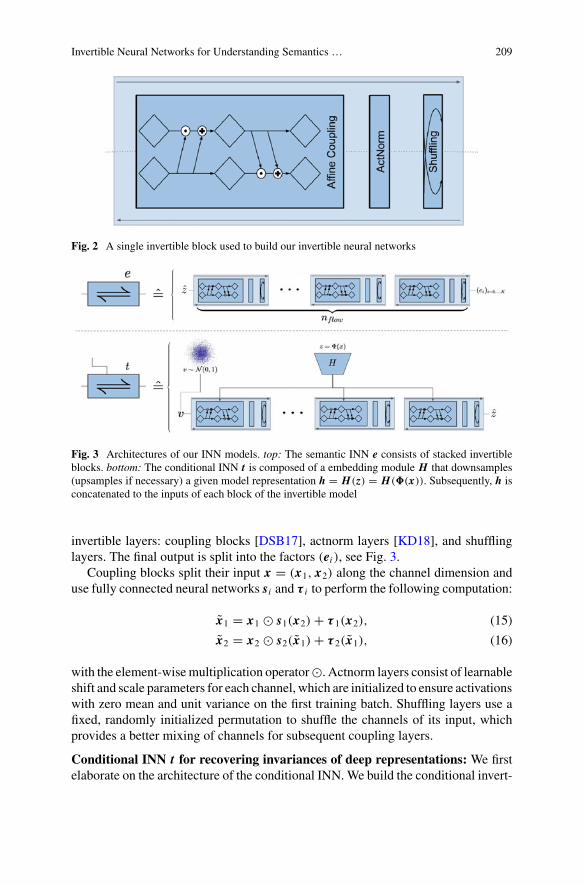
Invertible Neural Networks for Understanding Semantics … 209

Fig. 2 A single invertible block used to build our invertible neural networks

Fig. 3 Architectures of our INN models. top: The semantic INN e consists of stacked invertibleblocks. bottom: The conditional INN t is composed of a embedding module H that downsamples(upsamples if necessary) a given model representation h = H(z) = H(�(x)). Subsequently, h isconcatenated to the inputs of each block of the invertible model

invertible layers: coupling blocks [DSB17], actnorm layers [KD18], and shufflinglayers. The final output is split into the factors (ei ), see Fig. 3.

Coupling blocks split their input x = (x1, x2) along the channel dimension anduse fully connected neural networks si and τ i to perform the following computation:

x1 = x1 � s1(x2) + τ 1(x2), (15)

x2 = x2 � s2(x1) + τ 2(x1), (16)

with the element-wisemultiplication operator�. Actnorm layers consist of learnableshift and scale parameters for each channel, which are initialized to ensure activationswith zero mean and unit variance on the first training batch. Shuffling layers use afixed, randomly initialized permutation to shuffle the channels of its input, whichprovides a better mixing of channels for subsequent coupling layers.

Conditional INN t for recovering invariances of deep representations: We firstelaborate on the architecture of the conditional INN.We build the conditional invert-

210 R. Rombach et al.

Fig. 4 Graphical distinctionof information flow duringtraining and inference.During training of t , theencoder E provides an(approximately complete)data representation, which isused to learn the invariancesof a given model’srepresentations z. Atinference, the encoder is notnecessarily needed anymore:given a representationz = �(x), invariances canbe sampled from the priordistribution and decoded intodata space through t−1

ible neural network t by expanding the semantic model e as follows: Given a modelrepresentation z, which is used as the conditioning of the INN, we first calculate itsembedding

h = H(z) (17)

which is subsequently fed into the affine coupling block:

x1 = x1 � s1(x2, h) + τ 1(x2, h), (18)

x2 = x2 � s2(x1, h) + τ 2(x1, h), (19)

with � again being an element-wise multiplication operator, where si and τ i aremodified from (16) such that they are capable of processing a concatenated input(xi , h). The embeddingmodule H is usually a shallow convolutional neural networkused to down-/upsample a given model representation z to a size that the networkssi and τ i are able to process. This means that t , analogous to e, consists of stackedinvertible blocks, where each block is composed of coupling blocks, actnorm layers,and shuffling layers, cf. Sect. 3.3, details on the INN e for revealing semantics of deeprepresentations, and Fig. 2. The complete architectures of both t and e are depicted inFig. 3. Additionally, Fig. 4 provides a graphical distinction of the training and testingprocess of t . During training, the autoencoder D ◦ E provides a representation of the

Invertible Neural Networks for Understanding Semantics … 211

data that contains both the invariances and the representation of somemodel w.r.t. theinput x. After training of t , the encodermay be discarded and visual decodings and/orsemantic interpretations of a model representation z can be obtained by samplingand transforming v as described in (2).

4 Experiments

To explore the applicability of our approach,we conduct experiments on severalmod-els: SqueezeNet [IHM+16], which provides lightweight classification, FaceNet[SKP15], a baseline for face recognition and clustering, trained on the VGGFace2dataset [CSX+18], and variants of ResNet [HZRS16], a popular architecture oftenused when fine-tuning a classifier on a specific task and dataset.

Experiments are conducted on the following datasets: CelebA [LLWT15], Ani-malFaces [LHM+19], Animals (containing carnivorous animals), ImageNet[DDS+09], and ColorMNIST, which is an augmented version of the MNIST dataset[LCB98], where both background and foreground have random, independent colors.Evaluation details follow in Sect. 4.5.

4.1 Comparison to Existing Methods

A key insight of our chapter is that reconstructions from a given model’s repre-sentation z = �(x) are impossible if the invariances the model has learned are notconsidered. In Fig. 5, we compare our approach to existing methods that either tryto reconstruct the image via gradient-based optimization [MV16] or by traininga reconstruction network directly on the representations z [DB16]. By condition-ally sampling images x = D( z), where we obtain z via the INN t as described in(2) based on the invariances v ∼ p(v) = N (0, I), we bypass this shortcoming andobtain natural imageswithout artifacts for any layer depth. The increased image qual-ity is further confirmed by the Fréchet inception distance (FID) scores [HRU+17]reported in Table 4.

4.2 Understanding Models

Interpreting a face recognition model: FaceNet [SKP15] is a widely acceptedbaseline in the field of face recognition. This model embeds input images of humanfaces into a latent space where similar images have a small L2-distance. We aim tounderstand the process of face recognition within this model by analyzing and visu-alizing learned invariances for several layers explicitly; see Table 6 for a detailedbreakdown of the various layers of FaceNet. For the experiment, we use a pre-

212 R. Rombach et al.

Fig. 5 Comparison to existing network inversion methods for AlexNet [KSH12]. In contrastto the methods of [DB16] (D&B) and [MV16] (M&V), our invertible method explicitly samplesthe invariances of � w.r.t. the data, which circumvents a common cause for artifacts and producesnatural images independent of the depth of the layer which is reconstructed

Table 4 FID scores for layer visualizations of AlexNet, obtained with our method and [DB16](D&B). Scores are calculated on the Animals dataset

Layer conv5 fc6 fc7 fc8 Output

ours 23.6 ± 0.5 24.3 ± 0.7 24.9 ± 0.4 26.4 ± 0.4 27.4 ± 0.3D&B 25.2 24.9 27.2 36.1 352.6

trained FaceNet and train the generative model presented in (2) by conditioning onvarious layers. Figure 6 depicts the amount of variance present in each selected layerwhen generating n = 250 samples for each of the 100 different input images. Thisvariance serves as a proxy for the amount of abstraction capability FaceNet haslearned in its respective layers: more abstract representations allow for a rich varietyof corresponding synthesized images, resulting in a large variance in image spacewhen being decoded. We observe an approximate exponential growth of learnedinvariances with increasing layer depth, suggesting abstraction mainly happens inthe deepest layers of the network. Furthermore, we are able to synthesize images thatcorrespond to the given model representation for each selected layer.

How does relevance of different concepts emerge during training? Humans tendto provide explanations of entities by describing them in terms of their semantics,e.g., size or color. In a similar fashion, we want to semantically understand how anetwork (here: SqueezeNet) learns to solve a given problem.

Invertible Neural Networks for Understanding Semantics … 213

Fig. 6 Left: VisualizingFaceNet representations and their invariances. Samplingmultiple recon-structions x = D(t−1(v|z�)) shows the degree of invariance learned by different layers �. Theinvariance w.r.t. pose increases for deeper layers as expected for face identification. Surprisingly,FaceNet uses glasses as an identity feature throughout all its layers as evident from the spatialmean and variance plots, where the glasses are still visible. This reveals a bias and weakness of themodel. Right: spatially averaged variances over multiple x and layers

Intuitively, a network should, for example, be able to solve a given classificationproblem by focusing on the relevant information while discarding task-irrelevantinformation. To build on this intuition, we construct a toy problem: digit classifica-tion on ColorMNIST. We expect the model to ignore both the random backgroundand foreground colors of the input data, as it does not help making a classificationdecision. Thus, we apply the invertible approach presented in Sect. 3.2 and recoverthree distinct factors: digit class, background color, and foregroundcolor. To capture the semantic changes occurring over the course of training of thisclassifier, we couple 20 instances of the invertible interpretation model on the lastconvolutional layer, each representing a checkpoint between iteration 0 and iteration40000 (equally distributed). The result is shown in Fig. 7: we see that the digit fac-tor becomes increasingly more relevant, with its relevance being strongly correlatedto the accuracy of the model.

4.3 Effects of Data Shifts on Models

This section investigates the effects that altering input data has on the model wewant to understand. We examine these effects by manipulating input data throughadversarial attacks or image stylization.

How do adversarial attacks affect network representations?Here, we experimentwith the fast gradient sign method (FGSM) [GSS15], which manipulates the inputimage by maximizing the objective of a given classification model. To understand

214 R. Rombach et al.

Fig. 7 Analyzing the degree to which different semantic concepts are captured by a networkrepresentation changes as training progresses. For SqueezeNet on ColorMNIST, we measurehow much the data varies in different semantic concepts ei and how much of this variability iscaptured by z at different training iterations. Early on, z is sensitive to foreground and backgroundcolor, and later on it learns to focus on the digit attribute. The ability to encode this semantic conceptis proportional to the classification accuracy achieved by z. At training iterations 4k and 36k, weapply ourmethod to visualizemodel representations and thereby illustrate how their content changesduring training

how such an attack modifies representations of a given model, we first compute theimage’s invariances with respect to the model as v = t(E(x)|�(x)). For an attackedimage x∗, we then compute the attacked representation as z∗ = �(x∗). Decodingthis representation with the original invariance v allows us to precisely visualizewhat the adversarial attack changed. This decoding, x∗ = D(t(v|z∗)), is shown inFig. 8. We observe that, over layers of the network, the adversarial attack graduallychanges the representation toward its target. Its ability to do so is strongly correlatedwith the amount of invariances, quantified as the total variance explained by v, for agiven layer as also observed in [JBZB19].

How does training on different data affect the model? Geirhos et al. [GRM+19]proposed the hypothesis that classification networks based on convolutional blocksmainly focus on texture patterns to obtain class probabilities. We further validatethis hypothesis by training our invertible network t conditioned on pre-logits z =�(x) (i.e., the penultimate layer) of two ResNet-50 realizations. As shown inFig. 9, a ResNet architecture trained on standard ImageNet is susceptible to the

Invertible Neural Networks for Understanding Semantics … 215

Fig. 8 Visualizing FGSM adversarial attacks on ResNet-101. To the human eye, the originalimage and its attacked version are almost indistinguishable. However, the input image is correctlyclassified as “Siamese cat”, while the attacked version is classified as “mountain lion”. Our approachvisualizes how the attack spreads throughout the network. Reconstructions of representations ofattacked images demonstrate that the attack targets the semantic content of deep layers. The varianceof z explained by v combined with these visualizations shows how increasing invariances causevulnerability to adversarial attacks

so-called “texture-bias”, as samples generated conditioned on representation of puretexture images consistently show valid images of corresponding input classes. Wefurthermore visualize that this behavior can indeed be removed by training the samearchitecture on a stylized version of ImageNet1; the classifier does focus on shape.Rows 10–12 of Fig. 9 show that the proposed approach can be used to generatesketch-based content with the texture-agnostic network.

4.4 Modifying Representations

Invertible access to semantic concepts enables targeted modifications of represen-tations z. In combination with a decoder for z, we obtain semantic image editingcapabilities. We provide an example in Fig. 10, where we modify the factors haircolor, glasses, gender, beard, age, and smile. We infer z = E(x) froman input image. Our semantic INN e then translates this representation into semanticfactors (ei )i = e( z), where individual semantic concepts can be modified indepen-dently via the corresponding factor ei . In particular, we can replace each factor withthat from another image, effectively transferring semantics from one representationonto another. Due to the invertibility of e, the modified representation can be trans-

1 We used weights available at https://github.com/rgeirhos/texture-vs-shape.

216 R. Rombach et al.

Fig. 9 Revealing texture bias in ImageNet classifiers. We compare visualizations of z from thepenultimate layer of ResNet-50 trained on standard ImageNet (left) and a stylized version ofImageNet (right). On natural images (rows 1–3) both models recognize the input, removing texturesthrough stylization (rows 4–6) makes images unrecognizable to the standard model, however itrecognizes objects from textured patches (rows 7–9). Rows 10–12 show that a model withouttexture bias can be used for sketch-to-image synthesis

lated back into the space of the autoencoder and is readily decoded to a modifiedimage x∗.

To observe which semantic concepts FaceNet is sensitive to, we compute theaverage distance ‖ f (x) − f (x∗)‖ between its embeddings of x and semanticallymodified x∗ over the test set (last row in Fig. 10). Evidently, FaceNet is particu-larly sensitive to differences in gender and glasses. The latter suggests a failure ofFaceNet to identify persons correctly after they put on glasses.

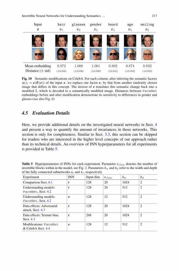
Invertible Neural Networks for Understanding Semantics … 217

Fig. 10 Semantic modifications on CelebA. For each column, after inferring the semantic factors(ei )i = e(E(x)) of the input x, we replace one factor ei by that from another randomly chosenimage that differs in this concept. The inverse of e translates this semantic change back into amodified z, which is decoded to a semantically modified image. Distances between FaceNetembeddings before and after modification demonstrate its sensitivity to differences in gender andglasses (see also Fig. 6)

4.5 Evaluation Details

Here, we provide additional details on the investigated neural networks in Sect. 4and present a way to quantify the amount of invariances in those networks. Thissection is only for completeness. Similar to Sect. 3.3, this section can be skippedfor readers who are interested in the higher level concepts of our approach ratherthan its technical details. An overview of INN hyperparameters for all experimentsis provided in Table 5.

Table 5 Hyperparameters of INNs for each experiment. Parameter n f low denotes the number ofinvertible blocks within in the model, see Fig. 2. Parameters hw and hd refer to the width and depthof the fully connected subnetworks si and τ i , respectively

Experiment INN Input dim. n f low hw hd

Comparison Sect. 4.1 t 128 20 1024 2

Understanding models:FaceNet, Sect. 4.2

t 128 20 512 2

Understanding models:FaceNet, Sect. 4.2

e 128 12 512 2

Data effects: Adversarialattack, Sect. 4.3

t 128 20 1024 2

Data effects: Texture bias,Sect. 4.3

t 268 20 1024 2

Modifications: FaceNet& CelebA Sect. 4.4

e 128 12 512 2

218 R. Rombach et al.

Table 6 High-level architectures of FaceNet and ResNet, depicted as pytorch-modules.Layers investigated in our experiments are marked in bold. Spatial sizes are provided as a visual aidand vary from model to model in our experiments. If not stated otherwise, we always extract fromthe last layer in a series of blocks (e.g., on the right: 23× BottleNeck down → R

8×8×1024 refersto the last module in the series of 23 blocks)

Throughout our experiments, we interpret four different models: SqueezeNet,AlexNet, ResNet, and FaceNet. Summaries of each of model’s architecture areprovided in Table 6 and Table 7. Implementations and pretrained weights of thesemodels are taken from:

• SqueezeNet (1.1) https://pytorch.org/docs/stable/_modules/torchvision/models/squeezenet;• ResNet: https://pytorch.org/docs/stable/_modules/torchvision/models/resnet.html;• AlexNet: https://pytorch.org/docs/stable/_modules/torchvision/models/alexnet.html;• FaceNet: https://github.com/timesler/facenet-pytorch.

Explained variance: To quantify the amount of invariances and semantic concepts,we use the fraction of the total variance explained by invariances (Fig. 8) and thefraction of the variance of a semantic concept explained by the model representation(Fig. 7).

Invertible Neural Networks for Understanding Semantics … 219

Table 7 High-level architectures of SqueezeNet and AlexNet, depicted as pytorch-modules. See Table 6 for further details

Using the INN t , we can consider z = t−1(v|z) as a function of v and z. The totalvariance of z is then obtained by sampling v, via its prior which is a standard normaldistribution, and z, via z = �(x) with x ∼ pvalid(x) sampled from a validation set.We compare this total variance to the average variance obtained when sampling v

for a given z to obtain the fraction of the total variance explained by invariances:

Ex′∼pvalid(x′)

⎡⎢⎢⎢⎢⎣

Varv∼N (v|0,I) t−1(v|�(x′))Var x ∼ pvalid(x)

v ∼ N (v|0, I)

t−1(v|�(x))

⎤⎥⎥⎥⎥⎦ . (20)

In combination with the INN e, which transform z to semantically meaningfulfactors, we can analyze the semantic content of a model representation z. To analyzehow much of a semantic concept represented by factor ei is captured by z, we use eto transform z into ei and measure its variance. To measure how much the semanticconcept is explained by z, we simply swap the roles of z and v in (20), to obtain

220 R. Rombach et al.

Ev′∼N (v′|0,I)

⎡⎢⎢⎢⎢⎣

Varx∼pvalid(x) e(t−1(v′|�(x)))i

Varv ∼ N (v|0, I)x ∼ pvalid(x)

e(t−1(v|�(x)))i

⎤⎥⎥⎥⎥⎦ . (21)

Figure 8 reports (20) and its standard error when evaluated via 10k samples, andFig. 7 reports (21) and its standard error when evaluated via 10k samples.

Conclusions

Understanding a representation in terms of both its semantics and learned invariancesis crucial for interpretation of deep networks.We presented an approach (i) to recoverthe invariances a model has learned and (ii) to translate the representation and itsinvariances onto an equally expressive yet semantically accessible encoding. Ourdiagnostic method is applicable in a plug-and-play fashion on top of existing deepmodels with no need to alter or retrain them. Since our translation onto semantic fac-tors is bijective, it loses no information and also allows for semantic modifications.Moreover, recovering invariances probabilistically guarantees that we can correctlyvisualize representations and sample them without leaving the underlying distribu-tion, which is a common cause for artifacts. Altogether, our approach constitutes apowerful, widely applicable diagnostic pipeline for explaining deep representations.

References

[AKW+19] L. Ardizzone, J. Kruse, S. Wirkert, D. Rahner, E.W. Pellegrini, R.S. Klessen, L.Maier-Hein, C. Rother, U. Köthe, Analyzing inverse problems with invertible neuralnetworks, in Proceedings of the International Conference on Learning Representa-tions (ICLR) (New Orleans, LA, USA, 2019), pp. 1–20

[AS18] Alessandro Achille, Stefano Soatto, Emergence of invariance and disentanglementin deep representations. J. Mach. Learn. Res. (JMLR) 19(50), 1–34 (2018)

[BBM+15] Sebastian Bach, Alexander Binder, Grégoire. Montavon, Frederick Klauschen,Klaus-Robert. Müller, Wojciech Samek, On pixel-wise explanations for non-linearclassifier decisions by layer-wise relevance propagation. PLOS ONE 10(7), 1–46(2015)

[BDS19] A. Brock, J. Donahue, K. Simonyan, Large scale GAN training for high fidelitynatural image synthesis, in Proceedings of the International Conference on LearningRepresentations (ICLR) (New Orleans, LA, USA, 2019), pp. 1–35

[BMDO21a] A. Blattmann, T. Milbich, M. Dorkenwald, B. Ommer, Behavior-driven synthesis ofhuman dynamics, in Proceedings of the IEEE/CVF Conference on Computer Visionand Pattern Recognition (CVPR), virtual conference (2021), pp. 12236–12246

[BMDO21b] A. Blattmann, T. Milbich, M. Dorkenwald, B. Ommer, iPOKE: poking a still imagefor controlled stochastic video synthesis, in Proceedings of the IEEE InternationalConference onComputer Vision (ICCV), virtual conference (2021), pp. 14707–14717

Invertible Neural Networks for Understanding Semantics … 221

[BZK+17] D. Bau, B. Zhou, A. Khosla, A. Oliva, A. Torralba, Network dissection: quantifyinginterpretability of deep visual representations, in Proceedings of the IEEE/CVF Con-ference on Computer Vision and Pattern Recognition (CVPR) (Honolulu, HI, USA,2017), pp. 6541–6549

[BZS+19] D. Bau, J-Y. Zhu, H. Strobelt, B. Zhou, J.B. Tenenbaum, W.T. Freeman, A. Torralba,GAN dissection: visualizing and understanding generative adversarial networks, inProceedings of the International Conference on Learning Representations (ICLR)(New Orleans, LA, USA, 2019), pp. 1–18

[CSX+18] Q. Cao, L. Shen, W. Xie, O.M. Parkhi, A. Zisserman, VGGFace2: a dataset forrecognising faces across pose and age, in Proceedings of the IEEE InternationalConference on Automatic Face & Gesture Recognition (FG) (Xi’an, China, 2018),pp. 67–74

[CWG+18] S.A. Cadena, M.A. Weis, L.A. Gatys, M. Bethge, A.S. Ecker, Diverse feature visu-alizations reveal invariances in early layers of deep neural networks, in Proceedingsof the European Conference on Computer Vision (ECCV) (Munich, Germany, 2018),pp. 225–240

[DB16] A. Dosovitskiy, T. Brox, Generating images with perceptual similarity metrics basedon deep networks, in Proceedings of the Conference on Neural Information Process-ing Systems (NIPS/NeurIPS) (Barcelona, Spain, 2016), pp. 658–666

[DDS+09] J. Deng, W. Dong, R. Socher, L-J. Li, K. Li, F-F. Li, ImageNet: a large-scale hier-archical image database, in Proceedings of the IEEE/CVF Conference on ComputerVision and Pattern Recognition (CVPR) (Miami, FL, USA, 2009), pp. 248–255

[DMB+21] M. Dorkenwald, T. Milbich, A. Blattmann, R. Rombach, K.G. Derpanis, B. Ommer,Stochastic image-to-video synthesis using cINNs, in Proceedings of the IEEE/CVFConference on Computer Vision and Pattern Recognition (CVPR), virtual conference(2021), pp. 3742–3753

[DSB17] L.Dinh, J. Sohl-Dickstein, S. Bengio, Density estimation using real NVP, inProceed-ings of the International Conference on Learning Representations (ICLR) (Toulon,France, 2017), pp. 1–32

[DW19] B. Dai, D. Wipf, Diagnosing and enhancing VAE models, in Proceedings of theInternational Conference on Learning Representations (ICLR) (New Orleans, LA,USA, 2019), pp. 1–12

[EHO19] P. Esser, J. Haux, B. Ommer, Unsupervised robust disentangling of latent character-istics for image synthesis, in Proceedings of the IEEE International Conference onComputer Vision (ICCV) (Seoul, Korea, 2019), pp. 2699–2709

[ERO20] P. Esser, R. Rombach, B. Ommer, A disentangling invertible interpretation networkfor explaining latent representations, in Proceedings of the IEEE/CVF Conferenceon Computer Vision and Pattern Recognition (CVPR), virtual conference (2020), pp.9223–9232

[Eur20] European Commission, White Paper on Artificial Intelligence – A EuropeanApproach to Excellence and Trust. Technical report, European Union (2020). https://eur-lex.europa.eu/legal-content/EN/TXT/?uri=COM:2020:65:FIN

[FV18] R. Fong, A. Vedaldi, Net2Vec: quantifying and explaining how concepts are encodedby filters in deep neural networks, in Proceedings of the IEEE/CVF Conference onComputer Vision and Pattern Recognition (CVPR) (Salt Lake City, UT, USA, 2018),pp. 8730–8738

[GAOI19] L. Goetschalckx, A. Andonian, A. Oliva, P. Isola, GANalyze: toward visual def-initions of cognitive image properties, in Proceedings of the IEEE InternationalConference on Computer Vision (ICCV) (Seoul, Korea, 2019), pp. 5744–5753

[GF17] BryceGoodman, Seth Flaxman, European union regulations on algorithmic decision-making and a “right to explanation”. AI Mag. 38(3), 50–57 (2017)

[GRM+19] R. Geirhos, P. Rubisch, C. Michaelis, M. Bethge, F.A. Wichmann, W. Brendel,ImageNet-trained CNNs are biased towards texture; increasing shape bias improvesaccuracy and robustness, inProceedings of the International Conference on LearningRepresentations (ICLR) (New Orleans, LA, USA, 2019), pp. 1–22

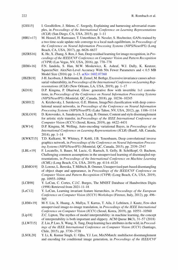
222 R. Rombach et al.

[GSS15] I. Goodfellow, J. Shlens, C. Szegedy, Explaining and harnessing adversarial exam-ples, in Proceedings of the International Conference on Learning Representations(ICLR) (San Diego, CA, USA, 2015), pp. 1–11

[HRU+17] M. Heusel, H. Ramsauer, T. Unterthiner, B. Nessler, S. Hochreiter, GANs trained bya two time-scale update rule converge to a local nash equilibrium, in Proceedings ofthe Conference on Neural Information Processing Systems (NIPS/NeurIPS) (LongBeach, CA, USA, 2017), pp. 6626–6637

[HZRS16] K. He, X. Zhang, S. Ren, J. Sun, Deep residual learning for image recognition, inPro-ceedings of the IEEE/CVF Conference on Computer Vision and Pattern Recognition(CVPR) (Las Vegas, NV, USA, 2016), pp. 770–778

[IHM+16] F.N. Iandola, S. Han, M.W. Moskewicz, K. Ashraf, W.J. Dally, K. Keutzer,SqueezeNet: AlexNet-Level Accuracy With 50x Fewer Parameters and < 0.5 MBModel Size (2016) pp. 1–13. arXiv:1602.07360

[JBZB19] J-H. Jacobsen, J. Behrmann,R. Zemel,M.Bethge, Excessive invariance causes adver-sarial vulnerability, inProceedings of the International Conference on Learning Rep-resentations (ICLR) (New Orleans, LA, USA, 2019), pp. 1–17

[KD18] D.P. Kingma, P. Dhariwal, Glow: generative flow with invertible 1x1 convolu-tions, in Proceedings of the Conference on Neural Information Processing Systems(NIPS/NeurIPS) (Montréal, QC, Canada, 2018), pp. 10236–10245

[KSH12] A. Krizhevsky, I. Sutskever, G.E. Hinton, ImageNet classification with deep convo-lutional neural networks, in Proceedings of the Conference on Neural InformationProcessing Systems (NIPS/NeurIPS) (Lake Tahoe, NV, USA, 2012), pp. 1106–1114

[KSLO19] D. Kotovenko, A. Sanakoyeu, S. Lang, B. Ommer, Content and style disentanglementfor artistic style transfer, in:Proceedings of the IEEE International Conference onComputer Vision (ICCV) (Seoul, Korea, 2019), pp. 4422–4431

[KW14] D.P. Kingma, M. Welling, Auto-encoding variational Bayes, in Proceedings of theInternational Conference on Learning Representations (ICLR) (Banff, AB, Canada,2014), pp. 1–14

[KWKT15] T.D. Kulkarni, W. Whitney, P. Kohli, J.B. Tenenbaum, Deep convolutional inversegraphics network, in Proceedings of the Conference on Neural Information Process-ing Systems (NIPS/NeurIPS) (Montréal, QC, Canada, 2015), pp. 2539–2547

[LBL+19] F. Locatello, S. Bauer, M. Lucic, G. Raetsch, S. Gelly, B. Schölkopf, O. Bachem,Challenging common assumptions in the unsupervised learning of disentangled rep-resentations, in Proceedings of the International Conference on Machine Learning(ICML) (Long Beach, CA, USA, 2019), pp. 4114–4124

[LBMO19] D. Lorenz, L. Bereska, T.Milbich, B.Ommer,Unsupervised part-based disentanglingof object shape and appearance, in Proceedings of the IEEE/CVF Conference onComputer Vision and Pattern Recognition (CVPR) (Long Beach, CA, USA, 2019),pp. 10955–10964

[LCB98] Y. LeCun, C. Cortes, C.J.C. Burges, The MNIST Database of Handwritten Digits(1998) Retrieved from 2021-11-18

[LeC12] Y. LeCun, Learning invariant feature hierarchies, in Proceedings of the EuropeanConference on Computer Vision (ECCV) Workshops (Firenze, Italy, 2012), pp. 496–505

[LHM+19] M-Y. Liu, X. Huang, A. Mallya, T. Karras, T. Aila, J. Lehtinen, J. Kautz, Few-shotunsupervised image-to-image translation, in Proceedings of the IEEE InternationalConference on Computer Vision (ICCV) (Seoul, Korea, 2019), pp. 10551–10560

[Lip18] Z.C. Lipton, The mythos of model interpretability: in machine learning, the conceptof interpretability is both important and slippery. ACM Queue 16(3), 31–57 (2018)

[LLWT15] Z. Liu, P. Luo,X.Wang,X. Tang,Deep learning face attributes in thewild, inProceed-ings of the IEEE International Conference on Computer Vision (ICCV) (Santiago,Chile, 2015), pp. 3730–3738

[LSOL20] Y. Li, K. Kumar Singh, U. Ojha, Y.J. Lee, MixNMatch: multifactor disentanglementand encoding for conditional image generation, in Proceedings of the IEEE/CVF

Invertible Neural Networks for Understanding Semantics … 223

Conference on Computer Vision and Pattern Recognition (CVPR), virtual conference(2020), pp. 8039–8048

[Mil19] Tim Miller, Explanation in artificial intelligence: insights from the social sciences.Artif. Intell. 267, 1–38 (2019)

[MLB+17] Grégoire. Montavon, Sebastian Lapuschkin, Alexander Binder, Wojciech Samek,Klaus-Robert Müller, Explaining nonlinear classification decisions with deep Taylordecomposition. Pattern Recognit. 65(5), 211–222 (2017)

[MOT15] A. Mordvintsev, C. Olah, M. Tyka, Inceptionism: going deeper into neural networks(2015). Accessed 2021-11-18

[MSM18] Grégoire. Montavon, Wojciech Samek, Klaus-Robert. Müller, Methods for interpret-ing and understanding deep neural networks. Digital Signal Process. 73, 1–15 (2018)

[MV16] Aravindh Mahendran, Andrea Vedaldi, Visualizing deep convolutional neural net-works using natural pre-images. Int. J. Comput. Vis. (IJCV) 120, 233–255 (2016)

[NDY+16] A. Nguyen, A. Dosovitskiy, J. Yosinski, T. Brox, J. Clune, Synthesizing the pre-ferred inputs for neurons in neural networks via deep generator networks, inProceed-ings of the Conference on Neural Information Processing Systems (NIPS/NeurIPS)(Barcelona, Spain, 2016), pp. 3387–3395

[NKW19] C. Nash, N. Kushman, C.K.I. Williams, Inverting supervised representations withautoregressive neural densitymodels, inProceedings of the International Conferenceon Artificial Intelligence and Statistics (AISTATS) (Naha, Japan, 2019), pp. 1620–1629

[PASC+20] G. Plumb, M. Al-Shedivat, Á.A. Cabrera, A. Perer, E. Xing, A. Talwalkar, Regular-izing black-box models for improved interpretability, in Proceedings of the Confer-ence on Neural Information Processing Systems (NIPS/NeurIPS), virtual conference(2020), pp. 10526–10536

[Red93] A. Norman Redlich, Supervised factorial learning. Neural Comput. 5(5), 750–766(1993)

[REO20] R. Rombach, P. Esser, B. Ommer, Network-to-network translation with conditionalinvertible neural networks, in Proceedings of the Conference on Neural InformationProcessing Systems (NIPS/NeurIPS), virtual conference (2020), pp. 2784–2797

[RMW14] D.J. Rezende, S. Mohamed, D. Wierstra, Stochastic backpropagation and approxi-mate inference in deep generative models, in Proceedings of the International Con-ference on Learning Representations (ICLR) (Banff, AB, Canada, 2014), pp. 1–14

[SCD+20] Ramprasaath R. Selvaraju, Michael Cogswell, Abhishek Das, Ramakrishna Vedan-tam, Devi Parikh, Dhruv Batra, Grad-CAM: visual explanations from deep networksvia gradient-based localization. Int. J. Comput. Vis. (IJCV) 128, 336–359 (2020)

[SGM+20] A. Shocher, Y. Gandelsman, I. Mosseri, M. Yarom,M. Irani,W.T. Freeman, T. Dekel,Semantic pyramid for image generation, inProceedings of the IEEE/CVFConferenceon Computer Vision and Pattern Recognition (CVPR), virtual conference (2020), pp.7457–7466

[SIT+19] S. Santurkar, A. Ilyas, D. Tsipras, L. Engstrom, B. Tran, A. Madry, Image synthesiswith a single (robust) classifier, in Proceedings of the Conference on Neural Infor-mation Processing Systems (NIPS/NeurIPS) (Vancouver, BC, Canada, 2019), pp.1260–1271

[SKP15] F. Schroff, D. Kalenichenko, J. Philbin, FaceNet: a unified embedding for face recog-nition and clustering, in Proceedings of the IEEE/CVF Conference on ComputerVision and Pattern Recognition (CVPR) (Boston, MA, USA, 2015), pp. 815–823

[SR15] M. Simon, E. Rodner, Neural activation constellations: unsupervised part modeldiscovery with convolutional networks, in Proceedings of the IEEE InternationalConference on Computer Vision (ICCV) (Santiago, Chile, 2015), pp. 1143–1151

[SRD14] M. Simon, E. Rodner, J. Denzler, Part detector discovery in deep convolutional neu-ral networks, in Proceedings of the Asian Conference on Computer Vision (ACCV)(Singapore, Singapore, 2014), pp. 162–177

224 R. Rombach et al.

[SVZ14] K. Simonyan, A. Vedaldi, A. Zisserman, Deep inside convolutional networks: visu-alising image classification models and saliency maps, in Proceedings of the Inter-national Conference on Learning Representations (ICLR) Workshops (Banff, AB,Canada, 2014), pp. 1–8

[SWM17] W.Samek, T.Wiegand,K-R.Müller,ExplainableArtificial Intelligence:Understand-ing. Visualizing and Interpreting Deep Learning Models (Springer, 2017)

[SZS+14] C. Szegedy, W. Zaremba, I. Sutskever, J. Bruna, D. Erhan, I. Goodfellow, R. Fer-gus, Intriguing properties of neural networks, in Proceedings of the InternationalConference on Learning Representations (ICLR) (Banff, AB, Canada, 2014), pp.1–10

[UGP+17] P. Upchurch, J. Gardner, G. Pleiss, R. Pless, N. Snavely, K. Bala, K.Weinberger, Deepfeature interpolation for image content changes, in Proceedings of the IEEE/CVFConference on Computer Vision and Pattern Recognition (CVPR) (Honolulu, HI,USA, 2017), pp. 7064–7073

[XYA19] Z.Xiao,Q.Yan,Y.Amit,GenerativeLatent Flow (2019), pp. 1–18. arXiv:1905.10485[YCN+15] J. Yosinski, J. Clune, A. Nguyen, T. Fuchs, H. Lipson, Understanding neural net-

works through deep visualization, in Proceedings of the International Conference onMachine Learning (ICML) Workshops (2015), pp. 1–12

[ZF14] M.D. Zeiler, R. Fergus, Visualizing and understanding convolutional networks, inProceedings of the European Conference on Computer Vision (ECCV) (Zurich,Switzerland, 2014), pp. 818–833

[ZIE+18] R. Zhang, P. Isola, A.A. Efros, E. Shechtman, O. Wang, The unreasonable effec-tiveness of deep features as a perceptual metric, in Proceedings of the IEEE/CVFConference on Computer Vision and Pattern Recognition (CVPR) (Salt Lake City,UT, USA, 2018), pp. 586–595

[ZKL+15] B. Zhou, A. Khosla, A. Lapedriza, A. Oliva, A. Torralba, Object detectors emergein deep scene CNNs, in Proceedings of the International Conference on LearningRepresentations (ICLR) (San Diego, CA, USA, 2015), pp. 1–12

[ZKL+16] B. Zhou, A. Khosla, A. Lapedriza, A. Oliva, A. Torralba, Learning deep features fordiscriminative localization, in Proceedings of the IEEE/CVF Conference on Com-puter Vision and Pattern Recognition (CVPR) (Las Vegas, NV, USA, 2016), pp.2921–2929

[ZNWZ18] Q. Zhang, Y.NianWu, S-C. Zhu, Interpretable convolutional neural networks, inPro-ceedings of the IEEE/CVF Conference on Computer Vision and Pattern Recognition(CVPR) (Salt Lake City, UT, USA, 2018), pp. 8827–8836

Open Access This chapter is licensed under the terms of the Creative Commons Attribution 4.0International License (http://creativecommons.org/licenses/by/4.0/), which permits use, sharing,adaptation, distribution and reproduction in any medium or format, as long as you give appropriatecredit to the original author(s) and the source, provide a link to the Creative Commons license andindicate if changes were made.

The images or other third party material in this chapter are included in the chapter’s CreativeCommons license, unless indicated otherwise in a credit line to the material. If material is notincluded in the chapter’s Creative Commons license and your intended use is not permitted bystatutory regulation or exceeds the permitted use, you will need to obtain permission directly fromthe copyright holder.

Confidence Calibration for ObjectDetection and Segmentation

Fabian Küppers, Anselm Haselhoff, Jan Kronenberger, and Jonas Schneider

Abstract Calibrated confidence estimates obtained from neural networks are cru-cial, particularly for safety-critical applications such as autonomous driving or med-ical image diagnosis. However, although the task of confidence calibration has beeninvestigated on classification problems, thorough investigations on object detectionand segmentation problems are still missing. Therefore, we focus on the investi-gation of confidence calibration for object detection and segmentation models inthis chapter. We introduce the concept of multivariate confidence calibration that isan extension of well-known calibration methods to the task of object detection andsegmentation. This allows for an extended confidence calibration that is also awareof additional features such as bounding box/pixel position and shape information.Furthermore, we extend the expected calibration error (ECE) to measure miscali-bration of object detection and segmentation models. We examine several networkarchitectures on MS COCO as well as on Cityscapes and show that especially objectdetection as well as instance segmentation models are intrinsically miscalibratedgiven the introduced definition of calibration. Using our proposed calibration meth-ods, we have been able to improve calibration so that it also has a positive impact onthe quality of segmentation masks as well.

F. Küppers (B) · A. Haselhoff · J. KronenbergerHochschule Ruhr West, Duisburger Str. 100, 45479 Mülheim a.d. Ruhr, Germanye-mail: fabian.kueppers@hs-ruhrwest.de

A. Haselhoffe-mail: anselm.haselhoff@hs-ruhrwest.de

J. Kronenbergere-mail: jan.kronenberger@hs-ruhrwest.de

J. SchneiderElektronische Fahrwerksysteme GmbH, Dr.-Ludwig-Kraus-Str. 6,85080 Gaimersheim, Germanye-mail: jonas.schneider@efs-auto.com

© The Author(s) 2022T. Fingscheidt et al. (eds.), Deep Neural Networks and Data for Automated Driving,https://doi.org/10.1007/978-3-031-01233-4_8

225

226 F. Küppers et al.

1 Introduction

Common neural networks for object detection must not only determine the positionand class of an object but also denote their confidence about the correctness ofeach detection. This also holds for instance or semantic segmentation models thatoutput a score for each pixel indicating the confidence of object mask membership.A reliable confidence estimate for detected objects is crucial, particularly for safety-critical applications such as autonomous driving, to reliably process detected objects.Another example ismedical diagnosis, where, for example, the shape of a brain tumorwithin an MRI image is of special interest [MWT+20].

Each confidence estimate might be seen as a probability of correctness, reflect-ing the model’s uncertainty about a detection or the pixel mask. During inference,we expect the estimated confidence to match the observed precision for a predic-tion. For example, given 100 predictions with 80% confidence each, we expect 80predictions to be correctly predicted [GPSW17, KKSH20]. However, recent workhas shown that the confidence estimates of either classification or detection modelsbased on neural networks are miscalibrated, i.e., the confidence does not match theobserved accuracy in classification [GPSW17] or the observed precision in objectdetection [KKSH20]. While confidence calibration within the scope of classificationhas been extensively investigated [NCH15, NC16, GPSW17, KSFF17, KPNK+19],we recently defined the term of calibration for object detection and proposedmethodsto measure and resolve miscalibration [KKSH20, SKR+21]. In this context, wemea-suredmiscalibration w.r.t. the position and scale of detected objects by also includingthe regression branch of an object detector into a calibration mapping. We have beenable to show that modern object detection models also tend to be miscalibrated.On the one hand, this can be mitigated using standard calibration methods. On theother hand, we show that our proposed methods for position- and shape-dependentcalibration [KKSH20] are able to further reduce miscalibration.

In this chapter we review our methods for position- and shape-dependent confi-dence calibration and provide a definition for confidence calibration for the taskof instance/semantic segmentation. To this end, we extend the definition of theexpected calibration error (ECE) to measure miscalibration within the scope ofinstance/semantic segmentation. Furthermore, we adapt the extended calibrationmethods originally designed for object detection [KKSH20] to enable position-dependent confidence calibration for segmentation tasks as well.

This chapter is structured as follows. In Sect. 2 we review the most importantrelated works regarding confidence calibration. In Sect. 3 we provide the definitionsof calibration for the tasks of object detection, instance segmentation, and semanticsegmentation. Furthermore, in Sect. 4 we present the extended confidence calibrationmethods for object detection and segmentation. Extensive experimental evaluationson a variety of architectures and computer vision problems, including object detectionand instance/semantic segmentation, are discussed in Sect. 5. Finally, we provideconclusions and discuss our most important findings.

Confidence Calibration for Object Detection and Segmentation 227

2 Related Works

In the past, most research focused on measuring and resolving miscalibration forclassification tasks. In this scope, the expected calibration error (ECE) [NCH15] iscommonly used in conjunctionwith theBrier score and negative log likelihood (NLL)loss to measure miscalibration. For calculating the ECE, all samples are grouped intoequally sized bins by their confidence. Afterward, for each bin the accuracy is calcu-lated and used as an approximation of the accuracy of a single sample in its respectivebin. Recently, several extensions such as classwise ECE [KPNK+19], marginal cali-bration error [KLM19], or adaptive calibration error [NDZ+19] for the evaluation ofmulti-class problems have also been proposed, where the ECE is evaluated for eachclass separately. In contrast to previous work, we extend the common ECE definitionto the task of object detection [KKSH20] and instance/semantic segmentation. Thisextension allows for a position-dependent miscalibration evaluation so that it is pos-sible to quantify miscalibration separately for certain image regions. The definitionis given in Sect. 3.

Besides measuring miscalibration, it is also possible to resolve a potential mis-calibration by using calibration methods that are applied after inference. These post-hoc calibration methods can be divided into binning and scaling methods. Binningmethods such as histogram binning [ZE01], isotonic regression [ZE02], Bayesianbinning into quantiles (BBQ) [NCH15], or ensemble of near-isotonic regression(ENIR) [NC16] group all samples into several bins by their confidence (similar tothe ECE calculation) and perform a mapping from uncalibrated confidence esti-mates to calibrated ones. In contrast, scaling methods such as logistic calibration(Platt scaling) [Pla99], temperature scaling [GPSW17], beta calibration [KSFF17],or Dirichlet calibration [KPNK+19] scale the network logits before sigmoid/softmaxactivation to obtain calibrated confidences. The scaling parameters are commonlyobtained by logistic regression.Other approaches comprise binwise temperature scal-ing [JJY+19] or scaling-binning calibrator [KLM19], combining both approaches tofurther improve calibration performance for classification tasks.

Recently, we proposed an extension of common calibration methods to objectdetection by also including the bounding box regression branch of an object detectorinto a calibration mapping [KKSH20]. On the one hand, we extended the histogrambinning [ZE01] to perform calibration using a multidimensional binning scheme. Onthe other hand, we also extended scaling methods to include position informationinto a calibration mapping. Both approaches are presented in Sect. 4 in more detail.

Unlike classification, the task of instance or semantic segmentation calibrationhas not yet been addressed by many authors. In the work of [WLK+20], the authorsperform online confidence calibration of the classification head of an instance seg-mentation model and show that this has a significant impact on the mask quality. Theauthors in [KG20] use a multi-task learning approach for semantic segmentationmodels to improve model calibration and out-of-distribution detection within thescope of medical image diagnosis. A related approach is proposed by [MWT+20],where the authors train multiple fully-connected networks as an ensemble to obtain

228 F. Küppers et al.

well-calibrated semantic segmentation models. However, none of these methodsprovide an explicit definition of calibration for segmentation models (instance orsemantic). This problem is addressed by [DLXS20], where the authors explicitlydefine semantic segmentation calibration and propose a local temperature scaling forsemantic image masks. This approach utilizes the well-known temperature scaling[GPSW17] and assigns a temperature for each mask pixel separately. Furthermore,they use a dedicated convolutional neural network (CNN) to infer the temperatureparameters for each image. Our definition of segmentation calibration in Sect. 3 isconformwith their definition. Our approach differs from their proposed image-basedtemperature scaling as we use a single position-dependent calibration mapping tomodel the probability distributions for all images.

3 Calibration Definition and Evaluation

In this section, we review the term of confidence calibration for classification tasks[NCH15, GPSW17] and extend this definition to object detection, instance segmen-tation, and semantic segmentation. Furthermore, we derive the detection expectedcalibration error (D-ECE) to measure miscalibration.

3.1 Definitions of Calibration

Classification: In a first step, we define the datasetsD of size |D| = N with indicesi ∈ I = {1, . . . , N }, consisting of images x ∈ I

H×W×C , I = [0, 1], with height H ,width W , and number of channels C . Each image has ground-truth information thatconsists of the class information Y ∈ Y = {1, . . . ,Y }. As an introduction into thetask of confidence calibration, we start with the definition of perfect calibration forclassification. A classification model Fcls outputs a label Y and a correspondingconfidence score P indicating its belief about the prediction’s correctness. In thiscase, perfect calibration is defined by [GPSW17]

P(Y = Y |P = p) = p ∀p ∈ [0, 1]. (1)

In otherwords, the accuracy P(Y = Y |P = p) for a certain confidence level p shouldmatch the estimated confidence. If we observe a deviation, a model is called miscal-ibrated. In binary classification, we rather consider the relative frequency of Y = 1instead of the accuracy as the calibration measure. We illustrate this difference usingthe following example. Consider N = 100 images of a datasetDwith binary ground-truth labels Y ∈ {0, 1}, where 50 images are labeled as Y = 0 and 50 images withY = 1. Furthermore, consider a classification model Fcls with a sigmoidal outputin [0, 1], indicating its confidence for Y = 1. In our example, this model is able toalways predict the correct ground-truth label with confidences P = 0 and P = 1 for

Confidence Calibration for Object Detection and Segmentation 229

Y = 0 and Y = 1, respectively. Thus, the network is able to achieve an accuracy of100% but with an average confidence of 50%. Therefore, we consider the relativefrequency for Y = 1 in a binary classification task as the calibration goal that is also50% in this scenario.

Object detection: In the next step, we extend our dataset and model to the task ofobject detection. In contrast to a classification dataset, an object detection datasetconsists of ground-truth annotations Y ∈ Y = {1, . . . ,Y } for each object within animage as well as the ground-truth position and shape information R ∈ R = [0, 1]A(A denotes the size of the normalized box encoding, comprising the center x and ypositions cx , cy , as well as width w and height h). An object detection model Fdet

further outputs a confidence score P ∈ [0, 1], a label Y ∈ Y, and the correspondingposition R ∈ R for each detection in an image x. Extending the original formulationfor confidence calibration within classification tasks [GPSW17], perfect calibrationfor object detection is defined by [KKSH20]

P(M = 1|P = p, Y = y, R = r) = p (2)

∀p ∈ [0, 1], y ∈ Y, r ∈ R,

where M = 1 denotes a correctly classified prediction that matches a ground-truthobjectwith a certain intersection-over-union (IoU) score.Commonly, an object detec-tion model is calibrated by means of its precision, as the computation of the accuracyis not possible without knowing all anchors of a model [KKSH20, SKR+21]. Thus,P(M = 1) is a shorthand notation for p(Y = Y , R = R) that expresses the precisionfor a dedicated IoU threshold.

Instance segmentation:At this point, we adapt this idea to define confidence calibra-tion for instance segmentation. Consider a dataset with K annotated objectsK overall images. For notation simplicity, we further use j ∈ Jk = {1, . . . , Hk · Wk} as theindex for pixel j within a bounding boxRk of object k ∈ K in the instance segmenta-tion dataset, where Hk and Wk denote the width and height of object k, respectively.In addition to object detection, a ground-truth dataset for instance segmentation alsoconsists of pixel-wise mask labels denoted by Y j ∈ Y∗ = {0, 1} for each pixel jin the bounding box Rk of object k. Note that we introduce the star superscript(∗) here to distinguish between the bounding box label/prediction encoding and theinstance segmentation label/prediction encoding. An instance segmentation modelFins predicts the membership Y j ∈ Y∗ for each pixel j in the predicted boundingbox Rk to the object mask with a certain confidence Pj ∈ [0, 1]. We further denoteR j ∈ R∗ = [0, 1]A∗

as the position of pixel j within the bounding box Rk , where A∗denotes the size of the used position encoding of a pixel within its bounding box. Incontrast to object detection, it is possible to treat the confidence scores of each pixelwithin an instance segmentation mask as a binary classification problem. In this case,the confidence Pj can be interpreted as the probability of a pixel belonging to theobject mask. Therefore, the aim of confidence calibration for instance segmentationis that the pixel confidence should match the relative frequency that a pixel is part

230 F. Küppers et al.

of the object mask. According to the task of object detection, we further include aposition dependency into the definition, for instance, segmentation and obtain

P(Y j = Y j |Y = y, Pj = p,R j = r) = p, (3)

∀p ∈ [0, 1], y ∈ Y, r ∈ R∗, j ∈ Jk, k ∈ K .

The former term can be interpreted as the probability that the prediction Y j for apixel with index j within an object k matches the ground-truth annotation Y j givena certain confidence p, a certain pixel position r within the bounding box, as well asa certain object category y that is predicted by the bounding box head of the instancesegmentation model.

Semantic Segmentation: Compared to object detection or instance segmentation, asemantic segmentation dataset does not hold ground-truth information for individualobjects but rather consists of pixel-wise class annotations Y j ∈ Y = {1, . . . ,Y },j ∈ J = {1, . . . , H · W }. A semantic segmentation model Fsem outputs pixel-wiselabels Y j and probabilities Pj with relative position R j within an image. Therefore,we can define perfect calibration for semantic segmentation as

P(Y j = Y j |Pj = p,R j = r) = p, (4)

∀p ∈ [0, 1], r ∈ R∗, j ∈ J,

that is related to the calibration definition of classification [GPSW17]. In addition,the confidence score of each pixel must not only reflect its accuracy given a certainconfidence level but also at a certain pixel position.

3.2 Measuring Miscalibration

We can measure the miscalibration of an object detection model as the expecteddeviation between confidence and observed precision which is also known as thedetection expected calibration error (D-ECE) [KKSH20]. Let further s = (p, y, r)denote a single detectionwith confidence p, class y, and bounding box r so that s ∈ S,where S is the aggregated set of the confidence space [0, 1], the set of ground-truthlabelsY, and the set of possible bounding box positions R. Since M is a continuousrandom variable, we need to approximate the D-ECE using the Riemann-Stieltjesintegral [GPSW17]

EP,Y ,R[|P(M = 1|P = p, Y = y, R = r) − p|] (5)

=∫S

∣∣P(M = 1|P = p, Y = y, R = r) − p∣∣ dFP,Y ,R(s) (6)

with FP,Y ,R(s) as the joint cumulative distribution of P , Y , and R. Let a =(ap, ay, ar1 , . . . , arA)

T ∈ S and b = (bp, by, br1 , . . . , brA)T ∈ S denote interval

Confidence Calibration for Object Detection and Segmentation 231

boundaries for the confidence ap, bp ∈ [0, 1], the estimated labels ay, by ∈ Y andeach quantity of the bounding box encoding ar1 , br1 , . . . arA , brA ∈ [0, 1] defined onthe joint cumulative FP,Y ,R(s) so that1 FP,Y ,R(b) − FP,Y ,R(a) = P(P ∈ [ap, bp],Y ∈ [ay, by], R1 ∈ [ar1 , br1 ], . . . , RA ∈ [arA , brA ]). The integral in (6) is now approx-imated by

∑m∈B

P(sm) · ∣∣P(M = 1|P = pm, Y = ym, R = rm) − pm∣∣, (7)

with B as the number of equidistant bins used for integral approximation so thatB ={1, . . . , B}, and pm ∈ [0, 1], ym ∈ Y and rm ∈ R being the respective bin entities foraverage confidence, the current label, and the average (unpacked) bounding boxscores within bin m ∈ B, respectively. Let Nm denote the amount of samples withina single bin m. For large datasets |D| = N , the probability P(M = 1|P = pm, Y =ym, R = rm) is approximated by the average precisionwithin a single binm, whereaspm is approximated by the average confidence, so that the D-ECE can finally becomputed by

∑m∈B

1

Nm

∣∣prec(m) − conf(m)∣∣, (8)

where prec(m) and conf(m) denote the precision and average confidence within binm, respectively.

Similarly, we can extend the D-ECE to instance segmentation by

EY ,Pj ,R j[∣∣P(Y j = Y j |Y = y, Pj = p,R j = r) − p

∣∣] (9)

≈∑m∈B

1

Nm

∣∣freq(m) − conf(m)∣∣, (10)

with a binning scheme over all pixels and freq(m) as the average frequency withineach bin. In this case, each pixel is treated as a separate prediction and binned byits confidence, label class, and relative position. In the same way, the D-ECE forsemantic segmentation is approximated by

EPj ,R j[∣∣P(Y j = Y j |Pj = p,R j = r∗) − p

∣∣] (11)

≈∑m∈B

1

Nm

∣∣acc(m) − conf(m)∣∣, (12)

with accuracy acc(m) within each bin m.

1 For discrete random variables (e.g., Y ), we use a continuous density function of the form pY (y) =∑y∗∈Y P(y∗)δ(y − y∗) with δ(x) as the Dirac delta function.

232 F. Küppers et al.

For the calibration evaluation of object detection models, we can use the relativeposition cx , cy , and the shape h, w, of the bounding boxes [KKSH20]. For segmen-tation, we consider the relative position x, y, of each pixel within a bounding box(instance segmentation) or within the image (semantic segmentation), as well asits distance d to the next segment boundary, as we expect a higher uncertainty inthe peripheral areas of a segmentation mask. We use these definitions to evaluatedifferent models in Sect. 5.

4 Position-Dependent Confidence Calibration

For post-hoc calibration, we distinguish between binning and scaling methods.According to the approximation in (7), binning methods such as histogram bin-ning [ZE01] divide all samples into several bins by their confidence and measurethe average accuracy/precision within each bin. In contrast, scaling methods rescalethe logits of a neural network before sigmoid/softmax activation to calibrate a net-work’s output. In this section, we extend standard calibrationmethods so that they arecapable of dealing with additional information such as position and/or shape. Theseextendedmethods can be used for confidence calibration of object detection, instancesegmentation, and semantic segmentation tasks. We illustrate the difference betweenstandard calibration and position-dependent calibration using an artificially createddataset in Fig. 1. This dataset consists of points with a confidence score and a binaryground-truth information in {0, 1}, so that we are able to compute the frequencyof the points across the whole image. We observe that standard calibration onlyshifts the average confidence to fit the average precision/accuracy. This leads to an

0.0 0.25 0.5 0.75 1.00.0

0.25

0.5

0.75

1.0

position

position

0% 5% 10% 15% 20% 25%(a) Uncalibrated

0.0 0.25 0.5 0.75 1.0position

0% 5% 10% 15% 20% 25%(b) After standard calibration

0.0 0.25 0.5 0.75 1.0position

0% 5% 10% 15% 20% 25%(c) After position-dependent calibration

Fig. 1 a Consider an artificial dataset with low calibration error in the center and increasingmiscalibration toward the image boundaries. bA common logistic calibration model only shifts theaverage confidence to match the accuracy. This leads to a better global ECE score but also degradesthe miscalibration in the center of the image. c In contrast, position-dependent calibration is capableof possible dependencies and leads to an overall improvement of calibration (example taken fromprevious work [KKSH20])

Confidence Calibration for Object Detection and Segmentation 233

increased calibration error in the center of the image. In contrast, position-dependentcalibration as defined in this section is able to capture correlations between positioninformation and calibration error and reduces the D-ECE across the whole image.

4.1 Histogram Binning

Given a binning scheme with B different bins so that B = {1, . . . , B} with theaccording bin boundaries 0 = a1 ≤ a2 ≤ · · · ≤ aB+1 = 1 and the corresponding cal-ibrated estimate θm within each bin, the objective for histogram binning to estimate� = {θm |m ∈ B} is the minimization

min�

∑i∈I

∑m∈B

1(am ≤ pi < am+1) · (θm − yi )2, (13)

with 1(·) as the indicator function, yielding a 1 if its argument is true and a 0 if it isfalse [ZE01, GPSW17]. This objective converges to the fraction of positive sampleswithin each bin under consideration. However, within the scope of object detectionor segmentation, we also want to measure the accuracy/precision w.r.t. position andshape information. As an extension to the standard histogram binning [ZE01], wetherefore propose a multidimensional binning scheme that divides all samples intoseveral bins by their confidence and by all additional information such as position andshape [KKSH20].We further denote S = (P, R) of size Q = A + 1 as the input vec-tor to a calibration function consisting of the confidence and the bounding box encod-ing, so that Q = {1, . . . , Q}. In a multidimensional histogram binning, we indicatethe number of bins as B = (B1, . . . , BQ) so that B∗ = {Bq = {1, . . . , Bq}|q ∈ Q}with bin boundaries {0 = a1,q ≤ a2,q ≤ · · · ≤ aBq+1,q = 1|q ∈ Q}. For each bincombination m1 ∈ B1, . . . ,mQ ∈ BQ , we have a dedicated calibration parameterθm1,...,mQ ∈ R so that the calibration parameters�∗, with |�∗| = ∏

q∈Q Bq , are givenas �∗ = {θm1,...,mQ |m1 ∈ B1, . . . ,mQ ∈ BQ}. This results in an objective functiongiven by

min�∗

∑i∈I

J (si ), (14)

where

J (si ) ={

(θm1,...,mQ − yi )2, if (am,q ≤ si,q < am,q) ∀q ∈ Q,∀m ∈ Bq

0, otherwise,(15)

which again converges to the fraction of positive samples within each bin. The termJ (si ) simply denotes that the loss is only applied if a sample si falls in a certain bincombination. A drawback of using this method is that the number of bins is given by∏

q∈Q Bq , which grows exponentially as the number of dimensions Q grows.

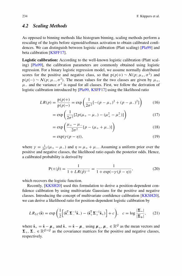
234 F. Küppers et al.

4.2 Scaling Methods

As opposed to binning methods like histogram binning, scaling methods perform arescaling of the logits before sigmoid/softmax activation to obtain calibrated confi-dences. We can distinguish between logistic calibration (Platt scaling) [Pla99] andbeta calibration [KSFF17].

Logistic calibration: According to the well-known logistic calibration (Platt scal-ing) [Pla99], the calibration parameters are commonly obtained using logisticregression. For a binary logistic regression model, we assume normally distributedscores for the positive and negative class, so that p(p|+) ∼ N(p;μ+, σ 2) andp(p|−) ∼ N(p;μ−, σ 2). The mean values for the two classes are given by μ+,μ− and the variance σ 2 is equal for all classes. First, we follow the derivation oflogistic calibration introduced by [Pla99, KSFF17] using the likelihood ratio

LR(p) = p(p|+)

p(p|−)= exp

(1

2σ 2[−(p − μ+)2 + (p − μ−)2]

)(16)

= exp

(1

2σ 2[2p(μ+ − μ−) − (μ2

+ − μ2−)]

)(17)

= exp

(μ+ − μ−

2σ 2[p − (μ+ + μ−)]

)(18)

= exp(γ (p − η)), (19)

where γ = 12σ 2 (μ+ − μ−) and η = μ+ + μ−. Assuming a uniform prior over the

positive and negative classes, the likelihood ratio equals the posterior odds. Hence,a calibrated probability is derived by

P(+| p) = 1

1 + LR( p)−1= 1

1 + exp(−γ ( p − η)), (20)

which recovers the logistic function.Recently, [KKSH20] used this formulation to derive a position-dependent con-

fidence calibration by using multivariate Gaussians for the positive and negativeclasses. Introducing the concept of multivariate confidence calibration [KKSH20],we can derive a likelihood ratio for position-dependent logistic calibration by

LRLC(s) = exp

(1

2

[(sT−�−1

− s−) − (sT+�−1+ s+)

]+ c

), c = log

|�−||�+| , (21)

where s+ = s − μ+ and s− = s − μ− using μ+,μ− ∈ RQ as the mean vectors and

�+,�− ∈ RQ×Q as the covariance matrices for the positive and negative classes,

respectively.

Confidence Calibration for Object Detection and Segmentation 235

Beta calibration:Similarly,we can also extend thebeta calibrationmethod [KSFF17]to a multivariate calibration scheme. However, we need a special form of a multivari-ate beta distribution as the Dirichlet distribution is only defined over a Q-simplexand thus is not suitable for this kind of calibration. Therefore, we use a multivariatebeta distribution proposed by [LN82] which is defined as

p(s|α) = 1

B(α)

∏q∈Q

[λ

αqq (s∗

q )αq−1

( s∗q

sq

)2][

1 +∑q∈Q

λq s∗q

]−∑q∈Q0 αq

, (22)

with Q0 = {0, . . . , Q} and the shape parameters α = (α0, . . . , αq)T, β =

(β0, . . . , βq)T that are restricted to αq , βq > 0. Furthermore, we denote λq = βq

β0and

s∗q = sq

1−sq. In this context, B(α) denotes the multivariate beta function. However,

this kind of beta distribution is only able to capture positive correlations [LN82].Nevertheless, it is possible to derive a likelihood ratio given by

LRBC(s) = exp

( ∑q∈Q

[α+q log(λ+

q ) − α−q log(λ−

q ) + (α+q − α−

q ) log(s∗q )

]+ (23)

∑q∈Q0

[α−q log

( ∑j∈Q

λ−j s

∗j

)− α+

q log

(∑j∈Q

λ+j s

∗j

)]+ c

),

with α+,α− and λ+,λ− as the shape parameters for the multivariate beta distribution

in (22) and for the positive and negative class, respectively, so that c = log(

B(α−)

B(α+)

).

We investigate the effect of position-dependent calibration in the next section usingthese methods.

5 Experimental Evaluation and Discussion

In this section, we evaluate our proposed calibration methods for the tasks of objectdetection, instance segmentation, and semantic segmentation using pretrained neu-ral networks. For calibration evaluation, we use the MS COCO validation dataset[LMB+14] consisting of 5,000 images with 80 different object classes for objectdetection and instance segmentation. For semantic segmentation, we use the panop-tic segmentation annotations consisting of 171 different object and stuff categories intotal. Our investigations are limited to the validation dataset since the training set hasalready been used for network training and no ground-truth annotations are availablefor the respective test dataset. Thus, we use a 50%/50% random split and use thefirst set for calibration training, while the second set is used for the evaluation of thecalibration methods. Furthermore, we also utilize the Cityscapes validation dataset

236 F. Küppers et al.

[COR+16] consisting of 500 images with 19 different classes that are used for modeltraining. The Munster and Lindau images are used for calibration training, whereasthe Frankfurt images are held back for calibration evaluation.

5.1 Object Detection

We evaluate our proposed calibration methods histogram binning (HB) (14), logisticcalibration (LC) (21) and beta calibration (BC) (23) for the task of object detectionusing a pretrainedFaster R-CNN X101-FPN [RHGS15, WKM+19] aswell as apretrained RetinaNet [LGG+17, WKM+19] on theMS COCO validation set. ForCityscapes, we use a pretrained Mask R-CNN R50-FPN [HGDG17, WKM+19],where only the predicted bounding box information is used for calibration. For cal-ibration evaluation, we use the proposed D-ECE with the same subsets of data thathave been used for calibration training. Thus, we use a binning scheme of B = 20using the confidence p only. In contrast, we use Bq = 5 for Q = 5 when all auxiliaryinformation is used. Each binwith less than 8 samples is neglected to increaseD-ECErobustness. We further measure the Brier score (BS) and the negative log likelihood(NLL) of each model to evaluate its calibration properties. It is of special interestto assess if calibration has an influence to the precision/recall. Thus, we also denotethe area under precision/recall curve (AUPRC) for each model. As opposed to pre-vious examinations [KKSH20], we evaluate calibration using all available classeswithin each dataset. Each of these scores is measured for each class separately. In ourexperiments, we denote weighted average scores that are weighted by the amount ofsamples for each class. We perform calibration using IoU scores of 0.50 and 0.75,respectively. Furthermore, only bounding boxes with a score over 0.3 are used forcalibration to reduce the amount of non-informative predictions. We give a qualita-tive example Fig. 2 that illustrates the effect of confidence calibration in the scopeof object detection.

In our experiments, we first apply the standard calibration methods (Table 1)and compare the results with the baseline miscalibration of the detection model.We can already observe a default miscalibration of each examined network. Thismiscalibration is reduced by standard calibration where the scaling methods offerthe best performance compared to the histogram binning. In a next step, we apply ourbox-sensitive calibration that includes the confidence p, position cx , cy and shape w

and h into a calibration mapping (Table 2). Similar to the confidence-only case inTable 1, the scaling methods consistently outperform baseline and histogram binningcalibration.

In each calibration case, we observe a miscalibration of the base network thatis alleviated using our proposed calibration methods. By examining the reliabil-ity diagram (Fig. 3), we observe that the networks are consistently miscalibratedfor all confidence levels. This can be alleviated either by standard calibration orby position-dependent calibration. By examining the position-dependence of the

Confidence Calibration for Object Detection and Segmentation 237

baseline (a) standard (b) fullCar 100% 99% 99%Rider 99% 88% 95%Rider 99% 87% 85%

Fig. 2 Qualitative example of position-dependent confidence calibration on a Cityscapes imagewith detections obtained by a Mask-RCNN. First, standard calibration is performed using similarconfidence estimates p without any position information. This results in rescaled but still similarcalibrated confidence estimates (note that we have distinct calibration models for each class). Sec-ond, we can observe the effect of position-dependent calibration using the full position information(position and shape) as the two riders with similar confidence are rescaled differently. When usingall available information, we can observe a significant difference in calibration since both, positionand shape, have an effect to the calibration

0.0 0.2 0.4 0.6 0.8 1.00.0

0.2

0.4

0.6

0.8

1.0

Confidence

Precision

(a) Uncalibrated

0.0 0.2 0.4 0.6 0.8 1.00.0

0.2

0.4

0.6

0.8

1.0

Confidence

(b) After standard calibration

0.0 0.2 0.4 0.6 0.8 1.00.0

0.2

0.4

0.6

0.8

1.0

Confidence

(c) After position-dependent calibration

Fig. 3 Reliability diagram (object detection) for a Mask-RCNN class pedestrian inferred onCityscapes Frankfurt imagesmeasured using the confidence only. The blue bar denotes the precisionof samples that fall into this bin, with the gap to perfect calibration (diagonal) highlighted in red.a The Mask-RCNN model is consistently overconfident for each confidence level. b This can bealleviated by standard logistic calibration c as well as by position-dependent logistic calibration

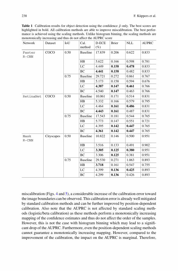
238 F. Küppers et al.

Table 1 Calibration results for object detection using the confidence p only. The best scores arehighlighted in bold. All calibration methods are able to improve miscalibration. The best perfor-mance is achieved using the scaling methods. Unlike histogram binning, the scaling methods aremonotonically increasing and thus do not affect the AUPRC score

Network Dataset IoU Cal.method

D-ECE(%)

Brier NLL AUPRC

FasterR-CNN

COCO 0.50 Baseline 17.839 0.206 0.622 0.833

HB 5.622 0.166 0.598 0.781

LC 4.449 0.158 0.478 0.833

BC 4.441 0.158 0.482 0.833

0.75 Baseline 29.721 0.272 0.861 0.767

HB 5.173 0.158 0.594 0.676

LC 4.387 0.147 0.461 0.766

BC 4.540 0.147 0.463 0.766

RetinaNet COCO 0.50 Baseline 10.061 0.171 0.514 0.831

HB 5.332 0.166 0.579 0.795

LC 4.464 0.161 0.486 0.831

BC 4.443 0.161 0.487 0.831

0.75 Baseline 17.543 0.181 0.544 0.765

HB 5.773 0.147 0.551 0.721

LC 4.395 0.142 0.447 0.765

BC 4.361 0.142 0.447 0.765

MaskR-CNN

Cityscapes 0.50 Baseline 10.822 0.146 0.500 0.951

HB 3.516 0.133 0.491 0.902

LC 3.305 0.125 0.380 0.951

BC 3.306 0.125 0.381 0.951

0.75 Baseline 29.530 0.271 1.063 0.893

HB 3.718 0.161 0.547 0.755

LC 4.399 0.136 0.425 0.893

BC 4.299 0.136 0.426 0.893

miscalibration (Figs. 4 and 5), a considerable increase of the calibration error towardthe image boundaries can be observed. This calibration error is alreadywellmitigatedby standard calibration methods and can be further improved by position-dependentcalibration. Also note that the AUPRC is not affected by standard scaling meth-ods (logistic/beta calibration) as these methods perform a monotonically increasingmapping of the confidence estimates and thus do not affect the order of the samples.However, this is not the case with histogram binning which may lead to a signifi-cant drop of the AUPRC. Furthermore, even the position-dependent scaling methodscannot guarantee a monotonically increasing mapping. However, compared to theimprovement of the calibration, the impact on the AUPRC is marginal. Therefore,

Confidence Calibration for Object Detection and Segmentation 239

Table 2 Calibration results for object detection using all available information p, cx , cy , w and h.Similar to the confidence-only case in Table 1, the scalingmethods consistently outperform baselineand histogrambinning calibration.However, in the position-dependent case, the calibrationmappingis not monotonically increasing. This has an effect to the AUPRC scores, but is marginal comparedto the improvement in calibration

Network Dataset IoU Cal.method

D-ECE[%]

Brier NLL AUPRC

FasterR-CNN

COCO 0.50 Baseline 7.519 0.206 0.622 0.833

HB 3.891 0.206 1.076 0.701

LC 3.100 0.175 0.627 0.807

BC 3.240 0.168 0.508 0.807

0.75 Baseline 13.277 0.272 0.861 0.767HB 3.848 0.200 1.037 0.587

LC 2.965 0.162 0.587 0.730

BC 3.217 0.159 0.492 0.719

RetinaNet COCO 0.50 Baseline 4.303 0.171 0.514 0.831HB 3.369 0.199 1.100 0.727

LC 3.124 0.177 0.615 0.804

BC 3.491 0.175 0.521 0.800

0.75 Baseline 6.724 0.181 0.544 0.765HB 3.241 0.176 1.026 0.640

LC 2.872 0.157 0.595 0.732

BC 3.205 0.153 0.479 0.725

MaskR-CNN

Cityscapes 0.50 Baseline 10.168 0.146 0.500 0.951

HB 5.241 0.151 0.535 0.854

LC 4.551 0.134 0.440 0.946

BC 6.117 0.134 0.413 0.925

0.75 Baseline 27.066 0.271 1.063 0.893

HB 8.062 0.195 0.607 0.681

LC 6.267 0.140 0.464 0.894BC 9.427 0.160 0.491 0.833

we conclude that our calibration methods are a valuable contribution especially forsafety-critical systems, since they lead to statistically better calibrated confidences.

5.2 Instance Segmentation

After object detection, we investigate the calibration properties of instance segmen-tation models. According to the definition of calibration for segmentation modelsin (9), we can use each pixel within a segmentation mask as a separate prediction.

240 F. Küppers et al.

0.0 0.2 0.4 0.6 0.8 1.00.0

0.2

0.4

0.6

0.8

1.0

cx position

Precision

/Confid

ence

(a) Uncalibrated

PrecisionConfidenceECE

0.0 0.2 0.4 0.6 0.8 1.0

cx position

(b) After standard calibration

PrecisionConfidenceECE

0.0 0.2 0.4 0.6 0.8 1.0

cx position

(c) After position-dependent calibration

0.00

0.05

0.10

0.15

0.20

0.25

0.30

Expecte

dCa

libratio

nError(EC

E)

PrecisionConfidenceECE

Fig. 4 Reliability diagram (object detection) for a Mask-RCNN class pedestrian inferred onCityscapes Frankfurt images measured by the confidence and the relative cx position of each bound-ing box. aWeobserve an increasing calibration error toward the boundaries of the images.bThis canbe alleviated by standard logistic calibration c as well as by position-dependent logistic calibration

0.0 0.25 0.5 0.75 1.00.0

0.25

0.5

0.75

1.0

position

position

0% 10% 20% 30%(a) Uncalibrated

0.0 0.25 0.5 0.75 1.0position

0% 10% 20% 30%(b) After standard calibration

0.0 0.25 0.5 0.75 1.0position

0% 10% 20% 30%(c) After position-dependent calibration

Fig. 5 Reliability diagram (object detection) for a Mask-RCNN class pedestrianmeasured using allavailable information. This diagram shows the D-ECE [%] for all image regions. aWe can observea default miscalibration that increases toward the image boundaries. b Standard logistic calibrationalready achieves good calibration results, c that can be further improved by position-dependentcalibration

This alleviates the problem of limited data availability and allows for a more robustcalibration evaluation. Recently, Kumar et al. [KLM19] started a discussion aboutthe sample-efficiency of binning and scaling methods. The authors show that binningmethods yield a more robust calibration mapping for large datasets but also tend tooverfit for a small database. We can confirm this observation as histogram binningprovides poor calibration performance in our examinations on object detection cal-ibration, particularly for classes with fewer samples. In contrast, scaling methodsare more sample-efficient but also more inaccurate [KLM19]. Furthermore, scalingmethods are computationally more expensive as they require an iterative update ofthe calibration parameters over the complete dataset, whereas a binning of samplescomes at low computational costs, especially for large datasets. Therefore, our exam-inations are focused on the calibration performance of a (multivariate) histogrambinning using 15 bins for each dimension. For inference, we use pretrained MaskR-CNN [HGDG17, WKM+19] as well as pretrained PointRend [KWHG20]mod-els to obtain predictions of instance segmentation masks for both datasets. As within

Confidence Calibration for Object Detection and Segmentation 241

object detection evaluation, all objects with a bounding box score below 0.3 areneglected. We perform standard calibration using the confidence only, as well as aposition-dependent calibration including the x and y position of each pixel. The pixelposition is scaled by the mask’s bounding box size to get position information in the[0, 1] interval. Furthermore, we also include the distance of each pixel to the nearestmask segment boundary as a feature in a calibration mapping since we expect ahigher uncertainty especially at the segment boundaries. The distance is normalizedby the bounding box’s diagonal to obtain distance values in [0, 1].

Since many data samples are available, we measure calibration using a D-ECEwith 15 bins neglecting each bin with less than 8 samples. We further assess theBrier score as well as the NLL loss as complementary metrics. The task of instancesegmentation is related to object detection. In a first step, the network also needsto infer a bounding box for each detected object. Similar to the calibration evalu-ation for object detection, we further use IoU scores of 0.50 and 0.75 to specifywhether a prediction has matched a ground-truth object or not. In contrast to objectdetection, the IoU score within instance segmentation is computed by the overlapof the inferred segmentation mask and the according ground-truth object. Usingthis definition, we can compute the AUPRC to evaluate the average quality of theobject detection branch as well as the according segmentation masks. All results forinstance segmentation calibration for IoU of 0.50 and 0.75 are shown in Tables 3and 4, respectively. These tables compare standard calibration (subset: confidenceonly) with position-dependent calibration (subset: full). We observe a significantmiscalibration of the networks by default. Using standard calibration or our cali-bration methods, it is possible to improve the calibration score D-ECE, Brier, andNLL for each case. The miscalibration is successfully corrected by histogram bin-ning using either the standard binning or the position-dependent binning. This isalso underlined by inspecting the reliability diagrams for the confidence-only case(Fig. 6). Furthermore, we can also observe miscalibration that is dependent on therelative x and y pixel position within a mask (Figs. 7 and 8). We can observe thatstandard histogram binning calibration already achieves good calibration results butalso offers a weak dependency on the pixel position as well. Although the position-dependent calibration only achieves a minor improvement in calibration comparedto the standard calibration case, it shows an equal calibration performance across thewhole image

In contrast to object detection, we observe a slightly increased miscalibrationtoward the center of a mask. As it can be seen in Fig. 9, most pixels belonging to anobject mask are also located in the center. This underlines the need for a position-dependent calibration. Interestingly, although position-dependent calibration doesnot seem to offer better Brier or NLL scores compared to the confidence-only case,it significantly improves the mask quality as we can observe higher AUPRC scoresfor position-dependent calibration. We further provide a qualitative example thatillustrates the effect of confidence calibration in Fig. 9. In this example, we can seethe difference between standard calibration and position-dependent calibration. Inthe former case, the mask scores are only rescaled by their confidence which mightlead to a better calibration but sometimes also to unwanted losses of mask segments

242 F. Küppers et al.

Table 3 Calibration results for instance segmentation @ IoU=0.50. The best D-ECE scores areunderlined for each subset separately, since it is not convenient to compare D-ECE scores withdifferent subsets to each other [KKSH20]. Furthermore, the best Brier, NLL, and AUPRC scores arehighlighted in bold. These scores are only calculated using the confidence information and thus canbe compared to each other. The histogram binning calibration consistently improves miscalibration.Furthermore, we find that although position dependence does not improve the Brier and NLL scoresas in the standard case, it leads to a significant improvement in the mIoU scoreNetwork Dataset Cal.

methodSubset: confidence only Subset: full

D-ECE[%]

Brier NLL AUPRC D-ECE[%]

Brier NLL AUPRC

MaskR-CNN

CS Baseline 7.088 0.110 0.432 0.724 11.205 0.110 0.432 0.724

HB 5.661 0.099 0.320 0.723 10.119 0.117 0.530 0.787

COCO Baseline 21.983 0.222 0.940 0.663 23.409 0.222 0.940 0.663

HB 6.420 0.150 0.442 0.662 13.640 0.171 0.776 0.760

PointRend CS Baseline 12.893 0.160 0.785 0.709 20.858 0.160 0.785 0.709

HB 2.706 0.105 0.326 0.698 19.021 0.190 1.299 0.758

COCO Baseline 22.284 0.222 0.946 0.672 23.973 0.222 0.946 0.672

HB 6.348 0.144 0.428 0.664 16.060 0.180 1.005 0.751

Table 4 Calibration results for instance segmentation@ IoU=0.75. The best scores are highlighted.We observe the same behavior in calibration for all models as for the IoU=0.50 case shown in Table 3Network Dataset Cal.

methodSubset: confidence only Subset: full

D-ECE[%]

Brier NLL AUPRC D-ECE[%]

Brier NLL AUPRC

MaskR-CNN

CS Baseline 12.862 0.147 0.622 0.375 14.470 0.147 0.622 0.375

HB 5.895 0.108 0.340 0.375 10.273 0.120 0.523 0.479

COCO Baseline 26.559 0.250 1.070 0.237 27.219 0.250 1.070 0.237

HB 6.006 0.144 0.423 0.235 12.888 0.165 0.720 0.425

PointRend CS Baseline 18.668 0.192 0.929 0.347 25.386 0.192 0.929 0.347

HB 3.899 0.115 0.349 0.344 18.415 0.191 1.247 0.486

COCO Baseline 26.643 0.248 1.060 0.258 27.377 0.248 1.060 0.258

HB 6.708 0.138 0.411 0.238 15.344 0.173 0.936 0.388

(especially small objects in the background). In contrast, position-dependent cali-bration is capable of possible correlations between confidence and pixel positionor the size of an object. This leads to improved estimates of the mask confidenceseven for smaller objects. Therefore, we conclude that multidimensional confidencecalibration has a positive influence on the calibration properties as well as on thequality of the object masks.

Confidence Calibration for Object Detection and Segmentation 243

0.0 0.2 0.4 0.6 0.8 1.00.0

0.2

0.4

0.6

0.8

1.0

Confidence

Rel.Frequency

(a) Uncalibrated

0.0 0.2 0.4 0.6 0.8 1.00.0

0.2

0.4

0.6

0.8

1.0

Confidence

(b) After standard calibration

0.0 0.2 0.4 0.6 0.8 1.00.0

0.2

0.4

0.6

0.8

1.0

Confidence

(c) After position-dependent calibration

Fig. 6 Reliability diagram (instance segmentation) for a Mask R-CNN class pedestrian inferredon MS COCO validation images measured using the confidence only. The blue bar denotes thefrequency of samples that fall into this bin, with the gap to perfect calibration (diagonal) highlightedin red. a The Mask R-CNN model is consistently overconfident for each confidence level. b Thiscan be alleviated by standard histogram binning calibration c as well as by position-dependentlogistic calibration

0.0 0.2 0.4 0.6 0.8 1.00.0

0.2

0.4

0.6

0.8

1.0

x position

Rel.Frequency/C

onfid

ence

(a) Uncalibrated

Rel. FrequencyConfidenceECE

0.0 0.2 0.4 0.6 0.8 1.0

x position

(b) After standard calibration

Rel. FrequencyConfidenceECE

0.0 0.2 0.4 0.6 0.8 1.0

x position

(c) After position-dependent calibration

0.00

0.05

0.10

0.15

0.20

0.25

0.30

Expecte

dCa

libratio

nError(EC

E)

Rel. FrequencyConfidenceECE

Fig. 7 Reliability diagram (instance segmentation) for a Mask R-CNN class pedestrian inferredon MS COCO validation images measured by the relative x position of each pixel within its bound-ing box. a Similar to the examinations for object detection, we observe an increasing calibrationerror toward the boundaries of the images. b Standard histogram binning significantly reduces thecalibration error, c whereas position-dependent histogram binning is capable of a slightly furtherrefinement of the position-dependent D-ECE

0.0 0.25 0.5 0.75 1.00.0

0.25

0.5

0.75

1.0

x position

ypo

sition

0% 2% 4% 6% 8% 10%(a) Uncalibrated

0.0 0.25 0.5 0.75 1.0x position

0% 2% 4% 6% 8% 10%(b) After standard calibration

0.0 0.25 0.5 0.75 1.0x position

0% 2% 4% 6% 8% 10%(c) After position-dependent calibration

Fig. 8 Reliability diagram (instance segmentation) for a Mask R-CNN class pedestrian inferredon MS COCO validation images. The diagram shows the D-ECE [%] that is measured using therelative x and y position of each pixel within its bounding box. Similar to the observations inFig. 7, standard calibration already reduces the calibration error. However, we can observe a slightlyincreased calibration error toward the image’s center. In contrast, position-dependent calibrationerror shows equal calibration performance across the whole image

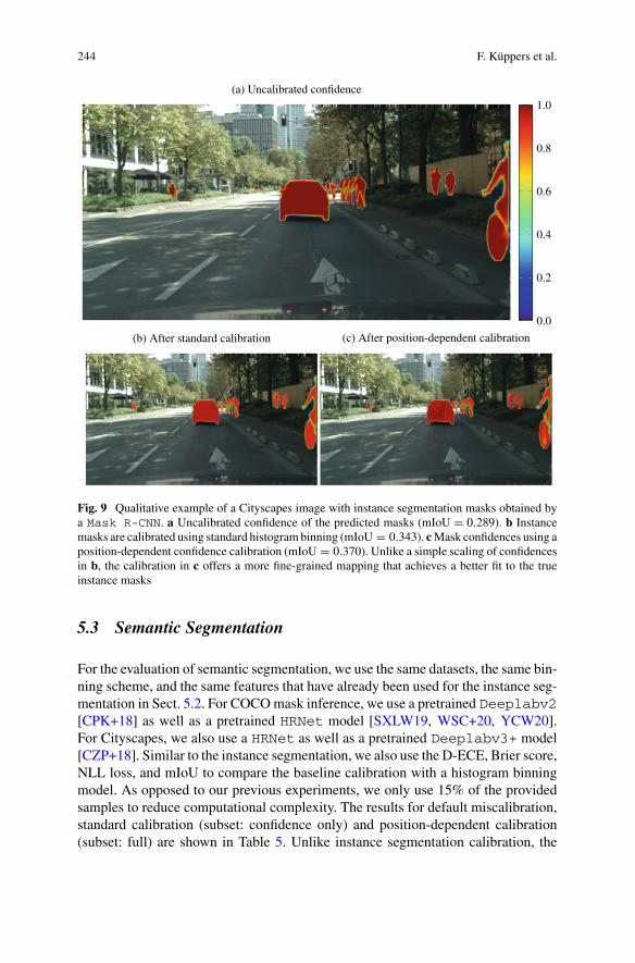
244 F. Küppers et al.

(a) Uncalibrated confidence

0.0

0.2

0.4

0.6

0.8

1.0

(b) After standard calibration (c) After position-dependent calibration

Fig. 9 Qualitative example of a Cityscapes image with instance segmentation masks obtained bya Mask R-CNN. a Uncalibrated confidence of the predicted masks (mIoU = 0.289). b Instancemasks are calibrated using standard histogram binning (mIoU = 0.343). cMask confidences using aposition-dependent confidence calibration (mIoU = 0.370). Unlike a simple scaling of confidencesin b, the calibration in c offers a more fine-grained mapping that achieves a better fit to the trueinstance masks

5.3 Semantic Segmentation

For the evaluation of semantic segmentation, we use the same datasets, the same bin-ning scheme, and the same features that have already been used for the instance seg-mentation in Sect. 5.2. For COCOmask inference, we use a pretrained Deeplabv2[CPK+18] as well as a pretrained HRNet model [SXLW19, WSC+20, YCW20].For Cityscapes, we also use a HRNet as well as a pretrained Deeplabv3+ model[CZP+18]. Similar to the instance segmentation, we also use the D-ECE, Brier score,NLL loss, and mIoU to compare the baseline calibration with a histogram binningmodel. As opposed to our previous experiments, we only use 15% of the providedsamples to reduce computational complexity. The results for default miscalibration,standard calibration (subset: confidence only) and position-dependent calibration(subset: full) are shown in Table 5. Unlike instance segmentation calibration, the

Confidence Calibration for Object Detection and Segmentation 245

Table 5 Calibration results for semantic segmentation. The best D-ECE scores are underlined foreach subset separately, since it is not convenient to compare D-ECE scores with different subsetsto each other [KKSH20]. Furthermore, the best Brier, NLL, and mIoU scores are highlighted inbold. These scores are only calculated using the confidence information and thus can be comparedto each other. In contrast to object detection and instance segmentation evaluation, we observe alow baseline calibration error that is only slightly affected by confidence calibrationNetwork Dataset Cal.

methodSubset: confidence only Subset: full

D-ECE[%]

Brier NLL mIoU D-ECE[%]

Brier NLL mIoU

Deeplabv3+ CS Baseline 0.162 0.060 0.139 0.623 0.186 0.060 0.139 0.623

HB 0.081 0.060 0.170 0.619 0.199 0.062 0.189 0.589

Deeplabv2 COCO Baseline 0.094 0.458 1.173 0.933 0.149 0.458 1.173 0.933

HB 0.060 0.456 1.515 0.933 0.150 0.485 1.790 0.913

HRNet CS Baseline 0.067 0.057 0.115 0.629 0.149 0.057 0.115 0.629

HB 0.083 0.057 0.148 0.628 0.191 0.060 0.171 0.582

COCO Baseline 0.455 0.779 5.812 0.939 0.455 0.779 5.812 0.939

HB 0.062 0.563 2.261 0.939 0.138 0.571 2.372 0.931

baselinemodel is already intrinsically well-calibrated, offering a very low calibrationerror. A qualitative example is shown in Fig. 10 to illustrate the effect of calibrationfor semantic segmentation. In this example, we can observe only minor differencesbetween the uncalibrated mask and the masks either after standard calibration orafter position-dependent calibration. This aspect is supported by the confidence reli-ability diagram shown in Fig. 11. Although we can observe an overconfidence, mostsamples are located in the low confident space with a low calibration error that alsoresults in an overall low miscalibration score. Furthermore, our calibration methodsare able to achieve even better calibration results, but mostly in the confidence-onlycalibration case. In addition, we also observe only a low correlation between positionand calibration error (Figs. 12 and 13). One reason for the major difference betweeninstance and semantic segmentation calibration may be the difference in model train-ing. An instance segmentationmodel needs to infer an appropriate bounding box firstto achieve qualitatively good results in mask inference. In contrast, a semantic seg-mentation model does not need to infer the position of objects within an image but isable to directly learn and improve mask quality. We also suspect an influence of theamount of available data points, since a semantic segmentation model is able to useeach pixel within an image as a separate sample, whereas an instance segmentationmodel is only restricted to the pixels that are available within an estimated bound-ing box. Therefore, we conclude that semantic segmentation models do not require apost-hoc confidence calibration as they already offer a good calibration performance.

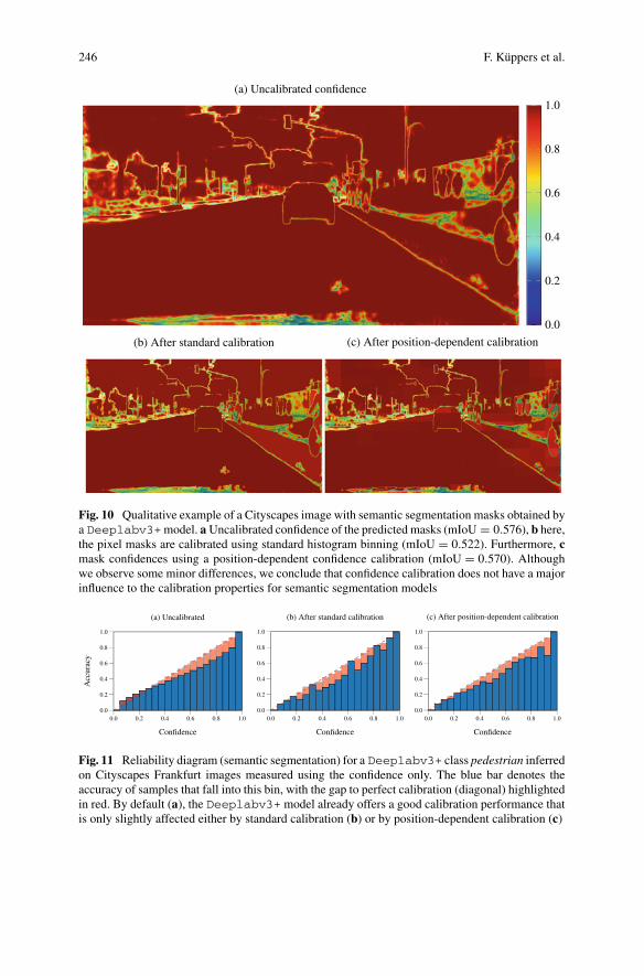
246 F. Küppers et al.

(a) Uncalibrated confidence

0.0

0.2

0.4

0.6

0.8

1.0

(b) After standard calibration (c) After position-dependent calibration

Fig. 10 Qualitative example of a Cityscapes image with semantic segmentation masks obtained bya Deeplabv3+model. aUncalibrated confidence of the predicted masks (mIoU = 0.576), b here,the pixel masks are calibrated using standard histogram binning (mIoU = 0.522). Furthermore, cmask confidences using a position-dependent confidence calibration (mIoU = 0.570). Althoughwe observe some minor differences, we conclude that confidence calibration does not have a majorinfluence to the calibration properties for semantic segmentation models

0.0 0.2 0.4 0.6 0.8 1.00.0

0.2

0.4

0.6

0.8

1.0

Confidence

Accuracy

(a) Uncalibrated

0.0 0.2 0.4 0.6 0.8 1.00.0

0.2

0.4

0.6

0.8

1.0

Confidence

(b) After standard calibration

0.0 0.2 0.4 0.6 0.8 1.00.0

0.2

0.4

0.6

0.8

1.0

Confidence

(c) After position-dependent calibration

Fig. 11 Reliability diagram (semantic segmentation) for a Deeplabv3+ class pedestrian inferredon Cityscapes Frankfurt images measured using the confidence only. The blue bar denotes theaccuracy of samples that fall into this bin, with the gap to perfect calibration (diagonal) highlightedin red. By default (a), the Deeplabv3+model already offers a good calibration performance thatis only slightly affected either by standard calibration (b) or by position-dependent calibration (c)

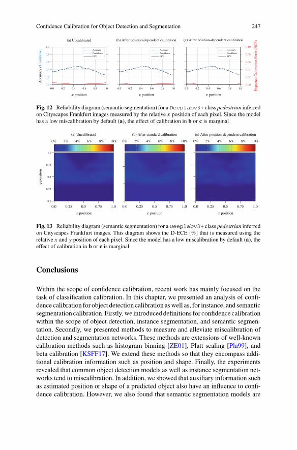
Confidence Calibration for Object Detection and Segmentation 247

0.0 0.2 0.4 0.6 0.8 1.00.0

0.2

0.4

0.6

0.8

1.0

x position

Accuracy

/Con

fidence

(a) Uncalibrated

AccuracyConfidenceECE

0.0 0.2 0.4 0.6 0.8 1.0

x position

(b) After position-dependent calibration

AccuracyConfidenceECE

0.0 0.2 0.4 0.6 0.8 1.0

x position

(c) After position-dependent calibration

0.00

0.02

0.04

0.06

0.08

0.10

Expecte

dCa

libratio

nError(EC

E)

AccuracyConfidenceECE

Fig. 12 Reliability diagram (semantic segmentation) for a Deeplabv3+ class pedestrian inferredon Cityscapes Frankfurt images measured by the relative x position of each pixel. Since the modelhas a low miscalibration by default (a), the effect of calibration in b or c is marginal

0.0 0.25 0.5 0.75 1.00.0

0.25

0.5

0.75

1.0

x position

ypo

sition

0% 2% 4% 6% 8% 10%(a) Uncalibrated

0.0 0.25 0.5 0.75 1.0x position

0% 2% 4% 6% 8% 10%(b) After standard calibration

0.0 0.25 0.5 0.75 1.0x position

0% 2% 4% 6% 8% 10%(c) After position-dependent calibration

Fig. 13 Reliability diagram (semantic segmentation) for a Deeplabv3+ class pedestrian inferredon Cityscapes Frankfurt images. This diagram shows the D-ECE [%] that is measured using therelative x and y position of each pixel. Since the model has a low miscalibration by default (a), theeffect of calibration in b or c is marginal

Conclusions

Within the scope of confidence calibration, recent work has mainly focused on thetask of classification calibration. In this chapter, we presented an analysis of confi-dence calibration for object detection calibration aswell as, for instance, and semanticsegmentation calibration. Firstly,we introduced definitions for confidence calibrationwithin the scope of object detection, instance segmentation, and semantic segmen-tation. Secondly, we presented methods to measure and alleviate miscalibration ofdetection and segmentation networks. These methods are extensions of well-knowncalibration methods such as histogram binning [ZE01], Platt scaling [Pla99], andbeta calibration [KSFF17]. We extend these methods so that they encompass addi-tional calibration information such as position and shape. Finally, the experimentsrevealed that common object detection models as well as instance segmentation net-works tend to miscalibration. In addition, we showed that auxiliary information suchas estimated position or shape of a predicted object also have an influence to confi-dence calibration. However, we also found that semantic segmentation models are

248 F. Küppers et al.

already intrinsically calibrated. Thus, the examined models do not require additionalpost-hoc calibration and already offer well-calibrated mask confidence scores. Weargue that this difference between instance and semantic segmentation is a resultof data quality and availability during training. This leads to the assumption thatlimited data availability is a direct cause for miscalibration during training and thusan effect of overfitting. Nevertheless, our proposed calibration framework is capa-ble to calibrate object detection and instance segmentation models. In safety-criticalapplications, the confidence in the applied algorithms is paramount. The proposedcalibration algorithms allow to detect situations of low confidence and thus performthe appropriate system reaction. Therefore, calibrated confidence values can be usedas additional information especially in safety-critical applications.

Acknowledgements The research leading to these results is fundedby theGermanFederalMinistryfor Economic Affairs and Energy within the project “Methoden und Maßnahmen zur Absicherungvon KI-basierten Wahrnehmungsfunktionen für das automatisierte Fahren (KI Absicherung)”. Theauthors would like to thank the consortium for the successful cooperation.

References

[COR+16] M. Cordts, M. Omran, S. Ramos, T. Rehfeld, M. Enzweiler, R. Benenson, U. Franke,S. Roth, B. Schiele, The cityscapes dataset for semantic urban scene understand-ing, in Proceedings of the IEEE/CVF Conference on Computer Vision and PatternRecognition (CVPR) (Las Vegas, NV, USA, June 2016), pp. 3213–3223

[CPK+18] Liang-Chieh. Chen, George Papandreou, Iasonas Kokkinos, Kevin Murphy, Alan L.Yuille, DeepLab: semantic image segmentation with deep convolutional nets, atrousconvolution, and fully connected CRFs. IEEE Trans. Pattern Anal. Mach. Intell.(TPAMI) 40(4), 834–848 (2018)

[CZP+18] L.-C. Chen, Y. Zhu, G. Papandreou, F. Schroff, H. Adam, Encoder-decoder withatrous separable convolution for semantic image segmentation, in Proceedings of theEuropean Conference on Computer Vision (ECCV) (Munich, Germany, September2018), pp. 833–851

[DLXS20] Y. Ding, J. Liu, J. Xiong, Y. Shi, Revisiting the evaluation of uncertainty estimationand its application to explore model complexity-uncertainty trade-off, in Proceedingsof the IEEE/CVF Conference on Computer Vision and Pattern Recognition (CVPR)Workshops virtual conference (June 2020), pp. 22–31

[GPSW17] C. Guo, G. Pleiss, Y. Sun, K.Q. Weinberger, On calibration of modern neural net-works, in Proceedings of the International Conference on Machine Learning (ICML)(Sydney, NSW, Australia, August 2017), pp. 1321–1330

[HGDG17] K. He, G. Gkioxari, P. Dollár, R. Girshick, Mask R-CNN, in Proceedings of the IEEEInternational Conference on Computer Vision (ICCV) (Venice, Italy, October 2017),pp. 2980–2988

[JJY+19] B. Ji,H. Jung, J.Yoon,K.Kim,Y. Shin,Bin-wise temperature scaling (BTS): improve-ment in confidence calibration performance through simple scaling techniques, inProceedings of the IEEE International Conference on Computer Vision (ICCV)Work-shops (Seoul, Korea, October 2019), pp. 4190–4196

[KG20] D. Karimi, A. Gholipour, Improving Calibration and Out-of-Distribution Detectionin Medical Image Segmentation With Convolutional Neural Networks (May 2020),pp. 1–12. arXiv:2004.06569

Confidence Calibration for Object Detection and Segmentation 249

[KKSH20] F. Küppers, J. Kronenberger, A. Shantia, A. Haselhoff, Multivariate confidence cali-bration for object detection, inProceedings of the IEEE/CVFConference onComputerVision and Pattern Recognition (CVPR) Workshops, virtual conference (June 2020),pp. 1322–1330

[KLM19] A. Kumar, P.S. Liang, T. Ma, Verified uncertainty calibration, in Proceedings of theConference on Neural Information Processing Systems (NIPS/NeurIPS) (Vancouver,BC, Canada, December 2019), pp. 3787–3798

[KPNK+19] M. Kull, M. Perello Nieto, M. Kängsepp, T. Silva Filho, H. Song, P. Flach, Beyondtemperature scaling: obtainingwell-calibratedmulti-class probabilities with Dirichletcalibration, in Proceedings of the Conference on Neural Information Processing Sys-tems (NIPS/NeurIPS) (Vancouver, BC, Canada, December 2019), pp. 12316–12326

[KSFF17] M. Kull, T. Silva Filho, P. Flach, Beta calibration: a well-founded and easily imple-mented improvement on logistic calibration for binary classifiers, in Proceedings ofthe International Conference on Artificial Intelligence and Statistics (AISTATS) (FortLauderdale, FL, USA, May 2017), pp. 623–631

[KWHG20] A. Kirillov, Y. Wu, K. He, R. Girshick, PointRend: image segmentation as render-ing, in Proceedings of the IEEE/CVF Conference on Computer Vision and PatternRecognition (CVPR), virtual conference (June 2020), pp. 9799–9808

[LGG+17] T.-Y. Lin, P. Goyal, R. Girshick, K. He, P. Dollár, Focal loss for dense object detection,in: Proceedings of the IEEE International Conference on Computer Vision (ICCV)(Venice, Italy, October 2017), pp. 2980–2988

[LMB+14] T.-Y. Lin, M. Maire, S. Belongie, J. Hays, P. Perona, D. Ramanan, P. Dollár,C. Lawrence Zitnick, Microsoft COCO: common objects in context, in Proceed-ings of the European Conference on Computer Vision (ECCV) (Zurich, Switzerland,September 2014), pp. 740–755

[LN82] David L. Libby, Melvin R. Novick, Multivariate generalized beta distributions withapplications to utility assessment. J. Educ. Stat. 7(4), 271–294 (1982)

[MWT+20] Alireza Mehrtash, WilliamM.Wells, Clare M. Tempany, Purang Abolmaesumi, TinaKapur, Confidence calibration and predictive uncertainty estimation for deep medicalimage segmentation. IEEE Trans. Med. Imaging 39(12), 3868–3878 (2020)

[NC16] M. Naeini, G. Cooper, Binary classifier calibration using an ensemble of near isotonicregression models, in Proceedings of the IEEE International Conference on DataMining (ICDM) (Barcelona, Spain, December 2016), pp. 360–369

[NCH15] M. Pakdaman Naeini, G. Cooper, M. Hauskrecht, Obtaining well calibrated proba-bilities using Bayesian binning, in Proceedings of the AAAI Conference on ArtificialIntelligence (Austin, TX, USA, January 2015), pp. 2901–2907

[NDZ+19] J. Nixon, M.W. Dusenberry, L. Zhang, G. Jerfel, D. Tran, Measuring calibration indeep learning, in Proceedings of the IEEE/CVF Conference on Computer Vision andPattern Recognition (CVPR) Workshops (Long Beach, CA, USA, June 2019), pp.38–41

[Pla99] J. Platt, Probabilistic outputs for support vector machines and comparisons to regular-ized likelihood methods, in Advances in Large Margin Classifiers. ed. by A.J. Smola,P. Bartlett, B. Schölkopf, D. Schuurmans (MIT Press, 1999), pp. 61–74

[RHGS15] S. Ren, K. He, R. Girshick, J. Sun, Faster R-CNN: towards real-time object detectionwith region proposal networks, in Proceedings of the Conference on Neural Informa-tion Processing Systems (NIPS/NeurIPS) (Montréal, QC, Canada, December 2015),pp. 91–99

[SKR+21] F. Schwaiger, M. Henne Fabian Küppers, F. Schmoeller Roza, K. Roscher, A. Hasel-hoff, From black-box to white-box: examining confidence calibration under differentconditions, in Proceedings of the Workshop on Artificial Intelligence Safety (SafeAI),virtual conference (February 2021), pp. 1–8

[SXLW19] K. Sun, B. Xiao, D. Liu, J. Wang, Deep high-resolution representation learning forhuman pose estimation, in Proceedings of the IEEE/CVF Conference on ComputerVision and Pattern Recognition (CVPR) (Long Beach, CA, USA, June 2019), pp.5693–5703

250 F. Küppers et al.

[WKM+19] Y. Wu, A. Kirillov, F. Massa, W.-Y. Lo, R. Girshick, Detectron2 (2019). [Online;assessed 2021-11-18]

[WLK+20] T. Wang, Y. Li, B. Kang, J. Li, J. Liew, S. Tang, S. Hoi, J. Feng, The devil is inclassification: a simple framework for long-tail instance segmentation, inProceedingsof the European Conference on Computer Vision (ECCV), virtual conference (August2020), pp. 728–744

[WSC+20] Jingdong Wang, Ke. Sun, Tianheng Cheng, Borui Jiang, Chaorui Deng, Yang Zhao,Dong Liu, Mu. Yadong, Mingkui Tan, Xinggang Wang et al., Deep high-resolutionrepresentation learning for visual recognition. IEEETrans. Pattern Anal.Mach. Intell.(TPAMI) 43(10), 3349–3364 (2020)

[YCW20] Y. Yuan, X. Chen, J. Wang, Object-contextual representations for semantic segmenta-tion, in Proceedings of the European Conference on Computer Vision (ECCV), virtualconference (August 2020), pp. 173–190

[ZE01] B. Zadrozny, C. Elkan, Obtaining calibrated probability estimates from decision treesand Naive Bayesian classifiers, in Proceedings of the International Conference onMachine Learning (ICML) (Williamstown, MA, USA, June 2001), pp. 609–616

[ZE02] B. Zadrozny, C. Elkan, Transforming classifier scores into accurate multiclass prob-ability estimates, in Proceedings of the ACM SIGKDD International Conference onKnowledge Discovery and Data Mining (KDD) (Edmonton, AB, Canada, July 2002),pp. 694–699

Open Access This chapter is licensed under the terms of the Creative Commons Attribution 4.0International License (http://creativecommons.org/licenses/by/4.0/), which permits use, sharing,adaptation, distribution and reproduction in any medium or format, as long as you give appropriatecredit to the original author(s) and the source, provide a link to the Creative Commons license andindicate if changes were made.

The images or other third party material in this chapter are included in the chapter’s CreativeCommons license, unless indicated otherwise in a credit line to the material. If material is notincluded in the chapter’s Creative Commons license and your intended use is not permitted bystatutory regulation or exceeds the permitted use, you will need to obtain permission directly fromthe copyright holder.

Uncertainty Quantification for ObjectDetection: Output- and Gradient-BasedApproaches

Tobias Riedlinger, Marius Schubert, Karsten Kahl, and Matthias Rottmann

Abstract Safety-critical applications of deep neural networks require reliable confi-dence estimationmethods with high predictive power. However, evaluating and com-paring different methods for uncertainty quantification is oftentimes highly context-dependent. In this chapter, we introduce flexible evaluation protocolswhich are appli-cable to a wide range of tasks with an emphasis on object detection. In this light,we investigate uncertainty metrics based on the network output, as well as metricsbased on a learning gradient, both of which significantly outperform the confidencescore of the network.While output-based uncertainty is produced by post-processingsteps and is computationally efficient, gradient-based uncertainty, in principle, allowsfor localization of uncertainty within the network architecture. We show that bothsources of uncertainty aremutually non-redundant and can be combined beneficially.Furthermore, we show direct applications of uncertainty quantification by improvingdetection accuracy.

1 Introduction

Deep artificial neural networks (DNNs) employed for tasks such as object detectionor semantic segmentation yield by construction probabilistic predictions on featuredata, such as camera images. Modern deep object detectors [RHGS15, LAE+16,LGG+17, RF18] predict bounding boxes for depicted objects of a given set of learnedclasses. The so-called “score” (sometimes also called objectness or confidence score)

T. Riedlinger (B) · M. Schubert · K. Kahl · M. RottmannUniversity of Wuppertal, Gaußstr. 20, 42119 Wuppertal, Germanye-mail: riedlinger@uni-wuppertal.de

M. Schuberte-mail: schubert@uni-wuppertal.de

K. Kahle-mail: kkahl@uni-wuppertal.de

M. Rottmanne-mail: rottmann@uni-wuppertal.de

© The Author(s) 2022T. Fingscheidt et al. (eds.), Deep Neural Networks and Data for Automated Driving,https://doi.org/10.1007/978-3-031-01233-4_9

251

252 T. Riedlinger et al.

0.0 0.5 1.00.00

0.25

0.50

0.75

1.00accuracy

AuROC = 0.965AP = 0.969

0.0 0.5 1.0confidence

AuROC = 0.976AP = 0.972

0.0 0.5 1.0

AuROC = 0.980AP = 0.978

Fig. 1 Confidence calibration plots for score (left),Monte-Carlo (MC) dropout uncertainty (center),and our proposed gradient uncertainty metrics G (right) on DKITTI

eval . For the sake of reference, weprovide the optimally calibrated diagonal in gray. See Sect. 4 for more details

indicates the probability that a bounding box provided by the DNN contains anobject. Throughout this chapter, we sometimes use the term “confidence” insteadof “score” to refer to quantities that represent the probability of a detection beingcorrect. The term confidence in a broader sense ismeant to reflect an estimated degreeof competency of the model when evaluating an input.

Reliable and accurate probabilistic predictions are desirable for many applica-tions, such as medical diagnosis or automated driving. It is well-known that pre-dictions of DNNs often tend to be statistically miscalibrated [SZS+14, GSS15,GPSW17], i.e., the score computed by the DNN is not representative for the rel-ative frequency of correct predictions. For an illustration of this, see Fig. 1, wherewe compare different sources of uncertainty in terms of their accuracy conditionedto confidence bins for a YOLOv3 model.

For individual DNN predictions, confidences that are not well-calibrated are mis-leading and constitute a reliability issue. Over-confident predictions might causeinoperability of a perception system due to producing non-existent instances (falsepositives / FP). Perhaps even more adverse, under-confidence might lead to falsenegative (FN) predictions, for instance overlooking pedestrians or other road userswhich could lead to dangerous situations or even fatalities. Given that the set of avail-able data features is fixed, the sources of uncertainty in machine learning (and deeplearning) can be divided into two types [HW21], referring to their primary source[Gal17, KG17]. Whereas aleatoric uncertainty refers to the inherent and irreduciblestochasticity of the distribution the data stems from, epistemic uncertainty refers tothe reducible part of the uncertainty. The latter originates from the finite size of a ran-dom data sample used for training, as well as from the choice of model and learningalgorithm.

Up to now, there exist a moderate number of established methods in the field ofdeep learning that have demonstrated to properly estimate the uncertainty of DNNs.In [KG17], DNNs for semantic segmentation are equipped with additional regres-sion output that model heteroscedastic (in machine learning also called predictive)uncertainty, with the aim to capture aleatoric uncertainty. For training, the uncer-

Uncertainty Quantification for Object Detection … 253

tainty output is integrated into the usual empirical cross-entropy loss. A number ofadaptations for different modern DNN architectures originate from that work. Froma theoretical point of view, Bayesian DNNs [DL90, Mac92], in which the modelweights are treated as random variables, yield an attractive framework for capturingthe epistemic uncertainty. In practice, the probability density functions correspondingto the model weights are estimated via Markov chain Monte-Carlo, which currentlyis infeasible already for a moderate number of model weights, hence being inapplica-ble in the setting of object detection. As a remedy, variational inference approacheshave been considered, where the model weights are sampled from predefined dis-tributions, which are often modeled in simplified ways, e.g., assuming mutual inde-pendence. A standard method for the estimation of epistemic uncertainty based onvariational inference is Monte-Carlo (MC) dropout [SHK+14, GG16]. Algorithmi-cally, this method performs several forward passes under dropout at inference time.Deep ensemble sampling [LPB17] follows a similar idea. Here, separately trainedmodels with the same architecture are deployed to produce a probabilistic inference.

In semantic segmentation, Rottmann et al. [RCH+20] introduced the tasks ofmetaclassification and regression that are both applied as post-processing to the outputof DNNs. Meta classification refers to the task of classifying a prediction as truepositive (TP) or FP. Meta regression is a more object detection-specific task withthe aim to predict the intersection-over-union (IoU) of a prediction with its groundtruth directly. These tasks are typically learned with the help of ground truth, butafterwards performed in the absence of ground truth, only on the basis of uncer-tainty measures stemming from the output of the DNN. The framework developed in[RCH+20], called MetaSeg, was extended into multiple directions: Time-dynamicuncertainty quantification for semantic segmentation [MRG20] and instance seg-mentation [MRV+21]; a study on the influence of image resolution [RS19]; con-trolled reduction of FN and meta fusion, the latter utilizes the uncertainty metricsto increase the performance of the DNN [CRH+19]; out-of-distribution detection[BCR+20, ORF20, CRG21]; and active learning [CRGR21]. Last but not least, asimilar approach solely based on the output of theDNNhas been developed for objectdetection in [SKR20] (called MetaDetect), however, equipped with different uncer-tainty metrics specifically designed for the task of object detection. This approachwas also used in an uncertainty-aware sensor fusion approach for object detectionbased on camera images and RaDAR point clouds; see [KRBG21].

In [ORG18], it was proposed to utilize a learning gradient, replacing the usuallyneeded ground truth labels by the prediction of the network itself, which is sup-posed to contain epistemic uncertainty information. Since the investigation of gra-dient metrics for image classification tasks, that method was considered in differentapplications as well. Gradient metrics were compared to other uncertainty quan-tification methods in [SFKM20]. It was found that gradient uncertainty is stronglycorrelated with the softmax entropy of classification networks. In natural languageunderstanding, gradient metrics turned out to be beneficial; see [VSG19]. Therein,gradient metrics and deep ensemble uncertainty were aggregated and yield well-calibrated confidences on out-of-distribution data. Recently, gradient metrics have

254 T. Riedlinger et al.

been developed for object detection in [RRSG21]. In order to demonstrate the predic-tive power of uncertaintymetrics, the framework ofmeta classification and regressionprovided by MetaDetect was used.

In this chapter, we review the works published in [SKR20, RRSG21] and putthem into a common context. More precisely, our contributions are as follows:

• We review the concepts of meta classification and regression, meta fusion, andconfidence calibration. We explain how they serve as a general benchmark forevaluating the predictive power of any uncertainty metric developed for objectdetection.

• We review output-based uncertainty metrics developed in [SKR20], as well asgradient-based ones from inside the network [RRSG21].

• We compare baseline uncertainty measures such as the DNN’s score, well-established ones like Monte-Carlo dropout [Gal17], the output-based uncertaintymetrics [SKR20], and finally the gradient-based uncertainty metrics [RRSG21]from inside the DNN. We do so in terms of comparing their standalone perfor-mances but also in terms of analyzing their mutual information and how muchperformance they add to the prediction of the network itself.

2 Related Work

In this section, we gather and discuss previous research related to the present work.

Epistemic and aleatoric uncertainty in object detection: In recent years, therehas been increasing interest in methods to properly estimate or quantify uncer-tainty in DNNs. Aleatoric uncertainty, the type of uncertainty resulting from thedata generating process, has been proposed to be captured by providing addi-tional regression output to the network architecture for learning uncertainty directlyfrom the training dataset [KG17]. Since the initial proposition, this approach hasbeen adapted to, among others, the object detection setting [LDBK18, CCKL19,HZW+19, LHK+21, HSW20, CCLK20]. The latter approaches add further regres-sion variables for aleatoric uncertainty which are assigned to their bounding boxlocalization variables, thereby learning localization as Gaussian distributions. Analternative approach to quantifying localization uncertainty is to learn for each pre-dicted box the corresponding IoU with additional regression variables [JLM+18].

Several methods have been proposed that aim to capture epistemic uncertainty,i.e., “reducible” kinds of uncertainty. Monte-Carlo (MC) dropout [SHK+14, GG16]employs forward passes under dropout and has become one of the standard tools forestimating epistemic uncertainty. As such, MC dropout has been investigated alsofor deep object detection [MNDS18, KD19, HSW20]. Similarly to MC dropout,deep ensemble methods [LPB17] employ separately trained networks (“experts”) toobtain variational inference, an approach which also has found adaptations in deepobject detection [LGRB20].

Uncertainty Quantification for Object Detection … 255

Uncertainty calibration: A large variety of methods have been proposed to rectifythe intrinsic confidence miscalibration of modern deep neural networks by intro-ducing post-processing methods (see, e.g., [GPSW17] for a comparison). Prominentexamples of such methods include histogram binning [ZE02], isotonic regression[ZE01], Bayesian binning [NCH15], Platt scaling [Pla99, NMC05], or temperaturescaling [HVD14]. Alternatively, calibrated confidences have been obtained by imple-menting calibration as an optimization objective [KP20] via a suitable loss term. Inthe realm of object detection, the authors of [NZV18] found that temperature scal-ing improves calibration. Also, natural extensions to make calibration localization-dependent have been proposed [KKSH20].

Meta classification andmeta regression:Meta classification denotes the task of dis-criminating FP and FN predictions based on uncertainty or confidence information,an idea that has been explored initially in [HG17]. In case a real-valued metric (e.g.,different versions of the IoU which is in [0, 1]) can be assigned to the quality of a pre-diction, meta regression denotes the task of predicting this quantity in the same spiritas meta classification. In contrast to the IoUNet framework introduced in [JLM+18],meta classification and meta regression do not require architectural changes or ded-icated training of the respective DNN. In [RRSG21], it has been found that metaclassifiers tend to yield well-calibrated confidences by default as opposed to the con-fidence score of DNNs. Applications of meta classification and meta regression havesince been introduced for several different disciplines [CRH+19, RS19, MRG20,RMC+20, RCH+20, MRV+21, KRBG21], including semantic image segmentation,video instance segmentation, and object detection. In all of these applications, thecentral idea is to use a simple classification model to learn the map between uncer-tainty and the binary labels TP/FP. A related idea trying to exploit meta classificationwas introduced as “meta fusion” in [CRH+19]. The ability to discriminateTPs againstFPs allows for an increase in the neural network’s sensitivity, thereby producing anincrease in FPs which are subsequently detected by a meta classifier decreasing thetotal number of errors made.

3 Methods

3.1 Uncertainty Quantification Protocols

Various methods for uncertainty or confidence estimation exist. While confidencescores are directly produced by a DNN, oftentimes other uncertainty-related quanti-ties, such as softmax margin or entropy, can be generated from the network output.In variational inference (e.g., MC dropout, deep ensembles, or batch norm uncer-tainty), for a single network input, several predictions are made. Their variance orstandard deviation is then interpreted as a measure of prediction uncertainty. Often-times, a common strategy for different kinds of uncertainty ismissing and comparisonbetween methods is highly context-dependent. Moreover, different methods to esti-

256 T. Riedlinger et al.

mate uncertainty may produce mutually redundant information which, for lack ofcomparability, cannot be established experimentally. We propose uncertainty aggre-gation methods as unifying strategy for different tasks.

Meta classification: In classification tasks, an input is categorized as one class outof a finite number of classes. Evaluation usually takes a binary value of either true orfalse. Meta classification can then be understood as the task of predicting the labeltrue or false from uncertainty metrics. To this end, a lightweight classification model(e.g., logistic regression, a shallow neural network, or a gradient boosting classifier)is fitted to the training dataset, where uncertainty metrics can be computed and theactual, true label for each sample can be established. This can be regarded as learninga binary decision rule based on uncertainty information. On an evaluation dataset,such a meta classification model can be evaluated in terms of classification metricslike the area under the receiver operating characteristic AuROC or the area underprecision-recall curve AuPR [DG06]. Different sources of uncertainty information,thus, serve as co-variables for meta classification models. Their performance canbe regarded as a unified evaluation of confidence information. Network-intrinsicconfidence scores naturally fit into this framework and can be either directly evaluatedas anymeta classificationmodel or also serve as a single co-variable for such amodel.In particular, different sources can be combined by fitting a meta classification modelon the combined set of uncertaintymetrics. This allows for the investigation ofmutualredundancy between uncertainty information. Meta classification can be applied toany setting where a prediction can be marked as true or false and has served as abaseline for image classification [HG17], but also the tasks of semantic segmentation(“MetaSeg”) [RCH+20] and object detection (“MetaDetect”) [SKR20] can be subjectto meta classification. In semantic segmentation, segments can be classified as true orfalse based on their intersection-over-union (IoU) with the ground truth being abovea certain threshold. Similarly, bounding boxes are ordinarily declared as true or falsepredictions based on their maximum IoU with any ground truth box (see Sect. 3.2).

Meta fusion: Obtaining well-performing meta classifiers allows for their incorpo-ration in the form of decision rules (replacing the standard score threshold) into theoriginal prediction pipeline. Doing so is especially useful in settings where the DNNprediction is based on positive (foreground/detection) and negative (background)predictions, such as semantic segmentation and object detection. Implementing metaclassifiers into such a framework is called meta fusion, whereby the improvementof the detection of false predictions over the DNN confidence is supplemented byincreased prediction sensitivity of the DNN (see Fig. 2). Greater sensitivity tends to

Fig. 2 Schematic sketch ofthe prediction baseline andthe alternative meta fusionpipeline

DNN predictiondecision rule filtered prediction

uncertaintymetrics

metaclassification

sensitivity ↑baseline

meta fusion

Uncertainty Quantification for Object Detection … 257

Fig. 3 Reliability plots(accuracy over confidence)for the confidence score anda gradient boosting metaclassifier based on theconfidence score (FasterR-CNN on DCOCO

val )

0.0 0.25 0.5 0.75 1.0score

0.0

0.2

0.4

0.6

0.8

1.0

accuracy

0.0 0.25 0.5 0.75 1.0meta class. probability

reduce false negative (FN) predictions and increase true (TP) and false positive (FP)predictions. The meta classifier’s task is then to identify the additional FPs as suchand filter them from the prediction which leads to a net increase in prediction perfor-mance of the combination DNN with the meta classifier over the standalone DNNbaseline. Such an increase can be evaluated utilizing metrics usually employed toassess the performance of a DNN in the respective setting, e.g., mean IoU in seman-tic segmentation [CRH+19] or mean average precision (mAP) in object detection[RRSG21].

Calibration: Confidence estimates with high predictive power (as measured in metaclassification) have useful applications, e.g., in meta fusion where detection accuracycan be improved by investing uncertainty information. In addition to this advantage,there is another aspect to the probabilistic estimation of whether the correspondingprediction is correct or not. Confidence calibration tries to gauge the accuracy of thefrequentistic interpretation, for example, from 100 examples each with a confidenceof about 1

4 , statistically we expect about 25 of those examples to be true predictions.This is often investigated by dividing the confidence range into bins of equal

width and computing the accuracy of predictions conditioned to the respective bin(see Fig. 3). For calibrated confidences, the resulting distribution should then beclose to the ideally calibrated diagonal. Meta classification is closely related to post-processing calibration methods in that a map is learned on a validation dataset whichyields confidences with improved calibration. In particular, meta classification withthe confidence score as the only co-variable is (up to the explicit optimization objec-tive) isotonic regression as introduced in [ZE02].

Meta regression: In a regression task, a continuous variable (e.g., inR) is estimatedgiven an input. By the same logic as in meta classification, whenever the qualityof the prediction of a DNN can be expressed as a real number, we may fit a sim-ple regression model (e.g., linear regression, shallow neural network, or a gradientboosting regression model) on a training dataset where both uncertainty metrics andthe actual prediction quality can be computed. This is called a meta regression modelwhich maps uncertainty information to an (e.g., R-valued) estimation of the predic-tion quality of the DNN (see Fig. 4). The relationship between actual and predictedquality can, again, be evaluated on a dedicated dataset in terms of the coefficient

258 T. Riedlinger et al.

Fig. 4 Scatter plot ofpredicted bounding box IoUover true IoU of a gradientboosting meta regressionmodel (RetinaNet onDKITTI

eval )

of determination R2, a well-established quality metric for regression models. Metaregression shares many features as an evaluation protocol as meta classification, per-haps with the exception that network confidence scores fit less directly into the metaregression logic. However, a meta regression model based on such a score still fol-lows the same design.We note that fitting non-linear regressionmodels (e.g., a neuralnetwork or a gradient boosting as opposed to a linear regression) on one variabletends to not significantly improve meta regression performance. The IoU or modi-fications thereof in semantic segmentation [RCH+20] or object detection [SKR20]are suitable quality measures to be used in meta regression.

3.2 Deep Object Detection Frameworks

We develop output- and gradient-based uncertainty metrics for the task of 2D bound-ing box (“object”) detection on camera images x ∈ I

H×W×C , with I = [0, 1]. ADNNtailored to this task usually produces a fixed number Nout ∈ N of output boxes

O(x; θ) = (O1(x; θ), . . . ,ONout (x; θ)

) ∈ (R4 × S × INC)Nout , (1)

where θ ∈ RNDNN with NDNN ∈ N denotes the number of weights in the respec-

tive DNN architecture and NC ∈ N is the fixed number of classes (the set ofclasses is denoted byNC = {1, . . . , NC}) to be learned. Each output boxO j (x; θ) =(ξ j , s j , p j ) ∈ R

4 × S × INC for j ∈ Nout = {1, . . . , Nout} is encoded by

• Four localization variables, e.g., ξ = (c jmin, r

jmin, c

jmax, r

jmax) ∈ R

4 (top-left andbottom-right corner coordinates),

• Confidence score s ∈ S = (0, 1) indicating the probability of an object existingat ξ j , and

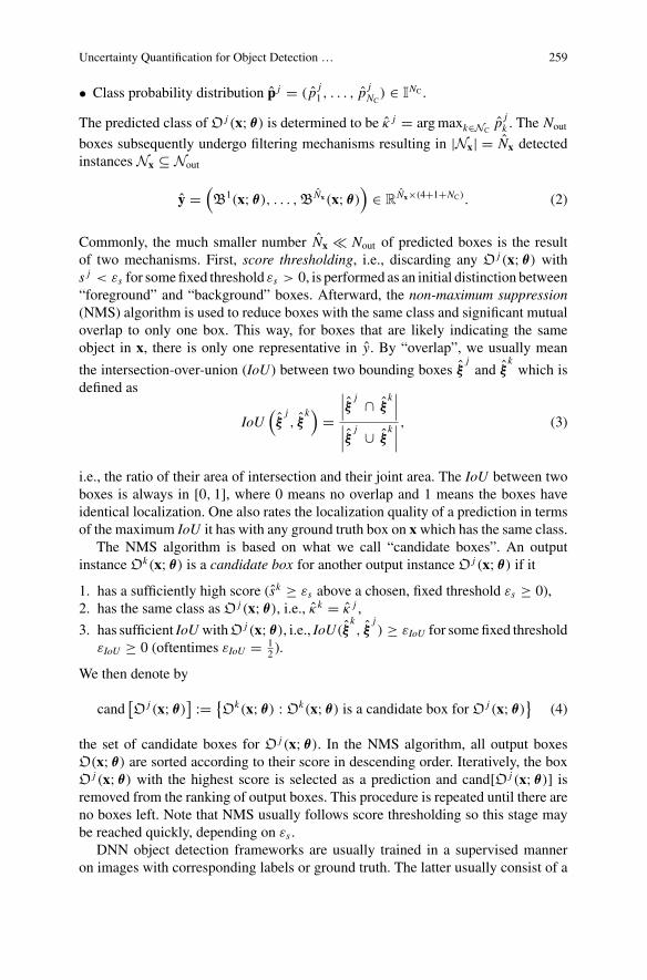
Uncertainty Quantification for Object Detection … 259

• Class probability distribution p j = ( p j1 , . . . , p

jNC

) ∈ INC .

The predicted class ofO j (x; θ) is determined to be κ j = argmaxk∈NCp jk . The Nout

boxes subsequently undergo filtering mechanisms resulting in |Nx| = Nx detectedinstances Nx ⊆ Nout

y =(B1(x; θ), . . . ,BNx(x; θ)

)∈ R

Nx×(4+1+NC). (2)

Commonly, the much smaller number Nx � Nout of predicted boxes is the resultof two mechanisms. First, score thresholding, i.e., discarding any O j (x; θ) withs j < εs for somefixed threshold εs > 0, is performed as an initial distinction between“foreground” and “background” boxes. Afterward, the non-maximum suppression(NMS) algorithm is used to reduce boxes with the same class and significant mutualoverlap to only one box. This way, for boxes that are likely indicating the sameobject in x, there is only one representative in y. By “overlap”, we usually mean

the intersection-over-union (IoU) between two bounding boxes ξjand ξ

kwhich is

defined as

IoU(ξj, ξ

k) =∣∣∣ξ

j ∩ ξk∣∣∣

∣∣∣ξ

j ∪ ξk∣∣∣, (3)

i.e., the ratio of their area of intersection and their joint area. The IoU between twoboxes is always in [0, 1], where 0 means no overlap and 1 means the boxes haveidentical localization. One also rates the localization quality of a prediction in termsof the maximum IoU it has with any ground truth box on x which has the same class.

The NMS algorithm is based on what we call “candidate boxes”. An outputinstance Ok(x; θ) is a candidate box for another output instance O j (x; θ) if it

1. has a sufficiently high score (sk ≥ εs above a chosen, fixed threshold εs ≥ 0),2. has the same class as O j (x; θ), i.e., κk = κ j ,

3. has sufficient IoU withO j (x; θ), i.e., IoU(ξk, ξ

j) ≥ εIoU for somefixed threshold

εIoU ≥ 0 (oftentimes εIoU = 12 ).

We then denote by

cand[O j (x; θ)

] := {Ok(x; θ) : Ok(x; θ) is a candidate box for O j (x; θ)

}(4)

the set of candidate boxes for O j (x; θ). In the NMS algorithm, all output boxesO(x; θ) are sorted according to their score in descending order. Iteratively, the boxO j (x; θ) with the highest score is selected as a prediction and cand[O j (x; θ)] isremoved from the ranking of output boxes. This procedure is repeated until there areno boxes left. Note that NMS usually follows score thresholding so this stage maybe reached quickly, depending on εs .

DNN object detection frameworks are usually trained in a supervised manneron images with corresponding labels or ground truth. The latter usually consist of a

260 T. Riedlinger et al.

number Nx of ground truth instances y = (y1, . . . , yNx) ∈ (R4 × NC)Nx consisting ofsimilar data as output boxes whichwe denote by the bar (·). In particular, each groundtruth instance y j has a specified localization ξ

j = (c jmin, r

jmin, c

jmax, r

jmax) ∈ R

4 andcategory κ j ∈ NC. From the network output O(x; θ) on an image x and the groundtruth y, a loss function J (O(x; θ), y) is computed and iteratively minimized overθ by stochastic gradient descent or some of its variants. In most object detectionframeworks, J splits up additively into

J = Jξ + Js + Jp, (5)

with Jξ punishing localization mistakes, Js punishing incorrect score assignmentsto boxes (incorrect boxes with high score and correct boxes with low score), andJp punishing an incorrect class probability distribution, respectively. In standardgradient descent optimization, the weights θ are then updated by the following rule:

θ ← θ − η ∇θ J (O(x; θ), y) , (6)

where η > 0 is the either fixed or variable learning rate parameter. The learninggradient g(x, θ , y) := ∇θ J (O(x; θ), y)will play a central role for the gradient-baseduncertainty metrics which will be introduced in Sect. 3.4.

3.3 Output-Based Uncertainty: MetaDetect

In this section, we construct uncertainty metrics for every B j (x; θ) ∈ y(x, θ). Wedo so in two stages, first by introducing the general metrics that can be obtainedfrom the object detection pipeline. Second, we extend this by additional metricsthat can be computed when using MC dropout. We consider a predicted boundingbox B j (x; θ) ∈ y(x, θ) and its corresponding filtered candidate boxes Ok(x; θ) ∈cand[B j (x; θ)] that were discarded by the NMS.

Thenumber of corresponding candidate boxesOk(x; θ) ∈ cand[B j (x; θ)]filteredby the NMS intuitively gives rise to the likelihood of observing a true positive.The more candidate boxes Ok(x; θ) belong to B j (x; θ), the more likely it seemsthat B j (x; θ) is a true positive. We denote by N ( j) the number of candidate boxesOk(x; θ) belonging toB j (x; θ), but suppressed by NMS.We increment this numberby 1 and also count inB j (x; θ).

For a given image x, we have the set of predicted bounding boxes y(x, θ) andthe ground truth y. As we want to calculate values that represent the quality of theprediction of the neural network, we first have to define uncertainty metrics for thepredicted bounding boxes in y(x, θ). For each B j (x; θ) ∈ y(x, θ), we define thefollowing quantities:

• the number of candidate boxes N ( j) ≥ 1 that belong to B j (x; θ) (i.e., B j (x; θ)

belongs to itself; one metric),

Uncertainty Quantification for Object Detection … 261

• the predicted box B j (x; θ) itself, i.e., the values of the tuple

(c jmin, r

jmin, c

jmax, r

jmax, s

j , p j1 , . . . , p

jNC

)∈ R

4 × S × INC , (7)

as well as∑

i∈NCp ji ∈ Rwhenever class probabilities are not normalized (6 + NC

metrics),• size d = (r j

max − r jmin) · (c j

max − c jmin) and circumference g = 2 · (r j

max − r jmin) +

2 · (c jmax − c j

min) (two metrics),• IoU j

pb: the IoU of B j (x; θ) and the box with the second highest score that wassuppressed byB j (x; θ). This value is zero if there are no boxes corresponding toB j (x; θ) suppressed by the NMS (i.e., N ( j) = 1; one metric),

• the minimum, maximum, arithmetic mean, and standard deviation for (r jmin,

r jmax, c

jmin, c

jmax, s j ), size d and circumference g fromB j (x; θ) and all the filtered

candidate boxes that were discarded from B j (x; θ) in the NMS (4 × 7 metrics),• the minimum, maximum, arithmetic mean, and standard deviation for the IoUof B j (x; θ) and all the candidate boxes corresponding to B j (x; θ) that weresuppressed in the NMS (four metrics),

• relative sizes rd = d/g, rdmax = d/gmin, rdmin = d/gmax, rdmean = d/gmean, andrdstd = d/gstd (five metrics),

• the maximal IoU of B j (x; θ) and all ground truth boxes in y; this is not an inputto a meta model but serves as the ground truth provided to the respective lossfunction.

Altogether, this results in 47 + NC uncertainty metrics which can be aggregatedfurther in a meta classifier or a meta regression model.

We now elaborate on how to calculate uncertainty metrics for every B j (x; θ) ∈y(x, θ) when using MC dropout. To this end, we consider the bounding boxB j (x; θ) ∈ y(x, θ) that was predicted without dropout and then we observe underdropout K times the output of the same anchor box that producedB j (x; θ) anddenotethem byB j (x; θ)1, ...,B

j (x; θ)K . For these K + 1 boxesB j (x; θ),B j (x; θ)1, ...,

B j (x; θ)K , we calculate the standard deviation for the localization variables, theobjectness score, and class probabilities. This is done for every B j (x; θ) ∈ y(x, θ)

and results in 4 + 1 + NC additional dropout uncertainty metrics which we denoteby stdMC(·) for each of the respective 4 + 1 + NC box features. Executing this pro-cedure for all available test images, we end up with a structured dataset. Each rowrepresents exactly one predicted bounding box and the columns are given by the reg-istered metrics. After defining a training/test splitting of this dataset, we learn metaclassification (IoU > 0.5 vs. IoU ≤ 0.5) and meta regression (quantitative IoU pre-diction) from the training part of this data. All the presented metrics, except for thetrue IoU, can be computed without the knowledge of the ground truth. We now wantto explore to which extent they are suited for the tasks of meta classification andmeta regression.

262 T. Riedlinger et al.

3.4 Gradient-Based Uncertainty for Object Detection

In the setting provided in Sect. 3.2, a DNN learns from a data point (x, y) ∈IH×W×C × (R4 × NC)Nx by computing the gradient g(x, θ , y). The latter is subse-quently used to iteratively adjust the current weights θ , for example, by the formulagiven in (6). As such, the quantity g(x, θ , y) can be interpreted as learning stress onθ induced by the training data (x, y). We explain next how a related quantity givesrise to confidence information.

Some intuition about gradient uncertainty: Generally, the loss function J mea-sures the “closeness” of output boxes to the ground truth y and g(x, θ , y) expressesthe induced change in θ for any deviation from the ground truth. If we assume thaty(x; θ) is close to y, only little change in θ will be required in an update step. We,therefore, expect g(x, θ , y) to be of comparably small magnitude. A DNN which isalready “well-trained” in the ordinary sense is expected to express high confidencewhen its prediction is correct for all practical purposes. Conversely, if the networkoutput deviates from the ground truth significantly, learning on (x, y) induces alarger adjustment in θ , leading to a gradient of larger magnitude. In this situation,the confidence in this prediction should be small.

The gradient g(x, θ , y) is not realizable as a measure of uncertainty or confidence,since it uses the ground truth y, which is not accessible during inference time. Anapproach to circumvent this shortcoming was presented in [ORG18], in that theground truth y was replaced by the prediction of the DNN y on x. We format theprediction so that it has the same format as the ground truth. Particularly, in the initialapplication to image classification, the softmax output of the DNN was collapsed byan argmax to the predicted class before insertion into J . With respect to boundingbox localization, there is no adjustment required. Additionally, when computing

g(x, θ , y

) = ∇θ J(O(x; θ), y

), (8)

we disregard the dependency of y on θ , thereby sticking to the design motivationfrom above. The quantity in (8) represents the weight adjustment induced in theDNN when learning that its prediction on x is correct. Uncertainty or confidenceinformation is distilled from g(x, θ , y) by taking it to a scalar. To this end, it isnatural to employ norms, e.g., || · ||1 or || · ||2, but we also use other maps such asminimal and maximal entry as well as the arithmetic mean and standard deviationover the gradient’s entries (see (9)). Gradient uncertainty metrics allow for someadditional flexibility. Regarding (8), we see that if J splits into additive terms (suchas in the object detection setting, see (5)), gradient metrics allow the extraction ofgradient uncertainty from each individual contribution. Additionally, we can restrictthe variables for which we compute partial derivatives. One might, for example, beinterested in computing the gradient g(x, θ �, y) for the weights θ � from only onenetwork layer �. In principle, this also allows for computing uncertainty metrics forindividual convolutional filters or even individual weights, thus, also offering a wayof localizing uncertainty within the DNN architecture.

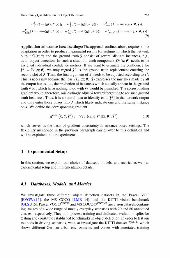
Uncertainty Quantification for Object Detection … 263

mθ1(J ) = ||g(x, θ , y)||1, mθ

2(J ) = ||g(x, θ , y)||2, mθmax(J ) = max(g(x, θ , y)),

mθmin(J ) = min(g(x, θ , y)), mθ

std(J ) = std(g(x, θ , y)), mθmean(J ) = mean(g(x, θ , y)).

(9)

Application to instance-based settings:The approach outlined above requires someadaptation in order to produce meaningful results for settings in which the networkoutput O(x; θ) and the ground truth y consist of several distinct instances, e.g.,as in object detection. In such a situation, each component O j (x; θ) needs to beassigned individual confidence metrics. If we want to estimate the confidence fory j := B j (x; θ), we may regard y j as the ground truth replacement entering thesecond slot of J . Then, the first argument of J needs to be adjusted according to y j .This is necessary because the loss J (O(x; θ), y) expresses the mistakes made by allthe output boxes, i.e., the prediction of instances which actually appear in the groundtruth y but which have nothing to do with y j would be punished. The correspondinggradient would, therefore, misleadingly adjust θ toward forgetting to see such groundtruth instances. Thus, it is a natural idea to identify cand[y j ] in the network outputand only enter those boxes into J which likely indicate one and the same instanceon x. We define the corresponding gradient

gcand(x, θ , y j

) := ∇θ J(cand[y j ](x, θ), y j

), (10)

which serves as the basis of gradient uncertainty in instance-based settings. Theflexibility mentioned in the previous paragraph carries over to this definition andwill be exploited in our experiments.

4 Experimental Setup

In this section, we explain our choice of datasets, models, and metrics as well asexperimental setup and implementation details.

4.1 Databases, Models, and Metrics

We investigate three different object detection datasets in the Pascal VOC[EVGW+15], the MS COCO [LMB+14], and the KITTI vision benchmark[GLSU15]. Pascal VOCDVOC12 andMSCOCODCOCO17 are vision datasets contain-ing images of a wide range of mostly everyday scenarios with 20 and 80 annotatedclasses, respectively. They both possess training and dedicated evaluation splits fortesting and constitute established benchmarks in object detection. In order to test ourmethods in driving scenarios, we also investigate the KITTI dataset DKITTI whichshows different German urban environments and comes with annotated training

264 T. Riedlinger et al.

Table 1 Dataset split sizes for training and testing

Dataset DVOC12train DVOC12

test DCOCO17train DCOCO17

val DKITTItrain DKITTI

eval

Size 14,805 4,952 118,287 5,002 5,481 2,000

images. From the annotated training set, we take 2,000 randomly chosen imagesfor evaluation. An overview of the sizes of the respective training and evaluationdatasets can be found in Table 1.

The experiments we present here have been carried out based on a YOLOv3[RF18] re-implementation in PyTorch. We have trained our model from scratchon each of the three training splits under dropout with a probability 0.5 between thelast and the second-to-last convolution layer in each of the regression heads. As metaclassification and meta regression models, we employ the gradient boosting modelsin [CG16] with standard settings.

For the evaluation of our meta classification models, we use cross-validated area-under-curve metrics (AuROC and AuPR [DG06]) instead of accuracy, since theformer measure the classification quality independently of any threshold, whereasaccuracy only reflects the decisions made for the classification probability 0.5. Forcross-validation, we use 10 individual image-wise splits of uncertainty metrics forthe training of meta classifiers and the respective complementary split for evalua-tion. This particular procedure is employed whenever cross-validation is used in thefollowing experiments. Especially in the VOC and KITTI dataset, AuROC valuesare mostly over 0.9, so we regard AuPR as a second classification metric. Objectdetection quality in meta fusion experiments will on the one hand be evaluated interms of cross-validated mean average precision (mAP) [EVGW+15]. However, asthe authors of [RF18] recognizedmAP as computed in the VOC challenge is insensi-tive to FPs, which is why, on the other hand, we compute the cross-validated mean F1

score (mF1) as well. For the precision-recall curves of each class, we compute indi-vidual F1 scores which are sensitive to FPs and we average them over all classes as acomplementary metric to mAP. Confidence calibration is usually evaluated in termsof expected or maximum calibration error (MCE) [NCH15], computed over bins ofwidth 0.1. As the expected calibration error is sensitive to the box count per bin, weinstead regard in addition to theMCE the average calibration error (ACE) [NZV18].Meta regression quality is evaluated by the usual coefficient of determination R2.

4.2 Implementation Details

Our object detection models receive a dropout layer between the second-to-last andthe last layers in each of the three YOLOv3 detection heads. Dropout is active duringtraining with a rate of 0.5 and also during MC inference, where we take standarddeviations over 30 dropout samples for each of the 4 + 1 + NC instance features of

Uncertainty Quantification for Object Detection … 265

all output boxes. The MetaDetect metrics introduced in Sect. 3.3 are computed froma score threshold of εs = 0.0, as it has been found in [SKR20] that lower thresholdslead to better performance in meta classification and meta regression.

Gradient uncertainty metrics were computed for the weights in the second-to-last(“T − 1”) and the last (“T ”) convolutional layers in the YOLOv3 architecture at thesame candidate score threshold as for the MetaDetect metrics. As there are threedetection heads, corresponding to a 76 × 76 (“S”), a 38 × 38 (“M”), and a 19 × 19(“L”) cell grid, we also compute gradient uncertainty metrics individually for eachdetection head. We use this distinction in our notation and, for example, indicate theset of parameters from the last layer (T ) of the detection head producing the 76 × 76cell grid (S) by θ(T,S). Moreover, as indicated in Sect. 3.4, we also exploit the splitof the loss function in (5). Each of the computed 2 × 3 × 3 = 18 gradients per boxresults in the 6 uncertainty metrics presented in (9) giving a total of 108 gradientuncertainty metrics per bounding box. Due to the resulting computational expense,we only compute gradient metrics for output boxes with score values s ≥ 10−4 andregard only those boxes for all of the following experiments.

4.3 Experimental Setup and Results

Starting from pre-trained models, we compute the DNN output, as well as MCdropout,MetaDetect, and gradient uncertaintymetrics on each evaluation dataset (seeTable 1). For each output box, we also compute themaximum IoU with the respectiveground truth such that the underlying relation can be leveraged. Before fitting anymodel, we perform NMS on the output boxes which constitutes the relevant casefor our meta fusion investigation. In the latter, we are primarily interested in findingtrue boxes which are usually discarded due to their low assigned score. We comparethe performance of different sets of uncertainty metrics in different disciplines. Inthe following, “Score” denotes the network’s confidence score, “MC” stands for MCdropout, and “MD” the MetaDetect uncertainty metrics as discussed in Sect. 3.3.Moreover, “G” denotes the full set of gradient uncertainty metrics from Sect. 3.4and the labels “MD+MC”, “G+MC”, “MD+G”, and “MD+G+MC” stand for therespective unions of MC dropout, MetaDetect, and gradient uncertainty metrics.

Meta classification: We create 10 splits of the dataset of uncertainty metrics andcomputed IoU by randomly dividing it 10 times in half. We assign the TP label tothose exampleswhichhave IoU > 0.5and theFP label otherwise.Oneach split,wefita gradient boosting classifier to the respective set of uncertaintymetrics (see Fig. 5) onone half of the data. The resulting model is used to predict a classification probabilityon the uncertainty metrics of the second half of the data and vice-versa. This resultsin meta classification predictions on all data points. We evaluate these in terms ofthe previously introduced area-under-curve metrics under usage of the TP/FP labelsgenerated from the ground truth, where we obtain averages and standard deviationsfrom the 10 splits shown in Fig. 5. Performance measured in either of the two area-

266 T. Riedlinger et al.

0.91 0.92 0.93 0.94 0.95 0.96 0.97 0.98

0.66

0.68

0.70

0.72

0.74

0.76

0.78

0.80

AuP

R

ScoreMCMDGMD+MCG+MCMD+GMD+G+MC

0.84 0.86 0.88 0.900.62

0.64

0.66

0.68

0.70

0.72

AuP

R

0.965 0.970 0.975 0.980 0.985AuROC

0.9675

0.9700

0.9725

0.9750

0.9775

0.9800

0.9825

0.9850

AuP

R

Fig. 5 Score and meta classification AuPR over AuROC from 10-fold cross-validation with respec-tive standard deviation error bars for DVOC12

test , DCOCO17val , and DKITTI

eval (from top to bottom)

Uncertainty Quantification for Object Detection … 267

under-curve metrics suggests that the models situated in the top-right separate TPfrom FP best. In all datasets, the meta classifiers MD, G, and combinations thereofoutperform the network confidence by a large margin (upwards of 6 AuROC percentpoints (ppts) onDVOC12

test , 2.5 onDCOCO17val , and 1.5 onDKITTI

eval ), withMC dropout beingamong the weakest meta classifiers. Note that for both DVOC12

test (top) and DCOCO17val

(center), the standard deviation bars are occluded by the markers due to the size ofthe range. On DKITTI

eval , we can see some of the error bars and the models forminga strict hierarchy across the two metrics with overlapping MD+MC and G+MC.Overall, the three sources of uncertainty MC, MD, and G show a significant degreeof non-redundancy across the three datasets with mutual boosts of up to 7 AuPR pptson DVOC12

test , 4.5 on DCOCO17val , and 1.1 on DKITTI

eval .

Meta fusion: We use the 10 datasets of uncertainty metrics and resulting confi-dences as in meta classification in combination with the bounding box informationas new post-NMS output of the network. Thresholding on the respective confidenceon decision thresholds εdec ∈ (0, 1) with a fixed step width of 0.01 reproduces thebaseline object detection pipeline in the case of the score. The network predic-tion with assigned confidence can then be evaluated in terms of the aforementionedclass-averaged performance measures for which we obtain averages and standarddeviations from the 10 splits, except for the deterministic score baseline. In our com-parison, we focus on the score baseline, MC dropout baseline, output- and gradient-based uncertainty metrics (MD and G), and the full model based on all availableuncertainty metrics (G+MD+MC). We show the resulting curves of mAP over mF1

in Fig. 6 on the right, where we see that the maximum mF1 value is attained by theconfidence score. In addition, we observe a sharp bend in the score curve resultingfrom a large count of samples with a score between 0 and 0.01, where the interpo-lation to the threshold εs = 0 reaches to 0.912 mAP at a low 0.61 mF1 (outside theplotting range). In terms of mAP, however, the score is surpassed by the meta fusionmodels G and in particular the meta classification models involving MD (maximummAP close to 0.92 at around 0.81 mF1). The raw MetaDetect confidences seem

0.80 0.82 0.84 0.86 0.88 0.90 0.92mF1

0.82

0.84

0.86

0.88

0.90

0.92

mAP

ScoreMCMDGG+MD+MC

0.3 0.35 0.4 0.4

5 0.5 0.55 0.6 0.6

5 0.7 0.75 0.8 0.8

5 0.9

R2

Score

MC

MD

G

MD+MC

G+MC

MD+G

MD+G+MCVOCCOCOKITTI

Fig. 6 Left: mAP over mF1 score for five meta fusion models computed from 10-fold cross-validation. We show standard deviation error bars obtained from cross-validation. Right: metaregression R2 for uncertaintymodels onDVOC12

test ,DCOCO17val , andDKITTI

eval . The plot shows the averagesover 10-fold cross-validation with standard deviation error bars hidden by the symbols

268 T. Riedlinger et al.

0.0 0.1 0.2 0.3Calibration Error

Score

Score (Platt)

MD

G

MD + G +MC

Error TypeMCEACE

0.0 0.1 0.2 0.3Calibration Error

0.0 0.1 0.2 0.3Calibration Error

Fig. 7 Average ACE and mean calibration error MCE of the score and meta classification confi-dences for DVOC12

test , DCOCO17val , and DKITTI

eval (from left to right)

to slightly improve over G+MD+MC in terms of mAP by about 0.3 ppts., whichmay be due to overfitting of the gradient boosting model, but could also result fromthe altered confidence ranking which is initially performed when computing meanaverage precision. Meta fusion based on MC dropout uncertainty shows the worstperformance of all four methods considered in this test.

Calibration: From the generated meta classification probabilities and the score, cal-ibration errors can be computed indicating their calibration as binary classifiers andcompared; see Fig. 7 with standard deviations indicated by error bars. In addition, weshow the Platt-scaled confidence score as a reference for a post-processing calibra-tion method. Naturally, ACE is smaller than MCE. The meta classification modelsshow consistently far-smaller calibration errors (maximumMCE of 0.11 onDKITTI

eval )than the confidence score (minimum MCE of 0.1 on DCOCO17

val ) with comparativelysmall miscalibration on the COCO validation dataset (center). We also observe thatmeta classifiers are also better calibrated than the Platt-scaled confidence score withthe smallest margin on DKITTI

eval . Note from the MCE that meta classification modelsshow generally good calibration with a maximum ACE around 0.05 as indicated inSect. 3 and by the example of Fig. 3.

Metaregression:Byananalogous approach tometa classification,we canfit gradientboosting regression models in a cross-validated fashion to sets of uncertainty metricsand the true maximum IoU with the ground truth. The resulting predicted IoU valuescan be evaluated in terms of R2 which is illustrated in Fig. 6 on the left. Note onceagain that error bars for the standard deviation are covered by themarkers.Weobservean overall similar trend of the metrics to the meta classification performance in thatcombinedmodels tend to perform better (boosts of up to 6 R2 ppts.) indicatingmutualnon-redundancy among the different sources of uncertainty. The models based onMD and G individually show significant improvements over the confidence score(over 5 R2 ppts. on all datasets) and a slight improvement over MC (up to 3 R2 ppts.)for all investigated datasets.

Parameter importance: We investigate which parameters are most important formeta classification in order to find the best performance with as few metrics as

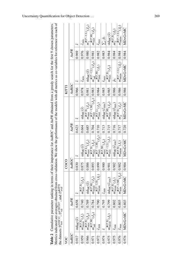
Uncertainty Quantification for Object Detection … 269

Table2

Cum

ulativeparameter

rank

ingin

term

sof

theirim

portance

forAuR

OC

andAuP

Robtained

from

agreedy

search

forthefirst9chosen

parameters.

Metrics

indicatedareaverages

obtained

from

cross-valid

ation.Weshow

theperformance

ofthemod

elswith

allm

etrics

asco-variables

forreferenceon

each

ofthedatasetsDV

OC12

test

,DCOCO17

val

,and

DKITTI

eval

VOC

COCO

KITTI

AuR

OC

AuP

RAuR

OC

AuP

RAuR

OC

AuP

R

0.917

std M

C(s

)0.658

s0.830

s0.623

s0.966

s0.969

s

0.959

mθ(T

,S)

mean

(J s

)0.740

mθ(T

,S)

max

(J p

)0.875

std M

C(s

)0.664

std M

C(s

)0.978

c min

0.976

c min

0.966

mθ(T

,S)

max

(J p

)0.769

std M

C(s

)0.886

mθ(T

,L)

max

(J p

)0.685

mθ(T

,S)

max

(J p

)0.981

std M

C(s

)0.980

mθ(T

−1,L

)1

(J p

)

0.971

mθ(T

,M)

std

(J p

)0.784

mθ(T

,M)

mean

(J p

)0.893

mθ(T

,S)

max

(J p

)0.704

mθ(T

−1,M

)max

(J p

)0.983

mθ(T

−1,L

)std

(J p

)0.981

mθ(T

,M)

max

(J p

)

0.972

c min

0.790

mθ(T

−1,S

)mean

(J ξ

)0.899

mθ(T

−1,M

)max

(J p

)0.710

mθ(T

,L)

max

(J p

)0.984

mθ(T

,M)

max

(J ξ

)0.982

r max

0.974

s0.795

c min

0.900

mθ(T

,M)

max

(J p

)0.713

std M

C(c

min)

0.985

r max

0.983

∑ip i

0.975

mθ(T

,S)

mean

(J ξ

)0.799

std M

C(c

min)

0.901

mθ(T

−1,L

)max

(J s

)0.715

mθ(T

,M)

max

(J p

)0.985

mθ(T

,S)

max

(J p

)0.984

std M

C(s

)

0.975

r min

0.802

mθ(T

,S)

mean

(J ξ

)0.902

std M

C(c

min)

0.716

std M

C(r

max

)0.986

p 10.984

mθ(T

,S)

2(J ξ

)

0.976

c max

0.803

mθ(T

−1,M

)max

(J p

)0.902

mθ(T

,S)

mean

(J s

)0.717

mθ(T

,S)

2(J p

)0.986

mθ(T

−1,L

)mean

(J ξ

)0.984

mθ(T

−1,L

)mean

(J ξ

)

0.976

MD+G+MC

0.803

MD+G+MC

0.904

MD+G+MC

0.720

MD+G+MC

0.986

MD+G+MC

0.984

MD+G+MC

270 T. Riedlinger et al.

possible. We pursue a greedy approach and evaluate single-metric models at first interms ofAuROC andAuPR in the cross-validatedmanner used before.We then fix thebest-performing single metric and investigate two-metric combinations and gatherthe resulting metrics ranking with their area-under-curve score in Table 2. In additionto the nested models, we also show the model using all metrics which is also depictedin Fig. 5. Note that the numbers represent cross-validated averages, where we choosenot to show standard deviations as we are mainly interested in seeing which metricscombine to yield well-separating meta classifiers. On all datasets, we find that a totalof 9 metrics suffices to come close to or reach the performance of the best model inquestion. The network confidence appears as the most informative single metric 5out of 6 times. Another metric that leads to early good improvements is the relatedMC dropout standard deviation of the confidence score. Other noteworthy metricsare the left border coordinate cmin and gradient metrics for the class probabilitycontribution Jp. Overall, gradient metrics contribute a large amount of informationto s and stdMC(s) which is indicative to meta classification performance.

Conclusions and Outlook

In this chapter, we have outlined two largely orthogonal approaches to quantifyingepistemic uncertainty in deep object detection networks, the output-based MetaDe-tect approach, and gradient-based uncertaintymetrics. Both compare favorably to thenetwork confidence score and MC dropout in terms of meta classification and metaregression with the additional benefit that meta classifiers give rise to well-calibratedconfidences irrespective of the set of metrics they are based on. Moreover, differentsources of uncertainty information lead to additional boosts when combined, indicat-ingmutual non-redundancy.We have seen that themeta fusion approach enables us totrade uncertainty information for network performance in terms ofmean average pre-cision with the best meta fusion models involving the MetaDetect metrics. In termsof raw meta classification capabilities, well-performing models can be achieved byonly regarding a small fraction of all metrics, with gradient-based uncertainty met-rics contributing highly informative components. The design of well-performingmeta classifiers and meta regression models opens up possibilities for further appli-cations. On the one hand, the implementation of meta classification models into anactive learning cycle could potentially lead to a drastic decrease in data annotationcosts. On the other hand, meta classification models may be applicable beneficiallyin determining the labeling quality of datasets and detecting labeling mistakes.

Acknowledgements The research leading to these results is fundedby theGermanFederalMinistryfor Economic Affairs and Energy within the project “Methoden und Maßnahmen zur Absicherungvon KI-basierten Wahrnehmungsfunktionen für das automatisierte Fahren (KI-Absicherung)”. Theauthors would like to thank the consortium for the successful cooperation. Furthermore, we grate-fully acknowledge financial support from the state Ministry of Economy, Innovation and Energyof Northrhine Westphalia (MWIDE) and the European Fund for Regional Development via theFIS.NRW project BIT-KI, grant no. EFRE-0400216. The authors gratefully acknowledge the Gauss

Uncertainty Quantification for Object Detection … 271

Centre for Supercomputing e.V. (www.gauss-centre.eu) for funding this project by providing com-puting time through the John von Neumann Institute for Computing (NIC) on the GCS Supercom-puter JUWELS at Jülich Supercomputing Centre (JSC).

References

[BCR+20] D. Brüggemann, R. Chan, M. Rottmann, H. Gottschalk, S. Bracke, Detecting outof distribution objects in semantic segmentation of street scenes, in Proceedingsof the European Safety and Reliability Conference (ESREL), virtual conference(November 2020), pp. 3023–3030

[CCKL19] J. Choi, D. Chun, H. Kim, H.-J. Lee, Gaussian YOLOv3: an accurate and fast objectdetector using localization uncertainty for autonomous driving, in Proceedings ofthe IEEE/CVF Conference on Computer Vision and Pattern Recognition (CVPR)(Long Beach, CA, USA, June 2019), pp. 502–511

[CCLK20] J. Choi, D. Chun, H.-J. Lee, H. Kim, Uncertainty-based object detector forautonomous driving embedded platforms, in Proceedings of the IEEE InternationalConference on Artificial Intelligence Circuits and Systems (AICAS), virtual confer-ence (August 2020), pp. 16–20

[CG16] T. Chen, C. Guestrin, XGBoost: a scalable tree boosting system, in Proceedingsof the ACM SIGKDD International Conference on Knowledge Discovery and DataMining (KDD) (August 2016), pp. 785–794

[CRG21] R. Chan, M. Rottmann, H. Gottschalk, Entropy maximization and meta classifica-tion for out-of-distribution detection in semantic segmentation, in Proceedings ofthe IEEE International Conference on Computer Vision (ICCV), virtual conference(October 2021), pp. 5128–5137

[CRGR21] P. Colling, L. Roese-Koerner, H. Gottschalk,M. Rottmann,MetaBox+: a new regionbased active learning method for semantic segmentation using priority maps, inProceedings of the International Conference on Pattern Recognition Applicationsand Methods (ICPRAM), virtual conference (February 2021), pp. 51–62

[CRH+19] R.Chan,M.Rottmann, F.Hüger, P. Schlicht,H.Gottschalk,Controlled false negativereduction of minority classes in semantic segmentation, in 2020 International JointConference on Neural Networks (IJCNN) (IEEE, July 2020), pp. 1–8

[DG06] J. Davis, M. Goadrich, The relationship between precision-recall and ROC curves,inProceedings of the International Conference onMachine Learning (ICML) (Pitts-burgh, PA ,USA, June 2006), pp. 233–240

[DL90] J.S. Denker, Y. LeCun, Transforming neural-net output levels to probability distribu-tions, in Proceedings of the Conference on Neural Information Processing Systems(NIPS/NeurIPS) (Denver, CO, USA, November 1990), pp. 853–859

[EVGW+15] M. Everingham, L. Van Gool, C.K.I. Williams, J. Winn, A. Zisserman, The Pascalvisual object classes challenge: a retrospective. Int. J. Comput. Vis. (IJCV) 111(1),98–136 (2015)

[Gal17] Y.Gal,Uncertainty inDeep Learning. Dissertation (University of Cambridge, 2017)[GG16] Y. Gal, Z. Ghahramani, Dropout as a Bayesian approximation: representing model

uncertainty in deep learning, in Proceedings of the International Conference onMachine Learning (ICML) (New York, NY, USA, June 2016), pp. 1050–1059

[GLSU15] A.Geiger, P. Lenz,C. Stiller, R.Urtasun, TheKITTIVisionBenchmarkSuite (2015).[Online; accessed 2021-11-18]

[GPSW17] C. Guo, G. Pleiss, Y. Sun, K.Q. Weinberger, On calibration of modern neural net-works, inProceedings of the InternationalConference onMachine Learning (ICML)(Sydney, NSW, Australia, August 2017), pp. 1321–1330

272 T. Riedlinger et al.

[GSS15] I. Goodfellow, J. Shlens, C. Szegedy, Explaining and harnessing adversarial exam-ples, in Proceedings of the International Conference on Learning Representations(ICLR) (San Diego, CA, USA, 2015), pp. 1–11

[HG17] D. Hendrycks, K. Gimpel, A baseline for detecting misclassified and out-of-distribution examples in neural networks, in Proceedings of the International Con-ference on Learning Representations (ICLR) (Toulon, France, April 2017), pp. 1–12

[HSW20] A. Harakeh, M. Smart, S.L. Waslander, BayesOD: a Bayesian approach for uncer-tainty estimation in deep object detectors, in Proceedings of the IEEE InternationalConference on Robotics and Automation (ICRA), virtual conference (May 2020),pp. 87–93

[HVD14] G. Hinton, O. Vinyals, J. Dean, Distilling the knowledge in a neural network,in Proceedings of the Conference on Neural Information Processing Systems(NIPS/NeurIPS) Workshops (Montréal, QC, Canada, December 2014), pp. 1–9

[HW21] Eyke Hüllermeier, Willem Waegeman, Aleatoric and epistemic uncertainty inmachine learning: an introduction to concepts and methods. Mach. Learn. 110,457–506 (2021)

[HZW+19] Y. He, C. Zhu, J. Wang, M. Savvides, X. Zhang, Bounding box regression withuncertainty for accurate object detection, in Proceedings of the IEEE/CVF Confer-ence on Computer Vision and Pattern Recognition (CVPR) (Long Beach, CA, USA,May 2019), pp. 2888–2897

[JLM+18] B. Jiang, R. Luo, J.Mao, T. Xiao, Y. Jiang, Acquisition of localization confidence foraccurate object detection, in Proceedings of the European Conference on ComputerVision (ECCV) (Munich, Germany, September 2018), pp. 784–799

[KD19] F. Kraus, K.Dietmayer, Uncertainty estimation in one-stage object detection, inPro-ceedings of the IEEE Intelligent Transportation Systems Conference (ITSC) (Auck-land, New Zealand, October 2019), pp. 53–60

[KG17] A. Kendall, Y. Gal, What uncertainties do we need in Bayesian deep learning forcomputer vision? in Proceedings of the Conference on Neural Information Pro-cessing Systems (NIPS/NeurIPS) (Long Beach, CA, USA, December 2017), pp.5574–5584

[KKSH20] F. Küppers, J. Kronenberger, A. Shantia, A. Haselhoff, Multivariate confidencecalibration for object detection, in Proceedings of the IEEE/CVF Conference onComputer Vision and Pattern Recognition (CVPR) Workshops, virtual conference(June 2020), pp. 1322–1330

[KP20] A. Kumar, B. Poole, On implicit regularization in β-VAEs, in Proceedings of theInternational Conference onMachine Learning (ICML) (July 2020), pp. 5480–5490

[KRBG21] K. Kowol,M. Rottmann, S. Bracke, H. Gottschalk, YOdar: uncertainty-based sensorfusion for vehicle detection with camera and radar sensors, in Proceedings of theInternational Conference on Agents and Artificial Intelligence (ICAART), virtualconference (February 2021), pp. 177–186

[LAE+16] W. Liu, D. Anguelov, D. Erhan, C. Szegedy, S. Reed, C.-Y. Fu, A.C. Berg, SSD: sin-gle shotmultibox detector, inProceedings of the EuropeanConference onComputerVision (ECCV) (Amsterdam, The Netherlands, October 2016), pp. 21–37

[LDBK18] M. Truong Le, F. Diehl, T. Brunner, A. Knol„ Uncertainty estimation for deep neuralobject detectors in safety-critical applications, inProceedings of the IEEE IntelligentTransportation Systems Conference (ITSC) (Maui, HI, USA, November 2018), pp.3873–3878

[LGG+17] T.-Y. Lin, P. Goyal, R. Girshick, K. He, P. Dollár, Focal loss for dense object detec-tion, in Proceedings of the IEEE International Conference on Computer Vision(ICCV) (Venice, Italy, October 2017), pp. 2980–2988,

[LGRB20] Z. Lyu, N. Gutierrez, A. Rajguru, W.J. Beksi, Probabilistic object detection viadeep ensembles, in Proceedings of the European Conference on Computer Vision(ECCV), virtual conference (August 2020), pp. 67–75

Uncertainty Quantification for Object Detection … 273

[LHK+21] Y. Lee, J.-w. Hwang, H.-I. Kim, K. Yun, J. Park, S. Ju Hwang, Localization Uncer-tainty Estimation for Anchor-Free Object Detectors (September 2021), pp. 1–10.arXiv:2006.15607

[LMB+14] T.-Y. Lin, M. Maire, S. Belongie, J. Hays, P. Perona, D. Ramanan, P. Dollár,C. Lawrence Zitnick, Microsoft COCO: common objects in context, in Proceed-ings of the European Conference on Computer Vision (ECCV) (Zurich, Switzerland,September 2014), pp. 740–755

[LPB17] B. Lakshminarayanan, A. Pritzel, C. Blundell, Simple and scalable predictive uncer-tainty estimation using deep ensembles, in Proceedings of the Conference on NeuralInformation Processing Systems (NIPS/NeurIPS) (Long Beach, CA, USA, Decem-ber 2017), pp. 6402–6413

[Mac92] D.J.C. MacKay, A practical Bayesian framework for backpropagation networks.Neural Comput. 4(3), 448–472 (1992)

[MNDS18] D. Miller, L. Nicholson, F. Dayoub, N. Sünderhauf, Dropout sampling for robustobject detection in open-set conditions, in Proceedings of the IEEE InternationalConference on Robotics and Automation (ICRA) (Brisbane, QLD, Australia, May2018), pp. 3243–3249

[MRG20] K. Maag, M. Rottmann, H. Gottschalk, Time-dynamic estimates of the reliabilityof deep semantic segmentation networks, in Proceedings of the IEEE InternationalConference on ToolsWith Artificial Intelligence (ICTAI) virtual conference (Novem-ber 2020), pp. 502–509

[MRV+21] K. Maag, M. Rottmann, S. Varghese, F. Hüger, P. Schlicht, H. Gottschalk, Improv-ing video instance segmentation by light-weight temporal uncertainty estimates, inProceedings of the International Joint Conference on Neural Networks (IJCNN)(July 2021), pp. 1–8

[NCH15] M. Pakdaman Naeini, G. Cooper, M. Hauskrecht, Obtaining well calibrated proba-bilities using Bayesian binning, in Proceedings of the AAAI Conference on ArtificialIntelligence (Austin, TX, USA, January 2015), pp. 2901–2907

[NMC05] A.Niculescu-Mizil, R.Caruana, Predicting goodprobabilitieswith supervised learn-ing, in Proceedings of the International Conference on Machine Learning (ICML)(Bonn, Germany, August 2005), pp. 625–632

[NZV18] L. Neumann, A. Zisserman, A. Vedaldi, Relaxed softmax: efficient confidence auto-calibration for safe pedestrian detection, in Proceedings of the Conference on Neu-ral Information Processing Systems (NIPS/NeurIPS) Workshops (Montréal, QC,Canada, December 2018), pp. 1–8

[ORF20] P. Oberdiek, M. Rottmann, G.A. Fink, Detection and retrieval of out-of-distributionobjects in semantic segmentation, in Proceedings of the IEEE/CVF Conference onComputer Vision and Pattern Recognition (CVPR), virtual conference (June 2020),pp. 1331–1340

[ORG18] P. Oberdiek, M. Rottmann, H. Gottschalk, Classification uncertainty of deep neuralnetworks based on gradient information, in Proceedings of the IAPR TC3 Work-shop on Artificial Neural Networks in Pattern Recognition (ANNPR) (Siena, Italy,September 2018), pp. 113–125

[Pla99] J. Platt, Probabilistic outputs for support vector machines and comparisons to reg-ularized likelihood methods, in Advances in Large Margin Classifiers. ed. by A.J.Smola, P. Bartlett, B. Schölkopf, D. Schuurmans (MIT Press, 1999), pp. 61–74

[RCH+20] M. Rottmann, P. Colling, T.-P. Hack, R. Chan, F. Hüger, P. Schlicht, H. Gottschalk,Prediction error meta classification in semantic segmentation: detection via aggre-gated dispersion measures of softmax probabilities, in Proceedings of the Inter-national Joint Conference on Neural Networks (IJCNN), virtual conference (July2020), pp. 1–9

[RF18] J. Redmon, A. Farhadi, Yolov3: An Incremental Improvement (April 2018), pp. 1–6.arXiv:1804.02767

274 T. Riedlinger et al.

[RHGS15] S. Ren, K. He, R. Girshick, J. Sun, Faster R-CNN: towards real-time object detectionwith region proposal networks, inProceedings of theConference onNeural Informa-tion Processing Systems (NIPS/NeurIPS) (Montréal, QC, Canada, December 2015),pp. 91–99

[RMC+20] M. Rottmann, K. Maag, R. Chan, F. Hüger, P. Schlicht, H. Gottschalk, Detection offalse positive and false negative samples in semantic segmentation, in Proceedingsof the Conference on Design, Automation and Test in Europe (DATE) (Grenoble,France, March 2020), pp. 1351–1356

[RRSG21] T. Riedlinger, M. Rottmann, M. Schubert, H. Gottschalk, Gradient-Based Quantifi-cation of Epistemic Uncertainty for Deep Object Detectors (July 2021), pp. 1–20.arXiv:2107.04517

[RS19] M. Rottmann, M. Schubert, Uncertainty measures and prediction quality rating forthe semantic segmentation of nested multi resolution street scene images, in Pro-ceedings of the IEEE/CVFConference on Computer Vision and Pattern Recognition(CVPR) Workshops (Long Beach, CA, USA, June 2019), pp. 1361–1369

[SFKM20] N. Ståhl, G. Falkman, A. Karlsson, G. Mathiason, Evaluation of uncertainty quan-tification in deep learning, in Proceedings of the International Conference on Infor-mation Processing and Management of Uncertainty in Knowledge-Based Systems(IPMU), virtual conference (June 2020), pp. 556–568

[SHK+14] Nitish Srivastava, Geoffrey Hinton, Alex Krizhevsky, Ilya Sutskever, RuslanSalakhutdinov, Dropout: a simple way to prevent neural networks from overfitting.J. Mach. Learn. Res. 15(56), 1929–1958 (2014)

[SKR20] M. Schubert, K. Kahl,M. Rottmann,Metadetect: uncertainty quantification and pre-diction quality estimates for object detection, in 2021 International Joint Conferenceon Neural Networks (IJCNN) (IEEE, 2021), pp. 1–10

[SZS+14] C. Szegedy, W. Zaremba, I. Sutskever, J. Bruna, D. Erhan, I. Goodfellow, R. Fergus,Intriguing properties of neural networks, in Proceedings of the International Con-ference on Learning Representations (ICLR) (Banff, AB, Canada, December 2014),pp. 1–10

[VSG19] V. Thanvantri Vasudevan, A. Sethy, A. Roshan Ghias, Towards better confidenceestimation for neural models, in Proceedings of the IEEE International Conferenceon Acoustics, Speech and Signal Processing (ICASSP) (Brighton, UK, May 2019),pp. 7335–7339

[ZE01] B. Zadrozny, C. Elkan, Obtaining calibrated probability estimates from decisiontrees and Naive Bayesian classifiers, in Proceedings of the International Conferenceon Machine Learning (ICML) (Williamstown, MA, USA, June 2001), pp. 609–616

[ZE02] B. Zadrozny, C. Elkan, Transforming classifier scores into accurate multiclass prob-ability estimates, in Proceedings of the ACM SIGKDD International Conferenceon Knowledge Discovery and Data Mining (KDD) (Edmonton, AB, Canada, July2002), pp. 694–699

Uncertainty Quantification for Object Detection … 275

Open Access This chapter is licensed under the terms of the Creative Commons Attribution 4.0International License (http://creativecommons.org/licenses/by/4.0/), which permits use, sharing,adaptation, distribution and reproduction in any medium or format, as long as you give appropriatecredit to the original author(s) and the source, provide a link to the Creative Commons license andindicate if changes were made.

The images or other third party material in this chapter are included in the chapter’s CreativeCommons license, unless indicated otherwise in a credit line to the material. If material is notincluded in the chapter’s Creative Commons license and your intended use is not permitted bystatutory regulation or exceeds the permitted use, you will need to obtain permission directly fromthe copyright holder.

Detecting and Learning the Unknownin Semantic Segmentation

Robin Chan, Svenja Uhlemeyer, Matthias Rottmann, and Hanno Gottschalk

Abstract Semantic segmentation is a crucial component for perception in auto-mated driving. Deep neural networks (DNNs) are commonly used for this task, andthey are usually trained on a closed set of object classes appearing in a closed opera-tional domain. However, this is in contrast to the openworld assumption in automateddriving that DNNs are deployed to. Therefore, DNNs necessarily face data that theyhave never encountered previously, also known as anomalies, which are extremelysafety-critical to properly cope with. In this chapter, we first give an overview aboutanomalies from an information-theoretic perspective. Next, we review research indetecting unknown objects in semantic segmentation. We present a method outper-forming recent approaches by training for high entropy responses on anomalousobjects, which is in line with our theoretical findings. Finally, we propose a methodto assess the occurrence frequency of anomalies in order to select anomaly types toinclude into a model’s set of semantic categories. We demonstrate that those anoma-lies can then be learned in an unsupervised fashion which is particularly suitable inonline applications.

1 Introduction

Recent developments in deep learning have enabled scientists and practitioners toadvance in a broad field of applications that were intractable before. To this end,deep neural networks (DNNs) are mostly employed which are usually trained in a

R. Chan (B) · S. Uhlemeyer · M. Rottmann · H. GottschalkUniversity of Wuppertal, Gaußstr. 20, 42119 Wuppertal, Germanye-mail: rchan@uni-wuppertal.de

S. Uhlemeyere-mail: suhlemeyer@uni-wuppertal.de

M. Rottmanne-mail: rottmann@uni-wuppertal.de

H. Gottschalke-mail: hanno.gottschalk@uni-wuppertal.de

© The Author(s) 2022T. Fingscheidt et al. (eds.), Deep Neural Networks and Data for Automated Driving,https://doi.org/10.1007/978-3-031-01233-4_10

277

278 R. Chan et al.

supervised fashion with closed-world assumption. However, when those algorithmsare deployed to real-world applications, e.g., artificial intelligence (AI) systems usedfor perception in automated driving, they often operate in an open-world settingwhere they have to face diversity of the real world. Consequently, DNNs are likelyexposed to data which is “unknown” to them and therefore possibly beyond theircapabilities to process. For this reason, having methods at hand, that indicate whena DNN is operating outside of its learned domain to seek for human intervention, isof utmost importance in safety-critical applications.

A generic term for such a task is anomaly detection, which is generally defined asrecognizing when something departs from what is regarded as normal or common.More precisely, identifying anomalous examples during inference, i.e., new examplesthat are “extreme” in some sense as they lie in low density regimes or even outside ofthe training data distribution, is commonly referred to as out-of-distribution (OoD) ornovelty detection in deep learning terminology. The latter is in close connection to thetask of identifying anomalous examples in training data, which is contrarily knownas outlier detection; a term originating from classical statistics to determine whetherobservational data is polluted. Those outlined notions are often used interchangeablyin deep learning literature. Throughout this chapter, we will stick to the general termanomaly and only specify when distinguishing is relevant.

For the purpose of anomaly detection, plenty of methods, ranging from classicalstatistical ones (see Sect. 2) to deep-learning-specific ones (see Sect. 4) have beendeveloped in the past. Nowadays for the most challenging computer vision taskstackled by deep learning, where both the model weights and output are of highdimension (in themillions), specific approaches to anomaly detection are mandatory.

Classical methods such as density estimation fail due to the curse of dimension-ality. Early approaches identify outliers based on the distance to their neighbors[KNT00, RRS00], i.e., they are looking for sparse neighborhoods. Other meth-ods consider relative densities to handle clusters of different densities, e.g., bycomparing one instance either to its k-nearest neighbors [BKNS00] or using anε-neighborhood as reference set [PKGF03]. However, the concept of neighborhoodsbecomes meaningless in high dimensions [AHK01]. More advanced approaches forhigh-dimensional data compute outlier degrees based on angles instead of distances[KSZ08] or even identify lower-dimensional subspaces [AY01, KKSZ09].

In deep-learning-driven computer vision applications, novelties are typicallyregarded as more relevant than outliers. In semantic segmentation, i.e., pixel-levelimage classification, novelty detection may even refer to a number of sub-tasks. Onthe one hand, we might be concerned with the detection of semantically anomalousobjects. This is also known as anomaly segmentation in the case of semantic segmen-tation. On the other hand, we also might be concerned with the detection of changedenvironmental conditions that are novel. The latter may be effects of a domain shiftand include change in weather, time of day, seasonality, location and time. In thischapter, we focus only on semantically novel objects as anomalies.

In general, an important capability of AI systems is to identify the unknown. How-ever, when striving for improved self-reflection capabilities, anomaly detection is notsufficient. Another important capability for real-world deployment of AI systems is

Detecting and Learning the Unknown in Semantic Segmentation 279

to realize that some specific concept appears over and over again and potentiallyconstitutes a new (or novel) object class. Incremental learning refers to the taskof learning new classes, however, especially in semantic segmentation, mostly in astrictly supervised or semi-supervised fashion where data for the new class is labeledwith ground truth [MZ19, CMB+20]. This is accompanied by an enormous data col-lection and annotation effort. In contrast to supervised incremental learning, humansmay recognize a novelty of a given class that appears over and over again very well,such that in the end a single feedback might be sufficient to assign a name to a novelclass. For the task of image classification, [HZ21] provides an unsupervised exten-sion of the semantic space, while for segmentation there exist only approaches forsupervised extension of the semantic space via incremental learning.

In this chapter, we first introduce anomaly detection from an information-basedperspective in Sect. 2. We provide theoretical evidence that the entropy is a suitablequantity for anomaly detection, particularly in semantic segmentation. In Sect. 3,we review recent developments in the fields of anomaly detection and unsupervisedlearning of new classes. We give an overview on existing methods, both in the con-text of image classification and semantic segmentation. In this setting, we present anapproach to train semantic segmentation DNNs for high entropy on anomaly datain Sect. 4. We compare our proposed approach against other established and recentstate-of-the-art anomaly segmentation methods and empirically show the effective-ness of entropy maximization in identifying unknown objects. Lastly, we propose anunsupervised learning technique for novel object classes in Sect. 5. Further, we pro-vide an outlook how the latter approach can be combined with entropy maximizationto handle the unknown at run time in automated driving.

2 Anomaly Detection Using Information and Entropy

Anomaly detection is a common routine in any data analysis task. Before training astatistical model on data, the data should be investigated whether the underlying dis-tribution generating the data is polluted by anomalies. In this context, anomalies cangenerally be understood as samples that do not fit into a distribution. Such anoma-lous samples can, e.g., be generated in the data recording process either by extremeobservations, by errors in recording and transmission, or by the fusion of datasetsthat use different systems of units. Most common for the detection of anomalies instatistics is the inspection of maximum and minimum values for each feature, orsimple univariate visualization via box-whisker plots or histograms.

More sophisticated techniques are applied in multivariate anomaly detection.Here, anomalous samples do not necessarily have to contain extreme values forsingle features, but rather an untypical combination of them. One of the applicationareas for multivariate anomaly detection is, e.g., fraud detection.

In both outlined cases, an anomaly z ∈ Rd can be qualified as an observation that

occurs at a location of extremely low density of the underlying distribution p(z) or,equivalently, has an exceptionally high value of the information

280 R. Chan et al.

I (z) = − log p(z) . (1)

Here, two problems occur: First, it is generally not specified what is considered asexceptionally high. Second, p(z) and thereby I (z) are generally unknown. Regardingthe latter issue, however, the estimate I (z) = − log p(z) can be used which in turnrelies on estimating p(z) from data associated to the probability density functionp(z). Estimation approaches for p(z) can be distinguished between parametric andnon-parametric ones.

The Mahalanobis distance [Mah36] is the best known parametric method foranomaly detection which is based on information of the multivariate normal distri-bution N . In fact, if z ∼ N (μ, �)with meanμ ∈ R

d and positive definite covariancematrix � ∈ R

d×d , then

I (z) = − log

(1

(2π)d/2(det�)1/2exp

(−1

2(z − μ)T�−1(z − μ

))(2)

= d

2log(2π) + 1

2log(det�) + 1

2(z − μ)T�−1(z − μ) = 1

2d�(z,μ)2 + c ,

(3)

whered� :=

√(z − μ)T�−1(z − μ) (4)

denotes the Mahalanobis distance. The estimation I (z) is obtained by replacing μ

and� by the arithmetic mean μ and the empirical covariance matrix �, respectively,and likewise d�(z,μ) by the empirical Mahalanobis distance d�(z, μ).

In contrast, non-parametric techniques of anomaly detection rely on non-parametric techniques to estimate p(z). Here, a large variety of methods from his-tograms, kernel estimators and many others exist [Kle09].We note, however, that thenon-parametric estimation of densities and information generally suffers from thecurse of dimensionality. To alleviate the latter issue in anomaly detection, estimationof information is often combined with techniques of dimensionality reduction, suchas, e.g., principal component analysis [HTF07] or autoencoders [SY14].

When using non-linear dimensionality reduction with autoencoders, densitiesobtained in the latent space depend on the encoder and not only on the data itself.This points towards a general problem in anomaly detection. If p(z) is the densityof a random quantity z and z′ = φ(z) is an equivalent encoding of the data z using abijective and differentiable mapping φ : Rd �→ R

d , the change of variables formula[Rud87, AGLR21]

p(z′) = p(z) · | det (∇z′z) | = p(z) · | det (∇zφ−1(z)

) | (5)

implies that the information of z′ is

I (z′) = − log (p(z)) − log(∣∣det (∇zφ

−1(z))∣∣) , (6)

Detecting and Learning the Unknown in Semantic Segmentation 281

where ∇zφ−1(z) denotes the Jacobian matrix of the inverse function φ−1. Thus,

whenever a high value of I (z) indicates an anomaly, there always exists anotherequivalent representation of the data z′, where the information I (z′) is low. In otherwords, if z is remote from other instances z j of a dataset and therefore consideredan anomaly, there will be a transformation z′ = φ(z) that brings z′ right into thecenter of the data z′

j = φ(z) j . In fact, via the Rosenblatt transformation [Ros52] anyrepresentation z of the data can be expressed via a representation z′ = φ(z) whereI (z′) is constant over all data points. This stresses the importance to understand thatan anomaly always refers to probability and encoding of the data z. This is true forboth the original data and its approximated lower-dimensional representation.

As a side remark, autoencoders designed from neural networks have been verysuccessfully applied in anomaly detection. Encoder and decoder networks possess theuniversal approximationproperty [Cyb89]. Furthermore, common training losses likethe reconstruction error are invariant under a change of the representation on latentspaces. Therefore, additional insights seem to be required to explain the empiricalsuccess of anomaly detection with autoencoders which is, however, not the scope ofthis chapter.

Another way of looking at the issue of anomaly detection in the context of differ-ent representations of same data is an explicit choice of a reference measure. Thisreference measure represents to which extent, or how likely, data is contaminatedby potential anomalies. Suppose we can associate the probability density panom(z)to the reference measure, then we can base anomaly detection on the quotient ofdensities, i.e., the odds p(z)

panom(z) , and apply a threshold whenever this ratio is low or,equivalently, when the relative information

I rel(z) := − log

(p(z)

panom(z)

)= I (z) − I anom(z) (7)

is high. We note that the relative information is independent under changes of therepresentation z′ = φ(z) as the − log | det(∇zφ

−1(z))| term from (6) occurs oncewith positive sign in I (z′) and once with negative sign in −I anom(z′) and thereforecancels. Thus, the choice of a reference measure and the choice of a representationfor the data is largely equivalent.

In practical situations, panom(z) is often represented by some data {zanomi }i∈T ′ thatare either simulated or drawn from some data source of known anomalies. A binaryclassifier p(anom|z) can thenbe trained onbasis of proper data {zi }i∈T and anomalousdata {zanomi }i∈T ′ . The assumed prior probability p(anom) for anomalies, i.e., thedegree of contamination, acts as a threshold for the estimated odds. Equivalently, theestimate of the relative information

I rel(z) = − log

(p(z)

panom(z)

)Bayes’ Theorem= − log

(p(non-anom|z)p(z)

p(non-anom)· p(anom)

p(anom|z)p(z)

)

(8)

= − log

(1 − p(anom|z)p(anom|z) · p(anom)

1 − p(anom)

)(9)

282 R. Chan et al.

= − log

(1 − p(anom|z)p(anom|z)

)− log

(p(anom)

1 − p(anom)

)(10)

= − log

(1 − p(anom|z)p(anom|z)

)+ c (11)

with the prior log-odds c = − log(

p(anom)

1−p(anom)

)being a parameter controlling the

threshold for the binary classifier p(anom|z).If specifying what is an exceptionally high value for the information I (z) or

relative information I rel(z), the distinction between the detection of outliers in thetraining data and the detection of novelties during inference has to be taken intoaccount. In outlier detection, observations, which have high (relative) informationbut which are in agreement with the extreme value of the (relative) information

Imax = maxi∈T

I (zi ) or I rel max = maxi∈T

I rel(zi ), (12)

are usually intentionally not eliminated. An outlier z for the level of significance0 < α < 1 can then be detected using the condition

P{zi }i∈T (Imax > I (z)) ≤ α or P{zi }i∈T (I rel max > I rel(z)) ≤ α. (13)

Note again that the distribution of I rel(z j ) has to be estimated to derive the associateddistribution for the extreme values, see, e.g., [DHF07], and also I rel(z) requires theestimation p(z) or panom(z). Therefore, a quantification of the epistemic uncertaintyis essential for a proper outlier detection. Given the already mentioned problems ofdensity estimation in high dimension, epistemic uncertainties may play a major role,unless a massive amount of data is available.

For the case of novelty detection taking place at inference, a comparison of theinformation of a single instance I rel(z) with the usual distribution of information Pzi

seems to be in order, which leads to the novelty criterion for level of significance0 < α < 1

Pzi (I (zi ) > I (z)) ≤ α or Pzi (I rel(zi ) > I rel(z)) ≤ α. (14)

As a variant to this criterion, I rel(zi ) could also be replaced by the extreme valuestatistics over the number of inferences alleviating the problem of generating falsenovelties by multiple testing. What has been stated on the necessity to quantify theepistemic uncertainty for the case of outlier detection equally applies for noveltydetection.

While anomaly detection is generally seen as a sub-field of unsupervised learning,some specific effects occur in the case of novelty detection in supervised learning.During the phase of inference, the data z = (y, x) contain an unobserved componenty ∈ S, which, e.g., represent the instance’s label in a classification problem for theclasses contained in S. Using the decomposition p(z) = p(y, x) = p(y|x)p(x), oneobtains the (relative) information from

Detecting and Learning the Unknown in Semantic Segmentation 283

I (z) = I (y|x) + I (x), or I rel(z) = I (y|x) + I rel(x) − I anom(y|x), (15)

where I (y|x) = − log(p(y|x)), I anom(y|x) = − log(panom(y|x)) is the conditionalinformation on the right hand side. Often, for the data of the reference measurepanom(z), the labels are not contained in S. In this case, one uses a non-informativeconditional distribution panom(y|x) = 1

|S| . If this is done, the last term of (15)becomes a constant that can be integrated into a threshold parameter.

The (relative) information cannot be computed without knowing y. Therefore,the conditional expectation is used as an unbiased estimate, yielding the expectedinformation

E I (x) = Ey∼p(y|x)(I rel(z)) = E(x) + I rel(x) + brel, (16)

where E(x) = ∑y∈S p(y|x)I (y|x) is the expected information, or entropy, of the

conditional distribution p(y|x) and brel is zero for the information and equal to− log(|S|) for the relative information with non-informative conditional distributionpanom(y|x). Note that E(x) is bounded by log(|S|). Therefore, under normal cir-cumstances, the term I rel(x) will outweigh E(x) by far. However, in problems likesemantic segmentation, each component of x is assigned a label from S. This impliessolving |I| classification problems, where I denotes the pixel space of x, thus themaximum value for E(x) yields |I| log(|S|).

Therefore, the first term in (16) contains significant contributions, especially insituations where |I| is large. The second term, I rel(x) loses importance under thehypothesis that the probability of the inputs x does not vary greatly. Despite thishypothesis could be supported by fair sampling strategies, it requires further criticalevaluation. But at least to a significant part, the expected information as an anomalymeasure with regard to instance x is given by a dispersion measure, namely theentropy of the conditional probability. As the entropy can be well estimated usinga supervised machine learning approach to estimate p(y|x) from the data {z j } j∈T ,this part of the information is well accessible in contrast to I rel(x), which requiresdensity estimation in high dimension.

Lastly in this section, let us give a remarkon the role of anomaly data {zanomj } j∈T ′ ={xanomj } j∈T ′ . If such data is available, it is desirable to train the machine learningmodel p(y|x) to produce high values for E(xanomj ) so that the tractable part of theexpected information E I (x) shows good separation properties. This requirementcan be inserted to the loss function, as it has been proposed in [HAB19, HMKS19]for classification. In fact, as the entropy E(x) is maximized by the uniform (non-informative) label distribution p(y|xanomj ) = 1

|S| , the aforementioned loss will favorthis prediction on anomalous inputs {xanomj } j∈T ′ . In this chapter, in Sect. 4, we willextend this approach to the computer vision task of semantic segmentation, afterhaving reviewed related works based on deep learning in the following section.

284 R. Chan et al.

3 Related Works

After the introduction to anomaly detection from a theoretical point of view, we nowturn to anomaly detection in deep learning. In this section, we review research in thedirection of detecting and learning unknown objects in semantic segmentation.

3.1 Anomaly Detection in Semantic Segmentation

An emerging body of work explores the detection of anomalous inputs on imagedata, where the task is more commonly referred to as anomaly or out-of-distribution(OoD) detection. Anomaly detection was first tackled in the context of image classi-fication by introducing post-processing techniques applied to softmax probabilitiesto adjust the confidence values produced by a classification model [HG17, LLLS18,LLS18, HAB19, MH20]. These methods have proven to successfully lower con-fidence scores for anomalous inputs at image-level, which is why they were alsoadapted to anomaly detection in semantic segmentation [ACS19, BSN+19], i.e.,to anomaly segmentation by treating each single pixel in an image as a potentialanomaly. Although those methods represent good baselines, they usually do not gen-eralize well to segmentation, e.g., due to the high prediction uncertainties at objectboundaries. The latter problem can, however, be mitigated by using segment-wiseprediction quality estimates [RCH+20], an approach which has also demonstratedto indicate anomalous regions within an image [ORF20].

Recent works have proposed more dedicated solutions to anomaly segmentation.Among the resulting methods, many originate from uncertainty quantification. Theintuition is that anomalous regions in an image correlate with high uncertainty. In thisregard, early approaches estimate uncertainty using Bayesian deep learning, treatingmodel parameters as distributions instead of point estimates [Mac92, Nea96]. Dueto the computational complexity, approximations are mostly preferred in practice,which comprise, e.g., Monte-Carlo dropout [GG16], stochastic batch normaliza-tion [AAM+19], or an ensemble of neural networks [LPB17, GDS20]; with someof them also being extended to semantic segmentation in [BKC17, KG17, MG19].Even when using approximations, Bayesian models still tend to be computationallyexpensive. Thus, they are not well suited to real time semantic segmentation whichis required for safe automated driving.

This is why tackling anomaly segmentation with non-Bayesian methods are morefavorable from a practitioner’s point of view. Some approaches therefore includetuning a previously trained model to the task of anomaly detection, by either mod-ifying its architecture or exploiting additional data. In [DT18], anomaly scores arelearned by adding a separate branch to the neural network. In [HMD19, MH20] thenetwork architecture is not changed but auxiliary outlier data, which is disjoint fromthe actual training data, is induced into the training process to learn anomalies. Thelatter idea motivated several works in anomaly segmentation [BSN+19, BKOŠ19,

Detecting and Learning the Unknown in Semantic Segmentation 285

JRF20, CRG21]. Nonetheless, such models have to cope with multiple tasks, hencepossibly leading to a performance loss with respect to the original semantic seg-mentation task [VGV+21]. Moreover, when including outlier datasets in the trainingprocess, it cannot be guaranteed that the chosen outlier data is a good proxy for allpossible anomalies.

Another recent line of works performs anomaly segmentation via generativemod-els that reconstruct original input images. These methods assume that reconstructedimages will better preserve the appearance of known image regions than that ofunknown ones. Anomalous regions are then identified by means of pixel-wise dis-crepancies between the original and reconstructed image. Thus, such an approachis specifically designed to anomaly segmentation and has been extensively studiedin [CM15, MVD17, LNFS19, XZL+20, LHFS21, BBSC21]. The main benefit ofthese approaches is that they do not require any OoD training data, allowing themto generalize to all possible anomalous objects. However, all these methods are lim-ited by the integrated discrepancy module, i.e., the module that identifies relevantdifferences between the original and reconstructed image. In complex scenes, suchas street scene images for automated driving, this might be a challenging task due tothe open world setting.

Regarding the dataset landscape, only few anomaly segmentation datasets exist.The LostAndFound dataset [PRG+16] is a prominent example which containsanomalous objects in various streets in Germany while sharing the same setup asCityscapes [COR+16]. LostAndFound, however, considers children and bicycles asanomalies, even though they are part of the Cityscapes training set. This was fil-tered and refined in Fishyscapes [BSN+19]. Another anomaly segmentation datasetaccompanies the CAOS benchmark [HBM+20], which considers three object classesfrom BDD100k [YCW+20] as anomalies. Both, Fishyscapes and CAOS, try to mit-igate low diversity by complementing their real images with synthetic data.

Efforts to provide anomalies in real images have beenmade in [LNFS19] by sourc-ing and annotating street scene images from the web and in [LHFS21, SKGK20] bycapturing and annotating images with small objects placed on the road. Just recently,the datasets published alongside the SegmentMeIfYouCan benchmark [CLU+21]build upon those works, particularly contributing to broad diversity of anomalousstreet scenes as well as objects.

3.2 Incremental Learning in Semantic Segmentation

Building upon the detection of anomalies, training data can be enriched in order tolearn novel classes. To avoid training from scratch, several approaches tackle the taskof incremental or even continuous learning, which can be understood as adaptingto continuously evolving environments. Besides learning novel classes, incrementallearning also encompasses adapting to alternative tasks or other domains. A com-prehensive framework to compare these different learning scenarios is provided in[vdVT19].

286 R. Chan et al.

When learning novel classes, the primary issue incremental learning approachesface is a loss of the original performance on previously learned classes, that is com-monly known as catastrophic forgetting [MC89]. To overcome this problem, amodelneeds to be both, “stable” and “plastic”, i.e., the model needs to retain its originalknowledge while being able to adapt to new environments. The complexity of meet-ing these requirements at the same time is called the stability-plasticity-dilemma[AR05]. In this regard, proposed solution strategies can be separated into three cat-egories, which are either based on architecture, regularization, or rehearsal. Most ofthese methods have been applied to image classification first.

Architecture strategies employ separate models for each sequential incrementallearning task, combined with a selector to determine which model will be used forinference [PUUH01, CSMDB19, ARC20]. However, these approaches suffer fromdata imbalances, consequently standard classification algorithms tend to favor themajority class. Approaches tomitigate skewed data distributions are usually based onover- or undersampling. Another line of works, such as [RRD+16, RPR20], employ“growing” models, i.e., enlarging the model capacity by increasing the number ofmodel parameters for more complex tasks. In [ACT17], the authors propose an auto-mated approach to select the proper task-specific model at test time. More efficientapproaches were introduced in [GK16, YYLH18], that restrict the adaptation ofparameters to relevant parts of the model in terms of the new task. The Self-Net[MCE20] is made up of an autoencoder that learns low-dimensional representationsof themodels belonging to previously learned tasks.By that, retaining existing knowl-edge via approximating the old weights instead of saving them directly is accom-panied with an implicit storage compression. The incremental adaptive deep modeldeveloped in [YZZ+19] enables capacity scalability and sustainability by exploitingthe fast convergence of shallow models at the initial stage and afterwards utilizingthe power of deep representations gradually. Other procedures perform continuouslearning, e.g., using a random-forest [HCP+19], an incrementally growing DNN,retaining a basic backbone [SAR20], or nerve pruning and synapse consolidation[PTJ+21].

Regularization strategies can be further distinguished between weight regulariza-tion, i.e., measuring the importance of weights, and distillation, i.e., transferring amodel’s knowledge into another. The former identifies parameters with great impacton the original tasks that are suppressed to be updated. Elastic weight consolida-tion (EWC) [KPR+17] is one representative method, evaluating weight importancebased on the Fisher information matrix, while the synaptic intelligence (SI) method[ZPG17] calculates the cumulative change of Euclidean distance after retrainingthe model. Both regularization methods were further enhanced, e.g., by combiningthem [CDAT18, AM19], or by including unlabeled data [ABE+18]. Another idea tomaintain model stability was adapted in [ZCCY21, FAML19], updating gradientsbased on orthogonal constraints. Bayesian neural networks are applied in [LKJ+17]to approximate a Gaussian distribution of the parameters from a single to a combinedtask.

Distillation is a regularization method, where the knowledge of an old modelcan be drawn into a new model to partly overcome catastrophic forgetting. Knowl-

Detecting and Learning the Unknown in Semantic Segmentation 287

edge distillation, proposed in [HVD14], was originally invented to transfer knowl-edge from a complex into a simple model. The earliest approach, which appliesknowledge distillation to incremental learning, is called learning without forgetting(LwF) [LH18]. A combination of knowledge distillation and EWC was proposed in[SCL+18]. Further approaches based on distillation loss are e.g., [JJJK18, YHW+19,KBJC19, LLSL19].

Rehearsal or pseudo-rehearsal-based methods, which were already proposed in[Rob95], mitigate catastrophic forgetting by allowing themodel to review old knowl-edge whenever it learns new tasks. While rehearsal-based methods retain a subset ofthe old training data, pseudo-rehearsal strategies construct a generator during retrain-ing,which learns to produce pseudo-data as similar to the old training data as possible.Hence, they provide the advantages of rehearsal even if the previously learned infor-mation is unavailable. Methods reusing old data are, e.g., incremental classifier andrepresentation learning (iCaRL) [RKSL17], which simultaneously learns classifiersand feature representation, or themethod presented in [CMJM+18],which proposes arepresentativememory. The bias correction (BiC)method [WCW+19] keeps old datain a similarmanner, but handles the data imbalancedifferently.Most pseudo-rehearsalapproaches include generative adversarial networks (GANs) [OOS17, WCW+18,MSC+19, OPK+19] or a variational autoencoder (VAE) [SLKK17]. The methodpresented in [HPL+18] combines distillation and retrospective (DR), whereby base-line approaches such as LwF are outperformed by a large margin.

Only fewworks exist, such as [KBDFs20, MZ21, TTA19], that adapt incrementallearning techniques to semantic segmentation. They adjust knowledge distillation,using no or only a small portion of old data, respectively. One challenge of continuouslearning for semantic segmentation is that images may contain unseen as well asknown classes. Hence, annotations that are restricted to some task assign a greatamount of pixels to a background class, exhibiting a semantic distribution shift.The authors of [CMB+20] provide a framework that mitigates biased predictionstowards this background class. While existing approaches require supervision, weemploy incremental learning in a semi-supervised fashion, as we do not have accessto any ground truth including novelties.

4 Anomaly Segmentation

The task of anomaly detection in the context of semantic segmentation, i.e., identi-fying anomalies at pixel-level, is commonly known as anomaly segmentation. Forthis task several approaches have been proposed that are either based on uncer-tainty quantification, generative models, or training strategies specifically tailored toanomaly detection. In this chapter, wewill first review some of thosewell-establishedmethods and, subsequently, report a performance comparison with respect to theircapability of identifying anomalies. In particular, we will demonstrate empiricallythat entropymaximization yields great performance on this segmentation task, which

288 R. Chan et al.

is in accordance to the statement of the entropy’s importance from the information-based perspective as presented in Sect. 2.

4.1 Methods

Let x ∈ IH×W×3, I = [0, 1], denote (normalized) color images of resolution H × W .

Feeding those images to a semantic segmentation network F : IH×W×3 → RH×W×S ,

the model produces pixel-wise class scores y = (yi,s)i∈I,s∈S = F(x) ∈ RH×W×S ,

with the set of pixel locations denoted by I = {1, . . . , H} × {1, . . . , W } and theset of trained (hence known) classes denoted by S = {1, . . . , S}. The correspond-ing predicted segmentation mask is given bym = (mi )i∈I ∈ {1, . . . , S}H×W , wherefor mi = argmaxs∈S yi,s ∀ i ∈ I the maximum a-posteriori probability principle isapplied. Regarding the task of anomaly segmentation, the ultimate goal is then toobtain a score map a = (ai )i∈I ∈ R

H×W that indicates the presence of an anomalyat each pixel location i ∈ I within image x, i.e., the higher the score the more likelythere should be an anomaly.

Each of the methods employed in this section provides such score maps. Theirunderlying segmentation networks (DeepLabV3+, [CZP+18]) are all trained onCityscapes [COR+16], i.e., objects not included in the set of Cityscapes object classesare considered as anomalies since they have not been seen during training and thusare unknown. The anomaly detection methods, however, differ in the way how thescores are obtained, which is why we briefly introduce the different techniques inthe following.

Maximum softmax probability: The most commonly-used baseline for anomalydetection at image level is thresholding at the maximum softmax probability (MSP)[HG17]. Therefore, thismethod assumes that anomalies are attached a lowconfidenceor, equivalently, high uncertainty. Using MSP in anomaly segmentation, the scoremap is computed via

ai = 1 − maxs∈S

softmax(yi ) ∀ i ∈ I . (17)

ODIN: A simple extension to improve MSP is applying temperature scaling aswell as adding perturbations, which is known as out-of-distribution detector forNeural networks (ODIN) [LLS18]. In more detail, let t ∈ R>0 be a hyperparameterfor temperature scaling and let ε ∈ R≥0 be a hyperparameter for the perturbationmagnitude. Then, the input x is modified as

x = (xi )i∈I with xi = xi − ε sign

(− ∂

∂xilogmax

s∈Ssoftmax

(yi

t

))∀ i ∈ I ,

(18)yielding prediction y = F(x) for which thresholding is applied at the MSP, i.e., theanomaly score map is given by

Detecting and Learning the Unknown in Semantic Segmentation 289

ai = 1 − maxs∈S

softmax(yi ) ∀ i ∈ I . (19)

Mahalanobis distance: This anomaly detection approach estimates how well latentfeatures fit to those observed in the training data. Let (L − 1) denote the penultimatelayer of a networkFwith L layers. In [LLLS18] the authors have shown that training asoftmax classifier fits a class-conditional Gaussian distribution for the output featuresfL−1. Hence, under that assumption

P(y(L−1)

i

∣∣∣ yi,s = 1)

= N(y(L−1)

i

∣∣∣ μs, �s

)∀ i ∈ I , (20)

where y(L−1) = fL−1(x) ∈ RH×W×CL−1 denotes the feature map of the penultimate

layer given inputx, andy the correspondingone-hot encodedfinal target. TheminimalMahalanobis distance d�s (x,μs) is then an obvious choice for an anomaly score map

ai = mins∈S

d�s (x,μs) = mins∈S

(y(L−1)i − μs)

T�−1s (y(L−1)

i − μs) ∀ i ∈ I , (21)

cf. (2). Note that the class means μs ∈ RCL−1 and class covariances �s ∈ R

CL−1×CL−1

are generally unknown, but can be estimated by means of the training dataset.

Monte-Carlo dropout: In semantic segmentation, Monte Carlo dropout representsthe most prominent technique to approximate Bayesian neural networks. Accordingto [MG19], (epistemic) uncertainty is measured as the mutual information whichmight serve as anomaly score map, i.e.,

ai = −∑s∈S

(1

R

∑r∈R

p(r)i,s

)log

(1

R

∑r∈R

p(r)i,s

)− 1

R

∑s∈S

∑r∈R

p(r)i,s log p

(r)i,s ∀ i ∈ I,

(22)

with p(r)i = (p(r)

i,s )s∈S = softmax(y(r)i ) in the sampling round r ∈ R = {1, . . . R}.

Typically, 8 ≤ R ≤ 12.

Void classifier:Neural networks can be trained to output confidences for the presenceof anomalies [DT18]. One approach in this context is adding an extra class to theset S of previously trained classes of a semantic segmentation network, which thenalso requires annotated anomaly data to learn from. To this end, the void class inCityscapes is a popular choice as proxy for all possible anomaly data [BSN+19], inparticular if the segmentation model was originally trained on Cityscapes. Thus, thesoftmax output of the additional class s = S + 1 represents the anomaly score map,i.e.,

ai = softmaxs=S+1(y′i ) ∀ i ∈ I , (23)

where y′ = (y′i )i∈I = (y′

i,s)i∈I,s∈{1,...,S+1} = F′(x),F′ : IH×W×3 → RH×W×(S+1).

290 R. Chan et al.

Learned embedding density: Let f�(x) ∈ RH�×W�×C� denote the feature map, or

equivalently feature embedding, at layer � ∈ L = {1, . . . , L} of a semantic segmen-tation network. By employing normalizing flows, the true distribution of featuresp(f�(x)) ∈ I

H�×W� , where x ∈ X train is drawn from the training dataset, can be trainedvia maximum likelihood, i.e., normalizing flows learn to produce the approximationp(f�(x)) ≈ p(f�(x)) [BSN+19]. At test time, the negative log-likelihood measureshow well features of a test sample fit to the feature distribution observed in thetraining data, yielding the anomaly score map

a = uplin(−log p(f�(x))

)(log applies log element-wise) (24)

with uplin : RH�×W� → RH×W denoting (bi-)linear upsampling.

Image resynthesis: After obtaining the predicted segmentation mask m ∈{1, . . . , S}H×W , m = (mi )i∈I , this output can be further processed by a generativemodelG : {1, . . . , S}H×W → I

H×W×3 aiming to reconstruct the original input image,i.e., x′ = G(m) ≈ x. This process is also called image resynthesis, and the intuitionis that reconstruction quality for anomalous objects is worse than for those on whichthe generative model is trained on. To determine pixel-wise anomalies, a discrepancynetwork [LNFS19]D : {1, . . . , S}H×W × I

H×W×3 × IH×W×3 → R

H×W can then beemployed, which classifies whether one pixel is anomalous or not, based on infor-mation provided by m, x′, and x. Here, D is trained on intentionally triggered clas-sification mistakes that are produced by flipping classes on predicted segmentationmasks. The anomaly score map is given by the output of the discrepancy network,i.e.,

a = D(m, x′, x) = D(m,G(m), x) . (25)

SynBoost: The image resynthesis approach is limited by the employed discrepancymodule D. In [BBSC21], the authors proposed to extend the discrepancy networkby incorporating further inputs based on uncertainty, such as the pixel-wise softmaxentropy

Hi (x) = −∑s∈S

softmaxs(yi ) log(softmaxs(yi )) ∀ i ∈ I, (26)

and the pixel-wise softmax probability margin

Mi (x) = 1 − maxs∈S

(softmax(yi )) + maxs∈S\{mi }

(softmax(yi )) ∀ i ∈ I . (27)

Furthermore, D is trained on anomaly data provided by the Cityscapes void class.Thus, the anomaly score map is given by

a = D(m, x′, x,H(x),M(x)) = D(m,G(m), x,H(x),M(x)) . (28)

with H(x) = (Hi (x))i∈I and M(x) = (Mi (x))i∈I .

Detecting and Learning the Unknown in Semantic Segmentation 291

Entropymaximization: Adesirable property of semantic segmentation networks isthat they attach high prediction uncertainty to novel objects. To this end, the softmaxentropy, see (26), is one intuitive uncertainty measure. The segmentation networkcan be trained for high entropy on anomalous inputs via the multi-criteria trainingobjective [CRG21]

J total = (1 − λ)E(y,x)∼D[JCE(F(x), y)] + λEx∼Danom [J anom(F(x))] , (29)

where D denotes non-anomaly training data (labels available) and Danom denotesanomaly training data (no labels available). In this approach, the COCO dataset[LMB+14] represents a set of so-called known unknowns, which is used as proxyfor Danom with the aim to represent all possible anomaly data. Moreover, λ ∈ I is ahyperparameter controlling the impact of each single loss function on the overall lossJ total. For non-anomaly data, the loss function is chosen to be the commonly-usedcross-entropy JCE, while for anomaly data, i.e., for known unknowns, we have

J anom(F(x)) = − 1

H · W

∑i∈I

1

S

∑s∈S

log softmaxs(yi ) , x ∼ Danom . (30)

Therefore, minimizing J anom is equivalent to maximizing the softmax entropy sinceboth reach their optimum when the softmax probabilities are uniformly distributed,i.e., softmaxs(yi ) = 1

S ∀ s ∈ S, i ∈ I. After training, the anomaly score map is thengiven by the (normalized) softmax entropy

ai = 1

log SHi (x) = − 1

log S

∑s∈S

softmaxs(yi ) log(softmaxs(yi )) ∀ i ∈ I . (31)

From an information-based point of view, the entropy contains significant contribu-tion to the expected information. This particularly applies for instance predictions insemantic segmentation, which motivates the entropy maximization approach for thedetection of unknown objects, cf. Sect. 2.

4.2 Evaluation and Comparison of Anomaly SegmentationMethods

Discriminating between anomaly and non-anomaly is essentially a binary classifi-cation problem. In order to evaluate the pixel-wise anomaly detection capability, weuse the receiver operating characteristic (ROC) curve as well as the precision recall(PR) curve. While for the ROC curve the true positive rate is plotted against the falsepositive rate at varying thresholds, in the PR curve precision is plotted against recallat varying thresholds. Note that we consider anomalies as the positive class, i.e.,correctly identified anomaly pixels are considered as true positive. In both curves,

292 R. Chan et al.

the degree of separability is then measured by the area under the curve (AUC), wherebetter separability corresponds to a higher AUC.

Themain difference between these two performancemetrics is how they copewithclass imbalance.While the ROC curve incorporates the number of true negatives (forthe computation of the false positive rate), in PRcurves true negatives are ignored and,consequently, more emphasis is put on finding the positive class. With the anomalyscore maps as defined in Sect. 4.1, in our case, finding the positive class correspondsto identifying anomalies.

As evaluation datasets, we use LostAndFoundNoKnown [BSN+19] and RoadOb-stacle21 [CLU+21], which are both part of the public SegmentMeIfYouCan anomalysegmentation benchmark.1 LostAndFoundNoKnown consists of 1043 road sceneimages where obstacles are placed on the road. This dataset is a subset of the promi-nent LostAndFound dataset [PRG+16] but considers only obstacles from objectclasseswhich are disjoint to those in theCityscapes labels [COR+16].More precisely,images with humans and bicycles are removed such that the remaining obstacles inthe dataset also represent anomalies to models trained on Cityscapes. Similar scenescan be found in RoadObstacle21. That dataset was published alongside the Segment-MeIfYouCan benchmark and contains 327 road obstacle scene images with diverseroad surfaces as well as diverse types of anomalous objects. Both datasets restrict theregion of interest to the road where anomalies appear. This task is extremely safety-critical as it is mandatory in automated driving to make sure that the drivable area isfree of any hazard. All anomaly segmentation methods introduced in the precedingSect. 4.1 are suited to be evaluated on these datasets. We provide a visual comparisonof anomaly scores produced by the tested methods in Fig. 1. We report numericalresults in Fig. 2 and in the corresponding Table1.

In general, we observe that anomaly detection methods originally designed forimage classification, includingMSP, ODIN andMahalanobis, do not generalize wellto anomaly segmentation. As the Mahalanobis distance is based on statistics of theCityscapes dataset, the anomaly detection is likely to suffer from performance lossunder domain shift. The same holds forMonte Carlo dropout and learned embeddingdensity, particularly resulting in poor performance inRoadObstacle21,where variousroad surfaces are available. Therefore, those methods potentially act as domain shiftclassifier rather than as detector of unknown objects.

The detection methods based on autoencoders, namely image resynthesis andSynBoost, show to be better suited for the task of anomaly segmentation, clearlybeing superior to all the approaches that already have been discussed. Autoencodersare limited by their discrepancy module, and we observe that anomaly detectionperformance significantly benefits from incorporating uncertainty measures, as doneby SynBoost. Only entropy maximization reaches similar anomaly segmentationperformance, even outperforming SynBoost in RoadObstacle21. This again can beexplained by the diversity of road surfaces, which detrimentally affects the discrep-ancy module.

1 www.segmentmeifyoucan.com.

Detecting and Learning the Unknown in Semantic Segmentation 293

[Input & annotation] [MSP] [ODIN]

[Mahalanobis] [MC dropout]

[Void classifier] [Embedding density]

[Image resynthesis] [SynBoost] [Entropy max.]

Fig. 1 Qualitative comparison of anomaly score maps for one example image of RoadAnomaly21.Here, red indicates high anomaly scores while blue indicates low ones. The ground truth anomalyinstance is highlighted by green contours. Note that the region of interest is restricted to the road,highlighted by red contours in the annotation

As a final remark, we draw attention to the use of anomaly data. The voidclassifier follows the same intuition as entropy maximization by including knownunknowns, but cannot reach nearly as good anomaly segmentation performance. Weconclude that the COCO dataset is better suited as proxy for anomalous objects thanthe Cityscapes unlabeled objects. Moreover, the results of that method empiricallydemonstrate the impact of the entropy in anomaly segmentation, which is in accor-dance to the statement of the entropy’s importance from the information perceptivedescribed in Sect. 2.

4.3 Combining Entropy Maximization and MetaClassification

Meta classification is the task of discriminating between a true positive predictionand a false positive prediction. For semantic segmentation, this idea was originally

294 R. Chan et al.

Max Softmax Probability ODIN Mahalanobis Distance

Monte Carlo Dropout Void Classifier Learned Embedding Density

Image Resynthesis SynBoost Entropy Maximization

0 0.2 0.4 0.6 0.8 1

0.0

0.2

0.4

0.6

0.8

1.0

False positive rate

Tru

epo

siti

vera

te

LostAndFoundNoKnowns

0 0.2 0.4 0.6 0.8 1

0.0

0.2

0.4

0.6

0.8

1.0

Recall

Pre

cisi

on

LostAndFoundNoKnowns

0 0.2 0.4 0.6 0.8 1

0.0

0.2

0.4

0.6

0.8

1.0

False positive rate

Tru

epo

siti

vera

te

RoadObstacle21

0 0.2 0.4 0.6 0.8 1

0.0

0.2

0.4

0.6

0.8

1.0

Recall

Pre

cisi

on

RoadObstacle21

Fig. 2 Receiver operating characteristic (left column) and precision recall (right column) curvesfor LostAndFoundNoKnowns (top row) and RoadObstacle21 (bottom row), respectively. Dashedred lines indicate the performance of random guessing, i.e., the “no-skill” baseline. The degree ofseparability between anomaly and non-anomaly is measured by the area under the curve

proposed in [RCH+20]. Bymeans of hand-craftedmetrics,which are based on disper-sion measures, geometry features, or location information, all derived from softmaxprobabilities, meta classifiers have shown to reliably identify incorrect predictionsat segment level. More precisely, connected components of pixels sharing the sameclass label are considered as segments in this context, and a false positive segmentthen corresponds to a segment-wise intersection-over-union (IoU) of 0.

Themeta classification approach can straightforwardly be adapted to post-processanomaly segmentation masks. This seems particularly reasonable in combination

Detecting and Learning the Unknown in Semantic Segmentation 295

Table 1 Pixel-wise anomaly detection performance on the datasets LostAndFoundNoKnown andRoadObstacle21, respectively. Themain evaluationmetric represents the area under precision-recallcurve (AuPRC). Moreover, the area under receiver operating characteristic (AuROC) and the falsepositive rate at a true positive rate of 95% (FPR95TPR) are reported for further insights

Method LostAndFoundNoKnown RoadObstacle21

AuPRC ↑ AuROC ↑ FPR95TPR ↓ AuPRC ↑ AuROC ↑ FPR95TPR ↓MaximumSoftmax

30.1 93.0 33.2 10.0 95.5 17.9

ODIN 52.9 95.1 30.0 11.9 96.0 16.4

Mahalanobis 55.0 97.5 12.9 19.5 95.1 21.7

Monte CarloDropout

36.8 92.2 35.5 4.9 83.5 50.3

Voidclassifier

4.8 79.5 47.0 10.4 89.7 41.5

Embeddingdensity

61.7 98.0 10.4 0.8 81.0 46.4

Imageresynthesis

42.7 96.4 17.4 37.5 98.6 4.7

SynBoost 81.7 98.3 4.6 71.3 99.4 3.2

Entropymaximiza-tion

77.9 98.0 9.7 76.0 99.7 1.3

with entropymaximization. Since entropymaximization generally increases the sen-sitivity towards predicting anomalies, it is possible that the entropy is also increasedat pixels belonging to non-anomalous objects. In the latter case, this would yieldfalse positive anomaly instance predictions, which, however, can be identified anddiscarded afterwards by meta classification. The concept of trading false-positivedetection for anomaly detection performance is motivated by [CRH+20]. Moreover,meta classifiers are expected to considerably benefit from entropy maximization,since in the original work [RCH+20] the entropy as metric has already been observedto be well correlated to the segment-wise IoU.

In our experiments on LostAndFound [PRG+16], we employ a logistic regres-sion as meta classifier that is applied as a post-processing step on top of softmaxprobabilities. We observe that the meta classifier is capable of reliably removingfalse-positive anomaly instance predictions, which in turn significantly improvesdetection performance of anomalous objects. The meta classification performance isreported inTable2, a visual example is given in Fig. 3.Wenote thatmeta classificationis applied to segmentation masks as input. Therefore, the output of the combinationof entropy maximization and meta classification does not yield pixel-wise anomalyscores to compare against the methods presented in Sect. 4.1.

The idea of meta classification can even be used to directly identify potentialanomalous objects in the semantic segmentation mask, see [ORG18], which will

296 R. Chan et al.

Table2

Detectio

nerrors

atobject

levelforLostAndFo

undanom

aliesat

differentanom

alyscore/entropythresholds

τ(togenerate

anom

alysegm

entatio

nmasks).The

quantitiesfalse-po

sitiv

es(FP)

andfalse-negativ

es(FN)arerepo

rted

atsegm

entlevel,w

ithanom

aliesas

positiv

eclass.The

F 1summarizes

these

quantitiesinto

anoverallm

easure.B

yδwedenotetheperformance

loss

ontheoriginaltask,w

hich

isthesemantic

segm

entatio

nof

City

scapes.Inthiscontext,

weconsider

aperformance

loss

of1%

asacceptable,partic

ularly

inregard

ofasign

ificantly

improved

anom

alydetectionperformance

Anomaly

score/entropy

threshold

Entropy

maxim

ization

+thresholding

Entropy

maxim

ization

+thresholding

+metaclassifier

a i≥

τ,i∈I

FP↓

FN↓

F 1↑

δin

%↓

FP↓

FN↓

F 1↑

δin

%↓

τ=

0.30

8,06

819

10.26

0.30

290

308

0.82

0.06

τ=

0.40

4,03

528

90.39

0.11

251

359

0.81

0.03

τ=

0.50

1,21

541

50.60

0.04

145

447

0.80

0.02

τ=

0.60

327

613

0.69

0.02

4961

90.76

0.02

τ=

0.70

135

879

0.61

0.01

2188

10.63

0.01

Detecting and Learning the Unknown in Semantic Segmentation 297

[without meta classifier]

[prediction quality rating] [with meta classifier]

Fig. 3 Meta classification as quality rating of anomaly instance predictions. Before applying themeta classifier (top), the anomaly segmentationmask contains anomaly instance predictions (orangesegments), with some false-positives on the road. Based on softmax probabilities, the meta classifierperforms a prediction quality rating (bottom left, red corresponds to poor quality), which is thenused to remove false positive anomaly instance predictions (bottom right). Note that the region ofinterest is restricted to the road, where ground truth anomalous objects (or obstacles) are indicatedby green contours

be subject to discussion in the following section about unsupervised learning ofunknown objects.

5 Discovering and Learning Novel Classes

If certain types of anomalies appear frequently, it might be reasonable to includethem as additional learnable classes of the segmentation model. In this section, wepropose an unsupervised method to further process anomaly predictions, all with thegoal to produce labels corresponding to novel classes. Afterwards, we will introducean incremental learning approach to train a model on novel classes by means of theretrieved unsupervised labels.

5.1 Unsupervised Identification and Segmentation of a NovelClass

Consider the dataset Dtest ⊆ X of unlabeled images x = (xi )i∈I ∈ IH×W×3, along

with a semantic segmentation network F : IH×W×3 → RH×W×S trained on the set of

classes S = {1, . . . , S}. Moreover, let a = (ai )i∈I ∈ RH×W denote a score map, as

298 R. Chan et al.

introduced in Sect. 4, which assigns the degree of anomaly to each pixel i ∈ I in x.Our unsupervised anomaly segmentation technique is a three-step procedure:

1. Image embedding: Image retrieval methods are commonly applied to construct adatabase of images that are visually related to a given image. On that account, suchmethods must quantify visual similarities, i.e., to measure the discrepancy or “dis-tance” between images. A simple idea is averaging over the pixel-wise differences.However, this approach is extremely sensitive towards data transformation such asrotation, variation in light, or different resolutions. More advanced approaches makeuse of visual descriptors that extract the elementary characteristics of the visual con-tents, e.g., color, shape, or texture. Thesemethods are invariant to data transformation,i.e., they perform well in identifying images representing the same item. If we wantto detect different instances of the same category, deep learning methods representthe state-of-the-art. In this regard, convolutional neural networks (CNNs) achievevery high accuracy in image classification tasks. These networks extract featuresof the images, that are stable regarding transformations as well as the representedobject itself, i.e., objects of the same category result in similar feature vectors. Wenow adapt this idea to identify anomalies that belong to the same class.

Let Ka|x denote the set of connected components within (a(τ )i )i∈I, a(τ )

i := 1{ai ≥τ }∀ i ∈ I for a given threshold τ ∈ R, after processing image x. Furthermore, letK :=⋃

x∈X Ka|x denote the set of all predicted anomaly components in Dtest. For eachcomponent k ∈ Ka|x, we tailor the input x to the image crop x(k) = (xi )i∈I ′ , I ′ ⊆ Iby means of the bounding box around k ∈ Ka|x. By feeding the crop x(k) to an imageclassificationnetworkG,wemapx(k) onto its feature vectorg(k) := GL−1(x(k)) ∈ R

n ,n ∈ N for all k ∈ K. Here, GL−1 denotes the output of the penultimate layer of G.

2. Dimensionality reduction: Feature vectors extracted by CNNs are usually veryhigh-dimensional. This evokes several problems regarding the clustering of suchdata. The first issue is known as curse of dimensionality, i.e., the amount of requireddata explodes with increasing dimensionality. Furthermore, distance metrics becomeless precise. Dimensionality reduction approaches project the feature vectors onto alow-dimensional representation, either by feature elimination, selection, or extrac-tion. The latter creates new independent features as a combination of the originalvectors and can be further distinguished between linear and non-linear techniques.A linear feature extraction approach, named principal component analysis (PCA)[Pea01], aims at decorrelating the components of the vectors by a change of basis,such that they are mostly aligned along the first axes. Thereby, not much informa-tion is lost if we drop the last components. A more recent non-linear method ist-distributed stochastic neighbor embedding (t-SNE) [vdMH08], which uses con-ditional probabilities representing pairwise similarities. Let us consider two featurevectors g(k), g(k ′) with k, k ′ ∈ K and let pk|k ′ ∈ I denote their similarity under a Gaus-sian distribution. Employing a Student t-distribution with one degree of freedom inthe low-dimensional space then provides a second probability qk|k ′ ∈ I. Hence, t-SNEaims at minimizing the following sum (or Kullback-Leibler divergence) [vdMH08]

Detecting and Learning the Unknown in Semantic Segmentation 299

∑k∈K

∑k ′∈K

pk|k ′ log

(pk|k ′

qk|k ′

)(32)

using gradient descent. We first perform dimensionality reduction via PCA, whichis then followed by t-SNE. In our experiments, we observed that this combinationof methods improves the effectiveness of mapping anomaly predictions onto a two-dimensional embedding space. Here, the embedding ideally creates neighborhoodsof visually related anomalies.

3. Novelty segmentation: If anomalies of the same category are detected morefrequently, they are expected to form a bigger cluster in the embedding space. Thoseclusters can be identified by employing algorithms such as density-based spatialclustering of applicationswith noise (DBSCAN) [EKSX96]. This algorithm supportsthe idea of non-supervision since it does not require any information of the potentialanomaly data, such as e.g., the number of clusters. Moreover, DBSCAN dividesdata points into core points, border points, and noise, depending on the size of theneighborhood ε ∈ [0,∞) and theminimal number of a core point’s neighbors δ ∈ N.

More precisely, let g(k) ∈ R2 denote the two-dimensional representation of x(k).

Then, g(k) is considered as a core point, if the corresponding point-wise densityρ(g(k)) := |{g(k ′) : ‖g(k) − g(k ′)‖ < ε, k ′ ∈ K}| ≥ δ, i.e., the ε-neighborhood of g(k)

contains at least δ points including itself. We denote the neighborhood of a core pointg(k), which corresponds to a component k ∈ K, as Bk := {g(k ′) : ‖g(k) − g(k ′)‖ <

ε, k ′ ∈ K}. If g(k) is not a core point but belongs to a core point’s neighborhood, wecall it a border point. Otherwise, i.e., if g(k) is neither a core point nor within a corepoint’s neighborhood, we call it noise.

Finally, a clusterC j ⊂ K, j ∈ J := {1, . . . , J } of components is formed bymerg-ing overlapping neighborhoods Bk , yielding J ∈ N clusters in total. In other words,clusters are formed from connected core points and their neighborhoods’ borderpoints. Given ρ(g(k)), we can determine the cluster density of C j , e.g.,

as the maximum maxk∈C j

ρ(g(k)) or as the average1

|C j |∑k∈C j

ρ(g(k)) .

The cluster C∗ ⊂ K, which is the cluster of highest density given a sufficient clustersize, is then selected to be further processed. To this end, let us consider the predictedsegmentation mask F(x) = m = (mi )i∈I , where mi = argmaxs∈S yi,s, i ∈ I. Thepseudo labels y = (yi )i∈I for the originally unlabeled x are then obtained by settingyi = S + 1 if pixel location i belongs to a component k ∈ C∗, and yi = mi otherwise.

5.2 Class-Incremental Learning

Let Y denote the set of pseudo labels, then the training data for some novel class S + 1can be represented byDS+1 ⊆ Dnovel × Y , whereDnovel denotes the set of previously-unseen images containing novel classes. By extending the semantic segmentationnetwork F to F+ : IH×W×3 → R

H×W×(S+1) and retraining F+ on DS+1, we perform

300 R. Chan et al.

incremental learning to add a novel and previously unknown class to the semanticspace of F.

Regularization:Knowledge distillation is a subcategory of regularization strategiesaiming to mitigate a catastrophic forgetting, i.e., these strategies try to mitigate per-formance loss on the previously-learned classes S = {1, . . . , S} while learning theadditional class S + 1. In [MZ19], the authors adapted incremental learning tech-niques to the task of semantic segmentation. Among others, they introduced theoverall objective

J total(x, y) = (1 − λ)JCE(F+(x), y) + λJD(F+(x),F(x)), λ ∈ I , (33)

where (x, y) ∈ DS+1. Here, JCE denotes the common cross-entropy loss over theenlarged set of class indices S+ := {1, . . . , S + 1} and JD the distillation loss. Thelatter loss is defined as

JD(F+(x),F(x)) := − 1

H · W

∑i∈I

∑s∈S

softmaxs(yi ) log(softmaxs(y+i )) (34)

with y = F(x) and y+ = F+(x). Knowledge distillation can be further improved byfreezing the weights of the encoder part of F+ during the training procedure [MZ19].

Rehearsal: If the original training data Dtrain ⊆ X × Y of network F is available,in incremental learning such data is usually re-integrated into the training set ofthe extended network F+, i.e., the training samples are drawn from Dtrain ∪ DS+1.To save computational costs of training and to balance the amount of old and newtraining data, established methods, e.g., [Rob95], only use a subset of Dtrain. Thissubset is typically obtained by randomly sampling a set from Dtrain that matches thesize of |DS+1|.

In combination with knowledge distillation, rehearsal strategies can be employedto mitigate a loss of performance on classes that are related to the novel class. Thisissue may arise e.g., through visual similarity such as between classes like bus andtrain, or due to class affiliation as in the case of bicycle and rider. Relevant classescan be identified by their frequency of being predicted on the relabeled pixels, i.e.,

ν tots :=

∑(x,y)∈DS+1

|{i ∈ I | mi = s ∧ yi = S + 1}| ∀s ∈ S , (35)

and hence

νrels := ν tot

s∑s ′∈S ν tot

s ′∀s ∈ S . (36)

The subset of Dtrain is then randomly sampled under the constraint that there are atleast νrel

s |DS+1| images containing the class s for all s ∈ S.

Detecting and Learning the Unknown in Semantic Segmentation 301

[Segmentation prediction of the initial model]

[Prediction quality rating]

Fig. 4 Predicted semantic segmentation mask of the initial model’s prediction (top) and corre-sponding segment-wise quality estimation (bottom) for one example from the Cityscapes test split.Green color indicates a high segment-wise IoU, red color indicates a low one

5.3 Experiments and Evaluation

In the following experiments, wewill employ a DeepLabV3+ [CZP+18]modelwithan underlying WiderResNet38 [ZSR+19] backbone for semantic segmentation.This network is initially trained on a set of 17 classes, which we will extend by anovel class. The already trained classes are the Cityscapes training classes exceptpedestrian and rider, i.e., we exclude any human in the training process of our initialsemantic segmentation network F.

The initial model was trained on the Cityscapes [COR+16] training data. For theincremental learning process, we use a portion of those data and combine them withour generated disjoint training set DS+1 containing previously unseen images andpseudo labels on novel objects. Here, the images from DS+1 are drawn from theCityscapes test data. For evaluation purposes, we use the Cityscapes validation data.Hence, during the incremental learning process only known objects are presented tothe model except humans and a few instances, such as the ego-car or mountains inan image background, belonging to the Cityscapes void category.

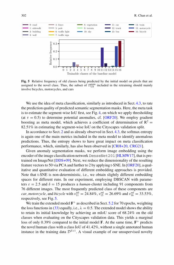
302 R. Chan et al.

0: road1: sidewalk2: building3: wall

4: fence5: pole6: traffic light7: traffic sign

8: vegetation9: terrain10: sky

11: car12: truck13: bus

14: train15: motorcycle16: bicycle

0 1 2 3 4 5 6 7 8 9 10 11 12 13 14 15 16Trainable classes of the baseline model

0.0

0.1

0.2

0.3

Rel

ativ

efr

eque

ncy

Fig. 5 Relative frequency of old classes being predicted by the initial model on pixels that areassigned to the novel class. Thus, the subset of Dtrain

CS included in the retraining should mainlyinvolve bicycles, motorcycles, and cars

We use the idea of meta classification, similarly as introduced in Sect. 4.3, to ratethe prediction quality of predicted semantic segmentation masks. Here, the meta taskis to estimate the segment-wise IoU first, see Fig. 4, on which we apply thresholding(at τ = 0.5) to determine potential anomalies, cf. [ORF20]. We employ gradientboosting as meta model, which achieves a coefficient of determination of R2 =82.51% in estimating the segment-wise IoU on the Cityscapes validation split.

In accordance to Sect. 2 and as already observed in Sect. 4.3, the softmax entropyis again one of the main metrics included in the meta model to identify anomalouspredictions. Thus, the entropy shows to have great impact on meta classificationperformance, which, similarly, has also been observed in [CRH+20, CRG21].

Given anomaly segmentation masks, we perform image embedding using theencoder of the image classification network DenseNet201 [HLMW17], that is pre-trained on ImageNet [DDS+09]. Next, we reduce the dimensionality of the resultingfeature vectors to 50 via PCA and further to 2 by applying t-SNE. In [ORF20], a qual-itative and quantitative evaluation of different embedding approaches is provided.Note that t-SNE is non-deterministic, i.e., we obtain slightly different embeddingspaces for different runs. In our experiment, employing DBSCAN with parame-ters ε = 2.5 and δ = 15 produces a human-cluster including 91 components from76 different images. The most frequently predicted class of these components arecar, motorcycle, and bicycle with νrel

11 = 24.84%, νrel15 = 26.69% and νrel

16 = 33.53%,respectively, see Fig. 5.

We train the extended model F+ as described in Sect. 5.2 for 70 epochs, weightingthe loss functions in (33) equally, i.e., λ = 0.5. The extendedmodel shows the abilityto retain its initial knowledge by achieving an mIoU score of 68.24% on the oldclasses when evaluating on the Cityscapes validation data. This yields a marginalloss of only 0.39% compared to the initial model F. At the same time, F+ predictsthe novel human class with a class IoU of 41.42%, without a single annotated humaninstance in the training data DS+1. A visual example of our unsupervised novelty

Detecting and Learning the Unknown in Semantic Segmentation 303

Fig. 6 Comparison of thepredicted semanticsegmentation masks before(top) and after (bottom)adapting the model to thenovel human class (orange)for one example of theCityscapes validation split(middle). Here, the novelcomponents are highlightedin orange, green contoursindicate the ground truthannotation of the novelty

[Prediction of initial model]

[Novel class in validation image]

[Prediction of extended model]

Fig. 7 A comparison of anomaly scores obtained by meta classification (left) and entropy (right)on an image from RoadObstacle21. The dog on the image is the anomaly of interest (indicated bygreen contours), which would have been overlooked by meta classification but entirely detected bythe entropy

segmentation approach is provided in Fig. 6, more details on the numerical evaluationis given in Table3.

304 R. Chan et al.

Table3

Evaluationof

theCity

scapes

valid

ationsplit

beforeandafterincrementallearningthenovelty

hum

an(highlighted

ingray)w

ithkn

owledg

edistillation

andrehearsal.The

classes

pede

stri

anand

ride

rareaggregated

tothenovelclass

hum

an.A

llotherclasses

aretreatedas

background,i.e.,they

areignoredduring

training,regarding

thedatafrom

DS+

1

metr

ic

road

sidewalk

building

wall

fence

pole

trafficlight

trafficsign

vegetation

terrain

sky

human

car

truck

bus

train

motorcycle

bicycle

meanexcl.human

meanincl.human

initial

IoU

97.3

480

.63

88.9

147

.24

51.0

352

.90

55.4

466

.66

89.9

556

.29

93.7

600

.00

90.6

169

.66

76.9

070

.35

24.4

554

.57

68.6

364

.82

Precision

98.3

589

.39

92.8

074

.57

66.7

672

.68

75.0

486

.22

93.6

077

.66

96.3

800

.00

92.9

780

.23

88.5

983

.33

28.5

759

.30

79.7

975

.36

Recall

98.9

689

.16

95.5

056

.32

68.4

166

.02

67.9

874

.61

95.8

567

.17

97.1

800

.00

97.2

784

.09

85.3

581

.87

62.9

287

.24

80.9

476

.44

ours

IoU

97.4

680

.78

89.3

047

.48

49.3

153

.25

55.2

865

.72

90.1

754

.53

93.4

741

.42

91.2

169

.30

72.5

262

.06

30.4

557

.72

68.2

466

.75

Precision

98.6

889

.31

93.1

178

.33

69.4

873

.74

76.0

288

.99

94.2

175

.66

95.6

959

.73

95.2

684

.88

87.2

691

.68

64.3

876

.01

84.2

882

.91

Recall

98.7

589

.43

95.6

254

.67

62.9

565

.70

66.9

671

.54

95.4

666

.13

97.5

757

.48

95.4

579

.06

81.1

165

.76

36.6

170

.57

76.0

875

.05

Detecting and Learning the Unknown in Semantic Segmentation 305

5.4 Outlook on Improving Unsupervised Learning of NovelClasses

In the preliminary experiments presented in this section, we demonstrated that asemantic segmentation network can be extended by a novel class in an unsupervisedfashion. As a basis to start, our unsupervised learning approach requires anomalysegmentation masks. Currently, these are obtained by meta classification [RCH+20],which is, however, not a method specifically tailored for the task of anomaly seg-mentation. In other words, the obtained masks are possibly inaccurate. To be evenmore precise on the limitation of plain meta classification, this method is only ableto find anomalies when the segmentation model produces a (false positive) objectprediction on those anomalies. By design, meta classifiers cannot find overlookedinstances, e.g., obstacles on the road which also have been classified as road. As anillustration of this issue, we refer to Fig. 7.

Having now several methods at hand, that we, e.g., introduced in Sect. 4.1, itseems obvious to replace the underlying anomaly segmentation method by a moresophisticated one as future work. In particular, given the decent performance of ourunsupervised learning approach relying only on meta classification and the entropymeasure as highly beneficial metric for meta classification, combining entropy max-imization and meta classification is a promising approach to improve the presentednovelty training approach.

Conclusions

Semantic segmentation as a supervised learning task is typically performedbymodelsthat operate on a given set containing a fixed number of classes. This is in clearcontrast to the open world scenarios to which practitioners contemplate the usage ofsegmentation models. There are important capabilities that standard segmentationmodels do not exhibit. Among them is the capability to know when they face anobject of a class they have not learned – i.e., to perform anomaly segmentation –as well as the capability to realize that similar objects, presumably of the same (yetunknown) class, appear frequently and should be learned either as a new class or beattributed to an existing one. In this chapter, we have seen first promising results fortwo tasks, for anomaly segmentation as well as for the detection and unsupervisedlearning of new classes.

For anomaly segmentation, we considered a number of generic baseline methodsstemming from image classification as well as some recent anomaly segmentationmethods. Since the latter clearly outperforms the former, this stresses the need forthe development of methods specifically designed for anomaly segmentation. Wehave demonstrated with our entropy maximization method empirically as well astheoretically that good proxies in combinationwith training on anomaly examples forhigh entropy are key to equip standard semantic segmentation models with anomaly

306 R. Chan et al.

segmentation capabilities. Particularly on the challenging RoadObstacle21 datasetwith diverse street scenarios, entropy maximization yields great performance whichis not reached by any other method so far. While there exists a moderate number ofdatasets for anomaly segmentation, there is clearly still the needof additional datasets.The number of possible unknown object classes not covered by these datasets isevidently enormous. Furthermore, also the vast variety of possible environmentalconditions and further domain shifts that may occur, possibly also in combinationwith unknown objects, continuously demand their exploration.

For detection and unsupervised learning of new classes, we demonstrated in pre-liminary experiments that a combination of well-established dimensionality reduc-tion and clustering methods along with the advanced uncertainty quantificationmethod for semantic segmentation called MetaSeg is well able to detect unknownclasses of which objects appear relatively frequently in a given test set. Indeed,MetaSeg can also be used to define segmentation proposals for pseudo ground-truthof new classes, which can also be learned incrementally by the segmentation model.For the considered scenario of subsequently learning humans within the Cityscapesdataset, this approach yields an IoU of 41.42% on the novel class without losing per-formance on the original classes. The proposedmethodologymay help to incorporatenew classes into existing models with low human labeling effort. The necessity forthis will occur repeatedly in future. An example are the electric scooters that recentlyarose in several metropolitan areas across the globe. This is an example for a globalphenomenon. However, also local phenomena, such as boat trailers at the coast, couldbe of interest. Such classes can be initially incorporated into an existing model usingourmethodology. Afterwards, the initial performance could be further improvedwithactive learning approaches, such as [CRGR21], still requiring only a small amountof human labeling effort. It is also an open question, to which extent the proposedmethod can be used iteratively to improve the performance on a new class. Also forthis track of research, the lack of data for pursuing that task is a limiting factor as ofnow.

Detecting and Learning the Unknown in Semantic Segmentation 307

Acknowledgements The research leading to these results is funded by the German Federal Min-istry for Economic Affairs and Energy within the projects “KI Absicherung - Safe AI for AutomatedDriving”, grant no. 19A19005R, and “KI Delta Learning - Scalable AI for Automated Driving”,grant no. 19A19013Q, respectively. The authors would like to thank the consortia for the successfulcooperation. The authors gratefully also acknowledge the Gauss Centre for Supercomputing e.V.(www.gauss-centre.eu) for funding this project by providing computing time through the John vonNeumann Institute for Computing (NIC) on the GCS Supercomputer JUWELS at Jülich Supercom-puting Centre (JSC).

References

[AAM+19] A. Atanov, A. Ashukha, D. Molchanov, K. Neklyudov, D. Vetrov, Uncertainty esti-mation via stochastic batch normalization, in Proceedings of the International Sym-posium on Neural Networks (ISNN) (Moscow, Russia, 2019), pp. 261–269

[ABE+18] R. Aljundi, F. Babiloni, M. Elhoseiny, M. Rohrbach, T. Tuytelaars, Memory AwareSynapses: Learning what (not) to forget, in Proceedings of the European Conferenceon Computer Vision (ECCV) (2018), pp. 139–154

[ACS19] M.Angus,K.Czarnecki, R. Salay, Efficacy of Pixel-LevelOODDetection for Seman-tic Segmentation (November 2019), pp. 1–13. arXiv:1911.02897

[ACT17] R.Aljundi, P.Chakravarty, T. Tuytelaars, Expert gate: lifelong learningwith a networkof experts, in Proceedings of the IEEE/CVF Conference on Computer Vision andPattern Recognition (CVPR) (Honolulu, HI, USA, July 2017), pp. 7120–7129

[AGLR21] H. Asatryan, H. Gottschalk, M. Lippert, M. Rottmann, A Convenient Infinite Dimen-sional Framework for Generative Adversarial Learning (January 2021), pp. 1–29.arXiv:2011.12087

[AHK01] C. Aggarwal, A. Hinneburg, D. Keim, On the surprising behavior of distance met-rics in high dimensional spaces, in Proceedings of the International Conference onDatabase Theory (London, UK, January 2001), pp. 420–434

[AM19] M. Amer, T. Maul, Reducing Catastrophic Forgetting in Modular Neural Networksby Dynamic Information Balancing (December 2019), pp. 1–15. arXiv:1912.04508

[AR05] W. Abraham, A. Robins, Memory retention – the synaptic stability versus plasticitydilemma. Trends Neurosci. 28(2), 73–78 (2005)

[ARC20] S. Agarwal, A. Rattani, C.R. Chowdary, A-iLearn: An adaptive incremental learningmodel for spoof fingerprint detection.MachineLearningwithApplications, 7, 100210(2020)

[AY01] C.C. Aggarwal, P.S. Yu, Outlier detection for high dimensional data, in Proceedingsof the ACM SIGMOD International Conference on Management of Data (MOD)(May 2001), pp. 37–46

[BBSC21] G. Di Biase, H. Blum, R. Siegwart, C. Cadena, Pixel-Wise Anomaly Detection inComplex Driving Scenes, in Proceedings of the IEEE/CVF conference on computervision and pattern recognition (2021), pp. 16918–16927

[BKC17] V. Badrinarayanan, A. Kendall, R. Cipolla, Bayesian SegNet: model uncertainty indeep convolutional encoder-decoder architectures for scene understanding, in Pro-ceedings of the British Machine Vision Conference (BMVC) (2017), pp. 1–12

[BKNS00] M.M. Breunig, H.-P. Kriegel, R.T. Ng, J. Sander, LOF: identifying density-basedlocal outliers. ACM SIGMOD Rec. 29(2), 93–104 (2000)

[BKOŠ19] P. Bevandic, I. Krešo, M. Oršic, S. Šegvic, Simultaneous semantic segmentationand outlier detection in presence of domain shift, in Proceedings of the GermanConference on Pattern Recognition (GCPR) (Dortmund, Germany, 2019), pp. 33–47

[BSN+19] H. Blum, P.-E. Sarlin, J. Nieto, R. Siegwart, C. Cadena, Fishyscapes: a benchmark forsafe semantic segmentation in autonomous driving, in Proceedings of the IEEE Inter-

308 R. Chan et al.

national Conference on Computer Vision (ICCV) Workshops (Seoul, Korea, October2019), pp. 2403–2412

[CDAT18] A. Chaudhry, P.K. Dokania, T. Ajanthan, P.H.S. Torr, Riemannian walk for incre-mental learning: understanding forgetting and intransigence, in Proceedings of theEuropean Conference on Computer Vision (ECCV) (Munich, Germany, September2018), pp. 556–572

[CLU+21] R. Chan, K. Lis, S. Uhlemeyer, H. Blum, S. Honari, R. Siegwart, P. Fua, M. Salz-mann, M. Rottmann, SegmentMeIfYouCan: a benchmark for anomaly segmenta-tion, in Proceedings of the Conference on Neural Information Processing Systems(NIPS/NeurIPS) – Datasets and Benchmarks Track, virtual conference (December2021), pp. 1–35

[CM15] C. Creusot, A. Munawar, Real-time small obstacle detection on highways using com-pressive RBM road reconstruction, in Proceedings of the IEEE Intelligent VehiclesSymposium (IV) (Seoul, Korea, June 2015), pp. 162–167

[CMB+20] F. Cermelli, M.Mancini, S. Rota Bulo, E. Ricci, B. Caputo,Modeling the backgroundfor incremental learning in semantic segmentation, in Proceedings of the IEEE/CVFConference on Computer Vision and Pattern Recognition (CVPR), virtual conference(June 2020), pp. 9233–9242

[CMJM+18] F.M. Castro, M.J. Marín-Jiménez, N. Guil, C. Schmid, K. Alahari, End-to-End Incre-mental Learning, in Proceedings of the European Conference on Computer Vision(ECCV) (2018), pp. 233–248

[COR+16] M. Cordts, M. Omran, S. Ramos, T. Rehfeld, M. Enzweiler, R. Benenson, U. Franke,S. Roth, B. Schiele, The Cityscapes dataset for semantic urban scene understand-ing, in Proceedings of the IEEE/CVF Conference on Computer Vision and PatternRecognition (CVPR) (Las Vegas, NV, USA, June 2016), pp. 3213–3223

[CRG21] R. Chan, M. Rottmann, H. Gottschalk, Entropy maximization and meta classificationfor out-of-distribution detection in semantic segmentation, inProceedings of the IEEEInternational Conference on Computer Vision (ICCV), virtual conference (October2021), pp. 5128–5137

[CRGR21] P. Colling, L. Roese-Koerner, H. Gottschalk, M. Rottmann, MetaBox+: a new regionbased active learning method for semantic segmentation using priority maps, in Pro-ceedings of the International Conference on Pattern Recognition Applications andMethods (ICPRAM), virtual conference (February 2021), pp. 51–62

[CRH+20] R. Chan, M. Rottmann, F. Hüger, P. Schlicht, H. Gottschalk, Controlled false neg-ative reduction of minority classes in semantic segmentation, in Proceedings of theInternational Joint Conference on Neural Networks (IJCNN), virtual conference (July2020), pp. 1–8

[CSMDB19] A. Chefrour, L. Souici-Meslati, I. Difi, N. Bakkouche, A novel incremental learn-ing algorithm based on incremental vector support machina and incremental neuralnetwork learn++. Revue d’Intelligence Artificielle 33(3), 181–188 (2019)

[Cyb89] G.Cybenko,Approximation by superpositions of a sigmoidal function.Math. ControlSignals Syst. 2(4), 303–314 (1989)

[CZP+18] L.-C. Chen, Y. Zhu, G. Papandreou, F. Schroff, H. Adam, Encoder-decoder withatrous separable convolution for semantic image segmentation, in Proceedings of theEuropean Conference on Computer Vision (ECCV) (Munich, Germany, September2018), pp. 833–851

[DDS+09] J. Deng, W. Dong, R. Socher, L.-J. Li, K. Li, F.-F. Li, ImageNet: a large-scale hier-archical image database, in Proceedings of the IEEE/CVF Conference on ComputerVision and Pattern Recognition (CVPR) (Miami, FL, USA, June 2009), pp. 248–255

[DHF07] L. De Haan, A. Ferreira, Extreme Value Theory: An Introduction (Springer, 2007)[DT18] T. DeVries, G.W. Taylor, Learning Confidence for Out-of-Distribution Detection in

Neural Networks (February 2018), pp. 1–12. arXiv:1802.04865[EKSX96] M. Ester, H.-P. Kriegel, J. Sander, X. Xu, A density-based algorithm for discovering

clusters in large spatial databases with noise, in Proceedings of the ACM SIGKDD

Detecting and Learning the Unknown in Semantic Segmentation 309

International Conference on Knowledge Discovery and Data Mining (KDD) (August1996), pp. 226–231

[FAML19] M. Farajtabar, N. Azizan, A. Mott, A. Li, Orthogonal gradient descent for continuallearning, in International Conference on Artificial Intelligence and Statistics (2020,June), pp. 3762–3773. PMLR

[GDS20] F.K.Gustafsson,M.Danelljan, T. BoSchön, Evaluating scalableBayesian deep learn-ing methods for robust computer vision, in Proceedings of the IEEE/CVF Conferenceon Computer Vision and Pattern Recognition (CVPR) Workshops, virtual conference(June 2020), pp. 1289–1298

[GG16] Y. Gal, Z. Ghahramani, Dropout as a Bayesian approximation: representing modeluncertainty in deep learning, in Proceedings of the International Conference onMachine Learning (ICML) (New York, NY, USA, June 2016), pp. 1050–1059

[GK16] A. Gepperth, C. Karaoguz, A bio-inspired incremental learning architecture forapplied perceptual problems. Cogn. Comput. 8(5), 924–934 (2016)

[HAB19] M. Hein, M. Andriushchenko, J. Bitterwolf, Why ReLU networks yield high-confidence predictions far away from the training data and how to mitigate the prob-lem, in Proceedings of the IEEE/CVF Conference on Computer Vision and PatternRecognition (CVPR) (Long Beach, CA, USA, June 2019), pp. 41–50

[HBM+20] D. Hendrycks, S. Basart, M. Mazeika, M. Mostajabi, J. Steinhardt, D. Song, ScalingOut-of-Distribution Detection for Real-World Settings (December 2020), pp. 1–12.arXiv:1911.11132

[HCP+19] C. Hu, Y. Chen, X. Peng, H. Yu, C. Gao, L. Hu, A novel feature incremental learningmethod for sensor-based activity recognition. IEEE Trans. Knowl. Data Eng. 31(6),1038–1050 (2019)

[HG17] D. Hendrycks, K. Gimpel, A baseline for detecting misclassified and out-of-distribution examples in neural networks, in Proceedings of the International Con-ference on Learning Representations (ICLR) (Toulon, France, April 2017), pp. 1–12

[HLMW17] G. Huang, Z. Liu, L. van der Maaten, K.Q. Weinberger, Densely connected convo-lutional networks, in Proceedings of the IEEE/CVF Conference on Computer Visionand Pattern Recognition (CVPR) (Honolulu, HI, USA, July 2017), pp. 4700–4708

[HMD19] D. Hendrycks, M. Mazeika, T. Dietterich, Deep anomaly detection with outlier expo-sure, in Proceedings of the International Conference on Learning Representations(ICLR) (New Orleans, LA, USA, May 2019), pp. 1–18

[HMKS19] D. Hendrycks, M. Mazeika, S. Kadavath, D. Song, Using self-supervised learningcan improve model robustness and uncertainty, in Proceedings of the Conference onNeural Information Processing Systems (NIPS/NeurIPS) (Vancouver, BC, Canada,December 2019), pp. 15637–15648

[HPL+18] S. Hou, X. Pan, C. Change Loy, Z. Wang, D. Lin, Lifelong learning via progres-sive distillation and retrospection, in Proceedings of the European Conference onComputer Vision (ECCV) (Munich, Germany, August 2018), pp. 452–467

[HTF07] T. Hastie, R. Tibshirani, J. Friedman, The Elements of Statistical Learning (Springer,2007)

[HVD14] G. Hinton, O. Vinyals, J. Dean, Distilling the knowledge in a neural network,in Proceedings of the Conference on Neural Information Processing Systems(NIPS/NeurIPS) Workshops (Montréal, QC, Canada, December 2014), pp. 1–9

[HZ21] J. He, F. Zhu, Unsupervised Continual Learning via Pseudo Labels (July 2021), pp.1–9. arXiv:2104.07164

[JJJK18] H. Jung, J. Ju, M. Jung, J. Kim, Less-forgetful learning for domain expansion in deepneural networks, in Proceedings of the AAAI Conference on Artificial Intelligence(New Orleans, LA, USA, February 2018), pp. 3358–3365

[JRF20] N. Jourdan, E. Rehder, U. Franke, Identification of uncertainty in artificial neuralnetworks, in Proceedings of the Uni-DAS e.V. Fahrerassistenz und automatisiertesFahren (FAS) Workshop, virtual conference (July 2020), pp. 1–11

310 R. Chan et al.

[KBDFs20] M.Klingner, A. Bär, P. Donn, T. Fingscheidt, Class-incremental learning for semanticsegmentation re-using neither old data nor old labels, in Proceedings of the IEEEIntelligent Transportation Systems Conference (ITSC), virtual conference (September2020), pp. 1–8

[KBJC19] D. Kim, J. Bae, Y. Jo, J. Choi, Incremental Learning With Maximum Entropy Reg-ularization: Rethinking Forgetting and Intransigence (February 2019), pp. 1–10.arXiv:1902.00829

[KG17] A. Kendall, Y. Gal, What uncertainties do we need in Bayesian deep learning forcomputer vision? inProceedings of the Conference on Neural Information ProcessingSystems (NIPS/NeurIPS) (Long Beach, CA, USA, December 2017), pp. 5574–5584

[KKSZ09] H.-P. Kriegel, P. Kröger, E. Schubert, A. Zimek, Outlier detection in axis-parallelsubspaces of high dimensional data, in Proceedings of the Pacific-Asia Conferenceon Knowledge Discovery and Data Mining (PAKDD) (Bangkok, Thailand, April2009), pp. 831–838

[Kle09] J. Sakari Klemelä, Smoothing of Multivariate Data: Density Estimation and Visual-ization (Wiley, 2009)

[KNT00] E.M. Knorr, R.T. Ng, V. Tucakov, Distance-based outliers: algorithms and applica-tions. Int. J. Very Larg. Data Bases 8(3–4), 237–253 (2000)

[KPR+17] J. Kirkpatrick, R. Pascanu, N. Rabinowitz, J. Veness, G. Desjardins, A.A. Rusu, K.Milan, J. Quan, T. Ramalho, A. Grabska-Barwinska, D. Hassabis, C. Clopath, D.Kumaran, R. Hadsell, Overcoming Catastrophic Forgetting in Neural Networks, inProceedings of the national academy of sciences, 114(13), 3521–3526 (2017)

[KSZ08] H.-P. Kriegel, M. Schubert, A. Zimek, Angle-based outlier detection in high-dimensional data, in Proceedings of the ACM SIGKDD International Conferenceon Knowledge Discovery and Data Mining (KDD) (Las Vegas, NV, USA, August2008), pp. 444–452

[LH18] Z. Li, D. Hoiem, Learning without forgetting. IEEE Trans. Pattern Anal.Mach. Intell.(TPAMI) 40, 2935–2947 (2018)

[LHFS21] K. Lis, S. Honari, P. Fua, M. Salzmann, Detecting road obstacles by erasing them(April 2021), pp. 1–18. arXiv:2012.13633

[LKJ+17] S.-W. Lee, J.-H.Kim, J. Jun, J.-W.Ha, B.-T. Zhang, OvercomingCatastrophic Forget-ting by Incremental Moment matching. Advances in neural information processingsystems, 30 (2017)

[LLLS18] K. Lee, K. Lee, H. Lee, J. Shin, A simple unified framework for detecting out-of-distribution samples and adversarial attacks, in Proceedings of the Conference onNeural Information Processing Systems (NIPS/NeurIPS) (Montréal, QC, Canada,December 2018), pp. 7167–7177

[LLS18] S. Liang, Y. Li, R. Srikant, Enhancing the reliability of out-of-distribution imagedetection in neural networks, in Proceedings of the International Conference onLearning Representations (ICLR) (Vancouver, BC, Canada, April 2018), pp. 1–15

[LLSL19] K. Lee, K. Lee, J. Shin, H. Lee, Overcoming catastrophic forgetting with unlabeleddata in the wild, in Proceedings of the IEEE International Conference on ComputerVision (ICCV) (Seoul, Korea, October 2019), pp. 312–321

[LMB+14] T.-Y. Lin, M. Maire, S. Belongie, J. Hays, P. Perona, D. Ramanan, P. Dollár,C. Lawrence Zitnick, Microsoft COCO: Common Objects in Context, in Proceed-ings of the European Conference on Computer Vision (ECCV) (Zurich, Switzerland,September 2014), pp. 740–755

[LNFS19] K. Lis, K. Nakka, P. Fua, M. Salzmann, Detecting the Unexpected via Image Resyn-thesis, in Proceedings of the IEEE International Conference on Computer Vision(ICCV) (Seoul, Korea, October 2019), pp. 2152–2161

[LPB17] B. Lakshminarayanan, A. Pritzel, C. Blundell, Simple and scalable predictive uncer-tainty estimation using deep ensembles, in Proceedings of the Conference on NeuralInformation Processing Systems (NIPS/NeurIPS) (Long Beach, CA, USA, December2017), pp. 6402–6413

Detecting and Learning the Unknown in Semantic Segmentation 311

[Mac92] D.J.C.MacKay,A practical Bayesian framework for backpropagation networks. Neu-ral Comput. 4(3), 448–472 (1992)

[Mah36] P. Chandra Mahalanobis, On the generalized distance in statistics. Proc. Natl. Inst.India 2(1), 49–55 (1936)

[MCE20] J.K. Mandivarapu, B. Camp, R. Estrada, Self-net: Lifelong learning via continualself-modeling. Frontiers in artificial intelligence, 3, 19

[MC89] M. McCloskey, N. Cohen, Catastrophic interference in connectionist networks: thesequential learning problem. Psychol. Learn. Motiv. 24, 109–165 (1989)

[MG19] J. Mukhoti, Y. Gal, Evaluating Bayesian deep learning methods for semantic seg-mentation (March 2019), pp. 1–13. arXiv:1811.12709

[MH20] A. Meinke, M. Hein, Towards neural networks that provably know when they don’tknow, in Proceedings of the International Conference on Learning Representations(ICLR), virtual conference (April 2020), pp. 1–18

[MSC+19] D.Mellado, C. Saavedra, S. Chabert, R. Torres, R.F. Salas, Self-improving generativeartificial neural network for pseudorehearsal incremental class learning. Algorithms12(10), 1–17 (2019)

[MVD17] A.Munawar, P.Vinayavekhin,G.DeMagistris, Limiting the reconstruction capabilityof generative neural network using negative learning, in Proceedings of the IEEEInternational Workshop on Machine Learning for Signal Processing (MLSP) (Tokyo,Japan, September 2017), pp. 1–6

[MZ19] U.Michieli, P. Zanuttigh, Incremental learning techniques for semantic segmentation,in Proceedings of the IEEE International Conference on Computer Vision (ICCV)Workshops (Seoul, Korea, October 2019), pp. 3205–3212

[MZ21] U.Michieli, P. Zanuttigh, Knowledge distillation for incremental learning in semanticsegmentation. Comput. Vis. Image Underst. 205, 103167 (2021)

[Nea96] R.M. Neal, Bayesian Learning for Neural Networks (Springer, 1996)[OOS17] A. Odena, C. Olah, J. Shlens, Conditional image synthesis with auxiliary classifier

GANs, in Proceedings of the International Conference on Machine Learning (ICML)(Sydney, NSW, Australia, August 2017), pp. 2642–2651

[OPK+19] O. Ostapenko, M. Puscas, T. Klein, P. Jähnichen, M. Nabi, Learning to remember:a synaptic plasticity driven framework for continual learning, in Proceedings of theIEEE/CVF Conference on Computer Vision and Pattern Recognition (CVPR) (LongBeach, CA, USA, June 2019), pp. 11313–11321

[ORF20] P. Oberdiek, M. Rottmann, G.A. Fink, Detection and retrieval of out-of-distributionobjects in semantic segmentation, in Proceedings of the IEEE/CVF Conference onComputer Vision and Pattern Recognition (CVPR), virtual conference (June 2020),pp. 1331–1340

[ORG18] P. Oberdiek, M. Rottmann, H. Gottschalk, Classification uncertainty of deep neuralnetworks based ongradient information, inProceedings of the IAPR TC3 Workshop onArtificial Neural Networks in Pattern Recognition (ANNPR) (Siena, Italy, September2018), pp. 113–125

[Pea01] K. Pearson, On lines and planes of closest fit to systems of points in space. Lond.Edinb. Dublin Philos. Mag. J. Sci. 2(11), 559–572 (1901)

[PKGF03] S. Papadimitriou, H. Kitagawa, P.B. Gibbons, C. Faloutsos, LOCI: fast outlier detec-tion using the local correlation integral, in Proceedings of the International Confer-ence on Data Engineering (Bangalore, India, March 2003), pp. 315–326

[PRG+16] P. Pinggera, S. Ramos, S. Gehrig, U. Franke, C. Rother, R. Mester, Lost and found:detecting small road hazards for self-driving vehicles, inProceedings of the IEEE/RSJInternational Conference on Intelligent Robots and Systems (IROS) (Daejeon, Korea,October 2016), pp. 1099–1106

[PTJ+21] J. Peng, B. Tang, H. Jiang, Z. Li, Y. Lei, T. Lin, H. Li, Overcoming long-term catas-trophic forgetting through adversarial neural pruning and synaptic consolidation, inIEEE Transactions on Neural Networks and Learning Systems (TNNLS) (February2021) early access, pp. 1–14

312 R. Chan et al.

[PUUH01] R. Polikar, L. Upda, S.S. Upda, V. Honavar, Learn++: an incremental learning algo-rithm for supervised neural networks. IEEE Trans. Syst. Man Cybern. Part C (Appl.Rev.) 31(4), 497–508 (2001)

[RCH+20] M. Rottmann, P. Colling, T.-P. Hack, R. Chan, F. Hüger, P. Schlicht, H. Gottschalk,Prediction error meta classification in semantic segmentation: detection via aggre-gated dispersion measures of softmax probabilities, in Proceedings of the Interna-tional Joint Conference on Neural Networks (IJCNN), virtual conference (July 2020),pp. 1–9

[RKSL17] S.-A. Rebuffi, A. Kolesnikov, G. Sperl, C.H. Lampert, iCaRL: incremental classifierand representation learning, in Proceedings of the IEEE/CVF Conference on Com-puter Vision and Pattern Recognition (CVPR) (Honolulu, HI, USA, July 2017), pp.5533–5542

[Rob95] A.V. Robins, Catastrophic forgetting, rehearsal and pseudorehearsal. Connect. Sci.7(2), 123–146 (1995)

[Ros52] M. Rosenblatt, Remarks on a multivariate transformation. Ann. Math. Stat. 23(3),470–472 (1952)

[RPR20] D. Roy, P. Panda, K. Roy, Tree-CNN: A Hierarchical Deep Convolutional NeuralNetwork for Incremental Learning. Neural Networks, 121, 148–160 (2020)

[RRD+16] A.A. Rusu, N.C. Rabinowitz, G. Desjardins, H. Soyer, J. Kirkpatrick, K.Kavukcuoglu, R. Pascanu, R. Hadsell, Progressive Neural Networks (September2016), pp. 1–14. arXiv:1606.04671

[RRS00] S. Ramaswamy, R. Rastogi, K. Shim, Efficient algorithms for mining outliers fromlarge data sets, in Proceedings of the ACM SIGMOD International Conference onManagement of Data (MOD) (May 2000), pp. 427–438

[Rud87] W. Rudin, Real and Complex Analysis (McGraw-Hill Inc., 1987)[SAR20] S. Shakib Sarwar, A.Ankit, K. Roy, Incremental learning in deep convolutional neural

networks using partial network sharing. IEEE Access 8, 4615–4628 (2020)[SCL+18] J. Schwarz,W. Czarnecki, J. Luketina, A. Grabska-Barwinska, Y.W.Teh, R. Pascanu,

R. Hadsell, Progress & Compress: A Scalable Framework for Continual Learning, inInternational Conference on Machine Learning (July, 2018), pp. 4528–4537. PMLR

[SKGK20] A. Singh, A. Kamireddypalli, V. Gandhi, K.M. Krishna, LiDARGuided Small Obsta-cle Segmentation, in 2020 IEEE/RSJ International Conference on Intelligent Robotsand Systems (IROS) (2020), pp. 8513–8520. IEEE

[SLKK17] H. Shin, J.K. Lee, J. Kim, J. Kim, Continual learning with deep generativereplay, in Proceedings of the Conference on Neural Information Processing Systems(NIPS/NeurIPS) (Long Beach, CA, USA, December 2017), pp. 2990–2999

[SY14] M. Sakurada, T. Yairi, Anomaly detection using autoencoders with nonlinear dimen-sionality reduction, inProceedings of the Workshop on Machine Learning for SensoryData Analysis (MLSDA) (Gold Coast, QLD, Australia, December 2014), pp. 4–11

[TTA19] O. Tasar, Y. Tarabalka, P. Alliez, Incremental learning for semantic segmentation oflarge-scale remote sensing data. IEEE J. Sel. Top. Appl. Earth Obs. Remote Sens.12(9), 3524–3537 (2019)

[vdMH08] L. van der Maaten, G. Hinton, Visualizing data using t-SNE. J. Mach. Learn. Res.9(86), 2579–2605 (2008)

[vdVT19] G.M. van de Ven, A.S. Tolias, Three Scenarios for Continual Learning (April 2019),pp. 1–18. arXiv:1904.07734

[VGV+21] S. Vandenhende, S. Georgoulis, W. Van Gansbeke, M. Proesmans, D. Dai, L. VanGool, Multi-task learning for dense prediction tasks: a survey, in IEEE Transactionson Pattern Analysis and Machine Intelligence (TPAMI) (January 2021), early access,pp. 1–20

[WCW+18] Y. Wu, Y. Chen, L. Wang, Y. Ye, Z. Liu, Y. Guo, Z. Zhang, Y. Fu, IncrementalClassifier Learning With Generative Adversarial Networks (February 2018), pp. 1–10. arXiv:1802.00853

Detecting and Learning the Unknown in Semantic Segmentation 313

[WCW+19] Y. Wu, Y.-J. Chen, L. Wang, Y. Ye, Z. Liu, Y. Guo, Y. Fu, Large scale incremen-tal learning, in Proceedings of the IEEE/CVF Conference on Computer Vision andPattern Recognition (CVPR) (Long Beach, CA, USA, June 2019), pp. 374–382

[XZL+20] Y. Xia, Y. Zhang, F. Liu, W. Shen, A. Yuille, Synthesize then compare: detectingfailures and anomalies for semantic segmentation, in Proceedings of the EuropeanConference on Computer Vision (ECCV), virtual conference (August 2020), pp. 145–161

[YCW+20] F. Yu, H. Chen, X. Wang, W. Xian, Y. Chen, F. Liu, V. Madhavan, T. Darrell,BDD100K: a diverse driving dataset for heterogeneous multitask learning, in Pro-ceedings of the IEEE/CVF Conference on Computer Vision and Pattern Recognition(CVPR) virtual conference (June 2020), pp. 2636–2645

[YHW+19] X. Yao, T. Huang, W. Chenglei, R. Zhang, L. Sun, Adversarial feature alignment:avoid catastrophic forgetting in incremental task lifelong learning. Neural Comput.31(11), 2266–2291 (2019)

[YYLH18] J. Yoon, E. Yang, J. Lee, S. Ju Hwang, Lifelong LearningWith Dynamically Expand-able Networks (June 2018), pp. 1–11. arXiv:1708.01547

[YZZ+19] Y. Yang, D. Wei Zhou, D. Chuan Zhan, H. Xiong, Y. Jiang, Adaptive deep modelsfor incremental learning: considering capacity scalability and sustainability, in Pro-ceedings of the ACM SIGKDD International Conference on Knowledge Discoveryand Data Mining (KDD) (Anchorage, AK, USA, July 2019), pp. 74–82

[ZCCY21] G. Zeng, Y. Chen, B. Cui, S. Yu, Continuous Learning of Context-dependent Pro-cessing in Neural Networks (June 2021), pp. 1–18. arXiv:1810.01256

[ZPG17] F. Zenke, B. Poole, S. Ganguli, Continual learning through synaptic intelligence, inProceedings of the International Conference on Machine Learning (ICML) (Sydney,NSW, Australia, August 2017), pp. 3987–3995

[ZSR+19] Y. Zhu, K. Sapra, F.A. Reda, K.J. Shih, S. Newsam, A. Tao, B. Catanzaro, Improvingsemantic segmentation via video propagation and label relaxation, in Proceedingsof the IEEE/CVF Conference on Computer Vision and Pattern Recognition (CVPR)(Long Beach, CA, USA, June 2019), pp. 8856–8865

Open Access This chapter is licensed under the terms of the Creative Commons Attribution 4.0International License (http://creativecommons.org/licenses/by/4.0/), which permits use, sharing,adaptation, distribution and reproduction in any medium or format, as long as you give appropriatecredit to the original author(s) and the source, provide a link to the Creative Commons license andindicate if changes were made.

The images or other third party material in this chapter are included in the chapter’s CreativeCommons license, unless indicated otherwise in a credit line to the material. If material is notincluded in the chapter’s Creative Commons license and your intended use is not permitted bystatutory regulation or exceeds the permitted use, you will need to obtain permission directly fromthe copyright holder.

Evaluating Mixture-of-ExpertsArchitectures for Network Aggregation

Svetlana Pavlitskaya, Christian Hubschneider, and Michael Weber

Abstract The mixture-of-experts (MoE) architecture is an approach to aggregateseveral expert components via an additional gating module, which learns to predictthe most suitable distribution of the expert’s outputs for each input. An MoE thusnot only relies on redundancy for increased robustness—we also demonstrate howthis architecture can provide additional interpretability, while retaining performancesimilar to a standalone network. As an example, we train expert networks to performsemantic segmentation of the traffic scenes and combine them into an MoE with anadditional gating network. Our experiments with two different expert model archi-tectures (FRRN and DeepLabv3+) reveal that the MoE is able to reach, and forcertain data subsets even surpass, the baseline performance and also outperforms asimple aggregation via ensembling. A further advantage of an MoE is the increasedinterpretability—a comparison of pixel-wise predictions of the whole MoE modeland the participating experts’ help to identify regions of high uncertainty in an input.

1 Introduction

An intelligent combination of redundant, complementary functional modules is oneof the strategies to enhance the accuracy of an overall system as well as its robustnessto unseen data. Existing aggregationmethods either combine neural network outputs,as is the casewith ensembles, or include combinations at the structural level, generallyreferred to as fusion, including multi-stream and multi-head neural networks.

Ensembles of identical models are a typical approach to gain superior accuracy bycombining several distinct modules. Combination strategies include (un-)weighted

S. Pavlitskaya (B) · C. Hubschneider · M. WeberFZI Research Center for Information Technology, Haid-und-Neu-Str. 10-14, 76131 Karlsruhe,Germanye-mail: pavlitskaya@fzi.de

C. Hubschneidere-mail: hubschneider@fzi.de

M. Webere-mail: weber@fzi.de

© The Author(s) 2022T. Fingscheidt et al. (eds.), Deep Neural Networks and Data for Automated Driving,https://doi.org/10.1007/978-3-031-01233-4_11

315

316 S. Pavlitskaya et al.

averaging, majority voting, stacking, or creating a committee with a combinationrule. Ensembles are conceptually simple, deterministic combination rules that areeasy to implement and interpret. The approach also easily scales to a multitudeof modules. Deep ensembles, i.e., ensembles of deep neural networks, trained withdifferent random initialization parameters, have become one of the de facto standardsfor achieving better test accuracy and model robustness [LPB17].

However, since combination rules in ensembling are static, no sophisticated com-binations are possible. In the case of deep learning models, each model usually needsto be trained separately. In addition, the overall results can only be calculated afterthe outputs of all experts are calculated.

Fusion is on the opposite side in the spectrum of model combination approaches.Information from several models is combined either starting from early layers (earlyfusion), over multiple network layers (slow fusion), or by merging only the lastlayers (late fusion) [KTS+14]. Regardless of the fusion type, these methods usuallyinvolve a complex implementation and allow for no or only little insights into thedecision-making process itself.

Themixture-of-experts architecture, first proposed by Jacobs et al. [JJNH91], takesa middle path and combines the simplicity and interpretability of the result with thepossibility to form sophisticated network architectures. Similar to an ensemble, amixture of experts combines several separate modules named experts. However, an

Expert 1

Expert 2

Expert 3

Combination Rule

Expert 1

Expert 2

Expert 3

Gate

(a) Aggregation via ensembling

(b) Aggregation via a mixture of experts

Fig. 1 In an ensemble (a), the combination rule is deterministic, so that the distribution of expertweights is fixed for all inputs. A mixture of experts (MoE) (b) contains an additional gate module,which predicts the distribution of the expert weights for each input

Evaluating Mixture-of-Experts Architectures for Network Aggregation 317

additional, trainable gating component allows to perform weighting of the expertoutputs on a per-input basis (see Fig. 1).

Here, we want to introduce the general concept more thoroughly and extendthe evaluation from our previous work [PHW+20] to demonstrate the abilities andpossibilities ofMoE architectures to perform the task at hand (semantic segmentationof traffic scenes) and to provide post-hoc explainability via a comparison of internaldecisions.

The contributions on top of our previous work [PHW+20] are as follows: Theexperiments are extended to include and evaluate a second expert architecture(DeepLabv3+). We also provide new results for the complete label set of the A2D2dataset. Moreover, a deeper analysis of the impact of the chosen feature extractionlayer for the FRRN architecture is performed, whereas in previous work only twolast pooling layers were considered. Then, expert weights as predicted by differentgate architectures and the benefit of an additional convolutional layer is analyzedand discussed. A more advanced MoE architecture is considered and evaluated, inwhich the encoder layers of the experts are shared. Finally, an additional comparisonof the proposed MoE architecture to an ensemble of experts is made.

2 Related Works

Mixtures of experts have primarily been applied for the divide-and-conquer tasks,where the input space is split into disjoint subsets, so that each expert is specializedon a separate subtask and a gating component learns a distribution of these experts.

One of the application areas of MoEs studied in current publications is the fine-grained image classification, where the task is to discriminate between classes ina sub-category of objects, such as the bird classification task [GBM+16]. Ahmedet al. [ABT16] propose a tree-like structure of experts, where the first expert (ageneralist) learns to discriminate between coarse groups of classes, whereas furtherexperts (specialists) learn to categorize within a specific group of objects. This way,at inference time, the generalist model acts as a gate by selecting the correct specialistfor each input.

Themixture-of-experts approach has also been extensively applied to tacklemulti-sensor fusion. To achieve this, each expert is trained on a certain sensor modality anda gating component combines outputs from experts for different input types. Mees etal. [MEB16] apply a mixture of three experts for different modalities (RGB, depth,and optical flow input) to the task of object recognition in mixed indoor and outdoorenvironments. An analysis of the weights predicted by a gate shows that the MoEadapts to the changing environment by choosing the most appropriate combinationof expert weights—e.g., a depth expert gets a higher weight for darker image frames.A similar setup is used in [VDB16], where it is applied to the task of semanticsegmentation. Similar to the previous setting, the MoE demonstrates the ability tocompensate for a failed sensor via an appropriate weight combination.

318 S. Pavlitskaya et al.

Furthermore, in [FC19] and [FC20] the MoE approach is used to handle themulti-modal end-to-end learning for autonomous driving.

A stacked MoE model, consisting of two MoEs, each containing its own expertsand corresponding gates, is proposed in [ERS14]. Although evaluated only onMNIST, this work was an important step toward studying large models, which applyconditional execution of a certain part of the whole architecture for each image. Theidea was further developed in an influential work on sparse MoEs for language mod-eling and machine translation [SMM+17], where a generic MoE layer is proposed.Similar to a general MoE, the embeddedMoE layer contains several expert networksas well as a gating component, but it forms only a part of the overall architecturetrained in an end-to-end manner. During the inference, the experts with non-zeroweights are activated in each MoE layer, thus enabling conditional computation ona per-input basis.

The mixture-of-experts approach is also tightly connected to the selective exe-cution or conditional computation paradigm. Normally, a straightforward way toboost the performance of a deep learning model, given a sufficiently large dataset,is to increase its capacity, i.e., the number of parameters. This, however, leads to thequadratic increase in the computational costs for training [SMM+17]. One of theapproaches to overcome this is to execute only a certain part of the network in aninput-dependent manner. In this area, primarily approaches such as dynamic deepnetworks [LD18] have been used. A large model with hundreds of MoE layers withdynamic routing is explored in [WYD+19]. Recent work [LLX+21] continues thisline of research and applies conditional computation and automatic sharding to alarge, sparsely gated MoE combined with transformers for neural machine transla-tion.

In contrast to existing work, we treat the MoE not only as a method to achievehigher accuracy but also as a post-hoc interpretability approach. The described archi-tecture is closer to earlier MoE methods [MEB16] and less complex than the stackedand embedded MoE.

3 Methods

In this section, we introduce the mixture-of-experts approach formally and showhow discrepancy masks may arise from a comparison of the intermediate predic-tions within an MoE and how they can serve as a means to allocate regions of highuncertainty in an input.

3.1 MoE Architecture

The mixture-of-experts architecture presented here originates from our previouswork [PHW+20] and is partially inspired by Valada et al. [VDB16]. In this set-

Evaluating Mixture-of-Experts Architectures for Network Aggregation 319

DecoderFeatureExtractor

DecoderFeatureExtractor

Gate

Con

v

Expert 1

Expert 2

Softm

axSo

ftmax

Softm

ax

Fig. 2 Architecture of an MoE with separate feature extractors. The gate module receives a con-catenation of feature maps fexpert1� and fexpert2� , extracted from the layer � in an encoder part of eachof the experts. The gate then predicts the expert weights wexpert1 and wexpert2

ting, the MoE consists of two experts, each trained on a separate subset of data, aswell as a small gating network. Deviating from the standardMoE approach, we reuseexisting feature maps, extracted from the encoder part of the experts, as inputs to agate. These feature maps are much smaller and can thus speed up both training andinference (see Fig. 2).

Formally, an MoE FMoE consists of n experts {Fexpertν }ν=1...n and a gate Fgate.Assume each expert Fexpertν follows an encoder-decoder architecture. We select acertain feature extraction layer � from the encoder part of each expert. The gate Fgate

receives a concatenation of feature maps fexpertν� from layer � of each expert andcomputes expert weights for an input x ∈ IH×W×C with height H , widthW , numberof channels C = 3, and I = [0, 1] via

(wexpert1 , ..., wexpertn ) = Fgate

(fexpertν�

∣∣∣ν=1,...,n

). (1)

To calculate the overall MoE prediction, the weighted sum of logits yexpertν of allexperts is computed as

y = FMoE(x) =n∑

ν=1

wexpertν · yexpertν . (2)

The resulting approach can thus be interpreted as an extension of ensembles,where weighting of the outputs of individual models is not predefined, but chosenaccording to the outputs of a trainable gate.

To further increase the capacity of the model, this architecture can be enhancedin a late fusion manner. This can be achieved by appending an additional convolu-tional layer which processes the weighted sum of the expert outputs before the finalprediction FMoE is computed (c.f. Fig. 2).

320 S. Pavlitskaya et al.

Decoder

Decoder

Gate

Con

v

Expert 1

Expert 2

Softm

axSo

ftmax

Softm

axFeatureExtractor

Fig. 3 Architecture of an MoE with a shared feature extractor. In contrast to the architecture inFig. 2, the gate module receives a single feature map fencoder� from the shared feature extractor asan input

Since convolutional neural networks tend to learn similar generic features in thelower layers, these layers can be shared across experts to reduce the overall numberof parameters (see Fig. 3). In this case, each of the expert decoders and the gatereceive the same pre-processed input fencoder� .

3.2 Disagreements Within an MoE

The multi-component nature of an MoE allows analyzing the final predictions viacomparison of several intermediate predictions, which are either taken into consider-ation or declined by the overall model. The final decision of an MoE is performed ona per-pixel basis and consists of weighting individual decisions of the participatingexperts.

By comparison of the predictions of single experts yexpertν and prediction of theMoE yMoE, we are able to decide for each pixel whether its classification presents adifficulty to the overall model.

We consider the following three cases that could arise. The discrepancy masky = (yh,w) ∈ BH×W has the same height H and width W as the MoE predictionyMoE, with h and w being row and column index, and B = {0, 1}. For each case, acorresponding discrepancy mask for an input image is calculated as follows (notethat the symbol

∧represents the logical conjunction operator):

• Perfect case: Here, the prediction by all experts and the MoE is the same. Theelements of the discrepancy mask yperfect for the perfect case are computed asfollows:

yperfecth,w = 1 ⇐⇒n∧

ν=1

((argmax(yexpertν )

)h,w

= (argmax(yMoE)

)h,w

). (3)

Evaluating Mixture-of-Experts Architectures for Network Aggregation 321

• Normal case: Here, the prediction by one of the experts and the MoE is the same.This case can further be split into normal case 1, where the same prediction isoutput by expert 1 and the MoE, normal case 2 for expert 2 and the MoE, etc. Theelements of the discrepancy mask ynormal1 for the normal case 1 are computed asfollows:

ynormal1h,w = 1 ⇐⇒

((argmax(yexpert1)

)h,w

= (argmax(yMoE)

)h,w

)∧

n∧ν=2

((argmax(yexpertν )

)h,w

�= (argmax(yMoE)

)h,w

).

(4)

• Critical case: The MoE and experts output different predictions. The elements ofthe discrepancy mask ycritical for the critical case are computed as follows:

ycriticalh,w = 1 ⇐⇒n∧

ν=1

((argmax(yexpertν )

)h,w

�= (argmax(yMoE)

)h,w

). (5)

The critical case, where the MoE outputs a prediction, which was not foreseenby any of the experts, helps to identify image regions, which are challenging for thecurrent model and could, for example, require more relevant examples in the trainingdata.

4 Experiment Setup

To demonstrate the mixture-of-experts architecture, we chose the application ofsemantic image segmentation of traffic scenes. The experiments build upon andextend our previous work [PHW+20].

4.1 Datasets and Metrics

Dataset: All experiments were performed using the A2D2 dataset [GKM+20], con-sisting of RGB images with detailed semantic segmentation masks. In addition tothe semantic segmentation labels, we manually labeled front camera images by roadtype (highway vs. urban vs. ambiguous). The disjoint subsets of highway and urbanimages were then used to train two expert networks, one for each data subset. Eventhough the urban images outnumber those depicting highway scenes, the same num-ber of training (6132) and validation (876) samples are used for each expert. Addi-tionally, 1421 test samples of each of the three road classes (including ambiguous)are available. All images are resized to 640 × 480 pixels for training and inference.

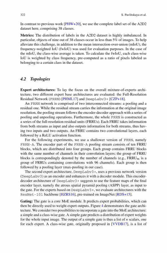
322 S. Pavlitskaya et al.

In contrast to previous work [PHW+20], we use the complete label set of the A2D2dataset here, comprising 38 classes.

Metrics: The distribution of labels in the A2D2 dataset is highly imbalanced. Inparticular, objects of nine out of 38 classes occur in less than 5% of images. To helpalleviate this challenge, in addition to the mean intersection-over-union (mIoU), thefrequency-weighted IoU (fwIoU) was used for evaluation purposes. In the case ofthe mIoU, the class-wise average is taken. To calculate the fwIoU, each class-wiseIoU is weighted by class frequency, pre-computed as a ratio of pixels labeled asbelonging to a certain class in the dataset.

4.2 Topologies

Expert architectures: To lay the focus on the overall mixture-of-experts archi-tecture, two different expert base architectures are evaluated: the Full-ResolutionResidual Network (FRRN) [PHML17] and DeepLabv3+ [CZP+18].

An FRRN network is comprised of two interconnected streams: a pooling and aresidual one. While the residual stream carries the information at the original imageresolution, the pooling stream follows the encoder-decoder approach with a series ofpooling and unpooling operations. Furthermore, the whole FRRN is constructed asa series of the full-resolution residual units (FRRUs). Each FRRU takes informationfrom both streams as input and also outputs information for both streams, thus hav-ing two inputs and two outputs. An FRRU contains two convolutional layers, eachfollowed by a ReLU activation function.

For the following experiments, we use a shallower version of FRRN, namelyFRRN-A. The encoder part of the FRRN-A pooling stream consists of ten FRRUblocks, which are distributed into four groups. Each group contains FRRU blockswith the same number of channels in their convolution layers; the group of FRRUblocks is correspondingly denoted by the number of channels (e.g., FRRU96 is agroup of FRRUs containing convolutions with 96 channels). Each group is thenfollowed by a pooling layer (max-pooling in our case).

The second expert architecture, DeepLabv3+, uses a previous network version(DeepLabv3) as an encoder and enhances it with a decoder module. This encoder-decoder architecture of DeepLabv3+ suggests to use the feature maps of the finalencoder layer, namely the atrous spatial pyramid pooling (ASPP) layer, as input tothe gate. For the experts based on DeepLabv3+, we evaluate architectures with theResNet-101 backbone [HZRS16], pre-trained on ImageNet [RDS+15].

Gating: The gate is a core MoE module. It predicts expert probabilities, which canthen be directly used to weight expert outputs. Figure 4 demonstrates the gate archi-tecture.We consider two possibilities to incorporate a gate into theMoE architecture:a simple and a class-wise gate. A simple gate predicts a distribution of expert weightsfor the whole input image. The output of a simple gate is thus a list of n scalars, onefor each expert. A class-wise gate, originally proposed in [VVDB17], is a list of

Evaluating Mixture-of-Experts Architectures for Network Aggregation 323

FC(128)Conv(3x3,1) + ReLU FC(2)Conv(3x3,1) + ReLU FC(128) Softmax

Fig. 4 Gate architecture. Gate input fexperts� is either the concatenation of feature maps fexpert1� and

fexpert2� (in case of MoE architecture from Fig. 2) or a single feature map fencoder� from the sharedencoder (in case of the MoE architecture from Fig. 3). Gate outputs wexpert1 and wexpert2 are thecorresponding expert weights

simple gates, one for each label. Each simple gate follows the same architecture asshown in Fig. 4. The output of a class-wise gate is thus a tensor of dimension n × m,where n is the number of experts and m is the number of classes. Via multiplicationwith the two-dimensional gate outputs, the expert outputs are therefore weighted ina class-wise manner. Overall, a simple gate learns to predict how much each expertcan be trusted for a specific input, whereas a class-wise gate learns to decide whichexpert is most suitable for each label given a specific input.

Moreover, we evaluate the addition of a further convolutional layer fconv� , followedby a ReLU activation function. fconv� is additionally inserted (see Figs. 2 and 3), suchthat the overall MoE output is then computed as follows:

y = FMoE(x) = σ(fconv� (yexpert1 · wexpert1 + yexpert2 · wexpert2)

). (6)

4.3 Training

Pipelines for training and evaluation are implemented in PyTorch [PGM+19].NVIDIA GeForce GTX 1080 Ti graphics cards are used for training and infer-ence. The MoE with separate feature extractors (as shown in Fig. 2) is trained in twostages. First, each expert is trained as a separate neural network on the correspondingdata subset. Then, the expert weights are frozen and the whole MoE architecture istrained end-to-end. In the case of a shared encoder architecture (as shown in Fig. 3),the expert networks are trained jointly at the first stage, whereas their encoder layersshare the parameters. Afterwards, the weights of the shared encoder and of the expertdecoders are frozen and the overall MoE is trained end-to-end. Each expert is trainedfor 50 epochs with a batch size of two. TheMoE is trained for 20 epochs with a batchsize of six. A smaller batch size is used for larger feature maps. SGD is used as anoptimizer for all models. The polynomial learning rate decay with an initial valueset to 0.01 is used.

324 S. Pavlitskaya et al.

5 Experimental Results and Discussion

In the following sections, we discuss our findings from the experiments regardingarchitectural choices, analyze the performance of the MoE model, and discuss itspotential as an interpretability approach.

5.1 Architectural Choices

Architectural choices reported in this section refer to Tables 1, and 2, 3 and have beenobtained on the test dataset. Note that a good generalization on unseen test data canonly be ensured if the respective ablation study is repeated on a separate validationdataset.

Expert feature extraction layer: For the FRRN-based architecture with separateencoders, which is shown in Fig. 2, we evaluate feature maps, extracted from thelast max-pooling layer in each FRRU block of the encoder. We additionally evaluatethe usage of input images directly as gate input as in the original MoE approach.Table 1 demonstrates the results for the MoE architecture with a simple gate withan extra convolutional layer. Using raw input data as gate input has led to betterresults only on the highway data, while achieving the worst results on the urban dataparts. Using the pooling layer of the last FRRU block as input, however, achievesthe highest mIoU values on the mixed dataset. A possible reason might be that theextracted high-level features from the later layers serve as a better representation ofthemore complex urban images. The feature resolution shrinks via a series of poolingoperations in the pooling stream, therefore the last FRRU blocks additionally lead toshorter training times. Since the best results on the mixed dataset were also achievedby a model with the second FRRU384 feature extraction layer, it was selected for allfurther experiments.

Gate architecture:To determine the best design choices for the gate architecture andwhether to add additional convolutional layers after the gate, we train and evaluate

Table 1 FRRN-based architecture: mIoU/fwIoU for different feature extraction layers. The resultsare for the simple gate architecture with the extra convolutional layer

Layer Feature mapsize

Highway Ambiguous Urban All

Input 640×480×3 0.449/0.949 0.396/0.939 0.395/0.806 0.412/0.890

FRRU96 240×320×16 0.342/0.938 0.419/0.936 0.479/0.861 0.478/0.911

FRRU192 120×160×16 0.342/0.938 0.420/0.938 0.480/0.861 0.479/0.911

FRRU384 60×80×16 0.346/0.940 0.420/0.938 0.480/0.861 0.480/0.912

2nd FRRU384 30×40×16 0.390/0.947 0.445/0.940 0.467/0.855 0.483/0.913

Evaluating Mixture-of-Experts Architectures for Network Aggregation 325

Table 2 FRRN-based architecture: mIoU/fwIoU for different gate architectures. The results are forthe second FRRU384 as a feature extraction layer

Gate Highway Ambiguous Urban All

Simple 0.349/0.938 0.418/0.937 0.473/0.859 0.475/0.910

Simple with conv. 0.390/0.947 0.445/0.940 0.467/0.855 0.483/0.913

Class-wise 0.373/0.942 0.443/0.939 0.472/0.861 0.475/0.913

Class-wise withconv.

0.366/0.939 0.408/0.938 0.482/0.863 0.483/0.912

Table 3 DeepLabv3+-based architecture: mIoU/fwIoU for different gate architectures

Gate Highway Ambiguous Urban All

Simple 0.405/0.956 0.349/0.942 0.334/0.854 0.345/0.917

Simple with conv. 0.415/0.955 0.339/0.942 0.342/0.854 0.358/0.917

Class-wise 0.399/0.953 0.360/0.943 0.314/0.849 0.333/0.914

Class-wise withconv.

0.404/0.954 0.369/0.942 0.333/0.853 0.351/0.916

MoE models with separate encoders (as shown in Fig. 2) for different combinationsof these features.

The analysis of the gate’s predictions has demonstrated that the simple gate tendsto select the correct expert for each data subset. As an example, the average expertweights as predicted by a simple gate for the DeepLabv3+-based architecture areas follows: 0.8 for the highway expert and 0.2 for the urban expert on the highwaydata subset, 0.04 for the highway expert and 0.96 for the urban expert on the urbandata subset, and 0.52 for the highway expert and 0.48 for the urban expert on theambiguous data.

The class-wise gate, however, predicts almost uniform weights for the majority ofclasses. Only a small overweight is assigned to the highway expert on the highwaydata and correspondingly to the urban expert on urban data. Classes for which theurban expert is assigned a significantly higher weight on all inputs are Signalcorpus, Sidewalk, Buildings, Curbstone, Nature object, and RDNormal Street. Moreover, we observed that the class-wise gate tends to predictthe same weights for all inputs.

Overall, the simple gate demonstrates much higher flexibility to input data, whichexplains the better results of the corresponding architectures (see Tables 2 and 3).Also, regardless of the gate architecture, an additional convolutional layer also leadsto higher mIoU values, because the overall model has a higher capacity. Both FRRN-and DeepLabv3+-based MoEs demonstrate the best performance for the simplegate with an additional convolutional layer after the gate.

326 S. Pavlitskaya et al.

5.2 MoE Performance

To compare the performance of the proposed MoE architecture with a baseline andwith further aggregation methods, we focus in the following experiments on theMoE with the separate feature encoders (as shown in Fig. 2), which uses the simplegate architecture, an additional convolutional layer and, in case of the FRRN-basedmodel, the second FRRU384 as its feature extraction layer. Our conclusions on theperformance of this model are also valid for almost all further architectural choices,presented in the previous subsection (cf. Tables 1, 2, and 3). Results discussed in thissection refer to Tables 4 and 5 and have been obtained on the test dataset.

MoE versus baseline versus experts: To ensure a proper basis for comparison, wetrain a baseline on a combined dataset of highway and urban data. Its architecture isidentical to that of an individual expert. Since the baseline was exposed to twice asmuch data as each expert, it outperforms the expert models that are trained on theirrespective data subset only. As expected, each of the experts demonstrates the bestresults on its corresponding data subset, whereas the urban expert shows a slightlybetter generalization due to a higher diversity of traffic scenes in its training data. Theperformance of the DeepLabv3+-based MoE with the separate feature encoders(as shown in Fig. 2) surpasses that of the baseline on the mixed dataset, whereas theFRRN-based MoE approaches the baseline.

MoE versus ensemble: We also evaluated an ensemble of experts as a concurrentaggregation approach. For this, the class-wise probabilities, predicted by the pre-trained experts, were combined using either by taking a mean or a maximum overthe experts. Both combination strategies consistently underperform compared to an

Table 4 FRRN-based architecture: mIoU/fwIoU for experts and the MoE. For the MoE, the resultsare shown for a simple gate with convolutional layer and second FRRU384 as its feature extractionlayer

Model\Dataset Highway Ambiguous Urban All

Baseline 0.425/0.946 0.415/0.940 0.458/0.859 0.475/0.914

Highway expert 0.498/0.952 0.298/0.919 0.149/0.616 0.227/0.820

Urban expert 0.323/0.934 0.407/0.936 0.476/0.859 0.472/0.908

MoE 0.390/0.947 0.445/0.940 0.467/0.855 0.483/0.913

Ensemble (mean) 0.453/0.949 0.399/0.938 0.382/0.819 0.417/0.900

Ensemble (max) 0.436/0.951 0.410/0.935 0.390/0.823 0.439/0.900

Highway expert(shared)

0.494/0.954 0.359/0.939 0.272/0.786 0.227/0.820

Urban expert(shared)

0.380/0.944 0.431/0.940 0.466/0.859 0.472/0.908

MoE (shared) 0.386/0.952 0.410/0.893 0.438/0.810 0.462/0.873

Evaluating Mixture-of-Experts Architectures for Network Aggregation 327

Table 5 DeepLabv3+ -based architecture: mIoU/fwIoU for experts and the MoE. For the MoE,the results refer to the simple gate with convolutional layer

Model\Dataset Highway Ambiguous Urban All

Baseline 0.421/0.956 0.364/0.944 0.302/0.841 0.321/0.913

Highway expert 0.405/0.955 0.252/0.928 0.098/0.607 0.154/0.821

Urban expert 0.334/0.942 0.353/0.941 0.334/0.854 0.333/0.912

MoE 0.415/0.955 0.339/0.942 0.342/0.854 0.358/0.917

Ensemble (mean) 0.372/0.953 0.320/0.942 0.235/0.802 0.266/0.897

Ensemble (max) 0.401/0.954 0.362/0.943 0.291/0.830 0.317/0.908

Highway expert(shared)

0.400/0.955 0.284/0.941 0.173/0.766 0.214/0.884

Urban expert(shared)

0.396/0.952 0.357/0.944 0.294/0.835 0.311/0.910

MoE (shared) 0.401/0.952 0.293/0.941 0.252/0.813 0.267/0.911

MoE with separate feature encoders on all data subsets, except for the FRRN-basedarchitecture on highway data. Moreover, of those two approaches, the combinationvia maximum has led to slightly better results.

MoE with a shared encoder: For the shared encoder architecture as shown inFig. 3, the differences in performance of experts are less drastic, whereas the MoEdemonstrates a slightly inferior mIoU when compared to an MoE with separateencoders. It seems as if the insufficient specialization of the experts negatively affectsthe performance of the MoE model. Although the shared encoder provides fasterinference, a further drawback of this approach is that joint training of both sharedexperts is muchmore time-consuming. This might limit the usage of the architecture,especially when a fast replacement of certain experts during inference is considered.

5.3 Disagreement Analysis

We compare pixel-wise predictions of each expert and of the overall MoE architec-ture. We report percentage of pixels belonging to each disagreement class in Tables 6and 7, using the test dataset. In both architectures, the experts and the overall MoEoutput the same predictions (perfect case) for the majority of pixels. Pixels belongingto the normal and critical cases take up to 5% of an image for highway and ambigu-ous data. For urban data, the MoE tends to rely heavily on the urban expert (up to27% of pixels), the urban expert is also more accurate on this data according to thereported mIoU and fwIoU.

328 S. Pavlitskaya et al.

Table 6 FRRN-based architecture: percentage of pixels, belonging to each disagreement case. Theresults refer to the architecture with an additional convolutional layer after the gate and secondFRRU384 as a feature extraction layer

Model Simple Class-wise

Highway Ambiguous Urban Highway Ambiguous Urban

Perfect case 97.00 95.84 70.76 96.93 95.84 70.74

Normalcase 1

0.63 0.40 0.55 0.59 0.40 0.64

Normalcase 2

2.14 3.51 27.87 2.18 3.51 27.70

Critical case 0.22 0.25 0.82 0.30 0.25 0.92

Table 7 DeepLabv3+ -based architecture: percentage of pixels, belonging to each disagreementcase. The results refer to the architecture with an additional convolutional layer after the gate

Gate Simple Class-wise

Highway Ambiguous Urban Highway Ambiguous Urban

Perfect case 97.53 96.67 72.94 97.52 96.54 72.92

Normalcase 1

2.02 1.34 0.39 1.62 1.17 1.12

Normalcase 2

0.28 1.78 25.98 0.61 1.91 24.94

Critical case 0.17 0.21 0.69 0.25 0.37 1.02

To facilitate visual analysis of the disagreement regions, we show a disagreementmask for each input (see Fig. 5). The perfect case pixels are left transparent, thenormal case pixels are colored green, and blue for the highway and urban expertscorrespondingly. The critical case pixels are highlighted in red. The visual analysisis consistent with the semantics of the objects in the scene. Regions mapped to thenormal case are those, which can confidently be segmented by the correspondingexpert, because they mostly occur in its training set and not in the training set of adifferent expert.

The critical cases are small image areas (up to 1% of pixels). Because we considerambiguous traffic scenes as out-of-distribution in our setting, they provide the mostinterestingmaterial for the visual analysis of the critical cases (see Fig. 6). The criticalcase areas are usually the overexposed, blurred, ambiguous, or hardly visible regionsof an image. Interestingly, sidewalk pixels are often classified as belonging to thecritical case in the ambiguous dataset.

Evaluating Mixture-of-Experts Architectures for Network Aggregation 329

Ground Truth MoE Prediction Disagreement MaskHighway

Urban

Ambiguous

Fig. 5 Disagreement masks and predictions. Perfect case pixels are shown as image pixels, normalcase pixels are highlighted green (agreement with the highway expert) or blue (agreement with theurban expert), and critical case pixels are highlighted red. The results are for the DeepLabv3+architecture with a simple gate and additional convolutional layer

Conclusions

Mixture of experts (MoE) is a network aggregation approach, which combines sim-plicity and intrinsic interpretability of ensembling methods with the possibility toconstruct more flexible models via the application of an additional gate module. Inthis chapter, we have studied how a mixture of experts can be used to aggregatedeep neural networks for semantic segmentation to increase performance and gainadditional interpretability.

Our experiments with two different expert architectures demonstrate that MoE isable to reach baseline performance and additionally reveal image regions, for whichthe model exhibits high uncertainty. In comparison to our previous experimentsin [PHW+20], the models were trained on a full A2D2 label set, which led not only

330 S. Pavlitskaya et al.

Ground Truth MoE Prediction Disagreement Mask

Fig. 6 Examples of disagreement masks with critical case from the ambiguous test set. Perfectcase pixels are shown as image pixels, normal case pixels are highlighted green (agreement withthe highway expert) or blue (agreement with the urban expert), and critical case pixels are high-lighted red. The results are for the DeepLabv3+ architecture with a simple gate and additionalconvolutional layer

to decreased performance on rare classes, as expected, but also to the increased occur-rence of disagreements between the overall architecture and the experts. Furthermore,we have evaluated the possibility to share the parameters of the feature extractionlayers of both experts. This leads to better cross-subset expert performance. How-ever, apparently the experts with a shared encoder are no longer specialized enoughwhich leads to a worseMoE performancewhen compared to anMoEwith standaloneexperts. Our evaluation has also shown that a mixture of experts, enhanced with agating network, beats a simple combination of experts via ensembling.

Evaluating Mixture-of-Experts Architectures for Network Aggregation 331

Further research directions might include conditional execution within an MoEmodel, combination of various modalities as inputs, as well as the perspective tofurther enhance the interpretability and robustness of the overall model.

Acknowledgements The research leading to these results is fundedby theGermanFederalMinistryfor Economic Affairs and Energy within the project “Methoden und Maßnahmen zur Absicherungvon KI-basierten Wahrnehmungsfunktionen für das automatisierte Fahren (KI Absicherung)”. Theauthors would like to thank the consortium for their successful cooperation.

References

[ABT16] K. Ahmed, M.H. Baig, L. Torresani, Network of experts for large-scale imagecategorization, in Proceedings of the European Conference on Computer Vision(ECCV) (Amsterdam, The Netherlands, 2016), pp. 516–532

[CZP+18] L-C. Chen, Y. Zhu, G. Papandreou, F. Schroff, H. Adam, Encoder-decoder withatrous separable convolution for semantic image segmentation, in Proceedings ofthe European Conference on Computer Vision (ECCV) (Munich, Germany, 2018),pp. 833–851

[ERS14] D. Eigen, M. Ranzato, I. Sutskever, Learning factored representations in a deepmixture of experts, in Proceedings of the International Conference on LearningRepresentations (ICLR) Workshops (Banff, AB, Canada, 2014), pp. 1–8

[FC19] S. Fang, A. Choromanska, Reconfigurable network for efficient inferencing inautonomous vehicles, in Proceedings of the IEEE International Conference onRobotics and Automation (ICRA) (Montréal, QC, Canada, 2019), pp. 1183–1189 ,pp. 1183–1189

[FC20] S. Fang, A. Choromanska, Multi-modal experts network for autonomous driving,in Proceedings of the IEEE International Conference on Robotics and Automation(ICRA), Virtual conference (2020), pp. 6439–6445

[GBM+16] Z. Ge, A. Bewley, C. McCool, P. Corke, B. Upcroft, C. Sanderson, Fine-grainedclassification via mixture of deep convolutional neural networks, in Proceedings ofthe Winter Conference on Applications of Computer Vision (WACV) (Lake Placid,NY, USA, 2016), pp. 1–6

[GKM+20] J. Geyer, Y. Kassahun, M. Mahmudi, X. Ricou, R. Durgesh, A.S. Chung, L.Hauswald, V.H. Pham,M.Mühlegg, S. Dorn, T. Fernandez, M. Jänicke, S. Mirashi,C. Savani, M. Sturm, O. Vorobiov, M. Oelker, S. Garreis, P. Schuberth, A2D2: AudiAutonomous Driving Dataset (2020), pp. 1–10. arXiv:2004.06320

[HZRS16] K. He, X. Zhang, S. Ren, J. Sun, Deep residual learning for image recognition, inProceedings of the IEEE/CVF Conference on Computer Vision and Pattern Recog-nition (CVPR) (Las Vegas, NV, USA, 2016), pp. 770–778

[JJNH91] R.A. Jacobs, M.I. Jordan, S.J. Nowlan, G.E. Hinton, Adaptive mixtures of localexperts. Neural Comput. 3(1), 79–87 (1991)

[KTS+14] A. Karpathy, G. Toderici, S. Shetty, T. Leung, R. Sukthankar, L.F. Fei, Large-scale video classification with convolutional neural networks, in Proceedings ofthe IEEE/CVF Conference on Computer Vision and Pattern Recognition (CVPR)(Columbus, OH, USA, 2014), pp. 1725–1732

[LD18] L. Liu, J. Deng, Dynamic deep neural networks: optimizing accuracy-efficiencytrade-offs by selective execution, in Proceedings of the AAAI Conference on Arti-ficial Intelligence (New Orleans, LA, USA, 2018), pp. 3675–3682

332 S. Pavlitskaya et al.

[LLX+21] D. Lepikhin, H. Lee, Y. Xu, D. Chen, O. Firat, Y. Huang, M. Krikun, N. Shazeer, Z.Chen, GShard: scaling giant models with conditional computation and automaticsharding, in Proceedings of the International Conference on Learning Representa-tions (ICLR), virtual conference (2021), pp 1–35

[LPB17] B. Lakshminarayanan,A. Pritzel, C. Blundell, Simple and scalable predictive uncer-tainty estimation using deep ensembles, inProceedings of the Conference onNeuralInformation Processing Systems (NIPS/NeurIPS) (Long Beach, CA, USA, 2017),pp. 6402–6413

[MEB16] O. Mees, A. Eitel, W. Burgard, Choosing smartly: adaptive multimodal fusion forobject detection in changing environments, in Proceedings of the IEEE/RSJ Inter-national Conference on Intelligent Robots and Systems (IROS) (IEEE, Daejeon,Korea, 2016), pp. 151–156

[PGM+19] A. Paszke, S. Gross, F. Massa, A. Lerer, J. Bradbury, G. Chanan, T. Killeen, Z. Lin,N. Gimelshein, L. Antiga, A. Desmaison, et al. PyTorch: an imperative style, high-performance deep learning library, in Proceedings of the Conference on NeuralInformation Processing Systems (NIPS/NeurIPS) (Vancouver, BC, Canada, 2019),pp. 8024–8035

[PHML17] T. Pohlen, A. Hermans, M.Mathias, B. Leibe, Full-resolution residual networks forsemantic segmentation in street scenes, inProceedings of the IEEE/CVFConferenceon Computer Vision and Pattern Recognition (CVPR) (Honolulu, HI, USA, 2017),pp. 4151–4160

[PHW+20] S. Pavlitskaya, C. Hubschneider, M.Weber, R.Moritz, F. Hüger, P. Schlicht, J. Mar-ius Zollner, Usingmixture of expertmodels to gain insights into semantic segmenta-tion, in Proceedings of the IEEE/CVF Conference on Computer Vision and PatternRecognition (CVPR), virtual conference (2020), pp. 1399–1406

[RDS+15] OlgaRussakovsky, JiaDeng, Su.Hao, JonathanKrause, SanjeevSatheesh, SeanMa,Zhiheng Huang, Andrej Karpathy, Aditya Khosla,Michael Bernstein, Alexander C.Berg, Li. Fei-Fei, ImageNet large scale visual recognition challenge. Int. J. Comput.Vis. (IJCV) 115(3), 211–252 (2015)

[SMM+17] N. Shazeer, A.Mirhoseini, K. Maziarz, A. Davis, Q. Le, G. Hinton, J. Dean, Out-rageously Large Neural Networks: The Sparsely-Gated Mixture-of-Experts Layer(2017), pp. 1–19. arXiv:1701.06538

[VDB16] A. Valada, A. Dhall, W. Burgard, Convoluted mixture of deep experts for robustsemantic segmentation, in Proceedings of the IEEE/RSJ International Conferenceon Intelligent Robots and Systems (IROS) Workshops (Daejeon, Korea, 2016), pp.1–2

[VVDB17] A. Valada, J. Vertens, A. Dhall,W. Burgard, AdapNet: adaptive semantic segmenta-tion in adverse environmental conditions, in Proceedings of the IEEE InternationalConference on Robotics and Automation (ICRA) (Singapore, Singapore, 2017), pp.4644–4651

[WYD+19] X. Wang, F. Yu, L. Dunlap, Y-A. Ma, R. Wang, A. Mirhoseini, T. Darrell, J.E.Gonzalez, Deep mixture of experts via shallow embedding, in Proceedings of theConference on Uncertainty in Artificial Intelligence (UAI) (Tel Aviv, Isreal, 2019),pp. 552–562

Evaluating Mixture-of-Experts Architectures for Network Aggregation 333

Open Access This chapter is licensed under the terms of the Creative Commons Attribution 4.0International License (http://creativecommons.org/licenses/by/4.0/), which permits use, sharing,adaptation, distribution and reproduction in any medium or format, as long as you give appropriatecredit to the original author(s) and the source, provide a link to the Creative Commons license andindicate if changes were made.

The images or other third party material in this chapter are included in the chapter’s CreativeCommons license, unless indicated otherwise in a credit line to the material. If material is notincluded in the chapter’s Creative Commons license and your intended use is not permitted bystatutory regulation or exceeds the permitted use, you will need to obtain permission directly fromthe copyright holder.

Safety Assurance of Machine Learningfor Perception Functions

Simon Burton, Christian Hellert, Fabian Hüger, Michael Mock,and Andreas Rohatschek

Abstract The latest generation of safety standards applicable to automated driv-ing systems require both qualitative and quantitative safety acceptance criteria to bedefined and argued. At the same time, the use of machine learning (ML) functions isincreasingly seen as a prerequisite to achieving the necessary levels of perception per-formance in the complex operating environments of these functions. This inevitablyleads to the question of which supporting evidence must be presented to demonstratethe safety of ML-based automated driving systems. This chapter discusses the chal-lenge of deriving suitable acceptance criteria for the ML function and describes howsuch evidence can be structured in order to support a convincing safety assurancecase for the system. In particular, we show how a combination of methods can beused to estimate the overall machine learning performance, as well as to evaluate andreduce the impact of ML-specific insufficiencies, both during design and operation.

S. BurtonFraunhofer Institute for Cognitive Systems IKS, Hansastraße 32, 80686 Munich, Germanye-mail: simon.burton@iks.fraunhofer.de

C. HellertContinental AG, Bessie-Coleman-Str. 7, 60549 Frankfurt am Main, Germanye-mail: christian.hellert@continental.com

F. HügerVolkswagen AG, Berliner Ring 2, 38440 Wolfsburg, Germanye-mail: fabian.hueger@volkswagen.de

M. MockFraunhofer Institute for Intelligent Analysis and Information Systems IAIS, SchlossBirlinghoven 1, 53757 Sankt Augustin, Germanye-mail: michael.mock@iais.fraunhofer.de

A. Rohatschek (B)Robert Bosch GmbH, Robert-Bosch-Campus 1, 71272 Renningen, Germanye-mail: andreas-juergen.rohatschek@de.bosch.com

© The Author(s) 2022T. Fingscheidt et al. (eds.), Deep Neural Networks and Data for Automated Driving,https://doi.org/10.1007/978-3-031-01233-4_12

335

336 S. Burton et al.

1 Introduction

The objective of systems safety engineering is to avoid unreasonable risk of hazardsthat could lead to harm to the users of the system or its environment. The definitionof an unreasonable level of risk must be determined for the specific system context inaccordance with societal moral concepts and legal considerations regarding productliability. This requires a careful evaluation of the causes and impact of system failures,an evaluation of the probability of their occurrence, and the definition of strategies toeliminate or reduce the residual risk associatedwith such failures. Current automotivesafety standards, such as ISO 26262 [ISO18] and ISO/DIS 21448 [ISO21], requirea safety case to be developed for safety-related functions that forms a structuredargument supported by systematically collected evidence that the appropriate levelof residual risk has been achieved. The term “evidence” refers to work productscreated during the development, test, and operation of the system that support theclaim that the system meets its safety goals.

In comparison to previous generations of vehicle systems, automated driving sys-tems (ADS) that make use of machine learning (ML) introduce significant new chal-lenges to the safety assurance process. Deep neural networks (DNNs), in particular,are seen as an enabling technology forADSperception functions due to their ability todistinguish features within complex, unstructured data. This allows for the develop-ment of functions, such as pedestrian detection within crowded, urban environmentsthat previously could not be specified and implemented based on algorithmic defini-tions. Paradoxically, this leads to one of themain challenges associatedwith the use ofmachine learning in safety-critical systems. The semantic gap [BHL+20] describesthe challenge of deriving complete and consistent technical (safety) requirementson the system that fulfil potentially only implicitly understood, societal and legalexpectations. The semantic gap is exacerbated in ML-based ADS due to the unpre-dictability and complexity of the operational domain and the reliance on properties ofthe training data rather than detailed specifications to derive an adequate approxima-tion of the target function. The semantic gap can in turn lead to an unclear definitionof the moral responsibility and legal liability for the system’s actions as well as anincomplete assurance argument that the (potentially incompletely defined) safetygoals for the system are met.

Furthermore, deep learning approaches have specific properties that limit theeffectiveness of established safety measures for software. These include the inherentuncertainty in the outputs of theMLfunction, the opaquemanner inwhich features arelearnt by the function which is often not understandable by humans and the difficultyof extrapolating from test results due to non-linear behaviour of the function andsensitivity to small changes in the input domain. Previous work related to the safetyassurance of machine learning has mainly focused on the structure of the assurancecase and associated processes with respect to existing safety standards [BGH17,SQC17, GHP+20, ACP21, BKS+21]. Other work has focused on the effectivenessof specificmetrics andmeasures on providingmeaningful statements related to safetyproperties of theML function [CNH+18, HSRW20, SKR+21, CKL21]. This chapter

Safety Assurance of Machine Learning for Perception Functions 337

complements this work by examining in more detail the role of combining varioustypes of evidence to form a convincing argument that quantitative acceptance criteriaas required by standards such as ISO 21448 are met.

This chapter discusses the challenge of deriving suitable acceptance criteria forML functions and describes how supporting evidence can be combined to providea convincing safety assurance case for the system. The aggregation of evidencecan be structured as an overall evidence-based safety argumentation as depicted in[MSB+21]. In the following section, we describe the challenge of deriving a set oftechnical safety requirements and associated acceptance criteria on ML functions.In Sect. 3, we provide a categorisation of safety evidence for machine learning andargue that an assurance case requires an appropriate combination of complementaryevidence. Section4 describes a collaborative approach between domain and safetyexperts for collecting and evaluating the safety evidence. Sections5.1–5.4 providespecific examples of each category of evidence and describe the conditions underwhich they can provide a meaningful contribution to the assurance case. Section6then demonstrates how the evidence can be combined into an overall assurance casestructure. The chapter concludes with a summary of open research questions and anoutlook for future work.

2 Deriving Acceptance Criteria for ML Functions

This section presents approaches to risk evaluation within the safety standards anddiscusses how safety acceptance criteria for ML functions can be derived in line withthese approaches.

2.1 Definition of Risk According to Current Safety Standards

Current standards related to the safety of vehicle systems provide little specific guid-ance related to the use of ML. Therefore, the approach described in this chapter willbe based upon an interpretation and transfer of the principles of ISO 26262, ISO/DIS21448, and ISO/TR4804 to the specific task of safety assurance formachine learning-based systems. ISO 26262 defines functional safety as the absence of unreasonablerisk due to hazards caused by malfunctioning behaviour of electrical/electronic sys-tems. Malfunctioning behaviour is typically interpreted as either random hardwarefaults or systematic errors in the system, hardware, or software design. ISO 26262applies a predominantly qualitative approach to arguing the safety of software. Safetygoals for a system are derived according to a hazard and risk analysis that evaluatesthe risk associated with each hazard according to qualitative criteria with various cat-egories for the risk parameters: severity, exposure, and controllability. The standardprovides a method for combining these parameters to derive an overall “Automo-tive Safety Integrity Level” (ASIL) within a range of A to D in order of increasing

338 S. Burton et al.

risk. Functions with no safety impact are assigned the level “QM” (only standardquality management approaches are necessary). An ASIL is allocated to each safetygoal derived from the hazards and to the functional and technical safety requirementsderived from these until eventually software-level requirements, including associatedASILs, are determined. The standard then provides guidance on which measures toapply, depending on ASIL, to achieve a tolerable level of residual risk. By doingso, the standard avoids the need to define specific failure rates to be achieved bysoftware but instead defines desirable properties (such as freedom from run-timeerrors caused by pointer mismatches, division-by-zero, etc.) and methods suited toensuring or evaluating these properties (e.g. static analysis).

ISO/DIS 21448 addresses safety in terms of the absence of unreasonable risk dueto functional insufficiencies of the system or by reasonably foreseeable misuse. Inthe context of ADS, this translates to a possible inability of a function to correctlycomprehend the situation and operate safely, e.g. due to a lack of robustness regardinginput variations or diverse environmental conditions. The risk model described byISO/DIS 21448 can be summarised as identifying as many known, unsafe scenarios(where performance insufficiencies could lead to hazards) as possible so that miti-gating measures can be applied, thus transforming them to known, safe scenarios. Inaddition, the number of residual unknown, unsafe scenarios should be minimised byincreasing the level of understanding of properties of the environment that could trig-ger performance deficiencies. The definition of safety of the intended functionality(SOTIF), therefore, seems well suited for arguing the performance of the trainedMLfunction over all possible scenarios within the operating domain. ISO/DIS 21448follows a similar process to identify hazards, associated safety goals, and require-ments as ISO 26262. However, instead of using risk categories according to ASILs,the standard requires the definition of quantitative acceptance criteria (also knownas validation targets) for each hazard, which in turn can be allocated to subsystemssuch as perception functions. However, these acceptance criteria are not described inmore detail and must, therefore, be defined according to the specific system context.

ISO/TR 4804 contains a set of guidelines for achieving the safety of automateddriving systemswith a focus on the Society of Automotive Engineers (SAE) levels 3–5 [SAE18]. ISO/TR 4804 defines safety acceptance criteria both in terms of a positiverisk balance (the system shall be demonstrably safer than an average human driver)as well as the avoidance of unreasonable risk. In doing so, the standard recommendsa combination of both qualitative and quantitative arguments. A similar philosophyis followed within this chapter when identifying and combining evidence for thesafety of a machine learning function.

Safety Assurance of Machine Learning for Perception Functions 339

2.2 Definition of Safety Acceptance Criteria for the MLFunction

In order to address the semantic gap described above, a systematic method of deriv-ing a set of technical safety requirements on an ML function is needed. This shouldinclude an iterative and data-driven approach to analyse the societal and legal expec-tations, operating domain, and required performance on the ML function within thetechnical system context (see Fig. 1). In this chapter, we focus on steps 4 and 5, inparticular, the systematic collection of evidence regarding the performance of anMLfunction to support a system-level assurance case.

In [BGH17], the authors recommend a contract-based design approach to derivespecific safety requirements for the machine learning function. These requirementsare expressed in the form of a set of safety guarantees that the function must ful-fil and a set of assumptions which can be made in the system’s environmental andtechnical context. This allows for a compositional approach to reasoning about thesafety of the system where the guarantees of one function can be used to justify theassumptions on the inputs of another. This requires a suitable definition of safetyat the level of abstraction of the ML function. For example, a superficially definedrequirement, such as “detect a pedestrian on the road”, would need to be refinedto define which characteristics constitute a pedestrian and from which distance andlevel of occlusion pedestrians should be detected. This process of requirements elic-itation should include the consideration of a number of stakeholder perspectives andsources of data. This could include current accident statistics and the considerationof ethical guidelines for AI as proposed by the European Commission [Ind19]. It isto be expected that for any particular automated driving function, a number of suchcontracts would be derived to define different properties of the ML function relatedto various safety goals, where each contract may also be associated with differentquantitative acceptance criteria and sets of scenarios in the operating domain.

Fig. 1 Iterative steps during the systems engineering process to bridge the semantic gap associatedwith the definition of technical safety requirements on ML functions

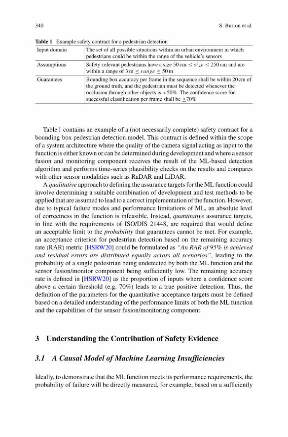
340 S. Burton et al.

Table 1 Example safety contract for a pedestrian detection

Input domain The set of all possible situations within an urban environment in whichpedestrians could be within the range of the vehicle’s sensors

Assumptions Safety-relevant pedestrians have a size 50 cm ≤ si ze ≤ 250 cm and arewithin a range of 3m ≤ range ≤ 50m

Guarantees Bounding box accuracy per frame in the sequence shall be within 20cm ofthe ground truth, and the pedestrian must be detected whenever theocclusion through other objects is <50%. The confidence score forsuccessful classification per frame shall be ≥70%

Table1 contains an example of a (not necessarily complete) safety contract for abounding-box pedestrian detection model. This contract is defined within the scopeof a system architecture where the quality of the camera signal acting as input to thefunction is either knownor can be determined during development andwhere a sensorfusion and monitoring component receives the result of the ML-based detectionalgorithm and performs time-series plausibility checks on the results and compareswith other sensor modalities such as RaDAR and LiDAR.

A qualitative approach to defining the assurance targets for theML function couldinvolve determining a suitable combination of development and test methods to beapplied that are assumed to lead to a correct implementation of the function.However,due to typical failure modes and performance limitations of ML, an absolute levelof correctness in the function is infeasible. Instead, quantitative assurance targets,in line with the requirements of ISO/DIS 21448, are required that would definean acceptable limit to the probability that guarantees cannot be met. For example,an acceptance criterion for pedestrian detection based on the remaining accuracyrate (RAR) metric [HSRW20] could be formulated as “An RAR of 95% is achievedand residual errors are distributed equally across all scenarios”, leading to theprobability of a single pedestrian being undetected by both the ML function and thesensor fusion/monitor component being sufficiently low. The remaining accuracyrate is defined in [HSRW20] as the proportion of inputs where a confidence scoreabove a certain threshold (e.g. 70%) leads to a true positive detection. Thus, thedefinition of the parameters for the quantitative acceptance targets must be definedbased on a detailed understanding of the performance limits of both the ML functionand the capabilities of the sensor fusion/monitoring component.

3 Understanding the Contribution of Safety Evidence

3.1 A Causal Model of Machine Learning Insufficiencies

Ideally, to demonstrate that theML function meets its performance requirements, theprobability of failure will be directly measured, for example, based on a sufficiently

Safety Assurance of Machine Learning for Perception Functions 341

Fig. 2 Causal model of ML-related SOTIF risks demonstrating the relationships between systemfailures, machine learning insufficiencies, their causes, and exacerbating factors as well as the roleof control measures to minimise the probability of hazardous system failures

large number of representative tests.However, this approach is feasible only for trivialexamples. Therefore, multiple sources of evidence are required to reason about thepresence of performance limitations and the ability of the system to detect and controlsuch failures during operation.

The dependability model of Avizienis et al. [ALRL04] forms the foundation ofmany safety analysis techniques. In this model, the risk of a system violating itsobjectives is determined by analysing the propagation path from causes of individualfaults in the system that could lead to an erroneous system state which in turn leadsto a failure to maintain the system’s objectives. Risk can thus be controlled by eithereliminating the causes of faults or by preventing them from leading to potentiallyhazardous erroneous states of the system.

Figure2 summarises how this approach to causal analysis can be applied to theproblem of determining the safety-related performance of an ML function and isinspired by the safer complex systems framework presented in [BMGW21]. A sys-tem failure can be defined as a condition where the safety contract as defined inTable1 is not met. An erroneous state leading to such a failure would relate to thepresence of insufficiencies in the machine learning function which, in turn, couldbe caused by either faults in its execution or limitations in the training data. Exam-ples for the latter are scalable oversight [AOS+16], uncertainty in the input domain,such as distributional shift [AOS+16], or the inherent inability of the ML approachto accurately represent the target function. Measures to improve the safety of thefunction can be categorised into those applied during design time to reduce the prob-ability of insufficiencies in the trained model and those applied during operation inorder to reduce the impact of residual insufficiencies. Both types of controls maybe undermined by exacerbating factors specific to the system context, for example,the difficulty in collecting balanced and sufficiently complete training data due tothe scarcity of critical scenarios or the difficulty of developing effective monitor-ing approaches due to the need for safe-operational fallback concepts. This modelof causality for ML-related safety of the intended functionality (SOTIF) risks is

342 S. Burton et al.

now used to determine the following contributions of safety evidence that will beillustrated in the next subsection.

3.2 Categories of Safety Evidence

Based on the causalmodel of SOTIF-related risk introduced above, the following fourcategories of evidence can now be defined. This category of evidence corresponds todevelopment work products and results of verification and validation activities thatsupport the argument of an acceptably low level of residual risk associated with MLinsufficiencies:

(1) Confirmation of residual failure rates: This category of evidence provides adirect estimate of the performance of the machine-learning component, e.g. in termsof false negative rates, or the intersection-over-union (IoU) related to bounding boxaccuracy. However, due to non-linear behaviour in the function and the limited num-ber of samples that can be realistically tested, such evidence is unlikely to provide astatistically relevant estimation. This category of evidencemust, therefore, be used incombinationwith othermeasures that increase confidence in the ability to extrapolatethe results to the entire input space that fulfils the contract’s assumptions.

(2) Evaluation of insufficiencies: This category of evidence is used to directlyindicate the presence or absence of specific ML insufficiencies that could not onlylead to a violation of the safety contract, but could also undermine confidence inthe category 1 evidence. The properties that would be evaluated by this category ofevidence would include prediction uncertainty, generalisation, brittleness, fairness,and explainability.

(3) Evaluation of the effectiveness of design-time controls: This category ofevidence is used to argue the effectiveness of design-time measures to increase theperformance of the function or to reduce the presence of insufficiencies. In manycases, a direct correlation between the design-time measures and the performance ofthe function may not be measured, leading to qualitative arguments for the effective-ness of the measures. However, metrics can be used to measure the level of rigourby which the measures have been applied. These could include properties of trainingdata and test data, or measures to increase the explainability of the trained model.

(4) Evaluation of the effectiveness of operation-time controls: This category ofevidence is used to demonstrate the effectiveness of operation-timemeasures to eitherincrease the performance of the function or to reduce the impact of insufficiencies.Examples of such could be a measurement of the effectiveness of out-of-distributiondetection to identify inputs that are outside of the training distribution (and beyondthe assumptions of the safety contract) such that they can be discarded.

In the following sections, we illustrate each category with specific examples andevaluate the conditions under which the evidence can provide a significant contribu-tion to the assurance case.

Safety Assurance of Machine Learning for Perception Functions 343

4 Evidence Workstreams—Empowering Expertsfrom Safety Engineering and ML to Produce Measuresand Evidence

In order to identify, develop, and evaluate effective evidence related to the vari-ous categories defined above, we propose to follow the procedure of so-called evi-dence workstreams: experts frommachine learning, safety, testing, and data workingtogether according to the procedure depicted in Fig. 3. The main purpose of the pro-cess is to help demonstrate the effectiveness of the methods, metrics, and measuresto be applied more generally. Related processes are also found in current literature.Picardi et al. [PPH+20] propose an engineering process to generate evidence at eachstage of the ML life cycle. Apart from the process in general, different patterns aredescribed that can be instantiated during theML life cycle. Furthermore, a three-layerprocess model is described by McDermid and Jia [MJ21], featuring a collaborativemodel to bring together the expertise from the ML and safety domain to generateevidence for the assurance case. In this work, there are some case studies, but detailedsteps for the process are missing.

The evidence workstreams proposed in this chapter enable a joint cooperation ofdifferent competencies and bring together new innovative methods and structuredapproaches rather than having separate work on each topic. An important key to thesuccessful creation of an assurance case is the continuous interaction of the differentcontributors. Before explaining the procedure, we, therefore, define four roles for thecontributors:

• The method developer is responsible to implement measures that mitigate spe-cific insufficiencies of an ML component. In addition, this role specifies data

StartMaintenance of

measure catalogueSelect prioritised measures

for each insufficiency

Design and implementeffectiveness tests

Determine othercriteria for evaluation

Implementprioritised measures

Evaluation andcomparison of measures

Measures effective?

Add measures tosystem development

Add test results asevidence to assurance case

Combine or picknew measures?

Combine different measures

Pick new measuresfrom catalogue

End

yes

no

combine

pick

Fig. 3 Flowchart of the evidence workstream process

344 S. Burton et al.

requirements for the implemented measures and defines metrics for evaluating theeffectiveness of the measure.

• Apart from the method developer specifying data requirements, a data engineeris responsible for creating and managing the dataset throughout the developmentprocess as well as performing data analyses to estimate the data coverage.

• In order to test the effectiveness of the measures, the test engineer develops testspecifications including required test data and metrics. These tests should thenbe performed by the method developer to demonstrate the effectiveness of themethod.

• Finally, the safety engineer ensures that the developed measures and respectivetest results are valid and generate the evidence for the assurance case.

The process starts by creating and maintaining a catalogue of potential design-timeand run-time measures to mitigate identified insufficiencies, which can be knowna priori (see Sect. 5.2) or identified during the development phase. Here, methoddevelopers and safety engineers are involved in the maintenance and also performa prioritisation of measures for each insufficiency. After the selection of measures,the test engineer designs and implements effectiveness tests. Furthermore, safety-aware metrics for the test are defined by the method developer and safety engineer,in addition to other criteria for the evaluation. Importantly, the data engineer needsto evaluate the database in order to allow for a statistical significance analysis for thedesigned tests. Afterwards, the prioritised measures are implemented following anevaluation and comparison according to the specified tests. Once the measures showsufficient effectiveness, they can be added to the system development and the safetyengineer can use the test results as evidence for the assurance case. If a measure wasnot effective, then we propose the two following options:

• Firstly, measures can be combined and optimised to increase the effectiveness.After combination, a re-evaluation is performed.

• Secondly, new measures can be picked from the catalogue and the test design andimplementation step is repeated.

Additionally, an iteration of the safety requirement derivation and system archi-tecture design process could lead to recommendations for additional components oradjusted specifications in order to mitigate remaining insufficiencies.

5 Examples for Evidence

This section discusses examples for the different categories of safety evidence intro-duced in Sect. 3.2, which can be obtained by the process introduced in Sect. 4.

Safety Assurance of Machine Learning for Perception Functions 345

5.1 Evidence from Confirmation of Residual Failure Rates

The quantification of model performance or residual failure rates of a machinelearning (ML) component is a crucial step in any ML-based system, especially forsafety-critical applications. Typically, the performance of ML components is mea-sured by metrics that calculate a mean performance over a specific test dataset.In [PNdS20] and [PPD+21], commonly used metrics for object detection are com-pared, including mean average precision (mAP) and mean intersection-over-union(mIoU). However, for safety-critical systems, only evaluating the mean performanceis not sufficient. On the one hand, there are unknown risks introduced by residualfailure rates, on the other hand, failures are not weighted by their relevance. Tocounteract this, for example, in [HSRW20], safety-aware metrics are proposed inthe literature to incorporate uncertainty to evaluate the remaining accuracy rate andremaining error rate. In [CKL21], safety-aware metrics for semantic segmentationare proposed, putting emphasis on perturbation and relevance.Volk et al. [VGvBB20]propose a safety metric that incorporates object velocity, orientation, distance, size,and a damage potential. Furthermore, ISO/TR 4804 [ISO20] proposes a generic con-cept, whereby safety-aware metrics need to be evaluated for perception componentsrealised with deep neural networks. In addition, it should be noted that the valid-ity of metrics depends strongly on the utilised dataset. In general, the creation ofsafety-aware metrics is still an open field in the domain of automated driving and forperception components in particular. Based on the references and insights above, thefollowing considerations should be taken into account to use performance metricsas evidence:

• Mean performance metrics should be evaluated within a specified input space.• Statistical significance of the metrics value should be evaluated and shown bymeasuring dataset coverage.

• The failure rate related to specific classes of errors should be evaluated, includingan analysis of their causes.

The evidence for performance or accuracy evaluation could be in the form of a testreport, where the specification of the input space and the data coverage evaluationis defined. Apart from detection or classification accuracy, localisation precision isalso an important factor and is often dependent on the accuracy. In addition to asummary of the safety-aware metrics, an analysis of various classes of errors, theirpotential causes and impact within the system should be included in the test report,allowing for a systematic evaluation of the residual risk associated with the functionat a system level.

The following example provides an intuition of conditions that have to be met sothat a performance metric can be used as evidence convincingly. The basis of nearlyevery performance metric is the calculation of the confusion matrix, containing thenumber of true positives (TP), false positives (FP), false negatives (FN), and truenegatives (TN) rates. Here, we consider the case of a 2D bounding box pedestriandetection on images for automated driving. In this case, the number of TNs is not

346 S. Burton et al.

reasonable since there will be a nearly infinite amount of those bounding boxes. Inorder to compute the confusion matrix, the intersection-over-union (IoU) metric istypically used to determine if a detection can be considered as a TP, FP, or FN byusing a threshold. This threshold, on the one hand, defines the localisation error perobject which must not be exceeded for the detection to be counted as TP, and, on theother hand, also influences the mean accuracy on a test dataset. Therefore, in the testreport, there should be an argument about why a certain threshold has been chosen.Furthermore, typically FP and FN are weighted equally, but for a safety analysis,FN might be more important and not all FN might be relevant. Hence, the test reportshould define relevant FN or FP based on the system architecture and assignedcomponent requirements by introducing specific weights. Of course, performancemetrics alone cannot give enough evidence to argue the safety of a perception systemfor automated driving. In addition, the performance needs to be evaluated in case ofrarely occurring situations, and also the robustness against perturbations needs to beconsidered.

5.2 Evidence from Evaluation of Insufficiencies

An essential feature in the development of deep neural networks during traininglies in the purely data-driven parameter fitting process without expert intervention:The deviation of the output (for a given parameterisation) of a neural network froma ground truth is measured. The loss function is chosen in such a way that theparameters depend on it in a differentiable way. As part of the gradient descentalgorithm, the parameters of the network are adjusted in each training step dependingon the derivative of the deviation (backpropagation). These training steps are repeateduntil some stopping criterion is satisfied. In this procedure, the model parameters aredetermined without an expert assessment or semantically motivated modelling. Thishas significant consequences for the properties of the neural network:

• Deepneural networks (DNNs) are largely opaque for humans and their calculationscannot be interpreted. This represents a massive limitation for systematic testingor formal verification.

• Deep neural networks are susceptible to harmful interference: Perturbations couldbe manually induced changes in the data (adversarial examples) or real-word cor-ruptions (e.g. sensor noise, weather influences, certain colours, or contrasts bysensor degeneration).

• It is unclear to which input characteristics an algorithm sensitises. The executionof neural networks in another domain (training in summer, execution in winter,etc.) sometimes reduces the functional quality dramatically.

This leads to DNN-specific insufficiencies and safety concerns as described in detailby Willers et al. [WSRA20], Sämann et al. [SSH20], and Schwalbe et al. [SKS+20].In our evidence strategy, we utilise metrics to evaluate the insufficiencies and usespecific values and justified bounds as specific evidence. In the following, this proce-

Safety Assurance of Machine Learning for Perception Functions 347

Augmented Image Baseline Segmentation Defended Segmentation

Fig. 4 Visualisation of the robustness of a semantic segmentation model: Rain augmentation viaHendryck’s augmentations [HD19] on Cityscapes [COR+16] (left), baseline performance on thecorrupted image (middle) and performance of a robustifiedmodel viaAugMixwith Jensen–Shannondivergence (JSD) loss [HMC+20] (right)

dure is shortly explained for the example of brittleness of DNNs. The strategies forthe other insufficiencies follow basically the same pattern, but the elaboration wouldgo beyond the scope of this chapter.

Measuring robustness of deep neural networks (DNNs): Regarding brittleness,the specific evidence that we want to define are test results achieving the requiredperformance even under reasonable perturbations. If the required performance isachieved for all required conditions, we call the DNN “robust”. To evaluate therobustness with respect to real-world corruptions, we suggest to use both, recordedand tagged real-word effects as well as augmented perturbations such as noise, blur,colour shift, etc., via Hendryck’s augmentations [HD19] as depicted in Fig. 4. Therequired parameters for the test conditions are extracted from operational designdomain (ODD), sensor, and data analysis.

5.3 Evidence from Design-Time Controls

Design-time controls systematically complement and integrate evidence gained viaoverall performance considerations or regarding specific insufficiencies. The majorgoal is to integrate the various aspects and metrics that have to be considered intoa holistic view, allowing the AI developer, firstly to incorporate measures that areoverall effective, such as architectural choices, and parameter optimisations, or datacoverage measures, and secondly, to handle potential trade-offs between differentoptimisation targets and requirements. It is important to note that the design-timecontrols are to be applied in an iterative workflow during development, aiming toprovide sufficient evidence for the overall safety argumentation. As a specific exam-ple of a design-time control, we sketch how developers and safety engineers can besupported by a visual analytics tool during the design and development phase.

Understanding DNN predictions via visual analytics: An important contributionto a complete safety argumentation can be made via methods that support humansin understanding and analysing why an AI system is coming to a specific decision.Insights into the inner operations of a DNN can increase trust into the entire applica-tion of that neural network. However, in a safety argumentation, it is not sufficient to

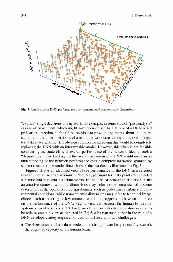
348 S. Burton et al.

Fig. 5 Landscape of DNN performance over semantic and non-semantic dimensions

“explain” single decisions of a network, for example, in some kind of “post analysis”in case of an accident, which might have been caused by a failure of a DNN-basedpedestrian detection, it should be possible to provide arguments about the under-standing of the inner operations of a neural network considering a huge set of inputtest data at design time. The obvious solution for achieving this would be completelyreplacing the DNN with an interpretable model. However, this often is not feasibleconsidering the trade-off with overall performance of the network. Ideally, such a“design-time understanding” of the overall behaviour of a DNN would result in anunderstanding of the network performance over a complete landscape spanned bysemantic and non-semantic dimensions of the test data as illustrated in Fig. 5.

Figure5 shows an idealised view of the performance of the DNN in a selectedrelevant metric, see explanations in Sect. 5.1, per input test data point over selectedsemantic and non-semantic dimensions. In the case of pedestrian detection in theautomotive context, semantic dimensions may refer to the semantics of a scenedescription in the operational design domain, such as pedestrian attributes or envi-ronmental conditions, while non-semantic dimensions may refer to technical imageeffects, such as blurring or low contrast, which are supposed to have an influenceon the performance of the DNN. Such a view can support the human to identifysystematic weaknesses of a DNN in terms of human-understandable dimensions. Tobe able to create a view as depicted in Fig. 5, a human user, either in the role of aDNN developer, safety engineer, or auditor, is faced with two challenges:

• The sheer amount of test data needed to reach significant insights usually exceedsthe cognitive capacity of the human brain.

Safety Assurance of Machine Learning for Perception Functions 349

• Finding and selecting the relevant dimensions that actually influence the networkperformance among all possible dimensions is far from being trivial, especiallytaking into account that the performance of a DNNmostly depends on a combina-tion of different dimensions and usually cannot be explained by considering onedimension alone.

In order to overcome these two challenges, tool support is needed. In [SMHA21],an approach is described to support the human user in finding and evaluatingmachinelearning models by means of visual analytics. In this approach, tool support is pro-vided to enable the user to perform visual analyses over huge amounts of data in suchaway that a quick and intuitive understanding of the nature of the underlying data andnetwork performance can be gained. Such an initial understanding usually enablesthe user to create hypotheses about the relevance of semantic and non-semanticdimensions, which then can be checked or refined interactively. Human understand-ing about semantics helps in a semantic understanding of the DNN in an iterativeprocess.

Figures6 and 7 show a snapshot of the visual analytics tool being used to inves-tigate the performance of a DNN for pedestrian detection based on a semantic seg-mentation of images. The so-called metadata that indicates the values regarding aspecific dimension of an input image (such as number of pedestrians, brightness ofthe image, and overall detection performance in the image) and the values regard-ing specific pedestrians in the image (such as size, position in the image, detectionperformance for this pedestrian) is listed in a tabular interface as illustrated in Fig. 6.The user can issue arbitrary queries against this table to select interesting subsets ofthe data. The plots shown in Fig. 7 give an additional overview of various attributes.Selected images, predictions, or ground truth can be visualised as shown in Fig. 9.

Figure8 shows an exemplary scatterplot of the pixel size of a pedestrian in animage versus the detection performance measured in IoU (intersection-over-union)for this pedestrian. The goal is to find out whether certain aspects, such as pixel sizeof the pedestrian in the image, have an effect on the detection performance of theunderlying DNN. It can be seen that there is a general tendency for pedestrians withlarger height (more to the left) to achieve higher (better) detection performance.How-ever, there exist some large pedestrians with relatively low detection performance(as highlighted by the selection box in Fig. 8). The visual analytics tool allows forinteractively selecting such sets of interesting points from a plot for further analysisjust by drawing a selection box around the points of interest. Selected images willthen be visualised in the drill down view of the tool shown in Fig. 9. In this particularexample, some of the selected images were showing “pedestrians” riding bicyclesas depicted in Fig. 9b). The human analyst could now use the visual analytics tool tofurther investigate the hypothesis that cyclists are not detected well enough by theDNN.

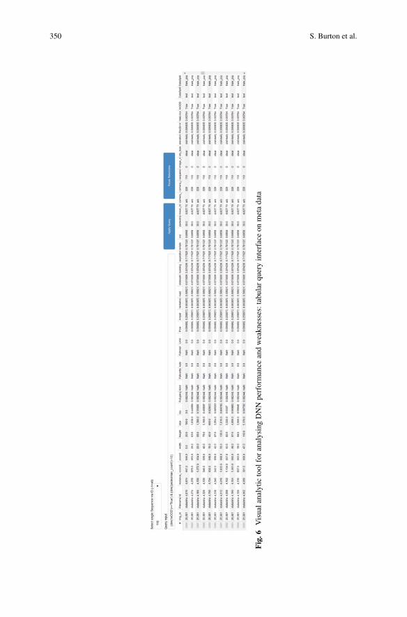
350 S. Burton et al.

Fig

.6Visualanalytic

tool

foranalysingDNNperformance

andweakn

esses:tabularqu

eryinterfaceon

metadata

Safety Assurance of Machine Learning for Perception Functions 351

Fig

.7Visualanalytic

tool

foranalysingDNNperformance

andweakn

esses:plotsof

selected

attributes

352 S. Burton et al.

Fig. 8 Plot of the pedestrian detection performance (IoU) in dependence of the height of thepedestrian in the image in pixels

(a) Overlay of input image andground truth

(b) Overlay of ground truth (left) and predictions (right): selectedcritical images often contain cyclists

Fig. 9 Visual analytic tool for analysing DNN performance and weaknesses: drill down viewshowing a a sample image, and b critical images selected from the correlation plot shown in Fig. 8(Images: BIT Technology Solutions)

5.4 Evidence from Operation-Time Controls

Operation-time controls are typically used to mitigate unacceptable risk occurringduring run-time of the system. For example, when the performance of a percep-tion component for automated driving degenerates, controls could become activeto mitigate the degeneration by handing vehicle controls back to a human driver orby using alternative perception components. The operation-time controls are par-ticularly important for automated driving, since such systems operate in the realworld. As during design time, not all possibly occurring situations can be foreseen,architectural solutions are required.

In this section, we give two examples of how evidence from operation-time con-trols can be derived. The first example deals with out-of-distribution detection andthe second one goes into detail for uncertainty estimation.

Out-of-distribution detection: One of the major causes of ML insufficiencies isthe fact that the data distribution of an operational domain is unknown. Therefore,it is only possible to sample from this unknown distribution and approximate thisdistribution by statistical approaches or machine learning (ML) techniques. Duringthe construction of the safety contract, a certain input domain is defined at a semanticlevel, which directly leads to a gap to the real data distribution of the operationaldomain. One of the resultingML insufficiencies is that there is an unknown behaviourwhen the ML function is presented with samples that are not within the training datadistribution. Therefore, a requirement could be that leaving the operational design

Safety Assurance of Machine Learning for Perception Functions 353

domain (ODD) has to be detected at run-time. Such a requirement could introducea monitoring component using complementary methods. Three example methodscould be:

• When the ODD defines certain areas of operation, e.g. urban intersections, locali-sation information in combination with map data can be utilised to detect leavingthe ODD.

• Some sensors can directly measure an environmental state, such as a rain sensor,which can be used to set bounds according to the ODD to detect whether the ODDis left.

• Out-of-distributionmethods [HG17, XYA20] can be used to detect a distributionalshift of the input samples during run-time with respect to the database used fortraining a ML model for perception or planning.

For the last method, there could furthermore be two types of evidence. Firstly, theeffectiveness of the methods should be shown by a test report including an evaluationof a metric that indicates the separation precision between in- and out-of-distributionsamples. Secondly, it has to be shown that the training and test data used to train theout-of-distribution detector is sufficient.

Uncertainty estimation: Uncertainty estimation methods can also be applied asoperation-time controls. Uncertainty is an inherent property of any machine learningmodel, which may result from either aleatoric sources, such as a non-deterministicbehaviour of the real world or issues in the data or labelling, or epistemic sources,referring to the inherent limitations of the machine learning model itself. Uncertaintyestimation methods aim to enable the DNN to indicate the uncertainty related to aspecific DNN prediction given a specific input at run-time. This may also contributeto out-of-distribution detection under the assumption that the uncertainty increaseswhen the DNN is applied outside of its training data distribution. This assumptionof course must be rigorously tested in order to provide the corresponding evidence.Among popular uncertainty estimation methods, methods based on Monte-Carlo(MC) dropout [GG16] receive particular attention in embedded applications as theyapproximate the performance of Bayesian Networks and hence usually outperformtechniques purely based on post-processing calibration, and comewith an acceptablerun-time overhead (compared to, e.g. full Bayesian networks or deep ensembles).Although originally intended for capturing epistemic uncertainty only, it can beextended to capture aleatoric uncertainty as well [KG17, SAP+21].

6 Combining Safety Evidence in the Assurance Case

While the insights sketched above surely help to understandweaknesses and improvethe development of theDNNunder investigation, the step towards arguing evidence inan assurance case still has to be performed. According to the principles of ISO 26262,ISO/DIS 21448, and ISO/TR 4804, the assurance case shall state in a convincing

354 S. Burton et al.

Fig. 10 Assurance case development: Integration of evidence into an assurance case

way: “The system is safe because...”. However, the assurance of DNNs leads toseveral problems, since this technology requires new paradigms in development.The software is no longer explicitly developed. Instead, the neural network is trainedand the network’s behaviour is implicitly influenced by the training models and data.The combination of safety evidence in the assurance case provides central elementsfor a holistic assurance strategy.

The core aspect of safety argumentation is to show that the mitigation of insuf-ficiencies was successful. If the insufficiency is reduced to an acceptable level, thisprovides evidence to be used in the safety argumentation. As shown in Fig. 10, onepossibility to combine safety evidence in the assurance case is to start on the toplevel with the definition of safety goals. These are goals that define mandatory stepsto avoid hazards. Then the safety requirements are refined step-by-step based onthe described causal model of SOTIF-related risk using the categories of evidence.This is supported by considering DNN-related safety concerns. Moreover, severalmetrics are defined to show the effectiveness of measures that mitigate the effectsof insufficiencies. The goal structuring notation (GSN) can be used to assemble evi-dence collected from various methods as they were presented in Sects. 5.1, 5.2, 5.3,and 5.4 to provide a structured overall safety argumentation. The GSN visualises

Safety Assurance of Machine Learning for Perception Functions 355

the elements of the safety argumentation. An assurance case can be presented ina clear and structured way in the GSN. A GSN tree consists of three central ele-ments: the argumentation goal, the description of the argumentation strategy, andthe evidence. These three elements are supported by assumptions, justifications, andcontext information. A central aspect is the iterative nature of this technique to refineunderstanding of insufficiencies in the function. Further iterations are started on thetop level (definition of safety goals).

7 Conclusions

Machine learning is an enabler technology for automated driving, especially for,but not limited to, the required perception components. However, assuring safetyfor such components is a challenge as standard safety-argumentation concepts arenot sufficient to capture the inherent complexity and data-dependency of functionsbased on machine learning. For example, a component realised with an ML functionis formally hard to describe, which in turn makes it especially difficult to defineappropriate evidence for the safety argumentation. Therefore, we introduce differenttypes of evidence as a structuring guidance: evidence from confirmation of residualfailure rates, evidence from evaluation of insufficiencies, evidence from design-timecontrols, and evidence from operation-time controls.

In order to create appropriate evidence, a process is required to ensure that knowl-edge from different domains (machine learning, safety, and testing) are broughttogether. Therefore, we propose the process of evidence workstreams to define evi-dence in a structured way. Furthermore, we show how to integrate evidence into anassurance case.

One of the main questions still remains open: Can a convincing assurance case beconstructed? We argue “yes” but only by explicitly acknowledging the insufficien-cies in the ML function within the system design, and by being able to determine theresidual failures with sufficient confidence. This implies directly defining an accept-able residual risk that is acknowledged by social acceptance and legal conditions,which is an open challenge.

Future research topics might be how to combine multiple quantitative and quali-tative pieces of evidence into the safety argumentation w.r.t. a given system architec-ture and how to balance them. Moreover, there is demand for derivation of evidencefrom the appropriate coverage of all possible situations within the operational designdomain (ODD) based on a structured ground context including tests. Further, theiterative and dynamic process of constructing the assurance case (or “continuousassurance”) requires work on formal models of the assurance case and on the con-tinuous evaluation of the assurance case.

Acknowledgements The research leading to these results is fundedby theGermanFederalMinistryfor Economic Affairs and Energy within the project “Methoden und Maßnahmen zur Absicherung

356 S. Burton et al.

von KI-basierten Wahrnehmungsfunktionen für das automatisierte Fahren (KI Absicherung)”. Theauthors would like to thank the consortium for the successful cooperation.

References

[ACP21] R. Ashmore, R. Calinescu, C. Paterson, Assuring the machine learning lifecycle:desiderata, methods, and challenges. ACM Comput. Surv. (CSUR) 54(5), 1–39(2021)

[ALRL04] A. Avizienis, J.-C. Laprie, B. Randell, C. Landwehr, Basic concepts and taxonomyof dependable and secure computing. IEEE Trans. Dependable Secur. Comput.(TDSC) 1(1), 11–33 (2004)

[AOS+16] D. Amodei, C. Olah, J. Steinhardt, P. Christiano, J. Schulman, D. Mané, Concreteproblems in AI safety (2016), pp. 1–29. arXiv:1606.06565

[BGH17] S. Burton, L. Gauerhof, C. Heinzemann, Making the case for safety of machinelearning in highly automated driving, in Proceedings of the International Confer-ence on Computer Safety, Reliability, and Security (SAFECOMP) (Trento, Italy,2017), pp. 5–16

[BHL+20] S. Burton, I. Habli, T. Lawton, J. McDermid, P. Morgan, Z. Porter, Mind the gaps:assuring the safety of autonomous systems from an engineering, ethical, and legalperspective. Artif. Intell. 279, 103201 (2020)

[BKS+21] S. Burton, I. Kurzidem, A. Schwaiger, P. Schleiss, M. Unterreiner, T. Graeber,P. Becker, Safety assurance of machine learning for chassis control functions, inProceedings of the International Conference on Computer Safety, Reliability, andSecurity (SAFECOMP) (York, UK, 2021), pp. 149–162

[BMGW21] S. Burton, J.A.McDermid, P. Garnett, R.Weaver, safety, complexity, and automateddriving: holistic perspectives on safety assurance. Computer 54(8), 22–32 (2021)

[CKL21] C.-H. Cheng, A. Knoll, H.-C. Liao, Safety metrics for semantic segmentation inautonomous driving (2021), pp. 1–8, arXiv:2105.10142

[CNH+18] C.-H.Cheng,G.Nührenberg, C.-H.Huang,H.Ruess, H.Yasuoka, Towards depend-ability metrics for neural networks, in Proceedings of the ACM/IEEE InternationalConference on Formal Methods and Models for System Design (MEMOCODE)(Beijing, China, 2018), pp. 43–46

[COR+16] M.Cordts,M.Omran, S. Ramos, T. Rehfeld,M.Enzweiler, R. Benenson,U. Franke,S. Roth, B. Schiele, The Cityscapes dataset for semantic urban scene understand-ing, in Proceedings of the IEEE/CVF Conference on Computer Vision and PatternRecognition (CVPR) (Las Vegas, NV, USA, 2016), pp. 3213–3223

[GG16] Y. Gal, Z. Ghahramani, Dropout as a Bayesian approximation: representing modeluncertainty in deep learning, in Proceedings of the International Conference onMachine Learning (ICML) (New York, NY, USA, 2016), pp. 1050–1059

[GHP+20] L. Gauerhof, R.D. Hawkins, C. Picardi, C. Paterson, Y. Hagiwara, I. Habli, Assur-ing the safety of machine learning for pedestrian detection at crossings, in Proceed-ings of the International Conference on Computer Safety, Reliability, and Security(SAFECOMP) (Virtual conference, 2020), pp. 197–212

[HD19] D. Hendrycks, T. Dietterich, Benchmarking neural network robustness to commoncorruptions and perturbations, in Proceedings of the International Conference onLearning Representations (ICLR) (New Orleans, LA, USA, 2019), pp. 1–15

[HG17] D. Hendrycks, K. Gimpel, A baseline for detecting misclassified and out-of-distribution examples in neural networks, in Proceedings of the International Con-ference on Learning Representations (ICLR) (Toulon, France, 2017), pp. 1–12

[HMC+20] D. Hendrycks, N. Mu, E.D. Cubuk, B. Zoph, J. Gilmer, B. Lakshminarayanan,Augmix: a simple data processing method to improve robustness and uncertainty,

Safety Assurance of Machine Learning for Perception Functions 357

inProceedings of the International Conference on Learning Representations (ICLR)(Virtual Conference, 2020), pp. 1–15

[HSRW20] M. Henne, A. Schwaiger, K. Roscher, G. Weiss, Benchmarking uncertainty estima-tion methods for deep learning with safety-related metrics, in Proceedings of theWorkshop on Artificial Intelligence Safety (SafeAI) (New York, NY, USA, 2020),pp. 1–8

[Ind19] Independent High-Level Expert Group on Artificial Intelligence. Ethics Guidelinesfor Trustworthy AI (European Commission, 2019)

[ISO18] ISO. ISO 26262: Road Vehicles—Functional Safety (International Organization forStandardization (ISO), 2018)

[ISO20] ISO. ISO/TR 4804: Road Vehicles—Safety and Cybersecurity for Automated Driv-ing Systems—Design, Verification and Validation (International Organization forStandardization (ISO), 2020)

[ISO21] ISO. ISO/DIS 21448: Road Vehicles—Safety of the Intended Functionality (Inter-national Organization for Standardization (ISO), 2021)

[KG17] A. Kendall, Y. Gal, What uncertainties do we need in Bayesian deep learning forcomputer vision? inProceedings of the Conference on Neural Information Process-ing Systems (NIPS/NeurIPS) (Long Beach, CA, USA, 2017), pp. 5574–5584

[MJ21] J. McDermid, Y. Jia, Safety of artificial intelligence: a collaborative model, inProceedings of the Workshop on Artificial Intelligence Safety (Virtual Conference,2021), pp. 1–8

[MSB+21] M.Mock, S. Scholz, F. Blank, F. Hüger, A. Rohatschek, L. Schwarz, T. Stauner, Anintegrated approach to a safety argumentation for AI-based perception functions inautomated driving, in Proceedings of the International Conference on ComputerSafety, Reliability, and Security (SAFECOMP) Workshops (York, UK, 2021), pp.265–271

[PNdS20] R. Padilla, S.L. Netto, E.A.B. da Silva, A survey on performance metrics for object-detection algorithms, in Proceedings of the IEEE International Conference on Sys-tems, Signals and Image Processing (IWSSIP) (Niteiro, Brazil, 2020), pp. 237–242

[PPD+21] R. Padilla, W.L. Passos, T.L.B. Dias, S.L. Netto, E.A.B. da Silva, A comparativeanalysis of object detection metrics with a companion open-source toolkit. Elec-tronics 10(3), 1–28 (2021)

[PPH+20] C. Picardi, C. Paterson, R.D. Hawkins, R. Calinescu, I. Habli, Assurance ArgumentPatterns and Processes for Machine Learning in Safety-Related Systems. In: Pro-ceedings of the Workshop on Artificial Intelligence Safety (SafeAI) (New York, NY,USA, 2020), pp. 1–8

[SAE18] SAE International. SAE J3016: Surface Vehicle Recommended Practice—Taxonomy and Definitions for Terms Related to Driving Automation Systems forOn-Road Motor Vehicles (SAE International, 2018)

[SAP+21] J. Sicking, M. Akila, M. Pintz, T. Wirtz, A. Fischer, S. Wrobel, A novel regressionloss for non-parametric uncertainty optimization, in Proceedings of the Symposiumon Advances in Approximate Bayesian Inference (Virtual conference, 2021), pp.1–27

[SKR+21] F. Schwaiger, M.H. Fabian Küppers, F.S. Roza, K. Roscher, A. Haselhoff, Fromblack-box to white-box: examining confidence calibration under different condi-tions, in Proceedings of the Workshop on Artificial Intelligence Safety (SafeAI)(Virtual Conference, 2021), pp. 1–8

[SKS+20] G. Schwalbe, B. Knie, T. Sämann, T. Dobberphul, L. Gauerhof, S. Raafatnia, V.Rocco, Structuring the safety argumentation for deep neural network based per-ception in automotive applications, in Proceedings of the International Conferenceon Computer Safety, Reliability, and Security (SAFECOMP) Workshops (VirtualConference, 2020), pp. 383–394

[SMHA21] E. Schulz, M. Mock, S. Houben, M. Akila, ScrutinAI: an iterative workflow forthe semantic analysis of DNN predictions (Technical report, Fraunhofer IAIS, St.Augustin, 2021)

358 S. Burton et al.

[SQC17] R. Salay, R. Queiroz, K. Czarnecki, An analysis of ISO 26262: using machinelearning safely in automotive software (2017), pp. 1–6. arXiv:1709.02435

[SSH20] T. Sämann, P. Schlicht, F. Hüger, Strategy to increase the safety of a DNN-basedperception for HAD systems (2020), pp. 1–14. arXiv:2002.08935

[VGvBB20] G. Volk, J. Gamerdinger, A. von Betnuth, O. Bringmann, A comprehensive safetymetric to evaluate perception in autonomous systems, in Proceedings of the IEEEIntelligent Transportation Systems Conference (ITSC) (Virtual Conference, 2020),pp. 1–8

[WSRA20] O. Willers, S. Sudholt, S. Raafatnia, S. Abrecht, Safety concerns and mitigationapproaches regarding the use of deep learning in safety-critical perception tasks, inProceedings of the International Conference on Computer Safety, Reliability, andSecurity (SAFECOMP) Workshops (2020), pp. 336–350

[XYA20] Z. Xiao, Q. Yan, Y. Amit, Likelihood regret: an out-of-distribution detection scorefor variational auto-encoder (2020), pp. 1–19. arXiv:2003.02977

Open Access This chapter is licensed under the terms of the Creative Commons Attribution 4.0International License (http://creativecommons.org/licenses/by/4.0/), which permits use, sharing,adaptation, distribution and reproduction in any medium or format, as long as you give appropriatecredit to the original author(s) and the source, provide a link to the Creative Commons license andindicate if changes were made.

The images or other third party material in this chapter are included in the chapter’s CreativeCommons license, unless indicated otherwise in a credit line to the material. If material is notincluded in the chapter’s Creative Commons license and your intended use is not permitted bystatutory regulation or exceeds the permitted use, you will need to obtain permission directly fromthe copyright holder.

A Variational Deep Synthesis Approachfor Perception Validation

Oliver Grau, Korbinian Hagn, and Qutub Syed Sha

Abstract This chapter introduces a novel data synthesis framework for validationof perception functions based on machine learning to ensure the safety and func-tionality of these systems, specifically in the context of automated driving. The maincontributions are the introduction of a generative, parametric description of three-dimensional scenarios in a validation parameter space, and layered scene generationprocess to reduce the computational effort. Specifically, we combine a module forprobabilistic scene generation, a variation engine for scene parameters, and a morerealistic sensor artifacts simulation. The work demonstrates the effectiveness of theframework for the perception of pedestrians in urban environments based on variousdeep neural networks (DNNs) for semantic segmentation and object detection. Ourapproach allows a systematic evaluation of a high number of different objects andcombined with our variational approach we can effectively simulate and test a widerange of additional conditions as, e.g., various illuminations. We can demonstratethat our generative approach produces a better approximation of the spatial objectdistribution to real datasets, compared to hand-crafted 3D scenes.

1 Introduction

This chapter introduces an automated data synthesis approach for the validation ofperception functions based on a generative and parameterized synthetic data genera-tion. We introduce a multi-stage strategy to sample the input domain of the possiblegenerative scenario and sensor space and discuss techniques to reduce the requiredvast amount of computational effort. This concept is an extension and generaliza-

O. Grau (B) · K. Hagn · Q. Syed ShaIntel Deutschland GmbH, Lilienthalstraße 15, 85579 Neubiberg, Germanye-mail: oliver.grau@intel.com

K. Hagne-mail: korbinian.hagn@intel.com

Q. Syed Shae-mail: syed.qutub@intel.com

© The Author(s) 2022T. Fingscheidt et al. (eds.), Deep Neural Networks and Data for Automated Driving,https://doi.org/10.1007/978-3-031-01233-4_13

359

360 O. Grau et al.

tion of our previous work on parameterization of the scene parameters of concretescenarios, called validation parameter space (VPS) [SGH20]. We extend this param-eterization by a probabilistic scene generator to widen the coverage of the generatedscenarios and a more realistic sensor simulation, which also allows to variate andsimulate different sensor characteristics. This ‘deep’ synthesis concept overcomescurrently available systems (as discussed in the next section) or manually, i.e., byhuman-operator-generated synthetic data. We describe, how our synthetic data val-idation engine makes use of the parameterized, generative content to implement atool supporting complex and effective validation strategies.

Perception is one of the hardest problems to solve in any automated system.Recently, great progress has been made in applying machine learning techniquesto deep neural networks to solve perceptional problems. Automated vehicles (AVs)are a recent focus as an important application of perception from cameras and othersensors, such as LiDAR and RaDAR [YLCT20]. Although the current main effortis on developing the hardware and software to implement the functionality of AVs,it will be equally important to demonstrate that this technology is safe. Universallyaccepted methodologies for validating safety of machine learning-based systems arestill an open research topic.

Techniques to capture and render models of the real world have matured sig-nificantly over the last decades and are now able to synthesize virtual scenes in avisual quality that is hard to distinguish from real photographs for human observers.Computer-generated imagery (CGI) is increasingly popular for training and valida-tion of deep neural networks (DNNs) (see, e.g., [RHK17, Nik19]). Synthetic datacan avoid privacy issues found with recordings of members of the public and canautomatically produce ground truth data at higher quality and reliability than costlymanually labeled data.Moreover, simulations allow synthesis of rare scene constella-tions helping validation of products targeting safety-critical applications, specificallyautomated driving.

Due to the progress in visual and multi-sensor synthesis, building systems forvalidation of these complex systems in the data center becomes feasible now andoffers more possibilities for the integration of intelligent techniques in the engineer-ing process of complex applications. We compare our approach with methods andstrategies targeting testing of automated driving [JWKW18].

The remainder of this chapter is structured as follows: The next section will givean outline of related work in the field. In Sect. 3 we give an overview of our approach.Section4 describes an outline of our synthetic data validation engine, our parame-terization, including a realistic sensor simulation, and the effective computation ofthe required variations. In Sect. 5 we present evaluation results, followed by Sect. 6with some concluding remarks.

A Variational Deep Synthesis Approach for Perception Validation 361

2 Related Work

The use of synthesized data for development and validation is an accepted tech-nique and has been also suggested for computer vision applications (e.g., [BB95]).Several methodologies for verification and validation of AVs have been developed[KP16, JWKW18, DG18] and commercial options exist.1 These tools were origi-nally designed for virtual testing of automotive functions, such as braking systems,and then extended to provide simulation and management tools for virtual test drivesin virtual environments. They provide real-time-capable models for vehicles, roads,drivers, and traffic which are then being used to generate test (sensor) data as well asAPIs for users to integrate the virtual simulation into their own validation system.

What is getting presented in this chapter is focusing on the validation of perceptionfunctions, which is an essential module of automated systems. However, by sepa-rating the perception as a component, the validation problem can also be decoupledfrom the validation of the full driving stack. Moreover, this separation allows, on theone hand, the implementation of various more specialized validation strategies and,on the other hand, there is no need to simulate dynamic actors and the connectedproblem of interrelations between them and the ego-vehicle. The full interaction ofobjects is targeted by upcoming standards like OpenScenario.2

Recently, specifically in the domain of driving scenarios, game engines have beenadopted for synthetic data generation by extraction of in-game images and labelsfrom the rendering pipeline [WEG+00, RVRK16]. Another virtual simulator system,which gained popularity in the research community, is CARLA [DRC+17], alsobased on a commercial game engine (Unreal4 [Epi04]). Although game enginesprovide a good starting point to simulate environments, they usually only offer aclosed rendering setup with many trade-offs balancing between real-time constraintsand a subjectively good visual appearance to human observers. Specifically, thelighting computation in this rendering pipelines is limited and does not producephysically correct imagery. Instead, game engines only deliver fixed rendering qualitytypically with 8 bit per RGB color channel and only basic shadow computation.

In contrast, physical-based rendering techniques have been applied to the genera-tion of data for training and validation, as in the Synscapes dataset [WU18]. For ourexperimental deep synthesis work, we use the physical-based open-source BlenderCycles renderer3 in high dynamic range (HDR) resolution, which allows realis-tic simulation of illumination and sensor characteristics increasing the coverage ofour synthetic data in terms of scene situations and optical phenomena occurring inreal-world scenarios.

The effect of sensor and lens effects on perception performance has not beenstudied a lot. In [CSVJR18, LLFW20], the authors are modeling camera effects toimprove synthetic data for the task of bounding box detection.Metrics and parameterestimation of the effects from real camera images are suggested by [LLFW20] and

1 For example, Carmaker from IPG or PreScan from TASS International.2 https://www.asam.net/standards/detail/openscenario/.3 https://www.blender.org/.

362 O. Grau et al.

[CSVJR19]. A sensor model including sensor noise, lens blur, and chromatic aberra-tion was developed based on real datasets [HG21] and integrated into our validationframework.

Looking at virtual scene content, themost recent simulation systems for validationof a complete AD system include simulation and testing of the ego-motion of avirtual vehicle and its behavior. The used test content or scenarios are thereforeaimed to simulate environments spanning a huge virtual space and are then virtuallydriving a high number of test miles (or km) in the virtual world provided [MBM18,WPC20, DG18]. Although this might be a good strategy to validate full AD stacks,one remaining problem for validation of perception systems is the limited coverageof data testing critical scene constellations (sometimes called ‘corner cases’) andparameters that lead to drop in performance of the DNN perception.

A more suitable approach is to use probabilistic grammar systems [DKF20,WU18] to generate 3D scenarios which include a catalog of different object classes,and places them relative to each other to cover the complexity of the input domain.In this chapter we demonstrate the effectiveness of a simple probabilistic grammarsystem together with our previous scene parameter variation [SGH20] with a novelmulti-stage strategy. This approach allows to systematically test conditions and rel-evant parameters for validation of perceptional function in a structured way.

3 Concept and Overview

The novelty of the framework introduced in this chapter is the combination of mod-ules for parameterized generation and testing of a wide range of scenarios and sceneparameters as well as sensor parameters. It is tailored towards exploration of factorsthat (hypothetically) define and limit the performance of perception modules.

A core design feature of the framework is the consequent parameterization ofthe scene composition, scene, and sensor parameters into a validation parameterspace (VPS) as outlined in Sect. 4.2. This parameterization only considers the nearproximity of the ego-car or sensor; in other words, only the objects visible to thesensor are generated. This allows a much more well-defined test of constellationsinvolving a specific number of object types, environment topology (e.g., types anddimensions of streets), and relation of objects, usually as an implicit function ofwhere objects are positioned relative in the scene.

This leads to a different data production and simulator pipeline than for conven-tional AV validation which typically provides a virtual world with a large extent tosimulate and test the driving functions down to a physical level, inspired by real-worldvalidation and test procedures [KP16, MBM18, DG18, JWKW18, WPC20].

Figure1 shows the building blocks of our VALERIE system. The system runsan expansion of the VPS specified in the ‘validation task’ description. Our currentimplementation is based on a probabilistic description of how to generate the scene

A Variational Deep Synthesis Approach for Perception Validation 363

ValidationEngineer

ValidationAutomation

Data Synthesis

Asset

Database

ScenarioPreparation

VALERIEValidation Flow Control

ProbabilisticScene

Generator

ParameterVariationGenerator

Sensor &EnvironmentSimulation

PerceptionFunction

EvaluationMetric

Ground

Truth

Fig. 1 Block diagram of the proposed validation approach

and defines the parameter variations in the parameter space. In the future, the vali-dation task should also include a more abstract target description of the evaluationmetrics.

The data synthesis block consists of three sub-components: The probabilisticscene generator generates a scene constellation, including a street layout, and placesthree-dimensional objects from the asset database according to probabilistic place-ment rules laid out in the scenario preparation. The parameter variation generatorproduces variations of that scene, including sun and light settings and variations ofthe placement of objects (see Fig. 2 for some examples). The sensor & environmentsimulation is using a rendering engine to compute a realistic simulation of the sensorimpressions.

Further, ground truth data is provided through the rendering process, which can beused for a pixel-accurate depth map (distance from camera to scene object) or metadata, like pixel-wise label identifiers of classes or object instances. Depending onthe perception task, this information is specifically used for training and evaluationof semantic segmentation (see Sect. 4.5).

The output of the sensor simulation is passed to the perception function under testand the response to that data is computed. An evaluation metric specific to the valida-tion task is based on the perception response. The ground truth data, as generated bythe rendering process is usually required here, e.g., to compute the similarity to theknown appearance of objects. In the experiments presented in this chapter we usedknown performance metrics for DNNs, such as the mean intersection-over-union(mIoU) metric, as introduced by [EVGW+15].

The parameterization along with the computation flow are described in detail inthe next section.

364 O. Grau et al.

4 VALERIE: Computational Deep Validation

The goal of validation is usually to demonstrate that the perception function (DNN)is performing to a level defined by the validation goal for all cases included andspecified in the ODD (operational design domain) [SAE18].

The framework presented in this contribution supports the validation of perceptionwith the data synthesis modules outlined above. Further, we suggest to consider threelevels or layers, which are supported in our framework:

1. The scene variation generates 3D scenes using a probabilistic grammar.2. The scene parameter variation generates variations of scene parameters, such as

moving objects or changing the illumination of the scene by changing the time ofthe day.

3. The sensor variation generates sensor faults and artifacts.

For an actual DNN validation, an engineer or team would build various scenariosand specify variations within these scenarios. The variations can contain lists ofalternative objects (assets), different topology and poses (including position andorientation of objects) and expansions of streets and object and global parameterssuch as direction of the sun. Our modular multi-level approach enables strategiesto sample the input space, typically by applying scene variation and this can bethen combined with more in-depth parameter variation runs and variation of sensorparameters, as required.

Specifically, the ability to either combine two or all three levels of our frame-work allows to cover a wider range of object and scene constellations. In particular,with our integrated asset management approach, a validation engineer can ensurethat certain, e.g., known critical object classes are included in the validation runs,i.e., he can explicitly control the coverage of these object classes. By combinationwith our parameter variation sub-system, local changes are varied, including relativepositioning of critical objects, the positioning of the ego-vehicle or camera, globalscene parameters such as the sun angle, etc. can be achieved.

4.1 Scene Generator

In computer graphics, a scene is considered as a collection O = {o1, o2, . . .} ofobjects oi and these are usually organized in scene graphs (see, e.g., [Wer94]) andthis model is also basis for file format specifications to exchange 3D models andscenes, e.g., VRML4 or glTF.5

Each object in this graph can have a position and orientation and scale in a (world)coordinate system. These are usually combined into a transformation matrix T. Sev-eral parameterizations for position and orientations are possible, for the position

4 ISO/IEC 14772-1:1997 and ISO/IEC 14772-2:2004 https://www.web3d.org.5 www.khronos.org/gltf.

A Variational Deep Synthesis Approach for Perception Validation 365

Table 1 Example placement description (json format)

{ "class_id" : "tree","copies" : 5,"target": { "v1" : [59.0, 20.0, 0.15], "v2": [59.8, 72.50, 0.15] },"rot_range" : [0.0, 360.0],"asset_list" : ["e649326c-061e-4881-b0a8-f2ad6297124c","3a742848-4166-4256-a045-c4a8f8ef94bc","4e153905-0ed6-4077-be33-74ef4c7509f5" ] }

usually a Cartesian 3D vector for orientation notations such as Euler angles or quater-nions are common.

Objects oi are described as geometry, e.g., as a triangular mesh and appearance(material).

Sensors, such as a camera, can also be represented in a scene graph and so can belight sources. Both also have a position and orientation, and accordingly, the sametransformation matrices as for objects can be applied (except scaling).

The probabilistic scene generator (depicted in Fig. 1) places objects oi accordingto a grammar file that specifies rules for placements and orientations in specific areasof the 3D scene. The example json file in Table1 specifies the placement of treeobjects in a rectangular area of the scene: Thetree objects are randomly drawn froma database, the field assets_list specifies a list of possible assets in universallyunique identifier (UUID) notation. The 3D models in the database are tagged with aclass_id, which specifies the type of objects, e.g., humans or buildings. The classinformation will be used in the generation of meta-data, semantic class labels, and aninstance object identifier which allows to determine on a pixel level the originating3D object.

The placement and orientation are determined by a pseudo random number gen-erator, with a controlled seed for the ability to exactly re-run experiments if required.The scene generator handles other constraints, such as specific target densities inspecific areas, distant ranges between objects, and it finally checks that the placedobject neither collides nor intersects with other objects in the scene.

The street base is also part of the input description for the scene generator. A streetcan be varied in width, type of crossings, and textures for street and sidewalk. In thecurrent simplistic implementation, the street base is limited to a flat ‘lego world’, i.e.,only rectangular structures are implemented. Each call of the scene generator gener-ated a different randomized scene according to the rules in the generation description.Figure2 shows scenes generated by a number of runs of the scene generator.

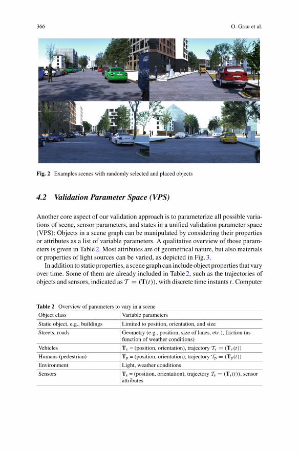
366 O. Grau et al.

Fig. 2 Examples scenes with randomly selected and placed objects

4.2 Validation Parameter Space (VPS)

Another core aspect of our validation approach is to parameterize all possible varia-tions of scene, sensor parameters, and states in a unified validation parameter space(VPS): Objects in a scene graph can be manipulated by considering their propertiesor attributes as a list of variable parameters. A qualitative overview of those param-eters is given in Table2. Most attributes are of geometrical nature, but also materialsor properties of light sources can be varied, as depicted in Fig. 3.

In addition to static properties, a scene graph can include object properties that varyover time. Some of them are already included in Table2, such as the trajectories ofobjects and sensors, indicated as T = (T(t)), with discrete time instants t . Computer

Table 2 Overview of parameters to vary in a scene

Object class Variable parameters

Static object, e.g., buildings Limited to position, orientation, and size

Streets, roads Geometry (e.g., position, size of lanes, etc.), friction (asfunction of weather conditions)

Vehicles Tv = (position, orientation), trajectory Tv = (Tv(t))

Humans (pedestrian) Tp = (position, orientation), trajectory Tp = (Tp(t))

Environment Light, weather conditions

Sensors Ts = (position, orientation), trajectory Ts = (Ts(t)), sensorattributes

A Variational Deep Synthesis Approach for Perception Validation 367

Fig. 3 Example of scene parameter variation; in this case the time of the day is varied, causingdramatic changes in the scene illumination according to contrast variations

graphic systems handle these temporal variations, also known as animations, and inprinciple, any attribute can be varied over time by these systems.

We introduce an important restriction in the current implementation of our valida-tion and simulation engine: Our animations are fixed, i.e., they do not change duringthe runtime of the simulation in order to allow deterministic and repeatable objectappearance, like poses of characters. This could be different for examplewhen a com-plete autonomous system is simulated, as the actions of the system might change theway other scene agents react. We will include these aspects in the discussion andoutlook and will discuss how these aspects could be mitigated.

For the use in our validation engine, as described in the next section, we augment adescription of the scene in a scene graph (the asset) as outlined above, with an explicitdescription of those parameters which are variable in a validation run. Currently, ourengine considers a list of numerical parameters with the following attributes:

parameter_name, scene_graph_ref, type, minimum, maximum

A specific example to describe variations of the position of a person in a 2-D planein pseudo markup notation is

{p1, scene.person-1.pos.x, FLOAT, 0.0, 20.0}

368 O. Grau et al.

Parameters, such as p1, are unique parameter identifiers used in the validationengine to produce and test variations of the scene.

4.3 Computation of Synthetic Data

Synthetic data is generated using computer graphics methods. Specifically for color(RGB) images, there are many software systems available, both commercially andas open source. For our experiments in this chapter, we are using Blender,6 as thistool allows importing, editing, and rendering of 3D content, including scripting.

The generation of synthetic data involves the following steps: First, a 3D scenemodel with a city model and pedestrians is generated using the probabilistic scenegenerator and is stored in one or more files.

The scene files are loaded into one scene graph and objects have a unique identifierand can be addressed by the following naming convention:

root_object.{subcomponent}.attribute

For the example used in Sect. 4.2, scene.person-1.pos.x refers to apath from the root object scene to the object person-1 and addresses theattribute pos.x in person-1. The object names are composed ofObjectClass-ObjectInstanceID. These conventions are used to assign aclass or instance labels during ground truth generation.

The labels for object classes will be mapped to a convention used in annotationformats (i.e., as used with in the Cityscapes dataset [COR+16]) for training andevaluation of the perception function. The 2D image of a scene is computed alongwith the ground truth extracted from the modeling software rendering engine.

Using a second parameter pos.y, as included in the example in Sect. 4.2, wouldallow the positioning of the person in a plane, spanned by x- and y-axis of thecoordinate system defined by the scene graph.

4.4 Sensor Simulation

We implemented a sensor model with the function blocks described in the chapter‘OptimizedData Synthesis for DNNTraining andValidation by Sensor Artifact Sim-ulation’ [HG22], Sect. 3.1 ‘Sensor Simulation’, and depicted in Fig. 2. The moduleexpects images in linear RGB space and floating point resolution as provided by thestate-of-the-art rendering software.

We simulate a camera error model by applying sensor noise, as additive Gaussiannoise (with zero mean and freely selectable variance) and an automatic, histogram-

6 www.blender.org.

A Variational Deep Synthesis Approach for Perception Validation 369

Fig. 4 Realistic sensor effect simulation: Standard Blender tone-mapped output (left), and thesensor simulation output (right)

based exposure control (linear tone-mapping), followed by non-linear Gamma cor-rection. Further, we simulate the following lens artifacts chromatic aberration andblur. Figure4 shows a comparison of the standard tone-mapped 8-bit RGB output ofBlender (left) with our sensor simulation. The parameters were adapted to matchthe camera characteristic of Cityscape images. The images do not only look morerealistic to the human eye, they also are closing the domain gap between the syn-thetic and real data (for details see the chapter ‘Optimized Data Synthesis for DNNTraining and Validation by Sensor Artifact Simulation’ [HG22]).

4.5 Computation and Evaluation of Perceptional Functions

Perception functions consist of a multitude of different approaches considering thewide range of different tasks. For experiments presented in this chapter, we areconsidering the tasks of semantic segmentation and 2D bounding box detection. Inthe first task, the perception function segments an input image into different objectsby assigning a semantic label to each of the input image pixels. One of the mainadvantages of semantic segmentation is the visual representation of the task whichcan be easily understood and analyzed for flaws by a human.

For semantic segmentation we consider two different topologies: DeeplabV3+as proposed in [CPK+18] and Detectron2 [WKM+19], both are utilizingResNet101 [HZRS16] backbones.

These algorithms are trained on three different datasets to create three differentmodels for evaluation. The first dataset is the Cityscapes dataset [COR+16], a collec-tion of European urban street scenes during daytime with good to medium weatherconditions. The second dataset is A2D2 [GKM+20]. Similar to theCityscapes datasetit is a collection of European urban street scenes and additionally it has sequencesfrom driving on a motorway. The last dataset, KI-A tranche 3, is a synthetic dataset

370 O. Grau et al.

provided by BIT-TS, a project partner of the KI-Absicherung project,7 consisting ofurban street scenes inspired by the preceding two real-world datasets. All of thesedatasets are labeled on a subset of 11 classes which are alike in these datasets to pro-vide comparability between the results of the different trained and evaluated models.

For the second task, the 2D-bounding box detection, we utilize the single-shotmultibox detector (SSD) by [LAE+16], a 2D-bounding box detector trained on thesynthetic data for pedestrian detection. This bounding box detector is applied on ourvariational data in Sect. 5.

To measure the performance of the task of semantic segmentation, the meanintersection-over-union (mIoU) from the COCO semantic segmentation benchmarktask is used [LSD15]. The mIoU is denoted as the intersections between predictedsemantic label classes and their corresponding ground truth divided by the unionof the same, averaged over all classes. Another performance measure utilized is thepixel accuracy (p Acc) which is defined as follows:

p Acc = T P + T N

T P + F P + F N + T N. (1)

The number of true positives (TP), true negatives (TN), false positives (FP), andtrue negatives (TN) are used to calculate p Acc, which can also be seen as a measurefor correctly predicted pixels over all pixels considered for evaluation.

For the 2D-bounding box detection we are interested in cases where, according toour definition, the performance-limiting factors are within bounds where the networkshould still be able to correctly predict a reasonable bounding box for each objectto detect. For each synthesized and inferred image, the true positive rate (TPR) iscalculated. The TPR is defined as the number of correctly detected objects (TP) overthe sum of correctly detected and undetected objects (TP+FN). As we are interestedin prediction failure cases we can then filter out all images with a true positive rate(TPR) of 1 and are left with images where the detection has omitted objects to detect.

4.6 Controller

The VALERIE controller (as depicted in Fig. 1, validation flow control) executes thevalidation run. This run can be configured in multiple ways depending on how muchsynthetic data is generated and evaluated. Two aspects have a major influence onthis: First, the specification of parameters to be varied, and second, the used samplingstrategy, which also depends on the validation goal. Both aspects are briefly describedin the following.

Specification of variable validation parameters: As outlined in Sect. 4.2, theapproach depends on the provision of a generative scene model. This consists ofa parameterized 3D scene model and includes 3D assets in the form of static and

7 https://www.ki-absicherung-projekt.de/.

A Variational Deep Synthesis Approach for Perception Validation 371

dynamic objects. On top of this, we define variable parameters in this scene as anexplicit list, as explained in Sect. 4.2.

For the specification of a validation run, all or a subset of these parameters areselected and a range and sampling distribution for that specific parameter is added.For example, to vary the x-position of a person in the scene along a line with theuniform or homogeneous distribution and a step size of 1 m, we define

{p1, UNIFORM, 1.5, 5.5, 1.0}

The parameters refer to the following: Parameter p1 refers to parameter declara-tions of x position of person-1 in the example of Sect. 4.2. The field UNIFORMrefers to a uniform sampling distribution. Other modes include GAUSSIAN (Gaus-sian distribution). The parameters 1.5, 5.5, 1.0 refer to the parameter range [1.5...5.5]and the initial step size of 1m.

Sampling of variable validation parameters: The actual expansion or samplingof the validation parameter space can be further configured and influenced in theVALERIE controller by selecting a sampler and validation strategy or goal.

The sampler object provides an interface to the controller to the validation param-eter space, considering the parameter ranges and optionally the expected parameterdistribution. We support uniform and Gaussian distributions.

In our current implementation, the controller can be configured to either samplethe validation parameter space by a full grid search, or by a Monte-Carlo randomsampling.

However, the step size can be iteratively adapted depending on the validation goal.One option here is to automatically refine the search for edge cases (or corner cases)in the parameter space: As an edge case, we consider here a parameter instance,where the evaluation function is changing between an ‘acceptable’ state to a ‘failed’state (using a continuous performance metric). For our use case of person detection,that means a drop in the performance metric below a threshold.

Other validation goals we are planning to implement could be the automateddetermination of sensitive parameters or (ultimately) more intelligent search throughhigh-dimensional validation parameter spaces.

4.7 Computational Aspects and System Scalability

Our approach is designed for execution in data centers. The implementation of thecomponents described above is modular and makes use of containerized modulesusingdocker.8 For the actual execution of themoduleswe use the Slurm9 schedul-ing tool, which allows running our validation engine with a high number of variantsin parallel, allowing the exploration of many states in the validation parameter space.

8 www.docker.com.9 https://slurm.schedmd.com.

372 O. Grau et al.

The results presented here are produced on an experimental setup using six dualXeon server nodes, each equipped with 380 GB RAM. The runtime of the renderingprocess as outlined above is mainly determined by the rendering and in the orderof 10...15min per frame, using the high-quality physically based rendering (PBR)Cycles render engine.

5 Evaluation Results and Discussion

To evaluate the effectiveness of our data synthesis approach, we conducted exper-iments in generating scenes, variation of a few important parameters, and then weevaluated the perception performance including an analysis of performance-limitingfactors, such as occlusions and distance to objects.

We used our scene generator to generate variations of street crossings, as depictedin Fig. 2. For these examples a base ground is generated first, with flexible topology(crossings, t-junction) and dimensions of streets, sidewalks, etc. In the next step,buildings, persons, and objects, including cars, traffic signs, etc. , are selected froma database and randomly placed by the scene generator, taking into account theprobabilistic description and rules. The approach can handle any number of objectassets. The current experimental setup includes a total of about 500 assets, with about60 different buildings, 180 different person models, and other objects, includingvegetation, vehicles, and so on.

Scene parameter variation: Within the generated scenes, we vary the position andorientations of persons and some occluding objects.

Further, we change the illumination by changing the time of the day. This has twomain effects: First, it is changing the illumination intensity and color (dominant atsunset and sunrise), and second, it is generating a variation of shadows casted intothe scene. In particular, from our experience, the latter creates challenging situationsfor the perception.

Comparison of object distribution: Fig. 5 shows the spatial distribution of personsin a) the Cityscapes dataset, b) KI-A tranche 3 dataset, and c) a dataset using ourgenerative scene generator, as depicted in Figs. 2 and 3. The diagrams present a top-view of the respective sensor (viewing cone) and the color encodes the frequency ofpersonswithin the sensor viewing cone, i.e., they give a representation of distance anddirection of persons in all considered frames of the dataset. The real-worldCityscapesdataset has a distribution that corresponds with most persons located left and right ofthe center, i.e., the street. There are slightly more persons on the right side, which canbe explained by the fact that often sidewalks on the left hand are occluded by vehiclesfrom the other road side. The distribution of our dataset resembles as expected thisdistribution, with slightly less occupation in the distance. In contrast, the distributionof the KI-A tranche 3 dataset shows a very sharp cumulation of the distribution onwhat corresponds to a narrow band on the sidewalks of their 3D simulation.

A Variational Deep Synthesis Approach for Perception Validation 373

(a)

(b) (c)

Fig. 5 Pedestrian distribution over horizontal angle and distance. a: Cityscapes. b: KI-A tranche3. c: Our synthetic data

Influence of different occluding objects on detection performance: A number ofobject and attribute variations are depicted in Fig. 6. On the left side, the SSD bound-ing box detector [LAE+16] is applied to the three images with different occludingobjects in front of a pedestrian. In all three images, two bounding boxes are pre-dicted for the same pedestrian. While one bounding box includes the whole body,the second bounding box only covers the non-occluded upper part of the pedestrian.On the right side, the DeeplabV3+ model trained on the KI-A tranche 3 is used tocreate a semantic map of the same three images. Besides the arms, the pedestrian isdetected, even partially through the occluding fence. However, another interestingobservation can be made: The ground the pedestrian stands on is always labeledas sidewalk. We interpret this as an indication to a bias in the training data, as thetraining data does not include enough images of pedestrians on the road, just on thesidewalk. This hypothesis can be further strengthened when we inspect the pedes-trian distributions in Fig. 5b, where the pedestrians are distributed narrowly left andright off the street in the middle. Additionally, both bounding box prediction and the

374 O. Grau et al.

Fig. 6 Scene with variation of occluding objects. Left: 2D bounding box detection. Right: semanticsegmentation

semantic segmentation do not include the pedestrian’s arms in their predictions. Thiscan also be attributed to a bias in the training data.

Influence of noise on detection performance: An experiment demonstrating oursensor simulation determines the influence of sensor noise on the predictive perfor-mance. In Fig. 7, Gaussian noise with increasing variance is applied to an image, andthree DeeplabV3+ models trained on A2D2, Cityscapes, and a synthetic dataset,respectively, are used to predict on the data. While image color pixels are repre-sented in the range xi ∈ [0, 255], the noise variance is in the range of σ 2 ∈ [0, 20]with a step size of 1. For each noise variance step, the mIoU performance metric onthe image prediction per model is calculated. While initially the models trained onCityscapes and the synthetic dataset increase in performance, all models’ predictive

A Variational Deep Synthesis Approach for Perception Validation 375

0 2 4 6 8 10 12 14 16 18 20noise variance

0

10

20

30

40

50

60

mIoU[%

]

DeeplabV3+ trained on A2D2DeeplabV3+ trained on CityscapesDeeplabV3+ trained on Synthetic data

Fig. 7 Top: mIoU performance decreases with increasing noise variance. Bottom (left to right):segmentation maps with increasing noise variance σ 2 ∈ {0, 10, 20}, image pixels xi ∈ [0, 255]

performance ultimately decreases with an increasing level of sensor noise. The initialincrease can be explained to stem from the domain shift of training to validation data,where in the training data a small noise variance can be observed.

Analysis of performance-limiting factors: Some scene parameters have a majorinfluence on the perception performance. This includes the occlusion rate of objects,with totally occluded objects that are obviously not detectable or the object size (inpixels) in the images, also with a natural boundary where detection breaks up ifthe object size is too small. Other performance-limiting factors include contrast andother physically observable parameters.

To measure the influence or sensitivity of perception functions againstperformance-limiting factors we designed an experiment using about 30,000 framescontaining one person each. The person is moved and rotated on the sidewalk andon the street. The occlusions are determined by rendering a mask of the person andcomparison with the actual instancemask considering occluding objects. A degree of100% represents a fully occluded object. Figure8 shows results of this experiment,each gray dot representing one frame and the colored curves showing regressionplots with differently clothed persons.

The figure shows a p Acc downwards trend with increasing occlusion rates. TheDetectron2 model (trained on Cityscapes) is comparatively more robust than

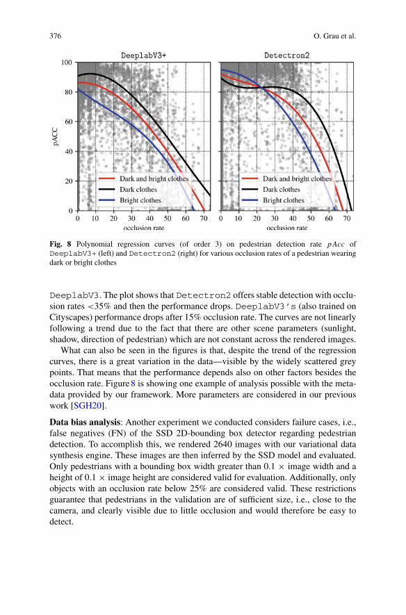
376 O. Grau et al.

Fig. 8 Polynomial regression curves (of order 3) on pedestrian detection rate p Acc ofDeeplabV3+ (left) and Detectron2 (right) for various occlusion rates of a pedestrian wearingdark or bright clothes

DeeplabV3. The plot shows that Detectron2 offers stable detection with occlu-sion rates <35% and then the performance drops. DeeplabV3’s (also trained onCityscapes) performance drops after 15% occlusion rate. The curves are not linearlyfollowing a trend due to the fact that there are other scene parameters (sunlight,shadow, direction of pedestrian) which are not constant across the rendered images.

What can also be seen in the figures is that, despite the trend of the regressioncurves, there is a great variation in the data—visible by the widely scattered greypoints. That means that the performance depends also on other factors besides theocclusion rate. Figure8 is showing one example of analysis possible with the meta-data provided by our framework. More parameters are considered in our previouswork [SGH20].

Data bias analysis: Another experiment we conducted considers failure cases, i.e.,false negatives (FN) of the SSD 2D-bounding box detector regarding pedestriandetection. To accomplish this, we rendered 2640 images with our variational datasynthesis engine. These images are then inferred by the SSD model and evaluated.Only pedestrians with a bounding box width greater than 0.1 × image width and aheight of 0.1 × image height are considered valid for evaluation. Additionally, onlyobjects with an occlusion rate below 25% are considered valid. These restrictionsguarantee that pedestrians in the validation are of sufficient size, i.e., close to thecamera, and clearly visible due to little occlusion and would therefore be easy todetect.

A Variational Deep Synthesis Approach for Perception Validation 377

0

10

20

30

40Cou

ntDetected pedestrianNon-detected pedestrian

ID: 1 2 3 4 5 6

Clothing: Veiled Casual Veiled Paramedic Business Physician

Ethnicity: Arabian Caucasian Arabian Caucasian Caucasian Caucasian

Gender: Woman Woman Man Man Man Man

Fig. 9 Count of detected and non-detected pedestrians for different pedestrian assets, i.e., differentclothing, ethnicity, and gender

With these restrictions in place we found that from all the pedestrian assets thesynthesis engine placed in the scene, there were six assets that were omitted by theSSD model as can be seen in Fig. 9.

The asset ID 1 is an Arabian womanwearing traditional clothes effectively veilingthe person. Asset ID 2 is a Caucasian woman clothed in summer casual, i.e., shortpants and short sleeves, revealing parts of her skin. The second Arabian ethnicityasset with the ID 3 is similar to asset 1 clothed in traditional veiling clothes but ofmale gender. The remaining assets 4, 5, and 6 are of male gender and Caucasianethnicity wearing different work clothes, i.e., a blue paramedical outfit for ID 4,business casual jeans and jacket for ID 5, and white physician clothes for ID 6.

The asset ID 2with the summer casual clothed woman is only miss-detected a fewtimes, in most cases the detection worked well, indicating no data bias for this asset.In contrast, the pedestrian asset ID 6 of a physician dressed in white hospital clothinghas not been detected at all. Additionally, two of the assets that were relatively mostoften overlooked by the network are the Arabian clothed woman with asset ID 1, aswell as an Arabian clothed man with the ID 3. This result would suggest that thesekind of pedestrian assets, i.e., IDs 1, 3, and 6, were not present in the data for trainingthe model and adding them to it will lead to a mitigation of this exact failure case.

378 O. Grau et al.

6 Outlook and Conclusions

This chapter has introduced a new generative data synthesis framework for the vali-dation of machine learning-based perception functions. The approach allows a veryflexible description of scenes and parameters to be varied and systematical tests ofparameter variations in our unified validation parameter space.

The conducted experiments demonstrate the benefits of splitting the validationprocess into scene variation that looks into randomized placement of objects and avariation of scene parameters and sensor simulation. Our simple probabilistic scenegenerator is scalable and able to produce scenes with a high number of differentobjects—as provided by an asset database. The spatial distribution of the positionedobjects, as demonstrated for persons in Fig. 5, is more realistic compared to manuallycrafted 3D scenes. Along with our sensor simulation (results discussed in the chapter‘Optimized Data Synthesis for DNN Training and Validation by Sensor ArtifactSimulation’ [HG22]), we present a step to close the domain-gap between syntheticand real data. Future work will continue to analyze the influence of other factors,such as rendering fidelity, scene complexity, and composition, to further improve thecapabilities of the framework and make it even more applicable for the validation ofreal-world AI functions.

Our experiments with performance-limiting factors, as shown for occlusion ratesand object size (as a function of distance to the camera) in the previous section givesclear evidence that the performance of perception functions cannot be characterizedby only a few factors. It is, however, a complex function of many parameters andaspects, including scene complexity, scene lighting and weather conditions, and thesensor characteristics. The deep validation approach described in this chapter isaddressing this multi-dimensional complexity problem and we designed a systemand methodology for flexible validation strategies to span all these parameters atonce.

Our validation parameterization, as demonstrated in the results section, is aneffective way to detect performance problems in perception functions. Moreover, itallows in its flexible design the sampling and a practical computation at scale allowingfor deep exploration of the multi-variate validation parameter space. Therefore, wesee our system as a valuable tool for the validation of perception functions.

Moving forward we are looking into using the deep synthesis approach to imple-ment sophisticated algorithms to support more complex validation strategies. Asanother key direction we target improvements in the computational efficiency of ourvalidation approach, allowing coverage of more complexity and parameter dimen-sions.

Acknowledgements The research leading to these results is fundedby theGermanFederalMinistryfor Economic Affairs and Energy within the project ‘Methoden und Maßnahmen zur Absicherungvon KI-basierten Wahrnehmungsfunktionen für das automatisierte Fahren (KI Absicherung)’. Theauthors would like to thank the consortium for the successful cooperation.

A Variational Deep Synthesis Approach for Perception Validation 379

References

[BB95] W. Burger, M.J. Barth, Virtual reality for enhanced computer vision, in VirtualPrototyping: Virtual Environments and the Product Design Process, ed. by J. Rix,S. Haas, J. Teixeira (Springer, 1995), pp. 247–257

[COR+16] M.Cordts,M.Omran, S. Ramos, T. Rehfeld,M.Enzweiler, R. Benenson,U. Franke,S. Roth, B. Schiele, The Cityscapes dataset for semantic urban scene understand-ing, in Proceedings of the IEEE/CVF Conference on Computer Vision and PatternRecognition (CVPR) (Las Vegas, NV, USA, 2016), pp. 3213–3223

[CPK+18] L.-C. Chen, G. Papandreou, I. Kokkinos, K.Murphy, A.L. Yuille, DeepLab: seman-tic image segmentation with deep convolutional nets, Atrous convolution, and fullyconnected CRFs. IEEE Trans. Pattern Anal. Mach. Intell. (TPAMI) 40(4), 834–848(2018)

[CSVJR18] A. Carlson, K.A. Skinner, R. Vasudevan, M. Johnson-Roberson, Modeling cam-era effects to improve visual learning from synthetic data, in Proceedings of theEuropean Conference on Computer Vision (ECCV) Workshops (Munich, Germany,2018), pp. 505–520

[CSVJR19] A. Carlson, K.A. Skinner, R. Vasudevan, M. Johnson-Roberson, Sensor transfer:learning optimal sensor effect image augmentation for sim-to-real domain adapta-tion, pp. 1–8 (2019). arXiv:1809.06256

[DG18] W. Damm, R. Galbas, Exploiting learning and scenario-based specification lan-guages for the verification and validation of highly automated driving, in Proceed-ings of the IEEE/ACM International Workshop on Software Engineering for AI inAutonomous Systems (SEFAIAS) (Gothenburg, Sweden, 2018), pp. 39–46

[DKF20] J. Devaranjan, A. Kar, S. Fidler, Meta-Sim2: learning to generate synthetic datasets,in Proceedings of the European Conference on Computer Vision (ECCV) (Virtualconference, 2020), pp. 715–733

[DRC+17] A. Dosovitskiy, G. Ros, F. Codevilla, A. Lopez, V. Koltun, CARLA: an open urbandriving simulator, in Proceedings of the Conference on Robot Learning CORL(Mountain View, CA, USA, 2017), pp. 1–16

[Epi04] Epic Games, Inc. Unreal Engine Homepage (2004). [Online; accessed 2021-11-18][EVGW+15] M. Everingham, L.V. Gool, C.K.I. Williams, J. Winn, A. Zisserman, The pascal

visual object classes challenge: a retrospective. Int. J. Comput. Vis. (IJCV) 111(1),98–136 (2015)

[GKM+20] J. Geyer, Y. Kassahun, M. Mahmudi, X. Ricou, R. Durgesh, A.S. Chung, L.Hauswald, V.H. Pham,M.Mühlegg, S. Dorn, T. Fernandez, M. Jänicke, S. Mirashi,C. Savani, M. Sturm, O. Vorobiov, M. Oelker, S. Garreis, P. Schuberth, A2D2: Audiautonomous driving dataset (2020), (pp. 1–10). arXiv:2004.06320

[HG21] K. Hagn, O. Grau, Improved sensor model for realistic synthetic data generation,in Proceedings of the ACM Computer Science in Cars Symposium (CSCS) (VirtualConference, 2021), pp. 1–9

[HG22] K.Hagn,O.Grau,Optimized data synthesis forDNN training and validation by sen-sor artifact simulation, inDeep Neural Networks and Data for Automated Driving—Robustness, Uncertainty Quantification, and Insights Towards Safety ed. byT. Fing-scheidt, H. Gottschalk, S. Houben (Springer, 2022), pp. 149–170

[HZRS16] K. He, X. Zhang, S. Ren, J. Sun, Deep residual learning for image recognition, inProceedings of the IEEE/CVF Conference on Computer Vision and Pattern Recog-nition (CVPR) (Las Vegas, NV, USA, 2016), pp. 770–778

[JWKW18] P. Junietz, W. Wachenfeld, K. Klonecki, H. Winner, Evaluation of differentapproaches to address safety validation of automated driving, in Proceedings ofthe IEEE Intelligent Transportation Systems Conference (ITSC) (Maui, HI, USA,2018), pp. 491–496

380 O. Grau et al.

[KP16] Nidhi Kalra, Susan M. Paddock, Driving to safety: how many miles of drivingwould it take to demonstrate autonomous vehicle reliability? Transp. Res. Part A:Policy Pract. 94, 182–193 (2016)

[LAE+16] W. Liu, D. Anguelov, D. Erhan, C. Szegedy, S. Reed, C.-Y. Fu, A.C. Berg, SSD:single shot multibox detector, in Proceedings of the European Conference on Com-puter Vision (ECCV) (Amsterdam, The Netherlands, 2016), pp. 21–37

[LLFW20] Zhenyi Liu, Trisha Lian, Joyce Farrell, Brian Wandell, Neural network generaliza-tion: the impact of camera parameters. IEEE Access 8, 10443–10454 (2020)

[LSD15] J. Long, E. Shelhamer, T. Darrell, Fully convolutional networks for semantic seg-mentation, in Proceedings of the IEEE/CVF Conference on Computer Vision andPattern Recognition (CVPR) (Boston, MA, USA, 2015), pp. 3431–3440

[MBM18] T. Menzel, G. Bagschik, M. Maurer, Scenarios for development, test and validationof automated vehicles, in Proceedings of the IEEE Intelligent Vehicles Symposium(IV) (Changshu, China, 2018), pp. 1821–1827

[Nik19] S.I. Nikolenko, Synthetic Data for Deep Learning (2019), pp. 1–156.arXiv:1909.11512

[RHK17] S.R. Richter, Z. Hayder, V. Koltun, Playing for benchmarks, in Proceedings of theIEEE International Conference on Computer Vision (ICCV) (Venice, Italy, 2017),pp. 2232–2241

[RVRK16] S.R. Richter, V. Vineet, S. Roth, V. Koltun, Playing for data: ground truth fromcomputer games, in Proceedings of the European Conference on Computer Vision(ECCV) (Amsterdam, The Netherlands, 2016), pp. 102–118

[SAE18] SAE International. SAE J3016: surface vehicle recommended practice—taxonomyand definitions for terms related to driving automation systems for on-road motorvehicles. SAE Int. (2018)

[SGH20] Q.S. Sha, O. Grau, K. Hagn, DNN analysis through synthetic data variation, inProceedings of the ACM Computer Science in Cars Symposium (CSCS) (VirtualConference, 2020), pp. 1–10

[WEG+00] B.Wymann, E. Espié, C.Guionneau, C.Dimitrakakis, R. Coulom,A. Sumner, et al.,TORCS—The Open Racing Car Simulator (2000). [Online; accessed 2021-11-18]

[Wer94] J. Wernecke, The Inventor Mentor: Programming Object-Oriented 3D GraphicsWith Open Inventor (Addison-Wesley, 1994)

[WKM+19] Y. Wu, A. Kirillov, F. Massa, W.-Y. Lo, R. Girshick, Detectron2 (2019). [Online;assessed 2021-11-18]

[WPC20] Mingyun Wen, Jisun Park, Kyungeun Cho, A scenario generation pipeline forautonomous vehicle simulators. HCIS 10, 1–15 (2020)

[WU18] M. Wrenninge, J. Unger, Synscapes: a photorealistic synthetic dataset for streetscene parsing (2018), pp. 1–13. arXiv:1810.08705

[YLCT20] Ekim Yurtsever, Jacob Lambert, Alexander Carballo, Kazuya Takeda, A survey ofautonomous driving: common practices and emerging technologies. IEEE Access8, 58443–58469 (2020)

A Variational Deep Synthesis Approach for Perception Validation 381

Open Access This chapter is licensed under the terms of the Creative Commons Attribution 4.0International License (http://creativecommons.org/licenses/by/4.0/), which permits use, sharing,adaptation, distribution and reproduction in any medium or format, as long as you give appropriatecredit to the original author(s) and the source, provide a link to the Creative Commons license andindicate if changes were made.

The images or other third party material in this chapter are included in the chapter’s CreativeCommons license, unless indicated otherwise in a credit line to the material. If material is notincluded in the chapter’s Creative Commons license and your intended use is not permitted bystatutory regulation or exceeds the permitted use, you will need to obtain permission directly fromthe copyright holder.

The Good and the Bad: Using NeuronCoverage as a DNN Validation Technique

Sujan Sai Gannamaneni, Maram Akila, Christian Heinzemann,and Matthias Woehrle

Abstract Verification and validation (V&V) is a crucial step for the certificationand deployment of deep neural networks (DNNs). Neuron coverage, inspired bycode coverage in software testing, has been proposed as one such V&V method.We provide a summary of different neuron coverage variants and their inspirationfrom traditional software engineering V&V methods. Our first experiment showsthat novelty and granularity are important considerations when assessing a coveragemetric. Building on these observations, we provide an illustrative example for study-ing the advantages of pairwise coverage over simple neuron coverage. Finally, weshow that there is an upper bound of realizable neuron coverage when test data aresampled from inside the operational design domain (in-ODD) instead of the entireinput space.

1 Introduction

In the past few years, there has been rapid growth in the usage of deep neural net-works (DNNs) for safety-critical applications. Computer visionmodels, in particular,are being used in, e.g., autonomous driving or medical diagnostics. This shift in usecases is met by increasing demand for verification and validation (V&V) methodsfor DNNs [BEW+18, ZHML20, RJS+20]. However, unlike in traditional software

S. S. Gannamaneni (B) · M. AkilaFraunhofer Institute for Intelligent Analysis and Information Systems IAIS,Schloss Birlinghoven 1, 53757 Sankt Augustin, Germanye-mail: sujan.sai.gannamaneni@iais.fraunhofer.de

M. Akilae-mail: maram.akila@iais.fraunhofer.de

C. Heinzemann · M. WoehrleRobert Bosch GmbH, Corporate Research, Robert-Bosch-Campus 1,71272 Renningen, Germanye-mail: christian.heinzemann@de.bosch.com

M. Woehrlee-mail: matthias.woehrle@de.bosch.com

© The Author(s) 2022T. Fingscheidt et al. (eds.), Deep Neural Networks and Data for Automated Driving,https://doi.org/10.1007/978-3-031-01233-4_14

383

384 S. S. Gannamaneni et al.

engineering, developing rigorous techniques for V&V of DNNs is challenging astheir intrinsic working is not directly of human design. Instead, the relevant param-eters are learned, and their meaning often eludes the human engineer.

With the strengthened focus on V&V for DNNs, there was a gradual shift awayfrom mere performance metrics to developing techniques that measure and inves-tigate, e.g., (local) interpretability or robustness. While insightful, such approachesfocus on specific instances of a given (test) dataset. However, they typically do notdetail the required number of elements in those datasets in the sense of sufficienttesting.

Inspired by testing in software engineering, Pei et al. proposed a variant of codecoverage called neuron coverage (NC) [PCYJ19]. In analogy to checking if a line ofcode is executed for any given test sample, NC provides us with the percentage ofactivated neurons for a given test dataset.

For a test (or in this case: coverage)metric, the granularity or “level of difficulty” iscrucial; if a test is too easy to fulfill, the chances are low that it will uncover errors. If,on the other hand, it is barely possible (or even impossible) to fully perform the test,it becomes ill-defined as no stopping criterion exists or can be found (cf. [SHK+19]).This makes the level of granularity of a test a decisive criterion. We can illustrate thison the example of classical code coverage for the pseudo-code shown inAlgorithm 1.

Algorithm 1 Code coverage example1: Set a2: c ← 23: if a > 2 then4: c ← −45: end if6: if a < 4 then7: a ← c · a8: end if9: return a + c

It takes a (real) input variable a and maps it onto a (real) output. Following codecoverage requirements, we would need to find inputs ai such that in total, eachline of code is executed at least once. The two values {a1 = 1, a2 = 5} would leadthe algorithm to either pass through the first or the second if-clause, respectively,and would thereby together fulfill this requirement. The advantage of this test isthat, besides being simple, it has a well-defined end when the full code is covered.Conversely, should not all of the code be coverable, it directly revealed unreachablestatements that can be removed from the code without changing its functionality.The latter would be seen as a step towards improving the code’s “readability” and asavoiding potentially unintended behavior, should those parts of code be reachable bysome unforeseen form of a statement. However, this form of coverage can provideonly a rudimentary test of the algorithm. For instance, the output in the examplediffers significantly if the algorithm runs through both clauses simultaneously, whichwould be the case, e.g., fora3 = 3.Wecannot (or at least notwith a reasonable amount

The Good and the Bad: Using Neuron Coverage as a DNN Validation Technique 385

of effort) test a given code for all potential eventualities. However, we can evaluatewith more complex test criteria, pair-wise tests in the place of the single-line tests.A reasonable approach could be to test if both if-clauses “A” and “B” were used inthe same run or whether only one of them was passed. While this approach wouldsurely have uncovered the potentially erroneous behavior from the third input a3,it also scales quadratically with the number of clauses, while the previous criterionscaled linearly. Additionally, it is a priori unclear to which extent an algorithm canbe covered in principle. For instance, in the example, no value for a can be foundsuch that both if-clauses would be skipped simultaneously.

The above example on algorithmic code coverage can be transferred to the cov-erage of neurons within a DNN. Assuming, as we will also do in the following, anarchitecture based on ReLU non-linearities, where ReLU (y) = max (y, 0), we maycount a unit (neuron) as covered, if, for a given input, its output after application ofthe ReLU is non-zero.1 Full coverage, for this measure, would thus be achieved ifa given test set X can be found such that for any unit of the DNN, at least one datasample xi ∈ X exists where that unit is covered. As with the code coverage before,the inability to construct or find such a sample xi could indicate that the unit inquestion is superfluous and might be removed (pruned) without changing the func-tionality of the DNN. The generalization to pair-wise metrics is straightforward butowing to the often sequential structure of feed-forward DNNs, a further restriction toadjacent layers is considered, i.e., pairs of only adjacent layers are considered whenevaluating with this metric. There are, however, two important distinctions to codecoverage. At first, interaction among layers, although reminiscent of the single con-trol flow in the above code example, is significantly more complicated. ExaminingAlgorithm 1 more closely, the interaction was mediated by a latent variable c. Tosome extent, each unit within a layer can be seen as such a variable allowing forvarious behaviors in the subsequent layer. Moreover, not activating a unit is not anomission but a significant statement in its own right, compare for instance [EP20].As a second point, input parameters and variations in classical software are oftenreasonably understood. For DNNs, on the contrary, often their use is motivated bythe inability to specify such variations. Therefore, a secondary use of coverage met-rics to determine the novelty of a data point x j w.r.t. a test set X ′ (x j /∈ X ′) becomesapparent by measuring how strongly the coverage values between X ′ and X ′ ∪ {x j }differ. Such a concept is based on the assumption that coverage, to some degree,represents the internal state (or “control flow” if seen from a software point of view)of the DNN and could thus be used to determine the completeness of the test set inthe sense that no further novel states of the DNN could be reached.

In this chapter, we address the following aspects: On the level of single unit cover-age, we investigate the effect of granularity, i.e., to which degree layer-wise resolvedmetrics allow for a more detailed test coverage. In this context, we also investi-gate whether the coverage metric is informative regarding the novelty of samples bycomparing trained and untrained DNNs on CIFAR-10. For both single and pairwise

1 While generalizations to non-zero thresholds exist, see for instance [MJXZ+18], we restrict our-selves to this case as it is a natural choice for ReLU non-linearities.

386 S. S. Gannamaneni et al.

coverage, we address under which circumstances (full) coverage can be reached. In a(synthetic) toy example, we also differentiate how strongly these statements dependon the restrictions posed on the test set data when staying within a DNN’s intendedinput domain (i.e., the operational design domain, ODD).

2 Related Works

Pei et al. [PCYJ19] introduced neuron coverage, i.e., looking at the percentage ofneurons activated in a network, as a testing method. Using a dual optimization goal,they generate realistic-looking test data that increases the percentage of activatedneurons. The method proposed in [MJXZ+18], a variant of [PCYJ19], uses the samedefinition of NC and additionally introduces k-multisection coverage and neuronboundary coverage. Another variant, [TPJR18], uses image transformations on syn-thetic images to maximize neuron coverage.

Sun et al. [SHK+19], inspired from modified condition/decision coverage(MCDC) in the software field, proposed four condition decision-based coveragemethods. Furthermore, they showed that the proposed methods subsumed earlierworks, i.e., satisfying their proposed methods also satisfies the weaker earlier cov-erage methods.

However, there are also several works expressing criticism of NC as a validationtechnique [DZW+19, HCWG+20, AAG+20]. While in [DZW+19], it is shown thatthere is limited to no correlation between robustness and coverage, Harel-Canadaet al. [HCWG+20] show that test sets generated by increasing NC, as defined in[PCYJ19, TPJR18], fail in specific criteria such as defect detection, naturalness, andoutput impartiality. Abrecht et al. [AAG+20] showed that there was a discrepancyin the way how neurons in different layers were evaluated in earlier works due todiffering definitions of what constitutes a neuron in a DNN. Furthermore, they showthat evaluating NC at a more granular level provides more insight than just lookingat coverage over the entire network. However, they also show that even this granularcoverage is still easy to achieve with simple augmentation techniques performingbetter than test data generation methods like DeepXplore [PCYJ19].

Abrecht et al. [AGG+21] presented an overview of testing methods of computervision DNNs in the context of automated driving. This includes a discussion ofdifferent types of adequacy criteria for testing and concretely of structural coveragefor neural networks as one form of an adequacy criterion that supports testing.

In this chapter, we follow the definitions of layer-wise coverage (LWC) [AAG+20]to determine NC and adjust it for pairwise coverage (PWC). While the fundamentaldefinition, i.e., a neuron or a unit is considered as covered as long as there is at leastone sample xi in the test setX such that the unit produces a non-zero output, remainsunchanged across definitions, the precise meaning of what constitutes a unit differs.Compared to other metrics, e.g., DeepXplore [PCYJ19], LWC provides a more finegranular resolution of coverage, especially concerning convolutional layers. Whileone could treat each channel of the convolutional layer as a single unit with respect

The Good and the Bad: Using Neuron Coverage as a DNN Validation Technique 387

to coverage, LWC demands that each instance of the use of the filter is counted as anindividual unit to be covered. In terms of an example, if a two-channel convolutionallayer results in an output of 3 × 3 × 2 real numbers, where the first two numbersare due to the size of the input image, LWC would require to cover each of the 18resulting “neurons” while DeepXplore would consider only two “neurons”, one foreach channel.

3 Granularity and Novelty

Several works [SHK+19, AAG+20] have shown that achieving high NC is trivialwith only a few randomly selected in-domain non-adversarial images. Abrecht etal. [AAG+20] have further shown that trained and untrained networks show similarNC behavior for a given test dataset. Intuitively, one would expect that, first, a metricused to investigate the safety of a DNN in terms of finding new input samples shouldnot be easily satisfiable and, second, that the metric should depend on the “quality”of the input. Typically, a DNN is trained to solve a specific problem that only covers avery small subset of all possible inputs, e.g., classifying an image as either showing acat or dog could be contrasted by completely unfitting inputs such as the figures in thischapter. Following the analogyof code coverage, thiswouldbe thedifferencebetweenexpected and fully random (and mostly unfitting) inputs, where for the latter, onewould expect nonsensical outputs or error messages. Especially for neural networks,this second point is of relevance as they are typically used in cases where a distinctionbetween reasonable and unreasonable input can be made only by human experts orDNNs but not via “conventional” algorithms. This makes an extension of the inputcoverage to novel examples challenging, as “errors” discovered on erroneous inputsmight lead to questionable insights into the DNNs trustworthiness or reliability.

Within this section, we elaborate on the two raised concerns by investigating anexample DNN on the level of (single-point) NC. For this, we will look not onlyat the reached coverage but take a closer look at its saturation behavior. Further,we compare both trained and untrained (e.g., randomly initialized) versions of theDNN using either actual test data (from the dataset) or randomly generated Gaussianinput. To be more precise, we use VGG16 [SZ15] networks with ReLU activationsand train them on CIFAR-10 [Kri09], a dataset containing RGB images of (pixel-,channel-) size 32 × 32 × 3 with 10 classes (containing objects, such as automobiles,but also creatures, such as frogs or cats) from scratch. After training,2 our networkreaches an average accuracy of 82% on the test set. As stated above, we employthe layerwise coverage (LWC) notion defined by Abrecht et al. [AAG+20] to mea-sure NC as it subsumes less granular metrics, such as the often-used definitions ofDeepXplore [PCYJ19]. Subsumption implies that if DeepXplore does not reach fullcoverage, neither will LWC but not necessarily the other way around.

2 We employ an SGD optimizer with a learning rate of 10−3 for 20 epochs and a learning rate decayof 0.1 at epochs 10 and 15.

388 S. S. Gannamaneni et al.

0 200 400 600 800 1,000

0.4

0.6

0.8

1

Number of test samples t

Neu

roncoverage

cifar10 trainedcifar10 untrainedrandom trainedrandom untrained

Fig. 1 Here, we show the neuron coverage in a VGG16 network. The blue solid and dashed linesshow mean coverage for trained and untrained models on CIFAR-10 test images, respectively. Theorange solid and dashed lines show mean coverage for trained and untrained models on randomlygenerated data samples, respectively. The standard deviation is shown for each experiment as theshaded area

In Fig. 1, we plot the NC of the used VGG16 DNNs with respect to 1000 testsamples for all four test cases. For each case, we employed five different DNNs,independently initialized and/or trained, and averaged the results for further stability.For evaluation, we use both the real CIFAR-10 test set data and randomly generateddata samples from a Gaussian distribution loosely fitting the overall data range.While the coverage behaves qualitatively similar in all cases, a clear separationbetween (assumed) limiting values and saturation speeds can be seen. This differenceis most pronounced between the trained DNN that is tested with CIFAR-10 test data,representing themost structured case as both the data and theweights carry (semantic)meaning, and all other cases, which contain at least one random component.

A rough understanding of the behavior of NC can be acquired when consideringthe following highly simplified thought experiment. Assuming that the activation of aneuron was an entirely probabilistic event in which a given input sample activates theneuron with probability 0 < p < 1, then the chance of said neuron to remain inactivefor t samples would be qt with q := 1 − p. While this suggests an exponentialsaturation rate for the coverage of a single neuron, the idea only carries over to the fullset of all considered neurons if one assumes further that their activation probabilitiesp′ were identical and their activations independent. Even omitting only the firstcondition (identicality) can lead to qualitatively different behavior, in which specificproperties would depend on the distribution of p’s among the neurons. A typical

The Good and the Bad: Using Neuron Coverage as a DNN Validation Technique 389

0 20 40 60 80 100

−12

−10

−8

−6

−4

−2

Number of test samples t

log(1

−C(t)/N)

cifar10 trainedcifar10 untrainedrandom trainedrandom untrainedcoin flip

First layer

100 101 102 103−3.5

−3

−2.5

−2

−1.5

−1

Number of test samples t

cifar10 trainedcifar10 untrainedrandom trainedrandom untrained

Penultimate layer

Fig. 2 Logplot ofmean coverage in first (left) and penultimate (right) layer for trained and untrainednetworks. In the first layer, neuron coverage shows similar behavior for trained and untrainednetworks. However, in the penultimate layer, there is a significant difference in behavior betweentrained and untrained networks. The standard deviation is shown as shaded region. As we considerlog(1 − C(t)/N ), with the number of covered neurons C(t), total neurons N and test samples t ,the value approaches “negative infinity” when full coverage is achieved. This behavior can be seenin the figure on the left. The x-axis on the right is on log scale

expectation for a broad distribution would be an approximately algebraic saturation.3

Unsurprisingly, we can recover both types of behavior within the experiments.A connection to the above thought experiment is obtained when investigating NC

layer-wise. While from the perspective of testing, one might argue that the coverageof any given layer is subsumed in the coverage of the fullmodel, the differing behaviorof the layers warrants investigating NC on this level of granularity. For the first andthe penultimate layer of VGG16, the results are depicted in Fig. 2. In the first layer,one would expect that, at least for random input, each neuron is equally well suitedto be activated, and thus saturation would be reached exponentially. As can be seen,this is almost ideally given for the untrained DNN if tested on random input, and ingood approximation still when using the structured CIFAR-10 input or when testingthe trained DNNwith the random samples. In the latter case, the decision boundariesof each trained neuron are “random” with respect to the incoming data, which doesnot represent any meaningful semantic concepts or correlations. Note that we do notshow the coverage in the figure but rather the number of not-yet-activated neurons ina logarithmic fashion; straight lines represent exponential saturation. Regarding thespeed of saturation, i.e., the exponent or probability p, the naive assumption is that aneuron separates the input via a half-plane and each case, activation or inactivation,is equally likely. This corresponds to a coin-flip with probability p = q = 1/2 andis depicted in the figure for comparison. Only the trained DNN, when tested onactual test data, deviates from this behavior and saturates more slowly. This might be

3 Consider, for comparison, how a superposition or mixture of Gaussians turns into a heavy-taileddistribution, e.g., Student’s t , if the standard deviations of each Gaussian differ strongly enough,cf. [Bar12].

390 S. S. Gannamaneni et al.

explained by the fact that the network can use feature-based correlation in the data,and a new test sample is therefore of a more limited novelty than a fully random, andthus unexpected one.

Turning to the penultimate layer, shown on the right-hand side in Fig. 2, we choosea double-logarithmic visualization such that algebraic saturation is now given bystraight lines. To some extent, all four test cases seem to satisfy this type of satu-ration. However, the exponent, i.e., the speed of saturation, differs significantly andis slowest for both cases of the untrained DNN. A possible explanation might sim-ply be the propagation of information that is not optimized in a random DNN. Bydesign, a (classification) DNN maps a large input (here 3072-dimensional) onto alow-dimensional output (10 classes) and, thus, has to discard large amounts of infor-mation along the layers. This heuristic assumption is supported by the behavior ofthe trained DNN, which achieves high coverage significantly faster, even more so ifthe input contains features it was optimized to recognize (i.e., actual test data).

As shown, NC does depend on the training and the use of an appropriate testset. Even then, the final coverage might be reached only slowly. However, returningto the original Fig. 1, relatively high coverage is reached early on with only a fewsamples. It is, therefore, more a question of resolving a “hand-full” of not-coveredneurons that might not be receptive to the data used. In the next section, we will lookmore closely into whether or not all neurons can even be covered if the used dataare restricted to the operational domain of the network. This property, catching largeamounts of the coverage with only limited effort, might not be desirable from theperspective of testing, especially if the novelty of samples is supposed to be judged.For such use cases, more granular tests might be more appropriate. A straightforwardextension might be to include not only “positive” neuron coverage (NC+) as donebefore but also “negative” coverage (NC-) where a neuron was not activated at leastonce. For a neuron, it might be the case that it is almost always active, and thereforethe rare cases where it does not fire might be of interest. For this reason, both typesof coverage are to some degree independent, i.e., while it can be possible for a DNNto reach full NC+ coverage, this does not necessarily ensure full (NC-) coverage,and vice versa. Especially for networks with ReLU activations, (NC-) coverage isof interest as the non-linearity only takes effect when a neuron is not active. For adiscussion, see, for instance, [EP20].

As discussed in the introduction, a further logical extension could be a switch frommeasuring single neuron activations or inactivations to a notion of pairwise coverage(PWC). Here, we follow a simplified version of the sign-sign coverage introducedin [SHK+19]. Due to the typically feed-forward type of network structure, we limitourselves to adjacent layers with a pair of neurons as the unit of interest. A pairof neurons, n�,i , n�+1, j from layers � and � + 1, counts as covered with respect toPWC++, if for a given input both neurons are active, i.e., assuming values greaterthan 0. Similarly, we define PWC–– for cases where the pre-activations are both non-positive, and the neuron outputs thus zero. Likewise, the two alternating activationpatterns, PWC+– and PWC–+, can be defined. It is easy to see that if a DNN is fullyPWC++ (or PWC––) covered, it is also fully NC+ (NC–, respectively) covered.Therefore, the PWC metrics subsume the single neuron NC metrics. However, this

The Good and the Bad: Using Neuron Coverage as a DNN Validation Technique 391

Table 1 NC and PWC: This table shows the big difference between the number of countable unitsof neurons in NC and pairwise evaluation in PWC. Neurons are defined as per LWC [AAG+20].For simplicity, we do not consider the effect of skip connections

Network NC [105] PWC [105]LeNet-5 [LBBH98] 0.081 81

VGG-16 [SZ15] 3.159 82,030

VGG-19 [SZ15] 3.425 85,428

ResNet-18 [HZRS16] 0.548 1,673

ResNet-34 [HZRS16] 0.804 2,265

ResNet-50 [HZRS16] 2.309 12,117

ResNet-101 [HZRS16] 3.354 13,721

increased granularity comes at a price. While the number of tests or conditionsrequired to be fulfilled to reach full NC coverage scales linearly with the number ofneurons or units, pairwise metrics follow a quadratic growth. Due to the restrictionto neighboring layers, the growth is effectively reduced by the number of layers,and the number of conditions can be approximated by (#neurons)2/#layers. Exactnumbers for a selected few architectures are reported in Table1 including the VGG16example used so far. Note that for simplicity, skip connection combinations, althoughforming direct links between remote layers, are not considered. Including them intothe pairwise metric would lead to larger numbers. Even without, the sheer magnitudeshows that it might be unlikely to test for full coverage. Additionally, it is unclearwhether full coverage can be reached in principle if the neuron output is correlatedacross layers. As this might pose a problem for tests that require an end criterionsignifying when the test is finished, we include those more elaborate metrics in thenext section where we investigate whether full coverage can be reached.

4 Formal Analysis of Achievable Coverage

In this section, we analyze coverage metrics based on a very simple task and a sim-ple domain as described in Sect. 4.1. The key design objectives for the creation ofthe task are that (i) arbitrary many data samples can be generated, (ii) a groundtruth oracle exists in closed form, and (iii) the trained network and the input domainare sufficiently small such that specific activation patterns can be computed analyti-cally. We describe the experimental setup in detail in Sect. 4.2, before providing theexperimental results in Sect. 4.3, followed by a discussion in Sect. 4.4.

392 S. S. Gannamaneni et al.

4.1 Description of the Task

Our simple task is counting the number of input “pixels” with positive values. Werestrict ourselves to a system with four input pixels, whose values are constrained tothe interval I = [−1, 1]. We call this the operational design domain (ODD) of ournetwork, following [KF19]. This is also our training distribution. We can obviouslyalso perform inference on samples outside this ODD, but these will be outside thetraining distribution since we only train on ODD samples. We frame this task as aclassification problem with five output classes: the integers from 0 to 4. Thus, ourinput domain is I4, our output domain is O = {0, 1, 2, 3, 4}, and we can define aground truth oracle as cardinality |{i |i ∈ I, i > 0}|, i.e., we count the pixels witha value above 0. In addition, we explicitly define all inputs in R

4 \ I4 as out-of-distribution samples, with I4 ⊂ R

4.The rationale of our approach is as follows: What can be achieved with perfect

knowledge of the system in the sense of (i) symbolically computing inputs to achieveactivation patterns, (ii) having a clear definition of in-ODD and out-of-ODD, and(iii) having a perfect labeling function for novel examples?

For this task, we use a multilayer perceptron (MLP) with three hidden fully con-nected layers FC(n) with n output nodes. The architecture of the MLP is shownin Fig. 3. We train our network using PyTorch. We generate one million inputsuniformly sampled from I4. We split these samples into training and test data sets

FC(12) + ReLU

FC(10) + ReLU

FC(6) + ReLU

FC(5)

Softmax

Argmax

x ∈ I4

y ∈ O

Fig. 3 Architecture of the MLP

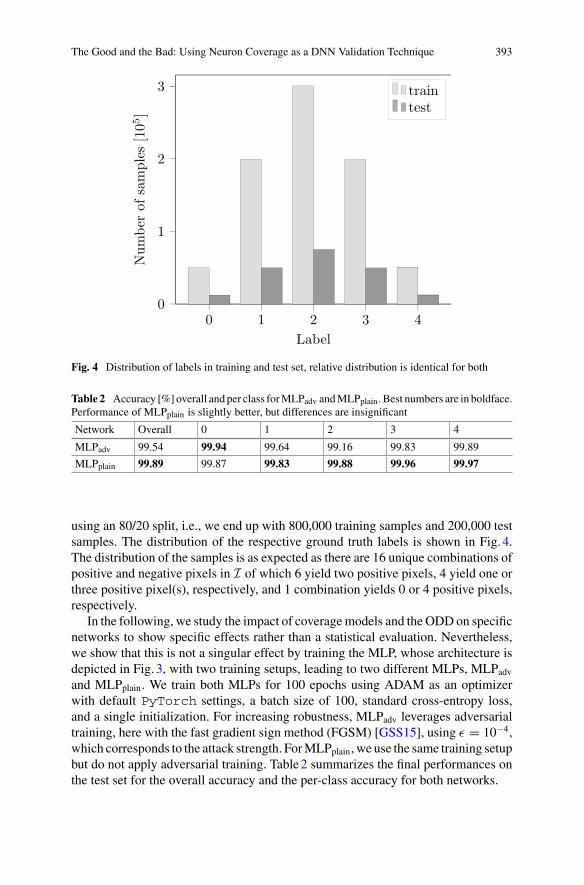
The Good and the Bad: Using Neuron Coverage as a DNN Validation Technique 393

0 1 2 3 40

1

2

3

Label

Num

berof

samples

[105]

traintest

Fig. 4 Distribution of labels in training and test set, relative distribution is identical for both

Table 2 Accuracy [%] overall and per class forMLPadv andMLPplain. Best numbers are in boldface.Performance of MLPplain is slightly better, but differences are insignificant

Network Overall 0 1 2 3 4

MLPadv 99.54 99.94 99.64 99.16 99.83 99.89

MLPplain 99.89 99.87 99.83 99.88 99.96 99.97

using an 80/20 split, i.e., we end up with 800,000 training samples and 200,000 testsamples. The distribution of the respective ground truth labels is shown in Fig. 4.The distribution of the samples is as expected as there are 16 unique combinations ofpositive and negative pixels in I of which 6 yield two positive pixels, 4 yield one orthree positive pixel(s), respectively, and 1 combination yields 0 or 4 positive pixels,respectively.

In the following, we study the impact of coveragemodels and the ODDon specificnetworks to show specific effects rather than a statistical evaluation. Nevertheless,we show that this is not a singular effect by training the MLP, whose architecture isdepicted in Fig. 3, with two training setups, leading to two different MLPs, MLPadvand MLPplain. We train both MLPs for 100 epochs using ADAM as an optimizerwith default PyTorch settings, a batch size of 100, standard cross-entropy loss,and a single initialization. For increasing robustness, MLPadv leverages adversarialtraining, here with the fast gradient sign method (FGSM) [GSS15], using ε = 10−4,which corresponds to the attack strength. ForMLPplain, we use the same training setupbut do not apply adversarial training. Table2 summarizes the final performances onthe test set for the overall accuracy and the per-class accuracy for both networks.

394 S. S. Gannamaneni et al.

We can see that MLPplain has a slightly higher accuracy overall, as well as for fourout of the five output classes, than MLPadv. Note that the lower accuracy of MLPadvis in line with standard robust training and shows that when trying to train a robustnetwork, more capacity may be necessary [GSS15]. We focus in the following onthe adversarially trained model for the sake of brevity since both setups resulted insimilar results.

4.2 Experimental Setup

In our experiments, we want to evaluate whether full coverage according to neuroncoverage (NC) and pairwise coverage (PWC) can be achieved. The networks for theexperiments are the trained MLPs described in the previous section. The goal of theexperiment is to calculate a minimal number of inputs that maximizes coverage onthe MLP and, if required, a number of non-coverable items.

Since the MLP is simple enough, we can solve the coverage generation sym-bolically. For this, we use a satisfiability modulo theory (SMT) solver, namely,Z3 [dMB08], and encode the problem of finding inputs maximizing coverage asSMT queries based on the theory of unquantified linear real arithmetic, i.e., Booleancombinations of inequations between linear polynomials over real variables. Notethat there are also further approaches based on SMT targeting larger neural networkslike Reluplex [KBD+17], which are, however, not needed for our example. Weiteratively compute solutions for individual neurons (or combinations of neurons) asshown in Algorithm 2: We determine all coverage items for a neural network as a setB. While there are still coverage items, we select one of these and try to cover it asdescribed in the following.We formulate the coverage of item i ∈ B as an SMTqueryand call the SMT solver on this query using runSMT(). If it succeeds as indicatedby the return value success being true, we run the network NN on the resulting inputx by executing callMLP(). This returns all resulting coverage items J , which areadded to the set of already covered coverage items C.Minimally, we find the coverageitem i from the SMT query, but there may be more. If the SMT solver cannot coveritem i , we add it to the set of uncoverable items U . Note that this implicitly alsodepends on a specific coverage metric, which we omit in the algorithm for simplicityof the presentation.

The function runSMT() generates individual samples based on a program forZ3 [dMB08], orZ3Py4, respectively, as a list of constraints. These constraints encodethe network, the input domain, and the coverage item.When the SMT determines theconstraint system as satisfiable, it returns a model. From this model, we can extractthe corresponding inputs to the network that lead to a satisfiable result.

For each coverage item, we run two experiments with and without a constrainedinput domain. First, we use constraints as shown above that allow the Z3 solverto only consider in-ODD samples from I4. Second, we also allow Z3 to generate

4 https://pypi.org/project/z3-solver.

The Good and the Bad: Using Neuron Coverage as a DNN Validation Technique 395

Algorithm 2 High-Level Algorithm1: procedure ComputeSMTCoverage(NN) � NN is the network to be covered2: B ← getCoverageItems(NN)3: C ← ∅ � items already covered4: U ← ∅ � uncoverable items5: while B \ {C ∪ U} = ∅ do6: Select i ∈ B \ {C ∪ U}7: success, x ← runSMT(NN, i) � x is an input for NN8: if success then9: J ← callMLP(x) � compute all possible coverage items for x10: C = C ∪ J11: else12: U = U ∪ {i}13: end if14: end while15: end procedure

arbitrary samples from R4, i.e., we allow Z3 to also generate out-of-ODD samples.

Naturally, the achievable coverage using only in-ODD samples can be at most ashigh as the coverage for the entire R4.

As a baseline, we compare the coverage achieved by the samples from Z3 withtwo sampling-based approaches: (i) We use random sampling from the input domain(further described below) since it is a commonly applied strategy for data acquisition.(ii) Due to the compactness of our input space, we can use a grid-based approachof the input domain. We include this comparison to check how easy or difficult it isto achieve maximum coverage using sampling-based approaches. In particular, weuse a grid-based sampling with a fixed number of samples per dimension, and wesample at random from a distribution. As for the structured generation, we performtwo experiments for each approach: One permitting only in-ODD samples from I4,and one also permitting out-of-ODD samples. Of course, since we know the exactmaximum coverage for each of the considered coveragemetrics from Z3, we are onlyinterested in how far below the optimum the sampling-based approaches remain.

For the grid-based approach, we sample from I4 with a resolution of 100 equidis-tant samples per dimension for the in-ODD samples. In addition, we sample fromR4 ⊂ R

4,R = [−2, 2] with a resolution of 100 equidistant samples per dimen-sion for a mixture of in-ODD and out-of-ODD samples. For the random samplingapproach, we sample 108 data points uniformly at random from I4 for in-ODD sam-ples. In addition, we sample 108 data points from a Gaussian distribution with zeromean and unit variance, which results in 78% out-of-ODD samples. For all datasets, we measure coverage based on PyTorch [PGM+19] as described above inAlgorithm 2 for the SMT-based approach.

396 S. S. Gannamaneni et al.

4.3 Experimental Results

Table3 shows the number of generated samples, whereas Table4 summarizes thecoverage results fromour experiments, both forMLPadv. Please note that these resultsare for a single network. However, we are not interested in the specific numbershere but rather compare different coverage models and data generation approachesqualitatively on a specific network. The structure of Table4 is as follows: Each rowcontains the results for one data generation approach. Thus, the first row containsthe result when optimizing for positive neuron coverage (NC (+)), i.e., getting apositive activation for each individual neuron. The second row contains the resultsfor neuron coverage in both directions (NC (both)), i.e., each individual neuron hasat least once a positive and a negative activation. The third row contains the resultswhen optimizing PWC. The final two rows contain the results for the two baselinesampling approaches.

The columns of the table show the resulting coverage for the different coveragemetrics. For each column, we provide separate columns All and ODD: The ODDcolumns contain the results when only in-ODD samples are used, whereas the Allcolumns contain the result when also allowing for out-of-ODD samples. For NC (+)and NC (both), the cells contain the coverage results for each of the three layers,denoted by L1 to L3. Please note that L1 is the layer directly after the input and L3constructs the representation, which is used in the final classification layer L4. ForPWC, we further split the All and ODD columns based on the layer combinationsthat are considered. The L1–L2 columns contain the results for the coverage of theinteraction between the neurons on layers L1 and L2 while the L2–L3 columnscontain the results for the interaction between L2 and L3, respectively. In thesecolumns, the entries in the single cells refer to the coverage of the four possiblecombinations of activations for the considered pairs of neurons. As an example, incolumnL1-L2, “+−” refers to all caseswhere a neuron inL1has a positive activation,and a neuron in L2 has a negative activation. In each row, we marked the cells withgray background where the reported coverage corresponds to the optimization targetin Z3. These entries signify the maximally possible coverage values.

In the following, we highlight some interesting aspects of the results. Note that,in general, the coverage in the All column must be larger or equal to the coverage inthe ODD column for each of the coverage metrics as R ⊃ I.

Intuitively, we would expect that the more elaborate a coverage metric is (i.e.,the more elements it requires to be covered), the more test samples are required toachieve coverage. In our results, this expectation is satisfied, i.e., we need more tests

Table 3 Number of tests per approach

NC (+) NC (both) PWC Grid Sample

All 6 10 39 108 108

ODD 5 10 47 108 108

The Good and the Bad: Using Neuron Coverage as a DNN Validation Technique 397

Table 4 Results from the coverage analysis, L� means layer �. The rows show different datageneration approaches (solver-based and sampling-based). The columns show coverage based ondifferent coverage metrics. Grey shaded cells show the results of metric that was optimized in SMT

for PWC than for NC, and we need more tests for NC (both) than for NC (+) asshown in Table3. In addition, we would expect that coverage is proportional to thenumber of tests for the first three rows, i.e., more tests imply higher coverage, giventhat we only add new tests if they actually increase coverage. Interestingly, this isnot satisfied for PWC, where we generate more tests for in-ODD samples than forAll, even though the resulting coverage for ODD is lower than for All. It seems thatin our particular MLP, it is easier to stimulate multiple neurons at once when usingout-of-ODD samples.

Let us now consider NC. When using arbitrary test samples, it is possible toachieve 100% coverage for both NC (+) and NC (-). However, when restricting thegeneration to only in-ODD samples, i.e., a subset of the complete input space of theMLP, full coverage can no longer be reached for NC (+). In particular, we observethat some neurons on layers L2 and L3 can no longer be stimulated to have a positive

398 S. S. Gannamaneni et al.

activation. Considering the use of SMT leading to this observation, we thus notonly have empirical evidence but also a tool-based mathematical proof that 100%coverage is not possible in this case.5

If you compare the coverage in the NC (+) column with the corresponding cov-erage for the two sampling-based approaches, you will notice that they achieve thesame non-100% coverage for in-ODD samples and a smaller non-100% coverage forAll samples. Thus, the sampling-based approaches failed to achieve 100% coveragefor NC (+) in both cases. While we know in this example that no better result wastheoretically possible for in-ODD samples, more coverage could have been possiblefor All. However, for a more complex task, these two cases cannot be distinguished,i.e., if we have coverage less than 100%, we cannot decide whether it is impossible toachieve more or whether our test set is yet incomplete. In addition, the result showsthat even in this simple domain, a relatively high number of samples do not achievemaximal coverage. Thus, it is highly unlikely to achieve the theoretically possiblecoverage with respect to more involved metrics such as PWC on complex domainsin computer vision using random or grid-based sampling.

As stated above, we can achieve higher coverage when also allowing for out-of-ODD samples. In our example, the network was not trained on such out-of-ODDsamples, so the question remains whether it is actually meaningful to include suchsamples in a test set just for increasing coverage. In our example, we can give someintuition on this. For this, we look in detail at samples generated by our SMT-basedapproach with and without input constraints. The results are shown in Fig. 5, wherewe plot samples SMT generated for the NC (both) criterion. Each run creates 10samples, as is shown in Table4. Each of these samples is labeled according to ourlabeling function, and the corresponding cross-entropy loss JCE is computed. Sincethe loss varies drastically, we show a logarithmic plot and since the loss can be zerofor perfect predictions, we specifically plot

log(JCE + 1). (1)

Remember from Table3 that there are 10 samples, each for the full input space andthe ODD space. As we can see, for both input domains, for the first three samples, thenetwork generates perfect predictions and therefore log(JCE + 1) := 0. For theODDsamples, we can see that the loss is quite low and at most in the order of themaximumtraining loss (as indicated by the dotted line). We also annotate for each sample ofthe full input space (All) whether the resulting sample is in the ODD, labeled as All(in) and indicated by a dot, or whether the sample is out-of-ODD, labeled as All (out)and indicated by a diamond shape. As we can see, when optimizing coverage withoutconstraints (All), most of the samples (7/10) produced by Z3 are out-of-ODD, eventhough also in-ODD samples would exist for the most part. In the figure, we cansee that these out-of-ODD samples are not suitable for a realistic evaluation: Eachout-of-ODD sample has a very high loss, at least an order of magnitude higher than

5 Please note that the large-scale experiments with random and grid-based sampling provide addi-tional empirical evidence.

The Good and the Bad: Using Neuron Coverage as a DNN Validation Technique 399

2 4 6 8 10

0

2

4

6

8

10

12

Index of data sample

log(JCE+

1)

ODDAll (in)All (out)Max train

Fig. 5 Log-modified cross-entropy losses (see (1)) on samples generated by SMT for NC (both).ODD refers to in-ODD samples, All (in/out) refer to in-ODD/out-of-ODD samples sampled froma mixed in-ODD/out-of-ODD input space, and Max train is the maximum training loss

the maximum training loss, marked by a dotted line. It can also be observed thatin-ODD samples have a significantly lower loss. Nevertheless, even here, we see thatthe SMT-based approach generates two very difficult examples.

Intuitively, we would expect that achieving a high coverage is more difficulton deeper layers because achieving a specific activation also requires establishingnecessary activations on the previous layers. This means these previous layers worklike constraints for the computation of an input that creates an activation on a deeperlayer. Thus, the deeper the layer, the more constraints need to be satisfied. While ourresults confirm this intuition in most cases, these are not as strong as you can see,e.g., when comparing the coverage for PWC. Here, the coverage for L2–L3 is onlyslightly lower in three out of four cases than for L1–L2, and in the fourth case, it iseven higher for the deeper layers. This is most probably the case because the networkis rather shallow.

Note that we additionally performed these experiments on MLPplain. While theresults are largely the same in direction (reductions), the magnitude of differences isslightly larger. We hypothesize that this is due to the lower robustness of representa-tions and, thus, preferred to show the results for the adversarially trained MLP.

400 S. S. Gannamaneni et al.

4.4 Discussion

Our results for the formal analysis of achievable coverage clearly show that evenfor simple networks, 100% coverage may not be achievable. This has two reasons:(i) Networks are trained in a way that they contain some activations that may onlyever be used in one direction. We can see this in the All columns of Table4 thathave coverage levels < 100%. In traditional software, we would refer to this as“dead code” that results in non-perfect coverage. One could argue that as with “deadcode” in traditional software, there may be a way to remove this by some form ofstatic analysis. (ii) Even if we remove this “static dead code”, we can still see adifference between All and ODD. This difference is harder to identify in practiceas—in contrast to our simple example—this distinction between All and ODD is notalways obvious for computer vision tasks. Hence, this is a harder form of “dead code”depending on the particular input/operational distribution. Both of these sourcesresult in incomplete coverage.

Let us summarize major differences between state-of-the-art DNNs used, e.g., incomputer vision for automated driving functions, and our presented MLP example:

• In a complex input domain, we do not have a clear definition of ODD and All,and we may not be able to decide whether a specific input is reasonable or not.For example, it is not clear whether a new image lies in the challenging part of theODD or is considered to lie outside the ODD.

• We usually want to focus on in-ODD examples.• Formal approaches such as the one used in these examples do not scale totypical state-of-the-art DNNs. Note that we cannot directly use more efficient,approximate works, e.g., on adversarial examples, since they perform an over-approximation while we are interested in under-approximations for coverage.

As a result, the identification of both sources of “dead code” is typically infeasible.This means that we do not know the real upper threshold for achievable coverageandmust over-approximate it with the complete number of coverage items, includingboth sources of “dead code”.

5 Conclusion

In summary, while neuron coverage remains promising in certain aspects for V&V,it comes with many caveats. The granularity of the metric in use determines howeffective the metric is at uncovering faults. The granularity of application of themetric, layerwise instead of full model, also reveals further interesting behavior ofthe model under test. Similarly, when studying the novelty of input samples, wesaw that random inputs show more novelty and lead to more coverage due to theirunexpected nature. Structured input with a trained network has lower novelty incomparison. While test generation using NC focuses on generating realistic novel

The Good and the Bad: Using Neuron Coverage as a DNN Validation Technique 401

samples, it is unclear if the increase in coverage from these generated samples isdue to some random noise injected into the generated image or meaningful semanticchange.

Coverage metrics are also hard to interpret if the metric converges to a valuebelow 100%. This means if we determine that a certain neuron is not coverable, wecannot determine (i) whether it is coverable with some input, and moreover (ii) withsome input inside our ODD. Note that, depending on the ODD, using an adversarialexample in some ε-environment may not be reasonable for the ODD. Consequently,the coverage metrics are not actionable in the sense that we can derive informationon which particular inputs we lack in our test set.

As we have shown, filling the test set with out-of-ODD samples for increasingcoverage has a questionable effect. Since they are out-of-ODD, the network undertest will usually not be trained on such samples. As a result, the network needsto extrapolate for classifying them and yields a high loss in our samples in Fig. 5.However, in real tasks, we do not necessarily knowwhether the newly generated datais out of the ODD, and the high loss may indicate that such samples should furtherbe considered, e.g., added to the training set.

Acknowledgements The research leading to these results is fundedby theGermanFederalMinistryfor Economic Affairs and Energy within the project “Methoden und Maßnahmen zur Absicherungvon KI-basierten Wahrnehmungsfunktionen für das automatisierte Fahren (KI Absicherung)”. Theauthors would like to thank the consortium for the successful cooperation.

References

[AAG+20] S. Abrecht, M. Akila, S.S. Gannamaneni, K. Groh, C. Heinzemann, S. Houben,M. Woehrle, Revisiting neuron coverage and its application to test generation, inProceedings of the International Conference on Computer Safety, Reliability, andSecurity (SAFECOMP) Workshops (Virtual Conference, 2020), pp. 289–301

[AGG+21] Stephanie Abrecht, Lydia Gauerhof, Christoph Gladisch, Konrad Groh, ChristianHeinzemann, Matthias Woehrle, Testing deep learning-based visual perception forautomated driving. ACM Trans. Cyber-Phys. Syst. 5(4), 1–28 (2021)

[Bar12] D. Barber,Bayesian Reasoning andMachine Learning (CambridgeUniversity Press,2012)

[BEW+18] M. Borg, C. Englund, K. Wnuk, B. Duran, C. Levandowski, S. Gao, Y. Tan, H.Kaijser, H. Lönn, J. Törnqvist, Safely entering the deep: a review of verification andvalidation formachine learning and a challenge elicitation in the automotive industry,pp. 1–29 (2018). arXiv:1812.05389

[dMB08] L. Mendonça de Moura, N. Bjørner. Z3: an efficient SMT solver, in Proceedingsof the International Conference on Tools and Algorithms for the Construction andAnalysis of Systems (TACAS) (Budapest, Hungary, 2008), pp. 337–340

[DZW+19] Y. Dong, P. Zhang, J. Wang, S. Liu, J. Sun, J. Hao, X. Wang, L. Wang, J.S. Dong, D.Ting, There is limited correlation between coverage and robustness for deep neuralnetworks, pp. 1–12 (2019). arXiv: 1911.05904

[EP20] T. Ergen,M. Pilanci, Convex geometry of two-layer ReLUnetworks: implicit autoen-coding and interpretable models, in Proceedings of the International Conferenceon Artificial Intelligence and Statistics (AISTATS) (Virtual Conference, 2020), pp.4024–4033

402 S. S. Gannamaneni et al.

[GSS15] I. Goodfellow, J. Shlens, C. Szegedy, Explaining and harnessing adversarial exam-ples, in Proceedings of the International Conference on Learning Representations(ICLR) (San Diego, CA, USA, 2015), pp. 1–11

[HCWG+20] F. Harel-Canada, L. Wang, M.A. Gulzar, Q. Gu, M. Kim, Is neuron coverage ameaningful measure for testing deep neural networks? in Proceedings of the ACMJoint Meeting on European Software Engineering Conference and Symposium onthe Foundations of Software Engineering (ESEC/FSE)) (Virtual Conference, 2020),pp. 851–862

[HZRS16] K.He, X. Zhang, S. Ren, J. Sun, Deep residual learning for image recognition, inPro-ceedings of the IEEE/CVF Conference on Computer Vision and Pattern Recognition(CVPR) (Las Vegas, NV, USA, 2016), pp. 770–778

[KBD+17] G. Katz, C. Barrett, D.L. Dill, K. Julian, M.J. Kochenderfer, Reluplex: an efficientSMT solver for verifying deep neural networks, in Proceedings of the InternationalConference on Computer Aided Verification (CAV) (Heidelberg, Germany, 2017),pp. 97–117

[KF19] P. Koopman, F. Fratrik, How many operational design domains, objects, and events?in Proceedings of the Workshop on Artificial Intelligence Safety (SafeAI) (Honolulu,HI, USA, 2019), pp. 1–8

[Kri09] A. Krizhevsky,Object Classification Experiments (Technical report, Canadian Insti-tute for Advanced Research, 2009)

[LBBH98] Y. LeCun, L. Bottou, Y. Bengio, P. Haffner, Gradient-based learning applied to doc-ument recognition. IEEE 86(11), 2278–2324 (1998)

[MJXZ+18] L. Ma, F. Juefei-Xu, F. Zhang, J. Sun, M. Xue, B. Li, C. Chen, T. Su, L. Li, Y. Liu,J. Zhao, Y. Wang, DeepGauge: multi-granularity testing criteria for deep learningsystems, in Proceedings of the ACM/IEEE International Conference on AutomatedSoftware Engineering (ASE) (Montpellier, France, 2018), pp. 120–131

[PCYJ19] KexinPei,YinzhiCao, JunfengYang, Suman Jana,DeepXplore: automatedwhiteboxtesting of deep learning systems. Commun. ACM 62(11), 137–145 (2019)

[PGM+19] A. Paszke, S. Gross, F. Massa, A. Lerer, J. Bradbury, G. Chanan, T. Killeen, Z.Lin, N. Gimelshein, L. Antiga, A. Desmaison, et al., PyTorch: an imperative style,high-performance deep learning library, in Proceedings of the Conference on NeuralInformation Processing Systems (NIPS/NeurIPS) (Vancouver, BC, Canada, 2019),pp. 8024–8035

[RJS+20] Vincenzo Riccio, Gunel Jahangirova, Andrea Stocco, Nargiz Humbatova, MichaelWeiss, PaoloTonella, Testingmachine learning based systems: a systematicmapping.Empir. Softw. Eng. 25(6), 5193–5254 (2020)

[SHK+19] Youcheng Sun, Xiaowei Huang, Daniel Kroening, James Sharp, Matthew Hill, RobAshmore, Structural test coverage criteria for deep neural networks. ACM Trans.Embed. Comput. Syst. (TECS) 18(5s), 1–23 (2019)

[SZ15] K. Simonyan, A. Zisserman, Very deep convolutional networks for large-scale imagerecognition, in Proceedings of the International Conference on Learning Represen-tations (ICLR) (San Diego, CA, USA, 2015), pp. 1–14

[TPJR18] Y. Tian, K. Pei, S. Jana, B. Ray, DeepTest: automated testing of deep-neural-network-driven autonomous cars, in Proceedings of the IEEE/ACM International Conferenceon Software Engineering (ICSE) (2018), pp. 303–314

[ZHML20] J.M. Zhang, M. Harman, L. Ma, Y. Liu, Machine learning testing: survey, landscapesand horizons. IEEE Trans. Softw. Eng. 48(01), 1–36 (2022). https://doi.org/10.1109/TSE.2019.2962027

The Good and the Bad: Using Neuron Coverage as a DNN Validation Technique 403

Open Access This chapter is licensed under the terms of the Creative Commons Attribution 4.0International License (http://creativecommons.org/licenses/by/4.0/), which permits use, sharing,adaptation, distribution and reproduction in any medium or format, as long as you give appropriatecredit to the original author(s) and the source, provide a link to the Creative Commons license andindicate if changes were made.

The images or other third party material in this chapter are included in the chapter’s CreativeCommons license, unless indicated otherwise in a credit line to the material. If material is notincluded in the chapter’s Creative Commons license and your intended use is not permitted bystatutory regulation or exceeds the permitted use, you will need to obtain permission directly fromthe copyright holder.

Joint Optimization for DNN ModelCompression and Corruption Robustness

Serin Varghese, Christoph Hümmer, Andreas Bär, Fabian Hüger,and Tim Fingscheidt

Abstract Modern deep neural networks (DNNs) are achieving state-of-the-artresults due to their capability to learn a faithful representation of the data they aretrained on. In this chapter, we address two insufficiencies of DNNs, namely, thelack of robustness to corruptions in the data, and the lack of real-time deploymentcapabilities, that need to be addressed to enable their safe and efficient deploymentin real-time environments. We introduce hybrid corruption-robustness focused com-pression (HCRC), an approach that jointly optimizes a neural network for achievingnetwork compression along with improvement in corruption robustness, such asnoise and blurring artifacts that are commonly observed. For this study, we primarilyconsider the task of semantic segmentation for automated driving and focus on theinteractions between robustness and compression of the network. HCRC improvesthe robustness of the DeepLabv3+ network by 8.39% absolute mean performanceunder corruption (mPC) on the Cityscapes dataset, and by 2.93% absolute mPCon the Sim KI-A dataset, while generalizing even to augmentations not seen bythe network in the training process. This is achieved with only minor degradationson undisturbed data. Our approach is evaluated over two strong compression ratios(30% and 50%) and consistently outperforms all considered baseline approaches.Additionally, we perform extensive ablation studies to further leverage and extendexisting state-of-the-art methods.

S. Varghese (B) · C. Hümmer · F. HügerVolkswagen AG, Berliner Ring 2, 38440 Wolfsburg, Germanye-mail: john.serin.varghese@volkswagen.de

C. Hümmere-mail: christoph.heummer@volkswagen.de

F. Hügere-mail: fabian.hueger@volkswagen.de

A. Bär · T. FingscheidtInstitute for Communications Technology (IfN), Technische Universität Braunschweig,Schleinitzstr. 22, 38106 Braunschweig, Germanye-mail: andreas.baer@tu-bs.de

T. Fingscheidte-mail: t.fingscheidt@tu-bs.de

© The Author(s) 2022T. Fingscheidt et al. (eds.), Deep Neural Networks and Data for Automated Driving,https://doi.org/10.1007/978-3-031-01233-4_15

405

406 S. Varghese et al.

1 Introduction

Motivation: Image classification [KBK20], object detection [YXC20], machinetranslation [SVS19], and reading comprehension [ZHZ11] are just some of the taskswhere deep neural networks (DNNs) excel at. They have proven to be an effectivewayto extract information from enormous amounts of data, and they are only expectedto become more advanced over time. Despite their rapid progress, two insufficien-cies of DNNs need to be addressed before deployment in real-time systems. First,in real-world applications, the edge devices on which these networks are deployedhave limited capabilities in terms of the availability of memory and computationalcomplexity (operations per second) that are required for neural network deployment.Second, the DNNs suffer from being not robust to even slight changes in the input(such as noise and weather conditions), which makes deployment in safety-criticalapplications challenging (Fig. 1).

Lack of DNN efficiency: To overcome the lack of efficiency, techniques such aspruning [HZS17, MTK+17, TKTH18], quantization [CLW+16, JKC+18, JGWD19]including quantization-aware trainings [GAGN15], knowledge distillation [HVD14],and encoding techniques [HMD16] are commonly used. All of these strategies seekto take advantage of the available redundancy in large DNNs to achieve run-timespeedup.

Lack of DNN robustness: In addition to this insufficiency, recent studies [AMT18,HD19, BHSFs19] show that DNNs are not robust to even slight changes to the inputimage. These changes vary from carefully crafted perturbations called adversarialattacks [XLZ+18, DFY+20, BKV+20], to real-world augmentations such as snow,fog, additive noise, etc. [HD19]. The changes in the input image could vary fromchanges in just a few pixels [SVS19] to more global changes such as contrast andbrightness [ZS18]. In the real world, such local or global changes are to be expected.For example, varying lighting conditions or foggy weather conditions can causechanges in the brightness and contrast of the input image.

Fig. 1 Automated driving functions underly the two possibly opposing goals of compression androbustness. Approaches in the compression paradigm (left) are focused on enabling real-time effi-cient networks and rarely consider the effect of such a compression on the robustness propertiesof the network. Similarly, the robustness paradigm (right) typically does not consider real-timeproperties of the network

Joint Optimization for DNN Model Compression and Corruption Robustness 407

In this chapter, we tackle the insufficiencies that were mentioned above and intro-duce hybrid corruption-robustness focused compression (HCRC), an approach tojointly optimize a neural network for achieving network compression along withimprovement in corruption robustness. By corruption, we refer to real-world aug-mentations, such as noise, blur, weather conditions, and digital effects, which arecommonly occurring in the real world, and are therefore of significance. Our majorcontributions in this chapter are described below.

First, HCRC focuses on real-world corruption robustness and proposes a hybridcompression strategy, combining pruning and quantization approaches. We obtain amore robust and compressed network and also perform comparisons with sequentialapplication of robustification and compression methods. Second, we approach theproblem of robustness by training with augmentations in a controlled severity fash-ion. With our method, we show a further improvement under corruption (rPC) notonly to the corruptions used during training but also to unseen corruptions includingnoise and blurring artifacts. Third, since all themethods discussed so far are only eval-uated on small datasets for image classification, such asMNIST [LBBH98], CIFAR-10 [Kri09], and SVHN [NWC+11], there remains the question of their transferabilityto complex tasks, such as semantic segmentation [XWZ+17]. We, for the first time,perform such a study on two road-scenes datasets (Cityscapes [COR+16] and SimKI-A) and a state-of-the-art semantic segmentation DeepLabv3+ [CPK+18] net-work. sss

This chapter is structured as follows: In Sect. 3, we describe the individual compo-nents of such a system and our HCRC methodology in detail. In Sect. 4, we describethe corruptions that are used during training and evaluation, the datasets that areused, and the metrics used in the experiments. In Sect. 5, we present our experimen-tal results and observations. Finally, in Sect. 6, we conclude our chapter.

2 Related Works

It is only recently that there have been studies to investigate the interaction betweenthe two techniques, model compression and network robustness that tried to individ-ually address the above-mentioned insufficiencies of DNNs.

Zhao et al. [ZSMA19] report one of the first investigations to empirically studythe interactions between adversarial attacks and model compression. The authorsobserve that a smaller word length (in bits) for weights, and especially activa-tions, makes it harder to attack the network. Building upon the alternating directionmethod of multipliers (ADMM) framework introduced by Ye et al. [YXL+19], Guiet al. [GWY+19] evaluated the variation of adversarial robustness (FGSM [GSS15]and also PGD [MMS+18]) with a combination of various compression techniquessuch as pruning, factorization, and quantization. In summary, so far we observe thatnetwork compression affects adversarial robustness, and a certain trade-off existsbetween them. The extent of the trade-off and the working mechanism behind itremains unsolved [WLX+20].

Some works have used compression techniques such as pruning and quantiza-tion that were traditionally used to obtain network compression, to improve the

408 S. Varghese et al.

robustness of networks. For example, Lin et al. [LGH19] use quantization not foracceleration of DNNs, but to control the error propagation phenomenon of adver-sarial attacks by quantizing the filter activations in each layer. On a similar line,Sehwag et al. [SWMJ20] propose to select the filters to be pruned by formulatingan empirical minimization problem by incorporating adversarial training (using thePGD attack [MMS+18]) in each pruning step. Very recently, in addition to proposingthe newevaluation criterionAER (that stands for accuracy, efficiency, and robustness)for evaluating the robustness and compressibility of networks, Xie et al. [XQXL20]describe a blind adversarial pruning strategy that combines adversarial training alongwith weight pruning.

In this chapter, we focus on real-world corruption robustness as opposed to therobustness to adversarial attacks. Additionally, we focus on the study of the inter-actions between robustness, quantization, and pruning methods within our proposedapproach, supported by ablation studies.

3 HCRC: A Systematic Approach

Our goal is to improve the robustness of common image corruptions and at the sametime reduce thememory footprint of semantic segmentation networks in a systematicway. In this section, we describe our systematic hybrid corruption-robustness focusedcompression (HCRC) approach to achieve compressed models that are also robustto commonly occurring image corruptions. Our proposed system can be broadlydivided into two objectives: the robustness objective and the compression objective.Both will be described in the following subsections.

3.1 Preliminaries on Semantic Segmentation

Wedefine x ∈ IH×W×C to be a clean image of the datasetX , with the image height H ,

image width W , C=3 color channels, and I = [0, 1]. The image x is an input to asemantic segmentation networkF(x, θ)with network parameters θ . Further, we referto a network layer using an index � ∈ L = {1, . . . , L}, withL being the set of layerindices. Within layer � we can define θ �,k ∈ R

H� × W� to be the kth kernel, wherek ∈ K� = {1, . . . , K�}, with the set of kernel indicesK� of layer �. The image inputx is transformed to class scores by

y = F(x, θ) ∈ IH×W×S . (1)

Each element in y=(yi,s) is a posterior probability yi,s(x) for the class s ∈ S ={1, 2, . . . , S} at the pixel position i ∈ I = {1, . . . , H · W } of the input image x, andS denoting the number of semantic classes.A segmentationmaskm = (mi ) ∈ SH×W

can be obtained from these posterior probabilities with elements

Joint Optimization for DNN Model Compression and Corruption Robustness 409

mi = argmaxs∈S

yi,s, (2)

by assigning a class to each pixel i . The accuracy of the prediction is evaluated bycomparing this obtained segmentationmaskm against the labeled (ground truth) seg-mentation mask m ∈ M, that has the same dimensions as the segmentation mask m.Likewise, y ∈ {0, 1}H×W×S is the one-hot encoded vector ground truth in three-dimensional tensor format that can be retrieved from m.

3.2 Robustness Objective

Data augmentation: In Fig. 2, the green data augmentation block on the left depictsthe image pre-processing method following Hendryks et al. [HMC+20]. Here, theinput image is augmented by mixing randomly sampled corruptions. The key idea isto introduce some amount of randomness in both, the type and the superposition ofimage corruptions. To achieve this, the input image is first split into three parts andthen passed as an input to the data augmenter sub-blocks. Within a data augmentersub-block, initially, a uniformly sampled corruption An ∈ Atrain is applied to theinput. Here, Atrain = {A1, A2, . . . , AN } denotes a set of N pre-defined corruptionfunctions An() that are used during training. The corresponding corrupted image iscomputed as

x = An(x, �) ∈ IH×W×C , (3)

where An(x, �) is the image corruption function and � is a parameter controllingthe strength of the applied augmentation. This random sampling and augmentationoperation is repeated consequently R = 4 times within each of the data augmentersub-blocks.

Fig. 2 Overview of the data augmentation strategy (left) and loss construction (right) for a semanticsegmentation DNN

410 S. Varghese et al.

The output of each of the N data augmenter sub-blocks is, therefore, an augmentedimage

xn =R∑

r=1

x(r)n =

R∑

r=1

A(r)n (x, �), n ∈ {1, 2, . . . , N }, (4)

that is a combination of R applications of corruptions from Atrain. Choosing N =3,these outputs are first passed to multipliers with weights w1, w2, and w3, whichare sampled from a Dirichlet distribution PDirichlet and then added. Thereafter, theadded output is multiplied by a factor γ that is sampled from a beta distributionPBeta

with parameters α=1 and β=1. Further, this is added to the input image x, whichis multiplied by a factor 1 − γ to obtain the augmented image x(b), with b ∈ B ={1, 2, . . . , B} denoting the index among the B final augmented images being usedin our proposed training method. Note that B + 1 is our minibatch size, where oneoriginal image and B augmented images are being employed.

Construction of losses: In Fig. 2, the gray block on the right shows the strategy toconstruct losses from the predictions of the semantic segmentation network. Follow-ing (1), y(b) denotes the class scores for an augmented input image x(b). In additionto the aforementioned data augmentation strategy in the pre-processing stage, a lossfunction with an auxiliary loss term is introduced to enforce regularization betweenthe responses of the semantic segmentation network to clean and augmented imagesin the training stage. The total loss is defined as

J = JCE + λJ JSD, (5)

where JCE is the cross-entropy loss and J JSD is the auxiliary loss, also called theJenson-Shannon divergence (JSD) loss [MS99]. The λ term is a hyper-parameterintroduced to adjust the influence of J JSD on the total loss J . The cross-entropyloss JCE is computed between the posterior probabilities y of the network conditionedon input x and its corresponding labels y. It is defined as

JCE = − 1

|I|∑

i∈I

∑

s∈Sαs yi,s · log(yi,s), (6)

by taking a mean over all pixels for the posterior probability y, where αs are theweights assigned to each class during training, following [WSC+20]. The auxiliaryloss, or the Jenson-Shannon Divergence (JSD) loss, is defined as

J JSD = 1

B + 1· (KL(y, y) +

∑

b∈BKL(y(b), y)). (7)

It is computed between the posterior probabilities y and y or y(b), where b ∈ B ={1, . . . , B}. Note that y = 1

B+1 · (y + ∑b∈B y(b)) being the mixtures of the prob-

abilities, and y(b) = F(x(b), θ). The auxiliary JSD loss is introduced to reduce the

Joint Optimization for DNN Model Compression and Corruption Robustness 411

variation in the probability distributions of the predictions between a clean input andan augmented input. To do this, two Kullback-Leibler (KL) divergence terms areintroduced in (7), e.g.,

KL(y(b), y) =∑

i∈Iy(b)i log

(y(b)i

yi

), (8)

defining a distribution-wise measure of how one probability distribution (here: y(b))differs from the reference mixture distribution (here: yi ).

3.3 Compression Objective

Network pruning:We define a neural network as a particular parameterization of anarchitecture, i.e., F(x, θ) for specific parameters θ . Neural network pruning entailstaking as input a model F(x, θ) and producing a new network F(x, M � θ). Here θ

is the set of parameter values that may be different from θ , but both sets are of thesame size |θ | = |θ |, and M ∈ {0, 1}|θ | is a binary mask that forces certain parametersto be 0, while � is the element-wise product operator. In practice, rather than usingan explicit mask, pruned parameters of θ are fixed to zero and are removed entirely.

We focus on producing a pruned network F(x, M � θ) from a network F(x, θ0),where θ0 is either sampled from an initialization distribution, or retrieved from anetwork pretrained on a particular task. Most neural network pruning strategies buildupon [HPTD15], where each parameter or structural element in the network is issueda score, and the network is pruned based on these scores. Afterward, as pruningreduces the accuracy of the network, it is trained further (known as fine-tuning) torecover this lost accuracy. The process of pruning and fine-tuning is often iteratedseveral times (iterative pruning) or performed only once (one-shot pruning).

In this chapter, we adopt the magnitude-based pruning approach [HPTD15] thatis described in Algorithm1. Although there exists a large body of more sophisti-cated scoring algorithms, the gain with such algorithms is marginal, if at all exist-ing [MBKR18]. Based on the number of fine-tuning iterations F iter, the number offilter weights to be pruned Fpruned (see Algorithm1), the total number of prunablefilter weights F total, and the type of pruning (see Algorithm1, Iterative Pruning), thefunction returns a sparser network θpruned and the binary weight mask M.

412 S. Varghese et al.

Algorithm 1 Magnitude-Based Filter Pruning and Fine-Tuning (Iterative Pruning)1: Input: F iter, the number of iterations of fine-tuning,2: X train, the dataset to train and fine-tune,3: F total, the total number of prunable filter weights,4: Fpruned, the number of filter weights to be pruned, and5: IterativePruning, a boolean. If true: iterative pruning, if false: one-shot

pruning.6: θ ← initialize() � Random/ImageNet pretrained weights initialization7: θ ← trainToConvergence(F(x, θ)) � Standard network training8: M ← rank(θ , Fpruned) � Filter weight rank computation (one-shot pruning)9: for i in 1 to F iter do10: if IterativePruning then11: Fcurrent ← 1 − (Fpruned/F total)i/F

iter � Adapt rule of pruning to iterative pruning12: M ← rank(θpruned, Fcurrent) � Updating M13: end if14: θpruned ← fineTune(F(x, M � θ)) � Network fine-tuning with sparsed weights15: end for16: Output: θpruned, the pruned network,17: M, the binary weight mask vector

Quantization: Low precision fixed-point representations replace floating-pointnumber representations in fixed-point scalar quantization methods. Fixed-pointscalar quantization operates on single weights θ�,k, j of the network parameters,where the floating-point format weights are generally replaced by Q-bit fixed-pointwords [GAGN15],with the extreme case of binarization (Q = 1) [CBD15].We focuson this uniform rounding scheme instead of other non-uniform schemes because itallows for fixed-point arithmetic with implementations in PyTorch. Quantizationof network weights contributes to a large reduction in the model size and gives pos-sibilities for acceleration on target hardware. In-training quantization (ITQ) refers totraining a network by introducing quantization errors (12) in the network weights,and post-training quantization (PTQ) refers to quantizing the weights of a networkafter the training process by calibrating on the X train and/or the X val set. Figure 3gives an overview of the in-training quantization (ITQ) and post-training quantiza-tion (PTQ) methods that are used in this chapter. Here, θ corresponds to the neuralnetwork which is the input to the quantization methods, and θquant refers to the fixed-point quantized codewords with lower precision. To do so, in the first block, thestatistics for the scale factor

ρ�,k = max j θ�,k, j − min j θ�,k, j

2Q − 1, (9)

which defines the spacing between bins, and the bias

δ�,k = round

(min j θ�,k, j

ρ�,k

)(10)

Joint Optimization for DNN Model Compression and Corruption Robustness 413

Fig. 3 Overview of quantization methods used in this work. Top: Within the in-training quantiza-tion (ITQ), for each iteration, based on the computed scale ρ = (ρ�,k) (9) and bias δ = (δ�,k) (10)terms, the network parameters θ are first quantized to θquant (11). Thereafter, each element in θ

quant�,k, j

is converted back to its floating-point representation based on a LUT (12). Bottom: Within thepost-training quantization (PTQ), similar statistics (ρ, δ) for a trained network are computed on thetraining and validation set and the network is quantized to θquant (11)

by which the codewords are shifted, are computed. Here, j ∈ J�,k , with J�,k is theset of parameter indices of kernel k in layer �. Thereafter, for both ITQ and PTQ,each weight θ�,k, j is mapped to its closest codeword θ

quant�,k, j by quantizing θ�,k, j using

θquant�,k, j = min(qmax,max(qmin, round(θ�,k,j/ρ�,k + δ�,k))). (11)

Here, qmin and qmax correspond to the minimum and maximum of the range of quan-tization levels depending on the chosen Q- bit quantization. For example, for an8-bit quantization, qmin =0 and qmax=255. For ITQ training, the quantized param-eters θ

quant�,k, j are converted back to floating-point representation θ

QA�,k, j based on an

integer-float lookup table (LUT) following

θQA�,k, j = (θ

quant�,k,i − δ�,k) · ρ�,k . (12)

This means that quantization errors are introduced within the network parame-ters θQA, which are then used within the training process. For PTQ, the quantizedparameters θquant are directly used in the evaluation of the semantic segmentationnetwork.

In this chapter, we focus on the uniform rounding scheme instead of other non-uniform schemes, because it allows for fixed-point arithmetic with implementationsin PyTorch. Throughout this chapter, we use a strong quantization of Q=8 bits toenable higher acceleration on edge devices.

414 S. Varghese et al.

Fig. 4 Overview of our training strategy to co-optimize for corruption robustness along withnetwork compression by the use of augmentation training,weight pruning, and quantizationmethods

3.4 HCRC Core Method

Within the HCRC framework, we systematically combine the robustness(Sect. 3.2), pruning, and quantization (Sect. 3.3) methods to co-optimize both robust-ness and compression objectives. Figure 4 gives an overview of our training strategy.The green block on the top depicts the augmentation strategy of the input image dataand the consequent construction of losses. For each input image x, the augmentedimages x(b) are initially computed and passed to the semantic segmentation network.The total loss (5) is then computed based on the clean and corrupted image pre-dictions. The orange block on the bottom depicts the quantization of the networkweights and activations and the blue block contains the pruning module. We start byinitializing the network parameters. In each training iteration, the scale factor (9) andthe bias (10) are computed, and the network parameters are quantized (11). Addi-tionally, in each training epoch, we use iterative pruning which continually prunes acertain percentage of the weights of the network (see blue block in Fig. 4).

4 Experimental Setup

In this section, the details of the semantic segmentation network, the road-scenesdatasets, and the semantic segmentation networks that have been used in this chapterare initially described. The image corruptions that are applied in both phases, trainingand evaluation, are then introduced. Finally, the evaluation metrics are described.

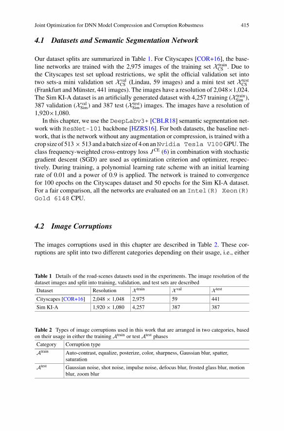
Joint Optimization for DNN Model Compression and Corruption Robustness 415

4.1 Datasets and Semantic Segmentation Network

Our dataset splits are summarized in Table 1. For Cityscapes [COR+16], the base-line networks are trained with the 2,975 images of the training set X train

CS . Due tothe Cityscapes test set upload restrictions, we split the official validation set intotwo sets-a mini validation set X val

CS (Lindau, 59 images) and a mini test set X testCS

(Frankfurt andMünster, 441 images). The images have a resolution of 2,048×1,024.The Sim KI-A dataset is an artificially generated dataset with 4,257 training (X train

Sim ),387 validation (X val

Sim) and 387 test (X testSim) images. The images have a resolution of

1,920×1,080.In this chapter, we use the DeepLabv3+ [CBLR18] semantic segmentation net-

work with ResNet-101 backbone [HZRS16]. For both datasets, the baseline net-work, that is the network without any augmentation or compression, is trained with acrop size of 513 × 513and abatch size of 4on anNvidia Tesla V100GPU.Theclass frequency-weighted cross-entropy loss JCE (6) in combination with stochasticgradient descent (SGD) are used as optimization criterion and optimizer, respec-tively. During training, a polynomial learning rate scheme with an initial learningrate of 0.01 and a power of 0.9 is applied. The network is trained to convergencefor 100 epochs on the Cityscapes dataset and 50 epochs for the Sim KI-A dataset.For a fair comparison, all the networks are evaluated on an Intel(R) Xeon(R)Gold 6148 CPU.

4.2 Image Corruptions

The images corruptions used in this chapter are described in Table 2. These cor-ruptions are split into two different categories depending on their usage, i.e., either

Table 1 Details of the road-scenes datasets used in the experiments. The image resolution of thedataset images and split into training, validation, and test sets are described

Dataset Resolution X train X val X test

Cityscapes [COR+16] 2,048 × 1,048 2,975 59 441

Sim KI-A 1,920 × 1,080 4,257 387 387

Table 2 Types of image corruptions used in this work that are arranged in two categories, basedon their usage in either the training Atrain or test Atest phases

Category Corruption type

Atrain Auto-contrast, equalize, posterize, color, sharpness, Gaussian blur, spatter,saturation

Atest Gaussian noise, shot noise, impulse noise, defocus blur, frosted glass blur, motionblur, zoom blur

416 S. Varghese et al.

Table 3 Corruptions and their parameterization used during training are listed. A dash (-) indicatesthat the corruption function is image-dependent and does not need any parameterization. An interval[a, b] indicates that the respective parameter is a real numberR sampled uniformly from this interval

Corruption type Auto-contrast Equalize Posterize Color

Parameterization – – [0, 4.0] [0.25, 4.0]

Corruption type Sharpness Gaussian blur Spatter Saturation

Parameterization [0.25, 4.0] 8 {0.65, 0.5, 0.3,0.7, 0.65}

{1.5, 0.1}

during training or during test. The corruptions Atest in the test process are adoptedfrom the neural network robustness benchmark1 from [HD19]. The corruptionsAtrain

used in the training process are adopted following a large body of work [HMC+20,CZM+19, TPL+19, SK19] that use these corruptions in different ways for trainingwith data augmentation. Table 3 gives an overview of the parameterization of eachcorruption within Atrain. For spatter corruption, the list of parameters correspondsto the location, scale, two sigma, and threshold values, respectively. For saturationcorruption, the list of parameters corresponds to the amount of saturation and thescale. For posterize, color, and sharpness corruptions, the parameter is sampled fromwithin the given interval.

Definition of severities: Various kinds of data augmentations exist, and it is ratherdifficult to compare between different augmentation types, although first attempts areknown [KBFs20]. Let us take an example of brightness and contrast augmentations.We can increase or decrease the brightness and contrast values for a given input imagebymanipulating the image pixel values. An increase in the brightness and an increasein the contrast do not necessarily correspond to the same effect on the input image.To standardize the method of measuring the strength of augmentations irrespectiveof the augmentation type, the structural similarity (SSIM) metric [WBSS04] is used.To do this, SSIM is computed between the clean input image x and the augmentedimage x(b). Here, SSIM(x, x(b))=0 indicates that the image x and the correspondingaugmented image x(b) are completely dissimilar. Similarly, SSIM(x, x(b))=1 indi-cates that the image x and the corresponding augmented image x(b) are identical, orno augmentation is applied. We define severity levels (V ) to indicate the strengthof the augmentation. Severity level V =0 indicates that no type of augmentation isapplied to the input image and severity level V =10 indicates that the input imageis completely dissimilar after the augmentation. This means that for every increasein level in V , the SSIM between the clean input image and the augmented imagereduces by 0.1. To control the severity of the data augmentation during training, theparameters (α, β) of the γ -function are varied (see Fig. 2) by keeping the corruptionparameters constant following Table 2.

1 https://github.com/hendrycks/robustness.

Joint Optimization for DNN Model Compression and Corruption Robustness 417

4.3 Metrics

Mean intersection-over-union (mIoU) between the predictions of the semanticsegmentation network and the human-annotated ground truth labels is commonlyused for evaluating semantic segmentation networks. The mIoU is defined as

mIoU= 1

S

∑

s∈S

TP(s)

TP(s) + FP(s) + FN(s)=mIoU(y, y), (13)

where TP(s), FP(s), and FN(s) are the class-specific true positives, false positives, andfalse negatives, respectively, computed between segmentation output y and groundtruth one-hot encoded segmentation y.

Mean performance under corruption (mPC) has been introduced by [HD19]for evaluating the robustness of neural networks under varying corruptions and vary-ing strengths. For this purpose, the individual augmentations An ∈ Atest are furthersub-divided with respect to the strength of the augmentations. We use the augmen-tations Atest (see Table 2) for the computation of mPC. This is computed by

mPC = 1

|Atest||Atest |∑

c=1

1

Nc

Nc∑

V=1

mIoUc,V , (14)

with corruption index c and Nc denoting the amount of severity conditions for a cor-ruption c. Here, mIoUc,V denotes the mIoU (13) of the model under the corruption cand severity V . The key factor here is choosing the severities, as this can vary on dif-ferent datasets, and even models, depending on the selection criteria. In this chapter,we use the SSIMmetric [HD19] as a means of finding severity thresholds. Using thismetric allows for standardized severities across a dataset, as it is task- and model-agnostic. Thus, different robustness improvement methods can be benchmarked andcompared easily using the mPC metric.

Relative performance under corruption (rPC) is simply the ratio of the mPC andthe mIoU of the semantic segmentation under the corruptions during evaluation, andis defined as

rPC = mPC

mIoU. (15)

4.4 Training Framework

For the task of achieving robust and compressed semantic segmentation networks,one can envision various different ways to approach it. An overview of all possibleapproaches is given in Fig. 5. For all the reference models, we start from the pre-trained checkpoint weights of the ResNet-101 backbone for the DeepLabv3+architecture.

418 S. Varghese et al.

Fig. 5 The training approaches used in this work are depicted. In addition to the simple baselines(Reference A, and Reference B), we compare our HCRC approach against sequential applications(Reference C, and Reference D) of the individual steps in the training framework

Reference A: In this approach, the DeepLabv3+ network with the ResNet-101backbone is trained for improving its corruption robustness. Here, no compressiontechniques are applied. The network is trained using the protocol defined in Sect. 4.1with the total loss (5) and λ=10−6.

Reference B: Here, the DeepLabv3+ undergoes one-shot pruning (see Algo-rithm 1). First, the network is trained using the protocol defined in Sect. 4.1 withthe class frequency weighted cross-entropy loss (6). Next, the statistics (9), (10) arecomputed on the X train and X val set and the network undergoes PTQ (see Fig. 3). Norobustness-related training is enforced.

Reference C: In this configuration, we perform sequential application of the robust-ness and compression goals. In the first step, the DeepLabv3+ is trained using theprotocol defined in Sect. 4.1 with the total loss (5) and λ=10−6 (see also ReferenceA) in combination with the data augmentation strategy described in Sect. 3.2 (seeFig. 2). Next, the network undergoes iterative pruning (see Algorithm1) followingagain the protocol defined in Sect. 4.1, this time with the class frequency weightedcross-entropy loss (6). Finally, statistics (9), (10) are computed on theX train andX val

set and the network undergoes PTQ (see Fig. 3).

Reference D: In this setup, the DeepLabv3+, the network is first one-shot pruned(seeAlgorithm1) and thenfine-tuned following the protocol defined inSect. 4.1 using

Joint Optimization for DNN Model Compression and Corruption Robustness 419

the class frequency weighted cross-entropy loss (6). In the next step, the networkis trained with the data augmentation strategy described in Sect. 3.2 (see Fig. 2)following again the protocol defined in Sect. 4.1, however, this time the total loss J (5)is used as the optimization criterion. Finally, statistics (9, 10) are computed on theX train and X val set and the network undergoes PTQ (see Fig. 3).

5 Experimental Results and Discussion

5.1 Ablation Studies

In-training quantization (ITQ) vs. post-training quantization (PTQ)We hypoth-esize that training the network with quantization errors is better than quantizing thenetwork after training.

In Table 4, we compare these two approaches of achieving quantized networks.The baseline DeepLabv3+ network has an mIoU of 69.78% and mPC of 44.03%.On one hand, we observe that mIoU drops by 5.35% and mPC by 2.76% (both:absolute) after PTQ. On the other hand, the drop in mIoU is only 1.8% after ITQ,within no change in mPC. This result supports the abovementioned hypothesis onquantization, that in-training quantization is superior to post-training quantization.Additionally, we increased the size of the calibration set used within PTQ by alsoincluding X val along with X train. This, however, resulted in no significant changes inthe performance of the quantized networks.

Controlled severity training: The semantic segmentation network is evaluated overvarious corruptions and various severity levels. From our initial experiments, weobserved that the data corruptions used during the training process [HMC+20] havea mean severity level of V = 1. It is intuitive that a network trained on data aug-mentations of higher severity should be, in theory, more robust to higher severitycorruptions during test. To study the effect of the training severity on the robustnessof the trained semantic segmentation network, we train the DeepLabv3+ networkwith three different severities of corruption. To do this, we vary the parameters of the

Table 4 Test set X testCS evaluation of mIoU, mPC, and rPC comparing the non-quantized

DeepLabv3+ network, and the corresponding PTQ and ITQ networks that are trained to conver-gence for 100 epochs. Note that the inference times are computed on the Intel(R) Xeon(R)Gold 6148 CPU. Best numbers reported in bold

Method mIoU [%] (13) mPC [%] (14) rPC [%] (15) Time (s)

DeepLabv3+ 69.78 44.03 63.09 5.23

with PTQ 64.43 41.27 64.05 2.66

with ITQ 67.98 44.04 64.78 2.66

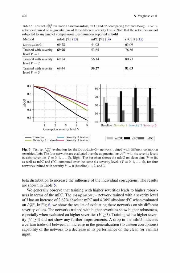
420 S. Varghese et al.

Table 5 Test setX testCS evaluation based onmIoU,mPC, and rPCcomparing the threeDeepLabv3+

networks trained on augmentations of three different severity levels. Note that the networks are notsubjected to any kind of compression. Best numbers reported in bold

Method mIoU [%] (13) mPC [%] (14) rPC [%] (15)

DeepLabv3+ 69.78 44.03 63.09

Trained with severitylevel V = 1

69.98 53.65 76.66

Trained with severitylevel V = 2

69.54 56.14 80.73

Trained with severitylevel V = 3

69.44 56.27 81.03

Fig. 6 Test set X testCS evaluation for the DeepLabv3+ network trained with different corruption

severities. Left: The four networks are evaluated over the augmentationsAtest with six severity levels(x-axis, severities V = 0, 1, . . . , 5). Right: The bar chart shows the mIoU on clean data (V = 0),as well as mPC and rPC, computed over the same six severity levels (V = 0, 1, . . . , 5), for fournetworks trained with severity V = 0 (baseline), 1, 2, and 3

beta distribution to increase the influence of the individual corruptions. The resultsare shown in Table 5.

We generally observe that training with higher severities leads to higher robust-ness in terms of the mPC. The DeepLabv3+ network trained with a severity levelof 3 has an increase of 2.62% absolute mPC and 4.36% absolute rPC when evaluatedon X test

CS . In Fig. 6, we show the results of evaluating these networks on six differentseverity values. The networks trained with higher severities show higher robustness,especially when evaluated on higher severities (V ≥3). Training with a higher sever-ity (V ≥4) did not show any further improvements. A drop in the mIoU indicatesa certain trade-off between an increase in the generalization (to unseen corruptions)capability of the network to a decrease in its performance on the clean (or vanilla)input.

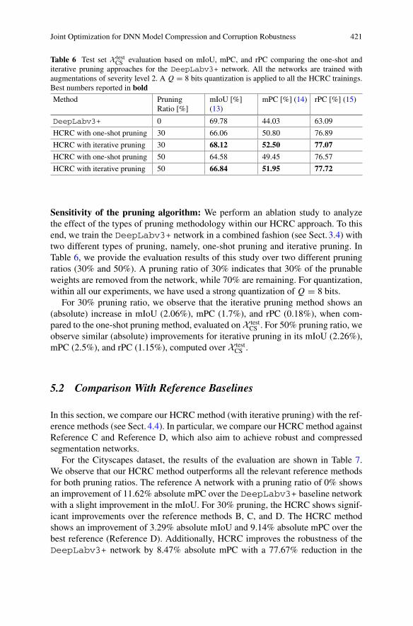
Joint Optimization for DNN Model Compression and Corruption Robustness 421

Table 6 Test set X testCS evaluation based on mIoU, mPC, and rPC comparing the one-shot and

iterative pruning approaches for the DeepLabv3+ network. All the networks are trained withaugmentations of severity level 2. A Q = 8 bits quantization is applied to all the HCRC trainings.Best numbers reported in bold

Method PruningRatio [%]

mIoU [%](13)

mPC [%] (14) rPC [%] (15)

DeepLabv3+ 0 69.78 44.03 63.09

HCRC with one-shot pruning 30 66.06 50.80 76.89

HCRC with iterative pruning 30 68.12 52.50 77.07

HCRC with one-shot pruning 50 64.58 49.45 76.57

HCRC with iterative pruning 50 66.84 51.95 77.72

Sensitivity of the pruning algorithm: We perform an ablation study to analyzethe effect of the types of pruning methodology within our HCRC approach. To thisend, we train the DeepLabv3+ network in a combined fashion (see Sect. 3.4) withtwo different types of pruning, namely, one-shot pruning and iterative pruning. InTable 6, we provide the evaluation results of this study over two different pruningratios (30% and 50%). A pruning ratio of 30% indicates that 30% of the prunableweights are removed from the network, while 70% are remaining. For quantization,within all our experiments, we have used a strong quantization of Q = 8 bits.

For 30% pruning ratio, we observe that the iterative pruning method shows an(absolute) increase in mIoU (2.06%), mPC (1.7%), and rPC (0.18%), when com-pared to the one-shot pruning method, evaluated onX test

CS . For 50% pruning ratio, weobserve similar (absolute) improvements for iterative pruning in its mIoU (2.26%),mPC (2.5%), and rPC (1.15%), computed over X test

CS .

5.2 Comparison With Reference Baselines

In this section, we compare our HCRC method (with iterative pruning) with the ref-erence methods (see Sect. 4.4). In particular, we compare our HCRC method againstReference C and Reference D, which also aim to achieve robust and compressedsegmentation networks.

For the Cityscapes dataset, the results of the evaluation are shown in Table 7.We observe that our HCRC method outperforms all the relevant reference methodsfor both pruning ratios. The reference A network with a pruning ratio of 0% showsan improvement of 11.62% absolute mPC over the DeepLabv3+ baseline networkwith a slight improvement in the mIoU. For 30% pruning, the HCRC shows signif-icant improvements over the reference methods B, C, and D. The HCRC methodshows an improvement of 3.29% absolute mIoU and 9.14% absolute mPC over thebest reference (Reference D). Additionally, HCRC improves the robustness of theDeepLabv3+ network by 8.47% absolute mPC with a 77.67% reduction in the

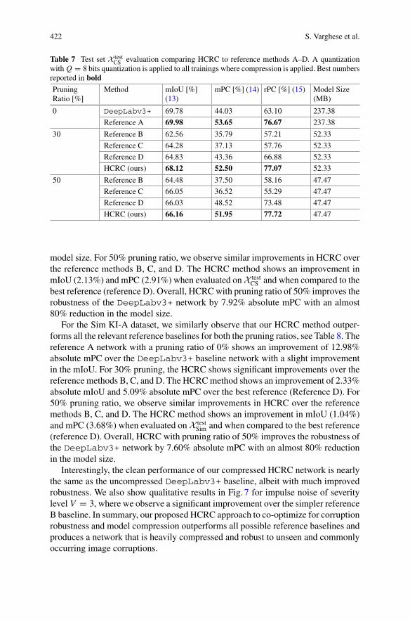
422 S. Varghese et al.

Table 7 Test set X testCS evaluation comparing HCRC to reference methods A–D. A quantization

with Q = 8 bits quantization is applied to all trainings where compression is applied. Best numbersreported in bold

PruningRatio [%]

Method mIoU [%](13)

mPC [%] (14) rPC [%] (15) Model Size(MB)

0 DeepLabv3+ 69.78 44.03 63.10 237.38

Reference A 69.98 53.65 76.67 237.38

30 Reference B 62.56 35.79 57.21 52.33

Reference C 64.28 37.13 57.76 52.33

Reference D 64.83 43.36 66.88 52.33

HCRC (ours) 68.12 52.50 77.07 52.33

50 Reference B 64.48 37.50 58.16 47.47

Reference C 66.05 36.52 55.29 47.47

Reference D 66.03 48.52 73.48 47.47

HCRC (ours) 66.16 51.95 77.72 47.47

model size. For 50% pruning ratio, we observe similar improvements in HCRC overthe reference methods B, C, and D. The HCRC method shows an improvement inmIoU (2.13%) and mPC (2.91%) when evaluated onX test

CS and when compared to thebest reference (reference D). Overall, HCRCwith pruning ratio of 50% improves therobustness of the DeepLabv3+ network by 7.92% absolute mPC with an almost80% reduction in the model size.

For the Sim KI-A dataset, we similarly observe that our HCRC method outper-forms all the relevant reference baselines for both the pruning ratios, see Table 8. Thereference A network with a pruning ratio of 0% shows an improvement of 12.98%absolute mPC over the DeepLabv3+ baseline network with a slight improvementin the mIoU. For 30% pruning, the HCRC shows significant improvements over thereference methods B, C, and D. The HCRCmethod shows an improvement of 2.33%absolute mIoU and 5.09% absolute mPC over the best reference (Reference D). For50% pruning ratio, we observe similar improvements in HCRC over the referencemethods B, C, and D. The HCRC method shows an improvement in mIoU (1.04%)and mPC (3.68%) when evaluated on X test

Sim and when compared to the best reference(reference D). Overall, HCRC with pruning ratio of 50% improves the robustness ofthe DeepLabv3+ network by 7.60% absolute mPC with an almost 80% reductionin the model size.

Interestingly, the clean performance of our compressed HCRC network is nearlythe same as the uncompressed DeepLabv3+ baseline, albeit with much improvedrobustness. We also show qualitative results in Fig. 7 for impulse noise of severitylevel V = 3, where we observe a significant improvement over the simpler referenceB baseline. In summary, our proposed HCRC approach to co-optimize for corruptionrobustness and model compression outperforms all possible reference baselines andproduces a network that is heavily compressed and robust to unseen and commonlyoccurring image corruptions.

Joint Optimization for DNN Model Compression and Corruption Robustness 423

Table 8 Test set X testSim evaluation comparing HCRC to reference methods A–D. A quantization

with Q = 8 bits is applied to all trainings where compression is applied. Best numbers reported inbold

PruningRatio [%]

Method mIoU [%](13)

mPC [%] (14) rPC [%] (15) Model Size(MB)

0 DeepLabv3+ 77.57 54.42 70.16 237.38

Reference A 77.05 67.40 87.48 237.38

30 Reference B 74.19 49.78 67.10 52.33

Reference C 72.44 51.56 71.17 52.33

Reference D 73.90 58.70 79.43 52.33

HCRC (ours) 76.23 63.79 83.68 52.33

50 Reference B 75.65 47.60 62.92 47.47

Reference C 75.08 47.82 63.69 47.47

Reference D 74.38 58.34 78.43 47.47

HCRC (ours) 76.12 62.02 81.48 47.47

Fig. 7 Example segmentations on the Cityscapes dataset. We show a snippet fromX testCS , where the

differences in the robustness of the compressed networks are more pronounced. We observe thatour HCRC method is compressed and has superior robustness to the DeepLabv3+ baseline andthe compressed network of reference B, in this example, for impulse noise corruption

6 Conclusions

In this chapter, we introduce hybrid corruption-robustness focused compression(HCRC), an approach to jointly optimize a neural network for achieving networkcompression along with improvement in corruption robustness, such as noise andblurring artifacts, which are commonly observed. For this study, we consider thetask of semantic segmentation for automated driving and look at the interactionsbetween robustness and compression of networks. HCRC improves the robustnessof the DeepLabv3+ network by 8.47% absolute mean performance under corrup-tion (mPC) on the Cityscapes dataset and 7.60% absolute mPC on the Sim KI-Adataset and generalizes even to augmentations not seen by the network in the train-ing process. This is achieved with only minor degradations on undisturbed data.

424 S. Varghese et al.

Our approach is evaluated over two strong compression ratios and consistently out-performs all considered baseline approaches. Additionally, we perform extensiveablation studies to further leverage and extend existing state-of-the-art methods.

Acknowledgements The research leading to these results is fundedby theGermanFederalMinistryfor Economic Affairs and Energy within the project “Methoden und Maßnahmen zur Absicherungvon KI-basierten Wahrnehmungsfunktionen für das automatisierte Fahren (KI Absicherung)”. Theauthors would like to thank the consortium for the successful cooperation.

References

[AMT18] A. Arnab, O. Miksik, P.H.S. Torr, On the robustness of semantic segmentation modelsto adversarial attacks, inProceedings of the IEEE/CVFConference onComputerVisionand Pattern Recognition (CVPR) (Salt Lake City, UT, USA, 2018), pp. 888–897

[BHSFs19] A. Bär, F. Hüger, P. Schlicht, T. Fingscheidt, On the robustness of redundant teacher-student frameworks for semantic segmentation, in Proceedings of the IEEE/CVF Con-ference onComputer Vision andPattern Recognition (CVPR)Workshops (LongBeach,CA, USA, 2019), pp. 1380–1388

[BKV+20] A. Bär, M. Klingner, S. Varghese, F. Hüger, P. Schlicht, T. Fingscheidt, Robust seman-tic segmentation by redundant networks with a layer-specific loss contribution andmajority vote, in Proceedings of the IEEE/CVF Conference on Computer Vision andPattern Recognition (CVPR) Workshops, virtual conference (2020), pp. 1348–1358

[CBD15] M. Courbariaux, Y. Bengio, J-P. David, Binary connect: training deep neural networkswith binary weights during propagations, in Proceedings of the Conference on NeuralInformation Processing Systems (NIPS/NeurIPS) (Montréal, QC, Canada, 2015), pp.3123–3133

[CBLR18] Z. Chen, V. Badrinarayanan, C-Y. Lee, A. Rabinovich, GradNorm: gradient normal-ization for adaptive loss balancing in deep multitask networks, in Proceedings of theInternational Conference on Machine Learning (ICML) (Stockholm, Sweden, 2018),pp. 794–803

[CLW+16] Y. Cao, M. Long, J. Wang, H. Zhu, Q. Wen, Deep quantization network for effi-cient image retrieval, in Proceedings of the AAAI Conference on Artificial Intelligence(Phoenix, AZ, USA, 2016), pp. 3457–3463

[COR+16] M. Cordts, M. Omran, S. Ramos, T. Rehfeld, M. Enzweiler, R. Benenson, U. Franke,S. Roth, B. Schiele, The Cityscapes dataset for semantic urban scene understanding,in Proceedings of the IEEE/CVF Conference on Computer Vision and Pattern Recog-nition (CVPR) (Las Vegas, NV, USA, 2016), pp. 3213–3223

[CPK+18] L.-C. Chen, G. Papandreou, I. Kokkinos, K. Murphy, A.L. Yuille, DeepLab: seman-tic image segmentation with deep convolutional nets, atrous convolution, and fullyconnected CRFs. IEEE Trans. Pattern Anal. Mach. Intell. (TPAMI) 40(4), 834–848(2018)

[CZM+19] E.D. Cubuk, B. Zoph, D. Mane, V. Vasudevan, Q.V. Le, AutoAugment: learning aug-mentation strategies from data, in Proceedings of the IEEE/CVF Conference on Com-puter Vision and Pattern Recognition (CVPR) (Long Beach, CA, USA, 2019), pp.113–123

[DFY+20] Y. Dong, Q-A. Fu, X. Yang, T. Pang, H. Su, Z. Xiao, J. Zhu, Benchmarking adversarialrobustness on image classification, in Proceedings of the IEEE/CVF Conference onComputer Vision and Pattern Recognition (CVPR), virtual conference (2020), pp.1322–1330

Joint Optimization for DNN Model Compression and Corruption Robustness 425

[GAGN15] S. Gupta, A. Agrawal, K. Gopalakrishnan, P. Narayanan, Deep learning with lim-ited numerical precision, in Proceedings of the International Conference on MachineLearning (ICML) (Lille, France, 2015), pp. 1737–1746

[GSS15] I. Goodfellow, J. Shlens, C. Szegedy, Explaining and harnessing adversarial examples,in Proceedings of the International Conference on Learning Representations (ICLR)(San Diego, CA, USA, 2015), pp. 1–11

[GWY+19] S. Gui, H.Wang, H. Yang, C. Yu, Z.Wang, J. Liu, Model compression with adversarialrobustness: a unified optimization framework, in Proceedings of the Conference onNeural Information Processing Systems (NIPS/NeurIPS) (Vancouver, BC, Canada,2019), pp. 1283–1294

[HD19] D.Hendrycks, T. Dietterich, Benchmarking neural network robustness to common cor-ruptions andperturbations, inProceedings of the InternationalConference onLearningRepresentations (ICLR) (New Orleans, LA, USA, 2019), pp. 1–15

[HMC+20] D. Hendrycks, N. Mu, E.D. Cubuk, B. Zoph, J. Gilmer, B. Lakshminarayanan, Aug-mix: a simple data processing method to improve robustness and uncertainty, in Pro-ceedings of the International Conference on Learning Representations (ICLR), virtualconference (2020), pp. 1–15

[HMD16] S. Han, H.Mao,W.J. Dally, Deep compression: compressing deep neural networkwithpruning, trained quantization and Huffman coding, in proceedings of the internationalconference on learning representations (ICLR) (2016), pp. 1–14

[HPTD15] S. Han, J. Pool, J. Tran,W.J. Dally, Learning both weights and connections for efficientneural networks, in Proceedings of the Conference on Neural Information ProcessingSystems (NIPS/NeurIPS) (Montréal, QC, Canada, 2015), pp. 1135–1143

[HVD14] G. Hinton, O. Vinyals, J. Dean, Distilling the knowledge in a neural network, in Pro-ceedings of theConference onNeural InformationProcessingSystems (NIPS/NeurIPS)Workshops (Montréal, QC, Canada, 2014), pp. 1–9

[HZRS16] K. He, X. Zhang, S. Ren, J. Sun, Deep residual learning for image recognition, in Pro-ceedings of the IEEE/CVF Conference on Computer Vision and Pattern Recognition(CVPR) (Las Vegas, NV, USA, 2016), pp. 770–778,

[HZS17] Y. He, X. Zhang, J. Sun, Channel pruning for accelerating very deep neural networks,in Proceedings of the IEEE International Conference on Computer Vision (ICCV)(Venice, Italy, 2017), pp. 1398–1406

[JGWD19] S. Jain, A. Gural, Mi. Wu, C. Dick, Trained uniform quantization for accurateand efficient neural network inference on fixed-point hardware (2019), pp. 1–17,arXiv:1903.08066

[JKC+18] B. Jacob, S. Kligys, B. Chen, M. Zhu, M. Tang, A.G. Howard, H. Adam, D.Kalenichenko, Quantization and training of neural networks for efficient integer-arithmetic-only inference, in Proceedings of the IEEE/CVF Conference on ComputerVision and Pattern Recognition (CVPR) (Salt Lake City, UT, USA, 2018), pp. 2704–2713

[KBFs20] M. Klingner, A. Bär, T. Fingscheidt, Improved noise and attack robustness for seman-tic segmentation by using multi-task training with self-supervised depth estimation, inProceedings of the IEEE/CVF Conference on Computer Vision and Pattern Recogni-tion (CVPR) Workshops , virtual conference (2020), pp. 1299–1309

[KBK20] I. Kim, W. Baek, S. Kim, Spatially attentive output layer for image classification, inProceedings of the IEEE/CVF Conference on Computer Vision and Pattern Recogni-tion (CVPR), virtual conference (2020), pp. 9533–9542

[Kri09] A.Krizhevsky,ObjectClassificationExperiments (Technical report,Canadian Institutefor Advanced Research, April 2009)

[LBBH98] Y. LeCun, L. Bottou, Y. Bengio, P. Haffner, Gradient-based learning applied to docu-ment recognition. IEEE 86(11), 2278–2324 (1998)

[LGH19] J. Lin, C.Gan, S. Han, Defensive quantization: when efficiency meets robustness,in Proceedings of the International Conference on Learning Representations (ICLR)(New Orleans, LA, USA, 2019), pp. 1–15

426 S. Varghese et al.

[MBKR18] D. Mittal, S. Bhardwaj, M. Khapra, B. Ravindran, Recovering from random pruning:on the plasticity of deep convolutional neural networks, in Proceedings of the WinterConference on Applications of Computer Vision (WACV) (Lake Tahoe, NV, USA,2018), pp. 848–857

[MMS+18] A. Madry, A. Makelov, L. Schmidt, D. Tsipras, A. Vladu, Towards deep learningmodels resistant to adversarial attacks, in Proceedings of the International Conferenceon Learning Representations (ICLR) (Vancouver, BC, Canada, 2018), pp. 1–10

[MS99] D. Christopher, Manning and Hinrich Schütze (MIT Press, Foundations of StatisticalNatural Language Processing, 1999)

[MTK+17] P. Molchanov, S. Tyree, T. Karras, T. Aila, J. Kautz, Pruning convolutional neural net-works for resource efficient inference, in Proceedings of the International Conferenceon Learning Representations (ICLR) (Toulon, France, 2017), pp. 1–17

[NWC+11] Y. Netzer, T. Wang, A. Coates, A. Bissacco, B. Wu, A.Y. Ng, Reading digits in naturalimageswith unsupervised feature learning, inProceedings of theConference onNeuralInformation Processing Systems (NIPS/NeurIPS) Workshops (Granada, Spain, 2011),pp. 1–9

[SK19] C. Shorten, T.M. Khoshgoftaar, A survey on image data augmentation for deep learn-ing. J. Big Data 60(6), 1–48 (2019)

[SVS19] J. Su, D.V. Vargas, K. Sakurai, One pixel attack for fooling deep neural networks.IEEE Trans. Evolut. Comput. (TEVC) 23(5), 828–841 (2019)

[SWMJ20] V. Sehwag, S. Wang, P. Mittal, S. Jana, HYDRA: pruning adversarially robust neuralnetworks (2020), pp. 1–22. arXiv:2002.10509

[TKTH18] L. Theis, I. Korshunova, A. Tejani, F. Huszár, Faster Gaze Prediction With DenseNetworks and Fisher Pruning (2018), pp. 1–18. arXiv:1801.05787

[TPL+19] Z. Tang, X. Peng, T. Li, Y. Zhu, D. Metaxas, Adatrans form: adaptive data transforma-tion, inProceedings of the IEEE International Conference on Computer Vision (ICCV)(Seoul, Korea, 2019), pp. 2998–3006

[WBSS04] Z. Wang, A.C. Bovik, H.R. Sheikh, E.P. Simoncelli, Image quality assessment: fromerror visibility to structural similarity. IEEE Trans. Image Process. 13(4), 600–612(2004)

[WLX+20] S. Wang, N. Liao, L. Xiang, N. Ye, Q. Zhang, Achieving Adversarial Robustness viaSparsity (2020), pp. 1–9, arXiv:2009.05423

[WSC+20] J. Wang, K. Sun, T. Cheng, B. Jiang, C. Deng, Y. Zhao, D. Liu, M. Yadong, M. Tan,X. Wang et al., Deep high-resolution representation learning for visual recognition.IEEE Trans. Pattern Anal. Mach. Intell. (TPAMI) 43(10), 3349–3364 (2020)

[XLZ+18] C. Xiao, B. Li, J-Y. Zhu, W. He, M. Liu, D. Song, Generating adversarial exampleswith adversarial networks (2018), pp. 1–8, arXiv:1801.02610

[XQXL20] H. Xie, L. Qian, X.g Xiang, N. Liu, Blind adversarial pruning: balance accuracy,efficiency and robustness (2020), pp. 1–12. arXiv: 2004.05913

[XWZ+17] C. Xie, J. Wang, Z. Zhang, Y. Zhou, L. Xie, A. Yuille, Adversarial examples forsemantic segmentation and object detection, in Proceedings of the IEEE InternationalConference on Computer Vision (ICCV) (Venice, Italy, 2017), pp. 1369–1378

[YXC20] M. Ye, S. Xu, T. Cao, HVNet: hybrid voxel network for LiDAR based 3d object detec-tion, in Proceedings of the IEEE/CVF Conference on Computer Vision and PatternRecognition (CVPR), virtual conference (2020), pp. 1631–1640

[YXL+19] S. Ye, K. Xu, S. Liu, H. Cheng, J.H. Lambrechts, H. Zhang, A. Zhou, K. Ma, Y. Wang,X. Lin, Adversarial robustness vs. model compression, or both? in Proceedings of theIEEE International Conference on Computer Vision (ICCV) (Seoul, Korea, October2019), pp. 111–120

[ZHZ11] M. Zhou,M.Huang, X. Zhu, Robust reading comprehensionwith linguistic constraintsvia posterior regularization. IEEE/ACM Trans. Audio, Speech, Lang. Process. 20(4),1096–1108 (2011)

[ZS18] Z. Zhang, M.R. Sabuncu, Generalized cross entropy loss for training deep neuralnetworks with noisy labels, in Proceedings of the Conference on Neural InformationProcessing Systems (NIPS/NeurIPS) (Montréal, QC, Canada, 2018), pp. 8792–8802

Joint Optimization for DNN Model Compression and Corruption Robustness 427

[ZSMA19] Y. Zhao, I. Shumailov, R. Mullins, R. Anderson, To compress or not to compress:understanding the interactions between adversarial attacks and neural network com-pression, inProceedings of the Conference onMachine Learning and Systems (MLSys)(Stanford, CA, USA, 2019), pp. 230–240

Open Access This chapter is licensed under the terms of the Creative Commons Attribution 4.0International License (http://creativecommons.org/licenses/by/4.0/), which permits use, sharing,adaptation, distribution and reproduction in any medium or format, as long as you give appropriatecredit to the original author(s) and the source, provide a link to the Creative Commons license andindicate if changes were made.

The images or other third party material in this chapter are included in the chapter’s CreativeCommons license, unless indicated otherwise in a credit line to the material. If material is notincluded in the chapter’s Creative Commons license and your intended use is not permitted bystatutory regulation or exceeds the permitted use, you will need to obtain permission directly fromthe copyright holder.