Decoupling spatial and temporal patterns in short-term beach shoreline response to wave climate
10
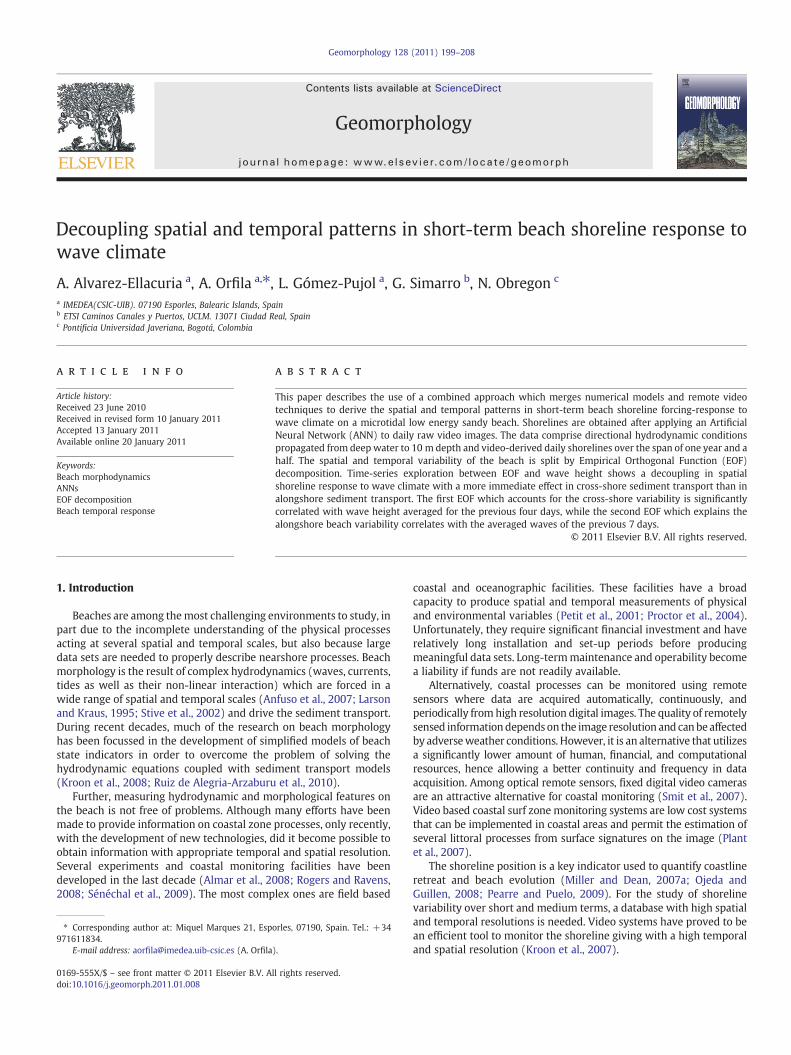
Decoupling spatial and temporal patterns in short-term beach shoreline response to wave climate A. Alvarez-Ellacuria a , A. Orfila a, ⁎, L. Gómez-Pujol a , G. Simarro b , N. Obregon c a IMEDEA(CSIC-UIB). 07190 Esporles, Balearic Islands, Spain b ETSI Caminos Canales y Puertos, UCLM. 13071 Ciudad Real, Spain c Pontificia Universidad Javeriana, Bogotá, Colombia abstract article info Article history: Received 23 June 2010 Received in revised form 10 January 2011 Accepted 13 January 2011 Available online 20 January 2011 Keywords: Beach morphodynamics ANNs EOF decomposition Beach temporal response This paper describes the use of a combined approach which merges numerical models and remote video techniques to derive the spatial and temporal patterns in short-term beach shoreline forcing-response to wave climate on a microtidal low energy sandy beach. Shorelines are obtained after applying an Artificial Neural Network (ANN) to daily raw video images. The data comprise directional hydrodynamic conditions propagated from deep water to 10 m depth and video-derived daily shorelines over the span of one year and a half. The spatial and temporal variability of the beach is split by Empirical Orthogonal Function (EOF) decomposition. Time-series exploration between EOF and wave height shows a decoupling in spatial shoreline response to wave climate with a more immediate effect in cross-shore sediment transport than in alongshore sediment transport. The first EOF which accounts for the cross-shore variability is significantly correlated with wave height averaged for the previous four days, while the second EOF which explains the alongshore beach variability correlates with the averaged waves of the previous 7 days. © 2011 Elsevier B.V. All rights reserved. 1. Introduction Beaches are among the most challenging environments to study, in part due to the incomplete understanding of the physical processes acting at several spatial and temporal scales, but also because large data sets are needed to properly describe nearshore processes. Beach morphology is the result of complex hydrodynamics (waves, currents, tides as well as their non-linear interaction) which are forced in a wide range of spatial and temporal scales (Anfuso et al., 2007; Larson and Kraus, 1995; Stive et al., 2002) and drive the sediment transport. During recent decades, much of the research on beach morphology has been focussed in the development of simplified models of beach state indicators in order to overcome the problem of solving the hydrodynamic equations coupled with sediment transport models (Kroon et al., 2008; Ruiz de Alegria-Arzaburu et al., 2010). Further, measuring hydrodynamic and morphological features on the beach is not free of problems. Although many efforts have been made to provide information on coastal zone processes, only recently, with the development of new technologies, did it become possible to obtain information with appropriate temporal and spatial resolution. Several experiments and coastal monitoring facilities have been developed in the last decade (Almar et al., 2008; Rogers and Ravens, 2008; Sénéchal et al., 2009). The most complex ones are field based coastal and oceanographic facilities. These facilities have a broad capacity to produce spatial and temporal measurements of physical and environmental variables (Petit et al., 2001; Proctor et al., 2004). Unfortunately, they require significant financial investment and have relatively long installation and set-up periods before producing meaningful data sets. Long-term maintenance and operability become a liability if funds are not readily available. Alternatively, coastal processes can be monitored using remote sensors where data are acquired automatically, continuously, and periodically from high resolution digital images. The quality of remotely sensed information depends on the image resolution and can be affected by adverse weather conditions. However, it is an alternative that utilizes a significantly lower amount of human, financial, and computational resources, hence allowing a better continuity and frequency in data acquisition. Among optical remote sensors, fixed digital video cameras are an attractive alternative for coastal monitoring (Smit et al., 2007). Video based coastal surf zone monitoring systems are low cost systems that can be implemented in coastal areas and permit the estimation of several littoral processes from surface signatures on the image (Plant et al., 2007). The shoreline position is a key indicator used to quantify coastline retreat and beach evolution (Miller and Dean, 2007a; Ojeda and Guillen, 2008; Pearre and Puelo, 2009). For the study of shoreline variability over short and medium terms, a database with high spatial and temporal resolutions is needed. Video systems have proved to be an efficient tool to monitor the shoreline giving with a high temporal and spatial resolution (Kroon et al., 2007). Geomorphology 128 (2011) 199–208 ⁎ Corresponding author at: Miquel Marques 21, Esporles, 07190, Spain. Tel.: + 34 971611834. E-mail address: aorfi[email protected] (A. Orfila). 0169-555X/$ – see front matter © 2011 Elsevier B.V. All rights reserved. doi:10.1016/j.geomorph.2011.01.008 Contents lists available at ScienceDirect Geomorphology journal homepage: www.elsevier.com/locate/geomorph
Transcript of Decoupling spatial and temporal patterns in short-term beach shoreline response to wave climate
Geomorphology 128 (2011) 199–208
Contents lists available at ScienceDirect
Geomorphology
j ourna l homepage: www.e lsev ie r.com/ locate /geomorph
Decoupling spatial and temporal patterns in short-term beach shoreline response towave climate
A. Alvarez-Ellacuria a, A. Orfila a,⁎, L. Gómez-Pujol a, G. Simarro b, N. Obregon c
a IMEDEA(CSIC-UIB). 07190 Esporles, Balearic Islands, Spainb ETSI Caminos Canales y Puertos, UCLM. 13071 Ciudad Real, Spainc Pontificia Universidad Javeriana, Bogotá, Colombia
⁎ Corresponding author at: Miquel Marques 21, Esp971611834.
E-mail address: [email protected] (A. Orfila
0169-555X/$ – see front matter © 2011 Elsevier B.V. Adoi:10.1016/j.geomorph.2011.01.008
a b s t r a c t
a r t i c l e i n f oArticle history:Received 23 June 2010Received in revised form 10 January 2011Accepted 13 January 2011Available online 20 January 2011
Keywords:Beach morphodynamicsANNsEOF decompositionBeach temporal response
This paper describes the use of a combined approach which merges numerical models and remote videotechniques to derive the spatial and temporal patterns in short-term beach shoreline forcing-response towave climate on a microtidal low energy sandy beach. Shorelines are obtained after applying an ArtificialNeural Network (ANN) to daily raw video images. The data comprise directional hydrodynamic conditionspropagated from deep water to 10 m depth and video-derived daily shorelines over the span of one year and ahalf. The spatial and temporal variability of the beach is split by Empirical Orthogonal Function (EOF)decomposition. Time-series exploration between EOF and wave height shows a decoupling in spatialshoreline response to wave climate with a more immediate effect in cross-shore sediment transport than inalongshore sediment transport. The first EOF which accounts for the cross-shore variability is significantlycorrelated with wave height averaged for the previous four days, while the second EOF which explains thealongshore beach variability correlates with the averaged waves of the previous 7 days.
orles, 07190, Spain. Tel.: +34
).
ll rights reserved.
© 2011 Elsevier B.V. All rights reserved.
1. Introduction
Beaches are among themost challenging environments to study, inpart due to the incomplete understanding of the physical processesacting at several spatial and temporal scales, but also because largedata sets are needed to properly describe nearshore processes. Beachmorphology is the result of complex hydrodynamics (waves, currents,tides as well as their non-linear interaction) which are forced in awide range of spatial and temporal scales (Anfuso et al., 2007; Larsonand Kraus, 1995; Stive et al., 2002) and drive the sediment transport.During recent decades, much of the research on beach morphologyhas been focussed in the development of simplified models of beachstate indicators in order to overcome the problem of solving thehydrodynamic equations coupled with sediment transport models(Kroon et al., 2008; Ruiz de Alegria-Arzaburu et al., 2010).
Further, measuring hydrodynamic and morphological features onthe beach is not free of problems. Although many efforts have beenmade to provide information on coastal zone processes, only recently,with the development of new technologies, did it become possible toobtain information with appropriate temporal and spatial resolution.Several experiments and coastal monitoring facilities have beendeveloped in the last decade (Almar et al., 2008; Rogers and Ravens,2008; Sénéchal et al., 2009). The most complex ones are field based
coastal and oceanographic facilities. These facilities have a broadcapacity to produce spatial and temporal measurements of physicaland environmental variables (Petit et al., 2001; Proctor et al., 2004).Unfortunately, they require significant financial investment and haverelatively long installation and set-up periods before producingmeaningful data sets. Long-termmaintenance and operability becomea liability if funds are not readily available.
Alternatively, coastal processes can be monitored using remotesensors where data are acquired automatically, continuously, andperiodically fromhigh resolution digital images. The quality of remotelysensed informationdependson the image resolution and canbeaffectedby adverseweather conditions. However, it is an alternative that utilizesa significantly lower amount of human, financial, and computationalresources, hence allowing a better continuity and frequency in dataacquisition. Among optical remote sensors, fixed digital video camerasare an attractive alternative for coastal monitoring (Smit et al., 2007).Video based coastal surf zone monitoring systems are low cost systemsthat can be implemented in coastal areas and permit the estimation ofseveral littoral processes from surface signatures on the image (Plantet al., 2007).
The shoreline position is a key indicator used to quantify coastlineretreat and beach evolution (Miller and Dean, 2007a; Ojeda andGuillen, 2008; Pearre and Puelo, 2009). For the study of shorelinevariability over short and medium terms, a database with high spatialand temporal resolutions is needed. Video systems have proved to bean efficient tool to monitor the shoreline giving with a high temporaland spatial resolution (Kroon et al., 2007).

200 A. Alvarez-Ellacuria et al. / Geomorphology 128 (2011) 199–208
In order to identify morphological patterns from shoreline data,statistical methods have been widely used. Among them, EmpiricalOrthogonal Functions (EOFs) and, recently, Canonical CorrespondenceAnalysis (CCA) have been proved to be the most successful incharacterizing the nearshore environment (Kroon et al., 2008). Analysisof shoreline EOFmodes allows us to obtain a better understanding of theshoreline variability at different temporal and spatial scales. Miller andDean (2007a; Miller and Dean, 2007b) have studied the correlation ofmodes with beach parameters; (Houser et al., 2008) have analyzed theeffect of storms in beach/dune position; (Muñoz-Perez et al., 2001)investigated the shoreline evolution after a nourishment; and Ruiz deAlegria-Arzaburu et al. (2010) have recently used the CCA to relateshoreline geometry with wave climate. From first physical principlesand from field observations it is clear that beaches adapt their profileand plan-view shape to the wave climate forcing, but it is not clear ifcross-shore and longshore components respond simultaneously or not.
This paper aims to investigate the beach response to wave climateusing theorthogonal (EOF)decomposition of shorelines obtained fromavideo observing system. Temporal amplitudes of each spatial mode areused to elucidate the cross-shore and longshore beach response in frontof shallow water wave conditions. Additionally, spatial modes areassessed by a 2-dimensional hydrodynamical model. The paper isstructured in four sections. Section 2 presents the observing system, thealgorithm for shoreline extraction and the wave data used. Section 3presents the dynamical aspects of the first two EOF modes at the studysite and, finally, in Section 4 the main conclusions are outlined.
2. Data and methods
To study the short-term shoreline evolution we developed aprocedure that integrates both the information provided by anobservational system and the use of different numerical models. Theobservational system (block A in Fig. 1) is formed by i) an autonomouscoastal video system and ii) deep water wave conditions acquisition.The shoreline position is extracted from raw images using an ArtificialNeural Network (ANN), and its spatial and temporal variability is splitusing Empirical Orthogonal Function (EOF) decomposition.
In addition, deep water waves are propagated to the shore using amild slope parabolic model, as already mentioned. The temporalamplitudes of the relevant EOF modes for the shoreline are correlatedwith the time series of the nearshore wave climate (block B in Fig. 1).
1. Observa
Spatial pattern
Short term beach
ANNAA
BB
Time series shoreline position
Temporal amplitude
2. EOF decomposition
2D Hydrodynamic model
Fig. 1. Schematic diagram of the beach observing syste
Further, thephysical explanationof sediment reallocation is providedbythe use of a 2-dimensional Navier–Stokes model that incorporates, as aforcing term, the radiation stresses obtained from thewave propagationmodels. This Navier–Stokes model allows the calculation of the meancurrents, which are important in sediment transport.
The system is applied in a low energetic beach to study its variabilityduring 71 weeks. Each of these elements is described below in detail.
2.1. Coastal video system
Coastline data is obtained from the SIRENA station video-monitoringsystem (Nieto et al., 2010). The use of digital images allows an objectiveanalysis as well as repeatability of the detection technique. Three typesof images were obtained from the video system: i) snap shot images,ii) variance images containing the standard deviation of the imageintensity, and iii) time exposure images consisting of the result ofaveraging 4500 images taken within 10 min (Fig. 2). Time exposureimages were used for shoreline detection since they remove visualfeatures related to individual waves or moving objects such as peoplepresent on the beach, being suitable to detect the shoreline or patternsof breaking waves (Plant et al., 2007). The images were obtained everyhour of daylight.
The first step to detect shorelines was to transform RGB (Red,Green, and Blue) images into HSV (Hue Saturation Value) images.Previous works on shoreline detection used a histogram of hue andsaturation values or grey-scale intensity to distinguish between wetand dry pixels (Aarninkhof et al., 2003). As already noted by Ojeda andGuillen (2008), some problems appear when using this methodology.We found that using the image resulting from multiplying the redchannel and the saturation channel gave better results for shorelinedetection in the area of interest (Alvarez-Ellacuria, 2010).
Images were obtained in Cala Millor Beach from February 2007until July 2008. Cala Millor is located in northeast coast of MallorcaIsland (Northwestern Mediterranean, Fig. 3). It is 1700 m long with avariable width from 15 m to 30 m. Tides are almost insignificant in theWestern Mediterranean (Orfila et al., 2005).
Shallow sectors in Cala Millor are arranged with a configuration ofbars and troughswhich evolve in time. The type of bottom is related tothe local depth. Up to depths of 2 m the bottom is sandy, althoughthere are some rock outcrops in the central and southward sectors ofthe beach. The bed is also sandy seaward of the bar system and up to
tional system
variability
Mild slope parabolic model
Shallow water conditions
Hydrodynamic conditions
3. Temporal response
m. Gray boxes indicate the numerical components.

Fig. 2. Timex images (a,b,c), black lines delimit the study area. In the central image (b) three patterns (sand, shoreline and water) are shown. The rectified image and the obtainedshoreline are given in UTM coordinates (d).
201A. Alvarez-Ellacuria et al. / Geomorphology 128 (2011) 199–208
depths between 6 and 8 m, where a crust of Posidonea oceanicarhizomes appears, separating sandy bottom and seaweed reefmeadows. Intense variations in bathymetry related to bar movementstake place in a range of depths between 0.5 and 4.5 m and can achievechanges in depth of 1 m during a storm event (Gomez-Pujol et al.,2007). These situations are the result of the shift between thedominant summer mild wave conditions, which drive the onshoresand bar migration, to the intense storms of the end of summer with astrong undertow driving the bar offshore. Monthly changes of thesubmerged beach imply an amount of sediment transport of3.1 ⋅104m3/month with maxima of 6.4m3/month (Tintore et al.,2009). Typical significant wave heights Hs, are around 1 m and theassociated periods Tp around 3–6 s (Alvarez-Ellacuria et al., 2009).
2.2. ANN for shoreline detection
A new method for the automatic detection of the shoreline hasbeen developed based on an artificial neural network (ANN). We useda feed-forward ANN, which is equivalent to a multivariate multiplenon-linear regression model. The ANN method has already beensuccessfully used in pattern recognition over terrestrial and coastalimages (Conger et al., 2005; Pape et al., 2007).
Given a time exposure image, we determine whether a given pixelis in the shoreline or not by using the 81 (9×9) surrounding pixelvalues (see Fig. 2b). The ANN consists on a layer of m=81 inputnodes, {xi}i=1
m (pixel intensity values) and one output d, which is oneif the 81 pixels contains the shoreline and zero otherwise. The ANNlearns the definition of shoreline patterns by a large number oftraining examples that consist of input/output pairs (xi/d). The 81connecting weightswi are chosen at random initially, and a non-linearlogistic function is used to adapt them so as to reduce the differencebetween the simulated output, y, and output signals, d. For eachcamera a neural network was trained for 200 epochs (an epoch is oneiteration of evaluating a network output and updating the networkweights with the chosen algorithm) (Kingston et al., 2000). Duringthe training process, around 10,000 patterns were introduced in theANN (around 5,000 consisted of shoreline patterns).
The training patterns were obtained from those images where theshoreline was correctly detected by using an edge detector over theresult of the red channel multiplied by the saturation channel. The
training process was done only over images taken between 11:00 and15:00 pm so as to avoid differences due to sunrise or sunset lighting.
As a result of the ANN, three matrices of 81 weights, one for eachcamera, were obtained. These weights were multiplied as a movingfilter over all the images to find the shoreline patterns, and then thecentral pixel was defined as the shoreline. Some filters were appliedover the images to avoid incorrect shoreline patterns due to shadows,umbrellas or trees. Finally the three images were joined andconverted to UTM coordinates and a smoothing filter applied overthe complete shoreline (Fig. 2d).
To test the new methodology for shoreline detection, the detectedshorelines were compared with topographical measurements of theshoreline defined as the limit between dry and wet beach. Thecomparisons were made with simultaneous measurements of imagesand topographical survey. The mean differences between the twomethods did not exceed 2.3±0.5 m.
2.3. EOF decomposition of shorelines
To study the shoreline variability we first transform the obliquecoordinates for the images into real coordinates (Holland et al., 1997).An example of a converted image is shown in Fig. 2d, where the beachwasdivided into three parts: north, central and south. The south part is asmall portion around 80 m length. This irregular division is due to thefact that the south part of the beach is not completely captured byCamera 3 (Fig. 2c). The pixel resolution ranges between 10 cm and 4 min the northern part of the region covered by Camera 1 (Fig. 2a). Videoimages are analyzed in a rectangle which is 630 m×70m (long-shore×cross-shore). Due to lens distortion not all the image pixelswereused, and the farthest parts of the beachwere not analyzed. A total of 71weekly shorelines are used for theperiodbetween01/02/2007 to31/07/2008. All the shorelines were smoothed using a five-point runningaverage filter to remove outliers in the detection process andinterpolated in equidistant longshore points.
Spatial and temporal variability was analyzed here using the EOFtechnique (Medellin et al., 2008; Miller and Dean, 2007a). EOFs arethe eigenfunctions of the covariance matrix for the data. Ordered bythe eigenvalue absolute value, the eigenfunctions represent thedominant patterns (or modes) of the variance. The amplitudes ofeach EOF represent the temporal variation of each spatial mode, and

Fig. 3. Cala Millor beach study site. Geographical location (a, b); position of the SIRENA video-monitoring station (c); and extension of the monitored beach (d).
202 A. Alvarez-Ellacuria et al. / Geomorphology 128 (2011) 199–208
have been correlated to the wave conditions, since they are thedriving mechanism of the sediment transport on the beach system.
2.4. Wave data and wave propagation
The wave climate is obtained by a reanalysis of the WAM modeldata which, in the western Mediterranean Sea, are provided by theSpanish Harbors Authority every 3 h over a mesh of 0.125º. For the 71studied weeks our input data consist of the significant wave height(Hs), peak period (Tp) and direction in deep water (ca. 50 m). Waveclimate at the shore was obtained by using an interpolation matrix(Alvarez-Ellacuria et al., 2010). This matrix is built using differentcombinations of Hs, Tp and directions that are propagated using a mildslope parabolic model (Kirby and Ozkan, 1994). The use of this
method enables a fast propagation of the deep water data informa-tion. Bathymetry was acquired by digital echo-sounding.
We consider as our shallow water wave conditions the average ofthe propagated wave field before breaking occurs, namely at a depthof 5 m (Hs, 50). Deep and shallow water wave conditions have beenthen correlated with temporal EOF amplitudes. Correlations weredone with the mean value of Hs, 50 obtained averaging the ξ daysbefore each shoreline extraction, considering ξ=1,…,7.
3. Results and discussion
Shoreline evolution was studied during 71 weeks. During thisperiod, wave climate and shoreline position showed a high variabilitythat has been addressed by means of EOF analysis.

203A. Alvarez-Ellacuria et al. / Geomorphology 128 (2011) 199–208
The first three EOF explain 78% of the total variability. The spatialpatterns and their corresponding amplitudes for these EOF arepresented in Fig. 4 and Fig. 5 respectively.
EOF1, which represents 50.7% of the total variance is negative in itsspatial mode (see Fig. 4, top panel). This indicates that EOF1 representsaccretion/erosion of the beach depending on negative/positive values ofits amplitude (see Fig. 5, top panel). The spatial mode of EOF2, whichrepresents 17.4% of the total variance, shows a central area where themode is negative, being positive in the northern and southern parts ofthe beach (see Fig. 4, second panel). This different configurationproduces a modal variation in this EOF depending on the sign of itscorresponding amplitude (Fig. 5, second panel). Finally, EOF3 explains10.1% of the total variability. The spatial pattern of EOF3 turns around acentral point with positive values in the north part of the beach andnegative values in the south (Fig. 4, bottom panel). Therefore, positiveamplitudes of EOF3 explain a clockwise rotation of the beach andnegative values of this temporal amplitude a counterclockwise rotation(Fig. 5, third panel). The significant wave height in shallow waters(Hs, 50
SW ) and in deep waters (Hs, 50DW ) are shown in Fig. 5 (third and fourth
panel, respectively) indicating those directions that affect the study site.To explore themorphological meaning of the first three EOFmodes,
the temporal amplitudes a1, a2 and a3 are correlated with deep andshallow water wave conditions. Moreover, shallow water waves weredecomposed from the local wave angle in alongshore and cross-shore(with respect to the beach) components. As expected, no significantcorrelationwas foundbetweena1 and the alongshorewave componentsfor shallow water waves. This mode can be related to the sedimentsupply provided by the bar system. It is widely accepted that in adynamically stable beach configuration, sandbars usuallymove offshoreduring storm episodes, when strong seaward currents (undertows)dominate the sediment transport phenomena and onshore sandbarmigration occurs between storm events when wave energy is lower(Hoefel and Elgar, 2003). Thereby, negative values of the temporalamplitude of EOF1 correspond to accretion processes associated to mild
Fig. 4. Alongshore plots of the first, second and third spatial
wave conditions and positive values to erosion after storm events withoffshore sandbar migration.
No significant correlation between a2 and the shallow water wavecomponents was obtained. By contrast, this amplitude is significantlycorrelated with deep water wave conditions. It is well known thatwaves approaching to the beach with a certain angle result insediment transport along the shore, therefore suggesting that thespatial mode of EOF2 represents the variability of the beach as theresult of alongshore sediment transport since waves in deep waters((kh≥3.3)) are not affected by refraction due to the bottom effectsthat are crucial in shallow waters.
The amplitude a3 has not shown to be significantly correlated witheither shallow or deep water waves. This could be due to the fact thatEOF3 is associated with processes at smaller scales than the onesstudied in the paper since we are filtering in the analysis all scales lessthan 1 day.
Table 1 displays significant (at 95% of confidence level) correlationcoefficients between the amplitude a1 and the cross-shore wavecomponent in shallow waters, and between a2 and deep water waveconditions. Even if a1 is also significantly correlated with deep waterwaves, correlation coefficients are much lower and therefore theyhave not been included in this Table. Wave conditions have beenevaluated for the average of the last 7, 6, 5, 4, 3, 2 and 1 previous daysof the shoreline extraction. First, temporal amplitude and cross-shorewave component in shallow waters (Hs, 50
SW ⊥) exhibits the highestcorrelation for the significant wave height averaged for the four daysbefore the shoreline detection (hereafter, Hs, 50
SW, 4⊥). For the secondamplitude, a2, highest correlations are obtained for the averaged deepwater wave conditions of the previous 7 days (hereafter Hs, 50
DW, 7).To further test the physical explanation of EOF1 and EOF2 we
represent the two amplitudes of these EOFs in Euclidean space (Fig. 6)where four different areas have been defined by the intersection of theaxes. Areas A1 and A2 correspond to positive values of the temporalamplitude of EOF1 and positive and negative values for the temporal
modes of the temporal variance from the EOF analysis.

Fig. 5. First second and third temporal amplitudes of the EOF1, 2, 3. The fourth and fifth panels display the significant wave height in shallow water (Hs, 50SW ) and the significant wave
height in deep water (Hs, 50DW ) for the period analyzed.
204 A. Alvarez-Ellacuria et al. / Geomorphology 128 (2011) 199–208
amplitude of EOF2, respectively. Those shorelines whose first two EOFslie near the ordinate axis corresponds to beach configurationswhere thelongshore sediment dominates the dynamics. The positive ordinate axisindicates a beach eroding in the central part and a sediment supply inthe southern and northern parts while negative ordinate indicates anaccretion in the central part with sediment transported from the twoextremes. Large values in the ordinate axis can be associated withchanges in the beach shape without changes in the total dry area (e.g.,shorelines 5 and 71). Those shorelines near the abscissa axis indicatemodal states where the cross-shore sediment transport dominates.Therefore, positive abscissa values correspond mainly to erosioninduced by severe storms while negative abscissa values to accretion
Table 1Correlation between first amplitude (a1) and cross-shore (⊥) component of Hs, 50 in shallow(DW). Correlations are given for wave data corresponding to periods ranging from 1 to 7 d
1 day 1–2 days 1–3 days
a1−Hs, 50SW ⊥ 0.31 0.37 0.38
a2−Hs, 50DW – 0.28 0.36
under relatively mild conditions. In fact, points near the abscissa axiscorrespond to changes in these shorelines that have beenproduced overthe total beach area (e.g., shorelines 59 and 12). Within A1 area, beachconfigurations are a mixture of both processes where the shoreline iseroding and the central part provides sedimentmostly for the southernpart. It has to be noted that wave directions in A1 are mostly from ENEand in A2 aremainly from ESE or E. The dynamics induced by thesewaveconditions explain the variation in EOF2 since, as stated, this is related tolongshore movements. Significant values of Hs, 50
SW, 4 as well as theirdirections are also indicated in Fig. 6.Most of the shorelinesmeasured insummer (crosses) fall near the origin, indicating almost null variabilityduring this period.
waters (SW) and correlation between second amplitude (a2) and Hs, 50 in deep watersays before shoreline extraction.
1–4 days 1–5 days 1–6 days 1–7 days
0.43 0.36 0.31 0.290.48 0.55 0.55 0.57

Fig. 6. First mode temporal amplitudes vs second mode temporal amplitude. Convention for each event is in the form of TTDIRHH, where TT is the week number, DIR states for theincoming wave direction and HH for Hs, 50
SW, 4.
Fig. 7. Surfzone currents induced by mean conditions between weeks 4 and 5 (top panel); between weeks 65 and 66 (center panel) and between weeks 68 and 69 (bottom panel).Gray lines represent the initial shoreline and black lines the final shorelines.
205A. Alvarez-Ellacuria et al. / Geomorphology 128 (2011) 199–208

206 A. Alvarez-Ellacuria et al. / Geomorphology 128 (2011) 199–208
The morphodynamical view provided by the EOF analysis is linkedwith a 2-dimensional numerical model (Gonzalez et al., 2007). Themodel is a 2D depth integrated Navier–Stokes solver with the radiationstresses used as a forcing term (Alvarez-Ellacuria et al., 2009). Waterwave conditions correspond to Hs, 50
DW, 4 (e.g., the Hs in deep watersaveraged the previous four days of shoreline detection). Three differentcases were selected to study specific shorelines. The first casecorresponds to the period between the weeks 4 and 5 (where a2dominates in Fig. 6) with averaged wave conditions at the beach ofHs, 50SW, 4=0.48 m, Tp=7.6 s and θ=ENE(74°) (Fig. 7, top panel). As seen,
prevailing breaking currents for this period induce a longshore sedimenttransport to the south. Sediment is transported to the southern partproducing a shoreline retreat in the central part and an accretion in thesouth (see grey line for the shoreline corresponding to week 4 and theblack line forweek 5). It is important to note that the shoreline forweek4 is near the negative abscissa axis in Fig. 6 while the shoreline for week5 is in the positive ordinate axis which explains the sediment supplyfrom the central part to the south.
The second case corresponds to the period between shorelines 65and 66 (where a1 dominates in Fig. 6). The averaged wave conditionsfor this period were Hs, 50
SW, 4=1.7 m, Tp=6.4 s and θ=E(109°). Underthese conditions, sediment is transported cross-shore moving backthe shoreline all along the beach from week 65 (grey) to week 66(black) (Fig. 7, middle panel). Note that shoreline 65 is over theordinate axis in Fig. 6 while shoreline 66 is near the positive abscissaaxis explaining not only the cross-shore erosion that occurredbetween these two weeks but also the pattern followed by theshoreline.
Fig. 8. Mean differences between two consecutive shorelines (top panel), its standard dev
Finally we explain the prevailing ESE conditions which occurbetween shorelines 68 and 69. The nearshore wave conditions for thisperiod are Hs, 50
SW, 4=0.33 m, Tp=6.6 s and θ=ESE(121°). A longshoretransport drives the sediment from the southern part of the beach tothe central part (Fig. 7, bottom panel). In this case both shorelinesretain the same abscissa values but increase in negative values alongthe ordinate axis (Fig. 6). Therefore, we can explain changes betweenthese two shorelines as the result of a longshore sediment transportwhich produces changes in the shape of the beach but almost nodifferences in the total dry area.
A further description of the dynamical sense of EOF modes can beobtained by computing the mean shoreline difference between twoconsecutive measurements and its standard deviation (Fig. 8, top andmiddlepanel). The shorelinemeandifference is related to changes in thebeach area while large values of its standard deviation to changes inshape that are not necessarily related to accretion or erosion of the drybeach. For instance, betweenweeks 4 and 5 there is almost no change inmean shoreline position (Fig. 8, top) but it exhibits a large value for itsstandard deviation (Fig. 8, middle). This situation corresponds to mildwave conditions (see Fig. 7, top). In fact, this situation corresponds inFig. 6 to large differences in the ordinate axis but small differences in theabscissa axis which, in turn, correspond to longshore sedimenttransport. A similar situation is obtained for the difference betweenweeks 68 and 69 with wave conditions inducing sediment transport inthe opposite direction.
Significant accretion corresponds to low energy conditions ofHs, 50SW, 4 (Fig. 8, bottom), while erosion corresponds to highly energetic
conditions (e.g. between weeks 5–6, 7–8, 14–15, 45–46 and 65–66).
iation (middle panel) and the corresponding wave conditions Hs, 50SW, 4 (bottom panel).

207A. Alvarez-Ellacuria et al. / Geomorphology 128 (2011) 199–208
Correlation between two consecutive mean shoreline differences andwave conditions at the nearshore was significant for all wave-averaged periods but again the highest value of −0.58, was obtainedfor Hs, 50
SW, 4⊥. Since the net differences are only related to the accretionor retreat of the shoreline this suggests that cross-shore movementsare correlated with the mean wave climate during the previous fourdays.
From the above results we suggest that the beach is acting in frontof wave climate by using two mechanisms: first, the beach is able todissipate wave energy retrieving its position by adding sand to thesubmerged sandbar. When this mechanism is not sufficient, the beachredistributes the sand alongshore to better dissipate the energy fromwaves. This redistribution is from the central part to the two lateralsides and vice-versa. These processes explain the transition betweenmorphodynamic configurations presented in this low energetic beach(Tintore et al., 2009). In that sense, the decoupled response of beachcross and alongshore components to the wave climate could beincorporated in short and medium term beach classification statemodels (Ranansinghe et al., 2004), specially in wave-dominated lowenergy environments (Gomez-Pujol et al., 2007; Jimenez et al., 2008).
4. Conclusions
In this work we present an approach to study short term, highfrequency beach variability in an attempt to determine the decoupledrelation between wave climate and beach cross-shore and alongshoreplan-shape components.. The method is presented by analyzing theshort-term variability of a microtidal low energetic beach. By applyingan ANN to raw images obtained from a video-monitoring system, dailyshorelines where obtained for the period of February 2007 to July 2008.The best detected image for each day was used to obtain a set of 71weeklymean shorelines. To study the spatial and temporal variability ofthe beach, a temporal EOF decomposition was applied to these data.From this analysis we can conclude that the first EOF corresponds to theshoreline change due to cross-shore sediment transport while thesecond and third EOFs to the change induced by longshore sedimenttransport. Thefirst twoEOFs,which represent68%of the beach shorelinevariability, have been correlated with the significant mean wave heightfor different periods. We found that the temporal amplitude of EOF1showed the highest correlation with the perpendicular component ofthe significant wave height in shallowwaters averaged for the previousfour days before shoreline detection (Hs, 50
SW, 4). For the temporalamplitude of EOF2, correlation with deep water data was obtainedwhich is larger for the mean significant wave height averaged for theprevious 7 days. No correlation was found for the second EOF and theshallow water wave data (parallel and perpendicular to the beach) dueto wave refraction in its propagation to the shore. The temporalamplitude of EOF3 has not been found to be correlated with shallow ordeep water waves. Some higher temporal scale processes (less than1 day) could be the drivingmechanism explaining the variability of thismode. Themovementof crescentic bars related to intense storms shouldbe investigated in order to explain the variability of this pattern.Unfortunately, during the experiment a tracking of the bars was notperformed so we cannot conclude anything about the third mode.
The beach studied, which is characterized as a microtidal, lowenergy and wave-dominated, shows two temporal scales of interre-lation between wave forcing and morphological change in the shortterm. We found that these scales are 4 days for the cross-shoresediment transport and 7 days for the longshore sediment transport.
Acknowledgments
The authors would like to express their gratitude for financialsupport from the UGIZC SIRENA project. AO and GS would like toacknowledge the financial support from MICINN Projects CTM2006-12072 and CTM2010-16915 and MEC Project PR2009-0307. LGP is
supported by funding from CSIC through the JAE-Doc Program. Thiswork was partially performed while AO was a visiting scientist at theProgram of AOS at Princeton University though a MICINN fellowship.Comments from two anonymous referees are gratefully acknowledged.
References
Aarninkhof, S.G.J., Turner, I.L., Dronkers, T.D.T., Caljouw, M., Nipius, L., 2003. A video-based technique for mapping intertidal beach bathymetry. Coastal Engineering 49,275–289.
Almar, R., Coco, G., Bryan, K., Huntley, D., Short, A., Senechal, N., 2008. Videoobservations of beach cusp morphodynamics. Marine Geology 254, 216–223.
Alvarez-Ellacuria, A., Orfila, A., Gomez-Pujol, L., Olabarrieta, M., Medina, R., Tintore, J.,2009. An alert system for beach hazard management in the Balearic Islands. CoastalManagement 37, 569–584.
Alvarez-Ellacuria, A., Orfila, A., Vizoso, G., Medina, R., Tintore, J., 2010. A nearshore waveand current operational forecasting system. Journal of Coastal Research 26,503–509.
Alvarez-Ellacuria, A., 2010 Nearshore hydrodynamics and shoreline evolution in theBaleric Islands. PhD Thesis. University of the Balearic Islands.
Anfuso, G., Dominguez, L., Gracia, F., 2007. Short and medium-term evolution of acoastal sector in Cadiz, SW Spain. Catena 70, 229–242.
Conger, C.L., Fletcher, C.H., Barbee, M., 2005. Artificial neural network classification ofsand in all visible submarine and subaerial regions of a digital image. Journal ofCoastal Research 21, 1173–1177.
Gomez-Pujol, L., Orfila, A., Canellas, B., Alvarez-Ellacuria, A., Mendez, F.J., Medina, R.,Tintoré, J., 2007. Morphodynamic classification of sandy beaches in low energeticmarine environment. Marine Geology 242, 235–246.
Gonzalez, M., Medina, R., Gonzalez-Ondina, J., Osorio, A., Mendez, F., Garcia, E., 2007. Anintegrated coastal modeling system for analyzing beach processes and beachrestoration projects, SMC. Computers and Geosciences 242, 916–931.
Hoefel, F., Elgar, S., 2003. Wave-induced sediment transport and sandbar migration.Science 299, 1885–1887.
Holland, K., Holman, R., Lippmann, T., Stanley, J., Plant, N., 1997. Practical use of videoimagery in nearshore oceanographic field studies. IEEE Journal of OceanicEngineering 22, 81–92.
Houser, C., Hobbs, C., Saari, B., 2008. Posthurricane airflow and sediment transport overa recovering dune. Journal of Coastal Research 24, 944–953.
Jimenez, J.A., Guillen, J., Falques, A., 2008. Comment on the article Morphodynamicclassification of sandy beaches in low energetic marine environment. MarineGeology 255, 96–101. doi:10.1016/j.margeo.2008.04.002.
Kingston, K.S., Ruessink, B.G., van Enckevort, I.M.J., Davidson, M.A., 2000. Artificialneural network correction of remotely sensed sandbar location. Marine Geology169, 137–160.
Kirby, J., Ozkan, H., 1994. Combined refraction diffraction model for spectral waveconditions. RefDif s version 1.1. Coastal Center Research.
Kroon, A., Davidson, M., Aarninkhof, S., Archetti, R., Armaroli, C., Gonzalez, M., Medri, S.,Osorio, A., Aagaard, T., Holman, R., Spanhoff, R., 2007. Application of remote sensingvideo systems to coastline management problems. Coastal Engineering 54,493–505.
Kroon, A., Larson, M., Möller, I., Yokoki, H., Rozynski, G., Cox, J., Larroude, P., 2008.Statistical analysis of coastal morphological data sets over seasonal to decadal timescales. Coastal Engineering 55, 581–600.
Larson, M., Kraus, N.C., 1995. Prediction of cross-shore sediment transport at differentspatial and temporal scales. Marine Geology 126, 111–127. doi:10.1002/esp. 2025.
Medellin, G., Medina, R., Falques, A., Gonzalez, M., 2008. Coastline sand waves on a low-energy beach at spit, Spain. Marine Geology 250, 143–156.
Miller, J.K., Dean, R.G., 2007a. Shoreline variability via empirical orthogonal functionanalysis: part I temporal and spatial characteristics. Coastal Engineering 54,111–131.
Miller, J.K., Dean, R.G., 2007b. Shoreline variability via empirical orthogonal functionanalysis. Part II: relationship to nearshore conditions. Coastal Engineering 54,133–150.
Muñoz-Perez, J.J., Lopez, B., Gutierrez-Mas, J.M., Moreno, L., 2001. Cost of beachmaintenance in the Gulf of Cadiz (SW Spain). Coastal Engineering 42, 143–153.
Nieto, M., Garau, B., Balle, S., Simarro, G., Zarruk, G., Ortiz, A., Tintoré, J., Alvarez-Ellacuria, A., Gómez-Pujol, L., Orfila, A., 2010. An open source, low cost video-basedcoastal monitoring system. Earth Surface Processes and Landforms 35, 1712–1719.
Ojeda, E., Guillen, J., 2008. Shoreline dynamics and beach rotation of artificial embayedbeaches. Marine Geology 253, 51–62.
Orfila, A., Jordi, A., Basterretxea, G., Vizoso, G., Marba, N., Duarte, C., Werner, F.E.,Tintore, J., 2005. Residence time and Posidonia oceanica in Cabrera ArchipelagoNational Park, Spain. Continental Shelf Research 25, 1339–1352.
Pape, L., Ruessink, B.G., Wiering, M.A., Turner, I.L., 2007. Recurrent neural networkmodeling of nearshore sandbar behavior. Neural Networks 20, 509–518.
Pearre, N.S., Puelo, J.A., 2009. Quantifying seasonal shoreline variability at RehobothBeach, Delaware, using automated imaging techniques. Journal of Coastal Research25, 900–914.
Petit, R., Austin, T., Edson, J., McGillis, W., Purcell, M., McElroy, M., 2001. The Martha'sVineyard Coastal Observatory: architecture, installation, and operation. AGU FallMeeting abstract OS31D-02.
Plant, N., Aarninkhof, S., Turner, I., Kingston, K., 2007. The performance of shorelinedetection models applied to video imagery. Journal of Coastal Research 23, 658–670.

208 A. Alvarez-Ellacuria et al. / Geomorphology 128 (2011) 199–208
Proctor, R., Howarth, J., Knight, P., Mills, D., 2004. The POL coastal observatory—methodology and some first results. Proc. 8th International Conference on Estuarineand Coastal Modeling, Monterey, California, USA. ASCE publication, pp. 273–287.1119pp.
Ranansinghe, R., Symonds, G., Black, K., Holman, R., 2004. Morphodynamics ofintermediate beaches: a video imaging and numerical modelling study. CoastalEngineering 51, 629–655.
Rogers, A., Ravens, T., 2008. Measurement of longshore sediment transport rates in thesurf zone on Galveston Island, Texas. Journal of Coastal Research 24, 62–73.
Ruiz de Alegria-Arzaburu, A., Pedrozo-Acuña, A., Horrillo-Caraballo, J.M., Masselink, G.,Reeve, D.E., 2010. Determination of wave-shoreline dynamics on a macrotidalgravel beach using Canonical Correlation Analysis. Coastal Engineering 57,290–303.
Sénéchal, N., Gouriou, T., Castelle, B., Parisot, J.P., Capo, S., Bujan, S., Howa, H., 2009.Morphodynamic response of a meso- to macro-tidal intermediate beach based on along-term data set. Geomorphology 107, 263–274.
Smit, M., Aarninkhof, S., Wijnberg, K., Gonzalez, M., Kingston, K., Southgate, H.,Ruessink, B., Holman, R., Siegle, E., Davidson, M., Medina, R., 2007. The role of videoimagery in predicting daily to monthly coastal evolution. Coastal Engineering 54,539–553.
Stive, M.J.F., Aarninkhof, S.G.J., Hamm, L., Hanson, H., Larson, M., Wijnberg, K.M.,Nicholls, R.J., Capobianco, M., 2002. Variability of shore and shoreline evolution.Coastal Engineering 47, 211–235.
Tintore, J., Medina, R., Gomez-Pujol, L., Orfila, A., Vizoso, G., 2009. Integrated andinterdisciplinary scientific approach to coastal management. Ocean and CoastalManagement 52, 493–505.