Declarations - UTas ePrints

The effects of model structure and complexity on the behaviour and

performance of marine ecosystem models.

by

Elizabeth Ann Fulton; BSc Hons

Submitted in fulfilment of the requirements for the Degree of

Doctor of Philosophy

University of Tasmania (September, 2001)

Declarations

Originality

I declare that this thesis is my own work and contains no material that has been accepted

in any form for another degree or diploma by the University of Tasmania or any other

institution, except by way of background information that is duly acknowledged in this

thesis. To the best of my knowledge and belief no material within this thesis has been

published or written by another person except where due acknowledgment is made in

the text of the thesis.

(signature)

Elizabeth Ann Fulton

Authority of Access

I declare that this thesis may be made available for loan and limited copying in

accordance with the Copyright Act 1968.

Qo/ 1/.16-‘) z_

(signature) (date)

Elizabeth Ann Fulton

(date)

Abstract

Despite increasing use of ecosystem models, the effects of model structure and

formulation detail on the performance of these models is largely unknown. Two

biogeochemical marine ecosystem models were constructed as the foundation of a study

considering many aspects of model simplification. The models use a trophic web that is

resolved to the level of functional groups (feeding guilds), and includes the main pelagic

and benthic guilds from primary producers to high-level predators. Both models are

process based, but the Integrated Generic Bay Ecosystem Model (IGBEM) is highly

physiologically detailed, while Bay Model 2 (BM2) uses simpler general assimilation

equations. Both models compare well with real systems under a wide range of

eutrophication and fishing schemes. They also conform to general ecological

checkpoints and produce spatial zonation and temporal cycles characteristic of natural

systems. The performance of IGBEM is not consistently better than that of BM2,

indicating that high levels of physiological detail are not always required when

modelling system dynamics. This was reinforced by a section of the study that fitted

BM2, IGBEM and an existing ecosystem model (ECOSIM) to Port Phillip Bay. The

predictions of all three models lead to the same general conclusions across a range of

fishing management strategies and scenarios for environmental change.

Models that are less resolved or use simpler formulations have lower

computational demands and can be easier to parameterise and interpret. However,

simplification may produce models incapable of reproducing important system

dynamics. To address these issues simplified versions of BM2 and IGBEM were

compared to the full models to consider the effects of trophic complexity, spatial

resolution, sampling frequency and the form of the grazing and mortality terms used in

the models on the performance of BM2 and IGBEM. It was clear in each case that some

degree of simplification is acceptable, but that using models with very little resolution

or very simplistic linear grazing and mortality terms is misleading, especially when

ecosystem conditions change substantially. The research indicates that for many facets

of model structure there is a non-linear (humped) relationship between model detail and

performance, and that there are some guiding principles to consider during model

development. Developmental recommendations include using a sampling frequency of 2

—4 weeks; including enough spatial resolution to capture the major physical

characteristics of the ecosystem being modelled; using quadratic mortality terms to

close the top trophic levels explicitly represented in the modelled web; aggregating

species to the level of functional groups when constructing the model's trophic web, but

if further simplification of the web is necessary then omission of the least important

groups is preferable to further aggregation of groups; giving careful consideration to the

grazing terms used, as the more complex lolling type responses may be sufficient; and

if an important process or linkage is not explicitly represented in the model, or is poorly

known, then a robust empirical representation of it should be included.

The work presented here also has implications for wider ecological topics (e.g.

the stability-diversity debate) and management issues. Consideration of the effects of

trophic complexity on model performance under a range of environmental conditions

supports the ecological "insurance hypothesis", but not the existence of a simple

relationship between diversity and stability. The biological interactions captured in the

web are a crucial determinant of ecosystem and model behaviour, but simple aggregate

measures such as diversity, interaction strength and connectance are not. Similarly, the

work on the effects of spatial resolution on model performance indicates that spatial

heterogeneity is a crucial system characteristic that contributes to many of the emergent

properties of the system.

The comparison of the full models with each other, and with ECOSIM, leads to

five general conclusions. First, shallow enclosed marine ecosystems react more strongly

iv

to eutrophication than to fishing. Second, a selected set of indicator groups can signal

and characterise the major ecosystem impacts of alternative management scenarios and

large-scale changes in environmental conditions. Third, policies focusing on the

protection of a small sub-set of groups (especially if they are concentrated at the higher

trophic levels) can fail to achieve sensible ecosystem objectives and may push systems

into states that are far from pristine. Fourth, multispecies and ecosystem models can

identify potential impacts of anthropogenic activities and environmental change that a

series of single species models cannot. Finally, and most importantly, the use of a single

"ultimate" ecosystem model is ill advised, but the comparative and confirmatory use of

multiple "minimum-realistic" models is very beneficial.

Acknowledgments

As with any body of work this large there are many, many, people who

contributed in some way to its completion (or at least to the survival of the author).

There are probably far too many to mention all of them by name, but there are some that

deserve special attention.

Firstly, I'd like to thank Shell Australia and the CSIRO Division of Marine

Research for providing my scholarships. I'd also like to thank the CSIRO Division of

Marine Research and the School of Zoology, University of Tasmania for funding my

research.

With regard to help, advice and inspiration in all matters technical and model

related I'd like to give special thanks to Jerry Blackford, Adam Davidson, Sandy

Murray, Francis Pantus, Jason Waring and Stephen Walker. Thank you also to Robert

Bell, Andy Edwards, Lars HAkanson, Xi He, Jaques Nihoul, Keith Sainsbury, Bill

Silvert, Carl Walters and Andy Yool for their willingness to participate in discussions

about modelling and model complexity. In particular, I'd like to thank Sandy Murray

for facilitating the extension and modification of PPBIIM, and John Parslow for his very

thoughtful (and thought provoking) comments, insights and discussions during the

entire course of this research — the models are all the better for them!

Moving into areas less technical, but nonetheless important, I'd like to thank the

multitude of people who supported and tolerated me during this period. Thanks to my

comrades in arms (Joe, Hugh, Piers, Jeff, Alice, Dirk, Phil and Reg) for the friendship

and offers of beer over the last few years (it was all heartily appreciated even if I didn't

drink the beer!). A very big thankyou to the Block 3 support crew (Nikki, Bronwyn,

Wendy and Tilla) who have been there from the start (when even I wasn't sure what I

was doing). An equally huge thank you to the Block 1 crew (David, Helen, Rich, Robin

and Sally) who not only leant me their computers, but made sure there was always lots

vi

of laughs to keep me going.

Lastly, to those people I couldn't have done without. Thanks to all my friends,

near and far, who were interested enough to ask how it was going and polite enough to

sit through my answer. Thanks must go to Craig Johnson for putting up with an esoteric

student who still thinks isopocis look like underwater cockroaches. A family sized

thankyou goes to the Smiths for all their generosity, in particular to Tony who is worth

immeasurably more than his weight in gold. A very big hug and thankyou to Jim whose

daily e-mails were a pleasure to look forward to — on top of which he kept a better

countdown than I ever could! And last, but never least, my family. I could not have

done it without your love and support (Mum you can stop stressing now!). In particular,

big, big hugs to the brave souls who travelled through this with me, Derek, Lachy,

Janneke and Mei (?), I love you very, very much!!

Dedication

For my family.

vii

Table of Contents

Page Number

Declarations . ii

Abstract

List of Figures xiii

List of Tables. xx

General Introduction 1

Chapter 1 An Integrated Generic Model of Marine Bay Ecosystems 8

1.1 Introduction: marine ecosystem models 8

1.2 Building IGBEM 11

1.3 Model runs 21

1.4 Results and discussion 23

1.4.A IGBEM vs real bays . 23

1.4.B Spatial and temporal form of meso- and eutrophic runs 40

1.4.0 Weaknesses and alternative formulations 53

1.5 Conclusions . 57

Chapter 2 The effect of physiological detail on ecosystem models I:

The generic behaviour of a biogeochemical ecosystem model 61

2.1 Introduction: ecosystem models and physiological detail 61

2.2 Building BM2 . 64

2.3 Model runs 69


2.4.A BM2 vs IGBEM and real bays. 72

2.4.B Spatio-temporal structure and the effects of environmental

Change 78

2.4.0 Strengths and weaknesses 89

viii

Page Number


Chapter 3 The Effect of Physiological Detail on Ecosystem Models II:

Models of Chesapeake Bay and Port Phillip Bay . 99

3.1 Introduction . 100

3.2 Methods 101


3.3.A BM2 vs IGBEM and real bays. 103

3.3.B Spatial structure 112

3.3.0 Strengths and weaknesses 117


Chapter 4 The large and the small of it: The effect of spatial resolution and

sampling frequency on the performance of ecosystem models . 122


4.2 Methods 125

4.2.A Spatial structure 128

4.2.B Sampling frequency 130

4.3 Results. 130


4.3.B Sampling frequency 142

4.4 Discussion 148


.4.B Sampling frequency . 153


ix

Page Number

Chapter 5 Lump or chop: The effect of aggregating or omitting

trophic groups on the performance of ecosystem models. 157


5.2 Methods 162

5.2.A Aggregating functional groups. 166

5.2.B Omitting functional groups 168

5.2.0 Altered ecosystem conditions . 170

5.2.D Analysis 171

5.3 Results. 173

5.4 Discussion 194


Chapter 6 Mortality and predation in ecosystem models: is it important how it

is done? 203


6.2 Methods 207

6.2.A Grazing functions 210

6.2.B Mortality schemes 211

6.2.0 Definition of the "standard" and alternative runs 211

6.2.D Parameter tuning 214

6.2.E Changing forcing conditions 214

6.2.F. Comparing the runs 216

6.3 Results. 217

6.3.A Sensitivity to Grazing Terms . 217

6.3.B Sensitivity to the form of mortality used in model closure 224

6.4 Discussion 234

Page Number


Chapter 7 Lessons learnt from the comparison of three ecosystem models for

Port Phillip Bay, Australia . 243


7.2 Methods 247

7.2.A Model Descriptions . 247

7.2.B Comparison of the three models 261

7.3 Results. 267

7.3.A Comparison of the "Base case" results 267

7.3.B Fishing policy analysis 279

7.4 Discussion 302


Chapter 8 Effect of complexity on ecosystem models . 312


8.2 A general history of the study of model complexity in ecology 320

8.3 Model scope . 328

8.4 Model Formulation 334

8.5 Model performance under changing conditions 343


References 348

Appendix A Biomass, production and consumption per set for real bays 392

Appendix B: Meaning of the acronyms, functional group codes and

symbols used . 406

xi

Page Number

Appendix C: Rate of change and process equations for Bay Model 2 . 408

C.1 Rate of change equations 408

C.2 Process equations 413

Appendix D: Equations for the dinoflagellates and mixotrophy in Bay

Model 2 420

Appendix E: Equations for bacteria and the sediment chemistry in Bay

Model 2 422

Appendix F: Equations for fish movement in Bay Model 2 427

xii

List of Figures

Figure Number Page Number

Figure 1.1: Map of box geometry used for the standard runs of IGBEM 10

Figure 1.2: Biological and physical interactions between the components

used in IGBEM 14

Figure 1.3: Map of the world showing the bays used to evaluate the

performance of IGBEM 24

Figure 1.4: Ranges and average values for the main sets of the model

(IGBEM) in comparison with field values worldwide 27

Figure 1.5: The relationship between the mean annual concentration of

DIN and chl a for real and modelled microtidal marine systems 32

Figure 1.6: The relationship between the mean annual concentration of

DIN and chl a for a selection of real and model microtidal marine

systems 32

Figure 1.7: Relationship between the maximum depth and the average

biomass of meiobenthos in the sediments of real and modelled

coastal marine systems 33

Figure 1.8: Growth curves for fish groups as produced by the model and

the species their parameterisations are based on 38

Figure 1.9: Maps of the location of the physical and biological areas

identified in the output of the PM run 41

Figure 1.10: Maps of the location of the physical and biological areas

identified in the output of the CM run 46

Figure 1.11: Relative biomass through time showing temporal patterns for

representative groups in the PM run of IGBEM 48


Figure 2.1: Map of the geometry used for the standard runs of BM2 65


used in BM2 . 66

Figure 2.3: Map of the world showing the bays used to evaluate the

performance of BM2 . 71

Figure 2.4: Range and average value for each of the main trophic sets

of BM2 compared with values from empirical observations

and from the output of IGBEM 73

Figure 2.5: Comparison of the mean annual DIN against mean annual

chl a for real microtidal marine systems, BM2 and IGBEM . 79

Figure 2.6: Plot of the average biomass of meiobenthos against maximum

depth of the system for marine systems from around the globe,

BM2 and IGBEM 79

Figure 2.7: Maps of the biological and physical areas identified by the

MDS, cluster and correlation analysis of the runs using the

loadings for Port Phillip Bay (the PM run) of BM2 and IGBEM 81

Figure 2.8: Maps of the biological and physical areas identified by the

MDS, cluster and correlation analysis of the runs using the

loadings for Chesapeake Bay (the CM run) of BM2 and IGBEM 82

Figure 2.9: Distribution of the main zones identified in the output of

BM2 and IGBEM 83

Figure 2.10: The biomass through time for the aerobic bacteria in box 23

of BM2 86

xiv


Figure 2.11: Declines in biomass of the demersal and planktivorous fish

with an increase in fishing for the standard run of BM2 and the run

using Beverton-Holt recruitment 93

Figure 3.1: The specific bays chosen to set alternative nutrient load

scenarios for BM2 . 102

Figure 3.2: Average value for the zooplankton in BM2, in comparison

with values for those sets in the field and in the output of IGBEM 106

Figure 3.3: Spatial distribution of the main communities identified

in the PM run of BM2 and IGBEM, as well as those recorded

in PPB . 113

Figure 3.4: Distribution of the main communities distinguished in

the CM run of BM2 and IGBEM 115

Figure 4.1: Trophic webs of BM2 and IGBEM 127

Figure 4.2: Maps of the geometries used with the models . 129

Figure 4.3: Variance of chlorophyll a in the "Yarra River" box over the

final 4 years of the 20 year runs for different levels of

spatial resolution in the BM2 and IGBEM models . 131

Figure 4.4: Variance in the bay-wide average chlorophyll a over the

final 4 years of the 20 year run for different levels of spatial

resolution in the BM2 and IGBEM models . 132

Figure 4.5: Effects of spatial resolution on self-simplification 135

Figure 4.6: Effects of spatial resolution on the spatial distribution of

functional groups . 138

Figure 4.7: Time-series of denitrification as defined by each of the

sampling frequencies for BM2 and IGBEM . 143

XV

Page Number Figure Number

Figure 4.8: Ratio of the estimated and true values of pelagic (water

column) and benthic primary production for BM2 and IGBEM

under various sampling frequencies .

Figure 4.9: Ratio of the estimated and true values of production by

benthic filter feeders BM2 and IGBEM under various sampling

frequencies

Figure 4.10: Ratio of the estimated and true values of pelagic primary

production for IGBEM under various sampling frequencies with

baseline nutrient conditions and a fivefold increase in nutrient

load .

Figure 4.11: Ratio of the estimated and true values of pelagic secondary

production for IGBEM under various sampling frequencies with

baseline fishing conditions and a fivefold decrease in fishing

pressure

Figure 5.1: Diagrams of the most common system configurations that

are simplified by aggregating groups.

Figure 5.2: Food web diagram for the ecosystem models BM2 and

IGBEM .

Figure 5.3: Plot of connectance (C) and the number of links in the

simplified food webs produced by aggregating components,

against the number of groups in the webs

Figure 5.4: Plot of connectance (C) and the number of links in the

simplified food webs, produced by omitting components,

against the number of functional groups in the webs.

146

146

147

149

160

163

174

175

xvi


Figure 5.5: Plots of the absolute relative differences in the predicted

values of indices between the simplified (with aggregated

trophic groups) and full versions of the models in relation

to the number of groups included in the models 177

Figure 5.6: Relative differences between the chlorophyll a concentrations

provided by the simplified (with aggregated trophic groups)

and full models 180

Figure 5.7: Comparison of the temporal dynamics of "large zooplankton"

in LP2, the time series produced by adding the time series for "small

zooplankton" and "large zooplankton" in LA6 and the time series

produced by adding the time series for all the zooplankton groups

in the standard (full) version of Bay Model 2 (BM2). 182

Figure 5.8: Comparison of the temporal dynamics of chl a in one cell

of the standard model and versions of BM2 with aggregated

groups. 182

Figure 5.9: Plot of the absolute relative differences in the predicted

values of indices between the simplified (with omitted trophic

groups) and full versions of the models in relation to the

number of groups included in the models 184

Figure 5.10: Absolute relative differences between estimates of primary

production between models with omitted groups and the full

model . 186

Figure 5.11: Absolute relative differences between estimates of

consumption between models with omitted groups and the full

model . 187

xvii


Figure 5.12: Comparison of the temporal dynamics of epifaunal

predators in one cell of the full IGBEM model and versions

with omitted groups . 190

Figure 5.13: Comparison of the temporal dynamics of the biomass of

diatoms in one cell of the full BM2 model and versions

with omitted groups . 190

Figure 5.14: Comparison of the temporal dynamics of the biomass of

diatoms in one cell of the full BM2 model and versions with

omitted groups when nutrient loads have been increased by

fivefold 195

Figure 5.15: Plot of the ratio of interaction strength (strong:weak) for the

BM2 runs simplified by omitting groups . 201


used in BM2 . 209

Figure 6.2: Spatial structure implemented for BM2 . 210

Figure 6.3: Proportion of the total average biomass of heterotrophic

flagellates in each box for each run with alternative grazing

formulations . 219

Figure 6.4: An example of only minor differences in time-series for

alternative forms of model closure 231

Figure 6.5: An example of major differences in time-series for alternative

forms of model closure 231

Figure 6.6: The "type 1", "type II" and "type HI" functional responses

for the large zooplankton 237

xviii


Figure 7.1: Schematic diagram showing the groups in BM2 and IGBEM

and their relative trophic positions 252

Figure 7.2: Depth map of Port Phillip Bay, Melbourne, Australia . 253

Figure 7.3: Schematic diagram of the Port Phillip Bay ECOPATH model,

showing the constituent groups and their relative trophic positions . 259

Figure 7.4: Overlay of a section of the time series of the Benthic Deposit

Feeder group in all three models 273

Figure 7.5: Overlay of a section of the time series of total phytoplankton

for the three models . 273

Figure 7.6: Overlay of a section of the time series of the planktivorous

fish group (clupeoids) in all three models 274

Figure 7.7: Plot of ECOSEVI biomass trajectories under the Fs that result

from an economically oriented objective function . 282

Figure 7.8: Plot of ECOSIM biomass trajectories under the Fs which

result from an ecologically oriented objective function 283

Figure 7.9: Plot of ECOSIM biomass trajectories under the Fs which

result from an objective function that is weighted for a

compromise of the ecological and economic strategies 287

Figure 7.10: Plot of ECOSIM biomass trajectories under the split Fs

which result from an economically oriented objective function

applied when there is a drop in productivity . 295

Figure 8.1: Plot of articulation against effectiveness for a number of

existing aquatic models 324

Figure 8.2: Plot of predictive power / accumulated error against the

number of x-variables for predictive lake models 326

xix

List of Tables

Table Number Page Number

Table 1.1: List of components in IGBEM compared to those in PPBIM

and the biological modules of ERSEM H 13

Table 1.2: Level of detail used in the model formulation for each of

the processes carried out in a standard run of IGBEM 15

Table 1.3: Diet matrix for the living components in a standard run

of IGBEM . 17

Table 1.4: Alternative regimes for fish recruitment implemented

in IGBEM 22

Table 1.5: Comparison of the community composition for the benthic

and fish communities determined from empirical estimates in

PPB and the PM model run . 29

Table 1.6: Summary of the Sheldon spectra for the pelagic classes in the

run where nutrient loads were at the levels recorded in Port

Phillip Bay (PM run) and Chesapeake Bay (CM run) 34

Table 1.7: Summary of the Sheldon spectra for the benthic classes in the

baseline (PM) and nutrient load x10 (CM) runs of IGBEM . 35

Table 1.8: Estimates of primary and secondary production and

consumption for PPB and the PM run of IGBEM . 36

Table 1.9: System level indices for a range of real coastal areas and three

separate runs of IGBEM 39

Table 1.10: Definitions for the various communities found in the output

of IGBEM runs 42

Table 1.11: Dominant communities and physical attributes characterising

each biological area identified in the PM run. 43

XX


Table 1.12: Dominant communities and physical attributes characterising

each biological area identified in the CM run 45

Table 2.1: Comparison of the underlying assumptions and formulations

of the standard implementations of BM2 and IGBEM 63

Table 2.2: The recruitment relationships available in BM2 . 71

Table 2.3: A summary of the Sheldon spectra for the pelagic classes

in the run of BM2 and IGBEM where the environmental conditions

match those in Port Phillip Bay 77

Table 2.4: A summary of the pooled Sheldon spectra for the benthic

classes in the run of BM2 and IGBEM where the environmental

conditions match those in Port Phillip Bay . 78

Table 2.5: Relative abundance of the large and small size fractions of

the phytoplankton and zooplankton communities in the runs of

BM2 and IGBEM using the nutrient loadings of Port Phillip

Bay (PM run) and Chesapeake Bay (CM run) 88

Table 2.6: Steepness values for the Beverton Holt stock recruit curves

implemented for the fish groups 92

Table 3.1: Average value for each set observed in PPB and Chesapeake

Bay (CB) and predicted by the associated runs (PM and CM

respectively) of BM2 and IGBEM . 104

Table 3.2: Comparison of the community composition for the fish

and benthic groups observed in PPB and predicted by BM2

and IGBEM in the runs with conditions matching those in PPB 108

xxi


Table 3.3: Comparison of the estimates of the ratios of

production:biomass and consumption:biomass for PPB and the

BM2 and IGBEM runs with conditions matching those in PPB 109

Table 3.4: List of indices and their associated values for PPB and the

runs of the ecosystem models BM2 and IGBEM where

the environmental conditions reflect those found in PPB

(the PM run) or Chesapeake Bay (the CM run) 111

Table 3.5: Dominant groups distinguishing the "edge" and

"central" communities 114

Table 3.6: Meaning of the codes used in Table 3.5 . 115

Table 4.1: Comparison of the underlying assumptions and formulations

of the standard implementations of BM2 and IGBEM 126

Table 4.2: Persistence of the trophic groups in runs of BM2 and IGBEM

using 8-box, 3-box and 1-box geometries 133

Table 4.3: Relative biomass, production and consumption for the runs

of BM2 and IGBEM on the smaller geometries 137

Table 4.4: Spatial distribution of assemblages predicted using BM2 on

59-, 8- and 3-box geometries . 139

Table 4.5: Groups demonstrating different responses to spatial structure

under alternative amounts of fishing and nutrient loads in BM2 141

Table 4.6: Groups demonstrating different responses to spatial structure

under alternative amounts of fishing and nutrient loads in IGBEM . 142

Table 4.7: Summary of the impact of changes in nutrient loading or

fishing pressure on the effects of sampling frequency 147

Table 4.8: Summary of the utility of a range of sampling frequencies 155


Table 5.1: List of the biological components in the full versions of

BM2 and IGBEM . 164

Table 5.2: Processes and structure of BM2 and IGBEM . 165

Table 5.3: List of the trophic simplifications of the food web made

by aggregating groups. 167

Table 5.4: List of the trophic simplifications of the food web made by

omitting groups. 169

Table 5.5: List of the trophic simplifications (models) considered

under a fivefold increase in nutrient load or fishing pressure. 170

Table 5.6: Comparison of the magnitude of average relative deviation

from the full models of the indices from runs produced by

aggregation and omission of groups for BM2 and IGBEM

178

Table 5.7: Overall performance indicators (V) for the simplified

versions of BM2 and IGBEM, when simplification was

by aggregating trophic groups 179

Table 5.8: Categories of the effects of aggregating groups on the

relative spatial distribution of the constituent components,

and associated processes, in BM2 and IGBEM

180

Table 5.9: Overall performance indicators (V) for runs of BM2 and

IGBEM, with groups omitted from the models 188

Table 5.10: Categories of the effects of omitting groups on the relative

spatial distribution of the constituent components, and associated

processes, in BM2 and IGBEM 188

Page Number Table Number

Table 5.11: The effects of model simplification by aggregation on

the relative spatial distribution of the constituent components,

and associated processes, in BM2 and IGBEM when the nutrient

load or fishing pressure is increased to five times that of the

"baseline" conditions.

Table 5.12: The effects of omitting groups on the relative spatial

distribution of the constituent components, and associated

processes, in BM2 and IGBEM when the nutrient load or fishing

pressure is increased to five times that of the "baseline"

conditions

Table 5.13: Predicted change in biomass of macrophytes for standard

(full) model and versions of BM2 with aggregated groups

Table 6.1: Biologically associated components present in BM2

Table 6.2: Alternative formulations of the grazing term per consumer

considered .

Table 6.3: List of the identifying names given to the runs and sets of

forcing conditions discussed in this paper .

Table 6.4: Proportional difference between the biomass predicted in the

"standard" run and those runs using alternative grazing

formulations .

Table 6.5: Number of boxes for which the relative spatial distributions

of the "standard" run differs from that predicted by the runs

using an alternative grazing term

192

193

193

208

212

215

218

219

xxiv

Page Number Table Number

Table 6.6: Quality of the match between the predicted time-series for

each component in the "standard" run and those runs using

alternative grazing formulations

Table 6.7: Proportional difference in the size of the trends predicted in

the "standard" run and those runs using alternative grazing

formulations when the nutrient load is increased fivefold .


the "standard" run and those runs using alternative grazing

formulations when the fishing pressure is increased fivefold



using an alternative grazing term when forcing conditions are

changing

Table 6.10: Quality of the match between the predicted time-series

under changing forcing conditions for each component in the

"standard" run and those runs using alternative grazing

formulations .

Table 6.11: Proportional difference between the biomass predicted in

the "standard" run and those runs using alternative forms of

model closure .

Table 6.12: Number of boxes for which the relative spatial distribution


using an alternative forms of model closure .

221

222

223

225

226

227

228

XXV


Table 6.13: Quality of the match between the predicted time-series for

each component in the "standard" run and those runs using

alternative forms of model closure 230

Table 6.14: Proportional difference in the size of the trends predicted

in the "standard" run and those runs using alternative forms of

model closure when the fishing pressure is increased fivefold 232


the "standard" run and those runs using alternative forms of model

closure when the nutrient load is increased fivefold . 233


of the "standard" run differs from that predicted by the runs using

an alternative forms of model closure when forcing conditions

are changing . 235

Table 6.17: Quality of the match between the predicted time-series

under changing forcing conditions for each component in the

"standard" run and those runs using alternative forms of model

closure. 236

Table 7.1: Comparison of the underlying structure and assumptions of

the three ecosystem models, ECOSIM, IGBEM and BM2 248

Table 7.2: Process detail involved in the phytoplankton production for

each model . 250

Table 7.3: The basic input parameters for the Port Phillip Bay ECOPATH

model . 255

Table 7.4: Landings, discard and total value information for the harvest

methods included in the Port Phillip Bay ECOPATH model. 258

xxvi


Table 7.5: Criteria used to define the objective functions used in the

ECOSIM policy analysis routines 266

Table 7.6: Comparison of the group data for the three models 268

Table 7.7: A comparison of ten system level indices for the "base case"

runs of the three models 271

Table 7.8: The relative change in biomasses for each of the three models

under the test scenarios 276

Table 7.9: System level indices for all the simulations 278

Table 7.10: Results of the policy analyses under constant environmental

conditions 280

Table 7.11: Comparison of the important "economic", "ecological" and

"intermediate" strategies 288

Table 7.12: The relative change in biomasses for each of the three models

under the ecological and economically based strategies 289

Table 7.13: Results of the policy analyses under changing environmental

conditions 293

Table 7.14: Changes in biomass that result from the implementation of

the suggested optimal fisheries policies 299

Table 7.15: Summary of the major conclusions and supporting results

from the three ecosystem models considered here 303

Table 8.1: Summary of the main strengths and weaknesses associated

with the main types of multispecies and ecosystem models . 315

Table A.1: DIN, chi a and primary production for real bays. 392

Table A.2: Zooplankton biomass, production and consumption for

real bays 394

xxvii


Table A.3: Fish biomass, production and consumption for real bays 395

Table A.4: Biomass of benthos and meiobenthos, maximum water

depth, and total benthic production and consumption for real bays 399

Table A.5: Macrophyte biomass and primary production for real bays 403

Table A.6: Total detritus for real bays 404

Table A.7: Biomass and primary production of tnicrophytobenthos

for real bays . 404

Table B.1: List of the acronyms commonly used in this thesis 406

Table B.2: List of components in BM2 and IGBEM, compared to those

in PPBIM 406

Table B.3: List of main terms used in the equations in the appendices

C to F . 407

General Introduction

The question in context

Over the last few decades, and particularly within the last five years, there has

been a shift in focus in managing natural resources. For aquatic systems, attention is

increasingly moving from specific system components, such as water quality or status

of fish stocks, to consideration of entire systems. Unfortunately, many of the tools to

facilitate this new focus are still in the early stages of development and understanding.

A prime example is ecosystem models. These t'whole of system" models first began to

appear during the International Biological Program (liBP) in the early 1970s. However,

they soon developed a poor reputation (Jorgensen et al. 1992), as many were found not

to be cost efficient (Watt 1975) and, more importantly, introducing detail to reflect a

growing knowledge base did not necessarily produce good model performance (O'Neill

1975, Silvert 1981, DeCoursey 1992).

With the new focus on system management and substantial increases in

computing power, ecosystem models have once again found favour. Unfortunately, the

potential pitfalls encountered during the B3P remain. Greater computing power may lift

computational constraints, but it cannot solve the issues of uncertainty about model

specification and the effects of model structure and detail on model performance

(Silvert 1981, Jorgensen 1994). There have been few attempts to systematically

consider the effects of model structure on model behaviour and performance,

particularly within the realm of marine models. The work presented here attempts to

give some insight into the effect of the level of detail in an ecosystem model on the

behaviour and performance of the model.

General methodology

Ecological data have a very low signal-to-noise ratio (Silvert 1981). This can

1

make it difficult to evaluate the effect of model structure on performance if models with

modified structure are compared using real data. However, knowledge of the effect of

model detail on performance is fundamental to informed model development,

interpretation and use. Before a robust understanding of the relationship between model

complexity and performance is attained, both data-based and formulation-based issues

must be addressed. In approaching these issues, it will be necessary to clearly separate

their individual effects.

The research discussed here considers only the effect of model formulation on

behaviour and does not attempt to consider effects of data uncertainty. A powerful

approach to ascertain the effect of model structure on model behaviour is to use a "deep

model-shallow model" comparison. In this approach a simulation model incorporating

complex processes, thought to occur in nature, acts as an artificial world or "baseline"

against which the performance of other (simpler) models are compared. The simulation

model is referred to as a "deep model" and the simpler models that are compared with it

are referred to as "shallow models". One of the greatest advantages of this approach is

that it allows the modeller to begin with a detailed, but validated, model and then

systematically simplify it to determine the level of detail that is sufficient and

parsimonious. In addition, it separates those parts of the optimal model complexity issue

that are linked to model structure from those dependent only on data, as it deals with

perfect knowledge.

The "deep model-shallow model" comparison approach was first used to good

effect by Ludwig and Walters (1981, 1985) in fisheries science. The overall approach,

of comparing simpler "assessment" models against more complex ones, has since

become a useful means of evaluating fishery harvest strategies, including stock

assessment methods, for single species fisheries management. In this context the

approach has been referred to as "operational management procedures" (Butterworth

2

and Punt, 1999) or "management strategy evaluation" (Smith et al. 1999). More recently

it has been extended to cover evaluations containing multi-species interactions

(Sainsbury et al. 2000, Punt et al. in press).

Biogeochemical ecosystem models were chosen as the basis for this study

because they capture processes known to be physically and biologically important

determinants of ecosystem behaviour. They also represent some of the most complex

ecosystem models available and so there is a lot of scope for simplification and

consideration of the effects of many aspects of model structure on performance.

Biogeochemical ecosystem models explicitly include complex trophic webs, nutrient

dynamics and recycling, temporal variation and forcing. They can also be spatially

resolved and include highly detailed process formulations. The degree of detail

employed in the formulation of any one of these features may have an impact upon

model behaviour and performance. Moreover, nutrient loading and fishing are two of

the biggest anthropogenic forces on coastal marine systems, and as biogeochemical

ecosystem models explicitly employ nutrients and a trophic structure spanning primary

producers to fish, it was possible to consider the robustness of any results to the effects

of changing anthropogenic forcing of the system. There are other successful types of

ecosystem model that use alternative assumptions and formulations. For example,

ECOS1M (Walters et al. 1997) is a dynamic simulation model that assumes mass

balance and explicitly incorporates top-down vs. bottom-up control, but it does not

include nutrient dynamics (using biomasses only), is not explicitly spatially structured

(assumes homogeneous spatial behaviour) and does not usually incorporate temporal

forcing. While knowledge of the sensitivity of ECOSIM to facets of its structure such as

the trophic complexity is necessary (Walters pers. corn.), in comparison with

biogeochemical models, ECOSIIVI and other types of ecosystem model do not readily

allow consideration of the same range of complexity issues and forcing conditions.

3

However, comparison of biogeochemical ecosystem models with these other types of

ecosystem model is a good way of checking for the effects of underlying system and

model assumptions on model behaviour.

This thesis

The first chapter introduces the "deep" ecosystem model, referred to as the

Integrated Generic Bay Ecosystem Model (IGBEM). This model is the most detailed

model used in the study and is one of two principle "deep" models in the "deep-shallow

model" comparison. Its formulation and development is presented, as is an analysis of

its performance assessed against real marine systems from around the world. This

analysis indicates that the model reproduces realistic dynamics and levels of biomass

and therefore provides a sound basis for the study of model complexity and structure.

In chapter 2 I introduce the second total ecosystem model developed in the

study, Bay Model 2 (BM2). This model has a two-fold purpose. First, because it is

simpler in formulation than IGBEM, it provides a form of "shallow" model. Second, it

is sufficiently detailed to also act as a "deep model" when considering the effects of

model structure on behaviour by reducing detail or scope. The development and

validation of the model as a generic system is presented, and the effect of reducing

physiological detail on model behaviour relative to IGBEM is examined. The question

of whether BM2 performs as well as IGBEM is crucial because although

physiologically intensive ecosystem models are used (Baretta et al. 1995, Baretta-

Beicker and Baretta 1997) they are controversial because they have large data and

maintenance requirements (Murray and Parslow 1999b). If simpler formulations

perform as well as physiologically intensive ones then this will temper some of the

controversy surrounding complex ecosystem models.

While chapter 2 considers performance of BM2 in the context of temperate

4

marine bays in general, in chapter 3 I extend the analysis presented in chapter 2 to

consider two specific bays (Port Phillip Bay in Australia and Chesapeake Bay in the

USA). This analysis of the effect of process detail on model behaviour considers the

models' abilities in specific circumstances. Generic models are good for developing

theory and general understanding, but models are usually applied to specific locations

and there can be system specific concerns about model behaviour. Thus, consideration

of the effects of model complexity on performance in specific systems is necessary.

The fourth chapter is concerned with specific aspects of the implementation of

IGBEM and BM2, and treats both models as "deep models". I address the effect of

spatial resolution and sampling frequency (the temporal spacing of output) on model

behaviour and how accurately it is interpreted. These are important issues that have

been central concerns in ecology and ecological modelling for over 40 years (Huffaker

1958, MacArthur and Wilson 1967, Levins 1970, Levin 1992, Keitt 1997, Rantajarvi et

al. 1998). The sampling scale (spatial and temporal) used in field studies and in models

has logistical implications (the more intensive the sampling the more it costs to collect,

store and analyse). It can also potentially affect the processes observed in the field and

how they are interpreted (Roughgarden et al. 1988, Rantajarvi et al. 1998), and in

models it can impact on both model predictions (Murray 2001) and the stability of the

modelled system (Gurney and Nisbet 1978, Hassell et al. 1994, Sharov 1996, Keitt

1997).

The fifth chapter examines the effect of trophic complexity on the performance

of IGBEM and BM2. It addresses how much of the web is needed to capture the

important dynamics, and the sensitivity of model performance to the way in which the

web is constructed. This is another issue that has occupied ecology and ecological

modelling for decades. In ecology, the debate over the relationship between stability and

diversity in foodwebs has focused on trying to determine which webs are stable and

5

why (Odum 1953, MacArthur 1955, May 1973, Pimm and Lawton 1978, Yodzis 1981,

Harding 1999, Yachi and Loreau, 1999, McCann 2000). However, as construction of

simpler models is often a goal (Iwasa et al. 1987, Sugihara et al. 1984, Lee and

Fishwick 1998), simplifying trophic complexity in models has received some attention

(Zeigler 1976, O'Neill and Rust 1979, Cale et al. 1983, Iwasa et al. 1987, Yodzis 2000).

There are two main ways in which trophic webs can be simplified, either by omitting

trophic groups or by aggregating several similar groups into a single component. Both

of these methods are commonly used in developing ecosystem models, but in the past

the effects of these decisions on model performance have not received equal attention as

researchers have largely concentrated on the effects of aggregating groups. Therefore,

here I consider their relative affects on model performance.

Chapter six considers two other specific aspects of model structure and its

impact on the dynamics of the BM2 model. I evaluate the form of the grazing term (or

functional response) used in the model and the way in which the model is 'closed' (the

form of the mortality terms imposed on the highest groups in the modelled web). Both

aspects are recognised as potentially having considerable effects on the dynamics of

multispecies models (May 1976, Hassell and Commins 1978, Begon and Mortimer

1986, Steele and Henderson 1992, Edwards and Mindley 1999, Murray and Parslow

1999a, Tett and Wilson 2000, Gao et al. 2000), but their effect on ecosystem models has

received little attention.

In chapter 7 I compare biogeochemical models, IGBEM and BM2, with another

ecosystem model, ECOPATH with ECOSIM. In this case all the models are calibrated

to Port Phillip Bay. The objectives of this part of the study are to compare the

predictions of the models under changing conditions (nutrient loads and fishing rates) or

alternative management policies, and to ascertain whether there are commonalities and

general conclusions that are robust to model structure and formulation. This comparison

6

also served to examine the effect of structure on model behaviour, as the three models

are dissimilar in their data requirements, underlying assumptions, trophic complexity

and process detail. A comparative and confirmatory approach to the consideration of the

potential effects of management policies and changes in ecosystem conditions, such as

the one in this chapter, is one of the most effective ways of using ecosystem models

(Reichert and Omlin 1997, Steele 1998, Duplisea 2000, Yodzis 2001a and b).

The final chapter reviews the topic of model structure and performance by

synthesising the findings of the present study in the context of published work on the

topic. While some clear guidelines emerge, it is clear that the field is still in an early

stage of development and much remains to be done.

7

Chapter 1 An Integrated Generic Model of Marine Bay Ecosystems

Abstract

The Integrated Generic Bay Ecosystem Model (IGBEM) is presented. It is a

coupled physical transport-biogeochetnical process model constructed as a basis to

explore the effects of model structure and complexity. The foundations for the model

are two existing models, the European Regional Seas Ecosystem Model II (ERSEM

and the Port Phillip Bay Integrated Model (PPBIM). Additional components (such as

benthic herbivorous invertebrates) and certain sub-models (to do with sediment

chemistry and mixing) had to be incorporated or modified to allow for extra factors of

interest and a seamless amalgam of ERSEM II and PPBIM. The standard form of the

entire model compares well with real systems, with similar physical features and of

varying eutrophication schemes, from Chesapeake Bay through to Port Phillip Bay

Australia. Furthermore, IGBEM conforms to general ecological checkpoints and

produces spatial zonation and long term cycles characteristic of natural systems. Despite

the model taking a generalised biomass per functional group form it captures crucial

system resource dynamics well and allows for some exploration of the effects of

ecological driving forces such as predation and competition.

Keywords

biogeochemical, model, ecosystem, ERSEM, Port Phillip Bay

1.1 Introduction: marine ecosystem models

There has been a proliferation of marine ecosystem models within the last two

decades with literally hundreds, of varying scope and quality, in existence. Most are

mass balance models, of Eulerian formulation, which typically concentrate on either end

of the trophic chain, i.e. fish or nutrients and phytoplankton, but rarely both. Those that

8

couple physics and biology tend to do so by linking sub-models that approach the

respective processes in quite different ways. Physical attributes are often dealt with via a

number of common and well defined methods, including box models, specified (often

Lagrangian) flows, prognostic dynamical flow models or general circulation models.

The most common methodologies employed in the biological side of ecosystem models

are pooled models (which conserve some biogeochemical currency within a chain, or

small network, of compartments that represent functional groups or trophic levels),

multispecies formulations (allowing for more realistic webs) and structured population

models. Generally speaking, it emerges that box models and specified flows are the best

way of considering biological processes in realistic flow environments, free of the

complexity of directly calculating the flow itself. It is also apparent that pool models

provide a useful framework for constructing a variety of models (Olson and Hood

1994). Models such as the European Regional Seas Ecosystem Model (ERSEM)

(Baretta et al. 1995) mix and match biological formulations based on trophic identity to

capture the critical performance of the different components.

The felicitous history of reductionist physical models was probably one of the

driving forces behind the bloom of highly detailed deterministic ecosystem models

during the 1970s (Young et al. 1996). However, it became apparent that complicated

models did not necessarily capture system dynamics well and there was a wide spread

and rapid return to simpler or more circumscribed models. With the advent of more

powerful computers and the push for an ecosystem perspective for resource and

environmental management, detailed ecosystem models are again finding some measure

of favour. While there is still debate about their usefulness for management, given their

dependence on exceedingly large numbers of, often uncertain, parameter values, they

are useful for locating gaps in our current understanding as well as learning about

system behaviour and its determinants. It is in this context that the Integrated Generic

9

Bay Ecosystem Model (IGBEM) was constructed. Consequently, it is not intended as a

simulated replica of any one system. For convenience it does utilise the physics of a

particular Australian bay (Port Phillip Bay, Melbourne (Figure 1.1)), but it has the

general biology and functional groups typical of most temperate bays.

IGBEM was constructed as a first step in understanding the effects of model

structure and complexity on model behaviour and thereby deriving some guidelines to

optimal model complexity. Though not a strict requirement, it was thought that such an

exercise would benefit from being built upon a reference model that resembled reality

as much as possible. Here we outline construction of the model and explore its capacity

to reflect real world behaviours.

Yarra River'

Elwood Canal'

Mordialloc Creek'

Patterson Creek +

Werdbee River*

Werribee Treatment Plant'

et,74t

Corlo Bar

Kororoit Creek+

Depth (m)

°

25

so Swan B

Bass Strait Boundary Condition Box

Great Sands*

Figure 1.1: Map of box geometry used for the standard runs of the Integrated Generic

Bay Ecosystem Model. It represents Port Phillip Bay, Melbourne, Australia (location

marked on map inset). Important geographical features (marked with *) and point

source-sinks used in the model (marked by +) are indicated.

10

1.2 Building IGBEM

Port Phillip Bay (PPB) has a number of features that make it an attractive site for

learning. It is a large marine embayment, approximately 1930 lcm2, that has over half its

volume in waters less than 8 m (it is 24m at its deepest point). Only 8 drainage basins

directly run off into the bay. Extensive sandbars form a tide delta in the southern end of

the bay and these restrict exchange between the bay and the open waters of Bass Strait.

This physically contained environment is therefore free of many of the often-worrisome

issues that are associated with boundary conditions. Since approximately three million

people reside within the urbanised portions of the bay's catchment area, the bay is also

under some of the stresses faced by other major temperate bays. Accordingly it is a

prime site to study ecosystem dynamics, human impacts and how they might best be

modelled. Fortuitously it has also been the subject of intensive study over many years,

which provides an extensive knowledge base to build from.

The biogeochemical model created as part of the most recent PPB study is both

detailed and successful (Murray and Parslow 1999a). However, as it is based on the

biogeochemistry of only the lower trophic levels it is not a suitable vehicle for the

examination of the effects of ecosystem model complexity and formulation, when

considering fisheries and eutrophication simultaneously. Since the Port Phillip Bay

Integrated Model (PPBIM) by Murray and Parslow (1999a) does not cover enough•

faunal groups, it was necessary to use another model to extend PPBLM to produce a

suitable generic model. The European Regional Seas Ecosystem Model II (ERSEM

(Baretta et al. 1995, Baretta-Bekker and Baretta 1997) is well suited to being grafted to

PPBIM, as it is a marine biogeochemical boxmodel with a similar architecture and it

includes more process detail than PPBIM and additional faunal groups. Between them,

PPBIM and ERSEM II include most of the major groups and processes thought to be

important in coastal marine systems and they represent state-of-the-art biogeochemical

11

models.

IGBEM was created by tying together the biological and physical sub-models of

PPBEVI (Murray and Parslow 1997 and 1999a) and the biological modules from

ERSEM II (Baretta et al. 1995, Baretta-Bekker and Baretta 1997). The 4 submodels of

PPBIM, 3 biological ones (water column, epibenthic, sediment) and a physical

submodel, formed the framework for IGBEM and the various ERSEM II modules were

translated and added directly to the appropriate sub-model. For those functional groups

that are covered by both ERSEM II and PPBLM both formulations are included in

IGBEM with a switch setting determining which is in use in any one run. Only the

ERSEM II formulations were employed in the runs presented here.

The final form of IGBEM provides a spatially and temporally resolved model of

nutrient cycles in an enclosed temperate bay. The model has twenty-four living

components, two dead, five nutrient, six physical and two gaseous components (Table

1.1). These components are linked through both biological and physical interactions and

the resultant network (Figure 1.2) is reminiscent of flow diagrams for real systems. The

model is replicated spatially using the 3 layer (water column, epibenthic, sediment), 59-

box geometry developed for PPBIM. Thus, the set of polygons and their bathymetry

map a physical area that represents PPB (Figure 1.1). Temporally, a daily time-step is

utilised for the standard runs of IGBEM as this best matches the transport model which

underlies the physical sub-model of IGBEM, and is little different from that of PPBIM.

The use of the transport model means that, like PPBIM, IGBEM is driven by seasonal

variations in solar irradiance and temperature, as well as nutrient inputs from point

sources, atmospheric deposition of dissolved inorganic nitrogen (DIN) and exchanges

with the Bass Strait boundary box. Further details of the transport model, the rationale

behind its use and how it links into the biological submodels of PPKIVI can be found in

Walker (1999) and Murray and Parslow (1999a). The level of process detail used in the

12

IGBEM formulations and IGBEM's diet matrix are outlined in Tables 1.2 and 1.3

respectively.

Table 1.1: List of components in the Integrated Generic Bay Ecosystem Model

(IGBEM) compared to those in the Port Phillip Bay Integrated Model (PPBIM) and the

biological modules of the European Regional Seas Ecosystem Model II (ERSEM II).

All living and dead components have C, N and P pools.

Component Codename Model

IGBEM ERSEM II PPBIM Diatoms* PL Y Y Y Autotrophic flagellates AF Y Y Picophytoplankton PS Y Y Y Dinoflagellates DF Y Y Y Pelagic bacteria PB Y Y Heterotrophic flagellates HF Y Y Microzooplankton ZS Y Y Y Large omnivorous zooplankton ZL Y Y Large carnivorous zooplankton ZLC Y Y Y Planktivorous fish FP Y Y Piscivorous fish FV Y Y Demersal fish FD Y Y Demersal herbivorous fish FG Y Macroalgae MA Y Y Seagrass SG Y Y Microphytobenthos* MB Y Y Macrozoobenthos (epifaunal carnivores) MZ Y Y Benthic (epifaunal) grazers BG Y Benthic suspension feeders BF Y Y Y Infaunal carnivores BC Y Y Benthic deposit feeders BD Y Y Meiobenthos OB Y Y Aerobic bacteria AEB Y Y Anaerobic bacteria ANB Y Y Labile detritus DL Y Y Y Refractory detritus* DR Y Y Y DON DON Y Y Y DIP DIP Y Y y** Ammonia NH Y Y Y Nitrate NO Y Y Y Dissolved silicate Si Y Y Y Dissolved oxygen 02 Y Y y** Carbon dioxide CO2 Y Y Light IRR Y Y Y Salinity SAL Y Y Sediment grain types PHI Y Y Bottom stress STRESS Y Y Porosity PORE Y Y Volume VOL Y Y

* Also have an Si internal pool. ** Handled as nitrogen fluxes scaled by the Redfield ratio N:C:P:0:Si = 1:5.7:0.143:16:3 (from Murray and Parslow 1997)

13

Mesozoonlangon ZL Omnivorous ZLC Carnivorous

411 Organ'c matter

DL Labile DR Refractory

Phytoplankton Diatoms Autotrophic

Flagellates Dinoflagellates Picophytoplankton Microphytobenthos*

Benthic Gases 02 Oxygen CO2 Carbon Dioxide

PL AF

DF PS MB

Zoobenthos Benthic Grazers Deposit Feeders Suspension Feeders Meiobenthos 414 Epibenthic Carnivores Carnivorous Infauna

Key

Living State Variable Group

Dead/Gas/Nutrient State Variable Group

Other Variables/ Constant Loss Terms

Flow of Matter Flow of a Nutrient Flow of a Gas

Intra-group processes

Benthic-pelagic exchange

L _ _ Organic Matter Labile Refractory

Sediment Bacteria

AEB Aerobic Bacteria ANB Anaerobic Bacteria

BG BD

—11"-13 F OB MZ BC

•

Figure 1.2: Biological and physical interactions between the components used in the Integrated Generic Bay Ecosystem Model IGBEM). A `*' indicates those components from the Port Phillip Bay Integrated Model, and those in bold are components built specifically for IGBEM, while the remainder are from the European Regional Seas Ecosystem Model II (Blackford and Radford 1995). The code for each component is given by its name.

- Large Predators ISMiSharks + Mammals

—V J External Predators' ISB 'Birds

:Man

'I Miscellaneous IPAV SWInit)7*- NI:Sediment Grains*

- :External loadings*

■ Fish G Herbivorous Fish

Demersal Fish IFD IFP Pelagic Fish

Piscivores

Gases 2 Oxygen 02 2arbon Dioxide

I Microzooplanktong Microzooplankton

IJ

Heterotrophic Flagellates

Nutrients DIP Phosphate NO Nitrate NH Ammonium Si Silicate

V

Benthic Primary Producers MB Microphytobenthos* MA Macroalgae* SG Seagrass*

411-

■••

-. Benthic Nutrients

o A

Z Z '65

Phosphate Nitrate Ammonium Silicate

14

Bacteria PB Pelagic Bacteria

r 1 i Dimensions of layers

4 -I Aerobic Layer Thickness L

Table 1.2: Level of detail used in the model formulation for each of the processes carried out in a standard run of the Integrated Generic Bay

Ecosystem Model. Component codes are as stated in Table 1.1 (except for C, N, P, Si which are Carbon, Nitrogen, Phosphorous and Silica

respectively). The symbols indicate the formulation used for each process as follows: activity; basal; constant (not dynamic); dynamic; DIN (epiphytic

growth) effect; search and handling times included; internal pool controls; light limitation; depth effect (m); nutrient effect; oxygen effect; performs

this physical activity; rest; starvation; temperature effect; crowding; assumed in formulation but not explicit; physical bottom stress effect; present (+);

absent (-). ** indicates that there is a flux of C from the static returns, but in the form of carbon dioxide.

Process Component Water Column C N P Si PL DF AF PS PB ZS HF ZL ZLC FP FV MB DR DL

Used by phytoplankton + + + + - - - Used by bacteria + + + + + Flux from excretion Mineralisation Nitrification

+ + + +

+ - - p p - - -

+ +

+ +

Oxygen production + + + + - - + Growth Int Int Int Int ra + + + + + + Int Respiration ra ra ra ra o ra ra ra ra ra ra ra Lysis (nutrient stress) Nutrient uptake

- -

+ i

+ i

+ i

+ i

+ i

-

Predation losses - + + + + + + + + + cd cd + + + Cannibalism Grazing (consumption)

- - -

- + +

+ +

+ h

+ h h

+ h

- -

Natural mortality x x x x + o o o o bs bs x Excretion i i i i i i i i i i i i Faeces + + + + + + + Flux from static returns' ** ± • -i- - - + + +

Sediment C N P Si BD BC OB AEB ANB PL DF PS AF MB DR DL Used by microphytobenthos + + + + -

15

Process Component C N P Si BD BC OB AEB ANB PL DF PS AF MB DR DL

Used by bacteria + + + ontm ontm Flux from excretion + + + + - - - Mineralisation - p p - Nitrification + - - Denitrification + - - - Oxygen production2 .. .. - - - - - - Growth ot ot ot ra ra - Respiration - ra ra ra otra2 otra2

-

Nutrient uptake - - - ontm ontm - Predation losses + + + + + Cannibalism _ _ + + - - Grazing (consumption) - + + + - Natural mortality ot ot ot + + + + + + + Excretion - i i i i Faeces _ _ + + + Impact upon bioirrigation/bioturbation + + + -

Epibenthic C N P Si MZ BF BG MA SG FD FG DR DL Used by macrophytes + + + - Flux from excretion - - + + Oxygen production + + + - - - - + + Growth - + + Respiration - - ot ot ot lntw lntw + + Lysis (nutrient stress) - ra ra ra x x ra ra Nutrient uptake - + + - Predation losses - + + + + + cd cd + + Cannibalism + - - + Grazing (consumption) - + + + - h h -

Natural mortality _ _ _ ot ot ot by be bs bs Excretion i i i an an i i Faeces + + + + + Flux from static returns' + + Impact upon bioirrigation and bioturbation - + + + -

1. i.e. a % of the losses to fishing/seabirds/large predators 2. used to determine the oxygen horizon

+ + + +

- +

lnt2 ra i + + +

16

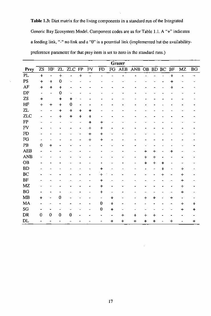
Table 1.3: Diet matrix for the living components in a standard run of the Integrated

Generic Bay Ecosystem Model. Component codes are as for Table 1.1. A "+" indicates

a feeding link, "-" no link and a "0" is a potential link (implemented but the availability-

preference parameter for that prey item is set to zero in the standard runs.)

Grazer Prey ZS HF ZL ZLC FP FV FD FG AEB ANB OB BD BC BF MZ BG

PL PS AF DF ZS

+ + +

+

- + + -0

+ 0 +

+

+

- - +.- -

_

-

_ -

- _ _ _

- - _ _

_ _ _ _ _

+ + +

FIF + + + 0 - _ _ _ ZI, + + + + - _ _ ZLC - + + + + - - - - FP - + + - _ _ _ FV - - + + - _ _ FD - - + + - _ _ _ FG - - + + - - PB 0 + - _ _ - - - - - AEB - - - - - - + + + - ANB - - - - - + + - - OB _ _ - _ - _ + ++ _ _ BD - _ _ + - - - + - + - BC '+ - - - + - + - BF - - + - - - - + - MZ _ _ - _ + - _ _ _ + _ BG - - - + - - - - + - MB + 0 - - + - + + - + - MA - - 0 + - - - + + SG - - • 0 + - _ _. - + + DR 000 0 - + + + + - - DL - - + + + + + - + +

17

Some components and processes in IGBEM do not feature in PPBIM or ERSEM

II, or have been modified from their original formulation to enable synthesis of the two

models. Important additions are components for epibenthic herbivorous scavengers and

herbivorous fish. These were added to take advantage of the macrophyte food sources

represented in PPBIM. These components were written by duplicating the general form

of appropriate existing components (using ERSEM's 'standard organism' concept

(Baretta et al. 1995)) and then adjusting diets and parameter values to those

representative of herbivorous grazers. Consumption of these new groups by predatory

groups within the model was also added (see the diet matrix, Table 1.3) based on diet

data from the literature (Shepherd and Thomas 1982, Heymans and Baird 1995,

Levinton 1995, Kuiter 1996, Gunthorpe et al. 1997).

Two biological components were modified in integrating PPBIM and ERSEM

II. Microphytobenthos was included with minor modification after Blackford (1999).

Also, the benthic suspension feeders of ERSEM II had their diets and habits modified

slightly to better match those of PPBIM. This involved changing one of their dietary

components from refractory to labile detritus and including an incidental transfer of

refractory detritus from the water column to the sediment via suspension feeding.

A number of the original chemical and physical processes in PPBLM and

ERSEM II required modification. The highly refractory detritus of ERSEM II, which

has a very slow breakdown rate (on the order of a century or more) was omitted. The

component referred to as refractory detritus in IGBEM is the equivalent of ERSEM II's

"Slowly degradable organics". The formulation of bioirrigation implemented in PPBIM

was left intact for IGBEM, but it is tied to the dynamical sediment fauna via an

"enhancement" term similar to that of ERSEM I (Ebenhoh et al. 1995). In contrast,

bioturbation received more attention in IGBEM than in PPBIM. Bioturbation was

considered during the formulation of PPBIM, but it was never implemented (Walker

18

1997), whereas it is a working part of ERSEM I (Ebenhoh et al. 1995). The inclusion of

well-elaborated formulations of bioturbation (a good example being that of Francois et

al. 1997) in an ecosystem model is no more feasible now then when ERSEM I was

originally formulated (Ebenhoh et al. 1995), so simple approximations are necessary.

IGBEM uses explicit sediment layers and includes the sediment mixing processes of

particulate diffusion, expulsion (whereby material at depth is moved to the surface), and

exchange (where material at the surface and at depth are exchanged). The only

components (tracers) acted upon by bioturbation were those particulate tracers that were

allowed in the sediments and were not macrobenthos. That is, sediment grains, settled

phytoplankton, microphytobenthos, meiobenthos, detritus and sediment bacteria. The

approximation used in IGBEM represents particulate diffusion, expulsion and exchange

with the surface by transferring sediment between the appropriate layers of the model.

Accordingly, the formulation implemented expresses the tracer concentration in the ith

sediment layer (Ci(t)) at the end of a time step as:

C, + AO= ki+i + C,_ 1 (t). + C,(t). — 2C, (t). k i m, g, +Cc,(t). go

ki+1 + ki_ i -F z, - 2k, — mi — g + go

ki = yr • (5' —1. • Oi

zi

mi = y • c5'• r• 19,

g i = 7.7 • • 1- • 0;

Where ki represents the thickness transferred from i due to particulate diffusion, mi is

the thickness moved to the surface from layer i by expulsion and gi is the thickness

moved from layer i due to exchange with surface layers and z i is the thickness of layer i.

The thicknesses k, mi and gi only differ in a single parameter. For the parameters they

share, 8 represents the base density of biological activity; t represents the modification

to the baseline to reflect dynamic sediment fauna activity in the ecological sub-model

(1.2)

(1.3)

(1.4)

19

(calculated in much the same way as that of ERSEM (see Ebenhoh et al. 1995)); and 0;

is the depth dependence of the mixing process (this is a simple functional form, as of

PPBIM, and though usually constant it is also possible to implement linear, parabolic

and half-Gaussian forms (Walker 1997)). The parameter which does differ in the

calculation of ki, mi and gi is the base rate of each process - w is the rate of particle

diffusion (m2 per At per unit biomass of bioturbative benthos per m 2), y is the rate of

expulsion (m per At per unit biomass of bioturbative benthos per m 2) and i is the rate of

exchange between the surface and deeper layers (m per At per unit biomass of

bioturbative benthos per m2). These simple representations minimise computational

costs and perform satisfactorily for the amounts involved under the model geometry

used in standard runs. A small amount of burial of sediments and associated detrital

particles is also enabled in IGBEM.

The implementation of sediment chemistry in IGBEM also differed from that of

ERSEM II and PPBEVI. An attempt was made to make the empirical model of PPIHNI

(Murray and'Parslow 1999a) more dynamic by incorporating more of the processes

included in the calculation of ERSEM I's density profiles. This highlighted the crucial

importance of the denitrification submodel. Blackford (1997) noted that ERSEM II

underestimated the levels of bacterial biomass in the sediments and this was also very

true of IGBEM. As a consequence any attempt to use bacterial activity to set levels of

nitrification and denitrification failed and the model output took on a "eutrophied" form

regardless of the levels of nutrient loading. In the short term this problem was solved by

reverting to using Murray and Parslow's (1999a) sediment chemistry model and

retaining bacteria only as tracers (as they had inherent value as indicators of system

state). All the runs presented here were completed in this way. In the long term a new

way of considering bacteria was developed as part of a related ecosystem model

(chapter 2).

20

Space precludes detailing the many other alternative settings that were built into

the model. These alternatives included forage- and density-dependent movement of fish

(in place of the prescribed movement of ERSEM II), invasions by specific functional

groups, fishing induced mortality on non-target groups and a basic effort model for the

fishery. Alternatives that were used in runs discussed here are identified below.

The parameter set used for IGBEM is based on the combined parameter sets of

PPBEVI and ERSEM II (corrected so that everything is at a reference temperature of 15

degrees Celsius and in mg IT1-3 (or mg IT1-2 if epibenthic)). Calibration of the model was

required to ensure mass balance and to achieve stability. However, the large number of

parameters (in excess of 775, disregarding those duplicated spatially or with age) means

that a systematic sensitivity analysis is not possible. Thus, growth and mortality

parameters and those associated with processes producing the greatest divergences or

instability were calibrated until stability was achieved and all functional groups

persisted. The restriction imposed on this calibration is that final parameter values must

be within the range of values recorded in the available literature for that parameter.

1.3 Model runs

All functional groups are active in the standard run of IGBEM. Runs usually

simulate a 20 year period, but a few simulate 100 years to allow consideration of long

term cycles and to check whether the model has reached a representative state by the

end of the usual 20 year run. The files containing the forcing for the transport model

cover only 4 years and so are looped such that when the model reaches the end of a 4-

year period it returns to the start of the forcing files and repeats them.

The standard run of IGBEM has fish migration as a forcing function, like

ERSEM H (Bryant et al. 1995) and fish recruitment is identical in time and space from

year to year, though the exact date of recruitment can vary by a few weeks. To check

21

Recruitment Regime Standard

Beverton-Holt stock-recruit relationship (distributed evenly across the recruitment period) Proportional to Primary Production

Formulation bo = J

(Ot • Lu

Lti

t x 11Fx • CHL

= 71chl

the impact of these assumptions an alternative movement scheme and a number of

alternative recruitment schemes were also tried. The alternative form of fish migration

is forage- and density-dependent and fish are distributed among spatial cells based on

available food resources in relation to metabolic requirements. The alternative

recruitment formulations include a Beverton-Holt stock recruitment curve; a case where

recruitment is related to primary production (used as a proxy for larval resource

availability); and a random number drawn from a lognormal distribution, which

simulates the often observed pattern of recruitment where there is the occasional very

strong year class. Each of these alternative forms was parameterised such that the mean

number of recruits returned would be very similar in each case and also very close to

that given by the constant case in the initial state of the system (Table 1.4).

Table 1.4: Alternative regimes for fish recruitment implemented in the Integrated

Generic Bay Ecosystem Model. Note bo is the number of recruits added to box j at time

t.

Definition of Specific Terms Ji = element t of the recruitment vector (constant spatially and temporally) a= Beverton-Holt a for the fish group fi= Beverton-Holt f3 for the fish group Ly = biomass of larvae in box j at time t tx = total length of recruit period 77Fx = recruitment coefficient for fish group FX

= water column chlorophyll in box j at time t richi= reference level of chlorophyll (1.5) Apx = recruitment multiplier for fish group FX y U(0,1) a= 0.3 ,u= -0.5 7r= 3.141592654

Lognormal distribution (—(log y—p)2 ) A Fx 2•o2 btj =

y • o- • 1,F277-i-

22

To evaluate how well the model replicates existing systems a number of other

bays around the world that have similar physical conditions (tidal range and relative size

of opening to the sea) (Figure 1.3) were identified. The inputs to these bays (from

Monbet 1992) were then scaled based on the area of the bay relative to PPB and then

the nutrient forcing files for IGBEM were adjusted to match. Thus, while the exact

geography of the bay was not changed, nutrient conditions were altered to try and

capture the state of several well-studied bays. Only minimal changes were made to the

biological parameters of the system. Since the biological parameters for the run under

baseline conditions have not been tuned to the species composition of any particular bay

to begin with, but are based on species from temperate marine bays in many parts of the

world, the decision not to tune the biological parameters in each case is justified. The

ability to achieve a plausible representation of these other bays was based on the

model's output values for chlorophyll a (chi a), DIN, biomasses and other measures

identified from the literature.

1.4 Results and discussion

1.4.A IGBEM vs real bays

Information on each of the individual components present in the model is not

generally available for real bays. Consequently output has to be pooled so that it

matches the most common resolution of the data available in the literature. To

differentiate between the individual functional groups of IGBEM and the pooled forms

of the output, the latter are referred to as trophic sets. The list of trophic sets is made up

of chi a (as a proxy for total phytoplankton), zooplankton, fish, macrophytes,

microphytobenthos, meiobenthos, benthos (all the other benthic consumer groups,

except bacteria) and detritus (labile and refractory).

23

Figure 1.3: Map of the world showing the bays used to evaluate the performance of the

Integrated Generic Bay Ecosystem Model (IGBEM). Boxes mark the locations of all the

systems for which marine biomass or production estimates are available for comparison

with the output of IGBEM. The solid black boxes indicate systems for which complete

biomass data are available. The inserts are maps of the particular estuaries or bays that

were used to set the level of nutrient inputs for the test runs, they were: (A) Port Phillip

Bay, (B) Cochin Backwater, (C) Firth of Clyde, (D) Flax Pond, (E) Chesapeake Bay,

(F) Apalachicola Bay and (G) San Francisco Bay. The scale bar in each case represents

10km, Flax Pond has no scale bar as its total length (west to east) is approximately

600m. The two bays with a bold border (Chesapeake and Port Phillip Bay) have enough

available information to allow for an intensive evaluation of the runs.

24

Biomasses

Empirical estimates of average biomasses for the trophic sets covered in IGBEM

were obtained from the literature for 276 coastal marine systems (Figure 1.3; a list of

the values and associated references is given in Appendix A). Estimates of the biomass

of all major trophic sets is available for only 10 of these locations (black squares in

Figure 1.3) and complete information of both inputs and the biomasses of the trophic

sets is available only for Chesapeake Bay and PPB (inserts with bold borders in Figure

1.3). Thus the published values allow a very general consideration of model output

across the various nutrient loadings, but a specific evaluation of performance is only

possible for the case of baseline inputs (equated with PPB) and a tenfold increase in

inputs (equated with Chesapeake Bay). Note that, there are insufficient data on the

biomass of bacteria to include them in the general comparisons of biomass. The

information that could be found shows that the values for biomass given by IGBEM for

the pelagic bacteria are high and the values for the sediment bacteria are very low,

something the model has inherited from ERSEM (Baretta-Bekker et al. 1995).

Range in biomass

Overall the model conforms well with the range of values seen in real systems,

but the level of performance is not consistent across all measures or trophic sets. The

biomass of each trophic set (Figure 1.4) is within the range of data from real bays. The

model ranges are often smaller than the ranges from field data, but this is

understandable given the small subset of possible nutrient inputs used (30x present

loading was the highest loading used in model runs, but real inputs in some bays would

reach as high as 1000x present loadings) and the use of geometry of a single bay

(whereas the empirical data derive from bays of various topographical forms, from open

coastal bays and shallow lagoons to deep, narrow fjords). Even though the model is of a

25

temperate bay, the sparse nature of empirical data for some trophic sets necessitates

including data from tropical systems in the field data ranges. This would have little or

no effect on the absolute ranges given for the field data for any trophic set with the

exception of the fish (the maximum value would fall to 21.16 g AFDW IT1-2 if only data

from temperate bays is included).

Average biomasses

The average biomasses indicate a more mixed, though still positive,

performance. Given the magnitude of the range in field values, the average model

values are not far from the average field values in most cases. Only three of the trophic

sets have an average model value that is more than 10% of the range away from the

average empirical value. Considering only the temperate average, the difference

between the model and field average is 27% of the range for the benthic trophic set,

29% for the microphytobenthos and 13% for the DIN. The model also consistently

yields detrital biomasses that are too low. That IGBEM does not include extremely

refractory detritus, whereas the field data may, might account for this in part. However,

it is also likely that estimates of the atmospheric component of detrital inputs to PPB are

too low so overall inputs are too low (by about a third). Moreover, assimilation rates by

deposit feeders are poorly known and may also be too high in the standard

parameterisation; similarly, the burial of detritus out of the model system may be too

fast.

Model biomasses in comparison with those of Port Phillip Bay and Chesapeake Bay

When the specific empirical values for the trophic sets in PPB and Chesapeake

Bay are compared with the appropriate model values, the estimates for trophic sets from

the model are usually within the bounds of empirical interannual variation, with the

26

160 —

120 —

ao —

40 —

n b

C--4

= 94 = 36

[14-CM

600 —

400 —

200 —

U 4-PM

n b

= 36 = 27

4- CM

4-PM

so —

40 —

30 —

20 —

10 —

n b

= 87 = 80

4-CM

4-PM

800 —

600 —

400 —

200 —

n b

P-,

= 32 = 26 300 —

200 —

100 —

4-CM

- 4-PM

n b

= 37 = 27

■-cm

4—PM

200 —

160 —

120 —

so —

—

n b

C-•

P-7

= 72 = 66

4-CM

4-Pm

12 —

8 —

4 —

n b

-

C—■

Pa,

= 45 = 45

120

so —

40 —

s-CM

4—PM

Chl a Zooplankton Fish Macrophytes Microphytobenthos Benthos Meiobenthos

n = 94 b = 36 12000 —

C-+

8000 —

4-CM

4000 —

P-,

1+— CM

4—PM

DIN Detritus

n = 14 b = 14

4-PM

• Real Bays Tropical Average — Overall Average

0 Model Bays Temperate Average

Minimum

4-CM Model Chesapeake 4-PM Model Port Phillip C--• Chesapeake Bay P-, Port Phillip Bay

Figure 1.4: Ranges and average values for the main sets of the model (IGBEM) in comparison with field values worldwide. The systems giving the

maximum and minimum for the field data for each set are marked beside the reference in Appendix A. The model values come from the runs under

different nutrient inputs based on inputs for real bays (A-G in Figure 4). The y-axis for zooplankton is Biomass in mg AFDW rn -3 ; for fish,

macrophytes, benthos, meiobenthos and detritus the y-axis is biomass in g AFDW IT1-2 ; the y-axis for chl a is mg chi a 111-3 ; for DIN it is mmol DIN IT1-3 ;

and for microphytobenthos it is mg chl a rI1-2 .

Maximum

27

exception of the microphytobenthos and detritus. These trophic sets do not realise

values within field measured levels of interannual variation and they are the only

trophic sets where the difference in averages (model vs field) is more than 10% of the

range in field values. The values for microphytobenthos are too low for the "Port Phillip

Bay run" (PM), though it was at an acceptable level for the "Chesapeake run" (CM).

There is also some suggestion that the predicted change in biomass of

microphytobenthos with eutrophication is opposite to that observed empirically. The

model average rose while the field values dropped marginally, if at all, given

interannual variation in field values.

Microphytobenthos is the only component in the model that fails to follow the

patterns of change with eutrophication that are predicted by field observations. The low

levels of microphytobenthos in the baseline (PM) run are, at least in part, the result of

two things. Firstly, this group competes with the large macrophyte pools, particularly

the macroalgae. This causes it to be confined to the deep central parts of the bay, which

have low light levels at the sediment surface. While low light levels in this area limit the

microphytobenthos pool, limitation is not as pronounced as for the other benthic

primary producers (the microphytobenthos light saturation is set at 3 W M-2 compared to

5 W m-2 for macroalgae and 60 W M-2 for seagrass). Also, as a result of very little

available information on benthic interactions, the availability of the microphytobenthos

to the deposit feeders and meiobenthos seems to be set too high. The efficiency of

deposit feeders mentioned above exacerbates this problem. As a result of these factors

the microphytobenthos is kept cropped to low levels. This facet could be improved by

further calibration of the microphytobenthos part of IGBEM. However, more

importantly, all aspects of the infauna and benthic microfauna in this, and other

biogeochemical models (Silvert 1991), would benefit from an increased understanding

of benthic interactions and ecology.

28

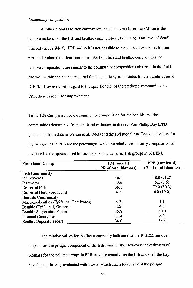
Community composition

Another biomass related comparison that can be made for the PM run is the

relative make-up of the fish and benthic communities (Table 1.5). This level of detail

was only accessible for PPB and so it is not possible to repeat the comparison for the

runs under altered nutrient conditions. For both fish and benthic communities the

relative compositions are similar to the community compositions observed in the field

and well within the bounds required for "a generic system" status for the baseline run of

IGBEM. However, with regard to the specific "fit" of the predicted communities to

PPB, there is room for improvement.

Table 1.5: Comparison of the community composition for the benthic and fish

communities determined from empirical estimates in the real Port Phillip Bay (PPB)

(calculated from data in Wilson et al. 1993) and the PM model run. Bracketed values for

the fish groups in PPB are the percentages when the relative community composition is

restricted to the species used to parameterise the dynamic fish groups in IGBEM.

Functional Group PM (model) (% of total biomass)

PPB (empirical) (% of total biomass)

Fish Community Planktivores 46.1 18.8 (31.2) Piscivores 13.6 5.1 (8.5) Demersal Fish 36.1 72.0 (50.3) Demersal Herbivorous Fish 4.2 6.0 (10.0) Benthic Community Macrozoobenthos (Epifaunal Carnivores) 4.3 1.1 Benthic (Epifaunal) Grazers 4.5 4.3 Benthic Suspension Feeders 45.8 50.0 Infaunal Carnivores 11.4 6.3 Benthic Deposit Feeders 34.0 38.3

The relative values for the fish community indicate that the IGBEM run over-

emphasises the pelagic component of the fish community. However, the estimates of

biomass for the pelagic groups in PPB are only tentative as the fish stocks of the bay

have been primarily evaluated with trawls (which catch few if any of the pelagic

29

species) and so the currently available estimate of the relative contribution of the

planktivores to the PPB community may be an underestimate. Further, the dynamic fish

groups in IGBEM do not represent the entire fish population, but only part of it. One of

the static closure terms imposed on the fish groups represents sharks and other large

demersal fish. If the relative composition for PPB is recalculated, based only on the

species-groups (for instance flatfish rather than all demersal fish) used to parameterise

the fish groups dynamically included in IGBEM, the two compositions are much closer

(bracketed values in Table 1.5). There is still an over representation of the pelagic

groups at the expense of the demersal groups, but the model values are much closer to

the field values. Thus, if the model is judged only on those groups it represents

dynamically then the trophic compositions produced by IGBEM do compare favourably

(though not perfectly) with those observed in PPB. However, as discussed below, the

fish groups are one of the weaker parts of IGBEM and it may well be that the standard

seed populations used do not produce the correct community composition in this case.

In contrast to the fish community, the relative composition of the benthic

community in IGBEM is close to that observed in PPB (Table 1.5). There is some

suggestion that the model may tend to favour the traditional primary production based

food web over the detritus based web that dominates in PPB. This is indicated in that

the contribution of both of the carnivorous groups is higher (by more than a factor of

two), while that of the suspension and deposit feeders is slightly lower, in the PM run

than in PPB. This tendency may be the product of two factors. Firstly, the static loss

term imposed on epifaunal groups (to represent predation by fish groups not

dynamically included in IGBEM), may not be high enough in the standard

parameterisation to completely capture the benthic community structure observed in

PPB. Secondly, there may be a mechanism in nature that influences the population

dynamics that is not present in IGBEM. For example, some kind of burrow effect may

30

be appropriate (as it would lessen the impact of anoxic conditions in the sediment).

Alternatively an index of habitat type (like the % of the area made up by hard substrata)

may be necessary so that epifaunal groups restricted by crowding and available habitat

in the wild are not inflated by the large homogeneous polygons used in the model.

Nevertheless, the community compositions produced by the model are adequate with

regard to IGBEM's role in generating data for a wider model study.

Standard relationships

While a good fit to biomasses across many trophic sets and under varying

conditions is a positive attribute, it is not sufficient given that IGBEM is the foundation

of a wider investigation of model structure and behaviour. Thus, the model output was

checked to see if it complied with existing patterns and relationships observed generally

in the field.

The work by Monbet (1992) indicates that there is a strong relationship between

mg chl a 1113 and mmol DIN 111-3 in the water column. As a further test of model

performance the values of chl a versus DIN for the model runs under varying rates of

nutrient forcing are plotted against values from real bays (Figure 1.5) (references for the

real bays are in Appendix A) to examine whether the model conforms with the observed

relationship. Only microtidal estuaries and bays (tidal range < 2m) are used in this

comparison since PPB (and thus the model) is a microtidal system and Monbet showed

that, relative to microtidal estuaries, macrotidal estuaries have much lower

concentrations of chl a for the same levels of DIN. All of the model points sit well

within the general relationship between chl a and DIN observed by Monbet (1992). On

a more specific level the model values are compared against the values from the bays

used to set the nutrient input levels for the various test tuns (Figure 1.6). This serves to

reinforce the strong performance of the model in this aspect, as all of the values are

31

within interannual variation measured in real bays.

Figure 1.5: The relationship between the mean annual concentration of dissolved inorganic nitrogen (DIN) and chlorophyll a (chl a) for real (open circles) and modelled (solid black circles) microtidal marine systems. See Appendix A for references used to give values for real bays.

(.? co

1 000

100 -

1 0 -

1 Oo

o

*0

0

00 0 00 0 n

on 10 sio igo43.2CD • Go 0 oZ4

0

o9t, oo °

0 0 o

01 10 100

1 000

mmol DIN m -3

Figure 1.6: The relationship between the mean annual concentration of dissolved inorganic nitrogen (DIN) and chlorophyll a (chl a) for a selection of real and model microtidal marine systems. See Appendix A for references used to give values for real bays.

100

co ▪ 10- 0

S San Francisco • Model San Francisco C Chesapeake c Model Chesapeake A Apalachicola a Model Apalachicola F Firth of Clyde f Model Firth of Clyde P Flax Pond p Model Flax Pond B Cochin Backwater b Model Cochin Backwater X Port Phillip Bay x Model Port Phillip Bay

S C

•

C c

A b

A A is pB F F

S s s S c

C sc

1 01 1 10

100

mmol DIN m -3

32

- 3.39671og(x)+ 8.27838

12

Maximum water depth (m)

Figure 1.7: Relationship between the maximum depth and the average biomass of

meiobenthos in the sediments of real (open circles) and modelled (solid black circles)

coastal marine systems. See Appendix A for references for the real bays.

A general property to emerge from the empirical data is a curvilinear upper

bound on the rate of decrease of the biomass of meiobenthos with increasing water

depth. A curve fitted to the highest points in the plot (marked by a solid line in Figure

1.7, equation for the line given on the plot) gives an r 2 of 0.97. The model output was

examined to see if it complies with this requirement (solid points in Figure 1.7). As all

the model points fall below the bound, it is judged that the model conformed with this

relationship.

Beyond the relationships between certain groups and physical characteristics of

a system, there are also relationships between relative biomasses within the biological

components of systems. In marine systems two such relationships are the biomass

spectrum, in logarithmic size classes, for benthic and pelagic communities. Sheldon et

al. (1972) observed that marine pelagic communities appear to have similar biomasses

33

in all logarithmic size classes of organisms. That is the "Sheldon spectrum" is almost

flat. In contrast, benthic communities have a "Sheldon spectrum" that is W-shaped

(Schwinghamer 1981). Sheldon spectra for the benthic and pelagic components were

obtained from the model and compared to observed empirical spectra. The spectrum for

the pelagic components of IGBEM (Table 1.6) indicates that the model output does hold

with Sheldon's finding that, over the entire size range of pelagic organisms,

concentration varies by only an order of magnitude. Constructing the "Sheldon

spectrum" is not simple for the benthic groups in IGBEM because the definitions of the

groups are primarily trophic with only minor concessions to size structure. As a

consequence it is necessary to use the totals per class (bacteria, rnicroalgae and

meiofauna, macrofauna) given by Schwinghamer rather than the specific values per size

interval (converting the form or the "Sheldon spectrum" from a "W" into a "U"). In this

case the spectrum (Table 1.7) indicates that the model does not conform well with field

observations and that, using Schwinghamer's relationship as a guide, the smallest fauna

in IGBEM (particularly bacteria) are under represented. The two larger classes

(meiofauna/microalgae and macrofauna) are within the bounds given by Schwinghamer,

but the bacteria are <2% of the field average.

Table 1.6: Summary of the Sheldon spectra for the pelagic classes in the run where

nutrient loads were at the levels recorded in Port Phillip Bay (PM run) and Chesapeake

Bay (CM run).

Class PM (cm3/m2) CM (cm3/m2) Bacteria 40.5 149.3 Phytoplankton 10.0 75.6 Zooplankton 10.5 18.5 Planktivorous fish 5.5 23.3 Other (larger) fish 6.4 19.9

34

Table 1.7: Summary of the Sheldon spectra for the benthic classes in the baseline (PM)

and nutrient load x10 (CM) runs of IGBEM. As a guide, the total mean biomass for

each class after Schwinghamer (1981) are also provided.

Class PM CM Schwinghamer (cm3/m2) (cm3/m2) (cm3/m2)

Bacteria 0.2 1.4 80.1 Meiobenthos and Microphytobenthos 0.7 4.3 6.1 Macrofauna 149.5 373.2 473.0

Production and consumption

Levels of daily production and consumption were obtained from the literature

for comparison with the predicted values from IGBEM. Generally the model values

compare favourably with the empirical field values of Production / Biomass (P/B) and

Consumption / Biomass (Q/B) (Table 1.8), with some noteworthy discrepancies.

Macrophyte production in the model is only a half of the field values and no easy

explanation can be found for this. It may be due, at least in part, to a "macrophyte-

barrens" which establishes itself in this particular run. This cycle is essentially a

predator-prey cycle between the macrophytes and the benthic grazers, facilitated by the

spatial and trophic structure of the model, and is discussed more fully below.

Consideration of the fish on an individual functional group level rather than an overall

pooled "fish" basis indicates that the P/B for the planktivores is much lower in the

model output than given by the field estimates. Evaluation of the benthic components

based on their habitat (epifauna vs infauna) rather than a single pooled value for all the

benthos, also indicates some differences between the model and field estimates (Table

1.8). It is interesting to note that those P/B values that are considered to be substantially

different between the field and the model show no consistent pattern, whereas Q/B

values of the model are almost always lower than the field estimates. This suggests that

while there may be multiple causes for the differences in production, the low

consumption estimates are probably all due to assimilation being too efficient.

35

A final production related comparison is possible. The growth curves for the fish

groups in the model were compared with those of real species used to parameterise the

model groups (Figure 1.8). The growth curve for the individual planktivores and the

herbivorous demersal fish are close matches to those for pilchards and mullet

respectively. The curve for the piscivores is also a good match for the growth curve of

barracouta and only the growth curve of individual demersal fish fails to fit its real-life

equivalent (flathead) closely, falling short in the older fish. These older demersal fish

have a diet that is primarily fish-based rather than invertivorous, and they experienced

competition with the smaller piscivores. While further tuning would improve the match

between the curve for the demersal fish group in IGBEM and flathead, the standard

parameterisation is retained for the purposes of the wider model study as it adequately

represents a demersal fish, even if it does not exactly match flathead.

Table 1.8: Estimates of primary and secondary production and consumption for Port

Phillip Bay (PPB) and the PM run of the Integrated Generic Bay Ecosystem Model.

Values for fish and benthos represent the pooled production or consumption value over

the pooled biomass value.

Production:Biomass Consumption:Biomass Set PPB PM PPB PM

(empirical) (model) (empirical) (model) Ph ytoplankton 210.3 241.8 - -

Zooplankton 2.1 1.8 3.4 2.9 Fish 3.1 4.0 21.7 13.5

Planktivorous 6.3 3.2 82.6 22.4 Piscivorous 2.0 2.6 8.2 5.9 Demersal 1.5 2.1 7.1 5.7 Demersal Herbivorous 1.2 3.1 9.6 7.0

Benthos 14.2 17.0 49.0 44.1 Epifauna 9.9 5.3 17.3 8.7 Infauna 17.6 31.1 85.1 86.6

Macrophytes 22.6 12.4 - Microphytobenthos 6.3 5.2 .■

36

System indices

Given the holistic nature of ecosystem studies, simple reductionist comparisons

of biomasses, productivity and other ecosystem attributes are far from a sufficient

summary of model performance. The fit of the model dynamics to system-level indices

must also be considered. To this end a number of system indices were calculated for the

baseline (PM) and nutrientsx10 (CM) runs of IGBEM. The most informative of these

(based on the findings of Christensen 1992) were compared with values for the same

indices calculated for 9 real marine systems (Table 1.9). The comparison indicates that

the model conforms well with the real systems. For most of the indices the values for

the model runs are within the range of the values calculated for the real systems. The

value for the total throughput for the CM run is beyond the range given by the real bays,

but this may be because the run is under a higher nutrient load (and is more eutrophic)

than any of the real systems being considered.

On a specific level only 4 of the 11 indices given show a relatively close match

between the values calculated for the PM run and PPB. The "System Omnivory. Index",

"Dominance of Detritus", "Path length" and "Relative Ascendancy" all suggest the real

and modelled systems are quite similar, while the remaining indices suggest

divergences. Much of this is due to the species used to parameterise IGBEM. The

standard parameter set is based primarily on northern hemisphere species (as they make

up the bulk of available information) and while the resulting model system does match

the levels of biomass and productivity reported for PPB reasonably well, it does not do a

consistently good job of matching higher level indicators. If the species used to set the

parameter values are those resident in PPB, then the match between model and real

system indices is vastly improved. The "BASE run" in Table 1.9 is based on parameters

determined from species resident in PPB and the match between the model and real

values is close for all but two of the 11 indices. Thus, the standard parameter set does a

37

4000 25

3000 -

Wet

wei

ght (

g)

2000 -

0

• 0

• 1000 -

8 10 2 4 6

Age (years)

8 10

..11 10 - 5

20 -

(a)

0

•

0

•

• 0

5 •

8 00 •

4 6

Age (years)

0 0

800

0 0 2

• •

0

0 (d) (c) 1200 - •

1000 -

—di -z 800 -

co

600 -

• 0 •

0 • 400 -

0 • 6 200 - 0

8 0 0

600 -

Wet

wei

ght (

g)

400 -

200 -

0

0

•

0 •

•

0

•

0

• 0

(b)

0

1400

Figure 1.8: Growth curves for fish groups as produced by the model (open circles) and the species their parameterisations are based on (solid black

circles). (a) Pilchard vs. IGBEM planktivore, (b) Barracouta vs. IGBEM piscivore, (c) Flathead vs. IGBEM demersal, and (d) Mullet vs. IGBEM

demersal herbivore.

0

2

4 6

8

10

0

2

4 6

8

10

Age (years)

Age (years)

38

Table 1.9: System-level indices for a range of real coastal areas (values for the first 8 locations are from Christensen 1992) and three separate runs of

the Integrated Generic Bay Ecosystem Model (IGBEM).

System (or run) \ Index

Sum of flows Primary Biomass / Biomass System Dominance (Throughput) Production / Throughput Supported Omnivory of Detritus

Biomass Index

Average organism size

Path Residence length Time

Schrodinger ratio

Relative Ascendency

Mandinga Lagoon, Gulf of Mexico 3075 36.6 0.008 0.016 0.26 0.36 0.023 2.98 0.02 27.31 36.0 Tamiahua Lagoon, Gulf of Mexico 1444 9.6 0.018 0.041 0.13 0.65 0.076 3.16 0.06 14.62 25.4 Coast, Western Gulf of Mexico 17191 5.8 0.018 0.052 0.15 0.78 0.100 3.56 0.07 13.56 31.4 Campeche Bank, Gulf of Mexico 10327 5.5 0.042 0.08 0.21 0.49 0.124 3.28 0.14 7.01 26.2 Shallow area, South China Sea 11895 74.9 0.004 0.008 0.27 0.42 0.010 3.26 0.01 52.03 21.7 Lingayen Gulf, Phillipines 7198 14.6 0.013 0.037 0.15 0.63 0.041 5.14 0.07 12.46 31.1 Etang de Thau, France 41929 5.1 0.045 0.099 0.35 0.72 0.123 4.26 0.19 5.06 30.6 Schlei Fjord, Germany 2825 3.9 0.071 0.151 0.03 0.45 0.198 3.63 0.26 2.79 32.1 Port Phillip Bay, Australia 13956 14.1 0.016 0.033 0.18 0.64 0.053 4.00 0.06 16.00 32.3 BASE run (IGBEM tuned to PPB) 13243 13.7 0.023 0.053 0.18 0.49 0.049 3.60 0.08 5.15 32.5 PM run (IGBEM baseline nutrients) 4702 4.6 0.051 0.13 0.14 0.62 0.128 4.21 0.21 3.16 32.3 CM run (IGBEM nutrients x10) 50702 18.7 0.019 0.04 0.15 0.47 0.0418 3.36 0.06 4.59 29.8

39

sound job of reproducing a generic coastal system while tuning can produce a close fit

to the holistic form of a specific system.

1.4.B Spatial and temporal form of meso- and eutrophic runs

To complete the evaluation of the standard behaviour of IGBEM, the spatial and

temporal dynamics are considered. This indicates that the model can produce a rich

collection of responses, from competitive exclusion to predator-prey cycles and the

formation of identifiable communities structured by biotic and abiotic factors.

Spatial structure

The predicted average biomasses per box over the final four years of the CM and

PM runs were analysed to determine whether there were spatial patterns in the model

output. The average biomasses of all groups in each box were compared on a two-

dimensional non-metric Multidimensional Scaling (MDS) plot derived from a Bray

Curtis similarity matrix to identify groups of boxes of similar community structure. The

average values of the physical variables and the biomass per group were examined

(using the SIMPER routine of the Primer software package) to ascertain which groups

determined the clustering. This analysis identified "areas" (boxes in the model sharing

biological and/or physical characteristics) in the model output. Only the PM and CM

runs were analysed in this way as they were considered representative of the

"mesotrophic" and "eutrophic" states of the model output.

Fourteen biological areas (Figure 1.9a) and twelve geophysical areas (Figure

1.9b) exist in the output of the PM run. While there is some correlation between the

two, the two sets of areas differ sufficiently that physical factors alone do not produce

the form of the biological areas. Biological interactions are also important to the spatial

patterning. For instance, certain functional groups consistently occur together with high

40

biomasses in the same cells, and these are called communities (Table 1.10). A

comparison of the communities and attributes per biological area (Table 1.11) shows

that Swan Bay (area 4) and Corio Bay (area 9) are distinct to the main bay. This is due

to their shallow depth, large macrophyte communities and restricted connection with the

main bay. Within the main bay a comparison of the biological areas reveals a depth-

based zonation. The areas around the edge of the bay (areas 1 — 10) are usually

distinguished by the presence of either one of two planktonic communities, as well as

rich fish, epibenthic and macrophyte assemblages. In contrast the deep central sections

of the bay (areas 11 — 14) all share a common planktonic community and the

macrobenthic groups are largely replaced by microscopic communities able to tolerate

the low light while exploiting the high levels of detritus. There is some seasonal and

interannual variation in the composition of the communities and some switching

between specific plankton communities expressed in the areas along the bay edge,

especially within the planktonic communities 1 and 2. This is mainly as a result of

responses to tidal forcing and the patterns of nutrient forcing within and across years.

Nevertheless, the overall differences between the central and edge areas persists over

time in the model output.

Figure 1.9: Maps of the location of the physical and biological areas identified in the output of the PM run. (a) The biological areas (sections of the bay in the same "biological area" are marked with the same number), and (b) the physical areas (sections of the bay in the same "physical area" are marked with the same letter).

41

Table 1.10: Definitions for the various communities found in the output of the Integrated Generic Bay Ecosystem Model runs.

Community Functional Groups Present 1 diatoms and autotrophic flagellates 2 picophytoplankton and microzooplankton 3 picophytoplankton, autotrophic flagellates, dinoflagellates, heterotrophic flagellates,

large omnivorous zooplankton and large carnivorous zooplankton 4 heterotrophic flagellates 1 benthic suspension feeders 2 macrozoobenthos (epifaunal carnivores) 1 seagrass 2 macroalgae and benthic (epifaunal) grazers 1 planktivores 2 piscivores 3 demersal herbivorous fish and demersal fish 4 piscivores and demersal fish 1 benthic deposit feeders and infaunal carnivores 2 meiobenthos and microphytobenthos 1 pelagic bacteria, aerobic bacteria, anaerobic bacteria, labile and refractory detritus 2 pelagic bacteria 3 aerobic bacteria 4 labile and refractory detritus

Planktonic

Epibenthic

Macrophyte

Fish

Benthic

Remineralisation (Remin)

Table 1.11: Dominant communities and physical attributes characterising each biological area identified in the PM run. Codes for the functional

communities are as for Table 1.10. For the biological communities a blank entry signifies that while a community of that kind may be present in the

area it was not large enough (relative to their size in other areas) to significantly contribute to the definition of the area. A blank entry for a physical

attribute signifies low to negligible levels for that attribute.

Biological Communities Physical Attribute Area Planktonic Fish Epibenthic Benthic Macrophyte Remin Tidal Influence Bottom Light Depth DIN Levels

Stress Levels 1 1 1 High High Moderate 2 1,2 1 Moderate Deep 3 2 1 High High Shallow 4 1 Very High Very Shallow Moderate 5 2 2 1 Shallow High 6 2 1 Moderate Shallow 7 2 2,3 1,2 1 4 Shallow Very High 8 1 1 2 4 Intermediate Moderate 9 2 1,2 Moderate Shallow Moderate 10 1 1,2,3 High Shallow 11 3 1 2 1 Moderate 12 3 1 2 1 Deep 13 3 1 2 1 Very Deep 14 3 Deep

43

When the CM run is analysed only 10 distinct biological areas and 9 physical

can be identified (Figure 1.10). The decline in the number of the physical areas results

directly from changes in the levels of inputs and indirectly from changes in the

biological components and their resultant effects on light, nutrients, detritus and bottom

stress. The two sets of areas do show some overlap and the correlation is more

pronounced than in the PM run, but it is still clear that abiotic factors alone are not the

cause of the biological areas. As before, the mix of biotic and abiotic agents is thought

to form the areas seen in the output. Once again there are clear differences between the

areas along the edge and those in the middle of the bay (Table 1.12). However, the

distribution of "central communities" is now much more widespread than in the PM run

and they have taken over much of what was previously the domain of the "edge

communities". An "edge community" still exists but it is restricted to the very edge of

the northern parts of the bay. Moreover, the distinction between "edge" and "central"

planktonic communities is less clear. Swan Bay and Corio Bay again stand out as being

substantially different from the main bay, but the contrast is much sharper than for the

PM run. Even though no functional groups disappeared from the run, some rose

substantially at the expense of others which where depressed to low levels and restricted

to much smaller areas. This suggests that the model is replicating the simplification of

habitat and the reduction in diversity seen with eutrophication.

Temporal dynamics

Distinct temporal patterns are evident in the long-term output of the PM run,

including seasonal, interannual and decadal cycles (Figure 1.11a-d). The cycles seen in

fish biomass will not be discussed here as they are largely prescribed by the movement

regime employed, with only minor amounts of variation occurring due to interannual

variation in growth tracking their food supply (Figure 1.11e).

44

-

Table 1.12: Dominant communities and physical attributes characterising each biological area identified in the CM run. Codes for the functional

communities are as for Table 1.10. For the biological communities a blank entry signifies that while a community of that kind may be present in the

area it was not large enough (relative to their size in other areas) to significantly contribute to the definition of the area. A blank entry for a physical

attribute signifies low to negligible levels for that attribute.

Biological Communities Physical Attribute Area Planktonic Fish Epibenthic Benthic Macrophyte Remin Tidal Influence Bottom Light Depth DIN Levels

Stress Levels 1 1, 4 1,2,3 1 2 1 High High Deep 2 2 2 High Moderate Shallow Moderate 3 1 1 High Very Shallow High 4 2,3 2 1,2 2 Shallow to High

Moderate 5 3 1,4 1 2 2 Shallow to High

Moderate 6 1,2 1,4 1 1 Shallow Very High 7 1,2 4 1,2 1,2 3,4 Shallow Very High 8 1 1,2 Moderate Shallow High 9 2,3 1 1,2 1 Moderate High 10 2,3 1 1 Deep High

45

Figure 1.10: Maps of the location of the physical and biological areas identified in the

output of the CM run. (a) The biological areas (sections of the bay in the same

"biological" area are marked with the same number), and (b) the physical areas

(sections of the bay in the same "physical area" are marked with the same letter). The

letters and numbers used in this figure do not correspond to any of those in Figure 1.9.

While there are high levels of short-term fluctuation in the phytoplankton

groups, seasonal cycles within the planktonic groups are nonetheless clear (Figure

1.11a). This cycle is characterised by blooms in the planktonic communities associated

with seasonal cycles in light levels, temperature, river flows and nutrient inputs

provided by the forcing files. The build up in DIN over the winter months, particularly

in the boxes fed by the two largest nutrient point sources (the Yarra River and the

Werribee Sewage Treatment Plant, Figure 1.1), leads to bloom events in spring when

light levels begin to rise. The form of the blooms is least stable in the Yarra and WTP

boxes where local flows cause a lot of variation. Further away from the point sources,

cycles are much more stable. Similar seasonal cycles can be seen in the benthic primary

producers (Figure 1.11b, c) and the detritus based web fed by them (Figure 1.11d). The

slow growing nature of the consumers in this set of cycles means that they show little, if

any, of the short-term fluctuations which are common in the planktonic dynamics.

The looping of the hydrodynamic files (the same cycle of 4 years is continually

repeated for the whole run) is apparent in the interannual variation. Many groups fall

46

into a steady repetition of interannual variation through time (Figure 1.11c, d) and this is

due to the influence of the hydrodynamics on nutrient supply, advection of the water

column communities and other food supplies. The strength of the impact of the cycle of

hydrodynamic forcing differs between boxes and is strongest in the central parts of the

bay, where boxes are distanced from point source inputs. The dependence of the

behaviour of so many groups on the hydrodynamic cycle (either directly or via the

impact of it upon their food and nutrient supplies) agrees with the findings of the

developers of PPBIM (Murray and Parslow 1997) and ERSEM (Ebenhoh et al. 1995). It

is interesting however, that even these cycles do not become regular bay-wide, as

variation is evident in the amplitude and period of the cycles. This variation in

amplitude and period would be lost within all the other forms of variation (and error) in

the field, but its existence is intriguing. Apparently the extra variation is due to the

effect of the point source impacts on prey groups in conjunction with the timing of the

few stochastic components of the model (for example the exact day that recruitment

begins in fish). The combination of bottom-up and top-down controls leads to

noticeable variation in a pattern that could be expected to be extremely predictable

given the cyclic nature of the forcing conditions.

The interaction of physical forcing and biotic interactions also underpins the

more interesting long-term cycles (5 — 20 years). The two cycles in question are in the

epibenthic groups. The first is a "macrophyte-barrens" cycle (example in Figure 1.11b)

where the macrophytes are at high levels (equivalent to temperate kelp forests) for

between 2 and 7 years before dropping to very low levels (<1 mg N 1113 in some cases)

for between 2 and 9 years. The cycles have a shorter period (about 4 years for a

complete cycle) in the areas with conditions conducive for macrophyte growth and are

much longer (up to 15 years) in those parts of the bay with conditions less hospitable to

macrophyte growth. The benthic grazers are also locked into this cycle, though the

47

8722 9086 9450 9814 10178

48 Day of Run

57%

150

6160 6524 6888 7252 7616 7980 8344

— Chlorophyll a —Mesozooplankton

(a)

120 (b) — MacraeWee — Benthic Grazer

90

60

30

0 8750

40

35

30

25

20

15

10

5

0 3388

1.8

1.6

1.4

1.2

12390 12026 11E62 11298 10934 10570 9842 10206 9478 9114

Microphytobenthos — Maiobanthos

4;16 5936 5572 52013 4844 4480 3752

— Epitaunal carnivore

— Deposit feeder

\

5362 6090 9002 9730 10458 11186 11914 12642 13370 14098

1

0.8 -

0.6 -

0.4 -

0.2 -

0 3178

3

4634 3906 7546 8274 6818

Rel

ativ

e bi

omas

s (Bi

omas

s / B

iom

ass o

n fir

st d

ay o

f the

plo

tted

peri

od)

Figure 1.11: Relative Biomass (Biomass / Biomass on first day of period shown) (y-axis) through time

(x-axis) showing temporal patterns for representative groups in the PM run of the Integrated Generic Bay

Ecosystem Model. The small spans marked by S are an example of seasonal variation, the large spans

marked by I are examples of interannual variation. The entire period plotted in (c) and (e) are examples of

decadal scale cycles. All but (d) are from edge boxes, while (d) is from the large central box.

amplitude expressed from one repetition of the cycle to the next is not necessarily

constant, as it also depends on levels of their predators. This cycle may be a model

artefact or a symptom of an instability as no such cycle has been recorded for PPB.

However it does a very good job of simulating the impact of urchin barrens in a

temperate system, a dynamic that has been widely reported and investigated (Hagen

1995, Leinaas and Christie 1996, Silvertsen 1997, Sala 1997). The whole cycle can be

suppressed by adjustments to the growth rates of the main groups involved in the cycle

(the macrophytes, benthic grazers and epifaunal carnivores) and by reducing the

availability to predation of the macrophytes and the benthic grazers.

The other long-term cycle is related to the "macrophyte-barrens" cycle. The

epifaunal carnivores show long term changes in the pattern of their interannual variation

(Figure 1.11d) depending on which food web they are receiving most prey from. The

amplitude of the cycle in their abundance is smaller if the detritus based web (infauna

and suspension feeders) makes up most of their diet and the benthic grazers are only a

relatively small part. If the contribution by the benthic grazers to the food supply of the

epifaunal carnivores rises above 20% (which occurs if the barren cycle begins its

decline slightly later in the year than normal) then the cycle switches to one with larger

amplitudes. This cycle gradually slips back into the previous state (where the benthic

grazers make up a smaller proportion of the diet) over time. These patterns (the

"macrophyte-barrens cycle and the one seen in the epifaunal carnivores) indicate that

long-term change in system dynamics and biomass may be a feature of systems that are

under a mixture of bottom-up, top-down and abiotic control. Attempts to ascertain the

impact of human actions under these circumstances would be problematic. Despite this,

human actions do have the potential to cause widespread changes in system behaviour if

they impact upon a crucial group or occur at a crucial time.

The patterns outlined here persist in runs with higher nutrient loadings. The

49

exact form and magnitude of the pattern often changes (in response to the higher levels

of nutrients and eutrophication), and some change from a 4 year to an 8 year period (for

example the microzooplankton in Corio Bay), but on the whole the cycles are still

recognisable. The only cycle that disappears is the long-term one identified in the

epifaunal carnivores. The contraction of the macrophyte community to only a handful of

boxes means that the coincidence of events required to cause the change in the cycle of

interannual variation in the epifaunal carnivores no longer occurs. This supports the

view that anthropogenically induced changes can cause large alterations in system

behaviour beyond simple reductions in diversity and shifts in biomass.

Effects of eutrophication

Monitoring studies have noted that as nutrients increase there is an initial

increase in production and biomass, which is reversed (particularly in the benthic

community) if the level of nutrients keeps rising (Harris et al. 1996). Studies have also

shown that these changes in productivity and biomass are also associated with a general

decline in species diversity and system complexity (Gray 1992). These findings are

borne out in the output of IGBEM across a range of nutrient loadings.

If the various runs are considered as points along a continuum of nutrient

increase, then within the water column there is a general increase in overall productivity

(by a factor of five to ten) as nutrients rise. There is a concomitant change in community

composition, with the larger phytoplankton and zooplankton groups dropping off and

being replaced by the small rapidly growing groups. In comparison to the patterns

observed in real systems suffering the effects of eutrophication, this result is not

completely as expected. It has been found that as nitrogen loadings increase the

composition of the phytoplankton shifts from one dominated by small cells to one

centred on large cells (Murray and Pars low 1997). This is opposite to predictions of the

50

model where the proportion of the phytoplankton community made up by the diatoms

and dinoflagellates fall by 5% with increasing nutrients in the water column. It has been

very difficult to determine what changes in community compositions result with

changes in nutrient levels for other ecosystem models, as results are usually given in

terms of "phytoplankton" rather than specific size classes. However, the fact that

ERSEM I and II consistently give ratios of small to large phytoplankton that are too

high, despite the fact that field observations suggest the reverse is true for the North Sea

(Varela et al. 1995, Ebenhoh et al. 1997), suggests that IGBEM has inherited this

characteristic from ERSEM II. Another potential explanation is that the elevated

nutrient loadings used moved the system to a state where the diatoms are silicate

limited, and thus the proportional contribution of small phytoplankton increased, as

predicted by Murray and Parslow (1997). In contrast with the phytoplankton dynamics,

the 20% increase in the proportion of the zooplankton community made up of small size

classes does match with relationships found in real estuarine systems (Park and

Marshall 2000). Thus, the gross dynamics of the planktonic trophic levels in IGBEM do

match field observations, but the exact form of the composition of the communities

within those trophic levels are not always consistent with real systems and this suggests

that the linkages and parameter values used need more consideration if the model is to

be applied to a specific system for prognostic purposes.

Within the fish groups there is some increase in production and biomass (it

increased by a factor of 3.5) with eutrophication, but it is not as pronounced as that in

the planktonic groups. More interestingly there is a change in the average size of the

demersal fish (it drops by up to 10%), so that the system is populated with more fish of

a smaller size. This also concurs with observations made in the field (Tober et al. 1996).

One thing to note at this point though, is that as nutrients rise to 30x baseline levels

there is no collapse in the fish stocks as might be predicted based on the recruitment

51

failures observed in certain real systems under this level of pressure. This is due to two

features. Firstly the system being modelled is shallow and vertically well mixed so there

is no stratification or anoxia like that observed in the Baltic and deep parts of other

coastal marine systems. As a result there is no substantial jump in the mortality of the

fish groups as eutrophication sets in. Secondly, recruitment in the standard run is

constant and so the population is buffered from negative reproductive impacts of the

high nutrient levels.

The well-mixed nature of the model system also prevents a complete devastation

of benthic groups by eutrophication-induced anoxia. However, they are not completely

spared and the initial rises in productivity and biomass (to fourfold original levels) soon

give way to declines (down to a third of the initial values) as conditions become

increasingly stressful and the epifaunal groups all but disappear (dropping to 20% of the

baseline biomass). Intense phytoplankton blooms in the water column starve the benthic

primary producers of light and nutrients and so these dwindle (the seagrass density

drops by an order of magnitude). A wide number of studies have observed this pattern

of change with eutrophication in benthic flora (Walker and McComb 1992, Harris et al.

1996). This decrease in the benthic flora causes some reduction in the oxygenation of

the sediments, though a weakness in the sediment chemistry model means that the

impact of this is not as strong as it should have been. Further, it causes a drop in one of

the major benthic food sources (as the benthic primary producers are food for the

grazers, but also supply much of the detritus for the deposit feeders). The increase in

detrital material coming from pelagic blooms more than compensates for the loss of

detritus from the macrophyte groups, and so the infaunal groups increase with the

nutrient inputs. It is anticipated that an improvement of the sediment chemistry model,

or an application of IGBEM to a system that is deeper and not so well mixed, would see

anoxia of the bottom sediments have a substantial impact on all the benthic groups. An

52

interesting result is that, despite the problems with the sediment chemistry model and

the bacterial dynamics in general, as the levels of nutrients rise in the model the ratio of

aerobic to anaerobic bacteria drops (from 2.8 to 0.14). Given that there is increasing

pressure to identify reliable indicators of ecosystem health that are also easy to measure,

identification of relationships such as this one could prove to be useful if they hold in

the field.

No component of the model completely disappears with an increase in nutrients,

but the change in relative compositions in all of the communities indicates a shift to

smaller, faster growing more opportunistic groups with eutrophication. Further, as

mentioned in the sections above, there is a simplification of habitat and a substantial

expansion of the communities tolerant to low light, high nutrients and detritus. Thus, the

model is showing a simplification of the overall system with eutrophication similar to

that observed in the field (Harris et al. 1996). This agreement between the patterns of

biomass, distribution of communities and productivity produced by the model and those

observed in real systems indicates that the model does reproduce realistic system

dynamics despite possible short comings of its current parameterisation.

1.4.0 Weaknesses and alternative formulations

Closure at the top

The form of the mortality terms applied to the top-most groups explicitly

represented in the modelled web is known as trophic closure or model closure (Murray

and Parslow 1999b). There are a number of forms of model closure, but the two most

common are linear and quadratic mortality terms and these have differing underlying

ecological assumptions (Edwards and Brindley 1999, Murray and Parslow 1999b). The

use of a linear term assumes that predation due to groups not explicitly included in the

web is either negligible or unresponsive (does not change with the size of the modelled

53

group in question). Whereas a quadratic term assumes that the biomass (and resulting

predation pressure) of the groups not explicitly covered by the model changes with the

biomass of the modelled group. Beyond their ecological implications the two forms of

model closure can lead to differing model behaviour (Steele and Henderson 1992,

Murray and Parslow 1999b). The issue of trophic closure in Nutrient-Phytoplankton-

Zooplankton models has received a good deal of attention (Steele and Henderson 1992,

Edwards and Brindley 1996 and 1999, Murray and Parslow 1999b, Edwards and Yool

2000). However, the same level of consideration does not seem to have been given to

higher trophic levels and by and large the different forms of mortality used are either

constants or they are assumed to be linear and additive.

Experience with IGBEM indicates that more thought about model closure is

necessary. It would be hoped that an ecosystem model could provide some insight into

the pristine state of systems that have been impacted by human actions. To this end runs

where there is no fishing were undertaken. Under the standard parameterisation there is

some shift seen in community composition and biomasses, but the model is still stable.

However, during an exploration of the parameter space it is found that if the system was

set more in line with the levels of fish biomass and community composition found in

places such as the North Sea then the linear closure teims are insufficient to ensure

model stability. This may simply reflect the magnitude of human impact on systems

such as the North Sea, and that models with fixed parameters cannot cope with the level

of change such systems manifest as they return to more pristine states. Nonetheless, it

can also be argued that failure to cope with the removal of fishing pressure in this case

suggests that there may be potential problems with the closure of the model and that the

issue of how models are closed, regardless of the number of trophic levels included,

needs wider consideration. In a study comparing three ecosystem models across a range

of eutrophication and fishing scenarios (chapter 7), it was found that using linear closure

54

terms for the predation effects caused by highest order predators may not be a suitable

model of system dynamics. This is because populations of the higher predators do not

change linearly with fluctuations in their major prey groups. Extension of the

individual-based handling of the fish groups to include seabirds, mammals and sharks

may be beneficial if only to check whether they can then be omitted. Similarly,

consideration of the impact of quadratic rather than linear closure of ecosystem models

may prove instructive, with regard to whether the extra parameters are justified in terms

of improved model stability, more realistic model behaviour and, potentially, more

realistic underlying assumptions.

Constant recruitment

It was found (chapter 7) that the constant recruitment term employed in IGBEM

could have a substantial influence on the predicted impacts of eutrophication and fishing

pressure. The fish groups in IGBEM are buffered against the impacts of large-scale

changes in system productivity due to their constant recruitment. Further assumptions

about the form of the linkages between the lower and upper ends of the trophic

spectrum could have profound consequences for model behaviour. To check this,

alternative recruitment formulations were trialed in IGBEM. Of the alternative

recruitment relationships, the use of the Beverton-Holt recruitment relationship gives

the most satisfactory result, as it displays the increases and declines with stock size and

productivity that have been observed in other models (chapter 7) and in the field.

Recruitment based on primary productivity requires further refinement as it does not

show decline in fish stocks with eutrophication (the biomasses actually rise by a factor

of 4.6 - 7.3). If this form of relationship is to be used then the relationship must be tied

to specific parts of the planktonic community if realistic dynamics are to be produced.

The final, lognormally distributed, recruitment relationship does not have the freedom

55

to respond to changes in productivity any more than does the constant recruitment term

(as the parameters used in the distribution do not change). Nevertheless, it may be

useful in the future for the evaluation of the effects of varying cohort strength at the

system level.

Prescribed movement

The prescription of fish movement does not have a large impact on the dynamics

of the model. However, the prediction of artificially high predation rates in some boxes

with low productivity (and vice versa) when using prescribed movement (Bryant et al.

1995), in conjunction with theories regarding optimal foraging, led to the creation of a

forage- and density-dependent based fish movement module. It was found that under

this movement scheme only the planktivorous fish show movement that is a close

approximation of that observed in PPB. These fish move north in the spring to take

advantage of the blooms in the northern boxes, but are more generally spread during

winter when they return to the southern boxes. This is largely in agreement with what is

observed for the anchovies in PPB (the pilchards do not remain in the bay all year

round, leaving in winter) (Gunthorpe et al. 1997). The demersal herbivorous fish show

some features that resemble the seasonal movements of mullet (entering the mouth of

the estuaries and bays in late summer). This resemblance is probably superficial, since

mullet migrate to these locations to spawn and then return to their more standard

habitats (Gunthorpe et al. 1997), whereas the demersal herbivorous fish were switching

from a winter (detritus based) to higher quality summer (macrophyte) based diet and

redistributing accordingly. The other two fish groups show little, if any, resemblance to

reported patterns (the demersal fish are consistently homogeneously spread across the

bay and the piscivores track the distribution of their major prey items). While an

56

intriguing beginning, this module requires more work before it shows any real

advantage over the use of prescribed movement.

1.5 Conclusions

All facets of society are becoming increasingly concerned with whole systems

rather than those directly affected by harvesting or pollution. As a consequence dynamic

models that try to concisely capture the important aspects of ecosystems are receiving

more attention (Bax and Eliassen 1990, Selcine et al. 1991, Riegman and Kuipers 1993,

Baretta et al. 1995, Baretta-Bekker and Baretta 1997, Walters et al. 1997, Murray and

Parslow 1999a, Walters et al. 1999, Walters et al. 2000). One specific area that is

proving to be crucial is the question of model complexity (O'Neill and Rust 1979,

Silvert 1981, Ludwig and Walters 1985, Costanza and Sklar 1985, Silvert 1996, Yool

1998). IGBEM was built as the foundation of a study of model complexity, to provide

the "baseline" against which other models of simpler form and detail could be

compared. For there to be confidence in the results of such a study it would be

advantageous if the output of IGBEM resembles real temperate coastal systems.

Consideration of the biomasses, productivity, temporal and spatial dynamics and the

response of the model's behaviour to changes in nutrient loading indicates that, despite

some weaknesses, the behaviour of IGBEM does resemble that of real temperate marine

systems. The ability to reproduce real world dynamics across a range of conditions

suggests IGBEM provides a sound reference for the study of complexity and the effects

of formulation.

Like all models, IGBEM has its weaknesses. While it does a good job of

addressing several issues that plague the models it was developed from (such as

resuspension and a web-like rather than a parallel chain structure) and considerably

extends the trophic coverage of its predecessors, it falls short in other areas. The

57

problems encountered with the sediment bacteria and nitrification-denitrification

submodel indicate that it may be advantageous to develop ways of making empirical

relationships more flexible with a minimum of additional formulation, rather than

replacing them with equations that need an order of magnitude more parameters,

interpretation and effort to validate.

Model validation and parameterisation is one of the largest constraints on the

widespread use of dynamic models of substantial complexity. IGBEM requires in

excess of 750 parameters, some of which are difficult to measure. While the set of

standard parameters is sufficient for the representation of a generic system or the gross

consideration of particular systems, it is obvious that use of IGBEM in a detailed

evaluation of a specific system requires tuning it to the local conditions and taxa.

Unfortunately, with such a large parameter set only the most intensively studied systems

(such as PPB, Chesapeake Bay and the North Sea) can provide appropriate levels of

information. Varela et al. (1995) expressed a similar concern with regard to the

validation of ERSEM. While more information on marine systems is required across the

board (Baretta et al. 1998), models of this level of physiological and process detail may

be approaching the upper bound of what can be usefully employed. Nevertheless, the

richness of the behaviour of these models may prove to be more than enough, at least

for learning purposes. For example, without explicitly building them into the model,

IGBEM can produce many of the behaviours observed in nature - competitive

exclusion, keystone groups, spatial self-organisation, stable state changes (with and

without human induced triggers) and adaptation to changes in ambient conditions. The

prognostic usefulness of such large models may still be under debate, but the learning

potential they provide cannot be denied.

Whether dynamic ecosystem models are used solely for learning or become an

integral part of the management of marine resources, it is clear that no single set of

58

assumptions will suffice (Harris et al. 1996). Sensitivity analysis has become an

accepted part of model construction (JOrgensen 1994), though it is commonly applied

only to the parameters and not the assumptions or structures used in a model. Sampling

schemes for the efficient use of computational experiments to assist in the analysis of

model sensitivity have received some attention (Morris 1991). Moreover, ecosystem

modelling packages such as ECOPATH explicitly acknowledge the need for sensitivity

analysis through the inclusion of modules such as ECORANGER, which allows for the

consideration of the implications of the levels of uncertainty associated with the

ECOPATH input parameters (Christensen et al. 2000). Unfortunately, it is still largely

impractical to attempt an inclusive and systematic sensitivity analysis of most models

with even modest numbers of parameters. This does not mean that model sensitivity can

be neglected. The judicious use of factor screening appears to be an expeditious means

of identifying the most sensitive parts of the model and the exploration of the effects of

the resulting restricted set of parameters is a much simpler task (Morris 1991). While

not as thorough as a formal and systematic sensitivity analysis it is a necessary first step

if the utility of any results are to be trusted with any significant measure of confidence.

Further, in these large scale and detailed system-level models it is not only the

parameter values that must be explored in this way, but the fundamental assumptions

used to build parts of the models. Building a number of modules in parallel and then

judging the performance and change in output that results when the different modules

are employed is a sound way of identifying structural sensitivity in the model as well as

identifying scenarios and options that are robust across a wide range of assumptions.

This can be taken a step further if multiple models of differing types rather than just

multiple modules are employed. For instance, biogeochemical models (e.g. IGBEM)

and dynamic aggregate models (e.g. ECOSIM) are based on very different modelling

philosophies but can be applied to the same questions (chapter 7). Nevertheless,

59

regardless of how it is done and whether the models are to be used as a learning or

management tool, the form and structure of the models must be given careful

consideration if preventable and unexpected events are to be avoided. This approach has

worked well with IGBEM. The model reproduces real world dynamics quite well across

a range of parameter settings and those areas where it does show some weaknesses have

been identified and can be monitored, or improved.

60

Chapter 2 The effect of physiological detail on ecosystem models I:

The generic behaviour of a biogeochemical ecosystem model

Abstract

The level of detail required to efficiently capture system dynamics in ecosystem

models has not been well defined. To this end an ecosystem model of a generalised bay,

Bay Model 2 (BM2), was constructed. It is a trophically diverse biogeochernical model

built using the general framework from a model of Port Phillip Bay, Australia. BM2

captures the essential features of real marine systems as well as another similar but more

complex ecosystem model (IGBEM), which contains much more physiological detail. It

is capable of reproducing realistic levels of biomass and conforms with known

ecological relationships. Novel handling of bacteria, as colonisers rather than as

consumers, and the inclusion of mixotrophy for the dinoflagellates lead to more realistic

dynamics for these groups. These dynamics represent a substantial improvement in

predictions for these components in comparison with IGBEM. The behaviour of BM2

indicates that, with regard to capturing common system dynamics, high levels of

physiological detail are not always required in ecosystem models.

Keywords

biogeochemical, model, ecosystem, ERSEM, Port Phillip Bay, IGBEM, BM2

2.1 Introduction: ecosystem models and physiological detail

The evolution of ecosystem models has seen a proclivity for increasingly

detailed process formulations and model structure. The mixed success and potentially

large computational demands of early attempts at highly detailed reductionist ecosystem

models (Hedgpeth 1977, Platt et al. 1981) lead to a return to "simple" models during the

61

late 1970s through to the mid 1990s. However, with no clear indication as to the effects

of complexity on model performance, the "complex model" has once again seen an

upswing in support. It is clear that the effect of model complexity on model

performance is an important issue begging immediate attention.

A powerful approach to the issue of complexity is to begin with a highly detailed

model and make systematic comparisons with simpler models. It may seem an unusual

beginning to start off with a complex model when their worth is still controversial

(Hedgpeth 1977, Silvert 1996a, Murray and Parslow 1999b), but this method has been

used extensively and successfully in fisheries (e.g. Ludwig and Walters 1981).

Moreover, as the models discussed here were to play a part in a much broader

examination of the effects of model structure, it was decided that the models needed to

incorporate some of the known complexities of the real world and be amenable to,

potentially extensive, simplification. Insight gained during the construction of the

Integrated Bay Ecosystem Model (IGBEM), a large generic bay ecosystem model,

suggested that building another process based ecosystem model that is less parameter

intensive may prove useful. This enabled a study of the effects of differing forms and

levels of model complexity. Thus, this paper discusses the comparison of two trophic

flow ecosystem models that are both reasonably large and complex, but which contain

very different levels of formulation detail (Table 2.1). IGBEM (chapter 1) is heavily

based on physiological detail and explicitly represents processes such as uptake,

excretion, defecation, mortality, basal-, activity- and stress-respiration. In contrast, Bay

Model 2 (BM2) uses simpler assimilation and generalised handling equations, which

aggregate the physiological processes into three equations — one each for growth, the

release of nutrients and the production of detritus. These differences allow for

consideration of the impact of the formulation of internal physiological details on

marine ecosystem models dealing with multiple trophic levels.

62

Table 2.1: Comparison of the underlying assumptions and formulations of the standard

implementations of Bay Model 2 (BM2) and the Integrated Generic Bay Ecosystem

Model (IGBEM).

Feature General features

Biomass units Input forcing

Level of group detail Resolution of the formulation used for the invertebrate groups Resolution of the formulation used for the fish groups

Process related Bioturbation and bioirrigation Consumption formulation Equations

Formulation detail

Light limitation

Mixotrophy Nutrient limitation

Nutrient ratio Oxygen limitation Sediment burial Sediment chemistry

Shading of primary producers Spatial structure

Temperature dependency Transport model used for hydrodynamics flows

Model closure Top predators represented by static loss terms Linear mortality terms Quadratic mortality terms

Fish and fisheries related Age structure for the fish groups Fishery Discards Invertebrate fisheries Stock-recruit relationship Stock structure

BM2

mg N/m3 nutrients and physics on interannual, seasonal, tidal frequencies functional group entire biomass pool of the functional group in the cell biomass (structural and reserve weight) of the "average individual" for the functional group in the cell and the number of individuals in the cell

yes type II five general sets of rate of change equations used (autotrophs, invertebrate consumer, vertebrate consumer, bacteria, inanimate)

general: only growth, mortality and excretion explicit.

optimal irradiance fixed

dinoflagellates external nutrients determine uptake

Redfield yes if enabled, then very low dynamic, with sediment bacteria

yes flexible with the potential for multiple vertical and horizontal cells yes yes

yes

yes yes

9 age classes target species only yes constant recruitment external: the reproductive stock outside the bay produces the recruits and the oldest age classes migrate out of the bay to join this stock

IGBEM

mg/m3 of C, N, P, Si nutrients and physics on interannual, seasonal, tidal frequencies functional group entire biomass pool of the functional group in the cell biomass (structural and reserve weight) of the "average individual" for the functional group in the cell and the number of individuals in the cell

yes mixed (type II, type III) eight general sets of rate of change equations used (microautotrophs, macrophytes, small zooplankton, large zooplankton, fish, zoobenthos, bacteria, inanimate) physiological: assimilation, basal/ activity/stress respiration, defecation, excretion, ingestion, mortality are all explicit phytoplankton can acclimate to ambient light levels none internal nutrient ratio determines nutrient uptake and disposal internal specific nutrient ratio yes yes empirical, sediment bacteria are a tracer only yes flexible with the potential for multiple vertical and horizontal cells yes yes

yes

yes no

9 age classes target species only no constant recruitment external: reproductive stock outside the bay produces the recruits and the oldest age classes migrate out of the bay to join this stock

63

2.2 Building BM2

The structure of BM2

For convenience many acronyms are used throughout this paper. They are

defined when first used, but for quick reference a list of acronyms and their meanings is

given in Table B.1 of Appendix B.

BM2 is a process model that tracks the nitrogen and silicon pools of twenty-five

living, two dead, four nutrient, six physical components and a gaseous component

(Table B.2, Appendix B). The spatial geometry is made up of 59 polygons (boxes),

which correspond to the geographical form of Port Phillip Bay. The area and shape of

the polygons reflect the speed with which physical variables change within particular

parts of the bay (Figure 2.1). This geometry was developed for the Port Phillip Bay

Integrated Model (PPBIM, Murray and Parslow 1999a, Walker 1999), which was used

as a base for the development of BM2. BM2 also uses the 3 layer (water column,

epibenthic, sediment) vertical resolution and daily time-step common to IGBEM

(chapter 1) and PPBIM. As a result, like PPBIIVI and IGBEM, BM2 is driven by

seasonal variation in solar irradiance and temperature, as well as nutrient inputs from

point sources, atmospheric deposition of dissolved inorganic nitrogen (DIN) and

exchanges with the Bass Strait boundary box. BM2 retains the bioirrigation components

used in PPBEVI (Walker 1997), and the enhancements made to the transport model

during the development of IGBEM (chapter 1). Hence, BM2 is identical to IGBEM

with regard to the physical parts of the system, with the exception that the rate of

sediment burial out of the modelled sediment layer is greatly reduced based on

observations made during the validation of IGBEM (chapter 1).

The major differences between IGBEM (full details of its formulation can be

found in chapter 1) and BM2 are in the biological aspects of the model system (Table

2.1). During the construction of BM2 the general form of the process equations

64

Bass Strait

Boundary Condition Box

Depth (m)

2°5

50

Figure 2.1: Map of the geometry used for the standard runs of Bay Model 2 (BM2). It

represents Port Phillip Bay, Melbourne, Australia (location marked on map inset). The

Bass Strait boundary condition box, the entry point of the Yan-a River (the river the city

of Melbourne is built around) and box 23 (referred to in Figure 2.10) are marked on the

map.

implemented for the biological components in PPBIM (Murray and Parslow 1997) were

replicated and extended (and modified where necessary) to cover all of the invertebrate

groups listed in Table B.2 of Appendix B. This differs from IGBEM, which is built

around a similar list of groups, but used the ERSEM 'standard organism' concept

(Baretta et al. 1995, chapter 1). The fish groups in BM2 are much closer to the "average

individual" model used in IGBEM, but the grazing and excretion processes are

simplified to keep them in line with the level of resolution found in the rest of BM2.

The general formulations for the phototrophic, invertebrate consumer and fish groups

are given in Appendix C.

The groups used in IGBEM and BM2 are closely matched to allow for direct

comparisons. BM2 contains a single trophic group and a small number of food web

linkages that IGBEM does not (marked in bold in Figure 2.2). In BM2 the pelagic

65

Large Predators ISM jSharks + Mammals

J External Predators] ISB !Birds

:Man

Miscellaneous TAVSERmty ,PHI' Sediment Grains

- !External loadings

-. Fish G Herbivorous Fish

IFD Demersal Fish IFP Pelagic Fish

Piscivores

matter Organic Labile Refractory

Bacteria PAB Pelagic Attached

Bacteria PFB Free-living Pelagic

Bacteria

■ Microzooplankton Microzooplankton

EL, IZ


PL AF

DF PS MB

Mesoz000langon ZL Omnivorous ZLC Carnivorous

•


Flagellates Dinoflagellates Picophytoplankton Microphytobenthos

Zoobenthos

Nutrients 0

Z Z

Nitrate Ammonium Silicate

•

• BG BD

'1111"13F OB

MZ BC

Benthic Grazers Deposit Feeders Suspension Feeders Meiobenthos Epibenthic Carnivores Carnivorous Infauna

Sediment Bacteria


V Benthic Gases

Oxygen

r Dimensions of layers 4

- i Aerobic Layer Thickness

Organic Matter Labile ii Refractory •

Key

Living State Variable Group


Other Variables/ Constant Loss Terms

Flow of Matter Flow of a Nutrient Flow of a Gas

Intra-group processes (M = mixotrophy)


••■■ 1

-. Benthic Nutrients 0

Z Z


Figure 2.2: Biological and physical interactions between the components used in Bay Model 2 (BM2). The pelagic attached bacteria and flows (arrows) in bold were built specifically for BM2 and do not appear in the Integrated Generic Bay Ecosystem Model (IGBEM). The figure is modified from that for the European Regional Seas Ecosystem Model (Blackford and Radford 1995).

.411

66

Benthic Primary Producers MB

A

[I

SG

Microphytobenthos Macroalgae Seagrass

bacteria are split into free and attached forms, while there is only a single lumped group

in IGBEM. Since the size of the attached bacterial pool in BM2 is strongly dependent

upon the water column pool of labile detritus (rather than the converse), differences in

trophic structure in the models are unlikely to confound comparisons. The additional

food web linkages are related to the introduction of two new processes in BM2 -

mixotrophy in the dinoflagellate group and a new method of dealing with bacterial

groups (particularly those in the sediment). These are two areas where IGBEM was

found to be in need of improvement. Since behaviour of the entire model system is one

of the most important issues in question, the benefit of adding extra linkages necessary

to accommodate changes in the handling of these two outweighs the 'cost' of omitting

them on the grounds of straightforward comparability with IGBEM.

Dinoflagellates are frequently represented explicitly in ecological models of the

water column, but mixotrophy is not. Apart from a handful of models examining the

microbial loop in detail (such as Stickney et al. 2000), mixotrophy is usually ignored in

ecosystem models. In the past this reflects that little was known about it and because it

was considered to have negligible impacts. However, there is now clear evidence that

dinoflagellates can have significant impacts (via predation and competition) on

phytoplankton and zooplankton, despite their relatively low densities and growth rates

(Hall et al. 1993, Jacobson 1999). Experience gained from working with PPBIM and

IGBEM suggested that some mechanism crucial in nature is lacking from standard

water quality and ecosystem models. The behaviour and persistence of dinoflagellates

observed in natural systems had previously proved difficult to reproduce in simulations

and mixotrophy seemed a prime candidate for this missing process. The dinoflagellates

in question had previously been considered pure autotrophs and, apparently, only

displayed mixotrophy in the field to offset low nutrient uptake affinities, low maximum

photosynthetic rates and high respiration costs (Smayda 1997, Legrand et al. 1998,

67

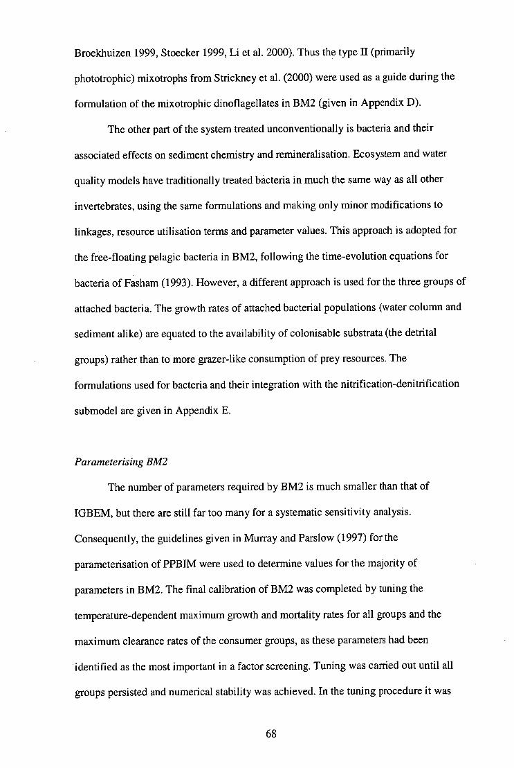
Broekhuizen 1999, Stoecker 1999, Li et al. 2000). Thus the type 11 (primarily

phototrophic) mixotrophs from Strickney et al. (2000) were used as a guide during the

formulation of the mixotrophic dinoflagellates in BM2 (given in Appendix D).

The other part of the system treated unconventionally is bacteria and their

associated effects on sediment chemistry and remineralisation. Ecosystem and water

quality models have traditionally treated bacteria in much the same way as all other

invertebrates, using the same formulations and making only minor modifications to

linkages, resource utilisation terms and parameter values. This approach is adopted for

the free-floating pelagic bacteria in BM2, following the time-evolution equations for

bacteria of Fasham (1993). However, a different approach is used for the three groups of

attached bacteria. The growth rates of attached bacterial populations (water column and

sediment alike) are equated to the availability of colonisable substrata (the detrital

groups) rather than to more grazer-like consumption of prey resources. The

formulations used for bacteria and their integration with the nitrification-denitrification

submodel are given in Appendix E.

Parameterising BM2

The number of parameters required by BM2 is much smaller than that of

IGBEM, but there are still far too many for a systematic sensitivity analysis.

Consequently, the guidelines given in Murray and Parslow (1997) for the

parameterisation of PPBIM were used to determine values for the majority of

parameters in BM2. The final calibration of BM2 was completed by tuning the

temperature-dependent maximum growth and mortality rates for all groups and the

maximum clearance rates of the consumer groups, as these parameters had been

identified as the most important in a factor screening. Tuning was carried out until all

groups persisted and numerical stability was achieved. In the tuning procedure it was

68

ensured that all parameter values were within the range of empirical values found in the

general literature. As a consequence of this method of tuning, parameter values did not

always reflect a particular observation or reported value, but they did reflect values from

the literature.

Optional submodels

BM2 is part of a wider study of ecosystem models and so many alternative

submodels were built into various parts of the main model. These were generally chosen

to correspond to those of IGBEM and include forage and density dependent fish

movement, a fisheries effort model, fishing induced mortality on non-target groups,

functional group invasions and multiple alternative functional responses and mortality

schemes. The majority of these are not discussed here, but some will be addressed in

other chapters (e.g. chapter 6). The submodels included here are outlined in the

following section.

2.3 Model runs

The standard runs of BM2 cover a 20 year time period, with output being

recorded every 14 days. This run length and record step matches that of IGBEM, and

the rationale for these choices may be found in chapter 1. One hundred year runs are

also undertaken to check for long period cycles and to verify that the model has reached

a representative state at the end of the 20 year period. Looping of the forcing files for

the physical transport model is necessary, as the files only span four years, and this is

done in the same manner as for IGBEM (chapter 1). The majority of the groups in the

modelled food web have a linear natural mortality term, but for those groups on the

upper edge of the web an additional quadratic mortality term is also imposed. This

second term represents predation due to groups not explicitly represented in the

69

modelled web. This combination of linear and quadratic mortality terms is used in all

standard runs of BM2, and the functional response employed in these runs is the one

used in PPBIM (a Holling type II). In the standard form of BM2 the recruitment of fish

is constant and fish migration is prescribed (as in IGBEM, chapter 1).

The assumptions underlying the formulations for the recruitment and movement

of fish are some of the weakest in BM2. Thus, to explore model behaviour under

alternative assumptions, runs that used alternative fish movement and recruitment

relationships were undertaken. Forced migration and constant recruitment of fish, as

employed by ERSEM H, was adopted initially, and this facilitates comparisons with

IGBEM. Other formulations examined included alternative recruitment formulations

and a forage and density dependent fish movement, which allocates fish to the cells

based on available resources, clumping around good resources and dispersing if

conditions were poor (rather than a fixed, prescribed, matrix of proportions) (Appendix

F). The alternative recruitment formulations include a lognormal distribution, a

Beverton-Holt stock recruitment curve, and a recruitment relationship which uses

primary production (as a proxy for larval resource availability) to dictate the number of

recruits settling out in each cell (Table 2.2). These recruitment relationships are

parameterised such that, if there is a constant stock size and no environmental changes,

the average number of recruits returned matches that of the initial state of the system.

To evaluate the performance of BM2 under varying conditions and to judge

how well the model replicates the behaviour of natural systems, the nutrient forcing files

for BM2 were scaled so that the new values matched the area-corrected inputs (from

Monbet 1992) for three other bays from around the world (Figure 2.3). The geometry

and hydrodynamics remained unchanged, but the levels of inflowing nutrient were

altered in an attempt to capture the state of other bays. In an effort to produce a generic

system rather than one tied to specific circumstances, the parameter set used in

70

Table 2.2: The recruitment relationships available in BM2. The number of recruits

added to box j at time t is represented by bu. Note that the number of recruits produced

by the Beverton Holt recruitment relationship is calculated at the beginning of the

recruitment period, but is delivered evenly across the recruitment period rather than

being delivered in a single pulse on the first day.

Recruitment Regime Standard

Formulation bo = J

ce' Li,

(fi-FL,J ) by = t x

cx b.

• CHL .,,, 71 chi

Definition of Specific Terms ft= element t of the recruitment vector (constant spatially and temporally) a= Beverton-Holt a for the fish group fl= Beverton-Holt (3 for the fish group Ly = biomass of larvae in box j at time t* tx = total length of recruit period 77Fx = recruitment coefficient for fish group FX CHL.,,,= water column chlorophyll in box j at time t 71chi = reference level of chlorophyll (1.5) AFx = recruitment multiplier for fish group FX y U(0,1) o= 0.3 p= -0.5 71- = 3.141592654

Beverton-Holt stock-recruit relationship (distributed evenly across the recruitment period) Proportional to Primary Production

Lognormal distribution

(-(tog y-pr 2.01 bd = AFx, e

y 11 2

* See equation B.11 in Appendix C.

Figure 2.3: Map of the world showing the bays used to evaluate the performance of

Bay Model 2 (BM2). Symbols mark the locations of all the systems for which marine

biomass or production estimates are available for comparison with the output of BM2.

The bays marked with a black symbol are the bays used to set the alternative nutrient

71

BM2 with baseline ecosystem conditions is not parameterised to match the species

composition of any particular bay. Instead the parameters used are based on species

from temperate bays across the globe and so there is no retuning with each change in

nutrient loading. This approach is also used with IGBEM (chapter 1) and proved to be

robust. A range of measures, including levels of chlorophyll a (chi a), DIN, biomasses

and system indices, are used to judge the model performance against available data

across the entire set of bays shown in Figure 2.3.

2.4 Results and discussion

2.4.A BM2 vs IGBEM and real bays

The groups in BM2 and IGBEM are identical and both use the same spatial

resolution and track the nitrogen content of the biomass pool, but aggregation of model

output is necessary for comparison with data from real bays, which is not available at

the same resolution. The pooling and nomenclature adopted during the analysis of

IGBEM (chapter 1) is adopted here. The pooled outputs refer to the trophic sets:

chlorophyll a (chl a) (as a proxy for total phytoplankton), zooplankton, fish,

macrophytes, microphytobenthos, meiobenthos, benthos (all the other benthic consumer

groups) and detritus (labile and refractory).

Range in biomass

Comparison of the range in biomass (for each trophic set) in real bays with that

predicted by the models indicates that BM2 performs satisfactorily (Figure 2.4). For the

majority of trophic sets the range of values produced by BM2 under different levels of

nutrient forcing is within the range of empirical values from bays around the world.

However, some trophic sets deviate from real world values. Ranges for the water

column trophic sets for BM2 are all much smaller than their real world counterparts,

whereas those for many of the benthic groups are as large (or larger) than those seen in

72

Figure 2.4: Range and average value for each of the main trophic sets of BM2

compared with values from empirical observations and from the output of IGBEM. The

y-axis for zooplankton is biomass in mg AFDW IT1-3 ; for fish, macrophytes, benthos,

meiobenthos and detritus the y-axis is biomass in g AFDW 111-2 ; the y-axis for chi a is

mg chi a rrl-3 ; for DIN it is mmol DIN 111-3 ; and for microphytobenthos it is mg chi a 111-2 .

The values from the empirical observations are taken from Appendix A.

003

80003 —

60303 —

40300 —

_

600.00 —

40300 —

IF

203D0 —

20303 —

5003 —

40.00 —

3300 —

2003 —

1000 —

60003 —

403.00 —

20003 —

16003 —

12003 —

8003 —

4003 —

■.1

Zooplankton Fish Macrophytes Microphytobenthos Chl a

• Real Bays

0 Model Bays (BM)

ka Model Bays (IGBEM)

Maximum

Trmiad Av.rox (Wag/wawa TemerrozAverape

Minimum

12opo —

8000 —

000

1203 — 1600000 —

Benthos Meiobenthos Detritus DIN

8C0 —

403 — 1 1200000 —

8030.00 —

430003 —

25003 —

20300 —

15000 —

10300 —

5000 —

73

the field. With respect to the ranges for biomass produced by IGBEM, the ranges

generated by BM2 are comparable, though they do tend to be larger. The small range of

values from the models for water column variables is not surprising given the very small

range of nutrient inputs used to force the models. The simulations covered the cases

from baseline loadings up to x30, whereas some real systems may reach as high as

x1000 (e.g. Loire Estuary in France, Monbet 1992). Trying the model under the same

range of loads as seen in nature is not possible, as sufficient biological and physical

forcing data is only available for systems with loads up to x30. In contrast to the water

column trophic sets, the predicted ranges of biomass for the benthic trophic sets often

match or exceed the empirical ranges of biomass for these sets. Therefore, the ranges for

biomass predicted for the models if loading were set to x1000 are unlikely to match

those observed in reality unless the benthic groups in the model experience down turns

when the nutrient forcing is raised above x30. There is some suggestion of this in the

model dynamics with increasing nutrients, but further evaluations at higher nutrient

loads would be necessary to confirm that the pattern of declines persists as nutrient

loading reach extreme levels.

That so many of the trophic sets in BM2 have a wider range of values than in

IGBEM suggests that the simpler process formulation used in BM2 is not as limiting as

the use of explicit physiological formulations and internal nutrient ratios in IGBEM.

This may explain why the biomass ranges for the benthic groups in BM2 tend to be

large. The simple assimilation equations used in BM2 apparently lack the degree of

potential regulation captured in the use of internal nutrient ratios in IGBEM.

Equations of the form used for the invertebrate groups in BM2 are commonly

used in water quality modelling. The field of water quality (and plankton) modelling is

well developed (e.g Fransz et al. (1991) identified 20 plankton models developed since

the 1970s for the Atlantic Ocean and adjoining seas) and so the equations used have

74

been examined extensively and their limitations and associated remedies (e.g. model

closure using quadratic mortality, see Steele and Henderson 1992, Edwards and

Brindley 1999, Murray and Parslow 1999b, Edwards and Yool 2000) are well

understood. By comparison, ecological modelling of benthic communities is at an early

stage. In particular, processes controlling the food web based on detritus are rather

unclear. Therefore, the general form of the pelagic invertebrate groups is also used for

the benthic invertebrates in BM2, with the addition of space based limitation of

sedentary epifauna and oxygen related constraints on the infauna. This structure is

adopted because there is no available information indicating that many additional

processes were necessary. However, our results suggest that benthic groups and

processes may be more constrained than previously thought. Detailed tracking of flows

in BM2 indicates that the dynamics of the benthic deposit feeder group is the primary

cause of the large biomass ranges produced for benthic trophic sets. This suggests that

this group may require some form of space limitation (via a crowding effect), similar to

that applied to the benthic suspension (filter) feeders. Given that these animals are

largely confined to the aerobic layers of the sediment (Barnes 1987, Webber and

Thurman 1991), which is typically shallow, there is a sound biological basis for this

idea. Overall, results for the ranges in biomass suggest that the water column

components of BM2 function well, but that the benthic components can be refined

further (see chapter 3).

Average biomass

Average values of the biomass for each trophic set and the values produced

under specific conditions are also informative in assessing model performance.

Accounting for the magnitude of the range in the field values, the average values

produced by BM2 are similar to those reported by IGBEM and observed empirically in

75

temperate bays (Figure 2.4). In all, 6 of the 9 trophic sets in BM2 were within 10% of

the average empirical value for temperate bays and all were within 33%. The best match

is by the macrophytes where the average biomass produced by BM2 is within 2% of the

average of empirical observations. The worst fit is the microphytobenthos, where the

difference between the model and empirical average is 32.5%. This performance is

similar to that of IGBEM. More importantly, the performance of IGBEM is not

consistently superior to that of BM2. Considering the 9 trophic sets in Figure 2.4, and

using the average biomass as the performance measure, both models did equally well

for chl a and benthic groups; the predictions of IGBEM are marginally better than BM2

for zooplankton, meiobenthos, detritus and microphytobenthos; while the performance

of BM2 surpasses that of IGBEM for the fish, macrophytes and DIN. This lends further

support to the view that the formulation of the water column components in BM2 is

largely sufficient to capture their dynamics faithfully, while the sediment groups may

require further attention if they are to behave as well as those in IGBEM.

The results for zooplankton (Figure 2.4) indicate a need for improvement of this

component. The results for average biomass of zooplankton given by BM2 are restricted

to the upper end of those given by IGBEM. While acceptable in a generic situation as a

heuristic tool, it suggests caution in prognostic application of BM2 to natural systems

(see chapter 3). -

Standard relationships

Monbet (1992), Schwinghamer (1981) and Sheldon et al. (1972) identified

strong system-level relationships (ecological and physical) that hold for systems from

around the world. Any ecosystem model, particularly one used as a foundation model

for an investigation of model structure and behaviour, should produce output that

conforms to these relationships. BM2 meets this requirement.

76

Two of the most significant biological relationships uncovered in marine

systems are the size-spectra (or "Sheldon spectra") identified by Sheldon et al. (1972)

for the pelagos, and Schwinghamer (1981) for the benthos. The Sheldon spectrum for

pelagic life is essentially flat (Sheldon et al. 1972), while the corresponding spectrum

for the benthos is W-shaped (Schwinghamer 1981). The classes identified by

Schwinghamer are pooled to match the size resolution used in the models, which

converts the benthic size-spectrum from a "W" into a "U". The spectra calculated for

BM2 match well with those of Sheldon et al. (1972) and Schwinghamer (1981), while

those for IGBEM do not (Table 2.3 and 2.4). This is especially true for the microscopic

classes, particularly in the benthos (Table 2.4). The behaviour of these classes are a

major weakness of IGBEM, but not of BM2. Values for benthic classes from BM2 are

well within the confidence intervals given by Schwinghamer for his general spectrum

(Schwinghamer 1981).

Table 2.3: A summary of the Sheldon spectra for the pelagic classes in the run of Bay

Model 2 (BM2) and the Integrated Generic Bay Ecosystem Model (IGBEM) where the

environmental conditions match those in Port Phillip Bay. Following the convention set

by Schwinghamer (1981) the unit area biomasses are given in cm3/m2 .

Class BM2 (cm3/m2) IGBEM (cm3/m2) Bacteria 3.48 40.50 Ph ytoplankton 8.72 10.02 Zooplankton 16.26 10.47 Planktivorous fish 8.84 5.45 Other (larger) fish 8.85 6.37

77

Table 2.4: A summary of the pooled Sheldon spectra for the benthic classes in the run

of Bay Model 2 (BM2) and the Integrated Generic Bay Ecosystem Model (IGBEM)

where the environmental conditions match those in Port Phillip Bay. The values given

by Schwinghamer (1981) are included for comparison.

Class BM2 IGBEM Schwinghamer (cm3/m2) (cm3/m2) (cm3/m2)

Bacteria 24.9 0.2 80.1 Meiobenthos and Microphytobenthos 5.63 0.7 6.1 Macrofauna 208.7 149.5 473.0

Monbet (1992) found a strong positive linear relationship between the

logarithms of the water column concentrations of chl a (mg m -3) and DIN (mmol m -3).

Tidal range is also an important part of this relationship as macrotidal and microtidal

(>2m and <2m tidal range respectively) systems cluster separately, with little overlap

(Port Phillip Bay is microtidal). Both BM2 and IGBEM comply with Monbet's

relationship (Figure 2.5), but the performance of IGBEM is better than that of BM2 in

which the response of chl a to DIN is flatter.

A final general relationship is that the maximum average biomass of

meiobenthos decreases as the depth of the overlying water column increases (chapter 1).

The biomass of meiobenthos given by the models reflects this relationship well (Figure

2.6), although those of BM2 tend to sit closer to the upper bound.

2.4.B Spatio-temporal structure and the effects of environmental change

Temporal and spatial behaviour are also important indicators of model

performance. The spatio-temporal dynamics of BM2 and IGBEM are similar, and can

produce sophisticated behaviours (such as competitive exclusion and long period

cycles) and reproduce spatial zonation and events observed in Port Phillip Bay (PPB).

78

Biom

ass

of M

e iob

enth

os (g

AFD

W m

-2)

200

(.? E co r 0

g

01

.1

10

1009

mmol DIN m -3

Figure 2.5: Comparison of the mean annual Dissolved Inorganic Nitrogen (DIN)

against mean annual chlorophyll a (chl a) for real (open circles) microtidal marine

systems (based on Monbet (1992) and additional values from the literature - see

Appendix A), BM2 (black squares) and IGBEM (grey diamonds).

Maximum water depth (m)

Figure 2.6: Plot of the average biomass of meiobenthos against maximum depth of the

system for marine systems from around the globe (open circles), BM2 (black squares)

and IGBEM (grey diamonds). The curve marking the upper bound was found by fitting

the curve to the highest points in the plot (chapter 1), where y is the biomass of

meiobenthos and x is the maximum water depth.

79

Spatial structure

The runs using the baseline nutrient loadings for Port Phillip Bay and

Chesapeake Bay are designated PM and CM respectively. The predicted average

biomasses per box over the final four years of the CM and PM runs, using both BM2

and IGBEM, were analysed to determine whether there are boxes that had similar

biological and physical properties, which would suggest spatial patterns in the model

output. The average biomasses of all groups in each box were compared on a two-

dimensional non-metric Multidimensional Scaling (MDS) plot derived from a Bray

Curtis similarity matrix to identify groups of boxes of similar community structure. The

average values of the physical variables and the biomass per group were then examined

(using the SIMPER routine of the Primer software package) to ascertain which groups

determined the clustering seen. This analysis identified "areas" (boxes in the model

sharing biological and physical characteristics) in the model output. Only the PM and

CM runs are analysed in this way because they encapsulate the general form and

dynamics of the "mesotrophic" and "eutrophic" states of the models under the current

geometry and forcing.

The two models contained a similar number of areas which are located in similar

positions around the bay (Figures 2.7 and 2.8). Areas predicted to share communities

(dominant biological groups) were pooled to produce "zones" and, as with the "areas",

the two models showed a good deal of agreement (Figure 2.9). A number of factors

produced this zonation and habitat suitability alone does not explain the sharp

distinction between the community assemblages around the edge of the bay and those of

the central zones of the bay. In the models, these discontinuities are due to predator-prey

dynamics (suppression and supply), resource partitioning and competitive exclusion,

particularly in the benthos. These sophisticated behaviours are emergent in the models.

An important predator-prey interaction is that of the benthic grazers and macrophytes.

80

Figure 2.7: Maps of the biological and physical areas (boxes with similar

characteristics and community compositions) identified by the MDS, cluster and

correlation analyses of the runs using the loadings for Port Phillip Bay (the PM run) of

BM2 and IGBEM. Areas with the same numbers or letters within each map were part of

the same cluster in the output of the analysis. (a) biological areas identified for BM2, (b)

physical areas identified for BM2, (c) biological areas identified for IGBEM, and (d)

physical areas identified for IGBEM.

(a)

(c)

riti, k

0' 1° ‘

.

rt

(b) N eg, / t

er' Ott' . 4111COP 4

rip\

/ et) 0101111)

(d)

°11I0 'I'llf111641\ #111‘i. Dk

ifA\

81

Figure 2.8: Maps of the biological and physical areas (boxes with similar

characteristics and community compositions) identified by the MDS, cluster and

correlation analyses of the runs using the loadings for Chesapeake Bay (the CM run) of

BM2 and IGBEM. Areas with the same numbers or letters within each map were part of

the same cluster in the output of the analysis and do not correspond to any of the

numbers or letters in Figure 2.7. (a) biological areas identified for BM2, (b) physical

areas identified for BM2, (c) biological areas identified for IGBEM, and (d) physical

areas identified for IGBEM.

(a) I%

.1 2,o r 4 4149/

(b)

/0 "A

iik, 1 I N

(c)

4 ,.. la4

gjAeh\ D 3

t im- g I it" (d) ei\

411) 411" 4 f

82

(a) (b)

Figure 2.9: Distribution of the main zones identified in the output of Bay Model 2

(BM2) and the Integrated Generic Bay Ecosystem Model (IGBEM) (a) PM run of BM2,

(b) PM run of IGBEM, (c) CM run of BM2, and (d) CM run of IGBEM. The zones in

white are part of Bass Strait or heavily influenced by it; the light grey zones are

characterised by specific plankton assemblages (dominated by diatoms or

microplankton), as well as a rich assemblages of fish, macrophyte and benthic

macrofauna; while the dark zones are characterised by another plankton assemblage

(dominated by flagellates and large zooplankton), and well developed populations of

meiobenthos, microphytobenthos, and bacteria.

83

Benthic grazers at high densities are only found in areas with persistent macrophyte

populations. Further, the "macrophyte-barrens" cycle involving these groups (detailed

below in the section on temporal dynamics) does not occur simultaneously around the

edge but is sequential and driven, in part, by the total flows around the bay. This

indicates that there is a refuge (macrophytes escape grazing) and pursuit (benthic

grazers find new prey reserves) dynamic in action.

The clearest example of resource partitioning observed in the output of the

models is within the detrital feeders and the effect is pronounced in BM2. The

distribution of the meiobenthos and deposit feeders in BM2 show little spatial overlap

and maintain healthy populations by spatial partitioning of their demands on shared

food groups. If this spatial segregation is prevented by running the model on a coarser

geometry (say 1 box instead of 59) then the model undergoes self-simplification and

either the deposit feeder or meiobenthic group is lost (chapter 4). Usually it is the

meiobenthos that goes extinct because it is both a competitor and prey of the deposit

feeders. This result emphasises the importance of spatial context and differentiation in

the model, as it provides a mosaic of spatial refuges and allows for emergent dynamics.

Competitive exclusion also arises in the benthic primary producer subweb, in

which the macrophytes displace the microphytobenthos. The macrophytes potentially

suffer from space limitation (if their biomass rises too high) and the effects of their

physical environment (macrophytes are uprooted in rough conditions and epiphytes foul

seagrass when nutrient levels are high). However, these factors arise only occasionally

so that the macrophyte-microphyte interaction is largely driven by limiting nutrients.

Because the microphytobenthos is limited by silica (Si), while the macrophytes are not,

this allows the macrophytes to dominate the microphytobenthos when silica levels are

low. However, the low light requirements of the microphytobenthos ensure its survival,

though in reduced amounts, in the central parts of the bay where the light conditions do

84

not allow macrophyte growth.

Temporal dynamics

BM2 displayed many of the temporal dynamics previously reported for IGBEM

(chapter 1). Both models demonstrate seasonal bloom dynamics, interannual variation

and the long-term "macrophyte-barren" dynamics. However, in BM2 the interannual

variation is often damped in the epibenthos, particularly in the macrozoobenthos, which

shows little interannual variation. Similarly the "macrophyte-barrens" cycle is also

different in BM2 compared with IGBEM. This cycle did not occur in all boxes

populated by macrophytes in BM2, but arose only in the more marginal macrophyte

habitats. Populations in more favourable sites showed only interannual fluctuations

related to the hydrodynamic forcing and nutrient inputs. Moreover, where a

"macrophyte-barren" cycle did occur it tended to have a shorter period and smaller

amplitude than in IGBEM. A "macrophyte-barren" cycle has not been observed in PPB,

so the dynamics predicted by BM2 appear to be closer to the natural state of PPB.

The much richer dynamics of the microfauna in BM2 translated into a wide

range of temporal dynamics. These groups displayed cycles in the short, medium and

long term (Figure 2.10). The short-term patterns reflected seasonal changes in growth

and the availability of food. The medium term cycles gave a clear indication of the

impact of the hydrodynamic forcing, which acts in the same way as reported for

IGBEM (chapter 1) and PPBLM (Murray and Parslow 1997). The long-term dynamics

were not as regular as the short and medium term patterns. Instead they often

represented transient events (although these could last for a decade or more), after

which the group would return to biomass levels and cycle characteristics very similar to

those before the event (one such event is included in Figure 2.10). These "events" were

caused by the coincidental occurrence of conducive physical and biological conditions

85

Interannual variation

Seasonal variation II

Long term variation

0 5390 6846 8302 9758 11214 12670 14126 15582 17038 18494

Day of run

Figure 2.10: The biomass (mg AFDW ni 2) through time for the aerobic bacteria in box

23 (see Figure 2.1) of BM2. This time-series of biomass reveals examples of seasonal,

interannual and long-term variation.

(primarily the densities of predators, prey and competitors). That both models suggest

that physical and biological interactions, free from the impacts of escalating human

activities, can cause substantial changes in biomass which persist for a decade or more

is intriguing. It also suggests that current efforts, focused by concern over climatic

change and other human impacts, may not be completely successful in separating

natural dynamics and anthropogenically driven change.

Effects of eutrophication

While models can highlight that not all major changes in ecosystem structure

and function are necessarily due to human intervention, they can also be instructive in

showing where to look for human induced change. To be useful in identifying critical

human-induced ecosystem behaviours, ecosystem models must be able to capture the

gross changes that occur when a system becomes eutrophied. Both BM2 and IGBEM

(chapter 1) capture the major system changes that occur with eutrophication; i.e.

86

simplification in biological structure, changes in relative community composition, a

"left-shift" to smaller animals in the size-spectrum and an eventual drop in productivity.

BM2 (like IGBEM) predicts that, with an increase in nutrients, the communities

usually found in the deep central parts of the bay expand to displace the communities

typically found in shallower water along the edge of the bay (compare Figure 2.9). This

in turn causes the decline of some groups (such as the benthic grazers) and the effective

extinction of seagrass. Thus, the dynamics of BM2 reflect the simplification in habitat

and biological diversity observed in real systems following eutrophication (Gray 1992).

The only macrofaunal groups to increase are deposit feeders, which are tracked by

benthic infaunal carnivores, as the levels of detritus in the sediments increase. This is

symptomatic of the general habitat change that accompanies replacement of a primary

production based trophic web with a detritus based web. Notably, the initial rises in

biomass and productivity predicted by BM2 under a modest rise in nutrients are

completely reversed when nutrients rise by x10 or more, at which point productivity

drops to between 20 to 50% of the original levels and biomass drops by more than half.

This is in agreement with the results of IGBEM (chapter 1) and field monitoring studies

(Harris et al. 1996).

The concordance of predicted dynamics in BM2 with those in nature is also

evident for water column groups. While the gross dynamics captured by IGBEM are

sound, it does not capture all of the changes in relative community composition that

occur with eutrophication. For example, IGBEM does not predict the increase in large

phytoplankton with increasing nutrients, but it does indicate that the large zooplankton

will be replaced by smaller groups (chapter 1). In contrast, BM2 correctly captures the

changes in composition of all planktonic groups (Table 2.5). With an increase in

nutrient load in BM2, there is a strong increase in the relative abundance of the larger

phytoplankton (diatoms and dinoflagellates) and a substantial (50%) decline in the

87

relative abundance of the large zooplankton. This closely follows observations in the

field (Murray and Parslow 1997, Park and Marshall 2000).

Table 2.5: Relative abundance of the large and small size fractions of the phytoplankton

and zooplankton communities in the runs of BM2 and IGBEM using the nutrient

loadings of Port Phillip Bay (PM run) and Chesapeake Bay (CM run). Empirical values

for Chesapeake Bay (CB) (Madden and Kemp 1996) and Port Phillip Bay (PPB) (Harris

et al. 1996) are included for comparison.

Size fraction PM- PM- PPB CM- CM- CB BM2 IGBEM BM2 IGBEM

Large phytoplankton (> 20pm) 0.30 0.27 0.28 0.65 0.22 0.75 Small phytoplankton (0.2 — 20gm) 0.70 0.73 0.72 0.35 0.78 0.25

Large zooplankton (2 — 200grn) 0.6 0.55 0.64 0.23 0.35 0.19 Small zooplankton (0.2 — 20mm) 0.4 0.45 0.36 0.77 0.65 0.81

Neither BM2 nor IGBEM predict extensive anoxia and subsequent die off of

benthic and fish fauna (as seen in places such as the Baltic), but BM2 does predict

seasonal drops in oxygen levels of up to 30% (due to the breakdown of phytoplankton

blooms). That this does not progress to anoxia is because the bay is well mixed. The

formulations used in BM2 and IGBEM should allow for the development of anoxia in

suitable physical conditions, but as yet physical geometries more conducive to the

formation of anoxic conditions under high loading (e.g. a deeper or more stratified bay)

have not been tested. While there is no anoxia-related collapse of the fish, BM2 does

predict a decline in the average size of fish. This is most severe for herbivorous fish,

which decline in size by 10% or more, which agrees with patterns recorded in the field

(Tober et al. 1996). This not only leaves fish vulnerable to predation for longer, but it

could significantly affect recruitment. This potential effect is masked by the constant

recruitment function employed in the standard runs of BM2 and IGBEM.

There are important physical and chemical consequences of increased nutrient

88

load, and these are more evident in BM2 due to its improved handling of the microfauna

in the sediments. There is a severe drop in denitrification efficiency, particularly in the

centre of the bay, as nutrient levels rise. This is severe enough under even a moderate

(fivefold) rise in nutrients that the usual route of nitrogen disposal (via denitrification) is

overwhelmed and nutrients build up to sufficiently high levels that they can now only be

exported by flushing. Because the flushing time for PPB is close to a year (Harris et al.

1996), and the storage capacity of the bay's sediments is immense, these conditions are

not easily reversed. Thus, the detritus based, highly eutrophied state of the bay persists

years after the model's nutrient input levels have been reduced below those used for the

PM run. This hysteresis was also observed in PPBIM (Murray and Parslow 1999) and

has not been diluted by addition of other trophic groups, or the modifications made to

the sediment model (see Appendix E), during the construction of BM2.

The final observation of note reflecting the effects of eutrophication is that the

change in the ratio of aerobic to anaerobic bacteria in BM2 mirrored that in IGBEM.

The index fell from 3.50 to 0.38 as the nutrient inputs were increased to x30 baseline

levels. This suggests that this index may be a robust indicator of system-level change.

2.4.0 Strengths and weaknesses

No model can be a perfect representation of nature and so each has its relative

strengths and weaknesses. The behaviour of BM2 in comparison to reality and IGBEM

were used to give insight into the model's strengths and weaknesses. Aberrant or

inaccurate behaviour is considered a weakness, while behaviour of a component that is

close to matching reality is considered a strength (especially if it used a simpler

formulation than employed in IGBEM). The weakest points in BM2 stem from its

simplicity, and reduced form, and are shared by all models that make the same sets of

assumptions and construction choices (such as PPBIM). Its greatest strengths also come

89

from its reduced form and the choices made during its development.

Nutrient limitation

The omission of limitation by phosphorus was a considered decision made early

in the development of BM2. Under the conditions considered here, it is a sensible

choice for bays such as Port Phillip Bay that have phosphorus in excess (Harris et al.

1996). However, this may not be true of all bay systems, such as the Bay of Seine,

France (Guillaud et al. 2000)). It is sensible and straightforward to include phosphorus

limitation of primary production in models of natural systems where it is known that

phosphorous is limiting.

The implementation of nutrient limitation and flows in ecosystem models is

made easier by the observation by Redfield et al. (1963) that the major chemical

constituents (N:C:P) are maintained in a relatively constant ratio (around 16:90:1).

Models such as BM2 use the external (water column) nutrient ratio to determine the

effective uptake of nutrients by the primary producers, whereas models such as IGBEM

use the internal (cellular) nutrient ratios to determine nutrient uptake (Baretta-Bekker et

al. 1997) (also see Table 2.1). Under oligotrophic conditions the application of Redfield

ratios and the use of external nutrient limitation may not work. In the case of highly

oligotrophic systems, such as the Baltic Sea (Thomas et al. 1999), there is evidence that

only internally based Droop-like equations (formulated following the ideas of Droop

1973, 1974) will accurately reflect the dynamics of the primary producers (Baretta-

Bekker et al. 1997). The nitrogen and phosphorus of the particulate organic matter in

these areas is preferentially remineralised and the resulting decline in dissolved

inorganic carbon (DIC) over the growing season is much greater than predicted from a

Redfield ratio conversion of the decline in nutrients (Thomas et al. 1999, Osterroht and

Thomas 2000). Simulation runs completed for IGBEM and BM2 in which nutrient

90

inputs were 20% of those in runs using baseline ecosystem conditions match these

observations. The new production predicted by IGBEM is between 1.2 and 2.5 times

that given by BM2 and this agrees with the findings of Osterroht and Thomas (2000)

that new production based on DIC consumption is, on average, 1.5 times that based on

nitrate consumption. These findings indicate that simple nutrient uptake and growth,

like that in BM2, is sufficient when nutrients are in excess. However, when nutrients are

low the luxury uptake of nutrients facilitated by Droop-like equations is required if

system-level behaviour is to be captured faithfully.

Recruitment and movement offish

A theoretical shortcoming of BM2 is the implementation of recruitment,

movement and mortality in the fish groups. Like IGBEM, the standard runs of BM2 use

constant recruitment and prescribed fish movement. These formulations do not reflect

particularly realistic assumptions regarding underlying processes. Consideration of

alternative formulations is crucial for judging the general performance of the standard

form of the model.

The effects on BM2 of the use of these features, or their alternatives, were

similar in BM2 and IGBEM. Constant recruitment buffers BM2 against large-scale

changes in productivity and especially against the effects of substantial changes in

fishing pressure (chapter 7). Of the three alternative recruitment schemes tested (Table

2.2), the Beverton-Holt is the most effective at correcting for aberrant effects of

constant recruitment. This is important as recruitment has a substantial impact on the

potential size, persistence and behaviour of the fish stocks. The stocks did demonstrate

more dynamic responses to changes in nutrients and fishing pressure when a Beverton-

Holt recruitment scheme is used. For instance, when fishing pressure is raised fivefold

for all harvested groups the constant recruitment for the fish groups in the standard run

91

buffered each group equally well so the decline and subsequent stabilisation of the

biomass occurred at about the same pace in each. However, in the run with the

Beverton-Holt stock recruit curves the planktivores did not decline at the same pace.

This is because the reduction in the number of their predators allowed them some

measure of release so enough adults remained (in spite of heavy fishing) to keep the

stock from total collapse for a few more years than is the case for the other groups of

fish (Figure 2.11). The steepness of the Beverton-Holt relationships used varied from

0.78 for the planktivores to 0.92 for the demersal herbivorous fish (Table 2.6). While

these steepness values are representative of those for many fish species (Francis 1992,

Koopman et al. 2000), they were derived here by tuning the parameters so that the

average number of recruits matched the constant recruitment case. It is possible that if

the Beverton-Holt stock recruit curve for each group had been taken from real fish,

rather than just fitted, that the steepness values may have been much lower (there are

cases where steepness is as low as 0.32 (Koopman et al. 2000)). If this were the case,

then the effect of using this form of recruitment may have lead to a different outcome.

Table 2.6: Steepness values for the Beverton Holt stock recruit curves implemented for

the fish groups.

Group Steepness Planktivorous Fish 0.78 Piscivorous Fish 0.81 Demersal Fish 0.79 Demersal Herbivorous Fish 0.92

92

1

Aver

age

biom

ass

FD (g

AFD

W m

-2)

3

2

1

Aver

age

biom

ass

FP (g

AFD

W m

-2)

0

• FD (standard Fx5) O FD (BH Fx5) • FP ( Standard Fx5) O FP (BH Fx5)

0 0 15 • • • 8 8 1.1 • • 8 A o

0 462 924 1386 1848 2310 2772

3234

3696

Days since stock collapse began

Figure 2.11: Declines in biomass of the demersal (141)) and planktivorous (FP) fish with

an increase in fishing for the standard run of BM2 and the run using Beverton-Holt

recruitment.

Recruitment as a function of primary production is more responsive in BM2 than

in IGBEM and this is due to the greater amplitude and greater number of short period

fluctuations in chi a in BM2. These fluctuations produced quite complex recruitment

patterns, especially if the spawning window coincided with a spike or trough. However,

the use of an index of total primary productivity as an index of recruitment is a problem

in BM2, as in IGBEM, as it did not allow for a drop in recruitment with eutrophication.

Use of this recruitment formulation requires the replacement of chl a (the index of total

primary production used here) with a measure of abundance of a specific planktonic

group as an index of year class strength.

Incorporating a random factor into recruitment, as well as density and forage

dependent movement, can be used to explore broader theoretical aspects of overall

model behaviour in BM2. Large recruitment and aggregation events are common in at

least some harvested stocks (Samoilys and Squire 1994, Power and Atkinson 1998).

93

Using random recruitment or forage- and density-dependent movement to reproduce

these events and consider their effects on the system as a whole could be instructive as a

guide to understanding the implications of these phenomena in nature. That is not the

aim of this model study though, so despite this potential they do not substantially

change the existing conclusions regarding the performance of BM2.

Trophic closure

The mortality terms used for the highest trophic groups explicitly included in the

model can have a substantial impact on model behaviour (Steele and Henderson 1992,

Edwards and Brindley 1999). In BM2 each functional group has a linear mortality term

representing the impacts of natural mortality, but ignoring the effects of higher

predation. Experience with IGBEM lead to the inclusion of a quadratic mortality term

for some functional groups in BM2. This quadratic term implicitly represents the effects

of predation from groups not explicitly represented in the model, such as sharks,

mammals and birds. Unfortunately, this did not completely correct for the problems of

non-responsive higher trophic levels identified in chapter 7.

Considering the entire model food web, quadratic mortality terms are imposed

on all groups that are at the edges of the web or link subwebs (such as the large

zooplankton and macrozoobenthos). That is, quadratic mortality is imposed on those

groups that had at least one predator not explicitly represented in the modelled web.

This increased model stability and reduced the parameter space within which explosive

growth is predicted, though it did not completely eradicate it across the range of

parameter values that were trialled. Comparisons with IGBEM, which does not include

quadratic mortality, indicates that system-level behaviours, biomasses and qualitative

conclusions based on the models do not change markedly due to the inclusion of

quadratic mortality. Though a more thorough sensitivity analysis may indicate

94

otherwise. This is a major concern within the literature discussing trophic closure in

Nutrient-Phytoplankton-Zooplankton models (Steele and Henderson 1992, Edwards and

Brindley 1996 and 1999, Murray and Parslow 1999b, Edwards and Yool 2000). There

are problems with deducing the effects of quadratic mortality from a comparison of

models built on differing premises. An investigation of the effect on model behaviour of

linear and quadratic mortality on a single ecosystem model may lead to different

conclusions. It was found (chapter 6) that the behaviour of BM2 with and without

quadratic mortality enabled differed markedly under changing conditions and it was

concluded that quadratic mortality is the most appropriate form of model closure as it

allowed for realistic predictions across a range of conditions, whereas linear closure did

not.

Mixotrophy

The implementation of mixotrophy in BM2 is effective as it successfully

reproduced the main features of this behaviour recorded in laboratory studies. In a

comparison of runs with and without mixotrophy, the biomass of dinoflagellates is

increased tenfold if mixotrophy is allowed. Further, the rate of growth increased by 1.5

to 1000 times with mixotrophy and this matches the increases seen in laboratory

experiments comparing phototrophic and mixotrophic growth in the dinoflagellates

Fragilidium (Jeong et al. 1999) and Gyrodinium galatheanum (Li et al. 1999). This

boost to growth allowed the dinoflagellates to persist when they would have dropped to

negligible levels if dependent on phototropic growth alone. Thus, a weakness in many

previous models is corrected by the inclusion of a rudimentary representation of a real

biological process, rather than by setting growth rates to the upper bounds given in the

literature (as is necessary to even partially correct the problem in IGBEM).

95

Attached bacteria and the sediment chemistry

The method of handling attached bacteria in BM2 also works well. It produces

bacterial biomasses that match field estimates. For instance, the estimate is within 10%

of that for the Kromme Estuary in South Africa (Heymans and Baird 1995), one of the

few for which estimates of bacterial biomass has been made.

Even though the standard form of BM2 is a generic system rather than PPB in

particular, the evaluation of the modifications made to the sediment chemistry model

are best served by a comparison with the original form in the PPEUM model. The

formulation used for attached bacteria in BM2 removes a weakness in the sediment

chemistry of PPBIM. The original form of the empirical model used in PPBIM

predicted an annual efflux from the sediments of PPB of about 11,000 to 16,000 t DIN.

This is much higher than the sediment chamber estimates of Nicholson et al. (1996),

which suggested the efflux is likely to be between 3,600 and 8,100 t DIN per year. The

prediction by BM2 that the efflux is roughly 6,500 t of DIN per year matches this

sediment chamber estimate well. Thus, the adaptation of the empirical nitrification-

denitrification model of Murray and Parslow (1997, 1999) to include the dynamics of

attached bacteria and infauna has preserved its strengths (such as the hysteresis

discussed above), while correcting for its weaknesses.

Is less detail permissible?

The primary aim of the study presented in this chapter and chapter 3 is to

evaluate whether the omission of physiological detail from an ecosystem model had a

significant effect on model dynamics and the ability to represent reality. The

performance of BM2 compares favourably with that of the far more detailed IGBEM.

For the purposes of understanding system dynamics and at least qualitative responses to

shifts in ecosystem forcing, BM2 is as capable of representing systems as accurately as

96

IGBEM. This shows that physiological detail is not always required and that simpler

formulations, such as those employed in BM2, are generally adequate for learning and

general predictive purposes. This is important because, in comparison with IGBEM,

BM2 uses less than half the number of parameters, required less than one sixth of the

development time, and one tenth of the time to validate, verify and calibrate.

There is some anomalous behaviour, such as the almost exponential growth of

the deposit feeders under certain parameterisations and nutrient conditions (chapter 3).

The occurrence of this kind of behaviour should be used to guide the application of

BM2 on a site-to-site basis and under extreme conditions of change and the model may

benefit from the addition of space limitation for the benthic groups (chapter 3).

2.5 Conclusions

A holistic approach to the environment is becoming an integrated part of the

way resource use is thought about and dealt with (Gislason et al. 2000). As a result

ecosystem models are being developed as predictive and heuristic tools. However, a lot

of work remains to be done with regard to understanding the most efficient and effective

ways of constructing these models. As one step in this process, BM2 was constructed to

allow for an analysis of the effect of formulation detail on model behaviour and

performance. Overall, BM2 does function well, reproducing patterns and values that

match far more detailed models and reality. This makes it a good basis for further study

of model complexity, for example, to investigate the effects of the form of grazing and

mortality terms. It also indicates that it is possible to capture the qualitative dynamics of

systems without resorting to highly detailed physiological structures that characterise

other ecosystem models (e.g. ERSEM II (Baretta et al. 1995, Baretta-Beldcer and

Baretta 1997) or IGBEM (chapter 1)). This is not to say that models such as BM2 are

not without drawbacks. There will be occasions when the simple formulations used in

97

BM2 will be incapable of reproducing the real dynamics accurately, e.g. in oligotrophic

waters Droop-like equations would be needed to describe phytoplankton growth. The

simpler structure used in BM2 does have some impacts on its performance in specific

circumstances and this is explored in chapter 3. In many instances it would not take

much effort to modify BM2 to include formulations (such as Droop-like equations) that

would correct or temper these problems. Nevertheless, even without such modification

and with an eye to consideration of common system dynamics and the representation of

a generic temperate marine bay system, BM2 is instructive while requiring less

information than other biogeochemical ecosystem models currently in use.

98

Chapter 3 The Effect of Physiological Detail on Ecosystem Models II:

Models of Chesapeake Bay and Port Phillip Bay

Abstract

Bay Model 2 (BM2) is a biogeochemical ecosystem model. The model

formulation uses general assimilation equations rather than intensive physiologically

based equations to characterise the biomass dynamics of the modelled groups. The

model was developed as a part of a larger study considering the effects of formulation

detail on model behaviour.

The behaviour of the generic form of BM2 indicates that it can capture general

system properties and behaviour (chapter 2). Consideration of its behaviour when

applied to specific systems indicates that it can usually reproduce large scale patterns

and levels of biomass that match those of the real system fairly well. However, its

performance is not as good for some of the poorly known groups (like infauna) or when

environmental conditions undergo extreme change. While BM2 requires retuning if

there are very large changes in loadings on the system or when applied to new systems

(a new bay), even without tuning the model is capable of predicting outcomes that are

qualitatively correct. Thus, as in the generic case, the performance of BM2 is

sufficiently sound to justify its use of simpler model equations (in comparison with total

system models that use extremely detailed physiological equations, such as IGBEM).

This supports the finding in chapter 2 that high levels of physiological detail are not

always required to achieve realistic dynamics and system responses in ecosystem

models, especially for the purposes of system understanding or general guidance of

management decisions.

99

Keywords

biogeochemical, model, ecosystem, ERSEM, IGBEM, BM2

3.1 Introduction

Much of the scepticism about ecosystem models generated by the earliest such

models (mainly from the International Biological Program of the early 1970s) stemmed

from the fact that their complexity often saw the available resources channelled into the

development and maintenance of the models not their application (Watt 1975). This

failure of the IBP models to cost effectively reproduce the dynamics of the systems to

which they were applied (O'Neill 1975, Patten et al. 1975, Watt 1975, Halfon 1979)

lead to the belief that complex total system models failed to match reality when applied

to specific systems (Silvert 1981). As a result it was decided that it was much easier,

more efficient and more productive to build simpler models that dealt with fewer

processes and tighter scopes (Silvert 1981). However, as ecosystem and ecological

theory advance it is hard to compare results across systems if they are built on differing

premises and assumptions (Halfon 1979). Consequently, large models that are flexible

enough to be applied in a range of locations, and that account for a large amount of the

system, are becoming attractive again. For instance, over 130 ECOPATH with ECOSINI

models have been published (Christensen et al. 2000) and the European Regional Seas

Ecosystem Model I and II (ERSEM I and ERSEM II) (Baretta et al. 1995) have been

applied in 18 locations.

Bay Model 2 is a biogeochemical ecosystem model built as part of a wider

model study considering the effects of model structure and formulation on model

behaviour. As the study is concerned with considering the effects of model structure in

general rather than modelling a specific bay much of the work done is set in a

hypothetical generic system (e.g. chapter 2). Generic models are very useful devices for

100

developing theory and general system understanding, but in most circumstances models

are applied to specific locations. Moreover, investigations of generic model behaviour

will not necessarily answer concerns regarding applications to specific systems. Thus, a

thorough evaluation of the effects of model complexity should consider model

performance for specific systems as well as generic behaviours and predictions. It is this

aspect of the work on the effect of formulation detail on model behaviour that is

presented here. The results in a generic setting can be found in chapter 2.

3.2 Methods

Bay Model 2 (BM2) is a biogeochemical ecosystem model that uses a

formulation framework based on general assimilation equations rather than intensive

physiologically based equations (chapter 2). This model was compared with empirical

observations from a number of real bays as well as the predicted values from another

ecosystem model (the Integrated Generic Bay Ecosystem Model) run under the same

environmental conditions. The Integrated Generic Bay Ecosystem Model (IGBEM) is

very similar to BM2 with regard to the food web, interactions and general processes

incorporated, but it includes much more explicit physiological detail. Comparing the

performance of these models to each other and to empirical values from real bays

should help to identify the level of detail required to capture system dynamics in

specific circumstances.

The runs of BM2 considered here cover a 20 year time period and use a

combination of linear and quadratic mortality, a Holling type H functional response for

grazing, constant recruitment and prescribed fish movement.

The standard form of BM2 uses a spatial geometry configured for Port Phillip

Bay, Australia (see Figure 2.1). Three other temperate bays (Figure 3.1) with similar

physical conditions (tidal range and relative size of opening to the sea) provided a

101

Figure 3.1: The specific bays chosen to set alternative nutrient load scenarios for BM2.

A is Port Phillip Bay, B is the Firth of Clyde, C is Chesapeake Bay and D is San

Francisco Bay.

foundation from which to evaluate the performance of BM2 under varying conditions

and to identify how well the model replicates the behaviour of particular natural

systems. Unfortunately, there is only enough available biological information to give a

full assessment, comparing the entire set of values of a specific bay with those for the

corresponding model, for the Chesapeake Bay and Port Phillip Bay (PPB) runs. These

runs will be referred to as CM and PM respectively. The results for the other bays

contribute to the findings on the generic behaviour of BM2 in chapter 2.

To reproduce the nutrient loadings in the three other bays considered, the

nutrient forcing files for BM2 were scaled so that the new values matched the area-

corrected inputs (from Monbet 1992) for each of the chosen bays. No attempt was made

to replicate the geometry of the other bays and the hydrodynamics also remained

unchanged, but the levels of inflowing nutrient were altered in an attempt to capture the

state of the other bays. The biological parameters used in BM2 and IGBEM are not

102

changed across the various runs as there is not enough information to recalibrate to local

species, or functional groups, in all cases. As the standard parameter set for BM2 is not

parameterised to match the species composition of any particular bay (the parameters

were based on species from temperate bays around the world), the absence of retuning

for each location (i.e. with each change in nutrient loading) is justified. As part of a

related piece of research (chapter 7) the parameters in BM2 and IGBEM were tuned to

represent the actual species composition of PPB rather than a generic temperate fauna

and flora. This work is referred to here briefly and is the only research mentioned in this

paper where the standard (generic) parameter sets are not used.

The same range of measures (biomasses and system indices) and pooled trophic

sets (chlorophyll a, zooplankton, fish, macrophytes, microphytobenthos, meiobenthos,

benthos and detritus) that were used to judge general performance in chapter 2 were also

used here to judge performance in the PM and CM runs.

3.3 Results and Discussion

3.3.A BM2 vs IGBEM and real bays

Biomasses

Comparison of empirical measures for each pooled trophic set in Port Phillip

Bay and Chesapeake Bay with the predicted values of BM2 and IGBEM under

corresponding nutrient load levels indicated good performance of BM2 (Table 3.1). In

most cases the values predicted by BM2 are within interannual variation of the field

values. However, there are some exceptions. The predicted biomass of meiobenthos is

high for both the CM and PM runs (Table 3.1), but meiobenthos is difficult to sample

(Schwinghamer 1981) and slight increases in the empirical estimates would see the

predicted values fall within interannual variation. It is likely that a limitation term for

crowding in the meiobenthos is also needed in BM2.

103

Table 3.1: Average value for each trophic set observed in Port Phillip Bay (PPB) and

Chesapeake Bay (CB) and predicted by the associated runs (PM and CM respectively)

of Bay Model 2 (BM2) and the Integrated Generic Bay Ecosystem Model (IGBEM).

DIN stands for dissolved inorganic nitrogen. The values used to determine the ranges

and averages for the trophic sets observed in CB and PPB are taken from Appendix A.

Set

Chlorophyll a Zooplankton Fish Macrophytes Microphytobenthos Benthos Meiobenthos Detritus DIN

Units

mg Chl a rri 3 mg AFDW ni3 g AFDW In-2 g AFDW m-2 mg Chi a in-2 g AFDW nI-2 g AFDW In-2 g AFDW In-2

mmol DIN In-3

PPB PM-BM2 PM- IGBEM

CB CM-BM2 CM- IGBEM

1.04 1.00 1.40 15.85 8.95 10.10 68.47 149.17* 84.34 112.74 165.62 149.62 3.33 3.89 2.60 6.61 6.27 9.51 7.75 15.19 12.52 123.60 260.84* 99.17 38.35 3.05* 5.13* 35.00 46.93 54.93 29.95 45.90 32.89 80.82 85.18 82.10 0.24 1.00* 0.15 1.41 2.31* 0.84

2953.37 3720.62 1771.96* 10417.00 7156.19* 604144* 1.00 1.472 1.49 19.49 20.20 13.50

*Outside the range of interannual variation observed in the field.

The macrophyte group in the CM run is also high (Table 3.1) and this probably

reflects the need to retune BM2 with substantial changes in nutrient loads. However,

while this level of biomass is not representative of Chesapeake Bay, it is found in other

systems with similar nutrient loading (Lotze et al. 1999). The dynamic can be traced

back to the differing behaviour of phytoplankton in BM2 and IGBEM under an increase

in nutrients (chapter 7). Both models include an epibenthic fouling term for seagrass,

which sees seagrass decline quite sharply under high nutrients, and this in turn frees

resources for other benthic primary producers. The bloom dynamics of the

phytoplankton in each model then determine whether the remaining primary producers

(macroalgae and microphytobenthos) exploit these resources. The phytoplankton in

IGBEM produce intense blooms under increased nutrient conditions and these starve the

underlying phytobenthos of light, preventing very large increases in biomass supported

by the excess nutrients. In contrast, BM2 predicts only moderate blooms and these do

not impede the transmission of light to the same extent as occurs in IGBEM.

Consequently, light levels reaching the sediment are high enough to allow an increase in

104

the biomasses of macroalgae and microphytobenthos. The pattern of change and bloom

dynamics predicted by IGBEM is the more common pattern in natural systems, but the

pattern predicted by BM2 also arises (Conley 1999, Herbert 1999, Lotze et al. 1999).

Another symptom of the need to retune BM2 is that the dynamics of change are

dissimilar under differing parameter sets. For example, with increasing nutrients the

macroalgal biomass grows more than that of the microphytobenthos if the standard

parameters are used, but if the parameter set employed in chapter 7 is used the situation

is reversed. Although these effects are caused by the same pelagic dynamic, the final

form of the effect is dependent upon the parameter set chosen.

The problems with the microphytobenthos in BM2 go beyond those already

mentioned. As with IGBEM, biomasses predicted by BM2 do not match those observed

in the field and they do not match the empirically observed patterns of change with

increasing nutrients (Table 3.1). This may be due to the factors causing corresponding

problems in IGBEM; the microphytobenthos are restricted to deeper, more inhospitable

parts of the bay due to competitive exclusion by the macrophytes, and (overly efficient)

infauna feeding on the microphytobenthos keeps it cropped to low levels (chapter 1).

Similarly, the low levels of detritus predicted for the CM run by BM2 (Table 3.1) may

reflect low input levels of detritus and overly efficient detrital feeders. The latter

problem is exacerbated in BM2 as detritus feeding infauna reach higher biomasses than

in IGBEM.

Potentially the most important problem with BM2 is that the predicted

zooplankton biomass in the PM run is high compared to recorded values from PPB

(Table 3.1). Water column modelling is well developed and usually results in very good

fits to reality (Fransz et al. 1991). The failure in this case reinforces the suggestion that

BM2 may require some tuning on a site-by-site basis. If it were strictly a mis-

specification it could be expected that the results would be problematic for all runs, not

105

just those under specific nutrient loads. Regardless, when using standard parameters,

BM2 tends to overestimate zooplankton biomass under low nutrient conditions. This

result indicates that the standard parameter set does not work equally well over all

nutrient conditions. Notably, calibrating BM2 to the dominant species in Port Phillip

Bay (PPB) results in predictions much closer to values measured in PPB and to the

output of IGBEM (Figure 3.2). It is likely that, unlike IGBEM which performs well

across a wide range of nutrient conditions without requiring additional tuning, BM2

may require tuning to particular sites. If so, then there are important ramifications in

200

0 CM

0 PM

0 CM

• CB

0 PM

• PPB 0 PTM

o Real Bays BM2

IGBEM

Figure 3.2: Average value for the zooplankton in Bay Model 2, in comparison with

values for this trophic set in the field and in the output of the Integrated Generic Bay

Ecosystem Model (IGBEM). The values used to determine the averages for the real

world sets are taken from Appendix A. CB stands for Chesapeake Bay, PPB for Port

Phillip Bay, PM for the model run with the nutrient loading from PPB, CM for the

model run with the nutrient loading from CB, and PTM is the run of BM2 which uses a

parameter set tuned to represent the biological groups of PPB rather than a standard

parameter set.

106

applying BM2 in situations where there are large changes in nutrient loads. It was found

(chapter 7) that under changing nutrient levels, there is qualitative agreement between

the system-level dynamics of BM2 and those predicted by IGBEM and ECOSIM

(Christensen and Pauly 1992, Walters et al. 1997). However, quantitatively there is

some divergence in the models, with biomass predictions for BM2 the least sensitive to

changes in nutrient loading and productivity. This implies that BM2 is capable of

correctly indicating the direction of change of a system under pressure, but it may not

indicate the true magnitude of this change. This failure suggests that BM2 is not as

robust as IGBEM against changes in species composition, as it is more sensitive to

shifts in parameter values that would probably accompany such changes in composition.

Based on the improvement in performance of BM2, relative to empirical values,

when it is tuned to PPB (chapter 7), at least some of the discrepancies noted for the

standard parameter set will disappear if BM2 is tuned when applied to a specific

location. However, the problems identified above for microphytobenthos and

meiobenthos may persist regardless of such tuning. While site-specific parameterisation

of as many functional groups as possible is best, the key groups to focus on appear to be

the zooplankton, zoobenthos (primarily the epifaunal carnivores) and the benthic

primary producers (in particular the seagrass and microphytobenthos). The deposit

feeders and meiobenthos can be sensitive to the parameter settings used, but this is more

likely the result of the omission of a crucial limiting factor (e.g. the availability of

space) for these groups.

Community composition

The relative composition of communities (in terms of biomass) is another

informative comparison, particularly for the fish and benthic groups. This comparison is

only possible for the PM run (Table 3.2) and shows that BM2 well represents patterns

107

Table 3.2: Comparison of the community composition for the fish and benthic groups

observed in Port Phillip Bay (PPB) and predicted by BM2 and IGBEM in the runs with

conditions matching those in PPB. The values given for PPB for the fish groups only

include those species used to parameterise the dynamic groups explicitly included in the

two models (BM2 and IGBEM).

% of total community biomass Functional Group BM2 IGBEM PPB Fish Community

Planktivores 50.0 46.1 31.2 Piscivores 3.1 13.6 8.5 Demersal fish 41.2 36.1 50.3 Demersal herbivorous fish 5.7 4.2 10.0

Benthic Community Macrozoobenthos (epifaunal carnivores) 1.5 4.3 1.1 Benthic (epifaunal) grazers 11.1 4.5 4.3 Benthic suspension feeders 45.8 45.8 50.0 Infaunal carnivores 2.0 11.4 6.3 Benthic deposit feeders 39.7 34.0 38.3

of relative abundance, particularly for the benthic groups.

Estimates of the fish community produced by the models indicate that the

predictions of both models are reasonably close to the values from PPB and that neither

model consistently out performs the other in this area. The estimates produced for BM2

are closer to the PPB values for the demersal fish groups, but the IGBEM estimates are

closer for the pelagic groups. Results for the benthic groups reflect favourably on BM2.

The predicted community composition reflects that observed in PPB and BM2 performs

as well as or better than IGBEM for the majority of benthic groups. Despite minor

divergences, our results show that BM2 captures the large-scale community level

dynamics of the fish and benthic groups.

Production and Consumption

Levels of daily production and consumption can be informative for management

and scientific purposes. Reasonably accurate predictions of these values by models not

only indicate their usefulness for prognostic purposes, but are also a good indication of

108

whether the model represents the system in a faithful manner.

The majority of the production/biomass (P/B) and consumption/biomass (Q/B)

values given by BM2 are reasonably close to the empirical estimate for PPB (Table 3.3).

The only two values that are less than half the PPB estimates are the P/B ratios for

planktivorous fish and macrophytes. Overall, both models perform equally well. In

some cases the predictions given by both models are very close (such as those for

zooplankton), while in others one or the other is much closer to the PPB estimate.

Table 3.3: Comparison of the estimates of the ratios of production:biomass and

consumption:biomass for Port Phillip Bay (PPB) and the BM2 and IGBEM runs with

conditions matching those in PPB.

Production: Biomass Consumption: Biomass Set PPB BM2 IGBEM PPB BM2 IGBEM Ph ytoplankton 210.3 200.1 241.8 Zooplankton 2.1 1.7 1.8 3.4 2.7 2.9 Fish 3.1 1.9 4.0 21.7 30.0 13.5

Planktivorous 6.3 2.1 3.2 82.6 49.8 22.4 Piscivorous 2.0 3.6 2.6 8.2 11.0 5.9 Demersal 1.5 1.4 2.1 7.1 9.9 5.7 Demersal Herbivorous 1.2 1.9 3.1 9.6 12.1 7.0

Benthos 14.2 7.7 17.0 49.0 46.5 44.1 Epifauna 9.9 6.7 5.3 17.3 30.2 8.7 Infauna 17.6 14.0 31.1 85.1 68.4 86.6

Macrophytes 22.6 8.5 12.4 Microphytobenthos 6.3 5.1 5.2

The most notable P/B values (Table 3.3) are those for macrophytes. Values

predicted by the models are only about a half of observed estimates. This is largely due

to the formation of a "macrophyte-barrens" cycle in the models. This is a "boom-bust"

cycle, of varying period, which involves the phytobenthos, demersal herbivorous fish

and the benthic grazers. In chapter 2 it was found that this "macrophyte-barrens" cycle

only occurs in the more marginal macrophyte habitat in BM2, whereas it is more

widespread in IGBEM. This cycle will be discussed further in the section on spatial

109

dynamics.

System indices

Just as ecosystem models should conform to observed empirical relationships

(such as size-spectra) they must also give realistic values for system-level indices.

Several of these (after Christensen 1992) were used to compare BM2 to IGBEM, PPB

and the maximum, minimum and average values from a range of other coastal systems

from around the world (Table 3.4). Both models generally produce realistic values for

the various indices. Though both models predict a total throughput that is outside the

range given by the coastal systems summarised by Christensen (1992), this probably

reflects that the nutrient loads used in the CM runs are beyond those experienced by any

of the bays covered by Christensen (1992).

In comparison with IGBEM, the PM run of BM2 better matches the system-

level indices estimated for PPB, with the predicted value of 7 of the 11 indices close to

the PPB estimates (compared with 4 for IGBEM). The match of some of the indices

improves if the standard parameter set is replaced with one tuned to the species

composition of PPB (from chapter 7) (for example Biomass/Throughput drops from

0.025 to 0.015, which is very close to the 0.016 estimated for PPB). However, even

when tuned, the System Omnivory Index remains too low, as does the Schrodinger

ratio. This is in contrast to IGBEM, where the majority of indices match once the model

is tuned to represent the flora and fauna of PPB. This suggests that while the models and

PPB are all quite similar in their gross form, there are internal mechanisms, linkages and

other details which culminate in substantial differences in specific details (e.g. the

System Omnivory Index).

110

Table 3.4: List of indices and their associated values for Port Phillip Bay (PPB) and the runs of the ecosystem models BM2 and IGBEM where the

environmental conditions reflect those found in PPB (the PM run) or Chesapeake Bay (the CM run). The "Maximum", "Minimum" and "Averages"

refer to values of these indices calculated for 8 coastal areas from around the world (from Christensen 1992).

System (or run) \ Index Sum of flows Primary Biomass / Biomass System Dominance (Throughput) Production / Throughput Supported Omnivory of Detritus

Biomass Index

Average organism

size

Path length

Residence Time

Schrodinger ratio

Relative Ascendency

Maximum 41929 74.9 0.071 0.151 0.35 0.36 0.198 5.14 0.26 52.03 36.0 Minimum 1444 3.9 0.004 0.008 0.03 0.78 0.010 2.98 0.01 2.79 21.7 Average 12204 18.9 0.026 0.057 0.19 0.57 0.083 3.70 0.10 16.76 31.1 Port Phillip Bay, Australia 13956 14.1 0.016 0.033 0.18 0.64 0.053 4.00 0.06 16.00 32.3 PM-B run (BM2 baseline nutrients) 18686 11.0 0.025 0.065 0.05 0.59 0.091 3.75 0.09 4.28 33.1 CM-B run (BM2 nutrients x10) 66216 12.9 0.021 0.048 0.05 0.60 0.077 4.04 0.09 8.03 29.2 PM-I run (IGBEM baseline nutrients) 4702 4.6 0.051 0.130 0.14 0.62 0.128 4.21 0.21 3.16 32.3 CM-I run (IGBEM nutrients x10) 50702 18.7 0.019 0.040 0.15 0.47 0.042 3.36 0.06 4.59 29.8

111

3.3.B Spatial structure

To consider the spatial dynamics of the PM and CM runs, the predicted average

biomasses per box over the final four years of the runs were analysed to determine

whether there are boxes with similar biological and physical properties. A two-

dimensional non-metric Multidimensional Scaling (MDS) plot, derived from a Bray

Curtis similarity matrix, was used to compare the average biomasses of all groups in

each box to see whether there are groups of boxes with similar community structure. To

ascertain which groups determined the clustering seen, the average values of the

physical variables and the biomass per group was then evaluated using the SIMPER

routine of the Primer software package. This analysis identified "areas" (boxes in the

model sharing biological and physical characteristics) in the model output and any

"areas" predicted to share communities (dominant biological groups) were pooled to

produce "zones". The general mechanisms producing the patterns are discussed in

chapter 2 and will not be repeated here; only specific details pertinent to the PM and

CM runs will be mentioned.

The two models contained a similar distribution of zones around the bay in both

the PM and CM runs (Figures 3.3 and 3.4). More importantly, the PM run of each

model also produces a set of zones broadly similar to those identified empirically in

PPB (Figure 3.3), although zonation patterns of BM2 better represent those observed in

PPB than do those from IGBEM.

The communities associated with the light grey zones (Figure 3.3) are "edge"

communities associated with sand and rock substrata, and they are consistently found

along the edges of the bay. Communities associated with the dark grey zones in the

centre of the bay are in deeper water associated with a mud substratum. The

composition of these communities (Table 3.5) show some overlap (primarily in the

water column groups), but there are also clear differences (especially in the epibenthos).

112

(c) (a) Yarra River mouth

Werribee Treatment Plant /

Corio Bay

Great Sands

Figure 3.3: Spatial distribution of the main communities identified in the PM run of (a) Bay Model 2 and (b) the Integrated Generic Bay Ecosystem

Model, as well as (c) those recorded in Port Phillip Bay (from findings in Hall 1992, Poore 1992, Parry et al. 1995, Beardall et all 1996, Nicholson et

al. 1996, Beardall and Light 1997). Dark grey indicates a "central" community that features meiobenthos, microphytobenthos, bacteria and a discrete

plankton assemblage (Table 3.5). Light grey (whether striped or solid) or white indicates an "edge" community that is usually dominated by one of two

alternative plankton assemblages, along with fish, macrophytes and benthic macrofauna (Table 3.5). Note that for ease of comparison the edges of the

zones for Port Phillip Bay have been matched to the boundaries of the boxes used in the models. The major landmarks of note in Port Phillip Bay are

marked on (a) and the northern shore from A to B is known as the Geelong Arm.

113

Table 3.5: Dominant groups distinguishing the "edge" and "central" communities. These groups are identified consistently in the output of both

models (BM2 and IGBEM) and from field observations in Port Phillip Bay. The meaning of the codes for each of the biological groups mentioned here

are given in Table 3.6. Those groups separated by an "or" indicate groups (or sets of groups) where one or the other is present at high levels, but rarely

both. Remin stands for the remineralisation groups (those groups, alive and dead, associated with remineralisation).

Biological Components Physical Characteristics Community Planktonic Fish Epibenthic Benthic Macrophyte Remin Edge PL, AF or PS, ZS FP, FV, FD, FG BF, BG, MZ BD, BC MA or SG PB, DRb, DLb Moderate to high light

levels, shallow to moderate depth, with high levels of bottom stress, tidal influences and DIN at some locations

Central PS, AF, DF, HF, ZL, BF, MZa OB, MB AEB, ANB, Low light, Moderate to ZLC DR, DL deep, with lower levels of

DIN a. Not predicted by IGBEM b. Only in the Geelong Arm of the bay (Figure 3.3).

114

Table 3.6: Meaning of the codes used in Table 3.5.

Code Component PL Diatoms AF Autotrophic flagellates PS Picophytoplankton DF Dinoflagellates PB Pelagic bacteria (attached and free living) HF Heterotrophic flagellates ZS Microzooplankton ZL Large omnivorous zooplankton

ZLC Large carnivorous zooplankton FP Planktivorous fish FV Piscivorous fish FD Demersal fish FG Demersal herbivorous fish MA Macroalgae SG Seagrass MB Microphytobenthos MZ Macrozoobenthos (epifaunal carnivores) BG Benthic (epifaunal) grazers BF Benthic suspension feeders BC Infaunal carnivores BD Benthic deposit feeders OB Meiobenthos

AEB Aerobic bacteria ANB Anaerobic bacteria DL Labile detritus DR Refractory detritus

Figure 3.4: Distribution of the main communities distinguished in the CM run of (a)

Bay Model 2 and (b) the Integrated Generic Bay Ecosystem Model. Dark grey indicates

a "central" community. Light grey (whether striped or solid) or white indicates an

"edge" community. The characteristics of these communities are as of Figure 3.3.

115

The shallow to moderately deep zones along the edge of the bay are usually dominated

by one of two alternative plankton assemblages, and a rich assemblage of fish,

macrophyte and benthic macrofauna. In contrast, the deeper central parts of the bay are

marked by a largely discrete plankton assemblage, and the macrofauna and flora typical

of the bay edge have been replaced by microfauna (meiobenthos, microphytobenthos,

and bacteria) which are more suited to the more stressful physical conditions found

there.

There are two notable points of difference between the model and observed

distributions of some groups. First, the dominance of the plankton community in the

'southern boxes of the models are overstated because of tidal influences, this appears to

be a boundary condition artefact. This has little impact on the overall community

composition and resulting zones produced by the models. The second point is that field

observations (Beardall and Light, 1997) and the output of the Port Phillip Bay

Integrated Model (PPBIM) created by Murray and Parslow (1997) show the highest

densities of microphytobenthos along the north-west shore, from Corio Bay to the Yarra

River (Figure 3.3), but reasonable levels exist throughout the bay north of the Great

Sands (Figure 3.3). BM2 gives some indication of this, predicting the highest levels of

microphytobenthos at points on the north-west shore, but this is patchy and the only

continuous populations are in the centre of the bay. IGBEM predicts that

microphytobenthos are restricted to the centre of the bay. Again, this does not have an

overwhelming effect on the wider agreement between observed and predicted

communities.

116

3.3.0 Strengths and weaknesses

Regardless of the degree of sophistication, no model is an exact replica of

reality. Each model has its own idiosyncrasies, strengths and weaknesses. Both the

strengths and weakness present in BM2 stem from its structure and relative simplicity.

Model calibration and stability

BM2 is more sensitive to parameter settings than IGBEM and it requires more

tuning on a case-by-case basis. The best example of this is the zooplankton groups

(Figure 3.2). For IGBEM the values are close to the observed values, while those for

BM2 require tuning if they are to closely match empirical values over a range of

conditions. This characteristic was noted in PPBIM (Murray and Parslow 1997) and

may be a general feature of the kind of formulation used in PPBIM and BM2.

Without site specific tuning the generic form of BM2 captures the magnitude of

the system and accurately reflects the trends in community dynamics that would be

caused by large-scale changes in nutrient loading. This qualitative level of information

is sufficient for giving advice on management strategies and the expected effects of

change, but more accurate predictions may still be desired and these can only be

supplied by site specific tuning. The groups most sensitive to the parameter setting used

in BM2 appear to be the zooplankton, zoobenthos (mainly the epifaunal carnivores,

deposit feeders and meiobenthos) and the benthic primary producers (particularly the

seagrass and microphytobenthos). Using the standard parameter values for these groups

will produce spatial distributions, relative biomasses and community compositions that

are close to those of the real system being modelled. However, there is a substantial

improvement in biomass, production and consumption estimates given by BM2 with the

site-specific tuning of these groups.

The formulation of BM2 does have implications for the stability and biological

117

predictions of the model. Explosive growth and associated trophic cascades are not seen

in IGBEM, but they are observed occasionally in BM2, primarily in the benthic groups.

In particular, the benthic deposit feeders and microphytobenthos in BM2 are observed

to escape predators and undergo almost exponential growth (in turn depressing

competitors and prey) under certain parameterisations and nutrient conditions. While

this may be symptomatic of the sensitivity of BM2 to parameter settings, it may also

imply that a critical limiting factor (such as the availability of space) has been omitted

from the formulation of the benthic groups (chapter 2). As benthic modelling matures it

may be pertinent to include spatial limitation, even for mobile groups and those not

confined to the sediment-water interface. Alternatively, more sophisticated and dynamic

grazing functions, ones that incorporate bounds or reflect the effects of predator

avoidance on feeding behaviours, may produce better performance (chapter 6). In spite

of these sensitivities and potential weaknesses, BM2 does capture the major changes

seen in systems that are under pressure. Thus, even if only qualitatively, BM2 can give

an indication of the likely consequences of a range of scenarios. Moreover, as there are

fewer parameters in the model, the causes of "misbehaviour" are transparent and easily

corrected.

Reduced complexity of detail is justified

Consideration of the relative performance of BM2 when applied to specific

systems reinforces the conclusions drawn based on the investigation of its general

dynamics (chapter 2). The output of BM2 often compares well with observations from

Chesapeake Bay and Port Phillip Bay. Crucially, the performance of BM2 compares

favourably with that of IGBEM under the same conditions and can even be better than it

for some aspects of the system (e.g. the community composition of the benthos).

However, the behaviour of BM2 is not as flexible as that of IGBEM when spanning

118

large changes in ecosystem forcing (e.g. large external inputs of nutrients). Moreover,

BM2 occasionally produced anomalous behaviours and this should be used to guide its

application on a site-by-site basis (particularly in oligotrophic conditions) and when

extreme changes in ecosystem conditions are a matter of interest. Despite these

warnings, for the purposes of understanding the general trends in system dynamics

under current or changing conditions, BM2 is as capable of representing system

behaviour as the more detailed model IGBEM. Thus it seems clear that simpler

formulations are as capable of capturing the emergent properties and characteristics of

marine ecosystems as larger models that include detailed physiology.

BM2 and IGBEM share many common features (like the trophic web), but they

do cover a slightly different set of processes (for instance, BM2 incorporates

mixotrophy while IGBEM does not). Considering their differences and their relative

performances, as well as findings from the broader study of model structure on

performance (this thesis) that this research was part of, there appears to be a few

minimum requirements for successful system models. If a coastal ecosystem model is

going to be used to aid in understanding system dynamics or predict change associated

with various nutrient loads then one of the most crucial features it must include is a

good representation of denitrification and sediment chemistry. This facet of the model

can have a disproportionate effect on model dynamics and if handled poorly the model

will not give a good indication of the effects of loading (Murray and Parslow 1997,

chapter 1). More generally, ecosystem models (whether biogeochernical or not) must

incorporate enough of the trophic web to capture alternative system states and

community shifts associated with anthropogenic pressures, such as fishing or changing

nutrient loads. This means that not only groups of interest (like harvested or indicator

species) should be included, but their "supporting groups" too. These "supporting

groups" often provide the links in the system which tie different habitats together (e.g.

119

the pelagic and demersal in shallow coastal systems) or allow for the state of the system

to shift, as they have different tolerances or allow for a redirection of trophic flows

when old paths are no longer efficient or available (Baretta et al. 1995, Pahl-Wostl

1997, chapter 5). The trophic web included in a model has a big impact on predictions

regarding productivity, community composition and habitat structure. In one way or

another these are the primary concerns of all ecosystem models. The inclusion of a good

sediment chemistry model (if concerned with the effects of nutrient loads) and more

importantly a food web with appropriate trophic coverage and resolution seems to be

much more important than the level of detail incorporated in the formulation of these

features.

3.4 Conclusions

As ecosystem approaches to resource management become increasingly

common, general tools will be required and are beginning to appear (Walters et al.

1997, Sainsbury et al. 2000). Ecosystem models are becoming more widespread and

some generic total system models are finding wide application (Christensen et al. 2000).

As a consequence, evaluation of ecosystem models must include specific comparisons

to particular systems in addition to more general analyses of performance and overall

behaviour. Consideration of the biogeochemical model BM2 in this way indicated that

its simpler structure was not as flexible as that of the more physiologically detailed

model IGBEM. This means that while it requires more tuning on a site-to-site basis and

may quantitatively break down under very large changes in nutrient loading, the

qualitative predictions of BM2 do match those of other models that do not suffer any

such degradation in performance with changing nutrient loads. Moreover, the model's

weakness are tied to specific conditions (e.g. oligotrophic conditions), or are highlighted

by anomalous behaviour (e.g. excessive benthic population expansions), or alleviated by

site specific tuning and so they are easily detected, acknowledged or avoided. Thus,

120

despite some weaknesses, BM2 can be applied successfully to coastal marine systems

and without requiring as much information as some of the other extant ecosystem

models, such as ERSEM h (Baretta et al. 1995, Baretta-Bekker and Baretta 1997) or

IGBEM (chapter 1).

121

Chapter 4 The large and the small of it: The effect of spatial

resolution and sampling frequency on the performance of

ecosystem models

Abstract

The effects of spatial scale on the dynamics and performance of ecosystem

models is an important issue. Simplifying models by using coarser spatial resolution can

be desirable, as it cuts down on computational requirements and can make model

interpretation easier. Models built on simple geometries may also require relatively few

data to parameterise and validate, but they may be incapable of reproducing important

dynamics observed in nature. To address this issue the effect of spatial structure on the

output of two trophic ecosystem models (Bay Model 2 and the Integrated Generic Bay

Ecosystem Model) was considered by performing simulation runs on 1-box, 3-box, 8-

box and 59-box spatial configurations. The results indicate that simpler geometries can

result in less short-term variation, changes in predicted spatial patterns and trophic self-

simplification (loss of functional groups), as the opportunity for spatial refuges is

reduced. More importantly models with very little spatial resolution (i.e. 1- and 3-box

models) do not capture the effects of eutrophication as well as do more complex

models. The results for the 8-box models used here indicate that some simplification is

acceptable, as overall model performance is not overwhelmed by the impacts of model

self-simplification and a loss of spatial heterogeneity. However, using models with very

little spatial resolution (i.e. 1- and 3-box models) can be misleading, as the impacts of

the reduced heterogeneity increase.

Sampling frequency is another important issue for both empirical and model

studies. Output simulating the state of the system on a daily basis was sub-sampled on

weekly, fortnightly, monthly, bimonthly, half-yearly and yearly scales to evaluate the

122

impacts of different sampling frequencies. It is clear that sampling infrequently (>

monthly) may miss important dynamics and variation, while sampling too often (<

weekly) does not provide any additional benefit as useful trends are swamped by noise.

An intermediate sampling frequency of between 1 —4 weeks was sufficient to

adequately represent system-level processes considered in the model.

Keywords: spatial structure, sampling frequency, biogeochemical, ecosystem, model,

BM2, IGBEM

4.1 Introduction

Spatial structure and scale have been an important focus of ecology for many

years (Huffaker 1958, MacArthur and Wilson 1967, Levins 1970, Maynard Smith 1974,

Weins 1989, Levin 1992, Rhodes and Chesser 1996, Keitt 1997). It has been found that

the scale of observations can have substantial impacts on the processes observed and

how they are interpreted. For example, the generality of rocky shore intertidal

communities shaped by keystone predators (Paine 1966) or competitive hierarchies

(Connell 1961) on rocky shores may be reinterpreted when the influence of large-scale

hydrodynamics and larval transport are considered (Roughgarden et al. 1988).

Modelling studies have also found that the inclusion of the spatial dimension is

important as it can allow for the production of more realistic dynamics (Sharov 1996)

and prevent extinction (Nisbet and Gurney 1976, Gurney and Nisbet 1978, Keitt 1997)

or competitive exclusion (Skellam 1951, Hassell et al. 1994, Johnson 1997), by

providing refugia.

Regarding application of models, additional spatial resolution can require much

more data for model construction, parameterisation, calibration and validation, and vast

increases in computing time. These issues have often led to models being built and

123

applied to natural systems at point locations (e.g. Balsfjord Norway, Box and Eliassen

1990), or the use of geometries that summarise large areas by a small number of boxes

(e.g. ERSEM I, Baretta et al. 1995). While this is not necessarily a bad choice, it can be

hard to discern any consequences of the use of a restricted geometry if only a single

representation is employed. Studies that have included the application of the same

model, or similar versions of a model (e.g. ERSEM I vs ERSEM II, Baretta et al. 1995,

Baretta-Bekker and Baretta 1997), to multiple geometries can be informative. For

example, Murray (2001) found that there are enough shared features between models

applied on alternative spatial scales that simpler models can be used as a design tool for

effective development of larger, more spatially detailed models. However, the same

study emphasizes that the similarities between predictions made by the two models

break down as nutrient loading changes.

The majority of research into the effects of spatial structure on the stability and

behaviour of models has concentrated on relatively simple trophic assemblages

(Donalson and Nisbet 1999) or substantial abstractions (Leibold 1996). Recently,

international treaties and national legislation have focused attention on responsible

ecosystem management, and as a result ecosystem models have become more popular.

It is unclear whether findings for simpler ecological models hold for the larger

ecosystem models, which have reticulated webs, mass conservation and more realistic

assumptions. In an attempt to clarify this issue, two ecosystem models (Bay Model 2

and the Integrated Generic Bay Ecosystem Model) were implemented on four different

geometries. This allowed for the evaluation of logistic (sampling and computational

demands) and ecological impacts at the various scales.

Space is not the only dimension that causes problems in ecology and modelling.

Time, and in particular how often sampling occurs, is another important topic. Sampling

frequency can have a significant impact on our ability to reliably detect events and

124

variation over a wide range of time scales, from days to decades (Rantajarvi et al. 1998).

Models can provide important insights into this issue as they present a case of perfect

knowledge and can clearly demonstrate what benefits or losses are associated with

particular sampling frequencies. As a complement to the consideration of spatial scale

and ecosystem models, we also investigated the effect of sampling frequency on the

conclusions drawn from Bay Model 2 and the Integrated Generic Bay Ecosystem

Model.

4.2 Methods

The output of two trophic ecosystem models, Bay Model 2 (BM2) and the

Integrated Generic Bay ecosystem Model (IGBEM), are used to consider the effects of

spatial structure and sampling frequency on model behavior and the conclusions that

can be drawn from the model output. The two models were developed as a part of a

wider study of the effects of model structure on performance. They cover many of the

same processes and use very similar trophic webs (Figure 4.1), but the formulations

used in each case differ greatly in the amount of physiological detail incorporated. A

brief overview of the models follows, but a summary of the major similarities and

differences between the two models is given in Table 4.1. More detailed descriptions of

the formulation of the models is given in chapters 1 and 2.

IGBEM is a physiologically explicit biogeochemical process model, which

follows the carbon, nitrogen, phosphorus and silicon pools of 7 primary producer groups

(3 benthic, 4 planktonic), 4 zooplankton groups, 3 infaunal groups, 3 epifaunal groups

and 4 fish groups (chapter 1). It was constructed from the biological groups of the

European Regional Seas Ecosystem Model II (ERSEM II) (Baretta et al. 1995, Baretta-

Bekker and Baretta 1997) and the physical and biogeochemical submodels of the Port

Phillip Bay Integrated Model (PPBIIVI) (Murray and Parslow 1997, 1999a).

125

Table 4.1: Comparison of the underlying assumptions and formulations of the standard

implementations of Bay Model 2 (BM2) and the Integrated Generic Bay Ecosystem

Model (IGBEM).



Level of group detail Process related

Bioturbation and bioirrigation Consumption formulation Formulation detail

BM2

mg N/m3 nutrients and physics on interannual, seasonal, tidal frequencies functional group

yes

type II general: only growth, mortality and excretion explicit



Redfield yes no dynamic, with sediment bacteria

yes

flexible with the potential for multiple vertical and horizontal cells yes yes

yes

yes yes


IGBEM

mg/m3 of C, N, P, Si nutrients and physics on interannual, seasonal, tidal frequencies functional group

yes

mixed (type II, type III) physiological: the processes of assimilation, basal/ activity/stress respiration, defecation, excretion, ingestion, mortality are all explicit phytoplankton can acclimate to ambient light levels none internal nutrient ratio determines nutrient uptake and disposal internal specific nutrient ratio yes yes empirical, sediment bacteria are a tracer only yes

flexible with the potential for multiple vertical and horizontal cells yes yes

yes

yes no


Light limitation






Fish and fisheries related Age structured fish Fishery Discards Invertebrate fisheries Stock-recruit relationship Stock structure

126

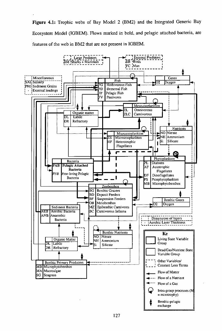
41/ Benthic Gases

•402 • Oxygen

•••• A

Figure 4.1: Trophic webs of Bay Model 2 (BM2) and the Integrated Generic Bay

Ecosystem Model (IGBEM). Flows marked in bold, and pelagic attached bacteria, are

features of the web in BM2 that are not present in IGBEM.

BG BD BF

• OB MZ BC

Organic Matter Labile Refractory

Primary Producers MB

A SG 1m

Benthic Microphytobenthos Macroalgae Seagrass


- Sediment Bacteria AEB Aerobic Bacteria ANB Anaerobic

Bacteria

A V

- -

127

--. Benthic Nutrients 0 Z Z


r . 1 i Dimensions of layers •I-- 4

- I Aerobic Layer Thickness I I.

Mesozooalanicion ZL Omnivorous ZLC Carnivorous

■ Microzooplankton Microzooplankton “

4 Heterotrophic

Flagellates

PL AF

DF PS MB

Zoobenthos

-1 I Large Predators 1- -/ -, ISM !Sharks + Mammals 1 _1

1 External Predators' ▪ i

▪

. -I _ft ISB [Birds 1

i C 11Man 1

Miscellaneous SAVSffinity ,PHI Sediment Grains

- 'External loadings

-. Fish G Herbivorous Fish


Piscivores

matter Organic Labile Refractory •

Nutrients Z Z


PhytoplanktonQ

Diatoms Autotrophic




Bacteria

1■1=14

Ke Living State Variable Group


Other Variables/ I Constant Loss Terms

Flow of Matter - Flow of a Nutrient

-41 Flow of a Gas

Intra-group processes (NI = mixotrophy)


This framework was then extended to cover benthic biological groups omitted from

ERSEM II (those in the benthic primary producer subweb) (chapter 1). This level of

process and trophic detail is at the upper bound of what is normally employed in

ecosystem models currently in use (e.g SSEM (Sekine et al. 1991) and ERSEM II

(Baretta-Bekker and Baretta 1997)) and it makes IGBEM one of the most highly

detailed ecosystem models published.

BM2 was developed from PPBIN4 by extending the framework of that model to

cover all of the groups in IGBEM. Consequently, BM2 includes the same trophic

groups and physical details (vertical layering, transport, mixing and spatial geometry) as

IGBEM, but there are important differences. The two models differ in the formulation

of the attached bacteria (chapter 2) and dinoflagellates, but the greatest difference lies in

the degree of process detail used in their formulation (Table 4.1). In BM2 physiological

processes are not modelled explicitly, but are dealt with as a whole by generalised

equations for assimilation and waste production (chapter 2). In addition, BM2 models

only the nitrogen components and relies on Redfield ratios, rather than internal nutrient

ratios, to determine the form of nutrient dependent activities. This general level of detail

is more representative of most existing models of eutrophication and water column

trophic dynamics (Fransz et al. 1991).

4.2.A Spatial structure

The transport model used as the physical basis of BM2 and IGBEM can be

applied on any geometry (any number of boxes). The standard geometry used during

development was 59 boxes (Figure 4.2a), but we also ran both ecosystem models on 8, 3

and 1-box equivalents (Figure 4.2b-d), constructed by summing over the flows between

boxes. The standard configuration was used in each case (standard parameter set, 2-

weekly record period, 20 year run with physical forcing files repeated every 4 years).

128

(a) 6

40/0 14. tel -w4 k y 11; °

-Njell

(b)

(c)

ed,

d) ( 100,

allir2c) "Sr

Figure 4.2: Maps of the geometries used with the models: (a) 59-boxes, (b) 1-box, (c)

3-boxes, and (d) 8-boxes. The "*" marks the box receiving inputs from the Yarra River

(reference site for later figures)

However, for numerical stability, it was necessary to retune some of the groups in BM2.

This is because the coarser model geometries average out the physical conditions and

BM2 is sensitive to environmental conditions (chapters 2 and 3). The groups that

required retuning were the metazoan infauna (meiobenthos, deposit feeders and benthic

infaunal carnivores), and the planktivorous and demersal herbivorous fish.

Only the final four years of the full twenty-year simulations are used to judge the

model performance as this removes the chance of confounding due to transient

dynamics produced by initial conditions. Relative production, consumption and

biomasses, or the variance of these measures, were found to be the most useful way of

129

comparing model behaviour across several geometries. To check for consistency in the

results across varying environmental conditions, the runs were repeated when fishing

pressure or nutrient load was increased or decreased fivefold.

4.2.B Sampling frequency

The start date, end date and sampling frequency of the output of BM2 and

IGBEM is flexible. Daily output is possible, but the standard runs use fortnightly

records due to storage requirements and our desire to mimic achievable intensive

monitoring of natural systems. This feature was used to consider the implications of

differing sampling frequencies. IGBEM and BM2 were run for 20 years under a

standard configuration, except that model output was stored daily for the final 2 years of

the run (storage of a longer time-series was not possible due to the immense storage

requirements). This output was sub-sampled weekly, 2-weekly, monthly, 2-monthly,

quarterly, half-yearly and yearly. The summary statistics of model behaviour used

include the variance of production, consumption, biomass and denitrification estimates.

Effects of shifting nutrient loads and fishing rates away from their baseline values were

also considered by repeating the sub-sampling on runs where these forcing conditions

were increased or decreased fivefold.

4.3 Results


Smoothing of local variation

Comparing the variance in the time-series for any of the groups or processes

with rapid dynamics (such as chlorophyll a, zooplankton or denitrification) across the

various model geometries indicates that decreased spatial resolution reduces short-term

fluctuations. This effect is clearest close to point source inputs such as the Yarra River,

130

• 10 -

0.1 -

• •

0.01 -

0.001

which flows into the northern most point of the bay (Figure 4.2). Comparing the

variance in chlorophyll a (chi a), over the final 4 years of each run, in the box fed by the

Yarra River there is a strong decrease in variance with increasingly aggregated

geometries, regardless of the model chosen (Figure 4.3). There is also a decrease in the

variance of bay-wide averages with coarser spatial resolution, but it is an order of

magnitude smaller (Figure 4.4). The variance observed at the bay-wide scale is much

smaller than in the box fed by the Yarra river inputs because at the bay-wide scale

fluctuations across the bay cancel each other out or are subsumed by the more stable

behaviour of boxes further from input sources.

1

3 8

59

Number of Boxes

Figure 4.3: Variance of chlorophyll a in the "Yarra River" box (marked by a * in

Figure 4.2) over the final 4 years of the 20 year runs for different levels of spatial

resolution in the Bay Model 2 (open circles) and Integrated Generic Bay Ecosystem

Model (solid black circles) models (1 — 59 boxes).

Var

(chl

orop

hyll)

131

Var(

bay

wid

e ch

loro

phy

ll)

0.12

0.10 -

0.08 -

• 0.06 -

0.04 - •

• • 0.02 -

0.00 1 3 8 59

Number of Boxes

Figure 4.4: Variance in the bay-wide average chlorophyll a over the final 4 years of the

20 year run for different levels of spatial resolution in the Bay Model 2 (open circles)

and Integrated Generic Bay Ecosystem Model (solid black circles) models (1 — 59

boxes).

Self Simplification

Potentially the most important effect of the use of differing geometries is that the

simpler geometries may not support the same food web as the 59-box case. In both

models trophic self-simplification (i.e. loss of functional groups) occurs when using the

simpler geometries (Table 4.2). In the water column groups, this simplification is

illustrated by the dependence on boundary conditions reseeding of the affected groups

(they persist only in the southern most boxes and their patterns of change are strongly

tied to the tidal forcing across the bay mouth). Within the benthos, simplification results

in the effective extinction of several groups (with the biomass dropping to <0.00001%

of the value in the 59-box model). In some cases the effect of reduction in spatial

132

Table 4.2: Persistence of the trophic groups in runs of Bay Model 2 (BM2) and the

Integrated Bay Ecosystem Model (IGBEM) using 8-box, 3-box and 1-box geometries.

The state of a trophic group after 20 simulated years are indicated by: Y = wide spread

and as abundant as in the 59-box geometry; R = restricted in distribution compared with

the 59-box geometry; BC = persists only because of continual reintroduction from the

Bass Strait boundary box; D = >75% reduction in abundance; and NO = decline to

baywide extinction. Note that pelagic attached bacteria are not present in IGBEM.

BM2 IGBEM Trophic Group 8-box 3-box 1-box 8-box 3-box 1-box Diatoms Y Y Y Y Y Y Picophytoplankton Y BC BC D D D Autotrophic flagellates Y Y Y BC BC BC Dinoflagellates BC BC BC Y Y Y Heterotrophic Flagellates BC BC BC BC BC BC Microzooplankton Y Y D D D D Large omnivorous zooplankton Y Y Y Y Y Y Large carnivorous zooplankton Y Y Y Y Y Y Pelagic attached bacteria Y Y D - - Pelagic free bacteria BC BC BC Y Y Y Planktivorous fish Y D D Y Y Y Piscivorous fish Y D D Y D D Demersal fish Y D D D D D Demersal herbivorous fish Y Y D Y D D Microphytobenthos BC BC BC BC BC BC Macroalgae R NO NO R NO NO Seagrass Y Y D Y Y Y Aerobic bacteria D D D D D D Anaerobic bacteria D D D D D D Meiobenthos D NO NO NO NO NO Benthic deposit feeder R Y NO Y Y Y Benthic infaunal carnivores R Y NO Y Y Y Benthic filter feeders Y D Y R Y Y Benthic herbivorous grazers Y Y D Y Y Y Macrozoobenthos Y Y Y Y Y Y

133

structure is obvious even for the 8-box geometry, while other groups show restricted

distribution in the 8-box case and only undergo bay-wide extinction in the 3-box and 1-

box runs (e.g. macroalgae (Figure 4.5)).

The self-simplification of the food web is not as strong across both models.

IGBEM loses half as many groups as does BM2 for the same reduction in spatial

resolution. The groups lost from IGBEM are also lost from BM2 except for autotrophic

flagellates, which shows no reduction in abundance in BM2 irrespective of the spatial

resolution employed. It is worth noting that the groups that are lost are all from the

lower to mid-trophic levels and are generally either microscopic or infaunal (Table 4.2).

The single exception is macroalgae, which is replaced by seagrass on the simpler

geometries.

Even those groups that are not totally displaced on the coarser geometries may

show depletion (Table 4.2). This is because they can no longer partition resources with

competitors or escape predator coverage as easily. The geometries with coarser spatial

resolution have more homogeneous physical conditions, as gradients in depth, nutrients

and hydrodynamic properties are reduced or removed. The reduction in the size of these

gradients affects the outcome of local interactions and partitioning of resources becomes

less likely. In addition, the models use differential equations and so, without lags

imposed by spatial structure, groups cannot escape the influence of their predators or

competitors.

Overall estimates

Those groups that are removed or depleted by self-simplification of the food

web on coarser geometries obviously do not have similar biomass estimates across all

model geometries. Within the groups that do remain, several display a relatively

constant average biomass across all the geometries. Large carnivorous zooplankton in

134

Figure 4.5: Effects of spatial resolution on self-simplification. This example shows that the distribution of macroalgae is contracted to the point of extinction with decreasing spatial resolution. The maps show the distribution of macroalgal biomass (mg N m -2) on day 6594 of the run for each geometry of the Bay Model 2 (BM2) and Integrated Generic Bay Ecosystem Model (IGBEM) models.

Biomass of macroalgae (mg N ni 2)

< 1

> 4200

135

BM2 is one example, with its mean biomass varying by less than 2% across the

geometries. In contrast, others increase either as a result or cause of the depletion of

other groups. For example, the biomass of autotrophic flagellates in BM2 increases by

145 - 160% in the run using 1-box compared with the run using a 59-box geometry.

This increase is largely as a result of an increase in influence of the boundary conditions

in the less spatially resolved geometries.

The effect of changes in biomass on higher level aggregated measures can vary

from minor to substantial. For example, the bay-wide average oxygen concentrations

within the sediments is almost identical regardless of the geometry used, while the

average bay-wide biomass of pooled biological groups is between 1000x too low to 4x

too high depending on the group of interest and which of the simpler geometries is used

(Table 4.3). Notably, total benthic primary production, sediment bacteria and

denitrification are too low when using fewer boxes in either model. This triplet failure is

pronounced as these things are all closely linked; low levels of benthic primary

production result in lower levels of detritus, which in turn means that there is less

bacterial activity and lower rates of denitrification. Aside from this triplet, the

performance of IGBEM was relatively consistent across all geometries, with most

estimates for the coarser resolution being within a twofold range of those for the 59-box

model. In contrast, the performance of BM2 shows widespread deterioration on the

lower geometries, with 40% of the estimates for the coarser geometries falling outside a

twofold range of the estimates from the 59-box model.

Spatial zonation

The physical characteristics of each cell are increasingly "smeared" as spatial

resolution is decreased. As a consequence, there is less of a gradient in community

structure and processes from the edge to the centre, and from the north to the south of

136

Table 4.3: Relative (value from the lower geometry run / value from the 59-box run)

biomass, production and consumption for the runs of Bay Model 2 (BM2) and the

Integrated Bay Ecosystem Model (IGBEM) on the smaller geometries. Any entries in

bold signify a difference of more than twofold between the simpler geometry and the

59-box case.

BM2 IGBEM 1-box 3-box 8-box 1-box 3-box 8-box

Bay-wide Average Biomass Chlorophyll a 1.26 1.69 1.59 1.11 1.34 1.05 Zooplankton 0.76 1.18 0.93 0.92 0.93 0.92 Fish 0.27 0.44 0.64 0.76 1.20 1.73 Benthic primary producers 0.42 1.29 1.04 0.77 0.23 0.64 Benthos 0.02 2.84 3.56 1.09 0.83 1.03

Infauna 0.00 2.96 3.73 1.09 0.83 1.03 Epifauna 0.40 0.69 0.55 1.02 0.80 0.78

Pelagic bacteria 1.57 0.98 1.04 0.56 0.63 0.72 Sediment bacteria 0.09 0.09 0.33 0.19 0.23 0.26 Oxygen 0.99 0.99 1.00 1.00 1.00 1.00

Bay-wide Annual Totals Denitrification 0.00 0.00 0.01 0.02 0.06 0.13 Water column primary production 1.03 1.30 1.01 2.87 1.97 0.74 Benthic primary production 0.03 0.27 0.14 0.54 0.26 0.34 Water column secondary production 1.56 1.53 1.08 1.22 0.90 0.81 Benthic secondary production 0.02 1.11 0.80 1.06 0.97 0.61 Water column consumption 1.45 1.47 1.08 1.10 0.88 0.79 Benthic consumption 0.09 0.79 0.94 1.11 1.08 0.64

the modelled bay. Moreover, because the cells cover larger areas as spatial resolution

declines, any group that is present in cells on the smaller geometries will cover a larger

part of the bay. It follows that the spatial distribution of groups that do persist on the

smaller geometries can be much more widespread than in the 59-box case. The best

examples of this are in the benthic groups, especially in IGBEM (Figure 4.6). As a

result of wider distributions, areas of the bay are less clearly demarcated on the smaller

geometries. The distinctive "edge" and "central" assemblages in the 59-box case are

less clear on the 3- and 8-box geometries, as more microfaunal groups are ubiquitous,

and of course any spatial zonation is impossible in the 1-box case (Table 4.4).

137

Figure 4.6: Effects of spatial resolution on the spatial distribution of functional groups. This example shows that the distribution of benthic deposit feeders expands with loss of spatial resolution. The maps show the distribution of the biomass (mg N m -3) of benthic deposit feeders on day 7280 of the run for each geometry of the Bay Model 2 (BM2) and Integrated Generic Bay Ecosystem Model (IGBEM) models.

NIM■1•11M111: < 5000 > 90000

Biomass of benthic deposit feeders (mg N m-3)

138

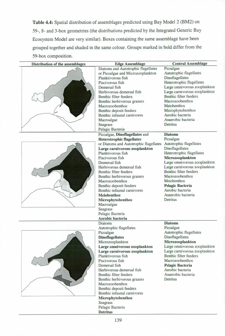
Table 4.4: Spatial distribution of assemblages predicted using Bay Model 2 (BM2) on

59-, 8- and 3-box geometries (the distributions predicted by the Integrated Generic Bay

Ecosystem Model are very similar). Boxes containing the same assemblage have been

grouped together and shaded in the same colour. Groups marked in bold differ from the

59-box composition.

Distribution of the assemblages

Edge Assemblage Diatoms and Autotrophic flagellates or Picoalgae and MicrozooplanIcton Planktivorous fish Piscivorous fish Demersal fish Herbivorous demersal fish Benthic filter feeders Benthic herbivorous grazers Macrozoobenthos Benthic deposit feeders Benthic infaunal carnivores Macroalgae Seagrass Pelagic Bacteria Picoalgae, Dinoflagellates and Heterotrophic flagellates or Diatoms and Autotrophic flagellates Large carnivorous zooplankton Planktivorous fish Piscivorous fish Demersal fish Herbivorous demersal fish Benthic filter feeders Benthic herbivorous grazers Macrozoobenthos Benthic deposit feeders Benthic infaunal carnivores Meiobenthos Microphytobenthos Macroalgae Seagrass Pelagic Bacteria Aerobic bacteria

Central Assemblage

Picoalgae Autotrophic flagellates Dinoflagellates Heterotrophic flagellates Large omnivorous zooplankton Large carnivorous zooplanIcton Benthic filter feeders Macrozoobenthos Meiobenthos Microphytobenthos Aerobic bacteria Anaerobic bacteria Detritus

Diatoms Picoalgae Autotrophic flagellates Dinoflagellates Heterotrophic flagellates Microzooplankton Large omnivorous zooplankton Large carnivorous zooplankton Benthic filter feeders Macrozoobenthos Meiobenthos Pelagic Bacteria Aerobic bacteria Anaerobic bacteria Detritus

Diatoms Autotrophic flagellates Picoalgae Dinoflagellates Microzooplankton Large omnivorous zooplankton Large carnivorous zooplankton Planktivorous fish Piscivorous fish Demersal fish Herbivorous demersal fish Benthic filter feeders Benthic herbivorous grazers Macrozoobenthos Benthic deposit feeders Benthic infaunal carnivores Microphytobenthos Seagrass Pelagic Bacteria Detritus

Diatoms Picoalgae Autotrophic flagellates Dinoflagellates Microzooplankton Large omnivorous zooplankton Large carnivorous zooplankton Benthic filter feeders Macrozoobenthos Pelagic Bacteria Aerobic bacteria Anaerobic bacteria Detritus

139

Model divergence with changing pressures

Self-simplification of the model food web (i.e. the loss of functional groups) and

inconsistencies in predicted estimates of biomass, production and consumption also

occurred with decreasing spatial resolution when nutrient loading and fishing pressures

are altered (increased or decreased). However, the nature of the effect of changing

spatial resolution does not always match those of the runs under baseline conditions

(Tables 4.5 and 4.6). Generally, changes in nutrient loading produces corresponding

changes in the resource base, particularly for the benthic groups, and this underpins

effects of spatial resolution on simplification. The impacts of a reduction in spatial

resolution observed under baseline conditions are expressed at a different level of

spatial resolution when nutrient loads or fishing pressure is changed. If nutrients

increased, the effects of self-simplification largely disappear from the 8-box case, while

decreasing nutrients usually intensifies the effects of self-simplification. A reduction in

nutrient load intensifies the effects of simplification for all but two groups in the 8-box

version of BM2 (Table 4.5), but in IGBEM some groups show fewer effects of a

reduction in spatial resolution. This may indicate that IGBEM has some sensitivity to

the forcing conditions used, but that they are at a different point to, and not as strong as,

those identified in BM2 (chapters 2 and 3). The effects of changing fishing pressure are

not so easily characterised, beyond the observation that trophic cascades are stronger on

simpler geometries. The lack of heterogeneity with coarser spatial resolution allows

predators and prey to overlap for longer periods and over larger areas. Thus, cascades

caused by the release or depletion of fish are more pronounced and extend further

through the web on the simpler geometries.

140

Table 4.5: Groups demonstrating different responses to spatial structure under

alternative amounts of fishing and nutrient loads in Bay Model 2. The number(s) in

brackets after the group name indicates the geometries (in terms of the number of boxes

used) where the effect of spatial resolution differed from runs using the baseline forcing.

The meaning of the codes for the state of a trophic group after 20 simulated years are:

"Macrophyte barren cycle" = longterm boom-bust cycling of macrophytes; "Constant"

= only small scale interannual variation present; "More widespread" = wider spatial

distribution even accounting for larger cell sizes on coarser geometries; Y = wide spread

and as abundant as in the 59-box geometry under the same forcing conditions; R =

restricted in distribution compared with the 59-box geometry under the same forcing

conditions; BC = persists only because of continual reintroduction from the Bass Strait

boundary box; D = >75% reduction in abundance; and NO = decline to baywide

extinction.

Conditions Change in response to spatial

Groups structure

Increased fishing pressure

Decreased fishing pressure

Increased nutrient loading

Decreased nutrient loading

Macrophyte barren cycle ----> Constant D--)BC Y BC BC —> D D —> Y

More widespread Y BC Y —> D

Y BC —Y D Y

More widespread R —> Y

Y-+BC Y —> R D Y

Y —> D Y

Seagrass (8,3) Microzooplankton (1) Microzooplankton (8,3) Picoalgae (3,1) Planktivorous fish (3) Seagrass (8,3) Diatoms (3) Picoalgae (8) Piscivorous fish (8) Demersal herbivorous fish (3) Benthic infaunal carnivore (3) Benthic filter feeder (8,1) Benthic deposit feeder (3) Dinoflagellates (8,3,1) Meiobenthos (8) Anaerobic bacteria (8,3) Seagrass (8,3) Macroalgae (8) Benthic deposit feeder (8) Benthic infaunal carnivore (8) Picoalgae (8) Benthic filter feeder (8) Meiobenthos (8) Benthic deposit feeder (8) Herbivorous demersal fish (3) Benthic infaunal carnivore (3)

141

Table 4.6: As for Table 4.5, but for the Integrated Generic Bay Ecosystem Model.

Conditions Change in response to spatial structure

D —> Y More widespread

R —) D Y —> D

Groups

Increased fishing pressure Microzooplankton (8,3,1) Diatoms (8,3) Large omnivorous zooplankton (8,3) Seagrass (8,3) Benthic deposit feeder (8,3) Benthic infaunal carnivore (8,3) Benthic filter feeders (8) Planktivorous fish (3,1) Piscivorous fish (8) Demersal herbivorous fish (8)

Decreased fishing pressure More widespread

R —> D R —> NO Y —> D

Benthic deposit feeder (8,3) Benthic infaunal carnivore (8,3) Benthic filter feeders (8) Macroalgae (8) Piscivorous fish (8) Demersal herbivorous fish (8)

Increased nutrient loading D Y

R —> NO R —> Y Y —> D

Picoalgae (8) Microzooplankton (8) Demersal fish (8) Macroalgae (8) Benthic filter feeders (8) Dinoflagellates (1) Large omnivorous zooplankton (3,1) Macrozoobenthos (8,3,1)

Decreased nutrient loading D —> Y

More widespread

R —> NO

Picoalgae (8,3,1) Microzooplankton (1) Demersal fish (8) Demersal herbivorous fish (1) Anaerobic bacteria (8,3,1) Microzooplankton (8,3) Benthic deposit feeder (8,3) Benthic infaunal carnivore (8,3) Macrozoobenthos (8,3) Macroalgae (8)


As would be expected, reducing the frequency of sampling reduces the amount

of variation observed in the system (e.g. consider the time-series for bay-wide

denitrification in BM2 and IGBEM in Figure 4.7). Two-weekly or even monthly

sampling removes much of the noise present in the daily samples, but still reveals the

underlying trend. Decreasing the frequency further to half-yearly or annual sampling

leads to a substantial loss of useful information.

142

150

0

Figure 4.7: Time-series of denitrification as defined by each of the sampling

frequencies for

(a) Bay Model 2

1 •

Yearly

• •

• •

Half-yearly

• •

. • • • •

• •

Quarterly

• 1 •

• • • • • • • •

• •

2-monthly

• • • II •

• • • • • • • • • • • • • • • •

* •

• •

Monthly

•• • • • • •

•0, •.• • • ••,•• ••

•••• • OO OOO • • • • . - • , , 0 • • • • • •

• •

2-weekly

• 0,•••••#• •%ease, sapowasesseepsiadkl"„ovessaineeassiosessesees,

••■•••••80~•••

Weekly

Daily

6600 6700 6800 6900 7000 7100 7200

Day of Run

143

(b) the Integrated Generic Bay Ecosystem Model

•

Yearly

• • •

Half-yearly

•

• • • • •

• •

Quarterly

• •

• • • • • • • •

• •

2-monthly

• • • • • • • • • • • • • • • • • • •• •

• . • •

Monthly

• • • • • • a • • • • • • • • •, • • • • • • • • • * • • •• • . • ••

•• • . • • 2-weekly

•••••••••••%• to•••••• ••••••••••00..... _

--"Ire• •••ftese.44,,p••••••••0 •••••••••••••0••••••1le Weekly

Daily

6600 6700 6800 6900 7000 7100 7200

Day of Run

400

r?E

a) 0

0

144

The effect of apparently reducing variance can have a marked effect on

estimates of system-level measures. For example, using sampling frequencies of one or

two months cause time-averaged primary production to be overestimated, while longer

sampling frequencies often yield substantial underestimates (Figure 4.8). The problem is

exacerbated if the sub-samples coincide with extreme peaks or troughs in the series.

The issue of the effects of sub-sampling is much stronger for groups or

processes with fast dynamics (many events or generations per year) while estimates

involving slower growing groups are not as heavily affected. For example, the estimate

for mean production of benthic filter feeders is only marginally affected by sampling

frequency (Figure 4.9).

Changing the external forcing of the system (i.e. nutrient loads and fishing rates)

does not have a consistent effect across all groups, and different changes to forcings

yielded dissimilar results (Table 4.7). Reducing the nutrient load weakens the effects of

sampling frequency as much of the variation in the system is removed; i.e. there are

fewer, short-term, high-magnitude fluctuations in denitrification, biomass and

productivity. When the nutrient load is increased the inaccuracy introduced by using

longer sampling frequencies is substantially increased for measures associated with the

primary producer and planktonic groups, particularly in IGBEM (e.g. water column

primary productivity (Figure 4.10)). The inaccuracy of measures (e.g. productivity) for

the other groups, such as the fish and sediment fauna, shows no real change with

increasing nutrient load. The ratio of the true value to estimates based on longer

sampling frequencies changes by less than 1% for these measures. In contrast, a

reduction in fishing pressure and the resulting shifts to higher biomasses and stronger

interactions between groups causes an amplification of the effects of using longer

sampling frequencies, particularly for the fast-lived groups and associated processes

(e.g. water column secondary productivity (Figure 4.11)), but it has little effect on

145

—0— Water column - IGBEM •• 0" Benthic - IGBEM —v— Water column - BM2 —v • Benthic 8M2

Estim

ated

BE

prod

uctio

n / T

rue

BF p

rodu

ctio

n 1.250

1.125

1.000

0.875

0.750

'1-7) 1.2

2 0.

1.1

a. a) 1.0

o

•

0.9 - '5

2 0.8

co .— 8_ 0.7 -o a)

E 0 . 6

100

200

300

400

Sampling frequency (days)

Figure 4.8: Ratio of the estimated and true values of pelagic (water column) and

benthic primary production for Bay Model 2 (BM2) and Integrated Generic Bay

Ecosystem Model (IGBEM) under various sampling frequencies.

•

• • • •

100

200

300

400


Figure 4.9: Ratio of the estimated and true values of production by benthic filter

feeders (BF) for Bay Model 2 (open circles) and Integrated Generic Bay Ecosystem

Model (solid black circles) under various sampling frequencies.

146

--0— Baseline conditions - IGBEM •• 0 • Nutrient loading x5 - IGBEM —v— Baseline conditions - BM2

•• Nutrient loading x5 - BM2

Table 4.7: Summary of the impact of changes in nutrient loading or fishing pressure on

the effects of sampling frequency.

Change in Conditions Impact Reduced effect of sampling frequency as less variation translates to less inaccuracy when using longer sampling frequencies Increase in the effects of sampling frequency, but only for the groups with fast-dynamics Increase in the effects of sampling frequency for the harvested groups and prey groups with fast-dynamics Reduced effect of sampling frequency for the harvested groups. No change in the effects on other groups, unless the sampling frequency aligns (aliases) with fluctuations in prey biomass caused by the establishment, prior to fish-down, of new recruits to the fished stocks — this is particularly a problem with annual sampling.

Decreased nutrient loading

Increased nutrient loading

Decreased fishing pressure

Increased fishing pressure

100

200

300

400


Figure 4.10: Ratio of the estimated and true values of pelagic primary production for

the Integrated Generic Bay Ecosystem Model under various sampling frequencies with

baseline nutrient conditions and a fivefold increase in nutrient load.

147

denitrification estimates. Again, this effect is stronger in IGBEM. Lastly, an increase in

fishing pressure reduces the effects of using longer sampling frequencies, especially for

the harvested groups, as their depleted biomasses show less variation through the year.

Measures associated with prey groups, which may be released from predator control

with an increase in fishing, do not show any increased effects of using longer sampling

frequencies under higher fishing loads, except when annual sampling regimes are

employed. At this point, aligning (aliasing) sampling times with peaks or troughs in the

fish stocks can cause distortion of estimates, particularly for groups with fast dynamics.

Under heavy fishing, if sampling coincides with a point just prior to recruitment, when

stocks of fish are low, then estimates of the biomass or production of prey groups may

be substantially overestimated (by as much as 50%). The converse holds if annual

sampling coincides with the short period when recruits are of sufficient size to depress

prey populations, but before fishing depletes their numbers to the point that their main

prey groups recover.

4.4 Discussion


Harris et al. (1996) found that there is a decrease in local variation on less

spatially resolved geometries for the original Port Phillip Bay Integrated Model

(PPBIM). This matches the observation that BM2 and IGBEM display more short-term

fluctuation when applied on more spatially resolved geometries. The mechanisms

identified by Harris et al. (1996) for the behaviour of PPBEVI also explains the

corresponding behaviour of BM2 and IGBEM. The first of these is that more finely

resolved spatial resolution results in a higher degree of local variation in environmental

conditions due to changes in advection and mixing along broad-scale gradients

produced by the location of the point source inputs. Secondly, point source inputs will

148

1.8 —0— Baseline conditions - IGBEM

0.. Fishing mortality x5th - IGBEM —v-- Baseline conditions - BM2 --v • • Fishing mortality x5th - BM2 1.6 -

1.4 -

1.2 -

-V

0.8

Estim

ated

sec

onda

ry p

rodu

ctio

n / T

rue

seco

ndar

y pr

oduc

tion

100 200 300

400


Figure 4.11: Ratio of the estimated and true values of pelagic secondary production for

the Integrated Generic Bay Ecosystem Model under various sampling frequencies with

baseline fishing conditions and a fivefold decrease in fishing pressure.

have a larger local, short-term influence when spatial resolution is finer as the inputs are

not immediately diluted by mixing with sizeable proportions of the total capacity of the

bay, as is the case on the coarser resolutions. Lastly, advection on the more detailed

geometries continually brings local communities into contact with new levels of

nutrients. Thus, these groups can never reach steady state as they are in a perpetual state

of flux. As a result of these mechanisms, the less spatially resolved geometries

underestimate local variation as they damp the many influences of environmental

heterogeneity and allow the planktonic groups to inappropriately attain steady state.

The decrease in variation with coarser spatial resolution is reminiscent of the

drop in the variation in the observed output of cellular-automata predator-prey models

when increasingly large observation windows are used (e.g. Pascual and Levin 1999).

However, Pascual and Levin's work differed from ours in that they considered the same

149

total number of cells and only changed the size of their observational windows, while

this study considered different numbers of cells describing the same total area. Both

methods remove heterogeneity. By averaging, Pascual and Levin (1999) smooth out

local heterogeneity in population sizes at the time of "sampling", while the models in

this study remove heterogeneity in population sizes and local environmental conditions

by using fewer larger cells in the less spatially resolved geometries.

The most pronounced impact of removing heterogeneity when applying models

on the coarser geometries is the tendency for self-simplification of the food webs.

Collapse of the web in this way is produced by two interacting consequences of the

smearing of environmental conditions with coarser spatial resolution. The first is that

changing spatial resolution produces systems with differing depth profiles and nutrient,

chemical and hydrodynamic properties. Coarser geometries do not have the steep depth

gradients seen in the 59-box model and so, for example, sediment light levels are more

conducive to widespread seagrass populations rather than the restricted populations seen

in the 59-box model. More importantly, the flushing time of the bay for coarser

geometries is much shorter than in the 59-box model. With a drop in resolution over the

southern boxes around the bay mouth, flushing time drops from more than 270 days for

the 59-box geometry to less than 93 days for the 3-box model (Walker and Sherwood

1997). It was not possible to calculate flushing time for the 1-box model. However, it

must be noted that, like the boxes at the mouth of the bay in more complex geometries,

the 1-box model shows tidal aliasing and so the exchange between the boundary

conditions of Bass Strait and the bay as a whole are over-stated. Flushing time and other

environmental conditions have direct habitability effects on at least some of the

biological components of the system and this alone could produce differing dynamics

(including extinction) depending on the geometry used. That the differing geometries

capture different physical environments is highlighted by the relative responsiveness of

150

the two models. BM2 requires retuning for numerical stability when the spatial

resolution is changed, while IGBEM does not. This is in keeping with previous work

that has found that BM2 needs more tuning as the underlying physical conditions

change (chapters 2 and 3).

The "smearing" of the physical conditions with reduced spatial resolution has an

additional biological effect. The removal of boxes and the general homogenisation of

conditions removes refugia that allowed the persistence of some groups. For instance

deposit feeders and meiobenthos, which are competitors but also predator and prey, are

spatially disjunct in the 59-box case. The deposit feeders line the edge of the bay while

the meiobenthos inhabit the deeper areas of the bay. With coarser geometries this spatial

partitioning is not possible and the meiobenthos is completely excluded. This is a direct

result of the use of differential equations in the model. Within each box competitors and

predators are effectively "everywhere" and encounter rates are not related to abundance

as they are in nature. The functional response used for grazing does include an

"availability" parameter, but as this is a fixed proportion of the prey biomass the

equations do not inherently include many refuges or lags. However, these refuges may

be added by using a spatially resolved system, as differential abundance across the

boxes creates lags and refugia. As a result the full trophic web is supported when the

models are run on spatially resolved geometries, but the web collapses when coarser

geometries are used. This effect of spatial resolution on trophic stability is particularly

important given that many of the traditional models considering the effects of system

complexity have omitted it (May 1974, Pimm 1982, Cohen and Newman 1988).

More recent work with spatial models shows different and multifaceted

relationships between complexity, stability and invasiveness. As observed in nature, the

relationships depend on network topology (the magnitude and direction of biological

interactions between network members) (Dunstan and Johnson submitted). These recent

151

models still use assumptions that are unrealistic and there has been speculation over

whether the findings from conventional consideration of the effects of trophic

complexity would hold if more realistic conditions (including nutrient conservation,

spatial structure and coupling, temporal forcing, omnivory, detrital infusion, ontogenetic

diet shifts and mixotrophy) are included in the models (May 1974, Leibold 1996, Polis

and Strong 1996, Keitt 1997). The models considered here include these processes.

Self-simplification of the food webs with a reduction in spatial resolution seen in

this study suggests that a large number of trophic groups does not destabilise the system

when environmental heterogeneity is present, but when the heterogeneity is removed the

additional reticulation and detail in the food web cannot preserve the system and the

web collapses. This implies that spatial heterogeneity is one form of complexity that is a

required part of the theoretical consideration of realistic food web dynamics and

community structure. Dunstan and Johnson (submitted) reach similar conclusions for

competition systems, and modelling work by Keitt (1997) and Donalson and Nisbet

(1999) also indicate that species persistence increases with system size and

heterogeneity. They posit that larger systems have a greater capacity for ephemeral

refugia, as physical and biological fluctuations in different regions can be out of phase.

This is not possible in smaller systems so these systems go extinct. This is one of the

mechanisms underlying the responses observed here.

The biological components included in the biogeochemical model of PPB

(PPBIIVI) constructed as part of the Port Phillip Bay Environmental Study are largely

from those groups that show the least impact of spatial structure, with macroalgae

notable as the single exception. This is not surprising given that Murray and Parslow

(1997) carefully selected the web structure in PPBIM to allow for maximum stability. It

may also explain why Murray (2001) found a 1-box version of PPBIM very helpful

during the development of the full model, whereas a similar approach would not be as

152

useful when trying to consider the full web that underlies IGBEM and BM2.

One area in which Murray (2001) and the findings here agree is in model

divergence with changing conditions. Murray (2001) illustrated the limitations of the

"simple modelling approach" by comparing the 1-box and 59-box versions of PPBIM

under increasing nutrient loads. It was found that as conditions changed the 1-box

model no longer reflects the dynamics of the 59-box model, as different processes

emerge as important in the two cases. Spatial variation proves to be a crucial

determinant of bay dynamics as the PPB1M model system moves from a mesotrophic to

a eutrophic state (Murray 2001). Similarly, trends in the effect of spatial structure noted

under baseline conditions of BM2 and IGBEM do not hold as nutrient loads and fishing

pressure changes. For example, under an increase in nutrients, the standard 59-box run

of BM2 predicts that seagrass will effectively become extinct throughout the bay. This

is not the case when using simpler geometries, where it persists despite the change in

nutrient levels. In the less spatially resolved cases seagrass biomass is reduced and the

magnitude of interannual cycles is increased with increased nutrient loading, but only

the 8-box model gives any indication that the distribution would contract and that the

population would be in danger of disappearing from the bay. Thus, as is the case with

PPBIM, complex system behaviour introduced by spatial heterogeneity cannot be

ignored if the models are to be used to evaluate the impact of changing conditions.


Despite differences in the models, and either damping or enhancing of variation

by different sampling scenarios, there is a consistent pattern as to the usefulness of the

various sampling frequencies (Table 4.8). At one extreme there are potentially large

inaccuracies introduced by half-yearly or annual sampling, while at the other the noise

inherent in daily sampling does not justify the immense storage requirements (or

153

expense) associated with computer generated or empirical observations of this detail.

Under the circumstances considered here, of no observational error and complete

knowledge, sampling frequencies of a week to a month are optimal. The lower end of

this range agrees with field studies that have indicated that weekly sampling is best for

measures such as primary productivity and sediment oxygen (Taylor and Howes 1994,

Rantajarvi et al. 1998). These field studies do not find the monthly sampling as reliable

as does the model study. The forcing files used in BM2 and IGBEM do not capture all

of the temporal variability seen in real systems. The extra variation in natural systems

may overwhelm the usefulness of monthly sampling suggested by the models.

The model and field studies point to similar conclusions regarding the effects of

a poorly chosen sampling frequency. If longer sampling frequencies are implemented

then estimates can be inaccurate and misleading with regard to understanding system

dynamics. These concerns are particularly important when deciding on monitoring

schemes as part of a system wide management strategy. Logistics may mean that

sampling on the order of 7 to 14 days is impractical and prohibitively expensive.

Unfortunately, evidence from field studies (Taylor and Howes 1994, Rantajarvi et al.

1998, Bennion and Smith 2000) and the work presented here indicates that opting for

longer sampling frequencies is inadequate for informed management. This is

particularly true for events that can happen very quickly, but have long lasting effects,

such as oxygen-crises in the sediment. If longer sampling frequencies are to be

successful in the future an index of overall system state which is robust to sampling

frequency needs to be found. No such index was identified in this study, but it is likely

that if one exists it will be a variable with slower dynamics.

154

Table 4.8: Summary of the utility of a range of sampling frequencies.

Daily Dominated by noise, which can mask underlying trends. This frequency does not add much to what can be captured by weekly sampling, except when trying to track oxygen stress events, which can occur for less than a week, but have long lasting impacts.

Monthly Similar to weekly and fortnightly, but monthly sampling does lose some of the short-term variation. It is also important to be aware of potential aliasing problems. Overall, it still captures the seasonal trends well.

2-monthly The loss of information is becoming evident for the groups with fast dynamics (seasonal trends are becoming "saw-toothed"). Satisfactory for groups with slow dynamics (much of the larger benthos)

Quarterly Loss of information is evident for all groups, though those with fast dynamics are impacted the most.

Half-yearly Annually These frequencies miss important events and much of the seasonal information. Aliasing is a critical problem. Sampling at these frequencies can lead to inaccuracies in estimates of annual denitrification, production and consumption of more than 25 — 50% depending on the ambient conditions. This is particularly true for measures associated with groups with fast dynamics (such as the plankton).

Weekly 2-weekly These frequencies are very similar with regard to the amount of information captured (and consequently any conclusions drawn).

155

4.5 Conclusions

Spatial and temporal resolution is a critical issue when considering the dynamics

of ecosystems. The complex and emergent features of ecosystem behaviour mean that

there are strong limitations on minimum sampling effort in time and space. Removing

complexity, by sampling on long time scales or using coarse spatial dimensions relative

to the dynamics of the system, is a two edged sword. The scale at which sampling is

undertaken not only impacts upon the costs of a field sampling program, it can also

influence the processes detected and how they are interpreted. An observation scheme

that reduces costs by concentrating on large spatial and temporal scales may miss

crucial mechanisms that occur on a fine scale, but have far reaching impacts (e.g.

oxygen crises). Moreover, modelling and field studies indicate that space itself is an

important resource in an ecosystem and ignoring it can have a substantial impact on

conclusions drawn.

The impacts of scale are not only an important concern in the field, but they can

have substantial influences on modelling too. By simplifying model systems and

increasing the scale at which variation is considered, storage requirements are reduced

drastically, calibration time falls sharply and some trends are easier to discern.

However, this comes at the cost of losing crucial emergent properties, the ability to

capture the full web structure and changing importance of mechanisms that appear to

characterize natural systems. Models need not be highly resolved, but to be informative

the spatial and temporal resolution employed must allow for expression of the dominant

gradients and dynamics in the system. As pointed out by Polis and Strong (1996),

complexity and variation may be inconvenient to a theoretical understanding of

ecosystems, but they may also be two of the most important driving forces of those

systems. Without their inclusion it may be impossible to use models to understand

systems and how they respond to change.

156

Chapter 5 Lump or chop: The effect of aggregating or omitting

trophic groups on the performance of ecosystem models

Abstract

As ecosystem models become more commonly applied, questions regarding

optimal complexity and parsimonious methods of simplification arise. Simplification of

the underlying trophic complexity is one viable approach. Two potential methods of

achieving this are to omit or aggregate components in the simulated food web. When

applied to two biogeochemical ecosystem models, it was found that if the system is

already aggregated to the level of functional groups then further aggregation will not

work as well as the strategic omission of less important groups. The relationship

between simplification and performance is nonlinear, but it is possible to identify two

general principles. First, over-simplification of the web leads to poor model

performance. Second, if important processes or couplings (such as between the pelagos

and benthos in shallow coastal systems) cannot be included explicitly, simple forcing is

unlikely to be a reliable alternative. Some form of robust empirical representation will

be necessary.

The results of model simplification also have implications for the ecological

stability-diversity debate. Shifts in the relative importance of different groups with

changing ecosystem conditions, and dependence of the effect of simplification on

ecosystem state, support the concept of the ecological "insurance hypothesis". The

models used here do not support the idea of a simple relationship between connectance

or interaction strength and the stability of system behaviour. The biological details of

the web, the trophic and non-trophic, direct and indirect interactions included are a

crucial determinant of ecosystem and model behaviour that cannot be ignored.

157

Keywords: trophic complexity, trophic structure, aggregation, omission, stability,

diversity, biogeochemical, ecosystem, model, IGBEM, BM2

5.1 Introduction

Natural ecological systems are inherently complex and it is neither possible nor

desirable to model them exactly. Increasing focus on using ecosystem models as an

integrated part of fisheries, water quality and general system level management has

highlighted the importance of the issue of simplification. Simplified models have a

number of desirable characteristics. They are often easier to comprehend (Iwasa et al.

1987), they can be economically or logistically attractive as they require less input

information (Sugihara et al. 1984), and they are less computationally intensive (Lee and

Fishwick 1998). Ludwig and Walters (1985) have also shown that simplified models

can be more effective than more complex versions, as the simpler models do not suffer

as much error propagation or sensitivity to parameterisation. Another potential

advantage of simplified models, particularly aggregated ones, is that they are not tied to

individual species and so, by definition, are more generic. Consequently, they may be

more robust to change and amenable to application. Simplifications must be made and

one way in which this can be done is by simplifying the underlying food web.

Model simplification by aggregation involves simplifying the model (and

associated food web) by combining components that share common predators, prey or

other characteristics. Given the universal use of aggregation in ecology it is not

surprising that it has received some attention within the areas of theoretical systems

ecology (O'Neill and Rust 1979, Iwasa et al. 1987) and biogeochemical modelling

(Zeigler 1976, Cale and Odell 1980, Gardner et al. 1982, Cale et al. 1983). A common

finding across many studies is that components of a system may be aggregated with

little error if the property being scaled is highly correlated among the components

158

(Bartell et al. 1988), or if their rate constants are similar (Wiegert 1977, O'Neill and

Rust 1979, Cale and Odell 1980, Gardner et al. 1982, Cale et al. 1983, Iwasa et al.

1987), or if one of the components is consistently comparatively rare (O'Neill and Rust

1979, Cale et al. 1983). However, it is also recognised widely that because an aggregate

is not capable of producing exactly the same behaviour as the constituent components,

errors due to inappropriate aggregation can be excessive (O'Neill 1979, Cale and Odell

1980, Gardner et al. 1982, Cale and O'Neill 1988, Iwasa et al. 1987, Rastetter et al.

1992). For example, aggregating components that are serially linked (Figure 5.1a) is ill

advised in most cases, while aggregating components that are in parallel (Figure 5.1b),

or share a common predator or prey (Figures 5.1c and 5.1d), is usually acceptable if

their rate constants are within two- or threefold of each other (Gardner et al. 1982). It

has also been found that if aggregated parameters cannot be measured accurately then

the compounding effects of aggregation and measurement error result in significant

output error and poor model performance (Gardner et al. 1982, Rastetter et al. 1992).

An alternative method of model simplification is reduction in model complexity

by omitting, rather than aggregating, components. This method follows from the

suggestion that system behaviour may be characterised by the dynamics of dominant, or

representative, species. Despite being central to the concept and use of indicator species,

this approach has not received the same level of theoretical and modelling attention as

simplification by aggregation. There is little work that directly considers the effects of

omitting groups on model performance, and the implication for the use of models

simplified in this way. The work that has been done has largely concentrated on models

using randomly constructed food webs to investigate the effects of diversity on system

stability (May 1973), or food chain models where entire trophic levels are considered

•rather than individual species or guilds (Carpenter and Kitchell 1993), or models of

plankton ecology (Yool 1998, Edwards 2001). Conclusions pertaining to more complete

159

+ (b)

Key biological component 1 I

---wEl input of material or energy

El— loss of material or energy to predation

t export of material or energy from the system (by fishing or migration)

1 loss of material or energy to respiration

i flow of material or energy to detritus

component or flow that is separate from those being aggregated

4.-

Figure 5.1: Diagrams of the most common system configurations that are simplified by

aggregating groups: (a) in series, (b) in parallel, (c) triangular with a shared predator, (d)

triangular with a shared prey and (e) the aggregated form (identical for all).

(a)

(c)

(d)

A

40; i

i

(e)

#

160

or realistic ecosystem models may be drawn by considering changes in model

performance as models are constructed incrementally (e.g. ERSEM I vs ERSEM II

(Baretta et al. 1995, Baretta-Bekker and Baretta 1997)). The "insurance" or

"redundancy" hypothesis (Yachi and Loreau, 1999) suggests that without any change in

ecosystem conditions at least some of the redundant species or groups could be removed

without the system changing substantially. However, the idea that overall mean

interaction strength is closely linked to system behaviour implies that removing a single

species could cause a significant shift in system dynamics (McCann 2000). Work by

Yodzis (2000) on the diffusion of the effects of interactions through food webs supports

the idea that, at least in some ecosystems, considering only a small subset of the food

web is inappropriate as even the influences of small perturbations will not be

represented accurately. However, the issue is far from resolved. Those studies

considering the effect of trophic complexity on models of plankton ecology indicate that

some simplification is possible, e.g. models that omit bacteria and certain nutrient

groups still perform well (Yool 1998), but the effects of simplification can be dependent

on the linkages captured in the modelled web (Edwards 2001). However, because the

food webs included in the full versions of these plankton models are very simple, more

work considering larger and more realistic food webs is necessary.

The greatest interest in the effects of trophic complexity on ecosystem models

was born of the modelling efforts associated with the International Biological Program

(e.g. O'Neill 1975, Watt 1975 and Wiegert 1975). However, it has a wider place within

theoretical ecology in the long running debate over the relationship between stability

and diversity in food webs. Historically, field studies suggested that an increased

number of biological components would confer greater stability on a community (Odum

1953, MacArthur 1955, Elton 1958). In contrast, some mathematical studies suggested

the opposite and indicated that randomly constructed model communities tended to

161

destabilise as they became more complex (Gardner and Ashby 1970, May 1973, Pimm

and Lawton 1978). Later studies have shown that these two sides of the problem are not

inconsistent as natural systems are not constructed randomly and are characterised by a

large number of buffering mechanisms, as well as material conservation and external

dependencies or linkages (De Angelis 1975, Yodzis 1981, Tilman and Downing 1994,

Sterner et al. 1996, McCann et al. 1998, Harding 1999). However, the debate is not yet

resolved and the consideration of models using more realistic food webs, constraints

(e.g. material conservation) and physical forcing still has much to offer, given that it is

doubtful that there is a simple relationship between diversity and stability when more

realistic systems are considered. If theories such as the "weak interaction effect"

(McCann 2000) are correct, it is likely that simplification of a system will take the

system through alternating periods of increased and decreased stability as the ratio of

strong:weak interactions is modified in one direction or another. Monitoring the

behaviour of models under a series of simplifications may help to give some insight on

this topic.

Here we report the effects of model simplification by aggregating or omitting

groups in two biogeochemical ecosystem models. The work and ecosystem models used

are part of a larger study on the effects of model structure and complexity on the

performance and behaviour of ecosystem models.

5.2 Methods

To investigate the effects of trophic complexity on model performance the food

web (Figure 5.2) implemented in two biogeochemical ecosystem models is modified in

a number of ways, while other features of the models (e.g. spatial resolution,

stoichiometry, processes included) are left unchanged. The two models are Bay Model 2

(BM2) (chapter 2) and the Integrated Generic Bay Ecosystem Model (IGBEM) (chapter

162

PL AF

F PS MB



0402

V Benthic Gases

Oxygen

Key Living State Variable Group w

Figure 5.2: Food web diagram for the ecosystem models Bay Model 2 (BM2) and the

Integrated Generic Bay Ecosystem Model (IGBEM). The Pelagic Attached Bacteria and

any flows marked in bold are present in BM2, but not in IGBEM.

-, Miscellaneous

SAVSZinity ,PHI Sediment Grains

- External loadings

■ Fish G Herbivorous Fish


IFV Piscivores



Bacteria


Benthic Primary Producers

I

Microphytobenthos Macroalgae Seagrass

I -r . 1 1 ' Dimensions of layers I - ' Aerobic Layer Thickness I 1. :

I

■111111■ 11111E1 I■ I Zoobenthos


.10 411-

.4 Sediment Bacteria


-.BG BD E

F B

MZ BC 411

-1 i Large Predators I40- i- J ISM jSharlcs + Mammals 1 1

1- -I External Predators' J 1

ISB !Birds i :Man i

'

0. \

% ■ Benthic Nutrients 0

Z

Z


163

Mesozoorolanan ZL Omnivorous ZLC _ Carnivorous

I Microzooplankton Microzooplankton 3`


Orgarfc matter Labile Refractory

L _ Nutrients 0

Z

Z



; - - —1 Other Variables/ 1 _ _ _ an I Constt Loss Terms _

.4____ Flow of Matter -41- - - - Flow of a Nutrient -• Flow of a Gas

Intra-group processes (M = mixotrophy)


Q

$

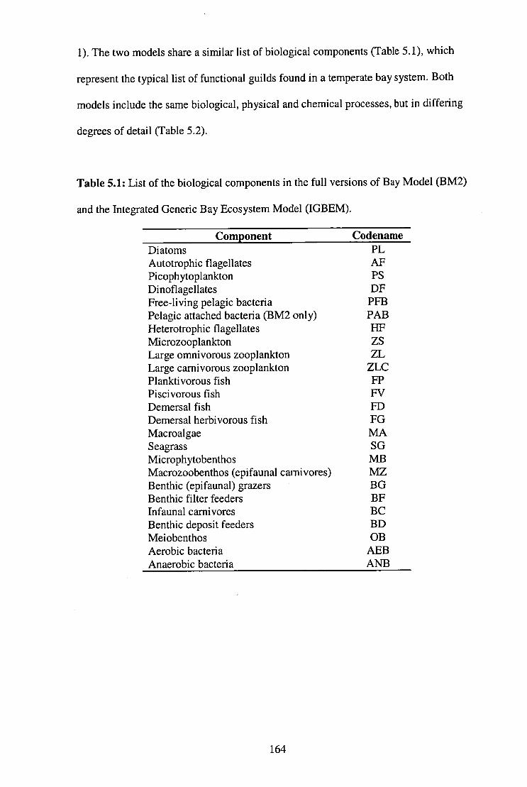
1). The two models share a similar list of biological components (Table 5.1), which

represent the typical list of functional guilds found in a temperate bay system. Both

models include the same biological, physical and chemical processes, but in differing

degrees of detail (Table 5.2).

Table 5.1: List of the biological components in the full versions of Bay Model (BM2)

and the Integrated Generic Bay Ecosystem Model (IGBEM).

Component Codename Diatoms PL Autotrophic flagellates AF Picophytoplankton PS Dinoflagellates DF Free-living pelagic bacteria PFB Pelagic attached bacteria (BM2 only) PAB Heterotrophic flagellates HF Microzooplankton ZS Large omnivorous zooplankton ZL Large carnivorous zooplankton ZLC Planktivorous fish FP Piscivorous fish FV Demersal fish FD Demersal herbivorous fish FG Macroalgae MA Seagrass SG Microphytobenthos MB Macrozoobenthos (epifaunal carnivores) MZ Benthic (epifaunal) grazers BG Benthic filter feeders BF Infaunal carnivores BC Benthic deposit feeders BD Meiobenthos OB Aerobic bacteria AEB Anaerobic bacteria ANB

164

Table 5.2: Processes and structure of Bay Model 2 (BM2) and the Integrated Generic

Bay Ecosystem Model (IGBEM).



Level of group detail Process related

Bioturbation and bioirrigation Consumption formulation Formulation detail

Light limitation






Fish and fisheries related Age structured fish Fishery Discards Invertebrate fisheries Stock-recruit relationship Stock structure

BM2

mg N/m3 nutrients and physics on interannual, seasonal, tidal frequencies functional group

yes type II general: only growth, mortality and excretion explicit



Redfield yes no dynamic, with sediment bacteria

yes flexible with the potential for multiple vertical and horizontal cells yes yes

yes

yes yes


IGBEM

mg/m3 of C, N, P, Si nutrients and physics on interannual, seasonal, tidal frequencies functional group

yes mixed (type II, type III) physiological: the processes of assimilation, basal/ activity/stress respiration, defecation, excretion, ingestion, mortality are all explicit phytoplankton can acclimate to ambient light levels none internal nutrient ratio determines nutrient uptake and disposal internal specific nutrient ratio yes yes empirical, sediment bacteria are a tracer only yes flexible with the potential for multiple vertical and horizontal cells yes yes

yes

yes no


Briefly, IGBEM is a physiologically explicit biogeochemical process model,

which follows the carbon, nitrogen, phosphorus and silicon pools of its biological

components (chapter 1). It was constructed using the physical and biogeochemical

submodels of the Port Phillip Bay Integrated Model (PPBIM) (Murray and Parslow

165

1997, 1999a) and the biological groups of the European Regional Seas Ecosystem

Model II (ERSEM II) (Baretta et al. 1995, Baretta-Bekker and Baretta 1997). The

benthic primary producers included in PPBLM were retained in IGBEM, as there was no

analog present in ERSEM H. In addition, herbivorous benthic invertebrates and fish

were added, using the same general formulation structure as ERSEM, to exploit the

benthic primary production and complete the food web.

In comparison with IGBEM, BM2 has much less process detail, using relatively

simple general equations of assimilation and waste handling, and only representing the

nitrogen and silicon pools of the biological components. This formulation was the one

used in PPBIM, and BM2 was developed by extending that formulation to cover all of

the groups in IGBEM (chapter 2).

5.2.A Aggregating functional groups

When components and their associated links are aggregated all the original

linkages to the separate components are kept but directed to the aggregated group. The

parameter values used for the aggregated group represent the weighted average of the

parameters for the constituent components. Thirty-three simplifications of the web

structure are made by aggregating components (Table 5.3). These simplifications reflect

aggregations made in other field and model studies (for example "other benthos" is a

common feature of the ECOPATH models primarily concerned with finfish, but which

attempt to include a broad picture of the entire web (Christensen 1992)). We consider a

range of intensity of amalgamation, from slightly aggregated cases to a massively

reduced web with only phytoplankton, zooplankton, fish, benthos and macrophyte

aggregated groups. The aggregated webs also span cases where only the pelagos or

benthos is considered. Thus, some runs include only pelagic components, while others

have only benthic components (apart from a pelagic food group, which is a forcing

166

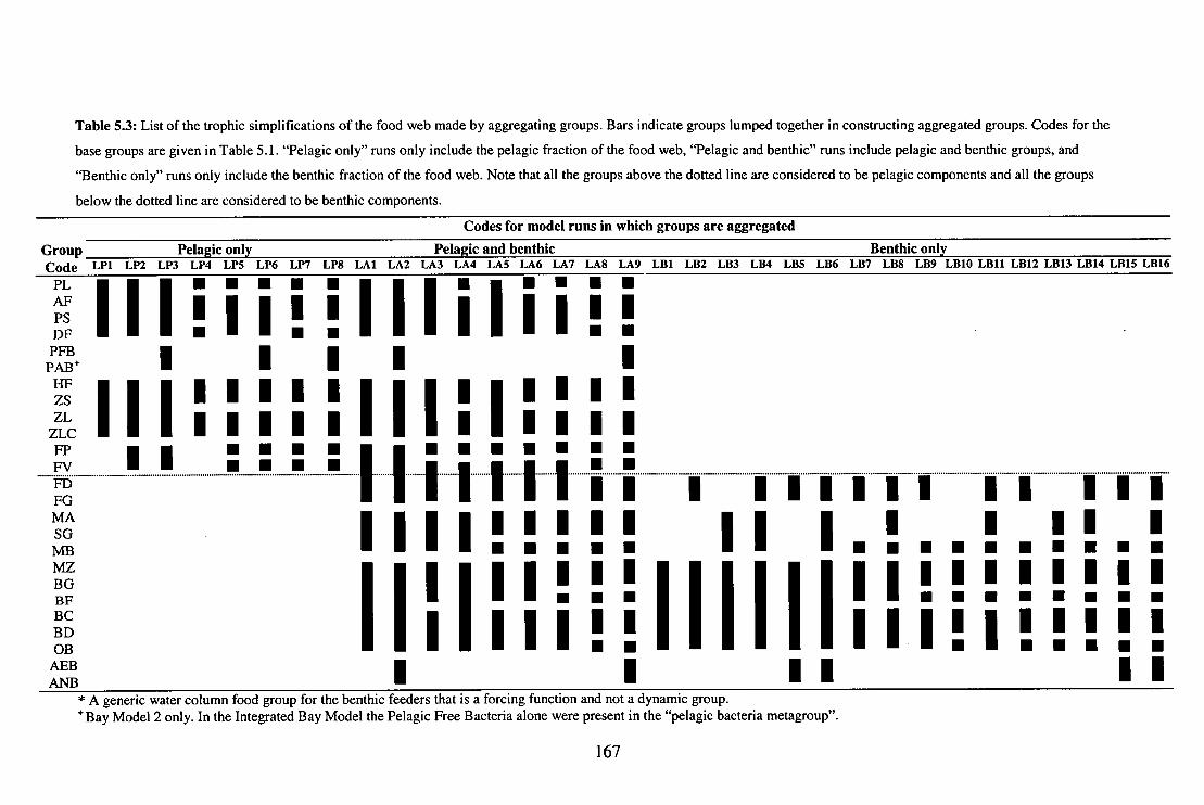
Table 5.3: List of the trophic simplifications of the food web made by aggregating groups. Bars indicate groups lumped together in constructing aggregated groups. Codes for the base groups are given in Table 5.1. "Pelagic only" runs only include the pelagic fraction of the food web, "Pelagic and benthic" runs include pelagic and benthic groups, and "Benthic only" runs only include the benthic fraction of the food web. Note that all the groups above the dotted line are considered to be pelagic components and all the groups below the dotted line are considered to be benthic components.

Codes for model runs in which groups are aggregated

Group Pelagic only Pelagic and benthic Benthic only Code LP1 LP2 LP3 LP4 LP5 LP6 LP7 LP8 LA1 LA2 LA3 LA4 LAS LA6 LA7 LA8 LA9 LB1 LB2 LB3 LB4 LB5 LB6 L117 LB8 LB9 LB10 LB11 LB12 LB13 LB14 LB15 LB16

PL AF PS DF • PFB

I PAB I I I

III +

II

ZS I I I :III:I I

IIII

ZL I I I ZLC

FVFP 171 1: • • •• 11 • • • • • •

FD MIM 111111 I III

II I 111 FG

MA SG • 1111!!!! I II INA iihrid MB MZ BG

11111 1111

1

111111

11 BF BC BD OB

AEB II II ANB

* A generic water column food group for the benthic feeders that is a forcing function and not a dynamic group. + Bay Model2only. In the Integrated Bay Model the Pelagic Free Bacteria alone were present in the "pelagic bacteria metagroup".

167

function). For ease of reference, each of the runs using aggregated webs has a code

(listed in Table 5.3). These codes begin with L, the second letter indicates the fraction of

the ecosystem considered (P for pelagic only, B for benthic only, and A for benthic and

pelagic), and the number represents the degree of aggregation (the lower the number the

more highly aggregated the model web).

5.2.B Omitting functional groups

When a group is omitted from the web there are no re-parameterisations of the

remaining components or changes in model formulations, with two exceptions. When a

predatory group is removed from the web, the mortality parameters of its prey groups

are adjusted to implicitly include the predation pressure that was explicit when the

predator was still active in the web. Second, when bacteria are omitted from BM2 runs,

the empirical model of denitrification proposed by Murray and Parslow (1999a) for

PPBIM is used in place of the sediment chemistry module that was dependent on

bacteria. This empirical sediment chemistry model is standard for all runs of IGBEM.

Overall, twenty-one simplified forms of the original web are made by omitting groups

(Table 5.4). These range from the complete omission of all but two of the components

to the omission of only a few components, primarily those that are not as commonly

included in system models. One special class of omission is truncation. The most

common form of truncation is when either the lower or top ends of the trophic web are

removed (e.g. consider the pelagic groups of OP1, where every group above

zooplankton is omitted). The list of simplified forms includes examples of truncation.

Another form of truncation is when an entire subweb is dropped, restricting the

coverage of the web to certain habitat types. For example, some runs include only

pelagic biological components (though the sediment chemistry and detritus pools

remain), while others have only the benthos as dynamic components (a pelagic food

168

Table 5.4: List of the trophic simplifications of the food web made by omitting groups. "Y" indicates inclusion of the group in that version of the modified food

web. The codes for the groups are given in Table 5.1. "Pelagic only" runs only include the pelagic fraction of the food web, "Pelagic and benthic" runs include

pelagic and benthic groups, and "Benthic only" runs only include the benthic fraction of the food web. Note that all the groups above the dotted line are considered

to be pelagic components and all the groups below the dotted line are considered to be benthic components.

Codes for model runs in which groups are omitted Pelagic only Pelagic and benthic Benthic only

Group Code OP1 0P2 0P3 0P4 0P5 0P6 0P7 °Al 0A2 0A3 0A4 0A5 OB1 0B2 0B3 0B4 0B5 0B6 0B7 0B8 0B9 PL Y Y Y Y Y Y Y Y Y Y Y Y* Y* Y* Y* Y* Y* Y* Y* Y* AF PS Y Y Y Y Y Y Y Y Y DF Y Y Y

PFB Y Y FAB + Y+ Y+

HF ZS Y Y Y Y Y Y Y Y ZL YY Y Y Y Y Y Y Y Y YY

ZLC FP Y Y Y Y Y Y Y Y YY FV Y Y FD Y Y Y YY Y Y Y Y Y FG Y Y Y MA Y Y Y YY Y Y Y Y Y Y Y Y Y SG Y Y Y Y Y Y Y Y Y MB Y Y Y Y Y MZ Y Y Y YY Y Y Y Y Y Y Y Y Y BG Y Y Y Y Y BF Y Y Y YY Y Y Y Y Y Y Y Y Y BC Y Y Y Y Y Y Y Y Y BD Y Y Y Y Y Y Y Y Y Y OB Y Y Y Y

AEB Y Y Y Y ANB Y Y Y Y

* A generic water column food group for the benthic feeders that is a forcing function and not a dynamic group. + Bay Model 2 only.

169

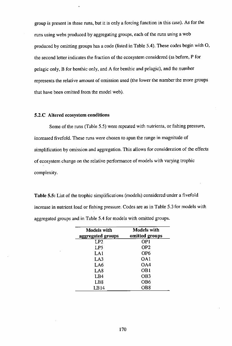
group is present in these runs, but it is only a forcing function in this case). As for the

runs using webs produced by aggregating groups, each of the runs using a web

produced by omitting groups has a code (listed in Table 5.4). These codes begin with 0,

the second letter indicates the fraction of the ecosystem considered (as before, P for

pelagic only, B for benthic only, and A for benthic and pelagic), and the number

represents the relative amount of omission used (the lower the number the more groups

that have been omitted from the model web).

5.2.0 Altered ecosystem conditions

Some of the runs (Table 5.5) were repeated with nutrients, or fishing pressure,

increased fivefold. These runs were chosen to span the range in magnitude of

simplification by omission and aggregation. This allows for consideration of the effects

of ecosystem change on the relative performance of models with varying trophic

complexity.

Table 5.5: List of the trophic simplifications (models) considered under a fivefold

increase in nutrient load or fishing pressure. Codes are as in Table 5.3 for models with

aggregated groups and in Table 5.4 for models with omitted groups.

Models with Models with aggregated groups omitted groups

LP2 OP I LP5 OP2 LA1 OP6 LA3 OA 1 LA6 0A4 LA8 OB1 LB4 OB3 LB 8 OB6

LB14 OB8

170

5.2.D Analysis

Summarising the overall effects of model simplification

To summarise the range of system structures encompassed by the simplifications

we examine, the number of links and connectance (C) of the system is plotted against

the number of groups in each case. C was calculated as given in Putman (1994):

c = L \ MN —1 )

where C is connectance, L is the number of links in the web and N is the number of

separate "species" in the web (in this case either the original components or the

aggregated groups). A number of indices (chlorophyll a, levels of sediment oxygen,

denitrification and the biomass, production and consumption of each of the components

in the models) are used to judge the relative performance of the models. In each case the

runs are compared by considering the absolute relative value of the difference between

the averages (over the entire bay for the final four years of each run) of the simplified

and standard (full version) runs of the model. Finally, the following measure was taken

as an overall indicator of performance:

std

= i I s. td

1

(5.2)

where I, is the jth relevant indicator (i.e. Vs calculated for runs containing pelagic

components only are based only on pelagic indicators) and "std" and "simplif' indicate

the value of the jth indicator for the standard run and simplified run respectively. The

simplified model with the smallest value of this overall measure V is considered to have

the best overall performance. It is recognised that a very low contribution for a single

indicator (If) by a run with generally poor performance could better a consistent

performance by another run. Fortunately this situation does not arise here. For models

that omitted groups, the models that produced the minimum values of V are also the

ones that are consistently sound performers (within the top 25%). The relative quality of

(5.1)

171

each run, as specified by the indicators, is not as consistent for models with aggregated

• groups as for models with omitted groups. However, the use of V as an overall summary

statistic is still acceptable as the "best" run was usually within the top 35% for every

indicator.

Summarising the fine scale spatial and temporal effects of model simplification

The output is also considered on a cell-by-cell basis, not just for the bay as a

whole. This allows for detection of effects of model simplification on the spatial details

of the output.

To judge the effects of model simplification on the fine scale spatial dynamics of

the models the relative spatial distributions of each component was tracked over the

final four years of each run. The quality of the match at each point is based on the

number of boxes for which the distribution in the run using a simplified web differs

from the distribution predicted in the standard run. To summarise these results across

runs, three broad categories of responses are recognised:

the spatial distribution of the component matches the spatial distribution in the

standard run for the majority of the tuns using simplified webs

- there is no match between the spatial distribution of the component in the standard

run and any of the runs using simplified webs

- there is only a match between the spatial distribution of the component in the

standard run and the runs using simplified webs that have the lowest values for V

(as defined above).

A simple comparison of the time series of each component (achieved by overlaying the

time series from simplified runs on the time series from the standard run) is used to

judge the effects of model simplification on the temporal dynamics of the model.

172

5.3 Results

When simplification of the food web is produced by aggregating components

there is a clear increase in connectance as the number of nodes (individual components

or aggregated groups) is decreased (Figure 5.3). This reflects the marked decrease in the

number of links remaining in the web as the number of nodes is reduced (Figure 5.3).

Results for simplified food webs produced by omitting groups are similar (Figure 5.4),

but the relationships are not as tight. In both cases (omission and aggregation of

groups) the small differences in web structure between BM2 and IGBEM (BM2 has an

additional pelagic bacteria group) have little effect on the results (Figure 5.3(a) vs.

5.3(b), and Figure 5.4(a) vs. 5.4(b)).

Effects of aggregating groups

In both IGBEM and BM2, a number of the models with aggregated groups that

only consider the benthos (the LB models) show trophic self-simplification through the

extinction of some functional groups. Some of the simplified versions of BM2 that are

the most highly aggregated (runs LB2 — LB4, see Table 5.3 for definitions of the codes)

lose the composite "all benthos" component, as does the LB4 run of IGBEM. While no

groups go extinct in the less aggregated LB runs of BM2, some groups are lost in

IGBEM with the same level of aggregation. The LB8, LB9 and LB 12 runs of IGBEM

all suffer some form of trophic self-simplification. All of these runs have an aggregated

demersal fish group, microphytobenthos and infauna and epifauna groups that are

aggregated to slightly different degrees. In LB8 all but the microphytobenthos drop to

negligible levels of biomass; LB9 loses the lumped "all infauna" group; and LB 12 loses

the "large infauna" aggregated group. It is noteworthy that these models undergo

trophic self-simplification in IGBEM when they do not in BM2 and that even other

versions of IGBEM with very similar levels of aggregation (e.g. LB 10 and LB 11) do

173

2

03U

e43

eUU

O3

Figure 5.3: Plot of connectance (C) (open circles) and the number of links (solid black

circles) in the simplified food webs produced by aggregating components, against the

number of groups (individual functional groups or aggregated groups) in the webs.

(a) Bay Model 2 (BM2)

100

•

Nu

mbe

r of

Lin

ks

80 -

60 -

40 -

o

•

5

•

00 00

. , 10 15 20 25

Number of Groups

30

20 -

o

(b) for the Integrated Bay Ecosystem Model (IGBEM)

Nu

mbe

r of

Lin

ks

03U

OP

OU

UO

3

80

60 -

40 -

20 -

o

o

O 000 • 0 00

O 000 Oo 0 00

0 i

• 00

•

0

II IIII.

o o 0

•

•

o

0.6

- 0.5

- 0.4

- 0.3

- 0.2

- 0.1

0.0 o 5

10 15 20

25

30

Number of Groups

174

0.00 • II • •

100

60 -

40 -

20 -

80 -

0

0 0 0 •

• • • • • I.. •

00

o o • •

•

0.35

- 0.30

- 0.25

- 0.20

- 0.15

- 0.10

- 0.05

60 -

Nu

mbe

r of

Lin

ks

40 -

20 -

e3ue

l3eu

uo

3

GO

UM

OU

U00

Figure 5.4: Plot of connectance (C) (open circles) and the number of links (solid black

circles) in the simplified food webs, produced by omitting components, against the

number of functional groups in the webs.

(a) Bay Model 2 (BM2)

10 15 20

25

30

Number of Groups

(b) the Integrated Bay Ecosystem Model (IGBEM)

80

•

0 0 0 00

0 0 0

00 0 •

•0 • •

• •

9 I

5

10 15 20

25

30

Number of Groups

Nu

mbe

r o

f Li

nks

0.35

- 0.30

0.25

0.20

0.15

0.10

- 0.05

0.00

175

not self-simplify in this way. Two of the runs that use aggregated food webs that span

pelagic and benthic components also predict the extinction of some groups. In the LA8

run of BM2 the benthic consumers, except the "mobile epifauna", decline to negligible

levels, and the LA9 run of IGBEM loses the diatoms and the aggregated group "small

zooplankton". There are also a number of versions of IGBEM with aggregated groups

where the system approaches numerical instability (these are LA3 and all of the LB runs

that include the aggregated groups "macrophytes" or "all phytobenthos").

It is possible to compare indices across the models despite extinction of some

groups and potential instabilities. A majority of the indices show no clear patterns when

the absolute relative differences in the values for the simplified and standard runs are

plotted against the number of groups in the run (Figure 5.5). Only denitrification shows

a clear effect of aggregating groups, and that is that the upper bound of the absolute

relative difference in predicted denitrification in the simplified vs full models increases

as more groups are aggregated (Figure 5.5). None of the indicators shows any clear

patterns when plotted against connectance for either BM2 or IGBEM.

A final way of considering the baywide averages for the indices is to evaluate

them in relation to the subwebs that are preserved in each run, that is to explicitly

consider the results per run. Considering the results of each run in this way, it is clear

that the behaviour of models with aggregated groups are frequently very different to

those of the full versions without aggregation. Deviations from the non-aggregated

models of the predicted values of the various indicators are often greater for versions of

BM2 and IGBEM with aggregated groups than for versions with omitted groups (Table

5.6). The amount of deviation has a non-linear relationship with the level of aggregation

used. For each indicator there is usually one or more runs with intermediate levels of

aggregation for which the amount of deviation is smaller than for other runs with higher

or lower levels of aggregation (e.g. chlorophyll a in the LP runs, Figure 5.6). This

176

(a)

v 614 •

• 01 cia

•

SO

• 00

(d) •

• •

• • • gEg•olgoc4rL_r___ 00

30

Abs

olu

te r

ela

tive

diff

e ren

ce

0.03

0.02

0.01

0.00 • 0

SO 5 10 15 20 25

0 •

4 03

00

0.0 10 15 20 25 30

6

(i)

2

•'war • 0

0 5 10 15 20 25 30

Figure 5.5: Plots of the absolute relative differences in the predicted values of indices

between the simplified (with aggregated trophic groups) and full versions of the models

in relation to the number of groups (individual functional groups or aggregates)

included in the models. (Note: the larger the number of components the lower the

degree of aggregation.) The results for Bay Model 2 (BM2) are represented by open

circles and those for the Integrated Generic Bay Ecosystem (IGBEM) by solid black

circles. The indices are: (a) chlorophyll a in the water column, (b) chlorophyll a on the

sediments, (c) denitrification, (d) concentration of oxygen in the sediments, (e) water

column primary production, (f) total consumption in the water column, (g) benthic

primary production, (h) total benthic consumption, (i) biomass of macrophytes, (j)

biomass of zooplankton, (k) biomass of benthos, and (1) biomass of fish.

5 10 15 20 25 30

1.0

5 10 15 20 25 30

• • (i) •

GM 00 00 0.5 00 OS elp 00

• 1.0 •

0.0 648, SO 0 5 10 15 20 25 30

0

0 c (c)

o 0 c° 80 o

0°02:Dre 10

o e SO-

15 20 25 30

1.0 OD OD • •

00

0.5 CV. 0 ei

1.5

(0

0.0

1.5

1.0

0.5

1.5

1.0

0.5

0.0

5 10 15 20 25 30

6.•1: • • ••

00 0

0 el 0

(h)

SO 5 10 15 20 25 30

00

(k)

:• so

• •• • • • • •„,

• 00 CX) 0

• • •

5 0.0 so

10 15 20 25 30 0 5 10 15 20 25 30

300.0

200.0

100.0

0 1.0- - 00604

0.5 .

CO

.Vcg 00 ••

(1)

Number of groups in the model

177

Table 5.6: Comparison of the magnitude of average relative deviation from the full

models of the indices from runs produced by aggregation and omission of groups for

Bay Model 2 (BM2) and the Integrated Bay Ecosystem Model (IGBEM). Values in the

table are the average ratio of the deviation for models with aggregated groups: the

deviation of models with omitted groups with the same degree of simplification.

Index BM2 IGBEM Biomass of fish 59.3 1.0 Biomass of macrophytes 7.7 2.2 Biomass of zooplanIcton 0.8 0.9 Biomass of benthos 0.5 0.5 Chlorophyll a 0.5 1.4 Consumption (water column) 1.0 1.2 Consumption (sediment) 1.5 2.2 Denitrification 1.2 1.8 Primary Production (water column) 2.3 1.3 Primary Production (sediment) 3.7 2.0 Sediment Oxygen 0.3 1.3

general pattern is also evident in the overall V statistics for models with aggregated

groups (Table 5.7). Consideration of the structure of the food web in each of the models

with aggregated groups (Table 5.3) that have the lowest V values (Table 5.7) suggests

that retaining broad trophic level and size structure is necessary for reasonable model

performance.

Considering fine-scale spatial and temporal resolution rather than baywide

averages, there are still strong effects of aggregating groups. Overall, there are relatively

few processes with a fairly consistent distribution over all the runs and these are driven

largely by production and consumption by the fish (Table 5.8). There are many more

components and processes for which the relative spatial distributions in the runs with

aggregated groups do not match the relative spatial distribution of the non-aggregated

model (Table 5.8). Many of these processes and measures are associated with bacteria.

A notable exception is the biomass of zooplankton. None of the runs with aggregated

groups predict a relative distribution for this measure which matched the relative

distribution in the full versions of BM2 or IGBEM. In comparison to the number of

components and processes that do not match the relative distribution of the standard run,

a similar number have relative spatial distributions that only match those of the standard

178

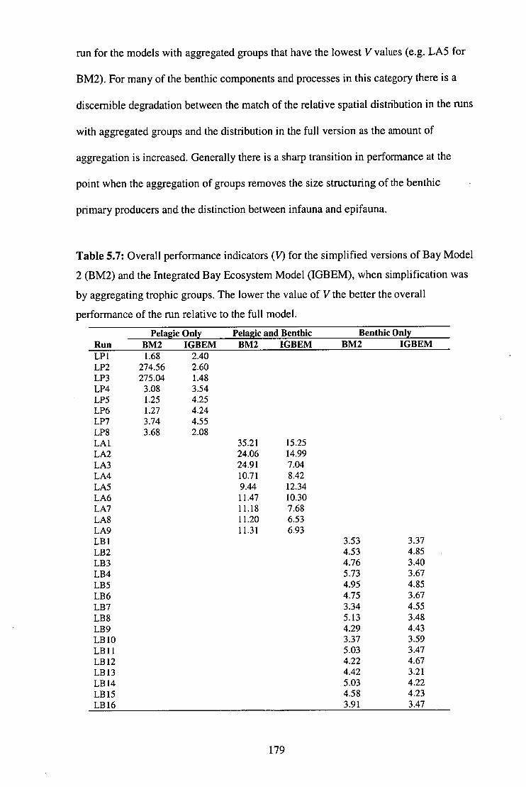
run for the models with aggregated groups that have the lowest V values (e.g. LA5 for

BM2). For many of the benthic components and processes in this category there is a

discernible degradation between the match of the relative spatial distribution in the runs

with aggregated groups and the distribution in the full version as the amount of

aggregation is increased. Generally there is a sharp transition in performance at the

point when the aggregation of groups removes the size structuring of the benthic

primary producers and the distinction between infauna and epifauna.

Table 5.7: Overall performance indicators (V) for the simplified versions of Bay Model

2 (BM2) and the Integrated Bay Ecosystem Model (IGBEM), when simplification was

by aggregating trophic groups. The lower the value of V the better the overall

performance of the run relative to the full model.

Pelagic Only Pelagic and Benthic Benthic Only Run BM2 IGBEM BM2 IGBEM BM2 IGBEM LPI 1.68 2.40 LP2 274.56 2.60 LP3 275.04 1.48 LP4 3.08 3.54 LP5 1.25 4.25 LP6 1.27 4.24 LP7 3.74 4.55 LP8 3.68 2.08 LAI 35.21 15.25 LA2 24.06 14.99 LA3 24.91 7.04 LA4 10.71 8.42 LAS 9.44 12.34 LA6 11.47 10.30 LA7 11.18 7.68 LA8 11.20 6.53 LA9 11.31 6.93 LB I 3.53 3.37 LB2 4.53 4.85 LB3 4.76 3.40 LB4 5.73 3.67 LB5 4.95 4.85 LB6 4.75 3.67 LB7 3.34 4.55 LB8 5.13 3.48 LB9 4.29 4.43 LBIO 3.37 3.59 LB 1 I 5.03 3.47 LBI2 4.22 4.67 LBI3 4.42 3.21 LBI4 5.03 4.22 LB15 4.58 4.23 LBI6 3.91 3.47

179

•

•

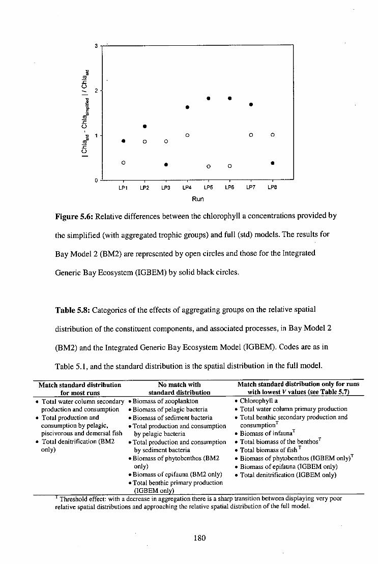
0

• 0 0

LP1 LP2 LP3 LP4 LP5 LP6

LP7 LP8

Run

Figure 5.6: Relative differences between the chlorophyll a concentrations provided by

the simplified (with aggregated trophic groups) and full (std) models. The results for

Bay Model 2 (BM2) are represented by open circles and those for the Integrated

Generic Bay Ecosystem (IGBEM) by solid black circles.

Table 5.8: Categories of the effects of aggregating groups on the relative spatial

distribution of the constituent components, and associated processes, in Bay Model 2

(BM2) and the Integrated Generic Bay Ecosystem Model (IGBEM). Codes are as in

Table 5.1, and the standard distribution is the spatial distribution in the full model.

Match standard distribution for most runs

• Total water column secondary production and consumption

• Total production and consumption by pelagic, piscivorous and demersal fish

• Total denitrification (BM2 only)

No match with standard distribution

• Biomass of zooplankton • Biomass of pelagic bacteria • Biomass of sediment bacteria • Total production and consumption

by pelagic bacteria • Total production and consumption

by sediment bacteria • Biomass of phytobenthos (BM2

only) • Biomass of epifauna (BM2 only) • Total benthic primary production

(IGBEM only)

Match standard distribution only for runs with lowest V values (see Table 5.7)

• Chlorophyll a • Total water column primary production • Total benthic secondary production and

cons umptionT • Biomass of infaunaT • Total biomass of the benthosT • Total biomass of fish T • Biomass of phytobenthos (IGBEM only) r • Biomass of epifauna (IGBEM only) • Total denitrification (IGBEM only)

Threshold effect: with a decrease in aggregation there is a sharp transition between displaying very poor relative spatial distributions and approaching the relative spatial distribution of the full model.

180

The temporal dynamics displayed by the models with aggregated groups are

more often like each other than the corresponding components in the standard run of

BM2 or IGBEM. For example, for BM2 the time series for "large zooplankton" in LP2

is similar to the time series produced by adding the time series for "small zooplankton"

and "large zooplankton" in LA6, but is markedly different from the time series

produced by adding the time series for all the zooplankton groups in the standard run

(Figure 5.7). The general forms of the dynamics of aggregated and non-aggregated

models is more similar when the amount of aggregation is lower, though even then

critical details such as bloom peaks are not predicted accurately in versions with

aggregated groups (Figure 5.8). If the degree of aggregation is high then there is little, if

any, resemblance between the temporal dynamics of the standard and simplified runs

for a large number of the trophic groups, particularly the fish, benthos and macrophytes.

Effects of omitting groups

BM2 demonstrates trophic self-simplification, in which functional groups went

extinct in the run, in 5 cases. In 0A2 (see Table 5.4 for definitions of the codes),

macroalgae was lost from the system, while in 0B4, 0B6, 0B8 and 0B9 the biomass of

the benthic deposit feeders fell to negligible levels. In contrast, for IGBEM, macroalgae

and the benthic deposit feeders show a reduced spatial distribution for some of the runs,

but no component is entirely lost from the system.

There are a number of runs where the system becomes susceptible to the effects

of increased short-term nutrient loading (e.g. flooding of the Yarra River, which is a key

point source of inputs in the model). As a result the system exhibits extreme behaviours

(such as high amplitude oscillations in some components) or approaches numerical

instability. This is more common in IGBEM than in BM2. In BM2 only 0A5 exhibits

this problem, while for IGBEM the runs 0B2 — 0B9 (inclusive) also display this

behaviour.

181

30

— full model LP2 -- LA6

25 -

20 -

/A , A

/

/ 1 7

...-N •• • ‘, . •

15 -

10

— full model LP4 -- LA1

or' a 1 \ 1\11 G

il

i

ll

I

- - 1 I cm 1 \ 1 E

V I 1 A A al 1/4 r 7E 2 - 0

V v

Figure 5.7: Comparison of the temporal dynamics of "large zooplankton" in LP2, the

time series produced by adding the time series for "small zooplankton" and "large

zooplankton" in LA6 and the time series produced by adding the time series for all the

zooplankton groups in the standard (full) version of Bay Model 2 (BM2). The codes for

the runs simplified by aggregating groups (LP2, LA6) are given in Table 5.3 and all

time series come from the same cell of the model (close to the mouth of the modelled

bay).

4788 4892 4996 5100 5204 5308 5412 5516 5620 5724 5828 5932 6036 6140

Day of run

Figure 5.8: Comparison of the temporal dynamics of chlorophyll a (Chl a) in one cell

(covering an input point from a sewage treatment plant) of the standard (full) model and

versions of Bay Model 2 with aggregated groups. For clarity, only a selection of the

simplified models are displayed, but all the simplified models produced levels of Chl a

between the extremes presented here.

0 11 1 1 1 1 1 1 1 1 1

4788 4892 4996 5100 5204 5308 5412 5516 5620 5724 5828 5932 6036 6140

Day of the Run

Tota

l bio

mas

s of

zoo

pla

nkto

n (m

g N

m-3)

182

Despite the extinction of some groups and instabilities, it is possible to compare

indices across the models. When the absolute relative differences between the simplified

versions (with omitted groups) and the standard (full) model are plotted against the

number of groups, there are some clear results and these patterns are stronger for

IGBEM than BM2 (Figure 5.9). For BM2 there is no clear overall pattern of the effect

of omitting groups on the levels of oxygen (Figure 5.9d) or chlorophyll in the sediment

(Figure 5.9b), or the predicted average biomass of planktivorous fish (Figure 5.91) or

macroalgae (Figure 5.9i). There is a clear pattern for the rest of the indices for BM2, but

it is not usually as marked as that shown by IGBEM. The general pattern of the effect of

omitting groups is that the upper bound on the absolute relative difference between the

simplified and full versions of the model increases as more groups are omitted (Figure

5.9). The pattern is not equally strong across all indices, even in IGBEM, and is clearest

for water column variables, such as chlorophyll a (Figure 5.9a), the biomass of large

omnivorous zooplankton (Figure 5.9j), and denitrification in the sediments (Figure

5.9c). This relationship, between the absolute relative difference between the models

and the number of groups omitted, is less evident for the biomass of the benthic groups,

for example benthic filter feeders (Figure 5.9k). In contrast to the consistent patterns

between performance of reduced models and the number of groups they contain, there is

no clear relationship between any of the indices and connectance for either BM2 or

IGBEM.

Considering the results of each run individually shows that there are crucial links

that have to be included if the behaviour of the simplified models is to approach that of

the full version of BM2 or IGBEM. This is indicated clearly by estimates for primary

production and consumption (Figures 5.10 and 5.11). If few groups are included in the

simplified web then the productivity estimates from simplified models usually diverge

from equivalent estimates from the full model by as much as 50-85%. The effect is

183

4

3

2

0

0.008

0.006

0.004

0.002

0.000 0

1.5

1.0

0.5

0.0

3

2

0

8 0

00 90

0 0

0

0 .0.,

0 0 0 00 I.. •

(a)

5 10 15 20 25 30

•

••

0 c0

• •

• • • 5.

es • eo 0

0 cool 0

(d)

o 0 5 10 15 20

00 25 30

•

• • 0

cP

SS* 00 ea* 0

0 oo •

• on

(g)

so

1.0

0.5

0.0

• •

0 o

0 8 5

10 15

• 13 • • 0

°

20 25 30

(i)

.0

1.0

0.5

0.0 10 15 20 25 30

•

Abso

lute

rela

tive

diffe

renc

e

•

25 30

• (e)

25 30 s•-o-ok-8—o°

5 10 15 20

(h)

SO

• (k)

15 25 20

•

cx 0 d . .

10 15 20

(f)

(i) 000

8 • • • • , 0-•,--•

5 10 15 20 25 30

1.5

1.0

0,5

0.0

1.5

1.0

0.5

0.0

1.0

• • • • 0.5 •

00 0 a o op

Cop • • 0.0 c?-0-9?-Q-0—c) •0

5 10 15 20 25 30 0 5 10 15 20 25 30

co • 8 o • s•

5 10 15 20 25 30

—dr

30

Figure 5.9: Plot of the absolute relative differences in the predicted values of indices

between the simplified (with omitted trophic groups) and full versions of the models in

relation to the number of groups included in the models. (Note: the larger the number of

components the fewer groups that have been omitted.) The results for Bay Model 2

(BM2) are represented by open circles and those for the Integrated Generic Bay

Ecosystem (IGBEM) by solid black circles. The indices are: (a) chlorophyll a in the

water column, (b) chlorophyll a on the sediments, (c) denitrification, (d) concentration

of oxygen in the sediments, (e) water column primary production, (0 total consumption

in the water column, (g) benthic primary production, (h) total benthic consumption, (i)

biomass of macroalgae, (j) biomass of large omnivorous zooplankton, (k) biomass of

benthic filter feeders, and (1) biomass of planktivorous fish.

Number of groups in the model

184

particularly severe in the "benthic only" runs, where benthic primary production is

consistently more than 35% from the value given by the full model, except for some of

the simplest of the BM2 cases (0B1 and 0B3) where it is within 2% of the standard

estimate (Figure 5.10). The results for consumption (Figure 5.11) are largely similar to

those for production. Runs with only a few groups in them produce estimates of

consumption that deviate most from the standard estimate (by as much as 90%).

Notably the consumption estimate from the run with the fewest omitted groups usually

also performs poorly (as poorly as the most simplified runs). This suggests that the

inclusion of bacteria may not be appropriate in simplified webs.

Consideration of food web structure (Table 5.4) in each of the runs with the

lowest values of the V statistic (Table 5.9) indicates that some representation of size

structure is required in simplified food webs and that benthic subwebs may need to be

more highly resolved than pelagic subwebs. Further, the results suggest that

representing many of the microfaunal functional groups may not be necessary.

As might be expected given the overall responses of the model to omitting

groups, the fine scale output of the models is also affected by omitting groups. As

occurs in the overall indices, not all components and processes in the models are

affected to the same degree by the omission of groups. Generally, the relative spatial

distribution of some microfauna (meiobenthos and the pelagic bacteria) does not match

the standard case for any of the simplified runs in which they are included (Table 5.10).

In contrast, the distribution of fish, picoplankton and total water column production is

virtually identical to that of the full model for all runs of the simplified versions of BM2

and IGBEM (Table 5.10). There are also a couple of components (macroalgae in BM2

and anaerobic bacteria in IGBEM) for which the relative spatial distributions in the

simplified and standard runs are close matches in only one of the two models. It is not

surprising that the relative spatial distributions of the fish are close matches in all the

185

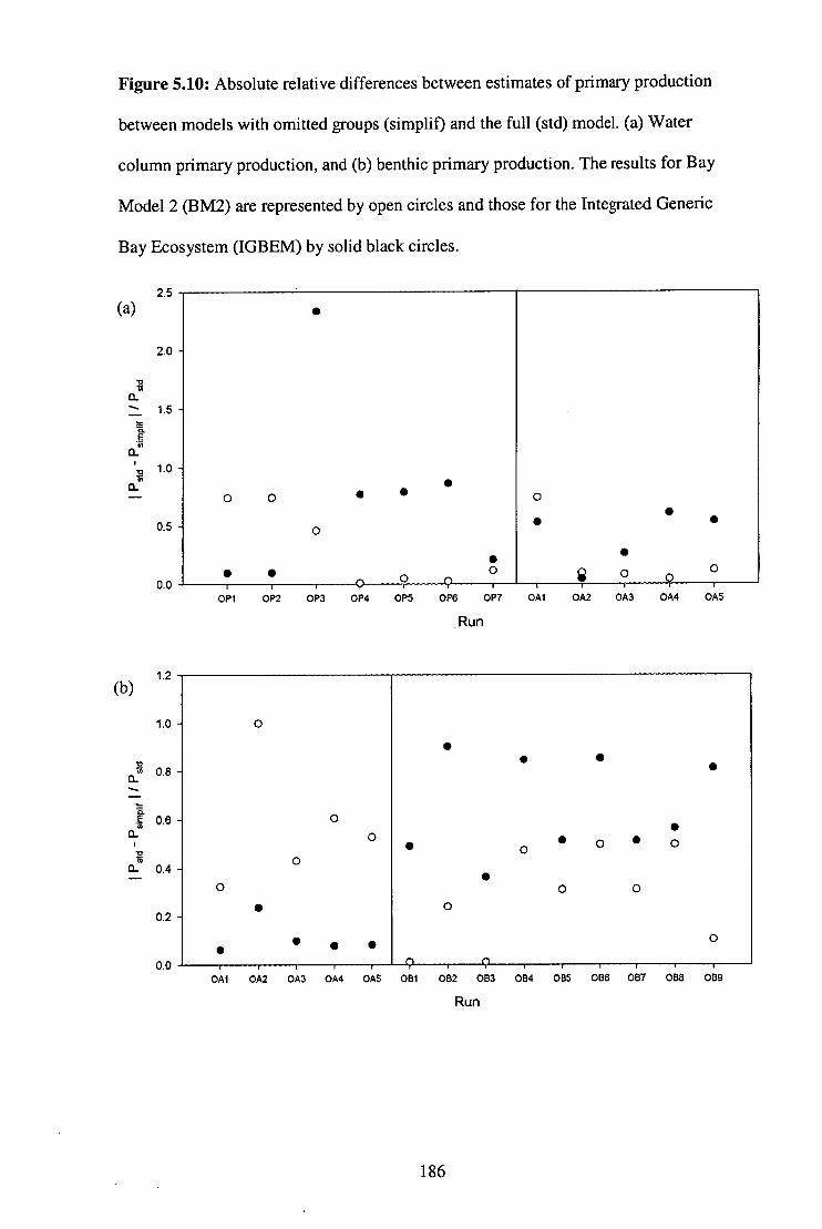
I 'std

- Ps

impl

if I '

Pstd

0.8

0.13

0.4

0.0

1.2 (b)

1.0

0.2

• •

• • • •

• •

• • • • 9 9

Figure 5.10: Absolute relative differences between estimates of primary production

between models with omitted [groups (simplif) and the full (std) model. (a) Water

column primary production, and (b) benthic primary production. The results for Bay

Model 2 (BM2) are represented by open circles and those for the Integrated Generic

Bay Ecosystem (IGBEM) by solid black circles.

2.5 (a)

2.0

1.5

• • • •

•

•

0

0.5

0.0 OP' OP2 OP3 OP4 OP5 OP6 OP7

Run

0A1 0A2 0A3 0A4 0A5

0A1 0A2 0A3 0A4 0A5 OBI

0132 083 084 0135 086 0B7 OBS OB9

Run

186

1.2 (a)

I Qstd

- Q

s im

plif I I

Qst

d

1.0

0.8

0.6

0.4

0.2

0.0

• • •

•

8 • • 0

• •

o • o

• 0 • •

• • • • • • •

•

Figure 5.11: Absolute relative differences between estimates of consumption between

models with omitted groups (simplif) and the full (std) model. (a) Water column

consumption, and (b) benthic consumption. The results for Bay Model 2 (BM2) are

represented by open circles and those for the Integrated Generic Bay Ecosystem

(IGBEM) by solid black circles.

OP1

OP2

OP3

OP4

OP5

OP6 OP7

°Ai

0A2

0A3

0A4

0A5

Run

too (b)

0.75

0.25

0.00

.o 0.50 0

0A1 0A2

0A3 0A4 0A5 OBI

0132 OB3

0134 085 0B6 087 0138 089

Run

187

Table 5.9: Overall performance indicators (V) for runs of Bay Model 2 (BM2) and the

Integrated Bay Ecosystem Model (IGBEM), with groups omitted from the models. The

lower the value of V the better the overall performance of the run relative to the full

model.

Pelagic Only Pelagic and Benthic Benthic Only Run BM2 IGBEM BM2 IGBEM BM2 IGBEM OP1 3.00 4.45 0P2 3.49 4.61 0P3 6.98 8.57 0P4 1.62 2.47 0P5 3.82 2.07 0P6 1.83 3.00 0P7 1.92 1.42 OA1 7.63 7.22 0A2 6.87 3.20 0A3 6.40 2.45 0A4 6.81 3.37 0A5 14.58 6.69 OB1 2.57 3.89 0B2 2.71 6.26 0B3 2.58 3.41 0B4 3.09 3.92 0B5 2.96 6.20 0B6 2.54 3.81 0B7 2.95 6.49 0B8 2.54 3.22 0B9 3.20 3.72

Table 5.10: Categories of the effect of omitting groups on the relative spatial

distribution of the constituent components, and associated processes, in Bay Model 2

(BM2) and the Integrated Generic Bay Ecosystem Model (IGBEM). Codes as are as in

Table 5.1, and the standard distribution is the spatial distribution in the full model.

Match standard distribution for No match with standard Match standard distribution only for nearly all runs distribution runs with lowest V values

(see Table 5.9) • FD*, FG*, FP*, FV*, PS, • OB, PB (PAB and PFB for • AEB, BC, BD, BF, BG, MB, MZ, • Total water column primary BM2), PL, SG, ZL, ZS, Chlorophyll a,

production, • Total production and • Total benthic primary production, • Total production and consumption by pelagic bacteria, • Total benthic secondary production

consumption by FD and FV, • DF (BM2 only) and consumption, • ANB (IGBEM only), • Total water column secondary • Macroalgae (BM2 only) production and consumption,

• Total denitrification, • Total production and consumption by

benthic bacteria, • Total production and consumption by

FG and FP, • ANB (BM2 only)

* A fixed migration matrix gives the spatial distribution of the biomass of these groups. However, the distribution of production and consumption by these groups is not fixed as that depends on the local density of their food groups.

188

runs because a migration matrix fixes their distribution. However, it is noteworthy that

the relative spatial distributions for the picophytoplankton, and the macroalgae in BM2

are close matches in all the runs. Nevertheless, only a minority of the components in the

runs with omitted groups have relative spatial distributions that either match the

distribution in the full model closely or not at all. The relative spatial distribution of the

majority of components and processes only approaches that of the standard run for those

models with omitted groups that are identified by the overall indicator (V) as being close

to the standard output (e.g. 0A3).

The temporal dynamics of the models with omitted groups indicated that the

turnover time of a component is one of the central factors determining the degree to

which omitting groups degrades the model performance. The slower growing

components usually show little change in temporal patterns as a result of omission (e.g.

biomass of the epifaunal carnivores, Figure 5.12), while the greatest changes are

associated with groups with rapid dynamics (e.g. diatoms, Figure 5.13).

Influence of changes to the ecosystem conditions on the effects of simplifying models

Increasing nutrient load or fishing pressure does not change the general pattern

of effects of simplification based on baywide measures reported above, but there are

some quantitative differences. The upper bound of the difference between the simplified

runs and the full models declines as the total number of groups in the models increased.

As for the results under baseline conditions, this pattern is stronger for IGBEM than for

BM2. Again, there is no relationship between the differences of the simplified and

standard runs and connectance.

In contrast to the baywide results, the quality of the matches of the relative

spatial distributions of the simplified and full models changes substantially for some of

the groups and processes when ecosystem conditions are altered. Within models that

have either omitted or aggregated groups, the changes tend to be the same whether it is

189

Biom

ass

of M

Z (g

AFD

W m

-2)

Figure 5.12: Comparison of the temporal dynamics of epifaunal predators (MZ) in one

cell (offshore from a sewage treatment plant) of the full Integrated Generic Bay

Ecosystem Model and versions with omitted groups. For clarity, only a selection of the

runs has been displayed, but all the runs produced biomasses of MZ between the

extremes presented here.

1596

1804

2012

2220 2428

2636

2844

3052

Day of the Run

Figure 5.13: Comparison of the temporal dynamics of biomass of diatoms (PL) in one

cell (covering an input point from a sewage treatment plant) of the full Bay Model 2

model and versions with omitted groups. For clarity, only a selection of the runs has

been displayed, but all the runs produced biomasses of PL between the extremes

presented here.

16

— full model OP2

OP5

Bio

mas

s of

PL

(mg

N m

-3)

1

0

4788 4996 5204

5412 5620

5828

6036

Day of the Run

190

fishing pressure or nutrient loading that changes. However, comparing the changes

across models that use different forms of simplification, it is clear that the direction of

change is often similar, but the groups and processes affected are different for models

that aggregate groups (Table 5.11) and models that omit groups (Table 5.12). The

effects of aggregating groups on relative spatial distributions does not change with

changing ecosystem conditions for many groups and processes. The majority of the

groups and processes for which the effects of aggregation on spatial distributions do

change with changing ecosystem conditions move from occasionally matching the

distribution in the full model to never matching it (Table 5.11). A similar pattern of

change in the results occurs for models with omitted groups when ecosystem conditions

are altered. The majority of the components that only show occasional agreement with

the full version under baseline conditions now show no agreement (Table 5.12).

However, the match for denitrification, benthic primary production and the production

and consumption by planktivorous and herbivorous fish improve with altered ecosystem

conditions, and many of the components that display relatively consistent spatial

distributions across all of the models with omitted groups under baseline conditions

continued to do so (Table 5.12).

The same temporal patterns of behaviour, in the simplified models relative to the

full model, hold under changed conditions, except that the deviations from the standard

run are more exaggerated (e.g. diatoms, Figure 5.14). This is due to the higher levels of

resources available to primary producers, or lower predation pressure on the fish prey

groups, under the new conditions. These deviations arise when groups are either

aggregated or omitted, but are much worse in the former. There are a few cases in the

models with aggregated groups where the effects of changing ecosystem conditions are

opposite to those predicted by the full model. For example, the overall behaviour of the

"macrophyte" group more closely resembles the behaviour of the seagrass in the full

191

Table 5.11: The effects of model simplification by aggregation on the relative spatial distribution of the constituent components, and associated

processes, in Bay Model 2 (BM2) and the Integrated Generic Bay Ecosystem Model (IGBEM) when the nutrient load (x5) or fishing pressure (Fx5) is

increased to five times that of the "baseline" conditions. Codes are as in Table 5.1, and the standard distribution is the spatial distribution in the full

model under the same nutrient load and fishing pressure.

Match standard distribution for most runs Never match standard distribution Occasionally match standard distribution Fx5 x5 Fx5 x5 Fx5 x5

• Total biomass of fish • Total biomass of fish • Biomass of epifauna • Biomass of epifauna • Biomass of zooplankton • Biomass of zooplankton • Total denitrification • Total denitrification • Chlorophyll a • Chlorophyll a • Biomass of infauna • Biomass of infauna • Total production and • Total consumption by • Biomass of phytobenthos • Biomass of phytobenthos • Total biomass of benthos • Total production by pelagic,

consumption by pelagic, pelagic, piscivorous and • Total benthic primary • Total biomass of benthos • Total water column primary piscivorous and demersal fish piscivorous and demersal fish

demersal fish production • Total water column primary production

• Total benthic primary production

production, • Total benthic secondary

production and consumption • Total water column secondary

production and consumption

• Total benthic secondary production and consumption

• Total water column secondary production and consumption

192

Table 5.12: The effects of omitting groups on the relative spatial distribution of the constituent components, and associated processes, in Bay Model 2

(BM2) and the Integrated Generic Bay Ecosystem Model (IGBEM) when the nutrient load (x5) or fishing pressure (Fx5) is increased to five times that

of the "baseline" conditions. Codes are as in Table 5.1, and the standard distribution is the spatial distribution in the full model under the same nutrient

load and fishing pressure.

Match standard distribution for most runs Never match standard distribution Occasionally match standard

distribution Fx5 x5

• PL, • PL, MZ, ZL, • Chlorophyll a • Chlorophyll a

Fx5 • BG, FD, FG, FP, FV, MA, SG,

ZL • Total denitrification • Total production and

consumption by FD, FG, FP and FV

x5 • BG, FD, FG, FP, FV, MA • Total benthic primary

Production • Total denitrification • Total production and

consumption by FD, FG, FP and FV

Fx5 • BC, BD, BF, DF, MB, MZ, PS, ZS • Total water column primary

production • Total water column secondary

production and consumption • Total benthic secondary production

and consumption

x5 • BC, BD, BF, DF, MB, PS, SG,

ZS • Total water column primary

production • Total water column secondary

production and consumption • Total benthic secondary

production and consumption

Table 5.13: Predicted change in biomass (average biomass when nutrient loads x5 / average biomass under baseline conditions) of macrophytes for

standard (full) model and versions of Bay Model 2 with aggregated groups.

Run

Standard 1.62

LA1 LA3 LA6 LA8 LB4 LB8 LB14 Change in Biomass

0.09 0.79 0.44 0.97 0.51 0.46 0.15

193

model than the macroalgae. Consequently, when nutrients rise the "macrophyte" group

is lost from the system in the models with aggregated groups, while the biomass of

macrophytes (the sum of the biomasses of macroalgae and seagrass) persists and even

rises in the standard form of BM2 (Table 5.13).

5.4 Discussion

It is possible to make a number of generalisations from the relative performance

of the various kinds of simplified models. First, groups with the fastest dynamics often

show the greatest effects of reduced model complexity (e.g. consider the temporal

dynamics of the various components of the models). This is due to the greater ability of

groups with fast dynamics to respond to changes in ambient physical and ecological

conditions. The resources and forces on these groups are in a constant state of flux (due

to advection and diffusion). As a result, small variations in effective predation pressure

and competition can lead to large deviations as they build upon potentially large short-

term changes in resources, the outcomes of these interactions can then accumulate or

compound. However, as with all groups, the exact form of these responses to differing

ecological and physical conditions are due to a mixture of trophic and non-trophic, as

well as direct and indirect interactions. Thus, the greatest deviations are often seen when

the simplified models are linear chains and furthest in form from the web of the

standard case.

The relationship between trophic complexity and performance

Our findings that a high degree of simplification, whether by aggregating or

omitting groups, leads to poor model performance is consistent with earlier studies

(Sugihara et al. 1984, Costanza and Sklar 1985, Pahl-Wostl 1997). Simplification of

trophodynamic models is possible, but thresholds exist beyond which insufficient detail

194

Bio

mas

s of

PL

(mg

N m

-3)

0 4788 4996 5204 5412 5620 5828 6036

Figure 5.14: Comparison of the temporal dynamics of the biomass of diatoms (PL) in

one cell (covering an input point from a sewage treatment plant) of the full Bay Model 2

model and versions with omitted groups when nutrient loads have been increased by

fivefold. For clarity, only a selection of the runs has been displayed, but all the runs

produced biomasses of PL between the extremes presented here.

Day of the Run

remains to effectively reproduce the dynamics of complex systems. This is particularly

crucial when successional or other sequential details are important. For example,

without explicit representation of the size classes of phytoplankton, accurate bloom

dynamics (and thus primary production) cannot be reproduced satisfactorily (Murray

and Parslow 1997).

Unfortunately, the relationship between trophic complexity and performance is

not linear, and is usually not even asymptotic. The overall measure V, as well as the

relative spatial distributions and other indices, frequently suggest a more parabolic form

to the pattern of performance over the entire range of simplification. This concurs with

the findings of others (e.g Costanza and Sklar (1985)) for overall model performance

with increasing complexity, as well as other studies of the effects of aggregating groups

195

(e.g. Gardner et al. 1982). The other relationship observed between trophic complexity

and performance of the models is a threshold-triggered step-function. In the simplified

models with aggregated groups, there is often a clear and sudden transition from a poor

to a good performance when considering the relative spatial distributions of the

components and processes (Table 5.8). This suggests that in these cases there is some

minimum set required or some specific linkages that must be explicit for model

behaviour to approach that of the full model. The most important of these triggers or

critical requirements is the inclusion of both seagrass and macroalgae and the addition

of benthic deposit feeders. This is not surprising given the overwhelming importance of

these groups in large shallow marine systems (Harris et al. 1996) like the one modelled

here.

Some mechanisms responsible for the shape of the response surfaces relating

complexity and performance reported in previous studies (Gardner et al. 1982, Sugihara

et al. 1984, Costanza and Sklar 1985, Rastetter et al. 1992) do not apply in our study.

For example, in previous studies decline in performance with an increase in the number

of components in the models was thought to be due to increasing effects of

measurement error as more and more parameters were included. The models used here

are all built with "perfect knowledge" of the standard system. Apart from the

adjustments made to account for mortality due to groups no longer explicitly included in

the simplified models, there is no adjustment of model parameters. It could be argued

that model recalibration would be necessary even for models that omit groups, as the

retuning represents "compensation" for the removal of explicit non-trophic interactions.

However, these interactions can be exceedingly difficult to quantify even in a model

setting. Moreover, an investigation of the effects of trophic simplification on model

• performance is more transparent without retuning. As there is no retuning and no

measurement error to influence the behaviour of the simplified runs, the relative

196

performances can only be explained in terms of the adequate representation of the true

web.

Empirical representation of subwebs

The explicit inclusion of a number, or even a majority, of the members and

interactions of a particular subweb may not guarantee satisfactory model performance.

If the subweb under consideration is strongly linked with another web, or if it is

dependent on inputs from another web, then that other web must also be represented

sensibly. For example, in large (1930 lcm 2) and shallow (24 m) systems such as the one

modelled here, the inclusion of pelagos is a necessary requirement for an accurate

representation of the benthos. The links between the pelagic and benthic communities in

these systems are strong and consist of a number of trophic (predator-prey) and non-

trophic (competitive) interactions. Consequently, simple forcing functions will not

suffice, as evidenced by the poor performance of the OB and LB runs here. However,

robust empirical representations of the pelagic-benthic link may be satisfactory. A good

deal of attention has been paid to representing benthic returns to pelagic models (Fransz

et al. 1991, Silvert 1991, McCreary et al. 1996), but empirical and explicit

representation of the reverse needs more thought. The relative performance of the BM2

runs with and without explicit handling of the bacteria is evidence of how well an

empirical sub-model can compensate for not explicitly representing a poorly, or

incompletely, known component that has a potentially crucial role in the system. There

is little if any improvement in overall model performance with the addition of bacteria

to the simplified runs. In this case, given the effects of the other trophic simplifications

on the model structure, the explicit inclusion of bacteria does not seem warranted. This

is in contrast with the impressive increase in performance of the standard models after

the addition of bacteria and an interactive form of the denitrification submodel (chapter

197

2).

Aggregation vs omission of groups

While the same broad effects of simplification are evident whether aggregating

or omitting groups, omitting groups frequently has much less impact on performance

than does aggregating groups. Previous consideration of the standard models has shown

they reasonably reflect the biomass and dynamics of real systems (chapters 1 — 3). The

standard models use food webs resolved to the level of functional groups (groups which

share predators and prey, have similar degrees of mobility and metabolic rate constants

within two to threefold of one another). The performance of the standard models implies

that aggregation up to the level of functional groups is a valid method of handling

complex systems. However, our results that aggregation of functional groups leads to

poor model performance compared with omitting functional groups, indicates the

presence of non-linear responses to aggregation of trophic complexity. It also indicates

a "natural" level of aggregation. Thus, when simplifying a food web already aggregated

to the level of functional groups, judicious choice and retention of the most important

functional groups in a system appears to be a much more reliable method of

constructing simplified webs than aggregating across functional groups in an effort to

represent everything. One reason for this may be that aggregating functional groups

breaks the "aggregation rules" laid down in previous studies. The web-like structure of

natural systems means that aggregating functional groups produces an increasing

number of instances where "serially-linked" aggregation cannot be avoided. This form

of aggregation is known to be ill advised even at low levels of aggregation (Gardner et

al. 1982). Further, aggregating functional groups often entails aggregating groups with

rate constants more than two to threefold different to each other, which also appears to

be ill advised (Wiegert 1977, O'Neill and Rust 1979, Cale and Odell 1980, Gardner et

198

al. 1982).

Changing ecosystem conditions and the stability-diversity debate

There are limitations to the approach of simplifying food webs by aggregating

species to the level of functional groups and then omitting the least important functional

groups. Predictions about system behaviour are often most wanted when there are large

scale changes in external forcing, but this is when models that are too simplified fail to

continue to faithfully reproduce system behaviour. Further, groups that may not have

been important when the system was in one state may have a much greater role when

conditions change. This is one of the fundamental ideas behind the ecological insurance

hypothesis (Yachi and Loreau 1999). Formal consideration of which model with

omitted groups performed the best under altered conditions is not possible, but it is

nonetheless clear that the dynamics of models that are the least simplified are closest to

the dynamics of the full models under changed nutrient loads. While the results are not

as clear-cut in the scenario where fishing pressure is increased, the majority of the

indices are closer to the standard for those runs with a minimum of simplification. This

lends strong support to the suggestion that diversity provides natural communities with

a buffer against change (Naeem and Li 1997, Naeem 1998, Yachi and Loureau 1999).

Removing a few species will usually make little difference provided that the functional

groups remain, as evidenced by the reliable performance of the standard runs, which

only represent functional groups. Any further simplification of the system will have

some effect, but it may be minimal if non-critical groups and interactions are lost.

However, the full force of the effects of a loss in diversity will not present themselves

until conditions have changed, as may arise given anthropogenic impacts on the

environment. Thus, the behaviours of our simplified models are in agreement with the

ecological insurance hypothesis.

199

The consideration of the effects of simplification by omission provides insight

into another facet of the diversity-stability debate. It has been posited that connectance

is a key factor in determining stability, but whether it improves (MacArthur 1955) or

reduces (Gardner and Ashby 1970) stability is a matter of debate. There are no clear

patterns of stability or performance in relation to connectance in the simplified models.

This suggests that in webs that more closely resemble those in nature, it is not

connectance per se but the identity of the links included that is important. Furthermore,

the standard runs (that is the most complex runs) are stable, while other runs with fewer

groups (but not the fewest) undergo self-simplification. Thus, the absolute number of

components included in a model doesn't determine stability either, as was suggested in

the early phases of the stability-diversity debate (Elton 1958, May 1973). One possible

mechanism determining the system characteristics is the ratio of strong:weak

interactions. Those runs with higher ratios of interaction strength (Figure 5.15) often

exhibit instabilities, or trophic self-simplification or substantial departures in predicted

distributions or total biomass for one or more groups. Moreover, the runs with the best

overall performance are usually among those that had lower ratios of interaction

strength (Figure 5.15). However, by itself the ratio of interaction strength is not a

complete explanation as there are runs with low ratios that do not perform as well (e.g.

0P3) and runs with high ratios that work reasonably well (e.g 0B3). Simple rules of

thumb do not completely describe behaviour of the models, at least not in this case. The

details of the links and components included are also important.

5.5 Conclusions

By definition, ecosystem models are simplified versions of the real world

systems they are designed to represent. The use of trophospecies or functional guilds

has been a successful method for capturing system dynamics without requiring species

runs simplified by omitting groups. The strength of each interaction was assessed using

200

Figure 5.15: Plot of the ratio of interaction strength (strong:weak) for the Bay Model 2

the availability parameters of the grazing term; availabilities greater than 0.5 were

classed as strong interactions.

--S

•

•

• •

• • •

• • •

le

•

•

•

•

-

•

•

•

• •

Fun OP1 0P2 0P3 0P4 0P5 0P6 0P7 OA1 0A2 0A3 0A4 0A5 OBI 0B2 0B3 084 085 0B6 087 088 089

Run

level detail (Fransz et al. 1991, Baretta et al. 1995, Murray and Parslow 1997, Baretta et

al. 1998, chapters 1 — 3). However, even at this level models can be highly

complex structures and for reasons of logistics, computational demands and

intelligibility, further simplification can be attractive. The results of the simplifications

performed here suggest that there are no simple answers to questions about trophic

complexity and model performance. There is a clear indication that once the system has

been aggregated to the level of the functional group further aggregation is unwise and

complete omission of less important groups is a better option. Unfortunately, during

model validation multiple models with varying levels of simplification will still be

required to check whether critical components and links have been omitted. Even then

the relative performance of the final simplified model may be inaccurate if the system is

subject to large shifts in nutrient loads or exploitation levels. Our results suggest two

general guides:

1) Reducing the complexity of a model web (which represents the food web of an

Ratio

of i

nter

actio

n st

reng

th

3

2

0

201

entire system aggregated to the level of functional groups) to less than 20 — 25%

of its original size (whether through omission or aggregation of groups) is rarely

beneficial. Overly simplified models lose too many of the feedbacks, and the

trophic and non-trophic interactions that characterise the system and structure its

behaviour. Representing the distinctions between the large and small flora and

fauna, or mobile and sedentary fauna, may be crucial for success.

2) If an important process (e.g. denitrification) or linkage (e.g. pelagic-benthic

coupling) is to be omitted from the model, then an empirical representation must

be included if model performance is to be satisfactory.

These guides are in addition to any that have been stated elsewhere that deal with the

added problems of measurement error and imperfect knowledge (Wiegert 1977, O'Neill

and Rust 1979, Cale and Odell 1980, Innis and Rextad 1983, Halfon 1983 a and b,

Gardner et al. 1982, Iwasa et al. 1987).

That it is not possible to find simple rules relating diversity with stability and

other aspects of system behaviour in this study suggests that there may be no general

solution to the stability-diversity debate. The results lend further credence to the

ecological insurance hypothesis, but they do not suggest any simple relationship

between connectance, or the ratio of interaction strength, and system behaviour and

stability. Rather they imply that the biological details of the web, trophic as well as non-

trophic, can be very important.

202

Chapter 6 Mortality and predation in ecosystem models: is it

important how it is done?

Abstract

The effects of the form of the grazing and mortality terms used in plankton

models are well known. The same cannot be said for ecosystem models. As ecosystem

models become an increasingly utilised scientific tool more must be known about the

effects of model formulation on model behaviour and performance. The impact of the

form of the functional response and mortality terms used in a biogeochemical ecosystem

model are considered here. We show that in the large and inter-linked webs used in

ecosystem models, model behaviour is far more sensitive to the form of the grazing

term than to that of the mortality terms used to close the modelled food web. In

comparison with the simpler Holling disk equation, the most dynamic and sophisticated

functional responses describing grazing require extra parameters and validation, but

usually still lead to the same general conclusions about system state and the effects of

changes in forcing functions. Thus, the use of more complex functional responses is not

necessarily warranted in many cases. Similarly, the extra effort and data required to

explicitly represent the top predators (sharks, mammals and birds) is not generally

necessary, as a quadratic mortality term applied to intermediate predators (such as

piscivores) is sufficient to achieve sensible model behaviour. However, it should be

noted that some degree of sophistication is required in the grazing and mortality terms.

Use of simple linear functional responses and mortality terms is unsuitable for models

used to consider a range of nutrient loading or harvesting scenarios.

Keywords functional response, mortality term, model closure, biogeochemical,

ecosystem, model, IGBEM, BM2

203

6.1 Introduction

Modern marine resource management is increasingly focused upon multiple use

and sustainable management of marine systems. An important aspect of such a

management approach is the use of appropriate tools. This is one of the driving forces

behind the recent interest in ecosystem models (Walters et al. 1997, Hollowed et al.

2000, Sainsbury et al. 2000). These models, whether primarily biogeochemical or

ecological, have a lot of potential, but several areas of their performance and structure

need investigation.

While there are only a few accepted ways of handling the mechanics of

hydrodynamics, biological processes can be formulated in a multitude of ways (Gao et

al. 2000). In eutrophication models the issue of the effect of the formulation of

biological processes on model performance has begun to be thoroughly analysed

(Fransz et al. 1991, Edwards and Brindley 1999, Murray and Parslow 1999b, Edwards

and Yool 2000, Gao et al. 2000, Tett and Wilson 2000). However, this has not been the

case for ecosystem models that encompass whole food webs.

Due to their aims and scope, ecosystem models can often be quite large, highly

detailed and potentially unwieldy. A comprehensive sensitivity analysis of parameters

used in these models is often a daunting, if not impossible, task. Thus, the effects of

alternative formulations of key processes may seem even less likely to be tackled.

However, the work of Steele and Henderson (1992, 1995), Murray and Parslow (1999b)

and Gao et al. (2000), amongst others, indicates that the behaviour of eutrophication

models can be strongly dependent on these formulations. With the additional groups and

linkages found in ecosystem models, it is unlikely that the effect of formulation is any

less important.

Over the last quarter of a century theoretical and model studies have shown that

the form of predation incorporated into models can have a large effect on their

204

performance (including stability) and predictions (May 1976, Hassel 1978, Hassell and

Comins 1978, Begon and Mortimer 1986, Steele and Henderson 1992, Edwards and

Brindley 1999, Gao et al. 2000). There are two areas in which predation and its

formulation must be considered in biogeochemical models with multiple biological

components. The first is the grazing terms used, which functional responses are

implemented and whether these responses reasonably represent animal behaviour. The

second is the formulation of the mortality terms for the species or groups at the highest

trophic level of the web explicitly represented in the model. Natural mortality is applied

to all biological components of models, but at the highest trophic levels in a model extra

assumptions may be necessary. One important consideration is whether the effect of

predators not explicitly covered in the web is constant or reacts to the size of the prey

population, as one would expect populations of predators to respond. As a result, linear

and quadratic mortality terms are the most common means of handling model closure

(i.e. the mortality terms used for the top predators represented in the model). However,

it is important to assess whether the model's behaviour is sensitive to the form of the

mortality term used (Steele and Henderson 1992, Edwards and Brindley 1999, Murray

and Parslow 1999b).

Examination of water quality models has indicated that the form of the grazing

term used is not as important a determinant of model behaviour as the form of model

closure employed (Steele and Henderson 1992, Edwards and Brindley 1999, Murray

and Parslow 1999b, Edwards and Yool 2000). These investigations of the performance

of water quality models also indicate that quadratic mortality is the most appropriate

form of closing the food web in a model. Studies of the performance of water quality

models also indicates that quadratic mortality appears to be the most appropriate form

of closing the food web. Such studies have been restricted to planktonic webs and as

there is little (if any) consideration of this topic in other areas of ecological modelling so

205

extension of these findings to larger webs is open to doubt.

Linear mortality is used in the majority of published ecological models without

mention of its potential effects. In contrast, the effect of functional responses has

received more widespread attention. Holling (1959) classified the range of relationships

between consumption rate and prey density observed in nature into three "types": type I

(linear increase in consumption rate with prey density up to some threshold density

where consumption rate becomes constant); type II (smooth increase to an asymptote);

and type III (sigmoidal). These three types are still widely used (Biissenschtitt and Pahl-

Wostl 2000), though they have been criticised for their simplicity and dependence on

prey abundance. Much of the criticism has resulted from (1) the "boom and bust"

predictions of models which use type I or II responses (Biissenschiitt and Pahl-Wostl

2000); (2) the problem of the paradox of enrichment (where models predict only top

predators will benefit from increased primary production, while empirical observations

suggest all trophic levels benefit) (Hairstone et al. 1960, Arditi and Ginzburg 1989,

Ginzburg and Akcakaya 1992); and (3) unrealistic behaviour at high predator

abundance (Abrams 1993). As a result, other more complicated responses have been

proposed. A review of all of these responses is beyond the scope of this paper, but it can

be said that there have been mixed results and that the debate is far from over. For

example, ratio-dependent responses were initially promising (Arditi and Ginzburg 1989,

Matson and Berryman 1992), but their usefulness in general models (like the one

considered here) has been questioned (Gleeson 1994, Samelle 1994, Abrams 1994,

Abrams and Ginzburg 2000, Biissenschtitt and Pahl-Wostl 2000). Nonetheless,

functional responses, such as the one included in ECOSIM (Walters et al. 2000), which

attempt to incorporate the pressure on an organism to maximise foraging time while

minimising predation risk, are useful.

During the development of two biogeochemical ecosystem models, Bay Model 2

206

(BM2) (chapter 2) and the Integrated Generic Bay Ecosystem Model (IGBEM) (chapter

1), it became clear that the way in which feeding and mortality is modelled can be

critical to model behaviour. For example, using only linear mortality terms for the fish

groups in IGBEM (linear model closure) can result in unstable behaviour under some

conditions (chapter 1). The work here examines some aspects of the effect of the form

of the grazing terms and model closure on the dynamics and performance of an

ecosystem model. This work is one part of a wider model study considering the effects

of model structure and formulation on model behaviour.

6.2 Methods

To consider the effects of the formulation of the grazing term and model closure

on model dynamics and performance, alternative forms of these terms are considered in

the ecosystem model BM2. BM2 is a biogeochemical ecosystem model constructed at

the level of trophic guilds. It follows the nitrogen and silicon pools of 21 living groups

(pelagic and benthic) and a number of detrital and nutrient pools (Table 6.1). The food

web (Figure 6.1) and associated processes are for a generic temperate bay system, rather

than any particular bay. For convenience the physics used is a transport model built for

Port Phillip Bay, in southern Australia, but the model captures the dynamics typical of

many temperate coastal systems (chapter 2). An 8-box form of this model is used to

investigate the alternative formulations considered. This spatial resolution provides a

balance between computational requirements and potential impacts of model trophic

self-simplification due to system homogeneity and refuge losses (chapter 4). There are

some effects of self-simplification in the 8-box compared with the complete 59:box

spatial configuration usually used with BM2 (Figure 6.2), but they are small and so the

benefits of much shorter run times outweighs potential costs.

207

Table 6.1: Biologically associated components present in Bay Model 2 (BM2).

Component Codename Diatoms* PL Autotrophic flagellates AF Picophytoplankton PS Dinoflagellates DF Free-living pelagic bacteria PFB Pelagic attached bacteria PAB Heterotrophic flagellates HF MicrozooplanIcton ZS Large omnivorous zooplankton ZL Large carnivorous zooplankton ZLC Planktivorous fish FP Piscivorous fish FV Demersal fish FD Demersal herbivorous fish FG Macroalgae MA Seagrass SG Microphytobenthos* ME Macrozoobenthos (epifaunal carnivores) MZ Benthic (epifaunal) grazers BG Benthic suspension feeders BF Infaunal carnivores BC Benthic deposit feeders BD Meiobenthos OB Aerobic bacteria AEB Anaerobic bacteria ANB Cephalopods + CEP Seabirds + SB Wading birds + WAD Sharks + SH Marine mammals + MAM Labile detritus DL Refractory detritus* DR DON DON Ammonia NH Nitrate NO Dissolved silicate Si Dissolved oxygen 02

* Also have an Si internal pool. + Not present explicitly in the standard model, but added under one of the alternative model closure schemes.

208

-I -I -1 External Losses 1 i-

1FC 'Man (fishing) i L I I

Fish FG Herbivorous Fish+

Demersal Fish + 1-D FP Pelagic Fish+ FV Piscivores* CEP Cephalopods

Birds SB

Seabirds *WAD Waders

Large Predator' SH Sharks

MAM Mammals

Microzooplanktori ZS Microzooplankton* HF Heterotrophic

Flagellates'

Sediment Bacteria





Bacteria

BG BD

BF

•

Figure 6.1: Biological and physical interactions between the components used in Bay

Model 2 (BM2). The flows (arrows) in bold are the linkages associated with the top

predators (names in bold) that are not normally included explicitly in the web. Groups

marked with * have both quadratic and linear mortality terms, as do those groups

marked with a +. However, the later have very small (<0.000001) quadratic mortality

coefficients in the "standard" run.

matter Organic DL Labile DR Refractory

BC

Primary Producers MB

A SG 1m

Benthic Microphytobenthos + Macroalgae Seagrass

lit

Diatoms Autotrophic

Phytoplankton PL AF

DF PS MB


41-

Zoobenthos Benthic Grazers Deposit Feeders Suspension Feeders* Meiobenthos Epifaunal Carnivores* Carnivorous Infauna*

V Benthic Gases Oxygen

1- -r - . Dimensions of layers - L'Aerobic Layer Thickness

I

Key Living State Variable Group


— —1 Other Variables/ I _ _ Constant Loss Terms _

Flow of Matter .. -- Flow of a Nutrient Flow of a Gas

Intra-group processes (NI = mixotrophy)


- - -

-. Benthic Nutrients 0 x

,z z e:3


Miscellaneous SA1iS1TñIty ',PHI Sediment Grains

- :External loadings 1

209

Mesozooplank on ZL Omnivorous ZLC Carnivorous*

Nutrients NO Nitrate NH Ammonium Si Silicate

Figure 6.2: Spatial structure implemented for Bay Model 2 (BM2). The 8-box

configuration marked in bold is the standard structure used for the runs discussed in this

paper, while the 59-box structure is the default for BM2.

6.2.A Grazing functions

Six alternative grazing functions are trialled (Table 6.2). The formulations used

are taken from the general ecological literature (Holling 1966, Begon and Mortimer

1986) or represent grazing formulations used in other ecological and ecosystem models

(Baretta et al. 1995, Bryant et al. 1995, Ebenhoh et al. 1995, Walters et al. 2000). The

formulations chosen cover a wide range of structural assumptions, from simple

proportionality in the "type I" grazing term to complex behaviours trading predation

risk against food requirements in the "ecosim-based" formulation. In each case the same

grazing term is used for all consumers. This assumption that a single functional

response is appropriate for all consumers, vertebrate and invertebrate alike, may not be

valid. However, as there are no earlier studies to work from and as the modelled web is

large and complex, it is considered to be an acceptable first step. Future studies may

benefit from considering the effects of differing functional responses across the trophic

levels.

210

6.2.B Mortality schemes

Four mortality (trophic closure) schemes are trialled. Unlike the grazing terms,

the various schemes for trophic closure do not all represent completely different

formulations. Every group in BM2 has a linear (or "basal") mortality term and any

"special" mortality terms (due to bottom stress, eutrophication or oxygen stress) are

applied separately to this "basal" mortality. In addition to these "basal" and "special"

mortality terms the groups in each subweb which are predated upon by functional

groups not explicitly included in the modelled web also have a quadratic mortality term.

These groups (marked in Figure 6.1) are: heterotrophic flagellates, microzooplankton,

large omnivorous zooplankton, large carnivorous zooplankton, microphytobenthos,

planktivorous fish, piscivorous fish, demersal fish, demersal herbivorous fish,

macrozoobenthos (epifaunal carnivores), benthic suspension feeders, and infaunal

carnivores. The difference between the "standard", "no-linear" and "no-quadratic"

mortality schemes is in the value given to the coefficients for linear and quadratic

mortality applied to these groups. In the "standard" scheme both linear and quadratic

mortality have non-zero coefficients. In the "no-linear" scheme the coefficient for the

linear mortality term is set to zero and in the "no-quadratic" scheme the coefficient for

the quadratic mortality term is set to zero. The final form of model closure considered

("top") involves extending the web to explicitly include more of the higher functional

groups omitted (e.g. sharks) from the "standard" version of BM2 (these additional

groups are in bold in Figure 6.1).

6.2.0 Definition of the "standard" and alternative runs

For convenience each model run is given an identifying name (Table 6.3), which

will be used for the remainder of this paper. The "standard" run is the run using the

standard settings of BM2 — the top predators have non-zero linear and quadratic

211

Name Standard (type II)

Equation

Px,y • Y 'cx

Gx,y =

i+-- (' ex z • Px,z •Z) zz

Type I Gxy = nu+ x • px,y •

lx

Type III Gx,y (Px,y -Y )2 -cx

1 + -.(c -(_);ex,z .(px ,z . 42 x

where Tx = min tx Jr • 1— a + ax •Qx X Vrpre

G = "'YY hx •Tx • Pxy •(1+Ty)+vX • X -TX

1+vx •Z•Tz

Ecosim-like vx •Tx • Pxy • Y • Ty

Table 6.2: Alternative formulations of the grazing term (Gx,y) per consumer considered. Additional crowding and oxygen limitation factors are not

shown as they were only relevant in some groups. Definitions cx = maximum clearance rate of predator X* exz = assimilation efficiency of predator X on prey Z ix = maximum growth rate of predator X* Px,y= availability of prey YY to predator X Y = biomass of prey Y cx = maximum clearance rate of predator X* /x = maximum growth rate of predator X* Px.y= availability of prey Y to predator X

= biomass of prey Y cx = maximum clearance rate of predator X* exz = assimilation efficiency of predator X on prey Z /x = maximum growth rate of predator X* pxy = availability of prey Y to predator X

= biomass of prey Y ax = feeding time adjustment factor (how quickly adjustments to relative feeding time occur) hx = handling time of predator X Grv = previous per consumer grazing for predator X Pxy= availability of prey Y to predator X Qx = optimal per consumer grazing for predator X vx = search rate of predator X tx = maximum relative feeding time allowed for predator X Tx = relative feeding time for predator X

Source Murray and Parslow 1997

Murray and Parslow 1997

Murray and Parslow 1997

Christensen et al. 2000.

and Qx =

( 7, prey X 1+ a x

G j T older Erzv x

ax

Trey = previous relative feeding time for predator X o Ide r

I X = relative feeding time for predator X from time period before last. Ty = relative feeding time for predator Y Tz = relative feeding time for predator Z X = biomass of predator X

= biomass of prey Y

212

Table 6.2: Continued

Name Equation Bounded

Gx,y =

PX,Y • Y • cx 1x

2 v 2 • Px,y

py. y + kx1

)

2 z 2 Px,z •

z Px,z*Z+kx1

Dynamic search and handling Gx,y

Px,y • Y -Vx

1+ H1 •YPx,z•Z

where Vxx and Hxx are constants for non-finfish, but are size dependent for finfish such that

Vx = va,x • Xs vb ' x

H = ha,x • X h ' x s b

Definitions Source cx = maximum clearance rate of predator X* Radford 1996 kxl = lower prey biomass threshold for feeding by predator X

kxu = half saturation coefficient for feeding by predator X ix = maximum growth rate of predator X* Px,y = availability of prey Y to predator X px,z = availability of prey Z to predator X Y = biomass of prey Y Hx = Handling time of predator X (as function of size in Radford 1996 finfish, constant in other groups) ha,x = coefficient of handling time for finfish X hb,x = exponent of handling time for finfish X px, y = availability of prey Y to predator X px,z = availability of prey Z to predator X Vx = search rate of predator X (as function of size in finfish, constant in other groups) va.x = coefficient of search rate for finfish X Vax= exponent of search rate for finfish X

= structure weight of finfish X Y = biomass of prey Y

* Temperature dependent. The standard Qio temperature correction formula was used to adjust these rates, with a reference temperature of 15 degrees Celsius and a Qio coefficient of 2.

213

mortality terms and all consumers use standard (type II) grazing terms. This run is used

as the standard to compare against for the runs using alternative grazing terms and the

runs using alternative trophic closure. Apart from this common run, consideration of the

alternative (non-standard) grazing and mortality terms is done separately. For all the

grazing term runs, the standard trophic closure (non-zero linear and quadratic mortality

terms for the top predators) is used; and for all the model closure runs the standard

grazing term (standard (type II)) is used. Consideration of the effects of different

combinations of trophic closure and grazing terms, as well as different grazing terms for

different functional groups (rather than one formulation applied to all groups), is left for

future study.

6.2.D Parameter tuning

The original form of BM2 was calibrated by tuning the temperature-dependent

maximum growth and mortality rates for all groups and the maximum clearance rates of

the consumer groups (chapter 2). The final tuned values for these parameters are

required to lie within the range of empirical estimates reported in the literature, rather

than to match a specific set of observations (chapter 2). Consequently, limited re-tuning

is allowed in each case investigated here. For the grazing terms, only those parameters

in the grazing formulation are tuned, while for the mortality schemes only the mortality

coefficients are modified for those groups present in the standard food web used in

BM2. The additional groups added for the final mortality scheme are all calibrated in

the same way as for the standard BM2 groups.

6.2.E Changing forcing conditions

The sensitivity of the model to different formulations is examined for "baseline"

conditions. The examination is then repeated under various forcing conditions to gauge

214

Table 6.3: List of the identifying names given to the runs and sets of forcing conditions discussed in this paper.

Run name Run details Top predators have non-zero linear and quadratic mortality terms and all consumers use standard (type II) grazing terms

Standard

Grazing term runs Mortality terms for top predators as of the standard run, only grazing terms differ between runs bounded Uses the equation for the Bounded functional response formulation in Table 6.2 dynamic Uses the equation for the Dynamic search and handling functional response formulation in Table 6.2 ecosim-based Uses the equation for the Ecosim-like functional response formulation in Table 6.2 type I Uses the equation for the Type I functional response formulation in Table 6.2 type III Uses the equation for the Type III functional response formulation in Table 6.2

Model closure runs Grazing terms as of the standard run, only mortality terms for the top predators differ between runs no-linear Linear mortality term is set to zero for the top predators no-quadratic Quadratic mortality term is set to zero for the top predators top Marine mammals, seabirds, wading birds and cephalopods are explicitly included in the model

215

how the model's predictions regarding the effect of changing environmental conditions

differ between runs using different formulations. The "baseline" conditions used the

default nutrient forcing files and levels of fishing pressure for BM2 (chapter 2), while a

change in environmental conditions is reflected by increasing the nutrient load or

fishing pressure used by fivefold ("Nx5" and "Fx5" respectively). This degree of

change in forcing conditions has previously been found to cause the standard form of

BM2 to predict a change in system state, marked by substantial shifts in the biomass

and spatial distribution of many of the modelled groups (chapter 2)

6.2.F Comparing the runs

Several measures are used to compare the various runs. These include the

baywide average biomass per group, relative spatial distributions, the form of the

temporal dynamics, and overall levels of pelagic, benthic and bacterial production and

consumption. The degree of conformity between the relative spatial distributions

predicted by the runs is evaluated using the number of boxes for which the relative

spatial distribution of a functional group in a run using an alternative formulation differs

from the distribution in the "standard" run. In contrast, the match between the temporal

dynamics of the predicted time-series in the run using an alternative formulation and the

"standard" run is ranked based on the matches between their respective shapes,

amplitude, mean and timing. An exact match is given a rank of 1 and an additional 1 is

added to this rank for each feature (shape, amplitude, mean or timing) which differs

between the two time-series. Thus; a rank of 5 indicates no match in any feature

between the time-series.

As the predicted value of the biomass, consumption and production per group

may differ between runs under "baseline" conditions, simply repeating the comparison

of these values for the runs under altered forcing conditions is not informative. Runs

216

predicting the same effects of changing forcing conditions may end up with different

absolute results, because their "baseline" estimates differ and so the estimates under

changing forcing conditions also differ. Thus, under altered conditions the relative

change of a measure (average value under changed conditions / average value under

"baseline" conditions) is a better choice, as it allows for the assessment of the predicted

system changes in each run and it removes any potentially confounding effects caused

by different runs predicting different values under "baseline" conditions.

The measures used here give a good indication of the effects of the various

formulations on the model output and behaviour. However, since results for production

and consumption reinforce the results based on biomass, and do not impart any new

insights, they are not presented here.

6.3 Results

6.3.A Sensitivity to Grazing Terms

The relative differences between the average overall biomasses in the alternative

runs indicates that under "baseline" conditions the "type I" grazing term produces

results that are closest to those of the "standard" run (usually <30% difference). The run

using a "bounded" grazing term shows the greatest overall divergence from the results

of the "standard" run (with only 44% of the groups having predicted biomasses within

50% of the estimates from the "standard" run). This run is the only run where the

majority of groups in the run is not within 50% of that predicted in the "standard" run

(Table 6.4). However, even in the runs where the majority of groups are within 50%,

there are a few groups (in particular those with high turnover rates) where the difference

can be much larger (peaking at 507.95 times larger for meiobenthos in the "type HI"

run).

Considering the conformity of relative spatial distributions, it is clear that the

217

spatial distribution of some groups is influenced by the choice of grazing term and as a

result there are some differences in spatial distributions between runs. The distributions

for the "type I" run matches those of the "standard" run for all but the zooplankton

groups, where there are some minor differences (Table 6.5). The other runs show more

differences in their spatial distributions, primarily within those groups with faster

dynamics (Table 6.5). The run employing the "bounded" grazing term shows the

greatest degree of spatial divergence from the "standard" run. The "bounded" grazing

term tends to predict evenly distributed populations where other grazing terms suggest

stronger spatial structuring with local peaks in density (e.g heterotrophic flagellates,

Figure 6.3).

Table 6.4: Proportional difference between the biomass predicted in the "standard" run

and those runs using alternative grazing formulations. Codes for the components are as

of Table 6.1 and codes for the runs are as of Table 6.3. Component Type I Type III Ecosim-like Bounded Dynamic AEB 0.06 0.46 1.64 2.09 0.88 AF 0.11 0.08 0.01 0.38 0.07 ANB 0.06 0.46 101.88 93.96 53.43 BC <0.01 1.04 0.60 0.08 0.07 BD 0.26 0.45 0.99 0.90 0.37 BF 0.03 0.09 0.25 0.86 0.15 BG <0.01 <0.01 0.25 0.38 0.50 DF 0.05 0.49 0.50 0.50 0.05 FD <0.01 <0.01 0.56 0.07 <0.01 FG 0.04 0.03 0.71 0.47 0.32 FP 0.06 0.09 0.23 0.21 0.03 FV 0.16 0.80 0.06 0.21 0.08 HF 0.08 0.04 0.64 1.09 0.19 MA 0.19 0.21 0.08 1.00 1.00 MB 0.16 3.12 0.43 0.89 1.84 MZ <0.01 <0.01 0.50 4.03 0.39 OB 0.91 507.95 220.73 261.18 22.98 PAB 0.04 0.16 0.71 1.09 0.81 PFB 0.01 0.27 2.95 5.60 3.42 PL 0.06 0.25 0.17 0.12 0.09 PS 0.08 1.37 9.57 4.94 9.14 SG 0.07 0.33 0.78 2.64 0.33 ZL 0.12 0.30 0.28 0.53 0.31 ZLC 0.28 1.76 0.38 0.07 0.02 ZS 0.19 0.13 0.32 0.17 0.19 Average 0.12 20.80 13.81 15.34 3.87

218

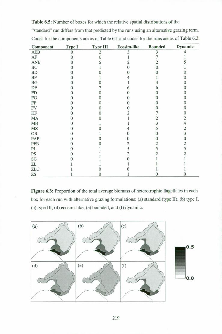
Table 6.5: Number of boxes for which the relative spatial distributions of the

"standard" run differs from that predicted by the runs using an alternative grazing term.

Codes for the components are as of Table 6.1 and codes for the runs are as of Table 6.3.

Component Type I Type III Ecosim-like Bounded Dynamic AEB 0 2 3 3 4 AF 0 0 1 7 1 ANB 0 5 2 2 5 BC 0 1 0 0 1 BD 0 0 0 0 0 BF 0 1 4 1 0 BG 0 0 1 3 0 DF 0 7 6 6 0 FD 0 0 0 0 0 FG 0 0 0 0 0 FP 0 0 0 0 0 FV 0 0 0 0 0 HF 0 0 2 7 0 MA 0 0 1 2 2 MB 0 1 1 3 4 MZ 0 0 4 5 2 OB 0 1 0 0 3 PAB 0 0 0 0 0 PFB 0 0 2 2 2 PL 0 1 5 5 5 PS 0 1 2 2 2 SG 0 1 0 1 1 ZL 1 1 1 1 1 ZLC 1 0 6 1 1 ZS 1 0 1 0 0

Figure 6.3: Proportion of the total average biomass of heterotrophic flagellates in each

box for each run with alternative grazing formulations: (a) standard (type II), (b) type I,

(c) type III, (d) ecosim-like, (e) bounded, and (f) dynamic.

0.5

0.0

219

The form of the time series for each group is generally more sensitive to the

details of the grazing term than the time average values of the runs or the relative spatial

distributions (Table 6.6). Runs with "type 1111" and "type I" functional responses are the

least affected, with 30 — 40% of their component groups showing no difference to use of

the "standard" grazing term. Runs using the other grazing functions diverge more from

the "standard" model, though not all groups show major changes in their temporal

dynamics (Table 6.6).

With changing nutrient loads and fishing pressure, some of the groups in the

runs using alternative grazing terms have predicted biomass trends that diverge from the

predicted trends in the "standard" run under the same change in forcing conditions

(Tables 6.7 and 6.8). When nutrients increase ("Nx5"), the run employing the "ecosim-

like" grazing term shows the greatest divergence from the "standard" run under the

same conditions. In contrast, the run using "type I" grazing terms is the most different to

the "standard" run when fishing pressure increases. The majority of groups in most runs

using alternative grazing terms did follow the same general trends as for the "standard"

run under the same changing forcing conditions. However, with an increase in fishing

pressure, the predicted trend for the benthic deposit feeders in each of the runs using

alternative grazing terms is consistently more than 1880 times the size of the trend

predicted by the "standard" run (Table 6.8). The differences in the trends in biomass in

the various runs are not just in size, but for some groups the predicted direction of

change is also different (marked by a * in Table 6.7 and 6.8). For example, with an

increase in nutrient loading (Table 6.8), the predicted change in biomass for the

picoplankton in the run employing "ecosim-like" grazing terms is not only 2.92 times

the magnitude of the trend in the "standard" run with an increasing nutrient load, but it

is in the opposite direction (an increase rather than a decline).

220

Table 6.6: Quality of the match between the predicted time-series for each component

in the "standard" run and those runs using alternative grazing formulations. Codes for

the components are as of Table 6.1 and codes for the runs are as of Table 6.3. The

entries are ranks indicating the degree to which the time-series matched that of the

standard run. An exact match of the predicted time-series in the run using an alternative

grazing term and the "standard" run has a rank of 1, and an additional 1 is added to this

rank for each feature (shape, amplitude, mean or timing) which differs between the two

time-series. Thus, a rank of 5 indicates no match in any feature between the time-series.

Component Type I Type III Ecosim-like Bounded Dynamic AEB 1 3 3 3 3 AF 3 5 5 5 5 ANB 1 3 5 5 5 BC 1 1 3 5 5 BD 3 3 5 5 3 BF 3 3 5 5 5 BG 1 1 2 3 1 DF 1 3 3 3 3 FD 1 1 5 5 2 FG 1 1 1 3 1 FP 1 1 1 2 1 FV 1 1 1 1 1 HF 5 5 5 5 5 MA 3 3 5 5 5 MB 5 5 5 5 5 MZ 1 1 5 5 4 OB 3 1 5 5 5 PAB 3 3 3 3 3 PFB 3 3 5 5 5 PL 3 3 5 5 5 PS 3 5 5 5 5 SG 2 3 5 5 4 ZL 3 5 5 5 5 ZLC 3 3 5 5 5 ZS 3 5 5 5 5

221

ZZZ

.asuaroui uu jo aouid u! =Hoop u `aouuisu! Joj - suompuoo aims alp Japun uru „prepums„ aqi jo mil pap!pu.nuoo

uopuirmuoj anpuLuailu alp Aq paio!pard (aulloap .ro asuarou!) auuqo Jo uoppar!p aqi * g9'0 960 Zg'Z ZVO £6 .0 °Runny

*SWE *6E£ *Z6 . 0 010 g0 .0 SZ 91'0 8T0 *17£'0 0Z*0 100> DIZ L8'0 1700 T £ .0 g I '0 1 T*0 'IZ £17'0 SO'Z 8£'0 160 Lg'0 DS

*LZ . £ *960 *Z67 I7T '0 10'0 Sd OZ•O *17£'I L0*0 600 170•0 Id .17I '0 OVO 100 T 0 . 0 > T 0 . 0 > Hdd 600 t£'0 g T '0 900 6Z*0 HVd 001 001 00'T 001 TWO HO *g£'0 080 £9'0 000 100> ZIAT *9W0 *£8'0 Lg'0 *Z6 .0 Zg'OT MAI 8C0 LL*0 *LWO 610 SZ*0 VW Z T '0 T 1 '0 800 600 900 dH WO 900 OS'S I 00'i WO Ad 0£'0 91'0 090 001 T0'0 did £0 - 0 SZ*0 6C0 001 Z0*0 Od

10*0 > 9£'0 *Lt7'17Z 001 100> ad Z T '0 100 100 T00> £0'0 Al ScO OL'O SWO 17E0 10*0 > OH

*£Z1 *WI *ZS' T 800 6£'0 dg £9 .0 OVO 017'0 690 g I '0 ag oco avo zvo IVO 090 DH Z I '0 8£'I *L81 SVC) t79 . 17 ENV

*Z£'0 g8'0 T T*0 ZT '0 1700 dV Z£'0 * T 9' g *Z8'17 9Z . 0 *17917 gav

anuutda papunoti ami-uilsoaa m aciSi I gal, wauodtuop

•E.9 °Nu jo S1 OM SUM OLD 10j Sgp00 puu T . 9 aiqui

jo su oi sluauoduroo oqi .roj sapop oq mil aloN .plojami pasmoul s! pum luaulriu

alp uaqm suogumuuoj 2u!zu.r2 anputuaqu 2u!sn suru 05041 puu uru „pmpums„ alp

u! pap!pard (suompuoa „aullasuq„ Japun ssuurom amanu suompuop 2u!2u1qo .rapun

ssutuom aulanu) ssuarolq ut amp 0141 uaamlaq aouarawp muo!uodom :L.9 am',

Table 6.8: Proportional difference between the change in biomass (average biomass

under changed conditions / average biomass under "baseline" conditions) predicted in

the "standard" run and those runs using alternative grazing formulations when the

fishing pressure is increased fivefold. Codes for the components are as of Table 6.1 and

codes for the runs are as of Table 6.3.

Component Type I Type III Ecosim-like Bounded Dynamic AEB 3.41* 0.40 0.70 0.69 0.68 AF 0.03 0.10 0.14 <0.01 0.12 ANB 3.44* 0.40 0.73 0.73 0.70 BC 0.52 0.16 0.52 0.52 0.52 BD 3739•49* 1887.85* 3312.18 3321.52 3543.97 BF 0.17* 0.21 0.08 0.07 0.08 BG 1.67 0.31 2.09* 1.64 1.67 DF 0.04 0.01 0.01 0.01 0.01 FD 0.05 <0.01 2.05 0.11 3.08 FG 0.07 0.03 0.46 0.11 0.98 FP 0.01 0.08 1.60 0.30 1.78 FV 0.18 0.45 0.05 0.64 0.68 HF 0.05 0.13 0.21* 0.18 0.15 MA 0.06 0.30 0.07 0.10 0.10 MB 0.62* 0.51 0.15* 0.22* 0.08 MZ 0.15 0.15 0.22* 0.14 0.16 OB 1.00* 1.00 1.00 1.00 1.00 PAB 0.19 0.06 0.05 0.08 0.09 PFB 0.01 <0.01 0.07* 0.01 0.01 PL 0.20 0.01 0.10 0.12 0.04 PS 0.11 0.44 0.57* 0.03 0.45 SG 0.32 0.25 0.31 0.31 0.31 ZL 0.28 0.31 0.03 0.44 0.25 ZLC 0.18 0.69 0.64 0.63 0.63 ZS 3•59* 0.34 1.73 1.72 1.85 Average 150.23 75.77 133.03 133.25 142.38 * The direction of change (increase or decline) predicted by the alternative formulation contradicted that of the "standard" run under the same conditions - for instance, a decline in place of an increase.

•

223

In the runs using the alternative grazing terms, there is an increase in the number

of groups with spatial and/or temporal patterns which do not conform with those of the

"standard" run under the same change in forcing conditions (Tables 6.9 and 6.10). The

most noticeable differences are for groups in the "type I" run. Under "baseline"

conditions, the relative distributions of all groups in the run with "type I" grazing terms

conform with the relative distribution in the "standard" run for 7 or more boxes. In

contrast, when nutrient loading increases fivefold ("Nx5"), only 68% of the groups in

the run using "type I" grazing terms conform with the relative distribution predicted by

the "standard" run, under the same conditions, for 7 or more boxes (Table 6.9).

Similarly, with changing forcing conditions, there are an increasing number of groups in

the run using "type I" grazing terms that have time-series that differ markedly from the

form of the time-series in the "standard" run under the same forcing conditions (Table

6.10).

6.3.B Sensitivity to the form of mortality used in model closure

The relative difference between the baywide mean biomasses of the "standard"

run and the runs using alternative forms of model closure indicates that under "baseline"

conditions the greatest changes occur when the linear mortality term is set to zero for

those groups which have predators not explicitly represented in the modelled web

(Table 6.11). Generally, the run ("top") where the top predators (sharks, mammals and

birds) are included explicitly shows the least divergence from the "standard" tun, with

predicted biomasses usually within 5% of the "standard" run. There is no run using an

alternative form of model closure for which the predicted biomasses of the majority of

the groups are not within 50% of the estimates in the "standard" run. However, there are

still some groups in each run which differed substantially from the estimate in the

"standard" run (the largest difference is for benthic deposit feeders in the run with the

224

"no-linear" model closure, which differ from the "standard" run by 355%).


"standard" run differs from that predicted by the runs using an alternative grazing term

when forcing conditions are changing. Codes for the components are as of Table 6.1 and

codes for the runs are as of Table 6.3. The columns headed Nx5 are the patterns when

nutrient loading rises fivefold and those headed Fx5 were from the runs where the

fishing pressure rises fivefold.

Component Type I Type III Ecosim-like Bounded Dynamic

Nx5 Fx5 Nx5 Fx5 Nx5 Fx5 Nx5 Fx5 Nx5 Fx5 AEB 5 2 1 7 3 4 3 4 0 1 AF 2 6 6 6 3 5 1 1 6 2 ANB 5 3 1 6 3 4 3 4 1 0 BC 4 1 1 0 1 1 1 1 1 0 BD 0 0 1 0 1 0 1 0 1 1 BF 6 1 4 3 6 5 62 6 1 BG 0 0 0 0 1 1 2 2 2 0 DF 0 0 7 7 6 6 6 6 0 0 FD 0 0 0 0 0 0 0 0 0 0 FG 0 0 0 0 0 0 0 0 0 0 FP 0 0 0 0 0 0 0 0 0 0 FY 0 0 0 0 0 0 0 0 0 0 HF 0 0 0 0 6 0 7 7 1 1 MA 0 0 0 0 3 1 2 2 2 2 MB 4 0 2 0 1 2 1 3 1 4 MZ 0 0 0 0 4 4 6 5 1 2 OB 4 1 4 4 4 1 4 1 5 5 PAB 0 0 0 0 0 0 0 0 0 0 PFB 0 0 0 0 2 2 2 2 2 2 PL 5 1 2 1 4 4 2 0 5 1 PS 0 0 1 1 2 2 2 2 2 2 SG 1 1 2 0 2 1 2 2 3 0 ZL 0 0 1 1 0 0 1 0 0 1 ZLC 0 1 1 0 7 2 0 1 0 1 ZS 1 6 0 6 0 6 3 6 4 6

225

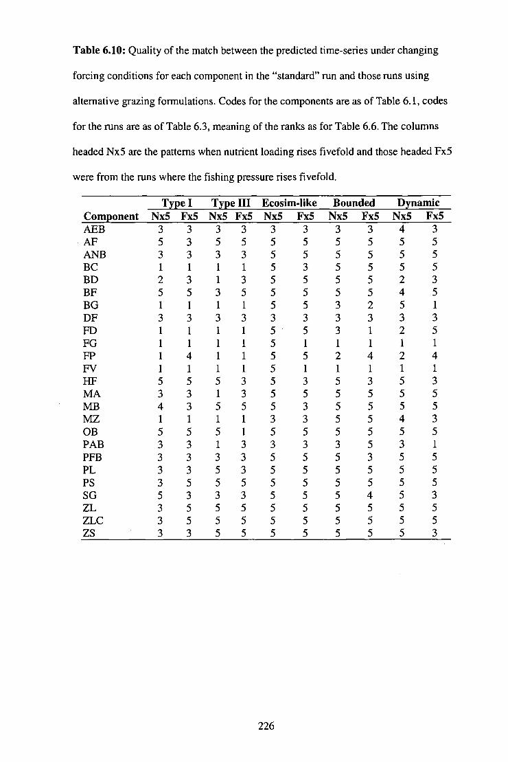
Table 6.10: Quality of the match between the predicted time-series under changing

forcing conditions for each component in the "standard" run and those runs using

alternative grazing formulations. Codes for the components are as of Table 6.1, codes

for the runs are as of Table 6.3, meaning of the ranks as for Table 6.6. The columns

headed Nx5 are the patterns when nutrient loading rises fivefold and those headed Fx5

were from the runs where the fishing pressure rises fivefold.

Component Type I Type III Ecosim-like Bounded Dynamic

Nx5 Fx5 Nx5 Fx5 Nx5 Fx5 Nx5 Fx5 Nx5 Fx5 AEB 3 3 3 3 3 3 3 3 4 3 AF 5 3 5 5 5 5 5 5 5 5 ANB 3 3 3 3 5 5 5 5 5 5 BC 1 1 1 1 5 3 5 5 5 5 BD 2 3 1 3 5 5 5 5 2 3 BF 5 5 3 5 5 5 5 5 4 5 BG 1 1 1 1 5 5 3 2 5 1 DF 3 3 3 3 3 3 3 3 3 3 FD 1 1 1 1 5 5 3 1 2 5 FG 1 1 1 1 5 1 1 1 1 1 FP 1 4 1 1 5 5 2 4 2 4 FV 1 1 1 1 5 1 1 1 1 1 HF 5 5 5 3 5 3 5 3 5 3 MA 3 3 1 3 5 5 5 5 5 5 MB 4 3 5 5 5 3 5 5 5 5 MZ 1 1 1 1 3 3 5 5 4 3 OB 5 5 5 1 5 5 5 5 5 5 PAB 3 3 1 3 3 3 3 5 3 1 PFB 3 3 3 3 5 5 5 3 5 5 PL 3 3 5 3 5 5 5 5 5 5 PS 3 5 5 5 5 5 5 5 5 5 SG 5 3 3 3 5 5 5 4 5 3 ZL 3 5 5 5 5 5 5 5 5 5 ZLC 3 5 5 5 5 5 5 5 5 5 ZS 3 3 5 5 5 5 5 5 5 3

226

Table 6.11: Proportional difference between the biomass predicted in the "standard"

run and those runs using alternative forms of model closure. Codes for the components

are as of Table 6.1 and codes for the runs are as of Table 6.3.

Component Top No-linear No-quadratic AEB 0.01 0.97 1.00 AF 0.01 0.58 0.01 ANB 0.01 0.97 1.00 BC • <0.01 2.41 0.66 BD 1.11 3.55 0.44 BF <0.01 0.77 0.34 BG <0.01 0.12 0.49 DF <0.01 0.29 0.16 FD <0.01 <0.01 <0.01 FG <0.01 0.26 0.03 FP <0.01 <0.01 <0.01 FV 0.04 0.01 0.01 BF <0.01 0.60 0.03 MA 0.17 0.96 0.22 MB 0.01 0.74 0.82 MZ <0.01 0.18 0.29 OB 1.00 1.00 1.00 PAB 0.02 0.55 0.50 PFB <0.01 0.02 <0.01 PL 0.01 0.15 0.02 PS 0.02 0.34 0.15 SG 0.02 2.54 2.45 ZL <0.01 0.03 0.02 ZLC 0.01 0.02 0.03 ZS 0.03 0.19 0.11 Average 0.10 0.69 0.39

While there are some dissimilarities between the relative spatial distributions of

the "standard" run and the runs using alternative forms of model closure, these

differences are not as large as for some of the runs using alternative grazing functions.

The relative spatial distributions of each group, in the run where the top predators are

included explicitly ("top"), are identical to those of the "standard" run, except for the

meiobenthos where the distribution matches that of the runs using the other alternative

forms of model closure. The runs where there is "no-linear" or "no-quadratic" mortality

do not show as much spatial conformity (with the "standard" rim) as the "top" run. The

227

run using an alternative model closure scheme that has the poorest spatial conformity

with the "standard" run is "no-linear". In this run only 40% of the groups have relative

distributions which match the "standard" run and 24% of the groups have spatial

distributions that suggest a more widespread population, or one that is centred in a

different part of the bay, to that predicted by the "standard" model run (Table 6.12). The

spatial conformity of the run with "no-quadratic" model closure is better, with the

relative distributions of a majority of the groups matching the distributions predicted by

the "standard" tun. The "no-linear" and "no-quadratic" model closure runs do not

conform as well with the "standard" run as the "top" run, but they are closer than some

Table 6.12: Number of boxes for which the relative spatial distribution of the

"standard" run differs from that predicted by the runs using an alternative forms of

model closure. Codes for the components are as of Table 6.1 and codes for the runs are

as of Table 6.3.

Component Top No-linear No-quadratic AEB 0 2 2 AF 0 1 0 ANB 0 2 3 BC 0 1 1 BD 0 0 0 BF 0 5 7 BG 0 1 0 DF 0 4 1 FD 0 0 0 FG 0 0 0 FP 0 0 0 FV 0 0 0 HF 0 2 0 MA 0 0 0 MB 0 1 1 MZ 0 0 0 OB 2 2 2 PAB 0 1 1 PFB 0 0 0 PL 0 1 0 PS 0 1 0 SG 0 1 1 ZL 0 0 0 ZLC 0 0 1 ZS 0 1 0

228

of the runs using alternative grazing terms. In the runs using "ecosim-like", "bounded"

or "dynamic" grazing terms 36 —48% of the relative distributions differed by more than

2 boxes from the distribution predicted by the "standard" run (Table 6.5).

The form of the patterns observed in the time-series of each group is dependent

on the form of model closure used. The run with explicit top predators included ("top")

shows the least effect of using alternative model closures, while the other two

configurations are more heavily impacted (Table 6.13). For each run there are some

groups that show the same form of time-series as the "standard" run, and these are

mostly the slower growers (fish and benthic groups). However, each of the runs using

an alternative form of model closure also has groups whose time-series do not match

that of the "standard" run (Table 6.13). In some cases (e.g. for the large carnivorous

zooplankton) the differences are only minor, with the same general pattern holding

regardless of the form of closure used, but where there are changes in the amplitude or

the mean or timing of the pattern (Figure 6.4). In other cases (e.g. the meiobenthos) the

change in temporal dynamics is striking (Figure 6.5).

When fishing pressure is increased, there is little difference in the overall

performance of the runs using the alternative forms of model closure, though the run

employing the "no-quadratic" model closure does diverge slightly more from the

"standard" run than the others (Table 6.14). When nutrient loading is increased the run

using "no-quadratic" model closure diverges from the "standard" run much more than

does either of the other two alternatives (Table 6.15). When nutrient loads or fishing

pressure are increased, the predicted trends for the sediment infauna (macro- or

microscopic) can be orders of magnitude larger in runs using alternative model closure

than for the "standard" run, under the same conditions (Tables 6.14 and 6.15). For

example, when fishing pressure increases fivefold the change in biomass for the benthic

deposit feeders is more than 3442 times that of the "standard" run in all the runs using

229

Table 6.13: Quality of the match between the predicted time-series for each component

in the "standard" run and those runs using alternative forms of model closure. Codes for

the components are as of Table 6.1, codes for the runs are as of Table 6.3, meaning of

the ranks as for Table 6.6.

Component Top-predators explicit No-linear No-quadratic AEB 1 3 5 AF 3 5 3 ANB 1 3 5 BC 1 1 5 BD 3 3 5 BF 1 5 5 BG 1 1 1 DF 1 2 1 FD 5 1 1 FG 5 1 1 FP 5 1 1 FV 5 1 1 HF 1 3 2 MA 2 3 3 MB 1 3 3 MZ 1 1 3 OB 5 5 5 PAB 1 3 3 PFB 2 3 3 PL 2 3 2 PS 3 5 2 SG 1 3 3 ZL 2 4 2 ZLC 3 3 2 ZS 3 3 1

230

--o— Standard —0-- No linear —0— No quadratic

Bio

mas

s of ZL

C (

mg

N m

4)

1

■ ■ ■ I ■ i

6032 6240 6448 6656 6864 7072

Day of Run

5824

6448 6656

Day of Run

Bio

mas

s o

f A

F (m

g N

m4)

12

10 -

8 -

6 -

4 -

2 -

0 5824

231

6240 6032 7072 6864

Figure 6.4: An example of only minor differences in time-series for alternative forms of

model closure. Shown here is the biomass of large carnivorous zooplankton (ZLC) in

box 8 (in the centre of the bay) over the same four-year period for runs using the

"standard", "no-linear" and "no-quadratic" forms of model closure.

Figure 6.5: An example of major differences in time-series for alternative forms of

model closure. Shown here is the biomass of autotrophic flagellates (AF) in box 8 (in

the centre of the bay) over the same four-year period for the runs using the "standard"

and "no-linear" forms of model closure.



the "standard" run and those runs using alternative forms of model closure when the

fishing pressure is increased fivefold. Codes for the components are as of Table 6.1 and

codes for the runs as of Table 6.3.

Component Top -predators explicit No- linear No-quadratic AEB 0.81 0.87 0.38 AF <0.01 0.16 0.03 ANB 0.82 0.88 0.69 BC 0.52 0.52 0.52 BD 3442.71 3333.79 3587.31 BF 0.13 0.05 0.42 BG 1.67 1.69 1.67 DF 0.02 0.01 0.10 FD 0.02 0.01 <0.01 FG <0.01 0.07 0.05 FP 0.02 <0.01 <0.01 FV 0.05 <0.01 0.01 HF 0.02 0.02 0.01 MA 0.14 0.10 0.08 MB 0.06 0.04 0.03 MZ 0.15 0.15 0.15 OB 1.00 1.00 1.00 PAB 0.16 0.09 0.17 PFB <0.01 0.01 <0.01 PL 0.05 0.04 0.07 PS 0.02 0.44 0.13 SG 0.29 0.31 0.31 ZL 0.02 <0.01 0.06 ZLC 0.02 0.05 0.03 ZS 0.03 0.14 0.02 Average 137.95 133.62 143.73

232



the "standard" run and those runs using alternative forms of model closure when the

nutrient load is increased fivefold. Codes for the components are as of Table 6.1 and

codes for the runs as of Table 6.3.

Component Top-predators explicit No-linear No-quadratic AEB < 0.01 0.93 38.02* AF 0.02 0.16 0.05 ANB <0.01 0.98 9.13* BC <0.01 0.77 0.80 BD 0.42 0.51 0.54 BF <0.01 0.24 1.49* BG <0.01 0.10 <0.01 DF <0.01 <0.01 0.20 FD <0.01 <0.01 <0.01 FG <0.01 0.19 0.01 FP <0.01 0.02 0.01 FV <0.01 0.08 0.06 HF 0.01 0.11 0.06 MA 0.10 0.45 0.21 MB <0.01 0.67* 0.65 MZ <0.01 <0.01 <0.01 OB 31.23 1.00* 1.00 PAB 0.01 0.46 0.49 PFB <0.01 0.01 0.01 PL 0.01 0.08 0.02 PS 0.03 0.13 0.05 SG 0.07 0.76 0.01 ZL 0.01 0.20 0.13 ZLC 0.01 0.17 0.13 ZS 0.01 0.05 0.06 Average 1.28 0.32 2.13

* The direction of change (increase or decline) predicted by the alternative formulation contradicted that of the "standard" run under the same conditions - for instance, a decline in place of an increase.

233

alternative forms of model closure (Table 6.14). Once again there are a few cases where

the differences in the trends go beyond differences in magnitude. However, the only

groups for which the predicted trend in biomass is in the opposite direction to the trend

in the "standard" run, under the same conditions, are in the runs employing "no-linear"

and "no-quadratic" mortality when nutrient loading increases (Table 6.15).

Generally, for the runs using "no-linear" model closure or explicit top predators

("top"), spatial and temporal conformity with the patterns predicted by the "standard"

run are as good under changing forcing as under "baseline" conditions (Tables 6.16 and

6.17). This is not the case for either of the runs using "no-quadratic" mortality when

forcing conditions change. When nutrient loads or fishing pressure increases there is a

reduction in the number of groups for which the patterns predicted by the run with "no-

quadratic" mortality match those of the "standard" run (Tables 6.16 and 6.17). More

generally, under changing forcing conditions, any differences in the spatial patterns

observed in the tuns employing alternative forms of model closure are usually stronger

than under "baseline" conditions (Table 6.16). Such a consistent result is not evident for

the form of the temporal dynamics predicted in each run (Table 6.17).

6.4 Discussion

Given their direct impact throughout the web, rather than just at higher trophic

levels, it is not surprising that the effects of alternative grazing terms were larger and

more pervasive than those due to using different forms of model closure. However, this

does not agree with the findings of Steele and Henderson (1992) or Murray and Parslow

(1999b). They found that the form of the model closure was generally far more

important in determining model behaviour than internal details, such as the functional

responses of consumers. This difference may reflect that the web used in the ecosystem

model investigated here incorporates many more consumers in a more highly

234


"standard" run differs from that predicted by the runs using an alternative forms of

model closure when forcing conditions are changing. Codes for the components are as

of Table 6.1 and codes for the runs as of Table 6.3. The columns headed Nx5 are the

patterns when nutrient loading rises fivefold and those headed Fx5 were from the runs

where the fishing pressure rises fivefold.

Component Top-predators explicit No-linear No-quadratic

Nx5 Fx5 Nx5 Fx5 Nx5 Fx5 AEB 0 4 4 4 3 4 AF 0 0 1 1 0 0 ANB 0 4 4 4 7 5 BC 0 1 8 2 8 2 BD 0 0 1 0 1 0 BF 0 1 2 3 4 5 BG 0 0 0 1 0 0 DF 0 0 4 5 1 1 FD 0 0 0 0 0 0 FG 0 0 0 0 0 0 FP 0 0 0 0 0 0 FV 0 0 0 0 0 0 HF 0 0 3 6 0 0 MA 0 0 0 0 0 0 MB 1 0 2 1 2 1 MZ 2 3 0 3 1 4 OB 0 3 4 3 4 3 PAB 0 0 1 1 0 1 PFB 0 0 0 0 0 0 PL 0 0 2 1 0 2 PS 0 0 1 0 0 0 SG 0 1 1 2 2 2 ZL 0 0 0 0 0 0 ZLC 0 0 1 0 0 0 ZS 0 0 1 1 0 1

235

Table 6.17: Quality of the match between the predicted time-series under changing

forcing conditions for each component in the "standard" run and those runs using

alternative forms of model closure. Codes for the components are as of Table 6.1, codes

for the runs are as of Table 6.3, meaning of the ranks as for Table 6.6. The columns

headed Nx5 are the patterns when nutrient loading rises fivefold and those headed Fx5

were from the runs where the fishing pressure rises fivefold.

Component Top-predators explicit No-linear No-quadratic

Nx5 Fx5 Nx5 Fx5 Nx5 Fx5 AEB 1 3 5 3 5 5 AF 3 3 5 5 3 3 ANB 1 1 5 5 5 5 BC 1 1 1 1 5 5 BD 1 3 1 3 5 5 BF 1 3 5 5 5 5 BG 1 1 1 1 1 1 DF 1 1 3 1 3 3 FD 5 1 1 1 1 1 FG 5 4 1 1 1 1 FP 5 5 1 3 1 4 FV 5 1 1 1 1 1 HF 1 3 2 3 2 5 MA 1 1 1 3 3 3 MB 1 1 5 5 5 3 MZ 1 1 3 1 3 3 OB 3 5 5 5 5 5 PAB 1 3 3 3 3 3 PFB 1 3 3 5 3 3 PL 1 3 3 3 3 3 PS 3 1 3 3 3 5 SG 2 1 5 3 5 3 ZL 3 2 3 3 3 3 ZLC 3 1 3 1 3 3 ZS 2 3 3 3 3 3

interconnected web than the simple Nutrient-Phytoplankton-Zooplankton chains

considered by Steele and Henderson (1992) and Murray and Parslow (1999b).

Functional responses

The sensitivity of model behaviour to the form of the grazing term, especially

under changing ecosystem conditions, indicates that careful thought must be given to

the choice of grazing term and the associated assumptions and data requirements. For

236

0.4

— Type I -- Type II (Standard) — • • Type III

0.0

Biom

ass

cons

umed

per

day

per

mg

N of

ZL

0.3 -

0.2

0.1 -

the simpler "lolling-type" functional responses, the behaviour of the model under

"baseline" conditions indicates that the biomasses of the various prey groups are at a

level where the potentially destabilizing nature of the simpler functional responses

(Begon and Mortimer 1986) is of little importance. There are the occasional exceptions

(like meiobenthos when using the "type ifi" response), but overall there is very little

difference in the outcome of the standard, "type I" and "type III" runs under "baseline"

conditions. This is because the prey biomasses keep the functional response curves

within a section where they are similar to each other (Figure 6.6). This finding is similar

to that of previous studies (Gao et al. 2000, Tett and Wilson 2000). It is only under

increasing nutrient loads and/or fishing pressures that the differences in the curves

influence model behaviour as the biomasses become very large or small (depending on

the prey groups in question). Even under these more extreme conditions there is little to

00 0.5 1.0 1.5 2.0 2.5 3.0 3.5 4.0 4.5

5.0

55

Available Prey Biomass (mg N rn -3 )

Figure 6.6: The "type 1", "type II" (the response used in the standard run) and "type

III" functional responses for the large omnivorous zooplankton (ZL). The range of prey

biomasses shown covers the typical levels of available prey biomass, although the

available biomass can jump to much higher levels (2 — 5 fold higher) for short periods

during bloom events.

237

recommend the general use of a Type IQ curve over that of a Type II if coefficients of

prey availability feature in the formulations (as they do in this case). However, in the

mixed case, where the same functional response is not applied to all groups, selective

use of a Type III may prove to be beneficial for those groups whose behaviour in the

field matches the formulation's assumptions.

The simple "Holling-type" functional responses are used widely in food chain

and ecosystem models (Btissenschtitt and Pahl-Wostl 2000), but they are not the only

functional responses employed. Other functional responses in use include: the modified

disk equation that incorporates thresholds (Radach and Moll 1993, Baretta et al. 1995,

Tett and Wilson 2000); the Ivlev formula (McGillicuddy et al. 1995); ratio-dependent

functions (Arditi and Ginzburg 1989, Matson and Berryman 1992); and a two-

dimensional function of the biomasses of predator and prey (Btissenschtitt and Pahl-

Wostl 2000). Consideration of the complete list of functional responses is beyond the

scope of our work and recent work suggests that ratio-dependent functions may not be

suitable for use in general models such as BM2 (Gleeson 1994, Sarnelle 1994, Abrams

1994, Abrams and Ginzburg 2000, Biissenschtitt and Pahl-Wostl 2000). Conversely, the

arguments regarding the effects of thresholds (Frost 1975, Bryant et al. 1995) and the

impacts on behaviour and feeding of groups other than the predator and prey (Abrams

and Ginzburg 2000, Walters et al. 2000) are well made. For this reason we examined the

effects of using "bounded", "dynamic" and "ecosim-like" functional responses. The

effects of using these formulations are often greater than moving from the standard to

"type I" or "type III" functional responses. They also tend to have greatest impact on

groups that are poorly known or only beginning to attract attention in biogeochemical

models (such as infauna, flagellates and bacteria). For many of these groups the

behaviour under the more sophisticated functional response is no closer to real biomass

dynamics than that achieved with the simpler standard functional response. However,

238

the performance of the benthic deposit feeding group is substantially improved,

particularly when nutrient loading increases. The behaviour of this group is a weakness

of the standard form of BM2 (chapter 2), which seems to be corrected if the additional

checks inherent in the more complex functional responses are added. By itself however,

this is no reason to include high levels of added complexity in functional responses

across all groups as a matter of course. While the "type I" functional response is

obviously insufficient if the model is to behave realistically as conditions change,

careful thought must be given to how much flexibility should be added - to how many

feedbacks, thresholds and inflexion points are added — when more sophisticated

responses are used. Jorgensen (1994), amongst others, has advocated structurally

dynamic models (models where parameters change according to a goal function) as the

best way of capturing changes in species with changes in conditions. Without going to

that extent, functional responses with the flexibility of the "ecosim-like" response used

here, set within a multi-linked web, are also able to reflect the more dynamic changes

that may occur within a web as ecosystem conditions change. However, given the high

number of parameters biogeochernical models can require and that trends rather than

specific quantitative values are usually sufficient for model interpretation and

subsequent recommendations, "Holling-type" functional responses may still suffice. As

stated above, this topic requires careful thought and should be a key part of any model

formulation discussion.

One recommendation that can be made based on the results presented here is

that research aimed at empirically determining the nature of functional responses in real

systems is clearly needed. It is likely that, unlike the model presented here, in real

systems different groups will have different types of functional responses. Furthermore,

many bay ecosystems are changing and given the sensitivity of models like BM2 to the

form of functional response used, there is a real need to properly establish the nature of

239

the functional responses in real systems (at least for some groups).

Model closure

Plankton modelers recognize that the form of model closure used requires

careful consideration. While it is notable that the form of model closure does not have

the dominating effect on the BM2 ecosystem model that it has on simpler plankton

models (Steele and Henderson 1992, Edwards and Brindley 1999, Murray and Parslow

1999b, Edwards and Yool 2000), it was important nevertheless. Detailed bifurcation

analysis, such as in Edwards and Brindley (1999), is not possible for a model of this

size, so our conclusions must be based on the simulation runs. Previous papers on the

subject (Steele and Henderson 1992, Edwards and Brindley 1999, Murray and Parslow

1999b, Edwards and Yool 2000) have concentrated on the steady-state stability status

achieved when using different closure terms, while this paper has concentrated on the

overall effects on model dynamics. Despite these differences, comparison of

conclusions from the different works is instructive.

The necessity of including responsive top predators (either explicitly or

implicitly via a quadratic mortality term) agrees with the general findings of the earlier

studies. The change in behaviour of the run employing "no-linear" model closure under

"baseline" conditions also gives some support for inclusion of separate natural mortality

(linear) and higher predation (quadratic) terms. McGillicuddy et al. (1995), Murray and

Parslow (1997) and Brostrom (1998) have successfully used this division of mortality

terms, and the findings of Edwards and Brindley (1999) and Edwards and Yool (2000)

do recommend it. However, Edwards and Brindley (1999) and Edwards and Yool

(2000) caution that the use of both mortality terms requires the estimation of two (rather

than one) poorly known parameter, which may mitigate against its use. Thus, given our

results, the argument for the use of both terms is not overwhelming, and use of the

240

linear term may not be necessary. However, this may not be the case under oligotrophic

conditions or extreme overfishing. In both of these cases the biomasses of many groups

may be very low, which is precisely the situation in which quadratic mortality alone

may yield unrealistic dynamics (Edwards and Brindley 1999). Further work to address

this issue is required.

One final concern about model closure is whether or not the top predators must

be included explicitly. A comparative analysis of the application of BM2, IGBEM and

ECOSIIVI (Christensen and Pauly 1992, Walters et al. 1997) to Port Phillip Bay

suggested that the implicit representation of the top predators (sharks, mammals and

birds) in the biogeochemical models may not be capable of capturing some of the

dynamics of that part of the web (chapter 7). This suggests that the top predators might

need to be included explicitly, but the expansion of BM2 to explicitly represent the top

predators did not see any substantial shifts in model behaviour. The clear indication is

that unless the top predators are of particular concern in themselves (due to being a

large component of the system, a conservation concern, or harvested group), their

explicit inclusion in biogeochemical models is not required. Quadratic model closure

appears to be acceptable regardless of the size of the web being considered.

6.5 Conclusions

Ecosystem models are One tool that has been advocated for ecosystem

management (Walters et al. 1997, Sainsbury et al. 2000). Consequently, the impact of

formulation decisions on their behaviour needs to be considered. Predation, in the form

of grazing terms and model closure, is a crucial part of ecosystem models that

incorporate ecology or biogeochemistry (Edwards and Yool 2000, Tett and Wilson

2000). The work discussed here indicates that, unless the top predators of a system are

of particular interest, the additional complexity of their explicit inclusion can be avoided

241

by the use of a quadratic term for model closure. The use of a quadratic mortality term

to close the model allows for realistic predictions across a range of conditions.

The specification of a suitable grazing term is more complex. Whereas linear

plankton models have predicted that the grazing term has little real effect on model

behaviour, our results for more complex webs indicate otherwise. Thus, careful

consideration must be given to this part of the model formulation. There are biologically

and mathematically sound arguments for including the more sophisticated dynamics of

functional responses such as the "bounded", "dynamic" and "ecosim-like" responses

trialled here (Bryant et al. 1995, Walters et al. 2000, Abrams and Linzburg 2000).

However, given the extra detail and increased information required to parameterise and

validate these formulations, a simpler "Holling-type" functional response may be

sufficient. This is particularly true if preliminary studies or modelling exercises indicate

that the "Holling-type" functional responses will lead to the same general conclusions

and behaviour as more sophisticated functional responses. Nevertheless, some degree of

sophistication is required in the functional response employed as the simple application

of a "type I" response is unlikely to be useful under changing ecosystem conditions (e.g.

increasing nutrient loads or fishing pressure). It is doubtful that any one functional

response will be suitable for all groups, models and environments. The demonstration

here, that model behaviour can be sensitive to the form of the grazing terms used, shows

that efforts to empirically determine the form of functional responses in real systems are

warranted. Along with the topology and the form of the trophic web that defines the

framework of the model, the grazing terms are a feature that require particularly careful

consideration during the conceptualisation and development of ecosystem models.

242

Chapter 7 Lessons learnt from the comparison of three ecosystem

models for Port Phillip Bay, Australia

Abstract

Three ecosystem models were tuned to data from Port Phillip Bay, Australia.

Several general conclusions can be drawn by comparing predictions of the three models

across a range of fishery management strategies and scenarios for environmental

change. First, the large, shallow and enclosed physical structure of Port Phillip Bay and

the dependency of many fish groups on spawning stocks from outside the immediate

area may see the bay react more strongly to eutrophication than to fishing. Second, a

selected set of indicator groups (in this case, sharks, seagrass and chlorophyll a) seems

to capture the major ecosystem impacts of alternative management scenarios, whether

the biomass and productivity of important groups declines, persists or increases. This

has obvious implications for system monitoring in an adaptive management approach.

Third, multispecies or ecosystem models can identify potential impacts that a series of

single species models cannot, such as non-intuitive changes in biomass when species

interactions outweigh fishery induced pressures. Finally, policies that focus on

protection of species or groups only at higher trophic levels can fail to achieve sensible

ecosystem objectives and may push systems into states that are far from pristine.

Keywords

biogeochemical, ecosystem, model, ECOSIM, ECOPATH, Port Phillip Bay

Note: This chapter resulted from work undertaken at an ECOPATH with ECOSIIVI

workshop on the use of ecosystem models to investigate multispecies management

strategies for capture fisheries held at the University of British Columbia, Vancouver

243

Canada, in July 2000. The work involved fitting the models to the current conditions of

Port Phillip Bay and then considering the potential effects of management strategies. As

a result, some of the terminology used in this chapter differs from that used in the rest of

the thesis. Most importantly, whereas the term "standard run" is used to refer to the

default run of the full models in all the other chapters the term "base case" is used here.

Further, whereas "baseline" is used to refer to the default nutrient loadings and fishing

pressures in all the other chapters the terms "current conditions" or "status quo" are

used in this chapter. I apologise for any confusion this may cause.

7.1 Introduction

Concern over sustainable and responsible management of ecosystems, rather

than particular species of interest, has grown over the last century, and particularly

within the last decade. This is reflected in the increasing adoption in international

treaties and national legislation of policies that take explicit account of such concerns.

For example, Australia has adopted a national oceans policy that requires, inter alio,

development of regional marine plans based upon principles of ecosystem management.

Despite this level of interest and activity, the scientific and management tools to

underpin such policies are poorly developed. In particular, the tools to predict the

impact of alternative uses and management strategies are still being developed

(Sainsbury et al. 2000). In the context of ecosystem management, the use of trophic

models has been proposed to predict such impacts (Walters et al. 1997, Walters et al.

1999). A range of such models has been developed, but to date there has been little

effort to compare and contrast such models, or to compare their strengths and

weaknesses (Baretta et al. 1994, Baretta et al. 1996, this thesis).

In this study, three separate ecosystem models are used to explore the utility of

such models for the assessment of potential management strategies and their likely

244

consequences. These three models span a range of process detail, from ECOSIM with

its relatively compact formulation (Christensen et al. 2000), to the more nutrient-

oriented Bay Model 2 (BM2) (chapter 2), and finally to a highly detailed process model,

the Integrated Generic Bay Ecosystem Model (1GBEM) (chapter 1). Between them,

these three models reflect much of the range of detail found in simulation models

currently being built and used to understand and predict the ecosystem effects of fishing

and eutrophication. Unfortunately, their respective histories and the varying purposes

for which they were developed mean that the models do differ in many ways and that

there is no systematic variation in assumptions. This can make extraction of organising

principles or conclusions difficult. However, there is value in determining whether

various existing ecosystem models of different forms predict similar outcomes in

response to changing conditions and management policies. This kind of information can

be instructive with regard to understanding the implications of the formulations used

and whether results are robust across modelling methodologies.

The real world system used as the data source and guide for this model

comparison is Port Phillip Bay (PBB), adjacent to Melbourne, Australia. During the 160

years since European settlement, PPB has come under increasing pressure from nutrient

enrichment and fisheries exploitation. Approximately 15% of Australia's population

live within the catchment area of PPB, and the bay has become the focal point for many

of their recreational pursuits. It has been estimated that the annual recreational effort is

around 670,000 angler hours, which results in the landing of about 470t of fish (Anon

1997). The bay's commercial finfish fisheries land over 60 species, with a total annual

take of between 700 and 2000t worth about $3 million AUD wholesale. A number of

invertebrate species are also landed, though many only opportunistically as bycatch.

The main targeted invertebrate harvests are cultured mussels and wild abalone, with

annual landings of 600t worth $1.5 million AUD and 50t worth $1 million AUD

245

respectively. Until the late 1990s scallops were the most intensively harvested and

valuable fishery in PPB, with up to 10,000t (shell weight) being landed per year.

However, the fishery was highly variable (fluctuating by two orders of magnitude in 3

years) and the sediment plumes associated with the dredges used in the fishery led to

public concern. The fishery was closed in 1997.

PPB is a relatively "easy" system to model as it is a shallow and nearly enclosed

temperate bay. It has an area of approximately 1930 km2 , mostly of waters less than 8m

deep, though it reaches 24m at its deepest points. With only 8 drainage basins feeding

the bay, and a large sand bar delta and narrow seaward opening restricting exchange

with Bass Strait, it has minimal boundary condition problems. The bay has also been the

subject of a number of quite extensive environment studies, one or more per decade

since the late 1940s, and so there is a large amount of good quality information

available for use in model construction and validation (Harris et al. 1996).

Eutrophication and fishing are the two most significant anthropogenic impacts

on PPB. The difficulties inherent in interpreting and managing the consequences of

human actions on marine systems have meant that fisheries and nutrient related

concerns have traditionally been dealt with separately. This is not just the case for

Australian bays and near shore waters, but is commonplace worldwide. However, there

is increasing evidence that primary productivity and fisheries are more tightly linked

than previously thought (Houde and Rutherford 1993, Nielsen and Richardson 1996).

With this in mind, the three models are compared across a range of levels of fishing

pressure and nutrient inputs.

246

7.2 Methods

7.2.A Model Descriptions

A brief description of the general form of each model is given below, but space

precludes an extended discussion of each of their features, structures and assumptions.

To allow for an informed comparison, the essential details of the models and how they

vary are listed in Table 7.1. Further, to give some idea of the degree of variation in

process detail between the models, the formulation for phytoplankton production is

given in Table 7.2. This example is a fair representation of the difference in formulation

detail for the lower trophic levels. However at the highest levels, especially those where

split pools (juvenile and adults) are included in ECOSIM, the detail can swing back

more the other way. At these levels all the models include age structure, explicit

recruitment and split food intake into portions allocated to growth and reproduction,

though the exact method of doing this does vary between models (Christensen et al.

2000, chapters 1 and 2).

The variation in process detail between the models is one of the motivating

forces for the comparison of the models and their predictions. However, other major

differences in underlying model assumptions must be kept in mind in comparing the

models and their dynamics. These include:

(a) the consumption formulations (a forage arena approach is used in ECOSIM, but

Holling Type functional responses are used in the other two models),

(b) the lack of bycatch in the standard versions of IGBEM and BM2,

(c) the omission of invertebrate fisheries from IGBEM,

(d) the absence of explicit spatial structure in ECOSIM

(e) the static nature of the birds, mammals and sharks in BM2 and IGBEM and

(f) the stock structure of the fish groups with its inherent implications for the form

of the stock-recruit relationship used.

247

Table 7.1: Comparison of the underlying structure and assumptions of the three ecosystem models, ECOSIM, IGBEM and BM2. The standard set-ups

used for the runs in this study are given, any feature where alternatives may be implemented are marked with a *.

Model Feature General features


Level of group detail

Formulation related Consumption formulation Formulation detail

Light limitation

Mixotrophy

Nutrient limitation Nutrient ratio Oxygen limitation Sediment burial Sediment chemistry

Shading of primary producers

ECOSIM

t/km2 (wet weight) yes (of primary producers), interannual variable (age group of species up to entire trophic levels)

forage arena simple (expansion of ECOPATH master equation)

no

no (no mixed consumers-producers defined in the ECOPATH model) no - no no no

no

BM2

mg N/m3 (dry weight) yes (of nutrients and physics), interannual, seasonal, tidal functional group

type II* general (growth, mortality, excretion explicit)


yes (Dinoflagellates)*

yes (external) Redfield yes no yes (dynamic, with sediment bacteria) yes

IGBEM

mg/m3 of C, N, P, Si (dry weight) yes (of nutrients and physics), interannual, seasonal, tidal functional group

mixed (type II, type III) physiological (assimilation, basal/ activity/stress respiration, defecation, excretion, ingestion, mortality all explicit) phytoplankton can adapt to changes in ambient light levels no

yes (internal) internal nutrient ratio yes yes* yes (empirical, sediment bacteria are a tracer only) yes

248


Model Feature

Spatial structure

Temperature dependency Model closure

Status of birds Status of mammals Status of sharks

Fish and fisheries related Age structured fish Fishery Discards Invertebrate fisheries

Stock-recruit relationship Stock structure

ECOSIM no explicit spatial structure (ECOSPACE model not considered here) no

dynamic dynamic dynamic

yes (juvenile + adult) target and bycatch species yes

dynamic self-seeding (entire stock in the bay)

BM2 explicit (8 and 59 box versions)*

yes

static loss term on fish only static loss term on fish only static loss term on fish only

yes (9 age classes) target species only* yes

constant recruitment external (reproductive stock outside the bay produces the recruits, oldest age classes migrate out of the bay to join this stock)

IGBEM explicit (8 and 59 box versions)*

yes

static loss term on fish only static loss term on fish only static loss term on fish only

yes (9 age classes) target species only no ('fix' implemented by adjusting the mortality terms of the groups concerned) constant recruitment external (reproductive stock outside the bay produces the recruits, oldest age classes migrate out of the bay to join this stock)

249

Table 7.2: Process detail involved in the phytoplankton production for each model. ECOSIM BM2

IGBEM

= PArr ON •B where B = Biomass (mg N m -3) of the phytoplankton group (4 types) p= maximum temperature dependent growth rate

= nutrient limitation factor DIN

KN +DIN

and DIN = Ammonia + Nitrate unless also limited by Silica (Si) then

Si = mi

( . ( DIN KN +DIN' lcSi + Si

x-xx = is the half saturation constant for the uptake of the nutrient XX tirr = light limitation factor

.( = mtn —,1 K irr

1RR

IRR = Light Kirr = is the half saturation constant for the uptake light

= P • 6 irr • Nut • B, where Bc = Biomass (mg C m -3) of the phytoplankton group (4 types)** p= maximum temperature dependent growth rate CoNut = nutrient limitation factor

= min(8 N , p )

N = min(1, max(0, B c fi mow

13CXXIow = minimum permissible nutrient ratio of C:XX for the cell ficxxiow = standard internal nutrient ratio of C:XX for the cell unless also limited by Silica (si) then

Si ))

= m1n[min(5 N , S p ), min(1,

= light limitation factor IRR = min(1,

lRR = Light Kirr = is the half saturation constant for the uptake light adjusted for acclimation to new ambient light conditions

r • B 1+ B • h

where B = Biomass of the phytoplankton r = the maximum P/B ratio that can be realised (at low B)

and —r = the maximum net primary

production when the biomass is not limiting to production (at high B) CN int — 13 CNIow

p = min[1, ma+, B c cmow

fi CP int — 13 CPlow

2 . Ks,

K irr _adjusted

** There are also N and P pools of the biomass explicit in IGBEM and the production in these is based on the internal nutrient ratio and the production for the B c pool.

250

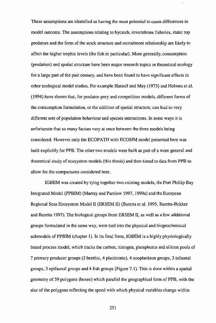
These assumptions are identified as having the most potential to cause differences in

model outcome. The assumptions relating to bycatch, invertebrate fisheries, static top

predators and the form of the stock structure and recruitment relationship are likely to

affect the higher trophic levels (the fish in particular). More generally, consumption

(predation) and spatial structure have been major research topics in theoretical ecology

for a large part of the past century, and have been found to have significant effects in

other ecological model studies. For example Hassell and May (1973) and Holmes et al.

(1994) have shown that, for predator-prey and competition models, different forms of

the consumption formulation, or the addition of spatial structure, can lead to very

different sets of population behaviour and species interactions. In some ways it is

unfortunate that so many factors vary at once between the three models being

considered. However only the ECOPATH with ECOSIM model presented here was

built explicitly for PPB. The other two models were built as part of a more general and

theoretical study of ecosystem models (this thesis) and then tuned to data from PPB to

allow for the comparisons considered here.

IGBEM was created by tying together two existing models, the Port Phillip Bay

Integrated Model (PPBIM) (Murray and Parslow 1997, 1999a) and the European

Regional Seas Ecosystem Model II (ERSEM II) (Baretta et al. 1995, Baretta-Bekker

and Baretta 1997). The biological groups from ERSEM II, as well as a few additional

groups formulated in the same way, were tied into the physical and biogeochemical

submodels of PPBIM (chapter 1). In its final form, IGBEM is a highly physiologically

based process model, which tracks the carbon, nitrogen, phosphorus and silicon pools of

7 primary producer groups (3 benthic, 4 planktonic), 4 zooplankton groups, 3 infaunal

groups, 3 epifaunal groups and 4 fish groups (Figure 7.1). This is done within a spatial

geometry of 59 polygons (boxes) which parallel the geographical form of PPB, with the

size of the polygons reflecting the speed with which physical variables change within

251

Mixotrophic Dinoflagellates

Dinoflagellates Autotrophio flagellates

Picea!gas Diatoms

## Juvenile herbivorous

fish

Adult herbivorous

fish

Meiobenthos Benthic Grows Deposit Feeders

Detritus Seagrass Macroalgae Labile Detritus Microphytopbenthos

I

HeterotrophIc flagellates

Microzooplankton

5

4

2

Figure 7.1: Schematic diagram showing the groups in BM2 and IGBEM and their relative trophic positions. The bacterial groups are omitted

from the diagram and the model comparisons as no equivalent group exists in the ECOPATH model. The greyed box indicates the position of

the dinoflagellates when mixotrophy was allowed in BM2. The dashed boxes indicate the position of the static predator groups implemented for

the nutrient model runs used here. Groups marked with a # are fished explicitly in IGBEM and those marked with a * are fished in BM2.

F ===== 1 Sharks Adult

= = = = = Juvenile #*

PiscMores

Pisolvores

Adult IS* Planktivores

Adult if # Demersal

Fish fite

Infaunal carnivores

Epifaunal carnivores

Juvenile ## Demersal

Fish

= = = = I Birds

and I Marine

mammals = = = =

Carnivorous z000lankton

Juvenile

Planktivore

Omnivorous z000lankton

Fitter feeders

252

Figure 7.2: Depth map of Port Phillip Bay, Melbourne, Australia. The inset map of

Australia indicates the location of Port Phillip Bay. The polygons marked on the large

map are those of the standard 60 box geometry used for BM2 and IGBEM.

that part of the bay (Figure 7.2). The level of detail included in this model is considered

to be at the upper level, but not beyond, that which is employed in ecosystem models

currently in use (e.g SSEM (Sekine et al. 1991), ERSEM II (Baretta-Bekker and Baretta

1997) and ATLSS (DeAngelis et al. 1998)).

BM2 has the same trophic groups, general submodels (water column, sediment,

epibenthic) and physical (transport, mixing and spatial geometry) details as IGBEM.

BM2 does not have sediment burial, but does have dinoflagellate mixotrophy, while

IGBEM has the reverse. The greatest difference between IGBEM and BM2 lies in the

level of process detail. BM2 is an order of magnitude simpler, with very similar

dynamical representation to PPBIM (Murray and Parslow 1997, 1999a). Processes such

as excretion and respiration are not modelled explicitly, but are subsumed into

253

generalised assimilation and waste production equations (chapter 2). Further, BM2 only

models the nitrogen component, and relies on Redfield ratios, rather than internal

nutrient ratios, to determine the form of nutrient dependent activities. This level of

detail is more representative of the most commonly utilised eutrophication and water

column trophic models (Fransz et al. 1991).

Data from the Port Phillip Bay Environmental Study (PPBES), primarily for the

years 1994 — 1995, were used to calibrate IGBEM and BM2 to achieve a satisfactory

representation of the biological conditions in PPB (in mg N m-3). In a few instances it

was necessary to draw values from the general literature or use data from other years to

fill in gaps, but this was kept to a minimum. The same data were then used to construct

an ECOPATH model, converting from mg N 111-3 to t lcm-2 wet weight under the

assumption that N makes up 1% of an organism's wet weight. The resulting model

contains one phytoplankton group, small and large zooplankton groups, 9 benthic

invertebrate groups, 3 benthic primary producers, 16 fish groups (some of which were

species split into juvenile and adult groups), marine mammals, birds and detritus. While

the level of aggregation of species in the ECOPATH model does not match that in BM2

and IGBEM, it is felt that it was better suited to, and more typical of, what is usually

found in ECOPATH models. Moreover some of the group splitting was necessary to

avoid high levels of cannibalism, though this is not possible for the zooplankton or

piscivore groups due to a lack of relevant information. The identity of the various

groups and the value and source of the input parameters for the ECOPATH model are

given in Table 7.3 and a schematic diagram of the system in Figure 7.3. Eight

harvesting enterprises are also included in the model. These are the purse seine, scallop

dredge, haul seine, longline, mesh net, dive and pot fisheries as well as the culture of

mussels (details summarised in Table 7.4). There is not enough information to specify a

separate recreational fishery, so the recreational catches are aggregated with those for

254

Table 7.3: The basic input parameters for the Port Phillip Bay ECOPATH model. All values shown are those of the final balanced model, but changes

made during balancing are noted. In addition the original P/B and Q/B for pilchards are halved and all those for all other fish (juvenile snapper down to

rays) were quartered during balancing. Those columns marked by * were calculated by ECOPATH. The TS values stated are the correction values used

to correct the trawl data to give total biomass estimates for that group.

Group name Group description Habitat B (t/km2) P/B area (/yr)

Q/B Unassim (/yr) Q

EE* P/Q* Catch (t/km2

/yr)

Discards Notes on Balancing References (t/km2/

yr) Phytoplankton Lumped phytoplankton 1 7.617 250 - 0.604 - 0 0 P/B increased 15% Murray and Parslow, 1997 Small zooplankton Zooflagellates and small

copepods 1 6.477 36.8 59.781 0.3 0.713 0.616 0 0 Q/B increased 32%. Beattie et al. 1996

Holloway and Jenkins 1993 Large zooplankton Mesozooplankton 1 9.974 23.8 38.609 0.3 0.866 0.616 0 0 Q/B increased 32% Beattie et al. 1996 (Q/B, B)

Holloway and Jenkins 1993 (P/B)

Deposit feeders Sediment eating invertebrates

0.835 69.948 4.8 66.7 0.3 0.73 0.072 0 0 B decreased 40% Poore 1992 Wilson et al. 1993

Scallops and mussels Wild scallops and cultured mussels

0.835 4.922 3.1 10.9 0.3 0.25 0.284 0.862 0.25 B decreased 10% Kailola et al. 1993 Poore 1992 Wilson et al. 1993

Filter feeders Non commercial filter feeders (including oysters)

0.85 73.511 2.8 11.8 0.3 0.756 0.237 0 0.025 B decreased 35% Poore 1992 Wilson et al. 1993

Infaunal predators Burrowing worms and other predatory infauna

0.4 13.575 5.4 58.4 0.2 0.999 0.092 0 0 B decreased 20% As for filter feeders

Epifaunal predators Crustaceans, gastropods and starfish.

0.4 2.363 2.9 21.9 0.2 0.978 0.132 0 0.026 B decreased 10% As for filter feeders

Southern rock lobster 0.37 0.068 0.73 12.41 0.2 0.874 0.059 0.003 0 B decreased 2% Anon 1996 Wilson et al. 1993

Abalone Green and black lip abalone 0.37 0.699 0.73 12.41 0.3 0.994 0.059 0.048 0 B decreased 2% Anon 1996 Poore 1992 Wilson et al. 1993

255


Group name Group description Habitat B (t/km2) P/B area (/yr)

Q/B Unassim (/yr) Q

EE* P/Q* Catch (t/km2

/yr)

Discards Notes on Balancing References (t/km2/

yr) Other grazers All other grazers, only

urchins fished. 0.4 2.249 0.88 11.68 0.3 0.758 0.075 0 0 B decreased 10% Anon 1996

Kailola et al. 1993 Poore 1992 Wilson et al. 1993

Scavengers All epifauna opportunistic scavenging feeders

0.4 9.326 6.86 55.48 0.25 0.834 0.124 0 0 B decreased 10% Poore 1992 Wilson et al. 1993

Microphytobenthos 1 18.135 44 0.14 - 0 0 P/B increased 25% Murray and Parslow 1997 Seagrass 0.1 2.591 24 0.345 - 0 0.01 P/B increased 25% As for microphytobenthos Macroalgae 0.7 25.907 20 0.301 - 0 0.01 P/B increased 25% As for microphytobenthos Clupeoids Pilchards, anchovy and

sprat. 1 2.85 1.15 30.15 0.2 0.993 0.038 0.812 0 P/B and Q/B

decreased 50% Anon 1996 . Hall 1992 Parry et al. 1995

Juvenile snapper <3 yrs. VBGF k = 0.1079, Wavg/Wk = 1.16

0.7 0.469 0.548 2.737 0.2 0.973 0.2 0.012 0 P/B and Q/B decreased 75%

Officer and Parry 1996 Parry et al. 1995 Gunthorpe et al. 1997

Snapper 3+ yrs (splits based on recruitment to fishery and

0.7 0.376 0.493 2.737 0.2 0.785 0.18 0.033 0.001 P/B and Q/B decreased 75%

As for juvenile snapper

50% maturity) Juvenile flatfish <3 yrs. VBGF k = 0.19,

Wavg/Wk = 1.2 0.75 2.319 0.821 2.737 0.2 0.977 0.3 0.004 0.001 PM and Q/B

decreased 75% As for juvenile snapper

Flatfish 3+ yrs 0.75 2.285 0.411 2.737 0.2 0.902 0.15 0.143 0.011 P/B and Q/B decreased 75%


Juvenile KG whiting <3 yrs. VBGF k = 0.16, Wavg/Wk = 1.1. TS = 5

0.8 0.142 0.821 2.737 0.2 0.936 0.3 0.06 0 P/B and Q/B decreased 75%


KG whiting 3+ yrs. TS =5 0.8 0.117 0.548 2.737 0.2 0.293 0.2 0.001 0 P/B and Q/13 decreased 75%


Juvenile piscivores <3 yrs. VBGF k = 0.42, Wavg/Wk = 1.1. TS = 20

0.72 0.567 0.821 2.737 0.2 0.999 0.3 0 0 P/B and Q/B decreased 75%


Piscivores 3+ yrs. TS =20 0.72 0.288 0.411 2.737 0.2 0.92 0.15 0.001 0 PM and Q/B decreased 75%


256

_ Table 7.3: Continued

Group name Group description Habitat B (t/km2) P/B Q/B Unassim EE* P/Q* Catch Discards Notes on Balancing References area (/yr) (/yr) Q

(t/km2 (t/km2/

/yr) yr) FIB and Q/B decreased 75% P/B and Q/B decreased 75% P/B and Q/B decreased 75%

P/B and QM decreased 75%

Juvenile mullet

Mullet and garfish

Other demersals

Southern calamari

Sharks

Birds

Marine mammals

Detritus

<3 yrs. VBGF k = 0.271, Wavg/Wk = 1.15. TS = 4.45 3+ yrs. TS = 4.45

All other demersal finfish. TS =2 TS =4

To get B used demersal trawl data, TS = 13.35. Shorebirds (based on representative densities of shorebirds in similar habitats elsewhere) Dolphins and seals

Biomass represents top 20cm of sediment. 398.96 t imported per yr.

0.825 0.526 0.411 2.737 0.3 0.993 0.15 0 0

0.825 0.383 0.329 2.737 0.3 0.909 0.12 0.053 0

0.965 4.899 0.548 2.737 0.2 0.849 0.2 0.041 0

0.93 0.319 1.825 18.25 0.2 0.785 0.1 0.05 0

0.945 0.415 1.369 9.125 0.2 0.952 0.15 0 0 0.9 6.166 0.234 1.56 0.2 0.007 0.15 0 0

0.62 0.148 0.234 1.56 0.2 0.639 0.15 0.002 0.001

1 1.018 0.07 1.69 0.2 0.145 0.041 0 0

1 0.02 0.09 19.88 0.2 0.006 0.005 0 0

1 14766.84 - - 0.994 - 0 0




Officer and Parry 1996 Parry et al. 1995 Gunthorpe et al. 1997 Lee 1994 As for southern calamari Officer and Parry 1996 Parry et al. 1995 Gunthorpe et al. 1997 Schmid et al. 1993 As for rays

Briggs et al. 1997 PICES 1998

Dolphin Research Institute 2000 Nicholson et al. 1996 Harris et al. 1996

Other cephalopods Octopus. TS = 4 Rays

257

Table 7.4: Landings, discard and total value information for the harvest methods included in the Port Phillip Bay ECOPATH model.

Fishery Target Species Bycatch Species Landings Discards Value (t/km2/yr) (t/km2/yr) (SAUD)

Purse seine Clupeoids 0.812 0 1,500,000 Scallop dredge Scallops Scallops 0.551 0.3205 8,000,000

Filter feeders Epifaunal predators Seagrass Macroalgae Flatfish

Haul seine Juvenile and adult King George whiting Snapper 0.1639 0.001 930,000 Mullet and garfish Southern calamari Other cephalopods

Longline Juvenile and adult snapper Juvenile and adult flatfish 0.041 0.012 500,000 Sharks

Mesh nets Juvenile and adult snapper Marine mammals 0.1945 0.00001 780,000 Juvenile and adult flatfish Piscivores Other demersals Sharks

Dive Abalone Epifaunal predators 0.0483 0.0005 1,175,000 Other grazers

Aquaculture Mussels 0.311 0 1,500,000 Pot Southern rock lobster 0.003 0 125,000

258

5

4

2

Figure 7.3: Schematic diagram of the Port Phillip Bay ECOPATH model, showing the constituent groups and their relative trophic positions. Groups

marked with a * are landed by fisheries included in the model, whereas groups marked with a # are species that are taken and discarded.

Marine mammals

#* Sharks

JLcrenlle Pisohrores

Pisoivores

Southern calamari

Birds Other

cepahalopods

#* Flatfish

Juvenile KG Whiting

Juvenile' Snapper

14* Snapper

Clupeoids

5th Rock Lobster

Epifaunal 'Predators

Rays Other

demersals

Juvenile Flatfish

KG Whiting

Infaunal Predators

Juvenile Mullet

Soallops #* Large and

zooplanvzon mussels Scavengers

Small zooplankton Fitter Feeders Deposit

Feeders Abalone

Other Grazers

Mullet and

Garfish

Phytoplankton

Detritus klicrophytobenthos Seagrass

Maoroalgae

it

259

the commercial fishery using the same gear. As with all ECOPATH models some

balancing is required. This process involved adjusting some, ideally the most uncertain,

of the diet compositions, biomasses and the Production/Biomass ratios (P/B) and

Consumption/Biomass ratios (Q/B) input until all of the ecotrophic efficiencies are less

than 1 and the gross food conversion efficiencies are within sensible bounds for each

group. However all parameter values remain within the ranges given in the PPBES

technical reports (though many are moved from the centre to one end or the other of the

quoted ranges). The biomass of the deposit feeders proves to be a critical value in the

model, but this is also one of the most uncertain.

In hindsight a potentially confounding issue arises from the fact the nutrient

models (IGBEM and BM2) are calibrated, while the ECOPATH model undergoes

balancing. The nutrient models are calibrated by setting their parameters (growth,

mortality etc) based on the species composition of PPB and then minor adjustments are

made to these so that the biomass levels output are reasonable reflections of those

reported in the PPBES technical reports. While the biomasses from the technical reports

are also used in the ECOPATH model they undergo some significant changes during

balancing. Thus the biomass values in the final version of the ECOPATH model no

longer match those used to calibrate the nutrient models. (While not cripplingly

important for all groups in the model, it became obvious that in an ideal situation more

tuning would have been beneficial in spots and these will be identified in the following

discussion.)

When the ECOPATH model is extended into an ECOSIM model, a mediation

effect is added, to reflect the critical importance of seagrass to juvenile King George

whiting. This does not have a deleterious impact on model stability and behaviour. As

the vulnerability settings used in an ECOSIM model can be crucial (Christensen et al.

2000), alternative sets of vulnerabilities are tested. To avoid confusion with the term

260

vulnerability as used in fisheries science, the ECOSIM vulnerabilties are referred to as

"refuge parameters" for the remainder of this chapter. In setting the refuge parameters

for the fished groups estimates of virgin levels of egg production are used to give initial

estimates of the refuge parameters and then these are adjusted slightly to obtain stable

equilibria (no inherent rate of increase or decline) under status quo fishing mortalities

(Fs). Refuge parameters for all groups are set at 0.5 with the following exceptions.

Scallops, abalone, clupeoids, and both piscivore age classes are at lower levels (0.48,

0.45, 0.45, 0.4 and 0.4 respectively) while southern rock lobster, juvenile snapper,

marine mammals and both King George whiting groups are at higher levels (0.8, 0.6,

0.9, 0.8 and 0.8 respectively).

IGBEM and BM2 are spatially explicit models, but an ECOSPACE form of the

ECOSIM model for PPB has not been fully developed. Consequently, the final four

years of the 20 year runs from IGBEM and BM2 are spatially averaged to give values

for the entire bay and these are then used in the comparisons discussed here. The

biomass units used in the internal model calculations of the three models also differ, so

all biomasses have been converted to t/km2 to facilitate comparisons. Despite this, BM2

and IGBEM are referred to as nutrient models (as they deal with nutrient pools rather

than total biomasses).

7.2.B Comparison of the three models

Once tuned to the data for PPB, the comparison of the three models and the

potential management strategies was undertaken in a multi-step process. The following

is an outline of the overall process, with each step briefly outlined in its own subsection.

This multi-step process allows for the clearest grasp of the individual and

combined changes in the systems due to the effects of anthropogenically induced

change in nutrient load and fish mortality and management intervention to do with these

261

factors. Base cases are compared first so that differences in the models when there is no

change, or simple changes, can be understood before the more complex interaction of

optimal and changing management strategies are applied.

7.2.B.1 Comparison of the "base case" results

Comparison of biomasses and Comparison of P/B and Q/13 ratios

The spatially averaged output of the nutrient models is compared to the values

used to construct the balanced ECOPATH model. As mentioned above, the Biomass

(B), Production/Biomass (P/B .-- Total mortality) and Consumption/Biomass (Q/B)

values used in the ECOPATH model came from estimates reported in the PPBES. In

contrast, the Biomass, P/B and Q/B values produced by the nutrient models are the

outcome of tuning the physiological and process parameters to represent the species of

PPB. Thus, there is uncertainty associated with the values produced by all three models.

However, a model comparison is easier if there is an identifiable baseline to compare

against and the easiest way of doing this is to designate one of the three models as that

baseline. Moreover, the work presented here was done in the context of a larger

evaluation of ECOSIM as a tool for considering the effect of fisheries policy. As a

consequence, it was decided that the ECOPATH values are as good a baseline as any

and so the nutrient models are measured against them. Ideally, all three models should

be compared to an independent data set for the bay, but this is not possible at this time.

System-level indices

A comparison of the biomass, P/B and Q/B values provides only a partial

summary of how well each model captures the overall state of the system. Production,

consumption, biomass and catch results for each group are output routinely by the

nutrient models and estimates of these values exist for PPB (the same data used to

262

construct the ECOPATH model). It is possible, therefore, to calculate an extended list

of system-level indicators for the "base case" of each model. Unfortunately, this is not

so easily done for any of the later simulation runs. Thus, only Mean Trophic Level (for

the entire system), Mean Trophic Level for the Catch (including bycatch groups) and

Total System Biomass are presented for these later runs.

Temporal dynamics

An important validation of simulation models is how well temporal dynamics

are captured. Overall averages may be close, but this can conceal quite large phase lags

and mismatches in the patterns produced through time by the models. Therefore, the

temporal dynamics of biomass for each of the models is compared.

Alternative forcing scenarios

The models are compared under alternative nutrient and fishing mortality

regimes. The regimes examined included:

increase in nutrients (fivefold increase on current levels)

- decrease in nutrients (decrease to a fifth of current levels)

increase in fishing mortality (across the board fivefold increase on current

levels)

- decrease in fishing mortality (across the board reduction to a fifth of current

levels)

The various regimes all represent longterm gradual change and are implemented in

ECOSIM by taking the nutrient input files used to force IGBEM and BM2 and using

them to force the phytoplankton and macrophyte groups in the ECOS1M model.

Changes in F are sketched into the Ecosrm model directly via the scribble pad

provided in the software (Christensen et al. 2000). The level of change implemented in

263

the scenarios is not an arbitrary choice. A fivefold increase in nutrients is known to

cause eutrophication in the Port Phillip Bay Integrated Model (Murray and Parslow

1999a), and fivefold changes in F have not been uncommon during the history of some

of the PPB fisheries.

Summary of conclusions for "base case" results

A summary of the major findings are presented from the "base case" runs before

any fisheries policy analysis is implemented.

7.2.B.2 Fishing policy analysis

ECOSIM, with no change in nutrient load

The open and closed loop policy analysis option in ECOSWI is used to find

optimal fishing strategies under a number of economic, social and ecological criteria

(defined in Table 7.5).

"Optimal" policies implemented in BM2 and IGBEM, with no change in nutrient load

The optimal policies derived in ECOS1M are trialed in IGBEM and BM2 to see

what effects are produced in these models.

Change in F scenarios vs the results of the optimisations

As the optimisation with an economically weighted objective function produces

an increase in most Fs and the optimisation with an ecologically weighted objective

function produces a general drop in Fs, another comparison is possible. The changes in

biomass that result from the scenarios where there are across the board changes in F are

compared with the results of the optimisations.

264

Fishing policy analysis by ECOSIM, with a change in nutrients

The optimisation process is repeated for those cases where there is a long-term

change in nutrients. As the nutrients (and thus productivity) undergo large changes with

time, a single F applied for the entire period is unlikely to be optimal. Thus, the policy

analysis is completed twice in this case: once where a single F is found, per fishery, for

the entire simulation period and once where there is one policy for the first twenty years

and a second for the final twenty years of the simulation. The second policy does not

begin until there has been an obvious change in productivity and system conditions.

"Optimal" policies implemented in nutrient models, with a change in nutrients

The two-stage policies (split policies) that are suggested as optimal by ECOSIM

are implemented in IGBEM and BM2.

Nutrient scenarios vs the results of the optimisations with a change in nutrients

The change in nutrients has a much larger impact upon the system-level

measures of catch and economic value than the results of the optimisations when there

is a change in nutrients. Therefore, the outputs of these optimisations are compared to

the scenarios where there is a change in nutrients, but no change in F.

Summary of conclusions for fishing policy results

A synthesis is made of the general results to come out of the fishing policy

analysis and the many comparisons.

265

Table 7.5: Criteria used to define the objective functions used in the ECOSIM policy

analysis routines.

(a) ecological weightings used in the ECOSIM analysis

Strategies Charismatic All species represented

Group Mandated Relative Mandated Relative Relative Weight Relative Weight Biomass Biomass

Phytoplankton 1 0 1 0 Small zooplanIcton 1 0 1.5 0 Large zooplankton 1 0 1.5 0 Deposit feeders 1 0 1.5 0.2 Scallops and mussels 1 0 5 0.4 Filter feeders 1 0 1 0.4 Inf. predators 1 0 1 0.2 Epi. predators 1 0 2 0.4 Sth rock lobster 1 0 5 1.4 Abalone 1 0 3 1.4 Other grazers 1 0 1.5 1.2 Scavengers 1 0 1 0.2 Microphytobenthos 1 0 1 0 Seagrass 1 1 1 0 Macroalgae 1 0 1 0 Clupeoids 1 0 2 0.8 Juvenile snapper 1 0 1 1.8 Snapper 4 0.1 4 2 Juvenile flatfish 1 0 1 1.2 Flatfish 1 0 2 2.4 Juvenile KG whiting 1 0 1 1.2 KG whiting 5 0.1 5 1.8 Juvenile piscivores 1 0 1 1.2 Piscivores 1 0 3 2.4 Juvenile mullet 1 0 1 2.4 Mullet and garfish 1 0 2 3 Other demersals 1 0 2 1.8 Southern calamari 1 0 2 0.6 Other cephalopods 1 0 1.5 0.8 Rays 1 0.1 1 4.2 Sharks 2 1 2 4.2 Birds 3 1 3 14.2 Marine mammals 4 1 4 11.2

(b) social weightings used in the ECOSIM analysis

Gear Type Jobs/Catch Purse seine 1 Scallop dredge 1 Haul seine 1 Longline 0.5 Mesh nets 1 Dive 0.2 Aquaculture 0.1 Pots 0.5

266

7.3 Results

7.3.A Comparison of the "base case" results

The final parameterisations of IGBEM and BM2 result in simulated systems that

are fairly close to the summarised form of the bay as captured by the ECOPATH model.

Comparison of Biomasses

The majority of groups, both in IGBEM and BM2, have biomasses within a

factor of two of the values for the balanced ECOPATH model (Table 7.6). However for

IGBEM, this is a bare majority. Eight groups were more than a factor of two from the

ECOPATH values. The benthic grazer and epifaunal predator groups are nearly three

times larger than the corresponding group in ECOPATH, which may be symptomatic of

IGBEM's apparent tendency to emphasise a trophic web based on primary production

over the detritus-based web. The biomass of detritus is a factor of three lower for

IGBEM.

Although it would be possible to tune IGBEM to more closely match more of

the biomasses in PPB, this would entail moving a number of the clearance, growth and

mortality parameters for the benthic groups beyond the biological limits currently

recorded in the literature. This suggests that there may be an additional mechanism or

property at work in the bay that IGBEM does not include or cannot capture. It may also

suggest that the loss of epifauna to the 'static fish' (a constant loss term in IGBEM) may

not be quite high enough (chapter 1). The macrophyte groups (seagrass and macroalgae)

are much higher than the ECOPATH values and this is undoubtedly due to the spatial

structure in IGBEM, which allows for a roughly five year cycle of "macrophyte-

barrens" formation and recovery as nutrient availability interacts with the density of

benthic grazers. A linked cycle of this form has not been recorded for PPB and this may

be a model artefact. At the other extreme, the other benthic primary producer

267

Table 7.6: Comparison of the group data for the three models. The values are given as

the relative size of the Biomass, P/B and Q/B values output by IGBEM and BM2 in

relation to those in ECOPATH (value for model x / value in ECOPATH). The values

are only given for those groups shared by all three models. To allow for this

comparison, the plankton groups in the nutrient models are aggregated to the levels of

ECOPATH; the benthic invertebrate groups in ECOPATH are aggregated to the level of

trophic groups; the demersal fish of the nutrient models are equated with the flatfish in

ECOPATH; and the herbivorous fish were equated with the mullets.

IGBEM BM2 Group B P/B Q/B B P/B QM Phytoplankton 1.09 1.42 - 1.21 1.12 - Small zooplankton 1.37 0.70 0.69 1.40 0.68 0.67 Large zooplankton 1.14 1.03 1.02 0.77 1.09 1.24 Deposit feeders 0.80 2.12 0.80 1.20 1.89 0.59 Filter feeders 0.96 0.42 0.27 0.96 1.05 1.16 Infaunal predators 1.38 1.98 0.54 1.11 2.13 0.39 Epifaunal predators 2.92 1.13 0.55 0.64 1.08 0.57 Benthic grazers 2.49 0.27 0.08 0.85 2.34 0.70 Microphytobenthos 0.10 1.10 0.13 1.00 Seagrass 4.10 1.00 2.23 0.17 Macroalgae 2.01 0.25 1.01 0.74 - Clupeoids 1.92 1.92 0.27 1.66 1.90 0.25 Juvenile flatfish 1.05 1.26 1.03 1.56 1.49 1.20 Flatfish 0.80 0.92 0.43 1.17 1.01 0.68 Juvenile piscivores 2.22 1.40 0.91 0.29 0.75 1.42 Piscivores 1.24 0.41 0.37 1.16 0.80 0.73 Juvenile mullet 0.64 3.50 1.15 0.92 2.90 1.05 Mullet 0.40 1.42 0.49 2.32 1.67 0.85 Detritus 0.30 1.34 -

(microphytobenthos) is only a tenth of the ECOPATH value. This is probably due to the

competitive exclusion of the group by the large macrophyte groups and a poor

calibration of a relatively new part of the final IGBEM model (chapter 1). This is an

unfortunate consequence of the fact that the nutrient models were developed in another

context prior to this particular investigation.

Within the fish groups, the biomass of juvenile piscivores in IGBEM is more

than double that of the ECOPATH model, suggesting the survival of 0+ to 2+

268

individuals is probably too high in IGBEM. While the same groups prey on the juvenile

piscivores in all three models, the mortality imposed by the static predators in IGBEM

(sharks, birds and mammals) is tuned based on older age classes and total longevity of

the fish group. As a result it does not seem to be high enough for the younger, more

vulnerable, age classes. Further, as the elevated biomass is damped with the aging of

cohorts into the older age classes, it is possible that the mortality rate of the oldest age

classes is a little too high. Thus, while the mix of age-specific and general pressures on

the fish groups serves to represent the dynamics of the intermediate age classes of the

piscivorous fish group well, it does not perform as satisfactorily for the younger and

older age classes. In contrast to the juvenile piscivores, the adult mullet biomass is two

and half times lower in IGBEM than ECOPATH. This is due to additional mortality

resulting from the starvation of mullet in IGBEM during those periods when the

macrophytes are in a "barrens" state. Lastly, the biomass of the detritus in IGBEM was

only a third of the estimate used in the ECOPATH model. This is a result of a

combination of factors in IGBEM: the point source detrital input is about two thirds of

what it should have been, the assimilation by the detritus feeders is too efficient and

detrital burial is too fast.

The comparison of the biomass values in the BM2 and ECOPATH models

shows that these two are much closer. Between the two, only the microphytobenthos,

seagrass, juvenile piscivore and mullet groups differ by more than twofold.

Microphytobenthos is once again only a tenth of that in the ECOPATH model, whereas

seagrass is nearly three times higher in BM2 than in ECOPATH. These results suggest

that more time should have been spent tuning the macrophytes and investigating

whether or not it was possible to suppress their competitive exclusion of the

microphytobenthos. The dynamics of the competitive exclusion and its relation to a

"macrophyte-barrens" cycle, which is also displayed by BM2, are only obvious once the

269

full spatial models are considered (chapter 2) and will not be discussed here. It is worth

noting that the "macrophyte-barrens" cycle in BM2 has a shorter period and is not of the

same amplitude or as spatially widespread as that in IGBEM (chapter 2) and as a result

has a smaller impact on the participating groups.

With regard to the fish, it is noteworthy that the same groups stand out in

comparison to ECOPATH for both IGBEM and BM2, but that the direction of

difference is reversed between the two nutrient models. Apparently the feeding and

migration regimes in BM2 are different enough to allow for the dynamic predators to

target the juvenile piscivores more effectively, while the adult mullet escape starvation.

Comparison of P/B and Q/B ratios

The comparison of P/B and Q/B ratios amongst the three models proves to be

insightful. The P/B ratios produced by the nutrient models are generally close to those

in the ECOPATH model, within a factor of two.

In IGBEM the P/B ratios for the benthic deposit feeders and juvenile mullet are

more than twice as high as those in ECOPATH, while those for filter feeders, benthic

grazers, macroalgae and piscivores are less than half. It may be that, with so many

explicit processes to be parameterised in IGBEM, their cumulative effect can result in

inappropriate levels of productivity. This would seem to be supported by the fact that all

of the consumer groups with low P/13 ratios also had low Q/B ratios. It is the low P/B

ratio for macroalgae that cannot be easily explained.

For BM2, the P/B ratios for the infaunal predators, benthic grazers and juvenile

mullet are all more than double those of ECOPATH, whereas the ratio for seagrass is

less than half. The general form of the equations and the specific conversion efficiencies

used for groups on diets of low nutritive value in BM2 may allow for P/Bs for

consumers that are too high. Resetting the efficiencies of these groups to lower levels

270

could correct this problem. The mechanism causing the low levels of seagrass

productivity is much harder to identify.

The Q/B ratios are much more easily explained. In general, the values produced

by the nutrient models are often too low in comparison to those in ECOPATH . This

suggests that overall the assimilative processes have the potential to be much more

efficient in the nutrient models and may be too high, at least for some groups.

System-level indices

Another useful way to compare models is to use system or flow indices (Finn

1976, Ulanowicz 1986, Christensen 1995). A selection of such indices calculated for

each of the models is given in Table 7.7. It is obvious that the models do not match as

well under all the indices presented. Relative Ascendancy, Mean Trophic Level, Mean

Trophic Level of the Catch, Primary Production / Biomass and Total Biomass / Total

Throughput all suggest that the model systems are close in form and system maturity. In

contrast, Finn's Mean Path Length, Net Primary Production and Total Biomass indicate

Table 7.7: A comparison of ten system-level indices for the "base case" runs of the

three models. Finn's Recycling Index and Relative Ascendancy are given as proportions

not percentages here. The bracketed figure for Mean Trophic Level of the Catch for

ECOSIN4 and BM2 is the value when only finfish are considered as in IGBEM.

System index ECOSIM BM2 IGBEM Finn's Mean Path length 4.0 4.9 3.6 Finn's Recycling Index 0.2 0.24 0.07 Mean Trophic Level 1.98 2.16 2.05 Mean Trophic Level Catch 2.8 (3.19) 2.42 (3.2) 3.28 Net Primary Productivity 3070.99 4860.84 4131.38 Primary Production/Biomass 14.12 13.56 13.74 Relative Ascendancy 0.32 0.30 0.33 System Omnivory Index 0.18 0.06 0.18 Total Biomass (excluding detritus) 217.45 358.0 300.69 Total Biomass / Total Throughput 0.016 0.015 0.023

271

large differences between the model systems. Finn's Recycling Index and the System

Omnivory Index are intermediate, suggesting that one or other of the nutrient models is

close to the ECOPATH model while the other is not. In combination these indices

suggest that the gross form of the model systems are quite similar, while the internal

details producing this form vary in some crucial respects.

Temporal Dynamics

Moving from the static to the dynamic, the patterns of biomass dynamics for the

ECOSIM model are in good agreement with the temporal dynamics of the nutrient

models, ignoring those dynamics caused by the spatial structure of the trophic models —

such as the "macrophyte-barrens" cycles. Once forced by the time series of primary

production, even the interannual variability in the ECOSIM model mirrors that of the

nutrient models, especially for the dominant benthic deposit feeder group (Figure 7.4).

Given that phytoplankton are commonly used as an indicator group in monitoring

studies (via chlorophyll a measurements), it is worth noting that there is not a good

match between the three models for the phytoplankton (Figure 7.5). This resulted from a

lack of a seasonal and tidal cycle in the ECOSIM implementation, and a differential in

the sensitivity to forcing in the nutrient models. The clupeoids (or planktivorous fish)

are another group that show some notable differences in temporal pattern between

ECOS1M and the nutrient models. This group is more responsive in ECOSIM than in

the nutrient models (Figure 7.6). This is contrary to expectations based upon the

dynamics of their prey species. Of the three models, the planktonic groups in ECOSIEVI

show the least response to forcing. Thus, a reversal of responsiveness higher in the

trophic web is not anticipated.

272

1

2

1.5 -

1

0.5 -

I 1 1 6 8

Year

0 - 4

Figure 7.4: Overlay of a section of the time series of the benthic deposit feeder group in

all three models. The period shown represents one cycle of the forcing function file.

Light grey line is ECOSIM, dark grey line is BM2 and black is IGBEM.

1 1 1

4

6

8 Year

Figure 7.5: Overlay of a section of the time series of total phytoplankton for the three

models. The period shown represents one cycle of the forcing function file. Light grey

line is ECOSIM, dark grey line is BM2 and black is IGBEM.

Bio

mas

s / O

rigin

a l B

iom

ass

273

Figure 7.6: Overlay of a section of the time series of the planktivorous fish group

(clupeoids) in all three models. The period shown represents one cycle of the forcing

function file. Light grey line is ECOSIM, dark grey line is BM2 and black is IGBEM.

Bio

mas

s / O

rigin

a l B

iom

ass

Alternative forcing scenarios

While there is relatively good agreement between models in the "base case"

runs, greater differences between the models become apparent under changing

conditions (fishing pressure or nutrient loading).

The period of transient dynamics in response to new ambient conditions is

similar in all models. The most responsive (short lived, high turnover) groups reach

their new densities within 2 years and the slower groups within 5 years. However some

of the slower groups in ECOSIM appear to track their faster food groups too quickly, in

comparison with the nutrient models.

The general patterns of biomass change seen in the three models under changing

conditions are given in Table 7.8. On the whole, the qualitative changes seen in the

groups as conditions changed do correspond — all the models agreeing (i.e. the direction

of change matched) in 65% of cases. On an individual basis qualitative agreement is

274

even higher, ECOSIM agreed with BM2 in 72% of cases and with IGBEM in 78% of

cases. In the majority of cases where the models do not agree, ECOSEVI recorded no

change whereas the nutrient models record some change. There is only direct

disagreement (direction of change opposite) between ECOSIM and the nutrient models

in less than 5% of cases. However, the magnitude of change often differs substantially

between the various models. The magnitude of change observed in ECOSIM differs

from that seen in BM2 by more than a factor of 2 in 27% of cases (in over half of those

the magnitude of change differs by more than a factor of 5). In comparison, the

magnitude of change seen in ECOSIM and IGBEM differs by more than a factor of 2 in

only 19% of cases (less than half of which are cases where they differ by more than a

factor 5). It is noteworthy that the cause of the divergences in the magnitude of

change is not the same across all the scenarios. In those scenarios where it was the

nutrient levels that change, it is usually the higher trophic groups of ECOSIM that

show the most divergence, suggesting less buffering up the trophic web in ECOSIM

than in the nutrient models. Conversely, in the scenarios where F changes with time it is

the biomass of the groups (particularly the fish) within the nutrient models that undergo

the greatest changes. The formulation of the consumption and closure terms in the

various models is probably at least one of the explanations for these effects. The forage

arena formulation in ECOSIM allows for compensatory dynamics, especially under

stock declines. This is something the feeding formulations in the nutrient models do not

capture nearly as well, if at all. Moreover, the dynamic top predator groups included in

ECOSIM not only track their prey but are often bycatch groups themselves. As a

consequence, when there are changes in F they undergo direct and indirect impacts on

their population size and so react in a more complex fashion than the simple decline that

the closure terms of the nutrient models allow. The end result is that the formulation of

the food web interactions for the fish in the nutrient models cannot adjust for the effects

275

Table 7.8: The relative change in biomasses (biomass after change / biomass before

change) for each of the three models under the test scenarios. As only qualitative

comparisons are possible, the values presented are rounded in most cases. The lumping

and association of groups noted for Table 7.6 also applies here. Due to their value as a

potential indicator group, sharks are also given for ECOSIM.

(a) nutrient change scenarios

Nutrient input rises Nutrient input drops Group ECOSIM BM2 IGBEM ECOSIM BM2 IGBEM Phytoplankton 6 2 10 0.15 0.5 0.2 Small zooplankton 6 2 5 0.15 0.5 0.1 Large zooplankton 10 1.2 4.5 0.1 0.75 0.15 Deposit feeders 2 2.2 3 0.5 0.1 0.3 Filter feeders 8 1.4 2 0.02 0.8 0.3 Infaunal predators 4 1.5 2 0.2 1 0.25 Epifaunal predators 8 1 4 0.2 1 -0.3 Benthic grazers 0.5 0.8 0.3 1.3 2 1.5 Microphytobenthos 20 100 1.5 0.05 0.5 0.25 Seagrass 0.05 0.08 0.07 10 1.2 20 Macroalgae 4 5 0.1 0.05 0.75 1.2 Clupeoids 7 1.1 1.2 0.03 0.8 0.75 Flatfish 5 1 1 0.1 1 1 Piscivores 2 1.2 1.2 0.1 0.8 0.75 Mullet 0.05 0.75 0.75 4 1 0.75 Sharks 9 - 0.25 Detritus 2 2 2.5 0.3 0.8 0.5

(b) change in F scenarios

Fishing pressure rises Fishing pressure drops Group ECOSIM BM2 IGBEM ECOSIM BM2 IGBEM Phytoplankton 1 1.1 1 1 0.1 1 Small zooplankton 0.75 0.05 1.2 1.2 2 1.2 Large zooplankton 1.5 2 1.5 0.75 0.01 0.75 Deposit feeders 1 1 1 1 1 1 Filter feeders 0.5 0.001 0.8 1.2 1.1 1.1 Infaunal predators 1 1 1 1 1 1 Epifaunal predators 1.2 0.005 1.2 0.9 1 0.9 Benthic grazers 0.75 0.001 0.75 1.2 4 1.2 Microphytobenthos 1 1 1 1 0.5 1 Seagrass 1.2 1.2 1.2 0.9 0.9 1 Macroalgae 1 1 1 1 1.5 1 Clupeoids 0.3 0.1 0.2 1.5 2 1.5 Flatfish 0.5 0.05 0.12 1.2 2.5 2 Piscivores 0.8 0.2 0.15 1.1 2.5 2 Mullet 0.12 0.1 0.3 1.5 2 1.5 Sharks 0.25 1.5 Detritus 1 0.4 1 1 1 1

276

of top-down fishing-imposed pressures as effectively as the formulation implemented in

ECOSIM.

Beyond these general observations, one of the most notable points is that

microphytobenthos increases by two orders of magnitude in BM2 under rising nutrients,

while macroalgae declines to negligible levels in IGBEM. Both of these responses can

be traced back to the size of the phytoplankton blooms produced by each model as

nutrient input rises. IGBEM produces quite intense blooms, which starve the underlying

macrophytes of light and so even the macroalgae cannot compete. This is not the case in

BM2 where only moderate blooms occur. In this case enough light reaches the

sediment, but epibenthic fouling kills off the seagrass allowing microphytobenthos to

take its place and spread from that foothold. Both of these patterns have been identified

in eutrophied systems (Conley 1999, Herbert 1999, Lotze et al. 1999), though the

pattern produced by IGBEM is more common.

Consideration of the system indices (Table 7.9) in conjunction with the patterns

of biomass change again shows that consideration of multiple indicators is necessary for

the formation of a complete picture. Between them, the Mean Trophic Level indices and

the Total Biomass do capture the fact that the model systems shift in much the same

way, just to different extents. However, they don't reflect the changes in the levels of

biomass that occur in some groups.

Across all the measures used to compare the models, it is noteworthy that there

is no consistent grouping of the models. Given their similar origins and internal

premises one might expect that IGBEM and BM2 would behave in a similar way. This

is true for the groups in the nutrient models that are modelled in a similar fashion, such

as the fish groups. It is not the case for many of the other groups where the formulations

are quite different between IGBEM and BM2 (the differences noted in Table 7.1 are

strongest in the non-fish groups). For instance the water column groups in BM2 do not

277

Table 7.9: System-level indices for all the simulations. The bracketed figure for Mean

Trophic Level Catch for ECOSIM and BM2 is the value when only finfish are

considered as in IGBEM.

STATUS QUO SIMULATION System Index ECOSEVI BM2 IGBEM Mean Trophic Level 1.98 2.16 2.05 Mean Trophic Level Catch 2.8 (3.19) 2.41 (3.2) 3.28 Total Biomass 217.45 359.0 300.69

BASE CASE SCENARIOS Nutrient input rises Nutrient input drops

System Index ECOSIM BM2 IGBEM ECOSIM BM2 IGBEM Mean Trophic Level Mean Trophic Level Catch Total Biomass

2.09 2.21 2.37 2.0 2.73 (3.21) 2.74 (3.08) 3.27 1.97 (2.26)

1731.65 629.57 646.22 23.13

2.22 2.84 (3.09)

159.83

1.8 3.32

196.21 Fishing pressure rises Fishing pressure drops


1.99 2.26 2.01 2.01 2.98 (3.23) 2.76 (3.12) 3.37 2.68 (3.2)

218.48 331.95 289.48 220.21

1.98 2.91 (3.04)

245.40

2.15 3.26

314.65

FISHERIES POLICY RUNS Economic Strategy Ecological Strategy


1.97 2.1 2.28 2.01 2.87 (3.2) 2.86 (3.42) 3.48 2.72 (3.21)

215.3 134.62 259.86 220.42

2.24 2.29 (3.04)

381.72

2.49 3.64

316.25 Nutrients Rise

Split Economic Split Ecological System Index ECOSIM BM2 IGBEM ECOSIM BM2 IGBEM Mean Trophic Level Mean Trophic Level Catch

Total Biomass

2.00- 1.95 2.24 - 2.22 2.41 - 2.46 2.00 - 2.03

2.76- 2.6 2.82 - 2.89 2.80- 2.69 (3.20 - 3.20) (3.06 - 3.08) 3.52 - 3.55 (3.21 - 3.20)

217.44- 387.44- 393.84- 217.31- 1401.16 805.4 396.47 1366.65

2.20 - 2.23 2.84 - 2.91 (3.04 - 3.09)

316.89- 833.56

2.38 - 2.44

3.46 - 3.54 383.05 - 388.64

Nutrients drop Split Economic Split Ecological

System Index ECOSIM BM2 IGBEM ECOSIM BM2 IGBEM Mean Trophic Level Mean Trophic Level Catch

Total Biomass

1.98 - 2.04 2.2 - 2.31 2.39 - 2.41 2.01 - 2.06 2.88 - 2.02 2.84 - 2.90 2.86- 1.93 (3.16 - 2.20) (3.04 - 3.09) 3.51 -3.52 (3.21 -2.74)

216.68- 316.1- 258.01- 220.18- 39.5 271.29 232.93 39.98

2.21 - 2.28 2.52 - 2.13 (3.03 -3.05)

349.42- 308.6

2.61 - 2.43

3.66 - 3.56 301.59 - 226.64

278

react as strongly as those in IGBEM, which respond similarly to those in ECOSIM

(despite the omission of light and nutrient limitation from the ECOSIM formulation).

Summary of conclusions for "base case" results

The history of each model's development is quite telling and the nutrient models

may have benefited from more tuning. In spite of this a number of general conclusions

can be drawn. The ECOSIM model is not as buffered against nutrient related changes as

the nutrient models are, but it is more buffered against changes in the fisheries. The

spatial structure of the nutrient models also allow for the expression of some more

complex model behaviour. In general the behaviour of the low to middle trophic groups

in the nutrient models is probably more realistic than that in ECOSIM, but the higher

trophic groups react more sensibly in ECOSIM than the nutrient models. This is

probably another consequence of their respective focus and development histories.

7.3.B Fishing policy analysis

The open and closed loop policy optimisation features of the ECOSIM software

are used to explore "optimal" fishing strategies (Fs for each fishery) given a range of

economically and ecologically weighted objective functions.

The main strategies suggested by the policy analysis are then implemented in the

nutrient models to see if the outcomes agreed with those predicted by ECOSIM. For

ease of understanding, the ECOSIM optimisations will be presented and then the

outcomes of the nutrient models will be discussed. This two step presentation will then

be repeated for the optimisation done when nutrient forcing changes during the period

of the simulation. As with the comparisons discussed above, there is usually qualitative

agreement between the models, though specific responses can vary widely.

279

ECOSIM, with no change in nutrients

The results of the ECOSIM policy analyses under constant environmental

conditions are summarised in Table 7.10. A full description is given below, but in short,

over the entire range of objective function weightings trialed, only three results are

produced: an economically based strategy, an ecologically based strategy, and a

compromise between the two. These outcomes also persisted, with very little change,

across a range of refuge parameter settings used in a sensitivity analysis performed on

the model and optimisation process.

Table 7.10: Results of the policy analyses under constant environmental conditions.

The Fs given are those found by the ECOSIM open loop analysis (with a Status Quo

entry included for comparative value) and the summary statistics are for the ECOSIM

output under the suggested Fs. The Overall Average Total Catch and Total Value

indicate the cumulative totals over the entire run. The "Ratio End/Start Values" are the

ratios of the instantaneous total catch, economic value and biomass at the beginning and

end of the run.

Strategy Status Quo

Economic Ecological (no mand.)

Ecological (mand)

Compromise

Weighting Economic Social

1 0.0001

0.0001 0.0001

0.0001 0.0001

0.5 0.5

Mandated rebuilding 0.0 0.0 10 1 Ecosystem - 0.0001 1 1 1

Estimated Relative Fs Purse seine 1 1.9 0.9 0.4 1.7 Scallop dredge 1 2.0 0.2 0.2 3.0 Haul seine 1 0.5 0.005 0.02 0.2 Longline 1 1.2 0.04 0.06 0.5 Mesh nets 1 20.1 0.3 0.2 1.1 Dive 1 1.3 2.6 0.4 1.2 Pots 1 0.75 0.5 0.2 0.6 Aquaculture (omitted from search)

1 1 1 1 1

Overall Average Total Catch (t/lcm2) 880 1420 570 376 1161 Total Value (x106) 1.2 1.9 0.7 0.5 1.4

Ratio End/Start Values Total Catch 1 0.56 0.97 1.15 0.76 Total Value 1 0.77 0.4 1.46 0.89 Total Biomass 1 0.79 1.05 1.1 0.91

280

The "economic" strategy sees the Fs increase, relative to current levels, for all .

but the haul seine and pot fisheries. The mesh net fishery undergoes the most extreme

change as the optimisation suggests increasing its F to 20x current levels (Table 7.10).

The resulting biomasses (Figure 7.7) indicate that under the proposed set of Fs, the

sharks and flatfish are effectively extirpated. By reducing these predatory groups, their

higher value prey species can flourish, thus improving the economic performance to

about 1.5x status quo levels. Among the invertebrate fisheries, the increase in F

produces a moderate decline in the biomass of the high value species, abalone and

scallops. Within the bycatch species the most important effects are that, under this

economically optimal set of Fs, the big piscivorous finfish and the marine mammals

decline to about half of their status quo levels. The drop in these groups furthers the

release from predation of the high value prey species (King George whiting and

southern rock lobster, see Figure 7.7), the mechanism apparently motivating the very

large increase in F for the meshnet fishery. In spite of the overall increase in total catch

and value relative to status quo, the widespread depletion of so many groups causes the

annual catch and value to drop by nearly a quarter and biomass by almost half from the

beginning to the end of the simulation.

The "economic" strategy shows the least sensitivity to changes in the refuge

parameters, though the species currently considered most heavily impacted by fishing

(snapper, King George whiting and southern rock lobster) do vary a little from case to

case. Overall, the only significant change is when all v's are set to 0.7, which sees a flip

to a result more closely resembling the standard "ecological" strategy described below.

A variety of weightings of the ecological objective function all produce largely

similar results (Figure 7.8), with lower Fs for the majority, if not all, the fisheries (Table

7.10). The one fishery that is sensitive to the ecological objective function and criteria

chosen is the dive fishery for abalone. When mandatory population restoration is given

281

Figure 7.7: Plot of ECOSIM biomass trajectories under the Fs that result from an

economically oriented objective function. Note that, in the interests of plot clarity,

interannual variation in forcing has been removed here.

Phytoplankton • mall zooplankt arge zooplankt • eposit Feeder callops_and m min: 1UUZ

titer Feeders

Inf. Predators pi. Predators . th Rock Lobst balone I ther Grazers •cavengers

1. icrop yto • ent' • eagrass T acroa gae upeoi • s I uveni e napp napper

uveni e at i < min: 100%

\C...

at is min: 100%

PI I uveni e TT max: 80%

• TTiting. max: 1087

• - ,

I uveni e • isciv min: 100%

iscivores min: 100%

Juvenile Mullet u et and Garf

-

I ther demersals

_

outhern calam I ther cepahalo i • ays

S'harks < miry 1004

• irds arine mammal-

Time

Bio

mas

s /

Ori

ginal B

iom

ass

282

Figure 7.8: Plot of ECOSIM biomass trajectories under the Fs that result from an

ecologically oriented objective function.

(a) with no mandatory stock restoration implemented,

Phytoplankton •mall zooplankt arge zooplankt I eposit Feeder• callops and m ilter Feeders

Inf. Predators pi. Predators •th Rocki_obst • max: SO4'

.-

balone . min: 1004

_- -

I ther Grazers . cavengers

T icrop yto•ent eagrass acroa gae upeoi • s

ram I uvenie napp napper

uveni e ati at is lu en' e ' • ax: 100%

' IT iting max: 1 on iscivores luvenie isciv

uveni e ' U et u et . • ar max: I .

It er •emersa s out ern ca am I t er cepa a co •ays

Sharks : irds wine mammal ,

Time

Bio

mas

s /

Ori

ginal B

iom

ass

283

(b) with some mandatory stock restoration implemented and ecological weighting given

to all species not just those of immediate social interest. Note that, in the interests of

plot clarity, interannual variation in forcing has been removed here.

Phytoplankton •mall zooplankt arge zooplankt I eposit Feeder callops and m liter Feeders

Inf. Predators pr Predators • th R bst.. ma . .

balone I ther Grazers •cavengers

'!crop yto • en ' • eagrass

—

acroa gae upeot • s

_

I uveni e napp napper

uveni e at I at is I u e -- -v- — ax: 100%

r W aim , ax: 100%

I uven1 e ism iscivores

uyent e T u et

_.,

u et an • ar I t er . emersa s • out ern ca am I t er cepa 80 i • ays

Sharks : lids erne mammal'

Time

Biom

ass

/ Orig

ina l

Bio

mas

s

284

little or no weight, the F for abalone fishery actually increases. This is probably due to

its competition with the mullets (a fish identified as a group to be conserved or restored)

and its very high market price (which is still of some importance given the small but

non-negligible economic weight in the objective function). This results in the abalone

biomass being depressed to the level of commercial extinction (Figure 7.8a) and the

annual total value, for that run, falling by more than half. In contrast, when mandatory

population restoration and maintenance are given at least some weight, the F for the

dive fishery either remains at current levels or falls with the other fisheries. This

indicated how critical the ecological criteria can be to certain species. If ecological

concern is focused only on the charismatic or favoured recreational species then other

components of the ecosystem, such as the abalone, continued to be quite intensively

exploited (Figure 7.8a). When ecological criteria emphasise at least some conservation

of all groups a much more balanced, mature system results (Figure 7.8b). However, this

balance comes at the expense of the landed catch, with the total catch falling to about a

quarter of that taken under the economic objective, while the total value is down by

more than two thirds. The low Fs do allow the target groups to grow steadily though and

the annual catch, value and biomass all rise from the beginning to the end of the period.

Even with a low exploitation rate, the value of the pot fishery more than doubles,

increasing the average total value of all fisheries.

The "ecological" strategy is more heavily impacted by changes in the refuge

parameters, with the greatest variation in behaviour shown in the high value epifaunal

groups, as well as in the cephalopods and the snapper groups. Nevertheless, there is

little qualitative change in the predictions. The most significant variations are observed

at low refuge parameter settings (v=0.2), where a more "even" ecosystem (one not so

heavily skewed toward the charismatic species) results regardless of the explicit

ecological criteria specified.

285

Attempts to find a compromise between the ecologically and economically

based optimisations do not identify a smooth transition from one to the other. Rather, as

the weightings are gradually changed from economically to ecologically dominated, the

"economic" strategy given above persists as the optimal outcome for a wide range of

weightings. It is not displaced as the optimal policy outcome until the point where the

economic:ecological weight equalled 0.71:1. At this point there is a flip-point, which

sees the optimal outcome returned as either the "economic" or "compromise" strategy

depending on the initial start point of the search routine. The "compromise" strategy

(Figure 7.9 and Table 7.10) closely resembles the "economic" strategy and is apparently

heavily influenced by the economic contribution to the objective function. This is

obvious not only from the pattern of biomass change, but also from a majority of the F

settings, the total catch and value of the entire run and the instantaneous catch, value

and biomass results. A direct comparison of the important statistics for the three main

optimisation solutions can be found in Table 7.11. Many of the values for the

"compromise" strategy are very similar to those for the "economic" strategy. However,

the ecosystem contribution is still present and showed up in the values of the predatory

species, which are depressed under the "economic" strategy. These groups do not suffer

the excessive depletion under the compromise strategy. The biomass of the snapper

groups reverses the pattern of change seen under the "economic" strategy and increases

rather than decreases; while that of the sharks and marine mammals remain at status quo

levels and the flatfish are not depleted to the point of extinction. As the objective

function weightings are moved still further, this "compromise" strategy is the only

outcome returned until the point where the economic:ecological weight equalled 0.5:1.

From this point on, as the economic weighting is reduced still further, the optimal

strategy is the "ecological" strategy.

286

Figure 7.9: Plot of ECOSIIVI biomass trajectories under the Fs that result from an

objective function that is weighted for a compromise of the ecological and economic

strategies. Note that, in the interests of plot clarity, interannual variation in forcing has

been removed here.

Phytoplankton • mall zooplankt arge zooplankt I eposit Feeder callops_and m mm: 11.11.1%.

liter Feeders

Inf. Predators pi Predators • th Rock Lobs t' , balone I ther Grazers • cavengers

'!crop yto .ent eagrass acroa gae upeol us I uveni e napp napper

uveni e at 1 at is I uveni e • m -

, — : 10 -4,

I uveni e ism iscivores

uvent e ' U et u et an. ar It er . emersa s • out ern ca am It em cepa a o.

—

' ays

Sharks . lids amine mammal

Time

Bio

mas

s / O

rigin

al B

iom

ass

287

Table 7.11: Comparison of the important "economic", "ecological" and "compromise"

strategies. The "ecological" strategy refers to the case where there is mandatory

restoration of groups. The relative change in biomass indicates the ratio of the biomass

that results from the implementation of the fisheries policy: the status quo biomass for

the group. Only groups that demonstrate significantly different biomass trajectories

between the various strategies are given. For flatfish and snapper the juvenile and adult

groups act in the same way, so only the values for the adult group are provided.

Strategy Economic Compromise Ecological

Estimated Relative Fs Purse seine 1.9 1.7 0.4 Scallop dredge 2.0 3.0 0.2 Haul seine 0.5 0.2 0.02 Longline 1.2 0.5 0.06 Mesh nets 20.1 1.1 0.2 Dive 1.3 1.2 0.4 Pots 0.75 0.6 0.2

Relative change in biomass Large zooplankton 1.1 1.1 0.9 Scallops and mussels 0.7 0.7 1.2 Epifaunal predators 1.4 1.0 0.9 Southern rock lobster 1.35 1.4 3.0 Abalone 0.8 0.9 1.5 Seagrass 0.95 0.95 0.9 Clupeoids 0.9 0.9 1.1 Snapper 0.9 1.4 1.2 Flatfish <0.01 0.8 1.1 Other cephalopods 0.75 0.6 0.9 Rays 0.95 0.9 1.1 Sharks <0.01 1.5 1.9 Mammals 0.75 1.2 1.4

288

Table 7.12: The relative change in biomasses (biomass under new policy / "base case"

biomass) for each of the three models under the ecological and economically based

strategies. The lumping and association of groups noted for Table 7.6 also apply here

and sharks are given for ECOSIM.

Economic Strategy Ecological Strategy Group ECOSIM BM2 IGBEM ECOSIIVI BM2 IGBEM Ph ytoplankton 1 2 2 1 1 1.5 Small zooplankton 1 1 3 1 0.9 4 Large zooplankton 1 4 1.2 1 1.2 0.9 Deposit feeders 1 5 2 1 0.75 0.75 Filter feeders 0.5 0.01 1.5 1.2 1.2 2 Infaunal predators 1 1 1.5 1 1 1.5 Epifaunal predators 1.5 0.1 1.5 1.7 3 1.5 Benthic grazers 0.9 2 0.5 1.5 1.5 0.3 Microphytobenthos 1 2 1 1 1 1 Seagrass 1 1 1 0.75 1.1 20 Macroalgae 1 1 2 1 1 3 Clupeoids 0.8 0.5 0.5 1 1 1 Flatfish 0.1 0.01 0.02 1.5 3 1.5 Piscivores 0.5 0.75 0.75 0.75 5 2 Mullet 1.5 2 1.2 2 2.5 2 Sharks 0.05 2 - Detritus 1 0.5 2 1 1.5 1.5

"Optimal" policies implemented in nutrient models, with no change in nutrients

The sets of Fs associated with the two strategies ("ecological" and "economic")

identified by the ECOSIIVI policy optimisation routines are tested in IGBEM and BM2.

The relative changes in biomass for all three models are given in Table 7.12.

Under the ecologically oriented set of Fs there is very good qualitative

agreement between the three models with regard to the biomass trajectories of the

various groups. There are some minor differences between IGBEM and the other two

models, due to the fact that IGBEM does not allow for the fishing of invertebrates.

Attempts to mimic fishing mortality in these groups using general background (natural)

mortality did not succeed. The majority of the differences seen between IGBEM and the

other two models, in this case, are due to this failure and its cascade effects. The more

289

important divergence between the ECOSIM and nutrient model predictions is in the

piscivorous groups. The nutrient models predicted that the piscivorous fish would

increase, whereas ECOSIM suggests that the group would decline marginally. This

difference is almost certainly due to the fact that the highest trophic levels (sharks, birds

and marine mammals) are only static not dynamic components of IGBEM and BM2. In

ECOSINI these groups are free to change with the system, and impact the piscivorous

group accordingly.

When the economically driven set of Fs are applied in IGBEM and BM2, there

is, again, wide qualitative agreement between the time-series produced by the models.

In this case all the models are in agreement over the impact of the proposed fishing

mortalities on the fish groups. The same does not hold true for the invertebrate groups.

As with the ecological case, IGBEM predicts an increase in the filter feeders, while the

other models do not. BM2 actually predicts a collapse in the population of filter feeders,

leading to a significant drop in the epifaunal predators (despite the drop in F for the pot

fishery). This in turn releases the benthic grazers and allows that biomass to grow

(despite the increase in F for the dive fishery). Thus, due to food web interactions, two

of the three harvested invertebrate groups respond contrary to what would be expected

from a simple consideration of the change in F of the fisheries targeting them.

Another important difference between the models is in the detritus, where there

is no concurrence between any of the models — ECOSIM predicts no change, BM2 a

twofold drop and IGBEM a twofold increase. This appears to be due to the dynamics of

the major detritus producers and consumers in each model. The collapse of the flatfish

and epifaunal predators in BM2 allows the deposit feeders in that model to increase by

fivefold and this in turn depletes the standing stock of available detritus. In IGBEM the

major producers of detritus (the primary producer groups) all increase, leading to an

increase in the amount of detritus. The biomass of deposit feeders in IGBEM does

290

increase a little, but not to the extent seen in BM2 as the epifaunal carnivores also

increase and kept the deposit feeders in check. Consequently, the detritus remains

slightly higher than the status quo level. In ECOSIM there is no change in the biomass

of the major producers or consumers of biomass so the detritus remains unchanged.

The system indices (Table 7.9) do capture the general shifts in the model

systems and the fact that the shift differs between the models. The much larger response

by the harvested groups in the nutrient models is reflected in the much greater changes

in Total Biomass, relative to the status quo value (Table 7.9), displayed by these

models. Further, the three indices taken as a whole also highlight the fact that overall

ECOSIM does not respond as strongly over as many groups as the nutrient models do.

However, these system-level indices do not capture the very large responses in a few of

the groups.

Change in F scenarios vs the results of the optimisations

At face value, the "economic" strategy could be equated with the scenario where

there is a general increase in F (Table 7.8b). Similarly, the "ecological" strategy could

be equated to the scenario where there is a general decrease in F (Table 7.8b).

Comparing these results, a few very important differences can be observed between the

patterns of change in the two cases.

For ECOSIIVI, the most notable contrast is that a general (across the board) rise

in F results in a decline in the mullet, whereas this group increases under the

"economic" strategy. Several differences are apparent for the nutrient models. In

IGBEM, the response of two groups differs in comparing the "ecological" strategy with

the general decrease in F. The benthic grazers fall under the "ecological" strategy (Table

7.11), while they do not change at all under the general decrease in F (Table 7.8b). In

turn this contributes to a sizeable increase in the biomass of seagrass. Comparing results

291

from the four strategies for BM2, many more groups show very different responses in

biomass. Comparing the "ecological" strategy with the "drop in F", the greatest contrast

occurs with the phytoplankton and large zooplankton. They remain relatively steady

under the "ecological" strategy, but both groups decline severely in the scenario where

there is a general decrease in F. Comparing the "economic" strategy with the "rise in F',

a number of groups show different responses. The small zooplankton, deposit feeders,

benthic grazers, epifaunal predators and mullet are all much higher under the

"economic" strategy than under the general increase in F.

These differences appear to be due to at least two proximate factors. First, the

changes in F under the optimal policies are not all of the same size (as is the case under

the blanket change in the scenarios) and some fall or rise by much more (or less) than

fivefold. Secondly, under the "economic" strategy the Fs do not increase for all groups

(the Fs for the Haul seine and Pot fisheries actually fall). Both these factors can clearly

lead to differences in biomass response between the fished groups. However the

differences in the non-fished groups are not directly attributable to changes in F. Several

groups that are predators, prey or competitors of the harvested groups show very

different responses between the scenarios of broad changes in F and the specific sets of

F suggested by the optimisations. This is something single species models would

obviously not be able to predict.

Fishing policy analysis by ECOSIM, with a change in nutrients

A summary of the outcomes of the ECOSIM policy analyses under changing

nutrients and ecological or economic criteria is given in Table 7.13.

For an economically oriented objective function, there is little difference

in Fs between the cases of constant and decreasing nutrients. In contrast, Fs under

292

Table 7.13: Results of the policy analyses under changing environmental conditions. The Fs given are those found by the ECOSIM open loop analysis

and the summary statistics are for the ECOSIM output under the suggested Fs. The Overall Average Total Catch and Total Value indicate the

cumulative totals over the entire run. The "Ratio End/Start Values" are the ratios of the instantaneous total catch, economic value and biomass at the

beginning and end of the run.

Nutrients Rise Nutrients drop Single

Economic Split

Economic Single

Ecological Split

Ecological Single

Economic Split

Economic Single

Ecological Split

Ecological Estimated Relative Fs

Purse seine 1.3 1.1 - 1.15 0.7 1.6 - 1.1 1.8 1.75 - 1.3 0.4 0.1 - 1.1 Scallop dredge 2.1 0.8 - 1.5 1.5 1 - 1.2 2.45 2 - 0.5 0.2 0.08 - 0.3 Haul seine 1.25 0.8 - 1.1 0.5 0.6 - 1 0.6 0.5 - 1 0.02 0.02 - 0.02 Longline 0.85 1.2 - 1.3 0.9 0.6- 1.1 1.9 2.5 -0.75 0.06 0.03 -0.06 Mesh nets 0.65 1.4- 1.1 1.1 0.7 - 1.9 15.0 11.9 -0.7 0.1 0.01 -0.3 Dive 0.9 1.2 -0.7 1.3 0.5 - 1.2 1.9 1.2 - 2.4 0.45 0.25 -0.6 Pots 1.5 1.1 - 2.1 0.9 1.7 - 1.4 1.1 0.9 - 1.2 0.1 0.1 - 0.1 Aquaculture (omitted from the search)

1 1 - 1 1 1 - 1 1 1 - 1 1 1 - 1

Overall Average Total Catch (t/km2) 5267 4325 4030 4028 931 813 221 169 Total Value (x106) 5.6 5.5 5.0 5.1 1.4 1.2 0.5 0.4

Ratio End/Start Values Total Catch 6.59 6.86 6.6 4.77 0.02 0.06 0.01 0.04 Total Value 6.15 6.03 5.77 4.56 <0.01 <0.01 <0.01 <0.01 Total Biomass 2.35 2.3 2.29 2.28 0.72 0.73 0.73 0.73

293

increasing nutrients diverge from those found to be optimal with no change in nutrients

for all but the scallop dredge and purse seine fisheries. The optimal policy in this case is

more a mix of the "economic" and "ecological" strategies when there is no change in

nutrients. The Fs for the purse seine, longline and dive fisheries are basically averages

of the "economic" and "ecological" strategies for those fisheries. The Fs for the scallop

dredge, haul seine and pot fisheries are the same size as, or even larger than, those for

the "economic" strategy baseline, while the meshnet fishery is almost as low as in the

"ecological" strategy when there is no change in nutrients.

With an economically oriented objective function, the set of two policies (split-

policies) chosen under a fall in productivity was intuitively reasonable. The policy

begins by following the path of the "economic" strategy suggested when there is no

change in nutrients. Once the change in productivity occurs the split policy changes

from one resembling the "economic" strategy to the "ecological" one as the policy

optimisation attempts to correct for the declines initiated by the drop in productivity

(Figure 7.10). For rising nutrient inputs the response is somewhat different. Depending

on the basal food group (phytoplankton or detritus vs macrophyte), some sub-webs

increase substantially while others collapse. As a consequence, the objective function

surface seems to have become highly complex and the best result that can be found is to

stay fairly close to current Fs both before and after the change in conditions.

Under an ecological objective, the solutions produced under constant conditions

and the single solution when productivity falls are substantially similar. However, in

this case the Fs suggested for the meshnet and pot fisheries are about half of those under

constant conditions — as would be expected given the reduction in the target groups of

these fisheries with the fall in productivity. As with the economic objective, the single F

spanning a rise in productivity is different from that for the constant conditions. The

result is much closer to the "economic" than the "ecological" strategy obtained when

294

Figure 7.10: Plot of ECOSIM biomass trajectories under the split Fs that result from an

economically oriented objective function applied when there is a drop in productivity.

Note that, in the interests of plot clarity, interannual variation in forcing has been

removed here.

Phy.toplankton < min: 1UU4

•mall zoodpnkt min: 1UU4

IL

are ziopplankt min: 1 UU4

D eposit Feeder' •callops_and m min: 1UU%

liter Feesieis min: 1UUZ

111%l. n'

:re •

UauzWI

< rnin . p.ifiin-r el ors •trnirtcl 4• st •a one

• max: 10 * .IP•

t er J ms • max: 1 U4

cavengm ram: 10U4

T icrop yto.ent •eagr 4, max. UO%

acroa gae ' 'Arc' 60% umvP1 arPP

ii...

rare100%

hillbr-scivores mil: 100%

link uveni e atm

< miry 100% at is min: 100%

uveni e ' . min: 100% • 1 min: 11 161(9%

-

uveni e isciv min: 100%

Juvenil=, Myllet > max: UU4

ullet an max: II 4.

ther demersals

Mai

outhern calam

NM

ther ceptalo •min: 1 uu,

ay.s min: 100%

.51 S < mln: 100%

II s min: 20%

arine mamma

Time

there is no change in nutrients. All but the purse seine and meshnet fisheries have Fs at

or just below the level of those for the constant "economic" strategy. For the two

exceptions (purse seine and meshnet) there are substantial increases in F in comparison

with constant conditions (rising by two and six-fold respectively). Despite this, these

two fisheries are still closer to the standard "ecological" strategy.

When a split policy is implemented with an ecologically weighted objective

Biom

ass

/ Or ig

inal

Bio

mas

s

295

function, results under both increasing and decreasing productivity appear to be

intuitively reasonable, though some of the details are surprising. In the case where

productivity rises over time, the solution is as expected. It begins by paralleling the

constant "ecological" strategy and then the Fs generally rise after the increase in

productivity takes effect. The Fs for the longline, dive and pot fisheries reach the levels

of those in the "economic" strategy. Under a fall in productivity the solution once again

begins by tracking the "ecological" strategy. Interestingly, even though the absolute F

values continued to remain low after the conditions changed (all but the dive fishery

remaining closer to the "ecological" than the "economic" strategy), they do increase in

relative terms (rising by between two and tenfold). It is unclear exactly why this occurs.

However, one suggestion is that in finding the Fs for the second half of the split-policy,

the optimisation is responding to the increase in biomasses that occur as a result of the

low Fs set in the first half of the policy and raises Fs accordingly.

One clear result emerges from comparison of the overall catch and objective

function values for each of the runs, as well as the ratios of instantaneous catch, value

and biomass at the beginning and end of each run. The effects of the change in

productivity all but overwhelm any due to the fishing strategies implemented. If

productivity rises, then all these summary statistics rise too, regardless of the strategy.

Similarly, if productivity falls then all the summary statistics fall whether an

"economic" or "ecological" strategy is implemented. However, the effects of the

policies are not completely subsumed by the effects due to the changes in nutrients. The

"economic" strategies continue to produce total catches and values, for the entire period,

that are appreciably higher then those produced by the "ecological" strategies. The

disparities in the values are much more striking for the case where there is a drop in

productivity. The "ecological" total catches are about a quarter and the total values are

about a third of the "economic" ones. Under a rise in productivity the "ecological" total

296

catches are only 5 — 25% smaller, and the total value only 5 — 10% smaller, than those

from the "economic" strategies. The values of the ratios of the instantaneous measures

are not so neatly partitioned along policy lines. When there is a rise in productivity the

three measures are similar for both the single solution policies and the split "economic"

strategy, though the single "ecological" strategy is marginally lower. In comparison to

these three policy outcomes, the split "ecological" strategy produces much lower values

for all three indices. The similarity among the values is not surprising given the very

similar Fs in each case. Moreover, the split "ecological" strategy actually results in the

greatest general increase in Fs over the course of the run. Consequently, it yields the

smallest increase in the three measures as the higher Fs mitigate, to a limited extent, the

effects of the higher productivity. In those cases where the productivity drops, the

effects of the change in productivity almost completely overwhelm the effects of the

policies. The only values, for any of the three relative measures, which differ amongst

the various policies are those for the ratio of catches. Both the split policies have a

higher ratio of catch than the single policy cases.

"Optimal" policies implemented in nutrient models, with a change in nutrients

The split-policy Fs for both the nutrient change scenarios (rise and fall),

identified in the ECOSIM policy analysis, are applied in BM2 and IGBEM. The

biomass trajectories in IGBEM (Table 7.14a and b) do largely concur with those of

ECOSIM, at least at a qualitative level, though ECOSIM tends to result in more extreme

changes in biomasses (Table 7.14a). This is true for both the ecological and

economically driven Fs for both of the nutrient cases. As with the comparisons for no

change in nutrients, there are some differences in the biomasses predicted for a few of

the groups that are treated differently in the various models.

The dynamics of the piscivores in the nutrient models do not closely match those

297

in ECOSIM, particularly for the "ecological" strategies under falling nutrients and the

"economic" strategies under rising nutrients. In both of these cases ECOSLM predicts a

large fall in biomass while the other models suggest a small to negligible rise. Once

again, this appears to be due to the static representation of the birds, sharks and

mammals in IGBEM and BM2. This combined with the changing fishing pressures

helps to force all of the fish groups in a different direction to that of ECOSIM, with its

dynamic handling of all groups. The effect is amplified by the differing stock

recruitment assumptions used in the models. For instance, under either policy, the case

of falling nutrients sees ECOSIM predict large falls in flatfish, whereas IGBEM and

BM2 predicted modest rises in the long-term as their benthic prey groups only fell

marginally and the final Fs are lower than current levels. The impact of the initially high

F under the "economic" strategy soon disappears from the nutrient models due to their

constant recruitment term. In contrast, for the herbivorous and planktivorous fish the

same mechanism prevents the nutrient models from allowing the large increases in

biomass that ECOSLIVI predicts, as the constant recruitment in the nutrient models does

not allow for the positive feedback between stock size and recruitment. The models also

differed with regard to the dynamics of the abalone biomass. While all the models

produced similar outcomes in the case of the ecologically based Fs under decreasing

productivity, this is not the case any of the other scenarios. This cannot be explained by

the failure of the 'invertebrate fishing fix' employed in IGBEM, but apparently arises

from the differences observed in the dynamics of the macrophyte groups. ECOSIM

consistently predicts a much smaller change in these groups with changes in nutrients,

which could be traced to a lack of a shading effect by phytoplankton and other

suspended material in the ECOSIIVI model. It is conceivable that a mediation or forcing

function could be built into ECOSIM to mimic this, but this was not attempted. These

long-term predictions do not take into consideration interim stock dynamics due to the

298

Table 7.14: Changes in biomass that result from the implementation of the suggested optimal fisheries policies.

(a) The relative change in end-point biomasses (end biomass under new policies and nutrient change / end biomass in "base case"), for each of the

three models under the ecological and economically based strategies.

Nutrients Rise Nutrients drop Split Economic Split Ecological Split Economic Split Ecological

Group ECOSIM BM2 IGBEM ECOSIM BM2 IGBEM ECOSIM BM2 IGBEM ECOSIM BM2 IGBEM Phytoplankton 6 0.2 3 5 1.5 5.5 0.15 1 0.5 0.2 0.8 0.5 Small zooplankton 7 2 2.5 7 2 3 0.1 0.5 0.5 0.1 0.9 0.75 Large zooplankton 8 0.75 1.6 6 1.5 2 0.1 1.5 0.9 0.1 0.8 0.9 Deposit feeders 4 2 2.5 4 2 2 0.5 0.5 0.75 0.5 0.75 0.75 Filter feeders 8 1.3 2 8 1.5 2 0.13 1.1 0.75 0.13 0.9 0.9 Infaunal predators 4 1 3 8 1 3 0.2 1 0.75 0.3 1 0.9 Epifaunal predators 10 1.2 2 10 1.2 2 0.1 0.15 0.2 0.1 0.75 0.3 Benthic grazers 0.5 4 0.1 10 0.3 0.1 0.7 3 , 1.2 2 2 1.3 Microphytobenthos 8 4 0.6 10 100 1 0.1 0.75 2 0.1 1.2 1.1 Seagrass 0.1 0.1 0.3 0.1 0.01 0.2 7 1.4 1.1 10 0.8 1.2 Macroalgae 2 1.5 5 10 1.5 3 0.1 0.2 0.01 0.1 0.01 0.01 Clupeoids 6 1.2 1.2 8 0.5 1 0.1 1.5 0.8 0.1 1 1 Flatfish 4 0.75 0.8 2.5 1.5 0.6 0.1 1.3 1.2 0.1 2 2 Piscivores 3 0.8 1 5 2 0.9 0.1 1.5 0.75 0.1 2 1.5 Mullet 1.5 2 1.5 4 1.1 1.2 5 1 1 10 4 1.5 Sharks 9 - 9 0.05 1.5 - Detritus 2.5 2 2 3 2 2 0.5 0.9 1.5 0.5 0.13 0.75

299

(b) The direction of biomass change for the group once the nutrient and fishing policy changes have occurred ( stands for increase, 'V indicates a

decrease and `—` represents no significant change). The lumping and association of groups noted for table 7.6 also apply here and sharks are given for

ECOSIM.

Nutrients Rise Nutrients drop Split Economic Split Ecological Split Economic Split Ecological

Group ECOSIM BM2 IGBEM ECOSIM BM2 IGBEM ECOSIM BM2 IGBEM ECOSIM BM2 IGBEM Phytoplankton / \ / / / / \ \ \ / / Small zooplankton / / / / / / \ \ \ \ \ \ Large zooplankton / \ / / / / \ \ \ \ / \ Deposit feeders / / / / / / \ \ \ \ \ \ Filter feeders / / / / / / \ / \ \ / \ Infaunal predators / / / / - / \ \ \ \ \ Epifaunal predators / / / / / / \ \ \ \ \ \ Benthic grazers \ \ \ / \ \ \ \ - / \ \ Microphytobenthos / / / / \ \ - \ / / Seagrass \ \ \ \ \ \ / / / / Macroalgae \ / / / / / \ \ \ \ \ \ Clupeoids / / / / - / \ / \ \ \ Flatfish / / / / - \ \ / / \ - \ Piscivores / / / / - \ \ / / \ \ \ Mullet - / / / - / / Sharks / NA NA / NA NA \ NA NA / NA NA Detritus / / / / / / \ \ \ \ \ \

300

split policy structure.

When the patterns of biomass change are considered (Table 7.14b) rather than

the change in final biomasses, the observed biomass trajectories are similar under the

various policies and nutrient conditions for the three models. The biomass trajectories

corresponded for more than 91% of cases under ecologically based strategies, and for

more than 96% of cases under economically based strategies. Of the three models,

BM2 is the one that most often produces a different direction of change in biomass to

the other two models.

The system indices (Table 7.9), in particular Total Biomass, reinforce the

impression that ECOSIM is much more responsive than the other two models. The

Mean Trophic Level indicated that as a whole the system usually shifts in the same way,

for each of the models, as the policy and productivity changes came into effect.

However, the bycatch groups that are taken in ECOSIM see its Mean Trophic Level for

Catch drop slightly rather than rise slightly, as is the case for the other models.

Nutrient scenarios vs the results of the optimisations with a change in nutrients

Given the overwhelming impact of the productivity on the total values and

catch, this section provides a comparison of the scenarios where there is a change in

nutrients but no change in policy, with scenarios where the optimal policies under

changing nutrients are found. Under each of the split policies, the mullets were less

intensively exploited than in the "base case" (as the Haul seine had an F < 1). This

allows mullet biomass to increase during the first twenty years of the simulation. This

resulted in higher biomass when the productivity changes, which in turn impacts on the

benthic primary producers and their biomasses. There are also impacts on other groups

such as a few of the planktonic groups, which are not directly affected by the change in

Fs. An interaction between the change in productivity and the Fs is possible, but the

301

exact mechanism is unclear.

Conclusions from fishing policy analyses

Analysis of the fisheries strategies reinforces the impression that ECOSIM is

more sensitive to changes in nutrients, and that the nutrient models are more sensitive to

changes in F. The analysis also highlights the fact that trophic models predict

unexpected changes in species not directly impacted by fishing. Such effects cannot, of

course, be predicted from single species models.

7.4 Discussion

It is now widely accepted that human activity has had a significant impact on

biogeochemical cycles at local, regional and even global scales (Ver et al. 1999). One

response to this realisation has been the call for an ecosystem perspective in assessing

and managing human impacts such as fishing and nutrient discharge. Developing the

tools to meet this challenge has proved demanding for scientists. Until recently,

limitations in knowledge and technological limits in computing have constrained

attempts to model marine ecosystems. Despite earlier attempts (such as Andersen and

Ursin 1977) and derived methods (for instance MSVPA (Spam 1991)), comprehensive

marine ecosystem models have not been widely available until the last decade, and their

utility as predictive tools is still questioned by many. This paper sheds light on at least

one aspect of the "robustness" of ecosystem models, by comparing different models

developed for the same marine ecosystem, and examining some of their policy

implications.

Four general conclusions appear to emerge from the analyses reported in this

paper (they have been summarised in Table 7.15).

302

Table 7.15: Summary of the major conclusions and supporting results from the three ecosystem models considered here.

Major Supporting Evidence Summary of Conclusions Multi-species effects: Changes in biomass and productivity that single species models would not identify as they are due to interspecies interactions.

ECOSIM BM2 Best multispecies example from each model: The direct (bycatch) effect of fishing Benthic grazers rise despite an increase on top predators is compounded by in fishing pressure (economic strategy). indirect (prey removal) effects.

IGBEM

An increase in Chl a as a result of increased fishing pressure on clupeoids.

Sensitivity to nutrients rather than fishing: Changes in nutrients have a much larger, and more widespread, impact than changes in fishing pressure Choice of indicator, groups: The dynamics of groups such as seagrass, sharks and chlorophyll a (as a proxy for phytoplankton) consistently characterise the behaviour of many other groups and may summarise wider system responses and changes.

Ratio nutrient/fishing pressure induced change in biomass for each model: Approximately 1.5 to 60. 1.5 to >1000. Approximately 1.5 to 20.

Linked pairs of Groups — Indicator reflecting the behaviour of those groups in each model: Planktonic — Phytoplankton Planktonic — Chlorophyll a Planktonic — Chlorophyll a Benthic Herbivores — Seagrass Benthic Herbivores — Seagrass Benthic Herbivores — Seagrass Herbivorous Fish — Seagrass +sharks Herbivorous Fish — Seagrass + piscivores Herbivorous Fish — Seagrass + piscivores Other Fish —. Sharks Other Fish — Piscivores Other Fish — Piscivores Harvested groups — Sharks Harvested groups — Piscivores Other Benthos — Chlorophyll a Other Benthos — Phytoplankton Other Benthos — Chlorophyll a + detritus Top predators — Sharks

303


Summary of Conclusions Robustness to model formulation: Many results showed qualitative agreement across models, but there were a few important differences. These differences usually occurred when one or the other of the nutrient models produced results that differed from results that held across the other two models.

F changes: No conflict.

Economic F: Detritus unchanged.

Ecological F: Zooplankton unchanged, piscivores and seagrass drop.

Split econ F and N rises: No conflict.

Split econ F and N drops: Mullet rise only in this model.

Split ecol F and N rises: Benthic grazers rise.

Split ecol F and N drops: Microphytobenthos, clupeiods, flatfish and piscivores drop and seagrass rises.

F changes: When F rises detritus drops only in this model.

Economic F: Detritus drops.

Ecological F: Small zooplankton drop and large zooplankton rise.

Split econ F and N rises: Phytoplankton and large zooplankton drop.

Split econ F and N drops: Large zooplankton, clupeoids and piscivores rise.

Split ecol F and N rises: Clupeoids drop.

Split ecol F and N drops: No conflict.

F changes: No conflict.

Economic F: Detritus rises.

Ecological F: Small zooplankton rise and large zooplankton drop.

Split econ F and N rises: No conflict.

Split econ F and N drops: Detritus rise sand benthic grazers drop.

Split ecol F and N rises: Flatfish and piscivores drop.

Split ecol F and N drops: No conflict.

Major Supporting Evidence ECOSIM BM2

Groups for which the models do not all agree in each scenario* Nutrients change: No conflict. Nutrients change: No conflict.

IGBEM

Nutrients change: Change in macroalgae opposite to other models.

* "No conflict" indicates that the model agrees with at least one other model for all groups.

304

Multi-species effects

One possible value of ecosystem models is in identifying impacts that other

methods would miss. For instance, single species models cannot predict the potential

fall in epifaunal predators and rise in benthic grazers that BM2 predicts would result

from the "economic" strategy. This effect arises from a combination of direct and

indirect multi-species interactions, and is in direct contradiction to what single species

models would predict, given the drop in the direct harvesting of epifaunal predators and

the rise in the targeting of benthic grazers under the suggested policy.

Sensitivity to nutrients rather than fishing

In looking for conclusions about the real system (Port Phillip Bay) that appear to

be robust to model uncertainty, one result stands out. Given the enclosed nature of the

bay and the stock structure for most of the fished species (few entirely "local" stocks),

the bay is much more likely to respond strongly to the effects of eutrophication than to

those of fishing. For all models, all system-level indices are more sensitive to a change

in nutrients than to a change in F (Table 7.9). The bay's geography (large and shallow,

with restricted oceanic access) is such that if nutrient inputs change significantly -

especially if they reach the level where nitrogen disposal, by flushing and

denitrification, is overwhelmed (Murray and Parslow 1997) - the entire system can be

quite heavily impacted. This scenario occurs when nutrients are increased by fivefold,

though the increase in the biomasses of the higher trophic levels is probably overstated

in ECOSLM. Extensive impacts as a result of large changes in nutrients have been found

to be true of other models of Port Phillip Bay (Murray and Parslow 1999a), not just the

ones discussed here. Such impacts also have the potential to be quite long-lived (chapter

2). This is due to positive feedbacks involving denitrification (Murray and Parslow

1997, 1999a), the immense nitrogen reservoir in the bay's sediments, and the apparent

305

dominance of a detritus based, rather than a more traditionally recognised primary

production based, food web (Harris et al. 1996, chapter 2).

Turning to impacts of fishing, many of the finfish species recruit, at least in part,

from externally based reproductive stocks (Gunthorpe et al. 1997). This means that at

least some of the effects of fishing within the bay may be limited, so long as the external

stocks are healthy. Although all three models showed less sensitivity to fishing than to

nutrient impacts, there are notable differences between the nutrient models and

ECOSIM that are attributable to model structure and assumptions. The damping of

responses to productivity by the constant recruitment term in the nutrient models does

suggest that it may play a significant role in compensating for changes in F. Despite

this stabilizing feature in the nutrient models, substantial shifts in the Fs still result in

corresponding shifts in the local population sizes of the target species, their competitors,

predators and prey. For example, such impacts can be seen in the change in the

biomasses of the flatfish, epifaunal carnivores, sharks and deposit feeders across the

three models under the "economic" strategy. In general, impacts of fishing are likely to

be greater on species that recruit locally, such as snapper (Coutin 1997, Gunthorpe et al.

1997), than on species that recruit principally from outside the Bay (for example King

George whiting (Gunthorpe et al. 1997, Smith and MacDonald 1997)).

This phenomenon, whereby anthropogenically induced changes in nutrient status

dominate over the effects from fishing, is not unique to Port Phillip Bay. Worldwide,

many semi-enclosed bays have seen nutrient impacts overwhelm or modify the impacts

from fishing (Caddy 2000). As Caddy points out, these nutrient impacts on marine

catchment basins make integrated management essential, as fisheries management alone

cannot address the problems.

306

Choice of indicator groups

Another general result of interest is that, across the range of management

objeCtives and fishing and nutrient pressures imposed upon the ECOSIM model of Port

Phillip Bay, only three qualitatively different system states arose. Moreover these

system states can be characterized by the status of a few key groups. Given the

increasing management interest in identification of indicator species, it is notable that a

small group of species is sufficient to broadly characterise these three states. Using the

sharks as an indicator group, the three states are characterized by:

The biomass of sharks declining to negligible levels. This characterizes a

fishing policy heavily influenced by economic objectives and/or a drop in

the system's productivity (nutrient input).

Sharks persisting at about the current levels of biomass. This characterizes a

system free from recent extensive productivity shifts. It also arises from a

fishing policy which attempts to find a compromise between ecological and

economic objectives, although it is not clear that a deliberative strategy of

this sort is the cause of the current state of the resources in PPB itself.

The biomass of sharks increasing. This reflects a fishing policy guided

primarily, or entirely, by ecological objectives and/or a wholesale rise in the

system's productivity (though not to the point where the system is highly

eutrophied as ECOSB4 is currently unable to capture the indirect effects of

changes in the nutrient and denitrification based system dynamics)

The persistence of the three system states across a range of refuge parameter settings,

management objectives and environmental scenarios, in conjunction with the lack of

response to fishing by many ancillary or lower trophic groups, does seem to result from

the nature of the bay as discussed above. It is perhaps not surprising that a bay with as

many in-built buffers as PPB has only a few "managed system" states where it is stable,

307

requiring quite large perturbations to push it from one state to another.

Despite the generalization noted above, the sharks alone do not summarize the

entire state of the system under all policies and environmental changes. However a set

of indicators comprising chlorophyll a, seagrass and sharks captures most of the effects,

and changes in these indicators do seem to provide a warning that larger changes in the

state of the system may have begun. Chlorophyll a is a much stronger indicator of the

effects of changes in system productivity than any of the other groups and should be

included in a set of indicators for that purpose. In contrast, the biomass of the larger

fish, particularly sharks within ECOSIM, are good indicators of fishery based impacts

on the system, though they also respond to changes in productivity. Seagrass is included

in the list as it is particularly sensitive to changes in nutrient conditions, but is also

impacted upon by the effects of fishing (either through habitat destruction or change in

predation pressure). Thus between the three, they gave a good indication of what force

is having the largest effect on the system and what overall state the system is in. It

should be noted that this conclusion is limited to a "perfect information" case for a

modelled system. In monitoring real systems in the field, a larger set of indicator groups

may be more appropriate as they not only indicate change, but may also suggest some

explanation of the cause. However it is encouraging that groups frequently referred to as

being sensitive to change in nature are those which stand out as indicator species within

the models. The loss of large shark species and the incursions of dogfish mark regime

shifts in systems such as the Gulf of Alaska (Wright and Hulbert 2000) and the Grand

Banks (Fogarty and Murawslci 1998), while the loss of seagrass has been noted in many

studies of impacted estuaries (Nienhuis 1983, Walker and McComb 1992). Chlorophyll

a (as an easily measurable index of phytoplankton) is already used in monitoring for the

effects of eutrophication (Harris et al. 1996) and is increasingly the subject of

correlative studies with fisheries production (Lima and Costello 1995, Parsons and Chen

308

1994). Identifying species, or groups, which are persistently identified as being sensitive

to changes in ambient environmental conditions and anthropogenic activities may be a

first step to finding a set of useful indicators.

Robustness to model formulation

In spite of the qualitative agreement between the models at the broadest level,

and the consistent form of the policy solutions found by ECOSIM, the differences in

detail within and between the models also serve as a warning. For example, some of the

policy conclusions from ECOSIIVI are found to be sensitive to the refuge parameters

used. This underlines the requirement for analysis of parameter sensitivity regardless of

the complexity of ecosystem models. Since completely inclusive, systematic sensitivity

analyses are not possible for such models, a good understanding of likely key

parameters is essential (chapter 1).

The results from this study also serve to underline the broader sensitivity to

model formulation and approach. Formulation of multiple models, or at least multiple

formulations of crucial mechanisms and processes, can identify groups that are sensitive

to key assumptions. Substantial differences in some key groups have been demonstrated

in this study in all three models examined. For example with the "economic" strategy

and no change in nutrients, the interaction of the impact of fishing and the food web

dynamics in the three models leads to three different patterns of change in the detritus.

Given the long-term storage of nutrients that detritus represents in PPB, such a range of

outcomes is a crucial result. While different models may agree qualitatively at the

overall system level, management objectives are often concerned with particular groups

and species, and conclusions about impacts on these can vary widely between model

formulations (e.g. abalone).

However, a cautionary note must be sounded about the assumption that

309

conclusions that match across models are robust. While such an assumption is sound

with regard to the assumptions that differ between models it cannot guard against the

situation where the models share similarities in ecosystem structure and do not allow for

processes which result in fundamental change to that structure. This is potentially one of

the greatest problems facing "ecosystem" models. Where should the line be drawn,

beyond which it is declared that model uncertainties and lack of process knowledge are

too great to dare to use process-based models to extrapolate system state at the level of

the entire system? This is a question that remains to be answered. For instance, the

biogeochemical models employed here do a reasonable job of capturing the effects of

mild to moderate eutrophication, but may well fail under conditions of extreme

eutrophication (chapters 1 and 2).

7.5 Conclusions

Three further general points arising from this study are worth noting.

First, care needs to be taken in specifying objective functions for policy analysis.

Clearly and not surprisingly, emphasis on economic objectives alone can result in

systems that are very different from pristine. Perhaps more importantly, even where

ecological criteria are included in the objective function, emphasis on particular groups

(particularly the "charismatic megafauna" beloved of some conservation groups) can

also result in systems that are far from pristine. The results in this paper suggest that

focusing attention on the conservation of higher trophic groups does not produce a

balanced system. A system populated only by those sub-webs featuring marine

mammals is no more inherently balanced and representative than a system where they

do not feature at all. Balanced objectives are not only required across sectors of human

interest (say, economic and ecological), but also across the trophic groups that make up

the systems being impacted.

310

Second, this study draws attention to an ongoing need to identify reliable means

of synthesizing the often complex and voluminous information that can be produced by

ecosystem models. A wide range of output indices have been presented in this study,

including indices for individual groups as well as a few system-level indicators. None of

these alone captures the key differences across policy options and forcing scenarios. On

the other hand, a small set of key indices that can be intuitively and quickly grasped will

be needed to communicate results to policy makers and decision makers.

Finally, while ecosystem models are emerging as key tools for investigating

options for managing marine ecosystems, there is still much to learn about these tools.

In this context, comparisons of predictions across alternative model formulations for the

same system can be informative. The results from this study suggest that while some

conclusions may be robust to model uncertainty, others clearly are not. While the use of

ecosystem models for investigating management of marine systems has increased

substantially in the last few years, there are as yet very few instances of multiple

implementations for the same system. This study suggests that this comparative

approach may lead to better understanding of key processes and assumptions in the use

of these tools for ecosystem management.

311

Chapter 8 Effect of complexity on ecosystem models

Abstract

Ecosystem rather than species management has become an explicit part of

policies that feature in international treaties and national legislation. Many of the tools

that will be needed to fulfil the requirements of these policies are still in an early stage

of development. One such tool is trophic ecosystem modelling. These models have been

put forward as an instrument that can aid system-level understanding and provide

insight into the potential impacts of human activities. Despite this, there are many gaps

in our knowledge of their strengths and weaknesses. In particular, little is known about

the effect of the level of detail in a model on its performance. There has been some

consideration of the effects of model formulation, as well as the effects of physical,

biological and chemical scope of ecosystem models on their performance. A review of

existing research indicates that there is a humped relationship between model detail and

performance, and that there are some guiding principles to consider during model

development. Our review also gives some insight into which model structures and

assumptions are likely to aid understanding and management, and which may be

unnecessary. Further, it provides some understanding of whether some models can

capture properties of real systems that other models cannot. The main recommendation

is that, the use of a single "ultimate" ecosystem model is ill advised, while the

comparative and confirmatory use of multiple "minimum-realistic" models is strongly

recommended.

Keywords

biogeochemical, ecosystem, model, theoretical modelling, mass balance, complexity,

model structure, model scope, model closure, multispecies

312

8.1 Introduction

During the last 30 years, every time there has been a major push to understand

entire ecosystems, rather than isolated components, ecosystem models have become a

popular tool (Watt 1975, Halfon 1979, Walters et al. 1997, Sainsbury et al. 2000).

However, in the past complex general models have acquired a poor reputation, at least

in some quarters, primarily because of two factors (Jorgensen et al. 1992). First, these

models are often so large and complex that they are not necessarily cost efficient, with

the majority of the modelling resources often spent in development and maintenance

rather than on their application (Watt 1975). Second, complexity introduced for the sake

of completeness accomplishes nothing if the resulting model is actually of poor quality

(O'Neill 1975, Silvert 1981, DeCoursey 1992). While modern computing power makes

ecosystem models attractive as computational restraints are lifted (Beck 1999), this does

not solve the problems of uncertain model specification, parameterisation and system

understanding, or the effects of model structure and detail on model performance

(Silvert 1981, Jorgensen 1994). These areas of modelling still require much attention

and the need becomes more urgent with increasing pressure on scientists and managers

for "whole system" approaches, predictions and policies.

Ecosystem Models

Terminology associated with ecosystem models is confusing in that ecosystem

models can refer to everything from total system models to models that focus solely on

fisheries (the "top end" of the web) or water quality (the "bottom end" of the web). Here

we use the term ecosystem model to refer to total system models rather than those

multispecies models tied to one end of the food web or the other, which will be

identified as water quality and fisheries multispecies models.

Within the last few decades, increasing computer power and a shift in the focus

313

of scientific and political thought has lead to a rapid growth in the number of

multispecies and ecosystem models in existence (Silvert et al. 1981, Breckling and

Muller 1994). For marine systems, the majority of multispecies and ecosystem models

(a) use time-dependent differential equations, (b) conserve some currency (either

biomass or nutrients), (c) concentrate on one part of the trophic web (either the nutrients

and plankton, or the fish and other harvested species) and (d) separate physical and

biological components and handle them in different ways. It is not surprising that the

majority of published and applied multispecies models tend to concentrate on one end

of the food web or the other, as the two main fields to embrace and make principal use

of such models are fisheries and water quality. In both fields, the history of model

development can be "characterised by the growing intricacy of their internal structure"

(Fransz 1991). There have been a number of attempts at producing trophic ecosystem

models for the marine environment, including: the cove model of Patten et al. (1975);

the multispecies model by Andersen and Ursin (1977); the Fjord model of Bax and

Eliassen (1990); ECOPATH with ECOSIM (Christensen et al. 2000); ERSEM I (Baretta

et al. 1995) and II (Baretta-Bekker and Baretta 1997); and IGBEM and BM2 (chapters 1

and 2). Nevertheless, compared with the widespread use of water quality and fisheries

multispecies models, the use of ecosystem models remains limited. As a result, there is

still a lot of scope for the development of a thorough understanding of the implications

of model structure on performance for these kind of models.

The various types of multispecies and ecosystem models each have associated

advantages and problems (Table 8.1), but there is a list of features and potential

drawbacks common to them all. In general, such models improve our understanding of

systems by reflecting the two-way nature of system dynamics. Human impact on one

part of a system can spread to other parts of the system, but system feedbacks and

interrelations can also mean that an impact can have unexpected consequences even for

314

Table 8.1: Summary of the main strengths and weaknesses associated with the main types of multispecies and ecosystem models.

Model Type Pelagic Pooled Ecosystem Models (or Water Quality Models)

Multi-species Models

Biomass Size Spectrum Models

Examples Potential Strengths NPZ, NPZD, FINEST • Usually include environmental forcing

• Some include environmental heterogeneity (though often only vertically)

• Usually include constraints (via nutrient limitation)

• Effects of formulation have received some attention .

• Some include size-age structure of all biological components (though may not always be justified)

Technical Interaction Models • Can usually account for age-size (TIM), dependencies and temporal variation Statistical Assessment Models (except for MPMs) (SAM), • Often include constraints (e.g. Multispecies Production Models conservation of total biomass) (MPM), MSVPA, MSFOR • The effects of many underlying

assumptions are well known

• Can incorporate the entire trophic web • Do not require extensive diet matrices

as the only distinguishing characteristic used is size class (body weight)

• Do not require extensive population or taxonomic data

• Ignore bottom-up effects from lower trophic Hollowed et al. 2000 levels (e.g. primary producers)

• Often ignore nutrient or environmental forcing

• Some do not explicitly describe the trophic interactions (TIMs) or feedbacks (SAMs).

• Often employ unsophisticated mortality terms

• Can be sensitive to assumptions regarding recruitment

• Assumptions with regard to feeding habits Silvert 1996b, may not hold for benthic communities

Duplisea and Bravington 1999 • Ignore influx due to reproduction and

mortality other than fishing and predation • Mathematical properties of the underlying

equations make them unsuitable for use over long time periods

• Assume one preferred predator-prey weight ratio for the entire system

• Often do not incorporate satiation or seasonality

Potential Weaknesses • Ignore top-down effects from fish and

fisheries (some even ignore zooplankton) • Can have a heavy reliance on source and sink

terms • Tend to ignore benthic communities • May be steady-state or purely empirical

References Fransz et al. 1991, Murray and Parslow 1997, Hollowed et al. 2000, Tett and Wilson 2000

315

Potential Weaknesses • Steady-state or instantaneous system state • Often use constant growth and production

terms • Trophic aggregation not consistent across the

web (this may affect results if aggregation is inappropriate)

• Can be sensitive to diet-matrix used

References Christensen et al. 2000, Hollowed et al. 2000

• Seasonal behavioural changes difficult or Christensen et al. 2000, impossible to incorporate Hollowed et al. 2000,

• Can be sensitive to the value of the predator- chapter 7 prey vulnerability parameters

• Trophic aggregation not consistent across the web (this may affect results if aggregation is inappropriate)

• Often ignore environmental forcing. • Lack buffering against the effects of

eutrophication •


Dynamic Aggregate Models ECOSIM, DYNUMES, ECOSPACE

Potential Strengths • Can make use of existing information

and meta-analyses that would not be sufficient for intensive species based biogeochemical models

• Trophic aggregation not consistent across the web (if aggregation is appropriate then this reduces the data needed for parameterisation)

• Can incorporate the entire trophic web.

• Constraints included (mass-balance, with the capability to build in biomass accumulation and depletion)

• Trophic aggregation not consistent across the web (split-pool handling of groups is possible), which reduces data needs

• Can incorporate the entire trophic web.

• Forcing functions and trophic mediation functions can be applied

• Use of predator-prey vulnerability parameters captures within pool heterogeneity with regard to predation (removes mass-action assumptions)

• Constraints included (mainly via mass balance assumptions and predator-prey vulnerability)

Model Type Static Aggregate Models

Examples ECOPATH, Skebub

316


Model Type Examples Biogeochemical Total System ERSEM, IGBEM, BM2 Model

Potential Strengths • Incorporate age-size dependencies for

members of the higher trophic levels • Incorporate temporal variation and

environmental forcing • Can incorporate the entire trophic web

(in the form of functional groups) • Nutrient dynamics and recycling

explicit. • Use of prey availability parameters

captures within pool heterogeneity with regard to predation (removes mass-action assumptions)

• Usually include spatial structure • Can have individual based

components • Many constraints built in (e.g. nutrient

limitation and predator satiation)

Potential Weaknesses • Can be process and parameter intensive

(therefore validation can be difficult and there can be large uncertainty, particularly in the benthic components)

• Can be sensitive to assumptions regarding recruitment

• Lack buffering against the effects of fishing • Lower trophic levels are represented by an

aggregated pool per functional group, with no size or age structure (inappropriate if there are ontogenetic changes in habit or long generation spans)

References Baretta et al. 1995, Baretta-Bekker and Baretta 1997, Hollowed et al. 2000, this thesis

317

those groups directly affected by anthropogenic activities (Hollowed et al. 2000, Mace

2001, chapter 7). There are also a number of potential problems common to

multispecies and ecosystem models: (1) they often require more information than single

species models (which has associated costs); (2) they are more prone to suffer from

issues about optimal complexity (what should be included in the implementation and

what should be omitted); (3) operational objectives and monitoring indices can be hard

to define for the real systems to be modelled, and if indices are to be used to summarise

model output then the problem of defining appropriate measures also arises for the

models; and (4) there are often alternative hypotheses about system structure and

function (Silvert 1981, Jorgensen 1994, Mace 2001). These features are particularly

important when dealing with ecosystem models. However, as multispecies and

ecosystem models are the only models with the potential to answer the environmental

questions that single species and pure hydrodynamic models cannot (Hollowed 2000,

Mace 2001), the advantages of the intelligent and attentive application of such models

can outweigh their potential pitfalls.

One of the main criticisms aimed at ecosystem models is that their potentially

immense complexity can make predictions highly uncertain (Duplisea 2000). If the

model output is to be used directly to determine management actions (as in a fisheries

stock assessment model), such a characteristic is clearly undesirable (Butterworth

1989). In contrast, when such models are used as a guide to possible impacts and to

explore implications of alternative broad policies, this property is no longer such a

problem. This is particularly true if the robustness of the conclusions is tested against a

range of models incorporating different structural and parametric assumptions,

representing a range of plausible alternative hypotheses about how the particular system

may work. Such a comparative and confirmatory approach has many advantages as it

allows for the identification of effects and policies robust across levels of complexity,

318

uncertainty and underlying system and model assumptions (Reichert and Omlin 1997,

Duplisea 2000, chapter 7). Another related use for more complex ecosystem models is

as a test bed for simpler models that may be used in assessment of the system, or part of

it. Applying simpler assessment models to "data" generated from ecosystem models is a

useful way of checking the robustness of the assessment models, and of identifying the

circumstances in which it may be appropriate to use them for more "tactical"

management advice.

Regardless of their potential drawbacks, ecosystem models have the potential to

identify issues and causes beyond the bounds possible in single species models, or even

multispecies models in some cases. Management strategies implemented to achieve a

certain goal may have the opposite effect if multispecies or ecosystem considerations

are not included. For example, without multispecies models, the potential of a seal cull

to have an effect opposite to the one intended would be overlooked (Punt and Leslie

1995, Yodzis 2001a). Beyond even these multispecies considerations, without the

inclusion of the links between the upper and lower ends of the food web and the forces

driving them, erroneous conclusions may be drawn about environmental and

anthropogenic impacts, as alternative explanations and scenarios are overlooked (Steele

1998, Yodzis 2001b, chapter 7). For example, a decline in the biomass of a herbivorous

fish may indicate overfishing, but it may equally indicate degradation of their main food

reserves as a result of eutrophication (chapter 7).

Unfortunately, although the need to integrate comprehensive biological, physical

and chemical models is recognised, reconciling and reducing the dimensions of

complexity required in each of the areas is an enormous and often poorly understood

task (Mace 2001, Nihoul and Delhez 1998). Much of the handling of model complexity

has been dealt with by drawing on experience from prior modelling efforts (Murray and

Parslow 1997). As a result, the systematic understanding of the effects of model

319

structure and detail on the performance of ecosystem models is still at an early stage.

There have not been many studies of the effect of model structure on marine ecosystem

models. Unfortunately, this is a problem shared by the many branches of mathematical

modelling (Brooks and Tobias 1996). Despite this, the study of model complexity in

ecology can provide a sound point of departure for the study of the effects of the

structure of ecosystem models on their performance. In turn, this can aid in

understanding the mechanisms underlying the dynamics of real ecological systems.

8.2 A general history of the study of model complexity in ecology

Model aggregation

Optimal levels of model complexity, or appropriate degrees of trophic

aggregation, remain a major problem in describing ecological systems. Thus, the study

of the general properties of aggregation, and its limitations as a tool for use in model

development and application, has received some attention in theoretical systems over

the last 40 years. For instance, a number of researchers have considered the effects of

aggregation from a theoretical standpoint and have produced some useful guidelines

(Zeigler 1976, O'Neill 1979, O'Neill and Rust 1979, Cale and Odell 1980, Gardner et al.

1982, Cale et al. 1983, Iwasa et al. 1987, Bartell et al. 1988, Rastetter et al. 1992,

chapter 5). The two most important rules that emerge to guide the use of trophic

aggregation in model simplification are: (1) do not aggregate serially linked groups

(predator and prey) (Gardner et al. 1982, chapter 5); and (2) do not aggregate species,

age classes or functional groups with rate constants more than two- to three-fold

different (Wiegert 1977, O'Neill and Rust 1979, Cale and Odell 1980, Gardner et al.

1982, chapter 5). Ignoring either of these guidelines is likely to result in a significant

decline in model performance. Within the context of ecosystem models, this means that

aggregating species to the level of functional groups is acceptable, but further

320

aggregation will lead to a model that performs poorly (chapter 5).

Construction rules

Generally most studies considering the complexity of ecological models have

created (subjective) rules to apply during model creation and simplification to ensure

that the most efficient model is employed (e.g. Innis and Rextad 1983). The most

thorough of these was performed by Halfon (1983a,b) who used Bosserman's (1980)

complexity measure (ë) to consider the effect of additional links between existing state

variables (Halfon 1983a) and Hasse diagrams to investigate the structural properties of a

number of different models (Halfon 1983b). Another notable, though more theoretical,

approach was put forward by Iwasa et al. (1987). They gave formal mathematical rules

that could be used to determine where aggregation of model variables was possible

without loss of information. While these predominantly abstract theoretical and model

development studies did present some examples with their discussions, they did not

apply their methods to investigate the effects of complexity.

Formative studies of model complexity

Investigations of the effect of model structure on performance have usually

occurred in less theoretical settings. One of the best analyses of the issues of model

complexity and aggregation, and its impacts on subsequent management performance,

was undertaken in the area of single species fisheries assessment and management.

Ludwig and Walters (1981, 1985) demonstrated that for estimating the true optimal

fishing policy a small and highly aggregated model can perform better than a more

complex and "realistic" one, with the same fundamental structure, even if the "data"

were generated using the more complex model. This has been attributed to the

parametric sensitivity of more detailed models, and its potential to propagate errors,

321

which may mask the underlying contrast in the data and thereby create problems during

parameter estimation (Iwasa et al. 1987).

This approach (comparing simpler "assessment" models against more complex

ones) has subsequently been widely adopted in evaluating fishery harvest strategies,

including stock assessment methods, mainly for single species management. This

approach has been called "operational management procedures" (Butterworth and Punt,

1999) or "management strategy evaluation" (Smith et al. 1999) and has recently been

extended to include evaluations involving multi-species interactions (Sainsbury et al.

2000, Punt et al. in press).

Within the more general ecological and ecosystem modelling literature, attempts

to determine optimal complexity by comparing different models with each other or with

data are scarce. Costanza and Maxwell (1994) began to span the divide between

development and application when they examined the relationship between resolution

and the predictive capacity of models — their discussion was based on the spatial

dimension and was assumed to extend to the temporal dimension and number of

components necessary. At the other extreme Kremer and Kremer (1982) and Hurtt and

Armstrong (1996) both give examples of a search for optimal complexity through

practical applications (they simplify or extend an existing model and discuss whether or

not there is an improvement in performance). Overall, however, there are only a few

attempts that take model performance into account while seriously considering the

effects of model complexity on predictive models in a thorough or systematic way.

One of the earliest considerations of the structure of ecological models and its

effect on model performance is the work by Wiegert (1975, 1977), who compared 5

models with differing trophic structure, levels of aggregation, spatial heterogeneity and

formulation assumptions. The results suggested that the simplest of the models

performed as well as the most complex, with a dip in performance for models with

322

intermediate levels of aggregation and simplification. This pattern of results was due to

inadequate handling of spatial heterogeneity and time lags in the models with

intermediate levels of complexity, whereas the simplest model did not require time

delays and so that problem was avoided (Wiegert 1975). The modelling issues

associated with varying degrees of model complexity in this study are strongly tied to

the system being modelled and the modelling methods and assumptions employed. This

may be why the relationship between complexity and performance observed by Wiegert

(1975, 1977) is not reported in any other study considering the effects of model

complexity.

The next major study to consider the effects of model complexity (Costanza and

Sklar 1985) compared the predictive ability (judged against field data) of eighty-seven

existing models of freshwater or shallow water bodies using three indices (articulation,

accuracy and effectiveness). This work also found a non-linear relationship between

model performance and complexity. The results were summarised in a plot showing that

the relationship between effectiveness (explanatory power) and articulation (the amount

of detail in conjunction with the physical and biological scope of the model) has a

humped form (Figure 8.1). This finding supported anecdotal accounts from experienced

modellers, particularly those that were involved in the International Biological Program

of the early 1970s (e.g. Botkin 1977). One explanation for the shape of this relationship

can be found in Jester et al. (1977). They suggested that at some point (as model

complexity increases) the accuracy of the model reaches an asymptote, while the

uncertainty continues to grow exponentially. Combining these into one plot of overall

performance (incorporating accuracy and uncertainty) vs complexity gives the humped

form found by Costanza and Sklar (1985).

323

40 30 35 0 5 10 15 20 25

Effe

ctiv

enes

s

18

16

14

12

10

Figure 8.1: Plot of articulation (measure of model complexity) against effectiveness

(measure of model performance) for a number of existing aquatic models, redrawn from

Figure 2 in Costanza and Sklar (1985).

Articulation

The implications of data with a low signal-to-noise ratio

A different approach (a likelihood ratio test) was used by Yearsley and

Lettenmaier (1987) to discriminate between three linear compartment models with

varying levels of complexity (produced by aggregating compartments). The model

comparison was made on the basis of synthetically generated data from a non-linear

model of the global carbon cycle. They found that with realistic levels of measurement

error even the most highly aggregated models are valid (a likelihood ratio test could not

discriminate between even the most aggregated compartment model and the nonlinear

model used to generate the "data"). Similar findings have also been reported for

limnological models (van Tongeren 1995) and models of radionuclide transport in soils

(Elert et al. 1999). These findings, that uncertainties in input data have a greater impact

on the results than the model employed, are supported by the information theory

concept of a model as a communication channel converting input data to output data. As

324

the signal-to-noise ratio of ecological and environmental data is typically low, there is

no reason to expect that a large model spanning many noisy measurements will be any

better than a model which deals with fewer, more precise, measurements (Silvert 1981).

Quantifying model complexity

One of the biggest problems in considering the effect of model structure on

performance is how to quantify the amount of detail in the model (Costanza and Sklar

1985). Hakanson (1995) considered predictive ecosystem models for lakes and coastal

areas and tried to compare empirical and dynamic models by first considering the r2

values of a number of stepwise multiple regression models and then by examining the

standard deviation of a number of additive and multiplicative models. Once again it was

shown that there was a humped relationship between an indicator of performance and

the number of variables included, though the peak of the plot was closer to the smaller

model sizes in this case (Figure 8.2). Hakanson's (1995) work provides evidence (as

does Costanza and Sklar (1985)) for the long held belief that predictive power increases

quickly with the elaboration of simple models, but the trend is eventually reversed as

accumulating errors and process and parameter uncertainty negate any potential benefits

of increased detail. Extending this work, Hakanson (1997) defined a measure of

predictive power (PP) of a model (based on the fit to multiple datasets) and used it to

examine the predictive capabilities of models of the transport of radiocesium in lakes.

The models considered included both empirical and dynamic models of differing size

and complexity. This study also identified a humped relationship between predictive

power and model size. More importantly, Hakanson (1997) gave another explanation

for the decline in performance with increased detail. Accumulated uncertainty alone was

not responsible for the drop. When it comes to using models in a prognostic sense, large

models can be prescriptive rather than predictive (Hakanson 1997) - all the extra detail

325

can hardwire the responses rather than introduce flexibility. Further, Manson (1997)

points out that the predictive power of a model is not determined by its strongest point,

but by its weakest.

Figure 8.2: Plot of predictive power (I or r 2) / accumulated error (V or SD) against the

number of x-variables (n) for predictive lake models, redrawn from Figure 6a in

Hakanson (1995). I is the information value, V is the accumulated uncertainty (relative

standard deviation = SD/MV), SD is the standard deviation and MV is the mean value.

5

10 15 20

25

30

35

n (number of x-variables)

The study of marine models

Regarding models of marine systems in particular, several researchers have

considered how the form of parts of models (such as grazing and mortality) affect their

dynamics (Steele and Henderson 1992, Edwards and Brindley 1999, Murray and

Parslow 1999b, Gao et al. 2000), but only a few have considered how the structure of

entire models influences their behaviour (Yool 1998, Nihoul 1998, Nihoul and Djenidi

1998, Hoch and Garreau 1998, Tett and Wilson 2000, Murray 2001, this thesis). The

work of Hoch and Garreau (1998) and Nihoul's body of research (Nihoul 1998a and

1998b, Nihoul and Delhex 1998, Nihoul and Djenidi 1998), though primarily concerned

326

with complexity from a hydrodynamic standpoint, should be of interest to all ecosystem

modellers. Their findings highlight that not only are ecosystem models hampered by the

same issues of internal complexity as any model, but they must also find a balance (or

trade-off) between their various physical, chemical, geological and biological features

(Hoch and Garreau 1998, Nihoul 1998a).

Within the field of single species fisheries modelling there is a well-established

methodology for addressing the issue of model complexity. The approach involves

simulation testing the performance of simpler models against a more complex one,

using the latter to capture some of the possible complexities of the real world.

Essentially, the "testbed" model is a simulation model incorporating complex processes,

thought to occur in nature, which acts as an artificial world. This artificial world (and

the "data" it provides) then becomes a useful testbed against which to judge the

performance of simpler models that display a range of structural complexity and form.

The more complex "testbed" model is referred to as a "deep" model, while the simpler

operational models are called "shallow" models. Therefore the methodology is referred

to as "deep-shallow model comparison".

Given the signal-to-noise ratio of ecological data and what this may mean for

model performance and interpretation, the use of the "deep-shallow" model comparison

(as applied by Ludwig and Walters (1981, 1985) to fisheries science) is very attractive.

The advantage of employing this methodology is that it allows the modeller to begin

with a model that is known to work and then to "strip it back" to identify the level of

detail that is effective and most efficient. Moreover, it provides a baseline of perfect

knowledge (i.e. data generated by the deep model rather than gathered from the field)

and therefore enables separation of the effects of model complexity due to model

structure from those due to data uncertainty. Both sides of the problem must eventually

be addressed, but keeping the two separate will clarify interpretation of any results.

327

Yool (1998), Murray (2001) and I (this thesis) apply the deep-shallow model

methodology in a more general marine ecology setting. Yool (1998) decomposed the

Fasham (1993) plankton ecosystem model and then reconstructed it stepwise in order to

determine if a "best minimum model" existed. Murray (2001) compared a simplified

version of the Port Phillip Bay Integrated Model with the original. Lastly, I compared a

number of ecosystem models of varying degrees of detail and complexity. In addition I

considered the effects of a range of simplifications or alternative assumptions on model

performance. Each of these studies found that some degree of simplification (of

structure, trophic coverage or physical scope) is possible without degrading the model,

but simplifying too much leads to a substantial decline in model performance,

particularly for the purposes of predicting the effects of changing conditions. While the

study of the effects of the complexity of marine models as a whole is at an early stage,

the work so far has provided some useful insights into two main areas of model

construction and these are discussed in more detail below.

8.3 Model scope

The scope of a model is largely defined by its spatial resolution, the temporal

spacing of output (the model equivalent of sampling frequency in the field), the

nutrients that are represented explicitly, and the biological web that the model describes.

Along with the particulars of model formulation (discussed below), model scope is

potentially one of the most important aspects of model complexity. Computational

demands and the logistical requirements associated with collecting sufficient

information to parameterise and validate ecosystem models are one of their biggest

drawbacks (Silvert 1981, Sugihara et al. 1984, Lee and Fishwick 1998). Simplifying the

biological or physical scope can make a model much easier to construct, summarise and

interpret. The problem is that removing too much detail can leave a model that is simple

328

to parameterise and quick to run, but that has limited prognostic use (Tett and Wilson

2000, Murray 2001, chapters 4 and 5). The challenge is to define an optimum scope that

minimises complexity, but which facilitates valid and robust predictions.

Trophic complexity

The trophic complexity of a model is concerned with two aspects of model

structure, the number of trophic levels explicitly represented in the model and how these

levels are divided into species or functional groups (Murray and Parslow 1997, Pahl-

Wostl 1997). It is understandable that multispecies models concerned primarily with

water quality or harvested species may not include all trophic levels, but this assumes

that groups at one end of the web don't significantly influence the behaviour at the

other. In ecosystem models that may be used to consider many alternative

anthropogenic scenarios, or the direct and indirect effects of processes such as fishing,

the representation of a greater number of trophic levels is probably required.

Unfortunately, the problem of where to draw the line remains an issue as every

additional group included increases the complexity, modelling and data requirements. It

may be desirable to truncate the web and omit the top predators, but the way this is done

can strongly influence model behaviour (chapter 6). This aspect of the problem is

discussed below in the context of model closure.

The number of species Or functional groups (as defined by size classes, feeding

linkages, shared predators and life history strategies) represented in a model needs

careful consideration. Species level detail could mean the complete collapse of many

biogeochemical ecosystem models and is beyond what is possible based on collected

data from many systems. Nonetheless, without the flexibility inherent in a trophic web

rather than a chain, realistic dynamics, especially under changing conditions, may be

very difficult to capture (Baretta et al. 1995, Pahl-Wostl 1997). Thus, the systematic

329

consideration of the effects of trophic complexity on model behaviour is an important

concern.

Randomly constructed food web models have been investigated by many

researchers (Gardner and Ashby 1970, May 1973, Siljak 1974 and 1976, Waide and

Webster 1976, Pinun and Lawton 1978). Within the context of ecosystem models

however, consideration of realistically structured webs is more enlightening (Bosserman

1982). Consideration of changes in the behaviour of models. with realistic web structure

when the web is simplified by aggregation or omission of groups indicates that

simplifying trophic structure too much is rarely beneficial (Christensen 1992, Sugihara

et al. 1984, Optiz 1996, Pahl-Wostl 1997, Yool 1998, chapter 5). The simplified webs,

especially those reduced to less than 25% of the size of the original model web, are not

able to represent enough of the processes and interactions in the system to faithfully

reproduce system dynamics, particularly when the strength of environmental or

anthropogenic pressures change (chapter 5). This finding may also give some insight

into the effect of a loss of biodiversity in real ecosystems. If real ecosystems respond to

the loss of species or functional groups in the same way models do then it is likely that

the impacts of a loss of biodiversity will be minimal if non-critical groups and

interactions are lost and ecosystem conditions do not change. However, the magnitude

of the impacts is much larger if conditions do change, as a result of environmental

forcing (e.g. ENSO) or anthropogenic activities. This agrees with the ecological

insurance hypothesis (Yachi and Loreau 1999), which proposes that diversity provides

natural communities with a buffer against change.

As with the relationship between model performance and structural detail in

general (Figure 8.1 or 8.2), there appears to be a nonlinear relationship between trophic

complexity and behaviour. This relationship can be of two forms. It can be humped, like

the overall relationship (Bosserman 1982, Gardner et al. 1982, chapter 5) or it can be in

330

the form of a threshold-triggered step-function (Tett and Wilson 2000, chapter 5). The

second of these relationships is less common and is tied to groups with critical

ecological roles, which must be explicitly represented to capture correct system

dynamics.

Connectance (MacArthur 1955), the ratio of the number of strong:weak

interactions in the web (McCann 2000) and redundant groups (Yachi and Loreau 1999)

have all been proposed as explanations for the patterns of change in model dynamics

with varying levels of trophic complexity. However, the work by Yool (1998), Edwards

(2001) and the work presented in chapter 5 suggests that none of these alone can explain

the patterns of performance observed and that the identity of the components and links

included can be the most important determinants of performance. Thus, as with any

other kind of model, it is far more important that crucial system characteristics are

captured rather than rote application of a set of "modelling rules". The findings given in

chapter 5 also have important implications for the debate within ecology about whether

increased diversity stabilises (MacArthur 1955) or destabilises (Gardner and Ashby

1970) an ecosystem. Many theories put forward in this debate assume a linear

relationship between diversity and stability, but the relationship observed in the work on

ecosystem models presented in chapter 5 is nonlinear. This suggests that there is no

simple relationship between diversity and system behaviour and stability.

Simple rules may not always be guaranteed to work, but they may still prove to

be useful. Within the context of ecosystem models and trophic complexity, the finding

that over-simplifying is not usually advantageous is probably the strongest and most

useful guideline for model development. One way in which this is exemplified is the

effect of trophic aggregation on model behaviour. While aggregating species with rate

constants that differ by less than threefold, which also have similar or common

predators and prey, into functional groups is a successful modelling technique, pooling

331

functional groups is less successful than omitting the least important functional groups

entirely (chapter 5). This stems directly from the guidelines given by the general papers

on the effects of model aggregation mentioned above (Wiegert 1977, O'Neill and Rust

1979, Cale and Odell 1980, Gardner et al. 1982) and is shown explicitly in chapter 5.

The other general guideline to come from studies of model complexity deals with the

use of empirical submodels in the place of important, but poorly known, or omitted,

processes, groups and linkages. This will be discussed in the section on model

formulation below.

Nutrients included explicitly in models

Tett and Wilson (2000) advised that ecosystem models should be

biogeochemical, as they must conserve one or more elements so that the potential

growth of groups can be capped. The success of ECOSIM models (Walters 1998)

suggests that conservation of biomass may also be sufficient.

In biogeochemical models, it is quite common to use the most limiting

macronutrient (carbon, nitrogen or phosphorous) as the model currency and assume that

the conversion of the other nutrients conforms to the Redfield ratio (Murray and

Parslow 1997). However, this approach does not allow the model to adjust to spatial and

temporal differences in nutrient availability (Baretta et al. 1995). This inability should

not present a significant problem and will not (in general) lead to large model

divergences if the system state is mesotrophic to eutrophic. This is because the other

nutrients should remain in excess, even if not exactly in Redfield ratios. However, when

a system is in an oligotrophic state the dependence of the model on a single

macronutrient currency can be a problem (chapter 7). Under these conditions the

identity of the limiting nutrient may well change and the preferential remineralisation of

nitrogen and phosphorous will cause significant departures from the Redfield ratio, with

332

potentially catastrophic implications for production estimates and the dynamics of

transmission up the food web. The successful application of models such as ECOPATH

with ECOSIM to the open oceans (Christensen et al. 2000) suggests that models

employing the conservation of biomass may not suffer as much from this problem.

However, environmental influences are not usually present in such models, and if they

are they are usually in the form of prescribed forcing functions (Hollowed et al. 2000).

If environmental conditions became a more integrated part of these models, then the

problems observed in biogeochemical models may appear in models like ECOSIIVI too,

but this remains to be seen.

Physical scope

The last important aspect of model scope that can affect model behaviour is the

physical scope of the model, and in particular the spatial resolution of the model. Many

multispecies and ecosystem models (e.g. mass balance aggregate system models such as

ECOSIIVI) do not include any explicit spatial representation. However, space is a vital

system resource in its own right in many marine systems and as such the way in which

it is represented can have a significant impact on model dynamics and predictions

(Murray 2001, chapter 4). Many of the model stability issues identified in ecological

and ecosystem models in the past (May 1974, Pinun 1982, Cohen and Newman 1988,

Christensen et al. 2000) disappear with the introduction of explicit spatial (and thus

environmental and/or ecological) heterogeneity (Johnson 1997, chapter 4). This

assertion does not only apply to biogeochemical ecosystem models (like those

employed in chapter 4), but extends to other types of multispecies and aggregate system

models (like ECOSIIVI). There are many examples of these models being explicitly

(through the development of ECOSPACE (Walters et al. 1999)) or implicitly (by

separating individual model groups into inshore and offshore components (Christensen

333

pers. corn)) expanded to incorporate spatial partitioning. This is not to say that

ecosystem models must be tied to general circulation models. Such a move would be

computationally prohibitive and probably of little assistance. The box-model approach

to transport processes is useful as it neglects small-scale gradients, but still allows for

regional differences and spatial self-structuring which, in turn, lead to the formation of

distinct communities and ecological zones (Baretta et al. 1995, chapters 1 — 3). Even

when using box-models, large numbers of cells may not be necessary. For example, the

work presented in chapter 4 shows that an 8-box model was a good compromise

between the computational intensity associated with a 59-box version and the trophic

self-simplification and degradation in performance associated with 3- and 1-box

versions of the same model. This is another facet of model structure where intermediate

complexity is best.

8.4 Model Formulation

The main concern of the majority of model studies considering the effect of

model structure is model formulation not model scope. The way in which a model is

implemented can have a large impact upon its performance and usefulness (Silvert

1981). The key areas of model formulation which have received some attention for

marine system models concern process detail (particularly with regard to grazing

functions and mortality terms) and the role of empirical submodels and forcing.

Process detail

Whereas physical oceanographers have a set of "basic hydrodynamic equations"

there is no such set of equations in ecological modelling (Tett and Wilson 2000). The

problem is compounded in ecosystem models, as the modeller must integrate a variety

of processes and interactions with differing characteristic temporal and spatial scales

334

(Barthel and Gorii 1995). Consequently, ecosystem models run the very real risk of

incorporating too much detail to be comprehensible, or over-compensating in the other

direction and not including enough to be realistic or of any real use. Given this risk, and

the increasing number of ecosystem models, there has been surprisingly little published

on the effects of formulation detail on the dynamics of ecosystem models. Moreover,

despite the contention that confirmatory and comparative model studies show the

greatest promise for guiding management decisions, there have been few studies to

compare different forms of ecosystem models (chapter 7).

Specific aspects of the effect of process detail will be discussed in the following

sections, but there are some pertinent observations about overall detail that arise. The

work by Hfikanson (1997) and I (chapters 2 and 3) indicate that highly detailed, often

physiologically based, process detail is not a pre-requisite for a successful ecosystem

model. In chapters 2 and 3, I compared the outputs and predictions of two ecosystem

models that covered the same web and processes, but with differing levels of process

detail. The Integrated Generic Bay Ecosystem Model (IGBEM) is highly

physiologically detailed, while Bay Model 2 (BM2) uses the same functional groups,

but much simpler assimilative equations. It was found that, with regard to understanding

system dynamics and qualitative responses to changing conditions, BM2 can represent

systems as well as IGBEM and in some cases the performance of BM2 is better than

that of IGBEM. In comparison with real bays, the predictions from BM2 are better than

those from IGBEM in the areas of microfaunal dynamics, relative community

composition, size structure, and sediment chemistry. IGBEM is better for biomass and

consumption estimates of some groups, such as zooplankton, the ratio of chlorophyll a

to dissolved inorganic nitrogen in the water column and for robust dynamics across a

wide range of nutrient loadings. BM2 does have some weaknesses related to its

simplified form: it is more sensitive to parameter values than IGBEM; the detritus

335

feeding benthic groups and microphytobenthos occasionally show almost exponential

growth (suggesting the lack of a limiting factor for these groups, such as the availability

of space); and the assumption that nutrients are always in Redfield ratios causes BM2 to

perform poorly in oligotrophic conditions (where this assumption is often violated)

(chapters 2 and 3). Despite these weaknesses, the overall performance of BM2 is as

good or better than IGBEM and this shows that physiological detail is not necessarily

required and that simpler formulations can work. This is a boon given that when using

BM2 instead of IGBEM the number of parameters required drops by more than 50%

and the computational demands also decline substantially (the run time drops by 30 — 60

%)(chapter 2). The amount of process detail required is only as great as that needed to

successfully capture crucial system dynamics. The findings of Hakanson (1997)

reinforce this assertion. In that study the simpler model had the most predictive power

and the more complex the least.

The work of Tett and Wilson (2000) cautions against taking the process of

simplification too far. They found that models that sacrifice large amounts of

biogeochemical or ecological detail in favour of the other cannot adequately describe

the dynamics of the plankton. A minimum level of both biogeochernical and ecological

detail is required. The research of Murray and Parslow (1999b) and Murray (2000)

arrives at a similar conclusion. They found that a much simpler model compared

favorably with a more complex model of the same system, but with some caveats. This

made the simplified model an excellent aid in the development of a more sophisticated

model, but the inability of the simple model to capture certain dynamics in some

conditions meant that it could not replace the sophisticated model. The extra detail of

the larger model was required for fully informed system management and to allow

scientists and managers to understand and consider a number of alternative scenarios.

Hakanson (1997) considered the effects of complexity on performance by sequentially

336

increasing the detail included in the models considered, rather than systematically

reducing detail as in this study. However, Hakanson's (1997) findings about the

minimal realistic model also indicate that the "correct" level of process detail is that

needed to successfully capture crucial system dynamics.

These studies on the "correct" level of process detail needed in ecosystem

models may also be instructive when considering the dominant processes in real

ecosystems. It is likely that the processes required in models to successfully capture

crucial system dynamics are the dominant processes structuring systems. Furthermore,

consideration of the dynamics displayed by ecosystem models may further the

understanding of the behaviour, or potential behaviour, of real ecosystems. For

example, even ecosystem models that do not incorporate detailed representations of

physiological processes (e.g. BM2) can produce runs which show major transitions in

system state (where some groups with high biomasses in one state decline to much

lower levels in the other state and vice versa). In real systems the occurrence of such

events are assumed to be linked to anthropogenic activities or changes in external

forcing, but in ecosystem models they can occur even in the absence of these factors.

This suggests that at least some of the transitions in system state observed in real

systems may be emergent behaviour caused by internal system interactions or resource

dynamics rather than the result of some external force.

Studies comparing the performance or predictions of different types of model

are useful for judging how robust general findings are to the underlying assumptions of

the models (chapter 7). However, they are also an excellent source of information on the

effects of process detail on model dynamics. Duplisea and Bravington (1999) found that

the results from a length-cohort model very similar to a MSFOR (multispecies forecast

model) and a size-spectrum mass transfer model both lead to the same conclusions

regarding fisheries management strategies. Thus, within the context of the system

337

dynamics related to the particular question of interest, the explicit process detail of the

MSFOR did not confer any advantage over the far simpler size-spectrum model. In

general, size-spectrum models are a successful methodology, at least for pelagic aquatic

ecosystems (Silvert 1996b). However, in the context of the evaluation of management

strategies Duplisea and Bravington (1999) recommend a few modifications, such as

allowing some disaggregation into functional trophic-groups and including more

realistic grazing terms. The popularity of ECOSIM suggests that it may also be a

successful methodology. This is supported by the finding given in chapter 7 that, with a

few exceptions, ECOSIM gave the same qualitative predictions as the biogeochemical

ecosystem models IGBEM and BM2. The differences observed stem mostly from the

lack of spatial detail in ECOSIM, or parts of the web that are poorly known. The main

differences between the biogeochemical models and ECOSIM that are a direct result of

model formulation are that the biogeochemical models are not as buffered against

changes in fisheries as ECOSIM is, but they are more buffered against changes in

nutrient loading. This is a reflection of the more realistic behaviour of the low to middle

trophic groups in the biogeochemical models, whereas the higher trophic groups react

more sensibly in ECOSIM (chapter 7). This is not surprising given their respective

development histories and structure, but does caution against the assumption that a

formulation that works at one level will work for every level.

Grazing terms

General ecological research, as well as the results of more directed marine

modelling, has shown that the form of grazing terms used can have important effects on

overall model behaviour and predictions (May 1976, Hassell and Comins 1978, Begon

and Mortimer 1986, Steele and Henderson 1992, Tett and Wilson 2000, Gao et al. 2000,

chapter 6). Evaluation of the effects of the functional response used in plankton models,

338

built around relatively simple food chains, indicated that they do not have as great an

impact as other parts of the model (Steele and Henderson 1992, Murray and Parslow

1999b). In contrast, consideration of the effect of the grazing terms used in a total

system model, with a complex trophic web, (BM2) in chapter 6 indicates that they can

have a substantial impact on model behaviour. In chapter 6 I concluded that, while there

are biologically and mathematically sound arguments for the inclusion of sophisticated

and dynamic functional responses, the extra parameterisation is not justified because the

lolling "type II" response predicted the same general patterns of behaviour, and thus

the same conclusions about system dynamics. Nevertheless, it is also stressed that very

simple responses (such as the Holling "type I") do not allow for realistic dynamics over

the range of conditions of most interest in system management scenarios. Tett and

Wilson (2000) reach a similar conclusion, whereas Gao et al. (2000) conclude that the

optimal functional form will depend on the specific study and that more observations

and understanding of real marine systems are required before the matter can be clarified.

The latter may well be true, but for models incorporating a realistic food web, simpler

grazing terms may suffice due to the many other stabilising features inherent in the web

(Tett and Wilson 2000).

Model closure

The other main aspect of model formulation that has received explicit attention

is the form of model closure (Steele and Henderson 1992, Edwards and Brindley 1999,

Murray and Parslow 1999b, chapter 6). Model closure refers to the form of the mortality

term applied to the top most group(s) explicitly included in the model. Linear and

quadratic mortality terms are the most common means of dealing with model closure

and these reflect the cases when the effect of predators not included in the model are

assumed to either be constant (linear mortality) or to change (quadratic mortality) with

339

the population of their prey (the top most modelled group(s)). The specific form used

can have a substantial impact on model behaviour (Murray and Parslow 1999b).

Steady-state analysis of simple food chain plankton models indicates that model

closure can be the most important determinant of model behaviour (Steele and

Henderson 1992, Edwards and Brindley 1999, Murray and Parslow 1999b). In contrast,

its effect on a total system model (with a complex trophic web) shows it is much less

important than other aspects of model structure (chapter 6). However, even in the case

of the total system model the need for the representation of higher predators (either

explicitly or implicitly via quadratic mortality terms) is recognised. Unfortunately,

conflicting conclusions regarding the dynamics of the highest predators (sharks,

mammals and birds), when there are large changes in conditions and differential

stability of the various forms of closure across a range of conditions, mean that further

work on this topic is necessary (chapter 6). Nevertheless, it seems likely that, as a

general guideline, the use of quadratic closure is acceptable regardless of the size of the

implemented web (chapter 6).

Forcing functions and empirical submodels

The last facet of model formulation that has received some attention, is the value

and usage of empirical formulations. Empirical formulations (or empirical models as

they are also known) are functions that describe observed patterns or relationships in

data, but without trying to capture real process dynamics. These formulations have both

advantages and disadvantages. They can be developed without much understanding of

the phenomenon of interest, they are simple (as they do not need to include complex

causality) and they can be developed rapidly (DeCoursey 1992). All of these features

make empirical models attractive, and within their range of applicability they can often

provide better predictive power than dynamic models (Hakanson 1997). Their limiting

340

feature is that many domains of interest can be outside the range of applicability. This,

along with the arbitrary nature of these models and the associated risk of adopting a

misleading approach or false assumptions, can mean they are less than ideal

(DeCoursey 1992).

Within the realm of marine ecosystem models, the choices are more complex

than empirical vs. purely process models. The two approaches usually have different

purposes and often complement rather than compete with each other (Hakanson 1995).

Moreover, empirical models can play a role within dynamic process models. Given that

the understanding of some components of marine ecosystems are poor (e.g. the

processes and forces shaping the behaviour of the benthic infauna) and that a model is

only as strong as its weakest part, the use of empirical submodels for the least known

parts of the system is an attractive alternative. The inappropriate use of simple forcing

functions can lead to very poor model performance, while the use of a structured

empirical submodel can work very well (chapter 5). Such a submodel can compensate

for not explicitly representing a poorly, or incompletely, known component, which has a

potentially crucial role in the modelled system. For example, in the empirical model of

nitrification-denitrification by Murray and Parslow (1999a) the amount of ammonia

available for nitrification-denitrification was calculated using a temperature-dependent

rate of breakdown of the form

Rx = (I) X (8.1)

where Rx is the ammonia released by remineralisation of component X, (13 is the

temperature-dependent rate of breakdown for the component X and X stands for labile

detritus (DL), refractory detritus (DR) or dissolved organic nitrogen (DON) in the

sediments. This available ammonia is then used in the following nitrification (SNrr) and

denitrification equations (SDENHT)

341

S Nrr= R • OD • max ( 0 ,1 R

NET • y

sED )

ro

SDarn, = SN/T • min(1, R' • rSED OrD

where eDmAx is the maximum rate of denitrification, tio is the temperature-dependent

minimum rate of respiration that supports nitrification, EiD is the peak of the

nitrification-denitrification curve (as defined by Murray and Parslow 1999a), ysed the

depth of the sediment layer considered in the model and RNET is the total available

ammonia, which is given by

RNET = max(0 RDON RDL RDR PNH,MB (8.4)

where PNH,mB is the amount of ammonia in the sediments taken up by

microphytobenthos for growth. This empirical model performs well and is robust

(Murray and Parslow 1999a), but it is not interactive, in the sense that it is not

dependent on the activity of the benthic groups included in models with more complex

trophic structure. Therefore, modifications were made to allow it to be interactive when

it was included in the ecosystem model BM2. In BM2 the amount of ammonia available

for nitrification and denitrification is determined by the activity of the attached bacterial

populations and other sediment dwelling fauna and flora (chapter 2). Nitrification and

denitrification is then completed using the empirical formulations of Murray and

Parslow (equations 8.2 and 8.3 above). This empirically based bacteria-denitrification

submodel is an improvement over the purely empirical model of Murray and Parslow

(1999a). It was also a vast improvement over other process based attempts at modelling

bacteria and denitrification (chapter 1), subjects that are still poorly known in many

respects. Thus, the use of an empirical representation of an important process can

prevent degradation of model performance. This is especially true if the causal

mechanisms for the process are poorly known, or if explicit inclusion of the details of

(8.2)

(8.3)

342

the mechanism is beyond the scope of the model or the capability of the available data

or computational resources.

8.5 Model performance under changing conditions

Using ecosystem models to gain insight into a system and indicate (at least)

qualitative trends associated with a change in "forcing" conditions is one of their most

useful roles. It is also at this point that assumptions underlying the model formulation

can have their greatest impacts. Thus, confirmatory comparison of models is strongly

advocated. A comparison of three ecosystem models (ECOSIM, BM2 and IGBEM) in

chapter 7 indicated that overall model structure and formulation can be robust (i.e.

provide the same general predictions) under changing conditions, but still predict some

potentially important differences in specific cases. For example, applying a fisheries

management strategy developed purely to maximise economic gains to all three models

produced predictions that coincided for the majority of the biological components in all

the models and there was agreement between at least two of the models for all the

components except detritus. The three models all gave different results for detritus

(ECOSIM predicted no change, BM2 predicted a decline and IGBEM an increase).

Given the role of detritus as a long-term storage of nutrients in enclosed bays like the

one modelled, such a range of outcomes is a crucial result. This illustrates how

conclusions drawn from different models can be very different for particular

components of a system, even when the models generally agree overall.

The effects of implemented process detail and model scope are usually most

apparent under changing conditions (such as changing nutrient loads or fishing

pressures). A change in conditions or pressures on a system may be beyond the "range

of applicability" of an empirical model or may expose a flaw in a chosen formulation

(Murray 2001, chapter5, chapter 6, chapter 7). I undertook many evaluations of different

343

aspects of model structure as part of an investigation of the effect of model structure on

the behaviour of ecosystem models. It was repeatedly found that formulations of

varying complexity can have very similar dynamics, or show only small divergences,

under baseline conditions, but show much larger differences under altered nutrient loads

or fishing pressures. For example, the problems associated with spatial resolution that

are too restricted, or overly simplified trophic structures, or grazing and mortality terms

that do not include some form of limitation all lead to poor performance under changing

conditions. Thus, performance under changing conditions is an important measure of

how robust model behaviour is to the level of complexity employed in a particular

aspect of model structure or scope.

One of the clearest symptoms of this problem is model instability or

manifestation of aberrant behaviours. This was one way to identify the potential

weaknesses of the benthic deposit feeder group in BM2 (chapter 3). In certain

circumstances the model allows this group to undergo almost exponential growth, an

indication that this poorly known group has had a critical limiting factor omitted from

the formulation during model development. While this highlights an area that needs

more attention in the field, it is also an area that would have been missed if the model

had been considered only under a restricted set of conditions.

Unfortunately, model failure need not be expressed in such an obvious way. A

model that incorrectly specifies some process (like feeding or mortality) or has a scope

that is too restricted may still appear to have "acceptable" behaviour (in relation to its

state under current conditions), but the predicted behaviour may be incorrect (with

regard to what would really occur) (chapters 4 — 6). For example, the lack of spatial

structure in the 1 box model evaluated in Murray (2001) causes it to overestimate the

nutrient loads that the Port Phillip Bay could tolerate (as predicted by the 59-box

version) by 30%. This is a large problem if this version of the model is used to guide

344

management of nutrient loading and water quality in this bay.

8.6 Conclusions

The multitude of links and processes that make up a real ecosystem mean that

the ultimate effects of anthropogenic actions will probably be much wider than expected

and may even lead to counterintuitive outcomes. Ecosystem models are a prime

candidate as a tool to aid in the understanding of these potential outcomes. This does not

mean they do not have potential drawbacks (often to do with their own size and

complexity), but careful consideration of these problems and the intelligent application

of the models (particularly in a confirmatory framework) can avoid or minimise many

of these problems. As concerns and management at a system level become an increasing

focus of many sectors of human society, ecosystem models can be a valuable tool in

addressing such issues (Walters et al. 1997). However, greater understanding of the

effects of model structure and scope on model performance are necessary. This is

particularly the case if we are to avoid the situation where frustration resulting from

poorly structured ecosystem models, or the inappropriate use of existing ecosystem

models, leads us to reject the modelling approach altogether.

Studies of the effect of model structure that have already taken place indicate

that there is a humped form to the relationship between model detail and performance

(Costanza and Sklar 1985, Hakanson 1995, this thesis). Too much complexity leads to

too much uncertainty and problems to do with interpretation of the model's dynamics

and predictions, while too little detail results in models that cannot produce realistic

behaviours. These studies have also provided a few important guidelines which can

usefully extend or augment the "rules of thumb" proposed in earlier works on ecological

models (VViegert 1977, O'Neill and Rust 1979, Cale and Odell 1980, Innis and Rextad

1983, Halfon 1983 a and b, Gardner et al. 1982, Iwasa et al. 1987):

345

(1) Physiological detail is not always necessary. However, the use of explicit

physiological detail can be important in certain circumstances (such as oligotrophic

conditions when simple assumptions about nutrient uptake and the ratio of limiting

nutrients are violated).

(2) If an important process or linkage (e.g. to an external web) is poorly known,

or is not explicitly represented in the model, then an empirical representation should

be included in its place. This can avoid introducing uncertainty without risking the

degradation of performance associated with neglecting a crucial aspect of a system.

(3) Some level of spatial resolution is likely to be necessary for adequate

performance of the model. A 1-box model is unlikely to be sufficient, as space is

itself an important system resource. This is particularly true in systems where benthic

groups are important. Moreover, there must be enough spatial resolution in the model

to capture the major physical characteristics of the system. Trophic self-

simplification of the web (the loss of one or more components from the web) is often

a good indicator of an overly restricted spatial representation.

(4) Sampling frequency (the time period at which model output is recorded) can

have a large impact on model interpretation and the predictions deduced from the

output. At a system level, a 2-4 weekly scheme is an adequate compromise between

excessive noise and a loss of information.

(5) The inclusion of a complete trophic web at the level of species is neither

necessary nor desirable, but the way in which the web is handled is critical. The use

of functional groups is a successful means of representing the system web

realistically (particularly if some age or size structure is included for the highest

groups). Aggregation beyond the level of functional groups is ill advised, and

omission of the least important groups is a better strategy if further simplification is

necessary. Moreover, simplifying a model web (which represents the food web of an

346

entire system aggregated to the level of functional groups) to less than 20-25% of its

original size is rarely beneficial, as representing the distinctions between large and

small, or mobile and sedentary, groups may be crucial.

(6) Quadratic closure of the top-most parts of the trophic web is a successful

method of closing the web, regardless of its size. The explicit inclusion of the highest

predators may only be necessary when they are of direct interest.

(7) The form of the grazing functions used must be given careful consideration

so that they contain enough flexibility without introducing extraneous detail. Rolling

"type-I" responses are unlikely to be sufficient (especially under changing

conditions), but the more complex Holling type functions may be acceptable. More

sophisticated responses, incorporating more behavioural dynamics (e.g. balancing

predator avoidance with the need to forage) may be required in some circumstances,

but the value of their inclusion should be checked.

In summary, potentially the best rule of thumb to remember is, in the words of Albrecht

(1992), "as simple and as highly aggregated as possible and as complex and

disaggregated as necessary!".

The topic of the effect of model complexity on model behaviour and

performance is far from a closed chapter, especially with regard to ecosystem models.

Within the context of trophic complexity and ECOSIM, Walters (pers. com.) stresses

that "this [exploration of the effects] is a really crucial issue that has not yet been

systematically explored by any of the science groups involved in ECOSIIVI modeling."

However, this point is not restricted to trophic complexity or ECOSIM, but pertains to

many facets of model structure and the many methodologies and ecosystem models

currently in use. The work covered in this review is a useful start, but it is still early

days.

347

References

Abrams, P.A., 1993. Why predation rate should not be proportional to predator

density. Ecology, 74: 726 — 733.

Abrams, P.A., 1994. The fallacies of "ratio-dependent" predation. Ecology, 75: 1842

— 1850.

Abrams, P.A. and L.R. Ginzburg, 2000. The nature of predation: prey dependent, ratio

dependent or neither? Trends in Ecology and Evolution, 15: 337 — 341.

Abreu, P.C., C. Hartmann and C. Odebrecht, 1995. Nutrient-rich saltwater and its

influence on the phytoplankton of the Patos Lagoon estuary, southern Brazil.

Estuarine, Coastal and Shelf Science, 40: 219 — 229.

Adams, S.M., 1976. The ecology of eelgrass, Zostera marina (L.), fish communities I:

Structural analysis. Journal of Experimental Marine Biology and Ecology, 22:

269 — 291.

Albrecht, K.-F., 1992. Problems of modelling and forecasting on the basis of

phenomenological investigations. Ecological Modelling, 63: 45 — 69.

Alongi, D.M., 1998. Coastal Ecosystem Processes. CRC Press: New York, London.

Andersen, K.P. and E. Ursin, 1977. A Multispecies Extension to the Beverton and

Holt Theory of Fishing, with Accounts of Phosphorus Circulation and Primary

Production. Meddelelser Fra Danmarks Fiskeri — Og Havundersogelser. N.S., 7:

319 — 435.

Anon, 1996. Catch and Effort Information Bulletin 1995. Conservation and Natural

Resources: Victorian Fisheries Research Institute: Queenscliff, Victoria,

Australia.

Anon, 1997. Bays and Inlets Scalefish Fisheries Review: Review of Scalefish Fishing

Practices in Victoria's Bays and Inlets. WBM Oceanics Australia, Final Report.

348

State of Victoria, Fisheries Co-management Council

Ansari, Z.A., A. Chatterji, B.S. Ingole, R.A. Sreepada, C.U. Rivonkar and A.H.

Parulekar, 1995. Community structure and seasonal variation of an inshore

demersal fish community at Goa, west coast of India. Estuarine, Coastal and

Shelf Science, 41: 593 — 610.

Arditi, R. and L.R. Ginzburg, 1989. Coupling in predator-prey dynamics: ratio-

dependence. Journal of Theoretical Biology, 139: 311 - 326

Arias, A.M. and P. Drake, 1994. Structure and production of the benthic

macroinvertebrate community, in a shallow lagoon in the Bay of Cadiz. Marine

Ecology Progress Series, 115: 151 — 167.

Ariasgonzalez, J.E., 0. Hertel and R. Galzin, 1998. Trophic pattern of a reef

ecosystem in French Polynesia. Cybium, 22: 159 — 182.

Bachelet, G., X. de Montaudouin and J-C Dauvin, 1996. The quantitative distribution

of subtidal macrozoobenthic assemblages in Arcachon Bay in relation to

environmental factors: a multivariate analysis. Estuarine, Coastal and Shelf

Science, 42: 371 — 391.

Bardach, J.E., 1959. The summer standing crop of fish on a shallow Bermuda reef.

Limnology and Oceanography, 4: 77 — 85.

Baretta, J.W., J.G. Baretta-Beklcer and P. Ruardij, 1996. From EMS to ERSEM,

towards generic coastal ecosystem models. Japanese Journal of Aquabiology

104 (8-3): 197 — 209.

Baretta, J.W., J.G. Baretta-Beklcer and P. Ruardij, 1998. Data needs for ecosystem

modelling. ICES Journal of Marine Science, 55(4): 756 — 766.

Baretta, J.W., W. Ebenhi5h and P. Ruardij, 1995. The European Regional Seas

Ecosystem Model, a complex marine ecosystem model. Netherlands Journal of

349

Sea Research, 33: 233 — 246.

Baretta, J.W., P. Ruardij, H.J. Vested and J.G. Baretta-Beklcer, 1994. Eutrophication

modelling of the North Sea: two different approaches. Ecological Modelling

75/76: 471 —483.

Baretta-Bekker, J.G. and J.W. Baretta (eds.), 1997. Special Issue: European Regional

Seas Ecosystem Model II. Journal of Sea Research, 38(3/4).

Baretta-Bekker, J.G., J.W. Baretta and W. Ebenhoh, 1997. Microbial dynamics in the

marine ecosystem ERSEM II with decoupled carbon assimilation and nutrient

uptake. Journal of Sea Research, 38(3/4): 195 — 211.

Baretta-Bekker, J.G., J.W. Baretta and K. Rasmussen, 1995. The microbial food web

in the European regional Seas ecosystem model. Netherlands Journal of Sea

Research, 33(3/4): 363 — 379.

Barnes, R.D., 1987. Invertebrate Zoology: 5 th ed. Saunders HBJ: Orlando.

Bartell, S.M., W.G. Cale, R.V. O'Neill and R.H. Gardner, 1988. Aggregation error:

research objectives and relevant model structure. Ecological Modelling, 41: 157

— 168.

Barthel, K-G. and R. Gotii, 1995. Preface. Netherlands Journal of Sea Research, 33:

229.

Bax, N. and J.-E. Eliassen, 1990. Multispecies analysis in Balsfjord, northern

Norway: solution and sensitivity analysis of a simple ecosystem model. Journal

du Conseil, 47: 175 — 204.

Beardall, J., and B. Light, 1997. Microphytobenthos in Port Phillip Bay: Distribution

and Primary Productivity. Technical Report No. 30. Port Phillip Bay

Environmental Study. CSIRO: Canberra, Australia.

Beardall, J., S. Roberts and R. Royle, 1996. Phytoplankton in Port Phillip Bay: Spatial

350

and seasonal trends in biomass and primary productivity. Technical Report No.

35. Port Phillip Bay Environmental Study. CSIRO: Canberra, Australia.

Beattie, G., A. Redden and R. Royle, 1996. Microzooplankton Grazing on

Phytoplankton in Port Phillip Bay. Technical Report No. 31. Port Phillip Bay


Beck, M.B., 1999. Coping with ever larger problems, models, and databases. Water

Science and Technology, 39: 1 — 11.

Begon, M. and M. Mortimer, 1986. Population ecology: A unified study of animals

and plants. Blackwell Science Publications: London, Melbourne, Boston.

Bell, J.D., D.A. Pollard, J.J. Burchmore, B.C. Pease and M.J. Middleton, 1984.

Structure of a fish community in a temperate tidal mangrove creek in Botany

Bay, New South Wales. Australian Journal of Freshwater Research, 35: 33 — 46.

Bennion, H. and M.A. Smith, 2000. Variability in the water chemistry of shallow

ponds in southeast England, with special reference to the seasonality of

nutrients and implications for modeling trophic status. Hydrobiologia, 436: 145

— 158.

Berry, P.F., R.P. van der Elst, P. Hanekom, C.S.W Joubert and M.J. Smale, 1982.

Density and biomass of the icthyofauna of a Natal littoral reef. Marine Ecology

Progress Series, 10: 49 — 55.

Blaber, S.J.M. and D.A. Milton, 1990. Species composition, community structure and

zoogeography of fishes of mangrove estuaries in the Solomon Islands. Marine

Biology, 105: 259 — 276.

Blaber, S.J.M., D.T. Brewer, J.P. Salini, 1989. Species composition and biomasses of

fishes in different habitats of a tropical northern Australian estuary: Their

occurrence in the adjoining sea and estuarine dependence. Estuarine, Coastal

351

and Shelf Science, 29: 509 — 531.

Blaber, S.J.M., D.T. Brewer and A.N. Harris, 1994. Distribution, biomass and

community structure of demersal fishes of the Gulf of Carpentaria, Australia.

Australian Journal of Marine and Freshwater Research, 45: 375 — 396.

Blackburn, T.H., 1987. Microbial food webs in sediments. In: Sleigh M.A. (ed.),

Microbes in the sea. Ellis Horwood Ltd: New York.

Blackford, J.C., 1997. An analysis of benthic biological dynamics in a North Sea

ecosystem model. Journal of Sea Research, 38(3/4): 213 — 230.

Blackford, J.C. 1999. The potential role of phytobenthic populations in shallow

Northern Adriatic ecosystems. Proceedings of 4th MTP Workshop, Perpignan.

Blackford, J.C. and P.J. Radford, 1995. A structure and methodology for marine

ecosystem modelling. Netherlands Journal of Sea Research, 33(3/4): 247 — 260.

Briggs, K.T., W.B. Tyler, D.B. Lewis, D.B. and D.R. Carlson, 1987. Bird

Communities at Sea off California: 1975-1983. Studies in Avian Biology. 11.

Bock, M.T., B.S. Miller and A.W. Bowman, 1999. Assessment of eutrophication in

the Firth of Clyde: Analysis of coastal water data from 1982 to 1996. Marine

Pollution Bulletin, 38: 222 —231.

Borkman, D.G. and J.T. Turner, 1993. Plankton studies in Buzzards Bay,

Massachusetts, USA II: Nutrients, chlorophyll a and phaeopigments, 1987 to

1990. Marine Ecology Progress Series, 100: 27 — 34.

Bosserman, R.W., 1980. Complexity measures for assessment of environmental

impact in ecosystem networks. In: Proceedings of the Pittsburgh Conference of

Modelling and Simulation, Pittsburgh, PA, USA, April 20 — 23, 1980.

Bosserman, R.W., 1982. Structural comparisons for four lake ecosystem models. In:

L. Troncale (ed), Systems Science and Science, Proceedings of the twenty-sixth

352

Annual Meeting of the Society for General Systems Research with the

American Association for the Advancement of Science, Washington, D.C.,

January 5 — 9, 1982. Society for General Systems Research: Louisville,

Kentucky.

Botkin, D.B., 1977. Bits, bytes, and IBP. Bioscience, 27: 385.

Boynton, W.R., J.D. Hagy, L. Murray and C. Stokes, 1996. A comparative analysis of

eutrophication patterns in a temperate coastal lagoon. Estuaries, 19: 408 —421.

Breckling, B. and F. Muller, 1994. Current trends in ecological modelling at the 8th

ISEM conference on the state-of-the-art. Ecological Modelling, 75/76: 667 —

675.

Brock, I.M, 1977. Trophic relationships in a seagrass community (Thalassia

testudinum), in Card Sound, Florida: Fish diets in relation to macrobenthic and

cryptic faunal abundance. Transactions of the American Fisheries Society,

106(3): 219 — 229.

Broekhuizen, N., 1999. Simulating motile algae using a mixed Eulerian-Lagrangian

•approach: does motility promote dinoflagellate persistence or co-existence with

diatoms? Journal of Plankton Research, 21(7): 1191 — 1216.

Brooks, R.J. and A.M. Tobias, 1996. Choosing the best model: level of detail,

complexity, and model performance. Mathematical Computer Modelling 24: 1 —

14.

Brostrom, G. 1998. A note on the C/N and C/P ratio of the biological production of

the Nordic seas. Tellus, 50B: 93 — 109.

Bryant, A.D., M.R. Heath, N. Broekhuizen, J.G. 011ason, W.S.C.Gurney and S.P.R.

Greenstreet, 1995. Modelling the predation, growth and population dynamics of

fish within a spatially-resolved shelf-sea ecosystem model. Netherlands Journal

353

of Sea Research, 33: 407 —421.

Burford, M.A., P.C. Rothlisberg and Y. Wang, 1995. Spatial and temporal distribution

of tropical phytoplankton species and biomass in the Gulf of Carpentaria,

Australia. Marine Ecology Progress Series, 118: 255 — 266.

Buskey, E.J., 1994. Annual pattern of micro- and mesozooplankton abundance and

biomass in a subtropical estuary. Journal of Plankton Research, 15: 907 — 924.

Biissenschiitt, M and C. Pahl-Wostl, 2000. A discrete, allometric approach to the

modelling of ecosystem dynamics. Ecological Modelling, 126: 33 — 48.

Butterworth, D.S., 1989. The Benguela Ecology Programme: successful and

appropriate? South African Journal of Marine Science 85: 633 — 643.

Butterworth, D.S. and Punt, A.E. 1999. Experiences in the evaluation and

implementation of management procedures. ICES Journal of Marine Science,

56: 985 — 998.

Buzzelli, C.P., R.L. Wetzel and M.B. Meyers, 1998. Dynamic simulation of littoral

zone habitats in lower Chesapeake bay 11: Seagrass habitat primary production

and water quality relationships. Estuaries, 21: 673 — 689.

Caddy, J.F., 2000. Marine catchment basin effects versus impacts of fisheries on

semi-enclosed seas. ICES Journal of Marine Science, 57(3): 628 — 640.

Cadee, G.C. and J. Hegeman, 1977. Distribution of primary production of the benthic

microflora and accumulation of organic matter on a tidal flat area, Balgzand,

Dutch Wadden Sea. Netherlands Journal of Sea Research, 11: 21 —41.

Cale, W.G. and Odell, P.L., 1980. Behaviour of aggregate state variable in ecosystem

models. Mathematical Biosciences, 49: 121 — 137.

Cale, W.G. and R.V. O'Neill, 1988. Aggregation and consistency problems in

theoretical models of exploitative resource competition. Ecological Modelling,

354

40: 97 — 109.

Cale, W.G., R.V. O'Neill and R.H. Gardner, 1983. Aggregation error in nonlinear

ecological models. Journal of Theoretical Biology, 100: 539 — 550.

Carpenter, S.R. and J.F. Kitchell, 1993. Aquatic Trophic Cascades. Cambridge

University Press, Cambridge, UK.

Carrer, S. and S. Opitz, 1999. Trophic network model of a shallow lagoon area in the

northern part of the Lagoon of Venice. Ecological Modelling, 124: 193 — 219.

Chavez, E.A., M. Garduno and F. Arreguin-Sanchez, 1993. Trophic dynamic structure

of Celestun lagoon, Southern Gulf of Mexico. In V. Christensen and D. Pauly

(ed.$) Trophic Models of aquatic ecosystems. ICLARM Conference

Proceedings, 26: 186 — 192.

Chidgey, S.S. and M.J. Edmunds, 1997. Standing crop and nutrient content of

macrophytes in Port Phillip Bay. Technical Report No. 32. Port Phillip Bay


Christensen, V., 1992. Network analysis of trophic interactions in aquatic ecosystems.

Royal Danish School of Pharmacy, Copenhagen, Denmark. PhD thesis, pp 55 +

13 Appendices.

Christensen, V., 1995. Ecosystem maturity — towards quantification. Ecological

Modelling 77: 3 — 32.

Christensen, V. and D. Pauly, 1992. ECOPATH II — a software for balancing steady-

state ecosystem models and calculating network characteristics. Ecological

Modelling, 61: 169— 185.

Christensen, V., C.J. Walters and D. Pauly 2000. ECOPATH with ECOSB4: A user's

guide. October 2000 edition. Fisheries Centre, University of British Columbia,

Vancouver, Canada and International Centre for Living Aquatic Resources

355

Management, Penang, Malaysia.

Clarke, A. and R.J.G. Leakey, 1996. The seasonal cycle of phytoplankton,

macronutrients, and the microbial community in a nearshore Antarctic marine

ecosystem. Limnology and Oceanography, 41: 1281 — 1294.

Colijn, F. and V.N. de Jonge, 1984. Primary production of microphytobenthos in the

Ems-Dollard estuary. Marine Ecology Progress Series, 14: 185 — 196.

Cohen, J.E. and C.M. Newman, 1988. Dynamic basis of food web organization.

Ecology, 69: 1655 — 1664.

Conley, D.J., 1999. Biogeochemical nutrient cycles and nutrient management

strategies. Hydrobiologia, 410: 87 — 96.

Connell, J., 1961. The influence of interspecific competition and other factors on the

distribution of the barnacle Chthamalus stellatus. Ecology, 42: 710 — 723.

Costanza, R and T. Maxwell, 1994. Resolution and predictability: An approach to the

scaling problem. Landscape Ecology, 9: 47-57.

Costanza, R. and F.H. Sklar, 1985. Articulation, accuracy and effectiveness of

mathematical models: a review of freshwater wetland applications. Ecological

Modelling, 27: 45 — 68.

Coutin, P. (ed) 1997. Snapper — 1996. Compiled by the Bay & Inlet Fisheries and

Stock Assessment Group. Fisheries Victoria Assessment Report No. 12.

Fisheries Victoria: East Melbourne.

Dauer, D.M. and R.W. Alden III, 1995. Long-term trends in the macrobenthos and

water quality of the lower Chesapeake Bay (1985 — 1991). Marine Pollution

Bulletin, 30: 840 — 850.

Dean, T.A., L. Haldorson, D.R. Laur, S.C. Jewett, A. Blanchard, 2000. The

distribution of nearshore fishes in kelp and eelgrass communities in Prince

356

William Sound, Alaska: associations with vegetation and physical habitat

characteristics. Environmental Biology of Fishes, 57: 271 —287.

DeAngelis, D.L., 1975. Stability and connectance in food web models. Ecology, 65:

238 — 243.

DeAngelis, D., L.J. Gross, M.A. Huston, W.F. Wolff, D. M. Fleming, E.J. Comiskey

and S.M. Sylvester, 1998. Landscape Modeling for Everglades Ecosystem

Restoration. Ecosystems, 1: 64 — 75.

DeCoursey, D.G., 1992. Developing models with more detail: do more algorithms

give more truth? Weed Technology 6: 709 — 715.

Del Amo, Y., 0. Le Pape, P. Treguer, B. Queguiner, A. Menesguen and A. Aminot,

1997. Impacts of high-nitrate freshwater inputs on macrotidal ecosystems I:

Seasonal evolution of nutrient limitation for the diatom-dominated

phytoplankton of the Bay of Brest (France). Marine Ecology Progress Series,

161: 213 — 224.

Delgadillo-Hinojosa, F., G. Gaxiola-Castro, J.A. Segovia-Zavala, A. Mutioz-Barbosa

and M.V. Orozco-Borbon, 1997. The effect of vertical mixing on primary

production in a bay of the Gulf of California. Estuarine, Coastal and Shelf

Science, 45: 135 — 148.

Delos Reyes, M. and R. Martens, 1994. Geoecology of Laguna de Bay, Philipines I.

Techno-commerical impact on the trophic level structure of the Laguna de Bay

aquatic ecosystem 1968 — 1980. Ecological Modelling, 75/76: 497 — 509.

Dickey-Collas, M., R.J. Gowen and C.J. Fox, 1996. Distribution of larval and juvenile

fish in the western Irish Sea: relationship to phytoplankton, zooplankton

biomass and recurrent physical features. Marine and Freshwater Research, 47:

169 — 181.

357

Dolphin Research Institute 2000. Dolphin Education Project Question and Answers.

Dolphin Research Institute: Frankston, Victoria, Australia. Also available at

http://www.dolphinresearch.org.au/institute.html.

Donalson, D.D. and R.M. Nisbet, 1999. Population dynamics and spatial scale: effects

of system size on population persistence. Ecology, 80: 2492 — 2507.

Drgas, A., T. Radziejewska and J. Warzocha, 1998. Biomass size spectra of near-

shore shallow-water benthic communities in the Gulf of Gadarisk (Southern

Baltic Sea). P.S.Z.N. Marine Ecology, 19: 209 — 228.

Droop, M.R., 1973. Some thoughts on nutrient limitation in algae. Journal of

Phycology, 9: 264 — 272.

Droop, M.R., 1974. The nutrient status of algal cells in continuous culture. Journal of

the Marine Biology Association of the United Kingdom, 54: 825 — 855.

Dunstan, P.K. and C.R. Johnson, submitted. Linking richness, stability and invasion

resistance with area in model marine communities.

Duplisea, D.E., 2000. The ecological hierachy, model complexity, predictive ability

and robust management. In: Report on the Young Scientists Conference on

Marine Ecosystem Perspectives, ICES Cooperative Research Report No. 240.

International Council for the Exploration of the Sea, Copenhagen, Denmark.

Duplisea, D.E. and M.V. Bravington, 1999. Harvesting a size-structured ecosystem.

ICES 1999/Z:01 Ecosystem Management. International Council for the

Exploration of the Sea, Copenhagen, Denmark.

Durbin, A.G. and E.G. Durbin, 1998. Effects of Menhaden predation on plankton

populations in Narragansett Bay, Rhode Island. Estuaries, 21: 449 — 465.

Ebenhoh, W.C., J.G. Baretta-Bekker and J.W. Baretta, 1997. The primary production

module in the marine ecosystem model ERSEM H, with emphasis on the light

358

forcing. Journal of Sea Research, 38: 173 — 194.

Ebenh8h, W., C. Kohlmeier and P.J. Radford, 1995. The benthic biological submodel

in the European Regional Seas Ecosystem Model. Netherlands Journal of Sea

Research, 33: 423 — 452.

Edgar, G.J., 1990. The use of size structure of benthic macrofaunal communities to

estimate faunal biomass and secondary production. Journal of Experimental

Marine Biology and Ecology, 137: 195 — 214.

Edgar, G.J. and C. Shaw, 1995. The production and trophic ecology of shallow-water

fish assemblages in southern Australia LH: General relationships between

sediments, seagrasses, invertebrates and fishes. Journal of Experimental Marine

Biology and Ecology, 194: 107 — 131.

Edgar, G.J., C. Shaw, G.F. Watson and L.S. Hammond, 1994. Comparisons of species

richness, size-structure and production of benthos in vegetated and unvegetated

habitats in Western Port, Victoria. Journal of Experimental Marine Biology and

Ecology, 176: 201 — 226.

Edwards, A.M., 2001. Adding detritus to a nutrient-phytoplankton-zooplankton

model: a dynamical approach. Journal of Plankton Research, 23: 389 — 413.

Edwards, A.M. and J. Brindley, 1996. Oscillatory behaviour in a three-component

plankton population model. Dynamics and Stability of Systems, 11: 347 — 370.

Edwards, A.M. and J. Brindley, 1999. Zooplankton mortality and the dynamical

behaviour of plankton population models. Bulletin of Mathematical Biology,

61: 303 — 339.

Edwards, A.M. and A. Yool, 2000. The role of higher predation in plankton

population models. Journal of Plankton Research, 22: 1085 — 1112.

Elert, M., A. Butler, J. Chen, C. Dovlete, A. Konoplev, A. Golubenkov, M. Sheppard,

359

0. Togawa and T. Zeevaert 1999. Effects of model complexity on uncertainty

estimates. Journal of Environmental Radioactivity, 42: 255 — 270.

Elton, C.S., 1958. Ecology of invasions by animals and plants. Chapman and Hall:

London.

Fasham, M.J.R., 1993. Modelling the marine biota. In: M. Heimann (ed.), The Global

Carbon Cycle. Springer-Verlag: Berlin. pp. 457 — 504.

Finn, J.T., 1976. Measures of ecosystem structure and function derived from analysis

of flows. Journal of Theoretical Biology, 56: 363 — 380.

Flores-Verdugo, F., F. Gonzalez-Farfas, F. Amezcua-Linares, A Yafiez-Arancibia, M.

Alvarez-Rubio and J.W. Day Jr., 1990. Mangrove ecology, aquatic primary

productivity, and fish community dynamics in the Teacapan-Agua Brava

lagoon-estuarine system (Mexican Pacific). Estuaries, 13: 219 — 230.

Fogarty, M.J. and S.A. Murawslci, 1998. Large-scale disturbance and the structure of

marine system-fishery impacts on the Georges Bank. Ecological Applications,

8(1 Suppl S): S6 — S22.

Francis, R.I.C.C, 1992. Recommendations concerning the calculation of maximum

constant yield (MCY) and current annual yield (CAY). N.Z. Fisheries

Assessment Research Document 92/8.

Francois, F., J.C. Poggiale, J.P. Durbec and G. Stora, 1997. A new approach for the

modelling of the sediment reworking induced by a macrobenthic community.

Acta Biotheretica, 45: 295 — 319.

Francour, P., 1997. Fish assemblages of Posidonia oceanica beds at Port-Cros

(France, NW Mediterranean): Assessment of composition and long-term

fluctuations by visual census. P.S.Z.N. Marine Ecology, 18(2): 157 — 173.

360

Fransz, H.G., Mommaerts, J.P. and G. Radach, 1991. Ecological Modelling of the

North Sea. Netherlands Journal of Sea Research, 28(1/2): 67-140.

Fredette, T.J., R.J. Diaz, J. van Montfrans and R.J. Orth, 1990. Secondary production

within a seagrass bed (Zostera marina and Ruppia maritima) in Lower

Chesapeake Bay. Estuaries, 13: 431 — 440.

Freidlander, A.M. and J.D. Parrish, 1997. Fisheries harvest and standing stock in a

Hawaiian bay. Fisheries Research, 32: 33 — 50.

Frost, B.W., 1975. A threshold feeding behaviour in Calanus pacificus. Limnology

and Oceanography, 20: 263 — 266.

Gallegos, C.L., T.E. Jordan and D.L. Correll, 1997. Interannual variability in spring

bloom timing and magnitude in the Rhode River, Maryland, USA: observations

and modelling. Marine Ecology Progress Series, 154: 27 — 40.

Gao, H, H. Wei, W. Sun and X. Zhai, 2000. Functions used in biological models and

their influences on simulations. Indian Journal of Marine Science, 29: 230 —

237.

Gardner, M.R. and W.R. Ashby, 1970. Connectance of large dynamic (cybernetic)

systems: critical values for stability. Nature, 228: 784.

Gardner, R.H., W.G. Cale and R.V. O'Neill, 1982. Robust analysis of aggregation

error. Ecology, 63: 1771 — 1779.

Gasca, R. and I. Castellanos, 1993. Zooplankton of Chetumal Bay, Caribbean of

Mexico. Revista de Biologia Tropical, 41: 619 —625.

Gislason, H., M. Sinclair, K. Sainsbury and R. O'Boyle, 2000. Symposium overview:

incorporating ecosystem objectives within fisheries management. ICES Journal

of Marine Science, 57: 468 — 475.

Gerbal, M and M. Verlaque, 1995. Soft-bottom macrophytobenthos and associated

361

environmental factors in Thau lagoon (France, Mediterrranean). Oceanologica

Acta, 18(5): 557 - 571.

Gibbs, M.M. and W.N. Vant, 1997. Seasonal changes in factors controlling

phytoplankton growth in Beatrix Bay, New Zealand. N.Z. Journal of Marine and

Freshwater Research, 31: 237 - 248.

Gibson, R.N. and A.D. Ansell and L. Robb, 1993. Seasonal and annual variations in

abundance and species composition of fish and macrocrustacean communities

on a Scottish sandy beach. Marine Ecology Progress Series, 98: 89 - 105.

Ginzburg, L.R. and H.R. Akcakaya, 1992. Consequences of ratio-dependent predation

for steady-state properties of ecosystems. Ecology, 73: 1536 - 1543.

Gleeson, S.K., 1994. Density dependence is better than ratio dependence. Ecology,

75: 1834- 1835.

Goswami, S.C. and G. Padmavati, 1996. Zooplankton production, composition and

diversity in the coastal waters of Goa. Canadian Journal of Fisheries and

Aquatic Sciences, 25: 91 - 97.

Gray, J.S., 1992. Eutrophication in the sea. In: G. Colombo, I. Ferrari, V. Ceccherelli

and R. Rossi (ed.$), Marine Eutrophication and Population Dynamics: 25 th

European Marine Biology Symposium, University of Ferrara, pp: 3 - 15.

Gremare, A., J.M. Amouroux and G. Vetion, 1998. Long-term comparison of

macrobenthos within the soft bottoms of the Bay of Banyuls-sur-mer

(northwestern Mediterranean Sea). Journal of Sea Research, 40: 281 - 302.

Grontved, J., 1960. On the productivity of microbenthos and phytoplankton in some

Danish fjords. Meddelelser Fra Danmarks Fiskeri - Og Havundersogelser. N.S.,

3: 55 - 92.

Grove, S.L. and P.K. Probert, 1999. Sediment macrobenthos of upper Otago Harbour,

362

New Zealand. N.Z. Journal of Marine and Freshwater Research, 33: 469 — 480.

Guillaud, J.F., F. Andrieux and A. Menesguen, 2000. Biogeochemical modelling in

the Bay of Seine (France): an improvement by introducing phosphorus in

nutrient cycles. Journal of Marine Systems, 25: 369 — 386.

Gunthorpe, L., P. Hamer and S. Walker, 1997. Bays and Inlets Scalefish Fisheries

Review: Volume 1: Life cycles and habitat requirements of selected Victorian

fish species, including an assessment of the main habitat threatening processes

and recommendations for habitat maintenance, rehabilitation and enhancement.

Marine and Freshwater Resources Institute: Queenscliff, Victoria, Australia.

Gurney, W.S.0 and R.M. Nisbet, 1978. Predator-prey fluctuations in patchy

environments. Journal of Animal Ecology, 47: 85 — 102.

Hagen, N.T., 1995. Recurrent destructive grazing of successionally immature kelp

forests by Green Sea Urchins in Vestfjorden, Northern Norway. Marine

Ecology Progress Series, 123: 95 — 106.

Hairstone, N.G., F.E. Smith and L.B. Slobodlcin, 1960. Community structure,

population control and competition. American Naturalist, 94: 421 — 425.

Halfon, E., 1979. Computer-based development of large-scale ecological models:

problems and prospects. In: G.S. Innis and R.V. O'Neill (eds), Systems analysis

of ecosystems. International Co-operative Publishing House: Fairland,

Maryland.

Halfon, E., 1983a. Is there a best model structure? I. Modeling the fate of a toxic

substance in a lake. Ecological Modelling, 20: 135-152.

Halfon, E., 1983b. Is there a best model structure? II. Comparing the Model structures

of different fate models. Ecological Modelling, 20: 153-163.

Hall, D.N. (ed), 1992. Port Phillip Bay Environmental Study: Status Review.

363

Technical Report No. 9. Port Phillip Bay Environmental Study. CSlRO:

Canberra, Australia.

Hall, J.A., D.P. Barrett and M.R. James, 1993. The importance of phytoflagellate,

heterotrophic flagellate and ciliate grazing on bacteria and picophytoplankton

sized prey in a coastal marine environment. Journal of Plankton Research, 15:

1075 — 1086.

Hakanson, L., 1995. Optimal size of predictive models. Ecological Modelling,

78:195-204

HAkanson, L., 1997. Modelling of Radiocesium in Lakes — on Predictive Power and

Lessons for the Future. In: G. Desmet, R.J.Blust, R.N.J.Comans, J.A.Fernandez,

J.Hilton and A.Bettencourt (eds), Freshwater and Estuarine Radioecology,

Studies in Environmental Science 68.

Harding, S.P., 1999. Food web complexity enhances community stability and climate

regulation in a geophysical model. Tellus, 51B: 815 — 829.

Hargrave, B.T., N.J. Prouse, G.A. Phillips and P.A. Neame, 1983. Primary production

and respiration in pelagic and benthic communities at two intertidal sites in the

upper bay of Fundy. Canadian Journal of Fisheries and Aquatic Sciences,

40(Suppl. 1): 229 — 243.

Harris, G., G. Batley, D. Fox, D. Hall, P. Jernakoff, R. Molloy, A. Murray, B. Newell,

J. Parslow, G. Skyring and S. Walker, 1996. Port Phillip Bay Environmental

Study Final Report. CSIRO, Canberra, Australia.

Harvey, W.H., 1950. On the production of living matter in the sea off Plymouth. J.

Mar. Biol. Assoc. 24: 97 — 137.

Hassell, M.P., 1976. The dynamics of competition and predation. Edward Arnold:

London.

364

Hassell, M.P. and H.N. Commins, 1978. Sigmoid functional responses and population

stability. Theoretical Population Biology, 14: 62 — 67.

Hassell, M.P. and R.M. May, 1973. Stabillity in insect host-parasite models. Journal

of Animal Ecology, 42: 693 — 736.

Hassell, M.P., H.N. Cornins and R. May, 1994. Species coexistence and self-

organizing spatial dynamics. Nature, 370: 290 — 292.

Heck, K.L. Jr., K.W. Able, C.T. Roman and M.P. Fahay, 1995. Composition,

abundance, biomass, and production of macrofauna in a New England estuary:

Comparisons among eelgrass meadows and other nursery habitats. Estuaries,

18: 379 — 389.

Hedgpeth, J.W., 1977. Models and muddles: some philosophical observations.

Helgolander wiss. Meeresunters, 30: 92 — 104.

Herbert, R.A., 1999. Nitrogen cycling in coastal marine ecosystems. FEMS

Microbiology Reviews, 23(5): 563 — 590.

Heymans, J.J. and D. Baird, 1995. Energy flow in the Krornme estuarine ecosystem,

St Francis Bay, South Africa. Estuarine, Coastal and Shelf Science, 41: 39 — 59.

Hibbert, C.J., 1976. Biomass and production of a bivalve community on an intertidal

mud-flat. Journal of Experimental Marine Biology and Ecology, 25: 249 — 261.

Hoch, T. and P. Garreau, 1998. Phytoplankton dynamics in the English Channel: a

simplified three-dimensional approach. Journal of Marine Systems, 16: 133 —

150.

Holling, C.S., 1959. Some characteristics of simple types of predation and parasitism.

Canadian Entomologist 91: 385 — 398.

365

Holloway, M., and G. Jenkins, 1993. The Role of Zooplanlcton in Nitrogen and

Carbon Cycling in Port Phillip Bay. Technical Report No. 11. Port Phillip Bay


Hollowed, A.B., N. Bax, R. Beamish, J. Collie, M. Fogarty, P., Livingston, J. Pope

and J.C. Rice, 2000. Are multispecies models an improvement on single-species

models for measuring fishing impacts on marine ecosystems? ICES Journal of

Marine Science, 57: 707 — 719.

Holmes, EE., M.A. Lewis, J.E. Banks and R.R. Veit, 1994. Partial differential

equations in ecology — spatial interactions and population dynamics. Ecology,

75(1): 17 — 29.

Hoperoft, R.R., J.C. Roff and D. Lombard, 1998. Production of tropical copepods in

Kingston Harbour, Jamaica: the importance of small species. Marine Biology,

130: 593 — 601.

Houde, E.D. and E.S. Rutherford, 1993. Recent trends in estuarine fisheries —

predictions of fish production and yield. Estuaries, 16(2): 161 — 176.

Huffaker, C.B., 1958. Experimental studies on predation: dispersion factors and

predator-prey oscillations. Hilgardia, 27: 343 — 383.

Hurtt G.0 and R.A. Armstrong, 1996. A pelagic ecosystem model calibrated with

BATS data. Deep-Sea Research II, 43: 653-683.

Innis, G.S. and E. Rexstad, 1983. Simulation and model simplification techniques.

Simulation, 41: 7— 15.

Iriarte, A., I. de Madariaga, F. Deiz-Garagarza, M. Revilla and E. Orive, 1996.

Primary plankton production, respiration and nitrification in a shallow

temperate estuary during summer. Journal of Experimental Marine Biology and

Ecology, 208: 127— 151.

366

Iwasa, Y., V. Andreasen and S. Levin, 1987. Aggregation in model ecosystems I:

Perfect aggregation. Ecological Modelling, 37: 287 — 302.

Jacobson, D.M., 1999. A brief history of dinoflagellate feeding research. Journal of

Eukaryotic Microbiology, 46: 376 — 381.

Jean, F. and G. Thouzeau, 1995. Estimate of state variables of a trophic web model in

the bay of Brest. Comptes Redus de l'Academie des Sciences Serie III —

Sciences de la Vie-Life Sciences. 318: 145 — 154.

Jeong, H.J., J.H. Shim, J.S. Kim, J.Y. Park, C.W. Lee and Y. Lee, 1999. Feeding by

the mixotrophic thecate dinoflagellate Fragilidium cf. Mexicanum on red-tide

and toxic dinoflagellates. Marine Ecology Progress Series, 176: 263 — 277.

Jester, D.B. Jr, D.L. Jr Garling, A.R. Tipton and R.T. Lackey, 1977. A general

population dynamics theory for Largemouth Bass. FWS 1 — 77, Virginia

Polytechnic Inst. and State Univ.

Johnson, C.R., 1997. Self-organizing in spatial competition systems. In: N.J. Klomp

and I.D. Lunt (eds), Frontiers in ecology — building the links. Elsevier:

Amsterdam.

JOrgensen, S.E., 1994. Fundamentals of ecological modelling, 2" ed. Developments

in Environmental Modelling 19. Elsevier: Amsterdam, London, New York.

Jorgensen, S.E., B.C. Patten and M. Straglcraka, 1992. Ecosystems emerging: toward

an ecology of complex systems in a complex future. Ecological Modelling, 62:

1 — 27.

Kailola, P.J., M.J. Williams, P.C. Stewart, R.E. Reichelt, A. McNee and C. Grieve,

1993. Australian Fisheries Resources. Bureau of Resource Sciences,

Department of primary Industries and Energy and the Fisheries Research and

Development Corporation: Canberra, Australia.

367

Kallianiotis, A., K. Sophronidis, P. Vidoris and A. Tselepides, 2000. Demersal fish

and megafaunal assemblages on the Cretan continental shelf and slope (NE

Mediterranean): seasonal variation in species density, biomass and diversity.

Progress in Oceanography, 46: 429 — 455.

Keitt, T.H. 1997. Stability and complexity on a lattice: coexistence of species in an

individual-based food web model. Ecological Modelling, 102: 243 — 258.

Kinney, E.H and C.T. Roman, 1998. Response of primary producers to nutrient

enrichment in a shallow estuary. Marine Ecology Progress Series, 163: 89 — 98.

KiOrboe, T. and T.G. Nielsen, 1994a. Regulation of zooplankton biomass and

production in a temperate, coastal ecosystem 1: Copepods. Limnology and

Oceanography, 39: 493 — 507.

Kiorboe, T. and T.G. Nielsen, 1994b. Regulation of zooplankton biomass and

production in a temperate, coastal ecosystem 2: Ciliates. Limnology and


Kjerfve, B., C.H.A. Rjbeiro, G.T.M. Dias, A.M. Filippo and V. Da Silva Quaresma,

1997. Oceanographic characteristics of an impacted coastal bay: Baia de

Guanabara, Rio de Janeiro, Brazil. Continental Shelf Research, 17: 1609 —

1643.

Koopman, M.T., A.E. Punt and D.C. Smith, 2000. Production parameters from the

fisheries literature for SEF-like species. Final Report to Australian Fisheries

Management, ARF Project R99/0308.

Koski, M., M. Viitasalo and H. Kuosa, 1999. Seasonal development of meso-

zooplankton biomass and production on eth SW coast of Finland. Ophelia, 50:

69— 91.

Kremer J.N. and P. Kremer, 1982. A three-trophic level estuarine model: Synergism

368

of two mechanistic simulations. Ecological Modelling, 415: 145-157.

Kuiter, R.H., 1996. Guide to sea fishes of Australia. New Holland Publishers Ltd:

London, Sydney.

Kulbicici, M., P. Labrosse and Y. Letourneur, 2000. Fish stock assessment of the

northern New Caledonian lagoons: 2 — Stocks of lagoon bottom and reef-

associated fishes. Aquatic Living Resources, 13(2): 77 — 90.

Kumari, L.K. and S.C. Goswami, 1993. Biomass and biochemical composition of

zooplankton from northwest Bay of Bengal during January 1990. Indian Journal

of Marine Science, 22: 143 — 145.

Leach, J.H., 1970. Epibenthic algal production in an intertidal mudflat. Limnology

and Oceanography, 15: 514 —521.

Lee, P.G., 1994. Nutrition of Cephalopods: Fueling the System. Marine Behaviour

and Physiology, 25 (1-3): 35-51.

Lee, K. and P.A. Fishwick, 1998. Generation and selection of the optimal model for

real-time simulation. SHE Aerosense Conference, April, 1998, Orlando,

Florida. pp. 164 — 175.

Legrand, C., E. Graneli and P. Carlsson, 1998. Induced phagotrophy in the

photosynthetic dinoflagellate Heterocapsa triquetra. Aquatic Microbial

Ecology, 15: 65 —75.

Leibold, M.A. 1996. A graphical model of keystone predators in food webs: trophic

regulation of abundance, incidence, and diversity patterns in communities.

American Naturalist, 147: 784 — 812.

Leinaas, H.P. and H. Christie, 1996. Effects of removing sea urchins

(Strongylocentrotus droebachiensis)— stability of the barrens state and

succession of kelp forest recovery in the east Atlantic. Oecologia, 105: 524 —

369

536.

Letourneur, Y., 1998. Composition, structures et reseaux trophiques des peuplements

de poissons de la cote au vent de File de La Reunion. Cybium, 22: 267 — 283.

Letourneur, Y., M. Kulbicici and P. Labrosse, 2000. Fish stock assessment of the

northern New Caledonian lagoons: 1 — Structure and stocks of coral reef fish

communities. Aquatic Living Resources, 13(2): 65 — 76.

Levin, S.A., 1992. The problem of pattern and scale in ecology. Ecology, 73: 1943 —

1967.

Levins, R., 1970. Extinction. In: M. Gerstenhaber (ed), Some Mathematical Problems

in Biology. Lectures on Mathematics in Life Sciences Vol IL The American

Mathematical Society: Providence. Pp 77 — 107.

Levinton, J.S., 1995. Marine Biology: Function, biodiversity, ecology. Oxford

University Press: New York, Oxford.

Li, A.S., D.K. Stoecker and J.E. Adolf, 1999. Feeding, pigmentation, photosynthesis

and growth of the mixotrophic dinoflagellate Gyrodinium galatheanum. Aquatic

Microbial Ecology, 19: 163 — 176.

Li, A.S., D.K. Stoecker and D.W. Coats, 2000. Mixotrophy in Gyrodinium

galatheanum (Dinophyceae): Grazing responses to light intensity and inorganic

nutrients. Journal of Phycology, 36: 33 — 45.

Lima, I.D. and J.P Castello, 1995. Distribution and abundance of South-west Atlantic

anchovy spawners (Engraulis anchoita) in relation to oceanographic processes

in the Southern Brazilian Shelf. Fisheries Oceanography, 4(1): 1 — 16.

Lin, H.J., K.T. Shao, S.R. Kuo, H.L. Hsieh, S.L. Wong, L.M. Chen, W.T. Lo and J.J.

Hung, 1999. A trophic model of a sandy barrier lagoon at Chiku in southwestern

Taiwan. Estuarine, Coastal and Shelf Science, 48: 575 — 588.

370

Loneragan, N.R., I.C. Potter, R.J.C. Lenanton and N. Caputi, 1986. Spatial and

seasonal differences in the fish fauna in the shallows of a large Australian

estuary. Marine Biology, 92: 575 — 586.

Lotze, H.K., W. Schramm, D. Schories and B. Worm, 1999. Control of macroalgal

blooms at early developmental stages: Pilayella littoralis versus Enteromorpha

spp. Oecologia, 119(1): 46 — 54.

Love M.S., J.E. CaseIle and L. Snook, 2000. Fish assemblages around seven oil

platforms in the Santa Barbara Channel area. Fisheries Bulletin, 98: 96 — 117.

Lubbers, L., W.R. Boynton and W.M. Kemp, 1990. Variations in structure of

estuarine fish communities in relation to abundance of submersed vascular

plants. Marine Ecology Progress Series, 65: 1 — 14.

Ludwig, D. and C.J. Walters, 1981. Measurement errors and uncertainty in parameter

estimates for stock recruitment. Canadian Journal of Fisheries and Aquatic

Sciences, 38: 711-720.

Ludwig, D. and C.J. Walters, 1985. Are age-structured models appropriate for catch-

effort data? Canadian Journal of Fisheries and Aquatic Sciences, 42: 1066 —

1072.

MacArthur, R.H., 1955. Fluctuations of animal populations and a measure of

community stability. Ecology, 36: 533 — 536.

MacArthur, R.H. and E.O. Wilson, 1967. The Theory of Island Biogeography.

Princeton University Press: Princeton.

MacIntyre, H.L., R.J. Geider and D.C. Miller, 1996. Microphytobenthos: The

ecological role of the "secret garden" of unvegetated, shallow-water marine

habitats I: Distribution, abundance and primary production. Estuaries, 19: 186 —

201.

371

Mace, P.M., 2001. A new role for MSY in single-species and ecosystem approaches

to fisheries stock assessment and management. Fish and Fisheries, 2: 2 — 32.

Madden, C.J. and W.M. Kemp, 1996. Ecosystem model of an estuarine submersed

plant community: calibration and simulation of eutrophication responses.

Estuaries, 19: 457 — 474.

Manickchand-Heileman, S., F. Arreguin-Sanchez, A. Lara-DomInguez and L.A. Soto,

1998. Energy flow and network analysis of Terrninos Lagoon SW Gulf of

Mexico. Journal of Fish Biology, 53(Supl. A): 179 — 197.

Matheke, G.E.M and R. Horner, 1974. Primary productivity of the benthic microalgae

in the Chukchi Sea near Barrow, Alaska. Journal of the Fisheries Research

Board of Canada, 31: 1779 — 1786.

May, R.M., 1973. Stability and complexity in model ecosystems. Princeton University

Press: Princeton, New Jersey.

May, R.M., 1974. Stability and Complexity in Model Ecosystems, 2' edn.

Monographs in Population Biology No. 6. Princeton University Press:

Princeton.

May, R.M., 1976. Theoretical ecology. Saunders: Philadelphia.

Maynard Smith, J., 1974. Models in Ecology. Cambridge University Press:

Cambridge.

Matson, P. and A.A. Berryman, 1992. Special feature: ratio-dependent predator-prey

theory. Ecology, 73: 1529 — 1566.

McCann, K.S., 2000. The diversity-stability debate. Nature, 405: 228 — 233.

McCann, K., A. Hastings and G.R. Huxel, 1998. Weak trophic interactions and the

balance of nature. Nature, 395: 794 — 798.

McClanahan, T.R. and E. Sala ,1997. A Mediterranean rocky-bottom ecosystem

372

fisheries model. Ecological Modelling, 104: 145 — 164.

McCreary, J.P. Jr., Kohler, K.E., Hood, R.R. and D.B. Olson, 1996. A Four-

Component Ecosystem Model of Biological Activity in the Arabian Sea.

Progress in Oceanography, 37: 193 — 240.

McGillicuddy, D.J., J.J. McCarthy and A.R. Robinson, 1995. Coupled physical and

biological modelling of the spring bloom in the north Atlantic (I): Model

formulation and one dimensional bloom processes. Deep-Sea Research, 42:

1313 — 1357.

Menasveta, P., T. Wongratana, N. Chaitanawisuti and S. Rungsupa, 1986. Species

composition and standing crop of coral reef fishes in Sichang Islands, Gulf of

Thailand. Galaxea, 5: 115— 121.

Mills, E.L., 1975. Benthic organisms and the structure of marine ecosystems. Journal

of the Fisheries Research Board of Canada, 32: 1657 — 1663.

Moller, P. and R. Rosenberg, 1982. Production and abundance of the amphipod

Corophium volutator on the west coast of Sweden. Netherlands Journal of Sea

Research, 16: 127 — 140.

Moller, P., L. Pihl and R. Rosenberg, 1985. Benthic faunal energy flow and biological

interaction in some shallow marine soft bottom habitats. Marine Ecology


Monbet, Y., 1992. Control of phytoplankton biomass in estuaries: A comparative

analysis of microtidal and macrotidal estuaries. Estuaries, 15: 563 — 571.

Morris, M.D., 1991. Factorial sampling plans for preliminary computational

experiments. Technometrics, 33(2): 161 — 174.

Mortazavi, B., R.L. Iverson, W.M. Landing, F.G. Lewis and W. Huang, 2000. Control

of phytoplankton production and biomass in a river-dominated estuary:

373

Apalachicola Bay, Florida, USA. Marine Ecology Progress Series, 198: 19 — 31.

Morton, R.M., 1990. Community structure, density and standing crop of fishes in a

subtropical Australian mangrove area. Marine Biology, 105: 385 — 394.

Murray, A.G., 2001. The use of simple models in the design and calibration of a

dynamic 2D model of a semi-enclosed Australian bay. Ecological Modelling,

136: 15 — 30.

Murray, A., and J. Parslow, 1997. Port Phillip Bay Integrated Model: Final Report.

Technical Report No. 44. Port Phillip Bay Environmental Study. CSIRO:


Murray, A.G. and J.S. Parslow, 1999a. Modelling of nutrient impacts in Port Phillip

Bay — a semi-enclosed marine Australian ecosystem. Marine and Freshwater

Research, 50(6): 597 — 611.

Murray, A.G. and J.S. Parslow, 1999b. The analysis of alternative formulations in a

simple model of a coastal ecosystem. Ecological Modelling, 119: 149 — 166.

Murray, L. and R.L. Wetzel, 1987. Oxygen production and consumption associated

with the major autotrophic components in two temperate seagrass communities.

Marine Ecology Progress Series, 38: 231 — 239.

Naeem, S. 1998. Species redundancy and ecosystem reliability. Conservation

Biology, 12: 39 — 45.

Naeem, S. and S.B. Li, 1997. Biodiversity enhances ecosystem reliability. Nature,

390: 507 — 509.

Nicholson, G.J., A.R. Longmore and R.A. Cowdell, 1996. Nutrient Status of the

Sediments of Port Phillip Bay. Technical Report No. 26. Port Phillip Bay


Nielsen, E. and K. Richardson, 1996. Can changes in the fisheries yield in the

374

Kattegat (1950 — 1992) be linked to changes in primary production. ICES

Journal of Marine Science, 53(6): 988 — 994.

Nienhuis, P.H., 1983. Temporal and spatial patterns of eelgrass (Zostera marina L.) in

a former estuary of the Netherlands, dominated by human activities. Marine

Technology Society Journal, 17: 69 — 77.

Nihoul, J.C.J., 1998a. Optimum complexity in ecohydrodynamic modelling: An

ecosystem dynamics standpoint. Journal of Marine Systems, 16: 3 —5.

Nihoul, J.C.J., 1998b. Modelling marine ecosystems as a discipline in Earth Science.

Earth-Science Review, 44: 1 — 13.

Nihoul, J.C.J and E.J.M. Delhez, 1998. Preface, 28 th International Liege Colloquium

on Ocean Hydrodynamics: Liege, May 6 — 10, 1996: Modelling

hydrodynamically dominated marine ecosystems. Journal of Marine Systems,

16: 1 — 2.

Nihoul, J.C.J. and S. Djenidi, 1998. Chapter 18: Coupled physical, chemical and

biological models. In: K.H. Brink and A.R. Robinson (eds), The Sea. John

Wiley & Sons Inc: New York, London.

Nisbet, R.M. and W.S.0 Gurnney, 1976. A simple mechanism for population cycles.

Nature, 334: 147 — 149.

Odum, E.P., 1953. Fundamentals of ecology. Saunders: Philadelphia

Odum, H.T. and E.P. Odum, 1955. Trophic structure and productivity of a windward

coral reef community on Eniwetok Atoll. Ecological Monographs, 25: 291 —

320.

Officer, R.A., and G.D. Parry, 1996. Food Webs of Demersal Fish in Port Phillip Bay.

Technical Report No. 36. Port Phillip Bay Environmental Study. CHRO:


375

Olivieri, R.A. and F.P. Chavez, 2000. A model of plankton dynamics for the coastal

upwelling system of Monterey Bay, California. Deep-Sea Research H, 47: 1077

— 1106.

Olson, D.B. and R.R. Hood, 1994. Modelling Pelagic Biogeography. Progress in

Oceanography, 34: 161-205.

O'Neill, R.V., 1975. Modeling in the eastern deciduous forest biome. In: B.C. Patten

(ed), System analysis and simulation in ecology, III. Academic Press: New

York, London. pp: 49 — 72.

O'Neill, R.V., 1979. Transmutations across hierarchical levels. In: G.S. Innis and

R.V. O'Neill (eds.), Systems analysis of ecosystems. International Co-operative:

Fairland, Maryland USA. pp: 59 — 78.

O'Neill, R.V. and B. Rust, 1979. Aggregation error in ecological models. Ecological

Modelling, 7: 91 — 105.

Optiz, S., 1996. Trophic interactions in Caribbean coral reefs. ICLARM Technical

Report 43.

Osterroht, C. and H. Thomas, 2000. New production enhanced by nutrient supply

from non-Redfield remineralisation of freshly produced organic material.

Journal of Marine Systems, 25: 33 —46.

Pahl-Wostl, C., 1997. Dynamic structure of a food web model: comparison with a

food chain model. Ecological Modelling, 100: 103 — 123.

Paine, R.T., 1966. Food web complexity and species diversity. American Naturalist,

100: 65 — 75.

Palomares, M.L.D., P. Reyes-Marchant, N. Lair, M. Zainure, G. Barnabe and G.

Lasserre, 1993. A trophic model of a Mediterranean Lagoon, Etang de Thau,

France. In V. Christensen and D. Pauly (ed.$) Trophic Models of aquatic

376

ecosystems. ICLARM Conference Proceedings, 26: 20 - 28.

Park, G.S. and H.G. Marshal, 2000. Estuarine relationships between zooplankton

community structure and trophic gradients. Journal of Plankton Research, 22:

121 - 135.

Parry, G.D., D.K. Hobday, D.R. Currie, R.A. Officer and A.S. Gason, 1995. The

Distribution, Abundance and Diets of Demersal Fish in Port Phillip Bay.



Parsons, T.R. and Y.L.L. Chen, 1994. Estimates of trophic efficiency, based on the

size distribution of phytoplankton and fish in different environments. Zoological

Studies, 33(4): 296 - 301.

Pascual, M. and S. A. Levin, 1999. From individuals to population densities:

searching for the intermediate scale of nontrivial determinism. Ecology, 80:

2225 - 2236.

Patten, B.C, D.A. Egloff and T.H. Richardson, 1975. Total ecosystem model for a

cove in Lake Texoma. In: B.C. Patten (ed), Systems analysis and simulation in

ecology, vol III. Academic Press: New York.

Pennington, J.T. and F.P. Chavez, 2000. Seasonal fluctuations of temperature,

salinity, nitrate, chlorophyll and primary production at station H3/M1 over 1989

- 1996 in Monterey Bay, California. Deep-Sea Research II, 47: 947 - 973.

PICES Working Group 11, 1998. Consumption of Marine Resources by Marine Birds

and Mammals in the PICES Region. 1998 Report of Working Group 11.

Sidney, Canada. Also available at http://picesios.bc.ca/wg/wgf.htm.

Pihl, L., H. Wennhage and S. Nilsson, 1994. Fish assemblage structure in relation to

macrophytes and filamentous epiphytes in shallow non-tidal rocky- and soft-

377

bottom habitats. Environmental Biology of Fishes, 39: 271 - 288.

Pihl-Baden, S. and L. Pihl, 1984. Abundance, biomass and production of motile

epibenthic fauna in Zostera marina (L.) meadows, western Sweden. Ophelia 23:

65 - 90.

Pimm, S.L., 1982. Food Webs. Chapman and Hall: London.

Pimm, S.L. and J.H. Lawton, 1978. On feeding on more than one trophic level.

Nature, 275: 542 - 544.

Platt, T.K., H. Mann and R.E. Ulanowicz (eds.), 1981. Mathematical Models in

Biological Oceanography. The UNESCO Press:Paris. 156p.

Plounevez, S. and G. Champalbert, 1999. Feeding behaviour and trophic environment

of Engraulis encrasicolus (L.) in the Bay of Biscay. Estuarine, Coastal and

Shelf Science, 49: 177 - 191.

Polis, G.A. and D.R. Strong, 1996. Food web complexity and community dynamics.

American Naturalist, 147: 813 - 846.

Poore, G.C.B, 1992. Soft-bottom macrobenthos of Port Phillip Bay: a literature

review. Technical Report No. 2. Port Phillip Bay Environmental Study. CSIRO:


Poulet, S.A., M. Laabir and Y. Chaudron, 1996. Characteristic features of

zooplankton in the Bay of Biscay. Scientia Marina, 60(Supl. 2): 79 - 95.

Power, D. and D.B. Atkinson, 1998. The status of Redfish in Unit 2 (Laurentian

Channel Management Unit). DFO Canadian Stock Assessment Secretariat

Research Document 98/021. Canadian Stock Assessment Secretariat, Fisheries

and Oceans (Station 1256), Ottawa, Canada.

Punt, A.E. and R.W. Leslie, 1995. The effects of future consumption by the Cape fur

seal on catches and catch rates of the Cape hakes .1. Feeding and diet of the

378

Cape hakes Merluccius capensis and M-paradoxus. South African Journal of

Marine Science — Suid-Afrikaanse Tydskrif Vir Seewetenskap, 16: 37 — 55.

Punt, A.E., A.D.M. Smith and G. Cui. (In press) Evaluation of management tools for

Australia's South East Fishery. 2. How well do commonly-used stock

assessments methods perform?. Marine and Freshwater Research.

Putman, R.J., 1994. Community ecology. Chapman and Hall: New York, London. pg

44.

Quast, J.C., 1968. Estimates of the populations and the standing crop of fishes. Fish

Bulletin, 139: 57 — 79.

Radach, J. and A. Moll, 1993. Estimation of the variability of production by

simulating annual cycles of phytoplankton in the central North Sea. Progress in


Radford 1996. The Modules of the European Regional Seas Ecosystem Model II,

1993 — 1996. Plymouth Marine Laboratory, Plymouth, UK.

Rantatajarvi, E., R. Olsonen, S. Hallfors, J.-M. Leppanen and M. Raateoja, 1998.

Effect of sampling frequency on detection of natural variability in

phytoplankton: unattended high-frequency measurements on board ferries in the

Baltic Sea. ICES Journal of Marine Science, 55: 697 — 704.

Rastetter, E.B., A.W. King, B.J. Cosby, G.H. Hornberger, R.V. O'Neill and J.H.

Hobbie, 1992. Aggregating fine-scale ecological knowledge to model coarser-

scale attributes of ecosystems. Ecological Applications, 2: 55 — 70.

Redfield, A.C., B.H. Ketchum and F.A. Richards 1963. The influence of organisms

on the composition of seawater. In: M.N. Hill (ed), The sea volume 2. Wiley-

Interscience: New York.

Reichert, P. and M. Omlin, 1997. On the usefulness of overparameterized ecological

379

models. Ecological Modelling, 95: 289 — 299.

Reigman, R. and B.R. Kuipers, 1993. Resource Competition and Selective Grazing of

Plankton in a Multispecies Pelagic Food Web Model. Marine Ecology, 15(2):

153-164.

Rhodes, K.L., 1998. Seasonal trends in epibenthic fish assemblages in the near-shore

waters of the western Yellow Sea, Qingdao, People's Republic of China.


Rhodes, O.E. and R. K. Chesser (eds), 1996. Population Dynamics in Ecological

Space and Time. University of Chicago Press: London.

Robertson, A.I., 1980. The structure and organization of an eelgrass fish fauna.

Oecologia, 47: 76 — 82.

Robertson, A.I., 1984. Trophic interactions between the fish fauna and macrobenthos

of an eelgrass community in Western Port, Victoria. Aquatic Botany, 18: 135 —

153.

Robertson, A.I. and N.C. Duke, 1990. Mangrove fish-communities in tropical

Queensland, Australia: spatial and temporal patterns in densities, biomass and

community structure. Marine Biology, 104: 369 — 379.

Roden, E.E. and J.H. Tuttle, 1996. Carbon cycling in mesohaline Chesapeake Bay

sediment: Kinetics of particulate and dissolved organic carbon turnover. Journal

of Marine Research, 54: 343 — 383.

Rosado-Solorzano, R. and S.A. Guzman del Proo, 1998. Preliminary trophic structure

model of Tampamachoo lagoon, Vaeracruz, Mexico. Ecological Modelling,

109: 141 — 154.

Ross, S.T., R.H. McMichael Jr, and D.L. Rupel, 1987. Seasonal and diel variation in

the standing crop of fishes and macroinvertebrates from a Gulf of Mexico surf

380

zone. Estuarine, Coastal and Shelf Science, 25: 391 —412.

Roughgarden, J., S. Gaines and H. Possingham, 1988. Recruitment dynamics in

complex life cycles. Science, 241: 1460— 1466.

Rudnik, D.T., R. Elmgren and J.B. Frithsen, 1985. Meiofaunal prominence and

benthic seasonality in a coastal marine ecosystem. Oecologia, 67: 157 — 168.

Russell, B.C., 1977. Population and standing crop estimates for rocky reef fishes of

north-eastern New Zealand. N.Z. Journal of Marine and Freshwater Research,

11(1): 23 — 36.

Saggiomo, V., A. Goffart, G.C. Canada and J.H. Hecq, 1994. Spatial patterns of

phytoplanktonic pigments and primary production in a semi-enclosed

periantarctic ecosystem: the Strait of Magellan. Journal of Marine Systems, 5:

119 — 142.

Sainsbury, K.J., 1987. Assessment and management of the demersal fishery on the

continental shelf of Northwestern Australia. In: Polovina, JJ., and S. Ralston

(ed.$), Tropical snappers and groupers: biology and fishery management.

Westview Press:London. pp: 465 — 503.

Sainsbury, K., A.E. Punt and A.D.M. Smith, 2000. Design of operational management

strategies for achieving fishery ecosystem objectives. ICES Journal of Marine

Science, 57: 731 —741.

Sakshaug, E., A. Bjorge, B. Gulliksen, H. Loeng and F. Mehlum, 1994. Structure,

biomass distribution and energetics of the pelagic ecosystem in the Barents Sea

— a synopsis. Polar Biology, 14(6): 405 —411.

Sala, E., 1997. Fish predators and scavengers of the sea urchin Paracentrotus lividus

in protected areas of the north-west Mediterranean Sea. Marine Biology, 129:

531 —539.

381

Samoilys, M.A. and L.C. Squire, 1994. Preliminary observations on the spawning

behaviour of coral trout, Plectropomus leopardus (Pisces: Sen-anidae), on the

Great Barrier Reef. Bulletin of Marine Science, 54: 332 - 342.

Santos, P.J.P., J. Castel and L.P. Souza-Santos, 1996. Seasonal variability of

meiofaunal abundance in the oligo-mesohaline area of the Gironde estuary,

France. Estuarine, Coastal and Shelf Science, 43: 549 — 563.

Santschi, P.H., 1995. Seasonality in nutrient concentrations in Galveston Bay. Marine

Environmental Research, 40: 337 — 362.

Samelle, 0., 1994. Inferring process from pattern: trophic level abundances and

imbedded interactions. Ecology, 75: 1835 — 1841.

Schmid, T. H., F.L. Murru and F. McDonald, 1993. Feeding habits and growth rates

of bull (Carcharinas leucas), sandbar (Carcharinas plumbeus), sandtiger

(Eugomphodus taurus), and nurse (Ginglymostoma cirratum) sharks. Journal of

Aquariculture and Aquatic Sciences, 5(4): 100-105.

Schreiber, R.A. and J.R. Pennock, 1995. The relative contribution of benthic

microalgae to total microalgal production in a shallow sub-tidal estuarine

environment. Ophelia, 42: 335 — 352.

Schwinghamer, P., 1981. Characteristic size distribution of integral benthic

communities. Canadian Journal of Fisheries and Aquatic Sciences, 38: 1255 —

1263.

Sekine, M., H. Nakanishi, M. Ulcita and S. Murakami (1991) A Shallow-Sea

Ecological Model Using an Object-Oriented Programming Language.

Ecological Modelling, 57: 221 — 236.

Sharov, A.A., 1996. Modeling insect dynamics. In: E. Korpilahti, H. Mukkela, and T.

Salonen (eds.) Caring for the forest: research in a changing world. Congress

382

Report, Vol. H., IUFRO XX World Congress, 6-12 August 1995, Tampere,

Finland. Gunamerus Printing, Jyvaskyla (Finland). pp. 293 - 303.

Sheldon, R.W., A. Prakash and W.H. Sutcliffe Jr., 1972. The size distribution of

particles in the ocean. Limnology and Oceanography, 17: 327 - 340.

Sheperd, S.A. and I.M. Thomas, 1982. Marine invertebrates of southern Australia.

D.J. Woolman, Government Printer, South Australia

Siljak, D.D., 1974. Connective stability of complex ecosystems. Nature, 249: 280.

Siljak, D.D., 1976. When is a complex ecosystem stable? Mathematical Biosciences,

25: 25 - 50.

Silvert, W.L., 1981. Principles of ecosystem modelling. In: A.R. Longhurst (ed),

Analysis of marine ecosystems. Academic Press: New York.

Silyert, W. 1991. Experiments in benthic modelling. In: P. M. J. Herman and C. H. R.

Heip (ed.$), Report of the workshop Modelling the Benthos, Yerseke,

Netherlands, 20-22 March 1991. Delta Institute for Hydrobiological Research,

Royal Netherlands Academy of Arts and Sciences, Comm. No. 538, pp. 175 -

188.

Silvert, W.L., 1996a. Complexity. Journal of Biological Systems, 4: 585 - 591.

Silvert, W.L., 1996b. Size-aggregation in models of aquatic ecosystems. The Science

and the Total Environment, 183: 107 - 114.

Silvertsen, K., 1997. Geographic and environmental factors affecting the distribution

of kelp beds and barren grounds and changes in biota associated with kelp

reduction at sites along the Norwegian coast. Canadian Journal of Fisheries and

Aquatic Sciences, 54: 2872 - 2887.

Skellam, J.G., 1951. Random dispersal in theoretical populations. Biometrica, 38: 196

-218.

383

Skovgaard, A., 1996. Mixotrophy in Fragilidium subglobosum (Dinophyceae) —

growth and grazing responses as functions of light intensity. Marine Ecology


Smayda, T.J., 1983. The phytoplankton of estuaries. In: B.H. Ketchum (ed.), Estuaries

and enclosed seas. Elsevier:Amsterdam. P: 65 — 102.

Smayda, T.J., 1997. Harmful algal blooms — their ecophysiology and general

relevance to phytoplankton blooms in the sea. Limnology and Oceanography,

45: 1137 — 1153.

Smith, D.C. and C.M. MacDonald (eds.), 1997. King George whiting — 1996.

Compiled by the Bay & Inlet Fisheries and Stock Assessment Group. Fisheries

Victoria Assessment Report No 15. Fisheries Victoria: East Melbourne.

Smith, A.D.M., K.J. Sainsbury and R.A. Stevens (1999) Implementing effective

fisheries management systems — management strategy evaluation and the

Australian partnership approach. ICES Journal of Marine Science, 56: 697 —

979.

Soetaert, K. and P.M.J. Herman, 1994. One foot in the grave: zooplankton drift into

the Westerschelde estuary (the Netherlands). Marine Ecology Progress Series,

105: 19 — 29.

Soetaert, K., M. Vincx, J. Wittoeck, M. Tulkens and D. Van Gansbeke, 1994. Spatial

patterns of Westerschelde meiobenthos. Estuarine, Coastal and Shelf Science,

39: 367 — 388.

Sparre, P., 1991. An introduction to multispecies virtual population analysis. ICES

Marine Science Symposia, 193: 12 — 21.

Steele, J.H., 1998. From carbon flux to regime shift. Fisheries Oceanography, 7: 176 —

181.

384

Steele, J.H. and I.E. Baird, 1968. Production ecology of a sandy beach. Limnology

and Oceanography, 13: 14 — 25.

Steele, J.H. and E.W. Henderson, 1992. The role of predation in plankton models.

Journal of Plankton Research, 14: 157 — 172.

Steele, J.H. and E.W. Henderson, 1995. Predation control of plankton demography.

ICES Journal of Marine Science, 52: 565 — 573.

Steimle, F.W. Jr., 1982. The benthic macroinvertebrates of the Block Island Sound.


Steimle, F.W. Jr., 1985. Biomass and estimated productivity of the benthic

macrofauna in the New York Bight: A stressed coastal area. Estuarine, Coastal

and Shelf Science, 21: 539 — 554.

Sterner, R.W., J.J. Elser, T.H. Chrzanowslci, J.H. Schampel and N.B. George, 1996.

Biogeochemistry and trophic ecology: a new food web diagram. In: G.A. Polis

and K.O. Winemiller (ed.$), Food webs: integration of patterns and dynamics.

Chapman and Hall, New York, London.

Stickney, H.L., R.R. Hood and D.K. Stoecker, 2000. The impact of mixotrophy on

planktonic marine ecosystems. Ecological Modelling, 125: 203 — 230.

Stoecker, D.K., 1999. Mixotrophy among dinoflagellates. Journal of Eukaryotic

Microbiology, 46: 397 —401.

Sugihara G., S. Garcia, J.A. Gulland, J.H. Lawton, H. Maske, R.T. Paine, T. Platt, E.

Rachor, B.J. Rothschild, E.A. Ursin and B.K.K. Zeitzschel, 1984. Ecosystem

Dynamics: Group Report. In: R.M. May (ed), Exploitation of Marine

Communities, Dahlem Konferenzen 1984. Spinger-Verlag:Berlin, Heidelberg,

New York, Tokyo. pp 131 — 153.

Talley, T.S., P.K. Dayton and S.E. Ibarra-Obando, 2000. Tidal flat macrofaunal

385

communities and their associated environments in estuaries of southern

California and northern Baja California, Mexico. Estuaries, 23: 97- 114.

Taylor, C.D. and B.L. Howes, 1994. Effect of sampling frequency on measurements

of seasonal primary production and oxygen status in near-shore coastal

ecosystems. Marine Ecology Progress Series, 108: 193 - 203.

Tett, P and H. Wilson, 2000. From biogeochemical to ecological models of marine

microplankton. Journal of Marine Systems„ 25: 431 -446.

Thayer, G.W., D.R. Colby and W.F. Hettler Jr., 1987. Utilization of the red mangrove

prop root habitat by fishes in south Florida. Marine Ecology Progress Series, 35:

25 - 38.

Thomas, H., V. Ittekkot, C. Osterroht and B. Schneider, 1999. Preferential recycling

of nutrients - the ocean's way to increase new production and to pass nutrient

limitation? Limnology and Oceanography, 44: 2005 - 2011.

Tilman, D. and J.A. Downing, 1994. Biodiversity and stability in grasslands. Nature,

367: 363 - 365.

Tober, J., C. Fritz, E. LaBrecque, P.J. Behr and I. Valiela, 1996. Abundance, biomass,

species richness of fish communities in relation to Nitrogen-loading rates of

Waquiot Bay estuaries. Biological Bulletin, 191: 321 - 322.

Tremblay, J.E., L. Legendre and J.C. Therriault, 1997. Size-differential effects of

vertical stability on the biomass and production of phytoplankton in a large

estuarine system. Estuarine, Coastal and Shelf Science, 45: 415 -431.

Turner, J.T., S.F. Bruno, R.J. Larson, R.D. Staker and G.M. Sharma, 1983.

Seasonality of plankton assemblages in a temperate estuary. P.S.Z.N. Marine

Ecology, 4: 81 -99.

Ulanowicz, R.E., 1986. •Growth and development: ecosystem phenomenology.

386

Springer-Verlag:New York.

Valentine, J.F. and K.L. Heck, 1993. Mussels in seagrass meadows: their influence on

macroinvertebrate abundance and secondary production in the northern Gulf of

Mexico. Marine Ecology Progress Series, 96: 63 - 74.

Valiela, I., K. Foreman, M. LaMontagne, D. Hersh, J. Costa, P. Peckol, B. DeMeo-

Andreson, C. D'Avanzo, M. Babione, C. Sham, J. Brawley and K. Lajtha, 1992.

Couplings of watersheds and coastal waters: sources and consequences of

nutrient enrichment in Waquiot Bay, Massachusetts. Estuaries, 15: 443 - 457.

Valiela, I., J. McClelland, J. Hauxwell, P.J. Behr, D. Hersh and K. Foreman, 1995.

Macroalgal blooms in shallow estuaries: Controls and ecophysiological and

ecosystem consequences. Limnology and Oceanography, 42: 1105 - 1118.

Varela, R.A., A. Cruzado and J.E. Gabaldon, 1995. Modelling primary production in

the North Sea using the European Regional Seas Ecosystem Model. Netherlands

Journal of Sea Research, 33: 337 - 361.

van Tongeren, 0.F.R., 1995. Data analysis or simulation model: a critical evaluation

of some methods. Ecological Modelling, 78: 51 - 60.

Vanhove, S., H.J. Lee, M. Beghyn, D. Van Gansbeke, S. Brocicington and M. Vincx,

1998. The metazoan meiofauna in its biogeochemical environment: the case of

an Antarctic coastal sediment. Journal of the Marine Biology Association of the

United Kingdom, 78: 411 -434.

Ver, L.M.B., F.T. Mackenzie and A. Lerman, 1999. Biogeochemical responses of the

carbon cycle to natural and human perturbations: Past, present, and future.

American Journal of Science. 299(7-9): 762 - 801.

Waide, J.B. and J.R. Webster, 1976. Engineering systems analysis: applicability to

ecosystems. In: B.C. Patten (ed), Systems Analysis and Simulation in Ecology.

387

Academic Press: New York.

Walker, S.J., 1997. Hyrdodynamic models of Port Phillip Bay. Technical Report No.

38. Port Phillip Bay Environmental Study. CSIRO: Canberra, Australia.

Walker, S.J., 1999. Coupled hydrodynamic and transport models of Port Phillip Bay,

a semi-enclosed bay in south-eastern Australia. Marine and Freshwater

Research, 50: 469 — 482.

Walker, D.I. and A.J. McComb, 1992. Seagrass degradation in Australian coastal

waters. Marine Pollution Bulletin, 25: 191 - 195.

Walker, S.J. and C.R. Sherwood, 1997. A Transport Model of Port Phillip Bay.



Walters, C., 1998. ECOSIM and ECOSPACE: basic considerations. In: D. Pauly (ed),

Use of ECOPATH and ECOSIM to Evaluate Strategies for Sustainable

Exploitation of Multi-species Resources: Proceedings of a Workshop held

March 25 — 27, 1998. Fisheries Centre, University of British Columbia:

Vancouver, Canada.

Walters, C., V. Christensen and D. Pauly, 1997. Structuring dynamic models of

exploited ecosystems from trophic mass-balance assessments. Reviews in Fish

Biology and Fisheries, 7: 139 — 172.

Walters, C., D. Pauly and V. Christensen, 1999. ECOSPACE: prediction of mesoscale

spatial patterns in trophic relationships of exploited ecosystems, with emphasis

on the impacts of marine protected areas. Ecosystems, 2(6): 539 — 554.

Walters, C., D. Pauly, V. Christensen and J.F. Kitchell, 2000. Representing density

dependent consequences of life history strategies in an ecosystem model:

ECOSIM II. Ecosystems, 3: 70 — 83.

388

Wanteiz, L., M. Harmelin-Vivien and M. Kulbicki, 1996. Spatial and temporal

variation in a soft-bottom fish assemblage in St. Vincent Bay, New Caledonia.

Marine Biology, 125: 801 — 812.

Wantiez, L., 1996. Comparison of fish assemblages sampled by a shrimp trawl and a

fish trawl in St Vincent Bay, New Caledonia. Journal of the Marine Biology

Association of the United Kingdom, 76: 759 — 775.

Wantiez, L., 1998. Structure des communates de poissons des fonds meubles du lagon

nord de nouvelle-caledonie et leurs relations avec le milieu. Cybium, 22(2): 107

— 122.

Warburton, K., 1979. Growth and production of some important species of fish in a

Mexican coastal lagoon system. Journal of Fish Biology, 14: 449 —464.

Warwick, R.M. and R. Price, 1975. Macrofauna production in an estuarine mud-flat.

Journal of the Marine Biology Association of the United Kingdom, 55: 1 — 18.

Watt, K.E.F., 1975. Critique and comparison of biome ecosystem modeling. In: B.C.

Patten (ed), System analysis and simulation in ecology, III. Academic Press:

New York, London. pp: 139 — 152.

Webber, H.H. and H.V. Thurman, 1991. Marine Biology; 2' d ed. Harper Collins

Publishers:New York

Weins, J.A., 1989. Spatial scaling and ecology. Functional Ecology, 3: 385 — 397.

Welsh, B.L., 1980. Comparative nutrient dynamics of marsh-mudflat ecosystem.


Whitfield, A.K., 1993. Fish biomass estimates from the littoral zone of an estuarine

coastal lake. Estuaries, 16: 280 — 289.

Wiegert, R.G., 1975. Simulation modeling of the algal-fly components of a thermal

ecosystem: effects of spatial heterogeneity, time delays, and model

389

condensation. In: B.C. Patten (ed), System analysis and simulation in ecology,

III. Academic Press: New York, London. pp: 157 — 181.

Wiegert, R.G., 1977. A model of a thermal spring food chain. In, C. Hall and J.W.

Day (ed.$), Ecosystem Modelling In Theory and Practice. Wiley and Sons: New

York, London, Sydney. pp: 290 — 315.

Williams, D.McB. and A.I. Hatcher, 1983. Structure of fish communities on outer

slopes of inshore, mid-shelf and outer-shelf reefs of the Great Barrier Reef.

Marine Ecology Progress Series, 10: 239 — 250.

Wilson, R.S., B. F. Cohen and G.C.B. Poore, 1993. The Role of Suspension-feeding

and Deposit-feeding Benthic Macroinvertebrates in Nutrient Cycling in Port

Phillip Bay. Technical Report No. 10. Port Phillip Bay Environmental Study.

CSTRO: Canberra, Australia.

Wilson, R.S., S. Heislers and G.C.B. Poore, 1998. Changes in benthic communities of

Port Phillip Bay, Australia, between 1969 and 1995. Marine and Freshwater

Research, 49: 847 — 861.

Wright, B.A. and L. Hulbert, 2000. Shark abundance increases in the Gulf of Alaska.

PICES Press, 8(2)

Wolff, M., 1994. A trophic model for Tongoy Bay — a system exposed to suspended

scallop culture (Northern Chile). Ecological Modelling, 182: 149 — 168.

Yachi, S. and M. Loreau, 1999. Biodiversity and ecosystem functioning in fluctuating

environments: the insurance hypothesis. Proceedings of National Academy of

Sciences USA 96: 1463 — 1468.

Yearsley, J.R. and Lettenmaier D.P., 1987. Model complexity and data worth: An

assessment of changes in the global carbon budget. Ecological Modelling, 39:

201-226.

390

Yodzis, P., 1981. The stability of real ecosystems. Nature, 289: 674 — 676.

Yodzis, P., 2000. Diffuse effects in food webs. Ecology, 81: 261 —266.

Yodzis, P., 2001a. Must top predators be culled for the sake of fisheries? Trends in

Ecology and Evolution, 16: 78 — 84.

Yodzis, P., 2001b. Culling predators to protect fisheries: a case of accumulating

uncertainties — response. Trends in Ecology and Evolution, 16: 282 — 283.

Yool, A., 1998. The Dynamics of Open-Ocean Plankton Ecosystem Models. PhD

Thesis, Ecology and Epidemiology, Department of Biological Sciences,

University of Warwick. pp 354.

Young, P., S. Parkinson and M. Lees, 1996. Simplicty out of complexity in

environmental modelling: Occam's razor revisited. Journal of Applied

Statistics, 23: 165 —210.

Zeigler, B.P., 1976. The aggregation problem. In: B.C. Patten (ed), System analysis

and simulation in ecology, IV. Academic Press: New York, London. pp: 299 —

311.

391

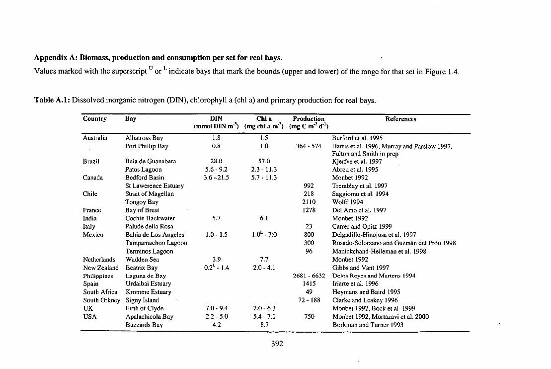
1.8 0.8

28.0 5.6 - 9.2 3.6 - 21.5

1.5 1.0

57.0 2.3 - 11.3 5.7- 11.3

Appendix A: Biomass, production and consumption per set for real bays.

Values marked with the superscript u or L indicate bays that mark the bounds (upper and lower) of the range for that set in Figure 1.4.

Table A.1: Dissolved inorganic nitrogen (DIN), chlorophyll a (chl a) and primary production for real bays.

Country Bay DIN Chl a Production References (mmol DIN ni3) (mg chl a ni3) (mg C 111-2 (0)

Albatross Bay Port Phillip Bay

Baia de Guanabara Patos Lagoon Bedford Basin St Lawerence Estuary Strait of Magellan Tongoy Bay Bay of Brest Cochin Backwater Palude della Rosa Bahia de Los Angeles Tampamachoo Lagoon Terminos Lagoon Wadden Sea Beatrix Bay Laguna de Bay Urdaibai Estuary Kronune Estuary Signy Island Firth of Clyde Apalachicola Bay Buzzards Bay

Burford et al. 1995

364 - 574 Harris et al. 1996, Murray and Parslow 1997, Fulton and Smith in prep Kjerfve et al. 1997 Abreu et al. 1995 Monbet 1992

992 Tremblay et al. 1997

218 Saggiomo et al. 1994

2110 Wolff 1994

1278 Del Amo et al. 1997 Monbet 1992

23 Caner and Opitz 1999

800 Delgadillo-Hinojosa et al. 1997

300 Rosado-Solorzano and Guzman del Pr6o 1998

96 Manickchand-Heileman et al. 1998 Monbet 1992 Gibbs and Vant 1997

2681 - 6632 Delos Reyes and Martens 1994

1415 Iriarte et al. 1996

49 Heymans and Baird 1995

72 - 188 Clarke and Leakey 1996 Monbet 1992, Bock et al. 1999

750 Monbet 1992, Mortazavi et al. 2000 Borkman and Turner 1993

Australia

Brazil

Canada

Chile

France India Italy Mexico

Netherlands New Zealand Philippines Spain South Africa South Orkney UK USA

5.7

6.1

1.0- 1.5

1.0L - 7.0

3.9

7.7 0•2L - 1.4

2.0 - 4.1

7.0 - 9.4

2.0 - 6.3 2.2 - 5.0

5.4 - 7.1 4.2

8.7

392

Table A.1: Continued.

Country Bay DIN Chi a Production References (mmol DIN ni3) (mg chi a m-3) (mg C 1112 d-1)

Charlotte Harbour 6.6 - 15.3 4.8 - 15.2 Monbet 1992 Chesapeake Bay 5.5 - 42.2 9.9 - 33.7 Monbet 1992 Chincoteague Bay 7.5 22.0 1100 Boynton et al. 1996 Columbia River 15.3 7.3 Monbet 1992 Flax Pond 4.6 - 5.2 5.5 - 5.8 Monbet 1992 Galveston Bay 16.0 6.9 Santschi 1995 Hilsborough 47.1 -48.1 13.4- 19.3 Monbet 1992 Hudson River 33.6 - 45.6 2.7 - 23.7 Monbet 1992 Isle of Wight Bay 11.0 38.0 Boynton et al. 1996 James River 54.3 41.4 Monbet 1992 Long Island Sound 8.2 8.6 Borkman and Turner 1993 Massachusetts Bay 6.5 3.1 Borkman and Turner 1993 Monterey Bay 5.0 - 10.0 3.0 - 6.0 Pennington and Chavez 2000 Narragansett Bay 4.7 - 10.2 9.1 - 10.3 Monbet 1992, Smayda 1983 Neuse River 5.0 12.8 Monbet 1992 North Inlet 27.0 7.0 Monbet 1992 Patuxent River 8.6 - 63.9 12.3 - 48.1 Monbet 1992 Peconic Bay 2.6 2.9 Turner et al. 1983 Potomac River 8.8 - 119.2u 12.7 - 78.9 Monbet 1992 Rappahanock River 3.4 - 24.7 4.5 - 21.7 Monbet 1992 Rhode River 10.0 - 15.3 8.1 - 150.0u Monbet 1992, Gallegos et al. 1997 San Francisco Bay 4.0 - 40.9 8.9 - 25.2 Monbet 1992 South River 9.7 16.8 Monbet 1992 York River 4.8 - 4.9 3.3 - 4.0 Monbet 1992

Table A.2: Zooplankton biomass, production and consumption for real bays.

Country Bay Zooplankton Production Consumption References (mg AFDW I11-3) (mg C m-2 d-1 ) (mg C m-2 d-1)

Australia Port Phillip Bay 68.4 - 68.5 143.4 - 169.0 232.7 Holloway and Jenkins 1993, Beattie et al. 1996, Murray and Parslow 1997, Fulton and Smith in prep

Baltic Northern Baltic 32.9 Koski et al. 1999 Chile Tongoy Bay 20.0 197.3 867.9 Wolff 1994 Denmark Kattegatt 106.0 400.0 Kiorboe and Nielsen 1994a, b France Arcachon Bay 150.0 Poulet et al. 1996

Cantabrian Coast 82.4 - 102.0 Poulet et al. 1996 Gironde 43.8 Plounevez and Champalbert 1999 Ushant 50.0 Poulet et al. 1996 West English Channel 150.0 Poulet et al. 1996

France/UK Celtic Sea 200.0 Poulet et al. 1996 Finland Bothnian Bay 16.4 Koski et al. 1999

Sallvik 28.8 Koski et al. 1999 Storfjarden 31.0 Koski et al. 1999 Langden 76.9 Koski et al. 1999

India Bay of Bengal 36.3 Kumari and Goswami 1993 Goa 48.9 Goswami and Padmavati 1996

Ireland West Irish Sea 26.9 Dickey-Collas et al. 1996 Italy Palude della Rosa 72.7 18.1 Carrer and Opitz 1999 Jamaica Kingston Harbour 331.0 Hoperoft et al. 1998 Mexico Chetumal Bay 10.7 1' Gasca and Castellanos 1993

Tenninos Lagoon 322.0 26.3 111.1 Manickchand-Heileman et al. 1998 Tampamachoo Lagoon 79.2 4.4 22.2 Rosado-Solorzano and Guzman del Pr6o 1998

Netherlands Westerschelde 60.0 Soetaert and Herman 1994 Philippines Laguna de Bay 400.0 - 563.0u 253.2 - 456.9 1019.8 - 1823.3 Delos Reyes and Martens 1994 Russia Barents Sea 60.0 Sakshaug et al. 1994 South Africa ICromme Estuary 30.0 11.2 36.5 Heymans and Baird 1995 Spain Galicia 125.0 Poulet et al. 1996

La Coruna 170.8 Poulet et al. 1996

394

Table A.2: Continued. Country

Sweden Taiwan UK USA

Bay Zooplankton Production Consumption (mg AFDW ni3) (mg C 111-2 4:1-1) (mg C 111.2 4:14)

16.4 40.8 30.0

71.4- 148.0 144.8 28.0 201.8

References

Central Baltic Chiku Lagoon Plymouth Chesapeake Bay Corpus Christi Bay Monterey Bay Narragansett Bay

Koski et al. 1999 Lin et al. 1999 Harvey 1950 Park and Marshal 2000 Buskey 1994 Olivieri and Chavez 2000 Durbin and Durbin 1998

Table A.3: Fish biomass, production and consumption for real bays.

Country Bay Total fish Total production Total consumption References (g AFDW m-2) (mg AFDW ni2 4:1-1) (mg AFDW I11.2 d-1)

Australia Albatross Bay 5.5 Blaber et al. 1994 Alligator Creek 2.4 Robertson and Duke 1990 Bagot Point 65.2 Edgar and Shaw 1995 Barker Inlet 82.2 Edgar and Shaw 1995 Botany Bay 1.4 Bell et al. 1984 Cararma Inlet 14.6 Edgar and Shaw 1995 Cloudy Lagoon 69.8 Edgar and Shaw 1995 Crib Point 13.1 Robertson 1980 Embley Estuary 15.8 Blaber et al. 1989 French Island 3.6 Edgar and Shaw 1995 Frenchmans Bay 5.5 Edgar and Shaw 1995 Groote Eylandt 5.5 Blaber et al. 1994 Great Barrier Reef 35.6 Williams and Hatcher 1983 Gulf of Carpentaria 2.7 Blaber et al. 1994 Lake King 58.6 Edgar and Shaw 1995 Moreton Bay 3.1 Morton 1990 North West Shelf > 0.47 Sainsbury 1987

395


Country Bay Total fish Total production Total consumption References (g AFDW m -2) (mg AFDW m 2 (1-1) (mg AFDW In-2 CO)

One Tree 47.6u Russell 1977 Parker Point 44.2 Edgar and Shaw 1995 Peel-Harvey Estuary 0•5 L Loneragan et al. 1986 Porpoise Bay 2.0 Edgar and Shaw 1995 Port Gawler 12.8 Edgar and Shaw 1995 Port Phillip Bay 3.3 6.2 55.7 - 72.2 Hall 1992, Parry et al. 1995, Fulton and

Smith in prep Princess Royal Bay 90.9 Edgar and Shaw 1995 Rockingham 36.2 Edgar and Shaw 1995 South East Gulf 2.8 Blaber et al. 1994 Thomsons Bay 1.6 Edgar and Shaw 1995 Western Port Bay 1.2 Robertson 1980 Woodmans Point 5.2 Edgar and Shaw 1995

Bermuda Bermuda 10.8 Bardach 1959 Chile Tongoy Bay 4.6 54.6 377.3 Wolff 1994 China Western Yellow Sea >0.1 Rhodes 1998 Crete Heraklion Bay 9.5 Kallianiotis et al. 2000 Egypt Gulf of Aqaba 21.2 Whitfield 1993 Eritrea Dahlak Archipelago 7.7 Russell 1977 France Port Cros 1.7 Francour 1997 Hawaii French Frigate Shoals 29.7 Freidlander and Parrish 1997

Hanalei Bay 16.6 Freidlander and Parrish 1997 Hawaii 20.4 Russell 1977 Hulopoe-Manele 44.6 Freidlander and Parrish 1997 Kaneohe Bay 23.8 Freidlander and Parrish 1997 Midway Atoll 28.6 Freidlander and Parrish 1997 Oahu 20.5 - 21.0 Freidlander and Parrish 1997 Waikiki 5.8 Freidlander and Parrish 1997

India Marmugao Bay 1.5 Ansari et al. 1995 Aguada Bay 1.1 Ansari et al. 1995

S.

396


Country Bay Total fish Total production Total consumption (g AFDW ni2) (mg AFDW n12 (1 -1) (mg AFDW 111-2 d-1)

References

Indian Ocean

Italy Mexico

New Caledonia

New Zealand Pacific Ocean Philippines ,Russia

Mayotte Reunion Palude della Rosa Huizache-Caimanero Lagoon Tampamachoo Lagoon

Teacapan-Agua Brava Lagoon Terminos Lagoon Barrier reefs

Belep Island Chesterfield Islands Cooks Reef East Reefs

Francais Reef Fringing reefs

Intermediate reefs

Lagoon bottoms North Lagoon Ouvea South Reefs St Vincent Bay West Reefs

Goat Island Eniwetok Atoll Laguna de Bay Barents Sea

30.9 Letourneur et al. 2000

21.45 Letourneur 1998

2.5 10.5 Caner and Opitz 1999

2.3 16.0 Warburton 1979

1.2 5.7 63.3 Rosado-Solorzano and Guzman del Preo 1998

2.2 Flores-Verdugo et al. 1990

1.4 - 2.5

4.0

61.5

Manickchand-Heileman et al. 1998

>5.07

Letourneur et al. 2000, Kulbicki et al. 2000

23.1

Letourneur et al. 2000

30.8


39.0


15.8


44.7


> 4.99


>5.87


> 8.41

Kulbicki et al. 2000

2.0

Wantiez 1998

49.2


25.9

Letourneur et al. 2000 > 1.07 - > 1.89

Wantiez 1996, Wanteiz et al. 1996

25.8


11.4

Russell 1977

10.6

Odum and Odum 1955 3.2 - 4.2

37.2 - 50.4

78.0 - 299.4

Delos Reyes and Martens 1994

7.9

Sakshaug et al. 1994

397

2.6 Blaber and Milton 1990 10.9 Whitfield 1993 12.4 11.9 171.3 Heymans and Baird 1995 15.1 Berry et al. 1982 2.7 Whitfield 1993 15.0 McClanahan and Sala 1997

47.6 18.3

> 1.0 >0.88

2.9 15.1 0.7 1.3

1.2- 12.0 4.9 8.3 1.6 2.6 12.4

1.6- 1.65 7.6

25.5 0.6 2.0 2.5 1.5

35.2

Lin et al. 1999 Menasveta et al. 1986 Wanteiz et al. 1996 Gibson et al. 1993 Harvey 1950 Quast 1968 Brock 1977 Adams 1976 Lubbers et al. 1990 Whitfield 1993 Quast 1968 Ross et al. 1987 Whitfield 1993 Russell 1977 Russell 1977 Quast 1968 Love et al. 2000 Whitfield 1993 Russell 1977 Thayer et al. 1987 Dean et al. 2000 Russell 1977

7.1

Table A.3: Continued. Country Bay Total fish Total production Total consumption

(g AFDW 111-2) (mg AFDW 1112 (11) (mg AFDW m 2 (1-1) References

Solomon Islands Solomon Islands South Africa Cape of Good Hope

Kromme Estuary Durban Swartvlei Lake

Spain/France North West Mediterranean

Taiwan Chiku Lagoon Thailand Sichang Islands

South China Sea UK Ardmucknish Bay

Plymouth USA Bathtub Rock

Biscayne Bay Bogue Sound Chesapeake Bay Corpus Christi Del Mar Horn Island Laguna Madre Monterey Bay Mustang Island Papalote Bay Santa Barbara Channel St Andrew Bay Sth New England Whitewater Bay

USA (Alaska) Prince William Sound Virgin Islands Virgin Islands

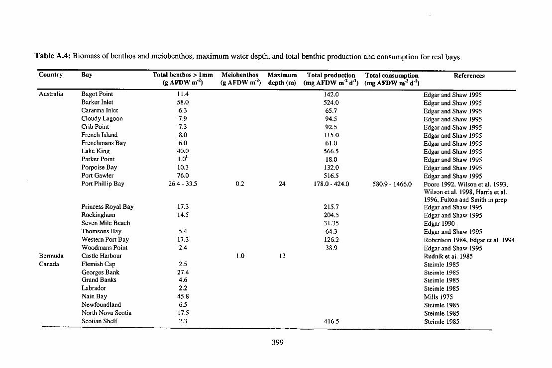
Table A.4: Biomass of benthos and meiobenthos, maximum water depth, and total benthic production and consumption for real bays.

Country Bay Total benthos > lmm Meiobenthos Maximum Total production Total consumption References (g AFDW 111-2) (g AFDW 111-2) depth (m) (mg AFDW 1112 (1.1) (mg AFDW I11-2 d -1)

Australia Bagot Point 11.4 142.0 Edgar and Shaw 1995 Barker Inlet 58.0 524.0 Edgar and Shaw 1995 Cararma Inlet 6.3 65.7 Edgar and Shaw 1995 Cloudy Lagoon 7.9 94.5 Edgar and Shaw 1995 Crib Point 7.3 92.5 Edgar and Shaw 1995 French Island 8.0 115.0 Edgar and Shaw 1995 Frenchmans Bay 6.0 61.0 Edgar and Shaw 1995 Lake King 40.0 566.5 Edgar and Shaw 1995 Parker Point 1.0L 18.0 Edgar and Shaw 1995 Porpoise Bay 10.3 132.0 Edgar and Shaw 1995 Port Gawler 76.0 516.5 Edgar and Shaw 1995 Port Phillip Bay 26.4 - 33.5 0.2 24 178.0 - 424.0 580.9 - 1466.0 Poore 1992, Wilson et al. 1993,

Wilson et al. 1998, Harris et al. 1996, Fulton and Smith in prep

Princess Royal Bay 17.3 215.7 Edgar and Shaw 1995 Rockingham 14.5 204.5 Edgar and Shaw 1995 Seven Mile Beach 31.35 Edgar 1990 Thomsons Bay 5.4 64.3 Edgar and Shaw 1995 Western Port Bay 17.3 126.2 Robertson 1984, Edgar et al. 1994 Woodmans Point 2.4 38.9 Edgar and Shaw 1995

Bermuda Castle Harbour 1.0 13 Rudnik etal. 1985 Canada Flemish Cap 2.5 Steimle 1985

Georges Bank 27.4 Steimle 1985 Grand Banks 4.6 Steimle 1985 Labrador 2.2 Steimle 1985 Nain Bay 45.8 Mills 1975 Newfoundland 6.5 Steimle 1985 North Nova Scotia 17.5 Steimle 1985 Scotian Shelf 2.3 416.5 Steimle 1985

399

Table A.4: Continued. Country Bay Total benthos > lmm Meiobenthos Maximum Total production Total consumption References

(g AFDW 111-2) (g AFDW n12) depth (m) (mg AFDW 111-2 dr') (mg AFDW 111.2 CI-1)

Chile Tongoy Bay 16.3 1.8 90 158.2 685.1 Wolff 1994 Denmark Kysing Fjord 0.2 1 Rudnik et al. 1985

Oresund 2.5 54 Rudnik et al. 1985 France Arcachon Bay 5.4 Bachelet et al. 1996

Bay of Banyuls-sur-mer 3.3 - 4.3 87.0 1.3 Rudnik et al. 1985, Grdmare et al. 1998

Bay of Brest 19.2 Jean and Thouzeau 1995 Bay of Lyon 0.4 30 Rudnik et al. 1985 Etang de Thau Lagoon 43.0 Palomares et al. 1993 Gironde Estuary 0.4 5 Santos et al. 1996

France/Spain North West 70.7 McClanahan and Sala 1997 Mediterranean

Finland Tvarminne 1.5 55 Rudnik et al. 1985 Germany Helgoland Bight 0.4 49 Rudnik et al. 1985

Kiel Bight 0.2 26 Rudnik et al. 1985 India Bay of Bengal <OI L 230 Rudnik et al. 1985

Goa 0.2 30 Rudnik et al. 1985 Ireland Irish Sea 0.5 121 Rudnik et al. 1985 Iran/Iraq Tigris and Euphrates 0.2 18 Rudnik et al. 1985

Estuary Italy Adriatic Sea 0.2 17 Rudnik et al. 1985

Palude della Rosa 96.7 10.2u 0.5 230.2 Carrer and Opitz 1999 Mexico Celestun Lagoon 2.6 3.3 Chavez et al. 1993

Gulf of Mexico 115.0 Talley et al. 2000 Tampamachoo Lagoon 2.0 1.2 54.2 236.8 Rosado-Solorzano and Guzman

del Pr6o 1998 Terminos Lagoon 14.6 5.2 3.5 316.4 1446.8 Manickchand-Heileman et al.

1998 Netherlands Dutch Wadden Sea 16.5 Moller et al. 1985

Grevelingen Estuary 147.9 Steimle 1985 North Wadden Sea 137.0 Steimle 1985 Wadden Sea 71.2 Steimle 1985

400


Country Bay Total benthos > lmm Meiobenthos Maximum Total production Total consumption References (g AFDW nI2) (g AFDW nf2) depth (m) (mg AFDW ilf2 (1 -1) (mg AFDW ill2 CO)

Westerschelde 0.3 20 Soetaert et al. 1994 North Sea Fladen 0.5 101 Rudnik et al. 1985 Pacific Eniwetok Atoll 92.0 Odum and Odum 1955 Philippines Laguna de Bay 5.6 136.0- 155.0 544.2 - 628.5 Delos Reyes and Martens 1994 Poland Gulf of Gadansk 33.3 Drgas et al. 1998 South Africa ICromme Estuary 30.5 0.4 3 183.4 5292.2 Heymans and Baird 1995 South Orkney Signy Island 4.5 10 Vanhove et al. 1998 Spain Bay of Cadiz 18.4 61.2 Arias and Drake 1994

Ria de Arosa 0.2 19 Rudnik et al. 1985 Ria de Muros <0.1 22 Rudnik et al. 1985

Sweden Baltic Sea 21.0 2.1 Moller et al. 1985 Bassholm 5.6 67.8 Moller and Rosenberg 1982 Bothnian Bay 0.3 220 Rudnik et al. 1985 Bothnian Sea 12.8 0.7 100 1.2 Moller et al. 1985, Rudnik et al.

1985 Central Baltic 1.2 46 Rudnik et al. 1985 Gota Estuary 0.2 52 Rudnik et al. 1985 Gullmarsvik 2.4 14.9 Moller and Rosenberg 1982 Kungsbacha 0.1 16 Rudnik et al. 1985 Mid-Baltic 29.6 Steimle 1985 Northern Baltic 19.7 Steimle 1985 Sandvik 1.6 13.0 Moller and Rosenberg 1982 Skagerrak 38.0 416.5 Willer et al. 1985 Swedish Sound 5.2 36.8 Moller et al. 1985 Sweden 25.4 Pihl-Baden and Pihl 1984 West Central Baltic 0.1 211 Rudnik et al. 1985

Taiwan Chiku Lagoon 59.0 Lin et al. 1999 UK Clyde Sea 0.2 166 Rudnik et al. 1985

Cornwall 36.4 Steimle 1985 English Channel 0.2 45 Rudnik et al. 1985 Hamble Spit 602.7 Hibbert 1976 Liverpool Bay 0.5 10 Rudnik et al. 1985

-

■••• 401

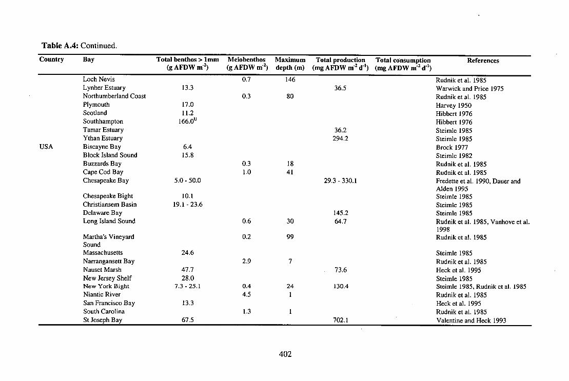
Table A.4: Continued. Country Bay Total benthos > lmm Meiobenthos Maximum Total production Total consumption References

(g AFDW ni2) (g AFDW II12) depth (m) (mg AFDW 111-2 d4) (mg AFDW 111-2 CO)

Loch Nevis 0.7 146 Rudnik et al. 1985 Lynher Estuary 13.3 36.5 Warwick and Price 1975 Northumberland Coast 0.3 80 Rudnik et al. 1985 Plymouth 17.0 Harvey 1950 Scotland 11.2 Hibbert 1976 Southhampton 166.0u Hibbert 1976 Tamar Estuary 36.2 Steimle 1985 Ythan Estuary 294.2 Steimle 1985

USA

Biscayne Bay 6.4 Brock 1977 Block Island Sound 15.8 Steimle 1982 Buzzards Bay 0.3 18 Rudnik et al. 1985 Cape Cod Bay 1.0 41 Rudnik et al. 1985 Chesapeake Bay 5.0 - 50.0 29.3 - 330.1 Fredette et al. 1990, Dauer and

Alden 1995 Chesapeake Bight 10.1 Steimle 1985 Christiansem Basin 19.1 - 23.6 Steimle 1985 Delaware Bay 145.2 Steimle 1985 Long Island Sound 0.6 30 64.7 Rudnik et al. 1985, Vanhove et al.

1998 Martha's Vineyard 0.2 99 Rudnik et al. 1985 Sound Massachusetts 24.6 Steimle 1985 Narrangansett Bay 2.9 7 Rudnik et al. 1985 Nauset Marsh 47.7 73.6 Heck et al. 1995 New Jersey Shelf 28.0 Steimle 1985 New York Bight 7.3 - 25.1 0.4 24 130.4 Steimle 1985, Rudnik et al. 1985 Niantic River 4.5 1 Rudnik et al. 1985 San Francisco Bay 13.3 Heck et al. 1995 South Carolina 1.3 1 Rudnik et al. 1985 St Joseph Bay 67.5 702.1 Valentine and Heck 1993

402

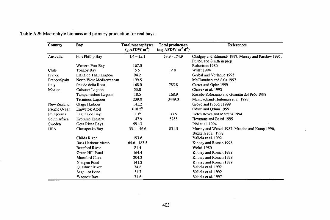
Table A.5: Macrophyte biomass and primary production for real bays.

Country

Australia

Bay Total macrophytes Total production (g AFDW m-2) (mg AFDW M-2 d -11 )

References

Port Phillip Bay 1.4 - 15.1

53.9 - 174.9 Chidgey and Edmunds 1997, Murray and Parslow 1997, Fulton and Smith in prep Robertson 1980 Wolff 1994 Gerbal and Verlaque 1995 McClanahan and Sala 1997 Carrer and Opitz 1999 Chavez et al. 1993 Rosado-Solorzano and Guzman del Proo 1998 Manickchand-Heileman et al. 1998 Grove and Probert 1999 Odum and Odum 1955 Delos Reyes and Martens 1994 Heymans and Baird 1995 Pihl et al. 1994 Murray and Wetzel 1987, Madden and Kemp 1996, Buzzelli et al. 1998 Valiela et al. 1992 Kinney and Roman 1998 Welsh 1980 Kinney and Roman 1998 Kinney and Roman 1998 Kinney and Roman 1998 Valiela et al. 1992 Valiela et al. 1992 Valiela et al. 1997

Chile France France/Spain Italy Mexico

New Zealand Pacific Ocean Philippines South Africa Sweden USA

Western Port Bay Tongoy Bay Etang de Thau Lagoon North West Mediterranean Palude della Rosa Celestun Lagoon Tampamachoo Lagoon Terminos Lagoon Otago Harbour Eniwetok Atoll Laguna de Bay Kromme Estuary Gota River Bays Chesapeake Bay

Childs River Bass Harbour Marsh Branford River Green Hill Pond Mumford Cove Ninigret Pond Quashnet River Sage Lot Pond Waquoit Bay

167.0 5.5

2.8 94.2 199.5 168.0 785.8 35.0 10.5

168.9 239.0

3449.0 141.2

618.2u Li L 33.5

147.9

5255 591.3

33.1 -46.6

831.5

193.6 64.6 - 183.5

81.4 164.4 204.2 141.2 74.8 31.7 71.6

Table A.6: Total detritus for real bays.

Country Bay Total detritus References (g AFDW m-2)

Australia Bagot Point 3•2L Edgar and Shaw 1995 Cararma Inlet 10.6 Edgar and Shaw 1995 Lake King 101.0 Edgar and Shaw 1995 Porpoise Bay 4519.0 Edgar and Shaw 1995 Port Gawler 331.0 Edgar and Shaw 1995 Port Phillip Bay 1731.0- 2953.4 Nicholson et al. 1996, Fulton and Smith in prep Rockingham 1659.0 Edgar and Shaw 1995 Woodmans Point 1940.0 Edgar and Shaw 1995

French Polynesia Tiahura 677.5 Ariasgonzalez et al. 1998 Italy Palude della Rosa 750.4 Caner and Opitz 1999 Mexico Terminos Lagoon 12.7 Manickchand-Heileman et al. 1998 South Africa Kromme Estuary 3000.0 Heymans and Baird 1995 Taiwan Chiku Lagoon 48.6 Lin et al. 1999 USA Chesapeake Bay 10417.0u Roden and Tuttle 1996

Table A.7: Biomass and primary production of microphytobenthos for real bays.

Country Bay Microphytobenthos Production References (mg chl a m-2) (mg c m-2 d-1)

Australia Peel-Harvey Estuary 295.0u MacIntyre et al. 1996 Port Phillip Bay 25.0- 51.7 101.1 - 240.5 Murray and Parslow 1997, Fulton and Smith in prep

Canada Bay of Fundy 255.0 Hargrave et al. 1983 Denmark Danish Fjords 318.0 Grontved 1960

Smalandshavet 555.0 MacIntyre et al. 1996 France Golfe de Fos 38.0 MacIntyre et al. 1996

Mediterranean Coast 44.0 Schreiber and Pennock 1995

404

Table A.7: Continued. Country Bay Microphytobenthos

(mg chi a ni2) Production

(mg C n12 C1-1)

References

Madagascar Madagascar 58.0 181.0 Schreiber and Pennock 1995 Netherlands Dutch Wadden Sea 220.0 - 225.0 485.0 - 567.5 Cadee and Hegeman 1977, MacIntyre et al. 1996

Ems-Dollard Estuary 65.0 - 282.5 463.0 - 985.0 Colijn and de Jonge 1984, MacIntyre et al. 1996 Lake Grevelingen 215.0 295.0 MacIntyre et al. 1996

Russia Vostok Bay 135.0 MacIntyre et al. 1996 Slovenia Bay of Prian 240.0 MacIntyre et al. 1996 South Africa ICromme Estuary 1.6E' 232.0 Heymans and Baird 1995 Spain Ria de Arosa 66.5 MacIntyre et al. 1996 Sweden Laholm Bay 24.5 147.0 MacIntyre et al. 1996

Oresund 75.5 565.0 Schreiber and Pennock 1995 UK Loch Ewe 17.8 Steele and Baird 1968

Ythan estuary 84.9- 117.5 Leach 1970 USA Bolsa Bay 285.0 494.5 Schreiber and Pennock 1995

Boston Harbour 190.0 MacIntyre et al. 1996 Buzzards Bay 52.5 MacIntyre et al. 1996 Chesapeake Bay 35.0 MacIntyre et al. 1996 Chukchi Sea 73.5 - 180.0 13.7 Matheke and Horner 1974, MacIntyre et al. 1996 Delaware Estuary 122.5 MacIntyre et al. 1996 Duplin River Marsh 289.0 MacIntyre et al. 1996 Graveline Bay 215.0 MacIntyre et al. 1996 La Jolla 182.5 MacIntyre et al. 1996 Long Island Sound 113.5 MacIntyre et al. 1996 Netarts Bay 162.5 MacIntyre et al. 1996 North Inlet 65.0 - 70.0 MacIntyre et al. 1996 Potter Pond Lagoon 235.0 MacIntyre et al. 1996 San Antonio Bay 8.0 - 29.5 43.5 MacIntyre et al. 1996 Tijuana Estuary 1472.0 MacIntyre et al. 1996 Weeks Bay 15.6 246.6 Schreiber and Pennock 1995

Appendix B: Meaning of the acronyms, functional group codes and

symbols used. Table B.1: List of the acronyms commonly used in this thesis

Acronym Meaning BM2 Bay Model 2 CM Model runs with nutrient loadings scaled to match the loadings of Chesapeake Bay IGBEM Integrated Generic Bay Ecosystem Model PPB Port Phillip Bay (near Melbourne, Australia) PPBIM Port Phillip Bay Integrated Model PM Model runs with nutrient loadings scaled to match the loadings of Port Phillip Bay

Table B.2: List of components in Bay Model 2 (BM2) and the Integrated Generic Bay Ecosystem Model (IGBEM), compared to those in the Port Phillip Bay Integrated Model (PPBIM). All living and dead components have nitrogen pools, in IGBEM they also have carbon and phosphorous pools.

Model Component Codename BM2 / IGBEM PPBIM

Diatoms* PL Y Y Autotrophic Flagellates AF Y Picophytoplankton PS y y Dinoflagellates DF Y Y Free-living Pelagic Bacteria PFB Y Pelagic Attached Bacteria** PAB y Heterotrophic Flagellates FIF y Microzooplankton ZS Y Y Large Omnivorous Zooplankton ZL Y Large Carnivorous Zooplankton ZLC Y Y Planktivorous Fish . FP Y Piscivorous Fish FV Y Demersal Fish FD y Demersal Herbivorous Fish FG y Macroalgae MA Y Y Seagrass SG Y Y Microphytobenthos* MB Y y Macrozoobenthos (Epifaunal carnivores) MZ y Benthic (Epifaunal) Grazers BG Y Benthic Suspension Feeders BF Y Y Infaunal Carnivores BC Y Benthic Deposit Feeders BD Y Meiobenthos OB Y Aerobic Bacteria AEB Y Anaerobic Bacteria ANB Y Labile Detritus DL Y Y Refractory Detritus* DR Y Y DON DON Y Y Ammonia NH Y Y Nitrate NO Y Y Dissolved Silicate Si Y Y Dissolved Oxygen 02 Y y*** Light IRR Y Y Salinity SAL Y Y Sediment Grain Types PHI Y Y Bottom Stress STRESS Y Y Porosity POR Y Y Volume VOL Y Y

* Also have an internal silicon pool. ** Only present as a separate entity in BM2, in IGBEM there is a single pelagic bacteria component. *** Handled as nitrogen fluxes scaled by the Redfield ratio N:0 --= 1:16

406

Table B.3: List of main terms used in the equations in the appendices C to F. All terms,

variables, constants and expressions are defined in the relevant appendices, but this

table may be a useful quick reference for the main terms and conventions.

Term Meaning E Excretion (ammonia produced by a consumer) F Fishing (catch) G Growth M Mortality P Uptake R Remineralisation S Sediment chemistry (nitrification or denitrification, the subscript will

denote which on a case-by-case basis) W Waste (detritus produced by a consumer) XX All doubles (and triples) refer to components of the model (see Table

A3 for definitions). They do not represent multiplications at any time and any multiplications will be explicitly denoted by a "*".

407

Appendix C: Rate of change and process equations for Bay Model 2

Note: For quick reference, a list of the main terms used in the equations in this

appendix is given in Appendix B, Table B.3.

C.1 Rate of change equations

Autotrophs

Rate of change for standard water column primary producer (PX):

= ‘-r PX M lys, PX s, dt i =predator groups

d(PX sed ) _ — nat,px,,,d dt

Where Gpx stands for the growth of PX, Mlys,px is the loss of PX due to lysis, Mnatyx is

the natural mortality losses of PX when in the sediments and Ppx j are the losses of PX

due to predation. The equations for the benthic primary producers are slightly different.

The rate of change of microphytobenthos is given by:

d(MB) dt i= water predator

lys, MB „ E PMB,„

groups

d(MB sed ) = G mB.d — m nat , s4/3.1 E 4,413„, dt i=sed predator groups

The macrophytes (MX) are restricted to the epibenthic layer and have no water column

or sediment pools. The general form of their rate of change is as follows:

dt = G mx M mx EPmx,i

The process equations for primary producers are outlined below and modifications to

these equations due to mixotrophy in dinoflagellates are noted in the main text of

chapter 2.

(C.1)

(C.2)

(C.3)

(C.4)

d(MX ) (C.5) i =predator

groups

408

Invertebrate Consumers

Rate of change for a standard invertebrate consumer (CX):

c/(CX I-Tcx Mcx EPcx..—Fcx

dt i=predator groups

where Fcx stands for losses due to fishing on this group (this is set to zero in all

standard runs of Bay Model 2 (BM2)). Invertebrate consumers are restricted to having

only a water column or epibenthic or sediment pool and can not have pools in multiple

layers.

Fish consumers

The following are the rates of change for a fish group (FX).

c/(FX ; )= G

dt FX,,

AFX ; r) = GFxj,

dt

— — — E IMM,FX ; TEM,FX; M. P —FX, j FFX ; dt i=predator groups

Where the subscript i represents age group i (there is one equation for each age class

included), s stands for structural weight (skeletal and other material that can not be

reabsorbed), r for reserve weight (fats and other tissues that can be broken down when

food is scarce) and d for density. The T terms represent the movement of fish in to

(Timm ,F„;) and out of (TEAuxi) the cell. In addition there are short-term spawning and

recruitment events which effect the various FX pools. At the same point each year (the

exact day dependent on the fish and with a window of +/- 14 days) the fish spawn and

the materials required to do this is removed from the reserve weight of FX. At this point

all fish are aged one age class and the oldest age class leaves the bay (this is used in

place of a plus group as it is more representative of the dynamics of Port Phillip Bay

(C.6)

d(FX; ,„ )= T

(C.7)

(C.8)

(C.9)

409

(Gunthorpe et al. 1997)). Sometime later (the exact period dependent on the group) the

recruits settle out and their weights and density are assigned to the youngest age class.

The amount of reserve weight (mg N per individual) that is used up during

spawning is given by

1.4x, • max (0, (Z Fx • (1 + X Rs )• FX,,,—YFx )) , FX ; , s + FX ;., > (1+ X Rs )• FX,,,

(

Fx, [ZFx(1+XRs)-FX,,s+(FX,,s+FX;4

U •max 0, 1),

—YFx —(1+ XRs).FXj,s FX+ FX ; ,, < (1+ XRs )*FX4s

(C.10)

where UF,d is the proportion of age group i that is reproductively mature, ZFx is the

fraction of the weight of FX used in spawning, YFx is the spawning function constant

and XRS is the ratio of structural to reserve weight in well fed fish.

The formulations for recruitment are given in the main text of chapter 2 and

Table 2.2. It should be noted that the biomass of larvae of fish group FX in cell j at time

t (4), referred to in Table 2, is determined as follows:

L ti = ESFx , • FX ; , d

i =age class (C.11)

Inanimate pools

Rates of change for ammonia (NH) in the water column is:

cl(ATH) = D NHi PNII,„MB„, PNH„„MA PNH,„PFB + E Ei E Ei E Ei - SNIT,PAB + R NET, w

dt i =PX „, i=CX , BF i=FX i =pelagic bacteria

(C.12)

and in the sediment:

d(VHsed )= R NET ,sed — SNIT,sed dt PNTH,.„,MBd — ' NH„d ,SG +E1

i*I3F,CX„ (C.13)

where Priu,xx is the uptake of NH by the autroph XX, Ecx is the production of NH by

the consumer CX, SNrr,xu is the amount of NH lost due to nitrification by the bacteria

410

— E PNO PNOMB w PNOw .MA 1- SNIT ,PAB dt i=PX w

d(NO w )

(C.14)

XB, RNET is the amount of NH produced by denitrification.

The rates of change for nitrate (NO) in the water column is given by:


C10/0 sed — NIT,sed SDENTT ,sed PNO.d .MB s, PNOSG dt (C.15)

The rates of change of dissolved silicate (Si) in the water column is:

d(Si = DD DSisol,w Eis.„„i at i=PL,MI3w (C.16)

and the rate of change of detrital silica (DSi) in the water column is given by:

C/(D57 w ) v L 'SiN E lys,i EPi, J — R DSisol,w dt i=PL,MB,„ (C.17)

where XSiN is the Redfield ratio of silicon and nitrogen (set at 3.0 (Murray and Parslow

1997)) and RDSisol is the amount of detrital silica remineralised. Note that the equations

for Si sed and DSi sed are as for (C.16) and (C.17) except that CX s,d is used in the place of

CXw and MB is the only PX present in the sediment that uses Si.

The rates of change for dissolved oxygen (02) in the water column is given by:

d(02,, )= xoN Gen EGi GmBw GmA E Ei — EE; — 1E1 — R dt i=PX,,, 2 i*infauna, i=FX i=pelagic

MZ,BG bacteria

DON,w1


(C.18)

c/(02„d ) „oN G MB + 2- - E E1 — R DON,sed ,.d dt 2 i=infauna.

MZ,BG (C.19)

where XoN is the Redfield ratio of oxygen and nitrogen (set at 16.0 (Murray and

411

d(DONsed ) dt WDON,sed R DON,sed (C.21)

= WDRI PDR „„i —PDR ,P AB — JDR dt

d(DR )

(C.24)

Parslow 1997)) and RDoN is the DON lost due to remineralisation.

The rates of change of dissolved organic nitrogen (DON) in the water column is:

ADON w ) • = WDON,w — R DON,w — PDON,PFB dt


(C.20)

where WDoN is the DON produced by bacteria, RDoN is the DON lost due to

remineralisation and PD0N,pFB is the DON taken up by pelagic free bacteria (PFB).

The rates of change of labile detritus (DL) in the water column is:

d(DL w ) dt E WDL,„ + E WDL w + WDL,„i + + Mlys,MB +M PDL,„ ,PAB PDL„„BF

i=CX „ i=FX i =pelagic i=PX,v bacteria

(C.22)


M nat,i + MntMB a,,„d + M lysM ,B R,d + MSG + (WDL,i PDL„d ,i E — PDL,, dt i.,„„d i =infauna i=epifauna

PDL,i (C.23)

i=FX

where WDLcx is the amount of DL in the waste products from consumer CX and PDL,CX

is the DL consumed by CX.

The rates of change of refractory detritus (DR) in the water column is given by:

d(DL sed ). E


d(DR sed ) E wDR

dt i=infauna vvd ,1 'DR + JDR

i =infauna (C.25)

where WDR,cx is the DR in the wastes of consumer CX, PDR,cx is the amount of detritus

412

consumed by CX, infauna includes sediment bacteria and JDR is the amount of DR

transferred from the water column to sediment pool due to the feeding activities of the

benthic filter feeders.

C.2 Process equations

Growth of primary producers

GPX = PPX • °kr • 8N • 8space • PX (C.26)

with ,upx is the maximum growth rate, the nutrient limitation factor due to nitrogen is

given by:

D 45 =

IN N

NPX + DIN ,

(C.27)

(where DIN=NH+NO) except for those primary producers which are also limited by the

availability of Si then nutrient limitation is given by:

(

, DIN Si )

8N = min (C.28) '. N,PX + DIN ' Ksi,px+ Si

and light limitation is given by:

= min( IRR

,1) (C.29) Kirr,PX

with the lc representing the half saturation constants for the respective processes, and

space limitation as follows:

°space = 1 PX (C.30) PXmax

Using the above formulations for growth and nutrient limitation the nutrient

uptake functions for the primary producer PX are given by:

NH K + DIN NH , PX PINH ,PX = G PX

/CNN + NH DIN , PX (C.31)

413

NO KNH,PX PNO,PX = GPX DIN 1‘ 1,1H ,px + NH (C.32)

where KNH,Px is the half saturation constant for the uptake of NH. In addition, for PL and

MB there is the uptake of Si as follows:

PSi,PX = XSIN GPX (C.33)

Growth of consumers

The growth of an invertebrate consumer (CX) is given by:

GCx = ecx • Eftcx + E (Pi.cx • ecx,; 8space • °a i=living j=DL,DR

Prey (C.34)

with ecx the growth efficiency of CX when feeding on live prey, ecx,i the efficiency

when feeding on detritus (DL treated separately to DR), space limitation given by:

(cx - e ). (cx -o )

{1 +K , CX = BF and CX > Ocxiow (cx —ecx,ow ). cx-o-Fecx,. (cx-ec„ ) K 8space CXthresh

1 , otherwise (C.35)

where ecxmax is the maximum biomass per area allowed for CX, ecmow is the crowding

lower threshold, xsat is the crowding half saturation level, and Kcx thr„h is the crowding

threshold (this formulation is based on that of the European Regional Seas Ecosystem

Model II (ERSEM II) (Blackford 1997)). The oxygen limitation in the standard runs of

BM2 is given by:

7o2

702 KCX,Mo2

1

, if epifauna or infauna

, if pelagic

or 802 =

(C.36)

where 72 is the depth of the oxygen horizon and Kcx,m02 is the half oxygen mortality

depth.

The growth for each fish group, is calculated by equation of the same form as

414

, if > Oand G >0 X Rs 4- X PRYX X Rs •FX.

FXi r

) 1 Fx, FX ; X Rs X 3 .F2C 1 ,

, otherwise

(C.34), but per age group of each fish, the result is then apportioned to structural and

reserve weight increases such that:

G Fx = A• G Fx (C.37)

GFx., = — A). Gpx. (C.38)

where

(C.39)

with XRs the maximum ratio of reserve to structural weight FX can have and X pR,Fx is

the relative degree to which FX concentrates on replenishing reserves rather than

undergoing structural growth when underweight.

In the standard form of BM2 presented here the grazing term is given by:

CX kcx • Ppre y ,cx *PreY

ecx.[

E P jgx • il+ 6cx,DL 'PDL,CX ECX PR 'PDR,CX hve prey

Pcx (C.40)

where "prey" is the group being consumed by CX, lc c„ is the clearance rate of CX and

Pprey,Cx is preference (or availability) of that prey for the predator CX. This last

parameter is similar to the "vulnerability" parameters in ECOSIM (Christensen et al.

2000) and represents the fact that the entire prey population will not be available to the

predators at any one time (some may be hiding for instance). The availability of the

food is further modified if the spatial range of the predator and prey do not completely

overlap (and so explicit spatial refuges exist). The available fish in cohort i of fish group

FX (FX;), for the fish eating cohorts of piscivorous (FV) and demersal (FD) fish (Fy i),

is given by:

Fx j.,+FX ix ) * FXi EPFXi,FYJ • cell_ vol e • FY. FX <e •

, low, FY j, s s, FY. — up, FY i,s A Fx , = 0 ,otherwise (C.41)

Pprey,CX

1+ kcx •

415

where elow,Fy is the lower prey selection size limit for FY and eup,Fy is the upper prey

selection size limit. The availability of benthic prey to their predators (fish and

invertebrate alike) is calculated in a slightly different way and is as follows:

A prey = prey • dprey (C.42)

where, if aerobic

d PreY

, roc < rtop

, rtop < rcx < 7

, rtop < 702 < rCX (C.43)

(r.2-rt.)/

and if anaerobic

1

dprey

rCX < rtOP

rtOp < rCX < 702

$ rtop < 702 < rCX (C.44)

where ycx is the depth in the sediment that the predator CX can forage down to and Ytop

is set to zero for all standard runs (as there is only one sediment layer).

Mortality and loss functions

The mortality terms for invertebrate consumers and autotrophs are in terms of lost

biomass while those for fish refer to the number of individuals lost. Nevertheless the

general form of the equations is the same (but the units of the coefficients obviously

differ between the fish and other groups). The natural mortality term for group XX is

given by

M XX = m 1 0 • XX + Mquad,XX • XX 2 + — 8 ). o2 111 02,XX • XX M special,XX • XX M top,XX • XX

(C.45)

where is the coefficient of linear mortality for XX, m- ---quad,XX is the coefficient of

quadratic mortality for the group XX, m02,xx is the coefficient of oxygen dependent

mortality and Mspecial,XX is the special (additional) loss rate for XX. This rate of "special"

416

{

MFC,FX

COT = MFCmax,FX

1+ e(m,.FF„,.,_,) , effort model on

, standard runs

(C.51)

mortality is usually set to zero, except in the following cases:

= STRESS • m m special,MA STRESS

= DIN • m DiN m special,SG

(C.46)

(C.47)

where msTREss and moiN are the coefficient of mortality due to mechanical stress and

fouling by epiphytes, respectively. Lastly:

Mspecial,FX ; =

Mstarve,FX • °starve • (1 + XRS ). { FX i ,s — ( FX ; ., + FX ; . ) , if > 0 0 + XRs ). FXi,s

= 0 , otherwise (C.48)

with Mstarve,FX is the threshold ratio of reserve to structural weight at which death due to

starvation is likely. The final term of equation (C.45) was adopted from ERSEM I

(Bryant et al. 1995) to represent the impact of seabirds and other top predators and is

given by:

M top,XX = Mseabird,XX Mshark,XX

(C.49)

While all the groups in the standard run of the model had a linear mortality term, some

groups (the fish and higher trophic level zooplankton and benthic groups) suffered

mortality described by a quadratic term. Only benthic consumers had oxygen dependent

mortality, the macrophyte and fish groups had special mortality as shown above and

mtop is only applied to the fish groups.

Fishing is another process that is only applied to fish in the standard runs. The

amount caught at time t is given by:

= Ceff • (FX, , j FX,, 1 )•FX6 , • q Fx. (C.50)

where qFx; is the catchability of the ith age group of FX and

with mFc,Fx the coefficient of fishing mortality for FX, mFcmax,Fx the maximum fishing

417

mortality allowed for FX and MFca,FX the coefficient of spread for the fishing mortality

of FX. As indicated by (C.50) and (C.51) the fishing implemented for standard runs is a

simple catch equation.

The final loss term is one that is applied to the microscopic primary producers

only and it represents lysis. The losses of a primary producer (PX) to lysis is formulated

as follows:

Mlys,PX • PX Mlys,PX 8N + 0' 1

with Mlys,PX the rate of lysis.

(C.52)

Waste processes

The production of waste products by invertebrate consumers and fish are handled in the

same way, but in the case of fish the mortality term has to be converted from a density

to a biomass before being used in the following equations. The production of labile

detritus (DL) by consumer group XX is given by:

-Exx ).rxx • EP - exx,DL) rXX,DL i =living prey

group

— eXX , DR )• rXX,DR • PDR, XX + VXX • MXX )

•PDL, XX

WDL =

•f XX , DL

(C.53)

with (oxx the proportion of mortality losses assigned to detritus, rxx the proportion of

the growth inefficiency of XX when feeding on live prey that is sent to detritus, rxx,oi,

the proportion of the growth inefficiency of XX when feeding on DL that is sent to

detritus, rxx,DR the proportion of the growth inefficiency of XX when feeding on

refractory detritus (DR) that is sent to detritus and fxx,oi. is the proportion of the total

detritus produced that is of the type DL. The same equation is used for the production of

DR (WDR), except that the final multiplication of the brackets by f xx, DL is replaced by

multiplication by (1-fxx,oL).

The other main waste product is excreted ammonia. The general formulation

418

used for the production of ammonia by a consumer XX (invertebrate or fish) is as

follows:

R. XX 1- EXX ,DL ) rXX,D) • Pli.)0C i=living prey

group

1- (1 — EXX ,DR 4-r)0C,DR )*PD (C.54)

Physical processes

The only physical processes in BM2 that differ from those in the Port Phillip Bay

Integrated Model (detailed in Murray and Parslow 1997, Walker 1997) are bioturbation,

bioirrigation (detailed in the main text of chapters 1 and 2) and the calculation of the

light attenuation coefficient. The formulation of the coefficient used in the Integrated

Generic Bay Ecosystem Model (IGBEM) is adopted in BM2 and it is an expanded form

of the one used in PPBIM. The coefficient is given by:

n = nDON • DON + nD • (DL + DR)+ n p • EPX +nsun, SUSP (C.55) i=PX

with n,„, the background extinction coefficient, //DON the contribution due to DON, nD the

contribution due to detritus, np the contribution due to phytoplankton (PX) and n susp the

contribution due to suspended sediments (SUSP).

419

dt = GDF M DF E PDF,i d(DF )

i=DF,ZL

Appendix D: Equations for dinoflagellates and mixotrophy in Bay

Model 2



The formulation for the rate of change of dinoflagellates is:

(D.1)

where MDF describes losses due to lysis suffered by the dinoflagellate pool (DF); PDF,i

are predation losses suffered by the dinoflagellate pool; and the total growth (GDF) is

given by

GDF = Gphs,DF eDF Gphag,DF (D.2)

where photosynthetic growth (Gphs,DF) is given by

Gphs,DF — PDF °kr 8N DF

(D.3)

while the phagotrophic contribution (Gphag,DF) to total growth is given by

Gphag,DF = min E PI.DF , PDF 8,r, • (1 — 8N ). DF ( (D.4) prey groups EDF

EDF is the assimilation efficiency of the mixotrophic dinoflagellates (set at 0.6); ,uDF is

the temperature dependent maximum daily growth rate of the dinoflagellates (set at 0.5

mg N d-1 , Murray pers. corn.), 4,, is the light limitation factor, 45N the nutrient limitation

factor and Pi,DF the amount of prey group i grazed by the predator DF, which is

calculated in the same way as for all other grazers in BM2. The light and nutrient

limitation factors were largely calculated as for the pure autotrophs in BM2. Since there

is strong evidence that dinoflagellates show an increase in efficiency at low light levels

(Jeong et al. 1999, Li et al. 1999), there were some modifications made to the

formulation of light limitation for this group. The modification is based on general

420

DIN 8N = K.

NDF + DIN ,

(D.6)

observations that, due to increased efficiency at low light levels, mixotrophic growth

rates are two- to three-fold higher than those of strict phototrophic growth under

identical (low light) conditions (Skovgaard 1996, Legrand et al. 1998, Li et al. 1999).

The final form of the light limitation factor (40 is:

min(/RR•0.01+0.018,1),

min( IRR ic,n , DF

0 < IRR O.1

otherwise (D.5)

and the nutrient limitation factor as

where DIN represents the total inorganic nitrogen pool (made up of ammonia and

nitrate).

421

Appendix E: Equations for bacteria and sediment chemistry in Bay

Model 2



The general formulation for the dynamics of aerobic attached bacteria (where XB stands

for Pelagic Attached Bacteria (PAB) or sediment bound Aerobic Bacteria (AEB)) is:

dt E= G

xB — M"

B — Px13,i

where the growth of the group of bacteria (Gxs) is given by

GXB = JUXB • XB • max (0 , (1 — P XB T ) and

XB

PXB = (rDL,XB . DL + rDR,XB . DR) . 802 . 8stim

with ,uxB representing the maximum temperature-dependent daily growth rate for the

group XB. XB is the current pool of bacteria and DL and DR are the labile and

refractory detrital pools (all in mg N m-3); TDL, xs and TDR, xs represent the maximum

possible biomass of XB per biomass of that grade of detritus; vis the exponent

dictating the reduction in growth as the bacterial pool approaches its maximum

attainable levels (set to 3 in all standard runs) and ciL)2 is the oxygen limitation factor,

which is given by:

=J 702 , XB benthic

802 702 + rXB

1 , otherwise (E.4)

where rx,3 is the half oxygen mortality depth for XB, and the oxygen horizon (/02) is

given by:

d(XB) i=consurner

groups

(E.1)

(E.2)

(E.3)

422

102 = 2 -02 sed • Ysed

02 b,„ (E.5)

with 02,ed the concentration of oxygen in the sediments, 02 bw the concentration in the

bottom water and ysed the depth of the sediment layer considered in the model. Finally

4tirn indicates the degree of stimulation of the bacteria by bioturbation and it is

calculated as follows:

asti. = 193.75 (E.6) gte • 250 • (POR-0.225) KB benthic

1 , otherwise

Use of a compound effect of enhanced bioturbation (4 e calculated in the same way as

for IGBEM — chapter 1), and porosity (POR) is based on observations by Alongi (1998)

and the relationship detailed by Blackburn (1987). Using equations (E.2) to (E.5), the

utilisation of labile detritus by aerobic bacteria is given by:

PDL,XB GXB PXB • TXB,DL • DL

XB • eXB,DL

(E.7)

where Ex13,DL is the assimilation efficiency of the bacteria on labile detritus. The uptake

of refractory detritus is calculated similarly. The natural mortality term (MxB) is as for

the other invertebrates (Appendix B), but the term representing predation losses to

predator group i (PxB,i) is given by:

PXB,i = PDL,i • PXB • TXB,DL PDR,i PXB • TXB,DR (E.8)

The waste handling equations for bacteria are also different to those for other

invertebrates since wastes are channelled into DON not DL. All of the equations for the

Anaerobic Bacteria (ANB) are as for XB here, except that any eb2 factors in the

equations are replaced by (1-&,2). Adopting these equations for the attached bacteria

made it easier to identify a method of introducing dynamic flexibility to the empirical

nitrification-denitrification model proposed by Murray and Parslow (1999a) for PPBIM.

To integrate a more interactive form of the processes governing nitrification and

423

denitrification into BM2, the empirical sediment chemistry model used in PPBIM

(Murray and Parslow 1999a) is linked directly to the activities of sediment bacteria and

infauna. The amount of ammonia produced by the remineralisation of DON (R D0N) is

handled as in PPBIM, that is:

RN = (13• DON • POR (E.9)

where (13 is the temperature-dependent rate of breakdown for DON (set at 0.00176 d -1 ,

Murray pers. corn.). In PPBIM, equations similar to (E.9) were used to calculate the

production of ammonia due to the breakdown of DL and DR (Murray and Parslow

1997). This is not the case in BM2, where the production of the remainder of the

ammonia is dependent upon the activity of sediment dwelling fauna and flora. Thus, the

total ammonia available for nitrification and denitrification (RNET) is:

RNET = max(O , RN EAEB EANB • (EDB EBD PNKNIB (E.10)

where PNg,mg is the uptake of NH by MB (see equations for autotrophs in Appendix C),

Ex,x is the ammonia released by XX and is the fraction of the excreted NH by infauna

that contributes available nitrogen for nitrification and denitrification (set to 0.95 in the

standard runs). The form of Exx for OB and BD is of the general form given for

heterotrophs in Appendix B, but that for AEB and ANB is slightly different and is given

by:

EXB = PDL,XB - EXB,DL + PDR,XB - 6XB,DR )+ M XB WDON WDR (E.11)

where Exg is the release of NH by XB, Exg,Dx is the efficiency of XB on the detritus

fraction DX, and the production of DON (W D0N) and DR (WDR) are calculated as

follows:

WDON = (PDL,XB • (1 - 6XB,DL + PDR,XB • (1 6X8 DR )+ M XB • 9XB ) • f XB,DON (E.12)

WDR = (PDL,XB - EXB,DL )+ M XB • WXB ) • f XB,DR (E.13)

where 9xE indicates the fraction of the losses of XB due to natural mortality that are not

424

released as NH and fxB ,Dx is the fraction of the products of growth inefficiency and

mortality directed to the detritus fraction DX. Using equation (E.10) the processes of

nitrification and denitrification were completed using the form of the empirical model of

Murray and Parslow (1999a), giving nitrification (S Nrr) as:

S N rr = R • °DMAX • max( 0,1 R

NET • y

sED )

ro

and denitrification (SDENrr) as:

S =S •min(1, RNET • Ifs') DEN1T NIT OrD

(E.14)

(E.15)

where OpmAx is the maximum rate of denitrification (set at 0.25, Murray pers. com .), Oro

is the temperature-dependent minimum rate of respiration that supports nitrification (set

at 200, Murray and Parslow 1997) and ar, (set at 10, Murray and Parslow 1997) is the

peak of the nitrification-denitrification curve (as defined by Murray and Parslow

1999a). This general form is adopted from PPBIM due to its demonstrated performance

and robustness (Murray and Parslow 1999a, chapter 1).

The more interactive representation of sediment processes lead to a minor

modification to the bioirrigation equations. The formulation remained unchanged from

that of PPBIM (Walker 1997) and IGBEM (chapter 1) for the majority of groups, but

for oxygen it became:

°2bw,t+1

t • VOLb ,,,, + 02,e0 = VOLim, +VOLpor

1 + 1 ) (02 t • VOLbw + 0 2 sed3 VOLpor

+e •(02bw,t VOLbW + VOLpor

(E.16)

= 02 sed3 VOLbw (E.17)

VOLpor

where tun, is the exchange rate due to irrigation (calculated as for IGBEM (chapter 1)),

425

02sED,t is the concentration of oxygen in the sediment at time t, 02b,,, t is the

concentration of oxygen in the bottom water at time t, VOLbw is the volume of the

bottom water layer and the porewater volume above the oxygen horizon is given by:

VOL,. =P OR 702 • Xcell

VOLsed (E.18)

with VOLsed being the volume of the entire sediment layer and Xcell is the area of the

cell. All other parts of the transport model were as implemented in IGBEM (chapter 1).

426

Appendix F: Equations for fish movement in Bay Model 2



Fish movement (in terms of the density d of fish group FX, age class i, in cell j) in the

standard set-up of BM2 is given by:

FX i'd'i

= FX (29 (FDEN — FDEN imt,Fx FDEN , qrt =4 FX i , tot (61 • (EDEN j4„+1 ,0( — FDEN ivioc )+ FDEN j,cirtFx , qrt < 4

(FA)

where FXi,tot is the total number of FX in age class i in the entire system (that is the sum

over all cells), z9 is the proportion of the current quarter of the year which has already

passed, FDEN,q,,,Fx is the proportion of the population of FX found in cell j in the qrt

quarter of the year.

For the forage and density dependent fish movement scheme, the following

formulation is used:

g roc_mult GFX,i, j G . > g FX,1, j thesh

GFX,i, j, potential = otherwise

(F.2) 7

g roc_mult

G 10 = E GFX,i, j all j

(F.3)

FX i,tot • GFX,i, j,potential FX (F.4) =

GFX,i, tot

where GFx,ii,potentiai is a measure of the potential attractiveness of the cell j based on the

available forage, GFx,ii is calculated as of Go( in equation C.34, 2 4,1'oc_mult is a constant

reflecting how much more attractive a sight with forage sufficient to support FX; is over

a site with poor food resources and g ...thresh is the potential growth rate (as an index of the

quality of the resources) where FX; switch from finding the site desirable to undesirable.

427

Declarations - UTas ePrints

Documents

Transcript of Declarations - UTas ePrints