Decision making in xia 2

research papers

1260 doi:10.1107/S0907444913015308 Acta Cryst. (2013). D69, 1260–1273

Acta Crystallographica Section D

BiologicalCrystallography

ISSN 0907-4449

Decision making in xia2

Graeme Winter,a* Carina M. C.

Lobleya and Stephen M. Princeb

aDiamond Light Source, Harwell Science

and Innovation Campus, Didcot,

Oxfordshire OX11 0DE, England, and bFaculty

of Life Sciences, University of Manchester,

131 Princess Street, Manchester M1 7DN,

England

Correspondence e-mail:

[email protected]

xia2 is an expert system for the automated reduction of

macromolecular crystallography (MX) data employing well

trusted existing software. The system can process a full MX

data set consisting of one or more sequences of images at one

or more wavelengths from images to structure-factor ampli-

tudes with no user input. To achieve this many decisions are

made, the rationale for which is described here. In addition,

it is critical to support the testing of hypotheses and to allow

feedback of results from later stages in the analysis to earlier

points where decisions were made: the flexible framework

employed by xia2 to support this feedback is summarized here.

While the decision-making protocols described here were

developed for xia2, they are equally applicable to interactive

data reduction.

Received 6 November 2012

Accepted 2 June 2013

1. Introduction

Careful reduction of diffraction data is key to the success of

the diffraction experiment (Dauter, 1999). This is typically an

interactive process, with the crystallographer making use of

prior knowledge about the project and data-reduction tools

with which they are familiar, as well as a body of knowledge

acquired from the analysis of previous data sets. The objec-

tives are to determine the unit cell and symmetry, refine a

model of the experimental geometry, measure the reflection

intensities and obtain error estimates and correct for experi-

mental effects via scaling. In recent years, however, the

increase in the throughput of macromolecular crystallography

(MX) beamlines has made it difficult to interactively process

all data in this way while close to the experiment, giving rise to

a need for automated data-analysis software. Several systems

have been developed to assist users in these circumstances.

Of particular relevance are Elves (Holton & Alber, 2004),

autoPROC (Vonrhein et al., 2011) and xia2 (Winter, 2010).

More recently, many synchrotron facilities have developed

their own MX data-processing ‘pipelines’, for example

XDSME at Synchrotron SOLEIL, go.com at the Swiss Light

Source, fast_dp at Diamond Light Source, RAPD at NE-CAT

at the Advanced Photon Source and AutoProcess at the

Canadian Light Source. Also, the generate_XDS.INP script

may be used to run XDS with no user input, generating the

input on the user’s behalf.

The aim of Elves is to allow the user to focus on data

collection while the software performs routine data-processing

tasks using MOSFLM (Leslie & Powell, 2007), SCALA

(Evans, 2006) and tools from the CCP4 suite (Winn et al.,

2011). In appropriate circumstances the system is able to

proceed from diffraction images to an automatically built

structure with essentially no user input, although the Elves

system includes a ‘conversational user interface’ which allows

http://scripts.iucr.org/cgi-bin/cr.cgi?rm=pdfbb&cnor=ba5195&bbid=BB25

http://crossmark.crossref.org/dialog/?doi=10.1107/S0907444913015308&domain=pdf&date_stamp=2013-06-18

the user to provide additional information using natural

language. The system itself takes the form of a substantial C

shell script.

The user interface to autoPROC differs from that of

Elves (and xia2) by requiring the user to perform the data-

processing task in several steps (Vonrhein et al., 2011), and it

has sophisticated handling of data from Kappa goniometers.

XDSME, fast_dp and RAPD are all scripts to automate the

usage of XDS in a beamline environment and focus on

processing of single sweeps of data rather than more complex

data sets, which was one of the key requirements of xia2.

While many MX data sets consist of a single sequence of

images (a single sweep), the general MX data set may consist

of more than one wavelength [as necessary to solve the phase

problem using the multi-wavelength anomalous diffraction

(MAD) technique], each of which may consist of more than

one sweep, for example low-dose and high-dose passes, owing

to the limited dynamic range of some detectors. The correct

treatment in these circumstances is to scale all of the data

simultaneously but to merge only those reflections that belong

logically to the same set of intensities.

For the processing of diffraction images, the first step is to

index the diffraction pattern; that is, to analyse the positions

of the observed spots and to determine unit-cell vectors that

describe their positions. At this stage, a choice may be made

about the Bravais lattice based on the unit-cell parameters and

possible space groups may be enumerated. This model of the

unit cell and experimental geometry is typically refined before

integrating the data, usually employing profile-fitting tech-

niques. The subsequent integration step measures the inten-

sities of all of the reflections in the data set. Once all of the

data have been integrated in this way, it is necessary to place

all of the measurements on a common scale and to correct for

systematic experimental effects (scaling) before averaging

symmetry-related observations in each wavelength (merging).

The scaling requires that the data have the correct symmetry

assigned and that they have consistent definitions of the a, b

and c unit-cell vectors. In some circumstances the ‘shape’ of

the unit cell may be misleading and may suggest a higher

symmetry than the true crystal symmetry, and the correct

point group may only be determined after the data have been

integrated. In this situation it may be necessary to repeat the

indexing and integration of the data with the correct symmetry

assigned. In the whole crystallographic process the true

symmetry may only be known with confidence once the

structure has been solved and refined, which is inconvenient

given its importance in the initial stages of data processing.

Unlike, for example, fast_dp, the xia2 system was designed

from the outset to support the full complexity possible for an

MX data set. In addition, at some stages alternative methods

are available; for example, different algorithms and software

packages that may be employed (e.g. two-dimensional profile-

fitting integration in MOSFLM versus three-dimensional

profile-fitting integration in XDS). Again, unlike many of the

systems described above, xia2 embraces the opportunity to

offer the user alternative methods with which to process the

data. However, in common with much of the software listed

earlier, xia2 was designed to assist users in performing

diffraction experiments as part of the e-HTPX project (Allan

et al., 2003).

A key part of any automated diffraction data reduction will

be the implementation of the decision-making processes.

In interactive processing these decisions are based on the

experience of the user and advice from the program authors,

as well as knowledge of the problem in hand. These decisions

include the selection of images for the initial characterization

of the sample, testing of autoindexing solutions, selection of

processing parameters, handling of resolution limits, identifi-

cation of the point group and selection of a suitable model for

scaling. In the development of xia2 it was necessary to take a

systematic approach to building up this expertise, and a study

was undertaken using data from the Joint Centre for Struc-

tural Genomics (JCSG; http://www.jcsg.org.) Any results from

this are necessarily empirical, as it is impossible to derive the

correct choices from first principles. The conclusions of this

investigation will be described here, along with the expert

system framework in which the decision making was

embedded to develop the final data-reduction tool xia2.

1.1. Data model for macromolecular diffraction data

The raw diffraction data for MX using the rotation method

take the form of sequences of ‘images’ recorded as the sample

is rotated in the beam. The minimum useful data set will

consist of at least one contiguous sequence of images, here-

after described as a sweep, in the majority of cases corre-

sponding to a rotation in excess of 45�. When multiple sweeps

are measured the logical structure of the data must be

considered: low-dose and high-dose passes logically belong to

the same set of intensity measurements. However, when data

are recorded at particular wavelengths of a MAD data set

each must remain separate, but all must be placed on a

common scale to ensure that the differences between the

observations at different wavelengths are accurately

measured. Therefore, the sweeps must be logically grouped

into wavelengths. Finally, within the CCP4 MTZ hierarchy

(Winn et al., 2011) additional groupings of PROJECT and

CRYSTAL are defined, with DATASET corresponding to this

definition of wavelength. These conventions are also adopted

in xia2 to ensure consistency with downstream analysis in the

CCP4 suite.

1.2. Workflow of MX data reduction

Taken from the top level, the workflow of data reduction for

MX may be considered in three phases: (i) characterization of

the diffraction pattern, (ii) integration of data from individual

sweeps and (iii) scaling and merging of all sweeps taken from a

given crystal. The aim of the characterization of the diffraction

pattern is to determine a model for the experimental geometry

and a list of possible indexing solutions (described in more

detail in x2) and to select a proposal from these. The aim of

the integration is to obtain for each reflection the number of

‘counts’ recorded (the intensity), which involves predicting

the locations of the reflections and modelling the reflection

research papers

Acta Cryst. (2013). D69, 1260–1273 Winter et al. � Decision making in xia2 1261

profiles, after which the intensity is estimated by scaling the

model profile to the observed reflection. The precision of

this intensity measurement may be estimated from Poisson

statistics and the goodness of fit of the model profile. In the

final step of scaling and merging these measured intensities

are empirically corrected for experimental effects such as

variation in the illuminated volume, absorption of the

diffracted beams and radiation damage. This flow is summar-

ized in Fig. 1, in which feedback is shown as dotted lines.

Decisions made in the characterization of the diffraction

pattern have implications for subsequent analysis, and infor-

mation from the integration or scaling may contradict these

earlier decisions. Any system to automate data reduction must

therefore be sufficiently flexible to manage this situation

gracefully, considering all ‘decisions’ made about the data set

as hypotheses to be subsequently tested, with conclusions only

being reached once all tests have been passed. The structure

of the system must also mirror this workflow to provide the

framework into which to embed decision-making expertise.

The requirement for feedback arises from the relationships

between the Bravais lattice, the crystal point group (and

incidentally space group) and the unit-cell constants. Strictly

speaking, the initial characterization of the diffraction pattern

provides a set of triclinic unit-cell vectors which may be used

to describe the positions of the observed reflections. The shape

of this triclinic basis (i.e. the unit-cell constants) may be used

to inform the selection of Bravais lattice, typically based on

some kind of penalty measuring the deviation from the

corresponding lattice constraints (see, for example, Le Page,

1982; Grosse-Kunstleve et al., 2004). Selection of a Bravais

lattice will have implications for possible point groups as, for

example, a crystal with a tetragonal lattice can only have point

groups 4/m and 4/mmm. In the majority of cases a lattice thus

assigned will prove to be correct; however, in a small fraction

of cases the lattice shape will be misleading; for example, a

monoclinic lattice may have � = 90� to within experimental

errors. This mis-assignment of the point group may be

uncovered in the scaling analysis (Evans, 2006).

A second cause of complexity may arise when the lattice has

higher symmetry than the crystal point group (e.g. a tetragonal

lattice will have twofold symmetry about the a and b axes that

is not present in point group 4/m). In such cases, when more

than one sweep of data is included care must be taken to

ensure that the sweeps are consistently indexed.

Once the Bravais lattice and point group have been

assigned some consideration may be given to the space group.

For diffraction data from macromolecular crystals the number

of possible space groups for a given point group is typically

small and may be further reduced by an analysis of the

systematically absent reflections. It is, however, impossible to

determine the hand of a screw axis (e.g. 41 versus 43) from

intensity data alone.

1.3. Software architecture of xia2

As the workflow of data reduction is expressed in three

phases, some of which may be performed with multiple soft-

ware packages, the framework of the overall system should

reflect these phases. Within xia2 this is achieved by defining

Indexers and Integraters, which act on sweeps of images, and

Scalers, which act on all of the data from one sample (i.e. all

sweeps, organized in wavelengths). Examples of Indexers,

Integraters and Scalers may be implemented for every

appropriate software package used in the analysis and will

embed package-specific information on how to perform the

tasks and understand the results. This includes factors such

as keyword usage, log-file interpretation and specific decision-

making processes. Provided that these definitions are well

designed then the different software packages will be func-

tionally interchangeable. The details of this architecture and

benefits that it brings are discussed in detail in x5.

1.4. Blueprint of xia2

The choices made in data reduction may be grouped into

two categories: those for which a general selection may prove

to be effective and those where the choice must be tailored to

the data being processed. The first example could include the

specification of the I/�(I) threshold for the selection of spots

for indexing, where a given threshold tends to work well

(Battye et al., 2011). The second class may be illustrated by the

parameters used to define the reflection-profile region, which

will be data-set-dependent and where the cost of determining

these appropriately is well justified.

The guidelines for the first class of decisions may be

determined from an empirical analysis of a large number of

data sets recorded in a consistent fashion, which should ideally

be free of artefacts such as split spots, sample misalignment

during data collection and ice rings, allowing the purely

crystallographic decisions to come to the fore. At the time

when xia2 development began in 2006, the only publicly

available substantial source of raw diffraction data meeting

these criteria came from the Joint Centre for Structural

research papers

1262 Winter et al. � Decision making in xia2 Acta Cryst. (2013). D69, 1260–1273

Figure 1Diagram showing the overall workflow of MX data reduction for multiplesweeps of data, where solid arrows represent the usual path and dottedlines represent feedback to earlier stages. Each must first be characterizedbefore being integrated, after which the data must be scaled, which canalso generate feedback.

Genomics, a California-based Protein Structure Initiative

consortium, who took the time and effort to make their raw

and processed diffraction data available to methods devel-

opers. The data sets from the archive used for this study are

summarized in Supplementary Table S11 and cover symme-

tries from P1 to P622, resolutions from 1.3 to 3.2 A and unit-

cell constants from 30 to 270 A. These data sets also include

MAD, SAD, multi-pass and pseudo-inverse-beam data sets,

allowing a wide coverage of likely experiment types. The

details of how these were used will be discussed in xx2, 3 and 4.

Finally, it is important to recognize that the software for MX

is constantly evolving and that new packages will become

available which may be useful to incorporate into xia2. As

such, some emphasis on abstraction of steps in the workflow

is also helpful to allow existing components within the system

to be replaced. Currently, xia2 includes support for two main

integration packages, MOSFLM (Leslie & Powell, 2007)

and XDS (Kabsch, 2010), which are accessed as the ‘two-

dimensional’ and ‘three-dimensional’ pipelines, respectively,

reflecting the approach taken for profile fitting. These are used

in combination with SCALA (Evans, 2006), XSCALE and

more recently (confirming the assertion that new software will

become available) AIMLESS (Evans & Murshudov, 2013), as

well as other tools from the CCP4 suite such as TRUNCATE

(French & Wilson, 1978) and CTRUNCATE, to deliver the

final result. In addition, LABELIT (Sauter et al., 2004) is also

supported for autoindexing, offering a wide range of conver-

gence of the initial beam-centre refinement. This was parti-

cularly important in the early days of xia2 development, when

a reliable beam centre in the image headers could not be

guaranteed. Finally, the cctbx toolbox (Grosse-Kunstleve et al.,

2002) is also extensively used in the analysis to allow lower

level calculations to be performed in the xia2 code itself.

As the crystallographic data-analysis workflow is consid-

ered in three phases within xia2, the processes by which the

general and specific decision-making protocols were arrived

at will be detailed in the next three sections. As the usage of

the underlying software packages listed above tends to break

down into a two-dimensional and a three-dimensional pipeline

(run as xia2 -2d and xia2 -3d, respectively), the specific

decision-making protocols for each will be described sepa-

rately, drawing parallels where possible. Clearly, it is impos-

sible to arrive at rigorously derived protocols as xia2 is

emulating user decisions. Any justification for the protocols

can only be empirical in nature, based on those processes

which give the most accurate results for the test data set as a

whole.

2. Decision making for data reduction:characterization of the diffraction pattern

Within xia2 the Indexer carries out the characterization of the

diffraction pattern, which consists of an initial peak search and

the indexing of the spot list to give a list of possible Bravais

lattice options and appropriate unit-cell constants for each,

updated values for the model of the experimental geometry

and a Bravais lattice/cell proposal, based on an analysis of the

possible options. In addition, any crystal orientation matrices

calculated should be available. For each program, the choices

to make are the selection of images to use for the peak search,

the I/�(I) threshold to use for indexing, the selection of the

‘best’ solution and analysis to ensure that that selected solu-

tion meets the acceptance criteria. It is important to reiterate

here that any selection of the best Bravais lattice and unit-cell

combination is a proposal to be subsequently tested and does

not represent a conclusion drawn.

The primary result of the characterization is a list of Bravais

lattice/unit-cell pairs. In cases in which multiple unit-cell

permutations are found for a given Bravais lattice (as will

be the case for monoclinic lattices for a sample with an

approximately orthorhombic cell) it is assumed that the

selection with the lowest residual is correct. To date, no

counter examples to this assumption have been found. Finally,

if subsequent analysis determines that the selected solution

is not appropriate, it is the responsibility of the Indexer to

eliminate this from consideration and provide the next highest

symmetry solution for assessment.

2.1. LABELIT and MOSFLM

LABELIT and MOSFLM share the same underlying one-

dimensional FFT indexing algorithm (Steller et al., 1997),

although the implementation in LABELIT allows an addi-

tional search to refine the direct beam centre over a radius of

�4 mm. As such, the behaviour of the programs in indexing is

similar, requiring only one analysis for the selection of images

with the consideration of solutions dependent on the program

used since they have differing penalty schemes. The authors

of both LABELIT and MOSFLM recommend the use of two

images for indexing spaced by an �90� rotation (Sauter et al.,

2004; Leslie et al., 2002), giving an orthogonal coverage of

reciprocal space from which to determine the basis vectors.

A detailed investigation of the effect of the reciprocal-space

coverage on the accuracy of the indexing solutions is included

in the Supplementary Material. In summary, the use of 1–10

images spaced by 5–90� were scored by means of the metric

penalty (Grosse-Kunstleve et al., 2004) for the correct solution

for 86 sweeps from the data sets detailed in Supplementary

Table S1, with the conclusion that the use of three images

spaced by �45� rotation typically gave the most accurate unit-

cell constants.

While indexing with LABELIT and MOSFLM generally

shares the same input and output, MOSFLM ideally requires

an I/�(I) threshold for the spot search for indexing. Within

xia2 this threshold value is obtained by performing an addi-

tional analysis of the I/�(I) of the spots on the images used for

indexing to give at least 200 spots per image to ensure more

reliable operation (Powell, 1999).

In terms of selection of the solution, both LABELIT and

MOSFLM propose an appropriate Bravais lattice and unit cell

research papers


1 Supplementary material has been deposited in the IUCr electronic archive(Reference: BA5195). Services for accessing this material are described at theback of the journal.

scored by deviations from the lattice constraints. These

suggestions are taken in the first instance, tested and revised

as necessary. However, if the user has proposed a unit cell

and symmetry from the outset this will override any other

decision making.

2.2. XDS

Whereas MOSFLM and LABELIT take spots found on a

small number of isolated images, the typical use of XDS is to

find spots on one or more sequences of images, allowing the

centroids in the rotation direction to be calculated (Kabsch,

2010). Indeed, it is perfectly possible to index with peaks taken

from every image in the sweep, a process which may be

desirable in some circumstances, and the generate_XDS.INP

script developed by the author of XDS uses the first half of the

sweep by default. Determination of an effective selection of

images for indexing with XDS is therefore necessary and is

described in the Supplementary Material, following a similar

protocol to the procedure for LABELIT and MOSFLM. In

summary, the use of reflections from the entire sweep was

compared with 1–10 wedges of 1–10� of data spaced by 5–90�

by analysis of the metric penalty of the correct solution

computed from the triclinic cell constants from indexing using

tools from cctbx, with the conclusion that the use of three

wedges of data each of �5� and spaced in excess of �20–30�

was found to give the most accurate results. The authors of this

manuscript note that this conclusion is based on essentially

good quality data from a structural genomics programme and

that this may not be appropriate for weaker data. In this case,

the user may instruct the spot search to be performed on every

image in the sweep by providing the -3dii command-line

option to xia2.

When characterization is performed with XDS it is neces-

sary to decide which of the 44 ‘lattice characters’ may corre-

spond to a reasonable solution. In the default use, as expressed

by generate_XDS.INP, no selection is made and all integration

is performed with a triclinic basis. The XDS indexing step

IDXREF outputs a penalty for each of the 44 lattice char-

acters, normalized to the range 0–999, and in this study no

examples were found where the correct solution had a penalty

of greater than 40 given an accurate beam centre. Therefore,

when no additional guidance is provided to xia2 all solutions

with a penalty lower than this will be considered, removing

duplicate lattice solutions, and the highest symmetry solution

will be proposed for subsequent analysis.

2.3. Summary

The protocols for the selection of images for autoindexing

were found to have a high degree of commonality given the

disparate algorithms used. All autoindexing schemes seek

out an appropriate set of unit-cell vectors which describe the

reciprocal-space coordinates of the peaks observed on the

images. If a single image or narrow wedge of images is used, at

least one direction will be represented only as linear combi-

nations of basis vectors. However, if three well spaced images

or wedges are used the coverage of reciprocal space is more

complete, increasing the likelihood of observing the basis

vectors in isolation and hence more accurately reporting their

directions and lengths.

While XDS, MOSFLM and LABELIT are all supported for

the initial characterization stage in xia2, LABELIT is chosen

by default (when available) as the beam-centre refinement was

found to make the analysis process as a whole more reliable.

While the output of LABELIT is entirely compatible with

MOSFLM and can be used immediately (Sauter et al., 2004),

the assumptions made about the experimental geometry are

inconsistent with the more general model implemented in

XDS (Kabsch, 2010). In the situation where XDS is to be used

for integration while LABELIT has been used for character-

ization, the indexing will be repeated with XDS, taking the

refined model from LABELIT as input.

3. Decision making for data reduction: integration

The objective of the integration step is to accurately measure

the intensities of the reflections. During this process the results

of the characterization will be tested and a refined model of

the experimental geometry and crystal lattice will be deter-

mined. While the first objective of accurately measuring the

reflection intensities must be the focus of the integration, for

an expert system the validation of the initial characterization

is also significant, since images are not inspected to ‘see’

whether something is wrong, unlike a user performing inter-

active processing. This is illustrated in Fig. 2, where data from

JCSG sample 12487 (PDB entry 1vr9) with C2 symmetry close

to I222 have been indexed and refined with iMosflm. From

simply inspecting the alignment of the measurement boxes

with the spots on the image characterized with an ortho-

rhombic body-centred (oI) lattice (Fig. 2a) it is clear that the

pattern is not well modelled, particularly when compared with

the same image characterized with a monoclinic centred (mC)

lattice (Fig. 2b).

In addition to the testing of the characterization, the system

must emulate the behaviour of an expert user, perhaps

working with a graphical user interface. This will lead to a

certain amount of additional bookkeeping that may otherwise

be handled by the graphical interface, and will be discussed

below. For XDS this is less of an issue, as the command-line

interface is used exclusively by the interactive user as well as

xia2, although images are output by XDS for viewing with

XDS-Viewer for diagnostic purposes.

Finally, while the results of XDS characterization are

sufficient to allow integration to proceed, with MOSFLM

some additional preparation is necessary, in particular

refinement of the unit cell and experimental geometry. As

such, the integration process is explicitly separated into

preparation for integration and integration proper, with the

cell refinement playing a major part in the preparation phase.

3.1. Two-dimensional pipeline: integration with MOSFLM

A typical interactive integration session with iMosflm starts

with indexing followed by refinement of the cell. By working

research papers


through this process a significant amount of information about

the images is accumulated by iMosflm; for example, spot-

profile parameters from the peak search prior to indexing.

In automating this analysis, particularly when alternative

programs may be used for some of the steps, a specific effort

must be made to reproduce this information. This process,

coupled with the cell-refinement step, is characterized in the

xia2 two-dimensional pipeline as ‘preparation for integration’.

3.1.1. Preparation for integration with MOSFLM. The task

of preparing for integration is threefold: to refine the unit-cell

constants and experimental geometry, to emulate the process

the user performs using MOSFLM via iMosflm and to perform

some analysis of the results of characterization. Preparation

includes using a subset of the available data for cell refine-

ment. Consequently, the optimal subset of data needs to be

selected. Within xia2 this choice of subset is made in a manner

identical to the selection of images for XDS characterization,

with the additional constraint of using at most 30 frames (a

limitation in MOSFLM when this decision was studied and

implemented). In essence, the cell refinement is performed

without lattice constraints (i.e. in P1) using 1–10 wedges of

three images uniformly distributed in the first 90� of data

followed by a test using 2–10 images per wedge and a spacing

of 10–45�. The conclusion was that the use of three wedges of

three images, with spacing as close as possible to 45�, gave the

most accurate cell constants. The full results of this analysis

are included in the Supplementary Material. It is important to

note that this procedure emphasizes the stability of refinement

in the absence of lattice constraints.

The cell-refinement step also emphasizes some of the more

procedural requirements of integration with MOSFLM. In

particular, when MOSFLM is used for autoindexing the spot

search determines reasonable starting parameters for the

reflection-profile description. If MOSFLM is not used, it will

be necessary to obtain these initial profile parameters else-

where. Within xia2 this is achieved by performing a peak

search on the first frame of each wedge used for cell refine-

ment. The peak search also provides a conservative estimate

of the resolution limit, which is applied during the cell-

refinement step.

To replace the visual analysis of the characterization, as

highlighted in Fig. 2, an algorithmic approach is needed.

Initially, the cell refinement was performed without lattice

constraints, and the refined cell parameters with their error

estimates reported by MOSFLM were compared with the

lattice constraints. The estimated standard deviations were

found to be rather unreliable (for example, refining � to 7�away from 90� for a tetragonal lattice) and the approach does

not emulate a visual inspection of the images. Equally, analysis

of the positional deviations between the observed and the

predicted spot positions was also unreliable, as sample quality

makes a significant contribution to, for example, the spot size.

The approach developed for xia2 does in fact use the root-

mean-square (r.m.s.) deviations between the observed and

predicted spot positions, but ‘normalizes’ this by performing

the cell refinement with and without the lattice constraints and

comparing the deviations in a pairwise manner as a function of

image and refinement-cycle number. If the lattice constraints

research papers


Figure 2One quadrant of a diffraction image recorded for JCSG sample 12847 (PDB entry 1vr9) which has close to I222 symmetry. The image in (a) has beenindexed and refined with iMosflm imposing orthorhombic lattice constraints, while the image in (b) has been indexed and refined imposing monoclinicconstraints. While the pattern in (b) is clearly better predicted, both were ‘successfully’ processed in subsequent interactive integration, although theintensities integrated with a monoclinic lattice were much more accurately measured.

are appropriate the deviations should be at least as good in

the constrained case as in the unconstrained case. If the r.m.s.

deviations are made substantially worse by applying the

Bravais lattice constraints it is unlikely that the lattice

constraints are appropriate. The ratio of the r.m.s. deviations

with and without the lattice constraints was lower than 1.5

in all cases where the correct solution was chosen. In the

example shown in Fig. 2 this ratio was 2.06 for oI and 1.04 for

mC, showing that the method is effective at least for this

example. It is useful to note that the data may be processed

(poorly) in I222 with iMosflm (including the POINTLESS

analysis and the quick scaling with AIMLESS) simply by

pressing ‘ignore’ once: POINTLESS does not identify the

incorrect point-group assignment. For reference, the correct �angle for the lattice in the mI setting is 90.6�.

3.1.2. Integration with MOSFLM. Once the preparation for

integration is complete, the integration itself may proceed.

There are a number of choices to be made in terms of how to

perform integration, as well as some procedural considera-

tions. The choices to make are whether to perform the inte-

gration applying the lattice constraints (as recommended by

the authors of MOSFLM; Leslie & Powell, 2007), whether to

refine cell parameters during integration (not usually recom-

mended by the authors of MOSFLM) and whether to re-

integrate the data with the final resolution limit applied as

opposed to integrating all reflections across the detector face.

The procedural aspects of performing integration are

straightforward. Some careful bookkeeping is needed to

ensure that the program state at the end of successful cell

refinement is reproduced at the start of integration (to be

specific: the sample misorientation angles, experimental

geometry and reflection-profile parameters.) In addition, if

parallel integration is desired some additional refinement of

the sample-misorientation angles at the start of each sweep

will be needed to ensure that no discontinuities are introduced

into the integration model between processing blocks.

To address the specific, rather than procedural, choices for

integration of the data, 38 sweeps from the 86 used in the

characterization study (corresponding to 12 JCSG data sets)

were integrated in their entirety several times. The assessment

of the quality of the resulting intensities was performed as

follows: the data from each integration run were reindexed

and sorted in the correct point group with POINTLESS and

the data were scaled with SCALA (as AIMLESS did not exist

at the time) using smoothed scaling on the rotation axis with

5� intervals, secondary-beam correction (with six orders of

spherical harmonics) and smoothed B-factor correction with

20� intervals (the default in CCP4i). These corrections allow

the overall intensity of the diffraction to be corrected over

relatively short intervals, allow empirical absorption correc-

tions and allow slow decay owing to radiation damage, all of

which are appropriate for the data sets used in the study. The

overall Rmerge for the data set was used as the test metric; this

was justified as follows. Firstly, the resolution limit and the

extent of the data set were unchanging, so the multiplicity-

dependence of the statistic was not relevant. Secondly, the

Rmerge is directly related to the I/�(I) of the data (Weiss &

Hilgenfeld, 1997) when the �(I) estimates are reliable. Here,

however, the �(I) estimates may not be reliable, but the Rmerge

calculation itself has no �(I) dependence, making it a more

reliable indicator than I/�(I). Also, it may be expected that

better choices for the integration would result in improve-

ments in the measured intensities, which should in turn result

in better agreement with symmetry-related observations after

scaling.

The protocols tested, as summarized in Table 1, were (1) the

procedures recommended by the authors of MOSFLM, inte-

gration allowing refinement of the unit cell with (5) and

without (2) the application of the lattice constraints, integra-

tion with a triclinic lattice but with fixed unit-cell constants (3)

and the recommended procedure but with the final resolution

limit additionally imposed (4). The results of these runs are

also summarized in Table 1, which shows the average Rmerge

normalized to the first integration procedure and the number

of successful and failed runs. Reassuringly, the recommended

procedure gives results as good as any other, with those

protocols not recommended by the authors of MOSFLM

proving to be unreliable and giving poor results when

successful. The conclusion from this is to fix the cell constants,

apply the lattice constraints and to integrate reflections from

the entire active area of the detector, applying the resolution

limit later in scaling. Two final procedural choices are made: if

MOSFLM provides an updated value for the detector gain in

the warnings at the end of the output this updated value is

used and the integration is repeated. Also, if the integration

fails owing to an error in the refinement of the measurement-

box parameters it is repeated with these parameters fixed at

their values from the end of the cell refinement.

3.2. Three-dimensional pipeline: integration with XDS

Whereas MOSFLM is typically run through the graphical

user interface iMosflm, XDS is run on the command line with

instructions in a text file. In addition, almost all of the inter-

mediate files are written as plain text and are well described

in the program documentation, making XDS very well suited

for implementation within an automated system. The authors

of XDS also provide generate_XDS.INP, which can be used to

compose an XDS input file from the headers of a sequence of

images. This will instruct XDS to autoindex from peaks found

research papers


Table 1Average Rmerge values for processing of 38 sweeps of diffraction data withMOSFLM following five integration protocols, each normalized to thevalue resulting from the recommended protocol.

Clearly, performing cell refinement during integration is less reliable (ingeneral) and gives poorer results. Otherwise, adjustments to the recommendedprotocol have little effect.

Integration protocol R/Rrecommended Success Failure

(1) Recommended 1.00 38 0(2) P1 + cell refinement 1.15 14 24(3) P1, no cell refinement 1.00 38 0(4) Recommended + resolution limit 1.00 38 0(5) Refine cell with lattice constraints 1.23 17 21

in the first half of the sweep, perform all integration with a

triclinic basis and decide the appropriate Bravais lattice and

point group at the scaling stage. By default, no parameter

recycling is performed, although the methods for parameter

recycling are well documented. At the time when this study

was performed, however, generate_XDS.INP did not exist.

The aim here is to determine the processing choices which

will generally give good results with XDS for use within xia2.

Ideally, these should not impose an excessive computational

cost, for example more than doubling the processing time. As

integration with XDS is already largely automatic, only a small

number of choices need to be made; namely, whether to

impose the Bravais constraints during processing and to what

extent to ‘recycle’ experimental parameters after processing.

The latter may include the reflection-profile parameters,

the globally refined orientation matrix and experimental

geometry and the local detector distortions from post-refine-

ment (which may be assumed to be ‘small’ for image-plate,

corrected CCD and pixel-array detector images). As with the

analysis for MOSFLM, Rmerge will be used to assess the benefit

or otherwise of these choices compared with the straightfor-

ward process as embodied in the generate_XDS.INP instruc-

tions.

The results of integrating the 38 sweeps using the five

integration protocols are summarized in Table 2, from which

two results are clear: all of the protocols make insignificant

differences in the accuracy of the measured intensities (for

good data) and the processing is generally reliable in all cases.

The only choice that had a measurable benefit was the recy-

cling of the reflection-profile parameters that define the

transformation of the data from the image to reciprocal space.

To apply these refined values requires that the integration of

the data set is repeated. As the recycling of the GXPARM file

made little difference but caused no problems, this is also used

in the repeated integration. The same approach was taken for

the Bravais lattice constraints, as they may improve the results

for poorer quality data.

With the integration with MOSFLM, post-refinement was

used to assess the appropriateness of the Bravais lattice

constraints. With XDS the post-refinement is performed after

the integration is complete; however, the approach of chal-

lenging the lattice assignment via post-refinement remains

valid. Whereas MOSFLM provides r.m.s. deviations of the

spot positions as a function of every frame and cycle, XDS

provides only an overall r.m.s. deviation in position and

rotation at the end of refinement. Therefore, for the XDS

output these r.m.s. deviations are divided by their unrestrained

counterparts and added in quadrature to give the overall

score. As with MOSFLM no correctly assigned lattices were

found with this ratio exceeding 1.5, and the pseudosymmetric

lattice showed in Fig. 2 had a ratio of 2.6. Therefore, 1.5 is

taken as the limit on acceptable values, and no counter-

examples have been found to date.

3.3. Summary

The decision-making protocols for the integration of

diffraction data with MOSFLM and XDS have been

presented. For MOSFLM this is split into two phases, essen-

tially the cell-refinement step and integration, with the former

used to test the assignment of the Bravais lattice. A key finding

was that performing the cell refinement with three wedges of

images spaced by �45� was found to give the most reliable

refinement. For integration itself the conclusion was that the

protocol recommended by the authors of MOSFLM of

applying the lattice constraints, fixing the unit-cell constants

and integrating across the entire detector face was suitable.

For integration with XDS small improvements were found

from recycling some of the processing parameters; however,

all protocols proved reliable with good quality data. This may

explain the popularity of XDS within the beamline automated

data-processing systems listed earlier. Finally, while tools such

as generate_XDS.INP can be used to run XDS for integration

in an automated manner, they are limited in terms of scaling

more than one sweep

research papers


Table 2Average Rmerge values for processing of 38 sweeps of diffraction data withXDS following five protocols, each normalized to the value corre-sponding to generate_XDS.INP.

Clearly, all protocols are reliable and offer only small differences in theaccuracy of the measured intensities, although the recycling of the reflection-profile parameters gave a measurable improvement.

Integration protocol R/Rrecommended Success Failure

(1) generate_XDS.INP 1.00 38 0(2) + lattice constraints 1.00 38 0(3) + recycle GXPARM 1.00 38 0(4) + recycle profile parameters 0.98 38 0(5) + recycle all corrections including

detector distortions1.02 38 0

Figure 3Overall workflow for the preparation for scaling showing details of howthe scaling is performed, where solid lines represent the flow of data foreach sweep and dashed lines represent feedback. The details of the testsare shown in Figs. 4 and 5.

4. Decision making for data reduction: scaling

The objective of xia2 has always been to process a data set

consisting of one or more sweeps from diffraction images to

scaled and merged intensities. When the entire data set

consists of one sweep, this is relatively straightforward. When

the data set consists of more than one sweep, substantially

more work is needed (as illustrated in Fig. 1) as the integrated

data must be tested for consistency in the Bravais lattice

choice and indexing basis. The point group determined for the

measured intensities for each sweep must also be consistent

with the Bravais lattice choice used for processing. These

procedures require careful management of derived data and

must allow the possibility of feedback to earlier stages in the

data analysis. To help with this, the scaling process is split into

three phases: preparation for scaling, the scaling itself and the

subsequent analysis.

Given the use of MOSFLM and XDS for integration,

SCALA/AIMLESS and XSCALE are used for scaling. In

addition, substantial use of POINTLESS is made within the

preparation phases and of (C)TRUNCATE, CAD and other

tools within the CCP4 suite for subsequent analysis. For

scaling data from XDS additional procedural decisions are

needed, namely whether to scale the data in both the XDS

CORRECT step and XSCALE and how to merge the scaled

data.

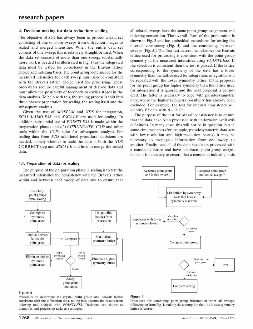
4.1. Preparation of data for scaling

The purpose of the preparation phase in scaling is to test the

measured intensities for consistency with the Bravais lattice

within and between each sweep of data and to ensure that

all related sweeps have the same point-group assignment and

indexing convention. The overall ‘flow’ of the preparation is

shown in Fig. 3 and has embedded procedures for testing the

internal consistency (Fig. 4) and the consistency between

sweeps (Fig. 5.) The first test determines whether the Bravais

lattice used for processing is consistent with the point-group

symmetry in the measured intensities using POINTLESS. If

the selection is consistent then the test is passed. If the lattice

corresponding to the symmetry of the data has a lower

symmetry than the lattice used for integration, integration will

be repeated with the lower symmetry lattice. If the proposal

for the point group has higher symmetry than the lattice used

for integration it is ignored and the next proposal is consid-

ered. The latter is necessary to cope with pseudosymmetric

data, where the higher symmetry possibility has already been

excluded. For example, the test for internal consistency will

identify P2 data with � = 90.0�.

The purpose of the test for overall consistency is to ensure

that the data have been processed with uniform unit-cell axis

definitions. In many cases this will not be in question, but in

some circumstances (for example, pseudosymmetric data sets

with low-resolution and high-resolution passes) it may be

necessary to propagate information from one sweep to

another. Finally, once all of the data have been processed with

a consistent lattice and have consistent point-group assign-

ments it is necessary to ensure that a consistent indexing basis

research papers


Figure 5Procedure for combining point-group information from all sweeps,following on from Fig. 4, making the assumption that the lowest symmetrylattice is correct.

Figure 4Procedure to determine the crystal point group and Bravais latticeconsistent with the diffraction data, taking into account the results fromindexing and analysis with POINTLESS. Decisions are shown asdiamonds and processing tasks as rectangles

is used. In situations in which the Bravais lattice has higher

symmetry than the point group it is possible to assign equally

valid but inconsistent basis vectors. For scaling it is critical that

these are consistently defined so that xia2 compares the

indexing of second and subsequent sweeps with the first using

POINTLESS and the data are reindexed as required. These

preparation for scaling steps are common to both the two-

dimensional and the three-dimensional pipelines.

4.2. Two-dimensional pipeline: scaling with SCALA

The approach to scaling performed by SCALA and

AIMLESS is to determine a parameterized empirical model

for the experimental contributions to the measured intensities

and then to adjust the parameters of this model to minimize

the differences between symmetry-related intensity observa-

tions. The recommended protocol for scaling (as expressed

in CCP4i; Evans, 2006) is to have the overall scale smoothed

over 5� intervals, to allow an isotropic B-factor correction

smoothed over 20� intervals (for radiation damage) and to

have an absorption surface for the diffracted beam para-

meterized with six orders of spherical harmonics. While this

model works well, there are examples where including addi-

tional corrections (e.g. the TAILS correction for partial bias)

may substantially improve the level of agreement between the

observations. As such, a decision is needed as to the most

appropriate scaling model to apply.

Initially, an investigation was performed for 12 JCSG data

sets, testing eight scaling models with each, as summarized

in Table 3. The Rmerge values for each were normalized to the

range 0–1, where 0 corresponds to the lowest and 1 to the

highest. As is clear from Fig. 6, no single model reliably gave

the lowest merging residuals. The conclusion was therefore

that the optimum scaling model must be determined for each

case. Within xia2 this process is implemented by initially

allowing five cycles of scale refinement and is scored by Rmerge

in the low-resolution shell and the convergence rate. The low-

resolution Rmerge is used as the scale factors for the data set are

dominated by the strong low-resolution data and the extent of

the data set is unchanging (i.e. the usual criticism of Rmerge

does not apply). In addition, the low-resolution data contri-

bute to all elements of the scaling corrections owing to the way

in which the corrections are parameterized, making the

process robust. Once the scaling model has been selected

more cycles are allowed for full scaling.

Resolution limits are calculated following the procedures

set out in x4.4 based on an analysis of the intensities after the

initial scaling. In terms of the fine-grained parameterization

(e.g. the rotation spacing for the B-factor correction) little

benefit was found in deviating from the defaults. Finally, early

versions of xia2 included an iterative remerging protocol to

refine the error-correction parameters to obtain �2 = 1. As

both AIMLESS and SCALA now perform this refinement this

now-redundant process was removed.

4.3. Three-dimensional pipeline: scaling with XSCALE

SCALA and AIMLESS use a parameterized model to

determine the scale factors for each reflection. In contrast,

XDS and XSCALE use arrays of correction factors to remove

the correlation of the measured intensities with image number

and detector position (Kabsch, 2010). Correction factors are

applied for sample decay, absorption and detector sensitivity,

and the combination of corrections to apply is under the

control of the user, although the default if no instruction is

given is to apply all corrections.

In the XDS CORRECT step the corrections are determined

for each sweep in isolation, whereas the corrections are jointly

refined for all sweeps in XSCALE. When this was investigated

during xia2 development little benefit was observed in scaling

the data twice (i.e. in the XDS CORRECT step and in

XSCALE) as this doubled the number of correction factors,

so the choice was made to scale the data only in XSCALE.

Subsequent discussion with the authors of XDS highlights that

research papers


Table 3Eight different scaling models tested for the 12 JCSG data sets,corresponding to the normalized merging residuals shown in Fig. 6.

The first run corresponds to a very simple scaling model, while the last includesall corrections and run 4 corresponds to the CCP4i default.

Scaling runPartiality correct(i.e. ‘tails’)

Decay correction(i.e. ‘bfactor on’)

Absorption correction(i.e. ‘secondary 6’)

1 No No No2 No No Yes3 No Yes No4 No Yes Yes5 Yes No No6 Yes No Yes7 Yes Yes No8 Yes Yes Yes

Figure 6Rmerge values for each of the 12 JCSG data sets used (with a differentcolour for each) for all eight permutations of the scaling model shown inTable 3, normalized to the range 0–1 (lowest to highest). Clearly, no singlemodel systematically gives the lowest residual and almost all models workwell for at least one example and are hence worth considering.

this apparent doubling of the number of correction factors

may be misleading (Kay Diederichs, private communication).

In terms of the choice of corrections to apply, it was found

that, unlike in SCALA and AIMLESS, applying all of the

possible corrections always gives the lowest residual. Conse-

quently, all corrections are applied in xia2, with a user option

to override this decision. After initial scaling the resolution

limits are determined following the procedures set out in x4.4,

after which the scaling is repeated with the limits applied. The

scaled intensities are then output unmerged, converted to

MTZ format and merged with SCALA or AIMLESS to

generate a report of merging statistics.

4.4. Resolution-limit calculation

One of the key decisions to make in MX data reduction is

the assignment of a resolution limit. Too low a limit will result

in throwing away useful data, while too high a limit may not

improve the structure solution and refinement and may

suggest excessive precision in the resulting atomic coordinates.

Historically, a wide range of heuristic criteria have been used

to decide the high-resolution limit of the data, including

thresholds on the I/�(I), Rmerge and completeness. Recent

systematic studies suggest that methods based on correlation

coefficients may give a more robust insight (Evans &

Murshudov, 2013; Karplus & Diederichs, 2012); however,

these have yet to be implemented in xia2.

Within xia2, the I/�(I), Rmerge and completeness may be

used as criteria for resolution-limit determination. By default

the merged and unmerged I/�(I) are used, with thresholds of

2 and 1, respectively. While the former reflects a ‘digest’ of

several CCP4 Bulletin Board discussions on the subject of

resolution limits, it is important to note that the user has

complete control over the resolution-limit criteria. The latter

limitation becomes more significant with high-multiplicity

(tenfold or more) data. To be specific: during the development

of xia2 it was found that in high-multiplicity cases an I/�(I) of

2 may correspond to an unmerged I/�(I) of <0.5. In these cases

it was found that the merged intensity measurements in the

outer resolution shells tended towards a normal distribution

rather than the expected exponential distribution (as assessed

by the statistic E4), suggesting that the measurements were

dominated by noise. While this result may indicate a poor

treatment of the experimental errors for weak reflections,

the choice was made to additionally impose a limit on the

unmerged I/�(I) to ensure that the reduced data were reliable.

This has the side effect of typically limiting the Rmerge in the

outer shell to be less than 100%. The authors note that a

treatment of resolution limits based on correlation coefficients

would not suffer from these issues.

To calculate the resolution limits, early versions of xia2 used

an analysis of the SCALA log-file output. This was found to

be sensitive to the choice of resolution bins, so more recent

versions of xia2 compute the merged and unmerged I/�(I),

the Rmerge and the completeness directly from the scaled but

unmerged reflection data and fit an appropriately smoothed

curve before identifying the limit. In addition to having fine-

grained control over the resolution-limit criteria, the user may

also set an explicit resolution limit. Finally, inclusion of the

option of correlation coefficient based resolution limits is

planned for the near future.

4.5. Post-processing

Although the primary objective of xia2 is to arrive at

correctly integrated, scaled and merged intensities, there are

a small number of downstream analysis steps which make the

system more useful to the user by providing data files ready

for immediate structure solution and refinement. The analysis

steps are to calculate structure-factor amplitudes from the

intensities following the TRUNCATE procedure (French &

Wilson, 1978) as implemented in CTRUNCATE, to perform

local scaling using SCALEIT (Howell & Smith, 1992) for data

with more than one logical wavelength and to determine an

‘average’ unit cell for downstream analysis. Additionally,

reflection-file manipulation is performed with CAD from the

CCP4 suite and the data are assessed for twinning using

methods included in cctbx.

The calculation of structure-factor amplitudes from inten-

sities fundamentally consists of a scaled square root. The scale

factor reflects the fact that the intensities are recorded on an

arbitrary scale while the structure-factor amplitude scale

depends on the contents of the unit cell (Wilson, 1942). The

square root corresponds to the fact that the intensities are

proportional to the square of the structure-factor amplitude.

The TRUNCATE procedure is a treatment for measured

negative intensities, computing the most likely value for the

true intensity given the positivity constraint. For this to be

correctly applied it is critical that the systematically absent

reflections are removed. Absent reflections resulting from

centring operations (e.g. h + k + l odd for body-centred

systems) are excluded during integration based on the Bravais

lattice choice. To remove those resulting from the screw axes

of the space group it is first necessary to identify a space group

consistent with these absences: for this POINTLESS is used.

While the result of this analysis is typically not unique, it is

assumed that the result should be appropriate for reducing the

bias in the TRUNCATE procedure. The user should be aware

that although the point-group assignment from xia2 is typi-

cally reliable, the space-group assignment may be incorrect

and is also reliant on the axial reflections having been

recorded. A list of all likely space groups (i.e. those consistent

with the observed systematic absences) is provided in the

console output.

If a sequence file is found alongside the diffraction data or

is provided in the input file, an estimate of the number of

molecules in the asymmetric unit is made following a prob-

abilistic procedure (Kantardjieff & Rupp, 2003) and an

appropriate solvent content is provided to the TRUNCATE

procedure. In the absence of this information a solvent frac-

tion of 50% is assumed, with the remaining volume filled with

‘average’ protein (as described in the TRUNCATE manual

page).

research papers


5. Implementing automated data reduction

Up to this point, the emphasis of this paper has been on the

decision-making protocols for MX data reduction. To provide

a useful tool for the user, these decisions must be embedded in

a framework which expresses the overall workflow of the data

analysis. In this section, the technical details of how xia2 works

will be described.

5.1. Data management

As an expert system can only make decisions and perform

analysis based on the information available, careful manage-

ment of all data is critical. Most of the data familiar to

macromolecular crystallographers define static information,

including coordinate and reflection files. Within xia2 some

information is static, for example user input, but the majority

of the information is dynamic in nature: the current state of

hypotheses which are subject to change depending on the

outcome of subsequent analysis. In the case of dynamic

information it is important that their provenance is tracked, so

that if a hypothesis is invalidated (e.g. the assignment of the

Bravais lattice) all of the results derived from that hypothesis

(e.g. the integrated data) are also invalidated. Within xia2 the

approach to resolving this challenge is to maintain links to all

of the sources of information and to ensure that information is

freshly requested every time it is needed rather than stored.

The main information provided to the system is the raw

diffraction data, with suitable metadata (i.e. image headers;

detailed in Supplementary Material) to describe the experi-

ment. Provided that the data are from a single sample or set of

equivalent crystals this information will be sufficient to build

a useful model of how the experiment was performed. Within

xia2 the raw data are structured in terms of sweeps of

diffraction data, which belong to wavelengths (which are

merged to a single MTZ data set in the output), which in turn

belong to crystals, which are finally contained within projects.

Crystals are also the fundamental unit of data for scaling.

All of these data structures (project, crystal, wavelength and

sweep) map directly onto objects within xia2 and initially

contain only static data: from this information it is possible to

perform analysis using the procedures described earlier and to

draw conclusions. In the situation where the data are not from

a single sample or set of equivalent samples (for example,

isomorphous derivatives recorded at a single wavelength) xia2

cannot know from the image headers alone how best to treat

the data. In this situation it is necessary for the user to prepare

a xia2 input file defining the logical structure of the data to be

processed (see the xia2 manual for details.)

Within xia2 the analysis steps are performed by software

modules (Indexers, Integraters and Scalers), each of which have

a well defined responsibility within the processing workflow.

As described above, there will be situations where the analysis

in one step will be dependent on the results of a previous step,

and as such a reference to these results must be kept. This is

greatly simplified if all implementations of a given function

(i.e. indexing, integration and scaling) share a common

description: in software terms they share a common interface.

Within xia2 links to information are maintained via this

common interface, greatly simplifying the bookkeeping

components of the software.

5.2. Expert system interfaces

The use of abstract interfaces for software modules is a

common paradigm in modern software development, as other

software using that module does not need to know about the

internal details. In particular, the module may be replaced

with another instance sharing the same interface with no loss

of functionality. Within xia2 abstract interfaces are defined for

the key analysis steps, with the intention that the modules

which perform these key analysis steps (e.g. wrappers around

MOSFLM, LABELIT or XDS) interact only through the

abstract interfaces. As an example, both MOSFLM and

LABELIT may be used to index a diffraction pattern based on

a small number of images from a sweep, so both may present

an Indexer interface. The details of how the indexing is

performed and how the results are interpreted will be

program-specific and are implemented in MosflmIndexer and

LabelitIndexer, respectively. This approach has several

advantages. Firstly, new modules may be added to the system

without modification of the rest of the system. Secondly, code

that is common to all implementations of a given interface

may reside within the interface definition rather than being

duplicated. An example of this is the handling of indexing

solutions, where the management of the solutions and the

handling of Bravais lattice solutions is in the Indexer interface

code. Finally, this simplifies the two-way connections between

modules, as they can share a common ‘language’. This is

particularly important where, for example, a Bravais lattice

choice is found to be incorrect late in the analysis: the beha-

viour of how to recover this situation is independent of the

indexing software used.

Finally, it was decided that each analysis interface would be

split into three phases, prepare, do and finish, arranged within

loops (Fig. 7). The status of each phase is managed within the

module and each phase will be performed until it is success-

research papers


Figure 7General flow of expert system interfaces, showing how the prepare, doand finish functions are used to ensure that all prior tasks are completedbefore a new step is initiated

fully completed or an error occurs. Once the finish phase is

completed it will be assumed that all results derived are valid

until proven otherwise, which will be verified when the results

are requested. If subsequent analysis indicates that a result is

incorrect this will be flagged and a new result calculated in

response to the next request. Any change in the input may also

invalidate the internal state, ensuring that the next time the

results are requested they will be recalculated taking this

change into consideration. While such a structure may appear

to be complex, it has real benefits when linked to the data

hierarchy described in x5.1.

5.3. Linking data structures and interfaces

The benefit of having standard interfaces to the key analysis

steps and clear links to the data hierarchy is that the source

of any particular piece of information is well known. In xia2

links are made from objects in the data hierarchy to analysis

modules which act on these objects, namely from sweeps to

Indexers and Integraters and from crystals to Scalers. This

means that if a sweep is asked for the unit cell and Bravais

lattice it may delegate this request to the Indexer. If no

indexing has yet been performed or the solution has been

invalidated then the sweep may be indexed automatically to

provide the result. If a valid result is available this will be

returned immediately.

This structure means that all analysis is performed when the

results are needed and not before, ensuring that no unneces-

sary processing is performed. The loop structure of each

module ensures that invalid results can be recalculated before

the processing can proceed. In addition, the second outcome

of this structure is that, since the dependency relationships

between all pieces of information are well known, the

processing necessary to deliver a result is performed implicitly.

The result of this is that the ‘main program’ of xia2 is in effect

a print statement, with the processing performed to provide

the results to print.

6. Discussion

The growth in the field of MX and the emphasis on answering

biological questions has led to a strong push for the

development of high-throughput techniques. One outcome of

this has been the emergence of a new class of user of MX: the

biologist using MX as a tool without themselves being an

expert crystallographer. This has created a demand for more

expert tools to help the user to collect and analyse their data

and to solve and refine their structures. xia2 provides a plat-

form for the reduction and analysis of raw crystallographic

data and embeds within it expertise on the use of several well

respected data-reduction packages. By encoding decisions as

hypotheses to be tested as analysis proceeds, xia2 has the

flexibility to use results from all steps in the analysis. The

architecture also allows extension to include new software as

and when it becomes available to adapt to the demands of

crystallographers and to keep pace with new developments.

The decision-making protocols here reflect a systematic

study of processing options for structural genomics data. Many

of the conclusions of this reassuringly reflect ‘common sense’;

for example, following the recommendations from the authors

of MOSFLM on integration protocols with that program!

Other outcomes suggest that small changes in established

protocols can result in improvements to the reliability of the

processing or to the accuracy of the results. As such, even

with interactive processing with, for example, iMosflm these

suggestions may be useful. While the fact that the study was

performed with structural genomics data may suggest some

bias to the effectiveness of xia2 with less than ideal data,

experience (and citations) suggest that the results derived here

have more widespread applicability.

The authors would like to thank the JCSG, the Division of

Structural Biology at the Wellcome Trust Centre for Human

Genetics and numerous users for providing the test data which

were used in developing this software. We would also like to

thank the reviewers for their comments on the manuscript, as

well as the staff and users at Diamond Light Source for their

input into xia2 and feedback on its effectiveness. The authors

would like to thank Harry Powell and Andrew Leslie for help

with making the best use of MOSFLM, Nicholas Sauter for

help with LABELIT and specific modifications to the

program, Phil Evans for help with SCALA, AIMLESS and

POINTLESS, including specific changes to those programs,

and Wolfgang Kabsch and Kay Diederichs for help with XDS/

XSCALE. Without the many years of effort put into these

packages, xia2 would not be possible. Development work for

xia2 is currently supported by Diamond Light Source Ltd and

has also been supported by the BBSRC through the e-Science

pilot project e-HTPX and the EU Sixth Framework through

BioXHit and CCP4.

References

Allan, R. et al. (2003). Proceedings of the UK e-Science All HandsMeeting 2003, edited by S. Cox, p. 230. http://www.nesc.ac.uk/events/ahm2003/AHMCD/pdf/049.pdf.

Battye, T. G. G., Kontogiannis, L., Johnson, O., Powell, H. R. & Leslie,A. G. W. (2011). Acta Cryst. D67, 271–281.

Dauter, Z. (1999). Acta Cryst. D55, 1703–1717.Evans, P. (2006). Acta Cryst. D62, 72–82.Evans, P. & Murshudov, G. (2013). Acta Cryst. D69, 1204–1214.French, S. & Wilson, K. (1978). Acta Cryst. A34, 517–525.Grosse-Kunstleve, R. W., Sauter, N. K. & Adams, P. D. (2004). Acta

Cryst. A60, 1–6.Grosse-Kunstleve, R. W., Sauter, N. K., Moriarty, N. W. & Adams,

P. D. (2002). J. Appl. Cryst. 35, 126–136.Holton, J. & Alber, T. (2004). Proc. Natl Acad. Sci. USA, 101, 1537–

1542.Howell, P. L. & Smith, G. D. (1992). J. Appl. Cryst. 25, 81–86.Kabsch, W. (2010). Acta Cryst. D66, 125–132.Kantardjieff, K. A. & Rupp, B. (2003). Protein Sci. 12, 1865–1871.Karplus, P. A. & Diederichs, K. (2012). Science, 336, 1030–1033.Le Page, Y. (1982). J. Appl. Cryst. 15, 255–259.Leslie, A. G. W. & Powell, H. R. (2007). Evolving Methods for

Macromolecular Crystallography, edited by R. J. Read & J. L.Sussman, pp. 41–51. Dordrecht: Springer.

research papers

























Leslie, A. G. W., Powell, H. R., Winter, G., Svensson, O., Spruce, D.,McSweeney, S., Love, D., Kinder, S., Duke, E. & Nave, C. (2002).Acta Cryst. D58, 1924–1928.

Powell, H. R. (1999). Acta Cryst. D55, 1690–1695.Sauter, N. K., Grosse-Kunstleve, R. W. & Adams, P. D. (2004). J. Appl.

Cryst. 37, 399–409.Steller, I., Bolotovsky, R. & Rossmann, M. G. (1997). J. Appl. Cryst.

30, 1036–1040.

Vonrhein, C., Flensburg, C., Keller, P., Sharff, A., Smart, O., Paciorek,W., Womack, T. & Bricogne, G. (2011). Acta Cryst. D67, 293–302.

Weiss, M. S. & Hilgenfeld, R. (1997). J. Appl. Cryst. 30, 203–205.

Wilson, A. J. C. (1942). Nature (London), 150, 152.Winn, M. D. et al. (2011). Acta Cryst. D67, 235–242.Winter, G. (2010). J. Appl. Cryst. 43, 186–190.

research papers


















Decision making in xia 2

Documents

Transcript of Decision making in xia 2