1

Data Partitioning with a Realistic Performance Model of Networks of Heterogeneous Computers

Alexey Lastovetsky, Ravi Reddy Department of Computer Science University College Dublin, Belfield Dublin 4, Ireland

E-mail: Alexey.Lastovetsky@ucd.ie, Manumachu.Reddy@ucd.ie Abstract---In this paper, we address the problem of optimal distribution of computational tasks on a network of heterogeneous computers when one or more tasks do not fit into the main memory of the processors and when relative speeds cannot be accurately approximated by constant functions of problem size. We design efficient algorithms to solve the scheduling problem using a realistic performance model of network of heterogeneous computers. This model integrates many essential features of a network of heterogeneous computers having a major impact on its performance such as the processor heterogeneity, the heterogeneity of memory structure, and the effects of paging. Under this model, the speed of each processor is represented by a continuous and relatively smooth function of the size of the problem whereas standard models use single numbers to represent the speeds of the processors. We formulate a problem of partitioning of an n-element set over p heterogeneous processors using this model and design efficient algorithms for its solution whose worst-case complexity is O(p2×log2n) but the best-case complexity is O(p×log2n). Index Terms---Heterogeneous systems, Scheduling and task partitioning, Load balancing and task assignment

1. Introduction

In this paper, we deal with the problem of optimal distribution of computational tasks across heterogeneous computers when one or more tasks do not fit into the main memory of the processors and when relative speeds cannot be accurately approximated by constant functions of the problem size. These tasks are processed in parallel by the computers. Examples of applications include search for patterns in text, audio, graphical files, processing of very large linear data files as in signal processing, image processing, and experimental data processing, linear algebra algorithms, simulation, combinatorial optimization algorithms, and many others. We design efficient algorithms to solve this scheduling problem using a performance model that integrates some of the essential features of a heterogeneous network of computers (HNOC) having a major impact on the performance, such as the processor heterogeneity, the heterogeneity of memory structure, and the effects of paging.

A number of algorithms of parallel solution of scientific and engineering problems on HNOCs have been designed and implemented [1], [2], [3], [4]. They use different performance models of HNOCs to distribute computations amongst the processors involved in their execution. All the models use a single positive number to represent the speed of a processor, and computations are distributed amongst the processors such that their volume is proportional to this speed of the processor. Cierniak, Zaki and Li [5] use the notion of normalized processor speed (NPS) in their machine model to solve the problem of scheduling parallel loops at compile time for HNOCs.

2

NPS is a single number and is defined as the ratio of time taken to execute on the processor under consideration, with respect to the time taken on a base processor. In [6] and [7], normalized cycle-times are used, i.e. application dependent elemental computation times, which are computed via small-scale experiments (repeated several times, with an averaging of the results). Several scheduling and mapping heuristics have been proposed to map task graphs onto HNOCs [8], [9], [10]. These heuristics employ a model of a heterogeneous computing environment that uses a single number for the computation time of a subtask on a machine. Yan, Zhang, and Song [11] use a two-level model to study performance predictions for parallel computing on HNOCs. The model uses two parameters to capture the effects of an owner workload. These are the average execution time of the owner task on a machine and the average probability of the owner task arriving on a machine during a given time step.

However these models are efficient only if the relative speeds of the processors involved in the execution of the application are a constant function of the size of the problem and can be approximated by a single number. This is true mainly for homogeneous distributed memory systems where:

• The processors have almost the same size at each level of their memory hierarchies, and • Each computational task assigned to a processor fits in its main memory.

But these models become inefficient in the following cases: • The processors have significantly different memory structure with different sizes of

memory at each level of memory hierarchy. Therefore, beginning from some problem size, the same task will still fit into the main memory of some processors and stop fitting into the main memory of others, causing the paging and visible degradation of the speed of these processors. This means that their relative speed will start significantly changing in favor of non-paging processors as soon as the problem size exceeds the critical value.

• Even if the processors of different architectures have almost the same size at each level of the memory hierarchy, they may employ different paging algorithms resulting in different levels of speed degradation for the task of the same size, which again means the change of their relative speed as the problem size exceeds the threshold causing the paging.

Thus considering the effects of processor heterogeneity, memory heterogeneity, and the effects of paging significantly complicates the design of algorithms distributing computations in proportion with the relative speed of heterogeneous processors. One approach to this problem is to just avoid the paging as it is normally done in the case of parallel computing on homogeneous multi-processors. However avoiding paging in local and global HNOCs may not make sense because in such networks it is likely to have one processor running in the presence of paging faster than other processors without paging. It is even more difficult to avoid paging in the case of distributed computing on global networks. There may not be a server available to solve the task of the size you need without paging.

Therefore, to achieve acceptable accuracy of distribution of computations across heterogeneous processors in the possible presence of paging, a more realistic performance model of a set of heterogeneous processors is needed. In this paper, we suggest a model where the speed of each processor is represented by a continuous and relatively smooth function of the problem size whereas standard models use a single number to represent the speed. This model integrates some of the essential features underlying applications run on general-purpose common heterogeneous networks, such as the processor heterogeneity in terms of the speeds of the processors, the memory heterogeneity in terms of the number of memory levels of the memory hierarchy and the size of each level of the memory hierarchy, and the effects of paging. This

3

Table 1 Specifications of four heterogeneous computers

Machine Name Architecture cpu MHz

Main Memory (kBytes)

Cache (kBytes)

Comp1 Linux 2.4.20-8

Intel(R) Pentium(R) 4 2793 513304 512

Comp2 SunOS 5.8 sun4u sparc

SUNW,Ultra-5_10 440 524288 2048

Comp3 Windows XP 3000 1030388 512

Comp4 Linux 2.4.7-10 i686 730 254524 256

ArrayOpsF

Size of the array

Abs

olu

te s

peed

(MF

lops

)

Comp3

Comp4

Comp2

Comp1

P

P

P

P

(a)

MatrixMultATLAS

Size of the matrix

Abs

olu

te s

peed

(MF

lops

)

Comp4

Comp2

Comp1

P

PP

MatrixMult

Size of the matrix

Ab

solu

te s

pee

d (

MF

lop

s)

Comp3

Comp2

Comp1

Comp4

P

P

P

(b) (c)

Fig. 1. The effect of caching and paging in reducing the execution speed of each of the four applications run on network of heterogeneous computers shown in Table 1. (a) ArrayOpsF, (b) MatrixMultATLAS, and (c) MatrixMult. P is the point where paging starts occurring. model is application-centric in the sense that generally speaking different applications will characterize the speed of the processor by different functions.

In this model, we do not incorporate one feature, which has a significant impact on the optimal distribution of computations over heterogeneous processors. This feature is the latency and the bandwidth of the communication links interconnecting the processors. This factor can be ignored if the contribution of communication operations in the total execution time of the application is

4

negligible compared to that of computations. Otherwise, any algorithm of distribution of computations aimed at the minimization of the total execution time should take into account not only the heterogeneous processors but also the communication links whose maximal number is equal to the total number of heterogeneous processors squared. This significantly increases the space of possible solutions and increases the complexity of data partitioning algorithms. Any performance model must also take into account the contention that may be caused in the network. On a heterogeneous network of workstations using Ethernet as the interconnect, the performance will suffer if many messages are being sent at the same time. Therefore it is desirable to schedule a parallel program in such a way that only one processor sends a message at a given time. So optimal communication schedules must be obtained to reduce the overall communication time. The communication scheduling algorithms must be adaptive to variations in network performance and that derive the schedule at runtime based on current information about network load. However the problem of finding the optimal communication schedule is NP-complete. The issues involved in including the cost of communications are discussed in more detail in [12]. Bhat et al. [13] present a heuristic algorithm that is based on a communication model that represents the communication performance between every processor pair using two parameters: a start-up time and a data transmission rate. The incorporation of communication cost in our functional model and subsequent derivation of efficient data partitioning algorithms using this model is a subject of our future research. In this paper, we intend to fully focus on the impact of the heterogeneity of processors on optimal distribution of computations.

There are two main motivations behind the representation of the speed of the processor by a continuous and relatively smooth function of the problem size. First of all, we want the model to adequately reflect the behavior of common, not very carefully designed applications. Consider the experiments with a range of applications differently using memory hierarchy that are presented in [14] and shown in Figure 1. Carefully designed applications ArrayOpsF and MatrixMultAtlas, which efficiently use memory hierarchy, demonstrate quite a sharp and distinctive performance curve of dependence of the absolute speed on the problem size. For these applications, the speed of the processor can be approximated by a step-wise function of the problem size. At the same time, application MatrixMult, which implements a straightforward algorithm of multiplication of two dense square matrices and uses inefficient memory reference patterns, displays quite a smooth dependence of speed on the problem size. For such applications, the speed of the processor can not be accurately approximated by a step-wise function. It should be approximated by a continuous and relatively smooth function of the problem size if we want the performance model to be accurate enough.

The other main motivation is that we target general-purpose common heterogeneous networks rather than dedicated high performance computer systems. A computer in such a network is persistently performing some minor routine computations and communications just as an integrated node of the network. Examples of such routine applications include email clients, browsers, text editors, audio applications, etc. As a result, the computer will experience constant and stochastic fluctuations in the workload. This changing transient load will cause a fluctuation in the speed of the computer in the sense that the execution time of the same task of the same size will vary for different runs at different times. The natural way to represent the inherent fluctuations in the speed is to use a speed band rather than a speed function. The width of the band characterizes the level of fluctuation in the performance due to changes in load over time. The shape of the band makes the dependence of the speed of the computer on the problem size

5

MatrixMultATLAS

0 2000 4000 6000 8000 10000

Size of the matrix

Ab

solu

te s

pee

d (

MF

lop

s)

8%5%

30%

MatrixMultATLAS

0 2000 4000 6000 8000 10000

Size of the matrix

Ab

solu

te s

pee

d (

MF

lop

s)

7% 5%35%

(a) (b)

MatrixMultATLAS

0 1000 2000 3000 4000

Size of the matrix

Abs

olut

e sp

eed

(MFl

ops)

7% 5%40%

(c)

Fig. 2. Effect of workload fluctuations on the execution of application MatrixMultATLAS on computers shown in Table 1. The width of the performance bands is given in percentage of the maximum speed of execution of the application. (a) Performance band for Comp1, (b) Performance band for Comp2, and (c) Performance band for Comp4. less distinctive and sharp even in the case of carefully designed applications efficiently using the memory hierarchy. Therefore, even for such applications the speed of the processor can be realistically approximated by a continuous and relatively smooth function of the problem size. Figure 2 shows experiments conducted with application MatrixMultATLAS on a set of computers whose specifications are shown in Table 1. The application employs the level-3 BLAS routine dgemm [15] supplied by Automatically Tuned Linear Algebra Software (ATLAS) [16]. ATLAS is a package that generates efficient code for basic linear algebra operations. The computers have varying specifications and varying levels of network integration and are representative of the range of computers typically used in networks of heterogeneous computers.

Representation of the dependence of the speed on the problem size by a single curve is reasonable for computers with moderate fluctuations in workload because in this case the width of the performance band is quite narrow. On networks with significant workload fluctuations, the speed function of the problem size should be characterized by a band of curves rather than by a single curve. In the experiments that we have conducted, we observed that computers with high level of integration into the network produce fluctuations in speed that is in the order of 40% for small problem sizes declining to approximately 6% for the maximum problem size solvable on the computer. The influence of workload fluctuations on the speed becomes less significant as

6

the execution time increases. There is a close to linear decrease in the width of the performance band as the execution time increases. For computers with low level of integration, the width of the performance band was not greater than around 5-7% even when there was heavy file sharing activity. It is observed that for computers already engaged in heavy computational tasks, the addition of heavy loads just shifts the band to a lower level with the width of the band remaining constant, that is, the upper and lower levels of speed are reduced with the width representing the difference between the levels remaining the same. However more experimental study needs to be carried out to accurately represent the width of the performance bands for computers with varying levels of integration to increase the efficiency of the model. This is a subject of our future research where we intend to improve our functional model by adding an additional parameter that reflects the level of workload fluctuations in the network.

The functional model does not take into account the effects on the performance of the processor caused by several users running heavy computational tasks simultaneously. It supposes only one user running heavy computational tasks and multiple users performing routine computations and communications, which are not heavy like email clients, browsers, audio applications, text editors etc.

In the section on experimental results, we present a practical procedure that adopts a heuristic approach to build the speed function for a processor in our experiments. However, the problem of efficiently building and maintaining the functional model requires further study and is open for research.

The problem of optimally scheduling divisible loads has been studied extensively and the theory is commonly referred to as Divisible Load Theory (DLT). The main features of earlier works in DLT [17], [18] are they assume distributed systems with a flat memory model and use a linear mathematical model where the speed of the processor is represented by a constant function of the problem size. Drozdowski and Wolniewicz [19] propose a new mathematical model that relaxes the above two assumptions. They study distributed systems, which have both the hierarchical memory model and a piecewise constant dependence of the speed of the processor on the problem size. However the model they formulate is targeted mainly towards optimal distribution of arbitrary tasks for carefully designed applications on dedicated distributed multiprocessor computer systems whereas our model is aimed towards optimal distribution of arbitrary tasks for any arbitrary application on general-purpose common heterogeneous networks.

The rest of the paper is organized as follows. In section 2, we formulate a problem of partitioning of an n-element set over p heterogeneous processors using the functional model and design efficient algorithms for its solution whose worst-case complexity is O(p2×log2n) but the best-case complexity is O(p×log2n). This problem is a simple variant of the more general partitioning problem [20] formulated below:

• Given: (1) A set of n elements with weights wi (i=0,…,n-1), and (2) A well-ordered set of p processors whose speeds are functions of the size of the problem, si=fi(x), with an upper bound bi on the number of elements stored by each processor (i=0,…,p-1),

• Partition the set into p disjoint partitions such that: (1) The sum of weights in each partition is proportional to the speed of the processor owning that partition, and (2) The number of elements assigned to each processor does not exceed the upper bound on the number of elements stored by it.

We use the simple variant to explain how complex is the problem of scheduling arbitrary tasks amongst processors when they have significantly different memory structure and when one or

7

more tasks do not fit into the main memory of the processors. We also use this variant to explain in simple terms how our data partitioning algorithms using the functional model can be used to achieve better data partitioning on networks of heterogeneous computers before moving on to solve the most advanced problem.

To demonstrate the efficiency of our data partitioning algorithms using the functional model, we perform experiments using naïve parallel algorithms for linear algebra kernel, namely, matrix multiplication and LU factorization using striped partitioning of matrices on a local network of heterogeneous computers. Our main aim is not to show how matrices can be efficiently multiplied or efficiently factorized but to explain in simple terms how the data partitioning algorithms using the functional model can be used to optimally schedule arbitrary tasks on networks of heterogeneous computers before moving on to solve the most advanced problem. We also view these algorithms as good representatives of a large class of data parallel computational problems and a good testing platform before experimenting more challenging computational problems.

2. Algorithms of partitioning sets

In this section, we present the algorithms of partitioning sets. In the figures we present for illustration, we use the notion of problem size. Kumar et al. [21] define the problem size as the number of basic computations in the best sequential algorithm to solve the problem on a single processor. Because it is defined in terms of sequential time complexity, the problem size is a function of the size of the input. For example, the problem size is O(n3) for n×n matrix multiplication and for irregular applications such as EM3D [22], [23] and N-body simulation [24], the problem size is O(n), where n is the number of nodes in a bipartite graph representing the dependencies between the nodes and number of bodies respectively.

However we do not use this computational complexity definition for problem size because it does not influence the speed of the processor. We define the size of the problem to be the amount of data stored and processed by the algorithm. For example for matrix-matrix multiplication of two dense n×n matrices, the size of the problem is equal to 3×n2.

One of the criteria to partitioning a set of n elements over p heterogeneous processors is that the number of elements in each partition should be proportional to the speed of the processor owning that partition. When the speed of the processor is represented by a single number, the algorithm used to perform the partitioning is quite straightforward, of complexity O(p2) [6]. The algorithm uses a naive implementation. The complexity can be reduced down to O(p×log2p) using ad hoc data structures [6].

This problem of partitioning a set becomes non-trivial when the speeds of the processors are given as a function of the size of the problem. Consider a small network of two processors, whose speeds as functions of problem size during the execution of the matrix-matrix multiplication are shown in Figure 3. If we use the single number model, we have to choose a point and use the absolute speeds of the processors at that point to partition the elements of the set such that the number of elements is proportional to the speed of the processor. If we choose the speeds ( )0100 , ss at points ( )00, sx and ( )01, sx to partition the elements of the set, the

distribution obtained will be unacceptable for the size of the problem at points ( )10, sy

and ( )11, sy where processors demonstrate different relative speeds compared to the relative

speeds at points ( )00, sx and ( )01, sx . If we choose the speeds ( )1110 , ss at points ( )10, sy

8

Matrix-Matrix Multiplication

Size of the problem

Ab

solu

te s

pee

d (

MF

lop

s)

),( 00sx

),( 01sx

),( 10sy

),( 11sy

Figure 3. A small network of two processors whose speeds are shown against the size of the problem. The Matrix-Matrix Multiplication used here uses a poor solver that does not use memory hierarchy efficiently. Figure 4. Optimal solution showing the geometric proportionality of the number of elements to the speed of the processor. and ( )11, sy to partition the elements of the set, the distribution obtained will be unacceptable for

the size of the problem at points ( )00, sx and ( )01, sx where processors demonstrate different

relative speeds compared to the relative speeds at points ( )10, sy and ( )11, sy . In some such cases,

the partitioning of the set obtained could be the worst possible distribution where the number of elements per processor obtained could be inversely proportional to the speed of the processor. In

Size of the problem

Ab

solu

te s

pee

d )(1 xs

)(2 xs

)(3 xs

)(4 xs

1x 2x 3x 4x

( ))(, 131 xsx

( ))(, 242 xsx( ))(, 313 xsx

( ))(, 424 xsx

4

42

3

31

2

24

1

13 )()()()(

x

xs

x

xs

x

xs

x

xs===

9

Size of the problem

Ab

solu

te s

pee

d)(1 xs

)(2 xs

)(3 xs

Maximum

Figure 5. Typical shapes of the graphs representing the speed functions of the processors observed experimentally. The graph represented by s1(x) is strictly a decreasing function of the size of the problem. The graph represented by s2(x) is initially an increasing function of the size of the problem followed by a decreasing function of the size of the problem. The graph represented by s3(x) is strictly an increasing function of the size of the problem. such cases, it is better to use an even distribution of equal number of elements per processor than the distribution based on using such wrong points.

The algorithms we propose are based on the following observation: If a distribution of the elements of the set amongst the processors is obtained such that the number of elements is proportional to the speed of the processor, then the points, whose coordinates are number of elements and speed, lie on a straight line passing through the origin of the coordinate system and intersecting the graphs of the processors with speed versus the size of the problem in terms of the number of elements. This is shown by the geometric proportionality in Figure 4.

Our general approach to finding the optimal straight line can be summarized as follows: 1. We assume that the speed of each processor is represented by a continuous function of the

size of the problem. The shape of the graph should be such that there is only one intersection point of the graph with any straight line passing through the origin. These assumptions on the shapes of the graph are representative of the most general shape of graphs observed for applications experimentally. The experiments conducted by Lastovetsky and Twamley [14] justify these assumptions. Applications that utilize memory hierarchy efficiently and applications that reference memory randomly deriving no benefits from caching produce speed functions that are an increasing function of problem size before a maximum followed by a decreasing function of problem size whereas applications that use inefficient memory reference patterns produce speed functions that are strictly decreasing functions of problem size. Some of the sample shapes of the graphs are shown in Figure 5.

2. At each step, we have two lines both passing through the origin. The sum of the number of elements at the intersection points of the first line with the graphs is less than the size of the problem, and the sum of the number of elements at the intersection points of second line with the graphs is greater than the size of the problem.

3. The region between these two lines is divided by a line passing through the origin into two smaller regions, the upper region and the lower region. If the sum of the number of elements at the intersection points of this line with the graphs is less than the size of the problem, the optimal

10

Size of the problem

Ab

solu

te s

pee

d)(1 xs

)(2 xs

)(3 xs

OptimalNon-optimal

),( 1111 sx

),( ,1,1 optopt sx

),( ,2,2 optopt sx

),( ,3,3 optopt sx

),( 2121 sx

),( 3131 xx

Figure 6. Uniqueness of the solution for a problem size n. The dashed line represents the optimal solution whereas the dotted line represents a non-optimal solution. line lies in the lower region. If this sum is greater than the size of the problem, the optimal line lies in the upper region.

4. In general, the exact optimal line intersects the graphs in points with non-integer sizes of the problem. This line is only used to obtain an approximate integer-valued solution. Therefore, the finding of any other straight line, which is close enough to the exact optimal one to lead to the same approximate integer-valued solution, will be an equally satisfactory output of the searching procedure. A simple stopping criterion for this iterative procedure can be the absence of points of the graphs with integer sizes of the problem within the current region. Once the stopping region is reached, the two lines limiting this region are input to the fine tuning procedure, which determines the optimal line.

Note that it is the continuity and the shape of the graphs representing the speed of the processors that make each step of this procedure possible. The continuity guarantees that any straight line passing through the origin will have at least one intersection point with each of the graphs, and the shape of the graph guarantees no more than one such an intersection point.

We now prove the uniqueness of the solution using mathematical induction starting by illustrating with an example for p=3. We safely assume that for each processor, for all x ≥ y, where x and y are problem sizes, the execution times tx and ty to execute problems of sizes x and y respectively are related by tx ≥ ty. Consider a small network of three processors, whose speeds as functions of problem size are shown in Figure 6. The graph represented by s1(x) is strictly a decreasing function of the size of the problem. The graph represented by s2(x) is initially an increasing function of the size of the problem followed by a decreasing function of the size of the problem. The graph represented by s3(x) is strictly an increasing function of the size of the problem. We show two solutions for a problem size n. The non-optimal solution is given by (x11,x21,x31) such that x11+x21+x31=n and the optimal solution is given by (x1,opt,x2,opt,x3,opt) such that x1,opt+x2,opt+x3,opt=n. The time of execution for the optimal solution topt is (x1,opt/s1,opt) or (x2,opt/s2,opt) or (x3,opt/s3,opt) because (x1,opt/s1,opt)=(x2,opt/s2,opt)=(x3,opt/s3,opt). The time of execution

11

Size of the problem

Ab

solu

te s

pee

dinitial line

final line

1θ

2θ

line with half of the slopes of the initial line and final line

( )2

21 θθ +

Upper half Lower half

Figure 7. Determination of the slope of the line equal to half of the slopes of the initial and final lines. of the non-optimal solution is )

s

x(

i1

i13

1max

=i

. Since x21>x2,opt, we can conclude that time of execution

t21of the problem size x21 equal to x21/s21 is always greater the time of execution given by the optimal solution topt i.e., t21>topt. Thus it can be inferred that the time of execution of the application obtained using the non-optimal solution is always greater than or equal to the time of execution of the application using the optimal solution. We can easily prove the same for different shapes of the speed functions.

Assuming this to be true for p=k processors, we have to prove the optimality for p=k+1 processors. For a given problem size n, let us assume the distribution given by our algorithm to be (x1,opt,x2,opt,…,xk+1,opt) such that (x1,opt/s1,opt)=(x2,opt/s2,opt)=…=(xk+1,opt/sk+1,opt)=topt and x1,opt+x2,opt+…+xk+1,opt=n where topt is the time of execution of the algorithm by the optimal solution. Now consider a distribution (x'1,x'2,..,x'k+1) such that x'1+x'2+…+x'k+1=n and x'i ≠ xi,opt for all i=1,2,…,k+1. If (x'1/s'1)=(x'2/s'2)=…=(x'k+1/s'k+1)=t'e, then it can be inferred that if t'e=topt, then x'i>xi,opt or x'i<xi,opt for all i=1,2,…,k+1 in which case the equality x'1+x'2+…+x'k+1=n is broken. If the proportionality (x'1/s'1)=(x'2/s'2)=…=(x'k+1/s'k+1) is ignored but the equality x'1+x'2+…+x'k+1=n is satisfied, then it can be easily seen that for atleast one processor i (i=1,2,…,k+1), x'i>xi,opt, thus giving an execution time t'i, which is greater than the execution time given by our algorithm topt.

Without loss of generality, in the figures we show the application of the algorithm only in the regions where absolute speed is a decreasing function of the size of the problem.

Let us estimate the cost of one step of this procedure. At each step we need to find the points of intersection of p graphs y=s1(x), y=s2(x), ..., y=sp(x), representing the absolute speeds of the processors, and the straight line y=c×x passing through the origin. In other words, at each step we need to solve p equations of the form c×x =s1(x), c×x =s2(x), ..., c×x =sp(x). As we need the same constant number of operations to solve each equation, the complexity of this part of one step will be O(p). According to our stopping criterion, a test for convergence can be reduced to testing p inequalities of the form li - ui <1, where li and ui are the size coordinates of the intersection points of the i-th graph with the lower and upper lines limiting the region respectively (i=1,2,…,p). This testing is also of the complexity O(p). Therefore, the total complexity of one step including the convergence test will still be O(p).

12

Size of the problem

Ab

solu

te s

pee

d)(1 xs

)(2 xs

)(3 xs

)(4 xs

line 1

line 2

line 3:

line 4:

1x 2x 3x 4x

nxxxx <+++ 4321

Optimally sloped line

nxxxx optoptoptopt =+++ ,4,3,2,1

nxxxx >+++ '4

'3

'2

'1

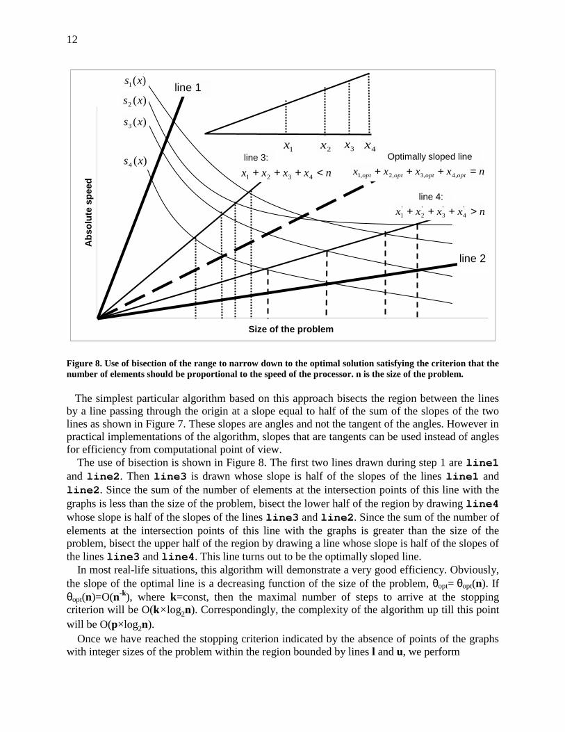
Figure 8. Use of bisection of the range to narrow down to the optimal solution satisfying the criterion that the number of elements should be proportional to the speed of the processor. n is the size of the problem.

The simplest particular algorithm based on this approach bisects the region between the lines by a line passing through the origin at a slope equal to half of the sum of the slopes of the two lines as shown in Figure 7. These slopes are angles and not the tangent of the angles. However in practical implementations of the algorithm, slopes that are tangents can be used instead of angles for efficiency from computational point of view.

The use of bisection is shown in Figure 8. The first two lines drawn during step 1 are line1 and line2. Then line3 is drawn whose slope is half of the slopes of the lines line1 and line2. Since the sum of the number of elements at the intersection points of this line with the graphs is less than the size of the problem, bisect the lower half of the region by drawing line4 whose slope is half of the slopes of the lines line3 and line2. Since the sum of the number of elements at the intersection points of this line with the graphs is greater than the size of the problem, bisect the upper half of the region by drawing a line whose slope is half of the slopes of the lines line3 and line4. This line turns out to be the optimally sloped line.

In most real-life situations, this algorithm will demonstrate a very good efficiency. Obviously, the slope of the optimal line is a decreasing function of the size of the problem, θopt= θopt(n). If θopt(n)=O(n-k), where k=const, then the maximal number of steps to arrive at the stopping criterion will be O(k×log2n). Correspondingly, the complexity of the algorithm up till this point will be O(p×log2n).

Once we have reached the stopping criterion indicated by the absence of points of the graphs with integer sizes of the problem within the region bounded by lines l and u, we perform

13

Size of the problem

Ab

solu

te s

pee

d)(1 xs)(2 xs

M

)(3 xsl

u2,x l

1,x l

pl ,x1,x u

pu ,x

2,x u

(x)sp

3,lx

3,ux⊗⊗ ⊗

⊗⊗ ⊗

Figure 9. Fine tuning procedure chooses the final p points of intersection from the p integer points closest to the non-integer points on line l and p integer points closest to the non-integer points on line u. There are no integers between the lines l and u. The integers closest to the non-integer points on lines l and u are indicated by crossed dots whereas integer points lying on lines l and u are indicated by dark dots. additional fine tuning to find the p integer points on the curves representing the speed functions of the processors thus giving us a solution closest to the optimal non-integer solution. This is illustrated in Figure 9. As can be seen from the figure, there are 2×p points, p integer points (xl,1,xl,2,…,xl,p), some of which could be closest to the non-integer points on line l whereas the rest of them lying on line l and similarly p integer points (xu,1,xu,2,…,xu,p) pertaining to line u. We have to choose an optimal set of p points from these 2×p points. The fine tuning procedure consists of the following steps:

1. We find out the times of execution xi/si of the problem sizes at these 2×p points where xi is the problem size assigned to the processor i and si is its speed exhibited at this problem size. This step is of complexity O(p).

2. We then sort these 2×p execution times using Quicksort algorithm and choose the p best execution times. The complexity of the Quicksort algorithm is O(2×p×log2(2×p)) = O(p×log2p).

The total complexity of the fine tuning process is O(p)+O(p×log2p) = O(p×log2p). So the total complexity of our partitioning algorithm is given by O(p×log2n)+O(p×log2p) = O(p×log2(n×p)).

If n»p, the total complexity of our partitioning algorithm is given by O(p×log2n). At the same time, in some situations this algorithm may be quite expensive. For example, if

θopt(n)=O(e-n), then the number of steps to arrive at the optimal line will be O(n). Correspondingly, the complexity of the algorithm will be O(p×n). After fine tuning, the complexity of the algorithm will be O(p×n)+O(p×log2p) = O(p×n).

We modify this algorithm to achieve reasonable performance in all cases, independent on how the slope of the optimal line depends on the size of the problem. To introduce the modified algorithm, let us re-formulate the problem of finding the optimal straight line as follows:

14

Size of the problem

Ab

solu

te s

pee

d)(1 xs

)(2 xsX

( )2X( )4

X

X = Space of solutions

Optimally sloped line

Figure 10. Bisection of the space of solutions in the modified algorithm.

Size of the problem

Ab

solu

te s

pee

d

)(1 xs

)(2 xs

)(3 xs

line 1

line 2

line 4:

nxxx <++ 321

First bisection

Second bisection

line 3:

Final bisection

Optimally sloped line

nxxx >++ '3

'2

'1

nxxx optoptopt =++ ,3,2,1

Figure 11. Modification of the algorithm shown in Figure 8 where the bisection results in efficient solution. n is the size of the problem.

15

Size of the problem

Ab

solu

te s

pee

d)(1 xs

)(2 xs

line 1

line 2

First bisection

Second bisection Optimally sloped line

M

)(xs p

nxxx p =+++ L21

pp nnn n solutions ofnumber Total 21 ≅×××= L

≤≤×××=

2 , ,

2 bisection secondAfter 2

11

1222

1

12 p

pp

nnnnn

nn L

LL , , ,2

bisection first After 221

111

21

11 nnnn

nnn p ≤≤×××=

M

( ) npn p22 log log bisections ofnumber Total ==

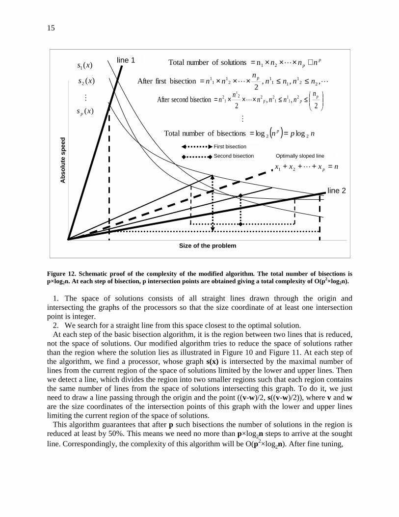
Figure 12. Schematic proof of the complexity of the modified algorithm. The total number of bisections is p×log2n. At each step of bisection, p intersection points are obtained giving a total complexity of O(p2×log2n).

1. The space of solutions consists of all straight lines drawn through the origin and intersecting the graphs of the processors so that the size coordinate of at least one intersection point is integer.

2. We search for a straight line from this space closest to the optimal solution. At each step of the basic bisection algorithm, it is the region between two lines that is reduced,

not the space of solutions. Our modified algorithm tries to reduce the space of solutions rather than the region where the solution lies as illustrated in Figure 10 and Figure 11. At each step of the algorithm, we find a processor, whose graph s(x) is intersected by the maximal number of lines from the current region of the space of solutions limited by the lower and upper lines. Then we detect a line, which divides the region into two smaller regions such that each region contains the same number of lines from the space of solutions intersecting this graph. To do it, we just need to draw a line passing through the origin and the point ((v-w)/2, s((v-w)/2)), where v and w are the size coordinates of the intersection points of this graph with the lower and upper lines limiting the current region of the space of solutions.

This algorithm guarantees that after p such bisections the number of solutions in the region is reduced at least by 50%. This means we need no more than p×log2n steps to arrive at the sought line. Correspondingly, the complexity of this algorithm will be O(p2×log2n). After fine tuning,

16

Size of the problem

Ab

solu

te s

pee

d)(1 xs

)(2 xs

)(3 xs line 1

line 2)(4 xs

Size of the problem = n

p

nx =

Figure 13. For most real-life situations, the optimal solution lies in the region with polynomial slopes. The optimal solution lies between line1 and line2 and they enclose a region with all polynomial slopes.

Size of the problem

Ab

solu

te s

pee

d

)(1 xs

)(2 xs

Minimum problem size Maximum experimentally obtained problem size

Figure 14. Using piece-wise linear approximation to build speed functions for 2 processors. The speed functions are built from 3 experimentally obtained points. the complexity of the algorithm will be O(p2×log2n)+O(p×log2p) = O(p2×log2n). A schematic proof of the algorithm is shown in Figure 12.

One can see that the modified bisection algorithm is not sensitive to the shape of the graphs of the processors, always demonstrating the same efficiency. The basic bisection algorithm is sensitive to their shape. It demonstrates higher efficiency than the modified one in better cases but much lower efficiency in worse cases.

An ideal bisection algorithm would be of the complexity O(p×log2n) reducing at each step the space of solutions by 50% and being insensitive to the shape of the graphs of the processors. The design of such an algorithm is still a challenge.

In cases where the magnitude of the size of the problem is of order millions, it might be worth relaxing the stopping criterion and not using the fine-tuning procedure. However it should be noted that the complexity of the algorithm will remain the same as fine-tuning procedure does

17

Size of the problem

Ab

solu

te s

pee

d)(1 xs

)(2 xs

)(3 xs

line 1

line 2

If the optimal solution lies in upper half, use simplest algorithm

If the optimal solution lies in lower half, use modified algorithm

)(4 xs

Figure 15. Using a combination of simplest and modified algorithm to efficiently solve problems for real-life applications. not add to the overall complexity although the cost in practice is minimized by relaxing the stopping criterion. If all the sub-optimal solutions are close to each other as to be indistinguishable as in this case, we can provide an approximate solution that is sufficiently accurate and at the same time economical in terms of practical cost. We intend to investigate this further in future research to provide an approximate solution that maintains a balance between accuracy and economy.

For a large range of problem sizes, it is very likely that the optimal solutions lie in the region with polynomial slopes as shown in Figure 13. In these cases, the simplest algorithm gives the optimal solution with best efficiency. However for very large problem sizes where the shapes of the speed functions tend to be horizontal, the modified algorithm gives the optimal solution with best efficiency. However both the simplest and the modified algorithm can be combined to solve data partitioning problems in real-life applications efficiently.

One approach consists of the following steps: 1. Speed functions are built for the processors involved in the execution of the parallel

application using a set of few experimentally obtained points. One of the ways to build a speed function for a processor is to use piece-wise linear function approximation as shown in Figure 14. Such approximation of the speed function is compliant with the requirements of the functional model. Also such an approximation of the speed function should give the speed of the processor for a problem size within acceptable limits of deviation from the speed given by an ideal speed function or the speed functions built with sets with more number of points. A practical procedure to build this piece-wise linear function approximation of speed function is explained in detail in Section 3.1.

2. Having built the speed functions for the processors, we use the simplest algorithm to bisect the region between the lower and upper lines as shown in Figure 15. If the solution lies in the upper half and the line bisecting the region between the lower and the upper lines

18

intersects the graphs of the processors at polynomial slopes, we use the simplest algorithm to obtain the optimal solution. This is because we know that the speed functions have polynomial slopes in the upper region and in such a case the simplest algorithm gives an optimal solution with ideal complexity. In other cases such as when the solution lies in the upper half and if the line bisecting the region between the lower and the upper lines intersects one or more graphs at horizontal slope or when the solution lies in the lower half, we use modified algorithm to obtain the optimal solution. This is because in such a case, we know that the modified algorithm is proven to demonstrate better efficiency than the simplest algorithm.

3. Experimental results

The experimental results are divided into two sections. The first section is devoted to building the functional model. We present the parallel applications and the network of heterogeneous computers on which the applications are tested. For each application, we explain how to estimate the processor speed. This is followed by presentation of the procedure to build the speed functions of the processors. For each application, we determine the problem sizes beyond which point paging starts happening and we also give the cost of building the speed function of each processor. We discuss the cost involved in finding the optimal solution using the partitioning algorithm and find it negligible compared to the cost of building the speed functions and the execution times of the parallel applications. In the second section, we present the experimental results obtained by running these applications on the network of heterogeneous computers.

3.1 Applications A small heterogeneous local network of 12 different Solaris and Linux workstations shown in Table 2 is used in the experiments. The network is based on 100 Mbit Ethernet with a switch enabling parallel communications between the computers. The amount of memory, which is the difference between the main memory and free main memory shown in the tables, is used by the operating system processes and few other user application processes that perform routine computations and communications such as email clients, browsers, text editors, audio applications etc. These processes use a constant percentage of CPU.

There are two applications used to demonstrate the efficiency of our data partitioning algorithms using the functional model. The first application shown in Figure 16(a) multiplies matrix A and matrix B, i.e., implementing matrix operation C=A×BT, where A, B, and C are dense square n×n matrices. The application uses a parallel algorithm of matrix-matrix multiplication of two dense matrices using horizontal striped partitioning [25, p.199], which is based on a heterogeneous 1D clone of the parallel algorithm used in ScaLAPACK [26] for matrix multiplication. The matrices A, B, and C are partitioned into horizontal slices such that the total number of elements in the slice is proportional to the speed of the processor.

The second application shown in Figures 17(a), 17(b) is based on the parallel algorithm of LU factorization of a dense square n×n matrix A using a variant of Group Block distribution [27],[28] that we called the Variable Group Block distribution. Given a dense n×n square matrix A and a block size of b, the Variable Group Block distribution is a static data distribution that vertically partitions the matrix into m groups of blocks whose column sizes are g1,g2,…,gm as

19

Table 2. Specifications of the twelve computers. Paging is the size of the matrix beyond which point paging started happening.

Machine

Name Architecture cpu

MHz Main Memory

(kBytes) Free Main Memory (kBytes)

Cache (kBytes)

Paging (MM)

Paging (LU)

X1 Linux 2.4.20-20.9 i686

Intel Pentium III

997 513304 363264 256 4500 6000

X2 Linux 2.4.18-3 i686 Intel Pentium III

997 254576 65692 256 4000 5000

X3 Linux 2.4.20-20.9bigmem

Intel(R) Xeon(TM)

2783 7933500 2221436 512 6400 11000

X4 Linux 2.4.20-20.9bigmem

Intel(R) Xeon(TM)

2783 7933500 3073628 512 6400 11000

X5 Linux 2.4.18-10smp Intel(R) XEON(TM)

1977 1030508 415904 512 6000 8500

X6 Linux 2.4.18-10smp Intel(R) XEON(TM)

1977 1030508 364120 512 6000 8500

X7 Linux 2.4.18-10smp Intel(R) XEON(TM)

1977 1030508 215752 512 6000 8000

X8 Linux 2.4.18-10smp Intel(R) XEON(TM)

1977 1030508 134400 512 5500 6500

X9 Linux 2.4.18-10smp Intel(R) XEON(TM)

1977 1030508 134400 512 5500 6500

X10 SunOS 5.8 sun4u sparc SUNW,Ultra-

5_10

440 524288 409600 2048 4500 5000

X11 SunOS 5.8 sun4u sparc SUNW,Ultra-

5_10

440 524288 418816 2048 4500 5000

X12 SunOS 5.8 sun4u sparc SUNW,Ultra-

5_10

440 524288 395264 2048 4500 5000

shown in Figure 17(b). The groups are non-square matrices of sizes n×(g1×b),n×(g2×b),…,n×(gm×b) respectively. The steps involved in the distribution are:

1). To calculate the size g1 of the first group G1 of blocks, we adopt the following procedure: • Using our data partitioning algorithms, we obtain an optimal distribution of matrix A

such that the number of elements assigned to each processor is proportional to the speed of the processor. The optimal distribution derived is given by (xi, si), where xi is

the size of the subproblem such that ∑−

=

=1p

0i

2i nx and si is the absolute speed of the

processor used to compute the subproblem xi for processor i. • The size of the group g1 is equal to

∑−

=

−

=)ss(1

1p

0iii

1p

0imin for all i=0,1,…,p-1. If g1/p<2, then

g1=

∑−

=

−

=)ss(2

1p

0iii

1p

0imin . This condition is imposed to ensure there is a sufficient number of

blocks in the group. • This group G1 is now partitioned such that the number of blocks g1,i is proportional to

the speeds of the processors si where 1

1p

0i1,i gg =∑

−

=

for all i=0,1,…,p-1.

20

(a)

(b) Figure 16. (a) Matrix operation C=A×BT with matrices A, B, and C. Matrices A, B, and C are horizontally sliced. The number of elements in each slice is proportional to the speed of the processor. (b) Serial matrix multiplication A1×B1 (B1=BT) of two dense non-square matrices of sizes n1×n2 and n2×n1 respectively to estimate the absolute speed of processor 1. The parameter n2 is fixed during the application of the set partitioning algorithm and is equal to n.

2). To calculate the size g2 of the second group, we repeat step 2 for the number of elements equal to (n-g1)

2 in matrix A. This is represented by the sub-matrix An-g1,n-g1 shown in Figure 17(b). We continue this procedure until we have fully vertically partitioned the matrix A.

3). In the last group Gm of the matrix, processors are reordered to keep the fastest processor last for load balance purposes.

The Variable Group Block distribution is a static allocation of column blocks to processors that is aimed at balancing the updates of all steps as the factorization progresses. It also takes into account the effects of paging. In LU Factorization, the size of the matrix shrinks as the computation goes on. This means that the size of the problem to be solved shrinks with each step. Consider the first step. After the factorization of the first block of b columns, there remain n-b columns to be updated. At the second step, the number of columns to update is only n-2×b. Thus the speeds of the processors to be used at each step should be based on the size of the problem solved at each step, which means that for the first step, the absolute speed of the processors calculated should be based on the update of n-b columns and for the second step, the absolute speed of the processors calculated should be based on the update of n-2×b columns. Since the Variable Group Block distribution uses the functional model where absolute speed of the processor is represented by a function of a size of the problem, the distribution uses absolute speeds at each step that are calculated based on the size of the problem solved at that step.

For the application implementing matrix operation C=A×BT, the absolute speed of a processor must be obtained based on multiplication of two dense non-square matrices of sizes n1×n2 and n2×n1 respectively as illustrated in Figure 16(b). Even though there are two parameters n1 and n2

representing the size of the problem, the parameter n2 is fixed and is equal to n during the application of the set partitioning algorithm. To apply the set partitioning algorithm to determine the optimal data distribution for such an application, we need to extend it for problem size represented by two parameters, n1 and n. The speed function of a processor is geometrically a surface when represented by a function of two parameters s=f(n1,n2). However since the

,

C=AxBT

A B

n2

n1

A

n2

n1B

A1

B1

21

(a) A

g1 n - g1

n - g1An-g1,n-g1

n

A

g1 g2 n - (g1+g2)

n - (g1+g2)

A

g1 g2 g3 (b)

A n2

n A0,0n

g1 g2 g3

A

n A0,1

n2

g1 n - g1

A

n

n2

A0,2

g1 g2 n - (g1+g2) (c)

Figure 17. (a) One step of the LU factorization algorithm of a dense square matrix A of size n×n. (b) The matrix A is partitioned using Variable Group Block distribution. This figure illustrates the distribution for n=576,b=32,p=3. The distribution inside groups G1, G2, and G3 are {0,0,0,1,1,2}, {0,0,0,1,2}, and {2,2,1,1,0,0,0}. In the last group, the distribution starts with the slowest processors. (c) Serial LU factorization of a dense non-square matrix is used to estimate the absolute speed of a processor. Since the Variable Group Block distribution uses the functional model where absolute speed of the processor is represented by a function of a size of the problem, the distribution uses absolute speeds at each step of the LU decomposition that are based on the size of the problem solved at that step. As seen in this figure, at each of the steps for processor 0, the functional dependence of the absolute speed on the problem size gives the speeds based on the problem size at that step, which is equal to the number of elements in matrices A0,0, A0,1, and A0,2 respectively. parameter n2 is fixed and is equal to n, the surface is reduced to a line s=f(n1,n2)= s=f(n1,n). Thus the set partitioning problem for this application reduces to the algorithm that we presented in this paper. However additional computations are involved in obtaining experimentally the geometric surfaces representing the speed functions of the processors and then reducing them to lines.

Our algorithm of partitioning of a set can be extended easily to obtain optimal solutions for problem spaces with two or more parameters representing the problem size. Each such problem space is reduced to a problem formulated using a geometric approach and tackled by extensions of our geometric set-partitioning algorithm. Consider for example the case of two parameters representing the problem size where neither of them is fixed. In this case, the speed functions of

U

L

A A

U

L

U11

L11

A21

L21 A22

22

Table 3 Results of serial matrix-matrix multiplication

Size of matrix

Absolute speed

(MFlops)

Size of matrix

Absolute speed

(MFlops)

Size of matrix

Absolute speed

(MFlops)

Size of matrix

Absolute speed

(MFlops) 256×256 67 1024×1024 67 2304×2304 67 4096×4096 59

128×512 68 512×2048 66 1152×4608 67 2048×8192 60

64×1024 67 256×4096 67 576×9216 69 1024×16384 59

32×2048 67 128×8192 67 288×18432 70 512×32768 60

Table 4 Results of serial LU factorization

Size of matrix

Absolute speed

(MFlops)

Size of matrix

Absolute speed

(MFlops)

Size of matrix

Absolute speed

(MFlops)

Size of matrix

Absolute speed

(MFlops)

1024×1024 115 2304×2304 129 4096×4096 131 6400×6400 132

512×2048 115 1152×4608 130 2048×8192 132 3200×12800 131

256×4096 116 576×9216 129 1024×16384 132 1600×25600 132

128×8192 117 288×18432 129 512×32768 131 800×51200 131

the processors are represented by surfaces. The optimal solution provided by a geometric algorithm would divide these surfaces to produce a set of rectangular partitions equal in number to the number of processors such that the number of elements in each partition (the area of the partition) is proportional to the speed of the processor. We do not present the extensions of our algorithm here for such multi-dimensional representations of the size of the problem. We think it would complicate the paper.

To calculate the absolute speed of the processor, we use a serial version of the parallel algorithm of matrix-matrix multiplication. The serial version performs matrix-matrix multiplication of two dense square matrices. Though the absolute speed must be obtained by multiplication of two dense non-square matrices, we observed that our serial version gives almost the same speeds for multiplication of two dense square matrices if the number of elements in a dense non-square matrix is the same as the number of elements in a dense square matrix. This is illustrated in Table 3 for one Linux computer X8 whose specification is shown in Table 2. The behavior exhibited is the same for other computers. Thus speed functions of the processors built using dense square matrices will be the same as those built using dense non-square matrices.

For the application implementing LU factorization, the absolute speed of a processor must be obtained based on LU factorization of a dense non-square matrix of size n1×n2 as shown in Figure 17(c). Even though there are two parameters n1 and n2 representing the size of the problem, the parameter n1 is fixed and is equal to n during the application of the set partitioning algorithm. The set partitioning algorithm can also be extended here easily as explained for matrix multiplication. To calculate the absolute speed of the processor, we use a serial version of the parallel algorithm of LU factorization. The serial version performs LU factorization of a dense square matrix. Though the absolute speed must be obtained by using LU factorization of a dense non-square matrix, we observed that our serial version gives almost the same speeds for LU factorization of a dense square matrix if the number of elements in a dense non-square matrix is the same as the number of elements in a dense square matrix. This is illustrated in Table 4 for

23

Size of the problem

Abso

lute

spee

d

)(1 xs

)(2 xs

)(3 xs

Size of the problem = n

line 1 line 2

=

p

nx

Figure 18. Detection of the initial two lines between which the solution lies.

size of the problem

Ab

solu

te s

pee

d

real-life speed functionstraight line

size of the problem

Ab

solu

te s

pee

dreal-life speed functionstraight line

(a) (b)

size of the problem

Ab

solu

te s

pee

d

a b1bx

Real behaviorPiece-wise linear function approximation

),( εb

)0,(b

),( aa ssa ×+ε

),( aa ssa ×−ε

(c)

Fig. 19. (a) Shape of real-life speed function of processor for applications that use memory hierarchy efficiently, (b) Shape of real-life speed function of processor for applications that use memory hierarchy inefficiently, (c) Using a bisection results in erroneous piece-wise linear function approximation of the speed function for a processor for an application that utilizes memory hierarchy efficiently.

24

computers X8 whose specification is shown in Table 2. The behavior exhibited is the same for other computers.

The absolute speed of the processor in number of floating point operations per second is calculated using the formula

executionoftime

nnnMF

executionoftime

nscomputatioofvolumespeedAbsolute

×××==

where n is the size of the matrix. MF is 2 for Matrix Multiplication and 2/3 for LU factorization. The two lines line1 and line2, between which the solution lies, are also inputs to the

partitioning algorithms. We detect these lines as shown in Figure 18. Suppose the problem size is n and the number of processors involved in the execution of the problem size is p. Obtain the speeds of the processors with each processor executing a problem size of (n/p). The first line line1 is drawn passing through the origin and a point, the coordinates of which are (n/p) and the highest speed. The second line line2 is drawn passing through the origin and a point, the coordinates of which are (n/p) and the lowest speed.

We use piece-wise linear function approximation illustrated in Figure 14 to represent the speed function. This approximation of speed function for a processor is built using a set of few experimentally obtained points. The more the number of points used to build it, the more accurate it is. However it is prohibitively expensive to use large number of points. Hence for each processor, an optimal set of few points needs to be chosen to build an efficient piece-wise linear function approximation of the speed function. Such an approximation built gives the speed of the processor for any problem size with certain deviation from the ideal speed function and speed functions built with sets with more number of points. This deviation must be within acceptable limits, ideally not exceeding the inherent deviation of the performance of computers typically observed in the network. In our experiments, we set the acceptable deviation to be

%5± . This implies that the speed function built using piece-wise linear function approximation should give the speed of the processor for a problem size within %5± limits of deviation from the speed given by an ideal speed function or the speed functions built with sets with more number of points.

Before we present the procedure to build the piece-wise linear function approximation of the speed function of a processor, we make a realistic assumption on the shape of the real-life speed function of a processor. This assumption is that a straight line intersects the real-life speed function of a processor in no more than one point between its endpoints, as shown for applications that use memory hierarchy efficiently in Figure 19(a) and for applications that use memory hierarchy inefficiently as shown in Figure 19(b). The procedure to build the piece-wise linear function approximation of the speed function of a processor consists of the following steps and is illustrated in Figure 20:

1. We select an interval [a,b] of problem sizes where a is the problem size that can fit into the top level of memory hierarchy of the computer (L1 cache) and b is the problem size that is obtained based on heuristics that take into consideration the sum of amount of main memory and swap space available on the computer. We assume that the problem size b is large enough to make the speed of the processor practically equal to zero. We obtain the absolute speed of the processor at point a given by sa and we set the absolute speed of the processor at point b to 0. Our initial approximation of the performance band of the speed function is a performance band connecting the points (a,sa+ε×sa), (a,sa-ε×sa), (b,0), and (b,ε), with the width of the band ε representing the limit of deviation of 5%. This is illustrated in Figure 20(a).

25

size of the problem

Ab

solu

te s

pee

d

a b

),( εb

)0,(b

),( aa ssa ×+ε

),( aa ssa ×−ε

size of the problem

Abso

lute

spee

d

a b

),( εb)0,(b

),( aa ssa ×+ε

),( aa ssa ×−ε

1bx

),(111 bbb ssx ×+ ε

),(111 bbb ssx ×−ε

2bx

),( 111

''bbb ssx ×+ε

),( 111

''bbb ssx ×−ε ),( 222

''bbb ssx ×+ ε

),( 222

''bbb ssx ×−ε

(a) (b)

size of the problem

Ab

solu

te s

pee

d

a b

),( εb)0,(b

),( aa ssa ×+ε

),( aa ssa ×−ε

1bx2bx

),(222 bbb ssx ×+ ε

),(222 bbb ssx ×− ε

),( 222

''bbb ssx ×+ ε),( 222

''bbb ssx ×−ε

),( 111

''bbb ssx ×+ε

),( 111

''bbb ssx ×−ε

size of the problem

Abs

olut

e sp

eed

a b

),( εb

)0,(b

),( aa ssa ×+ε

),( aa ssa ×−ε

1bx

),(111 bbb ssx ×+ ε

),(111 bbb ssx ×−ε

2bx

),(222 bbb ssx ×+ ε

),(222 bbb ssx ×− ε

),( 111

''bbb ssx ×+ε

),( 111

''bbb ssx ×−ε

),( 222

''bbb ssx ×+ ε

),( 222

''bbb ssx ×−ε

(c) (d)

size of the problem

Abso

lute

spee

d

a b

),( εb)0,(b

),( aa ssa ×+ ε

),( aa ssa ×−ε

1bx2bx

3bx

),( 333

''bbb ssx ×+ε

),( 333

''bbb ssx ×−ε

),(333 bbb ssx ×+ε),(

333 bbb ssx ×−ε),(

444 bbb ssx ×+ ε),(

444 bbb ssx ×−ε

4bx size of the problem

Abso

lute

spee

d

a b

Real behaviorPiece-wise linear function approximation

(e) (f)

Fig. 20. Circular points are experimentally obtained points. Square points are points of intersection that are calculated but not experimentally obtained. Illustration of the procedure to obtain the piece-wise linear function approximation of the speed function for a processor.

26

Cost of the partitioning algorithm

0

0.02

0.04

0.06

0.08

0.1

0.12

0 500000000 1000000000 1500000000 2000000000

size of the problem

cost

(se

con

ds)

p=1080p=810p=540p=270

Figure 21. The cost of finding the optimal solution using the partitioning algorithm. p is the number of processors.

2. We divide this interval [a,b] into three sub-intervals [a,xb1], [xb1

,xb2], and [xb1

,b] of equal

length. The trisection of the interval ensures correct approximation of the performance band of the speed function due to our assumptions on the nature of the shape of the real-life speed function. Figure 19 (c) illustrates why using just bisection of the interval may result in erroneous approximation of the performance band of the speed function of a processor. The point is that in the case of bisection, the experimental point may fall in the linear approximation of the performance band just by accident. The trisection excludes such an accident because, according to our assumption about the shape of the speed function, two experimental points cannot lie on the straight line connecting the endpoints of the curve representing the function. We obtain experimentally the absolute speed of the processor sb1

and sb2 for the problem sizes xb1

and xb2. We also calculate the absolute

speeds at the point of intersections of the lines x=xb1 and x=xb2

with the current

approximation of the performance band of the speed function. These are given by s'b1

±ε×s'b1 and s'b2

±ε×s'b2.

a. If (s'b1-ε×s'b1

)≤sb1≤(s'b1

+ε×s'b1) and (s'b2

-ε×s'b2)≤sb2

≤(s'b2+ε×s'b2

), that is, if the

experimentally obtained absolute speeds fall within the current approximation of the performance band of the speed function, we stop building the approximation of the speed function. The current approximation of the performance band of the speed function is chosen as the final piece of our piece-wise linear function approximation.

b. If sb1<(s'b1

-ε×s'b1) or sb1

>(s'b1+ε×s'b1

) and (s'b2-ε×s'b2

)≤sb2≤(s'b2

+ε×s'b2), we replace

the current approximation of the performance band of the speed function with two connected bands, the first one connecting the points (a,sa+ε×sa), (a,sa-ε×sa), (xb1

,sb1-ε×sb1

), and (xb1,sb1

+ε×sb1) and the second one connecting the points

(xb1,sb1

+ε×sb1), (xb1

,sb1-ε×sb1

), (xb2,s'b2

-ε×s'b2), and (xb2

,s'b2+ε×s'b2

). This is

illustrated in Figure 20(b) for the case when sb1>(s'b1

+ε×s'b1) and (s'b2

-

27

ε×s'b2)≤sb2

≤(s'b2+ε×s'b2

). If (sa-ε×sa)≤sb1≤(sa+ε×sa) we recursively apply the

procedure for the interval [xb1,xb2

] else we recursively apply the procedure for the

intervals [a,xb1] and [xb1

,xb2] separately.

c. If sb2<(s'b2

-ε×s'b2) or sb2

>(s'b2+ε×s'b2

) and (s'b1-ε×s'b1

)≤sb1≤(s'b1

+ε×s'b1), we replace

the current approximation of the performance band of the speed function with two connected bands, the first one connecting the points (xb1

,s'b1+ε×s'b1

), (xb1,s'b1

-

ε×s'b1), (xb2

,sb2-ε×sb2

), and (xb2,sb2

+ε×sb2) and the second one connecting the

points (xb2,sb2

+ε×sb2), (xb2

,sb2-ε×sb2

), (b,0), and (b,ε). This is illustrated in Figure

20(c) for the case when sb2<(s'b2

-ε×s'b2) and (s'b1

-ε×s'b1)≤sb1

≤(s'b1+ε×s'b1

). If

0≤sb2≤ε we recursively apply the procedure for the interval [xb1

,xb2] else we

recursively apply the procedure for the intervals [xb1,xb2

] and [xb1,b] separately.

d. If both the conditions (b) and (c) are not true, we replace the current approximation of the performance band of the speed function with three connected bands. Figure 20(d) illustrates the case when sb1

>(s'b1+ε×s'b1

) and

sb2<(s'b2

-ε×s'b2). If (sa-ε×sa)≤sb1

≤(sa+ε×sa) and 0≤sb2≤ε, we recursively apply the

procedure for the interval [xb1,xb2

]. Otherwise we recursively apply the procedure

for the intervals [a,xb1] and [xb1

,xb2] separately if 0≤sb2

≤ε, [xb1,xb2

] and [xb1,b]

separately if (sa-ε×sa)≤sb1≤(sa+ε×sa). If both the conditions (sa-ε×sa)≤sb1

≤(sa+ε×sa)

and 0≤sb2≤ε are not satisfied, we recursively apply the procedure for the intervals

[a,xb1], [xb1

,xb2], and [xb1

,b] separately.

3. The stopping criterion of the procedure is satisfied when we don’t have any sub-interval to divide.

For matrix-matrix multiplication, the computer X5 exhibited the fastest speed of 250 MFlops for multiplying two dense 4500×4500 matrices whereas the computer X10 exhibited the lowest

speed of 31 MFlops at that problem size. The ratio 0.831

250 ≈ suggests that the processor set is

reasonably heterogeneous. It should be noted that paging has not started happening at this problem size for both the computers. Similarly for LU factorization, the computer X6 exhibited the fastest speed of 130 MFlops for factorizing a dense 8500×8500 matrix whereas the computer X1 exhibited the lowest speed of 19 MFlops for factorizing a dense 4500×4500 matrix. The ratio

8.619

130 ≈ suggests that the processor set is reasonably heterogeneous and it should also be noted

that paging has not started happening at this problem size for both the computers. Figure 21 displays the cost in seconds of finding the optimal solution using the partitioning

algorithm for varying number of processors for large problem sizes. The speed function for each processor is built using the above procedure (5 experimental points appeared enough to build the functions). It can be inferred that this cost is negligible compared to the execution time of the applications which varies from minutes to hours.

3.2 Numerical Results

28

Matrix-Matrix Multiplication

0

0.5

1

1.5

2

2.5

3

15000 17000 19000 21000 23000 25000 27000 29000 31000

Size of the matrix (n)

Sp

eed

up

40004000×500500×

(a)

LU Factorization

0

0.5

1

1.5

2

16000 18000 20000 22000 24000 26000 28000 30000 32000

Size of the matrix (n)

Sp

eed

up

50005000×20002000×

(b)

Figure 22. Results obtained using the network of heterogeneous computers shown in Table 2. The speedup calculated is the ratio of the execution time of the application using the single number model over the execution time of the application using the functional model. (a) Comparison of speedups of matrix-matrix multiplication. For the single number model, the speeds are obtained using serial matrix-matrix multiplication of two dense square matrices. For the solid lined curve, the matrices used are of size 500×500. For the dashed curve, the matrices used are of size 4000×4000. (b) Comparison of speedups of LU factorization. For the single number model, the speeds are obtained using serial LU factorization of a dense square matrix. For the solid lined curve, the matrix used is of size 2000×2000. For the dashed curve, the matrix used is of size 5000×5000. In this section, we present the experimental results comparing the data partitioning algorithms using the functional model over the data partitioning algorithms using the single number model. In the figures, for each problem size, the speedup calculated is the ratio of the execution time of the application using the single number model over the execution time of the application using the functional model.

29

The experimental results show that the parallel applications using the functional model demonstrate good speedup over parallel applications using the single number model. At a first glance, it may look strange that there is no problem size where the single number model demonstrates the same speed as the functional model. Actually in heterogeneous environment, the distribution given by the single number model cannot in principle be better than the distribution given by the functional model. This is because the speeds used in the single number model are obtained based on the fact that all the processors get the same number of elements and hence solve problems of the same size as in a homogeneous environment. Consider for example an application employing a serial matrix-matrix multiplication algorithm, the absolute speeds of the processors for this application to be used in the single number model are calculated based on a particular size of matrix, that is, the same number of elements. So whatever problem size is used, it will give wrong estimation of distribution for at least one processor.

Figure 22 (a) shows the speedup of the matrix-matrix multiplication executed on this network using the functional model over the matrix-matrix multiplication using the single number model. There are two curves, the solid lined curve corresponds to the single number speed of the processor obtained based on the multiplication of two dense 500×500 matrices and the dashed curve corresponds to the single number speed of the processor obtained based on the multiplication of two dense 4000×4000 matrices.

Figure 22 (b) shows the speedup of the matrix factorization executed on this network using the functional model over the matrix factorization using the single number model. There are two curves, the solid curve corresponds to the single number speed of the processor obtained based on the matrix factorization of a dense 2000×2000 matrix and the dashed curve corresponds to the single number speed of the processor obtained based on the matrix factorization of a dense 5000×5000 matrix.

As can be seen from the figures, the functional model performs better than the single number model for a network of heterogeneous computers when one or more tasks do not fit into the main memory of the processors and when relative speeds cannot be accurately approximated by constant functions of problem size and our data partitioning algorithms using this model deliver efficient solutions.

4 Conclusions and future work

In this paper, we address the problem of optimal distribution or scheduling of arbitrary tasks in heterogeneous environments when one or more tasks do not fit into the main memory of the processors. We particularly address the problem of optimal data partitioning in heterogeneous environments when relative speeds of processors cannot be accurately approximated by constant functions of the problem size. We designed efficient algorithms of data partitioning using a performance model of a network of heterogeneous computers, where absolute speed of a processor is represented by a smooth and continuous function of problem size. We formulate a problem of partitioning of an n-element set over p heterogeneous processors using this model and give its efficient solution whose worst-case complexity is O(p2×log2n) but the best-case complexity is O(p×log2n).

In the presented research we do not take account of communication cost. Although we well understand the importance of its incorporation in our performance model, this is just out of scope of this paper. We also understand the importance of the problems of efficient building and

30

maintaining of our model. These two problems are also out of scope of the paper and are subjects of our current research.

References

[1] P. Crandall and M. Quinn, “Block Data Decomposition for Data-Parallel Programming on a Heterogeneous Workstation Network,” In Proceedings of the Second International Symposium on High Performance Distributed Computing (HPDC '93), Spokane, WA, USA, IEEE Computer Society, ISBN 0-8186-3900-4, pp.42-49, July 20-23, 1993. [2] P. Crandall and M. Quinn, “Problem Decomposition for Non-Uniformity and Processor Heterogeneity,” In Journal of the Brazilian Computer Society, Volume 2, No. 1, pp.13-23, July 1995. [3] A. Kalinov and A. Lastovetsky, “Heterogeneous Distribution of Computations Solving Linear Algebra Problems on Networks of Heterogeneous Computers,” In Journal of Parallel and Distributed Computing, Volume 61, No. 4, pp.520-535, April 2001. [4] O. Beaumont, V. Boudet, F. Rastello, and Y. Robert, “Matrix Multiplication on Heterogeneous Platforms,” In IEEE Transactions on Parallel and Distributed Systems, Volume 12, No. 10, pp.1033-1051, October 2001. [5] M. Cierniak, W. Li, and M. J. Zaki, “Compile-time scheduling algorithms for heterogeneous network of workstations,” In Computer Journal, special issue on Automatic Loop Parallelization, Volume 40, No. 6, December 1997. [6] O. Beaumont, V. Boudet, A. Petitet, F. Rastello, and Y. Robert, “A Proposal for a Heterogeneous Cluster ScaLAPACK (Dense Linear Solvers),” In IEEE Transactions on Computers, Volume 50, No. 10, pp.1052-1070, October 2001. [7] A. P. Petitet and J. Dongarra, "Algorithmic Redistribution Methods for Block-Cyclic Decompositions," In IEEE Transactions on Parallel and Distributed Systems, Volume 10, No. 12, pp.1201-1216, December 1999. [8] M. Tan, H. J. Siegel, J. K. Antonio, and Y. A. Li, “Minimizing the Application Execution Time through Scheduling of Subtasks and Communication Traffic in a Heterogeneous Computing System”, In IEEE Transactions on Parallel and Distributed Systems, Volume 8, No. 8, pp.857-871, August 1997. [9] M. Maheswaran, and H. J. Siegel, “A dynamic matching and scheduling algorithm for heterogeneous computing systems,” In Proceedings of the Seventh Heterogeneous Computing Workshop (HCW 1998), Orlando, FL, pp.57-69, IEEE Computer Society Press, March 1998. [10] M. Iverson and F. Ozguner, “Dynamic, Competitive Scheduling of Multiple DAGs in a Distributed Heterogeneous Environment,” In Proceedings of the Seventh Heterogeneous Computing Workshop (HCW '98), Orlando, FL, IEEE Computer Society Press, pp.70-78, March 1998. [11] Y. Yan, X. Zhang, and Y. Song, "An effective and practical performance prediction model for parallel computing on non-dedicated heterogeneous NOW," In Journal of Parallel and Distributed Computing, Volume 38, No. 1, pp.63-80, October 1996. [12] J. Dongarra and A. Lastovetsky, “An Overview of Heterogeneous High Performance and Grid Computing,” In Engineering the Grid, B. D. Martino, J. Dongarra, A. Hoisie, L. Yang, and H. Zima, editors, Nova Science Publishers, Inc. [13] P. B. Bhat, V. K. Prasanna, and C. S. Raghavendra, “Block-Cyclic Redistribution over Heterogeneous Networks,” In Proceedings of the Eleventh IASTED International Conference on

31

Parallel and Distributed Computing and Systems (PDCS 1999), Fort Lauderdale, Florida, August 18-20, 1999. [14] A. Lastovetsky and J. Twamley, “Towards a Realistic Performance Model for Networks of Heterogeneous Computers,” In International Symposium on High Performance Computational Science and Engineering HPSCE’04, Toulouse, France, August 22-27, 2004. [15] J. Dongarra, J. D. Croz, I. S. Duff, and S. Hammarling, “A set of level-3 basic linear algebra subprograms,” In ACM Transactions on Mathematical Software, Volume 16, No. 1, pp.1-17, March 1990. [16] R. C. Whaley, A. Petitet, and J. Dongarra, “Automated empirical optimizations of software and the atlas project,” Technical report, Department of Computer Sciences, University of Tennessee, Knoxville, March 2000. [17] V. Bharadwaj, D. Ghose, V. Mani, and T. G. Robertazzi, Scheduling Divisible Loads in Parallel and Distributed Systems, IEEE Computer Society Press and John Wiley & Sons, 312 pages, 1996. [18] M. Drozdowski and P. Wolniewicz, “Divisible Load Scheduling in Systems with Limited Memory,” In Cluster Computing, Volume 6, No. 1, pp.19-29, January 2003. [19] M. Drozdowski and P. Wolniewicz, “Out-of-Core Divisible Load Processing,” In IEEE Transactions on Parallel and Distributed Systems, Volume 14, No. 10, pp.1048-1056, October 2003. [20] A. Lastovetsky and R. Reddy, “Classification of Partitioning Problems for Networks of Heterogeneous Computers,” In Proceedings of the 5th International Conference on Parallel Processing and Applied Mathematics (PPAM 2003), Czestochowa, Poland, Lecture Notes in Computer Science, 3019, pp.921-929, September 2003. [21] V. Kumar, A. Grama, A. Gupta, and G. Karypis, Introduction to Parallel Computing: Design and Analysis of Algorithms, Benjamin-Cummings, Addison-Wesley, 597 pages, 1994. [22] K. Yelick, C. Wen, S. Chakrabarti, E. Deprit, J. A. Jones, and A. Krishnamurthy, “Portable Parallel Irregular Applications,” In Workshop on Parallel Symbolic Languages and Systems (PLPS’95), Beaune, France, October 2-4, 1995, Lecture Notes in Computer Science, 1068, pp.157-173, 1996. [23] D. E. Culler, A. Dusseau, S. C. Goldstein, A. Krishnamurthy, S. Lumetta, T. von Eicken, and K. Yelick, “Parallel Programming in Split-C,” In Proceedings of Supercomputing '93, Portland, Oregon, pp.262-273, November 1993. [24] G. Blelloch and G. Narlikar, “A Practical Comparison of N-Body Algorithms,” In Parallel Algorithms, DIMACS Series in Discrete Mathematics and Theoretical Computer Science, American Mathematical Society, Volume 30, pp.81-96, 1997. [25] A. Lastovetsky, Parallel Computing on Heterogeneous Networks, John Wiley & Sons, 423 pages, 2003. [26] J. Choi, J. Demmel, I. Dhillon, J. Dongarra, S. Ostrouchov, A. Petitet, K. Stanley, D. Walker, and R.C. Whaley, “ScaLAPACK: A Portable Linear Algebra Library for Distributed Memory Computers - Design Issues and Performance,” In Computer Physics Communication, Volume 97, pp.1-15, 1996. [27] J. Barbosa, J. Tavares, and A. J. Padilha, “Linear Algebra Algorithms in a Heterogeneous Cluster of Personal Computers,” In Proceedings of the 9th Heterogeneous Computing Workshop (HCW 2000), Cancun, Mexico, pp.147-159, IEEE Computer Society Press, May 2000. [28] J. Barbosa, C. N. Morais, and A. J. Padilha, “Simulation of Data Distribution Strategies for LU Factorization on Heterogeneous Machines,” In Proceedings of the 17th International Parallel

32

and Distributed Processing Symposium (IPDPS 2004), 26-30 April 2004, New Mexico, France, CD-ROM/Abstracts Proceedings, IEEE Computer Society 2004.