Data-driven estimates of the number of clusters in multivariate time series

Christian Rummel,1,2,* Markus Müller,2,3 and Kaspar Schindler1

1Department of Neurology, University Hospital and University of Bern, 3010 Bern, Switzerland2Facultad de Ciencias, Universidad Autónoma del Estado de Morelos, 62209 Cuernavaca, Mexico

3Max-Planck-Institute for the Physics of Complex Systems, 01187 Dresden, Germany�Received 25 April 2008; revised manuscript received 13 October 2008; published 19 December 2008�

An important problem in unsupervised data clustering is how to determine the number of clusters. Here weinvestigate how this can be achieved in an automated way by using interrelation matrices of multivariate timeseries. Two nonparametric and purely data driven algorithms are expounded and compared. The first exploitsthe eigenvalue spectra of surrogate data, while the second employs the eigenvector components of the inter-relation matrix. Compared to the first algorithm, the second approach is computationally faster and not limitedto linear interrelation measures.

DOI: 10.1103/PhysRevE.78.066703 PACS number�s�: 05.10.�a, 89.75.Fb, 05.45.Tp, 87.19.L�

I. INTRODUCTION

The general problem of finding clusters in multivariatedata, i.e., decomposing the data set into subsets that share acommon characteristic, has a long history and yielded a va-riety of different solutions, see, e.g., �1–3�. Despite theseefforts in time series analysis, a reliable, computationallysimple and parameter-free approach is still lacking and mightbe helpful for a wide range of applications in diverse fieldssuch as physics, finance, social sciences, physiology, andmedicine. In all these fields multivariate time series are re-corded. To better understand the underlying processes onemay identify groups within the M �1 signal channels thatare related with respect to some bivariate interrelation mea-sure.

Recently, in �4� a clustering algorithm based on “affinitypropagation” has been proposed and in �5� coarse-graining ofMarkov chains has been applied. Within the variety of ap-proaches to data clustering, these methods are of particularinterest because they treat two fundamental problems ofclustering on the same footing:

�a� estimation of the number K of clusters and�b� attribution of the objects or data channels to these

clusters.This feature distinguishes the methods �4,5� from many

clustering approaches that either start from prior knowledgeor from assumptions about K or they require optimizing K interms of a posterior evaluation of the “goodness of fit.”

Here we extend our previous work �6,7� in order to deter-mine K in the context of another recent approach to dataclustering. This approach consists of analyzing the compo-nents of the eigenvectors corresponding to the largest eigen-values �in the sequel abbreviated as “large eigenvectors”� ofequal-time correlation matrices �8–10� or of synchronizationmatrices �11,12�. Using appropriate channel labeling, interre-lation clusters are delineated in the matrix C of bivariateinterrelation coefficients Cij �i , j=1, . . . ,M� between pairs ofdata channels. These clusters appear as blocks with on aver-age larger interrelation coefficients within the blocks than

between them. In this case, it is straightforward to show thatfor systems containing K clusters with mk�1 �k=1, . . . ,K�contributing channels �and sufficiently small intercluster re-lations�, for each cluster one eigenvalue of C is increasedwith respect to the uncorrelated situation and mk−1 eigen-values are decreased �“level repulsion”�. Unclustered chan-nels �note that different to parts of the literature we do notaddress channels without partners as clusters of size mk=1here� are not affected by the level repulsion and conse-quently represent the center of the eigenvalue spectrum,which is termed “bulk.” Consequently, it can be expectedthat the number K of clusters and the total number of clus-tered channels �k=1

K mk can be estimated by counting the num-bers of “large” and of “small” eigenvalues in an appropriateway. Note that the described repulsion scheme of eigenval-ues is independent of channel labeling, while the block struc-ture of the interrelation matrix becomes visible only for ap-propriate channel numberings.

The presence of interrelation clusters is also reflected inthe structure of the eigenvectors. Using the signal channelsfor representing the M-dimensional phase space �“channelbasis”�, the eigenvectors corresponding to the repelled eigen-values at both edges of the eigenvalue spectrum have domi-nant entries exclusively for those components correspondingto the correlated data channels. In other words, these eigen-vectors are dominantly aligned to the subspace spanned bythe channels that contribute to one of the clusters �“clustersubspace”�. The bulk eigenvectors, on the other hand, havenonzero components mainly in the orthogonal subspace.While the identification of channels that contribute to any ofthe clusters can be achieved on the basis of the largest eigen-vector, their attribution to a particular interrelation cluster isa more delicate problem. This is due to mixing of the largesteigenvectors by any finite intercluster relations and by noisesuch that the clusters can no longer be deduced directly fromtheir components.

To approach this problem, in �6,7�, the concept of clusterparticipation vectors �CPV� was introduced. They consist ofthose orthogonal linear combinations of largest eigenvectorsthat maximize a certain distance measure. Each CPV hasdominant components for those data channels only that con-tribute to the same interrelation cluster. Consequently, differ-*crummel@web.de

PHYSICAL REVIEW E 78, 066703 �2008�

1539-3755/2008/78�6�/066703�12� ©2008 The American Physical Society066703-1

ent to the largest eigenvectors themselves, the CPV can beused to group channels to clusters, even if considerable in-tercluster relations are present. Like the majority of cluster-ing algorithms, these recent developments concentrate onproblem �b�, whereas for �a�, only heuristic ideas based onrepulsion of the largest few eigenvalues from the bulk arediscussed briefly in �6,7�. Some of those ideas are limited apriori to very special situations like linear cross-correlationas interrelation measure or signals with white power spectra.

To overcome the limitations of our previous work, wehere introduce two nonparametric and data driven solutionsfor problem �a�. Both of them identify the numbers KL of“large” and KS of “small” eigenvalues that are affected bythe level repulsion without requiring a �prejudiced� ad hocsetting of thresholds. Consequently, apart from choosing asignificance level 0���1 for statistical tests, the methodsare parameter-free. The first solution �Sec. III� employs ei-genvalue spectra of ensembles of surrogate time series gen-erated independently for each of the data channels. For linearcross-correlation clusters and arbitrary power spectra, thisapproach yields reliable results, but is computationally slow.The second approach �Sec. IV� makes use of the eigenvectorcomponents of the underlying interrelation matrix C, regard-less of the eigenvalue spectrum. Focusing on appropriatelydefined distances between normalized eigenvectors, themethod overcomes the restriction of the surrogate-basedmethod to linear interrelation measures. In addition, it iscomputationally much faster.

The paper is organized as follows: In Sec. II, we present amodel used subsequently as a test framework to evaluate theperformance of the algorithms. This model offers large flex-ibility to set up different linear correlation patterns betweendata channels. Additionally, linear univariate properties ofthe signals can be adjusted to experimental data. In thissense, the employed data sets reflect important features of thereal world data one is interested in, while at the same time avariety of correlation patterns can be simulated. Thereafter,the algorithms are described separately in Secs. III and IV.The performance of both approaches is compared in Sec. Vby testing under which conditions the number of interrelationclusters is determined correctly. Finally, we apply the meth-ods exemplarily to the electroencephalogram �EEG� of anepileptic patient in Sec. VI.

II. ARTIFICIAL LINEAR COUPLING OF REAL WORLDTIME SERIES

In Refs. �6,7� time series sampled from Gaussian whitenoise were used as a model system for performance tests.Cross-correlation clusters were constructed in a controlledway by mixing joint and individual white noise components.For this model some results are known analytically for theuncorrelated case. The amount of random correlations �non-zero values of the correlation coefficient that are solely dueto the finite length T of the time series but do not reflectgenuine interrelations� decreases approximately as �1 /�T.Furthermore, the density ���� of the eigenvalues of theequal-time cross-correlation matrix can be written in a closedexpression in the limit of an infinite M and T such that the

ratio Q=T /M =const�1 �13�. As shown in �9� numericaldata obtained for the same Q values are in excellent agree-ment with the analytical result. Therefore one may use de-viations from the analytical formula of the level density foran eigenvalue-based estimation of the cluster number �7,8�.However, finite autocorrelation times are typical for manykinds of real world data. They may drastically alter thewidths of the distribution of the elements Cij of the cross-correlation matrix and consequently they change also theshape of the level density and the width of the eigenvaluespectrum �14�. This effect becomes more pronounced as thepower of slow Fourier frequencies increases. For this reason,we extend the mixing model of �6,7� such that power spectraof real world time series are adopted, while linear cross-correlations remain adjustable.

We start from a set of multivariate real world time serieswith arbitrary correlation structure Xi�t� �i=1, . . . ,M and t=1, . . . ,T� and normalize the channels to zero mean and unitvariance as defined over T data points by

Xi�t� → Xi�t� =Xi�t� − �Xi

�i. �1�

Next, for every channel “i” of the normalized real world time

series Xi�t�, an independent surrogate �15,16� is generated

Xi→ Xisurr. By definition they conserve univariate linear prop-

erties like the power spectrum and consequently the autocor-relations of each data channel, whereas phase relations andthus linear as well as nonlinear relationships between thedata channels are destroyed. We used an implementation ofthe iterative amplitude adjusted Fourier transform �IAAFT�algorithm �15,16� independently for each data channel. Tointroduce an adjustable correlation pattern within 1KM /2 subgroups of size 2mkM �k=1, . . . ,K; 2�kmkM�, the average signals of all channels involved incluster “k” and cluster pair “kk�” are calculated at each timestep t:

k�t� =1

mk�i�k

Xisurr�t� , �2�

��kk���t� =1

mk + mk��

i�k�k�

Xisurr�t� . �3�

The degree of correlation between subgroups of artificialtime series Yi�t� is controlled via mixing the normalized time

series k�t� �representing the common intracluster compo-

nent� and ��kk���t� �representing the common intercluster

component� to the channels’ individual components Xisurr�t�:

Yi�t� = �k

�ikk�t� + ��kk��

�i�kk����kk���t� + �iXisurr�t� . �4�

Here the channels’ independence

�i = 1 − �k

�ik − ��kk��

�i�kk�� �5�

must fall into the interval �0,1� for all channels “i” in order tobe able to vary between completely correlated and com-

RUMMEL, MÜLLER, AND SCHINDLER PHYSICAL REVIEW E 78, 066703 �2008�

066703-2

pletely uncorrelated situations. In-existence of clusters �K=0� corresponds to �i1. If the independence �i� of allchannels is equal, 1−� is a measure for the total correlationin the system. The strength of the linear “intracluster corre-lations” is controlled by the coupling parameters �ik, whichhave nonzero values only if channel “i” belongs to cluster“k.” Similarly, the coupling parameters �i�kk�� control thestrength of the linear “intercluster correlations” and are finiteonly if channel “i” belongs to one of the clusters k or k��k.

Note that besides noise and random correlations, the pres-ence of intercluster correlations complicates searching forthe cluster number as well as attributing the channels to theclusters. In addition, finite intercluster correlations even addsome arbitrariness to the genuine concept of clusters. Forsizable intercluster correlations, it is not obvious whetherseparate clusters or a common cluster with substructure is the“correct” interpretation. For these reasons, we set in the fol-lowing the conditions �i�kk��max��ik ,�ik�� to ensure thatintracluster correlations are stronger than intercluster corre-lations.

Due to mixing �Eq. �4�� the linear univariate properties ofthe input channels Xi and the output channels Yi cannot beidentical. Rather, the model supplies multivariate time seriesYi that offer a compromise between �a� easily adjustable lin-ear correlation patterns and �b� power spectra and autocorre-lations that are “realistic” enough to serve as a model for theclass of real world time series Xi of interest. As our finalapplication will be cluster detection in time series of humanelectroencephalograms �EEG�, we illustrate this statementwith the example of a seizure and artifact-free EEG epoch�2 days after electrode implantation and 2 days before thefirst seizure� of T=1024 data points length, selected from acontinuous intracranial recording of an epileptic patient �seeSec. VI for further details concerning the clinical data set�.The results shown in this and the subsequent sections do notdepend sensitively on the specific choice of the data seg-ment. Figures 1�a� and 1�b� show the power spectrum �nor-malized to total power� and autocorrelation functions for twochannels X1 and X2 of the original data. In Figs. 1�c� and 1�d�the corresponding quantities are shown for two stronglycoupled channels Y1 and Y2. Due to the mixing procedure �4�these quantities are more similar to each other for the outputchannels Yi than for the input data Xi. For weaker coupling,this effect diminishes. The important point here, however, isthat qualitatively characteristic features of the input data likethe decay of the power spectrum �approximately 1 / f� and ofthe autocorrelation function at small delays t are well cap-tured by the correlated output data.

III. SURROGATE-BASED ALGORITHM

In order to determine the number K of linear cross-correlation clusters, it was suggested in �7� to compare theeigenvalue spectrum �l �l=1, . . . ,M� of the equal-time cross-correlation matrix �17,18�

C =1

TYYt �6�

constructed from the measured data with the distribution ofeigenvalues �l

n �n=1, . . . ,Nsurr� of an ensemble of surrogates

produced from the same data. In Eq. �6�, Y is the M �T datamatrix with elements Yit= Yi�t�, normalized as in Eq. �1�. Inthe sequel, it is assumed that the eigenvalues are orderedaccording to their size: �l+1��l. Based on the eigenvaluerepulsion scheme described in the Introduction, a cluster willbe defined for each eigenvalue �k at the upper end of thespectrum that is significantly larger than the correspondingsurrogate eigenvalues �k

n. Thus we begin with the largesteigenvalue �M and count for how many large eigenvalues thenull hypothesis Hk that �k stems from the distribution of the��k

n� can be rejected �without interruption�. This numbergives an estimate Ksurr

L of the number of clusters in the data.For time series recorded from neurons in vitro, a similarsurrogate-based idea was used recently in �19�.

A few technical details are in order here: As each clusterconsists of at least two channels, the maximal possible clus-ter number is Kmax=M /2. To formalize the comparison ofthe eigenvalue spectra in a nonparametric way, we rank orderfor each of the Kmax largest eigenvalues �k=M −Kmax+1, . . . ,M� the joint distribution �k= ��k ,�k

n� of the originaland the surrogate eigenvalues. The probability that the origi-nal eigenvalue �k has at least rank Nsurr+1−�k �where 0�kNsurr� in �k if it is actually consistent with the surro-gates’ distribution can be calculated. Given Nsurr sets of sur-rogates, it is pk= ��k+1� / �Nsurr+1�. To detect significant de-viations in the eigenvalue spectrum on an overallsignificance level 0���1, the individual significance levels�k of the multiple comparisons must be reduced. We use theHolm-Bonferroni correction �20� and reject Hk if pk��k=� / �Kmax−rank�pk�+1�. Similar to the more conservativeBonferroni correction where �k� /Kmax the size Nsurr of thesurrogate ensemble is fixed by � and Kmax in the followingway: Nsurr=Kmax /�−1. The maximally needed number ofsurrogates is thus given by Nsurr=M / �2��−1. As this numbercan be large, the workload can be reduced considerably forpractical applications by confining the search to a reasonablychosen 1�Kmax�M /2 a priori. A flowchart of this algo-rithm is given in Fig. 2.

0.0 0.5 1.0 1.5 2.0 2.5

delay t [sec]

-0.4

-0.2

0.0

0.2

0.4

0.6

0.8

1.0

auto

corr

elat

ion b)

1 10 102

frequency [Hz]

10-5

10-4

10-3

10-2

10-1

1

rela

tive

pow

er

a)

0.0 0.5 1.0 1.5 2.0 2.5

delay t [sec]

-0.4

-0.2

0.0

0.2

0.4

0.6

0.8

1.0

auto

corr

elat

ion d)

1 10 102

frequency [Hz]

10-5

10-4

10-3

10-2

10-1

1

rela

tive

pow

er

c)

FIG. 1. �Color online� Comparison of relative power �normal-ized to the total power, left� and autocorrelation functions �right� oftwo original EEG channels �top� and two artificially correlated��=0.9, �=0.0, �=0.1� data channels �bottom�. The fully drawn redand dotted blue lines refer to data channels “1” and “2”respectively.

DATA-DRIVEN ESTIMATES OF THE NUMBER OF… PHYSICAL REVIEW E 78, 066703 �2008�

066703-3

To illustrate this method, we show in Fig. 3�a� an exampleof the eigenvalue spectra for four strongly correlated clus-ters, each of them containing five data channels, and somemoderate intercluster correlations. The total number of datachannels is M =34 and the cross-correlation matrix �6� isconstructed over T=1024 sample points. In the original ei-genvalue spectrum, increased gaps �l+1−�l are found be-tween the two largest eigenvalues �34 and �33 �better visibleon the linear scale� as well as between �31 and �30. The firstgap suggests a single cluster, whereas the second one impliesfour clusters. Indeed, the gap between the two largest eigen-values is caused by the presence of intercluster correlations.As discussed above, several clusters with sizable interclustercorrelations could also be interpreted as a single cluster witha certain finer structure. Hence if the first noticeable gap wasused for defining the cluster number, this single cluster pic-ture is implicitly applied. In Fig. 3�a�, the largest four eigen-values of the original data are clearly larger than the maximalvalues of the Nsurr=339 surrogates �open symbols� corre-sponding to Kmax=M /2 and a significance level of �=0.05.Following the scheme described above, the cluster numberK=4 in the data can be correctly deduced regardless of thefinite intercluster correlations. Note the additional pro-nounced gap between �17 and �16 that clearly distinguishes agroup of Ksurr

S =16 small eigenvalues from the bulk. Thus, forthis example, also the total number of clustered channels canbe estimated correctly as �k=1

K mk=KsurrL +Ksurr

S =20.For data without any genuine correlations, the situation is

shown in Fig. 3�b�. Here all eigenvalues are compatible withthose derived from the surrogates within the statistical error.Note that in Fig. 3 the surrogate eigenvalue spectra are con-siderably broader than expected for uncorrelated white noise

time series �gray shaded region 0.669�l1.397, compareto �13��. This pronounced deviation is solely due to the dif-ferent power spectra of our EEG based time series �4� anddemonstrates why a simple comparison with white noisemodel data is not sufficient.

From these observations it becomes evident that in prin-ciple the cluster number K can be deduced by comparing theoriginal and surrogate eigenvalues. A similar result has beenobtained recently from a parametric testing procedure in�19�. However, there are two important deficiencies of thisapproach. First, the generation of IAAFT surrogate en-sembles of size Nsurr�Kmax /� is computationally expensive.In �15� it was shown that in order to reach accuracy � for thepower spectra, roughly 1 /� iterations are necessary. Thecomputational complexity of the surrogate-based algorithmis accordingly given by the generation of Kmax /� univariatesurrogates of IAAFT type for each of the M channels withaccuracy � using the fast Fourier transform �complexityT log2 T �21�� and amounts to �Kmax /��M�1 /���T log2 T�.Only if one needs to calculate surrogate eigenvalues anyway,e.g., in order to estimate the genuine cross-correlationstrength �14� in the multivariate data set, the additionalworkload of the surrogate-based algorithm for estimating Kis negligibly small.

Second, the surrogate-based method can be used for linearinterrelation measures such as cross correlation only. Withinthe error tolerated during generation of the surrogates, linearunivariate properties like the autocorrelation function are thesame as for the original data. Genuine cross correlations,however, are destroyed and the surrogates may serve to testthe null hypothesis of their complete absence, even though

0 5 10 15 20 25 30 35

eigenvalue number

0.01

0.1

1.0

10

l

0 5 10 15 20 25 30 35

eigenvalue number

0.2

0.5

1.0

2.0

l

FIG. 3. Illustrative examples for the eigenvalue spectrum of thecorrelation matrix of model data �full symbols� and the distributionof Nsurr=339 surrogates, for which the average and extremal valuesare shown �open symbols, the errors bars span from the maximal tothe minimal �l

n�. Top: K=4 clusters of m=5 channels each ��=0.44, �=0.12, �=0.2�. Bottom: purely randomly correlated caseK=0. In both panels the gray shaded region indicates the range ofnonzero eigenvalue density for multivariate time series producedfrom uncorrelated white noise and the same parameters M and T,see text.

FIG. 2. Flowchart of the surrogate-based algorithm, see text fordetails.

RUMMEL, MÜLLER, AND SCHINDLER PHYSICAL REVIEW E 78, 066703 �2008�

066703-4

the correlation coefficient Cij is influenced by the autocorre-lation. On the other hand, nonlinear univariate properties ofthe signals are destroyed by the IAAFT surrogates togetherwith linear and nonlinear interrelations. Otherwise, this tech-nique could not be used for nonlinearity testing �16�. Thisimplies that in cases where nonlinear univariate propertiesmight have some impact on nonlinear bivariate dependen-cies, IAAFT surrogates are no longer suitable to probe thenull hypothesis of zero nonlinear interrelations. An alterna-tive might consist of the computationally even more expen-sive constrained randomization of time series �22� tailored toconserve exactly those univariate nonlinear properties of in-terest.

IV. EIGENVECTOR-BASED ALGORITHM

Different to the previous section, in the following we donot need to restrict ourselves to any specific interrelationmeasure between two of the M data channels. We use linearcross correlation only for illustration. All we need in generalis that the matrix C constructed from bivariate interrelationcoefficients fulfills three requirements. �i� The measure mustbe normalizable, −1Cij 1. �ii� Each channel must be per-fectly interrelated with itself, Cii=1. �iii� The measure mustbe symmetric, Cji=Cij, in order to obtain real eigenvalues �land eigenvectors vl.

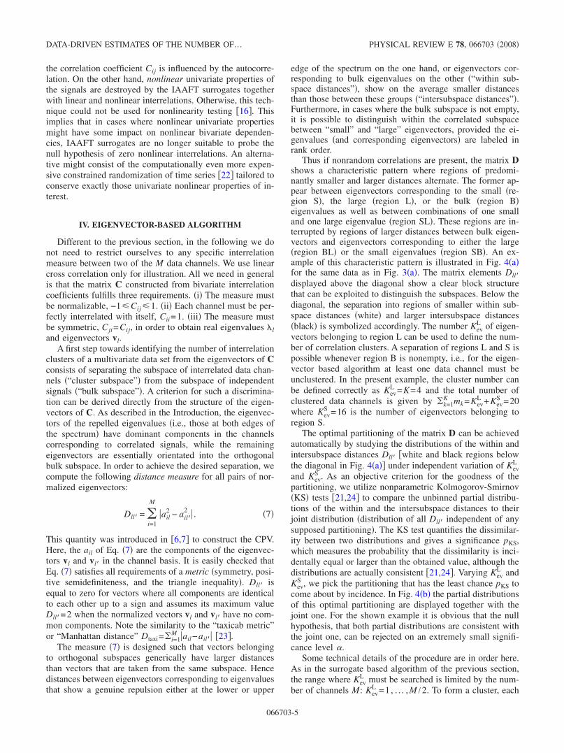
A first step towards identifying the number of interrelationclusters of a multivariate data set from the eigenvectors of Cconsists of separating the subspace of interrelated data chan-nels �“cluster subspace”� from the subspace of independentsignals �“bulk subspace”�. A criterion for such a discrimina-tion can be derived directly from the structure of the eigen-vectors of C. As described in the Introduction, the eigenvec-tors of the repelled eigenvalues �i.e., those at both edges ofthe spectrum� have dominant components in the channelscorresponding to correlated signals, while the remainingeigenvectors are essentially orientated into the orthogonalbulk subspace. In order to achieve the desired separation, wecompute the following distance measure for all pairs of nor-malized eigenvectors:

Dll� = �i=1

M

ail2 − ail�

2 . �7�

This quantity was introduced in �6,7� to construct the CPV.Here, the ail of Eq. �7� are the components of the eigenvec-tors vl and vl� in the channel basis. It is easily checked thatEq. �7� satisfies all requirements of a metric �symmetry, posi-tive semidefiniteness, and the triangle inequality�. Dll� isequal to zero for vectors where all components are identicalto each other up to a sign and assumes its maximum valueDll�=2 when the normalized vectors vl and vl� have no com-mon components. Note the similarity to the “taxicab metric”or “Manhattan distance” Dtaxi=�i=1

M ail−ail� �23�.The measure �7� is designed such that vectors belonging

to orthogonal subspaces generically have larger distancesthan vectors that are taken from the same subspace. Hencedistances between eigenvectors corresponding to eigenvaluesthat show a genuine repulsion either at the lower or upper

edge of the spectrum on the one hand, or eigenvectors cor-responding to bulk eigenvalues on the other �“within sub-space distances”�, show on the average smaller distancesthan those between these groups �“intersubspace distances”�.Furthermore, in cases where the bulk subspace is not empty,it is possible to distinguish within the correlated subspacebetween “small” and “large” eigenvectors, provided the ei-genvalues �and corresponding eigenvectors� are labeled inrank order.

Thus if nonrandom correlations are present, the matrix Dshows a characteristic pattern where regions of predomi-nantly smaller and larger distances alternate. The former ap-pear between eigenvectors corresponding to the small �re-gion S�, the large �region L�, or the bulk �region B�eigenvalues as well as between combinations of one smalland one large eigenvalue �region SL�. These regions are in-terrupted by regions of larger distances between bulk eigen-vectors and eigenvectors corresponding to either the large�region BL� or the small eigenvalues �region SB�. An ex-ample of this characteristic pattern is illustrated in Fig. 4�a�for the same data as in Fig. 3�a�. The matrix elements Dll�displayed above the diagonal show a clear block structurethat can be exploited to distinguish the subspaces. Below thediagonal, the separation into regions of smaller within sub-space distances �white� and larger intersubspace distances�black� is symbolized accordingly. The number Kev

L of eigen-vectors belonging to region L can be used to define the num-ber of correlation clusters. A separation of regions L and S ispossible whenever region B is nonempty, i.e., for the eigen-vector based algorithm at least one data channel must beunclustered. In the present example, the cluster number canbe defined correctly as Kev

L =K=4 and the total number ofclustered data channels is given by �k=1

K mk=KevL +Kev

S =20where Kev

S =16 is the number of eigenvectors belonging toregion S.

The optimal partitioning of the matrix D can be achievedautomatically by studying the distributions of the within andintersubspace distances Dll� �white and black regions belowthe diagonal in Fig. 4�a�� under independent variation of Kev

L

and KevS . As an objective criterion for the goodness of the

partitioning, we utilize nonparametric Kolmogorov-Smirnov�KS� tests �21,24� to compare the unbinned partial distribu-tions of the within and the intersubspace distances to theirjoint distribution �distribution of all Dll� independent of anysupposed partitioning�. The KS test quantifies the dissimilar-ity between two distributions and gives a significance pKS,which measures the probability that the dissimilarity is inci-dentally equal or larger than the obtained value, although thedistributions are actually consistent �21,24�. Varying Kev

L andKev

S , we pick the partitioning that has the least chance pKS tocome about by incidence. In Fig. 4�b� the partial distributionsof this optimal partitioning are displayed together with thejoint one. For the shown example it is obvious that the nullhypothesis, that both partial distributions are consistent withthe joint one, can be rejected on an extremely small signifi-cance level �.

Some technical details of the procedure are in order here.As in the surrogate based algorithm of the previous section,the range where Kev

L must be searched is limited by the num-ber of channels M: Kev

L =1, . . . ,M /2. To form a cluster, each

DATA-DRIVEN ESTIMATES OF THE NUMBER OF… PHYSICAL REVIEW E 78, 066703 �2008�

066703-5

large eigenvector must have at least one small partner andhence Kev

S �KevL . In addition, in order to be able to distin-

guish between regions L and S, at least one eigenvector mustfall into the bulk subspace B. Thus Kev

S is limited to the rangeKev

S =KevL , . . . ,M −1−Kev

L . The �M2 /4 elements of the spacespanned by Kev

L and KevS can be scanned systematically for the

best partitioning.In order to optimize the partitioning, we search the mini-

mum of the sum P= pKSwithin+ pKS

inter, where pKSwithin gives the sig-

nificance of the dissimilarity between the distribution of thewithin subspace distances �white region in Fig. 4�a�� and thejoint distribution of all off-diagonal matrix elements Dll��gray shaded in Fig. 4�b��. pKS

inter is the same for intersubspacedistances �black region in Fig. 4�a��. Note that different toonly quantifying the dissimilarity of two distributions, thesignificances pKS in addition take into account the effect ofdifferent sample sizes induced by varying Kev

L and KevS

�21,24�. Finally, the partitioning that minimizes P is acceptedonly if at least one of the partial distributions is incompatiblewith the joint one on a chosen significance level �. As thesystematic scan of the space spanned by Kev

L and KevS may

lead to incidentally small pKS in every trial, again a Bonfer-roni correction for the number of trials �M2 /4 must be car-ried out. Thus the partitioning is accepted only ifmin�pKS

within , pKSinter��4� /M2. If this requirement is not ful-

filled, we reject the partitioning as probably incidental andset Kev

L =KevS =0.

This eigenvector-based algorithm for estimating the clus-ter number Kev

L and the total number of clustered channels�k=1

K mk=KevL +Kev

S is summarized in the flowchart in Fig. 5.Different to the surrogate-based algorithm of Sec. III, appli-cation of this recipe to nonlinear interrelation measures ispossible. A second advantage is that neither the chosen levelof significance � influences the eigenvector-based algo-rithm’s additional workload given by M3 �construction of thedistance matrix D� nor are iterations necessary. Therefore, ascompared to IAAFT surrogates, the time complexity T of theeigenvector based algorithm is

Tsurr

Tev�

Kmax

�

1

�

T log2 T

M2 �8�

times smaller, i.e., typically several orders of magnitude. Inthis respect, online estimation of the cluster number in con-tinuously recorded multivariate signals is easily feasible,which is in practice a serious problem for the algorithmbased on IAAFT surrogates due to huge computation times.

V. PERFORMANCE TEST

In the following, the performance of the two algorithms isassessed in terms of correct estimates of the cluster numberK. Using the model of Sec. II the performance is quantifiedby the ratio R=NK /Nens of the number NK of correct detec-

FIG. 5. Flowchart of the eigenvector-based algorithm, see textfor details.

5 10 15 20 25 30

eigenvalue number

5

10

15

20

25

30

eige

nval

uenu

mbe

r

0.0 2.0

‘‘S’’

‘‘B’’

‘‘L’’

‘‘SL’’‘‘SB’’

‘‘BL’’

0.0 0.5 1.0 1.5 2.0

D

0

20

40

60

80

100

120

140

160

coun

ts

FIG. 4. Left: Distance matrix for the same example as in Fig. 3�a� �K=4, m=5, �=0.44, �=0.12, �=0.2�. Whereas above the diagonalthe original matrix elements are shown, the idealized block structure of within and intersubspace distances to be revealed by the algorithmis symbolized as white and black regions below the diagonal. Right: Histograms of the distributions of the within �fully drawn� andintersubspace distances �dotted�. The significances of a KS test for consistency of the partial with the joint distribution of all off-diagonalmatrix elements �gray shaded� are pKS

within=6.0�10−40 and pKSinter=3.9�10−40, respectively.

RUMMEL, MÜLLER, AND SCHINDLER PHYSICAL REVIEW E 78, 066703 �2008�

066703-6

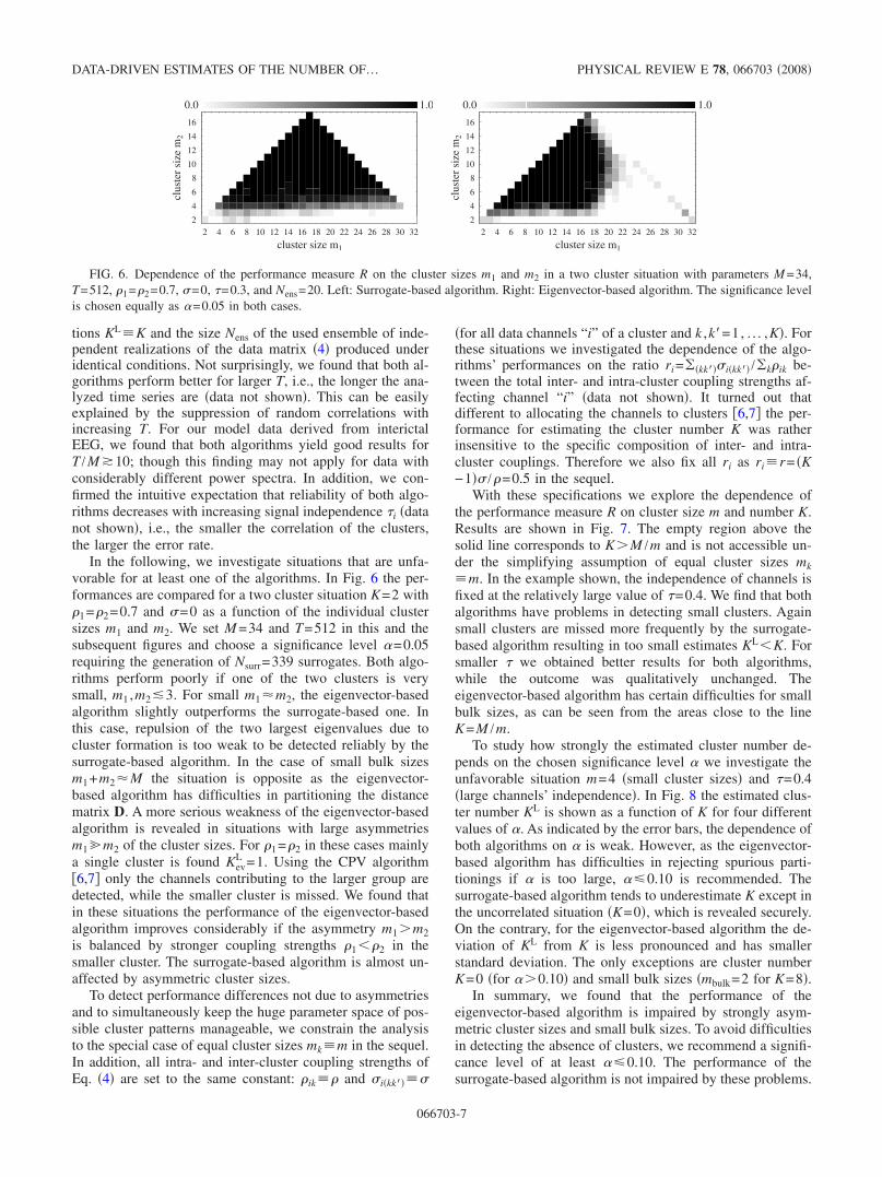
tions KLK and the size Nens of the used ensemble of inde-pendent realizations of the data matrix �4� produced underidentical conditions. Not surprisingly, we found that both al-gorithms perform better for larger T, i.e., the longer the ana-lyzed time series are �data not shown�. This can be easilyexplained by the suppression of random correlations withincreasing T. For our model data derived from interictalEEG, we found that both algorithms yield good results forT /M �10; though this finding may not apply for data withconsiderably different power spectra. In addition, we con-firmed the intuitive expectation that reliability of both algo-rithms decreases with increasing signal independence �i �datanot shown�, i.e., the smaller the correlation of the clusters,the larger the error rate.

In the following, we investigate situations that are unfa-vorable for at least one of the algorithms. In Fig. 6 the per-formances are compared for a two cluster situation K=2 with�1=�2=0.7 and �=0 as a function of the individual clustersizes m1 and m2. We set M =34 and T=512 in this and thesubsequent figures and choose a significance level �=0.05requiring the generation of Nsurr=339 surrogates. Both algo-rithms perform poorly if one of the two clusters is verysmall, m1 ,m2�3. For small m1�m2, the eigenvector-basedalgorithm slightly outperforms the surrogate-based one. Inthis case, repulsion of the two largest eigenvalues due tocluster formation is too weak to be detected reliably by thesurrogate-based algorithm. In the case of small bulk sizesm1+m2�M the situation is opposite as the eigenvector-based algorithm has difficulties in partitioning the distancematrix D. A more serious weakness of the eigenvector-basedalgorithm is revealed in situations with large asymmetriesm1�m2 of the cluster sizes. For �1=�2 in these cases mainlya single cluster is found Kev

L =1. Using the CPV algorithm�6,7� only the channels contributing to the larger group aredetected, while the smaller cluster is missed. We found thatin these situations the performance of the eigenvector-basedalgorithm improves considerably if the asymmetry m1�m2is balanced by stronger coupling strengths �1��2 in thesmaller cluster. The surrogate-based algorithm is almost un-affected by asymmetric cluster sizes.

To detect performance differences not due to asymmetriesand to simultaneously keep the huge parameter space of pos-sible cluster patterns manageable, we constrain the analysisto the special case of equal cluster sizes mkm in the sequel.In addition, all intra- and inter-cluster coupling strengths ofEq. �4� are set to the same constant: �ik� and �i�kk���

�for all data channels “i” of a cluster and k ,k�=1, . . . ,K�. Forthese situations we investigated the dependence of the algo-rithms’ performances on the ratio ri=��kk���i�kk�� /�k�ik be-tween the total inter- and intra-cluster coupling strengths af-fecting channel “i” �data not shown�. It turned out thatdifferent to allocating the channels to clusters �6,7� the per-formance for estimating the cluster number K was ratherinsensitive to the specific composition of inter- and intra-cluster couplings. Therefore we also fix all ri as rir= �K−1�� /�=0.5 in the sequel.

With these specifications we explore the dependence ofthe performance measure R on cluster size m and number K.Results are shown in Fig. 7. The empty region above thesolid line corresponds to K�M /m and is not accessible un-der the simplifying assumption of equal cluster sizes mkm. In the example shown, the independence of channels isfixed at the relatively large value of �=0.4. We find that bothalgorithms have problems in detecting small clusters. Againsmall clusters are missed more frequently by the surrogate-based algorithm resulting in too small estimates KL�K. Forsmaller � we obtained better results for both algorithms,while the outcome was qualitatively unchanged. Theeigenvector-based algorithm has certain difficulties for smallbulk sizes, as can be seen from the areas close to the lineK=M /m.

To study how strongly the estimated cluster number de-pends on the chosen significance level � we investigate theunfavorable situation m=4 �small cluster sizes� and �=0.4�large channels’ independence�. In Fig. 8 the estimated clus-ter number KL is shown as a function of K for four differentvalues of �. As indicated by the error bars, the dependence ofboth algorithms on � is weak. However, as the eigenvector-based algorithm has difficulties in rejecting spurious parti-tionings if � is too large, �0.10 is recommended. Thesurrogate-based algorithm tends to underestimate K except inthe uncorrelated situation �K=0�, which is revealed securely.On the contrary, for the eigenvector-based algorithm the de-viation of KL from K is less pronounced and has smallerstandard deviation. The only exceptions are cluster numberK=0 �for ��0.10� and small bulk sizes �mbulk=2 for K=8�.

In summary, we found that the performance of theeigenvector-based algorithm is impaired by strongly asym-metric cluster sizes and small bulk sizes. To avoid difficultiesin detecting the absence of clusters, we recommend a signifi-cance level of at least �0.10. The performance of thesurrogate-based algorithm is not impaired by these problems.

2 4 6 8 10 12 14 16 18 20 22 24 26 28 30 32

cluster size m1

2

4

6

8

10

12

14

16

clus

ter

size

m2

0.0 1.0

2 4 6 8 10 12 14 16 18 20 22 24 26 28 30 32

cluster size m1

2

4

6

8

10

12

14

16

clus

ter

size

m2

0.0 1.0

FIG. 6. Dependence of the performance measure R on the cluster sizes m1 and m2 in a two cluster situation with parameters M =34,T=512, �1=�2=0.7, �=0, �=0.3, and Nens=20. Left: Surrogate-based algorithm. Right: Eigenvector-based algorithm. The significance levelis chosen equally as �=0.05 in both cases.

DATA-DRIVEN ESTIMATES OF THE NUMBER OF… PHYSICAL REVIEW E 78, 066703 �2008�

066703-7

However, for small cluster sizes it performs worse than theeigenvector-based algorithm and under certain conditions theunderestimation of the cluster number is more pronounced.

VI. APPLICATION TO INTRACRANIALLY RECORDEDEEG

Epilepsy is the second most common neurological diseaseand roughly one-third of the patients are not renderedseizure-free by current therapies. It is plausible that a betterunderstanding of the spatiotemporal evolution of epilepticseizures may ultimately promote development of new toolsfor seizure control. Importantly, epileptic seizures are notproduced by single neurons, but are the result of the emer-gent activity of large neuronal networks that coalesce intoclusters with pathologic collective dynamics �25�. Thereforeinvestigating cluster formation and disintegration in EEG re-

cordings seems to be a reasonable approach to assess seizuredynamics. To demonstrate the usefulness of the methods de-veloped in the present paper in this context, we show in thefollowing their application to EEG recordings. Other interre-lation matrix-based clustering approaches to multivariateneurophysiological data have been made in �6,12,19�. Differ-ent clustering approaches to EEG data from epilepsy patientswere recently presented in �26,27�.

Here, we discuss in detail the evolution of the clusterpattern in an intracranially recorded EEG of an 18-year-oldmale suffering from pharmacoresistant temporal lobe epi-lepsy. The patient underwent evaluation for the possibility ofepilepsy surgery at the Inselspital in Bern, Switzerland. Hehad signed informed consent that EEG and imaging datamight be used for research purposes, and the study protocolhad previously been approved by the ethics committee of theUniversity of Bern. Using four implanted strip and two fora-men ovale electrodes �40 contacts in total, see the x-ray im-

2 3 4 5 6 7 8 9 10 11 12 13 14 15 16 17

cluster size m

0123456789

1011121314151617

clus

ter

num

ber

K

0.0 1.0

2 3 4 5 6 7 8 9 10 11 12 13 14 15 16 17

cluster size m

0123456789

1011121314151617

clus

ter

num

ber

K

0.0 1.0

FIG. 7. Dependence of the performance measure R on cluster size m and cluster number K. M =34, T=512, �=0.4, r=0.5, and Nens

=20. Left: Surrogate-based algorithm. Right: Eigenvector-based algorithm. The significance level is chosen equally as �=0.05 in both cases.As a fully drawn line the function K=M /m is shown.

0 1 2 3 4 5 6 7 8

true cluster number K

0

1

2

3

4

5

6

7

8

9

estim

ated

clus

ter

num

ber

KL = 0.01

= 0.05= 0.10= 0.20

0 1 2 3 4 5 6 7 8

true cluster number K

0

1

2

3

4

5

6

7

8

9

estim

ated

clus

ter

num

ber

KL = 0.01

= 0.05= 0.10= 0.20

FIG. 8. �Color online� Dependence of the estimated cluster number KL on the true cluster number K for various significance levels �.M =34, T=512, m=4, �=0.4, r=0.5, and Nens=20. Left: Surrogate-based algorithm. Right: Eigenvector-based algorithm. For better visibilitythe symbols are shifted slightly along the x axis and the line KL=K is shown for eye guidance.

RUMMEL, MÜLLER, AND SCHINDLER PHYSICAL REVIEW E 78, 066703 �2008�

066703-8

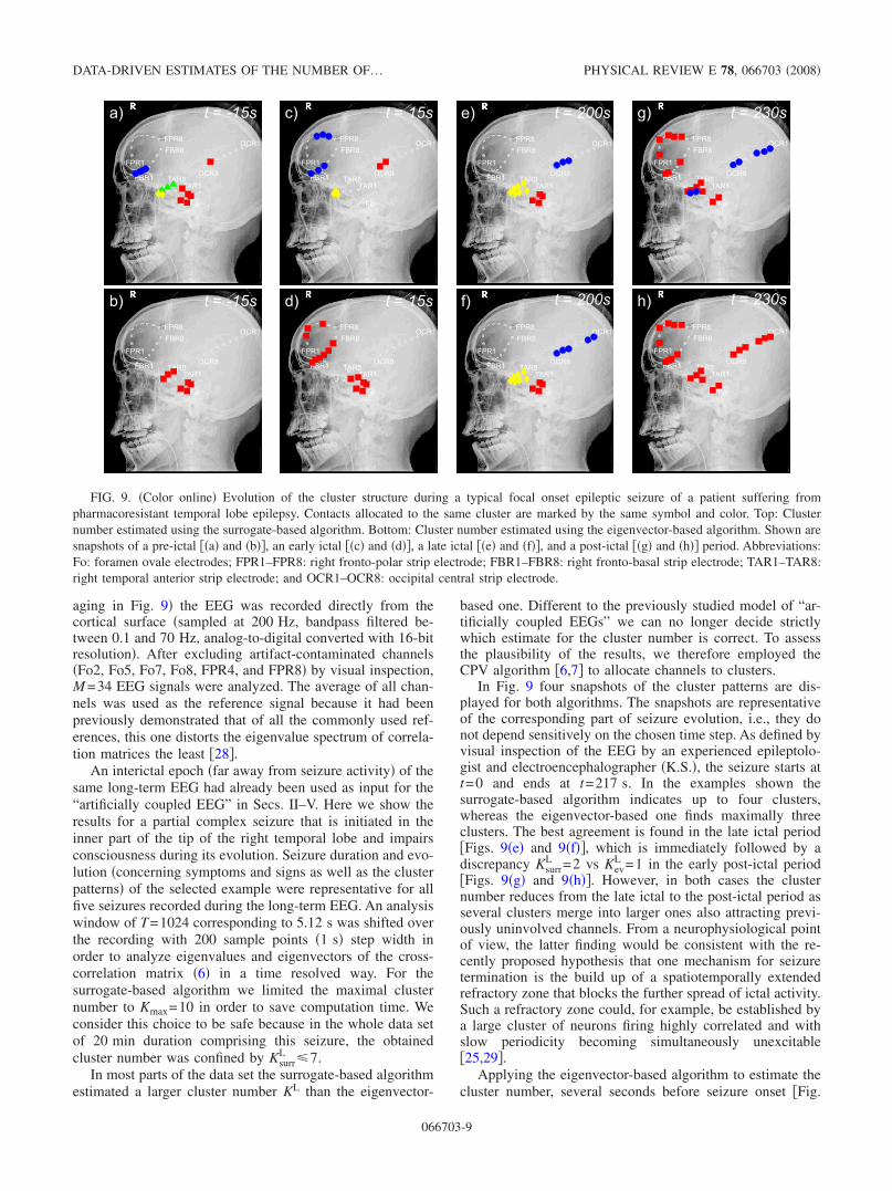
aging in Fig. 9� the EEG was recorded directly from thecortical surface �sampled at 200 Hz, bandpass filtered be-tween 0.1 and 70 Hz, analog-to-digital converted with 16-bitresolution�. After excluding artifact-contaminated channels�Fo2, Fo5, Fo7, Fo8, FPR4, and FPR8� by visual inspection,M =34 EEG signals were analyzed. The average of all chan-nels was used as the reference signal because it had beenpreviously demonstrated that of all the commonly used ref-erences, this one distorts the eigenvalue spectrum of correla-tion matrices the least �28�.

An interictal epoch �far away from seizure activity� of thesame long-term EEG had already been used as input for the“artificially coupled EEG” in Secs. II–V. Here we show theresults for a partial complex seizure that is initiated in theinner part of the tip of the right temporal lobe and impairsconsciousness during its evolution. Seizure duration and evo-lution �concerning symptoms and signs as well as the clusterpatterns� of the selected example were representative for allfive seizures recorded during the long-term EEG. An analysiswindow of T=1024 corresponding to 5.12 s was shifted overthe recording with 200 sample points �1 s� step width inorder to analyze eigenvalues and eigenvectors of the cross-correlation matrix �6� in a time resolved way. For thesurrogate-based algorithm we limited the maximal clusternumber to Kmax=10 in order to save computation time. Weconsider this choice to be safe because in the whole data setof 20 min duration comprising this seizure, the obtainedcluster number was confined by Ksurr

L 7.In most parts of the data set the surrogate-based algorithm

estimated a larger cluster number KL than the eigenvector-

based one. Different to the previously studied model of “ar-tificially coupled EEGs” we can no longer decide strictlywhich estimate for the cluster number is correct. To assessthe plausibility of the results, we therefore employed theCPV algorithm �6,7� to allocate channels to clusters.

In Fig. 9 four snapshots of the cluster patterns are dis-played for both algorithms. The snapshots are representativeof the corresponding part of seizure evolution, i.e., they donot depend sensitively on the chosen time step. As defined byvisual inspection of the EEG by an experienced epileptolo-gist and electroencephalographer �K.S.�, the seizure starts att=0 and ends at t=217 s. In the examples shown thesurrogate-based algorithm indicates up to four clusters,whereas the eigenvector-based one finds maximally threeclusters. The best agreement is found in the late ictal period�Figs. 9�e� and 9�f��, which is immediately followed by adiscrepancy Ksurr

L =2 vs KevL =1 in the early post-ictal period

�Figs. 9�g� and 9�h��. However, in both cases the clusternumber reduces from the late ictal to the post-ictal period asseveral clusters merge into larger ones also attracting previ-ously uninvolved channels. From a neurophysiological pointof view, the latter finding would be consistent with the re-cently proposed hypothesis that one mechanism for seizuretermination is the build up of a spatiotemporally extendedrefractory zone that blocks the further spread of ictal activity.Such a refractory zone could, for example, be established bya large cluster of neurons firing highly correlated and withslow periodicity becoming simultaneously unexcitable�25,29�.

Applying the eigenvector-based algorithm to estimate thecluster number, several seconds before seizure onset �Fig.

FIG. 9. �Color online� Evolution of the cluster structure during a typical focal onset epileptic seizure of a patient suffering frompharmacoresistant temporal lobe epilepsy. Contacts allocated to the same cluster are marked by the same symbol and color. Top: Clusternumber estimated using the surrogate-based algorithm. Bottom: Cluster number estimated using the eigenvector-based algorithm. Shown aresnapshots of a pre-ictal ��a� and �b��, an early ictal ��c� and �d��, a late ictal ��e� and �f��, and a post-ictal ��g� and �h�� period. Abbreviations:Fo: foramen ovale electrodes; FPR1–FPR8: right fronto-polar strip electrode; FBR1–FBR8: right fronto-basal strip electrode; TAR1–TAR8:right temporal anterior strip electrode; and OCR1–OCR8: occipital central strip electrode.

DATA-DRIVEN ESTIMATES OF THE NUMBER OF… PHYSICAL REVIEW E 78, 066703 �2008�

066703-9

9�b�� only one cluster is found. Allocated contacts are fora-men ovale electrodes and several contacts of the right tem-poral anterior strip electrode �TAR�, i.e., the electrode thatcovers the pole of the right temporal lobe. This finding isneurophysiologically plausible because they are closest tothe seizure onset zone probed by contact TAR1 and aretherefore expected to be entrained by ictal activity early dur-ing the seizure or even before seizure activity may be delin-eated visually. Different from the eigenvector-based algo-rithm the surrogate-based one detects four clusters �Fig.9�a��. Three of them can be seen as a decomposition of thecluster found by the eigenvector-based algorithm. ContactsTAR1 �red square�, TAR4 and TAR5 �yellow diamonds�, andTAR6 to TAR8 �green triangles� belong to different clusters,though they are located on the same strip electrode. Thisreveals that spatial closeness does not necessarily imply in-volvement in the same cluster. The reason for the differencemight be that the strip electrode TAR is wrapped around thelateral temporal lobe and the involved contacts record fromcortical areas with different functionality. In addition, thesurrogate-based algorithm finds a cluster involving contactsof the spatially relatively distant electrode FBR �bluecircles�, which records from the basal part of the right frontallobe. This cluster is not found with the eigenvector-basedalgorithm.

During seizure �Figs. 9�c�–9�f��, typically more contactsbecome allocated to the correlation clusters. Using theeigenvector-based algorithm, in the early phase of the seizure�Fig. 9�d��, the frontal strip electrodes �FPR and FBR� areinvolved in the same cluster as the foramen ovale electrodesand the contacts TAR1 and TAR2. Again, the surrogate-based algorithm �Fig. 9�c�� reveals a more detailed result byseparating the contacts on the frontal, the temporal, and theoccipital electrodes into three distinct clusters. As the clus-ters on the TAR and the OCR electrodes are much smallerthan the frontal one, the fact that these channels are not al-located to clusters by the eigenvector-based algorithm is inline with the findings of Sec. V, compare discussion of Fig.6�b�.

Before seizure termination �Figs. 9�e� and 9�f�� both algo-rithms find the same cluster number Ksurr

L =KevL =3 and also

the cluster pattern obtained by the CPV algorithm is verysimilar. One cluster comprises the foramen ovale electrodes�red squares� and a second one the contacts of the temporalanterior electrode �yellow diamonds�. Interestingly, the con-tact TAR1, recording directly from the seizure onset zone isno longer involved in any cluster in this seizure phase. Athird cluster comprises the contacts of the occipital centralelectrode �blue circles� and contains the only difference be-tween both algorithms for the cluster number. It can be at-tributed to the probabilistic aspect of the maximization pro-cedure of the CPV algorithm, see �6,7�.

In the time period early after seizure termination �Figs.9�g� and 9�h��, most channels are allocated to correlationclusters. Again, TAR1 is not part of one of the clusters. Thesurrogate-based algorithm �Fig. 9�g�� finds two clusters, thelarger one comprising frontal, most temporal anterior, andforamen ovale electrodes �red squares�. In the smaller one,contacts of the temporal anterior and the occipital electrodesare involved �blue circles�. Different to most of the panels in

the upper row, here, the contribution of relatively distantcontacts to joint clusters suggests that functional similaritiesrather than spatial closeness is relevant for involvement inthe same cluster.

In contrast to the surrogate-based algorithm theeigenvector-based one �Fig. 9�h�� obtains only one globalcluster to which the majority of contacts contribute. To in-vestigate the reason we studied the size of the absolute intra-and inter-cluster elements of the equal-time cross-correlationmatrix. The intracluster elements of the cluster symbolizedby red squares are 0.45�0.19 and 0.50�0.22 in the onecorresponding to blue circles �given are mean and standarddeviation�. The average matrix elements between these clus-ters are relatively large, too: 0.28�0.22. This suggests thatthe surrogate-based algorithm treats this situation as distinctbut interrelated clusters, whereas the eigenvector-based oneinterprets the result as a single cluster with substructure. Asimilar situation is given for the clusters of the TAR and theforamen ovale electrodes of Fig. 9�a�.

As already mentioned, the observed formation of clustersand the subsequent evolution of cluster patterns towards astrongly and globally correlated state after seizure termina-tion via cluster reorganization is consistent with recent find-ings of �25,29�. More detailed neurophysiological interpreta-tions are subject of ongoing research with a larger number ofEEG recordings and go beyond the scope of the present pa-per.

VII. SUMMARY AND CONCLUSIONS

In the present paper two algorithms for estimating thecluster number K in multichannel data have been investi-gated. Different to our previous work �6,7� but similar to thealgorithms presented in �4,5�, the algorithms treat the estima-tion of K on the same footing as the allocation of data chan-nels to interrelation clusters, which is usually done in a sec-ond step. Moreover, the methods go without artificiallydefining any threshold. Rather, data-driven criteria based ona chosen significance level � for nonparametric statisticaltests are used exclusively. This makes both methods candi-dates for unsupervised data clustering.

Using a model system with power spectra realistic forinterictal EEG, in large parts of the scanned parameter spacethe surrogate-based algorithm presented in Sec. III and theeigenvector-based algorithm of Sec. IV perform comparablywell. The occasionally better performance of the surrogate-based algorithm, which appears more robust for stronglyasymmetric cluster sizes and small bulk sizes �note that theeigenvector-based algorithm is not applicable if the bulk isempty�, is contrasted by two deficiencies, the first one con-sisting of the long computation time for generating IAAFTsurrogate ensembles. The eigenvector-based algorithm iscomputationally faster by orders of magnitude.

In principle, the generation of surrogate data is a delicateissue, and, depending on the data, the results might not re-flect the desired properties, see, e.g., �16�. Therefore we re-peated the computations of Sec. V using the much fastermethod of simple shift surrogates as proposed in �30�. Thismethod conserves power spectra and amplitude distributions

RUMMEL, MÜLLER, AND SCHINDLER PHYSICAL REVIEW E 78, 066703 �2008�

066703-10

exactly, while destroying cross correlations by independentlytime shifting the data sets relative to each other and wrap-ping the extra values around to the beginning of the data set.For the studied data the obtained results differ only margin-ally from those included in the present paper. Anothermethod of speeding up the surrogate generation process con-sists of using amplitude adjusted Fourier transform surro-gates �AAFT� �31� that omit the costly iteration procedure.However, for any particular class of real world data it mustbe carefully checked which algorithm for surrogate genera-tion is appropriate. Note that IAAFT surrogates might notalways be the optimal solution. For instance, if the experi-mental data show strong quasiperiodic characteristics, like,e.g., in electrocardiograms or even in EEG of primary gen-eralized seizures with spike and wave activity, it might bemore adequate to use the approach proposed in �32�.

The second deficiency of the surrogate-based algorithm ofSec. III is its principal restriction to linear interrelation mea-sures. In contrast, application of the eigenvector-based algo-rithm to symmetric and normalizable nonlinear interrelationmeasures such as, e.g., mean phase coherence �33,34� or mu-tual information �35–37� is possible.

In application to equal-time cross-correlation matricescomputed from intracranial EEG recordings, the clusternumber estimated by both algorithms may differ. However,the cluster patterns revealed by both methods show physi-ologically plausible characteristics consistent with recent hy-potheses about mechanisms for seizure termination �25,29�.In contrast to the eigenvalue-based algorithm the surrogate-

based one allows some insight into the clusters’ “fine struc-ture.”

A problem that our estimation of the cluster numbershares with most other approaches to data clustering is that itstarts from a model assumption. Obviously, every sharplydefined block in the interrelation matrix C produces one re-pelled large eigenvalue and the eigenvector components areconfined to the corresponding subspace of theM-dimensional phase space. However, at present our strate-gies for cluster search invert this reasoning without provingthat this is justified: The surrogate-based algorithm definesan interrelation cluster for every large eigenvalue �k that isnot compatible with the surrogates. Similarly, theeigenvector-based algorithm partitions the distance matrix Din an optimal way and defines a cluster for every eigenvectorin region L. Although we could show that both approachesperform reasonably well in general, it remains to be investi-gated which alternative patterns �rings, trees, etc.� are alsodetected by the methods of the present paper.

ACKNOWLEDGMENTS

We would like to thank the anonymous referees for theirconstructive remarks which helped to improve the paper con-siderably. The authors thank Gerold Baier, Carsten Allefeld,Stephan Bialonski, and Klaus Lehnertz for fruitful discus-sions. The work was supported by Deutsche Forschungsge-meinschaft, Germany �Grant No. RU 1401/1-2�, CONACyT,Mexico �Project No. 48500�, and Novartis Jubiäumsstiftung,Switzerland.

�1� A. K. Jain and R. C. Dubes, Algorithms for Clustering Data�Prentice-Hall, Englewood Cliffs, NJ, 1988�.

�2� A. Jain, M. Murty, and P. Flynn, ACM Comput. Surv. 31, 264�1999�.

�3� J. Kogan, Introduction to Clustering Large and High-Dimensional Data �Cambridge University Press, Cambridge,England, 2007�.

�4� B. J. Frey and D. Dueck, Science 315, 972 �2007�.�5� C. Allefeld and S. Bialonski, Phys. Rev. E 76, 066207 �2007�.�6� C. Rummel, G. Baier, and M. Müller, Europhys. Lett. 80,

68004 �2007�.�7� C. Rummel, Phys. Rev. E 77, 016708 �2008�.�8� P. Gopikrishnan, B. Rosenow, V. Plerou, and H. E. Stanley,

Phys. Rev. E 64, 035106�R� �2001�.�9� V. Plerou, P. Gopikrishnan, B. Rosenow, Luis A. Nunes Ama-

ral, T. Guhr, and H. E. Stanley, Phys. Rev. E 65, 066126�2002�.

�10� A. Utsugi, K. Ino, and M. Oshikawa, Phys. Rev. E 70, 026110�2004�.

�11� C. Allefeld, M. Müller, and J. Kurths, Int. J. Bifurcation ChaosAppl. Sci. Eng. 17, 3493 �2007�.

�12� S. Bialonski and K. Lehnertz, Phys. Rev. E 74, 051909 �2006�.�13� A. M. Sengupta and P. P. Mitra, Phys. Rev. E 60, 3389 �1999�.�14� M. Müller, G. Baier, C. Rummel, and K. Schindler, Europhys.

Lett. 84, 10009 �2008�.

�15� T. Schreiber and A. Schmitz, Phys. Rev. Lett. 77, 635 �1996�.�16� T. Schreiber and A. Schmitz, Physica D 142, 346 �2000�.�17� T. Anderson, An Introduction to Multivariate Statistical Analy-

sis �Wiley, New York, 2003�.�18� D. F. Morrison, Multivariate Statistical Methods, 4th ed. �Th-

omson, Belmont, 2005�.�19� X. Li, D. Cui, P. Jiruska, J. E. Fox, X. Yao, and J. G. R.

Jefferys, J. Neurophysiol. 98, 3341 �2007�.�20� S. Holm, Scand. J. Stat. 6, 65 �1979�.�21� W. H. Press, S. A. Teukolsky, W. T. Vetterling, and B. P. Flan-

nery, Numerical Recipes in C, The Art of Scientific Computing,2nd ed. �Cambridge University Press, Cambridge, England1992�.

�22� T. Schreiber, Phys. Rev. Lett. 80, 2105 �1998�.�23� E. F. Krause, Taxicab Geometry: An Adventure in Non-

Euclidean Geometry �Dover, New York, 1986�.�24� S. Siegel, Non-Parametric Statistics for the Behavioral Sci-

ences �McGraw-Hill, New York, 1956�.�25� K. Schindler, H. Leung, C. E. Elger, and K. Lehnertz, Brain

130, 65 �2007�.�26� A. Hedge, D. Erdogmus, D. S. Shiau, J. C. Principe, and C. J.

Sackellares, Computational Intelligence Neurosci. 2007,83416 �2007�.

�27� G. J. Ortega, L. Menendez de la Prida, R. G. Sola, and J.Pastor, Epilepsia 49, 269 �2008�.

DATA-DRIVEN ESTIMATES OF THE NUMBER OF… PHYSICAL REVIEW E 78, 066703 �2008�

066703-11

�28� C. Rummel, G. Baier, and M. Müller, J. Neurosci. Methods166, 138 �2007�.

�29� K. Schindler, C. E. Elger, and K. Lehnertz, Clin. Neuro-physiol. 118, 1955 �2007�.

�30� T. Netoff and S. Schiff, J. Neurosci. 22, 7297 �2002�.�31� J. Theiler, S. Eubank, A. Longtin, B. Galdrikian, and J.

Farmer, Physica D 58, 77 �1992�.�32� M. Small, D. Yu, and R. G. Harrison, Phys. Rev. Lett. 87,

188101 �2001�.�33� F. Mormann, K. Lehnertz, P. David, and C. E. Elger, Physica D

144, 358 �2000�.�34� F. Mormann, R. G. Andrzejak, T. Kreuz, C. Rieke, P. David, C.

E. Elger, and K. Lehnertz, Phys. Rev. E 67, 021912 �2003�.�35� R. Quian Quiroga, A. Kraskov, T. Kreuz, and P. Grassberger,

Phys. Rev. E 65, 041903 �2002�.�36� A. Kraskov, H. Stögbauer, and P. Grassberger, Phys. Rev. E

69, 066138 �2004�.�37� A. Kraskov, H. Stögbauer, R. G. Andrzejak, and P. Grass-

berger, Europhys. Lett. 70, 278 �2005�.

RUMMEL, MÜLLER, AND SCHINDLER PHYSICAL REVIEW E 78, 066703 �2008�

066703-12