RESEARCH ARTICLE

Cumulative effects of land use on fish metrics in different typesof running waters in Austria

Clemens Trautwein • Rafaela Schinegger •

Stefan Schmutz

Received: 16 December 2010 / Accepted: 7 July 2011

� The Author(s) 2011. This article is published with open access at Springerlink.com

Abstract The catchment land-use composition of 249

fish sampling sites in Austrian running waters revealed

effects on the biological integrity. Beyond correlative

analysis, we investigated (1) which land-use category had

the strongest effect on fish, (2) whether metrics of func-

tional fish guilds reacted differently, (3) whether there were

cumulative effects of land-use categories, and (4) whether

effects varied in strength across river types. We fed 5 land-

use categories into regression trees to predict the European

Fish Index or fish metric of intolerant species (mainly

Salmo trutta fario). Agriculture and urbanisation were the

best predictors and indicated significant effects at levels of

[23.3 and [2%, respectively. Model performance was

R2 = 0.15 with the Fish Index and R2 = 0.46 with intol-

erant species. The tree structure showed a cumulative

effect from agriculture and urbanisation. For the intolerant

species metric, a combination of high percentages for

agriculture and urbanisation was related to moderate status,

whereas \7.3% agriculture were related to good status,

although urbanisation was higher than 1.8%. Headwater

river types showed stronger responses to land use than river

types of lower gradient and turned out to be more sensitive

to urbanisation than agriculture.

Keywords Land use � Fish � Cumulative effect �Stream integrity � Fish metrics � IBI � Moran’s I �Landscape composition

Abbreviations

EFT European fish type

CLC CORINE land cover

CRT Classification and regression trees

IBI Index of biotic integrity

MI Moran’s I index

Introduction

Land use and stream response

Rivers in the context of their catchments—also called

riverscapes—are considered to be ecosystems that are

strongly affected by human actions in the landscape (Allan

2004b). The guiding principle of much riverine research at

the landscape-scale is that human actions impact the

composition and function of aquatic organisms, e.g., fish.

Human alterations and impacts that directly affect the

physico-chemical conditions of running waters and

strongly influence the aquatic biota are referred to as

pressures in this study. Many, although not all, impacts on

streams are entirely or partly linked to human activities in

the landscape and thus can be quantified from data on land

use (Allan 2004a). A useful way to measure land use is to

assess landscape composition at the class level (Botequilha

Leitao et al. 2006).

A (higher) proportion of agriculture has been shown to

have detrimental effects on biota (Allan 2004b; Allan et al.

1997; Richards et al. 1996; Roth et al. 1996). Urbanisation,

impervious land cover and roads frequently have signifi-

cant impacts on rivers. The upstream drainage area for fish

sampling locations—referred to as catchment area—is

commonly understood as an important scale of

C. Trautwein (&) � R. Schinegger � S. Schmutz

Department of Water, Atmosphere and Environment,

Institute of Hydrobiology and Aquatic Ecosystem Management,

BOKU, University of Natural Resources and Life Sciences,

Max Emanuel-Strasse 17, 1180 Vienna, Austria

e-mail: clemens.trautwein@boku.ac.at

URL: http://www.wau.boku.ac.at/ihg.html

Aquat Sci

DOI 10.1007/s00027-011-0224-5 Aquatic Sciences

123

investigation. Even relatively small amounts of urbanised

areas within a stream catchment, e.g., \5%, have adverse

effects on stream integrity. Non-linearity in the relationship

between urbanisation and stream condition has been

reported by Gergel et al. (2002) and Miltner et al. (2004).

Linkages are related to altered hydrology (e.g., increased

peak surface runoff), altered sediment delivery patterns,

intrusion of pollutants and toxins, and habitat degradation

(Beechie et al. 2010).

Fish react to both chemical and physical water quality

and hydro-morphological conditions; therefore, fish are an

ideal indicator for multiple-impacted rivers (EC of Euro-

pean Parliament 2000, WFD). Fish are present in most

surface waters, they occupy a wide variety of riverine

habitats, are relatively easy to identify, and their taxonomy

and ecological requirements are well studied. Because of

their migration patterns and longevity, fish communities

reflect aquatic conditions over relatively large spatial and

long time scales (Pont et al. 2006).

Integrative measures of river condition, such as Indices

of Biotic Integrity (IBIs), are particularly useful for

assessing overall stream health because they integrate

multiple influences. IBIs are multi-metric indices based on

structural (taxonomic) and functional (species guilds and

traits) metrics (Karr 1981). However, Allan (2004a) argues

that multi-metric bioassessment methods may fail in

diagnosing causes of degradation because these indices are

constructed with the intention to reflect multiple stressors.

This calls for testing single metrics of species traits,

feeding and reproductive guilds, taxa of known tolerance to

particular stressors, and other less-aggregated measures for

evaluating pathways and mechanisms between landscapes,

instream habitats and fish IBIs (Poff 1997).

Most studies have identified landscape effects for single

land-use categories only. Agriculture and urbanisation are

well-studied human impacts. Nonetheless, the interaction

effects and cumulative effects from multiple land-use cat-

egories are poorly understood. This can be attributed to the

use of (multiple) linear regression analysis. Because of the

multitude of ecological variables in landscape studies, only

the main effects were considered, whereas interaction

effects were not included. New and innovative statistical

methods are needed to obtain results that better interpret

interactions, cumulative effects and threshold values.

Numerous studies have dealt with few sampling sites

and focused on streams dominated by either agricultural

(Stewart et al. 2001; Roth et al. 1996) or urban land use

(Wang et al. 2001, 2003). Larger datasets covering many

different river types can be used to analyse effects of

multiple land use and differences in response between river

types.

Relationships and processes are considered to have dif-

ferent influences within river typologies. The Ecoregion

concept of Illies and Andrassy (1978) or Omernik and

Bailey (1997) delineates both geographically and ecologi-

cally homogeneous areas. Huet (1949) conceptualised fish

zones for running waters mainly based on river slope. Fish

zones account for the natural variability of fish communities

along the longitudinal gradient of rivers. They imply that

typical assemblages, e.g., brown trout dominated commu-

nities (S. trutta L.), occur throughout the many ecoregions

all over Europe. Considering these two concepts, Melcher

et al. (2007) identified assemblage types for European fish

fauna and developed a predictive model using abiotic

characteristics. Thus, the model of Melcher covers the

aspects of regionalism and longitudinal river zonation. Steel

et al. (2010) also proposed to examine landscape-fish rela-

tionships across disparate catchments, ecoregions and

ecosystems to test whether there are, in fact, generalisable

effects. However, using a heterogeneous dataset in terms of

spatial distribution and river size requires considering the

underlying abiotic and biotic characteristics, which can lead

to spurious effects in the results.

We hypothesise that different fish assemblages respond

differently to land uses. Upper tributaries that mainly host

assemblages with low species numbers may be less vul-

nerable to land-use impacts compared to assemblages of

medium to large rivers. This is due to the importance of

lateral connectivity and the exchange of nutrients, organic

and inorganic materials, which increases with river size

(Ward 1989).

The present study was designed to identify empirical

relationships between human land use and the biotic

integrity of rivers and streams. Besides using a general fish

index as a measure of ecological status, we also focus on

fish metrics of certain ecological functional groups (trophic

and reproduction guilds). These metrics of fish species with

special feeding and reproductive behaviour may help to

interpret linkages between landscape-scale human actions

and in-stream biotic responses.

Research questions addressed within this study were (1)

is there a relationship between the composition of land use

and fish assemblages, and which land-use category has the

strongest effect on fish, (2) do metrics of functional fish

guilds respond differently to land use, and which guilds

were most strongly affected by land use, (3) can we iden-

tify a cumulative effect for several land-use categories

showing a stronger impact than single land-use categories

and quantify thresholds, and (4) do land use effects vary in

strength across different Austrian river types?

Methods and data

To characterise landscapes, we calculated the landscape

composition (percentage of six different land-use

C. Trautwein et al.

123

categories) within a catchment area for individual fish

sampling sites. Our scale of investigation was the catch-

ment scale because this has been the most influential scale

in several studies of landscape-river research (Allan 2004b;

Allan and Johnson 1997; Roth et al. 1996). It also showed a

higher relative effect for impacted sites than local or reach

scales (Wang et al. 2006b), which were reported to be

subject to a hierarchy of controls from large to small spatial

extents (Durance et al. 2006).

Land cover data, delineated European watersheds and

river networks were processed with GIS software (ArcGIS

Desktop 9.3, ESRI � 1999–2008).

We used the CORINE land cover data 2000 (CLC2000;

European Environmental Agency; www.eea.europa.eu/) for

landscape characterisation. The CCM River and Catchment

database, version 2.0 (CCM2) (Vogt et al. 2007) was used

to determine the catchments associated with each sampling

point. That is, each sampling point was assigned to distinct

hydrologic primary catchments (surface area draining into

confluent to confluent river segment). The tool ‘thematic

raster summary’ (Beyer 2004) performed a spatial overlay

of land cover data to evaluate the absolute area of each

land-cover/land-use (hereafter land-use) category within

primary catchments. The hydrologic coding of CCM

allowed tracking of all upstream primary catchments along

the upstream drainage network. The hydrologically coded

database structure was used to aggregate absolute values of

land-use variables within the whole upstream catchment

area. Finally, land-use composition is the ratio between the

area of each land-use category and catchment size.

Accordingly, 0.40 agriculture means that 40% of the

catchment is occupied by agricultural use.

We evaluated the amounts of six land-use categories in a

slightly modified level three definition of CLC2000 code

(official CLC three-digit code in brackets in Table 1):

agriculture, pasture, urban land, forest, shrubland, and non-

vegetated areas. Table 1 provides details on the organisa-

tion of the land-use variables. Non-vegetated areas were

excluded from further analysis because of their scarce

occurrence (median = 0, standard deviation = 0.0969).

Data from single-pass electric fishing by wading and

boating according to standards of the CEN norm EN 14011

(CEN 2003) provided the basis for the biotic variables in

this study. The fish were identified to species level, their

length and weight recorded, and then released back to the

stream.

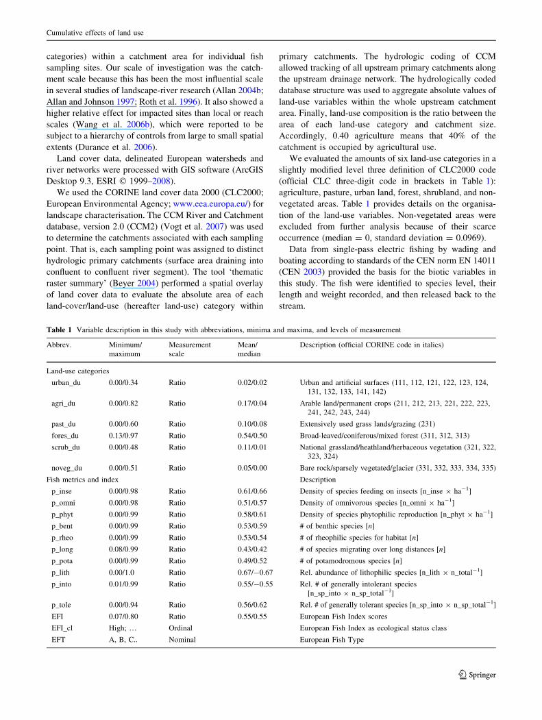
Table 1 Variable description in this study with abbreviations, minima and maxima, and levels of measurement

Abbrev. Minimum/

maximum

Measurement

scale

Mean/

median

Description (official CORINE code in italics)

Land-use categories

urban_du 0.00/0.34 Ratio 0.02/0.02 Urban and artificial surfaces (111, 112, 121, 122, 123, 124,

131, 132, 133, 141, 142)

agri_du 0.00/0.82 Ratio 0.17/0.04 Arable land/permanent crops (211, 212, 213, 221, 222, 223,

241, 242, 243, 244)

past_du 0.00/0.60 Ratio 0.10/0.08 Extensively used grass lands/grazing (231)

fores_du 0.13/0.97 Ratio 0.54/0.50 Broad-leaved/coniferous/mixed forest (311, 312, 313)

scrub_du 0.00/0.48 Ratio 0.11/0.01 National grassland/heathland/herbaceous vegetation (321, 322,

323, 324)

noveg_du 0.00/0.51 Ratio 0.05/0.00 Bare rock/sparsely vegetated/glacier (331, 332, 333, 334, 335)

Fish metrics and index Description

p_inse 0.00/0.98 Ratio 0.61/0.66 Density of species feeding on insects [n_inse 9 ha-1]

p_omni 0.00/0.98 Ratio 0.51/0.57 Density of omnivorous species [n_omni 9 ha-1]

p_phyt 0.00/0.99 Ratio 0.58/0.61 Density of species phytophilic reproduction [n_phyt 9 ha-1]

p_bent 0.00/0.99 Ratio 0.53/0.59 # of benthic species [n]

p_rheo 0.00/0.99 Ratio 0.53/0.54 # of rheophilic species for habitat [n]

p_long 0.08/0.99 Ratio 0.43/0.42 # of species migrating over long distances [n]

p_pota 0.00/0.99 Ratio 0.49/0.52 # of potamodromous species [n]

p_lith 0.00/1.0 Ratio 0.67/-0.67 Rel. abundance of lithophilic species [n_lith 9 n_total-1]

p_into 0.01/0.99 Ratio 0.55/-0.55 Rel. # of generally intolerant species

[n_sp_into 9 n_sp_total-1]

p_tole 0.00/0.94 Ratio 0.56/0.62 Rel. # of generally tolerant species [n_sp_into 9 n_sp_total-1]

EFI 0.07/0.80 Ratio 0.55/0.55 European Fish Index scores

EFI_cl High; … Ordinal European Fish Index as ecological status class

EFT A, B, C.. Nominal European Fish Type

Cumulative effects of land use

123

Ecological status was assessed according to Pont et al.

(2007) with the readily available software tool for the

European Fish Index (EFI, http://fame.boku.ac.at/). This

tool derives theoretical fish metric values for individual

sites based on a predictive model of reference conditions.

The larger the difference between predicted and observed

conditions of the fish fauna, the worse the ecological status.

Input variables needed for reference modelling are envi-

ronmental variables describing the sampling site: altitude,

lakes upstream, distance from source, flow regime, wetted

width, geology, air temperature, river slope, and catchment

size (Pont et al. 2007).

Finally, the mean of 10 fish metrics (see Table 1) based

on species richness and densities make up the European

Fish Index. They represent five ecological functional

groups: (1) trophic structure (insectivorous and omnivorous

species), (2) reproduction strategy (phytophilic and litho-

philic sp.), (3) physical habitat preference (benthic and

rheophilic sp.), (4) migratory behaviour (long-distance

migrating and potamodromous sp.), and (5) tolerance to

disturbance (intolerant and tolerant sp.) (Pont et al. 2007;

Noble et al. 2007).

Seven of these 10 fish metrics decrease in response to

human pressures, whereas three tend to increase with such

pressure; the latter are the density of omnivorous and phyt-

ophilic species and relative number of tolerant species. For

consistency Pont et al. (2007) transformed residuals into the

probability of being a reference site. Accordingly, fish met-

rics and the European Fish Index range from 0 to 1. EFI

scores are assigned to five ecological status classes ([0.669

= high; 0.449–0.669 = good; 0.0279–0.449 = moderate;

0.187–0.279 = poor;\0.187 = bad).

A simplified European fish assemblage typology (Mel-

cher et al. 2007) served as a grouping variable in the later

analysis to determine special relationships between land

use and fish.

Melcher et al. (2007) identified 15 homogeneous fish

assemblage types in 11 ecoregions and described six main

European Fish Types (EFT). These groups represent river

types of (A) headwaters with low species richness domi-

nated by brown trout (S. trutta fario), (B) sections with a

low gradient dominated by common minnow (Phoxinus

phoxinus), (C) assemblages dominated by Thymallus thy-

mallus, known as the greyling zone, (D) rivers dominated

by anadromous and potamodromous salmonids, i.e., Salmo

salar, S. trutta lacustris, S. trutta trutta, (E) southern fish

assemblages including Mediterranean endemics, and

(F) lowland rivers. We used the EFT calculation tool

included in the EFI software package to predict EFT

based on seven environmental descriptors for each sam-

pling site (http://fame.boku.ac.at). Melcher et al. (2007)

used discriminate functions for altitude, distance from

source, wetted width, river slope, mean annual air tem-

perature, longitude, and latitude to predict EFT. Four

EFTs occurred in the Austrian dataset of the present study

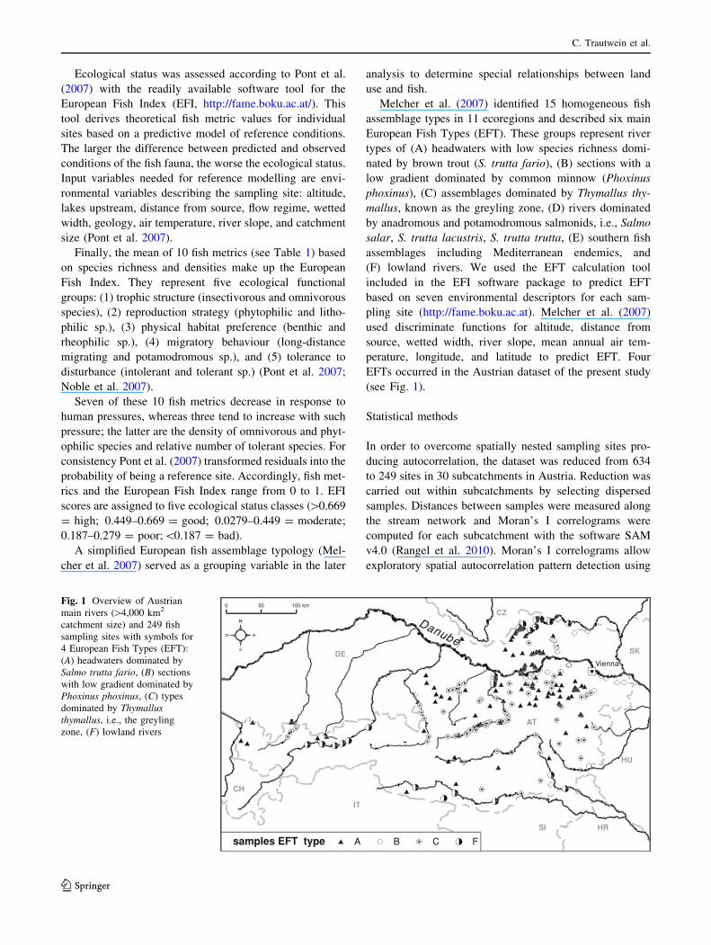
(see Fig. 1).

Statistical methods

In order to overcome spatially nested sampling sites pro-

ducing autocorrelation, the dataset was reduced from 634

to 249 sites in 30 subcatchments in Austria. Reduction was

carried out within subcatchments by selecting dispersed

samples. Distances between samples were measured along

the stream network and Moran’s I correlograms were

computed for each subcatchment with the software SAM

v4.0 (Rangel et al. 2010). Moran’s I correlograms allow

exploratory spatial autocorrelation pattern detection using

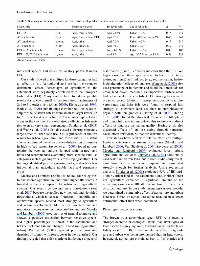
Danube

AT

DE

IT

CZ

SI HR

HU

CH

SK

Vienna

0 50 100 km

samples EFT type A B C F

Fig. 1 Overview of Austrian

main rivers ([4,000 km2

catchment size) and 249 fish

sampling sites with symbols for

4 European Fish Types (EFT):

(A) headwaters dominated by

Salmo trutta fario, (B) sections

with low gradient dominated by

Phoxinus phoxinus, (C) types

dominated by Thymallusthymallus, i.e., the greyling

zone, (F) lowland rivers

C. Trautwein et al.

123

Moran’s I coefficients, calculated for a set of distance

classes. We set the tool to use default number of classes,

default distance class size (equal number of pairs), sym-

metric distances (upper right distance matrix), and testing

for significance by permutation 999 times. Threshold val-

ues for dispersed samplings that did not show auto-

correlative patterns were drawn from the one distance class

in Moran’s I correlogram where Moran’s I falls below 0.3

for both variables EFI and agri_du.

In the reduced dataset, replicative samples occurred in

25 subcatchments, five were sampled only once. Six sub-

catchments had more than 10 samples and therefore they

were again tested for spatial autocorrelation. Spatial

structure analysis (Moran’s I correlogram) based on stream

network distance between sampling sites within the sub-

catchments after reduction did not show significant

autocorrelation patterns for the dependent variable EFI

(highest in subcatchment Traun: Moran’s I index

(MI) = 0.23, p = 0.32 for distance class centre 29.3 km).

The main explanatory variable agri_du also showed no

autocorrelation patterns in four out of six tested subcatch-

ments. In subcatchment Mur and subcatchment March MI

for each was still 0.57 (p \ 0.05) in the distance class

34.6 km and 15 km, respectively. Correlograms for

urban_du showed no autocorrelation pattern. MI for

past_du was significantly high in subcatchment Kamp only

(MI = 0.55; p = 0.01) and forest showed no significant MI

values in all but the subcatchment March (MI = 0.48;

p = 0.04).

Further statistics were performed in R: A Language and

Environment for Statistical Computing, version 2.11 (R

Development Core Team 2009). We applied Pearson cor-

relation two-tailed tests within land-use metrics, within fish

metrics and also for relations between both. In order to

reduce the number of dependent variables (biotic vari-

ables), we chose the fish metric that was best correlated to

land use. Other fish metrics with a medium correlation

(|r| [ 0.5) to land use, while at the same time correlating

(|r| C 0.6) to the chosen fish metric, were omitted from

further modelling.

Independent variables (land-use) with a minor occur-

rence (median\1%) were excluded from descriptive plots.

Correlated land-use variables were kept in the modelling

effort because they are not a problem in answer tree

methods, whereas collinear variables are a major problem

in regression analysis. Tree models deal better with non-

linearity and interaction between explanatory variables

than does regression (Zuur et al. 2007). Principal compo-

nent analysis (PCA) was applied for land-use variables. We

used the command ‘prcomp’ from the package ‘stats’ in R.

Wilcoxon rank sum test and Kruskal–Wallis test were used

for testing differences between groupes in descriptive

analysis of land use data. Alpha values in multiple pairwise

tests were adjusted according to Bonferroni.

We used Classification and regression trees (CRT), a

recursive partitioning method, to model the EFI and other

fish metrics (as one dependent variable at a time) as a

function of land-use variables (independent variables).

CRT methods were available in the R-library (R-project

CRAN) rpart. The ‘rpart’ algorithms follow the tree

function of Breiman et al. (1984). In general, predicting the

values of a continuous variable from one or more contin-

uous and/or categorical predictor variables is a regression-

type problem. Common methods for regression-type

problems are multiple regression or some general linear

models (GLM). Nonetheless, classification-type problems

are generally those in which categorical dependent vari-

ables are predicted from one or more continuous and/or

categorical predictor variables. The dependent variables in

this study were of continuous scale and, thus, the ‘‘anova’’

method was used to build the regression models that will be

presented as binary trees.

Tree classification techniques, such as CRT, can pro-

duce predictions based on logical if–then conditions.

Advantages of tree methods are their nonparametric basis,

no implicit assumption of linearity, the simplicity of results

for interpretation, and the ability of predictive classification

for new observations.

One major issue when applying CRT is to avoid over-

fitting the model. In principal there are two mechanisms in

choosing the ‘right-sized’ tree: first, stop generating new

split nodes when an improvement of prediction becomes

low or when certain criteria are met—termed forward

pruning. Second, post pruning means pruning back highly

branched trees to a simpler tree (Dakou et al. 2006).

Reading and interpreting a ‘big’ tree with many nodes is

more difficult. A good tree should be sufficiently complex

to account for the known facts, but at the same time be as

simple as possible. We used forward pruning criteria with

maximum depth of tree = 3 in an iterative process.

The model fitting algorithm ‘rpart’ (Therneau and

Atkinson 1997) uses 10-fold cross-validation. The training

set is split into 10 (roughly) equally sized parts and the tree

is grown on nine parts while using the tenth for testing

(Venables and Ripley 2003, p. 258). This procedure can be

performed in 10 ways (always using another tenth for

testing). The results are averaged and expressed as xerror,

that is the cross-validated error estimation of the model as

mean square error of the predictions at each split in the

tree. We used xerror as an indicator for the model’s per-

formance and to compare different models by the 1-SE rule

(Venables and Ripley 2003). One minus xerror stands for

the explained variance by the regression tree model

(hereafter, R-squared = R2).

Cumulative effects of land use

123

The graphical output of a regression tree analysis is a

branch-like graph splitting at the nodes by the split con-

dition. Data for which the condition is true follow the left

path. Vertical spacing between the nodes is proportional to

improvement of the fit (Therneau and Atkinson 1997). In

this study, we built models with the CRT method for each

of the variables EFI, p_into, p_omni, and p_lith as

dependent variables (n = 233). Two sub models for

intolerant species on EFT = A and EFT = (B, C, F)

explored land use within these grouped river types.

Study design

We used 249 fish sampling sites from 106 distinct Austrian

rivers nested in 30 subcatchments draining into the Danube

(geographical overview see Fig. 1). The data set comprised

rivers of 1st to 7th stream order. Most of the sites (65%,

n = 162) are 3rd to 5th order, 14 sites 1st, 34 sites 2nd, 33

sites 6th, and 6 sites 7th order. The Austrian sites were

spread over a broad range of environmental characteristics

and over four EFT. Altitude range of sampling sites:

139–1,193 m above sea level; river slope range:

0.001–13.2%; upstream catchment size range: 1.65

to *10,200 km2.

Table 2 lists the species abundance in the dataset in total

and for each EFT. Number of species in total and for the

functional guilds of intolerant, lithophilic, and omnivorous

are provided. Brown trout (S. trutta fario), greyling

(T. thymallus), and chub (Leuciscus cephalus) were the

most abundant species in the samples (34, 10.5, 9.4%,

respectively).

Results

We found seven medium-level correlations (|r| [ 0.50)

within 11 biotic variables (10 metrics, 1 Index). Pearson

correlation coefficients of all pairs are shown in Table 3.

Intolerant species, later seen as best correlated with agri-

cultural land use, were correlated with omnivorous and

Table 2 Number of individuals and number of species in total and within river types

European fish type (EFT) Total Cum. (%)

A B C F

Number of intolerant species 10 10 10 9 12

Number of lithophilic species 19 26 18 19 28

Number of omnivorous species 10 15 8 13 16

Number of species total 33 50 34 37 54

Salmo trutta farioa,b 51.2% 8.3% 38.3% 17.1% 34.0% 34.0

Thymallus thymallusa,b 2.3% 1.3% 22.9% 19.9% 10.5% 44.5

Leuciscus cephalusb,c 5.7% 19.4% 5.9% 11.4% 9.4% 53.9

Oncorhynchus mykissb 9.5% 1.1% 10.4% 6.3% 7.6% 61.5

Cottus gobioa,b 11.0% 2.0% 9.2% 1.3% 7.4% 68.9

Gobio gobio 4.4% 12.7% 0.5% 5.6% 5.1% 74.0

Alburnus alburnusc 0.0% 18.5% 0.0% 4.0% 4.5% 78.6

Rutilus rutilusc 4.5% 5.6% 0.6% 10.4% 4.1% 82.7

Barbus barbusb 0.1% 3.7% 7.1% 1.2% 3.2% 85.9

Barbatula barbatulab 5.1% 2.1% 0.7% 2.1% 2.7% 88.6

Phoxinus phoxinusb 3.3% 2.7% 1.1% 1.2% 2.3% 90.9

Alburnoides bipunctatusa,b 0.4% 6.8% 0.5% 3.4% 2.2% 93.1

Leuciscus leuciscusb,c 0.9% 3.9% 0.3% 5.3% 1.8% 94.9

Chondrostoma nasusb 0.0% 2.6% 0.7% 2.4% 1.1% 96.0

Others 1.4% 9.2% 1.8% 8.6% 4.0% 100.0

% of total # individuals 100.0% 100.0% 100.0% 100.0% 100.0%

Number of individuals total 19,861 12,370 17,927 5,997 56,155

Species names sorted by % total; bold names are classified as general intolerant species (FAME-Consortium 2004)

EFT: A (headwater streams), B (lower gradient streams), C (greyling zone), F (lowland rivers)a Intolerant speciesb Lithophilic speciesc Omnivorous species

C. Trautwein et al.

123

lithophilic species (r values 0.69, 0.58, respectively; both

p \ 0.01).

In general, agriculture and forest were the predominant

land-use categories; these were negatively correlated

(-0.43, p \ 0.01, n = 249; Table 4). The median value

of agriculture was 4.2%, the 3rd quartile at 31.2%. The

median value of forest was 50.1%. The other categories

exhibited lower median values: shrubs = 1.3%, pas-

ture = 8.3%, urban = 1.7%.

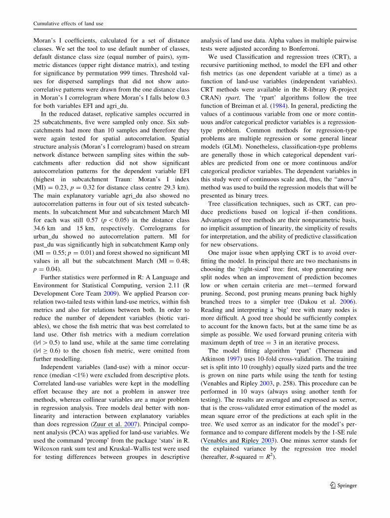
In a PCA with urban, agriculture, pasture, forest, and

shrubland, the first component explained 33.9% of the

variation, the second component 27.8% and the third

component 24.3%. Hence, the first three principal com-

ponents (PC) explained 85.9% of the variation. The biplot

(Fig. 2) of the first two PCs of all five land-use variables

showed that forest and pasture are similarly loaded and that

urban and shrubland are clearly inversely related. Agri-

culture was the main antagonist to forest. In the first PC of

the rotated loadings matrix, agriculture loads with 0.67,

shrubland with -0.56 urban with 0.42. In the second PC,

forest loads with 0.59, pasture with 0.54, shrubland with

-0.43.

From correlation analysis, we learned that coefficients

for urbanisation were low (|r| B 0.25, p \ 0.05) with all

other categories. Pasture correlated with all coefficients

below absolute values of 0.27 (Table 4).

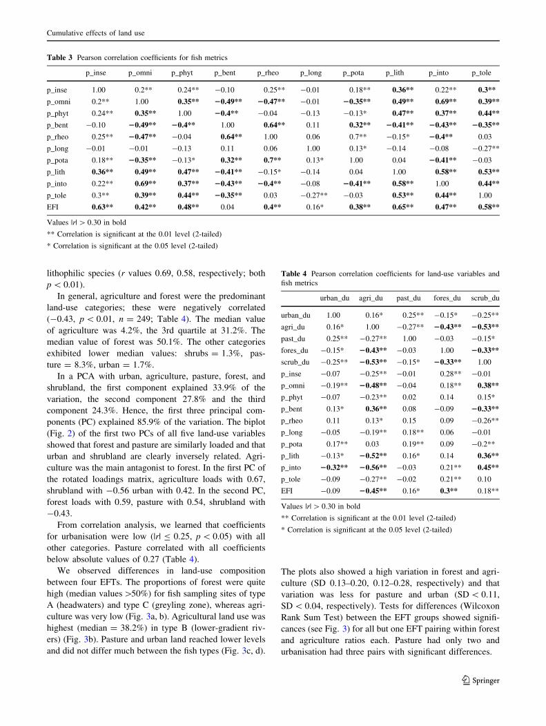
We observed differences in land-use composition

between four EFTs. The proportions of forest were quite

high (median values[50%) for fish sampling sites of type

A (headwaters) and type C (greyling zone), whereas agri-

culture was very low (Fig. 3a, b). Agricultural land use was

highest (median = 38.2%) in type B (lower-gradient riv-

ers) (Fig. 3b). Pasture and urban land reached lower levels

and did not differ much between the fish types (Fig. 3c, d).

The plots also showed a high variation in forest and agri-

culture (SD 0.13–0.20, 0.12–0.28, respectively) and that

variation was less for pasture and urban (SD \ 0.11,

SD \ 0.04, respectively). Tests for differences (Wilcoxon

Rank Sum Test) between the EFT groups showed signifi-

cances (see Fig. 3) for all but one EFT pairing within forest

and agriculture ratios each. Pasture had only two and

urbanisation had three pairs with significant differences.

Table 3 Pearson correlation coefficients for fish metrics

p_inse p_omni p_phyt p_bent p_rheo p_long p_pota p_lith p_into p_tole

p_inse 1.00 0.2** 0.24** -0.10 0.25** -0.01 0.18** 0.36** 0.22** 0.3**

p_omni 0.2** 1.00 0.35** 20.49** 20.47** -0.01 20.35** 0.49** 0.69** 0.39**

p_phyt 0.24** 0.35** 1.00 20.4** -0.04 -0.13 -0.13* 0.47** 0.37** 0.44**

p_bent -0.10 20.49** 20.4** 1.00 0.64** 0.11 0.32** 20.41** 20.43** 20.35**

p_rheo 0.25** 20.47** -0.04 0.64** 1.00 0.06 0.7** -0.15* 20.4** 0.03

p_long -0.01 -0.01 -0.13 0.11 0.06 1.00 0.13* -0.14 -0.08 -0.27**

p_pota 0.18** 20.35** -0.13* 0.32** 0.7** 0.13* 1.00 0.04 20.41** -0.03

p_lith 0.36** 0.49** 0.47** 20.41** -0.15* -0.14 0.04 1.00 0.58** 0.53**

p_into 0.22** 0.69** 0.37** 20.43** 20.4** -0.08 20.41** 0.58** 1.00 0.44**

p_tole 0.3** 0.39** 0.44** 20.35** 0.03 -0.27** -0.03 0.53** 0.44** 1.00

EFI 0.63** 0.42** 0.48** 0.04 0.4** 0.16* 0.38** 0.65** 0.47** 0.58**

Values |r| [ 0.30 in bold

** Correlation is significant at the 0.01 level (2-tailed)

* Correlation is significant at the 0.05 level (2-tailed)

Table 4 Pearson correlation coefficients for land-use variables and

fish metrics

urban_du agri_du past_du fores_du scrub_du

urban_du 1.00 0.16* 0.25** -0.15* -0.25**

agri_du 0.16* 1.00 -0.27** 20.43** 20.53**

past_du 0.25** -0.27** 1.00 -0.03 -0.15*

fores_du -0.15* 20.43** -0.03 1.00 20.33**

scrub_du -0.25** 20.53** -0.15* 20.33** 1.00

p_inse -0.07 -0.25** -0.01 0.28** -0.01

p_omni -0.19** 20.48** -0.04 0.18** 0.38**

p_phyt -0.07 -0.23** 0.02 0.14 0.15*

p_bent 0.13* 0.36** 0.08 -0.09 20.33**

p_rheo 0.11 0.13* 0.15 0.09 -0.26**

p_long -0.05 -0.19** 0.18** 0.06 -0.01

p_pota 0.17** 0.03 0.19** 0.09 -0.2**

p_lith -0.13* 20.52** 0.16* 0.14 0.36**

p_into 20.32** 20.56** -0.03 0.21** 0.45**

p_tole -0.09 -0.27** -0.02 0.21** 0.10

EFI -0.09 20.45** 0.16* 0.3** 0.18**

Values |r| [ 0.30 in bold

** Correlation is significant at the 0.01 level (2-tailed)

* Correlation is significant at the 0.05 level (2-tailed)

Cumulative effects of land use

123

Correlation analyses supported a statistical relationship

between agricultural land use and the ecological status of

rivers (Table 4). The results showed that values of the

European Fish Index were negatively correlated with the

amount of agriculture in the catchment (r = -0.45,

p \ 0.01, n = 249). Correlation between urbanised land

and the fish index was very low and not significant (r =

-0.09, p C 0.05).

Agriculture in the catchment was highly correlated with

omnivorous (r = -0.48, p \ 0.01), lithophilic (r = -0.52,

p \ 0.01), and intolerant (r = -0.56, p \ 0.01) species

metrics. The best relating metrics in respect of forest

were insectivorous and intolerant species (r = 0.28 and

r = 0.21, respectively, both p \ 0.01). Finally, urbanisa-

tion—with generally weaker coefficients—was best

correlated with intolerant species (r = -0.32, p \ 0.01).

Hence, we used intolerant species for further modelling

because of their best correlation with agricultural and urban

land use. Omnivorous and lithophilic species were con-

sidered redundant because they showed a high correlation

(r [ 0.58) with intolerant species.

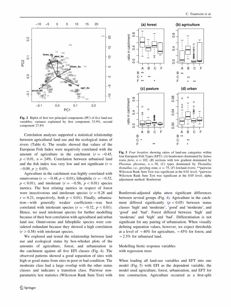
We explored and tested the relationship between land

use and ecological status by box-whisker plots of the

amounts of agriculture, forest, and urbanisation in

the catchment against all five EFI classes (Fig. 4). The

observed patterns showed a good separation of sites with

high or good status from sites in poor or bad condition. The

moderate class had a large overlap with the other status

classes and indicates a transition class. Pairwise non-

parametric test statistics (Wilcoxon Rank Sum Test) with

Bonferroni-adjusted alpha attest significant differences

between several groups (Fig. 4). Agriculture in the catch-

ment differed significantly (p \ 0.05) between status

classes ‘high’ and ‘moderate’, ‘good’ and ‘moderate’, and

‘good’ and ‘bad’. Forest differed between ‘high’ and

‘moderate’ and ‘high’ and ‘bad’. Differentiation is not

significant for any pairing of urbanisation. When visually

defining separation values, however, we expect thresholds

at a level of *40% for agriculture, *45% for forest, and

*2.5% for urbanised land.

Modelling biotic response variables

with regression trees

When loading all land-use variables and EFT into one

model (Fig. 5) with EFI as the dependent variable, the

model used agriculture, forest, urbanisation, and EFT for

tree construction. Agriculture occurred as a first-split

−0.1 0.0 0.1 0.2

−0.

1

0

.0

0.1

0

.2

PC1

PC

2

1

2

3

456

78

9

10

11 12

1314

15

16

17

18

19

20

21

22232425

262728293031

3233343536373839404142434445

464748

49

50

51

5253

54

55

565758

59

60

6162

63

64

65

66 67

686970

71

72

73

74

7576777879

8081

82

8384

858687888990

9192939495969798

99

100

101

102

103104105106107

108109

110

111

112

113114115116

117118

119

120121

122123

124

125126127

128129130

131132133

134135

136

137138139140141

142143

144

145

146

147

148

149150151152

153

154155

156157

158

159

160

161

162163

164

165

166

167

168

169

170 171172

173

174

175176177

178

179

180

181

182

183

184

185186187

188189

190

191

192193194195196197198199200

201202203204205

206

207208

209 210211212

213

214215

216

217218219

220

221222223224

225

226

227

228

229

230231

232233234235236237

238

239240

241242243244

245246

247

248

249

−10 −5 0 5 10 15 20

−10

−

5

0

5

10

15

2

0

urban_du

agri_du

past_dufores_du

scrub_du

Fig. 2 Biplot of first two principal components (PC) of five land-use

variables; variance explained by first component 33.9%, second

component 27.8%

A B C F

0.0

0.4

0.8

(a) forest

ratio

in c

atch

men

t

A B C F

0.0

0.4

0.8

(b) agriculture

A B C F0.

00.

40.

8

(c) pasture

ratio

in c

atch

men

tA B C F

0.00

0.04

0.08

(d) urban

BCF

BCF

BCF

BCF

** * **** *

** ** * **

* **

** ** *

Fig. 3 Four boxplots showing ratios of land-use categories within

four European Fish Types (EFT): (A) headwaters dominated by Salmotrutta fario, n = 102, (B) sections with low gradient dominated by

Phoxinus phoxinus, n = 30, (C) types dominated by Thymallusthymallus, i.e., greyling zone, n = 75, (F) lowland rivers; **pairwise

Wilcoxon Rank Sum Test was significant at the 0.01 level; *pairwise

Wilcoxon Rank Sum Test was significant at the 0.05 level; alpha

adjustment method: Bonferroni

C. Trautwein et al.

123

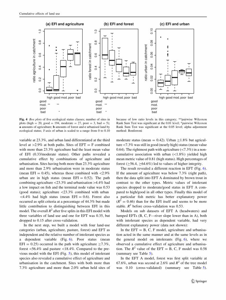
variable at 23.3%, and urban land differentiated at the third

level at [2.9% at both paths. Sites of EFT = F combined

with more than 23.3% agriculture had the least mean value

of EFI (0.33/moderate status). Other paths revealed a

cumulative effect by combinations of agriculture and

urbanisation. Sites having both more than 23.3% agriculture

and more than 2.9% urbanisation were in moderate status

(mean EFI = 0.45), whereas those combined with \2.9%

urban are in high status (mean EFI = 0.52). The path

combining agriculture\23.3% and urbanisation[4.4% had

a low impact on fish and the terminal node value was 0.53

(good status); agriculture \23.3% combined with urban

\4.4% had high status (mean EFI = 0.6). Forest also

occurred as split criteria at a percentage of 44.3% but made

little contribution to distinguishing between EFI in this

model. The overall R2 after five splits in this EFI model with

three variables of land use and one for EFT was 0.35, but

dropped to 0.15 after cross-validation.

In the next step, we built a model with four land-use

categories (urban, agriculture, pasture, forest) and EFT as

independent and the relative number of intolerant species as

a dependent variable (Fig. 6). Poor status (mean

EFI = 0.25) occurred in the path with agriculture C7.3%,

forest \56.4% and pasture \18.4%. Compared to the pre-

vious model with the EFI (Fig. 5), this model of intolerant

species also revealed a cumulative effect of agriculture and

urbanisation in the catchment. Sites with both more than

7.3% agriculture and more than 2.0% urban held sites of

moderate status (mean = 0.42). Urban C1.8% but agricul-

ture\7.3% was still in good (nearly high) status (mean value

0.64). The rightmost path with agriculture (\7.3%) in a non-

cumulative association with urban (\1.8%) yielded high

mean metric value of 0.81 (high status). High percentages of

forest (C56.4, C64.6%) led to values of higher integrity.

The result revealed a different reaction in EFT (Fig. 6).

If the amount of agriculture was below 7.3% (right path),

then the data split into EFT A dominated by brown trout in

contrast to the other types. Metric values of intolerant

species dropped to moderate/good status in EFT A com-

pared to high/good in all other types. Finally this model of

a particular fish metric has better explanatory power

(R2 = 0.46) than for the EFI itself and seems to be more

stable. R2 before cross-validation was 0.53.

Models on sub datasets of EFT A (headwaters) and

lumped EFTs (B, C, F—river slope lower than in A), both

with intolerant species as dependent variable, had very

different explanatory power (data not shown):

In the EFT = B, C, F model, agriculture and urbanisa-

tion acted in the same manner and at the same levels as in

the general model on intolerants (Fig. 6), where we

observed a cumulative effect of agriculture and urbanisa-

tion. The R2 value of the EFT = B, C, F model was 0.58

(summary see Table 5).

In the EFT A model, forest was first split variable at

67.6%, urban was second at 2.6% and R2 of the tree model

was 0.10 (cross-validated) (summary see Table 5).

0.0

0.2

0.

4

0.6

0.

8

1

.0

(a) EFI and agriculture (b) EFI and forest

high good mod. poor bad high good mod. poor bad high good mod. poor bad

(c) EFI and urban

ratio

agr

icul

ture

in c

atch

men

t

0.0

0.2

0.

4

0.6

0.

8

1

.0

ratio

fore

st in

cat

chm

ent

0.00

0.0

2

0.

04

0

.06

0.08

0.1

0

ratio

urb

an in

cat

chm

ent

goodmod.poorbad

** **

*

goodmod.poorbad

**

*

goodmod.poorbad

Fig. 4 Box plots of five ecological status classes; number of sites in

plots (high = 20, good = 194, moderate = 27, poor = 3, bad = 5);

a amounts of agriculture; b amounts of forest and c urbanised land by

ecological status; Y-axis of urban is scaled to a range from 0 to 0.10

because of low ratio levels in this category; **pairwise Wilcoxon

Rank Sum Test was significant at the 0.01 level; *pairwise Wilcoxon

Rank Sum Test was significant at the 0.05 level; alpha adjustment

method: Bonferroni

Cumulative effects of land use

123

Agriculture was an input variable, but not used by the

EFT = A model. The terminal node with worst ecological

status (mean EFI = 0.13/bad status) contained sites with

urbanisation exceeding 2.6% and pasture below 11.3%.

Pasture occurred in a positive trend to ecological integrity

within this model of headwaters (EFT = A).

Discussion

Agriculture was the primary explanatory variable in all

but one tree model (Table 5). Agriculture as split criteria

occurred at three levels: at 23.3% but also at *7.3 and

36–40%. Very often, urban land served as the secondary

split variable at about 2%, with minimum 1.8% and

maximum even at 4.4%. So, the regression tree method

affirmed our interpretation of thresholds in the descriptive

analysis. There was a clear interaction of agriculture and

urban. Sites with more than 7.3% agriculture and more

than 2.0% urban land were likely to result in poor or

moderate status. Urbanisation acted more strongly in river

types dominated by brown trout (S. trutta fario)

(EFT = A) than in river types of lower gradients

(EFT = B, C, F). The model for the relative number of

EFI

|agri_du>=0.233

EFT_type=F

urban_du>=0.029

fores_du>= 0.443

urban_du>=0.044

0.33n=9

0.45n=25

0.52n=46

0.54n=39 0.53

n=110.6

n=119

agri_du<0.233

EFT_type=A, B, C fores_du< 0.443

urban_du<0.044

urban_du<0.029

Fig. 5 Regression tree for EFI

based on land-use categories in

the catchment draining to the

fish sampling sites; n = 233;

R2 = 0.15; true split criteria at

nodes follows left path

p_into

|agri_du>=0.073

fores_du< 0.564

past_du< 0.184 urban_du>=0.021

EFT_type=A

fores_du< 0.646urban_du>=0.018

0.25n=60

0.43n=15

0.42n=14

0.61n=20 0.4

n=180.64n=37

0.64n=19

0.81n=66

agri_du<0.073

EFT_type=B,C,Ffores_du>= 0.564

>= 0.184 <0.021>= 0.646

<0.018

Fig. 6 Regression tree for

metric of relative number of

intolerant species in the EFI;

independent variables are

agriculture, forest, pasture,

urban and European Fish Types

(EFT); n = 233; R2 = 0.46;

true split criteria at nodes

follows left path

C. Trautwein et al.

123

intolerant species had better explanatory power than for

EFI.

Our study showed that multiple land-use categories had

an effect on fish. Agricultural land use had the strongest

detrimental effect. Percentages of agriculture in the

catchment were negatively correlated with the European

Fish Index (EFI). Many studies have found comparable

results for selected small to medium-sized catchments of

2nd to 3rd order rivers (Allan 2004b; Richards et al. 1996;

Roth et al. 1996); our findings corroborated this relation-

ship for the Austrian dataset from small to larger rivers (up

to 7th order) and across four different river types. Urban

areas in the catchment showed strong effects on fish met-

rics even at very small percentages. Snyder et al. (2003)

and Wang et al. (2003) also discussed a disproportionately

large effect of urban land use. Yet, significance of the test

results for urban, agriculture, and forest within EFI status

classes are limited due to an uneven distribution of samples

in high to bad status. Snyder et al. (2003) found no cor-

relation between agriculture (lumped with pasture) and

biota and recommended examining more specific land-use

categories such as grazing versus row-crop agriculture. Our

findings identified pasture (grazing and grassland) as less

influential than agriculture (arable land and permanent

crops).

Moerke and Lamberti (2006) also related four categories

to fish assemblage structure and found higher IBI scores in

forested streams compared to urban and agricultural

streams. Our results go beyond mere correlation (Steel

et al. 2010) because we applied new methods and identified

thresholds at which biota react. Intolerant, lithophilic, and

omnivorous species reacted most strongly to agriculture

and urban development. Metrics for insectivorous and

migratory species were less correlated to land use. Moerke

and Lamberti (2006) used metrics of general tolerance and

showed a positive association between sensitive species

and higher percentages of forest in the catchment, and

between tolerant fish and changes in land use (agriculture,

urban). Pess et al. (2002) reported positive correlated

densities of salmon with forest cover in the watershed. Our

findings revealed that a fish metric of intolerance to general

disturbance (p_into) is a better indicator than the EFI. We

hypothesise that these species react to both direct (e.g.,

toxins, nutrients) and indirect (e.g., sedimentation, hydro-

logic alteration) effects of land use. Wang et al. (2003) also

used percentage of intolerants and found that thresholds for

urban land cover (measured as impervious surface area)

had detrimental effects on fish at 11%. Among four aquatic

organism groups (diatoms, macrophytes, benthic macroin-

vertebrates and fish) fish were found to respond less

strongly to catchment land use than to eutrophication/

organic pollution gradients (Hering et al. 2006). Hering

et al. (2006) found the strongest response for lithophilic

and limnophilic species and related this to direct or indirect

effects of land-use on habitat quality. Hering et al. also

discussed effects of land-use acting through numerous

cause-effect relationships that are difficult to identify.

Few studies have dealt with relative effects of multiple

land-use categories on stream ecosystems (Moerke and

Lamberti 2006; Van Sickle et al. 2004; Snyder et al. 2003).

Moerke and Lamberti (2006) evaluated forest, urban,

agriculture and wetlands. Snyder et al. (2003) additionally

used water and barren land, but in both studies only forest,

agriculture and urban were frequent and associated

strongly enough for further analysis. Using regression

analysis, Snyder et al. (2003) explained 63% of IBI vari-

ation by urban land in the catchment alone. Neither forest

nor agriculture explained a significant amount of the

remaining variation in IBI after accounting for the effects

of urban land use. In our study, using answer tree models,

we determined a cumulative effect of agriculture and urban

land use. Urban or agriculture alone resulted in a lower

detrimental effect than when combined.

River-type-specific reactions

The brown trout assemblage type (EFT A) showed a

stronger decrease in ecological status than river types of

lower sections (greyling zone, lowland rivers). In the latter

fish types (EFT = BCF), the cumulative effect of agricul-

ture and urban was better pronounced than in headwaters.

In general, agriculture correlated best to fish metrics and

Table 5 Summary of the model results for fish metrics as dependent variable and land-use categories as independent variables

Model title y Independent used 1st level split 2nd level split R2 N

EFI—AT EFI Agri, fores, urban Agri 23.3% Urban *3% 0.15 249

AT intolerants P_into Agri, fores, urban, EFT Agri 7.3% Fores 44%, urban *2% 0.46 249

AT omnivorous p_omni Agri, urban Agri 7.3% Urban *2% 0.17 249

AT lithophilic p_lith Agri, urban, EFT Agri 40% Urban 3.3% 0.39 249

EFT = A, intolerants p_into Fores, past, urban Fores 67.6% Urban *2.5% 0.09 102

EFT = B, C, F intolerants p_into Agri, urban Agri 8% Agri 36.7%, urban 1.8% 0.58 131

Abbreviations see Table 1

Cumulative effects of land use

123

EFI, whereas all other land-use categories remained at a

very low correlation level. Headwaters, however, seemed

to be very sensitive although at low levels of agriculture

(\7.3%) and highly forested catchments (\64.6%). We

hypothesise that the underlying mechanisms are effects of

hydrology (e.g., increased peak runoff from impervious

surfaces), morphological alteration (e.g., channelization)

and removal of riparian vegetation (e.g., reduced shading,

increased water temperature) (Allan 2004b), and that they

act more strongly on small headwater streams. Addition-

ally, by nature, trout rivers are low-species-number rivers

with intolerant species and, therefore, intolerant-species-

metric responded more sensitively to disturbance.

Hering et al. (2006) produced weak correlation results

for mountain streams, while in lowland stream types the

explanatory power of the fish metrics was at a higher level

(r2 = 0.4). These findings are somehow contradictory to

our findings because headwaters respond even more sen-

sitively than other EFTs. However, a model for the

headwater fishtype (EFT = A) was much less powerful

than for streams of lower gradients (EFT = B, C, F). The

explanatory power of our models of land-use seem to be

comparable to Hering et al. (2006) with maximum at

R2 = 0.46. Nevertheless, we are aware of bias in the model

for headwaters. Full land-use gradients are limited in our

dataset because most headwaters are located in less

developed landscapes.

Conclusions

With this study we provide catchment-level relationships

for land use covering headwater streams (brown trout) to

medium- (greyling) and large-sized rivers in Austria. Mo-

erke and Lamberti (2006) have already concluded that

additional replicated, catchment-level studies in other

geographic areas will enhance our knowledge of how land

use affects stream ecosystems. Such findings help identify

characteristics that make streams more or less sensitive to

land-use change.

The regression tree models we used are very simple and

based on a large sample of sites. They can explain a

moderate amount of variability in biotic integrity based on

a few land-use categories (urban areas, agriculture, pasture,

and forest). These results are promising as building blocks

for designing models of cascades that represent mecha-

nistic relationships.

The present study does not explain the full pathways

from land use via physical habitat, water quality and/or

hydrologic alteration to a resulting biological impact, but

the results do go beyond mere correlative analysis.

Research into underlying mechanisms remains a challenge

(Steel et al. 2010; Wang et al. 2006a). Based on the current

findings, it will be possible to develop first steps of char-

acteristic cause and effect pathways for selected river

types.

Acknowledgments Work on this manuscript was funded by the

Austrian Science Fund (FWF, research project LANPREF, contract

number P 21735-B16). Basic ideas for this work arose within the

EFI ? project supported by the European Commission under FP6

(contract number 044096), and our sincere thanks go to all members

of the EFI ? consortium. We thank Andreas Melcher for valuable

discussions on early stages of the manuscript. Ashley Steel gave

precious input to consistency of the manuscript, discussion of the

results and the English, thank you. Two anonymous reviewers

addressed several substantive issues to improve the manuscript.

Open Access This article is distributed under the terms of the

Creative Commons Attribution Noncommercial License which per-

mits any noncommercial use, distribution, and reproduction in any

medium, provided the original author(s) and source are credited.

References

Allan JD (2004a) Influence of land use and landscape setting on the

ecological status of rivers. Limnetica 23:187–198

Allan JD (2004b) Landscapes and riverscapes: the influence of land

use on stream ecosystems. Annu Rev Ecol Evol S 35:257–284

Allan JD, Johnson LB (1997) Catchment-scale analysis of aquatic

ecosystems. Freshw Biol 37:107–111

Allan JD, Erickson DL, Fay J (1997) The influence of catchment land

use on stream integrity across multiple spatial scales. Freshw

Biol 37:149–161

Beechie TJ, Sear DA, Olden JD, Pess GR, Buffington JM, Moir H,

Roni P, Pollock MM (2010) Process-based principles for

restoring river ecosystems. Bioscience 60:209–222

Beyer HL (2004) Hawth’s Analysis Tools for ArcGIS. Available at

http://www.spatialecology.com/htools. Accessed 11 Feb 2008

Botequilha Leitao A, Miller J, Ahern J, McGarigal K (2006)

Measuring landscapes. Island, Washington, DC

Breiman L, Friedman J, Stone CJ, Olshen RA (1984) Classification

and regression trees. Chapman and Hall/CRC, Boca Raton

CEN (2003) Water quality—sampling of fish with electricity, EN

14011. European Committee for Standardisation, Brussels

Dakou E, D’heygere T, Dedecker AP, Goethals PLM, Lazaridou-

Dimitriadou M, Pauw N (2006) Decision tree models for

prediction of macroinvertebrate taxa in the river axios (northern

Greece). Aquat Ecol 41:399–411

Durance I, Lepichon C, Ormerod SJ (2006) Recognizing the

importance of scale in the ecology and management of riverine

fish. River Res Appl 22:1143–1152

EC of European Parliament (2000) Water framework directive—

Establishing a framework for community action in the field of

water policy. Off J Eur Comm L327:1–72

ESRI (2008) ArcGIS Desktop, Version 9.3, ArcInfo license. Red-

lands, CA

FAME-Consortium (2004) Manual for Application of the European Fish

Index—EFI. A fish-based method to assess the ecological status of

European rivers in support of the Water Framework Directive

(Version 1.1, January 2005). Available at: http://fame.boku.

ac.at/downloads/manual_Version_Februar2005.pdf. Accessed 2

Apr 2008

Gergel SE, Turner MG, Miller JR, Melack JM, Stanley EH (2002)

Landscape indicators of human impacts to riverine systems.

Aquat Sci 64:118–128

C. Trautwein et al.

123

Hering D, Johnson RK, Kramm S et al (2006) Assessment of

European streams with diatoms, macrophytes, macroinverte-

brates and fish: a comparative metric-based analysis of organism

response to stress. Freshw Biol 51(9):1757–1785

Huet M (1949) Apercu des relations entre la pente et les populations

piscicoles des eaux courantes. Schweiz Z Hydrol 11:332–351

Illies J, Andrassy I (1978) Limnofauna europaea—a checklist of the

animals inhabiting European inland waters, with accounts of

their distribution and ecology (except protozoa), vol 2, Second

revised edn. Gustav Fischer Verlag, Stuttgart, NY

Karr JR (1981) Assessment of biotic integrity using fish communities.

Fisheries 6:21–27

Melcher A, Schmutz S, Haidvogl G, Moder K (2007) Spatially based

methods to assess the ecological status of European fish

assemblage types. Fish Manag Ecol 14:453–463

Miltner R, White D, Yoder C (2004) The biotic integrity of streams in

urban and suburbanizing landscapes. Landsc Urban Plan

69:87–100

Moerke AH, Lamberti GA (2006) Relationships between land use and

stream ecosystems: a multistream assessment in southwestern

Michigan. Am Fish Soc Symp 2006:323–338

Noble RAA, Cowx IG, Goffaux D, Kestemont P (2007) Assessing the

health of European rivers using functional ecological guilds of

fish communities: standardising species classification and

approaches to metric selection. Fish Manag Ecol 14(6):381–392

Omernik JM, Bailey RG (1997) Distinguishing between watersheds

and ecoregions. J Am Water Resour Assoc 33:935–949

Pess GR, Montgomery DR, Steel EA, Bilby RE, Feist BE, Greenberg

HM (2002) Landscape characteristics, land use, and coho salmon

(Oncorhynchus kisutch) abundance, Snohomish River, Wash-

ington, USA. Can J Fish Aquat Sci 59:613–623

Poff NL (1997) Landscape filters and species traits: Towards

mechanistic understanding and prediction in stream ecology.

J N Am Benthol Soc 16:391–409

Pont D, Hugueny B, Beier U, Goffaux D, Melcher A, Noble R,

Rogers C, Roset N, Schmutz S (2006) Assessing river biotic

condition at a continental scale: a European approach using

functional metrics and fish assemblages. J Appl Ecol 43:70–80

Pont D, Hugueny B, ROGERS C (2007) Development of a fish-based

index for the assessment of river health in Europe: The European

fish index. Fish Manag Ecol 14:427–439

R Development Core Team (2009) R: A language and environment

for statistical computing. Vienna, Austria

Rangel TF, Diniz-Filho JAF, Bini LM (2010) SAM: a comprehensive

application for spatial analysis in macroecology. Ecography

33:1–5

Richards C, Johnson LB, Host GE (1996) Landscape-scale influences

on stream habitats and biota. Can J Fish Aquat Sci 53:295–311

Roth NE, Allan JD, Erickson DL (1996) Landscape influences on

stream biotic integrity assessed at multiple spatial scales.

Landscape Ecol 11:141–156

Snyder CD, Young JA, Villella R, Lemarie DP (2003) Influences of

upland and riparian land use patterns on stream biotic integrity.

Landscape Ecol 18:647–664

Steel EA, Hughes RM, Fullerton AH, Schmutz S, Young J,

Fukushima M, Muhar S, Poppe M, Feist BE, Trautwein C

(2010) Are we meeting the challenges of landscape-scale

riverine research? A review. Living Rev Lands Res 4:1

Stewart JS, Wang L, Lyons J, Horwatich JA, Bannerman R (2001)

Influences of watershed, riparian-corridor, and reach-scale

characteristics on aquatic biota in agricultural watersheds.

J Am Water Resour Assoc 37:1475–1487

Therneau TM, Atkinson EJ (1997) An introduction to recursive

partitioning using the rpart routines. http://www.mayo.edu/hsr/

techrpt/61.pdf (cited on 12/03/2010)

Van Sickle J, Baker J, Herlihy A, Bayley P, Gregory S, Haggerty P,

Ashkenas L, Li J (2004) Projecting the biological condition of

streams under alternative scenarios of human land use. Ecol

Appl 14:368–380

Venables WN, Ripley BD (2003) Modern applied statistics with S,

4th edn. Springer, New York

Vogt JV, Soille P, Jager AD, Rimaviciute E, Mehl W, Foisneau S,

Bodis K, Dusart J, Paracchini ML, Haastrup P, Bamps C (2007)

A pan-European river and catchment database. European

Commission, Joint Research Center, Institute for Environment

and Sustainability, Luxembourg

Wang L, Lyons J, Kanehl P, Bannerman R (2001) Impacts of

urbanization on stream habitat and fish across multiple spatial

scales. Environ Manage 28:255–266

Wang L, Lyons J, Kanehl P (2003) Impacts of urban land cover on

trout streams in Wisconsin and Minnesota. Trans Am Fish Soc

132:825–839

Wang L, Seelbach PW, Hughes RM (2006a) Introduction to

landscape influences on stream habitats and biological assem-

blages. Am Fish Soc Symp 2006:1–23

Wang L, Seelbach PW, Lyons J (2006b) Effects of levels of human

disturbance on the influence of catchment, riparian, and reach-scale

factors on fish assemblages. Am Fish Soc Symp 2006:199–219

Ward JV (1989) The 4-dimensional nature of lotic ecosystems. J N

Am Benthol Soc 8:2–8

Zuur AF, Ieno EN, Smith GM (2007) Analysing ecological data.

Springer, New York, NY

Cumulative effects of land use

123