
CUBIT Mesh Generation Environment Volume 1: Users Manual
179
Exceptional CUBIT Mesh Generation Environment Volume 1: Users Manual Cubit Development Team 1 Sandia National Laboratories Albuquerque, New Mexico 87185-0441 Abstract The CUBIT mesh generation toolkit is a two- and three-dimensional finite ele- ment mesh generation tool which is being developed to pursue the goal of ro- bust and unattended mesh generation—effectively automating the generation of quadrilateral and hexahedral elements. CUBIT generates surface and vol- ume meshes for solid model-based geometries; these meshes are used for finite element analysis applications. A combination of techniques including paving, mapping, submapping, sweeping, and various other algorithms being devel- oped are available for discretizing the geometry into a finite element mesh. The software is used for both production mesh generation and as a testbed for new algorithms. While CUBIT is specifically designed to reduce the time required to create all-quadrilateral and all-hexahedral meshes, it also provides the capa- bility to generate hex dominant and tetrahedral meshes. This manual is de- signed to serve as a reference and guide to creating finite element models in the CUBIT environment. This manual documents CUBIT Version 3.1. 1. See the next page for the members of the CUBIT Development Team. SAND94-1100 Unlimited Release Printed May 6, 1999 4:15 pm Distribution Category UC-705
-
Upload
khangminh22 -
Category
Documents
-
view
5 -
download
0
Transcript of CUBIT Mesh Generation Environment Volume 1: Users Manual

Exceptional
CUBIT Mesh GenerationEnvironment
Volume 1: Users Manual
Cubit Development Team1
Sandia National LaboratoriesAlbuquerque, New Mexico 87185-0441
Abstract
The CUBIT mesh generation toolkit is a two- and three-dimensional finite ele-ment mesh generation tool which is being developed to pursue the goal of ro-bust and unattended mesh generation—effectively automating the generationof quadrilateral and hexahedral elements. CUBIT generates surface and vol-ume meshes for solid model-based geometries; these meshes are used for finiteelement analysis applications. A combination of techniques including paving,mapping, submapping, sweeping, and various other algorithms being devel-oped are available for discretizing the geometry into a finite element mesh. Thesoftware is used for both production mesh generation and as a testbed for newalgorithms. While CUBIT is specifically designed to reduce the time requiredto create all-quadrilateral and all-hexahedral meshes, it also provides the capa-bility to generate hex dominant and tetrahedral meshes. This manual is de-signed to serve as a reference and guide to creating finite element models in theCUBIT environment.
This manual documents CUBIT Version 3.1.
1. See the next page for the members of the CUBIT Development Team.
SAND94-1100Unlimited Release
Printed May 6, 1999 4:15 pm
DistributionCategory UC-705

▼ Cubit Development Team Membership
Sandia National Laboratories, Albuquerque New Mexico
Patrick Knupp Parallel Computing Sciences
Robert W. Leland Manager, Parallel Computing Sciences
Darryl J. Melander Parallel Computing Sciences
Scott A. Mitchell Parallel Computing Sciences
W. Ann Sample Parallel Computing Sciences
Timothy J. Tautges Parallel Computing Sciences
David R. White Parallel Computing Sciences
Jason Shephard Parallel Computing Sciences
Brigham Young University, Provo, Utah
Steve Benzley Professor of Civil and Environmental Engineering
Robert Kerr Student in Department of Civil and Environmental Eng.
Steven R. Jankovich Student in Department of Mechanical Engineering
University of Wisconsin
Jason Kraftcheck Student in Department of Mechanical Engineering
Contractors
Ray J. Meyers Contractor, Provo, Utah
Michael Stepheson Contractor, Provo, Utah

Table of Contents
Document Version 2/2/00 CUBIT Reference Manual 5
▼ Table of Contents▼ Cubit Development Team Membership . . . . . . . . . . . . . . . . . . . . . . . . . . . . . 4▼ Table of Contents . . . . . . . . . . . . . . . . . . . . . . . . . . . . . . . . . . . . . . . . . . . . . . . 5▼ List of Figures . . . . . . . . . . . . . . . . . . . . . . . . . . . . . . . . . . . . . . . . . . . . . . . . . . 1▼ List of Tables . . . . . . . . . . . . . . . . . . . . . . . . . . . . . . . . . . . . . . . . . . . . . . . . . . . 3
Chapter 1: Getting Started . . . . . . . . . . . . . . . . . . . . . . . . . . . . . . . . . . . . . . 5
▼ Introduction . . . . . . . . . . . . . . . . . . . . . . . . . . . . . . . . . . . . . . . . . . . . . . . . . . . . 5▼ How to Use This Manual . . . . . . . . . . . . . . . . . . . . . . . . . . . . . . . . . . . . . . . . . 5▼ Features . . . . . . . . . . . . . . . . . . . . . . . . . . . . . . . . . . . . . . . . . . . . . . . . . . . . . . . 6
Geometry Creation, Modification and Healing . . . . . . . . . . . . . . . . . . . . . . 6Non-Manifold Topology. . . . . . . . . . . . . . . . . . . . . . . . . . . . . . . . . . . . . . . . 6Geometry Decomposition . . . . . . . . . . . . . . . . . . . . . . . . . . . . . . . . . . . . . . . 7Mesh Generation. . . . . . . . . . . . . . . . . . . . . . . . . . . . . . . . . . . . . . . . . . . . . . 7Boundary Conditions . . . . . . . . . . . . . . . . . . . . . . . . . . . . . . . . . . . . . . . . . . 7Element Types . . . . . . . . . . . . . . . . . . . . . . . . . . . . . . . . . . . . . . . . . . . . . . . 7Graphics Display Capabilities. . . . . . . . . . . . . . . . . . . . . . . . . . . . . . . . . . . . 7Command Line Interface . . . . . . . . . . . . . . . . . . . . . . . . . . . . . . . . . . . . . . . 7Hardware Platforms . . . . . . . . . . . . . . . . . . . . . . . . . . . . . . . . . . . . . . . . . . . 8
▼ Executing CUBIT . . . . . . . . . . . . . . . . . . . . . . . . . . . . . . . . . . . . . . . . . . . . . . . 8Execution Command Syntax. . . . . . . . . . . . . . . . . . . . . . . . . . . . . . . . . . . . . 8User Environment Settings . . . . . . . . . . . . . . . . . . . . . . . . . . . . . . . . . . . . . . 9Initialization File. . . . . . . . . . . . . . . . . . . . . . . . . . . . . . . . . . . . . . . . . . . . . . 9
▼ CUBIT Mailing Lists . . . . . . . . . . . . . . . . . . . . . . . . . . . . . . . . . . . . . . . . . . . . . 10▼ Problem Reports and Enhancement Requests . . . . . . . . . . . . . . . . . . . . . . . . 10
Chapter 2: Tutorial . . . . . . . . . . . . . . . . . . . . . . . . . . . . . . . . . . . . . . . . . . . . 11
▼ Introduction . . . . . . . . . . . . . . . . . . . . . . . . . . . . . . . . . . . . . . . . . . . . . . . . . . . . 11▼ Overview . . . . . . . . . . . . . . . . . . . . . . . . . . . . . . . . . . . . . . . . . . . . . . . . . . . . . . 12▼ Step 1: Beginning Execution . . . . . . . . . . . . . . . . . . . . . . . . . . . . . . . . . . . . . . 12▼ Step 2: Creating the Brick . . . . . . . . . . . . . . . . . . . . . . . . . . . . . . . . . . . . . . . . 14▼ Step 3: Creating the Cylinder . . . . . . . . . . . . . . . . . . . . . . . . . . . . . . . . . . . . . 14▼ Step 4: Adjusting the Graphics Display . . . . . . . . . . . . . . . . . . . . . . . . . . . . . 15▼ Step 5: Forming the Hole . . . . . . . . . . . . . . . . . . . . . . . . . . . . . . . . . . . . . . . . . 16▼ Step 6: Setting Interval Sizes . . . . . . . . . . . . . . . . . . . . . . . . . . . . . . . . . . . . . . 16▼ Step 7: Surface Meshing . . . . . . . . . . . . . . . . . . . . . . . . . . . . . . . . . . . . . . . . . . 17▼ Step 8: Volume Meshing . . . . . . . . . . . . . . . . . . . . . . . . . . . . . . . . . . . . . . . . . . 18▼ Step 9: Inspecting the Model . . . . . . . . . . . . . . . . . . . . . . . . . . . . . . . . . . . . . . 19▼ Step 10: Defining Boundary Conditions . . . . . . . . . . . . . . . . . . . . . . . . . . . . . 20▼ Step 11: Exporting the Mesh . . . . . . . . . . . . . . . . . . . . . . . . . . . . . . . . . . . . . . 21▼ Congratulations . . . . . . . . . . . . . . . . . . . . . . . . . . . . . . . . . . . . . . . . . . . . . . . . . 21

Table of Contents
6 CUBIT Reference Manual Document Version 2/2/00
Chapter 3: Environment . . . . . . . . . . . . . . . . . . . . . . . . . . . . . . . . . . . . . . . . 23
▼ Introduction . . . . . . . . . . . . . . . . . . . . . . . . . . . . . . . . . . . . . . . . . . . . . . . . . . . . 23▼ Command Syntax . . . . . . . . . . . . . . . . . . . . . . . . . . . . . . . . . . . . . . . . . . . . . . . 23▼ Executing CUBIT . . . . . . . . . . . . . . . . . . . . . . . . . . . . . . . . . . . . . . . . . . . . . . . 25
Execution Command Syntax. . . . . . . . . . . . . . . . . . . . . . . . . . . . . . . . . . . . . 25Environment Variables . . . . . . . . . . . . . . . . . . . . . . . . . . . . . . . . . . . . . . . . . 26Initialization File. . . . . . . . . . . . . . . . . . . . . . . . . . . . . . . . . . . . . . . . . . . . . . 26
▼ Session Control . . . . . . . . . . . . . . . . . . . . . . . . . . . . . . . . . . . . . . . . . . . . . . . . . 26▼ Command Recording and Playback . . . . . . . . . . . . . . . . . . . . . . . . . . . . . . . . 27
Journal File Creation & Playback. . . . . . . . . . . . . . . . . . . . . . . . . . . . . . . . . 27Automatic Journal File Creation. . . . . . . . . . . . . . . . . . . . . . . . . . . . . . . . . . 28
▼ Entity Specification . . . . . . . . . . . . . . . . . . . . . . . . . . . . . . . . . . . . . . . . . . . . . . 28▼ Command Line Editing . . . . . . . . . . . . . . . . . . . . . . . . . . . . . . . . . . . . . . . . . . 31▼ Graphics . . . . . . . . . . . . . . . . . . . . . . . . . . . . . . . . . . . . . . . . . . . . . . . . . . . . . . . 32
Updating the Display . . . . . . . . . . . . . . . . . . . . . . . . . . . . . . . . . . . . . . . . . . 32Graphics Modes . . . . . . . . . . . . . . . . . . . . . . . . . . . . . . . . . . . . . . . . . . . . . . 32Drawing and Highlighting Entities . . . . . . . . . . . . . . . . . . . . . . . . . . . . . . . . 33
Drawing Other Objects 34Mouse-Based View Navigation . . . . . . . . . . . . . . . . . . . . . . . . . . . . . . . . . . 35
Changing the View Transformation Button Bindings 36Navigational Drawing Mode 36Saving and Restoring Views 36
Selecting Entities with the Mouse. . . . . . . . . . . . . . . . . . . . . . . . . . . . . . . . . 37Information About the Selection 39
Mesh Slicing . . . . . . . . . . . . . . . . . . . . . . . . . . . . . . . . . . . . . . . . . . . . . . . . . 40Entity Labels . . . . . . . . . . . . . . . . . . . . . . . . . . . . . . . . . . . . . . . . . . . . . . . . . 41Colors . . . . . . . . . . . . . . . . . . . . . . . . . . . . . . . . . . . . . . . . . . . . . . . . . . . . . . 42Geometry and Mesh Entity Visibility . . . . . . . . . . . . . . . . . . . . . . . . . . . . . . 43Graphics Camera. . . . . . . . . . . . . . . . . . . . . . . . . . . . . . . . . . . . . . . . . . . . . . 44Graphics Windows . . . . . . . . . . . . . . . . . . . . . . . . . . . . . . . . . . . . . . . . . . . . 47Hardcopy Output. . . . . . . . . . . . . . . . . . . . . . . . . . . . . . . . . . . . . . . . . . . . . . 47Miscellaneous Graphics Options . . . . . . . . . . . . . . . . . . . . . . . . . . . . . . . . . 48
▼ Listing Information . . . . . . . . . . . . . . . . . . . . . . . . . . . . . . . . . . . . . . . . . . . . . . 49List Model Summary . . . . . . . . . . . . . . . . . . . . . . . . . . . . . . . . . . . . . . . . . . 49List Geometry . . . . . . . . . . . . . . . . . . . . . . . . . . . . . . . . . . . . . . . . . . . . . . . . 49List Mesh . . . . . . . . . . . . . . . . . . . . . . . . . . . . . . . . . . . . . . . . . . . . . . . . . . . 50List Special Entities . . . . . . . . . . . . . . . . . . . . . . . . . . . . . . . . . . . . . . . . . . . 51List CUBIT Environment . . . . . . . . . . . . . . . . . . . . . . . . . . . . . . . . . . . . . . . 51
▼ Obtaining Help . . . . . . . . . . . . . . . . . . . . . . . . . . . . . . . . . . . . . . . . . . . . . . . . . 57
Chapter 4: Geometry . . . . . . . . . . . . . . . . . . . . . . . . . . . . . . . . . . . . . . . . . . 59
▼ Introduction . . . . . . . . . . . . . . . . . . . . . . . . . . . . . . . . . . . . . . . . . . . . . . . . . . . . 59▼ CUBIT Geometry Model Definitions . . . . . . . . . . . . . . . . . . . . . . . . . . . . . . . 59

Table of Contents
Document Version 2/2/00 CUBIT Reference Manual 7
Topology. . . . . . . . . . . . . . . . . . . . . . . . . . . . . . . . . . . . . . . . . . . . . . . . . . . . 60Non-Manifold Topology. . . . . . . . . . . . . . . . . . . . . . . . . . . . . . . . . . . . . . . . 60
▼ Geometry Creation . . . . . . . . . . . . . . . . . . . . . . . . . . . . . . . . . . . . . . . . . . . . . . 60Geometric Primitives . . . . . . . . . . . . . . . . . . . . . . . . . . . . . . . . . . . . . . . . . . 60Importing Geometry . . . . . . . . . . . . . . . . . . . . . . . . . . . . . . . . . . . . . . . . . . . 63Bottom-Up Geometry Creation. . . . . . . . . . . . . . . . . . . . . . . . . . . . . . . . . . . 64
▼ Geometry Transforms . . . . . . . . . . . . . . . . . . . . . . . . . . . . . . . . . . . . . . . . . . . 67▼ Geometry Booleans . . . . . . . . . . . . . . . . . . . . . . . . . . . . . . . . . . . . . . . . . . . . . . 69▼ Geometry Decomposition . . . . . . . . . . . . . . . . . . . . . . . . . . . . . . . . . . . . . . . . . 70
Web Cutting . . . . . . . . . . . . . . . . . . . . . . . . . . . . . . . . . . . . . . . . . . . . . . . . . 70Split Periodic. . . . . . . . . . . . . . . . . . . . . . . . . . . . . . . . . . . . . . . . . . . . . . . . . 72
▼ Geometry Merging . . . . . . . . . . . . . . . . . . . . . . . . . . . . . . . . . . . . . . . . . . . . . . 72Merging. . . . . . . . . . . . . . . . . . . . . . . . . . . . . . . . . . . . . . . . . . . . . . . . . . . . . 73Unmerging . . . . . . . . . . . . . . . . . . . . . . . . . . . . . . . . . . . . . . . . . . . . . . . . . . 74Examining Merged Entities . . . . . . . . . . . . . . . . . . . . . . . . . . . . . . . . . . . . . 74Merge Tolerance . . . . . . . . . . . . . . . . . . . . . . . . . . . . . . . . . . . . . . . . . . . . . . 74Using Geometry Merging to Verify Geometry. . . . . . . . . . . . . . . . . . . . . . . 74
▼ Geometry Groups . . . . . . . . . . . . . . . . . . . . . . . . . . . . . . . . . . . . . . . . . . . . . . . 75▼ Geometry Attributes . . . . . . . . . . . . . . . . . . . . . . . . . . . . . . . . . . . . . . . . . . . . . 75
Entity Names. . . . . . . . . . . . . . . . . . . . . . . . . . . . . . . . . . . . . . . . . . . . . . . . . 75Persistent Attributes . . . . . . . . . . . . . . . . . . . . . . . . . . . . . . . . . . . . . . . . . . . 76
▼ Exporting Geometry . . . . . . . . . . . . . . . . . . . . . . . . . . . . . . . . . . . . . . . . . . . . . 78
Chapter 5: Mesh Generation . . . . . . . . . . . . . . . . . . . . . . . . . . . . . . . . . . . . 79
▼ Introduction . . . . . . . . . . . . . . . . . . . . . . . . . . . . . . . . . . . . . . . . . . . . . . . . . . . . 79Element Types . . . . . . . . . . . . . . . . . . . . . . . . . . . . . . . . . . . . . . . . . . . . . . . 79Mesh Generation Process . . . . . . . . . . . . . . . . . . . . . . . . . . . . . . . . . . . . . . . 80
▼ Interval Assignment . . . . . . . . . . . . . . . . . . . . . . . . . . . . . . . . . . . . . . . . . . . . . 81Interval Firmness . . . . . . . . . . . . . . . . . . . . . . . . . . . . . . . . . . . . . . . . . . . . . 81Explicit Specification of Intervals . . . . . . . . . . . . . . . . . . . . . . . . . . . . . . . . 81Automatic Specification of Intervals . . . . . . . . . . . . . . . . . . . . . . . . . . . . . . 82Interval Matching . . . . . . . . . . . . . . . . . . . . . . . . . . . . . . . . . . . . . . . . . . . . . 83Periodic Intervals . . . . . . . . . . . . . . . . . . . . . . . . . . . . . . . . . . . . . . . . . . . . . 84Relative Intervals . . . . . . . . . . . . . . . . . . . . . . . . . . . . . . . . . . . . . . . . . . . . . 84
▼ Meshing Schemes . . . . . . . . . . . . . . . . . . . . . . . . . . . . . . . . . . . . . . . . . . . . . . . 85Bias, Dualbias . . . . . . . . . . . . . . . . . . . . . . . . . . . . . . . . . . . . . . . . . . . . . . . . 85Circle. . . . . . . . . . . . . . . . . . . . . . . . . . . . . . . . . . . . . . . . . . . . . . . . . . . . . . . 86Copy . . . . . . . . . . . . . . . . . . . . . . . . . . . . . . . . . . . . . . . . . . . . . . . . . . . . . . . 87Dice. . . . . . . . . . . . . . . . . . . . . . . . . . . . . . . . . . . . . . . . . . . . . . . . . . . . . . . . 87Equal . . . . . . . . . . . . . . . . . . . . . . . . . . . . . . . . . . . . . . . . . . . . . . . . . . . . . . . 90HexToVoid . . . . . . . . . . . . . . . . . . . . . . . . . . . . . . . . . . . . . . . . . . . . . . . . . . 91HexTet. . . . . . . . . . . . . . . . . . . . . . . . . . . . . . . . . . . . . . . . . . . . . . . . . . . . . . 91Mapping . . . . . . . . . . . . . . . . . . . . . . . . . . . . . . . . . . . . . . . . . . . . . . . . . . . . 92Mirror . . . . . . . . . . . . . . . . . . . . . . . . . . . . . . . . . . . . . . . . . . . . . . . . . . . . . . 93

Table of Contents
8 CUBIT Reference Manual Document Version 2/2/00
Pave. . . . . . . . . . . . . . . . . . . . . . . . . . . . . . . . . . . . . . . . . . . . . . . . . . . . . . . . 94Plastering. . . . . . . . . . . . . . . . . . . . . . . . . . . . . . . . . . . . . . . . . . . . . . . . . . . . 95Submap . . . . . . . . . . . . . . . . . . . . . . . . . . . . . . . . . . . . . . . . . . . . . . . . . . . . . 95Sweep . . . . . . . . . . . . . . . . . . . . . . . . . . . . . . . . . . . . . . . . . . . . . . . . . . . . . . 98TetMesh . . . . . . . . . . . . . . . . . . . . . . . . . . . . . . . . . . . . . . . . . . . . . . . . . . . . 100Tetrahedron. . . . . . . . . . . . . . . . . . . . . . . . . . . . . . . . . . . . . . . . . . . . . . . . . . 100Triangle. . . . . . . . . . . . . . . . . . . . . . . . . . . . . . . . . . . . . . . . . . . . . . . . . . . . . 101Trimap. . . . . . . . . . . . . . . . . . . . . . . . . . . . . . . . . . . . . . . . . . . . . . . . . . . . . . 102TriMesh. . . . . . . . . . . . . . . . . . . . . . . . . . . . . . . . . . . . . . . . . . . . . . . . . . . . . 102Tridice. . . . . . . . . . . . . . . . . . . . . . . . . . . . . . . . . . . . . . . . . . . . . . . . . . . . . . 102Tripave . . . . . . . . . . . . . . . . . . . . . . . . . . . . . . . . . . . . . . . . . . . . . . . . . . . . . 103Whisker Weaving . . . . . . . . . . . . . . . . . . . . . . . . . . . . . . . . . . . . . . . . . . . . . 103
▼ Automatic Scheme Selection . . . . . . . . . . . . . . . . . . . . . . . . . . . . . . . . . . . . . . 105Notes: Surface Auto Scheme Selection . . . . . . . . . . . . . . . . . . . . . . . . . . . . 105Notes: Volume Auto Scheme Selection . . . . . . . . . . . . . . . . . . . . . . . . . . . . 106General Notes . . . . . . . . . . . . . . . . . . . . . . . . . . . . . . . . . . . . . . . . . . . . . . . . 106
▼ Mesh-Related Topics . . . . . . . . . . . . . . . . . . . . . . . . . . . . . . . . . . . . . . . . . . . . . 107Grouping Sweepable Volumes . . . . . . . . . . . . . . . . . . . . . . . . . . . . . . . . . . . 107FullHex versus NodeHex Representation. . . . . . . . . . . . . . . . . . . . . . . . . . . 108Surface Vertex Types . . . . . . . . . . . . . . . . . . . . . . . . . . . . . . . . . . . . . . . . . . 108
▼ Mesh Smoothing . . . . . . . . . . . . . . . . . . . . . . . . . . . . . . . . . . . . . . . . . . . . . . . . 109Smooth Scheme: Centroid Area Pull . . . . . . . . . . . . . . . . . . . . . . . . . . . . . . 111Smooth Scheme: Equipotential. . . . . . . . . . . . . . . . . . . . . . . . . . . . . . . . . . . 111Smooth Scheme: Laplacian. . . . . . . . . . . . . . . . . . . . . . . . . . . . . . . . . . . . . . 111Smooth Scheme: Optimize Area. . . . . . . . . . . . . . . . . . . . . . . . . . . . . . . . . . 112Smooth Scheme: Optimize Jacobian . . . . . . . . . . . . . . . . . . . . . . . . . . . . . . 112Smooth Scheme: Randomize . . . . . . . . . . . . . . . . . . . . . . . . . . . . . . . . . . . . 113Smooth Scheme: Winslow . . . . . . . . . . . . . . . . . . . . . . . . . . . . . . . . . . . . . . 113
▼ Mesh Deletion . . . . . . . . . . . . . . . . . . . . . . . . . . . . . . . . . . . . . . . . . . . . . . . . . . 113▼ Node and NodeSet Repositioning . . . . . . . . . . . . . . . . . . . . . . . . . . . . . . . . . . . 114▼ Mesh Importing and Duplicating . . . . . . . . . . . . . . . . . . . . . . . . . . . . . . . . . . 115
Importing mesh from an external file . . . . . . . . . . . . . . . . . . . . . . . . . . . . . . 115Duplicating mesh . . . . . . . . . . . . . . . . . . . . . . . . . . . . . . . . . . . . . . . . . . . . . 115
▼ Mesh Quality Assessment . . . . . . . . . . . . . . . . . . . . . . . . . . . . . . . . . . . . . . . . . 116Background. . . . . . . . . . . . . . . . . . . . . . . . . . . . . . . . . . . . . . . . . . . . . . . . . . 116Command Syntax . . . . . . . . . . . . . . . . . . . . . . . . . . . . . . . . . . . . . . . . . . . . . 117Example Output . . . . . . . . . . . . . . . . . . . . . . . . . . . . . . . . . . . . . . . . . . . . . . 118
▼ Mesh Validity . . . . . . . . . . . . . . . . . . . . . . . . . . . . . . . . . . . . . . . . . . . . . . . . . . . 119
Chapter 6: Finite Element Model Definition and Output . . . . . . . . . . . . . 121
▼ Introduction . . . . . . . . . . . . . . . . . . . . . . . . . . . . . . . . . . . . . . . . . . . . . . . . . . . . 121▼ Finite Element Model Definition . . . . . . . . . . . . . . . . . . . . . . . . . . . . . . . . . . . 121
Element Blocks . . . . . . . . . . . . . . . . . . . . . . . . . . . . . . . . . . . . . . . . . . . . . . . 121Nodesets . . . . . . . . . . . . . . . . . . . . . . . . . . . . . . . . . . . . . . . . . . . . . . . . . . . . 122

Table of Contents
Document Version 2/2/00 CUBIT Reference Manual 9
Sidesets . . . . . . . . . . . . . . . . . . . . . . . . . . . . . . . . . . . . . . . . . . . . . . . . . . . . . 122Element Types . . . . . . . . . . . . . . . . . . . . . . . . . . . . . . . . . . . . . . . . . . . . . . . 122
▼ Element Block Specification . . . . . . . . . . . . . . . . . . . . . . . . . . . . . . . . . . . . . . . 123▼ Nodesets and Sidesets . . . . . . . . . . . . . . . . . . . . . . . . . . . . . . . . . . . . . . . . . . . . 123
Nodeset Associativity Data. . . . . . . . . . . . . . . . . . . . . . . . . . . . . . . . . . . . . . 124▼ ExodusII Model Title . . . . . . . . . . . . . . . . . . . . . . . . . . . . . . . . . . . . . . . . . . . . 125▼ Exporting the Finite Element Model . . . . . . . . . . . . . . . . . . . . . . . . . . . . . . . . 125▼ References . . . . . . . . . . . . . . . . . . . . . . . . . . . . . . . . . . . . . . . . . . . . . . . . . . . . . 127
Appendix A: Examples . . . . . . . . . . . . . . . . . . . . . . . . . . . . . . . . . . . . . . . . . 129
▼ Introduction . . . . . . . . . . . . . . . . . . . . . . . . . . . . . . . . . . . . . . . . . . . . . . . . . . . . 129▼ General Comments . . . . . . . . . . . . . . . . . . . . . . . . . . . . . . . . . . . . . . . . . . . . . . 129▼ Simple Internal Geometry Generation . . . . . . . . . . . . . . . . . . . . . . . . . . . . . . 130▼ Octant of Sphere . . . . . . . . . . . . . . . . . . . . . . . . . . . . . . . . . . . . . . . . . . . . . . . . 132▼ Box Beam . . . . . . . . . . . . . . . . . . . . . . . . . . . . . . . . . . . . . . . . . . . . . . . . . . . . . . 132▼ Thunderbird 3D Shell . . . . . . . . . . . . . . . . . . . . . . . . . . . . . . . . . . . . . . . . . . . . 135▼ Advanced Tutorial . . . . . . . . . . . . . . . . . . . . . . . . . . . . . . . . . . . . . . . . . . . . . . 138▼ ExodusII File Specification . . . . . . . . . . . . . . . . . . . . . . . . . . . . . . . . . . . . . . . . 142
Element Block Definition Examples . . . . . . . . . . . . . . . . . . . . . . . . . . . . . . 142Surface Mesh Only 142Two-Dimensional Mesh 143
Appendix B: Available Colors . . . . . . . . . . . . . . . . . . . . . . . . . . . . . . . . . . . 145
Appendix C: CUBIT Licensing, Distribution and Installation . . . . . . . . . 149
Appendix D: Element Numbering . . . . . . . . . . . . . . . . . . . . . . . . . . . . . . . . 155
▼ Introduction . . . . . . . . . . . . . . . . . . . . . . . . . . . . . . . . . . . . . . . . . . . . . . . . . . . . 155▼ Node Numbering . . . . . . . . . . . . . . . . . . . . . . . . . . . . . . . . . . . . . . . . . . . . . . . . 155▼ Side Numbering . . . . . . . . . . . . . . . . . . . . . . . . . . . . . . . . . . . . . . . . . . . . . . . . . 155
Appendix E: Adaptive Meshing . . . . . . . . . . . . . . . . . . . . . . . . . . . . . . . . . . 157
▼ Introduction . . . . . . . . . . . . . . . . . . . . . . . . . . . . . . . . . . . . . . . . . . . . . . . . . . . . 157

Table of Contents
10 CUBIT Reference Manual Document Version 2/2/00

Table of Contents
Document Version 2/2/00 CUBIT Reference Manual 11

Table of Contents
12 CUBIT Reference Manual Document Version 2/2/00

CHAPTER
Document Version 2/2/00 CUBIT Version 3.0 Reference Manual 1
▼ List of FiguresFigure 2-1: Geometry for Cube with Cylindrical Hole..................................................... 12Figure 2-2: Generated Mesh for Cube with Cylindrical Hole .......................................... 13Figure 2-3: CUBIT startup screen. ................................................................................... 13Figure 2-4: Display of brick.............................................................................................. 14Figure 2-5: Brick and cylinder.......................................................................................... 15Figure 2-6: View from different perspective. ................................................................... 15Figure 2-7: Brick after subtracting cylinder. .................................................................... 16Figure 2-8: Geometry with curve labeling turned on. ...................................................... 17Figure 2-9: Surface meshed with paving. ......................................................................... 18Figure 2-10: Output from listing volume 3......................................................................... 19Figure 2-11: Wireframe view of volume mesh................................................................... 19Figure 2-12: Hiddenline (left) and shaded (right) view of volume mesh. .......................... 20Figure 2-13: Quality table from volume 3’s hex mesh....................................................... 21Figure 3-1: Examples of three most common viewing modes in CUBIT; Wireframe (left);
Hiddenline (center); Smoothshade (right). ................................................33Figure 3-2: Examples of other viewing modes in CUBIT; Flatshade (top left); Polygonfill(top
right); Painters(bottom left); Truehiddenline (bottom right). ....................33Figure 3-3: A meshed cylinder shown with graphics facets off (left) and graphics facets on
(right); note how geometry facets on the curved surface obscure mesh edges whenfacets are off...............................................................................................34
Figure 3-4: Schematic of From, At, Up, and Perspective Angle...................................... 44Figure 4-1: Geometry primitives available in CUBIT...................................................... 61Figure 4-2: Merging two manifold surfaces into a single non-manifold surface. ............ 73Table 1: Useful relative lengths. .................................................................................. 84Table 2: Equal and biased curve meshing.................................................................... 86Circle Primitive Mesh 86Table 3: Simple Dicing Example ................................................................................. 88Table 4: Scheme Map Logical Properties .................................................................... 92Table 5: Volume mapping of a 5-surfaced volume...................................................... 93Table 6: Surface 1 copied/mirrored onto surface 2...................................................... 94Map (left) and Paved (right) Surface Meshes 95Table 7: Plastering Examples....................................................................................... 96Table 8: Quadrilateral and hexahedral meshes generated by submapping .................. 96Table 9: Scheme Submap Logical Properties .............................................................. 97Table 10: Periodic Surface Meshing with Submapping................................................. 98Table 11: Sweep Volume Meshing................................................................................ 98Table 12: Multiple Surface Sweep Volume Meshing.................................................... 99Tetrahedral mesh generated with scheme TetMesh 101Sphere octant hex meshed with scheme Tetrahedron, surfaces meshed using scheme Triangle 101Triangle mesh generated with scheme TriMesh 103Table 13: Some simple Whisker Weaving meshes with good quality........................... 104Table 14: Non-trivial model meshed using automatic scheme selection....................... 107Table 15: Angle Types for Mapped and Submapped Surfaces: An End vertex is contained in

CHAPTER
2 CUBIT Version 3.0 Reference Manual Document Version 2/2/00
one element, a Side vertex two, a Corner three, and a Reversal four......108Table 16: Influence of vertex types on submap meshes; vertices whose types are changed are
indicated above, along with the mesh produced; logical submap shape shownbelow........................................................................................................110
Table 17: Illustration of Quadrilateral Shape Parameters (Quality Metrics)................. 116Table 18: Illustration of Quality Metric Graphical Output ............................................ 120Figure 6-1: Geometry for Cube with Cylindrical Hole..................................................... 131Figure 6-2: Sandia Thunderbird 3D shell ......................................................................... 136Figure 6-3: Geometry of Advanced Tutorial .................................................................... 139Figure 6-4: Mesh of Advanced Tutorial Problem............................................................. 141Figure 6-5: Local Node Numbering for CUBIT Element Types...................................... 155Figure 6-6: Local Side Numbering for CUBIT Element Types ....................................... 156

Document Version 2/2/00 CUBIT Version 3.0 Reference Manual 3
▼ List of TablesTable 3-1: Parsing of group commands; Group 1 consists of Surfaces 1-2 and Curve 1; Surfac-
es 1 and 2 are bounded by Curves 2-5. 30Table 3-2: Precedence of “Except” and “In” keywords; Group 1 consists of
Surfaces 1-2 and Curve 1. 30Table 3-3: Command Line Interface Line Editing Keys ................................................. 31Table 3-4: Default Mouse Function Mappings ............................................................... 35Table 3-5: Picking and key press operations on the picked entities................................ 37Table 3-6: Mesh slicing key press operations. ................................................................ 41Table 3-7: Journal file for List Examples....................................................................... 52Table 3-8: ‘List Model’ or ‘List Totals’ Example.......................................................... 53Table 3-9: ‘List Names’ Example ................................................................................... 53Table 3-10: ‘List Surface [range] Ids’ Examples .............................................................. 53Table 3-11: Using ‘List’ for Querying Connectivity......................................................... 54Table 3-12: ‘List Group Mesh Detail’ Example................................................................ 54Table 3-13: ‘List Surface Geometry’ Example ................................................................. 55Table 3-14: ‘List Curve’ Example..................................................................................... 55Table 3-15: ‘List <entities> x’ Example. .......................................................................... 56Table 3-16: ‘List Hex’ Examples ...................................................................................... 56Table 3-17: ‘List Block’ Example.................................................................................... 56Table 3-18: ‘List SideSet’ Example .................................................................................. 56Table 3-19: ‘List NodeSet’ Example................................................................................. 57Table 3-20: Sample Output from ‘List Settings’ Command ............................................. 57Table 3-21: Help on Volume & Label............................................................................... 57Table 4-1: Surface Extension Results.............................................................................. 66Table 4-2: Attribute types currently implemented in CUBIT. All attributes are set to automat-
ically read and write from and to ACIS model. 77Table 5-1: Basic element designators and elements corresponding to geometry entities. 80Table 5-2: Relative size factors. ...................................................................................... 82Table 5-1: Listing of logical sides................................................................................... 92Table 5-1: Tetrahedral mesh quality metrics................................................................... 117Table 5-2: Typical Summary for a Quality Command.................................................... 119Table 5-3: Legend for Quality Surface 1 Skew Draw Mesh........................................... 119Table 6-1: Element types defined in CUBIT................................................................... 122Table 6-2: Nodeset id base numbers for geometric entities ............................................ 124Table 6-3: CUBIT Features Exercised by Examples. .................................................... 130Table 6-4: Available Colors ............................................................................................ 145


Document Version 2/2/00 CUBIT Version 3.0 Reference Manual 5
Chapter 1: Getting Started▼ Introduction…5
▼ How to Use This Manual…5
▼ Features…6
▼ Executing CUBIT…8
▼ CUBIT Mailing Lists…10
▼ Problem Reports and Enhancement Requests…10
▼ IntroductionWelcome to CUBIT, the Sandia National Laboratory automated mesh generation toolkit. WithCUBIT the geometry of a part can be imported, created, and/or modified. The geometry can bediscretized into a finite element mesh using a combination of meshing algorithms and boundaryconditions can be applied to the mesh through the geometry and appropriate files for analysisgenerated. CUBIT is designed to reduce the time required to create quadrilateral, triangular,hexahedral, tetrahedral and mixed element meshes, with an emphasis on algorithms andtechniques for generating large, unstructured, and high-quality hexahedral meshes.
The CUBIT environment is designed to provide the user with a powerful toolkit of meshingalgorithms that require varying degrees of input to produce a complete finite element model. Assuch, the code is constantly being updated and improved. Feedback from our users indicates thatnew meshing tools are often needed and/or desired before they have been completely tested anddebugged; therefore, the released versin of CUBIT contains algorithms which are to beconsidered not quite ready for production use. These algorithms are identified in theirdocumentation later in this manual.
Experience has shown that generating meshes for complex, solid model-based geometriesrequires a variety of tools, from completely automatic tools to tools requiring large amounts ofuser input. The overall goal of the CUBIT project is to reduce the time to mesh for theseproblems, and this goal has been achieved by inegrating these tools in a common framework.The user is encouraged to become familiar with the available tools, so that he can choose theright tool for his particular job.
▼ How to Use This ManualThis manual provides specific information about the commands and features of CUBIT. It isdivided into chapters which roughly follow the process in which a finite element model isdesigned, from geometry creation to mesh generation to boundary condition application. Anexample is provided in a tutorial chapter to illustrate some of the capabilities and uses of

CHAPTER 1: Getting Started
6 CUBIT Version 3.0 Reference Manual Document Version 2/2/00
CUBIT. Appendices containing complete command usage, examples, installation instructions,and a list of available colors are included.
Integrated in CUBIT are algorithms and tools which are in auser bewarestate. As they arefurther tested (often with the assistance of users) and improved, the tool becomes more stableand production-worthy. Since documentation of the tool is necessary for actual use, we haveincluded the documentation of all available tools in the manual. However, to warn the user, a“hammer” icon is placed in the document next to those features which are in a state of work-in-progress (See “hammer” icon in left margin). When using these tools, the user should proceedwith caution.
Certain portions of this manual contain information that is vital for understanding andeffectively using CUBIT. These portions are hilighted with a “key” icon positioned in thedocument next to these sections.
This manual documents CUBIT Version 3.1, May, 1999.
▼ FeaturesThe CUBIT environment is designed to provide the user with a powerful toolkit of meshingalgorithms that require varying degrees of input to produce a complete finite element model.The following sections provide a brief overview of the various features in CUBIT.
Geometry Creation, Modification and HealingThe CUBIT package relies on the ACIS solid modeling engine for geometry representation andquerying. Geometry creation is accomplished using the geometric primitives and booleanoperations in CUBIT or by reading model from a file in the ACIS SAT file format. SAT files canbe written directly from several commercial CAD systems, including SolidWorks andAutoCAD. In addition, geometry models can be generated in and written from other CADsystems and translated to the SAT format; translators are available for many formats, includingPro/Engineer, IGES and STEP. CUBIT can also directly import planar surface geometry in theFASTQ [5] file format, a legacy meshing tool written at Sandia. Finally, there are efforts or plansunderway to port CUBIT directly to other CAD systems, including Pro/Engineer and Ideas.
The CUBIT project has purchased a limited number of licenses for geometric healing providedby Spatial Technology. This technology allows the users to “heal” or clean invalid geometricentities and topology resulting from translation or model creation artifacts. Currently, healing ishandled by sending “dirty” geometry to members of the CUBIT project for healing. For moreinformation about obtaining a license to do local healing, contact the CUBIT development team.
Non-Manifold TopologyTypical assembly meshes produced using CUBIT require contiguous mesh across multiple partsin an assembly. This “non-manifold topology” is accomplished in CUBIT by representingshared topological surfaces in the geometric model. Geometric models are always imported intoCUBIT as manifold models; then, surfaces which are pass a geometric and topologicalcomparison are “merged” to form shared surfaces. A similar technique is used to merge modeledges and vertices across parts. These comparisons are performed automatically, and canoptionally be restricted to subsets of the model (to allow representations of such features as slidelines).

CHAPTER 1: Getting Started
Document Version 2/2/00 CUBIT Version 3.0 Reference Manual 7
Geometry DecompositionSolid models often require decomposition to make them amenable to hexahedral meshing.CUBIT contains a wide variety of tools for interactive geometry decomposition, and a capabilityfor performing automatic geometry decomposition is also under development.
Mesh GenerationCUBIT contains a variety of tools for generating meshes in one, two and three dimensions.While the primary focus of CUBIT is on generating unstructured quadrilateral and hxahedralmeshes, algorithms are also available for structured mesh generation and triangle/tetrahedralmesh generation. Several algorithms for generating mixed hex-tet meshes are also beingdeveloped.
Boundary ConditionsCUBIT uses the EXODUS-II format specification for exporting mesh data. EXODUSrepresents boundary conditions on meshes using Element Blocks, Nodesets, and Sidesets.Element Blocks are used to group elements by material type. Nodesets can be used to groupnodes for application of nodal boundary conditions, for example enforced displacement ornodal temperature values. Sidesets are used to represent face-based and edge-based boundaryconditions like pressure or heat flux.
Using Element Blocks, Nodesets and Sidesets, a mesh and the appropriate boundary conditionscan be specified in an analysis-independent manner. Typically this specification is combinedwith an additional data file which designates the specific type of boundary condition(temperature, displacement, pressure, etc.), along with boundary condition values.
Element TypesElement types supported in CUBIT include 2 and 3 node bars and beams; 4, 8, and 9 nodequads; 3, 6, and 7 node triangles, 4, 8, and 9 node shells; 4, 8, 10, and 16 node tetrahedra, 5 nodepyramids, and 8, 20, and 27 node hex elements. Element types can be specified before or aftermesh generation is performed. Higher order nodes are projected to the solid geometry whereappropriate.
Graphics Display CapabilitiesCUBIT uses the HOOPS package for its graphics and rendering engine. CUBIT can displaygeometric and mesh entities in several modes, including hidden line, shaded or wireframemodes. CUBIT supports screen picking of geometric and mesh entities, as well as mouse-controlled operations on the model view like rotate, pan, and zoom. HOOPS contains driverswhich take advantage of hardware acceleration on most supported platforms, as well as supportfor a standard X11 display. PostScript files of any displayed image can also be generated.CUBIT can also be run without graphics, to allow execution in batch mode or over dialup lines.
Command Line InterfaceUser interaction with CUBIT is performed through a command line interface; no GUI isavailable at this time (though there are plans for providing a GUI in the near future). Commandscan be entered either interactively or in batch mode though a command file. The command line

CHAPTER 1: Getting Started
8 CUBIT Version 3.0 Reference Manual Document Version 2/2/00
interface supports the APREPRO command preprocessor, which when combined with CUBIT’sscripting capability allows parameterization of CUBIT input.
Hardware PlatformsCUBIT is written in “standard” C++ and is currently supported on Sun Solaris 2.6, Hewlett-Packard (HP-UX 10.20), and Silicon Graphics (IRIX 6.5) unix workstations. CUBIT has alsobeen ported to the Microsoft NT operating system; plans are underway to make this versionavailable to Sandia CUBIT users.
▼ Executing CUBIT
Execution Command SyntaxThe command syntax recognized by CUBIT is:
cubit [-help] [-initfile <val>] [-noinitfile] [-solidmodel <val>][-batch] [-nographics] [-nojournal] [-journalfile <file>] [-maxjournal <val>][-display <val>] [-noecho] [-debug=<val>] [-information={on|off}][-warning={on|off}] [-Include <path>] [-fastq <fastq_file>][<input_file_list>][<var=value>]...
where the quantities in square brackets[-options] are optional parameters that are used tomodify the default behavior of CUBIT and the quantities in angle brackets<values> are valuessupplied to the option. Optional arguments to CUBIT are summarized below.
-help Print a short usage summary of the command syntax to the terminal and exit.
-initfile <val> Use the file specified by<val> as the initialization file instead of the defaultinitialization file $HOME/.cubit .
-noinitfile Do not read any initialization file. The default behavior is to read the initializationfile $HOME/.cubit or the file specified by the-initfile option if it exists.
-solidmodel <val> Read the ACIS solid model geometry information from the file specifiedby <val> prior to prompting for interactive input.
-batch Specify that there will be no interactive input in this execution of CUBIT. CUBIT willterminate after reading the initialization file, the geometry file, and the<input_file_list>.
-nographics Run CUBIT without graphics. This is generally used with the-batch option orwhen running CUBIT over a line terminal.
-display Sets the location where the CUBIT graphics system will be displayed, analogous tothe DISPLAY environment variable for the X Windows system.
-nojournal Do not create a journal file for this execution of CUBIT. This option performs thesame function as theJournal Off command. The default behavior is to create a new journal filefor every execution of CUBIT.
-journalfile <file> Write the journal entries to<file> . The file will be overwritten if it alreadyexists.
-maxjournal <val> Only create a maximum of<val> default journal files. Default journalfiles are of the formcubit.#.jou where # is a number in the range 01 to 99.

CHAPTER 1: Getting Started
Document Version 2/2/00 CUBIT Version 3.0 Reference Manual 9
-noecho Do not echo commands to the console. This option performs the same function astheEcho Off command. The default behavior is to echo commands to the console.
-debug=<val> Set to “on” the debug message flags indicated by<val> , where<val> is acomma-separated list of integers or ranges of integers, e.g. 1,3,8-10.
-information={on|off} Turn on/off the printing of information messages from CUBIT to theconsole.
-warning={on|off} Turn on/off the printing of warning messages from CUBIT to the console.
-Include=<include_path> Set the patch to search for journal files and other input files to be<include_path>. This is useful if you are executing a journal file from another directory andthat journal file includes other files that exist in that directory also.
-fastq=<fastq_file> Read the mesh and geometry definition data in the FASTQ file<fastq_file> and interpret the data as FASTQ commands. See Reference [5] for a descriptionof the FASTQ file format.
<input_file_list> Input files to be read and executed by CUBIT. Files are processed in theorder listed, and afterwards interactive command input can be entered (unless the -batch optionis used.)Read the mesh and geometry definition data in the FASTQ file <fastq_file> andinterpret the data as FASTQ commands. See Reference [5] for a description of the FASTQ fileformat.
<variable=value> APREPRO variable-value pairs to be used in the CUBIT session. Valuescan be either doubles or character type (character values must be surrounded by double quotes.),
Command options can also be specified using theCUBIT_OPT environment variable (See“User Environment Settings” on page 9.)
User Environment SettingsCUBIT can interpret the following environment variables.
DISPLAY: X-Window display to which the graphics window should be displayed (and whichscreen should be used on displays with multiple monitors).
CUBIT_OPT: Execution command line parameter options. Any valid options described in“Execution Command Syntax” on page 8.
CUBIT_LICENSE: Directory location of MSC Aries tetrahedral mesher license file; bydefault, this license file is set for the ENGSCI LAN compute server and on the JAL LAN it islocated in /var/scrl1/.mscCAERoot on several personal machines. Contact the CUBITdevelopment team for more information on obtaining a license for this mesher.
Initialization FileIf the file$HOME/.cubit or the file specified by the optional-initfile <val> option exists whenCUBIT begins executing, it is read prior to beginning interactive command input. This file istypically used to perform initialization commands that do not change from one execution to thenext, such as turning off journal file output, specifying default mouse buttons, setting geometricand mesh entity colors, and setting the size of the graphics window.

CHAPTER 1: Getting Started
10 CUBIT Version 3.0 Reference Manual Document Version 2/2/00
▼ CUBIT Mailing ListsA mailing list is used to keep interested users informed of new features, bug-fixes, and otherpertinent information about CUBIT. The list can also be used for general discussions with otherCUBIT users as well as CUBIT developers. To send questions or comments to this list, sendemail to [email protected]. Users can subscribe to the mailing list by sending a mail messageto [email protected] with a body consisting of
subscribe cubit
An additional mailing list has been created for direct communication with the CUBITdevelopers. All messages sent to this list will be distributed to the CUBIT developers only. Thislist should be used for questions that are not of general interest to other CUBIT users and forreporting bugs in CUBIT. Messages are sent to the CUBIT developers by sending mail to theaddress:
▼ Problem Reports and EnhancementRequests
All CUBIT bugs, problem reports and enhancement requests for CUBIT should be sent [email protected]. These requests will be addressed as quickly as possible. The CUBITdevelopement team will review the problem or enhancement request. Pending the reviewprocess, an enhancement request or bug report will be added to CUBIT’s bug tracking system,and will be resolved in a timely manner. In general users should expect responses within 48hours.
Note: The existence and recommended use of an electronic mailing list to report bugs andrequest enhancements is not intended to discourage face-to-face discussion withCUBIT developers, but rather to minimize response time for bug fixes. Users areencouraged to discuss bugs, enhancements or general meshing issues with the CUBITdevelopment team.

Document Version 2/2/00 CUBIT Version 3.0 Reference Manual 11
Chapter 2: Tutorial▼ Introduction…11
▼ Overview…12
▼ Step 1: Beginning Execution…12
▼ Step 2: Creating the Brick…14
▼ Step 3: Creating the Cylinder…14
▼ Step 4: Adjusting the Graphics Display…15
▼ Step 5: Forming the Hole…16
▼ Step 6: Setting Interval Sizes…16
▼ Step 7: Surface Meshing…17
▼ Step 8: Volume Meshing…18
▼ Step 9: Inspecting the Model…19
▼ Step 10: Defining Boundary Conditions…20
▼ Step 11: Exporting the Mesh…21
▼ Congratulations…21
▼ IntroductionThe purpose of this chapter is to demonstrate the capabilities of CUBIT for finite element meshgeneration as well as provide a brief tutorial on the use of the software package. This chapter isdesigned to demonstrate step-by-step instructions on generating a simple mesh on a perforatedblock.
The following demonstrates the basics of using CUBIT to generate and mesh a geometry. Byfollowing this tutorial, you will become familiar with the command-line interface and with asmuch of the CUBIT environment as possible without stopping for detailed explanations. All thecommands introduced in this tutorial are thoroughly documented in subsequent chapters.
Here are a few tips in following the example in the tutorial:
• Focus on instructions preceded with “Step” numbers. These take you through a series ofexplicit activities that describe exactly what to do to complete the task.

CHAPTER 2: Tutorial
12 CUBIT Version 3.0 Reference Manual Document Version 2/2/00
• Refer to screen shots and other pictures that show you what you should see on your owndisplay as you progress through the tutorial.
• An example of the command line is shown below. In this tutorial, the command that youshould type will be preceeded by the word “Command” and a colon.
cubit> This is a Command Line
▼ OverviewThis tutorial demonstrates the use CUBIT to create and mesh a brick with a through-hole. Theprimary steps in performing this task are:
• Create geometry
• Set interval sizes and mesh schemes
• Mesh geometry
• Specify boundary conditions
• Export mesh
Each of these steps is described in detail in the following sections.
The geometry for this tutorial is a block with a cylindrical hole in the center, shown in Figure 2-1:. This figure also shows the curve and surface identification (ID) numbers, which are
referenced in the command lines shown with each step. The final meshed body is shown inFigure 2-2: and also at the end of this chapter.
▼ Step 1: Beginning ExecutionType “cubit” to begin execution of CUBIT. If you have not yet installed CUBIT, see instructionsfor doing so in the “CUBIT Installation” Appendix. A CUBIT console window will appear
Figure 2-1: Geometry for Cube with Cylindrical Hole
1517
18
19
28
20
27
1621
22
26
23
24
25
Curve Labels
10
11
12
13
14
15
16
Surface Labels

CHAPTER 2: Tutorial
Document Version 2/2/00 CUBIT Version 3.0 Reference Manual 13
which tells the user which CUBIT version is being run and the most recent revision date. (See
Figure 2-2: for a picture of this window). This window echos commands and relays informationabout the success or failure of attempted actions.
Some things to notice are:
• At the bottom of the CUBIT window you will be told where the commands entered in thisCUBIT session will be journalled. For example: “Commands will be journalled to‘cubit01.jou’.
• In addition to the CUBIT version, the code also reports the versions of ACIS and HOOPS thathave been compiled into CUBIT (above, versions 1.5 and 2.x, respectively.)
Figure 2-2: Generated Mesh for Cube with Cylindrical Hole
Figure 2-3: CUBIT startup screen.

CHAPTER 2: Tutorial
14 CUBIT Version 3.0 Reference Manual Document Version 2/2/00
• The command line prompt appears after the banner screen, and appears as “CUBIT>”.
• Commands are entered at that prompt, followed by the “Enter” key.
• Upon startup, a graphics window should also appear, with an axis triad in the lower left handcorner (this window will not appear if CUBIT is started with the -nograpics option.)
▼ Step 2: Creating the BrickNow you may begin generating the geometry to be meshed. You will create a brick of width 10,depth 10 and height 10. The width and depth correspond to the x and y dimensions of the objectbeing created. The “width” or x-dimension is screen-horizontal and the “depth” or y-dimensionis screen-vertical. The height or z-dimension is out of the screen. The command to create thisobject is:
cubit> Create Brick Width 10. Depth 10. Height 10.
The cube should appear in your display window as shown in Figure 2-4:.
• Note that the journalled version of the command is echoed above the next command linealong with the confirmation message “brick body 1 successfully created.”
• The command line is not case-sensitive, soBrick andWidth do not need to be capitalized.
• The “Create” qualifier is optional in thi s command; also, if the arguments to the Depth andHeight qualifiers are identical to that of the Width qualifier, they can be omitted. Therefore,identical results could be achieved with the command “Brick Width 10.”
▼ Step 3: Creating the CylinderNow you must form the cylinder which will be used to cut the hole from the brick. This isaccomplished with the command
cubit> create cylinder height 12 radius 3
At this point you will see both a cube and a cylinder appear in the CUBIT display window, asshown in Figure 2-5:.
Figure 2-4: Display of brick.

CHAPTER 2: Tutorial
Document Version 2/2/00 CUBIT Version 3.0 Reference Manual 15
▼ Step 4: Adjusting the Graphics DisplayThe geometry is drawn in the graphics display in perspective mode, by default from a viewingdirection of the +z axis. This view can now be adjusted to verify the proper orientation of thegeometry just created. To do this activate your graphics window by placing your cursor in thewindow or by clicking at the top of it (this will vary depending upon your window settings inyour operating system). To change your view, use the Left moust button to interactively rotatethe view, the Middel mouse button to zoom in or out, and the Right mouse button to pan theview. These changes could also be performed via the command line by specifically setting theview locations ( at the command prompt typehelp at or help from for the correct syntax).
Use the mouse buttons to make the display look like Figure 2-6:.
In the display, the wireframe picture shows the relative locations of the bodies. Viewing theimage in shaded mode improves the perspective; this will be described in Step 9: Inspecting theModel.
Figure 2-5: Brick and cylinder.
Figure 2-6: View from different perspective.

CHAPTER 2: Tutorial
16 CUBIT Version 3.0 Reference Manual Document Version 2/2/00
▼ Step 5: Forming the HoleNow the cylinder can be subtracted from the brick to form the hole in the block. Issue thefollowing command:
cubit> Subtract 2 From 1
Note: Note that both original bodies are deleted in the boolean operation and replaced witha new body (with an id of 3) which is the result of the boolean operationSubtract .
The result of this operation is a single body, a brick with a hole through it. This is shown inFigure 2-7:.
We have now completed creating the geometry, and are ready to generate a mesh.
▼ Step 6: Setting Interval SizesThe volume shown in Figure 2-7: will be meshed by sweeping a surface mesh from one side ofthe block to the other.Before generating any mesh, the user must specify the size of the elementsto be generated. In this example, one element size will be specified for the volume as a wholeand a smaller size will be specified for around the hole. A direct interval setting will be specifiedfor the sweep direction.
To set the interval size for the overall body, enter the command
cubit> body 3 interval size 1.0
Since the brick is 10 units in length on a side, this specifies that each straight curve is to receiveapproximately 10 mesh elements.
In order to better resolve the hole in the middle of the top surface, we set a smaller size for thecurve bounding this hole. To find the id number of the curve bounding the hole, the user caneither pick the curve (See “Selecting Entities with the Mouse” on page 37.) or turn curve labelson and regenerate the view. To do the latter, use the command
Figure 2-7: Brick after subtracting cylinder.

CHAPTER 2: Tutorial
Document Version 2/2/00 CUBIT Version 3.0 Reference Manual 17
cubit> label curve on
cubit> display
The result is shown in Figure 2-8:. Then the interval size can be set for the appropriate curve:
cubit> curve 15 interval size .5
Finally, we would like to generate exactly 3 element layers in the sweep direction. This isaccoplished by setting the intervals on curve 27:
cubit> curve 27 interval 3
▼ Step 7: Surface MeshingNow all necessary intervals have been set, and the meshing can proceed. Begin by meshing thefront surface (with the hole) using the paving algorithm. This is done in two steps. First set thescheme for that surface toPave, then issue the command toMesh . Since the surface to bepaved is number 11, issue the command:1
cubit> surface 11 scheme pave
With the meshing scheme specified, we proceed to mesh the surface:
cubit> mesh surface 11
A hidden line view of the result is shown Figure 2-9:.
Figure 2-8: Geometry with curve labeling turned on.
1. The surface id can be obtained using either of the two methods described in the previous step.
17
28
21
2617
28
21
26
18
2724
2818
2724
28
19
25
23
27
19
25
23
27
20
26
2225
20
26
2225
24
23
22
2116
24
23
22
2116
20
19
18
1715
20
19
18
1715
16
15
16
15
25
24
23
26
22
2116
27
20
28
19
18
1715

CHAPTER 2: Tutorial
18 CUBIT Version 3.0 Reference Manual Document Version 2/2/00
▼ Step 8: Volume MeshingThe volume mesh can now be generated. Again, the first step is to specify the type of meshingscheme should be used and the second step is to issue the order to mesh. In certain cases, thescheme can be determined by CUBIT automatically. For sweepable volumes, the automaticscheme detection algorithm also identifies the source and target surfaces of the sweepautomatically.
To instruct the code to automatically determine the meshing scheme and in this case the sourceand target surfaces, enter the command
cubit> volume 3 scheme auto
To view the results of auto scheme selection, certain data about the volume can be listed:
cubit> list volume 3
The results of this command are shown in Figure 2-10:; note that the scheme, and in this casethe source and target surfaces, are reported toward the top of the list output.
With the scheme set, themesh command may be given:
cubit> mesh volume 3
The final meshed body will appear in the display window, as shown in Figure 2-11:. By defaultonly the surface mesh is drawn, if you want to see all of the elements you can enter:
cubit> draw hex all in volume 3
Figure 2-9: Surface meshed with paving.

CHAPTER 2: Tutorial
Document Version 2/2/00 CUBIT Version 3.0 Reference Manual 19
▼ Step 9: Inspecting the ModelThe type, quality, and speed of the rendering the image can be controlled in CUBIT by usingseveralgraphics mode commands, such asWireframe , Hiddenline , andSmoothshade .For example:
Volume Entity (Id = 3)
Meshed: No
Mesh Scheme: sweep (automatically selected)
Source: Surface 11 (Id=11)
Target: Surface 12 (Id=12)
Sweep Smooth Scheme: Off
Smooth Scheme: equipotential fixed
Interval Count: 1
Interval Size: 1.000000
Block Id: 0
7 Owned Surfaces: Mesh Scheme Interval:
______Name______ Id +is meshed Smooth Scheme Count Size
Surface 10 10 submap- winslow fixed 1 1
Periodic Interval: 3, Soft
Surface 11 11 pave- winslow fixed 1 1
Surface 12 12 pave- winslow fixed 1 1
Surface 13 13 map- winslow fixed 1 1
Surface 14 14 map- winslow fixed 1 1
Surface 15 15 map- winslow fixed 1 1
Surface 16 16 map- winslow fixed 1 1
In Body 3.
Journaled Command: list volume 3
Figure 2-10: Output from listing volume 3
Figure 2-11: Wireframe view of volume mesh.

CHAPTER 2: Tutorial
20 CUBIT Version 3.0 Reference Manual Document Version 2/2/00
cubit> graphics mode hiddenline
The hidden line display is illustrated in Figure 2-12:. Next, try:
cubit> graphics mode smoothshade
The smoothshade display is also shown Figure 2-12:.
For detailed information on the viewing mode options, See “Graphics Modes” on page 32..
Although CUBIT automatically computes limited quality metrics after generating a mesh andwarns the user about certains cases of bad quality, it is still a good idea to inspect a broader setof quality measures. To do this, enter the command
cubit> quality volume 3
The results of the quality output are shown below. For an explanation of each quality metricalong with acceptable ranges, see Figure 2-13:. For the purposes of this tutorial, you can assumethe quality metrics shown below are in an acceptable range.
▼ Step 10: Defining Boundary ConditionsLet us assume that the we need to define one material type for the entire mesh, and a single node-based boundary condition on all surfaces. This accomplished by identifying an Element Blockand a Nodeset, respectively; the id numbers assigned to these entities are assigned by the user,usually by some convention meaningful to the analysis to be done. The element block andnodeset are identified using the commands:
Figure 2-12: Hiddenline (left) and shaded (right) view of volume mesh.

CHAPTER 2: Tutorial
Document Version 2/2/00 CUBIT Version 3.0 Reference Manual 21
cubit> block 100 volume 3
cubit> nodeset 100 surface all in volume 3
▼ Step 11: Exporting the MeshFinally, the mesh needs to be wrtten to an ExodusII file. This is easily done:
cubit> export genesis ‘brick_with_hole.g’
The filename and extension are arbitrary and, like the block and nodeset numbers, are usuallynamed according to a convention meaningful to the analysis.
▼ CongratulationsYou have created your first CUBIT mesh. The following chapters contain more detailedinformation about using CUBIT and an in-depth description of the meshing algorithmsavailable.
Volume 3 Hex quality, 333 elements:
------------------------------------------
Function Name Average Std Dev Minimum (id) Maximum (id)
----------------- --------- --------- -------------- -------------
Aspect Ratio 4.887e+00 1.312e+00 2.860e+00 (287) 8.866e+00 (142)
Skew 1.572e-01 1.071e-01 5.640e-03 (332) 4.455e-01 (87)
Taper 1.067e-15 1.054e-15 1.322e-17 (198) 6.916e-15 (223)
Element Volume 2.158e+00 1.089e+00 5.727e-01 (31) 4.593e+00 (176)
Stretch 3.145e-01 8.183e-02 1.557e-01 (148) 4.737e-01 (278)
Diagonal Ratio 9.830e-01 1.647e-02 9.331e-01 (87) 9.994e-01 (221)
Dimension 5.330e-01 1.329e-01 2.868e-01 (31) 7.861e-01 (158)
Oddy 6.200e+01 5.663e+01 1.081e+01 (64) 2.535e+02 (149)
Condition No. 2.711e+00 8.275e-01 1.675e+00 (64) 5.599e+00 (220)
Jacobian 1.728e+00 9.345e-01 4.218e-01 (38) 3.870e+00 (64)
Scaled Jacobian 9.236e-01 6.745e-02 6.467e-01 (109) 9.965e-01 (52)
------------------------------------
Journaled Command: quality volume 3
Figure 2-13: Quality table from volume 3’s hex mesh

CHAPTER 2: Tutorial
22 CUBIT Version 3.0 Reference Manual Document Version 2/2/00

Document Version 2/2/00 CUBIT Version 3.0 Reference Manual 23
Chapter 3: Environment▼ Introduction…23
▼ Command Syntax…23
▼ Executing CUBIT…25
▼ Session Control…26
▼ Command Recording and Playback…27
▼ Entity Specification…28
▼ Command Line Editing…31
▼ Graphics…32
▼ Listing Information…49
▼ IntroductionThe CUBIT user interface is designed to fill multiple meshing needs throughout the analysisprocess. The user interface options include a traditional command line interface as well as no-graphics and batch mode operation. This chapter covers the interface options as well as the useof journal files, control of the graphics, a description of methods for obtaining modelinformation, and an overview of the help facility.
▼ Command SyntaxThe execution of CUBIT is controlled either by entering commands from the command line orby reading them in from a journal file. Throughout this document, each function or process willhave a description of the corresponding CUBIT command; in this section, general conventionsfor command syntax will be described. The user can obtain a quick guide to proper commandformat by issuing the<keyword> help command; see “Obtaining Help” on page 57 fordetails.
CUBIT commands are described in this manual and in the help output using the followingconventions. An example of a typical CUBIT command is:
{volume_list} Scheme Project [Source {surface_list} Target {surface_list}]
The commands recognized by CUBIT are free-format and abide by the following syntaxconventions.
• Case is not significant.

CHAPTER 3: Environment
24 CUBIT Version 3.0 Reference Manual Document Version 2/2/00
• The “#” character in any command line begins a comment. The “#” and any charactersfollowing it on the same line are ignored.
• Commands may be abbreviated as long as enough characters are used to distinguish it fromother commands.
• The meaning and type of command parameters depend on the keyword. Some parametersused in CUBIT commands are:
• Numeric: A numeric parameter may be a real number or an integer. A realnumber may be in any legal C or FORTRAN numeric format (for example, 1,0.2, -1e-2). An integer parameter may be in any legal decimal integer format(for example, 1, 100, 1000, but not 1.5, 1.0, 0x1F).
• String: A string parameter is a literal character string contained within singleor double quotes. For example,‘This is a string’ .
• Filename:A filename parameter must specify a legal filename on the systemon which CUBIT is running. The filename must be specified using either arelative path (../cubit/mesh.jou ), a fully-qualified path (/home/jdoe/cubit/
mesh.jou ), or no path; in the latter case, the file must be in the workingdirectory or in a directory specified using the -path option to CUBIT (see“Executing CUBIT” on page 8 for details.) Like a string, the file name mustbe contained within single or double quotes.Environment variables andaliases may not be used in the filename specification; for example, the C-Shellshorthand of referring to a file relative to the user’s login directory (~jdoe/
cubit/mesh.jou ) is not valid.
• Toggle:Some commands require a “toggle” keyword to enable or disable asetting or option. Valid toggle keywords are “on”, “ yes”, and “true ” to enablethe option; and “off ”, “ no”, and “false ” to disable the option.
• Each command typically has either:
• an action keyword or “verb” followed by a variable number of parameters, forexample
Mesh Volume 1
HereMesh is the verb andVolume 1 is the parameter.
• or a selector keyword or “noun” followed by a name and value of an attributeof the entity indicated, for example
Volume 1 Scheme Project Source 1 Target 2
HereVolume 1 is the noun,Scheme is the attribute, and the remaining data are parametersto theScheme keyword.
The notation conventions used in the command descriptions in this document are:
• The command will be shown in a format thatlooks like this ,
• A word enclosed in angle brackets (<parameter> ) signifies a user-specified parameter. Thevalue can be an integer, a range of integers, a real number, a string, or a string denoting a

CHAPTER 3: Environment
Document Version 2/2/00 CUBIT Version 3.0 Reference Manual 25
filename or toggle. The valid value types should be evident from the command or thecommand description.
• A series of words delimited by a vertical bar (choice1 | choice2 | choice3 ) signifies achoice between the parameters listed.
• A word enclosed in square brackets ([optional] ) signifies optional input which can beentered to modify the default behavior of the command.
▼ Executing CUBIT
Execution Command SyntaxThe command syntax recognized by CUBIT is:
cubit [-help] [-initfile <val>] [-noinitfile] [-solidmodel <val>] [-batch] [-nographics] [-nojournal] [-journalfile <file>] [-maxjournal <val>] [-display<val>] [-noecho] [-debug=<val>] [-information={on|off}] [-warning={on|off}] [-Include <path>] [-fastq <fastq_file>][<input_file_list>][<var=value>]...
where the quantities in square brackets[-options] are optional parameters that are used tomodify the default behavior of CUBIT and the quantities in angle brackets<values> are valuessupplied to the option. Optional arguments to CUBIT are summarized below.
-help Print a short usage summary of the command syntax to the terminal and exit.
-initfile <val> Use the file specified by<val> as the initialization file instead of the defaultinitialization file $HOME/.cubit .
-noinitfile Do not read any initialization file. The default behavior is to read the initializationfile $HOME/.cubit or the file specified by the-initfile option if it exists.
-solidmodel <val> Read the ACIS solid model geometry information from the file specifiedby <val> prior to prompting for interactive input.
-batch Specify that there will be no interactive input in this execution of CUBIT. CUBIT willterminate after reading the initialization file, the geometry file, and the<input_file_list>.
-nographics Run CUBIT without graphics. This is generally used with the-batch option orwhen running CUBIT over a line terminal.
-display Sets the location where the CUBIT graphics system will be displayed, analogous tothe DISPLAY environment variable for the X Windows system.
-nojournal Do not create a journal file for this execution of CUBIT. This option performs thesame function as theJournal Off command. The default behavior is to create a new journal filefor every execution of CUBIT.
-journalfile <file> Write the journal entries to<file> . The file will be overwritten if it alreadyexists.
-maxjournal <val> Only create a maximum of<val> default journal files. Default journalfiles are of the formcubit.#.jou where # is a number in the range 01 to 99.
-noecho Do not echo commands to the console. This option performs the same function astheEcho Off command. The default behavior is to echo commands to the console.

CHAPTER 3: Environment
26 CUBIT Version 3.0 Reference Manual Document Version 2/2/00
-debug=<val> Set to “on” the debug message flags indicated by<val> , where<val> is acomma-separated list of integers or ranges of integers, e.g. 1,3,8-10.
-information={on|off} Turn on/off the printing of information messages from CUBIT to theconsole.
-warning={on|off} Turn on/off the printing of warning messages from CUBIT to the console.
-Include=<include_path> Set the patch to search for journal files and other input files to be<include_path>. This is useful if you are executing a journal file from another directory andthat journal file includes other files that exist in that directory also.
-fastq=<fastq_file> Read the mesh and geometry definition data in the FASTQ file<fastq_file> and interpret the data as FASTQ commands. See Reference [5] for a descriptionof the FASTQ file format.
<variable=value> APREPRO variable-value pairs to be used in the CUBIT session. Valuescan be either doubles or character type (character values must be surrounded by double quotes.),
Command options can also be specified using theCUBIT_OPT environment variable (See“User Environment Settings” on page 9.)
<input_file_list> Input files to be read and executed by CUBIT. Files are processed in theorder listed, and afterwards interactive command input can be entered (unless the -batch optionis used.)Read the mesh and geometry definition data in the FASTQ file <fastq_file> andinterpret the data as FASTQ commands. See Reference [5] for a description of the FASTQ fileformat.
Environment VariablesCUBIT uses the following environment variables.
DISPLAY: X-Window display to which the graphics window should be displayed (and whichscreen should be used on displays with multiple monitors).
CUBIT_OPT: Execution command line parameter options. Any valid options described in“Execution Command Syntax” on page 25.
CUBIT_LICENSE: Directory location of MSC Aries tetrahedral mesher license file; bydefault, this license file is located in /var/scrl1/.mscCAERoot on 836 and 880 LAN computeservers. Contact the CUBIT development team for more information on obtaining a license forthis module.
Initialization FileIf the file $HOME/.cubit or the file specified by the-initfile <val> option exists when CUBITbegins executing, it is read prior to beginning interactive command input. This file is typicallyused to perform initialization commands that do not change from one execution to the next, suchas turning off journal file output, specifying default mouse buttons, setting geometric and meshentity colors, and setting the size of the graphics window.
▼ Session ControlThe following commands are used to control CUBIT execution.

CHAPTER 3: Environment
Document Version 2/2/00 CUBIT Version 3.0 Reference Manual 27
• Exit : The CUBIT session can be discontinued with either of the following commands
Exit
Quit
• Reset: A reset of CUBIT will clear the CUBIT database of the current geometry and meshmodel, allowing the user to begin a new session without exiting CUBIT. This is accomplishedwith the command
Reset [Genesis | Blocks | Nodesets | Sidesets]
A subset of portions of the CUBIT database to be reset can be designated using the qualifierslisted. Advanced options controlled with theSet command are not reset.
• Version: To determine information on version numbers, enter the commandVersion .. Thiscommand reports the CUBIT version number, the date and time the executable was compiled,and the version numbers of the ACIS solid modeler and the HOOPS library linked into theexecutable. This information is useful when discussing available capabilities or softwareproblems with CUBIT developers.
• Command echo:By default, commands entered by the user will be echoed to the terminal.The echo of commands is controlled with the command:
[set] echo {on | off}
▼ Command Recording and PlaybackSequences of CUBIT commands can be recorded and used as a means to control CUBIT fromASCII text files. Command or “journal” files can be created within CUBIT, or can be createdand edited directly by the user outside CUBIT.
Journal File Creation & PlaybackCommand sequences can be written to a text file, either directly from CUBIT or using a texteditor. CUBIT commands can be read directly from a file at any time during CUBIT execution,or can be used to run CUBIT in batch mode. To begin and end writing commands to a file fromwithin CUBIT, use the command
Record ’<filename>’
Record Stop
Once initiated, all commands are copied to this file after their successful execution in CUBIT.
To replay a journal file, issue the command
Playback ’<filename>’
Journal files are most commonly created by recording commands from an interactive CUBITsession, but can also be created using automatic journalling (see below) or even by editing anASCII text file. Commands being read from a file can represent either the entire set ofcommands for a particular session, or can represent a subset of commands the user wishes toexecute repeatedly.
Two other commands are useful for controlling playback of CUBIT commands from journalfiles. Playback from a journal file can be terminated by placing theStop command after the lastcommand to be executed; this causes CUBIT to stop reading commands from the current journal

CHAPTER 3: Environment
28 CUBIT Version 3.0 Reference Manual Document Version 2/2/00
file. Playback can be paused using thePause command; the user is prompted to hit a key, afterwhich playback is resumed.
Journal files are most useful for running CUBIT in batch mode, often in combination with theparameterization available through the Aprepros capability in CUBIT (see ...). Journal files arealso useful when a new finite element model is being built, by saving a set of initializationcommands then iteratively testing different meshing strategies after playing that initializationfile.
Automatic Journal File CreationBy default, CUBIT automatically creates a journal file each time it is executed. The file iscreated in the current directory, and its name begins with the word “cubit ” followed by anumber between 01 and 991, e.g. cubit01.jou . Journal file names end with a “.jou”extension, though this is not strictly required for user-generated journal files. If no journallingis desired, the user may start CUBIT with the-nojournal command line option or use thecommand:
[set] Journal {Off | On}
Turning journalling back on resumes writing commands to the same journal file2.
Most CUBIT commands entered during a session are journalled; the exceptions are commandsthat require interactive input (such asZoom Cursor ), some graphics related commands, andthe Play command. All graphics related commands may be enabled or disabled with thecommand:
Journal Graphics {On | Off}
The default isJournal Graphics On .
When an entity is specified in a command using its name, the command may be journalled usingthe entity name, or by using the corresponding entity type and id. The method used to journalcommands using names is determined with the command:
Journal Names {On | Off}
The default isJournal Names On .
Note: If an entity is referred to using its entity type and id, the command will be journalledwith the entity type and id, even if the entity has been named.
▼ Entity SpecificationCUBIT identifies objects in the geometry, mesh, and elsewhere using ID numbers andsometimes names. IDs and names are used in most commands to specify which objects onwhich the command is to operate. These objects can be specified in CUBIT commands in avariety of ways, which are best introduced with the following examples (entity range input isitalicized):
1. This number increments for each new journal file generated in that directory
2. If CUBIT is started with the-nojournal option, journalling cannot be resumed with theJournal On command.

CHAPTER 3: Environment
Document Version 2/2/00 CUBIT Version 3.0 Reference Manual 29
• General ranges:Surface 1 2 4 to 6 by 2 3 4 5Scheme Pave
• Combined geometry, mesh, and genesis entities:DrawSideset 1 Curve 3 Hex 2 4 6
• Geometric topology traversal:Vertex in Volume 2Size 0.3
• Mesh topology traversal:DrawEdge in Hex 32
• All keyword: List Block all
• Expand keyword: my_curve_group expandScheme Bias Factor 1.5
• Exceptt keyword: List Curve 1 to 50 except 2 4 6
Types of Entity Range Input
The types of entity range input available in CUBIT can be classified in 4 groups:
• General range parsing
Entity ids can be listed in ranges using multiple combinations of id lists (3 4 5 ...) and/or idranges (1 to 7 by 2). In addition, the “all” identifier can be used anywhere a range is input.For example:
Draw Surface 1 2 4 to 6 Vertex all• Topological traversal
Topological traversal is indicated using the “in” identifier, can span multiple levels in aheirarchy, and can go either up or down the topology tree. For example, the followingentity lists are all valid:
• Vertex in Volume 3
• Volume in Vertex 2 4 6
• Curve 1 to 3 in Body 4 to 8 by 2
If ranges of entities are given on both sides of the “in” identifier, the intersection of the twosets results. For example, in the last command above, the curves that have ids of 1, 2 or 3and are also in bodies 4, 6 and 8 are used in the command.
At this time, topology traversal is valid only within a particular entity type (mesh entitiesor geometry entities) and not across entity types; no traversals are provided for genesisentities. Therefore, the following entity lists would not be valid:
• Node in Surface 3 (invalid!)
• Surface in Edge 362 (invalid!)
• Surface in Nodeset 3 (invalid!)
• Exclusion
Entity lists can be entered then filtered using the “except” identifier. This identifier and theids following it apply only to the immediately preceeding entity list, and are taken to bethe same entity type. For example, the following entity lists are valid:
• Curve all except 2 4 6
• Curve 1 2 5 to 50 except 2 3 4
• Curve all except 2 3 4 in surface 2 to 10
• Curve in surface 3 except 2 (produces empty entity list!)

CHAPTER 3: Environment
30 CUBIT Version 3.0 Reference Manual Document Version 2/2/00
• Group expansion
Groups in CUBIT can consist of any number of geometry entities, and the entities can beof different type (vertex, curve, etc.). Operations on groups can be classified as operationson the group itself or operations on all entities in the group. If a group identifier in a com-mand is followed immediately by the ‘expand’ qualifier, the contents of the group(s) aresubstituted in place of the group identifier(s); otherwise the command is interpreted as anoperation on the group as a whole. If a group preceding the ‘expand’ qualifier includesother groups, all groups are expanded in a recursive fashion.
For example, consider group 1, which consists of surfaces 1, 2 and curve 1. Surfaces 1 and2 are bounded by curves 2, 3, 4 and 5. The commands in Table 3-1 illustrate the behaviorof the ‘expand’ qualifier.
The ‘expand’ qualifier can be used anywhere a group command is used in an entity list; ofcourse, commands which apply only to groups will be meaningless if the group id is fol-lowed by the ‘expand’ qualifier.
Precedence of “Except” and “In”
Several keywords take precedence over others, much the same as some operators havegreater precedence in coding languages. In the current implementation, the keyword“Except” takes precedence over other keywords, and serves to separate the identifier listinto two sections. Any identifiers following the “Except” keyword apply to the list of enti-ties excluded from the entities preceding the “Except”. Table 3-2 shows the entity listsresulting from selected commands.
In the first command, the entities to be excluded are the contents of the list “[Curve] 1 inGroup 1”, that is the intersection of the lists “Curve 1” and “Curve in Group 1”; since theonly curve in Group 1 is Curve 1, the excluded list consists of only Curve 1. The remain-ing list, after removing the excluded list, is all curves except Curve 1.
Table 3-1: Parsing of group commands; Group 1 consists of Surfaces 1-2and Curve 1; Surfaces 1 and 2 are bounded by Curves 2-5.
Command Entity list produced
Curve in group 1 Curve 1
Curve in group 1 expand Curves 1, 2, 3, 4, 5
Table 3-2: Precedence of “Except” and “In” keywords; Group 1 consists ofSurfaces 1-2 and Curve 1.
Command Entity list produced
Curve all except 1 in Group 1 (All curves except curve 1)
Curve all except 2 3 4 in Surf 2 to 10 (All curves except 2, 3, 4)

CHAPTER 3: Environment
Document Version 2/2/00 CUBIT Version 3.0 Reference Manual 31
In the second command, the excluded list consists of the intersection of the lists“Curve 2 3 4” and “Curve in Surf 2 to 10”; this intersection turns out to be just Curves 2, 3and 4. The remaining list is all curves except those in the excluded list.
Placement in CUBIT Commands
In general, anywhere a range of entities is allowed, the new parsing capability can beused. However, there can be exceptions to this general rule, because of ambiguities thissyntax would produce. Currently, the only exception to this rule is the command used todefine a sideset for a surface with respect to an owning volume.
▼ Command Line EditingThe CUBIT command line interface supports an EMACS-style line editing input package forentering commands1. It allows the user to edit the current line and move through a list ofprevious commands. Commands replayed from a journal file are not saved in the history list.The keys used for command line editing are defined in Table 3-3.
1. The command line interface package used in CUBIT is Copyright 1991 by Chris Thewalt. The following copyright notice
appears in the source code: “Permission to use, copy, modify, and distribute this software for any purpose and without fee is
hereby granted, provided that the above copyright notices appear in all copies and that both the copyright notice and this
permission notice appear in supporting documentation. This software is provided “as is” without express or implied warranty”.
Table 3-3: Command Line Interface Line Editing Keys
Keya
a. The notation ^X refers to holding down the control key and then typing the letter X.Case is not significant.
Function
^A, ^E Move to beginning or end of line, respectively
^F, ^B Move forward or backward one position in the current line.
^D Delete the character under the cursor. Sends end-of-file if no characters onthe current line.
^H, DELb
b. See the documentation for your keyboard/workstation to determine which key sendsthe DEL character.
Delete the character to the left of the cursor.
^K Delete from the current cursor position to the end of the line
^P, ^N Move to the previous or next line in the history buffer.
^L Redraw the current line.
^U Delete the entire line.
NL, CRc Places current input on the history list, appends a newline and returns thatline to the CUBIT program for parsing.
? Provides “instant” help; see “Obtaining Help” on page 57 for details.

CHAPTER 3: Environment
32 CUBIT Version 3.0 Reference Manual Document Version 2/2/00
▼ GraphicsThe graphics display windows present a graphical representation of the geometry and/or themesh. The quality and speed of rendering the graphics, the visibility, location and orientation ofobjects in the window, and the labeling of entities, among other things, can all be controlled bythe user.
Unless the-nographics option was entered on the command line, a graphics window with ablack background and an axis triad will appear when CUBIT is first launched. The geometryand mesh will appear in this window, and can be viewed from various camera positions anddrawn in various modes (wireframe, hiddenline, shaded, etc.). This section will discuss methodsfor manipulating the graphics with the mouse and for controlling the appearance of entitiesdrawn in the graphics window.
Graphics in CUBIT operates on the principle of a “display list”, which keeps track of variousentities known to the graphics. All geometry and mesh objects created in CUBIT are put intothe display list automatically. The visibility and various other attributes of entities in the displaylist can be controlled individually. In addition, CUBIT can also optionally display entities in antemporary mode, independent of their visibility in the display list. Drawing of items intemporary mode can be combined with the display list to customize the appearance. The overalldisplay is controlled by various attributes like graphics mode, camera position, andlighting, tofurther enhance the graphics functionality.
Updating the DisplayAmong the most common graphics-related commands isDisplay . This command clears allhighlighting and temporary drawing, and then redraws the model according to the currentgraphics settings. Two related commands areGraphics Flush , which redraws the graphicswithout clearing highlighting or temporary drawing, andGraphics Clear , which clears thegraphics window without redrawing the scene, leaving the window blank.
Note: Although most changes to the model are immediately reflected in the graphics display,some are not (for graphics efficiency). TypingDisplay will update the display aftersuch commands.
Graphics ModesBy default, the scene is viewed as a wireframe model. That is, only curves and edges are drawn,and surfaces are transparent. Surfaces can be drawn differently by changing the graphics mode:
Graphics Mode {Wireframe | Hiddenline | Smoothshade | Truehiddenline |Flatshade | Polygonfill | Painters}
The first three modes listed above are used most often; a sample geometry and mesh displayedin each of these modes is shown in Figure 3-1:. These modes have the following distinguishingcharacteristics:
• WireFrame - Surfaces are transparent. This is the fastest graphics mode.
c. NL is a newline, typically ^J, CR is a carriage return entered the normal way you enda line of text.

CHAPTER 3: Environment
Document Version 2/2/00 CUBIT Version 3.0 Reference Manual 33
• HiddenLine - Surfaces are not drawn, but they obscure what is behind them, giving a morerealistic representation of the view.
• SmoothShade - Surfaces are filled and shaded. Shaded colors are interpolated across theentire surface. This is the slowest graphics mode, but produces the most realistic results.
The remaining modes are useful in specific circumstances, can be used to refine the appearanceof the display, or result in a display of slightly lower quality but one which is generated morequickly. Examles of each are shown in Figure 3-2:; their distinguishing characteristics are:
• FlatShade - Similar to Smoothshade, but with each facet of the surface drawn in a constantinstead of interpolated color. Gives slightly poorer display quality but with increase speedcompared to Smoothshade.
• PolygonFill - Surfaces are filled but not shaded. This is a relatively fast mode, but hasrelatively poor quality.
• Painters - Similar to Smoothshade mode, but with faster drawing and poorer quality. Thismode is slightly slower than FlatShade mode on most machines, but gives better quality.
• Truehiddenline - Similar to Hiddenline mode, but gives better results with a slight speedpenalty. TrueHiddenLine mode also gives you additional options:
Graphics TrueHiddenLine Visibiltiy {on|off} - If this option is turned off,TrueHiddenLine mode looks the same as HiddenLine mode. If it is turned on, geometry thatfalls behind a surface is dimmed instead of invisible.
Graphics TrueHiddenLine Dim Factor <factor> - This determines how dim the linesbehind surfaces are drawn. Factor may range from 0 (invisible) to 1 (full brightness).
Graphics TrueHiddenLine Pattern <pattern> - This determines what pattern is used todraw lines behind surfaces (e.g. dotted, dashed, etc.; see online help for a list of valid linepatterns).
There is another option that is similar to a graphics mode, set with the command
Graphics Use Facets [On|Off]
This command determines how shaded and filled surfaces are drawn when they are meshed. IfGraphics Use Facets is on, the mesh facets (element faces) are used to shade the model. This isparticularly helpful for curved surfaces which may cut through some of the mesh faces;seeFigure 3-3:.
Drawing and Highlighting EntitiesIn order to effectively visualize the model, it is often necessary to draw an entity by itself, orseveral entities as a group. This is easily done with the command
Draw {Entity specification} [Add]
Figure 3-1: Examples of three most common viewing modes in CUBIT; Wireframe (left);Hiddenline (center); Smoothshade (right).
Figure 3-2: Examples of other viewing modes in CUBIT; Flatshade (top left); Polygonfill(topright); Painters(bottom left); Truehiddenline (bottom right).

CHAPTER 3: Environment
34 CUBIT Version 3.0 Reference Manual Document Version 2/2/00
where Entity specification is an entity list as descibed in “Entity Specification” on page 28. Thiscommand clears the display before drawing the specified entity or entities. If theAdd option isspecified, the given entity is added to what is already drawn on the screen. The entities specifiedin this command are drawn regardless of their visibility setting (see “Geometry and Mesh EntityVisibility” on page 43 for more details about visibility).
Entities can be highlighted using the command
Highlight {Entity specification}
This command highlights the specified entities in the current display with the current highlightcolor. Highlighting can be removed using the command
Graphics Clear Highlight
To return to the normal display of the entire model, typeDisplay .
Drawing Other Objects
In addition to the common geometry, mesh and genesis entities, other objects may be drawnwith variations of the Draw command. As with the other Draw commands, typingDisplay afterdrawing these objects will restore the scene to its normal display.
• Entity Normals
The normal to a surfaces, face, or tri may be drawn with the command
Draw {Surface | Face | Tri} <id_range> Normal [Length <length>] [Face | Tri]
The normal is drawn as a line of lengthlength (a length of 1 is the default), starting at thecentroid of the entity, pointing in the direction of the entity’s normal. If the normal is beingdrawn for a surface, the normal for all faces or tris that belong to a surface may be drawn byusing theFace orTri qualifier with the command.
• Volume Sources and Targets
Once the source and target surfaces have been set on a volume that will be meshed with thesweep algorithm, the source and target may be visually identified with the command
Draw Volume <volume_id_range> [Source][Target] [Length <size>]
If theSource keyword is included, the normal of the source surface or surfaces will be drawnin green into the specified volume. If theTarget keyword is included, the normal of the targetsurface or surfaces will be drawn in red into the specified volume.
Figure 3-3: A meshed cylinder shown with graphics facets off (left) and graphics facets on(right); note how geometry facets on the curved surface obscure mesh edges when facets are
off.

CHAPTER 3: Environment
Document Version 2/2/00 CUBIT Version 3.0 Reference Manual 35
• Model Axis
The model axis may be drawn with the command
Draw Axis [Length <length>]
The axis is drawn as three lines beginning at the model origin, one line in each of the threecoordinate directions. The length of those lines is determined by thelength parameter, whichdefaults to 1.
Mouse-Based View NavigationThe mouse can be used to navigate through the scene using various view transformations. Thesetransformations are accomplished by clicking a mouse button in the graphics window anddragging, sometimes while holding a modifier key such as Shift or Control. When run withgraphics on, CUBIT is always in mouse mode; that is, mouse-based transformations are alwaysavailable, without needing to enter a CUBIT command.
Mouse-based view transformations are accomplished by placing the pointer in the graphicswindow and then either holding down a mouse button and dragging, or by clicking on a locationin the graphics window. Some functions also require one or more modifier keys to be held down;the modifier keys used in CUBIT are Shift (Sh), Control (Ctl), and Alt. Each of the availableview transformations has a default binding to a mouse button-modifier key combination; thisbinding can be changed by the user if desired. Transformations and button mappings aresummarized in Table 3-4.
Table 3-4: Default Mouse Function Mappings
Function Description Binding
Rotate Rotates the scene about the camera axis. Dragging the mouse near thecenter of the graphics window will rotate about the camera’s X- or Y-axis;dragging the mouse near the edge of the window will rotate about the Z-axis(i.e. about the camera’s line of sight). Type au in the graphics window tosee the dividing line between the two types of rotation.
B1
Zoom Zooms the scene in or out by clicking the mouse in the graphics windowand dragging up or down.
B2
Pan "Drags" the scene around with the mouse. B3
Rotate XY Rotates the scene about the X- or Y- camera axis but not about the Z-axis. Alt-B1
Rotate Z Rotates the scene about the Z- camera axis (the camera’s line of sight). Sh-Alt-B1
NavigationalZoom
Zooms the scene by moving both the camera and its focal point forward. Sh-B2
TelephotoZoom
Zooms the scene by decreasing the field of view. Sh-Ctl-B2
Zoom Cursor(Click)
Zooms the scene after user clicks on opposite corners of a box surroundingthe area to zoom.
Ctl-B2
Zoom Cursor(Drag)
Zooms the scene after user drags a box around the area to zoom. Alt-B2

CHAPTER 3: Environment
36 CUBIT Version 3.0 Reference Manual Document Version 2/2/00
Changing the View Transformation Button Bindings
The default mapping of functions to mouse buttons, described in Table 3-4 above, can bemodified. There are two ways to assign a function to a button/modifier combination.
First, you can use the command
Mouse Function <function_id> Button <1|2|3> [Shift][Control][Alt].
TypeHelp Mouse Function to see a list of function ids that may be used in this command.
Second, you can assign functions interactively. To do so, first put the pointer into a graphicswindow and then hit thef key. On-screen instructions will lead you through the rest of theprocess.
There is also a simplified function that will map the basic Rotate, Zoom, and Pan functions tounmodified mouse buttons:
Mouse ButtonMap Rotate <rotate_button> Zoom <zoom_button>Pan <pan_button>
This function will not change the bindings to mouse buttons plus modifier keys.
Navigational Drawing Mode
Navigational drawing is entered when a mouse button is pressed in a graphics window, and isexited when the button is released. While performing navigational drawing, the scene can bedrawn in anavigational drawing modeto speed up rendering; the display is returned to thedefault drawing mode after the button is released. There are three navigational drawing modes:
• Wireframe Geometry Mode -Any visible mesh disappears and the view changes to awireframe drawing of the visible geometry. This mode makes transformations faster, andoften makes it easier to locate a feature of interest. This mode is on by default. Set this modeby typing a ‘W’ while the mouse is in the graphics window.
The Wireframe Geometry Mode can also be used temporarily as the default drawing mode bytyping a ‘P’ while the mouse is in the graphics window. This allows multiple mousetransformations without having to render a complicated scene in hiddenline or smoothshademode after each transformation.
• Model Bounding Box Mode- This mode draws a single box representing the bounding boxof all existing geometry. This mode is even faster than wireframe geometry mode, but doesnot indicate the location of individual entities. This mode may be active at the same time asany other mode, and overrides the other modes when a mouse button is pressed. This mode isoff by default.Set this mode by typing a ‘B’ while the mouse is in the graphics window.
• Body Bounding Box Mode- Similar to Model Bounding Box Mode, this mode draws aseparate bounding box for each body in th emodel. This makes it slightly easier to locate itemsin the scene, without a substantial penalty in rendering speed. Set this mode by typing a ‘?’while the mouse is in the graphics window.
Saving and Restoring Views
Pan Cursor Click on new center of view. Sh-B3
Table 3-4: Default Mouse Function Mappings
Function Description Binding

CHAPTER 3: Environment
Document Version 2/2/00 CUBIT Version 3.0 Reference Manual 37
After performing view transformations, it may be useful to return to a previous view. A view isrestored by setting the graphics camera attributes to a given set of values. The following keys,pressed while the pointer is in the graphics window, provide this capability:
V - Restores the view as it was the last timeDisplay was entered.
F1 to F12 - These function keys represent 12 saved views. To save a view, hold down theControl key while pressing the function key. To restore that view later, press the samefunction key without the Control key.
You can also save a view by entering the command
View Save [Position <1-12>] [Window <window_id>]
The current view parameters will be stored in the specified position. If no position is specified,the view can be restored by pressingV in the graphics window. If a position is specified, theview can be restored with the command
View Restore Position <1-12> [Window <window_id>]
These commands are useful in as entries in a .cubit startup file. For example, to always have F1refer to a front view of the model, the following commands could be entered into a .cubit file:
From 0 0 1
At 0 0 0
Up 0 1 0
Graphics Autocenter On
View Save Position 1
The first three commands set the orientation of the camera. The fourth command ensures thatthe model will be centered each time the view is restored. The final command saves the viewparameters in position 1. The view can be restored by pressing F1 while the pointer is in agraphics window.
Selecting Entities with the MouseMany of the commands in CUBIT require the specification of an entity on which the commandoperates. These entities are usually specified using an object type and ID (see “EntitySpecification” on page 28) or a name. The ID of a particular entity can be found by turninglabels on in the graphics and redisplaying; however, this can be cumbersome for complicatedmodels. CUBIT provides the capability to select with the mouse individual geometry, mesh orgenesis entities. After being selected, the ID of the entity is reported and the entity is highlightedin the scene. After selecting the entities, other actions can be performed on the selection. Thevarious options for selecting entities in CUBIT are described below, and are summarized inTable 3-5.
Table 3-5: Picking and key press operations on the picked entities.
Key Action
Ctl-B1 Pick entity of the current picking type.
Sh-Ctl-B1 Add picked entity of the current picking type to current picked entity list.
Tab Query-pick; pick entity of current picking type which is below the last-picked entity.

CHAPTER 3: Environment
38 CUBIT Version 3.0 Reference Manual Document Version 2/2/00
Entity Selection
Selecting entities typically involves two steps:
1) Specifying the type of entity to select
Clicking on the scene can be interpreted in more than one way. For example, clicking on a curvecould be intended to select the curve, a mesh edge owned by the curve, or a sideset containingthe curve. The type of entity the user intends to select is called thepicking type.
In order for CUBIT to correctly interpret mouse clicks, the picking type must be indicated. Thiscan be done in one of two ways. The easiest way to change the picking type is to place thepointer in the graphics window and enter the dimension of the desired picking type and anoptional modifier key. The dimension corresponds to the dimension of the objects being picked(0-vertex/node, 1-curve/edge, 2-surface/face, 3-volume/element, 4-body). If a Shift modifierkey is held while typing the dimension, the picking type is set to the mesh entity ofcorresponding dimension, otherwise the geometry entity of that dimension is set as the pickingtype. For example, typing 2 while the pointer is in the graphics window sets the picking type sothat geometric surfaces are picked; typing Shift-1 sets the picking type so that mesh nodes arepicked.
The picking type can also be set using the command
Pick <entity_type>
N Lists what entities are currently selected
L Lists basic information about each selected entity. This is similar to entering a List commandfor each selected entity
G Lists geometric information about the selection. As if the List Geometry command wereissued for each selected entity. If there are multiple entities selected, a geometric summary ofall selected entities is printed at the end, including information such as the total bounding boxof the selection
I Makes the current selection invisible. This only affects entities that can be made invisible fromthe command line (i.e., geometric entities).
Shift-Z Zoom in on the current selection.
E Echo the ID of the selection to the command line.
A Add the current selection to the picked group. Only geometry will be added to the group (notmesh entities). If a selected entity is already in the picked group, it will not be added a secondtime.
R Remove the current selection from the picked group. If a selected entity was not found in thepicked group, this command will have no effect.
C Clear the picked group. The picked group will be empty after this command.
M Lists what entities are currently in the picked group.
D Display and select the entities in the picked group.
Table 3-5: Picking and key press operations on the picked entities.
Key Action

CHAPTER 3: Environment
Document Version 2/2/00 CUBIT Version 3.0 Reference Manual 39
where entity_type is one of the following:Body , Volume , Surface , Curve , Vertex , Hex,Tet, Face, Tri , Edge , Node , orDicerSheet .
2) Selecting the entities.
To select an object, hold down the control key and click on the entity (this command can bemapped to a different button and modifiers, as described in the section on interactive viewnavigation). Clicking on an entity in this manner will first de-select any previously selectedentities, and will then select the entity of the correct type closest to the point clicked. The newselection will be highlighted and its name will be printed in the command window.
Query-Selection
If the highlighted entity is not the object you intended to selected, press the Tab key to move tothe next closest entity. You can continue to press tab to loop through all possible selections thatare reasonably close to the point where you clicked. Shift-Tab will loop backwards through thesame entities.
Multiple Selected Entities
To select an additional entity, without first clearing the current selection, hold down the shift andcontrol keys while clicking on an object. You can select as many objects as you would like. Bychanging the picking type between selections, more than one type of entity may be selected ata time. When picking multiple entities, each pick action acts as a toggle; if the entity is alreadypicked, it is “unpicked”, or taken out of the picked entities list.
Information About the Selection
When an entity is selected, its name, entity type, and ID are printed in the command window.There are several other actions which can then be performed on the picked entity list. Theseactions are initiated by pressing a key while the pointer is in the graphics window. Table 3-5
summarizes the actions which operate on the selected entities.
Picked Group
There is a special group whose contents can be altered using picking. This group is namedpicked , and is automatically created by CUBIT. Other than its relationship to interactivepicking, it is identical to other groups and can be operated on from the command line. Like othergroups, only geometric entities can be held in the picked group. Table 3-5 lists the graphicswindow key presses used with thepicked group.
Note: It is important to distinguish between the current selection and the picked groupcontents. Clicking on a new entity will select that entity, but will not add it to the pickedgroup. De-selecting an entity will not remove an entity from the picked group.
Substituting the Selection into Commands
There are three ways to use mouse-based selection to specify entities in commands.

CHAPTER 3: Environment
40 CUBIT Version 3.0 Reference Manual Document Version 2/2/00
• The selection Keyword
You may refer to all currently selected entities by using the wordselection in a command; thepicked type and ID numbers of all selected entities will be substituted directly forselection .For example, if Volume 1 and Curve 5 are currently selected, typing
Color selection Blue
is identical to typing
Color Volume 1 Curve 5 Blue.
Note that theselection keyword is case sensitive, and must be entered as all lowercase letters.
• Echoing the ID of the Selection
Typing ane into a graphics window will cause the ID of each selected entity to be added to thecommand line at the current insertion point. This is a convenient way to use entities of whichyou don’t already know the name or ID.
As an added convenience, the picking type can be set based on the last word on the commandline using the~ key. For example, a convenient way to set the meshing scheme of a cylinder tosweep would be as follows:
Volume (hit ~, select cylinder, hit e)Scheme Sweep Source Surface (hit ~, selectendcap, hit e) Target (select other endcap, hit e)
The result will be something similar to
Volume 1 Scheme Sweep Source Surface 1 Target 2
Notice that you must use the word Surface in the command, or ~ will not select the correctpicking type.
• Using the Picked Group in Commands
Like other groups, the picked group may be used in commands by referring to it by name. Thename of the picked group ispicked . For example, if the contents of the picked group areVolume 1 and Volume 2, the command
Draw picked
is identical to
Draw Volume 1 Volume 2
Note thatpicked is case sensitive, and must be entered as all lowercase letters.
Mesh SlicingA volume mesh can be viewed one layer at a time using a visualization tool known as meshslicing. This tool divides the elements of one or more volumes into axis-aligned layers, and thenallows the mesh to be displayed one layer at a time. Mesh slicing is especially useful to view thequality of swept meshes that are axis aligned.
Note: Mesh slicing is only intended to be a rough visualization tool. Because the averagemesh edge length is used to determine the thickness of each layer, a layer may be morethan one element deep. Unstructured meshes, meshes with large variations in edgelength, and non-axis-aligned meshes will be more difficult to visualize with this tool.

CHAPTER 3: Environment
Document Version 2/2/00 CUBIT Version 3.0 Reference Manual 41
Mesh slicing can be started either by entering a keypress in the graphics window, which slicesthe mesh of the entire model, or by entering the command
Graphics Slice {Body | Volume} <id_range> Axis {X | Y | Z}
which slices only the bodies or volumes indicated, with a plane along the axis specified.
Key presses in the graphics window which control mesh slicing are summarized in Table 3-6.
Entity LabelsMost entities may be labeled with text that is drawn at the centroid of the entity.
Mesh entities can be labeled with their ID number. The command to control labels for meshentities is
Label {Hex | Face | Edge | Node} <On | Off>
Geometric entities can be labeled with their ID number or with other information using thecommand
Label {geom_entity_type} <On | Off | Ids | Name [Only | Ids] | Interval |Firmness | Merge | Size | Scheme>
The meaning of each of each label type is listed below. Note that some label types don’t makesense for every entity type.
• On - The same as Ids.
• Ids - The CUBIT ID of the entity.
• Name - Name of the entity, if the entity has been named. Default name otherwise.
• Name Only - If the entity has been named, use the name as the label. Otherwise, don’t use alabel.
• Name ID - If the entity has been named, use the name as the label. Otherwise, use the ID asthe label.
• Interval - The number of intervals set on the entity.
• Firmness - Same as interval, but followed by a letter indicating the firmness of the intervalsetting (see chapter 5 for description of firmness settings.)
• Merge - Whether or not the entity has been merged.
• Size - The mesh size set on this entity.
• Scheme - The meshing scheme set for this entity.
Table 3-6: Mesh slicing key press operations.
Key Action
X, Y, or Z Initiate mesh slicing using the X, Y or Z plane, respectively.
J Move the slicing plane in the positive coordinate direction.
K Move the slicing plane in the negative coordiante direction.
S Toggles drawing single or multiple slice layers in the view.
Q Exit from mesh slicing mode.

CHAPTER 3: Environment
42 CUBIT Version 3.0 Reference Manual Document Version 2/2/00
Labels for groups of entity types can be turned on or off with the command
Label <All | Geometry | Mesh> <On | Off>
ColorsColor Definitions
CUBIT has a palette of 85 pre-define colors; users may also define their own colors in additionto those define by Cubit. Each color is defined by its RGB components and by a name.
To define a color, use either of the commands
Color Define “<name>” RGB <r g b>
Color Define “<name>” R <r> G <g> B <b>.
A maximum of 15 user-defined colors may be stored at one time, so it may be necessary to cleara color definition. This is done with the command
Color “<color_name>”
Color names can be listed with the command
Help Color
They are also listed in the appendix of this manual, along with their RGB definitions. To viewa chart of color names and IDs, including those for user-defined colors, use the command
Draw Colortable
Specifying Colors in Commands
There are three ways to refer to a color in a command. They are
• ID <id>
• name
• User “name”
The first of these three methods may be used for either pre-defined or user-defined colors. Thesecond method is only valid for pre-defined colors, while the third is only valid for user-definedcolors. Some examples of specifying colors in commands are:
• By ID - Color Volume 1 ID 5
• By Name (Pre-Defined) -Color Volume 1 Red
• By Name (User-Defined) -Color Volume 1 User “mycolor”
Assigning Colors

CHAPTER 3: Environment
Document Version 2/2/00 CUBIT Version 3.0 Reference Manual 43
Colors can be assigned to all geometric entities except for vertices and to some other objects.To assign a color to an entity or other object, use one of the following commands.
Color <entity_specifier> [Mesh][Geometry] [<color> | default]
Color {NodeSet | SideSet | Block} <id_range> <color>
Color Background <color>.
Color Highlight <color>
Color Axis Text <color>
Color {Curve | Vertex | Hex | Face | Edge | Node | Tet | Tri} Labels <color>
Color Lines <color>
Including theMesh keyword will change the color of the mesh belonging to the specified entity,without changing the color of the entity geometry itself. Conversely, including theGeometrykeyword will change the geometry color without changing the mesh color. Including bothkeywords is identical to including neither keyword.
Colors are inherited by child entities. If you explicitly set the color for a volume, for example,all of its surfaces will also be drawn in that color. Once you assign a color to an entity, however,it will remain that color and will no longer follow color changes to parent entities. To make anentity follow the color of its parent after having explicitly set another color, useDefault as thecolor name in the color command.
Colors can also be assigned to nodesets, sidesets, and element blocks. These colors do not takeeffect, however, unless the nodeset, sideset, or element block is drawn with a Draw command.
The background color and the color used to draw highlighted entities can be changed to anycolor.
By default, the axes are labeled with a white X, Y, and Z, indicating the three primary coordinatedirections. If the background is changed to white, these labels are impossible to read; the colorused to draw axis labels can be changed to any color. Changing the axis label color will changethe text color for both the model axis and the triad (corner axis).
When several entity types are labeled, it can become difficult to determine which labels applyto which entities. To help distinguish which entities are being referred to by the labels, you maywant to change the color of labels for specific entity types.
When a meshed surface is drawn in a shaded graphics mode, the mesh edges are not drawn inthe same color as the surface. This is to prevent confusion between mesh edges and geometriccurves, and to make the mesh edges more visible. The color used to draw mesh edges in thissituation is known as the line color, and is gray by default; this color can be changed to any color.
Geometry and Mesh Entity VisibilityThe visibility of geometric and mesh entities can be turned on or off, either individually, byentity type, by general entity class (mesh, geometry, etc.), or globally. The commands to set thevisibility are:
{geom_list} [Mesh][Geometry] Visibility [On|Off]
{Vertex | Hex | Face | Edge | Node} Visibility [On | Off]
Mesh Visibility [On | Off]
Geometry Visibility [On | Off]

CHAPTER 3: Environment
44 CUBIT Version 3.0 Reference Manual Document Version 2/2/00
If the Mesh keyword is included, only the visibility of the mesh belonging to the specifiedentity is affected. Similarly, if theGeometry keyword is included, only the visibility of thegeometry is affected. Including neither keyword is identical to using both keywords.
Invisibility of geometry is inherited; visibility is not. For example, if a volume is invisible, itssurfaces are also invisible unless they also belong to some other visible volume. As another case,if the volume is visible, but a surface is set to invisible, the surface will not follow its parent’svisibility setting, but will remain invisible.
The visibility of some entity types has special meaning. If hex visibility is on, internal meshedges become visible. Face visibility only refers to external faces, and faces are only visiblewhen in a shaded graphics mode.
After turning mesh visibility off, all mesh will remain invisible until mesh visibility is turned onagain. This is true no matter what other visibility commands are entered.
Similarly, after turning geometry visibility off, all geometry will remain invisible until geometryvisibility is turned on again. This is true no matter what other visibility commands are entered.
Graphics CameraOne way to change what is visible in the graphics window is to manipulate the camera used togenerate the scene. A scene camera hasattributesdescribed below, and depicted graphically inFigure 3-4:. The values of these camera attributes determine how the scene appears in thegraphics window.
• Position (From) - The location of the camera in model coordinates.
• View Direction (At) - The focal point of the camera in model coordinates.
• Up Direction (Up) - The point indicating the direction to which the top of the camera ispointing. The Up point determines how the camera is rotated about its line of sight.
• Projection - Determines how the three-dimensional model is mapped to the two-dimensionalgraphics window.
• Perspective Angle- Twice the angle between the line of sight and the edge of the visibleportion of the scene.
Figure 3-4: Schematic of From, At, Up, and Perspective Angle
Perspective Angle
View From View At
View Up
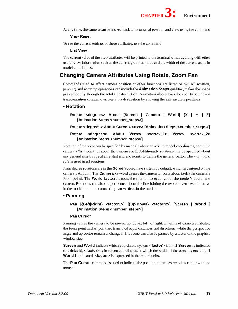
CHAPTER 3: Environment
Document Version 2/2/00 CUBIT Version 3.0 Reference Manual 45
At any time, the camera can be moved back to its original position and view using the command
View Reset
To see the current settings of these attributes, use the command
List View
The current value of the view attributes will be printed to the terminal window, along with otheruseful view information such as the current graphics mode and the width of the current scene inmodel coordinates.
Changing Camera Attributes Using Rotate, Zoom Pan
Commands used to affect camera position or other functions are listed below. All rotation,panning, and zooming operations can include theAnimation Steps qualifier, makes the imagepass smoothly through the total transformation. Animation also allows the user to see how atransformation command arrives at its destination by showing the intermediate positions.
• Rotation
Rotate <degrees> About [Screen | Camera | World] {X | Y | Z}[Animation Steps <number_steps>]
Rotate <degrees> About Curve <curve> [Animation Steps <number_steps>]
Rotate <degrees> About Vertex <vertex_1> Vertex <vertex_2>[Animation Steps <number_steps>]
Rotation of the view can be specified by an angle about an axis in model coordinates, about thecamera’s “At” point, or about the camera itself. Additionally rotations can be specified aboutany general axis by specifying start and end points to define the general vector. Theright handrule is used in all rotations.
Plain degree rotations are in theScreen coordinate system by default, which is centered on thecamera’s At point. TheCamera keyword causes the camera to rotate about itself (the camera’sFrom point). TheWorld keyword causes the rotation to occur about the model’s coordinatesystem. Rotations can also be performed about the line joining the two end vertices of a curvein the model, or a line connecting two vertices in the model.
• Panning
Pan [{Left|Right} <factor1>] [{Up|Down} <factor2>] [Screen | World ][Animation Steps <number_steps>]
Pan Cursor
Panning causes the camera to be moved up, down, left, or right. In terms of camera attributes,the From point and At point are translated equal distances and directions, while the perspectiveangle and up vector remain unchanged. The scene can also be panned by a factor of the graphicswindow size.
Screen andWorld indicate which coordinate system<factor> is in. If Screen is indicated(the default),<factor> is in screen coordinates, in which the width of the screen is one unit. IfWorld is indicated,<factor> is expressed in the model units.
ThePan Cursor command is used to indicate the position of the desired view center with themouse.

CHAPTER 3: Environment
46 CUBIT Version 3.0 Reference Manual Document Version 2/2/00
• Zooming
Zoom Cursor [Click | Drag] [Animation Steps <number_steps>]
Zoom Screen <factor> [Animation Steps <number_steps>]
Zoom <x_min> <y_min> <x_max> <y_max>[Animation Steps <number_steps>]
Zoom {Group | Body | Volume | Surface | Curve | Vertex | Hex | Tet | Face | Tri| Edge | Node} <id_range> [Animation Steps <number_steps>]
Zoom Reset
After enteringZoom Cursor , move the cursor to the graphics window. If theClick option wasentered, click on opposite corners of the desired zoom area; otherwise, drag a box around thearea to zoom by holding down the left mouse button until the desired area is boxed in.Click isthe default option for this command.
Zoom Screen will move the camera<factor> times closer to its focal point. The result is thatobjects on the focal plane will appear<factor> times larger.
Zooming on a specific portion of the screen is accomplished by specifying the zoom area inscreen coordinates; for example,Zoom 0 0 .25 .25 will zoom in on the bottom left quarter ofthe screen.
Zooming on a particular entity in the model is accomplished by specifying the entity type andID after enteringZoom . The image will be adjusted to fit bounding box of the specified entityinto the graphics window, and the specified entity will be highlighted.
To center the view on all visible entities, use theZoom Reset command.
Changing Camera Attributes Directly
Camera attributes are most easily modified using interactive mouse manipulation (see “Mouse-Based View Navigation” on page 35) or using the rotate, pan and zoom commands describedabove. However, the camera attributes can also be modified directly with the followingcommands:
From <x y z>
At <x y z>
Up <x y z>
Graphics Perspective <On|Off>
Graphics Perspective Angle <degrees>
If graphics perspective is on, a perspective projection is used; if graphics perspective is off, anorthographic projection is used. With a perspective projection, the scene is drawn as it wouldlook to a real camera. This gives a three-dimensional sense of depth, but causes most parallellines to be drawn non-parallel to each other. If an orthographic projection is used, no sense ofdepth is given, but parallel lines are always drawn parallel to each other.
In a perspective view, changing the perspective angle changes the field of view by changing theangle from the line of sight to the edge of the visible scene. The effect is similar to a telephotozoom with a camera. A smaller perspective angle results in a larger zoom. This command hasno effect when graphics perspective is off.

CHAPTER 3: Environment
Document Version 2/2/00 CUBIT Version 3.0 Reference Manual 47
Graphics WindowsWindow Size and Position
By default, CUBIT will create a single graphics window when it starts up (to run CUBITwithout a graphics window, include-nographics on the command line when launchingCUBIT.) The graphics window position and size is most easily adjusted using the mouse, likeany other window on an X-windows screen. However, the size of the graphics window can alsobe controlled using the following commands:
Graphics WindowSize <width_in_pixels> <height_in_pixels>
Graphics WindowSize Maximum
In addition, the graphics window size and position can be controlled by placing the followingline in the user’s .Xdefaults file:
cubit.graphics.geometry XxY xpos ypos
where theX andY are window width and height in pixels, respectively, andxpos andypos arethe offsets from the lower left hand corner.
Using Multiple Windows
You can use up to ten graphics windows simultaneously, each with its own camera and view.Each window has an ID, from 1 to 10, shown in the title bar of the window. Commands thatcontrol camera attributes apply to only one window at a time, theactive window.Currently, thedisplay lists of all windows are identical.
The following commands are used to create, delete, and make active additional graphicswindows.
Graphics Window Create [ID]
Graphics Window Delete <ID>
Graphics Window Active <ID>
Hardcopy OutputThe easiest way to make an image file of a graphics window is to use a screen capture programoutside of CUBIT, such as xv. However, CUBIT also has the ability to save its graphical outputto files of various formats. The commands for generating hardcopy output files are:
Hardcopy ‘<filename>’ [ Encapsulated | Postscript | Eps ] [Color |Monochrome] [Window <window_id=active>]
Hardcopy ‘<filename>’ Pict [xsize <xpixels>] [ysize <ypixels>][Window <window_id=active>]
Hardcopy ‘<filename>’ Cgm [ansi | cals | cleartext][Window <window_id=active>]
Hardcopy ‘<filename>’ Hpgl [Landscape | Portrait] [xsize <width>ysize <height>] [window <window_id=active>]
Each of these commands saves the view in the specified window (or the current window), to thespecified file, in the format indicated. The file can then be sent to a printer or inserted intoanother document.

CHAPTER 3: Environment
48 CUBIT Version 3.0 Reference Manual Document Version 2/2/00
Miscellaneous Graphics OptionsIn addition to the commands discussed above, there are several other graphics system optionsin CUBIT that can be controlled by the user.
• Silhouette Lines
Some shapes, such as cylinders, are drawn with silhouette lines; these lines don’t represent truegeometric curves, but help visualize the shape of a surface. Silhouette lines can be turned on oroff with the command
Graphics Silhouette [On|Off]
The pattern used to draw silhouette lines can be set using the command
Graphics Silhouette Pattern [solid | dashdot | dashed | dotted | dash_2dot |dash_3dot | long_dash | phantom]
• LineWidth
This option controls the width of the lines used in the wireframe and hiddenline displays. Thedefault is 1 pixel wide. The command to set the line width is
Graphics LineWidth <width_in_pixels>
• Highlight LineWidth
This option controls the width of the lines used when highlighting an entity. Setting this to awidth greater than the global line width often makes it easier to locate highlighted entities. Ifthis setting has not been changed, the line width set in the command above is used. Thecommand to set the highlighting line width is
Highlight LineWidth <width_in_pixels>
• Text Size.
This option controls the size of text drawn in the graphics window. The size given in thiscommand is the desired size relative to the default size. The command to set the text size is
Graphics Text Size <size>
• Point Size
This option controls the size of points drawn in the graphics window, such as vertices or headsof vectors; alternatively, the size of points representing nodes or vertices can be setindependently of the global point size. The commands to set the point sizes are
Graphics Point Size <size>
Graphics [Node | Vertex] Point Size <size>
• Point Style
Graphical points are drawn as dots by default. They may be drawn as other symbols, such asplus sign. Point styles for nodes and vertices can also be set independently of the global pointstyle. To change the point style, use the commands
Graphics Point Style <style_integer>
Graphics [Node | Vertex] Point Style <style_integer>
TypeHelp Point Style to see a list of valid style integers and the symbol they represent.
• Graphics Status

CHAPTER 3: Environment
Document Version 2/2/00 CUBIT Version 3.0 Reference Manual 49
All graphics commands can be disabled or re-enabled with the command
Graphics [On | Off]
While graphics are off, changes in the model will not appear in the graphics window, and allgraphics commands will be ignored. When graphics are again turned on, the scene will beupdated to reflect the current state of the model.
• Model Axis
The model axis may be drawn in the scene at the model origin. The axis is controlled with thecommand
Graphics Axis [Type <AXIS | Origin>] [on | off]
The command is used to specify whether the model axis is visible, and to determine how theaxis is drawn. If you includeType Axis , the axis will be drawn as three orthogonal lines; if youincludeType Origin , the axis will be drawn as a circle at the model origin.
• Corner Axis (Triad)
By default, an axis appears in the corner of the graphics window. This corner axis, also calledthe triad, can be disabled or re-enabled with the command
Graphics Triad [On | Off]
• Scene Border
By default, there is a black border drawn around the scene. To remove or restore the border, usethe command
Graphics Border [On | Off]
▼ Listing InformationThe List commands print information about the current model and session. There are fivegeneral areas:Model Summary, Geometry, Mesh, Special Entities, andCUBIT Environment.The descriptions of these areas includes example output based on the model generated by thejournal file in Table 3-7. The model consists of a 1x2x3 brick meshed with element size 0.1.
List Model SummaryThe following commands print identical summaries of the model: the number of entities of eachgeometric, mesh, and special type; see Table 3-8 for sample output.
List Model
List Totals
List GeometryThe following commands list information about the geometry of the model.
list names [group|body|volume|surface|curve|vertex|all]
list {group | body | volume | surface | curve | vertex} [range] [ids]
list {geom_list} [Geometry|Mesh [Detail]]
list {group | body | volume | surface | curve | vertex} <range> {x|y|z}

CHAPTER 3: Environment
50 CUBIT Version 3.0 Reference Manual Document Version 2/2/00
The first command lists the names in use, and the entity type and id corresponding to each name.Specifyingall lists names for all types; other options list names for a specific entity type. Thenames for an individual entity can be obtained by listing just that entity. Sample output from thelist names surface command is shown in Table 3-9. This output shows that, for example,Surface 2 has the name ‘BackSurface ’.
If ids is specified, the second command provides information on the number of entities in themodel and their identification numbers. This can be very useful for large models in whichseveral geometry decomposition operations have performed. Sample output from thelistsurface ids command is shown in Table 3-10.
The range can be very general using the general entity parsing syntax. Using arange andidsgives a brief synopsis of the local connectivity of the model, e.g. one can list the ids of thesurfaces containing vertex 2; see Table 3-11. An intermediately detailed synopsis can beobtained by placing the range of entities in a group, then listing the group.
The third command provides detailed information for each of the specific entities. Thisinformation includes the entity’s name and id, its meshing scheme and how that scheme wasselected, whether it is meshed and other meshing parameters such as smooth scheme, intervalsize and count. The entity’s connectivity is summarized by a table of the entity’s subentities anda list of the entity’s supentities. Also, the nodesets, sidesets, blocks, and groups containing theentity are listed.
Specifyinggeometry will additionally list the extent of the entity’s geometric bounding box,the geoemtric size of the entity, and, depending on entity type, other information such as surfacenormal. See also thelist {entities} x command below.
Specifyingmeshwill additionally list the number of mesh entities of each type interior to theentity and on bounding subentities.Mesh detail will list the ids of the mesh entities as well,following the format of thelist ids command above.
Table 3-12 through Table 3-13 show sample output for each of these options.
The fourth command lists the entities sorted by either the x, y, or z coordinate of their geometriccenter. For example, in a large, basically cylindrical model centered around z-axis, it is usefulto list the surfaces of a volume sorted by z to identify the source and target sweeping surfaces.An example for our toy model appears as Table 3-15, “‘List <entities> x’ Example.,” onpage 56.
List MeshThe following commands list mesh entity information.
list { hex | face | edge | node } <id_range>
list { hex | face | edge | node } <id_range> ids
For both of these commands, the range can be very general, following the general entity parsingsyntax. The first command provides detailed information. For an entity, the information includesits id, owning geometry, subentities and supentities. For a hex, the Exodus Id1 is also listed. Fora node, its coordinates are listed. The second command just lists the entity ids, and is usuallyused in conjunction with complex ranges. Table 3-16 gives examples.
1. The Exodus Id is the hex’s id in an exported Exodus database, not in the CUBIT model. Before writing the Exodus
database the Exodus Id appears as -1.

CHAPTER 3: Environment
Document Version 2/2/00 CUBIT Version 3.0 Reference Manual 51
List Special EntitiesList {special_type} [range]
Special entities include (element) blocks, sidesets and nodesets (representing boundaryconditions), and boundary layers. Like the list geometry and mesh commands, if no range isspecified then the number of entities of the given type is summarized. Otherwise, listing aspecial entity prints the mesh and geometry it contains. Sample output forlist block, list sideset,andlist nodesetis shown in Table 3-17, Table 3-18, and Table 3-19. (Some special entities areof interest mainly to developers and are not described here, e.g. whisker sheets, whisker hexes,and dicer sheets.)
List CUBIT EnvironmentThe user may list Information about the current CUBIT environment such asmessage outputsettings, memory usage, andgraphics settings.
Message Output Settings
There are several major categories of CUBIT messages.
• Info (Information) messages tell the user about normal events, such as the id of a newlycreated body, or the completion of a meshing algorithm.
• Warning messages signal unusual events that are potential problems.
• Error messages signal either user error, such as syntax errors, or the failure of someoperation, such as the failure to mesh a surface.
• Echomessages tell the user what was journaled.
• Debugmessages tell developers about algorithm progress. There are many types of Debugmessages, each one concentrating on a different aspect of CUBIT.
By default, Info, Warning, Error, and Echo messages are printed, and Debug messages are notprinted. Information, Warning and Debug message printing can be turned on or off (or toggled)with a set command; error messages are always printed. Debugging output can be redirected toa file. Current message printing settings can be listed.
List {echo | info | warning | debug }
Set {echo | info | warning } [on|off]
[Set] Debug <index> [on|off]
[Set] Debug <index> File <’filename’>
[Set] Debug <index> Terminal
Message flags can also be set using command line options, e.g.-warning={on|off} and -information={on|off} . Debug flags can be set on with-debug=<setting> , where<setting> is a comma-separated list of integers or ranges of integers denoting which flags toturn on. E.g. to set debug flags 1, 3, and 8 to 10 on, the syntax is-debug=1,3,8-10.
In addition to the major categories, there are some special purpose output settings.
[Set] Logging [on|off] [file <’filename’>]
List Logging

CHAPTER 3: Environment
52 CUBIT Version 3.0 Reference Manual Document Version 2/2/00
If logging is enabled, all echo, info, warning, and error messages will be output both to theterminal and to the logging file.
List Settings
The List Settings command lists the value of all the message flags, journal file and echosettings, as well as additional information; see Table 3-20. The first section lists a shortdescription of each debug flag and its current setting. Next come the other message settings,followed by some flags affecting algorithm behavior.
Graphical Display Information
List view prints the current graphics view and mode parameters; See “Graphics” on page 32.
Memory Usage Information
Users are encouraged to use Unix commands such as ‘top’ to check total CUBIT memory use.Developers may check internal memory usage with the following command:
List Memory [‘<object type>’]
Without an object type, the command prints memory use for all types of objects.
Table 3-7: Journal file for List Examples
brick x 1 y 2 z 3body 1 size 0.1mesh volume 1block 1 volume 1nodeset 1 surface 1sideset 1 surface 2group “my_surfaces” add surface 1 to 3
surface 2 name "BackSurface"surface 3 name "BottomSurface"surface 1 name "FrontSurface"surface 4 name "LeftSurface"surface 5 name "RightSurface"surface 6 name "TopSurface"

CHAPTER 3: Environment
Document Version 2/2/00 CUBIT Version 3.0 Reference Manual 53
Table 3-8: ‘List Model’ or ‘List Totals’ Example
CUBIT> list model
Model Entity Totals: Geometric Entities: 2 groups 1 bodies 1 volumes 6 surfaces 12 curves 8 vertices
Mesh Entities: 6000 hexes 0 pyramids 0 tets 7876 faces 0 tris 9854 edges 7161 nodes
Special Entities: 1 element blocks 1 sideSets 1 nodesets
Table 3-9: ‘List Names’ Example
CUBIT> list names surface______Name______ Type________Id BackSurface Surface 2 BottomSurface Surface 3 FrontSurface Surface 1 LeftSurface Surface 4 RightSurface Surface 5 TopSurface Surface 6
Table 3-10: ‘List Surface [range] Ids’ Examples
CUBIT> list surface idsThe 6 surface ids are 1 to 6.
CUBIT> list surf idsThe 108 surface ids are 192 to 266, 268 to 271, 273 to 301.

CHAPTER 3: Environment
54 CUBIT Version 3.0 Reference Manual Document Version 2/2/00
Table 3-11: Using ‘List’ for Querying Connectivity.
CUBIT> list surface in vertex 2 idsThe 3 entity ids are 1, 5, 6.
CUBIT> group “v2_surfs” equals surface in vertex 2CUBIT> list v2_surfsGroup Entity ’v2_surfs’ (Id = 3)It owns 3 entities: 3 surfaces.
Owned Entities: Mesh Scheme Interval:______Name______ Type________Id +is meshed Count Size
FrontSurface Surface 1 map+ 1 H 0.1TopSurface Surface 6 map+ 1 H 0.1
RightSurface Surface 5 map+ 1 H 0.1
Table 3-12: ‘List Group Mesh Detail’ Example
CUBIT> list my_surfaces mesh detailGroup Entity ’my_surfaces’ (Id = 2)It owns 3 entities: 3 surfaces.
Owned Entities: Mesh Scheme Interval: Edge ______Name______ Type________Id +is meshed Count Size Length FrontSurface Surface 1 map+ 1 H 0.1 BackSurface Surface 2 map+ 1 H 0.1 BottomSurface Surface 3 map+ 1 H 0.1
_______________Mesh_Information___________Element_Type Interior Boundary Total Face 700 0 700 Edge 1300 180 1480 Node 603 178 781
Note for groups’interior’ elements are inside one of the entities explicitly in the group and’boundary’ elements are on a subentity that is not explicitly in the group.
Mesh id ranges follow. The 700 interior face ids are 1 to 700. The 1300 interior edge ids are 61 to 430, 491 to 860, 921 to 1480. The 180 boundary edge ids are 1 to 60, 431 to 490, 861 to 920. The 1480 total edge ids are 1 to 1480. The 603 interior node ids are 61 to 231, 292 to 462, 521 to 781. The 178 boundary node ids are 1 to 60, 232 to 291, 463 to 520. The 781 total node ids are 1 to 781.

CHAPTER 3: Environment
Document Version 2/2/00 CUBIT Version 3.0 Reference Manual 55
Table 3-13: ‘List Surface Geometry’ Example
CUBIT> list surface 1 geometry
Surface Entity ’FrontSurface’ (Id = 1)
Meshed: Yes
Mesh Scheme: map (default)
Smooth Scheme: winslow fixed
Non-periodic
Interval Count: 1
Interval Size: 0.100000
An odd loop: No (Surface 1)
Block Id: 0
Total number of curves: 4
Mesh Scheme Arc Interval: Edge Vertex Type
______Name_____ Id +is meshed Length Count Size Length Start_T End_T
Curve 1 1 equal+ 2 20 H 0.1 0.1 1 2
Curve 2 2 equal+ 1 10 H 0.1 0.1 2 3
Curve 3 3 equal+ 2 20 H 0.1 0.1 3 4
Curve 4 4 equal+ 1 10 H 0.1 0.1 4 1
In Volume 1.
Contained in NodeSet 1, Group 2
Bounding Box: x = -0.5 to 0.5 (range 1)
y = -1 to 1 (range 2)
z = 1.5 to 1.5 (range 0)
Merge Setting = On
Surface Area: 2.000000
Surface Normal: xyz = 0.000000 0.000000 1.000000
At centroid: xyz = 0.000000 0.000000 1.500000
Table 3-14: ‘List Curve’ Example
CUBIT> list curve 1 to 8 by 2
Mesh Scheme Arc Interval: Edge Vertex Type
______Name_____ Id +is meshed Length Count Size Length Start_T End_T
Curve 1 1 equal+ 2 20 H 0.1 0.1 1 2
In FrontSurface, TopSurface.
Curve 3 3 equal+ 2 20 H 0.1 0.1 3 4
In FrontSurface, LeftSurface.
Curve 5 5 equal+ 2 20 H 0.1 0.1 5 6
In BackSurface, TopSurface.
Curve 7 7 equal+ 2 20 H 0.1 0.1 7 8
In BackSurface, LeftSurface.

CHAPTER 3: Environment
56 CUBIT Version 3.0 Reference Manual Document Version 2/2/00
Table 3-15: ‘List <entities> x’ Example.
CUBIT> list surface in volume 1 x
Entities sorted by geometric center x-coordinate:
______Name______ Type________Id x_Coordinate
LeftSurface Surface 4 -0.5
RightSurface Surface 5 0
BackSurface Surface 2 0
FrontSurface Surface 1 0
BottomSurface Surface 3 0
TopSurface Surface 6 0.5
Table 3-16: ‘List Hex’ Examples
CUBIT> list hex 5701
Hex 5701 -- Exodus ID = -1
Owned by Volume 1 (Volume 1)
Contains Faces: 6084, 6979, 7065, 7066, 11, 1901
Contains Edges: 8200, 82, 8206, 8204, 3783, 3841, 3842, 11, 9043, 79, 9127, 81
Contains Nodes: 70, 6872, 6901, 71, 12, 1913, 1942, 13
CUBIT> comment ‘find hexes containing both node 70 and 71’
CUBIT> list hex in node 70 and hex in node 71 ids
The 2 entity ids are 5101, 5701.
Table 3-17: ‘List Block’ Example
CUBIT> list block
The 1 block id is 1.
CUBIT> list block 1
Block 1 contains 6000 unexported 3D element(s) of type HEX8.
Owned Entities:
______Name______ Type________Id Mesh_Elements
Volume 1 Volume 1 6000
CUBIT> export genesis ‘f.gen’
...
CUBIT> list block 1
Block 1 contains 6000 exported 3D element(s) of type HEX8.
...
Table 3-18: ‘List SideSet’ Example
CUBIT> list sideset 1
SideSet 1 contains 200 exported element sides.
Owned Entities:
______Name______ Type________Id Mesh_Elements
BackSurface Surface 2 200

CHAPTER 3: Environment
Document Version 2/2/00 CUBIT Version 3.0 Reference Manual 57
▼ Obtaining HelpCUBIT can give help on command syntax in two ways. For help on a particular command orkeyword, the user can simply typehelp <keyword> . Or, if the user has typed part of acommand and is uncertain of the syntax of the remainder of the command, they can type aquestion mark? and help will be printed for all the keywords currently entered. The results ofthis type of command is shown in Table 3-21.
Table 3-19: ‘List NodeSet’ Example
CUBIT> list nodeset 1
NodeSet 1: contains 231 nodes.
Owned Entities:
______Name______ Type________Id Mesh_Elements
FrontSurface Surface 1 231
Table 3-20: Sample Output from ‘List Settings’ Command
CUBIT> list settings
Debug Flag Settings (flag number, setting, output to, description):
1 OFF terminal Debug Graphics toggle for some debug options.
2 OFF terminal Whisker weaving information
3 OFF terminal Timing information for 3D Meshing routines.
... (many lines deleted) ...
88 OFF terminal General virtual geometry stuff
89 OFF terminal Tet meshing warning and debug messages
echo = On
info = On
journal = On, journal file = ’cubit13.jou’
warning = On
logging = Off
recording = Off
keep invalid mesh = Off
default names = Off
name replacement character = ’_’, suffix character = ’@’
default blocks = Volumes
Matching Intervals is fast, TRUE; multiple curves will be fixed per interation.
Note in rare cases ’slow’, FALSE, may produce better meshes.
Match Intervals rounding is FALSE; intervals will be rounded towards the user-
specified intervals.
Table 3-21: Help on Volume & Label
CUBIT> volume 3 label fish ?
Help for words: volume & label
Label Volume [ on | off | name [only|id] | id | interval | size |
scheme | merge | firmness ]

CHAPTER 3: Environment
58 CUBIT Version 3.0 Reference Manual Document Version 2/2/00

Document Version 2/2/00 CUBIT Version 3.0 Reference Manual 59
Chapter 4: Geometry▼ Introduction…59
▼ CUBIT Geometry Model Definitions…59
▼ Geometry Creation…60
▼ Geometry Transforms…67
▼ Geometry Booleans…69
▼ Geometry Decomposition…70
▼ Geometry Merging…72
▼ Geometry Groups…75
▼ Geometry Attributes…75
▼ Exporting Geometry…78
▼ IntroductionThe geometry model in CUBIT serves as the basis for mesh generation, as it describes at theresolution of interest to the analysis. The geometric model is also used for the definition ofboundary conditions. The ACIS solid modeling engine is used by CUBIT for solid geometryoperations; CUBIT also builds a representation on top of the ACIS model, which it uses todefine non-manifold topology. The CUBIT representation is also used as a means for definingvirtual geometry, which is used for feature removal and other useful meshing-related tasks.
This chapter begins with definitions of geometric model used in CUBIT and the structure of thenonmanifold geometry represented by CUBIT. This is followed by sections describinggeometry import, creation, modification and export.
▼ CUBIT Geometry Model DefinitionsBefore describing the functionality in CUBIT for viewing and modifying solid geometry, it isuseful to give a precise definition of terms used to describe geometry in CUBIT. In this manual,the terms topology and geometry are both used to describe parts of the geometric model. Thedefinitions of these terms are:
Topology: the manner in which geometric entities are connected within a solid model;topological entities in CUBIT include vertices, curves, surfaces, volumes and bodies.

CHAPTER 4: Geometry
60 CUBIT Version 3.0 Reference Manual Document Version 2/2/00
Geometry: the definition of where a topological entity lies in space. For example, a curve maybe represented by a straight line, a quadratic curve, or a b-spline. Thus, an element of topology(vertex, curve, etc.) can have one of several different geometric representations.
TopologyWithin CUBIT, the topological entities consist ofvertices, curves, surfaces, volumes,andbodies.Each topological entity has a corresponding dimension, representing the number of freeparameters required to define that piece of topology. Each topological entity is bounded by oneor more topological entities of lower dimension. For example, a surface is bounded by one ormore curves, each of which is bounded by one or two vertices.
A CUBIT Body is defined as a collection of other pieces of topology, including curves, surfacesand volumes. While a Body is not required for a complete topological model, it is a convenientmechanism for grouping volumes. Bodies are also used as the basis for solid geometryoperations in CUBIT.
Non-Manifold TopologyIn many applications, the geometry consists of an assembly of individual parts, which togetherrepresent a functioning component. These parts often have mating surfaces, and for typicalanalyses these surfaces should be joined into a single surface. This results in a mesh on thatsurface which is shared by the volume meshes on either side of the shared surface. Thisconfiguration of geometry is loosely referred to as non-manifold topology1.
▼ Geometry CreationThere are three primary ways of creating geometry for meshing in CUBIT. First, CUBITprovides many geometry primitives for creating common shapes (spheres, bricks, etc.) whichcan then be modified and combined to build complex models. Secondly, geometry can beimported into CUBIT from an ACIS “.sat” file. Finally, geometry can be defined by building itfrom the “bottom up”, creating vertices, then curves from those vertices, etc. The three methodsfor creating geometry in CUBIT will be descibed in detail in this section, followed by methodsfor modifying that geometry.
Geometric PrimitivesThe geometric primitives supported within CUBIT are pre-defined templates of three-dimensional geometric shapes. Users can create specific instances of these shapes by providingvalues to the parameters associated with the chosen primitive. Primitives available in CUBIT
1. The definition of non-manifold topology used in the field of Topology is much broader thanthe definition used here, since it allows additional cases such as dangling faces and edges to existin the model. Although dangling faces and edges are allowed in the CUBIT geometry model,their use is not common. Unless otherwise stated, the use of the term non-manifold in thismanual will refer to the definition given in the text rather than the complete definition known inthe field of Topology.

CHAPTER 4: Geometry
Document Version 2/2/00 CUBIT Version 3.0 Reference Manual 61
include the brick, cylinder, torus, prism, frustum, pyramid, and sphere. Figure 4-1: shows a
sample of the available primitives. Each primitive, along with the command used to generate itand the parameters associated with it, are described next. For some primitives, several optionscan be used to generate them, and are described as well.
General Notes
• Primitives are created and given an ID equal to one plus the current highest body ID in themodel.
• Primitive solids are created with their centroid at the origin or the world coordinate system.
• For primitives with a Height or Z parameter, the axis going through these primitives will bealigned with the Z axis.
• For primitives with a Major Radius and a Minor Radius, the Major Radius will be along the Xaxis, the Minor Radius along the Y axis.
• For primitives with a Top Radius, this radius will be that along the X axis; the Y axis radiuswill be computed using the Major, Minor and Top Radii given.
Brick
The brick is a rectangular parallelepiped.
• Command:
[Create] Brick {Width|X} <width> [{Depth|Y} <depth>] [{Height|Z} <height>][Bounding Box entity_type <id_range> ]
• Notes:
• A cubical brick is created by specifying only the width or x dimension.
• A brick can be specified to occupy the bounding box of one or more entities, specified on thecommand line.
Figure 4-1: Geometry primitives available in CUBIT.
Pyramid
Frustum
Torus
Cylinder
Brick
Prism
Sphere
(Cone)

CHAPTER 4: Geometry
62 CUBIT Version 3.0 Reference Manual Document Version 2/2/00
• If a bounding box specification is used in conjuction with any of the other paramters (X, Y orZ), the parameters specified override the bounding box results for that or those dimensions.
Cylinder
The cylinder is a constant radius tube with right circular ends.
• Commands:
[Create] Cylinder [height | z] <z-height> radius <x/y-radius>
• Notes:
• A cylinder may also be created using thefrustum command with all radii set to the samevalue.
Prism
The prism is an n-sided, constant radius tube with n-sided planar faces on the ends of the tube.
• Commands:
[create] prism [height | z] <z-height> sides <nsides> radius <radius>
[create] prism [height | z] <z-height> sides <nsides> major [radius] <x-radius>minor [radius] <y-radius>
• Notes:
• The radius defines the circumradius of the n-sided polygon on the end caps.
• If a major and minor radius are used, the end caps are bounded by a circum-ellipse instead of acircumcircle.
• The number of sides of a prism must be greater than or equal to three.
• A prism may also be created using thepyramid command with all radii set to the same value.
Frustum
A frustum is a general elliptical right frustum, which can also be thought of as a portion of aright elliptical cone.
• Commands:
[create] frustum [height | z] <z-height> major [radius] <x-radius>[minor [radius] <y-radius> top <top-x-radius>]
• Notes:
• If used, Major Radius defines the x-radius and Minor Radius the y-radius.
• If used, Top Radius defines the x-radius at the top of the frustum; the top y radius is calculatedbased on the ratio of the major and minor radii.
Pyramid
A pyramid is a general n-sided prism.
• Command:
[create] pyramid [height | z] <z-height> sides <nsides> [major [radius] <x-radius> minor [radius] <y-radius> ] [top <top-x-radius>]

CHAPTER 4: Geometry
Document Version 2/2/00 CUBIT Version 3.0 Reference Manual 63
Sphere
The sphere command generates a simple sphere, or, optionally, a portion of a sphere or anannular sphere.
• Commands:
[create] sphere radius <radius> [xpositive] [ypositive] [zpositive] [delete][inner [radius] <radius>
• Notes:
• If Xpositive, Ypositive, and/or Zpositive are used, a sphere which occupies that side of thecoordinate plane only is generated, or, if the delete keyword is used, the sphere will occupythe other side of the coordinate plane(s) specified. These options are used to generatehemisphere, quarter sphere or a sphere octant (eighth sphere).
• If the inner radius is specified, a hollow sphere will be created with a void whose radius is thespecified inner radius.
Torus
The torus command generates a simple torus.
• Command:
[create] torus major [radius] <major-radius> minor [radius] <minor-radius>
• Notes:
• Minor Radius is the radius of the cross-section of the torus;Major Radius is the radius ofthe spine of the torus.
• The minor radius must be less than the major radius.
Importing GeometryCUBIT can import geometry in the ACIS “sat” file format. For compatability with Sandialegacy applications, FASTQ input decks can also be used to create geometry.
There are many ways to get geometry into the ACIS format, depending on where that geometryis created. If the geometry is constructed inside CUBIT, the model can be exported directly toan ACIS file (see ). If the model has been constructed in Pro/Engineer, there are several methodsfor translating Pro/E files to the ACIS format1. ACIS files can also be exported directly fromseveral commercial CAD packages, including SolidWorksTM, AutoCAD, and HP PE/SolidDesigner.
Importing ACIS Models
The command used to read an ACIS file is:
Import Acis ‘<acis_sat_filename>’
ACIS files can also be imported using the “-solid” command-line option (see “ExecutingCUBIT” on page 8 for details.) Note that the filename must be enclosed in single or double
1. For information about translating Pro/Engineer files into ACIS format, contact the CUBIT group at [email protected], or
see the web page http://sass2248.jal.sandia.gov/... on the Sandia Internal Restricted Network.

CHAPTER 4: Geometry
64 CUBIT Version 3.0 Reference Manual Document Version 2/2/00
quotes. This command will create as many bodies within CUBIT as there are bodies in the inputfile.
Importing FASTQ Models
Support is available for reading a FASTQ file directly into CUBIT. FASTQ files are importedinto CUBIT using the command:
Import Fastq ’<fastq_filename>’
Note that the filename must be enclosed in single or double quotes.
All FASTQ commands are fully supported except for theBody command (which is ignored, ifpresent, as it is unnecessary), the “corn” (corner) line type, and some of the specialized mappingprimitive Scheme commands. Standard mapping, paving, and triangle primitive schemecommands are handled. The pentagon, semicircle, and transition primitives are not handleddirectly, but are meshed using the paving scheme. The FASTQ input file may have to bemodified if theScheme commands use any non-alphabetic characters such as ‘+’, ‘(‘, or ‘)’.Circular lines with non-constant radius are generated as a logarithmic decrement spiral inFASTQ; in CUBIT they will be generated as an elliptical curve.
Since a FASTQ file by definition will be defined in a plane, it must be projected or swept togenerate three dimensional geometry. CUBIT supports sweeping options to convert importedFASTQ geometries into volumetric regions.
Importing ExodusII Files
ExodusII finite element data files can be imported under certain conditions. The capability togenerate new geometry from deformed mesh is available for 2D ExodusII files (4, 8, or 9 nodeQUAD or SHELL element types) that do not have enclosed voids (holes surrounded by mesh)and which were originally generated with CUBIT and exported to ExodusII with theNodesetAssociativity option set to on. TheNodeset Associativity command records the topologyof the geometry into special nodesets which allow CUBIT to reconstruct a new solid model fromthe mesh even after it has been deformed. The new solid model of the deformed geometry canbe remeshed with standard techniques or meshed with a sizing function that can also beimported into CUBIT from the same ExodusII file. CUBIT's implementation of the pavingalgorithm can generate a mesh following a sizing function to capture a gradient of any variable(element or nodal) present in the ExodusII file.
For more details on importing mesh for geometry, including command syntax, see ... (chapter5).
Bottom-Up Geometry CreationCUBIT supports the ability to create geometry from a collection of lower order entities. This isaccomplished by first creating vertices, connecting vertices with curves and connecting curvesinto surfaces. Currently bodies or volumes may not be constructed by stitching a set of surfacestogether, however surfaces may be swept or rotated to create bodies or volumes (see “Volume”on page 66). Existing geometry may be combined with new geometry to create higher orderentities. For example, a new surface can be created using a combination of new curves andcurves already extant in the model. Commands and details for creating each type of geometryentity are given below.
Vertex

CHAPTER 4: Geometry
Document Version 2/2/00 CUBIT Version 3.0 Reference Manual 65
The commands available for creating new vertices directly in CUBIT are:
Create Vertex <x><y><z> [on [Curve | Surface] <id>]
Create Vertex <fraction> from Vertex <id> on Curve <id>
A vertex can be created which lies on a curve or surface in the geometric model by specifyingthe curve or surface id; the position of the vertex will be the point on the specified entity whichis closest to the position specified on the command.
A vertex can be positioned a certain fraction of the arc length along a curve using the secondform of the command.
Curve
Curves are created by specifying the bounding lower-order topology (i.e. the vertices) and thegeometry (shape) of the curve (along with any parameters necessary for that geometry). Thereare three forms of this command:
Create Curve [Vertex] <vertex_id> [Vertex] <vertex_id>[On Surface <surface_id>]
Create Curve [Vertex] <vertex_id> [Vertex] <vertex_id> [Vertex] <vertex_id>[Parabolic]
Create Curve from Curve <curve_id>
The first form of the command creates a straight line or a line lying on the specified surface. Ifa surface is used, the curve will lie on that surface but will not be associated with the surface’stopology.
A parabolic curve is created by specifying a third vertex, which completes the definition of aparabolic arc which goes through the three vertices.
The third form of the command actually copies the geometric definition in the specified curveto the newly created curve. The new curve is free floating.
In all cases, the specified vertices are not used directly but rather their positions are used tocreate new vertices.
Surface
Surfaces are created in CUBIT by fitting an analytic or spline surface over a set of boundingcurves. The curves must form a closed loop and only one loop of curves may be supplied. Theresult is a “sheet body” or a body that has zero measurable volume (it does however have avolume entity). Booleans and special webcutting commands may be used with to decomposethis body or to use it for decomposing other bodies. Booleans can be used to cut holes out ofthese surfaces.
There are three forms of the create surface command:
Create Surface Curve <curve_id_1> <curve_id_2> <curve_id_3>…
Create Surface from Surface <surface_id>
Create Surface extended from Surface <surface_id>
The first form of this command produces an analytic or spline surface fit to cover the boundingcurves.

CHAPTER 4: Geometry
66 CUBIT Version 3.0 Reference Manual Document Version 2/2/00
The second form creates a surface using the same geometric description of the specified surface.The new surface will be a stand-alone sheet body that is geometrically identical to the usersupplied surface.
The third form of the command creates a surface that is extended from a given surface. Thespecified surface’s geometry is examined and extended out “infinitely” relative to the currentmodel in CUBIT (i.e. extended to just beyond the bounding box of the entire model). The givensurfaces are extended as shown in Table 4-1.
Volume
Currently, CUBIT can create volumes from surfaces only by sweeping a single surface into a3D solid. Sweeping of planar surfaces, belonging either to two- or three-dimensional bodies, isallowed - non-planar faces are not supported at this time.
There are two forms of the sweep command; the syntax and details for each are given below. Inboth forms, the optionaldraft_angle parameter specifies the angle at which the lateral facesof the swept solid will be inclined to the sweep direction. It can also be described as the angleat which the profile expands or contracts as it is swept. The default value is 0.0. The optionaldraft_type parameter is an ACIS-related parameter and specifies what should be done to thecorners of the swept solid when a non-zero draft angle is specified. A value of 0 is the defaultvalue and implies an extended treatment of the corners. A value of 1 is also valid and implies arounded (blended) treatment of the corners.
sweep surface {<surface_id_range> | all} vector <x_vector y_vectorz_vector> [distance <distance_value>] [draft_angle <degrees>][draft_type <0 | 1>]
Sweeps a surface a specified distance along a specified vector. Specifying the distance of thesweep is optional; if this parameter is not provided, the face is swept a distance equal to thelength of the specified vector.
sweep surface {<surface_id_range> | all} axis {<xpoint ypoint zpoint xvectoryvector zvector> | xaxis | yaxis | zaxis} angle <degrees> [steps<number_of_sweep_steps>] [draft_angle <degrees>] [draft_type <0 | 1>]
Table 4-1: Surface Extension Results
Given Surface Type Resulting Extended Surface
Spherical Shell of Full Sphere
Planar Plane of infinite size relative to model
Toroidal Shell of Full Taurus
Conical, cone, cylinder… Shell of outside conic axially alignedwith given conic of infinite heightrelative to model
Spline Surface is extended to extents of thespline definition. This may not be anyfurther than the surface itself, so cautionshould be used here.

CHAPTER 4: Geometry
Document Version 2/2/00 CUBIT Version 3.0 Reference Manual 67
Sweeps a surface about a specified vector or axis through a specified angle. Theaxis ofrevolution is specified using either a starting point and a vector, or by a coordinate axis. This axis
must lie in the plane of the surfaces being swept. Thesteps parameter defaults to a value of 0which creates a circular sweep path. If a positive, non-zero value (say,n) is specified, then thesweep path consists of a series ofn linear segments, each subtending an angle of[( sweep_angle) / ( steps-1 )] at the axis of revolution.
Note: Specifying multiple surfaces that belong to the same body will not work as expected,as ACIS performs the sweep operationin place. Hence, if a range of surfaces isprovided, they ought to each belong to different bodies.
The sweep operations have been designed to produce valid solids of positive volume, eventhough the underlying solid modeling kernel library that actually executes the operation, ACIS,allows the generation of solids of negative volume (i.e., voids) using a sweep.
▼ Geometry TransformsBodies can be modified in CUBIT using transform operations, which include align, copy, move,reflect, restore, rotate, and scale. With the exception of the copy operation, transform operationsin CUBIT donot create new topology, rather they modify the geometry of the specified bodies.
Align
The align command is a combination of the rotate and move commands. The align commandwill align the surface of a given body with any other surface in the model, such that the surfacecentroids are coincident and the normals are pointing either in the same or opposite direction(depending on their initial alignment.) The syntax of this command is:
Align Body <body_id> Surface <surface_id> with Surface <body_id>
This transformation is useful for aligning surfaces in preparation for geometry decomposition.
Copy
The copy command copies an existing body to a new body without modifying the existing body.A copy can be made of several bodies at once, and the resulting new bodies can be translated orrotated at the same time. The commands for copying bodies are:
Body <range> copy [move <x-offset> <y-offset> <z-offset>]
Body <range> copy [reflect {x | y | z}]
Body <range> copy [reflect <x-comp> <y-comp> <z-comp>]
Body <range> copy [rotate <angle> about {x | y | z}]
Body <range> copy [rotate <angle> about <x-comp> <y-comp> <z-comp>]
Body <range> copy [scale <scale-factor>]
If the copy command is used to generate new bodies, a copy of the original mesh generated inthe original body can also be copied directly into the new body. This is currently limited tocopies that do not interact with adjacent geometry through non-manifold topology. For detailson mesh copies, see “Mesh Importing and Duplicating” on page 115.

CHAPTER 4: Geometry
68 CUBIT Version 3.0 Reference Manual Document Version 2/2/00
Move
Themove command moves a body by a specified offset. The commands to move bodies are:
Body <id_range> [Copy] Move <dx> <dy> <dz>
Body <id_range> [Copy] Move {x|y|z} <distance>
Move {Body|Group} <id_range> Normal To Surface <id> Distance <val>
Move {Body|Group} <id_range> XYZ <x_val> <y_val> <z_val>
If the copy option is specified, a copy is made and the copy is moved by the specified offset.
It is also possible to move bodies to locations specified either absolutely or relative to othergeometry entities in the model:
Move {entity} <id_range> location entity <id> [except [x] [y] [z]]
Move {entity} <id_range> location [x <val>] [y <val>] [z <val>] [except [x] [y][z]]
Here entity is {vertex|curve|surface|volume|body}, and any combination of entities may bespecified (in this case, the body containing the specified entity is moved). This command movesthe center of the entities to the specified location. (Note that bodies are integral, so moving anentity also moves all other entities that are in the same body.) “Except” is used to preserve thex, y, or z plane in which the center of the entity lies.
Scale
The scale command resizes the body by a constant scale. The body will be scaled about itscentroid. The command to scale bodies is:
body <range> [copy] scale <scale>
If the copy option is specified, a copy is made and scaled the specified amount.
Rotate
Therotate command rotates a body about a given axis without adding any new geometry. If theAngle or anyComponents are not specified they are defaulted to be zero. The commands torotate a body or bodies are:
body <range> [copy] rotate <angle> about {x | y | z}
body <range> [copy] rotate <angle> about <x-comp> <y-comp> <z-comp>
Rotate {Body|Group} <id_range> Angle <val> Axis {X|Y|Z|Normal of Surface<id>| Vertex <id_1> Vertex <id_2>}
If the copy option is specified, a copy is made and rotated the specified amount.
Reflect
Thereflect command mirrors the body about a plane normal to the vector supplied. The reflectcommand willdestroythe existing body and replace it with the new reflected body, unless thecopy option is used.
body <range> [copy] reflect <x-comp> <y-comp> <z-comp>
body <range> [copy] reflect {x | y | z}
Restore

CHAPTER 4: Geometry
Document Version 2/2/00 CUBIT Version 3.0 Reference Manual 69
The restore command removes all previous geometry transformations from the specified body.The command to restore bodies is:
body <range> restore
▼ Geometry BooleansBoolean operations are ones that modify the geometry and/or the topology of existing solids.Boolean operators supported in CUBIT include imprint, intersect, separate, section, subtract,and union. These operations usually replace the original bodies input to the boolean with newones.
Imprint
To produce a non-manifold geometry model from a manifold geometry, coincident surfacesmust be merged together (see “Geometry Merging” on page 72); this merge can only take placeif the surfaces to be merged have like topology and geometry. While various parts of anassembly will typically have surfaces which coincide geometrically, an imprint is necessary tomake the surfaces have like topology.
The commands used to imprint bodies together are:
Imprint <body1_id> with <body2_id>
Imprint [Body] All
An Imprint All will imprint all bodies in the model pairwise; bounding boxes are used to filterout imprint calls for bodies which clearly don’t intersect.
Intersect
Theintersect command generates a new body composed of the space that is shared by the twobodies being intersected. Both of the original bodies will be deleted and the new body will begiven the next highest body ID available. The command is:
Intersect <body1_id> with <body2_id> [keep]
Thekeep option results in the original bodies used in the intersect being kept.
Section
This command will cut a body or group of bodies with a plane, keeping geometry on one sideof the plane and discarding the rest. The syntax for this command is:
Section {body|group} <id_range> {xplane|yplane|zplane} [offset <value>][reverse] [keep]
Section {body|group} <id_range> surface <id> [reverse] [keep]
In the first form, the specified coordinate plane is used to cut the specified bodies. The offsetoption is used to specify an offset from the coordinate plane. In the second form, an existing(planar) surface is used to section the model. In either case, the reverse keyword results indiscarding the positive side of the specified plane or surface instead of the other side. Thekeepoption results in keeping both sides; the section command used with this option is equivalent towebcutting with a plane.
Separate

CHAPTER 4: Geometry
70 CUBIT Version 3.0 Reference Manual Document Version 2/2/00
The separate command is used to separate a body with multiple volumes into a multiple bodieswith single volumes. The command is:
Separate Body {id_range|all}
Subtract
The subtract operation subtracts one body from another set of bodies. The order of subtractionis significant - the body or bodies specified before the From keyword is/are subtracted frombodies specified after From. Both of the original bodies are deleted and the new body is giventhe next highest body ID available, unless thekeep keyword is given. The command is:
Subtract <body1_id> from [Body] <body_id_range> [keep]
Unite
The unite operation combines two or more bodies into a single body. The original bodies aredeleted and the new body is given the next highest body ID available, unless thekeepoption isused. The commands are:
Unite <body1_id> with <body2_id> [keep]
Unite Body {<range> | all} [keep]
The second form of the command unites multiple bodies in a single operation. If theall optionis used, all bodies in the model are united into a single body. If the bodies that are united do notoverlap or touch, the two bodies are combined into a single body with multiple volumes.
▼ Geometry DecompositionGeometry decomposition is often required to generate an all-hexahedral mesh for three-dimensional solids, as fully automatic all-hex mesh generation of arbitrary solids is not yetpossible in CUBIT. While geometry booleans can be used for decomposition (and are the basisof the underlying implementation of advanced decomposition tools described here), CUBIT hasa webcut capability specially tuned for decomposition.
Web CuttingThe term “web cutting” refers to the act of cutting an existing body or bodies, referred to as the“blank”, into two or more pieces through the use of some form of cutting tool, or “tool”. Thetwo primary types of cutting tools available in CUBIT are surfaces (either pre-existing surfacesin the model or infinite or semi-infinite surfaces defined for webcutting), or pre-existing bodies.
The various forms of the webcut command can be classified by the type of tool used for cutting.These forms are described below, starting with the simplest type of tool and progressing to morecomplex types.
Webcut Using Planar or Cylindrical Surface

CHAPTER 4: Geometry
Document Version 2/2/00 CUBIT Version 3.0 Reference Manual 71
The commands used to webcut with a planar surface in CUBIT are:
webcut {blank} plane {xplane | yplane | zplane} [offset <value>]
webcut {blank} plane surface <surface_id>
webcut {blank} plane vertex <id> vertex <id> vertex <id>
webcut {blank} cylinder radius <val.> axis {x|y|z|normal of surface <id>|vertex <id_1> vertex <id_2>| <x_val> <y_val> <z_val>>} [center <x_val><y_val> <z_val>]
[NOIMPRINT|imprint][NOMERGE|merge] [group_results]
In the command’s simplest form, a coordinate plane can be used to cut the model, and canoptionally be offset a positive or negative distance from its position at the origin.
An existing planar surface can also be used to cut the model; in this case, the surface is identifiedby its ID as the cutting tool.
Finally, any arbitrary planar surface can be used by specifying three vertices which define theplane.
A semi-infinite cylindrical surface can be used by specifying the cylinder radius, andthe cylinderaxis. The axis is specified as a line corresponding to a coordinate axis, the normal to a specifiedsurface, two arbitrary points, or an arbitrary point and the origin. The “center” point throughwhich the cylinder axis passes can also be specified.
Webcut with Arbitrary Surface
An arbitrary “sheet” surface can also be used to webcut a body. This sheet need not be planar,and can be bounded or infinite. The following commands are used:
webcut {blank} with sheet {body|surface} <id> [webcut_options]
webcut {blank} with sheet extended from surface <id> [webcut_options]
In its first form, the command uses a sheet body, either one that is pre-existing or one formedfrom a specified surface. Note that in this latter case the (bounded) surface should completelycut the body into two pieces. Sheet bodies can be formed from a single surface, but can also bethe combination of many surfaces; this form of webcut can be used with quite complicatedcutting surfaces.
Extended sheet surfaces can also be used; in this case, the specified surface will be extended inall directions possible. Note that some spline surfaces are limited in extent, and so these surfacesmay or may not completely cut the blank.
Webcut Using Tool Body
Any existing body in the geometric model can be used to cut other bodies; the command to dothis is:
webcut {blank} tool [body] <id> [webcut_options]
This simply uses the specified tool body in a set of boolean operations to split the blank into twoor more pieces.
Webcut Options
The following options can be used with all webcut commands:

CHAPTER 4: Geometry
72 CUBIT Version 3.0 Reference Manual Document Version 2/2/00
Group_results: The various pieces resulting from the previous command are placed into agroup named ‘webcut_group’.
[Imprint | Noimprint]: In its default implementation, webcutting results in the pieces notbeing imprinted on one another; this option forces the code to imprint the pieces afterwebcutting.
[Merge | Nomerge]: By default, the pieces resulting from an imprint are manifold; specifyingthis option results in a merge check for all surfaces in the pieces resulting from the webcut.
General Notes
The primary purpose of web cutting is to make an existing model meshable with the hexmeshing algorithms available in CUBIT. While web cutting can also be used to build the initialgeometric model, the implementation and command interface to web cutting have beendesigned to serve its primary purpose. Several important things to remember about webcuttingare as follows:
• The geometric model should be checked for integrity (using imprinting and merging) beforestarting the decomposition process. This makes the checking process easier, since there arefewer bodies and surfaces to check. Once the model passes that initial integrity check, it israre that decompositions using webcut will result in a model that does not also pass the samechecks.
• The use of the Imprint option can in cases save execution time, since it limits the scope of theimprint operations and thereby works faster. The alternative is performing and Imprint All onthe pieces of the model after all decompositions have been completed; this operation has beenmade much faster in more current releases of CUBIT, but will still take a noticeable amountof time for complicated models.
• While the Webcut commands make it very simple to cut your model into very many pieces,we recommend that the user restrict the decomposition they perform to only that necessary formeshability or for obtaining an acceptable mesh. Having more volumes in the model maysimplify individual volumes, but may not always result in a higher quality mesh; it willalways increase the run time and complexity of the meshing task.
Appendix B contains some examples that demonstrate the use of webcutting operations.
Split PeriodicSolids which contain periodic surfaces include cylinders, torii and spheres. Splitting periodicsurfaces can in some cases simplify meshing, and will result in curves and surfaces being addedto the volume. The command used to split periodic surfaces is:
Split Periodic Body {id_range|all}
This command splits all periodic surfaces in a body or bodies.
▼ Geometry MergingAs stated in “Non-Manifold Topology” on page 60, geometry is created and imported in CUBITin a manifold state, by default. The process of converting manifold to non-manifold geometryis referred to as “geometry merging”, since it involves merging multiple geometric entities intosingle ones.

CHAPTER 4: Geometry
Document Version 2/2/00 CUBIT Version 3.0 Reference Manual 73
The merging of two manifold surfaces into one non-manifold surface is depicted in Figure 4-2:.
It is clear that merging geometry results in some surfaces, curves and vertices being removedfrom the model. By default, entities with the lowest ID are retained.
MergingThere are several steps to the geometry merging algorithm in CUBIT; they are:
• Check lower order geometry, merge if possible
• Check topology of current entities
• Check geometry of current entities
• If both topology and geometry are alike, merge entities
Thus, in order for two entities to merge, the entities must correspond geometrically andtopologically. The geometric correspondence usually comes from constructing the model thatway. The topological correspondence can come from that process as well, but also can beaccomplished in CUBIT using Imprinting (see “Imprint” on page 69.)
There are several options for merging geometry in CUBIT.
• Merge geometry automatically
Merge all [Vertex | Curve | Surface]
Merge Body <id_range>
All topological entities in the model or in the specified bodies are examined for geometric andtopological correspondence, and are merged if they pass the test.
If a specific entity type is specfied with the Merge all, only complete entities of that type aremerged. For example, if Merge all surface is entered, only vertices which are part ofcorresponding surfaces being merged; vertices which correspond but which are not part ofcorresponding surfaces will not be merged. This command can be used to speed up themerging process for large models, but should be used with caution as it can hide problemswith the geometry (see )
• Test for merging in a specified group of geometry
Merge [Vertex | Curve | Surface] <id_range>
All topological entities in the specfiied entity list, as well as lower order topology belongingto those entities, are examined for merging. This command can be used to prevent merging ofentities which correspond and would otherwise be merged, e.g. slide surfaces.
• Force merge specified geometry entities
Merge [Vertex | Curve | Surface] <id_range> Force
This command results in the specified entities being merged, whether they pass the geometriccorrespondence test or not. This command should only be used with caution and whenmerging otherwise fails; instances where this is required should be reported to the CUBITdevelopment team.
Figure 4-2: Merging two manifold surfaces into a single non-manifold surface.

CHAPTER 4: Geometry
74 CUBIT Version 3.0 Reference Manual Document Version 2/2/00
UnmergingIn some cases, the user may want to unmerge geometry, for example in preparation for doingfurther geometry decomposition. This can be done selectively or globally with the followingcommands:
Unmerge all [group | surface | curve | vertex]
Unmerge [body | group | surface | curve | vertex] <id_range>
Unmerging a lower order entity contained in higher order merged entities will result in thosehigher order entities being unmerged as well. So, for example, to unmerge all surfacescontaining a given vertex, one could use the command Unmerge Vertex <id>.
Examining Merged EntitiesThere are several mechanisms for examining which enties have been merged. The most usefulmechanism is assigning all merged or unmerged entities of a specified type to a group, andexamining that group graphically. This process can be used to examine the outer shell of anassembly of volumes, for example to verify if all interior surfaces have been merged. To put allthe merged or unmerged entities of a given type into a specified group, use the command:
Group {<‘name’>|<id>} [Surface | Curve | Vertex] [Merged | Unmerged]
If the entity type is unspecified, surfaces will be assumed.
Entities can also be labelled in the graphics according to whether or not they have been merged.To turn merge labeling on for a specified entity type, use the command
Label {Vertex | Curve | Surface} Merge
Merge ToleranceGeometric correspondence between entities is judged according to a specfied absolutenumerical tolerance. The particular kind of spatial check depends on the type of entity. Verticesare compared by comparing their spatial position; curves are tested geometrically by testingpoints 1/3 and 2/3 down the curve in terms of parameter value; surfaces are tested at several pre-determined points on the surface. In all cases, spatial checks are done comparing a givenposition on one entity with the closest point on the other entity. This allows merging of entitieswhich correspond spatially but which have different parameterizations.
The default absolute merge tolerance used in CUBIT is 5.0e-4. This means that points whichare at least this close will pass the geometric correspondence test used for merging. The usermay change this value using the following command:
Merge Tolerance <val>
If the user does not enter a value, the current merge tolerance value will be printed to the screen.There is no upper bound to the merge tolerance, although in experience there are few caseswhere the merge tolerance has needed to be adjusted upward. The lower bound on the tolerance,which is tied to the accuracy of the solid modeling engine in CUBIT, is 1e-6.
Using Geometry Merging to Verify GeometryGeometry merging is often used to verify the correctness of an assembly of volumes. Forexample, groups of unmerged surfaces can be used to verify the outer shell of the assembly (see

CHAPTER 4: Geometry
Document Version 2/2/00 CUBIT Version 3.0 Reference Manual 75
“Examining Merged Entities” on page 74.) There is other information that comes from theMerge all command that is useful for verifying geometry. In typical geometric models, verticesand curves which get merged will usually be part of surfaces containing them which get merged.So, if a Merge all command is used and the command reports that vertices and curves have beenmerged, this is usually an indication of a problem with geometry. In particular, it is often a signthat there are overlapping bodies in the model. The second most common problem indicated bymerging curves and vertices is that the merge tolerance is set too high for a given model. In anyevent, merged vertices and curves should be examined closely.
▼ Geometry GroupsGroups provide a powerful capability for performing operations on multiple geometric entitieswith minimal input. They can also serve as a means for sorting geometric entities according tovarious criteria.
The command syntax to create or modify a group is:
group {id | “name”} add <list of topology entities>
For example, the command,
group “Exterior” add surface 1 to 2, curve 3 to 5
will create the group namedExterior consisting of the listed topological entities. Any of thecommands that can be applied to the “regular” topological entities can also be applied to groups.For example,mesh Exterior , list Exterior , or draw Exterior . A topological entity can beremoved from a group using the command:
group <id> remove <entity list>
When a group is meshed, CUBIT will automatically perform an interval matching on allsurfaces in the group (including surfaces that are a part of volumes or bodies in the group).
There are several utilities in CUBIT which use groups as a means of visualizing output. Theseutilities are described elsewhere, but listed here for reference:
• Webcut results (see “Web Cutting” on page 70)
• Merged and unmerged entities (see “Examining Merged Entities” on page 74)
• Sweep groups (see “Web Cutting” on page 70)
• Interval matching (see “Web Cutting” on page 70)
▼ Geometry AttributesEach topological entity has attributes attached to it. These attributes specify aspects of the entitysuch as the color that entity is drawn in and the meshing scheme to be used when meshing thatentity. This section describes those geometry attributes that are not described elsewhere in thismanual.
Entity NamesTopological entities (including groups) are assigned integer identification numbers in CUBIT inascending order, starting with 1. Each new entity created within CUBIT receives a unique id.

CHAPTER 4: Geometry
76 CUBIT Version 3.0 Reference Manual Document Version 2/2/00
However, topological entities can also be assigned names, and these names can be propagatedexplicitly by the user. A topological entity may have multiple names, but a particular name mayonly refer to a single entity. The following command assigns names to topological entities inCUBIT:
{Group|Body|Volume|Surface|Curve|Vertex} Name ‘<entity_name>’
The name of each topological entity appears in the output of theList command. In addition,topological entities can be labeled with their names (see label command). A list of all namescurrently assigned and their corresponding entity type and id (optionally filtered by entity type)can be obtained with the command
list names [{group|body|volume|surface|curve|vertex|all}]
Note: In a merge operation, the names of the deleted entity will be appended to the names ofthe surviving entity.
Topological entities can be identified either by the entity type followed by an identificationnumber or by a unique name. Such a name can be used anywhere that an entity type and id maybe used. For example, if surface 3 is named CHAMFER1, the command “mesh CHAMFER1”has the same result as the command “mesh surface 3”.
Each topological entity can optionally be given a unique default name when it is first created.The default name consists of the type of topological entity (body, volume, surface, curve, orvertex), followed by the ID number of the entity. For example, curve number 21 would have adefault name, “curve21”. Default names can be useful to reduce the amount of time spentredoing id’s between CUBIT and ACIS versions. The command for setting the default names is:
set default names {on|off}
Persistent AttributesTypical data assigned to topological entities during a meshing session might include intervals,mesh schemes, group assignments, etc. By default, most of this data is lost between CUBITsessions, and must be restored using the original CUBIT commands. Using CUBIT’s persistentattributes capability, some of this data can be saved with the solid model and restoredautomatically when the model is imported into CUBIT.
Attribute Behavior
In this context, attributes are defined as data associated directly with a particular geometryentity. In CUBIT’s implementation of attributes, these data can occupy one of three “states” atany given time: they can exist only on the ACIS objects; they can exist in CUBIT’s attributeobjects; or they can be written to the appropriate data fields on CUBIT’s geometry entities.Movement of data between these states is defined by the following behaviors:
• Read: read data from ACIS objects into CUBIT attribute objects
• Actuate :assign data from CUBIT attribute objects to CUBIT geometry entities
• Update :assign data from CUBIT geometry entities to CUBIT attributes (opposite of Actuate)
• Write :write data from CUBIT attribute objects to ACIS objects (opposite of Read)
By default, the Actuate and Update functions are not performed automatically, and must berequested by the user, either for specific geometric entities or for all entities for a given attribute

CHAPTER 4: Geometry
Document Version 2/2/00 CUBIT Version 3.0 Reference Manual 77
type. The Read and Write functions are performed automatically, and are not normallycontrolled by the user.
Attribute Types
The attribute types currently implemented in CUBIT are shown in Table 4-2. There are also
plans for implementing attributes based on block, nodeset, sideset, mesh scheme, and severalother data.
Attribute Commands
The following commands are used to control attribute behavior in CUBIT.
{geom_list} Attribute {all | attribute_type} {actuate | remove | update | read |write}
Calls the function (actuate, update, etc.) for the designated attribute for the designated entity.
Set Attribute <attribute_type> Auto {actuate | update} {on | off}
Turn on or off the automatic actuation or updating for the given attribute.
List {Body | Volume | Surface | Curve | Vertex} <id_range> Attributes
List the attributes currently residing on the given entity.
Using CUBIT Attributes
A typical scenario for using CUBIT attributes would be as follows.
1. Construct geometry, merge, assign intervals, groups, etc. (i.e. normal CUBIT session)
2. Update all attributes using the commandVolume all Curve all Attribute all Update .
3. Export acis file (see export acis command).
Subsequent runs:
1. Set Attribute all Auto Actuate on.
2. Import acis file (see import acis command); all attributes stored on model get actuated, eitherwriting the data to the geometric entities (e.g. interval, name) or performing some action (e.g.merge, group).
Table 4-2: Attribute types currently implemented in CUBIT. All attributes are set toautomatically read and write from and to ACIS model.
AttributeType
DescriptionDefaultActuate
DefaultUpdate
Merge Information on which other entities are merged with this one. Manual Manual
Name Entity name assigned by user or by default. Auto Auto
Interval Interval number, size and firmness. Manual Manual
Group Groups to which the entity belongs. Manual Manual
RelativeLength
Relative length factor. Manual Manual

CHAPTER 4: Geometry
78 CUBIT Version 3.0 Reference Manual Document Version 2/2/00
Used in this manner, geometry attributes allow the user to store some data directly with thegeometry, and have that data be assigned to the corresponding CUBIT objects without enteringany additional commands.
▼ Exporting GeometryGeometry can also be exported from within CUBIT to the ACIS SAT format. The SAT formatcan be used to exchange geometry between ACIS-compliant applications. The user can,optionally, specify which subset of bodies are to be exported. The command used to exportgeometry is:
Export Acis ‘<acis_sat_filename>’ [Body <body_id_range>]
Note that the filename is enclosed in single or double quotes. If theBody keyword is notspecified, then all the bodies in the model are saved. Note that the model is saved as manifoldgeometry, and will have that representation when imported back into CUBIT (see“Non-Manifold Topology” on page 60 and “Geometry Merging” on page 72.)

Document Version 2/2/00 CUBIT Version 3.0 Reference Manual 79
Chapter 5: Mesh Generation▼ Introduction…79
▼ Interval Assignment…81
▼ Meshing Schemes…85
▼ Automatic Scheme Selection…105
▼ Mesh-Related Topics…107
▼ Mesh Smoothing…109
▼ Mesh Deletion…113
▼ Node and NodeSet Repositioning…114
▼ Mesh Importing and Duplicating…115
▼ Mesh Quality Assessment…116
▼ Mesh Validity…119
▼ IntroductionThe methods used to generate a mesh on existing geometry are discussed in this chapter. Thedefinitions used to describe the process are first presented, followed by descriptions of intervalspecification, mesh scheme selection, and available curve, surface, and volume meshingtechniques. The chapter concludes with a description of the mesh editing capabilities, and thequality metrics available for viewing mesh quality, .
Element TypesFor each topology type of entity in the model geometry, CUBIT can discretize the entity usingone or several types of basic elements; for each order entity in the geometry (vertex, curve, etc.),CUBIT uses a basic element designator to describe the corresponding entity or entities in themesh. A given geometric topology entity can be discretized with one or several kinds of basicelements in CUBIT. For example, a geometric surface in CUBIT is discretized into a number offaces; this is the basic element designator for surfaces. These faces can consist of two types ofbasic elements, quadrilaterals or triangles. The basic element designators corresponding to each

CHAPTER 5: Mesh Generation
80 CUBIT Version 3.0 Reference Manual Document Version 2/2/00
type of geometry entity, along with the types of basic elements supported in CUBIT, aresummarized in Table 5-1.
For each basic element, CUBIT also supports the definition of several element types, whose usedepends on the level of accuracy desired in the target finite element analysis. For example,CUBIT can write both linear (4-noded) and quadratic (8- or 9-noded) quadrilaterals. Theelement type used for a geometry entity is specified after meshing occurs, as part of theboundary condition specification. See... for a description of that process and the various elementtypes available in CUBIT.
Each mesh entity is associated with a geometry entity which owns it. This associativity allowsthe user to mesh, display, color, and attach attributes to the mesh through the geometry. Forexample, setting a mesh attribute on a surface affects all faces owned by that surface.
Mesh Generation ProcessStarting with a geometric model, the mesh generation process in CUBIT consists of fourprimary steps:
1) Set interval size and count for groups of or individual entities
2) Set mesh schemes
3) Generate the mesh for the model
4) Inspect mesh for quality and suitability for targeted analysis
There are also mechanisms for improving mesh quality locally using smoothing and local meshtopology changes. For complex models, this process is usually iterative, repeating steps two tofour above.
The mesh for any given geometry is usually generated hierarchically. For example, if the userissues a command to mesh a volume, first its vertices are meshed with nodes, then curves aremeshed with edges, then surfaces are meshed with faces, and finally the volume is meshed withhexes. Vertex meshing is of course trivial and thus the user is given little control over thisprocess. However, curve, surface, and volume meshing can be directly controlled by the user.
Each of the steps listed above are now described in detail.
Table 5-1: Basic element designators and elements corresponding togeometry entities.
GeometryEntity Type
Basic ElementDesignator
Basic Element(s) In CUBIT
Vertex Node Node
Curve Edge Edge
Surface Face Quadrilateral, Triangle
Volume Element Hexahedron, Tetrahedron, Pyramid

CHAPTER 5: Mesh Generation
Document Version 2/2/00 CUBIT Version 3.0 Reference Manual 81
▼ Interval AssignmentMesh density is usually controlled by theintervals,i.e. the number of mesh edges, specified oncurves. Intervals are set either directly by specifying the interval count for a curve, or byspecifying a desired size for each interval on a curve. Intervals can be specified for curvesindividually, or indirectly by specifying intervals for higher order geometry containing thosecurves. Because of interval constraints imposed by various meshing algorithms in CUBIT, theassignment of intervals to curves is not completely arbitrary. For this reason, a global intervalmatch must be performed prior to meshing one or more surfaces or volumes.
Interval FirmnessBefore describing the methods used to set and change intervals, it is important that the userunderstand the concept of interval firmness. An interval firmness value is assigned to a geometrycurve along with an interval count or size; this firmness is one of the following values:
hard: interval count is fixed and is not adjusted by interval size command or by intervalmatching
soft: current interval count is a goal and may be adjusted up or down slightly by intervalmatching or changed by other interval size commands
default: default firmness setting, used for detecting whether intervals have been set explicitlyby the user or by other tools
Interval firmness is used in several ways in CUBIT. Each curve is assigned an interval firmnessalong with an interval count or size. Commands and tools which change intervals also affect theinterval firmness of the curves. Those same commands and tools which change intervals canonly do so if the curves being changed have a lower-precedence interval firmness. The firmnesssettings are listed above in order of decreasing precedence. For example, some commands areonly able to change curves whose interval firmness issoft or default ; curves withhardfirmness are not changed by these commands.
More examples of interval setting commands and how they are affected by firmness are givenin the following sections.
A curve’s interval firmness can be set explicitly by the user, either for an individual curve or forall the curves contained in a higher order entity, using the command:
{geom_list} Interval {Default | Soft | Hard}
All curves are initialized with an interval firmness ofdefault , and any command that changesintervals (including interval assignment) upgrades the firmness to at leastsoft .
Explicit Specification of IntervalsThe density of edges along curves is specified by setting the actual number of intervals or byspecifying a desired average interval size. The number of intervals or interval size can beexplicitly set curve by curve, or implicitly set by specifying the intervals or interval size on asurface or volume containing that edge. For example, setting the intervals for a volume sets theintervals on all curves in that volume.

CHAPTER 5: Mesh Generation
82 CUBIT Version 3.0 Reference Manual Document Version 2/2/00
The commands to specify the number of intervals at the command line are:
{geom_list} Interval <intervals>
{geom_list} [Interval] Size <interval_size>
The first command above sets interval counts. When setting interval counts for surfaces,volumes, bodies and groups, an intervals firmness ofsoft is assigned to the owned curves.When setting the interval count for a curve, a firmness ofhard is assigned.
Interval size may be specified as well; the interval count for each owned curve is computed bydividing the curve’s arc length by the specified interval size. Interval size commands alwaysassign a firmness ofsoft to the specified entities.
The user can scale the current intervals or size with the following commands. Scaling is doneon an entity by entity basis.
{geom_list} Interval Factor <factor>
{geom_list} [Interval] Size Factor <factor>
Vertices are not allowed in thegeom_list for these commands.
Automatic Specification of IntervalsIn addition to specifying intervals explicitly based on a known count or size, CUBIT is also ableto compute interval counts automatically based on characteristics of the model geometry. Thefollowing automatic interval setting command can be used:
{geom_list} Size Auto [Factor <factor>]
Vertices are not allowed in thegeom_list for this command. Automatic interval assignmentworks by accumulating the distribution of arc lengths of all owned curves, and assigning aninterval size based on a known relative position within that distribution. The user has the optionof specifying a relative factor, between zero and eleven, which specifies a position within thatarc length distribution. The meaning of various points in this range is summarized in Table 5-2.
The default factor is six.
The user may assign the interval size to be the arc length of the smallest curve contained in thespecified entity or entities using the following command:
{geom_list} Size Smallest curve
Vertices are not allowed in thegeom_list for this command. This command assigns a softinterval firmness.
Table 5-2: Relative size factors.
Factor Interpretation
0 Size of zero
1 Size of smallest curve in entities specified.
10 Size of largest curve in entities specified.
11 1.5 times size of largest curve in entities specified.

CHAPTER 5: Mesh Generation
Document Version 2/2/00 CUBIT Version 3.0 Reference Manual 83
Interval MatchingEach meshing scheme in CUBIT imposes a set of constraints on the intervals assigned to thecurves bounding the entity being meshed. For example, meshing any surface with quadrilateralsrequires that the surface be bounded by an even number of mesh edges. This constrains theintervals on the bounding curves to sum to an even number. For a collection of connectedsurfaces and volumes, these interval constraints must be resolved globally to ensure that eachsurface will be meshable with the assigned scheme. The global solution technique implementedin CUBIT is referred to as interval matching.
When meshing a surface or volume, matching intervals is performed automatically. In somecases, interval matching needs to be invoked manually, for example when meshing a collectionof volumes, or a collection of surfaces not in a common volume. Interval matching can also becalled to check whether the assigned intervals and schemes are compatible.
The command syntax for manually matching intervals is the following:
Match Intervals {geom_list}
Here the entity list can be any mixed collection of groups, bodies, volumes, surfaces and curves.
The interval matcher assigns intervals as close as possible to the user-specified intervals, whilesatisfying global interval constraints. The goal is to minimize the relative change in pre-assignedintervals on all entities. Interval matching only changes curves with interval firmness ofsoft ordefault .
Extra constraints can be added by the user to improve mesh quality locally; in particular, curvescan be constrained to have the same intervals using the command
{curve_list} Interval {Same|Different}
Specifying that curves have the “same” intervals stores them in a set. More curves may be addedto an existing set, and sets merged, by future commands. The current contents of the affectedsets are printed after each command. A curve may be removed from a set by specifying that itsintervals are “different.”
The interval assignment algorithm tries to find one good interval solution from among thepossibly infinite set of solutions. However, if many curves are hard-set or already meshed, theremay be no solution. To improve the chances of finding a solution, it is suggested that curves aresoft-set whenever possible. Also, a solution might not exist due to the way the local selectionsof corners and sides of mapped surfaces interact globally. If there is no solution, the followingcommand may help in determining the cause:
Match Intervals {geom_list} [Seed Curve <range>][Assign Groups [Only|Infeasible]] [Map|Pave]
SpecifyingAssign Groups will create groups that contain independent subproblems of theglobal problem. SpecifyingAssign Groups Only will group independent subproblems, butthe algorithm will not attempt to solve these subproblems.Assign Groups Infeasible willput each independent subproblem with no solution into specially named groups. Often poorcorner choices and surface meshing schemes will be illuminated this way. IfMap or Pave isspecified, then only subproblems involving mapping or paving constraints will be considered.If a Seed Curve is specified, then only those subproblems containing that curve will beconsidered.

CHAPTER 5: Mesh Generation
84 CUBIT Version 3.0 Reference Manual Document Version 2/2/00
Advanced users may also wish to experiment with setting the following, which may change theinterval solution slightly:
Set Match Intervals Rounding {on|off}
Set Match Intervals Fast {on|off}
The user can also constrain the parity of intervals on curves:
{geom_list} Interval {Even | Odd}
If Even is specified, then during subsequent interval setting commands and during intervalassignment, curves areforced to have an even number of intervals. If the current number ofintervals is odd, then it is increased by one to be even. IfOdd is specified then intervalsmay beeither even or odd. Unless user specified, curves are odd. Setting intervals to even is useful inproblems where adjoining faces are paved one by one without global interval assignment.
Periodic IntervalsThe number of intervals on a periodic surface, such as a cylinder, in the dimension that is notrepresented by a curve is usually set implicitly by the surface size. However, periodic intervalsand firmness can be specified explicitly by the following commands:
{geom_list} Periodic Interval <intervals>
{geom_list} Periodic Interval {Default|Soft|Hard}
Relative IntervalsIf the user needs fine control over mesh density, then for curvy or slanted sides of sweptgeometries, it is often useful to treat curves as if they had a different length when setting intervalsizes. For example, the user may wish to specify that a slanting side curve and a straight sidecurve have the same “relative length, despite their true length; see Table 1:. These are not
interval matching constraints; interval matching may change intervals so that the user-specifiedratio does not hold exactly. The relative lengths of curves are set with the following command:
{geom_list} Relative Length <size>
The following command is used to assign intervals proportional to these lengths:
{geom_list} Relative Interval <base_interval>
For a curve with relative lengthx, setting a relative interval ofy producesxy intervals, roundedto the nearest integer.
Table 1: Useful relative lengths.
1.0
0.55
0.45
1.01.0

CHAPTER 5: Mesh Generation
Document Version 2/2/00 CUBIT Version 3.0 Reference Manual 85
▼ Meshing SchemesInformation on specific mesh schemes available in CUBIT is given in this section; the followingsections have important meshing-related information as well, and should be read beforeapplying any of the mesh schemes described below.
In most cases, meshing a geometry entity in CUBIT consists of three steps:
1) Set the interval number or size for the entity (see “Interval Assignment” on page 81.)
2) Set the scheme for the object, along with any scheme-specific information, using the schemesetting commands described below.
3) Mesh the object, using the command:
Mesh {geom_list}
This command will match intervals on the given entity (see “Interval Assignment” on page 81),then mesh any unmeshed lower order entities, then mesh the given entity. After meshing iscompleted, the mesh quality is automatically checked (see “Mesh Quality Assessment” onpage 116), then the mesh is drawn in the graphics window.
Bias, DualbiasApplies to: Curves
Summary: Meshes a curve with node spacing biased toward one or both curve ends.
Syntax:
{curve_list} scheme [Bias | Dualbias] [Factor <factor>] [Start vertex <id>]
Related Commands:
{curve_list} reversebias
Discussion:
The Bias and DualBias schemes bias the curve mesh toward / away from one or both ends of thecurve. The bias factor is used to geometrically increase or decrease the edge length along thecurve; whether the edge length gets increased or decreased depends on whether the bias factoris greater than or less than one. The starting edge length is that set by the interval commands(see “Interval Assignment” on page 81).
If no start or end vertex is specified, the curve’s start vertex is used as the starting point of thebias.
If a curve meshed with the bias scheme needs to have its nodes distributed towards the oppositeend, it can be easily edited using thereversebias command. Reversing the curve bias usingthis command is equivalent to setting a bias factor equal to the inverse of the original bias factor.

CHAPTER 5: Mesh Generation
86 CUBIT Version 3.0 Reference Manual Document Version 2/2/00
Table 2: shows the result of meshing two edges with equal and bias schemes.
Table 2: Equal and biased curve meshing
Circle
Applies to: Surfaces
Summary: Produces a circle-primitive mesh for a surface
Syntax:
{surface_list} Scheme Circle [Interval <int> | Delta_r <dr> ]
Discussion:
TheCircle scheme indicates that the region should be meshed as a circle. A “circle”consists ofa single bounding curve containing an even number of intervals. Thus, circle can be applied tocircles, ellipses, ovals, and regions with “corners” (e.g. polygons). The bounding curve shouldenclose a convex region. Non-planar bounding loops can also be meshed using the circleprimitive provided the surface curvature is not too great. The mesh resembles that obtained viapolar coordinates except that the cells at the “center” are quadrilaterals, not triangles. See Figure
Figure 5-1 Circle Primitive Mesh
BiasedEqual

CHAPTER 5: Mesh Generation
Document Version 2/2/00 CUBIT Version 3.0 Reference Manual 87
5-1 for an example of a circle mesh. Radial grading of the mesh may be achieved via the optional[intervals] input parameter or by specifying the radial size[delta_r] of the outermost element.
CopyApplies to: Curves, Surfaces, Volumes
Summary: Copies the mesh from one entity to another
Syntax:
{curve_list} Scheme Copy source curve <id_range> [Source Vertex <id>Target Vertex <id>]
{surface_list} Scheme Copy [Source Surface <id> Source Curve <id>Target Curve <id> Source Vertex <id> Target Vertex <id>Source Edge <id> Target Edge <id> Source Node <id> Target Node <id>]
{volume_list} Scheme Copy [Source Volume <id> Source Surface <id>Target Surface <id> Source Curve <id> Target Curve <id>Source Vertex <id> Target Vertex <id> ]
Related Commands:
Set Morph Smooth {on | off}
Discussion:
If the user desires to copy the mesh from a curve, surface or volume that has already beenmeshed, the copy mesh scheme can be used. Note that this scheme can be set before the sourceentity has been meshed; the source entity will be meshed automatically if necessary before themesh is copied to the target entity.
The user has the option of providing orientation data to specify how to orient the source meshon the target entity. For example, when copying a curve mesh, the user can specify which vertexon the source (the source vertex) gets copied to which vertex on the target (the target vertex). Ifno orientation data is specified, or if the data is insufficient to completely determine theorientation on the target entity, the copy algorithm will attempt to determine the remainingorientation data automatically. If conflicting or inappropriate orientation data is given, thealgorithm attempts to discard enough information to arrive at a proper mesh orientation.
Volume mesh copying depends on the surface copying scheme. Because of this, the targetvolume must not have any of its surfaces meshed already.
Because of how the copying algorithm works, the target mesh might not be an exact copy of thesource mesh. This happens because of the effects of smoothing. If an exact copy is required, theuser may set the morph smoothing flag on, which will activate a special smoother that willmatch up the meshes exactly.
DiceApplies to: Curves, Surfaces, Volumes
Summary: Refinement algorithm for refining edges, quads and hexes into smaller ones.
Syntax:
{geom_list} Scheme Dice

CHAPTER 5: Mesh Generation
88 CUBIT Version 3.0 Reference Manual Document Version 2/2/00
Related Commands:
{geom_list} Initialize Dicer
{geom_list} DicerSheet Interval <interval>
DicerSheet <id> interval <interval>
DicerSheet Default Interval <interval>
Replace Mesh {geom_list}
Set Node Constraint {on|off}
Delete Fine Mesh {geom_list} [Propagate]
Discussion:
It is occasionally more convenient to mesh a volume in two stages, first with a coarse mesh andthen converting the coarse mesh to a fine mesh. The method used to convert a coarse hex meshto a fine hex mesh is known as hex dicing.
Hex dicing replaces each coarse element with a grid of smaller elements. The grid is generatedby cutting the element any number of times along each of its three primary axes. The numberof fine elements in the grid depends on the number of cuts in each direction, and is known as therefinement interval. For example, a hex with a refinement interval of 2 in each direction will bereplaced by a grid of 8 smaller elements. A simple example is shown in Table 3:.
Dicing may also be performed on a quad mesh. The result is a grid of quads replacing eachcoarse quad element.
In order for the resulting fine mesh to be conformal, groups of coarse mesh edges must have thesame refinement interval. Each group of dependent edges is known as a dicer sheet. Dicer sheetsoften include edges from several surfaces and volumes, so dependencies may propagatethroughout the mesh. Dicer sheets are maintained automatically and enforce refinement intervaldependencies.
Hex dicing is performed in 4 steps:
Table 3: Simple Dicing Example

CHAPTER 5: Mesh Generation
Document Version 2/2/00 CUBIT Version 3.0 Reference Manual 89
1) Initialize the dicer
Before dicing may be carried out, the dicer must first be initialized. This will create thenecessary internal data needed to enforce constraints and correctly generate and store the finemesh. To initialize the dicer for a given entity, use theInitialize Dicer command
All appropriate internal data will be generated. If there are dependencies between any of thespecified entities, or any entity for which the dicer has already been initialized, thosedependencies will automatically be reflected in the internal data with dicer sheets.
2) Set refinement intervals
After the dicer has been initialized, refinement intervals should be set. This will determine thenumber of fine edges replacing each coarse edge in a given dicer sheet, ultimately determiningthe number of fine elements that will replace each coarse element. The refinement interval mustbe a positive integer, 1 or greater. A refinement interval of 1 will leave the coarse edgesessentially unchanged, replacing 1 coarse edge with 1 fine edge.
Refinement intervals may be set on a geometric entity, on individual dicer sheets, or using adefault value for all dicer sheets, using the commands:
{geom_list} DicerSheet Interval <interval>
DicerSheet <id> interval <interval>
DicerSheet Default Interval <interval>
The default dicer sheet interval is two.
3) Perform the dicing
Initializing the dicer for an entity will set the mesh scheme for that entity to Dice. Once thescheme has been set to Dice, the coarse mesh can be used to create the fine mesh using thecommand
Mesh {geom_list}
The fine mesh will be generated and will exist in memory, but at this point will not be appliedto the entity that was diced.
4) Replace the coarse mesh with the fine mesh
Once the fine mesh exists in memory, you may replace the coarse mesh with the fine mesh withthe command
Replace Mesh {geom_list}
This command works only with surfaces and volumes. Each coarse element will be replacedwith its grid of fine elements. As a result, the mesh on any child entities will also be replaced.In other words, replacing the mesh of a volume will also replace the mesh on each of thatvolume’s surfaces and curves.
As a coarse mesh is replaced, any coarse elements that are still needed by another portion of themesh will not be destroyed. For example, assume that two volumes have been merged andshared a surface. If both volumes are meshed, and the mesh on one volume is then replaced, theshared coarse surface mesh will still exist because it is needed by the other volume. At this point,the surface mesh is in an ambiguous state, simultaneously containing coarse and fine elements.If the second volume is then diced and its mesh is replaced, the coarse mesh on the sharedsurface will then be deleted and the fine mesh will be conformal between the two volumes.

CHAPTER 5: Mesh Generation
90 CUBIT Version 3.0 Reference Manual Document Version 2/2/00
• The Simplified Dicer Commands
The four step process normally used to dice a mesh may be simplified using commands verysimilar to those used for other meshing schemes. To use the simplified interface, follow thesesteps:
1) Set the mesh scheme to Dice for each entity to be diced, using a command such asVolume 1Scheme Dice .
2) Set the interval on the entity, using a command such asVolume 1 Interval 3 . This will setthe refinement interval for the specified volumes.
3) Mesh the entity, using a command such asMesh Volume 1 .
4) Replace the mesh, using a command such asReplace Mesh Volume 1 .
While the simplified interface still require four steps, the commands are familiar, similar tothose used for other meshing schemes. The simplified commands are automatically convertedto the appropriate dicing commands when the situation requires it.
• Additional Dicing Commands
Several utilities have been developed to assist the user during the refinement process.
• Constraining Nodes to Geometry
The user can control whether refinement nodes of surface and curve meshes get moved to thegeometry, or whether their positions remain as a straight-line interpolation between coarsenodes, via the following command:
Set Node Constraint {on|off}
If Node Constraint is on, which is the default, then nodes are constrained to lie on thegeometry.
• Deleting a Fine Mesh
The fine nodes generated by the Dicer may be deleted using the command
Delete Fine Mesh {geom_list} [Propagate]
This command only works before using theReplace Mesh command. Any fine mesh entitiesthat rely on the deleted fine nodes are also deleted. For example, if the fine nodes on a surfaceare deleted, the fine mesh of any attached volume is deleted along with the nodes on the surface.If the optionalPropagate keyword is used, the fine mesh will be deleted from any child entitiesas well.
• Interaction with Dicer Sheets
Dicer sheets can be drawn, picked, highlighted, and listed, like other entities in the CUBITmodel.
EqualApplies to: Curves
Summary: Meshes a curve with equally-spaced nodes
Syntax:
{curve_list} scheme Equal
Discussion:

CHAPTER 5: Mesh Generation
Document Version 2/2/00 CUBIT Version 3.0 Reference Manual 91
See “Interval Assignment” on page 81 for a description of how to set the number of nodes orthe node spacing on a curve.
HexToVoidApplies to: Volumes
Summary: Meshes a volume building hexes from the exterior surfaces of the volume untilhexes can no longer be inserted. In general this scheme will not produce a complete (closed)mesh for arbitrary volumes.
Syntax:
volume <volume_id_range> scheme hextovoid
Related Commands:
mesh volume <volume_id_range> [hexes <number_hexes>]
mesh volume <volume_id_range> [layers <number_layers>]
Discussion:
This algorithm is related to plastering, except that the exterior mesh remains fixed. In the generalcase, this will result in a partial all-hex mesh, and one or more unmeshed interior void regions.The algorithm currently successfully creates a partial mesh for most geometries. HexToVoid ismost often used as part of the HexTet meshing algorithm discussed below.
A partial mesh can be created instead of meshing the complete geometry. The number of hexelements or the number of completed layers inward can be specified at the command line.
HexTetApplies to: Volumes
Summary: Meshes a volume using theHexToVoid scheme until hex meshing terminates,finishes remaining void with schemeTetMesh.
Syntax:
volume <volume_id_range> scheme hextet
Related Commands:
set hextet transition_type { two_triangle | four_triangle | pyramid }
Discussion:
This algorithm combines the HexToVoid and TetMesh schemes to create a fully meshed, mixed-element mesh. The HexToVoid algorithm is first invoked to create as many hexes as possible inthe volume, working inward from the boundaries. The quadrilateral boundary is then convertedto a triangular boundary, and the remaining volume is filled with tetrahedra.
There are three methods currently supported to convert the quadrilateral void boundary totriangles. The two-triangle scheme subdivides each quadrilateral along its shortest diagonal,producing two boundary triangles. The four-triangle scheme inserts a center point on thequadrilateral and divides into four triangles. The pyramid scheme inserts a layer of pyramidelements on top of the quadrilaterals, resulting in a fully-conformal mesh.

CHAPTER 5: Mesh Generation
92 CUBIT Version 3.0 Reference Manual Document Version 2/2/00
MappingApplies to: Surfaces, Volumes
Summary: Meshes a surface/volume with a structured mesh of quadrilaterals/hexahedra.
Syntax:
{geom_list} Scheme Map
Discussion:
A structured mesh is defined as one where each interior node on a surface/volume is connectedto 4/6 other nodes. Mappable surfaces contain four logical sides and four logical corners of themap; each side can be composed of one or several geometric curves. Similarly, mappablevolumes have six logical sides and eight logical corners; each side can consist of one or severalgeometric surfaces. For example, in Table 4:, the logical corners selected by the algorithm are
indicated by arrows. Between these vertices the logical sides are defined; these sides aredescribed in Table 5-1. Interval divisions on opposite sides of the logical rectangle are matched
to produce the mesh shown in the right portion of Table 4: (i.e. The number of intervals onlogical side 1 is equated to the number of intervals on logical side 3). The process is similar for
Table 4: Scheme Map Logical Properties
Table 5-1: Listing of logical sides
Logical Side Curve Groups
Side 1 Curve 1
Side 2 Curve 2
Side 3 Curve 3, curve 4, curve 5
Side 4 Curve 6
3
4
5
1
6
SurfaceA
2
LogicalCorners
LogicalCorners
7

CHAPTER 5: Mesh Generation
Document Version 2/2/00 CUBIT Version 3.0 Reference Manual 93
volume mapping except that a logical hexahedron is formed from eight vertices. Note that thecorners for both surface and volume mapping can be placed on curves rather than vertices; thisallows mapping surfaces and volumes with less than four and eight vertices, respectively. Forexample, the mapped quarter cylinder shown in Table 5: has only five surfaces.
The choice of where to put the four or eight corners of a mapped mesh is performedautomatically, but in some cases produces undesirable results. The user has the option ofproviding guidance on where to put these corners by specifying surface vertex types; see“Surface Vertex Types” on page 108 for a discussion of this topic. A related discussion on theconstraints of the mapping and submapping surface schemes is presented to provide the userwith background information about which geometries are most appropriate for these meshingschemes (See “Surface Vertex Types” on page 108).
In some cases, namely for surfaces or volumes whose boundaries are concave, TFI can produceinverted meshes. In these cases, the mapped meshes can be smoothed to improve quality andyield a non-inverted mesh.
MirrorApplies to: Surfaces
Summary: Mirrors the mesh from one surface to another
Syntax:
{surface_list} scheme Mirror [Source Surface <id> Source Curve <id>Target Curve <id> Source Vertex <id> Target Vertex <id>Source Edge <id> Target Edge <id> Source Node <id> Target Node <id>]
Discussion:
Themirror scheme is very similar to thecopy scheme. In order to understand what is changed,a discussion of the copy command is in order. Depending on what the user enters for the copyscheme, the resulting mesh might be oriented one of two ways. For example, if the user entered:
Surface 1 scheme copy source surface 2 source vertex 5 target vertex 1
then the algorithm would match vertex 1 with vertex 5, but then would have to make a guessabout how to match the curves. Lacking other pertinent data, the match will be a direct match,as is shown in Table 6:.
Table 5: Volume mapping of a 5-surfaced volume

CHAPTER 5: Mesh Generation
94 CUBIT Version 3.0 Reference Manual Document Version 2/2/00
This default matching can be changed by specifying more information for matching, or the usercan specify scheme mirror. The mirror scheme sets up the copying information in such a way asto reverse the default orientation of the target mesh, as is shown in Table 6: (right).
PaveApplies to: Surfaces
Summary: Automatically meshes a surface with an unstructured quadrilateral mesh.
Syntax:
{surface_list} Scheme Pave
Related Commands:
[Set] Paver Smooth Method {DEFAULT|Smooth Scheme}
set Paver Grid Cell <factor> (Default = 2.5)
Discussion:
Paving (see reference [1]) allows the meshing of an arbitrary three-dimensional surface withquadrilateral elements. The paver supports interior holes, arbitrary boundaries, hard lines, zero-width cracks and hard points. It also allows for easy transitions between dissimilar sizes ofelements.
The Paving algorithm uses a grid cell index to decrease the algorithm from N^2 to NLogN,where N is the number of mesh edges around a boundary. Often however, some of the advancingfronts miss and breakout occurs. If that happens, the user can try adjusting the Grid Cell factorto something above 2.5. The user should note however that as the grid factor increases, thealgorithm will approach N^2 speed.
When meshing a surface geometry with paving, clean-up and smoothing techniques areautomatically applied to the paved mesh. These methods improve the regularity and quality ofthe surface mesh. Often the type of smoothing method used during this process will affect theresulting mesh quality. By default the paving method uses its own smoothing methods that arenot directly callable from CUBIT. Using one of CUBIT’s callable smoothing methods in placeof the default method will sometimes improve mesh quality, depending on the surface geometryand specific mesh characteristics. If the user finds that poor element quality is being producedby the paver, switching the smoothing scheme will often help. This is done by the command:
[Set] Paver Smooth Method {DEFAULT|Smooth Scheme}
Table 6: Surface 1 copied/mirrored onto surface 2.

CHAPTER 5: Mesh Generation
Document Version 2/2/00 CUBIT Version 3.0 Reference Manual 95
Where if the option “Smooth Scheme” is selected, the smoothing scheme specified for thesurface will be used in place of the paver’s smoother. See “Mesh Smoothing” on page 109 formore information about the callable smoothing schemes in CUBIT.
PlasteringApplies to: Volumes
Summary: Research algorithm for generating all-hexahedral meshes for arbitrary 3D volumes
Syntax:
{volume_list} Scheme Plaster
Related Commands:
Mesh {volume_list} [hexes <number_hexes>] [layers <number_layers>]
Discussion:
Plastering uses the discretized surface and projects elements into the interior of the volume. Thiscontinues until the volume fills, with adjustments made to the exterior surface mesh as deemednecessary. This algorithm is currently under development and not suggested for use although itmay be tested if desired. It should currently perform well for blocky structures where the surfacemesh will form a valid boundary for an interior hex mesh. Some examples of these structuresare shown in Table 7:. These structures allow very straightforward hex element connectivity anddo not contain any irregular nodes (nodes that are shared by other than four element edges in agiven layer).
A partial mesh can be created instead of meshing the complete geometry. The number of hexelements or the number of completed layers inward can be specified at the command line whengiving the mesh command by using the following syntax:
mesh {volume_list} [hexes <number_hexes>] [layers <number_layers>]
SubmapApplies to: Surfaces, Volumes
Summary: Produces a structured mesh for surfaces/volumes with more than 4/6 logical sides
Syntax:
{geom_list} Scheme Submap
Figure 5-2 Map (left) and Paved (right) Surface Meshes

CHAPTER 5: Mesh Generation
96 CUBIT Version 3.0 Reference Manual Document Version 2/2/00
Related Commands:
{geom_list} SubMap Smooth <on|off>
Discussion:
Submapping is a meshing tool based on the surface mapping capability discussed previously,and is suited for mesh generation on surfaces which can be decomposed into mappablesubsurfaces. This algorithm uses a decomposition method to break the surface into simplemappable regions. Submapping is not limited by the number of logical sides in the geometry orby the number of edges. The submap tool, however is best suited for surfaces and volumes thatare fairly blocky or that contain interior angles that are close to multiples of 90 degrees.
An example of a volume and its surfaces meshed with submapping is shown in Table 8:.
Table 7: Plastering Examples
Table 8: Quadrilateral and hexahedral meshes generated by submapping

CHAPTER 5: Mesh Generation
Document Version 2/2/00 CUBIT Version 3.0 Reference Manual 97
Like the mapping scheme, submapping uses vertex types to determine where to put the cornersof the mapped mesh (see “Surface Vertex Types” on page 108). For surface submapping, curveson the surface are traversed and grouped into “logical sides” by a classification of the curvesposition in a local “i-j” coordinate system. Volume submapping uses the logical sides for thebounding surfaces and the vertex types to construct a logical “i-j-k” coordinate system, whichis used to construct the logical sides of the volume. For surface and volume submapping, thesides are used to formulate the interval constraints for the surface or volume.
Table 9: shows an example of this logical classification technique, where the edges on the front
surface have been classified in the i-j coordinate system; the figure also shows the submappedmesh for that volume.
After submapping has subdivided the surface and applied the mapped meshing techniquementioned above, the mesh is smoothed to improve mesh quality1. Sometimes smoothing candecrease the quality of the mesh; in this case the following command can turn off the automaticsmoothing before meshing:
{geom_list} SubMap Smooth <on|off>
Surface submapping also has the ability to mesh periodic surfaces such as cylinders; an exampleof a periodic surface meshed with submapping is shown in Table 10:. The requirement formeshing these surfaces is that the top and bottom of the cylinder must have matching intervals.For periodic surfaces, there are no curves connecting the top and bottom of the cylinder; settingintervals in this direction on the surface can be done by setting the periodic intervals for thatsurface (see “Interval Assignment” on page 81). No special commands need to be given tosubmap a periodic surface, the algorithm will automatically detect this. Currently, periodicsurfaces with interior holes arenot supported.
Volume submapping is limited to geometries that meet the following two criteria:
1) the bounding surfaces have been meshed with surface submapping or mapping, and
Table 9: SchemeSubmap Logical Properties
1. Because the decomposition performed by submapping is mesh based, no geometry is created in the process and the
resulting interior mesh can be smoothed.
2
3
4
5
6
7
[+j]
[-i]
[+j]
[+i]
[-i][-j]
1

CHAPTER 5: Mesh Generation
98 CUBIT Version 3.0 Reference Manual Document Version 2/2/00
2) three, five, and six valent nodes occur only at junctions where surfaces meet.
SweepApplies to: Volumes
Summary: Produces an extruded hexahedral mesh for 2.5D volumes.
Syntax:
{volume_list} Scheme Sweep [Source [Surface] <id>] [Target [Surface] <id>]
Related Commands:
{volume_list} Sweep Smooth <on|off|winslow>
Discussion:
Thesweep algorithm can sweep general 2.5D geometries and can also do pure translation orrotations. Table 11: displays swept meshes involving mapped and paved source surfaces. The
Table 10: Periodic Surface Meshing with Submapping
Table 11: Sweep Volume Meshing
SourceSurface
TargetSurface
SourceSurface
TargetSurface

CHAPTER 5: Mesh Generation
Document Version 2/2/00 CUBIT Version 3.0 Reference Manual 99
sweep algorithm can also handle multiple surfaces linking the source surface and the targetsurfaces. An example of this is shown in Table 12:. Note that for the multiple surface meshingcase, the interval requirement is that the total number of intervals along each multiple edge pathfrom the source surface to the target surface must be the same for each path.
In most cases swept meshes do not require smoothing, however in some cases smoothing isrequired in each layer of the sweep. In practice, volumes are swept without layer smoothing, andif the resulting mesh quality is poor, the user should turn on layer smoothing. The followingcommand enables layer-smoothing:
{volume_list} Sweep Smooth <on|off|winslow>
The default setting for layer smoothing isoff. This means that no smoothing will be applied tothe layer meshes. If layer smoothing is turned on, a weighted winslow smooth is performedwhich smooths the layer and preserves biasing of the source mesh in so far as possible. A thirdoption is to set sweep smooth to winslow, which results in unweighted winslow smoothingwhich does not preserve biasing but sometimes result in better mesh quality.
Some helpful hints in usingsweep:
1) Sweep runs faster if “sweep smooth” is off. If the geometry/surface mesh permits translation,rotation, or scaling then no smoothing should be needed.
2) The source and linking surfaces of the volume will be automatically meshed if the user has notalready meshed them prior to meshing the volume with sweep. It is important to have highquality meshes on the linking surfaces that are synchronized with one another to that sweepcan succeed.For example, if the geometry suggests translation as the appropriate technique, atranslated mesh will still not result from sweep unless the meshes on the volume surfaces areset up accordingly. If there are bad quadrilaterals on the surface meshes, sweep automaticallyaborts.
3) The target may be meshed by the user or that task may be left to sweep. If the target surface ismeshed prior to invoking sweep, then the target mesh must be topologically equivalent to theset of source surface meshes.
Table 12: Multiple Surface Sweep Volume Meshing
Target Surface
Linking Surfaces

CHAPTER 5: Mesh Generation
100 CUBIT Version 3.0 Reference Manual Document Version 2/2/00
4) Biasing of the curve meshes in the direction of the sweep is preserved by the sweep. Biasingof the source mesh boundary is not preserved under a sweep. To accomplish the latter, theuser must bias the target surface boundary.
5) The most common error message generated by sweep reads “Target partially reached. Checkintervals on Linking Surfaces.” The error-trap that provokes this message is quite general andmay occur for a number of reasons, not necessarily the reason given. One of the most frequentcauses for this message is a geometry with a thru-hole with the linking surfaces having adifferent number of intervals on the inside vs. the outside of the volume.
6) If either or both the source and/or target surfaces are omitted from the scheme settingcommand, CUBIT will determine source and target surfaces (see “Automatic SchemeSelection” on page 105). Sweeping can be further automated using the “sweep groups”command.
7)Limitations: Not all geometries are sweepable. Even some that appear sweepable may notbe, depending on the linking surface meshes. Highly curved source and target surfaces maynot be meshable with the current sweep algorithm. Multiple target surfaces are currently notallowed.
TetMeshApplies to: Volumes
Summary: Automatically produces tetrahedral elements by using a commercial library fromthe MacNeal-Schwendler Corporation (MSC). Requires license file on machine where CUBITis run.
Syntax:
{volume_list} Scheme Tetmesh
Related Commands:
TetDice Volume All
Discussion:
The tetmesh scheme is used for automatically generating tetrahedral elements. The if no sizinginformation is specified the algorithm will calculate a default size. Unless already meshed, thesurfaces will be meshed using schemetrimesh.
Tetmeshing can be used to generate hexahedral meshes. Each of the tetrahedron can beconverted into 4 hexes, producing a fully conformal hexahedral mesh, albeit of poorer quality.These meshes can often be used in codes that are less sensitive to mesh quality and meshdirectionality. One caveat to this command is that all the tets in the model must be converted tohexes at once.
TetrahedronApplies to: Volumes
Summary: Meshes a 4 “sided” object with hexahedral elements using the standard tetrahedronprimitive.
Syntax:
{volume_list} Scheme Tetrahedron [combine surface <range>] [combinesurface <range>] [combine surface <range>] [combine surface <range>]

CHAPTER 5: Mesh Generation
Document Version 2/2/00 CUBIT Version 3.0 Reference Manual 101
Discussion:
Thetetrahedron scheme is used to hex mesh volumes with a standard primitive. The primitiveassumes that each of the four surfaces have been meshed with theTriangle meshing scheme. Ifmore than four surfaces form the tetrahedron geometry, the logical sides can be combinedthrough thecombine option.
TriangleApplies to: Surfaces
Summary: Produces a triangle-primitive mesh for a surface with three logical sides
Syntax:
{surface_list} Scheme Triangle
Discussion:
Figure 5-3 Tetrahedral mesh generated with scheme TetMesh
Figure 5-4 Sphere octant hex meshed with scheme Tetrahedron, surfaces meshed usingscheme Triangle

CHAPTER 5: Mesh Generation
102 CUBIT Version 3.0 Reference Manual Document Version 2/2/00
Thetriangle scheme indicates that the region should be meshed as a triangle. The definition ofthe triangle is general in that surfaces containing 3 natural corners can often be meshedsuccessfully with this algorithm. For instance, the surface of a sphere octant is handled nicelyby the triangle primitive. The algorithm requires that there be at least 6 intervals (2 per side)specified on the curves representing the perimeter of the surface and that the sum of the intervalson any two of the triangle’s sides be at least two greater than the number of intervals on theremaining side. Figure 5-4 illustrates a triangle mesh on a 3D surface.
TrimapApplies to: Surfaces
Summary: Places triangle elements at some vertices, and map meshes the remaining surface.
Syntax:
{surface_list} Scheme Trimap
Related Commands:
{surface_list} {vertex_list} Type {triangle|notriangle}
Discussion:
Some surfaces contain bounding curves which meet at a very acute angle. Meshing thesesurfaces with an all-quadrilateral mesh will result in a very skewed quad to resolve that angle.In some cases, this is a worse result than simply placing a triangular element to resolve thatangle. This scheme resolves this situation by placing a triangular element at such places, andfilling the remainder of the surface with a mapped mesh.
The algorithm computes whether a triangular element is necessary, along with where to placethat element, automatically. To override the choice of where triangular elements are used, thefollowing command can be used:
{surface_list} {vertex_list} Type {triangle|notriangle}
TriMeshApplies to: Surfaces
Summary: Automatically meshes surface geometry with triangle elements.
Syntax:
{surface_list} Scheme Trimesh
Discussion:
Similar to thetetmeshscheme, trimeshing is performed by the library from MSC. The trimeshermeshes off the parametric space of a surface. If the parametric space is invalid or missing, as isthe case with “Composite Geometry,”trimesh will fail. Use the tridice scheme for meshingsurfaces that fail withtrimesh.
TridiceApplies to: Surfaces

CHAPTER 5: Mesh Generation
Document Version 2/2/00 CUBIT Version 3.0 Reference Manual 103
Summary: Meshes surfaces with the paving algorithm then converts the quadrilateral elementsinto triangles.
Syntax:
{surface_list} Scheme Tridice
Discussion:
This command is used to mesh surfaces with triangular elements. It uses the quadrilateral pavingalgorithm first, the quads generated there are then split along the diagonal to produce triangles.This command is used as a backup for thetrimesh command, when it fails or can’t be used.
TripaveApplies to: Surfaces
Summary: Places triangle elements at some vertices, and paves the remaining surface.
Syntax:
{surface_list} Scheme Tripave
Related Commands:
{surface_list} {vertex_list} Type {triangle|notriangle}
Discussion:
Similar to the Trimap algorithm, but uses paving instead of mapping to fill the remainder of thesurface with quadrilaterals.
Whisker WeavingApplies to: Volumes
Summary: Research algorithm for all-hexahedral meshing of arbitrary 3D volumes
Syntax:
{volume_list} Scheme Weave
Figure 5-5 Triangle mesh generated with scheme TriMesh

CHAPTER 5: Mesh Generation
104 CUBIT Version 3.0 Reference Manual Document Version 2/2/00
Related Commands:
Pillow {volume_list}
{geom_list} Mesh [Fixed|Free]
Set AutoWeaveShrink [on|off]
Set Statelist [on|off]
Discussion:
Whisker Weaving is a volume meshing algorithm currently being researched and is not releasedfor general use. However, daring users may find the current form of the algorithm useful formostly-convex geometries.
Whisker Weaving holds the promise of being able to fill arbitrary geometries with hexahedrathat conform to a fixed surface mesh. The algorithm is based on rich information contained inthe Spatial Twist Continuum (STC), which is the grouping of the dual of an all-hexahedral meshinto an arrangement of surfaces calledsheets. Given a bounding quadrilateral surface mesh,Whisker Weaving constructs sheets advancing from the boundary inward. The sheets are thenmodified so that the arrangement dualizes to a well defined hexahedral mesh. Once the primalhex-mesh is generated, interior node positions are generated by smoothing.
Examples of meshes generated using the whisker weaving algorithm are shown in Table 13:.
Whisker Weaving Basic Commands
The basic steps for meshing a volume with Whisker Weaving are the following:
• Set the meshing scheme for the volume to weave,
{volume_list} Scheme Weave
• Mesh the volume, which generates hexes,
Mesh {volume_list}
• Pillow the volume to remove certain additional degenerate hexes,
Pillow {volume_list}
• and typically, smooth the mesh to improve quality, e.g.
{volume_list} Smooth Scheme Optimize Jacobian 1.05
Smooth {volume_list}
Whisker Weaving Options
Table 13: Some simple Whisker Weaving meshes with good quality.

CHAPTER 5: Mesh Generation
Document Version 2/2/00 CUBIT Version 3.0 Reference Manual 105
Currently, Whisker Weaving relies on being able to perturb the bounding quadrilateral mesh.However, a bounding surface’s mesh will not be changed if it is contained in another volumethat is already meshed. The user may also explicitly prevent Whisker Weaving from changing abounding mesh byfixing it with the following command:
{geom_list} Mesh [Fixed|Free]
The user may select an optional control strategy that doesn’t change the surface mesh by settingAutoWeaveShrink off, and settingStatelist on with the following commands:
Set AutoWeaveShrink [on|off]
Set Statelist [on|off]
Numerous developer commands are available for stepping through the algorithm, examiningresults, and toggling options. These are available via the online help but are not detailed here.
▼ Automatic Scheme SelectionFor volume and surface geometries the user may allow CUBIT to automatically select themeshing scheme. Automatic scheme selection is based on several constraints, some of whichare controllable by the user. The algorithms to select meshing schemes will use topological andgeometric data to select the best meshing tool. The command to invoke automatic schemeselection is:
{geom_list} Scheme Auto
Specifically for surface meshing, interval specifications will affect the scheme designation. Forthis reason it is recommended that the user specify intervals before calling automatic schemeselection. If the user later chooses to change the interval assignment, it may be necessary to callscheme selection again. For example, if the user assigns a square surface to have 4 intervalsalong each curve, scheme selection will choose the surface mapping algorithm. However if theuser designates opposite curves to have different intervals, scheme selection will choose paving,since this surface and its assigned intervals will not satisfy the mapping algorithm’s intervalconstraints. In cases where a general interval size for a surface or volume is specified and thenchanged, scheme selection will not change. For example, if the user specified an interval size of1.0 a square 10X10 surface, scheme selection will choose mapping. If the user changes theinterval size to 2.0, mapping will still be chosen as the meshing scheme from scheme selection.If a mesh density is not specified for a surface, a size based on the smallest curve on the surfacewill be selected automatically.
Notes: Surface Auto Scheme SelectionSurface scheme selection will choose between Pave, Submap, Triangle, and Map meshingschemes, and will always result in selecting a meshing scheme due to the existence of the pavingalgorithm, a general surface meshing tool (assuming the surface passes the even intervalconstraint; see “Interval Matching” on page 83).
Surface auto scheme selection uses an angle metric to determine the vertex type to assign to eachvertex on a surface; these vertex types are then analyzed to determine whether the surface canbe mapped or submapped (see “Surface Vertex Types” on page 108). Often, a surface’s meshingscheme will be selected asPave or Triangle when the user would prefer the surface to bemapped or submapped. The user can overcome this by several methods. First, the user can

CHAPTER 5: Mesh Generation
106 CUBIT Version 3.0 Reference Manual Document Version 2/2/00
manually set the surface scheme for the “fuzzy” surface. Second, the user can manually set the“vertex types” for the surface (see “Surface Vertex Types” on page 108). Third, the user canincrease the angle tolerance for determining “fuzziness.” The command to change schemeselection’s angle tolerances is:
[Set] Scheme Auto Fuzzy Tolerance {value} (value in degrees)
The acceptable range of values is between 0 and 360 degrees. If the user enters 360 degrees asthe fuzzy tolerance, no fuzzy tolerance checks will be calculated, and in general mapping andsubmapping will be chosen more often. If the user enters 0 degrees, only surfaces that are“blocky” will be selected to be mapped or submapped, and in general paving will be chosenmore often.
Notes: Volume Auto Scheme SelectionWhen automatic scheme selection is called for a volume, surface scheme selection is invokedon the surfaces of the given volume. Mesh density selections should also be specified beforeautomatic volume scheme selection is invoked due to the relationship of surface and volumescheme assignment.
Volume scheme selection chooses betweenMap, SubmapandSweepmeshing schemes. Otherschemes can be assigned manually, either before or after the automatic scheme selection.
Volume scheme selection is limited to selecting schemes for 2.5D geometries, with additionaltool limitations (e.g. Sweep can currently only sweep from several sources to a single target,notmultiple targets; see “Sweep” on page 98); this is due to the lack of a completely automatic 3Dhexahedral meshing algorithm. If volume scheme selection is unable to select a meshingscheme, the mesh scheme will remain as the default and a warning will be reported to the user.
Volume scheme selection can fail to select a meshing scheme for several reasons. First, thevolume may not be mappable and not 2.5D; in this case, further decomposition of the modelmay be necessary (see “Geometry Decomposition” on page 70). Second, volume schemeselection may fail due to improper surface scheme selection. Volume schemes such asMap,Submap,and Sweeprequire certain surface meshing schemes, as mentioned previously.
General NotesIn general automatic scheme selection reduces the amount of user input. If the user knows themodel consists of 2.5D meshable volumes, three commands to generate a mesh after importingor creating the model are needed. They are:
volume all size <value>
volume all scheme auto
mesh volume all
The non-trivial, academic model shown in Table 14: was meshed using these three commands(part of the model is not shown to reveal the internal structure of the model).
Scheme Firmness
Meshing schemes may be selected through three different approaches. They are: defaultsettings, automatic scheme selection, and user specification. These methods also affect thescheme firmness settings for surfaces and volumes. Scheme firmness is completely analogousto interval firmness (see “Interval Firmness” on page 81).

CHAPTER 5: Mesh Generation
Document Version 2/2/00 CUBIT Version 3.0 Reference Manual 107
Scheme firmness can be set explicitly by the user using the command
{geom_list} Scheme {Default | Soft | Hard}
Scheme firmness settings can only be applied to surfaces and volumes.
This may be useful if the user is working on several different areas in the model. Once she/he issatisfied with an area’s scheme selection and doesn’t want it to change, the firmness commandcan be given to hard set the schemes in that area. Or, if some surfaces were hard set by the user,and the user now wants to set them through automatic scheme selection then she/he may changethe surface’s scheme firmness tosoft or default .
▼ Mesh-Related TopicsThere are several topics not related to any one specific mesh scheme, but which are importantto understand before using CUBIT to produce meshes. These topics are described in thissection.
Grouping Sweepable VolumesSwept meshing relies on the constraint that the source and target meshes are topologicallyidentical or the target surface is unmeshed (see “Sweep” on page 98.) This results in there beingdependencies between swept volumes connected through non-manifold surfaces; thesedependencies must be satisfied before the group of volumes can be meshed successfully. Forexample, if the model was a series of connected cylinders, the proper way to mesh the modelwould be to sweep each volume starting at the top (or bottom) and continuing through eachsuccessive connected volume.
With larger models and with models that contain volumes that require many source surfaces, theprocess of determining the correct sweeping ordering becomes tedious. The sweep groupingcapability computes these dependencies and puts the volumes into groups, in an order whichrepresents those dependencies. The volumes are meshed in the correct order when the resultinggroup is meshed.
Table 14: Non-trivial model meshed using automatic scheme selection.

CHAPTER 5: Mesh Generation
108 CUBIT Version 3.0 Reference Manual Document Version 2/2/00
To compute the sweep dependencies, use the command:
Group Sweep Volumes
This will create a group named “sweep_groups”, which can then be meshed using thecommand:
Mesh sweep_groups
FullHex versus NodeHex RepresentationCUBIT has two different internal representations of hexes: FullHexes and NodeHexes. TheNodeHex is a lighter weight datastructure, but occasionally nodeset and sideset shortcomingscan be overcome by using FullHexes. The user can select which type of hexes get created whengenerating or importing a volume mesh with the following command:
Set FullHex Use {on|off}
Using the FullHex representation increases the memory used to store a mesh by a factor ofapproximately five.
Surface Vertex TypesSeveral meshing algorithms in CUBIT “classify” the vertices of a surface or volume to producea high quality mesh. This classification is based on the angle between the edges meeting at thevertex, and helps determine where to place the corners of the map, submap or triangle, or thetriangles in the trimap or tripave. For example, a surface mapping algorithm must identify thefour vertices of the surface that best represent the surface as a rectangle. Table 15: illustrates the
vertex angle types for mapped and submapped surfaces, and the correspondence between vertextypes and the placement of corners in a mapped or submapped mesh.
Table 15: Angle Types for Mapped and Submapped Surfaces: An End vertex is contained inone element, a Side vertex two, a Corner three, and a Reversal four.
END
REVERSAL
CORNER
SIDE
(~90 deg.)
(~360 deg.)
(~180 deg.)
(~270 deg.)

CHAPTER 5: Mesh Generation
Document Version 2/2/00 CUBIT Version 3.0 Reference Manual 109
The surface vertex type is computed automatically during meshing, but can also be specifiedmanually. In some cases, choosing vertex types manually results in a better quality mesh or amesh that is preferable to the user. Vertex types are set using the following command:
{surface_list} {vertex_list} Type {end|side|corner|reversal}
Note that a vertex may be connected to several surfaces and its classification can be different foreach of those surfaces.
The influence of vertex types when mapping or submapping a surface is illustrated in Table 16:.There, the same surface is submapped in two different ways by adjusting the vertex types of tenvertices.
The user may specify the maximum allowable angle at a corner with the following command:
Set {Corner|End} Angle <degrees>
The user may also give greater priority to one automatic selection criteria over the others bychanging the following absolute weights. The “corner weight” considers how large angles areat corners. The “turn weight” considers how L-shaped the surface is. The “interval weight”considers how much intervals must change. The “large angle weight” affects only auto-schemeselection: surfaces with a large angle will be paved instead. Each weight’s default is 1 and mustbe between 0 and 10. The bigger a weight the more that criteria is considered.
Set Corner Weight <value>
Set Turn Weight <value>
Set Interval Weight <value>
Set Large Angle Weight <value>
An illustration of a mesh produced by the submapping algorithm is shown in Table 16:. Themeshes produced by submapping on the left and right result from adjusting the vertex types ofthe eight vertices shown.
▼ Mesh SmoothingAfter generating the mesh, it is sometimes necessary to modify that mesh, either by changingthe positions of the nodes or by removing the mesh altogether. CUBIT contains a variety ofmesh smoothing algorithms for this purpose. Node positions can also be fixed, either by specificnode or by geometry entity, to restrict the application of smoothing to non-fixed nodes.
Mesh smoothing in CUBIT operates in a similar fashion to mesh generation, i.e. it is a two-stepprocess whereby a smooth scheme is chosen and set, then a smooth command performs theactual smoothing. Like meshing algorithms, there is a variety of smoothing algorithmsavailable, some of which apply to multiple geometry entity types and some which only apply toone specific type (these algorithms are described below.) To smooth the mesh on a geometryentity, the user must perform the following steps:
1) Set the smooth scheme for the object, along with any scheme-specific information, using thesmooth scheme setting commands described below.
2) Smooth the object, using the command:
Smooth {geom_list}
Groups of entities may be smoothed, by smoothing a group or a body.

CHAPTER 5: Mesh Generation
110 CUBIT Version 3.0 Reference Manual Document Version 2/2/00
If a Body is specified, the volumes in that Body are smoothed. If a Group is specified, only thevolume meshes within these groups aresmoothed - no smoothing of the suface meshes isperformed.
Typically, smoothing algorithms move nodes in order to improve the quality of the mesh on agiven geometry entity. Smoothing is terminated either by satisfying a smoothing tolerance or byperforming the maximum number of smoothing iterations. The smooth tolerance may be set bythe user:
[Set] Smooth Tolerance <tol>
The value<tol> tells the smoother to stop when node movement is less than tol * the localminimum edge length. The default value for tol is 0.05. The maximum number of iterations maybe set by the user: For volumes, the smooth tolerance and iterations may be set by the user butthey are presently ignored by the smoothers:
Volume Smooth Tolerance <tol>
Volume Smooth Iterations <iters>
The default values are 0.05 for the tolerance and 18 * ( number of hexes / number of nodes )^(1/3)
Where used in the smooth schemes below, theFree keyword permits the nodes lying on thebounding entities to “float” along those entities; without this keyword, boundary nodes remainfixed.
Table 16: Influence of vertex types on submap meshes; vertices whose types are changed areindicated above, along with the mesh produced; logical submap shape shown below.
Mesh & Vertex Types
C C
EEE E
S S
S
S S
SSS
E E
Mesh & Vertex Types
Logical submap shape Logical submap shape

CHAPTER 5: Mesh Generation
Document Version 2/2/00 CUBIT Version 3.0 Reference Manual 111
Nodal positions may befixed so that no smoothing scheme, either implicit or explicit, willmove them, with the following command:
{geom_list} Node Position [Fixed|Free]
The following command does not fix nodal positions, but does fix the connectivity of the mesh,preventing certain volume schemes from changing the bounding mesh:
{geom_list} Mesh [Fixed|Free]
The specific smooth schemes available in CUBIT are now described in detail.
Smooth Scheme: Centroid Area PullApplies to: Surfaces
Summary: Attempts to create elements of equal area
Syntax:
{surface_list} Smooth Scheme Centroid Area Pull [Free] [Global]
Related Commands:
(none)
Discussion:
This smooth scheme attempts to create elements of equal area. Each node is pulled toward thecentroids of adjacent elements by forces proportional to the respective element areas [8].
Using theglobal keyword when smoothing a group of surfaces will allow smoothing of meshon shared curves to improve the quality of elements on both surfaces sharing that curve.
Smooth Scheme: EquipotentialApplies to: Volumes
Summary: Attempts to equalize the volume of elements attached to each node
Syntax:
{volume_list} Smooth Scheme Equipotential [Free]
Related Commands:
(none)
Discussion:
This smoother is a variation of theEquipotential [8] algorithm that has been extended tomanage non-regular grids [9]. This method tends to equalize element volumes as it adjusts nodallocations. The advantage of the equipotential method is its tendency to “pull in” badly shapedmeshes. This capability is not without cost: the equipotential method may take longer toconverge or may be divergent. To impose an equipotential smooth on a volume, each elementmust be smoothed in every iteration—a typically expensive computation. While a Laplacianmethod can complete smoothing operations with only local nodal calculations, the equipotentialmethod requires complete domain information to operate.
Smooth Scheme: LaplacianApplies to: Curves, Surfaces, Volumes

CHAPTER 5: Mesh Generation
112 CUBIT Version 3.0 Reference Manual Document Version 2/2/00
Summary: Tries to make equal edge lengths
Syntax:
{geom_list} Smooth Scheme Laplacian [Free] [Global]
Related Commands:
(none)
Discussion:
The length-weighted laplacian smoothing approach calculates an average element edge lengtharound the mesh node being smoothed to weight the magnitude of the allowed nodemovement [8]. Therefore this smoother is highly sensitive to element edge lengths and tends toaverage these lengths to form better shaped elements. However, similar to the mappingtransformations, the length-weighted Laplacian formulation has difficulty with highly concaveregions.
Currently, the stopping criterion for curve smoothing is 0.005, i.e., nodes are no longer movedwhen smoothing moves the node less than 0.005 * the minimum edge length. The maximumnumber of smoothing iterations is the maximum of 100 and the number of nodes in the curvemesh. Neither of these parameters can currently be set by the user.
Using theglobal keyword when smoothing a group of surfaces will allow smoothing of meshon shared curves to improve the quality of elements on both surfaces sharing that curve.
Smooth Scheme: Optimize AreaApplies to: Surfaces
Summary: Produces smooth variation of element across a mesh
Syntax:
{surface_list} Smooth Scheme Optimize Area
Related Commands:
(none)
Discussion:
SchemeOptimize Area generates a mesh by minimizing the sum of the squares of the area ofthe local elements attached to a node. These meshes often have positive jacobians and give goodgradations of element area across a mesh, but are not smooth in an elliptic sense.
Smooth Scheme: Optimize JacobianApplies to: Volumes
Summary: Produces locally-uniform hex meshes by optimizing element Jacobians
Syntax:
{volume_list} Smooth Scheme Optimize Jacobian [param]
Related Commands:
(none)
Discussion:

CHAPTER 5: Mesh Generation
Document Version 2/2/00 CUBIT Version 3.0 Reference Manual 113
The Optimize Jacobian method minimizes the sum of the squares of the Jacobians (i.e.,volumes) attached to the smooth node. Meshes smothed by this means tend to have locally-uniform hex volumes.
The parameter <param> has a default value of 1, meaning that the method will attempt to makelocal volumes equal. The parameter, which should always be between 1 and 2 (with 1.05recommended), can be used to sacrifice local volume equality in favor of moving towardsmeshes with all-positive Jacobians.
Smooth Scheme: RandomizeApplies to: Curves, Surfaces, Volumes
Summary: Randomizes the placement of nodes on a geometry entity
Syntax:
{geom_list} Smooth Scheme Randomize [percent]
Related Commands:
(none)
Discussion:
This scheme will create non-smooth meshes. If a percent argument is given, this sets the amountby which nodes will be moved as a percentage of the local edge length. The default value forpercent is 0.40. This smooth scheme is primarily a research scheme to help test other smoothschemes.
Smooth Scheme: WinslowApplies to: Surfaces
Summary: Elliptic smoothing technique for structured and unstructured surface meshes
Syntax:
{surface_list} Smooth Scheme Winslow [Free]
Related Commands:
(none)
Discussion:
Winslow elliptic smoothing is based on solving Laplaces equation with the independent anddependent variables interchanged. The method is widely used in conjunction with the mappingand submapping methods to give smooth meshes with positive Jacobians, even on non-convextwo-dimensional regions. The method has been extended in CUBIT to work on unstructuredmeshes.
▼ Mesh DeletionMeshing a complex model often involves iteration between setting mesh parameters, meshing,and checking mesh quality. This often requires removing mesh, for only an entity or for an entityand all its lower order geometry, or sometimes for the entire model.

CHAPTER 5: Mesh Generation
114 CUBIT Version 3.0 Reference Manual Document Version 2/2/00
The command to remove all existing mesh entities from the model is:
Delete mesh
The command for deleting mesh on a specific entity is:
Delete mesh {geom_list} [Propagate]
These commands automatically cause deletion of mesh on higher dimensional entities owningthe target geometry.
If the Propogate keyword is used, mesh on lower order entities is deleted as well, but only if thatmesh is not used by another higher order entity. For example, if two surfaces (surfaces 1 and 2)sharing a single curve are meshed, and the command“delete mesh surface 1 propagate”is entered, the mesh on surface 1 is deleted, as well as the mesh on all the curves boundingsurface 1 except the curve shared by surface 2.
In some cases, the capability to delete individual mesh faces on a surface is needed. Deleting amesh face involves closing a face by merging two mesh nodes indicated in the input. The syntaxfor this command is:
Delete Face <face_id> Node1 <node1_id> Node2 <node2_id>
This command is provided primarily for developers’ use, but also provides the user fine controlover surface meshes. At the present time, this command works only with faces appearing ongeometric surfaces and should be used before any hex meshing is performed on any volumecontaining the face to be deleted.
▼ Node and NodeSet RepositioningA capability to reposition nodesets and individual nodes is provided. This capability will retainall the current connectivity of the nodes involved, but it cannot guarantee that the new locationsof the moved nodes do not form intersections with previously existing mesh or geometry. Thiscapability is provided to allow the user maximum control over the mesh model beingconstructed, and by giving this control the user can possible create mesh that is self-intersecting.The user should be careful that the nodes being relocated will not form such intersections.
The user can reposition nodes appearing in the same nodeset using theNodeSet Movecommand. Moves can be specified using either a relative displacement or an absolute position.The command to reposition nodes in a nodeset is:
{nodeset_list} move <delta_x> <deleta_y> <deleta_z>
{nodeset_list} move to <x_position> <y_position> <z_position>
The first form of the command specifies a relative movement of the nodes by the specifieddistances and the second form of the command specifies absolute movement to the specifiedposition.
Individual nodes can be repositioned using the Node Move comand. Moves are specified asrelative displacements. The command syntax is:
Node <range> Move <delta_x> <deleta_y> <deleta_z>

CHAPTER 5: Mesh Generation
Document Version 2/2/00 CUBIT Version 3.0 Reference Manual 115
▼ Mesh Importing and DuplicatingLimited capability exists to instantiate new mesh by importing mesh from an external file andby copying mesh from inside the current mesh model.
Importing mesh from an external fileA limited capability exists to read in a previously created mesh from an existing ExodusII fileand associate the mesh (retaining full functionality for additional meshing or smoothingoperations which depend on the imported mesh) with matching geometry in the CUBIT model.This command is useful for continuing a previous meshing problem at the point it wasterminated rather than regenerating the entire mesh from the beginning. The geometry whichmatches the original mesh must be present in the model for the command to work.
Two methods have been implemented for associating a mesh with a geometry. The first methodis proximity-based, that is it compares node positions with those of vertices, curves, etc., todetermine the nodal associativity. This method has been known to fail when computingownership on periodic curves and surfaces, and may not be robust in cases where the proximitytest is not sufficiently restrictive. This method has been retained mainly for compatability withold meshes.
The second associativity method is based on logical associativity data stored in the ExodusIIfile. Each geometry entity has a corresponding nodeset which contains the nodes owned by thatentity, and nodesets are associated back to geometry entities using geometry IDs. (To storeassociativity information in the ExodusII file, theNodeSet Associativity command must beentered before issuing theExport Genesis command; see “Nodeset Associativity Data” onpage 124.) Note that before importing a mesh to be associated with a geometry, the geometrymust be in the same state it was in when the mesh block was written. That is, the topology mustbe the same, and each geometric entitiy must have the same ID as it did at the time the meshwas saved. This is typically done by executing the same geometry generation sequence.
The same command line syntax is used for both associativity methods. The second (logical)method is attempted first; if the logical associativity information is not located in the ExodusIIfile, the second method is used. The command line syntax for importing a mesh into CUBIT is:
Import Mesh ’<exodusII_filename>’ [{block_list}] [{volume_list}]
If neither a block nor a volume is specified, the entire mesh file is read. If a block is specifiedwithout specifying a volume, associativiy is used to determine which volume the block elementsshould be associated with. If a block and a volume are specified, the block elements areassociated with the specified volume. If a volume is specified without a block, associativity datais used to find a block corresponding to the given volume.
Duplicating meshIf the geometry to be meshed was generated using the body copy command explained in “CopyBodies” on page 52, then the mesh from the original geometry can be copied directly to the newgeometry using the command
Copy Mesh {geom_list} onto {geom_list}
This command applies only to surfaces and volumes. Note that if the copied bodies have hadany features merged (co-incident surfaces or curves joined), then the new bodies will no longer

CHAPTER 5: Mesh Generation
116 CUBIT Version 3.0 Reference Manual Document Version 2/2/00
be merged, and the co-incident surfaces and curves will exist once again. TheCopy Meshcommand similarily will not maintain the merged feature structure, and mesh will appear onboth co-incident surfaces if multiple bodies were copied which share surfaces. The solution isto perform merging on bodies after they have copied, and to only useCopy Mesh for volumesand surfaces which do not share any co-incident features with adjacent geometry.
▼ Mesh Quality AssessmentThe ‘quality’ of a mesh can be assessed using several element quality metrics available inCUBIT.
BackgroundThe quadrilateral element quality metrics that are calculated are aspect ratio, skew, taper,warpage, element area, and stretch. The calculations are based on metrics described in [18]. Anillustration of the shape parameters is shown in Table 17: The warpage is calculated as the Z
deviation from the ‘best-fit’ plane containing the element divided by the minimum of ‘a’ or ‘b’from Table 17:. The stretch metric is calculated by dividing the length of the shortest elementedge divided by the length of the longest element diagonal.
Five other quality metrics for quadrilaterals can be calculated: Minimum Angle, MaximumAngle, Oddy, Folding, Jacobian, and Scaled Jacobian. Minimum (Maximum) Angle is theminimum (maximum) of the four angles contained in the quadrilateral. The angle metrics rangefrom zero to 180 degrees. Oddy stands for Oddy’s metric (see [21]) which measures the amountof distortion from a square. The metric has the value zero for a square and goes to infinity forbadly distorted elements. The “folding” metric measures the maximum deviation from a 90-degree angle of each corner of the quadrilateral. If all of the angles are 90-degrees then thefolding metric attains the minimum value of zero. Badly distorted quadrilaterals will cause thefolding metric to go to infinity. The Jacobian metric is the minimum signed area (given by avector cross product) of the four triangles contained within the quadrilateral. All-positiveJacobians are a useful indicator of minimal mesh quality (i.e., meshes with negative Jacobianswill cause problems for most analysis codes). Scaled Jacobian scales the Jacobian quality metric
Table 17: Illustration of Quadrilateral Shape Parameters (Quality Metrics)
Base line
Aspect Ratio = a/b
ab
Skew = sin(A)
A
T1
T1 T1
T1
Taper = T1 & T2
T2
T2T2
T2

CHAPTER 5: Mesh Generation
Document Version 2/2/00 CUBIT Version 3.0 Reference Manual 117
by the volume of a right-angled triangle having sides of the same length as the original triangle.The scaled Jacobian thus varies from -1 to +1 and is a measure of the angular quality of themesh. Jacobians are negative if and only if scaled Jacobians are negative.
The hexahedral element quality metrics that are calculated are aspect ratio, skew, taper, elementvolume, stretch, diagonal ratio, dimension, Oddy, folding, Jacobian, and scaled Jacobian. Thecalculation of these metrics is similar to that used for the quadrialteral elements. A goodillustration and discussion of the mode shapes for an eight-node hexahedral element can befound in [19].
The quality metrics available for tetrahedral meshes are shown in Table 5-1. The “Aspect Ratio”
measure is the well-known circumsphere/in-sphere ratio, scaled so that an equilateraltetrahedron has a aspect ratio of one. The “Aspect Ratio Gamma” measure is the root meansquared edge length to the third power over the element volume. This measure is less expensiveto compute than the Aspect Ratio measure, but computed quality results should be similar.These measures are described in more detail in [21].
Quality measures for triangular meshes are similar to those already described for tetrahedra andquadrilaterals.
Command SyntaxThe base command to view the quality of a mesh is the following:
Quality {geom_and_mesh_list} [metric name] [quality options][filter options]
Where the list contains surfaces and volumes and groups that have been meshed with faces,triangles, hexes, and tetrahedra; the list can also specify individual mesh entities or ranges ofmesh entities.
If a specificmetric name is given, only that metric or metrics are computed for the specifiedentities. Note that the metric given must be one which applies to the given entities; qualitymetrics and which entities to which they apply are summarized above.
The quality options are:
• [ Global | Individual ]:
If the user specifiesindividual , one quality summary is generated for each entity specified onthe command line. If the user specifiesglobal , or specifies neither, then one quality summaryis generated for each mesh element type.
Table 5-1: Tetrahedral mesh quality metrics.
Metric Range Ideal
Aspect Ratio 1.0 - infinity 1.0
Aspect Ratio Gamma 1.0 - infinity 1.0
Jacobian -infinity - infinity > 0.0
Scaled Jacobian -1.0 - 1.0 1.0

CHAPTER 5: Mesh Generation
118 CUBIT Version 3.0 Reference Manual Document Version 2/2/00
• [ Draw [Histogram] [Mesh] [Monochrome] [Add] ]:
If the user specifiesdraw histogram , then histograms are drawn, in a separate graphicswindow. The window contains one histogram for each quality metric. If the user specifiesdrawmesh, then the mesh elements are drawn in the default graphics window. The histogram andmesh graphics are color coded by quality: a smallest metric value corresponds to red, a largestmetric value to blue, and in-between values according to the rainbow. Ifmonochrome isspecified, then the graphics are not color coded. Ifadd is specified, then the current display isnot cleared before drawing the mesh elements.
• [ List [Detail] [Id] [Verbose Errors] ]:
If the user specifiesList, then the quality data is summarized in text form.List Detail lists themesh elements by ascending quality metric.List Id lists the ids of the mesh elements. IfVerbose Errors is specified, then details about unacceptable quality elements are printed outabove the summaries.
There are several options available to filter the output of the quality command, using thefollowing filter options :
• [High <value>] [Low <value>]:
Discards elements with metric values above or below value; either or both can be used to getelements above or below a specified value or in a specified range.
• [Top <number>] [Bottom <number>]:
Keeps only number elements with the highest or lowest metric values. For example, “Qualityhex all top 10 ” would request the elements with the 10 highest values of the aspect ratiometric.
Example OutputThe typical summary output from the commandquality surface 24 is shown in Table 5-2.Table 18: left shows the corresponding histogram. The colored element display resulting from

CHAPTER 5: Mesh Generation
Document Version 2/2/00 CUBIT Version 3.0 Reference Manual 119
the commandquality surface 1 draw ‘Skew’ is shown in Table 18: right. A color legend isalso printed to the terminal; see Table 5-3.
▼ Mesh ValidityAfter a mesh is generated, it is checked to ensure that the mesh has valid connectivity. If aninvalid mesh is formed, then CUBIT automatically deletes it. This default behavior can bechanged with the following command:
Set Keep Invalid Mesh [on|off]
The current behavior can be viewed with the following command:
List Keep Invalid Mesh
The Jacobian quality metric is also computed automatically to check quality after a mesh isgenerated. If the quality is poor, a warning is printed to the terminal.
Table 5-2: Typical Summary for a Quality Command
Surface 24 Quad quality, 280 elements:
------------------------------------
Function Name Average Std Dev Minimum (id) Maximum (id)
--------------- --------- --------- -------------- -------------
Aspect Ratio 1.257e+00 2.574e-01 1.000e+00 (2) 2.504e+00 (346)
Skew 2.247e-01 1.808e-01 1.612e-03 (190) 8.153e-01 (80)
Taper 3.076e-02 3.456e-02 3.772e-05 (259) 1.992e-01 (349)
Warpage 1.199e-03 1.121e-03 2.369e-06 (271) 5.913e-03 (380)
Element Area 6.335e-04 4.724e-04 3.450e-05 (15) 2.219e-03 (329)
Stretch 7.406e-01 1.174e-01 3.266e-01 (156) 9.719e-01 (184)
Maximum Angle 1.137e+02 1.509e+01 9.089e+01 (184) 1.720e+02 (112)
Minimum Angle 6.835e+01 1.278e+01 3.110e+01 (80) 8.888e+01 (184)
Oddy 2.025e+00 1.159e+01 3.893e-03 (183) 1.913e+02 (112)
Folding 2.314e-01 1.447e-01 9.875e-03 (184) 8.703e-01 (112)
Jacobian 5.195e-04 4.107e-04 2.240e-05 (14) 1.889e-03 (212)
Scaled Jacobian 8.731e-01 1.353e-01 1.385e-01 (112) 9.998e-01 (184)
Table 5-3: Legend for Quality Surface 1 Skew Draw Mesh
Surface 24 Quad quality, 280 elements: Skew ranges from 1.612e-03 to 8.153e-01 (280 entities) Blue ranges from 1.612e-03 to 1.178e-01 (102 entities) Cyan ranges from 1.178e-01 to 2.341e-01 (60 entities) Green ranges from 2.341e-01 to 3.503e-01 (58 entities) Yellow ranges from 3.503e-01 to 4.666e-01 (29 entities) DkYellow ranges from 4.666e-01 to 5.828e-01 (15 entities) Pink ranges from 5.828e-01 to 6.990e-01 (12 entities) Red ranges from 6.990e-01 to 8.153e-01 (4 entities)

CHAPTER 5: Mesh Generation
120 CUBIT Version 3.0 Reference Manual Document Version 2/2/00
Quality Surface 24 DrawHistogram
Quality Surface 24 Skew
Draw MeshTable 18: Illustration of Quality Metric Graphical Output

Document Version 2/2/00 CUBIT Version 3.0 Reference Manual 121
Chapter 6: Finite Element ModelDefinition and Output
▼ Introduction…121
▼ Finite Element Model Definition…121
▼ Element Block Specification…123
▼ Nodesets and Sidesets…123
▼ ExodusII Model Title…125
▼ Exporting the Finite Element Model…125
▼ IntroductionThis chapter describes the techniques used to complete the definition of the finite element modeland the commands to export the finite element mesh to an Exodus database file. The definitionsof the basic items in an Exodus database are briefly presented, followed by a description of thecommands a user would typically enter to produce a customized finite element problemdescription.
▼ Finite Element Model DefinitionSandia’s finite element analysis codes have been written to transfer mesh definition data in theExodusII file format [6]. The ExodusII database exported during a CUBIT session is sometimesreferred to as a Genesis database file; this term is used to refer to a subset of an Exodus filecontaining the problem definition only, i.e., no analysis results are included in the database.
The ExodusII database contains mechanisms for grouping elements into Element Blocks, whichare used to define material types of elements. ExodusII also allows the definition of groups ofnodes and element sides in Nodesets and Sidesets, respectively; these are useful for definingboundary and initial conditions. Using Element Blocks, Nodesets and Sidesets allows thegrouping of elements, nodes and sides for use in defining boundary conditions, without storinganalysis code-specific boundary condition types. This allows CUBIT to generate meshes formany different types of finite element codes.
Element BlocksElement Blocks (also referred to as simply,Blocks) are a logical grouping ofelementsall havingthe same basic geometry and number of nodes. All elements within an Element Block arerequired to have the same element type. Access to an Element Block is accomplished through a

CHAPTER 6: Finite Element Model Definition and Output
122 CUBIT Version 3.0 Reference Manual Document Version 2/2/00
user-specified integer Block ID. Typically, Element Blocks are used by analysis codes toassociate material properties and/or body forces with a group of elements.
NodesetsNodesets are a logical grouping ofnodesaccessed through a user-specified Nodeset ID.Nodesets provide a means to reference a group of nodes with a single ID. They are typicallyused to specify load or boundary conditions on portions of the CUBIT model or to identify agroup of nodes for a special output request in the finite element analysis code.
SidesetsSidesets are another mechanism by which constraints may be applied to the model. Sidesetsrepresent a grouping ofelement sidesand are also referenced using an integer Sideset ID. Theyare typically used in situations where a constraint must be associated with element sides tosatisfactorily represent the physics (for example, a contact surface or a pressure.
Element TypesThe basic elements used to discretize geometry were described in a previous chapter (see“Element Types” on page 122). Within each basic element type, several specific element typesare available; these specific element types vary by the number of nodes used to define theelement, and result in different orders of accuracy of the element. The element types availablefor each basic element type defined in CUBIT are summarized in Table 6-1. For a descriptionof the node and side numbering conventions for each specific element type, see Appendix D.
Element types can be set for individual Element Blocks, either before or after meshing has beenperformed. Higher-order nodes are created only when the mesh is being exported to theExodusII file, and persist in the CUBIT database after file export.
Table 6-1: Element types defined in CUBIT.
Basic Element Type Specific Element Types Notes
Edge BAR, BEAM Bars have 2 DOF’s per node, Beams 3
Triangle TRI, TRI3, TRI6, TRI7 Tri element nodal coordinates arealways 3D.
Quadrilateral QUAD, QUAD4, QUAD8,QUAD9; SHELL,SHELL4, SHELL8,SHELL9
Quad element nodal coordinates are 2D,that is their nodes contain only x and ycoordinates. Shell element nodal coor-dinates are 3D.
Tetrahedron TETRA, TETRA4,TETRA8, TETRA10
TETRA8 contains vertex nodes andmid-face nodes, experimental elementused in Sandia FEA research
Hexahedron HEX, HEX8, HEX20,HEX27

CHAPTER 6: Finite Element Model Definition and Output
Document Version 2/2/00 CUBIT Version 3.0 Reference Manual 123
▼ Element Block SpecificationElement blocks are the method CUBIT uses to group related sets of elements into a single entity.Each element in an element block must have the same basic and specific element type. ElementBlocks may be defined for volumes, surfaces, and curves. Element blocks are defined with thefollowing Block commands.
Block <block_id> {Curve | Surface | Volume} <range>
Block <block_id_range> Element Type <type>
Block <block_id_range> Attribute <value>
Some important notes regarding Element Blocks are as follows:
• Multiple volumes, surfaces, and curves can be contained in a single element block
• A volume, surface, or curve can only be in one element block
• Element Block id’s are arbitrary and user-defined. They do not need to be in any contiguoussequence of integers.
• Element Blocks can be assigned a single floating point number, referred to as the blockAttribute; this number is used to represent the length or thickness of Bar and Shell elements,respectively. The attribute defaults to 1.0 if not specified.
When exporting an ExodusII file, if the user has not specified any Element Blocks, by defaultelement blocks will be written for any meshed volumes. This default behavior can be changed,to write surface, volume, or no meshes by default. This option can be set using the command
Set Default Blocks [on|off|Volume|Surface]
If the element type is not assigned for an element block, it will be assigned a default typedepending on which type of geometry entity is contained in the block; default element block id’sare also determined by the geometry entity being meshed. The default values used for elementtype and id are:
Volume: The default block ID will be set to the Volume ID and 8-node hexahedral elementswill be generated.
Surface: The block ID will be set to 0 and 4-node shell elements will be generated.
Curve: The block ID will be set to 0 and 2-node bar elements will be generated.
Several examples of specifying various types of element blocks are given in Appendix A:.
▼ Nodesets and SidesetsBoundary conditions such as constraints and loads are applied to the finite element model usingnodesets and sidesets. Nodesets can be created from groups of nodes categorized by theirowning volumes, surfaces, or curves. Nodes can belong to more than one nodeset. Sidesets canbe created from groups of element sides or faces categorized by their owning surfaces or curves.Element sides and faces can belong to more than one sideset. Nodesets and Sidesets can beviewed individually through CUBIT by employing theDraw Nodeset andDraw Sidesetcommands.

CHAPTER 6: Finite Element Model Definition and Output
124 CUBIT Version 3.0 Reference Manual Document Version 2/2/00
Nodesets and Sidesets may be assigned to the appropriate geometric entities in the model usingthe following commands:
Nodeset <nodeset_id> {Curve | Surface | Volume | Vertex} <range>
Sideset <sideset_id> {Curve | Surface} <range>
[Remove|Forward|Reverse|Both|wrt Volume <id>]
Like element blocks, Nodesets and Sidesets are given arbitrary, user-defined id numbers. NoNodesets or Sidesets are written to the ExodusII file by default.
With Sidesets, direction of the sidesets are often important. The direction may be altered byusing theForward, Reverseoptions. TheBoth option will allow sidesets to be written for thehexes that lie in volumes on both sides of the surface. The default is to put hexes in the sidesetsfrom the volume where the surface normal points outward from it. The user can additionallyspecifiy the volume from which the hexes should be taken by the wrt Volume option.
Nodeset Associativity DataNodesets can be used to store geometry associativity data in the ExodusII file. This data can beused to associate the corresponding mesh to an existing geometry in a subsequent CUBITsession. This functionality can be used either to associate a previously-generated mesh with ageometry (“Mesh Importing and Duplicating” on page 115), or to associate a field function witha geometry for adaptive surface meshing (see “Adaptive Meshing” on page 157).
The command syntax used to control whether or not associativity data is written to the ExodusIIfiles is:
NodeSet Associativity { on | off }
Associativity data is stored in the ExodusII file in two locations. First, a nodeset is written foreach piece of geometry (vertices, curves, etc) containing the nodes owned for that geometry.Then, the name of each geometry entity is associated with the corresponding nodeset by writinga property name and designating the corresponding nodeset as having that property. Nodesetnumbers used for associativity nodesets are determined by adding a fixed base number(depending on the order of the geometric entity) to the geometric entity id number. The basenumbers for various orders of geometric entities are shown in Table 6-2. For example, nodes
owned by curve number 26 would be stored in associativity nodeset 40026.
Table 6-2: Nodeset id base numbers forgeometric entities
Geometric Entity Base Nodeset Id
Vertex 50000
Curve 40000
Surface 30000
Volume 20000

CHAPTER 6: Finite Element Model Definition and Output
Document Version 2/2/00 CUBIT Version 3.0 Reference Manual 125
Instead of storing just the nodes owned by a particular entity, nodes for lower order entities arealso stored. For example, the associativity nodeset for a surface would contain all nodes ownedby that surface as well as the nodes on the bounding curves and vertices.
▼ ExodusII Model TitleCUBIT will automatically generate a default title for the Genesis database. The default title hasthe form:
cubit(genesis_filename): date: time
The title can be changed using the command:
Title ’<title_string>’
▼ Exporting the Finite Element ModelAfter defining the element blocks, nodesests and sidesets for a model, the model can be writtento the ExodusII file using the command:
Export Genesis ’<filename>’

CHAPTER 6: Finite Element Model Definition and Output
126 CUBIT Version 3.0 Reference Manual Document Version 2/2/00

Document Version 2/2/00 CUBIT Version 3.0 Reference Manual 127
▼ References1 T. D. Blacker and M. B. Stephenson, ‘Paving: a new approach to automated quadrilateral mesh generation’, SAND90-0249,
Sandia National Laboratories, (1990).
2 M. B. Stephenson, S. A. Canann, and T. D. Blacker, ‘Plastering: a new approach to automated, 3D hexahedral mesh genera-tion’, SAND89-2192, Sandia National Laboratories, (1992).
3 G. D. Sjaardema, et. al.,CUBIT Mesh Generation Environment, Volume 2: Developers Manual, SAND94-1101, Sandia Na-tional Laboratories, (1994).
4 Spatial Technology, Inc.,ACIS Test Harness Application Guide Version 1.4, Spatial Technology, Inc., Applied Geometry, Inc.,and Three-Space, Ltd., (1992).
5 T. D. Blacker,FASTQ Users Manual Version 1.2, SAND88-1326, Sandia National Laboratories, (1988).
6 L. A. Schoof,EXODUS II Application Programming Interface, internal memo, Sandia National Laboratories, (1992).
7 W. A. Cook and W. R. Oakes, ‘Mapping methods for generating three-dimensional meshes’,Comp. mech. eng., Volume 1,67-72 (1982).
8 R. E. Jones,QMESH: A Self-Organizing Mesh Generation Program, SLA - 73 - 1088, Sandia National Laboratories, (1974).
9 R. E. Tipton, ‘Grid Optimization by Equipotential Relaxation’, unpublished, Lawrence Livermore National Laboratory,(1990).
10 A. P. Gilkey and G. D. Sjaardema,GEN3D: A GENESIS Database 2D to 3D Transformation Program, SAND89-0485, San-dia National Laboratories, (1989).
11 G. D. Sjaardema,GREPOS: A GENESIS Database Repositioning Program, SAND90-0566, Sandia National Laboratories,(1990).
12 G. D. Sjaardema,GJOIN: A Program for Merging Two or More GENESIS Databases, SAND92-2290, Sandia National Lab-oratories, (1992).
13 G. D. Sjaardema,APREPRO: An Algebraic Preprocessor for Parameterizing Finite Element Analyses, SAND92-2291, San-dia National Laboratories, (1992).
14 G. D. Sjaardema,Overview of the Sandia National Laboratories Engineering Analysis Code Access System, SAND92-2292,Sandia National Laboratories, (1993).
15 S. C. Lovejoy and R. G. Whirley,DYNA3D Example Problem Manual, UCRL-MA--105259, University Of California andLawrence Livermore National Laboratory, (1990).
16 Open Software Foundation, Inc.,OSF/MotifTM User’s Guide Revision 1.2, PTR Prentice Hall, Englewood Cliffs, New Jersey,(1993).
17 J. M. Osier,Keeping Track, Managing Messages with GNATS, The GNU Problem Report Management System, Users manualfor GNATS Version 3.2, Cygnus Support, October 1993.
18 J. Robinson, “CRE method of element testing and Jacobian shape parameters,Eng. Comput., Vol. 4 (1987).
19 L. M. Taylor and D. P. Flanagan, Pronto 3D—A Three-Dimensional Transient Solid Dynamics Program, SAND87-1912, San-dia National Laboratories, (1989).
20 S. W. Attaway, unpublished, (1993).
21 A.Oddy, J. Goldak, M. McDill, and M. Bibby “A Distortion Metric for Isoparametric Finite Elements” Transactions of theCanadian Soc. Mech. Engr., pp213-217, Vol 12, No 4, 1988.
22 V. N. Parthasarathy, C.M. Graichen, A.F. Hathaway, "A comparison of tetrahedron quality measures", Finite Elem. Anal. Des.,Vol 15(1993), 255-261.

CHAPTER
128 CUBIT Version 3.0 Reference Manual Document Version 2/2/00

Document Version 2/2/00 CUBIT Version 3.0 Reference Manual 129
Appendix A: Examples▼ Introduction…129
▼ General Comments…129
▼ Simple Internal Geometry Generation…130
▼ Octant of Sphere…132
▼ Box Beam…132
▼ Thunderbird 3D Shell…135
▼ Advanced Tutorial…138
▼ ExodusII File Specification…142
▼ IntroductionThe purpose of this Appendix is to demonstrate the capabilities of CUBIT for finite elementmesh generation as well as provide a few examples on the use of CUBIT. Some examples alsodemonstrate the use of the ACIS test harness as well as other related programs. This Appendixis not intended to be a step-by-step tutorial.
▼ General CommentsThe examples in this appendix show the use of CUBIT under various scenarios. To reproducethese examples, the user would need the journal files containing the CUBIT commandsdescribed below, and in some cases an ACIS SAT file containing model geometry. The journalfiles and SAT files necessary for running these examples are available from the CUBIT web site.For examples not requiring SAT files, the user can also type in the commands described for thatexample.

APPENDIX A: Examples
130 CUBIT Version 3.0 Reference Manual Document Version 2/2/00
The examples in this appendix each cover several of CUBIT’s mesh generation capabilities. TheCUBIT features exercised by each example are shown in Table 6-3:.
▼ Simple Internal Geometry GenerationThis simple example demonstrates the use of the internal geometry generation capability withinCUBIT to generate a mesh on a perforated block. The geometry for this case is a block with acylindrical hole in the center. It illustrates thebrick , cylinder , subtract , pave , andtranslatecommands and boolean operations. The geometry to be generated is shown in Figure 6-1:. Thisfigure also shows the curve and surface labels specified in the CUBIT journal file. The finalmeshed body is shown in Figure A-1. The CUBIT journal file is:
# Internal Geometry Generation ExampleBrick Width 10. Depth 10. Height 10. # Create CubeCylinder Height 12. Radius 3. # Create cylinder through CubeView From 15 20 25 # Move to new ViewpointDisplay #You may want to move to graphics window to mouse
#around to get the feel for itSubtract 2 From 1 # Remove cylinder from cube—create holeBody 3 Size 1.0 # Default element size for modelLabel Curve OnLabel Surface On #Turn on curve and surface labels for scheme
#and size specificationDisplaySurface 10 Interval 10 # Change intervals on cylinder surfaceCurve 15 to 16 Interval 20 # Change intervals around cyl. circ.Surface 11 Scheme Pave # Front surface pavedVolume 3 Scheme Sweep Source 11 Target 12 #Remainder
# of block will be meshed by# sweeping front surface to back surface
Mesh Volume 3 # Create the meshGraphics Mode Hiddenline # Hiddenline view of cube (Figure B-2)
ExamplesGeometryFeatures
Surface MeshingFeatures
VolumeMeshingFeatures
Prim
itive
s
Boo
lean
s
Dec
ompo
sitio
n
Mer
ging
Inte
rval
Ass
ignm
ent
Sub
map
ping
Map
ping
Pav
ing
Tria
ngle
Too
l
Sm
ooth
ing
Sw
eepi
ng
Sub
map
ping
Map
ping
Tet
rahe
dron
Internal Geometry x x x x x x
Sphere Octant x x x x x x x x x x x
Box Beam x x x x
Thunderbird x x x x
Advanced Tutorial x x x x x x x x x x
Table 6-3: CUBIT Features Exercised by Examples.

APPENDIX A: Examples
Document Version 2/2/00 CUBIT Version 3.0 Reference Manual 131
The first two lines create a 10 unit cube centered at the origin and a cylinder with radius 3 unitsand height of 12 units also centered at the origin. The cylinder height is arbitrary as long as it isgreater than the height of the brick. Thesubtract command then performs the boolean bysubtracting the cylinder (body 2) from the block (body 1) to create the final geometry (body 3).The remainder of the commands simply assign the desired number of intervals and thengenerate the mesh. Note that since the cylindrical hole is a “periodic surface,” there are no edgesjoining the two curves so the number of intervals along its axis must be set by the surfaceinterval command.
Figure 6-1: Geometry for Cube with Cylindrical Hole
Figure A-1 Generated Mesh for Cube with Cylindrical Hole
1517
18
19
28
20
27
1621
22
26
23
24
25
Curve Labels
10
11
12
13
14
15
16
Surface Labels

APPENDIX A: Examples
132 CUBIT Version 3.0 Reference Manual Document Version 2/2/00
▼ Octant of SphereThis example also illustrates the internal geometry generation capabilities of CUBIT to generatean octant of a sphere. The procedure used is to generate the octant by creating a sphere only onthe positive quadrant of the reference frame. Two methods of meshing are demonstrated in thisexample: one is to decompose the octant into to volumes - a central “core” and an outer “peel”which are both meshable using the sweep schemes. The second is to mesh the octant with thetriangle and tetrahedron meshing scheme. This example uses thesphere, webcut, merge, auto,triangle, tetrahedron and smooth commands.
The following annotated CUBIT journal file will generate the meshes shown in Figure A-2.
## create an octant of a sphere on the positive quadrantSphere Radius 10.0 xpos ypos zpos #create the octantWebcut Body 3 Cylinder Radius 4 Axis z Noimprint Nomerge
## coalesce redundant surfacesMerge All
Volume 5 Size 0.4999Volume 4 Size 0.6
Volume all Scheme Auto #Use auto to set meshing schemesList Volume 4 #List the volume to see the schemesList Volume 5 #List the volume to see the schemesMesh Volume all
#now try it with the tetrahedron this wayResetSphere Radius 10. xpos ypos zpos #Create an octant## the tetrahedron scheme will mesh a tetrahedron with hexesVolume 3 scheme tetrahedron #mesh the volume with the primitiveSurface All Scheme Triangle #Surfaces must be scheme triangleVolume 3 size 0.7 #Set an interval sizeMesh Surface all #First mesh the surfacesSmooth Surface all #Scheme Triangle often requires smoothingMesh Volume 3 #Mesh the volumeExport Genesis’Octant.gen’ # Write out the mesh
▼ Box BeamA simple example using CUBIT is the box beam buckling problem shown in Figure A-3. Adescription of an analysis which uses this type of mesh is found in [15]. This example uses themerge , nodeset and block commands and the mapping mesh generation scheme. Thegeometry is generated inside of CUBIT using Aprepro commands and variables. The geometryfile is as follows:
# File: boxBeamGeom.jou# Side = {Side = 1.75}# Height = {Height = 12.0}# Upper = {Upper = 2.0}Brick Width {Side/2.0} depth {Side/2.0} height {Height-Upper}Body 1 name “lowerSection”Brick Width {Side/2.0} depth {Side/2.0} height {Upper}Body 2 name “upperSection”Move lowerSection xyz {Side/4.0} {Side/4.0} {(Height-Upper)/2.0}Move upperSection xyz {Side/4.0} {Side/4.0} {Upper/2.0 + Height

APPENDIX A: Examples
Document Version 2/2/00 CUBIT Version 3.0 Reference Manual 133
- Upper}Export acis “boxBeam.sat” #Save the file to SAT
Figure A-2 Mesh for Octant of Sphere via Coring/Sweeping (left) and the TetrahedronPrimitive (Right)
Figure A-3 Box Beam example

APPENDIX A: Examples
134 CUBIT Version 3.0 Reference Manual Document Version 2/2/00
In this example, it is assumed that subsequent analyses will take advantage of the problemsymmetry and therefore only one-quarter of the box beam will be meshed. It is worth noting thatthere are a variety of ways to construct a solid model for this problem; however, experience thusfar with ACIS and CUBIT indicates that the easiest way to model the box beam is to use ACISblock primitives1. Even though subsequent meshing will only be performed on the faces of thesolid model, the entire 3D body is saved as an ACIS.sat file. The CUBIT journal file for the boxbeam example is:
# File: boxBeam.jou
# Thickness = {Thickness = 0.06}# Crease = {Crease = 0.01}# XYInts = {XYInts = 10}# ZInts = {ZInts = 90}# UpperInts = {UpperInts = 15}
Import Acis ’boxBeam.sat’
Merge AllLabel Surface onLabel Curve onDisplay
Curve 1 To 8 Interval {XYInts}Curve 13 To 16 Interval {XYInts}
Curve 9 To 12 Interval {ZInts-UpperInts}Curve 21 To 24 Interval {UpperInts}
Mesh Surface 3Mesh Surface 6Mesh Surface 9Mesh Surface 12
NodeSet 1 Curve 1NodeSet 2 Curve 4
NodeSet 1 Move {-Crease} 0 0NodeSet 2 Move 0 {Crease} 0
Block 2 Surface 3Block 2 Surface 6
Block 1 Surface 9Block 1 Surface 12
Block 1 To 2 Attribute {Thickness}
Export Genesis ’boxBeam.exoII’Quit
Commands worth noting in the CUBIT journal file include:
• Block, Block Attribute Allows the user to specify that shell elements for thesurfaces of the solid model are to be written to the output (EXODUSII) database,and that shell elements be given a thickness attribute. This is necessary sinceCUBIT defaults to three-dimensional hexahedral meshing of solid model vol-umes.
• NodeSet Move Allows the user to actually move the specified nodes by a vec-tor (∆x, ∆y, ∆z). This is advantageous for the buckling problem, since the numer-
1. This geometry can also be generated using the internal CUBIT Brick primitive.

APPENDIX A: Examples
Document Version 2/2/00 CUBIT Version 3.0 Reference Manual 135
ical simulation requires a small “crease” in the beam in order to perform well.
• Merge Allows the user to combine geometric features (e.g. edges and surfaces).
Other commands in the journal file should be straightforward. Since the problem is sufficientlysimple to mesh using a mapping transformation, specification of a meshing “scheme” isunnecessary (mapping is the default in CUBIT).
Finally, note that both the CUBIT journal files (boxBeamGeom.jou and boxBeam.jou )contain macros that are evaluated using Aprepro. Themakefileis used to semi-automaticallygenerate the mesh is given below:
# File: Makefile
boxBeam.g:boxBeam.exoIIex2exlv2 boxBeam.exoII boxBeam.g
boxBeam.exoII:boxBeam.sat boxBeam.joucubit -batch -nographics boxBeam.jou
boxBeam.sat: boxBeamGeom.joucubit -batch -nographics boxBeamGeom.jou
boxBeam.jou: boxBeam.jou
clean:@-rm *.sat *.exoII *.g
While this particular example is a trivial use of the software, it does serve to demonstrate a fewof the capabilities offered by CUBIT.
▼ Thunderbird 3D ShellThis example is the three-dimensional paving of a shell shown in Figure 6-2:. The 2D wireframegeometry of the thunderbird is given by the following FASTQ file:
#File: tbird.fsqTITLEMESH OF SANDIA THUNDERBIRD
$ block {e = .2} int= {isq = 20}$ number of elements in block thick {iblkt = 5 } block thickness{blkt=.2 }$ block angle {angle=15}$ magnification factor = {magnificationFactor=1.0}$ bird {bthick = .018} {ithick = 3} {idepth = 20}$ {pi = 3.14159265359} {rad=magnificationFactor/pi} {bdepth=1.}$ preferred normalized element size = {elementSize=0.06}$ number of intervals along outside edges =$ {border_int=5} {corner_int=10} {side_int=20}$ {outsideIntervals= 2*corner_int+side_int}$ {boxTop=.2} {topIntervals = 8}
$ {insideCurveInt=8}
$ {MAG=magnificationFactor/3.0}
$ {middleInside=MAG*0.97}$ {xCurveStartInside=MAG*0.60}$ {yCurveStartInside=MAG*0.93}$ {curveMiddleInside=MAG*0.81}
$ {xCurveStartOutside=MAG*0.75}$ {yCurveStartOutside=MAG*1.17}

APPENDIX A: Examples
136 CUBIT Version 3.0 Reference Manual Document Version 2/2/00
$ {middleOutside=MAG*1.20}$ {curveMiddleOutside=MAG*1.01}$ {boundingBox = MAG*1.5}
$ Thunderbird Coordinates
POINT 1 {MAG*-.40} {MAG*.78}POINT 2 {MAG*-.40} {MAG*.59}POINT 3 {MAG*-.22} {MAG*.59}POINT 4 {MAG*-.22} {MAG*.40}POINT 5 {MAG*-.75} {MAG*.40}POINT 6 {MAG*-.78} {MAG*-.09}POINT 7 {MAG*-.75} {MAG*-.58}POINT 8 {MAG*-.53} {MAG*-.60}POINT 9 {MAG*-.54} {MAG*-.23}POINT 10 {MAG*-.42} {MAG*-.23}POINT 11 {MAG*-.42} {MAG*.07}POINT 12 {MAG*-.24} {MAG*.07}POINT 13 {MAG*-.27} {MAG*-.80}POINT 14 {MAG*.27} {MAG*-.80}POINT 15 {MAG*.24} {MAG*.07}POINT 16 {MAG*.42} {MAG*.07}POINT 17 {MAG*.42} {MAG*-.23}POINT 18 {MAG*.54} {MAG*-.23}POINT 19 {MAG*.53} {MAG*-.60}POINT 20 {MAG*.75} {MAG*-.58}POINT 21 {MAG*.78} {MAG*-.09}POINT 22 {MAG*.75} {MAG*.40}POINT 23 {MAG*.22} {MAG*.40}POINT 24 {MAG*.21} {MAG*.78}POINT 25 {MAG*0.0} {MAG*.80}
Figure 6-2: Sandia Thunderbird 3D shell

APPENDIX A: Examples
Document Version 2/2/00 CUBIT Version 3.0 Reference Manual 137
$ lines for Tbird
LINE 1 STR 1 2LINE 2 STR 2 3LINE 3 STR 3 4LINE 4 STR 4 5LINE 5 CIRM 5 7 6LINE 6 STR 7 8LINE 7 STR 8 9LINE 8 STR 9 10LINE 9 STR 10 11LINE 10 STR 11 12LINE 11 STR 12 13LINE 12 STR 13 14LINE 13 STR 14 15LINE 14 STR 15 16LINE 15 STR 16 17LINE 16 STR 17 18LINE 17 STR 18 19LINE 18 STR 19 20LINE 19 CIRM 20 22 21LINE 20 STR 22 23LINE 21 STR 23 24LINE 22 STR 24 1 0 7 1.0
$ REGIONS
SIZE {elementSize*MAG}
REGION 1 1 -1 -2 -3 -4 -5 -6 -7 -8 -9 -10 -11 -12 -13 -14 -15 * -16 -17 -18 -19 -20 -21 -22
SCHEME 0 XBODY 1EXIT
A command interpreter has been developed inside CUBIT to convert FASTQ geometry intoCUBIT’s modeling system (ACIS). The previous file, tbird.fsq, can be read into CUBIT by thecommand:
Import Fastq “<file_name>”
The file can be read into CUBIT and converted from a 2D “sheet” body to a 3D solid, by thefollowing commands:
#File: tbird3dGeom.jouimport fastq “tbird.fsq”cylinder radius.5 height 1.25rotate body 2 about x angle 90sweep surface 1 vector 0 0 1 distance 1intersect body 3 with body 2export acis “tbird3d.sat”
This example shows a powerful technique of generating two dimensional surfaces throughFASTQ or through CUBIT’s own bottom up geometry creation, and then sweeping them intothree dimensional shapes.
In this example, only the 3D shell of the thunderbird is desired for the finite element model, andthus, the block command is used to specify that only elements on the surface are to be created.The following CUBIT journal file demonstrates current 3D paving capability:
#File: tbird3d.jou
Import Acis ’tbird3d.sat’#You may want to move the view around by mousing in the Graphics#window to get a better idea of the 3D shaped surface.

APPENDIX A: Examples
138 CUBIT Version 3.0 Reference Manual Document Version 2/2/00
Label Surface onDisplayDraw Surface 23Draw Surface 24
Surface 24 Size 0.03Surface 24 Scheme PaveMesh Surface 24#Show the quality of mesh measured by skew (note the scale)Quality surface 24 draw mesh skew
Block 1 Surface 24Block 1 Attribute 0.03Export Genesis “tbird.g2”
▼ Advanced TutorialThe objective of this example is to illustrate the use of some advanced meshing operations tomesh a more complex geometry. The example purposely does not do everything right the firsttime to demonstrate the thought process a user would go through when meshing a real part forthe first time. This example demonstrates the use ofwebcut to decompose the model intosweepable volumes, manually settingmeshing schemeswhenscheme autofails for certainvolumes andmatching intervals to ensure meshing scheme constraints are meet. It should benoted that the sequence of commands is important to successfully generate the meshed model.It is recommended that the user first perform all the decomposition on the model, thenimprintthe entire model. Imprinting ensures that the topology of adjacent bodies match so that correctmerging of adjacent surfaces can be performed. Next, use the merge all command to merge thecommon surfaces and ensure a contiguous mesh throughout the model. It is important to watchthe merge all command output, since during typicalmerge alloperations, all of the curves andvertices will be merged during the surface merging. Thus unless specifically desired, curve andvertex merging messages should not be seen from this command. If these are reported duringthe execution of the command, it may indicate invalid topology (remedied by animprint all ) orsome other invalidity in the model. Performing animprint all after themerge all may corruptthe data base; the user should not perform geometry operations after themergecommand. Next,set the element size (e.g.volume all size 15) then the meshing schema (e.g.volume all schemeauto). The regime is finished when the mesh command is issued. Setting up BC’s andElementBlocks are not covered in this tutorial.
The command set default names on assigns names to the geometric entities. These names aresaved with the geometry when the file is saved and also remain constant within code revisions.Throughout the session, each entity will acquire multiple names and any name given for eachentity is valid for identification.
The ACIS SAT file for this tutorial can be obtained via the Cubit website at:
http://endo.sandia.gov/cubit/turorial_files.html
The geometry used in this example is shown in Figure 6-3:. The journal file for this exercise isgiven below as follows. The resulting mesh is shown in Figure 6-4:.
## Turn on the default names so when the file is read in,## the entities will be named.## Assign names to geometric entities such as cur01, surf10, #### etc.## read in the file## Some default names have already been set in the sat file.

APPENDIX A: Examples
Document Version 2/2/00 CUBIT Version 3.0 Reference Manual 139
## Turn on default names after the original has been read in## so only entities created after the import can be read.import acis “advanced_demo.sat”## Set a better graphics mode for viewing.graphics mode smoothshade## Look at each body to get a feel for what needs to occur.draw body 1draw body 2draw body 3## Make sure we do fast imprinting.set group imprint on## set body 1 as the only visible entity for better## visualization of subsequent decompositionbody all visibility offbody 1 visibility ondisplay## the geometry must be decomposed into sweepable volumeswebcut body all plane sur10webcut bod1@A with sheet extended from sur14## turn the visibility back onbody all vis on## center of cylinder is at origin.## Core out the center of the half sphere,## and include the block imprint inside the core.## rad 60 was a guess but the user can also use existing curves## to estimate the radius required to core the center.## NOTE: “WARNING: entity ignored ... cutting tool does not”## will appear. This is just information to the user that not## all the bodies were intersected with the cylinderwebcut body all cylinder radius 60 axis y## now cut in half to rotate the sphere portion. the mesh can## only be rotated 180 degrees so it has to be cut in half.webcut body all plane xplane## now we want 1 volume per body; currently one body has two## volumes.separate body all
Figure 6-3: Geometry of Advanced Tutorial

APPENDIX A: Examples
140 CUBIT Version 3.0 Reference Manual Document Version 2/2/00
##turn off graphics to run fastergraphics off## imprints the profile of mating or contacting surfaces onto## each other.compress ids renumbers the entities starting at 1imprint allgraphics on## set the element edge size for all the volumes and## Automatically select the meshing scheme for all volumesvol all size 15vol all scheme auto## After inspection, the 4 volumes that couldn’t be meshed, just## need help with setting the correct surface schemes.surface 190 198 name ’submap_surfs’surf 343 348 name ’map_surfs’submap_surfs submap_surfs@A scheme submapmap_surfs map_surfs@A scheme map## Try auto scheme again to be sure.vol all scheme auto## So one would think we are ready to mesh.## Lets save where we are.export acis "advanced_temp.sat"## But first we need to check to make sure the collection can be## meshed.## We need to do a merge all first.merge all## Note that no curves or vertices were merged seperatly so## merging was done successfully.## Redo the auto scheme because some of the entities were## deleted in the merge.vol all scheme defaultvol all scheme auto## Oops. (;-0)Given the other volumes meshing constraints, we## are left with a collection of volumes that need to be many to## many sweept(will be in future releases),## which we need to decompose.## While only one volume is reported, the other mirroring this## ones also need to be decomposed.## Here are the bodies that need further decomp.bod10 andbod108## Lets reset, to get rid of the merged entities, and read in## that file that we saved. Decomposing merged entities would## cause data base problems...reset## Everything is named, and we don’t need to keep namingset default names off## There will be lots of “Entity name” print statements that you## can ignore.import acis "advanced_temp.sat"## Lets decompose those two bodies.## bod2 and bod2@A. the "{Id(“group”)}" is an APREPRO command## which is acceptable in CUBIT## Decompose and group the results into a group.webcut bod2 plane sur27 group_results## This command names the group previous createdgroup {Id(“group”)} name “right_s”webcut bod2@A plane sur31 group_resultsgroup {Id(“group”)} name “left_s”## Now we still wouldn’t be able to mesh. sweep grouping would## show a problem. Rotating the mesh around with having## the many to one sweeps would cause mesh matching problems.## Esentially with the collection of volumes here we have a## many to many sweep. So really we need to get each volume## in the right_s and left_s groups to be 1 to 1 sweeps to get## the mesh to match correctly.webcut right_s plane sur25 group_resultswebcut left_s plane sur30 group_results## now chop the top part of both the right_s and left_s sides## This is further needed to get the group to be sweepable.## Doing this will generate a separte sweep path.group "rounds" equals body all in group 4 5webcut rounds plane sur32 noi nom group_results## So lets do a final imprint.graphics off

APPENDIX A: Examples
Document Version 2/2/00 CUBIT Version 3.0 Reference Manual 141
imprint all## At this point you could merge all, set a size, do auto scheme## and group sweep volumes and find out that everything is##meshable,with the exception of those surfaces we need to hand## set the chemes on.export acis "advanced-decomp.sat"resetgraphics on## Now the meshing part.import acis "advanced-decomp.sat"merge all#The 4 surfaces that had names were merged into two surfaces.group ’maps’ equals surface name ’map_surfs’#oops that got both.group ’submaps’ equals surface name ’submap_surfs’group ’maps’ subtract submaps from mapssurface all in submaps scheme submapsurface all in maps scheme mapvol all size 15vol all scheme auto## assign all sweepable surfaces to a group. This ensures that## the sweeping will be done in the proper order so the meshes## will match.## match intervals ensures that adjacent volumes have consistent## intervals.group sweep volumesmatch intervals vol all## First mesh the sweep groups.
mesh sweep_groups## Now mesh the volumes that are mappable or submappable.mesh vol all#Now fix up the mesh to make it nicer.delete mesh#improve the mesh by doing two things:#1) change the intervals to remove skew
Figure 6-4: Mesh of Advanced Tutorial Problem

APPENDIX A: Examples
142 CUBIT Version 3.0 Reference Manual Document Version 2/2/00
#2) use the boundary adjuster to improve it.curve 455 int 10#After changing intervals, you need to resolve the interval#solution.match int vol allmesh surf 67 77 146 191#straighten the skew on this surface firstadjust boundary surface 67#now make the nodes immovable to adjust the mesh on the nextsurface#without this it might undo our last adjustmentsurf 67 node position fixed#now fix the skew on the next surface.adjust boundary surf 77#The other two surfaces are a little different.#The optimal way to releive skew would be to do more#decomposition.#We don’t wantadjust boundary surf 191mesh sweep_groupsmesh vol all## Now lets look at quality.## The main thing to look for are 1: No negative Jacobains## 2: No skew near 1.0quality volume all## Now take a look at the interior:body 21 23 25 16 5 3 4 11 27 29 13 15 31 vis offdisplay## To show only exterior faces and not geometry do this:## (this generally gives better pictures)graphics use facets on
▼ ExodusII File Specification
Element Block Definition ExamplesMultiple Element Blocks
Multiple element blocks are often used when generating a finite element mesh. For example ifthe finite element model consists of a block which has a thin shell encasing the volume mesh,the following block commands would be used:
Block 100 Volume 1Block 100 Element Type Hex8Block 200 Surface 1 To 6Block 200 Element Type Shell4Block 200 Attribute 0.01Mesh Volume 1Export Genesis ‘block.g’
This sequence of commands defines two element blocks (100 and 200). Element block 100 iscomposed of 8-node hexahedral elements and element block 200 is composed of 4-node shellelements on the surface of the block. The “thickness” of the shell elements is 0.01. The finiteelement code which reads the Genesis file (block.g) would refer to these blocks using theelement block IDs 100 and 200. Note that the second line and the fourth line of the example arenot required since both commands represent the default element type for the respective elementblocks.
Surface Mesh Only

CHAPTER
Document Version 2/2/00 CUBIT Version 3.0 Reference Manual 143
If a mesh containing only the surface of the block is desired, the first two lines of the examplewould be omitted and theMesh Volume 1 line would be changed to, for example,MeshSurface 1 To 6.
Two-Dimensional Mesh
CUBIT also provides the capability of writing two-dimensional Genesis databases similar toFASTQ. The usermustfirst assign the appropriate surfaces in the model to an element block.Then aQuad* type element may be specified for the element block. For example
Block 1 Surface 1 To 4Block 1 Element Type Quad4
In this case, it is important for users to note that a two-dimensional Genesis database will result.In writing a two-dimensional Genesis database, CUBITignores all z-coordinate data.Therefore, the user must ensure that the Element Block is assigned to a planar surface lying ina plane parallel to the x-y plane. Currently, theQuad* element types are the only supportedtwo-dimensional elements. Two-dimensional shell elements will be added in the near future ifrequired.

CHAPTER
144 CUBIT Version 3.0 Reference Manual Document Version 2/2/00

Document Version 2/2/00 CUBIT Version 3.0 Reference Manual 145
Appendix B: Available ColorsAll color commands in CUBIT require the specification of a color name; Table 6-4 lists thecolors available in CUBIT at this time. Table 6-4 lists the color number (#), color name, and thered, green, and blue components corresponding to each color, for reference.
Table 6-4: Available Colors
# Color Name RedGree
nBlue
0 black 0.000 0.000 0.000
1 grey 0.500 0.500 0.500
2 green 0.000 1.000 0.000
3 yellow 1.000 1.000 0.000
4 red 1.000 0.000 0.000
5 magenta 1.000 0.000 1.000
6 cyan 0.000 1.000 1.000
7 blue 0.000 0.000 1.000
8 white 1.000 1.000 1.000
9 orange 1.000 0.647 0.000
10 brown 0.647 0.165 0.165
11 gold 1.000 0.843 0.000
12 lightblue 0.678 0.847 0.902
13 lightgreen 0.000 0.800 0.000
14 salmon 0.980 0.502 0.447
15 coral 1.000 0.498 0.314
16 pink 1.000 0.753 0.796
17 purple 0.627 0.125 0.941
18 paleturquoise 0.686 0.933 0.933
19 lightsalmon 1.000 0.627 0.478
20 springgreen 0.000 1.000 0.498
21 slateblue 0.416 0.353 0.804
22 sienna 0.627 0.322 0.176
23 seagreen 0.180 0.545 0.341
24 deepskyblue 0.000 0.749 1.000
25 khaki 0.941 0.902 0.549
26 lightskyblue 0.529 0.808 0.980
27 turquoise 0.251 0.878 0.816
28 greenyellow 0.678 1.000 0.184
29 powderblue 0.690 0.878 0.902
30 mediumturquoise 0.282 0.820 0.800
31 skyblue 0.529 0.808 0.922
32 tomato 1.000 0.388 0.278
33 lightcyan 0.878 1.000 1.000
34 dodgerblue 0.118 0.565 1.000
35 aquamarine 0.498 1.000 0.831
36 lightgoldenrodyellow 0.980 0.980 0.824
37 darkgreen 0.000 0.392 0.000
Table 6-4: Available Colors
# Color Name RedGree
nBlue

APPENDIX B Available Colors
146 CUBIT Version 3.0 Reference Manual Document Version 2/2/00
38 lightcoral 0.941 0.502 0.502
39 mediumslateblue 0.482 0.408 0.933
40 lightseagreen 0.125 0.698 0.667
41 goldenrod 0.855 0.647 0.125
42 indianred 0.804 0.361 0.361
43 mediumspringgreen 0.000 0.980 0.604
44 darkturquoise 0.000 0.808 0.820
45 yellowgreen 0.604 0.804 0.196
46 chocolate 0.824 0.412 0.118
47 steelblue 0.275 0.510 0.706
48 burlywood 0.871 0.722 0.529
49 hotpink 1.000 0.412 0.706
50 saddlebrown 0.545 0.271 0.075
51 violet 0.933 0.510 0.933
52 tan 0.824 0.706 0.549
53 mediumseagreen 0.235 0.702 0.443
54 thistle 0.847 0.749 0.847
55 palegoldenrod 0.933 0.910 0.667
56 firebrick 0.698 0.133 0.133
57 palegreen 0.596 0.984 0.596
58 lightyellow 1.000 1.000 0.878
59 darksalmon 0.914 0.588 0.478
Table 6-4: Available Colors
# Color Name RedGree
nBlue
60 orangered 1.000 0.271 0.000
61 palevioletred 0.859 0.439 0.576
62 limegreen 0.196 0.804 0.196
63 mediumblue 0.000 0.000 0.804
64 blueviolet 0.541 0.169 0.886
65 deeppink 1.000 0.078 0.576
66 beige 0.961 0.961 0.863
67 royalblue 0.255 0.412 0.882
68 darkkhaki 0.741 0.718 0.420
69 lawngreen 0.486 0.988 0.000
70 lightgoldenrod 0.933 0.867 0.510
71 plum 0.867 0.627 0.867
72 sandybrown 0.957 0.643 0.376
73 lightslateblue 0.518 0.439 1.000
74 orchid 0.855 0.439 0.839
75 cadetblue 0.373 0.620 0.627
76 peru 0.804 0.522 0.247
77 olivedrab 0.420 0.557 0.137
78 mediumpurple 0.576 0.439 0.859
79 maroon 0.690 0.188 0.376
80 lightpink 1.000 0.714 0.757
81 darkslateblue 0.282 0.239 0.545
82 rosybrown 0.737 0.561 0.561
83 mediumvioletred 0.780 0.082 0.522
84 lightsteelblue 0.690 0.769 0.871
85 mediumaquamarine 0.400 0.804 0.667
Table 6-4: Available Colors
# Color Name RedGree
nBlue

CHAPTER
Document Version 2/2/00 CUBIT Version 3.0 Reference Manual 147

CHAPTER
148 CUBIT Version 3.0 Reference Manual Document Version 2/2/00

Document Version 2/2/00 CUBIT Version 3.0 Reference Manual 149
Appendix C: CUBIT Licensing,Distribution and Installation
The CUBIT code is available for use by personnel inside Sandia, any other governmentlaboratory, or to personnel performing work under contract by a US government entity. Inaddition, CUBIT can be licensed for non-commercial and research use. For more informationon licensing of CUBIT, see the CUBIT web page (http://endo.sandia.gov/cubit) or send emailto [email protected].
Note: CUBIT installations have use restrictions. THE CUBIT CODE CANNOT BECOPIED TO ANOTHER COMPUTER AND THE NUMBER OF USER SEATS ONEACH COMPUTER OR LAN IS LIMITED. If additional user seats or additionalcopies of CUBIT are required, you MUST contact us to acquire them.
CUBIT incorporates code modules developed by outside code vendors and licensed to theCUBIT project. Since the number of licenses for these modules is limited, CUBIT cannot becopied and redistributed without notifying the CUBIT team.
CUBIT is distributed in statically linked executable form for each supported platform.Supported platforms include the HP 9000 series running HP-UX1, Sun SPARCstations runningSolaris2, and the SGI running IRIX3. Additional platforms will be added as required; inparticular, a port to Windows NT is underway and should be ready shortly.
Instructions for obtaining the CUBIT code will be given after licensing arrangements have beencompleted.
In addition to the CUBIT executable, the suite of example problems described in this manual isavailable upon request.
1. HP-UX is a registered trademark of Hewlett-Packard Company.
2. Sun, SunOS, and Solaris are registered trademarks of Sun Microsystems, Inc.
3. IRIX is a registered trademark of Silicon Graphics, Inc.

APPENDIX C CUBIT Licensing, Distribution and Installation
150 CUBIT Version 3.0 Reference Manual Document Version 2/2/00

APPENDIX C CUBIT Licensing, Distribution and Installation
Document Version 2/2/00 CUBIT Version 3.0 Reference Manual 151

APPENDIX C CUBIT Licensing, Distribution and Installation
152 CUBIT Version 3.0 Reference Manual Document Version 2/2/00

APPENDIX C CUBIT Licensing, Distribution and Installation
Document Version 2/2/00 CUBIT Version 3.0 Reference Manual 153


Document Version 2/2/00 CUBIT Version 3.0 Reference Manual 155
Appendix D: Element Numbering▼ Introduction…155
▼ Node Numbering…155
▼ Side Numbering…155
▼ IntroductionThis appendix describes the element node and side numbering conventions used in ExodusIIfiles written by CUBIT. This information is located here for convenience, but is identical to theinformation presented in [6].
▼ Node NumberingThe node numbering used for the basic elements is shown in Figure 6-5:. Specific element types
of lower order just contain the number of nodes needed for those elements; for example,QUAD4 or QUAD elements use just the first four nodes shown for quadrilaterals in Figure 6-5:.
▼ Side NumberingElement sides are used to specify boundary conditions that act over a length or area, for examplepressure- or flux-type boundary conditions. Each element side is represented in the ExodusIIformat by an element number and the local side number for that element. The local sidenumbering for the basic elements is shown in Figure 6-6:.
Truss, Beam,
Shell (2D)
Quadrilateral,
Shell (3D)
Hexahedral
Figure 6-5: Local Node Numbering for CUBIT Element Types
1 3 2
1 2
34
5
6
7
89
1 2
34
5 6
78
9
10
11
1213 14
151617
18
19
20
21

APPENDIX D Element Numbering
156 CUBIT Version 3.0 Reference Manual Document Version 2/2/00
Quadrilateral,
Shell (3D)
Hexahedral
Figure 6-6: Local Side Numbering for CUBIT Element Types
1 2
34
1
24
1 2
34
5 6
78
9
10
11
1213 14
151617
18
19
20
21

Document Version 2/2/00 CUBIT Version 3.0 Reference Manual 157
Appendix E: Adaptive Meshing▼ Introduction…157
▼ IntroductionCUBIT contains a sophisticated adaptive mesh generation capability for surfaces. This allowsthe generation of an unstructured quadrilateral surface mesh whose density is controlled by anexternally-defined sizing function. This capability has been used to demonstrate adaptive finiteelement analysis for structural mechanics applications (ref).

APPENDIX E Adaptive Meshing
158 CUBIT Version 3.0 Reference Manual Document Version 2/2/00

CHAPTER
Document Version 2/2/00 CUBIT Version 3.0 Reference Manual 159
E
Element Blocks. Element Blocks (also referred to as simply, Blocks) are a logical grouping of el-ements all having the same basic geometry and number of nodes. 121
N
Nodeset. Nodesets are a logical grouping of nodes also accessed through a single ID known as theNodeset ID. 122
S
Sideset. Sidesets represent a grouping of element sides and are also referenced using an integerSideset ID. 122

CHAPTER
160 CUBIT Version 3.0 Reference Manual Document Version 2/2/00

CHAPTER
Document Version 2/2/00 CUBIT Version 3.0 Reference Manual 161
Symbols
$HOME/.cubit 8, 9, 25, 26.cubit 8, 9, 25, 26
A
AnglePerspective 44
Aprepro 135At 44Attribute
Block 123
B
-batch 8, 25Block 134
Attribute 123Curve 123Element Type 123Surface 123Volume 123
BodyCopy 67List 49, 50Move 68Reflect 68Restore 68Rotate 68Scale 68
Booleans 69Intersect 69, 132Subtract 70, 130, 131, 132Unite 70
Boundary Condition 122SideSet 122
Brick 61, 130, 132
C
ColorTable 145
Command LineEcho 27

CHAPTER
162 CUBIT Version 3.0 Reference Manual Document Version 2/2/00
Copy 132Body 67
CreateBrick 61Cylinder 61, 62Frustum 61, 62Prism 61, 62Pyramid 61, 62Sphere 61, 63Torus 61, 63
Cube with Hole 12, 130CUBIT_OPT 9, 26Cursor
Zoom 46Curve 123
Block 123List 49, 50NodeSet 124Reverse Bias 85SideSet 124
Cylinder 61, 62, 130, 132
D
Debug 51-debug 9, 26, 51Decomposition 70
E
Echo 27Editing
Mesh 109Element Block 121Element Type 79
Block 123Environment Variable
CUBIT_OPT 9, 26Equipotential 111Error 51Example
Box Beam 132Cube with Hole 12, 130Octant of Sphere 132Thunderbird 3D Shell 135

CHAPTER
Document Version 2/2/00 CUBIT Version 3.0 Reference Manual 163
Execution Options-batch 8, 25-debug 9, 26, 51-fastq 9, 26-help 8, 25-Include 9, 26-information 9, 26, 51-initfile 8, 9, 25, 26-maxjournal 8, 25-noinitfile 8, 25-nojournal 9, 25, 28-solidmodel 8, 25-warning 9, 26, 51
Exit 27Exodus 121ExodusII 115
F
FaceList 49, 50
False (toggle) 24FASTQ 6, 64-fastq 9, 26Filename 24Files
$HOME/.cubit 8, 9, 25, 26Exodus 121ExodusII 115Genesis 121
From 44Frustum 61, 62
G
Genesis 121Geometry
Booleans 69Decomposition 70Manipulation 67Merge 132, 135Primitives 60
GraphicsLine Width 48Perspective

CHAPTER
164 CUBIT Version 3.0 Reference Manual Document Version 2/2/00
Angle 44Rotate 45Zoom 46
Cursor 46Reset 46Screen 46
GUI 23
H
Hardcopy 47-help 8, 25Hex
List 49, 50
I
ImportMesh 115
-Include 9, 26Information 51-information 9, 26, 51-initfile 8, 9, 25, 26Initialization File 8, 25Intersect 69, 132
J
JournalPlayback 27Record 27
Journal Off 8, 9, 25, 28-journalfile
Execution Options-journalfile 8, 25
L
Line Width 48List 49
Body 49, 50Curve 49, 50Face 49, 50Hex 49, 50Nodes 49, 50

CHAPTER
Document Version 2/2/00 CUBIT Version 3.0 Reference Manual 165
Settings 52Surface 49, 50Vertex 49, 50Volume 49, 50
M
makefile 135-maxjournal 8, 25Merge 132, 135
All 73Mesh
Editing 109Import 115
MessagesDebug 51Error 51Information 51Warning 51
Modelattributes 7
MoveBody 68NodeSet 114
N
No (toggle) 24Node
List 49, 50Repositioning 114
NodeSetCurve 124Move 114, 134Surface 124Vertex 124Volume 124
-noinitfile 8, 25-nojournal 9, 25, 28
O
Octant of Sphere 132Off (toggle) 24On (toggle) 24

CHAPTER
166 CUBIT Version 3.0 Reference Manual Document Version 2/2/00
OutputPICT 47PostScript 47
P
Parameter 24Optional 25
Pave 130, 132Perspective
Angle 44PICT 47Plaster
Volume Scheme 95Playback 27PostScript 47Primitives
Brick 61Cylinder 61, 62Frustum 61, 62Geometry 60Prism 61, 62Pyramid 61, 62Sphere 61, 63Torus 61, 63
Prism 61, 62Project 132
Volume Scheme 98Pyramid 61, 62
Q
Quit 27
R
Record 27Stop 27
ReflectBody 68
RepositioningNode 114
Reset 27Zoom 46
Restore

CHAPTER
Document Version 2/2/00 CUBIT Version 3.0 Reference Manual 167
Body 68Reverse Bias 85Rotate 45, 132
Body 68
S
ScaleBody 68
SchemePlaster 95Project 98Triangle 102
SettingsList 52
SideSet 122Curve 124Surface 124
-solidmodel 8, 25Sphere 61, 63, 132String 24Subtract 70, 130, 131, 132Surface 123
Block 123List 49, 50NodeSet 124SideSet 124
T
Thunderbird 3D Shell 135Title 125Toggle 24Torus 61, 63Translate 130Triangle 102True (toggle) 24
U
Unite 70Up 44User interface 23

CHAPTER
168 CUBIT Version 3.0 Reference Manual Document Version 2/2/00
V
Version 27Vertex
List 49, 50NodeSet 124
ViewAt 44From 44Up 44
Volume 123Block 123List 49, 50NodeSet 124Scheme
Plaster 95Project 98
W
Warning 51-warning 9, 26, 51
Y
Yes (toggle) 24
Z
Zoom 46Cursor 46Reset 46Screen 46

February 2, 2000
Distribution:MS-0321 W. J. Camp, 9200MS-0841 P. J. Hommert, 91009200, All managers (please route tostaff)9100, All managers (please route tostaff)MS-0865 J. L. Moya, 9735MS-0624 C. A. Neugebauer, 2984MS-0625 L. K. Grube, 2983MS-0105 A. J. Webb, 2435MS-9042 E. P. Chen, 8742MS-0437 J. Jung, 9135MS-0828 L. A. Schoof, 9121MS-0828 J. R. Stewart, 9121MS-0828 J. A. Schutt, 9121MS-0828 L. M. Taylor, 9121MS-0441 S. A. Mitchell, 9226MS-0441 T. J. Tautges, 9226MS-0441 D. R. White, 9226MS-0441 P. Knupp, 9226MS-0441 R. M. Garcia, 9226MS-0441 D. J. Melander, 9226MS-0441 L. Freitag, 9226MS-0437 S. W. Attaway, 9117MS-0443 C. M. Stone, 9117MS-0443 G. D. Sjaardema, 9117MS-0443 J. G. Arguello, 9117MS-0834 J. B. Aidun, 9117MS-0443 M. K. Neilsen, 9117MS-0443 G. W. Wellman, 9117MS-0443 J. Holland, 9117MS-0443 K. Brown, 9117MS-0443 S. W. Key, 9117MS-0443 J. D. Gruda, 9117MS-9042 A. M. Schauer, 8742MS-0521 S. T. Montgomery, 1567MS-0660 A. L. Ames, 9622MS-0826 D. K. Gartling, 9111MS-0826 M. A. Walker, 9111MS-0826 R. C. Givler, 9111MS-0826 P. R. Schunk, 9111MS-0834 P. L. Hopkins, 9112MS-0835 R. J. Cochran, 9113MS-0835 R. R. Lober, 9113MS-0835 S. E. Gianoulakis, 9113MS-0557 T. W. Simmermacher, 9119MS-1109 C. T. Vaughan, 9226MS-1111 S. Plimpton, 9221MS-1111 A. Salinger, 9221MS-1111 S. Hutchinson, 9221MS-1111 R. Schmidt, 9221MS-1111 J. Shadid, 9221MS-1111 D. Barnette, 9221MS-0819 M. A. Christon, 9231MS-0819 E. A. Boucheron, 9231MS-0819 J. R. Weatherby, 9231MS-0819 S. Petney, 9231MS-0819 A. C. Robinson, 9231
MS-0820 A. B. Farnsworth, 9232MS-1166 D. J. Riley, 9352MS-1186 M. F. Pasik, 9542MS-0441 CUBIT Report File
Dr. Steve Benzley & Research Assts.Associate Dean,General & Honors Education350 MSRBBrigham Young UniversityProvo, UT 84602
Steve StormCaterpillar Inc.Bldg. AD 3335600 W. Washington StreetEast Peoria, Illinois 61630-3335
Dr. Rajit Gadh347 Mech. Engr. Bldg1513 University AveMadison, WI 53706
Ray Meyers301 East 925 NorthAmerican Fork, UT 84003
Michael Stephenson2005 West 1550 NorthProvo UT, 84604-2212