Mesh Models of Images, Their Generation, and Their ...

Mesh Models of Images, Their Generation, and Their Application in Image Scaling

by

Ali Mostafavian

B.Sc., Iran University of Science and Technology, 2007

M.Sc., Sharif University of Technology, 2009

A Dissertation Submitted in Partial Fulfillment of the

Requirements for the Degree of

DOCTOR OF PHILOSOPHY

in the Department of Electrical and Computer Engineering

c© Ali Mostafavian, 2019

University of Victoria

All rights reserved. This dissertation may not be reproduced in whole or in part, by

photocopying or other means, without the permission of the author.

ii

Mesh Models of Images, Their Generation, and Their Application in Image Scaling

by

Ali Mostafavian

B.Sc., Iran University of Science and Technology, 2007

M.Sc., Sharif University of Technology, 2009

Supervisory Committee

Dr. Michael D. Adams, Supervisor

(Department of Electrical and Computer Engineering)

Dr. Pan Agathoklis, Departmental Member

(Department of Electrical and Computer Engineering)

Dr. Venkatesh Srinivasan, Outside Member

(Department of Computer Science)

iii

ABSTRACT

Triangle-mesh modeling, as one of the approaches for representing images based on

nonuniform sampling, has become quite popular and beneficial in many applications.

In this thesis, image representation using triangle-mesh models and its application

in image scaling are studied. Consequently, two new methods, namely, the SEMMG

and MIS methods are proposed, where each solves a different problem. In particular,

the SEMMG method is proposed to address the problem of image representation

by producing effective mesh models that are used for representing grayscale images,

by minimizing squared error. The MIS method is proposed to address the image-

scaling problem for grayscale images that are approximately piecewise-smooth, using

triangle-mesh models.

The SEMMG method, which is proposed for addressing the mesh-generation prob-

lem, is developed based on an earlier work, which uses a greedy-point-insertion (GPI)

approach to generate a mesh model with explicit representation of discontinuities

(ERD). After in-depth analyses of two existing methods for generating the ERD

models, several weaknesses are identified and specifically addressed to improve the

quality of the generated models, leading to the proposal of the SEMMG method.

The performance of the SEMMG method is then evaluated by comparing the quality

of the meshes it produces with those obtained by eight other competing methods,

namely, the error-diffusion (ED) method of Yang, the modified Garland-Heckbert

(MGH) method, the ERDED and ERDGPI methods of Tu and Adams, the Garcia-

Vintimilla-Sappa (GVS) method, the hybrid wavelet triangulation (HWT) method

of Phichet, the binary space partition (BSP) method of Sarkis, and the adaptive tri-

angular meshes (ATM) method of Liu. For this evaluation, the error between the

original and reconstructed images, obtained from each method under comparison, is

measured in terms of the PSNR. Moreover, in the case of the competing methods

whose implementations are available, the subjective quality is compared in addition

to the PSNR. Evaluation results show that the reconstructed images obtained from

the SEMMG method are better than those obtained by the competing methods in

terms of both PSNR and subjective quality. More specifically, in the case of the

methods with implementations, the results collected from 350 test cases show that

the SEMMG method outperforms the ED, MGH, ERDED, and ERDGPI schemes

in approximately 100%, 89%, 99%, and 85% of cases, respectively. Moreover, in the

case of the methods without implementations, we show that the PSNR of the recon-

iv

structed images produced by the SEMMG method are on average 3.85, 0.75, 2, and

1.10 dB higher than those obtained by the GVS, HWT, BSP, and ATM methods,

respectively. Furthermore, for a given PSNR, the SEMMG method is shown to pro-

duce much smaller meshes compared to those obtained by the GVS and BSP methods,

with approximately 65% to 80% fewer vertices and 10% to 60% fewer triangles, respec-

tively. Therefore, the SEMMG method is shown to be capable of producing triangular

meshes of higher quality and smaller sizes (i.e., number of vertices or triangles) which

can be effectively used for image representation.

Besides the superior image approximations achieved with the SEMMG method,

this work also makes contributions by addressing the problem of image scaling. For

this purpose, the application of triangle-mesh mesh models in image scaling is stud-

ied. Some of the mesh-based image-scaling approaches proposed to date employ mesh

models that are associated with an approximating function that is continuous every-

where, which inevitably yields edge blurring in the process of image scaling. More-

over, other mesh-based image-scaling approaches that employ approximating func-

tions with discontinuities are often based on mesh simplification where the method

starts with an extremely large initial mesh, leading to a very slow mesh genera-

tion with high memory cost. In this thesis, however, we propose a new mesh-based

image-scaling (MIS) method which firstly employs an approximating function with

selected discontinuities to better maintain the sharpness at the edges. Secondly, un-

like most of the other discontinuity-preserving mesh-based methods, the proposed

MIS method is not based on mesh simplification. Instead, our MIS method employs

a mesh-refinement scheme, where it starts from a very simple mesh and iteratively

refines the mesh to reach a desirable size. For developing the MIS method, the per-

formance of our SEMMG method, which is proposed for image representation, is

examined in the application of image scaling. Although the SEMMG method is not

designed for solving the problem of image scaling, examining its performance in this

application helps to better understand potential shortcomings of using a mesh gen-

erator in image scaling. Through this examination, several shortcomings are found

and different techniques are devised to address them. By applying these techniques,

a new effective mesh-generation method called MISMG is developed that can be used

for image scaling. The MISMG method is then combined with a scaling transfor-

mation and a subdivision-based model-rasterization algorithm, yielding the proposed

MIS method for scaling grayscale images that are approximately piecewise-smooth.

The performance of our MIS method is then evaluated by comparing the quality

v

of the scaled images it produces with those obtained from five well-known raster-

based methods, namely, bilinear interpolation, bicubic interpolation of Keys, the

directional cubic convolution interpolation (DCCI) method of Zhou et al., the new

edge-directed image interpolation (NEDI) method of Li and Orchard, and the recent

method of super-resolution using convolutional neural networks (SRCNN) by Dong

et al.. Since our main goal is to produce scaled images of higher subjective quality

with the least amount of edge blurring, the quality of the scaled images are first com-

pared through a subjective evaluation followed by some objective evaluations. The

results of the subjective evaluation show that the proposed MIS method was ranked

best overall in almost 67% of the cases, with the best average rank of 2 out of 6,

among 380 collected rankings with 20 images and 19 participants. Moreover, visual

inspections on the scaled images obtained with different methods show that the pro-

posed MIS method produces scaled images of better quality with more accurate and

sharper edges. Furthermore, in the case of the mesh-based image-scaling methods,

where no implementation is available, the MIS method is conceptually compared, us-

ing theoretical analysis, to two mesh-based methods, namely, the subdivision-based

image-representation (SBIR) method of Liao et al. and the curvilinear feature driven

image-representation (CFDIR) method of Zhou et al..

vi

Contents

Supervisory Committee ii

Table of Contents vi

List of Tables x

List of Figures xii

List of Acronyms xxiii

Acknowledgements xxiv

Dedication xxv

1 Introduction 1

1.1 Triangle Meshes for Image Representation . . . . . . . . . . . . . . . 1

1.2 Generation of Mesh Models of Images . . . . . . . . . . . . . . . . . . 3

1.3 Image Scaling . . . . . . . . . . . . . . . . . . . . . . . . . . . . . . . 4

1.4 Historical Perspective . . . . . . . . . . . . . . . . . . . . . . . . . . . 4

1.4.1 Related Work in Mesh Models . . . . . . . . . . . . . . . . . . 5

1.4.2 Related Work in Mesh Generation . . . . . . . . . . . . . . . . 5

1.4.3 Related Work in Image Scaling . . . . . . . . . . . . . . . . . 7

1.5 Overview and Contribution of the Thesis . . . . . . . . . . . . . . . . 11

2 Preliminaries 15

2.1 Notation and Terminology . . . . . . . . . . . . . . . . . . . . . . . . 15

2.2 Basic Geometry Concepts . . . . . . . . . . . . . . . . . . . . . . . . 15

2.3 Polyline Simplification . . . . . . . . . . . . . . . . . . . . . . . . . . 18

2.4 Otsu Thresholding Technique . . . . . . . . . . . . . . . . . . . . . . 19

2.5 Edge Detection . . . . . . . . . . . . . . . . . . . . . . . . . . . . . . 20

vii

2.5.1 Canny Edge Detection . . . . . . . . . . . . . . . . . . . . . . 21

2.5.2 SUSAN Edge Detection . . . . . . . . . . . . . . . . . . . . . 23

2.6 Anti-aliasing and Supersampling . . . . . . . . . . . . . . . . . . . . . 26

2.7 Triangulations . . . . . . . . . . . . . . . . . . . . . . . . . . . . . . . 27

2.8 Mesh Models of Images . . . . . . . . . . . . . . . . . . . . . . . . . . 30

2.9 ERD Mesh Model and Mesh-Generation Methods . . . . . . . . . . . 32

2.10 Image Scaling . . . . . . . . . . . . . . . . . . . . . . . . . . . . . . . 39

2.11 Objective Image Quality Measures . . . . . . . . . . . . . . . . . . . 40

2.11.1 Peak Signal-to-Noise Ratio (PSNR) . . . . . . . . . . . . . . . 40

2.11.2 Structural Similarity (SSIM) Index . . . . . . . . . . . . . . . 41

2.11.3 Percentage Edge Error (PEE) . . . . . . . . . . . . . . . . . . 42

3 Proposed SEMMG Method and Its Development 44

3.1 Overview . . . . . . . . . . . . . . . . . . . . . . . . . . . . . . . . . . 44

3.2 Development of SEMMG Method . . . . . . . . . . . . . . . . . . . . 44

3.2.1 Edge Detection Analysis . . . . . . . . . . . . . . . . . . . . . 45

3.2.1.1 Junction-Point Detection . . . . . . . . . . . . . . . 45

3.2.1.2 Edge-Detector Parameter Selection . . . . . . . . . . 51

3.2.2 Improving Wedge-Value Calculation . . . . . . . . . . . . . . . 54

3.2.3 Improving Point Selection . . . . . . . . . . . . . . . . . . . . 63

3.3 Proposed SEMMG Method . . . . . . . . . . . . . . . . . . . . . . . . 67

4 Evaluation and Analysis of the SEMMG Method 71

4.1 Overview . . . . . . . . . . . . . . . . . . . . . . . . . . . . . . . . . . 71

4.2 Comparison to Methods With Implementations . . . . . . . . . . . . 73

4.3 Comparison to Methods Without Implementations . . . . . . . . . . . 81

4.3.1 Comparison With the GVS Method . . . . . . . . . . . . . . . 82

4.3.2 Comparison With the HWT Method . . . . . . . . . . . . . . 83

4.3.3 Comparison With the BSP Method . . . . . . . . . . . . . . . 85

4.3.4 Comparison With the ATM Method . . . . . . . . . . . . . . 87

5 Proposed MIS Method and Its Development 89

5.1 Overview . . . . . . . . . . . . . . . . . . . . . . . . . . . . . . . . . . 89

5.2 Development of MIS Method . . . . . . . . . . . . . . . . . . . . . . . 90

5.2.1 Wedge-Value Calculation Revisited . . . . . . . . . . . . . . . 91

5.2.2 Backfilling-Based Approach . . . . . . . . . . . . . . . . . . . 95

viii

5.2.3 Point Selection Revisited . . . . . . . . . . . . . . . . . . . . . 96

5.2.4 Modified Centroid-Based Approach . . . . . . . . . . . . . . . 99

5.2.5 Model Rasterization Revisited . . . . . . . . . . . . . . . . . . 100

5.2.6 Subdivision-Based Mesh Refinement . . . . . . . . . . . . . . 103

5.2.7 Polyline Simplification Revisited . . . . . . . . . . . . . . . . . 105

5.2.8 Adaptive Polyline Simplification . . . . . . . . . . . . . . . . . 108

5.3 Proposed MIS Method . . . . . . . . . . . . . . . . . . . . . . . . . . 111

5.3.1 Mesh Generation . . . . . . . . . . . . . . . . . . . . . . . . . 111

5.3.2 Mesh Transformation . . . . . . . . . . . . . . . . . . . . . . . 113

5.3.3 Model Rasterization . . . . . . . . . . . . . . . . . . . . . . . 113

6 Evaluation and Analysis of the MIS Method 115

6.1 Overview . . . . . . . . . . . . . . . . . . . . . . . . . . . . . . . . . . 115

6.2 Experimental Comparisons . . . . . . . . . . . . . . . . . . . . . . . . 116

6.2.1 Test Data . . . . . . . . . . . . . . . . . . . . . . . . . . . . . 117

6.2.2 Subjective Evaluation . . . . . . . . . . . . . . . . . . . . . . 119

6.2.2.1 Methodology for Subjective Evaluation . . . . . . . . 119

6.2.2.2 Subjective Evaluation Results . . . . . . . . . . . . . 120

6.2.2.3 Analysis of Subjective Evaluation Results . . . . . . 121

6.2.3 Objective Evaluation . . . . . . . . . . . . . . . . . . . . . . . 130

6.2.3.1 Methodology for Objective Evaluation . . . . . . . . 130

6.2.3.2 Objective Evaluation Results and Analysis . . . . . . 130

6.2.4 Supplementary Discussions . . . . . . . . . . . . . . . . . . . . 140

6.3 Conceptual Comparison . . . . . . . . . . . . . . . . . . . . . . . . . 143

7 Conclusions and Future Work 145

7.1 Conclusions . . . . . . . . . . . . . . . . . . . . . . . . . . . . . . . . 145

7.2 Future Work . . . . . . . . . . . . . . . . . . . . . . . . . . . . . . . . 148

A Test Images For Mesh Generation 151

B Test Images For Image Scaling 153

C Supplementary Experimental Results 156

D Software User Manual 164

D.1 Introduction . . . . . . . . . . . . . . . . . . . . . . . . . . . . . . . . 164

ix

D.2 Building the Software . . . . . . . . . . . . . . . . . . . . . . . . . . . 165

D.3 File Formats . . . . . . . . . . . . . . . . . . . . . . . . . . . . . . . . 165

D.4 Detailed Program Descriptions . . . . . . . . . . . . . . . . . . . . . . 168

D.4.1 The mesh_generation Program . . . . . . . . . . . . . . . . . 168

D.4.2 The mesh_subdivision Program . . . . . . . . . . . . . . . . 170

D.4.3 The mesh_rasterization Program . . . . . . . . . . . . . . . 171

D.4.4 The img_cmp Program . . . . . . . . . . . . . . . . . . . . . . 172

D.5 Examples of Software Usage . . . . . . . . . . . . . . . . . . . . . . . 172

Bibliography 175

x

List of Tables

Table 3.1 Comparison of the mesh quality obtained using the ERDED method

with the optimization-based and line-search approaches. . . . . . 64

Table 4.1 Comparison of the mesh quality obtained with the ED, MGH,

ERDED, ERDGPI, and SEMMG methods . . . . . . . . . . . . 75

Table 4.2 Comparison of the mesh quality obtained with the GVS and

SEMMG methods (with the same mesh size) . . . . . . . . . . . 83

Table 4.3 Comparison of the mesh sizes obtained with the GVS and SEMMG

methods (with the same PSNR) . . . . . . . . . . . . . . . . . . 84

Table 4.4 Comparison of the mesh quality obtained with the HWT and


Table 4.5 Comparison of the mesh quality obtained with the BSP-Tritree

and SEMMG methods (with the same mesh size) . . . . . . . . 86

Table 4.6 Comparison of the mesh size obtained with the BSP-Tritree and

SEMMG methods (with the same PSNR) . . . . . . . . . . . . . 87

Table 4.7 Comparison of the mesh quality obtained with the ATM and


Table 6.1 Statistical properties of the ranks collected during the subjective

evaluation, with the lower rank corresponding to the better method121

Table 6.2 Comparison between the quality of the scaled images obtained at

scaling factor of k = 4 from the bilinear, bicubic, DCCI, NEDI,

SRCNN, and MIS methods, using the PSNR, SSIM, and PEE

metrics. . . . . . . . . . . . . . . . . . . . . . . . . . . . . . . . 131

Table A.1 List of the test images used in Chapters 2 to 5 of this thesis . . 151

Table B.1 List of the 20 test images used for evaluating the MIS method in

Chapter 6. . . . . . . . . . . . . . . . . . . . . . . . . . . . . . . 153

xi

Table C.1 Comparison of the mesh quality obtained with the ED, MGH,

ERDED, ERDGPI, and SEMMG methods. . . . . . . . . . . . . 157













xii

List of Figures

Figure 1.1 An example of how a triangle-mesh model is used for image rep-

resentation. The (a) original image and (b) continuous surface

associated with the raster image in (a). The (c) triangulation of

image domain, (d) triangle-mesh model, and (e) reconstructed

image. . . . . . . . . . . . . . . . . . . . . . . . . . . . . . . . . 2

Figure 2.1 Example of a (a) convex set and (b) nonconvex set. . . . . . . . 16

Figure 2.2 Example of a convex hull. (a) A set of points and (b) its convex

hull. . . . . . . . . . . . . . . . . . . . . . . . . . . . . . . . . . 16

Figure 2.3 Example of a PSLG with eight points and two line segments. . 17

Figure 2.4 Example of a polyline. . . . . . . . . . . . . . . . . . . . . . . . 17

Figure 2.5 An example of the polyline simplification using the DP algo-

rithm. (a) and (b) the procedures of the polyline simplification,

and (c) the simplified polyline. . . . . . . . . . . . . . . . . . . 18

Figure 2.6 An example of image thresholding. The (a) original lena image

and (b) the corresponding binary image obtained with τ = 128. 20

Figure 2.7 An example of an edge detection. (a) The original peppers image

and (b) the edge map produced by edge detection. . . . . . . . 21

Figure 2.8 An example of USAN area. (a) Original image with three circular

masks placed at different regions and (b) the USAN areas as

white parts of each mask. . . . . . . . . . . . . . . . . . . . . . 25

Figure 2.9 Example of anti-aliasing using a small part of the cherry image.

(a) The aliased image with jagged edges and (b) the image after

anti-aliasing. . . . . . . . . . . . . . . . . . . . . . . . . . . . . 26

Figure 2.10Example of splitting a single pixel in supersampling using 3× 3

grid algorithm. . . . . . . . . . . . . . . . . . . . . . . . . . . . 27

Figure 2.11An example of a DT. . . . . . . . . . . . . . . . . . . . . . . . . 28

Figure 2.12Example of two valid DTs for the same set of sample points. . . 29

xiii

Figure 2.13Examples of visibility. (a) p is visible from the interior of triangle

4abc, and (b) p is not visible from the interior of triangle 4abc. 30

Figure 2.14Example of a constrained DT. (a) The PSLG and (b) its corre-

sponding constrained DT. . . . . . . . . . . . . . . . . . . . . . 31

Figure 2.15An example of how a triangle-mesh model is used for image rep-

resentation. The (a) original image and (b) continuous surface

associated with the raster image in (a). The (c) triangulation of

image domain, (d) triangle-mesh model, and (e) reconstructed

image. . . . . . . . . . . . . . . . . . . . . . . . . . . . . . . . . 33

Figure 2.16Example of an error image using the bull image. Parts of the (a)

original, (b) reconstructed, and (c) error images. . . . . . . . . 34

Figure 2.17The relationship between vertices, constrained edges, and wedges.

Each wedge is colored with a different shade of gray. The (a)

single-wedge and (b) multiple-wedge cases. . . . . . . . . . . . . 35

Figure 2.18Selection of the initial triangulation. (a) Part of the input image

bull. The (b) binary edge map of (a). (c) The unsimplified

polylines representing image edges in (b). (d) The simplified

polylines. (e) The part of the initial triangulation corresponding

to (a), with constrained edges denoted by thick lines. . . . . . . 37

Figure 2.19The line search process used in the ERDED and ERDGPI meth-

ods to calculate the wedge values. . . . . . . . . . . . . . . . . . 38

Figure 3.1 An example of how broken polylines at junctions can degrade

the mesh quality using the wheel image. The (a) part of the

original image containing the junction as marked with the black

rectangle, (b) closer view of the junction area, corresponding

(c) edge map, (d) triangulation and polylines, (e) reconstructed

image, and (f) error image. . . . . . . . . . . . . . . . . . . . . 47

Figure 3.2 (a) A trihedral junction properly modeled with three wedge val-

ues. (b) The same junction improperly modeled with two wedge

values. . . . . . . . . . . . . . . . . . . . . . . . . . . . . . . . . 48

xiv

Figure 3.3 A comparison between the meshes obtained with ERDED method

using the modified Canny and SUSAN edge detectors for the

same junction area shown in Figure 3.1. Top row (a), (b), and

(c) are the edge map, triangulations and polylines (i.e., thick

lines), and error image obtained by the modified Canny edge de-

tector, respectively. Bottom row (d), (e), and (f) are the edge

map, triangulations and polylines (i.e., thick lines), and error

image obtained by the SUSAN edge detector, respectively. . . . 49

Figure 3.4 Examples showing the inefficiency of the SUSAN edge detector

in producing accurate edge contours. The magnified areas of

the (a)(d)(g) bull and (j) peppers images. The corresponding

edge maps obtained with the (b)(e)(h)(k) SUSAN and (c)(f)(i)(l)

Canny edge detectors. . . . . . . . . . . . . . . . . . . . . . . . 50

Figure 3.5 An example showing artificial dependency between the edge de-

tector sensitivity and sampling density of the mesh in the edge

detector implemented in the ERDED/ERDGPI method. The

(a) original image. The (b) and (c) original image superimposed

with edge maps obtained with sampling density of 1% and 4%,

respectively. . . . . . . . . . . . . . . . . . . . . . . . . . . . . . 52

Figure 3.6 An example of using the Otsu thresholding method in the Canny

edge detector. The (a) original image and (b) original image

superimposed with the edge map obtained with the sampling

density of 1% or 4%. . . . . . . . . . . . . . . . . . . . . . . . . 54

Figure 3.7 Examples of error images obtained by the ERDED method using

the lena and bull images. The (a), (b), and (c) parts of original

images with regions of interest marked with black rectangles.

The (d), (e), and (f) magnified views of the regions of interest in

original images. The (g), (h), and (i) error images. . . . . . . . 56

Figure 3.8 Sharp image-edge profile. The (a) top view of the triangulation,

(b) cross-section of the image intensity, and (c) magnitude of the

second-order directional derivative of the image intensity. . . . . 57

Figure 3.9 Blurred image-edge profile. The (a) top view of the triangulation,

(b) cross-section of the image intensity, and (c) magnitude of the

second-order directional derivative of the image intensity. . . . . 57

Figure 3.10The relationship between wedges, corners, and corner values. . . 58

xv

Figure 3.11An example of a triangulation showing three different optimiza-

tion cases. . . . . . . . . . . . . . . . . . . . . . . . . . . . . . . 60

Figure 3.12Examples of error images obtained by the ERDED method with

the line-search and optimization-based approaches for the same

regions of lena and bull images shown in Figure 3.7. The (a),

(b), and (c) error images obtained with the line-search approach.

The (d), (e), and (f) error images obtained with the proposed

optimization-based approach. . . . . . . . . . . . . . . . . . . . 62

Figure 3.13An example of the distortions produced by the ERDGPI method

using the peppers image. The (a) part of the original image and

(b) its corresponding part from the reconstructed image. . . . . 65

Figure 3.14An example for comparing the reconstructed images obtained us-

ing the error-based and centroid-based approaches for the pep-

pers image. The (a) part of the original image and its corre-

sponding part from the reconstructed images obtained with the

(b) error-based and (c) centroid-based approaches. . . . . . . . 66

Figure 3.15Selection of the initial triangulation in step 1 of the SEMMG

method. (a) Part of the input image. The (b) binary edge map

of (a). The (c) unsimplified polylines representing image edges

in (b). The (d) simplified polylines. (e) The initial triangula-

tion corresponding to the part of the image shown in (a), with

constrained edges denoted by thick lines. . . . . . . . . . . . . . 68

Figure 3.16An example showing how inserting a new point affects the wedges.

The (a) triangulation before inserting new point q. The (b) cor-

responding triangulation after q has been inserted. Constrained

edges are denoted by thick lines. . . . . . . . . . . . . . . . . . 70

Figure 4.1 Subjective quality comparison of the ED and SEMMG methods

using the lena image. Part of the (a) original image and its

corresponding part from the reconstructed images obtained at

a sampling density of 2% with the (b) ED (25.83 dB) and (c)

SEMMG (30.39 dB) methods. . . . . . . . . . . . . . . . . . . . 76

xvi

Figure 4.2 Subjective quality comparison of the MGH and SEMMG meth-

ods. Part of the original images of (a) bull and (d) cherry. The

reconstructed images of bull obtained at a sampling density of

0.125% with the (b) MGH (30.74 dB) and (c) SEMMG (34.10

dB) methods. The reconstructed images of cherry obtained at

a sampling density of 0.03125% with the (e) MGH (28.10 dB)

and (f) SEMMG (38.78 dB) methods. . . . . . . . . . . . . . . 77

Figure 4.3 Subjective quality comparison of the ERDED and SEMMG meth-

ods. Part of the original images of (a) pig2 and (d) doll. The

reconstructed images of pig2 obtained at a sampling density of

0.03125% with the (b) ERDED (30.93 dB) and (c) SEMMG

(46.22 dB) methods. The reconstructed images of doll obtained

at a sampling density of 0.25% with the (e) ERDED (34.08 dB)

and (f) SEMMG (37.11 dB) methods. . . . . . . . . . . . . . . 79

Figure 4.4 Subjective quality comparison of the ERDGPI and SEMMG

methods. Part of original images of (a) doll, (d) pepper, and

(g) fruits. The reconstructed images of doll obtained at a sam-

pling density of 0.25% with the (b) ERDGPI (32.19 dB) and (c)

SEMMG (37.11 dB) methods. The reconstructed images of pep-

per obtained at a sampling density of 0.25% with the (e) ERDGPI

(37.57 dB) and (f) SEMMG (40.70 dB) methods. The recon-

structed images of fruits obtained at a sampling density of 0.25%

with the (h) ERDGPI (28.58 dB) and (i) SEMMG (31.14 dB)

methods. . . . . . . . . . . . . . . . . . . . . . . . . . . . . . . 80

Figure 4.5 An example of an image-edge feature that is modeled differently

in the GVS and SEMMG methods. The edge is modeled with

(a) a pair of parallel polylines in the GVS method and (b) one

polyline in the SEMMG method. . . . . . . . . . . . . . . . . . 82

xvii

Figure 5.1 An example of the artifacts of type 1 generated by using the

SEMMG method in image scaling for the bull image with a scal-

ing factor of k = 4. The (a) part of the input low-resolution

image and (d) its corresponding part from the scaled image,

with the region of interest marked by a rectangle. The mag-

nified view of the regions of interest in (b) low-resolution and

(e) scaled images. The corresponding part in the triangulation

obtained with the SEMMG method at a sampling density of 1%

superimposed on the region of interest in (c) low-resolution and

(f) scaled images. The constrained edges are denoted by thick

lines in the mesh and the high-resolution image was produced

with no antialiasing. . . . . . . . . . . . . . . . . . . . . . . . . 93

Figure 5.2 An example of the artifacts of type 2 generated by using the

SEMMG method in image scaling for the bull image with a scal-

ing factor of k = 4. The (a) part of the input low-resolution

image and (d) its corresponding part from the scaled image,

with the region of interest marked by a rectangle. The mag-

nified view of the regions of interest in (b) low-resolution and

(e) scaled images. The corresponding part in the triangulation

obtained with the SEMMG method at a sampling density of 1%

superimposed on the region of interest in (c) low-resolution and

(f) scaled images. The constrained edges are denoted by thick

lines in the mesh and the high-resolution image was produced

with no antialiasing. . . . . . . . . . . . . . . . . . . . . . . . . 94

Figure 5.3 Two examples of the set S for calculating the wedge value asso-

ciated with the wedge w in the backfilling-based approach. The

case (a) where S = b, c and case (b) where S = m,n. . . . 97

xviii

Figure 5.4 An example showing the shading artifacts produced by the MISMG0

method using the bull image. The (a) part of the input low-

resolution image and (d) its corresponding part from the scaled

image, with the region of interest marked by a rectangle. The

magnified view of the regions of interest in (b) low-resolution and

(e) scaled images. The (c) corresponding part in the triangula-

tion obtained with the MISMG0 method at a sampling density of

4% superimposed on the region of interest in the low-resolution

image. The constrained edges are denoted by thick lines in the

mesh and the high-resolution image was produced with no an-

tialiasing. . . . . . . . . . . . . . . . . . . . . . . . . . . . . . . 98

Figure 5.5 Subjective quality comparison between the MISMG0 and MISMG1

methods using the bull image at a scaling factor of k = 4. The

parts of the scaled images obtained from the (a) MISMG0 and (d)

MISMG1 methods. The closer views of the scaled images ob-

tained from the (b) MISMG0 and (e) MISMG1 methods. the

corresponding parts from the triangulations obtained at a sam-

pling density of 4% with the (c) MISMG0 and (f) MISMG1 meth-

ods superimposed on the low-resolution input image. The con-

strained edges in the triangulations are denoted by thick lines

and the scaled images were produced with no antialiasing. . . . 101

Figure 5.6 Two examples showing the edge contours with low level of smooth-

ness from the scaled image obtained with the MISMG1 method

using the bull image with scaling factor of k = 4. The (a) and (c)

parts of the input low-resolution image. The (b) and (d) corre-

sponding parts from the scaled image obtained with the MISMG1

method. The scaled image was produced with no antialiasing. . 102

Figure 5.7 An example of the subdivision-based mesh refinement using the

bull image. The part of the mesh generated at a sampling density

of 1% using the MISMG1 method (a) before subdivision and (b)

after three levels of subdivision. . . . . . . . . . . . . . . . . . . 104

xix

Figure 5.8 Subjective quality comparison of the scale images obtained before

and after using the subdivision-based mesh refinement using the

bull image with scaling factor of k = 4. The (a) and (d) parts of

the input low-resolution image. The (b) and (e) corresponding

parts from the scaled image obtained by the MISMG1 method

without subdivision. The (c) and (f) corresponding parts from

the scaled image obtained by the MISMG1 method after applying

subdivision. The scaled images were produced with no antialiasing.105

Figure 5.9 Visual examples of the excessively-smoothed edge contours ob-

tained by the MISMG1 method after subdivision in image scaling

for the bull image with a scaling factor of k = 4. The (a) and

(c) parts of the input low-resolution image. The (b) and (d) cor-

responding parts in the scaled image obtained by the MISMG1

method with subdivision. The regions of interest with high cur-

vatures are marked with rectangles. The high-resolution images

were produced with no antialiasing. . . . . . . . . . . . . . . . . 106

Figure 5.10Subjective quality comparison between the scaled images ob-

tained by the MISMG1 and MISMG2 methods both with the

subdivision-based mesh refinement using the bull image with a

scaling factor of k = 4. The (a) and (d) parts of the input

low-resolution image. The (b) and (e) corresponding parts in

the scaled image obtained by the MISMG1 method. The (c)

and (f) corresponding parts in the scaled image obtained by the

MISMG2 method. The regions of interest with high curvatures

are marked with rectangles and the high-resolution images were

produced with no antialiasing. . . . . . . . . . . . . . . . . . . . 110

Figure 6.1 A screenshot of the survey software developed and used for the

subjective evaluation. The magnifier tool can be moved around

the two images. . . . . . . . . . . . . . . . . . . . . . . . . . . . 120

Figure 6.2 The distributions of the votes collected during the subjective

evaluation among six ranks in percentage for the (a) bilinear,

(b) bicubic, (c) DCCI, (d) NEDI, (e) SRCNN, and (f) MIS meth-

ods. . . . . . . . . . . . . . . . . . . . . . . . . . . . . . . . . . 122

xx

Figure 6.3 Scaling results obtained by the bilinear, bicubic, DCCI, NEDI,

SRCNN, and MIS methods for the monster image with k = 4.

(a) A part of the ground-truth high-resolution image with the

area of interest marked by a rectangle. The magnified region

of interest in the (b) ground-truth and (c) test images. The

same region in the scaled image obtained from the (d) bilinear,

(e) bicubic, (f) DCCI, (g) NEDI, (h) SRCNN, and (i) MIS methods.123


SRCNN, and MIS methods for the fish image with k = 4. (a) A

part of the ground-truth high-resolution image with the area of

interest marked by a rectangle. The magnified region of interest

in the (b) ground-truth and (c) test image. The same region

in the scaled image obtained from the (d) bilinear, (e) bicubic,

(f) DCCI, (g) NEDI, (h) SRCNN, and (i) MIS methods. . . . . 125


SRCNN, and MIS methods for the rooster image with k = 4.







SRCNN, and MIS methods for the shadow2 image with k = 4.






Figure 6.7 An example of a geometric distortion produced by the MIS method

for the dragon image at k = 4. (a) A part of the ground-truth

high-resolution image with the area of interest marked by a rect-

angle. The magnified region of interest in the (b) ground-truth

and (c) test images. The same region in the scaled images ob-

tained from the (d) bilinear, (e) bicubic, (f) DCCI, (g) NEDI,

(h) SRCNN, and (i) MIS methods. . . . . . . . . . . . . . . . . 129

xxi

Figure 6.8 An example showing how a missed junction point can affect the

scaled image obtained from the MIS method using the dragon

image at k = 4. (a) A magnified area of the ground-truth high-

resolution image containing a junction point. The corresponding

part from the (b) downscaled test image and (c) resulting edge

map. The same junction region in the scaled images obtained

with the (d) bilinear, (e) bicubic, (f) DCCI, (g) NEDI, (h) SR-

CNN, and (i) MIS methods. . . . . . . . . . . . . . . . . . . . . 134


SRCNN, and MIS methods for the dragon image with k = 4.

Magnified regions containing the same edge in the (a) ground-

truth and (b) low-resolution test image. The same region in

the scaled images obtained from the (c) bilinear (PEE 29.61%),

(d) bicubic (PEE 20.04%), (e) DCCI (PEE 27.59%), (f) NEDI

(PEE 27.80%), (g) SRCNN (PEE 0.56%), and (h) MIS (PEE

0.51%) methods. . . . . . . . . . . . . . . . . . . . . . . . . . . 137

Figure 6.10Scaling results obtained by the bilinear, bicubic, DCCI, NEDI,

SRCNN, and MIS methods using the frangipani image at k = 4.

(a) A part of the ground-truth high-resolution image, with a

region of interest being marked by a rectangle. The magnified

region of interest from the (b) ground-truth and (c) test images.

The same part in the scaled images obtained with the (d) bilin-

ear (PEE 15.83%), (e) bicubic (PEE 13.44%), (f) DCCI (PEE

14.96%), (g) NEDI (PEE 13.10%), (h) SRCNN (PEE 2.66%),

and (i) MIS (PEE -2.49%) methods. . . . . . . . . . . . . . . . 139

Figure 6.11An example of the scaled images obtained with the SRCNN and

MIS methods with the scaling factor of k = 2, with the dragon

image. (a) A magnified part of the test image. (b) The same part

from the the scaled image obtained with the SRCNN method

with a model that is trained for k = 4. (c) The same part from

the scaled image obtained with the MIS method with the same

model previously used with k = 4. . . . . . . . . . . . . . . . . 142

xxii

Figure A.1 Thumbnails of the test images used in Chapters 2 to 5 of this

thesis. The (a) lena, (b) peppers, (c) wheel, (d) ct, (e) elaine,

(f) teddy, (g) house, (h) bull, (i) bowling, (j) pepper, (k) cherry,

(l) fruits, (m) doll, and (n) pig2 images. . . . . . . . . . . . . . 152

Figure B.1 Thumbnails of the test images used for evaluating the MIS method

in Chapter 6 (Part 1 of 2). The (a) frangipani, (b) balloons,

(c) dragon, (d) ammo, (e) apple, (f) bird, (g) fish, (h) monster,

(i) rooster, (j) pig1, (k) pig2, and (l) candle images. . . . . . . . 154

Figure B.2 Thumbnails of the test images used for evaluating the MIS method

in Chapter 6 (Part 2 of 2). The (a) dahlia, (b) owl, (c) potato,

(d) rose, (e) shadow1, (f) shadow2, (g) shadow3, and (h) shadow4

images. . . . . . . . . . . . . . . . . . . . . . . . . . . . . . . . 155

Figure D.1 An example of a ERD model, where constrained edges are de-

noted by thick lines and corner z values are written inside each

triangle corner. . . . . . . . . . . . . . . . . . . . . . . . . . . . 167

Figure D.2 The .model file of the mesh model shown in Figure D.1. . . . . 169

xxiii

List of Acronyms

AMA adaptive triangular meshesARBF anisotropic radial basis functionATM adaptive triangular meshesBSP binary space partitionCFDIR curvilinear feature-driven image representationdB decibelDCCI directional cubic-convolution interpolationDDT data-dependent triangulationDP Douglas-PeuckerDT Delaunay triangulationED error diffusionERD explicit representation of discontinuitiesERDED ERD using EDERDGPI ERD using GPIGPI greedy point insertionGPR greedy point removalGPRFS GPR from subsetGVS Garcia-Vintimilla-SappaHWT hybrid wavelet triangulationMED modified EDMGH modified Garland-HeckbertMIS mesh-based image scalingMISMG MIS mesh generationMSE mean squared errorNEDI new edge-directed image interpolationPEE percentage edge errorPSLG planar straight line graphPSNR peak signal-to-noise ratioSBIR subdivision-based image-representationSEMMG squared-error minimizing mesh generationSRCNN super-resolution using convolutional neural networkSRGAN super-resolution using generative adversarial networkSSIM structural similaritySUSAN smallest univalue-segment assimilating nucleusSVD singular value decompositionVDSR very deep super-resolution

xxiv

ACKNOWLEDGEMENTS

This thesis would have never been written without the help and support from

numerous people. I would like to take this opportunity to express my sincere gratitude

to certain individuals in particular.

First and foremost, I would like to thank my supervisor, Dr. Michael Adams. It

has been an honor to be his first Ph.D. student. I, as a person who had zero knowledge

in C++, truly appreciate all he has taught me in C++ programming, from the very

basic to advanced concepts. All the efforts he put into preparing C++ materials,

exercises, and lectures have significantly helped me to improve my programming skills

which will surely help me into my future career. I am also really grateful for all his

time and patience to review my writings, including the current dissertation. His

thoughtful comments and feedback have greatly improved my writing skills as well as

this dissertation. I sincerely appreciate his respectable dedication, commitment, and

patience in guiding and supporting me throughout my Ph.D. program.

Next, I would like to express my appreciation to Dr. Pan Agathoklis and Dr.

Venkatesh Srinivasan whose insightful comments and feedback in different stages of

my Ph.D. program have really helped me to improve the work presented in this

dissertation. Moreover, I want to thank my External Examiner, Dr. Ivan Bajic,

whose thoughtful recommendations and detailed feedback have significantly improved

the quality of this work. Furthermore, I would really like to thank our departmental

IT technical support staff, especially Kevin Jones, who always patiently resolved any

technical issues with the laboratory machines. Also, I truly thank my dear friend, Ali

Sharabiani, for his great help in preparing the survey platform that is used for the

subjective evaluation as part of the work in this thesis.

Lastly, I would like to thank my dearest family for all their love, support, and

patience. I am thankful to my mom and dad, for being so supportive, understanding,

and encouraging. I also thank my brother, Amin, who has always inspired me through

this tough Ph.D. journey. And most of all, I am grateful to my beloved, encouraging,

supportive, and patient wife, Susan, whose faithful support during the final and

toughest stages of this Ph.D. is so appreciated. Thank you.

Success is not final, failure is not fatal: it is the courage to continue that counts.

Winston S. Churchill

xxv

DEDICATION

To my beautiful wife, inspiring brother, supportive dad, and caring mom.

Chapter 1

Introduction

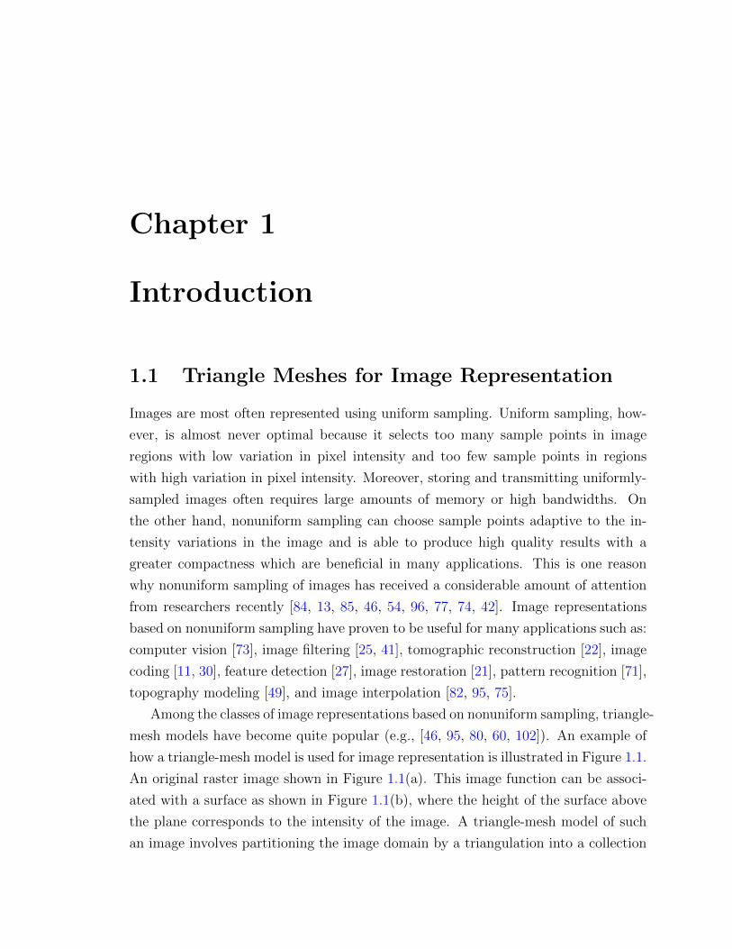
1.1 Triangle Meshes for Image Representation

Images are most often represented using uniform sampling. Uniform sampling, how-

ever, is almost never optimal because it selects too many sample points in image

regions with low variation in pixel intensity and too few sample points in regions

with high variation in pixel intensity. Moreover, storing and transmitting uniformly-

sampled images often requires large amounts of memory or high bandwidths. On

the other hand, nonuniform sampling can choose sample points adaptive to the in-

tensity variations in the image and is able to produce high quality results with a

greater compactness which are beneficial in many applications. This is one reason

why nonuniform sampling of images has received a considerable amount of attention

from researchers recently [84, 13, 85, 46, 54, 96, 77, 74, 42]. Image representations

based on nonuniform sampling have proven to be useful for many applications such as:

computer vision [73], image filtering [25, 41], tomographic reconstruction [22], image

coding [11, 30], feature detection [27], image restoration [21], pattern recognition [71],

topography modeling [49], and image interpolation [82, 95, 75].

Among the classes of image representations based on nonuniform sampling, triangle-

mesh models have become quite popular (e.g., [46, 95, 80, 60, 102]). An example of

how a triangle-mesh model is used for image representation is illustrated in Figure 1.1.

An original raster image shown in Figure 1.1(a). This image function can be associ-

ated with a surface as shown in Figure 1.1(b), where the height of the surface above

the plane corresponds to the intensity of the image. A triangle-mesh model of such

an image involves partitioning the image domain by a triangulation into a collection

2

(a) (b)

(c)

0800

50

100

600 800

150

200

600400

250

300

400200 200

0 0

(d)

(e)

Figure 1.1: An example of how a triangle-mesh model is used for image representa-tion. The (a) original image and (b) continuous surface associated with the rasterimage in (a). The (c) triangulation of image domain, (d) triangle-mesh model, and(e) reconstructed image.

3

of non-overlapping triangles as shown in Figure 1.1(c). The image function is then

approximated over each face (i.e., triangle) in the triangulation. Next, by stitching

all the approximating functions over faces together, the original image surface is ap-

proximated as shown in Figure 1.1(d). Finally, through a rasterization process, the

triangulated surface in Figure 1.1(d) is converted to the reconstructed raster image

shown in Figure 1.1(e). Using the triangle-mesh models as described above, images

can still be represented in high quality, but with many fewer sample points and lower

memory cost. Another practical advantage of using triangle-mesh models is that once

a mesh model of an image, as the one shown in Figure 1.1(d), is generated, it can

be stored and later used for different purposes, such as image editing, or any type of

affine transformations, like scaling, rotation, and translation.

1.2 Generation of Mesh Models of Images

In order to use a mesh model, its parameters must first be chosen. The method

to select the parameters of the mesh model is known as mesh generation. Given a

particular mesh model, various methods are possible to generate that specific model,

but each one can employ different parameter-selection techniques. For example, one

parameter that is crucial to almost any mesh model is the set of sample points used by

the model. Some mesh-generation methods select all the sample points in one step,

whereas other methods select them by an iterative process with adding/removing

points.

Several factors must be taken into consideration when choosing a mesh-generation

method, such as the characteristics of the model, the type of the approximating

function (e.g., linear and cubic), and the application in which the model is being

used. For example, some methods are designed to only generate mesh models that are

associated with continuous functions. As another example, methods that are designed

for generating mesh models for a certain application (e.g., image representation) may

not be much beneficial to other applications (e.g., image scaling). Therefore, the

quality of a mesh-generation method is typically evaluated based on how effective the

generated model performs in its specific application.

4

1.3 Image Scaling

Image scaling, as one of the classical and important problems in digital imaging

and computer graphics, has received much attention from researchers. Image scaling

refers to the operation of resizing digital images to obtain either a larger or a smaller

image. The image-scaling application that is considered in this work is the operation

of producing a raster image of larger size (i.e., higher resolution) from a raster image

of smaller size (i.e., lower resolution), which is also referred to as upscaling, super-

resolution, or resolution enhancement. Although image scaling is generally applicable

to both grayscale and color images, the work in this thesis focuses on scaling grayscale

images to keep the complexity low. As a future research, however, the work herein

can be extended for color images too.

Image scaling is required in many applications such as in producing high-resolution

images from the old images taken in the past with low-resolution cameras. Moreover,

for printing images on a very large papers/posters, such as on billboards, the image

scaling operation is needed to produce images of the size as large as the billboard

size. Last, but not least, image scaling is the main operation required by any image

zooming tool used in many applications (e.g., medical imaging, satellite imaging, and

digital photography).

Image scaling is most commonly performed using an image interpolation method.

Many different types of approaches for image interpolation are available. Some are

raster based while others are vector based. An interpolation technique is often evalu-

ated based on how well it handles undesired effects that can arise during the scaling

process (e.g., edge blurring and ringing) and how well it preserves the qualitative

attributes of the input image.

1.4 Historical Perspective

Due to the many advantages of triangle-mesh modeling, various types of triangle-

mesh models and numerous mesh-generation schemes have been developed over the

years. Similarly, different types of approaches have also been developed to solve the

image-scaling problem. Therefore, in what follows, a historical perspective of the

related work done in each of the above areas is presented.

5

1.4.1 Related Work in Mesh Models

Different triangle-mesh models can be categorized based on the type of the approx-

imating functions associated with them. Most of the proposed mesh models are

associated with an approximating function that is continuous everywhere, such as

the work in [96, 43, 74, 12, 42, 82, 75, 102, 83, 63]. Images, however, usually contain

a large number of discontinuities (i.e., image edges). Many types of mesh models

have been proposed to consider image-edge information, however, they still use a

continuous approximating function. For example, mesh models proposed by Garcia

et al. [42] and Zhou et al. [102] employ a technique to represent the image edges using

parallel polylines. The mesh model of Phichet et al. [83], however, uses a wavelet-

based method to approximate the image-edge directions and then triangle edges are

aligned with the image edges. Recently, Liu et al. [63] proposed a feature-preserving

mesh model that considers the anisotropicity of feature intensities in an image. For

this purpose, they have used anisotropic radial basis functions (ARBFs) to restore

the image from its triangulation representation. Their method considers not only the

geometrical (Euclidean) distances but also the local feature orientations (anisotropic

intensities). Moreover, instead of using the intensities at mesh nodes, which are of-

ten ambiguously defined on or near image edges, their method uses intensities at the

centers of mesh faces.

Another category of mesh models is the one that is associated with an approximat-

ing function which allows for selected discontinuities, such as the models in [72, 49,

90, 60, 84, 66]. For example, Tu and Adams [84] employed an explicitly-represented

discontinuities (ERD) mesh model inspired by the model proposed in [72]. The ap-

proximating function associated with the ERD model is allowed to have discontinuities

across certain triangulation edges. Typically, mesh models, such as the ERD model,

that explicitly use image-edge information result in more compact meshes than the

models, such as in [74], that do not consider image-edge features.

1.4.2 Related Work in Mesh Generation

In addition to the type of the mesh model itself, the method for generating such

a model is of great importance too. Generally, mesh-generation methods can be

classified into non-iterative and iterative approaches, based on how the sample points

are selected. In non-iterative approaches, all the sample points are selected in one

step, such as the methods in [96, 22, 40]. For example, Yang et al. [96] proposed

6

a highly effective technique that uses the classical error-diffusion (ED) algorithm of

Floyd and Steinberg [37] to select all the sample points such that their local density is

proportional to the maximum magnitude of the second-order directional derivative of

the image. Their method is fast with a low computational cost and easy to implement.

The ED-based method of [96] was recently adapted by Tu and Adams [84] to generate

the ERD model, resulting in the ERD with ED (ERDED) mesh-generation method.

Iterative mesh-generation methods themselves can be categorized into schemes

that are based on mesh refinement, mesh simplification, or a combination of both.

The mesh-refinement schemes begin with an initial mesh (such as a coarse mesh) and

then iteratively refine the mesh by adding more points to the mesh until a desired

mesh quality (or a certain number of sample points) is reached, such as the methods

of [43, 12, 84, 42, 74, 102, 66]. For example, Garland and Heckbert [43] proposed a

technique to iteratively select and insert the points with the highest reconstruction

error into the mesh, using a L1-norm error metric. This method was later modified

in [12] as called the modified-Garland-Heckbert (MGH) method, where a L2-norm

error metric is used. In the MGH method a greedy point-insertion (GPI) scheme

is used to make the point-selection process adaptive to the local squared error in

the mesh. More specifically, in each iteration in the MGH method, the point with

the highest absolute reconstruction error inside the face with largest squared error is

inserted into the mesh. Then, the image function is approximated using a continuous

function. Recently, Tu and Adams [84] adapted the GPI scheme of [12] to generate

the ERD model, resulting in the ERD with GPI (ERDGPI) mesh-generation method.

In contrast, the mesh-simplification schemes start with a refined initial mesh, by

selecting all or a portion of all the grid points in the image domain as the vertices

in the mesh. Then, one or more vertices/edges are iteratively deleted based on some

error metric, until a desired number of vertices is reached, such as the methods of [54,

30, 36, 13, 60]. The mesh-simplification methods, such as the well-known greedy

point-removal (GPR) scheme of Demaret and Iske [30] (called “adaptive thinning”

in [30]), are very effective in generating meshes of superior quality, but often have large

computational and memory costs. This drawback, motivated researchers to propose

some techniques to reduce the computational cost of the GPR method. For example,

Adams [13] modified the GPR scheme by replacing the initial set of all image points

with a subset of the points and introduced a new framework called GPR from subset

(GPRFS). Then, the ED and modified ED (MED) schemes were utilized for selecting a

subset of the points in the GPRFS framework and two new methods called GPRFS-

7

ED and GPRFS-MED were proposed, respectively. Both of these methods were

shown to have much lower computational and memory complexities than the GPR

scheme, but with different tradeoffs between mesh quality and computational/memory

complexity.

The third category of iterative mesh-generation methods is the one that combines

the mesh-refinement and mesh-simplification schemes. These methods, such as the

incremental/decremental techniques of [14, 15, 64] and the wavelet-based approach

of [83], take advantage of both point-insertion and point-removal operations. They

typically tend to achieve meshes of higher quality than those obtained by mesh-

refinement approaches, but such hybrid schemes can sometimes be extremely slow,

even slower the the mesh-simplification methods.

In addition to the mesh-generation methods that build a mesh from beginning,

another type of work, which has recently become more popular, is based on mesh

optimization/adaptation. This type of work focuses on improving the quality of a

mesh, which may have been generated from any method, through an iterative process

of mesh optimization or adaptation. These mesh optimization/adaptation methods

may not be directly considered as mesh-generation schemes essentially because they

do not generate the mesh from the beginning. For example, the mesh-optimization

methods of Xie et al. in [92, 91] perform both geometry and topology optimizations to

strictly reduce the total energy. In their mesh-optimization algorithm, the position of

a vertex can be re-adjusted several times, so that the local optimality of that vertex

would not be corrupted during later processing of other vertices. In another recent

work, Li [58] introduced an anisotropic mesh-adaptation (AMA) method for image

representation. The AMA method of Li [58] starts directly with an initial triangular

mesh and then iteratively adapts the mesh based on a user-defined metric tensor to

represent the image.

1.4.3 Related Work in Image Scaling

In addition to studying the triangle-mesh models for image representation, a sig-

nificant part of this thesis is focused on the application of mesh models in image

scaling. The problem of image scaling, which also goes by the names of image re-

sizing, resolution enhancement, and super-resolution, is essentially ill-posed because

much information is lost in the degradation process of going from high to low resolu-

tion. Much work has been done on this topic over many years, with some considerable

8

advancements made over the recent years. Each super-resolution method has different

advantages and drawbacks. Many image scaling approaches are based on the classical

convolution-based interpolation techniques, such as nearest-neighbor, bilinear, bicu-

bic [51], and cubic spline [48] interpolation. Although these methods are fast with

very low computational cost, they have the problem of producing blurring (or other

artifacts such as blocking and ringing) around image edges. This drawback of the

classical methods is mainly because they are not able to recover the high frequency

components which provide visual sharpness to an image.

Since the human visual system is particularly drawn to distortions in edges, many

edge-directed image interpolation methods have been proposed to reduce the artifacts

produced by the classical interpolation methods. Some examples of the effective edge-

directed raster-based methods can be found in [59, 99, 24, 44, 17, 101, 98]. In these

methods, a crucial step is to explicitly or implicitly estimate the edge directions in

the image. For example, the new edge-directed image interpolation (NEDI) method

of Li and Orchard [59] uses the local covariances of the image to estimate the edge

directions. This method was later improved by Asuni and Giachetti [17] by reducing

numerical instability and making the region used to estimate the covariance adaptive.

In another work, Giachetti and Asuni [44] proposed an iterative curvature-based in-

terpolation, which is based on a two-step grid filling technique. After each step, the

interpolated pixels are iteratively corrected by minimizing an objective function de-

pending on the second-order directional derivatives of the image intensity while trying

to preserve strong discontinuities. Moreover, in the directional cubic-convolution in-

terpolation (DCCI) method of Zhou et al. [101], which is an extension of the classical

cubic convolution interpolation of Keys [51], local edge direction is explicitly esti-

mated using the ratio of the two orthogonal directional gradients for a missing pixel

position. Then, the value at the missing pixel is estimated as the weighted average

of the two orthogonal directional cubic-convolution interpolation values. Although

these edge-directed super-resolution approaches can improve the subjective quality

of the scaled images by tuning the interpolation to preserve the edges of the image,

they have high computational complexity. Moreover, although the high-resolution

images produced using these methods have sharper edges than those obtained by the

classical methods, they often still contain some degree of artifacts like blurring and

rippling at the edges.

The most recent advances in the image scaling (also called super-resolution) tech-

niques are based on machine learning. The excellent performance of image scaling

9

methods based on machine learning has recently gained much attention from re-

searchers [89, 33, 62, 52, 78, 86, 57]. In general, learning-based techniques for image

super-resolution can be divided into external and internal methods [89]. External

methods, such as [39, 53, 94], learn the mapping between low-resolution and high-

resolution image patches, from a large and representative external set of image pairs

based on external image samples. Internal methods, however, such as [93, 45, 38], are

motivated by the fact that images generally contain a lot of self-similarities. There-

fore, internal methods search for example patches from the input image itself, based

on the fact that patches often tend to recur within the image or across different im-

age scales. Both external and internal image super-resolution methods have different

advantages and disadvantages. For example, external methods perform better for

smooth regions as well as some irregular structures that barely recur in the input,

but these methods are prone to producing either noise or over-smoothness. Internal

methods, however, perform better in reproducing unique and singular features that

rarely appear externally but repeat in the input image.

Recently, Wang et al. [89] proposed a joint super-resolution method to adaptively

combine the external and internal methods to take advantage of both. Another recent

and well-known work is the SRCNN method of Dong et al. [33], which is an image

super-resolution (SR) method based on deep convolutional neural networks (CNN).

The SRCNN method directly learns an end-to-end mapping between the low/high-

resolution images (i.e., it is an external example-based method). The mapping is

represented as a deep convolutional neural network that takes the low-resolution im-

age as the input and outputs the high-resolution one. Through experimental results,

Dong et al. [33] demonstrated that deep learning is useful in the classical problem of

image super-resolution, and can achieve good quality and speed. They designed the

SRCNN method based on a three-layer network and concluded that deeper structure

does not always lead to better results. Later, Kim et al. [52], however, improved

over the SRCNN method and showed that using a deeper structure can achieve bet-

ter performance. They proposed a very deep super-resolution (VDSR) method that

employs a network with depth of 20 layers as apposed to three layers in the SRCNN

method. Similar to the most existing super-resolution methods, the SRCNN model

is trained for a single scale factor and is supposed to work only with that specified

scale. Thus, if a new scale is demanded, a new model has to be trained. In the VDSR

model of [52], however, a single network is designed and trained to handle the super-

resolution problem with multiple scale factors efficiently. Despite all the advances

10

and breakthroughs in accuracy and speed of image super-resolution using faster and

deeper convolutional neural networks, one essential problem has always been how to

recover the finer texture details at large upscaling factors. In a very recent work, Ledig

et al. [57] proposed an advanced super-resolution (SR) technique using a generative

adversarial network (GAN) called SRGAN, which can recover photo-realistic textures

from heavily downsampled images. Previous works commonly relied on minimizing

the mean squared error (MSE) between the recovered high-resolution image and the

ground truth, but minimizing MSE does not necessarily reflect the perceptually bet-

ter super-resolution result [57]. The SRGAN method, however, relies on a novel

perceptual loss function to recover visually more convincing scaled images. Most of

the learning-based super-resolution methods, especially those based on deep learning,

are very powerful general-purpose methods with excellent performance. They are,

however, computationally expensive and need a huge training dataset to be able to

perform reasonably well.

Another category of image interpolation techniques, is based on triangle-mesh

modeling. Since the triangle-mesh model obtained from an image is resolution-

independent, it can be rasterized to an image grid of any arbitrary resolution. This

fact has motivated researchers to use triangle-mesh models in the application of image

scaling as in [82, 75, 102, 100, 61, 67]. For almost all of these triangulation-based

methods to be effective in image scaling, the first essential step is to estimate the

edge directions in the image. Then, the second step is to maintain the parallelism of

the triangle edges with the image edges. Su and Willis [82], for instance, proposed

an edge-directed image interpolation technique by pixel-level data-dependent trian-

gulation (DDT), where the image-edges directions are locally estimated by evaluating

the four intensity values at each set of four pixels forming the smallest square in the

image grid. Their method, however, only considers the diagonal edge directions. This

method was later improved by Shao et al. [75] by considering the horizontal and ver-

tical edge directions in addition to the diagonal direction. Moreover, they defined a

threshold for each direction to determine whether it is an edge or not. Later, Zhen-

jie et al. [100] improved upon the work of Su and Willis [82] by proposing a more

effective algorithm to determine the edge direction. More recently, Liu et al. [61]

proposed an image interpolation technique using the DDT and a new weighted sub-

division scheme. In their method, an image is first converted to a triangular mesh

using a DDT. The mesh is then subdivided by controlling the weight coefficients of

a rational subdivision. Using the proposed rational subdivision, the image edges are

11

kept sharper during the subdivision process.

As reviewed earlier, most of the mesh-based image interpolation techniques used

for image scaling (e.g., [82, 75, 100, 61]) are based on DDTs where all of the grid

points in the image are used to generate the mesh. Although using all image points

helps to capture details and textures in the image more accurately, this greatly in-

creases the computational and memory cost. In contrast, some methods, such as

the curvilinear feature driven technique of Zhou et al. [102], start with a smaller

initial mesh and iteratively refine the mesh. In the work of [102], the locations and

directions of image edges are first estimated using an edge detector. This edge infor-

mation is then explicitly used in the triangle-mesh model to preserve the sharpness

of the edges in the reconstructed images after scaling. Similar to the work of [61],

the proposed method of [102] employs subdivision techniques to produce sufficiently

smooth edge curvatures and image functions during scaling. The methods, which do

not use all the image points, have much lower computational cost and usually work

perfectly for cartoon images. For natural images, however, they have not been widely

used because they are not able to capture the complicated textures and details that

usually exist in natural images. The mesh-based super-resolution techniques have

recently become increasingly popular because, unlike other convolution-based and

learning-based methods, they are capable of producing reusable image models that

are compact, editable, and scalable. Moreover, they have lower computational and

memory cost compared with many state-of-the-art methods based on deep learning

that require a huge training dataset.

1.5 Overview and Contribution of the Thesis

In this thesis, image representation using triangle-mesh models and its application

in image scaling are explored, resulting in two new methods for solving two differ-

ent problems. More specifically, a new squared-error minimizing mesh-generation

(SEMMG) method is first proposed to address the problem of image representation,

by generating ERD mesh models that are effective for grayscale-image representation.

Then, to solve the image-scaling problem, the application of the ERD mesh models in

image scaling is studied, leading to the proposal of a new mesh-based image scaling

(MIS) method for grayscale images that are piecewise-smooth.

The remainder of this thesis consists of six chapters and three appendices. This

material is organized as follows.

12

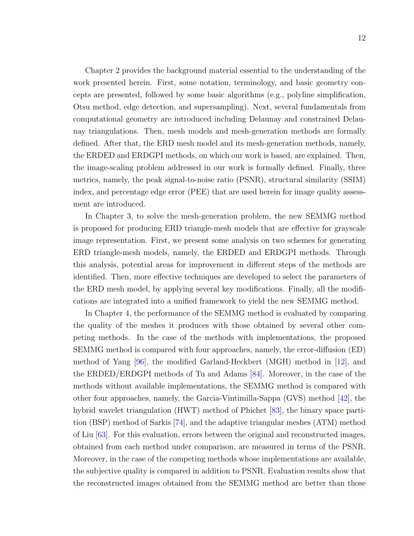
Chapter 2 provides the background material essential to the understanding of the

work presented herein. First, some notation, terminology, and basic geometry con-

cepts are presented, followed by some basic algorithms (e.g., polyline simplification,

Otsu method, edge detection, and supersampling). Next, several fundamentals from

computational geometry are introduced including Delaunay and constrained Delau-

nay triangulations. Then, mesh models and mesh-generation methods are formally

defined. After that, the ERD mesh model and its mesh-generation methods, namely,

the ERDED and ERDGPI methods, on which our work is based, are explained. Then,

the image-scaling problem addressed in our work is formally defined. Finally, three

metrics, namely, the peak signal-to-noise ratio (PSNR), structural similarity (SSIM)

index, and percentage edge error (PEE) that are used herein for image quality assess-

ment are introduced.

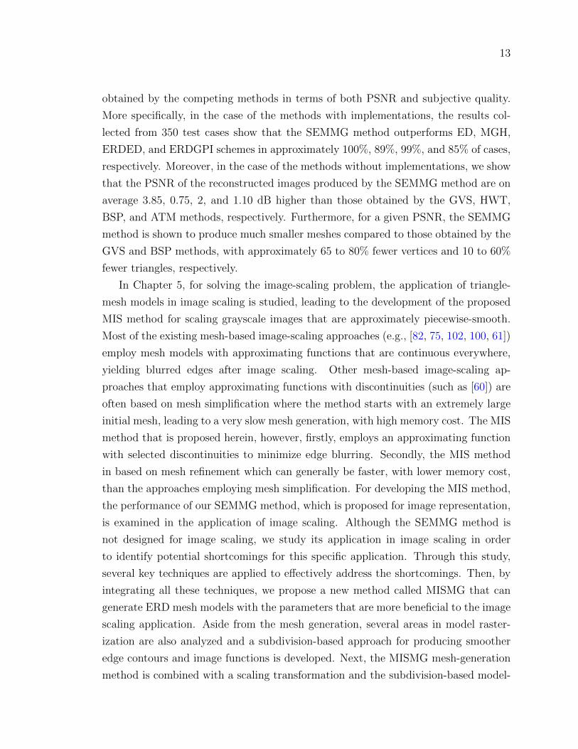
In Chapter 3, to solve the mesh-generation problem, the new SEMMG method

is proposed for producing ERD triangle-mesh models that are effective for grayscale

image representation. First, we present some analysis on two schemes for generating

ERD triangle-mesh models, namely, the ERDED and ERDGPI methods. Through

this analysis, potential areas for improvement in different steps of the methods are

identified. Then, more effective techniques are developed to select the parameters of

the ERD mesh model, by applying several key modifications. Finally, all the modifi-

cations are integrated into a unified framework to yield the new SEMMG method.

In Chapter 4, the performance of the SEMMG method is evaluated by comparing

the quality of the meshes it produces with those obtained by several other com-

peting methods. In the case of the methods with implementations, the proposed

SEMMG method is compared with four approaches, namely, the error-diffusion (ED)

method of Yang [96], the modified Garland-Heckbert (MGH) method in [12], and

the ERDED/ERDGPI methods of Tu and Adams [84]. Moreover, in the case of the

methods without available implementations, the SEMMG method is compared with

other four approaches, namely, the Garcia-Vintimilla-Sappa (GVS) method [42], the

hybrid wavelet triangulation (HWT) method of Phichet [83], the binary space parti-

tion (BSP) method of Sarkis [74], and the adaptive triangular meshes (ATM) method

of Liu [63]. For this evaluation, errors between the original and reconstructed images,

obtained from each method under comparison, are measured in terms of the PSNR.

Moreover, in the case of the competing methods whose implementations are available,

the subjective quality is compared in addition to PSNR. Evaluation results show that

the reconstructed images obtained from the SEMMG method are better than those

13

obtained by the competing methods in terms of both PSNR and subjective quality.

More specifically, in the case of the methods with implementations, the results col-

lected from 350 test cases show that the SEMMG method outperforms ED, MGH,

ERDED, and ERDGPI schemes in approximately 100%, 89%, 99%, and 85% of cases,

respectively. Moreover, in the case of the methods without implementations, we show

that the PSNR of the reconstructed images produced by the SEMMG method are on

average 3.85, 0.75, 2, and 1.10 dB higher than those obtained by the GVS, HWT,

BSP, and ATM methods, respectively. Furthermore, for a given PSNR, the SEMMG

method is shown to produce much smaller meshes compared to those obtained by the

GVS and BSP methods, with approximately 65 to 80% fewer vertices and 10 to 60%

fewer triangles, respectively.

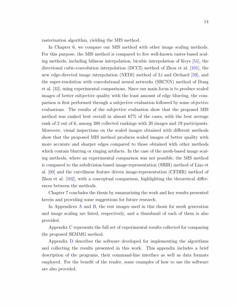
In Chapter 5, for solving the image-scaling problem, the application of triangle-

mesh models in image scaling is studied, leading to the development of the proposed

MIS method for scaling grayscale images that are approximately piecewise-smooth.

Most of the existing mesh-based image-scaling approaches (e.g., [82, 75, 102, 100, 61])

employ mesh models with approximating functions that are continuous everywhere,

yielding blurred edges after image scaling. Other mesh-based image-scaling ap-

proaches that employ approximating functions with discontinuities (such as [60]) are

often based on mesh simplification where the method starts with an extremely large

initial mesh, leading to a very slow mesh generation, with high memory cost. The MIS

method that is proposed herein, however, firstly, employs an approximating function

with selected discontinuities to minimize edge blurring. Secondly, the MIS method

in based on mesh refinement which can generally be faster, with lower memory cost,

than the approaches employing mesh simplification. For developing the MIS method,

the performance of our SEMMG method, which is proposed for image representation,

is examined in the application of image scaling. Although the SEMMG method is

not designed for image scaling, we study its application in image scaling in order

to identify potential shortcomings for this specific application. Through this study,

several key techniques are applied to effectively address the shortcomings. Then, by

integrating all these techniques, we propose a new method called MISMG that can

generate ERD mesh models with the parameters that are more beneficial to the image

scaling application. Aside from the mesh generation, several areas in model raster-

ization are also analyzed and a subdivision-based approach for producing smoother

edge contours and image functions is developed. Next, the MISMG mesh-generation

method is combined with a scaling transformation and the subdivision-based model-

14

rasterization algorithm, yielding the MIS method.

In Chapter 6, we compare our MIS method with other image scaling methods.

For this purpose, the MIS method is compared to five well-known raster-based scal-

ing methods, including bilinear interpolation, bicubic interpolation of Keys [51], the

directional cubic-convolution interpolation (DCCI) method of Zhou et al. [101], the

new edge-directed image interpolation (NEDI) method of Li and Orchard [59], and

the super-resolution with convolutional neural networks (SRCNN) method of Dong

et al. [33], using experimental comparisons. Since our main focus is to produce scaled

images of better subjective quality with the least amount of edge blurring, the com-

parison is first performed through a subjective evaluation followed by some objective

evaluations. The results of the subjective evaluation show that the proposed MIS

method was ranked best overall in almost 67% of the cases, with the best average

rank of 2 out of 6, among 380 collected rankings with 20 images and 19 participants.

Moreover, visual inspections on the scaled images obtained with different methods

show that the proposed MIS method produces scaled images of better quality with

more accurate and sharper edges compared to those obtained with other methods

which contain blurring or ringing artifacts. In the case of the mesh-based image scal-

ing methods, where an experimental comparison was not possible, the MIS method

is compared to the subdivision-based image-representation (SBIR) method of Liao et

al. [60] and the curvilinear feature driven image-representation (CFDIR) method of

Zhou et al. [102], with a conceptual comparison, highlighting the theoretical differ-

ences between the methods.

Chapter 7 concludes the thesis by summarizing the work and key results presented

herein and providing some suggestions for future research.

In Appendices A and B, the test images used in this thesis for mesh generation

and image scaling are listed, respectively, and a thumbnail of each of them is also

provided.

Appendix C represents the full set of experimental results collected for comparing

the proposed SEMMG method.

Appendix D describes the software developed for implementing the algorithms

and collecting the results presented in this work. This appendix includes a brief

description of the programs, their command-line interface as well as data formats

employed. For the benefit of the reader, some examples of how to use the software

are also provided.

15

Chapter 2

Preliminaries

2.1 Notation and Terminology

First, a brief digression concerning the notation and terminology used herein is ap-

propriate. Some of the notational conventions employed are as follows. The symbols

Z and R denote the sets of integers and real numbers, respectively. The cardinality of

a set S is denoted by |S|. A triangle formed by three vertices A,B, and C is denoted

by 4ABC. An edge (or a line segment) connecting two points A and B is denoted

by AB.

2.2 Basic Geometry Concepts

In this section, we introduce some basic concepts in geometry that are used later. To

begin, we introduce the concepts of convex set and convex hull.

Definition 2.1. (Convex set). A set P of points in R2 is said to be convex if, for

every pair of points p, q ∈ P , the line segment pq is completely contained in P .

An example of a convex set and a nonconvex set is illustrated in Figure 2.1. As can

be seen from this figure, for the set P in Figure 2.1(a), any line segment connecting a

pair of arbitrary points is completely contained in P , such as the line pq. Thus, the

set P in Figure 2.1(a) is convex. In contrast, for the set P in Figure 2.1(b), a line

such as pq is not fully contained in P . Therefore, the set P in Figure 2.1(b) is not

convex. Having introduced the concept of convex set, in what follows, we provide the

definition of a convex hull.

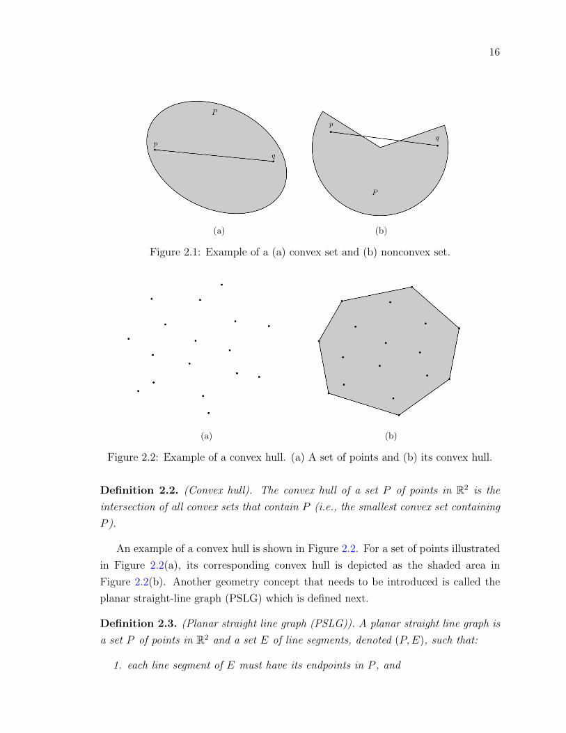
16

(a) (b)

Figure 2.1: Example of a (a) convex set and (b) nonconvex set.

(a) (b)

Figure 2.2: Example of a convex hull. (a) A set of points and (b) its convex hull.

Definition 2.2. (Convex hull). The convex hull of a set P of points in R2 is the

intersection of all convex sets that contain P (i.e., the smallest convex set containing

P ).

An example of a convex hull is shown in Figure 2.2. For a set of points illustrated

in Figure 2.2(a), its corresponding convex hull is depicted as the shaded area in

Figure 2.2(b). Another geometry concept that needs to be introduced is called the

planar straight-line graph (PSLG) which is defined next.

Definition 2.3. (Planar straight line graph (PSLG)). A planar straight line graph is

a set P of points in R2 and a set E of line segments, denoted (P,E), such that:

1. each line segment of E must have its endpoints in P , and

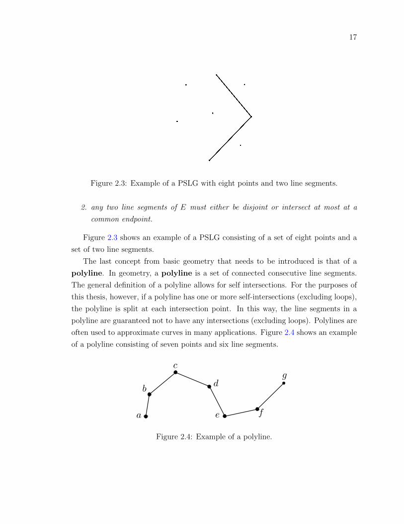
17

Figure 2.3: Example of a PSLG with eight points and two line segments.

2. any two line segments of E must either be disjoint or intersect at most at a

common endpoint.

Figure 2.3 shows an example of a PSLG consisting of a set of eight points and a

set of two line segments.

The last concept from basic geometry that needs to be introduced is that of a

polyline. In geometry, a polyline is a set of connected consecutive line segments.

The general definition of a polyline allows for self intersections. For the purposes of

this thesis, however, if a polyline has one or more self-intersections (excluding loops),

the polyline is split at each intersection point. In this way, the line segments in a

polyline are guaranteed not to have any intersections (excluding loops). Polylines are

often used to approximate curves in many applications. Figure 2.4 shows an example

of a polyline consisting of seven points and six line segments.

Figure 2.4: Example of a polyline.

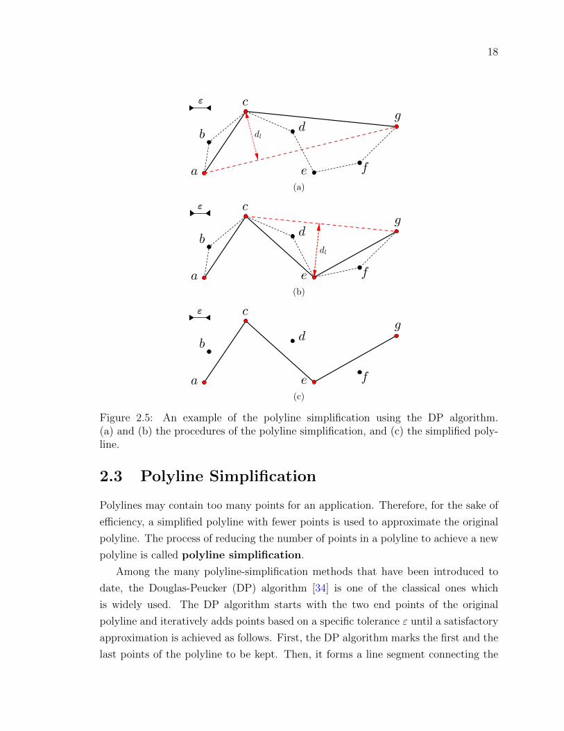
18

(a)

(b)

(c)

Figure 2.5: An example of the polyline simplification using the DP algorithm.(a) and (b) the procedures of the polyline simplification, and (c) the simplified poly-line.

2.3 Polyline Simplification

Polylines may contain too many points for an application. Therefore, for the sake of

efficiency, a simplified polyline with fewer points is used to approximate the original

polyline. The process of reducing the number of points in a polyline to achieve a new

polyline is called polyline simplification.

Among the many polyline-simplification methods that have been introduced to

date, the Douglas-Peucker (DP) algorithm [34] is one of the classical ones which

is widely used. The DP algorithm starts with the two end points of the original

polyline and iteratively adds points based on a specific tolerance ε until a satisfactory

approximation is achieved as follows. First, the DP algorithm marks the first and the

last points of the polyline to be kept. Then, it forms a line segment connecting the

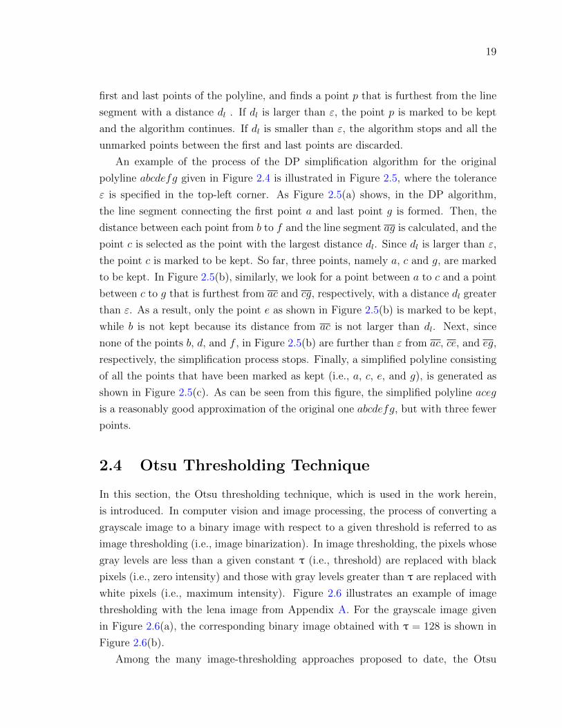
19

first and last points of the polyline, and finds a point p that is furthest from the line

segment with a distance dl . If dl is larger than ε, the point p is marked to be kept

and the algorithm continues. If dl is smaller than ε, the algorithm stops and all the

unmarked points between the first and last points are discarded.

An example of the process of the DP simplification algorithm for the original

polyline abcdefg given in Figure 2.4 is illustrated in Figure 2.5, where the tolerance

ε is specified in the top-left corner. As Figure 2.5(a) shows, in the DP algorithm,

the line segment connecting the first point a and last point g is formed. Then, the

distance between each point from b to f and the line segment ag is calculated, and the

point c is selected as the point with the largest distance dl. Since dl is larger than ε,

the point c is marked to be kept. So far, three points, namely a, c and g, are marked

to be kept. In Figure 2.5(b), similarly, we look for a point between a to c and a point

between c to g that is furthest from ac and cg, respectively, with a distance dl greater

than ε. As a result, only the point e as shown in Figure 2.5(b) is marked to be kept,

while b is not kept because its distance from ac is not larger than dl. Next, since

none of the points b, d, and f , in Figure 2.5(b) are further than ε from ac, ce, and eg,

respectively, the simplification process stops. Finally, a simplified polyline consisting

of all the points that have been marked as kept (i.e., a, c, e, and g), is generated as

shown in Figure 2.5(c). As can be seen from this figure, the simplified polyline aceg

is a reasonably good approximation of the original one abcdefg, but with three fewer

points.

2.4 Otsu Thresholding Technique

In this section, the Otsu thresholding technique, which is used in the work herein,

is introduced. In computer vision and image processing, the process of converting a

grayscale image to a binary image with respect to a given threshold is referred to as

image thresholding (i.e., image binarization). In image thresholding, the pixels whose

gray levels are less than a given constant τ (i.e., threshold) are replaced with black

pixels (i.e., zero intensity) and those with gray levels greater than τ are replaced with

white pixels (i.e., maximum intensity). Figure 2.6 illustrates an example of image

thresholding with the lena image from Appendix A. For the grayscale image given

in Figure 2.6(a), the corresponding binary image obtained with τ = 128 is shown in

Figure 2.6(b).

Among the many image-thresholding approaches proposed to date, the Otsu

20

(a) (b)

Figure 2.6: An example of image thresholding. The (a) original lena image and (b)the corresponding binary image obtained with τ = 128.

method [68] is a well-known automated clustering-based technique which is used fre-

quently in computer vision and image processing. With the assumption that the

image approximately has a bimodal histogram with two classes of pixels, the Otsu

algorithm computes the optimum threshold to separate the two classes so that their

inter-class variance is maximal (or equivalently, the intra-class variance is minimal).

In the context of image thresholding, the input to the Otsu method is a grayscale im-

age and the output is the optimum threshold value. Once the threshold is determined,

the binary image can be simply obtained using the threshold.

2.5 Edge Detection

In image processing and computer graphics, edges are one of the most fundamen-

tal features of an image since they contain vital information for many applications.

Studies have also shown that the human visual system attaches a great importance

to edges. An edge can be defined as a contour in an image at which the image func-

tion changes abruptly. In other words, edges represent the locations of discontinuities

in the image function and the process that estimates the presence and position of

edges in an image is known as edge detection. The input to the edge detection is

a grayscale image and the output is a binary edge map, where each pixel is marked

either as an edge point or as a non-edge point. An example of an edge map is illus-

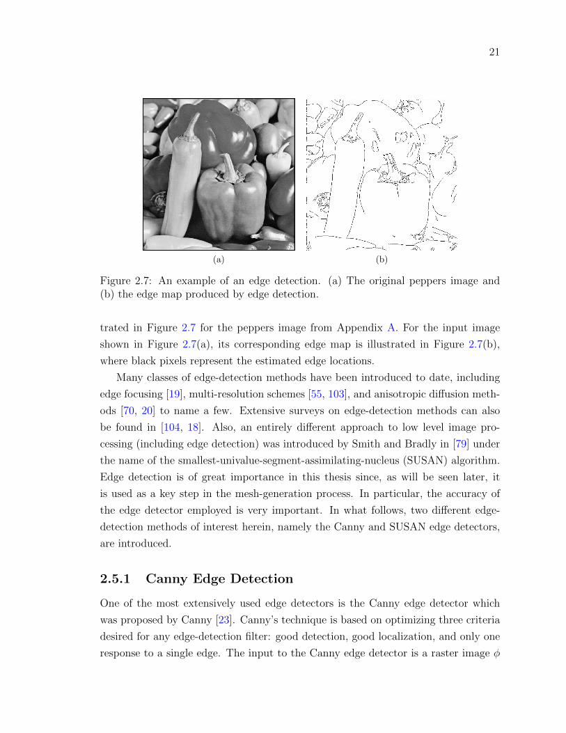
21

(a) (b)

Figure 2.7: An example of an edge detection. (a) The original peppers image and(b) the edge map produced by edge detection.

trated in Figure 2.7 for the peppers image from Appendix A. For the input image

shown in Figure 2.7(a), its corresponding edge map is illustrated in Figure 2.7(b),

where black pixels represent the estimated edge locations.

Many classes of edge-detection methods have been introduced to date, including

edge focusing [19], multi-resolution schemes [55, 103], and anisotropic diffusion meth-

ods [70, 20] to name a few. Extensive surveys on edge-detection methods can also

be found in [104, 18]. Also, an entirely different approach to low level image pro-

cessing (including edge detection) was introduced by Smith and Bradly in [79] under

the name of the smallest-univalue-segment-assimilating-nucleus (SUSAN) algorithm.

Edge detection is of great importance in this thesis since, as will be seen later, it

is used as a key step in the mesh-generation process. In particular, the accuracy of

the edge detector employed is very important. In what follows, two different edge-

detection methods of interest herein, namely the Canny and SUSAN edge detectors,

are introduced.

2.5.1 Canny Edge Detection

One of the most extensively used edge detectors is the Canny edge detector which

was proposed by Canny [23]. Canny’s technique is based on optimizing three criteria

desired for any edge-detection filter: good detection, good localization, and only one

response to a single edge. The input to the Canny edge detector is a raster image φ

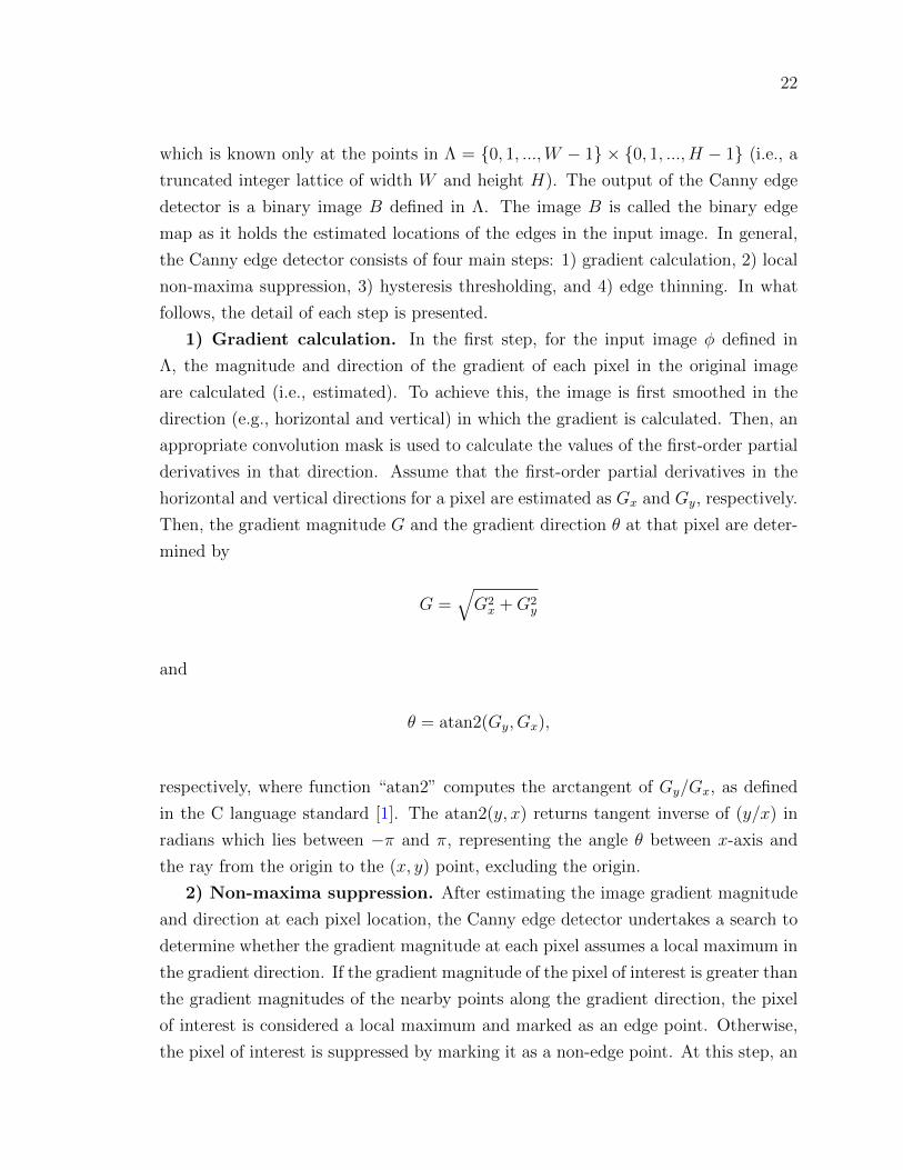
22

which is known only at the points in Λ = 0, 1, ...,W − 1 × 0, 1, ..., H − 1 (i.e., a

truncated integer lattice of width W and height H). The output of the Canny edge

detector is a binary image B defined in Λ. The image B is called the binary edge

map as it holds the estimated locations of the edges in the input image. In general,

the Canny edge detector consists of four main steps: 1) gradient calculation, 2) local

non-maxima suppression, 3) hysteresis thresholding, and 4) edge thinning. In what

follows, the detail of each step is presented.

1) Gradient calculation. In the first step, for the input image φ defined in

Λ, the magnitude and direction of the gradient of each pixel in the original image

are calculated (i.e., estimated). To achieve this, the image is first smoothed in the

direction (e.g., horizontal and vertical) in which the gradient is calculated. Then, an

appropriate convolution mask is used to calculate the values of the first-order partial

derivatives in that direction. Assume that the first-order partial derivatives in the

horizontal and vertical directions for a pixel are estimated as Gx and Gy, respectively.

Then, the gradient magnitude G and the gradient direction θ at that pixel are deter-

mined by

G =√G2x +G2

y

and

θ = atan2(Gy, Gx),

respectively, where function “atan2” computes the arctangent of Gy/Gx, as defined

in the C language standard [1]. The atan2(y, x) returns tangent inverse of (y/x) in

radians which lies between −π and π, representing the angle θ between x-axis and

the ray from the origin to the (x, y) point, excluding the origin.

2) Non-maxima suppression. After estimating the image gradient magnitude

and direction at each pixel location, the Canny edge detector undertakes a search to

determine whether the gradient magnitude at each pixel assumes a local maximum in

the gradient direction. If the gradient magnitude of the pixel of interest is greater than

the gradient magnitudes of the nearby points along the gradient direction, the pixel

of interest is considered a local maximum and marked as an edge point. Otherwise,

the pixel of interest is suppressed by marking it as a non-edge point. At this step, an

23

edge map fe is obtained containing a set of non-maxima suppressed edge points.

3) Hysteresis thresholding. The next step is thresholding. Pixels with larger

gradient magnitudes are more likely to correspond to actual edges than those with

smaller gradient magnitudes. In most cases, however, deciding whether a pixel with a

given gradient magnitude corresponds to an edge by specifying only a single threshold

is difficult. Therefore, the Canny edge detector uses hysteresis thresholding as follows.

Thresholding with hysteresis employs two thresholds, a high threshold τh and a low

threshold τl. If the gradient magnitude of an edge pixel in image fe (from the previous

step) is greater than τh, the pixel will be kept as a strong edge point. The pixels whose

gradient magnitudes are smaller than τl will not be considered as an edge point. In

the case of the pixels whose gradient magnitudes are between τl and τh, the pixels are

traced and if they are connected to a strong edge point, they will be kept as an edge

point in ffinal. In this way, hysteresis thresholding can help to find weak edges.

4) Edge thinning. Finally, an image processing task called edge thinning is

performed on the edge map ffinal to result in the edge map B with one-pixel-thick

edge elements.

Once the above four-step process is complete, we have the output binary edge map

B (e.g., Figure 2.7(b)), where each pixel is marked either as an edge point or as a non-

edge point. Numerous variations of the Canny edge detector have been introduced

to date. The modified Canny edge detector proposed by Ding and Goshtasby in [32]

improves the accuracy of the detected edges in the vicinity of intersecting edges, where

the original Canny edge detector often performs poorly.

2.5.2 SUSAN Edge Detection

The smallest-univalue-segment-assimilating-nucleus (SUSAN) algorithm [79] is a dif-

ferent approach to low level image processing that can be used for edge and corner

detection and structure-preserving noise reduction. A nonlinear filtering is used to

define which parts of the image are closely related to each individual pixel. Each pixel

is then associated with a local image region that is of similar brightness to that pixel.

Same as the Canny edge detector, the input to the SUSAN edge detector is a raster

image φ which is known only at the points in Λ = 0, 1, ...,W − 1× 0, 1, ..., H − 1(i.e., a truncated integer lattice of width W and height H). The output of the SUSAN

edge detector is a binary edge map B defined in Λ, where each pixel is marked either

as an edge point or as a non-edge point.

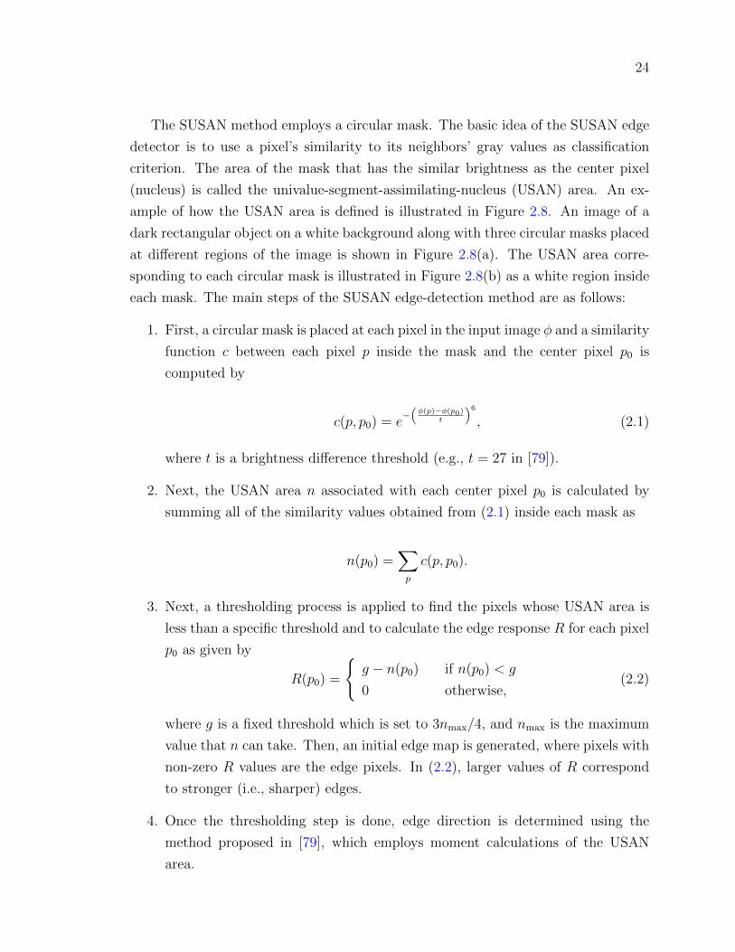
24

The SUSAN method employs a circular mask. The basic idea of the SUSAN edge

detector is to use a pixel’s similarity to its neighbors’ gray values as classification

criterion. The area of the mask that has the similar brightness as the center pixel

(nucleus) is called the univalue-segment-assimilating-nucleus (USAN) area. An ex-

ample of how the USAN area is defined is illustrated in Figure 2.8. An image of a

dark rectangular object on a white background along with three circular masks placed

at different regions of the image is shown in Figure 2.8(a). The USAN area corre-

sponding to each circular mask is illustrated in Figure 2.8(b) as a white region inside

each mask. The main steps of the SUSAN edge-detection method are as follows:

1. First, a circular mask is placed at each pixel in the input image φ and a similarity

function c between each pixel p inside the mask and the center pixel p0 is

computed by

c(p, p0) = e−(φ(p)−φ(p0)

t

)6

, (2.1)

where t is a brightness difference threshold (e.g., t = 27 in [79]).

2. Next, the USAN area n associated with each center pixel p0 is calculated by

summing all of the similarity values obtained from (2.1) inside each mask as

n(p0) =∑p

c(p, p0).

3. Next, a thresholding process is applied to find the pixels whose USAN area is

less than a specific threshold and to calculate the edge response R for each pixel

p0 as given by

R(p0) =

g − n(p0) if n(p0) < g

0 otherwise,(2.2)

where g is a fixed threshold which is set to 3nmax/4, and nmax is the maximum

value that n can take. Then, an initial edge map is generated, where pixels with

non-zero R values are the edge pixels. In (2.2), larger values of R correspond

to stronger (i.e., sharper) edges.

4. Once the thresholding step is done, edge direction is determined using the

method proposed in [79], which employs moment calculations of the USAN

area.

25

(a)

(b)

Figure 2.8: An example of USAN area. (a) Original image with three circular masksplaced at different regions and (b) the USAN areas as white parts of each mask.

5. Then, non-maxima suppression is performed on the initial edge map in the

direction perpendicular to the edge.

6. Finally, the non-maxima-suppressed edge map is thinned to obtain the final

binary edge map B with one-pixel-thick edge elements.

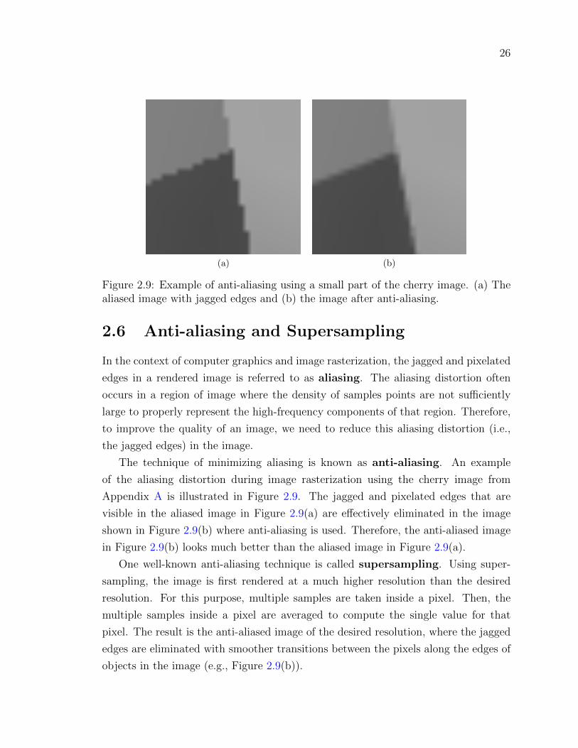
26

(a) (b)

Figure 2.9: Example of anti-aliasing using a small part of the cherry image. (a) Thealiased image with jagged edges and (b) the image after anti-aliasing.

2.6 Anti-aliasing and Supersampling

In the context of computer graphics and image rasterization, the jagged and pixelated

edges in a rendered image is referred to as aliasing. The aliasing distortion often

occurs in a region of image where the density of samples points are not sufficiently

large to properly represent the high-frequency components of that region. Therefore,

to improve the quality of an image, we need to reduce this aliasing distortion (i.e.,

the jagged edges) in the image.

The technique of minimizing aliasing is known as anti-aliasing. An example

of the aliasing distortion during image rasterization using the cherry image from

Appendix A is illustrated in Figure 2.9. The jagged and pixelated edges that are

visible in the aliased image in Figure 2.9(a) are effectively eliminated in the image

shown in Figure 2.9(b) where anti-aliasing is used. Therefore, the anti-aliased image

in Figure 2.9(b) looks much better than the aliased image in Figure 2.9(a).

One well-known anti-aliasing technique is called supersampling. Using super-

sampling, the image is first rendered at a much higher resolution than the desired

resolution. For this purpose, multiple samples are taken inside a pixel. Then, the

multiple samples inside a pixel are averaged to compute the single value for that

pixel. The result is the anti-aliased image of the desired resolution, where the jagged

edges are eliminated with smoother transitions between the pixels along the edges of

objects in the image (e.g., Figure 2.9(b)).

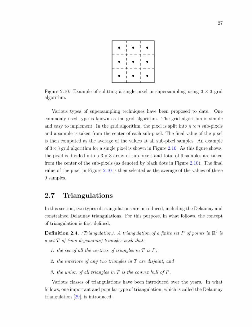
27

Figure 2.10: Example of splitting a single pixel in supersampling using 3 × 3 gridalgorithm.

Various types of supersampling techniques have been proposed to date. One

commonly used type is known as the grid algorithm. The grid algorithm is simple

and easy to implement. In the grid algorithm, the pixel is split into n× n sub-pixels

and a sample is taken from the center of each sub-pixel. The final value of the pixel

is then computed as the average of the values at all sub-pixel samples. An example

of 3×3 grid algorithm for a single pixel is shown in Figure 2.10. As this figure shows,

the pixel is divided into a 3 × 3 array of sub-pixels and total of 9 samples are taken

from the center of the sub-pixels (as denoted by black dots in Figure 2.10). The final

value of the pixel in Figure 2.10 is then selected as the average of the values of these

9 samples.

2.7 Triangulations

In this section, two types of triangulations are introduced, including the Delaunay and

constrained Delaunay triangulations. For this purpose, in what follows, the concept

of triangulation is first defined.

Definition 2.4. (Triangulation). A triangulation of a finite set P of points in R2 is

a set T of (non-degenerate) triangles such that:

1. the set of all the vertices of triangles in T is P ;

2. the interiors of any two triangles in T are disjoint; and

3. the union of all triangles in T is the convex hull of P .

Various classes of triangulations have been introduced over the years. In what

follows, one important and popular type of triangulation, which is called the Delaunay

triangulation [29], is introduced.

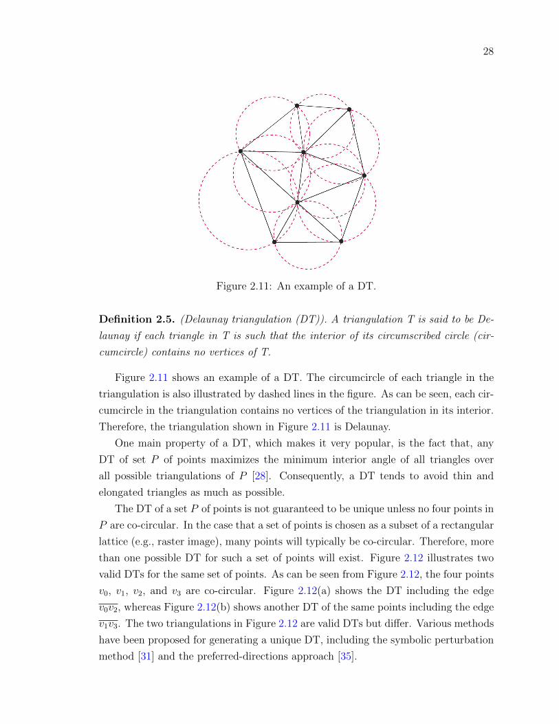
28

Figure 2.11: An example of a DT.

Definition 2.5. (Delaunay triangulation (DT)). A triangulation T is said to be De-

launay if each triangle in T is such that the interior of its circumscribed circle (cir-

cumcircle) contains no vertices of T.

Figure 2.11 shows an example of a DT. The circumcircle of each triangle in the

triangulation is also illustrated by dashed lines in the figure. As can be seen, each cir-

cumcircle in the triangulation contains no vertices of the triangulation in its interior.

Therefore, the triangulation shown in Figure 2.11 is Delaunay.

One main property of a DT, which makes it very popular, is the fact that, any

DT of set P of points maximizes the minimum interior angle of all triangles over

all possible triangulations of P [28]. Consequently, a DT tends to avoid thin and

elongated triangles as much as possible.

The DT of a set P of points is not guaranteed to be unique unless no four points in

P are co-circular. In the case that a set of points is chosen as a subset of a rectangular

lattice (e.g., raster image), many points will typically be co-circular. Therefore, more

than one possible DT for such a set of points will exist. Figure 2.12 illustrates two

valid DTs for the same set of points. As can be seen from Figure 2.12, the four points

v0, v1, v2, and v3 are co-circular. Figure 2.12(a) shows the DT including the edge

v0v2, whereas Figure 2.12(b) shows another DT of the same points including the edge

v1v3. The two triangulations in Figure 2.12 are valid DTs but differ. Various methods

have been proposed for generating a unique DT, including the symbolic perturbation

method [31] and the preferred-directions approach [35].

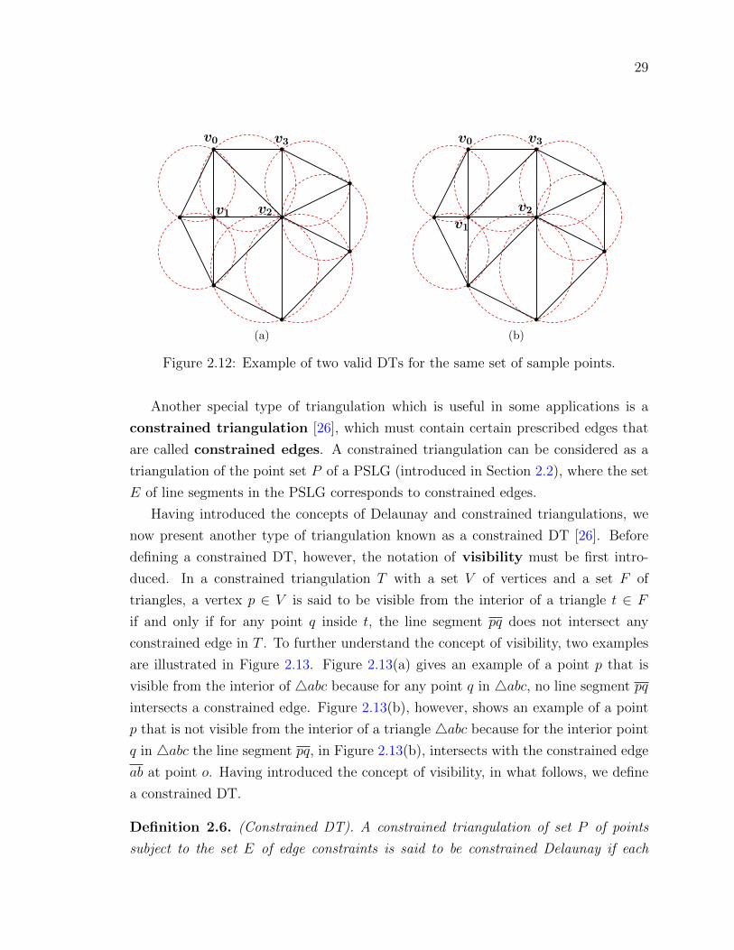
29

(a) (b)

Figure 2.12: Example of two valid DTs for the same set of sample points.

Another special type of triangulation which is useful in some applications is a

constrained triangulation [26], which must contain certain prescribed edges that

are called constrained edges. A constrained triangulation can be considered as a

triangulation of the point set P of a PSLG (introduced in Section 2.2), where the set

E of line segments in the PSLG corresponds to constrained edges.

Having introduced the concepts of Delaunay and constrained triangulations, we

now present another type of triangulation known as a constrained DT [26]. Before

defining a constrained DT, however, the notation of visibility must be first intro-

duced. In a constrained triangulation T with a set V of vertices and a set F of

triangles, a vertex p ∈ V is said to be visible from the interior of a triangle t ∈ F

if and only if for any point q inside t, the line segment pq does not intersect any

constrained edge in T . To further understand the concept of visibility, two examples

are illustrated in Figure 2.13. Figure 2.13(a) gives an example of a point p that is

visible from the interior of 4abc because for any point q in 4abc, no line segment pq

intersects a constrained edge. Figure 2.13(b), however, shows an example of a point

p that is not visible from the interior of a triangle 4abc because for the interior point

q in 4abc the line segment pq, in Figure 2.13(b), intersects with the constrained edge

ab at point o. Having introduced the concept of visibility, in what follows, we define

a constrained DT.

Definition 2.6. (Constrained DT). A constrained triangulation of set P of points

subject to the set E of edge constraints is said to be constrained Delaunay if each

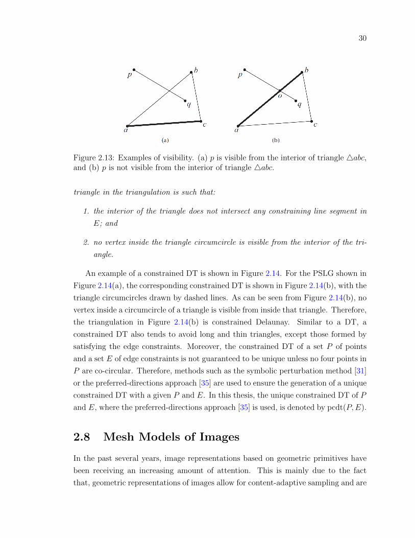
30

Figure 2.13: Examples of visibility. (a) p is visible from the interior of triangle 4abc,and (b) p is not visible from the interior of triangle 4abc.

triangle in the triangulation is such that:

1. the interior of the triangle does not intersect any constraining line segment in

E; and

2. no vertex inside the triangle circumcircle is visible from the interior of the tri-

angle.

An example of a constrained DT is shown in Figure 2.14. For the PSLG shown in

Figure 2.14(a), the corresponding constrained DT is shown in Figure 2.14(b), with the

triangle circumcircles drawn by dashed lines. As can be seen from Figure 2.14(b), no

vertex inside a circumcircle of a triangle is visible from inside that triangle. Therefore,

the triangulation in Figure 2.14(b) is constrained Delaunay. Similar to a DT, a

constrained DT also tends to avoid long and thin triangles, except those formed by

satisfying the edge constraints. Moreover, the constrained DT of a set P of points

and a set E of edge constraints is not guaranteed to be unique unless no four points in

P are co-circular. Therefore, methods such as the symbolic perturbation method [31]

or the preferred-directions approach [35] are used to ensure the generation of a unique

constrained DT with a given P and E. In this thesis, the unique constrained DT of P

and E, where the preferred-directions approach [35] is used, is denoted by pcdt(P,E).

2.8 Mesh Models of Images

In the past several years, image representations based on geometric primitives have

been receiving an increasing amount of attention. This is mainly due to the fact

that, geometric representations of images allow for content-adaptive sampling and are

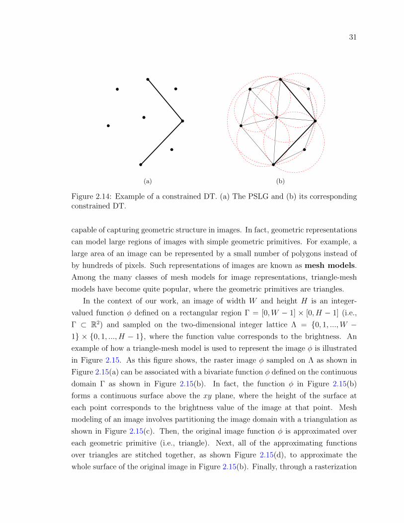
31

(a) (b)

Figure 2.14: Example of a constrained DT. (a) The PSLG and (b) its correspondingconstrained DT.

capable of capturing geometric structure in images. In fact, geometric representations

can model large regions of images with simple geometric primitives. For example, a

large area of an image can be represented by a small number of polygons instead of

by hundreds of pixels. Such representations of images are known as mesh models.

Among the many classes of mesh models for image representations, triangle-mesh

models have become quite popular, where the geometric primitives are triangles.

In the context of our work, an image of width W and height H is an integer-

valued function φ defined on a rectangular region Γ = [0,W − 1] × [0, H − 1] (i.e.,

Γ ⊂ R2) and sampled on the two-dimensional integer lattice Λ = 0, 1, ...,W −1 × 0, 1, ..., H − 1, where the function value corresponds to the brightness. An

example of how a triangle-mesh model is used to represent the image φ is illustrated

in Figure 2.15. As this figure shows, the raster image φ sampled on Λ as shown in

Figure 2.15(a) can be associated with a bivariate function φ defined on the continuous

domain Γ as shown in Figure 2.15(b). In fact, the function φ in Figure 2.15(b)

forms a continuous surface above the xy plane, where the height of the surface at

each point corresponds to the brightness value of the image at that point. Mesh

modeling of an image involves partitioning the image domain with a triangulation as

shown in Figure 2.15(c). Then, the original image function φ is approximated over

each geometric primitive (i.e., triangle). Next, all of the approximating functions

over triangles are stitched together, as shown Figure 2.15(d), to approximate the

whole surface of the original image in Figure 2.15(b). Finally, through a rasterization

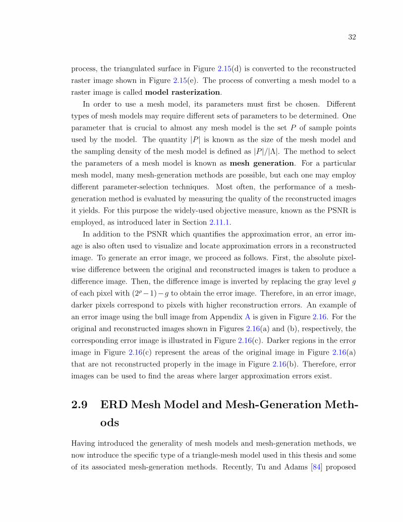
32

process, the triangulated surface in Figure 2.15(d) is converted to the reconstructed

raster image shown in Figure 2.15(e). The process of converting a mesh model to a

raster image is called model rasterization.

In order to use a mesh model, its parameters must first be chosen. Different

types of mesh models may require different sets of parameters to be determined. One

parameter that is crucial to almost any mesh model is the set P of sample points

used by the model. The quantity |P | is known as the size of the mesh model and

the sampling density of the mesh model is defined as |P |/|Λ|. The method to select

the parameters of a mesh model is known as mesh generation. For a particular

mesh model, many mesh-generation methods are possible, but each one may employ

different parameter-selection techniques. Most often, the performance of a mesh-

generation method is evaluated by measuring the quality of the reconstructed images

it yields. For this purpose the widely-used objective measure, known as the PSNR is

employed, as introduced later in Section 2.11.1.

In addition to the PSNR which quantifies the approximation error, an error im-

age is also often used to visualize and locate approximation errors in a reconstructed

image. To generate an error image, we proceed as follows. First, the absolute pixel-

wise difference between the original and reconstructed images is taken to produce a

difference image. Then, the difference image is inverted by replacing the gray level g

of each pixel with (2ρ−1)−g to obtain the error image. Therefore, in an error image,

darker pixels correspond to pixels with higher reconstruction errors. An example of

an error image using the bull image from Appendix A is given in Figure 2.16. For the

original and reconstructed images shown in Figures 2.16(a) and (b), respectively, the

corresponding error image is illustrated in Figure 2.16(c). Darker regions in the error

image in Figure 2.16(c) represent the areas of the original image in Figure 2.16(a)

that are not reconstructed properly in the image in Figure 2.16(b). Therefore, error

images can be used to find the areas where larger approximation errors exist.

2.9 ERD Mesh Model and Mesh-Generation Meth-

ods

Having introduced the generality of mesh models and mesh-generation methods, we

now introduce the specific type of a triangle-mesh model used in this thesis and some

of its associated mesh-generation methods. Recently, Tu and Adams [84] proposed

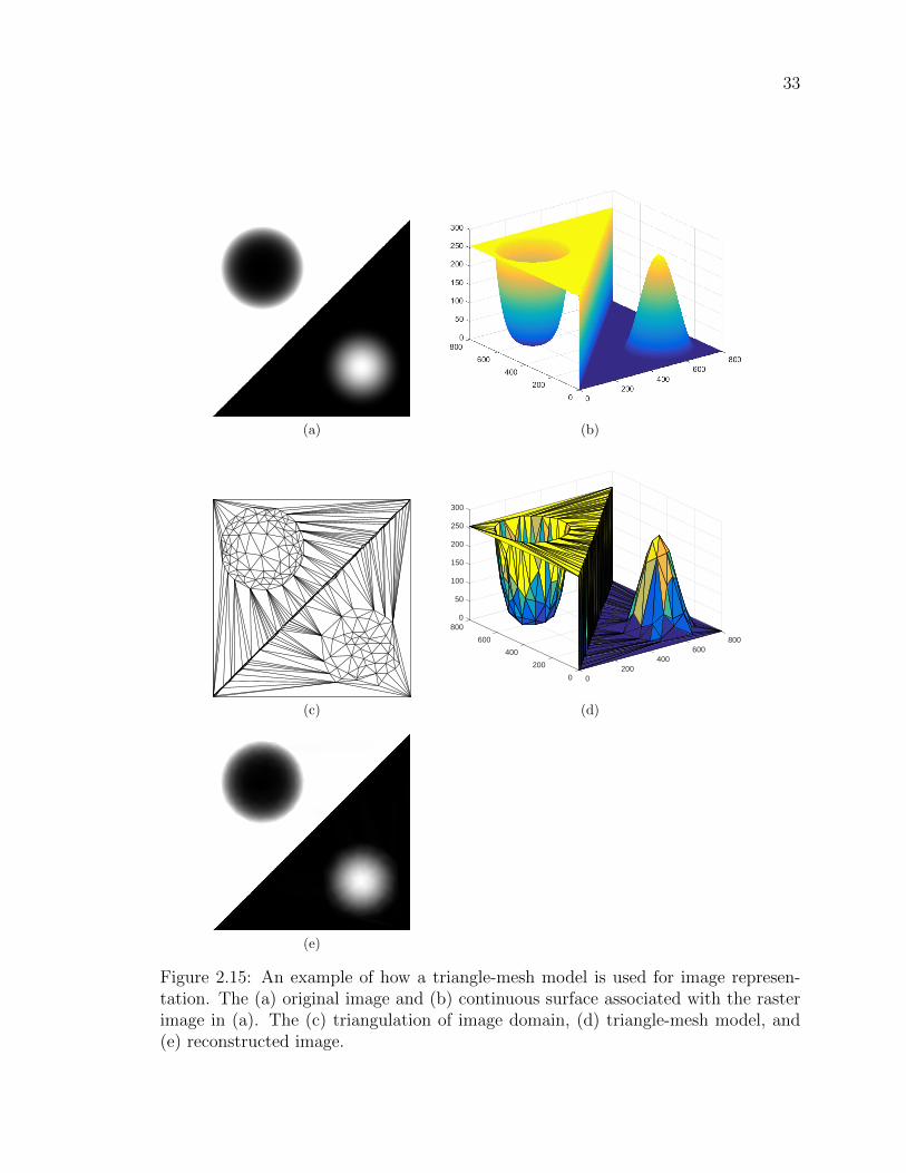
33

(a) (b)

(c)

0800

50

100

600 800

150

200

600400

250

300

400200 200

0 0

(d)

(e)

Figure 2.15: An example of how a triangle-mesh model is used for image represen-tation. The (a) original image and (b) continuous surface associated with the rasterimage in (a). The (c) triangulation of image domain, (d) triangle-mesh model, and(e) reconstructed image.

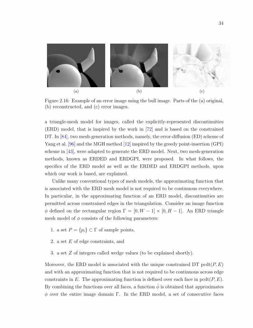
34

(a) (b) (c)

Figure 2.16: Example of an error image using the bull image. Parts of the (a) original,(b) reconstructed, and (c) error images.

a triangle-mesh model for images, called the explicitly-represented discontinuities

(ERD) model, that is inspired by the work in [72] and is based on the constrained

DT. In [84], two mesh-generation methods, namely, the error-diffusion (ED) scheme of

Yang et al. [96] and the MGH method [12] inspired by the greedy point-insertion (GPI)

scheme in [43], were adapted to generate the ERD model. Next, two mesh-generation

methods, known as ERDED and ERDGPI, were proposed. In what follows, the

specifics of the ERD model as well as the ERDED and ERDGPI methods, upon

which our work is based, are explained.

Unlike many conventional types of mesh models, the approximating function that

is associated with the ERD mesh model is not required to be continuous everywhere.

In particular, in the approximating function of an ERD model, discontinuities are

permitted across constrained edges in the triangulation. Consider an image function

φ defined on the rectangular region Γ = [0,W − 1] × [0, H − 1]. An ERD triangle

mesh model of φ consists of the following parameters:

1. a set P = pi ⊂ Γ of sample points,

2. a set E of edge constraints, and

3. a set Z of integers called wedge values (to be explained shortly).

Moreover, the ERD model is associated with the unique constrained DT pcdt(P,E)

and with an approximating function that is not required to be continuous across edge

constraints in E. The approximating function is defined over each face in pcdt(P,E).

By combining the functions over all faces, a function φ is obtained that approximates

φ over the entire image domain Γ. In the ERD model, a set of consecutive faces

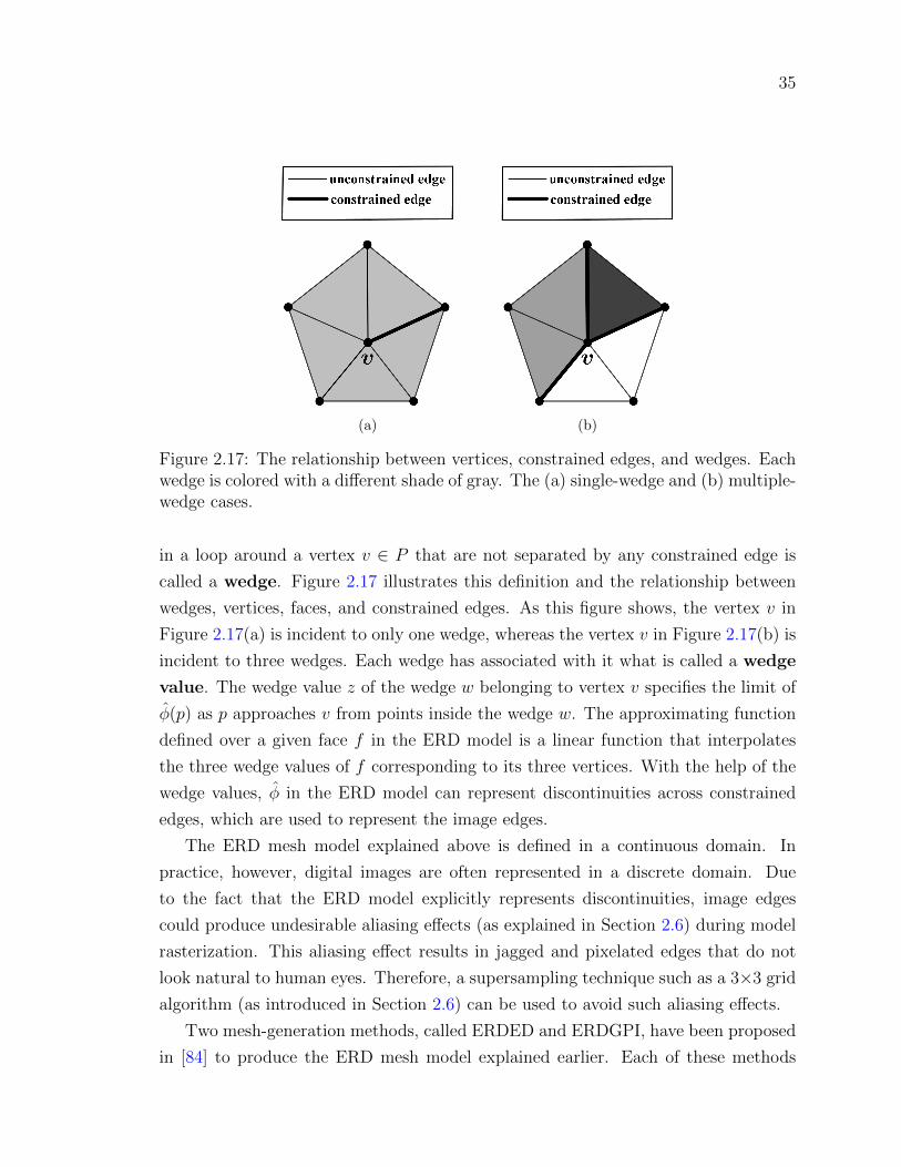
35

(a) (b)

Figure 2.17: The relationship between vertices, constrained edges, and wedges. Eachwedge is colored with a different shade of gray. The (a) single-wedge and (b) multiple-wedge cases.

in a loop around a vertex v ∈ P that are not separated by any constrained edge is

called a wedge. Figure 2.17 illustrates this definition and the relationship between

wedges, vertices, faces, and constrained edges. As this figure shows, the vertex v in

Figure 2.17(a) is incident to only one wedge, whereas the vertex v in Figure 2.17(b) is

incident to three wedges. Each wedge has associated with it what is called a wedge

value. The wedge value z of the wedge w belonging to vertex v specifies the limit of

φ(p) as p approaches v from points inside the wedge w. The approximating function

defined over a given face f in the ERD model is a linear function that interpolates

the three wedge values of f corresponding to its three vertices. With the help of the

wedge values, φ in the ERD model can represent discontinuities across constrained

edges, which are used to represent the image edges.

The ERD mesh model explained above is defined in a continuous domain. In

practice, however, digital images are often represented in a discrete domain. Due

to the fact that the ERD model explicitly represents discontinuities, image edges

could produce undesirable aliasing effects (as explained in Section 2.6) during model

rasterization. This aliasing effect results in jagged and pixelated edges that do not

look natural to human eyes. Therefore, a supersampling technique such as a 3×3 grid

algorithm (as introduced in Section 2.6) can be used to avoid such aliasing effects.

Two mesh-generation methods, called ERDED and ERDGPI, have been proposed

in [84] to produce the ERD mesh model explained earlier. Each of these methods

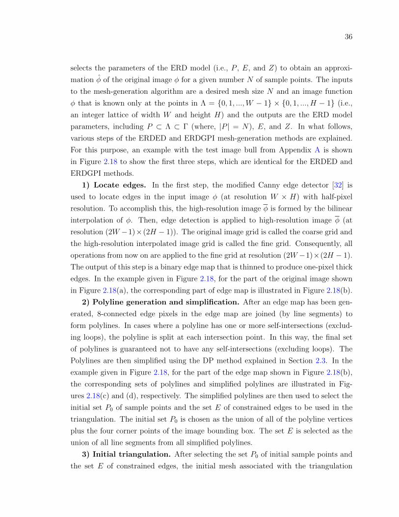
36

selects the parameters of the ERD model (i.e., P , E, and Z) to obtain an approxi-

mation φ of the original image φ for a given number N of sample points. The inputs

to the mesh-generation algorithm are a desired mesh size N and an image function

φ that is known only at the points in Λ = 0, 1, ...,W − 1 × 0, 1, ..., H − 1 (i.e.,

an integer lattice of width W and height H) and the outputs are the ERD model

parameters, including P ⊂ Λ ⊂ Γ (where, |P | = N), E, and Z. In what follows,

various steps of the ERDED and ERDGPI mesh-generation methods are explained.

For this purpose, an example with the test image bull from Appendix A is shown

in Figure 2.18 to show the first three steps, which are identical for the ERDED and

ERDGPI methods.

1) Locate edges. In the first step, the modified Canny edge detector [32] is

used to locate edges in the input image φ (at resolution W × H) with half-pixel

resolution. To accomplish this, the high-resolution image φ is formed by the bilinear

interpolation of φ. Then, edge detection is applied to high-resolution image φ (at

resolution (2W −1)× (2H − 1)). The original image grid is called the coarse grid and

the high-resolution interpolated image grid is called the fine grid. Consequently, all

operations from now on are applied to the fine grid at resolution (2W −1)×(2H − 1).

The output of this step is a binary edge map that is thinned to produce one-pixel thick

edges. In the example given in Figure 2.18, for the part of the original image shown

in Figure 2.18(a), the corresponding part of edge map is illustrated in Figure 2.18(b).

2) Polyline generation and simplification. After an edge map has been gen-

erated, 8-connected edge pixels in the edge map are joined (by line segments) to

form polylines. In cases where a polyline has one or more self-intersections (exclud-

ing loops), the polyline is split at each intersection point. In this way, the final set

of polylines is guaranteed not to have any self-intersections (excluding loops). The

Polylines are then simplified using the DP method explained in Section 2.3. In the

example given in Figure 2.18, for the part of the edge map shown in Figure 2.18(b),

the corresponding sets of polylines and simplified polylines are illustrated in Fig-

ures 2.18(c) and (d), respectively. The simplified polylines are then used to select the

initial set P0 of sample points and the set E of constrained edges to be used in the

triangulation. The initial set P0 is chosen as the union of all of the polyline vertices

plus the four corner points of the image bounding box. The set E is selected as the

union of all line segments from all simplified polylines.

3) Initial triangulation. After selecting the set P0 of initial sample points and

the set E of constrained edges, the initial mesh associated with the triangulation

37

(a) (b) (c)

(d) (e)

Figure 2.18: Selection of the initial triangulation. (a) Part of the input image bull.The (b) binary edge map of (a). (c) The unsimplified polylines representing imageedges in (b). (d) The simplified polylines. (e) The part of the initial triangulationcorresponding to (a), with constrained edges denoted by thick lines.

pcdt(P0, E) is constructed. Let N0 = |P0| be the initial mesh size. In the example

given in Figure 2.18, for the part of simplified polylines illustrated in Figure 2.18(d),

the corresponding part of the initial mesh is shown in Figure 2.18(e).

4) Initial wedge values. Once the initial triangulation is constructed, for each

wedge w around each vertex v ∈ P0, the corresponding wedge value z is selected as

follows. If v has zero or one incident constrained edge (e.g., as in Figure 2.17(a)), its

single wedge value z is simply chosen as the value of the (bilinear-interpolated) high-

resolution image function φ at v (i.e., z = φ(v)). Otherwise, if v has more than one

incident constrained edge (as shown in Figure 2.17(b)), the wedge value associated

with each wedge is calculated using a line-search approach as follows. The grid points

along the ray (called the bisecting line) originating from v and bisecting the wedge w

are searched. During the line search, the point p whose maximum magnitude second-

order directional derivative (MMSODD) is largest is selected. Then, the wedge value

z is chosen as the value of φ at p (i.e., z = φ(p)). To prevent p from falling far outside

of the corresponding triangle face, the line search is restricted to distance d ∈ [1, 1.5]

units in the coarse grid (or, equivalent d ∈ [2, 3] units in the fine grid) from v. The

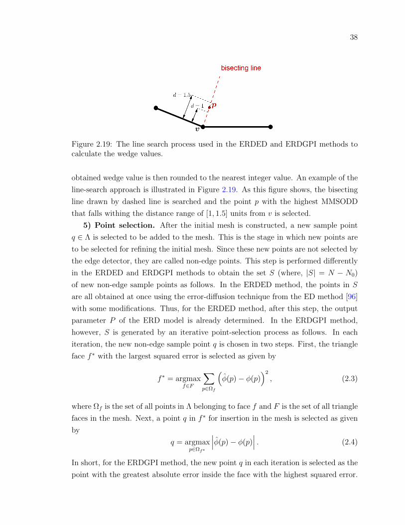
38

Figure 2.19: The line search process used in the ERDED and ERDGPI methods tocalculate the wedge values.

obtained wedge value is then rounded to the nearest integer value. An example of the

line-search approach is illustrated in Figure 2.19. As this figure shows, the bisecting

line drawn by dashed line is searched and the point p with the highest MMSODD

that falls withing the distance range of [1, 1.5] units from v is selected.

5) Point selection. After the initial mesh is constructed, a new sample point

q ∈ Λ is selected to be added to the mesh. This is the stage in which new points are

to be selected for refining the initial mesh. Since these new points are not selected by

the edge detector, they are called non-edge points. This step is performed differently

in the ERDED and ERDGPI methods to obtain the set S (where, |S| = N − N0)

of new non-edge sample points as follows. In the ERDED method, the points in S

are all obtained at once using the error-diffusion technique from the ED method [96]

with some modifications. Thus, for the ERDED method, after this step, the output

parameter P of the ERD model is already determined. In the ERDGPI method,

however, S is generated by an iterative point-selection process as follows. In each

iteration, the new non-edge sample point q is chosen in two steps. First, the triangle

face f ∗ with the largest squared error is selected as given by

f ∗ = argmaxf∈F

∑p∈Ωf

(φ(p)− φ(p)

)2

, (2.3)

where Ωf is the set of all points in Λ belonging to face f and F is the set of all triangle

faces in the mesh. Next, a point q in f ∗ for insertion in the mesh is selected as given

by

q = argmaxp∈Ωf∗

∣∣∣φ(p)− φ(p)∣∣∣ . (2.4)

In short, for the ERDGPI method, the new point q in each iteration is selected as the

point with the greatest absolute error inside the face with the highest squared error.

39

6) Point insertion. Once the new point q is selected, it is inserted in the

triangulation. If q is on a constrained edge, the edge is split at q into two constrained

edges, and the wedge value is computed for each of the two new wedges around the

vertex q using the line-search approach explained in step 4. If, however, q is not

on a constrained edge, the wedges remain the same and no wedge values need to

be computed. After each point insertion, the set Pi+1 of sample points for the next

iteration is selected as Pi ∪ q.7) Stopping criterion. For the ERDED method, if |Pi+1| < N , go to step 6

and insert another non-edge point from S that has not yet been inserted. Otherwise,

set the output parameter P = Pi+1 and stop. In the case of the ERDGPI method,

however, if |Pi+1| < N , go to step 5 to select another non-edge point for insertion.

Otherwise, set the output parameter P = Pi+1 and stop.

After completing the above steps, all parameters of the ERD model are deter-

mined, including the set P of sample points, set E of constrained edges, and set Z of

wedge values.

2.10 Image Scaling

As one of the classical and important problems in image processing and digital pho-

tography, image scaling refers to the operation of resizing digital images to obtain

a larger or a smaller image. More specifically, if the scaled image is larger than the

original image the operation is called upscaling (also super-resolution), and if it is

smaller, then the operation is referred to as downscaling. In this thesis, since we are

interested in the upscaling operation, the term “scaling” always refers to the upscaling

operation, unless otherwise stated.

The image-scaling problem that is being addressed in this thesis can be stated as

follows. A low-resolution raster image φl of width W and height H and an integer

scaling factor of k > 1 are assumed. The image-scaling problem of interest herein

is to find the high-resolution raster image φh of size kW × kH as the scaled version

of φl, so that the qualitative attributes of φl are preserved well in φh, with the least

amount of edge blurring that can arise during image scaling.

As can be perceived from the above problem definition, the scaled raster image φh

has more grid points than the low-resolution raster image φl (i.e., k times more points

in each dimension). Those newly-generated grid points in φh can be assumed as empty

grid points that must be filled with new intensity (i.e., graylevel) values. The missing

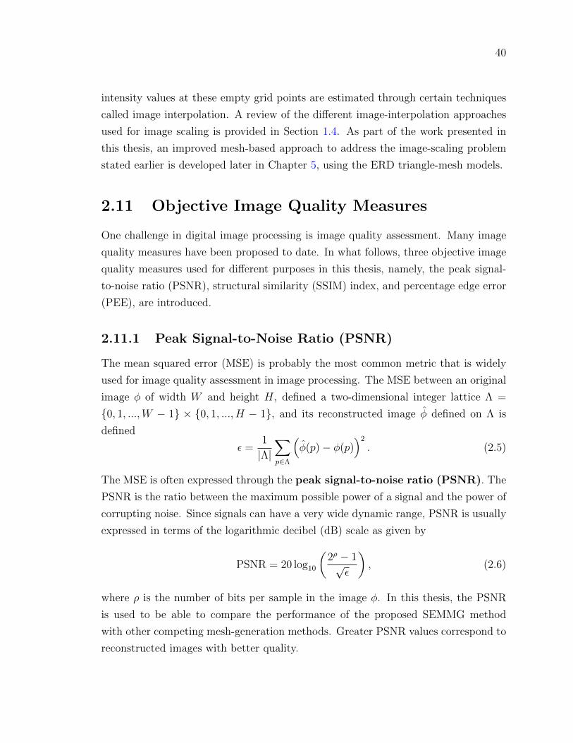
40

intensity values at these empty grid points are estimated through certain techniques

called image interpolation. A review of the different image-interpolation approaches

used for image scaling is provided in Section 1.4. As part of the work presented in

this thesis, an improved mesh-based approach to address the image-scaling problem

stated earlier is developed later in Chapter 5, using the ERD triangle-mesh models.

2.11 Objective Image Quality Measures

One challenge in digital image processing is image quality assessment. Many image

quality measures have been proposed to date. In what follows, three objective image

quality measures used for different purposes in this thesis, namely, the peak signal-

to-noise ratio (PSNR), structural similarity (SSIM) index, and percentage edge error

(PEE), are introduced.

2.11.1 Peak Signal-to-Noise Ratio (PSNR)

The mean squared error (MSE) is probably the most common metric that is widely

used for image quality assessment in image processing. The MSE between an original

image φ of width W and height H, defined a two-dimensional integer lattice Λ =

0, 1, ...,W − 1 × 0, 1, ..., H − 1, and its reconstructed image φ defined on Λ is

defined

ε =1

|Λ|∑p∈Λ

(φ(p)− φ(p)

)2

. (2.5)

The MSE is often expressed through the peak signal-to-noise ratio (PSNR). The

PSNR is the ratio between the maximum possible power of a signal and the power of

corrupting noise. Since signals can have a very wide dynamic range, PSNR is usually

expressed in terms of the logarithmic decibel (dB) scale as given by

PSNR = 20 log10

(2ρ − 1√

ε

), (2.6)

where ρ is the number of bits per sample in the image φ. In this thesis, the PSNR

is used to be able to compare the performance of the proposed SEMMG method

with other competing mesh-generation methods. Greater PSNR values correspond to

reconstructed images with better quality.

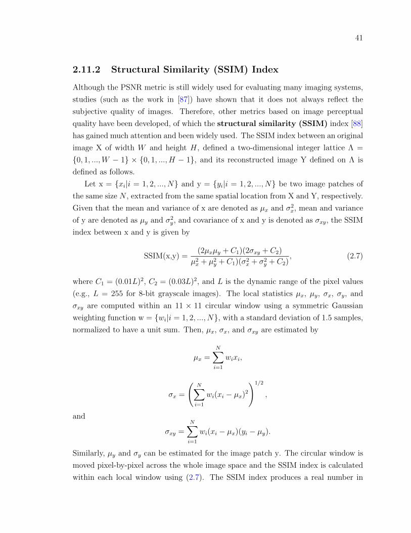
41

2.11.2 Structural Similarity (SSIM) Index

Although the PSNR metric is still widely used for evaluating many imaging systems,

studies (such as the work in [87]) have shown that it does not always reflect the

subjective quality of images. Therefore, other metrics based on image perceptual

quality have been developed, of which the structural similarity (SSIM) index [88]

has gained much attention and been widely used. The SSIM index between an original

image X of width W and height H, defined a two-dimensional integer lattice Λ =

0, 1, ...,W − 1 × 0, 1, ..., H − 1, and its reconstructed image Y defined on Λ is

defined as follows.

Let x = xi|i = 1, 2, ..., N and y = yi|i = 1, 2, ..., N be two image patches of

the same size N , extracted from the same spatial location from X and Y, respectively.

Given that the mean and variance of x are denoted as µx and σ2x, mean and variance

of y are denoted as µy and σ2y, and covariance of x and y is denoted as σxy, the SSIM

index between x and y is given by

SSIM(x,y) =(2µxµy + C1)(2σxy + C2)

µ2x + µ2

y + C1)(σ2x + σ2

y + C2), (2.7)

where C1 = (0.01L)2, C2 = (0.03L)2, and L is the dynamic range of the pixel values

(e.g., L = 255 for 8-bit grayscale images). The local statistics µx, µy, σx, σy, and

σxy are computed within an 11 × 11 circular window using a symmetric Gaussian

weighting function w = wi|i = 1, 2, ..., N, with a standard deviation of 1.5 samples,

normalized to have a unit sum. Then, µx, σx, and σxy are estimated by

µx =N∑i=1

wixi,

σx =

(N∑i=1

wi(xi − µx)2

)1/2

,

and

σxy =N∑i=1

wi(xi − µx)(yi − µy).

Similarly, µy and σy can be estimated for the image patch y. The circular window is

moved pixel-by-pixel across the whole image space and the SSIM index is calculated

within each local window using (2.7). The SSIM index produces a real number in

42

[0, 1], where higher values correspond to a better image reconstruction. Finally, a

mean SSIM index of all windows is calculated as a single overall quality measure

between the entire images X and Y.

2.11.3 Percentage Edge Error (PEE)

In the application of image scaling studied in this thesis, our main goal is to produce

scaled images of better subjective quality, without losing sharpness of the image edges.

For this particular goal, neither the PSNR nor SSIM metrics is designed to measure

the sharpness at image edges. Therefore, a metric called percentage edge error

(PEE) is used for measuring the sharpness of the edges in scaled images.

Between an original image φ of widthW and heightH, defined on a two-dimensional

integer lattice Λ = 0, 1, ...,W − 1 × 0, 1, ..., H − 1, and its reconstructed image φ

defined on Λ, the PEE measures how close the edges in φ are to the original edges in

φ. The PEE between φ and φ is determined by

PEE =ES(φ)− ES(φ)

ES(φ)× 100, (2.8)

where ES(φ) and ES(φ) are the edge strengths of the original and reconstructed

images, respectively. The procedure to calculate ES is identical to the one used

in [16]. For an image of φ, its ES is calculated using the following steps:

1. Gradient calculation. Using simple convolution masks, first-order partial deriva-

tives in horizontal and vertical directions at each pixel in φ are estimated as gx

and gy, respectively. Then, the gradient magnitude g at that pixel is determined

by g =√g2x + g2

y. Next, a gradient image G is generated in which each pixel

holds the value of its estimated gradient magnitude.

2. Gradient thresholding. Then, G is passed through a simple thresholding process

to obtain the edge intensity image E, as given by

E(x, y) =

G(x, y), G(x, y) ≥ τ

0, otherwise,

with threshold τ = G + σG, where G and σG are the mean value and standard

deviation of G.

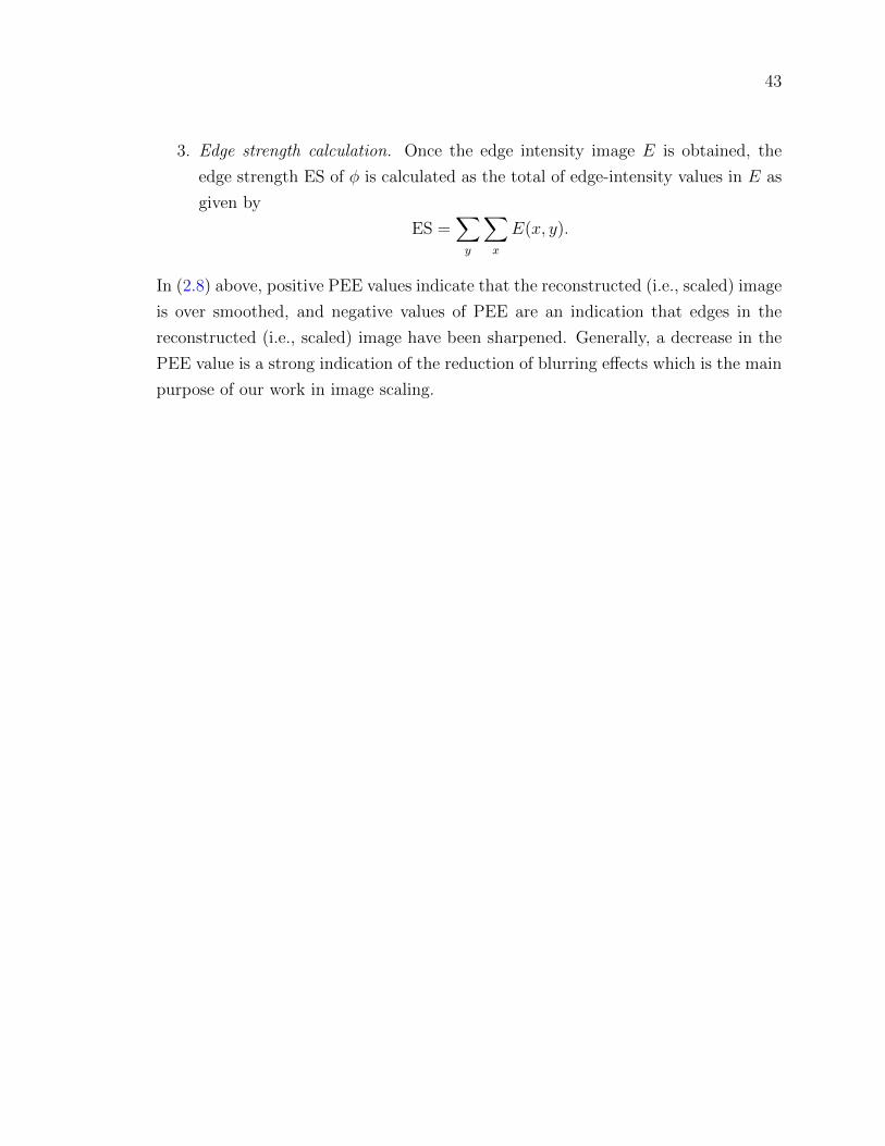
43

3. Edge strength calculation. Once the edge intensity image E is obtained, the

edge strength ES of φ is calculated as the total of edge-intensity values in E as

given by

ES =∑y

∑x

E(x, y).

In (2.8) above, positive PEE values indicate that the reconstructed (i.e., scaled) image

is over smoothed, and negative values of PEE are an indication that edges in the

reconstructed (i.e., scaled) image have been sharpened. Generally, a decrease in the

PEE value is a strong indication of the reduction of blurring effects which is the main

purpose of our work in image scaling.

44

Chapter 3

Proposed SEMMG Method and Its

Development

3.1 Overview

In this chapter, a new method called the squared-error minimizing mesh-generation

(SEMMG) method is proposed for producing ERD triangle-mesh models for the rep-

resentation of grayscale images. We start by presenting in-depth analyses of two

previously proposed methods for generating ERD models, namely, the ERDED and

ERDGPI methods, which were introduced in Section 2.9. Through these analyses,

we identify potential areas for improvement in different steps of the methods, includ-

ing edge detection, wedge-value calculation, and non-edge point selection. Moreover,

after identifying problems in each of these steps, solutions are found to address these

problems. Then, our SEMMG mesh-generation method is proposed by integrating

all the recommended modifications into a unified framework.

3.2 Development of SEMMG Method

Having introduced all of the necessary background material in Chapter 2, we now

present how the SEMMG mesh-generation method proposed in this thesis was de-

veloped. As mentioned in previous chapters, the work in this thesis focuses on the

application of ERD triangle-mesh models, due to their benefit of preserving the image

discontinuities. Thus, we first present some in-depth analyses on the existing methods

for generating ERD models. Two effective mesh-generation methods for producing

45

ERD models are the ERDED and ERDGPI methods as proposed in [84]. As we

recall from Section 2.9, the general algorithmic framework of each of these methods

composed of the following main steps:

1. edge detection,

2. polyline generation and simplification,

3. initial triangulation,

4. initial wedge-value calculation,

5. point selection, and

6. point insertion.

In what follows, through detailed analysis and experimental results, we identify sev-

eral weaknesses in different approaches employed in above framework. Then, for each

weakness, we explore modifying the framework in order to improve upon the weak-

ness. The modifications that result in improvements will later be integrated into the

proposed SEMMG method.

3.2.1 Edge Detection Analysis

The primary step in either the ERDED or ERDGPI mesh-generation scheme (and

almost any other edge-preserving mesh-generation method) is to locate edges in the

input image. The edge-detection step (as we recall from Section 2.9) is performed

using the same approach in both the ERDED and ERDGPI methods. Thus, our

analysis focuses on one of them, which is the the ERDED method herein. In what

follows, two potential areas for improvements in the edge-detection technique used

in the ERDED method are analyzed, including junction-point detection and edge-

detector parameter selection.

3.2.1.1 Junction-Point Detection

In-depth investigations on the reconstructed images obtained with the ERDED method

showed that often some approximation errors exist around the polylines that were

broken at junctions (i.e., where three or more image edges meet). Analyses with nu-

merous test cases showed that the root cause of such broken polylines near junctions

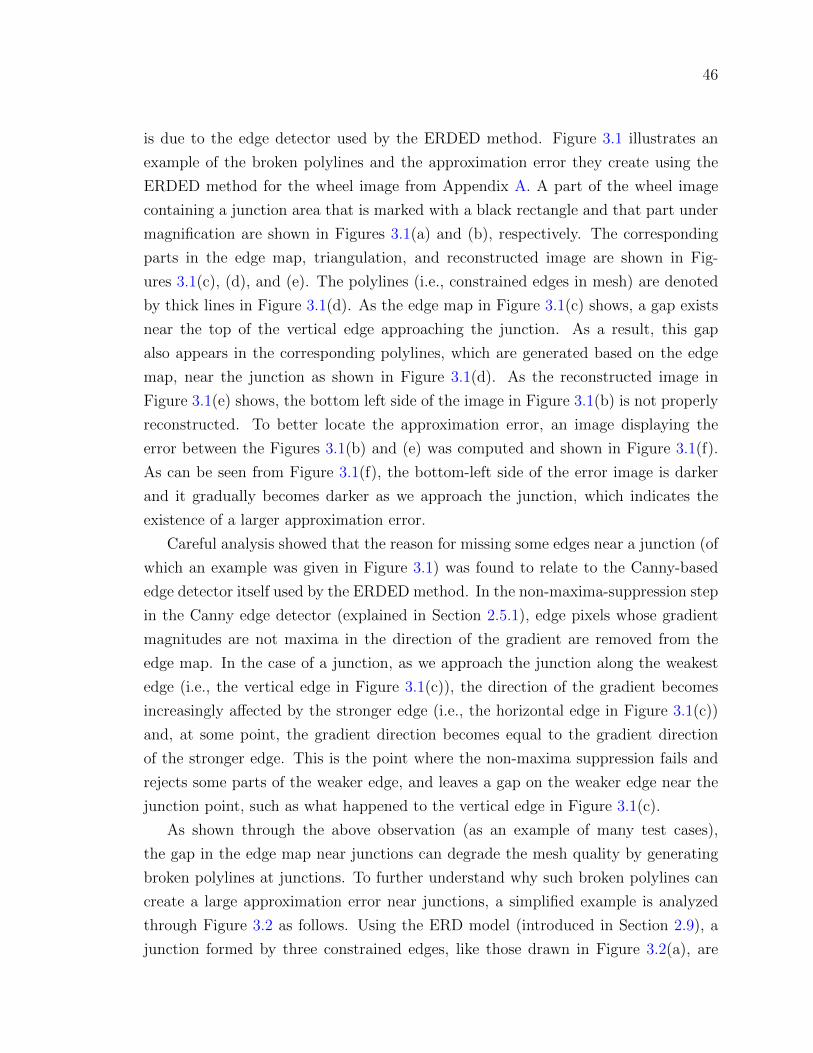
46

is due to the edge detector used by the ERDED method. Figure 3.1 illustrates an

example of the broken polylines and the approximation error they create using the

ERDED method for the wheel image from Appendix A. A part of the wheel image

containing a junction area that is marked with a black rectangle and that part under

magnification are shown in Figures 3.1(a) and (b), respectively. The corresponding

parts in the edge map, triangulation, and reconstructed image are shown in Fig-

ures 3.1(c), (d), and (e). The polylines (i.e., constrained edges in mesh) are denoted

by thick lines in Figure 3.1(d). As the edge map in Figure 3.1(c) shows, a gap exists

near the top of the vertical edge approaching the junction. As a result, this gap

also appears in the corresponding polylines, which are generated based on the edge

map, near the junction as shown in Figure 3.1(d). As the reconstructed image in

Figure 3.1(e) shows, the bottom left side of the image in Figure 3.1(b) is not properly

reconstructed. To better locate the approximation error, an image displaying the

error between the Figures 3.1(b) and (e) was computed and shown in Figure 3.1(f).

As can be seen from Figure 3.1(f), the bottom-left side of the error image is darker

and it gradually becomes darker as we approach the junction, which indicates the

existence of a larger approximation error.

Careful analysis showed that the reason for missing some edges near a junction (of

which an example was given in Figure 3.1) was found to relate to the Canny-based

edge detector itself used by the ERDED method. In the non-maxima-suppression step

in the Canny edge detector (explained in Section 2.5.1), edge pixels whose gradient

magnitudes are not maxima in the direction of the gradient are removed from the

edge map. In the case of a junction, as we approach the junction along the weakest

edge (i.e., the vertical edge in Figure 3.1(c)), the direction of the gradient becomes

increasingly affected by the stronger edge (i.e., the horizontal edge in Figure 3.1(c))

and, at some point, the gradient direction becomes equal to the gradient direction

of the stronger edge. This is the point where the non-maxima suppression fails and

rejects some parts of the weaker edge, and leaves a gap on the weaker edge near the

junction point, such as what happened to the vertical edge in Figure 3.1(c).

As shown through the above observation (as an example of many test cases),

the gap in the edge map near junctions can degrade the mesh quality by generating

broken polylines at junctions. To further understand why such broken polylines can

create a large approximation error near junctions, a simplified example is analyzed

through Figure 3.2 as follows. Using the ERD model (introduced in Section 2.9), a

junction formed by three constrained edges, like those drawn in Figure 3.2(a), are

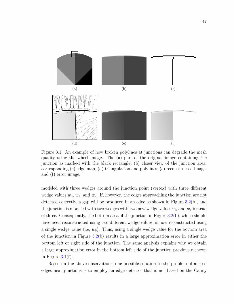
47

(a) (b) (c)

(d) (e) (f)

Figure 3.1: An example of how broken polylines at junctions can degrade the meshquality using the wheel image. The (a) part of the original image containing thejunction as marked with the black rectangle, (b) closer view of the junction area,corresponding (c) edge map, (d) triangulation and polylines, (e) reconstructed image,and (f) error image.

modeled with three wedges around the junction point (vertex) with three different

wedge values w0, w1, and w2. If, however, the edges approaching the junction are not

detected correctly, a gap will be produced in an edge as shown in Figure 3.2(b), and

the junction is modeled with two wedges with two new wedge values w0 and w1 instead

of three. Consequently, the bottom area of the junction in Figure 3.2(b), which should

have been reconstructed using two different wedge values, is now reconstructed using

a single wedge value (i.e, w0). Thus, using a single wedge value for the bottom area

of the junction in Figure 3.2(b) results in a large approximation error in either the

bottom left or right side of the junction. The same analysis explains why we obtain

a large approximation error in the bottom left side of the junction previously shown

in Figure 3.1(f).

Based on the above observations, one possible solution to the problem of missed

edges near junctions is to employ an edge detector that is not based on the Canny

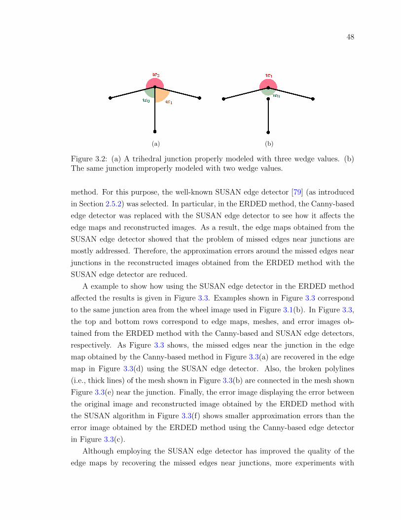
48

(a) (b)

Figure 3.2: (a) A trihedral junction properly modeled with three wedge values. (b)The same junction improperly modeled with two wedge values.

method. For this purpose, the well-known SUSAN edge detector [79] (as introduced

in Section 2.5.2) was selected. In particular, in the ERDED method, the Canny-based

edge detector was replaced with the SUSAN edge detector to see how it affects the

edge maps and reconstructed images. As a result, the edge maps obtained from the

SUSAN edge detector showed that the problem of missed edges near junctions are

mostly addressed. Therefore, the approximation errors around the missed edges near

junctions in the reconstructed images obtained from the ERDED method with the

SUSAN edge detector are reduced.

A example to show how using the SUSAN edge detector in the ERDED method

affected the results is given in Figure 3.3. Examples shown in Figure 3.3 correspond

to the same junction area from the wheel image used in Figure 3.1(b). In Figure 3.3,

the top and bottom rows correspond to edge maps, meshes, and error images ob-

tained from the ERDED method with the Canny-based and SUSAN edge detectors,

respectively. As Figure 3.3 shows, the missed edges near the junction in the edge

map obtained by the Canny-based method in Figure 3.3(a) are recovered in the edge

map in Figure 3.3(d) using the SUSAN edge detector. Also, the broken polylines

(i.e., thick lines) of the mesh shown in Figure 3.3(b) are connected in the mesh shown

Figure 3.3(e) near the junction. Finally, the error image displaying the error between

the original image and reconstructed image obtained by the ERDED method with

the SUSAN algorithm in Figure 3.3(f) shows smaller approximation errors than the

error image obtained by the ERDED method using the Canny-based edge detector

in Figure 3.3(c).

Although employing the SUSAN edge detector has improved the quality of the

edge maps by recovering the missed edges near junctions, more experiments with

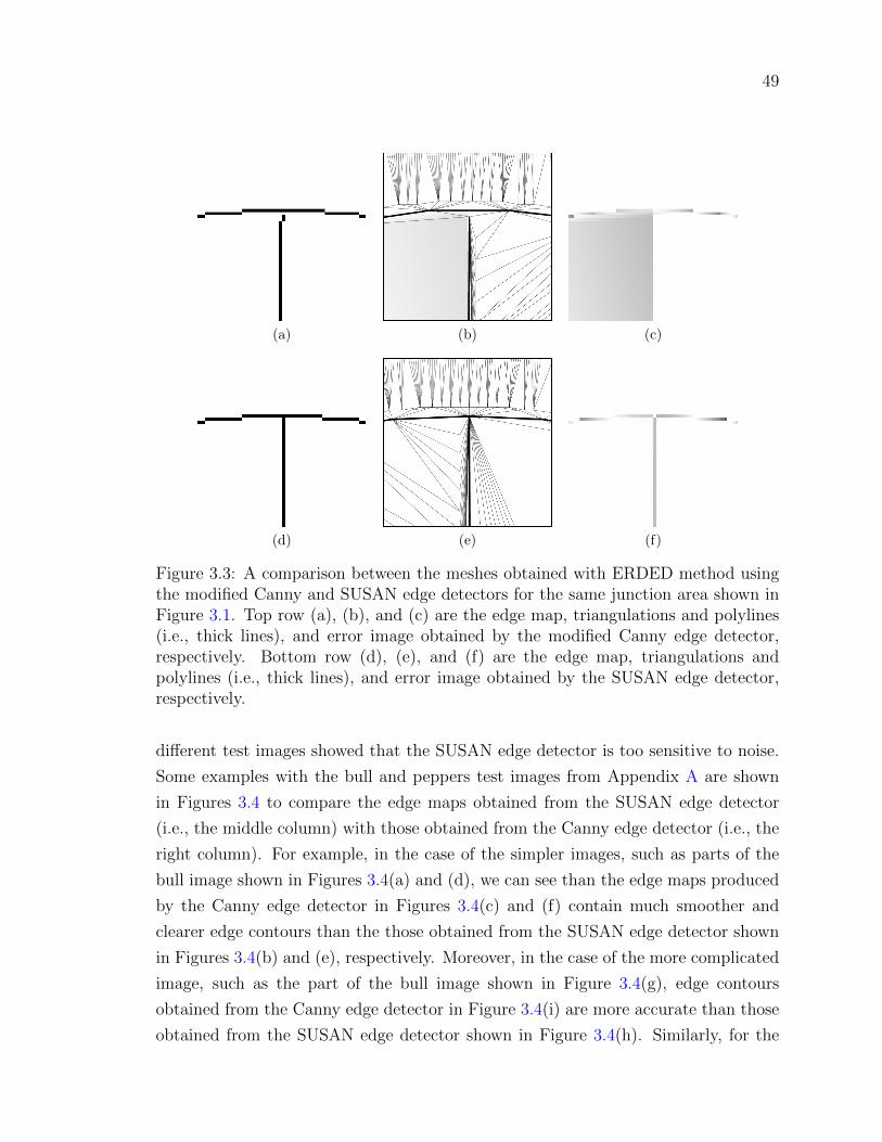
49

(a) (b) (c)

(d) (e) (f)

Figure 3.3: A comparison between the meshes obtained with ERDED method usingthe modified Canny and SUSAN edge detectors for the same junction area shown inFigure 3.1. Top row (a), (b), and (c) are the edge map, triangulations and polylines(i.e., thick lines), and error image obtained by the modified Canny edge detector,respectively. Bottom row (d), (e), and (f) are the edge map, triangulations andpolylines (i.e., thick lines), and error image obtained by the SUSAN edge detector,respectively.

different test images showed that the SUSAN edge detector is too sensitive to noise.

Some examples with the bull and peppers test images from Appendix A are shown

in Figures 3.4 to compare the edge maps obtained from the SUSAN edge detector

(i.e., the middle column) with those obtained from the Canny edge detector (i.e., the

right column). For example, in the case of the simpler images, such as parts of the

bull image shown in Figures 3.4(a) and (d), we can see than the edge maps produced

by the Canny edge detector in Figures 3.4(c) and (f) contain much smoother and

clearer edge contours than the those obtained from the SUSAN edge detector shown

in Figures 3.4(b) and (e), respectively. Moreover, in the case of the more complicated

image, such as the part of the bull image shown in Figure 3.4(g), edge contours

obtained from the Canny edge detector in Figure 3.4(i) are more accurate than those

obtained from the SUSAN edge detector shown in Figure 3.4(h). Similarly, for the

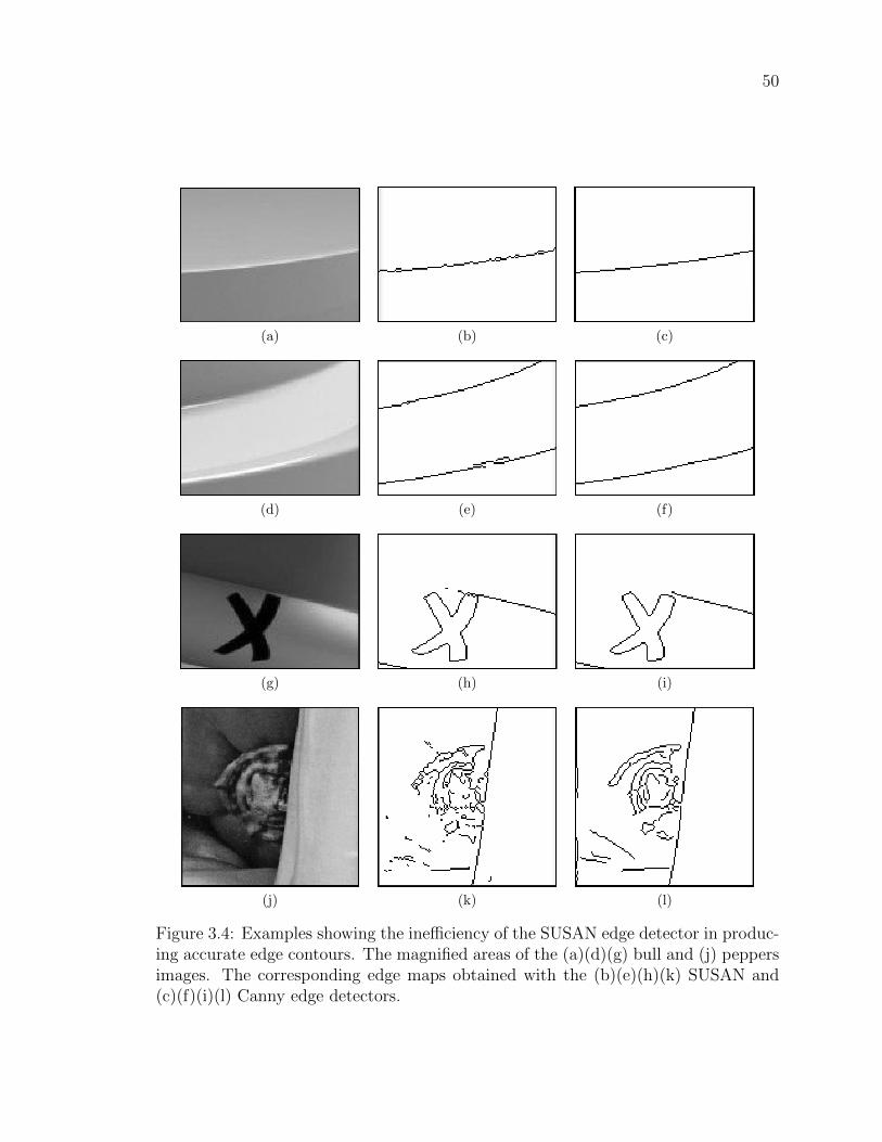
50

(a) (b) (c)

(d) (e) (f)

(g) (h) (i)

(j) (k) (l)

Figure 3.4: Examples showing the inefficiency of the SUSAN edge detector in produc-ing accurate edge contours. The magnified areas of the (a)(d)(g) bull and (j) peppersimages. The corresponding edge maps obtained with the (b)(e)(h)(k) SUSAN and(c)(f)(i)(l) Canny edge detectors.

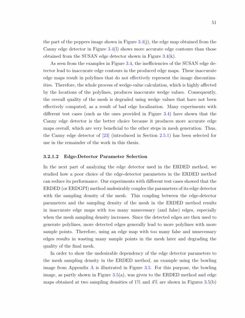
51

the part of the peppers image shown in Figure 3.4(j), the edge map obtained from the

Canny edge detector in Figure 3.4(l) shows more accurate edge contours than those

obtained from the SUSAN edge detector shown in Figure 3.4(k).

As seen from the examples in Figure 3.4, the inefficiencies of the SUSAN edge de-

tector lead to inaccurate edge contours in the produced edge maps. These inaccurate

edge maps result in polylines that do not effectively represent the image discontinu-

ities. Therefore, the whole process of wedge-value calculation, which is highly affected

by the locations of the polylines, produces inaccurate wedge values. Consequently,

the overall quality of the mesh is degraded using wedge values that have not been

effectively computed, as a result of bad edge localization. Many experiments with

different test cases (such as the ones provided in Figure 3.4) have shown that the

Canny edge detector is the better choice because it produces more accurate edge

maps overall, which are very beneficial to the other steps in mesh generation. Thus,

the Canny edge detector of [23] (introduced in Section 2.5.1) has been selected for

use in the remainder of the work in this thesis.

3.2.1.2 Edge-Detector Parameter Selection

In the next part of analyzing the edge detector used in the ERDED method, we

studied how a poor choice of the edge-detector parameters in the ERDED method

can reduce its performance. Our experiments with different test cases showed that the

ERDED (or ERDGPI) method undesirably couples the parameters of its edge detector

with the sampling density of the mesh. This coupling between the edge-detector

parameters and the sampling density of the mesh in the ERDED method results

in inaccurate edge maps with too many unnecessary (and false) edges, especially

when the mesh sampling density increases. Since the detected edges are then used to

generate polylines, more detected edges generally lead to more polylines with more

sample points. Therefore, using an edge map with too many false and unnecessary

edges results in wasting many sample points in the mesh later and degrading the

quality of the final mesh.

In order to show the undesirable dependency of the edge detector parameters to

the mesh sampling density in the ERDED method, an example using the bowling

image from Appendix A is illustrated in Figure 3.5. For this purpose, the bowling

image, as partly shown in Figure 3.5(a), was given to the ERDED method and edge

maps obtained at two sampling densities of 1% and 4% are shown in Figures 3.5(b)

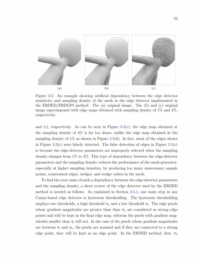
52

(a) (b) (c)

Figure 3.5: An example showing artificial dependency between the edge detectorsensitivity and sampling density of the mesh in the edge detector implemented inthe ERDED/ERDGPI method. The (a) original image. The (b) and (c) originalimage superimposed with edge maps obtained with sampling density of 1% and 4%,respectively.

and (c), respectively. As can be seen in Figure 3.5(c), the edge map obtained at

the sampling density of 4% is far too dense, unlike the edge map obtained at the

sampling density of 1% as shown in Figure 3.5(b). In fact, most of the edges shown

in Figure 3.5(c) were falsely detected. The false detection of edges in Figure 3.5(c)

is because the edge-detector parameters are improperly selected when the sampling

density changes from 1% to 4%. This type of dependency between the edge-detector

parameters and the sampling density reduces the performance of the mesh generator,

especially at higher sampling densities, by producing too many unnecessary sample

points, constrained edges, wedges, and wedge values in the mesh.

To find the root cause of such a dependency between the edge-detector parameters

and the sampling density, a short review of the edge detector used by the ERDED

method is needed as follows. As explained in Section 2.5.1, one main step in any

Canny-based edge detector is hysteresis thresholding. The hysteresis thresholding

employs two thresholds, a high threshold τh and a low threshold τl. The edge pixels

whose gradient magnitudes are greater than than τh are considered as strong edge

points and will be kept in the final edge map, whereas the pixels with gradient mag-

nitudes smaller than τl will not. In the case of the pixels whose gradient magnitudes

are between τl and τh, the pixels are scanned and if they are connected to a strong

edge point, they will be kept as an edge point. In the ERDED method, first, τh

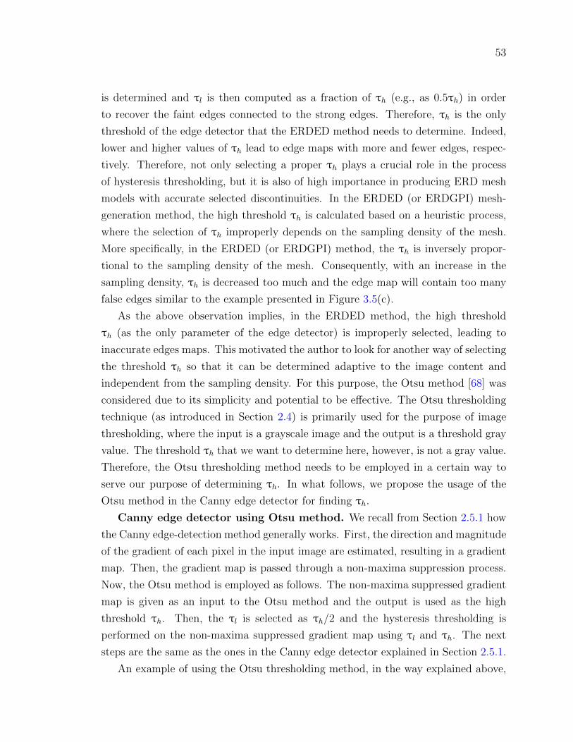
53

is determined and τl is then computed as a fraction of τh (e.g., as 0.5τh) in order

to recover the faint edges connected to the strong edges. Therefore, τh is the only

threshold of the edge detector that the ERDED method needs to determine. Indeed,

lower and higher values of τh lead to edge maps with more and fewer edges, respec-

tively. Therefore, not only selecting a proper τh plays a crucial role in the process

of hysteresis thresholding, but it is also of high importance in producing ERD mesh

models with accurate selected discontinuities. In the ERDED (or ERDGPI) mesh-

generation method, the high threshold τh is calculated based on a heuristic process,

where the selection of τh improperly depends on the sampling density of the mesh.

More specifically, in the ERDED (or ERDGPI) method, the τh is inversely propor-

tional to the sampling density of the mesh. Consequently, with an increase in the

sampling density, τh is decreased too much and the edge map will contain too many

false edges similar to the example presented in Figure 3.5(c).

As the above observation implies, in the ERDED method, the high threshold

τh (as the only parameter of the edge detector) is improperly selected, leading to

inaccurate edges maps. This motivated the author to look for another way of selecting

the threshold τh so that it can be determined adaptive to the image content and

independent from the sampling density. For this purpose, the Otsu method [68] was

considered due to its simplicity and potential to be effective. The Otsu thresholding

technique (as introduced in Section 2.4) is primarily used for the purpose of image

thresholding, where the input is a grayscale image and the output is a threshold gray

value. The threshold τh that we want to determine here, however, is not a gray value.

Therefore, the Otsu thresholding method needs to be employed in a certain way to

serve our purpose of determining τh. In what follows, we propose the usage of the

Otsu method in the Canny edge detector for finding τh.

Canny edge detector using Otsu method. We recall from Section 2.5.1 how

the Canny edge-detection method generally works. First, the direction and magnitude

of the gradient of each pixel in the input image are estimated, resulting in a gradient

map. Then, the gradient map is passed through a non-maxima suppression process.

Now, the Otsu method is employed as follows. The non-maxima suppressed gradient

map is given as an input to the Otsu method and the output is used as the high

threshold τh. Then, the τl is selected as τh/2 and the hysteresis thresholding is

performed on the non-maxima suppressed gradient map using τl and τh. The next

steps are the same as the ones in the Canny edge detector explained in Section 2.5.1.

An example of using the Otsu thresholding method, in the way explained above,

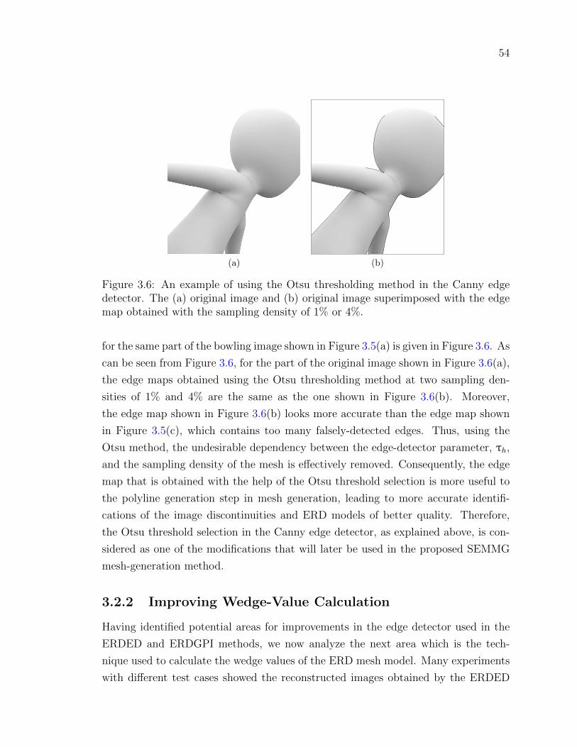
54

(a) (b)

Figure 3.6: An example of using the Otsu thresholding method in the Canny edgedetector. The (a) original image and (b) original image superimposed with the edgemap obtained with the sampling density of 1% or 4%.

for the same part of the bowling image shown in Figure 3.5(a) is given in Figure 3.6. As

can be seen from Figure 3.6, for the part of the original image shown in Figure 3.6(a),

the edge maps obtained using the Otsu thresholding method at two sampling den-

sities of 1% and 4% are the same as the one shown in Figure 3.6(b). Moreover,

the edge map shown in Figure 3.6(b) looks more accurate than the edge map shown

in Figure 3.5(c), which contains too many falsely-detected edges. Thus, using the

Otsu method, the undesirable dependency between the edge-detector parameter, τh,

and the sampling density of the mesh is effectively removed. Consequently, the edge

map that is obtained with the help of the Otsu threshold selection is more useful to

the polyline generation step in mesh generation, leading to more accurate identifi-

cations of the image discontinuities and ERD models of better quality. Therefore,

the Otsu threshold selection in the Canny edge detector, as explained above, is con-

sidered as one of the modifications that will later be used in the proposed SEMMG

mesh-generation method.

3.2.2 Improving Wedge-Value Calculation

Having identified potential areas for improvements in the edge detector used in the

ERDED and ERDGPI methods, we now analyze the next area which is the tech-

nique used to calculate the wedge values of the ERD mesh model. Many experiments

with different test cases showed the reconstructed images obtained by the ERDED

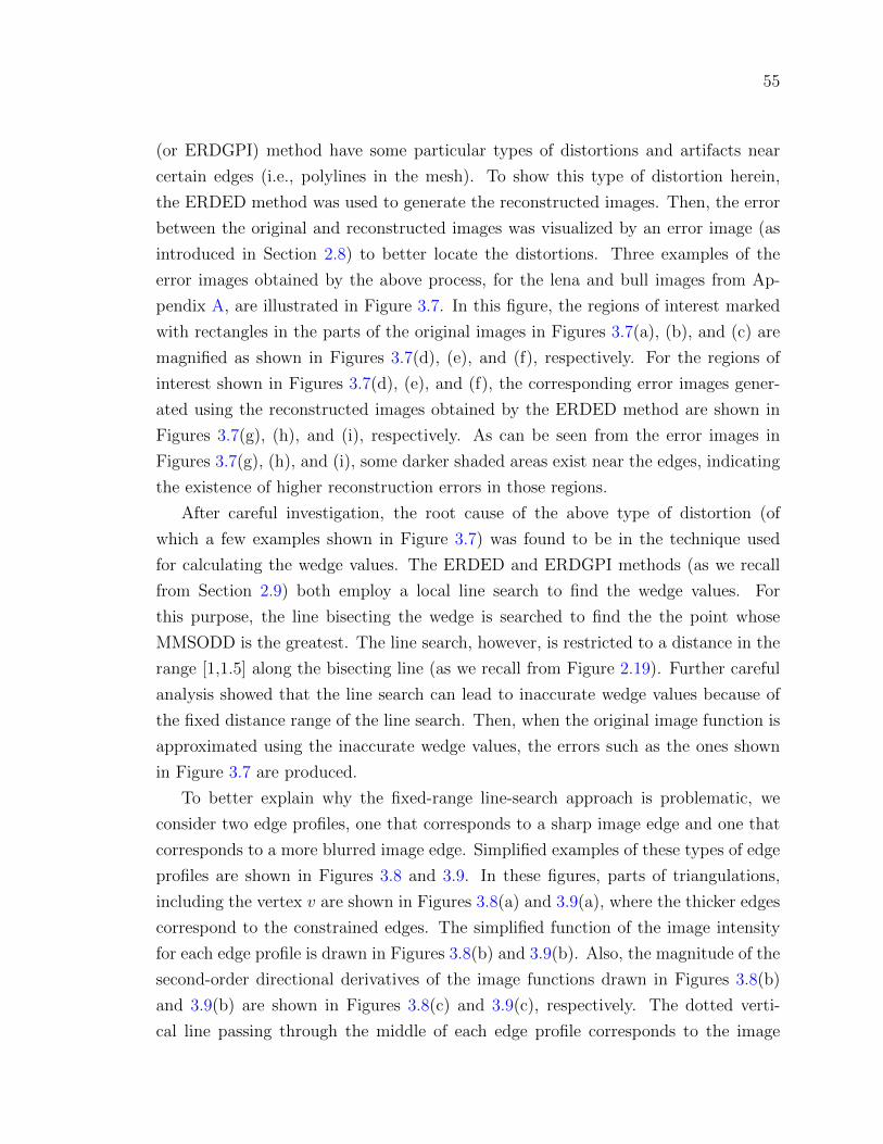
55

(or ERDGPI) method have some particular types of distortions and artifacts near

certain edges (i.e., polylines in the mesh). To show this type of distortion herein,

the ERDED method was used to generate the reconstructed images. Then, the error

between the original and reconstructed images was visualized by an error image (as

introduced in Section 2.8) to better locate the distortions. Three examples of the

error images obtained by the above process, for the lena and bull images from Ap-

pendix A, are illustrated in Figure 3.7. In this figure, the regions of interest marked

with rectangles in the parts of the original images in Figures 3.7(a), (b), and (c) are

magnified as shown in Figures 3.7(d), (e), and (f), respectively. For the regions of

interest shown in Figures 3.7(d), (e), and (f), the corresponding error images gener-

ated using the reconstructed images obtained by the ERDED method are shown in

Figures 3.7(g), (h), and (i), respectively. As can be seen from the error images in

Figures 3.7(g), (h), and (i), some darker shaded areas exist near the edges, indicating

the existence of higher reconstruction errors in those regions.

After careful investigation, the root cause of the above type of distortion (of

which a few examples shown in Figure 3.7) was found to be in the technique used

for calculating the wedge values. The ERDED and ERDGPI methods (as we recall

from Section 2.9) both employ a local line search to find the wedge values. For

this purpose, the line bisecting the wedge is searched to find the the point whose

MMSODD is the greatest. The line search, however, is restricted to a distance in the

range [1,1.5] along the bisecting line (as we recall from Figure 2.19). Further careful

analysis showed that the line search can lead to inaccurate wedge values because of

the fixed distance range of the line search. Then, when the original image function is

approximated using the inaccurate wedge values, the errors such as the ones shown

in Figure 3.7 are produced.

To better explain why the fixed-range line-search approach is problematic, we

consider two edge profiles, one that corresponds to a sharp image edge and one that

corresponds to a more blurred image edge. Simplified examples of these types of edge

profiles are shown in Figures 3.8 and 3.9. In these figures, parts of triangulations,

including the vertex v are shown in Figures 3.8(a) and 3.9(a), where the thicker edges

correspond to the constrained edges. The simplified function of the image intensity

for each edge profile is drawn in Figures 3.8(b) and 3.9(b). Also, the magnitude of the

second-order directional derivatives of the image functions drawn in Figures 3.8(b)

and 3.9(b) are shown in Figures 3.8(c) and 3.9(c), respectively. The dotted verti-

cal line passing through the middle of each edge profile corresponds to the image

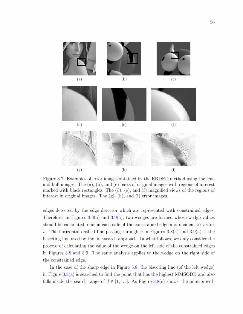
56

(a) (b) (c)

(d) (e) (f)

(g) (h) (i)

Figure 3.7: Examples of error images obtained by the ERDED method using the lenaand bull images. The (a), (b), and (c) parts of original images with regions of interestmarked with black rectangles. The (d), (e), and (f) magnified views of the regions ofinterest in original images. The (g), (h), and (i) error images.

edges detected by the edge detector which are represented with constrained edges.

Therefore, in Figures 3.8(a) and 3.9(a), two wedges are formed whose wedge values

should be calculated, one on each side of the constrained edge and incident to vertex

v. The horizontal dashed line passing through v in Figures 3.8(a) and 3.9(a) is the

bisecting line used by the line-search approach. In what follows, we only consider the

process of calculating the value of the wedge on the left side of the constrained edges

in Figures 3.8 and 3.9. The same analysis applies to the wedge on the right side of

the constrained edge.

In the case of the sharp edge in Figure 3.8, the bisecting line (of the left wedge)

in Figure 3.8(a) is searched to find the point that has the highest MMSODD and also

falls inside the search range of d ∈ [1, 1.5]. As Figure 3.8(c) shows, the point p with

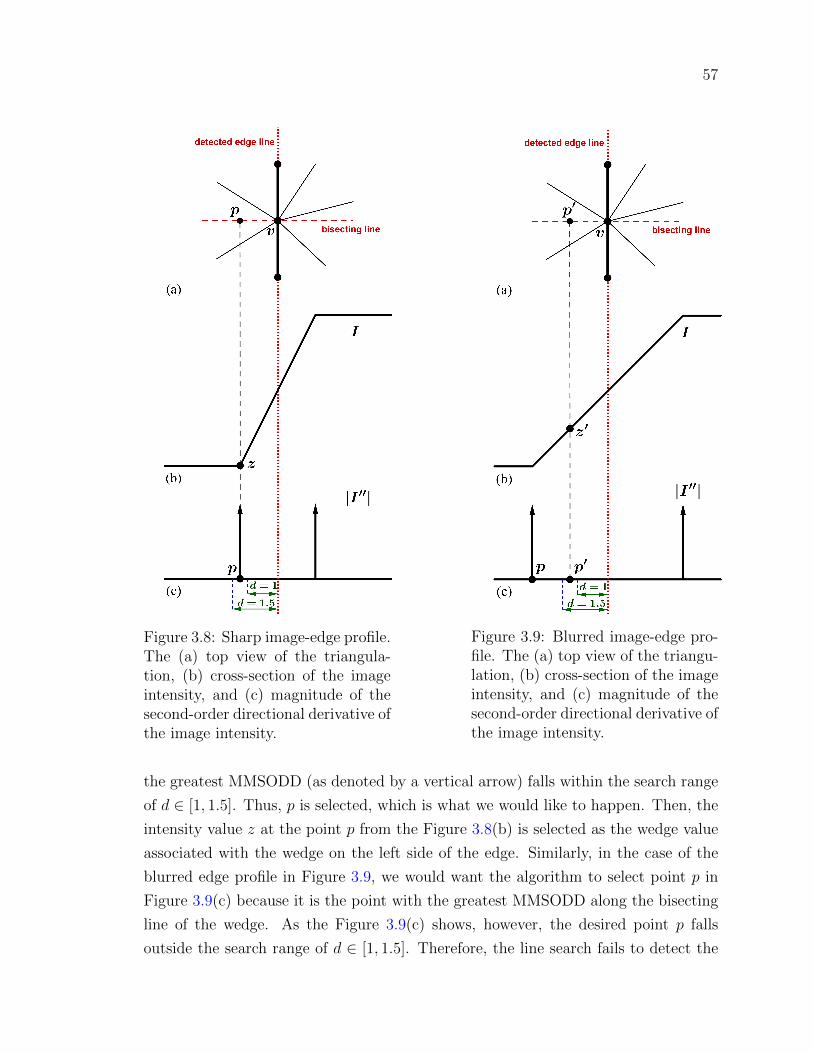
57

Figure 3.8: Sharp image-edge profile.The (a) top view of the triangula-tion, (b) cross-section of the imageintensity, and (c) magnitude of thesecond-order directional derivative ofthe image intensity.

Figure 3.9: Blurred image-edge pro-file. The (a) top view of the triangu-lation, (b) cross-section of the imageintensity, and (c) magnitude of thesecond-order directional derivative ofthe image intensity.

the greatest MMSODD (as denoted by a vertical arrow) falls within the search range

of d ∈ [1, 1.5]. Thus, p is selected, which is what we would like to happen. Then, the

intensity value z at the point p from the Figure 3.8(b) is selected as the wedge value

associated with the wedge on the left side of the edge. Similarly, in the case of the

blurred edge profile in Figure 3.9, we would want the algorithm to select point p in

Figure 3.9(c) because it is the point with the greatest MMSODD along the bisecting

line of the wedge. As the Figure 3.9(c) shows, however, the desired point p falls

outside the search range of d ∈ [1, 1.5]. Therefore, the line search fails to detect the

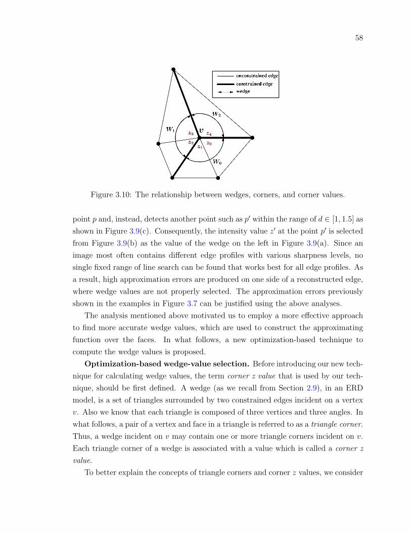
58

Figure 3.10: The relationship between wedges, corners, and corner values.

point p and, instead, detects another point such as p′ within the range of d ∈ [1, 1.5] as

shown in Figure 3.9(c). Consequently, the intensity value z′ at the point p′ is selected

from Figure 3.9(b) as the value of the wedge on the left in Figure 3.9(a). Since an

image most often contains different edge profiles with various sharpness levels, no

single fixed range of line search can be found that works best for all edge profiles. As

a result, high approximation errors are produced on one side of a reconstructed edge,

where wedge values are not properly selected. The approximation errors previously

shown in the examples in Figure 3.7 can be justified using the above analyses.

The analysis mentioned above motivated us to employ a more effective approach

to find more accurate wedge values, which are used to construct the approximating

function over the faces. In what follows, a new optimization-based technique to

compute the wedge values is proposed.

Optimization-based wedge-value selection. Before introducing our new tech-

nique for calculating wedge values, the term corner z value that is used by our tech-

nique, should be first defined. A wedge (as we recall from Section 2.9), in an ERD

model, is a set of triangles surrounded by two constrained edges incident on a vertex

v. Also we know that each triangle is composed of three vertices and three angles. In

what follows, a pair of a vertex and face in a triangle is referred to as a triangle corner.

Thus, a wedge incident on v may contain one or more triangle corners incident on v.

Each triangle corner of a wedge is associated with a value which is called a corner z

value.

To better explain the concepts of triangle corners and corner z values, we consider

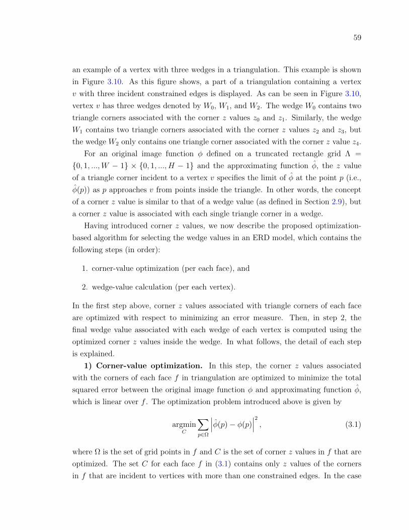
59

an example of a vertex with three wedges in a triangulation. This example is shown

in Figure 3.10. As this figure shows, a part of a triangulation containing a vertex

v with three incident constrained edges is displayed. As can be seen in Figure 3.10,

vertex v has three wedges denoted by W0, W1, and W2. The wedge W0 contains two

triangle corners associated with the corner z values z0 and z1. Similarly, the wedge

W1 contains two triangle corners associated with the corner z values z2 and z3, but

the wedge W2 only contains one triangle corner associated with the corner z value z4.

For an original image function φ defined on a truncated rectangle grid Λ =

0, 1, ...,W − 1 × 0, 1, ..., H − 1 and the approximating function φ, the z value

of a triangle corner incident to a vertex v specifies the limit of φ at the point p (i.e.,

φ(p)) as p approaches v from points inside the triangle. In other words, the concept

of a corner z value is similar to that of a wedge value (as defined in Section 2.9), but

a corner z value is associated with each single triangle corner in a wedge.

Having introduced corner z values, we now describe the proposed optimization-

based algorithm for selecting the wedge values in an ERD model, which contains the

following steps (in order):

1. corner-value optimization (per each face), and

2. wedge-value calculation (per each vertex).

In the first step above, corner z values associated with triangle corners of each face

are optimized with respect to minimizing an error measure. Then, in step 2, the

final wedge value associated with each wedge of each vertex is computed using the

optimized corner z values inside the wedge. In what follows, the detail of each step

is explained.

1) Corner-value optimization. In this step, the corner z values associated

with the corners of each face f in triangulation are optimized to minimize the total

squared error between the original image function φ and approximating function φ,

which is linear over f . The optimization problem introduced above is given by

argminC

∑p∈Ω

∣∣∣φ(p)− φ(p)∣∣∣2 , (3.1)

where Ω is the set of grid points in f and C is the set of corner z values in f that are

optimized. The set C for each face f in (3.1) contains only z values of the corners

in f that are incident to vertices with more than one constrained edges. In the case

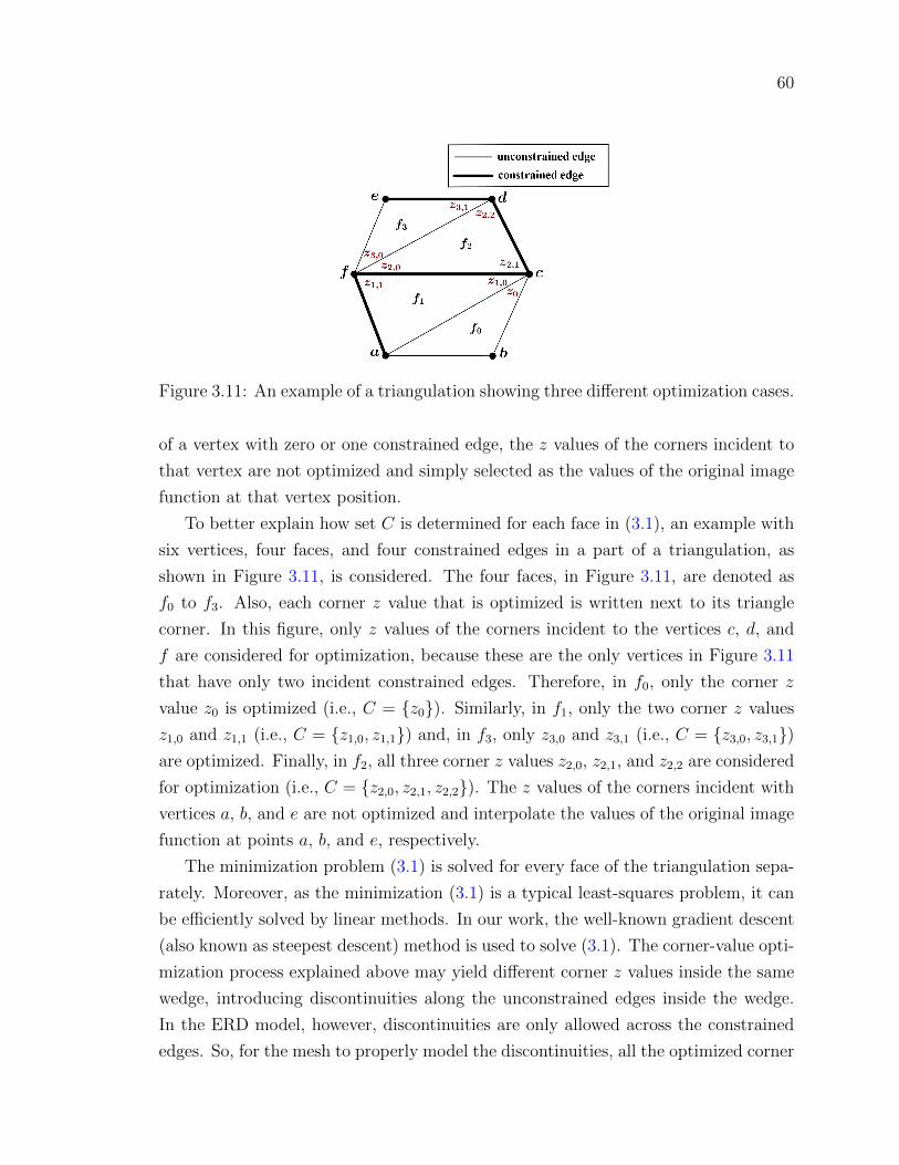
60

Figure 3.11: An example of a triangulation showing three different optimization cases.

of a vertex with zero or one constrained edge, the z values of the corners incident to

that vertex are not optimized and simply selected as the values of the original image

function at that vertex position.

To better explain how set C is determined for each face in (3.1), an example with

six vertices, four faces, and four constrained edges in a part of a triangulation, as

shown in Figure 3.11, is considered. The four faces, in Figure 3.11, are denoted as

f0 to f3. Also, each corner z value that is optimized is written next to its triangle

corner. In this figure, only z values of the corners incident to the vertices c, d, and

f are considered for optimization, because these are the only vertices in Figure 3.11

that have only two incident constrained edges. Therefore, in f0, only the corner z

value z0 is optimized (i.e., C = z0). Similarly, in f1, only the two corner z values

z1,0 and z1,1 (i.e., C = z1,0, z1,1) and, in f3, only z3,0 and z3,1 (i.e., C = z3,0, z3,1)are optimized. Finally, in f2, all three corner z values z2,0, z2,1, and z2,2 are considered

for optimization (i.e., C = z2,0, z2,1, z2,2). The z values of the corners incident with

vertices a, b, and e are not optimized and interpolate the values of the original image

function at points a, b, and e, respectively.

The minimization problem (3.1) is solved for every face of the triangulation sepa-

rately. Moreover, as the minimization (3.1) is a typical least-squares problem, it can

be efficiently solved by linear methods. In our work, the well-known gradient descent

(also known as steepest descent) method is used to solve (3.1). The corner-value opti-

mization process explained above may yield different corner z values inside the same

wedge, introducing discontinuities along the unconstrained edges inside the wedge.

In the ERD model, however, discontinuities are only allowed across the constrained

edges. So, for the mesh to properly model the discontinuities, all the optimized corner

61

z values inside the same wedge should be combined to produce a single z value, which

is used as the wedge value of that wedge. This process of combining the optimized

corner z values in each wedge is performed in the next step.

2) Wedge-value calculation. Once the corner z values in the triangulation are

optimized, the wedge value of each wedge is computed as follows. First, weighted

average of all corner z values inside the same wedge are computed. For this purpose,

the weight associated with each corner z value is the number of grid points inside

the face to which the corner z value belongs. The wedge value is then obtained by

rounding the averaged value to its nearest integer. In a general case, for a wedge

of n triangle faces with n optimized corner z values zin−1i=0 , the wedge value w is

computed by

w = round

n−1∑i=0

|Ωi|zin−1∑i=0

|Ωi|

, (3.2)

where Ωi is the set of grid points in the face to which zi belongs andn−1∑i=0

|Ωi| 6= 0.

The operator “round” in (3.2) rounds a real number to its nearest integer value. If,

however,∑n−1

i=0 |Ωi| = 0, then wedge value w is simply computed as the mean value

of all corner z values zin−1i=0 . Using the weighted averaging technique in (3.2), the

optimized corner z value that belongs to a triangle with a larger area (i.e., |Ω|) receives

more weight in the averaging process. Moreover, the effect of (undesirable) corner z

values obtained from very thin or tiny triangles is effectively reduced in the averaging

process.

In order to perform a preliminary evaluation of the proposed optimization-based

wedge-value-selection algorithm, the ERDED mesh-generation scheme was tested

with the two old and new approaches for wedge-value selection, namely, the line-search

and proposed optimization-based approaches. For this purpose, the two versions of

the ERDED method were used to generate the reconstructed images. Then, the error

between the original and reconstructed image was visualized by an error image (as

introduced in Section 2.8) to better locate the distortions. The error images were then

compared to see whether the proposed optimization-based method for wedge-value

selection reduced the approximation errors. The results showed that the proposed

optimization-based approach effectively reduces those types of artifacts produced by

the line-search approach. For the sake of comparison, the same three examples of the

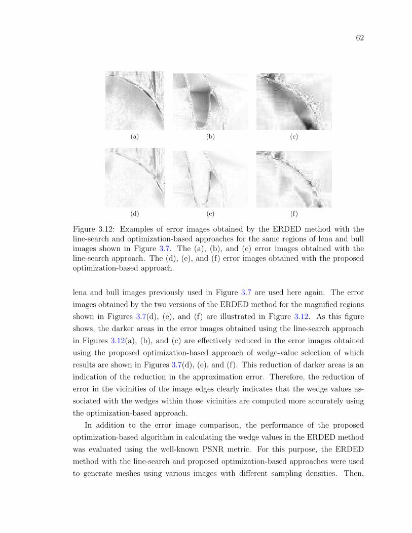
62

(a) (b) (c)

(d) (e) (f)

Figure 3.12: Examples of error images obtained by the ERDED method with theline-search and optimization-based approaches for the same regions of lena and bullimages shown in Figure 3.7. The (a), (b), and (c) error images obtained with theline-search approach. The (d), (e), and (f) error images obtained with the proposedoptimization-based approach.

lena and bull images previously used in Figure 3.7 are used here again. The error

images obtained by the two versions of the ERDED method for the magnified regions

shown in Figures 3.7(d), (e), and (f) are illustrated in Figure 3.12. As this figure

shows, the darker areas in the error images obtained using the line-search approach

in Figures 3.12(a), (b), and (c) are effectively reduced in the error images obtained

using the proposed optimization-based approach of wedge-value selection of which

results are shown in Figures 3.7(d), (e), and (f). This reduction of darker areas is an

indication of the reduction in the approximation error. Therefore, the reduction of

error in the vicinities of the image edges clearly indicates that the wedge values as-

sociated with the wedges within those vicinities are computed more accurately using

the optimization-based approach.

In addition to the error image comparison, the performance of the proposed

optimization-based algorithm in calculating the wedge values in the ERDED method

was evaluated using the well-known PSNR metric. For this purpose, the ERDED

method with the line-search and proposed optimization-based approaches were used

to generate meshes using various images with different sampling densities. Then,

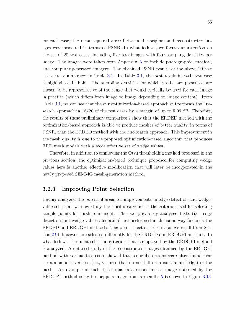
63

for each case, the mean squared error between the original and reconstructed im-

ages was measured in terms of PSNR. In what follows, we focus our attention on

the set of 20 test cases, including five test images with four sampling densities per

image. The images were taken from Appendix A to include photographic, medical,

and computer-generated imagery. The obtained PSNR results of the above 20 test

cases are summarized in Table 3.1. In Table 3.1, the best result in each test case

is highlighted in bold. The sampling densities for which results are presented are

chosen to be representative of the range that would typically be used for each image

in practice (which differs from image to image depending on image content). From

Table 3.1, we can see that the our optimization-based approach outperforms the line-

search approach in 18/20 of the test cases by a margin of up to 5.06 dB. Therefore,

the results of these preliminary comparisons show that the ERDED method with the

optimization-based approach is able to produce meshes of better quality, in terms of

PSNR, than the ERDED method with the line-search approach. This improvement in

the mesh quality is due to the proposed optimization-based algorithm that produces

ERD mesh models with a more effective set of wedge values.

Therefore, in addition to employing the Otsu thresholding method proposed in the

previous section, the optimization-based technique proposed for computing wedge

values here is another effective modification that will later be incorporated in the

newly proposed SEMMG mesh-generation method.

3.2.3 Improving Point Selection

Having analyzed the potential areas for improvements in edge detection and wedge-

value selection, we now study the third area which is the criterion used for selecting

sample points for mesh refinement. The two previously analyzed tasks (i.e., edge

detection and wedge-value calculation) are performed in the same way for both the

ERDED and ERDGPI methods. The point-selection criteria (as we recall from Sec-

tion 2.9), however, are selected differently for the ERDED and ERDGPI methods. In

what follows, the point-selection criterion that is employed by the ERDGPI method

is analyzed. A detailed study of the reconstructed images obtained by the ERDGPI

method with various test cases showed that some distortions were often found near

certain smooth vertices (i.e., vertices that do not fall on a constrained edge) in the

mesh. An example of such distortions in a reconstructed image obtained by the

ERDGPI method using the peppers image from Appendix A is shown in Figure 3.13.

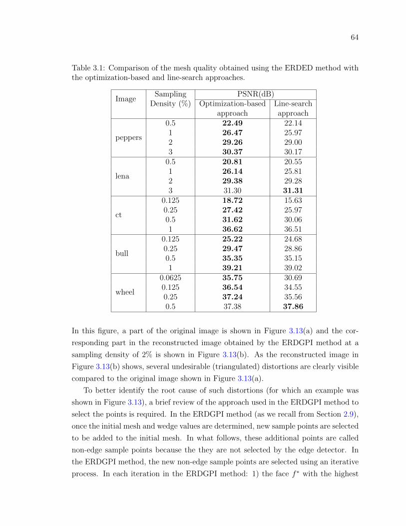
64

Table 3.1: Comparison of the mesh quality obtained using the ERDED method withthe optimization-based and line-search approaches.

ImageSampling

Density (%)PSNR(dB)

Optimization-basedapproach

Line-searchapproach

peppers

0.5 22.49 22.141 26.47 25.972 29.26 29.003 30.37 30.17

lena

0.5 20.81 20.551 26.14 25.812 29.38 29.283 31.30 31.31

ct

0.125 18.72 15.630.25 27.42 25.970.5 31.62 30.061 36.62 36.51

bull

0.125 25.22 24.680.25 29.47 28.860.5 35.35 35.151 39.21 39.02

wheel

0.0625 35.75 30.690.125 36.54 34.550.25 37.24 35.560.5 37.38 37.86

In this figure, a part of the original image is shown in Figure 3.13(a) and the cor-

responding part in the reconstructed image obtained by the ERDGPI method at a

sampling density of 2% is shown in Figure 3.13(b). As the reconstructed image in

Figure 3.13(b) shows, several undesirable (triangulated) distortions are clearly visible

compared to the original image shown in Figure 3.13(a).

To better identify the root cause of such distortions (for which an example was

shown in Figure 3.13), a brief review of the approach used in the ERDGPI method to

select the points is required. In the ERDGPI method (as we recall from Section 2.9),

once the initial mesh and wedge values are determined, new sample points are selected

to be added to the initial mesh. In what follows, these additional points are called

non-edge sample points because the they are not selected by the edge detector. In

the ERDGPI method, the new non-edge sample points are selected using an iterative

process. In each iteration in the ERDGPI method: 1) the face f ∗ with the highest

65

(a) (b)

Figure 3.13: An example of the distortions produced by the ERDGPI method usingthe peppers image. The (a) part of the original image and (b) its corresponding partfrom the reconstructed image.

squared error is found (using (2.3)); and 2) then the point q with the highest absolute

error in f ∗ is selected (using (2.4)). In what follows, this way of selecting non-edge

points in the ERDGPI method is referred to as the “error-based approach”.

After in-depth analyses on many reconstructed images obtained with the ERDGPI

method, the point q with highest approximation error in f ∗ was found to often corre-

spond to the noisiest pixel in f ∗. Typically, the value of the noisiest pixel significantly

differs from the values of the nearby pixels. Thus, in the error-based approach, noisi-

est pixels are often selected because they often have the largest reconstruction errors

among the other nearby pixels in f ∗. Also, the approximating function for the ERD

model (as we recall from Section 2.9) linearly interpolates the z values at sample

points in the original image. Therefore, if the noisiest point q is selected and inserted

into the mesh, the approximating function has to interpolate its original z value,

which corresponds to the value of the noisiest pixel. Consequently, the noisiest z

value in f ∗ will be used in the approximating function, resulting in undesirable local

distortions in the reconstructed images (like that shown in Figure 3.13(b)). Finally,

as the above analysis shows, the root cause of such distortions is the criterion used by

the error-based approach, which is selecting the point with the highest absolute error

in f ∗. This problem of the error-based approach motivated the author to consider

finding a more effective criterion for selecting the non-edge points. As a solution, in

what follows, a centroid-based approach for selecting the non-edge points is proposed.

Centroid-based approach. In the centroid-based approach, once the face f ∗

with the highest squared error is found, the point q is selected as the point that is

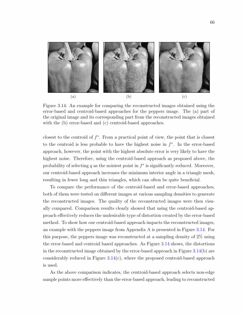
66

(a) (b) (c)

Figure 3.14: An example for comparing the reconstructed images obtained using theerror-based and centroid-based approaches for the peppers image. The (a) part ofthe original image and its corresponding part from the reconstructed images obtainedwith the (b) error-based and (c) centroid-based approaches.

closest to the centroid of f ∗. From a practical point of view, the point that is closest

to the centroid is less probable to have the highest noise in f ∗. In the error-based

approach, however, the point with the highest absolute error is very likely to have the

highest noise. Therefore, using the centroid-based approach as proposed above, the

probability of selecting q as the noisiest point in f ∗ is significantly reduced. Moreover,

our centroid-based approach increases the minimum interior angle in a triangle mesh,

resulting in fewer long and thin triangles, which can often be quite beneficial.

To compare the performance of the centroid-based and error-based approaches,

both of them were tested on different images at various sampling densities to generate

the reconstructed images. The quality of the reconstructed images were then visu-

ally compared. Comparison results clearly showed that using the centroid-based ap-

proach effectively reduces the undesirable type of distortion created by the error-based

method. To show how our centroid-based approach impacts the reconstructed images,

an example with the peppers image from Appendix A is presented in Figure 3.14. For

this purpose, the peppers image was reconstructed at a sampling density of 2% using

the error-based and centroid based approaches. As Figure 3.14 shows, the distortions

in the reconstructed image obtained by the error-based approach in Figure 3.14(b) are

considerably reduced in Figure 3.14(c), where the proposed centroid-based approach

is used.

As the above comparison indicates, the centroid-based approach selects non-edge

sample points more effectively than the error-based approach, leading to reconstructed

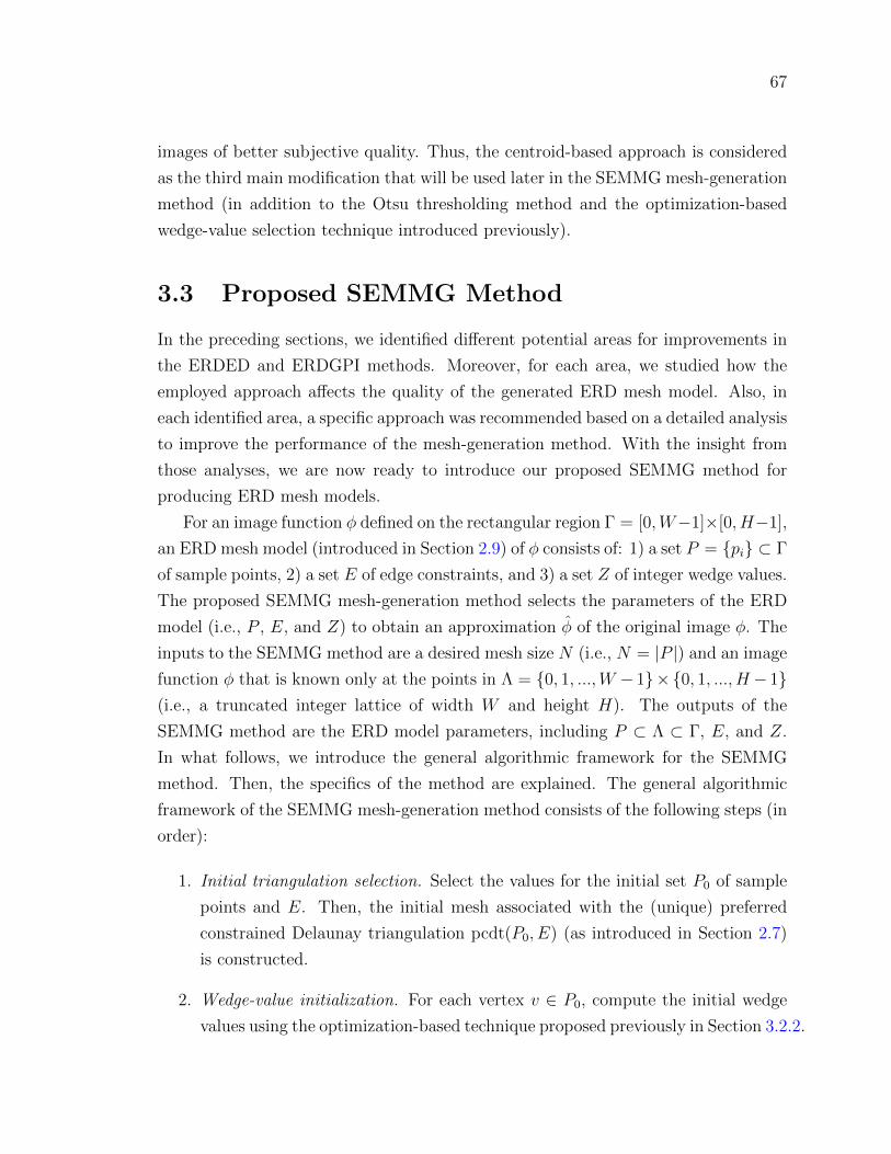
67

images of better subjective quality. Thus, the centroid-based approach is considered

as the third main modification that will be used later in the SEMMG mesh-generation

method (in addition to the Otsu thresholding method and the optimization-based

wedge-value selection technique introduced previously).

3.3 Proposed SEMMG Method

In the preceding sections, we identified different potential areas for improvements in

the ERDED and ERDGPI methods. Moreover, for each area, we studied how the

employed approach affects the quality of the generated ERD mesh model. Also, in

each identified area, a specific approach was recommended based on a detailed analysis

to improve the performance of the mesh-generation method. With the insight from

those analyses, we are now ready to introduce our proposed SEMMG method for

producing ERD mesh models.

For an image function φ defined on the rectangular region Γ = [0,W−1]×[0, H−1],

an ERD mesh model (introduced in Section 2.9) of φ consists of: 1) a set P = pi ⊂ Γ

of sample points, 2) a set E of edge constraints, and 3) a set Z of integer wedge values.

The proposed SEMMG mesh-generation method selects the parameters of the ERD

model (i.e., P , E, and Z) to obtain an approximation φ of the original image φ. The

inputs to the SEMMG method are a desired mesh size N (i.e., N = |P |) and an image

function φ that is known only at the points in Λ = 0, 1, ...,W − 1×0, 1, ..., H− 1(i.e., a truncated integer lattice of width W and height H). The outputs of the

SEMMG method are the ERD model parameters, including P ⊂ Λ ⊂ Γ, E, and Z.

In what follows, we introduce the general algorithmic framework for the SEMMG

method. Then, the specifics of the method are explained. The general algorithmic

framework of the SEMMG mesh-generation method consists of the following steps (in

order):

1. Initial triangulation selection. Select the values for the initial set P0 of sample

points and E. Then, the initial mesh associated with the (unique) preferred

constrained Delaunay triangulation pcdt(P0, E) (as introduced in Section 2.7)

is constructed.

2. Wedge-value initialization. For each vertex v ∈ P0, compute the initial wedge

values using the optimization-based technique proposed previously in Section 3.2.2.

68

(a) (b) (c)

(d) (e)

Figure 3.15: Selection of the initial triangulation in step 1 of the SEMMG method.(a) Part of the input image. The (b) binary edge map of (a). The (c) unsimplifiedpolylines representing image edges in (b). The (d) simplified polylines. (e) The initialtriangulation corresponding to the part of the image shown in (a), with constrainededges denoted by thick lines.

3. Point selection. Select a new sample point q ∈ Λ to add to the mesh using the

centroid-based approach proposed previously in Section 3.2.3.

4. Point insertion. Insert q in the triangulation. Calculate the wedge values of

the affected wedges in the mesh using the same optimization-based technique

(proposed in Section 3.2.2) and select the set Pi+1 of sample points for the next

iteration as Pi ∪ q.

5. Stopping criterion. If |Pi+1| < N , go to step 3. Otherwise, set the output

parameter P = Pi+1 and stop.

In the framework above, steps 1 and 2 choose an initial coarse mesh of size N0,

where N0 = |P0|. Then, in steps 3 to 5, the initial mesh is iteratively refined by

adding N − N0 sample points to the mesh. In what follows, the selection of P0 and

E in step 1 and point insertion of step 4 will be described in more detail.

Selection of P0 and E. In step 1 of the SEMMG method, P0 and E are first

selected and then the triangulation pcdt(P0, E) is constructed. An example with the

69

test image bull from Appendix A is used in Figure 3.15 to show different stages of

selecting P0, E, and initial triangulation. The sets P0 and E are selected as follows.

First, the Canny edge detector in [23] is applied to the input image φ defined on Λ to

produce the binary edge map B, in which an entry is one if it corresponds to an edge

pixel, and zero otherwise. In the Canny edge detector, the high threshold τh is com-

puted using the Ostu-based approach proposed earlier in Section 3.2.1.2. Then the

low threshold τl is selected as τl = τh/2. In the example given in Figure 3.15, for the

part of the input image given in Figure 3.15(a), the corresponding binary edge map

B is shown in Figure 3.15(b), where edge pixels are shown in black. Then, from B, a

collection of polylines is generated to represent edges. To achieve this, edge pixels in

B that are 8-connected are joined (by line segments) to form a polyline. If a polyline

has one or more self-intersections (excluding loops), the polyline is split at each in-

tersection point. In this way, the final set of polylines are guaranteed to not to have

any intersections (excluding loops). In the example given in Figure 3.15, for the edge

map shown in Figure 3.15(b), a set of polylines like the one shown in Figure 3.15(c) is

constructed. Next, the polylines are simplified. To perform this, polylines with fewer

than ` points are disregarded. In our method, ` = round(0.01 max(W,H)), where

the operator “round” rounds a real number to its nearest integer value. Then, from

each remaining polyline, we generate another polyline with fewer points that well

approximates the original polyline, resulting in a new set of simplified polylines. For

this purpose, the well-known Douglas-Peucker (DP) simplification method from [34]

(introduced in Section 2.3) is employed, with the tolerance parameter ε = 1. The

output of the polyline simplification process is a set D of simplified polylines. In the

example given in Figure 3.15, for the polylines given in Figure 3.15(c), a correspond-

ing set D of simplified polylines is illustrated in Figure 3.15(d). Finally, P0 is chosen

as the union of all vertices in D, plus the extreme convex-hull points of Λ (i.e., the

four corner points of the bounding box of input image) and E is selected as the union

of all line-segments in D.

Once P0 and E are selected using the above procedure, the pcdt(P0, E) is con-

structed. In the example given in Figure 3.15, for the part of the simplified polylines

given in Figure 3.15(d), the corresponding part from the initial triangulation is shown

in Figure 3.15(e), where constrained edges are denoted by thick lines.

Point insertion. After the new point q has been selected in step 3 of the above

framework, it will be inserted as a new vertex into the mesh and wedge values of the

affected wedges should be calculated as follows. If q is on a constrained edge, the

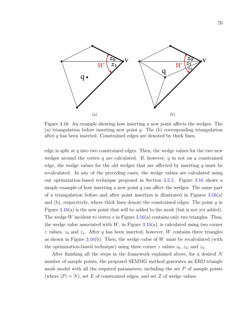
70

(a) (b)

Figure 3.16: An example showing how inserting a new point affects the wedges. The(a) triangulation before inserting new point q. The (b) corresponding triangulationafter q has been inserted. Constrained edges are denoted by thick lines.

edge is split at q into two constrained edges. Then, the wedge values for the two new

wedges around the vertex q are calculated. If, however, q in not on a constrained

edge, the wedge values for the old wedges that are affected by inserting q must be

recalculated. In any of the preceding cases, the wedge values are calculated using

our optimization-based technique proposed in Section 3.2.2. Figure 3.16 shows a

simple example of how inserting a new point q can affect the wedges. The same part

of a triangulation before and after point insertion is illustrated in Figures 3.16(a)

and (b), respectively, where thick lines denote the constrained edges. The point q in

Figure 3.16(a) is the new point that will be added to the mesh (but is not yet added).

The wedge W incident to vertex v in Figure 3.16(a) contains only two triangles. Thus,

the wedge value associated with W , in Figure 3.16(a), is calculated using two corner

z values, z0 and z1. After q has been inserted, however, W contains three triangles

as shown in Figure 3.16(b). Then, the wedge value of W must be recalculated (with

the optimization-based technique) using three corner z values z0, z2, and z3.

After finishing all the steps in the framework explained above, for a desired N

number of sample points, the proposed SEMMG method generates an ERD triangle

mesh model with all the required parameters, including the set P of sample points

(where |P | = N), set E of constrained edges, and set Z of wedge values.

71

Chapter 4

Evaluation and Analysis of the

SEMMG Method

4.1 Overview

Having introduced the proposed SEMMG mesh-generation method, we now evaluate

its performance by comparing the quality of the meshes obtained from it with those

obtained from other mesh-generation schemes. In general, comparing to other mesh-

based methods is very difficult because of the following two reasons. Firstly, due to

the high complexity of the mesh-based methods, implementing each of them often

requires at least several months of work, including coding, testing, and debugging.

Secondly, since so much effort is involved in implementing such methods, researchers

often do not want to make their code freely available. Thus, finding implementation

of other methods is very difficult too. For evaluating our SEMMG method herein,

in cases where the implementations of competing methods were available, they were

used, but in most cases, no implementation was available. Then, in cases where no

implementation was available, the results that could be compared to were used from

the publication. With the consideration of the above limitations in comparing to

other mesh-based methods, the SEMMG method is compared to eight approaches

in total, in two categories of the methods with and without implementations. In

particular, the SEMMG method is compared to the following four approaches, where

an implementation was available:

• the ED method of Yang et al. [96],

• the MGH method [12], inspired by the work in [43],

72

• the ERDED method of Tu and Adams [84], and

• the ERDGPI method of Tu and Adams [84].

Moreover, the SEMMG method is compared to the following four schemes, where no

implementation was available:

• the GVS method of Garcia et al. [42],

• the HWT method of Phichet [83],

• the BSP method of Sarkis and Diepold [74], and

• the ATM method of Liu et al. [63].

The above eight competing methods are based on mesh-refinement schemes and gen-

erate mesh models that are all associated with an approximating function that is

piecewise-linear and interpolates the original image function at the sample points

(same as the SEMMG method), except the ATM method, which employs a non-linear

and non-interpolating approximating function.

For the purpose of comparison, a C++ software implementation of the SEMMG

method was developed by the author of this thesis. The details of the software imple-

mentation are presented in Appendix D. The performance of the SEMMG method was

evaluated by comparing it in terms of mesh quality with each of the above competing

methods. The qualities of the meshes obtained by these methods were all measured

in terms of the well-known PSNR (as introduced in Section 2.6). The selection of

test images was limited by some of the factors mentioned earlier. For example, if

the implementation of a method was available, such as the ED, MGH, ERDED and

ERDGPI methods, more results were collected with more test images. In the case

of the methods without implementations, however, the test images were limited to

the only few available ones for which results were reported in the literature. The test

images that are used in the following sections are all listed in Appendix A. In what

follows, our SEMMG method is compared with each of the previously-listed compet-

ing methods. Furthermore, the main differences between the SEMMG method and

each of the competing methods are also highlighted. Some of the results presented in

this chapter have also been published in the author’s paper [66].

73

4.2 Comparison to Methods With Implementations

Due to the various limitations explained earlier, in the case of the related and compa-

rable mesh-generation methods for which implementations are available, the proposed

SEMMG method is compared to the following four methods:

1. the ED method of Yang et al. [96],

2. the MGH method [12], inspired by the work in [43],

3. the ERDED method of Tu and Adams [84], and

4. the ERDGPI method of Tu and Adams [84].

In order to compare the performance of our SEMMG method with the above four

methods, the implementation of each method was used to generate meshes. For the

ED and MGH methods, their implementations that were developed by the author

of [12] were used. For the ERDED and ERDGPI methods, their implementations

that were developed by the first author of [84] were used.

It is worth mentioning that the sampling densities that are used here for mesh

generation are the input parameters to the methods. Thus, sampling densities are

generally defined by the user based on what mesh quality or size is more preferable

in an application where a mesh-generation method is used. For example, with a

low sampling density of 0.03125% for complicated photographic and small images,

such as lena, the SEMMG method yields a very poor image reconstruction (with

approximately 17 dB in PSNR). In the case of the larger and simpler images, such

as cherry, however, the sampling density of 0.03125% is high enough for the SEMMG

method to produce a reconstructed image of satisfactory quality (with approximately

39 dB in PSNR). Therefore, in practice, the range of sampling densities that would be

typically used for producing a satisfactory image reconstruction may differ from image

to image. In other words, using a fixed range of sampling densities for all images may

not always lead to image reconstructions of the same (or even similar) qualities. For

consistency, however, in our evaluation, a set of 35 test images was given to each of

the five methods (i.e., the ED, MGH, ERDED, ERDGPI, and SEMMG methods) and

meshes were generated at 10 sampling densities within a fixed range of 0.0078125%

to 3% per image, leading to a test set of 350 cases per method. Then, a reconstructed

image from each mesh was produced. Next, for each test case, the mean-squared error

between the original image and the reconstructed image was measured in terms of

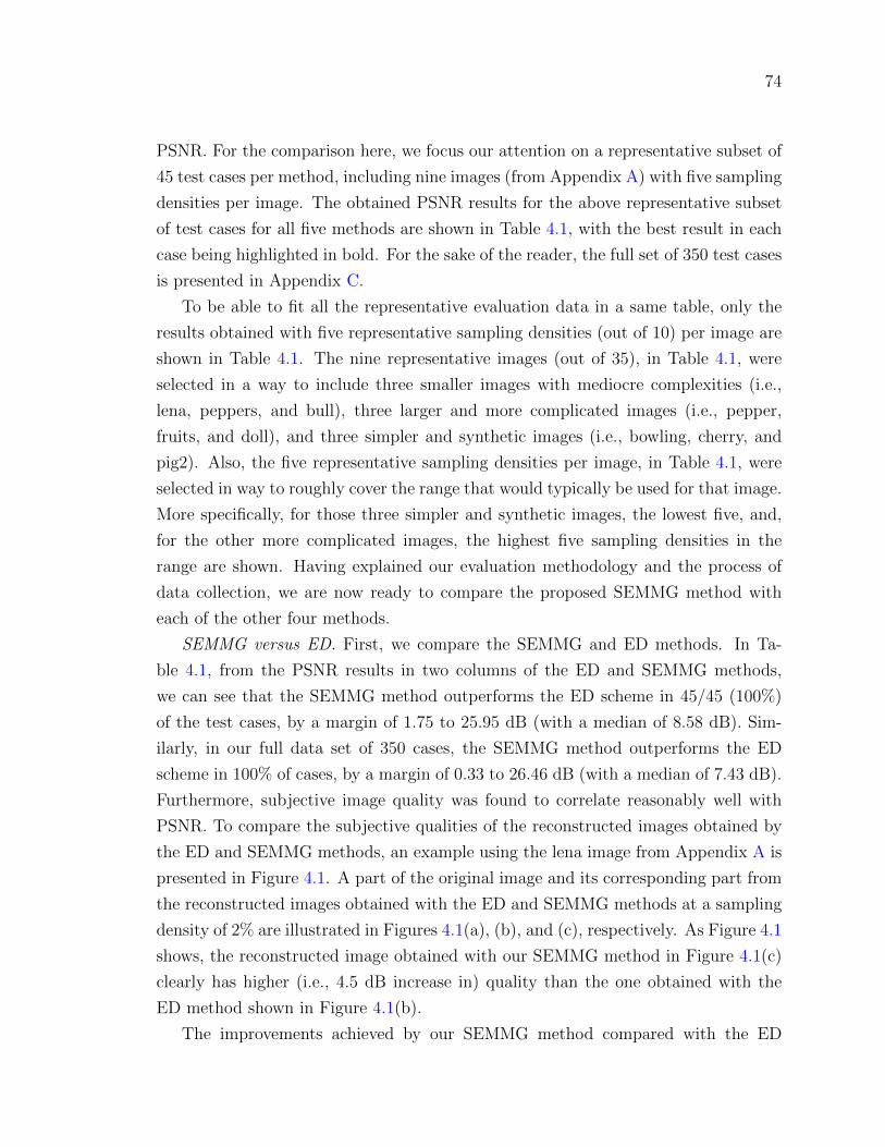
74

PSNR. For the comparison here, we focus our attention on a representative subset of

45 test cases per method, including nine images (from Appendix A) with five sampling

densities per image. The obtained PSNR results for the above representative subset

of test cases for all five methods are shown in Table 4.1, with the best result in each

case being highlighted in bold. For the sake of the reader, the full set of 350 test cases

is presented in Appendix C.

To be able to fit all the representative evaluation data in a same table, only the

results obtained with five representative sampling densities (out of 10) per image are

shown in Table 4.1. The nine representative images (out of 35), in Table 4.1, were

selected in a way to include three smaller images with mediocre complexities (i.e.,

lena, peppers, and bull), three larger and more complicated images (i.e., pepper,

fruits, and doll), and three simpler and synthetic images (i.e., bowling, cherry, and

pig2). Also, the five representative sampling densities per image, in Table 4.1, were

selected in way to roughly cover the range that would typically be used for that image.

More specifically, for those three simpler and synthetic images, the lowest five, and,

for the other more complicated images, the highest five sampling densities in the

range are shown. Having explained our evaluation methodology and the process of

data collection, we are now ready to compare the proposed SEMMG method with

each of the other four methods.

SEMMG versus ED. First, we compare the SEMMG and ED methods. In Ta-

ble 4.1, from the PSNR results in two columns of the ED and SEMMG methods,

we can see that the SEMMG method outperforms the ED scheme in 45/45 (100%)

of the test cases, by a margin of 1.75 to 25.95 dB (with a median of 8.58 dB). Sim-

ilarly, in our full data set of 350 cases, the SEMMG method outperforms the ED

scheme in 100% of cases, by a margin of 0.33 to 26.46 dB (with a median of 7.43 dB).

Furthermore, subjective image quality was found to correlate reasonably well with

PSNR. To compare the subjective qualities of the reconstructed images obtained by

the ED and SEMMG methods, an example using the lena image from Appendix A is

presented in Figure 4.1. A part of the original image and its corresponding part from

the reconstructed images obtained with the ED and SEMMG methods at a sampling

density of 2% are illustrated in Figures 4.1(a), (b), and (c), respectively. As Figure 4.1

shows, the reconstructed image obtained with our SEMMG method in Figure 4.1(c)

clearly has higher (i.e., 4.5 dB increase in) quality than the one obtained with the

ED method shown in Figure 4.1(b).

The improvements achieved by our SEMMG method compared with the ED

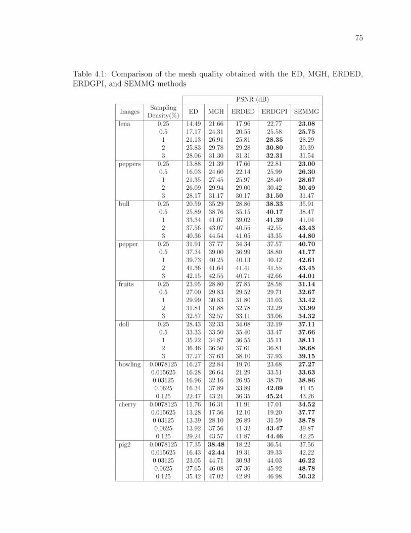
75

Table 4.1: Comparison of the mesh quality obtained with the ED, MGH, ERDED,ERDGPI, and SEMMG methods

PSNR (dB)

ImagesSampling

Density(%)ED MGH ERDED ERDGPI SEMMG

lena 0.25 14.49 21.66 17.96 22.77 23.080.5 17.17 24.31 20.55 25.58 25.751 21.13 26.91 25.81 28.35 28.292 25.83 29.78 29.28 30.80 30.393 28.06 31.30 31.31 32.31 31.54

peppers 0.25 13.88 21.39 17.66 22.81 23.000.5 16.03 24.60 22.14 25.99 26.301 21.35 27.45 25.97 28.40 28.672 26.09 29.94 29.00 30.42 30.493 28.17 31.17 30.17 31.50 31.47

bull 0.25 20.59 35.29 28.86 38.33 35.910.5 25.89 38.76 35.15 40.17 38.471 33.34 41.07 39.02 41.39 41.042 37.56 43.07 40.55 42.55 43.433 40.36 44.54 41.05 43.35 44.80

pepper 0.25 31.91 37.77 34.34 37.57 40.700.5 37.34 39.00 36.99 38.80 41.771 39.73 40.25 40.13 40.42 42.612 41.36 41.64 41.41 41.55 43.453 42.15 42.55 40.71 42.66 44.01

fruits 0.25 23.95 28.80 27.85 28.58 31.140.5 27.00 29.83 29.52 29.71 32.671 29.99 30.83 31.80 31.03 33.422 31.81 31.88 32.78 32.29 33.993 32.57 32.57 33.11 33.06 34.32

doll 0.25 28.43 32.33 34.08 32.19 37.110.5 33.33 33.50 35.40 33.47 37.661 35.22 34.87 36.55 35.11 38.112 36.46 36.50 37.61 36.81 38.683 37.27 37.63 38.10 37.93 39.15

bowling 0.0078125 16.27 22.84 19.70 23.68 27.270.015625 16.28 26.64 21.29 33.51 33.630.03125 16.96 32.16 26.95 38.70 38.860.0625 16.34 37.89 33.89 42.09 41.450.125 22.47 43.21 36.35 45.24 43.26

cherry 0.0078125 11.76 16.31 11.91 17.01 34.520.015625 13.28 17.56 12.10 19.20 37.770.03125 13.39 28.10 26.89 31.59 38.780.0625 13.92 37.56 41.32 43.47 39.870.125 29.24 43.57 41.87 44.46 42.25

pig2 0.0078125 17.35 38.48 18.22 36.54 37.560.015625 16.43 42.44 19.31 39.33 42.220.03125 23.05 44.71 30.93 44.03 46.220.0625 27.65 46.08 37.36 45.92 48.780.125 35.42 47.02 42.89 46.98 50.32

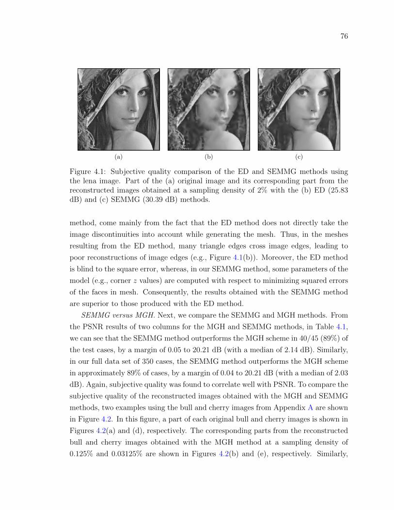
76

(a) (b) (c)

Figure 4.1: Subjective quality comparison of the ED and SEMMG methods usingthe lena image. Part of the (a) original image and its corresponding part from thereconstructed images obtained at a sampling density of 2% with the (b) ED (25.83dB) and (c) SEMMG (30.39 dB) methods.

method, come mainly from the fact that the ED method does not directly take the

image discontinuities into account while generating the mesh. Thus, in the meshes

resulting from the ED method, many triangle edges cross image edges, leading to

poor reconstructions of image edges (e.g., Figure 4.1(b)). Moreover, the ED method

is blind to the square error, whereas, in our SEMMG method, some parameters of the

model (e.g., corner z values) are computed with respect to minimizing squared errors

of the faces in mesh. Consequently, the results obtained with the SEMMG method

are superior to those produced with the ED method.

SEMMG versus MGH. Next, we compare the SEMMG and MGH methods. From

the PSNR results of two columns for the MGH and SEMMG methods, in Table 4.1,

we can see that the SEMMG method outperforms the MGH scheme in 40/45 (89%) of

the test cases, by a margin of 0.05 to 20.21 dB (with a median of 2.14 dB). Similarly,

in our full data set of 350 cases, the SEMMG method outperforms the MGH scheme

in approximately 89% of cases, by a margin of 0.04 to 20.21 dB (with a median of 2.03

dB). Again, subjective quality was found to correlate well with PSNR. To compare the

subjective quality of the reconstructed images obtained with the MGH and SEMMG

methods, two examples using the bull and cherry images from Appendix A are shown

in Figure 4.2. In this figure, a part of each original bull and cherry images is shown in

Figures 4.2(a) and (d), respectively. The corresponding parts from the reconstructed

bull and cherry images obtained with the MGH method at a sampling density of

0.125% and 0.03125% are shown in Figures 4.2(b) and (e), respectively. Similarly,

77

(a) (b) (c)

(d) (e) (f)

Figure 4.2: Subjective quality comparison of the MGH and SEMMG methods. Partof the original images of (a) bull and (d) cherry. The reconstructed images of bullobtained at a sampling density of 0.125% with the (b) MGH (30.74 dB) and (c)SEMMG (34.10 dB) methods. The reconstructed images of cherry obtained at asampling density of 0.03125% with the (e) MGH (28.10 dB) and (f) SEMMG (38.78dB) methods.

the same parts from the reconstructed bull and cherry images obtained with the

SEMMG method at a same sampling density of 0.125% and 0.03125% are shown in

Figures 4.2(c) and (f), respectively. As can be seen from Figure 4.2, the reconstructed

images obtained by the SEMMG method in Figures 4.2(c) and (f) have significantly

better qualities than those produced by the MGH method shown in Figures 4.2(b)

and (e), respectively. These improvements are mainly due to the fact that the MGH

method does not take any image-edge information into account. Thus, the MGH

method results in meshes, where the triangle edges cross the image edges, causing

high distortions around edges.

SEMMG versus ERDED. Now, we compare the SEMMG and ERDED methods.

From the PSNR results of two columns for the ERDED and SEMMG methods in

Table 4.1, we can see that the SEMMG method outperforms the ERDED scheme in

44/45 (98%) of the test cases, by a margin of 0.22 to 25.66 dB (with a median of 3.31

78

dB). Similarly, in our full data set of 350 cases, the SEMMG method outperforms the

ERDED scheme in approximately 99% of cases, by a margin of 0.05 to 26.30 dB (with

a median of 3.67 dB). The subjective quality was also found to correlate well with

PSNR. To compare the subjective quality of the reconstructed images obtained with

the ERDED and SEMMG methods, two examples using the pig2 and doll images

from Appendix A are shown in Figure 4.3. In this figure, a part of each original pig2

and doll images is shown in Figures 4.3(a) and (d), respectively. The corresponding

parts from the reconstructed pig2 and doll images obtained with the ERDED method

are shown in Figures 4.3(b) and (e), respectively. Similarly, the same parts from the

reconstructed pig2 and doll images obtained with the SEMMG method are shown in

Figures 4.3(c) and (f), respectively. As can be seen from Figure 4.3, the reconstructed

images obtained by the SEMMG method in Figures 4.3(c) and (f) obviously have

better qualities than those produced by the ERDED method shown in Figures 4.3(b)

and (e), respectively.

The significant improvements of the SEMMG method over the ERDED scheme

can be justified as follows. On one hand, the ERDED method (unlike the ED method)

takes image-edge information into account (as explained in Section 2.9) and is able

to preserve the image edges. This property of the ERDED method helps to prevent

triangle edges from crossing the image edges, leading to better image reconstructions

than the ED method. On the other hand, the other drawback of the ED method (as

explained previously) still exists in the ERDED method. Similar to the ED scheme,

the ERDED method still does not take the squared error into account when selecting

the non-edge points, leading to the reconstruction errors, of which examples shown in

Figures 4.3(b) and (e). The SEMMG method, however, uses a more effective criterion

to select the non-edge points which considers the squared errors of faces and improves

the mesh quality, such as the examples shown in Figures 4.3(c) and (f).

SEMMG versus ERDGPI. Finally, we compare the SEMMG and ERDGPI meth-

ods. From the PSNR results of two columns for the ERDGPI and SEMMG methods,

in Table 4.1, we can see that the SEMMG method outperforms the ERDGPI scheme

in 34/45 (76%) of the test cases, by a margin of 0.06 to 18.56 dB (with a median of

2.05 dB). Similarly, in our full data set of 350 cases, the SEMMG method outperforms

the ERDGPI scheme in approximately 85% of cases, by a margin of 0.02 to 24.72 dB

(with a median of 1.60 dB).

Closer inspection of the PSNR results obtained from the ERDGPI and SEMMG

methods, in Table 4.1, show that the ERDGPI method can produce comparable, and

79

(a) (b) (c)

(d) (e) (f)

Figure 4.3: Subjective quality comparison of the ERDED and SEMMG methods.Part of the original images of (a) pig2 and (d) doll. The reconstructed images ofpig2 obtained at a sampling density of 0.03125% with the (b) ERDED (30.93 dB)and (c) SEMMG (46.22 dB) methods. The reconstructed images of doll obtained ata sampling density of 0.25% with the (e) ERDED (34.08 dB) and (f) SEMMG (37.11dB) methods.

sometimes better, mesh qualities in the case of the smaller images (e.g., lena, peppers,

and bull). This is because the ERDGPI method (as we recall from Section 2.9) uses a

high-resolution image grid to locate the edges with half-pixel accuracy. Such a more

accurate edge localization is sometimes more beneficial in the case of the smaller

images and can lead to meshes with higher qualities. In the case of the larger images

in Table 4.1 (e.g., fruits, doll, and pig2), however, the SEMMG method clearly beats

the ERDGPI method because employing such an edge detector with higher accuracy

is not as advantageous as it was for smaller images.

In order to compare the subjective quality of the reconstructed images obtained

with the SEMMG and ERDGPI methods, three examples using the doll, pepper,

and fruits images from Appendix A are presented in Figure 4.4. In this figure, a

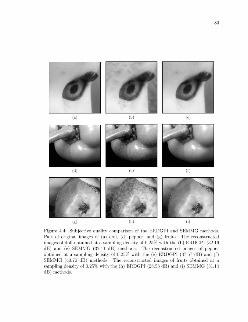
80

(a) (b) (c)

(d) (e) (f)

(g) (h) (i)

Figure 4.4: Subjective quality comparison of the ERDGPI and SEMMG methods.Part of original images of (a) doll, (d) pepper, and (g) fruits. The reconstructedimages of doll obtained at a sampling density of 0.25% with the (b) ERDGPI (32.19dB) and (c) SEMMG (37.11 dB) methods. The reconstructed images of pepperobtained at a sampling density of 0.25% with the (e) ERDGPI (37.57 dB) and (f)SEMMG (40.70 dB) methods. The reconstructed images of fruits obtained at asampling density of 0.25% with the (h) ERDGPI (28.58 dB) and (i) SEMMG (31.14dB) methods.

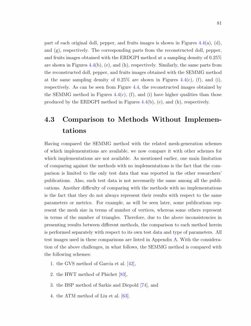
81

part of each original doll, pepper, and fruits images is shown in Figures 4.4(a), (d),

and (g), respectively. The corresponding parts from the reconstructed doll, pepper,

and fruits images obtained with the ERDGPI method at a sampling density of 0.25%

are shown in Figures 4.4(b), (e), and (h), respectively. Similarly, the same parts from

the reconstructed doll, pepper, and fruits images obtained with the SEMMG method

at the same sampling density of 0.25% are shown in Figures 4.4(c), (f), and (i),

respectively. As can be seen from Figure 4.4, the reconstructed images obtained by

the SEMMG method in Figures 4.4(c), (f), and (i) have higher qualities than those

produced by the ERDGPI method in Figures 4.4(b), (e), and (h), respectively.

4.3 Comparison to Methods Without Implemen-

tations

Having compared the SEMMG method with the related mesh-generation schemes

of which implementations are available, we now compare it with other schemes for

which implementations are not available. As mentioned earlier, one main limitation

of comparing against the methods with no implementations is the fact that the com-

parison is limited to the only test data that was reported in the other researchers’

publications. Also, such test data is not necessarily the same among all the publi-

cations. Another difficulty of comparing with the methods with no implementations

is the fact that they do not always represent their results with respect to the same

parameters or metrics. For example, as will be seen later, some publications rep-

resent the mesh size in terms of number of vertices, whereas some others represent

in terms of the number of triangles. Therefore, due to the above inconsistencies in

presenting results between different methods, the comparison to each method herein

is performed separately with respect to its own test data and type of parameters. All

test images used in these comparisons are listed in Appendix A. With the considera-

tion of the above challenges, in what follows, the SEMMG method is compared with

the following schemes:

1. the GVS method of Garcia et al. [42],

2. the HWT method of Phichet [83],

3. the BSP method of Sarkis and Diepold [74], and

4. the ATM method of Liu et al. [63].

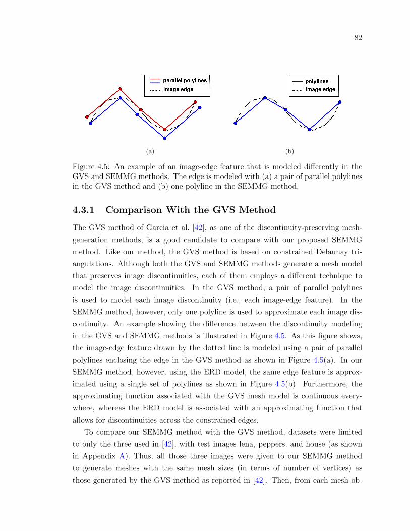
82

(a) (b)

Figure 4.5: An example of an image-edge feature that is modeled differently in theGVS and SEMMG methods. The edge is modeled with (a) a pair of parallel polylinesin the GVS method and (b) one polyline in the SEMMG method.

4.3.1 Comparison With the GVS Method

The GVS method of Garcia et al. [42], as one of the discontinuity-preserving mesh-

generation methods, is a good candidate to compare with our proposed SEMMG

method. Like our method, the GVS method is based on constrained Delaunay tri-

angulations. Although both the GVS and SEMMG methods generate a mesh model

that preserves image discontinuities, each of them employs a different technique to

model the image discontinuities. In the GVS method, a pair of parallel polylines

is used to model each image discontinuity (i.e., each image-edge feature). In the

SEMMG method, however, only one polyline is used to approximate each image dis-

continuity. An example showing the difference between the discontinuity modeling

in the GVS and SEMMG methods is illustrated in Figure 4.5. As this figure shows,

the image-edge feature drawn by the dotted line is modeled using a pair of parallel

polylines enclosing the edge in the GVS method as shown in Figure 4.5(a). In our

SEMMG method, however, using the ERD model, the same edge feature is approx-

imated using a single set of polylines as shown in Figure 4.5(b). Furthermore, the

approximating function associated with the GVS mesh model is continuous every-

where, whereas the ERD model is associated with an approximating function that

allows for discontinuities across the constrained edges.

To compare our SEMMG method with the GVS method, datasets were limited

to only the three used in [42], with test images lena, peppers, and house (as shown

in Appendix A). Thus, all those three images were given to our SEMMG method

to generate meshes with the same mesh sizes (in terms of number of vertices) as

those generated by the GVS method as reported in [42]. Then, from each mesh ob-

83

Table 4.2: Comparison of the mesh quality obtained with the GVS and SEMMGmethods (with the same mesh size)

PSNR (dB)Image Number of vertices GVS SEMMG

lena 7492 28.30 31.27peppers 7224 26.48 31.09house 1649 27.62 31.55

tained from the SEMMG method, a reconstructed image was produced. Next, the

mean-squared error between the original and reconstructed images was measured and

compared with the mean-squared error reported in [42]. The mean-squared errors are

represented in terms of the PSNR herein. Since in [42] only one sampling density per

each test image was used, our comparison is limited to only three test cases as listed

in Table 4.2, with the best result in each case being highlighted in bold. As can be

seen from Table 4.2, with the same mesh size (i.e., number of vertices), the SEMMG

method clearly outperforms the GVS method by producing better reconstructed im-

ages with the PSNR improvements of approximately 3.0, 4.6, and 3.9 dB for the lena,

peppers, and house images, respectively.

Furthermore, the sizes of the meshes obtained with the SEMMG and GVS methods

were also compared. For this purpose, our SEMMG method was used to generate

meshes with the same mean-squared error as reported in [42] for the GVS method.

Then, the sizes of the meshes (in terms of the number of vertices) obtained from

the SEMMG method were compared to those reported in [42] for the GVS method.

The results of this size comparison for all three test cases are presented in Table 4.3,

with the best result in each case being highlighted in bold. As can be seen from

Table 4.3, for a given PSNR, the SEMMG method generates much smaller meshes

with approximately 65%, 80%, and 78% fewer vertices than the GVS method in the

case of the lena, peppers, and house images, respectively. Consequently, as both the

mesh-quality and size comparisons presented in Tables 4.2 and 4.3 show, our SEMMG

method is superior to the GVS method by producing meshes of higher quality with

significantly fewer vertices.

4.3.2 Comparison With the HWT Method

The next method that is compared with our SEMMG method is the hybrid wavelet-

based triangulation (HWT) method of Phichet in [83]. This method is discontinuity

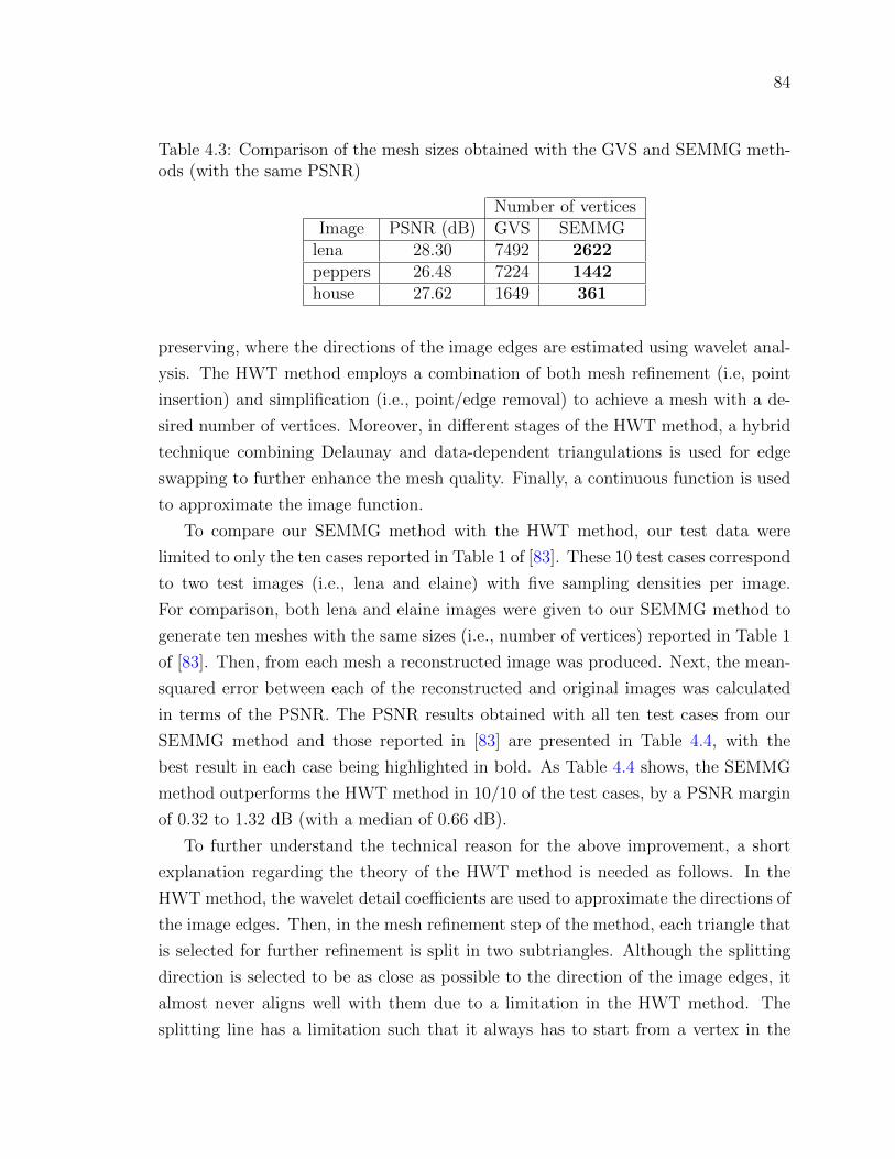
84

Table 4.3: Comparison of the mesh sizes obtained with the GVS and SEMMG meth-ods (with the same PSNR)

Number of verticesImage PSNR (dB) GVS SEMMG

lena 28.30 7492 2622peppers 26.48 7224 1442house 27.62 1649 361

preserving, where the directions of the image edges are estimated using wavelet anal-

ysis. The HWT method employs a combination of both mesh refinement (i.e, point

insertion) and simplification (i.e., point/edge removal) to achieve a mesh with a de-

sired number of vertices. Moreover, in different stages of the HWT method, a hybrid

technique combining Delaunay and data-dependent triangulations is used for edge

swapping to further enhance the mesh quality. Finally, a continuous function is used

to approximate the image function.

To compare our SEMMG method with the HWT method, our test data were

limited to only the ten cases reported in Table 1 of [83]. These 10 test cases correspond

to two test images (i.e., lena and elaine) with five sampling densities per image.

For comparison, both lena and elaine images were given to our SEMMG method to

generate ten meshes with the same sizes (i.e., number of vertices) reported in Table 1

of [83]. Then, from each mesh a reconstructed image was produced. Next, the mean-

squared error between each of the reconstructed and original images was calculated

in terms of the PSNR. The PSNR results obtained with all ten test cases from our

SEMMG method and those reported in [83] are presented in Table 4.4, with the

best result in each case being highlighted in bold. As Table 4.4 shows, the SEMMG

method outperforms the HWT method in 10/10 of the test cases, by a PSNR margin

of 0.32 to 1.32 dB (with a median of 0.66 dB).

To further understand the technical reason for the above improvement, a short

explanation regarding the theory of the HWT method is needed as follows. In the

HWT method, the wavelet detail coefficients are used to approximate the directions of

the image edges. Then, in the mesh refinement step of the method, each triangle that

is selected for further refinement is split in two subtriangles. Although the splitting

direction is selected to be as close as possible to the direction of the image edges, it

almost never aligns well with them due to a limitation in the HWT method. The

splitting line has a limitation such that it always has to start from a vertex in the

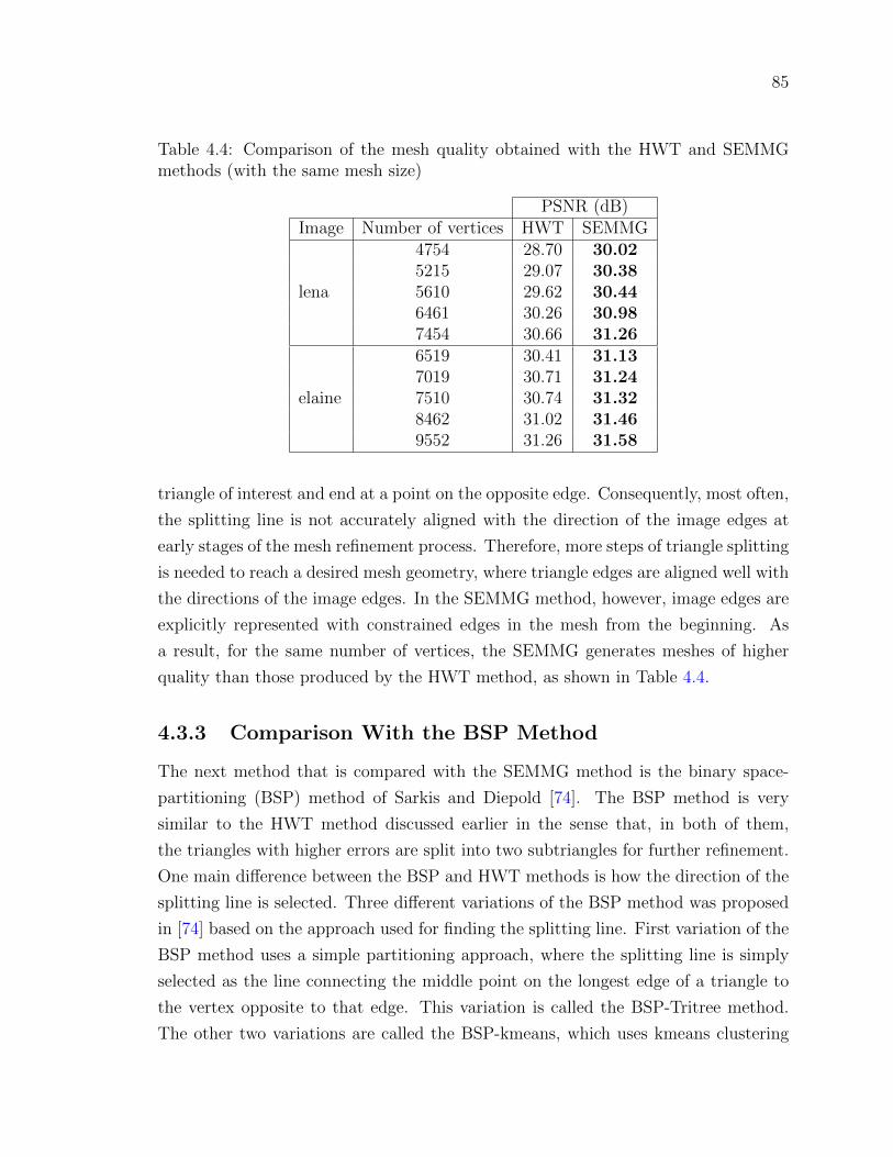
85

Table 4.4: Comparison of the mesh quality obtained with the HWT and SEMMGmethods (with the same mesh size)

PSNR (dB)Image Number of vertices HWT SEMMG

lena

4754 28.70 30.025215 29.07 30.385610 29.62 30.446461 30.26 30.987454 30.66 31.26

elaine

6519 30.41 31.137019 30.71 31.247510 30.74 31.328462 31.02 31.469552 31.26 31.58

triangle of interest and end at a point on the opposite edge. Consequently, most often,

the splitting line is not accurately aligned with the direction of the image edges at

early stages of the mesh refinement process. Therefore, more steps of triangle splitting

is needed to reach a desired mesh geometry, where triangle edges are aligned well with

the directions of the image edges. In the SEMMG method, however, image edges are

explicitly represented with constrained edges in the mesh from the beginning. As

a result, for the same number of vertices, the SEMMG generates meshes of higher

quality than those produced by the HWT method, as shown in Table 4.4.

4.3.3 Comparison With the BSP Method

The next method that is compared with the SEMMG method is the binary space-

partitioning (BSP) method of Sarkis and Diepold [74]. The BSP method is very

similar to the HWT method discussed earlier in the sense that, in both of them,

the triangles with higher errors are split into two subtriangles for further refinement.

One main difference between the BSP and HWT methods is how the direction of the

splitting line is selected. Three different variations of the BSP method was proposed

in [74] based on the approach used for finding the splitting line. First variation of the

BSP method uses a simple partitioning approach, where the splitting line is simply

selected as the line connecting the middle point on the longest edge of a triangle to

the vertex opposite to that edge. This variation is called the BSP-Tritree method.

The other two variations are called the BSP-kmeans, which uses kmeans clustering

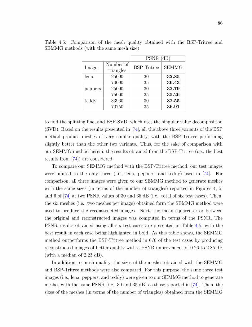
86

Table 4.5: Comparison of the mesh quality obtained with the BSP-Tritree andSEMMG methods (with the same mesh size)

PSNR (dB)

ImageNumber oftriangles

BSP-Tritree SEMMG

lena 25000 30 32.8570000 35 36.43

peppers 25000 30 32.7975000 35 35.26

teddy 33960 30 32.5570750 35 36.91

to find the splitting line, and BSP-SVD, which uses the singular value decomposition

(SVD). Based on the results presented in [74], all the above three variants of the BSP

method produce meshes of very similar quality, with the BSP-Tritree performing

slightly better than the other two variants. Thus, for the sake of comparison with

our SEMMG method herein, the results obtained from the BSP-Tritree (i.e., the best

results from [74]) are considered.

To compare our SEMMG method with the BSP-Tritree method, our test images

were limited to the only three (i.e., lena, peppers, and teddy) used in [74]. For

comparison, all three images were given to our SEMMG method to generate meshes

with the same sizes (in terms of the number of triangles) reported in Figures 4, 5,

and 6 of [74] at two PSNR values of 30 and 35 dB (i.e., total of six test cases). Then,

the six meshes (i.e., two meshes per image) obtained form the SEMMG method were

used to produce the reconstructed images. Next, the mean squared-error between

the original and reconstructed images was computed in terms of the PSNR. The

PSNR results obtained using all six test cases are presented in Table 4.5, with the

best result in each case being highlighted in bold. As this table shows, the SEMMG

method outperforms the BSP-Tritree method in 6/6 of the test cases by producing

reconstructed images of better quality with a PSNR improvement of 0.26 to 2.85 dB

(with a median of 2.23 dB).

In addition to mesh quality, the sizes of the meshes obtained with the SEMMG

and BSP-Tritree methods were also compared. For this purpose, the same three test

images (i.e., lena, peppers, and teddy) were given to our SEMMG method to generate

meshes with the same PSNR (i.e., 30 and 35 dB) as those reported in [74]. Then, the

sizes of the meshes (in terms of the number of triangles) obtained from the SEMMG

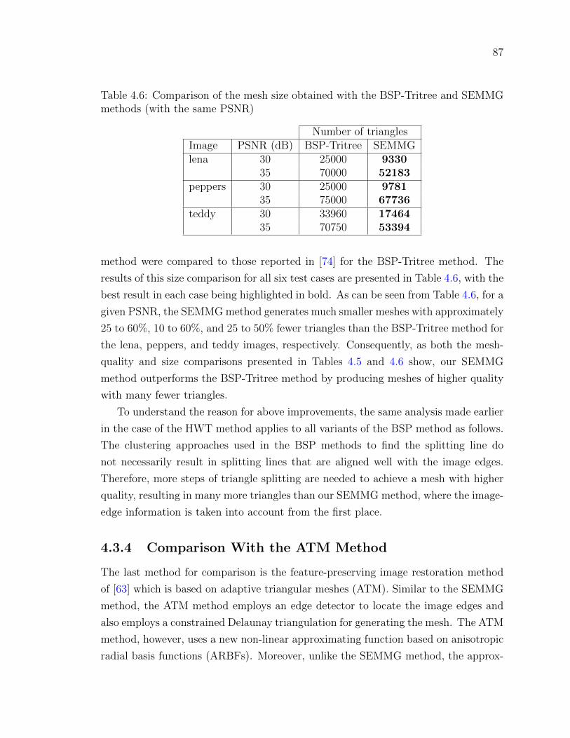
87

Table 4.6: Comparison of the mesh size obtained with the BSP-Tritree and SEMMGmethods (with the same PSNR)

Number of trianglesImage PSNR (dB) BSP-Tritree SEMMGlena 30 25000 9330

35 70000 52183peppers 30 25000 9781

35 75000 67736teddy 30 33960 17464

35 70750 53394

method were compared to those reported in [74] for the BSP-Tritree method. The

results of this size comparison for all six test cases are presented in Table 4.6, with the

best result in each case being highlighted in bold. As can be seen from Table 4.6, for a

given PSNR, the SEMMG method generates much smaller meshes with approximately

25 to 60%, 10 to 60%, and 25 to 50% fewer triangles than the BSP-Tritree method for

the lena, peppers, and teddy images, respectively. Consequently, as both the mesh-

quality and size comparisons presented in Tables 4.5 and 4.6 show, our SEMMG

method outperforms the BSP-Tritree method by producing meshes of higher quality

with many fewer triangles.

To understand the reason for above improvements, the same analysis made earlier

in the case of the HWT method applies to all variants of the BSP method as follows.

The clustering approaches used in the BSP methods to find the splitting line do

not necessarily result in splitting lines that are aligned well with the image edges.

Therefore, more steps of triangle splitting are needed to achieve a mesh with higher

quality, resulting in many more triangles than our SEMMG method, where the image-

edge information is taken into account from the first place.

4.3.4 Comparison With the ATM Method

The last method for comparison is the feature-preserving image restoration method

of [63] which is based on adaptive triangular meshes (ATM). Similar to the SEMMG

method, the ATM method employs an edge detector to locate the image edges and

also employs a constrained Delaunay triangulation for generating the mesh. The ATM

method, however, uses a new non-linear approximating function based on anisotropic

radial basis functions (ARBFs). Moreover, unlike the SEMMG method, the approx-

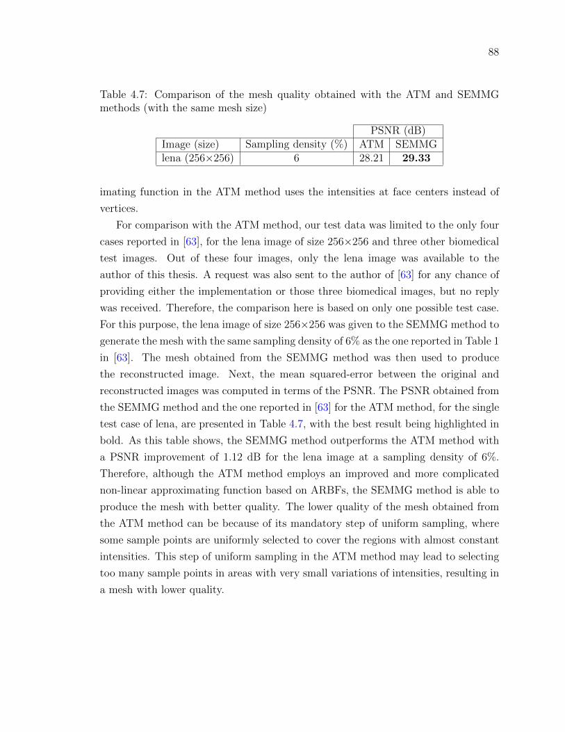
88

Table 4.7: Comparison of the mesh quality obtained with the ATM and SEMMGmethods (with the same mesh size)

PSNR (dB)Image (size) Sampling density (%) ATM SEMMGlena (256×256) 6 28.21 29.33

imating function in the ATM method uses the intensities at face centers instead of

vertices.

For comparison with the ATM method, our test data was limited to the only four

cases reported in [63], for the lena image of size 256×256 and three other biomedical

test images. Out of these four images, only the lena image was available to the

author of this thesis. A request was also sent to the author of [63] for any chance of

providing either the implementation or those three biomedical images, but no reply

was received. Therefore, the comparison here is based on only one possible test case.

For this purpose, the lena image of size 256×256 was given to the SEMMG method to

generate the mesh with the same sampling density of 6% as the one reported in Table 1

in [63]. The mesh obtained from the SEMMG method was then used to produce

the reconstructed image. Next, the mean squared-error between the original and

reconstructed images was computed in terms of the PSNR. The PSNR obtained from

the SEMMG method and the one reported in [63] for the ATM method, for the single

test case of lena, are presented in Table 4.7, with the best result being highlighted in

bold. As this table shows, the SEMMG method outperforms the ATM method with

a PSNR improvement of 1.12 dB for the lena image at a sampling density of 6%.

Therefore, although the ATM method employs an improved and more complicated

non-linear approximating function based on ARBFs, the SEMMG method is able to

produce the mesh with better quality. The lower quality of the mesh obtained from

the ATM method can be because of its mandatory step of uniform sampling, where

some sample points are uniformly selected to cover the regions with almost constant

intensities. This step of uniform sampling in the ATM method may lead to selecting

too many sample points in areas with very small variations of intensities, resulting in

a mesh with lower quality.

89

Chapter 5

Proposed MIS Method and Its

Development

5.1 Overview

In this chapter, a new mesh-based approach for image scaling, called the MIS method,

is proposed for grayscale images that are approximately piecewise-smooth, with no

(or minimal) textures or patterns. The inputs to the proposed MIS method are a

low-resolution raster image and an integer scaling factor and the output is a high-

resolution raster image. In what follows, we first explain how the MIS method was

developed. For this purpose, the performance of our SEMMG method, which was

previously proposed for image representation in Chapter 3, is examined in the ap-

plication of image scaling. Having the knowledge that the SEMMG method solves

a totally different problem than image scaling, we would not expect it to perform

well for this purpose without modification. For example, the polylines used in the

SEMMG method to approximate the edges would obviously look rough and jagged

if they are scaled. We also would not want to prematurely discard the SEMMG

method. Thus, we study how it performs for image scaling in order to better under-

stand potential shortcomings for this application. Through this study, different key

techniques are devised to address the shortcomings. By applying these techniques,

the mesh-generation method under analysis progressively evolves to a new one called

the mesh-based image scaling mesh-generation (MISMG) method that can be effec-

tively used for image scaling. As part of this progression, three intermediate methods,

which are called MISMG0, MISMG1, and MISMG2, are also introduced, where each

90

method has an added modification to its predecessor. Aside from the mesh genera-

tion, the model rasterization is also analyzed and a subdivision-based approach for

producing smoother edge contours and image functions is developed. Finally, the

MISMG mesh-generation method is combined with a scaling transformation and the

subdivision-based model-rasterization algorithm, yielding the proposed MIS method.

5.2 Development of MIS Method

We now present how the proposed MIS method was gradually developed. The MIS

method is designed to solve the image scaling problem, where a low-resolution raster

image and an integer scaling factor are the inputs and a high-resolution raster im-

age is the output. The MIS method includes three main stages (in order): 1) mesh

generation, 2) mesh transformation, and 3) model rasterization. In stage 1, a mesh-

generation method is required to produce a mesh model from the input raster image

sampled on a low-resolution grid. Then, in stage 2, an affine transformation is applied

to the vertices of of the mesh. Finally, in stage 3, the scaled image is reconstructed

by rasterizing the (scaled) mesh model to a high-resolution grid. Although, in the

stage 2 above, any combination of affine transformations, such as scaling, rotation,

and translation, can be used, this work focuses on the image scaling application. For

this purpose, in stage 2, all vertices in the mesh are scaled with respect to k. Once

a mesh is generated in stage 1, the process of scaling the vertices and rasterizing the

model is almost trivial. Therefore, one may think that any mesh-generation method

that is effective for image representation can also be effective in image scaling if used

in the stage 1 above. Image representation and scaling, however, are two different

problems. Therefore, in this section, we show that, for a mesh-generation method that

is initially designed for image representation (at native resolution) to be effective in

image scaling, several modifications are required to adapt the method for this specific

application. Consequently, another mesh-generation method is required to produce a

model with the parameters effectively selected for image scaling. Moreover, we show

that, in stage 3 above, a simple model rasterization is not sufficiently effective to pro-

duce scaled images of good qualities. Therefore, a more effective model rasterization

is also required.

For developing the MIS method, we use the SEMMG method, which is proposed

in Section 3.3 for mesh generation, in stage 1 of the above image scaling process. As

stated earlier, although we know that the SEMMG method is not designed to solve

91

the image-scaling problem, it is only used (as a guide) to identify potential areas for

improvement. The general scaling procedure that is used in the subsequent sections

is as follows. An input low-resolution raster image φl defined on an integer lattice of

width W and height H is given to the SEMMG method (or any other intermediate

method that is introduced later) and the ERD mesh model is generated. Given an

integer scaling factor of k > 1, the vertices of the ERD model are first scaled with

respect to k, and then, the model is rasterized to an integer lattice of width kW

and height kH, resulting in the high-resolution raster image φh as a scaled version

of φl. As we recall from Section 2.9, the ERD mesh model is rasterized using an

approximating function that is piecewise linear and interpolates the values at original

sample points.

In what follows, the SEMMG method is used in the scaling procedure described

above and various approaches in the method are revisited to identify shortcomings

that create artifacts in the scaled images. For this purpose, all the figures presented

in the this section are obtained without using any antialiasing (i.e., supersampling)

technique, to focus only on the effects generated by image scaling. Then, based on the

root causes of each type of artifacts, specific solutions are recommended to gradually

adapt the mesh-generation method for the image scaling application. Through this

progression, three intermediate mesh-generation methods, which are called MISMG0,

MISMG1, and MISMG2, are introduced, where each method has an additional mod-

ification to its predecessor. All these modifications will later be combined to form

the MISMG mesh-generation method, which is specifically designed for image scal-

ing and is later used in the proposed MIS method. In addition to examining the

performance of the mesh generation in image scaling, the model rasterization is also

revisited and a subdivision-based approach for producing smoother edge contours and

image functions is developed.

5.2.1 Wedge-Value Calculation Revisited

The first approach that is revisited here is the one used for calculating the wedge

values. In-depth investigations on several scaled images obtained by the SEMMG

method (using the scaling procedure explained before) revealed that some distortions

and artifacts exist near some edges in the scaled image. More careful analyses of the

scaled images (as will be seen shortly) showed that most of these artifacts are related

to the optimization-based approach used in the SEMMG method for computing wedge

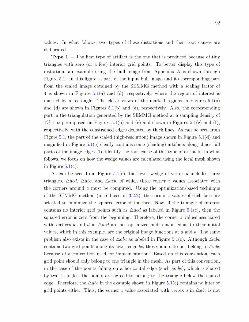
92

values. In what follows, two types of these distortions and their root causes are

elaborated.

Type 1 − The first type of artifact is the one that is produced because of tiny

triangles with zero (or a few) interior grid points. To better display this type of

distortion, an example using the bull image from Appendix A is shown through

Figure 5.1. In this figure, a part of the input bull image and its corresponding part

from the scaled image obtained by the SEMMG method with a scaling factor of

4 is shown in Figures 5.1(a) and (d), respectively, where the region of interest is

marked by a rectangle. The closer views of the marked regions in Figures 5.1(a)

and (d) are shown in Figures 5.1(b) and (e), respectively. Also, the corresponding

part in the triangulation generated by the SEMMG method at a sampling density of

1% is superimposed on Figures 5.1(b) and (e) and shown in Figures 5.1(c) and (f),

respectively, with the constrained edges denoted by thick lines. As can be seen from

Figure 5.1, the part of the scaled (high-resolution) image shown in Figure 5.1(d) and

magnified in Figure 5.1(e) clearly contains some (shading) artifacts along almost all

parts of the image edges. To identify the root cause of this type of artifacts, in what

follows, we focus on how the wedge values are calculated using the local mesh shown

in Figure 5.1(c).

As can be seen from Figure 5.1(c), the lower wedge of vertex a includes three

triangles, 4acd, 4abc, and 4aeb, of which three corner z values associated with

the corners around a must be computed. Using the optimization-based technique

of the SEMMG method (introduced in 3.2.2), the corner z values of each face are

selected to minimize the squared error of the face. Now, if the triangle of interest

contains no interior grid points such as 4acd as labeled in Figure 5.1(c), then the

squared error is zero from the beginning. Therefore, the corner z values associated

with vertices a and d in 4acd are not optimized and remain equal to their initial

values, which in this example, are the original image functions at a and d. The same

problem also exists in the case of 4abc as labeled in Figure 5.1(c). Although 4abccontains two grid points along its lower edge bc, those points do not belong to 4abcbecause of a convention used for implementation. Based on this convention, each

grid point should only belong to one triangle in the mesh. As part of this convention,

in the case of the points falling on a horizontal edge (such as bc), which is shared

by two triangles, the points are agreed to belong to the triangle below the shared

edge. Therefore, the 4abc in the example shown in Figure 5.1(c) contains no interior

grid points either. Thus, the corner z value associated with vertex a in 4abc is not

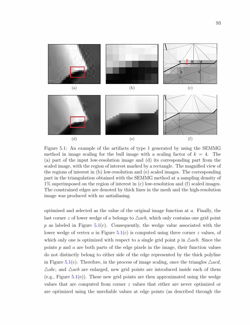
93

(a) (b) (c)

(d) (e) (f)

Figure 5.1: An example of the artifacts of type 1 generated by using the SEMMGmethod in image scaling for the bull image with a scaling factor of k = 4. The(a) part of the input low-resolution image and (d) its corresponding part from thescaled image, with the region of interest marked by a rectangle. The magnified view ofthe regions of interest in (b) low-resolution and (e) scaled images. The correspondingpart in the triangulation obtained with the SEMMG method at a sampling density of1% superimposed on the region of interest in (c) low-resolution and (f) scaled images.The constrained edges are denoted by thick lines in the mesh and the high-resolutionimage was produced with no antialiasing.

optimized and selected as the value of the original image function at a. Finally, the

last corner z of lower wedge of a belongs to 4aeb, which only contains one grid point

p as labeled in Figure 5.1(c). Consequently, the wedge value associated with the

lower wedge of vertex a in Figure 5.1(c) is computed using three corner z values, of

which only one is optimized with respect to a single grid point p in 4aeb. Since the

points p and a are both parts of the edge pixels in the image, their function values

do not distinctly belong to either side of the edge represented by the thick polyline

in Figure 5.1(c). Therefore, in the process of image scaling, once the triangles 4acd,

4abc, and 4aeb are enlarged, new grid points are introduced inside each of them

(e.g., Figure 5.1(e)). These new grid points are then approximated using the wedge

values that are computed from corner z values that either are never optimized or

are optimized using the unreliable values at edge points (as described through the

94

(a) (b) (c)

(d) (e) (f)

Figure 5.2: An example of the artifacts of type 2 generated by using the SEMMGmethod in image scaling for the bull image with a scaling factor of k = 4. The(a) part of the input low-resolution image and (d) its corresponding part from thescaled image, with the region of interest marked by a rectangle. The magnified view ofthe regions of interest in (b) low-resolution and (e) scaled images. The correspondingpart in the triangulation obtained with the SEMMG method at a sampling density of1% superimposed on the region of interest in (c) low-resolution and (f) scaled images.The constrained edges are denoted by thick lines in the mesh and the high-resolutionimage was produced with no antialiasing.

above example). Consequently, such artifacts (e.g., in Figures 5.1(d) and (e)) will be

generated near the reconstructed edges after scaling in the high-resolution image, as

a result of using improper wedge values.

Type 2 − The second type of artifact is the one produced because of the long/thin

triangles near the constrained edges in the mesh. To better display this type of

distortion, an example using the bull image from Appendix A is shown through

Figure 5.2. In this figure, a part of the input bull image and its corresponding part

from the scaled image obtained by the SEMMG method with a scaling factor of

4 is shown in Figures 5.2(a) and (d), respectively, where the region of interest is

marked by a rectangle. The closer views of the marked regions in Figures 5.2(a)

and (d) are shown in Figures 5.2(b) and (e), respectively. Also, the corresponding

part in the triangulation generated by the SEMMG method at a sampling density of

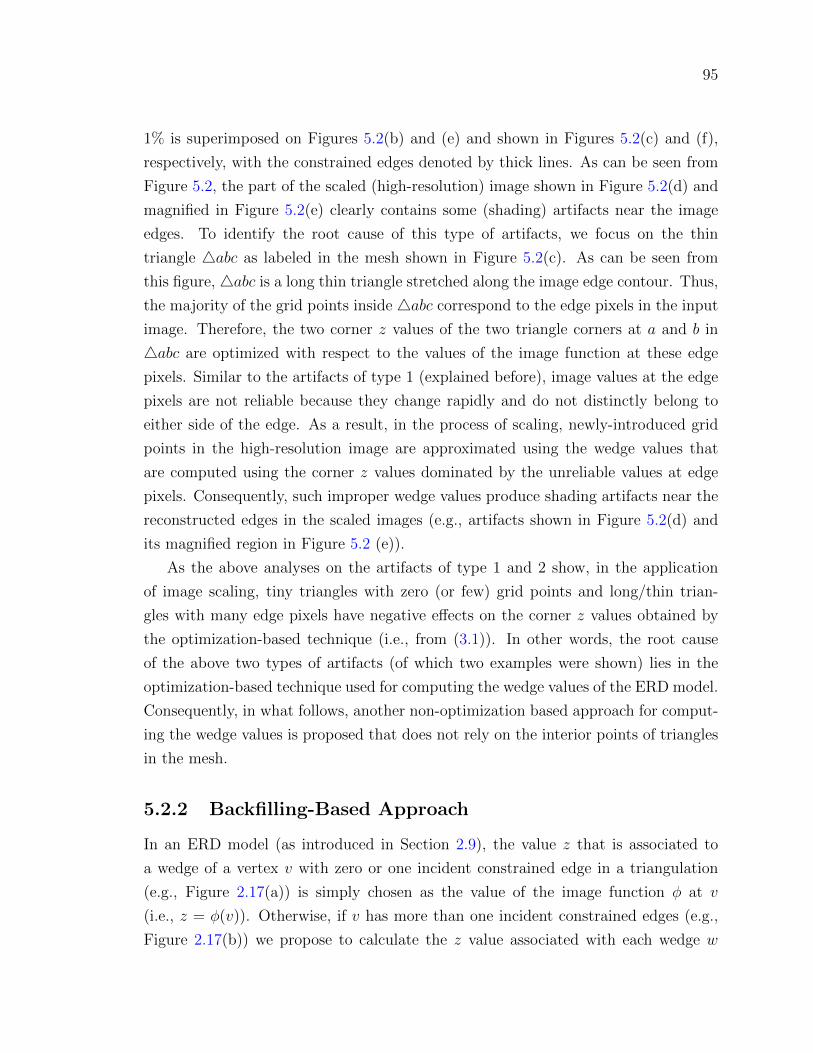
95

1% is superimposed on Figures 5.2(b) and (e) and shown in Figures 5.2(c) and (f),

respectively, with the constrained edges denoted by thick lines. As can be seen from

Figure 5.2, the part of the scaled (high-resolution) image shown in Figure 5.2(d) and

magnified in Figure 5.2(e) clearly contains some (shading) artifacts near the image

edges. To identify the root cause of this type of artifacts, we focus on the thin

triangle 4abc as labeled in the mesh shown in Figure 5.2(c). As can be seen from

this figure, 4abc is a long thin triangle stretched along the image edge contour. Thus,

the majority of the grid points inside 4abc correspond to the edge pixels in the input

image. Therefore, the two corner z values of the two triangle corners at a and b in

4abc are optimized with respect to the values of the image function at these edge

pixels. Similar to the artifacts of type 1 (explained before), image values at the edge

pixels are not reliable because they change rapidly and do not distinctly belong to

either side of the edge. As a result, in the process of scaling, newly-introduced grid

points in the high-resolution image are approximated using the wedge values that

are computed using the corner z values dominated by the unreliable values at edge

pixels. Consequently, such improper wedge values produce shading artifacts near the

reconstructed edges in the scaled images (e.g., artifacts shown in Figure 5.2(d) and

its magnified region in Figure 5.2 (e)).

As the above analyses on the artifacts of type 1 and 2 show, in the application

of image scaling, tiny triangles with zero (or few) grid points and long/thin trian-

gles with many edge pixels have negative effects on the corner z values obtained by

the optimization-based technique (i.e., from (3.1)). In other words, the root cause

of the above two types of artifacts (of which two examples were shown) lies in the

optimization-based technique used for computing the wedge values of the ERD model.

Consequently, in what follows, another non-optimization based approach for comput-

ing the wedge values is proposed that does not rely on the interior points of triangles

in the mesh.

5.2.2 Backfilling-Based Approach

In an ERD model (as introduced in Section 2.9), the value z that is associated to

a wedge of a vertex v with zero or one incident constrained edge in a triangulation

(e.g., Figure 2.17(a)) is simply chosen as the value of the image function φ at v

(i.e., z = φ(v)). Otherwise, if v has more than one incident constrained edges (e.g.,

Figure 2.17(b)) we propose to calculate the z value associated with each wedge w

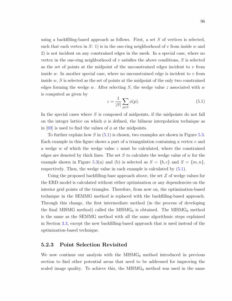
96

using a backfilling-based approach as follows. First, a set S of vertices is selected,

such that each vertex in S: 1) is in the one-ring neighborhood of v from inside w and

2) is not incident on any constrained edges in the mesh. In a special case, where no

vertex in the one-ring neighborhood of v satisfies the above conditions, S is selected

as the set of points at the midpoint of the unconstrained edges incident to v from

inside w. In another special case, where no unconstrained edge is incident to v from

inside w, S is selected as the set of points at the midpoint of the only two constrained

edges forming the wedge w. After selecting S, the wedge value z associated with w

is computed as given by

z =1

|S|∑p∈S

φ(p). (5.1)

In the special cases where S is composed of midpoints, if the midpoints do not fall

on the integer lattice on which φ is defined, the bilinear interpolation technique as

in [69] is used to find the values of φ at the midpoints.

To further explain how S in (5.1) is chosen, two examples are shown in Figure 5.3.

Each example in this figure shows a part of a triangulation containing a vertex v and

a wedge w of which the wedge value z must be calculated, where the constrained

edges are denoted by thick lines. The set S to calculate the wedge value of w for the

example shown in Figure 5.3(a) and (b) is selected as S = b, c and S = m,n,respectively. Then, the wedge value in each example is calculated by (5.1).

Using the proposed backfilling-base approach above, the set Z of wedge values for

the ERD model is calculated without either optimization or any dependencies on the

interior grid points of the triangles. Therefore, from now on, the optimization-based

technique in the SEMMG method is replaced with the backfilling-based approach.

Through this change, the first intermediate method (in the process of developing

the final MISMG method) called the MISMG0 is obtained. The MISMG0 method

is the same as the SEMMG method with all the same algorithmic steps explained

in Section 3.3, except the new backfilling-based approach that is used instead of the

optimization-based technique.

5.2.3 Point Selection Revisited

We now continue our analysis with the MISMG0 method introduced in previous

section to find other potential areas that need to be addressed for improving the

scaled image quality. To achieve this, the MISMG0 method was used in the same

97

(a) (b)

Figure 5.3: Two examples of the set S for calculating the wedge value associated withthe wedge w in the backfilling-based approach. The case (a) where S = b, c andcase (b) where S = m,n.

image scaling procedure previously explained and used for the SEMMG method.

Several investigations on different scaled images obtained by the MISMG0 method

revealed that some other type of shading artifacts are now generated near the image

edges. More analyses on the scaled images showed that these artifacts are related

to the point-selection approach used in the MISMG0 method. To better describe

this type of artifact, an example using the bull image from Appendix A is presented

in Figure 5.4. In this figure, a part of the input low-resolution image bull and its

corresponding part from the scaled image obtained by the MISMG0 method with a

scaling factor of 4 is shown in Figures 5.4(a) and (d), respectively, where a region of

interest is marked with a rectangle. The closer views of the regions of interest in the

low-resolution and high-resolution (i.e., scaled) images are shown in Figures 5.4(b)

and (e), respectively. Also, the corresponding part from the triangulation obtained

with the MISMG0 method at a sampling density of 4% is superimposed on the region

of interest in the low-resolution image and is shown in Figure 5.4(c), where constrained

edges are denoted as thick lines. As can be seen from Figure 5.4, the part of the scaled

image shown in Figure 5.4(d) and magnified in Figure 5.4(e) clearly contains some

(shading) artifacts near the image edges.

To identify the root cause of this type of artifact, we focus on the part of the

triangulation shown in Figure 5.4(c). As this figure shows, many vertices are located

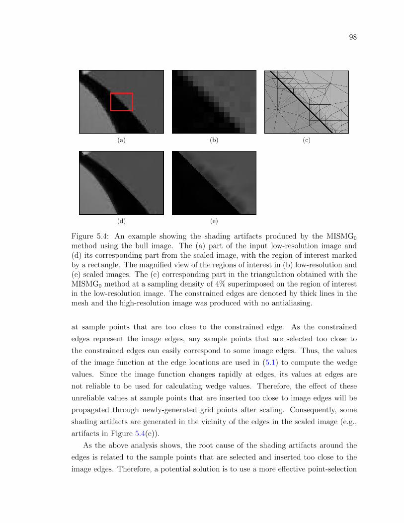
98

(a) (b) (c)

(d) (e)

Figure 5.4: An example showing the shading artifacts produced by the MISMG0

method using the bull image. The (a) part of the input low-resolution image and(d) its corresponding part from the scaled image, with the region of interest markedby a rectangle. The magnified view of the regions of interest in (b) low-resolution and(e) scaled images. The (c) corresponding part in the triangulation obtained with theMISMG0 method at a sampling density of 4% superimposed on the region of interestin the low-resolution image. The constrained edges are denoted by thick lines in themesh and the high-resolution image was produced with no antialiasing.

at sample points that are too close to the constrained edge. As the constrained

edges represent the image edges, any sample points that are selected too close to

the constrained edges can easily correspond to some image edges. Thus, the values

of the image function at the edge locations are used in (5.1) to compute the wedge

values. Since the image function changes rapidly at edges, its values at edges are

not reliable to be used for calculating wedge values. Therefore, the effect of these

unreliable values at sample points that are inserted too close to image edges will be

propagated through newly-generated grid points after scaling. Consequently, some

shading artifacts are generated in the vicinity of the edges in the scaled image (e.g.,

artifacts in Figure 5.4(e)).

As the above analysis shows, the root cause of the shading artifacts around the

edges is related to the sample points that are selected and inserted too close to the

image edges. Therefore, a potential solution is to use a more effective point-selection

99

approach, where the sample points that are too close to image edges are excluded

from being inserted into the mesh. To achieve this, in what follows, a modified

point-selection approach is proposed.

5.2.4 Modified Centroid-Based Approach

As mentioned earlier, the general algorithmic framework of the MISMG0 method

is the same as the one used in the SEMMG method (introduced in Section 3.3).

Therefore, in the mesh refinement process of the MISMG0 method (like the SEMMG

method), a new point q required to be iteratively selected and added to the mesh.

If φ and φ are the original image and its approximating functions, respectively, the

modified centroid-based approach selects the new point q in two steps. First, the

triangle face f ∗ with the largest squared error is selected as given by

f ∗ = argmaxf∈F

∑p∈Ωf

(φ(p)− φ(p)

)2

, (5.2)

where Ωf is the set of all the grid points in face f and F is the set of all triangle faces

in the mesh. Now, let ωf be the set of all the interior grid points in f ∗ that are not

8-connected to any detected edge points. Then, q is selected as the point in ωf that

is closest to the centroid of f ∗.

Using the modified centroid-based approach introduced above, the new point q

that is selected for insertion is guaranteed to not fall on (or within one-pixel neigh-

borhood of) any detected edges in the image. Thus, in the process of computing

wedge values in (5.1), the set S will not contain the vertices that correspond to any

points that fall on, or are too close to, the detected image edges. In order to evalu-

ate the modified centroid-based approach, first, the old point-selection technique in

the MISMG0 method was replace with the new one (i.e., the modified centroid-based

approach). Through this change, the second intermediate method (in the process

of developing the final MISMG method) called the MISMG1 method was obtained.

Next, the MISMG1 method was used to produce different scaled images (using the

same image scaling procedure as before). The scaled images were then compared with

those obtained by the MISMG0 method to see if the shading artifacts near the edges

are reduced. An example to compare the subjective qualities of the scaled images ob-

tained with the MISMG0 (using the old point-selection approach) and MISMG1 (using

the new point-selection approach) methods is presented in Figure 5.5. For generating

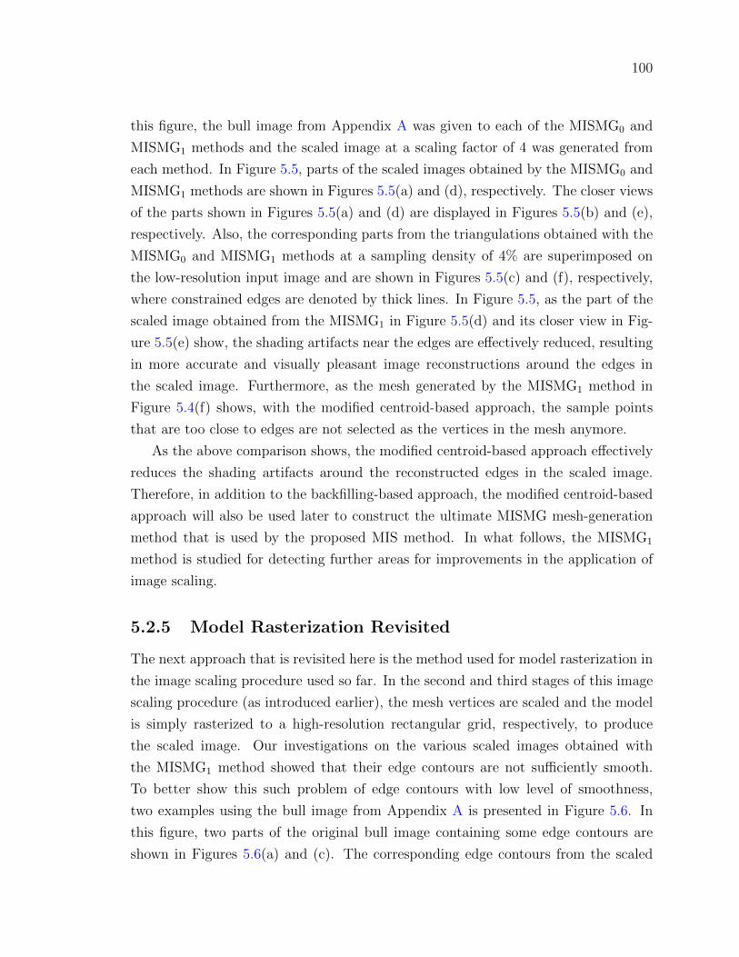
100

this figure, the bull image from Appendix A was given to each of the MISMG0 and

MISMG1 methods and the scaled image at a scaling factor of 4 was generated from

each method. In Figure 5.5, parts of the scaled images obtained by the MISMG0 and

MISMG1 methods are shown in Figures 5.5(a) and (d), respectively. The closer views

of the parts shown in Figures 5.5(a) and (d) are displayed in Figures 5.5(b) and (e),

respectively. Also, the corresponding parts from the triangulations obtained with the

MISMG0 and MISMG1 methods at a sampling density of 4% are superimposed on

the low-resolution input image and are shown in Figures 5.5(c) and (f), respectively,

where constrained edges are denoted by thick lines. In Figure 5.5, as the part of the

scaled image obtained from the MISMG1 in Figure 5.5(d) and its closer view in Fig-

ure 5.5(e) show, the shading artifacts near the edges are effectively reduced, resulting

in more accurate and visually pleasant image reconstructions around the edges in

the scaled image. Furthermore, as the mesh generated by the MISMG1 method in

Figure 5.4(f) shows, with the modified centroid-based approach, the sample points

that are too close to edges are not selected as the vertices in the mesh anymore.

As the above comparison shows, the modified centroid-based approach effectively

reduces the shading artifacts around the reconstructed edges in the scaled image.

Therefore, in addition to the backfilling-based approach, the modified centroid-based

approach will also be used later to construct the ultimate MISMG mesh-generation

method that is used by the proposed MIS method. In what follows, the MISMG1

method is studied for detecting further areas for improvements in the application of

image scaling.

5.2.5 Model Rasterization Revisited

The next approach that is revisited here is the method used for model rasterization in

the image scaling procedure used so far. In the second and third stages of this image

scaling procedure (as introduced earlier), the mesh vertices are scaled and the model

is simply rasterized to a high-resolution rectangular grid, respectively, to produce

the scaled image. Our investigations on the various scaled images obtained with

the MISMG1 method showed that their edge contours are not sufficiently smooth.

To better show this such problem of edge contours with low level of smoothness,

two examples using the bull image from Appendix A is presented in Figure 5.6. In

this figure, two parts of the original bull image containing some edge contours are

shown in Figures 5.6(a) and (c). The corresponding edge contours from the scaled

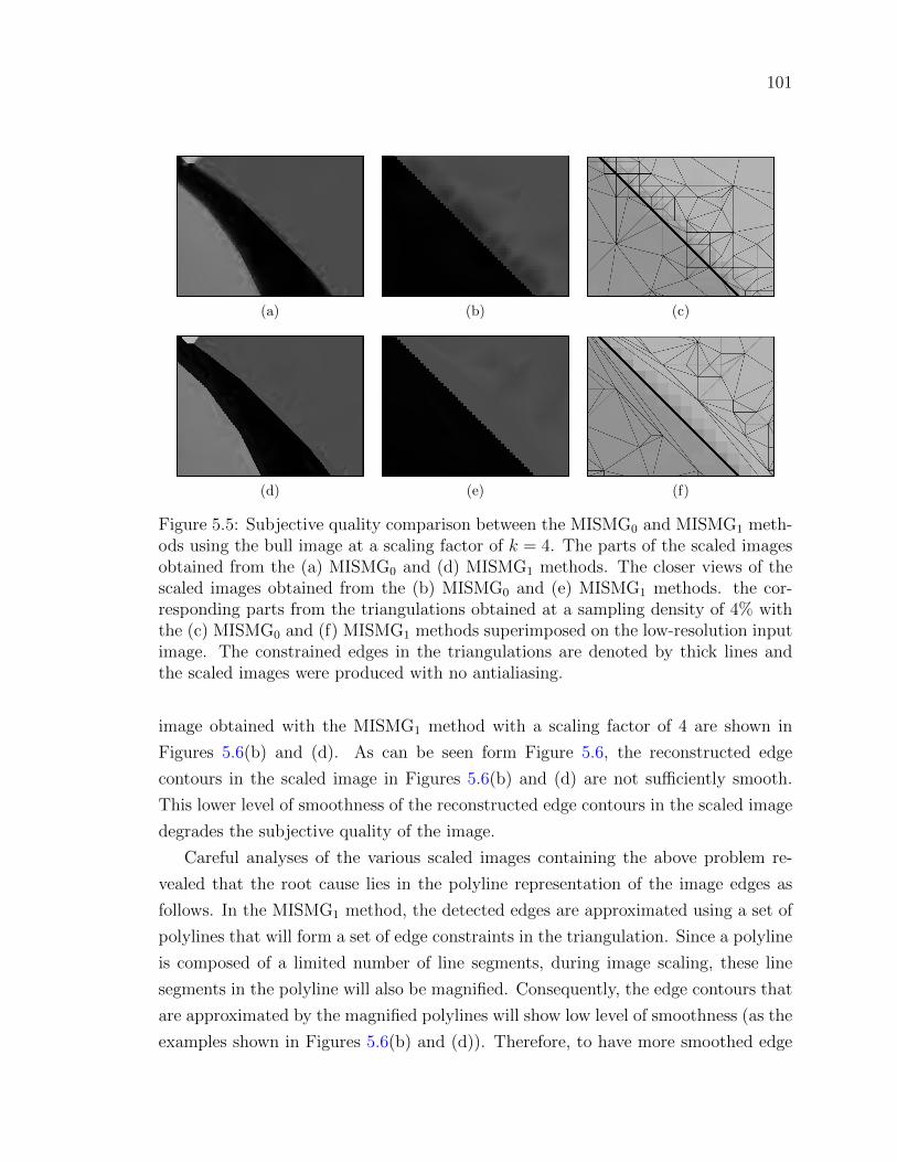
101

(a) (b) (c)

(d) (e) (f)

Figure 5.5: Subjective quality comparison between the MISMG0 and MISMG1 meth-ods using the bull image at a scaling factor of k = 4. The parts of the scaled imagesobtained from the (a) MISMG0 and (d) MISMG1 methods. The closer views of thescaled images obtained from the (b) MISMG0 and (e) MISMG1 methods. the cor-responding parts from the triangulations obtained at a sampling density of 4% withthe (c) MISMG0 and (f) MISMG1 methods superimposed on the low-resolution inputimage. The constrained edges in the triangulations are denoted by thick lines andthe scaled images were produced with no antialiasing.

image obtained with the MISMG1 method with a scaling factor of 4 are shown in

Figures 5.6(b) and (d). As can be seen form Figure 5.6, the reconstructed edge

contours in the scaled image in Figures 5.6(b) and (d) are not sufficiently smooth.

This lower level of smoothness of the reconstructed edge contours in the scaled image

degrades the subjective quality of the image.

Careful analyses of the various scaled images containing the above problem re-

vealed that the root cause lies in the polyline representation of the image edges as

follows. In the MISMG1 method, the detected edges are approximated using a set of

polylines that will form a set of edge constraints in the triangulation. Since a polyline

is composed of a limited number of line segments, during image scaling, these line

segments in the polyline will also be magnified. Consequently, the edge contours that

are approximated by the magnified polylines will show low level of smoothness (as the

examples shown in Figures 5.6(b) and (d)). Therefore, to have more smoothed edge

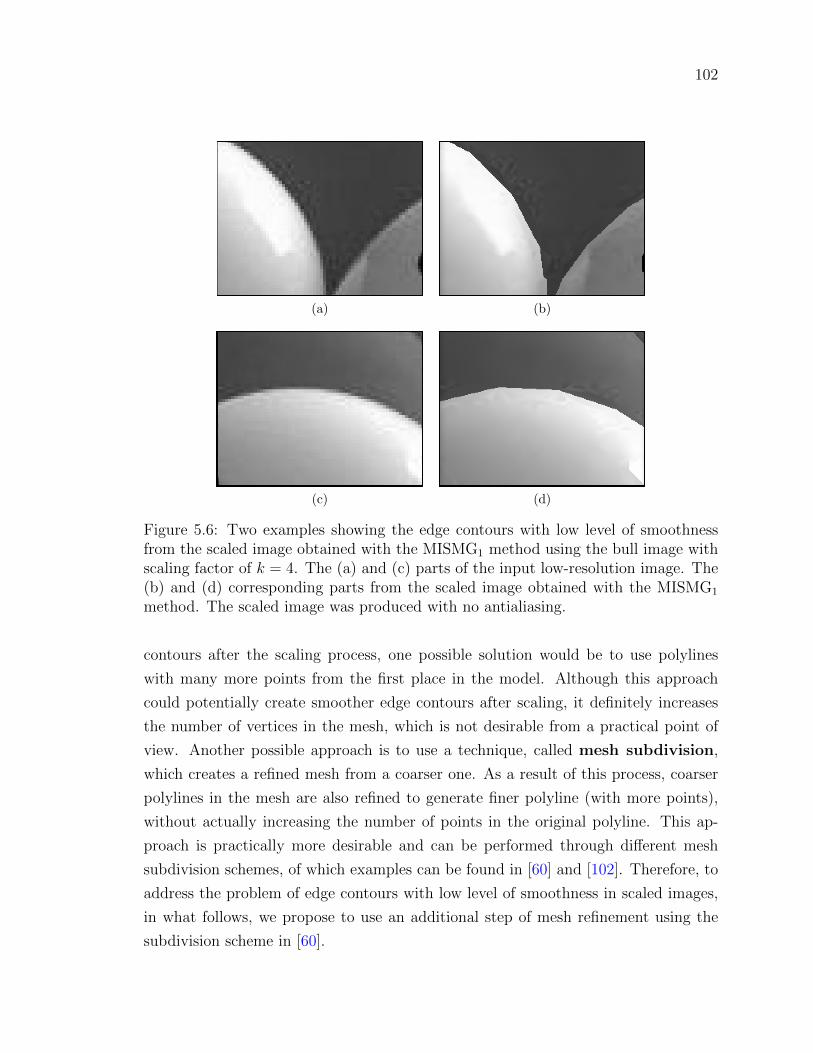
102

(a) (b)

(c) (d)

Figure 5.6: Two examples showing the edge contours with low level of smoothnessfrom the scaled image obtained with the MISMG1 method using the bull image withscaling factor of k = 4. The (a) and (c) parts of the input low-resolution image. The(b) and (d) corresponding parts from the scaled image obtained with the MISMG1

method. The scaled image was produced with no antialiasing.

contours after the scaling process, one possible solution would be to use polylines

with many more points from the first place in the model. Although this approach

could potentially create smoother edge contours after scaling, it definitely increases

the number of vertices in the mesh, which is not desirable from a practical point of

view. Another possible approach is to use a technique, called mesh subdivision,

which creates a refined mesh from a coarser one. As a result of this process, coarser

polylines in the mesh are also refined to generate finer polyline (with more points),

without actually increasing the number of points in the original polyline. This ap-

proach is practically more desirable and can be performed through different mesh

subdivision schemes, of which examples can be found in [60] and [102]. Therefore, to

address the problem of edge contours with low level of smoothness in scaled images,

in what follows, we propose to use an additional step of mesh refinement using the

subdivision scheme in [60].

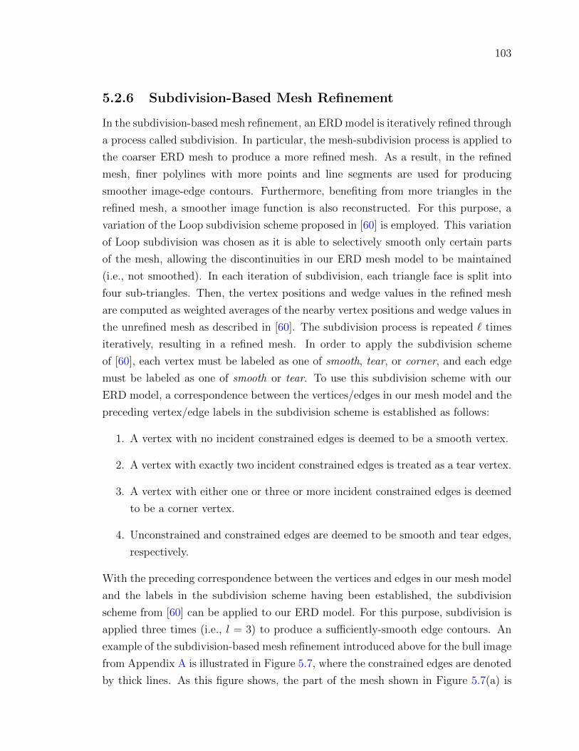
103

5.2.6 Subdivision-Based Mesh Refinement

In the subdivision-based mesh refinement, an ERD model is iteratively refined through

a process called subdivision. In particular, the mesh-subdivision process is applied to

the coarser ERD mesh to produce a more refined mesh. As a result, in the refined

mesh, finer polylines with more points and line segments are used for producing

smoother image-edge contours. Furthermore, benefiting from more triangles in the

refined mesh, a smoother image function is also reconstructed. For this purpose, a

variation of the Loop subdivision scheme proposed in [60] is employed. This variation

of Loop subdivision was chosen as it is able to selectively smooth only certain parts

of the mesh, allowing the discontinuities in our ERD mesh model to be maintained

(i.e., not smoothed). In each iteration of subdivision, each triangle face is split into

four sub-triangles. Then, the vertex positions and wedge values in the refined mesh

are computed as weighted averages of the nearby vertex positions and wedge values in

the unrefined mesh as described in [60]. The subdivision process is repeated ` times

iteratively, resulting in a refined mesh. In order to apply the subdivision scheme

of [60], each vertex must be labeled as one of smooth, tear, or corner, and each edge

must be labeled as one of smooth or tear. To use this subdivision scheme with our

ERD model, a correspondence between the vertices/edges in our mesh model and the

preceding vertex/edge labels in the subdivision scheme is established as follows:

1. A vertex with no incident constrained edges is deemed to be a smooth vertex.

2. A vertex with exactly two incident constrained edges is treated as a tear vertex.

3. A vertex with either one or three or more incident constrained edges is deemed

to be a corner vertex.

4. Unconstrained and constrained edges are deemed to be smooth and tear edges,

respectively.

With the preceding correspondence between the vertices and edges in our mesh model

and the labels in the subdivision scheme having been established, the subdivision

scheme from [60] can be applied to our ERD model. For this purpose, subdivision is

applied three times (i.e., l = 3) to produce a sufficiently-smooth edge contours. An

example of the subdivision-based mesh refinement introduced above for the bull image

from Appendix A is illustrated in Figure 5.7, where the constrained edges are denoted

by thick lines. As this figure shows, the part of the mesh shown in Figure 5.7(a) is

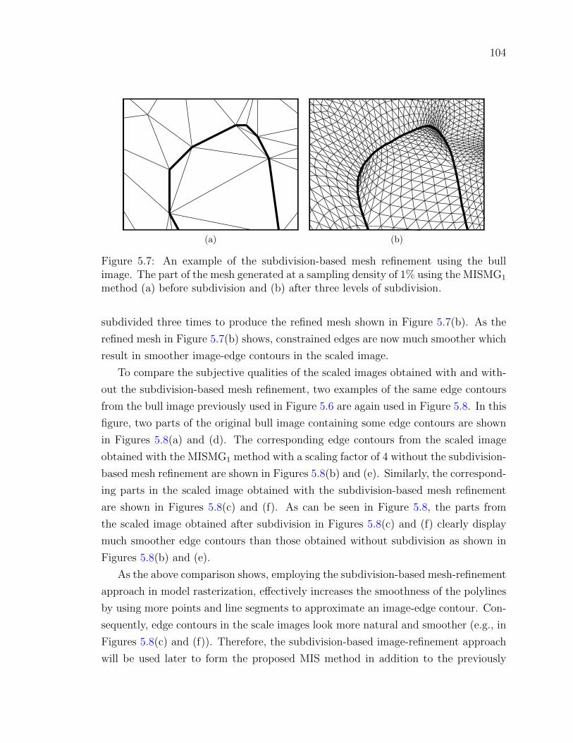
104

(a) (b)

Figure 5.7: An example of the subdivision-based mesh refinement using the bullimage. The part of the mesh generated at a sampling density of 1% using the MISMG1

method (a) before subdivision and (b) after three levels of subdivision.

subdivided three times to produce the refined mesh shown in Figure 5.7(b). As the

refined mesh in Figure 5.7(b) shows, constrained edges are now much smoother which

result in smoother image-edge contours in the scaled image.

To compare the subjective qualities of the scaled images obtained with and with-

out the subdivision-based mesh refinement, two examples of the same edge contours

from the bull image previously used in Figure 5.6 are again used in Figure 5.8. In this

figure, two parts of the original bull image containing some edge contours are shown

in Figures 5.8(a) and (d). The corresponding edge contours from the scaled image

obtained with the MISMG1 method with a scaling factor of 4 without the subdivision-

based mesh refinement are shown in Figures 5.8(b) and (e). Similarly, the correspond-

ing parts in the scaled image obtained with the subdivision-based mesh refinement

are shown in Figures 5.8(c) and (f). As can be seen in Figure 5.8, the parts from

the scaled image obtained after subdivision in Figures 5.8(c) and (f) clearly display

much smoother edge contours than those obtained without subdivision as shown in

Figures 5.8(b) and (e).

As the above comparison shows, employing the subdivision-based mesh-refinement

approach in model rasterization, effectively increases the smoothness of the polylines

by using more points and line segments to approximate an image-edge contour. Con-

sequently, edge contours in the scale images look more natural and smoother (e.g., in

Figures 5.8(c) and (f)). Therefore, the subdivision-based image-refinement approach

will be used later to form the proposed MIS method in addition to the previously

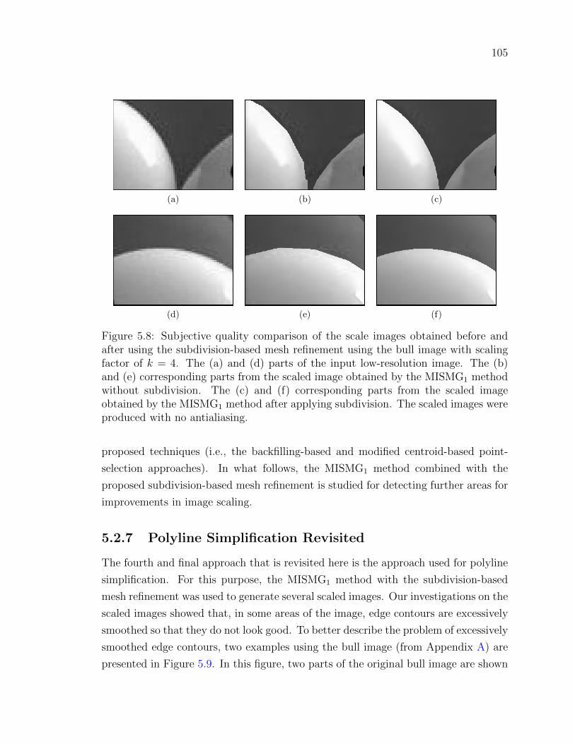
105

(a) (b) (c)

(d) (e) (f)

Figure 5.8: Subjective quality comparison of the scale images obtained before andafter using the subdivision-based mesh refinement using the bull image with scalingfactor of k = 4. The (a) and (d) parts of the input low-resolution image. The (b)and (e) corresponding parts from the scaled image obtained by the MISMG1 methodwithout subdivision. The (c) and (f) corresponding parts from the scaled imageobtained by the MISMG1 method after applying subdivision. The scaled images wereproduced with no antialiasing.

proposed techniques (i.e., the backfilling-based and modified centroid-based point-

selection approaches). In what follows, the MISMG1 method combined with the

proposed subdivision-based mesh refinement is studied for detecting further areas for

improvements in image scaling.

5.2.7 Polyline Simplification Revisited

The fourth and final approach that is revisited here is the approach used for polyline

simplification. For this purpose, the MISMG1 method with the subdivision-based

mesh refinement was used to generate several scaled images. Our investigations on the

scaled images showed that, in some areas of the image, edge contours are excessively

smoothed so that they do not look good. To better describe the problem of excessively

smoothed edge contours, two examples using the bull image (from Appendix A) are

presented in Figure 5.9. In this figure, two parts of the original bull image are shown

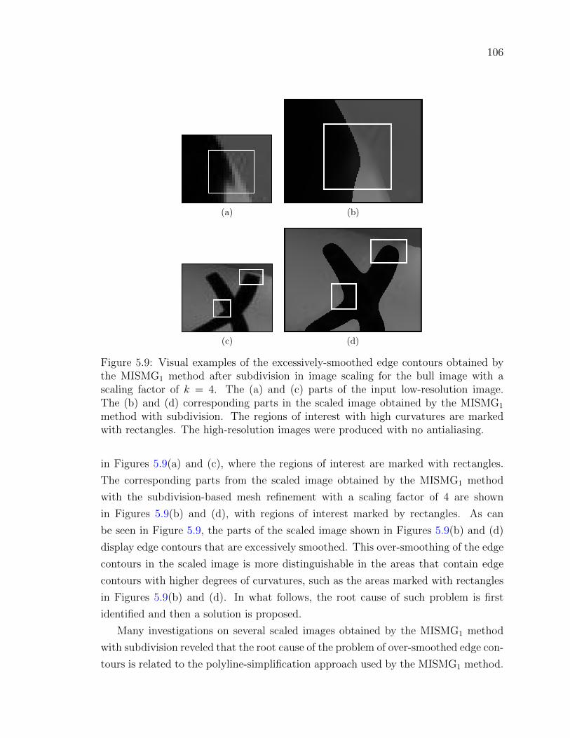
106

(a) (b)

(c) (d)

Figure 5.9: Visual examples of the excessively-smoothed edge contours obtained bythe MISMG1 method after subdivision in image scaling for the bull image with ascaling factor of k = 4. The (a) and (c) parts of the input low-resolution image.The (b) and (d) corresponding parts in the scaled image obtained by the MISMG1

method with subdivision. The regions of interest with high curvatures are markedwith rectangles. The high-resolution images were produced with no antialiasing.

in Figures 5.9(a) and (c), where the regions of interest are marked with rectangles.

The corresponding parts from the scaled image obtained by the MISMG1 method

with the subdivision-based mesh refinement with a scaling factor of 4 are shown

in Figures 5.9(b) and (d), with regions of interest marked by rectangles. As can

be seen in Figure 5.9, the parts of the scaled image shown in Figures 5.9(b) and (d)

display edge contours that are excessively smoothed. This over-smoothing of the edge

contours in the scaled image is more distinguishable in the areas that contain edge

contours with higher degrees of curvatures, such as the areas marked with rectangles

in Figures 5.9(b) and (d). In what follows, the root cause of such problem is first

identified and then a solution is proposed.

Many investigations on several scaled images obtained by the MISMG1 method

with subdivision reveled that the root cause of the problem of over-smoothed edge con-

tours is related to the polyline-simplification approach used by the MISMG1 method.

107

More specifically, edge contours that are excessively smoothed in the scaled images

often correspond to the image edges that are poorly approximated with the polylines

because of using a polyline-simplification approach that is not suitable for image scal-

ing. This can be elaborated as follows. Since the subdivision scheme of [60] that is

used for the purpose of mesh refinement is approximating, the subdivided (smoother)

polyline is not guaranteed to pass through the points of the control (coarser) polyline.

On one hand, using an approximating subdivision scheme results in smoother edge

curves after subdivision that look more natural and pleasant to the human observer.

On the other hand, since the resulting subdivided polyline does not necessarily pass

through the points in the control polyline, the subdivided polyline can, in some places,

deviate too much from its control polyline. Many experiments on different test cases

showed that this excessive shifting of the subdivided polyline from its corresponding

control polyline occurs wherever both of the following conditions are satisfied:

1. the control polyline corresponds to an edge contour with high degree of curva-

ture in the low-resolution image, and

2. the control polyline does not contain a sufficient number of control points to

accurately approximate that high-curvature part of the edge contour.

When above two conditions are satisfied, the subdivided polyline will most probably

shift too much away from its corresponding control polyline near the high-curvature

parts of the edge contour. Consequently, the edge contours in the scaled image,

which are reconstructed based the subdivided polylines, also deviate too much from

their original edge curves in the low-resolution image, resulting in over-smoothed edge

contours (as previously shown in Figures 5.9(b) and (d)).

Since the subdivision-based mesh refinement is applied as a post processing step

after mesh generation, the polyline-simplification approach, in the MISMG1 method,

is blind to the subdivided polylines. Therefore, polylines are simplified as if there will

be no subdivision later. Consequently, they most probably are simplified too much

at high-curvature edge contours so that, after subdivision, the subdivided polyline

deviates too much from the simplified polyline. In what follows, a solution to address

this problem is proposed.

108

5.2.8 Adaptive Polyline Simplification

Having identified the root cause of the problem of excessively-smoothed edge contours

to be in the polyline-simplification approach of the MISMG1 method, we now propose

an adaptive polyline-simplification (APS) approach to address the problem as follows.

The input to our APS method is an original polyline P of N consecutively-connected

points (i.e., P = p0, p1, ..., pN−1) and the output is the simplified polyline P . The

proposed APS approach is comprised of the following steps (in order):

1. Apply the simplification method of DP [34] to P , as explained in Section 2.3, to

generate the simplified polyline P ′, with the tolerance ε = 0.75 (i.e., P ′ ⊂ P ).

2. Compute the subdivided polyline P ′′ from P ′ using the subdivision scheme

of [60], with ` level of iterations, where l = 3.

3. Find a set Q of high-error points in P ′ whose distances from P ′′ is greater than

a shifting threshold τ (to be explained later).

4. For each point p′i ∈ P ′, if p′i is a high-error point (i.e., p′i ∈ Q), find a point

pj ∈ P , where pj = p′i, then insert two extra points pj−1 and pj+1 from P into

P ′ as the new points p′i−1 and p′i+1, respectively.

5. Finally, select P = P ′.

Selection of τ. In step 3 of the APS approach explained above, threshold τ is

selected adaptive to the local curvature profile of the polyline P ′ at each point. To

achieve this, for a point p′i ∈ P ′, first, the angle α between the line segments p′ip′i−1

and p′ip′i+1 is computed which is in the range 0 ≤ α ≤ 180. Then, τ is determined

as

τ =

0.5, α ≤ 135

1.0, 135 < α < 160

1.4, α ≥ 160.

(5.3)

The α in (5.3) indicates an estimation of the local curvature level of the polyline P ′

at p′i. In particular, a smaller (i.e., sharper) and larger (i.e., wider) angle α represents

a higher and lower degree of curvature at p′i, respectively. Our analyses on several

scaled images showed that the problem of the excessively-shifted polylines is more

annoying (and evident) when it occurs at the edge contours with a higher degree

of curvature. Therefore, through several experiments with the above thresholding

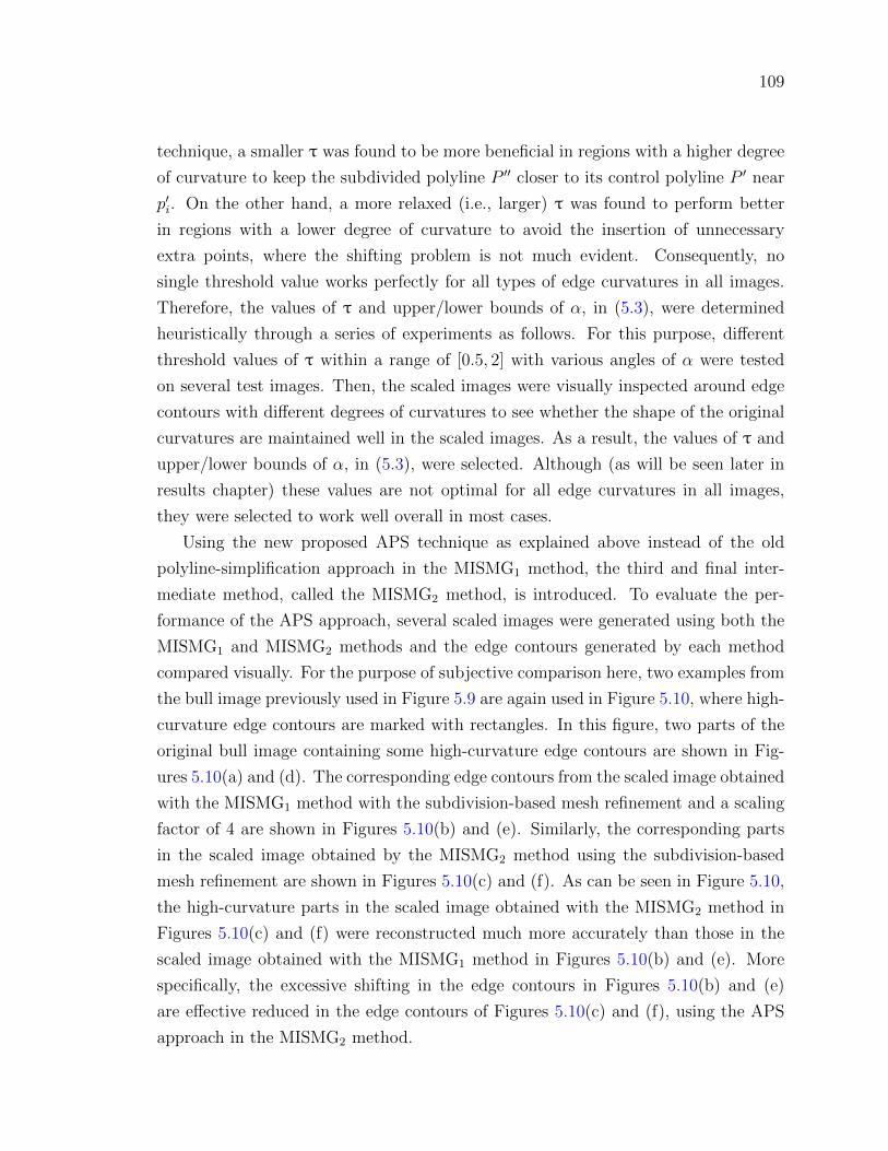
109

technique, a smaller τ was found to be more beneficial in regions with a higher degree

of curvature to keep the subdivided polyline P ′′ closer to its control polyline P ′ near

p′i. On the other hand, a more relaxed (i.e., larger) τ was found to perform better

in regions with a lower degree of curvature to avoid the insertion of unnecessary

extra points, where the shifting problem is not much evident. Consequently, no

single threshold value works perfectly for all types of edge curvatures in all images.

Therefore, the values of τ and upper/lower bounds of α, in (5.3), were determined

heuristically through a series of experiments as follows. For this purpose, different

threshold values of τ within a range of [0.5, 2] with various angles of α were tested

on several test images. Then, the scaled images were visually inspected around edge

contours with different degrees of curvatures to see whether the shape of the original

curvatures are maintained well in the scaled images. As a result, the values of τ and

upper/lower bounds of α, in (5.3), were selected. Although (as will be seen later in

results chapter) these values are not optimal for all edge curvatures in all images,

they were selected to work well overall in most cases.

Using the new proposed APS technique as explained above instead of the old

polyline-simplification approach in the MISMG1 method, the third and final inter-

mediate method, called the MISMG2 method, is introduced. To evaluate the per-

formance of the APS approach, several scaled images were generated using both the

MISMG1 and MISMG2 methods and the edge contours generated by each method

compared visually. For the purpose of subjective comparison here, two examples from

the bull image previously used in Figure 5.9 are again used in Figure 5.10, where high-

curvature edge contours are marked with rectangles. In this figure, two parts of the

original bull image containing some high-curvature edge contours are shown in Fig-

ures 5.10(a) and (d). The corresponding edge contours from the scaled image obtained

with the MISMG1 method with the subdivision-based mesh refinement and a scaling

factor of 4 are shown in Figures 5.10(b) and (e). Similarly, the corresponding parts

in the scaled image obtained by the MISMG2 method using the subdivision-based

mesh refinement are shown in Figures 5.10(c) and (f). As can be seen in Figure 5.10,

the high-curvature parts in the scaled image obtained with the MISMG2 method in

Figures 5.10(c) and (f) were reconstructed much more accurately than those in the

scaled image obtained with the MISMG1 method in Figures 5.10(b) and (e). More

specifically, the excessive shifting in the edge contours in Figures 5.10(b) and (e)

are effective reduced in the edge contours of Figures 5.10(c) and (f), using the APS

approach in the MISMG2 method.

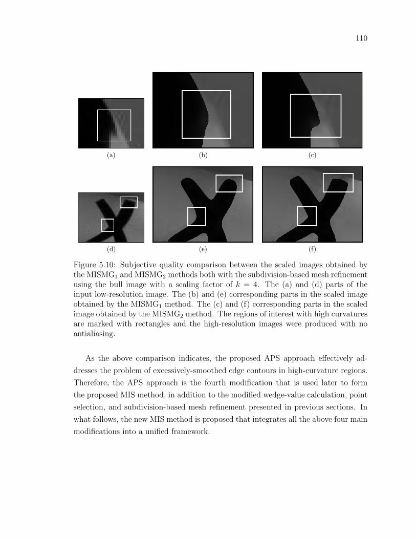
110

(a) (b) (c)

(d) (e) (f)

Figure 5.10: Subjective quality comparison between the scaled images obtained bythe MISMG1 and MISMG2 methods both with the subdivision-based mesh refinementusing the bull image with a scaling factor of k = 4. The (a) and (d) parts of theinput low-resolution image. The (b) and (e) corresponding parts in the scaled imageobtained by the MISMG1 method. The (c) and (f) corresponding parts in the scaledimage obtained by the MISMG2 method. The regions of interest with high curvaturesare marked with rectangles and the high-resolution images were produced with noantialiasing.

As the above comparison indicates, the proposed APS approach effectively ad-

dresses the problem of excessively-smoothed edge contours in high-curvature regions.

Therefore, the APS approach is the fourth modification that is used later to form

the proposed MIS method, in addition to the modified wedge-value calculation, point

selection, and subdivision-based mesh refinement presented in previous sections. In

what follows, the new MIS method is proposed that integrates all the above four main

modifications into a unified framework.

111

5.3 Proposed MIS Method

In the preceding sections, the performances of various approaches in different steps of

mesh generation and model rasterization for image scaling were studied. As a result

of this study, several problematic areas that have negative effects on the quality of

the resulting scaled images were identified. Moreover, for each problematic case, a

specific modification proposed to further adapt the processes of mesh generation and

model rasterization for image scaling. With the insight from those analyses, we are

now ready to introduce our proposed method for mesh-based image scaling (MIS).

The MIS method is based on the ERD models (introduced in Section 2.9) and, as

stated earlier, is designed to solve the problem of image scaling, for grayscale raster

images that are approximately piecewise-smooth, with no (or minimal) textures or

patterns. More specifically, the inputs to the MIS method are a low-resolution raster

image φl defined on an integer lattice of width W and height H and an integer scaling

factor of k > 1. The output of the MIS method is a high-resolution raster image φh

defined on an integer lattice of width kW and height kH. The proposed MIS method

is comprised of the following three stages (in order):

1. mesh generation,

2. mesh transformation, and

3. model rasterization.

In stage 1, an ERD mesh model from φl is generated. Then, in stage 2, the mesh

vertices are transformed using a scaling operation. Finally, in stage 3, the scaled

ERD model obtained from stage 2 is rasterized using a subdivision-based approach

to produce the scaled image φh. In what follows, each stage will be described in

detail.

5.3.1 Mesh Generation

As mentioned earlier, in the first stage of our MIS method, an ERD mesh model is

generated from the input low-resolution image φl. For this purpose, the mesh-based

image-scaling mesh-generation (MISMG) method is designed to generate the ERD

models that are effective in image scaling. The MISMG method is the ultimate ver-

sion of the intermediate methods (i.e., the MISMG0, MISMG1, and MISMG2 meth-

ods) previously introduced in the development process. In particular, the MISMG

112

method integrates all the modifications used by those intermediate methods, includ-

ing modified approaches for wedge-value calculation, polyline simplification, and point

selection. In what follows, we explain how the MISMG method works.

For a low-resolution image function φl defined on the rectangular region Γ =

[0,W−1]×[0, H−1], an ERD triangle mesh model of φl (as introduced in Section 2.9)

consists of: 1) a set P = pi ⊂ Γ of sample points, 2) a set E of edge constraints,

and 3) a set Z of integer wedge values. The proposed MISMG method selects the

parameters of the ERD model (i.e., P , E, and Z) that is effective in image scaling.

The input to the MISMG algorithm is the low-resolution image function φl that is

known only at the points in Λ = 0, 1, ...,W − 1× 0, 1, ..., H − 1 (i.e., a truncated

integer lattice of width W and height H). The outputs of the MISMG method are the

ERD model parameters, including P (i.e., P ⊂ Λ ⊂ Γ), E, and Z. In what follows,

we first introduce the general algorithmic framework for the MISMG method. Then,

the specifics of the method are explained. The general algorithmic framework of the

MISMG method consists of the following steps (in order):

1. Initial triangulation selection. Select the values for the initial set P0 of sample

points and E. Then, the initial mesh associated with the preferred triangulation

pcdt(P0, E) is constructed.

2. Wedge-value initialization. For each vertex v ∈ P0, compute the initial wedge

values using the backfilling-based technique proposed in Section 5.2.2.

3. Point selection. Select a new sample point q ∈ Λ to add to the mesh using the

modified centroid-based approach proposed in Section 5.2.4.

4. Point insertion. Insert q in the triangulation. Calculate the wedge values of the

affected wedges in the mesh using the same backfilling-based approach proposed

in Section 5.2.2 and select the set Pi+1 of sample points for the next iteration

as Pi ∪ q.

5. Stopping criterion. If |Pi+1| < 0.04|Λ|, go to step 3. Otherwise, set the output

parameter P = Pi+1 and stop.

The steps 1 and 2, in the framework above, choose an initial coarse mesh of size

|P0|. Then, in steps 3 to 5, the initial mesh is iteratively refined by adding more

sample points to achieve the mesh of size 0.04|Λ| (i.e., with a sampling density of

4%).

113

Selection of P0 and E. In step 1 of the above framework, the procedure to

select the initial set P0 and E is same as the one introduced in Section 3.3 for the

SEMMG method, except that the new APS method proposed in Section 5.2.8 is used

to simplify the polylines, instead of the DP method used in the SEMMG method.

5.3.2 Mesh Transformation

Once the ERD mesh model is generated in stage 1, in stage 2 of the MIS method,

the vertices of the model are scaled with any scale factor of interest. While the MIS

method specifically focuses on the scaling operation, the mesh model that is generated

from stage 1 can be stored and used anytime later for different purposes, such as mesh

editing or applying any combination of affine transformations like scaling, translation,

and rotation. Indeed, such properties of the MIS method simply allow for producing

image models that are portable, editable, and reusable, which may not be easily (or

ever) achievable with other state-of-the-art raster-based scaling methods.

5.3.3 Model Rasterization

Having introduced the MISMG method and mesh transformation used in stages 1

and 2 of the MIS method, respectively, we now describe the third stage, which is

model rasterization. The model rasterization, in the MIS method, consists of two

steps (in order):

1. mesh refinement and

2. mesh rasterization.

In step 1, the ERD mesh model of φl obtained using the MISMG method from

the mesh-generation stage (introduced in Section 5.3.1) is refined. For this purpose,

the subdivision-based mesh-refinement approach previously proposed in Section 5.2.6

is used. Although, in principle, we could simply rasterize the mesh obtained from

the mesh-generation and mesh-transformation stages (i.e., omit the mesh-refinement

step), this would lead to an image reconstruction with artifacts. In particular, the

image discontinuity contours in the scaled image (as studied in Section 5.2.5) would

lack a desirable level of smoothness as well as the image function itself. By employing

the subdivision-based mesh refinement, however, we are able to obtain a mesh with

better smoothness.

114

In step 2 of the above model rasterization approach, the refined (i.e., subdivided)

ERD mesh model is rasterized to a high-resolution lattice grid to produce the scaled

image. For this purpose, with a raster low-resolution image φl of width W and height

H and a scaling factor of k > 1, the scaled and refined ERD model is rasterized

to a high-resolution lattice grid of width kW and height kH. To achieve this, the

piecewise-linear interpolating function associated with the ERD model (as described

in Section 2.9) is used to produce the high-resolution image φh as a scaled version

of φl. Since the ERD model explicitly represents discontinuities, edges in the recon-

structed image could generate undesirable aliasing effects. Thus, a supersampling

technique based on the 3×3 grid algorithm (introduced in Section 2.6) is used during

rasterization to avoid such aliasing effects at the edges.

115

Chapter 6

Evaluation and Analysis of the

MIS Method

6.1 Overview

Having introduced the proposed MIS method, we now compare it with other im-

age scaling methods. Different categories of image scaling methods (as introduced

in Section 1.4) have been proposed to date, of which two important ones are those

based on raster-based and mesh-based interpolation techniques. Regarding the the

raster-based methods, many implementations are readily available which make the

comparison with them practically easy to perform. Therefore, the comparison be-

tween the MIS and raster-based methods here is performed through various experi-

mental comparisons, including subjective and objective evaluations. Regarding the

mesh-based image-scaling methods, since the MIS method is based on a mesh-based

technique, a comparison between the MIS and those methods is also desirable. This

type of comparison, however, is not straightforward due to the difficulties mentioned

previously in Section 4 and also reminded as follows. Firstly, due to the high com-

plexity of the mesh-based methods, implementing them often requires at least several

months of work, including coding, testing, and debugging. Secondly, since so much

effort is involved in implementing mesh-based methods, researchers often do not want

to make their code freely available. Thus, finding implementations of other compet-

ing mesh-based methods is often impossible. Because of such reasons, for evaluating

our MIS method, no implementations of any other mesh-based approaches could be

obtained. One approach for comparing to methods, where no implementation was

116

available, would be to compare to the results reported in other researcher’s publica-

tions (as it was done previously in Section 4.3 for evaluating the SEMMG method).

For this purpose, however, the same test data that was used to produce the results in

other publications should be accessible and also has to be a valid input for the method

under evaluation. Otherwise, there is no basis for comparison. Because of the reasons

explained above, performing an experimental comparison between the MIS and other

mesh-based scaling methods became impractical. In such cases, however, a conceptual

comparison is provided through presenting the theoretical differences and similarities

between the methods. In what follows, first, the experimental comparisons between

the MIS and several raster-based methods are presented, including both the subjec-

tive and objective evaluations, followed by some supplementary discussions. Finally,

a conceptual comparison between the MIS method and two other relevant mesh-based

methods is performed. Some of the results presented in this chapter have also been

published in the author’s paper [67].

6.2 Experimental Comparisons

Among the numerous raster-based image-scaling methods that have been proposed

over the years, the MIS method is compared to the following five well-known ap-

proaches:

1. bilinear interpolation,

2. bicubic interpolation of Keys [51],

3. the DCCI method of Zhou et al. [101],

4. the NEDI method of Li and Orchard [59], and

5. the SRCNN method of Dong et al. [33].

These methods were selected in a way to include two methods from the classical

and convolutional techniques (i.e., bilinear and bicubic methods), two methods from

the edge-directed class (i.e, the DCCI and NEDI methods), and one from the most

recent class of methods based on deep learning (i.e., the SRCNN method). Due to

the availability of implementations of the above methods, a comparison between the

MIS method and each of the above techniques is made through experimental results,

including both subjective and objective evaluations.

117

The software implementations of the MIS method were developed by the author

of this thesis and written in C++. The details of the software implementation are

presented in Appendix D. In the case of bilinear and bicubic methods, their cor-

responding built-in functions from MATLAB were used. Moreover, for the DCCI,

NEDI, and SRCNN methods, their MATLAB implementations from [2], [3], and [4],

respectively, were used to generate results.

In what follows, the test data used for the experimental comparisons is first in-

troduced. Then, the subjective evaluation is presented, including its methodology,

results, and analysis. Next, the objective evaluation is presented as well as its method-

ology, results, and analysis. Finally, some supplementary discussions are presented

to highlight the benefits and drawbacks of the methods under comparison.

6.2.1 Test Data

For test data we use a set of 20 low-resolution images listed in Appendix B. In our

experimental comparisons, the evaluation is performed in terms of multiple metrics.

In particular, we consider a subjective and several objective measures. The objective

measures require a ground-truth image as a reference, whereas the subjective measure

does not. Therefore, our test data must have be chosen in a way to, first, accommodate

the ground-truth image for the objective measures, and second, be consistent across

the subjective and objective evaluations. For these reasons, all of the 20 test images

that are used here were generated from their high-resolution counterparts using a

downscaling process. In our work, such a reduction in resolution, was performed using

a simple pixel-averaging (also called pixel-mixing) technique, provided as the default

resizing method by the Netpbm toolkit [5], with a factor of k = 4. Therefore, the

same set of 20 test images can be used for both subjective and objective evaluations.

Furthermore, the high-resolution image corresponding to each test image can be used

as a ground truth for computing the metric of interest in the objective evaluation.

Regarding the test images for image scaling, two considerations need to be taken

into account as follows. One consideration is that, as explained earlier, a downscal-

ing process is involved to, first, obtain a low-resolution test image φl from its high-

resolution ground-truth counterpart φh. Then, the test image φl is used as the input

to the scaling methods under comparison. In the case of the proposed MIS method

(as we recall from Section 5.3), the MISMG approach, used by the MIS method, ini-

tially detects the edges in the input image (i.e., φl herein). Moreover, the accuracy

118

of the edge localization is critically important to the performance of the MIS method

because the constrained edges (as one of the critical parameters) in the mesh model

are selected directly based on the detected edges. Although a more advanced edge

detector with sub-pixel accuracy could potentially have been used in the MISMG

method for more accurate edge localization, a Canny edge detector (with one pixel

accuracy) was used in order to avoid unnecessarily increasing computational complex-

ity. Also, with the recent increase in the resolutions of today’s typical images, such an

edge detector with one-pixel accuracy works reasonably well with them. Later, in the

evaluation process, however, the downscaling-based procedure was found to produce

too small low-resolution images if applied to some standard test images, such as those

used in Chapter 3. For example, in the case of the commonly-used test images, such

as lena and peppers, the ground-truth image φh is of size 512 by 512 pixels. Thus,

with a typical scaling factor of k = 4, the low-resolution test image φl will be of size

128 by 128. For such a small test image, however, a more advance edge detector is

needed to locate edges with sub-pixel accuracy. Therefore, due to such a usability

limitation in the MIS method, the ground-truth image φh itself cannot be too small

so that the low-resolution test image φl can still be handled by an edge detector with

one-pixel accuracy.

The other consideration when selecting the test data for image scaling is the

fact that our MIS method (as introduced in Section 5.3) is not intended to work

with textured images, where the image is not approximately piecewise smooth. The

two previously mentioned considerations for selecting the test data in evaluating the

MIS method, however, were not much necessary in the case of the SEMMG method

proposed in Chapter 3. This is because (as we recall from Chapter 3) the SEMMG

method was designed to solve a completely different problem, where it could handle

images with smaller sizes and with small to moderate textures. Thus, the set of test

data that was used for evaluating the SEMMG method in Chapter 3 cannot be fully

utilized for evaluating the MIS method too. Consequently, the new set of 20 test

images, as introduced earlier and listed in Appendix B, was collected by the author

to contain images with larger resolutions and with approximately piecewise-smooth

functions (such as cartoon images). This test data was chosen to include images

with low, medium, and high levels of detail. Moreover, some natural photographic

images with low amount of texture (e.g., frangipani, dahlia, balloons, and rose) are

also included to facilitate the analysis.

119

6.2.2 Subjective Evaluation

Having introduced the test data for experimental comparisons, we now focus on the

subjective evaluation. Since our ultimate goal is to generate scaled images of better

quality with respect to the human visual system, the most accurate and also reliable

way of assessing the quality of scaled images is through a subjective evaluation. In

this evaluation, a group of people are asked to give their opinion about the scaled

images obtained from different methods. In what follows, the methodology used

for performing the subjective evaluation is first explained. Then, the results of the

subjective evaluation are presented followed by their analysis.

6.2.2.1 Methodology for Subjective Evaluation

Since several methodologies can be used to perform a subjective evaluation, the spe-

cific method used here is explained. A rigorous industrial-scale subjective evaluation

requires having a complete control over many factors, including lighting conditions,

display devices, viewing distances/angles, subjects vision ability, and subjects mood.

Several international standards have been proposed (e.g., ITU-R BT.500-13 [50]) on

how to control and set the aforementioned factors for various applications, such as

(high-definition) television images and video quality assessments. An extensive sur-

vey on different standardized subjective methods can be found in [65]. In the case of

our subjective evaluation, providing such an industrial-scale environment to satisfy

all the standards was impractical due to the limited laboratory facilities. The subjec-

tive evaluation, however, was performed in the most rigorous way possible, given our

limited laboratory facilities. In what follows, the details of this subjective evaluation

are explained.

The subjective evaluation was performed in the Digital Signal Processing labo-

ratory in the University of Victoria using two monitors of the same models. The

ambient lighting conditions, monitors resolutions, brightnesses, and contrasts were

all kept the same during the test for all participants. For our subjective evaluation,

a methodology based on ordering by force-choice pairwise comparison in [65] and a

voting platform similar to the one developed by [89], were used. For this purpose, the

test set of 20 low-resolution images (as introduced in Section 6.2.1) and the scaling

factor of k = 4 were given to each of the six scaling methods under comparison to

produce the scaled images. Thus, six different high-resolution images were generated

from each low-resolution image. In our subjective assessment, first, each participant

120

Figure 6.1: A screenshot of the survey software developed and used for the subjectiveevaluation. The magnifier tool can be moved around the two images.

in the survey was shown a pair of randomly selected scaled (high-resolution) images

obtained using two different methods from the same low-resolution image. Using a

magnifier tool, the participant would inspect different parts of the images and decide

which one is better than the other in terms of perceptual quality. Next, the winning

image was kept and the losing image was replaced with a scaled image obtained with

another randomly selected method under competition. This process would continue

until the (first) best scaled image was found and removed from the dataset. Then,

the whole procedure was repeated in multiple rounds to find the second, third, fourth,

fifth, and sixth best scaled images. Consequently, for each test image, the six com-

peting scaling methods were ranked from the first (i.e, best) to sixth (i.e., worst)

methods. A screenshot of the survey software developed and used for the subjective

evaluation is illustrated in Figure 6.1. In what follows, the results of the subjective

evaluation are presented.

6.2.2.2 Subjective Evaluation Results

Using the methodology explained above, the subjective evaluation was performed

with a total of 19 participants who were given 300 pairwise comparisons, over 20 test

images, leading to a total of 380 rankings. The obtained ranking results for the six

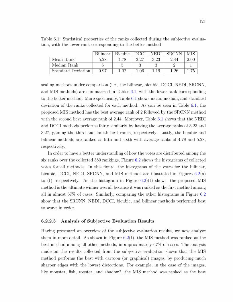
121

Table 6.1: Statistical properties of the ranks collected during the subjective evalua-tion, with the lower rank corresponding to the better method

Bilinear Bicubic DCCI NEDI SRCNN MISMean Rank 5.28 4.78 3.27 3.23 2.44 2.00Median Rank 6 5 3 3 2 1Standard Deviation 0.97 1.02 1.06 1.19 1.26 1.75

scaling methods under comparison (i.e., the bilinear, bicubic, DCCI, NEDI, SRCNN,

and MIS methods) are summarized in Tables 6.1, with the lower rank corresponding

to the better method. More specifically, Table 6.1 shows mean, median, and standard

deviation of the ranks collected for each method. As can be seen in Table 6.1, the

proposed MIS method has the best average rank of 2 followed by the SRCNN method

with the second best average rank of 2.44. Moreover, Table 6.1 shows that the NEDI

and DCCI methods performs fairly similarly by having the average ranks of 3.23 and

3.27, gaining the third and fourth best ranks, respectively. Lastly, the bicubic and

bilinear methods are ranked as fifth and sixth with average ranks of 4.78 and 5.28,

respectively.

In order to have a better understanding of how the votes are distributed among the

six ranks over the collected 380 rankings, Figure 6.2 shows the histograms of collected

votes for all methods. In this figure, the histograms of the votes for the bilinear,

bicubic, DCCI, NEDI, SRCNN, and MIS methods are illustrated in Figures 6.2(a)

to (f), respectively. As the histogram in Figure 6.2)(f) shows, the proposed MIS

method is the ultimate winner overall because it was ranked as the first method among

all in almost 67% of cases. Similarly, comparing the other histograms in Figure 6.2

show that the SRCNN, NEDI, DCCI, bicubic, and bilinear methods performed best

to worst in order.

6.2.2.3 Analysis of Subjective Evaluation Results

Having presented an overview of the subjective evaluation results, we now analyze

them in more detail. As shown in Figure 6.2(f), the MIS method was ranked as the

best method among all other methods, in approximately 67% of cases. The analysis

made on the results collected from the subjective evaluation shows that the MIS

method performs the best with cartoon (or graphical) images, by producing much

sharper edges with the lowest distortions. For example, in the case of the images,

like monster, fish, rooster, and shadow2, the MIS method was ranked as the best

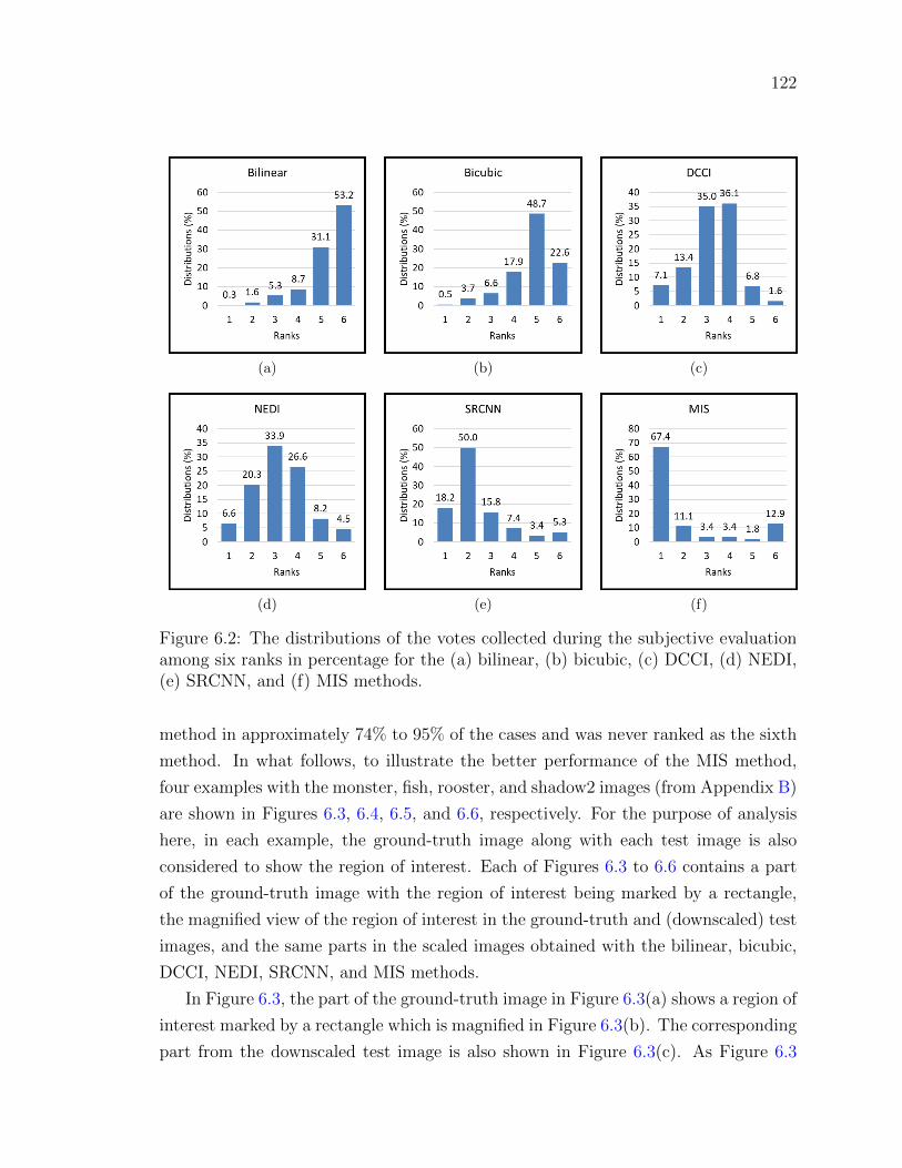
122

(a) (b) (c)

(d) (e) (f)

Figure 6.2: The distributions of the votes collected during the subjective evaluationamong six ranks in percentage for the (a) bilinear, (b) bicubic, (c) DCCI, (d) NEDI,(e) SRCNN, and (f) MIS methods.

method in approximately 74% to 95% of the cases and was never ranked as the sixth

method. In what follows, to illustrate the better performance of the MIS method,

four examples with the monster, fish, rooster, and shadow2 images (from Appendix B)

are shown in Figures 6.3, 6.4, 6.5, and 6.6, respectively. For the purpose of analysis

here, in each example, the ground-truth image along with each test image is also

considered to show the region of interest. Each of Figures 6.3 to 6.6 contains a part

of the ground-truth image with the region of interest being marked by a rectangle,

the magnified view of the region of interest in the ground-truth and (downscaled) test

images, and the same parts in the scaled images obtained with the bilinear, bicubic,

DCCI, NEDI, SRCNN, and MIS methods.

In Figure 6.3, the part of the ground-truth image in Figure 6.3(a) shows a region of

interest marked by a rectangle which is magnified in Figure 6.3(b). The corresponding

part from the downscaled test image is also shown in Figure 6.3(c). As Figure 6.3

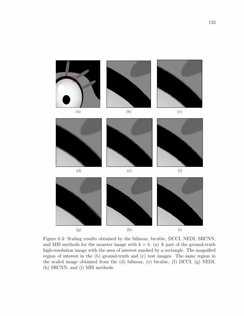
123

(a) (b) (c)

(d) (e) (f)

(g) (h) (i)

Figure 6.3: Scaling results obtained by the bilinear, bicubic, DCCI, NEDI, SRCNN,and MIS methods for the monster image with k = 4. (a) A part of the ground-truthhigh-resolution image with the area of interest marked by a rectangle. The magnifiedregion of interest in the (b) ground-truth and (c) test images. The same region inthe scaled image obtained from the (d) bilinear, (e) bicubic, (f) DCCI, (g) NEDI,(h) SRCNN, and (i) MIS methods.

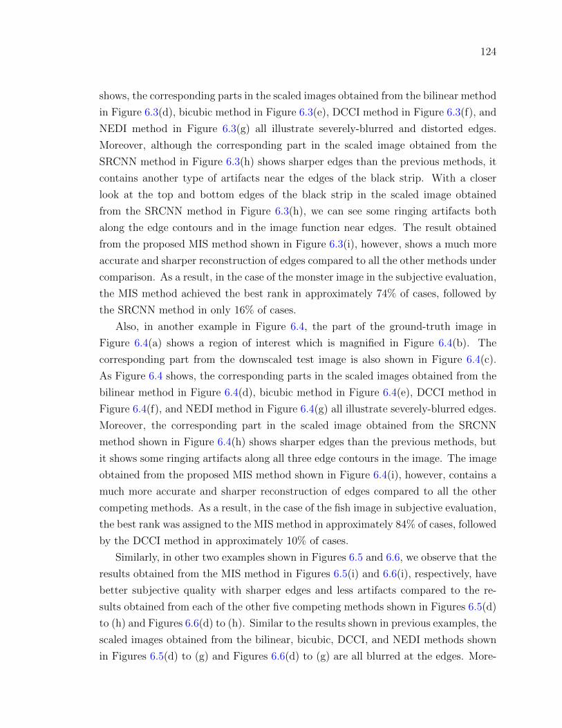
124

shows, the corresponding parts in the scaled images obtained from the bilinear method

in Figure 6.3(d), bicubic method in Figure 6.3(e), DCCI method in Figure 6.3(f), and

NEDI method in Figure 6.3(g) all illustrate severely-blurred and distorted edges.

Moreover, although the corresponding part in the scaled image obtained from the

SRCNN method in Figure 6.3(h) shows sharper edges than the previous methods, it

contains another type of artifacts near the edges of the black strip. With a closer

look at the top and bottom edges of the black strip in the scaled image obtained

from the SRCNN method in Figure 6.3(h), we can see some ringing artifacts both

along the edge contours and in the image function near edges. The result obtained

from the proposed MIS method shown in Figure 6.3(i), however, shows a much more

accurate and sharper reconstruction of edges compared to all the other methods under

comparison. As a result, in the case of the monster image in the subjective evaluation,

the MIS method achieved the best rank in approximately 74% of cases, followed by

the SRCNN method in only 16% of cases.

Also, in another example in Figure 6.4, the part of the ground-truth image in

Figure 6.4(a) shows a region of interest which is magnified in Figure 6.4(b). The

corresponding part from the downscaled test image is also shown in Figure 6.4(c).

As Figure 6.4 shows, the corresponding parts in the scaled images obtained from the

bilinear method in Figure 6.4(d), bicubic method in Figure 6.4(e), DCCI method in

Figure 6.4(f), and NEDI method in Figure 6.4(g) all illustrate severely-blurred edges.

Moreover, the corresponding part in the scaled image obtained from the SRCNN

method shown in Figure 6.4(h) shows sharper edges than the previous methods, but

it shows some ringing artifacts along all three edge contours in the image. The image

obtained from the proposed MIS method shown in Figure 6.4(i), however, contains a

much more accurate and sharper reconstruction of edges compared to all the other

competing methods. As a result, in the case of the fish image in subjective evaluation,

the best rank was assigned to the MIS method in approximately 84% of cases, followed

by the DCCI method in approximately 10% of cases.

Similarly, in other two examples shown in Figures 6.5 and 6.6, we observe that the

results obtained from the MIS method in Figures 6.5(i) and 6.6(i), respectively, have

better subjective quality with sharper edges and less artifacts compared to the re-

sults obtained from each of the other five competing methods shown in Figures 6.5(d)

to (h) and Figures 6.6(d) to (h). Similar to the results shown in previous examples, the

scaled images obtained from the bilinear, bicubic, DCCI, and NEDI methods shown

in Figures 6.5(d) to (g) and Figures 6.6(d) to (g) are all blurred at the edges. More-

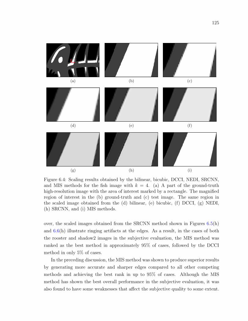
125

(a) (b) (c)

(d) (e) (f)

(g) (h) (i)

Figure 6.4: Scaling results obtained by the bilinear, bicubic, DCCI, NEDI, SRCNN,and MIS methods for the fish image with k = 4. (a) A part of the ground-truthhigh-resolution image with the area of interest marked by a rectangle. The magnifiedregion of interest in the (b) ground-truth and (c) test image. The same region inthe scaled image obtained from the (d) bilinear, (e) bicubic, (f) DCCI, (g) NEDI,(h) SRCNN, and (i) MIS methods.

over, the scaled images obtained from the SRCNN method shown in Figures 6.5(h)

and 6.6(h) illustrate ringing artifacts at the edges. As a result, in the cases of both

the rooster and shadow2 images in the subjective evaluation, the MIS method was

ranked as the best method in approximately 95% of cases, followed by the DCCI

method in only 5% of cases.

In the preceding discussion, the MIS method was shown to produce superior results

by generating more accurate and sharper edges compared to all other competing

methods and achieving the best rank in up to 95% of cases. Although the MIS

method has shown the best overall performance in the subjective evaluation, it was

also found to have some weaknesses that affect the subjective quality to some extent.

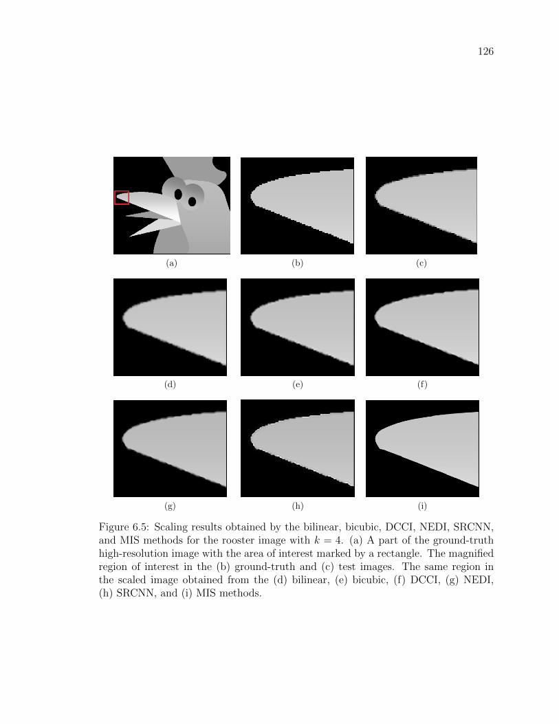
126

(a) (b) (c)

(d) (e) (f)

(g) (h) (i)

Figure 6.5: Scaling results obtained by the bilinear, bicubic, DCCI, NEDI, SRCNN,and MIS methods for the rooster image with k = 4. (a) A part of the ground-truthhigh-resolution image with the area of interest marked by a rectangle. The magnifiedregion of interest in the (b) ground-truth and (c) test images. The same region inthe scaled image obtained from the (d) bilinear, (e) bicubic, (f) DCCI, (g) NEDI,(h) SRCNN, and (i) MIS methods.

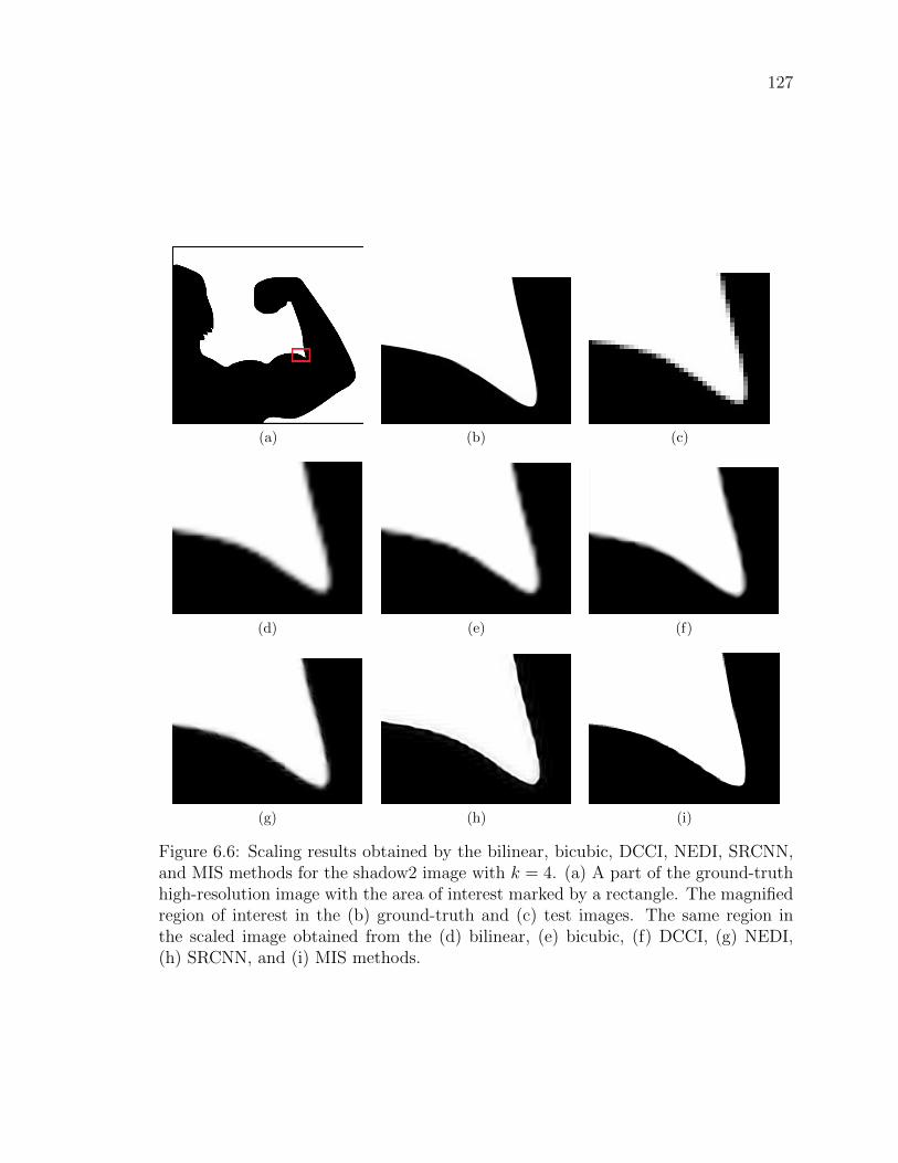
127

(a) (b) (c)

(d) (e) (f)

(g) (h) (i)

Figure 6.6: Scaling results obtained by the bilinear, bicubic, DCCI, NEDI, SRCNN,and MIS methods for the shadow2 image with k = 4. (a) A part of the ground-truthhigh-resolution image with the area of interest marked by a rectangle. The magnifiedregion of interest in the (b) ground-truth and (c) test images. The same region inthe scaled image obtained from the (d) bilinear, (e) bicubic, (f) DCCI, (g) NEDI,(h) SRCNN, and (i) MIS methods.

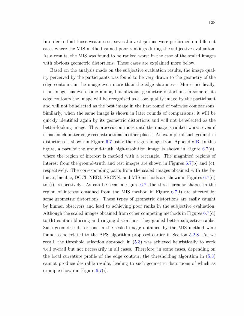
128

In order to find those weaknesses, several investigations were performed on different

cases where the MIS method gained poor rankings during the subjective evaluation.

As a results, the MIS was found to be ranked worst in the case of the scaled images

with obvious geometric distortions. These cases are explained more below.

Based on the analysis made on the subjective evaluation results, the image qual-

ity perceived by the participants was found to be very drawn to the geometry of the

edge contours in the image even more than the edge sharpness. More specifically,

if an image has even some minor, but obvious, geometric distortions in some of its

edge contours the image will be recognized as a low-quality image by the participant

and will not be selected as the best image in the first round of pairwise comparisons.

Similarly, when the same image is shown in later rounds of comparisons, it will be

quickly identified again by its geometric distortions and will not be selected as the

better-looking image. This process continues until the image is ranked worst, even if

it has much better edge reconstructions in other places. An example of such geometric

distortions is shown in Figure 6.7 using the dragon image from Appendix B. In this

figure, a part of the ground-truth high-resolution image is shown in Figure 6.7(a),

where the region of interest is marked with a rectangle. The magnified regions of

interest from the ground-truth and test images are shown in Figures 6.7(b) and (c),

respectively. The corresponding parts from the scaled images obtained with the bi-

linear, bicubic, DCCI, NEDI, SRCNN, and MIS methods are shown in Figures 6.7(d)

to (i), respectively. As can be seen in Figure 6.7, the three circular shapes in the

region of interest obtained from the MIS method in Figure 6.7(i) are affected by

some geometric distortions. These types of geometric distortions are easily caught

by human observers and lead to achieving poor ranks in the subjective evaluation.

Although the scaled images obtained from other competing methods in Figures 6.7(d)

to (h) contain blurring and ringing distortions, they gained better subjective ranks.

Such geometric distortions in the scaled image obtained by the MIS method were

found to be related to the APS algorithm proposed earlier in Section 5.2.8. As we

recall, the threshold selection approach in (5.3) was achieved heuristically to work

well overall but not necessarily in all cases. Therefore, in some cases, depending on

the local curvature profile of the edge contour, the thresholding algorithm in (5.3)

cannot produce desirable results, leading to such geometric distortions of which as

example shown in Figure 6.7(i).

129

(a) (b) (c)

(d) (e) (f)

(g) (h) (i)

Figure 6.7: An example of a geometric distortion produced by the MIS method forthe dragon image at k = 4. (a) A part of the ground-truth high-resolution imagewith the area of interest marked by a rectangle. The magnified region of interestin the (b) ground-truth and (c) test images. The same region in the scaled imagesobtained from the (d) bilinear, (e) bicubic, (f) DCCI, (g) NEDI, (h) SRCNN, and(i) MIS methods.

130

6.2.3 Objective Evaluation

As part of our experimental comparisons, in addition to the subjective evaluation, an

objective evaluation is performed to quantitatively compare the quality of the scaled

images obtained with the proposed MIS and those produced by the competing meth-

ods. In what follows, the methodology used for the objective evaluation is explained

followed by presenting and analyzing the results.

6.2.3.1 Methodology for Objective Evaluation

One of the most well-known objective metrics that is often used for assessing image

quality is the PSNR (as introduced in Section 2.11.1). Although the PSNR does not

always reflect the human visual perception of image quality (as studied in [87]), it is

still widely used in many applications. Many other metrics based on image perceptual

quality have also been introduced (e.g., [76, 56, 97, 47]), of which the SSIM [88] (as

introduced in Section 2.11.2) has gained much attention and has been widely used.

Thus, for our objective evaluation, both the PSNR and SSIM are used. Moreover,

since our main goal is to reduce the blurring artifacts in scaled images, the PEE metric

(as introduced in Section 2.11.3) is also used to measure the sharpness of edges in

scaled images because neither PSNR or SSIM is designed to perform that.

For the objective evaluation, we proceeded as follows. In order to be consistent

with the subjective evaluation, the same set of 20 low-resolution test images and the

sampling factor k = 4, which were used previously for the subjective evaluation, were

given to each of the six scaling methods under comparison. Then, the resulting scaled

image obtained from each method was compared with its ground-truth high-resolution

counterpart to compute the PSNR, SSIM, and PEE metrics.

6.2.3.2 Objective Evaluation Results and Analysis

Using the methodology explained above, the computed PSNR, SSIM, and PEE results

with the bilinear, bicubic, DCCI, NEDI, SRCNN, and MIS methods, for a represen-

tative subset of 10 images, are summarized in Table 6.2. As will be seen shortly,

the objective results are not necessarily consistent with the subjective results and

results of different metrics are not even consistent well with each other either. Such

inconsistencies in the objective results are because of the fact that devising objective

metrics that always match well with subjective image quality, as it is perceived by

humans, is extremely difficult. Therefore, all objective metrics, including the ones

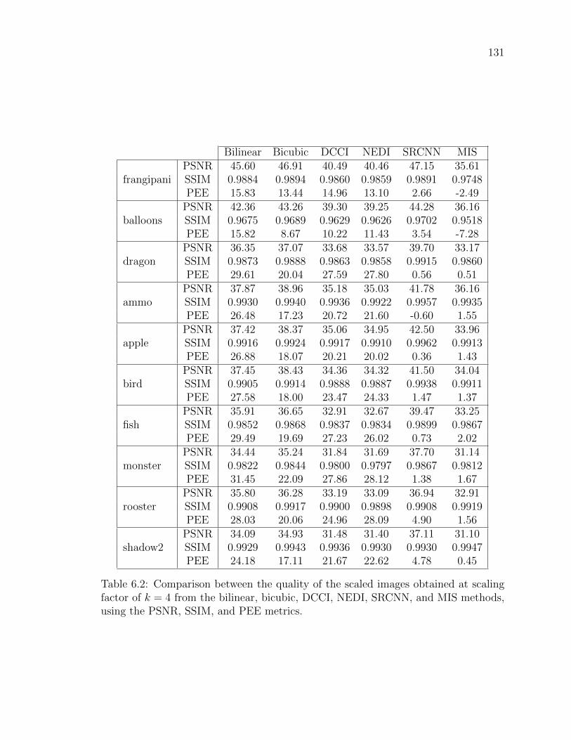
131

Bilinear Bicubic DCCI NEDI SRCNN MIS

frangipaniPSNR 45.60 46.91 40.49 40.46 47.15 35.61SSIM 0.9884 0.9894 0.9860 0.9859 0.9891 0.9748PEE 15.83 13.44 14.96 13.10 2.66 -2.49

balloonsPSNR 42.36 43.26 39.30 39.25 44.28 36.16SSIM 0.9675 0.9689 0.9629 0.9626 0.9702 0.9518PEE 15.82 8.67 10.22 11.43 3.54 -7.28

dragonPSNR 36.35 37.07 33.68 33.57 39.70 33.17SSIM 0.9873 0.9888 0.9863 0.9858 0.9915 0.9860PEE 29.61 20.04 27.59 27.80 0.56 0.51

ammoPSNR 37.87 38.96 35.18 35.03 41.78 36.16SSIM 0.9930 0.9940 0.9936 0.9922 0.9957 0.9935PEE 26.48 17.23 20.72 21.60 -0.60 1.55

applePSNR 37.42 38.37 35.06 34.95 42.50 33.96SSIM 0.9916 0.9924 0.9917 0.9910 0.9962 0.9913PEE 26.88 18.07 20.21 20.02 0.36 1.43

birdPSNR 37.45 38.43 34.36 34.32 41.50 34.04SSIM 0.9905 0.9914 0.9888 0.9887 0.9938 0.9911PEE 27.58 18.00 23.47 24.33 1.47 1.37

fishPSNR 35.91 36.65 32.91 32.67 39.47 33.25SSIM 0.9852 0.9868 0.9837 0.9834 0.9899 0.9867PEE 29.49 19.69 27.23 26.02 0.73 2.02

monsterPSNR 34.44 35.24 31.84 31.69 37.70 31.14SSIM 0.9822 0.9844 0.9800 0.9797 0.9867 0.9812PEE 31.45 22.09 27.86 28.12 1.38 1.67

roosterPSNR 35.80 36.28 33.19 33.09 36.94 32.91SSIM 0.9908 0.9917 0.9900 0.9898 0.9908 0.9919PEE 28.03 20.06 24.96 28.09 4.90 1.56

shadow2PSNR 34.09 34.93 31.48 31.40 37.11 31.10SSIM 0.9929 0.9943 0.9936 0.9930 0.9930 0.9947PEE 24.18 17.11 21.67 22.62 4.78 0.45

Table 6.2: Comparison between the quality of the scaled images obtained at scalingfactor of k = 4 from the bilinear, bicubic, DCCI, NEDI, SRCNN, and MIS methods,using the PSNR, SSIM, and PEE metrics.

132

used in our evaluation, sometimes fail to accurately reflect the image quality that is

actually perceived by humans. Therefore, due to this limitation, multiple objective

metrics sometimes result in different image quality measurements that are inconsistent

not only with themselves, but also with the actual perceived image quality. Despite

the above shortcomings, such objective measures are still used in many applications,

where performing a subjective evaluation is not practical, but they leave much to be

desired. Therefore, analyzing such results needs more careful considerations which is

presented below.

Starting with the PSNR results in Table 6.2, we realize that the bicubic method

always performs better than the bilinear method, which is consistent with the sub-

jective results. Similarly, comparing the PSNR results between the DCCI and NEDI

methods shows that they perform fairly close, with the DCCI method being slightly

better than the NEDI method, which also is consistent with the subjective results.

Between the bicubic and DCCI methods, however, the PSNR results in Table 6.2

show that the bicubic method is always better than the DCCI method, with a PSNR

margin of approximately 3 dB (for rooster image) to 6 dB (for frangipani image). Sim-

ilarly, the PSNR results in Table 6.2 show that even the bilinear method performs

better than the DCCI method in all the cases with a PSNR margin of over 2 dB

(for apple image) to 5 dB (for frangipani image). Thus, based on the PSNR results,

the bilinear/bicubic methods perform much better than the DCCI/NEDI methods,

by a considerable margin. According to the subjective evaluation, however, the DC-

CI/NEDI methods achieved better ranks than the bilinear/bicubic methods overall.

Therefore, the better performance of the bilinear/bicubic methods compared to the

DCCI/NEDI methods, based on Table 6.2, fully contradicts the subjective results

previously presented in Table 6.1 and Figure 6.2. In the case of the SRCNN method,

however, the PSNR results in Table 6.2 show that it performs better than the bi-

linear, bicubic, DCCI, and NEDI methods, which is consistent with the subjective

results. In the case of the proposed MIS method, the PSNR results in Table 6.2 show

that it produces the lowest PSNRs in almost all cases, except for the ammo and fish

images, where the MIS method outperforms the DCCI and NEDI methods with an

average margin of 0.66 dB and 0.85 dB, respectively. The lower performance of the

MIS method in terms of PSNR again contradicts the subjective results, where the

MIS method ranked best overall in approximately 67% of the cases. As explained

earlier, such inconsistencies that are observed between the PSNR and subjective re-

sults are due to the significant limitations of PSNR in accurately measuring the error

133

as perceived by the human visual system.

The lower PSNRs obtained by the MIS method, in Table 6.2, can be justified

as follows. Firstly, as shown previously through subjective evaluation results, two

strengths of the MIS method are producing sharper edges and smoother edge con-

tours. Secondly, the image functions at points on the opposite sides of image edges

often differ by a large amount. Consequently, even minor changes in the image func-

tion near edges (made by edge sharpening) and minor shifting in the location of the

edges (made by edge-contour smoothing) can drastically affect the PSNR. Such edge

sharpening and edge-contour smoothness in the MIS method may not necessarily

generate a poor image reconstruction as proved through the subjective evaluation,

but they can definitely reduce the PSNR. Another factor that can negatively affect

the PSNR is the deficiency of the edge detector at junctions points, where three (or

more) edges meet. In some junctions areas, where the edge detector fails to detect

the junction point and its nearby edges, a reconstruction error will happen which

has a negative effect on the PSNR. An example of such a missed junction point is

shown in Figure 6.8, using a junction area in the dragon image from Appendix B. In

this figure, a magnified area of the ground-truth high-resolution image containing a

junction point, its corresponding part from the downscaled test image, and the corre-

sponding part from the resulting edge map are shown in Figures 6.8(a), (b), and (c),

respectively. The corresponding junction areas from the scaled images obtained us-

ing the bilinear, bicubic, DCCI, NEDI, SRCNN, and MIS methods are shown in

Figures 6.8(d) to (i), respectively. As can be seen in Figure 6.8, the three edges ap-

proaching the junction point in Figure 6.8(b) were not fully detected in the edge map

shown in Figure 6.8(c). Thus, the edge map contains a gap near the junction area.

Consequently, the corresponding junction area in the scaled image obtained from the

MIS method shown in Figure 6.8(i) shows some reconstruction error in that region,

which can decrease the PSNR. Moreover, although the scaled images obtained from

other methods, such as the bicubic and SRCNN methods in Figures 6.8(e) and (h),

have higher PSNRs, they all have other types of artifacts like blurring and ringing

near the edges, which reduce the perceptual image quality.

Having studied the PSNR results in Table 6.2, we now focus on the SSIM results.

Similar to PSNR, the SSIM results, in Table 6.2, show that the bicubic and DCCI

methods perform better that the bilinear and NEDI methods, respectively, in all

the test cases. These improvements in SSIM, however, are very marginal (unlike

the improvements in PSNR) and reasonably consistent with the subjective results.

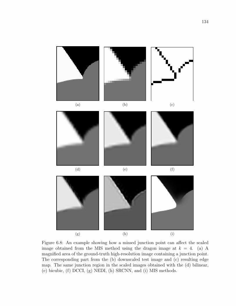
134

(a) (b) (c)

(d) (e) (f)

(g) (h) (i)

Figure 6.8: An example showing how a missed junction point can affect the scaledimage obtained from the MIS method using the dragon image at k = 4. (a) Amagnified area of the ground-truth high-resolution image containing a junction point.The corresponding part from the (b) downscaled test image and (c) resulting edgemap. The same junction region in the scaled images obtained with the (d) bilinear,(e) bicubic, (f) DCCI, (g) NEDI, (h) SRCNN, and (i) MIS methods.

135

Between the bicubic and DCCI methods, however, the SSIM results in Table 6.2

indicate that the bicubic method still performs better that the DCCI method, with

a margin of 0.0003 (for ammo image) to 0.0060 (for balloons image). It is worth

mentioning that although the SSIM results for the bicubic and DCCI methods are

not completely consistent with the subjective evaluation, the differences in the SSIM

values are not as significant as they are in the PSNR results. For example, for images

like ammo, apple, and shadow2 from Table 6.2, the bilinear method outperforms

the DCCI method with an average PSNR margin of 3.5 dB, but with an average

SSIM margin of only 0.0005. Consequently, in this example, the average of 3.5 dB

difference is considered reasonably high for PSNR, whereas the 0.0005 difference is not

that large for SSIM and indicates a very comparable perceptual quality between the

images under comparison and also a better consistency with the subjective results.

In the case of the SRCNN and bicubic methods in Table 6.2, the SSIM results

show that bicubic method outperforms the SRCNN method in the frangipani, rooster,

and shadow2 images. In terms of PSNR, however, the SRCNN method was shown to

perform better than the bicubic method in all cases in Table 6.2, indicating the incon-

sistency between the PSNR and SSIM metrics. Finally, regarding the MIS method,

the SSIM results collected from all 20 test images shows that, unlike the PSNR results,

in the case of the cartoon/graphical images, the MIS method produces comparable

or even better results compared to the bilinear, bicubic, DCCI, and NEDI methods.

For example, in the case of the eight cartoon/graphical images in the representative

results shown in Table 6.2 (i.e., all excluding the frangipani and balloons images), the

MIS method outperforms the NEDI method in 8/8 of cases with an average SSIM

margin of 0.0016. Similarly, the MIS method outperforms the DCCI method in 5/8 of

cases by an average SSIM margin of 0.0019. In the remaining 3/8 of cases, however,

the MIS method performs fairly comparable with an average SSIM of only 0.0003

smaller. Between the SRCNN and SIM method, the MIS method outperforms the

SRCNN method in 2/8 of cases, for the rooster and shadow2 images, with an av-

erage SSIM margin of 0.0014. With respect to PSNR, however, the MIS method

falls behind the SRCNN method with a average PSNR margin of approximately 5

dB, which is another example of inconsistency between the PSNR and SSIM metrics.

As explained before, such inconsistencies between different objective metrics, such as

PSNR and SSIM, is due to the limitations of each of them in accurately capturing

the perceived image quality. In the case of the two natural photographic and moder-

ately textured images in Table 6.2, such as frangipani and balloons, the MIS method

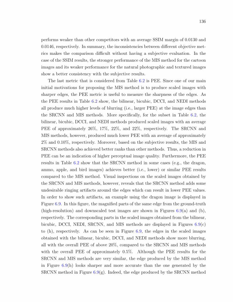
136

performs weaker than other competitors with an average SSIM margin of 0.0130 and

0.0146, respectively. In summary, the inconsistencies between different objective met-

rics makes the comparison difficult without having a subjective evaluation. In the

case of the SSIM results, the stronger performance of the MIS method for the cartoon

images and its weaker performance for the natural photographic and textured images

show a better consistency with the subjective results.

The last metric that is considered from Table 6.2 is PEE. Since one of our main

initial motivations for proposing the MIS method is to produce scaled images with

sharper edges, the PEE metric is useful to measure the sharpness of the edges. As

the PEE results in Table 6.2 show, the bilinear, bicubic, DCCI, and NEDI methods

all produce much higher levels of blurring (i.e., larger PEE) at the image edges than

the SRCNN and MIS methods. More specifically, for the subset in Table 6.2, the

bilinear, bicubic, DCCI, and NEDI methods produced scaled images with an average

PEE of approximately 26%, 17%, 22%, and 22%, respectively. The SRCNN and

MIS methods, however, produced much lower PEE with an average of approximately

2% and 0.10%, respectively. Moreover, based on the subjective results, the MIS and

SRCNN methods also achieved better ranks than other methods. Thus, a reduction in

PEE can be an indication of higher perceptual image quality. Furthermore, the PEE

results in Table 6.2 show that the SRCNN method in some cases (e.g., the dragon,

ammo, apple, and bird images) achieves better (i.e., lower) or similar PEE results

compared to the MIS method. Visual inspections on the scaled images obtained by

the SRCNN and MIS methods, however, reveals that the SRCNN method adds some

undesirable ringing artifacts around the edges which can result in lower PEE values.

In order to show such artifacts, an example using the dragon image is displayed in

Figure 6.9. In this figure, the magnified parts of the same edge from the ground-truth

(high-resolution) and downscaled test images are shown in Figures 6.9(a) and (b),

respectively. The corresponding parts in the scaled images obtained from the bilinear,

bicubic, DCCI, NEDI, SRCNN, and MIS methods are displayed in Figures 6.9(c)

to (h), respectively. As can be seen in Figure 6.9, the edges in the scaled images

obtained with the bilinear, bicubic, DCCI, and NEDI methods show more blurring,

all with the overall PEE of above 20%, compared to the SRCNN and MIS methods

with the overall PEE of approximately 0.5%. Although the PEE results for the

SRCNN and MIS methods are very similar, the edge produced by the MIS method

in Figure 6.9(h) looks sharper and more accurate than the one generated by the

SRCNN method in Figure 6.9(g). Indeed, the edge produced by the SRCNN method

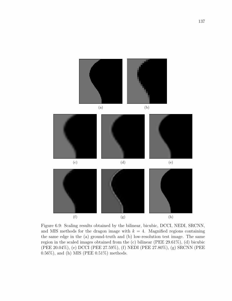
137

(a) (b)

(c) (d) (e)

(f) (g) (h)

Figure 6.9: Scaling results obtained by the bilinear, bicubic, DCCI, NEDI, SRCNN,and MIS methods for the dragon image with k = 4. Magnified regions containingthe same edge in the (a) ground-truth and (b) low-resolution test image. The sameregion in the scaled images obtained from the (c) bilinear (PEE 29.61%), (d) bicubic(PEE 20.04%), (e) DCCI (PEE 27.59%), (f) NEDI (PEE 27.80%), (g) SRCNN (PEE0.56%), and (h) MIS (PEE 0.51%) methods.

138

in Figure 6.9(g) shows an undesirable bright strip along the edge contour which can

undesirably produce large gradients, leading to a small overall PEE value.

The negative PEE values, in some cases in Table 6.2, such as the frangipani and

balloons images obtained by the MIS method, show that the scaled image contains

edges that are sharper than those in its ground-truth counterpart. Thus, the negative

PEE values do not necessary indicate a weak edge reproduction, as long as the gen-

eral structure of the image and edge contours are maintained well and the absolute

value of the PEE is close enough to zero. The collected PEE results show that, with

natural photographic images, the MIS method more often produces scaled images

with negative PEE values. This behavior can be justified as follows. In photographic

images, some (parts of) objects almost always fall outside of the lens depth of field,

where the objects are supposed to appear acceptably sharp. As a result, those parts

that intentionally/unintentionally fall outside of the lens depth of field look much

more blurred. Moreover, objects that fall inside the depth of field themselves do

not have absolute sharp edges, due to lens optics limitations and maybe because of

some post processing that is applied by some cameras internally. Therefore, when

such photographic images are used with the MIS method, all those intentionally/un-

intentionally blurred edges are sharpened during the the scaling process because the

MIS method has originally been designed to produce sharp edges. Consequently, the

scaled images obtained with the MIS method most often contain sharper edges than

the ground-truth image, leading to negative PEE results. Whether such sharpening

is desirable is very subjective, but the overall results from our subjective evaluation

seem to suggest that, for the average/typical person, sharpening is usually preferred

over blurring or ringing.

In order to illustrate the sharpening effect that often exists in the case of the

natural photographic images as explained above, an example using the frangipani

image from Appendix B is shown Figure 6.10. In this figure, a part of the ground-

truth image, with the region of interest being marked by a rectangle is shown in

Figure 6.10(a). As can be seen from the magnified views of the region of interest

in the ground-truth and test images shown in Figures 6.10(b) and (c), respectively,

they themselves show some level of blurriness due to the reasons explained earlier.

Therefore, the blurring/ringing artifacts that happen by the the bilinear, bicubic,

DCCI, NEDI, and SRCNN methods are not much visually recognizable in the scaled

images shown in Figures 6.10(d) to (h) because the original images themselves are

already blurred. The corresponding part in the scaled image obtained by the MIS

139

(a) (b) (c)

(d) (e) (f)

(g) (h) (i)

Figure 6.10: Scaling results obtained by the bilinear, bicubic, DCCI, NEDI, SRCNN,and MIS methods using the frangipani image at k = 4. (a) A part of the ground-truthhigh-resolution image, with a region of interest being marked by a rectangle. Themagnified region of interest from the (b) ground-truth and (c) test images. The samepart in the scaled images obtained with the (d) bilinear (PEE 15.83%), (e) bicubic(PEE 13.44%), (f) DCCI (PEE 14.96%), (g) NEDI (PEE 13.10%), (h) SRCNN (PEE2.66%), and (i) MIS (PEE -2.49%) methods.

140

method shown in Figure 6.10(i), however, shows considerably sharper edges than

all other images (including the ground-truth image), leading to a negative PEE of

-2.49%. Such an observation, of which as example shown in Figure 6.10, is often valid

in the case of the natural photographic images, where many edges are usually blurred

either intentionally (by the photographer) or unintentionally.

In summary, as the analysis of the objective results shows, the PSNR, SSIM, and

PEE metrics all performed differently, with the PSNR and PEE metrics being shown

to have the lowest and highest consistency with the subjective results, respectively.

Moreover, some objective metrics, such as PSNR and SSIM, were shown not to repre-

sent consistent results due to their limitations. Therefore, for evaluating complicated

imaging systems, such as image scaling, objective metrics along with a subjective

evaluation should be taken into consideration, as objective measures by themselves

often cannot accurately reflect perceptual image quality.

6.2.4 Supplementary Discussions

With the insights obtained through the experimental comparisons between the MIS

and other relevant scaling methods, we now provide some supplementary discussions

on the advantages and disadvantages of each method. As the results of the experi-

mental comparisons in previous sections showed, no single scaling method is yet able

to perform perfectly well with all types of images in all aspects.

The classical convolution-based interpolation techniques, such as bilinear and bicu-

bic methods, were shown to produce scaled images with weaker perceptual qualities

and significantly blurred edges. Given all their weaknesses, these methods have been

still being used as the main upscaling techniques in many commercial software, such

as Adobe Photoshop for many years, due to their simplicity, fast speed, and ease

of implementation. Other edge-directed approaches, such as the NEDI and DCCI

methods, however, have shown to be capable of handling the edge-blurring problem

to some extent. The improvements in the perceptual quality of the scaled images

obtained by these methods, however, are too marginal to justify the added computa-

tional complexity.

The SRCNN method, as a representative of the most recent and advanced meth-

ods based on deep learning, showed a reasonably better performance compared to

other raster-based methods in our comparisons. Using a deep convolutional neural

network, the SRCNN method is able to reduce the edge-blurring that can happen

141

during image scaling. As shown in our experiments, however, the scaled images

obtained with the SRCNN method often contain some undesirable ringing artifacts

which reduce the subjective quality. Such deep-learning based scaling methods have

recently become very advanced and probably been known as the best general-purpose

image scaling methods. These methods, however, have some serious drawbacks that

should be taken into consideration as follows. First of all, deep-learning based scaling

methods are known to be computationally very expensive and require a huge train-

ing dataset to perform reasonably well. Therefore, often graphics processing units

(GPUs) with multiple cores are used to perform the training stage. Because of such

a large training data and high computational cost, the SRCNN method can take up

to several days to train its network. Moreover, such methods have a very high mem-

ory cost. For example, in our experiment, to generate a scaled image with a high

resolution of approximately 6000 × 6000, the SRCNN method would require more

than 20 gigabytes (GB) of RAM which is too much with respect to the typical RAM

sizes in today’s personal computers. Lastly, almost all deep-learning based scaling

methods, including the SRCNN method, are trained for a single scale factor and are

only guaranteed to work well only with that specified scale. Thus, for a new scale

factor, a new model has to be trained. One may intuitively think that if a network is

trained for a larger scale factor it may then work well with smaller factors too, but

that is not true (as will be shown shortly).

Regarding the proposed MIS method, although it has higher computational com-

plexity than the convolution-based scaling methods, the subjective evaluation has

shown that the MIS method obtained the best rank among all. Compared to the SR-

CNN method, however, the MIS method has lower computational complexity mainly

because no training stage is involved to take several days long. Moreover, in our

experiment, the MIS method could generate scaled images with large resolutions of

up to 9000 × 9000 with a moderate CPU and typical RAM of 4 GB, which is much

lower than the RAM needed by the SRCNN method. Furthermore, one of the most

beneficial advantages of the MIS method is the fact that, once an image mesh model

is generated, it can be used with almost any scale factor (unlike the SRCNN method).

Figure 6.11 shows an example, where the same mesh model from the MIS method

and the same trained model with the SRCNN method, used in the previous experi-

ments for a scale factor of k = 4, tested with a new factor of k = 2 on the dragon

image. In Figure 6.11, a magnified part of the low-resolution test image is shown

in Figure 6.11(a). The corresponding part in the scaled image obtained with the

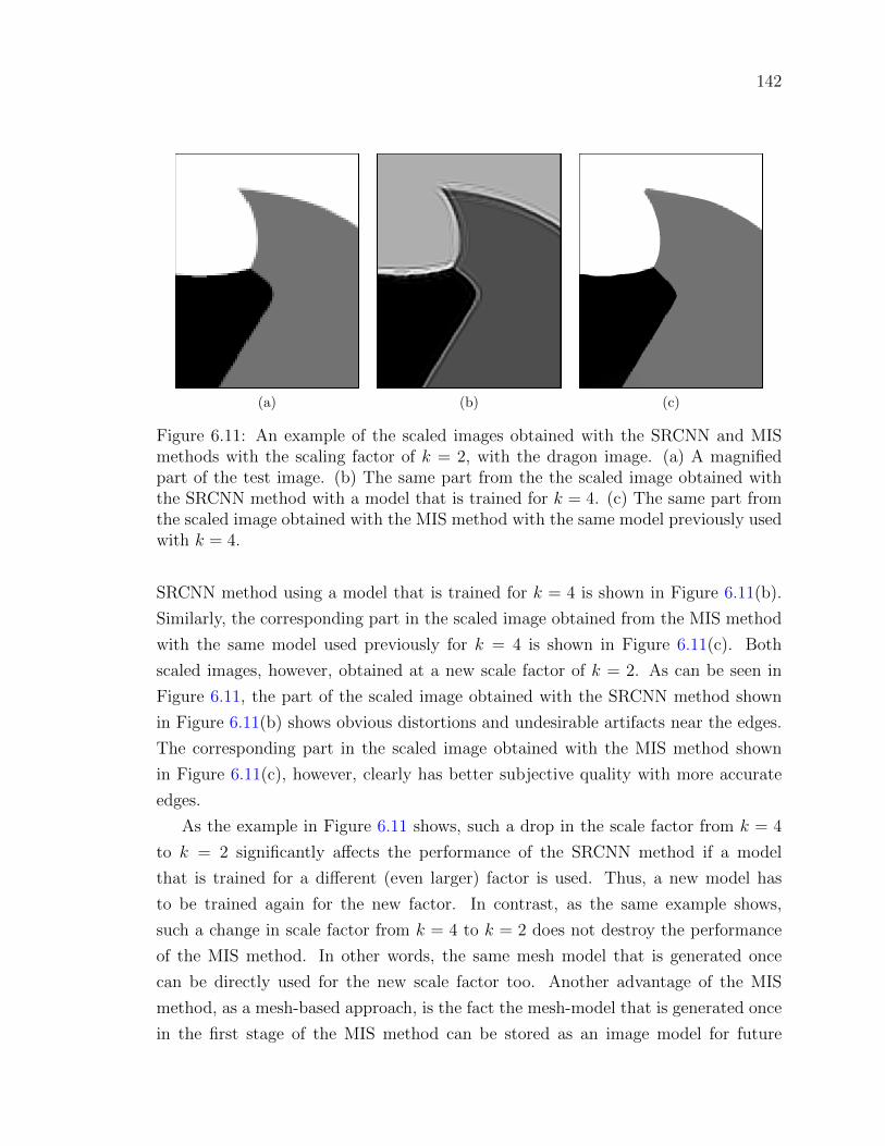
142

(a) (b) (c)

Figure 6.11: An example of the scaled images obtained with the SRCNN and MISmethods with the scaling factor of k = 2, with the dragon image. (a) A magnifiedpart of the test image. (b) The same part from the the scaled image obtained withthe SRCNN method with a model that is trained for k = 4. (c) The same part fromthe scaled image obtained with the MIS method with the same model previously usedwith k = 4.

SRCNN method using a model that is trained for k = 4 is shown in Figure 6.11(b).

Similarly, the corresponding part in the scaled image obtained from the MIS method

with the same model used previously for k = 4 is shown in Figure 6.11(c). Both

scaled images, however, obtained at a new scale factor of k = 2. As can be seen in

Figure 6.11, the part of the scaled image obtained with the SRCNN method shown

in Figure 6.11(b) shows obvious distortions and undesirable artifacts near the edges.

The corresponding part in the scaled image obtained with the MIS method shown

in Figure 6.11(c), however, clearly has better subjective quality with more accurate

edges.

As the example in Figure 6.11 shows, such a drop in the scale factor from k = 4

to k = 2 significantly affects the performance of the SRCNN method if a model

that is trained for a different (even larger) factor is used. Thus, a new model has

to be trained again for the new factor. In contrast, as the same example shows,

such a change in scale factor from k = 4 to k = 2 does not destroy the performance

of the MIS method. In other words, the same mesh model that is generated once

can be directly used for the new scale factor too. Another advantage of the MIS

method, as a mesh-based approach, is the fact the mesh-model that is generated once

in the first stage of the MIS method can be stored as an image model for future

143

usages. For example, the same image model can also be used for mesh editing or

any combination of other affine transformation, such as translation, rotation, and

shearing. Such flexible functionalities of the MIS method, which allow for image

models that are portable, editable, and reusable, however, are not (easily) provided

with other raster-based methods, including the SRCNN method.

6.3 Conceptual Comparison

Due to the difficulties of comparing with the mesh-based methods as explained before,

an experimental comparison between the MIS method and other mesh-based image-

scaling methods was not feasible. In what follows, however, a conceptual comparison

through theoretical analysis is made between the MIS method and the following two

relevant mesh-based image scaling methods:

1. the subdivision-based image-representation (SBIR) method of Liao et al. [60],

and

2. the curvilinear feature driven image-representation (CFDIR) method of Zhou

et al. [102].

Like our MIS method, the SBIR and CFDIR methods are based on triangle-mesh

models and employ a subdivision-based technique to create smoother edge contours.

Moreover, both of them are edge preserving, but each method employs a different

technique for preserving the image edges. Furthermore, both of the SBIR and CFDIR

methods employ a function that approximates the original image function at sample

points, unlike the MIS method where an interpolating function is used. In what

follows, other specific similarities and differences between our MIS method and each

of the above methods are discussed.

Comparison with the SBIR method. The SBIR method, like our MIS

method, employs an approximating function that allows for discontinuities. More-

over, the SBIR method applies subdivision to a mesh model that is associated with

an approximating function with discontinuities. In our MIS method, the subdivision

scheme of the SBIR method is adapted and applied to the ERD mesh model. When

mesh generation is considered, the SBIR method employs a technique that is fun-

damentally different from the one employed by the MIS method. More specifically,

the mesh-generation technique of the SBIR method is based on mesh simplification,

144

where a mesh is initially generated using all sample points in the input image as

the vertices in the mesh. Then, the initial mesh is iteratively simplified to achieve

a desired number of vertices. Such mesh-generation schemes typically have a very

high computational and memory cost because of generating meshes with a very large

number of sample points at early stages of the simplification process. In our MIS

method, however, a mesh-generation approach based on mesh refinement is used to

reduce the complexity, where a very coarse mesh is initially generated and then it-

eratively refined by point insertion. The mesh-refinement scheme used by the MIS

method potentially has lower computational complexity and also is believed to have

much lower memory cost than the mesh-simplification scheme of the SBIR method

in comparable conditions.

Comparison with the CFDIR method. The CFDIR method, like our MIS

method, employs a mesh-generation scheme that is based on mesh refinement and

a constrained Delaunay triangulation. The CFDIR method, however, uses a com-

pletely different model that is associated with a continuous approximating function.

Therefore, in the CFDIR method, image discontinuities are modeled differently by

enclosing each image-edge feature with a pair of parallel polylines (similar to the

GVS method as illustrated previously in Figure 4.5). The MIS method, however,

employs a model that is associated with an approximating function that allows for

discontinuities. Thus, each image-edge feature is modeled with only one polyline,

which potentially results in meshes with many fewer vertices. Furthermore, because

the CFDIR method uses a continuous function everywhere, it will still create in-

evitable blurring artifacts during image scaling. To address this issue, in our MIS

method, however, a function with selected discontinuities is used to effectively reduce

(if not eliminate) edge blurring during image scaling (as previously shown through

the experimental comparisons in Section 6.2).

145

Chapter 7

Conclusions and Future Work

7.1 Conclusions

In this thesis, we have addressed two problems: 1) mesh generation, where mesh

models of images are generated to minimize squared error, and 2) image scaling,

where raster images are scaled using mesh models. To solve the mesh-generation

problem, the SEMMG method was proposed to generate triangle-mesh models that

are effective for representing grayscale images. To solve the image-scaling problem, the

MIS method was proposed for scaling grayscale raster images that are approximately

piecewise-smooth, using triangle-mesh models.

The SEMMG method, which was proposed for solving the mesh-generation prob-

lem, was developed by analyzing and modifying two existing schemes for generating

ERD triangle-mesh models, namely, the ERDED and ERDGPI methods. Through

this analysis, potential areas for improvement in different steps of the methods were

identified. Then, different techniques were developed to select more effective param-

eters for the ERD model, by applying several key modifications. Finally, all the

modifications were integrated into a unified framework to yield the new SEMMG

method. For evaluating the SEMMG method, it was compared with eight compet-

ing methods. Through experimental results, we demonstrated that the reconstructed

images obtained by the SEMMG method have higher quality than those obtained by

the competing methods, in terms of PSNR. Moreover, in the case of the competing

methods whose implementations are available, the subjective quality was compared

in addition to the PSNR. Evaluation results showed that the reconstructed images

obtained from the SEMMG method are better than those obtained by the competing

146

methods in terms of both PSNR and subjective quality. More specifically, in cases

where an implementation of the competing method was available, our experimental

results collected from 350 test cases show that the SEMMG method outperforms the

ED, MGH, ERDED, and ERDGPI schemes in approximately 100%, 89%, 99%, and

85% of cases, respectively. Furthermore, in the case of the methods without imple-

mentations, the results that are reported in their publications were used for com-

parison. Through this comparison, we showed that the PSNR of the reconstructed

images produced by the SEMMG method are on average 3.85, 0.75, 2.00, and 1.10

dB higher than those obtained by the GVS, HWT, BSP, and ATM methods, as re-

ported in their publications, respectively. Moreover, for a given PSNR, the SEMMG

method was shown to produce much smaller meshes compared to those obtained by

the GVS and BSP methods, with approximately 65% to 80% fewer vertices and 10%

to 60% fewer triangles, respectively. The better performance of the SEMMG method

is due to employing the advantageous ERD mesh model and, more importantly, ef-

fective techniques used to select parameters of the model. More specifically, with

the Otsu threshold-selection approach, a more useful set of edge constraints is found.

Furthermore, the optimization-based technique selects more effective wedge values

for the ERD model. Moreover, the centroid-based approach selects more accurate

set of sample points, by reducing the chance of selecting noisy pixels. Finally, with

the help of the ERD model, image discontinuities can be explicitly represented in

the mesh using fewer sample points. Therefore, as our experimental results show,

the SEMMG method is capable of producing triangular meshes of higher quality and

smaller sizes (i.e., number of vertices or triangles) which can be effectively used for

image representation.

For addressing the image-scaling problem, the MIS method was proposed which

produces scaled images of higher subjective quality with minimal edge blurring. The

MIS method was developed based on triangle-mesh modeling techniques. For evaluat-

ing the MIS method, it was compared with five well-known raster-based image-scaling

approaches called bilinear, bicubic, DCCI, NEDI, and SRCNN, using a subjective

evaluation followed by objective evaluations. The results of the subjective evaluation

show that the proposed MIS method was ranked best overall in almost 67% of the

cases, with the best average rank of 2 out of 6, among 380 collected rankings with

20 images and 19 participants. Moreover, visual inspections on the scaled images ob-

tained with different methods show that the proposed MIS method produces scaled

images of better quality with more accurate and sharper edges. Furthermore, in the

147

case of two other mesh-based scaling methods, named SBIR and CFDIR, where an ex-

perimental comparison was impractical, a conceptual comparison was made between

the MIS method and them. The comparison showed that, unlike the SBIR and CFDIR

methods, where either a continuous approximating function or a mesh-simplification

approach is used, the MIS method employs both a mesh-refinement technique and

an approximating function that allows for selected discontinuities. Therefore, the

MIS method is capable of producing sharper scaled images with smaller meshes and

potentially lower memory cost. The better performance of the proposed MIS method

observed in our subjective evaluation is, first, because of employing the ERD model,

which can explicitly represent discontinuities in the image, resulting in a great re-

duction in the blurring artifacts. Second, and more importantly, with the help an

improved mesh generator, an ERD mesh model with the parameters that are effec-

tively selected for image scaling is generated. In particular, the backfilling-based

technique used in the MIs method selects a more effective set of wedge values for the

ERD model. Moreover, the modified centroid-based approach selects a more useful set

of sample points, resulting in distortion-free edges. Furthermore, the proposed APS

method effectively selects the set of edge constraints to preserve curvatures of the edge

contours in the scaled image. Finally, using a subdivision-based model rasterization,

the MIS method produces scaled images with edge contours and image functions that

are sufficiently smooth. Therefore, as our experimental comparisons show, the MIS

method is capable of producing scaled images with overall higher subjective quality,

with more accurate and sharper edges, than some well-known methods that are often

used for image scaling. Aside from the improvements in subjective quality of the

scaled images, the MIS method allows for other practical functionalities that may not

easily (or ever) provided by state-of-the-art raster-based methods. For example, most

of the image scaling methods based on deep learning are guaranteed to work well with

the only specific scale factor for which they are trained. Using the MIS method, how-

ever, the image mesh model that is generated in the first stage of the method works

well with almost any scaling factor of interest to produce the high-resolution image.

Moreover, the same image model can be stored by its own and reused anytime later

for other purposes like image editing or any combination of affine transformations

(other than just scaling), such as translation, rotation, and shearing. Such flexible

functionalities of the MIS method, which allow for image models that are portable,

editable, and reusable, when combined with the improvements it makes in the subjec-

tive quality of the scaled images, makes the MIS method very practical and beneficial

148

to many image processing applications.

7.2 Future Work

In this thesis, triangle-mesh models of images, their generation, and their application

in image scaling were studied, which lead to the proposal of a new mesh-generation

method and a mesh-based image-scaling method. Throughout this work, various as-

pects of generating mesh models that are effective for image representation and image

scaling were analyzed and new methods were proposed to improve the quality of the

meshes and scaled images. Although our proposed mesh-generation and image-scaling

methods work fairly well, further research on certain areas may still be potentially

beneficial. In what follows, these areas are briefly described.

As discussed earlier, in our proposed mesh-generation methods, which employ

image edge information, edge detection is a crucial step to find the constrained edges

for the ERD mesh model. Therefore, the consistency and accuracy of the detected

edges are critically important in selecting more effective edge constraints. In our

methods, to keep the computational complexity lower, a Canny edge detector (with

one-pixel accuracy) is employed, which was shown to work well with images with

today’s typical resolutions. Our experiments on different test images, however, showed

that in case of the smaller images, an edge localization with only one-pixel accuracy is

not good enough. As a future work, one might consider employing a more advanced

edge detector to detect edges with subpixel accuracy, if input images with very low

resolutions are considered. In this case, using a more accurate edge detector could be

quite beneficial to image representation, and also to image scaling, by selecting more

accurate set of edge constraints.

Another important aspect of our proposed methods is the selection of wedge values

for an ERD model. As mentioned earlier, wedge values are one of the most significant

parameters of an ERD model. In this work, two different techniques for computing

the wedge values were introduced, for generating mesh models that are effective for

image representation and image scaling. For example, in our optimization-based

technique, first, corner z-values associated with the corners inside the wedge are

optimized and then the wedge value is computed as the weighted average of them.

Although the weighted averaging reduces the negative effects of the less-reliable corner

z-values, they still can affect the final computed wedge value. Therefore, another

future work could be finding a more effective way to select the wedge values. For

149

example, using a technique which directly optimizes the wedge values themselves may

be more beneficial, instead of optimizing the corner z-values and averaging them.

Another potential area for future work is to find a better way to employ mesh

subdivision for image scaling. In our proposed method of image scaling, the mesh

subdivision is applied as a post-processing step after the mesh is completely generated.

Although, in the process of the polyline simplification, the effect of subdivision on

each polyline is considered, the effect of subdivision on other parts of the mesh, such

as faces, is not taken into account. Thus, as a future research, one might consider

embedding the mesh subdivision into the mesh generation, instead of applying it only

after the mesh is generated. This may potentially increase the mesh quality for the

following two reasons. Firstly, by applying the mesh subdivision in each iteration of

the mesh generation process, the candidate face for point insertion can be selected as

the face that, if it were subdivided, it would still have the highest squared error. This

procedure efficiently insert points into the faces that after subdivision still have the

highest squared error, not before the subdivision. Secondly, in our proposed method of

image scaling, because the subdivision is applied after the mesh generation, the wedge

values associated with the new vertices produced by subdivision are computed based

on specific rules dictated by the subdivision scheme. The actual image function,

however, may not necessarily follow the pattern of the subdivision scheme. Thus,

applying subdivision at the time of mesh generation would allow us to select the

new wedge values produced by subdivision based on the actual image function (not

just based on subdivision rules), using techniques such as the optimization-based or

backfilling-based approaches.

Another potential future work would be to extend the proposed SEMMG and MIS

methods for color images. Since the experimental results showed that our methods

perform well in the case of the grayscale images, one potential future work would be

to extend these methods to work with color images too. Although such an extension

may sound trivial, some aspects need to be considered more carefully. For example,

the most trivial way would be to generate an ERD mesh model with the same triangu-

lation for all color channels in the image. For this purpose, the intensity value at each

vertex in the mesh is simply extended from a single grayscale value of z to a 3-tuple

of (r, g, b), to represent the intensity values of Red, Green, and Blue channels in the

image. Also, the face squared errors that are required during the mesh generation for

point insertion, can be easily computed based on the new 3-tuples. Consequently, an

image model is achieved where the same triangulation will be used for all three color

150

channels. In this approach, a single edge map that has to reflect the image edges from

all color channels should have also been obtained to start. More effective approach

to model a color image, however, would be to construct an image model that has a

separate triangulation for each color channel. This is mainly due to the fact that the

face with highest squared error with respect to one color channel (e.g., red) may not

necessarily be the same as the face with highest squared error with respect to another

color channel (e.g., blue). Therefore, a different face must be selected with respect to

each color channel for point insertion, leading to the insertion of different points too.

Consequently, such process may result in an image model where a different triangu-

lation is used per each color channel. In this approach, a separate edge map per each

color channel should also be obtained which may be more reasonable than merging

all edges in one edge map.

Another potential future work would be to develop a more effective means of

measuring the sharpness of the scaled images. The PEE metric, which was used

herein for measuring the sharpness of the scaled images, is blind to the location of

the edges in the ground-truth and scaled images. As a result, based on the PEE

definition in Section 2.11.3, a scaled image can have a lower PEE value (i.e., sharper

edges) but contain edges that are placed in different locations than the edges in the

ground-truth image. Consequently, the PEE metric, as defined in Section 2.11.3,

cannot be alone considered if it is not accompanied by a proper subjective evaluation

or other objective metrics such as PSNR and SSIM. Therefore, developing a modified

PEE metric that considers the location of the edges in the ground-truth and scaled

images as well as the sharpness of edges would be potentially beneficial.

Last, but not least, another potential future work would be to employ a more

detailed statistical analysis to compare the scaling methods based on the collected

ranks in the subjective evaluation. One potential approach would be to use a t-

test [81], which is a type of inferential statistic often employed to determine if the

means of two groups differ significantly. The t-test is mostly used when the datasets

follow a normal distribution. Using the t-statistic, t-distribution values, and degrees

of freedom, a t-test determines the probability of difference between two groups of

datasets. For our purpose, a t-test could be performed on the ranks of any pair of

scaling methods for which the means are presented in Table 6.1 to determine how

likely the difference between the means occurred by chance, or whether the datasets

really have intrinsic differences.

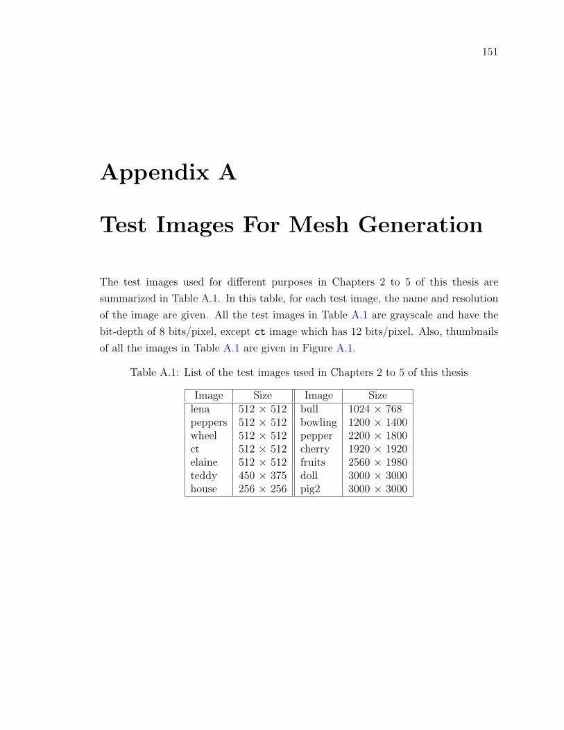
151

Appendix A

Test Images For Mesh Generation

The test images used for different purposes in Chapters 2 to 5 of this thesis are

summarized in Table A.1. In this table, for each test image, the name and resolution

of the image are given. All the test images in Table A.1 are grayscale and have the

bit-depth of 8 bits/pixel, except ct image which has 12 bits/pixel. Also, thumbnails

of all the images in Table A.1 are given in Figure A.1.

Table A.1: List of the test images used in Chapters 2 to 5 of this thesis

Image Size Image Sizelena 512 × 512 bull 1024 × 768peppers 512 × 512 bowling 1200 × 1400wheel 512 × 512 pepper 2200 × 1800ct 512 × 512 cherry 1920 × 1920elaine 512 × 512 fruits 2560 × 1980teddy 450 × 375 doll 3000 × 3000house 256 × 256 pig2 3000 × 3000

152

(a) (b) (c) (d)

(e) (f) (g) (h)

(i) (j) (k) (l)

(m) (n)

Figure A.1: Thumbnails of the test images used in Chapters 2 to 5 of this thesis.The (a) lena, (b) peppers, (c) wheel, (d) ct, (e) elaine, (f) teddy, (g) house, (h) bull,(i) bowling, (j) pepper, (k) cherry, (l) fruits, (m) doll, and (n) pig2 images.

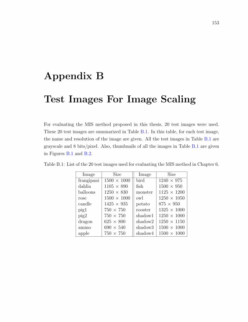
153

Appendix B

Test Images For Image Scaling

For evaluating the MIS method proposed in this thesis, 20 test images were used.

These 20 test images are summarized in Table B.1. In this table, for each test image,

the name and resolution of the image are given. All the test images in Table B.1 are

grayscale and 8 bits/pixel. Also, thumbnails of all the images in Table B.1 are given

in Figures B.1 and B.2.

Table B.1: List of the 20 test images used for evaluating the MIS method in Chapter 6.

Image Size Image Sizefrangipani 1500 × 1000 bird 1240 × 975dahlia 1105 × 890 fish 1500 × 950balloons 1250 × 830 monster 1125 × 1200rose 1500 × 1000 owl 1250 × 1050candle 1425 × 935 potato 875 × 950pig1 750 × 750 rooster 1325 × 1000pig2 750 × 750 shadow1 1250 × 1000dragon 625 × 800 shadow2 1250 × 1150ammo 690 × 540 shadow3 1500 × 1000apple 750 × 750 shadow4 1500 × 1000

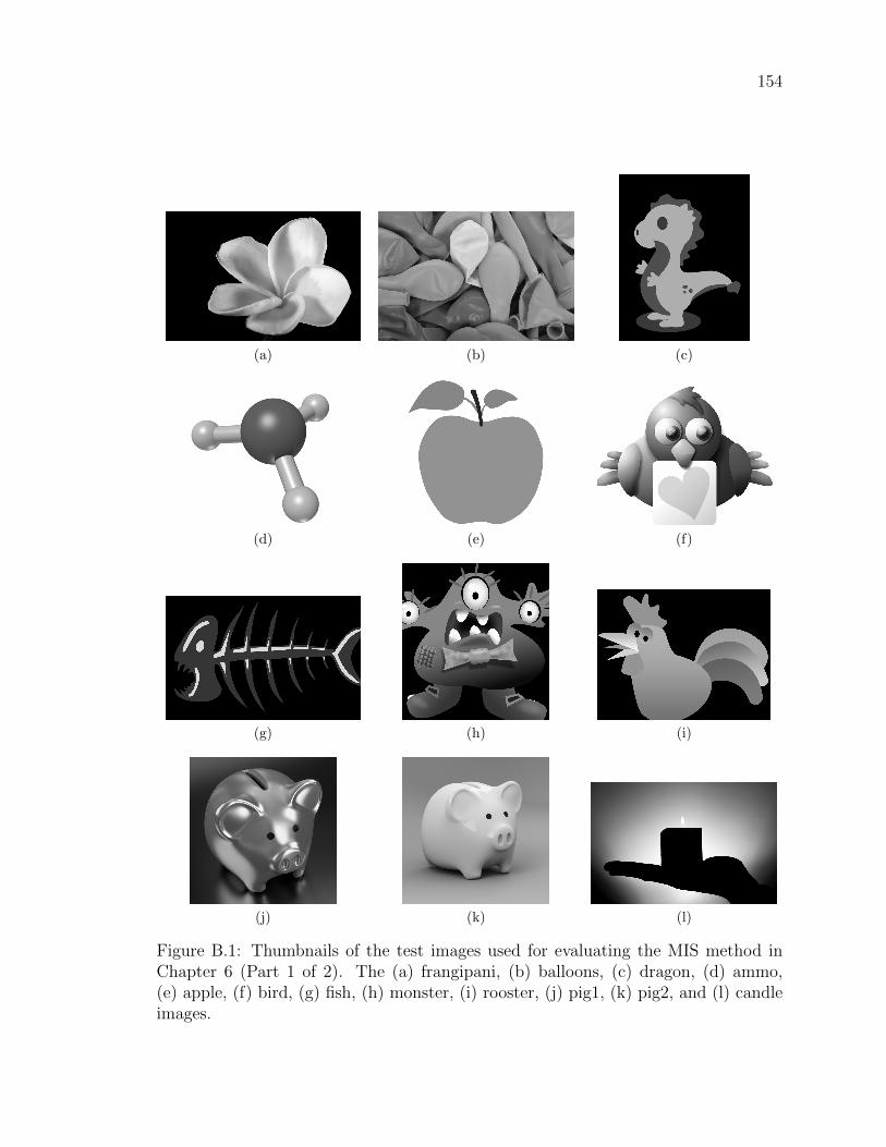
154

(a) (b) (c)

(d) (e) (f)

(g) (h) (i)

(j) (k) (l)

Figure B.1: Thumbnails of the test images used for evaluating the MIS method inChapter 6 (Part 1 of 2). The (a) frangipani, (b) balloons, (c) dragon, (d) ammo,(e) apple, (f) bird, (g) fish, (h) monster, (i) rooster, (j) pig1, (k) pig2, and (l) candleimages.

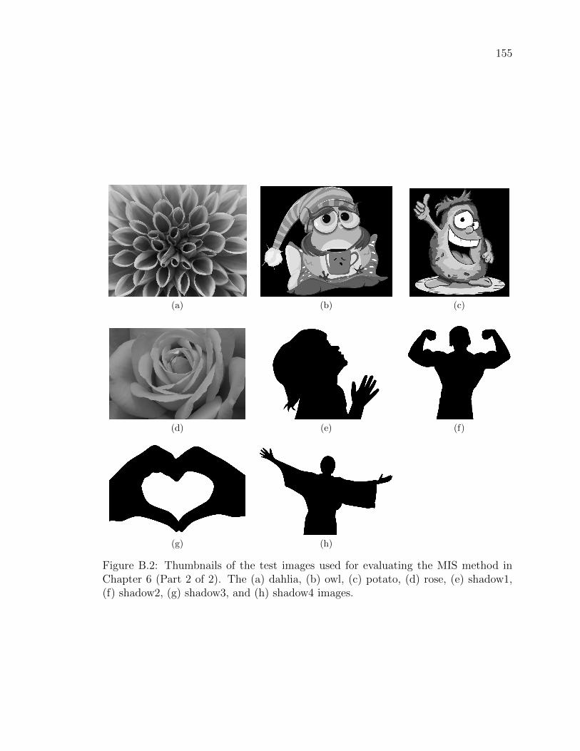
155

(a) (b) (c)

(d) (e) (f)

(g) (h)

Figure B.2: Thumbnails of the test images used for evaluating the MIS method inChapter 6 (Part 2 of 2). The (a) dahlia, (b) owl, (c) potato, (d) rose, (e) shadow1,(f) shadow2, (g) shadow3, and (h) shadow4 images.

156

Appendix C

Supplementary Experimental

Results

The full set of 350 test cases collected for comparing the proposed SEMMG method

with the ED, MGH, ERDED, and ERDGPI methods is presented in Tables C.1 to C.7.

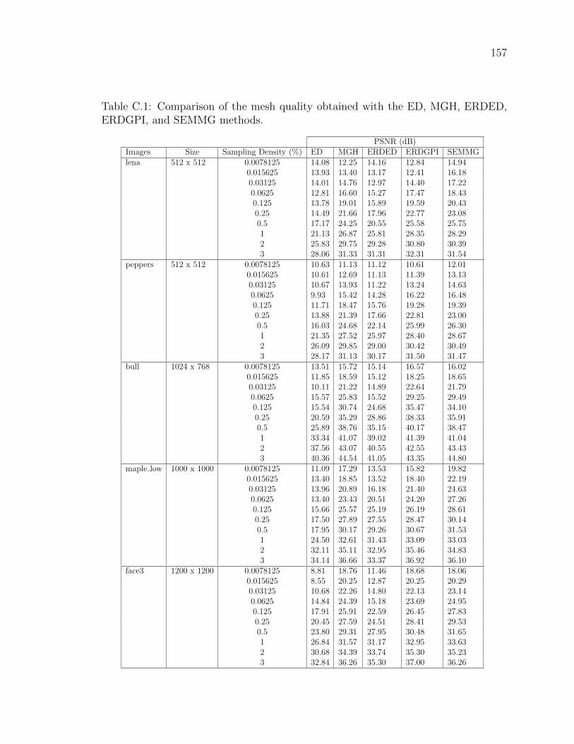
157

Table C.1: Comparison of the mesh quality obtained with the ED, MGH, ERDED,ERDGPI, and SEMMG methods.

PSNR (dB)Images Size Sampling Density (%) ED MGH ERDED ERDGPI SEMMGlena 512 x 512 0.0078125 14.08 12.25 14.16 12.84 14.94

0.015625 13.93 13.40 13.17 12.41 16.180.03125 14.01 14.76 12.97 14.40 17.220.0625 12.81 16.60 15.27 17.47 18.430.125 13.78 19.01 15.89 19.59 20.430.25 14.49 21.66 17.96 22.77 23.080.5 17.17 24.25 20.55 25.58 25.751 21.13 26.87 25.81 28.35 28.292 25.83 29.75 29.28 30.80 30.393 28.06 31.33 31.31 32.31 31.54

peppers 512 x 512 0.0078125 10.63 11.13 11.12 10.61 12.010.015625 10.61 12.69 11.13 11.39 13.130.03125 10.67 13.93 11.22 13.24 14.630.0625 9.93 15.42 14.28 16.22 16.480.125 11.71 18.47 15.76 19.28 19.390.25 13.88 21.39 17.66 22.81 23.000.5 16.03 24.68 22.14 25.99 26.301 21.35 27.52 25.97 28.40 28.672 26.09 29.85 29.00 30.42 30.493 28.17 31.13 30.17 31.50 31.47

bull 1024 x 768 0.0078125 13.51 15.72 15.14 16.57 16.020.015625 11.85 18.59 15.12 18.25 18.650.03125 10.11 21.22 14.89 22.64 21.790.0625 15.57 25.83 15.52 29.25 29.490.125 15.54 30.74 24.68 35.47 34.100.25 20.59 35.29 28.86 38.33 35.910.5 25.89 38.76 35.15 40.17 38.471 33.34 41.07 39.02 41.39 41.042 37.56 43.07 40.55 42.55 43.433 40.36 44.54 41.05 43.35 44.80

maple low 1000 x 1000 0.0078125 11.09 17.29 13.53 15.82 19.820.015625 13.40 18.85 13.52 18.40 22.190.03125 13.96 20.89 16.18 21.40 24.630.0625 13.40 23.43 20.51 24.20 27.260.125 15.66 25.57 25.19 26.19 28.610.25 17.50 27.89 27.55 28.47 30.140.5 17.95 30.17 29.26 30.67 31.531 24.50 32.61 31.43 33.09 33.032 32.11 35.11 32.95 35.46 34.833 34.14 36.66 33.37 36.92 36.10

face3 1200 x 1200 0.0078125 8.81 18.76 11.46 18.68 18.060.015625 8.55 20.25 12.87 20.25 20.290.03125 10.68 22.26 14.80 22.13 23.140.0625 14.84 24.39 15.18 23.69 24.950.125 17.91 25.91 22.59 26.45 27.830.25 20.45 27.59 24.51 28.41 29.530.5 23.80 29.31 27.95 30.48 31.651 26.84 31.57 31.17 32.95 33.632 30.68 34.39 33.74 35.30 35.233 32.84 36.26 35.30 37.00 36.26

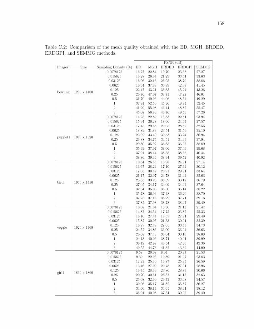
158


PSNR (dB)Images Size Sampling Density (%) ED MGH ERDED ERDGPI SEMMG

bowling 1200 x 1400

0.0078125 16.27 22.84 19.70 23.68 27.270.015625 16.28 26.64 21.29 33.51 33.630.03125 16.96 32.16 26.95 38.70 38.860.0625 16.34 37.89 33.89 42.09 41.450.125 22.47 43.21 36.35 45.24 43.260.25 26.76 47.07 38.71 47.22 46.010.5 31.70 49.96 44.06 48.54 49.291 32.91 52.50 45.36 48.94 52.452 41.29 55.08 46.44 48.85 55.473 45.08 56.86 46.76 49.56 57.26

puppet1 1980 x 1320

0.0078125 14.25 22.89 15.83 22.81 23.940.015625 15.94 26.28 18.66 24.44 27.570.03125 17.45 29.68 20.05 28.89 32.560.0625 18.89 31.83 23.54 31.56 35.100.125 23.92 33.49 30.53 33.24 36.940.25 26.88 34.75 34.51 34.93 37.940.5 29.80 35.92 36.85 36.06 38.891 35.39 37.07 38.06 37.06 39.682 37.91 38.44 38.58 38.58 40.443 38.86 39.36 38.94 39.52 40.92

bird 1940 x 1430

0.0078125 10.64 26.55 13.98 24.91 27.140.015625 13.67 28.24 17.10 27.64 30.120.03125 17.05 30.42 20.91 29.91 33.640.0625 21.17 32.07 24.78 31.42 35.630.125 23.83 33.26 30.59 33.12 36.790.25 27.05 34.17 34.09 34.04 37.640.5 32.34 35.06 36.50 35.14 38.221 35.78 36.04 37.48 36.20 38.702 37.25 37.18 38.29 37.71 39.163 37.85 37.98 38.78 38.47 39.49

veggie 1920 x 1469

0.0078125 10.08 21.04 13.30 21.13 21.470.015625 14.87 24.54 17.75 23.85 25.330.03125 16.10 27.44 19.57 27.91 29.490.0625 15.82 30.05 21.33 30.91 32.390.125 16.77 32.49 27.65 33.43 34.730.25 24.52 34.86 33.00 36.04 36.630.5 20.68 37.48 36.04 38.10 38.081 24.13 40.06 38.74 40.01 39.992 36.12 42.92 40.54 42.30 42.363 40.55 44.73 41.32 43.39 44.00

girl1 1860 x 1860

0.0078125 9.58 20.08 8.04 20.97 21.530.015625 9.69 22.95 10.89 21.97 23.830.03125 12.23 25.30 16.87 25.35 26.590.0625 13.46 27.09 20.78 27.01 28.960.125 16.45 28.69 23.86 28.83 30.660.25 20.20 30.51 26.37 31.13 32.630.5 25.08 32.60 29.43 33.38 34.571 30.06 35.17 31.82 35.87 36.272 34.60 38.14 34.65 38.31 38.123 36.94 40.08 37.54 39.96 39.40

159



cherry 1920 x 1920

0.0078125 11.76 16.31 11.91 17.01 34.520.015625 13.28 17.56 12.10 19.20 37.770.03125 13.39 28.10 26.89 31.59 38.780.0625 13.92 37.56 41.32 43.47 39.870.125 29.24 43.57 41.87 44.46 42.250.25 23.07 55.71 41.71 44.28 49.520.5 37.16 61.18 42.99 44.75 57.891 39.69 65.10 43.35 44.94 63.052 47.48 70.75 43.37 44.95 67.473 53.57 inf 43.36 44.94 69.67

pepper 2200 x 1800

0.0078125 8.23 27.88 11.68 28.00 28.520.015625 13.41 30.99 13.36 29.52 31.530.03125 17.85 32.86 18.06 32.54 33.490.0625 22.10 35.26 27.10 34.76 36.330.125 25.77 36.57 31.67 36.49 39.320.25 31.91 37.77 34.34 37.57 40.700.5 37.34 39.00 36.99 38.80 41.771 39.73 40.25 40.13 40.42 42.612 41.36 41.64 41.41 41.55 43.453 42.15 42.55 40.71 42.66 44.01

fruits 2560 x 1980

0.0078125 12.11 20.35 11.56 20.18 20.590.015625 13.21 22.31 11.71 20.75 21.720.03125 16.26 24.21 13.63 23.57 24.620.0625 18.47 26.15 22.79 25.81 27.590.125 21.07 27.69 25.45 27.33 29.670.25 23.95 28.80 27.85 28.58 31.140.5 27.00 29.83 29.52 29.71 32.671 29.99 30.83 31.80 31.03 33.422 31.81 31.88 32.78 32.29 33.993 32.57 32.57 33.11 33.06 34.32

rose 3000 x 2250

0.0078125 12.21 22.76 15.30 23.07 24.070.015625 13.41 27.22 17.50 28.14 27.310.03125 13.17 31.27 19.96 33.05 32.170.0625 14.64 35.48 27.93 36.94 36.740.125 22.12 39.07 32.26 39.38 39.520.25 30.32 42.99 36.76 42.40 42.260.5 37.86 45.29 39.88 44.95 45.141 42.54 47.35 41.39 45.95 47.752 46.61 49.45 43.61 47.28 49.993 48.23 50.76 44.15 47.82 51.17

doll 3000 x 3000

0.0078125 13.60 26.50 14.80 25.13 26.300.015625 16.57 27.93 16.77 27.57 28.920.03125 16.64 29.11 25.24 28.96 32.710.0625 20.25 30.17 28.64 29.51 34.470.125 23.78 31.22 31.44 30.92 36.070.25 28.43 32.33 34.08 32.19 37.110.5 33.33 33.50 35.40 33.47 37.661 35.22 34.87 36.55 35.11 38.112 36.46 36.50 37.61 36.81 38.683 37.27 37.63 38.10 37.93 39.15

160



dahlia 4420 x 3560

0.0078125 14.74 15.15 9.38 15.55 19.500.015625 14.68 18.23 12.32 17.68 22.010.03125 15.10 20.41 17.24 20.11 24.970.0625 16.48 22.14 20.88 22.08 27.010.125 17.87 23.40 23.83 23.79 28.190.25 20.35 24.44 26.33 24.88 28.700.5 23.37 25.42 27.72 25.78 29.101 25.65 26.41 28.48 26.77 29.482 27.20 27.48 28.98 27.96 29.863 28.07 28.21 29.26 28.72 30.13

puppet2 3456 x 4608

0.0078125 19.01 30.37 16.42 28.67 28.920.015625 20.42 33.00 23.85 32.58 32.410.03125 23.29 34.62 28.19 34.13 35.570.0625 26.42 35.87 30.44 35.02 38.500.125 29.88 36.81 35.66 36.69 40.820.25 33.76 37.70 38.55 37.58 41.760.5 38.49 38.65 40.24 38.58 42.261 40.25 39.74 40.84 39.91 42.692 41.21 40.99 41.49 41.38 43.173 41.74 41.85 41.85 42.24 43.52

pig1 3000 x 3000

0.0078125 14.76 27.75 14.14 25.42 25.590.015625 16.86 31.69 16.52 29.08 29.910.03125 20.26 34.95 22.85 34.13 33.660.0625 23.30 36.82 26.04 36.34 38.690.125 26.72 38.07 30.43 37.72 40.910.25 31.05 38.98 34.46 38.69 42.090.5 37.13 39.80 38.46 39.62 42.751 40.72 40.68 40.81 40.89 43.162 42.00 41.73 41.81 42.15 43.603 42.42 42.50 41.94 42.76 43.95

pig2 3000 x 3000

0.0078125 17.35 38.48 18.22 36.54 37.560.015625 16.43 42.44 19.31 39.33 42.220.03125 23.05 44.71 30.93 44.03 46.220.0625 27.65 46.08 37.36 45.92 48.780.125 35.42 47.02 42.89 46.98 50.320.25 42.86 47.97 45.52 47.53 51.190.5 47.22 49.08 48.16 49.04 51.701 49.43 50.34 48.29 49.27 52.162 50.39 51.83 49.37 51.40 52.743 50.84 52.86 49.70 52.12 53.18

frangipani 6000 x 4000

0.0078125 11.98 34.70 13.23 32.54 31.620.015625 14.73 36.92 17.05 34.78 35.110.03125 16.00 38.99 19.28 38.41 39.660.0625 16.87 40.69 23.01 40.05 42.290.125 17.91 42.27 25.39 41.65 44.180.25 20.52 43.68 28.76 43.14 45.670.5 26.29 45.01 35.85 44.48 46.861 31.03 46.38 43.06 46.45 47.852 44.87 48.05 45.17 48.11 48.903 45.78 49.36 45.76 49.17 49.69

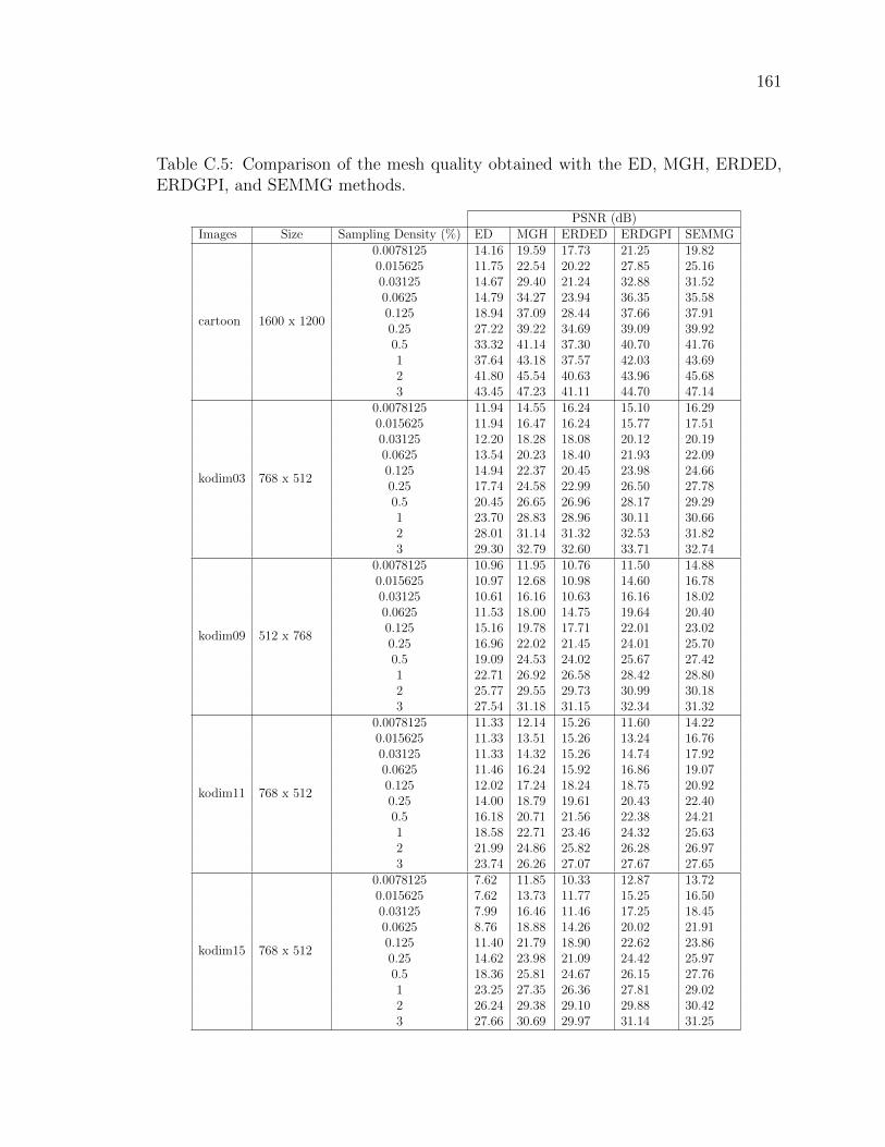
161



cartoon 1600 x 1200

0.0078125 14.16 19.59 17.73 21.25 19.820.015625 11.75 22.54 20.22 27.85 25.160.03125 14.67 29.40 21.24 32.88 31.520.0625 14.79 34.27 23.94 36.35 35.580.125 18.94 37.09 28.44 37.66 37.910.25 27.22 39.22 34.69 39.09 39.920.5 33.32 41.14 37.30 40.70 41.761 37.64 43.18 37.57 42.03 43.692 41.80 45.54 40.63 43.96 45.683 43.45 47.23 41.11 44.70 47.14

kodim03 768 x 512

0.0078125 11.94 14.55 16.24 15.10 16.290.015625 11.94 16.47 16.24 15.77 17.510.03125 12.20 18.28 18.08 20.12 20.190.0625 13.54 20.23 18.40 21.93 22.090.125 14.94 22.37 20.45 23.98 24.660.25 17.74 24.58 22.99 26.50 27.780.5 20.45 26.65 26.96 28.17 29.291 23.70 28.83 28.96 30.11 30.662 28.01 31.14 31.32 32.53 31.823 29.30 32.79 32.60 33.71 32.74

kodim09 512 x 768

0.0078125 10.96 11.95 10.76 11.50 14.880.015625 10.97 12.68 10.98 14.60 16.780.03125 10.61 16.16 10.63 16.16 18.020.0625 11.53 18.00 14.75 19.64 20.400.125 15.16 19.78 17.71 22.01 23.020.25 16.96 22.02 21.45 24.01 25.700.5 19.09 24.53 24.02 25.67 27.421 22.71 26.92 26.58 28.42 28.802 25.77 29.55 29.73 30.99 30.183 27.54 31.18 31.15 32.34 31.32

kodim11 768 x 512

0.0078125 11.33 12.14 15.26 11.60 14.220.015625 11.33 13.51 15.26 13.24 16.760.03125 11.33 14.32 15.26 14.74 17.920.0625 11.46 16.24 15.92 16.86 19.070.125 12.02 17.24 18.24 18.75 20.920.25 14.00 18.79 19.61 20.43 22.400.5 16.18 20.71 21.56 22.38 24.211 18.58 22.71 23.46 24.32 25.632 21.99 24.86 25.82 26.28 26.973 23.74 26.26 27.07 27.67 27.65

kodim15 768 x 512

0.0078125 7.62 11.85 10.33 12.87 13.720.015625 7.62 13.73 11.77 15.25 16.500.03125 7.99 16.46 11.46 17.25 18.450.0625 8.76 18.88 14.26 20.02 21.910.125 11.40 21.79 18.90 22.62 23.860.25 14.62 23.98 21.09 24.42 25.970.5 18.36 25.81 24.67 26.15 27.761 23.25 27.35 26.36 27.81 29.022 26.24 29.38 29.10 29.88 30.423 27.66 30.69 29.97 31.14 31.25

162



kodim17 512 x 768

0.0078125 13.65 12.26 13.72 13.31 15.480.015625 13.65 14.08 13.72 13.79 15.880.03125 12.98 15.67 14.38 16.63 17.770.0625 12.37 17.38 17.50 17.57 19.400.125 14.25 18.87 18.36 20.08 21.320.25 16.08 20.90 20.34 22.28 23.430.5 18.03 22.80 22.52 24.39 25.581 21.13 25.40 25.38 27.01 27.812 24.54 28.37 28.15 29.73 29.813 26.92 30.20 29.61 31.36 30.90

kodim19 512 x 768

0.0078125 13.76 12.24 12.93 12.85 16.120.015625 13.75 13.58 14.91 14.29 17.010.03125 15.99 14.75 14.99 14.49 17.360.0625 14.85 16.27 14.71 16.93 18.890.125 14.13 17.32 16.59 18.39 20.470.25 15.97 18.46 19.76 20.39 21.980.5 17.27 19.76 21.86 22.11 23.841 18.43 21.39 23.80 24.50 25.412 21.36 23.80 26.27 26.80 26.523 22.99 25.50 27.11 28.12 27.37

kodim20 768 x 512

0.0078125 6.02 12.69 9.89 12.25 13.530.015625 5.89 14.28 9.89 13.68 16.010.03125 6.09 15.81 7.26 17.07 18.040.0625 9.77 17.83 7.82 19.16 20.160.125 11.31 20.34 10.43 21.63 22.350.25 16.04 22.38 17.32 24.30 25.800.5 18.46 24.59 24.32 26.33 27.581 22.66 27.05 27.89 28.43 28.722 26.11 29.63 29.49 30.40 30.423 28.09 31.26 30.43 31.69 31.51

kodim04 768 x 512

0.0078125 13.12 11.67 15.17 14.01 14.540.015625 13.14 15.57 14.33 15.97 17.360.03125 13.08 17.43 14.35 16.48 18.960.0625 15.09 19.66 16.57 19.23 20.660.125 15.30 21.39 19.99 21.83 23.640.25 18.10 23.27 22.06 24.10 25.310.5 19.60 24.86 23.96 25.65 27.251 22.11 26.66 25.92 27.61 28.792 25.82 28.87 28.32 29.33 30.423 27.65 30.31 29.58 30.76 31.22

kodim07 512 x 768

0.0078125 10.45 13.42 15.50 14.14 15.290.015625 10.45 13.81 14.08 14.66 17.470.03125 10.45 15.00 14.20 15.58 17.970.0625 12.26 16.53 15.45 16.39 18.770.125 13.28 18.10 15.88 19.03 20.480.25 15.28 19.82 19.13 20.95 21.870.5 16.80 21.52 21.17 22.99 24.341 19.70 24.95 24.12 26.69 27.742 23.84 29.14 27.68 30.83 29.953 26.56 31.47 30.49 32.63 31.25

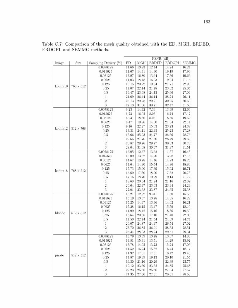
163


PSNR (dB)Image Size Sampling Density (%) ED MGH ERDED ERDGPI SEMMG

kodim10 768 x 512

0.0078125 11.66 13.23 12.44 14.24 16.240.015625 11.67 14.41 14.30 16.19 17.960.03125 13.97 16.80 13.64 17.36 19.660.0625 14.03 18.48 16.03 19.94 21.150.125 16.15 20.22 19.84 21.71 22.960.25 17.07 22.14 21.78 23.32 25.050.5 19.47 23.98 24.13 25.66 27.091 21.69 26.44 26.14 28.24 29.112 25.13 29.28 29.21 30.95 30.603 27.13 31.06 30.71 32.47 31.60

kodim12 512 x 768

0.0078125 6.23 14.42 7.39 13.99 12.660.015625 6.23 16.02 8.03 16.74 17.120.03125 6.23 18.36 8.05 18.66 19.620.0625 9.47 19.96 14.00 21.84 22.140.125 9.16 22.27 15.03 23.23 24.380.25 13.31 24.11 22.45 25.23 27.280.5 16.66 25.93 24.77 26.66 28.751 22.66 27.76 27.30 28.49 29.692 26.87 29.76 29.77 30.83 30.703 28.04 31.08 30.67 31.97 31.51

kodim18 768 x 512

0.0078125 15.05 12.57 13.52 11.67 16.430.015625 15.09 13.52 14.20 13.98 17.180.03125 14.67 13.78 14.46 14.23 18.250.0625 14.64 14.90 15.54 14.86 18.800.125 15.73 15.90 17.39 15.92 19.710.25 15.69 17.30 18.90 17.62 20.730.5 17.16 18.70 19.99 19.14 21.721 18.68 20.34 21.24 21.16 22.822 20.64 22.37 23.03 23.34 24.293 22.01 23.68 23.87 24.65 25.38

blonde 512 x 512

0.0078125 15.21 12.92 9.34 11.80 15.550.015625 15.19 13.37 13.78 14.35 16.290.03125 15.25 14.37 13.46 14.62 16.210.0625 15.28 16.15 13.47 15.59 18.100.125 14.99 18.42 15.16 18.86 19.590.25 13.64 20.58 17.10 21.40 22.060.5 17.50 22.74 21.54 24.09 24.741 20.07 24.87 24.47 26.54 27.022 23.70 26.82 26.91 28.32 28.513 25.34 28.03 28.24 29.51 29.31

pirate 512 x 512

0.0078125 13.79 13.39 13.78 13.07 14.830.015625 13.81 15.31 13.51 14.29 15.920.03125 13.78 14.92 13.73 15.24 17.050.0625 14.52 16.24 15.82 16.44 18.170.125 14.92 17.61 17.31 18.42 19.460.25 14.87 19.39 19.13 20.10 21.550.5 16.30 21.16 20.29 22.39 23.751 19.12 23.39 23.32 24.85 25.682 22.23 25.86 25.66 27.04 27.573 24.35 27.36 27.31 28.61 28.58

164

Appendix D

Software User Manual

D.1 Introduction

As part of the work presented in this thesis, a software implementation of the mesh-

generation and image-scaling methods proposed herein was developed. The software

was all implemented in C++ by the author of this thesis, with significant help from

his supervisor, Dr. Michael Adams. The software implementation consists of over

14000 lines of code and involves quite complicated algorithms and data structures.

For the implementation of this software, various C++ libraries were utilized, includ-

ing the Computational Geometry Algorithms Library (CGAL) [6], the Open Source

Computer Vision Library (OpenCV) [7], the Signal Processing Library (SPL) [8] and

its extension library (SPLEL), and the Boost library [9].

The software implements all the methods proposed and developed in this thesis,

including the SEMMG, MISMG, and MIS methods. Moreover, the software includes

different image quality assessment measures used in this thesis, such as the PSNR,

MSSIM, and PEE metrics. The software package contains the following four exe-

cutable programs:

1. mesh_generation: generates an ERD mesh model using either the SEMMG or

MISMG method from an input grayscale raster image.

2. mesh_subdivision: subdivides an input ERD mesh with a given number of

subdivision levels.

3. mesh_rasterization: rasterizes an ERD model to a raster image with a given

scaling factor k > 1.

165

4. img_cmp: computes the PSNR, MSSIM, or PEE image quality assessments

metrics between two input images.

The remainder of this appendix provides details on how to build the software, followed

by complete descriptions of each of the above programs. Also, specific examples are

provided to illustrate how to use the software.

D.2 Building the Software

For the purpose of building the software, the Make tool is used. Since the programs

in the software utilize several features from C++17 features, the compiler which is

used needs to be compatible with C++17. As mentioned earlier, our software utilizes

several libraries such as CGAL, SPL, SPLEL, OpenCV, and Boost. Therefore, before

building the software, users need to ensure that these libraries are installed. The

versions of the libraries used by the author and known to work are as below:

• CGAL version 4.2

• SPL version 2.0.3

• SPLEL version 2.0.5

• OpenCV version 3.0

• Boost version 1.53

In order to compile all of the source files and link the object files, one should set the

directory to the top-level directory for the software, which contains the Makefile file,

and run the following commands:

make clean

make

The command make clean is optional and deletes all the object files and executable

files that may have been generated during the previous building process.

D.3 File Formats

As mentioned earlier, the inputs to the mesh_generation and img_cmp programs

and the output of the mesh_rasterization program are grayscale raster images.

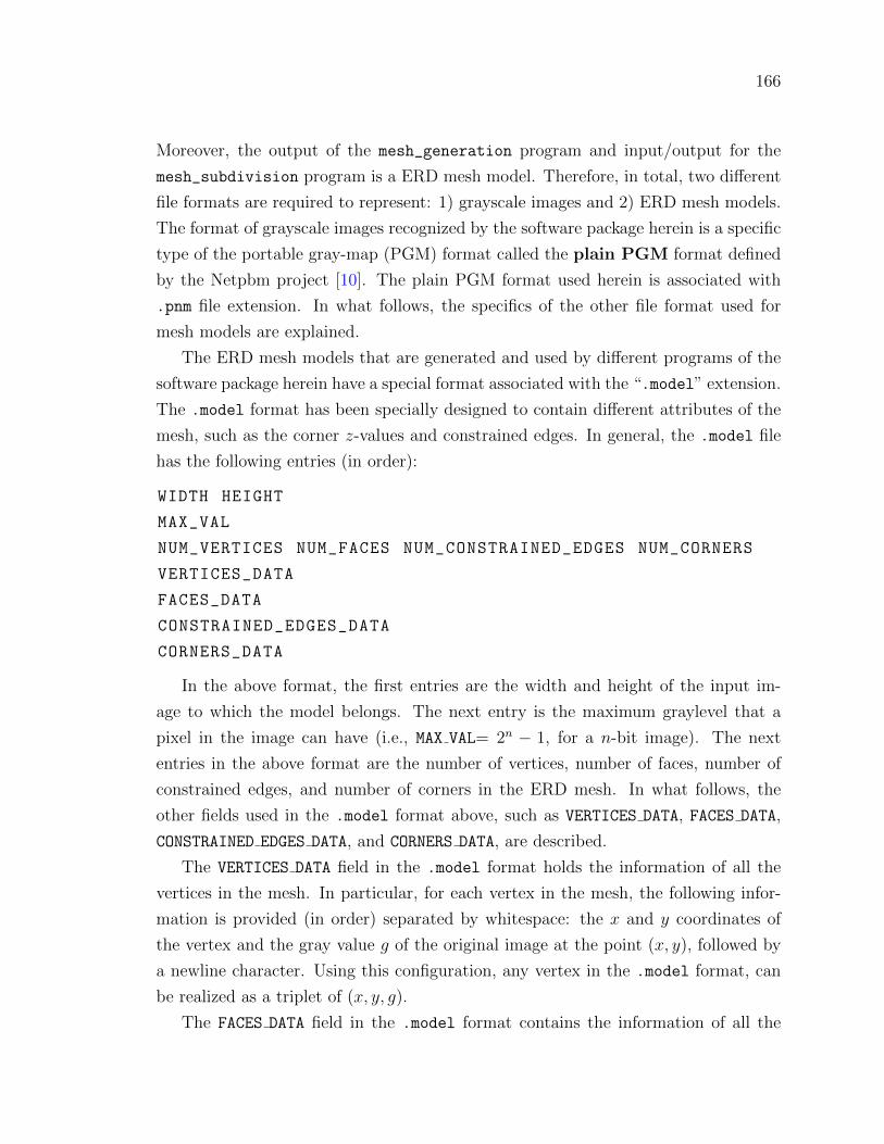
166

Moreover, the output of the mesh_generation program and input/output for the

mesh_subdivision program is a ERD mesh model. Therefore, in total, two different

file formats are required to represent: 1) grayscale images and 2) ERD mesh models.

The format of grayscale images recognized by the software package herein is a specific

type of the portable gray-map (PGM) format called the plain PGM format defined

by the Netpbm project [10]. The plain PGM format used herein is associated with

.pnm file extension. In what follows, the specifics of the other file format used for

mesh models are explained.

The ERD mesh models that are generated and used by different programs of the

software package herein have a special format associated with the “.model” extension.

The .model format has been specially designed to contain different attributes of the

mesh, such as the corner z-values and constrained edges. In general, the .model file

has the following entries (in order):

WIDTH HEIGHT

MAX_VAL

NUM_VERTICES NUM_FACES NUM_CONSTRAINED_EDGES NUM_CORNERS

VERTICES_DATA

FACES_DATA

CONSTRAINED_EDGES_DATA

CORNERS_DATA

In the above format, the first entries are the width and height of the input im-

age to which the model belongs. The next entry is the maximum graylevel that a

pixel in the image can have (i.e., MAX VAL= 2n − 1, for a n-bit image). The next

entries in the above format are the number of vertices, number of faces, number of

constrained edges, and number of corners in the ERD mesh. In what follows, the

other fields used in the .model format above, such as VERTICES DATA, FACES DATA,

CONSTRAINED EDGES DATA, and CORNERS DATA, are described.

The VERTICES DATA field in the .model format holds the information of all the

vertices in the mesh. In particular, for each vertex in the mesh, the following infor-

mation is provided (in order) separated by whitespace: the x and y coordinates of

the vertex and the gray value g of the original image at the point (x, y), followed by

a newline character. Using this configuration, any vertex in the .model format, can

be realized as a triplet of (x, y, g).

The FACES DATA field in the .model format contains the information of all the

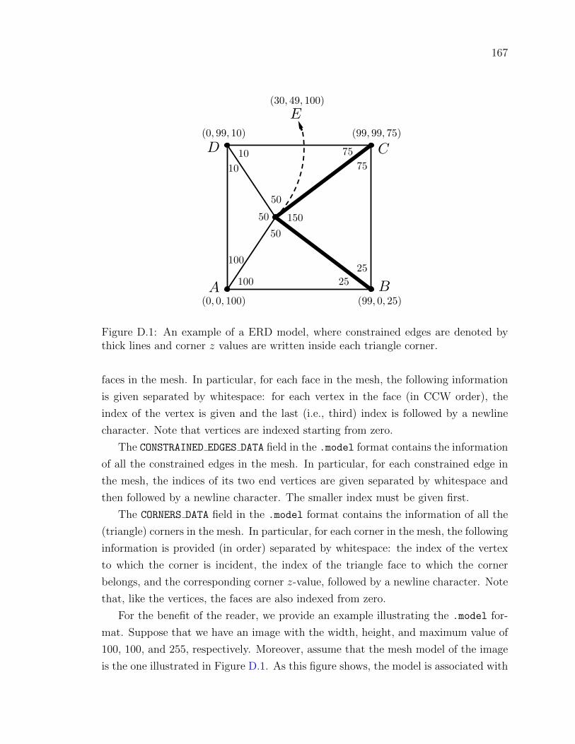
167

Figure D.1: An example of a ERD model, where constrained edges are denoted bythick lines and corner z values are written inside each triangle corner.

faces in the mesh. In particular, for each face in the mesh, the following information

is given separated by whitespace: for each vertex in the face (in CCW order), the

index of the vertex is given and the last (i.e., third) index is followed by a newline

character. Note that vertices are indexed starting from zero.

The CONSTRAINED EDGES DATA field in the .model format contains the information

of all the constrained edges in the mesh. In particular, for each constrained edge in

the mesh, the indices of its two end vertices are given separated by whitespace and

then followed by a newline character. The smaller index must be given first.

The CORNERS DATA field in the .model format contains the information of all the

(triangle) corners in the mesh. In particular, for each corner in the mesh, the following

information is provided (in order) separated by whitespace: the index of the vertex

to which the corner is incident, the index of the triangle face to which the corner

belongs, and the corresponding corner z-value, followed by a newline character. Note

that, like the vertices, the faces are also indexed from zero.

For the benefit of the reader, we provide an example illustrating the .model for-

mat. Suppose that we have an image with the width, height, and maximum value of

100, 100, and 255, respectively. Moreover, assume that the mesh model of the image

is the one illustrated in Figure D.1. As this figure shows, the model is associated with

168

a triangulation consisting of four triangles, namely 4ABE, 4BCE, 4CDE, and

4DAE, and two constrained edges EB and EC. In the model shown in Figure D.1,

vertices A, B, C, D, and E have xy-coordinates (0,0), (99,0), (99,99), (0,99), and

(30,49), respectively. Furthermore, the gray values at A, B, C, D, and E are 100, 25,

75, 10, and 100, respectively. Also, the z-values associated with the face corners are

the ones written inside each corner in Figure D.1. Therefore, the .model file of the

above mesh model (shown in Figure D.1) is shown in Figure D.2.

D.4 Detailed Program Descriptions

In the following sections, a detailed description of the command line interface for each

program is provided.

D.4.1 The mesh_generation Program

SYNOPSIS

mesh_generation [OPTIONS] < input_image

DESCRIPTION

This program reads a grayscale image of either PGM or plain PGM format (which

is associated with .pnm extension) from standard input and generates the ERD mesh

model with respect to the mesh-generation method and sampling density specified

by the user. This program can write different types of data, such as the edge map,

triangulation, polylines, and mesh model, to a file specified by the command line

options. Any of the two mesh-generation methods used in this thesis, namely, the

proposed SEMMG method and the MISMG method that is used by the MIS method

can be selected through the options provided for this program. Although, in theory,

either of these methods can be selected for mesh generation, the SEMMG method

was mainly designed for the purpose of image representation where no image scaling

is involved, whereas the MISMG method was primarily designed to be used for image

scaling.

OPTIONS

-d $samplDensity Sets the mesh sampling density in percent to $samplDensity.

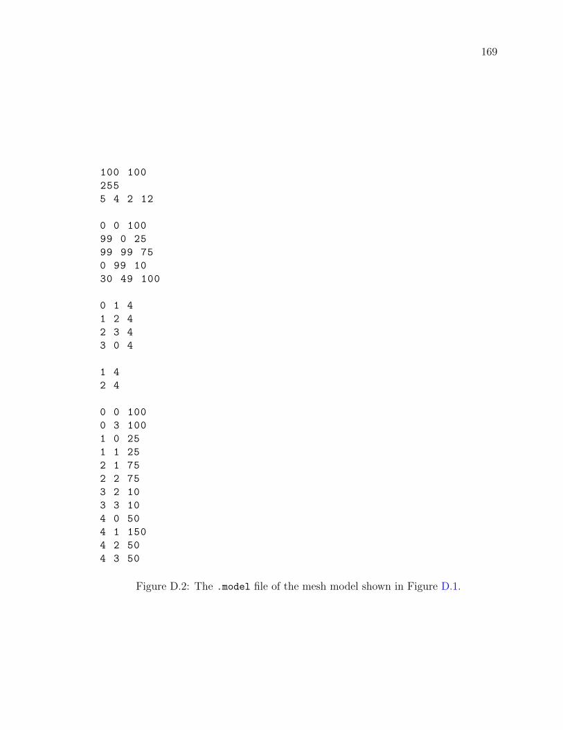
169

100 100

255

5 4 2 12

0 0 100

99 0 25

99 99 75

0 99 10

30 49 100

0 1 4

1 2 4

2 3 4

3 0 4

1 4

2 4

0 0 100

0 3 100

1 0 25

1 1 25

2 1 75

2 2 75

3 2 10

3 3 10

4 0 50

4 1 150

4 2 50

4 3 50

Figure D.2: The .model file of the mesh model shown in Figure D.1.

170

-n $methodFlag Specifies the mesh-generation method to be used. In particular,

if $methodFlag is set to 0 the SEMMG method and if it is set

to 1 the MISMG method is selected.

-b $modelFile Sets the output .model file name to $modelFile in which the

generated mesh model is stored.

-p $polyFile Sets the output polyline file name to $polyFile in which the

generated set of polylines is stored in the format used by iviewer

software.

-t $triFile Sets the output triangulation file name to $triFile in which the

triangulation data is stored in a format similar to the one used by

the iviewer software. Note that, in the generated triangulation

file, the entry of the number of edges must be deleted, before

using the iviewer.

-e $edgeFile Sets the name of the binary edge map obtained by the edge

detector to $edgeFile in the plain PGM format.

-s $edgeDetector Specifies the edge-detection method to be used. If

$edgeDetector is set to susan the SUSAN method and if it

is set to canny the Canny method is selected for generating edge

maps. If this option is not specified, the default is the Canny

method.

-v $tol Specifies the tolerance parameter used in the DP polyline-

simplification method to be $tol, which is a positive real number.

D.4.2 The mesh_subdivision Program

SYNOPSIS

mesh_subdivision [OPTIONS] < input_mesh

DESCRIPTION

This program reads an input ERD mesh in .model format from standard input and

subdivides the mesh with respect to the number of subdivision steps specified by the

171

user. This program can write different types of data, such as the subdivided trian-

gulation mesh, subdivided polylines, and subdivided mesh model, to a file specified

by the command line options. For the subdivision scheme, a variation of the Loop

method proposed in [60] was implemented.

OPTIONS

-s $subStep Sets the number of subdivision steps to $subStep.

-o $modelFile Sets the output subdivided mesh-model file name to $modelFile in

which the subdivided mesh is stored in .model format.

-p $polyFile Sets the subdivided polyline file name to $polyFile in which the

subdivided polyline is stored in the format used by the iviewer soft-

ware.

-t $triFile Sets the subdivided triangulation file name to $triFile in which

the subdivided triangulation mesh is stored in the format used by

the iviewer software.

D.4.3 The mesh_rasterization Program

SYNOPSIS

mesh_rasterization [OPTIONS] < input_mesh

DESCRIPTION

This program reads an input ERD mesh in .model format from standard input and

rasterizes it to obtain the reconstructed image with respect to a scaling factor specified

by the user.

OPTIONS

-k $scaleFactor Sets the scaling factor to $scaleFactor, which is a pos-

itive integer.

-a $superSamplingFactor Specifies the supersampling factor used during the ras-

terization process to be $superSamplingFactor, which

172

is a positive integer number (for antialiasing). For exam-

ple, if $superSamplingFactor is set to 3, the program

applies a 3×3 grid algorithm (introduced in Section 2.6)

for supersampling. If this option is not specified, the ras-

terization process is performed with no supersampling.

-r $reconstImg Sets the output raster-image file name to $reconstImg

in the plain PGM format.

D.4.4 The img_cmp Program

SYNOPSIS

img_cmp origImg reconstImg [$errorMetric]

DESCRIPTION

This program takes the original and reconstructed images as inputs specified by

$origImg and $reconstImg, respectively, in PGM (or plain PGM) format and com-

putes the error between them in terms of the optional error metric specified by

$errorMetric. The computed answer is written to standard output. Valid entries for

$errorMetric are psnr, mssim, and pee which compute PSNR, MSSIM, and PEE,

respectively. If no error metric is specified, the program only computes the PSNR by

default.

D.5 Examples of Software Usage

Having introduced all the programs in the software package implemented for this the-

sis, we provide some examples to show how to use the software for different purposes

in what follows.

Example 1. Suppose that, for the image peppers.pnm, we want to

use the SEMMG method to generate the ERD mesh model with a sam-

pling density of 2% and tolerance parameter of 1.0. We also want to save

the resulted edge map, polylines, triangulation, and mesh model to the files

peppers edgeMap.pnm, peppers semmg d2%.poly, peppers semmg d2%.tri, and

peppers semmg d2%.model, respectively. For this purpose, the following command

can be used:

173

./ mesh_generation -n 0 -d 2 -v 1.0 -e peppers_edgeMap.pnm

-p peppers_semmg_d2 %.poly -t peppers_semmg_d2 %.tri -b

peppers_semmg_d2 %.model < peppers.pnm

Once the mesh model is generated, we may then want to rasterize it with a 3 × 3

grid algorithm for supersampling and store the reconstructed image (with the same

resolution) to the file peppers semmg d2%.pnm. This can be done using the following

command:

./ mesh_rasterization -k 1 -a 3 -r peppers_semmg_d2 %.pnm <

peppers_semmg_d2 %.model

Then, for the purpose of measuring the error between the original image peppers.pnm

and the reconstructed image peppers semmg d2%.pnm in terms of the PSNR, the

following command can be used:

./ img_cmp peppers.pnm peppers_semmg_d2 %.pnm psnr

Example 2. For this example, suppose that we want to use the MIS method

to scale the input image dahlia.pnm with a scaling factor of 4 and a sampling den-

sity of 2% and store the scaled image to dahlia mis k4 d2%.pnm. As we recall from

Section 5.3, the MIS method comprised of three distinct stages, including mesh gen-

eration, mesh transformation, and mesh rasterization. The mesh-rasterization stage

itself contains two steps of mesh subdivision and model rasterization. In stage 1

of the MIS method, the MISMG method is used to generate the ERD mesh model

with tolerance parameter of 0.75. Suppose that we want to save the resulting edge

map, polylines, triangulation, and mesh model to the files dahlia edgeMap.pnm,

dahlia mismg d2%.poly, dahlia mismg d2%.tri, and dahlia mismg d2%.model, re-

spectively. For this purpose, the following command can be used:

./ mesh_generation -n 1 -d 2 -v 0.75 -e dahlia_edgeMap.pnm

-p dahlia_mismg_d2 %.poly -t dahlia_mismg_d2 %.tri -b

dahlia_mismg_d2 %. model < dahlia.pnm

Then, the generated mesh is subdivided with three steps of subdivision. Suppose that

we want to save the subdivided polylines, subdivided triangulation, and subdivided

mesh model to the files dahlia mismg d2% s3.poly, dahlia mismg d2% s3.tri, and

dahlia mismg d2% s3.model, respectively. For this purpose, the following command

can be used:

174

./ mesh_subdivision -s 3 -p dahlia_mismg_d2%_s3.poly -t

dahlia_mismg_d2%_s3.tri -o dahlia_mismg_d2%_s3.model <

dahlia_mismg_d2 %. model

Finally, the scaled image dahlia mis k4 d2%.pnm is obtained using the following

command:

./ mesh_rasterization -k 4 -a 3 -r dahlia_mis_k4_d2 %.pnm <

dahlia_mismg_d2%_s3.model

It is worth mentioning that the MIS method was implemented in the way that

the mesh transformation in stage 2, which is scaling operation, was implemented

as part of the model rasterization in stage 3 of the MIS method. So, no separate

program is needed to apply the scaling operation. Also, note that in the above

example, the scaled image (i.e., dahlia mis k4 d2%.pnm) is four times larger than

the original image (i.e., dahlia.pnm) in each dimension. Therefore, the img_cmp

program cannot be used to compute the error between them because they do not

have the same resolution. For the purpose of evaluation, however, a low-resolution

version of the dahlia.pnm, for example dahlia LR4.pnm, which is four times smaller

in each dimension, should be used instead of the dahlia.pnm. Then, using the similar

commands as above, the same steps of mesh generation, mesh subdivision, and mesh

rasterization are applied to dahlia LR4.pnm to obtain the scaled image named as

dahlia LR4 mis k4 d2%.pnm. Now, since the ground-truth image (i.e., dahlia.pnm)

and the scaled image (i.e., dahlia LR4 mis k4 d2%.pnm) have the same resolution,

the PEE between them can be computed using the following command:

./ img_cmp dahlia.pnm dahlia_LR4_mis_k4_d2 %.pnm pee

175

Bibliography

[1] C11 language standard: ISO/IEC 9899:2011.

https://www.iso.org/standard/57853.html, 2018.

[2] The MATLAB implementation of the DCCI method:

https://www.mathworks.com/matlabcentral/fileexchange/38570-image-

zooming-using-directional-cubic-convolution-interpolation, 2018.

[3] The MATLAB implementation of the NEDI method:

https://www.mathworks.com/matlabcentral/fileexchange/49900-image-

interpolation, 2018.

[4] The MATLAB implementation of the SRCNN method:

http://mmlab.ie.cuhk.edu.hk/projects/SRCNN.html, 2018.

[5] Netpbm homepage. http://netpbm.sourceforge.net/, 2018.

[6] Computational Geometry Algorithms Library. http://www.cgal.org, 2018.

[7] Open Source Computer Vision Library. http://www.opencv.org, 2018.

[8] Signal Processing Library. http://www.ece.uvic.ca/ frodo/SPL, 2018.

[9] Boost C++ Library. http://www.boost.org, 2018.

[10] PGM grayscale image format. http://netpbm.sourceforge.net/doc/pgm.html,

2018.

[11] M. D. Adams. An efficient progressive coding method for arbitrarily-sampled

image data. Signal Processing Letters, IEEE, 15:629–632, 2008.

[12] M. D. Adams. An evaluation of several mesh-generation methods using a simple

mesh-based image coder. In 15th IEEE International Conference on Image

Processing, pages 1041–1044, Oct. 2008.

176

[13] M. D. Adams. A flexible content-adaptive mesh-generation strategy for image

representation. IEEE Transactions on Image Processing, 20(9):2414–2427, Sep.

2011.

[14] M. D. Adams. An incremental/decremental Delaunay mesh-generation frame-

work for image representation. In 2011 18th IEEE International Conference on

Image Processing, pages 189–192, Sep. 2011.

[15] M. D. Adams. A highly-effective incremental/decremental Delaunay mesh-

generation strategy for image representation. Signal Processing, 93(4):749 –

764, 2013.

[16] A. S. Al-Fohoum and A. M. Reza. Combined edge crispiness and statistical

differencing for deblocking JPEG compressed images. IEEE Transactions on

Image Processing, 10(9):1288–1298, Sep. 2001.

[17] N. Asuni and A. Giachetti. Accuracy improvements and artifacts removal in

edge based image interpolation. In 2008 3rd International Conference on Com-

puter Vision Theory and Applications (VISAPP), pages 58–65, 2008.

[18] M. Basu. Gaussian-based edge-detection methods-a survey. IEEE Transac-

tions on Systems, Man, and Cybernetics, Part C (Applications and Reviews),

32(3):252–260, Aug. 2002.

[19] F. Bergholm. Edge focusing. IEEE Transactions on Pattern Analysis and

Machine Intelligence, PAMI-9(6):726–741, Nov. 1987.

[20] M. J. Black, G. Sapiro, D. H. Marimont, and D. Heeger. Robust anisotropic

diffusion. IEEE Transactions on Image Processing, 7(3):421–432, Mar. 1998.

[21] J. G. Brankov, Y. Yang, and N. P. Galatsanos. Image restoration using content-

adaptive mesh modeling. In 2003 International Conference on Image Processing

(ICIP), volume 2, pages 997–1000, Sep. 2003.

[22] J. G. Brankov, Y. Yang, and M. N. Wernick. Tomographic image reconstruc-

tion based on a content-adaptive mesh model. IEEE Transactions on Medical

Imaging, 23(2):202–212, Feb. 2004.

[23] J. Canny. A computational approach to edge detection. IEEE Transactions on

Pattern Analysis and Machine Intelligence, PAMI-8(6):679–698, Nov. 1986.

177

[24] G. Casciola, L. B. Montefusco, and S. Morigi. Edge-driven image interpola-

tion using adaptive anisotropic radial basis functions. Journal of Mathematical

Imaging and Vision, 36(2):125–139, 2010.

[25] P. Civicioglu and M. Alcı. Impulsive noise suppression from highly distorted

images with triangular interpolants. International Journal of Electronics and

Communications, 58(5):311–318, 2004.

[26] L. P. Chew. Constrained Delaunay triangulations. In 3rd Annual Symposium

on Computational Geometry (SCG), pages 215–222. ACM, 1987.

[27] S. A. Coleman, B. W. Scotney, and M. G. Herron. Image feature detection on

content-based meshes. In 2002 International Conference on Image Processing,

volume 1, pages 844–847, 2002.

[28] M. de Berg, O. Cheong, M. Kreveld, and M. Overmars. Computational Geom-

etry Algorithms and Applications. Springer, 3rd edition, 2008.

[29] B. Delaunay. Sur la sphere vide. a la memoire de georges voronoi. Bulletin

de l’Academie des Sciences de l’URSS, Classe des sciences mathematiques et

naturelles, (6):793–800, 1934.

[30] L. Demaret and A. Iske. Advances in digital image compression by adaptive

thinning. Annals of the Marie-Curie Fellowship Association, 3:105–109, 2004.

[31] O. Devillers and M. Teillaud. Perturbations and vertex removal in a 3D Delau-

nay triangulation. In Proceedings of the 14th Annual Symposium on Discrete

Algorithms (SODA), pages 313–319, ACM-SIAM, Philadelphia, PA, USA, 2003.

[32] L. Ding and A. Goshtasby. On the canny edge detector. Pattern Recognition,

34:721–725, 2001.

[33] C. Dong, C. C. Loy, K. He, and X. Tang. Image super-resolution using deep

convolutional networks. IEEE Transactions on Pattern Analysis and Machine

Intelligence, 38(2):295–307, Feb. 2016.

[34] D. H. Douglas and T. K. Peucker. Algorithms for the reduction of the number

of points required to represent a digitized line or its caricature. Cartographica:

The International Journal for Geographic Information and Geovisualization,

10(2):112–122, 1973.

178

[35] C. Dyken and M. S. Floater. Preferred directions for resolving the non-

uniqueness of Delaunay triangulations. Computational Geometry, 34(2):96–101,

2006.

[36] N. Dyn, M. S. Floater, and A. Iske. Adaptive thinning for bivariate scat-

tered data. Journal of Computational and Applied Mathematics, 145(2):505–

517, Aug. 2002.

[37] R. W. Floyd and L. Steinberg. An adaptive algorithm for spatial greyscale.

Proceedings of the Society of Information Display, 17(2):75–77, 1976.

[38] G. Freedman and R. Fattal. Image and video upscaling from local self-examples.

ACM Trans. Graph., 30(2):12:1–12:11, Apr. 2011.

[39] W. T. Freeman, T. R. Jones, and E. C. Pasztor. Example-based super-

resolution. IEEE Computer Graphics and Applications, 22(2):56–65, Mar. 2002.

[40] M. A. Garcia and A. D. Sappa. Efficient generation of discontinuity-preserving

adaptive triangulations from range images. IEEE Transactions on Systems,

Man, and Cybernetics, Part B (Cybernetics), 34(5):2003–2014, Oct. 2004.

[41] M. A. Garcia and B. X. Vintimilla. Acceleration of filtering and enhancement

operations through geometric processing of gray-level images. In 2000 Interna-

tional Conference on Image Processing (ICIP), volume 1, pages 97–100, 2000.

[42] M. A. Garcia, B. X. Vintimilla, and A. D. Sappa. Approximation and pro-

cessing of intensity images with discontinuity-preserving adaptive triangular

meshes. In European Conference on Computer Vision (ECCV) - Lecture Notes

in Computer Science, volume 1842, pages 844–855. Springer, Berlin, Heidelberg,

2000.

[43] M. Garland and P. S. Heckbert. Fast polygonal approximation of terrains

and height fields. Tech. Rep. CMU-CS-95-181. School of Computer Science,

Carnegie Mellon University, Pittsburgh, PA, USA, Sep. 1995.

[44] A. Giachetti and N. Asuni. Real-time artifact-free image upscaling. IEEE

Transactions on Image Processing, 20(10):2760–2768, Oct. 2011.

179

[45] D. Glasner, S. Bagon, and M. Irani. Super-resolution from a single image. In

2009 IEEE 12th International Conference on Computer Vision, pages 349–356,

Sep. 2009.

[46] M. Grundland, C. Gibbs, and N. A. Dogson. Stylized multiresolution image

representation. Journal of Electronic Imaging, 17(1):013009.1–17, 2008.

[47] H. Hadizadeh and I. V. Bajic. Full-reference objective quality assessment of

tone-mapped images. IEEE Transactions on Multimedia, 20(2):392–404, Feb.

2018.

[48] H. Hou and H. Andrews. Cubic splines for image interpolation and digital filter-

ing. IEEE Transactions on Acoustics, Speech, and Signal Processing, 26(6):508–

517, Dec. 1978.

[49] M. Hugentobler and B. Schneider. Breaklines in coons surfaces over triangles

for the use in terrain modelling. Computers and Geosciences, 31(1):45–54, 2005.

[50] ITU-R Recommendation BT.500-13. Methodology for the subjective assessment

of the quality of television pictures. International Telecommunication Union

(ITU), Geneva, Switzerland, 2012.

[51] R. Keys. Cubic convolution interpolation for digital image processing. IEEE

Transactions on Acoustics, Speech, and Signal Processing, 29(6):1153–1160,

Dec. 1981.

[52] J. Kim, J. K. Lee, and K. M. Lee. Accurate image super-resolution using very

deep convolutional networks. In 2016 IEEE Conference on Computer Vision

and Pattern Recognition (CVPR), pages 1646–1654, Jun. 2016.

[53] K. I. Kim and Y. Kwon. Single-image super-resolution using sparse regression

and natural image prior. IEEE Transactions on Pattern Analysis and Machine

Intelligence, 32(6):1127–1133, Jun. 2010.

[54] P. Kocharoen, K. M. Ahmed, R. M. A. P. Rajatheva, and W. A. C. Fernando.

Adaptive mesh generation for mesh-based image coding using node elimination

approach. In 2005 IEEE International Conference on Communications (ICC),

volume 3, pages 2052–2056 Vol. 3, May 2005.

180

[55] V. Lacroix. The primary raster: a multiresolution image description. In 10th

International Conference on Pattern Recognition, volume i, pages 903–907 vol.1,

Jun. 1990.

[56] E. C. Larson and D. M. Chandler. Most apparent distortion: full-reference

image quality assessment and the role of strategy. Journal of Electronic Imaging,

19:19–21, 2010.

[57] C. Ledig, L. Theis, F. Huszr, J. Caballero, A. Cunningham, A. Acosta,

A. Aitken, A. Tejani, J. Totz, Z. Wang, and W. Shi. Photo-realistic single

image super-resolution using a generative adversarial network. In 2017 IEEE

Conference on Computer Vision and Pattern Recognition (CVPR), pages 105–

114, Jul. 2017.

[58] X. Li. Anisotropic mesh adaptation for image representation. EURASIP Jour-

nal on Image and Video Processing, 2016(1):26, Sep. 2016.

[59] X. Li and M. T. Orchard. New edge-directed interpolation. IEEE Transactions

on Image Processing, 10(10):1521–1527, Oct. 2001.

[60] Z. Liao, H. Hoppe, D. Forsyth, and Y. Yu. A subdivision-based representation

for vector image editing. IEEE Transactions on Visualization and Computer

Graphics, 18(11):1858–1867, Nov. 2012.

[61] C. Liu, H. Pang, L. Ren, Z. Zhao, and S. Zhang. An image interpolation method

based on weighted subdivision. International Journal of Pattern Recognition

and Artificial Intelligence, 32(04):1854009, 2018.

[62] D. Liu, Z. Wang, B. Wen, J. Yang, W. Han, and T. S. Huang. Robust single

image super-resolution via deep networks with sparse prior. IEEE Transactions

on Image Processing, 25(7):3194–3207, Jul. 2016.

[63] K. Liu, M. Xu, and Z. Yu. Feature-preserving image restoration from adaptive

triangular meshes. In Computer Vision - ACCV 2014 Workshops, pages 31–46.

Springer International Publishing, Cham, 2015.

[64] B. E. E. Marzouki and M. D. Adams. An improved incremental/decremental

Delaunay mesh-generation strategy for image representation. In 2017 IEEE

Pacific Rim Conference on Communications, Computers and Signal Processing

(PACRIM), pages 1–6, Aug. 2017.

181

[65] P. Mohammadi, A. Ebrahimi-Moghadam, and S. Shirani. Subjective and ob-

jective quality assessment of image: A survey. CoRR, abs/1406.7799, 2014.

[66] S. Mostafavian and M. D. Adams. An optimization-based mesh-generation

method for image representation. In 2015 IEEE Pacific Rim Conference on

Communications, Computers and Signal Processing, pages 234–239, Aug. 2015.

[67] S. Mostafavian and M. D. Adams. A novel edge-preserving mesh-based method

for image scaling. In 2017 IEEE Pacific Rim Conference on Communications,

Computers and Signal Processing (PACRIM), pages 1–6, Aug. 2017.

[68] N. Otsu. A threshold selection method from gray-level histograms. IEEE Trans-

actions on Systems, Man, and Cybernetics, 9(1):62–66, Jan. 1979.

[69] V. Patel and K. Mistree. A review on different image interpolation techniques

for image enhancement. International Journal of Emerging Technology and

Advanced Engineering, 3:129–133, Dec. 2013.

[70] P. Perona and J. Malik. Scale-space and edge detection using anisotropic

diffusion. IEEE Transactions on Pattern Analysis and Machine Intelligence,

12(7):629–639, Jul. 1990.

[71] M. Petrou, R. Piroddi, and A. Talebpour. Texture recognition from sparsely

and irregularly sampled data. Computer Vision and Image Understanding,

102(1):95 – 104, 2006.

[72] D. Salesin, D. Lischinski, and T. DeRose. Reconstructing illumination func-

tions with selected discontinuities. In 3rd Eurographics Workshop on Rendering,

pages 99–112, 1992.

[73] M. Sarkis and K. Diepold. A fast solution to the approximation of 3D scat-

tered point data from stereo images using triangular meshes. In 7th IEEE-RAS

International Conference on Humanoid Robots, pages 235–241, Nov. 2007.

[74] M. Sarkis and K. Diepold. Content adaptive mesh representation of im-

ages using binary space partitions. IEEE Transactions on Image Processing,

18(5):1069–1079, May 2009.

[75] W. Shao, P. Shen, X. Xiao, L. Zhang, M. W. Z. Li, C. Qin, and X. Zhang. Ad-

vanced edge-preserving pixel-level mesh data-dependent interpolation technique

182

by triangulation. In 2011 IEEE International Conference on Signal Processing,

Communications and Computing (ICSPCC), pages 1–6, Sep. 2011.

[76] H. R. Sheikh and A. C. Bovik. Image information and visual quality. IEEE

Transactions on Image Processing, 15(2):430–444, Feb. 2006.

[77] X. Shen, G. Zeng, and Z. Wei. Nonuniform sampling and reconstruction for

high resolution satellite images. In International Conference on Image Analysis

and Signal Processing (IASP), pages 187–191, Oct. 2011.

[78] W. Shi, J. Caballero, F. Huszar, J. Totz, A. P. Aitken, R. Bishop, D. Rueck-

ert, and Z. Wang. Real-time single image and video super-resolution using an

efficient sub-pixel convolutional neural network. CoRR, abs/1609.05158, 2016.

[79] S. M. Smith and J. M. Brady. SUSAN-A new approach to low level image

processing. International Journal of Computer Vision, 23(1):45–78, 1997.

[80] A. Sood, M. Kaul, and R. Siddavatam. Fast novel image reconstruction algo-

rithm using adaptive R-tree based segmentation and linear bivariate splines. In

Proceedings of the Second International Conference on Computational Science,

Engineering and Information Technology, CCSEIT ’12, pages 676–682, ACM,

New York, NY, USA, 2012.

[81] Student. The probable error of a mean. Biometrika, 6(1):1–25, Mar. 1908.

[82] D. Su and P. Willis. Image interpolation by pixel-level data-dependent trian-

gulation. Computer Graphics Forum, 23(2):189–201, 2004.

[83] P. Trisiripisal, S. M. Lee, and A. L. Abbott. Iterative image coding using hybrid

wavelet-based triangulation. In Advances in Multimedia Modeling, pages 309–

321. Springer, Berlin, Heidelberg, 2006.

[84] X. Tu and M. D. Adams. Improved mesh models of images through the explicit

representation of discontinuities. Canadian Journal of Electrical and Computer

Engineering, 36(2):78–86, Spring 2013.

[85] R. Verma, R. Mahrishi, G. K. Srivastava, and S. Rajesh. A fast image recon-

struction algorithm using significant sample point selection and linear bivariate

splines. In TENCON 2009 - 2009 IEEE Region 10 Conference, pages 1–6, Jan.

2009.

183

[86] L. Wang, Z. Huang, Y. Gong, and C. Pan. Ensemble based deep networks for

image super-resolution. Pattern Recogn., 68(C):191–198, Aug. 2017.

[87] Z. Wang and A. C. Bovik. Mean squared error: Love it or leave it? A new look

at signal fidelity measures. IEEE Signal Processing Magazine, 26(1):98–117,

Jan. 2009.

[88] Z. Wang, A. C. Bovik, H. R. Sheikh, and E. P. Simoncelli. Image quality

assessment: from error visibility to structural similarity. IEEE Transactions on

Image Processing, 13(4):600–612, Apr. 2004.

[89] Z. Wang, Y. Yang, Z. Wang, S. Chang, J. Yang, and T. S. Huang. Learning

super-resolution jointly from external and internal examples. IEEE Transac-

tions on Image Processing, 24(11):4359–4371, Nov. 2015.

[90] T. Xia, B. Liao, and Y. Yu. Patch-based image vectorization with auto-

matic curvilinear feature alignment. ACM Transactions on Graphics (TOG),

28(5):115:1–115:10, Dec. 2009.

[91] H. Xie and R. Tong. Image meshing via hierarchical optimization. Frontiers of

Information Technology & Electronic Engineering, 17(1):32–40, Jan. 2016.

[92] H. Xie, R. Tong, and Y. Zhang. Image meshing via alternative optimization.

10:82098217, Oct. 2014.

[93] C. Yang, J. Huang, and M. Yang. Exploiting self-similarities for single frame

super-resolution. In Ron Kimmel, Reinhard Klette, and Akihiro Sugimoto,

editors, Computer Vision – ACCV 2010, pages 497–510, Springer, Berlin, Hei-

delberg, 2011.

[94] J. Yang, J. Wright, T. S. Huang, and Y. Ma. Image super-resolution via sparse

representation. IEEE Transactions on Image Processing, 19(11):2861–2873,

Nov. 2010.

[95] X. Yang and J. Pei. 3D interpolation of image elastic deformation using De-

launay triangulation. In 2009 3rd International Conference on Bioinformatics

and Biomedical Engineering (ICBBE), pages 1–4, Jun. 2009.

184

[96] Y. Yang, M. N. Wernick, and J. G. Brankov. A fast approach for accurate

content-adaptive mesh generation. IEEE Transactions on Image Processing,

12(8):866–881, Aug. 2003.

[97] H. Yeganeh and Z. Wang. Objective quality assessment of tone-mapped images.

IEEE Transactions on Image Processing, 22(2):657–667, Feb. 2013.

[98] K. Zhang, B. Wang, W. Zuo, H. Zhang, and L. Zhang. Joint learning of multiple

regressors for single image super-resolution. IEEE Signal Processing Letters,

23(1):102–106, Jan. 2016.

[99] X. Zhang and X. Wu. Image interpolation by adaptive 2-D autoregressive

modeling and soft-decision estimation. IEEE Transactions on Image Processing,

17(6):887–896, Jun. 2008.

[100] H. Zhenjie, X. Fei, and Y. Dezheng. Fast algorithm for image interpolation

based on data dependent triangulation. Bio Technology An Indian Journal,

10(23):14238–14243, 2014.

[101] D. Zhou, X. Shen, and W. Dong. Image zooming using directional cubic con-

volution interpolation. IET Image Processing, 6(6):627–634, Aug. 2012.

[102] H. Zhou, J. Zheng, and L. Wei. Representing images using curvilinear fea-

ture driven subdivision surfaces. IEEE Transactions on Image Processing,

23(8):3268–3280, Aug. 2014.

[103] D. Ziou and S. Tabbone. A multi-scale edge detector. Pattern Recognition,

26(9):1305–1314, 1993.

[104] D. Ziou and S. Tabbone. Edge detection techniques - an overview. International

Journal of Pattern Recognition and Image Analysis, 8:537–559, 1998.

Mesh Models of Images, Their Generation, and Their ...

Documents

Transcript of Mesh Models of Images, Their Generation, and Their ...