crystal structures, electron impact mass spectra and ...
251
Informatics and computational methods in physical chemistry: crystal structures, electron impact mass spectra and thermochemistry Peter Robert Spackman BA (Hons) & BSc, W. Aust. This thesis is presented for the degree of Doctor of Philosophy of The University of Western Australia School of Molecular Sciences December 2017 Supervisors Assoc. Prof. Dylan Jayatilaka* Asst. Prof. Amir Karton Assoc. Prof Mark Reynolds
-
Upload
khangminh22 -
Category
Documents
-
view
2 -
download
0
Transcript of crystal structures, electron impact mass spectra and ...

Informatics and computational methods in physical
chemistry: crystal structures, electron impact mass
spectra and thermochemistry
Peter Robert Spackman
BA (Hons) & BSc, W. Aust.
This thesis is presented for the degree of
Doctor of Philosophy of The University of Western Australia
School of Molecular Sciences
December 2017
Supervisors
Assoc. Prof. Dylan Jayatilaka*
Asst. Prof. Amir Karton
Assoc. Prof Mark Reynolds


Thesis Declaration
I, Peter Robert Spackman, certify that:
This thesis has been substantially accomplished during enrolment in the degree.
This thesis does not contain material which has been accepted for the award of any other
degree or diploma in my name, in any university or other tertiary institution.
No part of this work will, in the future, be used in a submission in my name, for any other
degree or diploma in any university or other tertiary institution without the prior approval of
The University of Western Australia and where applicable, any partner institution responsible
for the joint-award of this degree.
This thesis does not contain any material previously published or written by another person,
except where due reference has been made in the text.
The work(s) are not in any way a violation or infringement of any copyright, trademark, patent,
or other rights whatsoever of any person.
The work described in this thesis was funded by the Danish National Research Foundation
(Center for Materials Crystallography, DNRF-93).
This thesis contains published work and/or work prepared for publication, some of which has
been co-authored.
Signature:
Date:
ii
20/03/2018

Abstract
This thesis comprises a body of work that investigates the development, assessment, and
application of computational methods and processes in chemistry. The work may be broadly
separated into two parts: the first exploring a novel and efficient description of molecular
shape and properties within molecular crystals, and the second focused on the assessment of
state-of-the-art quantum chemical predictions for small molecular geometries, energies and
electron impact mass spectra.
It is highly desirable to incorporate molecular shape into quantitative studies, especially
given the wealth of accurate experimental data available in the Cambridge Structural Database.
It is shown that molecular shape – defined as either the Hirshfeld surface or a promolecular
density surface – can be accurately described through spherical harmonic transform, and rotation
invariant shape descriptors may be used to measure similarity, and thus cluster or group like
with like. Further, by coupling surface properties like electrostatic potential with the shape
description, we show that molecules with similar interaction propensities can be described in
the same manner.
Accurate and timely prediction of an Electron Impact Mass Spectrum (EIMS) from a given
molecule would prove invaluable in metabolomics, natural products analysis and many other
fields where identification of unknown small molecules is labour intensive and time consuming.
To this end, the Quantum Chemical Electron Impact Mass Spectrum (QCEIMS) method is
examined, and its predicted spectra are compared with an entirely different prediction technique
– Competitive Fragmentation Modeling (CFM) – and experiment.
Finally, accurate energies and equilibrium geometries may be utilised for predicting a
wide variety of electronic and spectroscopic properties of small molecules. Knowledge and
understanding of trends associated with increasing basis-set size are of extreme importance if
chemical accuracy (i.e. an error bound within approximately 4 kJ mol−1) is sought. Therefore,
different basis-set extrapolation techniques for the ab initio method ‘CCSD’ are examined in order
to identify the most appropriate and cost-effective method to accelerate basis set convergence.
Similarly, the basis-set convergence of molecular geometries optimised with CCSD(T) and the
newer explicitly correlated CCSD(T)-F12 methods are examined in order to establish appropriate
standards for high accuracy theoretical calculations.

ii

Acknowledgments
I would never have been able to complete this thesis if not for the help of a large support base
of family, friends and colleagues.
First and foremost, my gratitude and thanks go to my supervisors, Dylan Jaytilaka, Amir
Karton and Mark Reynolds. Dylan, for taking me on as a student – a risk I’m not sure many
would take. When I began this research, I had no chemistry background at the higher degree
level. With Dylan’s knowledge, patience and assistance I have learned so much about chemistry,
physics, mathematics and much more. Simply put, I would not be in the position I am today
without his support. You’ve been a great teacher, friend and colleague, and have always made
me feel welcome, listened to my ideas or concerns and given me helpful feedback. Amir, who
likewise has imparted a great deal of scientific knowledge, but also provided great support and
advice. Thanks to you I’m a lot more savvy than I’d have been without you, and it has been a
privilege to work with you. I count myself very lucky to have had such supportive, patient and
enthusiastic researchers to collaborate with and learn from throughout my PhD.
Likewise, all of those I have collaborated closely with throughout my PhD. Sajesh Thomas,
whose ideas, discussions and perspectives had a huge impact on the direction of my research,
and my general scientific outlook. Mike Turner, whose guidance and discussion helped me
greatly in approaching software in science. Bjorn Bohman, whose perspectives and knowledge
of mass spectrometry and chemistry made Chapter 5 of this thesis possible.
I am incredibly thankful for the financial support of the Danish National Research Foundation
(Center for Materials Crystallography, DNRF-93), which made this PhD possible, and particularly
Bo Iversen (Aarhus) for having faith that I could do this. Additionally, this research was
supported by an Australian Government Research Training Program (RTP) Scholarship.
I would also like to thank those I have collaborated with in other publications, for their
valuable contributions: Simon Grabowsky (Bremen), Mingwen Shi, Li-Juan Yu, Campbell
Mackenzie, Scott Stewart, Alexandre Sobolev, Birger Dittrich (Gottingen), Tanja Schirmeister,
Peter Luger, Malte Hesse and Yu-Sheng Chen.
I owe many thanks to the people here at the School of Molecular Sciences at UWA, for
making my time here enjoyable, and for many interesting conversations. In particular Graham
Chandler, for his time, patience and knowledge of topics in theoretical chemistry, but also for
many great stories he’s shared with me – these have helped humanise many figures in theoretical
iii

chemistry. Also, the perennial UWA visitor Hans-Beat Burgi who I’ve known far longer than
I’ve known his influence in chemistry, your wisdom has been greatly appreciated.
Of course, my family and my friends for their support, patience and love throughout these
years. My mother, my sisters in particular have always been there for me, as has my girlfriend
Melinda – who has also no doubt helped me retain my sanity.
And finally, my father, Mark Spackman, without whom I would never have had the opportu-
nities I do in science. From you I have learned so much – some directly, a lot simply through
simply being around you most of my life. Through you I’ve had the opportunity to meet many
academics in chemistry for much of my life, and only through the research here did I really
come to grips with just who they were in this field. You’ve stayed out of direct involvement in
this work, but I’m sure anyone can directly see the influence you’ve had on me and my thought
processes, and I’m incredibly fortunate to have such a wonderful father.
iv

Authorship declaration: co-authored publications
This thesis contains the following work that has been published and/or prepared for
publication, in which the candidate is the first author and primary contributor:
Spackman, P. R., Thomas, S. P. & Jayatilaka, D. High Throughput Profiling of Molecular
Shapes in Crystals. Scientific Reports 6, 22204 (2016).
Location in thesis: Part II, Chapter 3
PRS and DJ designed the research. PRS performed all calculations, implemented all software
to describe molecular shape and analysed all results. PRS wrote the manuscript, which was
finalized with the help of DJ and SPT. (Overall contribution by PRS: 90%)
Spackman, P.R., Yu, L.-J., Morton, C., Bond, C.S., Spackman, M.A., Jayatilaka, D., &
Thomas, S.P, Fast Screening of Crystal Structures for ligands based on molecular shape and
intermolecular interactions. Planned for publication
Location in thesis: Part II, Chapter 4
PRS and SPT designed the research. PRS implemented all software to describe molecular
shapes and analyzed all results. PRS wrote the manuscript, with feedback from DJ, SPT.
(Overall contribution by PRS: 85%)
Spackman, P. R., Bohman, B., Karton, A. & Jayatilaka, D. Quantum chemical electron
impact mass spectrum prediction for de novo structure elucidation: Assessment against
experimental reference data and comparison to competitive fragmentation modeling.
International Journal of Quantum Chemistry e25460–N/A (2017)
Location in thesis: Part III, Chapter 5
PRS, AK and BB designed the research. PRS performed all calculations, and performed all
analysis of the results. PRS wrote the manuscript, which was finalized with AK, DJ and BB.
(Overall contribution by PRS: 90%)
Spackman, P. R., Jayatilaka, D. & Karton, A. Basis set convergence of CCSD(T) equilibrium
geometries using a large and diverse set of molecular structures. J. Chem. Phys. 145, 104101
(2016).
Location in thesis: Part III, Chapter 6
PRS and AK designed the research. PRS performed processing of calculation results, including
calculation of equilibrium bond lengths and angles. PRS and AK performed the analysis, and
wrote the manuscript. (Overall contribution by PRS: 75%)
v

Spackman, P. R. & Karton, A. Estimating the CCSD basis-set limit energy from small basis
sets: basis-set extrapolations vs additivity schemes. AIP Advances 5, 057148 (2015).
Location in thesis: Part III, Chapter 7
PRS and AK designed the research. PRS and AK performed the analysis of the results. PRS
and AK finalized the manuscript. (Overall contribution by PRS: 60%)
I, Peter Spackman, certify that the my statements regarding my contribution to each of the
works listed above are correct.
Student signature:
Date:
I, Dylan Jayatilaka, certify that the student statements regarding their contribution to each of
the works listed above are correct.
Coordinating supervisor signature:
Date:
vi
20/03/2018
23/03/2018

Other co-authored publications during the Ph.D candida-
ture
The first pages of other publications to which the candidate has contributed, but not as first
author, are included as appendices.
Shi, M. W. et al. Shi, M.W., Stewart, S.G., Sobolev, A.N., Dittrich, B., Schirmeister, T., Luger,
P., Hesse, M., Chen, Y.S., Spackman, P.R., Spackman, M.A. & Grabowsky, S. Approaching
an experimental electron density model of the biologically active trans-epoxysuccinyl amide
group—Substituent effects vs. crystal packing. Journal of Physical Organic Chemistry 36,
e3683 (2017).
Mackenzie, C. F., Spackman, P. R., Jayatilaka, D. & Spackman, M. A. CrystalExplorer
model energies and energy frameworks: extension to metal coordination compounds, organic
salts, solvates and open-shell systems. IUCrJ 4, (2017).
Edwards, A. J., Mackenzie, C., Spackman, P.R., Jayatilaka, D. & Spackman, M. A.
FDHALO17: Intermolecular interactions in molecular crystals: What’s in a name? Faraday
Discussions (2017).
vii

viii

Contents
Contents ix
List of Figures xv
List of Tables xix
List of Abbreviations and Symbols xxiii
I Introduction and Background 1
1 Background 3
1.1 Foreword . . . . . . . . . . . . . . . . . . . . . . . . . . . . . . . . . . . . . . . . 3
1.2 Science and computers . . . . . . . . . . . . . . . . . . . . . . . . . . . . . . . . 3
1.2.1 History and philosophy . . . . . . . . . . . . . . . . . . . . . . . . . . . . 3
1.2.2 Data, information, knowledge and science . . . . . . . . . . . . . . . . . 5
1.2.3 Informatics and computer science . . . . . . . . . . . . . . . . . . . . . . 8
1.2.4 The role of computers in chemistry . . . . . . . . . . . . . . . . . . . . . 9
1.3 Structural and theoretical chemistry . . . . . . . . . . . . . . . . . . . . . . . . . 10
1.3.1 Chemical characterisation . . . . . . . . . . . . . . . . . . . . . . . . . . 10
1.3.2 The role of computers in chemical characterisation . . . . . . . . . . . . . 11
1.3.3 Crystal engineering . . . . . . . . . . . . . . . . . . . . . . . . . . . . . . 12
1.3.4 The promolecule . . . . . . . . . . . . . . . . . . . . . . . . . . . . . . . 12
1.3.5 Atoms in molecules . . . . . . . . . . . . . . . . . . . . . . . . . . . . . . 13
1.3.6 Molecules in crystals: the Hirshfeld surface . . . . . . . . . . . . . . . . . 13
1.3.7 Hirshfeld surface fingerprints . . . . . . . . . . . . . . . . . . . . . . . . . 15
1.4 Quantum and computational chemistry . . . . . . . . . . . . . . . . . . . . . . . 15
1.4.1 The time-independent Schrodinger equation . . . . . . . . . . . . . . . . 16
1.4.2 The Born-Oppenheimer approximation and independent particle model . 17
1.4.3 Hartree-Fock theory . . . . . . . . . . . . . . . . . . . . . . . . . . . . . 18
1.4.4 Basis functions and basis sets . . . . . . . . . . . . . . . . . . . . . . . . 19
ix

CONTENTS
1.4.5 Perturbation theory, configuration interaction and coupled cluster theory 23
1.4.6 Explicitly correlated methods . . . . . . . . . . . . . . . . . . . . . . . . 26
1.4.7 Density functional theory . . . . . . . . . . . . . . . . . . . . . . . . . . 26
1.4.8 Born-Oppenheimer molecular dynamics . . . . . . . . . . . . . . . . . . . 29
1.5 Chemoinformatics . . . . . . . . . . . . . . . . . . . . . . . . . . . . . . . . . . . 29
1.5.1 Molecules, their properties, and their representation . . . . . . . . . . . . 30
1.5.2 Data types in chemistry . . . . . . . . . . . . . . . . . . . . . . . . . . . 32
1.5.3 Machine learning . . . . . . . . . . . . . . . . . . . . . . . . . . . . . . . 32
1.5.4 Chemical databases . . . . . . . . . . . . . . . . . . . . . . . . . . . . . . 35
1.5.5 Virtual screening . . . . . . . . . . . . . . . . . . . . . . . . . . . . . . . 35
2 Introduction to a series of papers 47
2.1 Molecular shapes in crystals . . . . . . . . . . . . . . . . . . . . . . . . . . . . . 47
2.2 Assessment of the accuracy of quantum chemical methods . . . . . . . . . . . . 48
II Molecular shapes in crystals 51
3 High throughput profiling of molecules in crystals 53
3.1 Introduction . . . . . . . . . . . . . . . . . . . . . . . . . . . . . . . . . . . . . . 53
3.2 Results and Discussion . . . . . . . . . . . . . . . . . . . . . . . . . . . . . . . . 57
3.2.1 Hirshfeld surfaces of metallic crystals . . . . . . . . . . . . . . . . . . . . 57
3.2.2 Hirshfeld surfaces of molecular crystals . . . . . . . . . . . . . . . . . . . 59
3.2.3 High throughput processing of structures in CSD . . . . . . . . . . . . . 61
3.3 Future research and prospects . . . . . . . . . . . . . . . . . . . . . . . . . . . . 62
3.4 Methods . . . . . . . . . . . . . . . . . . . . . . . . . . . . . . . . . . . . . . . . 64
3.4.1 Representing Hirshfeld surfaces with spherical harmonics . . . . . . . . . 64
3.4.2 Rotation invariant shape descriptors . . . . . . . . . . . . . . . . . . . . 65
3.4.3 Efficiency and computer implementation considerations . . . . . . . . . . 65
3.5 Acknowledgements . . . . . . . . . . . . . . . . . . . . . . . . . . . . . . . . . . 66
3.6 Author contributions statement . . . . . . . . . . . . . . . . . . . . . . . . . . . 66
4 Fast screening of crystal structures for ligands based on molecular shape and
intermolecular interactions 69
4.1 Introduction . . . . . . . . . . . . . . . . . . . . . . . . . . . . . . . . . . . . . . 69
4.2 Methodology . . . . . . . . . . . . . . . . . . . . . . . . . . . . . . . . . . . . . 71
4.2.1 Selection of crystal structures . . . . . . . . . . . . . . . . . . . . . . . . 72
4.2.2 Selected ligands . . . . . . . . . . . . . . . . . . . . . . . . . . . . . . . . 72
4.2.3 Calculation of the Hirshfeld and Promolecule electron density isosurfaces 73
4.2.4 Calculation of combined shape and surface property descriptors . . . . . 75
x

CONTENTS
4.2.5 Construction of the shape descriptor library . . . . . . . . . . . . . . . . 77
4.2.6 Wavefunction calculations . . . . . . . . . . . . . . . . . . . . . . . . . . 77
4.2.7 Electrostatic potential (ESP) calculations . . . . . . . . . . . . . . . . . . 78
4.2.8 Shape Matching . . . . . . . . . . . . . . . . . . . . . . . . . . . . . . . . 78
4.2.9 Docking . . . . . . . . . . . . . . . . . . . . . . . . . . . . . . . . . . . . 78
4.3 Results . . . . . . . . . . . . . . . . . . . . . . . . . . . . . . . . . . . . . . . . . 79
4.3.1 Docking scores for the best-matching ligands . . . . . . . . . . . . . . . . 79
4.3.2 Matches with known drugs in the CSD . . . . . . . . . . . . . . . . . . . 81
4.3.3 Small polymorphic drug molecules in the CSD . . . . . . . . . . . . . . . 83
4.4 Summary and future perspectives . . . . . . . . . . . . . . . . . . . . . . . . . . 84
III Assessment of quantum chemical predictions in chemistry 91
5 Quantum Chemical Electron Impact Mass Spectrum prediction for de novo
structure elucidation 93
5.1 Introduction . . . . . . . . . . . . . . . . . . . . . . . . . . . . . . . . . . . . . . 93
5.2 Methodology . . . . . . . . . . . . . . . . . . . . . . . . . . . . . . . . . . . . . 96
5.2.1 Selection of compounds for analysis . . . . . . . . . . . . . . . . . . . . . 96
5.2.2 QCEIMS and CFM-EI calculations . . . . . . . . . . . . . . . . . . . . . 96
5.2.3 Spectrum matching . . . . . . . . . . . . . . . . . . . . . . . . . . . . . . 98
5.2.4 Ranking comparison . . . . . . . . . . . . . . . . . . . . . . . . . . . . . 98
5.2.5 Spectrum normalization for statistical comparisons . . . . . . . . . . . . 98
5.2.6 Estimates of the errors in the calculated peak heights . . . . . . . . . . . 99
5.3 Results . . . . . . . . . . . . . . . . . . . . . . . . . . . . . . . . . . . . . . . . . 99
5.3.1 The QCEIMS method . . . . . . . . . . . . . . . . . . . . . . . . . . . . 100
5.3.2 The CFM-EI method . . . . . . . . . . . . . . . . . . . . . . . . . . . . . 102
5.4 Discussion . . . . . . . . . . . . . . . . . . . . . . . . . . . . . . . . . . . . . . . 103
5.4.1 Detailed analysis of the predicted spectra . . . . . . . . . . . . . . . . . . 103
5.5 Conclusion . . . . . . . . . . . . . . . . . . . . . . . . . . . . . . . . . . . . . . . 107
5.6 Acknowledgements . . . . . . . . . . . . . . . . . . . . . . . . . . . . . . . . . . 109
6 Basis set convergence of CCSD(T) equilibrium geometries using a large and
diverse set of molecular structures 115
6.1 Introduction . . . . . . . . . . . . . . . . . . . . . . . . . . . . . . . . . . . . . . 116
6.2 Computational Methods . . . . . . . . . . . . . . . . . . . . . . . . . . . . . . . 117
6.3 Results . . . . . . . . . . . . . . . . . . . . . . . . . . . . . . . . . . . . . . . . . 118
6.3.1 Overview of the molecules in the W4-11 database and reference geometries118
6.3.2 Basis set convergence of bond distances . . . . . . . . . . . . . . . . . . . 120
xi

CONTENTS
6.4 Conclusions . . . . . . . . . . . . . . . . . . . . . . . . . . . . . . . . . . . . . . 132
6.5 Acknowledgements . . . . . . . . . . . . . . . . . . . . . . . . . . . . . . . . . . 133
7 Estimating the CCSD basis-set limit energy from small basis sets 141
7.1 Introduction . . . . . . . . . . . . . . . . . . . . . . . . . . . . . . . . . . . . . . 142
7.2 Computational Methods . . . . . . . . . . . . . . . . . . . . . . . . . . . . . . . 143
7.3 Results and Discussion . . . . . . . . . . . . . . . . . . . . . . . . . . . . . . . . 145
7.3.1 Performance of conventional basis set extrapolations for obtaining the
CCSD correlation component of the TAEs in the W4-11 dataset . . . . . 145
7.3.2 System-dependent basis set extrapolations of the CCSD correlation energy147
7.3.3 Performance of basis-set additivity schemes for obtaining the CCSD
correlation component of the TAEs in the W4-11 dataset . . . . . . . . . 151
7.3.4 Performance of basis-set extrapolations and additivity schemes for the
CCSD correlation energy for TAEs of larger molecules . . . . . . . . . . 153
7.4 Conclusions . . . . . . . . . . . . . . . . . . . . . . . . . . . . . . . . . . . . . . 155
7.5 Acknowledgements . . . . . . . . . . . . . . . . . . . . . . . . . . . . . . . . . . 156
IV Conclusion 163
8 Concluding remarks and future prospects 165
8.1 Molecular shape . . . . . . . . . . . . . . . . . . . . . . . . . . . . . . . . . . . . 165
8.2 Assessment of quantum chemical predictions . . . . . . . . . . . . . . . . . . . . 167
Appendices 171
A Journal Article: Approaching an experimental electron density model of the
biologically active trans-epoxysuccinyl amide group—Substituent effects vs.
crystal packing 173
B Journal Article: Intermolecular interactions in molecular crystals: what’s in
a name? 177
C Journal Article: CrystalExplorer model energies and energy frameworks:
extension to metal coordination compounds, organic salts, solvates and open-
shell systems 181
D Description of CFM-EI and QCEIMS methods for prediction of mass spectra185
D.1 Competitive Fragmentation Modeling (CFM) . . . . . . . . . . . . . . . . . . . 185
D.2 Quantum Chemical prediction of Electronic Impact Mass-spectra (QCEIMS) . . 186
xii

CONTENTS
E Cartesian multipole expansion of electrostatic interaction energy 191
F Software: Simple Binary Format 195
F.1 Motivation . . . . . . . . . . . . . . . . . . . . . . . . . . . . . . . . . . . . . . . 195
F.2 Performance . . . . . . . . . . . . . . . . . . . . . . . . . . . . . . . . . . . . . . 196
xiii

CONTENTS
xiv
List of Figures
1.1 Relative abundance of words in the Google Books English corpus from years
1800-2000 (out of all words in this corpus). Note the rise of the terms ‘Science’
over the past 150 years, and ‘Computer’ or ‘Software’ since 1960, along with their
apparent correlation, indicating their fundamental connection. . . . . . . . . . . 4
1.2 A broad overview of the cyclical nature of the scientific method. The cyclical
nature is intended to demonstrate how our knowledge informs the way we design
experiments (or theoretical calculations), and from the resulting data we distill
information, which in turn may affect our knowledge of the world. . . . . . . . 6
1.3 2D Voronoi diagram vs. a Hirshfeld surface . . . . . . . . . . . . . . . . . . . . . 14
1.4 Visual representation of distance to the nearest internal atom (di) and nearest
external atom (de) for the Hirshfeld surface of a urea molecule in its crystal
structure. . . . . . . . . . . . . . . . . . . . . . . . . . . . . . . . . . . . . . . . 15
1.5 Behaviour of a GTO (green) vs. a STO (blue), note the behaviour around the
cusp (0 A) and the long range behaviour (i.e. past 1 A). This is partially overcome
by using multiple GTOs to model each STO . . . . . . . . . . . . . . . . . . . . 21
1.6 Visualization of the occupied and virtual orbitals under HF and single and double
excitations. . . . . . . . . . . . . . . . . . . . . . . . . . . . . . . . . . . . . . . 23
1.7 Some examples of common representations and descriptions of chemical structure,
including skeleton/2D representations, 3D ball and stick models, IUPAC naming,
SMILES, InChi and excerpts from a text file representation of a Z-matrix and
cartesian geometries. . . . . . . . . . . . . . . . . . . . . . . . . . . . . . . . . . 31
3.1 Views of (a) crystalline environment in the co-crystal of the anti-inflammatory
drug indomethacin with nicotinamide, and (b) corresponding Hirshfeld dnorm
surface around indomethacin. Close contacts appear as red regions, while more
distant interactions will appear from white to blue. . . . . . . . . . . . . . . . . 55
xv

LIST OF FIGURES
3.2 From left to right, reconstructed (lmax = 9 and lmax = 20) and original Hirshfeld
surfaces for BENZEN07 (top) and INDMET (bottom). Surfaces have been
coloured based on the dnorm property at each vertex. While the reproductions at
lmax = 9 are not exact, descriptions at this level clearly capture the essential idea
of the shape of the HS . . . . . . . . . . . . . . . . . . . . . . . . . . . . . . . . 56
3.3 2D PCA for the metallic crystals dataset, with squares indicating CCP structures,
and hexagons indicating HCP structures. . . . . . . . . . . . . . . . . . . . . . . 57
3.4 Hirshfeld surfaces for 3 CCP metals and 3 HCP metals with dnorm mapped on
the surface. Note the distinct patterns in both the shape of the surface and dnorm
correspond to the lattice structure in the crystal environment, along with the
heightened tendency toward asphericity as the packing becomes ’tighter’ (closer
interatomic distance with regard to electron density). . . . . . . . . . . . . . . . 58
3.5 Molecular structures of the three classes of substituted benzenes, naphthalenes
and phenylbenzamides and their pyridine analogues examined in this study. Note
that the pyridine ring N atom and R group may have varying positions. . . . . 59
3.6 (a) 2D PCA projection of selected benzene, naphthalene and phenylbenzamide
scaffolds , and (b) the same projection coloured by clusters assigned using
HDBSCAN. In both plots, circles are used to indicate phenylbenzamide type
scaffolds, squares to indicate naphthalene type scaffolds, and triangles used to
indicate benzene type scaffolds. . . . . . . . . . . . . . . . . . . . . . . . . . . . 60
3.7 (a) A histogram of the interplanar angles between the two phenyl rings in
the phenylbenzamides. Note the distinct peaks around 0-20°and 60°, with a
more diffuse region between 60°and 90°, and (b) A 2D PCA plot of the set of
phenylbenzamides alone, again coloured by the clusters from HDBSCAN. . . . . 61
3.8 Hexagonally binned 2D histogram of the first two principal components from
invariants up to lmax = 9 along with the mean radius of all 14,772 structures.
Note that the the region highlighted as red square in the histogram represents
closely related structures in 10-dimensional principal component space, and not
necessarily the components in the 2D PCA. The similarity in corresponding
molecular shapes can be visualised in the representative structures contained
within this cluster. . . . . . . . . . . . . . . . . . . . . . . . . . . . . . . . . . . 63
4.1 The ligand KNI-1689 (from PDB refcode 3A2O) in its binding pocket (left), and
Hirshfeld surface and surrounding region decorated with electrostatic potential
calculated using B3LYP/cc-pVDZ (right) . . . . . . . . . . . . . . . . . . . . . . 71
4.2 2D chemical structures of the four ligands presented in this study. . . . . . . . . 73
xvi

LIST OF FIGURES
4.3 Top: The Hirshfeld-ESP pharmacophore model generated from ligand (ganciclovir)
1 and the Hirshfeld- ESP surfaces of matching ligands discovered from the CSD;
bottom: the molecular structures of ligand 1 (ganciclovir) and the ligands showing
significant differences in their chemical structures. Docking scores included. . . . 79
4.4 Violin plots of the distributions of the docking scores of the top 100 shape-dnorm
matching ligands from the CSD database, for the four protein ligands and coloured
according to surface type. The thickness of the violins represents the relative
density of scores in that region. In the centre of each plot is a box-and-whisker
plot of docking scores. The red line represents the score of the reference ligand in
the protein-ligand complex. . . . . . . . . . . . . . . . . . . . . . . . . . . . . . 80
4.5 Top 20 matches for small-molecule drugs with polymorphic structures in the CSD
(refcodes listed in Table 4.2) for Hirshfeld-dnorm, Promolecule-dnorm Hirshfeld-ESP,
Promolecule-ESP shape-property descriptors. Each square represents a match,
with colour indicating if it is either a polymorph of the molecule in question or
re-determinaton of the same crystal structure (green), or some other molecule.
The mean rankings are also given for each case. . . . . . . . . . . . . . . . . . . 85
5.1 Structures of the molecules chosen for analysis grouped into chemical classes . . 97
5.2 The number of molecules predicted correctly at a given rank for the QCEIMS
method. There were four molecules which were not matched to any molecule in
the NIST database. . . . . . . . . . . . . . . . . . . . . . . . . . . . . . . . . . . 100
5.3 Difference between predicted (QCEIMS/CFM-EI) and experimental (NIST) spec-
tra. Green bars indicate the presence of a correct peak, yellow indicates a missing
peak, and red indicates a peak which is incorrect i.e. should not have been
predicted. . . . . . . . . . . . . . . . . . . . . . . . . . . . . . . . . . . . . . . . 104
5.4 Difference the between predicted (QCEIMS) and experimental (NIST) mass
spectrum for ethylbenzene. . . . . . . . . . . . . . . . . . . . . . . . . . . . . . . 107
6.1 Linear correlation between CCSD(T)/A′V6Z and CCSD(T)/VDZ bond distances
(in A) for the 181 bond lengths in the GEOM-AV6Z dataset. . . . . . . . . . . . 125
7.1 Normal distributions of system-dependent extrapolation exponents (αideal), ob-
tained from eq. 7.6 for the 140 molecules in the W4-11 database. The ideal
exponents reproduce the CCSD/CBS energy for each molecule from the (a)
A′V{D,T}Z and (b) A′V{T,Q}Z basis-set pairs. The Gaussians are centered
around 2.22 (A′V{D,T}Z) and 3.46 (A′V{T,Q}Z), and have standard deviations
of 0.50 and 0.25, respectively. . . . . . . . . . . . . . . . . . . . . . . . . . . . . 148
xvii

LIST OF FIGURES
xviii

List of Tables
1.1 Composition of primitive and contracted Gaussian basis functions for the correlation-
consistent (cc) basis sets (adapted from Jensen [165]) . . . . . . . . . . . . . . . 22
1.2 Terms for the different kinds of DFT functionals, including local density ap-
proximations (LDA), and generalized gradient approximations (GGA). The first
column indicates whether the functionals in this class utilise the density, ρ, its
derivatives and/or incorporate HF exchange (EHFx ). . . . . . . . . . . . . . . . . 28
4.1 Protein-ligand co-crystals examined within this study, with an indication of the
nature of their biological activity . . . . . . . . . . . . . . . . . . . . . . . . . . 72
4.2 Small drug molecules exhibiting polymorphism with their Cambridge Structural
Database (CSD) refcode(s). Those that appear in bold were used as the ‘query’
polymorphs for this investigation, and their references are provided. Refer to
text for details. . . . . . . . . . . . . . . . . . . . . . . . . . . . . . . . . . . . . 74
4.3 Comparison of the root mean-squared deviation (RMSD), mean-signed deviation
(MSD) and mean absolute-deviation between the exact and approximate electro-
static potentials (ESPs) (in au) for the ligand in the ligand-protein complex using
electron densities for ligand wavefunctions at the B3LYP/6-31G(d,p) level. Also
shown are the number of atoms in the ligand natoms, the number of points in the
isosurfaces npoints, and representative times for the calculations of the exact ESP
texact and for the approximate ESP (tb=1) where the multipole approximation is
used for atoms separated by more than two bond connections. Refer to text for
further details. . . . . . . . . . . . . . . . . . . . . . . . . . . . . . . . . . . . . 77
4.4 Pearson correlation coefficients R between shape-property descriptors used in this
paper and and docking scores from FRED/Chemgauss4 for the top 100 matches.
Refer to text for details. . . . . . . . . . . . . . . . . . . . . . . . . . . . . . . . 82
4.5 Ligands found in the top 100 matches which are labelled as drugs in the Cambridge
Structural database. . . . . . . . . . . . . . . . . . . . . . . . . . . . . . . . . . 83
xix

LIST OF TABLES
5.1 Relative ranking position (RRP) of the matching mass spectra found by the
QCEIMS program produced by the NIST MS Search program (version 2.0g).
Ranking is relative to the total number isomers nisomers. NM indicates that no
match was found in the database. . . . . . . . . . . . . . . . . . . . . . . . . . . 99
5.2 Mean Relative ranking position (RRP) for the QCEIMS and CFM-EI methods
for different classes of compounds, with the number of compounds in each class.
Overall mean RRPs are given in the final line. Only molecules in which both
methods matched are compared. . . . . . . . . . . . . . . . . . . . . . . . . . . . 102
5.3 Mean root mean square deviation (RMSD) and mean absolute deviation (MAD)
for the QCEIMS and CFM-EI methods for different classes of compounds, .
Overall mean RMSDs and MADs are given in the final line. . . . . . . . . . . . 103
6.1 Overview of the 122 molecules in the W4-11-GEOM database for which we were
able to obtain CCSD(T)/A′V6Z or CCSD(T)/A′V5Z reference geometries. . . . 119
6.2 Overview of the bonds in the W4-11-GEOM and GEOM-AV6Z datasets (for
additional details see Table S1 of the Supporting Information). . . . . . . . . . . 120
6.3 Overview of the basis set convergence of the CCSD(T) and CCSD(T)-F12 methods
for the 181 unique bond lengths in the GEOM-AV6Z dataset (A). The reference
values are CCSD(T)/A′V6Z bond distances. . . . . . . . . . . . . . . . . . . . . 121
6.4 Computational resources used for the CCSD(T)/VnZ and CCSD(T)-F12/VnZ-
F12 single-point energy calculations for naphthalene and anthracene. . . . . . . 124
6.5 Overview of the performance of scaled and extrapolated CCSD(T) and CCSD(T)-
F12 bond distances for the 181 unique bonds in the GEOM-AV6Z dataset (A).
The reference values are CCSD(T)/A′V6Z bond distances. . . . . . . . . . . . . 126
6.6 Overview of the basis set convergence of the CCSD(T) and CCSD(T)-F12 methods
for the 75 H−X, 49 X−Y, 43 X−−Y, and 14 X−−−Y bonds in the GEOM-AV6Z
dataset (RMSDs, in A) . . . . . . . . . . . . . . . . . . . . . . . . . . . . . . . . 127
6.7 Overview of the performance of the CCSD(T) and CCSD(T)-F12 methods for
the 246 unique bonds in the W4-11-GEOM dataset (A). The reference values are
108 CCSD(T)/A′V6Z and 14 CCSD(T)/A′V5Z bond distances (See Table 6.1). . 129
6.8 Effect of CCSD(T) and CCSD(T)-F12 reference geometry on molecular energies
calculated at the CCSD(T)/CBS level of theory for the 108 molecules in the
GEOM-AV6Z database (kJ mol−1). . . . . . . . . . . . . . . . . . . . . . . . . . 131
7.1 Error statistics for global extrapolations of the valence CCSD correlation com-
ponent over the 140 total atomization energies in the W4-11 dataset (kJ mol−1).
The reference values are CCSD/A′V{5, 6}Z total atomization energies from W4
theory. . . . . . . . . . . . . . . . . . . . . . . . . . . . . . . . . . . . . . . . . . 146
xx

LIST OF TABLES
7.2 Error statistics for the system-dependent extrapolations of the valence CCSD
correlation component over the 140 total atomization energies in the W4-11 test
set (kJ mol−1) . The reference values are CCSD/A′V{5, 6}Z total atomization
energies from W4 theory . . . . . . . . . . . . . . . . . . . . . . . . . . . . . . . 150
7.3 Error statistics for the valence CCSD correlation component over the 140 total
atomization energies in the W4-11 test set obtained via the CCSD/X(MP2/Y)
additivity scheme kJ mol−1. The reference values are CCSD/A′V{5, 6}Z total
atomization energies from W4 theory. . . . . . . . . . . . . . . . . . . . . . . . . 152
7.4 Error statistics for the global and system-dependent extrapolations of the valence
CCSD correlation energies over the 20 total atomization energies in the TAE20
dataset (kJ mol−1). . . . . . . . . . . . . . . . . . . . . . . . . . . . . . . . . . . 154
F.1 Relationship between SBF data types and their respective declaration in different
languages . . . . . . . . . . . . . . . . . . . . . . . . . . . . . . . . . . . . . . . 196
xxi

LIST OF TABLES
xxii

List of Abbreviations and Symbols
Abbreviations
ANO Atomic natural orbitals
BO Born-Oppenheimer
CBS Complete basis-set
CC Coupled cluster
cc correlation-consistent
CCSD Coupled cluster with single and double excitations
CCSD(T) Coupled cluster with singles, doubles and quasi-perturbative triples
CFM Competitive fragmentation modeling
CI Configuration interaction theory
CIF Crystallographic information file
CSD Cambridge Structural Database
DFT Density functional theory
EIMS Electronic impact mass spectrometry
GGA Generalised gradient approximation
GTO Gaussian-type orbital
HF Hartree-Fock
HS Hirshfeld surface
IAM Independent Atom Model
xxiii

LIST OF ABBREVIATIONS AND SYMBOLS
IR Infra-red (spectrometry)
IUPAC International Union of Pure and Applied Chemistry
LBVS Ligand-based virtual screening
LCAO Linear combination of atomic orbitals
LDA Local density approximation
MD Molecular Dynamics
ML Machine learning
MO Molecular orbital
MP Møller-Plesset perturbation theory
MS Mass spectrometry
NMR Nuclear magnetic resonance
PCA Principal component analysis
PDB Protein Data Bank
QCEIMS Quantum Chemical Electronic Impact Mass Spectrum
RS Range-separated
RSPT Rayleigh-Schrodinger perturbation theory
SBVS Structure-based virtual screening
SCF Self-consistent field
SMILES Simplified molecular-input line-entry system
STO Slater-type orbital
UV/VIS Ultra-violet/visible light (spectrometry)
xxiv

LIST OF ABBREVIATIONS AND SYMBOLS
Symbols
χ A basis function
de Distance from a point on the isosurface to the nucleus of the nearest external atom
di Distance from a point on the isosurface to the nucleus of the nearest internal atom
dnorm Combined distance from point on the isosurface to the nucleus of the nearest internal
and external atoms, normalized by van der Waals radii
E Energy
H Hamiltonian operator
Te Electronic kinetic energy operator
Tn Nuclear kinetic energy operator
∇ Laplacian operator
Z Nuclear charge
Vee Electron-electron electrostatic interaction operator
Ven Electron-nuclei electrostatic interaction operator
Vnn Nuclei-nuclei electrostatic interaction operator
r Particle coordinates
ρ Density (electronic), usually at a given position
Ψ Wavefunction of a system
Y ml Spherical harmonic function
xxv

LIST OF ABBREVIATIONS AND SYMBOLS
xxvi

Part I
Introduction and Background
1


Chapter 1
Background
1.1 Foreword
This thesis is primarily focussed on the development, evaluation and application of computational
techniques and their relation to physical chemistry problems. All of the work in this thesis
required genuine understanding of not only the science behind the work – be it crystal structures,
electron impact mass spectra or electronic structure theory – but also an in depth knowledge of
possibilities made available by contemporary computers, programming languages and software.
It is imperative that we understand the role that computation and theory play in contemporary
science: not only as tools to ‘get the job done’, but as bona fide pillars of science, capable
of changing our understanding and our scientific worldview. Computers are now ubiquitous
in science, and the impact of advances in computer science, informatics and mathematics on
chemical understanding is not to be underestimated. Only by understanding scientific problems
and their solution from the top-to-bottom, from the high-level abstract ontologies of science
down to the details of their representation on modern computer architectures is it possible
to solve some new scientific problems, or shift perspectives when addressing existing scientific
problems. To that end, the following chapter is intended to provide philsophical, historical and
theoretical context in order to help understand the work presented in the body of the thesis.
1.2 Science and computers
1.2.1 History and philosophy
The overwhelming majority of scientific research now relies on software of some kind. There is
little doubt that the ‘microcomputer revolution’ in the 1960s [1], coincided with an immense
shift in the importance of computer hardware and software in society. Likewise, the roles
performed by computers in science have changed in both nature and prevalence, moving beyond
mainstream and into ubiquity. This shift of computers into ubiquity is reflected in our language,
3

1.2. SCIENCE AND COMPUTERS
concepts of ”techne”, which refers to know-how or technology, and ”episteme”, which refers to
(particularly scientific) knowledge. This duality provides a concise framework in which we can
explore some of the impact of computers in science, without focussing too much on epistemology
from a philosophical standpoint.
For the purpose of providing a background to this thesis, it is primarily important to examine
the roles computers have played throughout their history in chemistry and chemical problems,
how those have changed, and where the current state of affairs lies on this landscape. To do
so, it is worth not only discussing chemistry in isolation, but bringing in broader scientific,
technological and philosophical context.
1.2.2 Data, information, knowledge and science
A computational perspective fundamentally alters our perceptions and attitudes about data, but
at first glance it may seem unlikely to some that it alters our sense of scientific reality. However,
the scientific method is built upon data, information and knowledge and their relation to one
another. From data we derive information, and from information we can derive knowledge.
Data, information and knowledge elude straightforward and precise definitions, and as the focus
of this thesis is not epistemology simple working definitions will suffice here.
Data can be understood as facts of the world – with or without context (often referred to as
metadata i.e. data about the data). Facts, in this case, can simply be true statements about
the world. Data may come in the form of scientific observations from a person, raw frames from
a digital camera or any other of the myriad data sources in contemporary science.
Information, then, is the encapsulation of data – be it summarised or annotated or whatever.
As an example, let us say I measured the mass of an electron through some experiment. I can
now report this mass verbally, write down the number in whatever units I wish – perhaps even
send it to a friend via a postcard or an email. None of this changes the actual mass of the
electron, I am sending information, but the mass itself is data.
Finally, knowledge is – to put it tautologically – what we know. It is a true, justified belief,
and may not be about the physical world at all. For example, I know my feelings, I know that
I exist (and that perhaps you do too!). If I know the mass of the electron, I can encode that
knowledge in information. Perhaps I can use the same knowledge to predict the mass of some
other particle or other based on a theoretical framework. Knowledge requires a subject (i.e.
me, or you etc.) and an object (the world, the electron etc.). The aforementioned concepts of
episteme and techne refer to knowledge, and attempt to subdivide that concept into knowledge
of the world (episteme) and practical knowledge or know-how (techne).
The relationship between data, information and knowledge is often visualized as a hierarchy
[5, 6] (also typically including wisdom), but in Figure 1.2 it is visualized as a cyclic graph.
This representation reinforces that not only does information provide us with knowledge, but it
5


1.2. SCIENCE AND COMPUTERS
as valid a concept as temperature. Indeed, some theories prove valuable before their reification.
For example, the existence of genes as a scientific concept predates their physical realisation in
DNA etc.
A theory can also be productive2 – even if it is not really correct. Perhaps the best historical
example of this is phlogiston, a substance which (in the 18th century) was said to exist in all
combustible materials and was released upon combustion. Of course, we now know that the
concept of phlogiston is clearly wrong (and indeed as a concept it was proven so by weighing
mercury before and after combustion – the mass increased rather than decreased). Nevertheless,
phlogiston theory helped scientists find the structure of N2, CO2, and even that water was not
an element but a compound.
Scientific reductionism, where some properties or entities are ‘nothing over and above’ more
fundamental entities and their interactions, is arguably the dominant scientific paradigm. As the
underlying causes for observable properties or previously held concepts are identified, concepts
may be be reduced to simply being useful but not ‘real’ (e.g. Lewis diagrams, bond order etc.)
or eliminated entirely (as was the case with phlogiston). These concepts are unreal only insofar
as they they do not reflect accurately the underlying physics, yet they still describe nature
sufficiently to prove useful in communication or teaching.
Indeed, scientific reductionism can be clearly seen in the following (all too common) quote
from Dirac [10]:
The underlying physical laws necessary for the mathematical theory of a large
part of physics and the whole of chemistry are thus completely known, and the
difficulty is only that the exact application of these laws leads to equations much too
complicated to be soluble. It therefore becomes desirable that approximate practical
methods of applying quantum mechanics should be developed, which can lead to
an explanation of the main features of complex atomic systems without too much
computation.
It is such approximations that form the majority of modern quantum chemistry and theoretical
chemistry, along with refining and developing the conceptual framework used in chemical
information. Computational chemistry, and by extension cheminformatics, then, provide us
the tools or techne that allow us to develop and test new approximations. Further, the
approximations and know-how (techne) we utilise to discuss scientific observations inform
our conception of reality (episteme), which elucidates the clear motivation in ensuring their
correctness – or at least adherence to reality.
2During his plenary talk at IUCr Florence 2005 [9] Roald Hoffmann said of Bader’s quantum theory of atomsin molecules that it was ”neither predictive nor productive.” Putting aside the accuracy of this claim, I believethe notion of predictive or productive encapsulates nicely two of the major values a theory can have in science:its capacity to provide accurate predictions, or how it might aid us in being productive through its concepts.
7

CHAPTER 1. BACKGROUND
1.2.3 Informatics and computer science
Informatics is the practice of information processing and engineering information systems.
Evidently, it exists at the intersection of scientific theory, concepts and their representation in
computers. Informatics is essential to science as it enables and expedites research that may
otherwise have been proven impossible, but also because the representation of information
influences our perception of reality. Consider, for example, the pervasiveness of the two-
dimensional structural diagram of molecules. From this simple abstraction, notions of chemical
bonding, Lewis structures, Natural Bond Orbital (NBO) theory, Valence Bond (VB) theory and
many more ideas find their grounding.
A significant change in the relationship between computers and science more recently has
been the shift from computational power as the ‘bottleneck’ in much scientific research. As
progress in computer throughput largely followed Moore’s law [11] (until recently [12]), a large
portion of scientific problems are no longer really limited by computation time but instead by the
time it takes to understand the data. Indeed, while scientific practice has undoubtedly changed
as a result of computers, the limits of human comprehension have not. An individual may be
able to process or understand hundreds or even thousands of chemical compounds, positions,
calculations. Perhaps some may even be able to comprehend tens of thousands. But hundreds
of thousands, or millions? It seems clear that there is an order of magnitude more chemical
information than a human can fathom, and past that we are entirely reliant on computers and
electronic storage of data. It is for the purpose of processing this vast amount of scientific data
that the field of informatics3 has burgeoned since the microcomputer revolution. Indeed, what
can be said to be the most transformative technological change for society over the last few
decades – the growth of the world wide web, and particularly search engines like Google – may
be readily understood as an informatics project.
Despite often being referred to as an ‘emerging’ discipline, informatics is not especially
new – or at least only insofar as computers are new or emerging. Informatics, or at least
the German Informatik was essentially synonymous with ‘computer science’ (and there is still
significant overlap). Further, much of the work performed in the early 20th century which
would be called informatics in contemporary science existed long before such a classification
was widespread – it was simply a part of the process of science or chemistry, i.e. information
processing. Such references to informatics as an emerging discipline, then, are more a result
of the rapidly expanding role of computers in science bringing these concepts to the forefront
within the broader scientific consciousness than the concepts themselves being new. This rapidly
expanding role is particularly exemplified by the burgeoning field of bioinformatics from its
roots in the late 20th century to the present, and even now may be seen through the changing
language in technology focused jobs. Increasing use of terms like ‘data science’, and ‘machine
3The term informatics is thought to have been coined by Karl Steinbuch in his 1957 book Informatik:Automatische Informationsverarbeitung i.e. ”Informatics: automatic information processing”
8

1.2. SCIENCE AND COMPUTERS
learning’ in job advertisements and consumer electronics make it plainly evident that the roles
of data and information analysis strategies are of increasing importance.
1.2.4 The role of computers in chemistry
Chemistry has as long and storied a history with computers as any other science. As such, this
section will focus only on areas touched on within this thesis: the intersection of computers and
cheminformatics developments with quantum chemistry, crystallography and electron impact
mass spectrometry.
Computational chemistry may broadly be described as chemistry explored using computers
rather than in the lab. It is something of a nebulous term, sometimes encompassing chemin-
formatics, statistical mechanics, molecular mechanics, semi-empirical methods and ab initio
quantum chemistry. Computational chemistry is not (and should not be) conceived as a re-
placement for experimental studies, but instead as in enabling chemists to both explain and
rationalise known chemistry or to explore new or unknown chemistry in ways not possible
through experiment.
Cheminformatics4 has been explained as “the design, creation, organization, management,
retrieval, analysis, dissemination, visualization and use of chemical information” [14], and
elsewhere as “the application of informatics methods to solve chemical problems” [13].
Prior to the advent of computers, quantum chemistry was, like any other mathematical
method, computed by hand. The limitations this enforced are evident in the early methods in
quantum chemistry which had to utilise significant approximations and simplifications to make
calculations achievable (e.g. using one-electron wave functions [15, 16]), and even then were
limited by the scale of the systems (generally limited to atoms or diatomic systems, or exploiting
symmetry [17]) Huckel theory [18], for example, allowed calculations of energy levels of the
π-electrons in conjugated hydrocarbons like ethene, butadiene and even benzene.5 Without the
simplification of these problems they were simply intractable, and indeed this may be readily
seen in the collections of Huckel theory molecular orbitals published by Heilbronner [20], and the
tables of molecular wavefunctions published (see McLean & Yoshimine [21] and Snyder & Basch
[22]), where largely diatomics or linear molecules (where confocal elliptic coordinate systems
could be used, greatly simplifying the calculations) are evaluated. Now, a simple Hartree-Fock
SCF calculation for these sorts of molecules takes seconds with computer programs. There is
little doubt that computers completely changed the scope and scale of quantum chemistry.
Likewise, it’s no exaggeration to state that computers revolutionised X-ray crystallography.
Prior to their use, it involved intensive calculations by hand, limiting the kinds of crystals which
4It has been noted that the terms cheminformatics and chemoinformatics occur with approximately equalfrequency in the literature [13]; throughout this thesis cheminformatics will be used
5It was later extended by Roald Hoffmann to include sigma orbitals [19], making it a bona-fide semi-empiricalquantum chemistry method.
9

CHAPTER 1. BACKGROUND
could be characterised.6 As computers have gotten faster, crystallographers have been more and
more ambitious in their investigations. The current state-of-the-art in crystallography might be
said to be the use of X-ray free electron lasers [24] in studying the structure of molecules in
nanocrystals. For this to be successful, in just one example [25] – solution of a crystal structure
of rhodopsin – 5 million detector frames were collected, including diffraction patterns from
18,874 crystals. It should be immediately apparent that without (fast) computers, such studies
would simply not be possible.
It was recognised early on that the amount of information embedded in mass spectra (MSp)
was too difficult for an individual to process, and so the DENDRAL [26] project was proposed.
The goal of the project was, broadly, to aid organic chemists in identifying unknown organic
molecules, by analyzing their MSp – using knowledge of chemistry to design a computer system
capable of performing the task. It is telling that the DENDRAL project is still cited as one of
the earliest examples of ‘expert systems’ on computing; it is one of many examples of scientific
goals pushing the boundaries of computing.
The dual motivation for cheminformatics, then, becomes clear: a) Many problems in chemistry
are too complex to be solved by methods based on first principles through theoretical calculations
and b) chemistry produces a huge amount of data.
Though they have different names and terminology, there is often no hard separation between
bioinformatics and cheminformatics, just as there is often no clear separation between chemistry
and biochemistry. The two fields are inextricably related. Likewise, it is common to see
terms like computational chemistry and molecular modelling used both interchangeably and
as separate monikers. Some would definitely claim there to be a sharp distinction between
cheminformatics and computational chemistry, with the latter primarily focused on theoretical
quantum mechanical calculations [13], but the boundaries between these fields are not always
clear, and certainly much of the work within this thesis blurs the boundaries.
1.3 Structural and theoretical chemistry
1.3.1 Chemical characterisation
Chemical characterisation, the determination of chemical structure and properties is such a
fundamental process in chemistry and materials science, that without it little to no scientific
understanding of chemicals and materials could be ascertained. Throughout the last few centuries,
a wide variety of characterisation methods including microscopy, spectroscopy, thermal analysis,
ultrasound and many more have been utilised to determine chemical structure or composition.
Arguably, the three current ‘workhorse’ methods7 for chemical characterisation are mass
6Dorothy Crowfoot Hodgkin was one of the first to use computers to solve crystal structures, the use ofHollerith machines aided in solving the structure of penicillin between 1937-1947 [23]
7Typically supplemented by other methods like infra-red spectra, ultra-violet/visible spectra, spectroscopic
10

1.3. STRUCTURAL AND THEORETICAL CHEMISTRY
spectral methods, including electron impact mass spectra (EIMS), crystallographic methods (i.e.
X-ray and neutron diffraction) and nuclear magnetic resonance (NMR). For the sake of brevity,
and because no work in this thesis focuses on NMR, only the first two methods will be detailed
in this section (crystallography and EIMS).
Crystallography, since pioneering work in X-ray diffraction (XRD) by William and Lawrence
Bragg [27] has been an immensely powerful characterisation tool – in many senses the ‘gold
standard’. Its use has led to the structure of many of the most important chemicals – biological
or otherwise. Indeed, this has been recognised through over 25 Nobel Prizes associated with
crystallography since 1914. The Braggs first used it in concert with NaCl crystals – demonstrating
the absence of molecules and salt’s structure as an ionic lattice. In 1928, Kathleen Lonsdale
reported the structure of benzene [28] – having six equal sized bonds and not alternating
double and single bonds. Dorothy Crowfoot Hodgkin won the Nobel Prize in 1964 for ”for
her determinations by X-ray techniques of the structures of important biochemical substances”
which included cholesterol, penicillin, vitamin B-12, insulin and many more [23]. To this day,
X-ray and neutron diffraction and crystallography are of the utmost importance in determining
chemical structure.
Mass spectrometry (MS), on the other hand, has its roots in J.J. Thomson and E. Everett’s
exploration of cathode rays, measuring e/m (i.e. the ratio of electronic charge e to electronic
mass m) in 1897. Two years later, they built an instrument that could simultaneously measure
e/m and e, i.e. indirectly measuring the mass of the electron. For this work in “discovering”
the electron, Thomson received the 1906 Nobel Prize in Physics. By stark contrast with the
contemporary state of affairs, until the 1940s MS was still dominated by physicists, predominantly
used to answer fundamental questions about the nature of atoms. Today different MS techniques
are used throughout chemistry and biochemistry in the identification of natural products [29],
metabolomics [30] and many other chemical problems.
1.3.2 The role of computers in chemical characterisation
Crystallographers were early adopters of computers, primarily to enable and speed up the
calculation of Fourier syntheses. Beginning mainly with home-brew analog computers, by the
late 1940s they gradually shifted to IBM punchcard tabulators programmed via plugboards [31].
The first crystallographic applications of programmable computers were done on EDSAC [32]
and the Manchester Mark II [33] in 1952–1953 on inorganic crystals. The first application of
computers to protein crystallography was also for the first high-resolution structure, that of
myoglobin, in 1958 [34].
By the 1960s, crystallographers were enthusiastic users of computers, not only for core primary
calculations but for many related routines as well; this even extended to visualization, including
methods etc.
11

CHAPTER 1. BACKGROUND
interactive molecular graphics first done by Cyrus Levinthal at the Massachusetts Institute
of Technology, who utilised an oscilloscope display connected to a time-sharing mainframe to
render a wireframe model [35].
Crystallography, in concert with computation, has been so prolific that there are now over
875 000 molecular crystal structures determined and available in the Cambridge structural
data base (CSD), and over 125 000 structures in the Protein Data Bank (PDB). These crystal
structures provide a wealth of experimental information regarding three dimensional chemical
structure, intermolecular interactions, biological activity and more.
With this background in mind, it is worth going into some more detail on the intersection of
crystallography and theoretical chemistry, which informs a huge part of the background and
motivation for Part II of this thesis.
1.3.3 Crystal engineering
The notion that macro-level properties of molecular crystals such as their shape, heat capacity
and plasticity are significantly determined by the micro-level properties of their constituents
can be said to be the primary basis of crystal engineering [36]. The major problem for crystal
engineering, then, is how to predict a crystal structure or associated physical properties of a
crystal from knowledge of its constituents. With the exception of specific cases such as the
aluminosilicates (zeolites) [37] and more recently the metal-organic frameworks (MOFS) [38]),
this problem remains unresolved. As a result, it is natural to pose the following question:
how best might we define a ‘constituent’ to predict and control molecular crystal structure?
The emphasis here is on organic molecular crystals, as these molecules can be constructed
more-or-less at will, unlike more general inorganic or metal-organic molecules.
One of the key notions utilised in crystal engineering is that of a ‘supramolecular synthon’
[39]. This term borrows from the term ‘synthon’ [40] as applied in organic chemistry – where
it was originally used in retrosynthesis to describe a unit within a molecule which is related
to a potential synthetic operation. A ‘supramolecular synthon’, is considered to be a building
block in supramolecular interactions i.e. in crystallisation. Canonical examples would include
carboxylic acid dimers, where the hydrogen bonding is strong enough that it makes it extremely
likely two molecules will bind through this interaction. It is difficult to say, however, how useful
the notion of supramolecular synthons becomes in structure determination when moving beyond
the canonical examples of hydrogen bonding.
1.3.4 The promolecule
The term promolecule was first used by Hirshfeld & Rzotkiewicz [41], and refers to a reference
electron density based on the Hartree product (see section 1.4.3) of spherical atomic wavefunctions
in a molecule. It is equivalent to the independent atom model (IAM) frequently used in electron
12

1.3. STRUCTURAL AND THEORETICAL CHEMISTRY
scattering and X-ray crystallography, and being well defined quantum mechanically, it constitutes
an approximate molecular wavefunction which can be used to make predictions based on electron
density.
Clearly, the promolecule wavefunction is not adequate for chemical accuracy in predictions
for some properties, but nevertheless the total electron density is not as far from ‘proper’
approximations to the wavefunction as one might conceive. Further, the deviation in electron
density from the the promolecule – typically referred to as the ‘deformation density’ – can be
used to provide insights into chemical bonding and other intramolecular properties [42].
1.3.5 Atoms in molecules
Atoms do not explicitly arise in quantum mechanics: all that appears is a Hamiltonian in terms
of interparticle interactions, where electrons and nuclei are the particles generally considered.
Nevertheless, the idea of an atom is so conceptually essential in chemistry that there have
repeated efforts to provide satisfactory definitions within the quantum mechanical framework.
The earliest (and possibly most complex) effort toward this end came from Moffitt [43],
who proposed that an ‘atom’ should be described by an n-electron wavefunction made up from
one-electron atomic orbitals. The rise in popularity of density functional theory subsequently
led researchers to look for the definition of an atom in the electron density. Bader [44] proposed
using a ‘zero-flux surface’, where flux is understood to mean the gradient of the electron density,
in order to define an atom. Such atoms have the property that their kinetic energy has a well
defined form, when evaluated using laplacian and gradient-squared forms. Bader’s atoms have
been used extensively for analysing experimental electron densities [45], however their derivation
from Schwinger’s principle has been questioned [46, 47]. Other, less popular, kinds of atoms
based on the electron density have been proposed by Gill [48] and Hunter [49]. Unlike density
based schemes, Roby [50] defined atoms in one-electron Hilbert space using projection operators,
and this was extended by Gould et al. [51] (a more complete discussion of these topics may be
found in Sukumar [52]). The most relevant method to this work is Hirshfeld’s atom partitioning
scheme [53] which is described in more detail in the following section.
1.3.6 Molecules in crystals: the Hirshfeld surface
The Hirshfeld surface (HS) [54–56] originally emerged from attempts to define the region of space
occupied by a molecule within a crystal structure. Construction of the HS involves partitioning
the electron density in a crystal structure into regions belonging to each constituent molecule
(akin to the Hirshfeld partitioning of a molecule into atoms [53]). In this way, the HS can be
considered as similar to a Wigner-Seitz [57] cell, or more generally a Voronoi diagram [58] which
partitions regions of space as belonging to a set of points, breaking it up into regions ‘belonging’
13


CHAPTER 1. BACKGROUND
idea is that chemistry is to be regarded as a collection of particles –protons and electrons –
interacting through fundamental physical forces, which are primarily electromagnetic. The
paradigm is reductive because chemistry, in effect, is reduced to the positions of these particles.
However, unlike classical mechanics, on which quantum mechanics is based, the properties of
these particles, for example their velocity or acceleration in a classical and macroscopic picture
which we are accustomed to are not directly related to their positions. Rather the particles are
described by a complex function (in the sense of complex numbers) of the particle positions,
and operators on these complex functions are associated with measurements of properties (such
as velocity and acceleration). In this section the details of this paradigm relevant to this thesis
are described.
1.4.1 The time-independent Schrodinger equation
It is fair to say that modern theoretical chemistry really began with quantum mechanics, and
the Schrodinger equation. Erwin Schrodinger proposed his non-relativistic wave equation [63, 64]
incorporating the earlier formulation of Heisenberg’s matrix mechanics. Schrodinger postulated
how a system, described by a wavefunction Ψ, evolves in time analogous to how Newton
showed how the positions of particles evolve in response to the forces applied to those particles.
However, chemistry is often concerned with time-independent properties. For such systems, the
relationship between the total energy of a system E and the wave function representing the
system Ψ is through the following eigenvalue equation:11
HΨ = EΨ (1.2)
where Ψ is a function of the particle coordinates, and H is the Hamiltonian (energy) operator
of the system, given by
H = Te + Vee + Ven + Tn + Vnn. (1.3)
This Hamiltonian contains kinetic energy terms for the electrons and nuclei (Te, Tn), and
potential energy terms for the electron-electron, electron-nuclear and nuclear-nuclear electrostatic
11Note that in this and the sections that follow, Ψ and all other operators are functions of particle coordinatesR; r including nuclear and electronic location and spin
16

1.4. QUANTUM AND COMPUTATIONAL CHEMISTRY
interaction operators (Vee, Ven, Vnn), defined by
Te = −∇2i
2(1.4)
Tn = − ∇2A
2MA
(1.5)
Vee =∑i>j
1
rij(1.6)
Ven = −∑A,i
ZArAi
(1.7)
Vnn =∑A>B
ZAZBrAB
. (1.8)
Here ∇ is the Laplacian, i, j denote electrons, A,B denote nuclei with Z charge and M mass
and r is the distance between two particles. All operators are in atomic units.
Solution of the Schrodinger equation allows prediction of any chemical or physical property
of an atom or molecule from knowledge of its wavefunction, typically via derivatives of the
energy with respect to some external parameters. For example, knowledge of the first derivative
of E with respect to nuclear coordinates is related to the force on that nucleus, and thus can be
used to find equilibrium geometries and transition structures.
1.4.2 The Born-Oppenheimer approximation and independent par-
ticle model
The Born-Oppenheimer approximation [65] (BO) allows separate treatment of the motion of
nuclei and electrons. The basis of this stems from the huge discrepancy in the mass of electrons
and nuclei, in addition to the premise that electronic velocity tends to far exceed that of nuclei.
The nuclei are then treated in a fixed position, while the electrons are are not.
In this manner, the BO approximation greatly simplifies the Hamiltonian in eq. 1.3 as the
nuclear kinetic energy term (Tn) does not act on ψn, and the nuclear-nuclear electrostatic energy
is constant. Equation 1.3 then becomes:
H = Te + Vee + Ven + Vnn (1.9)
A BO wavefunction then would be written as the product of a nuclear and an electronic
wavefunction:
Ψ = ΨeΨn (1.10)
where Ψe is the electronic wavefunction in the fixed nuclei field and Ψn is the nuclear wavefunction.
The electronic and nuclear Schrodinger equations, then, are given by the following equations:
17

CHAPTER 1. BACKGROUND
Heψe = Eeψe (1.11)
[Hn + Ee]ψn = Enψn (1.12)
Hn = Tn (1.13)
The electronic energy eigenvalues Ee depend on the position of the nuclei, so varying these
positions in small steps and repeatedly solving the electronic Schrodinger equation yields Ee as
a function of the positions of the nuclei, known as the potential energy surface (PES), which
governs motion of the nuclei. In other words, once the solution to Ee is known, the nuclear
Schrodinger equation may be solved.
1.4.3 Hartree-Fock theory
The simplest ab initio method is Hartree-Fock (HF), so called because of its roots in work by
Douglas Hartree [66, 67] and Vladimir Fock [68] (see also Slater [69]). HF addresses the problem
of exact many-body solutions to he Schrodinger equation by reducing two electron integrals into
a series of one electron terms and an averaged field, with the restriction that the solution is
expressed as a single Slater determinant.
Underlying the HF approximation is the variational principle: that the energy determined
from any approximate wavefunction is greater than the energy for the exact wavefunction. This
provides a straightforward method to approach the exact wavefunction: minimize the total
energy of the system.12
In addition to the BO approximation, HF relies on the independent electron approximation,
and utilises the linear combination of atomic orbitals (LCAO) approximation.
Perhaps the best way of understanding the independent electron model, is to examine the
Hartree product. A Hartree wavefunction Ψ may be conceived of as the product of individual
one-electron wavefunctions.
Ψ = ψ1ψ2 . . . ψn (1.14)
The individual one-electron wavefunctions ψn are typically called molecular orbitals (MO). This
form of the wavefunction does not allow for instantaneous interactions between electrons, instead
they feel the averaged field of all other electrons in the system. This is the independent electron
model.
However, one of the postulates of quantum mechanics is that the total wavefunction must
be antisymmetric with respect to interchange of electron coordinates (the Pauli Principle). The
12For nonrelativistic Hamiltonians where there is a lowest energy eigenavlue. The variational theorem can alsobe applied to effective relativistic Hamiltonians, even though the true Hamiltonain does not have a minimumenergy eigenvalue.
18

1.4. QUANTUM AND COMPUTATIONAL CHEMISTRY
Hartree product is not antisymmetric, but may be made so (and thus into a Hartree-Fock
wavefunction) by adding all signed permutations:
Ψ =1√N !
∣∣∣∣∣∣∣∣∣∣∣∣
ψ1(r1) ψ2(r1) · · · ψN(r1)
ψ1(r2) ψ2(r2) · · · ψN(r2)...
.... . .
...
ψ1(rN) ψ2(rN) · · · ψN(rN)
∣∣∣∣∣∣∣∣∣∣∣∣(1.15)
where r are the electronic coordinates. This equation is in the form of a Slater determinant,
and eq. 1.15 would typically be written as |ψ1ψ2 . . . ψN〉. This is what is meant when HF is
called a single determinant method. By antisymmetrising the Hartree product we ensure that
all electrons are indistinguishable, and therefore associated with every orbital.
By conceiving of the MOs (or one electron wavefunctions) as LCAO, we may express an MO
ψi as follows:
ψi =∑µ
cµiχµ (1.16)
where cµi are the MO coefficients and χµ are the atomic orbitals or basis functions.
Computing the HF energy implies computing the MO coefficients. To compute the MO
coefficients we must minimise the HF energy according to the variational principle. In order to
find MO coefficients, HF (and indeed the majority of quantum chemical methods) rely on a
so-called self-consistent field (SCF) approach, where an initial guess for the MOs is provided via
an effective Hamiltonian method, then iterated until some convergence criteria are met.
Due to the independent electron model (the averaged-field electron-electron interactions) HF
theory neglects the so called ‘correlation’ of electrons. Methods that incorporate the remaining
correlation energy (Ecorr = E − EHF ) generally require multi-determinant wave functions13,
rendering them much more expensive to calculate.
In contemporary quantum chemistry, HF tends to constitute a starting point for further ab
initio calculations, be they so-called post-HF methods (coupled-cluster, configuration interaction)
or density functional theory. Before examining these methods, it is worth first exploring the
typical basis functions and basis-sets used in modern quantum chemistry.
1.4.4 Basis functions and basis sets
As outlined in the previous section, MOs in quantum chemistry are made up of basis functions.
These basis functions could take many (arbitrary) forms, but in quantum chemistry, because
we are typically interested in molecules – and atoms within them – work is predominantly
13However, DFT also handles dynamic correlation with a single determinant
19

CHAPTER 1. BACKGROUND
performed within the LCAO formalism, where so-called atomic basis functions are used.14
Generally atomic basis functions are broken into angular and radial components, (stemming
from the exact solution to the hydrogen atomic orbitals):
χ(r) = R(r)Y ml (r) (1.17)
where R(r) is the radial component and Y ml is the angular term from the corresponding spherical
harmonic function.
Slater-type orbitals (STOs) were the one of the earliest radial components for LCAO basis
sets [69]. STOs have the following radial component:
R(r) = Nrle−αr (1.18)
where N is some normalization constant typically chosen such that∞∫0
drr2|R(r)|2 = 1. Though
it may not be immediately apparent, the biggest issue with STOs is the difficulty in calculation
of the (many) two electron integrals which must be solved in order to calculate Vee.
By far the most common kinds of basis function used at present are Gaussian-type orbitals
(GTOs), which have the following radial component:
R(r) = Nrle−αr2
(1.19)
Despite having both incorrect short-range (or cusp) and long range behaviour, GTOs allow
rapid calculation of the two-electron integrals due to the Gaussian product theorem (reducing
four centre terms to two centre terms).
More GTOs must be used in order to achieve appropriate accuracy, and there is some history
behind their usage over STOs15 but it is clear that their use did not become favoured over STOs
prior to the involvement of computers in SCF calculations. Indeed, the biggest advantage of
GTOs is the ease of evaluating the integrals exactly in in computer SCF calculations.
Basis sets in the LCAO formalism can by classified by the number and type of basis functions
they include. In perhaps the majority of chemical situations(i.e. molecules, bonding situations),
it is the valence electrons that are principally responsible and of interest. As a result, it is
common to represent valence orbitals by multiple basis functions (particularly for GTOs) so there
are more degrees of freedom to describe the electronic behaviour. Such ‘split-valence‘ basis sets
with two or more basis functions describing valence orbitals are commonly classified as double-,
triple-, quadruple-zeta basis sets and so on [76]. Basis functions may be used to describe the
14In solid state or periodic systems, plane wave basis sets are commonly used. Further, in some multi-resolutionmethods e.g. Yanai et al. [70] wavelets are utilised.
15It is fair to credit S.F. Boys [71] with the introduction of GTOs into quantum chemistry, but theircontemporary dominance is largely due to work done by R.F Stewart (a pioneer of crystallographic chargedensity studies), W.J. Hehre and J.A. Pople [72–75]
20
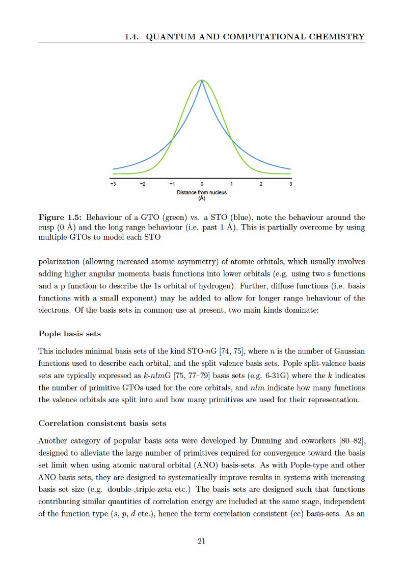

CHAPTER 1. BACKGROUND
example, the first d-function provides a significant lowering in energy, but the contribution from
a second d-function is much more similar to that of the first f-function. The energy lowering
from a third d-function in turn is similar in magnitude to that from the second f-function and
the first g-function. Therefore, the inclusion of addition of polarization functions is performed
in the following order: 1d, 2d1f, 3d2f1g etc.
An additional aspect of the cc basis sets is that the energy error from the sp-basis should be
similar to (and not exceed) the correlation error arising from the incomplete polarization space,
and the sp-basis therefore also increases as the polarization space is extended. Typically, these
basis sets are denoted as cc-pVnZ, where p indicates incorporation of polarisation functions,
and nZ indicates the degree of split valency (see Table 1.1 for the composition of contracted
and primitive gaussians). When these basis sets are augmented with diffuse functions, they are
typically referred to as aug-cc-pVnZ.
Basis Hydrogen 1st row elements 2nd row elements
Contracted Primitive Contracted Primitive Contracted Primitive
cc-pVDZ 2s1p 4s 3s2p1d 9s4p 4s3p2d 12s8p
cc-pVTZ 3s2p1d 5s 4s3p2d1f 10s5p 5s4p3d1f 15s9p
cc-pVQZ 4s3p2d1f 6s 5s4p3d2f1g 12s6p 6s5p4d2f1g 16s11p
cc-pV5Z 5s4p3d2f1g 8s 6s5p4d3f2g1h 14s8p 7s6p5d3f2g1h 20s12p
cc-pV6Z 6s5p4d3f2g1h 10s 7s6p5d4f3g2h1i 16s10p 8s7p6d4f3g2h1i 21s14p
Table 1.1: Composition of primitive and contracted Gaussian basis functions for the correlation-consistent (cc) basis sets (adapted from Jensen [83])
The complete basis set limit
When introducing split-valence basis sets, the indexing scheme (double-, triple-, quadruple-
zeta etc.) implies a natural progression of larger basis sets, indeed the primary advantage
of these basis-sets is the capacity to generate a set of basis-sets which converge toward the
complete basis-set (CBS) limit systematically. Practical calculation of the CBS limit, then,
is only sensible when using groups of basis-sets designed specifically for the purpose e.g. the
correlation-consistent (cc-pvXZ) or polarization-consistent basis sets (pc-n) [84].
E(L) = E∞ + Ae−BL (1.20)
Given the systematic convergence of the cc basis sets several different schemes have been
proposed for extrapolation to the CBS limit, generally utilising the highest angular momentum
L included in the basis set as the extrapolation parameter. At the HF (or density functional
theory) level, the convergence is expected to be exponential, and functions of the form in
22


CHAPTER 1. BACKGROUND
H0 = T + Vne + V HF (1.21)
H = H0 + λV (1.22)
Here, H0 is termed known as the unperturbed Hamiltonian and V is termed the perturbation.
In RSPT, the perturbed wavefunction and perturbed energy are expressed as a power series in
λ:
Ψ = limm→∞
m∑i=0
λiΨ(i) (1.23)
E = limm→∞
m∑i=0
λiE(i) (1.24)
Møller-Plesset (MP) perturbation theory [87] takes H0 to be the sum of the one-electron Fock
operators, and treats electron correlation as the perturbation to the zeroth-order Hamiltonian.
MP perturbation theory is by far the most commonly used variant of perturbation theories
in the field of quantum chemistry. One of the most important features of MPn16 is its size-
extensivity: the predicted energy for every order of perturbation in MPn scales with the number
of non-interacting particles in a given system.
Second order MP perturbation theory, or MP2 is by far the most commonly used variant of
PT. Higher order perturbation expansions not only become significantly more computationally
expensive, but due to the convergence of MP-PT, do not necessarily improve the resulting
energy of the system. Further, the only new information required to obtain the MP2 energy is
the first order wavefunction.
The MP2 correction may be expressed as follows:
EMP2 =1
4
∑i,j,a,b
〈ψiψj| 1r12|ψaψb〉〈ψiψj| 1
r12|ψaψb〉
εi + εj − εa − εb(1.25)
where ψi and ψj are occupied orbitals and ψa and ψb are virtual orbitals, and ε are their
respective orbital energies.
Systematic studies of MP perturbation theory have shown that it is not necessarily a
convergent theory at high orders. Convergence can be highly erratic or even non-existent,
depending on the precise chemical system or basis set [88].
Where HF would normally scale as O(N4) (where N is the number of basis functions), full
16Orders of MP perturbation theory are generally indexed from two onward e.g. MP2, MP3 etc. indicating towhich order the power series is truncated.
24

1.4. QUANTUM AND COMPUTATIONAL CHEMISTRY
CI will scale as O(NN !), rendering it computationally intractable for any remotely large basis
set.
One of the rigorous, and arguably the most reliable and computationally affordable, methods
for estimating the electronic correlation energy is the coupled cluster (CC) method. Since its
introduction in the 1950s by Coester and Kummel, CC has been developed to correct a reference
wavefunction to a given order of perturbation.
Begin with an excitation operator of the following form:
T = T1 + T2 + T3 + · · ·+ Tn (1.26)
where n is the total number of electrons. The various operators Ti acting on a reference HF
wavefunction Φ0 generate all possible i-th excited Slater determinants. As an example:
T1Φ0 =∑i∈occ
∑a∈virt
caiΦai (1.27)
where c is the expansion coefficient of amplitude. A CI wavefunction may be obtained from this
excitation operator on a HF wavefunction:
ΨCI = (1 + T )Φ0 (1.28)
The corresponding CC wavefunction may be obtained by:
ΨCC = eTΦ0
eT =∞∑k=0
1
k!T k
(1.29)
This exponential operator may be rewritten as:
eT = 1 + T1 + (T2 +1
2T 2
1 ) + (T3 + T2T1 +1
6T 3
1 )
+(T4 + T3T1 +1
2T 2
2 +1
2T2T
21 +
1
24T 4
1 ) + · · ·(1.30)
The first term (1) generates the HF wavefunction and the second term (T1) generates all single
excitations. The first parenthesised group (T2 + 12T 2
1 ) generates all double excitations and so on.
With a CC wavefunction, the Schrodinger equation becomes:
HeTΦ0 = EeTΦ0 (1.31)
If all possible cluster operators Tn are included then all possible excited determinants will be
generated and the CC wavefunction is equivalent to full CI. In general, these will be truncated at
25

CHAPTER 1. BACKGROUND
some excitation level (e.g. CCSD truncates after the double excitation level). Clearly, this then
results in an approximate wavefunction. The truncated exponential form used in CC theory is,
however, generally preferable to a CI truncation. This is because, if an exponential form is used,
then when a system is broken into subsystems, say by pulling those parts apart, the energy is
additive, a rather fundamental property known as size extensivity. This additivity is due to
the property EA+B = eAeB of exponentials, so the wavefunction conveniently separates into a
product of subsystem wavefunctions. Remarkably, CI (and other multireference wavefunctions)
often do not have this property, which can lead to sizable errors for large systems, where the
different parts are effectively isolated from one another.
It is worth mentioning the approximate perturbative triples coupling term that is frequently
utilised as part of the CCSD(T) method. Here the T3 contribution is calculated using the MP4
formula with converged CCSD amplitudes, and one additional fifth-order term describing the
coupling between singles and triples. In fact CCSD(T) is generally a better approximation than
CCSDT due to error cancellation of opposite signs (ignored quadruple excitations, along with
overestimation of the triples correction) [89].
1.4.6 Explicitly correlated methods
Recently, explicitly correlated CC methods have achieved widespread usage – largely due to
their rapid basis-set convergence (relative to ‘vanilla’ CC). There are a wide variety of explicitly
correlated methods, but they can be broadly separated into two categories – those that use
explicitly correlated two-electron basis functions (also referred to as geminals), and those that
only utilise a one-electron basis. For detailed reviews of these methods, see Kong et al. [90],
Ten-no & Noga [91] and Hattig et al. [92]. Broadly, the CCSD-R12 formalism is given by the
following equations:
T = T1 + T2 + R (1.32)
R =1
2!3tyxyR
xyαβa
αβij (1.33)
The geminal operator, R, is the basis for the variety of approximations and formalisms in
CCSD-R12. One such family of approximations are the CCSD(T)-F12 [93] methods, which in
Chapter 6 are utilised via the CCSD(T)-F12b method [94], providing significant improvements
over CCSD(T) for smaller basis-set sizes.
1.4.7 Density functional theory
It would be remiss to provide an overview of modern quantum chemistry without at least touching
on density functional theory (DFT). To that end, it is worth examining some fundamentals
26

1.4. QUANTUM AND COMPUTATIONAL CHEMISTRY
of DFT, on the way providing some idea as to how and why there exists the current ‘zoo’ of
density functionals.
Just as a mathematical function f(x) = x2 might take as input a number and yield a resulting
value (e.g. f(3) = 9), a functional takes as its input a function and results in a value. DFT,
then, is focused on functionals of the electron density. For example, the following functional:
N[ρ]
=
∫ρ(r)dr (1.34)
takes the density as its argument and returns the number of electrons in a given system.
DFT in computational chemistry is primarily concerned with functionals which yield the energy
of a given system.
DFT is based primarily on the Hohenberg-Kohn theorems [95]. However, Levy’s constrained
search theorems [96] are simpler to derive and do not suffer from some technical problems in
Hohenberg-Kohn derivation. Levy says that the ground state wavefunction is a functional of
the electron density, specifically:
E [ρ] = Q [ρ] +
∫ven(r)ρ(r) (1.35)
Q [ρ] = minΨ→ρ〈Ψ|T + Vee|Ψ〉 (1.36)
Q [ρ] searches all antisymmetric wavefunctions which yield a fixed trial electron density ρ,
delivering the expectation value which is a minimum.
Almost all DFT calculations rely on the Kohn-Sham [97] (KS) approximation, which avoids
the need for a kinetic energy functional – as Te is very difficult to approximate, since it is a
direct functional of the Kohn-Sham orbitals rather than the electron density.
Under the KS formalism the electronic energy is obtained from a system of non-interacting
electrons, where the exact energy is given by:
Eee [ρ] =N∑i
εKSi = −1
2J [ρ] + EXC [ρ]−
∫vXC(r)ρ(r)dr (1.37)
EXC [ρ] = Vee [ρ]− J [ρ] + T [ρ]− Ts [ρ] (1.38)
where T is the exact kinetic energy functional, J is the classical coulomb energy, Vee is the
exact electron repulsion energy, Ts is the kinetic energy of a non-interacting system of electrons
described exactly by a single determinant, but having an electron density of ρ. Normally, EXC
and vXC (the potential) are approximated by the so-called density functionals we are discussing
(usually separated into Ecorrelation and Eexchange components). The difference between T and Ts
is ignored [98].
27

CHAPTER 1. BACKGROUND
Functional utilises Kind Examples
ρ LDA SVWN [95, 99]
ρ, ∇ρ GGA BLYP [100, 101], PBE [102], N12 [103]
ρ, ∇ρ, ∇2ρ meta-GGA TPSS [104], BB95 [105], HCTH [106]
ρ, ∇ρ, EHFx hybrid-GGA B3PW91 [107], B3LYP [108], PBE0 [109]
ρ, ∇ρ, ∇2ρ, EHFx hybrid-meta-GGA B1B95[105], TPSSh [110], M06 [111]
Table 1.2: Terms for the different kinds of DFT functionals, including local density approxi-mations (LDA), and generalized gradient approximations (GGA). The first column indicateswhether the functionals in this class utilise the density, ρ, its derivatives and/or incorporate HFexchange (EHF
x ).
Different DFT methods differ in the way they represent Eexchange and Ecorrelation. Typically,
these are functionals of the density ρ, and its derivatives (see Table 1.2 for a broad overview).
Despite the apparent simplicity of the differences between DFT and HF, actual computation
of DFT involves integrals which cannot be solved in closed form, requiring numerical quadratures.
It was largely due to Becke [112] and his work based on Lebedev grids [113, 114] that routine
DFT calculations with appropriate accuracy for molecules became possible.
Hybrid density functionals
DFT typically makes a local (LDA) or semilocal (GGA etc.) approximation for the exchange-
correlation energy functional Exc = Ecorrelation[ρ]
+ Eexchange[ρ]
of the electron density, despite
providing MOs from which the Fock or ‘exact’ exchange energy may be calculated. So called
‘hybrid’ density functionals are those that incorporate some amount of this exact exchange,
which has been demonstrated to provide improvement over non-empirical functionals when
calculating atomization energies, bond lengths, and vibrational frequencies for most molecules
[115, 116].
The original scheme developed by Becke [107] for the first hybrids e.g. B3PW91 is as follows:
Exc = (1− a)Elocalx + aEHF
x + b∆Enon-localx + cElocal
c + (1− c)Enon-localc (1.39)
Of all modern density functionals, the most widely used hybrid functional is almost certainly
B3LYP [108], which uses the same scheme in eq. 1.39 incorporating the Becke88 [100] exchange
functional, and the LYP [101] and VWN3 [99] correlation functionals in conjunction with the
HF exchange.
The scheme in Equation 1.39 is for a hybrid GGA functionals, but in a similar manner hybrid
meta-GGAs can be defined, typically with some fixed portion of the exact exchange. Additionally,
28

1.5. CHEMOINFORMATICS
there are popular range-separated (RS) functionals which vary this portion based on electron-
electron separation. Finally, in the last decade so-called ‘double-hybrids’, which incorporate
electron correlation from MP2, have been developed – producing even more accurate results
than hybrid density functionals or MP217 (approaching ‘chemical accuracy’ of approximately 4
kJ mol−1) over a wide variety of applications [117].
1.4.8 Born-Oppenheimer molecular dynamics
Chapter 5 of this thesis examines a method to predict electron impact mass spectra, based on
Born-Oppenheimer molecular dynamics. As such, a brief overview of molecular dynamics is
warranted here. Molecular dynamics (MD) is the procedure by which molecules are modelled by
empirical force fields (typically Hooke’s-law relations, Lennard-Jones relations, or charged-pair
Coulomb relations) between pairs, triples and quartets of atoms, and then these molecules
are subject to Newton’s Laws of motion constraining either volume or pressure. It is widely
employed in chemistry, biochemistry and materials science, and has been a common area of
study for chemists and biochemists. Popular visualisation and simulation packages like VMD
[118] provide sophisticated tools to investigate the formation of molecular assemblies, among
other things.
In ab initio molecular dynamics the interatomic forces FI = −∇RIψ are determined on-the-fly
using first principles electronic structure methods. That means that AIMD is not relying on
any adjustable parameter, but only on R, However, finding the corresponding many-body
Hamiltonian at each MD step comes at a significant computational cost, which has to be
carefully balanced against the size and sampling requirements of MD. In Born-Oppenheimer
molecular dynamics (BOMD) then, the potential energy E [ψi; R] is minimized at every MD
step with respect to ψi.
1.5 Chemoinformatics
The field of chemoinformatics arguably began with the problem of trying to search for chemical
substructures for use in literature and other databases, sixty years ago [119], and shortly
afterwards, with the attempt to correlate biological acitivity with partition coefficients and
other structural information [120]. Since then, the infiltration of computers into chemistry has
lead to an explosion of applications. Chemoinformatics is critical in the pharmaceutical and
agribusiness sectors for the design of drugs, herbicides and pesticides. In the following sections
the concept of chemical information is elaborated, focussing on the manner in which chemical
information is represented.
17It is worth noting that this success is not without sacrifice: these methods no longer adhere to the Hohenberg-Kohn theorem i.e. the energy is no longer computed as a unique functional of the density only. This means thatenergy is the only property recoverable by these methods.
29

CHAPTER 1. BACKGROUND
1.5.1 Molecules, their properties, and their representation
By far the most important abstraction in chemistry is that of the molecule (or the ion in charged
cases). But a molecule need not be described exclusively in terms of its quantum mechanical
representations: there are as many ways to describe molecules as there are molecular properties.
Which description is useful or valuable in a given context will obviously change depending on the
circumstances, and the questions of interest to the scientist. We might describe a molecule by the
coordinates of its nuclei in their equilibrium geometry, or by their relative positions and angles,
or by its connectivity according to chemical bonding. We might describe molecular properties
like shape (including symmetry, isotropy, size, promolecular density isosurface, or some other
isosurface), its electrostatics (charges, dipoles, quadrupoles etc.) or molecular connectivity
(bonding) or even magnetic or spin properties of the molecule. Although it hardly needs to be
said, the precise representation of this molecular description is referred to as the “descriptor”.
The chemical importance of the descriptor is clearly the first consideration when describing
molecules or their properties, and this will depend entirely on the chemical question we wish
to answer. It should be clear, when exploring chemical questions, that the foremost priority
is the representation of chemical structure (be it two- or three-dimensional) including atomic
composition and any possible bonding information. This is reflected in the typical requirements
for chemical publications, with standardised naming schemes to describe chemical structure
(IUPAC systematic naming), and standard two-dimensional drawing styles e.g. aromatic rings,
single-, double- and triple-bonds etc.
Representations of chemical structure and reactions
There is a plethora of representations of chemical structure used in modern chemistry (see Figure
1.7 for a visual representation of some of them). The most commonly used and understood
representation of chemical structure is still the 2D structure diagram or skeletal formula. Indeed,
this representation is so embedded in chemistry that it is one of the first things taught in
high-school classes, and the required representation for chemical structures in some journals.
This represenation embeds a huge amount of information (and assumptions) about chemical
structure, but many may not even consider its influence on our ideas of chemical bonding and
molecular structure. Consider how benzene rings are drawn, that carbon atoms are generally
not explicitly drawn or that single-, double- and triple-bonds are the canonical representations
of bonding. These diagrams represent a large class of organic chemistry, but in reality chemistry
occurs in three dimensions, and naturally some structures will be more difficult to represent in
2D than others (e.g. fullerenes).
Along with the solution of the 3D structure of molecules from crystallography and other
characterisation methods, 3D representations and depictions of molecules became more common
and more useful. 3D ball-and-stick representations – stemming from the physical models still
30


CHAPTER 1. BACKGROUND
1.5.2 Data types in chemistry
Chemistry deals with data and information in a wide variety of forms, many of them very complex.
The representation of numerical data, for example is generally straightforward (representing
numbers is, after all, widely standardised and accepted). How best to represent chemical
structure (2D or 3D) and spectral data (UV/VIS, NMR, IR, MS or otherwise) is far more
difficult. Yet, the representation of this kind of data is of the utmost importance in the nature
and scale of chemical problems we can solve when using this data. There is a vast number of
different chemical structure formats for electronic storage, predominantly based on connection
tables.
In the field of crystallography there is a standard file format for crystallographic data, the
crystallographic information file (CIF) [122–124], something that has been a great boon for
productivity in data dissemination and analysis. It is a shame, then, that there has been no such
central standardisation of file formats for wavefunctions, basis sets etc. in quantum chemistry
or indeed cheminformatics, as this would radically simplify a great many of the inconveniences
for users and developers in this area.
The proliferation of file formats, some proprietary and others open standards, is the raison
d’etre of software projects like Open Babel [125]. Indeed, that Open Babel can convert between
over 110 chemical file formats (the majority of which are chemical structure formats), speaks
volumes about how urgently standardisation is needed in this space – such redundancy is not
only a waste of productive time in science, every change in format increases the likelihood of
the introduction of errors into studies.
Numerical data
In addition to the storage of chemical structure information, representation of molecular
properties may involve numerical data of high dimensionality (i.e. greater than two). While
representation of numerical data is for the most part not particularly complicated, the transfer and
portability of this data between programs and programming languages can be cumbersome and
error prone. For this reason, primarily for wavefunction and HS data (along with accompanying
properties on the surface) the Simple Binary Format (SBF) described in Appendix F was
developed allowing the straightforward transfer of binary numerical data between the C, C++,
Fortran and Python programming languages.
1.5.3 Machine learning
Further to general informatics techniques, we might use machine learning (ML) in order to
find new molecular descriptors or properties (or refine old ones). Broadly speaking, ML is the
field of enabling computers to ‘learn’ patterns or relationships in data without being explicitly
programmed. ML has become increasingly popular in computer vision, natural language
32

1.5. CHEMOINFORMATICS
processing and indeed in scientific questions that do not lend themselves to straightforward
analytical descriptions, but where large amounts of (reliable) data are available. ML may be
conceived as a stepping stone or component of artificial intelligence, but it does not have as a
primary goal the creation of an intelligent system or being. The goal of ML in general is to
solve problems of a practical nature, usually to make testable predictions.
Because ML encompasses a huge number of disparate problems and approaches, it is well
and truly outside the scope of this introduction to describe them in any form that would do
them justice. Instead this section will focus on the concepts of classification and regression, and
further describe some of the ML techniques which are used in this thesis.
Classification and Regression
Classification problems result in class membership, they take a query object descriptor (or
descriptors) and return the resulting class to which the object is said to belong, based on this
descriptor. Multiple classification approaches are generally built up from binary classifiers,
where membership of one class is all that is interrogated. Classes may be known prior, for
example if we were training a model to determine whether an image contains a cat by providing
a series of images appropriately labelled. Classes may also be ‘discovered’, or unknown, for
example in cluster analysis.
Regression problems, on the other hand, result in a property: they take a query descriptor (or
descriptors) and return some resulting property. Straightforward regression might be something
like linear interpolation of functions, but generally ML concerns some more complicated function
or property. An example of a regression technique would be prediction of a mass spectrum from
a given chemical structure (see discussion of the CFM[126] techniques in Chapter 5).
Cluster analysis
Broadly speaking, cluster analysis is the task of classifying a set of observations in such a manner
that those in the same group or cluster are, in some sense, more similar to one-another than to
those outside the cluster. The clustering performed in this project will be hierarchical in nature.
That is to say that there will be levels or thresholds of proximity, and if we take a cut off at one
of these levels we are left with a group of flat clusters.
There are many different types of cluster analysis, and indeed clustering techniques themselves
(some of which, including methods for implementation are contained in [127]), and applications
of the techniques are as wide ranging as Google’s page-rank algorithms on the world-wide-web
to the field of bioinformatics where the similarity of genetic data is clustered to examine and
infer population structures or assign genotypes.
Clustering variants include (but are not limited to):
• Hierarchical clustering or connectivity based clustering, which is based on the idea that
33

CHAPTER 1. BACKGROUND
nearer objects are more related than those far away. This includes single linkage, complete
linkage, average linkage clustering etc.
• Centroid based clustering in which clusters are represented by a central vector. When the
number of clusters is fixed, k-means clustering provides a formalisation as an optimization
problem (where squared distance from the centre of each cluster is minimised.)
• Distribution based clustering and density based clustering.
Nearest neighbour search
A related problem to cluster analysis is that of nearest-neighbour search (NNS). NNS is a form
of proximity search, which is to say it is an optimization problem of finding the point in a given
set that is closest (most similar) to another given point. Typically, closeness is expressed in
terms of a distance function: less similar objects are ‘further’ from each other. Formally, the
NNS problem is defined as follows: given a set S of points in a space M and a query point
q ∈ M, find the closest point in S to q. An immediate generalization of this problem is to
extend it to the k nearest points, known as k-nearest neighbours (k-NN).
The use case for NNS and kNN is clear when we have a molecular descriptor represented as
a vector or numerical values. Here we can use Euclidean distance d(x) =√∑
x2i (or square
distance function d(x) =∑
x2i ) to find the closest matches to a given query molecule. NNS use
is also widespread in ML algorithms, particularly in the k-NN classification or regression.
Principal Component Analysis
Principal component analysis (PCA) is a procedure that utilises an orthogonal transformation to
convert a set of observations (vectors) in a (possibly) correlated vector space into a set of vectors
in a space of linearly uncorrelated variables termed principal components. More intuitively, it
can be thought of as fitting an n-dimensional ellipsoid to a set of data, such that the axes of the
ellipsoid maximally account for the variance within the set of observations.
PCA can be used for dimensionality reduction, as it identifies axes (which are linear
combinations of the original axes) which maximally account for the variance within the data.
This proves immensely useful for visualising and processing high-dimensional datasets (and it is
used for visualisation in Chapter 3), while still retaining as much of the variance in the dataset
as possible. It is frequently used with only the first two principal components to project a higher
dimensional data set onto the 2D plane, as the resulting projection will be optimally ‘spread
out’, enabling easier visualisation and representation of the differences in the data. PCA can
also be used to align objects or meshes in 3D, by determining the orientation of the primary
axes.
34

1.5. CHEMOINFORMATICS
1.5.4 Chemical databases
Perhaps the most visible achievement of cheminformatics in the last 50 years has been databases
of chemical information [128]. Access to high quality data is of crucial importance to modeling,
as any inaccuracies or errors will be propagated throughout the model. There is, at present, a
wide variety of chemical databases, many with enormous amounts of curated information. There
are general purpose chemical databases (e.g. Pubchem [129], ChemSpider [130]), which provide
free access to fundamental information about chemical structure, computed or experimentally
recorded properties like biological activity, and more. While these databases have found
widespread use in pharmaceutical research and drug discovery, their applicability is far more
widespread. Further, there are many more specific databases, some for mass spectrometry data
(e.g. NIST17 [131], The Wiley/NBS Registry [132]) others for crystallographic data, (e.g. the
aforementioned CSD [133] and PDB [134]).
This widespread availabilty of comprehensive chemical information provides a vital starting
point for chemical modeling: both for helping to parameterise models and for investigating their
success. Without a doubt, the success of cheminformatics (and indeed computational chemistry)
relies on the availabilty, accessibility and veracity of chemical data in databases like these.
Additionally, there are databases consisting entirely of virtual molecules i.e. those which
have been generated by exploration of the ‘chemical space’ but not synthesized. Such databases
find particular use in the field of drug discovery.
1.5.5 Virtual screening
Computers play many roles in drug discovery [135], but a particularly important role is so-called
Virtual screening (VS). The aim of a VS process is to identify molecules that may bind to a
macromolecular target of interest, usually binding to a drug target protein receptor or enzyme.
This is performed via searching or ‘screening’ a large library of potential chemical structures
(e.g. those mentioned in the prior section, ZINC [136] and many more), consisting or real or
virtual chemical structures. VS methods can be broadly separated into two distinct approaches:
methods focussed on matching ligands which are known to bind to the target – ligand-based
virtual screening (LBVS) – and methods focussed on matching potential ligands to the binding
site of the target – structure-based virtual screening (SBVS) [137, 138].
Ligand based virtual screening
Most LBVS methods attempt to design or discover new molecules that satisfy certain similarity
criteria with a known binding ligand [139, 140]. Such matching may be performed based on:
• Intermolecular interaction sites (such as hydrogen-bond donors and acceptors) [136],
35

CHAPTER 1. BACKGROUND
• So-called ‘pharmacophore‘ models built from knowledge of a set of ligands which bind to
a given receptor [141, 142],
• 2D chemical similarity analysis (i.e. skeletal or scaffold similarity) [143, 144],
• 3D molecular shape [145, 146] and/or electrostatics [147–150],
Some LBVS procedures make use of machine learning techniques to assess similarity [151], be it
using one or more of the above methods or otherwise. Because of its dependence only on a small
molecule ligand structure, typical LBVS processes are relatively cheap and efficient. Chapter 4
of this thesis demonstrates the potential use of the spherical harmonic shape descriptors in this
process, for searching small molecule crystal structure databases.
Structure based virtual screening
SBVS typically involves ‘docking’ procedures [152], which utilise a scoring function to estimate
binding or non-binding interactions between a candidate ligand and the desired protein-receptor
site. Docking procedures usually involve a step to find the most favourable orientation in the
receptor pocket, and a variety of molecular conformations (or conformers). Optimisation of the
conformers within the space is prohibitatively expensive (especially if the surrounding area of the
protein is not fixed) for large scale studies, and so generally some number of diverse low energy
molecular conformers are generated and treated as rigid. Further, SBVS approaches generally
require significantly more computation than LBVS procedures, due to their incorporation of a
larger chemical environment (the structure of the entire binding site). This limits the scale of
virtual screenings, or requires larger computational resources in order to perform these searches.
There are many approaches to SBVS (see Lionta et al. [153] or Cheng et al. [137] for recent
overviews), but as the topic is largely tangential to this thesis (with the exception of the docking
scores in Chapter 4) it will not be explored further here.
36

Bibliography
1. Calhoun, C. J. The Microcomputer Revolution? Sociol. Methods Res. 9, 397 (1981).
2. Kuhn, T. The Structure of Scientific Revolutions (University of Chicago Press, Chicago,
1962).
3. Hey, T. The Fourth Paradigm: Data-Intensive Scientific Discovery (eds Hey, T., Tolle,
K. M. & Tansley, S.) (Microsoft Research, Seattle, 2009).
4. Vardi, M. Y. Science has only two legs. Commun. ACM 53, 5 (2010).
5. Henry, N. L. Knowledge Management: A New Concern for Public Administration. Pub.
Admin. Rev. 34, 189 (1974).
6. Rowley, J. The wisdom hierarchy: representations of the DIKW hierarchy. J. Inf. Sci. 33,
163 (2007).
7. Bridgman, P. W. The Logic of Modern Physics (Macmillan, New York, 1927).
8. Popper, K. Conjectures and Refutations (Routlege & Kegan Paul, New York, 1962).
9. Hoffmann, R. A theoretician’s view of crystallography. Acta Crystallogr. A 61, c1 (2005).
10. Dirac, P. A. M. Quantum Mechanics of Many-Electron Systems. Proc. Royal Soc. A 123,
714 (1929).
11. Moore, G. E. Cramming more components onto integrated circuits. Electronics 38, 114
(1965).
12. Simonite, T. Moore’s Law is Dead. Now What? https://www.technologyreview.com/
s/601441/moores-law-is-dead-now-what/ (2017).
13. Engel, T. Basic Overview of Chemoinformatics. J. Cheminf. Model. 46, 2267 (2006).
14. Warr, W. A. Balancing the needs of the recruiters and the aims of the educators in Book
of Abstracts, 218th ACS National Meeting (New Orleans, 1999).
15. Mulliken, R. S. Electronic Structures of Polyatomic Molecules and Valence. Phys. Rev.
40, 55 (1932).
16. Mulliken, R. S. Electronic Structures of Polyatomic Molecules and Valence. II. Quantum
Theory of the Double Bond. Phys. Rev. 41, 751 (1932).
37

BIBLIOGRAPHY
17. Mulliken, R. S. Electronic Structures of Polyatomic Molecules and Valence. V. Molecules
RX n. J. Chem. Phys. 1, 492 (1933).
18. Huckel, E. Die freien Radikale der organischen Chemie. Z. Phys. 83, 632 (1933).
19. Hoffmann, R. An Extended Huckel Theory. I. Hydrocarbons. J. Chem. Phys. 39, 1397
(1963).
20. Heilbronner, E. & Straub. Huckel Molecular orbitals (Springer-Verlag, Berlin, 1966).
21. McLean, A. D. & Yoshimine, M. Computation of Molecular Properties and Structure.
IBM J. Res. Dev. 12, 206 (1968).
22. Snyder, L. C. & Basch, H. Molecular wave functions and properties: (ed Basch, H.)
(Wiley-Interscience, New York, 1972).
23. Ferry, G. Dorothy Hodgkin: A Life (Bloomsbury, London, 2014).
24. Huang, Z. & Kim, K.-J. Review of x-ray free-electron laser theory. Phys. Rev. Accel.
Beams 10 (2007).
25. Kang, Y. et al. Crystal structure of rhodopsin bound to arrestin by femtosecond X-ray
laser. Nature 523, 561 (2015).
26. Buchanan, B. G., Lederberg, J. & Feigenbaum, E. The Heuristic DENDRAL program for
explaining empirical data 1971.
27. Bragg, W. H. & Bragg, W. L. The Reflection of X-rays by Crystals. Proc. Royal Soc. A
88, 428 (1913).
28. Lonsdale, K. The structure of the benzene ring. Nature 122, 810 (1928).
29. Bouslimani, A., Sanchez, L. M., Garg, N. & Dorrestein, P. C. Mass spectrometry of
natural products: current, emerging and future technologies. Nat. Prod. Rep. 31, 718
(2014).
30. Dettmer, K., Aronov, P. A. & Hammock, B. D. Mass spectrometry-based metabolomics.
Mass Spec. Rev. 26, 51 (2007).
31. Cranswick, L. M. D. Busting out of crystallography’s Sisyphean prison: from pencil
and paper to structure solving at the press of a button: past, present and future of
crystallographic software development, maintenance and distribution. Acta Crystallogr. A
64, 65 (2008).
32. Bennett, J. M. & Kendrew, J. C. The computation of Fourier synthesis with a digital
electronic calculating machine. Acta Crystallogr. 5, 109 (1952).
33. Ahmed, F. R. & Cruickshank, D. W. J. A refinement of the crystal structure analyses of
oxalic acid dihydrate. Acta Crystallogr. 6, 385 (1953).
38

BIBLIOGRAPHY
34. Kendrew, J. C. et al. A Three-Dimensional Model of the Myoglobin Molecule Obtained
by X-Ray Analysis. Nature 181, 662 (1958).
35. Levinthal, C. Molecular model-bilding by computer. Sci. Amer. 214, 42 (1966).
36. Desiraju, G. R., Vittal, J. J. & Ramanan, A. Crystal engineering (Co-Published with
Indian Institute of Science (IISc), Bangalore, India, 2011).
37. Verheyen, E. et al. Design of zeolite by inverse sigma transformation. Nature Mat. 11,
1059 (2012).
38. Yaghi, O. M. et al. Reticular synthesis and the design of new materials. Nature 423, 705
(2003).
39. Desiraju, G. R. Supramolecular Synthons in Crystal Engineering—A New Organic Syn-
thesis. Angew. Chem. Int. Ed. 34, 2311 (1995).
40. Corey, E. General methods for the construction of complex molecules. Pure Appl. Chem.
14, 19 (1967).
41. Hirshfeld, F. L. & Rzotkiewicz, S. Electrostatic binding in the first-row AH and A2
diatomic molecules. Mol. Phys 27, 1319 (1974).
42. Coppens, P. & Hall, M. B. Electron Distributions and the Chemical Bond (Springer,
Boston, USA, 1982).
43. Moffitt, W. Atoms in Molecules and Crystals. Proc. Royal Soc. A 210, 245–268 (1951).
44. Bader, R. Atoms in Molecules: A Quantum Theory isbn: 9780198558651 (Clarendon
Press, Oxford, 1994).
45. Coppens, P. X-Ray Charge Densities and Chemical Bonding (Oxford University Press,
Oxford, 1997).
46. Cassam-Chenaı, P. & Jayatilaka, D. Some fundamental problems with zero flux partitioning
of electron densities. Theor. Chem. Acc. 104, 213–218 (3 2000).
47. Cassam-Chenaı, P. & Jayatilaka, D. A complement to “Some fundamental problems with
zero flux partitioning of electron densities”. Theor. Chem. Acc. 107, 383–384 (6 2002).
48. Gill, P. M. W. Extraction of Stewart Atoms from Electron Densities. J. Phys. Chem. 100,
15421–15427 (38 1996).
49. Hunter, G. Atoms in molecules from the exact one-electron wave function. Can. J. Chem.
74, 1008–1013 (6 1996).
50. Roby, K. R. Quantum theory of chemical valence concepts. Mol. Phys. 27, 81–104 (1
1974).
39

BIBLIOGRAPHY
51. Gould, M. D., Taylor, C., Wolff, S. K., Chandler, G. S. & Jayatilaka, D. A definition for
the covalent and ionic bond index in a molecule. Theor. Chem. Acc. 119, 275–290 (1–3
2008).
52. Sukumar, N. A Matter of Density (Wiley, New Jersey, 2012).
53. Hirshfeld, F. L. Bonded-atom fragments for describing molecular charge densities. Theor.
Chem. Acc. 44, 129 (1977).
54. Spackman, M. A. & Byrom, P. G. A novel definition of a molecule in a crystal. Chem.
Phys. Lett. 267, 215 (1997).
55. McKinnon, J. J., Spackman, M. A. & Mitchell, A. S. Novel tools for visualizing and
exploring intermolecular interactions in molecular crystals. Acta Crystallogr. B 60, 627
(2004).
56. Spackman, M. A. & Jayatilaka, D. Hirshfeld surface analysis. CrystEngComm 11, 19.
57. Wigner, E. & Seitz, F. On the Constitution of Metallic Sodium. Phys. Rev. 43, 804
(1933).
58. Voronoi, G. Nouvelles applications des parametres continus a la theorie des formes
quadratiques. Premier memoire. Sur quelques proprietes des formes quadratiques positives
parfaites. J. reine angew. Math. 1908, 97 (1908).
59. Blatov, V. A., Shevchenko, A. P. & Proserpio, D. M. Applied Topological Analysis of
Crystal Structures with the Program Package ToposPro. Cryst. Growth Des. 14, 3576
(2014).
60. Spackman, M. A. & McKinnon, J. J. Fingerprinting intermolecular interactions in molec-
ular crystals. Crystengcomm 4, 378 (2002).
61. McKinnon, J. J., Jayatilaka, D. & Spackman, M. A. Towards quantitative analysis of
intermolecular interactions with Hirshfeld surfaces. Chem. Commun. 267, 3814 (2007).
62. Parkin, A. et al. Comparing entire crystal structures: structural genetic fingerprinting.
Crystengcomm 9, 648 (2007).
63. Schrodinger, E. Quantisierung als Eigenwertproblem. Ann. Phys. (Berl). 384, 361 (1926).
64. Schrodinger, E. An Undulatory Theory of the Mechanics of Atoms and Molecules. Phys.
Rev. 28, 1049 (1926).
65. Born, M. & Oppenheimer, R. Zur Quantentheorie der Molekeln. Ann. Phys. (Berl.) 389,
457 (1927).
66. Hartree, D. R. The Wave Mechanics of an Atom with a Non-Coulomb Central Field. Part
I. Theory and Methods. Math. Proc. Camb. Philos. Soc. 24, 89 (1928).
40

BIBLIOGRAPHY
67. Hartree, D. R. The Wave Mechanics of an Atom with a Non-Coulomb Central Field. Part
II. Some Results and Discussion. Math. Proc. Camb. Philos. Soc. 24, 111 (1928).
68. Fock, V. Naherungsmethode zur Losung des quantenmechanischen Mehrkorperproblems.
Z. Phys. 61, 126 (1930).
69. Slater, J. C. Atomic Shielding Constants. Phys. Rev. 36, 57 (1930).
70. Yanai, T., Fann, G. I., Gan, Z., Harrison, R. J. & Beylkin, G. Multiresolution quantum
chemistry in multiwavelet bases: Analytic derivatives for Hartree–Fock and density
functional theory. J. Chem. Phys. 121, 2866 (2004).
71. Boys, S. F. Electronic wave functions - I. A general method of calculation for the stationary
states of any molecular system. Proc. Royal Soc. A 200, 542 (1950).
72. Stewart, R. F. Small Gaussian Expansions of Slater-Type Orbitals. J. Chem. Phys. 52,
431 (1970).
73. Hehre, W. J., Stewart, R. F. & Pople, J. A. Atomic electron populations by molecular
orbital theory. Symp. Faraday Soc. 2, 15 (1968).
74. Hehre, W. J., Stewart, R. F. & Pople, J. A. Self-Consistent Molecular-Orbital Methods. I.
Use of Gaussian Expansions of Slater-Type Atomic Orbitals. J. Chem. Phys. 51, 2657
(1969).
75. Hehre, W. J., Ditchfield, R. & Pople, J. A. Self—Consistent Molecular Orbital Methods.
XII. Further Extensions of Gaussian—Type Basis Sets for Use in Molecular Orbital
Studies of Organic Molecules. J. Chem. Phys. 56, 2257 (1972).
76. Davidson, E. R. & Feller, D. Basis set selection for molecular calculations. Chem. Rev.
86, 681 (1986).
77. Binkley, J. S., Pople, J. A. & Hehre, W. J. Self-consistent molecular orbital methods. 21.
Small split-valence basis sets for first-row elements. J. Am. Chem. Soc. 102, 939 (1980).
78. Krishnan, R., Binkley, J. S., Seeger, R. & Pople, J. A. Self-consistent molecular orbital
methods. XX. A basis set for correlated wave functions. J. Chem. Phys. 72, 650 (1980).
79. Frisch, M. J., Pople, J. A. & Binkley, J. S. Self-consistent molecular orbital methods 25.
Supplementary functions for Gaussian basis sets. J. Chem. Phys. 80, 3265 (1984).
80. Dunning, T. H. Gaussian-basis sets for use in correlated molecular calculations .1. the
atoms boron through neon and hydrogen. J. Chem. Phys. 90, 1007 (1989).
81. Kendall, R. A., Dunning, T. H. & Harrison, R. J. Electron-affinities of the 1st-row atoms
revisited - systematic basis-sets and wave-functions. J. Chem. Phys. 96, 6796 (1992).
82. Dunning, T. H., Peterson, K. A. & Wilson, A. K. Gaussian basis sets for use in correlated
molecular calculations. X. The atoms aluminum through argon revisited. J. Chem. Phys.
114, 9244 (2001).
41

BIBLIOGRAPHY
83. Jensen, F. Introduction to Computational Chemistry 2nd ed. (Wiley, Hoboken, USA,
2007).
84. Jensen, F. Polarization consistent basis sets: Principles. J. Chem. Phys. 115, 9113 (2001).
85. Karton, A. & Martin, J. M. L. Comment on: “Estimating the Hartree–Fock limit from
finite basis set calculations” [Jensen F (2005) Theor Chem Acc 113:267]. Theor. Chem.
Acc. 115, 330 (2006).
86. Szabo, A. & Ostlund, N. S. Modern Quantum Chemistry (Courier Corporation, London,
1989).
87. Møller, C. & Plesset, M. S. Note on an Approximation Treatment for Many-Electron
Systems. Phys. Rev. 46, 618 (1934).
88. Leininger, M. L., Allen, W. D., Schaefer III, H. F. & Sherrill, C. D. Is Møller–Plesset
perturbation theory a convergent ab initiomethod? J. Chem. Phys. 112, 9213 (2000).
89. Helgaker, T., Klopper, W., Koch, H. & Noga, J. Basis-set convergence of correlated
calculations on water. J. Chem. Phys. 106, 9639 (1997).
90. Kong, L., Bischoff, F. A. & Valeev, E. F. Explicitly Correlated R12/F12 Methods for
Electronic Structure. Chem. Rev. 112, 75 (2011).
91. Ten-no, S. & Noga, J. Explicitly correlated electronic structure theory from R12/F12
ansatze. Wiley Interdiscip. Rev. Comput. Mol. Sci. 2, 114 (2012).
92. Hattig, C., Klopper, W., Kohn, A. & Tew, D. P. Explicitly Correlated Electrons in
Molecules. Chem. Rev. 112, 4 (2011).
93. Adler, T. B., Knizia, G. & Werner, H.-J. A simple and efficient CCSD(T)-F12 approxi-
mation. J. Chem. Phys. 127, 221106 (2007).
94. Knizia, G., Adler, T. B. & Werner, H.-J. Simplified CCSD(T)-F12 methods: Theory and
benchmarks. J. Chem. Phys. 130, 054104 (2009).
95. Hohenberg, P. & Kohn, W. Inhomogeneous Electron Gas. Phys. Rev. 136, B864B871
(1964).
96. Levy, M. Universal variational functionals of electron densities, first-order density matrices,
and natural spin-orbitals and solution of the v-representability problem. Proc. Natl. Acad.
Sci. U.S.A 76, 6062 (1979).
97. Kohn, W. & Sham, L. J. Self-Consistent Equations Including Exchange and Correlation
Effects. Phys. Rev. 140, A1133A1138 (1965).
98. Parr, R. G. & Yang, W. Density functional theory of atoms and molecules (Oxford
University Press, Oxford, 1989).
42

BIBLIOGRAPHY
99. Vosko, S. H., Wilk, L. & Nusair, M. Accurate spin-dependent electron liquid correlation
energies for local spin density calculations: a critical analysis. Can. J. Phys. 58, 1200
(1980).
100. Becke, A. D. Density-functional exchange-energy approximation with correct asymptotic
behavior. Phys. Rev. A 38, 3098 (1988).
101. Lee, C., Yang, W. & Parr, R. G. Development of the Colle-Salvetti correlation-energy
formula into a functional of the electron density. Phys. Rev. B 37, 785 (1988).
102. Perdew, J. P., Burke, K. & Ernzerhof, M. Generalized Gradient Approximation Made
Simple. Phys. Rev. Lett. 77, 3865 (1996).
103. Peverati, R. & Truhlar, D. G. Exchange–Correlation Functional with Good Accuracy for
Both Structural and Energetic Properties while Depending Only on the Density and Its
Gradient. J. Chem. Theory Comput. 8, 2310 (2012).
104. Tao, J., Perdew, J. P., Staroverov, V. N. & Scuseria, G. E. Climbing the Density Functional
Ladder: Nonempirical Meta21Generalized Gradient Approximation Designed for Molecules
and Solids. Phys. Rev. Lett. 91, 146401 (2003).
105. Becke, A. D. Density-functional thermochemistry. IV. A new dynamical correlation
functional and implications for exact-exchange mixing. J. Chem. Phys. 104, 1040 (1996).
106. Hamprecht, F. A., Cohen, A. J., Tozer, D. J. & Handy, N. C. Development and assessment
of new exchange-correlation functionals. J. Chem. Phys. 109, 6264 (1998).
107. Becke, A. D. Density-functional thermochemistry. III. The role of exact exchange. J.
Chem. Phys. 98, 5648 (1993).
108. Stephens, P. J., Devlin, F. J., Chabalowski, C. F. & Frisch, M. J. Ab Initio Calculation of
Vibrational Absorption and Circular Dichroism Spectra Using Density Functional Force
Fields. J. Phys. Chem. 98, 11623 (1994).
109. Adamo, C. & Barone, V. Toward reliable density functional methods without adjustable
parameters: The PBE0 model. J. Chem. Phys. 110, 6158 (1999).
110. Staroverov, V. N., Scuseria, G. E., Tao, J. & Perdew, J. P. Comparative assessment of
a new nonempirical density functional: Molecules and hydrogen-bonded complexes. J.
Chem. Phys. 119, 12129 (2003).
111. Zhao, Y. & Truhlar, D. G. The M06 suite of density functionals for main group thermo-
chemistry, thermochemical kinetics, noncovalent interactions, excited states, and transition
elements: two new functionals and systematic testing of four M06-class functionals and
12 other functionals. Theor. Chem. Acc. 120, 215 (2008).
112. Becke, A. D. A multicenter numerical integration scheme for polyatomic molecules. J.
Chem. Phys. 88, 2547 (1988).
43

BIBLIOGRAPHY
113. Lebedev, V. I. Quadratures on the sphere. Zh. Vychisl. Mat. Mat. Fiz. 16, 293 (1976).
114. Lebedev, V. I. Spherical quadrature formulas exact to order-25-order-29. Sib. Math. J.
18, 99 (1977).
115. Perdew, J. P., Ernzerhof, M. & Burke, K. Rationale for mixing exact exchange with
density functional approximations. J. Chem. Phys. 105, 9982 (1996).
116. Goerigk, L. & Grimme, S. A thorough benchmark of density functional methods for
general main group thermochemistry, kinetics, and noncovalent interactions. Phys. Chem.
Chem. Phys. 13, 6670 (2011).
117. Goerigk, L. & Grimme, S. Double-hybrid density functionals. Wiley Interdiscip. Rev.
Comput. Mol. Sci. 4, 576 (2014).
118. Humphrey, W., Dalke, A. & Schulten, K. VMD Visual Molecular Dynamics. J. Mol.
Graph. 14, 33 (1996).
119. Ray, L. C. & Kirsch, R. A. Finding Chemical Records by Digital Computers. Science
126, 814 (1957).
120. Hansch, C., Maloney, P. P., Fujita, T. & Muir, R. M. Correlation of Biological Activity
of Phenoxyacetic Acids with Hammett Substituent Constants and Partition Coefficients.
Nature 194, 178 (1962).
121. Bonchev, D. & Rouvray, D. H. Chemical Topology: Introduction and Fundamentals (CRC
Press, Boca Raton, Florida).
122. Hall, S. R., Allen, F. H. & Brown, I. D. The crystallographic information file (CIF): a
new standard archive file for crystallography. Acta Crystallogr. A 47, 655 (1991).
123. Hall, S. R. et al. in International Tables for Crystallography Volume G: Definition
and exchange of crystallographic data (eds Hall, S. R. & McMahon, B.) 20 (Springer
Netherlands, Dordrecht, 2005).
124. Brown, I. D. & McMahon, B. CIF: the computer language of crystallography. Acta
Crystallogr. B 58, 317 (2002).
125. O’Boyle, N. M. et al. Open Babel: An open chemical toolbox. J. Cheminform 3, 33
(2011).
126. Allen, F., Pon, A., Greiner, R. & Wishart, D. Computational Prediction of Electron
Ionization Mass Spectra to Assist in GC/MS Compound Identification. Anal. Chem. 88,
7689 (2016).
127. Press, W. H., Teukolsky, S. A., Vetterling, W. T. & Flannery, B. P. Numerical Recipes
3rd Edition: The Art of Scientific Computing 3rd ed. (Cambridge University Press, New
York, NY, USA, 2007).
44

BIBLIOGRAPHY
128. Gasteiger, J. Chemoinformatics: Achievements and Challenges, a Personal View. Molecules
21 (2016).
129. Kim, S. et al. PubChem Substance and Compound databases. Nucleic Acids Res. 44,
D1202D1213 (2016).
130. ChemSpider Home Page https://www.chemspider.com (2017).
131. NIST Standard Reference Database 1A v17 https : / / www . nist . gov / srd / nist -
standard-reference-database-1a-v17 (2017).
132. Wiley Registry of Mass Spectral Data, 11th Edition http://wiley.com/WileyCDA/
WileyTitle/productCd-1119171016.html (2017).
133. Groom, C. R., Bruno, I. J., Lightfoot, M. P. & Ward, S. C. The Cambridge Structural
Database. Acta Crystallogr. B 72, 171 (2016).
134. Berman, H. M. The Protein Data Bank. Nucleic acids research 28, 235 (2000).
135. Jorgensen, W. L. The many roles of computation in drug discovery. Science 303, 1813
(2004).
136. Irwin, J. J. & Shoichet, B. K. ZINC − A Free Database of Commercially Available
Compounds for Virtual Screening. J. Cheminf. Model. 45, 177 (2005).
137. Cheng, T., Li, Q., Zhou, Z., Wang, Y. & Bryant, S. H. Structure-Based Virtual Screening
for Drug Discovery: a Problem-Centric Review. AAPS J. 14, 133 (2012).
138. Di Giovanni, A. L. & C. Virtual Screening Strategies in Drug Discovery: A Critical Review.
Curr. Med. Chem. 20, 2839 (2013).
139. Willett, P. Enhancing the Effectiveness of Ligand-Based Virtual Screening Using Data
Fusion. QSAR Comb. Sci. 25, 1143 (2006).
140. Stahura, F. L. & Bajorath, J. New methodologies for ligand-based virtual screening. Cur.
Pharm. Des. 11, 1189 (2005).
141. Cho, S. J. & Sun, Y. FLAME: A Program to Flexibly Align Molecules. J. Chem. Inf.
Model. 46, 298 (2006).
142. Khedkar, S. A., Malde, A. K., Coutinho, E. C. & Srivastava, S. Pharmacophore modeling
in drug discovery and development: an overview. Med. Chem. 3, 187 (2007).
143. Willett, P., Barnard, J. M. & Downs, G. M. Chemical Similarity Searching. J. Chem. Inf.
Model. 38, 983 (1998).
144. Sheridan, R. P. & Kearsley, S. K. Why do we need so many chemical similarity search
methods? Drug Discov. Today 7, 903 (2002).
145. Bemis, G. W. & Kuntz, I. D. A fast and efficient method for 2D and 3D molecular shape
description. J. Comput. Aided Mol. Des. 6, 607 (1992).
45

BIBLIOGRAPHY
146. Hahn, M. Three-Dimensional Shape-Based Searching of Conformationally Flexible Com-
pounds. J. Chem. Inf. Comput. Sci. 37, 80 (1997).
147. Hodgkin, E. E. & Richards, W. G. Molecular similarity based on electrostatic potential
and electric field. Int. J. Quantum Chem. 32, 105 (1987).
148. Buchbauer, G., Klinsky, A., Weiß-Greiler, P. & Wolschann, P. Ab initio Molecular
Electrostatic Potential Grid Maps for Quantitative Similarity Calculations of Organic
Compounds. Mol. Model. Ann. 6, 425 (2000).
149. Melani, F., Gratteri, P., Adamo, M. & Bonaccini, C. Field Interaction and Geometrical
Overlap: A New Simplex and Experimental Design Based Computational Procedure for
Superposing Small Ligand Molecules. J. Med. Chem. 46, 1359 (2003).
150. Vainio, M. J., Puranen, J. S. & Johnson, M. S. ShaEP: Molecular Overlay Based on
Shape and Electrostatic Potential. J. Chem. Inf. Model. 49, 492 (2009).
151. Hert, J. et al. New Methods for Ligand-Based Virtual Screening: Use of Data Fusion
and Machine Learning to Enhance the Effectiveness of Similarity Searching. J. Chem.
Inf. Model. 46, 462 (2006).
152. Kitchen, D. B., Decornez, H., Furr, J. R. & Bajorath, J. Docking and scoring in virtual
screening for drug discovery: methods and applications. Nat. Rev. Drug Discov. 3, 935
(2004).
153. Lionta, E., Spyrou, G., Vassilatis, D. K. & Cournia, Z. Structure-based virtual screening
for drug discovery: principles, applications and recent advances. Curr. Top. Med. Chem.
14, 1923 (2014).
46

Chapter 2
Introduction to a series of papers
It should be clear from the previous sections that computational chemistry encompasses a
wide variety of chemical, mathematical and software development problems. Throughout the
following series of papers, some these problems are explored in detail. With the exception of
Chapter 4, all of the following chapters have been previously published in peer-reviewed journals.
The content from these publications has been modified only to fit the formatting of this thesis,
no more. The papers comprising this thesis can be broadly separated into two parts: those
primarily focussed on molecular shape in crystals, and those focussed on assessing the accuracy
of quantum chemical calculations for their practical application.
2.1 Molecular shapes in crystals
The first part of this thesis is concerned with the development and application of a novel
description technique for molecular shapes. In these papers shape has been defined in terms of
electronic isosurfaces: the Hirshfeld Surface [292] and the promolecular density isosurface.
Chapter 3 consists of a publication laying out the description of molecular shapes with
spherical harmonic functions, and the process of constructing rotation-invariant shape descriptors
from the coefficients of the spherical harmonic transform. Further, this chapter contains
application to small examples: the classification of atomic Hirshfeld surfaces in metallic crystals
according to their lattice type, and the classification of different molecular scaffolds based on
these shape descriptors.
Chapter 4 represents the first significant application of these shape descriptors: to improve
the process of Ligand Based Virtual Screening (LBVS) in rational drug discovery, and enable
the use of large databases of small-molecule crystals as potential ligands. This paper consists of
the description of four protein-ligand systems in terms of the aforementioned spherical harmonic
shape descriptors, a description which is then utilised to find the top matching molecules
from a selection of over 110 thousand crystal structures from the CSD. Further, this paper
demonstrates the immense potential value of the usage of molecular conformers obtained from
47

CHAPTER 2. INTRODUCTION TO A SERIES OF PAPERS
their small-molecule crystal structures: an energetically favourable environment in which they
are interacting with neighbouring molecules. Finally, the impacts of different surface properties
(dnorm and electrostatic potential) and surface types (Hirshfeld surface and promolecule surface)
are explored with reference to their characteristic description of local molecular environment vs.
encapsulation of the crystal environment.
2.2 Assessment of the accuracy of quantum chemical
methods
The second part of this thesis is concerned with assessment and characterisation of existing
prediction techniques in quantum chemistry.
Chapter 5 primarily examines Grimme and Bauer’s method for the prediction of the electronic
impact mass spectrum of arbitrary molecules: Quantum Chemical Electronic Impact Mass
Spectrum (QCEIMS). This technique is evaluated for a set of 61 small molecules from different
common, and important (in terms of their fragmentation propensity), chemical compound
classes. The performance of this method is examined with reference to experimental spectra,
and compared with another (radically different) state-of-the-art approach in Competitive
Fragmentation Modelling (CFM). This chapter, then, consists of comparison between ab initio
predictions and machine learning predictions for EIMS, with the purpose of establishing a
baseline of correctness for use in identification of natural products and semiochemicals, or
metabolomics as complementary to experimental work.
Chapter 6 examines basis-set convergence of equilibrium geometries using CCSD(T), along
with newer explicitly correlated CCSD(T)-F12 methods. The basis-set convergence of equilibrium
geometries is especially important in high-accuracy thermochemical calculations, and this
publication investigates the relationship between correlation-consistent basis-set size and bond-
length convergence, along with the corresponding energies, providing practical recommendations
for their use. Further, the effect of the corresponding geometries on the total energies of
the systems, along with the relative scale of these effects in terms of other approximations
(relativistic effects, core-valence contributions etc.) present in typical CCSD(T) calculations is
established.
Finally, Chapter 7 explores two different categories of complete basis-set (CBS) extrapolations
for CCSD single point energy calculations from relatively small double-zeta and triple-zeta basis
sets. This is particularly important, as CC calculations with all single and double excitations
(CCSD) converge very slowly with the size of the one-particle basis set, and the scaling of the
computational cost with increasing basis-set size is severe. Further, the potential use of a system-
dependent basis-set extrapolation scheme, in which unique basis-set extrapolation exponents
for each system are obtained from lower-cost MP2 calculations is explored. This establishes a
48

2.2. ASSESSMENT OF THE ACCURACY OF QUANTUM CHEMICALMETHODS
protocol for high-accuracy CCSD calculations with accelerated basis-set convergence relative to
global extrapolation schemes.
49

CHAPTER 2. INTRODUCTION TO A SERIES OF PAPERS
50

Part II
Molecular shapes in crystals
51


Chapter 3
High throughput profiling of molecules
in crystals
ABSTRACT
Molecular shape is important in both crystallisation and supramolecular assembly, yet its role
is not completely understood. We present a computationally efficient scheme to describe and
classify the molecular shapes in crystals. The method involves rotation invariant description of
Hirshfeld surfaces in terms of spherical harmonic functions. Hirshfeld surfaces represent the
boundaries of a molecule in the crystalline environment, and are widely used to visualise and
interpret crystalline interactions. The spherical harmonic description of molecular shapes are
compared and classified by means of principal component analysis and cluster analysis. When
applied to a series of metals, the method results in a clear classification based on their lattice
type. When applied to around 300 crystal structures comprising of series of substituted benzenes,
naphthalenes and phenylbenzamide it shows the capacity to classify structures based on chemical
scaffolds, chemical isosterism, and conformational similarity. The computational efficiency of
the method is demonstrated with an application to over 14 thousand crystal structures. High
throughput screening of molecular shapes and interaction surfaces in the Cambridge Structural
Database (CSD) using this method has direct applications in drug discovery, supramolecular
chemistry and materials design.
3.1 Introduction
Molecular shape plays a fundamental role in our understanding of chemistry and biochemistry,
with the supramolecular assembly of molecular species generally being understood both in terms
of the intermolecular interactions and the complementarity of molecular shapes. In this area,
Lehn’s conception of supramolecular chemistry focused on specific molecular recognition leading
53

CHAPTER 3. HIGH THROUGHPUT PROFILING OF MOLECULES INCRYSTALS
to ‘supramolecules’.[1] Similarly, much of the known molecular recognition processes (such as
drug-receptor binding, enzymatic reactions etc.) can be understood with the ‘lock and key’
paradigm of steric fit proposed by Fischer[2] over a century ago.
Much of our present understanding of crystal structures, from Kitaigorodskii’s principles
of crystal packing [3] – the maximum utilisation of space and minimisation of free energy –
to Desiraju’s approach to crystal engineering[4] – the notion of ’supramolecular synthons’ as
recognition units based on chemical functionality – has emphasised the importance of molecular
shape.
Yet, beyond cartoon depictions of shape complementarity and qualitative arguments the
role of molecular shape is largely sidelined in quantitative analysis of supramolecular chemistry
and crystal engineering. It is our view that this is largely due to the lack of a straightforward
method allowing us to incorporate molecular shape into such studies. It would appear, then, that
computational approaches for describing molecular shapes in an accurate, systematic manner
are highly desirable.
With regard to molecular crystals, it is hard to overstate the scientific value that has been
derived from the magnitude of experimental crystal structure data available, curated within
the Cambridge Structural Database[5]. Such a database represents an opportune target for
the purposes of quantitative analysis. To adequately utilise this growing amount of data,
automation and algorithmic analysis (be it traditional statistical methods or machine learning)
are required. So, for the dual purposes of classification and understanding molecular shapes in
crystal structures, we present an efficient computational method based on spherical harmonics
with the capacity to accurately describe molecular shapes in their crystal environment.
In order to account for molecular shape, some degree of chemical information (i.e. the effects
of different elements), and some aspects of the crystal environment, we utilise the Hirshfeld
surface[6] (HS) as a summary object of molecules in crystals. The HS developed by Spackman
et al. is an isosurface surrounding a molecule in its crystal structure, defined as the boundary
where the contribution of electron density ‘belonging’ to the molecule is equal to that of its
crystalline surroundings. The densities in each case are approximated by a superposition of
quantum mechanically derived spherical atomic densities, a so-called promolecular[7] density.
Much like van der Waals or CPK[8] surfaces, the HS represents a realistic molecular surface,
albeit one generated from the experimental X-ray geometry. Further, it encompasses information
about the packing and intermolecular interactions within a crystal, and includes some molecular
size effects, both of which may be encompassed in its shape.
The HS is often decorated with properties such as di (the distance to the nearest internal
atom), de (the distance to the nearest external atom), and dnorm (the distance between internal
and external atoms normalised by van der Waals radii). Figure 3.1 demonstrates some of the
capacity for these properties to visually represent aspects of the crystal environment, such as
the red spots here indicating close contacts between molecules.
54

3.1. INTRODUCTION
Figure 3.1: Views of (a) crystalline environment in the co-crystal of the anti-inflammatorydrug indomethacin with nicotinamide, and (b) corresponding Hirshfeld dnorm surface aroundindomethacin. Close contacts appear as red regions, while more distant interactions will appearfrom white to blue.
HS properties, namely de and di, have been previously used by Gilmore and co-workers [9,
10] when they proposed so-called ‘genetic fingerprinting’ based on rasterisation of the Hirshfeld
fingerprints[11, 12] (2D histogram representations of de and di from the HS). This constituted a
similar use of the HS as a summary object of molecules in crystals, but the descriptors used
by these workers do not directly express the shape of the HS. As such they do not provide a
straightforward means of incorporating molecular shape in quantitative analysis.
Outside of the domain of molecules in crystals, there are a number of other methods routinely
applied to surfaces (e.g. Van der Waals surfaces) and domains (e.g. binding pockets in proteins)
that represent shapes, molecular or otherwise, using spherical harmonic functions. Rotation
invariant descriptors have been been applied in the field of drug design[13, 14] and more generally
in 3D shape recognition[15, 16], where they are used to perform shape matching without the high
computational cost of ‘docking’. Docking essentially consists of rotating the two shapes prior
to comparison so that they are in maximum coincidence, and it rapidly becomes an extremely
costly step in the comparison procedure as large numbers of structure comparisons are required.
An important aspect of utilising spherical harmonic descriptors is the natural parameter lmax
(i.e. the highest order of spherical harmonic functions used in the transform) which provides
a systematic parameter of the level of detail in the shape description. As a brief example of
of how accurate the description may be for higher values of lmax, Figure 3.2 shows two HS
reconstructions (i.e. meshes generated from the resulting coefficients of the spherical harmonic
transform), one for the benzene crystal and the other for an indomethacin crystal. Both
reconstructions include the dnorm property which colours the surface. In practice we have found
that typically lmax = 9 constitutes an acceptable compromise between precision and brevity in
55

CHAPTER 3. HIGH THROUGHPUT PROFILING OF MOLECULES INCRYSTALS
Figure 3.2: From left to right, reconstructed (lmax = 9 and lmax = 20) and original Hirshfeldsurfaces for BENZEN07 (top) and INDMET (bottom). Surfaces have been coloured based on thednorm property at each vertex. While the reproductions at lmax = 9 are not exact, descriptionsat this level clearly capture the essential idea of the shape of the HS
the description of the HS.
Since the method outlined here also involves rotationally invariant shape descriptors, it
enables computationally efficient shape matching in a very large number of structures (taken here
from the CSD). The full description of the details of the method, along with a brief description
of the HS, is provided in the methods section.
The potential value of an efficient, numerical, rotation invariant description of the HS in a
crystal will be demonstrated here through its application to selected sets of crystal structures.
The first dataset consists of 29 metallic crystal structures; a mix of hexagonal close-packed
(HCP) and cubic close-packed (CCP) crystal lattices. The second set consists of over 300
structures; comprising a series of substituted benzenes, naphthalenes and phenylbenzamides,
along with some pyridine analogues of each kind. The separation and grouping of both these
datasets in a principal component analysis (PCA) and cluster analysis based on the shape
descriptors is discussed with reference to crystal packing, chemical scaffolds, chemical isosterism
and molecular conformation. Finally, the computational efficiency of this technique will be
outlined by examining a dataset comprising over 14,000 organic crystal structures.
56


CHAPTER 3. HIGH THROUGHPUT PROFILING OF MOLECULES INCRYSTALS
Figure 3.4: Hirshfeld surfaces for 3 CCP metals and 3 HCP metals with dnorm mapped on thesurface. Note the distinct patterns in both the shape of the surface and dnorm correspond tothe lattice structure in the crystal environment, along with the heightened tendency towardasphericity as the packing becomes ’tighter’ (closer interatomic distance with regard to electrondensity).
and linearity of CCP metals in the descriptor space may be readily understood in terms of the
symmetry constraints brought by CCP: there is no degree of freedom in the shape of the unit
cell. Thus the only variation in this group must stem from a variation in interatomic distance
and electron density. Indeed, as we traverse the CCP metals along the approximate line from
Fe through to Pd (see Figure 3.4), we may see the increased similarity between the HS and the
space filling Voronoi or Wigner-Seitz cell[17].
The HCP group, on the other hand, exhibits more variation in its HS shape. This variation
may be accounted for by the varying degrees of of anisotropy in the different HCP metals, i.e.
the extra degree of freedom in the c axis of the unit cell. Examining the ratios of unit cell
lengths ca
in the HCP metals, it is evident that those with radically different ratios tend to be
separated, and the apparent outlier Cd can be explained by its notably large ratio (1.89) i.e. its
high degree of anisotropy. Indeed, Cd is the only element with a ratio higher than the ideal of
1.633[18]. The immediate separation of Cd indicates that its unusual degree of anisotropy in the
unit cell is directly associated with the HS shape, and that this shape is adequately described
by this technique.
Given the sharp differentiation seen for Cd, one might expect, then, that structures with
identical unit cell ratio would be co-located in the descriptor space. This is not the case, as while
they may have the same symmetry the different atomic lattices may, just as the CCP metals,
vary in their electron densities and interatomic distances. For example, while Co and Mg share
a close to ideal ca
ratio (both have a value 1.62 vs. the ideal value of 1.633) they differ in their
interatomic distance within the lattice, with Co being rather more tightly packed (interatomic
58


CHAPTER 3. HIGH THROUGHPUT PROFILING OF MOLECULES INCRYSTALS
the CSD with structure refinement R-factor < 0.03, only one molecular residue, the heaviest
permitted element was Xe, and for which the HS was ‘star shaped’ (17,646 were not ‘star
shaped’).
The meaning of the 2D PCA distribution is not itself the target of discussion (though the
lack of clear separation may indicate that two dimensions is not enough to visualise such a
diverse dataset). Rather, we emphasise that clustering this dataset takes less than five seconds
on a single-processor laptop. This demonstrates the potential for the technique in analysing
even larger scale datasets. More details of the speed and efficiency are outlined in the Efficiency
and implementation considerations section.
Even though it is not the main focus of this example, it would be remiss not to discuss
some aspects of the results obtained from this large cluster analysis. First, we observe very
many different small clusters, many of which are nearly identical. These nearly identical clusters
usually correspond to several determinations of the same crystal structure (for any reasonable
technique it should be expected that duplicate crystal structures will be co-located in the
descriptor space). Focusing on one cluster located in the selected region in in Figure 3.8, we
may see a visual similarity in the HS of the selected objects. This displays the potential of this
method to screen for a particular molecular shape or ‘interaction surface’ in the CSD, irrespective
of the similarity in chemical structure or elemental composition of the molecules. In other words,
this method provides a shape based structural comparison tool which is fundamentally distinct
from the conventional chemical connectivity-based CSD search tools[21].
3.3 Future research and prospects
In this paper we have presented the first application of rotationally invariant spherical harmonic
shape descriptors based on Hirshfeld surfaces for analysing the nature of molecular packing in
crystals. The advantage of using the technique is that once the descriptors are defined it can be
applied without bias, automatically and efficiently on potentially large datasets — too large for
direct examination by an individual.
The technique we have developed need not be applied to Hirshfeld surfaces: any surface
which is characteristic of the molecular packing in crystals may be used. As outlined, it may
also be applied to any properties mapped on the HS, such as dnorm (a property which generally
reflects the intermolecular interactions of the molecule).
Further, the capacity to process large-scale datasets provides promise in the fields of drug
discovery and crystal engineering. In addition to the conventional drug discovery techniques that
largely rely on functionalisation and systematic modification of selected chemical scaffolds, a
systematic and quantitative method based on shape affords new possibilities. For example, this
technique could be used to profile the shape of protein receptor pockets, along with a property
mapped onto the surface of the pocket (e.g. dnorm or electrostatic potential), subsequently
62

3.3. FUTURE RESEARCH AND PROSPECTS
Figure 3.8: Hexagonally binned 2D histogram of the first two principal components frominvariants up to lmax = 9 along with the mean radius of all 14,772 structures. Note that thethe region highlighted as red square in the histogram represents closely related structuresin 10-dimensional principal component space, and not necessarily the components in the 2DPCA. The similarity in corresponding molecular shapes can be visualised in the representativestructures contained within this cluster.
63

CHAPTER 3. HIGH THROUGHPUT PROFILING OF MOLECULES INCRYSTALS
searching through the large number of diverse structures in CSD extracting the best-matching
candidates, on the assumption that the HS of a molecule in a crystal or co-crystal constitutes
an acceptable proxy for the receptor pocket. Similarly, in the field of crystal engineering
and supramolecular chemistry, the molecular shape based approach could help in developing
systematic design strategies that utilise more of the chemical information inherent in shape and
interaction surfaces, information that may be difficult to incorporate for a human investigator.
3.4 Methods
3.4.1 Representing Hirshfeld surfaces with spherical harmonics
The Hirshfeld surface has been used primarily as a graphical object for visualisation. It is an
isosurface of a particular function of the type and positions of a subset of the atomic nuclei in
an infinite periodic crystal. It is represented as a set of vertices V = {vi, i = 1, . . . , nv} which
are connected in triangular facets. Typically, V comprises thousands of vertices, making it
prohibitively large for search and comparison algorithms on large datasets.
The first step in representing the HS with spherical harmonics is the determination a
suitable origin. Since the number of vertices is large and evenly distributed, the mean position
v = n−1v
∑Ni=1 vi represents an adequate centre.
Next, the surface must be normalised to have roughly unit radius via the transformation
ui = r−1(vi − v). The mean radius is r = n−1v
∑i |vi − v|. If u is one of the vertices ui, this
defines a function on the unit sphere f(θ, φ) = |u| where the polar angles are defined in the
usual way by
ux = |u| sin θ cosφ, uy = |u| sin θ sinφ, uz = |u| cos θ. (3.1)
f is the normalised HS; it can be defined at points other than the given vertices by interpolation.
Note that we consider only surfaces for which there is a unique normalised vertex for every polar
coordinate. This restricts the surfaces to so-called star-shaped domains, which comprise the
majority of small-molecule HS.
Any function of polar angles such as f may be represented to arbitrary accuracy (which
may be parameterised by lmax) using the spherical harmonic functions, Y ml (θ, φ), as a basis as
follows:
f =lmax∑l=0
m=l∑m=−l
cml Yml (θ, φ) (3.2)
64

3.4. METHODS
The coefficients cml are the spherical harmonic expansion coefficients.
cml = 〈Y ml |f〉 =
2π∫0
π∫0
Y m?l (θ, φ)f(θ, φ) sin θdθdφ (3.3)
These coefficients cml may be more readily computed through the use of a Lebedev quadrature[22,
23],
cml =
NLebedev∑i=0
wiYm?l (θi, φi)f(θi, φi). (3.4)
The quadrature weights and points (wi, θi, φi) are fixed for a given choice of l ≤ lmax. Such
grids are widely used in quantum chemistry, and provide an efficient means to exactly integrate
polynomials or spherical harmonics on the surface of a sphere. If the summation in (3.3) is
restricted to lmax there will be (lmax + 1)2 expansion coefficients.
The expansion procedure described above may also be used to encode other properties which
are recorded on the same set of vertices in V . The procedure is identical except that one uses
the set of property values P = {pi, i = 1, . . . , nv} instead of V to define the normalised HS i.e.
fP (θi, φi) = pi. One then obtains the spherical expansion coefficients for this colouring of the
surface.
3.4.2 Rotation invariant shape descriptors
Because we wish to obtain numerical descriptors independent of the orientation of the HS
it is desirable to process the coefficients of the spherical harmonic transform such that they
are rotation invariant. Weyl[24] has described the general procedure for constructing all such
invariants (see also Biedenharn and Louck[25]). Burel and Henocq[26] have proposed a more
limited set of invariants, and our experience has shown that using only the simplest “N” type
invariants yields acceptable results. These invariants may be evaluated as follows:
Nl =l∑
m=−l
cml [cml ]?. (3.5)
If it is desirable to factor size into the shape analysis, we need only include the mean radius
as an additional invariant by appending it to our feature vector for comparison. As previously
mentioned, These descriptors may also be applied to quantities decorating the HS or indeed any
other scalar function on the HS.
3.4.3 Efficiency and computer implementation considerations
On average, for the data set comprising 14,772 structures, the HS calculation and analysis took
between 1-3s per crystal structure on a typical Intel single processor laptop. The majority of
65

CHAPTER 3. HIGH THROUGHPUT PROFILING OF MOLECULES INCRYSTALS
this calculation time is spent in calculating the triangulated HS. There is potential for great
speed up by not triangulating the Hirshfeld surfaces at all, but by calculating the required
HS points and the quadrature points directly. For lmax = 9 which is more than sufficient for
descriptor purposes there are only 50 grid points; this is 2-3 orders of magnitude smaller than
the number of points needed for high quality graphical display. This has not been pursued as
the software is currently in a proof-of-concept state, and the meshes for the Hirshfeld surfaces
themselves are useful for comparison.
All associated surface data has been stored using Hierarchical Data Format HDF5 [27]. This
has minimal impact on the descriptors themselves (as we have only 10 per surface). Even for 1
million structures the storage of their entire feature vectors up to lmax = 9 would require less
than 100 MB of storage. Thus, the data retrieval aspect of the process requires only a trivial
amount of time.
By contrast, the distance calculations required for cluster analysis necessarily scale as O(N2)
where N is the number of structures considered, since we must calculate distances between each
possible pair of structures. Therefore, the computation of this distance matrix will become the
bottleneck as N gets large. Despite this, even for the large data set (14,772 objects) considered
here, the total computation for HDBSCAN clustering (once the shape descriptors have been
calculated) was less than five seconds on a consumer-grade laptop.
It is the efficiency of the representation of shape here that will allow shape to be incorporated
into further algorithmic analysis of the CSD (or any other crystal structure databases). Such
possibilities will be explored in future publications.
3.5 Acknowledgements
We gratefully acknowledge the financial support of the Danish National Research Foundation
(Center for Materials Crystallography, DNRF-93) to Peter R. Spackman.
3.6 Author contributions statement
P. R. S. implemented all software, analysed results and prepared the manuscript. S. P. T and D.
J. contributed to the design of this study and the preparation and revision of the manuscript.
66

Bibliography
1. Lehn, J.-M. Supramolecular Chemistry: Concepts and Perspectives isbn: 9783527607433.
doi:10.1002/3527607439. http://dx.doi.org/10.1002/3527607439 (Wiley, 2006).
2. Fischer, E. Einfluss der Configuration auf die Wirkung der Enzyme. Ber. Dtsch. Chem.
Ges. 27, 2985. issn: 1099-0682 (1894).
3. Kitaigorodskii, A. I. Principle of close packing and condition of thermodynamic stability
of organic crystals. Acta Crystallogr. 18, 585 (1965).
4. Desiraju, G. R. Supramolecular Synthons in Crystal Engineering—A New Organic Syn-
thesis. Angew. Chem. Int. Ed. 34, 2311 (1995).
5. Allen, F. H. The Cambridge Structural Database: a quarter of a million crystal structures
and rising. Acta Crystallogr. B 58, 380 (2002).
6. McKinnon, J. J., Spackman, M. A. & Mitchell, A. S. Novel tools for visualizing and
exploring intermolecular interactions in molecular crystals. Acta Crystallogr. B 60, 627
(2004).
7. Spackman, M. A. & Maslen, E. N. Chemical-properties from the promolecule. J. Phys.
Chem. 90, 2020 (1986).
8. Corey, R. B. & Pauling, L. Molecular models of amino acids, peptides, and proteins. Rev.
Sci. Instr. 24, 621 (1953).
9. Parkin, A. et al. Comparing entire crystal structures: structural genetic fingerprinting.
Crystengcomm 9, 648 (2007).
10. Collins, A., Wilson, C. C. & Gilmore, C. J. Comparing entire crystal structures using
cluster analysis and fingerprint plots. Crystengcomm 12, 801 (2010).
11. Spackman, M. A. & McKinnon, J. J. Fingerprinting intermolecular interactions in molec-
ular crystals. Crystengcomm 4, 378 (2002).
12. Spackman, M. A. & Jayatilaka, D. Hirshfeld surface analysis. Crystengcomm 11, 19
(2009).
67

BIBLIOGRAPHY
13. Morris, R. J., Najmanovich, R. J., Kahraman, A. & Thornton, J. M. Real spherical
harmonic expansion coefficients as 3D shape descriptors for protein binding pocket and
ligand comparisons. Bioinformatics 21, 2347 (2005).
14. Mak, L., Grandison, S. & Morris, R. J. An extension of spherical harmonics to region-based
rotationally invariant descriptors for molecular shape description and comparison. J. Mol.
Graph. Model. 26, 1035 (2008).
15. Tangelder, J. W. H. & Veltkamp, R. C. A survey of content based 3D shape retrieval
methods. Multimed. Tools Appl. 39, 441. issn: 1573-7721 (2007).
16. Xu, D. & Li, H. Geometric moment invariants. Pattern Recognit. 41, 240 (2008).
17. Spackman, M. A. Molecules in crystals. Phys. Scripta 87, 048103 (2013).
18. Hummel, R. E. Understanding Materials Science 32 (Springer, New York, 2004).
19. Campello, R. J. G. B., Moulavi, D., Zimek, A. & Sander, J. Hierarchical Density Estimates
for Data Clustering, Visualization, and Outlier Detection. ACM Trans. Knowl. Discov.
Data 10, 5:1. issn: 1556-4681 (2015).
20. Thornber, C. W. Isosterism and molecular modification in drug design. Chem. Soc. Rev.
8, 563 (1979).
21. Bruno, I. J. et al. New software for searching the Cambridge Structural Database and
visualizing crystal structures. Acta Crystallogr. B 58, 389 (2002).
22. Lebedev, V. I. Quadratures on the sphere. Zh. Vychisl. Mat. Mat. Fiz. 16, 293 (1976).
23. Lebedev, V. I. Spherical quadrature formulas exact to order-25-order-29. Sib. Math. J.
18, 99 (1977).
24. Weyl, H. The Classical Groups: Their Invariants and Representations 8th ed. (Princeton
University Press, 1973).
25. Biedenharn, L. C. & Louck, J. D. Angular momentum in quantum physics: theory and
application 307 (Addison-Wesley, 1981).
26. Burel, G. & Henocq, H. 3-dimensional invariants and their application to object recognition.
Sig. Proc. 45, 1 (1995).
27. The HDF Group. Hierarchical data format version 5 http://www.hdfgroup.org/HDF5.
68

Chapter 4
Fast screening of crystal structures for
ligands based on molecular shape and
intermolecular interactions
ABSTRACT
An efficient method to represent interaction surfaces of molecules in crystals has led to a new
approach to drug discovery. Interaction surfaces (Hirshfeld and promolecular density isosurfaces)
of molecules in crystal structures, and ligands in receptor-protein pockets have been described
using spherical harmonics and utilized to identify potential ligand molecules with similar shape
and intermolecular interaction propensity. The method has been demonstrated through a series
of small drug molecules and drug-protein crystal structures via a high-throughput profiling of
molecular shapes extracted from around 110,000 small molecule, high accuracy, crystal structures
in the Cambridge Structural Database (CSD). Molecular dynamics simulations of ligand-protein
structures in aqueous environment, followed by generation of Hirshfeld surfaces of ligands and
the electrostatic potentials mapped on these surfaces has resulted in the identification of suitable
molecules from the CSD as potential ligands to bind to the same location. The similarity of
these candidates to drug-like molecules obtained by our screening method has been validated
through docking scores, which were found to be comparable to, or in some cases higher than,
the original ligand.
4.1 Introduction
Identifying suitable ligand molecules that bind to the receptor protein sites is a significant
step in rational drug discovery. Drug-protein supramolecular chemistry may still be broadly
conceived of in terms of the simple lock and key model proposed by Fischer[1] more than a
69

CHAPTER 4. FAST SCREENING OF CRYSTAL STRUCTURES FORLIGANDS BASED ON MOLECULAR SHAPE AND INTERMOLECULARINTERACTIONS
century ago. Thus the ligand molecules that most effectively interact with the receptor – those
that best fit the receptor pockets – are ranked as the most suitable drug candidates in structure
based virtual screening (SBVS) procedures, [2, 3] be it via docking procedures, or ligand based
virtual screening (LBVS). Since the role of molecular shapes (and shape complementarity with
respect to the pockets in binding sites) is crucial in determining the most effective inhibitor, a
number of computer-aided drug design/discovery methods focus on profiling molecular, shapes[4,
5] and/or electrostatics [6–9], identification of so-called ‘pharmacophore’ points[10, 11], and
other mathematical descriptions or fingerprints associated with molecular shape.
While most LBVS methods attempt to design or discover new molecules that satisfy certain
structural criteria for intermolecular interactions (such as hydrogen bond donors and acceptors)
for a given query molecule, few (if any) LBVS approaches make use of the vast number of
experimental, small-molecule crystal structures present in the Cambridge Structural Database[11]
(CSD). The CSD contains an enormous amount of chemical information embedded in small-
molecule crystal structures. It comprises over 875 000 curated crystal structures, complete with
a wide array of metadata and structural information.1
The CCDC software distribution already contains tools for docking conformers to a given
binding site[13], and ligand based virtual screening (LBVS) tools involving pharmacophore
models. These packaged drug discovery tools, while informed by the wealth of connectivity
and geometry information embedded in the CSD, do not currently exploit the geometries (or
molecular conformations) from small-molecule structures themselves as potential ligands. In
light of the immense value[14] that small molecule crystal structures provide when used in
combination with protein-ligand structures from the PDB in drug discovery, it seems reasonable
to propose the CSD as a potential ligand database.
Further, it has previously been noted [15] that while known drugs binding to the same
target tend to exhibit a high level of two-dimensional similarity, it is more likely that this is
a consequence of inductive bias in the process of human reasoning in the drug development
process, than a result of some underlying physical basis.
Thus, virtual screening methods which account for molecular shapes in three dimensions
are desirable, and the intermolecular interactions that are intrinsic to small molecule crystal
structures – in an energetically favourable environment – may prove to be an underutilised
path to identifying potential ligands apart from structural analogues of a model molecule (and
potentially apart from patented chemistry).
In this context, we recently developed an efficient computational method[16] that enables high-
throughput profiling of molecular shapes in crystals using spherical harmonic shape descriptors
of Hirshfeld surfaces (HS). This method has been used to classify metals based on their lattice
types, to identify molecular structures in the CSD based on chemical scaffolds and conformational
similarity, and to identify chemically isosteric structures.
1For reference, the Protein Data Bank[12] (PDB) contains roughly 120 000 crystal structures.
70


CHAPTER 4. FAST SCREENING OF CRYSTAL STRUCTURES FORLIGANDS BASED ON MOLECULAR SHAPE AND INTERMOLECULARINTERACTIONS
Ligand PDB Recorded
# refcode Activity
1 1KI2 [20] DNA polymerase inhibitor
2 1UWH [21] Protein kinase inhibitor
3 1Z95 [22] Nonsteroidal antiandrogen
4 3A2O [23] HIV protease inhibitor
Table 4.1: Protein-ligand co-crystals examined within this study, with an indication of thenature of their biological activity
4.2.1 Selection of crystal structures
In order to produce a database of reliable single crystal structures for molecules with light nuclei
(suitable for quantum chemical calculations) the following protocol, was adopted. Structures
were selected from the CSD based on the following criteria: No disorder, no powder structures,
no ions, no polymers, 3D coordinates determined, and X-ray R-factor less than 0.05. Also,
the heaviest permitted element was Argon. In order to obtain reliable H atom position, the
geometries of these structures were adjusted so that B−H, C−H, N−H and O−H bond lengths
were equal to the standard neutron values.[19].
During the process of calculating surfaces for all molecules in the unit cell of each crys-
tal structure (see below for details) some calculations failed, and as such their respective
crystal structures were discarded. The complete list of 116 006 structures is available from
https://figshare.com/ under https://doi.org/10.6084/m9.figshare.5576350.v1.
4.2.2 Selected ligands
Protein-ligand systems
The four protein-ligand systems (Table 4.1 and Figure 4.2) studied in this paper were selected
based their reported drug activity, and to be representative of a variety of molecular sizes and
shapes, along with chemical diversity. More importantly, all four ligands have high quality
crystal structures (Table 4.1) with their respective proteins in their binding site of activity.
Small drug molecules exhibiting polymorphism
Further to the study of protein-ligand interactions, in order to further examine the impact
of ESP as the described surface property as opposed to dnorm, we have examined use of this
procedure for a set of eight drug molecules in the CSD exhibiting polymorphism (Table 4.2).
These structures all have at least one structural polymorph in the CSD, along with some
redeterminations of the same structures. The different crystal structures allow us to explore
72

4.2. METHODOLOGY
1 Ganciclovir
3 Bicalutamide
2 Sorafenib
4 KNI-1689
Figure 4.2: 2D chemical structures of the four ligands presented in this study.
not only the effect of the different conformations, but of different interaction environments
which may be exhibited through polymorphism (i.e. changes in close contacts). The ability
of the method to identify similar shaped molecules from the CSD for a given query ligand is
thus tested – based on the success of identifying its own polymorphs in the CSD i.e. the same
molecule exhibiting different crystal structures.
4.2.3 Calculation of the Hirshfeld and Promolecule electron density
isosurfaces
The promolecule[32] electron density of a molecule comprises the sum of the spherically-averaged
electron densities of the constituent atoms. The isosurfaces of the promolecule electron density
used in this work were calculated at an isovalue of 0.02 au, which has been found to produce
shapes which agree well with the CPK model[33] and which account well for the void spaces
observed from Helium pycnometry measurements [34].
The Hirshfeld Surfaces describes the shape of a molecule within some surroundings (for
example, the surrounding molecules in the infinite crystal lattice). It is defined as the bounding
surface such that, within the surface, more than half of the promolecule electron density comes
from the enclosed molecule[35].
In reality, however, the protein pockets and the binding ligands are generally surrounded by
water molecules in biological environment, constituting a crystal-like environment in the sense
73

CHAPTER 4. FAST SCREENING OF CRYSTAL STRUCTURES FORLIGANDS BASED ON MOLECULAR SHAPE AND INTERMOLECULARINTERACTIONS
Structure (Polymorph) Name Other Polymorphs
ACSALA21 (I) [24] Aspirin ACSALA20 (II)
ATDZSA03 (II) [25] Acetazolamide ATDZSA04 (I)
CBMZPN01 (III) [26] Carbamazepine CBMZPN11 (I)
CBMZPN03 (II)
CBMZPN12 (IV)
CBMZPN16 (V)
HCSBTZ03 (I) [27] Hydrochlorothiazide HCSBTZ04 (II)
HXACAN07 (I) [28] Paracetamol HXACAN08 (II)
NICOAM06 (I) [29] Nicotinamide NICOAM04 (II)
SLFNMA01 (Pbca) [30] Sulfamerazine SLFNMA03 (P21/c)
SLFNMA04 (Pna21)
SUTHAZ07 (I) [31] Sulfathiazole SUTHAZ03 (II)
SUTHAZ11 (III)
SUTHAZ04 (IV)
SUTHAZ05 (V)
Table 4.2: Small drug molecules exhibiting polymorphism with their Cambridge StructuralDatabase (CSD) refcode(s). Those that appear in bold were used as the ‘query’ polymorphs forthis investigation, and their references are provided. Refer to text for details.
74

4.2. METHODOLOGY
of intermolecular interactions which would contribute to a HS or surface properties like dnorm.
In order to account for this aqueous environment, and to ensure closed interaction surfaces
around the ligand molecules we performed molecular dynamics simulations with a large number
of water molecules solvating the protein-ligand systems.
Molecular Dynamics simulations
The initial coordinates used to build the protein-ligand models for the present study were based
on the X-ray crystal structures presented in Table 4.1. The bound ligand and the protein
were described by the AMBER GAFF force field[36] and the AMBER14SB force field[37],
respectively. The electrostatic potential (ESP) was calculated at the HF/6-31G(d) level of
theory using Gaussian 09 program suite.[38] The computed ESP of the bound ligandwas fitted
using restrained electrostatic potential (RESP) charge [39] fitting in antechamber.
The whole system was solvated into an 81× 85× 78 �A3rectangular box (taking 1KI2 for
example) of TIP3P water[40] with a 12 �A buffer distance between the box edge and the nearest
solute atoms. The system was neutralized by adding Na+/Cl– ions. The protons were added
automatically, and the topology parameters as well as initial coordinates were generated by the
tleap AmberTool. After the energy minimization (step (1)), the system was heated gradually
from 0 to 300 K for 100 ps (step (2)), and another 100 ps MD simulation was carried out to relax
the system density to 1.0 g cm−3 (step (3)). Finally, the standard 10 ns MD simulation under
isothermal-isobaric (NPT) ensemble was employed with an integration time step of 2 fs using the
periodic boundary condition (step (4)). The cutoff value was set to 10 �A for van der Waals and
electrostatic interaction calculations. Long-range electrostatic interactions were dealt with by
the Particle Mesh Ewald (PME) method.[41, 42] The Langevin thermostat (NTT = 3) was used
to maintain the temperature at 300 K. All the bonds involving hydrogen atoms were constrained
using the SHAKE scheme[43]. The whole protein (including the inhibitor) was frozen when
running steps (2)-(4), but no residues were frozen when running the energy minimisation step.
After all 4 steps finished, the final models were obtained by removing all the residues beyond 5�A of the inhibitor based on the stable protein structure. All MD simulations were accomplished
using the AMBER 14 software[44].
4.2.4 Calculation of combined shape and surface property descrip-
tors
The method used to describe Hirshfeld and promolecular surfaces by spherical harmonic transform
(SHT) is almost identical to that previously described[16], with one difference: the definition of
the function to be analysed is no longer three-dimensional shape alone. Because we wish to
examine both shape and properties mapped on the isosurface, we encode this information in a
75

CHAPTER 4. FAST SCREENING OF CRYSTAL STRUCTURES FORLIGANDS BASED ON MOLECULAR SHAPE AND INTERMOLECULARINTERACTIONS
single complex-valued function
f(θ, φ) = r′(θ, φ) + i prop′(θ, φ). (4.1)
Using a complex valued function, equation (4.1), with the real component as the shape and
the imaginary component reduces the number of invariants i.e. size of the matching vector (see
ESI for complete details) compared to performing separate transforms for each property. In the
above equation, (θ, φ) are the polar and azimuthal angles coordinates of a point on the surface
relative to the barycenter of the triangulated surface (see below), r′ is the normalized distance
from the barycentre of the surface, prop′ is the surface property (i.e. either the electrostatic
potential V or dnorm), scaled to fit the interval [0, 1] as follows:
r′(θ, φ) =r(θ, φ)
r(4.2)
prop′(θ, φ) =prop(θ, φ)−min(prop)
max(prop)−min(prop), (4.3)
where r(θ, φ) and prop(θ, φ) are the raw non-normalised surface radius and surface property,
respectively (i.e. either the electrostatic potential or dnorm) and r is the mean radius of the
shape. The shape description vector then has the following form:
{r,min(prop),max(prop)−min(prop), N0, N1 . . . Nlmax} (4.4)
encoded through a spherical harmonic transform, and then using N type rotation invariants[16],
clm =
2π∫0
dφ
π∫0
dθ sin(θ)f(θ, φ)Y ml (θ, φ)∗ (4.5)
Nl =l∑
m=−l
clmc∗lm (4.6)
The values of the function f on the triangulated surfaces (See below) were obtained by interpo-
lation, as described previously[16].
In this work lmax was taken to be 20 i.e. 20 N -type invariants, in combination with 3 other
invariants describing extent (mean radius), minimum surface property and range of the surface
property. Thus the shape descriptors were 23-dimensional vectors. All spherical harmonic
transforms (synthesis and analysis) in this work were performed using th SHTns library [45].
76

4.2. METHODOLOGY
4.2.5 Construction of the shape descriptor library
Triangulated Hirshfeld and promolecular surfaces with isovalue 0.02 were calculated as described
previously for each symmetry unique molecule in the unit cell, along with surface properties
like de, di, dnorm[46] etc. The surfaces, along with dnorm were used as the library for querying
matches for given molecules, consisting of 138 527 surfaces described up to lmax = 20 – yielding
24 descriptors for each molecular shape.
Once the top 100 matches for each candidate structure in Table 4.1 were found, their wave
functions were calculated and descriptors using the ESP on the surface were examined, in
order to assess the potential benefit of accurate potentials as opposed to simpler proxies for
interactions on the surface.
4.2.6 Wavefunction calculations
Molecular wavefunctions, used to calculate the ESP on the Hirshfeld or promolecular surfaces
for the top n matches (n = 100 in the case of the protein-ligand structures, n = 20 in the case
of polymorphic drug molecules), were calculated using B3LYP/6-31G(d,p) at the experimental
geometries, except that anyB−H, C−H, N−H and O−H bond lengths were adjusted to the
standard neutron values[19] (i.e. the same geometries were used for surfaces and wavefunctions).
Ligand natoms npoints RMSD MSD MAD texact tb=1
/s /s
1 31 6024 0.0071 -0.00069 0.0044 66 8
2 48 10114 0.0066 -0.00021 0.0052 286 24
3 43 8950 0.0057 -0.00130 0.0050 220 20
4 80 12786 0.0048 -0.00026 0.0032 871 47
Table 4.3: Comparison of the root mean-squared deviation (RMSD), mean-signed deviation(MSD) and mean absolute-deviation between the exact and approximate electrostatic potentials(ESPs) (in au) for the ligand in the ligand-protein complex using electron densities for ligandwavefunctions at the B3LYP/6-31G(d,p) level. Also shown are the number of atoms in theligand natoms, the number of points in the isosurfaces npoints, and representative times for thecalculations of the exact ESP texact and for the approximate ESP (tb=1) where the multipoleapproximation is used for atoms separated by more than two bond connections. Refer to textfor further details.
77

CHAPTER 4. FAST SCREENING OF CRYSTAL STRUCTURES FORLIGANDS BASED ON MOLECULAR SHAPE AND INTERMOLECULARINTERACTIONS
4.2.7 Electrostatic potential (ESP) calculations
Since ESP calculation on large grids can rapidly become prohibitively expensive for large
molecules, and since in this work we only use the ESP for the purposes of truncated SHT shape
and property descriptors, we have adopted a fast and approximate scheme for ESP evaluation.
First, the electron density is assigned to an atom using Tanaka’s partitioning technique
– itself a modification of Mulliken’s[47] method, applied at the primitive basis function level,
which makes use of the gaussian product theorem[48]. The contributions to the ESP involving
basis functions on atom-pairs which are within a certain number of bonds b are evaluated
exactly (whether atoms are ‘bonded’ is decided using a distance criteria also employed by the
Cambridge Structural Database[11]). The contributions from the remaining basis-function pairs
are evaluated using a multipole expansion up to octupole moments (details of the multipole
formulae are given in the appendix since they have not appeared in the literature in exactly the
form we use them). The required matrix elements are evaluated using the Rys method[49], and
the method was implemented in the open-source Tonto package[50].
In order to test and quantify the accuracy of the apprimation scheme we present statistics
comparing ESPs calculated exactly, and with our approximation with b = 1, in Table 4.3
evaluated on Hirshfeld Surfaces and promolecular density isosurfaces with isovalue equal to 0.01
au. Even though the mean signed deviation is systematically negative (the approximated ESP
is smaller than the exact ESP) the deviations are very small. We find the agreement to be very
satisfactory, and the timings for the ESP evaluation are much reduced.
4.2.8 Shape Matching
Once the vector of shape descriptors for each library compound is calculated, the closest matches
or most similar shapes for a given query shape reduces to the problem of nearest neighbours
in a coordinate space. In this analysis, this was performed through construction of a K-d-tree
with d = 12[51] and using Euclidean distances between the shape descriptor vectors. The
‘score’ associated with each shape was it’s distance from the reference shape. Matching the top
100 candidates using this scheme with the database described was very quick, less than one
millisecond on a normal computer.
4.2.9 Docking
Docking calculations (along with the previously described ESP calculations) was restricted only
to the top 100 matches for each compound with both surface types (Hirshfeld and promolecular
density). Thus the docking scores, and shape-ESP surfaces for approximately 800 compounds
were calculated in order to examine the value of this method in LBVS approaches, and to assess
the additional potential value offered by calculation of ESP in addition to the surface. A broad
78
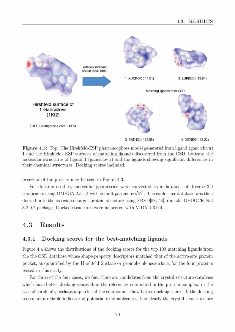


4.3. RESULTS
a useful library to find potential drug candidates.
For both the Hirshfeld and promolecule surfaces, the distribution off the docking scores
is multimodal. Analysis of these main modes, perhaps by cluster analysis, may give useful
information as concerning the responsible shape-property patterns.
The Hirshfeld and promolecule surfaces show a somewhat similar distributions in docking
scores, with roughly the same number of modes. The Hirshfeld surface shows a slightly higher
peak in the main mode of the distribution. It is noteworthy that the top 100 matches for the
different surface types had only small overlaps: 3, 19, 9 and 10 respectively for ligands 1, 2,
3 and 4. This indicates that the HS and PS do indeed select for distinct molecules based on
shape and intermolecular interactions. Further, these overlaps between PS and HS matches
in concert with the distributions of docking scores in Figure 4.4, indicates that the available
similar molecules in the CSD are more abundant for smaller, simpler molecules like ligand 1
than for larger molecules like ligand 2.
It is interesting to test whether the shape-dnorm scores have any correlation with the docking
scores. Results for correlation coefficients of the top 100 matches are shwon in Table (4.4).
However, only a weak correlation was found (the best was 0.48). There are also some negative
correlations, indicating that further ‘distances’ of the shape descriptors from the reference are
associated with better docking scores. This indicates that the method presented here and the
docking scores are distinct, or in some sense ‘orthogonal’ or ‘independent’. Perhaps this is
unsurprising, given how different the methods are.
It is worth noting that the case of ligand 2 may represent a problematic case for single
centre expansions under the spherical harmonic transform as the barycentre of the molecule lies
outside its surface. This can be seen by small artifacts present in the reconstruction of the shape
vs. the original shape, with errors of 1.7%, 8.1%, 4.1% and 2.8% (RMSD, over all grid points)
respectively for ligands 1, 2, 3, and 4. Nevertheless, because these errors are small, largely
localised to the higher order spherical harmonic coefficients and similar errors associated with
this will be likely be present in molecules of the same shape in the CSD, it seems that the results
for the shape description are not significantly affected – indicating that despite limitations this
shape description is still good enough to prove useful.
4.3.2 Matches with known drugs in the CSD
The CSD contains roughly 2000 structures which are indicated to be drugs2, of which 500 or so
were within our restricted subset. It is interesting to examine if any of the top 100 matches are
drug molecules according to this definition. Table 4.5) shows that, in fact, 12 existing drugs
were found.
If the docking scores are any indication, then many of these drugs may share activity with the
2In this case, matching text search for ‘drug’ or possessing a DrugBank[55] identifier
81

CHAPTER 4. FAST SCREENING OF CRYSTAL STRUCTURES FORLIGANDS BASED ON MOLECULAR SHAPE AND INTERMOLECULARINTERACTIONS
Ligand Surface Property r
1KI2 Hirshfeld dnorm 0.17
ESP -0.01
Promolecule dnorm 0.24
ESP 0.33
1UWH Hirshfeld dnorm 0.48
ESP 0.15
Promolecule dnorm 0.27
ESP -0.25
1Z95 Hirshfeld dnorm 0.08
ESP 0.02
Promolecule dnorm -0.11
ESP 0.19
3A2O Hirshfeld dnorm -0.03
ESP -0.42
Promolecule dnorm 0.17
ESP 0.38
Table 4.4: Pearson correlation coefficients R between shape-property descriptors used in thispaper and and docking scores from FRED/Chemgauss4 for the top 100 matches. Refer to textfor details.
82

4.3. RESULTS
actual protein ligand. Indeed, in the case of 2, (QABCEE) is a known kinase inhibitor, and for 4,
both (WUWCUO) and (DIJWOJ) are drugs with known antiviral activity (specifically targeting
HIV). This gives us confidence that the methods developed here are producing potentially
valuable matches, through identifying molecules which have already been assessed for their
biocompatibility and utilising them for novel targets.
Ligand Surface CSD Molecular Docking
# type Refcode Formula Score
1 Hirshfeld BHHPHE C13H21NO3 -10.94
2 Hirshfeld KAJFEJ C23Cl2H27N3O2 -13.32
Promolecule QABCEE C21ClF4H15N4O3 -17.36
MELFIT C23Cl2H27N3O2 -13.32
3 Hirshfeld INDMET C19ClH16NO4 -11.46
CERRAS C22H25N3O2 -12.96
WUWCUO C20H32N5O8P 1.42
CIHFAA C16H14N2O6S -6.58
Promolecule VEHRAB C24Cl2H21NO6 -5.08
4 Hirshfeld WUWCUO C20H32N5O8P -9.24
Promolecule ACTDGN C29H44O9 -10.23
DIJWOJ C36H47N5O4 -10.00
Table 4.5: Ligands found in the top 100 matches which are labelled as drugs in the CambridgeStructural database.
4.3.3 Small polymorphic drug molecules in the CSD
In order to further examine the differences between using dnorm as opposed to the ESP and the
surface property in the descriptors, we applied both shape-property descriptors to find the top
20 matches for the given drug molecule polymorphs listed in Table 4.2. The intention is to
examine what effect molecular conformation crystal environment of the ligand might have on
potential drug candidates. Since polymorphs are different crystal structures associated to the
same molecule, they will have different Hirshfeld structures, and different conformations of these
molecules in these polymorphs will have different promolecular density isosurfaces. Results are
83

CHAPTER 4. FAST SCREENING OF CRYSTAL STRUCTURES FORLIGANDS BASED ON MOLECULAR SHAPE AND INTERMOLECULARINTERACTIONS
presented in Figure 4.5.
We observe that more polymorphs or structure re-determinations are found with the PS
rather than the HS shape. This is understandable, as the PS is independent of crystal structure
(but will depend on conformation) whereas the HS is dependent on both. Therefore we expect
that the PS (and the ESP on that surface) are largely conserved under polymorphism. These
results highlight the advantages and disadvantages in terms of conformational and crystalline
environment specificity between different surfaces and surface properties: if one wants matches
more related to the crystal environment then the HS or dnorm should be used, whereas if
one wants matches characteristic of only the molecule, then the PS should be used. This is
particularly evident in the case of sulfathiazole, where polymorphs and redeterminations made
up 3/8 (HS/PS) of the top 20 matches with dnorm, but 17/18 (HS/PS) when using ESP.
An intriguing result can be seen in the case of the top matches for sulfamerazine, where
sulfathiazole (SUTHAZ) and sulfamethoxazole (SLFNMB) can be found to in the top matches
when using PS, in many cases closer than other sulfamerazine structures. All three of these
ligands are sulfonamide molecules with antibiotic activity. They are also similar in terms of their
3D shapes, but because of their ‘U’ shape and the different angular conformations the shapes
may appear quite distinct under a spherical harmonic expansion. Nevertheless, the similarity of
these drugs in terms of structure, shape and even their effect (they are both antibiotic drugs) is
echoed in their matching under the proposed shape descriptors.
4.4 Summary and future perspectives
In summary, the search for potential ligand molecules in the CSD, based on the ‘molecular shape
plus surface property’ matching method shows promising outcomes. While a search based on the
HS generated from the known drug-receptor structures resulted in ligands with comparable or
higher docking scores, their chemical structures showed significant variety. The validity of this
method has been further verified through the examination of a series of drug molecules in the
CSD exhibiting polymorphism. The results demonstrate the potential of combining quantitative
approaches to profile intermolecular interaction surfaces in crystals with the wealth of chemical
information embedded in a small molecule crystal structure database (the CSD) for rational
drug discovery.
In this paper we have described a method to create rotation-invariant shape-property
descriptors for isolated molecules, and molecules in an environment. The method has been used
to search the Cambridge Structural Database. The method has proven to successfully describe
shape sufficiently to find related drug molecules, and efficiently enough to do perform real-time
querying of desired ligands for LBVS.
There remain some key areas for possible improvement. For example, it may be the case
that we are over-describing the shape, and more rudimentary (i.e. lower angular momenta l
84


CHAPTER 4. FAST SCREENING OF CRYSTAL STRUCTURES FORLIGANDS BASED ON MOLECULAR SHAPE AND INTERMOLECULARINTERACTIONS
levels) descriptions might prove more effective in LBVS approaches. Further, this method could
be extended by modification of the surface decoration: by only ‘colouring’ specific regions of
interest on the surface i.e. those which are associated with only specific interactions, rather
than the holistic approach undertaken here. This might prove more effective particularly for
larger compounds, where some regions of ESP might be largely irrelevant to the binding affinity.
While we used the model HS and ESP generated from known ligand-protein structures as a
pharmacophore descriptor in the present study, it is also possible to extend this method for drug
design. Instead of generating the HS around the ligand, it is possible to build a hypothetical,
ideal ligand molecule in the receptor pocket and use the volume occupied by this ideal ligand
for the search-and- match procedure. The ideal ligand can be designed utilizing the concept
of supramolecular synthons, as a molecule with adequate functional groups that can form the
most effective intermolecular interactions with the pocket. Such descriptors would not simply
represent the molecular structure, but the shape and intermolecular interactions in terms of the
Hirshfeld-ESP surfaces of the ideally designed ligands, and thus they may be used to find the
most suitable inhibitor molecules from the CSD or other small molecule databases.
86

Bibliography
1. Fischer, E. Einfluss der Configuration auf die Wirkung der Enzyme. Ber. Dtsch. Chem.
Ges. 27, 2985. issn: 1099-0682 (1894).
2. Cheng, T., Li, Q., Zhou, Z., Wang, Y. & Bryant, S. H. Structure-Based Virtual Screening
for Drug Discovery: a Problem-Centric Review. AAPS J. 14, 133 (2012).
3. Di Giovanni, A. L. & C. Virtual Screening Strategies in Drug Discovery: A Critical Review.
Curr. Med. Chem. 20, 2839 (2013).
4. Bemis, G. W. & Kuntz, I. D. A fast and efficient method for 2D and 3D molecular shape
description. J. Comput. Aided Mol. Des. 6, 607 (1992).
5. Hahn, M. Three-Dimensional Shape-Based Searching of Conformationally Flexible Com-
pounds. J. Chem. Inf. Comput. Sci. 37, 80 (1997).
6. Hodgkin, E. E. & Richards, W. G. Molecular similarity based on electrostatic potential
and electric field. Int. J. Quantum Chem. 32, 105 (1987).
7. Buchbauer, G., Klinsky, A., Weiß-Greiler, P. & Wolschann, P. Ab initio Molecular
Electrostatic Potential Grid Maps for Quantitative Similarity Calculations of Organic
Compounds. Mol. Model. Ann. 6, 425 (2000).
8. Melani, F., Gratteri, P., Adamo, M. & Bonaccini, C. Field Interaction and Geometrical
Overlap: A New Simplex and Experimental Design Based Computational Procedure for
Superposing Small Ligand Molecules. J. Med. Chem. 46, 1359 (2003).
9. Vainio, M. J., Puranen, J. S. & Johnson, M. S. ShaEP: Molecular Overlay Based on
Shape and Electrostatic Potential. J. Chem. Inf. Model. 49, 492 (2009).
10. Cho, S. J. & Sun, Y. FLAME: A Program to Flexibly Align Molecules. J. Chem. Inf.
Model. 46, 298 (2006).
11. Groom, C. R., Bruno, I. J., Lightfoot, M. P. & Ward, S. C. The Cambridge Structural
Database. Acta Crystallogr. B 72, 171 (2016).
12. Berman, H. M. The Protein Data Bank. Nucleic acids research 28, 235 (2000).
13. Jones, G., Willett, P., Glen, R. C., Leach, A. R. & Taylor, R. Development and validation
of a genetic algorithm for flexible docking. J. Mol. Biol. 267, 727.
87

BIBLIOGRAPHY
14. Groom, C. R. & Cole, J. C. The use of small-molecule structures to complement protein-
ligand crystal structures in drug discovery. Acta Crystallogr. D 73, 240 (2017).
15. Cleves, A. E. & Jain, A. N. Effects of inductive bias on computational evaluations of
ligand-based modeling and on drug discovery. J. Comput. Aided Mol. Des. 22, 147 (2008).
16. Spackman, P. R., Thomas, S. P. & Jayatilaka, D. High Throughput Profiling of Molecular
Shapes in Crystals. Sci. Rep. 6, 22204 (2016).
17. Huang, N., Shoichet, B. K. & Irwin, J. J. Benchmarking Sets for Molecular Docking. J.
Med. Chem. 49, 6789 (2006).
18. Mysinger, M. M., Carchia, M., Irwin, J. J. & Shoichet, B. K. Directory of Useful Decoys,
Enhanced (DUD-E): Better Ligands and Decoys for Better Benchmarking. J. Med. Chem.
55, 6582 (2012).
19. Allen, F. H. & Bruno, I. J. Bond lengths in organic and metal-organic compounds revisited:
X-H bond lengths from neutron diffraction data. Acta Crystallogr. B 66, 380 (2010).
20. Champness, J. N. et al. Exploring the active site of herpes simplex virus type-1 thymidine
kinase by X-ray crystallography of complexes with aciclovir and other ligands. Proteins
32, 350 (1998).
21. Wan, P. T. C. et al. Mechanism of activation of the RAF-ERK signaling pathway by
oncogenic mutations of B-RAF. Cell 116, 855 (2004).
22. Bohl, C. E., Gao, W., Miller, D. D., Bell, C. E. & Dalton, J. T. Structural basis for
antagonism and resistance of bicalutamide in prostate cancer. Proceedings of the National
Academy of Sciences of the United States of America 102, 6201 (2005).
23. Hidaka, K. et al. Small-sized human immunodeficiency virus type-1 protease inhibitors
containing allophenylnorstatine to explore the S2’ pocket. J Med Chem 52, 7604 (2009).
24. Arputharaj, D. S., Hathwar, V. R., Guru Row, T. N. & Kumaradhas, P. Topological
Electron Density Analysis and Electrostatic Properties of Aspirin: An Experimental and
Theoretical Study. Crystal Growth & Design 12, 4357 (2012).
25. Thomas, S. P., Jayatilaka, D. & Guru Row, T. N. S[three dots, centered]O chalcogen
bonding in sulfa drugs: insights from multipole charge density and X-ray wavefunction of
acetazolamide. Phys. Chem. Chem. Phys. 17, 25411 (2015).
26. Reboul, J. P., Cristau, B., Soyfer, J. C. & Astier, J. P. 5 H-Dibenz[ b, f]azepinecarboxamide-
5 (carbamazepine). Acta Crystallogr. B 37, 1844 (1981).
27. Leech, C. K., Fabbiani, F. P. A., Shankland, K., David, W. I. F. & Ibberson, R. M. Accurate
molecular structures of chlorothiazide and hydrochlorothiazide by joint refinement against
powder neutron and X-ray diffraction data. Acta Crystallogr. B 64, 101 (2008).
88

BIBLIOGRAPHY
28. Nichols, G. & Frampton, C. S. Physicochemical Characterization of the Orthorhombic
Polymorph of Paracetamol Crystallized from Solution. J. Pharma. Sci. 87, 684 (1998).
29. Jarzembska, K. N. et al. Combined Experimental and Computational Studies of Pyrazi-
namide and Nicotinamide in the Context of Crystal Engineering and Thermodynamics.
Cryst. Growth Des. 14, 3453 (2014).
30. Ravindra Acharya, K., Kuchela, K. N. & Kartha, G. Crystal structure of sulfamerazine.
J. Crystallogr. Spectrosc. Res. 12, 369 (1982).
31. Drebushchak, T. N., Boldyreva, E. V. & Mikhailenko, M. A. Crystal structures of
sulfathiazole polymorphs in the temperature range 100–295 K: A comparative analysis. J.
Struct. Chem. 49, 84 (2008).
32. Spackman, M. A. & Maslen, E. N. Chemical-properties from the promolecule. J. Phys.
Chem. 90, 2020 (1986).
33. Mitchell, A. S. & Spackman, M. A. Molecular surfaces from the promolecule: A comparison
with Hartree–Fock ab initio electron density surfaces. Journal of Computational Chemistry
21, 933 (2000).
34. Turner, M. J., McKinnon, J. J., Jayatilaka, D. & Spackman, M. A. Visualisation and
characterisation of voids in crystalline materials. CrystEngComm 13, 1804 (2011).
35. Spackman, M. A. & Byrom, P. G. A novel definition of a molecule in a crystal. Chem.
Phys. Lett. 267, 215 (1997).
36. Wang, J., Wolf, R. M., Caldwell, J. W., Kollman, P. A. & Case, D. A. Development
and testing of a general amber force field. Journal of Computational Chemistry 25, 1157
(2004).
37. Maier, J. A. et al. ff14SB: Improving the Accuracy of Protein Side Chain and Backbone
Parameters from ff99SB. Journal of Chemical Theory and Computation 11, 3696 (2015).
38. Frisch, M. J. et al. Gaussian 09 Revision D. 01
39. Bayly, C. I., Cieplak, P., Cornell, W. & Kollman, P. A. A well-behaved electrostatic
potential based method using charge restraints for deriving atomic charges: the RESP
model. J. Phys. Chem. 97, 10269 (1993).
40. Jorgensen, W. L., Chandrasekhar, J., Madura, J. D., Impey, R. W. & Klein, M. L.
Comparison of simple potential functions for simulating liquid water. J. Chem. Phys. 79,
926 (1983).
41. Darden, T., York, D. & Pedersen, L. Particle mesh Ewald: An Nlog( N) method for Ewald
sums in large systems. J. Chem. Phys. 98, 10089 (1993).
42. Essmann, U. et al. A smooth particle mesh Ewald method. J. Chem. Phys. 103, 8577
(1995).
89

BIBLIOGRAPHY
43. Ryckaert, J.-P., Ciccotti, G. & Berendsen, H. J. C. Numerical integration of the cartesian
equations of motion of a system with constraints: molecular dynamics of n-alkanes. Journal
of Computational Physics 23, 327 (1977).
44. Case, D. A. et al. Amber 14 (2014).
45. Schaeffer, N. Efficient spherical harmonic transforms aimed at pseudospectral numerical
simulations. Geochem. Geophys. 14, 751 (2013).
46. Spackman, M. A. & McKinnon, J. J. Fingerprinting intermolecular interactions in molec-
ular crystals. Crystengcomm 4, 378 (2002).
47. Mulliken, R. S. Electronic Population Analysis on LCAO–MO Molecular Wave Functions.
I. J. Chem. Phys. 23, 1833 (1955).
48. Tanaka, K. X-ray analysis of wavefunctions by the least-squares method incorporating
orthonormality. I. General formalism. Acta Crystallogr. A: Crystal Physics 44, 1002
(1988).
49. Rys, J., Dupuis, M. & King, H. F. Computation of electron repulsion integrals using the
rys quadrature method. J. Comput. Chem. 4, 154 (1983).
50. Jayatilaka, D. & Grimwood, D. J. in Computational Science — ICCS 2003: International
Conference, Melbourne, Australia and St. Petersburg, Russia, June 2–4, 2003 Proceedings,
Part IV (eds Sloot, P. M. A. et al.) 142 (Springer Berlin Heidelberg, Berlin, Heidelberg,
2003).
51. Jones, E., Oliphant, T., Peterson, P., et al. SciPy: Open source scientific tools for Python
[Online; accessed 01/11/2017]. 2001. http://www.scipy.org/.
52. Hawkins, P. C. D., Skillman, A. G., Warren, G. L., Ellingson, B. A. & Stahl, M. T.
Conformer Generation with OMEGA: Algorithm and Validation Using High Quality
Structures from the Protein Databank and Cambridge Structural Database. J. Chem.
Inf. Model. 50, 572 (2010).
53. McGann, M. FRED and HYBRID docking performance on standardized datasets. J.
Comput. Aided Mol. Des. 26, 897 (2012).
54. McGann, M. FRED Pose Prediction and Virtual Screening Accuracy. J. Chem. Inf. Model.
51, 578 (2011).
55. Wishart, D. S. et al. DrugBank: a comprehensive resource for in silico drug discovery and
exploration. Nucleic acids research 34, D668 (2006).
90

Part III
Assessment of quantum chemical
predictions in chemistry
91


Chapter 5
Quantum Chemical Electron Impact
Mass Spectrum prediction for de novo
structure elucidation
ABSTRACT
We investigate the success of the Quantum Chemical Electron Impact Mass Spectrum (QCEIMS)
method in predicting the electron impact mass spectra of a diverse test set of 61 small molecules
selected to be representative of common fragmentations and reactions in electron impact mass
spectra. Comparison with experimental spectra is performed using the standard matching
algorithms, and the relative ranking position of the actual molecule matching the spectra
within the NIST-11 library is examined. We find that the correct spectrum is ranked in
the top two matches from structural isomers in more than 50% of the cases. QCEIMS thus
reproduces the distribution of peaks sufficiently well to identify the compounds, with the
RMSD and mean absolute difference (MAD) between appropriately normalized predicted and
experimental spectra being at most 9% and 3% respectively, even though the most intense
peaks are often qualitatively poorly reproduced. We also compare the QCEIMS method to
competitive fragmentation modeling for electron ionization (CFM-EI), a training-based mass
spectrum prediction method, and remarkably we find the QCEIMS performs equivalently or
better. We conclude that QCEIMS will be very useful for those who wish to identify new
compounds which are not well represented in the mass spectral databases.
5.1 Introduction
Mass spectrometry (MS) is of major importance for identifying the presence of small quantities
of a compound in a mixture, particularly because it is several orders of magnitude more sensitive
93

CHAPTER 5. QUANTUM CHEMICAL ELECTRON IMPACT MASSSPECTRUM PREDICTION FOR DE NOVO STRUCTURE ELUCIDATION
than equivalent structure determination methods[1]. Indeed, MS is often the only feasible
identification method[2–4] in contexts like the identification of semiochemicals [5–7], where
abundances of critical compounds may be in the ng range.
Electron-impact mass spectrometry (EIMS) coupled to some chromatographic separation
techniques is, at present, likely to be the predominant form of MS practiced for small molecules.
The typical protocol for identifying unknown compounds using EIMS involves matching against
a known mass spectrum (MSp), using spectral libraries in conjunction with software to identify
matches[8–13]. For example, the National Institute of Standards and Technology (NIST)
mass spectral library (version 11) contains electron impact (EI) spectra of more than 2× 10⁵
compounds, and may be readily searched using the NIST MS Search program. However large,
such a library may only contain a tiny fraction of the total number of small molecular species
found in the universe, which for molecules less than 500 Daltons in weight is estimated to be in
excess of 1060[14]. Simply put, the huge number of possible structural isomers for each molecular
formula renders it practically impossible for a library to be exhaustive. If the identification
of a compound whose spectra has yet to be characterized (i.e. its spectra is not in a library)
is desired, much of the value provided by MS matching/library methods is lost (though the
structure of the close matches may still provide insight).
In this paper, we are concerned with the problem of identifying the structures of unknown
compounds present in low abundances which have not been previously characterized by MS. We
will use the term de novo structure determination from the mass spectrum (MSp) to describe this.
In this case, the only way to confirm the structure is to synthesize several putative candidate
compounds in significant amounts, characterize their structure independently (say using nuclear
magnetic resonance (NMR), or X-ray crystallography), then compare the candidates MSp with
the original unknown spectrum to see which (if any of them) agree. It should come as no surprise
that this is a time- and labor-intensive process.
One way to ease the process of de novo compound identification is to predict the MSp for
each candidate using computational methods. If such computed MSp were accurate enough,
only one candidate compound need be synthesized and characterized in order to to confirm the
structure. Indeed, if the computed MSp were always reliably accurate it would not even be
necessary to confirm the structure by synthesis and alternative means; MS may then become
competitive with NMR or crystallography as a structure determination method.
Computational methods for the prediction of the MSp have been well reviewed by Bauer
and Grimme [15]. They may be broadly separated into two categories:
1. Expert systems. Expert systems produce a MSp using rules derived from experimental
spectra, for example fitted to experimental MSp using a model such as a neural network[16,
17]. The ‘system’ is trained or based on a library of MSps for which the structure
is known. Indeed, the prototypical example of an expert computer system based on
rules[18] concerned the identification of molecular structure from MSp: the DENDRAL[19]
94

5.1. INTRODUCTION
project. Regardless of the successes (or failures[1, 20]) of the original DENDRAL project,
recently learning-based methods such as competitive fragment modeling (CFM)[21, 22] for
predicting EIMS spectra (CFM-EI) have gained more traction, and proved more successful.
It should be noted, though, that within any such system there will always exist some bias,
both in the model it represents and the data used to ‘train’ it; such bias may lead to
unquantifiable inaccuracies.
2. First principles simulation techniques. First principles simulation techniques aim to
actively simulate the underlying physical processes involved in MS. Such methods are
not in principle dependent on an existing library of known spectra, but are limited by
the accuracy with which one is able to solve the time-dependent Schrodinger equation
(or more correctly, the time-dependent Liouville equations for the density matrix[23]).
Unfortunately such calculations were, in general, time consuming to the point of being
impractical. However, recently the QCEIMS program from Grimme et al.[24] has allowed
practical calculation of MSps using ab initio techniques. By directly modeling the time-
dependent fragmentation process via Born-Oppenheimer molecular dynamics (BOMD)
finite-temperature (fractional orbital occupied) quantum chemical (QC) methods[15, 24,
25], coupled with knowledge of isotopic distributions[26], QCEIMS has proven remarkably
accurate. Other quantum chemical methods based on bond indices have also been
proposed[27], and are examined by us in related work.
The purpose of this paper is to investigate the performance of, QCEIMS, which, although
having been applied to many molecules[15, 24, 25, 28, 29], has not yet been tested by the
conventional MSp matching algorithms used to identify compounds from the MSp; an essential
task if it is to be used for de novo compound identification. For this purpose, we make use of
the standard programs and databases from the National Institute of Standards (NIST). We
also provide an estimate of the errors associated with their predicted spectra, using counting
statistics. Our goal is to identify patterns or trends with any errors in the prediction, particularly
those seen to be associated with a chemical class of compounds; such information is invaluable
for practical application of QCEIMS.
Despite expert systems and first principles methods having radically different philosophical
approaches, for the purposes of de novo structure determination these differences mean little.
As such, we also assess the performance of QCEIMS method against the CFM-EI model-based
spectrum calculator, both as a contemporary reference point and to investigate the differences
in accuracy between the two techniques.
95

CHAPTER 5. QUANTUM CHEMICAL ELECTRON IMPACT MASSSPECTRUM PREDICTION FOR DE NOVO STRUCTURE ELUCIDATION
5.2 Methodology
All data analysis and processing of calculations for this paper was performed using the Python
programming language. Notably, the numpy[30], pandas[31] packages, and matplotlib[32] for
the generation of figures.
5.2.1 Selection of compounds for analysis
When selecting a set of molecules for investigation, the following criteria were considered: they
must have an experimental MSp and structural isomers with experimental MSp, they must
be representative of common/important fragmentations in EIMS i.e. made up of a variety of
functional groups, they must be relatively small molecules (natom < 25). Further, it is desirable
to have a mixture of easy and difficult cases for differentiating between structural isomers. As
such, a set of 61 small molecules were chosen, made up of alcohols (6), aldehydes (3), alkenes
(7), amines (6), alkylbenzenes (8), carboxylic acids (5), esters (16), ketones (2), alkylphenols
(8). The complete list is shown in Table 5.1, and the structures are available in Figure 5.1. The
primary motivation for the selection of small molecules is the identification of failed predictions
and their underlying cause. Both of these aspects are significantly more straightforward in
the case of small molecules. Further, the reduced computational time requirements associated
with quantum-chemical predictions with small molecules render them ideal for such a study.
Additionally, when establishing the viability for such methods in de novo structure elucidation,
having several structural isomers distinguishable via their MSp is vitally important.
5.2.2 QCEIMS and CFM-EI calculations
Initial geometries were drawn by hand in a standard molecular builder program Avogadro2 [33]
and then optimized using the generalized Amber force field [34]. MSp prediction calculations
were then performed using the QCEIMS program version 2.26, as described by Grimme and
coworkers[15, 24] using the default parameters, namely: using the OM2-D3[35] semi-empirical
quantum mechanical wavefunction method from MNDO99[36] version 7.0. The default QCEIMS
parameters were used, with an initial temperature of 500K, at 70 eV and the number of
trajectories set to 25× nheavyatoms. The resulting spectra were normalized in the typical manner:
such that the highest peak had an intensity of 100. The time taken for calculations varied
with molecular size (see ESI Table S2 for full details), with the shortest being methyl formate
(roughly 1.5 CPU hours) and the longest being 4-propan-2-ylphenol (roughly 80 CPU hours).
It should be noted that these calculations are readily parallelized across computing clusters,
drastically reducing the wall-clock time required.
CFM-EI Calculations were performed using the method described by Allen et al.[22] with
the provided trained parameters for EI-MS, using the Windows executable ‘cfm-predict’, version
96

5.2. METHODOLOGY
CH3
HOCH
3
CH3
HO
CH3
HO
CH3
H3C
HO
CH3
HO
H3C
CH3
CH3
OHH3C
CH3
O
CH3
O
H3C
CH3
O
CH2
H3C
CH3
H3C CH
2
H3C
CH3
CH3
H2C
CH3
CH3
H3C
CH3
CH3
CH3
H2N
CH3
CH3
H2N
CH3
H2N
CH3
H3C
H2N
CH3
H2N
H3C
CH3
CH3
NH2
H3C
CH3
H3C
CH3
H3C CH
3
H3C
H3C
CH3
CH3
CH3
H3C
OH
O
CH3
OH
OCH
3
HO
O
H3C
CH3
CH3
OH
O
CH3
OH
O
H3C
O
OH3C
O
O
H3C
H3C
O
O
CH3
H3C
CH3
O
OH3C
OO
CH3
CH3
O
O
H3C
CH3
H3C CH
3O
O CH3
H3C
H3C
O
O CH3
H3C
O
O
CH3
H3C
O
O
CH3
H3C
O
O CH3
CH3
H3C
O
O CH3
H3C
O
O
CH3
CH3
H3C
O
O
CH3
CH3
H3C
O
O
CH3
H3C
O
O CH3
CH3
CH3
CH3
O
CH3
H3C
O
OH
OH
CH3
OH
CH3
OH
CH3
OH
CH3
H3C
OH
CH3
OH
CH3
CH3
OH
CH3
H3C
Figure 5.1: Structures of the molecules chosen for analysis grouped into chemical classes
97

CHAPTER 5. QUANTUM CHEMICAL ELECTRON IMPACT MASSSPECTRUM PREDICTION FOR DE NOVO STRUCTURE ELUCIDATION
2.2.
5.2.3 Spectrum matching
Rankings between standard-normalized calculated and experimental MSp were made using the
NIST MS Search v2.0g software coupled with the NIST11 database. Search was performed with
the ‘identity’ matching method where the square root of intensity of the MSp was taken and
weighted by the mass-to-charge ratio squared. The difference between this and the available
‘similarity’ metric (which differs only in the the mass weighting) is negligible for our purposes
– see [10] for a comprehensive study of the impact of matching algorithms on the accuracy
of matches). Searches were carried out by limiting to molecules to have the same molecular
formula, using only the two most abundant isotopes.
5.2.4 Ranking comparison
It is not meaningful to directly compare ranks when the number of possible candidates differs.
To overcome this, the relative ranking position[3, 22] has been used:
RRP =r − 1
n− 1(5.1)
where r is the rank, and n is the total number of candidates with the same molecular weight
(this expression is equivalent to that presented in Kerber et al. [3]). Thus a rank of one maps to
zero, and a rank of n maps to 1. The RRP is not defined for a class with only one member.
This quantity constitutes the metric for direct comparison between compounds with different
molecular formulae, as they clearly have different possible numbers of structural isomers and
therefore differing numbers of entries in the database.
5.2.5 Spectrum normalization for statistical comparisons
It is standard to normalize the mass spectra such that the highest peak has an intensity with
value 100. However, such a normalization makes direct comparison relative between error
statistics such as root mean square deviation (RMSD) across different compounds meaningless.
As such, these metrics (see Table 5.3) have been calculated with spectral intensities normalized
such that the sum of the intensities is unity for both the spectra being compared. A byproduct
of this normalization scheme is that the mean signed error between two spectra is always zero.
Such a normalization scheme has been used previously, by Rasmussen and Isenhour [37] who
demonstrated that this kind of probability distribution normalization (which they call ‘total
ion current normalization’) does not lead to a significant effect when tested for the purposes of
identifying a known mass spectrum.
98

5.3. RESULTS
Chemical RRP
No. Name Formula /nisomers
Alcohols
1 propan-1-ol C3H8O 1/3
2 propan-2-ol C3H8O 1/3
3 butan-1-ol C4H10O 1/8
4 butan-2-ol C4H10O 1/8
5 2-methylpropan-1-ol C4H10O 1/8
6 2-methylpropan-2-ol C4H10O 5/8
Aldehydes
7 propanal C3H6O 1/7
8 2-methylpropanal C4H8O 3/21
9 butanal C4H8O 3/21
Alkenes
10 but-1-ene C4H8 4/6
11 but-2-ene C4H8 1/6
12 pent-1-ene C5H10 3/13
13 pent-2-ene C5H10 3/13
14 hex-1-ene C6H12 6/30
15 hex-2-ene C6H12 1/30
16 hex-3-ene C6H12 9/30
Amines
17 propan-1-amine C3H9N 1/4
18 propan-2-amine C3H9N 1/4
19 butan-1-amine C4H11N 1/8
20 butan-2-amine C4H11N 1/8
21 2-methylpropan-1-amine C4H11N 2/8
22 2-methylpropan-2-amine C4H11N 1/8
Benzenes
23 benzene C6H6 1/5
24 toluene C7H8 3/13
25 ethylbenzene C8H10 8/23
26 propylbenzene C9H12 2/42
27 cumene C9H12 16/42
28 butylbenzene C10H14 3/74
29 butan-2-ylbenzene C10H14 6/74
30 2-methylpropylbenzene C10H14 1/74
Chemical RRP
No. Name Formula /nisomers
Carboxylic acids
31 propanoic acid C3H6O2 1/9
32 butanoic acid C4H8O2 7/27
33 2-methylpropanoic acid C4H8O2 3/27
34 2-methylbutanoic acid C5H10O2 3/47
35 3-methylbutanoic acid C5H10O2 5/47
Esters
36 methyl formate C2H4O2 1/3
37 methyl acetate C3H6O2 2/9
38 ethyl acetate C4H8O2 1/27
39 methyl propanoate C4H8O2 1/ 27
40 propyl acetate C5H10O2 NM/47
41 propan-2-yl acetate C5H10O2 4/47
42 methyl 2-methylpropanoate C5H10O2 1/47
43 ethyl propanoate C5H10O2 1/47
44 methyl butanoate C5H10O2 5/47
45 propyl propanoate C6H12O2 1/80
46 propan-2-yl propanoate C6H12O2 3/80
47 ethyl butanoate C6H12O2 4/80
48 methyl 2-methylbutanoate C6H12O2 2/80
49 methyl 3-methylbutanoate C6H12O2 7/80
50 propyl butanoate C7H14O2 2/83
51 propan-2-yl butanoate C7H14O2 NM/83
Ketones
52 acetone C3H6O 1/7
53 butan-2-one C4H8O 1/21
Phenols
54 phenol C6H6O 2/4
55 4-methylphenol C7H8O 2/17
56 4-ethylphenol C8H10O 16/43
57 4-propylphenol C9H12O NM/112
58 4-propan-2-ylphenol C9H12O 16/112
59 4-butylphenol C10H14O NM/163
60 4-butan-2-ylphenol C10H14O 3/163
61 4-(2-methylpropyl)phenol C10H14O 2/163
Table 5.1: Relative ranking position (RRP) of the matching mass spectra found by theQCEIMS program produced by the NIST MS Search program (version 2.0g). Ranking is relativeto the total number isomers nisomers. NM indicates that no match was found in the database.
5.2.6 Estimates of the errors in the calculated peak heights
Since the spectra are built up by counting independent fragmentation processes we assume that
the number of counts in a particular peak of the mass spectrum has a Poisson distribution.
Then the absolute error in a particular peak with Ni counts is√Ni. If Ntotal =
∑iNi is
the total number of counts in the whole mass spectrum the absolute error in a particular
probability-normalized mass spectrum with peak heights Ni/Ntotal is√Ni/Ntotal. It is important
to keep in mind that the reproducibility error in a particular mass spectrum is about 5-10% in
the peak heights, and in some cases even up to 30% [24].
5.3 Results
Table 5.1 shows the predicted RRPs for the QCEIMS method for the 61 molecules considered
in this study; rankings for CFM-EI (Table S0), along with predicted and experimental MSp for
each compound (Figures S1-S122) are shown in the electronic supplementary material (ESI)
and selected spectra are presented and discussed later.
99

CHAPTER 5. QUANTUM CHEMICAL ELECTRON IMPACT MASSSPECTRUM PREDICTION FOR DE NOVO STRUCTURE ELUCIDATION
0.0 0.1 0.2 0.3 0.4 0.5 0.6QCEIMS RRP
0
5
10
15
20
25
30
Freq
uency
Figure 5.2: The number of molecules predicted correctly at a given rank for the QCEIMSmethod. There were four molecules which were not matched to any molecule in the NISTdatabase.
5.3.1 The QCEIMS method
Overall success rate. We see from the table that using the QCEIMS method we are able to
identify the correct structure from the NIST database (using the standard spectrum matching
algorithm for compounds with the same chemical formula) in 24 of the 61 cases. The correct
spectrum is ranked in the top two in 32 of the cases (greater than 50% success rate) and in
the top three in 42 of the cases (69% success rate). Thus if the QCEIMS method were to be
used to actually identify the structure of an unknown compound similar to those in the test
set one might expect to get the correct result in the top three matches two-thirds of the time.
However one must qualify this statement in at least two respects. First, the test set is rather
small; and even with this small set there were four cases providing unacceptable matches (shown
as NM in the table). Also, as we previously remarked, comparing actual ranks is problematic
because different chemical classes have different numbers of isomers. Therefore, in Figure 5.2
we present a histogram of the number of molecules given a particular rank. Our conclusions
based on actual rank are essentially the same as those based on RRP.
Dependence of the quality of the rankings on the chemical class of the compound. Some of
the classes have too few candidates to make any clear statements, but we may still make the
following observations:
• In the case of the alcohols, all the primary alcohols are correctly ranked, but the tertiary
alcohol 6 was not correctly predicted (rank 5!).
• Some of the alkenes are very poorly ranked, but there is no clear correlation of the results
with the position of the double bond.
• Rankings for the amines were remarkably good, with all with the exception of 21 being
100

5.3. RESULTS
matched correctly.
• For the substituted benzenes, poorer results are obtained for candidates with multiple
alkyl substituents. This trend is exacerbated for the phenols where two of the compounds
57 and 59 were not matched at all.
• Substituted esters are generally well ranked, but tend to be more poorly predicted when
(like the substituted benzene) one of the groups becomes more branched.
Dependence of the quality of the results on the mass of the molecules. There is a weak trend
that increasing size of molecule produces worse matches perhaps best exemplified by the esters
(Pearson’s correlation coefficients r = 0.40). It should be kept in mind that matches were only
considered in the database between molecules of the same molecular formula. It should also be
noted that the size of the molecules is very small, and one might expect a strong dependence
with molecular weight.
Mean RRPs for each chemical class. Table 5.2 summarizes some of the discussion above
in a more quantitative way, presenting the mean RRPs for each chemical class. Although the
results for ketones and aldehydes seem very good, there are too few systems to consider the
mean RRPs meaningful for these two classes of compounds. However, we see that the esters and
amines are very well predicted, with the means RRPs for carboxylic acids, substituted benzenes
and phenols all being quite similar and low. The alcohols seem not well predicted but are in
fact skewed by one bad result. The alkenes are ranked the worst. It also deserves to be noted
that in the cases where there are a large number of isomers the matching algorithm ranks the
QCEIMS spectra very near the top e.g. for 30 we have 1/74 and for 61 we have 2/163.
Comparison of spectra with experiment. Table 5.3 gives the mean root-mean-square deviation
(RMSD) and mean absolute error (MAD) in the probability normalized spectra. We observe
that the spectra which agree the worst on the RMSDs (which highlight outlier differences)
are in order: the alcohols (with one outlier already noted in the previous section), aldehydes,
carboxylic acids, esters and alkenes. With regard to MADs, the worst classes are again the
alchohols, alkenes, and ketones. In the ESI we present the mass spectra produced for all the
compounds. Most informative are the differences between the predicted and observed spectra:
peaks are coloured green if they were present in both spectra, yellow if present only in the
experiment, and red if present only in the QCEIMS model spectra. Positive differences indicate
that the calculated spectra overestimate the peak intensities, an d error bars on the QCEIMS
spectra are presented. We see that the errors due to counting statistics are very small, the
maximum always less than 8% and usually much smaller, and then only appearing on the peaks
which have the largest counts. Therefore the difference in intensity between the experimental
and QCEIMS peaks for the larger peaks is not to be attributed to counting statistics. Also,
the differences in the larger peaks far exceeds the sum of the counting statistics error and any
101

CHAPTER 5. QUANTUM CHEMICAL ELECTRON IMPACT MASSSPECTRUM PREDICTION FOR DE NOVO STRUCTURE ELUCIDATION
Mean RRP No. of
Class QCEIMS CFM-EI Compounds
Alcohols 0.11 0.21 5
Aldehydes 0.07 0.02 3
Alkenes 0.20 0.30 7
Amines 0.02 0.08 6
Benzenes 0.12 0.12 8
Carboxylic acids 0.10 0.14 3
Esters 0.03 0.04 14
Ketones 0.00 0.00 2
Phenols 0.18 0.14 5
Overall 0.09 0.12 53
Table 5.2: Mean Relative ranking position (RRP) for the QCEIMS and CFM-EI methodsfor different classes of compounds, with the number of compounds in each class. Overall meanRRPs are given in the final line. Only molecules in which both methods matched are compared.
reproducibility error associated with the EIMS experiment. A typical example showing error
bars in presented in Figure 5.4, ethylbenzene, discussed in more detail later.
5.3.2 The CFM-EI method
Overall success rate. The CFM-EI has a very similar first match rate compared to the QCEIM
method, with 24 matching in first position, 35 in the top two positions.
Dependence of the quality of results on the chemical class. The full set of rankings for the
CFM-EI method is shown in Table S1 of the ESI. The following observations can be made.
• The alcohols are well ranked except for one outlier (3) which is placed in the 5th position
(this is not the same compound ranked 5th in the QCEIMS method).
• The alkenes are rather poorly ranked: both 12 and 16 are ranked at position 10.
• The amines are remarkably well ranked: all are ranked in the first position except 18 and
22, which are ranked in second place.
• For the substituted benzenes and phenols there are some very poor rankings, which are a
bit worse than for the QCEIMS method. For example, 28 is in position 20, 59 in position
35, and 61 had no match.
Mean RRPs for each chemical class. Table 5.2 shows that, as for the QCEIMS method, the
alkenes are worst predicted, followed by the alcohols. The results for the alcohols and alkenes are
102

5.4. DISCUSSION
Mean RMSD Mean MAD
Class QCEIMS CFM-EI QCEIMS CFM-EI
Alcohols 0.09 0.05 0.03 0.03
Aldehydes 0.08 0.03 0.03 0.01
Alkenes 0.05 0.05 0.02 0.03
Amines 0.04 0.03 0.02 0.02
Benzenes 0.04 0.04 0.01 0.02
Carboxylic acids 0.06 0.04 0.02 0.02
Esters 0.06 0.04 0.02 0.02
Ketones 0.04 0.05 0.02 0.03
Phenols 0.04 0.04 0.01 0.02
Overall 0.05 0.04 0.02 0.02
Table 5.3: Mean root mean square deviation (RMSD) and mean absolute deviation (MAD) forthe QCEIMS and CFM-EI methods for different classes of compounds, . Overall mean RMSDsand MADs are given in the final line.
also significantly worse than in the QCEIMS method (RRPs respectively 0.21 and 0.30 versus
0.11 and 0.20). The next worst grouping was among the benzenes, phenols and carboxylic acids,
again generally worse ranked than compared to the QCEIMS method. Based on the individual
class results, it is therefore not surprising that the overall ranking from CFM-EI is worse than
from the QCEIMS method (mean RRPs respectively 0.12 versus 0.09).
Dependence of the quality of the results on the mass of the molecules. There is a weak trend
that results are worse predicted as the mass of the molecule increases (r = 0.47) and this trend
is a bit stronger than for the QCEIMS method.
Comparison of QCEIMS and CFM-EI. Table 5.3 shows rather uniformly low RMSDs and
MADs for the predicted and observed spectra: in both cases the MADs were less than 3%.
However, based on the RMSDs the CFM-EI seems to produce a slightly more accurate i.e. the
spectrum shows fewer outlying peaks relative to experiment. Nevertheless, a qualitatively better
MSp does not translate into a a superior ranking of the MSp (see discussion on the RRPs).
5.4 Discussion
5.4.1 Detailed analysis of the predicted spectra
Alcohols. QCEIMS underestimates the abundance of most small peaks it predicts. As the
peak intensities are relative, this indicates that QCEIMS is systematically overestimating the
abundance of the primary fragmentation relative to the others.
103


5.4. DISCUSSION
On the other hand, CFM-EI seems to be underestimating the primary fragmentation with
respect to others.
Further, there exists a tendency for CFM-EI to overestimate the abundance of the molecular
ion. This over-abundance is reflected in the poor results in predicting both propan-2-ol and
butan-1-ol (see Figure 5.3) by CFM-EI.
It is noteworthy that both methods generally underestimate the loss of water (M− 18) from
primary alcohols, which is reflected in the MS of butan-1-ol with the low m/z = 56 peak.
Both methods predict the existence of few peaks not in the experimental spectra, (shown in
red in Fig 5.3). CFM-EI particularly in the cases of 2-methylpropan-1-ol and, to a lesser extent,
butan-1-ol predicts significant peaks non-existent in the experimental MSp.
Aldehydes and ketones. Importantly, QCEIMS clearly demonstrates the capacity to ‘discover’
McLafferty rearrangements. An illustrative example,the case of butanal, shows in the m/z = 44
(M− 28) peak, from loss of ethene via a McLafferty rearrangement. While the relative abundance
of this peak was underestimated by QCEIMS, its existence is vitally important. In the case of
2-methylpropanal QCEIMS seems to be missing or underestimating characteristic m/z = 27
and m/z = 41 peaks.
The predictions by CFM in the case of 2-methylpropanal is closer to experiment, but still
systematically underestimated. Again, as was the case in the alcohols, CFM-EI seems to
overestimate the abundance of the molecular ion in some cases (particularly 2-propanone).
Neither MS prediction technique displays any egregious false peaks in the aldehydes or
ketones, they simply tend to underestimate the relative occurrence of certain rearrangements or
cleavages.
In the case of the aldehydes, both methods seem to consistently fail to match experimental
spectra, and this is reflected in the rankings (2s/3s for both butanal and 2-methylpropanal).
Contrast this with the case of the two ketones, where the predictions are almost perfectly on
the mark. This might be associated with the decreased importance of α-cleavages in the case of
the aldehydes as compared to the ketones, strong conclusions require more studies.
Esters. It is evident for both techniques that McLafferty type rearrangements are absent or
underestimated for all relevant esters – particularly in methyl butanoate, where m/z = 74 is
virtually absent in the predicted spectrum. This is not to say that these methods are not capable
of predicting rearrangement fragmentations in-principle, as may be seen upon the examination
of the the prominent m/z = 88 in ethyl butanoate.
Amines QCEIMS underestimates or fails to predict some portions of the MSp, notably in
the 25 < m/z < 30 region of propan-2-amine and 2-methylpropan-2-amine.
Intriguingly, despite the QCEIMS MS for propan-2-amine overall having many missing peaks
and generally incorrect intensities (i.e. looking qualitatively worse) than that produced by
CFM-EI, the spectra proves to be a better match. In this instance, CFM clearly overestimates
(once again) the abundance of the molecular ion, which may have resulted in this poor match
105

CHAPTER 5. QUANTUM CHEMICAL ELECTRON IMPACT MASSSPECTRUM PREDICTION FOR DE NOVO STRUCTURE ELUCIDATION
against experiment. The cases of 2-methylpropan-1- and 2-methylpropan-2-amine proved more
difficult for both prediciton techniques, though the spectra were very close to experiment. Both
cases yield significantly different spectra, something reflected in both predictive techniques.
A significant error in both methods appears to be the overestimated abundance of loss of
a proton (M− 1), highlighted particularly in the m/z = 72 peak of the CFM-EI MSp for
2-methylpropan-2-amine, but also in the m/z = 72 and m/z = 58 peaks for the QCEIMS
spectra for butan-1-amine and propan-2-amine, respectively.
Alkenes. The case of alkenes, in particular those chosen here, requires precise predictions in
order to achieve the closest match with experiment. The differences between structural isomers
in their MSp tend to be independent of the double bond position (unless highly substituted or
conjugated)[38]. This, coupled with the tendencies of isomerization through migration of the
double bond in these low molecular weight, straight chain alkenes makes discrimination between
candidates a much more difficult task.
In general, both techniques overestimate the abundance of the molecular ion, further
exaggerated in the hexene series where the relative abundance of the molecular ion is much
lower than in the pent- and butenes. The regions 25 < m/z < 30 and 40 < m/z < 45, and
the m/z = 55 peak for pent- and hexene are the discriminating regions of these spectra. It is
notable that in these regions, both QCEIMS and CFM come close to the experimental spectra
in their predictions. The poor rankings (as seen in Table 5.2) over the alkene set are a contrast
with the relatively good error statistics (see Table 5.3). This is consistent with the rather subtle
differences in MSps where the only difference in the molecule is the double bond position. It
is not the case, then that the two techniques are failing to accurately predict the spectra of
alkenes, merely that their predications are not accurate enough for the purposes of matching
within sets of structural isomers.
Carboxylic Acids. From the results presented in Table 5.2, it would appear that performance
for the majority of carboxylic acids was far from satisfactory. Both techniques showed failures
in their spectral predictions, but it would seem that in this case QCEIMS outperforms CFM in
producing an EIMS matching more closely to experiment.
For longer chain carboxylic acids, QCEIMS seems to severely underestimate crucial McLaf-
ferty rearrangements, giving rise to inadequate prediction of mass spectra of these compounds.
An illustrative example is the virtual absence of m/z = 74, the base peak of 2-methylbutanoic
acid. These issues seem to be even more significant for CFM-EI with several carboxylic acids,
giving rise to very inaccurate spectra.
Benzenes. The only significant discrepancy from experiment for QCEIMS is shown in the
case of (1-methylethyl)benzene, where this method seems to make a charged fragment of the
isopropyl moiety, which does not occur in the real spectrum.
As many alkylbenzenes show similarities in the mass spectra, errors in approximations of
abundance of fragments can mean that the rank is relatively low although the correct fragments
106


CHAPTER 5. QUANTUM CHEMICAL ELECTRON IMPACT MASSSPECTRUM PREDICTION FOR DE NOVO STRUCTURE ELUCIDATION
represented in the search library (a fact which unfortunately cannot be established before the
structure is known).
We have also established that the counting statistics errors on the peaks produced in QCEIMS
are much smaller than the experimental reproducibility error in the mass spectrum; and that
the spectra are often reproduced better than the corresponding rankings relative to isomers.
This demonstrates that the QCEIMS method achieves its successful matches not because of an
accurate match in the peak heights, but rather that the peak heights and the distribution of the
peak positions as a function of mass-to-charge ratio is sufficiently different for different isomers
to achieve a high ranking.
As regards the performance of QCEIMS for different chemical classes, we find that the
alcohols have the best matching spectra, with a mean MAD of about 0.03. The normalized
spectra are therefore reproduced rather well. On the other hand, the worst ranked spectra were
the alkenes and substituted phenols with mean relative ranking positions above 0.18. It should
be noted, though, that even in these cases the correct candidate is placed in the top fifth of
isomers.
The problem with QCEIMS, recognized by the authors, is that it is a time consuming
calculation to perform, often taking days or weeks for a single spectrum; by comparison the
CFM-EI method can be performed in the browser. We do not think this is necessarily a problem
for those working to identify semiochemicals, where in a worst case situation it takes years to
identify the structure of an unknown: in this case it is more useful for the information to be
correct rather than timely. Still, the length of time required for QCEIMS means that it is best
used sparingly after other methods have been used to narrow the field of candidates.
One of the great difficulties with EIMS prediction is that it is not only about simple
fragmentations, but frequently involves rearrangements within the molecule.
Both methods tended to suffer from the same problems: underestimation or failure to predict
specific rearrangements (e.g. McLafferty rearragements), and overestimation of the molecular
ion. These failures are especially salient given the radically different manner in which both
techniques function. Perhaps this indicates that reassessment of some of the fundamental
abstractions (namely the notion that it is simply a matter of predicting the fragmentation)
involved need to be re-evaluated for general EIMS prediction.
There remains work to be done – ideally the identification protocol would start from an
observed MS and predict the molecular geometry, not the current prediction of MS from a
geometry. While numerous existing tools function quite well at predicting the molecular formula
from the observed spectra (see Scheubert et al.[1]), the ‘brute force’ approach of generating all
possible isomers is simply infeasible for even slightly large molecules, due to the exponential
relationship between M and the number of possible isomers. Clearly, the goal of the DENDRAL
project remains yet to be realized.
108

5.6. ACKNOWLEDGEMENTS
5.6 Acknowledgements
We gratefully acknowledge financial support from the Australian Research Council (grant
DE160101313) to BB, and the financial support of the Danish National Research Foundation
(Center for Materials Crystallography, DNRF-93) to PRS.
109

CHAPTER 5. QUANTUM CHEMICAL ELECTRON IMPACT MASSSPECTRUM PREDICTION FOR DE NOVO STRUCTURE ELUCIDATION
110

Bibliography
1. Scheubert, K., Hufsky, F. & Bocker, S. Computational mass spectrometry for small
molecules. J. Cheminf. 5, 12 (2013).
2. Mun, I. K. & Mclafferty, F. W. in Supercomputers in Chemistry 117 ().
3. Kerber, A., Meringer, M. & Rucker, C. CASE via MS: Ranking Structure Candidates by
Mass Spectra. Croat. Chem. Acta 79, 449 (2006).
4. Kind, T. & Fiehn, O. Advances in structure elucidation of small molecules using mass
spectrometry. Bioanal. Rev. 2, 23 (2010).
5. Bohman, B. et al. Discovery of pyrazines as pollinator sex pheromones and orchid
semiochemicals: implications for the evolution of sexual deception. New Phytol. 203, 939
(2014).
6. Bohman, B., Flematti, G. R. & Barrow, R. A. Identification of hydroxymethylpyrazines
using mass spectrometry. J. Mass Spectrom. 50, 987 (2015).
7. Bohman, B., Phillips, R. D., Flematti, G. R., Barrow, R. A. & Peakall, R. The chemical
web of a spider orchid - Sulfurous semiochemicals seduce male wasp pollinator. Angew.
Chem. Int. Ed. (2017).
8. Hertz, H. S., Hites, R. A. & Biemann, K. Identification of mass spectra by computer-
searching a file of known spectra (Anal. Chem., 1971).
9. Stein, S. E. Estimating probabilities of correct identification from results of mass spectral
library searches. J. Am. Soc. Mass Spectrom. 5, 316 (1994).
10. Stein, S. E. & Scott, D. R. Optimization and testing of mass spectral library search
algorithms for compound identification. J. Am. Soc. Mass Spectrom. 5, 859 (1994).
11. Stein, S. E. An integrated method for spectrum extraction and compound identification
from gas chromatography/mass spectrometry data. J. Am. Soc. Mass Spectrom. 10, 770
(1999).
12. Wan, K. X., Vidavsky, I. & Gross, M. L. Comparing similar spectra: from similarity index
to spectral contrast angle. J. Am. Soc. Mass Spectrom. 13, 85 (2002).
111

BIBLIOGRAPHY
13. McLafferty, F. W., Stauffer, D. A., Loh, S. Y. & Wesdemiotis, C. Unknown identification
using reference mass spectra. Quality evaluation of databases. J. Am. Soc. Mass Spectrom.
10, 1229 (1999).
14. Dobson, C. M. Chemical space and biology. Nature 432, 824 (2004).
15. Bauer, C. A. & Grimme, S. How to Compute Electron Ionization Mass Spectra from First
Principles. J. Phys. Chem. A 120, 3755 (2016).
16. Zupan, J. & Gasteiger, J. Neural networks: A new method for solving chemical problems
or just a passing phase? Anal. Chim. Acta 248, 1 (1991).
17. Jalali-Heravi, M. & Fatemi, M. H. Simulation of mass spectra of noncyclic alkanes and
alkenes using artificial neural network. Anal. Chim. Acta 415, 95 (2000).
18. Russell, S. J. & Norvig, P. Artificial Intelligence (Prentice Hall, 2010).
19. Buchanan, B. G., Lederberg, J. & Feigenbaum, E. The Heuristic DENDRAL program for
explaining empirical data 1971.
20. Gasteiger, J., Hanebeck, W. & Schulz, K. P. Prediction of mass spectra from structural
information. J. Chem. Inf. Model. 32, 264 (1992).
21. Allen, F., Greiner, R. & Wishart, D. Competitive fragmentation modeling of ESI-MS/MS
spectra for putative metabolite identification. Metabolomics (2015).
22. Allen, F., Pon, A., Greiner, R. & Wishart, D. Computational Prediction of Electron
Ionization Mass Spectra to Assist in GC/MS Compound Identification. Anal. Chem. 88,
7689 (2016).
23. N N Bogolubov, J. Introduction to Quantum Statistical Mechanics (World Scientific,
2010).
24. Grimme, S. Towards First Principles Calculation of Electron Impact Mass Spectra of
Molecules. Angew. Chem. Int. Ed. 52, 6306 (2013).
25. Grimme, S. & Bauer, C. A. First principles calculation of electron ionization mass spectra
for selected organic drug molecules. Org. Biomol. Chem. 12, 8737 (2014).
26. Valkenborg, D., Mertens, I., Lemiere, F., Witters, E. & Burzykowski, T. The isotopic
distribution conundrum. Mass Spectrom. Rev. 31, 96 (2012).
27. Mayer, I., Knapp-Mohammady, M. & Suhai, S. Bond orders and energy components in
polymers. Chem. Phys. Lett. 389, 34 (2004).
28. Bauer, C. A. & Grimme, S. Elucidation of Electron Ionization Induced Fragmentations of
Adenine by Semiempirical and Density Functional Molecular Dynamics. J. Phys. Chem.
A 118, 11479 (2014).
112

BIBLIOGRAPHY
29. Asgeirsson, V., Bauer, C. A. & Grimme, S. Quantum chemical calculation of electron
ionization mass spectra for general organic and inorganic molecules. Chem. Sci. 52, 6306
(2017).
30. Van der Walt, S., Colbert, S. C. & Varoquaux, G. The NumPy Array: A Structure for
Efficient Numerical Computation. Comput. Sci. Eng. 13, 22 (2011).
31. McKinney, W. Data Structures for Statistical Computing in Python in Proceedings of the
9th Python in Science Conference (eds van der Walt, S. ’. & Millman, J.) (2010), 51.
32. Hunter, J. D. Matplotlib: A 2D Graphics Environment. Comput. Sci. Eng. 9, 90 (2007).
33. Hanwell, M. D. et al. Avogadro: an advanced semantic chemical editor, visualization, and
analysis platform. J. Cheminf. 4, 17 (2012).
34. Wang, J., Wolf, R. M., Caldwell, J. W., Kollman, P. A. & Case, D. A. Development and
testing of a general amber force field. J. Comput. Chem. 25, 1157 (2004).
35. Weber, W. & Thiel, W. Orthogonalization corrections for semiempirical methods. Theor.
Chem. Acc. 103, 495 (2000).
36. Thiel, W. MNDO99, version 7.0 2004.
37. Rasmussen, G. T. & Isenhour, T. L. The evaluation of mass spectral search algorithms. J.
Chem. Inf. (1979).
38. McLafferty, F. W. & Turecek, F. Interpretation Of Mass Spectra (University Science
Books, 1993).
113

BIBLIOGRAPHY
114

Chapter 6
Basis set convergence of CCSD(T)
equilibrium geometries using a large
and diverse set of molecular structures
ABSTRACT
We examine the basis set convergence of the CCSD(T) method for obtaining the structures
of the 108 neutral first- and second-row species in the W4-11 database (with up to five non-
hydrogen atoms). This set includes a total of 181 unique bonds: 75 H−X, 49 X−Y, 43 X−−Y,
and 14 X−−−Y bonds (where X and Y are first- and second-row atoms). As reference values,
geometries optimized at the CCSD(T)/aug′-cc-pV(6+d)Z level of theory are used. We consider
the basis set convergence of the CCSD(T) method with the correlation consistent basis sets
cc-pV(n+d)Z and aug′-cc-pV(n+d)Z (n = D,T,Q, 5) and the Weigend-Ahlrichs def2-n ZVPP
basis sets (n = T,Q). For each increase in the highest angular momentum present in the
basis set, the root-mean-square deviation (RMSD) over the bond distances is decreased by
a factor of ∼4 For example, the following RMSDs are obtained for the cc-pV(n+d)Z basis
sets 0.0196 (D), 0.0050 (T), 0.0015 (Q), and 0.0004 (5) A. Similar results are obtained for the
aug′-cc-pV(n+d)Z and def2-n ZVPP basis sets. The double-zeta and triple-zeta quality basis
sets systematically and significantly overestimate the bond distances. A simple and cost-effective
way to improve the performance of these basis sets is to scale the bond distances by an empirical
scaling factor of 0.9865 (cc-pV(D+d)Z) and 0.9969 (cc-pV(T+d)Z). This results in RMSDs of
0.0080 (scaled cc-pV(D+d)Z) and 0.0029 (scaled cc-pV(T+d)Z) A. The basis set convergence of
larger basis sets can be accelerated via standard basis-set extrapolations. In addition, the basis
set convergence of explicitly correlated CCSD(T)-F12 calculations is investigated in conjunction
with the cc-pVnZ-F12 basis sets (n = D,T ). Typically, one “gains” two angular momenta in the
explicitly correlated calculations. That is, the CCSD(T)-F12/cc-pVnZ-F12 level of theory shows
similar performance to the CCSD(T)/cc-pV(n+2)Z level of theory. In particular, the following
115

CHAPTER 6. BASIS SET CONVERGENCE OF CCSD(T) EQUILIBRIUMGEOMETRIES USING A LARGE AND DIVERSE SET OF MOLECULARSTRUCTURES
RMSDs are obtained for the cc-pVnZ-F12 basis sets 0.0019 (D) and 0.0006 (T) A. Overall,
the CCSD(T)-F12/cc-pVDZ-F12 level of theory offers a stellar price-performance ratio and we
recommend using it when highly accurate reference geometries are needed (e.g., in composite ab
initio theories such as W4 and HEAT).
6.1 Introduction
Coupled-cluster theory is one of the most cost-effective methods of approximating the exact
solution for the nonrelativistic electronic Schrodinger equation.[1, 2] Coupled-cluster theory
entails a hierarchy of approximations that can be systematically improved towards the exact
quantum mechanical solution, providing a roadmap for the determination of highly accurate and
reliable chemical properties.[3–7] The CCSD(T) method (coupled-cluster with single, double,
and quasiperturbative triple excitations) has been found to be a cost-effective approach for
the calculation of highly accurate thermochemical and kinetic data,[8–16] as well as molecular
properties based on energy derivatives (e.g., equilibrium structures, vibrational frequencies,
and electrical properties).[4, 17–21] The CCSD(T) model is therefore often referred to as the
“gold standard in quantum chemistry.”1 It should be stressed, however, that this expression can
be misleading since in some cases the CCSD(T) shows poor performance (most notably, but
not limited to,[6, 22] multireference systems).[3–7] The basis set convergence of the CCSD(T)
method has been extensively studied for energetic properties.[3, 4, 6–8, 13, 15, 17, 18, 23–27]
There has been substantial work[6, 18, 19, 21, 28–37] exploring the potential accuracy of
CCSD(T) molecular structures relative to experimental reference values, typically including
other energetic contributions (e.g., post-CCSD(T), core-valence, and relativistic effects). Fewer
studies have been dedicated to the basis set convergence of molecular geometries. Studies of the
basis set effects on the molecular structures have been predominantly limited to small species
(molecules with at most two non-hydrogen atoms) and pathologically multireference systems
such as halogen oxides.[35, 36] Heckert et al.[38] have explored the basis-set convergence of
CCSD(T) equilibrium structures for a set of 17 small first-row molecules, namely HF, H2O, CH2
(1A1), NH3, CH4, CO, N2, F2, HCN, HNC, C2H2, CO2, OH, CN, NH2, CH2 (3B1), and NO,
relative to CCSD(T)-R12 reference values at the CBS limit. The basis set convergence of these
geometries was found to be smooth. The mean-absolute deviations (MADs) relative to the CBS
reference values were found to be 0.0008 (cc-pVQZ), 0.00033 (cc-pV5Z), and 0.00021 (cc-pV6Z)
A. They further reported that CCSD(T)/cc-pV5,6Z extrapolations are required for target
accuracies of 0.0001 A, and that extrapolations using small basis sets are not recommended.
Knizia et al.[37] considered the basis set convergence of explicitly correlated CCSD(T)-F12b
calculations for a set of 13 first-row diatomics relative to CCSD(T)/aug-cc-pV5,6Z reference
1To the best of our knowledge, this expression was first coined by T.H. Dunning, Jr. in a lecture series in thelate 1990s
116

6.2. COMPUTATIONAL METHODS
values. They found that the CCSD(T)-F12b/aug-cc-pVnZ level of theory generates results
comparable in quality to the CCSD(T)/aug-cc-pV(n+2)Z level of theory. More recently, Feller
et al.[39] explored a set of somewhat larger hydrocarbons (of up to C6H12) and C2, again
finding a gain in accuracy of about two “zetas” in the basis set when using explicitly correlated
CCSD(T)-F12b calculations relative to the conventional CCSD(T) calculations. In the present
work, we investigate the basis set convergence of the CCSD(T) method for the molecular
structures in the W4-11 database.[5] Excluding pathologically multireference systems (e.g., O3,
C2, and BN) for which the CCSD(T) approximation breaks down, the W4-11 database includes
122 species (results for the multireference systems are provided in Figures S1 and S2 of the
supplementary material). These species cover a broad spectrum of bonding situations with a
range of single and multiple bonds that involve varying degrees of covalent and ionic characters.
As such the W4-11 database constitutes an excellent benchmark set for analysis of basis set
effects on the molecular structures. For most of the systems in the W4-11 database, we were
able to obtain reference structures at the CCSD(T)/aug′-cc-pV(6+d)Z level of theory, whilst for
larger molecules (with low spatial symmetries), we use CCSD(T)/aug′-cc-pV(5+d)Z reference
geometries. Using this large and diverse set of accurate reference geometries, we attempt to
answer questions such as the following:
1. What is the accuracy of bond distances calculated with the CCSD(T) method in conjunc-
tion with the cc-pV(n+d)Z, aug′-cc-pV(n+d)Z, and def2-n ZVPP basis sets?
2. What is the accuracy of bond distances calculated with the CCSD(T)-F12 method in
conjunction with the cc-pV(n+d)Z-F12 basis sets?
3. Do different bond types (e.g., single, double, and triple bonds) exhibit different rates of
basis set convergence?
4. Can we accelerate the basis set convergence of CCSD(T) bond distances using basis set
extrapolations or even simple scaling factors?
5. To what extent does the accuracy of the reference geometries affect the molecular energies
calculated at the CCSD(T)/CBS level of theory?
6.2 Computational Methods
All calculations were carried out on the Linux cluster of the Karton group at the University of
Western Australia. All calculations were carried out using the MOLPRO program suite.[40, 41]
Most of the CCSD(T) geometry optimizations and single-point energy calculations were carried
out with the correlation-consistent basis sets of Dunning and co-workers.[42–44] The notation
A′VnZ indicates the combination of the standard correlation-consistent cc-pVnZ basis sets on
117

CHAPTER 6. BASIS SET CONVERGENCE OF CCSD(T) EQUILIBRIUMGEOMETRIES USING A LARGE AND DIVERSE SET OF MOLECULARSTRUCTURES
hydrogen,[42] the aug-cc-pVnZ basis sets on first-row elements,[43] and the aug-cc-pV(n+d)Z
basis sets on second-row elements.[44] The notation VnZ indicates the combination of the cc-
pVnZ basis sets on hydrogen and first-row elements and the cc-pV(n+d)Z basis sets on second-row
elements. Geometry optimizations were also carried out with the Weigend–Ahlrichs def2-TZVPP
and def2-QZVPP basis sets.[45] The explicitly correlated CCSD(T)-F12b calculations[37, 46]
were carried out in conjunction with the Vn Z-F12 basis sets of Peterson et al.[47]
6.3 Results
6.3.1 Overview of the molecules in the W4-11 database and refer-
ence geometries
The W4-11 database contains 122 small first- and second-row molecules (excluding the 16
pathologically multireference and 3 beryllium-containing species which are not considered in
the present work).2 Table 6.1 lists the molecules in this set, which will be referred to as the
W4-11-GEOM dataset. The systems in the W4-11-GEOM dataset include 85 closed shell, 21
radical, 9 singlet carbene, and 7 triplet species. In terms of elemental composition, the dataset
includes 88 first-row species (containing H and B—F), 17 second-row species (containing H
and Al—Cl), and 17 mixed first- and second-row species (containing H, B—F, and Al—Cl
atoms). Overall, the W4-11-GEOM dataset includes hydrogen-containing (82), hydrogen-free
(40), organic (63), and inorganic (59) compounds.
Table 6.2 gives an overview of the types of bonds in the W4-11-GEOM dataset. Overall, it
includes 246 symmetry unique bonds. Of these, 182 are single bonds, 49 are double bonds, and
15 are triple bonds. The set of 182 single bonds includes 117 H−X and 65 X−Y bonds (where
X and Y are non-hydrogen atoms from the first and second rows of the periodic table). For
the complete list of bonds in the W4-11-GEOM dataset, see Table S1 of the supplementary
material.
We were able to optimize the geometries for a subset of 108 molecules at the CCSD(T)/A′V6Z
level of theory (hereinafter referred to as the GEOM-AV6Z dataset). These include molecules
with up to five non-hydrogen atoms such as BF3, CF4, C2N2, C2F2, F2CO, F2O2, AlF3, SiF4,
SO3, Cl2O2, P4, S4, and AlCl3 (Table 6.1 lists the molecules in the GEOM-AV6Z subset). The
entire W4-11-GEOM database includes 14 CCSD(T)/A′V5Z geometries of organic molecules
in addition to the 108 CCSD(T)/A′V6Z geometries in the GEOM-AV6Z subset. In Section
2
The 14 highly multireference systems, for which the %TAE[(T)] diagnostic is in excess of 10%, are: Be2, B2,C2(1Σ+), BN(1Σ+), OF, F2O, FOO, FOOF, Cl2O, ClOO, OClO, O3, S3, and S4. Note that cis−HO3 andtrans−HO3 for which %TAE[(T)] = 7.4 and 7.9, respectively, are also included in this subset, see refs. [3] and[5] for further details. We also exclude two two additional beryllium systems, for which not all the consideredbasis sets are available, and they are BeF2 and BeCl2.
118

6.3. RESULTS
CCSD(T)/A′V6Z reference geometriesb
AlCl CH2 (3B1) HCl NH3
AlCl3 CH2C HCN NO
AlF CH2F2 HCNH NO2
AlF3 CH2NH HCNO O2
AlH CH3 HCO OCS
AlH3 CH3F HCOF OH
allene CH4 HF oxirane
B2H6 Cl2 HNC oxirene
BF ClCN HNCO P2
BF3 ClF HN3 P4
BH ClO HNO PH3
BH3 CN HOCl S2
BHF2 CO HOCN S2O
BN (3Π) CO2 HOF Si2H6
cis−HCOH CS HONC SiF
cis−HONO CS2 HOO SiF4
cis−N2H2 dioxirane HOOH SiH
C2H2 F2 HS SiH3F
C2H4 F2CO ketene SiH4
C2H6 C2F2 N2 SiO
CCH glyoxal N2H SO
CCl2 H2 N2H4 SO2
CF H2CN N2O SO3
CF2 H2CO NCCN S2H
CF4 H2O NH trans−HCOH
CH H2S NH2 trans−HONO
CH2 (1A1) HCCF NH2Cl trans−N2H2
CCSD(T)/A′V5Z reference geometries
acetaldehyde CH2CH ethanol propene
acetic acid CH2NH2 formic acid propyne
C2H3F CH3NH methanol
C2H5F CH3NH2 propane
a The entire set of 122 molecules will be referred to as the W4-11-GEOM dataset.
b The subset of 108 molecules for which we were able to obtainCCSD(T)/A′V6Z reference geometries will be referred to as theGEOM-AV6Z dataset.
Table 6.1: Overview of the 122 molecules in the W4-11-GEOM database for which we wereable to obtain CCSD(T)/A′V6Z or CCSD(T)/A′V5Z reference geometries.a
119

CHAPTER 6. BASIS SET CONVERGENCE OF CCSD(T) EQUILIBRIUMGEOMETRIES USING A LARGE AND DIVERSE SET OF MOLECULARSTRUCTURES
Bond type Numberb Comment
W4-11-GEOM dataset (122 molecules, 246 unique bonds)
H−X 117 X = H, B-F, Al-Cl
X−Y 65 X, Y = B-F, Al-Cl
X−−Y 49 X, Y = C, N, O, Si, S, Cl
X−−−Y 15 X, Y = B, C, N, P
GEOM-AV6Z dataset (108 molecules, 181 unique bonds)
H−X 75 X = H, B-F, Al-Cl
X−Y 49 X, Y = B-F, Al-Cl
X−−Y 43 X, Y = C, N, O, Si, S, Cl
X−−−Y 14 X, Y = B, C, N, P
a For the complete list of bonds see Table S1 of the SupportingInformation
b Number of unique bonds (i.e., not equivalent by symmetry, forexample CH3Cl has two unique bonds).
Table 6.2: Overview of the bonds in the W4-11-GEOM and GEOM-AV6Z datasets (foradditional details see Table S1 of the Supporting Information).a
6.3.2.1-4, we use the GEOM-AV6Z dataset to evaluate the performance of the CCSD(T)/A′VnZ
(n = D − 5), CCSD(T)/VnZ (n = D − 5), CCSD(T)/def2-n ZVPP (n = T,Q), and CCSD(T)-
F12/VnZ-F12 (n = D,T ) levels of theory. In Section 6.3.2.5, we use the larger W4-11-GEOM
dataset to evaluate the performance of the CCSD(T) and CCSD(T)-F12 methods in conjunction
with basis sets of up to quadruple-zeta quality.
6.3.2 Basis set convergence of bond distances
Basis set convergence of conventional CCSD(T) calculations against CCSD(T)/A′V6Z
reference geometries
Table 6.3 gives the error statistics for the CCSD(T)/A′VnZ (n = D − 5), CCSD(T)/VnZ
(n = D−5), CCSD(T)/def2-nZVPP (n = T,Q), and CCSD(T)-F12/Vn Z-F12 (n = D,T ) levels
of theory relative to the CCSD(T)/A′V6Z bond distances for the GEOM-AV6Z dataset (which
includes 108 molecules and 181 unique bonds). We begin by making three general observations:
• All the levels of theory tend to systematically overestimate the bond lengths as evident
from MSD ≈ MAD. The extent of overestimation decreases with the size of the basis
set.
• The VnZ basis sets show similar (or even slightly better) performance than the A′VnZ
120

6.3. RESULTS
Basis set RMSD MAD MSD LND LPD
VDZ 0.0196 0.0174 0.0174 N/A 0.0611 (O−−Cl)
VTZ 0.0050 0.0037 0.0037 –0.0026 (C−F) 0.0172 (Cl−Cl)
VQZ 0.0015 0.0010 0.0009 –0.0016 (C−F) 0.0060 (O−−Cl)
V5Z 0.0004 0.0003 0.0001 –0.0005 (C−F) 0.0017 (Cl−Cl)
A′VDZ 0.0222 0.0200 0.0200 N/A 0.0525 (Cl−Cl)
A′VTZ 0.0059 0.0048 0.0048 N/A 0.0185 (Cl−Cl)
A′VQZ 0.0017 0.0013 0.0013 N/A 0.0060 (Cl−Cl)
A′V5Z 0.0005 0.0003 0.0003 –0.0001 (H−Cl) 0.0018 (Cl−Cl)
VDZ-F12 0.0019 0.0015 0.0014 –0.0030 (Al−Cl) 0.0081 (N−O)
VTZ-F12 0.0006 0.0005 0.0005 –0.0006 (Al−Cl) 0.0026 (F−F)
Def2-TZVPP 0.0047 0.0034 0.0034 –0.0023 (H−Cl) 0.0181 (Cl−Cl)
Def2-QZVPP 0.0015 0.0010 0.0009 –0.0006 (N−H) 0.0056 (Cl−Cl)
a RMSD = root-mean-squared deviation, MAD = mean absolute deviation, MSD = meansigned deviation, LND = largest negative deviation, and LPD = largest positive deviation(the molecules associated with the LND and LPD are given in parenthesis).
Table 6.3: Overview of the basis set convergence of the CCSD(T) and CCSD(T)-F12 methodsfor the 181 unique bond lengths in the GEOM-AV6Z dataset (A). The reference values areCCSD(T)/A′V6Z bond distances.a
basis sets.
• The def2-nZVPP basis sets show similar performance to the VnZ basis sets.
• The CCSD(T)-F12/VnZ-F12 level of theory shows similar performance to the CCSD(T)/A′V(n + 2)Z
level of theory at a significantly reduced computational cost. This is in agreement with
previous studies[37, 39], albeit the current study includes a more diverse set of molecules
consisting of both first- and second-row elements.
Let us first consider the basis set convergence with the orbital VnZ and A′VnZ basis
sets in conventional CCSD(T) calculations. The VDZ basis set has been found to significantly
overestimate bond lengths in MP2 and CCSD(T) geometry optimizations due to the lack of higher
angular momentum polarization functions.[31, 34, 48–51] Our results confirm these observations
over a very large and diverse set of chemical bonds. In particular, the CCSD(T)/VDZ level of
theory systematically overestimates the CCSD(T)/A′V6Z bond lengths by significant amounts
and results in a mean-signed deviation (MSD) of +0.0174 Aand a root-mean-square deviation
(RMSD) of 0.0196 A. The VDZ basis set shows particularly poor performance for bonds involving
second-row atoms. For example, overestimations ranging between 0.04 and 0.06 A are seen for
the bonds involving second-row atoms in SiF4, NH2Cl, P4, SiH3F, Cl2, SiF, HOCl, ClF, and
ClO. This poor performance for the second-row systems is also reflected in the percentage errors.
121

CHAPTER 6. BASIS SET CONVERGENCE OF CCSD(T) EQUILIBRIUMGEOMETRIES USING A LARGE AND DIVERSE SET OF MOLECULARSTRUCTURES
For instance, the largest percentage errors are obtained for SiF (2.8), Cl−O bond in HOCl
(2.8), ClF (3.4), F2 (3.4), and ClO (3.9%). We note, however, that removing the 35 second-row
systems from the training set only results in a minor improvement in performance.3 Namely,
the RMSD for the 73 first-row systems with 138 unique bonds is 0.0167 A (see Table S2 of
the supplementary material for additional error statistics for the subset of first-row systems).
Notably, the addition of diffuse functions does not bring succor and the A′VDZ basis set results
in similar performance to the VDZ basis set (Table 6.3).
Increasing the basis set size from a double-zeta to triple-zeta reduces the RMSD by a factor
of ∼4 The VTZ basis sets result in RMSDs of 0.0050 A (cf., an RMSD of 0.02 A for the VDZ
basis set). The VTZ basis set still tends to systematically overestimate the bond lengths, where
particularly large deviations of 0.015–0.017 A are obtained for the bonds involving second-row
atoms in S2O, ClO, S2H, and Cl2. We note that upon removing the second-row systems from
the training set, the RMSD is reduced to 0.0036 A (Table S2 of the supplementary material).
Similar to the performance of the VDZ and A′VDZ basis sets, the addition of diffuse functions
does not lead to an improvement in performance, namely, the CCSD(T)/A′VTZ level of theory
results in an RMSD and MAD of 0.0059 and 0.0048 A, respectively, for the entire GEOM-AV6Z
dataset (Table 6.3). The CCSD(T)/VQZ level of theory is used for optimizing geometries in
highly accurate composite theories such as the W4[27, 52, 53] and HEAT[54–56] thermochemical
protocols.[3] Here the performance of this level of theory is assessed against a large and diverse
set of geometries. Relative to our CCSD(T)/A′V6Z reference values, the CCSD(T)/VQZ level of
theory results in a respectable RMSD of 0.0015 A and a MAD of 0.0010 A. Again, the similarity
of the MSD of 0.0009 A to the MAD indicates that the bond lengths are still systematically
overestimated. The largest overestimations of 0.004–0.006 A are obtained for the bonds involving
second-row atoms in CCl2, P4, S2, NH2Cl, HOCl, S2O, S2H, Cl2, and ClO. Removing the 35
second-row systems from the training set has a noticeable effect on the performance, namely,
the error statistics are reduced to RMSD = 0.0009, MAD = 0.0007,and MSD = 0.0005 A
(Table S2 of the supplementary material). Further, the largest overestimations are reduced to
below 0.003 A, namely, 0.0029 (O−O bond in dioxirane) and 0.0027 (F2) A.
The V5Z and A′V5Z basis sets both yield bond distances that are very close to the
CCSD(T)/A′V6Z bond lengths. The V5Z basis set results in an RMSD of 0.0004 A and
a MAD of 0.0003 A. An MSD of 0.0001 indicates that there is a very small bias towards
overestimating the bond distances. The largest deviation, an overestimation of 0.0017 A, is
obtained for Cl2. Upon eliminating the second-row systems, the RMSD and MAD are reduced
to 0.0003 and 0.0002 A, respectively.
Lastly, we note that the def2-TZVPP and def2-QZVPP basis sets result in overall error
statistics that are very similar to those obtained for the VTZ and VQZ basis sets, respectively
3The 35 systems containing second-row elements are AlH, AlH3, AlF, AlF3, AlCl, AlCl3, SiH, SiH4, Si2H6,SiO, SiF, SiH3F, SiF4, PH3, P2, P4, HS, H2S, CS, CS2, SO, SO2, SO3, OCS, S2, S2H, S2O, HCl, CCl2, ClCN,NH2Cl, ClO, HOCl, ClF, and Cl2.
122

6.3. RESULTS
(Table 6.3).
Basis set convergence of explicitly correlated CCSD(T)-F12 calculations
It is well established that inclusion of ”geminal” terms that explicitly depend on the interelec-
tronic distance into the wavefunction drastically accelerates the basis set convergence.[57–59]
Experience with CCSD-F12 energy calculations has shown that typically the gain amounts to 1–2
angular momenta.[47, 57–60] Table 6.3 gives an overview of the performance of the CCSD(T)-
F12/Vn Z-F12 level of theory (n = D,T ) for the bond distances in the GEOM-AV6Z dataset.
The CCSD(T)-F12/VDZ-F12 level of theory results in RMSD = 0.0019, MAD = 0.0015, and
MSD = 0.0014A. This performance is significantly better than that of the CCSD(T)/VTZ
level of theory (RMSD = 0.0037) and is comparable to that of the CCSD(T)/VQZ level of
theory (RMSD = 0.0015 A, Table 6.3). The CCSD(T)-F12/VDZ-F12 level of theory tends to
systematically overestimate the bond distances. However, whilst the largest overestimations
for the CCSD(T)/VTZ and CCSD(T)/VQZ levels of theory are obtained for bond distances
involving second-row elements, the largest deviations for the CCSD(T)-F12/VDZ-F12 level of
theory are obtained for first-row systems such as F2 (0.007), the N−O bond in trans-HONO
(0.008), and the O−O bond in dioxirane (0.008 A). Consequently the error statistics for the
CCSD(T)-F12/VDZ-F12 level of theory for the 73 first-row systems are very similar to those
obtained for the entire GEOM-AV6Z dataset (Table S2 of the supplementary material).
We note that the CCSD(T)-F12/VDZ-F12 level of theory represents a significant saving
in computational resources compared to the CCSD(T)/VQZ level of theory. Table 6.4 gives
relative central processing unit (CPU) times and disk space used by these levels of theory for two
medium-sized systems (naphthalene and anthracene). For anthracene (C14H10), a single-point
energy CCSD(T)-F12/VDZ-F12 calculation which entails 510 basis functions in D2h symmetry
requires only 10% of the time required for the CCSD(T)/VQZ calculation which involves more
than twice the number of basis functions (1070 basis functions). In terms of the disk usage,
the CCSD(T)-F12/VDZ-F12 calculation uses 25 GB of scratch disk, whilst the CCSD(T)/VQZ
calculation uses a total of 335 GB of disk space. Considering these very significant savings in
terms of CPU time and disk usage for obtaining molecular geometries of similar quality, we
recommend using the CCSD(T)-F12/VDZ-F12 level of theory rather than CCSD(T)/VQZ when
high-quality geometries are needed (e.g., in thermochemical protocols such as W4lite, W4, and
W4-F12).[52, 53] Finally, we note that the CCSD(T)-F12/VDZ-F12 calculations have a similar
computational cost to that of CCSD(T)/VTZ calculations (Table 6.4); however, the former level
of theory leads to much more accurate bond distances (Table 6.3).
The CCSD(T)-F12/VTZ-F12 level of theory results in an RMSD of 0.0006 A, which is
comparable to that of the CCSD(T)/V5Z level of theory (RMSD = 0.0004 A, Table 6.3). Similar
to the VDZ-F12 basis set, the largest overestimations for the VTZ-F12 basis set are obtained
for bonds involving first-row atoms, such as F2 (0.003) and the O−O bond in dioxirane (0.002
123

CHAPTER 6. BASIS SET CONVERGENCE OF CCSD(T) EQUILIBRIUMGEOMETRIES USING A LARGE AND DIVERSE SET OF MOLECULARSTRUCTURES
Naphthalene Anthracene
Basis Set Timeb Diskc Timeb Diskc
VDZ 1 0.6 1 2
VTZ 25 10 22 31
VQZ 253 111 204 335
V5Z 1977 906 N/A N/A
VDZ-F12 31 7 20 25
VTZ-F12 191 68 138 218
a All the calculations ran on 8 cores of otherwiseidle dual Intel Xeon E5-2670v2 systems (3.1GHz, 256 GB RAM).
b The numbers given are the ratios between theCPU time for the different levels of theory andthat for the CCSD(T)/VDZ level of theory
c Scratch disk usage in GB.
Table 6.4: Computational resources used for the CCSD(T)/VnZ and CCSD(T)-F12/VnZ-F12single-point energy calculations for naphthalene and anthracene.a
A). Thus, it seems like the CCSD(T)-F12 method shows a more balanced performance for first-
and second-row systems than conventional CCSD(T) calculations in conjunction with double-
and triple-zeta basis sets. Table 6.4 illustrates the significant computational savings of the
CCSD(T)-F12/VTZ-F12 level of theory compared to the CCSD(T)/V5Z level of theory. For a
medium-sized system such as naphthalene, the CCSD(T)- F12/VTZ-F12 calculation uses about
10% of the CPU time and disk space as the CCSD(T)/V5Z calculation.
Accelerating the basis set convergence of CCSD(T) and CCSD(T)-F12 calculations
In Section 6.3.2.1, we have seen that the VDZ and A′VDZ basis sets systematically and severely
overestimate the bond lengths. For all the 181 bonds in the GEOM-AV6Z database, these
basis sets overestimate the CCSD(T)/ A′V6Z bond distances by amounts ranging from 0.0017
(C—F bond in CH3F) to 0.0611 (Cl=O) A. For both the VDZ and A′VDZ basis sets, we find
that there is a high statistical correlation with the CCSD(T)/A′V6Z bond distances. Namely,
the squared correlation coefficient (R2) is equal to 0.9991 (VDZ) and 0.9992 ( A′VDZ). For
the larger basis sets, we obtain R2 values > 0.99991, for additional details see Table S3 of the
supplementary material. The high statistical correlation between the bond distances obtained
at the CCSD(T)/A′V6Z and CCSD(T)/VDZ levels of theory is illustrated in Figure 6.1 and
suggests that simple linear scaling of the bond distances may improve the accuracy.
Table 6.5 gives an overview of the performance of the scaled CCSD(T)/VnZ and CCSD(T)/A′VnZ
bond distances in conjunction with basis sets of up to quadruple- zeta quality. Let us begin with
the performance of the double-zeta quality basis sets in conventional CCSD(T) calculations. The
124

6.3. RESULTS
Figure 6.1: Linear correlation between CCSD(T)/A′V6Z and CCSD(T)/VDZ bond distances(in A) for the 181 bond lengths in the GEOM-AV6Z dataset.
CCSD(T)/VDZ and CCSD(T)/A′VDZ levels of theory result in a large RMSD of ∼0.02 A(Table
6.3). Upon scaling of the bond distances by empirical factors of 0.9865 (VDZ) and 0.9842
(A′VDZ), the RMSDs are reduced by about 60% to 0.0080 (scaled VDZ) and 0.0076 (scaled
A′VDZ) A.
Moving to the triple-zeta quality basis sets, the RMSD for the unscaled bond lengths is
0.0050 (VTZ) and 0.0059 (A′VTZ) A (Table 6.3). These relatively large RMSDs are reduced
by about 50% upon scaling. Namely, they are 0.0029 (scaled VTZ) and 0.0027 (scaled A′VTZ)
A. Again a near-zero MSD of −0.0003 Aobtained for both basis sets indicates that scaling
eliminates the systematic bias towards overestimating the bond lengths. For comparison, the
unscaled VTZ and A′VTZ results lead to MSDs which are more than one order of magnitude
larger (namely, 0.004 and 0.005 A, respectively).
The unscaled CCSD(T)/VQZ and CCSD(T)/A′VQZ methods lead to respectable RMSDs
of 0.0015 and 0.0017 A, respectively. Scaling of the VQZ bond distances leads to a small
improvement in performance (RMSD = 0.0011 A); however, scaling the A′VQZ bond distances
reduces the RMSD by nearly 50% (RMSD = 0.0009 A). Finally, we note that scaling the
def2-TZVPP and def2-QZVPP bond distances results in overall error statistics that are very
similar to those obtained for the scaled VTZ and VQZ basis sets (Table 6.5).
What about extrapolating the bond lengths? This approach has been previously found to
accelerate the basis set convergence in conjunction with sufficiently large basis sets.[6, 28, 29, 32,
34, 38] Here we test this approach for a wider and more diverse set of bond lengths. We consider
a two-point extrapolation formula of the form D(L) = D inf +A/Lα where D is the bond
distance, L is the highest angular momentum present in the basis set, and α is an extrapolation
125

CHAPTER 6. BASIS SET CONVERGENCE OF CCSD(T) EQUILIBRIUMGEOMETRIES USING A LARGE AND DIVERSE SET OF MOLECULARSTRUCTURES
Basis sets αb RMSD MAD MSD LND LPD
Scaled VDZ 0.9865 0.0080 0.0056 –0.0001 –0.0197 (H−Al) 0.0390 (O−−Cl)
VTZ 0.9969 0.0029 0.0022 –0.0003 –0.0069 (C−F) 0.0109 (Cl−Cl)
VQZ 0.9992 0.0011 0.0008 –0.0001 –0.0027 (C−F) 0.0048 (O−−Cl)
A′VDZ 0.9842 0.0076 0.0055 –0.0004 –0.0228 (H−Al) 0.0256 (O−−Cl)
A′VTZ 0.9960 0.0027 0.0020 –0.0003 –0.0050 (H−S) 0.0105 (Cl−Cl)
A′VQZ 0.9989 0.0009 0.0007 –0.0001 –0.0016 (H−Al) 0.0038 (Cl−Cl)
VDZ-F12 0.9989 0.0013 0.0008 0.0000 –0.0053 (Al−Cl) 0.0065 (N−O)
Def2-TZVPP 0.9971 0.0028 0.0020 –0.0003 –0.0060 (H−Cl) 0.0123 (Cl−Cl)
Def2-QZVPP 0.9992 0.0010 0.0007 –0.0001 –0.0015 (H−N) 0.0040 (O−−Cl)
Extrap.c V{D,T}Z 4.0000 0.0033 0.0025 0.0003 –0.0060 (F−Si) 0.0120 (S−S)
V{T,Q}Z 4.5000 0.0007 0.0005 –0.0002 –0.0014 (H−F) 0.0024 (O−−Cl)
A′V{D,T}Z 3.5000 0.0026 0.0020 0.0001 –0.0046 (H−H) 0.0091 (S−S)
A′V{T,Q}Z 4.4000 0.0004 0.0003 –0.0001 –0.0008 (H−F) 0.0015 (O−−Cl)
Def2-{T,Q} 4.3000 0.0006 0.0004 –0.0001 –0.0015 (B−F) 0.0022 (H−C)
a Footnote a of Table 6.3 applies here.b Scaling factors and extrapolation exponents used in the two-point extrapolations, these are optimized to minimize
the RMSD over the set of 181 bond lengths in the GEOM-AV6Z dataset.c Extrapolated using the DL = D∞ + A/Lα extrapolation formula (where D is the bond distance and L is the
highest angular momentum represented in the basis set).
Table 6.5: Overview of the performance of scaled and extrapolated CCSD(T) and CCSD(T)-F12 bond distances for the 181 unique bonds in the GEOM-AV6Z dataset (A). The referencevalues are CCSD(T)/A′V6Z bond distances.a
126

6.3. RESULTS
Basis set H−X X−Y X−−Y X−−−Y
VDZ 0.0148 0.0245 0.0199 0.0215
VTZ 0.0014 0.0071 0.0058 0.0057
VQZ 0.0004 0.0022 0.0017 0.0013
V5Z 0.0002 0.0006 0.0005 0.0003
A′VDZ 0.0137 0.0304 0.0229 0.0228
A′VTZ 0.0022 0.0086 0.0064 0.0058
A′VQZ 0.0005 0.0026 0.0020 0.0016
A′V5Z 0.0001 0.0007 0.0005 0.0004
VDZ-F12 0.0007 0.0029 0.0020 0.0019
VTZ-F12 0.0004 0.0009 0.0006 0.0005
a For a comprehensive overview of the error statis-tics obtained for the H−X, X−Y, X−−Y, and X−−−Ysubsets see Table S4 of the Supporting Information
Table 6.6: Overview of the basis set convergence of the CCSD(T) and CCSD(T)-F12 methodsfor the 75 H−X, 49 X−Y, 43 X−−Y, and 14 X−−−Y bonds in the GEOM-AV6Z dataset (RMSDs,in A)a
exponent which is optimized to minimize the RMSD over the GEOM-AV6Z dataset. These
results are presented in Table 6.5. Extrapolating from the VD,TZ or A′V{D,T}Z basis set pairs
results in RMSDs of 0.0033 and 0.0026 A, respectively. This does not represent an improvement
over simple scaling (Table 6.5) and we do not recommend using basis set extrapolations that
involve double-zeta quality basis sets. Extrapolating from the VT,QZ or A′V{T,Q}Z basis
set pairs results in RMSDs of 0.0007 and 0.0004 A, respectively. This performance represents
an improvement over simple linear scaling of the VQZ (RMSD = 0.0011) and A′VQZ results
(RMSD = 0.0009 A). Thus, extrapolations from triple-zeta and quadruple- zeta quality basis sets
can be considered as a viable alternative to simple scaling. Extrapolations from the def2-TZVPP
and def2-QZVPP basis sets result in overall error statistics that are similar to those obtained
from the VT,QZ extrapolations (Table 6.5).
Basis set convergence for subsets of the GEOM-AV6Z dataset
In this subsection, we examine more closely the basis set convergence for the H−X, X−Y,
X−−Y, and X−−−Y bonds in the GEOM-AV6Z dataset (Table 6.2). Table 6.6 gathers the RMSDs
obtained for the H—X, X—Y, X−−Y, and X−−−Y subsets. For a comprehensive overview of the
error statistics, see Table S4 of the supplementary material.
A few interesting features emerge from Table 6.6. First, the performance of all the considered
basis sets is significantly better for the H—X bonds compared to the performance for the X−Y,
X−−Y, and X−−−Y bonds. This is not surprising since bonds involving hydrogen are expected
127

CHAPTER 6. BASIS SET CONVERGENCE OF CCSD(T) EQUILIBRIUMGEOMETRIES USING A LARGE AND DIVERSE SET OF MOLECULARSTRUCTURES
to converge faster to the basis set limit than the X−Y, X−−Y, and X−−−Y bonds. Second, all
the considered basis sets show similar performance for the X−−Y and X−−−Y bonds. This result
is somewhat counterintuitive, particularly for the double- and triple-zeta basis sets, and is
attributed to the fact that the X−−Y subset includes many bonds involving second- row elements,
whilst the X−−−Y subset includes mainly first-row elements. Table S5 of the supplementary
material gives the RMSDs over the bonds involving only first-row elements. After removing
the bonds involving second-row elements from both subsets, we obtain RMSDs of 0.0158 (X−−Y
bonds) and 0.0211 (X−−−Y) for the VDZ basis set, and 0.0045 (X−−Y) and 0.0050 (X−−−Y) for the
VTZ basis set. Thus, it appears that the triple bonds converge more slowly to the basis set
limit compared to the double bonds. It should be noted that for basis sets of quadruple-zeta
quality (and higher), the RMSDs for the X−−Y and X−−−Y bonds are practically the same (see
Table S5 of the supplementary material). Similar trends are observed for the A′VnZ basis sets.
The subset of 49 X—Y bonds seems to be particularly challenging for the conventional
CCSD(T) calculations involving double- and triple-zeta quality basis sets. The VDZ and A′VDZ
basis sets result in large RMSDs of 0.025 and 0.030 A, respectively. The VTZ and A′VTZ basis
sets result in RMSDs larger than 0.007 A. The VQZ, A′VQZ, and cost-effective VDZ-F12 basis
sets result in RMSDs of 0.002–0.003 A. The V5Z and A′V5Z basis sets result in small RMSDs
of about 0.0006 A (Table 6.6). These RMSDs are reduced after removing the bonds involving
second-row elements (see Table S5 of the supplementary material).
Basis set convergence for the entire W4-11-GEOM dataset
The GEOM-AV6Z dataset contains systems with up to 5 non-hydrogen atoms. The largest
systems in this database are highly symmetric, mostly inorganic systems, such as BF3, CF4,
C2N2, C2F2, F2CO, F2O2, AlF3, SiF4, SO3, Cl2O2, P4, S4, and AlCl3. The largest organic
systems that are present in the GEOM-AV6Z dataset are allene, ketene, glyoxal, oxirene, oxirane,
and dioxirane. It is therefore of interest to include larger organic systems in the dataset. For
this purpose, we generate an additional test set (W4-11-GEOM) with the remaining systems
from the W4-11 dataset (Table 6.1). The additional 14 systems are relatively large organic
systems involving first-row elements (namely, acetic acid, acetaldehyde, C2H3F, C2H5F, CH2CH,
CH2NH2, CH3NH, CH3NH2, ethanol, formic acid, methanol, propane, propene, and propyne).
We were able to optimize the geometries of these systems at the CCSD(T)/A′V5Z level of theory.
As we saw in Section 6.3.2.1, the performance of the A′V5Z basis set for bond involving only
first-row elements is very close to that of the A′V6Z basis set (RMSD = 0.0003 A, Table S2
of the supplementary material). Due to the use of 14 CCSD(T)/A′V5Z reference geometries,
we will only assess the performance of basis sets of up to quadruple-zeta quality against this
dataset. Overall, the W4-11-GEOM datasets contain 122 molecules involving 246 unique bond
distances. Table 6.7 gathers the error statistics for the W4-11-GEOM dataset.
Generally, the error statistics obtained for the W4-11-GEOM database (Table 6.7) are
128

6.3. RESULTS
Basis sets RMSD MAD MSD LND LPD
VDZ 0.0184 0.0165 0.0165 N/A 0.0611 (O−−Cl)
VTZ 0.0045 0.0033 0.0032 –0.0029 (C−F) 0.0172 (Cl−Cl)
VQZ 0.0013 0.0008 0.0007 –0.0018 (C−F) 0.006 (O−−Cl)
A′VDZ 0.0207 0.0188 0.0188 N/A 0.0525 (Cl−Cl)
A′VTZ 0.0053 0.0043 0.0043 N/A 0.0185 (Cl−Cl)
A′VQZ 0.0015 0.0011 0.0011 N/A 0.006 (Cl−Cl)
VDZ-F12 0.0017 0.0013 0.0013 –0.003 (Al−Cl) 0.0081 (N−O)
Scaledb VDZ 0.0075 0.0051 –0.0006 –0.0197 (H−Al) 0.039 (O−−Cl)
VTZ 0.0027 0.0022 –0.0007 –0.0073 (C−F) 0.0109 (Cl−Cl)
VQZ 0.0011 0.0008 –0.0003 –0.0029 (C−F) 0.0048 (O−−Cl)
A′VDZ 0.0070 0.0051 –0.0012 –0.0228 (H−Al) 0.0256 (O−−Cl)
A′VTZ 0.0026 0.0020 –0.0007 –0.005 (H−S) 0.0105 (Cl−Cl)
A′VQZ 0.0009 0.0007 –0.0003 –0.0016 (H−Al) 0.0038 (Cl−Cl)
VDZ-F12 0.0012 0.0007 –0.0001 –0.0053 (Al−Cl) 0.0065 (N−O)
a Footnote a to Table 6.3 applies hereb The scaling factors are given in Table 6.5
Table 6.7: Overview of the performance of the CCSD(T) and CCSD(T)-F12 methods for the 246unique bonds in the W4-11-GEOM dataset (A). The reference values are 108 CCSD(T)/A′V6Zand 14 CCSD(T)/A′V5Z bond distances (See Table 6.1).a
129

CHAPTER 6. BASIS SET CONVERGENCE OF CCSD(T) EQUILIBRIUMGEOMETRIES USING A LARGE AND DIVERSE SET OF MOLECULARSTRUCTURES
similar to those obtained for the GEOM-AV6Z dataset ( Tables 6.3 and 6.5), and thus, our
main conclusions in Sections 6.3.2.1-4 remain largely unchanged. We note that inclusion of
the 14 organic systems improves the performance for all the considered levels of theory. In
particular, the RMSDs for the entire W4-11-GEOM database are ∼0.02 (VDZ and A′VDZ),
∼0.005 (VTZ and A′VTZ), and ∼0.001 (VQZ and A′VQZ) A. For the scaled bond distances, we
obtain RMSDs of 0.008 (VDZ and A′VDZ), 0.003 (VTZ and A′VTZ), and ∼0.001 (VQZ and
A′VQZ) A. Thus, again we see that scaling (in particular of the VDZ and A′VDZ distances)
results in significant improvements in performance at no additional computational cost.
Energetic consequences of the level of theory used for optimizing the geometries
In Section 6.3.2, we have shown that the basis set incompleteness error can result in RMS
deviations from CCSD(T)/A′V6Z bond distances ranging from ∼0.02 (VDZ and A′VDZ) to
∼0.002 (VQZ and A′VQZ), to ∼0.0005 (V5Z and A′V5Z) A. We note that errors in the bond
distances (whether they are overestimations or underestimations) will always lead to overesti-
mation of the molecular energies (or underestimation of the atomization energies) relative to
those obtained at the CCSD(T)/CBS equilibrium geometries. However, a number of important
questions arise as follows: (i) by how much an RMSD of say 0.02, 0.002, or 0.0005 A in the
bond distances affects the CCSD(T)/CBS molecular energies? (ii) Is the geometry effect going
to increase with the molecular size (e.g., when going from diatomics, to triatomics, and to tetra-
atomics)? These questions are particularly relevant when deciding which reference geometry to
use in highly accurate composite ab initio methods such as Wn,[8, 27, 52, 53] HEAT,[54–56]
and Feller-Peterson-Dixon (FPD)[4, 6, 17, 61] theories.[3] Here we will address these questions
in the context of a large and diverse set of molecules.
We calculate the molecular energies at the CCSD(T)/CBS level of theory for the 108
molecules in the GEOM-AV6Z database using the following reference geometries: CCSD(T)/VnZ
(n = D − 5); CCSD(T)/A′VnZ (n = D − 5); and CCSD(T)-F12/VnZ-F12 (n = D,T ). The
single-point CCSD(T)/CBS energies are calculated using W2-F12 theory.[8] An overview of
these results is given in Table 6.8, whilst individual errors for all the molecules are given in
Table S6 of the supplementary material.
Calculating the W2-F12 energies using CCSD(T)/VDZ and CCSD(T)/A′VDZ reference
geometries leads to very large deviations from W2-F12 energies calculated using CCSD(T)/A′V6Z
geometries. In particular, the RMSDs are 2.4 (VDZ) and 3.0 (A′VDZ) kJ mol−1, and the largest
deviations exceed 10 kJ mol−1. Such large errors far exceed the intrinsic accuracy of highly
accurate composite ab initio methods,[3] and CCSD(T)/VDZ and CCSD(T)/A′VDZ geometries
should not be used for these purposes.
Moving to the triple-zeta quality basis sets, we obtain an RMSD of ∼0.2 kJ mol−1for the
CCSD(T)/VTZ and CCSD(T)/A′VTZ geometries. These geometries should not be used in
composite ab initio methods that attempt to approximate the full configuration interaction
130

6.3. RESULTS
Basis sets RMSD MAD MSD LPD
VDZ 2.380 1.900 1.900 10.39 (SiF4)
VTZ 0.170 0.130 0.130 0.62 (P4)
VQZ 0.020 0.010 0.010 0.07 (SO3)
V5Z 0.002 0.001 0.001 0.008 (SO3)
A′VDZ 3.010 2.420 2.420 10.42 (SO3)
A′VTZ 0.220 0.170 0.170 0.92 (SO3)
A′VQZ 0.030 0.020 0.020 0.13 (SO3)
A′V5Z 0.003 0.002 0.002 0.017 (SO3)
VDZ-F12 0.030 0.020 0.020 0.10 (CF4)
VTZ-F12 0.004 0.003 0.003 0.015 (SO3)
a Footnote a to Table 6.3 applies here.b The reference values are non-relativistic, valence
CCSD(T)/CBS values from W2-F12 theory calculatedwith CCSD(T)/A′V6Z reference geometries.
Table 6.8: Effect of CCSD(T) and CCSD(T)-F12 reference geometry on molecular energiescalculated at the CCSD(T)/CBS level of theory for the 108 molecules in the GEOM-AV6Zdatabase (kJ mol−1).a,b
(FCI) CBS energy (e.g., HEAT, W4, and W4-F12), since these theories are capable of predicting
atomization energies with 95% (2σ) confidence intervals narrower (or even significantly narrower)
than 1 kJ mol−1(see Table 2 of ref. [3] for more details). On the other hand, for composite ab
initio methods that approximate the CCSD(T)/CBS energy (e.g., Wn and Wn-F12, n = 1, 2)
which are capable of 95% confidence intervals narrower than ∼1 kcal mol−1, one can consider
using VTZ and A′VTZ geometries. Nevertheless, it should be stressed that for a similar
computational cost, one can obtain CCSD(T)-F12/VDZ-F12 geometries which lead to much
better performance (vide infra).
The CCSD(T)/VQZ level of theory, which is used for optimizing geometries in the W4 and
HEAT thermochemical protocols, leads to a near-zero RMSD of 0.02 kJ mol−1. This confirms
that this level of theory is adequate for optimizing the geometries in these highly accurate
composite theories. The CCSD(T)/A′VQZ level of theory leads to a similar RMSD of 0.03
kJ mol−1. In both cases the largest deviations (of ∼0.1 kJ mol−1) are obtained for SO3.
An important finding is that the CCSD(T)-F12/VDZ-F12 geometries lead to a similar
performance to that of the CCSD(T)/VQZ and CCSD(T)/A′VQZ geometries, at a significantly
reduced computational cost (Table 6.4). In particular, the CCSD(T)-F12/VDZ-F12 geometries
result in an RMSD of 0.03 kJ mol−1and a largest deviation of 0.1 kJ mol−1(CF4). Thus, we
recommend using this economical level of theory for optimizing geometries in composite theories
such as HEAT and W4.
131

CHAPTER 6. BASIS SET CONVERGENCE OF CCSD(T) EQUILIBRIUMGEOMETRIES USING A LARGE AND DIVERSE SET OF MOLECULARSTRUCTURES
Finally, we note that quintuple-zeta quality basis sets lead to RMSD of below 0.003
kJ mol−1and largest deviations below 0.02 kJ mol−1. What about the dependence of the geome-
try effect on the size of the molecule? Inspection of Table S6 (supplementary material) reveals
that, in general, there is an increase in the geometry effect with the number of non-hydrogen
atoms in the system. For example, for the CCSD(T)/VDZ geometries, we obtain RMSDs of
0.9 (over the 21 systems with one non-hydrogen atom), 2.1 (over the 48 systems with two
non-hydrogen atoms), 2.5 (over the 27 systems with three non-hydrogen atoms), and 3.3 (over
the 9 systems with four non-hydrogen atoms). Similarly, for the CCSD(T)/VTZ geometries, we
obtain RMSDs of 0.03 (one non- hydrogen atom), 0.1 (two non-hydrogen atoms), 0.2 (three
non-hydrogen atoms), and 0.3 (four non-hydrogen atoms).
6.4 Conclusions
We have optimized reference geometries for a diverse set of 108 molecules at the CCSD(T)/A′V6Z
level of theory. This set includes inorganic species with up to five non-hydrogen atoms (e.g., BF3,
F2O2, AlF3, SiF4, SO3, Cl2O2, P4, S4, and AlCl3) as well as organic compounds of similar size
(e.g., allene, ketene, glyoxal, oxirene, oxirane, dioxirane, CF4, C2N2, C2F2, and F2CO). Overall,
the set includes a total of 181 unique bonds: 75 H−X, 49 X−Y, 43 X−−Y, and 14 X−−−Y bonds
(where X and Y are first- and second-row atoms). We use these CCSD(T)/A′V6Z reference
geometries to examine the basis set convergence of the CCSD(T) method with the VnZ and
A′VnZ basis sets (n = D,T,Q, 5), def2-nZVPP basis sets (n = T,Q), and the CCSD(T)-F12
method with the VnZ-F12 basis sets (n = D,T ). Our main conclusions can be summarized as
follows:
• In CCSD(T) calculations, the RMSD over the bond distances is reduced by a factor of 3–4
with each additional ‘zeta’ in the basis set. For example, the RMSD for the CCSD(T)/VnZ
levels of theory is 0.0196 (VDZ), 0.0050 (VTZ), 0.0015 (VQZ), and 0.0004 (V5Z) A. A
similar trend is obtained for the A′VnZ basis sets.
• An important finding is that the explicitly correlated CCSD(T)-F12/Vn Z-F12 levels of the-
ory show similar performance to the CCSD(T)/A′V(n + 2)Z levels of theory. For instance,
the CCSD(T)-F12/VDZ-F12 and CCSD(T)/VQZ levels of theory attain RMSDs of 0.0019
and 0.0015 A, respectively. Similarly, the CCSD(T)-F12/VTZ-F12 and CCSD(T)/V5Z
levels of theory attain RMSDs of 0.0006 and 0.0004 A, respectively. In both cases,
the CCSD(T)-F12 calculations use about 10% of the CPU time and disk space as the
conventional CCSD(T) calculations. Given these findings it seems pointless to use conven-
tional CCSD(T) calculations for geometry optimizations. We recommend replacing the
CCSD(T)/VQZ geometries used in highly accurate composite ab initio theories (e.g., W4
and HEAT) with computationally more economical CCSD(T)- F12/VDZ-F12 geometries.
132

6.5. ACKNOWLEDGEMENTS
• Due to systematic errors in conventional CCSD(T) calculations, we find that simple scaling
of the bond distances is an effective way to improve the performance at no additional
computational cost. This is particularly true for the smaller double-zeta and triple-zeta
quality basis sets. For example, the RMSD for the unscaled CCSD(T)/VDZ bond distances
(0.0196 A) is reduced by about 60% upon scaling (0.0080 A). Thus, in cases where a
CCSD(T)-F12/VDZ-F12 geometry optimization is computationally too expensive, we
recommend using scaled CCSD(T)/VDZ bond distances.
• Finally, we note that the use of CCSD(T)/VDZ geometries in composite ab initio theories
(such as W1-F12 and W2-F12) leads to an RMSD of over 2.4 kJ mol−1relative to the use of
CCSD(T)/A′V6Z geometries. This RMSD is reduced to 0.2 kJ mol−1(for CCSD(T)/VTZ
geometries) and merely 0.02 kJ mol−1(for CCSD(T)/VQZ geometries). However, the
computationally economical CCSD(T)-F12/VDZ-F12 geometries also result in a near-zero
RMSD of 0.02 kJ mol−1. We therefore recommend using the latter in highly accurate
composite ab initio methods such as W4lite, W4, and W4-F12.
• The performance of the def2-TZVPP and def2-QZVPP basis sets is very similar to that of
the VTZ and VQZ basis sets
6.5 Acknowledgements
We gratefully acknowledge the system administration support provided by the Faculty of Science
at UWA to the Linux cluster of the Karton group, the financial support of Danish National
Research Foundation (Center for Materials Crystallography, DNRF-93) to P.R.S., and an
Australian Research Council (ARC) Discovery Early Career Researcher Award to A.K. (Grant
No. DE140100311).
133

CHAPTER 6. BASIS SET CONVERGENCE OF CCSD(T) EQUILIBRIUMGEOMETRIES USING A LARGE AND DIVERSE SET OF MOLECULARSTRUCTURES
134

Bibliography
1. Shavitt, I. & Bartlett, R. J. Many-body methods in chemistry and physics: MBPT and
coupled-cluster theory, Cambridge molecular science series (Cambridge University Press,
Cambridge, 2009).
2. Bartlett, R. J. & Musia l, M. Coupled-cluster theory in quantum chemistry. Rev. Mod.
Phys. 79 (2007).
3. Karton, A. A computational chemist’s guide to accurate thermochemistry for organic
molecules. Wiley Interdiscip. Rev. Comput. Mol. Sci. 6, 292 (2016).
4. Peterson, K. A., Feller, D. & Dixon, D. A. Chemical accuracy in ab initio thermochemistry
and spectroscopy: current strategies and future challenges. Theor. Chem. Acc. 131, 1079
(2012).
5. Karton, A., Daon, S. & Martin, J. M. L. W4-11: A high-confidence benchmark dataset
for computational thermochemistry derived from first-principles W4 data. Chem. Phys.
Lett. 510, 165 (2011).
6. Feller, D., Peterson, K. A. & Dixon, D. A. A survey of factors contributing to accurate
theoretical predictions of atomization energies and molecular structures. J. Chem. Phys.
129, 204105 (2008).
7. Helgaker, T., Klopper, W. & Tew, D. P. Quantitative quantum chemistry. Mol. Phys.
106, 2107 (2008).
8. Raghavachari, K., Trucks, G. W., Pople, J. A. & Headgordon, M. A 5th-order perturbation
comparison of electron correlation theories. Chem. Phys. Lett. 157, 479 (1989).
9. Watts, J. D., Gauss, J. & Bartlett, R. J. Coupled-cluster methods with noniterative triple
excitations for restricted open-shell hartree-fock and other general single determinant
reference functions - energies and analytical gradients. J. Chem. Phys. 98, 8718 (1993).
10. Karton, A. & Martin, J. M. L. Explicitly correlated Wn theory: W1-F12 and W2-F12. J.
Chem. Phys. 136, 124114 (2012).
11. Curtiss, L. A., Redfern, P. C. & Raghavachari, K. Gn theory. Wiley Interdiscip. Rev.
Comput. Mol. Sci. 1, 810 (2011).
135

BIBLIOGRAPHY
12. N. DeYonker, T. R. C. & Wilson, A. K. Advances in the Theory of Atomic Molecular
Systems, Progress in Theoretical Chemistry Physics 197–224 (Springer, Netherlands,
Dordrecht, 2009).
13. Martin, J. M. L. Computational thermochemistry: A brief overview of quantum mechanical
approaches. Annu. Rep. Comput. Chem 1 (2005).
14. Helgaker, T. et al. in (ed Ciolowski, J.) 1 (Kluwer, Dordrecht, 2001).
15. Martin, J. M. L. & Parthiban, S. Quantum-Mechanical Prediction of Thermochemical
Data, Understanding Chemical Reactivity 31 (Kluwer, Dordrecht, 2001).
16. Raghavachari, K. Historical perspective on: A fifth-order perturbation comparison of
electron correlation theories [Volume 157, Issue 6, 26 May 1989, Pages 479-483]. Chem.
Phys. Lett. 589, 35 (2013).
17. D. A. Dixon, D. F. & Peterson, K. A. Chapter One - A Practical Guide to Reliable First
Principles Computational Thermochemistry Predictions Across the Periodic Table. Annu.
Rep. Comput. Chem. 8 (2012).
18. Feller, D., Peterson, K. A. & Dixon, D. A. Further benchmarks of a composite, con-
vergent, statistically calibrated coupled-cluster-based approach for thermochemical and
spectroscopic studies. Mol. Phys 110, 2381–2399 (2012).
19. Karton, A. & Martin, J. M. L. Performance of W4 theory for spectroscopic constants and
electrical properties of small molecules. J. Chem. Phys. 133, 144102 (2010).
20. Martin, J. M. L. & Kesharwani, M. K. Assessment of CCSD(T)-F12 Approximations and
Basis Sets for Harmonic Vibrational Frequencies. J. Chem. Theory Comput. 10, 2085
(2014).
21. Tentscher, P. R. & Arey, J. S. Geometries and Vibrational Frequencies of Small Radicals:
Performance of Coupled Cluster and More Approximate Methods. J. Chem. Theory
Comput. 8, 2165 (2012).
22. Karton, A. How large are post-CCSD(T) contributions to the total atomization energies
of medium-sized alkanes? Chem. Phys. Lett. 645, 118–122. issn: 0009-2614 (2016).
23. Schwenke, D. W. The extrapolation of one-electron basis sets in electronic structure
calculations: How it should work and how it can be made to work. J. Chem. Phys. 122,
014107 (2005).
24. Barnes, E. C., Petersson, G. A., Feller, D. & Peterson, K. A. The CCSD(T) complete
basis set limit for Ne revisited. J. Chem. Phys. 129, 194115 (2008).
25. Feller, D., Peterson, K. A. & Hill, J. G. On the effectiveness of CCSD(T) complete basis
set extrapolations for atomization energies. J. Chem. Phys. 135, 044102 (2011).
136

BIBLIOGRAPHY
26. Feller, D. Benchmarks of improved complete basis set extrapolation schemes designed for
standard CCSD(T) atomization energies. J. Chem. Phys. 138, 074103 (2013).
27. Karton, A., Taylor, P. R. & Martin, J. M. L. Basis set convergence of post-CCSD
contributions to molecular atomization energies. J. Chem. Phys. 127, 064104 (2007).
28. Feller, D., Peterson, K. A. & Crawford, T. D. Sources of error in electronic structure
calculations on small chemical systems. J. Chem. Phys. 124, 054107 (2006).
29. Heckert, M., Kallay, M. & Gauss, J. Molecular equilibrium geometries based on coupled-
cluster calculations including quadruple excitations. Mol. Phys 103, 2109–2115 (2005).
30. Feller, D., Peterson, K. A., de Jong, W. A. & Dixon, D. A. Performance of coupled cluster
theory in thermochemical calculations of small halogenated compounds. J. Chem. Phys.
118, 3510–3522 (2003).
31. Bak, K. L. et al. The accurate determination of molecular equilibrium structures. J. Chem.
Phys. 114, 6548–6556 (2001).
32. Feller, D. & Peterson, K. A. An examination of intrinsic errors in electronic structure
methods using the Environmental Molecular Sciences Laboratory computational results
database and the Gaussian-2 set. J. Chem. Phys. 108, 154 (1998).
33. Helgaker, T., Klopper, W., Koch, H. & Noga, J. Basis-set convergence of correlated
calculations on water. J. Chem. Phys. 106, 9639 (1997).
34. Feller, D. & Peterson, K. A. Probing the limits of accuracy in electronic structure
calculations: Is theory capable of results uniformly better than “chemical accuracy”? J.
Chem. Phys. 126, 114105 (2007).
35. Feller, D., Peterson, K. A. & Dixon, D. A. Refined Theoretical Estimates of the Atom-
ization Energies and Molecular Structures of Selected Small Oxygen Fluorides. J. Phys.
Chem. A 114. PMID: 19968310, 613–623 (2010).
36. Karton, A., Kaminker, I. & Martin, J. M. L. Economical Post-CCSD(T) Computational
Thermochemistry Protocol and Applications to Some Aromatic Compounds. J. Phys.
Chem. A 113, 7610 (2009).
37. Knizia, G., Adler, T. B. & Werner, H.-J. Simplified CCSD(T)-F12 methods: Theory and
benchmarks. J. Chem. Phys. 130, 054104 (2009).
38. Heckert, M., Kallay, M., Tew, D. P., Klopper, W. & Gauss, J. Basis-set extrapolation
techniques for the accurate calculation of molecular equilibrium geometries using coupled-
cluster theory. J. Chem. Phys. 125, 044108 (2006).
39. Feller, D., Peterson, K. A. & Hill, J. G. Calibration study of the CCSD(T)-F12a/b
methods for C2 and small hydrocarbons. J. Chem. Phys. 133, 184102 (2010).
137

BIBLIOGRAPHY
40. Werner, H.-J. et al. MOLPRO, version 2012.1, a package of ab initio programs see. 2012.
41. Werner, H.-J., Knowles, P. J., Knizia, G., Manby, F. R. & Schuetz, M. Molpro: a general-
purpose quantum chemistry program package. Wiley Interdiscip. Rev. Comput. Mol. Sci.
2, 242 (2012).
42. Dunning, T. H. Gaussian-basis sets for use in correlated molecular calculations .1. the
atoms boron through neon and hydrogen. J. Chem. Phys. 90, 1007 (1989).
43. Kendall, R. A., Dunning, T. H. & Harrison, R. J. Electron-affinities of the 1st-row atoms
revisited - systematic basis-sets and wave-functions. J. Chem. Phys. 96, 6796 (1992).
44. Dunning, T. H., Peterson, K. A. & Wilson, A. K. Gaussian basis sets for use in correlated
molecular calculations. X. The atoms aluminum through argon revisited. J. Chem. Phys.
114, 9244 (2001).
45. Weigend, F. & Ahlrichs, R. Balanced basis sets of split valence, triple zeta valence and
quadruple zeta valence quality for H to Rn: Design and assessment of accuracy. Phys.
Chem. Chem. Phys. 7, 3297 (2005).
46. Adler, T. B., Knizia, G. & Werner, H.-J. A simple and efficient CCSD(T)-F12 approxi-
mation. J. Chem. Phys. 127, 221106 (2007).
47. Peterson, K. A., Adler, T. B. & Werner, H.-J. Systematically convergent basis sets for
explicitly correlated wavefunctions: The atoms H, He, B-Ne, and Al-Ar. J. Chem. Phys.
128, 084102 (2008).
48. Wang, S. Y. & Schaefer, H. F. The small planarization barriers for the amino group in
the nucleic acid bases. J. Chem. Phys. 124, 044303 (2006).
49. Wiberg, K. B. Basis set effects on calculated geometries: 6-311++G** vs. aug-cc-pVDZ.
J. Comput. Chem. 25, 1342 (2004).
50. Martin, J. M. L. & Taylor, P. R. Structure and vibrations of small carbon clusters from
coupled-cluster calculations. J. Phys. Chem. 100, 6047 (1996).
51. Xie, Y. M., Scuseria, G. E., Yates, B. F., Yamaguchi, Y. & Schaefer, H. F. Methylnitrene
- theoretical predictions of its molecular-structure and comparison with the conventional
c-n single bond in methylamine. J. Am. Chem. Soc. 111, 5181 (1989).
52. Karton, A., Rabinovich, E., Martin, J. M. L. & Ruscic, B. W4 theory for computational
thermochemistry: In pursuit of confident sub-kJ/mol predictions. J. Chem. Phys. 125,
144108 (2006).
53. Sylvetsky, N., Peterson, K. A., Karton, A. & an M. L. Martin, J. Toward a W4-F12 ap-
proach: Can explicitly correlated and orbital-based ab initio CCSD(T) limits be reconciled?
J. Chem. Phys. 144, 214101 (2016).
138

BIBLIOGRAPHY
54. Tajti, A. et al. HEAT: High accuracy extrapolated ab initio thermochemistry. J. Chem.
Phys. 121, 11599 (2004).
55. Bomble, Y. J. et al. High-accuracy extrapolated ab initio thermochemistry. II. Minor
improvements to the protocol and a vital simplification. J. Chem. Phys. 125, 064108
(2006).
56. Harding, M. E. et al. High-accuracy extrapolated ab initio thermochemistry. III. Additional
improvements and overview. J. Chem. Phys. 128, 114111 (2008).
57. Hattig, C., Klopper, W., Kohn, A. & Tew, D. P. Explicitly Correlated Electrons in
Molecules. Chem. Rev. 112, 4 (2011).
58. Kong, L., Bischoff, F. A. & Valeev, E. F. Explicitly Correlated R12/F12 Methods for
Electronic Structure. Chem. Rev. 112, 75 (2011).
59. Ten-no, S. & Noga, J. Explicitly correlated electronic structure theory from R12/F12
ansatze. Wiley Interdiscip. Rev. Comput. Mol. Sci. 2, 114 (2012).
60. Hill, J. G., Peterson, K. A., Knizia, G. & Werner, H.-J. Extrapolating MP2 and CCSD
explicitly correlated correlation energies to the complete basis set limit with first and
second row correlation consistent basis sets. J. Chem. Phys. 131, 194105 (2009).
61. Feller, D., Peterson, K. A. & Ruscic, B. Improved accuracy benchmarks of small molecules
using correlation consistent basis sets. Theo. Chem. Acc. 133, 1407. issn: 1432-2234
(2013).
139

BIBLIOGRAPHY
140

Chapter 7
Estimating the CCSD basis-set limit
energy from small basis sets
ABSTRACT
Coupled cluster calculations with all single and double excitations (CCSD) converge exceed-
ingly slowly with the size of the one-particle basis set. We assess the performance of a number
of approaches for obtaining CCSD correlation energies close to the complete basis-set limit
in conjunction with relatively small DZ and TZ basis sets. These include global and system-
dependent extrapolations based on the A + B/Lα two-point extrapolation formula, and the
well-known additivity approach that uses an MP2-based basis-set-correction term. We show that
the basis set convergence rate can change dramatically between different systems(e.g.it is slower
for molecules with polar bonds and/or second-row elements). The system-dependent basis-set
extrapolation scheme, in which unique basis-set extrapolation exponents for each system are
obtained from lower-cost MP2 calculations, significantly accelerates the basis-set convergence
relative to the global extrapolations. Nevertheless, we find that the simple MP2-based basis-set
additivity scheme outperforms the extrapolation approaches. For example, the following root-
mean-squared deviations are obtained for the 140 basis-set limit CCSD atomization energies in
the W4-11 database: 9.1 (global extrapolation), 3.7 (system-dependent extrapolation), and 2.4
(additivity scheme) kJ mol−1. The CCSD energy in these approximations is obtained from basis
sets of up to TZ quality and the latter two approaches require additional MP2 calculations with
basis sets of up to QZ quality. We also assess the performance of the basis-set extrapolations and
additivity schemes for a set of 20 basis-set limit CCSD atomization energies of larger molecules
including amino acids, DNA/RNA bases, aromatic compounds, and platonic hydrocarbon
cages. We obtain the following RMSDs for the above methods: 10.2 (global extrapolation), 5.7
(system-dependent extrapolation), and 2.9 (additivity scheme) kJ mol−1.
141

CHAPTER 7. ESTIMATING THE CCSD BASIS-SET LIMIT ENERGYFROM SMALL BASIS SETS
7.1 Introduction
Coupled-cluster theory is one of the most reliable, yet computationally affordable, methods for
solving the nonrelativistic electronic Schrodinger equation.[1] Coupled-cluster theory entails a
hierarchy of approximations that can be systematically improved towards the exact quantum
mechanical solution, providing a roadmap for highly accurate chemical properties.[2–8] In
particular, the CCSD(T) method (coupled-cluster with single, double, and quasiperturbative
triple excitations) has been found to be a cost-effective approach for the calculation of reliable
thermochemical and kinetic data(e.g. reaction energies and barrier heights) as well as molecular
properties based on energy derivatives (e.g. equilibrium/transition structures, vibrational
frequencies, and electrical properties).[9–14] However, one of the greatest weaknesses of the
CCSD(T) method is that it converges exceedingly slowly to the complete basis set (CBS) limit.
This is particularly true for the double excitations, as they reflect dynamical rather than static
electron correlation effects.[2, 3]
One way to accelerate the basis set convergence is to use basis set extrapolations that exploit
the systematic behavior of the correlation-consistent basis sets of Dunning and coworkers.[15–17]
There has been an extensive discussion in the literature on the form that this extrapolation
should take,[18–41], where the focus has been on extrapolations that use relatively large basis
sets of at least quadruple-zeta quality. References [32–41] provide a comprehensive review of
the previous works. These extrapolations use a global extrapolation formula for all systems
regardless of the unique electronic structure and bonding situations of each system. The use of
a global extrapolation formula is valid when large basis sets are used, however, it becomes less
valid for basis sets that are far from the asymptotic limit.
In the present work we consider two alternative approaches for obtaining CCSD atomization
energies close to the basis-set limit in conjunction with relatively small basis sets. The first is a
system-dependent extrapolation scheme that accounts for the different basis-set convergence
rate between different systems. We show that the basis-set convergence rate of the CCSD
correlation energy can differ substantially between different molecular systems, and we introduce
a system-dependent extrapolation scheme to account for these differences. In this scheme, unique
extrapolation exponents for each molecular system are obtained from lower-cost second-order
Møller-Plesset perturbation theory (MP2) calculations. In this context, it is worth mentioning
the work of Bakowies,[36] which highlights the limitations of conventional extrapolations and
proposes an empirically motivated extrapolation formula for MP2 and CCSD correlation energies.
The scaling factors in this extrapolation depend on the number of hydrogen atoms and the
number of correlated electrons in each system.The second approach is an additivity scheme
in which the CCSD energy is calculated with a relatively small basis set and an MP2-based
basis-set-correction term is added in order to approximate the CCSD/CBS energy.This cost-
effective approach, which is widely used in conjunction with the correlation-consistent basis
142

7.2. COMPUTATIONAL METHODS
sets for obtaining noncovalent interaction energies at the CCSD(T)/CBS limit[42–45], has been
recently shown to give good performance for reaction energies[46, 47] and barrier heights[48].
7.2 Computational Methods
All calculations were carried out on the Linux cluster of the Karton group at UWA. All MP2
and CCSD calculations were carried out with the correlation-consistent basis sets, using version
2012.1 of the MOLPRO program suite.[49, 50] The notation A′VnZ indicates the combination of
the standard correlation-consistent cc− pV nZ basis sets on hydrogen,[15] the aug− cc− pV nZbasis sets on first-row elements,[16] and the aug − cc− pV (n + d)Z basis sets on second-row
elements.[17] All correlated calculations were performed within the frozen-core approximation,
i.e. the 1s orbitals (for first-row atoms) and the 1s, 2s, and 2p orbitals (for second-row atoms) are
constrained to be doubly occupied in all configurations.We consider the two-point extrapolation
formula of Halkier et al.[26]
E(L) = E∞ + A/Lα (7.1)
where L is the highest angular momentum represented in the basis set, and α can be a
global exponent (Section III A) or a system-dependent exponent obtained individually for
each system from lower-cost MP2 calculations (Section III B). We note that the global two-
point extrapolations are extensively used in highly accurate composite methods (e.g. Wn[2, 4,
10, 51, 52], Wn-F12[53], and HEAT)[5–7] in conjunction with relatively large basis set of at
least quadruple-ζ quality. We also consider the empirical two-point extrapolation formula of
Schwenke[34].
E∞ = E(L) + F [E(L+ 1)− E(L)] (7.2)
which does not involve L (where F is an empirical scaling factor). We note that this expression
is equivalent to the above inverse power extrapolation with an empirical extrapolation exponent.
The notation A′V{n, n + 1}Z indicates extrapolation from the A′VnZ and A′V(n + 1)Z basis
sets using the aforementioned two-point formulas. Basis set extrapolations that use only a single
extrapolation parameter (α or F) for all systems will be referred to as global extrapolations,
whereas extrapolations that use a unique extrapolation exponent for each system will be referred
to as system-dependent extrapolations. We also assess the performance of an additivity-based
approach for approximating the CCSD/CBS energy. In this approach the CCSD base-energy
is calculated with a small basis set and an MP2-based basis-set-correction term (∆ MP2) is
calculated with larger basis sets
CCSD /CBS ≈ CCSD /X(MP2 /Y) = CCSD /A′VXZ + ∆ MP2 (7.3)
where ∆ MP2 is given by
143

CHAPTER 7. ESTIMATING THE CCSD BASIS-SET LIMIT ENERGYFROM SMALL BASIS SETS
∆ MP2 = MP2 /A′V{Y–1,Y}Z– MP2 /A′VXZ (7.4)
and the MP2/A′V{Y–1,Y}Z energy is extrapolated to the basis set limit with a global
two-point extrapolation formula (eq. 7.1). We note that the popular Gn(MP2) composite
thermochemical methods use a similar approach in conjunction with Pople-type basis sets
to approximate the CCSD(T)/TZ energy.[54–56] The performance of the various basis-set
extrapolations and additivity schemes are evaluated relative to the basis-set limit valence CCSD
atomization energies in the W4-11 database.[4] This database includes 140 total atomization
energies (TAEs) of species that cover a broad spectrum of bonding situations and as such it
is an excellent benchmark set for the validation of basis-set extrapolation techniques. The
W4-11 dataset includes the following species: closed shell (97), radicals (27), singlet carbenes
(9), and triplet systems (7). In terms of elemental composition the dataset includes 100 first-
row species, 19 second-row species, and 21 mixed first- and second-row species.[4] The CCSD
atomization energies in the W4-11 dataset were obtained by means of the W4 thermochemical
protocol.[2] In particular, they are extrapolated from the A′V5Z and A′V6Z basis sets. Following
the suggestion of Klopper[32], they are partitioned into singlet-coupled pair energies, triplet-
coupled pair energies, and T1 terms. The singlet-coupled and triplet-coupled pair energies
are extrapolated using eq. 7.1 with αs = 3 and αt = 5, respectively, and the T1 term (which
exhibits a weak basis-set dependence) is set equal to that in the largest basis set. In addition,we
evaluate the performance of the basis-set extrapolations and additivity schemes for a set of 20
TAEs of systems that are much larger than those in the W4-11 database. These include:
• Benzene and fulvene (C6H6), phenyl radical (C6H5), pyridine (C5H5N), pyrazine (C4H4N2),
furan (C4H4O), 1,3-butadiene (C4H6), and cyclobutene (cyc-C4H6). The CCSD correlation
component of the TAEs for these systems are obtained from W3.2 theory (i.e. extrapolated
from the A′V{Q, 5}Z basis-set pair, see Ref. 10 for further details).
• The DNA/RNA bases adenine (H5C5N5), cytosine (H5C4N3O), thymine (H6C5N2O2), and
uracil (H4C4N2O2). The amino acids alanine (H7C3NO2), cysteine (H7C3NO2S), glycine
(H5C2NO2), methionine (H11C5NO2S), and serine (H7C3NO3). The platonic hydrocarbon
cages tetrahedrane (C4H4), triprismane (C6H6), and cubane (C8H8). The CCSD/CBS
TAEs for these compounds are obtained from W2-F12 theory (i.e. extrapolated from the
V{T,Q}Z-F12 basis-set pair). These reference values are taken from Ref. [53] (DNA/RNA
bases), Ref. [46] (amino acids), and Ref. [48] (platonic hydrocarbons).
144

7.3. RESULTS AND DISCUSSION
7.3 Results and Discussion
7.3.1 Performance of conventional basis set extrapolations for ob-
taining the CCSD correlation component of the TAEs in the
W4-11 dataset
Table 7.1 gives the error statistics for the CCSD component of the TAEs extrapolated from the
A′V{D,T}Z, A′V{T,Q}Z, and A′V{Q, 5}Z basis-set pairs. The individual errors can be found
in Table S1 of the supplementary material. As expected, extrapolating the CCSD energy from
the A′V{D,T}Z basis sets with α = 3 results in a very large RMSD of 13.5kJ mol−1. This level
of theory tends to systematically and severely underestimate the basis-set-limit TAEs, as evident
from the mean signed deviation (MSD) and mean absolute deviation (MAD) being practically
the same (MAD ≈ MSD = –10.8kJ mol−1). Ad hoc optimization of α to minimize the RMSD
over the W4-11 training set leads to α = 2.357. Using this empirical extrapolation exponent
alleviates the bias toward underestimation of the basis-set limit TAEs (e.g. the MSD drops
to -2.2 kJ mol−1). However, an RMSD of 9.1 kJ mol−1is still unacceptably large (Table 7.1).
Remarkably, Truhlar obtained a very similar extrapolation exponent of α = 2.400 by minimizing
the RMSD over a much smaller set of correlation energies [27]. These two empirical exponents
(α = 2.357 and 2.400) result in similar overall error statistics for the W4-11 dataset. Using
Schwenke’s extrapolation in conjunction with the A′V{D,T}Z basis sets leads to a slightly higher
RMSD of 9.3 kJ mol−1[34]. We note that Schwenke’s extrapolation in this case is equivalent to
an inverse power extrapolation with α = 2.451.
Using the A′V{T,Q}Z basis sets in the extrapolations significantly improves the performance.
We note that these basis sets are used for extrapolating the CCSD correlation energy in W1w
theory [51]. An extrapolation exponent of α = 3 results in an RMSD of 2.8 kJ mol−1and a
largest positive deviation of 6.7 kJ mol−1(AlCl3). Using an empirical extrapolation exponent of
α = 3.403, which minimizes the RMSD over the TAEs in the W4-11 dataset, reduces the RMSD
to merely 1.2 kJ mol−1and the largest positive deviation to 3.08 kJ mol−1(Si2H6). We note that
Schwenke’s extrapolation (which is equivalent to an inverse power extrapolation with α = 3.803)
leads to an RMSD of 2.3 kJ mol−1and to a largest positive deviation of 5.8 kJ mol−1(Table 7.1).
Using the A′V{Q, 5}Z basis-set pair, which is used for the CCSD extrapolations in W2.2
theory,[2, 51],results in excellent performance. For example, with α = 3 we obtain an RMSD
of 0.8 kJ mol−1, and an empirical extrapolation exponent of 3.220 results in an RMSD of only
0.5 kJ mol−1. We note that in this case, Schwenke’s extrapolation leads to practically the same
RMSD (this extrapolation is equivalent to an inverse power extrapolation with α = 3.171).
145

CHAPTER 7. ESTIMATING THE CCSD BASIS-SET LIMIT ENERGYFROM SMALL BASIS SETS
Basis sets αd RMSD MAD MSD LND LPD
A′V{D,T}Zb 3 13.54 10.99 -10.83 -41.34 (SO3) 3.81 (B2H6)
A′V{D,T}Zb 2.357e 9.12 6.86 2.19 -32.57 (SO3) 20.67 (C3H8)
A′V{D,T}Zb 2.400f 9.16 6.89 -2.92 -32.32 (SO3) 18.55 (C3H8)
A′V{D,T}Zc g 9.30 6.99 -3.76 -34.16 (SO3) 16.51 (B2H6)
A′V{T,Q}Zb 3 2.80 2.38 2.37 -0.84 (ClO2) 6.66 (AlCl3)
A′V{T,Q}Zb 3.403e 1.15 0.88 0.07 -3.57 (S4) 3.08 (Si2H6)
A′V{T,Q}Zc g 2.27 1.87 1.83 -1.35 (ClO2) 5.78 (AlCl3)
A′V{Q, 5}Zb 3 0.81 0.54 0.51 -0.38 (CF4) 3.59 (AlCl3)
A′V{Q, 5}Zb 3.220e 0.54 0.38 -0.02 -1.01 (HCNO) 2.69 (AlCl3)
A′V{Q, 5}Zb g 0.55 0.42 -0.14 -1.17 (HCNO) 2.50 (AlCl3)
a RMSD = root-mean-squared deviation, MAD = mean absolute deviation, MSD = meansigned deviation, LND = largest negative deviation, and LPD = largest positive deviation(the molecules associated with the LND and LPD are given in parenthesis).
b Using eq. 7.1c Using Schwenke’s single parameter extrapolation formula eq. 7.2d Extrapolation exponent used in the two-point extrapolations.e Optimized to minimize RMSD over the 140 TAEs in the W4-11 dataset.f Extrapolation exponent taken from Ref. 27g The extrapolation fitting constants from Ref. 34 are F = 1.5877616 (A′V{D,T}Z),
1.7001115 (A′V{T,Q}Z), and 1.9303174 (A′V{Q, 5}Z)
Table 7.1: Error statistics for global extrapolations of the valence CCSD correlation componentover the 140 total atomization energies in the W4-11 dataset (kJ mol−1). The reference valuesare CCSD/A′V{5, 6}Z total atomization energies from W4 theory.a
146

7.3. RESULTS AND DISCUSSION
7.3.2 System-dependent basis set extrapolations of the CCSD cor-
relation energy
The global extrapolations considered in Section III A work well in conjunction with sufficiently
large basis sets (e.g. A′V{T,Q}Z and larger). With the A′V{T,Q}Z basis-set pair the 1/Lα
extrapolation results in RMSDs of 2.8 (α = 3) and 1.2 kJ mol−1(α = 3.403). However, using
this extrapolation in conjunction with the A′V{D,T}Z basis sets significantly worsens the
performance, such that even an empirical exponent results in an unacceptably large RMSD of
9.1 kJ mol–1. A natural question that arises is: can a single extrapolation exponent adequately
describe the basis set convergence of all systems in conjunction with small basis sets? For
systems for which we have results at the one-particle basis-set limit, this question can easily
be answeredby backtracking the ideal extrapolation exponents that will reproduce the CCSD
basis-set limit energies. A narrow distribution of the ideal extrapolation exponents around a
single value indicates a uniform basis set convergence, whereas a broad distribution of the ideal
extrapolation exponents indicates that a global extrapolation cannot possibly do a good job for
many systems. The two-point extrapolation formula from the A′VnZ and A′V(n + 1)Z basis
sets can be written in the form
E∞ = En+1 +En+1 − En(n+1
n)α − 1
(7.5)
Where En, En+1, and E∞ are the CCSD/A′VnZ, CCSD/A′V(n + 1)Z, and CCSD/CBS
energies, respectively. A simple rearrangement of eq. 7.1, gives the ideal extrapolation
exponent(αideal) that will exactly reproduce E∞ from En and En+1
αideal =ln( En+1−En
E∞−En+1+ 1)
ln(n+1n
)(7.6)
ideal extrapolation exponent can be obtained for any system for which En, En+1, and E∞
are known. Table S2 of the supplementary material1 gives the ideal exponents that will exactly
reproduce the CCSD/A′V{5, 6}Z energies from the A′V{D,T}Z, A′V{T,Q}Z, and A′V{Q, 5}Zbasis-set pairs, whilst Figure 1 shows the standard distributions of these ideal exponents. We
note three general observations:
• The Gaussian distribution for the ideal exponents for the A′V{D,T}Z, A′V{T,Q}Z and
A′V{Q, 5}Z basis-set pairs are centered at values that are progressively closer to 3.
1See supplementary material at http://dx.doi.org/10.1063/1.4921697 for the individual errors for the globalextrapolations (Table S1); ideal extrapolation exponents for system-dependent extrapolations that will reproducethe CCSD/CBS energies (Table S2 and Figure S1); individual errors for the system-dependent extrapolations(Table S3); extrapolation exponents for system-dependent extrapolations obtained from MP2 calculations (TableS4); individual errors for the CCSD/X(MP2/Y) additivity scheme (Table S5
147

CHAPTER 7. ESTIMATING THE CCSD BASIS-SET LIMIT ENERGYFROM SMALL BASIS SETS
Figure 7.1: Normal distributions of system-dependent extrapolation exponents (αideal), ob-tained from eq. 7.6 for the 140 molecules in the W4-11 database. The ideal exponents reproducethe CCSD/CBS energy for each molecule from the (a) A′V{D,T}Z and (b) A′V{T,Q}Z basis-setpairs. The Gaussians are centered around 2.22 (A′V{D,T}Z) and 3.46 (A′V{T,Q}Z), and havestandard deviations of 0.50 and 0.25, respectively.
• The ideal exponents for the A′V{D,T}Z basis-set pair are distributed over a much wider
interval than those for the A′V{T,Q}Z and A′V{Q, 5}Z basis-set pairs.
• Hydrogen-rich molecules tend to converge faster to the basis set limit whereas molecules
with polar bonds and/or second-row elements exhibit a slower basis set convergence.
The normal distribution functions for the ideal exponents are centered at 2.220 (A′V{D,T}Z),
3.462 (A′V{T,Q}Z), and 3.230 (A′V{Q, 5}Z). These mean values are in close agreement with
the empirical extrapolation exponents obtained for the global extrapolations by minimizing
the RMSD over the W4-11 dataset (Table 7.1). Specifically, the optimal global extrapolation
exponents are 2.357 (A′V{D,T}Z), 3.403 (A′V{T,Q}Z), and 3.220 (A′V{Q, 5}Z). The ideal
exponents for the A′V{D,T}Z basis-set pair span a wide range from 1.282 (SO2) to 3.504 (H2),
with a standard deviation of 0.502. This illustrates that a global extrapolation exponent cannot
possibly be a successful approach for estimating the CCSDbasis-set limit from the A′VDZ and
A′VTZ basis sets. The ideal exponents for the A′V{T,Q}Z basis-set pair span a narrower
interval, ranging from of 2.871 (ClO2) to 4.224 (AlH3), with a standard deviation of 0.251.
The narrower width of the normal distribution for the A′V{T,Q}Z basis sets indicates that a
global extrapolation scheme is more suitable to be used in conjunction with these larger basis
sets than with the A′V{D,T}Z basis-set pair. We note in passing that the ideal exponents
for the A′V{Q, 5}Z basis-set pair are asymmetrically distributed around the mean value and
therefore do not fit sufficiently well to a normal distribution. Nevertheless, they are narrowly
distributed around a value of 3.220 (Figure S1, supplementary material). The above results
illustrate the limitations of basis set extrapolations using a global exponent in conjunction with
148

7.3. RESULTS AND DISCUSSION
small basis sets and indicate that system-dependent extrapolations may result in performance
improvements. This raises the question: how can one obtain ideal (or effective) extrapolation
exponents without prior knowledge of the CCSD/CBS energy? In the present work,we consider
the possibility of estimating the exponents for each system from lower-cost MP2 calculations.
Such a system-dependent approach is not intended to be used as an actual extrapolation – as
it is not size consistent – but as a probe for the effective convergence rate. In particular, we
will use the following procedure to obtain effective (αeff) exponents for each system (atom or
molecule):
1. Extrapolate the MP2/CBS correlation energy from basis sets of at least A′V(n + 1)Z and
A′V(n + 2)Z quality using eq. 7.5.
2. Use eq. 7.6 to calculate an effective extrapolation exponent (αeff) that will reproduce the
MP2/CBS energy obtained in step (i) from the A′V{n, n + 1}Z basis-set pair.
3. Use the extrapolation exponent αeff to extrapolate the CCSD correlation energy from
the A′V{n, n + 1}Z basis-set pair. Table 7.2 gives error statistics for the CCSD TAEs
extrapolated from the A′V{D,T}Z basis-set pair in conjunction with system-dependent
exponents obtained via the above procedure. The supplementary material lists the errors
for each molecule (Table S3) and the system-dependent extrapolation exponents (Table
S4). Calculating the MP2/CBS energy from the A′V{T,Q}Z basis-set pair in step (i),
results in an RMSD of 4.4 kJ mol−1. This represents a significant improvement over the
global extrapolation from the same basis sets, which results in RMSDs of 13.5 (with α = 3)
and 9.1-9.3 kJ mol−1(with empirical exponents) (Table 7.1).
Note however, that our system-dependent approach is entirely devoid of empirical parameters.
The performance of the system-dependent extrapolation can be improved by introducing a global
scaling factor (λ) to account for systematic differences between the basis set convergence of the
MP2 and CCSDcorrelation energies [26, 27, 33, 36]. Introducing such an empirical scaling factor
optimized to minimize the RMSD over the W4-11 training set (i.e. multiplying all the system-
dependent extrapolation exponents by λ = 1.050) results in an RMSD of 3.7 kJ mol−1. We also
note that the largest negative and positive deviations for the system-dependent extrapolation
(–12.9 and 8.0 kJ mol−1, respectively) are significantly smaller than those obtained for the global
extrapolation (–32.6 and 20.7 kJ mol−1, respectively) (Table 7.1). Finally, it is worth pointing
out that the extra MP2/A′VQZ calculation that is needed for obtaining the system-dependent
extrapolation exponents is computationally more economical than the CCSD/A′VTZ calculation.
Therefore, the system-dependent approach does not significantly increase the computational cost
over the conventional approach. Calculating the MP2/CBS energy from the larger A′VQZ and
A′V5Z basis sets (eqs. 7.5 and 7.6) results in an RMSD of 3.2 kJ mol−1. It is also of interest to
assess the performance of the global and system-dependent CCSD/A′V{D,T}Z extrapolations
149

CHAPTER 7. ESTIMATING THE CCSD BASIS-SET LIMIT ENERGYFROM SMALL BASIS SETS
Basis setsb λf RMSD MAD MSD LND LPD
A′V{D,T}Zc N/A 4.42 3.47 1.80 -9.64 (SO3) 12.35 (C3H8)
A′V{D,T}Zc 1.050 3.65 2.77 -0.38 -12.88 (SO3) 8.02 (Si2H6)
A′V{D,T}Zd 1.050 3.18 2.52 -0.19 -10.68 (SO3) 7.83 (Si2H6)
A′V{T,Q}Zd 1.169 0.90 0.60 -0.02 -1.62 (ClO2) 5.36 (AlCl3)
A′V{T,Q}Ze 1.188 0.77 0.48 -0.01 -2.66 (ClO2) 3.40 (AlCl3)
A′V{Q, 5}Ze 1.114 0.24 0.17 0.00 -0.51 (C3H8) 1.06 (AlCl3)
a Footnore a from Table 7.1 applies here.b Basis sets used in the CCSD extrapolations (eq. 7.5)c The system-dependent extrapolation exponents are obtained from MP2 calculations in
conjunction with the A′VDZ, A′VTZ and A′VQZ basis sets (eq. 7.6)d The system-dependent extrapolation exponents are obtained from MP2 calculations in
conjunction with the A′VTZ, A′VQZ and A′V5Z basis sets (eq. 7.6)e The system-dependent extrapolation exponents are obtained from MP2 calculations in
conjunction with the A′VQZ, A′V5Z and A′V6Z basis sets (eq. 7.6)f Global scaling factor optimized to minimize the RMSD over the 140 TAEs in the W4-11
dataset.
Table 7.2: Error statistics for the system-dependent extrapolations of the valence CCSDcorrelation component over the 140 total atomization energies in the W4-11 test set (kJ mol−1) .The reference values are CCSD/A′V{5, 6}Z total atomization energies from W4 theorya
together with the Hartree–Fock (HF) and (T) contributions against CCSD(T)/CBS reference
values from the W4-11 database [4]. For this purpose we will take the HF and (T) components
from W1w theory [51],2 and add them to the CCSD/A′V{D,T}Z components calculated via
the global and system-dependent extrapolations. The global extrapolations result in RMSDs
that are close to those obtained for the CCSD component alone, namely they are 13.55 (α = 3)
and 9.50 (α = 2.357) kJ mol−1. The RMSDs for the system-dependent extrapolations increase
by about 10% relative to the RMSDs for the CCSDcomponent alone. In particular, calculating
the CCSD/A′V{D,T}Z energy using the non-empirical system-dependent extrapolation results
in an RMSD of 5.04 kJ mol−1. The empirical system-dependent extrapolations result in RMSDs
of 4.21 and 3.56 kJ mol−1(depending on the basis sets used for extrapolating the MP2/CBS
energy). So far we have shown that extrapolating the CCSD energy from the A′VDZ and A′VTZ
basis sets using system-dependent basis set extrapolations cuts the RMSD by over 50% relative
to the global basis set extrapolations.We now turn to CCSD extrapolations in conjunction with
the larger A′VTZ and A′VQZ basis sets. The system-dependent basis set extrapolation (with
an empirical scaling factor of λ = 1.169) results in an RMSD = 0.9 kJ mol−1.For comparison,
the global extrapolation with an optimized exponent of 3.403 results in an RMSD of 1.2
kJ mol−1(Table 7.1). Calculating the MP2/CBS energy from the A′V5Z and A′V6Z basis sets
results in a slightly lower RMSD of 0.8 kJ mol−1. Finally, extrapolating the CCSD energy from
2In W1w theory the HF energy is extrapolated from the A′V{T,Q}Z basis sets using eq. 7.1 with α = 5, andthe (T) contribution is extrapolated from the A′V{D,T}Z basis sets using the same extrapolation with α = 3.22.
150

7.3. RESULTS AND DISCUSSION
the A′V{Q, 5}Z basis-set pair using the system-dependent extrapolation results in a near-zero
RMSD of 0.2 kJ mol−1(in conjunction with a scaling factor of 1.114). Furthermore, the largest
deviations are very close to 1 kJ mol−1(Table 7.2). For comparison, the global extrapolation
(with an empirical exponent of α = 3.220) results in an RMSD that is roughly twice as large
(namely, 0.5 kJ mol−1), a largest positive deviation of 2.7 kJ mol−1, and a largest negative
deviation of –1.0 kJ mol−1(Table 7.1).
7.3.3 Performance of basis-set additivity schemes for obtaining the
CCSD correlation component of the TAEs in the W4-11 dataset
In the previous section we have shown that system-dependent extrapolations are superior to the
global basis-set extrapolations, most notably in conjunction with the A′V{D,T}Z basis set pair.
For example, the system-dependent approach results in RMSDs of 3.7 and 3.2 kJ mol−1(Table
7.2), whereas the global basis set extrapolation results in RMSDs of 9.1–13.5 kJ mol−1(Table
7.1). Another approach for estimating the CCSD/CBS energy through CCSD calculations with
smaller basis sets and MP2 calculations with larger basis sets is the additivity scheme (eqs. 7.3
and 7.4). Table 7.3 gives error statistics for the CCSD/X(MP2/Y) methods, the individual
deviations for the systems in the W4-11 database are given in Table S5 of the supplementary
material. Note that the CCSD/X(MP2/Y) notation indicates that the A′VXZ and A′VYZ basis
sets are the largest basis sets used in the CCSD and MP2 calculations, respectively.
Let us first consider the computationally most economical CCSD/D(MP2/Q) method. Using
an exponent of 3 for extrapolating the MP2 energy gives a relatively large RMSD of 11.8
kJ mol−1. Optimizing the exponent used in the MP2 extrapolation cuts the RMSD by more
than 50% and leads to an RMSD of 5.2 kJ mol−1. The performance of the CCSD/D(MP2/Q)
method with an empirical exponent is quite good considering its low computational cost. The
CCSD/T(MP2/Q) method results in an RMSD of 6.0 kJ mol−1with a non-empirical exponent
of α = 3. However, using an optimized exponent of α = 4.00 results in a remarkably low
RMSD of merely 2.4 kJ mol−1. For comparison, the system-dependent extrapolation from
the A′V{D,T}Z basis sets, which has the same computational cost as the CCSD/T(MP2/Q)
method, results in a larger RMSD of 3.7 kJ mol−1(Table 7.2).Extrapolating the MP2 energy
from the larger A′V{Q, 5}Z basis sets with an empirical extrapolation exponent further improves
the performance (RMSD = 1.9 kJ mol−1). Finally, calculating the CCSD energy in conjunction
with the A′VQZ basis set and extrapolating the MP2 energy from the A′V{Q, 5}Z basis
sets with an empirical exponent of α = 5.00 results in an RMSD of 0.78 kJ mol−1. The
system-dependent extrapolation with the same computational cost results in practically the
same RMSD of 0.77 kJ mol−1(Table 7.2). A useful way of looking at the performance of
the CCSD/X(MP2/Y) additivity scheme is to rewrite eq. 7.3 as ∆ CCSD ≈ ∆ MP2, where
∆ CCSD = CCSD /CBS– CCSD /A′VXZ and ∆ MP2 is given by eq. 7.4. Table S6 of the
151

CHAPTER 7. ESTIMATING THE CCSD BASIS-SET LIMIT ENERGYFROM SMALL BASIS SETS
CCSD MP2d αe RMSD MAD MSD LND LPD
A′VDZ A′V{T,Q}Z 3 11.76 10.23 10.20 -1.68 (BN) 29.54 (F2O2)
A′VDZ A′V{T,Q}Z 5.75f 5.18 3.62 0.54 -11.94 (AlCl3) 20.70 (F2O2)
A′VTZ A′V{T,Q}Z 3 6.01 5.23 5.18 -2.44 (AlCl3) 14.06 (C3H8)
A′VTZ A′V{T,Q}Z 4.00f 2.37 1.77 -0.05 -9.02 (AlCl3) 4.41 (F2O2)
A′VTZ A′V{Q, 5}Z 3 6.22 5.52 5.52 N/A 14.45 (P4)
A′VTZ A′V{Q, 5}Z 6.50f 1.90 1.44 0.22 -7.40 (AlCl3) 4.47 (F2O2)
A′VQZ A′V{Q, 5}Z 3 4.31 3.89 3.89 N/A 13.15 (P4)
A′VQZ A′V{Q, 5}Z 5.00f 0.78 0.62 -0.12 -3.12 (SO3) 1.70 (BN)
a Footnote a to Table 7.1 applies here.b The notation CCSD/X(MP2/Y) indicates that the CCSD correlation energy is calculated with the
A′VXZ basis set and the MP2correlation energy is extrapolated from the A′V(Y-1)Z A′VYZ basissets.
c Basis set used in the CCSD calculations (eq. (7.3)).d Basis sets used in the two-point MP2 extrapolations (eq. (7.4)).e Extrapolation exponent used in the MP2 extrapolations (eq. (7.1)).f Optimized to minimize the RMSD over the 140 TAEs in the W4-11 dataset.
Table 7.3: Error statistics for the valence CCSD correlation component over the 140 totalatomization energies in the W4-11 test set obtained via the CCSD/X(MP2/Y) additivity schemekJ mol−1. The reference values are CCSD/A′V{5, 6}Z total atomization energies from W4theory.a,b
supplementary material lists the ∆ MP2 and ∆ CCSD terms for the molecules in the W4-11
database. The magnitude of the ∆ CCSD term calculated in conjunction with the A′VDZ basis
set spans a wide range from 11.5 (F2) to 193.2 (P4) kJ mol−1. Inspection of Table S6 reveals
that for many systems the ∆ MP2 = MP2 /A′V{T,Q}Z– MP2 /A′VDZ basis-set correction
term does not provide a very good approximation to this ∆ CCSD term. For example, for
nearly 10% of the systems the difference between the ∆ MP2 and ∆ CCSD terms is greater
than 10 kJ mol−1(most notably, for oxides such as Cl2O, ClO2, F2O, FO2, HO3, O3, and
F2O2). On the other hand, the ∆ MP2 = MP2 /A′V{T,Q}Z– MP2 /A′VTZ term provides
an excellent approximation to the ∆ CCSD term calculated in conjunction with the A′VTZ
basis set. The difference between the ∆ MP2 and ∆ CCSD terms is smaller than 2 kJ mol−1for
67% of the systems, and it exceeds 5 kJ mol−1for only five molecules (S4, SiF4, SO3, P4, and
AlCl3). Upon removing these five second-row molecules from the evaluation set the RMSD for
the CCSD/T(MP2/Q) method drops from 2.4 to 1.9 kJ mol−1.
152

7.3. RESULTS AND DISCUSSION
7.3.4 Performance of basis-set extrapolations and additivity schemes
for the CCSD correlation energy for TAEs of larger molecules
The W4-11 dataset contains 140 first- and second-row species containing up to five non-hydrogen
atoms. For example, the largest systems in the W4-11 dataset are molecules such as acetic
acid (H4C2O2), cyanogen (N2C2), dioxygen difluoride (F2O2), aluminium trichloride (AlCl3),
sulfur trioxide (SO3), tetraphosphorus (P4), tetrafluoromethane (CF4), and tetrafluorosilane
(SiF4). It is also of interest to evaluate the performance of the basis-set extrapolations and
additivity schemes for larger molecules. This is important since the CCSD component to the
TAE increases with the size of the system. For example, the CCSD correlation component
for the molecules in the W4-11 database ranges between 77.5 (AlH) and 874.7 (propane)
kJ mol−1, whereas for the larger molecules considered in the present section (vide infra) it
ranges between 906.2 (1,3-butadiene) and 2130.1 (adenine) kJ mol−1. In addition, it is of
interest to evaluate the performance of the empirical extrapolations in which a single adjustable
parameter has been parameterized over the W4-11 dataset for molecules that are not included
in the training set. In particular, we will consider a set of 20 TAEs of larger molecules for
which we have CCSD/CBS reference values from W3.2lite (i.e. CCSD/A′V{Q, 5}Z) or W2-
F12 (i.e. CCSD-F12/V{T,Q}Z-F12) theory, this database will be referred to as the TAE20
dataset. These CCSD/CBS values allow us to evaluate the performance of conventional and
system-dependent basis-set extrapolations in conjunction with the A′V{D,T}Z basis-set pair.
The TAE20 dataset includes amino acids (alanine, cysteine, glycine, methionine, and serine);
DNA/RNA bases (adenine, cytosine, thymine, and uracil); aromatic compounds (benzene, phenyl
radical, pyridine, pyrazine, and furan); hydrocarbons (fulvene, 1,3-butadiene, and cyclobutene);
and hydrocarbon cages (tetrahedrane, triprismane, and cubane). Table 7.4 gives error statistics
for the CCSD/A′V{D,T}Z correlation energies extrapolated using the conventional basis-set
extrapolations. Using the two-point extrapolation with an exponent of α = 3 results in very
poor performance, which is much worse than the performance for the systems in the W4-11
database. To be specific, the RMSD for the TAE20 set is 27.0 kJ mol−1, compared to an RMSD
of 13.5 kJ mol−1for the W4-11 dataset. Using empirical exponents cuts the RMSD by about
60–70%, resulting in RMSDs of 15.1 (α = 2.357, this work), 12.6 (α = 2.357, Truhlar) [27], and
10.2 (α = 2.451, Schwenke) kJ mol−1. In all cases the largest deviations of 24.5–33.7 kJ mol−1are
obtained for cubane.
Using the system-dependent extrapolations in conjunction with the A′V{D,T}Z basis-set
pair results in RMSDs of 5.5–5.7 kJ mol−1(depending on the basis sets used for extrapolating the
MP2/CBS energy). These RMSDs are higher by about 2 kJ mol−1relative to the RMSDs obtained
for the W4-11 database (Table 7.2), nevertheless, they represent a substantial improvement over
the performance of the global extrapolations. The additivity approach significantly outperforms
the system-dependent extrapolations at no increase in the computational cost. In particular,
153

CHAPTER 7. ESTIMATING THE CCSD BASIS-SET LIMIT ENERGYFROM SMALL BASIS SETS
Basis setsc j RMSD MAD MSD LND LPD
Global extrapolations
A′V{D,T}Zd 3k 26.99 24.36 -24.36 -49.38 (adenine) N/A
A′V{D,T}Zd 2.357k 15.13 12.83 12.68 -1.52 (uracil) 33.71 (cubane)
A′V{D,T}Zd 2.400k 12.60 10.03 9.52 -4.88 (uracil) 29.39 (cubane)
A′V{D,T}Ze l 10.22 8.23 5.94 -8.69 (uracil) 24.48 (cubane)
System-dependent extrapolations
A′V{D,T}Zf 1.050m 5.70 5.27 5.27 N/A 9.70 (cubane)
A′V{D,T}Zg 1.050m 5.45 4.81 5.06 N/A 9.01 (cubane)
Additivity schemes
A′VDZh 5.75n 14.61 12.69 -12.69 -29.60 (adenine) N/A
A′VTZh 4.00n 2.88 2.18 -1.28 -7.35 (adenine) 2.15 (methionine)
A′VTZi 6.50n 2.53 1.93 -1.58 -5.32 (adenine) 1.20 (alanine)
a Footnote a to Table 7.1 applies here.b The reference values in the TAE20 database are calculated at the CCSD/A′V{Q, 5}Z (for benzene,
fulvene, phenyl radical, pyridine, pyrazine, furan, 1,3-butadiene, and cyclobutene) or CCSD-F12/V{T,Q}Z-F12 (for adenine, cytosine, thymine, uracil, alanine, cysteine, glycine, methionine,serine, tetrahedrane, triprismane, and cubane) levels of theory
c Basis sets used in the CCSD calculations.d Extrapolated using eq. (7.1).e Extrapolated using eq. (7.2).f The system-dependent extrapolation exponents are obtained from MP2calculations in conjunction
with the A′VDZ, A′VTZ, and A′VQZ basis sets (eq. (7.6)g The system-dependent extrapolation exponents are obtained from MP2calculations in conjunction
with the A′VTZ, A′VQZ, and A′V5Z basis sets (eq. (7.6)h The ∆ MP2 basis-set correction is calculated with the A′V{T,Q}Z basis sets (eq. (7.4)).i The ∆ MP2 basis-set correction is calculated with the A′V{Q, 5}Z basis sets (eq. (7.4)).j Single parameter used in the global and system-dependent extrapolations and in the additivity
schemes (see text).k Extrapolation exponent used in the two-point extrapolations (eq. (7.1)).l The extrapolation fitting constant from Ref. 34 is F = 1.5877616 (eq. (7.2)).m Scaling factor used in the system-dependent extrapolations.n Extrapolation exponent used in the MP2extrapolations (eq. (7.4)).
Table 7.4: Error statistics for the global and system-dependent extrapolations of the va-lence CCSD correlation energies over the 20 total atomization energies in the TAE20 dataset(kJ mol−1).a,b
154

7.4. CONCLUSIONS
the CCSD/T(MP2/Q)method results in an RMSD of 2.9 kJ mol−1, and the CCSD/T(MP2/5)
additivity scheme results in an RMSD of 2.5 kJ mol−1. We also note that the latter approach
results in a largest deviation (in absolute value) of only 5.3 kJ mol−1.
7.4 Conclusions
We assess the performance of a number of approaches for obtaining CCSDcorrelation energies
close to the complete basis set limit in conjunction with relatively small basis sets.These
approaches are evaluated against two datasets of highly accurate CCSD/CBS limit total
atomization energies. The first is the W4-11 database of 140 total atomization energies of
small molecules. The species in the W4-11 database cover a broad spectrum of bonding
situations and multireference character, and as such it is an excellent benchmark set for the
validation of basis-set extrapolation techniques. The reference values in the W4-11 database
are CCSD/A′V{5, 6}Z TAEs obtained from W4 theory. The second database is the TAE20 set
of 20 TAEs of larger molecules. This set includes five amino acids, four DNA/RNA bases, six
(hetero)aromatic compounds, three platonic hydrocarbon cages, and three simple hydrocarbons.
The reference values in the TAE20 database are either CCSD/A′V{Q, 5}Z TAEs (from W3.2
theory) or CCSD-F12/V{T,Q}Z-F12 TAEs (from W2-F12 theory). We consider the following
approaches for obtaining CCSD/CBS energies in conjunction with relatively small basis sets: (i)
global and system-dependent extrapolations based on the A+ B/Lα two-point extrapolation
formula, and (ii) the well-known additivity approach that uses an MP2-based basis-set-correction
term. In the system-dependent extrapolations the CCSD energy is extrapolated using the two-
point extrapolation formula A+B/Lαeff , where αeff is an effective extrapolation exponent that
is uniquely determined for each molecule (or atom) from lower-cost MP2 calculations. We
show that this system-dependent extrapolation scheme is superior to conventional basis-set
extrapolations, which use a global extrapolation exponent for all systems.For example, for the
W4-11 database we obtain the following RMSDs for the CCSD energies extrapolated from the
aug’-cc-pV(D+d)Z and aug’-cc-pV(T+d)Z basis sets: 9.1 (best global extrapolation), 3.7 (best
system-dependent extrapolation) kJ mol−1. For the TAE20 database we obtain somewhat higher
RMSDs, namely: 10.2 (best global extrapolation), 5.7 (best system-dependent extrapolation)
kJ mol−1. However, the additivity approach, which uses an MP2-based basis-set-correction term
and has the same computational cost as the above system-dependent extrapolation, significantly
outperforms the system-dependent extrapolation. In particular, it results in RMSDs of 2.4
(W4-11 dataset) and 2.9 (TAE20 dataset) kJ mol−1. Both the system-dependent extrapolation
and additivity approaches use a single adjustable parameter that minimizes the RMSD over the
W4-11 database. The CCSDcalculations in these two approaches are carried out in conjunction
with basis sets of up to aug’-cc-pV(T+d)Z quality and the MP2 calculations with basis sets of
up to aug’-cc-pV(Q+d)Z quality.
155

CHAPTER 7. ESTIMATING THE CCSD BASIS-SET LIMIT ENERGYFROM SMALL BASIS SETS
7.5 Acknowledgements
We gratefully acknowledge the system administration support provided by the Faculty of
Science at UWA to the Linux cluster of the Karton group, the financial support of Danish
National Research Foundation (Center for Materials Crystallography, DNRF-93) to PRS, and an
Australian Research Council (ARC) Discovery Early Career Researcher Award (DE140100311) to
AK.The authors would like to thank the referees of this manuscript for their valuable comments.
156

Bibliography
1. Shavitt, I. & Bartlett, R. J. Many-body methods in chemistry and physics: MBPT and
coupled-cluster theory, Cambridge molecular science series (Cambridge University Press,
Cambridge, 2009).
2. Karton, A., Rabinovich, E., Martin, J. M. L. & Ruscic, B. W4 theory for computational
thermochemistry: In pursuit of confident sub-kJ/mol predictions. J. Chem. Phys. 125,
144108 (2006).
3. Karton, A., Taylor, P. R. & Martin, J. M. L. Basis set convergence of post-CCSD
contributions to molecular atomization energies. J. Chem. Phys. 127, 064104 (2007).
4. Karton, A., Daon, S. & Martin, J. M. L. W4-11: A high-confidence benchmark dataset
for computational thermochemistry derived from first-principles W4 data. Chem. Phys.
Lett. 510, 165 (2011).
5. Tajti, A. et al. HEAT: High accuracy extrapolated ab initio thermochemistry. J. Chem.
Phys. 121, 11599 (2004).
6. Bomble, Y. J. et al. High-accuracy extrapolated ab initio thermochemistry. II. Minor
improvements to the protocol and a vital simplification. J. Chem. Phys. 125, 064108
(2006).
7. Harding, M. E. et al. High-accuracy extrapolated ab initio thermochemistry. III. Additional
improvements and overview. J. Chem. Phys. 128, 114111 (2008).
8. Klopper, W., Ruscic, B., Tew, D. P., Bischoff, F. A. & Wolfsegger, S. Atomization energies
from coupled-cluster calculations augmented with explicitly-correlated perturbation theory.
Chem. Phys. 356, 14 (2009).
9. Peterson, K. A., Feller, D. & Dixon, D. A. Chemical accuracy in ab initio thermochemistry
and spectroscopy: current strategies and future challenges. Theor. Chem. Acc. 131, 1079
(2012).
10. Karton, A., Kaminker, I. & Martin, J. M. L. Economical Post-CCSD(T) Computational
Thermochemistry Protocol and Applications to Some Aromatic Compounds. J. Phys.
Chem. A 113, 7610 (2009).
157

BIBLIOGRAPHY
11. Helgaker, T., Klopper, W. & Tew, D. P. Quantitative quantum chemistry. Mol. Phys.
106, 2107 (2008).
12. Martin, J. M. L. Computational thermochemistry: A brief overview of quantum mechanical
approaches. Annu. Rep. Comput. Chem 1 (2005).
13. Karton, A. & Martin, J. M. L. Performance of W4 theory for spectroscopic constants and
electrical properties of small molecules. J. Chem. Phys. 133, 144102 (2010).
14. Martin, J. M. L. & Kesharwani, M. K. Assessment of CCSD(T)-F12 Approximations and
Basis Sets for Harmonic Vibrational Frequencies. J. Chem. Theory Comput. 10, 2085
(2014).
15. Dunning, T. H. Gaussian-basis sets for use in correlated molecular calculations .1. the
atoms boron through neon and hydrogen. J. Chem. Phys. 90, 1007 (1989).
16. Kendall, R. A., Dunning, T. H. & Harrison, R. J. Electron-affinities of the 1st-row atoms
revisited - systematic basis-sets and wave-functions. J. Chem. Phys. 96, 6796 (1992).
17. Dunning, T. H., Peterson, K. A. & Wilson, A. K. Gaussian basis sets for use in correlated
molecular calculations. X. The atoms aluminum through argon revisited. J. Chem. Phys.
114, 9244 (2001).
18. Feller, D. The use of systematic sequences of wave-functions for estimating the complete
basis set, full configuration-interaction limit in water. J. Chem. Phys. 98, 7059 (1993).
19. Peterson, K. A., Woon, D. E. & Dunning, T. H. Benchmark calculations with correlated
molecular wave-functions .4. the classical barrier height of the h+h-2-]h-2+h reaction. J.
Chem. Phys. 100, 7410 (1994).
20. Martin, J. M. L. On the performance of correlation consistent basis sets for the calculation
of total atomization energies, geometries, and harmonic frequencies. J. Chem. Phys. 100,
8186–8193 (1994).
21. Martin, J. M. L. Ab initio total atomization energies of small molecules - Towards the
basis set limit. Chem. Phys. Lett. 259, 669 (1996).
22. Martin, J. M. L. & Lee, T. J. The atomization energy and proton affinity of NH3. An ab
initio calibration study. Chem. Phys. Lett. 258, 136 (1996).
23. Martin, J. M. L. & Taylor, P. R. Benchmark quality total atomization energies of small
polyatomic molecules. J. Chem. Phys. 106, 8620 (1997).
24. Wilson, A. K. & Dunning, T. H. Benchmark calculations with correlated molecular wave
functions .10. Comparison with ”exact” MP2 calculations on Ne, HF, H2O, and N-2. J.
Chem. Phys. 106, 8718 (1997).
25. Helgaker, T., Klopper, W., Koch, H. & Noga, J. Basis-set convergence of correlated
calculations on water. J. Chem. Phys. 106, 9639 (1997).
158

BIBLIOGRAPHY
26. Halkier, A. et al. Basis-set convergence in correlated calculations on Ne, N-2, and H2O.
Chem. Phys. Lett. 286, 243 (1998).
27. Truhlar, D. G. Basis-set extrapolation. Chem. Phys. Lett. 294, 45 (1998).
28. Feller, D. & Peterson, K. A. An examination of intrinsic errors in electronic structure
methods using the Environmental Molecular Sciences Laboratory computational results
database and the Gaussian-2 set. J. Chem. Phys. 108, 154 (1998).
29. Fast, P. L., Sanchez, M. L. & Truhlar, D. G. Infinite basis limits in electronic structure
theory. J. Chem. Phys. 111, 2921 (1999).
30. Feller, D. & Peterson, K. A. Probing the limits of accuracy in electronic structure
calculations: Is theory capable of results uniformly better than “chemical accuracy”? J.
Chem. Phys. 126, 114105 (2007).
31. Varandas, A. J. C. Basis-set extrapolation of the correlation energy. J. Chem. Phys. 113,
8880 (2000).
32. Klopper, W. Highly accurate coupled-cluster singlet and triplet pair energies from explicitly
correlated calculations in comparison with extrapolation techniques. Mol. Phys. 99, 481
(2001).
33. Valeev, E. F., Allen, W. D., Hernandez, R., Sherrill, C. D. & Schaefer, H. F. On the
accuracy limits of orbital expansion methods: Explicit effects of k-functions on atomic
and molecular energies. J. Chem. Phys. 118, 8594 (2003).
34. Schwenke, D. W. The extrapolation of one-electron basis sets in electronic structure
calculations: How it should work and how it can be made to work. J. Chem. Phys. 122,
014107 (2005).
35. Feller, D., Peterson, K. A. & Crawford, T. D. Sources of error in electronic structure
calculations on small chemical systems. J. Chem. Phys. 124, 054107 (2006).
36. Irk Bakowies, D. Accurate extrapolation of electron correlation energies from small basis
sets. J. Chem. Phys. 127, 164109 (2007).
37. Barnes, E. C., Petersson, G. A., Feller, D. & Peterson, K. A. The CCSD(T) complete
basis set limit for Ne revisited. J. Chem. Phys. 129, 194115 (2008).
38. Feller, D., Peterson, K. A. & Hill, J. G. On the effectiveness of CCSD(T) complete basis
set extrapolations for atomization energies. J. Chem. Phys. 135, 044102 (2011).
39. Feller, D. Benchmarks of improved complete basis set extrapolation schemes designed for
standard CCSD(T) atomization energies. J. Chem. Phys. 138, 074103 (2013).
40. Ranasinghe, D. S. & Petersson, G. A. CCSD(T)/CBS atomic and molecular benchmarks
for H through Ar. J. Chem. Phys. 138, 144104 (2013).
159

BIBLIOGRAPHY
41. Pansini, F. & Varandas, A. Toward a unified single-parameter extrapolation scheme for
the correlation energy: Systems formed by atoms of hydrogen through neon. Chem. Phys.
Lett. 631, 70. issn: 0009-2614 (2015).
42. Jurecka, P., Sponer, J., Cerny, J. & Hobza, P. Benchmark database of accurate (MP2
and CCSD(T) complete basis set limit) interaction energies of small model complexes,
DNA base pairs, and amino acid pairs. Phys. Chem. Chem. Phys. 8, 1985 (2006).
43. Goerigk, L., Karton, A., Martin, J. M. L. & Radom, L. Accurate quantum chemical
energies for tetrapeptide conformations: why MP2 data with an insufficient basis set
should be handled with caution. Phys. Chem. Chem. Phys. 15, 7028 (2013).
44. Liakos, D. G. & Neese, F. Improved Correlation Energy Extrapolation Schemes Based on
Local Pair Natural Orbital Methods. J. Phys. Chem. A 116, 4801 (2012).
45. Rina Brauer, B., anoj K. . Kesharwani, M. & an M. . L. . Martin, J. Some Observa-
tions on Counterpoise Corrections for Explicitly Correlated Calculations on Noncovalent
Interactions. J. Chem. Theory Comput. 10, 3791 (2014).
46. Karton, A., Yu, L.-J., Kesharwani, M. K. & Martin, J. M. L. Heats of formation of the
amino acids re-examined by means of W1-F12 and W2-F12 theories. Theoretical Chem.
Accounts 133, 1483 (2014).
47. He, X., Fusti-Molnar, L. & Merz, K. M. J. Accurate Benchmark Calculations on the
Gas-Phase Basicities of Small Molecules. J. Phys. Chem. A 113, 10096 (2009).
48. Mir Karton, A. & ars Goerigk, L. Accurate Reaction Barrier Heights of Pericyclic
Reactions: Surprisingly Large Deviations for the CBS-QB3 Composite Method and Their
Consequences in DFT Benchmark Studies. J. Computational Chem. 36, 622 (2015).
49. Werner, H.-J. et al. MOLPRO, version 2012.1, a package of ab initio programs see. 2012.
50. Werner, H.-J., Knowles, P. J., Knizia, G., Manby, F. R. & Schuetz, M. Molpro: a general-
purpose quantum chemistry program package. Wiley Interdiscip. Rev. Comput. Mol. Sci.
2, 242 (2012).
51. Martin, J. M. L. & de Oliveira, G. Towards standard methods for benchmark quality ab
initio thermochemistry - W1 and W2 theory. J. Chem. Phys. 111, 1843 (1999).
52. Boese, A. D. et al. W3 theory: Robust computational thermochemistry in the kJ/mol
accuracy range. J. Chem. Phys. 120, 4129 (2004).
53. Karton, A. & Martin, J. M. L. Explicitly correlated Wn theory: W1-F12 and W2-F12. J.
Chem. Phys. 136, 124114 (2012).
54. Curtiss, L. A., Redfern, P. C., Raghavachari, K., Rassolov, V. & Pople, J. A. Gaussian-3
theory using reduced Moller-Plesset order. J. Chem. Phys. 110, 4703 (1999).
160

BIBLIOGRAPHY
55. Curtiss, L. A., Redfern, P. C. & Raghavachari, K. Gaussian-4 theory using reduced order
perturbation theory. J. Chem. Phys. 127, 124105 (2007).
56. Curtiss, L. A., Redfern, P. C. & Raghavachari, K. Gn theory. Wiley Interdiscip. Rev.
Comput. Mol. Sci. 1, 810 (2011).
161

BIBLIOGRAPHY
162

Part IV
Conclusion
163


Chapter 8
Concluding remarks and future
prospects
This thesis focussed on the development, assessment, and application of cheminformatics and
quantum chemical methods for a range of important problems in physical chemistry. The
research presented here has covered a range of topics: molecular shape and volume in crystal
structures along with their description using spherical harmonics, approximating electrostatic
interactions, assessing the accuracy of a technique for quantum chemical prediction of electron
impact mass spectra, the basis-set convergence on CCSD(T) geometry optimisations, and
different methods for basis-set extrapolation for single-point energies when using CCSD and
MP2. This chapter will summarise the findings, successes and limitations, and summarise future
plans and possibilities involving this research.
8.1 Molecular shape
Part II of this thesis detailed the development of novel molecular shape descriptors in the crystal
environment, though the broader ideas of the technique need not be limited to crystal structures.
It was demonstrated that molecular surfaces (in this case, the Hirshfeld and promolecule surfaces)
could be accurately described via a spherical harmonic transform, with roughly 2% error for
typical surfaces at the level lmax = 20. This degree of accuracy is sufficient to be confident that
we are genuinely describing the shape and/or properties to a degree that can be utilised in
large-scale quantitative studies. By utilising rotation invariant descriptors based on the spherical
harmonic coefficients that result from the transform, we avoid the need to orient shapes in order
to determine similarity. It was demonstrated in Chapter 3 that these shape descriptors were
sufficient to classify metallic crystal structures according to their (an)isotropy, and to cluster
different molecular crystals based on their chemical scaffolds (i.e. structural similarity). Further,
in Chapter 4 these descriptors were modified to incorporate properties calculated on the surfaces
e.g. dnorm, electrostatic potential. The combined shape-property descriptors were utilised to
165

CHAPTER 8. CONCLUDING REMARKS AND FUTURE PROSPECTS
search through a subset of the Cambridge Structural Database (CSD) in order to find suitable
ligands as part of ligand-based virtual screening processes. The efficiency of these descriptors
was proven here, where finding the top n matches out of a set of approx. 140 000 molecules was
effectively instant (< 1 ms). The results of this study demonstrated the potential application of
these shape descriptors in ligand-based virtual screening (LBVS) processes, but also showed
the potential value of the CSD as a small-molecule database of potential ligands – something
largely overlooked in the drug discovery literature.
This straightforward vector of real numbers, each representing the magnitudes of different
angular momenta (l) spherical harmonic functions produced results exceeding our expectations.
It was particularly surprising how well these descriptors performed when examining large drug
ligands, such as the HIV-protease complex (PDB code 3A2O), where multiple existing antiviral
drugs (some targeting HIV) were found in the top 100 matches.
When initially developing this technique, the only goal was to find a method to incorporate
some description of a crystal structure involving molecular shape and interactions into quantita-
tive studies, but it seems the technique could be used as a bona fide step in LBVS procedures.
This being said, there is much that could be explored or optimised when using these descriptors.
Firstly, it remains to be explored to what maximum angular momenta (lmax) is required
for different purposes. Reducing this degree not only reduces computational time for the
initial description calculation, it further reduces the dimensionality of the dataset. Second, the
same shape-property descriptors could be applied to difference surfaces (e.g. CPK or other
surfaces which exist outside crystal environments) which may not only significantly speedup
the description process, but allow the description of molecules in the gas phase. The surface
property being described has much room for improvement; while dnorm is cheap to calculate,
incorporating some scalar function describing pharmacophores, hydrogen-bond donors/acceptors
or other typical notions used in drug discovery may prove incredibly useful, and as yet is
entirely unexplored. Finally, incorporation of these techniques with existing software (e.g.
CrystalExplorer, or the software suite accompanying the CSD) could prove incredibly useful to
researchers.
In the process of this research, software to calculate these shape descriptors, and find matches
for given molecules was written, which will be publicly available upon publication of the work
in Chapter 4. Further, a novel linear scaling method to calculate approximate electrostatic
potentials from a wavefunction on large grids (such as Hirshfeld surfaces) was developed using
a combination of the exact potential and atomic multipoles. This method should be explored
further and characterised completely, as the core of the idea (describing most of the electron
density exactly, and the rest with atomic multipoles) has more applications than just ESP and
could provide accurate, if approximate, results for a wide variety of electronic properties.
In summary, the technique to describe molecular shape presented in Chapters 3 and 4 proved
effective beyond expectations, and represents a fast, efficient and accurate way to incorporate
166

8.2. ASSESSMENT OF QUANTUM CHEMICAL PREDICTIONS
molecular shape into large scale studies of crystal structures. Further, this work is likely the first
use of the complex spherical harmonic transform to jointly describe molecular shape coupled
with a surface property, which provides a concise and efficient framework for a wide range of
possible chemical descriptors.
8.2 Assessment of quantum chemical predictions
Part III explored the accuracy of state-of-the-art quantum chemical predictions for thermochem-
istry, equilibrium geometries and electron impact mass spectra.
The capacity to accurately predict EIMS would be extremely valuable in some chemical
characterisation problems, particularly areas like de novo structure elucidation of natural
products. To that end, Chapter 5 assessed the performance of Grimme and Bauer’s QCEIMS
method against experimental MSp and compared it with the machine learning method CFM-EI.
It was found that QCEIMS overall outperformed CFM-EI, which was ‘trained’ on a wide variety
of metabolites and their experimental MS. It is immensely promising that such an ab initio
technique is capable of predicting, with a high degree of accuracy, the EIMS of a variety of
alcohols, ketones, phenols, aldehydes and other common classes of compounds encountered in de
novo structure elucidation. QCEIMS succeeded in matching the correct spectra in the first or
second rank from a field of isomers in more than half of the cases for our test set of 61 molecules.
Further, it was established that the counting statistics errors on the peaks produced by
QCEIMS were much smaller than the experimental reproducibility error in the mass spectrum;
and that these predicted spectra are often reproduced better than the corresponding rankings
relative to isomers. Importantly, this demonstrates that the QCEIMS method achieves its
success not simply due to accurate matching in the distribution of peak heights, but rather that
the peak heights and the distribution of the peak positions as a function of mass-to-charge ratio
(m/z) is sufficiently different for different isomers to achieve a high ranking.
One of the difficult barriers to successful EIMS prediction is that it is not simply a case
of predicting fragmentations, but frequently involves rearrangements or reactions within the
molecule in question. We found that both QCEIMS and CFM-EI tended to suffer from the
same problems: underestimation or failure to predict specific rearrangements (e.g. McLafferty
rearragements), and overestimation of the relative abundance of the molecular ion. These
failures are especially salient given the radically different approaches in both techniques. It may
be that this indicates that reassessment of some of the fundamental abstractions involved in
EIMS predictions must be re-evaluated for success. In the case of QCEIMS, it might be that
different Hamiltonians could improve the prediction (i.e. using quantum chemical methods of
higher accuracy to determine the Hamiltonian)– something which was not explored in the work
in Chapter 5.
Future work in this area would ideally involve working in concert with a genuine structure
167

CHAPTER 8. CONCLUDING REMARKS AND FUTURE PROSPECTS
elucidation problem: i.e. attempting to predict which structural isomer was observed through
its MSp without synthesizing the compounds, and confirming the accuracy of the prediction.
Such a study would not only prove the utility of these techniques, but showcase the exciting
intersection of quantum chemical predictions with experimental questions. QCEIMS (and CFM-
EI) may indeed prove valuable in the lab, particularly if accuracy of the predictions is known
and understood, so that it may save significant labour and synthesis time over synthesising all
possible structural isomers and recording their MSp;
Chapter 6 primarily focussed on the basis set convergence of equilibrium bond-lengths
optimized at the CCSD(T) level of theory. High accuracy thermochemistry requires highly
accurate geometries, and it was found that at least a quadruple-zeta basis is required for
convergence within 0.002A. Every increase in the highest angular momenta present in the basis
set (i.e. double-, triple- quadruple-zeta etc.) reduced the RMSD over bond distances by a factor
of ∼4 Similar results were found for both the A′VXZ basis sets and the def2-nZVPP basis sets.
Assessment of the explicitly correlated CCSD(T)-F12 calculations coupled with cc-pVnZ-F12
optimised basis sets demonstrated accelerated basis set convergence, with calculations at the
nZ level providing roughly equivalent accuracy to those at the n + 2Z level using CCSD(T).
CCSD(T)-F12/cc-pVDZ, then, provides an impressive perfomance for its computational cost,
and is recommended for use when highly accurate reference geometries are required. Due to the
systematic errors in conventional CCSD(T) calculations, it was found that simple scaling of
bond lengths was an effective method to improve performance at no additional cost. Double-
and triple-zeta basis sets significantly overestimate bond lengths, with RMSDs of 0.0196A and
0.0050A respectively, and these were reduced by roughly 60% upon scaling. As such, in cases
where explicitly correlated CCSD(T)-F12/VDZ-F12 are too expensive, it is recommended to
use scaled CCSD(T)/VDZ bond distances. The energetic implications of these errors in bond
distances were characterised, and the difference between CCSD(T)/VDZ and CCSD(T)/A′V6Z
geometries led to significant errors with an RMSD of over 2.4 kJ mol−1 for composite ab initio
theories like W1-F12 and W2-F12. This error is reduced to only 0.02 kJ mol−1 when using either
a QZ basis or CCSD(T)-F12/VDZ-F12, and since the latter is roughly 4 times computationally
cheaper it should be utilised when available.
For the future, similar studies should be performed on DFT and MP2, in order characterise
both the basis-set convergence of their predicted equilbrium geometries and the corresponding
energetic errors. This is especially important, as both DFT and MP2 are applicable to much
larger molecules, and as such are far more common in practical geometry optimizations in
computational studies. Further, it would be interesting to examine similar bond scaling
techniques for these methods as compared to CCSD(T) geometries. Clearly not all functionals
will perform in the same way, but if some DFT or MP2 techniques can accurately model the
potential energy surface, then they should have the capacity to identify roughly the correct
conformations and bond scaling methods may be readily applicable.
168

8.2. ASSESSMENT OF QUANTUM CHEMICAL PREDICTIONS
Finally, Chapter 7 evaluated the performance of a number of different approaches for
obtaining CCSD correlation energies close to the CBS limit while only using comparatively small
double- and triple-zeta basis sets. Both global (system-independent) and system-dependent
extrapolations based on the A+B/Lα two-point extrapolation formula were examined, along
with the well known additivity approach using an MP2-based basis set correction term. It was
found that, perhaps unsurprisingly, basis set convergence varied significantly between different
systems. In particular, systems with polar bonds and elements from the second row of the
periodic table proved to have much slower convergence when using CCSD or MP2 at the double-
or triple-zeta level of theory.
As such, the system dependent basis set extrapolation technique, where we obtain unique
extraploation exponents for each system using lower cost MP2 calculations significantly improves
convergence to the CBS limit over global extrapolation coefficients. This was demonstrated
through RMSDs against reference CBS calculations over the W4-11 database: 9.1 kJ mol−1
for global extrapolation, 3.7 kJ mol−1 using system dependent extrapolations and 2.4 kJ mol−1
when using the additivity scheme. Similar results were found over a set of 20 basis-set limit
CCSD calculations on larger molecules, including amino acids, DNA/RNA bases, aromatics and
platonic hydrocarbon cages. Overall this demonstrates that utilising lower cost MP2 calculations
can be used effectively to facilitate rapid predictions of CBS energies at the CCSD level of
theory, which generally converge very slowly with an increase in the size of the one-particle
basis sets.
Importantly, the additivity scheme, which uses an MP2-based basis set correction term was
found to significanly outperform system dependent extrapolation, resulting in RMSDs of 2.4
(over the W4-11 dataset) and 2.9 (over the TAE20 dataset) kJ mol−1.
In the future, it would be prudent to explore these schemes for explicitly correlated F12
methods, as these generally provide significant improvements in performance over conventional
CCSD(T) methods for the same cost.
In short, when it comes to CC calculations use of the CCSD(T)-F12 methods with a double-
zeta basis set provide highly accurate reference energies and geometries, but where these are
not available CCSD(T) with double-zeta may be used in concert with extrapolation (energies)
or scaling (bond lengths) to achieve similar results.
This thesis has explored both the development and application of a variety of techniques
applied to physical chemistry problems (crystal structures, electron impact mass spectra). In
doing so, the focus has been on the tools to advance scientific enquiry – something which
increasingly constitutes a large portion of the time (and money) spent on scientific research.
There is little doubt that the increasing complexity of the problems we face, and the tools we
use to solve them, is likely to necessitate more and more computer literacy among scientists. For
scientific research to be successful, then, those who write software (i.e. create the tools) must
bring people along for the ride (i.e. make their techniques more accessible and understandable),
169

CHAPTER 8. CONCLUDING REMARKS AND FUTURE PROSPECTS
and those who use these tools must continue to endeavour to understand enough about what
they’re using to not only justify their reasoning, but to find new ways to use existing tools –
both of which are essential to the topics of this body of work.
170

Appendices
171


Appendix A
Journal Article: Approaching an
experimental electron density model of
the biologically active
trans-epoxysuccinyl amide
group—Substituent effects vs. crystal
packing
173


Title Approaching an experimental electron density model of the
biologically active trans-epoxysuccinyl amide group –
Substituent effects vs. crystal packing
Authors Ming W. Shi, Scott G. Stewart, Alexandre N. Sobolev,
Birger Dittrich, Tanja Schirmeister, Peter Luger,
Malte Hesse, Yu-Sheng Chen, Peter R. Spackman,
Mark A. Spackman, Simon Grabowsky
Journal Journal of Physical Organic Chemistry
DOI 10.1002/poc.3683
Date of publication 24 January 2017
175

APPENDIX A. JOURNAL ARTICLE: APPROACHING AN EXPERIMENTALELECTRON DENSITY MODEL OF THE BIOLOGICALLY ACTIVETRANS-EPOXYSUCCINYL AMIDE GROUP—SUBSTITUENT EFFECTS VS.CRYSTAL PACKING
176

Appendix B
Journal Article: Intermolecular
interactions in molecular crystals:
what’s in a name?
177


Title Intermolecular interactions in molecular crystals: what’s in a name?
Authors Alison J. Edwards, Campbell F. Mackenzie, Peter R. Spackman,
Dylan Jayatilaka and Mark A. Spackman
Journal Faraday Discuss.
DOI 10.1039/C7FD00072C
Date of publication 08 March 2017
179

APPENDIX B. JOURNAL ARTICLE: INTERMOLECULAR INTERACTIONSIN MOLECULAR CRYSTALS: WHAT’S IN A NAME?
180

Appendix C
Journal Article: CrystalExplorer model
energies and energy frameworks:
extension to metal coordination
compounds, organic salts, solvates and
open-shell systems
181

research papers
IUCrJ (2017). 4 https://doi.org/10.1107/S205225251700848X 1 of 13
IUCrJISSN 2052-2525
CHEMISTRYjCRYSTENG
Received 12 April 2017
Accepted 7 June 2017
Edited by C. Lecomte, Universite de Lorraine,
France
Keywords: CrystalExplorer; model energies;
energy frameworks; coordination compounds;
open-shell systems; intermolecular interactions.
Supporting information: this article has
supporting information at www.iucrj.org
CrystalExplorer model energies and energy frame-works: extension to metal coordination compounds,organic salts, solvates and open-shell systems
Campbell F. Mackenzie, Peter R. Spackman, Dylan Jayatilaka and Mark A.Spackman*
School of Molecular Sciences, University of Western Australia, Perth, 6009, Australia. *Correspondence e-mail:
The application domain of accurate and efficient CE-B3LYP and CE-HF modelenergies for intermolecular interactions in molecular crystals is extended bycalibration against density functional results for 1794 molecule/ion pairsextracted from 171 crystal structures. The mean absolute deviation of CE-B3LYP model energies from DFT values is a modest 2.4 kJ mol!1 for pairwiseenergies that span a range of 3.75 MJ mol!1. The new sets of scale factorsdetermined by fitting to counterpoise-corrected DFT calculations result inminimal changes from previous energy values. Coupled with the use of separatepolarizabilities for interactions involving monatomic ions, these model energiescan now be applied with confidence to a vast number of molecular crystals.Energy frameworks have been enhanced to represent the destabilizinginteractions that are important for molecules with large dipole moments andorganic salts. Applications to a variety of molecular crystals are presented indetail to highlight the utility and promise of these tools.
1. Introduction
The detailed analysis of the interactions between moleculesand ions in crystals plays an increasingly important role inmodern solid-state chemistry and, in particular, crystal engi-neering, where the derivation of predictive structure propertyrelationships is key to a genuine ‘engineering’ of crystals. This,of course, was articulated some time ago by Desiraju (1989),who described crystal engineering as the ‘understanding ofintermolecular interactions in the context of crystal packingand the utilization of such understanding in the design of newsolids with desired physical and chemical properties’. Utili-zation and design require understanding as an essentialprecursor, and the context of crystal packing in this statementis especially important. Recent years have witnessed a rapidgrowth of publications that focus on the relative importance ofnoncanonical interactions (e.g. halogen, chalcogen, pnicogenand tetrel bonds), but it is not obvious that they haveenhanced our understanding of the relationship between thestructure of molecules (geometric and electronic), the crystalstructures they form and their consequent chemical andphysical properties. It seems pertinent to ask whether we areconverging on the requisite intimate, and ultimately useful,understanding of why molecules and ions are arranged incrystals as observed, or merely cataloguing an increasingnumber of examples of relatively weak intermolecular ‘inter-actions’ while ignoring their common origins?
The recent series of essays published in this journal (Dunitz,2015; Lecomte et al., 2015; Thakur et al., 2015) has highlighted

Title CrystalExplorer model energies and energy frameworks: extension
to metal coordination compounds, organic salts, solvates and
open-shell systems
Authors Campbell F. Mackenzie, Peter R. Spackman, Dylan Jayatilaka
and Mark A. Spackman*
Journal IUCrJ
DOI 10.1107/S205225251700848X
Date of publication 01 September 2017
183

APPENDIX C. JOURNAL ARTICLE: CRYSTALEXPLORER MODELENERGIES AND ENERGY FRAMEWORKS: EXTENSION TO METALCOORDINATION COMPOUNDS, ORGANIC SALTS, SOLVATES ANDOPEN-SHELL SYSTEMS
184

Appendix D
Description of CFM-EI and QCEIMS
methods for prediction of mass spectra
D.1 Competitive Fragmentation Modeling (CFM)
CFM models the fragmentation processes within a mass spectrometer in a generative, probablistic
manner. Their model consists of a stochastic Markov process made up of transitions between
discrete fragment states F0, F1, . . . , Fd that each take values from the set of all possible
fragments.
The set of all possible fragments is enumerated by a combinatorial approach, based on
systematic discconection of bonds, [1] which involves breaking every bond in the molecule (and
every pair in each ring) in turn, while considering all possible hydrogen rearrangements within
each pair of resulting fragments.
The transition between fragments fi and fj is assigned a break tendency value θij = wTΦij ∈R, where Φij is a vector of ‘chemical features’ which describe the possible transition (e.g. atoms
either side of the broken bond) and w is a vector of parameters corresponding to those features.
The approximate probability, then, that fi transitions to fj at a single time step is defined as:
ρ(fi, fj) =
exp θij
1 +∑k
exp θikwhere fi 6= fj
1
1 +∑k
exp θikwhere fi = fj
(D.1)
This softmax function models the competition between different possible fragmentation
events which originate from the same parent fragment fi, and it ensures all probablities sum to
unity. The second part of eq. D.1 shows that self-transitions are permitted, but are essentially
185

APPENDIX D. DESCRIPTION OF CFM-EI AND QCEIMS METHODS FORPREDICTION OF MASS SPECTRA
assigned a tendency θii of zero.
Isotope distribution has an important impact on EIMS – helping decide between alternative
explanations for the same peak. Within the CFM model, isotopic peaks are incorporated using
the weighted sum of Gaussians corresponding to the peaks in the fragment’s expected distribution
of isotopes. The expected isotopic spectrum for a fragment fi is denoted as E(Sfi) : {(m′, h′)}where {(m′, h′)} are a set of normalized mass and intensity pairs. CFM uses the program
emass[emass] to compute the expected isotope spectrum for a given molecular formula, with
the result thresholded to only include peaks with a normalized intensity above 0.01.
The probability, considering isotopic distrubutions, that a peak of mass m is produced can
be modeled by a random variable P , where P = m|Fd in this case is expressed as a weighted
sum of Gaussians with variance σ determined by the mass tolerance of the instrument and a
mean given by the mass Fd:
Pr(P = m|Fd) ≈ g(m,Fd;σ) =∑
(m′,h′)∈E(SFd)
h′
σ√
2πexp
{− 1
2
(m−m′)
σ
)2}(D.2)
The predicted MSp is then computed as the marginal of P given the input molecule F0:
Pr(P = m|F0;w) ≈∑F1
· · ·∑Fd
ρ(F0, F1) · · · ρ(Fd−1, Fd)g(m,Fd;σ) (D.3)
The machine learning aspect of CFM, then, primarily lies in training the model parameters
governing the calculation of the break tendency θij from the chemical feature vector describing
the break Φij. In the case of CFM-EI, θij is taken to be the output of a multilayer perceptron
(i.e. this relationship is modeled using a neural network) whose inputs are Φij and model
parameters are denoted by w. These parameters are estimated using expectation minimisation
(i.e. maximising the expected log-likelihood Q), and have been trained on a subset of the
NIST/EPA/NIH Mass Spectral Library (see Allen et al. [2] and Allen et al. [3] for complete
details).
D.2 Quantum Chemical prediction of Electronic Impact
Mass-spectra (QCEIMS)
QCEIMS is a procedure combining so-called ‘Ab-Initio Molecular Dynamics‘ (AIMD) with
stochastic and statistical elements in order to predict accurate EIMS without regard to pre-
conceived decomposition pathways. The program itself is coupled to several external pieces of
electronic structure software (e.g. MOPAC, ORCA, TURBOMOLE) allowing the internal MD
186

D.2. QUANTUM CHEMICAL PREDICTION OF ELECTRONIC IMPACTMASS-SPECTRA (QCEIMS)
procedure to be calculated with a variety of semi-empirical methods (e.g. DFTB3, OM2, PM3
and PM6) along with DFT functionals. For a detailed description of the methods involved, see
Grimme [4], Grimme & Bauer [5], Bauer & Grimme [6, 7], and Asgeirsson et al. [8].
Broadly, the QCEIMS procedure is made up of three steps: (1) equilibration and sampling of
potential neutral conformers, (2) calculation of the MO spectrum and (3) so-called ‘production
runs’. The first and last steps involve MD, where the neutral molecule (1) or cation (3) are
propagated in time by numerically integrating Newton’s equations of motion using the leap-frog
algorithm. Each time step (0.5 fs) the atomic forces are calculated on the fly using the requested
ab-initio method (i.e. semi-empirical or DFT).
(1) Equilibration and sampling The neutral input molecule is equlibrated over a short period
of time (e.g. 12.5 ps) in the canonical ensemble (NVT), with a constant temperature (default
500 K). The equilibration is followed by a conformer sampling in the micro-canonical ensemble
(NVE), where samples (1000s) of molecular geometry and nuclear velocities are randomly taken
and saved along a longer (e.g. 25.0 ps) trajectory.
(2) Molecular orbital spectrum A single point energy calculation is then performed (using
the specified semi-empirical or DFT method) in order to determine the MO spectrum, followed
by an MO resolved Mulliken population analysis. This calculation allows estimation of internal
excess energy (IEE), internal conversion (IC) time and MO-population derived nuclear velocity
scaling factors.
The IEE represents energy given to the molecule from the collision with the electron, and is
distributed among the vibrational modes of the molecular ion, by scaling the nuclear velocities
i.e. heating. The value of IEE for each run is chosen stochastically, and is assumed to be a
Poisson-type random variable:
P (E) =exp (cE(1 + ln(b/cE))− b)√
aE + 1(D.4)
where P(E) is the probability to have an IEE equal to E, a = 0.2 eV, b = 1.0 and c =1
aNel
. The
maximum value of IEE is Eimpact − εHOMO, where the former is an input parameter representing
the kinetic energy of the free electron (e.g. 70 eV in most EI experiments), and the IEE
distribution is set to have its mode at 0.6 eV per atom.
IC represents the time interval in which the ion is heated, and after the IC process all of the
IEE is converted into nuclear kinetic energy. The IC is calculated as follows from the energy-gap
law, depending on relative energies of the MOs:
tIC =M∑j>i
kh
Nel
exp (α(εi − εj)) (D.5)
where α = 0.5 eV−1 and kh = 2 ps, M is the ordinal number of the HOMO and εi is the orbital
187
APPENDIX D. DESCRIPTION OF CFM-EI AND QCEIMS METHODS FORPREDICTION OF MASS SPECTRA
energy of the i-th MO. For molecules with less than 35 atoms, MO-based velocity scaling factors
are used – proportional to the Mulliken population of that nucleus in the ionized MO.
(3) Production runs Here the sampled conformers are ionized (valence) and the coordinates
and nuclear velocities are used as initial conditions for the molecular ion in the production runs.
As each run is independent, they can be performed entirely in parallel, and a large number of
runs are performed for each molecule in order to ensure statistical convergence of the resulting
EIMS with regard to the observed fragments.
Within each run, the molecular ion is heated by scaling the nuclear velocities (as described in
the previous paragraph) in the first few picoseconds (IC time) of the simulation. Conceptually,
this corresponds to the notion that after an electron impact and electronically excited ion
will form, then relax to an excited level of the electronic ground state through IC followed
by intramolecular vibrational redistribution (IVR). Further propagation can then result in
decomposition of the molecular ion to favourable (possibly radical) neutral and charged moieties.
If fragmentation occurs, then the program evaluates the vertical IP of each fragmentation
product via SCF calculation. The statistical weight of each product is then given by:
Ci =exp
(−∆ESCFi
kBTAv
)M∑j
exp(−∆ESCFj
kBTAv
) (D.6)
where M is the number of fragments, TAv is the average temperature of the fragments and kB
is the Boltzmann constant. The product of this statistical weight Ci and the total molecular
charge yields the statistical charge of fragment i.
The fragment with the highest statistical charge is then propagated further in a so-called
‘cascade’, while other fragments are counted and stored. This allows the highest charged
secondary fragments to decompose further, introducing tertiary fragments where this is repeated
until fragmentation finishes. The sum of the statistical charges of all order fragments within
one run will be equal to the total molecular charge (i.e. +1), thus the sum of the statistcal
charges for a specific fragment over the ensemble of production runs will yield the total relative
intensity of that particular fragment, which along with the introduction of isotope distributions
after the simulation yields a purely theoretical MSp.
188

Bibliography
1. Hill, A. W. & Mortishire-Smith, R. J. Automated assignment of high-resolution collisionally
activated dissociation mass spectra using a systematic bond disconnection approach. Rapid
Commun. Mass Spectrom. 19, 3111–3118. issn: 1097-0231 (2005).
2. Allen, F., Greiner, R. & Wishart, D. Competitive fragmentation modeling of ESI-MS/MS
spectra for putative metabolite identification. Metabolomics (2015).
3. Allen, F., Pon, A., Greiner, R. & Wishart, D. Computational Prediction of Electron
Ionization Mass Spectra to Assist in GC/MS Compound Identification. Anal. Chem. 88,
7689 (2016).
4. Grimme, S. Towards First Principles Calculation of Electron Impact Mass Spectra of
Molecules. Angew. Chem. Int. Ed. 52, 6306 (2013).
5. Grimme, S. & Bauer, C. A. First principles calculation of electron ionization mass spectra
for selected organic drug molecules. Org. Biomol. Chem. 12, 8737 (2014).
6. Bauer, C. A. & Grimme, S. Elucidation of Electron Ionization Induced Fragmentations of
Adenine by Semiempirical and Density Functional Molecular Dynamics. J. Phys. Chem.
A 118, 11479 (2014).
7. Bauer, C. A. & Grimme, S. How to Compute Electron Ionization Mass Spectra from First
Principles. J. Phys. Chem. A 120, 3755 (2016).
8. Asgeirsson, V., Bauer, C. A. & Grimme, S. Quantum chemical calculation of electron
ionization mass spectra for general organic and inorganic molecules. Chem. Sci. 52, 6306
(2017).
189

BIBLIOGRAPHY
190

Appendix E
Cartesian multipole expansion of
electrostatic interaction energy
The electrostatic interaction energy between two densities ρA and ρB is
U =
∫∫drAdrB ρA(rA)ρB(rB) T (R), (E.1)
T (R) = R−1, (E.2)
R = |R|, (E.3)
R = rA − rB. (E.4)
We are interested in the Taylor expansion of this energy around a fixed point A in system A,
and fixed point B in system B (this will be the multipole expansion) so it is better to make
these fixed points new origins. Then by a slight abuse of notation we get
U =
∫∫drAdrB ρA(rA)ρB(rB) T (R), (E.5)
R = |R|, (E.6)
R = a− b, (E.7)
a = rA −A, (E.8)
b = rB −B. (E.9)
191

APPENDIX E. CARTESIAN MULTIPOLE EXPANSION OFELECTROSTATIC INTERACTION ENERGY
We will require derivatives of T = T (rA, rB) with respect to rA and rB so we have
TAα ≡∂T
∂rAα=
∂T
∂Rα
∂Rα
∂rAα=
∂T
∂Rα
= Tα, (E.10)
TBα ≡∂T
∂rBα=
∂T
∂Rα
∂Rα
∂rBα= − ∂T
∂Rα
,= −Tα, where (E.11)
Tα =∂T
∂Rα
. (E.12)
Therefore all derivatives of T with respect to a or b may be replaced with signed derivatives
of T with respect to R. The result is easy to generalise to higher derivatives using an obvious
notation e.g.
TABBBαβγδ ≡ ∂4T
∂rAα∂rBβ∂rBγ∂rBδ= TBABBβαγδ = TBBABβγαδ = TBBBAβγδα = −Tαβγδ. (E.13)
i.e. there is a negative sign for terms with odd number of derivatives with respect to components
of rB. Using this observation we can write down the Taylor expansion of around U(rA, rB) as:
U =
∫∫drAdrB ρA(rA)ρB(rB) T (R), (E.14)
=
∫∫drAdrB ρA(rA)ρB(rB)
×[T + aαT
Aα + bαT
Bα
+1
2!(aαaβT
AAαβ + 2aαbβT
ABαβ + bαbβT
BBαβ )
+1
3!(aαaβaγT
AAAαβγ + 3aαaβbγT
AABαβγ + 3aαbβbγT
ABBαβγ + bαbβbγT
BBBαβγ )
+1
4!(aαaβaγaδT
AAAAαβγδ + 4aαaβaγbδT
AAABαβγδ + 6aαaβbγbδT
AABBαβγδ
+ 4aαbβbγbδTABBBαβγδ + bαbβbγbδT
BBBBαβγδ ) + . . .
](E.15)
In the above lines we have made use of the symmetry of the mixed derivatives of the T ’s, e.g.
for the mixed second derivative terms in the third line of the equation above we should have
written
aαbβTABαβ + bαaβT
BAαβ = aαbβT
ABαβ + bβaαT
BAβα
= aαbβTABαβ + aαbβT
BAβα
= aαbβTABαβ + aαbβT
ABαβ (E.16)
= 2aαbβTABαβ . (E.17)
192

In the first line above we changed the dummy indices α and β around, in the second line
we swapped the two terms around, and in the third line we used the symmetry of the mixed
derivatives, TBAβα = TABαβ . From this it is clear that only terms with different numbers T
derivatives with respect to A and B will appear, as we have shown. The coefficients in front of
the terms are binomial coefficients. To get the final multipole expansion we reduce all terms to
derivatives with respect to R,
U =
∫∫drAdrB ρA(rA)ρB(rB)
×[T + aαTα − bαTα
+1
2!(aαaβTαβ − 2aαbβTαβ + bαbβTαβ)
+1
3!(aαaβaγTαβγ − 3aαaβbγTαβγ + 3aαbβbγTαβγ − bαbβbγTαβγ)
+1
4!(aαaβaγaδTαβγδ − 4aαaβaγbδTαβγδ + 6aαaβbγbδTαβγδ
− 4aαbβbγbδTαβγδ + bαbβbγbδTαβγδ) + . . .]
= M0AM
0BT + (M1
AαM0B −M0
AM1Bα)Tα +
1
2!(M2
AαβM0B − 2M1
AαM1Bβ +M0
AM2Bαβ)Tαβ
+1
3!(M3
AαβγM0B − 3M2
AαβM1Bγ + 3M1
AαM2Bβγ −M0
AM3Bαβγ)Tαβγ
+1
4!(M4
AαβγδM0B − 4M3
AαβγM1Bδ + 6M2AαβM2
Bγδ − 4M1AαM
3Bβγδ +M0
BM4Bαβγδ)Tαβγδ + . . .
(E.18)
The multipole moments are easily defined by inspection.
The electrostatic potential φB(rA) of density ρB evaluated at a point rA = A + a is easily
read off from the above expansion: it is simply all the terms involving the monopole term M0A
with that term removed. Likewise the potential gradient (that is the electric field) at the same
point from the density B is given by all those terms with M1Aα appearing, with that moment
term removed.
This cartesian multipole expansion has been incorporated into the Tonto [163] software
package, and will be utilised in CrystalExplorer to calculate lattice energies, in addition to use
in electrostatic potential calculations.
193

APPENDIX E. CARTESIAN MULTIPOLE EXPANSION OFELECTROSTATIC INTERACTION ENERGY
194
Appendix F
Software: Simple Binary Format
F.1 Motivation
In scientific software, we frequently deal with numerical data; arrays, matrices, tensors etc. are
used for a wide variety of purposes.
All too often, scientific programmers rely on text (ASCII or UTF-8) representations of
numerical data on disk. Primarily this is an issue of convenience. While there are robust, feature
filled libraries for all kinds of data [1] for many tasks these may be overkill, or their installation
and incorporation into existing code might be too difficult a task when the focus is simply to
get the job done.
ASCII data is particularly bad. Data corruption
In order to address some of these concerns, I designed the Simple Binary Formt (SBF) file.
The goals were twofold: be straightforward to incorporate into existing software, and be as low
overhead as possible in reading and writing data. The SBF library supports the Fortran (2008),
C++, C and python programming languages.
A SBF file consists of a header, identifying that it is an SBF file along with the version
number it is compatible with along with how many datasets are stored within the file, and some
number of datasets. Each dataset can be considered ‘self-describing’: information about the
data type (see Table F.1), the shape of the data, whether it is little- or big-endian, along with
an identifier for each dataset is stored.
Because the C language Application Binary Interface is somewhat well defined across
platforms (and indeed most programming languages have some way of interoperating with C
code), C data types were chosen as the basis in order to define SBF data types.
195

APPENDIX F. SOFTWARE: SIMPLE BINARY FORMAT
SBF Type C/C++ declaration Fortran declaration Numpy declaration
sbf byte uint8 t integer(c uint8 t) "uint8"
sbf character char character(c char) "S1"
sbf integer int32 t integer(c int32 t) "int32"
sbf long int64 t integer(c int64 t) "int64"
sbf float float real(c float) "float32"
sbf double double real(c double) "float64"
sbf complex float complex float complex(c float) "complex64"
sbf complex double complex doubles complex(c float) "complex128"
Table F.1: Relationship between SBF data types and their respective declaration in differentlanguages
F.2 Performance
As the goal of this library was to provide a straightforward, easy to use interface between
multiple programming languages, not a great deal of effort has been expended on fine-grained
performance. However, using self-describing binary representations is still orders of magnitude
faster than writing textual numerical data. As an example, in the CrystalExplorer software,
typically roughly 50-60% of the calculation time for an isosurface was spent writing and Tonto
output files and reading them into the GUI. This time has been reduced to a matter of 100ms or
so (depending on disk speed). Further, the file size of these intermediates has been reduced by
an order of magnitude. From a user perspective, this has reduced the calculation time required
by a huge margin. Relatedly, the work performed in Chapter 4 of this thesis would have been
significantly more difficult with the old output formats – it required approximately 1 TB of
Hirshfeld and promolecular surface data in SBF files, which would have required approx. 10 TB
in the old file format.
The SBF library is freely licensed, and available at github.com/peterspackman/sbf.
196

Bibliography
1. The HDF Group. Hierarchical data format version 5 http://www.hdfgroup.org/HDF5.
197

BIBLIOGRAPHY
198

Complete Bibliography
1. Adamo, C. & Barone, V. Toward reliable density functional methods without adjustable
parameters: The PBE0 model. J. Chem. Phys. 110, 6158 (1999).
2. Adler, T. B., Knizia, G. & Werner, H.-J. A simple and efficient CCSD(T)-F12 approxi-
mation. J. Chem. Phys. 127, 221106 (2007).
3. Ahmed, F. R. & Cruickshank, D. W. J. A refinement of the crystal structure analyses of
oxalic acid dihydrate. Acta Crystallogr. 6, 385 (1953).
4. Allen, F. H. The Cambridge Structural Database: a quarter of a million crystal structures
and rising. Acta Crystallogr. B 58, 380 (2002).
5. Allen, F., Greiner, R. & Wishart, D. Competitive fragmentation modeling of ESI-MS/MS
spectra for putative metabolite identification. Metabolomics (2015).
6. Allen, F., Pon, A., Greiner, R. & Wishart, D. Computational Prediction of Electron
Ionization Mass Spectra to Assist in GC/MS Compound Identification. Anal. Chem. 88,
7689 (2016).
7. Allen, F. H. & Bruno, I. J. Bond lengths in organic and metal-organic compounds revisited:
X-H bond lengths from neutron diffraction data. Acta Crystallogr. B 66, 380 (2010).
8. Alsberg, B. K., Goodacre, R., Rowland, J. J. & Kell, D. B. Classification of pyrolysis
mass spectra by fuzzy multivariate rule induction-comparison with regression, K-nearest
neighbour, neural and decision-tree methods. Anal. Chim. Acta 348, 389 (1997).
9. Arputharaj, D. S., Hathwar, V. R., Guru Row, T. N. & Kumaradhas, P. Topological
Electron Density Analysis and Electrostatic Properties of Aspirin: An Experimental and
Theoretical Study. Crystal Growth & Design 12, 4357 (2012).
10. Asgeirsson, V., Bauer, C. A. & Grimme, S. Quantum chemical calculation of electron
ionization mass spectra for general organic and inorganic molecules. Chem. Sci. 52, 6306
(2017).
11. Bader, R. Atoms in Molecules: A Quantum Theory isbn: 9780198558651 (Clarendon
Press, Oxford, 1994).
199

COMPLETE BIBLIOGRAPHY
12. Bak, K. L. et al. The accurate determination of molecular equilibrium structures. J. Chem.
Phys. 114, 6548–6556 (2001).
13. Barnes, E. C., Petersson, G. A., Feller, D. & Peterson, K. A. The CCSD(T) complete
basis set limit for Ne revisited. J. Chem. Phys. 129, 194115 (2008).
14. Bartlett, R. J. & Musia l, M. Coupled-cluster theory in quantum chemistry. Rev. Mod.
Phys. 79 (2007).
15. Bauer, C. A. & Grimme, S. Elucidation of Electron Ionization Induced Fragmentations of
Adenine by Semiempirical and Density Functional Molecular Dynamics. J. Phys. Chem.
A 118, 11479 (2014).
16. Bauer, C. A. & Grimme, S. How to Compute Electron Ionization Mass Spectra from First
Principles. J. Phys. Chem. A 120, 3755 (2016).
17. Bayly, C. I., Cieplak, P., Cornell, W. & Kollman, P. A. A well-behaved electrostatic
potential based method using charge restraints for deriving atomic charges: the RESP
model. J. Phys. Chem. 97, 10269 (1993).
18. Becke, A. D. A multicenter numerical integration scheme for polyatomic molecules. J.
Chem. Phys. 88, 2547 (1988).
19. Becke, A. D. Density-functional exchange-energy approximation with correct asymptotic
behavior. Phys. Rev. A 38, 3098 (1988).
20. Becke, A. D. Density-functional thermochemistry. III. The role of exact exchange. J.
Chem. Phys. 98, 5648 (1993).
21. Becke, A. D. Density-functional thermochemistry. IV. A new dynamical correlation
functional and implications for exact-exchange mixing. J. Chem. Phys. 104, 1040 (1996).
22. Bemis, G. W. & Kuntz, I. D. A fast and efficient method for 2D and 3D molecular shape
description. J. Comput. Aided Mol. Des. 6, 607 (1992).
23. Bennett, J. M. & Kendrew, J. C. The computation of Fourier synthesis with a digital
electronic calculating machine. Acta Crystallogr. 5, 109 (1952).
24. Berman, H. M. The Protein Data Bank. Nucleic acids research 28, 235 (2000).
25. Biedenharn, L. C. & Louck, J. D. Angular momentum in quantum physics: theory and
application 307 (Addison-Wesley, 1981).
26. Binkley, J. S., Pople, J. A. & Hehre, W. J. Self-consistent molecular orbital methods. 21.
Small split-valence basis sets for first-row elements. J. Am. Chem. Soc. 102, 939 (1980).
27. Blatov, V. A., Shevchenko, A. P. & Proserpio, D. M. Applied Topological Analysis of
Crystal Structures with the Program Package ToposPro. Cryst. Growth Des. 14, 3576
(2014).
200

COMPLETE BIBLIOGRAPHY
28. Boese, A. D. et al. W3 theory: Robust computational thermochemistry in the kJ/mol
accuracy range. J. Chem. Phys. 120, 4129 (2004).
29. Bohl, C. E., Gao, W., Miller, D. D., Bell, C. E. & Dalton, J. T. Structural basis for
antagonism and resistance of bicalutamide in prostate cancer. Proceedings of the National
Academy of Sciences of the United States of America 102, 6201 (2005).
30. Bohman, B., Flematti, G. R. & Barrow, R. A. Identification of hydroxymethylpyrazines
using mass spectrometry. J. Mass Spectrom. 50, 987 (2015).
31. Bohman, B., Phillips, R. D., Flematti, G. R., Barrow, R. A. & Peakall, R. The chemical
web of a spider orchid - Sulfurous semiochemicals seduce male wasp pollinator. Angew.
Chem. Int. Ed. (2017).
32. Bohman, B. et al. Discovery of pyrazines as pollinator sex pheromones and orchid
semiochemicals: implications for the evolution of sexual deception. New Phytol. 203, 939
(2014).
33. Bomble, Y. J. et al. High-accuracy extrapolated ab initio thermochemistry. II. Minor
improvements to the protocol and a vital simplification. J. Chem. Phys. 125, 064108
(2006).
34. Bonchev, D. & Rouvray, D. H. Chemical Topology: Introduction and Fundamentals (CRC
Press, Boca Raton, Florida).
35. Born, M. & Oppenheimer, R. Zur Quantentheorie der Molekeln. Ann. Phys. (Berl.) 389,
457 (1927).
36. Bouslimani, A., Sanchez, L. M., Garg, N. & Dorrestein, P. C. Mass spectrometry of
natural products: current, emerging and future technologies. Nat. Prod. Rep. 31, 718
(2014).
37. Boys, S. F. Electronic wave functions - I. A general method of calculation for the stationary
states of any molecular system. Proc. Royal Soc. A 200, 542 (1950).
38. Bragg, W. H. & Bragg, W. L. The Reflection of X-rays by Crystals. Proc. Royal Soc. A
88, 428 (1913).
39. Breitling, R., Ritchie, S., Goodenowe, D., Stewart, M. L. & Barrett, M. P. Ab initio predic-
tion of metabolic networks using Fourier transform mass spectrometry data. Metabolomics
2, 155 (2006).
40. Bridgman, P. W. The Logic of Modern Physics (Macmillan, New York, 1927).
41. Brown, I. D. & McMahon, B. CIF: the computer language of crystallography. Acta
Crystallogr. B 58, 317 (2002).
42. Bruno, I. J. et al. New software for searching the Cambridge Structural Database and
visualizing crystal structures. Acta Crystallogr. B 58, 389 (2002).
201

COMPLETE BIBLIOGRAPHY
43. Buchanan, B. G., Lederberg, J. & Feigenbaum, E. The Heuristic DENDRAL program for
explaining empirical data 1971.
44. Buchbauer, G., Klinsky, A., Weiß-Greiler, P. & Wolschann, P. Ab initio Molecular
Electrostatic Potential Grid Maps for Quantitative Similarity Calculations of Organic
Compounds. Mol. Model. Ann. 6, 425 (2000).
45. Burel, G. & Henocq, H. 3-dimensional invariants and their application to object recognition.
Sig. Proc. 45, 1 (1995).
46. Calhoun, C. J. The Microcomputer Revolution? Sociol. Methods Res. 9, 397 (1981).
47. Campello, R. J. G. B., Moulavi, D., Zimek, A. & Sander, J. Hierarchical Density Estimates
for Data Clustering, Visualization, and Outlier Detection. ACM Trans. Knowl. Discov.
Data 10, 5:1. issn: 1556-4681 (2015).
48. Case, D. A. et al. Amber 14 (2014).
49. Cassam-Chenaı, P. & Jayatilaka, D. Some fundamental problems with zero flux partitioning
of electron densities. Theor. Chem. Acc. 104, 213–218 (3 2000).
50. Cassam-Chenaı, P. & Jayatilaka, D. A complement to “Some fundamental problems with
zero flux partitioning of electron densities”. Theor. Chem. Acc. 107, 383–384 (6 2002).
51. Champness, J. N. et al. Exploring the active site of herpes simplex virus type-1 thymidine
kinase by X-ray crystallography of complexes with aciclovir and other ligands. Proteins
32, 350 (1998).
52. ChemSpider Home Page https://www.chemspider.com (2017).
53. Cheng, T., Li, Q., Zhou, Z., Wang, Y. & Bryant, S. H. Structure-Based Virtual Screening
for Drug Discovery: a Problem-Centric Review. AAPS J. 14, 133 (2012).
54. Cho, S. J. & Sun, Y. FLAME: A Program to Flexibly Align Molecules. J. Chem. Inf.
Model. 46, 298 (2006).
55. Cleves, A. E. & Jain, A. N. Effects of inductive bias on computational evaluations of
ligand-based modeling and on drug discovery. J. Comput. Aided Mol. Des. 22, 147 (2008).
56. Collins, A., Wilson, C. C. & Gilmore, C. J. Comparing entire crystal structures using
cluster analysis and fingerprint plots. Crystengcomm 12, 801 (2010).
57. Coppens, P. X-Ray Charge Densities and Chemical Bonding (Oxford University Press,
Oxford, 1997).
58. Coppens, P. & Hall, M. B. Electron Distributions and the Chemical Bond (Springer,
Boston, USA, 1982).
59. Corey, E. General methods for the construction of complex molecules. Pure Appl. Chem.
14, 19 (1967).
202

COMPLETE BIBLIOGRAPHY
60. Corey, R. B. & Pauling, L. Molecular models of amino acids, peptides, and proteins. Rev.
Sci. Instr. 24, 621 (1953).
61. Cranswick, L. M. D. Busting out of crystallography’s Sisyphean prison: from pencil
and paper to structure solving at the press of a button: past, present and future of
crystallographic software development, maintenance and distribution. Acta Crystallogr. A
64, 65 (2008).
62. Curry, B. & Rumelhart, D. E. MSnet: A Neural Network which Classifies Mass Spectra.
Tetrahedron Comput. Methodol. 3, 213 (1990).
63. Curtiss, L. A., Redfern, P. C., Raghavachari, K., Rassolov, V. & Pople, J. A. Gaussian-3
theory using reduced Moller-Plesset order. J. Chem. Phys. 110, 4703 (1999).
64. Curtiss, L. A., Redfern, P. C. & Raghavachari, K. Gaussian-4 theory using reduced order
perturbation theory. J. Chem. Phys. 127, 124105 (2007).
65. Curtiss, L. A., Redfern, P. C. & Raghavachari, K. Gn theory. Wiley Interdiscip. Rev.
Comput. Mol. Sci. 1, 810 (2011).
66. D. A. Dixon, D. F. & Peterson, K. A. Chapter One - A Practical Guide to Reliable First
Principles Computational Thermochemistry Predictions Across the Periodic Table. Annu.
Rep. Comput. Chem. 8 (2012).
67. Darden, T., York, D. & Pedersen, L. Particle mesh Ewald: An Nlog( N) method for Ewald
sums in large systems. J. Chem. Phys. 98, 10089 (1993).
68. Davidson, E. R. & Feller, D. Basis set selection for molecular calculations. Chem. Rev.
86, 681 (1986).
69. Desiraju, G. R. Supramolecular Synthons in Crystal Engineering—A New Organic Syn-
thesis. Angew. Chem. Int. Ed. 34, 2311 (1995).
70. Desiraju, G. R., Vittal, J. J. & Ramanan, A. Crystal engineering (Co-Published with
Indian Institute of Science (IISc), Bangalore, India, 2011).
71. Dettmer, K., Aronov, P. A. & Hammock, B. D. Mass spectrometry-based metabolomics.
Mass Spec. Rev. 26, 51 (2007).
72. Di Giovanni, A. L. & C. Virtual Screening Strategies in Drug Discovery: A Critical Review.
Curr. Med. Chem. 20, 2839 (2013).
73. Dirac, P. A. M. Quantum Mechanics of Many-Electron Systems. Proc. Royal Soc. A 123,
714 (1929).
74. Dobson, C. M. Chemical space and biology. Nature 432, 824 (2004).
75. Drebushchak, T. N., Boldyreva, E. V. & Mikhailenko, M. A. Crystal structures of
sulfathiazole polymorphs in the temperature range 100–295 K: A comparative analysis. J.
Struct. Chem. 49, 84 (2008).
203

COMPLETE BIBLIOGRAPHY
76. Dunning, T. H. Gaussian-basis sets for use in correlated molecular calculations .1. the
atoms boron through neon and hydrogen. J. Chem. Phys. 90, 1007 (1989).
77. Dunning, T. H., Peterson, K. A. & Wilson, A. K. Gaussian basis sets for use in correlated
molecular calculations. X. The atoms aluminum through argon revisited. J. Chem. Phys.
114, 9244 (2001).
78. Engel, T. Basic Overview of Chemoinformatics. J. Cheminf. Model. 46, 2267 (2006).
79. Essmann, U. et al. A smooth particle mesh Ewald method. J. Chem. Phys. 103, 8577
(1995).
80. Fahrenkamp-Uppenbrink, J., Szuromi, P., Yeston, J. & Coontz, R. Theoretical Possibilities.
Science 321, 783 (2008).
81. Fast, P. L., Sanchez, M. L. & Truhlar, D. G. Infinite basis limits in electronic structure
theory. J. Chem. Phys. 111, 2921 (1999).
82. Feller, D. The use of systematic sequences of wave-functions for estimating the complete
basis set, full configuration-interaction limit in water. J. Chem. Phys. 98, 7059 (1993).
83. Feller, D. & Peterson, K. A. An examination of intrinsic errors in electronic structure
methods using the Environmental Molecular Sciences Laboratory computational results
database and the Gaussian-2 set. J. Chem. Phys. 108, 154 (1998).
84. Feller, D., Peterson, K. A. & Crawford, T. D. Sources of error in electronic structure
calculations on small chemical systems. J. Chem. Phys. 124, 054107 (2006).
85. Feller, D. Benchmarks of improved complete basis set extrapolation schemes designed for
standard CCSD(T) atomization energies. J. Chem. Phys. 138, 074103 (2013).
86. Feller, D. & Peterson, K. A. Probing the limits of accuracy in electronic structure
calculations: Is theory capable of results uniformly better than “chemical accuracy”? J.
Chem. Phys. 126, 114105 (2007).
87. Feller, D., Peterson, K. A., de Jong, W. A. & Dixon, D. A. Performance of coupled cluster
theory in thermochemical calculations of small halogenated compounds. J. Chem. Phys.
118, 3510–3522 (2003).
88. Feller, D., Peterson, K. A. & Dixon, D. A. A survey of factors contributing to accurate
theoretical predictions of atomization energies and molecular structures. J. Chem. Phys.
129, 204105 (2008).
89. Feller, D., Peterson, K. A. & Dixon, D. A. Refined Theoretical Estimates of the Atom-
ization Energies and Molecular Structures of Selected Small Oxygen Fluorides. J. Phys.
Chem. A 114. PMID: 19968310, 613–623 (2010).
204

COMPLETE BIBLIOGRAPHY
90. Feller, D., Peterson, K. A. & Dixon, D. A. Further benchmarks of a composite, con-
vergent, statistically calibrated coupled-cluster-based approach for thermochemical and
spectroscopic studies. Mol. Phys 110, 2381–2399 (2012).
91. Feller, D., Peterson, K. A. & Hill, J. G. Calibration study of the CCSD(T)-F12a/b
methods for C2 and small hydrocarbons. J. Chem. Phys. 133, 184102 (2010).
92. Feller, D., Peterson, K. A. & Hill, J. G. On the effectiveness of CCSD(T) complete basis
set extrapolations for atomization energies. J. Chem. Phys. 135, 044102 (2011).
93. Feller, D., Peterson, K. A. & Ruscic, B. Improved accuracy benchmarks of small molecules
using correlation consistent basis sets. Theo. Chem. Acc. 133, 1407. issn: 1432-2234
(2013).
94. Ferry, G. Dorothy Hodgkin: A Life (Bloomsbury, London, 2014).
95. Fischer, E. Einfluss der Configuration auf die Wirkung der Enzyme. Ber. Dtsch. Chem.
Ges. 27, 2985. issn: 1099-0682 (1894).
96. Fock, V. Naherungsmethode zur Losung des quantenmechanischen Mehrkorperproblems.
Z. Phys. 61, 126 (1930).
97. Frisch, M. J. et al. Gaussian 09 Revision D. 01
98. Frisch, M. J., Pople, J. A. & Binkley, J. S. Self-consistent molecular orbital methods 25.
Supplementary functions for Gaussian basis sets. J. Chem. Phys. 80, 3265 (1984).
99. Gasteiger, J., Hanebeck, W. & Schulz, K. P. Prediction of mass spectra from structural
information. J. Chem. Inf. Model. 32, 264 (1992).
100. Gasteiger, J. Chemoinformatics: Achievements and Challenges, a Personal View. Molecules
21 (2016).
101. Gasteiger, J. & Engel, T. Chemoinformatics (eds Engel, T. & Gasteiger, J.) (Wiley,
Weinheim, 2003).
102. Geurts, P. et al. Proteomic mass spectra classification using decision tree based ensemble
methods. Bioinformatics 21, 3138 (2005).
103. Gill, P. M. W. Extraction of Stewart Atoms from Electron Densities. J. Phys. Chem. 100,
15421–15427 (38 1996).
104. Goerigk, L. & Grimme, S. A thorough benchmark of density functional methods for
general main group thermochemistry, kinetics, and noncovalent interactions. Phys. Chem.
Chem. Phys. 13, 6670 (2011).
105. Goerigk, L. & Grimme, S. Double-hybrid density functionals. Wiley Interdiscip. Rev.
Comput. Mol. Sci. 4, 576 (2014).
205

COMPLETE BIBLIOGRAPHY
106. Goerigk, L., Karton, A., Martin, J. M. L. & Radom, L. Accurate quantum chemical
energies for tetrapeptide conformations: why MP2 data with an insufficient basis set
should be handled with caution. Phys. Chem. Chem. Phys. 15, 7028 (2013).
107. Gould, M. D., Taylor, C., Wolff, S. K., Chandler, G. S. & Jayatilaka, D. A definition for
the covalent and ionic bond index in a molecule. Theor. Chem. Acc. 119, 275–290 (1–3
2008).
108. Grimme, S. Towards First Principles Calculation of Electron Impact Mass Spectra of
Molecules. Angew. Chem. Int. Ed. 52, 6306 (2013).
109. Grimme, S. & Bauer, C. A. First principles calculation of electron ionization mass spectra
for selected organic drug molecules. Org. Biomol. Chem. 12, 8737 (2014).
110. Groom, C. R., Bruno, I. J., Lightfoot, M. P. & Ward, S. C. The Cambridge Structural
Database. Acta Crystallogr. B 72, 171 (2016).
111. Groom, C. R. & Cole, J. C. The use of small-molecule structures to complement protein-
ligand crystal structures in drug discovery. Acta Crystallogr. D 73, 240 (2017).
112. Hahn, M. Three-Dimensional Shape-Based Searching of Conformationally Flexible Com-
pounds. J. Chem. Inf. Comput. Sci. 37, 80 (1997).
113. Halkier, A. et al. Basis-set convergence in correlated calculations on Ne, N-2, and H2O.
Chem. Phys. Lett. 286, 243 (1998).
114. Hall, S. R., Allen, F. H. & Brown, I. D. The crystallographic information file (CIF): a
new standard archive file for crystallography. Acta Crystallogr. A 47, 655 (1991).
115. Hall, S. R. et al. in International Tables for Crystallography Volume G: Definition
and exchange of crystallographic data (eds Hall, S. R. & McMahon, B.) 20 (Springer
Netherlands, Dordrecht, 2005).
116. Hamprecht, F. A., Cohen, A. J., Tozer, D. J. & Handy, N. C. Development and assessment
of new exchange-correlation functionals. J. Chem. Phys. 109, 6264 (1998).
117. Hansch, C., Maloney, P. P., Fujita, T. & Muir, R. M. Correlation of Biological Activity
of Phenoxyacetic Acids with Hammett Substituent Constants and Partition Coefficients.
Nature 194, 178 (1962).
118. Hansen, M. E. & Smedsgaard, J. A new matching algorithm for high resolution mass
spectra. J. Am. Soc. Mass Spectrom. 15, 1173 (2004).
119. Hanwell, M. D. et al. Avogadro: an advanced semantic chemical editor, visualization, and
analysis platform. J. Cheminf. 4, 17 (2012).
120. Harding, M. E. et al. High-accuracy extrapolated ab initio thermochemistry. III. Additional
improvements and overview. J. Chem. Phys. 128, 114111 (2008).
206

COMPLETE BIBLIOGRAPHY
121. Hartree, D. R. The Wave Mechanics of an Atom with a Non-Coulomb Central Field. Part
I. Theory and Methods. Math. Proc. Camb. Philos. Soc. 24, 89 (1928).
122. Hartree, D. R. The Wave Mechanics of an Atom with a Non-Coulomb Central Field. Part
II. Some Results and Discussion. Math. Proc. Camb. Philos. Soc. 24, 111 (1928).
123. Hattig, C., Klopper, W., Kohn, A. & Tew, D. P. Explicitly Correlated Electrons in
Molecules. Chem. Rev. 112, 4 (2011).
124. Hawkins, P. C. D., Skillman, A. G., Warren, G. L., Ellingson, B. A. & Stahl, M. T.
Conformer Generation with OMEGA: Algorithm and Validation Using High Quality
Structures from the Protein Databank and Cambridge Structural Database. J. Chem.
Inf. Model. 50, 572 (2010).
125. He, X., Fusti-Molnar, L. & Merz, K. M. J. Accurate Benchmark Calculations on the
Gas-Phase Basicities of Small Molecules. J. Phys. Chem. A 113, 10096 (2009).
126. Heckert, M., Kallay, M. & Gauss, J. Molecular equilibrium geometries based on coupled-
cluster calculations including quadruple excitations. Mol. Phys 103, 2109–2115 (2005).
127. Heckert, M., Kallay, M., Tew, D. P., Klopper, W. & Gauss, J. Basis-set extrapolation
techniques for the accurate calculation of molecular equilibrium geometries using coupled-
cluster theory. J. Chem. Phys. 125, 044108 (2006).
128. Hehre, W. J., Ditchfield, R. & Pople, J. A. Self—Consistent Molecular Orbital Methods.
XII. Further Extensions of Gaussian—Type Basis Sets for Use in Molecular Orbital
Studies of Organic Molecules. J. Chem. Phys. 56, 2257 (1972).
129. Hehre, W. J., Stewart, R. F. & Pople, J. A. Atomic electron populations by molecular
orbital theory. Symp. Faraday Soc. 2, 15 (1968).
130. Hehre, W. J., Stewart, R. F. & Pople, J. A. Self-Consistent Molecular-Orbital Methods. I.
Use of Gaussian Expansions of Slater-Type Atomic Orbitals. J. Chem. Phys. 51, 2657
(1969).
131. Heilbronner, E. & Straub. Huckel Molecular orbitals (Springer-Verlag, Berlin, 1966).
132. Helgaker, T., Klopper, W., Koch, H. & Noga, J. Basis-set convergence of correlated
calculations on water. J. Chem. Phys. 106, 9639 (1997).
133. Helgaker, T. et al. in (ed Ciolowski, J.) 1 (Kluwer, Dordrecht, 2001).
134. Helgaker, T., Klopper, W. & Tew, D. P. Quantitative quantum chemistry. Mol. Phys.
106, 2107 (2008).
135. Henry, N. L. Knowledge Management: A New Concern for Public Administration. Pub.
Admin. Rev. 34, 189 (1974).
207

COMPLETE BIBLIOGRAPHY
136. Hert, J. et al. New Methods for Ligand-Based Virtual Screening: Use of Data Fusion
and Machine Learning to Enhance the Effectiveness of Similarity Searching. J. Chem.
Inf. Model. 46, 462 (2006).
137. Hertz, H. S., Hites, R. A. & Biemann, K. Identification of mass spectra by computer-
searching a file of known spectra (Anal. Chem., 1971).
138. Hey, T. The Fourth Paradigm: Data-Intensive Scientific Discovery (eds Hey, T., Tolle,
K. M. & Tansley, S.) (Microsoft Research, Seattle, 2009).
139. Hidaka, K. et al. Small-sized human immunodeficiency virus type-1 protease inhibitors
containing allophenylnorstatine to explore the S2’ pocket. J Med Chem 52, 7604 (2009).
140. Hill, A. W. & Mortishire-Smith, R. J. Automated assignment of high-resolution collisionally
activated dissociation mass spectra using a systematic bond disconnection approach. Rapid
Commun. Mass Spectrom. 19, 3111–3118. issn: 1097-0231 (2005).
141. Hill, J. G., Peterson, K. A., Knizia, G. & Werner, H.-J. Extrapolating MP2 and CCSD
explicitly correlated correlation energies to the complete basis set limit with first and
second row correlation consistent basis sets. J. Chem. Phys. 131, 194105 (2009).
142. Hirshfeld, F. L. Bonded-atom fragments for describing molecular charge densities. Theor.
Chem. Acc. 44, 129 (1977).
143. Hirshfeld, F. L. & Rzotkiewicz, S. Electrostatic binding in the first-row AH and A2
diatomic molecules. Mol. Phys 27, 1319 (1974).
144. Hodgkin, E. E. & Richards, W. G. Molecular similarity based on electrostatic potential
and electric field. Int. J. Quantum Chem. 32, 105 (1987).
145. Hoffmann, R. A theoretician’s view of crystallography. Acta Crystallogr. A 61, c1 (2005).
146. Hoffmann, R. An Extended Huckel Theory. I. Hydrocarbons. J. Chem. Phys. 39, 1397
(1963).
147. Hohenberg, P. & Kohn, W. Inhomogeneous Electron Gas. Phys. Rev. 136, B864B871
(1964).
148. Huang, N., Shoichet, B. K. & Irwin, J. J. Benchmarking Sets for Molecular Docking. J.
Med. Chem. 49, 6789 (2006).
149. Huang, Z. & Kim, K.-J. Review of x-ray free-electron laser theory. Phys. Rev. Accel.
Beams 10 (2007).
150. Huckel, E. Die freien Radikale der organischen Chemie. Z. Phys. 83, 632 (1933).
151. Hummel, R. E. Understanding Materials Science 32 (Springer, New York, 2004).
152. Humphrey, W., Dalke, A. & Schulten, K. VMD Visual Molecular Dynamics. J. Mol.
Graph. 14, 33 (1996).
208

COMPLETE BIBLIOGRAPHY
153. Hunter, G. Atoms in molecules from the exact one-electron wave function. Can. J. Chem.
74, 1008–1013 (6 1996).
154. Hunter, J. D. Matplotlib: A 2D Graphics Environment. Comput. Sci. Eng. 9, 90 (2007).
155. I-J. uan Yu, L. & mir Karton, A. Assessment of theoretical procedures for a diverse set
of isomerization reactions involving double-bond migration in conjugated dienes. Chem.
Phys. 441, 166 (2014).
156. Interpretation of Mass Spectra, 4th ed. (McLafferty, Fred W.; Turecek, Frantisek). J.
Chem. Ed. 71, A54 (1994).
157. Irk Bakowies, D. Accurate extrapolation of electron correlation energies from small basis
sets. J. Chem. Phys. 127, 164109 (2007).
158. Irwin, J. J. & Shoichet, B. K. ZINC − A Free Database of Commercially Available
Compounds for Virtual Screening. J. Cheminf. Model. 45, 177 (2005).
159. Jacob, C. R. How Open Is Commercial Scientific Software? J. Phys. Chem. Lett. 7, 351
(2016).
160. Jalali-Heravi, M. & Fatemi, M. H. Simulation of mass spectra of noncyclic alkanes and
alkenes using artificial neural network. Anal. Chim. Acta 415, 95 (2000).
161. Jan H Schuur, Selzer, P. & Gasteiger, J. The Coding of the Three-Dimensional Structure of
Molecules by Molecular Transforms and Its Application to Structure-Spectra Correlations
and Studies of Biological Activity. J. Chem. Inf. Comput. Sci. 36, 334 (1996).
162. Jarzembska, K. N. et al. Combined Experimental and Computational Studies of Pyrazi-
namide and Nicotinamide in the Context of Crystal Engineering and Thermodynamics.
Cryst. Growth Des. 14, 3453 (2014).
163. Jayatilaka, D. & Grimwood, D. J. in Computational Science — ICCS 2003: International
Conference, Melbourne, Australia and St. Petersburg, Russia, June 2–4, 2003 Proceedings,
Part IV (eds Sloot, P. M. A. et al.) 142 (Springer Berlin Heidelberg, Berlin, Heidelberg,
2003).
164. Jensen, F. Polarization consistent basis sets: Principles. J. Chem. Phys. 115, 9113 (2001).
165. Jensen, F. Introduction to Computational Chemistry 2nd ed. (Wiley, Hoboken, USA,
2007).
166. Jones, E., Oliphant, T., Peterson, P., et al. SciPy: Open source scientific tools for Python
[Online; accessed 01/11/2017]. 2001. http://www.scipy.org/.
167. Jones, G., Willett, P., Glen, R. C., Leach, A. R. & Taylor, R. Development and validation
of a genetic algorithm for flexible docking. J. Mol. Biol. 267, 727.
168. Jorgensen, W. L. The many roles of computation in drug discovery. Science 303, 1813
(2004).
209

COMPLETE BIBLIOGRAPHY
169. Jorgensen, W. L., Chandrasekhar, J., Madura, J. D., Impey, R. W. & Klein, M. L.
Comparison of simple potential functions for simulating liquid water. J. Chem. Phys. 79,
926 (1983).
170. Jurecka, P., Sponer, J., Cerny, J. & Hobza, P. Benchmark database of accurate (MP2
and CCSD(T) complete basis set limit) interaction energies of small model complexes,
DNA base pairs, and amino acid pairs. Phys. Chem. Chem. Phys. 8, 1985 (2006).
171. Kamat, P. V. et al. Reaching Out with Physical Chemistry. J. Phys. Chem. Lett. 7, 103
(2016).
172. Kang, Y. et al. Crystal structure of rhodopsin bound to arrestin by femtosecond X-ray
laser. Nature 523, 561 (2015).
173. Karton, A. A computational chemist’s guide to accurate thermochemistry for organic
molecules. Wiley Interdiscip. Rev. Comput. Mol. Sci. 6, 292 (2016).
174. Karton, A. How large are post-CCSD(T) contributions to the total atomization energies
of medium-sized alkanes? Chem. Phys. Lett. 645, 118–122. issn: 0009-2614 (2016).
175. Karton, A., Daon, S. & Martin, J. M. L. W4-11: A high-confidence benchmark dataset
for computational thermochemistry derived from first-principles W4 data. Chem. Phys.
Lett. 510, 165 (2011).
176. Karton, A., Kaminker, I. & Martin, J. M. L. Economical Post-CCSD(T) Computational
Thermochemistry Protocol and Applications to Some Aromatic Compounds. J. Phys.
Chem. A 113, 7610 (2009).
177. Karton, A. & Martin, J. M. L. Comment on: “Estimating the Hartree–Fock limit from
finite basis set calculations” [Jensen F (2005) Theor Chem Acc 113:267]. Theor. Chem.
Acc. 115, 330 (2006).
178. Karton, A. & Martin, J. M. L. Performance of W4 theory for spectroscopic constants and
electrical properties of small molecules. J. Chem. Phys. 133, 144102 (2010).
179. Karton, A. & Martin, J. M. L. Explicitly correlated Wn theory: W1-F12 and W2-F12. J.
Chem. Phys. 136, 124114 (2012).
180. Karton, A., Rabinovich, E., Martin, J. M. L. & Ruscic, B. W4 theory for computational
thermochemistry: In pursuit of confident sub-kJ/mol predictions. J. Chem. Phys. 125,
144108 (2006).
181. Karton, A., Taylor, P. R. & Martin, J. M. L. Basis set convergence of post-CCSD
contributions to molecular atomization energies. J. Chem. Phys. 127, 064104 (2007).
182. Karton, A., Yu, L.-J., Kesharwani, M. K. & Martin, J. M. L. Heats of formation of the
amino acids re-examined by means of W1-F12 and W2-F12 theories. Theoretical Chem.
Accounts 133, 1483 (2014).
210

COMPLETE BIBLIOGRAPHY
183. Kendall, R. A., Dunning, T. H. & Harrison, R. J. Electron-affinities of the 1st-row atoms
revisited - systematic basis-sets and wave-functions. J. Chem. Phys. 96, 6796 (1992).
184. Kendrew, J. C. et al. A Three-Dimensional Model of the Myoglobin Molecule Obtained
by X-Ray Analysis. Nature 181, 662 (1958).
185. Kerber, A., Meringer, M. & Rucker, C. CASE via MS: Ranking Structure Candidates by
Mass Spectra. Croat. Chem. Acta 79, 449 (2006).
186. Khedkar, S. A., Malde, A. K., Coutinho, E. C. & Srivastava, S. Pharmacophore modeling
in drug discovery and development: an overview. Med. Chem. 3, 187 (2007).
187. Kim, S. et al. PubChem Substance and Compound databases. Nucleic Acids Res. 44,
D1202D1213 (2016).
188. Kind, T. & Fiehn, O. Advances in structure elucidation of small molecules using mass
spectrometry. Bioanal. Rev. 2, 23 (2010).
189. Kitaigorodskii, A. I. Principle of close packing and condition of thermodynamic stability
of organic crystals. Acta Crystallogr. 18, 585 (1965).
190. Kitchen, D. B., Decornez, H., Furr, J. R. & Bajorath, J. Docking and scoring in virtual
screening for drug discovery: methods and applications. Nat. Rev. Drug Discov. 3, 935
(2004).
191. Klopper, W. Highly accurate coupled-cluster singlet and triplet pair energies from explicitly
correlated calculations in comparison with extrapolation techniques. Mol. Phys. 99, 481
(2001).
192. Klopper, W., Ruscic, B., Tew, D. P., Bischoff, F. A. & Wolfsegger, S. Atomization energies
from coupled-cluster calculations augmented with explicitly-correlated perturbation theory.
Chem. Phys. 356, 14 (2009).
193. Knizia, G., Adler, T. B. & Werner, H.-J. Simplified CCSD(T)-F12 methods: Theory and
benchmarks. J. Chem. Phys. 130, 054104 (2009).
194. Koga, T., Kanayama, K., Watanabe, S. & Thakkar, A. J. Analytical Hartree–Fock wave
functions subject to cusp and asymptotic constraints: He to Xe, Li+ to Cs+, H– to I– .
Int. J. Quantum Chem. 71, 491 (1999).
195. Kohn, W. & Sham, L. J. Self-Consistent Equations Including Exchange and Correlation
Effects. Phys. Rev. 140, A1133A1138 (1965).
196. Kong, L., Bischoff, F. A. & Valeev, E. F. Explicitly Correlated R12/F12 Methods for
Electronic Structure. Chem. Rev. 112, 75 (2011).
197. Krishnan, R., Binkley, J. S., Seeger, R. & Pople, J. A. Self-consistent molecular orbital
methods. XX. A basis set for correlated wave functions. J. Chem. Phys. 72, 650 (1980).
211

COMPLETE BIBLIOGRAPHY
198. Krylov, A. I. et al. What Is the Price of Open-Source Software? J. Phys. Chem. Lett. 6,
2751 (2015).
199. Kuhn, T. The Structure of Scientific Revolutions (University of Chicago Press, Chicago,
1962).
200. Lebedev, V. I. Quadratures on the sphere. Zh. Vychisl. Mat. Mat. Fiz. 16, 293 (1976).
201. Lebedev, V. I. Spherical quadrature formulas exact to order-25-order-29. Sib. Math. J.
18, 99 (1977).
202. Lee, C., Yang, W. & Parr, R. G. Development of the Colle-Salvetti correlation-energy
formula into a functional of the electron density. Phys. Rev. B 37, 785 (1988).
203. Leech, C. K., Fabbiani, F. P. A., Shankland, K., David, W. I. F. & Ibberson, R. M. Accurate
molecular structures of chlorothiazide and hydrochlorothiazide by joint refinement against
powder neutron and X-ray diffraction data. Acta Crystallogr. B 64, 101 (2008).
204. Lehn, J.-M. Supramolecular Chemistry: Concepts and Perspectives isbn: 9783527607433.
doi:10.1002/3527607439. http://dx.doi.org/10.1002/3527607439 (Wiley, 2006).
205. Leininger, M. L., Allen, W. D., Schaefer III, H. F. & Sherrill, C. D. Is Møller–Plesset
perturbation theory a convergent ab initiomethod? J. Chem. Phys. 112, 9213 (2000).
206. Levinthal, C. Molecular model-bilding by computer. Sci. Amer. 214, 42 (1966).
207. Levy, M. Universal variational functionals of electron densities, first-order density matrices,
and natural spin-orbitals and solution of the v-representability problem. Proc. Natl. Acad.
Sci. U.S.A 76, 6062 (1979).
208. Liakos, D. G. & Neese, F. Improved Correlation Energy Extrapolation Schemes Based on
Local Pair Natural Orbital Methods. J. Phys. Chem. A 116, 4801 (2012).
209. Lionta, E., Spyrou, G., Vassilatis, D. K. & Cournia, Z. Structure-based virtual screening
for drug discovery: principles, applications and recent advances. Curr. Top. Med. Chem.
14, 1923 (2014).
210. Lonsdale, K. The structure of the benzene ring. Nature 122, 810 (1928).
211. Maier, J. A. et al. ff14SB: Improving the Accuracy of Protein Side Chain and Backbone
Parameters from ff99SB. Journal of Chemical Theory and Computation 11, 3696 (2015).
212. Mak, L., Grandison, S. & Morris, R. J. An extension of spherical harmonics to region-based
rotationally invariant descriptors for molecular shape description and comparison. J. Mol.
Graph. Model. 26, 1035 (2008).
213. Martin, J. M. L. Ab initio total atomization energies of small molecules - Towards the
basis set limit. Chem. Phys. Lett. 259, 669 (1996).
212

COMPLETE BIBLIOGRAPHY
214. Martin, J. M. L. Computational thermochemistry: A brief overview of quantum mechanical
approaches. Annu. Rep. Comput. Chem 1 (2005).
215. Martin, J. M. L. & de Oliveira, G. Towards standard methods for benchmark quality ab
initio thermochemistry - W1 and W2 theory. J. Chem. Phys. 111, 1843 (1999).
216. Martin, J. M. L. & Lee, T. J. The atomization energy and proton affinity of NH3. An ab
initio calibration study. Chem. Phys. Lett. 258, 136 (1996).
217. Martin, J. M. L. & Parthiban, S. Quantum-Mechanical Prediction of Thermochemical
Data, Understanding Chemical Reactivity 31 (Kluwer, Dordrecht, 2001).
218. Martin, J. M. L. & Taylor, P. R. Structure and vibrations of small carbon clusters from
coupled-cluster calculations. J. Phys. Chem. 100, 6047 (1996).
219. Martin, J. M. L. & Taylor, P. R. Benchmark quality total atomization energies of small
polyatomic molecules. J. Chem. Phys. 106, 8620 (1997).
220. Martin, J. M. L. On the performance of correlation consistent basis sets for the calculation
of total atomization energies, geometries, and harmonic frequencies. J. Chem. Phys. 100,
8186–8193 (1994).
221. Martin, J. M. L. & Kesharwani, M. K. Assessment of CCSD(T)-F12 Approximations and
Basis Sets for Harmonic Vibrational Frequencies. J. Chem. Theory Comput. 10, 2085
(2014).
222. Mayer, I., Knapp-Mohammady, M. & Suhai, S. Bond orders and energy components in
polymers. Chem. Phys. Lett. 389, 34 (2004).
223. McGann, M. FRED Pose Prediction and Virtual Screening Accuracy. J. Chem. Inf. Model.
51, 578 (2011).
224. McGann, M. FRED and HYBRID docking performance on standardized datasets. J.
Comput. Aided Mol. Des. 26, 897 (2012).
225. McKinney, W. Data Structures for Statistical Computing in Python in Proceedings of the
9th Python in Science Conference (eds van der Walt, S. ’. & Millman, J.) (2010), 51.
226. McKinnon, J. J., Jayatilaka, D. & Spackman, M. A. Towards quantitative analysis of
intermolecular interactions with Hirshfeld surfaces. Chem. Commun. 267, 3814 (2007).
227. McKinnon, J. J., Spackman, M. A. & Mitchell, A. S. Novel tools for visualizing and
exploring intermolecular interactions in molecular crystals. Acta Crystallogr. B 60, 627
(2004).
228. McLafferty, F. W., Hertel, R. H. & Villwock, R. D. Probability based matching of mass
spectra. Rapid identification of specific compounds in mixtures. J. Mass Spectrom. 9, 690
(1974).
213

COMPLETE BIBLIOGRAPHY
229. McLafferty, F. W., Stauffer, D. A., Loh, S. Y. & Wesdemiotis, C. Unknown identification
using reference mass spectra. Quality evaluation of databases. J. Am. Soc. Mass Spectrom.
10, 1229 (1999).
230. McLafferty, F. W. & Turecek, F. Interpretation Of Mass Spectra (University Science
Books, 1993).
231. McLafferty, F. W., Zhang, M. Y., Stauffer, D. B. & Loh, S. Y. Comparison of algorithms
and databases for matching unknown mass spectra. J. Am. Soc. Mass Spectrom. 9, 92
(1998).
232. McLean, A. D. & Yoshimine, M. Computation of Molecular Properties and Structure.
IBM J. Res. Dev. 12, 206 (1968).
233. McWeeny, R. X-ray scattering by aggregates of bonded atoms. III. The bond scattering
factor: simple methods of approximation in the general case. Acta Crystallogr. 6, 631
(1953).
234. Melani, F., Gratteri, P., Adamo, M. & Bonaccini, C. Field Interaction and Geometrical
Overlap: A New Simplex and Experimental Design Based Computational Procedure for
Superposing Small Ligand Molecules. J. Med. Chem. 46, 1359 (2003).
235. Mir Karton, A. & ars Goerigk, L. Accurate Reaction Barrier Heights of Pericyclic
Reactions: Surprisingly Large Deviations for the CBS-QB3 Composite Method and Their
Consequences in DFT Benchmark Studies. J. Computational Chem. 36, 622 (2015).
236. Mitchell, A. S. & Spackman, M. A. Molecular surfaces from the promolecule: A comparison
with Hartree–Fock ab initio electron density surfaces. Journal of Computational Chemistry
21, 933 (2000).
237. Moffitt, W. Atoms in Molecules and Crystals. Proc. Royal Soc. A 210, 245–268 (1951).
238. Møller, C. & Plesset, M. S. Note on an Approximation Treatment for Many-Electron
Systems. Phys. Rev. 46, 618 (1934).
239. Moore, G. E. Cramming more components onto integrated circuits. Electronics 38, 114
(1965).
240. Morozik, Y. I., Galyaev, G. V. & Smirnov, A. O. Prediction of electron-ionization mass
spectra of O-Alkyl-N,N-dialkylphosphoramido cyanidates. J. Anal. Chem. 66, 1285 (2011).
241. Morris, R. J., Najmanovich, R. J., Kahraman, A. & Thornton, J. M. Real spherical
harmonic expansion coefficients as 3D shape descriptors for protein binding pocket and
ligand comparisons. Bioinformatics 21, 2347 (2005).
242. Mulliken, R. S. Electronic Structures of Polyatomic Molecules and Valence. Phys. Rev.
40, 55 (1932).
214

COMPLETE BIBLIOGRAPHY
243. Mulliken, R. S. Electronic Population Analysis on LCAO–MO Molecular Wave Functions.
I. J. Chem. Phys. 23, 1833 (1955).
244. Mulliken, R. S. Electronic Structures of Polyatomic Molecules and Valence. II. Quantum
Theory of the Double Bond. Phys. Rev. 41, 751 (1932).
245. Mulliken, R. S. Electronic Structures of Polyatomic Molecules and Valence. V. Molecules
RX n. J. Chem. Phys. 1, 492 (1933).
246. Mun, I. K. & Mclafferty, F. W. in Supercomputers in Chemistry 117 ().
247. Mysinger, M. M., Carchia, M., Irwin, J. J. & Shoichet, B. K. Directory of Useful Decoys,
Enhanced (DUD-E): Better Ligands and Decoys for Better Benchmarking. J. Med. Chem.
55, 6582 (2012).
248. N N Bogolubov, J. Introduction to Quantum Statistical Mechanics (World Scientific,
2010).
249. N. DeYonker, T. R. C. & Wilson, A. K. Advances in the Theory of Atomic Molecular
Systems, Progress in Theoretical Chemistry Physics 197–224 (Springer, Netherlands,
Dordrecht, 2009).
250. Nichols, G. & Frampton, C. S. Physicochemical Characterization of the Orthorhombic
Polymorph of Paracetamol Crystallized from Solution. J. Pharma. Sci. 87, 684 (1998).
251. NIST Standard Reference Database 1A v17 https : / / www . nist . gov / srd / nist -
standard-reference-database-1a-v17 (2017).
252. O-ohata, K., Taketa, H. & Huzinaga, S. Gaussian Expansions of Atomic Orbitals. J. Phys.
Soc. Jpn. 21, 2306 (1966).
253. O’Boyle, N. M. et al. Open Babel: An open chemical toolbox. J. Cheminform 3, 33
(2011).
254. Pansini, F. & Varandas, A. Toward a unified single-parameter extrapolation scheme for
the correlation energy: Systems formed by atoms of hydrogen through neon. Chem. Phys.
Lett. 631, 70. issn: 0009-2614 (2015).
255. Parkin, A. et al. Comparing entire crystal structures: structural genetic fingerprinting.
Crystengcomm 9, 648 (2007).
256. Parr, R. G. & Yang, W. Density functional theory of atoms and molecules (Oxford
University Press, Oxford, 1989).
257. Perdew, J. P., Burke, K. & Ernzerhof, M. Generalized Gradient Approximation Made
Simple. Phys. Rev. Lett. 77, 3865 (1996).
258. Perdew, J. P., Ernzerhof, M. & Burke, K. Rationale for mixing exact exchange with
density functional approximations. J. Chem. Phys. 105, 9982 (1996).
215

COMPLETE BIBLIOGRAPHY
259. Peterson, K. A., Woon, D. E. & Dunning, T. H. Benchmark calculations with correlated
molecular wave-functions .4. the classical barrier height of the h+h-2-]h-2+h reaction. J.
Chem. Phys. 100, 7410 (1994).
260. Peterson, K. A., Adler, T. B. & Werner, H.-J. Systematically convergent basis sets for
explicitly correlated wavefunctions: The atoms H, He, B-Ne, and Al-Ar. J. Chem. Phys.
128, 084102 (2008).
261. Peterson, K. A., Feller, D. & Dixon, D. A. Chemical accuracy in ab initio thermochemistry
and spectroscopy: current strategies and future challenges. Theor. Chem. Acc. 131, 1079
(2012).
262. Peverati, R. & Truhlar, D. G. Exchange–Correlation Functional with Good Accuracy for
Both Structural and Energetic Properties while Depending Only on the Density and Its
Gradient. J. Chem. Theory Comput. 8, 2310 (2012).
263. Popper, K. Conjectures and Refutations (Routlege & Kegan Paul, New York, 1962).
264. Press, W. H., Teukolsky, S. A., Vetterling, W. T. & Flannery, B. P. Numerical Recipes
3rd Edition: The Art of Scientific Computing 3rd ed. (Cambridge University Press, New
York, NY, USA, 2007).
265. Raghavachari, K., Trucks, G. W., Pople, J. A. & Headgordon, M. A 5th-order perturbation
comparison of electron correlation theories. Chem. Phys. Lett. 157, 479 (1989).
266. Raghavachari, K. Historical perspective on: A fifth-order perturbation comparison of
electron correlation theories [Volume 157, Issue 6, 26 May 1989, Pages 479-483]. Chem.
Phys. Lett. 589, 35 (2013).
267. Ranasinghe, D. S. & Petersson, G. A. CCSD(T)/CBS atomic and molecular benchmarks
for H through Ar. J. Chem. Phys. 138, 144104 (2013).
268. Rasmussen, G. T. & Isenhour, T. L. The evaluation of mass spectral search algorithms. J.
Chem. Inf. (1979).
269. Ravindra Acharya, K., Kuchela, K. N. & Kartha, G. Crystal structure of sulfamerazine.
J. Crystallogr. Spectrosc. Res. 12, 369 (1982).
270. Ray, L. C. & Kirsch, R. A. Finding Chemical Records by Digital Computers. Science
126, 814 (1957).
271. Reboul, J. P., Cristau, B., Soyfer, J. C. & Astier, J. P. 5 H-Dibenz[ b, f]azepinecarboxamide-
5 (carbamazepine). Acta Crystallogr. B 37, 1844 (1981).
272. Rina Brauer, B., anoj K. . Kesharwani, M. & an M. . L. . Martin, J. Some Observa-
tions on Counterpoise Corrections for Explicitly Correlated Calculations on Noncovalent
Interactions. J. Chem. Theory Comput. 10, 3791 (2014).
216

COMPLETE BIBLIOGRAPHY
273. Roby, K. R. Quantum theory of chemical valence concepts. Mol. Phys. 27, 81–104 (1
1974).
274. Rowley, J. The wisdom hierarchy: representations of the DIKW hierarchy. J. Inf. Sci. 33,
163 (2007).
275. Russell, S. J. & Norvig, P. Artificial Intelligence (Prentice Hall, 2010).
276. Ryckaert, J.-P., Ciccotti, G. & Berendsen, H. J. C. Numerical integration of the cartesian
equations of motion of a system with constraints: molecular dynamics of n-alkanes. Journal
of Computational Physics 23, 327 (1977).
277. Rys, J., Dupuis, M. & King, H. F. Computation of electron repulsion integrals using the
rys quadrature method. J. Comput. Chem. 4, 154 (1983).
278. Schaeffer, N. Efficient spherical harmonic transforms aimed at pseudospectral numerical
simulations. Geochem. Geophys. 14, 751 (2013).
279. Scheubert, K., Hufsky, F. & Bocker, S. Computational mass spectrometry for small
molecules. J. Cheminf. 5, 12 (2013).
280. Schrodinger, E. Quantisierung als Eigenwertproblem. Ann. Phys. (Berl). 384, 361 (1926).
281. Schrodinger, E. An Undulatory Theory of the Mechanics of Atoms and Molecules. Phys.
Rev. 28, 1049 (1926).
282. Schwenke, D. W. The extrapolation of one-electron basis sets in electronic structure
calculations: How it should work and how it can be made to work. J. Chem. Phys. 122,
014107 (2005).
283. Shavitt, I. & Bartlett, R. J. Many-body methods in chemistry and physics: MBPT and
coupled-cluster theory, Cambridge molecular science series (Cambridge University Press,
Cambridge, 2009).
284. Shen, H., Duhrkop, K., Bocker, S. & Rousu, J. Metabolite identification through multiple
kernel learning on fragmentation trees. Bioinformatics 30, i157 (2014).
285. Sheridan, R. P. & Kearsley, S. K. Why do we need so many chemical similarity search
methods? Drug Discov. Today 7, 903 (2002).
286. Simonite, T. Moore’s Law is Dead. Now What? https://www.technologyreview.com/
s/601441/moores-law-is-dead-now-what/ (2017).
287. Slater, J. C. Atomic Shielding Constants. Phys. Rev. 36, 57 (1930).
288. Snyder, L. C. & Basch, H. Molecular wave functions and properties: (ed Basch, H.)
(Wiley-Interscience, New York, 1972).
289. Spackman, M. A. & Maslen, E. N. Chemical-properties from the promolecule. J. Phys.
Chem. 90, 2020 (1986).
217

COMPLETE BIBLIOGRAPHY
290. Spackman, M. A. Molecules in crystals. Phys. Scripta 87, 048103 (2013).
291. Spackman, M. A. & Jayatilaka, D. Hirshfeld surface analysis. Crystengcomm 11, 19
(2009).
292. Spackman, M. A. & McKinnon, J. J. Fingerprinting intermolecular interactions in molec-
ular crystals. Crystengcomm 4, 378 (2002).
293. Spackman, M. A. & Byrom, P. G. A novel definition of a molecule in a crystal. Chem.
Phys. Lett. 267, 215 (1997).
294. Spackman, M. A. & Jayatilaka, D. Hirshfeld surface analysis. CrystEngComm 11, 19.
295. Spackman, P. R., Thomas, S. P. & Jayatilaka, D. High Throughput Profiling of Molecular
Shapes in Crystals. Sci. Rep. 6, 22204 (2016).
296. Stahura, F. L. & Bajorath, J. New methodologies for ligand-based virtual screening. Cur.
Pharm. Des. 11, 1189 (2005).
297. Staroverov, V. N., Scuseria, G. E., Tao, J. & Perdew, J. P. Comparative assessment of
a new nonempirical density functional: Molecules and hydrogen-bonded complexes. J.
Chem. Phys. 119, 12129 (2003).
298. Stein, S. E. An integrated method for spectrum extraction and compound identification
from gas chromatography/mass spectrometry data. J. Am. Soc. Mass Spectrom. 10, 770
(1999).
299. Stein, S. E. Estimating probabilities of correct identification from results of mass spectral
library searches. J. Am. Soc. Mass Spectrom. 5, 316 (1994).
300. Stein, S. E. & Scott, D. R. Optimization and testing of mass spectral library search
algorithms for compound identification. J. Am. Soc. Mass Spectrom. 5, 859 (1994).
301. Stephens, P. J., Devlin, F. J., Chabalowski, C. F. & Frisch, M. J. Ab Initio Calculation of
Vibrational Absorption and Circular Dichroism Spectra Using Density Functional Force
Fields. J. Phys. Chem. 98, 11623 (1994).
302. Stewart, R. F. Small Gaussian Expansions of Slater-Type Orbitals. J. Chem. Phys. 52,
431 (1970).
303. Sukumar, N. A Matter of Density (Wiley, New Jersey, 2012).
304. Sylvetsky, N., Peterson, K. A., Karton, A. & an M. L. Martin, J. Toward a W4-F12 ap-
proach: Can explicitly correlated and orbital-based ab initio CCSD(T) limits be reconciled?
J. Chem. Phys. 144, 214101 (2016).
305. Szabo, A. & Ostlund, N. S. Modern Quantum Chemistry (Courier Corporation, London,
1989).
218

COMPLETE BIBLIOGRAPHY
306. Tajti, A. et al. HEAT: High accuracy extrapolated ab initio thermochemistry. J. Chem.
Phys. 121, 11599 (2004).
307. Tanaka, K. X-ray analysis of wavefunctions by the least-squares method incorporating
orthonormality. I. General formalism. Acta Crystallogr. A: Crystal Physics 44, 1002
(1988).
308. Tangelder, J. W. H. & Veltkamp, R. C. A survey of content based 3D shape retrieval
methods. Multimed. Tools Appl. 39, 441. issn: 1573-7721 (2007).
309. Tao, J., Perdew, J. P., Staroverov, V. N. & Scuseria, G. E. Climbing the Density Functional
Ladder: Nonempirical Meta21Generalized Gradient Approximation Designed for Molecules
and Solids. Phys. Rev. Lett. 91, 146401 (2003).
310. Ten-no, S. & Noga, J. Explicitly correlated electronic structure theory from R12/F12
ansatze. Wiley Interdiscip. Rev. Comput. Mol. Sci. 2, 114 (2012).
311. Tentscher, P. R. & Arey, J. S. Geometries and Vibrational Frequencies of Small Radicals:
Performance of Coupled Cluster and More Approximate Methods. J. Chem. Theory
Comput. 8, 2165 (2012).
312. The HDF Group. Hierarchical data format version 5 http://www.hdfgroup.org/HDF5.
313. Thiel, W. MNDO99, version 7.0 2004.
314. Thiel, W. Theoretical Chemistry—Quo Vadis? Angew. Chem. Int. Ed. 50, 9216 (2011).
315. Thomas, S. P., Jayatilaka, D. & Guru Row, T. N. S[three dots, centered]O chalcogen
bonding in sulfa drugs: insights from multipole charge density and X-ray wavefunction of
acetazolamide. Phys. Chem. Chem. Phys. 17, 25411 (2015).
316. Thornber, C. W. Isosterism and molecular modification in drug design. Chem. Soc. Rev.
8, 563 (1979).
317. Truhlar, D. G. Basis-set extrapolation. Chem. Phys. Lett. 294, 45 (1998).
318. Turner, M. J., McKinnon, J. J., Jayatilaka, D. & Spackman, M. A. Visualisation and
characterisation of voids in crystalline materials. CrystEngComm 13, 1804 (2011).
319. Vainio, M. J., Puranen, J. S. & Johnson, M. S. ShaEP: Molecular Overlay Based on
Shape and Electrostatic Potential. J. Chem. Inf. Model. 49, 492 (2009).
320. Valeev, E. F., Allen, W. D., Hernandez, R., Sherrill, C. D. & Schaefer, H. F. On the
accuracy limits of orbital expansion methods: Explicit effects of k-functions on atomic
and molecular energies. J. Chem. Phys. 118, 8594 (2003).
321. Valkenborg, D., Mertens, I., Lemiere, F., Witters, E. & Burzykowski, T. The isotopic
distribution conundrum. Mass Spectrom. Rev. 31, 96 (2012).
219

COMPLETE BIBLIOGRAPHY
322. Van der Walt, S., Colbert, S. C. & Varoquaux, G. The NumPy Array: A Structure for
Efficient Numerical Computation. Comput. Sci. Eng. 13, 22 (2011).
323. Varandas, A. J. C. Basis-set extrapolation of the correlation energy. J. Chem. Phys. 113,
8880 (2000).
324. Vardi, M. Y. Science has only two legs. Commun. ACM 53, 5 (2010).
325. Verheyen, E. et al. Design of zeolite by inverse sigma transformation. Nature Mat. 11,
1059 (2012).
326. Voronoi, G. Nouvelles applications des parametres continus a la theorie des formes
quadratiques. Premier memoire. Sur quelques proprietes des formes quadratiques positives
parfaites. J. reine angew. Math. 1908, 97 (1908).
327. Vosko, S. H., Wilk, L. & Nusair, M. Accurate spin-dependent electron liquid correlation
energies for local spin density calculations: a critical analysis. Can. J. Phys. 58, 1200
(1980).
328. Wan, K. X., Vidavsky, I. & Gross, M. L. Comparing similar spectra: from similarity index
to spectral contrast angle. J. Am. Soc. Mass Spectrom. 13, 85 (2002).
329. Wan, P. T. C. et al. Mechanism of activation of the RAF-ERK signaling pathway by
oncogenic mutations of B-RAF. Cell 116, 855 (2004).
330. Wang, J., Wolf, R. M., Caldwell, J. W., Kollman, P. A. & Case, D. A. Development
and testing of a general amber force field. Journal of Computational Chemistry 25, 1157
(2004).
331. Wang, J., Wolf, R. M., Caldwell, J. W., Kollman, P. A. & Case, D. A. Development and
testing of a general amber force field. J. Comput. Chem. 25, 1157 (2004).
332. Wang, S. Y. & Schaefer, H. F. The small planarization barriers for the amino group in
the nucleic acid bases. J. Chem. Phys. 124, 044303 (2006).
333. Warr, W. A. Balancing the needs of the recruiters and the aims of the educators in Book
of Abstracts, 218th ACS National Meeting (New Orleans, 1999).
334. Watts, J. D., Gauss, J. & Bartlett, R. J. Coupled-cluster methods with noniterative triple
excitations for restricted open-shell hartree-fock and other general single determinant
reference functions - energies and analytical gradients. J. Chem. Phys. 98, 8718 (1993).
335. Weber, W. & Thiel, W. Orthogonalization corrections for semiempirical methods. Theor.
Chem. Acc. 103, 495 (2000).
336. Weigend, F. & Ahlrichs, R. Balanced basis sets of split valence, triple zeta valence and
quadruple zeta valence quality for H to Rn: Design and assessment of accuracy. Phys.
Chem. Chem. Phys. 7, 3297 (2005).
220

COMPLETE BIBLIOGRAPHY
337. Werner, H.-J. et al. MOLPRO, version 2012.1, a package of ab initio programs see. 2012.
338. Werner, H.-J., Knowles, P. J., Knizia, G., Manby, F. R. & Schuetz, M. Molpro: a general-
purpose quantum chemistry program package. Wiley Interdiscip. Rev. Comput. Mol. Sci.
2, 242 (2012).
339. Weyl, H. The Classical Groups: Their Invariants and Representations 8th ed. (Princeton
University Press, 1973).
340. Wiberg, K. B. Basis set effects on calculated geometries: 6-311++G** vs. aug-cc-pVDZ.
J. Comput. Chem. 25, 1342 (2004).
341. Wigner, E. & Seitz, F. On the Constitution of Metallic Sodium. Phys. Rev. 43, 804
(1933).
342. Wiley Registry of Mass Spectral Data, 11th Edition http://wiley.com/WileyCDA/
WileyTitle/productCd-1119171016.html (2017).
343. Willett, P. Enhancing the Effectiveness of Ligand-Based Virtual Screening Using Data
Fusion. QSAR Comb. Sci. 25, 1143 (2006).
344. Willett, P., Barnard, J. M. & Downs, G. M. Chemical Similarity Searching. J. Chem. Inf.
Model. 38, 983 (1998).
345. Wilson, A. K. & Dunning, T. H. Benchmark calculations with correlated molecular wave
functions .10. Comparison with ”exact” MP2 calculations on Ne, HF, H2O, and N-2. J.
Chem. Phys. 106, 8718 (1997).
346. Wishart, D. S. et al. DrugBank: a comprehensive resource for in silico drug discovery and
exploration. Nucleic acids research 34, D668 (2006).
347. Xie, Y. M., Scuseria, G. E., Yates, B. F., Yamaguchi, Y. & Schaefer, H. F. Methylnitrene
- theoretical predictions of its molecular-structure and comparison with the conventional
c-n single bond in methylamine. J. Am. Chem. Soc. 111, 5181 (1989).
348. Xu, D. & Li, H. Geometric moment invariants. Pattern Recognit. 41, 240 (2008).
349. Yaghi, O. M. et al. Reticular synthesis and the design of new materials. Nature 423, 705
(2003).
350. Yanai, T., Fann, G. I., Gan, Z., Harrison, R. J. & Beylkin, G. Multiresolution quantum
chemistry in multiwavelet bases: Analytic derivatives for Hartree–Fock and density
functional theory. J. Chem. Phys. 121, 2866 (2004).
351. Zhao, Y. & Truhlar, D. G. The M06 suite of density functionals for main group thermo-
chemistry, thermochemical kinetics, noncovalent interactions, excited states, and transition
elements: two new functionals and systematic testing of four M06-class functionals and
12 other functionals. Theor. Chem. Acc. 120, 215 (2008).
221

COMPLETE BIBLIOGRAPHY
352. Zupan, J. & Gasteiger, J. Neural networks: A new method for solving chemical problems
or just a passing phase? Anal. Chim. Acta 248, 1 (1991).
222


![Synthesis, crystal structure and charge transport properties of one-electron oxidized zirconium diphthalocyanine, [ZrPc2]IBr2](https://static.fdokumen.com/doc/165x107/633691caa1ced1126c0b4678/synthesis-crystal-structure-and-charge-transport-properties-of-one-electron-oxidized.jpg)