Ad Hoc Networks 11 (2013) 712–732

Contents lists available at ScienceDirect

Ad Hoc Networks

journal homepage: www.elsevier .com/locate /adhoc

Cross-layer design and analysis of WSN-based mobile targetdetection systems

Paolo Medagliani a,1, Gianluigi Ferrari b,⇑, Vincent Gay c, Jérémie Leguay c

a Lepida spa, Viale Aldo Moro 64, I-40127 Bologna, Italyb WASN Lab, Dept. of Inf. Engin., Univ. of Parma, Viale G.P. Usberti 181/A, I-43124 Parma, Italyc Thales Communications, 160 Bd de Valmy, Colombes Cedex, France

a r t i c l e i n f o

Article history:Received 15 October 2010Received in revised form 2 April 2011Accepted 12 July 2011Available online 27 July 2011

Keywords:Wireless Sensor Network (WSN)Cross-layer energy modelProbability of detectionLatency of communicationX-MACCas-MAC protocol

1570-8705/$ - see front matter � 2011 Elsevier B.Vdoi:10.1016/j.adhoc.2011.07.009

⇑ Corresponding author. Tel.: +39 0521 906513; faE-mail addresses: paolo.medagliani@lepida.i

gianluigi.ferrari@unipr.it (G. Ferrari), vincent.GAY(V. Gay), jeremie.LEGUAY@fr.thalesgroup.com (J. Le

1 The largest part of this work was carried out wwas with the University of Parma.

a b s t r a c t

The limited node capabilities typical of Wireless Sensor Networks (WSNs) call for cross-layer design optimization. In this paper, we address the problem of designing and operat-ing long-lasting surveillance mobile target detection applications for unattended WSNswith a priori knowledge of the nodes’ positions. In particular, we focus on the cross-layerinteraction between the sensing layer (devoted to the detection of a mobile target crossingthe monitored area) and the communication layer (devoted to the transmission of the alert,upon detection, from a sensing node to the network sink). The performance of the sensinglayer is characterized by the probability of target missed detection and the delay before thefirst sensor detection act. The communication layer is investigated considering two Med-ium Access Control (MAC) protocols: X-MAC [1] and the novel Cascade (Cas)-MAC protocol,inspired by the principles of the D-MAC protocol [2]. At both layers, we validate analyticalmodels through realistic simulations and experiments. The cross-layer interaction betweenthe two layers is achieved considering a proper model for the network lifetime, based onthe average energy depletion at the node level. Finally, to highlight the benefits of the pro-posed framework, we present a cross-layer optimization approach for the configuration ofthe system parameters, considering several relevant network topologies.

� 2011 Elsevier B.V. All rights reserved.

1. Introduction

Wireless Sensor Networks (WSNs) are commonly usedfor environmental monitoring, surveillance operations,and home or industrial automation. These networks aretypically composed of small form factor sensors (or actua-tors) that have limited resources in terms of processingpower, data storage, and radio transmission [3]. Most ofthe time, WSN nodes operate on batteries and can monitorsimple phenomena as they embed physical transducers

. All rights reserved.

x: +39 0521 905758.t (P. Medagliani),@fr.thalesgroup.com

guay).hile Paolo Medagliani

with basic processing capabilities. For instance, in militaryscenarios, seismic and magnetic sensors can be left unat-tended to detect motorized vehicles in a given area [4].Recent advances in hardware miniaturization, low-powerradio communications, and battery lifetime, together withthe increasing affordability of such devices, are paving theroad for a widespread use of WSNs.

Through the use of embedded transducers, such asacoustic, seismic or infrared sensors, WSN nodes canperform local or collaborative target signature detectionand can consequently trigger actuators (e.g., flash lights,sirens). Despite their limited individual detection capabili-ties, a large number of networked sensors can lead to pow-erful WSN-based surveillance systems [5]. WSN nodes canbe easily deployed and recovered, are lightweight, and pro-vide cost-effective complements to existing surveillancesystems (e.g., cameras, radars). They can help securing

P. Medagliani et al. / Ad Hoc Networks 11 (2013) 712–732 713

and protecting people and assets in remote or inaccessibleareas.

This paper focuses, without loss of generality, on sur-veillance applications where WSNs perform continuousand long lasting detection of mobile targets (e.g., pedestri-ans, vehicles) in large areas. In this case, WSN nodes are of-ten referred to as Unattended Ground Sensors (UGSs) [4].In such vast and long-term deployments using resource-constrained devices, one of the main design goals is tomaximize the operational lifetime of the system whileensuring high target detection performance and short re-sponse times. It will be shown that system optimizationcalls for a cross-layer interaction between sensing (fordetection) and communication layers. Indeed, a numberof system parameters and functioning modes contributeto a general trade-off between the energy consumptionand the quality of service (in terms of detection capabilitiesand system response time). Therefore, the configurationand the design of WSN-based detection systems is compli-cated and represents a challenging cross-layer issue.

This paper proposes a cross-layer model, which can beused as an engineering toolbox, to efficiently deploy aWSN. This cross-layer model analyzes the performance ofkey functions such as sensing and communication, whichcorrespond to two critical system layers. Since the samebattery is used by a node for detection and communicationpurposes, it follows that the node energy model is a rele-vant cross-layer system aspect. More precisely, we con-sider battery-powered nodes that cyclically switch onand off their sensing and communication modules to saveenergy. By tuning these duty cycles, the system lifetimecan be extended at the price of lower detection capabilityand system reactivity. In addition, we assume that thenode placement is a priori known: this is accurate forWSN-based surveillance systems, as the nodes are de-ployed by the network operator. Knowledge of the exactnetwork topology is used to bound, for a given mobile tar-get model, the target detection probability. It is also shownthat node placement has an impact on the alert transmis-sion delay, as it determines the number of hops from asensor node to the sink.

In [6], the performance of WSN-based detectionsystems with stochastic node placement is analyzed. Thisallows to evaluate the average system performance, with-out, however, evidencing the cross-layer impact of theWSN topology.

The current paper extends prior work in [6,7], by con-sidering deterministic (and, thus, a priori known) nodeplacement and a larger number of performance indicators.This allows to evaluate more accurately and more compre-hensively the performance of WSN-based target detectionsystems, notably taking into account the specific topologyof the WSN. The system performance is analyzed and as-sessed through realistic simulations and experiments, con-sidering a variety of performance indicators, including theprobability of target missed detection, the delay beforefirst detection, the latency after detection, and the networklifetime. The latter indicators are described hereafter, aswell as the optimization techniques, pointing out the sig-nificant additional contributions of this paper with respectto previous work.

� Probability of target missed detection (sensing layer): thisindicator denotes the detection capability of a WSN. In[7], we extend the statistical average evaluation pro-posed in [6], deriving lower and upper bounds whichdepend on the specific topology at hand. In this paper,we extend previous work by refining the derivation oflower and upper bounds and evaluating more exten-sively their accuracy.� Delay before first detection (sensing layer): this newly

introduced performance indicator corresponds to thetime interval between the instant at which a targetenters the monitored area and the instant of first detec-tion act by a WSN node.� Latency after detection (communication layer): this indi-

cator represents the time interval between target detec-tion at a WSN node and alert reception at the sink. Thisindicator is representative of the network reactivity toan intrusion detection and mainly depends on the Med-ium Access Control (MAC) protocol. The latency is eval-uated considering, in a comparative way, the X-MACprotocol [1], already considered in [6] in the presenceof stochastic deployment, with a novel MAC protocolfor surveillance applications, inspired by the principlesof the D-MAC protocol [2] and denoted as Cascade(Cas) MAC, whose design aims at efficiently supportingthe dominant traffic pattern—namely, infrequent alertssent to the sink under tight latency constraints. TheCas-MAC protocol minimizes the latency after detectionwhile nodes operate in very low-power modes.� Network lifetime (cross-layer): the energy of a WSN node

is depleted by both sensing and communication opera-tions. As such, it has a direct impact on the network life-time, defined as the duration during which the WSNoperates before the average residual energy of at leastone of the nodes in the network reduces to zero. In thispaper, we extend the derivation of the model for theaverage network lifetime, already considered in [6] withthe use of the X-MAC protocol, by considering the spe-cific design of the newly introduced Cas-MAC protocol.� Optimization toolkit (cross-layer): we extend the optimi-

zation toolkit introduced in [6] to take into accountdeterministic node placement. This allows to directlyunderstand the cross-layer impact of the networktopology.

At the sensing layer, the probability of target misseddetection will be investigated as a function of the numberof sensing nodes and of the sensing duty cycle. It will beshown that the probability of target missed detection canbe increased at the cost of longer delay before first detec-tion. At the communication layer, it will be shown thatthe Cas-MAC protocol allows to reach better cross-layertrade-offs, in terms of network lifetime and latency, espe-cially in very low-power modes.

This paper is structured as follows. Section 2 is dedi-cated to related works. In Section 3, accurate bounds forthe probability of target missed detection are derived. InSection 4, the average delay before the first sensor detec-tion is computed. Section 5 is devoted to the evaluationof the latency after detection, considering X-MAC andCas-MAC protocols. In Section 6, a cross-layer node energy

714 P. Medagliani et al. / Ad Hoc Networks 11 (2013) 712–732

model is presented. In Section 7, cross-layer optimizationof a few representative WSN-based target detection sys-tems is considered. Section 8 concludes the paper.

2. Related work

In the literature, the cross-layer design of WSNs has re-ceived a significant attention in recent years. In [8,9], theauthors review the state-of-art techniques and propose ataxonomy including a power efficient approach similar tothat considered in the remainder of the current paperthrough the use of duty cycling. They also underline theneed for analytical tools able to predict the system perfor-mance. In [10–12], the authors present ANDES, an analyti-cal design tool, which allows to quantitatively estimatevarious performance attributes of target-detection WSNs.While ANDES derives models for the average detection de-lay and the probability of detection for duty cycled WSNs,it includes neither energy-based joint optimization normodeling for off-the-shelf communication protocols. Inaddition, the designers of ANDES make the strong assump-tion of a uniformly distributed deployment, whereas theoptimization toolkit proposed in the following holds for awider variety of node placements. The strategies and tech-niques for node placement are covered in [13,14], wherethe authors propose a taxonomy of deployments (e.g., ran-dom vs. deterministic, static vs. dynamic role attribution)and review the literature. For instance, in [13] the authorsprovide some insights about random/deterministic nodeplacement strategies to guarantee a minimum networkcoverage. However, these approaches do not provide a per-formance description in terms of probability of missed tar-get detection, when sensing duty cycles are considered.While we here undertake a pragmatic approach, consider-ing the impact of a few arbitrary node placements on thepredicted performance, in [15] the optimization of nodeplacement, with respect to area coverage or network con-nectivity and taking into account the dynamic allocationof the sink role among the nodes, is considered.

The design of target detection applications representsalso a very active area of research. Following an implemen-tation-oriented approach, in [5] the authors present thedesign and implementation of a monitoring system, re-ferred to as VigilNet, based on a WSN with the CrossbowMicaZ platform [16]. They derive an energy-efficient adap-tive surveillance strategy and validate it through experi-mental tests. In [17], under the assumptions that theroad network is known and the target movement is con-fined into roads, the authors describe an algorithm, re-ferred to as VIrtual Scanning Algorithm (VISA), whichguarantees that the incoming target will be detected be-fore reaching a given protection point. In [18], the benefitsbrought by the use of mobile nodes for target detection areevaluated. In [19], the authors introduce a duty cyclingstrategy, using magnetic sensors, for power-efficient andreliable target detection.

While the related works deal with specific aspects ofwireless sensor networking for target detection, our ap-proach considers a WSN-based system for mobile targetdetection as a whole, clearly highlighting relevant cross-layer interactions.

3. Sensing layer: Probability of target missed detection

In this section, we concentrate on the effect of sensingduty cycling on the probability of target missed detection.Assuming that a network operator deploys the availablenodes in known positions (e.g., in the proximity of cross-ings, building perimeter, etc.), the problem reduces toassessing the probability of target missed detection as afunction of the nodes’ configuration (e.g., the sensing dutycycle), their number, and their relative positions. In thiscontext, we derive upper and lower bounds for the proba-bility of missing an incoming target. These bounds allow anetwork designer to evaluate the effectiveness of a specificnode deployment for monitoring a critical area of interest.Once taken into account in a complete cross-layer frame-work, the probability of missed detection will contributeto an accurate cross-layer system perspective overview.

3.1. Preliminary system assumptions

The wireless sensor nodes considered in this paper areequipped with a seismic sensor, whose sensing range isdenoted as rs (dimension: [m]). To reduce the energyconsumption of the system, the sensing part can be period-ically switched off, according to a normalized duty cyclebsens 2 [0,1] over a period tsens (dimension: [s]). Moreprecisely, nodes sense the surrounding environment foran interval of length bsenstsens and sleep for an interval ofduration (1 � bsens)tsens. This sensing/sleeping patternrepeats cyclically. We assume that all sensors have thesame values of rs, bsens, and tsens. We assume that the sens-ing duty cycles at the nodes are not synchronized. Thisassumption holds for target detection purposes, as a nodeonly needs to have its sensing module on. At the opposite,in the communication phase, i.e., when a node is transmit-ting a packet to a neighboring node, both transmitting andreceiving nodes must be on at the same time, thus requir-ing a sort of synchronization between them.

To make the derivation of the probability of target detec-tion Pd (or, equivalently, of the probability of target misseddetection Pmd) feasible, we assume the monitored area tobe a square with sides of length ds (dimension: [m]). In thisarea, N sensors are placed in known positions, under theconstraint that their sensing ranges do not overlap. Thisconstraint is reasonable for surveillance applications whereWSNs are deployed by network operators: in fact, overlap-ping sensed areas would reduce the system detection capa-bilities. In addition, each node must have at least anothernode at a distance shorter than the transmission range, de-noted as rT (dimension: [m]), thus guaranteeing that it cantransmit a packet to at least a neighboring node.

We assume that the potential targets cross the moni-tored area following linear trajectories. An illustrativeexample is shown in Fig. 1. Each trajectory is characterizedby (i) an entrance angle, with respect to a reference axisgiven by the entrance side, uniformly distributed in[0,p]; and (ii) a constant target speed v (dimension: [m/s]). Since there is no information about the entrance point,we also assume that the target entrance point into themonitored area is uniformly distributed over the perimeterof the monitored surface.

Fig. 1. Illustrative example of the WSN-based detection system ofinterest, with two possible target trajectories.

Table 1Constant and variable parameters considered in the simulations. Thedefault values (used in the remainder of this paper) are indicated betweenparentheses.

Constant parametersSide of monitored area ds 1000 mSpeed of the target v 15 m/sTransmission range rT 250 mSensing period tsens 15 s

Variable parameters (with default value ranges)Number of nodes in the network N 5–25 (20)Sensing range of each node rs 20, 50 (20) mSensing duty cycle bsens 0.1–1

2 Note that each additive term in (2) is smaller, in absolute value, of theprevious one. In fact, consecutive terms correspond to the sum of theprobabilities of the intersections between a larger and larger number ofsets.

P. Medagliani et al. / Ad Hoc Networks 11 (2013) 712–732 715

The main model parameters introduced above are set tothe values listed in Table 1.

3.2. Probability of target missed detection

In the stochastic node deployment scenario consideredin [6], where the nodes are uniformly distributed overthe monitored area and their positions are not a prioriknown, all sensing nodes are independent and the proba-bility of missed detection simply reduces to the evaluationof the probability that a single sensor misses the target. Inthe deterministic node deployment scenario consideredhere, the nodes are not independent and identically dis-tributed over the monitored area but, rather, have specific(a priori known) positions. In order to evaluate the proba-bility of missed detection, one needs to compute the prob-ability that none of the sensors detects the target. Thiscomputation is analytically unfeasible, as it would requirethe evaluation of all possible trajectories (namely, theirintersections with the union of the sensed areas). However,the derivation of upper and lower bounds is analyticallytractable. In the following, we first derive these boundsin the absence of duty cycling and, then, extend it by incor-porating sensing duty cycling.

3.2.1. Absence of sensing duty cyclingGiven N sensors placed in known positions, the proba-

bility of target detection, defined as the probability that a

linear trajectory across the monitored area crosses at leastone node sensed area, can be expressed as [20]

Pd ¼ 1� Pmd ¼ Pð‘ \A1 [A2 [ � � � [ANÞ; ð1Þ

where ‘ is a generic line crossing the monitored surface,and A1; . . . ;AN are the sensed areas. The expression atthe right-hand side of (1) can be rewritten, using theFeller’s inclusion–exclusion principle [21], as the sum ofjoint probabilities of a line intersecting specific setarrangements:

Pd ¼XN

i¼1

Pð‘ \Ai – ;Þ �XN

i;j:i<j

Pð‘ \Ai \Aj – ;Þ þ � � �

þ ð�1ÞNPð‘ \A1 \A2 � � �ANÞ; ð2Þ

where Pð‘ \Ai – ;Þ denotes the probability that the lineartrajectory crosses the ith sensed area.

The expression at the right-hand side of (2) is difficultto evaluate, since it requires information on the probabilitythat a generic line crosses all sensors’ subsets. For instance,considering the first term at the right-hand side of (2), thesubset is formed by one sensor, whereas, considering thelast term, the subset is formed by all N nodes in the net-work. Therefore, the following upper and lower boundscan be simply obtained by considering only a few termsamong those in the expression at the right-hand side of(2):

XN

i¼1

Pð‘ \Ai – ;Þ|fflfflfflfflfflfflfflfflfflffl{zfflfflfflfflfflfflfflfflfflffl},m1ðiÞ

�XN

i;j:i<j

Pð‘ \Ai \Aj – ;Þ|fflfflfflfflfflfflfflfflfflfflfflfflfflfflfflffl{zfflfflfflfflfflfflfflfflfflfflfflfflfflfflfflffl},m2ði;jÞ

< Pd

<XN

i¼1

Pð‘ \Ai – ;Þ|fflfflfflfflfflfflfflfflfflffl{zfflfflfflfflfflfflfflfflfflffl}¼m1ðiÞ

; ð3Þ

where m1(i) is the probability that a generic line crossesthe area sensed by node i. Obviously, the larger is the usednumber of additive terms from the exact expression at theright-hand side of (2), the more accurate are the upper andlower bounds in (3).2 Being the area sensed by a node circu-lar, on the basis of the framework in [20] it can be shownthat

m1ðiÞ ¼2prs

4ds8i:

The term m2(i, j) in the lower bound in (3), instead, repre-sents the probability that the target trajectory crosses boththe areas sensed by nodes i and j. In this case, at least oneof the nodes i and j must be active when the target is cross-ing its sensed area, in order to detect the target. Its compu-tation, unlike that of m1, requires information about the(relative) node positions. In Appendix A, it is shown thatm2(i, j) can be given the expression (A.1).

716 P. Medagliani et al. / Ad Hoc Networks 11 (2013) 712–732

3.2.2. Presence of sensing duty cyclesWe consider the sensing duty cycle illustrated in Fig. 2:

the sensing unit of each node is active for 100bsens% of aperiod of duration tsens, and off for 100 (1 � bsens)% of theperiod. The absence of sensing duty cycling, consideredin the previous subsection, corresponds to the case wherethe sensing unit of each node is always switched on, i.e., tothe case with bsens = 1. In the following, we introduce thefollowing events:

EðiÞdet , fThe target is detected by node ig;

EðiÞdet , fThe target is detected by at

least one of the nodes i and jg;

ESoTi, fThe target’s trajectory crosses the

area sensed by node ig;

ESoTi;j, fThe target’s trajectory crosses both

areas sensed by nodes i and jg:

The bounds (3) can then be directly extended, to encom-pass the presence of sensing duty cycles, as follows:

XN

i¼1

m1ðiÞP EðiÞdetjESoTi

n o�XN

i;j:i<j

m2ði; jÞP Eði;jÞdet jESoTi;j

n o

< Pd <XN

i¼1

m1ðiÞP EðiÞdetjESoTi

n o; ð4Þ

where P EðiÞdetjESoTi

n ois the probability that the target is de-

tected by node i, given that the target crosses its sensed

area; and P Eði;jÞdet jESoTi;j

n ois the probability that the target

is detected by at least one of the nodes i and j, given thatthe target crosses the areas sensed by both nodes. In

Appendix B, it is shown that P EðiÞdetjESoTi

n o¼

PfEdetjESoTg;8i, and an expression for this probability is

derived. In Appendix C, an expression for P Eði;jÞdet jESoTi;j

n o;

8i; j : i < j is derived. From (4), it is straightforward to de-rive the following bounds for the probability of targetmissed detection:

1� 2prsN4ds

PfEdetjESoTg < Pmd

< 1� 2prsN4ds

PfEdetjESoTg

þXN

i;j:i<j

m2ði; jÞP Eði;jÞdet jESoTi;j

n o: ð5Þ

Fig. 2. Logical scheme of the sensing duty cycle.

3.3. Performance evaluation

We now analyze the accuracy of the proposed analyticalframework for evaluation of the probability of targetmissed detection by comparing the predicted performancewith realistic simulation results. According to the simula-tor implementation,3 we consider node deployments overa square area and use, for the system parameters, the valuesintroduced in Section 3.1. In each simulation run, a targetenters the monitored area from one of the sides (randomlyselected) with an entrance angle uniformly distributed be-tween 0 and p (with respect to the entrance side). The targetmoves with a constant speed v. If the target crosses a sensedarea while the sensing device is on, the target is detected.Otherwise, if the target exits the monitored area withoutbeing detected by any node, the target is declared lost. Toevaluate the probability of target missed detection, we aver-age the simulation results over 1000 different topologiesand, for each topology, we consider 1000 different target tra-jectories (each trajectory is associated with randomly gener-ated entrance point and angle).

In Fig. 3, the probability of missed detection is shown asa function of bsens. Considering the curves relative to N = 5,the upper and lower bounds are close to each other. In fact,since there are only a few nodes in the network, it is likelythat a target crosses only one or, at most, two sensed areas.In this case, the performance is well approximated byusing the terms {m1(i)} and {m2(i, j)}, which can be com-puted as described in Section 3.2. When bsens is small, thesimulated values of Pmd are slightly below the lowerbound. In this case, the lower bound—based only on theuse of the term {m1(i)}—is not sufficiently accurate to wellapproximate the true value of Pmd. In order to improve theaccuracy of the lower bound, the computation of the con-tribution of the higher-order terms in expression (2) wouldbe required. However, from a network designer perspec-tive, it may be sufficient that the upper bound is accurate.More precisely, one can minimize the upper bound for Pmd,thus guaranteeing that, for each considered topology, theeffective probability of missed detection will be lower thanthat predicted by the upper bound.

Considering the case with N = 10 nodes, instead, thesimulated performance lies inside the bounds for all valuesof bsens. In this case, however, the lower bound is quitecoarse. However, the upper bound remains quite close tothe simulation performance. In fact, the presence of theterms {m2(i, j)} allows to better approximate Pmd. WhenN = 25 nodes are considered in Fig. 3, it can be observedthat the simulation performance lies inside the boundsfor bsens P 0.2. While the upper bound tends to becomeloose for high values of bsens, the lower bound gets tight.In fact, it is more likely that there are three or more sensedareas crossing the target trajectory, so that the computa-tion of only the terms {m1(i)} is not sufficient to correctlyestimate Pmd. Thus, the terms {m2(i, j)} play a key roleand the LB becomes more accurate than the UB.

3 The simulator, available upon request, has been developed by theauthors in C.

0.2 0.4 0.6 0.8 1.00

0.1

0.2

0.3

0.4

0.5

0.6

0.7

0.8

0.9

N=5,simN=5,LBN=5, UBN=10, simN=10,LBN=10, UBN=25, simN=25, LBN=25, UB

N=5

N=10

N=25

β sens

P md

Fig. 3. Pmd as a function of bsens, considering various values for the number N of deployed sensor nodes. Simulation (sim) and analytical lower/upper bounds(LB/UB) are shown.

P. Medagliani et al. / Ad Hoc Networks 11 (2013) 712–732 717

Note that the floor on Pmd, asymptotically reached whenbsens = 1, can be analytically evaluated with the followingdiscretized approach. Recall preliminary that the entrancepoint can lie anywhere on the perimeter of the monitoredarea and for each entrance point, the entrance angle, withrespect to the entrance side, can vary in [0,p]. The (infinite)set of all possible trajectories can be discretized consider-ing linear steps, of width Dx, over the perimeter and, foreach step, angular steps of width Dh. This leads to a setof Ntraj , Nx � Nh trajectories, where Nx , 4ds/Dx andNh , p/Dh. Given a specific topology realization, for eachpossible discretized trajectory we check if it crosses at leasta sensed area. Denoting by Ncross the number of trajectorieswhich cross at least a sensed area, the asymptotic floor (i.e.,the value of Pmd in correspondence to bsens = 1) can be sim-ply estimated as Ncross/Ntraj. In Table 2, the estimated floor,obtained considering Dx = 20 m and Dh = p/30, is comparedwith the simulation values results shown in Fig. 3. By con-sidering smaller values of Dx and Dh, the accuracy of theestimated value of Pmd can be increased.

Due to the dependence of Pmd on the node positions(i.e., the specific topology realization), it is of interest toanalyze the impact of the node spatial distribution. To dothis, we consider the average distance, denoted as �dpair, be-tween all possible pairs of nodes. For each generated topol-ogy and associated value of �dpair, we compute the upperand lower bounds and check if the simulation-based (aver-aged out over 1000 runs) value of Pmd lies between thebounds. We consider 1000 topologies and count, for eachvalue of �dpair=ds (quantized in intervals of length 0.03),the number of cases where the obtained performance

Table 2Asymptotic (bsens = 1) values of Pmd (i) estimated using a discretizedtrajectory approach and (ii) evaluated by simulations.

N Estimated Pmd Simulated Pmd

5 0.7251 0.667610 0.5561 0.4554425 0.3199 0.1971

lies/does not lie between the bounds. The results, in termsof percentage of times that simulation results lie/do not liewithin the bounds are shown, as functions of the ratio�dpair=ds, in Fig. 4a and b, respectively. As one can see, thesimulated probability of missed detection lies outsidethe bounds only in a few cases, confirming the validity ofthe proposed analytical framework.

On the basis of other results (not presented here forconciseness), the following conclusions can be carried out.

� For small values of N, the number of topologies, whosesimulation-based value of Pmd is outside the bounds, islarger. In particular, by considering the node spatialdensity qs,N=d2

s (dimension: [m�2]), it can be con-cluded that, for qs > 5/10002 = 5 � 10�6 nodes/m2, theframework allows to accurately predict the probabilityof target missed detection in the considered scenarioswith rs = 50 m.� For small values of bsens, it is more likely that Pmd lies

outside the bounds.� Considering only the topologies whose performance lies

below the upper bound, the approximation works bet-ter, allowing a good performance prediction.

4. Sensing layer: Delay before first sensor detection

In this section, we derive an analytical model for theevaluation of the average delay before the first sensordetection, denoted as Ddet, defined as the average timeinterval between the instant at which a target enters themonitored area and the time at which it is first detectedby a sensor.

4.1. Absence of sensing duty cycling

In the absence of sensing duty cycling, i.e., with sensingunits always on, and under the assumption that anytrajectory crosses at least a sensed area, the average delaybefore the first sensor detection can be expressed asfollows:

Fig. 4. Percentage of times, for possible values of the ratio �dpair=ds, that the simulated probability of missed detection lies (a) inside or (b) outside thebounds. The number of nodes is N = 10.

718 P. Medagliani et al. / Ad Hoc Networks 11 (2013) 712–732

Ddet ¼ZDH

ZDX

Dðx; hÞfX;Hðx; hÞdxdh; ð6Þ

where X, whose specific realization is x, denotes the en-trance point (over the perimeter of the square area) ofthe target and H, whose specific realization is h, denotesthe entrance angle (with respect to the side from whichthe target is entering the area) of the target. Owing tothe randomness of the trajectory, X and H are independentand, therefore,

fX;Hðx; hÞ ¼ fXðxÞfHðhÞ;

where X � Unif[0,4ds] (Dx ¼ ½0; 4ds�, i.e., perimeter of themonitored area); H � Unif½0;p�ðDh ¼ ½0;p�Þ; and D(x,h)is the exact delay (before hitting the first sensed area4)associated with the specific target trajectory identified byx and h.

While expression (6) for the average delay holds pro-vided that any trajectory can be detected, in reality itmay happen that there are undetectable trajectories (see,for example, the lower trajectory in Fig. 1). In this case,the direct application of expression (6) is not possible, asthe delay of an undetectable trajectory would be infinite.Therefore, the average delay before the first detection actis a concept which does not apply to an undetectable tra-jectory. In other words, only detectable trajectories aremeaningful for the evaluation of the delay before the firstdetection act. More precisely, the average delay can beevaluated by taking into account that for each entrancepoint x there is an angular interval, denoted asDhðxÞ � ½0;p�, given by all entrance angles which corre-spond to detectable trajectories. The delay before firstdetection can then be written as

Ddet ¼Z 4ds

0

14ds

ZDhðxÞ

1jDhðxÞj

Dðx; hÞdhdx; ð7Þ

4 Note that the delay D(x,h) is simply given by the ratio between thedistance from the entrance point and the perimeter of the first hit sensedarea and the speed v of the target.

where jDhðxÞj 6 p is the ‘‘length’’ of the angular intervalDhðxÞ.

According to the notation already introduced in Section3.3, the integral expression (7) for the average delay can benumerically evaluated by considering discretized integra-tion steps, denoted as Dx and Dh, for the entrance position(along the perimeter) and angle (with respect to the en-trance side). Therefore, the average delay before firstdetection can be approximated as follows:

Ddet ’1

Nx

XNx

i¼0

1NhðiDxÞ

XNhðiDxÞ

j¼0

DðiDx; jDhÞ; ð8Þ

where Nx = 4ds/Dx is the fixed number of discretized linearsteps over the perimeter and Nh(iDx) is the number ofadmissible (i.e., corresponding to detectable trajectories)discretized angular steps, of fixed width Dh, in correspon-dence to the ith discretized entrance point along theperimeter.5 By considering sufficiently small values of Dx

and Dh, the accuracy of the numerical evaluation of the inte-gral (7) can be increased as desired.

4.2. Presence of sensing duty cycling

The final expression (7) for the average delay before thefirst detection holds when the sensing interface is alwayson, i.e., for bsens = 1. In this case, if a trajectory crosses atleast one sensed area, then the target is detected for sure.At the opposite, when the the sensing interfaces of thenodes are duty cycled, even if the trajectory crosses at leasta sensed area, it may happen that none of the sensorsdetects the target. In this case, the concept of delay is notdefined, as the delay is a meaningful performance metricgiven that the target is detected—also from a practical per-spective, it would be impossible to compute it. Therefore,the analysis in Section 4.1 has to be extended under theassumption of target detection.

5 We remark that while Nx is fixed, regardless of the entrance point alongthe perimeter, Nh(iDx) depends on the specific entrance point and thecurrent WSN topology realization.

0.2 0.4 0.6 0.8 1.0 β

sens

10

15

20

25

30

35

40

Dde

t [s]

N = 5, simN = 10, simN = 25, simN = 5, anaN = 10, anaN = 25, ana

Fig. 5. Average delay before first target detection as a function of bsens.Simulation (sim) and analytical (ana) results are presented for variousvalues of N.

0.2 0.4 0.6 0.8P

d

10

15

20

25

30

35

40

Dde

t [s]

N = 5, simN = 5, anaN = 10, simN = 10, anaN = 25, simN = 25, ana

βsens

0.1

0.2

0.5 0.8

1

Fig. 6. Average delay before first detection as a function of the probabilityof detection (curves parametrized in terms of bsens). Simulation (sim) andanalytical (ana) results are presented for various values of N.

P. Medagliani et al. / Ad Hoc Networks 11 (2013) 712–732 719

Expression (7) for the delay can be extended by observ-ing that (i) along an admissible trajectory, identified by(x,h), there might be more than one sensor and, therefore,(ii) the delay depends on which sensor actually detects thetarget. In general, one can write:

Ddet ¼Z 4ds

0

14ds

ZDhðxÞ

1jDhðxÞj

Dðx; hÞdhdx; ð9Þ

where Dðx; hÞ is the average detection delay along the tra-jectory identified by (x,h). In Appendix D, it is shown that

Dðx; hÞ ¼Xnðx;hÞh¼1

Dhðx; hÞ

�P E

ðhÞdetjx; h

n oQh�1k¼1P E

ðkÞdetjx; h

n oPnðx;hÞ

z¼1 P EðzÞdetjx; h

n oQz�1v¼1P E

ðvÞdetjx; h

n o ; ð10Þ

where Dh(x,h) is the delay when the hth sensor is the first

to detect the target and P EðhÞdetjx; h

n ois the probability that

the hth sensor along the trajectory (x,h) detects the target.As in the absence of sensing duty cycling, the average

delay before detection can be numerically approximatedas follows:

Ddet ’1

Nx

XNx

i¼0

1NhðiDxÞ

XNhðiDxÞ

j¼0

XnðiDx ;jDhÞ

h¼1

DhðiDx; jDhÞ

�P E

ðhÞdetjiDx; jDh

n oQh�1k¼1P E

ðkÞdetjiDx; jDh

n oPnðiDx ;jDhÞ

z¼1 P EðzÞdetjiDx; jDh

n oQz�1v¼1P E

ðvÞdetjiDx; jDh

n o ;ð11Þ

where Nx and Nh(iDx) are defined as at the end of Section4.1.

4.3. Performance evaluation

We now investigate the average delay before firstdetection. More precisely, together with the analyticalframework developed in the previous subsections, we alsoevaluate the delay by simulations, using the same simula-tor presented in Section 3.3. In particular, the averageperformance delay is evaluated, through simulations, asfollows. Among all randomly generated trajectories, weconsider only those which lead to target detection. Then,we simply consider the arithmetic average of the detectiondelays observed in these cases. The sensing range is set tors = 50 m, whereas the other system parameters are set asindicated in Table 1.

In Fig. 5, Ddet is shown as a function of bsens, consideringvarious values of the number N of sensors. As one can see,regardless of the value of N the average delay is a decreas-ing function of bsens. This is expected, as increasing bsens

increases the probability of detection by each sensor and,therefore, it becomes more likely that ‘‘early’’ sensors alonga detectable trajectory detect the target. It can be observedthat while there is a non-negligible discrepancy betweensimulations and analysis for the case with N = 5, the

agreement becomes good for increasing values of N. In allcases, however, the trend predicted by the analysis isconfirmed by the simulation results. Moreover, it can beobserved that the delay basically remains constant forbsens P 0.8.

As discussed at the beginning of Section 4.2, the delaybefore first detection is a concept applicable only to thecases where the target can be actually detected. In partic-ular, in the simulations only the trajectories, where the tar-get is detected, are considered. In this sense, it can be amisleading performance indicator, as it is not representa-tive of the probability of detecting a target—in other words,detecting 1% of the targets in a very short time might notbe useful in a surveillance system. Therefore, the delay be-fore detection becomes a more meaningful performanceindicator when correlated with the corresponding proba-bility of detection. In Fig. 6, we show the average delay

6 For experimental validation, we have used the implementation of X-MAC protocol provided by UPMA/MLA [22]. In the latter, the senderpreambles the data packet itself along with the destination address so thatthe receiver acknowledges the reception of the data packet.

720 P. Medagliani et al. / Ad Hoc Networks 11 (2013) 712–732

(predicted by the analysis and by the simulator) as a func-tion of the probability of detection, considering variousvalues of N. In the analytical case, the probability of detec-tion is estimated as the arithmetic average of the upperand lower bounds in (4). For each value of N, both simula-tion (solid lines) and analytical (dashed lines) results havebeen obtained by parameterizing in terms of bsens the re-sults in Figs. 3 and 5. It can be observed that for increasingvalues of bsens the delay reduces and the probability ofdetection increases. In other words, the two performanceindicators improve simultaneously for increasing valuesof bsens. Therefore, this implies that in the proposedWSN-based surveillance systems the two indicators cannotbe optimized independently of each other.

5. Communication layer: Latency after detection

Whenever an event of interest is detected, sensors com-municate an alert to the sink using the radio channel. Thiscommunication happens in a single or multihop fashiondepending on the relative locations of the sensing nodeand the sink. We call latency after detection the time inter-val between the instant of first detection of an event by asensor and the instant of its notification to the sink. The la-tency is an important indicator of the performance of aWSN-based detection system, as it is representative ofthe reactivity with which an operator would becomeaware of an alert. In real-time applications, the WSNshould guarantee that latency is shorter than a maximumtolerable value.

There are a number of parameters that influence the de-lay to transmit a message from node to node, such as radioduty cycling, propagation time, or processing time. In thefollowing, we make a few simplifying assumptions to de-rive a simple, yet accurate, analytical model of the latency.In particular, we consider that radio duty cycling and chan-nel access control represent the most significant sources ofdelay, with respect to which processing and propagationtimes can be neglected. As duty cycling was consideredat the sensing layer, it can also be considered at the com-munication layer. In fact, it is a widely used communica-tion mechanism in WSNs. More precisely, it refers to theactivation and deactivation of the radio chip interface, forenergy-saving purposes, on the basis of sleeping and wak-ing-up schedules. Communication duty cycling is typicallyin charge of the MAC protocol. When active, a node is ableto transmit or receive data; when sleeping, the node com-pletely turns off its radio to save energy.

Many schemes have been proposed in the literature tomitigate the latency caused by duty cycled MAC protocols.One can distinguish between the asynchronous ap-proaches, where nodes set the sleep/wake-up schedulesin a fully independent fashion, and the synchronous ones,where there is some kind of alignment. In [6], a latencymodel based on the asynchronous X-MAC protocol [1] isproposed. In the current paper, we propose another latencymodel based on the novel (synchronous) Cas-MAC proto-col. Although the latter protocol shares the principle ofoperations of the D-MAC protocol [2] (i.e., cascading theduty cycles), it goes many steps forward in terms of design,implementation, and performance modeling. The Cas-MAC

protocol design is tailored to meet the dominant trafficpattern encountered in a target detection system, i.e., traf-fic over a data gathering tree, in order to minimize evenfurther the delay at the price of little synchronizationoverhead.

We first recall the analytical latency model derived in[6] for the X-MAC protocol, and then introduce the Cas-MAC protocol and its associated analytical latency model.Both analytical models will be validated with experimentalresults.

5.1. An asynchronous MAC protocol: X-MAC

The X-MAC protocol uses Low-Power Listening (LPL), orpreamble sampling, to enable low-power communicationsbetween a sender and a receiver which do not synchronizetheir wake-up and sleep schedules. The X-MAC protocoluses a strobed preambling approach in which a sender withdata quickly alternates between the transmission of thedestination address and a short waiting time, so that thereceiver can potentially acknowledge that it is ready to re-ceive data. The preambling phase lasts for at most theduration of the sleeping interval.6

This approach allows to reduce energy consumptionand the per-hop latency with respect to protocols usinglong-preambles such as, for example, B-MAC [23]. In [22],the authors show that the X-MAC protocol performs atleast as well as some of well-known state-of-art MAC pro-tocols, including the Scheduled Channel Polling (SCP-MAC)protocol [24], standard TDMA [25], or B-MAC, in terms oflatency and throughput.

The average transmission latency per hop can be ex-pressed as

DX-MAC1 hop¼ ð1� bcommÞ

2tcomm

2þ Sp þ Sal þ Sd; ð12Þ

where bcomm is the (normalized) communication duty cy-cle over the period tcomm, and Sp, Sal, Sd are the durations(constant values, dimension: [s]) of the strobed preamble,the acknowledgment of the preamble, and the alert packet,respectively. Further details about the derivation ofexpression (12), obtained averaging over the worst andbest transmission cases, can be found in [6].

Considering a multi-hop path, the average global la-tency can be expressed as follows:

DX-MAC ¼ DX-MAC1 hopNhop; ð13Þ

where Nhop denotes the average number of hops that thealert message traverses to reach the sink and depends onthe network topology. Various relevant examples of WSNtopologies will be considered in Section 7.

5.2. A synchronous MAC protocol: Cas-MAC

As shown in [2], the most significant traffic pattern in aWSN for target detection is data gathering from the

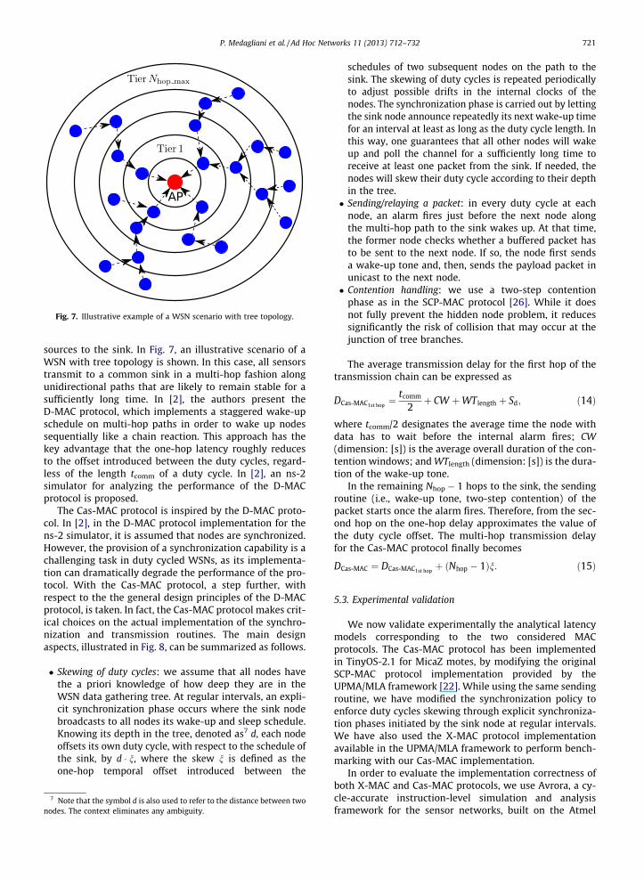
Fig. 7. Illustrative example of a WSN scenario with tree topology.

P. Medagliani et al. / Ad Hoc Networks 11 (2013) 712–732 721

sources to the sink. In Fig. 7, an illustrative scenario of aWSN with tree topology is shown. In this case, all sensorstransmit to a common sink in a multi-hop fashion alongunidirectional paths that are likely to remain stable for asufficiently long time. In [2], the authors present theD-MAC protocol, which implements a staggered wake-upschedule on multi-hop paths in order to wake up nodessequentially like a chain reaction. This approach has thekey advantage that the one-hop latency roughly reducesto the offset introduced between the duty cycles, regard-less of the length tcomm of a duty cycle. In [2], an ns-2simulator for analyzing the performance of the D-MACprotocol is proposed.

The Cas-MAC protocol is inspired by the D-MAC proto-col. In [2], in the D-MAC protocol implementation for thens-2 simulator, it is assumed that nodes are synchronized.However, the provision of a synchronization capability is achallenging task in duty cycled WSNs, as its implementa-tion can dramatically degrade the performance of the pro-tocol. With the Cas-MAC protocol, a step further, withrespect to the the general design principles of the D-MACprotocol, is taken. In fact, the Cas-MAC protocol makes crit-ical choices on the actual implementation of the synchro-nization and transmission routines. The main designaspects, illustrated in Fig. 8, can be summarized as follows.

� Skewing of duty cycles: we assume that all nodes havethe a priori knowledge of how deep they are in theWSN data gathering tree. At regular intervals, an expli-cit synchronization phase occurs where the sink nodebroadcasts to all nodes its wake-up and sleep schedule.Knowing its depth in the tree, denoted as7 d, each nodeoffsets its own duty cycle, with respect to the schedule ofthe sink, by d � n, where the skew n is defined as theone-hop temporal offset introduced between the

7 Note that the symbol d is also used to refer to the distance between twonodes. The context eliminates any ambiguity.

schedules of two subsequent nodes on the path to thesink. The skewing of duty cycles is repeated periodicallyto adjust possible drifts in the internal clocks of thenodes. The synchronization phase is carried out by lettingthe sink node announce repeatedly its next wake-up timefor an interval at least as long as the duty cycle length. Inthis way, one guarantees that all other nodes will wakeup and poll the channel for a sufficiently long time toreceive at least one packet from the sink. If needed, thenodes will skew their duty cycle according to their depthin the tree.� Sending/relaying a packet: in every duty cycle at each

node, an alarm fires just before the next node alongthe multi-hop path to the sink wakes up. At that time,the former node checks whether a buffered packet hasto be sent to the next node. If so, the node first sendsa wake-up tone and, then, sends the payload packet inunicast to the next node.� Contention handling: we use a two-step contention

phase as in the SCP-MAC protocol [26]. While it doesnot fully prevent the hidden node problem, it reducessignificantly the risk of collision that may occur at thejunction of tree branches.

The average transmission delay for the first hop of thetransmission chain can be expressed as

DCas-MAC1st hop¼ tcomm

2þ CW þWT length þ Sd; ð14Þ

where tcomm/2 designates the average time the node withdata has to wait before the internal alarm fires; CW(dimension: [s]) is the average overall duration of the con-tention windows; and WTlength (dimension: [s]) is the dura-tion of the wake-up tone.

In the remaining Nhop � 1 hops to the sink, the sendingroutine (i.e., wake-up tone, two-step contention) of thepacket starts once the alarm fires. Therefore, from the sec-ond hop on the one-hop delay approximates the value ofthe duty cycle offset. The multi-hop transmission delayfor the Cas-MAC protocol finally becomes

DCas-MAC ¼ DCas-MAC1st hopþ ðNhop � 1Þn: ð15Þ

5.3. Experimental validation

We now validate experimentally the analytical latencymodels corresponding to the two considered MACprotocols. The Cas-MAC protocol has been implementedin TinyOS-2.1 for MicaZ motes, by modifying the originalSCP-MAC protocol implementation provided by theUPMA/MLA framework [22]. While using the same sendingroutine, we have modified the synchronization policy toenforce duty cycles skewing through explicit synchroniza-tion phases initiated by the sink node at regular intervals.We have also used the X-MAC protocol implementationavailable in the UPMA/MLA framework to perform bench-marking with our Cas-MAC implementation.

In order to evaluate the implementation correctness ofboth X-MAC and Cas-MAC protocols, we use Avrora, a cy-cle-accurate instruction-level simulation and analysisframework for the sensor networks, built on the Atmel

Fig. 8. Design philosophy of the Cas-MAC protocol.

722 P. Medagliani et al. / Ad Hoc Networks 11 (2013) 712–732

AVR micro controller, presented in [27]. The Avrora frame-work allows the precise emulation of IEEE 802.15.4-basedprotocols without any modifications in the code developedfor the real hardware. In [28], the correctness of the emu-lation of the Texas Instruments Chipcon CC2420 radio chip,used in many sensor node platforms (such as the CrossbowMicaZ nodes), is proved.

For each of the experiments presented hereafter, theaverage latency is evaluated considering 100 sample pack-ets traversing a 6-hop chain path. For the X-MAC protocol,we observed that sending packets leads to aligned duty cy-cles, thus biasing the latency measurements. In order toeliminate this unintended effect, we decided to run onesimulation for each single sample packet and to averageover the set of simulations.

In Fig. 9a and b, the multi-hop latencies with the X-MACand Cas-MAC protocols, respectively, are shown asfunctions of the number of hops. As can be seen from theobtained results, there is an overall good agreementbetween experimental and analytical results. The averagelatency increases linearly as a function of the number ofa hops with a slope approximating tcomm/2 for the X-MACprotocol and n for the Cas-MAC protocol.

In order to evidence the low latency guaranteed by theCas-MAC protocol, in Fig. 9c we evaluate the 6-hop latencyfor various values of the duty cycle, considering both X-MAC and Cas-MAC protocols. In order to carry out thiscomparison, we fix the portion of time during which thenode is active, and increase the sleep interval, thus increas-ing the total duration tcomm of the duty cycle. For very lowvalues of bcomm, when the node is sleeping during a largefraction of time, the Cas-MAC protocol outperforms theX-MAC protocol. However, when bcomm gets higher, i.e.,the node is active for a larger fraction of time, the benefitsof the Cas-MAC protocol disappear.

To properly tune the Cas-MAC protocol, a key factor isthe length of the skew, which indicates the offset on eachhop along the path. If n is shortened, the average latency,which increases linearly as a function of number of hopswith slope n, reduces. However, it becomes more likelythat the sending alarm of a node will fire before it hasreceived the packet. In the latter case, this intermediatenode will have to buffer the packet until the next sendingopportunity, which will result in increasing the average

multi-hop latency. In Fig. 9d, we show the 6-hop latencywith the Cas-MAC protocol, using multiple values of n.The presented results underline that there is a thresholdvalue of n below which the average latency increases. Thishelps to determine the margin required because of clockdrift and processing time fluctuations.

6. A cross-layer network lifetime model

We now propose a simple energy model to completeour modeling framework. Node energy is a crucial commondenominator in our cross-layer modeling, as all the criticalfunctions (at sensing and communication layers) contrib-ute to its depletion and, thus, to the decrease of systemlifetime. The energy model creates the inter-dependenciesbetween all functional layers that guide the performancetrade-offs that a WSN operator may face between reliabil-ity, reactivity, and sustainability.

The energy consumed by a node is defined as the sum ofthe energies consumed by its hardware components. Forthe sake of simplicity, we only integrate in the energymodel the contributions from the sensing sub-unit andthe radio transceiver. The main parameters of the energymodel are listed in Table 3.

The network lifetime is defined as the time needed forthe average residual energy in the deployed WSN, denotedEr, to become lower than a threshold value Eth. Denotingthe initial energy of a node as Ei and denoting the powerconsumption (due to sensing and communication opera-tions) of the whole network (i.e., at all nodes) as Xcons,the average residual energy Er at time t (assuming thatthe network turns on at time 0) can be expressed as

ErðtÞ ¼ NEi �Xconst: ð16Þ

We now focus on the derivation of the energy model forthe Cas-MAC protocol, as the energy model for the X-MAC protocol can be found in [6]. According to the descrip-tion of the Cas-MAC protocol in Section 5, Xcons can then becomputed as follows:

Xcons ¼ ½ðXR þXTÞPdNtarget þXLPL� 1� tcomm

tsync

� �

þXsynctcomm

tsyncþXsensing; ð17Þ

5.0

4.0

3.5

3.0

2.5

2.0

1.5

1.0

0.5

1 2 3 4 5 6

DX

-MA

C [

s]

Nhop

exp-βcomm=25%theo-βcomm=25%exp-βcomm=10%

theo-βcomm=10%exp-βcomm=5%

theo-βcomm=5%exp-βcomm=2%

theo-βcomm=2%

1.5

1.25

1.0

0.75

0.50

0.25

1 2 3 4 5 6

DC

as-M

AC

[s]

Nhop

exp-βcomm=25%theo-βcomm=25%exp-βcomm=10%

theo-βcomm=10%exp-βcomm=5%

theo-βcomm=5%exp-βcomm=2%

theo-βcomm=2%

(a) (b)

3.0

2.0

1.5

1.0

0.5

5045403530252015105

6-ho

p la

tenc

y [s

]

βcomm [%]

DCas-MACDX-MAC

1.4

1.2

1.0

0.8

0.6

0.4

25 30 35 40 45 50

DC

as-M

AC

[s]

ξ [ms]

exptheo

(c) (d)

Fig. 9. Experimental results on latency measurements: (a) validation of X-MAC’s latency model, with experimental (dashed lines) against theoretical (solidlines) results; (b) validation of Cas-MAC’s latency model, with experimental (dashed lines) against theoretical (solid lines) results; (c) comparison of the 6-hop experimental latency for X-MAC (solid lines) and Cas-MAC (dashed lines) as function of bcomm; and (d) theoretical (solid lines) and experimental(dashed lines) latency results as function of the skew n, with Nhop = 6 and bcomm = 5%.

Table 3Constant and variable system parameters considered in the energy-model.

Constant parametersNumber of nodes in the network N 25 Scenario-specificPreamble duration Sp 0.26 ms Configuration-specificPacket duration Sd 0.93 ms Application-specificContention window duration CW 5 ms Configuration-specificWake-up tone length WTlength 20 ms Configuration-specificTransmission power consumption XTx 0.0511 W Device-specificReception power consumption XRx 0.0588 W Device-specificSensing power consumption Xsens 0.0036 W Device-specificSleep power consumption Xsleep 2.4 � 10�7 W Device-specific

Variable parameters (with default value ranges)Average number of hops Nhop 3.0, 3.1, 4.0, 5.8 Function of the topologySensing duty cycle bsens 0.1–1 Configuration-specificSensing period tsens 5–25 (15) s Configuration-specificCommunication duty cycle bcomm 0.002–1 Configuration-specificCommunication period tcomm 40–1000 (100) ms Configuration-specificSynchronization period tsync 30 s Configuration-specificNumber of incoming targets per day NT 10 Scenario-specific

P. Medagliani et al. / Ad Hoc Networks 11 (2013) 712–732 723

where Ntarget is the number of target appearances, Pd isthe target detection probability, tcomm is the communica-tion period, and tsync is the synchronization interval.One can distinguish the following sources of powerconsumption:

� XT and XR are the powers used to send and receive analert message over a period of duration tcomm,respectively;� Xsync is the power used for synchronization operations

over a period of duration tsync;

724 P. Medagliani et al. / Ad Hoc Networks 11 (2013) 712–732

� XLPL is the power required when performing the LowPower Listening (LPL) operations over a period of dura-tion tcomm;� Xsensing is the power consumption associated with the

sensing module in the activity period of duration tsens.

The expected power XT to send a data packet can be ex-pressed as

XT ¼ ½XTx ðWT length þ SdÞ þXRx CW � Nhop

tcomm; ð18Þ

where XTx ðWT length þ SdÞ is the energy spent to transmit awake-up tone followed by a data packet and XRx CW isthe energy spent while sensing the channel in order to de-tect potential transmissions from other neighboring nodes.The presence of the multiplicative term Nhop takes into ac-count the average number of relays from the sensor nodeto the sink. The value of Nhop can be determined by consid-ering all possible shortest (in terms of number of hops)paths using the Dijkstra algorithm [29].

Similarly, the expected power XR to receive a data pack-et can be expressed as

XR ¼ XRx ðSd þWT lengthÞNhop

tcomm: ð19Þ

The power consumed during synchronization opera-tions can be expressed as

Xsync ¼ XTxsync þ ðN � 1ÞXRxsync ; ð20Þ

where XTxsync and XRxsync are the powers consumed fortransmitting and receiving the synchronization message,respectively. In particular, the power XTxsync , consumed bythe sink for the transmission of the sync packet, can be gi-ven by the following expression:

XTxsync ¼SdXTx

34 bcommtsync

ð21Þ

where tsync is the time interval occurring between two syn-chronizations and the fact that the sink transmits, every34 bcommtcomm, a sync packet is taken into account. Similarly,the power XRxsync , consumed by the remote nodes to receivethe synchronization packet, can be expressed as

XRxsync ¼SdXRx

34 bcommtsync

: ð22Þ

The power associated with the LPL, or duty cycling,operations can be expressed as

XLPL ¼ NXRx bcomm þ NXsleepð1� bcommÞ � CTx ð23Þ

where CTx is a correction term used to refine the powerconsumption due to LPL operations. In fact, the transmis-sion operations overlap, for a short interval, with the LPLoperations. Therefore, without the correction term CTx ,the power consumption budget would be higher than thecorrect one. In particular, CTx can be expressed as

CTx ¼ ðWT length þ CW þ SdÞXsleepNhop

tcomm:

In fact, term CTx takes into account that during transmis-sion operations, such as (i) preamble transmission,

(ii) contention window, and (iii) packet transmission, thenode would normally be in the sleep state.

Finally, the power consumed during sensing operationscan be expressed as

Xsensing ¼ bsensXsensN: ð24Þ

Note that in the case of the X-MAC protocol, the derivationis slightly different for XLPL, XR and XT (see [6] for moredetails), since the X-MAC protocol does not have anysynchronization mechanism. In addition, while with theCas-MAC protocol a node with data broadcasts a wake-up tone constituted by short preambles and then transmitsthe data packet without acknowledgment, the X-MAC pro-tocol opts for the preambling of the very data packet andits acknowledgment by the receiving node.

Finally, the network lifetime L can be defined as theinterval between the initial instant at which the nodesare turned on and the time instant at which the residualnetwork energy Er(L) becomes equal to NEth, where Eth isa given residual node energy threshold (which takes intoaccount the physical behavior of the device). From (16),the following expression for the network lifetime L canbe straightforwardly derived:

L ¼ NðEi � EthÞXcons

: ð25Þ

7. System engineering: Two application cases

In this section, we consider two illustrative applicationcases to show how the cross-layer modeling frameworkcan help a network operator to predict the performanceof a deployed WSN. We first show how to optimize theoperational system parameters for a given topology. Then,we highlight the impact of nodes’ placement on the ex-pected performance.

7.1. Maximizing the system lifetime for given (illustrative)topologies

In this subsection, we present an application case inwhich a given surveillance system is optimally configuredto maximize the network lifetime L, for given Quality ofService (QoS) requirements in terms of probability ofmissed detection (Pmd) and latency after detection (D).Throughout this subsection, the target arrival rate Ntarget

is set to 10 targets per day. In Fig. 10, the considered topol-ogy, with 25 nodes deployed over a 1 km � 1 km area andwith the sink located at the bottom left corner of the mon-itored area, is shown. The considered network is com-pletely connected, the average number of hops is 3, andthe lowest achievable (with bsens = 1) value of Pmd is 0.6.

This application case consists of the optimization of asingle-objective function (the network lifetime), given con-straints on the two other functions (the maximum tolera-ble probability of missed detection, denoted as Pmd, andthe longest tolerable latency after detection, denoted asD⁄). Since Eqs. (5) and (25) are not linear, standard linearprogramming optimization techniques cannot be used.However, the three equations identify a convex set, which

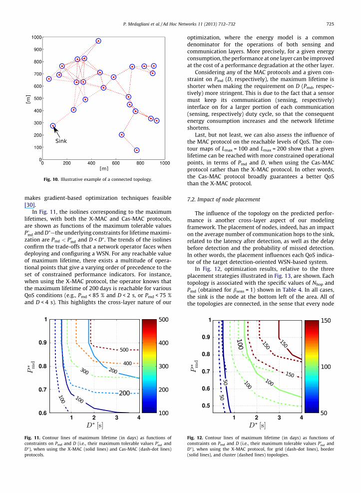
Fig. 10. Illustrative example of a connected topology.

P. Medagliani et al. / Ad Hoc Networks 11 (2013) 712–732 725

makes gradient-based optimization techniques feasible[30].

In Fig. 11, the isolines corresponding to the maximumlifetimes, with both the X-MAC and Cas-MAC protocols,are shown as functions of the maximum tolerable valuesPmd and D⁄—the underlying constraints for lifetime maximi-zation are Pmd < Pmd and D < D⁄. The trends of the isolinesconfirm the trade-offs that a network operator faces whendeploying and configuring a WSN. For any reachable valueof maximum lifetime, there exists a multitude of opera-tional points that give a varying order of precedence to theset of constrained performance indicators. For instance,when using the X-MAC protocol, the operator knows thatthe maximum lifetime of 200 days is reachable for variousQoS conditions (e.g., Pmd < 85 % and D < 2 s, or Pmd < 75 %and D < 4 s). This highlights the cross-layer nature of our

Fig. 11. Contour lines of maximum lifetime (in days) as functions ofconstraints on Pmd and D (i.e., their maximum tolerable values Pmd andD⁄), when using the X-MAC (solid lines) and Cas-MAC (dash-dot lines)protocols.

optimization, where the energy model is a commondenominator for the operations of both sensing andcommunication layers. More precisely, for a given energyconsumption, the performance at one layer can be improvedat the cost of a performance degradation at the other layer.

Considering any of the MAC protocols and a given con-straint on Pmd (D, respectively), the maximum lifetime isshorter when making the requirement on D (Pmd, respec-tively) more stringent. This is due to the fact that a sensormust keep its communication (sensing, respectively)interface on for a larger portion of each communication(sensing, respectively) duty cycle, so that the consequentenergy consumption increases and the network lifetimeshortens.

Last, but not least, we can also assess the influence ofthe MAC protocol on the reachable levels of QoS. The con-tour maps of Lmax = 100 and Lmax = 200 show that a givenlifetime can be reached with more constrained operationalpoints, in terms of Pmd and D, when using the Cas-MACprotocol rather than the X-MAC protocol. In other words,the Cas-MAC protocol broadly guarantees a better QoSthan the X-MAC protocol.

7.2. Impact of node placement

The influence of the topology on the predicted perfor-mance is another cross-layer aspect of our modelingframework. The placement of nodes, indeed, has an impacton the average number of communication hops to the sink,related to the latency after detection, as well as the delaybefore detection and the probability of missed detection.In other words, the placement influences each QoS indica-tor of the target detection-oriented WSN-based system.

In Fig. 12, optimization results, relative to the threeplacement strategies illustrated in Fig. 13, are shown. Eachtopology is associated with the specific values of Nhop andPmd (obtained for bsens = 1) shown in Table 4. In all cases,the sink is the node at the bottom left of the area. All ofthe topologies are connected, in the sense that every node

Fig. 12. Contour lines of maximum lifetime (in days) as functions ofconstraints on Pmd and D (i.e., their maximum tolerable values Pmd andD⁄), when using the X-MAC protocol, for grid (dash-dot lines), border(solid lines), and cluster (dashed lines) topologies.

Fig. 13. Examples of node placement strategies: (a) cluster, (b) border, and (c) grid topology.

Table 4Nhop and best Pmd associated to the topologies presented in Fig. 13.

Topology Nhop Best value of Pmd

Cluster 3.1 0.71Grid 4.0 0.46Border 5.8 0.45

Fig. 14. Contour lines of maximum lifetime (in days) as functions ofconstraints on Pmd and D (i.e., their maximum tolerable values Pmd andD⁄), when using the Cas-MAC protocol, for grid (dash-dot lines), border(solid lines), and cluster (dashed lines) topologies.

726 P. Medagliani et al. / Ad Hoc Networks 11 (2013) 712–732

is within the radio coverage of at least one neighbor, and amulti-hop path exists from each node to the sink. For eachtopology, we have represented a set of isolines for themaximum lifetime as function of the constraints Pmd <

Pmd and D < D⁄, when using the X-MAC protocol.The set of plots provides a number of insights on the

selection of the placement strategy.

� The topology has a direct influence on the ‘‘landscape’’ ofachievable operational points. For instance, when usingthe cluster topology, the best reachable value of Pmd is0.7. The bottom line is that the optimization techniquecannot find any (maximum) value of the lifetime underthe constraint Pmd < Pmd with Pmd ¼ 0:7. In the case thatan operator requires to operate the system with moredemanding QoS in terms of detection capability (i.e.,Pmd < 0.7), he should opt for the grid topology or theborder topology.� The average number of communication hops is a key factor

for QoS provisioning. Considering the grid and bordertopologies (i.e., with a respective average number ofhops of 4.0 for the grid, and 5.8 for the border), for agiven constraint on the delay (e.g., D < D⁄ with D⁄ = 4s), the maximum lifetime of 100 days is obtained witha better QoS in terms of Pmd when using the grid topol-ogy (i.e., Pmd smaller than 0.49), rather than the bordertopology (Pmd smaller than 0.55). This pertains to theoperations of the X-MAC protocol, as the model forthe delay shows that the latency depends on the num-ber of hops and on the value of the duty cycle. In partic-ular, for a given constraint on the delay, the larger thenumber of hops, the lower the one-hop delay, and thelonger the duty cycle, thus increasing the energy budgetfor the communication layer. As a consequence, the

same value of maximum lifetime can be reached onlyby relaxing the energy budget dedicated to the sensinglayer, i.e., by relaxing the constraint on Pmd.

Note that, in the case of the Cas-MAC protocol, the im-pact of the node placement, in terms of average number ofhops to the sink, is reduced with respect to that requiredby the X-MAC protocol. Indeed, the latency model showsa dependence on the communication duty cycle only forthe first hop. For the following hops, the one-hop delayonly depends on the introduced offset, regardless of theduty cycle. Since, in the lifetime model, the energy budgetfor communication only takes into consideration the aver-age number of hops, the isolines tend to be very close, asshown in Fig. 14. In particular, considering the grid andborder topologies (i.e., with corresponding average numberof hops equal to 4.0 and 5.8, respectively), the grid topologyallows to reach operational points slightly more con-strained than those allowed by the border topology.Comparing the cluster topology with the grid and bordertopologies, one can see that the most constrained isolines

P. Medagliani et al. / Ad Hoc Networks 11 (2013) 712–732 727

(e.g., maximum lifetime equal to 50 days) are achievedwhen using the cluster topology, rather than with the gridand border topologies. On the opposite, one can see thatthe least constrained isolines (e.g., maximum lifetimeequal to 200 days or 350 days) are achieved for more con-strained operational points when using the grid and bordertopologies, rather than with the cluster topology, especiallyfor loose constraints on D. In that case, the energy budgetdue to the operations of the MAC protocol tends to becomevery close for all the topologies, and the budget portionowing to sensing unit weighs more, at the disadvantageof the cluster topology.

To summarize, a few illustrative examples have shownthat the node placement can have a relevant impact interms of both achievable operational points and QoSprovisioning.

8. Concluding remarks

This paper has addressed the problem of engineeringenergy-efficient mobile target detection applications usingWSNs with deterministic (a priori known) node deploy-ment. In particular, we have first proposed an analyticalframework for the evaluation of several performance met-rics at sensing and communication layers: the probabilityof missed detection, the delay before the first detectionact, the latency after detection, and the energy consump-tion. We have then characterized, using this toolbox, thecross-layer interactions between sensing and communica-tion layers, evaluating the energy consumption under gi-ven constraints in terms of detection capability andlatency. Finally, we have illustrated the use of our toolboxto predict the performance of practical WSN-based surveil-lance systems under specific QoS requirements. Our resultsshow clearly that the network topology and the MAC pro-tocol have an impact on sensing and communication sys-tem capabilities and, therefore, lead to cross-layer trade-offs. For instance, the novel Cas-MAC protocol guaranteesa threefold network lifetime extension with respect tothe X-MAC protocol, considering given QoS requirementson the detection capability and responsiveness of theWSN. Focusing on illustrative relevant network topologies,we have shown that the system can reach more con-strained operational points, in terms of probability ofmissed detection, using specific node placements (e.g.,border or grid topologies rather then cluster topologies).

Further work along these lines include the extension ofthe engineering toolbox to take into account the use ofcomplex nodes, in order to improve the overall accuracyof the analytical performance predictions. In particular,there is room to refine the cross-layer models in order toencompass the effect of more realistic radio and sensingenvironments. At last, we envision to assess the validityof the predicted performance through large-scale fieldtesting with real hardware platforms.

Appendix A. Geometric derivation of m2(i, j)

The term m2(i, j) can be evaluated, as shown in [20], as afunction of the distance between the sensor nodes i and j

[31]. In particular, under the assumption of equal sensingranges, m2(i, j) can be expressed as follows:

m2ði; jÞ ¼2prs þ 2prs � Loutðdi;jÞ Ai \Aj – 0Linðdi;jÞ � Loutðdi;jÞ Ai \Aj ¼ 0

�; ðA:1Þ

where di,j is the distance between the sensor nodes i and j,Lin(di,j) (Lout(di,j), respectively) denotes the length of the in-ner (outer, respectively) string wrapped around the sens-ing areas of nodes i and j, as shown in Fig. A.15.

After a few geometrical considerations, one can showthat

Loutðdi;jÞ ¼ 2prs þ 2di;j;

Linðdi;jÞ ¼ 2rs 2p� 2 arccos2rs

di;j

� �� �þ 4

ffiffiffiffiffiffiffiffiffiffiffiffiffiffiffiffid2

i;j

4� r2

s

s:

Appendix B. Derivation of PfEdetjESoTg

Since the target moves at constant speed v, the crossingtime of a sensed area is Tcross = L/v, where L is the length ofthe intersection between the target trajectory and the areasensed by a sensor, as shown in Fig. B.16. As L is a randomvariable distributed in [0,2rs], Tcross is a random variablewith distribution in [0,2rs/v]. Since there is no informationabout the arrival instant of the target and under theassumption of infinite duty cycling, the delay with respectto beginning of the last duty cycle can be modeled as a ran-dom variable uniformly distributed in [0, tsens]. Withoutloss of generality, we now focus on a single period of dura-tion tsens. When the sensor is on, i.e., during the subintervalof duration bsenstsens, any incoming target will be detected.In the case that the sensor is off, i.e., during the subintervalof duration (1 � bsens)tsens, the following analysis can becarried out. Let Etarget be the event {The sensor is on atthe instant at which the target enters the sensed area}.Applying the total probability theorem [32], PfEdetjESoTgcan then be expressed as

PfEdetjESoTg ¼ PfEdetjEtarget;ESoTgPfEtargetjESoTgþ PfEdetjEtarget;ESoTgPfEtargetjESoTg; ðB:1Þ

where it is immediate to conclude that PfEdetjEtarget;

ESoTg ¼ 1; PfEtargetjESoTg ¼ bsens, and PfEtargetjESoTg ¼ 1�bsens: Therefore, Eq. (B.1) can be rewritten as:

PfEdetjESoTg ¼ bsens þ ð1� bsensÞPfEdetjEtarget;ESoTg: ðB:2Þ

The conditional probability at the right-hand side of (B.2)can be expressed as [6]

PfEdetjEtarget;ESoTg ¼Z Z

D

fTa ;Tcrossðt; sÞdt ds;

where the two-dimensional domain D can be expressed asfollows:

D ¼ ðt; sÞ 2 R2 : 0 < s < 2rs=v and

maxf�sþ c;0g < t < cg;

where c , (1 � bsens)tsens. An illustrative representationof D is shown in Fig. B.17, distinguishing two cases: (a)

(a) (b) (c)

Fig. A.15. Graphical derivation of Lin and Lout for a pair of nodes with sensing range rs at a distance di,j: (a) reference scenario, (b) closed line of length Lin(di,j),and (c) closed line of length Lout(di,j).

Fig. B.16. Model for the characterization of the intersection of a targettrajectory with a sensed area.

728 P. Medagliani et al. / Ad Hoc Networks 11 (2013) 712–732

2rs/v > c and 2rs/v < c. The joint probability density function(pdf) fTa ;Tcross ðt; sÞ can be expressed as [6]:

fTa ;Tcross ðt; sÞ ¼

v

pc

ffiffiffiffiffiffiffiffiffiffiffiffiffiffir2

s� vs2ð Þ

2q

0 < s < 2rs=v and 0 < t < c0 else:

8>>><>>>:

ðB:3Þ

At this point, given that Ta � Unif [0,c], it can be shown that

PfEdetjEtarget;ESoTg ¼

4rspcv

if 2rs=v < c4rs�2

ffiffiffiffiffiffiffiffiffiffiffiffiffiffiffi4r2

s�c2v2ppcv þ 1� 2asin cv

2rsð Þp

otherwise:

8>>>><>>>>:

ðB:4Þ

Fig. B.17. Integration domain for the evaluation of P

Appendix C. Derivation of P Eði;jÞdet jESoTi;j

n oP E

ði;jÞdet jESoTi;j

n ois the probability that the target is

detected during the active phase of at least one of thetwo sensors i and j, given that the target trajectory crossesboth sensed areas. Since the target trajectory is randomand there is no synchronization between the two sensors,and since the target detection can be carried out by (i) only

node i, (ii) only node j, or (iii) both nodes, P Eði;jÞdet jESoTi;j

n ocan

be expressed as

P Eði;jÞdet jESoTi;j

n o¼ P E

ðiÞdetjESoTi;j

n oþ P E

ðjÞdetjESoTi;j

n o� P E

ðiÞdetjESoTi;j

n o� P E

ðjÞdetjESoTi;j

n o; ðC:1Þ

where P EðiÞdetjESoTi;j

n ois the probability that node i is active,

given that the target crosses its sensed area (and that of

node j), and P EðjÞdetjESoTi;j

n ois the probability that node j is

active, given that the target crosses its sensed area (andthat of node i).

The allowed trajectories for the computation of m2 (i.e.,the trajectories which belong to both sensed areas) are asubset of all admissible ones for a single sensor, as shown,in terms of possible positions of the entrance point overthe perimeter of a sensed area, in Fig. C.18a. In fact, inthe case of m1, the entrance point of the target in the areasensed by a sensor can be the whole perimeter of thesensed area, so that the angle U, shown in Fig. B.16, canrange in the interval [0,2p]. Conversely, in the m2 case,one must consider, for node i, only the entrance pointswhich allow the target to cross both sensed areas. Refer-ring to the logical scheme shown in Fig. C.18a, the rangeof allowed entrance points for the first sensed area can

fEdetjEtarget ;ESoTg: (a) 2rs/v > c and (b) 2rs/v < c.

Table C.5Coefficients for the polynomial approximation of (C.4).

Coefficients Analytical expressions Numerical values

a1 � 2rs

ðp�hlimÞ2�38.06

a2 �2a1p 239.17a3 a1p2 + 2rs �275.69

(a)

(b)

Fig. C.18. Allowed entrance points: (a) along the area sensed by node i, toensure that the target crosses also the sensed area of node j, and (b) alongthe area sensed by node j, to ensure that the target crosses also the sensedarea of node i.

P. Medagliani et al. / Ad Hoc Networks 11 (2013) 712–732 729

be approximated as the arc, highlighted in Fig. C.18a,which insists on the angle ð2p� 2hlim1 Þ, where hlim1 is afunction of di,j (the distance between sensor i and sensorj) and rs. For each admissible entrance point position, theentrance angle belongs to a specific (limited) interval.

In order to simplify the derivation of P EðiÞdetjESoTi;j

n o, we

must find the distribution of the length Lði;jÞi of the intersec-tion between the target trajectory and the area sensed bynode i. Moreover, one also needs to compute, for node i,the joint pdf f

Ta ;TðiÞcrossðt; sÞ, which replaces that presented in

expression (B.3). Similar considerations can be carried

out for the derivation of P EðiÞdetjESoTi;j

n owhich, as shown in

Fig. C.18b, depends on the entrance point of the node inthe area sensed by node j. Assuming that the target has al-ready crossed the area sensed by node i, the range of pos-sible entrance points lies on the arc, highlighted inFig. C.18b, which insists on the angle ð2p� 2hlim2 Þ. As fornode i, we simplify the derivation of the distribution of

the length Lði;jÞj of the intersection between the target tra-jectory and the area sensed by j. In particular, referring toFig. C.18b, we assume that all targets enter in the areasensed by node i in the point lying on the line connectingthe nodes i and j.

On the basis of geometrical considerations—omittedhere for conciseness—the length of a chord L can be ex-pressed as the following function of the angle H8:

8 According to Fig. C.18, we should compute Lði;jÞi and Lði;jÞj by consideringthe angles Hði;jÞi and Hði;jÞj , respectively. However, since the expression is thesame in for both node i and node j and for ease of notation simplification,we refer to L and H, considering a generic pair of sensors.

L ¼ B1 � r2s þ d2 � 2rsd

"� 1� d sin H

B1

� ��(

� 1� rs sin HB1

� �1=2

þ rsd sin2 H

B21

#)1=2

ðC:2Þ

where B1,

ffiffiffiffiffiffiffiffiffiffiffiffiffiffiffiffiffiffiffiffiffiffiffiffiffiffiffiffiffiffiffiffiffiffiffiffiffiffiffiffiffiffiffir2

s þ d2 � 2rsd cos Hq

, and

d ¼di;j if L ¼ Lði;jÞi

di;j þ rs if L ¼ Lði;jÞj :

(ðC:3Þ

Since expression (C.2) is complicated, it can be shown thatit can be accurately approximated through a degree-2polynomial approximation.

More precisely, assuming that

L ’ a1H2 þ a2Hþ a3 ðC:4Þ

where a1, a2, and a3 are shown in Table C.5, it is possible toevaluate the joint pdf which replaces that of Eq. (B.3).9

Eq. (C.2) and its approximation (C.4) should depend on thedistance between the centers of nodes i and j. However, aftersome algebraic manipulations, the dependence on thedistance between the pair of sensors disappears and it canbe shown that:

f ðiÞTa ;Tcrossðt; sÞ ¼ f ðjÞTa ;Tcross

ðt; sÞ

¼

vcffiffiffiffiffiffiffiffiffiffiffiffiffiffiffiffiffiffi16r2

s�8rsvsp

0 < s < 2rs=v and 0 < t < c

0 else:

8><>:

ðC:5Þ

The evaluation of P EðiÞdetjESoTi;j

n odepends on the relation

between 2rs/v and (1 � bsens)tsens, but not on node i. Inparticular, it can be shown thatPfEdetjEtarget;ESoTi;j

g ¼ PfEdetjEtarget;ESoTi;jg

¼

4rs3cv if 2rs=v < c

4rs3 �

ðcvþ4rs Þffiffiffiffiffiffiffiffiffiffiffiffiffiffi16r2

s �8crsvp12rs

cv þffiffiffiffiffiffiffiffiffiffiffiffiffiffiffiffiffiffi16r2

s�8rscvp

4rs

else:

8>>><>>>:

ðC:6Þ

Since, at this point, P EðiÞdetjESoTi;j

n o¼ P E

ðjÞdetjESoTi;j

n o, we can

rewrite expression (C.1) as:

P Eði;jÞdet jESoTi;j

n o¼ 2P E

ðiÞdetjESoTi;j

n o� P E

ðiÞdetjESoTi;j

n o� �2:

ðC:7Þ

9 As for expression (C.2), for the sake of notational simplification, werefer to hlim, instead of hlim1

and hlim2.

10 Note that l(x,h) depends on the intersection of the target trajectory withthe sensed area of the kth sensor. In other words, for different values of k,l(x,h) is likely to change.

730 P. Medagliani et al. / Ad Hoc Networks 11 (2013) 712–732

At this point, the probability P EðiÞdetjESoTi;j

n ocan be analyzed

following the derivation of PfEdetjESoTg in Appendix B, butfor replacing the joint pdf (B.3) with the joint pdf (C.5).

Appendix D. Derivation of Ddet in the presence of dutycycling

Consider the trajectory identified by (x,h). Assumingthat there are n(x,h) sensor nodes on the trajectory andthat the target is detected along this trajectory, the proba-bility that the target is detected by the hth sensor node isequal to the probability that the previous (h � 1) sensornodes do not detect the target and the hth does—in otherwords, the hth sensor node along the trajectory is the firstone to detect the target. In other words, denoting as E

ðx;hÞdet

the event that the target is detected along the trajectory(x,h), one can write:

P The target is detected by the hth nodejEðx;hÞdet

n o

¼P E

ðhÞdetjx;h;E

ðh�1Þdet ; . . . ;E

ð1Þdet

n oQh�1k¼1P E

ðkÞdetjx;h;E

ðk�1Þdet ; . . . ;E

ð1Þdet

n oPnðx;hÞz¼1

P EðzÞdetjx;h;E

ðz�1Þdet ; . . . ;E

ð1Þdet

n oQz�1v¼1P E

ðvÞdetjx;h;E

ðv�1Þdet ; . . . ;E

ð1Þdet

n o h

¼1; . . . ;nðx;hÞ:ðD:1Þ

Note that the normalization comes from the fact that weare assuming that the target is detected. In fact, the prob-ability that the target is not detected is equal to

1�Xnðx;hÞz¼1

P EðzÞdetjx;h;E

ðz�1Þdet ; . . . ;E

ð1Þdet

n oYz�1

v¼1

P EðvÞdetjx;h;E

ðv�1Þdet ; . . . ;E

ð1Þdet

n o

but we do not account for this possibility, as it is meaning-less for the evaluation of the delay. Note, therefore, thatlooking only at the delay before detection might be mis-leading, as there may be a small delay because only afew targets are detected. In other words, the informationon the delay before detection needs to be correlated withthe probability of missed detection: this will be done inSection 4.3.

Denoting the delay associated with the detection fromthe hth node as Dh = Dh(x,h), it follows that the averagedelay Dðx; hÞ can be computed as follows:

Dðx;hÞ ¼Xnðx;hÞh¼1

DhP The target is detected by the hth node jEðx;hÞdet

n o;

ðD:2Þ

where P{The target is detected by the hth node} is is givenby (D.1). The delay expression at the right-hand side of(D.2) is given by the sum of the detection delays associatedwith the sensors on the trajectory identified by (x,h). Inparticular: the delay along this trajectory will be that ofthe second sensor provided that the first sensor missesthe target; the delay will be that of the third sensor pro-vided that the first and second sensors misses the target;and so on. Owing to the independence between the sen-sors, it follows that

P EðhÞdetjx; h;E

ðh�1Þdet ; . . . ;E

ð1Þdet

n o¼ P E

ðhÞdetjx; h

n o;

where P EðhÞdetjx; h

n ois derived in Appendix E.

Therefore, the average delay (D.2) along the (x,h)trajectory can be written as

Dðx; hÞ ¼Xnðx;hÞh¼1

Dh

P EðhÞdetjx; h

n oQh�1k¼1P E

ðkÞdetjx; h

n oPnðx;hÞz¼1

P EðzÞdetjx; h

n o Qz�1v¼1P E

ðvÞdetjx; h

n owhich corresponds to (10).

Appendix E. Derivation of P EðkÞdetjx; hn o

For the sake of notational conciseness, we simply de-

note P EðkÞdetjx; h

n oas PfEdetjx; hg, assuming implicitly that

we are considering the kth sensor node whose sensed areais intersected by the target trajectory identified by (x,h).

Let Etarget be the event {The sensor is on at the instant atwhich the target enters the sensed area}. Applying thetotal probability theorem [32], PfEdetjx; hg can then beexpressed as

PfEdetjx; hg ¼ PfEdetjEtarget; x; hgPfEtargetjx; hgþ PfEdetjEtarget; x; hgPfEtargetjx; hg ðE:1Þ

where PfEdetjEtarget; x; hg ¼ 1. Since Etarget is independent ofthe realizations of the entrance point and entrance angle ofthe target—in fact, the activity cycle of a sensor does notdepend on the target trajectory—one can write

PfEtargetjx; hg ¼ PfEtargetg ¼Z bsenstsens

0

1tsens

dt ¼ bsens

and, therefore, PfEtargetjx; hg ¼ 1� bsens: We are now goingto evaluate the last unknown probability at the right-handside of Eq. (E.1), i.e., PfEdetjEtarget; x; hg. According to theconditioning on Etarget and x,h, the target arrival time, de-noted as Ta, is a random variable uniformly distributedover an interval of length (1 � bsens)tsens. To have successfuldetection, the target must remain in the sensed area untilthe sensor turns on its sensing device in the following ac-tive period. Since the target arrives with a finite speed v,the crossing time of the sensed area is tcross = l(x,h)/v,where l(x,h) is the length of the intersection between thetarget trajectory (identified by (x,h)) and the area sensedby a sensor.10

In this case as well, depending on the given trajectory,one must distinguish between two cases: (i) tcross >(1 � bsens)tsens and (ii) tcross < (1 � bsens)tsens. In the formercase, the target will be detected, since it remains in thesensed area for a time interval longer than the sleepinginterval, i.e., PfEdetjEtarget; x; hg ¼ 1. Therefore, in this casePfEdetjx; hg ¼ 1. In the latter case, instead, the target willbe detected if it enters the sensed area in the last part ofthe sleeping interval, so that it will be detected in the fol-lowing active period. The evaluation of PfEdetjEtarget; x; hg in(E.1) can be carried out as follows. Letting End be the event{The target enters the sensed area while the sensing

P. Medagliani et al. / Ad Hoc Networks 11 (2013) 712–732 731

interface is off and it will be detected in the following dutycycle}, PfEdetjEtarget; x; hg can be then expressed as

PfEdetjEtarget;x;hg ¼ PfEdetjEtarget;x;h;EndgPfEndjEtarget;x;hgþPfEdetjEtarget;x;h;EndgPfEndjEtarget;x;hg;

ðE:2Þ

where PfEdetjEtarget; x; h;Endg ¼ 0 and PfEdetjEtarget; x; h;Endg ¼ 1. The last term at the right-hand side of (E.2) thatremains to be evaluated is PfEndjEtarget; x; hg. This term rep-resents the probability that the target enters the sensedarea when the sensing interface is off and it does not exitbefore the sensing interface switches on in the next cycle.This can be expressed as P{Ta + l/v > (1 � bsens)tsens � Ta}.Therefore, one can write

PfEndjEtarget; x; hg ¼Z ð1�bsensÞtsens

ð1�bsens Þtsens�l=v2

11� bsensð Þtsens

dta

¼ 12þ l=v

2ð1� bsensÞtsens: ðE:3Þ

Using (E.2) in (E.3), PfEdetjEtarget; x; hg can be expressed as

PfEdetjEtarget; x; hg ¼1� bsens

2þ l

2vtsens: ðE:4Þ

Finally, combining (E.2) and (E.3) in (E.1), one obtains

PfEdetjx; hg ¼1þbsens

2 þ l2vtsens

if tcross < ð1� bsensÞtsens

1 otherwise:

(

References

[1] M. Buettner, G. Yee, E. Anderson, R. Han, X-mac: a short preamblemac protocol for duty-cycled wireless sensor networks, in: Proc.ACM SenSys, 2006.

[2] G. Lu, B. Krishnamachari, C.S. Raghavendra, An adaptive energy-efficient and low-latency mac for data gathering in wireless sensornetworks, in: Proc. Parallel and Distributed Processing Symposium.

[3] I. Akyildiz, W. Su, Y. Sankarasubramaniam, E. Cayirci, A survey onsensor networks, IEEE Communications Magazine 40 (8) (2002) 102–114.

[4] K. Bobier, J. Wells, M. Dapper, Enhanced unattended ground sensorsystem communications, in: Proc. MILCOM, 2004.

[5] T. He, S. Krishnamurthy, L. Luo, T. Yan, L. Gu, R. Stoleru, G. Zhou, Q. Cao,P. Vicaire, J.A. Stankovic, T.F. Abdelzaher, J. Hui, B. Krogh, Vigilnet: anintegrated sensor network system for energy-efficient surveillance,ACM Transactions on Sensor Networks 2 (1) (2006) 1–38.

[6] P. Medagliani, J. Leguay, V. Gay, M. Lopez-Ramos, G. Ferrari,Engineering energy-efficient target detection applications inwireless sensor networks, in: Proc. IEEE PerCom, 2010.

[7] P. Medagliani, J. Leguay, G. Ferrari, V. Gay, M. Lopez-Ramos, Accurateperformance bounds for target detection in wsns with deterministicnode placement, in: Proc. IEEE ISWPC, 2010.

[8] N. Zhao, L. Sun, Research on cross-layer frameworks design inwireless sensor networks, in: Proc. IEEE ICWMC, 2007.

[9] T. Melodia, M.C. Vuran, D. Pompili, The state of the art in cross-layerdesign for wireless sensor networks, in: Proceedings of EuroNGIWorkshops on Wireless and Mobility, Springer Lecture Notes onComputer Science, LNCS 388, 2005.

[10] Q. Cao, T. Yan, J.A. Stankovic, T. Abdelzaher, Analysis of targetdetection performance for wireless sensor networks, in: Proc.DCOSS, 2005.

[11] V.Prasad, T. Yan, P. Jayach, Z. Li, S.H. Son, J.A. Stankovic, J. Hansson, T.Abdelzaher, Andes: an analysis-based design tool for wireless sensornetworks, in: Proc. RTSS, 2007.

[12] Y. Ting, Analysis Approaches for Predicting Performance of WirelessSensor Networks, Ph.D. Thesis, Charlottesville, VA, USA, Adviser –John A. Stankovic, 2006.

[13] H. Zhang, J. Hou, Is deterministic deployment worse than randomdeployment for wireless sensor networks? in: Proc. INFOCOM, 2006.

[14] H. Zhang, J. Hou, Maintaining sensing coverage and connectivity inlarge sensor networks, Journal Ad Hoc & Sensor Wireless Networks 1(1–2) (2005).

[15] M. Younis, K. Akkaya, Strategies and techniques for node placementin wireless sensor networks: a survey, Journal of Ad Hoc Networks 6(4) (2008) 621–655.

[16] xBow MICAz: Wireless Measurement System. <http://www.xbow.com/Products/Product_pdf_files/Wireless_pdf/MICAz_Datasheet.pdf>.

[17] J. Jeong, Y. Gu, T. He, D. Du, VISA: virtual scanning algorithm fordynamic protection of road networks, in: Proc. INFOCOM, 2009.

[18] E. Yanmaz, H. Guclu, Stationary and mobile target detection usingmobile wireless sensor networks, CoRR abs/1006.4326.

[19] Y. Cao, B. Yang, Intruding target detection using wireless sensornetwork, in: Proc. ICEMI, 2009.

[20] L. Lazos, R. Poovendran, J.A. Ritcey, Analytic evaluation of targetdetection in heterogeneous wireless sensor networks, ACMTransactions on Sensor Networks 5 (2) (2009) 1–38.

[21] W. Feller, An Introduction to Probability Theory and its Applications,New York, NJ, USA.

[22] K. Klues, G. Hackmann, O. Chipara, C. Lu, A component-basedarchitecture for power-efficient media access control in wirelesssensor networks, in: Proc. ACM SenSys, 2007.

[23] J. Polastre, J. Hill, D. Culler, Versatile low power media access forwireless sensor networks, in: Proc. SenSys, 2004.

[24] W. Ye, F. Silva, J. Heidemann, Ultra-low duty cycle mac withscheduled channel polling, in: Proc. ACM SenSys, 2006.

[25] S. Kulkarni, M. Arumugam, TDMA service for sensor networks, in:Proc. ICDCS04, ADSN workshop, 2004.

[26] W. Ye, F. Silva, J. Heidemann, Ultra-low duty cycle mac withscheduled channel polling, in: Proc. ACM SenSys, 2006.

[27] B.L. Titzer, D.K. Lee, J. Palsberg, Avrora: scalable sensor networksimulation, in: Proc. IPSN, 2005.

[28] R.P. Alberola, D. Pesch, Avroraz: extending Avrora with an IEEE802.15.4 compliant radio chip model, in: Proc. ACM PM2HW2N,2008.

[29] D. Bertsekas, R. Gallager, Data Networks, second ed., Upper SaddleRiver, NJ, USA, 1992.

[30] D. Bertsimas, J. Tsitsiklis, Introduction to Linear Optimization,Athena Scientific, Belmont, MA, USA, 1997.

[31] J. Sylvester, On a funicular solution of Buffon’s ‘‘problem of theneedle’’ in its most general form, Acta Mathematica 14 (1) (1890)185–205.

[32] A. Papoulis, Probability, Random Variables and Stochastic Processes,McGraw-Hill, New York, NJ, USA, 1991.

Paolo Medagliani was born in Cremona (CR),on July 1981. He received the ’’Laurea’’ degreein Telecommunications Engineering (3-yearprogram) on September 2003 and the ‘‘LaureaSpecialistica’’ degree on April 2006, respec-tively, from the University of Parma, Italy.From January 2007, he is a Ph.D. student inInformation Technologies at the InformationEngineering Department of the University ofParma, Italy. He is a member, at the Infor-mation Engineering Department of the Uni-versity of Parma, Italy, of the Wireless Ad-hoc

and Sensor Networks (WASN) Laboratory. His research interests are in thefield of performance analysis and design of wireless sensor networks andad hoc networks. In 2010 he got the PhD in Information Technologies at

the University of Parma. Dr. Medagliani is reviewer for some internationalconferences (SECON 2007, WCNC 2007, GLOBECOM 2007 and 2008,WPMC 2007, EWSN 2008, ICC 2008, and PIMRC 2008) and internationaljournals (IEEE Transactions on Wireless Communications). In addition, heis member of the technical committee of International Conference onAdvances in Satellite and Space Communications (SPACOMM 2009),Colmar, France, July 19–24, 2009 and of International Workshop on Per-formance Methodologies and Tools for Wireless Sensor NetworksWSN-Perf (WSNPerf 2009), Pisa, Italy, October 23, 2009. Dr. Medagliani has alsotaken part into research projects in collaboration with a few researchorganizations and private companies. As for now Dr. Medagliani isworking in Lepida s.p.a. in Bologna as a project manager.

732 P. Medagliani et al. / Ad Hoc Networks 11 (2013) 712–732

Gianluigi Ferrari was born in Parma, Italy, in1974. He received his ‘‘Laurea’’ and PhDdegrees from the University of Parma, Italy, in1998 and 2002, respectively. Since 2002, hehas been with the University Parma, where hecurrently is an Associate Professor of Tele-communications. He was a visiting researcherat USC (Los Angeles, CA, USA, 2000-2001),CMU (Pittsburgh, PA, USA, 2002-2004), KMITL(Bangkok, Thailand, 2007), and ULB (Brux-elles, Belgium, 2010). Since 2006, he has beenthe Coordinator of the Wireless Ad-hoc and

Sensor Networks (WASN) Lab in the Department of Information Engi-neering of the University of Parma.

As of today he has published more than 140 papers in leading inter-

national journals and conferences. He is coauthor of a few books,including Detection Algorithms for Wireless Communications, with Applica-tions to Wired and Storage Systems (Wiley: 2004), Ad Hoc Wireless Net-works: A Communication-Theoretic Perspective (Wiley: 2006), LDPC CodedModulations (Springer: 2009), and Sensor Networks with IEEE 802.15.4Systems: Distributed Processing, MAC, and Connectivity (Springer: 2011). Heedited the book Sensor Networks: Where Theory Meets Practice (Springer:2010). His research interests include digital communication systemsanalysis and design, wireless ad hoc and sensor networking, adaptivedigital signal processing, and information theory.

Prof. Ferrari is a co-recipient of a best student paper award atIWWAN’06 and a best paper award at EMERGING’10. He acts as a fre-quent reviewer for many international journals and conferences. He actsalso as a technical program member for many international conferences.He currently serves on the Editorial Boards of The Open Electrical andElectronic Engineering (TOEEJ) Journal(Bentham Publishers), the Interna-tional Journal of RF Technologies: Research and Applications (Taylor &Francis), and the International Journal of Future Generation Communicationand Networking (SERSC: Science & Engineering Research Support Center).He was a Guest Editor of the 2010 EURASIP JWCN Special Issue on‘‘Dynamic Spectrum Access: From the Concept to the Implementation.’’

Vincent Gay got the diploma in Networkingfrom the Ecole Nationale Supérieure desTélécommunications de Paris in 2007. Heentered the Laboratory for Advanced Infor-mation Technologies of Thales Communica-tions France in 2007. He is working onenergy-efficiency strategies in Wireless Sen-sor Networks in ITEA2 GEODES project, andon the integration of WSN into objecttoobjectsystems in ITEA2 USENET project. He has alsobeen involved in studies on networking pro-tocols for mobility and multi-homing (e.g.,

Mobile IPv6, HIP) in the context of FP6/IST ANEMONE and MULTINET, andFrench-RNRT REMORA.

Jérémie Leguay is an advanced studies engi-neer at Thales Communications, in Colombes,France. He received his Engineering Degree(2003) from EFREI (École Française d’Electro-nique et d’Informatique) and a Master of Sci-ence (2004) in Computer Science fromLinköping University in Sweden. From 2004 to2007 he has been a Ph.D. candidate at theComputer Science laboratory (LIP6) of Pierre &Marie Curie University and at Thales Com-munications where he conducted research inad hoc and delaytolerant networking. His

current research interests focus on networking solutions for mobile andconstrained environments.