Critical comparison of methods predicting the number of components in spectroscopic data
18
Analytica Chimica Acta 423 (2000) 51–68 Critical comparison of methods predicting the number of components in spectroscopic data Milan Meloun a,* , Jindˇ rich ˇ Capek a , Petr Mikš´ ık a , Richard G. Brereton b a Department of Analytical Chemistry, Faculty of Chemical Technology, University Pardubice, CZ-532 10 Pardubice, Czech Republic b School of Chemistry, University of Bristol, Cantock’s Close, Bristol BS8 1TS, UK Received 26 April 2000; accepted 27 July 2000 Abstract Determining the number of chemical components in a mixture is a first important step to further analysis in spectroscopy. The accuracy of 13 statistical indices for estimation of the number of components that contribute to spectra was critically tested on simulated and on experimental data sets using algorithm INDICES in S-Plus. All methods are classified into two categories, precise methods based upon a knowledge of the instrumental error of the absorbance data, s inst (A), and approximate methods requiring no such knowledge. Most indices always predict the correct number of components even a presence of the minor one when the signal-to-error ratio (SER) is higher than 10 but in case of RESO and IND higher than 6. On base of SER the detection limit of every index method is estimated. Two indices, RESO and IND, correctly predict a minor component in a mixture even if its relative concentration is 0.5–1% and solve an ill-defined problem with severe collinearity. For more than four components in a mixture the modifications of Elbergali et al. represent a useful resolution tool of a correct number of components in spectra for all indices. The Wernimont–Kankare procedure performs reliable determination of the instrumental standard deviation of spectrophotometer used. In case of real experimental data the RESO, IND and indices methods based on knowledge of instrumental error should be preferred. © 2000 Elsevier Science B.V. All rights reserved. Keywords: Chemometrics; Principal component analysis; PCA; Rank of matrix; Number of components; Real error; Extracted error; Method of logarithm of eigenvalues; Instrumental error of spectrophotometer; Number of components in a mixture 1. Introduction Determining the number of chemical components in a mixture is the first step for further qualitative and quantitative analysis in all forms of spectral data treat- ment. Procedures for determining the chemical rank of a matrix using a variety of empirical and statistical methods based on principal component analysis (PCA) have been reported [1]. Much work has been put into * Corresponding author. Tel.: +42-40-603-7026; fax: +42-40-603-7068 E-mail address: [email protected] (M. Meloun). developing methods for resolution of multi-component spectra but less work has been carried out to reveal the limitations of the methods and in the estimation of the minor component of resolved spectra. Throughout this work, it is assumed that the n × m absorbance data matrix A = εC containing the n recorded spectra as rows can be written as the product of the m × r matrix of molar absorptivities ε and the r × n concentration matrix C. Here m denotes the number of wavelengths for which each spectrum was recorded being equal to the number of columns of A matrix, n is the number of solutions for which spectra have been recorded being equal to the number of rows 0003-2670/00/$ – see front matter © 2000 Elsevier Science B.V. All rights reserved. PII:S0003-2670(00)01100-4
Transcript of Critical comparison of methods predicting the number of components in spectroscopic data
Analytica Chimica Acta 423 (2000) 51–68
Critical comparison of methods predicting the number ofcomponents in spectroscopic data
Milan Melouna,∗, Jindrich Capeka, Petr Mikšık a, Richard G. Breretonba Department of Analytical Chemistry, Faculty of Chemical Technology, University Pardubice, CZ-532 10 Pardubice, Czech Republic
b School of Chemistry, University of Bristol, Cantock’s Close, Bristol BS8 1TS, UK
Received 26 April 2000; accepted 27 July 2000
Abstract
Determining the number of chemical components in a mixture is a first important step to further analysis in spectroscopy.The accuracy of 13 statistical indices for estimation of the number of components that contribute to spectra was criticallytested on simulated and on experimental data sets using algorithm INDICES in S-Plus. All methods are classified into twocategories, precise methods based upon a knowledge of the instrumental error of the absorbance data,sinst(A), and approximatemethods requiring no such knowledge. Most indices always predict the correct number of components even a presence of theminor one when the signal-to-error ratio (SER) is higher than 10 but in case of RESO and IND higher than 6. On base of SERthe detection limit of every index method is estimated. Two indices, RESO and IND, correctly predict a minor component ina mixture even if its relative concentration is 0.5–1% and solve an ill-defined problem with severe collinearity. For more thanfour components in a mixture the modifications of Elbergali et al. represent a useful resolution tool of a correct number ofcomponents in spectra for all indices. The Wernimont–Kankare procedure performs reliable determination of the instrumentalstandard deviation of spectrophotometer used. In case of real experimental data the RESO, IND and indices methods basedon knowledge of instrumental error should be preferred. © 2000 Elsevier Science B.V. All rights reserved.
Keywords:Chemometrics; Principal component analysis; PCA; Rank of matrix; Number of components; Real error; Extracted error; Methodof logarithm of eigenvalues; Instrumental error of spectrophotometer; Number of components in a mixture
1. Introduction
Determining the number of chemical componentsin a mixture is the first step for further qualitative andquantitative analysis in all forms of spectral data treat-ment. Procedures for determining the chemical rankof a matrix using a variety of empirical and statisticalmethods based on principal component analysis (PCA)have been reported [1]. Much work has been put into
∗ Corresponding author. Tel.:+42-40-603-7026;fax: +42-40-603-7068E-mail address:[email protected] (M. Meloun).
developing methods for resolution of multi-componentspectra but less work has been carried out to revealthe limitations of the methods and in the estimation ofthe minor component of resolved spectra.
Throughout this work, it is assumed that then ×m absorbance data matrixAAA = εεεCCC containing thenrecorded spectra as rows can be written as the productof them× r matrix of molar absorptivitiesεεε and ther × n concentration matrixCCC. Here m denotes thenumber of wavelengths for which each spectrum wasrecorded being equal to the number of columns ofAAA
matrix,n is the number of solutions for which spectrahave been recorded being equal to the number of rows
0003-2670/00/$ – see front matter © 2000 Elsevier Science B.V. All rights reserved.PII: S0003-2670(00)01100-4
52 M. Meloun et al. / Analytica Chimica Acta 423 (2000) 51–68
ofAAAmatrix,r is the number of components that absorbin the chosen spectral range. The rank of the matrixAAA is obtained from the equation
rank(AAA) = min[rank(εεε), rank(CCC) ≤ min(m, r, n) (1)
Since the rank ofAAA is equal to the rank ofεεε or CCC,whichever is the smaller, and since rank(εεε) ≤ r andrank(CCC) ≤ r, then providedm ≥ r and n ≥ r, itwill only be necessary to determine the rank of matrixAAA which is equivalent to the number of significantcomponents [2,18].
Approaches for the determination of the rank ofAAA
are based on two different chemometric methods, ei-ther using pure PCA or by using PCA combined withcross-validation [3–12]. Generally, PCA will extractsome of noise, i.e. experimental and/or random errorwhich will usually be represented by the principalcomponents with smallest size or variance. When nonoise in spectra exists, the number of eigenvalues ofthe covariance matrixAAATAAA larger than zero is equiv-alent to the number of componentr, providing thatthe spectra of components in mixture are linearlyindependent.
In a recent tutorial, Malinowski [3] concludedthat spectra gleaned from a spectrophotometer oftencontains instrumental as well as experimental uncer-tainties that arise from several different sources: (a)spectrophotometer switches a filter and new uncer-tainty and also uncertainty of distribution are intro-duced; (b) changing sample cells or stock solventswill produce uncertainty distribution in the data; (c)data pretreatment such as smoothing, normalizing orstandardizing the data columns or data rows can seri-ously effect the uncertainty distribution; (d) data canbe distorted by a combination of these factors.
As all real data contain experimental noise, thenumber of eigenvalues different from zero is usuallylarger than the number of componentsr. Experimen-tal and/or random error can mask the identification ofthe true dimensionality of a data set. Malinowski [1,4]split this error into two sources — imbedded errorand extracted error. Extracted error (XE) is the errorwhich is contained within the minor PC dimensions((r + 1)th, (r + 2)th,. . . , mth) and therefore be re-moved, or extracted, from the data by retaining onlythe firstr dimensions. Imbedded error (IE) is the errorwhich mixes into the factor scheme and is containedwithin the first r dimensions: this error can never be
completely removed from a data set but may be scaledto a minimum [5].
Chen et al. [6] and Elbergali et al. [7] concludedthat although there are many multivariate statisticalmethods for determination of the number of signifi-cant components that have successfully solved certainproblems encountered in spectroscopy, if the spectra ofcomponents are very similar, or there are minor com-ponents, or the signal-to-noise ratio (SNR) is low, themethods may not perform well. Some methods maystill fail to give satisfactory results due to the existenceof some components and noise eigenvalues may be inthe same magnitude. All these methods to identify thetrue dimensionality of a data set are classified into twocategories: (a) precise methods based upon a knowl-edge of the instrumental error of the absorbance data,sinst(A) before statistical examination; (b) approximatemethods requiring no knowledge of the instrumentalerror of the absorbance data,sinst(A). Many of thesemethods are empirical functions.
The purpose of our study was to make a critical co-mparison of various PCA methods on both simulatedand experimental data and first results and algorithmwere already presented [26]. In this paper, statisticalproperties of the instrumental random error, i.e. itshomoscedastic magnitude but also heteroscedasticinfluence as well as a resolution under a presence ofminor components in mixture with a detection limitin case of 13 various indices methods are discussed.
2. Theoretical
2.1. PCA in spectral data analysis
Principal component analysis (PCA) has beenwidely used for spectral data analysis since it wasintroduced into chemistry by Kankare [18]. PCA per-forms a decomposition of an absorbance matrix intoa product of two matricesTTT andPPP T and the residualmatrixEEE according to
AAA = TPTPTPT +EEE (2)
Then×q score matrixTTT also called a matrix of latentvariables containsq column vectors or main compo-nents. Them×q loading matrixPPP containsq columnvectors which represents a measure of contribution of
M. Meloun et al. / Analytica Chimica Acta 423 (2000) 51–68 53
a particular latent variable. The indexq is the least ofn andm which in spectroscopy usually isn [9,13–17].The second moment of an absorbance matrix isdefined
ZZZ = 1
n− 1AAATAAA (3)
whereAAA is usually the mean-centered absorbance ma-trix. The matrixZZZ is often called the variance–covari-ance matrix and contains information about the scatterof points in multidimensional space. The latent rootand vector decomposition is defined by two equations
|ZZZ − gaIII | = 0 (4a)
ZpZpZpaaa = lapppaaa (4b)
whereZZZ is am×m variance–covariance matrix (some-times data can be scaled so that each variable is stan-dardized to equal variance down the columns: in whichcase the matrix becomes the correlation matrix); thematrixIII is the unit matrix, and0 is a matrix of zeroes.Eq. (4a) is a constrained maximization in whichg iscalled the Lagrange multiplier; thega are ther latentroots and are obtained as the roots of the polynomialequation of orderm defined by the determinant. Thega denote sum of squares of scores divided by thenumber of elements. Eq. (2) defines the correspondinglatent vectorspppaaa of dimensionn. Two constraints areplaced on the loadings vectors. Only the loadings haveunit length and are mutually orthogonal, the scoresdo not.
The following notations are used:I is the samplenumber,j is the wavelength number, anda is the eigen-value number. Thenn is the number of samples,kis the current number of components being testing,ris the true number of components andq is the totalpossible number of components.
2.2. Precise methods
Precise methods concern such indices which arebased upon a knowledge of the instrumental error ofthe absorbance data,sinst(A). Determination of a num-ber of significant components in mixture is based ona comparison of an actual index of method used withthe experimental error of instrument used,sinst(A).
2.2.1. Residual standard deviation, sk(A)Kankare in algorithm FA608 [2,18] uses the second
momentZZZ of an absorbance matrixAAA (Eq. (2)). Ap-plying eigenvaluesga of matrixZZZ the residual stan-dard deviation of absorbancesk(A) is estimated
sk(A) =√
tr(ZZZ)−∑ka=1ga
n− k(5)
where tr(ZZZ) is a trace of the matrixZZZ and r is theestimated number of components in a mixture.
Testing criterion: the valuessk(A) for different num-ber of componentsk are plotted against an integerk,sk(A) = f (k), and number of significant componentsis such integerr = k for whichsk(A) is close to the in-strumental standard deviation of absorbance,sinst(A).
2.2.2. Residual standard deviation, RSDThe RSD [1] is a measure of the lack of fit of a PC
model to a data set being calculated by
RSD(k) =√∑q
a=k+1ga
n(q − k)(6)
if the PCA is performed via the covariance matrix;wherega is the eigenvalue associated with thekth PCdimension.
Testing criterion: the true dimensionality of a dataset r is the number of dimensions required to reducethe RSD(k) to be approximately equal to the estimatedexperimental error of the absorbance data. The RSD(k)may be plotted againstk, RSD(k) = f (k), and whenthe RSD(k) reaches the value of the instrumental errorof spectrophotometer used,sinst(A), the correspondingk represents the number of significant components ina mixture,r = k.
2.2.3. Root mean square error, RMSThe root mean square error (RMS) [1] of an ab-
sorbance data matrix is a measure of the differencebetween the raw data and the data after reconstructionin the short cycle using the firstk principal compo-nents. It is also known as the extracted error XE(k)[1]. The RMS(k) is defined by
RMS(k) =√∑n
i=1∑mj=1(Aij − Aij )2
nm= XE(k) (7)
54 M. Meloun et al. / Analytica Chimica Acta 423 (2000) 51–68
whereAij = A +∑ka=1tiapaj and scores are denoted
by tia while loadings bypaj . The alternative way ofexpressing RMS(k) is as follows
RMS(k) =√∑m
a=k+1ga
nm(8)
wherega are eigenvalues of a covariance matrixZZZ andk is a guess which can vary from 1 toq and we aretesting to see whetherk = r or not.
Testing criterion: analogously as in previousmethod the estimates RMS(k) may be plotted as afunction of latent variables, RMS(k) = f (k) andon base of a comparison with the magnitude of aninstrumental error of the spectrophotometer used,sinst(A), the number of the significant components maybe estimated. Comparing relations for RSD(k) andRMS(k), and simplifying yields we get RMS(k) =√m− n/m(RSD(k)). Although related, RMS(k) and
RSD(k) measure different sources of error. RMS(k)measures the difference between raw data and repro-duced data usingk PC dimensions. RSD(k), however,measures the difference between the raw and the puredata containing no experimental error.
2.2.4. Average error criterion, AEThe average error of absorbance AE (ore) [1,22]
is simply the average of the absolute values of thedifferences between the raw and reproduced data,
e(k) = AE(k) =∑ni=1∑mj=1|Aij − Aij |nm
(9)
where Aij and Âij were described previously inSection 2.2.3.
Testing criterion: the true dimensionality of ab-sorbance data matrixr is the number of dimensionsrequired to reduce the average error to be approx-imately equal to the estimated average error of thedata. Values of the average error AE(k) are plottedagainst the number of latent variablesk and comparedwith the instrumental error of spectrophotometer used,sinst(A). When AE(k) reachessinst(A) correspondingkis equal to the number of significant components inmixture,r = k.
2.2.5. χ2 criterionFor absorbance data sets where the standard devia-
tion varies from one absorbance point to another and
is not constant Bartlett [19] proposed aχ2-criterion.This method takes into account the variability of theerror from one data point to the next, but has the majordisadvantage that one must have a reasonably accurateerror estimate for each data point. Theχ2-criterion isdefined by
χ2(k) =n∑i=1
m∑j=1
(Aij − Aij
σij
)2
(10)
whereσ ij is the standard deviation associated with themeasurableAij andÂij is the reproduced data usingkPC dimensions.
Testing criterion: the criterion is applied in an iter-ative manner (k = 1, 2, . . . , m) and the true dimen-sionality of the data is the first value ofk at whichχ2(k) < (n−k) (m−k) asχ2
expected= (n−k)(m−k).The number of significant components corresponds thefirst k value for whichχ2(k) is less than critical valueχ2
expected.
2.2.6. Standard deviation of eigenvalues, s(gk)Hugus and El-Alwady [20] related for the standard
deviation of an eigenvalue of the covariance matrixZZZ
the equation,
s(gk) =√√√√ m∑k=1
m∑j=1
q2laq
2jaσ
2lj (11)
where qla and qja are elements of a matrix ofeigenvaluesQQQ and σ lj are the standard deviationsof elements of a matrixZZZ given with the relationσ 2
lj = ∑ni=1(A
2ilσ
2ij + A2
ijσ2il ) for l 6= m and σ 2
ll =4∑Ni=1(A
2ilσ
2il ) for l = m, whereσ il andσ ij are the
estimates of standard deviations corresponding ele-mentsAil andAij of an absorbance matrixAAA.
Testing criterion: the number of significant compo-nents in mixture is equal to the number of eigenvalueswhich are greater thans(gk).
2.3. Approximate methods
If no knowledge of the experimental error associ-ated with the data is available then one of the follow-ing techniques has to be applied to approximate thetrue dimensionality of the data, although the resultsobtained from these could be used to approximate the
M. Meloun et al. / Analytica Chimica Acta 423 (2000) 51–68 55
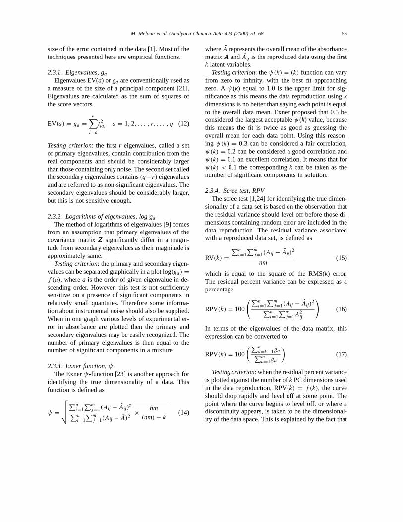
size of the error contained in the data [1]. Most of thetechniques presented here are empirical functions.
2.3.1. Eigenvalues, gaEigenvalues EV(a) or ga are conventionally used as
a measure of the size of a principal component [21].Eigenvalues are calculated as the sum of squares ofthe score vectors
EV(a) = ga =n∑i=at2ia, a = 1,2, . . . , r, . . . , q (12)
Testing criterion: the first r eigenvalues, called a setof primary eigenvalues, contain contribution from thereal components and should be considerably largerthan those containing only noise. The second set calledthe secondary eigenvalues contains(q−r) eigenvaluesand are referred to as non-significant eigenvalues. Thesecondary eigenvalues should be considerably larger,but this is not sensitive enough.
2.3.2. Logarithms of eigenvalues, log ga
The method of logarithms of eigenvalues [9] comesfrom an assumption that primary eigenvalues of thecovariance matrixZZZ significantly differ in a magni-tude from secondary eigenvalues as their magnitude isapproximately same.
Testing criterion: the primary and secondary eigen-values can be separated graphically in a plot log(ga) =f (a), wherea is the order of given eigenvalue in de-scending order. However, this test is not sufficientlysensitive on a presence of significant components inrelatively small quantities. Therefore some informa-tion about instrumental noise should also be supplied.When in one graph various levels of experimental er-ror in absorbance are plotted then the primary andsecondary eigenvalues may be easily recognized. Thenumber of primary eigenvalues is then equal to thenumber of significant components in a mixture.
2.3.3. Exner function,ψThe Exnerψ-function [23] is another approach for
identifying the true dimensionality of a data. Thisfunction is defined as
ψ =√√√√∑n
i=1∑mj=1(Aij − Aij )2∑n
i=1∑mj=1(Aij − A)2
× nm
(nm)− k(14)
whereA represents the overall mean of the absorbancematrixAAA andAij is the reproduced data using the firstk latent variables.
Testing criterion: theψ(k) = (k) function can varyfrom zero to infinity, with the best fit approachingzero. Aψ(k) equal to 1.0 is the upper limit for sig-nificance as this means the data reproduction usingkdimensions is no better than saying each point is equalto the overall data mean. Exner proposed that 0.5 beconsidered the largest acceptableψ(k) value, becausethis means the fit is twice as good as guessing theoverall mean for each data point. Using this reason-ing ψ(k) = 0.3 can be considered a fair correlation,ψ(k) = 0.2 can be considered a good correlation andψ(k) = 0.1 an excellent correlation. It means that forψ(k) < 0.1 the correspondingk can be taken as thenumber of significant components in solution.
2.3.4. Scree test, RPVThe scree test [1,24] for identifying the true dimen-
sionality of a data set is based on the observation thatthe residual variance should level off before those di-mensions containing random error are included in thedata reproduction. The residual variance associatedwith a reproduced data set, is defined as
RV(k) =∑ni=1∑mj=1(Aij − Aij )
2
nm(15)
which is equal to the square of the RMS(k) error.The residual percent variance can be expressed as apercentage
RPV(k) = 100
(∑ni=1∑mj=1(Aij − Aij )
2∑ni=1∑mj=1A
2ij
)(16)
In terms of the eigenvalues of the data matrix, thisexpression can be converted to
RPV(k) = 100
(∑ma=k+1ga∑ma=1ga
)(17)
Testing criterion: when the residual percent varianceis plotted against the number ofk PC dimensions usedin the data reproduction, RPV(k) = f (k), the curveshould drop rapidly and level off at some point. Thepoint where the curve begins to level off, or where adiscontinuity appears, is taken to be the dimensional-ity of the data space. This is explained by the fact that
56 M. Meloun et al. / Analytica Chimica Acta 423 (2000) 51–68
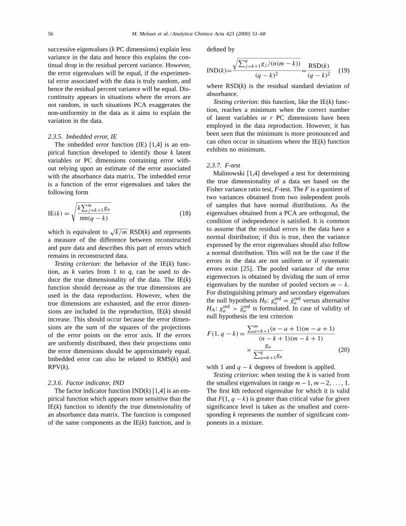
successive eigenvalues (k PC dimensions) explain lessvariance in the data and hence this explains the con-tinual drop in the residual percent variance. However,the error eigenvalues will be equal, if the experimen-tal error associated with the data is truly random, andhence the residual percent variance will be equal. Dis-continuity appears in situations where the errors arenot random, in such situations PCA exaggerates thenon-uniformity in the data as it aims to explain thevariation in the data.
2.3.5. Imbedded error, IEThe imbedded error function (IE) [1,4] is an em-
pirical function developed to identify thosek latentvariables or PC dimensions containing error with-out relying upon an estimate of the error associatedwith the absorbance data matrix. The imbedded erroris a function of the error eigenvalues and takes thefollowing form
IE(k) =√k∑mj=k+1ga
nm(q − k)(18)
which is equivalent to√k/m RSD(k) and represents
a measure of the difference between reconstructedand pure data and describes this part of errors whichremains in reconstructed data.
Testing criterion: the behavior of the IE(k) func-tion, as k varies from 1 toq, can be used to de-duce the true dimensionality of the data. The IE(k)function should decrease as the true dimensions areused in the data reproduction. However, when thetrue dimensions are exhausted, and the error dimen-sions are included in the reproduction, IE(k) shouldincrease. This should occur because the error dimen-sions are the sum of the squares of the projectionsof the error points on the error axis. If the errorsare uniformly distributed, then their projections ontothe error dimensions should be approximately equal.Imbedded error can also be related to RMS(k) andRPV(k).
2.3.6. Factor indicator, INDThe factor indicator function IND(k) [1,4] is an em-
pirical function which appears more sensitive than theIE(k) function to identify the true dimensionality ofan absorbance data matrix. The function is composedof the same components as the IE(k) function, and is
defined by
IND(k)=√∑q
j=k+1gj/(n(m− k))
(q − k)2= RSD(k)
(q − k)2(19)
where RSD(k) is the residual standard deviation ofabsorbance.
Testing criterion: this function, like the IE(k) func-tion, reaches a minimum when the correct numberof latent variables orr PC dimensions have beenemployed in the data reproduction. However, it hasbeen seen that the minimum is more pronounced andcan often occur in situations where the IE(k) functionexhibits no minimum.
2.3.7. F-testMalinowski [1,4] developed a test for determining
the true dimensionality of a data set based on theFisher variance ratio test,F-test. TheF is a quotient oftwo variances obtained from two independent poolsof samples that have normal distributions. As theeigenvalues obtained from a PCA are orthogonal, thecondition of independence is satisfied. It is commonto assume that the residual errors in the data have anormal distribution; if this is true, then the varianceexpressed by the error eigenvalues should also followa normal distribution. This will not be the case if theerrors in the data are not uniform or if systematicerrors exist [25]. The pooled variance of the erroreigenvectors is obtained by dividing the sum of erroreigenvalues by the number of pooled vectorsm − k.For distinguishing primary and secondary eigenvaluesthe null hypothesisH0: gred
a = greda versus alternative
HA: greda > gred
a is formulated. In case of validity ofnull hypothesis the test criterion
F(1, q − k)=∑ma=k+1(n− a + 1)(m− a + 1)
(n− k + 1)(m− k + 1)
× ga∑q
a=k+1ga(20)
with 1 andq − k degrees of freedom is applied.Testing criterion: when testing thek is varied from
the smallest eigenvalues in rangem−1,m−2, . . . , 1.The firstkth reduced eigenvalue for which it is validthatF(1, q − k) is greater than critical value for givensignificance level is taken as the smallest and corre-spondingk represents the number of significant com-ponents in a mixture.
M. Meloun et al. / Analytica Chimica Acta 423 (2000) 51–68 57
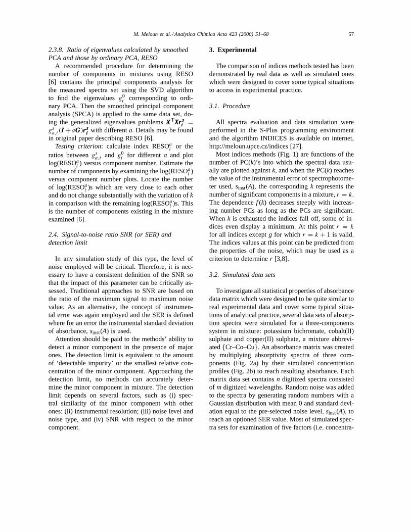
2.3.8. Ratio of eigenvalues calculated by smoothedPCA and those by ordinary PCA, RESO
A recommended procedure for determining thenumber of components in mixtures using RESO[6] contains the principal components analysis forthe measured spectra set using the SVD algorithmto find the eigenvaluesg0
i corresponding to ordi-nary PCA. Then the smoothed principal componentanalysis (SPCA) is applied to the same data set, do-ing the generalized eigenvalues problemsXXXTXrXrXr sssiii =gsa,i(III +aGGG)rrrsss
iiiwith differenta. Details may be found
in original paper describing RESO [6].Testing criterion: calculate index RESOai or the
ratios betweengsa,i and g0i for different a and plot
log(RESOai ) versus component number. Estimate thenumber of components by examining the log(RESOa
i )versus component number plots. Locate the numberof log(RESOai )s which are very close to each otherand do not change substantially with the variation ofkin comparison with the remaining log(RESOai )s. Thisis the number of components existing in the mixtureexamined [6].
2.4. Signal-to-noise ratio SNR (or SER) anddetection limit
In any simulation study of this type, the level ofnoise employed will be critical. Therefore, it is nec-essary to have a consistent definition of the SNR sothat the impact of this parameter can be critically as-sessed. Traditional approaches to SNR are based onthe ratio of the maximum signal to maximum noisevalue. As an alternative, the concept of instrumen-tal error was again employed and the SER is definedwhere for an error the instrumental standard deviationof absorbance,sinst(A) is used.
Attention should be paid to the methods’ ability todetect a minor component in the presence of majorones. The detection limit is equivalent to the amountof ‘detectable impurity’ or the smallest relative con-centration of the minor component. Approaching thedetection limit, no methods can accurately deter-mine the minor component in mixture. The detectionlimit depends on several factors, such as (i) spec-tral similarity of the minor component with otherones; (ii) instrumental resolution; (iii) noise level andnoise type, and (iv) SNR with respect to the minorcomponent.
3. Experimental
The comparison of indices methods tested has beendemonstrated by real data as well as simulated oneswhich were designed to cover some typical situationsto access in experimental practice.
3.1. Procedure
All spectra evaluation and data simulation wereperformed in the S-Plus programming environmentand the algorithm INDICES is available on internet,http://meloun.upce.cz/indices [27].
Most indices methods (Fig. 1) are functions of thenumber of PC(k)’s into which the spectral data usu-ally are plotted againstk, and when the PC(k) reachesthe value of the instrumental error of spectrophotome-ter used,sinst(A), the correspondingk represents thenumber of significant components in a mixture,r = k.The dependencef (k) decreases steeply with increas-ing number PCs as long as the PCs are significant.Whenk is exhausted the indices fall off, some of in-dices even display a minimum. At this pointr = k
for all indices exceptg for which r = k + 1 is valid.The indices values at this point can be predicted fromthe properties of the noise, which may be used as acriterion to determiner [3,8].
3.2. Simulated data sets
To investigate all statistical properties of absorbancedata matrix which were designed to be quite similar toreal experimental data and cover some typical situa-tions of analytical practice, several data sets of absorp-tion spectra were simulated for a three-componentssystem in mixture: potassium bichromate, cobalt(II)sulphate and copper(II) sulphate, a mixture abbrevi-ated{Cr–Co–Cu}. An absorbance matrix was createdby multiplying absorptivity spectra of three com-ponents (Fig. 2a) by their simulated concentrationprofiles (Fig. 2b) to reach resulting absorbance. Eachmatrix data set containsn digitized spectra consistedof m digitized wavelengths. Random noise was addedto the spectra by generating random numbers with aGaussian distribution with mean 0 and standard devi-ation equal to the pre-selected noise level,sinst(A), toreach an optioned SER value. Most of simulated spec-tra sets for examination of five factors (i.e. concentra-
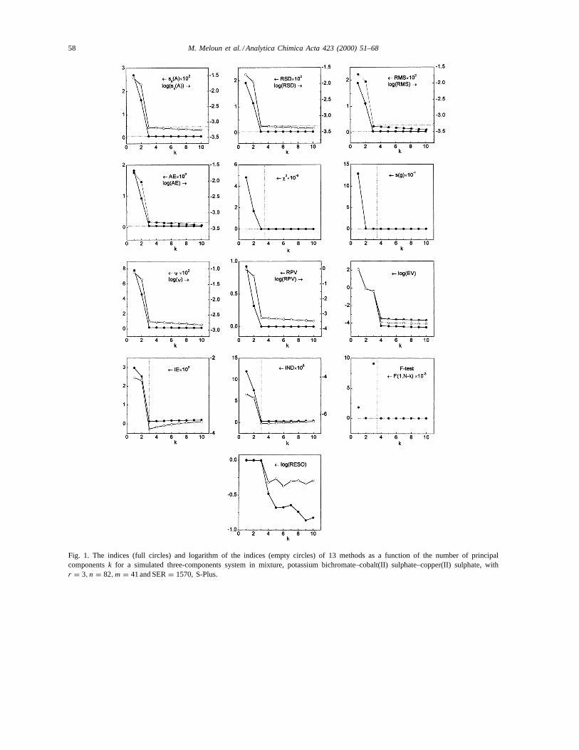
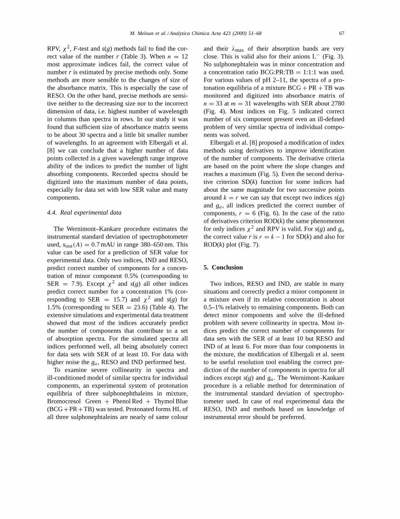
58 M. Meloun et al. / Analytica Chimica Acta 423 (2000) 51–68
Fig. 1. The indices (full circles) and logarithm of the indices (empty circles) of 13 methods as a function of the number of principalcomponentsk for a simulated three-components system in mixture, potassium bichromate–cobalt(II) sulphate–copper(II) sulphate, withr = 3, n = 82,m = 41 and SER= 1570, S-Plus.
M. Meloun et al. / Analytica Chimica Acta 423 (2000) 51–68 59
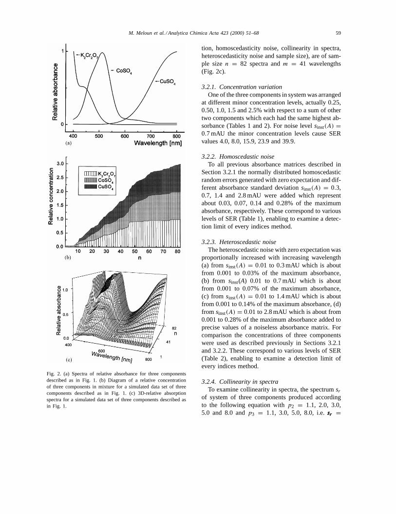
Fig. 2. (a) Spectra of relative absorbance for three componentsdescribed as in Fig. 1. (b) Diagram of a relative concentrationof three components in mixture for a simulated data set of threecomponents described as in Fig. 1. (c) 3D-relative absorptionspectra for a simulated data set of three components described asin Fig. 1.
tion, homoscedasticity noise, collinearity in spectra,heteroscedasticity noise and sample size), are of sam-ple sizen = 82 spectra andm = 41 wavelengths(Fig. 2c).
3.2.1. Concentration variationOne of the three components in system was arranged
at different minor concentration levels, actually 0.25,0.50, 1.0, 1.5 and 2.5% with respect to a sum of othertwo components which each had the same highest ab-sorbance (Tables 1 and 2). For noise levelsinst(A) =0.7 mAU the minor concentration levels cause SERvalues 4.0, 8.0, 15.9, 23.9 and 39.9.
3.2.2. Homoscedastic noiseTo all previous absorbance matrices described in
Section 3.2.1 the normally distributed homoscedasticrandom errors generated with zero expectation and dif-ferent absorbance standard deviationsinst(A) = 0.3,0.7, 1.4 and 2.8 mAU were added which representabout 0.03, 0.07, 0.14 and 0.28% of the maximumabsorbance, respectively. These correspond to variouslevels of SER (Table 1), enabling to examine a detec-tion limit of every indices method.
3.2.3. Heteroscedastic noiseThe heteroscedastic noise with zero expectation was
proportionally increased with increasing wavelength(a) from sinst(A) = 0.01 to 0.3 mAU which is aboutfrom 0.001 to 0.03% of the maximum absorbance,(b) from sinst(A) 0.01 to 0.7 mAU which is aboutfrom 0.001 to 0.07% of the maximum absorbance,(c) from sinst(A) = 0.01 to 1.4 mAU which is aboutfrom 0.001 to 0.14% of the maximum absorbance, (d)from sinst(A) = 0.01 to 2.8 mAU which is about from0.001 to 0.28% of the maximum absorbance added toprecise values of a noiseless absorbance matrix. Forcomparison the concentrations of three componentswere used as described previously in Sections 3.2.1and 3.2.2. These correspond to various levels of SER(Table 2), enabling to examine a detection limit ofevery indices method.
3.2.4. Collinearity in spectraTo examine collinearity in spectra, the spectrumsr
of system of three components produced accordingto the following equation withp2 = 1.1, 2.0, 3.0,5.0 and 8.0 andp3 = 1.1, 3.0, 5.0, 8.0, i.e.srsrsr =
60 M. Meloun et al. / Analytica Chimica Acta 423 (2000) 51–68
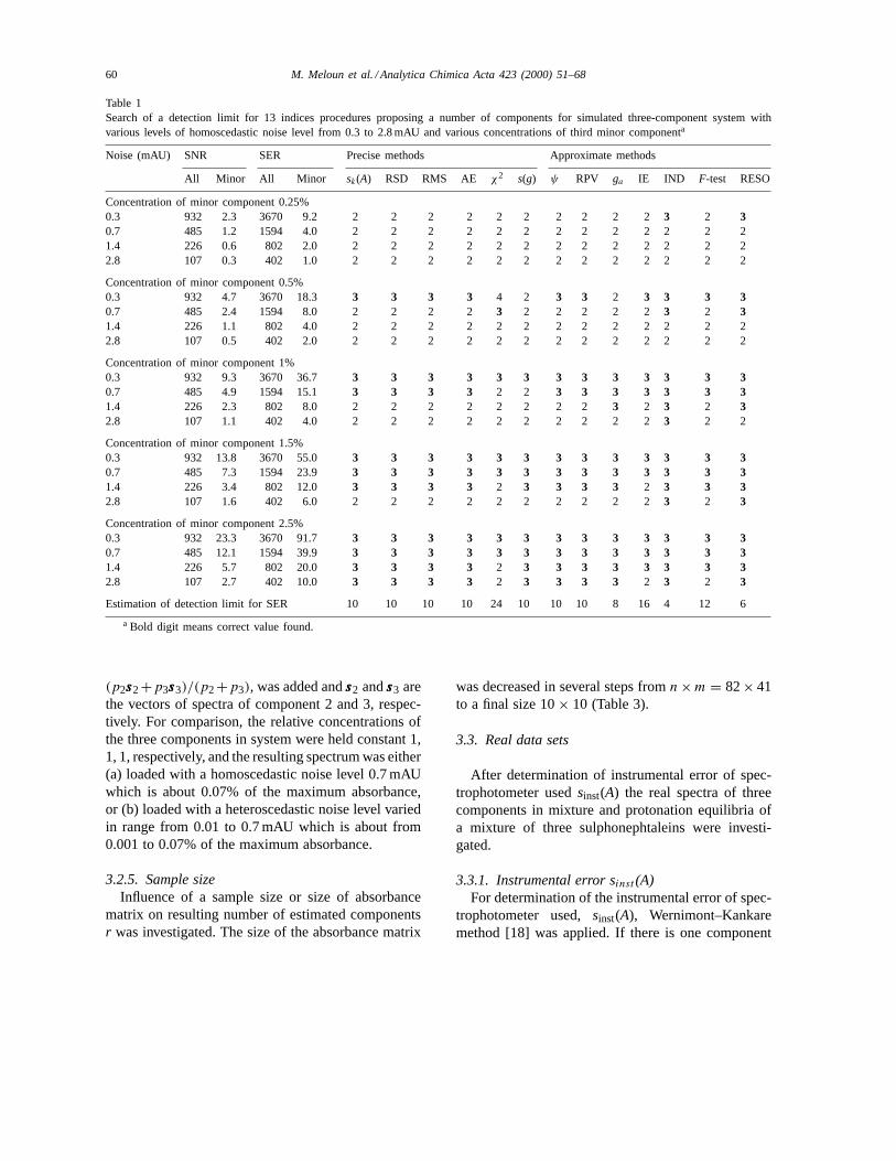
Table 1Search of a detection limit for 13 indices procedures proposing a number of components for simulated three-component system withvarious levels of homoscedastic noise level from 0.3 to 2.8 mAU and various concentrations of third minor componenta
Noise (mAU) SNR SER Precise methods Approximate methods
All Minor All Minor sk(A) RSD RMS AE χ2 s(g) ψ RPV ga IE IND F-test RESO
Concentration of minor component 0.25%0.3 932 2.3 3670 9.2 2 2 2 2 2 2 2 2 2 23 2 30.7 485 1.2 1594 4.0 2 2 2 2 2 2 2 2 2 2 2 2 21.4 226 0.6 802 2.0 2 2 2 2 2 2 2 2 2 2 2 2 22.8 107 0.3 402 1.0 2 2 2 2 2 2 2 2 2 2 2 2 2
Concentration of minor component 0.5%0.3 932 4.7 3670 18.3 3 3 3 3 4 2 3 3 2 3 3 3 30.7 485 2.4 1594 8.0 2 2 2 2 3 2 2 2 2 2 3 2 31.4 226 1.1 802 4.0 2 2 2 2 2 2 2 2 2 2 2 2 22.8 107 0.5 402 2.0 2 2 2 2 2 2 2 2 2 2 2 2 2
Concentration of minor component 1%0.3 932 9.3 3670 36.7 3 3 3 3 3 3 3 3 3 3 3 3 30.7 485 4.9 1594 15.1 3 3 3 3 2 2 3 3 3 3 3 3 31.4 226 2.3 802 8.0 2 2 2 2 2 2 2 2 3 2 3 2 32.8 107 1.1 402 4.0 2 2 2 2 2 2 2 2 2 23 2 2
Concentration of minor component 1.5%0.3 932 13.8 3670 55.0 3 3 3 3 3 3 3 3 3 3 3 3 30.7 485 7.3 1594 23.9 3 3 3 3 3 3 3 3 3 3 3 3 31.4 226 3.4 802 12.0 3 3 3 3 2 3 3 3 3 2 3 3 32.8 107 1.6 402 6.0 2 2 2 2 2 2 2 2 2 23 2 3
Concentration of minor component 2.5%0.3 932 23.3 3670 91.7 3 3 3 3 3 3 3 3 3 3 3 3 30.7 485 12.1 1594 39.9 3 3 3 3 3 3 3 3 3 3 3 3 31.4 226 5.7 802 20.0 3 3 3 3 2 3 3 3 3 3 3 3 32.8 107 2.7 402 10.0 3 3 3 3 2 3 3 3 3 2 3 2 3
Estimation of detection limit for SER 10 10 10 10 24 10 10 10 8 16 4 12 6
a Bold digit means correct value found.
(p2sss2+p3sss3)/(p2+p3), was added andsss2 andsss3 arethe vectors of spectra of component 2 and 3, respec-tively. For comparison, the relative concentrations ofthe three components in system were held constant 1,1, 1, respectively, and the resulting spectrum was either(a) loaded with a homoscedastic noise level 0.7 mAUwhich is about 0.07% of the maximum absorbance,or (b) loaded with a heteroscedastic noise level variedin range from 0.01 to 0.7 mAU which is about from0.001 to 0.07% of the maximum absorbance.
3.2.5. Sample sizeInfluence of a sample size or size of absorbance
matrix on resulting number of estimated componentsr was investigated. The size of the absorbance matrix
was decreased in several steps fromn×m = 82× 41to a final size 10× 10 (Table 3).
3.3. Real data sets
After determination of instrumental error of spec-trophotometer usedsinst(A) the real spectra of threecomponents in mixture and protonation equilibria ofa mixture of three sulphonephtaleins were investi-gated.
3.3.1. Instrumental error sinst (A)For determination of the instrumental error of spec-
trophotometer used,sinst(A), Wernimont–Kankaremethod [18] was applied. If there is one component
M. Meloun et al. / Analytica Chimica Acta 423 (2000) 51–68 61
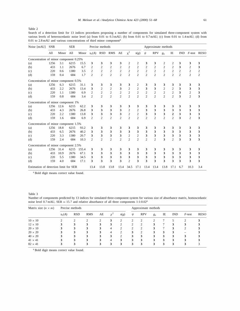
Table 2Search of a detection limit for 13 indices procedures proposing a number of components for simulated three-component system withvarious levels of heteroscedastic noise level (a) from 0.01 to 0.3 mAU; (b) from 0.01 to 0.7 mAU; (c) from 0.01 to 1.4 mAU; (d) from0.01 to 2.8 mAU and various concentrations of third minor componenta
Noise [mAU] SNR SER Precise methods Approximate methods
All Minor All Minor sk(A) RSD RMS AE x2 s(g) ψ RPV ga IE IND F-test RESO
Concentration of minor component 0.25%(a) 1256 3.1 6215 15.5 3 3 3 3 2 2 3 3 2 2 3 3 3(b) 433 1.1 2676 6.7 2 2 2 2 2 2 2 2 2 2 3 2 3(c) 220 0.6 1380 3.5 2 2 2 2 2 2 2 2 2 2 2 2 2(d) 159 0.4 684 1.7 2 2 2 2 2 2 2 2 2 2 2 2 2
Concentration of minor component 0.5%(a) 1256 6.3 6215 31.1 3 3 3 3 3 2 3 3 3 3 3 3 3(b) 433 2.2 2676 13.4 3 2 2 3 2 2 3 3 2 2 3 3 3(c) 220 1.1 1380 6.9 2 2 2 2 2 2 2 2 2 2 3 2 3(d) 159 0.8 684 3.4 2 2 2 2 2 2 2 2 2 2 3 2 3
Concentration of minor component 1%(a) 1256 12.6 6215 62.2 3 3 3 3 3 3 3 3 3 3 3 3 3(b) 433 4.3 2676 26.8 3 3 3 3 2 2 3 3 3 3 3 3 3(c) 220 2.2 1380 13.8 3 3 3 3 2 2 3 3 3 2 3 3 3(d) 159 1.6 684 6.9 2 2 2 2 2 2 2 2 2 2 3 2 3
Concentration of minor component 1.5%(a) 1256 18.8 6215 93.2 3 3 3 3 3 3 3 3 3 3 3 3 3(b) 433 6.5 2676 40.2 3 3 3 3 3 3 3 3 3 3 3 3 3(c) 220 3.3 1380 20.7 3 3 3 3 2 2 3 3 3 3 3 3 3(d) 159 2.4 684 10.3 2 2 2 2 2 2 2 2 3 2 3 3 3
Concentration of minor component 2.5%(a) 1256 31.4 6215 155.4 3 3 3 3 3 3 3 3 3 3 3 3 3(b) 433 10.9 2676 67.1 3 3 3 3 3 3 3 3 3 3 3 3 3(c) 220 5.5 1380 34.5 3 3 3 3 3 3 3 3 3 3 3 3 3(d) 159 4.0 684 17.1 3 3 3 3 2 3 3 3 3 3 3 3 3
Estimation of detection limit for SER 13.4 13.8 13.8 13.4 34.5 17.1 13.4 13.4 13.8 17.1 6.7 10.3 3.4
a Bold digit means correct value found.
Table 3Number of components predicted by 13 indices for simulated three-component system for various size of absorbance matrix, homoscedasticnoise level 0.7 mAU, SER= 15.7 and relative absorbance of all three components 1:1:0.02a
Matrix size (n×m) Precise methods Approximate methods
sk(A) RSD RMS AE χ2 s(g) ψ RPV ga IE IND F-test RESO
10× 10 2 2 2 2 3 2 2 2 2 7 5 2 312× 10 3 3 3 3 3 2 2 2 3 7 3 3 320× 10 3 3 3 3 4 2 2 2 3 7 3 2 320× 20 3 3 3 3 4 2 3 2 3 3 3 – 340× 20 3 3 3 3 3 2 3 3 3 3 3 3 341× 41 3 3 3 3 4 3 3 3 3 3 3 3 382× 41 3 3 3 3 3 3 3 3 3 3 3 3 3
a Bold digit means correct value found.
62 M. Meloun et al. / Analytica Chimica Acta 423 (2000) 51–68
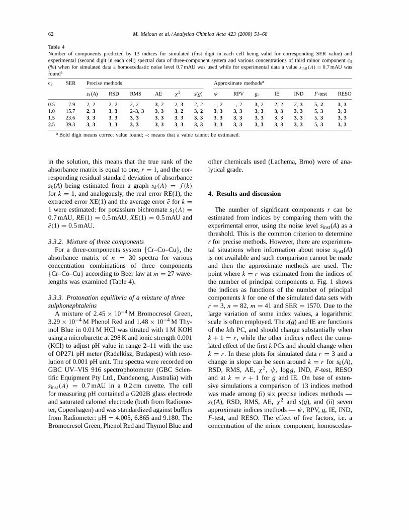
Table 4Number of components predicted by 13 indices for simulated (first digit in each cell being valid for corresponding SER value) andexperimental (second digit in each cell) spectral data of three-component system and various concentrations of third minor componentc3
(%) when for simulated data a homoscedastic noise level 0.7 mAU was used while for experimental data a valuesinst(A) = 0.7 mAU wasfounda
c3 SER Precise methods Approximate methodsa
sk(A) RSD RMS AE χ2 s(g) ψ RPV ga IE IND F-test RESO
0.5 7.9 2, 2 2, 2 2, 2 3, 2 2, 3 2, 2 –, 2 –, 2 3, 2 2, 2 2,3 5, 2 3, 31.0 15.7 2, 3 3, 3 2–3, 3 3, 3 3, 2 3, 2 3, 3 3, 3 3, 3 3, 3 3, 3 5, 3 3, 31.5 23.6 3, 3 3, 3 3, 3 3, 3 3, 3 3, 3 3, 3 3, 3 3, 3 3, 3 3, 3 5, 3 3, 32.5 39.3 3, 3 3, 3 3, 3 3, 3 3, 3 3, 3 3, 3 3, 3 3, 3 3, 3 3, 3 5, 3 3, 3
a Bold digit means correct value found; –: means that a value cannot be estimated.
in the solution, this means that the true rank of theabsorbance matrix is equal to one,r = 1, and the cor-responding residual standard deviation of absorbancesk(A) being estimated from a graphsk(A) = f (k)
for k = 1, and analogously, the real error RE(1), theextracted error XE(1) and the average errore for k =1 were estimated: for potassium bichromates1(A) =0.7 mAU, RE(1) = 0.5 mAU, XE(1) = 0.5 mAU ande(1) = 0.5 mAU.
3.3.2. Mixture of three componentsFor a three-components system{Cr–Co–Cu}, the
absorbance matrix ofn = 30 spectra for variousconcentration combinations of three components{Cr–Co–Cu} according to Beer law atm = 27 wave-lengths was examined (Table 4).
3.3.3. Protonation equilibria of a mixture of threesulphonephtaleins
A mixture of 2.45 × 10⁻⁴ M Bromocresol Green,3.29× 10−4 M Phenol Red and 1.48× 10⁻⁴ M Thy-mol Blue in 0.01 M HCl was titrated with 1 M KOHusing a microburette at 298 K and ionic strength 0.001(KCl) to adjust pH value in range 2–11 with the useof OP271 pH meter (Radelkisz, Budapest) with reso-lution of 0.001 pH unit. The spectra were recorded onGBC UV–VIS 916 spectrophotometer (GBC Scien-tific Equipment Pty Ltd., Dandenong, Australia) withsinst(A) = 0.7 mAU in a 0.2 cm cuvette. The cellfor measuring pH contained a G202B glass electrodeand saturated calomel electrode (both from Radiome-ter, Copenhagen) and was standardized against buffersfrom Radiometer: pH= 4.005, 6.865 and 9.180. TheBromocresol Green, Phenol Red and Thymol Blue and
other chemicals used (Lachema, Brno) were of ana-lytical grade.
4. Results and discussion
The number of significant componentsr can beestimated from indices by comparing them with theexperimental error, using the noise levelsinst(A) as athreshold. This is the common criterion to determiner for precise methods. However, there are experimen-tal situations when information about noisesinst(A)is not available and such comparison cannot be madeand then the approximate methods are used. Thepoint wherek = r was estimated from the indices ofthe number of principal componentsa. Fig. 1 showsthe indices as functions of the number of principalcomponentsk for one of the simulated data sets withr = 3, n = 82,m = 41 and SER= 1570. Due to thelarge variation of some index values, a logarithmicscale is often employed. Thes(g) and IE are functionsof the kth PC, and should change substantially whenk + 1 = r, while the other indices reflect the cumu-lated effect of the firstk PCs and should change whenk = r. In these plots for simulated datar = 3 and achange in slope can be seen aroundk = r for sk(A),RSD, RMS, AE, χ2, ψ , logg, IND, F-test, RESOand atk = r + 1 for g and IE. On base of exten-sive simulations a comparison of 13 indices methodwas made among (i) six precise indices methods —sk(A), RSD, RMS, AE,χ2 and s(g), and (ii) sevenapproximate indices methods —ψ , RPV, g, IE, IND,F-test, and RESO. The effect of five factors, i.e. aconcentration of the minor component, homoscedas-
M. Meloun et al. / Analytica Chimica Acta 423 (2000) 51–68 63
tic noise, collinearity in spectra, heteroscedastic noiseand sample size was investigated and the detection ofthe limit of the true value of number of componentsof each method was estimated. The indices were usedto analyze real experimental data and the derivationmodifications SD and ROD were also used.
4.1. Homoscedastic noise, heteroscedastic noise andconcentration of the minor component
All three factors may be examined commonly us-ing an effective resolution criterion, the SNR or theSER. Both criteria cover all three factors and there-fore can be used as the common resolution factor. Forsimulated data sets withr = 3, n = 82,m = 41 therewere adjusted various SER values of homoscedasticnoise (Table 1). It is obvious that when SER is equalor higher than a detection limit, every index methodfails. Table 1 demonstrates an estimate of detectionlimit for individual methods in case of homoscedasticnoise: SER= 24 forχ2, SER= 16 for IE, SER= 12for F-test, SER= 10 for sk(A), RSD, RMS, AE,s(g)andψ , SER= 8 for ga , SER= 6 for RESO, SER=4 for IND. It means that for determination of the mi-nor component two methods, RESO and IND workbest and appear to be the most reliable. It is worthmentioning that most of the methods do not behavein the same way if the SER criterion decreases nearlyto their detection limit. Indicess(g), χ2 andF-test aredefinite, they are fully based on statistic criterion andit is not complicated to predictr. The situation is sim-ple in case of precise methods. Here we take thek forwhich the value of criterion is closest to the value ofexperimental error,sinst(A). However, we lose a helpfunction of the curve shape being used here as an ef-ficient criterion. Thus the indicesψ , and RPV whichare based on detecting a break-point on the curve, arenot very reliable in prediction ofr in case of decreas-ing a SER. Thega and RESO are reliable enough.
For heteroscedastic noise (Table 2) an esti-mate of detection limit for individual methods are:SER = 34.5 for χ2, SER = 17.1 for s(g) and IE,SER = 13.4–13.8 for sk(A), RSD, RMS, AE, RPV,ga andψ , SER = 10.3 for F-test, SER= 6.7 forIND and SER = 3.4 for RESO. Once again RESOand IND work best, which demonstrates their abilityin the presence of heteroscedastic noise. A possibleexplanation [6] might be that heteroscedastic noise
does affect the eigenvalues of both SPCA and PCAbut has no influence on their ratios.
4.2. Collinearity in spectra
Even severe collinearity in spectra that arranged allthe indices predicted a correct number of componentsin mixture.
4.3. Sample size
Decreasing size from(n × m) = (82 × 41) to(40× 20) all indices found correct value of the num-ber r. Decreasing size from (40× 20) to (20× 20)
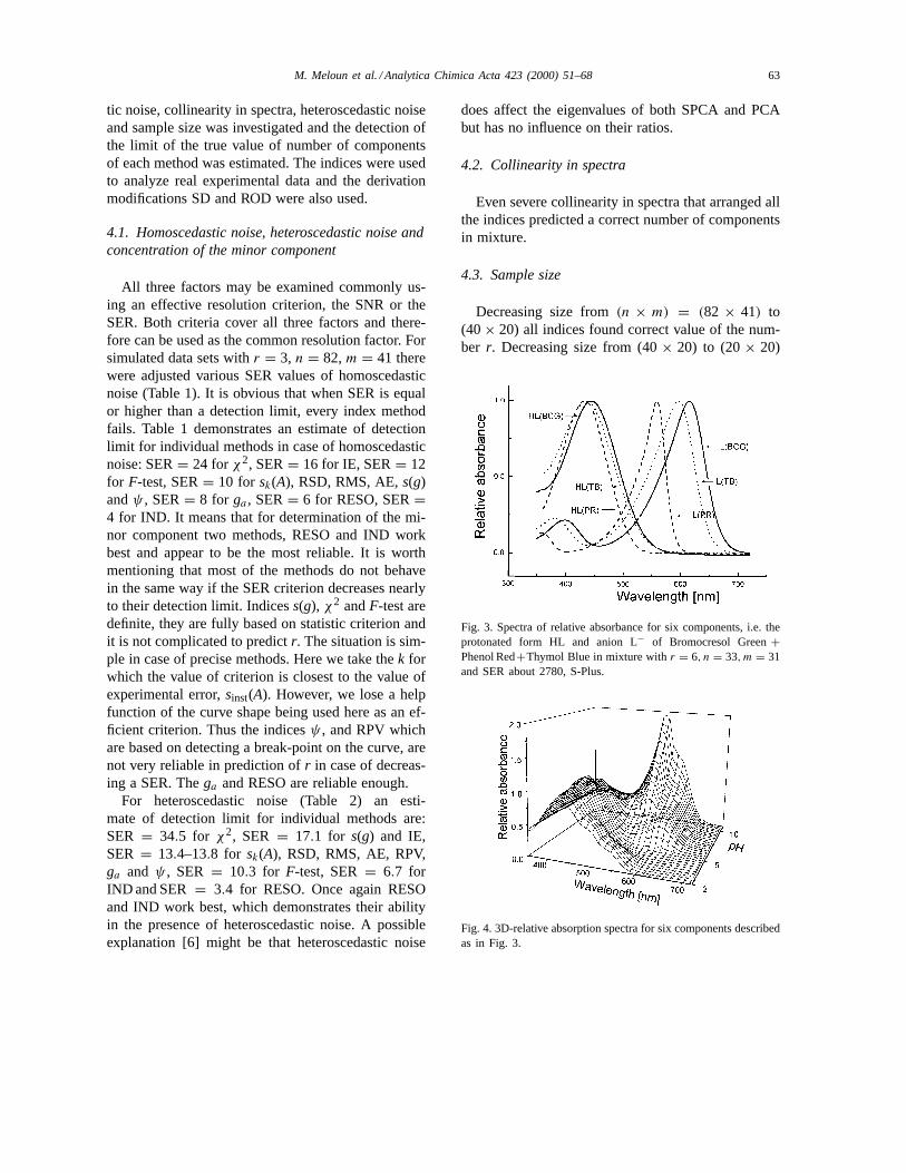
Fig. 3. Spectra of relative absorbance for six components, i.e. theprotonated form HL and anion L− of Bromocresol Green+Phenol Red+Thymol Blue in mixture withr = 6, n = 33,m = 31and SER about 2780, S-Plus.
Fig. 4. 3D-relative absorption spectra for six components describedas in Fig. 3.
64 M. Meloun et al. / Analytica Chimica Acta 423 (2000) 51–68
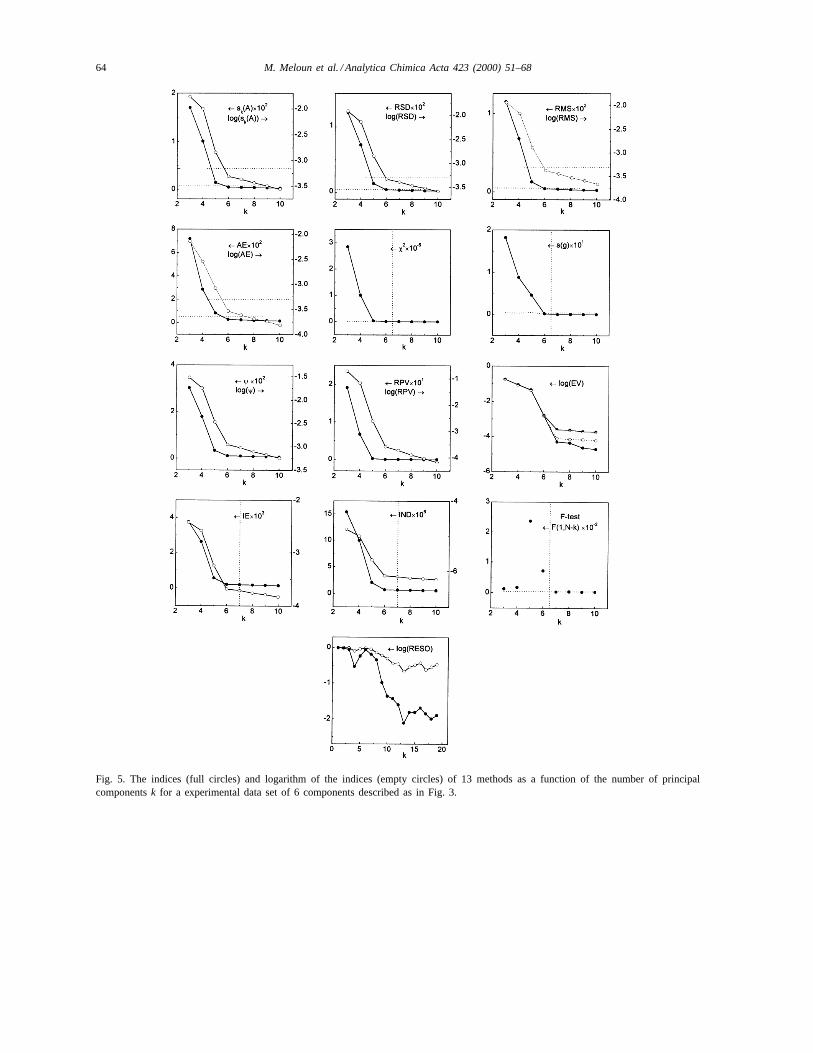
Fig. 5. The indices (full circles) and logarithm of the indices (empty circles) of 13 methods as a function of the number of principalcomponentsk for a experimental data set of 6 components described as in Fig. 3.

M. Meloun et al. / Analytica Chimica Acta 423 (2000) 51–68 65
Fig. 6. The second derivative detection criterium applied on 11 indices methods described as in Fig. 3.
66 M. Meloun et al. / Analytica Chimica Acta 423 (2000) 51–68
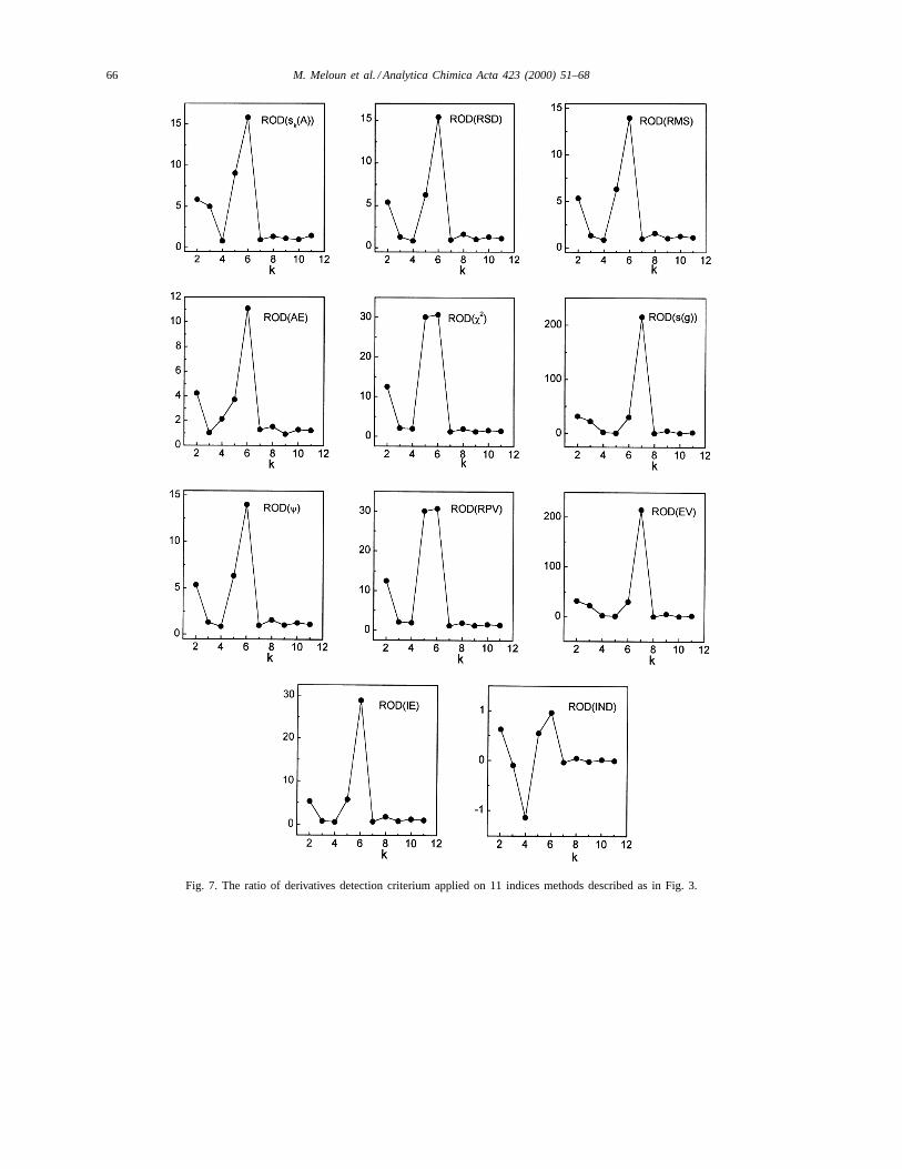
Fig. 7. The ratio of derivatives detection criterium applied on 11 indices methods described as in Fig. 3.
M. Meloun et al. / Analytica Chimica Acta 423 (2000) 51–68 67
RPV,χ2, F-test ands(g) methods fail to find the cor-rect value of the numberr (Table 3). Whenn = 12most approximate indices fail, the correct value ofnumberr is estimated by precise methods only. Somemethods are more sensible to the changes of size ofthe absorbance matrix. This is especially the case ofRESO. On the other hand, precise methods are sensi-tive neither to the decreasing size nor to the incorrectdimension of data, i.e. highest number of wavelengthin columns than spectra in rows. In our study it wasfound that sufficient size of absorbance matrix seemsto be about 30 spectra and a little bit smaller numberof wavelengths. In an agreement with Elbergali et al.[8] we can conclude that a higher number of datapoints collected in a given wavelength range improveability of the indices to predict the number of lightabsorbing components. Recorded spectra should bedigitized into the maximum number of data points,especially for data set with low SER value and manycomponents.
4.4. Real experimental data
The Wernimont–Kankare procedure estimates theinstrumental standard deviation of spectrophotometerused,sinst(A) = 0.7 mAU in range 380–650 nm. Thisvalue can be used for a prediction of SER value forexperimental data. Only two indices, IND and RESO,predict correct number of components for a concen-tration of minor component 0.5% (corresponding toSER = 7.9). Exceptχ2 and s(g) all other indicespredict correct number for a concentration 1% (cor-responding to SER= 15.7) and χ2 and s(g) for1.5% (corresponding to SER= 23.6) (Table 4). Theextensive simulations and experimental data treatmentshowed that most of the indices accurately predictthe number of components that contribute to a setof absorption spectra. For the simulated spectra allindices performed well, all being absolutely correctfor data sets with SER of at least 10. For data withhigher noise thega , RESO and IND performed best.
To examine severe collinearity in spectra andill-conditioned model of similar spectra for individualcomponents, an experimental system of protonationequilibria of three sulphonephthaleins in mixture,Bromocresol Green+ Phenol Red+ Thymol Blue(BCG+PR+TB) was tested. Protonated forms HL ofall three sulphonephtaleins are nearly of same colour
and their λmax of their absorption bands are veryclose. This is valid also for their anions L− (Fig. 3).No sulphonephtalein was in minor concentration anda concentration ratio BCG:PR:TB= 1:1:1 was used.For various values of pH 2–11, the spectra of a pro-tonation equilibria of a mixture BCG+ PR+ TB wasmonitored and digitized into absorbance matrix ofn = 33 atm = 31 wavelengths with SER about 2780(Fig. 4). Most indices on Fig. 5 indicated correctnumber of six component present even an ill-definedproblem of very similar spectra of individual compo-nents was solved.
Elbergali et al. [8] proposed a modification of indexmethods using derivatives to improve identificationof the number of components. The derivative criteriaare based on the point where the slope changes andreaches a maximum (Fig. 5). Even the second deriva-tive criterion SD(k) function for some indices hadabout the same magnitude for two successive pointsaroundk = r we can say that except two indicess(g)and ga , all indices predicted the correct number ofcomponents,r = 6 (Fig. 6). In the case of the ratioof derivatives criterion ROD(k) the same phenomenonfor only indicesχ2 and RPV is valid. Fors(g) andgathe correct valuer is r = k− 1 for SD(k) and also forROD(k) plot (Fig. 7).
5. Conclusion
Two indices, RESO and IND, are stable in manysituations and correctly predict a minor component ina mixture even if its relative concentration is about0.5–1% relatively to remaining components. Both candetect minor components and solve the ill-definedproblem with severe collinearity in spectra. Most in-dices predict the correct number of components fordata sets with the SER of at least 10 but RESO andIND of at least 6. For more than four components inthe mixture, the modification of Elbergali et al. seemto be useful resolution tool enabling the correct pre-diction of the number of components in spectra for allindices excepts(g) andga . The Wernimont–Kankareprocedure is a reliable method for determination ofthe instrumental standard deviation of spectropho-tometer used. In case of real experimental data theRESO, IND and methods based on knowledge ofinstrumental error should be preferred.
68 M. Meloun et al. / Analytica Chimica Acta 423 (2000) 51–68
Acknowledgements
Financial support of Grant Agency of the Czech Re-public (Grant No 303/00/1559) is thankfully acknowl-edged. Karel Kupka is acknowledged for his help withINDICES written in S-Plus.
References
[1] E.R. Malinowski, Factor Analysis in Chemistry, 2nd Edition,Wiley, New York, 1991.
[2] M. Meloun, J. Havel, E. Högfeldt, Computation of SolutionEquilibria, Ellis Horwood, Chichester, 1988.
[3] E.R. Malinowski, J. Chemom. 13 (1999) 69.[4] E.R. Malinowski, Anal. Chem. 49 (1977) 612.[5] J.M. Deane, H.J.H. MacFie, J. Chemom. 3 (1989) 477.[6] Z.-P. Chen, Y.-Z. Liang, J.-H. Jiang, Y. Li, J.-Y. Qian, R.-Q.
Yu, J. Chemom. 13 (1999) 15.[7] Z.-P. Chen, J.-H. Jiang, Y. Li, H.-L. Shen, Y.-Z. Liag, R.-Q.
Yu, Anal. Chim. Acta 381 (1999) 233.[8] A.K. Elbergali, J. Nygren, M. Kubista, Anal. Chim. Acta 379
(1999) 143.[9] J.M. Dean, Data reduction using principal components
analysis, in: R.G. Brereton (Ed.), Multivariate Pattern Reco-gnition in Chemometrics Illustrated by Case Studies, Elsevier,Amsterdam, 1992.
[10] A.K. Elbergali, R.G. Brereton, Chemom. Intell. Lab. Syst. 27(1995) 55.
[11] Y.-Z. Liang, O. Kvalheim, A.M. Rahmani, R.G. Brereton, J.Chemom. 7 (1993) 15.
[12] S. Wold, C. Albano, W.J. Dunn, K. Esbensen, S. Hellberg,E. Johansson, M. Sjöström, in: Proceedings of the IUFOSTConference, Food Research and Data Analysis, AppliedScience Publishers, London, 1983, p. 147.
[13] M.A. Saraf, D.L. Illman, B.R. Kowalski, Chemometrics,Wiley, Chichester, 1986.
[14] H. Martens, T. Naes, Multivariate Calibration, Wiley,Chichester 1989.
[15] D.R. Cox, D. Oakes, Analysis of Survival Data, Chapman &Hall, London, 1984.
[16] D.L. Massart, R.G. Brereton, R.E. Dessy, P.K. Hopke, C.H.Spiegelman, W. Wegscheider (Eds.), Chemometrics Tutorials,Elsevier, Amsterdam, 1990.
[17] D.L. Massart, W. Wegscheider, B.G. Vandeginste, S.N.Deming, Y. Michotte, L. Kaufman, Chemometrics: A Text-book, Elsevier, Amsterdam, 1990.
[18] J.J. Kankare, Anal. Chem. 42 (1970) 1322.[19] M.S. Bartlett, Br. J. Psych. Stat. Sec. 3 (1950) 77.[20] Z.Z. Hugus Jr., A.A. El-Awady, J. Phys. Chem. 75 (1971)
2954.[21] T.M. Rossi, I.M. Warner, Anal. Chem. 54 (1986) 810.[22] H.F. Kaiser, Educ. Psych. Meas. 20 (1966) 141.[23] J.H. Kindsvater, P.H. Weiner, T.J. Klingen, Anal. Chem. 46
(1974) 982.[24] R.D. Catell, Multivariate Behav. Res. 1 (1966) 245.[25] E.R. Malinowski, J. Chemom. 1 (1987) 49.[26] M. Meloun, P. Miksik, Karel Kupka, Critical comparison
of factor analysis methods in spectra analysis determiningthe number of light-absorbing species, in: Proceedings ofthe XIIIth Seminar on Atomic Spectrochemistry, Podbánské,September 1996, pp. 307–329, ISBN 80-967325-7-9.
[27] Algorithm INDICES: http://meloun.upce.cz/indices.