PERIODICA POLYTECHNICA SER. SOC. MAN. SCI. VOL. 11, NO. 1, PP. 95–110 (2003)

CREDIT SCORING PROCESSES FROM A KNOWLEDGEMANAGEMENT PERSPECTIVE

Ferenc KISS

Department of Information and Knowledge ManagementBudapest University of Technology and Economics

H–1521 Budapest, HungaryPhone: (36 1) 463-1832, Fax: (36 1) 463-1225

e-mail: fek@itm.bme.hu

Received: January 9, 2003

Abstract

The success of credit/lending decisions is basically influenced by two factors: the quality of basic data(completeness, accuracy, credibility) and the quality of the decision making model (for individualdeals, the decision making process). While, however, the former is a rather technical criterion, thelatter is far more complex; still, to a great extent it depends on the knowledge and experience ofthe business experts shaping and implementing the decision making process. This work intendsto examine the relationship between widely used credit scoring models and the expansion and/orpreservation of the knowledge wealth of the organization.

Keywords: credit scoring, decision making process, knowledge wealth.

1. Changes in the Formalization of Lending Experience throughout theDevelopment of Credit Scoring

The lending practice of financial institutions shows four identifiable decision makingprocesses:

1. When the deal is initiated:

• Should the borrower be extended any credit at all?• Under what terms should the borrower be extended any credit?

2. During the lifecycle of the deal:

• Is there any intervention required in the deal process for any reason (de-lay, nonpayment, changes in the conditions of the bank or the customer,etc.)?

• If an intervention is required, how should the deal be continued (mod-ified interest and/or installment conditions, rescheduling, legal action,etc)?

Credit scoring methods were originally used to find answers to the first twoquestions only, but at present the new versions of these models – incorporatingseveral additional criteria – are also applied in later phases of the credit lifecycle.

96 F. KISS

In the beginning, credit/lending experience was transferred through involve-ment and cooperation, and required a long training period. In addition to the abilityto value the collaterals offered, this knowledge was based to a considerable extenton information about, and the assessment of, the applicant, the applicant’s employerand the society’s opinion on the intended purpose of the loan.

The foundations of the 60-plus-year history of credit scoring were laid byFISHER’s article published in 1936 [13], which examined the distinguishability ofgroups in a plant population based on various measured characteristics. As far as weknow, it was DUNHAM in 1938 [1] who first mentioned a system for the evaluationof credit applications, in which he used five criteria, as follows:

• position held;• income statement;• financial statement;• guarantors or collateral;• loan repayment data from banks.

DUNHAM argued that the importance of the various criteria should be deter-mined on the basis of experience (i.e. without applying any statistical technique).

It was DURAND in 1941 who wanted to know which parameters lenders foundimportant and which characteristics were significant statistically [12]. He was thefirst to use discrimination analysis, based on FISHER’s results. With this he actuallyprovided the impetus for the development of a theoretical framework that can beused to determine whether the significance of a certain criterion is justified. He alsomade recommendations for the analysis of credit risk. Therefore Durand may beregarded as the founder of the present-day credit scoring systems. In his 1941 studyhe presented a score-based system that could be used for the classification of peopleapplying for a loan to buy a second-hand car. The most important parameters of hisexamination were as follows:

• the applicant’s job/position;• the number of years spent in the current position;• the number of years spent at the current address;• bank accounts, life insurance policies;• sex;• the amount of the monthly installment.

DURAND’s model is the first formalized version of lending knowledge gainedfrom experience that lending companies could use as a decision making algorithm,without the continuous involvement of credit/lending experts. In this period, severalcompanies attempted to put down the knowledge of experienced experts in somesort of recipe; these sets of decision making rules can be regarded as the firstcredit/lending expert systems [16].

Experiments based on several parameters were conducted by CORDNER,MYERS and FORGY, among others, who focused more on financial characteris-tics and previous payment discipline as references [36], [37]. In 1963 MYERS and

CREDIT SCORING PROCESSES 97

FORGY also recommended the application of multivariate discrimination analysisto these parameters.

In an article published in the same year, MYERS also tried to gain insightinto the extent and direction of selection as performed by the person making thecredit decision. However, he did not investigate the correctness and farsightednessof such a decision [27].

It was MOORE and KLEIN who first wrote down in 1967 how criteria relatedto the performance of obligations changed with time [27]. This approach addedto previously applied decision making criteria the psychological and sociologicalconcepts used to describe the behaviour of the individual and communities.

The mass popularity of credit cards made it clear that the time required forone decision had to be maximized. This opened the door for scoring, which meantthe efficient formalization of lender knowledge. Starting in the late fifties, moreand more companies sprang up that offered the development and maintenance ofcredit scoring systems, and the acquisition and continuous updating of data requiredtherefor. The pioneering venture, and by far the biggest and most reputable to date,is Fair, Isaac & Co., established in 1956. It was BOGESS in an 1967 article [1]who first called for the use of a computer background, which made it possibleto examine large sets of data from various angles and try the complex tools ofmultivariate statistics, which led soon to the development of much more accuratemodels.

As scoring models have developed, the evaluation of mass lending productshas been characterized by increasing algorithmization. The bigger part of lend-ing knowledge is extracted from an experience database by mathematical analyses;these models are made up of edge conditions – specified by the lender – and math-ematically generated rules and formulas. This allows an increasing degree of au-tomation in the decision making process, resulting in a much less time requirementfor decisions than before.

At present, every lender supports the decision making processes of its lendingactivities and the monitoring of lending deals with data markets and data ware-houses. Data markets and data warehouses store not only information but alsoknowledge. The metadatabases created in data warehouses contain lots of defini-tions – approved by a consensus of the organization’s experts – that describe andexplain the dimensions of available databases for users. This information materialincludes not only coursebook definitions on the given set of data, but also a descrip-tion of the generation or creation of the information in question and – as part of thecompany’s own culture – special knowledge, interpretation, internal terminologyand wording related to the given subject.

2. The Most Widely Used Credit Scoring Models Are as Follows:

In terms of the theories and methods used to date, credit scoring models may bedivided into two large groups:

98 F. KISS

1. Parameteric credit scoring models• Linear probability model;• Probit and Logit models;• Discrimination analysis-based models;• Neural networks.

2. Non-parameteric credit scoring models• Mathematical programming;• Classification trees (recursive partitioning algorithms);• Nearest neighbours model;• Analytical hierarchy process;• Expert systems.

There is another class of artificial intelligence methods used widely in scoringsystems: genetic algorithms. These, however, do not constitute a separate modellingprocess; instead, they find the optimal version through a mutation of the existingset of score cards.

3. Linear Probability Model

The linear probability model is basically a regression model, where the value of thedependent variable is 0 or 1 according to whether the application in question hasbeen approved or not [6]. In mathematical terms, the decision making rule may beexpressed as follows:

y = b1x1 + b2x2 + . . . + bk xk + u, (1)

where: y is the dependent variable (the result of the decision),xi is explanatory variable (criterion) i ,bi is the weight assigned to explanatory variable i ,u is the random error, P(u) = 0.

In a vector expression:y = b′x + u, (2)

where: x is the vector of the explanatory variables,b′ the transpose of the parameter vector of the explanatory variables.

Consequently, theP(y | x) = b′x (3)

conditional probability can also be interpreted as the probability of approval of theapplication belonging to parameter group x. The estimated probability of approvalmay be interpreted similarly. Thus (1) yields the regression estimate of weights,so the estimated probability of approval may be calculated for a new application.When the lending decision is made, the score thus received should be compared toa cutoff score limit.

CREDIT SCORING PROCESSES 99

4. Probit and Logit Models

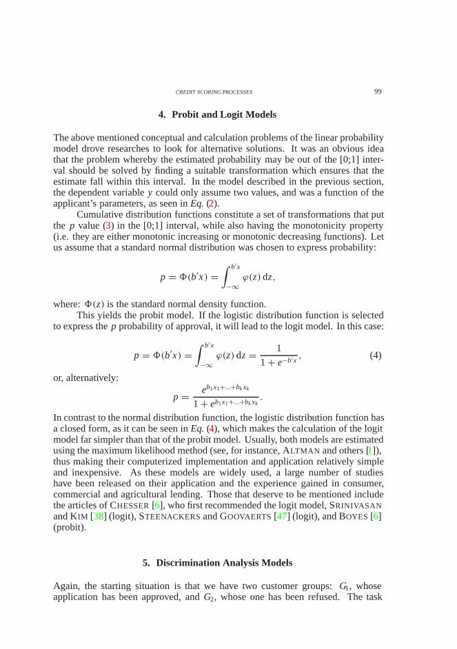
The above mentioned conceptual and calculation problems of the linear probabilitymodel drove researches to look for alternative solutions. It was an obvious ideathat the problem whereby the estimated probability may be out of the [0;1] inter-val should be solved by finding a suitable transformation which ensures that theestimate fall within this interval. In the model described in the previous section,the dependent variable y could only assume two values, and was a function of theapplicant’s parameters, as seen in Eq. (2).

Cumulative distribution functions constitute a set of transformations that putthe p value (3) in the [0;1] interval, while also having the monotonicity property(i.e. they are either monotonic increasing or monotonic decreasing functions). Letus assume that a standard normal distribution was chosen to express probability:

p = �(b′x) =∫ b′x

−∞ϕ(z) dz,

where: �(z) is the standard normal density function.This yields the probit model. If the logistic distribution function is selected

to express the p probability of approval, it will lead to the logit model. In this case:

p = �(b′x) =∫ b′x

−∞ϕ(z) dz = 1

1 + e−b′x , (4)

or, alternatively:

p = eb1x1+...+bk xk

1 + eb1x1+...+bk xk.

In contrast to the normal distribution function, the logistic distribution function hasa closed form, as it can be seen in Eq. (4), which makes the calculation of the logitmodel far simpler than that of the probit model. Usually, both models are estimatedusing the maximum likelihood method (see, for instance, ALTMAN and others [1]),thus making their computerized implementation and application relatively simpleand inexpensive. As these models are widely used, a large number of studieshave been released on their application and the experience gained in consumer,commercial and agricultural lending. Those that deserve to be mentioned includethe articles of CHESSER [6], who first recommended the logit model, SRINIVASANand KIM [38] (logit), STEENACKERS and GOOVAERTS [47] (logit), and BOYES [6](probit).

5. Discrimination Analysis Models

Again, the starting situation is that we have two customer groups: G1, whoseapplication has been approved, and G2, whose one has been refused. The task

100 F. KISS

is to classify a new applicant using the parameter vector x = (x1, x2, . . . , xk)representing them. The discrimination analysis solves this problem by generatinga so-called discrimination function λ′x, where λ is the vector of the coefficients andweights assigned to criteria xi . The model determines these values by creating thebiggest possible difference between the two groups.

We assume that vector x, which contains the applicant’s characteristics, ismultivariate and has normal distribution in the two groups. The groups may have thevector pairs (µ1,�1) and (µ2,�2) assigned to them, which represent group meansand covariances, respectively. pi should mean the probability that a certain applicantbelongs to group i , while ci j should mean the cost incurred due to misclassification,when an applicant in group i must be transferred to group j . In the event thatthe covariance matrixes of the two groups are equal, i.e. �1 = �2 = �, theclassification rule may be defined from the minimization of costs resulting from theanticipated misclassification. This yields the following results:an applicant characterized by data set x will be classified in a group G1 if

λ′x ≥ α + ln

(c21 p2

c12 p1

), (5)

where: λ = �−1(µ1 − µ2),

α = λ′(µ1 + µ2)

2.

In all other cases the applicant should be classified in group G2.The classification heuristics implemented with the above model is very simple.

The discrimination function, λ′x, may be generated through the linear weighting ofvector x, and then the resulting value must be compared to the cutoff score below:

‘cutoff’ = α + ln

(c21 p2

c12 p1

).

If the applicant is above the limit, he will be classified in group G1, otherwise inG2.

As in the previous model (5) the discrimination function has x as primaryparameter, this method is often referred to as linear discrimination analysis. Inthe event that the covariances of the two groups are not equal (�1 �= �2), theclassification rule will be quadratic for x, therefore this model is also referred to asquadratic discrimination analysis.1

1Other renowned scientists contributing significantly to the study of the development and ap-plication problems of models are included SEXTON [38] and REICHERT [39] in consumer lending,ORGLER [38] in commercial lending and HARDY and WEED [22] in agricultural lending.

CREDIT SCORING PROCESSES 101

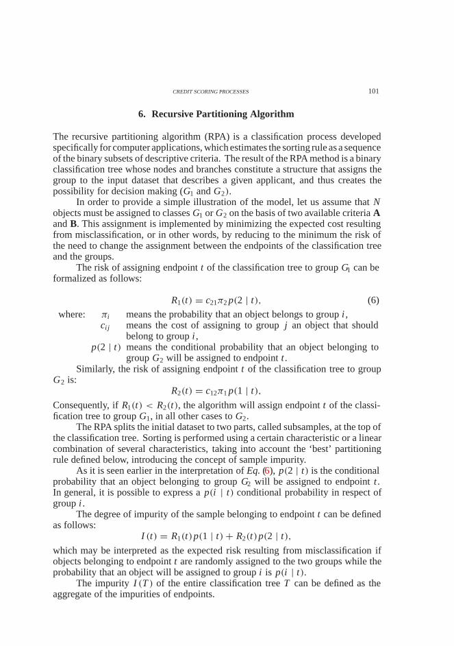
6. Recursive Partitioning Algorithm

The recursive partitioning algorithm (RPA) is a classification process developedspecifically for computer applications, which estimates the sorting rule as a sequenceof the binary subsets of descriptive criteria. The result of the RPA method is a binaryclassification tree whose nodes and branches constitute a structure that assigns thegroup to the input dataset that describes a given applicant, and thus creates thepossibility for decision making (G1 and G2).

In order to provide a simple illustration of the model, let us assume that Nobjects must be assigned to classes G1 or G2 on the basis of two available criteria Aand B. This assignment is implemented by minimizing the expected cost resultingfrom misclassification, or in other words, by reducing to the minimum the risk ofthe need to change the assignment between the endpoints of the classification treeand the groups.

The risk of assigning endpoint t of the classification tree to group G1 can beformalized as follows:

R1(t) = c21π2 p(2 | t), (6)

where: πi means the probability that an object belongs to group i ,ci j means the cost of assigning to group j an object that should

belong to group i ,p(2 | t) means the conditional probability that an object belonging to

group G2 will be assigned to endpoint t .Similarly, the risk of assigning endpoint t of the classification tree to group

G2 is:R2(t) = c12π1 p(1 | t),

Consequently, if R1(t) < R2(t), the algorithm will assign endpoint t of the classi-fication tree to group G1, in all other cases to G2.

The RPA splits the initial dataset to two parts, called subsamples, at the top ofthe classification tree. Sorting is performed using a certain characteristic or a linearcombination of several characteristics, taking into account the ‘best’ partitioningrule defined below, introducing the concept of sample impurity.

As it is seen earlier in the interpretation of Eq. (6), p(2 | t) is the conditionalprobability that an object belonging to group G2 will be assigned to endpoint t .In general, it is possible to express a p(i | t) conditional probability in respect ofgroup i .

The degree of impurity of the sample belonging to endpoint t can be definedas follows:

I (t) = R1(t)p(1 | t) + R2(t)p(2 | t),

which may be interpreted as the expected risk resulting from misclassification ifobjects belonging to endpoint t are randomly assigned to the two groups while theprobability that an object will be assigned to group i is p(i | t).

The impurity I (T ) of the entire classification tree T can be defined as theaggregate of the impurities of endpoints.

102 F. KISS

It is obvious that the impurity of the sample distributed at any point of thetree is bigger than the total of the impurities of the subsamples derived from it.Consequently, at node t the best classification rule is the one that yields the biggestreduction in impurity. Therefore, the RPA first finds the best rule at the givenpoint for every characteristic and the combinations thereof, and creates subsampleson this basis. The binary classification procedure will continue until any furtherpartitioning becomes impossible, i.e. when impurity cannot be reduced further.Here the classification process ends, and the resulting classification tree is Tmax.

The last step of the RPA is the selection of the appropriate complexity of thetree through cross validation processes. Tmax trees tend to be highly complicated,and the risk of the need for re-assignment is often considerably underestimated.The latter usually stems from the fact that the expected misclassification error ofthe model is estimated on the basis of the same dataset as the parameters of themodel are. The processes applied in the selection of the optimum tree include, forinstance, the use for validation purposes of a properly selected portion of the dataavailable for the development of the model, or the bootstrap process.

The RPA method has been examined and used successfully by many re-searchers. FRYDMAN, ALTMAN and KAO analyzed the classification problem ofcompanies in difficult situations, comparing the efficiency of the RPA with that ofprocesses based on discrimination analysis [16]. MARAIS, PATELL and WALFSONstudied the usability of RPA and probit models in commercial lending [27]. KIMand SRINIVASAN examined the applicability of the RPA in industrial lending, com-paring the logit model with multivariate discrimination analysis [38] . All thesestudies have clearly pointed out that the RPA provides a much better classificationaccuracy than the other methods examined. The authors agree that this propertystems from the non-parameterized nature of models created with the RPA method.

7. Mathematical Programming

In addition to parameterized classification methods, another promising alternativeis the mathematical programming, the applicability of which was first studied byFREED and GLOVER in 1981 [16]. They showed that a group classification problemmay be expressed as a linear programming exercise, and thus greater freedom maybe achieved in modelling, because possibilities are not restricted by distributionestimates, as it is seen in parameterized statistical models. To illustrate the model,let us examine a simple exercise of dividing objects into two groups.

Let us assume that we have N objects, which we want to classify in twogroups (G1 and G2). Parameters and classification criteria belonging to object iare contained in vector Ai . The task is to determine vector x and limit value b thatmeet

Aix ≤ b, if Aix ∈ G1

and

CREDIT SCORING PROCESSES 103

Aix ≥ b, if Aix ∈ G2.

Separating hyperplane Ax = b separates the two groups we are looking for. Ifαi describes the extent to which an object characterized by data Ai violates thisseparation, then the task can be expressed in a way that we must find the followingminimum:

Min∑

i

ciαi , (7)

where:

Aix ≤ b + αi , if Aix ∈ G1,

Aix ≥ b − αi , if Aix ∈ G2.

Presented as a linear programming exercise, the above Eq. (7) expresses the simpleproblem of separation into two groups.2. Note that the ciαi product can be inter-preted as a target function, as the cost resulting from the misclassification of objecti , while b is the cutoff score. Therefore it is clear that this model can also be used tosolve credit scoring problems. If the b and ci values are selected appropriately, theminimization of the expected cost of object misclassification Ai will yield vectorx. If we know the optimal vector x, we can calculate for each application a scoreAix, whereupon classification may be performed through a comparison with cutoffscore limit b.

Further FREED and GLOVER developed this evaluation technique, based on arelatively simple model, in the same year, to solve much more complex problems,including multi-group classification exercises [17]. In 1985 HARDY and ADRIANused a slightly modified form of Eq. (7) to examine the score-based evaluationsystem used in agricultural lending [22]. They showed that mathematical program-ming could be used to classify problem loans just as effectively as traditional modelsbased on discrimination analysis. Also, they pointed out that this method offeredresearchers much more flexibility in modelling. Setting the ci weights in the targetfunction to lower or higher values, for example, the conservative or liberal changesin credit/lending policy can be followed easily.

SRINIVASAN and KIM also dealt with this method in their above-mentionedstudy [38], and asserted that the classification accuracy of the linear programmingmodel they had developed was at least as good as that of discrimination analysis-based models.

8. Analytical Hierarchy Process

The development of the analytical hierarchy process (AHP) is attributable to SAATY.It is based on the principle that when we decide on a given matter, we actuallyconsider a lot of information bits and factors, and there is an information hierarchy

2In other words, it is a linear separation exercise. For details, see [16].

104 F. KISS

between these pieces of partial information and the decision task. The knowledgeof this system of relationships helps decision making. In other words:

When decision makers prepare to make a decision and must analyze thesituation and the possibilities, they tend to face a complex, complicated system of(usually interrelated) factors, such as available funds and other resources, plannedresults, market situation, prices, etc. When the aspects to consider, or the elementsof the system and their relationships are too many to be reviewed together, theyare naturally divided into groups based on certain characteristics. By repeating thisprocess several times, the groups – or, rather, the common characteristics definingthem – are further examined as the elements of a further level in the knowledgesystem. By classifying these elements according to another criterion we create anew, higher level of hierarchy, until we finally reach the uppermost element of thesystem, which represents the general description of the decision making problemand/or the comprehensive purpose of the decision itself. The knowledge systemthus created is a model of reality, and allows the examination of the impact thatindividual components have on the system as a whole.

The most important question that must be answered in hierarchy analysisis how elements at the lowest level affect the top-level factor. As this impact isusually not identical for all factors, we must define their weight, in other wordstheir intensity or priority.

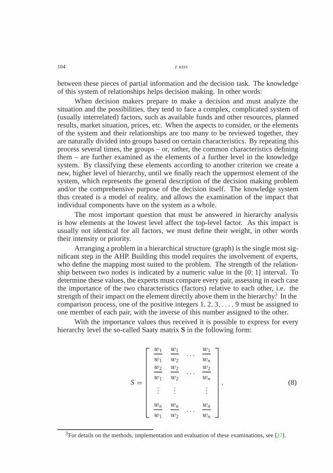
Arranging a problem in a hierarchical structure (graph) is the single most sig-nificant step in the AHP. Building this model requires the involvement of experts,who define the mapping most suited to the problem. The strength of the relation-ship between two nodes is indicated by a numeric value in the [0; 1] interval. Todetermine these values, the experts must compare every pair, assessing in each casethe importance of the two characteristics (factors) relative to each other, i.e. thestrength of their impact on the element directly above them in the hierarchy.3 In thecomparison process, one of the positive integers 1, 2, 3, . . . , 9 must be assigned toone member of each pair, with the inverse of this number assigned to the other.

With the importance values thus received it is possible to express for everyhierarchy level the so-called Saaty matrix S in the following form:

S =

w1

w1

w1

w2. . .

w1

wnw2

w1

w2

w2. . .

w2

wn

......

...

wn

w1

wn

w2. . .

wn

wn

, (8)

3For details on the methods, implementation and evaluation of these examinations, see [27].

CREDIT SCORING PROCESSES 105

where: wi means the relative weight of criterion i among the n objects at thegiven level;

n means the number of criteria at the given hierarchy level.S is a positive inverse matrix, and is characterized by

Sij · S jk = Sik,

andS · w = n · w,

where: S is the Saaty matrix;w the vector of the weight values.

It can be shown that in a positive inverse matrix, a slight perturbation of the co-efficients causes only a slight perturbation of eigenvalues, thus the eigenvector isinsensitive to small changes in evaluation [41].

The elements of eigenvector w of the highest eigenvalue Lmax of matrix Syield the weights of relations in the hierarchy. The value of vector w is received asthe solution to the equation below:

(S − nI) = 0.

The model based on the AHP can be derived from the calculation of these weightsfor the nodes. It can be shown that in every possible case Lmax ≥ n, and we canintroduce the following index to measure decision consistency:

λ = Lmax − n

n − 1.

SAATY and MARIANO showed that λ ≤ 10% may be regarded as a very good value[44].

When the AHP is used as a credit scoring process, there are only two nodesat the lowest level of the hierarchy:

• approval of the requested credit in full;• refusal of the application.

9. Expert Systems

Although expert systems have also been the subject of extensive research fordecades, scientific literature offers several, slightly varying definitions of the term.In general, we can say that the expert system is a computer system that is capable,in its area of application, of storing and managing expert knowledge, and handlingthis knowledge in a manner so that it can give users targeted information, or performcertain tasks alone. The official definition of the British Computer Society is asfollows:

106 F. KISS

‘An expert system is regarded as the embodiment within a computer of aknowledge-based component from an expert skill in such a form that the systemcan offer intelligent advice or take an intelligent decision about a processing func-tion. A desirable additional characteristic, which many experts would considerfundamental, is the capability of the system, on demand, to justify its own line ofreasoning in a manner directly intelligible to the enquirer. The programming toolthat meets these characteristics is rule-based programming.’

Expert systems have four key characteristics:

• the system is based on a knowledge base;• it has the tools to maintain and expand the knowledge base;• it can draw conclusions;• it can explain (justify) its decisions.

Expert systems can be divided into three units. The fundamental knowledgebase contains not only data and facts, but also rules as to how the knowledge shouldbe processed. Rules may be given in the form of mathematical-logical relationships.Both the logic built into the system and the syntax of rules may vary. The efficiencyof the system and the depth of the knowledge stored, however, greatly depends onwhether they are chosen appropriately.

In the following I list a few possible rules of varying complexity that mayappear in expert systems used for credit scoring:

• if the person has applied for a loan before, but it turned out that he providedfalse data, refuse the application automatically;

• if the applicant has had a credit/lending deal before, and always paid his debtson schedule, increase his score by 10;

• if the applicant’s total score is below 318, refuse the application, if it is above375, approve it automatically, otherwise make him fill in the additional form.

• if the applicant’s net income less other liabilities is less than the total of theinstallment of the loan requested and the official subsistence level calculatedconsidering the number of members in their family, but the per capita incomeof the family exceeds 120% of the subsistence level defined for such families,increase the total score by 5, otherwise reduce it by 8 (other liabilities includechild support, other repayments, etc.).

The other important part of the expert system is the user interface. It mustensure easy and efficient use and error detection.

The third component not mentioned yet is the so-called ‘conclusion machine’,which is the responding part of the system. This has access to rules and generatesthe appropriate conclusions. The conclusion machine is usually independent ofrules, so they may be replaced or updated without changing it.

The creators of expert systems must face several obstacles. One of them isthat not all knowledge can be expressed by rules or other formal methods. Simpleeveryday logic, or ‘common sense’, for example, cannot be described in this manner,as it is too general and diversified, though almost every human being possesses it.

CREDIT SCORING PROCESSES 107

Therefore, expert systems can only operate successfully in areas that are narrowenough to be properly describable, but complex enough to require such a tool.Furthermore, the creation and maintenance of the system requires experts of thegiven field, whose knowledge can be used as a starting point. It is an importantrequirement that these specialists should be in agreement about the fundamentalissues of the subject.4

The evaluation of credit/loan applications and customer rating, for exam-ple, is such an area. HOLSAPPLE and his associates [25] and PAU [39] examinedthe applicability of expert systems in financial management, primarily in lending.Brooks gave the first summary of comprehensive application experience gained inthe evaluation of consumer and mortgage loan applications [3].

10. Neural Networks

Research into neural networks began in 1943 with the publication written by MC-CULLOCH and PITT [30]. According to the proclaimed principle, a mathematicalmodel had to be developed that could simulate the natural operation of the neuron.For us, the important parts of a neuron are the dendrites, through which the neuronreceives signals, and the axons, which help to forward processed information toother neurons. Synapses play a significant part in processing information. It isthrough them that axons connect to the dendrites of other neurons.

The operation of the mathematical neuron model is relatively simple. Usinga given function they process the information received from dendrites, and if theincoming signal exceeds a so-called stimulus threshold, they forward the informa-tion via axons. The most important property of the neuron is that it is continuouslychanging its operation (i.e. its internal function) on the basis of the data received– it is ‘learning’. Synapses play an important role in this learning process, as theyare able to amplify or subdue the signals coming from other neurons. In the learn-ing process, signal amplification factors (referred to as ‘weights’ in the model inlight of their function) on synapses change. In the neuron model, the change ormodification of these weights means learning.

There are several articles discussing the development and application of creditscoring models based on neural networks. TAM, for example, compared the effi-ciency of these models with that of classic methods in relation to a corporate andbanking bankruptcy forecasting exercise [48], [49]. MCLEOD and his associatesexamined lending applications in 1993 [31], ROBINS and JOST summed up the

4Note that so far, 6,000 rules has been the maximum that could be built into a single systemeffectively. The inclusion of further rules, instead of improving system performance, in fact worsenedit, as it created less and less transparent sets of relationships. The reason is that a larger number of rulesdemands more and more complex and complicated relationships to be defined, which usually proveimpossible to create and evaluate. At the same time, estimates suggest that the level of knowledge thata real expert, such as a university professor or a chess grand master possesses, can only be expressedby approximately 10,000 rules. For details, see [33].

108 F. KISS

initial experience gained in the application of neural networks in marketing [41],[27]. They agree that the model is capable of more accurate forecasts than previousscoring systems. It also pays back the costs of implementation sooner as the devel-opment and maintenance of a decision making model based on neural networks ischeaper and faster than with earlier systems.

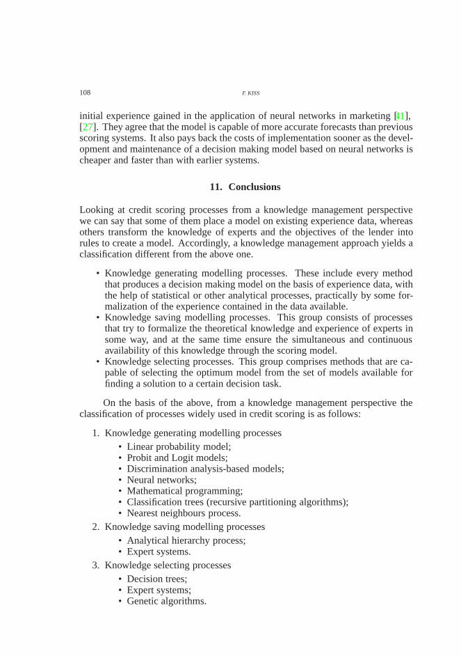
11. Conclusions

Looking at credit scoring processes from a knowledge management perspectivewe can say that some of them place a model on existing experience data, whereasothers transform the knowledge of experts and the objectives of the lender intorules to create a model. Accordingly, a knowledge management approach yields aclassification different from the above one.

• Knowledge generating modelling processes. These include every methodthat produces a decision making model on the basis of experience data, withthe help of statistical or other analytical processes, practically by some for-malization of the experience contained in the data available.

• Knowledge saving modelling processes. This group consists of processesthat try to formalize the theoretical knowledge and experience of experts insome way, and at the same time ensure the simultaneous and continuousavailability of this knowledge through the scoring model.

• Knowledge selecting processes. This group comprises methods that are ca-pable of selecting the optimum model from the set of models available forfinding a solution to a certain decision task.

On the basis of the above, from a knowledge management perspective theclassification of processes widely used in credit scoring is as follows:

1. Knowledge generating modelling processes• Linear probability model;• Probit and Logit models;• Discrimination analysis-based models;• Neural networks;• Mathematical programming;• Classification trees (recursive partitioning algorithms);• Nearest neighbours process.

2. Knowledge saving modelling processes• Analytical hierarchy process;• Expert systems.

3. Knowledge selecting processes• Decision trees;• Expert systems;• Genetic algorithms.

CREDIT SCORING PROCESSES 109

In managing the knowledge wealth of a lending organization, the three groupsof processes should be treated differently: to augment the knowledge wealth, topreserve the existing one and to increase the effectiveness of its use. How to do allthis, however, requires further research.

References

[1] ALTMAN, E. I. – AVERY, R. B. – EISENBEIS, R. A. – SINKEY, J., Application of Classi-fication Techniques in Business, Banking and Finance, JAI Press, Greenwich, CT, 8 (1981),pp. XX–418.

[2] ALTMAN, E. I. – HALDEMAN, G. G. – NARAYANAN, P., ZETA Analysis: A New Modelto Identify the Bankruptcy Risk of Corporations, Journal of Banking and Finance, 1977 June,pp. 29–54.

[3] BIERMAN, H. – HAUSMAN, W., The Credit Granting Decision, Management Science, 16 1970April, pp. 519–532.

[4] BROOKS, N. A. L., Expert Systems, Bank Administration, 65 1989 August, Iss. 8., pp. 36–37.[5] BOGGESS, W. P., Screen-Test Your Credit Risks, Harvard Business Review, 1967 Nov.-Dec.,

pp. 113–122.[6] BOYES, W. J. – HOFFMAN, D. L. – LOW, S. A., An Econometric Analysis of the Bank Credit

Scoring Problem, Journal of Econometrics, 40 1989 January, Iss. 1., pp. 3–14.[7] BREIMAN, L. – FRIEDMAN, J. H. – OLSHEN, R. A. – STONE, C. J., Classification and

Regression Trees, Wadsworth International Group, Belmont, CA, 1984.[8] CHESSER, D. L., Prediction Loan Non-compliance, Journal of Commercial Bank Lending, 56

1974 August, Iss. 8., pp. 28–38.[9] CHHIKARA, R. K., The State of the Art in Credit Evaluation, American Journal of Agricultural

Economics, 71 1989 December, Iss. 5., pp. 1138–1144.[10] DIRICKX, Y. M. – WAKEMAN, L., An Extension of the Bierman-Hausman Model for Credit

Granting, Managerial Science, 22 (1976), pp. 1229–1237.[11] DUNHAM, H. L., A Simple Credit Rating for Small Loans, Bankers Monthly, 1938.[12] DURAND, D., Risk Elements in Consumer Instalment Lending, National Bureau of Economic

Research, New York, 1941, Vol. study #8.[13] EDELSTEIN, R. H., Improving the Selection of Credit Risk: An Analysis of a Commercial

Bank Minority Lending Program, Journal of Finance, 30 (1975), pp. 37–55.[14] EWERT, D. C., Trade Credit Manager: Selection of Accounts Receivable Using a Statistical

Model, Krennert Graduate School of Industrial Administration Work. Pap. No. 236. PurdueUniversity, USA, 1969.

[15] FISHER, R. A., The Use of Multiple Measurements in Taxonomic Problems, Annals of Eugen-ics, 7 (1936) pp. 179–188.

[16] FREED, N. – GLOVER, F., A Linear Programming Approach to the Discriminant Problem,Decision Science, 12 (1981a), pp. 68–74.

[17] FREED, N. – GLOVER, F., Simple but Powerful Goal Programming Approach to the Discrim-inant Problem, European Journal of Operational Research, 7 (1981b), pp. 44–60.

[18] FRYDMAN, H. – ALTMAN, E. – KAO, D.-L., Introducing Recursive Partitioning for FinancialClassification: The Case of Financial Distress, Journal of Finance, 40 1985 March, Iss. 1.,pp. 269–291.

[19] FÜSTÖS, L. – MESZÉNA, GY. – SIMONNÉ, MOSOLYGÓ, N., A sokváltozós adatelemzésstatisztikai módszerei, Akadémiai Kiadó, 1986.

[20] FÜSTÖS, L. – MESZÉNA, GY. – SIMONNÉ, MOSOLYGÓ, N., Térstatisztika, Aula Kiadó, 1997.[21] FÜSTÖS, L. – KOVÁCS, E., A számítógépes adatelemzés statisztikai módszerei, Tankönyvki-

adó, 1989.

110 F. KISS

[22] GUSTAFSON, C. R., Stochastic Dynamic Modelling: An Aid to Agricultural Lender DecisionMaking, Western Journal of Agricultural Economics, 14 1989 July, pp. 157–165.

[23] HARDY, W. E. – ADRIAN, J. L., A Linear Programming Alternative to Discriminant Analysisin Credit Scoring, Agribusiness, 1 (1985), Iss. 4., pp. 285–292.

[24] HARDY, W. E. – WEED, J. B., Objective Evaluation for Agricultural Lending, Southern Jour-nal of Agricultural Economics, 12 (1980), pp. 159–164.

[25] HOLSAPPLE, C. W., et al., Adapting Expert System Technology to Financial Management,Financial Management, 19 1988 Autumn, pp. 12–22.

[26] JOHNSON, R. W., Legal, Social and Economic Issues Implementing Scoring in the US. In:Thomas, L.C., Crook, J.N. and Edelman, D.B. (Eds.): Credit Scoring and Credit Control,Oxford University Press, Oxford, 1992. pp. 19–32.

[27] JOST, A., Neural Networks, Credit World, 81 1993 Mar/Apr., Iss. 4., pp. 26–33.[28] KINDLER, J. – PAPP, O., Komplex rendszerek vizsgálata, Muszaki Könyvkiadó, 1977.[29] LAURENTIUS, M. M. – PATELL, J. M. – WALFSON, M. A., The Experimental Design of

Classification Models: An Application of Recursive Partitioning and Bootstrapping to Com-mercial Bank Loan Classifications, Journal of Accounting Research, Supplement to volume 22,22 (1984), pp. 87–118.

[30] MCCULLOCK, W. – PITTS, W., A Logical Calculus of the Ideas Immanent in Nervous Activity,Bulletin of Mathematical Biophysics, 7 (1943), pp. 115–133.

[31] MCLEOD, R. W., et. al., Predicting Credit Risk: A Neural Network Approach, Journal ofRetail Banking, 15 1993 Fall, Iss. 3., pp. 37–40.

[32] MESZÉNA, GY., Bevezetés a sokváltozós statisztikába. Eloadás sorozat a Budapesti Közgaz-daságtudományi Egyetemen, 1993.

[33] MÉRO, L., Észjárások – a racionális gondolkodás korlátai és a mesterséges intelligencia,TypoTex, Budapest, 1994.

[34] MOORE, G. H. – KLEIN, P. A., The Quality of Consumer Instalment Credit, National Bureauof Economic Research, Columbia University Press, New York, 1963.

[35] MYERS, J. H., Predicting Credit Risk With a Numerical Scoring System, Journal of AppliedPsychology, 47 (1963), Iss. 5., pp. 348–352.

[36] MYERS, J. H. – CORDNER, W., Increase Credit Operation Profits, Credit World, 1957 Febru-ary, pp. 12–13.

[37] MYERS, J. H. – FORGY, W., The Development of Numerical Credit Evaluation Systems,Journal of the American Statistical Association, 58 1963 September, Iss. 303., pp. 799–806.

[38] ORGLER, Y. E., A Credit Scoring Model for Commercial Loans, Journal of Money, Credit,and Banking, 2 1970 November, Iss. 4., pp. 435–445.

[39] PAU, L. F. ed., Artificial Intelligence in Economics and Management, North-Holland PublishingCo., Amsterdam, 1986.

[40] REICHERT, A. K. – CHO, C. C. – WAGNER, G. M., An Examination of the Conceptual IssuesInvolved in Developing Credit-scoring Models, Journal of Business and Economic Statistics, 11983 April, Iss. 2., pp. 101–114.

[41] ROBINS, G., Credit Scoring, Stores, 75 1993 September, Iss. 9., pp. 28–30.[42] RULON, P. J. et. al., Multivariate Statistics for Personnel Classification, New York, John Wiley

& Sons, 1967.[43] SAATY, T. L., The Analytic Hierarchy Process, McGraw-Hill, New York, 1980.[44] SAATY, T. L. – MARIANO, R. S., Rationing Energy to Industries: Priorities and Input-Output

Dependence, Energy Systems and Policy, 1979 Winter.[45] SEXTON, D. E., Jr., Determining Good and Bad Credit Risk Among High and Low Income

Families, Journal of Business, 1977 April, pp. 236–239.[46] SRINIVASAN, V. – KIM, Y. H., Credit Granting: A Comparative Analysis of Classification

Procedures, Journal of Finance, 42 1987 July, Iss. 3., pp. 665–683.[47] STEENACKER, A. – GOOVAERTS, M. J., A Credit Scoring Model for Personal Loans, Insur-

ance: Mathematics & Economics, 8 1989 March, Iss. 1., pp. 31–34.[48] TAM, K. Y., Neural Network Model and the Prediction of Bank Bankruptcy, Omega. The

International Journal of Management Science, 19 (1991), Iss. 5., pp. 429–445.[49] TAM, K. Y. – KIANG, M. Y., Managerial Applications of Neural Networks: The Case of Bank

Failure Predictions, Management Science, 38 1992 July, Iss. 7., pp. 926–947.