Covariant Hamiltonian formalism for the calculus of variations with several variables:...

c© 2004 International PressAdv. Theor. Math. Phys. 8 (2004) 565–601

Covariant Hamiltonian formalism

for the calculus of variations with

several variables: Lepage–Dedecker

versus De Donder–Weyl

Frederic Heleina and Joseph Kouneiherb

a Institut de Mathematiques de Jussieu, UMR 7586, Universite DenisDiderot – Paris 7, Site de Chevaleret, 16 rue Clisson, 75013 Paris,France

b LUTH, Laboratoire de l’Univers et de ses Theories, CNRS UMR 8102,Observatoire de Paris, 92195, Meudon Cedex, France

[email protected], [email protected]

Abstract

The main purpose in the present paper is to build a Hamiltoniantheory for fields which is consistent with the principles of relativity.For this we consider detailed geometric pictures of Lepage theories inthe spirit of Dedecker and try to stress out the interplay between theLepage-Dedecker (LP) description and the (more usual) De Donder-Weyl (DDW) one. One of the main points is the fact that the Legen-dre transform in the DDW approach is replaced by a Legendre corre-spondence in the LP theory (this correspondence behaves differently:ignoring the singularities whenever the Lagrangian is degenerate).

e-print archive: http://lanl.arXiv.org/abs/math-ph/0401046

566 COVARIANT HAMILTONIAN FORMALISM . . .

1 Introduction

1.1 Presentation

Multisymplectic formalisms are finite dimensional descriptions of variationalproblems with several variables (or field theories for physicists) analogueto the well-known Hamiltonian theory of point mechanics. For exampleconsider on the set of maps u : Rn −→ R a Lagrangian action of the type

L[u] =∫

Rn

L(x, u(x),∇u(x))dx1 · · · dxn.

Then it is well-known that the maps which are critical points of L are char-acterized by the Euler–Lagrange equation ∂

∂xµ

(∂L

∂(∂µu)

)= ∂L

∂u . By analogy

with the Hamiltonian theory we can do the change of variables pµ := ∂L∂(∂µu)

and define the Hamiltonian function

H(x, u, p) := pµ ∂u

∂xµ− L(x, u,∇u),

where here ∇u =(

∂u∂xµ

)is a function of (x, u, p) defined implicitly by pµ :=

∂L∂(∂µu)(x, u,∇u). Then the Euler-Lagrange equation is equivalent to thegeneralized Hamilton system of equations⎧⎪⎪⎨

⎪⎪⎩∂u

∂xµ=

∂H

∂pµ(x, u, p)∑

µ

∂pµ

∂xµ= −∂H

∂u(x, u, p).

(1)

This simple observation is the basis of a theory discovered by T. De Donder[3] and H. Weyl [20] independently in 1935. This theory can be formu-lated in a geometric setting, an analogue of the symplectic geometry, whichis governed by the Poincare–Cartan n-form θ := eω + pµdu ∧ ωµ (whereω := dx1 ∧ · · · ∧ dxn and ωµ := ∂µ ω) and its differential Ω := dθ, oftencalled multisymplectic (or polysymplectic form).

Although similar to mechanics this theory shows up deep differences. Inparticular there exist other theories which are analogues of Hamilton’s oneas for instance the first historical one, constructed by C. Caratheodory in1929 [2]. In fact, as realized by T. Lepage in 1936 [16], there are infinitelymany theories, due to the fact that one could fix arbitrary the value of sometensor in the Legendre transform (see also [18], [6]). Much later on, in 1953,P. Dedecker [4] built a geometrical framework in which all Lepage theories

F. HELEIN & J. KOUNEIHER 567

are embedded. The present paper, which is a continuation of [9], is devotedto the study of the Lepage–Dedecker theory. We also want to compare thisformalism with the more popular De Donder–Weyl theory.

First recall that the range of application of the De Donder–Weyl theory isrestricted in principle to variational problems on sections of a bundle F . Theright framework for it, as expounded e.g. in [8], consists in using the first jetbundle J1F and its affine dual

(J1)∗ F as analogues of the tangent and the

cotangent bundles for mechanics respectively. For non degenerate variationalproblems the Legendre transform induces an immersion of J1F in

(J1)∗F .

In contrast the Lepage theories can be applied to more general situationsbut involve, in general, many more variables and so are more complicated todeal with, as noticed in [15]. This is probably the reason why most papers onthe subject focus on the De Donder–Weyl theory, e.g. [14], [8]. The generalidea of Dedecker in [4] for describing Lepage’s theories is the following: if weview variational problems as being defined on n-dimensional submanifoldsembedded in a (n+ k)-dimensional manifold N , then what plays the role ofthe (projective) tangent bundle to space-time in mechanics is the Grassmannbundle GrnN of oriented n-dimensional subspaces of tangent spaces to N .The analogue of the cotangent bundle in mechanics is ΛnT ∗N . Note thatdimGrnN = n + k + nk so that dimΛnT ∗N = n + k + (n+k)!

n!k! is strictlylarger than dimGrnN + 1 unless n = 1 (classical mechanics) or k = 1(submanifolds are hypersurfaces). This difference between the dimensionsexplains the multiplicity of Lepage theories: as shown in [4], we substituteto the Legendre transform a Legendre correspondence which associates toeach n-subspace T ∈ Grn

qN (a “generalized velocity”) an affine subspaceof ΛnT ∗

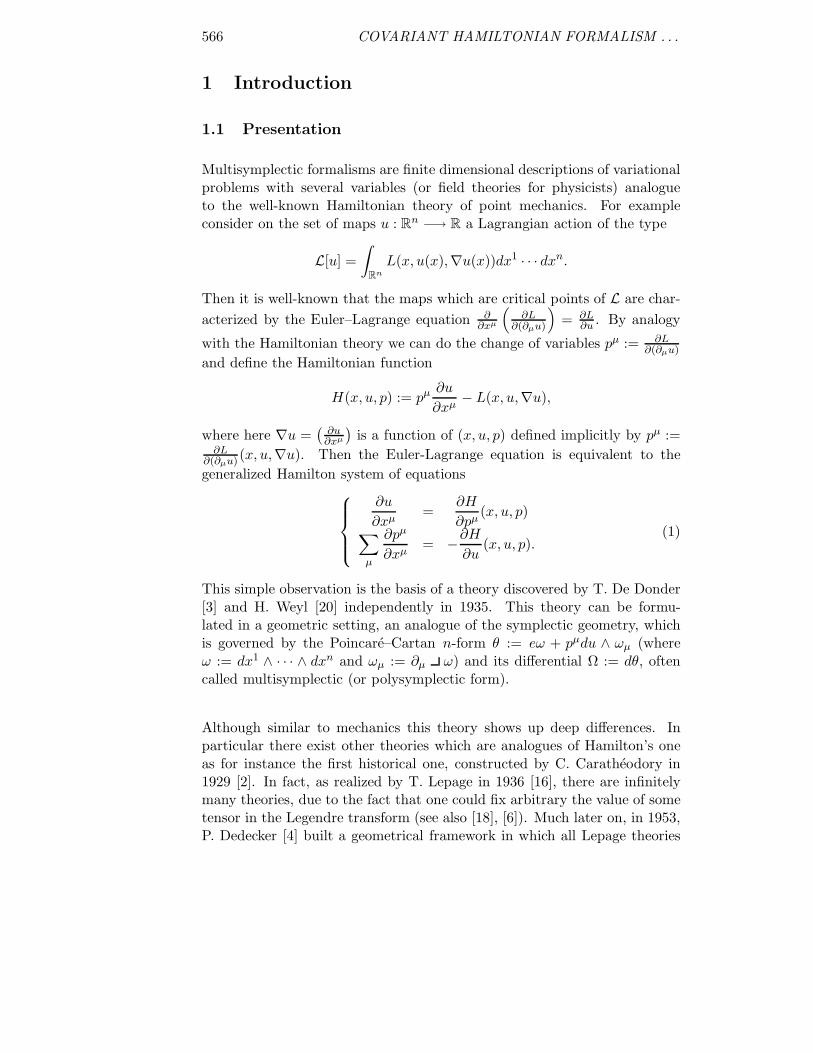
qN called pseudofibre by Dedecker. Then two points in the samepseudofiber do actually represent the same physical (infinitesimal) state, sothat the coordinates on ΛnT ∗N , called momentoıdes by Dedecker do notrepresent physically observable quantities. In this picture any choice of aLepage theory corresponds to a selection of a submanifold of ΛnT ∗N , which— when the induced Legendre transform is a well-defined map — intersectstransversally each pseudofiber at one point (see Figure 1.1): so the Legendrecorrespondence specializes to a Legendre transform. For instance the DeDonder–Weyl theory can be recovered in this setting by the restriction tosome submanifold of ΛnT ∗N (see Section 2.2).

In [9] and in the present paper we consider a geometric pictures of Lepagetheories in the spirit of Dedecker and we try to stress out the interplaybetween the Lepage–Dedecker description and the De Donder–Weyl one.Roughly speaking a comparison between these two points of view shows upsome analogy with some aspects of the projective geometry, for which there


pseudofibres

a choice of a

Lepage theory

Figure 1: Pseudofibers which intersect a submanifold corresponding to the choice of aLepage theory

is no perfect system of coordinates, but basically two: the homogeneousones, more symmetric but redundant (analogue to the Dedecker description)and the local ones (analogue to the choice of a particular Lepage theory likee.g. the De Donder–Weyl one). Note that both points of view are based onthe same geometrical framework, a multisymplectic manifold:

Definition 1.1. Let M be a differential manifold. Let n ∈ N be somepositive integer. A smooth (n + 1)-form Ω on M is a multisymplecticform if and only if

(i) Ω is non degenerate, i.e.∀m ∈ M, ∀ξ ∈ TmM, if ξ Ωm = 0, thenξ = 0

(ii) Ω is closed, i.e. dΩ = 0.

Any manifold M equipped with a multisymplectic form Ω will be called amultisymplectic manifold.

For the De Donder–Weyl theory we chooseM to be(J1)∗F and for the

Lepage–Dedecker theoryM is ΛnT ∗N . In both descriptions solutions of thevariational problem correspond to n-dimensional submanifolds Γ (analoguesof Hamiltonian trajectories: we call them Hamiltonian n-curves) and arecharacterized by the Hamilton equation X Ω = (−1)ndH, where X is an-multivector tangent to Γ, H is a (Hamiltonian) function defined onM andby “ ” we mean the interior product.

We may insist on the point that many contributions on the De Donder–Weyltheory are devoted to the construction of multisymplectic manifolds havingthe same dimension as the Lagrangian formulation configuration space, i.e.J1F , either by pulling back the multisymplectic form by the Legendre map


as in [8], or by working on a quotient or a submanifold of (J1)∗F as for in-stance in [7] (see [5] for a comparaison between the different points of view).However when dealing with Lepage–Dedecker theories, one is forced to aban-don these points of view and to work with multisymplectic manifolds whosedimension is larger than the number of physical variables. The advantage ishowever is that we do not need for any extra structure, like connections, andin particular in our setting the Hamiltonian function is thought as a globalfunction on M.

Consequently, in Section 2 we present a complete derivation of the (Dedecker)Legendre correspondence and of the generalized Hamilton equations, using amethod that does not rely on any trivialization or connection on the Grass-mannian bundle. A remarkable property, which is illustrated in this paperthrough the examples given in Paragraph 2.2.2, is that when n and k aregreater than 2, the Legendre correspondence is generically never degenerate.The more spectacular example is when the Lagrangian density is a constantfunction — the most degenerate situation one can think about — then theLegendre correspondence is well-defined almost everywhere except preciselyalong the De Donder–Weyl submanifold. We believe that such a phenomenonwas not noticed before; it however may be useful when one deals for examplewith the bosonic string theory with a skewsymmetric 2-form on the targetmanifold (a “B-field”, as discussed in [9] and in subsection 2.2, example 5)or with the Yang–Mills action in 4 dimensions with a topological term inthe Lagrangian: then the De Donder–Weyl formalism may fail but one cancure this degenerateness by using another Lepage theory or by working inthe full Dedecker setting.

In this paper we also stress out another aspect of the (Dedecker) Legen-dre correspondence: one expects that the resulting Hamiltonian function onΛnT ∗N should satisfy some condition expressing the “projective” invariancealong each pseudofiber. This is indeed the case. On the one hand we observein Section 2.1 that any smoothly continuous deformation of a Hamiltoniann-curve along directions tangent to the pseudofibers remains a Hamiltoniann-curve1 (Corollary 2.1). On the other hand we give in Section 4.3 an intrin-sic characterization of the subspaces tangent to pseudofibers. This motivatesthe definition given in Section 3.3 of the generalized pseudofiber directionson any multisymplectic manifold.

1A property quite similar to a gauge theory behavior although of different meaning.Here we are interested by desingularizing the theory and avoid the problems related to thepresence of a constraints.


Beside these properties in this paper and in its companion paper [11] wewish to address other kind of questions related to the physical gain of thesetheories: the main advantage of multisymplectic formalisms is to offer usa Hamiltonian theory which is consistent with the principles of Relativity,i.e. being covariant. Recall for instance that for all the multisymplectic for-malisms which have been proposed one does not need to use a privilege timecoordinate. One of our ambitions in this paper was to try to extend thisdemocracy between space and time coordinates to the coordinates on fibermanifolds (i.e. along the fields themselves). This is quite in the spirit ofthe Kaluza–Klein theory and its modern avatars: 11-dimensional supergrav-ity, string theory and M-theory. This concern leads us naturally to replaceDe Donder–Weyl by the Dedecker theory. In particular we do not need inour formalism to split the variables into the horizontal (i.e. corresponding tospace-time coordinates) and vertical (i.e. non horizontal) categories.

Moreover we may think that we start from a (hypothetical) geometricalmodel where space-time and fields variables would not be distinguished apriori and then ask how to make sense of a space-time coordinate function(that we call a “r-regular” in Section 3.2). A variant of this question wouldbe how to define a constant time hypersurface (that we call a “slice” in Sec-tion 3.2) without referring to a given space-time background. We proposein Section 3.2 a definition of r-regular functions and of slices which, roughlyspeaking, requires a slice to be transversal to all Hamiltonian n-curves. Herethe idea is that the dynamics only (i.e. the Hamiltonian equation) should de-termine what are the slices. We give in Section 4.2 a characterization of theseslices in the case where the multisymplectic manifold is ΛnT ∗N .

These questions are connected to the concept of observable functionals overthe set of solutions of the Hamilton equation. First because by using a codi-mension r slice Σ and an (n − r)-form F on the multisymplectic manifoldone can define such a functional by integrating F over the the intersection ofΣ with a Hamiltonian curve. And second because one is then led to imposeconditions on F in such a way that the resulting functional carries only dy-namical information. The analysis of these conditions is the subject of ourcompanion paper [11]. And we believe that the conditions required on theseforms are connected with the definitions of r-regular functions given in thispaper, although we have not completely elucidated this point.

Lastly in a future paper [12] we investigate gauge theories, addressing thequestion of how to formulate a fully covariant multisymplectic for them.


Note that the Lepage–Dedecker theory expounded here does not answer thisquestion completely, because a connection cannot be seen as a submanifold.We will show there that it is possible to adapt this theory and that a conve-nient covariant framework consists in looking at gauge fields as equivariantsubmanifolds over the principal bundle of the theory, i.e. satisfying somesuitable zeroth and first order differential constraints.

1.2 Notations

The Kronecker symbol δµν is equal to 1 if µ = ν and equal to 0 otherwise.

We shall also set

δµ1···µpν1···νp :=

∣∣∣∣∣∣∣δµ1ν1 . . . δµ1

νp

......

δµpν1 . . . δ

µpνp

∣∣∣∣∣∣∣ .

In most examples, ηµν is a constant metric tensor on Rn (which may beEuclidean or Minkowskian). The metric on his dual space his ηµν . Also, ωwill often denote a volume form on some space-time: in local coordinatesω = dx1∧· · ·∧dxn and we will use several times the notation ωµ := ∂

∂xµ ω,ωµν := ∂

∂xµ ∧ ∂∂xν ω, etc. Partial derivatives ∂

∂xµ and ∂∂pα1···αn

will be some-time abbreviated by ∂µ and ∂α1···αn respectively.

When an index or a symbol is omitted in the middle of a sequence of in-dices or symbols, we denote this omission by . For example ai1···ip···in :=

ai1···ip−1ip+1···in , dxα1 ∧· · ·∧ dxαµ∧· · ·∧dxαn := dxα1 ∧· · ·∧dxαµ−1∧dxαµ+1∧· · · ∧ dxαn .

If N is a manifold and FN a fiber bundle over N , we denote by Γ(N ,FN )the set of smooth sections of FN . Lastly we use the following notationsconcerning the exterior algebra of multivectors and differential forms. IfN is a differential N -dimensional manifold and 0 ≤ k ≤ N , ΛkTN isthe bundle over N of k-multivectors (k-vectors in short) and ΛkT ∗N isthe bundle of differential forms of degree k (k-forms in short). SettingΛTN := ⊕N

k=0ΛkTN and ΛT ∗N := ⊕N

k=0ΛkT ∗N , there exists a unique

duality evaluation map between ΛTN and ΛT ∗N such that for every decom-posable k-vector field X, i.e. of the form X = X1 ∧ · · · ∧Xk, and for everyl-form µ, then 〈X,µ〉 = µ(X1, · · · ,Xk) if k = l and = 0 otherwise. Theninterior products and are operations defined as follows. If k ≤ l, the


product : Γ(N ,ΛkTN )× Γ(N ,ΛlT ∗N ) −→ Γ(N ,Λl−kT ∗N ) is given by

〈Y,X µ〉 = 〈X ∧ Y, µ〉, ∀(l − k)-vector Y.And if k ≥ l, the product : Γ(N ,ΛkTN )×Γ(N ,ΛlT ∗N ) −→ Γ(N ,Λk−lTN )is given by

〈X µ, ν〉 = 〈X,µ ∧ ν〉, ∀(k − l)-form ν.

2 The Lepage–Dedecker theory

We expound here a Hamiltonian formulation of a large class of first ordervariational problems in an intrinsic way. Details and computations in coor-dinates can be found in [14], [9].

2.1 Hamiltonian formulation of variational problems withseveral variables

2.1.1 Lagrangian formulation

The category of Lagrangian variational problems we start with is describedas follows. We consider n, k ∈ N∗ and a smooth manifold N of dimensionn + k; N will be equipped with a closed nowhere vanishing “space-timevolume” n-form ω. We define

• the Grassmannian bundle GrnN , it is the fiber bundle over N whosefiber over q ∈ N is Grn

qN , the set of all oriented n-dimensional vectorsubspaces of TqN .

• the subbundle GrωN := (q, T ) ∈ GrnN/ωq|T > 0.• the set Gω, it is the set of all oriented n-dimensional submanifoldsG ⊂ N , such that ∀q ∈ G, TqG ∈ Grω

qN (i.e. the restriction of ω on Gis positive everywhere).

Lastly we consider any Lagrangian function L, i.e. a smooth function L :GrωN −→ R. Then the Lagrangian of any G ∈ Gω is the integral

L[G] :=∫

GL (q, TqG)ω (2)

We say that a submanifold G ∈ Gω is a critical point of L if and only if, forany compact K ⊂ N , G∩K is a critical point of LK [G] :=

∫G∩K L (q, TqG)ω


with respect to variations with support in K.

It will be useful to represent GrnN differently, by means of n-vectors. Forany q ∈ N , we define Dn

qN to be the set of decomposable n-vectors2,i.e. elements z ∈ ΛnTqN such that there exist n vectors z1,...,zn ∈ TqNsatisfying z = z1 ∧ · · · ∧ zn. Then DnN is the fiber bundle whose fiber ateach q ∈ N is Dn

qN . Moreover the map

DnqN −→ Grn

qNz1 ∧ · · · ∧ zn −→ T (z1, · · · , zn),

where T (z1, · · · , zn) is the vector space spanned and oriented by (z1, · · · , zn),induces a diffeomorphism between

(Dn

qN \ 0)/R∗

+ and GrnqN . If we set

also DωqN := (q, z) ∈ Dn

qN/ωq(z) = 1, the same map allow us also toidentify Grω

qN with Dωq N .

This framework includes a large variety of situations as illustrated below.

Example 1 — Classical point mechanics — The motion of a point mov-ing in a manifold Y can be represented by its graph G ⊂ N := R × Y. Ifπ : N −→ R is the canonical projection and t is the time coordinate on R,then ω := π∗dt.Example 2 — Maps between manifolds — We consider maps u : X −→ Y,where X and Y are manifolds of dimension n and k respectively and Xis equipped with some non vanishing volume form ω. A first order La-grangian density can represented as a function l : TY ⊗X×Y T ∗X −→ R,where TY ⊗X×Y T ∗X := (x, y, v)/(x, y) ∈ X × Y, v ∈ TyY ⊗ T ∗

xX. (Weuse here a notation which exploits the canonical identification of TyY⊗T ∗

xXwith the set of linear mappings from TxX to TyY; note that the bundleTY⊗X×Y T ∗X −→ X×Y is diffeomorphic to the first jet bundle J1F −→ F ,where F = X × Y is a trivial bundle over X ). The action of a map u is

[u] :=∫Xl(x, u(x), du(x))ω.

In local coordinates xµ such that ω = dx1∧· · ·∧dxn, critical points of satisfythe Euler-Lagrange equation

∑nµ=1

∂∂xµ

(∂l

∂viµ(x, u(x), du(x))

)= ∂l

∂yi (x, u(x), du(x)),∀i = 1, · · · , k..Then we set N := X × Y and denoting by π : N −→ X the canonical pro-jection, we use the volume form ω π∗ω. Any map u can be represented by

2another notation for this set would be DΛnTqN , for it reminds that it is a subset ofΛnTqN , but we have chosen to lighten the notation.


its graph Gu := (x, u(x))/x ∈ X ∈ Gω, (and conversely if G ∈ Gω then thecondition ω|G > 0 forces G to be the graph of some map). For all (x, y) ∈ Nwe also have a diffeomorphism

TyY ⊗ T ∗xX −→ Grω

(x,y)N Dω(x,y)N

v −→ T (v),

where T (v) is the graph of the linear map v : TxX −→ TyY. Then if we setL(x, y, T (v)) := l(x, y, v), the action defined by (2) coincides with .Example 3 — Sections of a fiber bundle — This is a particular case of oursetting, where N is the total space of a fiber bundle with base manifold X .The set Gω is then just the set of smooth sections.

2.1.2 The Legendre correspondence

Now we consider the manifold ΛnT ∗N and the projection mapping Π :ΛnT ∗N −→ N . We shall denote by p an n-form in the fiber ΛnT ∗

qN . Thereis a canonical n-form θ called the Poincare–Cartan form defined on ΛnT ∗Nas follows: ∀(q, p) ∈ ΛnT ∗N , ∀X1, · · · ,Xn ∈ T(q,p) (ΛnT ∗N ),

θ(q,p)(X1, · · · ,Xn) := p (Π∗X1, · · · ,Π∗Xn) = 〈Π∗X1 ∧ · · · ∧Π∗n, p〉,where Π∗Xµ := dΠ(q,p)(Xµ). If we use local coordinates (qα)1≤α≤n+k on N ,then a basis of ΛnT ∗

qN is the family (dqα1 ∧ · · · ∧ dqαn)1≤α1<···<αn≤n+k andwe denote by pα1···αn the coordinates on ΛnT ∗

qN in this basis. Then θ writes

θ :=∑

1≤α1<···<αn≤n+k

pα1···αndqα1 ∧ · · · ∧ dqαn . (3)

Its differential is the multisymplectic form Ω := dθ and will play the roleof generalized symplectic form.

In order to build the analogue of the Legendre transform we consider thefiber bundle GrωN ×N ΛnT ∗N := (q, z, p)/q ∈ N , z ∈ Grω

qN DωqN , p ∈

ΛnT ∗qN and we denote by Π : GrωN ×N ΛnT ∗N −→ N the canonical

projection. To summarize:

GrωN ×N ΛnT ∗NΠL

ΠH

Π

ΛnT ∗NΠ

Mı

Π|M

GrnN GrωNı N


We define on GrωN ×N ΛnT ∗N the function

W (q, z, p) := 〈z, p〉 − L(q, z).

Note that for each (q, z, p) there a vertical subspace V(q,z,p) ⊂ T(q,z,p)(GrωN×NΛnT ∗N ), which is canonically defined as the kernel of

dΠ(q,z,p) : T(q,z,p) (GrωN ×N ΛnT ∗N ) −→ TqN .We can further split V(q,z,p) TzD

ωqN⊕TpΛnT ∗

qN , where TzDωqN KerdΠH

(q,z,p)

and TpΛnT ∗qN KerdΠL

(q,z,p). Then, for any function F defined onGrωN×NΛnT ∗N , we denote respectively by ∂F/∂z(q, z, p) and ∂F/∂p(q, z, p) the re-strictions of the differential3 dF(q,z,p) on respectively TzD

ωqN and TpΛnT ∗

qN .

Instead of a Legendre transform we shall rather use a Legendre correspon-dence: we write

(q, z)←→ (q, p) if and only if∂W

∂z(q, z, p) = 0. (4)

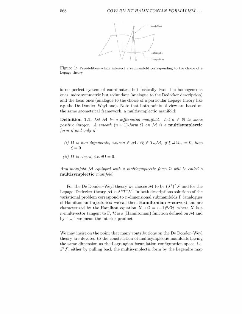
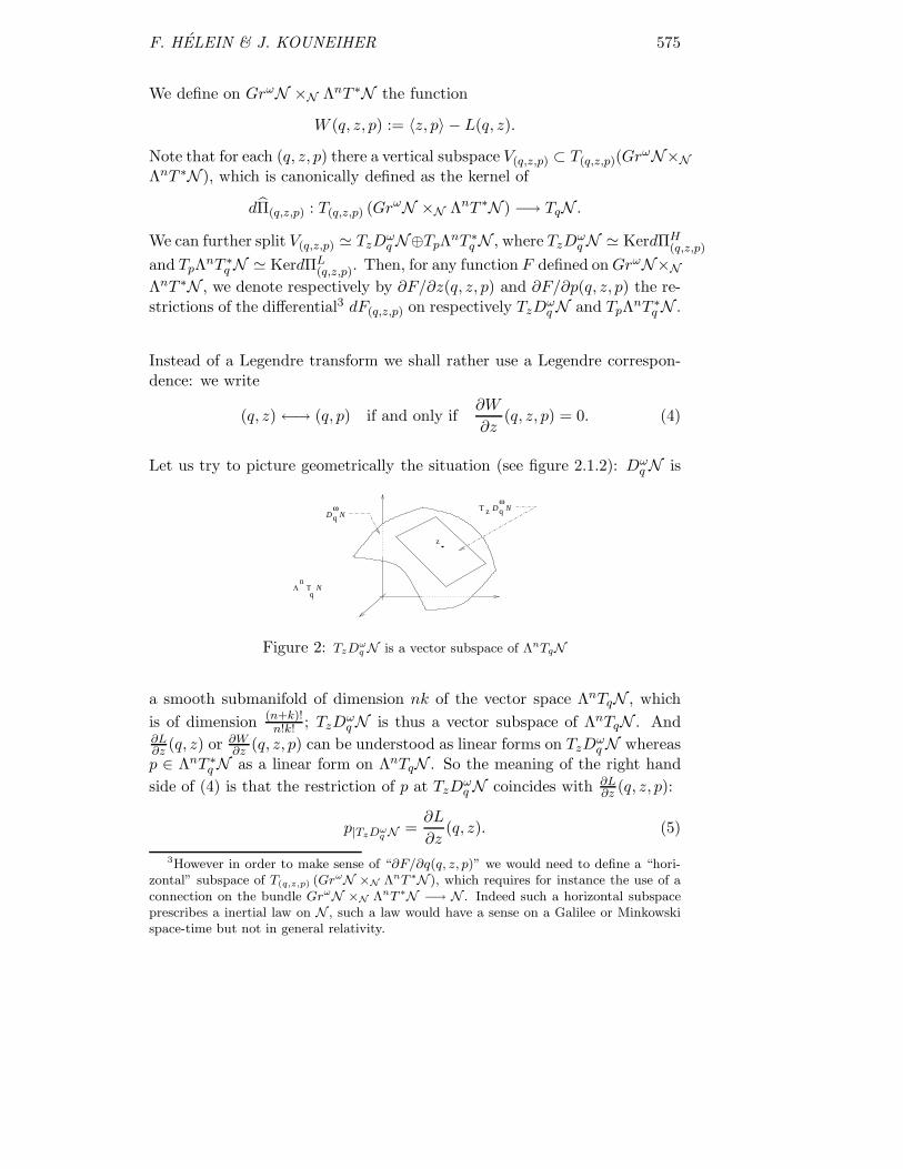
Let us try to picture geometrically the situation (see figure 2.1.2): DωqN is

Tq

q N

Λn

Dω D q N

z

T zω

N

Figure 2: TzDωq N is a vector subspace of ΛnTqN

a smooth submanifold of dimension nk of the vector space ΛnTqN , whichis of dimension (n+k)!

n!k! ; TzDωqN is thus a vector subspace of ΛnTqN . And

∂L∂z (q, z) or ∂W

∂z (q, z, p) can be understood as linear forms on TzDωqN whereas

p ∈ ΛnT ∗qN as a linear form on ΛnTqN . So the meaning of the right hand

side of (4) is that the restriction of p at TzDωqN coincides with ∂L

∂z (q, z, p):

p|TzDωq N =

∂L

∂z(q, z). (5)

3However in order to make sense of “∂F/∂q(q, z, p)” we would need to define a “hori-zontal” subspace of T(q,z,p) (GrωN ×N ΛnT ∗N ), which requires for instance the use of aconnection on the bundle GrωN ×N ΛnT ∗N −→ N . Indeed such a horizontal subspaceprescribes a inertial law on N , such a law would have a sense on a Galilee or Minkowskispace-time but not in general relativity.


Given (q, z) ∈ GrωN we define the enlarged pseudofiber in q to be:

Pq(z) := p ∈ ΛnT ∗qN/

∂W

∂z(q, z, p) = 0.

In other words, p ∈ Pq(z) if it is a solution of (5). Obviously Pq(z) is notempty; moreover given some p0 ∈ Pq(z),

p1 ∈ Pq(z), ⇐⇒ p1−p0 ∈(TzD

ωq N

)⊥ := p ∈ ΛnT ∗qN/∀ζ ∈ TzD

ωqN , p(ζ) = 0.

(6)So Pq(z) is an affine subspace of ΛnT ∗

qN of dimension (n+k)!n!k! −nk. Note that

in case where n = 1 (the classical mechanics of point) then dimPq(z) = 1:this is due to the fact that we are still free to fix arbitrarily the momentumcomponent dual to the time (i.e. the energy)4.

We now define

Pq :=⋃

z∈Dωq N

Pq(z) ⊂ ΛnT ∗qN , ∀q ∈ N

and we denote by P := ∪q∈NPq the associated bundle over N . We also let,for all (q, p) ∈ ΛnT ∗N ,

Zq(p) := z ∈ Grωq N/p ∈ Pq(z).

It is clear that Zq(p) = ∅ ⇐⇒ p ∈ Pq. Now in order to go further we needto choose some submanifold Mq ⊂ Pq, its dimension is not fixed a priori.

Legendre Correspondence Hypothesis — We assume that there existsa subbundle manifold M ⊂ P ⊂ ΛnT ∗N over N where dimM =: M suchthat,

• for all q ∈ N the fiber Mq is a smooth submanifold, possibly withboundary, of dimension 1 ≤M − n− k ≤ (n+k)!

n!k!

• for any (q, p) ∈ M, Zq(p) is a non empty smooth connected submani-fold of Grω

qN4a simple but more interesting example is provided by variational problems on maps

u : R2 −→ R2. Then one is led to the multisymplectic manifold Λ2T ∗R4. And given any(q, z) ∈ GrωR4 the enlarged pseudofiber Pq(z) ⊂ Λ2T ∗R4 is an affine plane parallel toR[(

v11v2

2 − v21v1

2

)dx1 ∧ dx2 − εijv

jνdyi ∧ dxν + dy1 ∧ dy2

] ⊕ Rdx1 ∧ dx2, where (using thenotations of Example 2) T (v) = z. For details see Paragraph 2.2.2.


• if z0 ∈ Zq(p), then we have Zq(p) = z ∈ DωqN/∀p ∈ TpMq, 〈z −

z0, p〉 = 0.

Remark — In the case where M = (n+k)!n!k! + n + k, then Mq is an open

subset of ΛnT ∗qN and so TpMq ΛnT ∗

qN . Hence the last assumption ofthe Legendre Correspondence Hypothesis means that Zq(p) is reduced to apoint. In general this condition will imply that the inverse correspondencecan be rebuild by using the Hamiltonian function (see Lemma 2.2 below).

Lemma 2.1. Assume that the Legendre correspondence hypothesis is true.Then for all (q, p) ∈M, the restriction of W to q×Zq(p)×p is constant.

Proof — Since Zq(p) is smooth and connected, it suffices to prove thatW is constant along any smooth path inside (q, z, p)/q, p fixed , z ∈ Zq(p).Let s −→ z(s) be a smooth path with values into Zq(p), then

d

ds(W (q, z(s), p)) =

∂W

∂z(q, z(s), p)

(dz

ds

)= 0,

because of (4).

A straightforward consequence of Lemma 2.1 is that we can define theHamiltonian function H :M−→ R by

H(q, p) := W (q, z, p), where z ∈ Zq(p), i.e.∂W

∂z(q, z, p) = 0.

Any function f constructed this way will be called Legendre ImageHamiltonian function. In the following, for all (q, p) ∈ M and for allz ∈ Dn

qN we denote by

z|TpMq: TpMq −→ R

p −→ 〈z, p〉

the linear map induced by z on TpMq. Then:

Lemma 2.2. Assume that the Legendre Correspondence Hypothesis is true.Then5

5The advised Reader may expect to have also the relation “ ∂H∂q

(q, p) = − ∂L∂q

(q, z)”. But

as remarked above the meaning of ∂H∂q

and ∂L∂q

is not clearly defined, because we did notintroduce a connection on the bundle GrωN ×N ΛnT ∗N . This does not matter and weshall make the economy of this relation later ! (cf footnote 2)


(i) ∀(q, p) ∈M and ∀z ∈ Zq(p),

∂H∂p

(q, p) = z|TpMq. (7)

As a corollary of the above formula, z|TpMqdoes not depend on the

choice of z ∈ Zq(p).

(ii) Conversely if (q, p) ∈ M and z ∈ DωqN satisfy condition (7), then

z ∈ Zq(p) or equivalently p ∈ Pq(z).

Proof — Let (q, p) ∈M and (0, p) ∈ T(q,p)M, where p ∈ TpMq. In order tocompute dH(q,p)(0, p), we consider a smooth path s −→ (q, p(s)) with valuesinto Mq whose derivative at s = 0 coincides with (0, p). We can further liftthis path into another one s −→ (q, z(s), p(s)) with values into Grω

qN ×Mq,in such a way that z(s) ∈ Zq(p(s)), ∀s. Then using (5) we obtain

d

ds(H(q, p(s)))|s=0 =

d

ds(〈z(s), p(s)〉 − L(q, p(s)) )|s=0

= 〈z, p〉+ 〈z, p〉 − ∂L

∂z(q, z)(z) = 〈z, p〉,

from which (7) follows. This proves (i).The proof of (ii) uses the Legendre Correspondence Hypothesis: considerz, z0 ∈ Dn

qN and assume that z0 ∈ Zq(p) and that z satisfies (7). Then byapplying the conclusion (i) of the Lemma to z0 we deduce that ∂H/∂p(q, p) =z0|TpMq

and thus (z− z0)|TpMq= 0. Hence by the Legendre Correspondence

Hypothesis we deduce that z ∈ Zq(p).

A further property is that, given (q, z) ∈ DωN , it is possible to find ap ∈ Pq(z) and to choose the value of H(q, p) simultaneously. This propertywill be useful in the following in order to simplify the Hamilton equations.For that purpose we define, for all h ∈ R, the pseudofiber:

P hq (z) := p ∈ Pq(z)/H(q, p) = h.

We then have:

Lemma 2.3. For all (q, z) ∈ GrωN the pseudofiber P hq (z) is a affine sub-

space6 of ΛnT ∗qN parallel to

(TzD

nqN

)⊥. Hence dim P hq (z) = dim Pq(z) −

1 = (n+k)!n!k! − nk − 1.

6again in the instance of variational problems on maps u : R2 −→ R2 and the multi-symplectic manifold Λ2T ∗R4, for any (q, z) ∈ GrωR4 the pseudofiber P h

q (z) ⊂ Λ2T ∗R4 isan affine line parallel to R

[(v11v2

2 − v21v1

2

)dx1 ∧ dx2 − εijv

jνdyi ∧ dxν + dy1 ∧ dy2

], where

T (v) = z. (See also Paragraph 2.2.2.)


Proof — We first remark that, ∀q ∈ N and ∀z ∈ DωqN , ωq belongs to(

TzDωq N

)⊥, because of the definition of DωqN . So ∀λ ∈ R, ∀p ∈ Pq(z), we

deduce from (6) that p+ λωq ∈ Pq(z) and thus

H(q, p+ λωq) = 〈z, p + λωq〉 − L(q, z)= H(q, p) + λ〈z, ωq〉 = H(q, p) + λ.

Hence we deduce that ∀h ∈ R, ∀p ∈ Pq(z), ∃!λ ∈ R such that

H(q, p+ λωq) = h,

so that P hq (z) is non empty. Moreover if p0 ∈ P h

q (z) then p1 ∈ P hq (z) if and

only if p1− p0 ∈(TzD

ωqN

)⊥ ∩ z⊥, where z⊥ := p ∈ ΛnT ∗qN/〈z, p〉 = 0. In

order to conclude observe that(TzD

ωqN

)⊥ ∩ z⊥ =(TzD

nqN

)⊥.

2.1.3 Critical points

We now look at critical points of the Lagrangian functional using the aboveframework. Instead of the usual approach using jet bundles and contactstructure, we shall derive Hamilton equations directly, without writing theEuler–Lagrange equation.

First we extend the form ω on M by setting ω Π∗ω, where Π :M−→ Nis the bundle projection, and we define Gω to be the set of oriented n-dimensional submanifolds Γ of M, such that ω|Γ > 0 everywhere. A conse-quence of this inequality is that the restriction of the projection Π to anyΓ ∈ Gω is an embedding into N : we denote by Π(Γ) its image. It is clearthat Π(Γ) ∈ Gω. Then we can view Γ as (the graph of) a section q −→ p(q)of the pull-back of the bundleM−→ N by the inclusion Π(Γ) ⊂ N .

Second, we define the subclass pGω ⊂ Gω as the set of Γ ∈ Gω such that,∀(q, p) ∈ Γ, p ∈ Pq(TqΠ(Γ)) (a contact condition). [As we will see later itcan be viewed as the subset of Γ ∈ Gω which satisfy half of the Hamiltonequations.] And given some G ∈ Gω, we denote by pG ⊂ pGω the family ofsubmanifolds Γ ∈ pGω such that Π(Γ) = G and we say that pG is the set ofLegendre lifts of G. We hence have pGω = ∪G∈GωpG.

Lastly, we define the functional on Gω

I[Γ] :=∫

Γθ −Hω.


Properties of the restriction of I to pGω — First we claim that

I[Γ] = L[G], ∀G ∈ Gω,∀Γ ∈ pG. (8)

This follows from∫Γθ −Hω =

∫G〈zG, p(q)〉ω −H(q, p(q))ω

=∫

G(〈zG, p(q)〉 − 〈zG, p(q)〉 + L(q, zG))ω =

∫GL(q, zG)ω,

where G −→ M : q −→ (q, p(q)) is the parametrization of Γ and where zGis the unique n-vector in Dω

qN (for q ∈ G) which spans TqG.Second let us exploit relation (8) to compute the first variation of I at anysubmanifold Γ ∈ pG, i.e. a Legendre lift of G ∈ Gω. We let ξ ∈ Γ(N , TN )be a smooth vector field with compact support and Gs, for s ∈ R, be theimage of G by the flow diffeomorphism esξ. For small values of s, Gs isstill in Gω and for all qs := esξ(q) ∈ Gs we shall denote by zs the uniquen-vector in Dω

qsN which spans TqsGs. Then we choose a smooth section

(s, qs) −→ p(q)s in such a way that p(q)s ∈ Pqs(zs). This builds a family ofLegendre lifts Γs = (qs, p(q)s). We can now use relation (8): I[Γs] = L[Gs]and derivate it with respect to s. Denoting by ξ ∈ T(q,p(q))M the vectord(qs, p(q)s)/ds|s=0, we obtain

δI[Γ](ξ) =d

dsI[Γs]|s=0 =

d

dsL[Gs]|s=0 = δL[G](ξ). (9)

Variations of I along TpMq — On the other hand for all Γ ∈ Gω and forall vertical tangent vector field along Γ ζ, i.e. such that dΠ(q,p)(ζ) = 0 orsuch that ζ ∈ TpMq ⊂ T(q,p)M, we have

δI[Γ](ζ) =∫

Γ

(〈zΠ(Γ), ζ〉 −

∂H∂p

(q, p)(ζ))ω, (10)

where zΠ(Γ) is the unique n-vector in DωqN (for q ∈ G(Γ)) which spans

TqΠ(Γ). Note that in the special case where Γ ∈ pGω , we have zΠ(Γ) ∈ Zq(p),so we deduce from (7) and (10) that δI[Γ](ζ) = 0. And the converse is true.So pGω can be characterized by requiring that condition (10) is true for allvertical vector fields ζ.

Conclusion — The key point is now that any vector field along Γ can bewritten ξ + ζ, where ξ and ζ are as above. And for any G ∈ Gω and for allΓ ∈ pG, the first variation of I at Γ with respect to a vector field ξ + ζ,where locally ξ lifts ξ ∈ TqN and ζ ∈ TpMq, satisfies

δI[Γ](ξ + ζ) = δL[G](ξ). (11)

We deduce the following.


Theorem 2.1. (i) For any G ∈ Gω and for all Legendre lift Γ ∈ pG, G is acritical point of L if and only if Γ is a critical point of I.(ii) Moreover for all Γ ∈ Gω, if Γ is a critical point of I then Γ is a Legendrelift, i.e.Γ ∈ pΠ(Γ) and Π(Γ) is a critical point of L.

Proof — (i) is a straightforward consequence of (11). Let us prove (ii):if Γ ∈ Gω is a critical point of I, then in particular for all vertical tangentvector field ζ ∈ TpMq, δI[Γ](ζ) = 0 and by (10) this implies (zΠ(Γ))|T ∗

p Mq=

(∂H/∂p)(q, p). Then by applying Lemma 2.2–(ii) we deduce that zΠ(Γ) ∈Zq(p). Hence Γ is a Legendre lift. Lastly we use the conclusion of the part(i) of the Theorem to conclude that G(Γ) is a critical point of L.

Corollary 2.1. Let Γ ∈ Gω be a critical point of I and let ψ : Γ −→ ΛnT ∗Nbe a smooth map satisfy:

(i) Π ψ = IdΓ (so ψ is a section of the pull-back of ΛnT ∗N by theinclusion map ι : Γ −→ ΛnT ∗N );

(ii) ∀(q, p) ∈ Γ, ψ(q, p) ψ(q) ∈ (TzDωqN

)⊥ (where z ∈ Zq(p)).

Then Γ := (q, p + ψ(q))/(q, p) ∈ Γ is another critical point of I.

Proof — By using Theorem 2.1–(ii) we deduce that Γ has the form Γ =(q, p)/q ∈ Π(Γ), p ∈ Pq(zΠ(Γ)) and thus Γ = (q, p + ψ(q))/q ∈ Π(Γ), p ∈Pq(zΠ(Γ)). This implies, by using (6), that Γ ∈ pΠ(Γ); then Γ is also acritical point of I because of Theorem 2.1–(i).

Note that, for any constant h ∈ R, by choosing ψ(q) = (h−H(q, p))ωq

(see the proof of Lemma 2.3) in the above Corollary we deform any criticalpoint Γ of I Γ ∈ Gω into a critical point Γ of I contained in Mh := m ∈M/H(m) = h.Definition 2.1. An Hamiltonian n-curve is a critical point Γ of I suchthat there exists a constant h ∈ R such that Γ ⊂Mh.

2.1.4 Hamilton equations

We now end this section by looking at the equation satisfied by critical pointsof I. Let Γ ∈ Gω and ξ ∈ Γ(M, TM) be a smooth vector field with compactsupport. We let esξ be the flow mapping of ξ and Γs be the image of Γ


by esξ. We let X be an n-dimensional manifold diffeomorphic to Γ and wedenote by

σ : (0, 1) ×X −→ M(s, x) −→ σ(s, x)

a map such that if γs : x −→ σ(s, x), then γ = γ0 is a parametrization of Γ,γs is a parametrization of Γs and ∂

∂s (σ(s, x)) = ξ (σ(s, x)). Then

I[Γs]− I[Γ] =∫Xγ∗s (θ −Hω)− γ∗(θ −Hω)

=∫

∂((0,s)×X )σ∗(θ −Hω) =

∫(0,s)×X

d (σ∗(θ −Hω))

=∫

(0,s)×Xσ∗(Ω − dH ∧ ω)).

Thus

lims→0

I[Γs]− I[Γ]s

= lims→0

1s

∫(0,s)×X

σ∗(Ω− dH ∧ ω)

=∫X

∂

∂sσ∗(Ω − dH ∧ ω) =

∫Xγ∗(ξ (Ω− dH ∧ ω))

=∫

Γξ (Ω− dH ∧ ω).

We hence conclude that Γ is a critical point of I if and only if ∀m ∈ Γ,∀ξ ∈ TmM, ∀X ∈ ΛnTmΓ,

ξ (Ω− dH ∧ ω)(X) = 0 ⇐⇒ X (Ω− dH ∧ ω)(ξ) = 0.

We thus deduce the following.

Theorem 2.2. A submanifold Γ ∈ Gω is a critical point of I if and only if

∀m ∈ Γ,∀X ∈ ΛnTmΓ, X (Ω− dH ∧ ω) = 0. (12)

Moreover, if there exists some h ∈ R such that Γ ⊂ Mh (i.e.Γ is a Hamil-tonian n-curve) then

∀m ∈ Γ,∃!X ∈ ΛnTmΓ, X Ω = (−1)ndH. (13)

Recall that, because of Lemma 2.3 and Corollary 2.1, it is always possibleto deform a Hamiltonian n-curve Γ −→ Γ in such a way that H be constanton Γ and Π(Γ) = Π(Γ).Proof — We just need to check (13). Let Γ ⊂ Mh. Since dH|Γ = 0,∀X ∈ ΛnTmΓ, X dH ∧ ω = (−1)n〈X,ω〉dH.. So by choosing the uniqueX such that 〈X,ω〉 = 1, we obtain X dH ∧ ω = (−1)ndH. Then (12) isequivalent to (13).


2.2 Some examples

We pause to study on some simple examples how the Legendre correspon-dence and the Hamilton work. In particular in the construction ofM we leta large freedom in the dimension of the fibersMq, having just the constraintthat dimMq ≤ dimPq = (n+k)!

n!k! . This leads to a large choice of approachesbetween two opposite ones: the first one consists in using as less variables aspossible, i.e. to choose M to be of minimal dimension (for example the DeDonder–Weyl theory), the other one consists in using the largest number ofvariables, i.e. to choose M to be equal to the interior of P (the advantagewill be that in some circumstances we avoid degenerate situations).

We focus here on special cases of Example 2 of the previous Section: weconsider maps u : X −→ Y. We denote by qµ = xµ, if 1 ≤ µ ≤ n, coordinateson X and by qn+i = yi, if 1 ≤ i ≤ k, coordinates on Y. Recall that ∀x ∈ X ,∀y ∈ Y, the set of linear maps v from T ∗

xX to TyY can be identified withTyY ⊗T ∗

xX . And coordinates representing some v ∈ TyY⊗T ∗xX are denoted

by viµ, in such a way that v =

∑α

∑i v

iµ

∂∂yi ⊗ dxµ. Then through the

diffeomorphism TyY ⊗ T ∗xX v −→ T (v) ∈ Grω

(x,y)N (where N = X × Y)we obtain coordinates on Grω

qN DωqN . We also denote by e := p1···n,

pµi := p1···(µ−1)i(µ+1)···n, pµ1µ2

i1i2:= p1···(µ1−1)i1(µ1+1)···(µ2−1)i2(µ2+1)···n, etc., so

that

Ω = de ∧ ω +n∑

j=1

∑µ1<···<µj

∑i1<···<ij

dpµ1···µj

i1···ij ∧ ωi1···ijµ1···µj ,

where, for 1 ≤ p ≤ n,

ω := dx1 ∧ · · · ∧ dxn

ωi1···ipµ1···µp := dyi1 ∧ · · · ∧ dyip ∧ ( ∂

∂xµ1 ∧ · · · ∧ ∂∂xµp ω

).

Remark — It can be checked (see for instance [9]) that, by denoting by p∗

all coordinates pµ1···µj

i1···ij for j ≥ 1, the Hamiltonian function has always theform H(q, e, p∗) = e+H(q, p∗).

2.2.1 The De Donder–Weyl formalism

In the special case of the De Donder–Weyl theory,MDDWq is the submanifold

of ΛnT ∗qN defined by the constraints pµ1···µj

i1···ij = 0, for all j ≥ 2 (Observe thatthese constraints are invariant by a change of coordinates, so that they have


an intrinsic meaning.) We thus have

ΩDDW = de ∧ ω +∑µ

∑i

dpµi ∧ ωi

µ..

Then the equation ∂W/∂z(q, z, p) = 0 is equivalent to pµi = ∂l/∂vi

µ(q, v), sothat the Legendre Correspondence Hypothesis holds if and only if (q, v) −→(q, ∂l/∂v(q, p)) is an invertible map. Note that then the enlarged pseud-ofibers Pq(z) intersectMDDW

q along lines eω+ ∂l∂vi

µ(q, v)ωi

µ/e ∈ R. So since

dimΛnT ∗qN = (n+k)!

n!k! , dimMDDWq = nk+ 1 and dimPq(z) = (n+k)!

n!k! −nk, theLegendre Correspondence Hypothesis can be rephrased by saying that eachPq(z) meets MDDW

q transversally along a line. Moreover Zq(eω + pµi ω

iµ)

is then reduced to one point, namely T (v), where v is the solution topµ

i = ∂l∂vi

µ(q, v).

For more details and a description using local coordinates, see [9].

2.2.2 Maps from R2 to R2 via the Lepage–Dedecker point of view

Let us consider a simple situation where X = Y = R2 and M ⊂ Λ2T ∗R4.It corresponds to variational problems on maps u : R2 −→ R2. For anypoint (x, y) ∈ R4, we denote by (e, pi

µ, r) the coordinates on Λ2T(x,y)R4, such

that θ = e dx1 ∧ dx2 + p1i dy

i ∧ dx2 + p2i dx

1 ∧ dyi + r dy1 ∧ dy2. An explicitparametrization of z ∈ D2

(x,y)R4/ω(z) > 0 is given by the coordinates

(t, viµ) through

z = t2∂

∂x1∧ ∂

∂x2+ t εµνvi

µ

∂

∂yi∧ ∂

∂xν+ (v1

1v22 − v1

2v21)

∂

∂y1∧ ∂

∂y2,

where ε12 = −ε21 = 1 and ε11 = ε22 = 0. One then finds that(TzD

2qR4

)⊥ is

R

[(v11v

22 − v2

1v12

)dx1 ∧ dx2 − εijvj

νdyi ∧ dxν + dy1 ∧ dy2], whereas

(TzD

ωq R4

)⊥is(TzD

2qR4

)⊥ ⊕ Rdx1 ∧ dx2.

We deduce that the sets Pq(z) and P hq (z) form a family of non parallel affine

subspaces so we expect that on the one hand these subspaces will intersect,causing obstructions there for the invertibility of the Legendre mapping, andon the other hand they will fill “almost” all of Λ2T ∗

(x,y)R4, giving rise to the

phenomenon that the Legendre correspondence is “generically everywhere”well defined.


Example 4 — The trivial variational problem — We just take l = 0, sothat any map map from R2 to R2 is a critical point of ! This example ismotivated by gauge theories where the gauge invariance gives rise to con-straints. In this case the sets Pq(z) are exactly

(TzD

ωq R4

)⊥ and ∪zPq(z) isequal to Pq := (e, pµ

i , r) ∈ Λ2T ∗q R4/r = 0 ∪ (e, 0, 0)/e ∈ R. If we assume

that r = 0 and choose Mq = (e, pµi , r) ∈ Λ2T ∗

q R4/r = 0, then

H(q, p) = e− p11p

22 − p1

2p21

r.

One can then check that all Hamiltonian 2-curves are of the form

Γ =(x, u(x), e(x)dx1 ∧ dx2 + εµνp

µi (x)dyi ∧ dxν + r(x)dy1 ∧ dy2

)/x ∈ R2

,

where u : R2 −→ R2 is an arbitrary smooth function, r : R2 −→ R∗ is also anarbitrary smooth function, e(x) = r(x)

(∂u1

∂x1 (x)∂u2

∂x2 (x)− ∂u1

∂x2 (x)∂u1

∂x2 (x))

+ h,

(for some constant h ∈ R) and pµi (x) = −r(x)εijεµν ∂uj

∂xν (x).

Example 5 — The elliptic Dirichlet integral (see also [9]) — The La-grangian is l(x, y, v) = 1

2 |v|2 +B(v11v

22 − v2

1v12) where7 |v|2 := (v1

1)2 + (v1

2)2 +

(v21)

2 + (v22)

2. We then find that

H(q, p) = e+1

1− (r −B)2

( |p|22

+ (r −B)(p11p

22 − p1

2p21)).

Example 6 — Maxwell equations in two dimensions — We choose l(x, y, v) =−1

2

(v12 − v2

1

)2, so that by identifying (u1, u2) with the components (A1, A2)of a Maxwell gauge potential, we recover the usual Lagrangian l(dA) =

−14

∑µ,ν

(∂Aν∂xµ − ∂Aµ

∂xν

)2for Maxwell fields without charges. We then obtain

H(q, p) = e+(p1

2 + p21)

2 − 4p11p

22

4r− 1

4(p1

2 − p21)

2

2 + r.

Conclusion — It is worth looking at the differences between the Lepage–Dedecker and the De Donder–Weyl theories through these examples. Indeedthe De Donder–Weyl theory can be simply recovered by letting r = 0. Onesees immediately that for the trivial variational problem this forces p1

1p22 −

p12p

21 to be 0: actually a more careful inspection shows that all pseudofibers

intersect along pµi = 0 so that all these components must be set to 0 in the

De Donder–Weyl theory. In the example of the elliptic Dirichlet functionalno constraint appears unless B = ±1. And for the Maxwell equations allpseudofibers intersect along the subspace p1

2 + p21 = p1

1 = p22 = 0 and so we

recover the constraints already observed in [14] and [9] in the De Donder–Weyl formulation.

7There B could be interpreted as a B-field of a bosonic string theory.


2.3 Invariance properties along pseudofibers

We have seen that for all q ∈ N , for h ∈ R and z ∈ DωqN , the pseudofiber

P hq (z) is an affine subspace of ΛnT ∗

qN parallel to(TzD

nqN

)⊥. Let us assumethat Mq is an open subset of ΛnT ∗

qN : then the Legendre CorrespondenceHypothesis implies that ∀(p, q) ∈ M, Zq(p) is reduced to one point that weshall denote by Z(q, p). Hence we can define the distribution of subspaceson M by:

∀(q, p) ∈M, LH(q,p) :=

(TZ(q,p)D

nqN

)⊥.

It is actually the subspace tangent to the pseudo-fiber passing through (q, p).In Section 3.3 we will propose a generalization of the definition of LH

(q,p)which makes sense on an arbitrary multisymplectic manifold. We will provein Section 4.3 that this generalized definition coincides with the first one inthe case where the multisymplectic manifold is ΛnT ∗N . Lastly Lemma 2.3and Corollary 2.1 can be rephrased as

Theorem 2.3. LetM be an open subset of ΛnT ∗N and let H be a Legendreimage Hamiltonian function on M (by means of the Legendre correspon-dence). Then

∀(q, p) ∈M,∀ξ ∈ LH(q,p), dH(q,p)(ξ) = 0. (14)

And if Γ ∈ Gω is a Hamiltonian n-curve and if ξ a vector field which is asmooth section of LH, then denoting by esξ the flow mapping of ξ

∀s ∈ R, small enough , esξ(Γ) is a Hamiltonian n−curve. (15)

2.4 Gauge theories

The above theory can be adapted for variational theories on gauge fields (con-nections) by using a local trivialization. More precisely, given a g-connection∇0 acting on a trivial bundle with structure group G (and Lie algebra g)any other connection ∇ can be identified with the g-valued 1-form A on thebase manifold X such that ∇ = ∇0 +A. We may couple A to a Higgs fieldϕ : X −→ Φ, where Φ is a vector space on which G is acting. Then anychoice of a field (A,ϕ) is equivalent to the data of an n-dimensional subman-ifold Γ in M := (g⊗ T ∗X ) × Φ which is a section of this fiber bundle overX . An example of this approach is the one that we use for the Maxwell fieldat the end of this paper.


But if we wish to study more general gauge theories and in particular con-nections on a non trivial bundle we need a more general and more covariantframework. Such a setting can consist in viewing a connection as a g-valued1-form a on a principal bundle F over the space-time satisfying some equiv-ariance conditions (under some action of the group G). Similarly the Higgsfield, a section of an associated bundle, can be viewed as an equivariant mapφ on F with values in a fixed space. Thus the pair (a, φ) can be picturedgeometrically as a section Γ, i.e. a submanifold of some fiber bundle N overF , satisfying two kinds of constraints:

• Γ is contained in a submanifold Ng (a geometrical translation of theconstraints “the restriction of af to the subspace tangent to the fiberFf is −dg · g−1”) and

• Γ is invariant by an action of G on N which preserves Ng.

Within this more abstract framework we are reduced to a situation similar tothe one studied in the beginning of this Section, but we need to understandwhat are the consequence of the two equivariance conditions. (In particularthis will imply that there is a canonical distribution of subspaces which istangent to all pseudofibers). This will be done in details in [12]. In particularwe compare this abstract point of view with the more naive one expoundedabove.

3 Multisymplectic manifolds

We now set up a general framework extending the situation encountered inthe previous Section.

3.1 Definitions

Recall that, given a differential manifoldM and n ∈ N a smooth (n+1)-formΩ on M is a multisymplectic form if and only if (i) Ω is non degenerate,i.e. ∀m ∈ M, ∀ξ ∈ TmM, if ξ Ωm = 0, then ξ = 0 (ii) Ω is closed,i.e. dΩ = 0. And we call any manifold M equipped with a multisymplecticform Ω a multisymplectic manifold. (See Definition 1.1.) In the following,N denotes the dimension of M. For any m ∈M we define the set

DnmM := X1 ∧ · · · ∧Xn ∈ ΛnTmM/X1, · · · ,Xn ∈ TmM,

of decomposable n-vectors and denote by DnM the associated bundle.


Definition 3.1. Let H be a smooth real valued function defined over a mul-tisymplectic manifold (M,Ω). A Hamiltonian n-curve Γ is a n-dimensionalsubmanifold of M such that for any m ∈ Γ, there exists a n-vector X inΛnTmΓ which satisfies

X Ω = (−1)ndH.We denote by EH the set of all such Hamiltonian n-curves. We shall alsowrite for all m ∈M, [X]Hm := X ∈ Dn

mM/X Ω = (−1)ndHm.

A Hamiltonian n-curve is automatically oriented by the n-vector X in-volved in the Hamilton equation. Remark also that it may happen thatno Hamiltonian n-curve exist. An example is M := Λ2T ∗R4 with Ω =∑

1≤µ<ν≤4 dpµν ∧ dqµ ∧ dqν for the case H(q, p) = p12 + p34. Assume thata Hamiltonian 2-curve Γ would exist and let X : (t1, t2) −→ X(t1, t2) be aparametrization of Γ such that ∂X

∂t1∧ ∂X

∂t2Ω = (−1)2dH. Then, denoting by

Xµ := ∂X∂tµ , we would have dxµ ∧ dxν(X1,X2) = ∂H

∂pµν, which is equal to ±1 if

µ, ν = 1, 2 or 3, 4 and to 0 otherwise. But this would contradict thefact that X1 ∧X2 is decomposable. Hence there is no Hamiltonian 2-curvein this case.

Note that beside the the Lepage–Dedecker multisymplectic manifold (ΛnT ∗N ,Ω)studied in the previous Section, other examples of multisymplectic manifoldsarises naturally as for example a multisymplectic structure associated to thePalatini formulation of pure gravity in 4-dimensional space-time (see [10],[11], [17]).

In the following we address questions related to the following general prob-lematic, set in the spirit of the general relativity: assume that a field theory(and in particular including a space-time description) is modelled by a mul-tisymplectic manifold (M,Ω) and possibly a Hamiltonian H. How could werecover its physical properties, i.e. understand how space-time coordinatesmerge out, how momenta and energy appear, without using ad hoc hypothe-ses ? We probably do not know enough to be able to answer such questionsand in the following we will content ourself with partial answers.

3.2 The notion of r-regular functions

This question is motivated by the search for understanding space-time coor-dinates. One could characterize components of a space-time chart as func-tions which: (i) are defined for all possible dynamics, (ii) allow us to separate


any pair of different points on space-time. The easiest way to fulfill the firstrequirement is to assume that any coordinate function is obtained as therestriction of a function f : M −→ R on the Hamiltonian n-curve describ-ing the dynamics. The infinitesimal version of the second requirement isthen to assume that the restriction of the n functions chosen f1, · · · , fn onany Hamiltonian n-curve is locally a diffeomorphism. This motivates thefollowing

Definition 3.2. Let (M,Ω) be a multisymplectic manifold and H ∈ C∞(M)a Hamiltonian function. Let 1 ≤ r ≤ n be an integer. A function f ∈C1(M,Rr) is called r-regular if and only if for any Hamiltonian n-curveΓ ⊂M the restriction f|Γ is a submersion.

The dual notion is:

Definition 3.3. Let H be a smooth real valued function defined over a mul-tisymplectic manifold (M,Ω). A slice of codimension r is a coorientedsubmanifold Σ ofM of codimension r such that for any Γ ∈ EH, Σ is trans-verse to Γ. By cooriented we mean that for each m ∈ Σ, the quotient spaceTmM/TmΣ is oriented continuously in function of m.

Indeed it is clear that the level sets of a r-regular function f :M−→ Rr

are slices of codimension r.Example 7 — The case when M = ΛnT ∗(X × Y) and that H(x, y, p) =e+H(x, y, p∗) as in Section 2.2 —Let ΠX :M−→ X be the natural projec-tion. Then for any function ϕ ∈ C1(X ,Rr) without critical point (i.e. dϕ is ofrank r everywhere) the function ϕΠX :M−→ Rr a r-regular function. In-deed because of the particular dependance of H on e a Hamiltonian n-curveis always a graph over X . A particular case is when r = 1, then any levelset Σ of ϕ is a codimension 1 slice and a (class of) vector τ ∈ TmM/TmΣ ispositively oriented if and only if dϕ(τ) > 0.

Note that in this framework an event in space-time can be represented by aslice of codimension n. The notion of slice is also important because it helpsto construct observable functionals on the set of solutions EH. Indeed if Fis a (n − 1)-form on M and if Σ is a slice of codimension 1 we define thefunctional denoted symbolically by

∫Σ F : EH −→ R by:

Γ −→∫

Σ∩ΓF.

Here the intersection Σ ∩ Γ is oriented as follows: assume that α ∈ T ∗mM is

such that α|TmΣ = 0 and α > 0 on TmM/TmΣ and let X ∈ ΛnTmΓ be posi-tively oriented. Then we require that X α ∈ Λn−1Tm(Σ ∩ Γ) is positively


oriented. We can further assume restrictions on the choice of F in orderto guarantee the fact that the resulting functional is physically observable.Such a situation is achieved if for example F is so that dF|TmΓ depends onlyon dHm (see [11] for details).

In the next Section we will study a characterization of r-regular functions inthe special case whereM = ΛnT ∗N .

3.3 Pataplectic invariant Hamiltonian functions

In Section 2.3 we gave a definition of the subspaces tangent to the pseud-ofibers LH

m which was directly deduced from our analysis of pseudofibers.In Section 4.3 we will prove that an alternative characterization of LH

m inΛnT ∗N exists and is more intrinsic. It motivates the following definition:given an arbitrary multisymplectic manifold (M,Ω) and a Hamiltonian func-tion H : M −→ R and for all m ∈ M we define the generalized pseud-ofiber direction to be

LHm :=

(T[X]HmD

nmM Ω

)⊥:= ξ ∈ TmM/∀X ∈ [X]Hm,∀δX ∈ TXD

nmM, ξ Ω(δX) = 0.

(16)And we write LH := ∪m∈MLH

m ⊂ TM for the associated distribution ofsubspaces.

Note that if we choose an arbitrary Hamiltonian function H, there is noreason for the conclusions of Theorem 2.3 to be true, unless we know that Hwas created out of a Legendre correspondence. This motivates the followingdefinition8:

Definition 3.4. We say that H is pataplectic invariant if

(i) ∀ξ ∈ LHm, dHm(ξ) = 0

(ii) for all Hamiltonian n-curve Γ ∈ EH, for all vector field ξ which is asmooth section of LH, then, for s ∈ R sufficiently small, Γs := esξ(Γ)is also a Hamiltonian n-curve.

8In the following if ξ is a smooth vector field, we denote by esξ (for s ∈ I , where I is aninterval of R) its flow mapping. And if E is any subset of M, we denote by Es := esξ(E)its image by esξ.


In [11] we prove that, if H is pataplectic invariant and if some furtherhypotheses are fulfilled, functionals of the type

∫Σ F are invariant by defor-

mations along LH.

4 The study of ΛnT ∗N

In this Section we analyze in details the special case where M is an opensubset of ΛnT ∗N . Since we are interested here in local properties of M,we will use local coordinates m = (q, p) = (qα, pα1···αn) on M, and themultisymplectic form reads Ω =

∑α1<···<αn

dpα1···αn ∧ dqα1 ∧ · · · ∧ dqαn . Form = (q, p), we write

dqH :=∑

1≤α≤n+k

∂H∂qα

dqα, dpH :=∑

1≤α1<···<αn≤n+k

∂H∂pα1···αn

dpα1···αn ,

so that dH = dqH+ dpH.

4.1 The structure of [X]Hm

Here we are given some Hamiltonian function H : M −→ R and a pointm ∈M such that [X]Hm = ∅ and9 dpHm = 0. Given any X = X1∧· · ·∧Xn ∈Dn

mM and any form a ∈ T ∗mM we will write that a|X = 0 (resp. a|X = 0)

if and only if (a(X1), · · · , a(Xn)) = 0 (resp. (a(X1), · · · , a(Xn)) = 0). Wewill say that a form a ∈ T ∗

mM is proper on [X]Hm if and only if it’s eithera point-slice

∀X ∈ [X]Hm, a|X = 0, (17)

or a co-isotropic∀X ∈ [X]Hm, a|X = 0. (18)

We are interested in characterizing all proper 1-forms on [X]Hm. We show inthis section the following.

Lemma 4.1. LetM be an open subset of ΛnT ∗N endowed with its standardmultisymplectic form Ω, let H :M−→ R be a smooth Hamiltonian function.Let m ∈M such that dpHm = 0 and [X]Hm = ∅. Then(i) the n+k forms dq1, · · · , dqn+k are proper on [X]Hm and satisfy the follow-ing property: ∀X ∈ [X]Hm and for all Y,Z ∈ TmM which are in the vector

9observe that, although the splitting dH = dqH + dpH depends on a trivialization ofΛnT ∗N , the condition dpHm = 0 is intrinsic: indeed it is equivalent to dH

m|KerdΠm= 0,

where Π : ΛnT ∗N −→ N .


space spanned by X, if dqα(Y ) = dqα(Z), ∀α = 1, · · · , n+ k, then Y = Z.(ii) Moreover for all a ∈ T ∗

mM which is proper on [X]Hm we have

∃!λ ∈ R,∃!(a1, · · · , an+k) ∈ Rn+k, a = λdHm +n+k∑α=1

aαdqα. (19)

(iii) Up to a change of coordinates on N we can assume that dq1, · · · , dqn

are point-slices and that dqn+1, · · · , dqn+k satisfy (18). Then a ∈ T ∗M is apoint-slice if and only if (19) occurs with (a1, · · · , an) = 0.

Proof — First step — analysis of [X]Hm. We start by introducing someextra notations: each vector Y ∈ TmM can be decomposed into a “vertical”part Y V and a “horizontal” part Y H as follows: for any Y =

∑1≤α≤n+k Y

α ∂∂qα +∑

1≤α1<···<αn≤n+k Yα1···αn∂

∂pα1···αn, set Y H :=

∑1≤α≤n+k Y

α ∂∂qα and Y V :=∑

1≤α1<···<αn≤n+k Yα1···αn∂

∂pα1···αn. Let X = X1 ∧ · · · ∧Xn ∈ Dn

m (ΛnT ∗N )and let us use this decomposition to each Xµ: then X can be split asX =

∑nj=0X(j), where each X(j) is homogeneous of degree j in the vari-

ables XVµ and homogeneous of degree n− j in the variables XH

µ .

Recall that a decomposable n-vector X is in [X]Hm if and only if X Ω =(−1)ndH. This equation actually splits as

X(0) Ω = (−1)ndpH (20)

andX(1) Ω = (−1)ndqH. (21)

Equation (20) determines in an unique way X(0) ∈ DnqN . The condition

dpH = 0 implies that necessarily10 X(0) = 0. At this stage we can choosea family of n linearly independent vectors X0

1 , · · · ,X0n in TqN such that

X01 ∧ · · · ∧X0

n = X(0). Thus the forms dqα are proper on [X]Hm, since theirrestriction on X are fully determined by their restriction on the vector sub-space spanned by X0

1 , · · · ,X0n. Furthermore the subspace of TmM spanned

by X is a graph over the subspace of TqN spanned by X(0). This proves thepart (i) of the Lemma..

Proving (ii) and (iii) requires more work. First we deduce that there exists aunique family (X1, · · · ,Xn) of vectors in TmM such that ∀µ, XH

µ = X0µ and

10Note also that (20) implies that dpH must satisfy some compatibility conditions sinceX(0) is decomposable.


X1 ∧ · · · ∧Xn = X. And Equation (21) consists in further underdeterminedconditions on the vertical components Xµ,α1···αn of the Xµ’s, namely∑

µ

∑α1<···<αn

Cµ,α1···αn

β Xµ,α1···αn = − ∂H∂qβ

,

whereCµ,α1···αn

β :=∑

ν

δανβ (−1)µ+ν∆α1···αν ..αn

1···µ···n

and

∆α1···αn−1µ1···µn−1 :=

∣∣∣∣∣∣∣Xα1

µ1. . . Xα1

µn−1

......

Xαnµ1

. . . Xαn−1µn−1

∣∣∣∣∣∣∣ .Step2 — Local coordinates. To further understand these relations we choosesuitable coordinates qα in such a way that dpHm = dp1···n and

XHµ =

∂

∂qµfor µ = 1, ...., n, (22)

so that (20) is automatically satisfied. In this setting we also have

(−1)nX(1) Ω = −∑µ

Xµ,1···ndqµ − (−1)n∑

µ

∑n<β

(−1)µXµ,1···µ···nβdqβ,

and so (21) is equivalent to⎧⎪⎪⎪⎪⎨⎪⎪⎪⎪⎩

Xµ,1···n = − ∂H∂qµ

, for 1 ≤ µ ≤ n

(−1)n∑

µ

(−1)µXµ,1···µ···nβ = − ∂H∂qβ

, for n+ 1 ≤ β ≤ n+ k.

(23)

Let us introduce some notations: I := (α1, · · · , αn)/1 ≤ α1 < · · · ≤αn ≤ n + k, I0 := (1, · · · , n), I∗ := (α1, · · · , αn−1, β)/1 ≤ α1 < · · · <αn−1 ≤ n, n + 1 ≤ β ≤ n + k, I∗∗ := I \ (I0 ∪ I∗) . We note also Mµ :=∑

(α1,··· ,αn)∈I∗ Xµ,α1···αn∂α1···αn , Rµ :=

∑(α1,··· ,αn)∈I∗∗ Xµ,α1···αn∂

α1···αn andMν

µ,β := (−1)n+νXµ,1···ν···nβ. Then the set of solutions of (20) and (21)satisfying (22) is

Xµ =∂

∂qµ− ∂H∂qµ

∂

∂p1···n+Mµ +Rµ, (24)

where the components of Rµ are arbitrary, and the coefficients of Mµ areonly subject to the constraint∑

µ

Mµµ,β = − ∂H

∂qβ, for n+ 1 ≤ β ≤ n+ k. (25)


Step 3 — The search of all proper 1-forms on [X]Hm. Now let a ∈ T ∗mM and

let us look at necessary and sufficient conditions for a to be a proper 1-formon [X]Hm. We write

a =∑α

aαdqα +

∑α1<···<αn

aα1···αndpα1···αn .

Let us write a∗ := (aα1···αn)(α1,··· ,αn)∈I∗ , a∗∗ := (aα1···αn)(α1,··· ,αn)∈I∗∗ and

〈Mµ, a∗〉 :=

∑ν

∑n<β

(−1)n+νMνµ,βa

1···ν···nβ,

and〈Rµ, a

∗∗〉 :=∑

(α1,··· ,αn)∈I∗∗Xµ,α1···αna

α1···αn .

Using (24) we obtain that

a(Xµ) = aµ − ∂H∂qµ

a1···n + 〈Mµ, a∗〉+ 〈Rµ, a

∗∗〉 .

Lemma 4.2. Condition (17) (resp. (18)) is equivalent to the two followingconditions:

a∗ = a∗∗ = 0 (26)

and (a1 − ∂H

∂q1a1···n, · · · , an − ∂H

∂qna1···n

)= 0 (resp. = 0). (27)

Proof — We first look at necessary and sufficient conditions on for a tobe a point-slice, i.e. to satisfy (17). Let us denote by A :=

(aµ − ∂H

∂qµa1···n

)µ

and M := (Mµ)µ, R := (Rµ)µ. We want conditions on aα1···αn in order that

the image of the affine map ( M, R) −→ A( M, R) := A+ 〈 M, a∗〉+ 〈R, a∗∗〉does not contain 0 (assuming that M satisfies the constraint (25)). We seeimmediately that if a∗∗ would be different from 0, then by choosing M = 0and R suitably, we could have A( M, R) = 0. Thus a∗∗ = 0. Similarly,assume by contradiction that a∗ is different from 0. Up to a change ofcoordinates, we can assume that

(a1···ν···n(n+1)

)1≤ν≤n

= 0. And by another

change of coordinates, we can further assume that a2···n(n+1) = λ = 0 anda1···ν···n(n+1) = 0, if ν ≥ 1. Then choose Mν

µ,β = 0 if β ≥ n+ 2, and⎛⎜⎜⎜⎝

M11,n+1 M1

2,n+1 M13,n+1 · · · M1

n,n+1

M21,n+1 M2

2,n+1 M23,n+1 · · · M2

n,n+1...

......

...Mn

1,n+1 Mn2,n+1 Mn

3,n+1 · · · Mnn,n+1

⎞⎟⎟⎟⎠ =

⎛⎜⎜⎜⎝

t1 t2 t3 · · · tn0 s 0 · · · 0...

......

...0 0 0 · · · 0

⎞⎟⎟⎟⎠ ,


where s = −t1−∂H/∂qn+1. Then we find thatAµ( M, R) = Aµ+(−1)n+1λtµ,so that this expression vanishes for a suitable choice of the tµ’s. Hence we geta contradiction. Thus we conclude that a∗ = 0 and A = 0. The analysis of1-forms which satisfies (18) is similar: this condition is equivalent to a∗ = 0and A = 0.

Conclusion. We translate the conclusion of Lemma 4.2 without using localcoordinates: it gives relation (19).

4.2 Slices and r-regular functions

As an application of the above analysis we can give a characterization ofr-regular functions. We first consider the case r = 1.

Indeed any smooth function f :M−→ R is 1-regular if and only if ∀m ∈M,dfm is a point-slice. Using Lemma 4.2 we obtain two conditions on dfm: thecondition (26) can be restated as follows: for all m ∈ M there exists a realnumber λ(m) such that dpfm = λ(m)dpHm. Condition (27) is equivalent to:∃(α1, · · · , αn) ∈ I, ∃1 ≤ µ ≤ n,

H, fα1···αnαµ

(m) :=∂H

∂pα1···αn

(m)∂f

∂qαµ(m)− ∂f

∂pα1···αn

(m)∂H∂qαµ

(m) = 0.

(28)[Alternatively using Lemma 4.1, dfm is a point-slice if and only if ∃λ(m) ∈R, ∃(a1, · · · , an+k) ∈ Rn+k such that dfm = λ(m)dHm +

∑n+kα=1 aαdq

α and(a1, · · · , an) = 0.] Now we remark that dpfm = λ(m)dpHm everywhere ifand only if there exists a function f of the variables (q, h) ∈ N × R suchthat f(q, p) = f(q,H(q, p)). So we deduce the following.

Theorem 4.1. Let M be an open subset of ΛnT ∗N endowed with its stan-dard multisymplectic form Ω, let H : M −→ R be a smooth Hamiltonianfunction and let f :M −→ R be a smooth function. Assume that dpH = 0and [X]H = ∅ everywhere. Then f is 1-regular if and only if there exists asmooth function f : N × R −→ R such that

f(q, p) = f(q,H(q, p)), ∀(q, p) ∈M

and ∀m ∈M,

∃(α1, · · · , αn) ∈ I,∃1 ≤ µ ≤ n, H, fα1···αnαµ

(m) = 0.


By the same token this result gives sufficient conditions for a hypersurfacedefined as the level set f−1(s) := m ∈M/f(m) = s of a given function tobe a slice: it suffices that the above condition be true along f−1(s).Example 8 — We come back here to critical points u : X −→ Y of a La-grangian functional l. We use the notations of Section 2.2 and denote by p∗

the set of coordinates pµ1···µj

i1···ij for j ≥ 1, so that H(q, e, p∗) = e+H(q, p∗). Letus assume that, ∀q ∈ N = X ×Y, there exists some value p∗0 of p∗ such that∂H/∂p∗(q, p∗0) = 0. Note that this situation arises in almost all standardsituation (if in particular the Lagrangian l(x, u, v) has a quadratic depen-dence in v). Assume further the hypotheses of Theorem 4.1 and consider a 1-regular function f ∈ C∞(M,R). We note that f(q, p) = f(q,H(q, p)) impliesthat H, fα1···αn

αµ(q, p) = ∂H

∂pα1···αn(q, p) ∂f

∂qαµ (q,H(q, p)). Now for all (q, h) ∈N × R, let p∗0 be such that ∂H/∂p∗(q, p∗0) = 0 and let e0 := h − H(q, p∗0).Since ∂H

∂p∗ (q, e0, p∗0) = 0 and ∂H∂e = 1, condition (28) at m = (q, e0, p∗0) means

that ∃µ with 1 ≤ µ ≤ n such that ∂f∂xµ (q, h) = ∂f

∂xµ (q,H(q, e0, p∗0)) = 0. Thissingles out space-time coordinates: they are the functions on M neededto build slices.

We now turn to the case where 1 ≤ r ≤ n. We consider a map f =(f1, · · · , f r) from M to Rr and look for necessary and sufficient conditionson f for being r-regular. We still assume that dpH = 0 and [X]H = ∅.We first analyze the situation locally. Given a point m ∈ M, the property“X ∈ [X]H =⇒ dfm|X is of rank r” is equivalent to:

∀(t1, · · · , tr) ∈ Rr \ 0, X ∈ [X]H =⇒r∑

i=1

tidfim|X = 0.

Hence by using Lemma 4.1 we deduce that the property X ∈ [X]H =⇒ rankdfm|X = r is equivalent to

• ∀(t1, · · · , tr) ∈ Rr \ 0, ∃λ(m) ∈ R,∑r

i=1 tidpfim = λ(m)dpHm. And

then one easily deduce that ∃λ1(m), · · · , λr(m) ∈ R, such that λ(m) =∑ri=1 tiλ

i(m).

• ∀(t1, · · · , tr) ∈ Rr\0, ∃(α1, · · · , αn) ∈ I,∃1 ≤ µ ≤ n, H,∑ri=1 tif

iα1···αnαµ

(m) = 0.

Now the second condition translates as ∀(t1, · · · , tr) ∈ Rr\0, ∃(α1, · · · , αn) ∈I,∃1 ≤ µ ≤ n,

r∑i=1

ti∂H

∂pα1···αn

(∂f i

∂qαµ− λi ∂H

∂qαµ

)= 0.


This condition can be expressed in terms of minors of size r from the matrix(∂f i

∂qαµ − λi ∂H∂qαµ

)i,αµ

. For that purpose let us denote by

H, f1, · · · , f r :=∑

1≤α1<···<αn≤n+k

∑1≤µ1<···<µr≤n⟨

∂

∂pα1···αn

∧ ∂

∂qαµ1∧ · · · ∧ ∂

∂qαµr, dH ∧ df1 ∧ · · · ∧ df r

⟩dpα1···αn∧dqαµ1∧· · ·∧dqαµr .

We deduce the following.

Proposition 4.1. Let M be an open subset of ΛnT ∗N endowed with itsstandard multisymplectic form Ω, let H :M−→ R be a smooth Hamiltonianfunction and let f : M −→ Rr be a smooth function. Let m ∈ M andassume that dpH = 0 and [X]H = ∅ everywhere. Then X ∈ [X]H =⇒ dfm|Xis of rank r if and only if

• ∃λ1(m), · · · , λr(m) ∈ R, ∀1 ≤ i ≤ r, dpfim = λi(m)dpHm.

• H, f1, · · · , f r(m) = 0.

And we deduce the global result:

Theorem 4.2. Let M be an open subset of ΛnT ∗N endowed with its stan-dard multisymplectic form Ω, let H : M −→ R be a smooth Hamiltonianfunction and let f :M−→ Rr be a smooth function. Assume that dpH = 0and [X]H = ∅ everywhere. Then f is r-regular if and only if there existsa smooth function f : N × R −→ Rr such that f(q, p) = f(q,H(q, p)) and∀m ∈M, H, f1, · · · , f r(m) = 0.

4.3 Generalized pseudofibers directions

We are now able to prove the equivalence in (an open subset of)M = ΛnT ∗Nbetween the two possible definitions of LH

m: either(TzD

nqN

)⊥ or

(T[X]HmD

nmM Ω

)⊥:= ξ ∈ T(q,p)M/ ∀X ∈ [X]H(q,p),∀δX ∈ TXD

n(q,p)M, ξ Ω(δX) = 0

as presented in Sections 2.3 and 3.3. First recall that the Legendre corre-spondence hypothesis implies here that Zq(p) is reduced to a point that weshall denote by Z(p, q). As a preliminary we prove the following:


Lemma 4.3. LetM be an open subset of ΛnT ∗N and let H be an arbitrarysmooth function fromM to R, such that dpH never vanishes. Let ξ ∈ LH

(q,p),then dqα(ξ) = 0, ∀α, i.e.

ξ =∑

α1<···<αn

ξα1···αn

∂

∂pα1···αn

.

Proof — We use the results proved in Section 4.1: we know that we canassume w.l.g. that dpH = dp1···n. Then any n-vector X ∈ Dn

(q,p)M such that(−1)nX Ω = dH can be written X = X1 ∧ · · · ∧Xn, where each vector Xµ

is given by (24) with the conditions on Mνµ,β and Rµ described in Section

4.1. We construct a solution X of (−1)nX Ω = dH =∑

α∂H∂qαdq

α + dp1···nby choosing

• Rµ = 0, ∀1 ≤ µ ≤ n• Mν

µ,β = 0 if (µ, ν) = (1, 1)

• M11,β = − ∂H

∂qβ , ∀n+ 1 ≤ β ≤ n+ k

in relations (24). It corresponds to⎧⎪⎪⎪⎨⎪⎪⎪⎩

X1 =∂

∂q1− ∂H∂q1

∂

∂p1···n+ (−1)n

n+k∑β=n+1

∂H∂qβ

∂

∂p2···nβ

Xµ =∂

∂qµ− ∂H∂qµ

∂

∂p1···n, if 2 ≤ µ ≤ n.

We first choose δX(1) ∈ TXDn(q,p)M to be δX(1) := δX

(1)1 ∧X2 ∧ · · · ∧ Xn,

where δX(1)1 := ∂

∂p1···n . It gives

δX(1) =∂

∂p1···n∧ ∂

∂q2∧ · · · ∧ ∂

∂qn.

Now let ξ ∈ LH(q,p), we must have ξ Ω(δX(1)) = 0. But a computation gives

ξ Ω(δX(1)) = (−1)nδX(1) Ω(ξ) = −dq1(ξ),so that dq1(ξ) = 0.

For n+1 ≤ β ≤ n+k, consider δX(β) := δX(β)1 ∧X2∧· · ·∧Xn ∈ TXD

n(q,p)M,

where δX(β)1 := ∂

∂p2···nβ. Then we compute that δX(β) Ω = dqβ . Hence, by


a similar reasoning, the relation ξ Ω(δX(β)) = 0 is equivalent to dqβ(ξ) =0.

Lastly by considering another solution X ∈ Dn(q,p)M to the Hamilton equa-

tion, where the role of X1 has been exchanged with the role of Xµ, for some2 ≤ µ ≤ n, we can prove that dqµ(ξ) = 0, as well.

Recall that the tangent space T(q,p) (ΛnT ∗N ) possesses a canonical “vertical”subspace KerdΠ(p,q) ΛnT ∗

qN : Lemma 4.3 can be rephrased by saying that,if dpH = 0 everywhere, then LH

(q,p) can be identified with a vector subspaceof this vertical subspace.

Proposition 4.2. Let M be an open subset of ΛnT ∗N and let H be aHamiltonian function onM built from a Lagrangian function L by means ofthe Legendre correspondence. Then, through the identification KerdΠ(p,q) ΛnT ∗

qN ,(T[X]HmD

nmM Ω

)⊥coincides with

(TZ(q,p)D

nqN

)⊥.

Proof — First we remark that the hypotheses imply that dpH never

vanishes (because dH(0, ω) = 1). Let ξ ∈(T[X]HmD

nmM Ω

)⊥, using the

preceding remark we can associate a n-form π ∈ ΛnT ∗qN to ξ with coordi-

nates πα1···αn = ξα1···αn , simply by the relation π = ξ Ω. Now let us lookat the condition:

∀X ∈ [X]H(q,p), ∀δX ∈ TXDn(q,p)M, ξ Ω(δX) = 0. (29)

By the analysis of section 4.1 we know that the “horizontal” part X(0) ofX is fully determined by H: it is actually X(0) = Z(q, p). Now take anyδX ∈ TXD

n(q,p)M and split it into its horizontal part δz ∈ TZ(q,p)D

nqN and

a vertical part δXV . We remark that

• δz ∈ TZ(q,p)DnqN

• ξ Ω(δX) = π(δX) = π(δz).

Hence (29) means that π ∈ (TZ(q,p)DnqN

)⊥. So the result follows.

References

[1] E. Binz, J. Snyatycki, H. Fisher, The geometry of classical fields, NorthHolland, Amsterdam (1989).


[2] C. Caratheodory, Variationsrechnung und partielle Differentialgleichun-gen erster Ordnung, Teubner, Leipzig (reprinted by Chelsea, New York,1982).

[3] T. De Donder, Theorie invariante du calcul des variations, Gauthiers-Villars, Paris, 1930.

[4] P. Dedecker, Calcul des variations, formes differentielles et champsgeodesiques, in Geometrie differentielle, Colloq. Intern. du CNRS LII,Strasbourg 1953, Publ. du CNRS, Paris, 1953, p. 17-34; On the gen-eralization of symplectic geometry to multiple integrals in the calcu-lus of variations, in Differential Geometrical Methods in MathematicalPhysics, eds. K. Bleuler and A. Reetz, Lect. Notes Maths. vol. 570,Springer-Verlag, Berlin, 1977, p. 395-456.

[5] A. Echeverrıa-Enrıquez, M. C. Munoz-Lecanda, N. Roman-Roy, Mul-tivector field formulation of Hamiltonian field theories: equations andsymmetries, J. Phys. A 32 (1999), no. 48, 8461–8484.

[6] M. Giaquinta, S. Hildebrandt, Calculus of variations, Vol. 1 and 2,Springer, Berlin 1995 and 1996.

[7] G. Giachetta, L. Mangiarotti, G. Sardanashvily, New Lagrangian andHamiltonian methods in field theory, World Scientific Publishing Co.,Inc., River Edge, NJ, 1997.

[8] M.J. Gotay, J. Isenberg, J.E. Marsden (with the collaboraton ofR. Montgomery, J. Snyatycki, P.B. Yasskin), Momentum maps andclassical relativistic fields, Part I/ covariant field theory, preprintarXiv/physics/9801019

[9] F. Helein, J. Kouneiher, Finite dimensional Hamiltonian formalism forgauge and quantum field theory, J. Math. Physics, vol. 43, No. 5 (2002).

[10] F. Helein, J. Kouneiher, Covariant Hamiltonian formalism for the cal-culus of variations with several variables, extended version, arXiv:math-ph/0211046

[11] F. Helein, J. Kouneiher, The notion of observable in the covariantHamiltonian formalism for the calculus of variations with several vari-ables, preprint.

[12] F. Helein, J. Kouneiher, Covariant multisymplectic formulations ofgauge theories, in preparation.

[13] F. Helein, J. Kouneiher, Multisymplectic versus pataplectic manifolds,in preparation.


[14] I. V. Kanatchikov Canonical structure of classical field theory in thepolymomentum phase space, Rep. Math. Phys. vol. 41, No. 1 (1998);arXiv:hep-th/9709229

[15] J. Kijowski, Multiphase spaces and gauge in the calculus of variations,Bull. de l’Acad. Polon. des Sci., Serie sci. Math., Astr. et Phys. XXII(1974), 1219-1225.

[16] T. Lepage, Sur les champs geodesiques du calcul des variations, Bull.Acad. Roy. Belg., Cl. Sci. 27 (1936), 716–729, 1036–1046.

[17] C. Rovelli, A note on the foundation of relativistic mechanics — II:Covariant Hamiltonian general relativity, arXiv:gr-qc/0202079

[18] H. Rund, The Hamilton-Jacobi Theory in the Calculus of Variations,D. van Nostrand Co. Ltd., Toronto, etc. 1966 (Revised and augmentedreprint, Krieger Publ., New York, 1973).

[19] W.M. Tulczyjew, Geometry of phase space, seminar in Warsaw, 1968,unpublished.

[20] H. Weyl, Geodesic fields in the calculus of variation for multiple inte-grals, Ann. Math. 6 (1935), 607–629.

Covariant Hamiltonian formalism for the calculus of variations with several variables:...

Documents

Transcript of Covariant Hamiltonian formalism for the calculus of variations with several variables:...