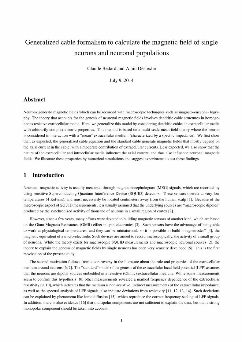
Generalized cable formalism to calculate the magnetic field of single

neurons and neuronal populations

Claude Bedard and Alain Destexhe

July 9, 2014

Abstract

Neurons generate magnetic fields which can be recorded with macroscopic techniques such as magneto-encepha- logra-phy. The theory that accounts for the genesis of neuronal magnetic fields involves dendritic cable structures in homoge-neous resistive extracellular media. Here, we generalize this model by considering dendritic cables in extracellular mediawith arbitrarily complex electric properties. This method is based on a multi-scale mean-field theory where the neuronis considered in interaction with a “mean” extracellular medium (characterized by a specific impedance). We first showthat, as expected, the generalized cable equation and the standard cable generate magnetic fields that mostly depend onthe axial current in the cable, with a moderate contribution of extracellular currents. Less expected, we also show that thenature of the extracellular and intracellular media influence the axial current, and thus also influence neuronal magneticfields. We illustrate these properties by numerical simulations and suggest experiments to test these findings.

1 Introduction

Neuronal magnetic activity is usually measured through magnetoencephalogram (MEG) signals, which are recorded byusing sensitive Superconducting Quantum Interference Device (SQUID) detectors. These sensors operate at very lowtemperatures (4 Kelvins), and must necessarily be located centimeters away from the human scalp [1]. Because of themacroscopic aspect of SQUID measurements, it is usually assumed that the underlying sources are “macroscopic dipoles”produced by the synchronized activity of thousand of neurons in a small region of cortex [2].

However, since a few years, many efforts were devoted to building magnetic sensors of another kind, which are basedon the Giant Magneto-Resistance (GMR) effect in spin electronics [3]. Such sensors have the advantage of being ableto work at physiological temperatures, and they can be miniaturized, so it is possible to build “magnetrodes” [4], themagnetic equivalent of a micro-electrode. Such devices are aimed to record microscopically, the activity of a small groupof neurons. While the theory exists for macroscopic SQUID measurements and macroscopic neuronal sources [2], thetheory to explain the genesis of magnetic fields by single neurons has been very scarsely developed [5]. This is the firstmovivation of the present study.

The second motivation follows from a controversy in the literature about the role and properties of the extracellularmedium around neurons [6, 7]. The “standard” model of the genesis of the extracellular local field potential (LFP) assumesthat the neurons are dipolar sources embedded in a resistive (Ohmic) extracellular medium. While some measurementsseem to confirm this hypothesis [8], other measurements revealed a marked frequency dependence of the extracellularresistivity [9, 10], which indicates that the medium is non-resistive. Indirect measurements of the extracellular impedance,as well as the spectral analysis of LFP signals, also indicate deviations from resistivity [11, 12, 13, 14]. Such deviationscan be explained by phenomena like ionic diffusion [15], which reproduce the correct frequency-scaling of LFP signals,In addition, there is also evidence [16] that multipolar components are not sufficient to explain the data, but that a strongmonopolar component should be taken into account.

1

2

These controversies have important consequences, because if the extracellular medium is non-resistive, several funda-mental theories of neural dynamics, such as the well-known cable theory of neurons [17, 18] or the Current-source densityanalysis [19], are incorrect and need to be reformulated accordingly [15, 20]. The same considerations may also hold forthe genesis of the magnetic fields, as the current theory [2] also assumes that the medium is resistive.

In the present paper, our aim is to build a neuron model to generate electromagnetic fields based on first principles, andthat does not make any a priori assumption, such as the nature of the impedance of the extracellular medium. However, tothis end, we cannot use the classic cable formalism, which was initially developed by Rall [17]. Although this formalismhas been one of the most successful formalism of theoretical neuroscience, explaining a large range of phenomena [18, 21,22, 23], it is non valid to describe neurons in non-resistive media. To palliate to this difficulty, we have recently generalizedcable theory to make it valid for neurons embedded in media with arbitrarily complex electrical properties [20]. In thepresent framework, we will use this generalized cable theory which will be extended to calculate neuronal magneticinduction and electric potential in extracellular space.

We start by outlining a generalized theoretical formalism to calculate the magnetic field around neurons, and we nextillustrate this formalism by using numerical simulations.

2 Theory

In this section, we develop a mean-field method to evaluate the magnetic induction ~B produced by one neuron or by apopulation of neurons, based on Maxwell theory of electromagnetism.

In a first step, we start from Maxwell equations in mean field [15] and in Fourier frequency space, to derive thedifferential equation for the magnetic induction ~B. Note that in principle, one should use the notation < ~B > for the spatialarithmetic average of ~B, but in the rest of the paper we will use the notation ~B for simplicity. The same convention will beused for the other quantities such as the magnetic field ~H, electric field ~E, electric displacement ~D, electric potential V,magnetic vector potential ~A, free-charge current density~j

f, generalized current density~j

g[20] and the impedance of the

extracellular medium zmedia. Note that taking the spatial arithmetic average of the medium impedance implies to take theharmonic mean over the medium admittance γ, because we have zmedia = 1/γ = 1/(σ + iωε).

In a second step, we evaluate ~B produced by a cylinder compartment embedded in a complex extracellular medium.We begin by calculating the the boundary conditions of ~B on the surface of the cylinder compartment. This method usesthe same approach results that we recently introduced and applied to calculate the transmembrane electric potential in thesame model [20]. This method will be used to calculate the boundary conditions of ~B, and these boundary conditions willthen be used to obtain an explicit solution of the differential equation that ~B must satisfy. Next, we will explicitly calculatethe field ~B.

In a third step, we use these results together with the superposition principle to obtain a general method to calculatethe field ~B produced by a large number of cylinder compartments, which can be either define a single neuron dendriticmorphology, or a population of neurons.

2.1 Differential equation for ~B

We now derive the differential equation for ~B in mean field and in an extracellular medium which is linear, heterogeneousand scalar1. In such media, we consider the general case where there can be formation of ions, through chemical reactions.

1Note that by definition, a given medium linear when the linking equations between the fields are convolution products that do not depend on thefield intensities. A medium is scalar when the parameters in the convolution products do not depend on direction in space (ie, are isotropic), which is agood approximation in a mean-field theory.

3

Such charge creation or annihilation will determine additional current densities. At any time, we have:ρ c+ + ρ c− = 0

~jc

= ~j+

+~j−

= ρc+~v ++ ρc−~v −

where ρc+ and ρc− are the variations of positive and negative charge densities, produced by chemical reactions in agiven volume. These relations express the fact that the free-charge density remains invariant when we have creation andannihilation of ions, but that the non-conservation of the total number of ions determines, in general, a current density ofcharge creation~j

c(because~j

+and~j

−necessarily have the same sign).

In such a case, according to classic electromagnetism theory, charge densities and current densities are linked by twosets of equations. The first set comprises four operatorial equations:

∇ · ~D (~x, ω) = ρ f (~x, ω) (i) ∇ · ~B (~x, ω) = 0 (iii)

∇ × ~E (~x, ω) = −iω~B (~x, ω) (ii) ∇ × ~H (~x, ω) = ~jg

(~x, ω) +~jc

(~x, ω) (iv)(1)

Note that ~jg

= ~jf

+ iω~D [Eq. (1 iv)]. where ~jf

is the free-charge current density and iω~D is the displacement currentdensity.

A second set of equations comprises the two linking equations between ~D and ~E, as well as ~H and ~B interaction fields,and one linking equation between the free-charge current density field ~j

fand ~E. Experiments [10, 24] and theory [25]

have shown that these linking equations can be represented by the following convolution equations

~D (~x, ω) = ε (~x, ω) ~E (~x, ω) (i)

~B (~x, ω) = µ (~x, ω) ~H (~x, ω) (ii)

~jf

(~x, ω) = σ (~x, ω) ~E (~x, ω) (iii)

(2)

for a linear and scalar medium. Note that all of the above was formulated in Fourier frequency space.

Assuming that if the base volume considered in the mean-field analysis is large enough, we have at any time the samenumber of creation and annihilation of ions, and we can write ~j

c(~x, t) ≈ 0, so that the Fourier transform of ~j

c(~x, t) can

be considered zero for physiological frequencies2. This is equivalent to consider that the current fluctuations caused bychemical reactions are negligible. It follows from Eqs. (1 iii) and (1 iv):

∇ × (∇ × ~B) = −∇2~B + ∇(∇ · ~B) = −∇2~B = µo∇ ×~jg. (3)

where ~jg

is the generalized current density. This current can be expressed as ~jg

= γ ~E = (σ + iωε) ~E, where γ is theadmittance of the scalar medium (in mean-field3; see also the linking equations [Eqs. (2)]). If the volume of the mean-fieldformalism is large enough, the admittance does not depend on spatial position, and we can write:

∇ ×~jg

= γ ∇ × ~E = −iωγ~B (4)

It follows that∇2~B = iωµoγ ~B . (5)

2Note that it is clear that one can have fluctuations of the number of ions per unit volume, independently of the size considered, when the timeinterval is sufficiently small. However, such contributions will necessarily participate to very high frequencies in the variation of ~j

c(~x, ω)), which are

well outside the “physiological” range of measurable frequencies in experiments (about 1-1000 Hz).3Note that in a mean-field theory, the electromagnetic parameters are calculated for a given volume, and therefore do not depend on spatial coordinates

(for a sufficiently large volume). However, the renormalization to obtain the “macroscopic” electric parameters results in a frequency-dependenceof these parameters. This occurs if electric parameters are not spatially uniform at microscopic scales, or from processes such as ionic diffusion,polarization, etc. [15, 26, 27].

4

Thus, one sees that in general, the differential equation for ~B depends on the admittance of the medium γ. This is dueto the fact that we have considered ∇ ×~j

g, 0 in Eq. (4), which is equivalent to allow electromagnetic induction to occur.

This is counter-intuitive, as ~B is usually believed to be independent of the electric parameters of the medium.

We will see later that, for physiological frequencies, the righthand term of Eq. (5) is negligible, so that we can in prac-tice calculate ~B very accurately using the expression ∇2~B = 0. Note that this approximation amounts to neglect electro-magnetic induction effects in the context of natural neurophysiological phenomena of low frequency (< 1000 Hz) becausethe righthand of Eq. (5) originates in the mathematic formalization of electromagnetic induction (Faraday-Maxwell law,Eq. (1 ii)). However, it is important to keep in mind that the righthand term in Eq. (5) cannot be neglected in the pres-ence of magnetic stimulation [28], because this technique uses electromagnetic induction to induce currents in biologicalmedia. Therefore, when considering magnetic stimulation, we will need to update this formalism accordingly.

2.2 Evaluation of ~B

In the preceding section, we have determined the differential equation that ~B must satisfy in Fourier frequency space.Note that the linearity of Eq. (5) implies that its solution for a given frequency does not depend on other frequencies(which would not be true if the equation was non-linear). However, this equation is not sufficient to determine ~B becausethe boundary conditions must be known to obtain an explicit solution. To solve this boundary condition problem, wemust use cable equations because we consider the “microscopic” case where the electromagnetic field results from theactivity of each individual neuron, rather than considering “macroscopic” sources representing the activity of thousandsof neurons as traditionally done. Moreover, to keep the formalism as general as possible, we consider the “generalizedcable equations” [20], which generalizes the classic cable equations of Rall [17, 18] to the general situation where theextracellular medium can have complex or inhomogeneous electrical properties. We will also use a similar method ofcontinuous cylinder compartment as introduced previously [20]4.

In the following, we first calculate the boundary conditions for an arbitrary cylinder compartment (with arbitrarylength and diameter) [20]. We will see that it is sufficient to evaluate the generalized axial current igi inside each con-tinuous cylinder compartment to evaluate its boundary conditions. Second, we consider the more realistic scenarion ofa dendritic branch of variable diameter, which is approximated by continuous cylinder compartments (Fig. 2). We thencalculate everywhere in space the value of ~B produced by this dendritic branch. Finally, we give a general descriptionof the computation of ~B produced by several dendritic branches. This description can apply in general to any dendriticmorphology, or axons, from one or several neurons.

Figure 1: (Color online) Coordinate ccheme for a cable segment of constant diameter. The scheme shows the cable with the cylindriccoordinate system used in the paper, as well as the surfaces A and C, which are the sections that cuts the cable perpendicular to itsmembrane (delimited by surface B). D is the interior volume of the segment, as delimited by these surfaces, and ∂D is the reunion ofthe two surfaces A and B.

2.2.1 Boundary conditions of ~B for a continuous cylinder compartment

We now calculate the boundary conditions of ~B on the surface of a continuous cylinder compartment. To do this, one mustfirst calculate the direction of ~B on the surface of the compartment. Once the direction of ~B is know, one can calculate theboundary conditions of ~B.

4The method of continuous cylinder compartments consists of solving analytically the cable equations in a continuous cylindric cable compartment,which can be of arbitrary length, but constant diameter (see details in [20]).

5

Direction of ~B To determine the direction of ~B over the surface of a continuous cylinder compartment of radius a, onecan use the expression of the Vector Potential ~A (~B = ∇ × ~A) in conditions of Coulomb’s Gauge (∇ · ~A = 0) and the lawof Kelvin-Maxwell (∇ · ~B = 0 [Eq. (1 iii)]).

Component Bz on the surface of the continuous cylinder compartment If one substitutes in Eq. (1 iv), ~B = ∇ × ~A(within Coulomb’s Gauge), we obtain:

∇ × ~B = ∇ × (∇ × ~A) ≡ −∇2~A + ∇(∇ · ~A) = −∇2~A = µo~jg. (6)

Thus, each component of ~A is solution of a “Poisson” type equation, and we can write in cylindric coordinates:

~A(~x, ω) =µo

4π

$Et

~jg(~x ′, ω)√

r2 + r′2 + 2rr′cos(θ − θ′) + (z − z′)2r′dr′dθ′dz′ (7)

if we assume that ~A = 0 at infinite distance . The integration domain Et represents all space. However, assumingthat the current field in a continous cylinder compartment follows cylindric symmetry, we can write that in any pointof space, the generalized current density is given by: ~j

g= jr g(r, z) er + jz g(r, z) ez where ez and er are respectively

parallel and perpendicular to the symmetry axis of the axial current. It follows that the Vector Potential is of the form~A = Ar(r, z) er+Az(r, z) ez [Eq. (7)]. Thus, the component Bz of ~B is always equal to zero, since we have Bz = (∇×~A) z = 0.

The component Br on the surface of the continuous cylinder compartment The application of Kelvin-Maxwell’slaw [Eq. (1 iii)] implies that the surface integral (Fig. 1) of Br gives:"

SB

Br dS =

"∂D

~B.n dS ≡$D

∇ · ~B dv = 0 (8)

because the component Bz = 0 ⇒!SA

~B · n =!SC

~B · n dS =!SA

|Bz|dS =!SC

|Bz|dS = 0 (for a plane perpendicular to

the surface SB of the compartment. Thus, we can deduce that Br = 0 because the integral of Br is zero for a surface ofarbitrary length SB. Consequently, the general expression of ~B over the surface of a continuous cylinder compartiment isgiven by:

~B = Bθeθ . (9)

Note that electromagnetic induction is taken into account in this derivation because we did not use the explicit value of∇ × ~E when deriving Eq. (1 ii).

Evaluation of Bθ on the surface of the continuous cylinder compartment We now evaluate Bθ as a function of thegeneralized current. We calculate the values of Bθ as a function of the generalized current over the surface SB (Fig. 1)using Ampère-Maxwell law [Eq. (1) iv]. We obtain:∮

∂SB

~B.d~s =

"SA

∇ × ~B · nSA dS = µo

"SA

~jg· nSA dS = µoi gi , (10)

where i gi is the generalized axial current inside the continuous cylinder compartment. Taking into account cylindicsymmetry gives:

~B = Bθeθ =µoi gi (z, ω)

2πaeθ , (11)

where i gi is the axial current inside the compartment and a is its radius.

This equation together with Eq. (5) show that the value of ~B around a dendritic compartment will depend on theimpedance of the extracellular medium (1/γ) for two different reasons. First, the righthand term of Eq. (5) explicitlydepends on the extracellular impedance, but we will see in the next section that these electromagnetic induction effects arelikely to be negligible. Second, Eq. (11) shows that the boundary conditions also depend on the extracellular impedance,

6

because the spatial and frequency profiles of i gi depend on this impedance [20]. However, we will see that, contraryto electromagnetic induction, this dependency cannot be neglected when calculating ~B, because this effect is potentiallyimportant. In the next section, we calculate magnetic induction in the extracellular space by directly solving Eq. (5) usingthe boundary conditions evaluated by Eq. (11).

Figure 2: (Color online) Scheme to calculate the magnetic induction produced by a dendritic branch. a. To evaluate the contributionof the dendritic segment, we divide space into three regions: L, P, R. We first evaluate Bθ in the principal region P, which correspondsto the space between Regions L and R. Next, we evaluate Bθ in the boundary regions L and R. Note that the knowlegde of Bθ in Region

P is necessary to evaluate Bθ in Regions L and R because it one must know Bθ on the two planes z = 0 and z =Np∑i=1

li = l, in order to

calculate its explicit value in Regions L and R using Eq. (5). b. Evaluation of Bθ for a segment of variable diameter. In this case, the

same procedure is followed, except that Region P is divided into Np compartments, each described by a continuous cylinder, P =Np⋃i=1

pi.

Note that the continuity conditions on the axial current and the transmembrane voltage allow one to define boundary conditions for Bθ

over the surfaces of the compartments pi. The figure shows an example with Np = 3.

2.2.2 General expression of ~B in extracellular space for a dendritic branch

In this section, we derive a method to calculate the expression of ~B for a dendritic branch (Fig. 2) In cylindric coordinates,Eq. (5) writes:

∇2~B = [ ∂2Br

∂r2 + 1r2∂2Br

∂θ2 + ∂2Br

∂z2 + 1r∂Br

∂r −2r2∂Bθ

∂θ− Br

r2 ] er

+ [ ∂2Bθ

∂r2 + 1r2∂2Bθ

∂θ2 + ∂2Bθ

∂z2 + 1r∂Bθ

∂r + 2r2∂Br

∂θ− Bθ

r2 ] eθ + [ ∂2Bz

∂r2 + 1r2∂2Bz

∂θ2 + ∂2Bz

∂z2 + 1r∂Bz

∂r ] ez

= iωµoγ~B = iωµoγ[Brer + Bθeθ + Bzez]

(12)

According to preceding section, the boundary conditions imply ~B = Bθ(r, z) eθ on the surface of each continuouscylinder compartment, as well as ~B = 0 for infinite distances. The cylindric symmetry of the boundary conditions impliesthat Br = Bz = 0 everywhere in space because the solution of Eq. (12) is unique. Consequently, to evaluate the value ofBθ produced by a dendritic branch, one must solve the following equation:

∂2Bθ

∂r2 +1r∂Bθ

∂r+∂2Bθ

∂z2 −Bθ

r2 = iωµoγBθ . (13)

2.2.3 Solving the equation of ~B for a continuous cylinder compartment

In this section, we introduce an iterative method to calculate the solution of Eq. (13) for a continuous cylinder compartmentof radius a and length l, when the values of Bθ at its surface are known. The goal of this approach is to provide analternative method and avoiding to solve Laplace equation (∇2Bθ = 0) using finite elements methods5. We approach the

5Equation (13) can be easily solved using the finite element method for a simple geometry. For example, Galerkin method works very well in thiscase, but requires significant computation time [29]

7

Figure 3: (Color online) Scheme to calculate Bθ. a Extension of the compartment in Regions L and R when the principal region (P)consists of a single cylinder compartment of radius a. b. Calculation scheme. In a first step, we calculate in Fourier space the field Bθ

by assuming that the boundary conditions on the cylinder are such that: Bθ(a, z < 0, ω) = 0 and Bθ(a, z > l, ω) = 0 in Regions L and R.The solution of Eq. (13) obtained in such conditions is called the first-order solution of Bθ. In a second step, we improve the boundaryconditions by applying the Hankel transform of order 1 relative to r, and the continuity principle of the solution at the borders L-P andP-R. We re-evaluate the solution of Eq. (13) with these new boundary conditions to obtain a second-order solution of Bθ. The sameiteration is continued.

solution analytically by using the mathematical relations between the different currents present in the neuron, and themagnetic induction that these currents produce.

We calculate Bθ in space assuming that Region P contains only one continuous cylinder compartment (Fig 2a), butthe method can be easily generalized to the case with several compartments (Fig 2b). In this case, to generalize to Np

compartments, one must determine the boundary conditions of Bθ for each compartment inside Region P. In all cases, weassume that Bθ satisfies: 1) Bθ is a continuous function on the borders L-P and P-R [Fig. 3]; 2) Bθ = 0 at infinite distance;3) Bθ = 0 on the symmetry axis of the compartment.

To calculate the solution, we extend the original compartment in Regions L and R using the same radius a (Fig. 3a).Note that by convention, we place the symmetry axis on the z-axis, and place the continuous cylinder between coordinatesz = 0 and z = l > 0.

At the first order of the iteration, we assume thatBθ(a, z < 0, ω) = 0

Bθ(a, z > l, ω) = 0

over the surfaces of the extended compartment (L and R), which ensures the spatial continuity of the first-order solutionat the borders L-P and P-R. A priori this choice is arbitrary but we have chosen here a particular attenuation law whichneglects the radius of the extended compartment. Following this first choice, we calculate the solution of Eq. (13) byusing complex Fourier transform along z. This leads to:

Bθ(r, z, ω) =1

2π

∫ +∞

−∞

g(r, kz, ω) e+ikzz dkZ , (14)

where

g(r, kz, ω) =

∫ +∞

−∞

Bθ(r, z, ω) e−ikzz dz . (15)

We next substitute Eq. (14) in Eq. (13), which leads to∫ +∞

−∞

[d2g

dr2 +1rg

dr− (k2

z +1r2 ) g] e+ikzzdz = 0 . (16)

Here, we have neglected electromagnetic induction (iωµoγBθ ≈ 0), because we have ωµo|γ| ≈ 0 for the typical size ofa neuron in cerebral cortex, and for frequencies lower than about 1000 Hz. Indeed µo = 4π×10−7 H/m and the admittance

8

of the extracellular medium is certainly lower than that of sea water, and thus we can write |γmedium| < |γsea water | < 1. Thisapproximation amounts to neglect the phenomenon of electromagnetic induction (in the absence of magnetic stimulation).Thus, the frequency dependence of ~B is essentially caused by the frequency dependence of the axial current igi . Note thatigi depends on the nature of extracellular and cytoplasm impedances, as shown previously [20].

Thus, we have (for kz and ω fixed) the following equality:

d2g

dr2 +1r

dgdr− (k2

z +1r2 ) g = 0 (17)

because the Fourier transform of zero is zero. It follows that the function g must be solution of the modified Besseldifferential equation of order 1. The general solution of such an equation is given by:

g(r, kz, ω) = c(kz, ω) I1 (|kz|r) + d(kz, ω) K1 (|kz|r) , (18)

where I1 is a a modified Bessel function of first kind of order 1 and K1 is a modified Bessel function of second kindof order 16. Such functions are illustrated in Fig. 4 as a function of r for typical parameter values that corresponds toneurons. Note that we must assume that kz is very small for function K1(|kz|r) to have a significant value for large r. For afixed value of K1, we have kz ∼ 1/r.

Finally, to evaluate the coefficients c(kz, ω) and d(kz, ω), we apply the continuity condition of Bθ between the interiorand exterior of the extended compartment, and that Bθ must be zero on the symmetry axis of the compartment (r = 0),as well as at infinite distance. Because |I1 (∞, ω)| = ∞, we must assume that c(kz, ω) = 0 outside of the cylinder, andbecause |K1 (0, ω)| = ∞, we must assume that d(kz, ω) = 0 inside of the cylinder. Taking these conditions into account,we obtain:

exterior r ≥ a d(kz, ω) =g(a,kz,ω)K1(|kz |a)

interior r ≤ a c(kz, ω) =g(a,kz,ω)I1(|kz |a)

(19)

It follows that the approximative solution of first-order is given by:exterior r ≥ a Bθ(r, z, ω) = 1

2π

∫ +∞

−∞g(a, kz, ω) K1(|kz |r)

K1(|kz |a) e+ikzz dkz

interior r ≤ a Bθ(r, z, ω) = 12π

∫ +∞

−∞g(a, kz, ω) I1(|kz |r)

I1(|kz |a) e+ikzz dkz

(20)

where the function g(a, kz, ω) is given by Eq. (15).

g(a, kz, ω) =

∫ +∞

−∞

Bθ(a, z, ω) e−ikzz dz . (21)

This first iteration gives us a first-order approximation of Bθ, which is refined in successive iterations, as schematizedin Fig. 3b. We use the first-order approximation in Region P to calculate the solutions in Regions L and R. To do this, weuse the first-order Hankel transform7 for the variable r. To do this, one applies the continuity principle at the borders L-Pand P-R. This gives the following relations:

Bθ(r, z, ω) =

∫ ∞0

krh1(kr, z, ω)J1(krr) dkr (22)

whereh1(kr, z, ω) =

∫ ∞0

rBθ(r, z, ω) J1(krr) dr (23)

in Regions L and R.

The Hankel tranform is a calculus technique similar to the wavelet transform (Fig. 4c-d). Note that the values of kr

vary inversely proportional to the values of r, similarly to the relation between parameter kz and z above (Fig. 5).6We have J1(ir′) = iI1(r′) and Y1(ir′) = I1(r′) + 2

π iK1(r′), where J1 is the modified Bessel function of first kind of order 1, and Y1 is the Besselfunction of second kind of order 1.

7This is equivalent to the first-order Fourier-Bessel transform. This particular transform was chosen here because the function J1(krr) has the sameboundary conditions as in the present problem (Fig. 4c-d): it is equal to zero for r = 0 and for r → ∞.

9

10−6

10−4

10−2

10−20

10−15

10−10

10−5

100

105

(a)

K1(k

r)0 0.5 1 1.5 2

x 10−6

0

1

2

3

4

5

6x 10

−3 (b)

I 1(k

r)

10−6

10−4

10−2

−0.4

−0.3

−0.2

−0.1

0

0.1

0.2

0.3

0.4

0.5

0.6

(c)

r (m)

J1(k

r)

0 0.5 1 1.5 2

x 10−6

0

0.005

0.01

0.015

0.02

0.025

0.03

(d)

r (m)J

1(k

r)

Figure 4: (Color online) Bessel functions for a continuous cylinder compartment. The Bessel functions are indicated as a functionof the distance r perpendicular to the axis of the cylinder; the cylinder had a length l of 300 µm and a radius a = 2 µm. We havek′ = 2 × 104 m−1. a. K1 as a function of distance. The red curve shows the function K1(kr) with k = k′. The black dashedstraight line represents the function 1/kr and the blue dashed curve represents the asymptotic behavior of K1 for r → ∞. We haveK1(kr)

∞−→

√π

2kr e−kr . At short distances (smaller than 2/k), the function K1 decays linearly with distance, but for large distances(r > π/k), it converges more rapidly than an exponential decay with distance. b. The function I1 (modified Bessel function of first kindof order 1) is well approximated by a straight line (I1(kr) = kr/2) for k = k′ when r < a. c. Bessel function of first kind of order 1 when

r > a. The blue and black curves correspond respectively to k = k′ and k = 5k′. Note that we have J1(kr)∞−→

√2πkr cos(kr − 3π

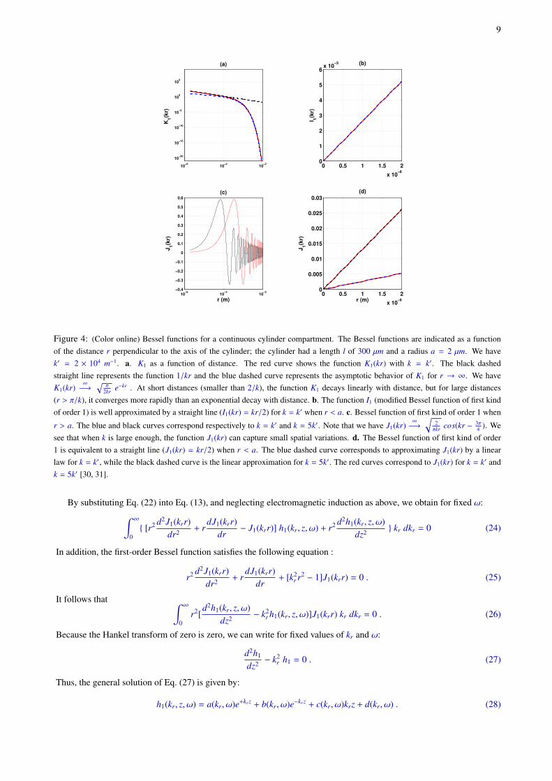
4 ). Wesee that when k is large enough, the function J1(kr) can capture small spatial variations. d. The Bessel function of first kind of order1 is equivalent to a straight line (J1(kr) = kr/2) when r < a. The blue dashed curve corresponds to approximating J1(kr) by a linearlaw for k = k′, while the black dashed curve is the linear approximation for k = 5k′. The red curves correspond to J1(kr) for k = k′ andk = 5k′ [30, 31].

By substituting Eq. (22) into Eq. (13), and neglecting electromagnetic induction as above, we obtain for fixed ω:∫ ∞0 [r2 d2J1(krr)

dr2 + rdJ1(krr)

dr− J1(krr)] h1(kr, z, ω) + r2 d2h1(kr, z, ω)

dz2 kr dkr = 0 (24)

In addition, the first-order Bessel function satisfies the following equation :

r2 d2J1(krr)dr2 + r

dJ1(krr)dr

+ [k2r r2 − 1]J1(krr) = 0 . (25)

It follows that ∫ ∞0

r2[d2h1(kr, z, ω)

dz2 − k2r h1(kr, z, ω)]J1(krr) kr dkr = 0 . (26)

Because the Hankel transform of zero is zero, we can write for fixed values of kr and ω:

d2h1

dz2 − k2r h1 = 0 . (27)

Thus, the general solution of Eq. (27) is given by:

h1(kr, z, ω) = a(kr, ω)e+krz + b(kr, ω)e−krz + c(kr, ω)krz + d(kr, ω) . (28)

10

100

102

104

106

10−16

10−15

10−14

10−13

10−12

10−11

10−10

10−9

10−8

(a)

kr

h1(k

r)

10−6

10−5

10−4

10−3

10−4

10−3

10−2

10−1

100

(b)

r

f(r)

Figure 5: (Color online) Example of application of the Hankel transform of order 1. (a). Approximation using the Hankel transformof order 1 of the function f (r) = H(r − a)1/r with a = 1 µm, 1 < kr < 5 × 106 and ∆kr = 103. The values smaller than 103 are notsignificant because of the value of ∆kr is larger than 1000. We can see that the approximation using the Hankel transform is valid fordistances up to 1 mm. (b). Inverse transform applied to this approximation (in blue), and comparison with the original function (inred), between 1 µm and 1 mm. The parameter kr of the Hankel transform plays a similar role as the wave number ( 2π

λ) in spatial Fourier

transform. The larger kr, the more sensitive to fine spatial details.

Using the condition that Bθ vanishes at infinite distance for each frequency, implies that, for each frequency, a = c = d = 0when z > l, and a = b = d = 0 when z < 0. Consequently, the solution in Regions L and R are given by:

Bθ(r, z, ω) =∫ ∞

0 hL1 (kr, ω)J1(krr) ke−kr |z| dkr z < 0

Bθ(r, z, ω) =∫ ∞

0 hR1 (kr, ω)J1(krr) ke−kr |z−l| dkr z > l

, (29)

where hi1 for i = L and i = R are given by the continuity conditions at z = 0 and z = l, and we obtain:

hL1 (kr, ω) = h1(kr, 0, ω) =

∫ ∞0 rBθ(r, 0, ω)J1(krr) dr

hR1 (kr, ω) = h1(kr, l, ω) =

∫ ∞0 rBθ(r, l, ω)J1(krr) dr

(30)

It follows that we can calculate the new limit conditions on the extended compartment, by applying Eqs. (29). We obtain:Bθ(a, z, ω) =

∫ ∞0 hL

1 (kr, ω)J1(kra) ke−kr |z| dkr z < 0

Bθ(a, z, ω) =∫ ∞

0 hR1 (kr, ω)J1(kra) ke−kr |z−l| dkr z > l

, (31)

11

After applying the Hankel transform of first-order, if we recover the same boundary conditions that were assumed atthe borders of the cylinder compartment, then we have reached the exact solution. If this is not the case, we can continueto improve the approximation of the solution by further iterations (Fig. 3). To do this, one considers the original boundaryconditions in Region P together with the new expressions for the boundary conditions at the extended compartment (Land R) according to Eqs. (31) One applies the complex Fourier transform on axis z [Eqs. (20) and (21)] to obtain ahigher-order approximation. The iteration is then continued until one obtains a satisfactory solution (Fig. 3b-c; see detailsin Appendix A).

2.2.4 Importance of the spatial profile of the axial current

In the previous section, we have calculated ~B without explicitly considering the current in the extracellular space aroundthe neuron. However, we know that this current necessarily produces a magnetic induction, and thus it is necessary toinclude this contribution to obtain a complete evaluation of ~B in extracellular space. In this section, we show that that thiscontribution of extracellular currents is implicitly taken into account by our formalism, through the spatial and frequencyprofile of igi .

According to Eqs. (1iv) and (2ii), we can evaluate the generalized current outside of a continuous cylinder compart-ment:

~jg

=1µo∇ × ~B (32)

when~jc

= 0 and for µ(~x, ω) = µo. Rewriting this expression in cylindric coordinates, we obtain

~jg

=1µo

[ (1r∂Bz

∂θ−∂Bθ

∂z) er + (

∂Br

∂z−∂Bz

∂r) eθ +

1r

(∂(rBθ)∂r

−∂Br

∂θ) ez ] (33)

It follows that~jg

=1µo

[−∂Bθ

∂zer + (

∂Bθ

∂r+

Bθ

r) ez] (34)

because the solution is of the form ~B(r, θ, z, ω) = Bθ(r, z, ω) eθ [Sec. 2.2.2]. We see that the generalized current densityoutside of the neuron is different from zero, if and only if we have

− ∂Bθ

∂z , 0

∂Bθ

∂r + Bθ

r , 0(35)

Thus, the external current around the neuron is taken into account because the solution depends on r and z in general (seepreceding section).

Note that we have ∂Bθ

∂z = 0 (Fig. 2) if and only if the spatial profile of the axial current igi does not depend on z[Eq. (11)]. In this case, the current im is zero, which implies that the electric field produced by the compartment is alsozero [17, 18, 20]. In addition, we know that in a neuron, one cannot have axial current without transmembrane current,and thus, it is impossible that ∂Bθ

∂z = 0 in a given compartment. Therefore, we can conclude that the external current istaken into consideration because ∇ × ~B , 0 outside of the compartment when ~B depends on z.

In the preceding section, we have calculated Bθ for a single continuous cylinder compartment. We now considerthe more complex case when this compartment is connected to a soma on one side, according to a “ball-and-stick”configuration. In this case, one can consider that the current density ~j

gin Region R satisfies ∇ · ~j

g= 0 (generalized

current conservation law) when~jc

= 0 and

∇ ×~jg

= (σe + iωε) ∇ × ~E = 0

(when electromagnetic induction is negligible, and in mean-field)8. It follows that we have ∇2~jg

= 0 in each pointof Region R. Thus, the field ~j

gdoes not explicitly depend on electomagnetic parameters, which is remarkable. With

8Note that we have considered several scales in [20]: the interior of the dendritic compartment, the interior of the soma, the membrane, and theextracellular medium.

12

Figure 6: (Color online) Illustration of the current fields around the soma of a ball-and-stick model. The current fields are shown(arrows) around the soma when the generalized membrane current is perpendicular to the soma membrane (red arrows). The isopotentialsurfaces are shown in blue and correspond to the soma membrane . If the soma has a different “diameter”, but coincides with theisopotential surface, then the geometry of these current lines and isopotential surfaces remains invariant. However, the value of theelectric potential is different on each equipotential surface.

the continuity condition of the current at the interface between Regions P and R, and the vanishing at infinite distances(~j

g ∞−→ 0), we have a unique solution (Dirichlet problem) in Region R.

However, the method to calculate the generalized cable for the ball-and-stick model implicitly considers the somaimpedance in the spatial and frequency profiles on the continuous cylinder compartment(s) [20]9. Thus, the somaimpedance is also taken into account implicitly here when calculating the current at the interface between Regions Pand R.

It is important to note that the same current geometries can be seen for different soma sizes (Fig. 4), and thus differentneuron models of identical dendritic structure but different soma will generate identical magnetic inductions in Region R(comprising the soma). Note that it does not apply to the electric field and potential around the soma because we have~E =

~jg

(σe+iω)ε where (σe + iωε) depends on the size of the soma membrane. Thus, the soma impedance is sufficient to

determine ~B but its exact size is not important if the soma coincides with an isopotential surface.

Consequently, taking into account the spatial and frequency profiles of Bθ over the surface of the cylinder compart-ments allows one to calculate everywhere in space the field ~B as well as the current fields inside and outside of themembrane. Thus, the spatial and frequency profiles of igi [Eq. (11)] implicitly take into account the screening effectcaused by the “return current” outside of the neuron, when present. Note that this conclusion is entirely consistent withMaxwell equations and the pseudo-parabolic equation (13) derived from it, because these equations determine a uniquesolution for a given set of boundary conditions. In the next section, we show how this method can be generalized tocomplex morphologies or populations of neurons (still under the condition that electromagnetic induction is negligible).

9In this paper, we have assumed that~jg

is perpendicular to the membrane surface at the soma. This implies that the internal and external surfaces ofthe soma are equipotential because (σe + iωε)~E is perpendicular to the soma membrane. Thus, the soma membrane is characterized by an impedanceZs =

Vmigi

, which affects the spatial and frequency profiles in the dendritic compartments.

13

Figure 7: (Color online) Example with 2 neurons. In order to calculate the value of the magnetic induction ~B generated by manyneurons, one has to sum the values of ~Bi produced by each branch. Thus, it is sufficient to know the axial current i gi at each branch tocalculate ~B.

2.3 The general expression of ~B for NB dendritic branches from one or several neurons

Assuming that electromagnetic induction is negligible, and that the medium is linear, we can apply the superpositionprinciple such that we can write ~B as:

~B =

NB∑i=1

~Bi (36)

where each ~Bi is the magnetic induction produced by each branch as if it was isolated.

Thus, at some distance away of an ensemble of dendritic branches assimilable to continuous cylinder compartments,the field ~B is the vectorial sum of the field ~B produced by each compartment, which is itself calculated from the averagespatial and frequency profile of the axial current in each compartment (see Sec. 2.2.3).

3 Numerical simulations

In this section, we show a few simulations with different types of media for a ball-and-stick type model. In a first step,we describe how to calculate the generalized axial current as a function of the synaptic current for a ball-and-stick typemodel. In a second step, we apply the method developed above to calculate the magnetic induction. We show here twoexamples, first when the extracellular and cytoplasm impedances are resistive, and second, when these two impedancesare diffusive (Warburg impedance).

3.1 Method to calculate the generalized axial current for a ball-and-stick model

In a first step, we determine the transmembrane voltage in the postsynaptic region. The current produced in this regionseparates in two parts: one that goes to the soma (“proximal”), and another one going in the opposite direction (“distal”)(Fig. 8). These two currents are given by the following relations, ZD(zi, ω) =

Vm(zi,ω)i giD(zi,ω) and ZP(zi, ω) =

Vm(zi,ω)i giP (zi,ω) , for the distal

and proximal regions, respectively. These expressions were derived previously [20].

Next, we determine the equivalent impedance at the position of the synapse (Fig. 8) [20]. We obtain

Zeq(zi, ω) =ZP(zi, ω)ZD(zi, ω)

ZP(zi, ω) + ZD(zi, ω)(37)

It follows that the transmembrane voltage at the position of the synapse is given by:

Vm(zi, ω) = Zeq(zi, ω) i gs (zi, ω) (38)

14

Figure 8: (Color online) Equivalent scheme to calculate the current flowing from distal to proximal at the position of the synapse,when the synaptic current is known.

when the synapse is at position zi. Next, we determine igA(zi, ω) and igD(zi, ω) from the following expressions:i gP (zi, ω) =

Vm(zi,ω)ZP(zi,ω)

i gD (zi, ω) =Vm(zi,ω)ZD(zi,ω)

(39)

We have seen in [20] that with the generalized current, the cable equations can be written in a form similar to thestandard cable equation:

∂2Vm(z, ω)∂z2 = κ2

λ Vm(z, ω) (40)

whereκ2λ =

zi (1+iωτm)rm

=zi (1+iωτm)

rm [1+z(m)erm

(1+iωτm)], (41)

where 1/rm, zi and τm are, respectively, the linear density of membrane conductance (in S/m), the impedance per unitlength of the cytoplasm (in [Ω/m]) and the membrane time constant. The parameter z(m)

e stands for the specific impedanceof the extracellular medium. This parameter impacts on the spatial and frequency profile of Vm, im and i gi , and has thesame units as rm.

The general solution of this equation in Fourier space ω , 0 is given by:VmD(z, ω) = A+

P(zi, ω) e+κλz + A−D(zi, ω) e−κλz

VmP(z, ω) = A+P(zi, ω) e+κλ(l−z) + A−P(zi, ω) e−κλ(l−z)

(42)

for a continuous cylinder compartment of length l and constant diameter, and when we know the synaptic current atposition z = zi. In such conditions, the coefficients of Eq. (37) are given by the following expressions (see Appendix F in[20]):

A+D(zi, ω) = 1

2 e−κλzi [ VmD(zi, ω) + ziκλ

i giD(zi, ω) ]

A−D(zi, ω) = 12 e+κλzi [ VmD(zi, ω) − zi

κλi giD(zi, ω) ]

A+

P(zi, ω) = 12 e−κλ(l−zi) [ VmP(zi, ω) + zi

κλi giP(zi, ω) ]

A−P(zi, ω) = 12 e+κλ(l−zi) [ VmP(zi, ω) − zi

κλi giP(zi, ω) ]

(43)

15

Note that we can verify that Vm is continuous, in which case we have VmP(zi, ω) = VmD(zi, ω), which is consistent with thefact that the electric field is finite. Thus, one sees that when the synaptic current is known at a given position, the spatialprofile of Vm can be calculated exactly for a continuous cylinder compartment.

It follows that one can deduce the spatial and frequency profiles of Vm when we know the current generated by eachsynapse, thanks to the superposition principle. Finally, one can directly calculate the generalized current by applying thefollowing equation :

i gi = −1zi

∂Vm

∂z(44)

on Eq. (36) [20] . We obtain the generalized axial current generated by a single synapse:i giD(z, ω) = −

κλzi

[ A+D(zi, ω) e+κλz + A−D(zi, ω) e−κλz ]

i giP(z, ω) = +κλzi

[ A+P(zi, ω) e+κλ(l−z) −

κλzi

A−P(zi, ω) e−κλ(l−z) ](45)

To obtain the total axial current, one has just to sum up the contributions of each synapse. Note that this “linear”assumption only holds for current-based inputs, and a modified model is needed to account for conductance-based inputs(not shown).

Finally, the knowledge of the generalized axial current permits to determine the boundary conditions on ~B and applythe method developed above [Eq. (11)]. In the next section, we apply this strategy to calculate the magnetic induction indifferent situations.

3.2 Simulations of ~B in extracellular space

In this section, we apply the theory to a ball-and-stick type model of the neuron [21, 22], using two different approxima-tions of the extracellular medium and cytoplasm impedance, either when they are purely resistive (Ohmic), or when ionicdiffusion is taken into account, resulting in Warburg type impedances [20].

To do this, we model the ensemble of synaptic current sources as a “stochastic dipole” consisting of two stochasticcurrents, stemming from excitatory and inhibitory synapses. Each synaptic current is described by a shot-noise given by:

is =

N∑n=1

cH(t − tn) e−(t−tn)/τm (46)

where H is the Heaviside function. The stochastic variable tn follows a time-independent law. We have chosen τm = 5 mswhich corresponds to in vivo conditions, c = +1 nA for excitatory synapses, and c = −1 nA for inhibitory synapses(Fig. 9).

In the simulations, we have simulated a ball-and-stick neuron model with a dendrite of 600 µm length and 2 µmconstant diameter, and a spherical soma of 7.5 µm radius. The synaptic currents were located at a distance of 57.5 µmof the soma for inhibitory synapses, and respectively 357.5 µm for excitatory synapses. Note that this particular choicewas made here to simplify the model. This arrangement generates a dipole which approximates the fact that inhibitorysynapses are more dense in the soma/proximal region of the neuron, while excitatory synapses are denser in more distaldendrites [32].

3.2.1 Magnetic field generated by a ball-and-stick model with resistive media

We start by calculating the magnetic induction for the “standard model” where the extracellular medium and cytoplasmare both resistive. The electric conductivity of cytoplasm was of 3 S/m, and that of the extracellular medium was of5 S/m, in agreement with previous models [17, 18, 22, 23].

The magnetic field generated by the resistive model is described in Fig. 10. We can see that, for a given frequency,the modulus of Bθ is almost constant in space over the dendritic branch in the region between the two locations of the

16

0 0.1 0.2 0.3 0.4 0.5 0.6 0.7 0.8 0.9 1−2

−1.5

−1

−0.5

0

0.5

1

1.5x 10

−8

t (s)

I (A

)

(a)

100

101

102

103

10−14

10−13

10−12

10−11

10−10

10−9

ν (Hz)

|I| (A

/Hz)

(b)

0 1000 2000 3000 4000−400

−300

−200

−100

0

100

ν (Hz)Φ

( d

eg

)

(c)

Figure 9: (Color online) Synaptic current sources used in the simulations. (a) Example of excitatory (blue, top curve) and inhibitory(black, bottom curve) current sources used in simulations. These examples consists of 1000 random synaptic events per second. (b)and (c): Modulus and phase, respectively, of the complex Fourier transform of these processes. Note that the inhibitory current innot represented in (b) because its modulus is identical to that of the excitatory current. The red dashed line in (b) corresponds to aLorentzian ( A

1+iωτm) with τm = 5 ms and |A| = 1 nA).

0 2 4 6

x 10−4

0

1

x 10−11

z(m)

|Bθ| (T

/Hz)

(a)

0 2 4 6

x 10−4

−2

−1

0

1

2

3

4

z (m)

Φ (

deg )

(b)

5 Hz

5 Hz

5 Hz

5 Hz

5000 Hz

5000 Hz5000 Hz

5000 Hz

Figure 10: (Color online) Magnetic induction for the resistive model. Bθ is shown here at the surface of the dendrite,as a function of position (distance to soma) for different frequencies between 1 Hz and 5000 Hz. The blue dashed linescorrespond to Bθ generated when only excitatory synapses were present, and the black curves correspond to both synapsespresent. Bθ is always decreasing with frequency, and is larger and approximately constant between the two locations ofthe synaptic currents.

synaptic currents. It is also smaller outside of this region. Note that the attenuation of Bθ is completely different whetherexcitatory or inhibitory synapses are present (Fig. 10, blue dashed curves). Finally, we also see that the attenuation of the

17

axial current is very close to a linear law although in reality we have a linear combination of exponentials (see Eq. 45).

100

102

10−15

10−14

10−13

10−12

10−11

10−10

ν (Hz)

|Bθ| (T

/Hz)

(a)

500 1500 2,500−3

−2

−1

0

1

2

3

4

ν (Hz)

Φ (

de

g )

(b)

20 µm

60 µm

260 µm

550 µm

260 µm

60 µm

20 µm

600 µm

270 µm

270 −550 µm

570 µm

570−600 µm

Figure 11: (Color online) Frequency profile of the magnetic field for the resistive model. Bθ at the surface of the dendriteis represented as a function of frequency at different positions (both excitatory and inhibitory synapses were present). Thered curves correspond to different positions between the inhibitory synapses and the soma, the blue curves are taken atdifferent positions between the excitatory synapses and the end of the dendrite, and the black curves represent positionsin between the two synapse sites. Note that the modulus of Bθ does not depend on position.

The frequency dependence of Bθ is shown in Fig. 11 for the resistive model. The frequency dependence depends onthe position on the dendrite. Between the two synapse sites (black curves), the frequency dependence does not depend onthe position, and the scaling exponent is close to -1.5. However, the phase of Bθ is position dependent, but is very small(between 0 and -3 degrees). In this region, the frequency scaling begins at frequencies larger than about 10 Hz.

In the “proximal” region, between the soma and the location of inhibitory synapses, the frequency dependence is dif-ferent according to the exact position on the dendrite (Fig. 11, red curves) and the frequency scaling occurs at frequencieslarger than 1000 Hz. However, the frequency scaling is almost identical and the exponent is of about -1. The contributionof this region to the value of Bθ can be negligible compared to the preceding region for the frequency range consideredhere (<1000 Hz). The phase also shows little variations and is of small amplitude (between 1 and 3 degrees).

Finally, for the “distal” region, away of the site of excitatory synapses, the frequency-dependence of the modulus ofBθ varies with the position on the dendrite, and is significant only from about 1000 Hz, similar to the proximal region. Thedependencies are almost identical between proximal and distal regions, except for frequencies larger than 1000 Hz. Notethat the contribution of these two regions to the value of Bθ is very small and can be considered negligible compared to theregion between the two synaptic sites (for frequencies smaller than 1000 Hz). The Fourier phase shows little variationsbetween 1 and 5000 Hz. The frequency scaling exponent is of the order of -1.5 between 2000 and 4000 Hz. Note that thenumerical simulations also indicate that the boundary conditions on the stick are very sensitive to the cytoplasm resistancebut are less sensitive to the extracellular resistance.

3.2.2 Magnetic field generated by a ball-and-stick model with diffusive media

We now illustrate the same example as above, but when the intracellular (cytoplasm) and extracellular media are describedby a diffusive-type Warburg impedance (Figs. 12 and 13). We have assumed that the cytoplasm admittance is γ =

3√ω (1+i)√

2S/m, while that of the extracellular medium is 5

√ω (1+i)√

2S/m. These values were chosen such that the modulus

of the admittance is the same as the preceding example with resistive media (see Section 3.2.1) for ω = 1.

18

0 2 4 6

x 10−4

0

0.5

1

1.5

2

2.5

3x 10

−11

z (m)

|Bθ| (T

/Hz)

(a)

0 2 4 6

x 10−4

−3

−2

−1

0

1

2

3

4

z (m)

Φ (

deg

)

(b)

5 Hz

5 Hz

5000 Hz

5000 Hz

5000 Hz

5000 Hz

5 Hz

5 Hz

Figure 12: (Color online) Magnetic induction Bθ on the surface of the dendrite for a neuron embedded in diffusive media. Bθ isrepresented for different frequencies. The blue dashed curves correspond to Bθ produced at the surface of the dendrite with onlyexcitatory synapses, and black curves correspond to excitatory and inhibitory synapses present. We see that Bθ is a decreasing functionof frequency, and is higher towards inhibitory synapses, and low outside of this region.

When calculating the magnetic induction, we see that the modulus of Bθ on the dendrite surface increases when oneapproaches the position of inhibitory synapses, but is very small outside of this region (Fig. 10, black curves). Note thatthe attenuation law of Bθ along the dendritic branch is completely different from that with only excitatory synapses present(Fig. 10, blue dashed curves). We also see that the attenuation of the axial current is very close to a straight line, but inreality it is given by a sum of exponentials (see Eqs. 45).

100

102

10−16

10−15

10−14

10−13

10−12

10−11

10−10

ν (Hz)

|Bθ| (T

/Hz)

(a)

500 1500 2500−3

−2

−1

0

1

2

3

ν (Hz)

Φ (

deg )

(b)

260 µm

60 µm

570 µm

600 µm

270 −550 µm

270 −550 µm

20 µm

20 −260 µm

570−600 µm

Figure 13: (Color online) Magnetic induction Bθ on the surface of the dendrite, as a function of frequency, for a neuron withindiffusive media. Bθ is represented for different positions on the dendrite, with both excitatory and inhibitory synapses present. One cansee three distinct regions: proximal region between the soma and the location of inhibitory synapses (red curves), region between thetwo synaptic sites (black curves), and the distal region between the location of excitatory synapses and the end of the dendrite (bluecurves). Note that the modulus of Bθ depends very weakly on dendritic position when we are in between the two synaptic sites.

We can also see that the frequency dependence of Bθ depends on the region considered in the dendrite (Fig. 13). Inbetween the two synaptic sites (black curves in Fig. 13), the frequency dependence is almost indepenent of position, witha scaling exponent close to -1 (in the resistive case, it was -1.5 for the same conditions; see Fig. 11). The Fourier phase ofBθ displays little variation. The frequency dependence begins at a frequency around 30 Hz.

In the “proximal” region, from the soma to the beginning of the dendrite, the frequency dependence of the modulus

19

of Bθ depends on position, and is present at all frequency bands. Between 1 and 10 Hz, the scaling exponent is close to1/4, which would imply a PSD proportional to 1/ f 1/2. This result is very different from the resistive case, which hada negligible dependence at those frequencies (see Fig. 11). Note that the contribution of this region to the value of Bθ

can be considered negligible compared to the preceding region, for all frequencies between 1 and 5000 Hz (which wasnot the case for resistive media; see Fig. 11). Finally, the Fourier phase is positive and approximately constant for thosefrequencies. The scaling exponent is -0.5 between 2000 and 4000 Hz, while it was -1 in the resistive case examined above.

Finally, for the “distal” region, at the end of the dendrite, the frequency dependence of the modulus of Bθ varies withposition, and we observe a resonance around 30 Hz (Fig. 13). A similar resonance was also seen previously in the cableequation for diffusive media [20]. Similar to the proximal region, the contribution of the distal region to the value of Bθ

is very weak (for frequencies lower than 1000 Hz). The Fourier phase shows little variations. The scaling exponent isaround -1 betwen 2000 and 4000 Hz, similarly to the region between the synaptic sites. As above, the boundary conditionsof the surface of the “stick” are much more sensitive to the cytoplasm impedance.

10−6

10−5

10−4

10−3

10−16

10−15

10−14

10−13

10−12

10−11

10−10

(a)

r (m)

|Bθ| (T

/Hz)

120 Hz

~1/r2~1/r

40 Hz

80 Hz

1 Hz

200 Hz

1 2 3 4 5

x 10−4

10−16

10−15

10−14

10−13

10−12

10−11

10−10

z (m)

|Bθ| (T

/Hz)

(b)

700 µm

10 µm

1 Hz

10 Hz

20 Hz

Figure 14: (Color online) Distance-dependence of the magnetic induction for a ball-and-stick model with resistive media.The boundary conditions are represented in Figs. 10 and 11. (a) Attenuation law for the modulus of Bθ relative to r(direction perpendicular to the axis of the stick). For r < 100 µm = l/6, the attenuation is varying as 1/r with aproportionality constant that depends on frequency. For r > 200 µm = l/3, the attenuation varies as 1/r2 and is roughlyindependent of frequency. (b) Attenuation law relative to z (direction parallel to the axis of the stick). The attenuationdoes not depend on frequency for positions outside the regions between the synapses. In all cases, the phase varied verylittle and was not represented.

3.2.3 Attenuation law with distance in extracellular space

In this section, we show that the attenuation law of Bθ relative to distance in the extracellular medium (Figs. 14 and 15)depends on the nature of the extracellular impedance. Fig. 14 shows an example of the attenuation obtained in a resistivemedium, while Fig. 15 shows the same for a medium with diffusive properties (Warburg impedance). The parameters arethe same as for Figs. 10-11, and Figs. 12-13, respectively.

>From Figs. 14 and 5, one can see that the nature of the extracellular medium has little effect on the attenuationlaw relative to distance r for a position z in between the synaptic sites. However, the nature of the medium is moreinfluential outside of this region. For r < 100 µm = l/6, the attenuation varies as 1/r and is dependent on frequency,while for r > 200 µm = l/3, the attenuation varies as 1/r2. The nature of the medium changes the position dependence ofthe magnetic induction. In a diffusive medium, the “return current” more strongly depends on frequency compared to aresitive medium, and the partial derivative of Bθ relative to z is less abrupt (low-pass filter).

When comparing Figures 10 to 14, one can see that the nature of the cytoplasm impedance has a larger effect thanthe extracellular impedance. The intracellular impedance has more effect on the slope of the frequency dependence of themagnetic induction on the surface of the neuron (boundary conditions), while the extracellular impedance affects morethe attenuation law with distance. The latter effect is due to the fact that the extracellular impedance affects the returncurrents, and therefore plays a screening effect on Bθ, in a frequency-dependent manner. It is interesting to see that the

20

10−6

10−5

10−4

10−3

10−16

10−15

10−14

10−13

10−12

10−11

10−10

r (m)

|Bθ| (T

/Hz)

(a)

120 Hz

~1/r2~1/r

40 Hz

80 Hz

1 Hz

200 Hz

1 2 3 4 5

x 10−4

10−16

10−15

10−14

10−13

10−12

10−11

z (m)

|Bθ| (T

/Hz)

(b)

10 µm

700 µm

1 Hz

10 Hz

20 Hz

Figure 15: (Color online) Distance-dependence of the magnetic induction for a ball-and-stick model with diffusive media.Same arrangement as in Fig. 14, but with boundary conditions as represented in Figs. 12 and 13. (a) Attenuation law forthe modulus of Bθ relative to r. As for the resistive model, the attenuation varies as 1/r for r < 100 µm = l/6, and as1/r2 for r > 200 µm = l/3. (b) Attenuation law relative to z. Contrary to the resistive model, the attenuation depends onfrequency for all positions.

nature of the impedances affects Bθ, although we have roughly the same magnetic permeability as vacuum.

Discussion

In this paper, we have derived a cable formalism to calculate the extracellular magnetic induction ~B generated by neuronalstructures. A first original contribution of this formalism is to allow, for the first time, to evaluate ~B in neurons embeddedin media which can have arbitrary complex electrical properties, such as for example taking into account diffusive orcapacitive effects in the extracellular space. To this end, it is necessary to use the “generalized cable” formalism indro-duced recently [20], which generalizes the classic Rall cable formalism [17, 18] but for neurons embedded in media withcomplex electrical properties. Using this generalized cable, it was shown that the nature of the medium influences manyproperties such as voltage and axial current attenuation [20].

The present formalism is based on a multi-scale mean-field theory. We consider the neuron in interaction with the“mean” extracellular medium, characterized by a specific impedance [20]. Using such a formalism, we can study theinfluence of the nature of the extracellular medium impedance on the axial current, and deduce its effect on the spatialand frequency profile of ~B. This represents a net advantage over a classical mean-field theory, where the medium isconsidered as a continuum where the biological sources are not explicitly represented. An alternative approach consists ofusing the Biot-Savart law in three dimensions, within a mean-field model of the cortex. This mean-field approach [2] canbe considered as a first-order approximation of the formalism we present here. However, this approach is strictly limitedto resistive media, and cannot be used to investigate the fields generated in non-resistive or non-homogeneous media, withcomplex electrical properties. In such a case, the present formalism should be used.

The preliminary simulations that we provided here for the magnetic cable show that the electric nature of the intracel-lular and extracellular media influence many properties of ~B. This result may seem surprising at first sight, because themagnetic field itself is not filtered by the medium, so we would expect ~B to be independent of the electrical propertiesof extracellular space. However, as mentioned above, these properties influence the membrane currents and the axialcurrents in the neuron, and thus, in turn, they also inflence ~B. So this property constitutes an important prediction ofthe present formalism, the nature of the extracellular medium influences the frequency dependence of ~B, which can bemeasured experimentally. Such an analysis constitutes an important future development of the present work.

A second contribution is that we have obtained an analytic estimate of ~B for a continuous cylinder compartment witharbitrarily complex extracellular space. This analytic expression relies on the assumption that the continuous cylinder isof constant diameter. It should be possible to represent any complex neuronal morphology using a set of such continuouscylinder compartments, and thus this formalism can lead to very efficient algorithms to simulate the magnetic field gener-

21

Figure A.1: (Color online) Organigram of the successive approximation mehod to calculate Bθ.

ated by complex neuronal morphologies or populations of neurons. This also constitutes a main follow-up of the presentwork.

It is important to note that some of the previously-proposed models are based on a direct application of the Biot-Savartlaw [5, 33], which neglects the return currents and is equivalent to consider that the neuron is embedded into vacuum. Inreality, the neuron exchanges currents with extracellular space, and generates return currents, which also participate to thethe genesis of ~B. One main advantage of the present formalism is that these return currents are taken into account, andthus we believe that it provides a good estimate of the “net” magnetic induction ~B generated by complex morphologiesembedded in realistic extracellular media.

Finally, it must also be stressed that the present formalism is compatible with magnetic stimulation. The emergenceof non-invasive techniques such as the trans-cranial magnetic stimulation [28] makes it very likely that such a stimulationwill become increasingly important in the future. In our formalism, it is possible to integrate this effect as shown inEq. (13). Here again, the effect of magnetic stimulation depends on the admittance of the medium, which constitutesanother way by which ~B will depend on the electric properties of extracellar space. It should be possible to use magneticstimulation as a “probe” to measure the electrical properties of extracellular space. Applying the present formalism tomagnetic stimulation, would also constitute a generalization of previous approaches [34].

Appendices

A Convergence of the method of successive approximations

In this appendix, we show that the successive approximation method of Section (2.2.3) converges to a unique solution.We show that the series of successive approximations of Bθ increase monotonically and are bounded, which is sufficientto prove convergence. At every cycle of the iteration, the Laplace equation is solved, which gives a approximation of forBθ. By virtue of the theorem of extremum solutions of the Laplace equation [35, 36], we can say that the minimum andmaximum values of the real and imaginary parts of the Fourier transform (in time) of Bθ are necessarily on the surfaceof the continuous cylinder compartment (or its extension), for a transform along the z axis. Similarly, for a transform

22

along the r axis, they are necessarily on that surface or at infinite. It follows that if Bθ = f + ig on the surface of thecylinder (or its extension) or at the L-P and P-R interfaces, then we have | f1| ≥ | f2| and |g1| ≥ |g2| at every point in spacewhen these inequalities are satisfied over the boundary conditions. Therefore, the absolute value of real and imaginaryparts of the solution, as well as its modulus, of the first-order solution Bθ

1 = f1 + ig1 are larger or equal to that of thesolution Bθ

2 = f2 + ig2. If this was not the case in a given point p, it would be in contradiction with the extremum valuetheorem, because Laplace equation is linear. Indeed, the difference between the solutions Bθ

2 − Bθ1 is also solution of

Laplace equation for the boundary conditions ( f1 − f2) + i(g1 − g2). Consequently, the real and imaginary parts of thesolution cannot become negative if the boundary conditions are positive.

To demonstrate that the absolute real and imaginary values are growing in successive approximations (Fig A.1),we first calculate the solution using the Fourier transform along z, but assuming that, on the surface of the extendedcompartment, Bθ is zero. In a second step, we calculate the solution using the Fourier transform along r and the continuityprinciple at the borders L-P and P-R. This second calculation gives new boundary conditions on the extended cylindriccompartment. These boundary conditions have real and imaginary values which are necessary larger or equal (in absolutevalue) than the ones given for zero boundary conditions, because the finite length of Region P is now taken into account onthe surface of the extended compartment. Thus, according to above, the modulus of the second-order solution (calculatedusing the Fourier transform along z) is necessarily larger than that of the first-order solution, at every point in space. Thisreasoning will also apply to the second-order solution because the extremum value theorem implies that the modulus ofthe second-order approximation is larger than the modulus of the first-order approximation at every point of the interfacesL-P and P-R (Fig. 3). It follows that applying the Fourier transform with respect to r gives larger values of the boundaryconditions for every point compared to the preceding order, and so on... Consequently, these successive approximationsproduce a series of monotonically increasing values of the modulus of Bθ at every point of space. This remarkable propertyis a consequences of the theorem of extremum solutions of Laplace equation.

Finally, we show that this series is bounded. Indeed, the first-order solution has real and imaginary values smaller thanthe solution with a finite compartment, because Bθ = 0 on the extended compartment. Thus, according to the extremumvalue theorem of Laplace equation, we can write that for every point in space, the modulus of the first-order solution issmaller or equal to the exact solution of a single compartment with no extension. It follows that, for every point in space,the modulus of the first-order solution of Bθ is bounded by the modulus of the exact solution of the compartment with noextension. This is also valid for the second-order solution, and so on... Consequently, the method converges to a uniquesolution in every point in space because we have a series which is growing and which is bounded. The unicity of Laplaceequation solution insures that the series converges towards the exact solution of the compartment without extension.

Acknowledgments

Research supported by the CNRS, and grants from the ANR (Complex-V1) and the European Union (BrainScales FP7-269921, Magnetrodes FP7-600730 and the Human Brain Project).

References

[1] H. Weinstock, SQUID Sensors: Fundamentals, Fabrication and Applications (Kluwer Academic Publishers 1996).

[2] M. Hamailainen, R. Hari, J. R. Ilmoniemi, J. Knuutila and O. V. Lousnasmaa, Rev. Mod. Phys., 65, No 2, 413 (1993).

[3] P. P. Freitas, F. A. Cardoso, V. C. Martins, S. A. M. Martins, J. Loureiro, J. Amaral, R. C. Chaves, S. Cardoso, L. P. Fonseca, A.M. SebastiÃco, M. Pannetier-Lecoeur, and C. Fermon, Lab on a Chip 12, 546 (2012).

[4] M. Pannetier-Lecoeur, L. Parkkonen, N. Sergeeva-Chollet, H. Polovy, C. Fermon and C. Fowley, Applied Physics Letters 98,153705 (2011).

[5] S. Murakami and Y. Okada, J. Physiol. 575.3 , 925 (2006).

23

[6] G. Buzsàki, C. A. Anastassiou and C. Koch, Nature Reviews Vol. 13, 407 (2012).

[7] A. Destexhe and C. Bedard, Local field potential (Scholarpedia 8 (8), 10713, 2013).

[8] N.K. Logothetis, C. Kayser, and A. Oeltermann, Neuron 55, 809 (2007).

[9] S. Gabriel, R.W. Lau, and C. Gabriel, Phys. Med. Biol.. 41 , 2231 (1996).

[10] S. Gabriel, R.W. Lau, and C. Gabriel, Phys. Med. Biol., 41, 2251 (1996).

[11] C. Bédard, H. Kröger, and A. Destexhe, Physical Review Lett. 97, 118102 (2006).

[12] M. Bazhenov, P. Lonjers , P. Skorheim , C. Bedard and A. Destexhe , Phil Trans R Soc A 369, 3802 (2011).

[13] C. Bédard, S. Rodrigues, , N. Roy, D. Contreras and A. Destexhe, J. Computational Neurosci. 29, 389 (2010).

[14] N. Dehghani, C. Bédard, S.S. Cash, , E. Halgren, and A. Destexhe, J. Computational Neurosci. 29, 405 (2010).

[15] C. Bédard and A. Destexhe, Physical Review E 84, 041909 (2011).

[16] J.J. Riera, T. Ogawa, T. Goto, A. Sumiyoshi, H. Nonaka, A. Evans, H. Miyakawa and R. Kawashima, J. Neurophysiol 108, 956(2012).

[17] W. Rall, Biophys J. 2, 145 (1962).

[18] W. Rall, The theoretical foundations of dendritic function (MIT Press, Cambridge, MA, 1995)

[19] U. Mitzdorf, Physiological Reviews, 65(1), 37 (1985).

[20] C. Bédard and Destexhe, A., Physical Review E, 88 , 022709 (2013).

[21] H.C. Tuckwell, Introduction to Theoretical Neurobiology: Linear cable theory and dendritic structure. (Cambridge UniversityPress, Cambdridge, UK, 1988)

[22] D. Johnston and S.M. Wu, Foundations of cellular neurophysiology (MIT Press,Cambridge, MA, 1995)

[23] C. Koch, Biophysics of Computation. (Oxford University press, Oxford, UK,1999).

[24] K. S. Cole, R. H. Cole, Journal of Chemical Physics, Vol. 9, 341 (1941).

[25] L.D. Landau and E.M. Lifshitz, Electrodynamics of Continuous Media. (Pergamon Press, Moscow, Russia, 1984)

[26] C. Bédard, H. Kröger, and A. Destexhe, Phys. Rev. E 73 , 051911 (2006) .

[27] C. Bédard and A. Destexhe, Biophys. J. 96, 2589 (2009).

[28] M. George, S. Lisanby, and H. Sackeim, Arch. Gen. Psychiatry, 56 (4) , 300 (1999).

[29] S.J. Salon, M.V.K. Chari, Numerical Methods in Electromagnetism,( Academic Press 1999) .

[30] H. Bateman, Higher Transcendental Functions. Vol. 1 (California Institute of Technology, A. Erdelyi Editor,1981).

[31] H. Bateman, Higher Transcendental Functions. Vol. 2 (California Institute of Technology, A. Erdelyi Editor, 1981).

[32] J. DeFelipe, P. Marco,I. Busturia,and A. Merchàn-Pérez, Cereb. Cortex 9 (7), 722 (1999).

[33] A.M. Cassarà, G.E. Hagberg, M. Bianciardi, M. Migliore, and B. Maraviglia, NeuroImage 39, 87 (2008).

[34] S.S. Nagarajan, D.M. Durand, Biomedical Engineering, IEEE Transactions on 43 (3), 304 (1996).

[35] V.I. Smirnov, A course of higher mathematics V.2, ( Pergamon Press,Moscow, Russia, 1964).

[36] V.I. Smirnov, A course of higher mathematics V.5, (Pergamon Press,Moscow, Russia,1964).