www.elsevier.com/locate/ynimg

NeuroImage 29 (2006) 838 – 852

Cortical reconstruction using implicit surface evolution: Accuracy and

precision analysis

Duygu Tosun,a Maryam E. Rettmann,b Daniel Q. Naiman,c Susan M. Resnick,b

Michael A. Kraut,d and Jerry L. Prince a,*

aDepartment of Electrical and Computer Engineering, The Johns Hopkins University, 3400 North Charles Street, Baltimore, MD 21218, USAbNational Institute on Aging, National Institutes of Health, Baltimore, MD 21224, USAcDepartment of Applied Mathematics and Statistics, Johns Hopkins University, Baltimore, MD 21218, USAdDepartment of Radiology, Division of Neuroradiology, Johns Hopkins Hospital, Baltimore, MD 21287, USA

Received 1 March 2005; revised 9 July 2005; accepted 31 August 2005

Available online 2 November 2005

Two different studies were conducted to assess the accuracy and

precision of an algorithm developed for automatic reconstruction of the

cerebral cortex from T1-weighted magnetic resonance (MR) brain

images. Repeated scans of three different brains were used to quantify

the precision of the algorithm, and manually selected landmarks on

different sulcal regions throughout the cortex were used to analyze the

accuracy of the three reconstructed surfaces: inner, central, and pial.

We conclude that the algorithm can find these surfaces in a robust

fashion and with subvoxel accuracy, typically with an accuracy of one

third of a voxel, although this varies with brain region and cortical

geometry. Parameters were adjusted on the basis of this analysis in

order to improve the algorithm’s overall performance.

D 2005 Elsevier Inc. All rights reserved.

Keywords: Cerebral cortex; Magnetic resonance; T1-weighted MR brain

images; Cortical reconstruction; Human brain mapping; Accuracy analysis;

Precision analysis; ANOVA; MANOVA

Introduction

Many brain mapping procedures require automated methods to

find and mathematically represent the cerebral cortex in volumetric

MR images. Such reconstructions are used for characterization and

analysis of the two-dimensional (2-D) geometry of the cortex—

e.g., computing curvatures (Cachia et al., 2001; Zeng et al., 1999),

geodesic distances (Cachia et al., 2002; Rettmann et al., 2002),

thickness and volume (Fischl and Dale, 2000; MacDonald et al.,

2000; Miller et al., 2000; Magnotta et al., 1999; Kruggel and von

Cramon, 2000; Tosun et al., 2001; Crespo-Facorro et al., 1999;

Kim et al., 2000; Jones et al., 2000; Kabani et al., 2001; Yezzi and

Prince, 2003; Lerch and Evans, 2005), segmenting sulci and gyri

1053-8119/$ - see front matter D 2005 Elsevier Inc. All rights reserved.

doi:10.1016/j.neuroimage.2005.08.061

* Corresponding author. Fax: +1 410 516 5566.

E-mail address: prince@jhu.edu (J.L. Prince).

URL: http://iacl.ece.jhu.edu (J.L. Prince).

Available online on ScienceDirect (www.sciencedirect.com).

(Cachia et al., 2002; Rettmann et al., 2002; Behnke et al., 2003),

surface flattening (Carman et al., 1995; Drury et al., 1996; Timsari

and Leahy, 2000), and spherical mapping (Fischl et al., 1999;

Tosun et al., 2004b; Angenent et al., 1999).

The cerebral cortex is a thin, folded sheet of gray matter

(GM). As illustrated in Fig. 1, the cortical GM is bounded by the

cerebrospinal fluid (CSF) on the outside, and by the white matter

(WM) on the inside. The boundary between GM and WM forms

the inner surface, and the boundary between GM and CSF forms

the pial surface. It is useful to define the central surface as well;

it lies at the geometric center between the inner and pial surfaces,

representing an overall 2-D approximation to the three dimen-

sional (3-D) cortical sheet. Many approaches have been proposed

in the literature for the reconstruction of these surfaces from MR

brain images (Mangin et al., 1995; Teo et al., 1997; Davatzikos

and Bryan, 1996; Sandor and Leahy, 1997; Joshi et al., 1999;

Dale et al., 1999; Zeng et al., 1999; Xu et al., 1999; MacDonald

et al., 2000; Kriegeskorte and Goebel, 2001; Shattuck and Leahy,

2002). These approaches mostly differ in their ability to capture the

convoluted cortical geometry, reconstruction accuracy, and robust-

ness against imaging artifacts. We have developed a 3-D

reconstruction method, called Cortical Reconstruction Using

Implicit Surface Evolution (CRUISE), for automatic reconstruction

of these three nested cortical surfaces from T1-weighted volumetric

axially acquired MR brain images (Han et al., 2001b, 2004).

This paper presents two different studies – a repeatability

analysis and a landmark accuracy study – characterizing the

precision and accuracy of CRUISE algorithms. The goal of these

studies is to evaluate the performance of CRUISE (in accuracy and

precision) and to suggest optimal parameters for CRUISE algo-

rithms. We note that a preliminary version of this work has appeared

as a conference paper (Tosun et al., 2004a). The organization of this

paper is as follows. CRUISE: cortical reconstruction using implicit

surface evolution briefly describes the CRUISE algorithms and the

relation between its parameters and the location of the reconstructed

surfaces. The precision and accuracy analysis is described in

Fig. 1. A cartoon drawing illustrating the definition of the three nested

cortical surfaces—‘‘inner’’, ‘‘central’’, and ‘‘pial’’—and the definition of the

three cortical geometries—‘‘sulcal fundus’’, ‘‘sulcal bank’’, and ‘‘gyral

crown’’.

D. Tosun et al. / NeuroImage 29 (2006) 838–852 839

Repeatability analysis and Landmark accuracy study on inner and

pial surfaces, respectively. Based on the results reported in Land-

mark accuracy study on inner and pial surfaces, Parameter adjust-

ment and evaluation describes an approach to adjust the parameters

used in CRUISE algorithms. The paper is summarized and

suggestions for future work are given in Discussion and future work.

CRUISE: cortical reconstruction using implicit surface

evolution

The general approach we use to find cortical surfaces from MR

image data is described in Xu et al. (1999). As described in Han et al.

(2001a,b, 2002, 2003), several improvements to this initial approach

have been made over the past several years. CRUISE is the current

embodiment of this basic approach together with the improvements,

and is described in Han et al. (2004). CRUISE is a data-driven

method combining a robust fuzzy segmentation method, an efficient

topology correction algorithm, and a geometric deformable surface

model. The algorithm has been targeted toward and evaluated on the

Baltimore Longitudinal Study of Aging MR imaging studies

(Resnick et al., 2000). A given data set comprises a volumetric

SPGR series (Wang andRieder, 1990) acquired axially on aGESigna

1.5 Tscanner with the following parameters: TE = 5, TR = 35, FOV=

24, flip angle = 45-, slice thickness = 1.5, gap = 0, matrix = 256 �256, NEX = 1. Thus, the native voxel size is 0.9375 mm � 0.9375

mm � 1.5 mm. We now briefly describe CRUISE, the algorithm

whose performance is evaluated in subsequent sections of this paper.

The first processing step in CRUISE is to re-slice the image

volume to horizontal cross-sections parallel to the plane passing

through the anterior and posterior commissures, followed by the

skull-stripping process to remove the cerebellum, extracranial tissue,

and brain stem (at the level of the diencephalon) as described in

(Talairach and Tournoux, 1988; Goldszal et al., 1998). In particular,

removal of extracranial tissue was accomplished by a sequential

application of morphological operators, thresholding, seeding,

region growing, and manual editing, as follows. First, the brain

tissue was detached from the surrounding dura by a 3-D mor-

phological erosion operator with a spherical structuring element of

radius 2 mm. Then, a 3-D seeded region growing extracted the brain

tissue. The tissue lost in the erosion step was recaptured by a 3-D

morphological dilation operator with a spherical structuring element

of radius 4mm. Since the CSF/dura interface is difficult to determine

reliably with the SPGR pulse sequence, a limitation of these

automated steps is that an undetermined amount of sulcal CSF is

typically removed. In addition, some manual editing was necessary

to extract the sagittal sinus anteriorly and posteriorly, to eliminate

extracranial tissues mesial to the temporal lobes, to remove portions

of the dura posteriorly, and to edit out the cerebellum and brainstem.

These steps required some manual interaction including identifica-

tion of the anterior and posterior commissures. The remaining image

volume is then resampled to obtain isotropic voxels each having size

0.9375 mm � 0.9375 mm � 0.9375 mm using cubic B-spline

interpolation in order to simplify numerical implementation, make

subsequent processing less sensitive to orientation, and avoid

computational errors due to non-isotropic voxels.

The next step in processing this ‘‘skull-stripped’’ MR image

volume is to apply a fuzzy segmentation algorithm (Pham and

Prince, 1999; Pham, 2001), yielding three membership function

image volumes representing the fractions of WM, GM, and CSF

within each image voxel, denoted by AWM, AGM, and ACSF, whilecompensating for intensity inhomogeneity artifacts inherent in MR

images, and smoothing noise. A sample axial cross-section from a

T1-weighted MR image volume and a skull-stripped MR image

volume are shown in Figs. 2a–b, and cross-sections of the computed

membership functions are shown in Figs. 2c–e.

Fig. 3 illustrates idealized, one-dimensional (1-D) profiles of

the membership functions, AWM, AGM, and ACSF, along a line

passing through cortical gray matter. From left to right, these

profiles indicate the presence of first white matter, then gray matter,

then cerebrospinal fluid. Here, a is a threshold that is used to locate

the interface defined between WM and GM tissues. Ideally, GM/

WM interface voxels contain both WM and GM, and the voxels

inside the GM/WM interface have larger WM fraction than GM

fraction. Therefore, an isosurface of the WM membership function

at an isolevel a = 0.5 provides a good approximation to the GM/

WM interface. It is apparent from Fig. 2c, however, that such an

isosurface will include non-cortical surfaces such as the subcortical

interfaces near the brainstem and within the ventricles.

To prevent undesirable parts of the WM membership isosurface

from being generated, an automatic method called AutoFill (Han et

al., 2001a) is used to edit AWM in order to fill the concavities

corresponding to the ventricles and the subcortical GM structures

such as the putamen and caudate nucleus with white matter. The

AutoFill-edited white matter membership is denoted by AWM, an

example of which is shown in Fig. 2f. The largest triangle mesh

surface of the a = 0.5 isosurface of AWM is a close approximation

to the GM/WM interface within each cortical hemisphere, and it

connects the two hemispheres across the corpus callosum at the top

and through the brainstem at the bottom. A graph-based topology

correction algorithm (GTCA) (Han et al., 2002) followed by a

topology-preserving geometric deformable surface model (TGDM)

(Han et al., 2003) is used to estimate a topologically correct and

slightly smoothed ‘‘inner surface’’ on the GM/WM interface, as

shown in Figs. 4a and 4d. The smooth, artificial surface on the

bottom of the brain is caused by AutoFill editing.

The inner surface serves as an initial surface for finding both the

central surface that lies at the geometric center of the GM tissue and

the pial surface that lies at the GM/CSF tissue interface. These

surfaces are difficult to find due to the effect of partial volume

averaging, which makes adjacent GM banks within narrow sulci

barely distinguishable. In particular, within each sulcal fold, twoGM

µWM(x) µGM(x) µCSF(x)

x

β=0.5α=0.5

1

0

Fig. 3. One-dimensional (1-D) profiles of WM, GM and CSF membership

functions.

Fig. 2. Cross-sectional view of (a) T1-weightedMR image volume; (b) skull-

strippedMR image volume; (c) WMmembership AWM; (d) GMmembership

AGM; (e) CSF membership ACSF; (f) AutoFill-edited WM membership AWM;

(g) ACE-edited GM membership AGM; (h) sum of AutoFill-edited WM

membership and ACE-edited GM membership AWM + AGM.

D. Tosun et al. / NeuroImage 29 (2006) 838–852840

banks separated by CSF should be clearly defined; but evidence of

CSF is often missing in tight sulci. To compensate for this effect,

CRUISE uses anatomically consistent enhancement (ACE) (Xu et

al., 2000; Han et al., 2001b), which automatically edits the gray

matter membership function, creating thin (artificial) CSF separa-

tions within sulci. An ACE-edited graymatter membership function,

denoted by AGM, is shown in Fig. 2g. This image shows sulcal CSF

where the original GM membership function (Fig. 2d) does not.

The ACE-edited GM membership function is used in two ways

to find the central and pial surfaces. First, a generalized gradient

vector flow (GGVF) external force (Xu et al., 1999) is computed

directly from AGM, as if it were an edge map itself. A TGDM

deformable surface is then initialized at the inner surface and is

driven toward the central surface using the GGVF forces. This

yields a central surface, as shown in Figs. 4b and 4e. To find the

pial surface, it is observed that the b = 0.5 isosurface of AWM +

AGM (shown in Fig. 2h) is a very good approximation to the pial

surface. Accordingly, a region-based TGDM deformable surface

model (Han et al., 2001b) is used to drive the central surface

toward the b = 0.5 isosurface of AWM + AGM, yielding an estimate

of the pial surface, as shown in Figs. 4c and 4f.

Connectivity consistent marching cubes (CCMC) algorithm

described in (Han et al., 2003) is used to compute the isosurfaces

from the results of each deformable model. When surfaces are

computed using geometric deformable models such as TGDM,

they contain no self-intersections. Also, in the TGDM deformable

surface models described above, an extra constraint is used to

ensure that the central surface is outside the inner surface and the

pial surface is outside the central surface. Thus, the three cortical

surfaces shown in Figs. 4a–f contain no self intersections, and they

are properly nested with no mutual intersections. Figs. 4g– i show

the contours of these nested cortical surfaces superposed on skull-

stripped MR image cross-sections. Visual inspection reveals

excellent fidelity of both the inner and central surfaces, with

occasional large errors on the pial surface. It is the goal of the

present paper to give quantitative measures to the accuracy and

precision of CRUISE on reconstructing these three nested surfaces.

Repeatability analysis

The first study is focused on the robustness of CRUISE against

imaging noise and artifacts to assess the precision on reconstructing

the nested surfaces. This is accomplished by conducting a

repeatability study using three subjects each scanned twice within

a short time interval during which the subject was repositioned in the

scanner. Ideally, our surfaces should be reproduced with high

precision in successive scans of the same subject’s brain. For

longitudinal analysis, repeatability is a critical feature of a cortical

reconstruction algorithm, since detection of subtle changes is the

main objective. The goal of the repeatability analysis is to measure

the differences in surface reconstruction from repeated scans of the

same subject, and to identify the regions where large differences are

observed. A preliminary repeatability analysis was reported in Han

et al. (2004); the present paper provides a complete description of the

analysis and provides additional results.

Surface masking

CRUISE was applied to each of the six MR image data sets

(the original and repeat scan MR images of the three individual

Fig. 4. Topologically correct cortical surfaces of a sample brain: (a) inner surface top view; (b) central surface top view; (c) pial surface top view; (d) inner

surface bottom view; (e) central surface bottom view; (f) pial surface bottom view. Estimated surfaces displayed as contours superposed on the skull-stripped

MR image (g) axial, (h) coronal, and (i) sagittal cross-sections. (inner: magenta, central: blue, and pial: yellow.)

D. Tosun et al. / NeuroImage 29 (2006) 838–852 841

subjects) to generate six sets of nested cortical surfaces. Surfaces

reconstructed from the MR image data sets are represented by

triangle meshes comprising approximately 300,000 vertices each.

Our aim is to measure how well CRUISE can reproduce the

cortical geometry despite changes in patient position and the

introduction of different MR noise and artifacts in the repeat scan.

Therefore, surface elements that do not correspond to cortex are

ignored in the analysis.

Surface elements that do not belong to cortex reside on the

artificial surface created by AutoFill joining the hemispheres below

the corpus callosum (see Figs. 2c and 2f and Figs. 4d–f).

Accordingly, we formed a mask for eachMR image data set marking

the regions that were modified by AutoFill. The modified regions

were identified automatically by subtracting the original WM

membership function AWM from the AutoFill-edited WM member-

ship function lWM. A binarized version of this difference volume

was then used to identify the triangle mesh vertices not correspond-

ing to cortical geometry. Vertices so identified are excluded from the

entire analysis given below, from 3-D surface alignment to distance

analysis, including all statistical performance analysis.

3-D surface alignment

We are interested in shape differences between the two repeat

scans; a rigid body difference should not matter. Therefore, the

repeat scan surface W is first aligned with the original surface V in

order to remove a shift or rotation that inevitably took place between

the two scans. Although a 3-D volumetric registration approach

could be used to align the original and repeat scan volumetric MR

image data sets, since our primary objective is to measure differ-

ences between the surfaces, a 3-D surface registration approach is

used instead to avoid possible surface differences due to the volume

registration errors. Specifically, we use a global 3-D rigid body

surface-based registration algorithm based on iterative closest point

algorithm (ICP) (Besl andMcKay, 1992). At each iteration, ICP first

finds the closest point correspondences between the point sets, and

then finds a rigid body transformation of one point set in order to

minimize the average distance of the corresponding points. These

steps are repeated until convergence. The reason that we applied ICP

to directly align the surfaces instead of using a volume registration

method is because here we are interested in comparing the shapes of

Table 1

Repeatability analysis: Statistics of the combined distance measure

incorporating both W-distance and V-distance (in mm)

V W Surface Signed distance (SD) Absolute Distance (AD)

Mean stdev Mean stdev >1 mm >2 mm

A1 A2 Inner 0.05 0.45 0.33 0.32 3.7% 0.3%

B1 B2 Inner 0.03 0.39 0.27 0.28 2.2% 0.3%

D. Tosun et al. / NeuroImage 29 (2006) 838–852842

the estimated cortical surfaces. Directly aligning the surfaces

removes the possibility that errors we report would be, in part, due

to errors in volume registration. ICP is an iterative method for

aligning two point sets.

The surfaces V andW are represented by vertices – {vi}iN= 1 in V

and {wj}jM

= 1 in W – connected by triangular surface elements.

Ordinarily, ICP ignores the fact that V and W are surfaces when

creating correspondences. Instead, it finds a mapping I ið Þ that givesthe point wI ið ÞaW corresponding to the closest vertex vi Z V.

Accordingly, the pair vi;wI ið Þ� �

forms a correspondence pair, and

ICP finds the rigid body transformation R(I) of points in W that

minimizes the average distance between correspondences, given by

f R;V ;Wð Þ ¼ 1

N

XNi¼1

�vi �R wI ið Þ� �

�; ð1Þ

where ||I|| gives the length of a vector.

Our modification to ICP acknowledges the fact that V and W

are triangulated surfaces rather than simple point sets. This means

that the closest point to vi Z V on W may not be a vertex, but may

instead be a point on a triangular element defined by the vertices

in W. This situation is illustrated in Fig. 5. In our modification to

ICP, correspondence pairs are identified by projection operators. In

particular, we identify the closest point to vi Z V on the surface W

by the projection PW við Þ, where PW Ið Þ is the projection (onto W)

operator. Similarly, the closest point to wj Z W on the surface V is

given by PV wj

� �, where PV Ið Þ is the projection (onto V) operator.

This identification yields the correspondence pairs vi;PW við Þ½ �, i =1,. . .,N and wj;PV wj

� �� �; j ¼ 1; N ;M . In order to reduce possible

directional bias, we define the modified ICP objective function in

a bilateral fashion, as follows

f R;V ;Wð Þ ¼ 1

N þM

�XNi ¼ 1

�vi � PR Wð Þ við Þ�

þXMj ¼ 1

�R wj

� �� PV R wj

� �� ��

!: ð2Þ

The fact that W is being moved under a rigid body trans-

formation is reflected in this expression by the use of the rigid body

transformation operator R Ið Þ.One additional aspect should be clarified. Each cortical

segmentation produces three cortical surfaces – inner, central,

and pial – and all three should be aligned before computing shape

differences. It is possible to align each surface separately using

modified ICP; but we elected to align them all together in one larger

modified ICP algorithm. To achieve this, it is necessary to modify

the projection operators so that they yield points on corresponding

vi

wj

PW(vi)

PV(wj)

Surface V Surface W

V-distance

W-distance

Fig. 5. Illustration of the ICP ‘‘correspondence pairs’’, and the distance

measures.

surfaces. For example, if vj represents an inner vertex, the

projection PW vj� �

yields a point on the inner surface of the model

W. We have modified ICP for this nested surface approach.

Distance measures

After the nested surface model W has been transformed into

alignment with V, we are in position to quantify the distance between

the two surfaces. One good measure of this distance is the modified

ICP objective function, Eq. (2). We use Eq. (2) as a measure of

absolute distance (AD) between two surfacesVandR Wð Þ, whereWis aligned with a (optimal, after ICP) rigid body transformation R.

To provide a thorough analysis on the absolute distance

measure, two distance measures defined from one surface to the

other are used. The first distance function ‘‘W-distance’’ is

defined on the mesh nodes R wj

� �� Mj¼1

of the surface R Wð Þ,as the norm of the difference vector between correspondence pair

R wj

� �;PV R wj

� �� �� �; j ¼ 1; N ;M . In an analogous fashion, the

second distance function ‘‘V-distance’’ is defined on the mesh

nodes {vi}i = 1N of the surface V, as the norm of the difference

vector between correspondence pair vj;PR Wð Þ við Þ� �

; i ¼ 1; N ;N.W-distance and V-distance measures are illustrated in Fig. 5.

W-distance and V-distance measures are small when the

surfaces are very similar and grow larger as the surfaces become

dissimilar. Differences in the smoothness of the two surfaces could

conceivably make W-distance and V-distance measures substan-

tially different (although we do not expect this in a repeatability

analysis, where the CRUISE algorithm uses the same parameters

in each trial). It is useful to identify a signed distance (SD)—for

example, to see whether one surface is always inside the other. To

provide a signed distance, the inner product of the difference

vector with the outward normal vector of the surface on which the

distance measure is defined is computed. If the inner product is

positive, then the signed distance is positive, and if the inner

product is negative, then the signed distance is negative.

Results

In Table 1, statistics of the combined distance measure

(incorporating both W-distance and V-distance) are reported, and

C1 C2 Inner 0.05 0.46 0.32 0.34 3.9% 0.5%

All Inner Points 0.04 0.43 0.31 0.32 3.3% 0.4%

A1 A2 Pial �0.06 0.42 0.30 0.31 3.4% 0.3%

B1 B2 Pial �0.08 0.38 0.26 0.30 2.8% 0.4%

C1 C2 Pial �0.06 0.37 0.25 0.28 2.4% 0.3%

All Pial Points �0.07 0.39 0.27 0.30 2.8% 0.4%

A1 A2 Central 0.01 0.37 0.26 0.27 2.1% 0.2%

B1 B2 Central 0.00 0.34 0.23 0.26 1.7% 0.2%

C1 C2 Central 0.01 0.39 0.26 0.29 2.5% 0.3%

All Central Points 0.01 0.37 0.25 0.27 2.1% 0.3%

A, B, C: different subjects.

Fig. 6. W-distance measure (in mm) on (a) inner, (b) central, and (c) pial surfaces of the three subjects. (Surface points masked out (see Surface masking) are

colored in white, all distances above 1mm are colored in red, and the distance in the range [0mm–1mm] are colored by a colormap linearly from dark blue to red.)

D. Tosun et al. / NeuroImage 29 (2006) 838–852 843

W-distance measures on the nested cortical surfaces of the three

subjects are displayed in Fig. 6. No specific pattern was observed

on any of the nested surfaces of the three individual subjects

analyzed in this study.

Overall, the mean signed distances for any surface are just a few

hundredths of a mm. This indicates that the corresponding surfaces

are well aligned and there are no gross geometric errors between the

two scans. The overall mean absolute distances are in the range

0.23–0.33 mm, which is slightly less than one third of a voxel size.

We conclude that CRUISE has sub-voxel precision on locating the

nested cortical surfaces. Smaller means and standard deviations are

observed on the central surface compared with those for the inner

and pial surfaces. This adds strength to the claim that the central

surface can be found in a more robust fashion (Xu et al., 1999).

Although the average and the standard deviations are

reasonably small, there are regions where the aligned surfaces

are separated by large distances. Table 1 indicates the percentage

of analyzed surface (ignores ‘‘AutoFill-edited WM points’’) where

the absolute distance is larger than 1.0 and 2.0 mm. This is

between 1.7 and 3.7% of the surface where AD > 1.0 mm and

0.2–0.5% of the surface where AD > 2.0 mm, which is small, but

of concern in longitudinal analysis where the sought changes

might be in the neighborhood of these small percentages. We

analyzed many of these regions manually, and found that large

separations can occur because of differences in skull-stripping,

AutoFill editing, topology correction, and ACE editing. Skull

stripping is particularly problematic because user interaction can

erroneously remove GM or leave dura, which can affect the

positioning of all three surfaces, particularly the central and pial

surfaces. The remaining sources of errors are noise spikes present

in one data set but not the other and subtle differences in partial

volume averaging due to the slight positioning differences

between the two scans. ACE-related differences are only present

on the central and pial surfaces.

Landmark accuracy study on inner and pial surfaces

Accurate representation of the cerebral cortex is crucial in

characterization and analysis of the geometry of the cortex. In this

section, we evaluate the reconstruction accuracy of CRUISE in

addition to its robustness against imaging artifacts. A landmark

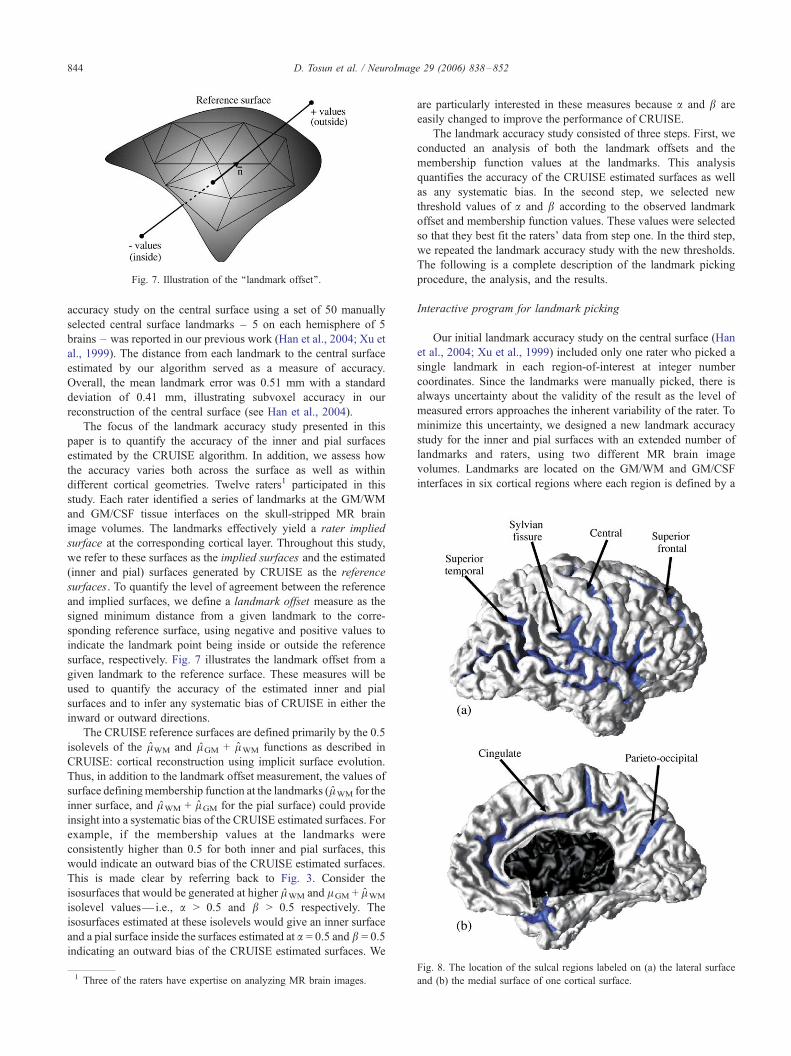
Fig. 7. Illustration of the ‘‘landmark offset’’.

D. Tosun et al. / NeuroImage 29 (2006) 838–852844

accuracy study on the central surface using a set of 50 manually

selected central surface landmarks – 5 on each hemisphere of 5

brains – was reported in our previous work (Han et al., 2004; Xu et

al., 1999). The distance from each landmark to the central surface

estimated by our algorithm served as a measure of accuracy.

Overall, the mean landmark error was 0.51 mm with a standard

deviation of 0.41 mm, illustrating subvoxel accuracy in our

reconstruction of the central surface (see Han et al., 2004).

The focus of the landmark accuracy study presented in this

paper is to quantify the accuracy of the inner and pial surfaces

estimated by the CRUISE algorithm. In addition, we assess how

the accuracy varies both across the surface as well as within

different cortical geometries. Twelve raters1 participated in this

study. Each rater identified a series of landmarks at the GM/WM

and GM/CSF tissue interfaces on the skull-stripped MR brain

image volumes. The landmarks effectively yield a rater implied

surface at the corresponding cortical layer. Throughout this study,

we refer to these surfaces as the implied surfaces and the estimated

(inner and pial) surfaces generated by CRUISE as the reference

surfaces. To quantify the level of agreement between the reference

and implied surfaces, we define a landmark offset measure as the

signed minimum distance from a given landmark to the corre-

sponding reference surface, using negative and positive values to

indicate the landmark point being inside or outside the reference

surface, respectively. Fig. 7 illustrates the landmark offset from a

given landmark to the reference surface. These measures will be

used to quantify the accuracy of the estimated inner and pial

surfaces and to infer any systematic bias of CRUISE in either the

inward or outward directions.

The CRUISE reference surfaces are defined primarily by the 0.5

isolevels of the lWM and lGM + lWM functions as described in

CRUISE: cortical reconstruction using implicit surface evolution.

Thus, in addition to the landmark offset measurement, the values of

surface definingmembership function at the landmarks (lWM for the

inner surface, and lWM + lGM for the pial surface) could provide

insight into a systematic bias of the CRUISE estimated surfaces. For

example, if the membership values at the landmarks were

consistently higher than 0.5 for both inner and pial surfaces, this

would indicate an outward bias of the CRUISE estimated surfaces.

This is made clear by referring back to Fig. 3. Consider the

isosurfaces that would be generated at higher lWM and lˆGM + lWM

isolevel values—i.e., a > 0.5 and b > 0.5 respectively. The

isosurfaces estimated at these isolevels would give an inner surface

and a pial surface inside the surfaces estimated at a = 0.5 and b = 0.5

indicating an outward bias of the CRUISE estimated surfaces. We

1 Three of the raters have expertise on analyzing MR brain images.

are particularly interested in these measures because a and b are

easily changed to improve the performance of CRUISE.

The landmark accuracy study consisted of three steps. First, we

conducted an analysis of both the landmark offsets and the

membership function values at the landmarks. This analysis

quantifies the accuracy of the CRUISE estimated surfaces as well

as any systematic bias. In the second step, we selected new

threshold values of a and b according to the observed landmark

offset and membership function values. These values were selected

so that they best fit the raters’ data from step one. In the third step,

we repeated the landmark accuracy study with the new thresholds.

The following is a complete description of the landmark picking

procedure, the analysis, and the results.

Interactive program for landmark picking

Our initial landmark accuracy study on the central surface (Han

et al., 2004; Xu et al., 1999) included only one rater who picked a

single landmark in each region-of-interest at integer number

coordinates. Since the landmarks were manually picked, there is

always uncertainty about the validity of the result as the level of

measured errors approaches the inherent variability of the rater. To

minimize this uncertainty, we designed a new landmark accuracy

study for the inner and pial surfaces with an extended number of

landmarks and raters, using two different MR brain image

volumes. Landmarks are located on the GM/WM and GM/CSF

interfaces in six cortical regions where each region is defined by a

Fig. 8. The location of the sulcal regions labeled on (a) the lateral surface

and (b) the medial surface of one cortical surface.

Fig. 9. Interactive program for landmark picking: (a) an example axial cross-section, (b) enlarged view around designated region for landmark picking, and

(c–d) orthogonal cross-sections through the last selected point.

D. Tosun et al. / NeuroImage 29 (2006) 838–852 845

cortical sulcus. These include the sylvian fissure (SYLV), superior

frontal (SF), superior temporal (ST), cingulate (CING), and

parieto-occipital (PO) sulci of each cortical hemisphere, and the

central (CS) sulcus of the left hemisphere. These sulcal regions are

Table 2

Landmark offset Statistics on Inner Surface (mean T stdev in mm)

Subject I (12 raters) Subject II (6 raters)

SD AD SD

Sulcus

LCS �0.50 T 0.57 0.59 T 0.48 �0.82 T 0.63

LSYLV �0.04 T 1.00 0.80 T 0.63 �0.63 T 0.63

LST �0.19 T 0.51 0.44 T 0.33 �0.30 T 0.63

LSF �0.18 T 0.49 0.41 T 0.33 �0.27 T 0.45

LCING 0.25 T 0.67 0.54 T 0.47 �0.23 T 0.52

LPO �0.59 T 0.55 0.62 T 0.51 �0.50 T 0.45

RSYLV �0.40 T 0.44 0.47 T 0.36 �0.78 T 0.53

RST �0.42 T 0.54 0.58 T 0.37 �0.27 T 0.63

RSF �0.14 T 0.43 0.36 T 0.27 �0.48 T 0.45

RCING �0.35 T 0.46 0.45 T 0.37 �0.56 T 0.61

RPO �0.46 T 0.67 0.63 T 0.50 �0.27 T 0.48

Geometry

Sulcal fundus �0.53 T 0.57 0.61 T 0.49 �0.64 T 0.51

Sulcal bank �0.33 T 0.51 0.49 T 0.37 �0.38 T 0.53

Gyral crown 0.04 T 0.68 0.50 T 0.46 �0.36 T 0.67

All �0.27 T 0.64 0.53 T 0.45 �0.47 T 0.59

colored on the right hemisphere of one cortical surface in Fig. 8.

Within each region, landmarks are defined on the three cortical

geometries—‘‘sulcal fundus’’, ‘‘sulcal bank’’, and ‘‘gyral crown’’.

Sulcal fundus points lie along the bottom of a cortical fold, sulcal

Both subjects (12 raters)

AD SD AD >1 >2

0.89 T 0.54 �0.60 T 0.61 0.69 T 0.52 23% 2.4%

0.68 T 0.58 �0.24 T 0.95 0.76 T 0.62 28% 5.5%

0.56 T 0.42 �0.23 T 0.56 0.48 T 0.36 8% 0.4%

0.42 T 0.31 �0.21 T 0.48 0.41 T 0.32 6% 0.0%

0.44 T 0.35 0.10 T 0.67 0.51 T 0.44 13% 0.2%

0.56 T 0.37 �0.56 T 0.52 0.60 T 0.47 18% 1.7%

0.85 T 0.42 �0.52 T 0.51 0.60 T 0.42 20% 0.2%

0.53 T 0.43 �0.37 T 0.58 0.56 T 0.39 16% 0.2%

0.54 T 0.38 �0.24 T 0.46 0.41 T 0.32 6% 0.0%

0.63 T 0.53 �0.42 T 0.53 0.51 T 0.44 12% 0.6%

0.44 T 0.33 �0.40 T 0.62 0.57 T 0.46 18% 0.9%

0.68 T 0.46 �0.57 T 0.55 0.63 T 0.48 21% 1.6%

0.50 T 0.43 �0.35 T 0.52 0.49 T 0.39 10% 0.6%

0.60 T 0.47 �0.09 T 0.70 0.54 T 0.47 15% 1.1%

0.60 T 0.46 0.34 T 0.63 0.55 T 0.45 15% 1.1%

Table 3

Landmark offsets on Pial Surface (mean T stdev in mm)

Subject I (12 raters) Subject II (6 raters) Both subjects (12 raters)

SD AD SD AD SD AD >1 >2

Sulcus

LCS �0.35 T 0.47 0.45 T 0.38 �0.27 T 0.50 0.47 T 0.31 �0.33 T 0.48 0.46 T 0.35 6% 0.0%

LSYLV �0.19 T 0.48 0.39 T 0.33 �0.26 T 0.44 0.41 T 0.31 �0.21 T 0.47 0.40 T 0.32 5% 0.0%

LST �0.45 T 0.51 0.54 T 0.42 �0.39 T 0.75 0.67 T 0.51 �0.43 T 0.60 0.58 T 0.45 15% 1.3%

LSF �0.32 T 0.54 0.46 T 0.43 �0.04 T 0.57 0.43 T 0.37 �0.23 T 0.56 0.45 T 0.41 8% 0.4%

LCING �0.25 T 0.34 0.33 T 0.25 �0.34 T 0.62 0.52 T 0.48 �0.28 T 0.45 0.39 T 0.36 6% 0.2%

LPO �0.41 T 0.41 0.45 T 0.38 �0.35 T 0.47 0.47 T 0.34 �0.39 T 0.43 0.45 T 0.37 8% 0.2%

RSYLV �0.54 T 0.42 0.56 T 0.38 �0.34 T 0.44 0.44 T 0.34 �0.47 T 0.43 0.52 T 0.37 14% 0.0%

RST �0.25 T 0.46 0.42 T 0.31 �0.31 T 0.48 0.44 T 0.36 �0.27 T 0.47 0.43 T 0.33 6% 0.0%

RSF �0.25 T 0.40 0.35 T 0.32 �0.30 T 0.48 0.45 T 0.35 �0.27 T 0.43 0.38 T 0.33 5% 0.0%

RCING �0.42 T 0.51 0.48 T 0.45 �0.26 T 0.62 0.50 T 0.44 �0.36 T 0.56 0.49 T 0.45 17% 0.0%

RPO �0.39 T 0.40 0.44 T 0.33 �0.19 T 0.53 0.45 T 0.34 �0.32 T 0.46 0.44 T 0.34 6% 0.0%

Geometry

Sulcal fundus �0.49 T 0.47 0.53 T 0.42 �0.48 T 0.55 0.58 T 0.45 �0.49 T 0.50 0.55 T 0.43 14% 0.4%

Sulcal bank �0.37 T 0.42 0.44 T 0.35 �0.19 T 0.47 0.40 T 0.32 �0.31 T 0.45 0.43 T 0.34 6% 0.1%

Gyral crown �0.18 T 0.44 0.36 T 0.32 �0.15 T 0.56 0.45 T 0.36 �0.17 T 0.48 0.39 T 0.33 5% 0.1%

nonACE �0.47 T 0.50 0.54 T 0.43 �0.49 T 0.51 0.57 T 0.42 �0.48 T 0.51 0.55 T 0.43 14% 0.4%

ACE �0.23 T 0.38 0.35 T 0.28 �0.01 T 0.47 0.36 T 0.30 �0.17 T 0.42 0.35 T 0.29 3% 0.0%

All �0.35 T 0.46 0.44 T 0.37 �0.28 T 0.55 0.48 T 0.39 �0.32 T 0.49 0.45 T 0.38 8% 0.2%

Table 4

Membership Values (lWM) at GM/WM Interface Landmarks (mean T stdev)

Subject I

(12 raters)

Subject II

(6 raters)

Both Subjects

(12 raters)

Sulcus

LCS 0.70 T 0.21 0.80 T 0.18 0.74 T 0.20

LSYLV 0.58 T 0.30 0.73 T 0.22 0.63 T 0.28

LST 0.62 T 0.25 0.65 T 0.24 0.63 T 0.25

LSF 0.61 T 0.20 0.64 T 0.23 0.62 T 0.21

LCING 0.48 T 0.24 0.63 T 0.23 0.52 T 0.25

LPO 0.75 T 0.18 0.75 T 0.19 0.75 T 0.18

RSYLV 0.70 T 0.21 0.81 T 0.19 0.73 T 0.21

RST 0.72 T 0.20 0.65 T 0.26 0.70 T 0.23

RSF 0.61 T 0.19 0.72 T 0.20 0.64 T 0.20

RCING 0.70 T 0.19 0.71 T 0.24 0.70 T 0.21

RPO 0.68 T 0.25 0.67 T 0.22 0.68 T 0.24

Geometry

Sulcal fundus 0.71 T 0.22 0.76 T 0.20 0.73 T 0.21

Sulcal bank 0.67 T 0.22 0.68 T 0.22 0.67 T 0.22

Gyral crown 0.57 T 0.25 0.68 T 0.25 0.61 T 0.25

All 0.65 T 0.23 0.70 T 0.23 0.67 T 0.23

D. Tosun et al. / NeuroImage 29 (2006) 838–852846

bank points lie along the sides of a fold, and gyral crown points lie

along the top of a fold, as illustrated in Fig. 1.

A visualization program was written using Open Visualization

Data Explorer 4.2.0, IBM Visualization Software to pick land-

marks inside a region-of-interest box on the pre-selected axial

cross-sections of the raw MR image volume. We chose to pick

landmarks by viewing axial cross-sections, the orientation on

which the MR images were acquired. A total of 66 axial cross-

sections were pre-selected, each corresponding to one of the eleven

sulcal regions, one of the three cortical geometries, and one of the

tissue interfaces. The purpose of the visualization program is to

provide a standard way of picking the landmarks so that a

statistical analysis approach could be used to compare the data of

different raters. The interface had two primary displays. The first

display, shown in Fig. 9(a), provided the information required to

pick the landmarks on that axial cross-section. This included

information on which tissue interface the landmarks should be

selected, the number of landmarks to select, and the cortical

geometry type. In addition, a counter was incremented after each

landmark selection indicating the number of picks remaining. A

blue box outlined a 10 voxel � 10 voxel region in which the rater

was required to pick the landmarks. In the second primary display,

shown in Fig. 9(b), an enlarged view around the 10 voxel � 10

voxel outlined by the blue box from the first display was shown.

The interface allowed the rater to adjust several parameters

including the center and size of the enlarged view in the second

display as well as the colormap scaling to improve the contrast

between different cortical tissues. The rater was able to select

between two possible colormaps—linear or logarithmic. In the

linear map, each colormap level corresponds to a constant intensity

range in the image. The second colormap utilizes logarithmic

scaling providing more contrast at low intensities. Each landmark

was selected in this second primary display with a right mouse

click and the selected point was marked in red in all displays. In

order to get a sense of the location of the point in 3-D, the two

orthogonal cross-sections through this point were also displayed, as

shown in Figs. 9c–d. The landmark was automatically recorded as

the physical position of the selected point with floating number

coordinates and landmarks identified by a given rater were forced

to be at least 0.50 mm apart from each other. The rater also had the

flexibility of removing any of the previously recorded landmarks.

All raters were asked to use the same linux workstation with fixed

monitor settings, but encouraged to vary the brightness and

contrast colormap table as desired. This encouraged raters to

concentrate on picking landmarks on the desired tissue interface,

Table 5

Membership values (sublWM + lGM) at GM/CSF Interface Landmarks

(mean T stdev)

Subject I

(12 raters)

Subject II

(6 raters)

Both subjects

(12 raters)

Sulcus

LCS 0.70 T 0.19 0.62 T 0.25 0.68 T 0.22

LSYLV 0.60 T 0.22 0.60 T 0.23 0.60 T 0.23

LST 0.74 T 0.15 0.65 T 0.29 0.71 T 0.21

LSF 0.71 T 0.23 0.54 T 0.28 0.66 T 0.26

LCING 0.60 T 0.20 0.64 T 0.24 0.62 T 0.22

LPO 0.79 T 0.15 0.65 T 0.26 0.75 T 0.20

RSYLV 0.77 T 0.14 0.67 T 0.24 0.73 T 0.18

RST 0.66 T 0.21 0.64 T 0.23 0.66 T 0.22

RSF 0.64 T 0.22 0.66 T 0.25 0.65 T 0.23

RCING 0.72 T 0.19 0.62 T 0.28 0.68 T 0.23

RPO 0.70 T 0.18 0.60 T 0.27 0.67 T 0.22

Geometry

Sulcal fundus 0.76 T 0.19 0.68 T 0.24 0.73 T 0.21

Sulcal bank 0.68 T 0.19 0.60 T 0.25 0.65 T 0.22

Gyral crown 0.64 T 0.21 0.61 T 0.28 0.63 T 0.23

nonACE 0.71 T 0.19 0.71 T 0.22 0.71 T 0.21

ACE 0.68 T 0.21 0.52 T 0.26 0.63 T 0.24

All 0.70 T 0.20 0.63 T 0.26 0.67 T 0.22

D. Tosun et al. / NeuroImage 29 (2006) 838–852 847

and not simply to pick intensity edges that they might observe on a

static display with fixed lighting conditions.

Data

Twelve raters participated in the landmark accuracy study

and the study was carried out using two different MR image

volumes. First six raters picked landmarks on both image

volumes and the remaining raters picked landmarks on only the

first image volume. Ten landmarks were picked on each of 66

pre-selected axial cross-sections. Each rater picked a total of 330

landmarks equally distributed across the different sulcal regions

and different geometry groups on each cortical tissue interface.

It took approximately 1 h and 30 min per brain to pick the

landmarks, with a substantial portion of this time required for

adjusting the parameters of the colormap scaling function for the

best contrast.

Two measures were computed in this study—landmark offset

and surface defining membership function value (SDMFV). The

SDMFV at each landmark point is defined as the value of the

AutoFill-edited WM membership function, AWM, for the inner

surface and the sum of the ACE-edited GM and AutoFill-edited

WM membership functions, AGM + AWM, for the pial surface. To

measure the landmark offset, first the minimum absolute distance

Table 6

Membership function value statistics for the training data—3 raters, 2 subjects (m

Region Measure Sulcal fundus

Inner surface lWM 0.75 T 0.21

Pial surface lWM + lGM 0.56 T 0.28

Pial surface—nonACE lWM + lGM 0.75 T 0.20

Pial surface—ACE lWM + lGM 0.42 T 0.25

Pial surface lWM + lGM 0.70 T 0.23

(AD) from landmark point to the corresponding reference surface

is computed, and then the absolute distance measurement is signed

according to the sign convention illustrated in Fig. 7, which gives

the signed distance (SD) from the landmark point to the

corresponding reference surface.

The landmark offset measure calculation requires finding the

closest point on the reference surface to the landmark point. Since

each landmark point is categorized by the sulcal region in which it

is picked, we restricted the distance calculation in the sulcal region

of interest. To identify the reference surface points in the sulcal

regions analyzed in this study, we utilized the sulcal segmentation

method described in Rettmann et al. (2002), and the assisted sulcal

labeling program described in Rettmann et al. (2005). Presumably

the 10 voxel � 10 voxel box provided to the rater in each pre-

selected axial cross-section includes only points within a given

sulcal region, however, due to the highly convoluted nature of the

cortex in 3-D, the landmark point and its corresponding closest

point might not be in the same sulcal region. For less than 2.0% of

the landmark points, the closest point on the corresponding

reference surface had a non-matching sulcal label. reference

surface either had a non-sulcal region label or had a different

sulcal region label than the given landmark point’s. These

landmark points were excluded from the entire analysis presented

below.

Data analysis

We first tested the effects of variable intensity inhomogeneity

and colormap scaling by comparing the algorithm versus rater

across the two different subjects, the three different cortical

geometries (sulcal fundus, sulcal bank, and gyral crown), and

eleven different sulcal regions. In this study, we analyzed the GM/

WM and GM/CSF interface data separately.

Statistical analyses were performed using R version 2.0.0 (The R

Development Core Team, 2003). The effects of ‘‘rater’’, ‘‘subject’’,

‘‘sulcus’’, and ‘‘geometry’’ on dependent SD and SDMFV measures

were analyzed in a series of multivariate analyses of variance

(MANOVA), with ‘‘subject’’, ‘‘sulcus’’, and ‘‘geometry’’ used as

nested grouping factors and ‘‘rater’’ as a repeated factor. The first

MANOVA focused on the effects of ‘‘rater’’, ‘‘subject’’, ‘‘sulcus’’,

and ‘‘geometry’’ on SD and SDMFV measures. Bartlett’s test

showed statistically significant (1% level) evidence against the null

hypothesis that the covariance matrices are homogeneous. Two-

tailed hypotheses were tested using Pillai’s trace criteria since it is

robust to violations of assumptions concerning homogeneity of the

covariance matrix. MANOVA revealed a significant effect of

‘‘rater’’, ‘‘sulcus’’, and ‘‘geometry’’, but ‘‘subject’’ failed to reach

significance for both GM/WM and GM/CSF interface data. The

threshold for significance was set at P < 0.01.

We conducted follow-up univariate analyses using Type III

sums of squares to elucidate these effects. The second MANOVA

ean T stdev)

Sulcal banks Gyral crown All

0.68 T 0.24 0.63 T 0.28 0.69 T 0.25

0.54 T 0.27 0.56 T 0.27 0.55 T 0.27

0.68 T 0.22 0.65 T 0.24 0.69 T 0.22

0.41 T 0.24 0.40 T 0.25 0.41 T 0.25

0.62 T 0.24 0.62 T 0.25 0.65 T 0.24

Table 7

Landmark offsets on Inner Surface for Test Data—9 raters, 2 subjects (mean T

stdev in mm)

Geometry a SD AD >1 >2

Sulcal fundus 0.50 �0.56 T 0.56 0.62 T 0.49 20% 1.9%

Sulcal bank 0.50 �0.36 T 0.49 0.48 T 0.37 8% 0.6%

Gyral crown 0.50 �0.07 T 0.66 0.49 T 0.44 14% 0.6%

All 0.50 �0.33 T 0.61 0.53 T 0.44 14% 1.0%

Sulcal fundus 0.69 �0.25 T 0.54 0.45 T 0.39 8% 0.7%

Sulcal bank 0.69 �0.03 T 0.57 0.38 T 0.42 5% 1.6%

Gyral crown 0.69 0.40 T 0.89 0.68 T 0.70 19% 7.0%

All 0.69 0.04 T 0.73 0.50 T 0.54 10% 3.1%

Table 8

Landmark offsets on Pial Surface for Test Data—9 raters, 2 subjects (mean T

stdev in mm)

Geometry a b SD AD >1 >2

Sulcal fundus 0.50 0.50 �0.51 T 0.50 0.56 T 0.45 15% 0.4%

Sulcal bank 0.50 0.50 �0.33 T 0.43 0.42 T 0.34 6% 0.1%

Gyral crown 0.50 0.50 �0.17 T 0.48 0.39 T 0.33 5% 0.1%

nonACE 0.50 0.50 �0.49 T 0.52 0.56 T 0.44 15% 0.4%

ACE 0.50 0.50 �0.18 T 0.40 0.34 T 0.27 2% 0.0%

All 0.50 0.50 �0.34 T 0.49 0.45 T 0.38 9% 0.2%

Sulcal fundus 0.69 0.55 �0.46 T 0.50 0.52 T 0.44 14% 0.8%

Sulcal bank 0.69 0.55 �0.25 T 0.43 0.38 T 0.32 5% 0.1%

Gyral crown 0.69 0.55 �0.10 T 0.48 0.38 T 0.32 4% 0.1%

nonACE 0.69 0.55 �0.40 T 0.53 0.51 T 0.42 12% 0.6%

ACE 0.69 0.55 �0.12 T 0.41 0.34 T 0.27 2% 0.0%

All 0.69 0.55 �0.27 T 0.50 0.43 T 0.37 8% 0.3%

Sulcal fundus 0.69 0.65 �0.35 T 0.52 0.48 T 0.40 11% 0.4%

Sulcal bank 0.69 0.65 �0.14 T 0.42 0.34 T 0.29 3% 0.1%

Gyral crown 0.69 0.65 �0.14 T 0.42 0.34 T 0.29 3% 0.1%

nonACE 0.69 0.65 �0.27 T 0.53 0.45 T 0.39 9% 0.4%

ACE 0.69 0.65 0.00 T 0.44 0.35 T 0.27 3% 0.0%

All 0.69 0.65 �0.14 T 0.51 0.40 T 0.34 6% 0.2%

Sulcal fundus 0.69 0.69 �0.31 T 0.52 0.47 T 0.39 10% 0.3%

Sulcal bank 0.69 0.69 �0.08 T 0.42 0.33 T 0.28 3% 0.0%

Gyral crown 0.69 0.69 0.13 T 0.50 0.41 T 0.32 6% 0.1%

nonACE 0.69 0.69 �0.21 T 0.54 0.44 T 0.38 9% 0.2%

ACE 0.69 0.69 0.05 T 0.46 0.36 T 0.28 3% 0.0%

All 0.69 0.69 �0.09 T 0.52 0.40 T 0.34 6% 0.1%

D. Tosun et al. / NeuroImage 29 (2006) 838–852848

focused on the effects of ‘‘rater’’, ‘‘subject’’, ‘‘sulcus’’, and

‘‘geometry’’ on the dependent measures of raters 1–6. Results

revealed no significant effect of ‘‘subject’’, but group differences in

‘‘rater’’, ‘‘sulcus’’, and ‘‘geometry’’. A third MANOVA focused on

the effects of ‘‘rater’’, ‘‘sulcus’’, and ‘‘geometry’’ on the dependent

measures of raters 7–12, and revealed significant group differ-

ences. Significant differences in the performance of the algorithm

relative to rater across different aspects of the cortical geometry

and across different sulcal regions may reflect variability in noise,

intensity inhomogeneity, abnormalities in the original MR brain

volume, and colormap scaling function for the different brain

features. On the other hand, the absence of an effect for ‘‘subject’’

reflects the intra-rater consistency of picking landmarks in different

MR images. A final MANOVA focused on the dependent SD and

SDMFV measures of each rater separately and tested the effects of

‘‘sulcus’’, ‘‘geometry’’, and, if applicable, ‘‘subject’’. The results

revealed significant ‘‘sulcus’’ and ‘‘geometry’’ group differences,

but not significant group difference of ‘‘subject’’ for both GM/WM

and GM/CSF interface data of the raters 1, 2, and 3.

Landmark offset on the inner surface

The landmark offset statistics on the inner surface for different

sulcal regions and different cortical geometries are shown in Table

2. The overall mean landmark offset is �0.34 mm with a standard

deviation of 0.63 mm, which can be interpreted as about one third

mm accuracy on the inner surface estimation. Only 15% of the

landmarks are farther than 1.0 mm from the estimated inner

surfaces, and about 1.0% of the landmarks are farther than 2.0 mm

from the estimated inner surfaces, indicating that gross errors are

not common.

In addition to variance on SDmeasure with cortical geometry and

position, we looked at the correlation between SD measure and the

inner cortical surface orientation relative to the normal direction of

axial cross-sections. For each landmark point, the relative orienta-

tion of the inner cortical surface was quantified using the angle

between the inner cortical surface patch around the closest surface

point to that landmark point and the axial cross-section on which the

landmark point was selected. The correlation coefficient between

SD measures and the relative inner cortical surface orientation is

�0.164. This statistically significant negative correlation (P < 0.01)

indicates that the accuracy is better when the local surface patch is

perpendicular to the axial cross-section. This could indicate that

raters are able to better localize interfaces that are perpendicular to

the viewing plane. It is also possible that this is related to the

underlying data resolution, which is poorest in (approximately) the

direction orthogonal to our axial cross sections.

Landmark offset on the pial surface

The landmark offset statistics on the pial surface are also

shown in Table 3. The overall mean landmark offset is �0.32 mm

with a standard deviation of 0.49 mm, and only 8% of the

landmarks are farther than 1.0 mm from the estimated pial

surfaces. Smaller standard deviations of the pial surface landmark

offsets compared with inner surface landmark offsets indicate a

higher stability for the pial surface. The higher stability on the pial

surface could be due to the ACE-processing in the CRUISE

algorithm (see CRUISE: cortical reconstruction using implicit

surface evolution). In ACE-processed regions, ACE is more

dominant than the membership isolevel criterion in defining the

surface location (Han et al., 2003). A smaller mean landmark

offset and standard deviation is observed at the ACE-processed

regions as compared with the mean landmark offset and standard

deviation of the regions not processed by ACE (see Table 3). This

suggests that the GM/CSF interface defined by ACE is more in

accordance with the rater implied surfaces. A study similar to the

one described in the previous section was carried out to assess the

correlation between the SD measure and the relative orientation of

the pial cortical surface but the estimated correlation coefficient

(0.040) is not statistically significant.

Consistent negative mean landmark offsets (more pronounced

on the sulcal fundus regions for both the GM/WM and GM/CSF

interface data) and the mean SDMFVs greater than 0.5 (reported in

Tables 4 and 5) may be interpreted as an outward bias of CRUISE.

To address this observation, a simple parameter adjustment study is

described in Parameter adjustment and evaluation.

D. Tosun et al. / NeuroImage 29 (2006) 838–852 849

Parameter adjustment and evaluation

In Landmark accuracy study on inner and pial surfaces, we

reported the landmark offsets on the inner and pial surfaces. We

observed consistent negative mean landmark offsets on both the

inner and pial surfaces, which indicates an outward bias of

CRUISE. Based on the observed SDMFV at the landmarks (cf.

Tables 4 and 5), we wanted to estimate the a and b thresholds that

best fit the landmark data and repeat the landmark accuracy

analysis with the surfaces estimated with the new a and bthresholds. For this purpose, we needed to divide the landmark data

into two groups; the first group (training data) was used to estimate

the new a and b thresholds, and the second group (test data) was

used to repeat the analysis to quantify any such improvement.

We wanted the training data to represent both MR brain images

and all possible cortical geometry and sulcus factors used in the

analysis presented in Landmark accuracy study on inner and pial

surfaces. Only the first six raters picked landmarks on both MR

brain images, hence, the training data should be a subset of these

raters’ data. The grouping was based on the intra-rater consistency

on picking landmarks reported in Landmark accuracy study on

inner and pial surfaces. Therefore, data of the raters 1, 2, and 3

formed the training data, and the rest of the data were used to test

the new a and b thresholds.

Fig. 10. A sample MR image cross-section with (a) inner, (b) central, and (c) pi

and b = 0.55)).

SDMFV statistics for the training data are reported in Table 6.

Although we observed that the a and b thresholds should be

functions of the cortical geometry – i.e., the ideal thresholds are

different for different parts of the brain – in this study, we chose a

simpler approach and set a and b to the observed mean SDMFV,

and repeated our previous analysis with these thresholds.

The average of AWM measure at the GM/WM landmarks of the

training group is 0.69. The inner surface was estimated using the

new a = 0.69 threshold and the repeated landmark offset statistics

for the GM/WM landmarks of the test group are given in Table 7.

For comparison reasons, we also included the landmark offset

statistics of the test group for the inner surface estimated using a =

0.5. Although the landmark offset measure is improved by 55% in

the sulcal fundus region and by 92% in the sulcal bank region, we

see a degradation of landmark offset measure in the gyral crown

region. The average inner surface accuracy over all cortical

geometries is 0.04 mm.

The TGDM to estimate the central surfaces was initialized at the

inner surface estimated by a = 0.69 threshold and the new central

surfaces were used as the initial condition for the TGDM with the

new b threshold to estimate the new pial surfaces (see CRUISE:

cortical reconstruction using implicit surface evolution). b threshold

was set to the average of AWM + AGM measure at the GM/CSF

landmarks of the training group; b = 0.55. The statistics of the

al surfaces of the first subject (blue (a = 0.5 and b = 0.5), red (a = 0.69

D. Tosun et al. / NeuroImage 29 (2006) 838–852850

landmark offset measure on the new pial surfaces are reported in

Table 8 with the landmark offset measure statistics on the old pial

surfaces for comparison purposes. By adjusting the b threshold,

10%–41% improvement on the landmark offset measure is

observed on different geometry groups. A sample axial cross-

section from the first MR image volume with surfaces estimated

with the original and the new a and b thresholds are shown in Fig.

10. Based on the visual inspection, a better performance has been

achieved both on the inner and pial surfaces with the use of the new

threshold values; however, the new threshold values have no

substantial effect on the central surface estimation.

By setting b threshold to the average of lWM + lGM measure

over all training group landmarks, we make the assumption that the

pial surface is determined solely by the isosurface of the lWM +

lGM function everywhere in the cortex. However, it is quite

evident from difference between the average lWM + lGM measure

on regions not edited by ACE and regions edited by ACE (cf.

Table 6) that the ACE stopping criterion is more dominant than the

isolevel criterion. To address this issue, we explored two

approaches. First, since the raters selected landmarks on the

original MR image volumes without any ACE editing, instead of

the lWM + lGM measure, we used the lWM + lGM measure and set

the b threshold to its average at the training landmarks; b = 0.65 as

reported in Table 6. 18%–58% improvement is observed on

different geometry regions. The results are reported in Table 8. We

observed perfect accuracy in the regions edited by the ACE

algorithm with this new b threshold adjustment. In the second

approach, we only used the training group landmarks on the

regions not edited by the ACE algorithm, but still used the lWM +

lGM measure. This time, the b threshold is set to 0.69 (see Table

6), and the resultant landmark offset measure statistics are given in

Table 8. This threshold adjustment yields 24%–76% improvement

on the landmark offset measure and the average pial surface

accuracy over all cortical geometries is 0.09 mm.

Different percentile improvements on the different geometry

groups, and occasional degradation support the claim that the a and

b thresholds should be defined as functions of the cortical

geometry. In future work, we will investigate the features that

can be extracted from the membership functions so that the a and bcan be defined as functions of cortical geometry, but still yield

topologically correct nested cortical surfaces.

In order to see the effect of the a and b thresholds on estimating

the central surface, we repeated the landmark accuracy study

reported in (Han et al., 2004) on the new central surfaces estimated

by using the new thresholds. Slight differences were observed on

the reported values, but no substantial improvement or change was

noted. These results show the robustness of the central surface

reconstruction with respect to the a and b thresholds, which

supports our previous claim about the stability of the central

surface and how well it captures the geometry of the cortex

compared with the inner and pial surfaces (Xu et al., 1999).

The repeatability analysis on the nested cortical surfaces was

also carried out using the new thresholds. Although slight

differences were observed in the reported values, no substantial

improvement or change was noted.

Discussion and future work

The purpose of this work was to evaluate the accuracy and

precision of the CRUISE algorithms developed for the automatic

reconstruction of the nested surfaces of the cerebral cortex from

MR image volumes. This was accomplished by conducting two

different studies. Our first conclusion is that the nested cortical

surfaces – inner, central, and pial – can be found in a robust

fashion using the CRUISE algorithms. Second, the three nested

cortical surfaces can be found with subvoxel accuracy, typically

with an accuracy of one third of a voxel. In this work, the

performance of the CRUISE algorithm was tested on a single

BLSA data set. The MR acquisition protocol that is used in the

BLSA is based on a well-established MR pulse sequence that is

very common in neuroscience research, and is capable of being

implemented on all MR scanners. Although performance will differ

when the algorithm is applied to data having different acquisition

protocols, we believe that acquisition parameters can be adjusted

on modern scanners to achieve equal or superior performance to

that described herein. Currently, we utilize ‘‘rater implied

surfaces’’, derived from rater selected landmarks, to quantify the

accuracy of CRUISE. In future work, we plan to create a nested

surface truth model from the visible human cyrosection and MR

image data (Spitzer et al., 1996), and validate our methods against

these data.

The nested surfaces can be reliably used for analysis of the

cortex geometry; however, the reported accuracy levels can be of

concern in longitudinal analysis since the sought changes might

be in the neighborhood of the observed errors. A simple

experiment to improve CRUISE by selecting new threshold

values which were more in accordance with the rater implied

surfaces was presented in Parameter adjustment and evaluation.

Our statistics on SD and SDMFV suggest that the positioning of

tissue interfaces with respect to the membership function values

varies spatially. In future research, we expect to show that a

variable threshold scheme – e.g., varying a and b thresholds as

functions of cortical geometry or position – will provide even

higher accuracy in the CRUISE reconstruction algorithm. Alter-

native segmentation methods may also yield new ways to further

improve CRUISE.

Acknowledgments

The authors would like to thank all the raters involved in the

landmark accuracy study for their time and their effort. This work

was supported in part by NIH/NINDS Grant R01NS37747.

References

Angenent, S., Haker, S., Tannenbaum, A., Kikinis, R., 1999. On the

Laplace–Beltrami operator and brain surface flattening. IEEE Trans.

Med. Imag. 18 (8), 700–711.

Behnke, K.J., Rettmann, M.E., Pham, D.L., Shen, D., Davatzikos, C.,

Resnick, S.M., Prince, J.L., 2003. Automatic classification of sulcal

regions of the human brain cortex using pattern recognition. Proc. SPIE:

Medical Imaging, vol. 5032, pp. 1499–1510.

Besl, P.J., McKay, N.D., 1992. A method for registration of 3 D shapes.

IEEE Trans. Pattern Anal. Mach. Intell. 14 (2), 239–255.

Cachia, A., Mangin, J.F., Riviere, D., Boddaert, N., Andrade, A., Kherif, F.,

Sonigo, P., Papadopoulos-Orfanos, D., Zilbovicius, M., Poline, J.-B.,

Bloch, I., Brunelle, F., Regis, J., 2001. A mean curvature based primal

sketch to study the cortical folding process from antenatal to adult brain.

In: Niessen, W., Viergever, M. (Eds.), Proc. MICCAI. Springer Verlag,

Berlin, pp. 897–904R LNCS 2208.

D. Tosun et al. / NeuroImage 29 (2006) 838–852 851

Cachia, A., Mangin, J.F., Riviere, D., Papadopoulos-Orfanos, D., Zilbovi-

cius, M., Bloch, I., Regis, J., 2002. Gyral parcellation of the cortical

surface using geodesic voronoi diagrams. In: Dohi, T., Kikinis, R.

(Eds.), Proc. MICCAI. Springer Verlag, Berlin, pp. 427–434R LNCS

2488.

Carman, G.J., Drury, H.A., van Essen, D.C., 1995. Computational methods

for reconstructing and unfolding the cerebral cortex. Cereb. Cortex 5

(6), 506–517.

Crespo-Facorro, B., Kim, J., Andreasen, N.C., O_Leary, D.S., Wiser, A.K.,

Bailey, J.M., Harris, G., Magnotta, V.A., 1999. Human frontal cortex: an

MRI-based parcellation method. NeuroImage 10 (5), 500–519 (April).

Dale, A.M., Fischl, B., Sereno, M.I., 1999. Cortical surface-based

analysis I: segmentation and surface reconstruction. NeuroImage 9

(2), 179–194.

Davatzikos, C., Bryan, N., 1996. Using a deformable surface model to

obtain a shape representation of the cortex. IEEE Trans. Med. Imag. 15

(6), 785–795.

Drury, H.A., Essen, D.C.V., Anderson, C.H., Lee, W.C., Coogan, T.A.,

Lewis, J.W., 1996. Computerized mapping of the cerebral cortex: a

multiresolution flattening method and a surface-based coordinate

system. J. Cogn. Neurosci. 8 (1), 1–28.

Fischl, B., Dale, A., 2000. Measuring the thickness of the human cerebral

cortex from magnetic resonance images. Proc. Natl. Acad. Sci., vol. 97,

pp. 11050–11055R September.

Fischl, B., Sereno, M.I., Dale, A.M., 1999. Cortical surface-based analysis

II: inflation, flattening, and a surface-based coordinate system. Neuro-

Image 9 (2), 195–207 (Feb.).

Goldszal, A.F., Davatzikos, C., Pham, D.L., Yan, M.X.H., Bryan, R.N.,

Resnick, S.M., 1998. An image processing system for qualitative and

quantitative volumetric analysis of brain images. J. Comput. Assist.

Tomogr. 22 (5), 827–837.

Han, X., Xu, C., Rettmann, M.E., Prince, J.L., 2001a. Automatic

segmentation editing for cortical surface reconstruction. Proc. of SPIE

Medical Imaging, vol. 4322. SPIE Press, Bellingham, WA, pp. 194–203

Feb.

Han, X., Xu, C., Tosun, D., Prince, J.L., 2001b. Cortical surface

reconstruction using a topology preserving geometric deformable

model. Proc. 5th IEEE Workshop on Mathematical Methods in

Biomedical Image Analysis (MMBIA2001). IEEE Press, Kauai,

Hawaii, pp. 213–220 Dec.

Han, X., Xu, C., Braga-Neto, U., Prince, J.L., 2002. Topology correction in

brain cortex segmentation using a multiscale, graph-based algorithm.

IEEE Trans. Med. Imag. 21, 109–121.

Han, X., Xu, C., Prince, J.L., 2003. A topology preserving level set method

for geometric deformable models. IEEE Trans. Pattern Anal. Mach.

Intell. 25, 755–768.

Han, X., Pham, D.L., Tosun, D., Rettmann, M.E., Xu, C., Prince, J.L.,

2004. CRUISE: cortical reconstruction using implicit surface evolution.

NeuroImage 23 (3), 997–1012.

Jones, S.E., Buchbinder, B.R., Aharon, I., 2000. Three-dimensional

mapping of cortical thickness using laplace’s equation. Hum. Brain

Mapp., vol. 11 (1), pp. 12–32.

Joshi, M., Cui, J., Doolittle, K., Joshi, S., Essen, D.V., Wang, L., Miller,

M.I., 1999. Brain segmentation and the generation of cortical surfaces.

NeuroImage 9, 461–476.

Kabani, N., Le Goualher, G., MacDonald, D., Evans, A.C., 2001.

Measurement of cortical thickness using an automated 3-D algorithm:

a validation study. NeuroImage 13 (2), 375–380.

Kim, J., Crespo-Facorro, B., Andreasen, N.C., O_Leary, D.S., Zhang, B.,Harris, G., Magnotta, V.A., 2000. An MRI-based parcellation method

for the temporal lobe. NeuroImage 11 (4), 271–288 (April).

Kriegeskorte, N., Goebel, R., 2001. An efficient algorithm for topologically

correct segmentation of the cortical sheet in anatomical MR volumes.

NeuroImage 14, 329–346.

Kruggel, F., von Cramon, D.Y., 2000. Measuring the cortical thickness.

Proc. of IEEE Workshop on Mathematical Methods in Biomedical

Image Analysis. IEEE Press, Hilton Head Island, SC, pp. 154–161.

Lerch, J.P., Evans, A.C., 2005. Cortical thickness analysis examined

through power analysis and a population simulation. NeuroImage 24

(1), 163–173.

MacDonald, D., Kabani, N., Avis, D., Evans, A., 2000. Automated 3D

extraction of inner and outer surfaces of cerebral cortex from MRI.

NeuroImage 12 (3), 340–356.

Magnotta, V.A., Andreasen, N.C., Schultz, S.K., Harris, G., Cizadlo, T.,

Heckel, D., Nopoulos, P., Flaum, M., 1999. Quantitative in vivo

measurement of gyrification in the human brain: changes associated

with aging. Cereb. Cortex 9, 151–160.

Mangin, J.F., Frouin, V., Bloch, I., Regis, J., Lopez-Krahe, J., 1995. From

3D magnetic resonance images to structural representations of the

cortex topography using topology preserving deformations. Math.

Imag. Vis. 5, 297–318.

Miller, M.I., Massie, A.B., Ratnanather, J.T., Botteron, K.N., Csernansky,

J.G., 2000. Bayesian construction of geometrically based cortical

thickness metrics. NeuroImage 12, 676–687.

Pham, D.L., 2001. Robust fuzzy segmentation of magnetic resonance

images. Proceedings of the Fourteenth IEEE Sympostum on Com-

puter-Based Medical Systems (CBMS2001). IEEE Press, Somerset,

NJ, pp. 127–131.

Pham, D.L., Prince, J.L., 1999. Adaptive fuzzy segmentation of magnetic

resonance images. IEEE Trans. Med. Imag. 18 (9), 737–752.

Resnick, S.M., Goldszal, A.F., Davatzikos, C., Golski, S., Kraut, M.A.,

Metter, E.J., Bryan, R.N., Zonderman, A.B., 2000. One-year age changes

in MRI brain volumes in older adults. Cereb. Cortex 10 (5), 464–472

(May).

Rettmann, M.E., Han, X., Xu, C., Prince, J.L., 2002. Automated sulcal

segmentation using watersheds on the cortical surface. NeuroImage 15,

329–344 (February).

Rettmann, M.E., Tosun, D., Tao, X., Resnick, S.M., Prince, J.L., 2005.

Program for the assisted labeling of sulcal regions (PALS): description

and reliability. NeuroImage 24 (2), 398–416.

Sandor, S., Leahy, R., 1997. Surface-based labeling of cortical anatomy

using a deformable atlas. IEEE Trans. Med. Imag. 16 (1), 41–54.

Shattuck, D.W., Leahy, R.M., 2002. BrainSuite: an automated cortical

surface identification tool. Med. Imag. Anal. 6, 129–142.

Spitzer, V., Ackerman, M.J., Scherzinger, A.L., Whitlock, D.J., 1996.

The visible male: a technical report. J. Am. Med. Inform. Assoc. 3,

118–130.

Talairach, J., Tournoux, P., 1988. Co-planar stereotaxic atlas of the human

brain. 3-Dimensional Proportional System: An Approach to Cerebral

Imaging. Thieme Medical Publisher, Inc., Stuttgart, NY.

Teo, P.C., Sapiro, G., Wandell, B.A., 1997. Creating connected representa-

tions of cortical gray matter for functional MRI visualization. IEEE

Trans. Med. Imag. 16 (6), 852–863.

The R Development Core Team, 2003. http://www.r-project.org/.

Timsari, B., Leahy, R., 2000. Optimization method for creating semi-

isometric flat maps of the cerebral cortex. Proc. SPIE Conf. Med. Imag.,

pp. 698–708.

Tosun, D., Rettmann, M.E., Tao, X., Han, X., Xu, C., Prince, J.L., 2001.

Calculation of human cerebral cortical thickness on opposing sulcal

banks. Proc. of 7th International Conference on Functional Mapping of

the Human Brain (HBM), vol. 4322. June.

Tosun, D., Rettmann, M.E., Naiman, D.Q., Resnick, S.M., Kraut,

M.A., Prince, J.L., 2004a. Cortical reconstruction using implicit

surface evolution: a landmark validation study. In: Barillot, C.,

Haynr, D.R., Hellier, P. (Eds.), Medical Image Computing and

Computer-Assisted Intervention-MICCAI 2004, 7th International Con-

ference Saint-Malo, France, Proceedings, Part I. of Lecture Notes in

Computer Science, vol. 3216. Springer Verlag, Berlin, pp. 384–392

September 26–29.

Tosun, D., Rettmann, M.E., Prince, J.L., 2004b. Mapping techniques

for aligning sulci across multiple brains. In: Ellis, R., Petters, T.

(Eds.). Medical Image Analysis-Special issue: Medical Image

Computing and Computer-Assisted Intervention-MICCAI 2003, vol.

8 (3), pp. 295–309.

D. Tosun et al. / NeuroImage 29 (2006) 838–852852

Wang, H.Z., Rieder, S.J., 1990. A spoiling sequence for suppression of

residual transverse magnetization. Magn. Reson. Med. 15 (2), 175–191.

Xu, C., Pham, D.L., Rettmann, M.E., Yu, D.N., Prince, J.L., 1999.

Reconstruction of the human cerebral cortex from magnetic resonance

images. IEEE Trans. Med. Imag. 18 (6), !467–480 (June).

Xu, C., Han, X., Prince, J.L., 2000. Improving cortical surface reconstruc-

tion accuracy using an anatomically consistent gray matter representa-

tion. Proc. of 6th International Conference on Functional Mapping of

the Human Brain. Academic Press, San Diego, CA, p. S581 June.

Yezzi Jr., A.J., Prince, J.L., 2003. An Eulerian PDE approach for computing

tissue thickness. TMI 22 (10), 1332–1339.

Zeng, X., Staib, L.H., Schultz, R.T., Duncan, J.S., 1999. Segmentation and

measurement of the cortex from 3-D MR images using coupled surfaces

propagation. IEEE Trans. Med. Imag. 18, 100–111.