University of Groningen

Correlation between X-Ray and Radio Absorption in Compact Radio GalaxiesOstorero, Luisa; Morganti, Raffaella; Diaferio, Antonaldo; Siemiginowska, Aneta; Stawarz,Łukasz; Moderski, Rafal; Labiano, AlvaroPublished in:The Astrophysical Journal

DOI:10.3847/1538-4357/aa8ef6

IMPORTANT NOTE: You are advised to consult the publisher's version (publisher's PDF) if you wish to cite fromit. Please check the document version below.

Document VersionPublisher's PDF, also known as Version of record

Publication date:2017

Link to publication in University of Groningen/UMCG research database

Citation for published version (APA):Ostorero, L., Morganti, R., Diaferio, A., Siemiginowska, A., Stawarz, Ł., Moderski, R., & Labiano, A. (2017).Correlation between X-Ray and Radio Absorption in Compact Radio Galaxies. The Astrophysical Journal,849(1), [34]. https://doi.org/10.3847/1538-4357/aa8ef6

CopyrightOther than for strictly personal use, it is not permitted to download or to forward/distribute the text or part of it without the consent of theauthor(s) and/or copyright holder(s), unless the work is under an open content license (like Creative Commons).

The publication may also be distributed here under the terms of Article 25fa of the Dutch Copyright Act, indicated by the “Taverne” license.More information can be found on the University of Groningen website: https://www.rug.nl/library/open-access/self-archiving-pure/taverne-amendment.

Take-down policyIf you believe that this document breaches copyright please contact us providing details, and we will remove access to the work immediatelyand investigate your claim.

Downloaded from the University of Groningen/UMCG research database (Pure): http://www.rug.nl/research/portal. For technical reasons thenumber of authors shown on this cover page is limited to 10 maximum.

Download date: 26-07-2022

Correlation between X-Ray and Radio Absorption in Compact Radio Galaxies

Luisa Ostorero1,2 , Raffaella Morganti3,4 , Antonaldo Diaferio1,2 , Aneta Siemiginowska5, Łukasz Stawarz6 ,Rafal Moderski7 , and Alvaro Labiano8

1 Dipartimento di Fisica, Università degli Studi di Torino, Via P. Giuria 1, I-10125 Torino, Italy; ostorero@ph.unito.it2 Istituto Nazionale di Fisica Nucleare (INFN), Sezione di Torino, Via P. Giuria 1, I-10125 Torino, Italy

3 Netherlands Institute for Radio Astronomy, Postbus 2, 7990 AA Dwingeloo, The Netherlands4 Kapteyn Astronomical Institute, University of Groningen, P.O. Box 800, 9700 AV Groningen, The Netherlands

5 Harvard-Smithsonian Center for Astrophysics, 60 Garden St., Cambridge, MA 02138, USA6 Astronomical Observatory, Jagiellonian University, ul. Orla 171, 30–244 Kraków, Poland

7 Nicolaus Copernicus Astronomical Center, Bartycka 18, 00–716 Warsaw, Poland8 Institute for Astronomy, Department of Physics, ETH Zurich, CH-8093 Zurich, Switzerland

Received 2016 July 27; revised 2017 September 20; accepted 2017 September 21; published 2017 October 27

Abstract

Compact radio galaxies with a GHz-peaked spectrum (GPS) and/or compact-symmetric-object (CSO) morphology(GPS/CSOs) are increasingly detected in the X-ray domain. Their radio and X-ray emissions are affected bysignificant absorption. However, the locations of the X-ray and radio absorbers are still debated. We investigatedthe relationship between the column densities of the total (NH) and neutral (NH I) hydrogen to statistically constrainthe picture. We compiled a sample of GPS/CSOs including both literature data and new radio data that weacquired with the Westerbork Synthesis Radio Telescope for sources whose X-ray emission was either establishedor under investigation. In this sample, we compared the X-ray and radio hydrogen column densities, and found thatNH and NH I display a significant positive correlation with NH I∝NH

b, where b=0.47 and b=0.35, dependingon the subsample. The NH–NH I correlation suggests that the X-ray and radio absorbers are either co-spatial ordifferent components of a continuous structure. The correlation displays a large intrinsic spread that we suggest tooriginate from fluctuations, around a mean value, of the ratio between the spin temperature and the covering factorof the radio absorber, T Cs f .

Key words: galaxies: active – galaxies: ISM – galaxies: jets – radio lines: galaxies – radio lines: ISM – X-rays:galaxies

1. Introduction

Compact radio galaxies are a class of radio sources whoseradio structure is fully contained within the host galaxy. Themost compact ones are well sampled by GHz-peaked spectrum(GPS) galaxies and Compact Symmetric Object (CSO)galaxies, two classes of sub-kpc scale radio galaxies thatlargely overlap; the former class is characterized by a spectralturnover observed at frequencies about 0.5–10 GHz, whereasthe latter displays a symmetric radio structure whose emissionis most often dominated by two mini-lobes. According tothe widely accepted youth scenario, GPS/CSO galaxiesrepresent the youngest fraction of the radio galaxy population(<104 years): they would first evolve into the larger, sub-galactic scale compact steep spectrum sources with mediumsymmetric object morphology (CSS/MSOs), and then possiblyfurther expand beyond their host galaxy, becoming large-scaleradio sources (Fanti et al. 1995; Readhead et al. 1996; Snellenet al. 2000). However, intermittency of the central engine(Reynolds & Begelman 1997; Czerny et al. 2009) and possibleslowing down or disruption of the jet flow (Alexander 2000;Wagner et al. 2012; Perucho 2016, and references therein) mayplay an important role in this evolutionary path. Regardless ofwhether they are newly born or restarted sources, GPS/CSOsare ideal laboratories to investigate the interplay between theactive galactic nucleus (AGN) and the interstellar medium(ISM) in the early phase of jet activity.

Although still relatively small, the sample of X-ray detectedcompact radio galaxies is steadily increasing. Among them,GPS/CSOs have displayed a very high detection rate (∼100%)

in a number of X-ray studies during the last decades (O’Deaet al. 2000; Risaliti et al. 2003; Guainazzi et al. 2004;Guainazzi et al. 2006; Vink et al. 2006; Siemiginowska et al.2008, 2016; Tengstrand et al. 2009); one of them was alsorecently detected in the γ-ray domain (Migliori et al. 2016).The best angular resolution currently available in the X-rayband (∼1″with Chandra) is not sufficient to resolve the X-raymorphology of most GPS/CSOs. Extended emission has beendetected only in two sources, PKS 1345+125 (Siemiginowskaet al. 2008) and PKS 1718−649 (Siemiginowska et al. 2016);therefore, both the nature and the production site of theobserved X-rays have been mostly investigated through X-rayspectral studies and are still highly model dependent. X-rays inGPS/CSOs have been proposed to be thermal emission fromthe ISM shocked by the expanding radio lobes (Heinzet al. 1998; O’Dea et al. 2000), thermal Comptonizationemission from the disc corona (Guainazzi et al. 2004;Guainazzi et al. 2006; Vink et al. 2006; Siemiginowska et al.2008, 2016; Tengstrand et al. 2009), or non-thermal emissionof compact lobes produced through inverse-Compton scatteringof the local radiation fields (Stawarz et al. 2008; Ostoreroet al. 2010; Siemiginowska et al. 2016). All these thermal andnon-thermal components are, in fact, likely to contribute to thetotal X-ray emission of compact radio galaxies, but they aredifficult to disentangle (Siemiginowska 2009; Tengstrand et al.2009; Siemiginowska et al. 2016).Both radio and X-ray emissions often appear to be affected

by significant absorption within the sources, and the absorbersmay be characterized by complex structures and geometries, asdetailed in Section 2. The neutral hydrogen column density of

The Astrophysical Journal, 849:34 (18pp), 2017 November 1 https://doi.org/10.3847/1538-4357/aa8ef6© 2017. The American Astronomical Society. All rights reserved.

1

the radio absorber, NH I, can be estimated from H Iabsorptionmeasurements, and the total hydrogen equivalent columndensity of the X-ray absorber, NH, can be derived from X-rayspectral studies.

The comparisons presented in the literature between NH andNH I in GPS/CSOs indicate that the NH values are system-atically larger than the NH I values by 1–2 orders of magnitudes(e.g., Vink et al. 2006; Tengstrand et al. 2009). Furthermore, asignificant positive correlation between NH and NH I wasdiscovered by Ostorero et al. (2009, 2010): in a sample of 10GPS/CSOs, they found µ aN NH H I, where a 1. Thiscorrelation is expected if the radio and X-ray absorbers arephysically connected and the physical and geometrical proper-ties of the absorbers are comparable in different GPS/CSOs.Conversely, no correlation is expected if the two absorbers arenot physically connected. Therefore, the possible relationshipbetween NH and NH I deserves to be carefully investigated.

Motivated by this finding, and with the aim of investigatingthe NH–NH I relationship for the whole sample of GPS/CSOsknown to be X-ray emitters, we carried out a program ofobservations with the Westerbork Synthesis Radio Telescope(WSRT) aimed at searching for H Iabsorption in the GPS/CSOs still lacking an H Idetection. Preliminary results of thisproject were presented in Ostorero et al. (2016).

The paper is organized as follows: in Section 2, we presentthe main physical and observational aspects of the X-ray andH Iabsorption measurements. In Section 3, we present theobservations and data analysis of the source sample that weobserved with the WSRT. In Section 4, we review the sourcesample that is the subject of our NH–NH I investigation. InSection 5 we present the correlation analysis. We discuss ourresults in Section 6, and we draw our conclusions in Section 7.

2. Physical and Observational Aspects of the Absorption

In the radio band, observations of the spin-flip transition ofneutral atomic hydrogen (H I) in absorption, at the rest-framefrequency of 1.420 GHz (λ=21 cm),9 are a powerful tool toprobe the neutral, atomic ISM. Several H Iabsorption surveysrevealed that compact radio galaxies display a significantexcess in the detection rate with respect to extended radiosources (Conway 1997; Morganti et al. 2001; Pihlström et al.2003; Vermeulen et al. 2003; Gupta et al. 2006; Chandolaet al. 2011; Curran et al. 2013; Geréb et al. 2014).

In particular, Curran et al. (2013) were able to associate thisexcess with compact sources characterized by projected linearsizes of 0.1–1 kpc (detected with a rate 50%, compared to arate 30% for sources with either smaller or larger sizes). Thisfinding may indicate that the typical cross-section of cold,absorbing gas is 0.1−1 kpc, in “resonance” with the radiosource size. The detection rate of H Iabsorption was also foundto be partly affected by the UV luminosity of the AGN: insources with >L 10UV

23 WHz−1, mostly extended, a largerfraction of the hydrogen reservoir may be ionized, decreasingthe likelihood of H Idetection (Curran & Whiting 2010;Allison et al. 2012). The statistics of H Idetections thus seemto suggest that compact radio sources are hosted by systemsthat are, on average, richer in neutral gas than extended sourcesand this gas is mostly concentrated in structures with typicallinear size of 0.1−1 kpc, i.e., larger than the pc-scale dusty torirequired by unification schemes (Antonucci 1993; Urry &

Padovani 1995; Tadhunter 2008) and recently imaged innearby Seyfert galaxies (e.g., Jaffe et al. 2004; Raban et al.2009; Tristram et al. 2009, 2014).Absorbers with a size of 0.1–1 kpc were also shown to best

account for the anticorrelation between the peak observedoptical depth, tobs,peak, and the projected linear size of radiosources (Curran et al. 2013); for a given intrinsic optical depth,τ, this anticorrelation arises from the proportionality betweentobs,peak and the fraction of the source covered by the absorber(i.e., the covering factor,Cf), and is thus a mere consequence ofgeometry. This anticorrelation also drives the anticorrelationbetween H Icolumn density, NH I, and projected linear sizediscovered by Pihlström et al. (2003) for compact radiosources.However, the actual geometry and dynamical state of the

absorbing gas are still a matter of debate. H Iabsorption spectraof compact sources reveal not only a wide range of observedoptical depths (t ~ –0.001 0.9obs,peak ), but also a remarkablevariety of line profiles (Gaussian, multi-peaked, irregular).These profiles are characterized (i) by widths spanning fromless than 10 km -s 1 to more than ∼1000 km -s 1 (with typicalvalues of 100–200 km -s 1), and (ii) by spectral velocities eithercoincident with the systemic velocity of the galaxy or red/blue-shifted up to ∼1000 km -s 1. Prominent red or blue wingsspanning several 100 km -s 1 are also detected in some sources(e.g., Vermeulen et al. 2003; Morganti et al. 2003, 2004;Glowacki et al. 2017). All this evidence suggests that thekinematics of the absorbing gas can be complex. Specifically,as shown by Geréb et al. (2014, 2015) and Glowacki et al.(2017), the tendency of compact sources to have broader,deeper, more asymmetric, and more commonly blue-/red-shifted absorption line profiles than extended sources likelyreflects the presence of unsettled gas distributions, possiblygenerated by the interaction of the expanding jets with thecircumnuclear medium. On the other hand, a fraction ofcompact sources seems to be depleted of cold atomic gas, asrevealed by stacking techniques applied to the spectra of non-detected sources (Geréb et al. 2014); the nature of thisdichotomy is not clear yet.In the limited sample of compact sources with available high

angular resolution H Iabsorption measurements, the H Iistypically detected against one or both radio lobes (Arayaet al. 2010; Morganti et al. 2013, and references therein),although not against the radio core (see, however, Peck &Taylor 2001). On the other hand, the core is often very weak orundetected at frequencies of 5 GHz or higher (Taylor et al.1996; Araya et al. 2010). The estimated H Icovering factors,Cf , vary from ∼0.2 (Morganti et al. 2004, 2013) to ∼1 (Pecket al. 1999). The general consensus is that the absorber has aninhomogeneous or clumpy structure, although the actualdistribution of the gas is not known. The proposed scenariosinclude circumnuclear, clumpy tori (e.g., Peck & Taylor 2001)and inclined, thin, clumpy discs (e.g., Araya et al. 2010) withsizes of ∼100 pc, and/or clouds interacting with the expandingjets and lobes (Morganti et al. 2004, 2013), falling toward thenucleus (Conway 1999), or located in a kpc-scale galactic disc(Perlman et al. 2002) that might be randomly oriented withrespect to the pc-scale torus (Curran et al. 2008; Emontset al. 2012). Evidence of circumnuclear atomic discs with sizesof ∼100 pc and/or infalling clouds was also found in thecentral regions of extended radio galaxies, including Centaurus9 This process is usually referred to as associated absorption.

2

The Astrophysical Journal, 849:34 (18pp), 2017 November 1 Ostorero et al.

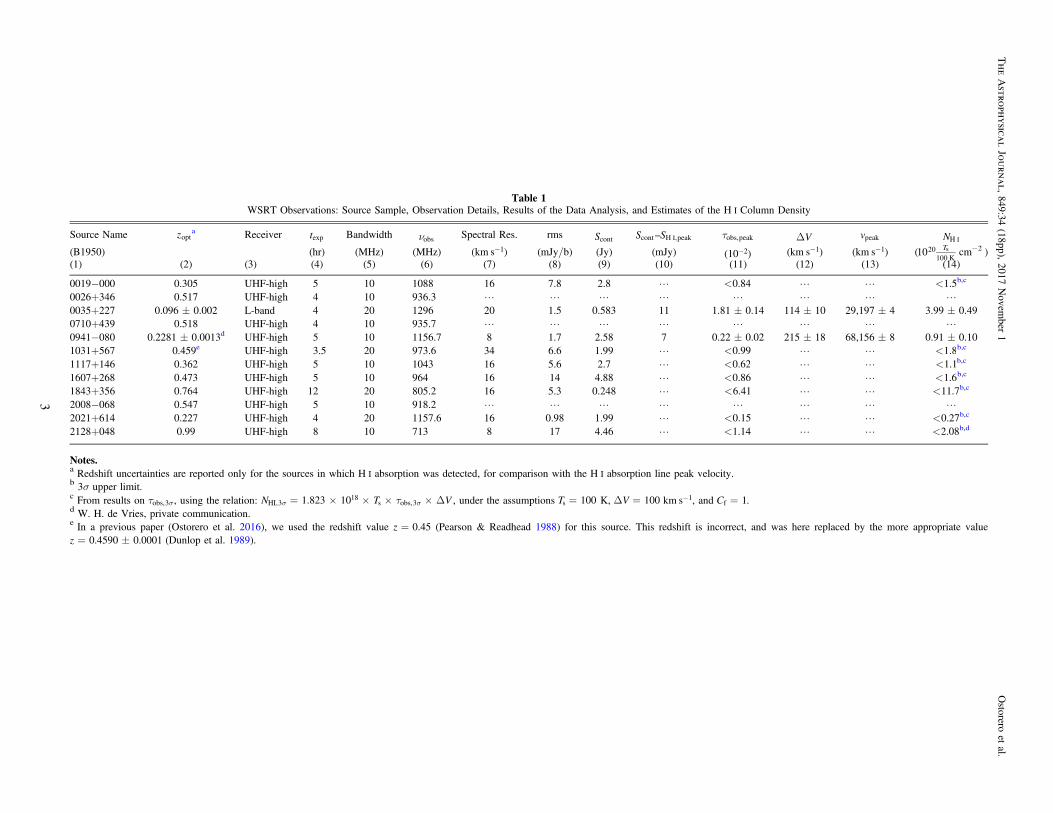
Table 1WSRT Observations: Source Sample, Observation Details, Results of the Data Analysis, and Estimates of the H IColumn Density

Source Name zopta Receiver texp Bandwidth nobs Spectral Res. rms Scont –S Scont H ,peakI tobs,peak DV vpeak NH I

(B1950) (hr) (MHz) (MHz) (km -s 1) (mJy/b) (Jy) (mJy) -( )10 2 (km -s 1) (km -s 1) (10 T20100 K

s cm−2 )(1) (2) (3) (4) (5) (6) (7) (8) (9) (10) (11) (12) (13) (14)

0019−000 0.305 UHF-high 5 10 1088 16 7.8 2.8 L <0.84 L L <1.5b,c

0026+346 0.517 UHF-high 4 10 936.3 L L L L L L L L0035+227 0.096±0.002 L-band 4 20 1296 20 1.5 0.583 11 1.81±0.14 114±10 29,197±4 3.99±0.490710+439 0.518 UHF-high 4 10 935.7 L L L L L L L L0941−080 0.2281±0.0013d UHF-high 5 10 1156.7 8 1.7 2.58 7 0.22±0.02 215±18 68,156±8 0.91±0.101031+567 0.459e UHF-high 3.5 20 973.6 34 6.6 1.99 L <0.99 L L <1.8b,c

1117+146 0.362 UHF-high 5 10 1043 16 5.6 2.7 L <0.62 L L <1.1b,c

1607+268 0.473 UHF-high 5 10 964 16 14 4.88 L <0.86 L L <1.6b,c

1843+356 0.764 UHF-high 12 20 805.2 16 5.3 0.248 L <6.41 L L <11.7b,c

2008−068 0.547 UHF-high 5 10 918.2 L L L L L L L L2021+614 0.227 UHF-high 4 20 1157.6 16 0.98 1.99 L <0.15 L L <0.27b,c

2128+048 0.99 UHF-high 8 10 713 8 17 4.46 L <1.14 L L <2.08b,d

Notes.a Redshift uncertainties are reported only for the sources in which H Iabsorption was detected, for comparison with the H Iabsorption line peak velocity.b 3σ upper limit.c From results on t sobs,3 , using the relation: t= ´ ´ ´ ´ Ds sN T V1.823 10HI,3

18s obs,3 , under the assumptions =T 100s K, D =V 100 km -s 1, and =C 1f .

d W. H. de Vries, private communication.e In a previous paper (Ostorero et al. 2016), we used the redshift value z=0.45 (Pearson & Readhead 1988) for this source. This redshift is incorrect, and was here replaced by the more appropriate value= z 0.4590 0.0001 (Dunlop et al. 1989).

3

TheAstro

physica

lJourn

al,

849:34(18pp),

2017Novem

ber1

Ostorero

etal.

A (Morganti et al. 2008) and Cygnus A (Struve &Conway 2010).

In the X-ray band, the spectra of GPS/CSOs reveal asignificant, although moderate, degree of intrinsic absorption.Tengstrand et al. (2009) found that the mean column densityvalue of their GPS/CSO sample, = ´N 3 10H

22 cm−2

(s 0.5NH dex), is much higher than that of a control sample ofextended radio galaxies of the FR-I type ( = ´-

+N 3.3 10H 0.72.1 21

cm−2), whose core emission does not appear to be obscured bydusty tori (Chiaberge et al. 1999; Donato et al. 2004) and isintermediate between the values of unobscured ( N 10H

22 cm−2)and highly obscured ( N 10H

23 cm−2) FR-II radio galaxies,where the presence of optically thick tori is supported by opticaland X-ray observations (Sambruna et al. 1999; Chiabergeet al. 2000). On the other hand, in the CSO sample analyzed bySiemiginowska et al. (2016), there appears to be an overabundance(∼60%) of sources with mild intrinsic obscuration, <N 10H

22

cm−2. The mean column density of the full sample is´ ( – )N 2 4 10H

21 cm−2 (s 0.3NH dex), depending onwhether only detections or both detections and upper limits aretaken into account; these values are consistent with the hydrogencolumn densities of FR-I and unobscured FR-II radio galaxies thatwe mentioned above.

The geometry and scales of the X-ray obscuring circum-nuclear structures in AGN are still debated: the ratio betweenType-2 and Type-1 AGN requires a geometrically thick torus,that is modeled in different ways, e.g., as a pc-scale, dustydonut (e.g., Krolik & Begelman 1988), or as a dust-free, sub-pcscale, clumpy outflow closely related to the broad-line emissionregion (Risaliti et al. 2007, 2010, 2011; Nenkova et al. 2008).Whether or not the X-ray obscuration of GPS/CSOs fits any ofthese scenarios is not clear, and any relationship between theradio and X-ray absorbers may help to clarify the picture.

As mentioned in Section 1, the neutral hydrogen columndensities, NH I, appear to be systematically lower than the totalhydrogen equivalent column densities, NH, by 1–2 orders ofmagnitudes, in GPS/CSOs for which both X-ray and spatiallyunresolved H Ispectra are available (e.g., Vink et al. 2006;Tengstrand et al. 2009). This discrepancy may indicate that theX-ray and radio measurements trace different absorbers, inagreement with a scenario where the X-rays originate in theaccretion-disc corona, and are consequently more affected byobscuration than the radio waves with l = 21 cm producedfarther from the AGN (e.g., Vink et al. 2006; Tengstrandet al. 2009). However, care should be taken when comparingthe radio and X-ray hydrogen column densities.

First, the estimate of NH I depends on the ratio between thespin temperature of the absorbing gas and the covering factor,T Cs f (e.g., Wolfe & Burbidge 1975; O’Dea et al. 1994;Gallimore et al. 1999), a parameter that is often poorlyconstrained; common assumptions are =T 100s K and =C 1f ,suitable for a cold gas cloud in thermal equilibrium, and thuswith the spin temperature equal to the kinetic temperature( =T Ts k), that fully covers the radio source. Second, theH Iabsorption measurements trace the content of the absorbingsystem in terms of neutral hydrogen (NH I), whereas the X-rayspectral measurements enable to constrain, for a given X-rayemission model, the content of total (i.e., neutral, molecular,and ionized) hydrogen (NH = NH I+NH2 +NH II) in an absorberwith a given elemental abundance (e.g., Wilms et al. 2000); fullcoverage of the X-ray source by the absorber is also typicallyassumed. A difference between NH I and NH is thus expected in

a single absorbing system composed of gas that is not fullyatomic and neutral; this difference is ultimately set by thetemperature of the gas (e.g., Maloney et al. 1996).When the absorber is cold, and the assumption= =T T 100k s K is reasonable for the H Igas, the abundance

of molecular hydrogen may be high (e.g., Maloney et al. 1996)and may partly account for the NH–NH I discrepancy. On theother hand, when the neutral hydrogen is warmer than typicallyassumed, with Ts few 103K, as expected in the circum-nuclear AGN environment (Bahcall & Ekers 1969; Maloneyet al. 1996; Liszt 2001), the NH I estimated from the observedoptical depth tobs increases accordingly, and may becomecomparable to the NH estimates.The assumption of a partial coverage of the source by the

absorber ( <C 1f ) affects both the NH I and the NH estimates,but the details of this effect are still to be investigated.Despite the above uncertainties, which affect the magnitude

of the NH–NH I offset, the existence of a correlation between NHand NH I (Ostorero et al. 2010, 2016), which we confirm below,clearly points toward a physical connection between the X-rayand radio absorbers.

3. H I Observations and Data Analysis

3.1. Target Sample

A summary of our observing program with the WSRT isreported in Table 1. We searched for H Iabsorption in a sampleof 12 GPS/CSOs, hereafter referred to as the target sample,drawn from a larger sample of X-ray emitting GPS/CSOsdescribed in Section 4. The target sources are listed in Table 1,Column 1 (and are also marked with an asterisk in the lastcolumn of Table 5). Their optical redshifts are reported inColumn 2 of the same table.Four out of twelve targets (i.e., 0035+227, 0026+346, 2008

−068, and 2128+048) were not searched for H Iabsorptionprior to our study. In the remaining eight targets, H Iabsorptionwas not detected in previous observations, and upper limits tothe H Ioptical depth could be estimated for five of them (seeTable 5). We observed these eight sources again to eitherimprove the available upper limits or attempt the first estimateof their H Ioptical depths.

3.2. Observations

The setup of the observations is summarized in Table 1,Columns 3–6.The observations were carried out with the WSRT in five

observing runs from 2008 to 2011. The target sources wereobserved either with the UHF-high-band receiver (appropriatewhen z 0.2) or with the L-band receiver (appropriate when<z 0.2), in dual orthogonal polarization mode. Each target was

observed for an exposure time of 3.5–12 hr. The observing bandwas either 10 or 20MHz wide, with 1024 spectral channels,centered at the frequency nobs where the H Iabsorption line isexpected to occur, based on the spectroscopical optical redshift.Compared to the H Isurvey of compact sources by Vermeulenet al. (2003), where a 10MHz wide band and 128 spectralchannels were available, our observations could benefit from alarger ratio between number of spectral channels andobserving bandwidth; this improvement, together with the longerexposure times, had the potential to enable a more effectiveseparation of narrow H Iabsorption features from radio frequencyinterferences (RFI). However, in many cases, we were forced

4

The Astrophysical Journal, 849:34 (18pp), 2017 November 1 Ostorero et al.

to adopt a 10MHz wide band in order to minimize the in-bandeffect of nearby RFI.10 The 10MHz bandwidth enabled us tocover a velocity range about the velocity centroid ofapproximately±1200 km -s 1 at z 0.1, increasing toapproximately±2000 km -s 1 at z 1. When we could use a20MHz wide band, the above velocity ranges increased toapproximately±2300 km -s 1 and±4200 km -s 1, respectively.

A primary calibrator (either 3C 48, 3C 147, or 3C 286) wasobserved before and after each target pointing, and used as aflux and bandpass calibrator.

3.3. Data Analysis

The integration time of our observations was typically ofonly a few hours (see Table 1). For an east–west array like theWSRT, this implies that the synthesized beam of the data cubesis very elongated. However, our targets are all unresolved bythe WSRT; therefore, this is not an issue for the resultspresented in this work.

The data were calibrated and reduced using the MIRIADpackage (Sault et al. 1995). The continuum subtraction wasdone by performing a linear fit of the spectrum through theline-free channels of each visibility record, and subtracting thefitting function from all the frequency channels (“UVLIN”).The spectral-line cube was obtained by averaging a few(typically three or four) channels together and adoptinguniform weighting. The data were Hanning smoothed tosuppress the Gibbs ripples. The final velocity resolution of thedata cubes, together with the 3σ rms noise, are listed in Table 1,Columns 7 and 8.

For all but one target source, we used the UHF-high-bandreceiver: this receiver, unlike the L-band receiver, is uncooled.

Therefore, despite the technical improvements described inSection 3.2, our observations were affected by a relatively highnoise level.

3.4. H I Results

We detected H Iabsorption in 2 out of 12 targets, 0035+227and 0941−080. For seven targets, we could estimate upperlimits to the optical depth of a putative H Iabsorption line.However, in three cases, the quality of our observations turnedout to be lower than the quality of the observations previouslyperformed by Vermeulen et al. (2003). This appears to be dueto degradation of the band caused by extra RFI. In these threecases, we used the constraints on the optical depth derived byVermeulen et al. (2003) for our correlation analysis (seeSection 5). For the remaining three targets, located at redshift= –z 0.517 0.547, the RFI were too strong to obtain any useful

data, despite the above technical improvements.For the sources in which we detected H Iabsorption, the

peak optical depth, tobs,peak, the line width,DV (correspondingto the full width at half maximum), and the peak velocity,vobs,peak, were determined through Gaussian fitting of theabsorption profiles. For the sources in which no H Iabsorptionwas detected, s3 upper limits to tobs,peak were estimated fromthe continuum flux density and the rms noise level of thespectra. The estimates of tobs,peak,DV , and vpeak are reported inTable 1, Columns 11, 12, and 13, respectively. The flux densityof the continuum and, for the detections only, its differencefrom the flux density of the line peak are given in Columns 9and 10, respectively.The atomic hydrogen column density along the line of sight

(in units of cm−2 ) is related to the velocity-integrated opticaldepth of the H Iabsorption profile through the followingrelationship (e.g., Wolfe & Burbidge 1975; O’Dea et al. 1994;Curran et al. 2013):

ò t= ´ ( ) ( )N T v dv1.823 10 , 1H18

sI

where Ts is the spin temperature in K, v is the velocity in unitsof km -s 1, and the optical depth is given by

tt

= - -⎡⎣⎢

⎤⎦⎥( ) ( ) ( )v

v

Cln 1 . 2obs

f

Here, the observed optical depth, t ( )vobs , is the ratio betweenthe spectral line depth in a given velocity channel and thecontinuum flux density of the background radio source:t º D( ) ( ) ( )v S v S vobs cont = -( ( ) ( )) ( )S v S v S vcont cont .

In the optically thin regime (i.e., for t 0.3), the observedoptical depth of the line is related to the actual optical depththrough t t»( ) ( )v v Cobs f , and Equation (1) can be approxi-mated by

ò t» ´ ( ) ( ) ( )N T C v dv1.823 10 . 3H18

s f obsI

Therefore, the H Icolumn density can be derived from theintegrated observed optical depth, òt tº ( )v dvobs obs , once theratio T Cs f is known.We computed the H Icolumn densities (in cm−2 ) of the

detected sources from Equation (3), with t ( )vobs replaced by itsGaussian fitting function. For consistency with the literature,we estimated NH I by assuming that the absorber fully coversthe radio source ( =C 1f ), and that the spin temperature of the

Figure 1. Spectrum of the CSO 0035+227, with velocities displayed in theoptical heliocentric convention. The systemic velocity of the optical galaxy is

= ( )v 28,780 600sys km -s 1: vsys is marked with a vertical, dotted line; thehorizontal, dotted line shows its 1σ uncertainty. A complex absorption line,with t = 0.0181 0.0014obs,peak and D = ( )V 114 10 km -s 1, is detectedabout vsys.

10 The frequencies corresponding to the redshifts of these sources are close tothe GSM band and bands allocated to TV broadcast.

5

The Astrophysical Journal, 849:34 (18pp), 2017 November 1 Ostorero et al.

absorbing gas is =T 100s K. These assumptions yield NH I

values that likely represent lower limits to the actual columndensities (see Section 2).

When we did not detect any H Iline, we used the followingequation to estimate s3 upper limits to NH I from the s3 upperlimits to the observed optical depth, t sobs,3 :

t= ´ Ds s( ) ( )N T C V1.823 10 , 4HI,318

s f obs,3

under the assumption that the putative absorption line hasD =V 100 km -s 1 (Vermeulen et al. 2003). Our estimates ofNH I are reported in Table 1, Column 14.

3.4.1. H I Absorption in 0035+227

Our spectrum of source 0035+227 is displayed in Figure 1.We detected one absorption feature with a complex profile. AGaussian fit to the optical depth velocity profile yields apeak optical depth t = 0.0181 0.0014obs,peak , a linewidth D = ( )V 114 10 km -s 1, and a peak velocity =vpeak

( )29,197 4 km -s 1. The systemic velocity of the host galaxy,derived from its heliocentric redshift, = z 0.096 0.002,estimated by Marcha et al. (1996) from an optical spectrumof the source, is = ( )v 28,780 600sys km -s 1. The peakvelocity of the absorption line is consistent with the systemicvelocity of the galaxy at 1σ confidence level. We derived anH Icolumn density = ´( )N 3.99 0.49 10H

20I cm−2 for the

gas responsible for the absorption line, under the assumptionthat =C 1f and =T 100s K.

3.4.2. H I Absorption in 0941−080

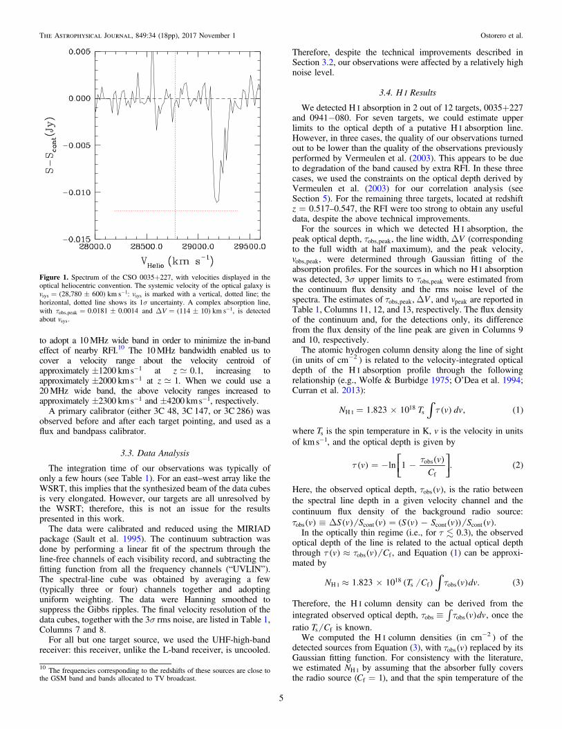
In the spectrum of 0941−080, shown in Figure 2, we detected abroad, multi-peaked absorption feature. A Gaussian fit to theoptical depth velocity profile yields a peak optical depth t =obs,peak

0.0022 0.0002, a line widthD = ( )V 215 18 km -s 1, and apeak velocity = (v 68,156peak )8 km -s 1. The systemic velocity

of the host galaxy, derived from the heliocentric redshift estimatedfrom the optical spectrum of the source, = z 0.2281 0.0013(de Vries et al. 2000; W. H. de Vries, private communication),is = ( )v 68,353 390sys km -s 1. The peak velocity of theabsorption line is consistent with the systemic velocity of thegalaxy at 1σ confidence level. For the gas responsible for thisassociated absorption, we derived an H Icolumn density

= ´( )N 9.1 1.0 10H19

I cm−2 , under the assumption that=C 1f and =T 100s K. This detection of H Iabsorption in the

source is the first ever, and it was enabled by the improvedobservation setup (see Section 3.2). Previous observations(Vermeulen et al. 2003) could only set upper limits to the opticaldepth of a putative absorption line (see Table 5). The optical depththat we measured is consistent with the previously estimated upperlimits.

4. NH–NH I Sample Definition

By using our own data and those from the literature, wecompiled the largest sample of GPS/CSOs that were targets ofboth X-ray and H I-absorption observations. The GPS/CSOsobserved in the X-rays were all detected in this band, and theyconstitute a subsample of the GPS/CSOs observed in theH Iband: therefore, the sample that we compiled consists of allthe X-ray detected GPS/CSOs that were also observed in theH Iband, i.e., 27 compact radio galaxies. This sample includessources that were investigated in the X-ray band, eitherindividually or in small samples, by different authors and withdifferent instruments; it can be considered as the merger of two,partly overlapping, subsamples of sources that were selectedfor X-ray investigations with different criteria. The firstsubsample is a flux- and volume-limited sample of 17 GPSgalaxies, with >F 15 GHz Jy and <z 1, extracted by Tengstrandet al. (2009) and Guainazzi et al. (2006) from the completesample of GPS sources compiled by Stanghellini et al. (1998);these GPS galaxies are located at redshift = –z 0.0773 0.99,and have radio luminosities at n = 1.4 GHz spanning the range

= –L 10 101.4 GHz25 28.4 W Hz−1; 16 of them were morphologi-

cally classified as CSOs. The second subsample is a sample of16 CSOs with known redshifts and estimated kinematic ages,compiled by Siemiginowska et al. (2016); these CSOs arelocated at redshift = –z 0.0142 0.764, and have radio luminos-ities at n = 1.4 GHz spanning the range = –L 10 101.4 GHz

24 27.6

WHz−1; 15 of them were spectroscopically classified as GPSsources. The two subsamples have six sources in common.Overall, the 27 sources of the full sample are located at redshift= –z 0.0142 0.99, and they have moderate to high radio

luminosities, = –L 10 101.4 GHz24 28.4 W Hz−1.11 Even though

the sample is not complete and well-defined in terms of fluxlimit and volume, it is the largest sample of GPS/CSOsavailable to date for which both X-ray and H Iobservationswere carried out. The main properties of the sources of thissample, including all the available H Iand X-ray columndensity estimates, are summarized in Tables 5 and 6.In order to perform the NH–NH I correlation analysis, from

the above sample of 27 GPS/CSOs, we extracted thesubsample of sources for which an estimate of both NH I andNH was available. By “estimate,” we mean either a value or anupper/lower limit. The three sources 0026+346, 0710+439,and 2008−068 have no NH I estimate (see Sections 4.1 and

Figure 2. Spectrum of the GPS/CSO galaxy 0941−080, with velocitiesdisplayed in the optical heliocentric convention. The systemic velocity of theoptical galaxy is = ( )v 68,353 390sys km -s 1: vsys is marked with a vertical,dotted line; the horizontal, dotted line shows its 1σ uncertainty. A broad, multi-peaked absorption feature with t = 0.0022 0.0002obs,peak andD = ( )V 215 18 km -s 1 is detected about vsys.

11 Only 3 out of 27 sources have <L 101.4 GHz25 W Hz−1: 1245+676, 1509

+054, and 1718−649.

6

The Astrophysical Journal, 849:34 (18pp), 2017 November 1 Ostorero et al.

Table 5), and the two sources 0116+319 and 1245+676 haveno NH estimate (see Section 4.2 and Table 6). Therefore, wewere left with a subsample of 22 sources, that we refer tohereafter as the correlation sample.

The correlation sample spans the redshift range = –z 0.01420.99 and the 1.4 GHz luminosity range = –L 101.4 GHz

24.2

1028.4 W Hz−1. Table 2 lists the sources of the correlationsample (Column 1), their optical redshifts (Column 2), theirradio spectral and morphological classification (Column 3), theestimates of NH I (Column 4) and NH (Column 5) that weused for the correlation analysis, the type of (NH, NH I) pair(Column 6), and the sample to which we associated each (NH,NH I) pair for the correlation analysis (Column 7), as describedin Section 4.3. More details on the quantities reported inTable 2, and the criteria that we applied to select the columndensity estimates given in this table among all the availablecolumn density estimates, can be found in the Appendix.

4.1. NH I Estimates

Detections of H Iabsorption features, and their corresp-onding NH I values, were available for 14 out of the 22 sources

of the correlation sample; NH I upper limits could be estimatedfor the remaining eight sources.We only used NH I estimates derived from low angular

resolution measurements, i.e., from measurements that were notable to spatially resolve the source; all our upper limits to NH I

are 3σ limits. As mentioned in Sections 2 and 3.4, the NH I

estimates depend on the value assumed for the ratio T Cs f .When an NH I value drawn from the literature was estimated bythe authors by assuming >T C 100s f K (i.e., >T 100s K and

=C 1f ), we rescaled it to an NH I value computed with=T C 100s f K. For the 12 sources with more than one NH I

estimate, we chose the most suitable estimate, according to thecriteria described in Appendix A. The selected NH I estimatesare summarized in Table 2, Column 4; they are also listed withthe corresponding references in Table 5; we thoroughlycomment on these data, as well as on on the properties of thefull NH I data set, in Appendix A.

4.2. NH Estimates

As anticipated in Section 2, the estimate of the columndensity of the X-ray absorbing gas located at the redshift of thesource (i.e., the local absorber) depends on the X-ray emission

Table 2Correlation Sample: Column Density Data Set, Pair Types, and Analysis Samples

Source Name zopt GPS/CSO NH I NH Pair Type Samplea

B1950 (10 T20100 K

s cm−2 ) (1022 cm−2 ) (1) (2) (3) (4) (5) (6) (7)

0019−000 0.305 GPS <1.5 <100 UU E′, E″0035+227 0.096±0.002 CSO 3.99±0.49 -

+1.4 0.60.8 VV E′, E″

0108+388 0.66847 GPS, CSO 80.5 -+47.5 12

12b VV E′

80.5 >90c VL –

0428+205 0.219 GPS, CSO 3.45d <0.69 VU E′, E″0500+019 0.58457 GPS, CSO 6.2 -

+0.5 0.160.18 VV E′, E″

0941−080 0.2281±0.0013 GPS, CSO 0.91±0.10 <1.26 VU E′, E″1031+567 0.459 GPS, CSO <1.26 0.50±0.18 VU E′, E″1117+146 0.362 GPS, CSO <0.63 <0.16 UU E′, E″1323+321 0.370 GPS, CSO 0.71 -

+0.12 0.050.06 VV E′, E″

1345+125 0.12174 GPS, CSO 6.2 4.8±0.4 VV E′, E″ 6.2 -

+2.543 0.5800.636 VV E′, E″

1358+624 0.431 GPS, CSO 1.88 -+2.9 1

2 VV E′, E″1404+286 0.07658 GPS, CSO 8.0 -

+0.13 0.100.12 VV E′

8.0 >90c VL –

1509+054 0.084 GPS, CSO <3.64 <0.23 UU E′, E″1607+268 0.473 GPS, CSO <1.6 <0.18 UU E′, E″1718−649 0.0142 GPS, CSO 1.477d 0.08±0.07 VV E′, E″1843+356 0.764 GPS, CSO <10.4 -

+0.8 0.70.9 VU E′, E″

1934−638 0.18129 GPS, CSO 0.06 -+0.08 0.06

0.07 VV E′

0.06 >250c VL –

1943+546 0.263 GPS, CSO 4.91 1.1±0.7 VV E′, E″1946+708 0.101 GPS, CSO 31.6 -

+1.7 0.40.5 VV E′

31.6 >280c VL –

2021+614 0.227 GPS, CSO <0.27 <1.02 UU E′, E″2128+048 0.99 GPS, CSO <2.08 <1.9 UU E′, E″2352+495 0.2379 GPS, CSO 2.84d -

+4 37 VV E′, E″

Notes.a The en-dash indicates that the corresponding pair was not included in any sample because it comprises a lower limit (see Section 4.3 for details).b This value of NH was estimated as the mean of the s3 lower limit > ´N 5 10H

22 cm−2 and the physical upper bound of the Compton-thin NH range, i.e.,> ´N 9 10H

23 cm−2 (see Appendix B and Table 6 for details).c This value of NH corresponds to the assumption that the absorber is Compton-thick (see Appendix B and Table 6 for details).d Total NH I, estimated as the sum of the NH I values derived from the two absorption lines detected in the spectrum (see Appendix A, Table 5).

7

The Astrophysical Journal, 849:34 (18pp), 2017 November 1 Ostorero et al.

model adopted to interpret the X-ray spectrum of the source, aswell as on the assumed photoionization cross-section of theISM. For a given abundance of chemical elements in theabsorbing gas, the X-ray spectral modeling enables to estimatethe equivalent hydrogen column density of the local absorber,NH, i.e., the column density of hydrogen atoms, molecules, andions toward the source, located at the source redshift (seeAppendix B for details).

In the correlation sample, detections of intrinsic X-rayabsorption, and corresponding values of NH, were available for9 out of 22 sources; upper limits to NH were available for eightsources. For the remaining five sources, multiple exposures andambiguity in the spectral modeling prevented us from selectinga single robust NH value. In particular, for one source, weselected two significantly different NH values corresponding todifferent observational epochs. For four of them, the ambiguitybetween a Compton-thin and a Compton-thick absorber in themodel adopted for the interpretation of the X-ray spectrum ofthe source led to the availability of NH estimates lower andgreater than 1024 cm−2 , respectively; we considered bothscenarios to be plausible, and associated with each of these foursources either an NH value (Compton-thin scenario) or a lowerlimit to NH (Compton-thick scenario).

The NH estimates that we used for our correlation analysisare summarized in Table 2, Column 5; they are also listed withthe corresponding references in Table 6; we thoroughlycomment on these data, as well as on the properties of thefull NH data set, in Appendix B.

4.3. NH–NH I Sample

The correlation sample consists of 22 sources associated with(NH, NH I) pairs of estimates of four different types: pairs ofvalues (hereafter referred to as VV pairs), pairs including a valueand an upper limit (VU pairs), pairs of upper limits (UU pairs),and pairs including a value and a lower limit (VL pairs).Specifically, the sample includes four sources unambiguouslyassociated with VU pairs, six with UU pairs, and eight with VVpairs. The sample also includes four sources whose X-rayabsorber may be either Compton-thin or Compton-thick (seeSection 4.2): each of them is associated with either a VV pair or aVL pair. The types of (NH, NH I) pairs associated with the sourcesof the correlation sample are listed in Table 2, Column 6.

In order to deal with the four ambiguous Compton-thin/Compton-thick sources, we considered two limiting cases in

our correlation study. In the first case, we assumed these foursources to be all Compton-thin, and hence we associated themwith VV pairs. This choice yielded a correlation samplecomposed of 12 sources with (NH, NH I) pairs of values (VVpairs), and 10 sources with (NH, NH I) pairs including upperlimits (either VU or UU pairs), for a total of 22 sources with 23(NH, NH I) pairs12 of estimates of either the VV, VU, orUUtype; hereafter, this sample is referred to as the estimate sampleE′. The data in sample E′ have only one type of censoring (i.e.,the sample pairs include only values and upper limits; there isno mix of upper and lower limits).In the second case, we assumed the above four sources to be

all Compton-thick, and associated them with the correspondingVL pairs. This left us with a correlation sample composed ofthree main subsamples: a subsample of eight sources with (NH,NH I) VV pairs, a subsample of 10 sources including upperlimits (either VU or UU pairs), and a subsample of four sourcesincluding lower limits (VL pairs). However, because ofdifficulties in performing the correlation analysis on samplesincluding data with two types of censoring (i.e., both upper andlower limits; see Section 5 for details), we chose to drop thefour VL pairs from the correlation sample. The reason whywe dropped this subsample of pairs is that this is the smaller ofthe two subsamples of censored data pairs. Dropping thesubsample that includes the VU and UU pairs would havelowered the total number of sources. Our choice left us with asample including eight sources with (NH, NH I) VV pairs and 10sources with (NH, NH I) pairs of estimates of either the VU orthe UU type, for a total of 18 sources with 19 (NH, NH I) pairs ofestimates of either the VV, the VU, or the UU type; hereafter,this sample is referred to as the estimate sample E″. Byconstruction, the data in sample E″ have only one type ofcensoring.

5. Correlation Analysis

We performed the correlation analysis on both the estimatesamples, E′ and E″, defined in Section 4.3. The results of thisanalysis are reported in Table 3 and discussed below. Figure 3displays the (NH, NH I) data for these two samples, as well asthe corresponding linear regression lines, to guide the eye.Before discussing these results, we emphasize that correlat-

ing NH with NH I is interesting from the point of view of the

Table 3Correlation and Regression Analysis for the Estimate Samples, E′ and E″, by means of Survival Analysis Techniques

Samplea NdataGeneralized Kendall

GeneralizedSpearmand Schmitt’s Linear Regressione

Akritas–Theil–Sen LinearRegression

(Nsources) zb Pc ρ Pc Slope (b) Intercept (a) Slope (b) Intercept (a)

E′ 23 (22) 3.044 0.0023 0.679 0.0014 0.820 2.42 0.467 10.3E″ 19 (18) 2.615 0.0089 0.667 0.0046 0.469 10.0 0.345 13.0

Notes.a The samples are defined in Section 4.3 and in Table 2.b According to the ASURV Rev. 1.3 software manual, z is an estimated function of the correlation and should not be directly compared to the Spearman’s correlationρ. The values to be compared are the corresponding probabilities.c Probability of the null hypothesis of no correlation being true. It is a two-sided significance level: because we are looking a priori for a positive correlation, this valueshould actually be divided by 2, improving the significance by a factor of 2.d According to the ASURV Rev. 1.3 software manual, the generalized Spearman correlation is not dependable for samples with <N 30 items, as in our case. In thesecases, the generalized Kendall’s τ test should be relied upon. We report it here only for comparison purposes.e For a bin number of 10 for the data set (see Section 5 for details).

12 One source is associated with two VV pairs; see Section 4.2.

8

The Astrophysical Journal, 849:34 (18pp), 2017 November 1 Ostorero et al.

physics of the sources, although the estimate of NH I is acombination of the measurement of tobs and the assumption onT Cs f ( tµ ´N T C ;H obs s fI see Equation (3)).

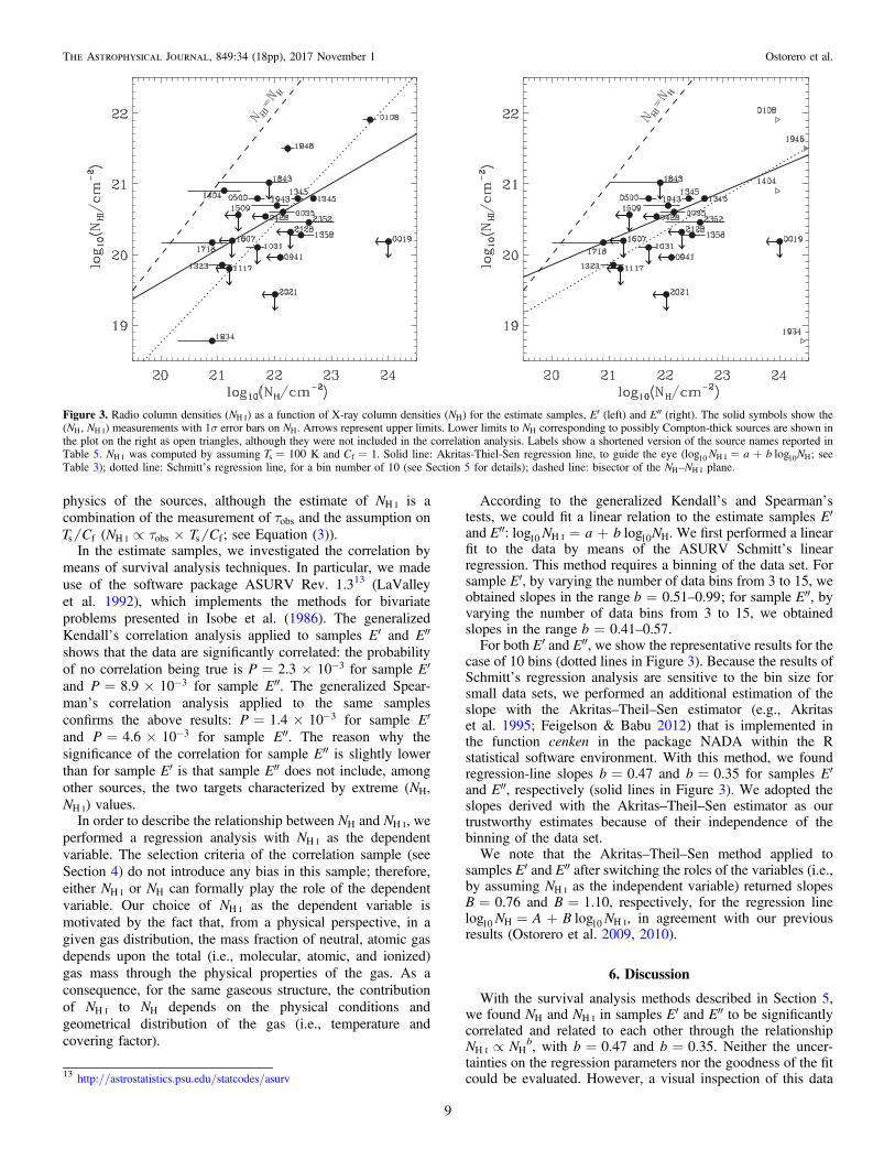
In the estimate samples, we investigated the correlation bymeans of survival analysis techniques. In particular, we madeuse of the software package ASURV Rev. 1.313 (LaValleyet al. 1992), which implements the methods for bivariateproblems presented in Isobe et al. (1986). The generalizedKendall’s correlation analysis applied to samples E′ and E″shows that the data are significantly correlated: the probabilityof no correlation being true is = ´ -P 2.3 10 3 for sample E′and = ´ -P 8.9 10 3 for sample E″. The generalized Spear-man’s correlation analysis applied to the same samplesconfirms the above results: = ´ -P 1.4 10 3 for sample E′and = ´ -P 4.6 10 3 for sample E″. The reason why thesignificance of the correlation for sample E″ is slightly lowerthan for sample E′ is that sample E″ does not include, amongother sources, the two targets characterized by extreme (NH,NH I) values.In order to describe the relationship between NH and NH I, we

performed a regression analysis with NH I as the dependentvariable. The selection criteria of the correlation sample (seeSection 4) do not introduce any bias in this sample; therefore,either NH I or NH can formally play the role of the dependentvariable. Our choice of NH I as the dependent variable ismotivated by the fact that, from a physical perspective, in agiven gas distribution, the mass fraction of neutral, atomic gasdepends upon the total (i.e., molecular, atomic, and ionized)gas mass through the physical properties of the gas. As aconsequence, for the same gaseous structure, the contributionof NH I to NH depends on the physical conditions andgeometrical distribution of the gas (i.e., temperature andcovering factor).

According to the generalized Kendall’s and Spearman’stests, we could fit a linear relation to the estimate samples E′and E″: = +N a b Nlog log10 H 10 HI . We first performed a linearfit to the data by means of the ASURV Schmitt’s linearregression. This method requires a binning of the data set. Forsample E′, by varying the number of data bins from 3 to 15, weobtained slopes in the range = –b 0.51 0.99; for sample E″, byvarying the number of data bins from 3 to 15, we obtainedslopes in the range = –b 0.41 0.57.For both E′ and E″, we show the representative results for the

case of 10 bins (dotted lines in Figure 3). Because the results ofSchmitt’s regression analysis are sensitive to the bin size forsmall data sets, we performed an additional estimation of theslope with the Akritas–Theil–Sen estimator (e.g., Akritaset al. 1995; Feigelson & Babu 2012) that is implemented inthe function cenken in the package NADA within the Rstatistical software environment. With this method, we foundregression-line slopes b=0.47 and b=0.35 for samples E′and E″, respectively (solid lines in Figure 3). We adopted theslopes derived with the Akritas–Theil–Sen estimator as ourtrustworthy estimates because of their independence of thebinning of the data set.We note that the Akritas–Theil–Sen method applied to

samples E′ and E″ after switching the roles of the variables (i.e.,by assuming NH I as the independent variable) returned slopesB=0.76 and B=1.10, respectively, for the regression line

= +N A B Nlog log10 H 10 H I, in agreement with our previousresults (Ostorero et al. 2009, 2010).

6. Discussion

With the survival analysis methods described in Section 5,we found NH and NH I in samples E′ and E″ to be significantlycorrelated and related to each other through the relationshipNH I∝NH

b, with b=0.47 and b=0.35. Neither the uncer-tainties on the regression parameters nor the goodness of the fitcould be evaluated. However, a visual inspection of this data

Figure 3. Radio column densities (NH I) as a function of X-ray column densities (NH) for the estimate samples, E′ (left) and E″ (right). The solid symbols show the(NH, NH I) measurements with 1σ error bars on NH. Arrows represent upper limits. Lower limits to NH corresponding to possibly Compton-thick sources are shown inthe plot on the right as open triangles, although they were not included in the correlation analysis. Labels show a shortened version of the source names reported inTable 5. NH I was computed by assuming =T 100s K and =C 1f . Solid line: Akritas-Thiel-Sen regression line, to guide the eye ( = +N a b Nlog log10 H 10 HI ; seeTable 3); dotted line: Schmitt’s regression line, for a bin number of 10 (see Section 5 for details); dashed line: bisector of the NH–NH I plane.

13 http://astrostatistics.psu.edu/statcodes/asurv

9

The Astrophysical Journal, 849:34 (18pp), 2017 November 1 Ostorero et al.

set suggests a dispersion larger than the typical uncertainties onNH I (see Figure 3).This fact is supported by the regression analysis of the

subsamples that we drew from E′ and E″ by selecting thedetections only. These two subsamples, hereafter referred to asdetection samples ¢D and D , respectively, display a significantNH–NH I correlation according to both Pearson’s and Kendall’scorrelation analysis. However, the best-fit linear relation turnsout not to be a good description of the data (c ~ 10red

2 ): thedispersion of the data is clearly larger than the typicaluncertainties.14

This evidence suggests that the observed NH–NH I relation isthe two-dimensional projection of a multi-dimensional relation,where T Cs f is a variable rather than a parameter. In fact, as weshow below, T Cs f is the most relevant additional variable inthe NH–NH I relation. There are only two other possiblevariables; however, either they have a modest impact or,ultimately, depend on Ts: (i) the abundance of chemicalelements that enters the photoionization cross-section of theX-ray absorbing gas, ultimately affecting the NH estimates inthe X-ray spectral fitting; and (ii) the amount of ionized andmolecular hydrogen, H IIand H2.

As for item (i), typical cross-sections adopted in the spectralanalysis are based on either solar or ISM abundances. Thesedifferent assumptions lead to variations of the cross-section bya factor of a few (e.g., Ride & Walker 1977; Wilmset al. 2000), implying corresponding variations of the NHestimates by a factor of a few. This variation is comparable tothe average NH uncertainty.

As for item (ii), the abundance of H IIand H2 is an unknownthat, in principle, can contribute both to the NH–NH I offset andthe spread. This abundance is ultimately set by the kinetictemperature of the gas, Tk. If all the sources were characterizedby a similar kinetic temperature of the absorber, the fractions ofH IIand/or H2 would be comparable in different sources andonly contribute to the offset. On the other hand, if the kinetictemperature were significantly different in different sources, theabundance of H IIand H2 would also contribute to the spread,and NH and NH I might even be uncorrelated in the case ofextreme temperature fluctuations. However, we do find acorrelation between NH and NH I; we can thus exclude extremefluctuations in the kinetic temperature, Tk.

Similarly, the ratio T Cs f might also significantly fluctuatefrom source to source; for example, it is seen to vary by a factorof at least ∼170 in damped Ly-α systems, where H Icolumndensities are known (Curran et al. 2013). Clearly, extremefluctuations of T Cs f from source to source might also erase theNH–NH I correlation. As in the case of Tk, the correlation wefound excludes extreme fluctuations in T Cs f . Because Tk andTs are related to each other, we can ultimately ascribe thecorrelation spread to fluctuations of T Cs f about the assumedvalue.

To sum up, for a given source, the NH I estimate from aspatially unresolved measurement of tobs must assume a valuefor the ratio T C ;s f typically, =T C 100s f K is assumed. Adifferent assumption about T Cs f clearly leads to a differentNH–NH I offset. When we look for a correlation between X-ray

and radio absorption in a sample of sources, we must alsoassume a T Cs f ratio for each source. The simplest assumptionis to assign the same ratio to all the sources. A posteriori, thisassumption appears to be reasonable because we do find acorrelation. However, this correlation shows a non-null spread,suggesting that each individual source might actually have aT Cs f ratio slightly different from the value assumed for theentire sample. By estimating the spread, one can, in principle,estimate the fluctuations of the T Cs f ratio of the individualsources about the value assumed for the entire sample. As aproof of concept, we estimate the spread of the detectionsamples ¢D and D in Section 6.1.

6.1. Quantifying the Spread of the NH–NH I Correlation

In order to simultaneously derive the correlation parametersof the NH–NH I relation and quantify, for a given NH, theintrinsic scatter of NH I that might be due to the fluctuation ofthe ratio T Cs f of the individual sources about a mean value, itis appropriate to resort to a Bayesian analysis. As a proof ofconcept, we performed a Bayesian analysis of the detectionsamples ¢D and D . We made use of the code APEMoST,15

which was developed by J.Buchner and M.Gruberbauer(Gruberbauer et al. 2009) and is suitable for non-censored datasets. A more sophisticated code, able to perform the Bayesiananalysis on samples that include double-censored data (as oursamples E′ and E″), could be constructed based on the modeldeveloped by Kelly (2007); however, this implementation isbeyond the scope of the present paper.Although samples ¢D and D are biased, because they do not

include non-detections, the results presented below are usefulto illustrate how the intrinsic spread of the NH–NH I relation canbe quantified and interpreted. An additional advantage of theBayesian analysis over the frequentist analysis is the possibilityto take the uncertainties on both variables into account, evenwhen the uncertainties are asymmetric.Our data set is DS={log10NH

k, log10NH Ik, Sk}, where

s s= + - + -{ }S , , ,k k k k k is the vector of the upper and loweruncertainties on the k-th measures NH

k and NH Ik. The

uncertainties on the NH I values, for a given T Cs f , are availablefor two measurements only: the relative uncertainties are equalto 12% and 14%, respectively. Assuming that the remainingNH I measurements are affected by comparable uncertainties,for the purpose of the Bayesian analysis only, to each of themwe associated a conservative, relative uncertainty of 15%.Because the uncertainties on NH I are much smaller than thoseon NH, all the NH I uncertainties have negligible effects on ourresults.Given our data set DS, we determined the multi-dimensional

probability density function (PDF) of the parametersq s= { }a b, , int,NHI , where a and b are the parameters of thecorrelation (i.e., our model M):

s= + ( )N a b Nlog log , 510 H 10 H int,NHII

and sint,NHI is the intrinsic spread of the dependent variable.In our analysis with APEMoST, we assumed independent

flat priors for parameters a and b. For the internal dispersion

14 For the detection samples, we performed the regression analysis on a dataset where NH is the dependent variable (i.e., = +N A B Nlog log10 H 10 H I),because the uncertainties are available for all the NH measurements, whereasthey are available for only a minority of NH I measurements. Because theuncertainties on NH I are typically smaller than those on NH, the lowsignificance of the linear fit also holds for the reverse relation.

15 Automated Parameter Estimation and Model Selection Toolkit; http://apemost.sourceforge.net/, 2011 February.

10

The Astrophysical Journal, 849:34 (18pp), 2017 November 1 Ostorero et al.

sint,NHI, which is a positive parameter, we assumed

sm

m=G

--( ∣ )( )

( ) ( )p Mr

x xexp , 6r

rint,NHI

1

where s=x 1 int,NHI2 , and G( )r is the Euler gamma function.

This PDF describes a variate with mean mr , and variancemr 2. We set m= = -r 10 5 to assure an almost flat prior.We used 2×106 MCMC iterations to guarantee a fairly

complete sampling of the parameter space. The boundaries ofthe parameter space were set to -[ ]1000, 1000 for the a and bparameters, and to [ ]0.01, 1000 for the sint,NHI parameter. Theinitial seed of the random number generator was set with thebash command GSL_RANDOM_SEED=$RANDOM.

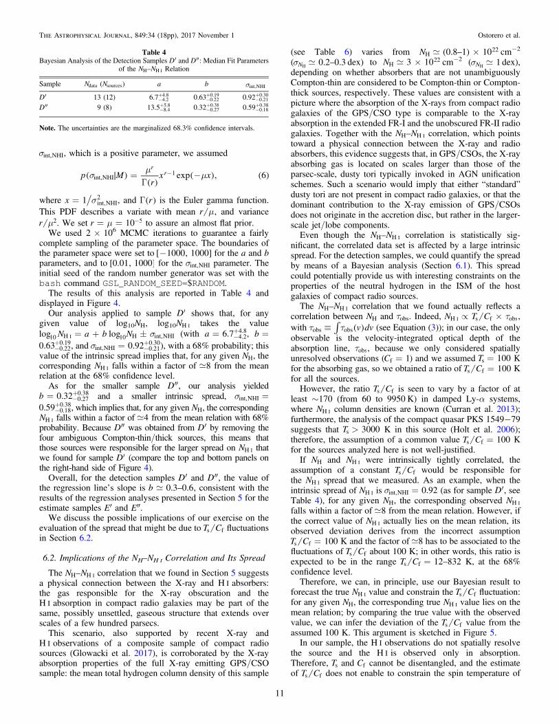
The results of this analysis are reported in Table 4 anddisplayed in Figure 4.

Our analysis applied to sample ¢D shows that, for anygiven value of log10NH, log10NH I takes the value

s= + N a b Nlog log10 H 10 H int,NHII (with = -+a 6.7 4.2

4.8, =b

-+0.63 0.22

0.19, and s = -+0.92int,NHI 0.21

0.30), with a 68% probability; thisvalue of the intrinsic spread implies that, for any given NH, thecorresponding NH I falls within a factor of 8 from the meanrelation at the 68% confidence level.

As for the smaller sample D , our analysis yielded= -

+b 0.32 0.270.38 and a smaller intrinsic spread, s =int,NHI

-+0.59 0.18

0.38, which implies that, for any given NH, the correspondingNH I falls within a factor of4 from the mean relation with 68%probability. Because D was obtained from ¢D by removing thefour ambiguous Compton-thin/thick sources, this means thatthose sources were responsible for the larger spread on NH I thatwe found for sample ¢D (compare the top and bottom panels onthe right-hand side of Figure 4).

Overall, for the detection samples ¢D and D , the value ofthe regression line’s slope is –b 0.3 0.6, consistent with theresults of the regression analyses presented in Section 5 for theestimate samples E′ and E″.

We discuss the possible implications of our exercise on theevaluation of the spread that might be due to T Cs f fluctuationsin Section 6.2.

6.2. Implications of the NH–NH I Correlation and Its Spread

The NH–NH I correlation that we found in Section 5 suggestsa physical connection between the X-ray and H Iabsorbers:the gas responsible for the X-ray obscuration and theH Iabsorption in compact radio galaxies may be part of thesame, possibly unsettled, gaseous structure that extends overscales of a few hundred parsecs.

This scenario, also supported by recent X-ray andH Iobservations of a composite sample of compact radiosources (Glowacki et al. 2017), is corroborated by the X-rayabsorption properties of the full X-ray emitting GPS/CSOsample: the mean total hydrogen column density of this sample

(see Table 6) varies from ´ ( – )N 0.8 1 10H22 cm−2

(s –0.2 0.3NH dex) to ´N 3 10H22 cm−2 (s 1NH dex),

depending on whether absorbers that are not unambiguouslyCompton-thin are considered to be Compton-thin or Compton-thick sources, respectively. These values are consistent with apicture where the absorption of the X-rays from compact radiogalaxies of the GPS/CSO type is comparable to the X-rayabsorption in the extended FR-I and the unobscured FR-II radiogalaxies. Together with the NH–NH I correlation, which pointstoward a physical connection between the X-ray and radioabsorbers, this evidence suggests that, in GPS/CSOs, the X-rayabsorbing gas is located on scales larger than those of theparsec-scale, dusty tori typically invoked in AGN unificationschemes. Such a scenario would imply that either “standard”dusty tori are not present in compact radio galaxies, or that thedominant contribution to the X-ray emission of GPS/CSOsdoes not originate in the accretion disc, but rather in the larger-scale jet/lobe components.Even though the NH–NH I correlation is statistically sig-

nificant, the correlated data set is affected by a large intrinsicspread. For the detection samples, we could quantify the spreadby means of a Bayesian analysis (Section 6.1). This spreadcould potentially provide us with interesting constraints on theproperties of the neutral hydrogen in the ISM of the hostgalaxies of compact radio sources.The NH–NH I correlation that we found actually reflects a

correlation between NH and tobs. Indeed, tµ ´N T CH s f obsI ,with òt tº ( )v dvobs obs (see Equation (3)); in our case, the onlyobservable is the velocity-integrated optical depth of theabsorption line, tobs, because we only considered spatiallyunresolved observations ( =C 1f ) and we assumed =T 100s Kfor the absorbing gas, so we obtained a ratio of =T C 100s f Kfor all the sources.However, the ratio T Cs f is seen to vary by a factor of at

least ∼170 (from 60 to 9950 K) in damped Ly-α systems,where NH I column densities are known (Curran et al. 2013);furthermore, the analysis of the compact quasar PKS 1549−79suggests that >T 3000s K in this source (Holt et al. 2006);therefore, the assumption of a common value =T C 100s f Kfor the sources analyzed here is not well-justified.If NH and NH I were intrinsically tightly correlated, the

assumption of a constant T Cs f would be responsible forthe NH I spread that we measured. As an example, when theintrinsic spread of NH I is s = 0.92int,NHI (as for sample ¢D , seeTable 4), for any given NH, the corresponding observed NH I

falls within a factor of 8 from the mean relation. However, ifthe correct value of NH I actually lies on the mean relation, itsobserved deviation derives from the incorrect assumption

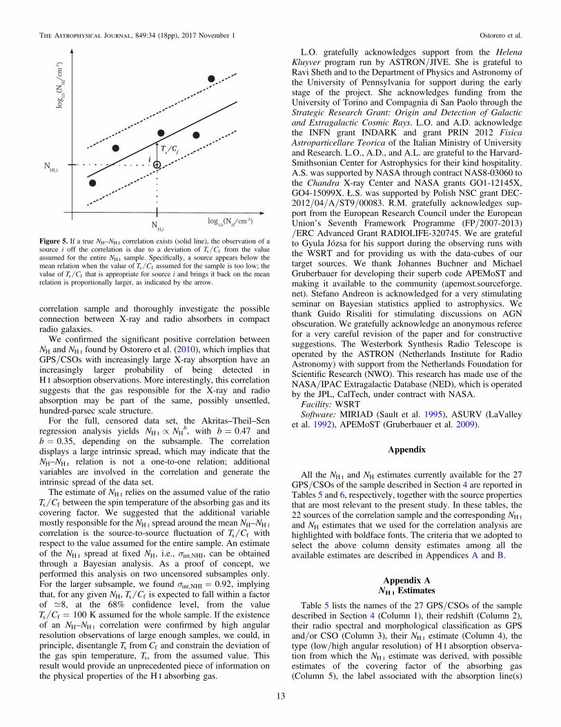
=T C 100s f K and the factor of8 has to be associated to thefluctuations of T Cs f about 100 K; in other words, this ratio isexpected to be in the range = –T C 12 832s f K, at the 68%confidence level.Therefore, we can, in principle, use our Bayesian result to

forecast the true NH I value and constrain the T Cs f fluctuation:for any given NH, the corresponding true NH I value lies on themean relation; by comparing the true value with the observedvalue, we can infer the deviation of the T Cs f value from theassumed 100 K. This argument is sketched in Figure 5.In our sample, the H Iobservations do not spatially resolve

the source and the H Iis observed only in absorption.Therefore, Ts and Cf cannot be disentangled, and the estimateof T Cs f does not enable to constrain the spin temperature of

Table 4Bayesian Analysis of the Detection Samples ¢D and D : Median Fit Parameters

of the NH–NH I Relation

Sample Ndata (Nsources) a b sint,NHI

¢D 13 (12) -+6.7 4.2

4.8-+0.63 0.22

0.19-+0.92 0.21

0.30

D 9 (8) -+13.5 8.4

5.8-+0.32 0.27

0.38-+0.59 0.18

0.38

Note. The uncertainties are the marginalized 68.3% confidence intervals.

11

The Astrophysical Journal, 849:34 (18pp), 2017 November 1 Ostorero et al.

the gas. On the other hand, if H Imeasures of a sufficientlylarge sample of sources were based on high angular resolutionobservations, constraining Ts would, in principle, be possible.Indeed, this kind of observation enables to locate theH Iabsorber; the absorption profiles are derived only for thesource region covered by the absorber, and the condition

=C 1f is readily justified. Moreover, Equations (1) and (3) aremore suitable for resolved observations; those equations holdunder the assumption that the source is homogeneous, asappropriate when the source fraction considered for theevaluation of NH I is small.

In conclusion, if a sample of resolved sources confirmed acorrelation between NH and NH I, the deviation between thedata-point of an individual source and the mean relation wouldreturn an estimate of the deviation of the spin temperature Ts ofthe H Iin that source from the Ts assumed for the NH I estimateof the entire sample.

7. Conclusions

We performed spatially unresolved H Iabsorption observa-tions of a sample of X-ray emitting GPS/CSO galaxies withthe WSRT, in order to improve the statistics of the NH–NH I

Figure 4. Bayesian analysis applied to sample ¢D (top) and D (bottom), with NH as the independent variable and NH I as the dependent variable. The left panels showthe marginalized PDFs of the parameters b and sint,NHI. Black, gray, and light-gray shaded regions correspond to the 68.3, 95.4, and 99.7% confidence levels,respectively. The crosses show the median values and their marginalized 1σ uncertainty. The right panels show the NH–NH I correlation: the solid symbols show the(NH, NH I) measurements with their 1σ error bars (relative uncertainties of 15% were assumed for the NH I values whose uncertainty was not available in the literature;see text for details); the solid, straight line is the NH–NH I relation = +N a b Nlog log10 H 10 HI ; the dashed lines show the s int,NHI standard deviation of the relation; theparameters a, b, and sint,NHI are listed in Table 4.

12

The Astrophysical Journal, 849:34 (18pp), 2017 November 1 Ostorero et al.

correlation sample and thoroughly investigate the possibleconnection between X-ray and radio absorbers in compactradio galaxies.

We confirmed the significant positive correlation betweenNH and NH I found by Ostorero et al. (2010), which implies thatGPS/CSOs with increasingly large X-ray absorption have anincreasingly larger probability of being detected inH Iabsorption observations. More interestingly, this correlationsuggests that the gas responsible for the X-ray and radioabsorption may be part of the same, possibly unsettled,hundred-parsec scale structure.

For the full, censored data set, the Akritas–Theil–Senregression analysis yields NH I∝NH

b, with b=0.47 andb=0.35, depending on the subsample. The correlationdisplays a large intrinsic spread, which may indicate that theNH–NH I relation is not a one-to-one relation; additionalvariables are involved in the correlation and generate theintrinsic spread of the data set.

The estimate of NH I relies on the assumed value of the ratioT Cs f between the spin temperature of the absorbing gas and itscovering factor. We suggested that the additional variablemostly responsible for the NH I spread around the mean NH–NH I

correlation is the source-to-source fluctuation of T Cs f withrespect to the value assumed for the entire sample. An estimateof the NH I spread at fixed NH, i.e., sint,NHI, can be obtainedthrough a Bayesian analysis. As a proof of concept, weperformed this analysis on two uncensored subsamples only.For the larger subsample, we found s = 0.92int,NHI , implyingthat, for any given NH, T Cs f is expected to fall within a factorof 8, at the 68% confidence level, from the value

=T C 100s f K assumed for the whole sample. If the existenceof an NH–NH I correlation were confirmed by high angularresolution observations of large enough samples, we could, inprinciple, disentangle Ts from Cf and constrain the deviation ofthe gas spin temperature, Ts, from the assumed value. Thisresult would provide an unprecedented piece of information onthe physical properties of the H Iabsorbing gas.

L.O. gratefully acknowledges support from the HelenaKluyver program run by ASTRON/JIVE. She is grateful toRavi Sheth and to the Department of Physics and Astronomy ofthe University of Pennsylvania for support during the earlystage of the project. She acknowledges funding from theUniversity of Torino and Compagnia di San Paolo through theStrategic Research Grant: Origin and Detection of Galacticand Extragalactic Cosmic Rays. L.O. and A.D. acknowledgethe INFN grant INDARK and grant PRIN 2012 FisicaAstroparticellare Teorica of the Italian Ministry of Universityand Research. L.O., A.D., and A.L. are grateful to the Harvard-Smithsonian Center for Astrophysics for their kind hospitality.A.S. was supported by NASA through contract NAS8-03060 tothe Chandra X-ray Center and NASA grants GO1-12145X,GO4-15099X. Ł.S. was supported by Polish NSC grant DEC-2012/04/A/ST9/00083. R.M. gratefully acknowledges sup-port from the European Research Council under the EuropeanUnion’s Seventh Framework Programme (FP/2007-2013)/ERC Advanced Grant RADIOLIFE-320745. We are gratefulto Gyula Józsa for his support during the observing runs withthe WSRT and for providing us with the data-cubes of ourtarget sources. We thank Johannes Buchner and MichaelGruberbauer for developing their superb code APEMoST andmaking it available to the community (apemost.sourceforge.net). Stefano Andreon is acknowledged for a very stimulatingseminar on Bayesian statistics applied to astrophysics. Wethank Guido Risaliti for stimulating discussions on AGNobscuration. We gratefully acknowledge an anonymous refereefor a very careful revision of the paper and for constructivesuggestions. The Westerbork Synthesis Radio Telescope isoperated by the ASTRON (Netherlands Institute for RadioAstronomy) with support from the Netherlands Foundation forScientific Research (NWO). This research has made use of theNASA/IPAC Extragalactic Database (NED), which is operatedby the JPL, CalTech, under contract with NASA.Facility: WSRTSoftware: MIRIAD (Sault et al. 1995), ASURV (LaValley

et al. 1992), APEMoST (Gruberbauer et al. 2009).

Appendix

All the NH I and NH estimates currently available for the 27GPS/CSOs of the sample described in Section 4 are reported inTables 5 and 6, respectively, together with the source propertiesthat are most relevant to the present study. In these tables, the22 sources of the correlation sample and the corresponding NH I

and NH estimates that we used for the correlation analysis arehighlighted with boldface fonts. The criteria that we adopted toselect the above column density estimates among all theavailable estimates are described in Appendices A and B.

Appendix ANH I Estimates

Table 5 lists the names of the 27 GPS/CSOs of the sampledescribed in Section 4 (Column 1), their redshift (Column 2),their radio spectral and morphological classification as GPSand/or CSO (Column 3), their NH I estimate (Column 4), thetype (low/high angular resolution) of H Iabsorption observa-tion from which the NH I estimate was derived, with possibleestimates of the covering factor of the absorbing gas(Column 5), the label associated with the absorption line(s)

Figure 5. If a true NH–NH I correlation exists (solid line), the observation of asource i off the correlation is due to a deviation of T Cs f from the valueassumed for the entire NH I sample. Specifically, a source appears below themean relation when the value of T Cs f assumed for the sample is too low; thevalue of T Cs f that is appropriate for source i and brings it back on the meanrelation is proportionally larger, as indicated by the arrow.

13

The Astrophysical Journal, 849:34 (18pp), 2017 November 1 Ostorero et al.

Table 5H IColumn Densities and Spectral Parameters

Source name zopt GPS/CSOaNH I

Res./Unres. Line nr. DV tobs,peak Instrument References

B1950 (10 T20 s100 K

cm−2 ) (and Cf ) (km -s 1) -( )10 2 (1) (2) (3) (4) (5) (6) (7) (8) (9) (10)

0019-000 0.305 GPS L U L L L WSRT P03 <1.5b,d U L L <0.84b WSRT (å)0026+346 0.517 GPS, CSO L L L L L WSRT (å)0035+227 0.096±0.002 CSO 3.99 0.49 U L 114±10 1.81±0.14 WSRT (å)0108+388 0.66847 GPS, CSO 80.7 U L 94±10 44±4 WSRT C98 80.5 U L 100 43.7 WSRT O060116+319 0.06 GPS, CSO 10.8 U II 153±6 3.7±0.1 VLA v89 12.2±0.14 U tot. 7.6, 153 3.0, 3.8 Arecibo G060428+205 0.219 GPS, CSO 2.52 U I 297 0.46 WSRT V03 0.93 U II 247 0.21 WSRT V030500+019 0.58457 GPS, CSO 6.2 U tot. ∼140 4 WSRT C98 2.5 U I 45±9 2.7±0.3 WSRT C98 4.5 U II 62±7 3.6±0.3 WSRT C980710+439 0.518 GPS, CSO L U L L L WSRT P03 L U L L L WSRT (å)0941–080 0.2281±0.0013 GPS, CSO <0.80c U L L <0.44 WSRT V03 <1.26b U L L L WSRT P03 0.91 0.10 U L 215±18 0.22±0.02 WSRT (å)1031+567 0.459 GPS, CSO <0.87c U L L <0.48 WSRT V03 <1.26b U L L L WSRT P03 <1.8b,d U L L <0.99b WSRT (å)1117+146 0.362 GPS, CSO <0.38c U L L <0.21 WSRT V03 <0.63b U L L L WSRT P03 <1.1b,d U L L <0.62b WSRT (å)1245+676 0.107 GPS, CSO 6.73 U tot. L L GMRT S071323+321 0.370 GPS, CSO 0.71 U L 229 0.17 WSRT V031345+125 0.12174 GPS, CSO 6.2 U tot. 150 1.38 Arecibo M89 ∼1.7 U II ∼2000 ∼0.15 WSRT M03a ∼2 U I L ∼1 WSRT M03b ∼1 U II L ∼0.2 WSRT M03b ∼100 R (∼0.2) I 150 60 VLBI M04

440g R I L 60 VLBI M13 46 R II L L VLBI M131358+624 0.431 GPS, CSO 1.88 U L 170 0.61 WSRT V031404+286 0.07658 GPS, CSO 1.83 U L 256 0.39 WSRT V03 0.0773 8.0 U L 1800 0.5 WSRT O061509+054 0.084 GPS, CSO <3.64 U L L <0.02 WSRT P031607+268 0.473 GPS, CSO L U L L L WSRT P03 <1.6b,d U L L <0.86b WSRT (å)1718–649 0.0142 GPS, CSO 0.703 U I 43(FWZI) 0.4 ATCA M14 0.774 U II 65(FWZI) 0.2 ATCA M141843+356 0.764 GPS, CSO <6.92c U L L <3.80 WSRT V03 <10.4b,d U L L <5.70b WSRT V03e

<11.7b,d U L L <6.41b WSRT (å)1934–638 0.18129 GPS, CSO 0.06 U L 100 0.22 ATCA, LBA V001943+546 0.263 GPS, CSO 4.91 U tot. 315 0.86 WSRT V031946+708 0.101 GPS, CSO 31.6 U tot. 357 5.00±0.7 VLA P03,P99 [2.5–27.33]f R (∼1) I-tot. [40.1–357] [3.3–7.0] VLBA P992008−068 0.547 GPS, CSO L U L L L WSRT (å)2021+614 0.227 GPS, CSO <0.24c U L L <0.13 WSRT V03 <0.398b U L L L WSRT P03 <0.27b,d U <0.15b WSRT (å)2128+048 0.99 GPS, CSO <2.08b,d U L L <1.14b WSRT (å)2352+495 0.2379 GPS, CSO 0.28 U I 13 1.16 WSRT V03 2.56 U II 82 1.72 WSRT V03 0.91±0.13f R(∼0.2) I 13±2 L VLBA A10 6.5±0.3f,g R(∼0.2) II 85±4 L VLBA A10

Notes. The NH I values in boldface fonts are those used for the correlation analysis described in Section 5. When two spectral lines are detected, the corresponding NH I are labeled as I (narrower line) andII (broader line).a References for GPS classification: de Vries et al. (1997), Tingay et al. (1997), Snellen et al. (1998), Stanghellini et al. (1998), Torniainen et al. (2007), and Vermeulen et al. (2003); references for CSOclassification: Augusto et al. (2006), Bondi et al. (2004), Dallacasa et al. (1998), Nagai et al. (2006), Orienti et al. (2006), Polatidis & Conway (2003), Stanghellini et al. (1997), Stanghellini et al. (1999),and Stanghellini et al. (2001).b 3σ upper limit.c 2σ upper limit, derived by V03 from the relation: t= ´ ´ ´ ´ Ds sN T V1.82 10HI,2

18s obs,2 , under the assumption =T 100s K, D =V 100 km -s 1, and =C 1f .

d From results on t sobs,3 , using the relation: t= ´ ´ ´ ´ Ds sN T V1.823 10HI,318

s obs,3 , under the assumptions =T 100s K, D =V 100 km -s 1, and =C 1f .e From the 2σ estimates by V03, we derived the 3σ estimates reported in this row.f NH I values rescaled to =T 100s K (A10 and P99 assumed =T 8000s K).gThis value of NH I was chosen for the Ts estimate discussed in Section 6.2.

References.(å): this work; A10: Araya et al. (2010); C98: Carilli et al. (1998); G06: Gupta et al. (2006); M14: Maccagni et al. (2014); M89: Mirabel (1989); M04: Morganti et al. (2004); M13: Morgantiet al. (2013); O06: Orienti et al. (2006); P03: Pihlström et al. (2003); P99: Peck et al. (1999); S07: Saikia et al. (2007); v89: van Gorkom et al. (1989); V00: Véron-Cetty et al. (2000); V03: Vermeulenet al. (2003).

14

The Astrophysical Journal, 849:34 (18pp), 2017 November 1 Ostorero et al.

the NH I estimate refers to (Column 6), the width of theabsorption line (Column 7) and its peak optical depth (Column8), the instrument used for the H Iobservation (Column 9), andthe reference for the H Imeasurement (Column 10).

In this table, the 22 sources of the correlation sample and thecorresponding NH estimates that we used for the correlationanalysis are highlighted with boldface fonts. The criteria thatwe adopted to select the column density estimates highlightedin Column 4 among all the available estimates are describedbelow.

For three sources of the correlation sample, both low angularresolution H Iabsorption measurements (unable to spatiallyresolve the source) and high angular resolution H Iabsorptionmeasurements (able to spatially resolve the source) wereavailable; in Table 5, Column 5, we denoted them by “U”(unresolved) and “R” (resolved), respectively. For self-consistency of the correlation analysis, we discarded the “R”measurements and made use of the “U” measurements only.For sources that were not detected, 3σ upper limits to NH I werechosen for the analysis.

After applying these criteria, our sample of 22 sources turnedout to be composed of two subsamples, in terms of number ofavailable NH I estimates. For 10 out of 22 sources, only oneunresolved NH I estimate was available—we took this value forour correlation data set. Conversely, more than one unresolvedNH I estimate was available for any of the remaining 12 sources.For the purpose of our correlation analysis, we proceeded asfollows.

For 5 out of 12 sources, two spectral features (marked with“I” and “II,” respectively, in Table 5, Column 6) were detectedin the H Iabsorption spectra. In three of them, NH I wasavailable for each absorption line, but not for the full spectrum;we associated with each of these sources a value of NH I

estimated as the sum of the NH I values of each spectral line(this is the value reported in Table 2). In the other two sources,besides the NH I of each line, the total NH I (marked with “tot.”in Table 5, Column 6) was also available—we associated thelatter NH I value with these sources.

For 7 out of 12 sources, either one or no absorption featureswere detected in different observations. When multipleNH Ivalues were available for a given source, we chose themost recent result. When an NH Ivalue and one or more upperlimits to NH I were available, we chose the NH I value. Whendifferent 3σ upper limits to NH I were available, we chose themost stringent one.

Appendix BNH Estimates

Table 6 lists the names of the 27 GPS/CSOs of the sampledescribed in Section 4 (Column 1), their redshift (Column 2),the Galactic column density, NH,Gal, toward the source(Column 3), the local (i.e., source-intrinsic) absorbing columndensity, NH, derived from the X-ray spectrum (Column 4), theX-ray photon spectral index (Column 5), and the reference forthe X-ray data (Column 6).

In this table, the 22 sources of the correlation sample and thecorresponding NH estimates that we used for the correlationanalysis are highlighted with boldface fonts. The criteria thatwe adopted to select the column density estimates highlightedin Column 4 among all the available estimates are describedbelow.

We took the NH estimates from the literature. Theseestimates were derived from the X-ray spectra with differentmethods. When the signal-to-noise ratio was good enough toperform a spectral analysis, NH was derived by fitting a modelspectrum, absorbed by both the Galactic and a local (i.e., atredshift zopt) gas column density, to the observed X-rayspectrum. In the fitting procedure, the Galactic column densityparameter, NH,Gal, was always fixed, whereas the local columndensity parameter, NH, and the photon spectral indexparameter, Γ, were left free to vary. On the other hand, whenthe signal-to-noise ratio was too low to enable a standardspectral analysis, in some cases (e.g., Vink et al. 2006;Siemiginowska et al. 2016), NH was constrained by performingthe above spectral fitting, but with Γ frozen to a value (or to arange of values) typical for radio galaxies. In other cases (e.g.,Tengstrand et al. 2009), NH constraints were derived with atechnique based on a comparison of the observed and simulatedhardness ratios of the X-ray spectra.All the available NH estimates, in the form of either values

with corresponding 1σ uncertainties, upper limits, or lowerlimits, are reported in Table 6, Column 4. The remainingparameters of the X-ray spectral fitting, NH,Gal and Γ, arereported in Columns 3 and 5 of the same Table, respectively.For some of the sources, different estimates of NH were

derived from the analysis of X-ray observations carried out atdifferent epochs and/or with different detectors, as well asfrom the analysis of the same X-ray data set either by differentauthors or with different techniques. Furthermore, the X-rayspectra of some sources could be satisfactorily fit with differentmodels, implying different absorption estimates.In all the cases in which we had multiple choices for the NH

estimate, we adopted the following criteria for the purpose ofour correlation analysis, unless otherwise stated. We discardedthe values derived from soft X-ray data only (e.g., ROSATdata). When more recent X-ray data of a given source provedthat the older results were affected by poor angular resolution,we chose the most accurate (also the most recent) value whenthe two values were consistent with each other at the 1σ level,whereas we took both values into account when they were notconsistent with each other, in that we could not rule out long-term column-density variations. When two different data setsyielded different NHupper limits, we chose the less stringentone.16 When the same data set was analyzed by differentauthors with the same model, we chose the result of the mostrecent analysis. When the same data set was analyzed by thesame authors with the same model, but with differenttechniques, we chose the result of the most robust analysis(e.g., we discarded an NH value derived by fixing the spectralindex Γ in favor of an upper or lower limit to NH derivedwithout any constraints on Γ). When more than one modelspectrum could be satisfactorily fit to a given observedspectrum, we selected the NH estimate derived from thesimplest model among those that include a Compton-thinabsorber. When a Compton-thick absorber scenario could also

16 We note that this choice differs from the choice taken for NH I upper limits atthe end of Section 4.1; when we have upper limits, we choose the most and theleast stringent limit for NH I and NH, respectively. This choice is motivated bythe fact that NH I upper limits are derived from the continuum flux density andrms noise level of the radio spectra, whereas NH upper limits are derived fromthe likelihood function of the parametric fit to the X-ray spectra. Therefore, inthe NH I case, the most stringent upper limit corresponds to data affected by thelowest noise, whereas in the NH case, the quality of the data of differentobservations is comparable and the least stringent upper limit represents themost conservative choice.

15

The Astrophysical Journal, 849:34 (18pp), 2017 November 1 Ostorero et al.

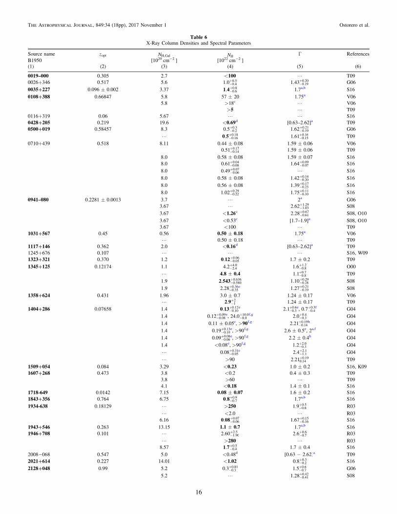
Table 6X-Ray Column Densities and Spectral Parameters

Source name zopt NH,Gal NH Γ ReferencesB1950 [1020 cm−2 ] [1022 cm−2 ] (1) (2) (3) (4) (5) (6)

0019–000 0.305 2.7 <100 L T090026+346 0.517 5.6 -

+1.0 0.40.5

-+1.43 0.19

0.20 G06

0035+227 0.096±0.002 3.37 -+1 4. 0.6

0.8 1.7a,b S16

0108+388 0.66847 5.8 57±20 1.75a V06 5.8 >18c L V06 >5 L T090116+319 0.06 5.67 L L S160428+205 0.219 19.6 <0.69d [0.63–2.62]a T090500+019 0.58457 8.3 -

+0.5 0.20.3

-+1.62 0.19

0.21 G06

L -+0 5. 0.16

0.18-+1.61 0.15

0.16 T09

0710+439 0.518 8.11 0.44±0.08 1.59±0.06 V06 -

+0.51 0.140.17 1.59±0.06 T09

8.0 0.58±0.08 1.59±0.07 S16 8.0 -

+0.61 0.080.04

-+1.64 0.07

0.09 S16

8.0 -+0.49 0.06

0.07 L S16

8.0 0.58±0.08 -+1.42 0.20

0.14 S16

8.0 0.56±0.08 -+1.39 0.23

0.17 S16

8.0 -+1.02 0.22

0.29-+1.75 0.10

0.11 S16

0941–080 0.2281±0.0013 3.7 L 2a G06 3.67 L -

+2.62 1.031.29 S08

3.67 <1.26c-+2.28 0.61

0.67 S08, O10

3.67 <0.53c [1.7–1.9]a S08, O10 3.67 <100 L T091031+567 0.45 0.56 0.50 0.18 1.75a V06 L 0.50±0.18 L T091117+146 0.362 2.0 <0.16d [0.63–2.62]a T091245+676 0.107 L L L S16, W091323+321 0.370 1.2 -

+0 12. 0.050.06 1.7±0.2 T09

1345+125 0.12174 1.1 -+4.2 2.4

4.0-+1.6 0.8

1.2 O00

L 4.8 0.4 -+1.1 0.8

0.7 T09

1.9 -+2 543. 0.580

0.636-+1.10 0.28

0.29 S08

1.9 -+2.28 0.35

0.36e-+1.27 0.19

0.21 S08

1358+624 0.431 1.96 3.0±0.7 1.24±0.17 V06 L -

+2 9. 12 1.24±0.17 T09

1404+286 0.07658 1.4 -+0 13. 0.10

0.12e-+2.1 0.3

0.6e, -+0.7 0.4

0.3f G04

1.4 -+0.12 0.08

0.09e, -+24.0 8.0

10.0f,g-+2.0 0.3

0.4 G04

1.4 0.11±0.05e, >90f,g-+2.21 0.14

0.19h G04

1.4 -+0.19 0.10

0.13e, >90f,g 2.6±0.5e, 2a,f G04

1.4 -+0.09 0.06

0.08e, >90f,g 2.2±0.4h G04

1.4 <0.08e, >90f,g-+1.2 0.3

2.0 G04

L -+0.08 0.05

0.31e-+2.4 1.1

2.1 G04

L >90 +2.210.140.19 T09

1509+054 0.084 3.29 <0.23 1.0±0.2 S16, K091607+268 0.473 3.8 <0.2 0.4±0.3 T09 3.8 >60 L T09 4.1 <0.18 1.4±0.1 S161718-649 0.0142 7.15 0.08 0.07 1.6±0.2 S161843+356 0.764 6.75 -

+0 8. 0.70.9 1.7a,b S16

1934-638 0.18129 L >250 -+1.9 0.6

0.5 R03

L <2.0 L R03 6.16 -

+0 08. 0.060.07

-+1.67 0.16

0.15 S16

1943+546 0.263 13.15 1.1 0.7 1.7a,b S161946+708 0.101 L -

+2.60 1.902.5

-+2.6 0.7

0.6 R03

L >280 L R03 8.57 -

+1 7. 0.40.5 1.7±0.4 S16

2008−068 0.547 5.0 <0.48d -[ ]0.63 2.62 a T092021+614 0.227 14.01 <1.02 -

+0.8 0.20.3 S16

2128+048 0.99 5.2 -+0.3 0.3

0.81-+1.5 0.7

0.6 G06

5.2 L -+1.28 0.41

0.42 S08

16

The Astrophysical Journal, 849:34 (18pp), 2017 November 1 Ostorero et al.

apply to the source, we always took into account also the NHlower limit ( N 10H

24 cm−2) derived in the framework of thisscenario. The latter case applied to a subsample of threesources. Finally, when a lower limit to NH was derived in aCompton-thin scenario,17 we could not state whether the sourcewas Compton-thin or Compton-thick; we thus considered bothscenarios to be plausible, as in the previous case. In theCompton-thin scenario, we associated with the source an NHvalue equal to the mean of the 3σ lower limit and the physicalupper bound of the Compton-thin NH range (i.e., N 10H

24

cm−2). We considered the NH range as a s3 interval, andthus associated with the mean NH the corresponding 1σuncertainty. Overall, the ambiguity between a Compton-thinand a Compton-thick absorber (and between the correspondingvalues of NH) affected a subsample of four sources of thecorrelation sample.

ORCID iDs

Luisa Ostorero https://orcid.org/0000-0003-3983-5980Raffaella Morganti https://orcid.org/0000-0002-9482-6844Antonaldo Diaferio https://orcid.org/0000-0002-4986-063XŁukasz Stawarz https://orcid.org/0000-0001-8294-9479Rafal Moderski https://orcid.org/0000-0002-8663-3882Alvaro Labiano https://orcid.org/0000-0002-2842-9971

References

Akritas, M. G., Murphy, S. A., & LaValley, M. P. 1995, JASA, 90, 170Alexander, P. 2000, MNRAS, 319, 8Allison, J. R., Curran, S. J., Emonts, B. H. C., et al. 2012, MNRAS, 423, 2601Antonucci, R. 1993, ARA&A, 31, 473Araya, E. D., Rodríguez, C., Pihlström, Y., et al. 2010, AJ, 139, 17Augusto, P., Gonzalez-Serrano, J. I., Perez-Fournon, I., & Wilkinson, P. N.

2006, MNRAS, 368, 1411Bahcall, J. N., & Ekers, R. D. 1969, ApJ, 157, 1055Bondi, M., Marchã, M. J. M., Polatidis, A., et al. 2004, MNRAS, 352, 112Carilli, C. L., Menten, K. M., Reid, M. J., Rupen, M. P., & Yun, M. S. 1998,

ApJ, 494, 175

Chandola, Y., Sirothia, S. K., & Saikia, D. J. 2011, MNRAS, 418, 1787Chiaberge, M., Capetti, A., & Celotti, A. 1999, A&A, 349, 77Chiaberge, M., Capetti, A., & Celotti, A. 2000, A&A, 355, 873Conway, J. 1997, in Gigahertz Peaked Spectrum and Compact Steep Spectrum

Radio Sources, ed. I. A. G. Snellen (Leiden: Leiden Observatory), 198Conway, J. E. 1999, NewAR, 43, 509Curran, S. J., Allison, J. R., Glowacki, M., Whiting, M. T., & Sadler, E. M.

2013, MNRAS, 431, 3408Curran, S. J., & Whiting, M. T. 2010, ApJ, 712, 303Curran, S. J., Whiting, M. T., Wiklind, T., et al. 2008, MNRAS, 391, 765Czerny, B., Siemiginowska, A., Janiuk, A., Nikiel-Wroczyński, B., &

Stawarz, Ł. 2009, ApJ, 698, 840Dallacasa, D., Bondi, M., Alef, W., & Mantovani, F. 1998, A&AS, 129, 219de Vries, W. H., Barthel, P. D., & O’Dea, C. P. 1997, A&A, 321, 105de Vries, W. H., O’Dea, C. P., Barthel, P. D., & Thompson, D. J. 2000, A&AS,

143, 181Donato, D., Sambruna, R. M., & Gliozzi, M. 2004, ApJ, 617, 915Dunlop, J. S., Peacock, J. A., Savage, A., et al. 1989, MNRAS, 238, 1171Emonts, B. H. C., Burnett, C., Morganti, R., & Struve, C. 2012, MNRAS,

421, 1421Fanti, C., Fanti, R., Dallacasa, D., et al. 1995, A&A, 302, 317Feigelson, E. D., & Babu, G. J. 2012, Modern Statistical Methods for

Astronomy (Cambridge: Cambridge Univ. Press)Gallimore, J. F., Baum, S. A., O’Dea, C. P., Pedlar, A., & Brinks, E. 1999,

ApJ, 524, 684Geréb, K., Maccagni, F. M., Morganti, R., & Oosterloo, T. A. 2015, A&A,

575, A44Geréb, K., Morganti, R., & Oosterloo, T. A. 2014, A&A, 569, A35Glowacki, M., Allison, J. R., Sadler, E. M., et al. 2017, MNRAS, 467, 2766Gruberbauer, M., Kallinger, T., Weiss, W. W., & Guenther, D. B. 2009, A&A,

506, 1043Guainazzi, M., Siemiginowska, A., Rodriguez-Pascual, P., & Stanghellini, C.

2004, A&A, 421, 461Guainazzi, M., Siemiginowska, A., Stanghellini, C., et al. 2006, A&A, 446, 87Gupta, N., Salter, C. J., Saikia, D. J., Ghosh, T., & Jeyakumar, S. 2006,

MNRAS, 373, 972Heinz, S., Reynolds, C. S., & Begelman, M. C. 1998, ApJ, 501, 126Holt, J., Tadhunter, C., Morganti, R., et al. 2006, MNRAS, 370, 1633Isobe, T., Feigelson, E. D., & Nelson, P. I. 1986, ApJ, 306, 490Jaffe, W., Meisenheimer, K., Röttgering, H. J. A., et al. 2004, Natur, 429, 47Kelly, B. C. 2007, ApJ, 665, 1489Krolik, J. H., & Begelman, M. C. 1988, ApJ, 329, 702Kuraszkiewicz, J., Wilkes, B. J., Schmidt, G., et al. 2009, ApJ, 692, 1143LaValley, M. P., Isobe, T., & Feigelson, E. D. 1992, BAAS, 24, 839Liszt, H. 2001, A&A, 371, 698Maccagni, F. M., Morganti, R., Oosterloo, T. A., & Mahony, E. K. 2014,

A&A, 571, A67

Table 6(Continued)

Source name zopt NH,Gal NH Γ ReferencesB1950 [1020 cm−2 ] [1022 cm−2 ] (1) (2) (3) (4) (5) (6)

5.2 <1.56 -+1.44 0.70

0.89 S08, O10

5.0 <1.9 -+1.98 0.4

0.5 T09

2352+495 0.2379 12.4 0.66±0.27 1.75a V06 L -

+4 37

-+1.8 0.9

1.6 T09

Notes. The values of NH in boldface fonts are those used for the correlation analysis in Section 5.a Fixed.b By varying Γ in the range [1.4–2.0], the authors get NH values consistent, to within 1σ, with the NH value given in this Table.c s3 (upper or lower) limit.d Upper bound of the 1.6σ interval [NHmin, NHmax] about the curve corresponding to the nominal hardness ratio, when Γ is constrained to the given range.e Soft X-rays.f Hard X-rays.g > ´N 9 10H

hard 23 cm−2 is associated with a Compton-reflection model for the hard X-rays.h Intrinsic, for the Compton-reflection model.References.G04: Guainazzi et al. (2004); G06: Guainazzi et al. (2006); K09: Kuraszkiewicz et al. (2009); O00: O’Dea et al. (2000); O10: Ostorero et al. (2010); R03:Risaliti et al. (2003); S08: Siemiginowska et al. (2008); S16: Siemiginowska et al. (2016); T09: Tengstrand et al. (2009); V06: Vink et al. (2006);W09: Watsonet al. (2009).

17 This case applies to one source only, i.e., 0108+388.

17

The Astrophysical Journal, 849:34 (18pp), 2017 November 1 Ostorero et al.

Maloney, P. R., Hollenbach, D. J., & Tielens, A. G. G. M. 1996, ApJ, 466561

Marcha, M. J. M., Browne, I. W. A., Impey, C. D., & Smith, P. S. 1996,MNRAS, 281, 425

Migliori, G., Siemiginowska, A., Sobolewska, M., et al. 2016, ApJL, 821, L31Mirabel, I. F. 1989, ApJL, 340, L13Morganti, R., Fogasy, J., Paragi, Z., Oosterloo, T., & Orienti, M. 2013, Sci,

341, 1082Morganti, R., Oosterloo, T., Struve, C., & Saripalli, L. 2008, A&A, 485, L5Morganti, R., Oosterloo, T. A., Tadhunter, C. N., et al. 2001, MNRAS,

323, 331Morganti, R., Oosterloo, T. A., Tadhunter, C. N., et al. 2004, A&A, 424, 119Morganti, R., Tadhunter, C. N., Oosterloo, T. A., et al. 2003, PASA, 20, 129Nagai, H., Inoue, M., Asada, K., Kameno, S., & Doi, A. 2006, ApJ, 648, 148Nenkova, M., Sirocky, M. M., Nikutta, R., Ivezić, Ž, & Elitzur, M. 2008, ApJ,

685, 160O’Dea, C. P., Baum, S. A., & Gallimore, J. F. 1994, ApJ, 436, 669O’Dea, C. P., De Vries, W. H., Worrall, D. M., Baum, S. A., & Koekemoer, A.

2000, AJ, 119, 478Orienti, M., Morganti, R., & Dallacasa, D. 2006, A&A, 457, 531Stawarz, Ł., Ostorero, L., Begelman, M. C., et al. 2008, ApJ, 680, 911Ostorero, L., Moderski, R., Stawarz, Ł., et al. 2009, AN, 330, 275Ostorero, L., Moderski, R., Stawarz, Ł., et al. 2010, ApJ, 715, 1071Ostorero, L., Morganti, R., Diaferio, A., et al. 2016, AN, 337, 148Pearson, T. J., & Readhead, A. C. S. 1988, ApJ, 328, 114Peck, A. B., & Taylor, G. B. 2001, ApJL, 554, L147Peck, A. B., Taylor, G. B., & Conway, J. E. 1999, ApJ, 521, 103Perlman, E. S., Stocke, J. T., Carilli, C. L., et al. 2002, AJ, 124, 2401Perucho, M. 2016, AN, 337, 18Pihlström, Y. M., Conway, J. E., & Vermeulen, R. C. 2003, A&A, 404, 871Polatidis, A. G., & Conway, J. E. 2003, PASA, 20, 69Raban, D., Jaffe, W., Röttgering, H., Meisenheimer, K., & Tristram, K. R. W.

2009, MNRAS, 394, 1325Readhead, A. C. S., Taylor, G. B., Pearson, T. J., & Wilkinson, P. N. 1996,

ApJ, 460, 634Reynolds, C. S., & Begelman, M. C. 1997, ApJL, 487, L135Ride, S. K., & Walker, A. B. C., Jr. 1977, A&A, 61, 339

Risaliti, G., Elvis, M., Bianchi, S., & Matt, G. 2010, MNRAS, 406, L20Risaliti, G., Elvis, M., Fabbiano, G., et al. 2007, ApJL, 659, L111Risaliti, G., Nardini, E., Salvati, M., et al. 2011, MNRAS, 410, 1027Risaliti, G., Woltjer, L., & Salvati, M. 2003, A&A, 401, 895Saikia, D. J., Gupta, N., & Konar, C. 2007, MNRAS, 375, L31Sambruna, R. M., Eracleous, M., & Mushotzky, R. F. 1999, ApJ, 526, 60Sault, R. J., Teuben, P. J., & Wright, M. C. H. 1995, in ASP Conf. Ser. 77,

Astronomical Data Analysis Software and Systems IV, ed. R. A. Shaw,H. E. Payne, & J. J. E. Hayes (San Francisco, CA: ASP), 433

Siemiginowska, A. 2009, AN, 330, 264Siemiginowska, A., LaMassa, S., Aldcroft, T. L., Bechtold, J., & Elvis, M.

2008, ApJ, 684, 811Siemiginowska, A., Sobolewska, M., Migliori, G., et al. 2016, ApJ, 823, 57Snellen, I. A. G., Schilizzi, R. T., de Bruyn, A. G., et al. 1998, A&AS, 131, 435Snellen, I. A. G., Schilizzi, R. T., Miley, G. K., et al. 2000, MNRAS, 319, 445Stanghellini, C., Dallacasa, D., O’Dea, C. P., et al. 2001, A&A, 377, 377Stanghellini, C., O’Dea, C. P., Baum, S. A., et al. 1997, A&A, 325, 943Stanghellini, C., O’Dea, C. P., Dallacasa, D., et al. 1998, A&AS, 131, 303Stanghellini, C., O’Dea, C. P., & Murphy, D. W. 1999, A&AS, 134, 309Struve, C., & Conway, J. E. 2010, A&A, 513, A10Tadhunter, C. 2008, NewAR, 52, 227Taylor, G. B., Readhead, A. C. S., & Pearson, T. J. 1996, ApJ, 463, 95Tengstrand, O., Guainazzi, M., Siemiginowska, A., et al. 2009, A&A, 501, 89Tingay, S. J., Jauncey, D. L., Reynolds, J. E., et al. 1997, AJ, 113, 2025Torniainen, I., Tornikoski, M., Lähteenmäki, A., et al. 2007, A&A, 469, 451Tristram, K. R. W., Burtscher, L., Jaffe, W., et al. 2014, A&A, 563, A82Tristram, K. R. W., Raban, D., Meisenheimer, K., et al. 2009, A&A, 502, 67Urry, C. M., & Padovani, P. 1995, PASP, 107, 803van Gorkom, J. H., Knapp, G. R., Ekers, R. D., et al. 1989, AJ, 97, 708Vermeulen, R. C., Pihlström, Y. M., Tschager, W., et al. 2003, A&A, 404, 861Véron-Cetty, M.-P., Woltjer, L., Staveley-Smith, L., & Ekers, R. D. 2000,

A&A, 362, 426Vink, J., Snellen, I., Mack, K.-H., & Schilizzi, R. 2006, MNRAS, 367, 928Wagner, A. Y., Bicknell, G. V., & Umemura, M. 2012, ApJ, 757, 136Watson, M. G., Schröder, A. C., Fyfe, D., et al. 2009, A&A, 493, 339Wilms, J., Allen, A., & McCray, R. 2000, ApJ, 542, 914Wolfe, A. M., & Burbidge, G. R. 1975, ApJ, 200, 548

18

The Astrophysical Journal, 849:34 (18pp), 2017 November 1 Ostorero et al.