Report No.: FAA-RD-74-125, 11-1

CORE ENGINE NOISE CONTROL PROGRAM

Volume I i, Supplement I - IDENTIFICATION OF NOISE GENERATION and SUPPRESSION MECHANISMS

FAA WJH Technical Center

111I1111I1111II11~~~lU~~{/1111111111111I1 R. K. Matta P. R. Mingier

AIRCRAFT ENGINE GROUP GENERAL ELECTR IC COMPANY

CINCINNATI, OHIO 45215

. ' ~'EC UBRAVV;~ .

SEP2R'16 . .

July, 1976

FINAL REPORT

Document is avai lable to the public through the National Technical Information Service,

Springfield, Virginia 22151

Prepared for

u.s. DEPARTMENT OF TRANSPORTATION FEDERAL AVIATION ADMWISTRATION

Systenls Research & Development Service Washington, D.C. 20590

..

NOTICE

This document is disseminated under the sponsorship of the Department of Transporation in the interest of information exchange. The United States Government assumes no liability for its contents or use thereof.

•

•

1. Report No. 3. Recipient's Catalog No. ,I FAA-RD-74-l25,II-I

2. Government Accession No.

4. Title and Subtitle 5. Report Date July 1976Core Engine Noise Control Program

Volume II Supplement I - Identification of Noise Generation and 6. Performing Organization Code Suppression Mechanisms R76AEG341

7. Author(s) 8. Performing Organization Report No.

R.K. Matta (Ed.) , S.B. Kazin (Prog. Tech. Dir. ), P.R. Mingler,­

10. Work Unit No. 9. Performing Organization Name and Address 36310

General Electric Company 11. Contract or Grant No.Advanced Engineering and Technology Programs Department

Aircraft Engine Group DOT-FA72WA-3023 Evendale, Ohio 45215

13. Type of Report and Period Covered 12. Sponsoring Agency Name and Address Final - Jan.- July 1975

U.S. Department of Transportation 14. Sponsoring Agency CodeFederal Aviation Administration

Systems Research and Development Service / Washington,D.C. 20590

15. Supplementary Notes

Volume I - Identification of Component Noise Sources., FAA-RD-74-l25, I Volume II - Identification of Noise Generation and Suppression Mechanisms, FAA-RD-74-125, II Volume III and Volume III Supplement I - Prediction Methods, FAA-RD-74-125, III and III-I

16. Abstract

The work reported herein is supplemental to the earlier investigations of the mechanisms of core engine noise generation and suppression which are reported in FAA-RD-74-125, III. The prediction models of Volume III were updated based on this effort.

TURBINE NOISE - Two source noise reduction mechanisms, blade row spacing, and vane lean, were exercised analytically to define the acoustic benefits associated with varying these parameters. It is shown how multi-stage turbines can be optimized through appropriate distribution of spacing between the blade pairs. The vane lean results indicate that very large reduction can be obtained in the acoustic energy associated with the dominant radial mode.

LOW FREQUENCY CORE NOISE - Three compact suppressor configurations were designed and tested in a hot flow, rectangular duct facility. Two of these (stacked and acoustic rectifier treatments) are recommended as engine compatible suppressors for low frequency core noise. The third con­figuration, side-branch resonator, yielded poor suppression results.

TURBINE TONE/JET STREAM INTERACTION - The turbulence scattering analysis defined earlier (Volume II) was exercised in a parametric study after using experimental data to model the shear layer turbulence. The scattered energy exhibits a strong dependence on the fan jet velocity, incident tone freq uency, and the distance between the fan and core exhaust planes.

17. Key Words (Suggested by Author(s))

Core Engine Noise, Turbofan Engine Noise, Jet Engine Noise Control, Combustor Noise, Core Noise, Turbine Noise, Tone/Jet Stream Interaction

18. Distribution Statement

Document is available to the public through the National Technical Information Service, Springfield, Virginia 22151

22. Price19. Security Classif. (of this report) 20. Security Classif. lof this page) 21. No. of P~ges

154Unclassified Unclassified

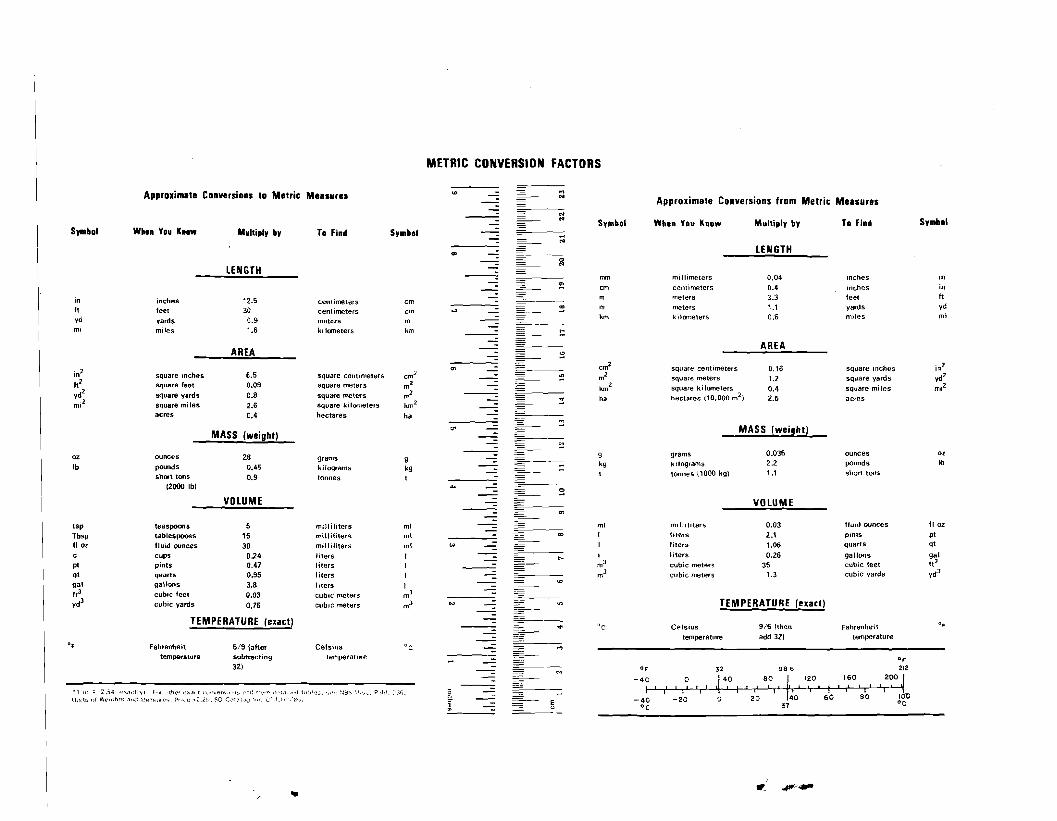
METRIC CONVERSION FACTORS

Approximate Conversions to Metric Measures '" =---­ ~ Approximate Conversions from Metric Measures

Symbol When Vou Know Multiply by To Find Symbol --

~ ~

Symbol When Vou Know Multiply by To Find Symbol

-- ­-

N ~~-

~

LENGTH

LENGTH ;: - mm millImeters 0.04 inches on

~ em centimeters 0.4 inches in

in

ft yd

inches

feet yards

--2.5

30 0.9

centimeters

centimeters meters

em

em m

-1

...

_

------;

-- ­ -_

m m

km

meters meters

ki10meters

3.3 1.1

0.6

feet yards

miles

ft yd

mi

rnl mi las 1.6 ki lometers km ~

AREA - == ::l AREA

in 2

tt 2

yd 2

ml2

square inches square feet

square yards square mi les

acres

6.5 0.09 C.8 2.6

0.4

square centimeters square meters

square ~ters square kilometers

hectares

cm 2

m 2

m 2

2 km

ha

C7\ :

_

_

-

~ __

~ ~ = ~:! == =----M

cm 2

m2

km2

ha

square centimeters square meters square kilometers hectares (10.000 m2)

0.16 1.2 0.4 2.5

square Inches square y~rds square miles acres

in2

~~ ml

MASS (weight)-- ­'" -

'" MASS (weight)

oz

Ib ounces

poun~1s shCl't tons

28 0.45 0.9

g~ams kilograms tannes

9 kg t

-_

-

... ~-----::; == -

9 kg

t

grams kilograms

lannes \1000 kg)

0.036 2.2

1.1

ounces pounds

short tons

Ol Ib

12000 Ib} ~ C>

VDLUME - ~ VOLUME

tsp Tbsp.Iol

teaspoons tablespoonsfluid ounces

5 15 30

. ..m~II~I~ters m~II~I~terr; milliliters

ml mt ml W

-

_

_

= _

en

00 ml (

I

milliliters liters liters

0.03 2.1 1.06

fluid ounces pints quarts

11 oz pt qt

I

t :1

cups pints qltarts

0.24 0.47 0.95

liters liters liters

I I I _ -

r-­ I m3

m3

liters cUb~c meters cubiC meters

0.26 35 1.3

gall.Ofls cubIC feet cubiC yards

g~

ft 3 yd

gal

1t 3

vd3

9a"005

cUb~c leet cubiC yards

3.8

0.03 0.76

liters

cub,c ",eters cubiC meters

I

m~ m

.., -

-

- '" TEMPERATURE (exact)

TEMPERATURE (exact) - -----.; "c Celsius 9/5lthen Fah,enheit 0,

Of fahrenheit 5/9 tafter Cels)us temperature subtracting tel'1lperature

32)

:,:,;: ,:, ~~~~h;~';;:,;j'~:~L::e ..t!,;:.~~·:~;:;·.~e~,~;;~,::~".::"Z.'\":~'.~:~:"af"'.' ,.. ,"" ,', p ,'"

°c

"".

_

!

_

-

-

M

=---------;; =-­

~~

OF'

-40I _:g

' I

I

temperature

32

0 140 ! , I I I ! I

_ 2'0 '0

add 32) temperature

or

98.6 212

80 -1 120 160 200 I I 1 I ! ! I , ! I ' , ! , ! ! ,

2'0 '31~0 ' 60 i a~ , J~O

.. , ..~

PREFACE

This report describes the work performed under the DOT/FAA Core Engine Noise Control Program (Contract DOT-FA72WA...3023). The original work under this contract is in Report Number FAA-RD-74-l25, Volumes I,ll, and III.

Supplements to Volumes II and III report additional work undertaken under this program after completion of the work reported in the original three volumes.

The objectives of the program were: -• Identification of component noise sources of core engine noise

(Phase I).

• Identification of mechanisms associated with core engine noise generation and noise reduction (Phases II and III).

• Development of techniques for predicting core engine noise in advanced systems for future technology aircraft (Phase IV).

• Extension of the core noise prediction (Phase V).

• Update of the core engine noise control effort (Phase VI).

The objectives were accomplished in six phases as follows:

Phase I - Analysis of engine and component acoustic data• to identify potential sources of core engine noise and classification of the sources into major and minor categories.

Phase II - Identification of the noise generating mechanism associated with each source through a balanced program of:

Analytical studies

Component and model tests

Acoustic evaluation of data from existing and advanced engine systems.

o Phase III . - Identification of noise reduction mechanisms for each source through a program with elements similar to Phase II.

CI Phase IV - Development of improved prediction techniques incorporating the results obtained during the preceding two phases.

Iii

Phase V Analysis of low frequency noise transmission through turbine blade rows and addition of engine and component data to the prediction method for core noise.

Phase VI - Analytical studies of turbine source noise sup­• ,pression and parametric trends in turbine tone/ jet stream interaction; an experimental study of compact low frequency noise suppressors and a prediction model update.

The work accomplished is reported in five volumes corresponding respec­tively to the five objectives stated above.

o Volume I - Identification of Component Noise Sources (FAA-RD-74-l25, I).

Volume II - Identification of Noise Generation and Suppression• Mechanisms (FAA-RD-74-l25, II).

Volume III - Prediction Methods (FAA-RD-125, III).• Volume III• Supplement I - Extension of Prediction Methods. (FAA-RD-74-l25, III-I)

Volume II• Supplement I - Extension to Identification of Noise Generation and

Suppression Mechanisms. (FAA-RD-74-l25, II-I)

A visual representation of the overall program and report organization is shown on pages v and vi.

This volume documents the results of the Phase VI activity which extended the initial core engine noise control work through:

1) Analytical studies of turbine noise reduction at the source through blade row spacing and through vane lean

,•2) Design and testing of three compact suppressors for low frequency noise attenuation.

•3) A parametric study on turbine tone modulation by coannular jet flows.

\ \ iv

\ \

,

"

CORE ENGINE NOISE CONTROL PROGRAM OVERALL REPORT ORGANIZATION

Contract Phase

Phase I

Phase II and

Phase II I

Phase IV

Volume I

Volume II

Volume III

Contract Documentation

Identification of Component Noise Sources FAA-RD-74-125,I

Definition of Mechanisms of Noise Generation

Definition of Mechanisms of Noise Reduction

FAA-RD-74-125 ,II

Development of Prediction Techniques FAA-RD-74-125,III

v

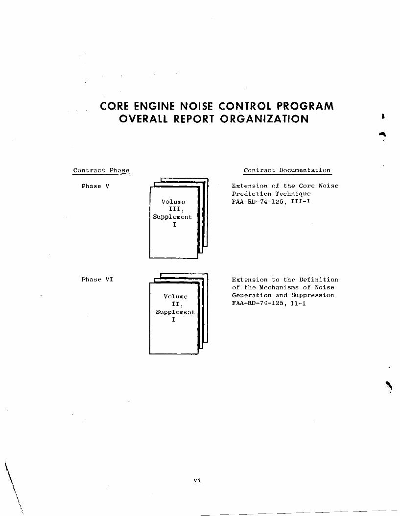
1 CORE ENGINE NOISE CONTROL PROGRAM

OVERALL REPORT ORGANIZATION

Contract Phase

Phase V

Phase VI

Volume III,

Supplement I

Volume II,

Supplement I

Contract Documentation

Extension of the Core Noise Prediction Technique FAA-RD-74-125, 111-1

Extension to the Definition of the Mechanisms of Noise Generation and Suppression FAA-RD-74-125, 11-1

,•

\vi

\,

The work reperted in this Volume is supplemental to the efforts of Phases 2 and 3: Identification of Mechanisms of Noise Generation and Suppression. Three cere engine neise sources were investigated: Turbine Noise, Low Frequency Core Noise, and Turhine Tone/Jet Stream Interaction.

Turbine Noise - Two source noise reduction mechanisms, blade row spacing and vane lean, were studied analytically to determine the relative acoustic - benefit associated with varying these geometric parameters.

The spacing study shows how to allocate any given amount of spacing between the various blade pairs in a multi-stage turbine to achieve optimum noise reduction. The allocation follows from consideration of the noise generation by each set of interactions.

Spacing results in noise reduction due to the decay of the viscous wake. Vane leaning results in noise reduction by phasing the wake interaction across the blade span. The results of this study show that the benefits are optimized by curved vanes, providing over 20 dB attenuation for the dominant first radial mode. These curved vanes, which are radial at the hub, also avoid secondary flow problems which would be associated with the acute angles that follow from strai~ht leaned vanes.

The prediction program for viscous wake interaction noise used in these source noise studies is provided in the appendices.

Low Frequency Core Noise Suppression - Three compact suppressor con­figurations compatible with aircraft engine installations were designed and tested in a hot flow, rectangular duct facility. The three configurations were stacked treatment, acoustic rectifier, and side-branch resonator. Design details and geometric definitions of each suppressor configuration are presented. The te~t results are shown and discussed for temperatures of 590 0 K and 720· K at Mach numbers of 0.2, 0.3, and 0.4.

The stacked treatment and the acoustic rectifier configurations are recommenced as engine compatible suppressors having the ability to achieve 10 dB suppression over a resonable frequency range below 2000 Hz. The side-.ranch resonator is not recommended due to poor suppression test results.

Turbine Tone/Jet Stream Interaction - The outer shear layer of a coannular flow configuration was modeled using engine and model data, and the scaling laws for interaction were established. The turbulence scattering analysis defined in Volume II was exercised in a parametric study. The energy in the scattered wave (haystack) exhibits a strong dependence on the

vii

tone frequency, fan velocity and the relative distance between the fan and core nozzle exhaust planes; increasing with all three. The fan velocity and the distance between the exhaust planes together serve to define the quality and quantity of the turbulence in the shear layer. At the same time, the influence of velocity ratio and area ratio appears to be minimal. ,

The results are in good agreement with the empirical prediction formulated using engine data in Volume III. This method is updated by formal inclusion of the frequency term as a prediction parameter in addition to the fan jet velocity and the relative distance between nozzle planes.

viii

Section

1.0

2.0-

3.0

4.0

~.

TABLE OF CONTENTS

PREFACE

SUMMARY

INTRODUCTION 1

TURBINE SOURCE NOISE REDUCTION 3 2.1 Turbine Discrete Frequency Noise 3 2.2 Spacing 3 2.3 Leaned Vanes 13 2.4 Discussion 27 2.5 Conclusions 31 2.6 Prediction Method Update 32

COMPACT SUPPRESSORS FOR LOW FREQUENCY NOISE 33 3.1 Background 33 3.2 Suppressor Concepts 33 3.3 Experimental Procedure 38 3.4 Test Results 51 3.5 Discussion 61 3.6 Conclusions and Recommendations 61 3.7 Prediction Method Update 62

TURBINE TONE/JET STREAM INTERACTION 64 4.1 Background and Objectives 64 4.2 Parametric Study 66 4.3 Discussion 74 4.4 Conclusions 80 4.5 Prediction Method Update 82

APPENDICES/PROGRAM LISTINGS

A. Analytical Turbine Tone Prediction 87 B. Interaction Effects 133

ix

NOMENCLATURE

A area, total resonator lwck nre:l

A nm

A 0

AR

II a

r

B

coefficients for acoustic pressure associated with duct modes

incident wave amplitude

exhaust nozzle area ratio, fan/core

unit vector in direction of observer

number of blades in rotor

•

BPF blade passing frequency

BPR bypass ratio, fan/core

b shear layer thickness

c acoustic velocity

D diameter

dB decibel

"1t F force induced by viscous wake interaction

f frequency

f c

f 0

G m

Hz

h

I

correlation frequency

incident tone or resonance frequency

coefficient of unsteady upwash

Hertz, cycles/sec

radius ratio, hub/tip

acoustic intensity

,. IGV inlet guide vane

i

J ( n

K ( n

)

)

Bessel function of 1st kind and nth order

modified Bessel function of nth order

x

k

kHz

k c

-L

Q, c

M

m

N

n

n'

OAPWL

OASPL

OGV

PWL

p

R

R a

NOMENCLATURE (continued)

integer index (Section 2)

kilo-Hertz

correlation wave number, w Ic c

wave number of incident wave, w Ic o

(n2w2 _ 1.. 2 )1/ 2 nm

distance between fan and core nozzle planes

resonator transmission loss

blade chord

eddy size

number of rotating line vortices

jet stream Mach number

duct Mach number

turbulence Mach number

slope

rotational speed, rpm

circumferential mode number (Section 2); number of openings in treatment (Section 3)

harmonic

overall power level

overall sound pressure level

outlet guide vane

acoustic power level

acoustic pressure

flow resistance of resonator neck

tip radius

xi

R nm

r

s

T

T n

t

toO

u

v

VR

v

w

WPS

X/pc

Y ( ) n

y

z

a

NOMENCLATURE (Continued)

cylinder function

radial coordinate

area of main duct

," sound pressure level

axial spacing between blade rows

temperature

BPF from nth stage

time

trailing edge thickness

physical neck length

equivalent neck length

blade speed

number of blades in stationary row (Section 2); volume (Sections 3 and 4)

velocity ratio, fan/core

flow velocity

weight flow rate

worst possible situation-maximizing noise generation

specific reactance component of impedance

Bessel function of 2nd kind and nth order

normal coordinate

axial coordinate

k t c c

physical blade lean. re hub

resonator dimensionless resistance. SR/Apc

air flow angle

xii

NOMENCLATURE (Continued)

resonator dimensionless reactance t Sc/~f V o

dimensionless perturbations in compressibility and density

unsteady circulation due to viscous wake interaction

, difference or increment

~ w-w s o

drop in tone intensity due to turbulence scattering

drop in tone SPL due to "hays tacking"

total wake lean, e + ~ e

ratio of flight velocity to jet velocity

n f If o c

n norm for cylinder functions nm

e angle

e effective aerodynamic lean e

1 (1E..)K compressibility, p ~p

wave length

:\ eigenvaluenm w II -~ - a. - k c r i L\ 2

2 [1 2 0 2 1 (~) ]® angle factor, cos 8exp - 2 ~s~c 2 w c

p density

pc acoustic impedance

b.lade row solidity, pitchchord

time delay

angle

blade geometrical lean, re turbine axis

angular velocity, rad/sec

x.i ii

w

w a

( ) ahs

( ) c

( ) core

( ) fan

( ) reI

t"> TI

( )'

< >

I I

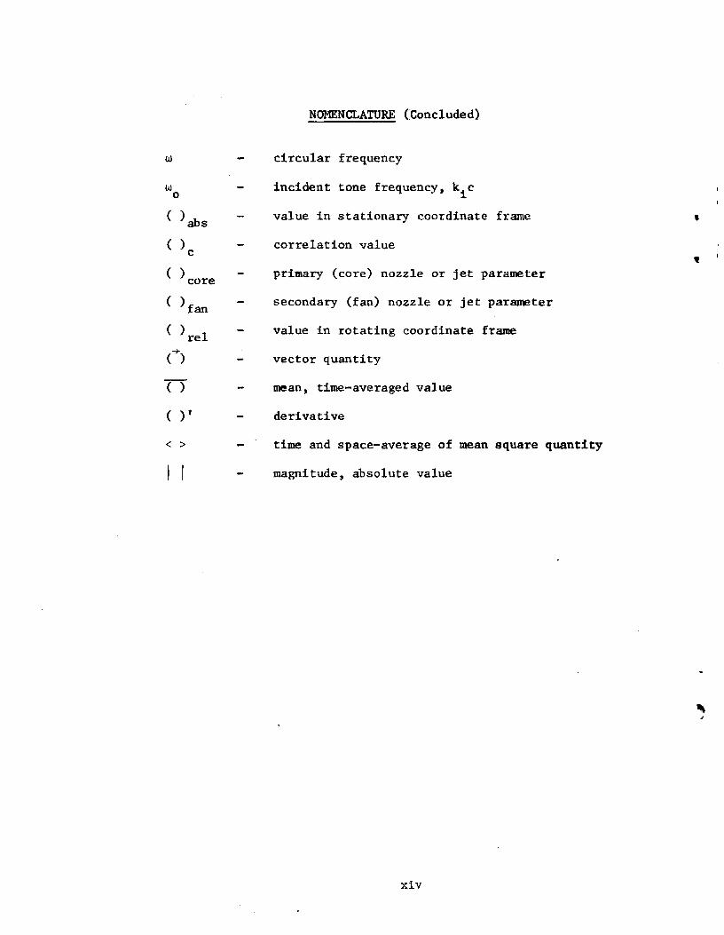
NOMENCLATURE (Concluded)

circular frequency

incident tone frequency, kic

value in stationary coordinate frame , correlation value

primary (core) nozzle or jet parameter

secondary (fan) nozzle or jet parameter

value in rotating coordinate frame

vector quantity

mean, time-averaged value

derivative

time and space-average of mean square quantity

magnitude, absolute value

xiv

SECTION 1.0

INTRODUCTION

The various sources of core engine noise generation were identified and rank ordered in Volume I of the Core Engine Noise Control Program. The major sources were shown to include turbine noise, turbine tone interaction with jet stream turbulence, and low frequency core (combustor) noise. The work reported herein seeks to extend some of the results obtained during the three succeeding phases for these three components.

Turbine Noise - One of the major achievements of the Core Engine Program was the development of an analytic prediction method for turbine tone power (Volume II, Section 4). Not only was the absolute power level accurately predicted, but also the change in level due to increased spacing between the turbine third stage rotor and nozzle. This analysis was also extended to circumferentially leaned turbine nozzles. In effect when a vane is leaned, the angle between the wake of a nozzle or rotor is increased relative to the leading edge of a downstream blade row. The result is a time phased inter­action which reduces the peak pressure pulse leaving the downstream blade.

Leaning and spacing can be used as source noise reduction techniques in turbines to produce noise reduction with a minimized impact on the engine system. This analytic prediction method provided the capability to conduct parametric studies which were used in this supplemental study to obtain design trade-off comparisons of the relative acoustic benefits associated with vary­ing these geometric parameters.

~ombllstor Noise - The combustor noise tests of Phase 3 (Volume II, Sec­tion 3) included successful demonstration of a low frequency suppressor con­figuration. The configuration, howev~r, was not compatible with an actual aircraft engine installation due to its size. Several ideas for potential low frequency suppressor configurations were identified which offer promise of being compatible with an actual installation. These configurations were tested in an existing rectangular duct facility which is capable of using heated flow to represent temperature conditions existing in the core nozzle. This effort established the configuration of a viable core noise suppressor and provided for the expansion of the range of acoustic treatment design parameters which will result in significant core noise suppression.

Tm::.t.ine '~on_~/.Jet Stream Interaction - An analysis was formulated in Phase 2 {Volume II, Section 5} -todescribe the turbulence scattering phenom­enon which leads to "haystacking" of turbine tones as they propagate through the exhaust jet mixing region(s). The analysis indicated that the pertinent parameters in this interaction would include the tone frequency, the jet velocity, the size of the mixing region, and the quality and quantity of the turbulence in the shear layer. A model of the shear layer and the turbulence encountered permitted an analytical study which isolated the most significant

]

parameters. Also t the study served to validate the empirical prediction method developed in Phase 4 (Volume III), Section 5) and to scope the appli ­cable range of this method.

In each element, the additional effort increased the utility of the results obtained under the initial program effort by exploring factors that were not apparent when the program was originally formulated.

,

2

SECTION 2.0

TURBINE SOURCE NOISE REDUCTION

2.1 TURBINE DISCRETE FREQUENCY NOISE

Viscous wake interaction between adjacent blade rows in the dominant tone generating mechanism in turbines. This mechanism is analytically modeled in Volume II (Section 4) and used to predict the discrete frequency acoustic power level (PWL). A brief description of the prediction method is provided in Volume III (Section 4). A listing of the computer program, the input re­quired and a typical output are shown herein in Appendix A.

This analytical model is useful for turbine source noise reduction studies because it "recognizes" and accounts for variations in the internal aerody­namics and mechanical configuration occurring in the turbine.

The objectives of this effort were to:

• Conduct parametric investigations varying blade row spacing in order to gain insight leading into optimizing configurations in multistage turbines.

• Define the effects of leaned vanes in turbines.

2.2 SPACING

The viability of opened blade row spacing as a noise reduction technique for multi-stage fan turbine~ is r.:ported in Volume II. Section 4. A highly .Loaded, 3-stage, fan turbine (Figllrt' 1, Table 1 was tested using the design spacing between blade rows (the bas~line cunfiguration) and then with add i ­ti,)!ld] spacing inserted i.n the L;~;t t\JCJ stages. Significant noise reduction \~ a~; I' /) t ;] i ned a.1 011 g \v i t h m.l n j rna 1 per f 0 nna nee 1P 5 S.~:O •

A parametric investigation of opened blade row spacing was conducted using the above-mentioned fan turbine. Such a study becomes necessary in a multi-stage turbine not only because the spacing can be split up between stages in different ways, but also because the choice exists of inserting spacing either upstream or downstream of the rotor for each blade passing frequency (BPF) (except, perhaps, that associated with last stage). Wakes from an upstream nozzle row interacting with the rotor, and those from the rotor interacting with a downstream nozzle row both generate the same tone frequency. Hence, two blade pairs, nozzle-rotor (N-R) and rotor-nozzle (R-N), account for the acoustic energy in each BPF (except, of course, that arising [I-om the last stage when there is no outlet guide vane).

INTERACTION BASELINE SPACED !-._~, ", (SIC) t (SjC)t ' I --l.--r~ N2-R2 .83R2~N3 .19

L N3~R3 .32 1 . .. .29 .143

-j--,. .89~ SPACING

KS .,.') ~ I, ~ 'f - . 1 ff!~'.~-~lll.!"~.....L; ---C;I .........' ~ , , .' ,.' f­----" .- ------r ' . 1:~ BLOCI£):~'}:'j~;~'. .iJ---"~·_n./ .,,:-./. ~,,;; ,,~0',,23ftc"o.,

I

F

1 l --: -- ~~,.r.::'" ~)".;3dl·" "I~ ~'.. fJ,

I _ T:1~.m~,,~llIM~ ~~ n' ~- .1

• ! I II ~ \ Nl!. I 'I; , Rl! \ N2 \; Ii' ] IR2~ 1\ \ I N3iI'

~ ~. (~~~. i I IR3 ' ---~)"1r,,i ~..r<-'., l!fi'JC1E!1liilfc '~_ -=--<-T --=-,' '" 61 "'- r...L L ~> ' I~--~ I~_" -Ili'=~ I' ~ ,~~-' \'I' ,". _I~'.'..:..!- . .; c-::'J ,"_~.. ,-< 'WI'fr F' ~~ -:..;;:- -t ~ / ~JTrT k;T ~ I ~'I •• t- ,,?

---L ",,--,-, , r~ -...- " '., -~ : • 'Ii ;= ,_ _ ' " """.1 ~ ..... - ,,,-,-]IF,- ,"''--- '-----/ ~_---_~..' ~ f -:~ -_J·,·-t.1 p

_ :c-~ '" ~: :",,,,,., / " ~. :-:~, ~ ,~---' - '-------.j

~L-=-:;::cii::fL)r~-'~SPACING B=KS

! I~J .._. -... --.c::;:....._ ."7 ~" (-,J..-J l, -'.. U;(

__ _ . _. _ _ .,-c:.====,- ",,' f-,

- .. _.. ,.. ... LlI --._._-,--------­

Figure 1 3-Stage Turbine Showing the Increased Spacing

,I A.*

Table 1. 3-Stage Turbine Rig Basic

Turbine Data at Desi~n

Average Pitch Loading, gJt.~ 1• .5 21:Up

Equivalent Specific Work, E/a 33.0 Btu/lb (76153 J/kg)cr

Equivalent Rotative Speed, N/~ 316ao rpmr

Equivalent Weight Flow, W.re-- E/6 28.0 1b/sec (12.7 kg/sec)cr

Inlet Swirl Angle o degrees

Exit Swirl Angle Without Guide Vanes ~ .5 degrees

Maximum Tip Diameter 28.4 inches (72.1 em)

Number of Stages 3

43.16

t.h/TT 0.0635

N/.-T; 138.98

Design Parameters Stage I Stage Stage 3~

gJlIhPitch Loading, 2.07 1. 76 0.85?i - P

Exit Ax! al Mach No. 0.424 0.459 0.407

Exit Absolute Mach No. 0.593 0.602 0.40~

Exit Swirl Angle (Degr<:!es) 44 40 3

NUnlbe r of Blades 106 102 112

Number of Vanes 64 108 100

Tip Speed (Ft/Sec) 384 418 456

Blade Row Sp-acing (5/1.) .2.17 .258 .298 P

s: .Axial Spad ng Between Blade Rows ~ : Nozzle Chord Length

5

I / Ba'el inc

I~ - ZS

6, 6, I ___-~--~~""---A~~

spaced7 f:::. Measured -

Probe Data

___Predictions

I

135

..-l ~ ..., s:: ~ 125 r-l

"C1s:: :;J ~

t 120 <d ....

CI.l

"C1 M

C") 115 1.0 2.0 3.0 1.0 5.0

3-Stage Turbine

Turbine Pressure Ratio, P r

Figure 2 Noise Generation by the Last Stage of a Low Pressure Turbine

6

This study provides a technique which permits evaluation of multi-stage fan turbines to define optimum placement of any given spacing and the amount of tone noise reduction to be expected.

Up to 7 inches (17.78 em) additional spacing was introduced between each blade pair. The tone power levels at the source were predicted using the com­puter program of Appendix A. ~he predictions shown are for the design point. However, since the exhaust air angles for turbines remain relatively constant over the operating range, the attenuation due to spacing also remains rela­tively constant (Figure 2). The tone PWL's for the three stage turbine rig are shown in Figures 3(a), (b) and (c) as functions of the blade spacing. Figure 3(a) shows that the NIRI viscous wake interaction is almost entirely responsible for energy in the first stage tone. This is due to the large chord of the first stage nozzle blades (spacing/chord ratio for the NIRI interactions are small, Table 2). Turbine tone noise reduction is best accomplished, based on the above, by increasing the spacing between the rotor (RI) and the upstream nozzle (NI).

Suppression of the 2nd stage BPF however, requires spacing to be intro­duced on either side of the rotor, because the two interactions contribute almost equally as is shown in Figure 3(b).

Curves were generated to define the optimum rotor location for any given amount of blade row spacing by moving the rotor from one extreme position to the other between the upstream and downstream nozzles. The results are shown in Figure 6 for the 1st and 2nd stage. Initially, the entire available spacing was inserted downstream of the rotor and the tone PWL was then generally con­trolled by the N-R interaction. Then, with the two nozzle rows fixed, the rotor was moved downstream. This results in a decrease of the N-R noise, but increases in the R-N noise. Since the tone is assumed to be the incoherent sum of the two interactions, an optimum location can be located. There is no R-N interaction for the last stage, and, therefore, no optimum. To illustrate how such a study might be used, assume two inches (5.08 cm) of additional spacing is available for stage 2. The minimum tone PWL for this spacing occurs with the rotor 1.43 inches (3.63 cm) from the upstream nozzle. Since the baseline spacing was 0.33 inches (0.84 cm), this means 1.10 inches (2.79 cm) should be introduced upstream of the rotor and the other 0.90 inches (2.29 cm) downstream.

The locus of the m1n1mums for each spacing was curve-fitted and a small study conducted to determine the optimum spacing distribution between the stages for any given overall turbine length increase. The governing criterion was to obtain the maximum reduction possible in turbine noise for any given spacing. Such a study would normally be done on a PNL basis, but in this case, all three (3) tones fall into the same 1/3 octave band and the total tone PWL is a sufficient indicator.

The attenuation suffered by a tone as it propagates through downstream blade rows must be known before source PWL predictions can be used to define the radiated PWL's. These data \"Ul be generated under contract DOT-FA75WA­J68H which i~ now in progress. However, until then empirical estimates must be used.

7

14 :> I I STAGE 1

I . I~

M ~

130 ..... I 0 .-l

-<1l ~

~

~ 120

iii

5 ~

00 lfJ

~ ...:l:= 110 0..

10nI

ADDED SPACING BETWEEN BLADE ROWS, in.

~ ~<-

TOTAL I

N1R1 ::::::::..-..

I

~ ~ ....... ~

...................

......J =:::::::-

-= =-==. =======---........

I io... ~

I ....................

........-... I ---

.............. ~ I I

...

I !

I

--'--~RN1 2

I

----t__

i

~-:....:

I I

----- ...

I I II

'-f..,..

! I

--.

i I I

o 1 2 3 4 5 6 7

Figure 3 (a) PWL Reduction with Spacing - 1st Stage BPF

'. ,J ~

l. 'l

~

CO "0 1201l) ­

~

~ CO g

\I)

~ 1101I

re

1001 o

140 I

IIi I I

I I

~. t

I I130;:c ''''" i CO') .-l I 0 TOTAL ~~-.-l -Ql NZRZ y~ ""+­~

I I STAGE 2

I

I~~--

~--=-~-~ r- ­ I,rR2N3

---~ r-­___

f~'---r---.. ---­1 I--.. '-I--~ 1-0_-­'-,~

~ --­~

~"'---""' ­

I I I I ! I --i' I I I

i+~~ji .I II I I , I I i

1 z 3 4 5 6 7

ADDED SPACING BETWEEN BLADE ROWS, in.

Figure 3 (b) PWL Reduction with Spacing - 2nd Stage BPF

I I

140

I 130C"'l== i~,...;

I 0,...; ~~TarAL (j) ... ~

CO

r---r--- '---­'C 120I r,q - r----:.. (,)

5 ~

f-' ------r---r--­0 Itf.l

i~ I

I,110~ ~ I

I I !

1 II I

I II1000 1

I

I

2 3 4 5 6 7

ADDED SPACING BETWEEN BLADE ROWS, in.

I STAGE

I

"-­

3

--­I I

Figure 3 (c) PWL Reduction with Spacing - 3rd Stage BPF

.-111 ~

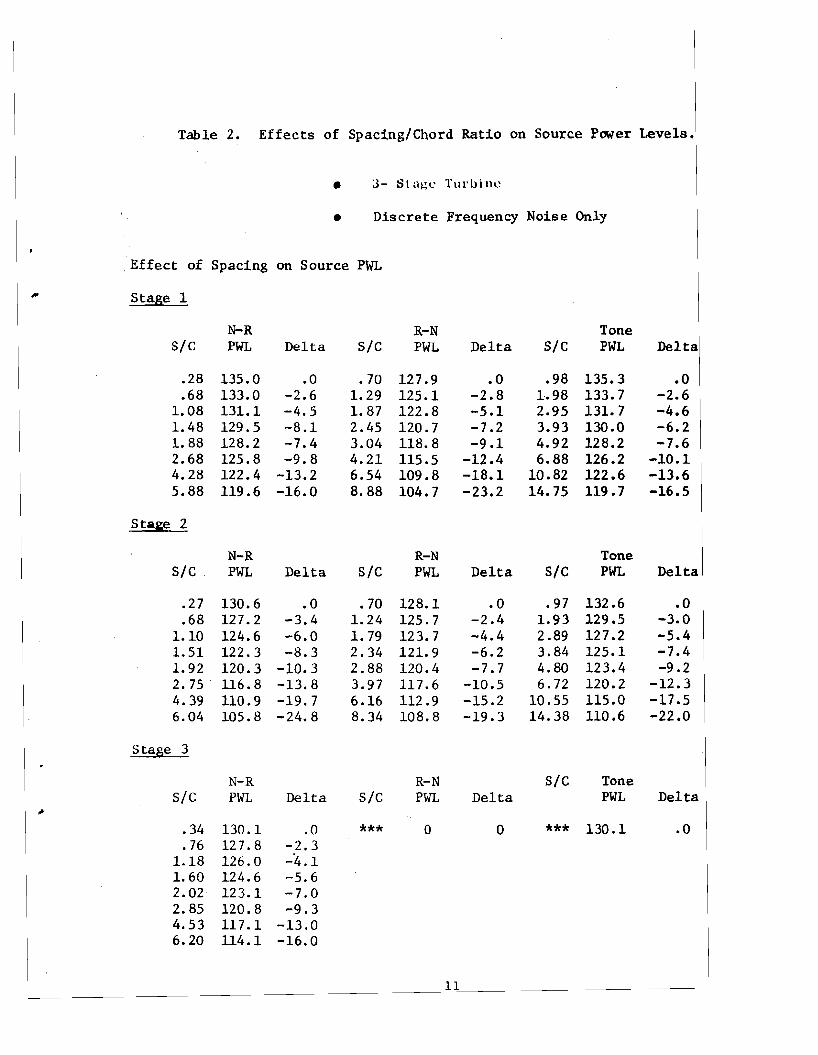
Table 2. Effects of Spacing/Chord Ratio on Source Power Levels.

• 3- Stage Turbine

• Discrete Frequency Noise Only

. Effect of Spacing on Source PWL

Stage 1

sIc N-R PWL Delta SIc

R-N PWL Delta SIc

Tone PWL Delta

.28

.68 1.08 1. 48 1. 88 2.68 4.28 5.88

135.0 133.0 131.1 129.5 128.2 125.8 122.4 119.6

.0 -2.6 -4.5 -8.1 -7.4 -9.8

-13.2 -16.0

.70 1. 29 1. 87 2.45 3.04 4.21 6.54 8.88

127.9 125.1 122.8 120.7 118.8 115.5 109.8 104.7

.0 -2.8 -5.1 -7.2 -9.1

-12.4 -18.1 -23.2

.98 1.98 2.95 3.93 4.92 6.88

10.82 14.75

135.3 133.7 131. 7 130.0 128.2 126.2 122.6 119.7

.0 -2.6 -4.6 -6.2 -7.6

-10.1 -13.6 -16.5

Stage 2

sIc N-R PWL Delta sIc

R-N PWL Delta siC

Tone PWL Delta

.27 130.6

.68 127.2 1.10 124.6 1.51 122.3 1.92 120.3 2.75 . 116.8 4.39 110.9 6.04 105.8

.0 -3.4 -6.0 -8.3

-10.3 -13.8 -19.7 -24.8

.70 1. 24 1. 79 2.34 2.88 3.97 6.16 8.34

128.1 125.7 123.7 121. 9 120.4 117.6 112.9 108.8

.0 -2.4 -4.4 -6.2 -7.7

-10.5 -15.2 -19.3

.97 1.93 2.89 3.84 4.80 6.72

10.55 14.38

132.6 129.5 127.2 125.1 123.4 120.2 115.0 110.6

.0 -3.0 -5.4 -7.4 -9.2

-12.3 -17.5 -22.0

Stage 3

sIc N-R PWL Delta sIc

R-N PWL Delta

Sic Tone PWL Delta

.34

.76 1.18 1. 60 2.02 2.85 4.53 6.20

130.1 127.8 126.0 124.6 123.1 120.8 117.1 114.1

.0 -2.3 -"4.1 -5.6 -7.0 -9.3

-13.0 -16.0

*** 0 0 *** 130.1 .0

11

3-Stage Turbine

o DESIGN POINT

128 , 12nd~AGE\ 1st ~TAGE I II

~\6S=1" I127

'v\\ L\s = I" 126 ,

~;L\S = r/ / I I I I I I125 l\[V if f/l~i;2" l/ II II124

Eo< \~S _3"/ ~;~71 71 ~ /1 /

><: ~

.... 123

\~ /,~ I J ~ 122 ~

~

~ ~t2 / I / ~ 121 r-Jr [rJL----+------r--~~~KS I i JEo< I j

~s = r / I /i /120

1~ls=6..:/119

~1--\I

118 ! .r--] \;:;:= 7"/ L! -1i . "i-/

I I I ! I LI , _~_-;------

117 r----- _.~ - ----I - ~ ! -+-- I -_._~ I 6s = ADDED

! I I Iill I116

1­I I I

SPA~ING

o 1.0 2.0 4.0 6.0 01 STANCE FROM ROTOR

(N-R SPACE)

8.0 o 2.0 4.0 DISTANCE FROM ROTOR

(N-R SPACE)

6.0 8.0

SPACING STUDY

Figure 4 Optimum Rotor Location for a Given Spacing

.,,1 41#

•

I

The turbine noise correlations shown in Volume III indicate very little atten­uation due to the last stage (data from both the last and second-to-last stage fall on the same correlating line). Data from stages further upstream lie considerably below, however, suggesting significant attenuation (up to 10 dB) by the blade rows upstream of the final stage.

The measured tone PWL's downstream of the turbine (Volume II, Section 4) were used as a starting point in the study. At design operating point, these were found to be:

Tone PWL Stage BPF (dB, re 10-13 Watt)

1 (Tl) 129.3 2 (T2) 136.5 3 (T3) 129.6 Total 137.9

The optimized spacing distribution between the blade rows for total given turbine elongations of 1, 2, and 3 inches, respectively, are given in Table

. 3. The maximum benefits obtainable for this particular turbine are total tone PWL of 2.7, 4.0, and 5.1 dB, respectively, for the three spacings.

The corresponding effect on the core engine EPNL is shown in Figure 5 for approach power. Four bypass ratio of 4 engines were used as powerplants on a 770,000 lb (349580 kg) TOGW aircraft. The 5.1 dB reduction in turbine tone OAPWL translated into 4.3 EPNdB reduction of the core engine EPNdB. Since the core engine noise levels in this case are dominated by the turbine noise, smaller OAPWL reductions would result in even more favorable PWL to EPNL con­versions.

This process can be duplicated for any multi-stage turbine to define an optimum spaced configuration for a given total amount of spacing or for a desired reduction in noise levels.

2.3 LEANED VANES

The primary purpose of blade lean is to phase the viscous wake interaction radially from hub to tip along the downstream blading (Figure 6). At the same time the upwash velocity component is reduced by a factor cos(u) where a is the local lean angle. Both effects tend to reduce the discrete frequency noise, but the latter effect is small in most cases.

The objective here was to define and detail (computerize) a leaned vane anGlysis to facilitate design and selection of leaned vanes for noise reduc­tion in turbines.

The word lean is used to denote azimuthal deviation from a radial line (see Figure 7). A leaned wake can result from a physically leaned blade, from aerodynamic flow considerations radially, or from blade twist along the leading or trailing edge. The lean which results from blade twist is normally about one order of magnitude smaller than the existing aerodynamic lean and can be ignored. Aerodynamic lean is a twisting of the wake due to varying exit angles from hub to tip.

13

• CORE ENGINE KOISE - BR = 4 TURBOFAN

• 4 ENGINES; 77000 lb (349580 kg) TOGW

• APPROACH POWER - 4~ Fn

• 370 ft (113 m.) ALTITUDE, 0.25 M n

MAX FRONT ANGLE 60° MAX AFT ANGLE 12~o

110

100

FAR36 - 10

I-' 90,j:o. i

80

70

.... ~

~ TURBINE SOURCE ~ ~ NOISE REDUCTION (SPACING)

~ ~ ~ ~ ~

~

-. ..... ~~ ~

[-4 [-4 ~ CIl (IJ ;:;l ~ :;:l ~ ~

~ § :z;

~ :z; :z;

a ..... .....0

~ !-'U

~ 15 ~ :i..... ..... ..... ..... ~

[-4 ~ ., ~ ~ E-< ~ gj ~ ~ ~ rII1 ~u 0 ., 0 u u

Figure 5 Effect of Turbine Spacing on Core Engine Noise

.. *'"

Table 3. Spacing Study.

(a) Baseline Spacing

Tone PWL (re 10-13 Watt)

129.3 dB

136.5 dB

129.6 dB

137.9 dB

(b) 1 in. (2.54 em.) Extra Space;

Use in Stage 2 + 0.75" N2R2 + 0.25" R2N3

and T1 = 129. 3

T = 132.02

T = 129.63

OAPWL = 135. 2

60APWL = 2.7 dB

(c) 2 in. (5.08 em.) Extra Space;

Stage 1 + 0.25" + 0.25" NlRl

Stage 2 + 1. 50" + 1. 0" N2R2, 0.5" R2N3

Stage 3 + 0.25" + 0.25" N3R3

l' 127.91 T 130.62 T 128.43

OAPWL 133.9

60APWL = 4.0 dB

(d) 3 in. (7.62 em.) Extra Space;

Stage 1 + 0.5" + 0.5" NIRI

Stage 2 + 1.75" + 1. 0" N2R2, + 0.75" R2N3

Stage 3 + o. 75" + 0.75" N3R3

T 126.71 130.11'2

T = 126.43 OAPWL 132.8

l\OAPWL = 5.1 dB

15

:j-:----~-- SIMULTANEOUS ALONG. ENTIRE

BLADE SLAPS NORMALLY INTO WAKE

INTERACTION BLADE

LEANED VANE

'P------;--- INTERACTION BLADE

VISCOUS WAKE

,\'" ..... ~" .. ­'IIo ..... ~,,',~: "," 'It "': :-~' .-. . .

'"':. ~ ......,.::::. ~-_.-,~ ;.---:.... ~:

BLADE SLICES OBLIQUELY INTO WAKE

PHASED ALONG

•

Figure 6 Noise Reduction Using Leaned Vanes

16

... 1t

RCn'OR-oGY INTERACTION

. 2"11' Q. F.: = F(r)B (51) 3 «(J _. 2

y'" IL )e-JnBO (t- """"V'1f)

I=O,1.2 •••..••• (Y-I)

.. ~

--:I r

[Negative Curvature Shown]B = Number of Rotor Blades

V = Number of Stator Blades

Figure 7 Definition of Source Plane for Viscous Wake Interaction

Physical lean of stationary blades is considered desirable due to mechan­ical problems in leaning rotor blades.

Initial consideration of an axisymmetric geometry (Figure 7) and a Rotor­OGV case will help illustrate the principles involved. The analysis may be extended to anIGV-Rotor if desired.

The wave equation in a duct can be expressed as

op = - Po 'i/ • 'j (2-1) \

2 2 2 2where 0 is the wave operator (a /a t - l/e 'i/, in the case of no mean flow), p is the acoustic perturbation and J the driving force. In the case of noise generation by rotating turbomachinery, ~ is zero except at the plane of noise generation, i.e., at the blade row. Further, a compact source assumption permits the driving force to be expressed in terms of delta functions.

The Dirac delta function is formally defined as a generalized function by the relationship:

(2-2)

Here F(x) is a "good" function (differentiable anywhere and any number of times) .

Also, (2-3) -co

Hence, using a cylindrical coordinate system (Figure 7), the force at the zeroeth blade for a rotor - outlet guide vane (R-oGV) interaction can be expressed as

._ -i n'Brl.t 'J' = ¥(r)c(z)c(S)e (2-4)o

where n' = harmonic number, B = number of rotor blades, rI. - angular velocity, and t are functions of r for leaned vanes as shown in Figure 7. The force on the t-th blade is given by:

i n 'BrI.(t _ 21ft)21f.Q.)e- Vri.Jt = .F(r)o(z)c(8 V

(2-5)

where V = number of stator blades.

Further, 8 and t can be expressed as

8(n) = 80 - e:(r) t(r) = to e:(r)/n } (2-6)

18

in order to separate out the radial dependency. Note that € is positive in the direction of rotation and ao and to are independent of r (the case of radial vanes).

Summing over the entire blade row and using the expansion formula

co i n (a _ 21ft) 0(6 _ 21ft) 1 V

V = 21f e n=-oo

equation (2-5) gives

V-1 co i(n6-n'Bnt) -i 21ft (n-n'B) (2-7)=F(r) 6(z) L e e V·

211" R,=O n=-oo

V-1 -i 2d (n-n'B)But L e V

t=O = V for n-n'B = kV, k = 0, + 1, ± 2, •••

= 0 otherwise

Hence, Equation (2-7) reduces to

V 00

e i (n6 0 -n'Bnt)J= 211" F (r)O(z) L (2-8a)

k=_oo

V 00 e i (n8 0 -n'Bnto)F (r)O (z) L ikV€ (r) (2-8b)211" ek=-oo

Equation (2-8b) shows that the driving force for leaned vanes is similar to that for radial vanes other than for the phasing provided by the exp (ikV€) factor. The system can literally be °tuned", through the € (r), to yield minimum integrated driving force.

A similar equation can be derived for inlet guide vane - rotor (IGV-R) interactions using a rotor-fixed coordinate system and then converting back to a stationary system:

00

J = B 211"

F (r)O (z) L n=oo

(2-9)

It should be noted that the term,T(r) itself arises from a Fourier Series expansion expressing the viscous wake interaction effect summed over the blades in the upstream row (see Volume II, Section 4).

19

Away from Z = Ot Equation (2-1) is homogeneous and may be solved by standard separation of variable techniques as in Volume II, Section 4.

In case a 2-D solution (Reference 1) is required t the coordinate 6 is replaced by y/a where 'a' is the mean radius and y the azimuthal circumfer­ential coordinate. A1so t the expansion formula becomes:

00

i -n (y-y ) (2-10)

o(y-Yo) = - 2~a ~ e a 0

m=-oo \

As an example of application of this ana1ysis t the Fourier coefficients (Anm) for the acoustic pressure expression in the analytical noise prediction [Volume III, Equation (4.2.1-6)} now include the phasing term:

1 M J ( ) e ikV£ (r)dr (2-11)Aom = r r r Rom (Aomr)

411'"nR c nnm h o

for a R-OGV case.

Equation (2-11) permits the vanes to be tuned for minimum noise radiation to the far-field. The blade number (B or V) tends to be rather high for a typical turbine stage and thus a s~ll amount of lean can lead to rather sub­stantial phasing.

The equivalent lean, £, includes both physical lean (~) and effective aerodynamic lean (6 e), that is

All three, £t ~ and 6e , are referenced to the rotor axis and are taken to be positive in direction of rotation. ~ is computed from the local vane lean (ah) as given in Volume III, Section 4:

-1 r hub ~ (r) = ah (r) - sin [ sin ah (r)] (2-12)

r

The local vane lean is referenced to the hub as shown in Figure 8.

The aerodynamic lean is determined through consideration of the wake­downstream blade interaction. The varying exit angles from hub to tip impart a twist to the wake leaving the upstream blade row. The twist seen by the downstream blade row" is a function of the axial spacing between the blade rows. For example, for an IGV-R case, the wakes are fixed to the vanes and therefore stationary. As the rotor blades slice through these t the following effective lean is generated:

6e (r) = (; tan ,sabs) Ir - (~ tan ,sabs) Ihub (2-l3a)

20

8-----1r

VANE

--­ LOCAL LEAN

TRACE -~=-.....~

HUB TIP

Fig'ure 8 Determination of the Physical (or Geometrical) Lean

•

21

where s = axial spacing between the blade rows

r = radius

a b = (absolute) air angle exiting from the upstream row a s

and Ir and Ihub denote evaluation at any radial location and at. the hub, re­spectively. The term (s/r tan $) simply denotes the wake swirl between the upstream blade trailing edge and the downstream blade leading edge.

However, for a R-OGV case, the wakes are fixed to the rotor blades and the effective lean must be computed using the relative exit angles, arel: \

ee (r) = (~tan BreI) 1- (~tan BreI) Ih b (2-13b)r r r u

Strip Theory. The solution to the viscous wake interaction problem is considerably simplified by use of a two-dimensional flow assumption. The 2-D problem is solved at several fixed radial locations by unwrapping the annulus out into flat infinite strips at each fixed radius. The total acoustic power is then computed by integrating over the annulus area. A case can be made for the use of strip theory, especially for high radius ratio annulii (see, for example, References I and 2). The latter reference compares the modal distribution resulting from strip theory and axisymmetric analysis for a radius ratio (hub/tip) of 0.75 and demonstrates good agreement for low cir­cumferential mode numbers. As either the radius ratio decreases or mode number increases, the approximation eventually breaks down. The degradation results from the fact that the cylinder function in the axisymmetric solution skews the energy towards the tip as the mode number increases, while the two dimen­sional solution is incapable of incorporating any such weighted (skewed) dis­tribution.

Estimations of the unsteady forces responsible for the noise generation however, are all on a two dimensional basis. This coupled with the inherent simplicity of the strip theory approach makes it an attractive tool to many investigators. Results herein are supplied for both a strip and an axisym­metric analysis.

The two-dimensional analysis provided by Mani (Reference 1) was used with the turbine viscous wake model (Volume II, Section 4) to predict the noise generation by the last two blade pairs for the 3-stage turbine. This turbine was described earlier in the spacing study (Section 2.2). Using conventional turbine nomenclature, the R2N3 case provides a rotor-outlet guide vane inter­action, and the N3R3 case an inlet guide vane-rotor interaction.

The force at each radial location was associated with a phase angle given by cos ~ where ~ is either kVe or nBe, depending on the interaction pair. A mean force was computed by integrating this force over the blade height. This roughly corresponds to attributing all the acoustic energy to the first (zeroeth order) radial mode in the duct. The higher order radial modes were neglected in this two-dimensional analysis because their distinctive property that the pressure disturbances average to zero over the blade span results in

22

comparatively inefficient sound transmission (this effect is particularly pronounced for wavelengths large compared to the radial inflexion distance). To use an analogy~ monopoles are in general more efficient radiators of sound than dipoles. and dipoles more efficient than quadrapoles.

Results are shown in Figures 9 and 10 for the R2N3 and N3R3 interactions for both straight and curved leaned vanes (N3).

Looking first at straight vanes and local lean angles of less than 15° the results suggest significant suppression for both cases (over 10 dB). over the worst possible situation (WPS). i.e •• when the wake interaction occurs in phase over the entire downstream blade. Note that the WPS does not neces­sarily occur for radial vanes. though it was very close to this for the N-R case used in this study. Due to the large inherent aerodynamic lean in the R-N case selected. the WPS was encountered near 160 lean.

The attenuation indicated can be enhanced through curved vanes tuned for optimum lean. Examples of such tuning are shown in Figures 9 and 10. Over 20 dB improvement was obtained for the R2N3 case and about 10 dB for the N3R3 case. The tuning was accomplished by looking at the indicated force phasing over the blade and selecting approximate lean angles to provide maxi­mum cancellation effect (Figure 11). The blade was then fine tuned through iteration on the computer. A simple way to pick an optimum curve is to design for 180 0 phasing between hub and pitch and pitch and tip when the hub. pitch and tip forces are of the same order of magnitude.

Axisymmetric Solution. The analysis presented in Volumes II and III was conveniently adapted to accommodate phasing through relationships like Equation (2-11). The phasing effect being confined to the blade row plane. the wave equation remains separable. the eigenvalues are real. and the solution can be expressed as:

00 00 z2 i n(e-wt) iknmp pc nw Anm e e (2-14)

with M fIr ( i¢Anm r r) RnmO'nmr ) e dr (2-15)

4TInRoC 11nm h

where p = pressure perturbation

p density perturbation

c acoustic velocity

Ra = tip radius

h nondimensionalized hub radius. rhub/Ro.

r(r) circulation around the blade row of interest

23

R2N3 of 3-Stage Turbi~

n = 2

"" "

30

CQ "0

~

CI)

l:l.c ~

Q) 1-<

Z 0 1-1

t.) ~

E til>

z ~

10

«

_5° o

: '&;;2':-;:';1 t 7 J"' t ~n ~I40, I Iff.

~.........

;'l.$

T5Q

;..-- ..• - _~

.c .,...,..,.:..c tJt = .~. ~~b_..> "lIt~ •• a·~'j" 3° t"

201---+--~~----J--6'£'+'--+----lL-_;I--""""'+"""""""""""'''''''''''''''''-4---t

/r- LEAN ANGLE( ;l0\,;ITIVE i OC

2):

LEAN AT TIP re- HUB. DEGREE

Figure 9 Noise Reduction for a Rotor-~~~i...

,

..

N3R3 of 3-Stage Turbine

71 = 12

40

30

CO '0

Cf.l 0­;;:: (1) 20 ...

t\:I OJ Z

0 t-t ~ <t: ;:J Z ~

~ 10 <t:

5-10 10 15°-15 o-5

~

OPTIMIZED CURVED VANE

I I a: = 0, gO, 11 0

= 0, 1.7 0 , 3.6 0

-

" STRAIGHT-.'\ J '"'"~ANES

I\... --... .......... ~

"" V~ ~

'"'-

'" /./..... . ~ - ~ - - - - --

LEAN AT TIP re HUB, DEGREES

Figure 10 Noise Reduction for a Nozzle-Rotor Interaction

¢ - DISTRIBUTION FORCE DISTRIBUTION

R-N

I 120Ii4

~ C1 ~,.~ 540 ~ .. Q) I HUB ~PITCH TIP

~ ;>~ .r'4 +C1 '--' Po~ 360 ><

Ii4 Q)

1 \.~"1' BLADE ~ Q)tI.l -- ;> "'"'"'"~'"'""J

~ ~ I

~ ~ 180 O'l H

0 r=..

, HUB PITCH TIP

TUNE BLADE TO PROVIDE ~ - DISTRIBUTION TIP SUCH THAT WEIGHTED f FwrdrIS MINIMIZED

HUB

Figure 11 Phasing and Force Cancellation Due to Lean

~

~

Iknml ~ (~2w2 _ A2nmll/2

1 2 nnm = J r RUm Onn?) dr

h

= ~ [(A~m - n2

) ~m(Anm) - (A~h2 - n2

) ~m (Anmh)]2Anm

Bum(Anmr) +n (Amnr) - ;~g:~ Yn (A_R)I J = Bessel functions of the first kind and nth order

n

Y = Bessel functions of the second kind and nth order n

~ = phase angle = kV£ for ~N interactions and -n'B£ for N-R interactions

( )' denotes a derivative with respect to the argument

The unsteady force fluctuations driving the acoustic waves can only be computed on a two-dimensional basis, hence the circulation is found at a number of discrete radial stations and curve-fitted before the integration indicated in (2-15) is carried out.

Tables 4 and 5 show the noise reduction in the first (zeroeth order) radial mode resulting from vane lean for the R2N3 and N3R3 cases. Both, straight and curved vanes were considered. The trends are similar to those from strip theory. There are some differences in the attenuation levels, but this is only to be expected considering the differences in the two models and that the radius ratio for the two test cases was about 0.65. The important detail is that both models indicate significant (more than 20 dB) attenuation of the first radial mode through leaned vanes.

Assuming for the moment that only half of this attenuation is actually realized, that is the turbine noise is reduced by 10 PNdB, over 6 EPNdB improvement is obtained in the core engine noise levels, possibly without weight or performance penalties, for the 770,000 lb (349580 kg) TOGW aircraft discussed earlier in Section 2.2. The core engine component levels are shown in Figure 12. It must be remembered that fan and airframe noise levels must bp added to obtain the full system EPNL.

2.4 DISCUSSION

The viability of.using opened blade row spacing as a source noise reduc­tion mechanism has been amply demonstrated through tests. The testing has been accomplished on high and low pressure turbines in single and multi-stage con­figurations (See Volume II, Section 4). The associated performance loss

27

• CORE ENGINE NOISE -,DR. 4 TURBQFAN

• . 4 ENGINES; 71000 Ib (349580 kg) TOGW

• APPROACH POWER - 4O'J r Il

.• 370 tt (113 a.) ALTI'lVDB, 0.25 lin

MAX FRONT -ANGLE 60·

110

~ Noise Reduction Due to Leaned VaRes

100

I V/A I t\:)

00

~ 90 !:

I I I ..... ~ lI,l

sot- I I :>

~ CJ ......

CJ~ I ! I I 70

Figure 12

f:... lii ~

...f: ~ ! tJ

I

ij

MAX AFT A."\GLE 120·

I

..... ~ f-t III :>

~ CJ ...... f:...

~ ~ ~

1 I

14:z:... I:' ~

~

Effect of Leaned Vanes on Core Engine Noise

rAR36 - 10 I I I

5 ...f: I:' ~

~

,. ~

appears to be small and, possibly, recoverable. Section 2.2 now shows how to define optimum configurations for any given spacing in a multi-stage turbine. The same scheme may be used to obtain the necessary spacing to achieve a desired amount of noise reduction. The reduction is a direct consequence of wake decay with distance.

Vane lean seeks to obtain noise reduction by destructive interference of forces over a blade span. The relationship defined in Section 2.3 between the force phasing and blade lean permits selection of blade lean to achieve maxi­mum cancellation. In general, the optimized blades tend to be curved. The

Table 4. Noise Attenuation Due to Leaned Vanes.

• R2N3

• First Radial Mode Only

• Axisymmetric Analysis

PWL Attenuation Local Lean (Degrees) Over WPS, dB

~ .E. t

Curved Vane

20.0

Straight Vanes

-150 19.2 -10 0 15.4 _50 14.7 o 12.7 50 9.3

10 0 8.9 150 7.5

curved blades are properly designed with zero lean at the hub in order to avoid acute corners and associated aerodynamic performance problems.

The phase cancellation was aimed at the first (zeroeth order) radial mode for three reasons. First, this is the dominant mode for typical spinning lobe numbers. For example, Table 6 shows the modal energy distribution for the n=12 spinning lo~e arising from the N3R3 interaction. As can be seen, the energy in higher order radial modes decreases rapidly, being down by 54 dB in the fifth radial mode. This effect is enhanced by decreasing lobe number.

29

Table 5. Noise Attenuation Due to Leaned Vanes.

• N3R3

• First Radial Mode Only

• Axisymmetric Analysis

PWL Attenuation Local Lean (Degrees) Over WPS. dB

.. Curved Blade

O. 5. 10 27.9

Straight Blades

-15° 10.1 -10° 6.7 _5° 3.8 o 0.4 5° 1.2

10° 6.6 15° 9.7

Table 6. Energy Distribution in Radial Modes.

• n = 12 spinning lobe. N3R3

• Zero lean

Radial Mode Number Radial Acoustic PWL (m) Inflexions dB re 10-13 Watt

1 0 130.1 2 1 122.1 3 2 102.6 4 3 110.5 5 4 86.2

30

Secondly, the higher radial modes include one or more inflexions in the spanwise force distribution; they tend to average out to zero, being exactly zero in strip theory, and result in relatively inefficient energy transfer. As the ratio of the BPF wavelength to the radial inflexion distance increases, the efficiency drops further.

Finally, the higher order modes attenuate far more rapidly while prop­agating down ducts. For example, lining effectiveness is greatly augmented by increasing radial mode number (Reference 3). Also, since the cut-off speed increases with the mode number, cut-off effects are obviously enhanced. This is particularly important since cut-off effects seem to extend over a gray area rather than being sharply defined.

The strip theory and axisymmetric results are in good agreement on the optimized curved vane for the low lobe number case (R2N3). However, there is some divergence in the N3R3 case because of the higher lobe number, as was expected. The cylinder function Rum heaVily weights the tip in the axisy~

metric analysis; thus a 0 to 360 0 phasing from hub to tip no longer provides maximum cancellation. Instead, the optimum vane design requires roughly 0, 90 0 and 270 0 phasing at hub, pitch and tip, respectively.

As stated earlier, an axisymmetric modeling is preferred to a two­dimensional model, especially where higher order modes and low radius ratios are involved. The axisymmetric analysis also permits inclusion of the phasing effect in the Fourier coefficient computations (Equation [2-15]) as an inte­gral part of the analysis (the lean effect had to be artifically inserted into the strip theory results by adding the indicated phase angle to the acoustic pressure at each radial location).

Considering the low radius ratio (0.65) and the above differences, the agreement between the two prediction sets is fairly good.

TIle full predicted attenuation may not be realized because of the assump­tions made in the analysis and the idealization imposed on the flowfield. The accuracy of the results, of course, depend on the performance data input. Turbine testing has shown that the actual flowfield fluctuates rather randomly about the mean predicted values (which are used as input to the leaned vane program). The fluctuations are small, but their effect on the force phasing over the blade is multiplied by the number of blades in the row of interest.

Since turbine stages typically contain 100 blades, the deviation from ideal conditions can be considerable. The predicted attenuations are too large to be ignored, however, but this concept merits further investigation.

Leaned vane theory also permits computation of the worst possible situa­tion (maximum base g~neration), a condition which should be avoided.

2.5 CONCLUSIONS

Opened blade row spacing and vane lean both appear to be pr0ffi1S1ng con­cepts in turbine source noise reduction. Using the former mechanism, optimized

31

multi-stage turbine configurations can be defined through consideration of the indiVidual interactions and the BPF acoustic power levels. A small amount of spacing can then yield significant overall noise relief when the spacing is distributed parametrically between and within the different stages.

The second mechanism, vane lean, indicates that very large (above 20 dB) reduction may be obtained in the energy in the first (zeroeth order) radial mode by tuning the vanes to obtain force cancellation over the blade span through appropriate phasing. The tuning generally results in curved vanes. though the curvature is small. This effect is predicted by both strip theory and axisymmetric models.

The tuning tends to increase the energy content in the higher order radial modes, but the sound transmission through these modes is a relatively inef~icient phenomenon and far more amenable to suppression.

The strip theory appears to provide a good approximation to the axisy~

metric optimum vane results for the low lobe number case, but shows some divergence for the higher lobe number case (illustrating the inherent limita­tions of a two-dimensional approach to an annular flow field - especially where low radius ratios are involved).

The potential benefits of leaned vanes, as derived from these analytical studies, suggest a comparatively superior noise source reduction mechanism. The spacing benefits, however, have been demonstrated on several actual tur­bines, Whereas the leaning benefits still remain to be demonstrated.

2.6 PREDICTION METHOD UPDATE

The analysis for viscous wake interaction in turbines was programmed and the coding is provided in Appendix A, along with a logical flow chart. This program was updated to accommodate the leaned vane analysis of Section 2.3 as an option. The option is exercised by setting FLEANl=T in the input. Due to the extreme complexity of the programming, the reader is referred to Appendix A for further discussion of this prediction method. A very detailed input sheet is also provided, along with a typical output. The output format is explained in the same appendix.

The strip theory computations are carried out as indicated in Reference 1, with the phasing inserted as explained in Section 2.3.

32

SECTION 3.0

COMPACT SUPPRESSORS FOR LOW FREQUENCY NOISE

3.1 BACKGROUND

Core engine noise is composed of low frequency noise, probably associ­ated with the combustor, and higher frequency turbine noise. Core engine noise is becoming more important as the system noise level is reduced to meet the lower noise limits that are now being proposed for aircraft certification. To meet the more restricted limits, suppression of not only combustor noise but also turbine noise might be required. In Phase 3 of this program a low fre­quncy core noise suppressor was designed and tested. Although considerable suppression was obtained, the suppressor was more than 12 in. (30.5 cm) deep. The current effort was directed toward decreasing the depth of the suppressor to achieve a flightworthy design. To achieve this goal three different design concepts were built and acoustically tested.

3.2 SUPPRESSOR DESIGN CONCEPTS

A typical spectrum including turbine and combustor noise is given in Figure 13. The NOY weighted spectrum shows that both low and high fre­quency suppression is desired. The NOY weighted low frequency noise peaks at 400 Hz and the turbine noise around 3150 Hz; the peaks are not sharp but are broadband in nature such that the suppressor must be effective over a relative wide frequency range.

A typical core engine exhaust envelope is shown in Figure 14. The available depth and length for the treatment are limited, but four suppressor concepts which can fit within these limits are shown in Figure 15. These include: (a) stacked treatment, (b) folded quarter-wave, (c) side-branch resonator, and (d) an acoustic rectifier concept.

(a) Stacked Treatment

l~e stacked treatment concept combines high and low frequency Helmholtz resonator (SDOF) dissipative panels by stacking the first on top of the second such that the thin treatment panel serves as the facesheet for the low frequency panel. Because the neck lengths involved in the openings to the low frequency panel cavities are relatively long, the thickness of the cavities is relatively small. For example, with a neck length of about 1.0 in. (2.54 cm), the low frequency treatment can be tuned-in with a cavity depth in the range of 4.0 in. to 5.0 in. (10.2 cm - 12.7 cm). Such a depth is much smaller than would be required if a simple faceplate were used. As a result of these features, the stacked treatment is very compact.

33

~-- "'--.. i'" ......

V ~ -r"'" ~ N~...

,.. ~

.~ ,.. ~,.. ,..,..

,,~

".,,'."

~."

~ , \

\ \

I:l:l

'" ~~~

'0 T ~,..10dB...:l

~

p..

1Cf.l

w ol:>

200 400 1000

NOY WEIGHTED TOTAL

V ............ ~ ~

.~ '" --"'" "lil

\TURBINE

~--I---~- 1"- .. i\-' ~ ....

~'ll,,-'10-,,- ,~

\ \ \

~

\ \ COMBUSTOR

\ \ \

\ \ \ \

i\ 2000 4000 10000

FREQUENCY, Hz

• 120 0 ACOUSTIC ANGLE • 152.4 m SIDELINE; 61.m ALTITUDE

(500') (200')

Figure 13 Core Noise Spectra

~TREAnlENT

tAl CJl

lO.2cm

t:«?"4/~//-0I ,////~/,///~ T> 12.7 em

«. 61 em Y 4--L..

(24" > .1

• TYPICAL DIMENSIONAL CONSTRAINTS

Figure 14 Core Suppressor Envelope Definition

(a) STACKED TREATMENT CONCEPT (b) FOLDED QUARTER-WAVE CONCEPT

DISSIPATIVE HELMHOLTZ RESONATOR REACTIVE

w m

(c) SIDE-BRANCH RESONATOR CONCEPT (d) ACOUSTIC RECTIFIER CONCEPT

REACTIVE HELMHOLTZ RESONATOR DISSIPATIVE RESONATOR

Figure 15 Compact Core Suppressor Concepts

(b) Folded-Quarter Wave

The folded-quarter wave concept places the high frequency SDOF treat­ment atop a low frequency panel which makes use of the quarter-wave resonance. In this case, the length required for the resonance is incorporated axially rather than radially; again the thickness is constrained to be within practical limits. The length needed to achieve the required low frequency suppression depends upon the effectiveness of one or more such cavities placed in series along the axis of the duct. As a result, the folded quarter-wave concept is gene~ally less compact than the stacked treatment concept.

(c) Side-Branch Resonator

The side-branch resonator concept for low frequency noise reduction is based on the reactive rather than dissipative mechanism. This means it reflects the noise back toward the source by introducing a large impedance change across the whole duct cross-section. This requires a matching of the volume in the resonator realtive to the duct cross-sectional area, but it does not require multiple segments in series (except for the purpose of tuning to different frequencies). The advantage of this concept is that it can make use of the volume in the core plug (for the low frequency cavities) which is otherwise wasted. Because the local impedance change extends across the whole duct. the low frequency resonator cavities are required on one side only~ Slots rather than holes, are used to cause the local impedance change to be uniform in the circumferential direction. The effect of such a slot arrangement has not been evaluated in terms of aerodynamic losses. The side-branch resonator concept therefore permits the use of otherwise wasted space to obtain a reasonably compact suppressor.

(d) Acoustic Rectifier

This concept is similar in principle to stacked treatment but differs from it in that the neck between the duct and cavity is tapered to provide a flow coefficient which is higher on entering the cavity than leaving it. Left unchecked, this baising would raise the steady state pressure in the cavities and effectively introduce a higher resistance and consequently a higher tuning frequency than desired. By bleeding air from the cavities the steady-state static pressure can be controlled so that the desired resistance can be main­tained. Preliminary calculations indicate that for the sound pressure levels to be suppressed (allowing for the pressure amplification within the cavity which is expected at the Helmholtz resonace) the amount of bleed air required is essentially insignificant in its effect on engine performance.

37

3 .3 EXPERIMENTAL PROCEDURE

Testing Goals

The goal was to develope a design for an engine compatible suppressor capable of a maximum suppression of approximately 10 dB across a 400 Hz bandwidth in a frequency range below 2000 Hz. The suppressor was determined by testing three suppressor concepts at two temperatures and three Mach numbers between 500° K - 1100° K and 0.1 - 0.4 respectively. The following test points were selected:

Temperature Mach Number

590° K (600° F) 0.2 920° K (1200° F) 0.3

0.4

The low frequency suppressors were designed for frequencies between 500 Hz and 1000 Hz. Thin treatment was included in the hardware designs to take advantage of the suppression bandwidth available below 2000 Hz.

Hardware Design

Three of the four concepts were built and tested, excluding the folded quarter-wave concept because estimated length requirements were excessive. Design parameters for the three remaining suppressor concepts are defined in the following paragraphs.

The stacked treatment suppressor is pictured in Figure 16 and geo­metrically defined in Figures 17 & 18. Since the test conditions cover a range of temperatures and Mach numbers, a design point of 1000° F (810° K) and Mn = 0.4 was selected. The low frequency panel was designed with three sections tuned to 500 Hz, 630 Hz, and 800 Hz: the thin treatment panel acted as the facesheet. Figure 19 shows the calculated reactance values versus the optimum reactance for the plane-wave mode. The intersections marked by the black circles identify the Helmholtz tuning frequencies. The black triangles indicate the quarter wave resonances of the cavities.

The side-branch resonator concept pictured in Figure 20 and defined in Figures.2l & 22, was designed for the same operating conditions and tuning frequencies as the stacked treatment design. The low frequency tuning frequencies were det~rminedby the following equation (Reference 1).

(3-1)

where f o ~ tuning frequency (Hz) c ~ speed of sound (m/sec,ft/sec)

38

... o tn tn Q,) ... Po go til

+> ~

~ +>til III

~ ~

~ +> to

'H o o +> o ~ p..

1

1

1

1

1

1

1

1

1

1

1

1

1

1

1

1

1

1

1

1

1

1

1

1

1

1

1

1

1

1

1

1

1

1

1

1

1

1

1

1

1 39

.,A..,c.,I o 00 0 0 0 0 -rI­'" .,. .pL

.". .,A o 000000 ...... ... .,... .. o 0 o 0 0 0 0 ..... .".

.... o

800 Hz 630 Hz 41s" ~ 8" ')/I" I< 500 Hz V/

. 24" 8" )ji'.>l

Flgure17 Stacked Treatment Suppressor (Geometrically Defined)

Neek Length

AIR FLOW'-----­..~

,­'lll i I 'J..II.! I

61. em ../-(24")

II llll lli tlJ II 111 1 1 lJ'..1'" IJIlill tlJ II 1 I

20.3 em (8")

I

~ Neck Lengthr - - I - - I _. I I _ ,_

.;:. >­ 630 Hz 500 Hz

I ISOO Hz.

20.3 em 20.3 em 20.3 em .. II I r (S") ~ .. (8") ~ .... (S")

THIN TREATMENT COMBUSTOR TREA'lMENT

POROSITY: 22.5% TUNING FREQUENCY (Hz) 800 630 FACEPLATE THICKNESS: (,032") 0.8 mm POROSITY (%) 20 20 HOLE DIAMETER: (.062") 1.6 rom NECK LENGTH em 3.2 4.4 CAVITY DEPTH: 0.0") 2.54 em (IN) (1.25) (1. 75)

CAVITY DEPTH em 6.4 7.6 (IN) (2.5) (3.0)

HOLE DIAMETER em 1.9 (1. 9) (IN) (0.74) (0.74)

Figure 18 Stacked Treatment Definition

500 20 5.7 (2.25) 10.2 (4.0) (1.9)

(0.74)

.2 I I I I'f I

DUCT HEIGHT = 20.32 cm (S ) TEMPERATURE = 8100 K (1000°F) ~lACH NUMBER = •4 ,,

0

U) Eo<

~ Z I~ OPTIMUM BASED8 -.2 ON u ~ A PHASE

~ Eo< U <t: ,~ -.4 u ,H

N ~ rz..

llo 6}0 sJo

! 1"--__ ---. QUARTER WAVE

1- ... RESONANCES., '. I- ~ ~

I"'- HELMHOLTZ 1\~I~ -.."... .. <,RESONANCES

'" " ",

I COMBUSTOR TREATMENT

I , I

,H U ,~ Po. U) \

-.6

-.8

~, \

\ \

1\ 200 500 1000 2000 5000

FREQUENCY. Hz

Figure 19 Stacked Treatment Reactance Curves

10000

43

I I I I I I I

oJ:> oJ:>

I

'I

II

III J

II 630 Hz I 800 Hz 'I I

500 Hz

Figure 21 Side-Branch Resonator Suppressor (Geometrically Defined)

I I'

20.3 em (8")

AIR FLOW •

I... 61 em ~l (24" )

~ t./1 800 Hz

I 630 Hz

I 500 Hz

20. 3 em I 20. 3 em I 20 • 3 em . I~ (8") --+- (S") ~ (8") ~ THIN TREATMENT COMBUSTOR TREATMENT

POROSITY: 10% TUNING FREQUENCY (Hz) SOO 630 500 HOLE DIAMETER: <'0625") 1.6 mm POROSITY (%) 12.5 12.5 12.5 FACEPLATE THICKNESS: <'032") 0.8 mm SLOT LENGTH em 2.54 5.0 7.6 CAVITY DEFrH: 0.0") 2.54 em (IN) (1. 0) (2.0) (3.0) OPPOSITE PANEL CAVITY DEPTH em 7.6 10.2 12.7 CAVITY DEPTH 0.5") 3.8 em (IN) (3.0) (4.0) (5.0)

SLOT WIDTH em 5.0 (5.0) (5.0) (IN) (1. 0) 0.0) (1,0)

Figure 22 Side-Branch Resonator Treatment Definition

A ~ resonator neck area (mZ,ft Z) V I resonator cavity volume (m3 ,ft3) t' ~ adjusted neck length (m,ft) = t o + .8 IA

The obtainable transmission loss for a side-branch resonator however is related to the duct and suppressor geometry by the following equation: (Reference 1):

CtR + .25 ]LTL = 10 10glO 1 + 2 2 2 (3-2)

[ CtR + ax (fifo - folf) .

where CtR ~ resonator resistance = SIRsIApc Sx ~ resonator reactance = Slc/2~foV

Sl ~ area of main duct (ft 2,M2) LTL~ resonator transmission loss (dB)

Using the above two equations, variations were made on the low frequency suppressor geometry to obtain 10 dB suppression over a large frequency range.

The third suppressor, the acoustic rectifier, is pictured in Figure 23 and defined in Figures 24 and 25. In designing this type of suppressor the low frequency tuning frequencies were difficult to define due to the tapered necks as a stacked treatment configuration with straight necks and reactance calculated at the design conditions of 1000° F (810° K) and Mn = 0.4 by standard SDOF calculations. This indicated the tuning frequency to be around 700 Hz. Next it was assumed that the system of tapered necks and bleed system would lower the tuning frequency and possibly vary the frequency along the suppressor length as a result of varying amounts of bleed.

A check of the suppressor at the test site indicated the tuning fre­quencies to be lower to the range of 500 Hz to 700 Hz. Thin treatment serving of a facesheet was omitted in this design so as not to confuse the evolution of the acoustic rectifier performance.

Test Set-Up

The hardware was tested on the High Temperature Duct Facility (HITAD) shown in Figure 26. The duct used two J79 type combustor cans to obtain and hold test temperatures. A siren noise source was used to achieve the required signal-to-noise ratio for the frequency range of 200 Hz to 2000 Hz. Data was acquired using a farfie1d array of half inch B&K microphones to measure the sound pressure levels at the radius and angles shown in Figure 26. Since the duct centerline height is 5 ft (1.52 m) and the micro­phones were located at a height of 4 in (10.2 em) on a 25 ft (7.62 m) arc, the first ground null does not appear until past 2000 Hz. The microphone signal was then filtered at the one-third octave band of interest and recorded on a level recorder while being monitored on an oscilloscope.

46

47

-­ "--' ~ '-' I,I I I I t

II I II I I

I I II I. II I

>1:0 00

I I

I / II/ I / IV I , t

I I

I I

. ,r It ,I I I I , I r I , I I I r It I 1 , 1

Figure 24 Acoustic Rectifier Suppressor (Geometrically Defined)

~

BLEED SYSTEM

20.3 emAIR FLOW • (8")

I .. 61 em I (24") •

~ ~

BLEED ..SYSTEM 630 Hz

COMBUSWR TREATMENT

TUNING FREQUENCY (Hz) 500 630 POROSITY (%) 7.0 10.0 NECK LENGTHS (em, in) 2.54 em (l.0") 2 • 54 em (l") CAVITY DEPTHS (em, in) 8.9 em (3.5") 8.9 em (3.5") MEAN HOLE DIAMETER (em, in) 1. 6 em (.625") 1.6 em (.625")

(HOLES TAPERED FROM .75" to .5")

Figure 25 Acoustic Rectifier Treatment Definition

-GROUND LEVEL MICROPHONE <4" ) ARRAY

OSCILLOSCOPE LEVEL RECORDER MULTIPLEXER POWER SUPPLY

1/3 OCTAVE BAND FILTER

COMBUSTION TUNNEL

,----­, I I I,-t·-:f -­

BURNER

U1 o

NOISE SOURCE: SIREN

INSTRUMENTATION FOR MACH NO. AND ACOUSTIC PANELSTEMPERATURE INSERTED IN THESEMEASUREMENTS

EXHAUST SIDE WALLS DIFFUSERACOUSTIC TREATMENT

5' CENTERLINESECTION PANELS ARE 20.3 emHEIGHT18" LONG j.<8" )-f I i

rnJ ~1\cm r-~:; m~ 10°,.9lID'I \

7.62 METERS 25' ARC

75°

Figure 26 Schematic of Building 306 High Temperature Acoustic Duct Facility

Test Procedure

Prior to each test, all instrumentation was checked using a calibrated B&K piston phone. The test points were set by first centering the siren at the midpoint of each one-third octave band in the range of 200 Hz to 2000 Hz and then adjusting the Mach number and temperature conditions. The measured sound pressure levels were recorded on the level recorder and input to the computer for conversion to sound power levels. The sound power levels were calculated in a two step process. First a strip area weighting was calculated for the microphone locations based on spherical radiation. Then, using the strip areas and sound pressure levels, the sound power level was determined. The corrected transmission loss was calculated from the sound power level differences, with and without treatment installed in the duct.

3.4 TEST RESULTS

The corrected transmission loss results are presented in Figures 27 through 35. These results are grouped according to suppressor configuration, Mach number, temperature, and cover a frequency range of 200 Hz to 2000 Hz.

The stacked treatment results are shown in Figures 27, 28, and 29. At the lower test temperature, 590 0 K, the Helmholtz tuning frequencies peak at 630 Hz and a quarter wave resonance is seen at 1250 Hz. Over 10 dB suppression is obtained approximately over a 300 Hz frequency range between 500 and 800 Hz for all Mach numbers. At the 920 0 K test points, the stacked treatment Helmholtz frequencies peak at 800 Hz. However, at Mach 0.2 the suppressor obtains a peak suppression of 30 dB, and 10 dB suppression bandwidth from 500 Hz to 1100 Hz. This suppression peak and frequency range decrease however with increasing Mach number, yielding a peak of 15 dB at Mn ; 0.4 and 10 dB suppression over a frequency range of 550 Hz to 900 Hz for the range of Mach numbers.

Results for the side-branch resonator treatment are shown in Figures 30, 31, and 32. All temperatures and Mach numbers show no suppression around 800 Hz and intermittent or poor suppression below 800 Hz. Above 1000 Hz, the suppression increases to 20 - 23 dB at 2000 Hz for both temperatures at the higher Mach numbers.

Figures 33, 34, and 35 show the acoustic rectifier suppressor transmission losses. The Helmholtz tuning frequencies peak at 630 Hz and a quarter wave resonance appears at 1250 Hz. The peak suppressions range between 20 and 30 dB with 10 dB suppression available over a frequency range of 300 Hz centered at 630 Hz as shown for all temperatures and Mach numbers except Mn ; 0.2 at 590 0 K. At this test condition, much less peak suppression is seen.

51

590 0 K 600°F

30 i

"'"' c:l "'C <J '-'

CI.l Cf.l

3 Z 0 ..... Cf.l CfJ .... ~ CfJ 7­

~ ~

01 N

~

C::l ['-< U '-J c:: ::::: p v

0

-10 I I I I. l 1 ~- .4 .63

920 0 K 1200 0 F

, 30 1 ~

,-.. tIl '0 <l '-'

CI.l 20 CI.l 0 ..:l

Z 0 ~

CI.l Cf.l ~ ::;j CI.l 10 Z < ~ Cl r:r:l E-t C,) r:r:l P:: P:: 0 0 C,)

,

, , , , , I I I-10, , , , , 2 0 n~ •1.0 2.0

FREQUENCY x FREQUENCY

I I1-

x-

DUCT TEMPERATURES = 590 0 K & 920 0 K

Figure 27 Suppression Spectra (~T.L. vs Frequency) for Stacked Treatment Suppressor at Duct MACH NO. = 0.2

590 0 K 600°F

30

.-. ~ '0 <l ....... 20 rn tf.l

:3 z 0 ~

rn tf:J 1-4 :;;; 10 rj)

z ~ 0::: [,-<

c.n w Cl

~ [,-< U ~ -'

ca 0

8

920 0 K 12000 F

30

,... ~ '0 <I ...."

tf.l tf.l

S z 0 1-4 U) tf.l 1-4 ::;;; 10 U)

Z ~ c:: E-<

0 ~ E-< C) ~ c:: 0c:: 8

.25 .4 .63 1.0 .25

FREQUENCY x 10-3 FREQUENCY x 10-3

DUCT TafPERATURES = 590 0 K & 920 0 K

Figure 28 Suppression Spectra (~T.L. vs Frequency) for Stacked Treatment Suppressor at Duct MACH NO. = 0.3

,.., a:l "0 <J '-"

Cfl tI)

0 ..J

Z 0 H Cfl tI) H ::;; tI)

z <:: ~

CJl >=l.l::>

Eo<"" U

""c::c:: 0 U

30

20

10

0

5900 K 600°F

.25

FREQUENCY x 10-3

920 0 K 1200°F

30

,.., a:l "0 <J'-" 20 tI) tI)

:3 Z 0 H tI) tI) H ::;; tI)

z <:: C%:: Eo<

>=l r.:l Eo< U

c:: "" C%:: 0 U

-10' I , I , I I I I I ,

.25 .4 .63 1.0 2.0

FREQUENCY x 10-3

DUCT TEMPERATURES = 590 0 K & 920 0 K

Figure 29 Suppression Spectra (~T.L. vs Frequency) for Stacked Treatment Suppressor at Duct MACH NO. = 0.4

30

..... l:Q 'tl <J....., 20

Cf) Cf)

9 z 0 I-f Cf) Cf) .... ~ Cf)

z <t:x: Eo<

CJ1 CJ1 Q

W Eo< C,) ~

:x::x: 0

8

5900 K 600°F

9200 K 12000 F

30

".... l:Q 'tl <J....., 20 Cf) Cf)

9 z 0 I-f Cf) Cf) I-f ~ Cf)

z ~ Eo<

0 W Eo< C,) w :x::x: 0 C,)

, , , I , I , , , , , .-10 , , , , , 2.0 -10 ' ! I , • u - 2.0-

FREQUENCY x 10-3 FREQUENCY x 10-3

DUCT TEMPERATURES = 590 0 K & 920

0 K

Figure 30 Suppression Spectra (~T.L. vs Frequency) for Side-Branch Resonator at Duct MACH NO. = 0.2

5900 K

30.600°F

,-.. ::Q '0 <I "" til til 0...:I

Z 0 .... til til .... ~ til Z ~

Ul m

c:: Eo<

Q t"l Eo< U 0 >::l c::c:: 8

-101 I

.25 .4 .63 • • I I I I I

FREQUENCY x 10-3

I

1.0

920 0 K 12000 F

30. t•

,-.. ::Q '0 ~ 20

til til 0 ...:I

Z 0.... til u.l .... ::s u.l Z

~ 0 PrJ Eo< U >::l 0c::c:: 0 u

I

2.0 .25 .4 .63 1.0 2.0

FREQUENCY x 10-3

DUCT TEMPERATURES ~ 590 0 K & 920 0 K

Figure 31 Suppression Spectra (L\T.L. VB Frequency) for Side-Branch Resonator at Duct MACH NO. ~ 0.3

5900 K 9200 K 600°F 30 1200°F30

I1

......

'" 'C <l '-'

tI.l 20

tI.l

S Z 0 ~

tI.l tI.l ~

::8 tI.l 10 Z < ~

CJ1 --.) 0

W Eo< Co) W c:: 0:: 0 8

-10 I

...... 'C '" <J .......

tI.l tI.l 200 ...:l

Z 0 ~

tI.l tI.l ~

::8 tI.l Z < ~ I:l P<:l Eo< C,) w 0:: 0::

8 0

I I I I I I I I I , ,I I ~ I L . ~ 2.0 -10' , , , 'u - - 2.0

FREQUENCY x 10-3 FREQUENCY x 10-3

DUCT TEMPERATURES = 590 0 K & 920 0 K

Figure 32 Suppression Spectra (~T.L. VB Frequency) for Side-Branch Resonator at Duct MACH NO. = 0.4

5900 K 30 GOOoF,

-.. co '0 <J '-"

20

W. w. 0 ~

C1I 00

Z 0 H w. Cf.l H ::a w. Z ~

~

10

0 ~ E-<

~ c::c::

0

8

-10 I I I I I I

.. I I

920 0 K 0

30 1200 F.., i I

-.. CO '0 <J 20 '-"

W. W.

9 Z 0 ~

W. w. 10 H ::a w. z ~ c:: E-< 0 ~ E-< Co) ~ 0 c::c:: 0 Co)

II I -10 .25 .4 .63 1,0 2.0 .25 .4 .63 1,0 2.0

FREQUENCY x 10-3 FREQUENCY x 10-3

DUCT TEMPERATURES = 590 0 K & 920 0 K

Figure 33 Suppression Spectra (~T.L. vs Frequency) for Acoustic Rectifier at Duct MACH NO. = 0.2

,-. o:l 'tl <J 20 "-"

C/) C/)

0 ~

z 0 >-l C/) C/) 10 >-l ::E C/)

Z <c:: E-<

Q

", "'l E-<

~ U "'l c:: l:l:: 0 u

590°F 600°F

-10 I I I I I L~_ A

FREQUENCY x

920°F 12000 F

301 ,

,-. lXl 'tl <J "-"

C/) C/)

0 ~

z 0 I-l C/) C/) >-l ::E C/)

Z <C l:l:: Eo< Q "'l Eo< U r:<:l l:l:: l:l::

8

I I I I I. _ 2 0 I I '" " • -10 ' L I '. ~ - • ~ 2.0

10-3 FREQUENCY x 10-3

DUCT TEMPERATURES = 590 0 K & 920 0 K

Figure 34 Suppression Spectra (AT.L. vs Frequency) for Acoustic Rectifier at Duct MACH NO. = 0.3

~

I

....... ::0 "C <1 '-'

rn rn 0 ...:l

Z 0 1-4 rn 10 rn 1-4 :::E rn Z

en <P::0 Eo-<

0 I:a Eo-< 0 ~ P:: P:: 0 U

0

590 0 K 600°F

,

-1 • •- • '. ' - ­

FREQUENCY x

I ,

• ­

10-3

, , ,

2 .0 -10' --, , . ~~ . ­

FREQUENCY x 10-3

920 0 K 1200°F

30,

....... ca "C <1..., rn rn 0 ...:l

Z 0 1-4 rn rn 1-4 :::E rn Z

~ Eo-<

0 I:a Eo-< 0 ~ P:: P:: 0 U

""" "

DUCT TEMPERATURES = 590 0 K & 920 0 K

Figure 35 Suppression Spec~a <AT.L. vs Frequency) for Acoustic Rectifier at Duct MACH NO. = 0.4

2.0

3.5 DISCUSSION

The corrected transmission loss results show a number of trends and suppression characteristics for each suppressor in the low frequency range from 200 to 2000 Hz.

The stacked treatment suppressor results behaved as predicted. The peak tuning frequency observed at 630 Hz for 590 0 K agrees with the predicted frequency at design conditions. With the increased temperature, 920 0 K, the tuning frequency shifted to 800 Hz. Also quarter-wave resonance tuned in at 1250 Hz. For both temperatures, the peak suppression, 25 - 30 dB atMn = 0.2, decreased as the Mach number increased. This trend indicates that the suppressor resistance was overdamped at the tuning frequency. By increasing the porosity of the low frequency cavities, the stacked treatment suppression can be improved. The stacked treatment, while achieving a 10 dB suppression only over a 300 Hz frequency range centered at 630 Hz for 590 0 K, met the desired suppression goals of approximately 10 dB over 400 Hz centered at 800 Hz for 920 0 K and Mn = 0.2, 0.3, and 0.4 test conditions.

Results for the side-branch resonator treatment show that it tuned-in in the range of 315 to 500 Hz, and the suppression at all test conditions was poor (except above 1000 Hz where the thin treatment contributed to the suppression). The side-branch resonator thin treatment did achieve the

. goal of 10 dB over 400 Hz at Mn = 0.3 and 0.4 for both test temperatures, however suppression in this frequency range (1600 - 2000 Hz) is not very effective if the combustor low frequency peak is not also suppressed.

The acoustic rectifier results indicate that it behaved in a similar manner to the stacked treatment suppression. The Helmholtz tuning frequencies occurred at 630 Hz and a strong quarter wave resonance appeared at 1250 - 1600 Hz. The peak suppression decreased little as Mach number increased, indi­cating that the tapered necks and bleed system had a positive effect on the suppressor resistance. The suppressor did obtain or exceed approximately 10 dB over a 400 Hz frequency range centered at 630 Hz for 920 0 K and Mn = 0.2 and 0.3, but achieved only a 200 to 300 Hz frequency range for the remaining test points.

3.6 CONCLUSIONS AND RECOMMENDATIONS

The low frequency suppressor study has shown that the goal of 10 dB suppression over a 400 Hz frequency range has been achieved in a configuration that is practical for application to flightworthy engines. The stacked treat­ment suppressor design can meet and exceed the goals when designed to the desired temperature and Mach number with the proper resistance and reactance impedance components. The side-branch resonator suppressor achieved poor peak suppression in this test series. The acoustic rectifier suppressor demon­strated that it also can be designed to meet or exceed the suppression goals. Since thpse concepts incorporate thin treatment panels as low frequency

61

facesheets, the suppressors could be designed to suppress both the low frequency combustor noise and higher frequency turbine noise.

The low frequency suppressor (stacked treatment) was identified, built, and tested and demonstrated to meet the design objective of 10 dB suppression over a frequency bandwidth of 400 Hz below a frequency of 2000 Hz. The porosity of the stacked treatment design was close to the estimated optimum porosity, based on the least-attenuated-mode design criteria. The porosities used were slightly lower than those which would provide peak suppression at a given design frequency. This allowed a thinner panel design, required for engine compatibility, and maintained the suppression bandwidth at a slight expense of peak suppression (which would occur in only a very narrow fre­quency band. This is essentially the design procedure followed for the QCSEE vehicle core suppressor in which the geometry was constrained by the allow­able thickness between core duct passage and outer cowl.

Both the stacked treatment and acoustic rectifier concepts appear to be good choices as compact low frequncy suppressors. Additional work should be done on the stacked treatment concept to obtain better suppression by defin­ing the more desirable impedance components and subsequently a better sup­pressor geometry by varying such parameters as porosity. Since the acoustic rectifier concept is innovative, additional work beyond the scope of this program should be done to better define the design parameters and to deter-" mine more desirable combinations of neck geometries and amounts of bleed. Both the stacked treatment and acoustic rectifier concepts have excellent possibilities as future compact core suppressors.

3.7 PREDICTION METHOD UPDATE

The suppressed combustor noise can be predicted by applying the sup­pression bandwidths from the stacked treatment of the acoustic rectifier to the predicted combustor noise (see Vol. III, Section 3). The bandwidth chosen should reflect the Mach number and temperature at the operating point where the maximum suppression is desired. If the operating point does not lie close to one of the test points, linear interpolation or extrapolation should be used.

62

REFERENCES

1. Beranek, L.L., Noise and Vibration Control, ch. 12, McGraw-Hill, New York, 1971.

63

SECTION 4.0

TURBINE TONE/JET STREAM INTERACTION

4.1 BACKGROUND AND OBJECTIVES

"Haystacking" can be attributed to turbulence scattering of turbine tones by inhomogeneities in the exhaust jet mixing regions. Using a simpli­fied analytical model, it has been shown (Volume II, Section 5) that as a coherent (discrete frequency) signal propagates through a region of turbu­lence, part of the incident acoustic energy is redistributed into a scattered wave by the turbulence cells. The change of inhomogeneities in time, as seen by the incident wave, produces a change in the frequency of the scat­tered wave and results in a broadening of the signal bandwidth. The nature of the broadening can be inferred from the form of the time autocorrelation functions of the amplitude and phase fluctuations. In particular, the frequency spread is determined by the correlation time of the turbulence eddies. The amplitude transformation is a strong function of the correlation length, of the eddies. and the turbulence intensity.

In the period since this modulation mechanism was first suggested by General Electric (during the Core Engine Noise Control Program) several investigators have indicated their apparent corroboration (References 1. 2, and 3) .

The analytical model splits the far-field signal into two distinct parts:

(a) the unaffected, or residual, portion of the initial wave

(b) the scattered or modulated wave;

The residual portion consists of the surviving discrete frequency signal. The scattered wave. however, reflects the turbulence spectrum and consists of a "hays tackll of noise, the peak frequency of which exhibits a Doppler shift due to the fact that the scattering cells are in motion. When the scattered wave contains less acoustic energy than the residual tone, a dis­crete frequency spike is seen capping the haystack (somewhat obscuring the Doppler shift of the haystack). When the scattered wave contains more energy than the residual tone, there is no visible tone content, and the haystack peak frequency shift can be observed quite clearly (the peak moving to higher frequencies as the observation angle, measured from the inlet, increases-Figure 36).

The objectives of the analytical modelling were to identify the perti ­nent parameters, to provide a base for data correlations. and to define parametric trends which could be utilized in a continuing study of this phenomenon. The first objective was accomplished as given in Volumes II and

64

70 ....--......--....,.----__.-_

501---+----+------4-=---.........1

(/)= 110°

60 I---++--+----=:!I~--I-----I

50 C'Il

El t)

70"­'0 (/)= 130 0

C'Il

70r---.,...--..,....----~....(/) = 120

0

60 1---+--::I---+-.....3Ila::--l-----I

. High Bypass Turbofan Engine0 0 . APPROACH POWER0• 60 150 Ft • (45.7m) ARC ..

20 Hz BAND WIDTH SPECTRUM ~

CQ '0 50 . T1 = TURBINE 1st Stg. BPF ~

fa 70

(/)= 1400

60

50 .......---+----4---+-----..3ItH

70..---..,...--...,..-----­(j)= 150

0

60 t-----+----I--_r+-------I

50t----~---+_---.j---.lI~_I

4 5 6 7 8 FREQUENCY, kHz

Figure 36 Haystack Peak Frequency Shift with Observer Angle

1n. A semI-empirical prediction method was derived from TF34 and Quiet Engine "C" data to predict both the tone amplitude reduction and the frequency spread. The prediction method was held to two variables due to the limited data available: the fan jet stream velocity and the distance between the fan and core exhaust planes.

The purpose of the present work was to conduct ;1 pal-;IIIll.'1 I"ll' :-lllltiv ,>I

the analytical model to quantitatively define the effect of other pertinent variables and to accordingly update the prediction method.

4.2 PARAMETRIC STUDY

Pertinent Equations - The analysis of Phase II models the turbulence cells encountered by a turbine tone as inhomogeneities in density, compres­sibility and velocity. An inhomogeneous wave equation is obtained which can be solved using a Green's function. The solution is limited to two terms by assuming the Born approximation is valid. Cases where this approximation becomes invalid are discussed by Howe (Reference 4).

The two terms represent the residual tone and the scattered wave. The spectral distribution and the intensity of the scattered wave expressed as fractions of the energy in the incident plane wave are given by the following two equations:

I ­w (r)

(4-1)

w 4 2 2 1 2 2 1 ~s 2 + 4(-) <M >cos 0]exp[- - 11 £, - -(-) ]

c t 2 s c 2 W c

I -+ 4 2 222 s (r) V a 4 2 ·2 2 l+n (1+0. cos 0){n <Y > + n <Y >'" 2 2 k P 2

!A 1/pcr hi'll" £, 1+0.0 c /1+0.2

2 222 1 4 2241+2n (1+0. cos 0) + 3 n (1+0. cos 0) }+ 12<~> (4-2)t (Ha2) 2

2 0 2. 2exp (4sin 2 + a S1n 0)]

66

-+ where I (~) = the time averaged intensity at r for any frequency,

W/21T -+ -+ IS(r) -+ r

=

=

overall intensity of the scattered wave

position vector of observer, (r,<p)

at -+ r

r = observation distance

<P = angle measured, from inlet

Ao p

=

= amplitude of incident plane wave

fluid density

c

ki

'YK,'Yp,Mt

<>

e -+ JJs

!I. a r 6s

l c 'wc

V

n

= acoustic velocity

~ = incident wave number, c

= perturbations in compressibility, density and Mach number due to inhomogeneities in the jet mixing region(s)

= time and space averaged mean

= angle between observer and incident plane wave and

w /\ -+ = - a - kl.'c r

-+ = unit vector in the r direction

=

= correlation length and frequency of eddies in the mixing region(s)

= volume of mixing region(s) encountered by the propa­gating tone

= wo/w c w Ii,

c c =

c

nle jet Mach numbers of interest here are low and since 'Yk,'Yp~(M~), these two equations can be simplified by dropping the first two terms on the right hand sides. The second equation is of primary interest to us and it becomes

-+ I (r) 465 = s 3 V a 2 Z Z 2 2

<1f > [1+Zn (l+a cos 8)--=2-1-~2lAo /pcr .,12; £c r-2 5

(l+a ) 2 21 4 224

+ 3n (l+a cos 8) exp [- n a Z(l+aZ)

t

(.4-3)

(4' 28+ 2 . 28)JS1n - a S1n ­Z

67

The exponent on the right hand side arises from the assumption of the form of the spatial - temporal spectral distribution of the inhomogeneities. It can be temporarily removed from the analysis by looking at the e = 0 case. The results so obtained then reflect the trends for a flat source distribu·· tion, that is the actual source distribution must be superimposed on the answers to provide the observed trends.

Putting e = 0 in equation (4-3) gives:

(4-4)

The various quantities V, ie' Mt , ~ and n must now be defined in terms of known flow parameters and nozzle dimensions.

Shear Layer Model - Engine data indicated that it was the outer stream that controlled the haystacking in turbofans (Volume III, Section 5). Hence a turbulence model is defined for the outer shear layer of a coannular flow configuration and equations (4-1) and (4-4) exercised in a parametric study with this model. The results are considered valid for conventional staggered and coplanar exhausts.

A coannular flow arrangement is characterized by three distinct regimes as shown in Figure 37.

Region I - two distinct shear layers are seen and both potential cores exis t.

Region II the outer region is in transition, while the inner poten­tial core still persists.

Region III - both potential cores have dissipated and the entire region is in transition. The two streams have fully coalesced.

Consideration of existing engine dimensions indicates that turbine tones from high bypass engines will normally encounter the first flow regime. Numerous investigators have shown that the width (b) of the mixing region is a linear function of the axial distance (2) downstream of the nozzle exit for round turbulent jets. For example, Hammersley (Reference 5) presents empirical data showing that for the outer flow,

(4-5)

where Zo = virtual origin. The virtual orlgln is actually a function of the fan nozzle diameter, but the variation appears to be small and 0.2 appears to be a good approximation to (Zo/fan jet diameter).

68

NOT DRAWN TO SCALE

SHEAR LAYER

f L. FAN ..

POTEXTIAL CORES

CORE

.-Jy--­

FAN .. IIIIII

(J': <J:

Figure 37 Coannular Flow Regimes

This width can be used to scale eddy length, convection velocity, the integral time scale and the turbulence spectrum. Hammersley's data suggest that for the range of parameters studied

(4-6)

in the outer layer. Other investigators (see, for example Reference 6) also indicate a weak Mach number dependence in the case of single conical nozzles:

(4-7)

where Mj = jet exit Mach number

kl slope constant

k2 '" •38

This leads to the relationship

.4bR-= (4-8)c

The eddies under discussion here are the small scale inhomogeneities that convect along with the flow with a phase velocity approximately equal to the local mean velocity in the shear layer. Thus, the phase velocity will vary between .6 and .7 of the fan exit velocity and as a first order approximation we can conveniently use:

V h = .65 V. (4-9)P ase Jet

As has been observed by Kolpin (Reference 7), different size eddies have different convective velocities larger eddies travel slower than the smaller (high frequency) eddies. Hence, if the large scale structure noted by Crow and Champagne (Reference 8) were to occur, the interaction effects would change perceptibly, as these large scale eddies convect at about half the jet exit velocity. This structure is normally encountered at higher Mach numbers only. .

Once eddy size and convection velocity are known, the correlation frequency is determined from

V = 2n ( phase)

R- c ( 4-10)

70

Thus far t neither the area ratio (fan I core) nor the velocity ratio feature prominently in the turbulence modeL Hammersley (Reference 5) con­cludes that the structure of the mixing region is constant. For the range of variables studies t the structure is independent of velocity ratio and area ratio. This explains why the various parameters scale on the width of till' shear layer which is a function only of the axial distance downstream.

It further appears that the turbulence intensity and spectrum are also largely invariant. Data from Engine 'e' (Figure 38) and from Hammersley's model tests show the turbulence velocity (u') initially accelerating in a very short distance to about 15% of the jet exit velocity and then remaining essentially constant throughout Region I. Hence a good approximation for <Mt> is 0.15 Mj • There will be no LID effect until the fan duct is shortened to such an extent that Region II is encountered t in which case <Mt > will increase with L.

lbe distribution of kinetic energy of the fluctuating velocity components over the various frequencies can be represented by a turbulence spectrum such as shown in Figure 39 (Reference 9). The spectrum at any location scales on shear layer width. Typically, the spectrum peaks at a low frequency and the energy density then falls off at about 6dB per octave as in Figure 39. In fact t the exact energy roll-off at high frequencies can be expressed by the 513 law (see t for example t References 10 and 11).

-513E(w) oC w (4-11)

where E is the turbulent energy per unit frequency. Recalling that the scattering at any angle e is determined only by a narrow portion of the turbulence spectrum near Wo = I(wo - we) I, where Wo = 2n (BPF), an 8000 Hz tone will then encounter about 6dB less turbulence energy than a 4000 Hz tone. This source distribution effect enters into the amplitude loss deter­mination through the exponent in equation (4-3), supplying a 20log(wo) decay in the form of exp(-n 2)t which is a good approximation to the 5/3 law.

Parametric Results - Equations (4-8) through (-10) along with the following assumptions are sufficient to define all the quantities in equation (4-4) •

(a) The turbulence intensity is assumed to be remain constant (at 15%) with increasing jet velocity, hence

222<Mt > oC MJ' = (V I c) ( 4-12) . fan

(b) The axial coordinate (Z - Zo) is replaced by (1 + LIDo) where L is the distance between the frol and nozzle e~laust planes and Do is a convenient constant,

71

• QUIET ENGINE 'C' • APPROACH POWER • DISTRIBUTION OF

AXIAL OOMPONENT STA OF TURBULENCE 8

STA 7

STA 6

STA STA STA STA STA 3 4 5

1 2

r-t u· -...] - PEAK TURBULENCE ~

J-t. 50 ips

~

Figure 38 Laser Velocimeter Measurements Showing Axial Turbulence Variation in a Coannular Flow Arrangement

AMBIENT JET M· = .5 Z1D = 6, r/ro = 1

~ oie,

~

. -10

," " , -L LV MEASUREMENT

~-. c::: 0 - ....--­t:.. -20

:iO ~----::J

-...l W ~ -30

u HOT FILM MEASUREMENT Co."'" U)

-40 ;;.. (;) c:::

-50' , , , , I I , ,I"'" ~ o 1 2 3 4 5 6 7 8 9

FREQUENCY, KHz

Figure 39 Axial Turbulence Spectrum in a Shear Layer

(c) The volume of turbulence seen by the tone is proportional to the shear layer width,

Vocb ( 4-13)

The results of exercising equation (4-4) parametrically for the distance between fan and core exhaust planes, incident tone frequency and jet velocity are provided in Figures 40 through 42. In addition, the spectral distribution for three different velocities is shown in Figure 43. The spectra were obtained using the <~> term only from equation (4-1), along with 0 = o. The absolute trends indicated by these figures are, of course, lindting values since the scattering experienced is due to two shear layers (core and fan).

The computer program used in this study is given in Appendix B.

4.3 DISCUSSION

Figures 40 through 42 indicate that

( 4-14)

where f o = incident tone frequency and n = 0.8 for Vfan < 300 ft/sec (91 m/sec) rising to 1.0 for Vfan = 1000 it/sec (305 m/sec).

It was noted earlier that source distribution effects are lost from ~5' due to the e = 0 assumption in equation (4-4), and must be entered separately to arrive at the observed amplitude loss. For example, the tur­bulence energy spectral distribution at once reduces the frequency dependence in (4-14) to 20logl0(fo). In addition, there is also a damping effect on the other two terms in (4-14).

Consideration of a and n in equation (4-3) su~gests that the source distribution is approximated by exp [(-n2a2)/(1+a2) ].

w i V V a = -E......£ 01:. phase oC fan

c c c

w R­o cand na =-­

c

74

~ .,-j

tn tl 4l

.jJ .s 4l

~ ~

'd --J ~ U1

a.> .jJ

~ J5

/

f ,/ V

10 dB l/V

./

V v

/

/ V

1.0 2.0 5.0 7.0 10.0 20.0 30.0

(1 + LID)

Figure 40 Intensity Variation with Nozzle Exhaust Plane Separation Distance

P "r"i co s::: ell

oj.)

~ ell

~ :l:

't:l

~ -..I CIIO'l ~

1d () ca

+10 dB

l/ V

VV

/VVV

/

V [7

1000 2000 5000. 7000 10000 20000 30000

Tone Frequency - Hz

Figure 41 Intensity Variation with Tone Frequency

--

0 0 >.0

.j.J(\J

.,-l

0 0,...., Q) :> .j.J

~ Q) >-:l

0 § s:: til1"'-

"­ 8 rx.. r-I ~

.c

"- .j.J

~ .,-l

"' ~ 0 I2i s::

'"'\ 0

~ .,-lt- t: 0

.j.J

til .,-l

>(\J M

8 :>til

1/'\

.j.J

.,-l

til s:: Q)!

\ .j.J

s::1'\ >.

H

o::l' '" Q) :..

"-, 0 ~

0 bJl (\J .,-l

rx..

co ~"P ­

0

8 r-I

77

,--, • OOPPLER SHm

NOT INCLUDED

It-TONE FREQUENCY

, 10dB

~ 1.L"'l1

Ielil ~lt, ~BOO

y y ~I "f vl .h=200

,7 /f-,--T"'l ~IVf,"~~O VVIA-l f\

V \ ~Jf I I I 1\

I I V' II' REFERENCED TO DIFFERENT ~ ARBITRARY LEVELS

! ill' 11If I I !I_--L I".__ ..------:-1-1_----L­__L----.-JLJ_JI I I I I

~ .... ll)

$ ~

~ Q)

~00 "" ~

rd

~ Q) ~

'\d S

5200 5600 6000 6400 6800 7200

FREQUENCY, Hz

Figure 43 Wave Intensity Spectral Distribution

When these source effects are superimposed on equation (4-14), we get

(4-15)

The prediction method includes all the turbulence parameters that are necessary to describe the shear layer. The eddy size and shear layer thick­ness are both functions of the distance between fan and core nozzle exhaust planes and thus are represented by the (l+L/Do ) term. Similarly, the turbu­lence Mach number is represented by the jet velocity. Equation (4-15) then provides a rank ordering of the pertinent parameters.

The variable dependence on Vfan is predicated on the turbulence inten­sity remaining constant, that is on the turublence velocity varying linearly with the jet velocity. It remains to be demonstrated whether this actually occurs.

In the prediction method given in Volume III, Section 5, the amplitude loss 0 is obtained by:

L Vfanb- ----) + 40log( 100 ) -25 (4-16) fan

A frequency dependence could not be included because of the limited amount of data available. However, a 20logl0(fo ) correction was suggested based on the classical results of Tatarski (Reference 11). Since Vfan and f o demonstrate a linear dependence on each other, the (40log Vfan) term in (4-16) could be taken as (20logVfan + 20log f o). The amplitude losses ~5 and 0 are equiv­alent parameters, and therefore the ana.Lytic and empirical formulations are seen to be in very good agreement. However the following changes are indi­cated:

(a) the frequency dependence should be entered 20logl0(fo /8000) since data used in the Volume [II correlation centered around a mean frequency of 8000 Hz.

(b) The non-dimensionalizing parameter Dfan should be replaced by a constant Do [6 ft (1.83 m)l.

The prediction method provides for increasing frequency spread with o. The same trends are indicated by equatiun (4-1), as can be seen from con­sideration of the various terms. The variation with jet velocity is given in Figure 43. The three scattered wave spectra [for Vfan = 200, 500 and 800 ft/sec, (61, 152 and. 244 m/sec)2 are referenced to different arbitrary levels in order to demonstrate the variation in the spreading.

In addition, the spectra must be frequency shifted to properly account for the mean motion of the turbulence cells. The scattering equation was derived for zero mean flow velocity, which corresponds to working in a

79

coordinate system convecting with the local stream velocity in the region of interest. In order to transform the results back to the stationary coordinate frame, a shift must be imposed on the scattered wave. The inci­dent wave is shifted twice - once into the moving coordinate system, and then once out of it, and the transformations are mutually off setting. 11\e calcu­lated and observed frequency shifts for Engine 'A' at approach power are shown in Figure 44.

TI1e analysis indicates minimal effect of velocity ratio and area ratio variations as long as the outer shear layer controls the interaction. Just as obviously, the interaction (haystacking) will be reduced by motion of the ambient surrounding air. The effect can be accounted for by appropriate amendmen t to the shear layer thickness equation (Reference 5 ) :

(4-17)

velocity of ambient airr;; = ___-::----:- "---=-~-e...;~.:...:::-...::;;:;:..::.where velocity of fan stream

The assumptions made in the analysis would appear to define the limits of applicability of the prediction method. Since the tone was assumed to propogate through Regime I, then L is obviously limited:

D - D L < (fan core)

.21

The variable dependency of 6°5 on Vfan suggests applying the prediction equation (4-15) to fan velocities below 1200 ft/sec (305 m/sec) only. Above this, the amplitude loss could be higher than given by (4-15)

The scattering analysis is valid only for tone frequencies such that A>;~C' For frequencies above this, geometrical optics must be applied.

The Green's function used to obtain the scattering term was simplified for far-field conditions, that is kir»l. Also, since the Born approximation was considered valid, YK , Yp and M must be small, say less than 0.2.t

4.4 CONCLUSIONS

The parametric study of the analytic model suggests the following:

(a) The amplitude loss of the incident tone intensity will vary as 20 10glO (1 + LIDo)' 20 10glO (fo) and approximately 20 10810 (Vfan) , increasing with all three.

(b) The observed frequency spread will increase with amplitude loss.

(c) The effect of area ratio and velocity ratio will be minimal for large L, when the interaction effect is controlled by the outer shear layer.

80

• QUIET E~GINE 'A' • APPROACH POWER • 150 FT (45.7m) ARC8000

N' ::r::

t> 7000 Z

§ ~

~ :::.. :.:: 6000 <: ~ p..

00 :.:: u I~ MEASURED < •Eo<

- PREDICTED,UJ 5000r>­< VpHASE = .65 VFAN::r::

4000' , I I I I 110 120 130 140 150

fu~GLE FROM ENGINE INLET, DEGREES

Figure 44 ComparisQl; of Observed and Predicted Haystack Peak Frequency Shift

(d) The scattered wave will exhibit a Doppler shift. The pertinent velocity is the local mean st ream velocity.

(e) The haystacking will be reduced infligh t by roughly 20 log [l-'~)] (l+~)] where ~ is the ratio of flight velocity to fan jet velocity.

4.5 PREDICTION UPDATE

A prediction method was evolved in Volume III, Section 5, using data from Engine 'c' and TF34. The amplitude loss (6) of the incident tone was determined as a function of Vfan and L/Dfan and the frequency spread then followed as a function of 6:

(4-16)

where 0 drop in 20 Hz narrow-band SPL at 120 0, dB

fan velocity, ft/secVfan L == distance between fan and core nozzle exhaust planes,

ft.

== fan nozzle exit diameter (outer) , ft.Dfan m == slope of haystack sides on a 20 Hz bandwidth spectrum

The data were too limited to yield a separate frequency correction, but a 20log10 (f o) correction was suggested based on the classical works of Tatarski (Reference 11) on turbulence scattering. The parametric study has now provided corroborating evidence as to the frequency effect and the cor­rection is formally entered into equation (4-16) through 2010g10 (fo/8000). The normalizing frequency, 8000 Hz, is the mean frequency of the data ,used in deriving equation (4-16). At the same time, the Vfan dependence is re­duced to 2010gVfan since Vfan and f o demonstrate a linear inter-relationship for engines. All this uses is the fact that the data of Volume III could be fitted equally well by (20logVfan + 2010g f o) or by (4010gVfan)' However, the former is now chosen because of the analytical justification.

The fan nozzle diameter was used as a convenient non-dimensiona1izing parameter. The shear layer model of Section 4.2 suggests that the Dfan dependence will be very weak, for coplanar exhaust configurations, appearing only in the virtual erigin term, ZOo Whether this diameter becomes a con­sideration for staggered plane exhausts remains to be seen. The coefficient for the L/Dfan term in equation (4-16) was actually determined from consider­ation of coplanar and a staggered exhaust plane configuration of Engine 'e', hence the Dfan was a constant [= 6 ft. (1.83 m.)] in the derivation. The physical geometries of the TF34 and Engine 'e' are sufficiently similar and the data scatter large enough to allow Dfan to be 6 ft. (1.83 m.) for the entire correlation. Therefore the (1 + L/Dfan) term can be replaced by (1 + Ll6).

82

The frequency spread equation (4-18) is being kept the same, as the parametric study does not suggest any obvious changes.

The updated prediction method is then given by:

o = 2010g (V /100) + 2010g (1+L/6) + 2010g (fo/8000)-25 (4-18)10 fan 10 10

and 1010g (l/m) = 0.856 + 8.4 (4-19)

where V28 is in ft/sec., L in ft. and f o in Hz. The amplitude drop (0) and frequency spread term (m) are defined in Figure 4S.

A flow chart for using this prediction method is provided in Figure 46.

83

- -

<

SPL

(X;...

- .....

!I 20 Hz BANDWID1H SPECTRUM

1: : FAN -CORE DFAN Tlh-T HYP01HETI CAL

I • UNATTENUATED~LJ~-

TONE I

c5

•,•

, I

i t'qYSTACKI

-~}SLOPE m = ASLP/~f/2) -7: K1

I

I) \ \\. -- ~"""'-- ~- -~M~

BPF

FREQUENCY, Hz

Figure 45 Definition of Interaction Effects

TURBINE TONE AND FAN/CONE JET STREAM INTERACTION EFFECTS

AT

INPUT VFAN, fo,

PURE TONE SPL 150 FT. (45.7m)

AND 120 0 ANGLE

L

ARC

SEMI-EMPIRICAL RELATIONSHIPS

EQNS. (4.5-2) AND (4.5-3)

AMPLITUDE DROP AND FREQUENCY SPREAD

FIG. (4.5-1)

NARROWBAND (20 Hz) SPECTRUM AT

150 FT. (45. 7m) ARC fu"lD 120 0 ANGLE

PNL PNLT

} EXTRAPOLATIONS

Figure 46 Flow Chart for Estimating Turbine Tone Interaction Effects

85

REFERENCES

1. Mani, R., "Disc rete Frequency Noise Generation from an Axial Fan Blade Row," ASME Paper No. 69-FE-12, 1969.

2. Morfey, C.L., "Rotating Pressure Patterns in Ducts: Their Generation and Transmission," J. Sound Vibra. 1.,1964.

J. Hotsinger, R.E., Kraft, R.E., and Zwick, J.W., "Design of Optimum Acoustic Treatment for Rectangular Ducts with Flow," to be published as an AS}lli Paper, International Gas Turbine Conference, 1976.

4. Hoch, R., Thomas, P. and Weiss, E., "An Experimental Investigation of the Core Engine Noise of a Turbofan Engine," AIM Paper No. 75-526, 1975.

5. Hatthews, D. C., aud ppracchio, A.A., "Progress in Core Engine and Turbine Noise Technology," AIM Paper No. 74-928, 1974.

6. Fitremann, J.N., and Ffowcs-Wi1liams, J.E., "Spectral Broadening and Variability of Discrete Turbine Tones Propagating Through Unsteady Flow," University of Cambridge, 1974.

l. Howe, N.S., "Multiple Scattering of Sound by Turbulence and Other Inhomogeneities," J. Sound Vibr. !:2, 4, p. 455, 1973.

;:L lJanul1ers1ey, R.J., "An Experimental Investigation of the Turbulent Q1aracteristics of Coannular Jets and their Role in Aerodynamic Noise Generation," PhD Thesis, Nucleur Energy Program, University of Illinois at Urbana-Champaign, Urbana, 1974.

9. Ollerhead, J.B., "On the Prediction of Nearfield Noise of Supersonic Jets," NASA CR-857, 1967.

I'). Ko1 pin, M.A., "Ve10ei ty Correlation Measurements in the Mixing Region of a Jet, tl AGARD Fluid Dynamic Meeting, Report 452, 1963.

11. Crow, S.C. and Champagne, F.H., "Orderly Structure in Jet Turbulence," J. Fluid Mechanics, 48, 3, p. 547, 1971.

12. Knott, P.R., "Supersonic Jet Exhaust Noise Investigation, Volume I ­SWl1mary Report," General Electric, Final Report under Air Force Contract Number F3361S-73-C-203l, to be published.

lJ. Hinze, J.O., Turbu1~ce, HcGraw Hill, New York, 1959.

14. Tatarski, V.I. Wave Pr~agation in a Turbulent Medium, transl. from the Russian by R.A. Silverman, Dover Publications, Inc., New York, 1967.

86

APPENDIX A

&~ALYTIC TURBINE TONE PREDICTION

The equations for predicting viscous wake interaction noise in turbines have been programmed and the coding in FORTRAN Y is provided here. The logical flow in the program, TURBINE AERODYNAMICALLY INDUCED NOISE (TAIN), is shown in Figure A-l.

The program has been updated to include leaned vane capability.

Input - The variables required are shown in Table A-I, and an input preparation sheet is provided in Table A-2. This sheet includes a brief explanation for each input variable required. As is noted on input sheet three following the variable DELLAM, if the user wishes to input eigenvalues (Anm) they should be included in the data deck at this point. To facilitate this process, eigenvalues (LAMBAY (I,J» and associated coupling coefficients (QAY (I,J» are output on punched cards in NAMELIST format each time they are calculated within a data case. When the program is initiated, the geometric and aerodynamic parameters are read in from cards and immediately displayed.

Preliminary Calculations - Absolute velocities, relative velocities, chords and phase angles are determined from the input geometric and aero­dynamic parameters. Optional calculations include lobe numbers, number of radial inflexions per lobe number, and drag coefficients.

Unsteady Force Distribution - The unsteady circulation generated by viscous wake interaction is computed at discrete radial stations and curve­fitted over the blade span.

Generation Analysis - The various circumferential lobe numbers and associated radial modes are computed internally if not input. The lobe numbers are limited to 100 as the energy transmission decreases with increasing lobe number. The Fourier coefficients for the acoustic pressure are determined for each radial and circumferential mode and the energy summed incoherently to yield the total acoustic energy in the BPF.

Output - The following are printed out:

(i) All input data

(ii) Data common to all generating mechanisms

Lobe numbers

Number of rotating line sources

Chords

"Drag" coefficients, (pressure loss coeff/solidity)

87

~tart; ,.t.:i-­

Input Geometric

And Aerodynamic

Parameters

·.-_.--·~~~::~::::~:~~-_t_. '-- .[ Perform Preliminary

Calculations

...... ~- --..f Determine Unsteady

Circulation Distribution at

Discrete Radial Stations It '1Perform Generation

I Analysis for Duct Modes

\ Stop \

Figure A-l. Flow Chart for TAIN.

88

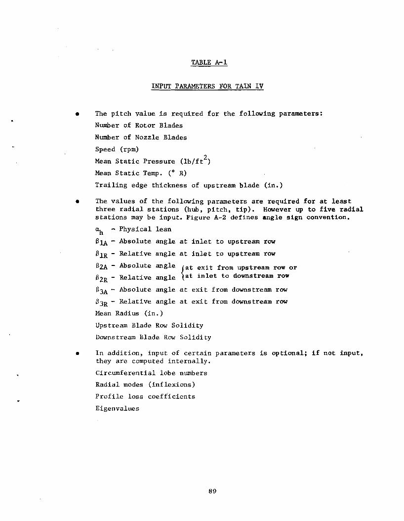
TABLE A-I

INPUT PARAMETERS FOR TAIN IV

• The pitch value is required for the following parameters:

Number of Rotor Blades

Number of Nozzle Blades

Speed (rpm)

Mean Static Pressure (lb/ftZ)

Mean Static Temp. (0 R)

Trailing edge thickness of upstream blade (in.)

• The values of the following parameters are required for at least three radial stations (hub, pitch, tip). However up to five radial stations may be input. Figure A-2 defines angle sign convention.

ah - Physical lean

SlA - Absolute angle at inlet to upstream row

SIR - Relative angle at inlet to upstream row

aZA - Absolute angle {at exit from upstream row or SZR - Relative angle at inlet to downstream row

S3A - Absolute angle at exit from downstream row

S3R - Relative angle at exit from downstream row

Mean Radius (in.)

Upstream Blade Row Solidity

Downstream Blade Row Solidity

• In addition, input of certain parameters is optional; if not input, they are computed internally.

Circumferential lobe numbers

Radial modes (inflexions)

Profile loss coefficients

Eigenvalues

89

: ! I

i YROlOR~:l I<::::- d

STATOR I I STATOR

I I I I

u I TJ

u

• Absolute Flow Angles are +ve in Direction of Rotation • Relative Flow Angles are +ve Opposite Direction of Rotation • Lean is +ve in Direction of Rotation

Figure A-2 Sign Convention for Flow Angles

90

__

TABLE A... 2

INPUT SHEETS

TURBINE AERODYNAMICALLY INDUCED NOISE

Sept., 1975

GE Class II TAIN

$INPUT

cash title TITLE=60H

MODE=6H TURBIN,

generating interaction

IRVSWK igv -rotor viscous wake

ROVSWK rotor-ogv viscous wake

IRVSWK or ORVSWK?

NMECH/MECH=6H~ __

hub radius tip radius no. of blades no. of vanes

-in­ -in-

HUBRAD= _ TIPRAD= _ NBLADE= _ NVANES-

wheel speed no of lobes harmonic no.

-rp~ (1 for fundamental)

SPEED= NLOBNO= NliAR}P __

input lobe no.'s?

(true or false (T or F», if true, enter lobe no.'s

INPLOB= LOBNO=__, __, __, __, __'

input radial inflexions?

(T or F), # if true, enter radial inf1extion no.'s

INPNIN=__, I NFLEC=__, __, __, __, __,

static pressure static temperature trailing edge thicknasB

-lbf/ft2 . _0 R- -in-

PSTAT= TSTAT= TET=__

Page 1 of 3

TAIN - IV

NAMELIST 1 of 3

_

91

---

---

TABLE A-2 (Continued)

Sept., 1975 Page 2 of 3

GE Class II TAIN TAIN - IV

NAMELIST 2 of 3

vane lean?

(T or F)

FLEANI== EFLEAN=L,

radial output stations

-in­

NOPRAD/OPRAD=__

radial stations at which aero data are given - first station must be hub

-in-

NRADP /RADTAB=__

enter the following for each radial station

physical lean for FLEANL=T only

-deg-

ALPHA=> _

upstream blade row absolute inlet angle

-deg-

BETAlA=

r-o, rotor relative inlet angle

-deg-

BETAlR=

i-r, rotor absolute inlet angle

r-o, rotor absolute exit angle

-deg­

BETA2A=__

i-r, rotor relative inlet angle

r-o, rotor relative exit angle

-deg­

92

TABLE A-2 (Continued)

Sept•• 1975 Page 3 of 3

GE Class II TAIN - IV TAIN-IV

NAMELIST 3 of 3

BETA2R=__ ---'. ---' i-r. rotor absolute exit angle

r-o. stator absolute exit angle

-deg­

BETA3A=--­i-r. rotor relative exit angle

-deg­

BETA3R=__

upstream blade rCN solidity

SIGMAl­__

downstream blade row solidity

SIGMA2=--­axial blade row spacing. trailing to leading edge

-in-

BP=--­input upstream blade rCN loss coeffs? (T or F)

if true. input (pressure loss coefficient/al)

INPCDl= CD1=__

pundl t:igenvalUeti?

(T or F)

PUNCH= _

delete eigenvalue calculations?

(T or F)

DELLAi'l=--­insert prepunched eigenvalues here if available

$

INPUT additional cases as:

$ INPUT variables that are changed

$

93

(iii) Data for each interaction

Unsteady circulation distribution

Phase angles in radians (leaned vanes only)

Data for each of the component modes

Eigenvalue

Residual associated with eigenvalue (This is the value of the characteristic function evaluated at the calculated eigenvalue and thus indicates the accuracy of the eigenvalue calculation. If eigenvalues are read from cards, the printed residuals do not apply).

Cut-off speed

Norm

Amplitude

Power

Power level

Radial distribution of pressure and pressure level

- Composite data for each lobe number summed over its radial modes (inflexions) •

Power

Power level

Radial distribution of pressure and pressure level

- Overall composite data summed over all lobe numbers.

Power

Power level

Radial distribution of pressure and pressure level.

(iv) Eigenvalues and associated coupling coefficients on punched cards in NAMELIST format for future use if these quantities were calculated.

A typical output is shown in Table A-3.

+

94

· ..-._--------------- ­

-----_.....- -------._._- ----.

H. •• _~ASe: TITJE~~S.A....l.!I tU~3.N2R2 BASE.__~T_t 1836. ~ _ .------_._-_..

________________________M~I;.HANH~_',_.!RVSfl:.:K _

'1Q)E TURBI ... ~uB~AO 8.900 T1P~AD ---. - 12:S60"NKLAoE 102 NVA-N£"S 10a--SPEf:D U7'7.---···-·--· \/U)'3'm 1 ~-lARM _ __ __ I. PSTA T I.'H2;OOO __ ..TS!AJ__5..!0.00Q_T.E!... O,0200!O_I~PI.D~ F

----- --l";>~IN F OI::LLAH T INPCDI F PUNCH F EFUEAN , FLEANa T \/LfA'41 2~

-----:lP~A)(f~)

12.560. RADT#.RU-}) .

8.90:1 10,700 12;5&0 •. ALPMACl-:5)

_ . .. ..0. .. Q.L._ .Q_~. BETA1AO-l)

_q9.300 _Q4.RCO _41:1008E TA lR (t -3) -.-----.---- ...--- -..-- - ----.-----------------~------

56.bO? 57.beo 60;200------. dE TAl! A(1-3) . - .-.-.-.._-._--. - -- - -.------ - - ---------------------.------­

BE TA2iiCi~3/' I !-q()~ 5_~~~S.0 5~~~0:!..0 ...:...... _

-S~.20? -45.300 .. .. -36;500Bf.TBA(t-l) ---- ..---- --_.-- ----. .

-46.100 . ~40 .000 ~38:000 ------.-.- B£ UJR (1-})

-- CO <;7.000- 55 800 _.. _~ _CII-'SiG ltt;:sy' .t.__ 58·100 MA

1.91:1 2.0~O 2:110 - - .. - --- SIGMA2( 1-3)

1.820 _.. . . __ } .650 ,;5bO Bp(l-'S)

__________~0,.3?0 0,330 0:290

**"'***.*.*.'-*-*­OlJTPU r OAT A

****. I: *il·. ****_. *** CtRCu~FERF.~TIAL LORES ROTATING LINE SOURCES . --- fa ..--- .."------- --- ­

~

~

~ ~ ~

U/S ~LADE Rn~ CH}~)(IN)

O.1A~ 1.276 t:'>'ifl )/5 iL~DE ~1. CH1~O(I~~

~.~Q; 1.0 liB ----.-- ­ --i~20/-._... ._------- ­ .

~/S ~LADE ~~~ CD ~~~27,~ 0./)19b& 0.01 724

* •• ***A*A*_.**** •• ~fC~A'IS~ t l-R VISCOUS ~4~K~E~ __

--.i***.iI(*a**._ •••-.-. --- -- --._­

T-:':':F(Il .~.f\f)'l(j -OdOH -~.O()l>o -0.00 9 7 -(l.Oln -0.01')5 -O,OI~t -0.0200 -0,0230 -0.02S2 .__._.. - ­_-"-~

-~-". :))7 J -O,tl"<l2 -o.v~o</ -0.n3,?" -0,0341) -0.055.J -0.05&4---;0.0574---~o,65BJ -"~O,O390 ;> ..q,(J)

_. -0. n 'I 0 V -O,,,:J '~,.j -I.'.vooo -o.oo'H -O.Ol?! -o,otS') -0,01 8 1 -0.020'- -0,0230 -0,0252 -1.1);>15 -0,0)</2 -0.1)'09 -0.0525 -0.03110 -0.0353 -0,0 364 -0.0314 ~O,0383 -0,03 9 0

. ~-- ...- .'ilL ( 1) n.7 ~!':i!l O. UH 0,7\93 0.7)/H. 0.7(>99 0.7653 0,11006 O,81bO 0,8313 o,840b O.8;,2G 0.8713 o.lh2h .. '0.9080--0.92B -- 0.9j!\7-· 0"~qS40--0-;%q3 0;9 lSi"-'!--l-;OO 0 0

AI« 1) 0, O. 0, 0, O. 0.319/\ -O.b76l 0;3174 o. O.

ALPCn!;(Tl O. O. O.

-_.- ----_.. "- __ ..._-- .~._----._--~--- , ._---~-_

UNSTEADY CIRCULATIJ~ ~tSTKIBUTI0~

RADI"'s RATIO cIRCui' ATI ON (F T**21SEC)

to o 709 0.?72/!E 00 O'l .- ---O:8~2 O~2bq3EOO

.1.000 0.2S 4SE 00

Ci)'1P MODE Er;~VAL RESIDUAL CIO SPI) .'1();{M AMP PJWER Pi'lL RADR RADIUS PRES SPL ( RP,'11 '(FT*L~f/S[C){DB) (l til (PSf) (De)

----r-b~--o--i,001" -'0 :-------"7 i 3:---0;3"017 E:;01--0~bO-ij c- 0II O,21911E 00 12"ij~~ooo 12,50 O.530BE 00--122,08

2 0; 1 tq,on O~ 1945: 0.lb40E-01 0;2200E-04 O,3103E;'01 11&~24 1.000 12,50 0.2454E 00 l1S.!8

3 1>; 2 U.7 4 l 0: 2"5U: ··0 .6'i3ClE-02'-0 :409 lE-04 0.IS03E 00 1?-3~Oql,OOO 12, So·.... O,!>ISbE 00 121.83

II b. 3 - -23 ;qll j ---0:-' 21139-:-O";ri177E-0 1 0.IS81E-Oll O.8boOE-01 120,70 1.0~12.50 o.3823r-OO---llQ.23

_. . __ .RADIAL COMP:)S%TE ~O~E._NO .__b__.... _ .. ..... . O,~67~E_ il.~_.. _.g_~.,?~ l,_OO.<> .. 1?_.5!) __ ~._1.&7.QE 01 132,06

OVERALL Ca~?OSITE __ ._ ...... O,1If37_Il..E_ OL__ J~~ .•_2.Q__...h~QO.. .. 12.5b._.JI..,tb74E 01 112,06

----"------ .. _~. __ ._--­

PROC TrilE;: 0 MIN 5 S.E~__

"TAIN" PROGRAM LISTING

~ FORTRAN DECK,MAP TAIN s INCOCE IBMF CrAIN TAIN - TURBINE AERODYNAMICAllV INDUCED NOISE

c C~ll I NPUTl

~ CAll INPUT2 CALL CVCMCH GO TO 5 l: ND

S FORTRAN DECK,MAP,XREF I~PUT

$ I Ncaa£: I BMF CINPUT INPUT ROUTINE: ,... FORTRAN-V 22APR1975 c

SUBROUTINE INPUTl COMMON/INPBlK/TITLElIO).MODE.MECH(5),NMECH,HuBRAD,TIPRAD,NBL~DE,

1 NVANES,SPEED,INPlOB,LOBNO(5),NLOBNO,INPNIN,INFlEC(S),NHARM,PSTAT, 2 TSTAT,TET,DEllAH.lAMBAYl20,5),QAYl20,5),OPRAD(20),NOPRAD,NRADP, 3 ~~OTAB(5).BETA1~l5),BETAIR(~),BETA2Af5l,BETA2Rf5),BETA3A(S),

4 BETA3R(5),SIGMAif5),SIGMA2f5),BP(S),INPCD1,CDlf5),PUNCH 5 ,EFL~AN,ALPHA(5),C.LAMBDAllj,5),RHO,GAM,DVVISC

LOGIC~l INPlOB,INPNIN,DElLAM,INPCD1,PUNCH l OG I CAL EFlEA N COMPLEX LAMBDA ~EAL LAMBAY COMMON/IVRBlK/IV~

DIMENSION NAMEflv),ADDRfSllJ),IDENT(lO) DIME~S10N CATSflO) DI~E~SION INTIT(.O) LOGI(AL EOF CJ~MO~ ICLEA~ll FL~AN~,~LtA~I,Rl(2v)

LOGICAL ~L[ANI

~AMlLIST/CO/~BR/IO/~AME.AcnRES,10ENT

NAMELlST/INPUT/TITL~,MOOE,MECH'NMECH.HUBRAD,TIPRAD,~BlADe,~VA~ES,

SPFtD,INPLOB,LObN[J,NLnBNC,lNPNIN,INFLEC,NHA~M,PSTAT,TSTAT,TEr,

2 ~ELLA~,LAMBAY,QAy,OPRAD.~OP~AD,NRADP,RADTAB,BETA1A.8ETAiR,

~ RETA2A,HETA2R,RETAlA,BETA3R,SIGMA1,SIGMA2,BP,I~PCD1,CD1,PU~:H

~ ,EFL~AN,4LPHA,lAMeDA,FlEA~l,NLEANI

DATA CATS/6H19000E,6HE/USER,'1*lH I DATA I~TIT(1)/60H* TAIN NAMEllST •

1 I CALL NLISTW(INTIT) CALL FXOPT(66,1,u,O) CALL FXOPTlb7,l,l. ') CALL FLGtOFf5,EOf) CAL L \>IV· P ( $I 0) CALL ClOCK(DUMY,OUMV,IMO~,IO~Y)

I DATF = I YR+ 1 UO. I DAV+ lOJJ",* I :WN R(AD(5,ID) WRITc(6,900) IOATE,~AME.~DOR=S.10ENT

900 FORM~TlIH1,51X,23H T A I N I l IlHRUN OATE-161111 2 45X,lJA61145X,laAbI145X,lOA6)

97

GO TO 5

ENTRY INPUT2 READ(5, INPUT) IF(EOFI GO TO lOv rJR IT c (6.905) TI TL E. ( I • ME CH ( I ) .I =1. NMECH)

90~ FORMATIIHl.51X.3(6H******)/50X.lOHINPUT OATA/52x,3f6H*****.)//1 1 ltiX,13HCASE TITLE - lOA611~7X.lJH~ECHANISM Il,lX,A61 ? 151X,Il,lX,A6» W~ITc(6,9101 MODE,HUBRAO,TIPRAD,N8lADE,NVANES,SPEEO,NlOB~O.~HARM.

~ PSTAT,TSTAT,TET,INPLOB,JNPNIN.DEllAM.INPCD1,PUNCH,EFlEAN 2.FLEANl,NLEANI

91~ FOR~AT(/5X.4HMODE.7X.A6.2X,6HHUBRAD,lX.FiO.3.2X,&HTIPRAD,lX.FIO.3, 1 2x,6HNBLADE.IX,IIO,2X,6HNVANtS,lX,I10,2x,5HSPEeO,2X,fl 0.01 L SX,6HNLOBNO,lX,IIU,2X,SHNHARM,2X,Il~,2X,5HPSTAT,2X,Flj.3.2X,

J 5HTSTAT,2x,FIO.~,2X,3HTET.~X,Fl~.6,2X.6HINPLDB,lX,llO/

4 5X,6HINPNINtlX,Llu,2X,6HOELL~M,lX,llO,2X,6HINPCDl,lX,lIO,2X,

S 5HPU~CH,2X,LIQ,2X,6HEFlEAN,:X,LIO,2X,6HFLEANl,IX,llO/,5~, . 66HNLEANI,lX,IIJ/)

IF(INPLOB) WRITE(6,91Sl 1\JLOB\JC.(LOBNOfl),I=l,NlOBNO) 91~ FORMATI5X,8HLOBNO(!-ll,lH)/jX.519X,llO»

IF(INPNIN) WRITE(6.920) ~lOBNO,(INFlEC(I),I=l.NlOBNO)

92 FORMaTI5X.9HINFLEC(1-I2,!~1!3X,5(9X,IIO»

IF 1'JOPRI'lD.G T. 0) WRI TE C6.925) NOPRAD, COPRAD( II. I =J. ,"lOPRAOI 92~ FORMAT(SX,8HOPAAD(~-I2,iHI/IJX,6(9X.FIO.3111

WRI TL 16 , q 30 I N~ ADP , 1KADT ABI I ) , I =1 , NRADP ) 93<, fORMATI5X,9HRAOTAB(1-11.lHI!.3X,5(9X,FIO.3)

W~l TE 16,931) NRADP, (AlPHA( I I, I=l,NRADP) 93: FORMATI5X,8HAlPHA(1-Il,iHI/3X.5(9X,FlO.3)1

WRITElb,93S) NRADP.(BETA:AII).I=l.NRAOP) 935 FORM~TI5X,9H8ETA~A(1-Il,~H)/3X,519X,FlO.3)1

w~ITEC6.940) NRADPdBETA1RlI I ,I=l,NRAOP) 9 4 0 FO~MAT(5X,9HBETAIRII-Il,lH)/3X,5(9X,FlO.3»

WRITE(6,945) NRADP.(AETAZA(JI,I=l.NRAOP) 945 FORMATISX.9HBETA2All-ll.lH)/3X.5(9X.FlO.31)

WRIT~(6,9501 NRADP.(BETA~RCI),I=ltNRADP)

95~ FnRMATISX.9HBETA2kll-ll,lHl/iX.5f9X,FlO.3» WRITE(b,95S) NRADP.(BETA3A(II,I=l,NRAOP)

9SS FORMATI5x.9HBETA3A(1-Il,lH)/3X,5(9X,FlO.3» WRIT~16,q60) NRADP,CBETA3R(I),I=1.NRAOP)

96) FORM~T(~X.9HBETAjR(1-ll,lH)/3X.5(9X,FIO.3)1 WRITEC6,965) NRAOP.ISIGMAlIII,I=L,NRAOP)

965 FOR~~T(5X.9HSIGMA1(1-11.lH)/3X,5(9~,FiO.31)

WRI TE ( 6 , 97 i) l NRA0 p • 1S I GM4 2 ( I I ,I =1 , NRA() P ) 97: fOR~AT(5X,9HSIGMA2(1-Il.lHI/3X.5(9X,FlO.31)

W~ I TI:: (6,975) NRADP, (AP (11,1= 1 ,NRADP I q75 FORM~T(5X,5HBP(1-1:,lHI/3X,519X.FIO.3»

IF(lNPCDl) WRITE(6.980) NR~DP,ICD1(1),1=1.NRAOP)

96~ FORMAT(5X,6HC01(1~Il,lHl/3X,5(9X.FiO.5»

~ RETURN 100 CONTINUE

10 CALL USELOG(bHF10051.bHTAIN ~,CATS)

STOP END

98

+ $ fORTRAN DECK,MAP,XREF BlKDAT S INCODE IBMF CBlK"AT BLOCK DATA C FORTRAN-Y 22APK1975

BLOCK DATA COMMONIl NPBLK I Tl TlE ( 10), MOOE, MECH (5), NMECH, HU61UD, T I PRAO, ~BlAOE,

.. NVANES,SPEED,INPLOB,lOBNC(5l,NLOBNO,INPNIN,INFLECt5l,~HARM,PSTAT,

~ TSTAT,TET,DEllAM,LAM8AY(20,5),OAY(20,S),OPRAO(20),~OP~AO,N~AOP,

3 RhDTABISl,AETAlA(Sl,8ETA:R(5),BETA2A(S),BETA2R(S),BETA3A(S), 4 BETA'3R.(5),SIG~Alt5),SIGMA2Ij),8PI5),INPCD1,COl(5),PUNCH

S ,EFLEAN,ALPHA(S),C,LAMBDA(1~,5),RHO,GAM,OYVISC

CO~PLEX LAMBDA LOGICAL INPLOB,INPNIN,DELlAM,INPCD1,PUNCH LOGICAL EFLEAN REAL LAMBAY COMMON/PRCBlK/NRLSAY(S),RADRTB(S),OPRR(20),AKC10),

1 RHUB,AlPCOE(3),GPRM1,GONE COMMUN/IYRBLK/IYR COMMON ICLEAN11 FLEAN1,NL~ANl,RL(20)

LOGICAL FL~A~l

DATA FlEAN1,NLEANI/F,20/ DATA MOOE/6HCOMPRE/ DATA INPLOB,INPNI~,DELLAM,INPCD1/4 •• FAlSE.1 nATA NHARM,C,RHO,GA~,NOPRAn/~,ll16.89,O.J16475.1.4,O/

DATA PSTAT,TSTAT/2116.,519.1 DATA PUNCH/.TRUE.I nATA IYR/75/ DATA EFLEAN/FI ':~D

+ , FORTRAN DECK,MAP $ INCOOE IAMF CLORNUM LOBE NU~B£RS

C FORTRAN-Y 22APR.1975 ,.... ,.... THIS PROCEDURE DET[RMI~~S THE fIRST FIVE LOBE ~U~8ERS, ,. ... ~ BEING A PARTICULAq LOBE NUMBER, ANO THEIR ASSOCIATED c VALUES OF K FROM THE RELATIONSHIP

N == NHARM*NBlADE + K*NVANES

AND PLACfS THEM IN NARY AND KARY RESPECTIVELY. ,. ... SUBROUTINE LOBNUM(~HARM,~eLADt,NVANES,NARY,KARYt

OIMENSION NARY(S).KARy(5),ARY(Z.11t I:O~ST = NHARM*NBLAOE IFINHARM .EO. Ol ICONST=NRL40E [)O '1 J==",ll t< == J-6 A~Vll.J) == IABSIICONST+K*NVANE$)

j J\q,YI2,J) = K

99

CAll SORTCARY,2,11,1,.TRUE.) 00 IO 1=1,5 NARY«l) = ARyel,!)

10 KARY(I) = ARYCZ,!) RETURN END

, $

FORTRAN INCODE

OECK,MAP IBMF

+ NRAOMO

CNRADMO RADIAL MODES PER LOBE NO. FORTRAN-Y 22APRl975

c ,. ... THIS PROCEDURE DETERMINES THE NUMBER OF RADIAL MODES TO BE 4NALYlED PER LOBE NUMBER (NRADMO) AS A FUNCTION OF LOBE ~UMBER eN) VIA AN EMPI~ICAL TABLE.

FU~CT[ON NRADMOCN) DIMENSION IRANGNL.OJ ,IRAD~O( .. 0) DATA NRANGN/9/.(IQADMO(l),I=l,9J/1,2,4,5,6,7,8,9,lv/,

i (IRANGN(IJ,I=1,8)/3,6,11,21,31,41,51,701 NRNGMl = NRANGN-l DO 5 I = ~ , NRNG M1 IFCN.LT.IRANGNCIJ) GO TO ~J

5 CONTINUE 1 = NRANGN

1; NRAOMO = IRADMO(IJ RETURN END

$ FORTRAN DECK,MAP + DECBEL$ INCODE IBMF

CDECHEL INTENSITY LEVEL FUNCTION : FORTRAN-Y 2ZAPR1975,. '" c THIS PROCEDURE DETERMI~~S INTENSITY LEVELS AS FOLLOWS, c

IF X.NE.J, OECBEL = C*ALOGIO(ABSeX)/REF).c IF X.EQ.O, OECBeL = o. C

FUNCTION DECBElCX,C,REF) IF(X.NE.O.J GO TO 5 OfCl3tl = o. GO TO l~,

1 OECBEL = C*AlOGlu(ABSfX)/REF) :0 RETURN

E~D

100

C

+ s FORTRAN DECK,MAP TIMERs I NCOOE I BMF CTI MER TI MI NG ROUTI ~E

FORTR.AN-V 22AP!~ 1975 SUBROUTINE lIMERl CbLL CLOCKtOUMV,Tl.DUMV.OUMV) GO TO 5 ENTRY TlMER2 CALL CLOCKtOUMY,T2.DUMY.nUMY) PT = T2-Tl MIN = PT/60.NScC = A~OOIPT.60.t

. WRIlE t 6 , 9'(0) MIN- t NSEC 90J FOR~AT(11100X,12HPROC TIME =

;; RETURN EN!)

$ $

FORTRAN DECK,MAP INCOOE IAMF SORT

+

:SORT GENERAL ALGEBRAIC SORT ROUTINE C FORTRAN-Y 2ZAPRl975 ,... c

SUBROUTINE SORTtARRAY,N,M,ISRT.ASCND) DIMENSIO~ ARRAY(N,M),BUFFIIO) LOGICAL ASCNO LNG=M+l MM~=~-~

DO 10 LOOP=I,plMI Lf\JG=LNG-: LNG~l=LNG-l

00 ~ ') J=l. LNGMi IFIASCND) GO TO ~o

IFIARRAY(ISRT,J).GE.ARRAYCIS~T.LNG)1 GO TO 15 GO T3 .i5

2v IFIAP.R~Y(ISRT,J).L~.ARRAY(ISRTtL~G») GO TO 1; 25 no :?J1 1=I.N

BUFFII)=ARRAy(I.LNG) 30 CONTINUE

')0 j5 l=i.N ARRAYCI,LNGI=ARRAY(l,JI

~:. CONTINUE nn 4tC I=I.N ARRAYCI.J)=BUFFCI)

4. CONTINUE :5 CONTI\IUE: 10 CONTINUF

RETURN [NO

101

+S FORTRAN LSTOU BESFITS I NeaOE I BMF

CRSFl ,.... BESFIT - LeAST SQUARES CURVE-FITTING ROUTINE ,... USING ORTHOGONAL POlY~~aMIALS WITH STATISTICAL ,.... TERMINATION c c

SUBROUTINE 8ESFITCN,X.Y.K,D,~ES) DIM[NSIO~ XIi),Ylll,DCll .,A(2jl,B(23).Sl2~).RES{2,},TAB(20',

1 P;l22,)I,P1l220I,R(Zl,ZU EOUlvAl~NCE (PO,R),(Pl,R(~2i»

DATA (TAB{I}.I=1,20)/12.7J6,4.3~3,3.1a2,2.776,2.571,2.447.

2.365,2.306,2.Z62,2.228,2.2'l,2.179.2.160,2.145,2.131,2.120, 2 2.llu,2.1L'l,2.V9,j,2.')861

KT=J IF =K M=N NDEG=M-l J=e: CO=M A I 1 • :: ij. ~ll)=a.

S(11=0. RES( 1)=:::'. DO 1 1= i, M POll) =0. PiII)=!. Sl 1) =SCl )+Y( I) A( ~ ) =J\ ( 1 ) +xI I )

1 ~ES(1)=YlI)**2+R[Sfl)

1\ I 1) =A( 1) ICO S{l)=SIU/CO RfS(:I=RES(1)-S(~)**2*CO

RMS=RESlll/ICO-l.) J J=J+l

IFIJ.LE.22) GO TO 24 27 I< =2C

LL=2: WRlTEI6,29) GO TO 4

24 r: 1=0. XPP=. YP=0. DO 2 1=1, to/!

(J=Plll) PI ( I ) =()( I I ) - A I j I ) *Q- B ( J) :$ P~l ( I ) POI I ) ;:Q

PP=P:'II)**2 Cl=PP+Cl XPP=XPP+)«I)*PP

102

2 VP=VP+VCI)*Plll) SIJ+l)=VP/Cl SSR=SCJ+l).*2*Cl

23~ESCJ+l)=RESCJ)-SSR

IFtRESIJ+~).GT.O.) GO TO ~3

1" K=J IFCREStJ).lT.ABSCRESeJ+l»)) Ll=K+l

4:'; WRITE<6,14) K GO fa 4

U ACJ+l)=XPP/Cl RCJ+:l=Ci/CO C~' =c 1 lL=J+l IFtIf.NE.O) IF(LL-IF) 3,~,4

~::: NDEG=NOEG-l RMS=RES(J+l)/FlO~Te~DEG)

ISUU=MINOtNDEG,20) T=SQRT( SSR/RMS)

IF CT. LE • TAB ( I S~8» GO TO 11,2 KT=O GO TO 3

L1 SCJ+~)={l.

RESIJ+l)=RESCJ) NDE(j=NOEG+l IFCKT.EO.l)

21 /(T=1 GO fU 3

18 LL=J-l K=J-2

" R(I",l):l. R I l ,2. ) =-.\ II ) RI2,2l=1. RI2,l)=".

GO TO .~

K=J-l

IFII<.-2) b.a,R d l")n 9 1=3,Ll

R I ~ , I ) =-411-1 ) *R t : .1-1) -I) C1- l. l* R( 1 • I -2) lOOP=I-2 R C1- 1 , 1 ) :: RI (- 2 , I -1 ) - 4 I 1- _ ) *R ( I - ~ , l-l ) RII,I)=l. no q JJ=2,lOOP R I J J , I ) =R ( J J -1 , I -1 ) - A( 1-. )*R ( JJ , 1-1 ) - B( 1-1 )*R ( J J, t - 2 )

':J CONTINUE 6 no ~'J JJ=l.ll

OIJJ)=.,. 00 ie L=JJ,LL

l~ nCJJ)=DCJJ)+SIL)*RIJJ,L) Qt"TUo<N

~4 FOKMATI1BHOQESFlf. RETUR~ED WITH ORDER 121/) 29 FnRMlTI3SHO~1:SflT LlMIT~D TO 20TH O~OER.II)

END

103

$ FURTRAN DECK,MAP ARCSIN to INC[JOf IBMF CARCSIN ARC SINE (PRINCIPAL VALUe) ARCSl\l~.)

: FO~T~AN-Y ZZAPR1975 FUNCTION ARCSIN(XI ARCSINOl IFIX.NE.O.O) GO TO 5 AQ CS1N..'2· ARCSIN = 0.(, ARCSI\103

A~ CS1 ~j 04GO TO 15 5 IFIA4S(X).NE.l.O) GO TO :0 ARCSI\J05.

Al:lCSI"J = SIGNI1.51,7963,X) AR.CSI~J6

GO TO 15 A~CSl"JC7

10 ARCSIN = ATAN(X/SQQTI1.-X**2.) AR.CSlr-.J08 .5 RETUK'\J ARCSINJ9

END ARCSI'HJ

+ $ FORTRAN AlNGMI ~ INCODE IBMF CAl"'G4~ N~TURAL LOGARITHM OF GA~MA FUNCTION Al~GA~O~ ,.. AlNGA .... 2 c AlNGAM .~~

C THIS PROCEDURE EVALUAT~S TH~ NATURAL LOGARITHM Of AlNr,~M[;4 ,.. GA~~A(X) FOR ALL R~6l X IN THE INTERVAL 10**-8 =X =10**6. AlNGA~CJ5

w

... C STIRLING-S FO~MULA IS USED FOR THE CENTRAL POLYNOMIAL PART ALNGAM~.6

C OF THE PROCEDURE. AlNGAM07 ,.... AlNGAMG8.. ... AL"4GAM l 9 ..,.. AlNGAlo\lO FUNCTION ALNGAM(XI AlNGAMll IF(X.GE.l.~-8.AND.X.lE.L.ES) GO TO 5 AlNGAM1Z W~ITE(6,9~vI X ALNGAI-'~ 3 ~ORMAT(72HO***~lNGAM ARGU~E~T FAULT. PROCEDURE REQUIRES =ARAL ~ GA M~ 4

IG =1(**6. ARG = EI5.M,21H. Rc$UlT SET = ARG***) AlNGAM~'5

l\l"JG6.M = X AL~GAM16

GO TI] ~: ALNG~M17

5 IF(X.lT.7.1 GO TO ~O. ALNGA~18

F :: ~. AlNG!l.M~9

Y :: X AlNGA"I2.i GO TO 25 h l NGA~· 21.

:0 F :: 1. ALNGAM22" Z :: x-to Al"lGA"'12? f)O 1'5 1=1,1 AlNGAMZ4 1 = l+!.. AlNGA"125 " IF(Z.GE.7.) GO TO 21 ALNGAMZ"J y :: 1 ALNGA~27

F = f*l ALNGA~i8

_5 CONTINUf: ALNGAM2<l -'- y = y+:". AlNGA~CO

F = -ALOGIF) AlNGAMJl 2';; l = i../v**Z ALNGAM32

ALN~AM = F+(Y-O.)1*4l0G(V)-V+~.q1893853+«((-O.0005q523~09.Z AL '~GAMJ3

~ +O.000793b50191*Z-O.00217717 7 B)*Z+L.JB3333333)/Y AlNGA~:~4

~E TUR 1\,/ ALNGA'~35 P~f) AlNGA~?'6

104

+

$ FORTRAN LSTOU,DECK.XREF CYCMCH CCYCMCH CYCLE THROUGH MECHANISMS C FORTRAN-Y 22AP~l975 ,. "..

SUBROUTINE CYCMCH EXTERNAL LINK1F.LINK1I,LINK2F.LINK2I COMMON/INPBLK/TITLEC1J),MODE,MECHCS).NMECH,HUBRAD,TIPRAO,~BLADE.

NVANES,SPEED.INPLOR,LOBNOCS)",NLOBNO.INPNIN.INFLECCS),NHAR~.PSTAT,

£ TSTAT,TET.D[LLAM,LA~BAYC20,5),QAYC20,S).OPRADC20),NOPRAD,~~ADP,

~ RADTARCS),BETAIACSJ.BETA1RC5J,BETA2A(SJ,BETA2R(S).AETA3A(~).

4 BETA3R(SJ,SIGMA1(S),SIGMA2(SJ.BPCS),INPC01.CD1(SJ.PUNCH 5 ,EFLEAN,ALPHACSJ,C,LAMBDA(lO.SJ,RHO,GAM.DYVISC

LOGICAL INPLOB,I~P~IN.DELL~M,INPCD1,PUNCH

LOGICAL EFLEAN COMPLEX LAMBDA I{E~L LA~BAY

COMMON/CYCBLK/~RLSAY(5),OPRR(20),H,HSQ,FNOMEG,FNOMSO,RCONST(4),

.i LSKEIG,AK(3).K C CYCMCH

CO~~ON ICLEANll FL~AN~,NLEA~I,RL(20)

LOGICAL FLEANl CDMMON ICLEAN)I MECHL1,KMODE(SJ LOGICAL LSKEIG D,l.ME NSJ ON MEC HSM ( 11. J • MCH 1 AG Cj ), DUMY CS J• RADR 1B (5) , VlC C; ) , V2 ( 5) ,

1 ALPHAlCS).ALPHA2(3),DELCU1Cj),DELCU2(S).Cl(S).C2(S),G4MTAB(S) DIMENSION ANG01(SJ,ANG02(S) INTEGER TURBIN LOGICAL ROTAlN,TIlT

DATA MECHSM/"bHIRVSWK,6HROVSWKIDATA TURBIN/~HTURBINI

nlTA RDPRDG/d.~i74S331 c c

()O ~o I=l,NMECH 00 5 J=1,2 IF(~ECHCI ).NE.MECHS~CJJJ GO TO S MCHTAGCIJ = J GO TO L,

') CONTINUt W~lTt(6.900) MECHCl)

~C0 FORMATC~8HO***I~VALIO MECHA~ISM. MECH=A6,3H***) GD TO 160

! v Co"H I NUE ~OTAlN = .fALSE. IFCMCHTAG(1)jLE.2) ROTALN = .TRUE.

I F ( • NOt. I NPLO R) Gn TO 2 S 8:) ,-_ l=l,NLOANO IFI.NOT.ROTALN) GO TO i5 ~>lRl s.\y( U = NBLAOt

105

c

GO TO 2. 15 NR.LSb.VUI = LOBNO(II 20 CONTINUE

(~O TO j5 i5 IF(.~OT.~OTALNI ~O TO 30

NlOW-JO ;; 1 LOP~O(:) ;; NHARM*NRlADE IF(NHAR~ .EO. ~l lOBNO(1)=N6LAOE ~RLS4Y(11 :: NBlADE GO TO 45

30 CALL LOBNUM(NHARM,r'WLADE,NVA"H:S,lOBNO.OUMVI CALL LORNUM(l,NBlAOE,NVA~ES,~RLSAY,DU~Y)

35 DO 40 I:::l.NlOBNQ IFINRLSAY(I).NE.OI GO TO ~O

WRIE16.9051 9i5 FOR~4rf36H0***ANhLVSIS INCIC~TES PLANE ~AVE***1

GO TO 160 40 c.orn I NUE 45 W~ITE(6,9101 (lOSN(J(II,NRLSAYfI),I=l.NLOBNO)

9:0 FQRMH( .Hl ,51X,3(6H"*****)/56X. HHOUTPUT OATA/52X.3(6H******)II/ 1 3dX,2lHCIRCUMFERf:NTtAL L1JBES.5X,llHROTATING LINE SOURces/ 2 (45X.I~,lOX,I511

wid E(6.915) 9 .. 5 FORMATCIHO)

c c

IFtINPNINI GO TO 55 DO 50 I=l.NLORNO

5\ INFLECt I) : NRAOMO(LOBNOCl)J.. ... ,.... 5~ no bU I=i,NRADP 6.; R4DRTB( I) :: RAOTABI J)/TI PRAD

00 bJ 1=1. "lOPRAD 65 OPRRII) = OP~AD(II/TIPRAO

: ••• hERO P~RAMETERS ••• RL.dOES ;; NBLAOc VANL:S :: NVANES H = HuaRAO/TIPRAD HSO :: H**2 UTIP ::: SPEED~TIPkAO/114.~g156

,. ... NOT[ t 114.~9156 :: J60/PI ) VlSC=Z.27E-~*TSTAT**1.51 ITST4T+i98.6) r.~~f.XP :: EXP(5500~/TSTAT)

GA~A :: :.+O.4/(1.+O.4*(S300./TSTAT)**2*GAMEXP!(GAMEXP-l.)**2) C :: SQRT(1716.4829*GAMA*TSTATI

c NOTe ( 17l6.4b2~ :: 53.35*GSUBC ) RHO = PSTAT/(53.3S*TSTAT) Htdl,.~ :: NHARM

106

IFINHAR~ .EQ.~) HARM=l. FNOMEG = SPEED*HARM*BLAOES*TIPRAD/I114.59156*C) F~OMSO = FNOMEG**2 RCONSTll) = 114.S91~6*C/IHARM*BlADES*TIPRAD) RCONSTIZ) = O.95492964/(C*TIPRAO)

C NOTE I 0.q54q29~4 = 3/Pl I RCO~ST(3) = O.339042:4E-~*TIPRAD**2*RHO*C**3*FNOMSQ

C NOTE I 0.339042t4E-3 = PI/(2*144*GSUBC) ) RCONST(4) = O.lq~79168E-3.HARM*SPEED*BLADES*TIPRAD*RHO.C

c NOTE I 0.19:79:66E-3 = 2*PI/ISQRT(2)*6~*12*GSUBC)

HA = TIPRAD-HUBRAO IPOINf = MCHTAG(~)

DO 90 l=l.NRADP B1AR = RDPRDC*BETALAIII BlRR = ROPROG*SETA1RII) B2AR = RDPRDG*BETA2AIII R2RR = ROPRnC*BETA2RII) R~AR = RDPROG*BETA2~(1)

~3~R = RDPRDG*RETA~R(II

SANGl = ·BIAR+BIRR SANG2 = B2AR+B2RR SANG? = B3AR+B3RK U = UTIP*~~DRTB(I)

:\RG2 = 6.2831853*R4DRTBI I )*TlPRAO ·V2A ~ U*COSI82RR)/SIN(SANG2)

V2R = U*COSI82ARI/SINISANG2) GO TOI7C,80),lPOINT

...,. ••• U/S VANE - ROTOR OR I-R ••• 7. VUII = V2A

ALPH~~ll) = ~~FrAZA(11

V2(I I = V2Q ~lPHA2( II = ~ET~2~(I)

V3A = U*COSIR)R~)/SINISQNG31

(7 := V24*COSIB2AQI ~fL~U.(I) = ABS(Cl*SI~tH.AR)/COS(BlAR)-Vl4*SIN(B2A~)1

DFLClJZ( I) = ABS( V2A*SI\J1 B2AI< I-V3A*SINIB3AR») IFIROT~LNI GO TO 9 l

(III) = ARG2*SIGMAlIII/VtI!\'::S eilI) = ARG2*SIGM~2(lI/BlAOE5

I F I I NPC 0 1) GO T.G 9;7., ~PS=A~SIBETA:!111-BETA2AIII) fPSp = 4.1486E-2+EPS.13.9q7b~-4+EPS.(-3.4270E-6+EPS*5.4403F.-8») (PSPP := Il.+FPSPI*P.9"5 )-I • .o

C P~OFlll LOSS APPROX. FROM TOTAL LOSS BY ASSJ~ING AN C I~FINIT~ ~SPECT RATlu

DH = (!..*Hf3*Ao.{G2*CflSIB2Af.lI/V'\N[S)/IARG2*COS(B2AR}/VA~ES+HB)

~H = RHO*V2A*OH/(3~6.Jg3*VISC)

FM';' = V2A/C cP$PPP ~111.~S/~H)**O.25*E~S~P)/(~.-F~2**2/4.+(2.-GAMA)*F~2**4/24.

1)

T4NB~A = SI~IBiAR)/COSld:~~)

107

TANH2A = SINtB2ARl/COSIH2~Rl

ALPHAM = ATAN(ITANB1A+TANe2Al/Z.) CDIII)=EPSPPP/ISIGMAIII)*2.j) GO TO 90

C ••• ROTOR - DIS VANE OR R-O ••• 80 VII I l '" V2R

ALPHAlll) = BETA2RII) V2(1) ,. V2A ALPH421 I) :: BETA ... A(1) VIA" U*COSIB1RR)/SINISANGll V1R = U*COS(BIARI!SINISANG1) OELCUIII) :: ABS(VIA*SIN(Bl~R)-V2A*SINIR2ARl)

Cl = V2A*COSIB2AR) DELCU21I) :: ABS(V2A*SINlaZARl-cZ*SIN(B3AR)/COS(B3AR)) IflROTAlNI GO TO 9a Clll) ,. ARG2*SIGMAillI/BlADFS C2(1) = ARGl*SIGMAC:I I l!VANES IFlINPCD1) GO TO 9J .

85 EPS=ABSIBETAIRl [)-BETA2R I I)) EPSP :: 4.1486E-2+EPS*13.Q97b[-4+EPS*(-3.4Z10E-6+EPS*5.4403E-8)) EPSPP = (1.+EPSP)*I~.975)-1.J

OH :: 12.*HB*ARG2*COS(B2RR)/BlAD~S)/(ARG2*COS(BZRR)/BLADES+HBt

RH = RHO*V2R*DH/1386.088*VISC) FMl :: V2R/C • EPSPPP =1(1.E5/RH)**C.2~*EPSPP)/ll.-F~Z.*2/4.+(2.-GAMA)*FM2••4/24.

1)

TANB~~ = SINlBlRRl/COSIBlRR) TANB:R :: SINlB2RR)!COSI82RR) ALPHAM :: ATAN(ITANBIR+TANP.2Rl/Z.) CDllI) = EPSPPP/lSI~MAlII)*2.)

qO COI\ITINUE [FtROTALN) GO TO 91 WRITE(6.Q,O) lC1(I).I=1,~~AOPI

920 FORM~T(I!5X.23HU/S RLADE ROW CHORO(lNI/3X,S(9X,FIO.3)) WRIT~(6.925) tC2Itl,I=1,NRAOP)

Q25 FOR~~T(~X,23HD/S BLADE ROW CHOROIIN)/~X,5(9X,F10.3»

IF(.NOT.INPCDl) WRITEI6,Q3)) ICDICI),I=1,NRAOP) 93G FURMATI5X,16HU/S BLADE ROh CO/3X,S(9X.FIO.S»

9 j IFI.NOT.DELLAM.ANO.PUNCH) PUI\ICH BUO,TITlE 800 FORM~T(lOH012345b789,lOA6,1~H9876543210)

LSKEtG = .FALSE.

C ••• CYCLE THROUGH GENERATING MECHANISMS ••• TIPRFT = TIPRAD/12. CALL LLINK(SHLINK21 CALL LLINK(4HDUM21 CALL FSAVE(22,LiNK2F,lINK2I,jhLINK2,l) CALL LLINKISHLINKll CALL LLTNK(4HDUMll no 155 ~=l,NMECH

CALL TIMERl

108

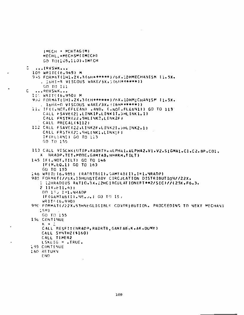
IMECH = ~CHTAGlMI

~EC~L~=~ECHSM(IMECH)

GO TDl105.11.0).IMfCH

••• IRVSWK ••• 105 WRITE(6.945) M 9~~ FOR~ATlIH1.2X.3loH******)/6X,1DHMECH4NISM 11.5X •

• ,1 6H I-R VI SCOUS WAKE/3X.) (611****** I' GO TO ill

C ••• QnvSwK ••• 1 FW R I T ~ ( b • 9 50' M 9jJ FORMAT(lHl.2X.ll(H****.*l/hX,lOHMECHANIS~Il.5X •

. 16HR-O VISCOUS WAKE/3X.~16H** ••*.» 11.. IF(I.NOT.EFLEAN' .AND. (.NOT.FlEANl)' GO TO 113'

CALL fSAVE(21,LlNKlf.LlNKlI.5HLINKl.U CALL FRSTR(~2,5HlINK2.LINK2FI

CALL PRECALI$llZI 112 CALL FSAVE(22.lINK2f.LINK2I.jHLINKZ.ll

C~LL FR~TR(2~.~HLINKl,LINK~f)

IFlfL=ANll GO TO l~3

[';0 TO 1'55

113 CALL VISCWKt UT IP,RADRTR,QlPHAl,ALPHA2.Vl,VZ,SIGMAl,Cl.C2.8P.C01, X NRADP.TET.~nOE.GAMTAB,NHARM.TIlT)

145 IF(.NOT.TILT) GO TO 146 IFIM.cQ.l) GO TO 16) GU TO 155

~46 WRrH(6.985) IRAI)RTB(I),(~A~TAB(I).I=I,NRADP)

98~ FOR~AT(115X.33HUNSTEADY CIRCULATION OISTRIBUTIQNI122X. : l2HRADIUS RATIO.~X,22HCIRCULATION(fT••2/SEC)I/(25x,F6.3. 2 llX,Ell.4») on l~j I=I,N~ADP

IFlGAMTAFHII.Nf: • .;.) GO Tf: 15/ w~IT::'(6,990)

QQ( FnPMATt/22x,53HNfGlIGIRlc CO~TRIBUTIO~. PROCEEDIN~ TO ~EXT ~fCHA~1

~SM)

GO TO 155 15t: CON T P'JUE

K :: .: CALL AESFIT(NRADD,RAORTB,GAMTAB.K.AK.OUMY) CALL SYNTHZl$1601 CALL TI~ERZ

lSKt:1G :: .TRUE. 't.55 CfJNTI"lUE ~ 6(" ~E TUR\!

r: NO

109

+ ~ FORTRAN DECK,MAP SYNTHI S INCOOE IBMF CSYNTHl SYNTHESIZE COMPOSITE C FORTR4N-Y ZZ4PR~975

C SUtlKOUTINE SYNTHZI*> COMMON/INPBlK/TITlE(1~).MOOE,~ECHI5),NMECH,HUBR\D,TIPRAO,~BlADE,

1 ~VANES.SPEEO,I~PLOB,LOBNO'5ItNl08~O,INPNIN.INFLEC(5),NHAR~,PSTAT,

2 TSTAT,TET,OElLAM.lAMB4Y(Z),jl,QAY(2C.5).OPRAOI20),NOPRAO,~RADP,

3 RAD TAB (5 ) • BET A1AI ~ ) , BET AlP ( j I , BET A2 A( 5 I , BET A2R ( 5 I , BETA 3A( '5 ) , 4 RET~3R(51,SIGMA.(~),SIGMA2(31,BP(5),INPC01,CD1(5),PUNCH

5 .EFLEAN,ALPHAI51.C,LAMBOAll J ,S},RHO,GAM,DYVISC L~GICAL [NPlOB,INPNIN,OELlAM,INPCD~,PUNCH

~f:Al lAt-IBAY CnMMO~/CYCBLK/NRLS~VI~),OPR~(2~).H,HSC,FNOMEG,FNOMSQ,RCONST(4),

.. lSKHG,AK(3) ,K LOGICAL lSKEIG ,. SYNTHl" REAL NOR,.. LOGICAL TllT,CUTUFF COMMO~ ICBESlFI PRESNMIZO),PHESM(ZO),PRES(ZO),SPLNM(ZO),

* SPLM(2J) ,SPl(2~I,RESOAYI2J),LAMBD,lAMBSQ,Q.* JLA~(11u).JLAMHlllG),YL4~(110).YLAMH(110I,CYl(110~21

REAL lAMAD.LAMBSQ,JLAM(110),NCRM.JLAM~Cl10)

COMMO~ IClEANll FLE~Ni,NlEANI,Rl(201

LOGICAL FlEANl CO~MON IClEAN21 PHIR(20J ,CCYL(20) COMMO~ ICLEAN31 MECHL1,KMCOE(;) nATA OPNPRN,ClSPRN,EOL/074JjJ .O(~O~~,034JJuJOOOJ~O,013JCOJ~'JJOOI

OATA PRSREF,POWREF/4.1772E-~,7.3756E-141

c c

DO I) [::l,NOPRAO ') PRESNI"( I J :: 0.

pnWNM :: G. ICOMP :: 0 W~ITt(6.8q9)

Bg9 FORM~T(7HO COMP,:X,4HMODE.4X.bHEGNVAl,3X,8HRESIOUAl,3X,7HC/O SPD. ~X.~H~ORM,9X,3HAMP,qX,5HPOWtR,7X.3HPWl.bX,4HRADR,3X,6HRADIUS,6X,

2 4HPRES,7X,3HSPl/3HX,5HlRPM}.28X.12HCFT*LRF/SECI,3X,4HCDBJ,13X, 3 4H(INI,6X,5H(PSF),6X.4HCCBJII)

c C

00 b~ lLOB=l,~LOBNO

N :: LOBt../OCILOBJ F N :: ~~

FN$Q = FN**2 '-.JPl :: N+1. NP2 = N+2 r~P't :: N+4 f\lP'; ;: N+5 MF :: I~FLEClll0H)

110

MFMl = MF-l NRLS = NRLSAY(IlQRI KM= KMODE ( aOB)

IF(nf.LLA~.OR.lSKtlG) GO Te lJ CALL EIGEN(H,N,U,MFM1,LAMBAV(l,IlOB),CAVC1,ILOB),RESoAV,TILT) IF(IILT) GO TO 13 IF(.NeT.PUNCH) GO TO 10 PUNCH a05,OPNPRN,ILOB,CLSPRN,~OL,(LAMBAY(I,IlOBl,I=1.MF)

8~~ rOR~AT(7H lAMBAY,Al,2Hl,tl.2~1.3(E15.8,lH,)/(lX.4(E15.8.1H.»))

PIJNCH 810,OPNPR\l.ILOB,ClSPRr~.£OL,(QAV(I,ILOB).I=1.MF)

810 FORMAT(1H QAV.Al,2Hl. Il.2Al.3(E15.8,lH. )/( lX.4CE15.8.1H,»),.... c

10 00 1.5 l=l.NOPRAO 15 f'RES~(I) :: o.

,POWM = " . ,. ,. " "­

no 50 IR~::l.MF ::;ICOMP ICOMP+l

NINFL :: IRM-~

LAMBD = LAMRAY(IRM,IlOB) LAMBSQ = lAMBO··Z Q = QAV(IRM.1l0B)

C CF5PED :: lAMBC.RCONS T( l) (FRATO = SPEEO/CFSPED IF(F~OMEG.GF.lAM~D) Go TO 2:> CUTOFF :: .TRUE. t-'ETA SQRT(lAMASQ-F~OMSQ):;

i, (l TO 2'J 20 curOFf :: .FALSE.

RETA = SORT(FNOMSQ-LAMBSO) C

2';; CAll r\ESSEL(lAMBO,t~P4,.IHUE.,JLAM,VLA~,TIlT)

If(TILTI GO Te 75 CALL ~ESSELILAM8D*H,NP4,.TRUE •• JLA~H.YLAMH.TILT)

IF(TIlT) GO TO 7; 00 3:j I=:.NP5 en C1.1) = JLAMHCI )-Q.YlA~HC r)

~ CYUI,2) = JLAM(I)-O*YLAfIA(l) c

NORM = C(LA~RSO-f~SO).CVLCNP1.2).*2

: -(LA~BSQ·HSC-FNSC)*CVL(NP1.11.*2)/(2.·LAMBSQ) ,.... ~UM :: 0. KP1 :; 1<+1

nf") ~J5 I=l.KPl CAll f{PYCYG( I ,N,lAMiiD,H' l •• CYl.RINIG,TIlT) IflTILTl GO Te 7~

111

c

c

c

c

~5 SUM = SU~.AK(I)*R'NTG

GO TU H 36 CALL INTZL(N,KM,SUM)

31 ANM = RCONST(Z)*FlOAT{NRlS)*SUM/(FN*NOR~)

POW~R = RCUNSTI3)*ANM**2*{CYL(NP1,21**Z-CYL(N,2)*CVlCNPZ,Z • • -HSO*ICYLtNP1,l)**Z-CYl(N,1)*CYLINPZ.l»)

POWM = POWM+POWER PWL = DECBEL(PO~~R.l~ •• PO~REF)

IF(NOPRAD.EQ.O) GO TO 45

DO 't".J l=l.NOPRAf) CALL BESSFULAMBD*OPRRf I) ,N,. TRUE •• JLAM,YLAM. TILT) IflTILTI GO TO 7~

PRESIII = RCONST(4)*ABS(~NM*IJLAMINPl)-Q.YLA~(NP1) •• PRESM( I. = PRESM( I •• PRES I I I

40 SPLIII = OECBELtPRES(IJ,20.,~RSREF)

4~ WRITL(b.gOu) ICOMP.N,~INFL,LA~BD,RESOAYIIRM).CFSPED,NORM,ANM,

L POWER,PWL 9CU FORMAT(4X,I2,2X.I2,lH,12,2X,FH.3.2X.E10.3,2X t F6.0.2X,E11.4.2X,

: E~i.~,LX,El:.4.2X.F7.2)

I FIN aPR A0 • NE • C) WR I TEl 6 t 9 '..; 5 ) (Q PRR( I ) ,0 PRA0 ( I ). PRE S ( I ), SPLI fl. 1 I=l,NOPRADl

90~ FnR~ATtlH+.92X,F6.3,2X,F7.2,~X,Ell.4.2XtF1.2/(93X.F6.3.

1 2X.F7.2t2XtEll.4 t 2X.F1.2» jl.) CONTINUE

PWLM = OECBEL(POWM.IO •• POWREF) 00 5:: 1=1, NOPRAO

55 SPlM(II = OECBEUPRESM(1),20.,PRSREF) ~RITc(6.qlOI N,POW~,PWLM

~l. FQR~ATI/IGX.25HRADIAL COMPOSITE LOBE NO 13,33X.Ell.4.ZX.F7.2) IF(~OPR&O.NE.O) WRITE(6.9LS) (OPRR(l).OPRAD(l),PRESM(I).SPl~CI),

1 I=l,NOPRAO' q~5 FnR~AT(~H.,9ZX,Fb.~,2X,F7.2,2X.~11.4.2X,F7.2/r93XtF6.3,

1 2X,f7.2,2X,Ell.4.2X,F1.Z) (If) 60 I:::~ .NOPRhO

cO PQ.i: SNM ( I' = PRE Si\lM (I , ... DR r: SM« 1 1**2 pnWN~ = POWNM+POW~

WQ.I H16.9201 q20 FORf>4.lf( lHO)

65 CONTI,,jUE

PWV-lM = OECBEL(POWNM,loO •• POwRtF) ,...,n 7C l=l,NOPRAO . PRESNMII) = SQRTlPRESNMlllt

!J SPlN~(I) = OECBEl(PRESNM(I),lJ.,PRSREF) w~ITc(6.925) POWNM.PWLNM

925 FORMAT( lOX.~7HOV=RALL CO~POSITE,44X.Ell.4,2X.F7.2)

112

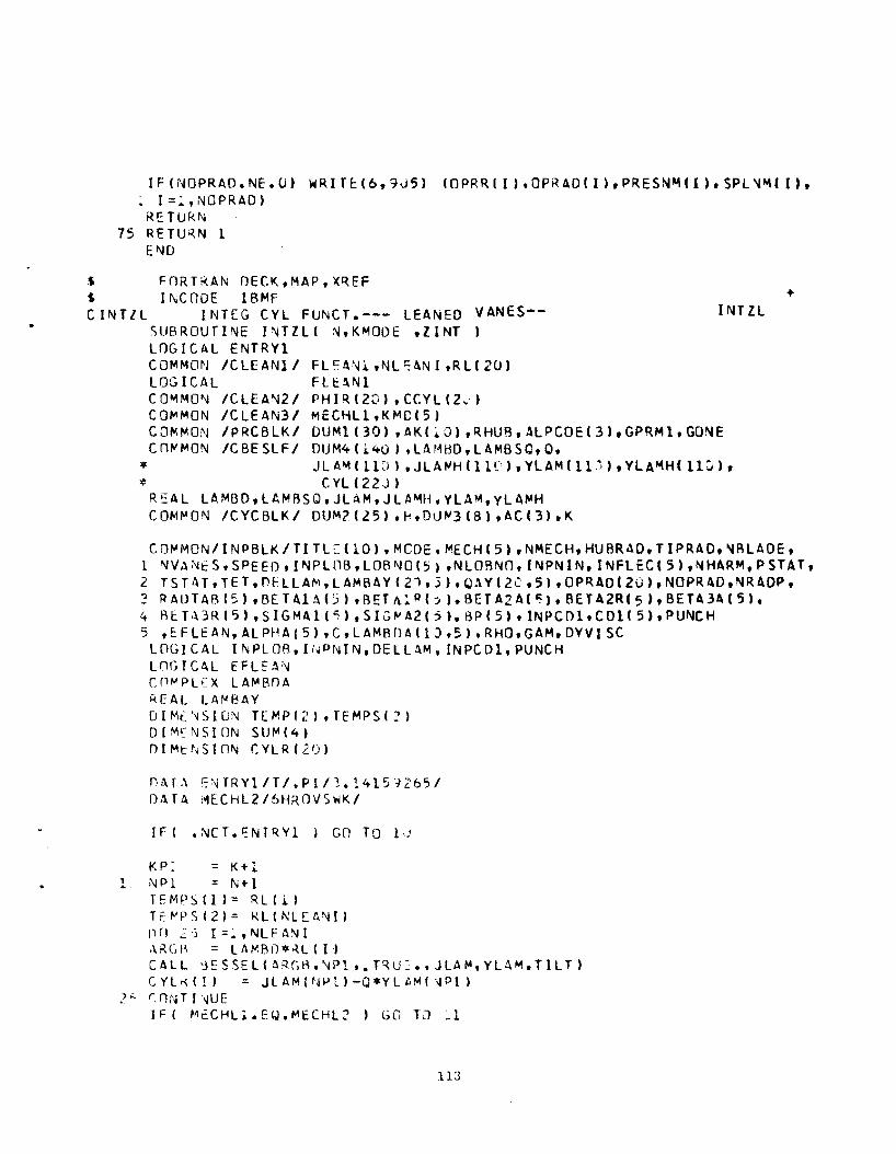
IF(NOPRAD.NE.()) WRITE:(6,9d5) (oPRRII).OPRAO(I),PRESN~(I),SPL'l~(I),

~ I=;',NOPRAO) RETURN

75 RETU~N 1 ET\lD

$ FORTRAN OECK,MAP.X~EF +$ INCODE I8MF

CINTlL INTEG CYl FUNCT.--- LEANED VANES-­ INTll SUBROUTINE I~TlL( N.KMODE ,lINT )

LOGICAL ENTRYl COMMON ICLEANII FL~ANi.NL~ANr,RL(20)

LOGICAL FLI:MH COMMOT\l ICLEA"J21 PHIRIZO) .CCYL(2",) COt-lMON ICLEAN31 MECHLl ,KMC( 5) CO~,MON IPRC8LKI DUM1(30) .AK(iO),RHUB,ALPCOE(3),GPRMl,GONE cntJMON ICBESLFI DUM4(i4Q).LAMHO.LAMBSC,O.

• JLA~(11J).JLA~H(110).YLAM(11~),YLA~H(llO),

CYL ( 22.j )* R~AL lAMBD,lAMRSQ.JLAM.JlA~H,YLAM.YLAMH

COMMON ICYCBLKI DUM?(25).H.D0~3(8).AC(3I,K

COMMON/INPBLK/TITLC(lO).MCDE.MECH(S),NMECH,HUBRAD,TIPRAD,~BLADE,

1 T\lVA~tS.SPEEO,INPLnB.LOBT\l0(5) ,NLOBNO.INPNIN.INFLEC(S),NHARM.PSTAT, 2 TSTAT.TET.DELlAM.lAMBAY(Zl,j).OAY(2C,5).OPRAD(lU),NOPRAD,NRADP, ? RAUTAB(5),BETAIA(5),RET4~P(j),BETA2AI~),BETA2R(5),BETA3A(5),

4 RcT~3R(51,SIGMA1(~),SIG~A2(j),8P(5),INPC01.CD1(5),PUNCH

5 ,EFLfAN,ALPHAIS),C,LAMADAIIJ,5),RHO,GAM.DYVISC LOGICAL INPLOR,Ii~PNIN,DELLAM. lNPCD1,PUNCH lnGICAL EFLEAT\J C(1MPL'~X LA~8nA

r<EAL LA""RAY DIMi~SIUN TEMPI21,TEMPS(!) OIMfNSION SUr-1(4) DIMt~SION CYLRIZO)

n~T~ ~~TRYl/T/.P[/1.1415}2651

DATA MECHL2/6HROVSWKI

IFI .NCT.~NTRYl I GO TO l~

KP: = K+l 1 ~Pl = N+I

TEMPSIl)= RUi) Tf~PS(2)= Kl(~L[A~II

Dr) .:>j I=:,NLE=A\.lI ~~G~ = LAMBO*~LII1

CALL ~=SSEL(~RGB,~Pl,.T~U= •• JLA~,YLAM.TlLT)

CYl,,(!) = JlAMPJ~U-Q*YLt>M(-lPl)

) '" r, n:\J T I ''-J UE IF I McCHLl.EQ."'ECHl2 I GO TJ ~l

113

C IGV-ROTOR

HARN:NHARM IF(NHAR~.EQ.O.O) HARN=l ANG1=-FLOATfNBLADE#HARN) GO TO 2.0

C R(lTll~ -OGV

11 ~~b

ANGl ~ ELGATl CONT P·HJE FIVE=PI/12.1J TT:J. ,j XINT=O.J no 2CJ 101=1,36 TT=TT+FIVE lII\jT ::: O. DO l·~O J:::l,KPl

KMOD~*NVANES

C iVALUATE INTEGRAND AT RL S

1i

DO ~0 I~l,NLcANI

IF( J.GT.l ) GO TO 18 PSIR = ANGi*PHIRlit

Itl ~o

C~NG.=COS(TT+PSI~)

CCYl(I)= RL(I)*CYl~ll)*CA~Gl

GO TO 2" CC YU 11 = RU 1) *CCYL( 1)

CON TI NUE

C INTeGRATE USING LSPFIT

C : C

T EM P ( 1) = v. CALL LSPFIT(~L,CCYL,NLEANI.T~~PS.TEMP.2.-~)

SUM(J)= TEMP(2) lINT : ZINT+AClJt*SUM(J)

1'). COtHII\IUE Zl=ABS(ZlNT) IFCZl.GT.xINT) XINT=ZZ WRITEl~6,30U)M.II~T.TT,PSIR.XINT

3Uj FOR~~T(bHM= ,I4.10H llI\lT=.F14.5.6H :F14.~,~H XINT:,Fi4.5J

20'.; CONTINUE ZItIlT=XINT

TT-.F14.5.8H

RFTUqN ENO

114

+$ FORTRAN DECK,XREF.~AP VISCWI<S INCODE IBMF CVISCWK VISCOUS WAKE INTERACTiON C FORTRAN-Y l~APR:975

C SUBROUTINE VISCWK{UTIP,~ACR,AlPHA1.AlPHA2,Vl,V2,SIGMA1,

1 Cl.C2.BP.CD1,NRADR, TcT,MODf, GAMMA,~HARM,TILT)

COMMON ICTHETA/THETAE{ZQ) COMMON ICLEANll FLEAN1,NlEANI,Rl(20) LOGICAL ~LEANI

COMMON ICLEA\l21 PHIR(20) .CCYUZO) COMMON IPRCALKI DI/MU30) ,AK(10) ,RHUB,AlPCOE(3),GPRM1,GOI\IE COMMON ICYCRLKI DUM2(25).H,DU~3(91,AC(3),K

OIMENSICN PHlfS) DIMENSION RADR(1).ALPHAlfl),~lPHA2(1).Vl(1),V2(11,SIGMAl(1).

: C. ( : I • C2 ( 1 ) , BP ( : ) • C0 i II I • GA ~ MA ( ~ I LOGICAL TILT fU-AL JIZl DOUBLE PRECISIllN SUM INTEGER TURBIN DATA PI/3.141591 DATA TURBINlbHTURBINI

5 RCJ1=:J.6 RCU2=1.391*PI ~C03=O.283

IPOINT = 2 11 CONT 1NU~

no 3 1=1,5 j PHIIII=O.O

IFI.NOT.FlEANll GO TO l~

I~ITI~LIl[ INTEGRATION RADII AND LEAN PARAMETERS c C~LCULATE ANGULAR DISPLACE~E~T.

"JL = NLEANI-l OR ::: ll.-H)/FLOAT{NL) RL{ll =H "0 1. I=Z,NLEANI ;)l(ll ::: RllI-l)+OR

1 CONTI~UE

ao 2. l=hNU.. ANI q,U = RLlII ALPR = ALPCOEll)+RL:*{ALPCOcI2)+ALPCOE(3t*~Llt

I\RG ::: PI-ALPR TE tol M, = HI RL1 *S };\I I ARG) GR- = ALP~-AR.CSI·H TF~'" ) THET~~II)= AK(6)+~Ll*IAKI 7)+~Kld)*RL1)

PH!R(I)= GR+THETAE{I)

115

~ CONT P'JUE CALL LSPFITIRL,PHIR,NLEANI,RACR,PHI,NRADR,O) WR I. E I C6,12 ) I TH ETA E f I ) , I :: 1 ,2 OJ ) , IPH lR ( I ) , I:: 1, ,0) , ( RL( I ), 1=1,2) ) ,

1 IAKII),I=l,lul,IALPCOEII),I=l,j) lZ FOP,t-IATflHl,9HTHETAE( I )/2( tOFi..').4/ l,7HPHIR( 1 l/2( 10flO.4/),5HRL fI)1

1 2110FIO.4/),5HAKII)/IOFIO.4/9HAlPCOEII)/3FLO.4) WkITtl06.l31

.. ~ FORM/HLHl) 10 DO qJ I=t,NRADR

C1SEMI :: CIII)/2. (2SEMI :: C2(11/2. ~LPH~R = O.0174S~3*AlPH4~II)

~LPH2R :: O.0174533*ALPHA2IT) CSALP~ = COSIALPH1~1

U = UTI P*RADR I I ) HFT~ = ALPH1R+4LPH2R OMEG& = C2SEMI*PI.*U*SIGMA£IIl/(C:SEMI*VZ(I) 8 = HPIII+C1SEMI*CSAL P l+C2SEMI*COSIALPH2R) XP()C i. S = I C2 SEMI I C1SEMI I *(RI { (2 S EMI*CSAL P 1. H· VU I 1I{ 2 • *1/ 2 ( I ) ) ) - ~ COL GO TU(15,20),IPOINT

15 OElTA = 0.3 GO TO 25

2J DELTA = 0.2 CD5=COIII)

2j FKl = RCD2*Vlll)*CDllll*SINldETAJ*SIGMAlII)*SQRTIXPOClS)/ ~ IVLII)*CXPOC1S+DELTA)*CSAlP~)*COS{PHI(I»

FK~ :: -?I*IRC03*SIGMAIII)/CS~lPl)**2.CDl(I)*XPOClS SU,.. :: O. DO j .. M=1,4(\ F~='" FMOMEG = FM*OMEGA

.:~ CONTI!ljU~

CALL BESSELIF~OMEG.l,.F~LSE •• J,DUMY.TILT) IFITILTI GO TO 45 FJSSU = «J(21**2+J(~)**?I*{J.lbli+FMOMEG)11

(O.loll+(O.1811*Pl+l.J*F~OMEG.2.*PI*FMOMEG·*2)

TtRM = FK1*EXP(FM**2*FK21*SQRT(FJSSQ) SUM = SUM+TERM IF(NHAR~ .NE. 01 GO TO 35 rF(OhBSITERM/SUM).LE.l.E-~) GO TO 35

3J CONTINUE WR I TF (6,9001

9C0 FOR~ATI61HO***SUBROUTINE VISCWK. SERIES CONVERGENCE FAULT. RETURNI ~NG*·*)

Tl LT = •TRUE. r,1') TU 45

j5 GAMMl\CI) = CC2SEMI*V2(1)/12.I*SUM "t) CONTINUE 45 RE TURN

END

116

$ F-ORTRAN OECK,MAP EIGENL So I NC[)I)E IBMF eEl GEN EIGENVALUE RUUTINE c FORTRAN-Y 22APQ. C c THIS PROCEDURE DETE~MINES THE CONSECUTIVE EIGENVALUES LAMB~Y{), .. ASSOCIATED RESIDUALS RESDAYC) ,A(~D COUPLING COEFFICIE'lTS CAY{. OF'" c THE CHARACTERISTIC EQUATICN c c Y-(LA~BD *H)*J-(LAMAC • Y-CLAMBD )*J-{LAMAD *H) = 0 c N N,M N N,M N N,M N 'I,M ,.... C FOR A GIVEN RADIuS RATIO H A~D SEQUENCE OF MODE NUMBERS N,~

C (M=MI,Ml+l, ••• ,MF) WHERE N A'~D M =0. C C SUBPROGRAM REFERENCES - CHARFN CEVALUATES CHAR FUNCTIO~).

C C C

SUHR0 IJT I NEE I GEN( H, N, MI , MF , LAMB AY, Q AY, RES f) AV, TI LT ) DIME~SlON QAV(1),RESDAYC1),CJNVECCS) OOlJ~L:: PRECISION L4M(3),tPSU),A,B,C,DISC R~AL LA~BAY(i),LAMPO,LAMRCl

LOGICAL TILT,FLAG DATA O~LAM/l.I,DELAM210.~1

TILT" • FALSE • FLAG=.FALSE. ICNT= ... MP: =1"11 +1 ~RG(JTS"~F-MI+l

c

c IFI~.~~.O.OR.MI.~f.0) GO TO _ L t.1~ I~:) " •.. y.;~I T::' 16.'1(1)

9Jl l-f)k~ldl107HC.~**StPi\(lUTl\ ;1",'-" ~Ic.[r-..VALUi: A"JD COUPLI"JG CO:':FFICh..· ion ,\RE Ncr DEF I"icfl FOR ro'l'Cf ''lUMBER ~ •..• ,.(t:TUR"JING***) (~:] T, 1 5 ~

IFIN.GT.O) GO TO 2 lAI'1HO O,MI (~I O) NSNCH=l LI\~BD=i.

Gil LJ 5 ,.,. L ,'1-1 (}Ii "'J, OJ I l!'l ",•• "'1 I ::;; , 1 .2 , •••• )

~ '\iSi'JC,"j=O L ,\"1, j [) '" r LnAT I ~j ,

- C 1\ L L CHARF '\j I , I • L AI~ ~ n , ~~ , TIL T• ;:. ;> S f\j • (' )

rrIT[LT) ,;0 TO ). [Fl:-:PSN.tC.J.1 GU rn 45 IF(FLAGI GO Tr l~

117

11 FL.AG::.TRlJE. rpSNl::£PSN LAr.., l\ D1 :: LAM B0 L~M~O::lA~BOl+DEl~~

1.) GO Tn 5 IFIEf>SN*EPSNl.LT • .i.) IF1"JSNCH.EQ.MPl) GO GO TO 10

,. ... 2. ­ LAM (1 }=LAMBDZ

LAM(21=LAMBDZ+DELAM2 lAM(31=LA/lBO EPS(l)::EPSNl

NSNCH="JSNCH+1. TO 20

CALL CHARFN(H,SNGLILAM(2ll,~.TILT,EPS2,Q)

IFITILT) GO Te 55 IF(cPS2.EQ.O.l GO TO 50 r:PS(ZI=EPS2 ':'PS(3)=EPSN NlTER=O NITE~=NlTER+l

LAMBDl=LAMBO IFINITER.LE.201 GO TO 25 WKITE(6,9CO) ICNT,CONVEC

9~_' FORM4Tld9HO***SUBROUTINE EIGEN. CONVERGENCE NOT ACHIEVED IN 20 ITE ~RATlONS. ITERATE HISTORY fOLlOwS./5X,6HLAMBOlIZ,3HI$ 2 5(lX,~15.8)/IX.31HCONTINUING WITH LAST ITERATE••• )

GO Tn 45 25 h=( ILAM(2l-lAMll»*EPS(31+(L~M(1)-LAM(3»*EPS(Z)+(LAM(3)-L~M(2».

E PS(t ) ) I ( ( lAM ( j ) -L 6. M(2 t ) *(L AM I 2) -l AM I 1 ) )"''' 2 ) B = I I L Afill 2 1-l AM( 1) ) *ll. • *L A~ t3 ) -L AM« Z ) -LAM I 1) ) *EP S( 3 )

1 -ILAfII(3)-lAfIIll»**Z*EPS(2)+ILAMI3)-lAMlZ»**Z*EPS(1», I I LAM I 3 ) -L AM ( 2 ) ) *(lAM ( ;; ) -L 4. '" ( 1 ) )** 2 )

C::(lAMI3t-LA~11»*EPSI3)/lLAM(21-lAM(1»)

0ISC=OSQRT(R**Z-4.*A*C) HlAM1=-2.*C/IB+DISC) HlA~2=-2.*C/IB-DISC)

ROUTl=lAM(3)+HLAMl RnOT~=lA~(3)+HLAM2

IF(RCOTl.GT.LAM(1).ANO.RCOT1.LT.lA~(3)) GO TO 30 LAMBD=ROOT2 r,O fO 35

~~ IFIROOT2.GT.LAM(1).AND.RCCT2.lT.lAM(3») Gn TO 31 LAMRO=RCOTl GO TO 3?

3: IF(B.lT.O.) Cc TO 32 lAMRD=RCOTl GO TO 3S

118

\

32 I.A",Bf)=RCOT235 IFINlfER.GE.16} CONVECCNITf-R-lS)=LAMBD

CALL CHARFN(H,LAMBO.~.TIlT.EPSN.Q)

IFITILT» GO TO 55 IF(f.PSN.~Q.O.) GO TQ ~S IFIAoSIILAM~D-LAMB01)/LAM~nz).LE.1.E-4) GO TO 45 IF(LAMBD.LT.LAMCZ) GO TO 4~

IA"""l)=L~,..tn

LA""'(2)=LAMBD f PS (1.) =f.IJS{2)

(PS{Z)=EPSN Gn TO 2L

4' LhMI::')=Lh~(2)

lAt-lIZ) =LA~BO

~PSI»=EPSI2l

EPS(21=EPSN GO TJ 2L

)0 LA''''RIJ=LA~(2)>

f;:PSN=J. 45 ICNT=ICNT+l

lAMA~Y(ICNT»=LAMHD

QAYIICNT)=Q PfSOAY( leNT )=EPSN IF- (I(NT .E:C.NRCOTS) GO TO 6;) LAMuO=L~MHf)+l.

MP~="'Pl"'l FLAG=.FALS~.

en T') 'J " TIL T =• r;;.: li" •

0::' PFrlpri f ~i r;

\ rIJ..).f ..,{~.\ r~:("K,~;i\~) +

it r :,~ Cit , ) t: 1 r- ~ ~ r CHfiQF\l

CCH (d"', r ~; ::. !1,', '" ,'\- r t I~, :, ~; ;' ; C }-', I I \! C, f 1l~ 4

C F0P'RA~-Y 1:~P~1~7~

c.­v

'y - I I. '\ ... H!) ;\ * l~ ) * J - ( L /"v ~ n .., - y - ( l A~ 8 nA » lOr J - ( LAM fir) A *H I I\J /I, • w. '\J ";0 M N N. M~. 'J • '"

• ,. ,.. .... -"d /!.~',(~crH~0 Cf1u"'LI'~~; COc.FFICIE:i\lT Q FOR A GIVE\! ,.

H.l:I,MhnA.i\\~n ~'J 1..1 =\ -~i .d • .­'-­

" 1 , l' fj :': l i : ! r" t C t i AQ, H, I H. l AM !" ,\ • \j • r II T f f lJ NC , () • ;\ i '~': >1" 1:;N YL/'I M I ~ '..;':: I • YL A"'1 II ( .. ):.: ) k ~ All. A /oJ F< f) II • J L A~ ( 1 : 2 » • J l A/-' H ( _ ,2 I LlC r C:I L TIL T rILr~.r-ALsr:.

119

N~l::"J

r-,jP.l.:: 'H- 2

CtLL ~ESSEL(LAMBDA,N+l,.TRUE.,JLAM'YLAM,TILT) IF(TILT) GO TO 10 CALL BESSEL(lAMBDA*H,N+l,.TRUE.,JLAMH.VLAMH,TIlTJIFITllT) GO TO l~

IF(N.GT.O) GO TO 5 FUNC=JLAM(2)-YlAM(:J*JLA~H(2J/VLAMH(ZI Q=JLAM(Z)/VlAM(2) (;0 Tt; to

5.fUNC::(JLl~(NMl)-JlAM(NPl)-(YLAM(NMl)-VLAM(NPlt)*(JLAMH(~Ml) 1 -JLh~H(NPl)/(YLAMH(NMl)-YLA~H(NPl») Q::(JLA~(NM1)-JLAM(~PIJ)/(YLAM(NM1)-VLAM(r-,jPl))

~d RETlJ;~N

~ND

$ fORTRAN DECK,MAP .. S I NCflDE I B~F R?YCY~

CKPYCYG POLYNOMIAL-CYLINDER FU~CTION INTEGRAL C FORTRAN-Y 22~PR.915

c c THIS PROCEDURE EVAl~~TES THE RE~L INTEGRAL ,.... C *IWPPER ,.. .... '" c RINTG = ~ R**P*Z (LAMIlDA*R).OR ... ,..

'" N c *RLOWER c

SUBROUTINE RPYCYG(P,N,LAMeOA,RlOwtR,RUPPER,CYL.RI~TG,TILT)

TIIH EGER P, PM 1 R.EAL LA~ROA

OIMENSION CYL(110,2) LOGICAL TILT liIMENSION SII~(2),R(2)

REAL INTlNP c C ••• ARGUMENT CHECK •••

IFIP •.GE.l.AND.N.GE.O) GO TO j

W~ITtlb,9CO) N,P,lA~BOA,RlOWER,RUPPER

90~ FOR~AT(4~HO.**SUHROUTINE RPYCYG. ARGU~ENT FAULT. N=I~.lH.P=12, • 1 oH,LA~BDA= cl5.at8H.RLOw~~::Fe.5,8H,~UPPER::F8.5,14H. RETUR~ING**.)

TILT:: .TRUE. (;O·TD 70

C ••• 1'1 1 ••• i) ~MP = N-P

PIal:: 1. 00 L0 J::~tP

1~ PlrH :: PI01.FLOAT(N~P+2*J-l)

120

c C ••• I"JDIClS •••

P"Il :: P-l NP2 = N+2 NPP :: N+P IPOINT :: ~OO(NPP.2)+t

GO TO(15,201,IPOINT C •• (N+P) Ev£t~ ••

l~ INOX1 = NPP/2-1 GO TO 25 ,..

v •• (N+P) ODD •• 20 INUX~ = {NPP-ll/i-~

c C ••• 1 (10011 TS l.eop •••

,::5 ~(:'l :: RlOWER R(Z) :: RUPPER ~COl = -l./lA~BDA

DO 6'j 1=1,2 c •• COMPONENT 1 ••

SliM ( I I = R( I I • *P*C'( L ( '" P2 • I ) I L AM BOA (F(P~l.LT.l) GO TO 4·)

•• COMPONENT 2 (SUMMATION OVER K=i,P-l) •• DO 3:. K=1,PMl PlOt:: l.

:)0 3,; J=l.K 30 PIOl = PI02*FlOAT(NMP+2*J-ll

INDX = NP2+K SliM! I) = SUM{ r) .;{ II **(P-K)*':Vl( JlWX.II*PI:2/LAMBOA**(1(+1)

~'') C!l;'i!!'JUF:: 011 C! jM ~)f ;;··~:..~,."T ~!' i<

h "- r',t<-,

I fo, Jf : j "J ~ .. iJ ". ,,~: t:' f \

..., :.J ! '\! 1 i i '-; P .::: ~ ( ~ i ~ \~.: ~:: f t. : : !,~ nX t Z: 1'~1 <' '~ r", ;, c <~ " C :) i, ~ j ;'! ¥ .' q P

_,. (1','; ;:·j~f-,·~,,:,r..;,iPnr'i1

.:;" I I\)l lit) .0 ~: j l' I'; i' • pI, ','!, ,~ C. '( \. <. d i

.., C '-1 I ': '-' r ~~ ,) " : i .. '1 r, i' * ; 1 l 'i Ii i.. Af~" \, l-iJ lAM P 9 T It, T } !t(fll'[) GU rr: 7,.1 T''41i ,;..' '" jr"r/,,;,'.:'( il*r(VI (l~', Hl.';;~""903*IHOlAMR*C'L(2~r)

.. f 1 ._ C 1\ M i~: ~ L 'f ~ :, ~ l' • J ~ .~

'... "l.' ~~ ~ j ~ .~ ("~ U J~. 1 I It".! .;. * j ;.); / :\) ;..\ / l. :-.;.?~ HD h *- *- p Ql~4r(;:= ,)U/lol(Li~'\lJM(li

,) ~J f T ( J j..,> .\l

f ~j ~~)

1.2 ;

$ FORTRAN DECK,MAP $ INCODE IBMF C~STRUV REAL STRUVE FUNCTIONS - HO(X),HlfX) ­C FORTRAN-Y 22APR1975 C

SUBROUTINE RSTRUV(X,HOX,H~X,TILT)

LOGICo.L TILT REAL J)«311 n}MENSION YXIZ) LOGICAL NEGl( TILT = .FUSE.

c C ***ARGUMENT TYPE •••

ABSX = ABSIX) IF(ARSX.NE.O.) GO TO 5

C •• SPECI4l CASE. X=o •• H")X = (,. H1X = C. r.0 TO 45

S ~~EGX = .FALSE. IFtX.LT.0.) NEGX = .TRUE. IF(ABSX.GE.10.1 GO TO 40 ,.

" C ***ARS(XI 1 *** Chll BESSELIABSX,30,.FAlSE.,JX,DUMY,TILT) [fITILT) GO TO 50 IFI.rmT.NEGX) GO T[J 15 DOlL 1=2,30,2

10 JXllJ : -JX(I),.v •• HOIX) - A~S 55(12.~.19) ••

1:- SUM = JX(l) 00 20 K=1,14 TER~ = JX(Z*K+2)/FlOAT(2*K+L) IF(AtlSITERM/SUM).LE.l.E-f) GO TO 2S <:;UM = SU~+- IE RM

2v CONTINUE 24 WRIT=(6.900) X

91, FORMATI25HG***SU8kCUTI~E ~STRUV. X=E15.A,40H. SERIES CONVE~GE~CE F :AULT. RETURNING••• )

GO TO 50 25 SUM = SUM+TERM

•H0x = 1.2732395*SUM •• H1(XI - AMS 55(12.1.20) ••

SLIM = JXn)/3. no ~'. K=2.15 TERM :: JX(2*K+l)fFLOATI4*K.*~-1)

IF(~HS(TERM/SU~).LE.l.E-h) GO TO 35 SUM = SU~+TEiH1

~,,' CONT rNUE GO FJ 21

122

3~ SU~ = SU~+TERM

Hlx = L.6366198*(1.-JX(1))+1.2132395*SUM GO TO .. 5

c C ••*AR$lX) =10•••

4" CAL L q ESSEl( ABSX.1 , • TRlJ E. ,JX, YX, TII T) IFlTILT) GO TC 50 ..,. •• H(lX),HllX) - AMS 55l12.:.30).(12.1.31),l12.1.18) •• T = l./ABSX TS~ = r •• 2 HOX = YXll)+O.63~6198.T*ll.-TSQ*(1.-TSQ.l9.-225 •• TSQ1» IFlNEGX) HOX = -HOX HIX = YX(2)+C.636619d*ll.+TSO*(1.-TSC*(3.-45••TSC»)

C 45 Rf TUR.N ">0 TILT = .TRUE.

CALL FXE~(66)

GO TO 45 F"JD

123

$ FORTR~N DECK,MAP,DEBUG.LSTOU,X~[F t3ESSH .INCO~E IBMF CBE SSEl lSt-VlD KI~m BESSEL FU"'JC (REAL ARGI HE 5 SEC·(,l C FURTRAN-Y 22APQ 1975

HESSE.' 2 c THIS PROCEI)\J:{E cVAlU4TCS BESSEL FUNCTIONS OF THE FIRST f'i:SSE.,:·3

AND SECOND KINDS OF REAL POSlTIVE ARGU~ENT X AND REAL '~:-SSEJC4

INTEGER ORDEI{S P=ljtl,2, •••• N. SCKIN') IS A LOGICAL lllJDICHOR a:: S Sf: i);) 5 SPECIFYING WHETHE~ OQ ~OT SECONC KIND FUNCTkoNS ARE 1E~SEI~

D~SIRfO. FIRST AND SEC1~D KIND FU~CTln~S ARE RET0R~ED IN -\CSSEOJ7 R~Al VECTORS J AND Y R~SP~CTIVELV fROM LOW TO HIGH ORDER 9~ 55£0;;8 (N+l ELEMENTS eACri). THE LOGICAL lNOICATO~ TILT WILL BE BESSEv09

c .TRUE. q~ RETURN F~CM aESSEL IF ~ATAL DIFFICULTIES ARISE. HSSEJlJ BESSOll BE SSE012 B~SSE'13

BESSU14 fH' 55:::015

c BE 5SE016 c ElESSE",17

***AUXILIARY SU3P~OGRAMS**. ':IESSEO~8 c AlNGAM - NATURAL LDG CF GI\,.,MA FUNC TI O~ RESSE:19

BES5E.·2:; Bj:SSE~\21

c BESSE,22 c BESSt023

SUBR8UTINE BES5ELIX.N.SCKIND.J,Y.TIlTI M SSE': 24 i<t=4l JIll I)€SSEOi? DIMENSION VI! 1 BESStD26 LOGICAL SCKIND.TIlT BE SSE ",27 fl! ME;,S ION f (3CC I I1ESSE i 28 R£:AL JOX :J,\:SSEOZ9 CALL FXOPT(6g,1.1.JI TILT = .FAlSE. B:: SSE :, :, .\

BE' SSi::'=-~ C ***ARGUMfNT CH=CK*** IE:~Si:J)2

IFIX.GE·.(\.O.AND.~.U:.U:LI GD TO S Kr SSE, 33 l-i~1 T' It.Yt;J) X"~.SCKlrw B"5SE.34

9uJ f-OI<.:...1t.TI2~}HO**~'SllGROUTl/\jt: 'J':SStl. x;;. f:15.a.3H N-=I3,oH SCKINI)=L2. BESSE035 1 24H lIRGllMENT FAULT. ~ETUk'JI'iC.**1 BE S5E036

GO TD 1 b5 BE 55!:: 137 ::. I F I X• 'JE. '~.) GOT 0 Z') 9E5SE;.,38

BE SSE03g JLI = 1. RiO: SSL4J IF-tl'J.EO."') GO TI) 1':. R;:SSE041 "4P.. -:: N+-.1 ~[SS£842 ro .:" I:t:,NP; BESSEi)43

1· Jill = ~. BESSEJ44 ~:: IF (.·jQT.SCKI~DI GO TO l&lJ 8f.SSE045

W~IT~(6.9051 X.N.SCKIND BE SSE r)46 9J5 FORMAT(~SHO*#*SUBRJUTINE aES~lL. X= E15.B.3H N=I3.8H SCKIND=L2. 8FSSE )1+7

1 ~7H y(~,~l GOES TO NEGATIV~ INFINITY. RETUR~lNG***' RF.SSE,J48 GO TO :65 BESSE049

p,ESSE:)50 c BFSSEj51

124

20 CALL OVfRFLCIOVFLI RCOI =ALOGIOCO.5*XI Re02 :: O.57721566+ALOGCO.S*X)

,INOXAP = IFIX(X)+2 M = MAXOIN.IFIXCX»-lO NPl = N+l

c c

25 M = M+IO MPl = M+l DO 3;) 1=1 ,MPl MPRM = MP1-l

C (MPRM=M,M-l.M-2, ••• ,2,1,O)FMPRM :; ~PRM

E XPJ~4)( :: FMPRM*RCO l-:). 4342944S*ALNGAM (FMPRM+l.1 IFIE)(PJNX.GT.(-2G.I) GO TO 35

30 CONTI~UE

WRITE(b,9101 X.N,SCKINO 910 FORMlTt25HO*.*SUBRQUTINE BESSEL. X= E15.8.3H N=I3,8H SCKINO=lZ,

1 35H J(X) AMPLITUDE FAULT. RETURrJING***) GO TO 165

35 MPRMPl :; MPRM+l IFI~PRM.GE.NI GO TO 45 MPRMP2 :: MPRM+2 00 "T) 1 ::MPRMP2 •. NPl

40 J ( I) :: J. c C .*.FIRST KINO FUNCTION JIXI**.

I:; L-II+Z

C 45 L :: MPRMPl

IfIMOOll,ZI.NE.O) l :: L+l I FlA:~ :: 1

c 50 L :: L+'t

IF(L.LE.2~OI cn TO 55 Wr<.ITi: \.'.,91';;) X.N,SCl<IND

9J.5 FJRMH(Z5 ti O**"'5UoROUTINE BES:;t:L. X= E15.8.3H N=I3.8H SCKIIIID::L2. 1 5LiH P'Hf:RNAL STURAGE' CF aR,,:,\V) EXCEEDED. ~ETURNli\lG***'

1,,0 TG l6'5 55 LM~ .:: L-:

lP~ ..: L+l FtL+21 :: O. F ( LP 1 I ::: 1, E- ) \J

.. 00 t>'~ II~:1.,l

C Il~l+1.L.L-l ••••• 4.3.2) Hl-l.I ,. 2.*FLOAHl-l)*FCI)/X-f(I+l) CALL OVfRFLllOVFLI

60 COf\lTINUE: IFIX.LT.IG.1 GO TO b~

BE SSE052 BESSE053 BESSE054 RESSE055 BESSE056 BESSE057 BES5E:>58 BESSE059 BESSE06J BE SSE061 BESSE062 RE5SE063 BESSE064 BESSE065 BESSE066 BESSE067 BESSE:Jb8 BESSE06CJ BE5SE070 f1E SSEOll BE SSE~ 12 BESSD73 RESSE07~

BESSEG7<; BE SSE)76 BESSf077 BESSE078 BESSE;"79 BESSE080 BE~Sr,O~l1

RiSS::C>82 ;~E SSE')"', 8::S~\=Je"+ P t: SSE :)iJ,')

f'FS',':OBt. b ': :\ ~ ": " ,;, ., g ES ~) ~ ,) \.~ ;"\ h::'S):'~;{;(1

de. s:.;·· v'';)

2. [S ,)t- ;.>'1: Bi::SSE09? '..ifSS[[)93 HSSE)')l.,. R£)'}['095 gE 5S£o096 BES~.l:Y}7

BE S )';:;<:1 ~l

BESSE106 BESSf:107

125

c IF(IFLAG.EQ.') T = :./X T')Q ;; T*T

GO TO 63

BESSEloa BESSEI09 BESSEll':> BESSEi.ll BESSE1l2

­

JOX = (1.+TSO*C-J.625C-l+TSO*IO.1035156ZEO+TSQ*(-O.54Z84668E0 BESSE113

1 i

+ TS \J * (. • '384 % 9 g 6 E: - TS Q*: . L 6 : 8 67<) E3 ) ) ) ) ) ,.. SORT C!). 63 66198* T I * COSC~./T+T*C-J •• :5EO+TSQ*Ca.b5~04167E-:+TSU*(-O.20957031EO

ljFSSE1l4 H,:SSEl15

3 +rSO*CO.163 A0463tl-TSQ*0.23475128E2»)}-O.7R539815) Bf:SSE116 63 SUM = FlII/J0X BESSE1l7

IFIABSISU~).NE.O.1 GO TO 66 6ESSEl18 WRITE<6.9211 X,N.SCKIND,JiJX BESSE1l9

921 FOR~ATC25HO***SUBROUTINt RESSil. X= E15.d,3H N=13,8H SCKIND=L21 Bt:SSU20 1 ')X,"l5H UNDERFLOW FAULT IN PHASE-AMPLITUDE APPROXIMATION (J~'X= BESSEl21 2 E15.8,15H). RETURNING••*) BE SSE 1.22

(;0 TO 165 BESSE123 c BESSE124

to .. SUM;; i.E-3C BESSE125 O~ 65 11=1,LMi.2 BESSE126 I = l-II BESSE;..27

c (I=l-1.L-;.l-5, ••• ,5.i,11 BESSE128 oj SU~ = SUM+FII) BESSE:"Zq

SUM = ~.*SUM-FCl) 8ESSE130 60 APRO~l = F(INOXAP)/SUM BESSEl::l

GO TO(7~,75),lflAG BESSE132 7u APRDx2 = APROXl BESSE133

IFLAG = 2 BESSL34 ron TO 50 BESSE135

1~ nElfA = APROX1-APROX2 BESSE136 ~~R;;~BSIOELTA/APROX2l

IF([RR .lE. 9.E-bl GO TO 9J IF(IOVFl .NE. II G'J TO 3j IF(EkR .LE. 9.E-~1 GO fQ q)

w~IT~(6.920) X,N.SCKIND.CK~

920 FORMAr(~5HO***SUBKOUTINE BESSEL. X= ElS.B,3H N=I3,8H SCKIND=l2/ BESSEI02 ~ 5X,56H ovERfLOW FAULT IN BACKWARD RECURRENCE FOR J(X). ERRDR= , X Fl'::.8)

(J{l Tel 9.J

,. ....

B~ 4PRox2=APROXl GO TO 5<.; BESSE:.39

BESSE140

•

gJ 00 95 I=~,lP~ BESSE141 9:5 F CI I = F ( I • I SUM BESSE142

K ;; NP~ BESSE143 IFIl.lT.NI K = lPl BfSSEi~4

, , . .. '" . no lOu JII) ::

J=1.K FIll

BESSE145 BfSSH46

105 IFC.NOT.SCKINDI GO TO 160 BESSE147 c AESSE14A

126

C •••SECOND KINO FUNCTION VlX) ••* BESSEl49110 IFCl.lT.6) GO TO 2S BESSE150c BESSE151SUM = F()) BESSEl52

l02 = LIZ BESSE15300 ~25 1=2,L02 B!:: SSE 15.4 TERM = (-1 •• *.(I-ll*F(Z*I+11/FlOATII) BESSE155IF! ABSITERM/SUMI.LE.l.E-61 GO TO 130 BESSEl56SUI" = SUM+TERM BESSEl57

125 CONTINUE BESSE158GO TO 25 BE SSEl59

13~ SUM = SUM+TERM BESSE160 YOI = O.6366198*IRC02*F(1)+2.*SUM) BESSE161

IFIN.EO.O) GO TO ~bO BESSEl62 C BE SSElb3

SUM = F(4)-F(2) BESSElb4 LM202 = IL-2)/2 BESSElb5 DO 145 1=2,LM202 BESSE16b TERM = 1-1.)**I*CFC2*II-Ft2*1+211/FLOATtI) BESSElb1 IFl ABS(TERM/SUM).LE.l.E-6) GO TO 150 BESSEl6B SUM = SUM+TERM BESSEl69

lltS CONTINUE BESSE110 GO TO 25 BESSElll

150 SUM = SUM+TERM BESSEl72 Y(2) = O.63b6198.tKC02*F(2)-FCII/X+SU~1 BESSEl73 IFIN.EQ.ll GO TO 16U BESSE174

c Bl:SSE175 00 155 1=1,NPl BESSE176 YIII =- ;;:.$flf)ATll-2'*Yll-d/X-YC{-21 BESSE:l17 CALL ~1VlRFl( IliVFLl BfS':;U76 IFI10~FL.NE.l' GO TO 155 BfSSflH [MI " l-l t\,=SSf180 wRl Ti-lo,9251 l...N,S(KINf.'l.llo1l bi'SSElSl

92~ FORMATI25HO***SUBROU1INE BES5tL. X= E15.~.3H N=I3,8H SCKI~D=l2/ bf-SSflR2 1 5-.~oH O~E~fLCW FAULT IN FOR~ARD RECURRENCl ro~ y(x) ~T O~DER 13)

155 CorITl~IUI. 8ES~EI.t.f,

BE:~~EIP.7

It>.) RcTu';', \J Br=SSUB8 165 TILT ~ .1RU[. BESSt:189

CALL fXc~( t6 BE s S.F 190 GO TO 160 ElfSSEl91 E NlJ tJESSE192

•

i27

$ FORTRAN OECK,MAP + $ INCOOE IBMF PRECAL ~PRECAL PRELIMINARY CALCUL~TIONS

C FORTRAN-Y 22APR1975

SUBROUTINE PRECALI*) CnMMONI I NPBlK / Tl Tl t I i.O I, MODE, /o1ECH« 5) ,NMECH, HU BRAD, TI PRAD. NBLADE,

1 NVANES.SPEEO, IN~LOB.LORNOI5 I ,NLOBNO, INPNIN, INFLECt 5) .NHARM,PSTAT, ~ TSTAT,TET,OELLAM,LAMBAY(ZO,S),QAY(20,5),OPRAD(20),NOP~AD,N~ADP,

j R1\ 0 TAR ( ~ I , BE- TAl A ( :» , B'= T A " R( ') ), BET Ac:: A( 5 ) , ~ ETA 2R( 5 ), BETA3 AI 5 ) , 4 BtTA3R(5),SIGMAlI5),SIGMA2(j),BP(5),INPCOl.CDl(SI.PUNCH 5 ,EFLEAN,ALPHA«SI.C,lAMBOA(lJ.5),RHO,GAM,DYVISC

LOGICAL EFlEAN.INPLOB.INPNIN,OELLAM, INPCDl.PUNCH COMPLEX lAMRDA COMMON/PRCBLK/NRLSAY(5),RAORTB«51,OPRR(2~).AKllO).

~ RHUB,ALPCOE«3).GPRM1,GON~

PRECAl COMMON ICLEANll fLCAN1.NLEANI,Rl(Zv) LOGICII.L FLEANI 01 MeNSI ON DUMY{51, VI (S), V2 (51 ,ALPHAl (5), ALPHA2( 5) .Cl (5) ,e2( 51,

~ GAMTAB(5).RES«3),T~ETAE(5).AlPHAR(5)

LOGICAL TILT rNTEGER TU~BIN,RuVSWK

OATA PI.RDPROG/3.141~~,o.a17~5331

nATA TURBIN/~HTURBINI

DA14 lRVSWK.ROVSWK/6HIRVS~K.ohROVSWKI

,... IF«.NOT. INPL081 GO TO Iv DO 5 l=l,NLOBNO

5 NRLSAV(II=lOANOll) GO TO 15

1 CALL LOBNUM(NHARM,NALAOE,NVA~ES.LOBNO,DUMYI

CALL LO~NUM(i,NBLAOE.NVANES,~RLSAY,DU~Y)

1:" DO 20 l=l,NLOBNO IFI~~LSAY(I) .NE. u) GO TO 2~

WRITf «6,9051 905 FORMAT(3b~O***AN~LYSlS INCIC~TES PLANE ~AVE***)

';0 TO 130 2.' CONTINUE ,.

",. .." IF ( I NPf\; I 1';) GO TO ~.;

DO 25 I=l,NlOBNO 25 I~fLcC(I) = NRAOMO(LOBNOIJI),...

c 3~ 00 35 l=i,NRADP

.HPH~R(I) = RDPRQG*AlPHA(11 15 RAORTB(I) = RAOTABIT)/TIPR40

128

IF(NOPRAO.EO.0) GO TO 45 DO 40 I=l,NOPRAD

,. 40 OPRRI[) = OPRAD{[)/TIPRAD .. :: *ClJRVE FIT PHYSICAL LEAN ANGLES*

DO 4~ 1=1, NRAOP IFIALPHARCI).EO.v.) GO TO 41 K = ;.

t C~LL 8ESFITCNRADP,RADRTB,ALPH4R,K,ALPCOE,R~S)

IF(K.LE.U ALPCOCCH = O. IF(K.tQ.I.·) Al.PCO(2) ::-J.

Gil Hi .. 5 ''.1 cr1N T [NU£:

~L pen:: L) -:: ;').

L\Lrcrlf(2) :.; ~'.

ALPClltl3) ;: 0.

,. '~

45 RlAU~S :; NBLADc VflNf.S :: NVANfS UTIP :: SPEEn.p(*lIPRAD/J~O.

GYV[SC=2.Z7[-3.1\TaT·*1.~/ITS1AT+198.61

l~.';Mt:.XP ::. EXPi'i:>JU./TSfAf} GA~~ :: 1.+O.4/11.+0.4*lj~JO./TSTAT)**2*GAMEXO/(GAMEXP-L.).*2)

C = SQ~Ttll16.4829*GAMA*TSTAT}

NOTt t 1716.4329 = 53.3S*GSUBC ) R~D = PSTAT/C53.35*TSTATI ~HUB = HUBRAO/TluRAO ARG = ROPROG*BETA2Alll b;{;; ='( 0 PRDG*B'= TA2 R( • ) qC0~::(RP(1)/RADT4B(1»*SlN(RKG)/COS(8RG)

i~COl :; lPP(1)/~AnrAR(l)I*SI'\j(ARG)/COS(ARGI

s NALP :: SIN ( 1\ L PH A~ l 1 ) I CS ALP :; ((1$ (I'd.. PH ,:.~ ( 1) )

t.LPPRM -= ALPCOELl+2.*ALDCOtl .~)*kADRTB(ll

RC~2 = Rcnl*cnS(ATAN(ALPP~~+(-ALPPRM*CSALP+SNAL~/RADRTR(l»1

~ SOf< I I: .-SNAl P**i») IF(MtCH.NE.IRVSWKI GO Tn ~o

IPOl"Jl ::; 1 GO ru 0;"

50 IF(MfCH.NF.~OVS~KI GO TO 5S [rOl\lT = 2 (,0 TrJ /:)~

~~ WRITc(6.910) MECH n (I FUR M.\ T ( 1/ 5 X, 27 H*I N V.'\ LI n /vi ECH~ N ISM. ME eli = A6. 1H*)

GO Tn ~30

6 Of") 1'.;> l=l,NQAOP M:AR = ROPRDG*RETA.A(I) RIRR = RnPRDr.*BETA~R([)

~2AR = RDPROr.*BfTA2AlII B2R~ = RDPRDG*BETA2R(I) ~3AR = RDPRDG*8F.TA3A(I)

129

R3RR :: ~OPRDG*AETA3RtII

SANGI :: AIAR+B1RR S6NG2 : B2AR+B2RR SANG] = B3AR+83RR U : UTIP*RAOR.TBIII ~RGZ = 1.*PI*RAORTU( I)*TIPRAD V2A = U*COS(R2RR)/Sl~ISANG21

V2R = U*COSfB2AR)/SI~ISANG2)

HR = TIPRAD-HU8RAD SNALP = SIN(ALPHARtl» CSAlP = COS{ALPHAR,III) GO TOl65,70l,IPOINT

*l-R* b~ ViII) = V2A

ALPHAlIl1 = BETA2AtI) V2 t I I = V2R I\LPHA21I1 :: BETI\2Rtll V3A : U*COSIB3RRI/StNISA~G31

CZ = V2A*COS(B2A~1 DE LCU~ : ABS (C Z*s gJ( Rl AR ) ICOS (B lAR I-V 2A*5 I Nf B2AR I I OELC~2 : ABSIV2A*SINIB2AR)-V3A*SINIB3AR» C1II) :: AqG2*SIG~\.\l(I)/Vf.NES , C2«() = ARG2*SIGMA2{I)/BLADES ALPPRM = AlPCOEI~I+2.*ALrCOEI31.RAORTeII) THETAE(II=(BPIII/RADTABIIJ)*SINIB2ARJ/COSIB2AR)-RCOl IFIINPCOIJ GO TO 7".>

66 F.PS = BETAIAIII+BETA2AII) lPSP : 4.1486E-2+EPS*13.9976E-4+EPS*I-3.4270E-6+EPS*S.4401E-8 tJ fPSPP = 11.+~PSPI*IO.975)-1.J

OH = (Z.*HB*ARG2*COSIB2ARI/VANESI/IARGZ*COS(BZARI/VANES+HBl RH : RHO*V2A*DH/(3io.O~8*DYV!SCJ

f-M2 = V2A/C EPSPPP =111.E5/RH).*0.25*EPSPPI/ll.-F~2**2/4.+(Z.-GAMA)*fM2.*4/24.

l. ) TANBIA = SINIHIARI/COS(BIAR) TA~B2A = SIN(B2A~J/COS(8ZA~)

ALPHA~ = ATAN«T~NGIA+TANB2A)/2.1

Cn~(I)=EPSPPP/(SIGMA1(II*2.0»

GO TO 75 .. .... *q-o* 7,) VI(!) = V2R

ALPHAlll) = BETA2RIJ) V21[) ::: V2A ALPHA21 I) = RETA2A(I» VIA = U*COSIBIRR}/SINISA~Gl)

VIR = U*COSIRIAR)/SIN(S~~Gll

OELCUL = ABSIVIA*SIN(fHAR)-V2A*SIN'(B2ARI) CZ = V2A*COS(BZAR) OeLCU2 : AtlS(V2A*SI~(B2AR)-Cl*SINIB3ARJ/COS(B3AR)1

(111) = ARG2*SIGMA~III/BlaDES

130

CZCI) = ARGZ*SJGHA2(I./VANES THETAECI.-(8PCI'/RAOTA8CI»*SINC8ZRR./COSC82RR.t-RCOl IFC(NPC01. GO TO 75

71 EPS = AETAIR(I'+BET~2RC(' EPS~ = 4.1~a6E-Z+EPS*C3.99l~E-4+EPS*C-3.42l~E-6+EPS*5.4403e-8')

EPSPP = Cl.+EP5P.*CD.975.-l.J . DH = (2.*H8*4RGZ*COS(82RR)/BLAOES./CARGZ*COSC82RR)/RlAOES+H~t

t RH = RHO*V2R*OH/C386.0aa*OYVISC) EPSPPP =(Cl.E5/RH'**(j.25*EPSPP)/Cl.-F~2**2/4.+(2.-GAMA)*FM2* *4/24.

i » .

fMZ : V2R/C TANB1R = SI~CBiRR"COSC6~R~)

TANB2R : SINCB2RR)/COSCB2RR) ALPHAM: AT4N(CTA~BIR+TANB2R)/2.' COICI)=~PSPPP/(SIGMA1(I'·2.0)

75 CONTINUf IFCFLEANi. GO TO 80 AKCb) = O. AKC7' = O. AKCS' = ~. THErAECNRADP) = O. GO TO 85

80 K = ~

CALL 8ESFITCNRADP.~ADRTB.THETAE.K.AKC6'.RES'

IFCK.LE.i' AKCS. = O. IFCK.EQ.O. AK(1) = O. IFCFLEAN1) GO TO 129

*EtG~NVALUE BOUNDARY CONDITION* 85 Gry 10CBb.S7 •• IPOINT ~b ARG = ALPHARCNRAOP)+THETAECNRADPI

SNARG = SINCARGt CSARG = COSCARGI A~G2 = ALPCOECZ)+2.*ALPCOEC3)+AKC1)+Z.*AKCS) GPRMl = ARG2+RHUB*(-ARGZ*CSARG+$NARG.,

~ SQRTC1.-CRHU8*SNA~G)**2)

GONE = ALPHARCNRAnp)+THETAECNRAOPI-ARCSI~(RHU8*SNARG)

GO TO 1~0

87 GPRM. = GPRMRC1.)-CAKC11+2.*AKC8 •• GONE = GOFRC1.)-TH~TAeCNRAOPt.

100 CALL VISCWKCUTIP.RAORT8.ALPHA1.ALPHA2.Vl.V2.SIGMA1.C1.C2.8P. • COL.NRAOP.AK.AlPCOE.TET.MOOE.IPOINT.GAMTAB.NHARM.TllT)

IFCTILTJ GO TO 130 . 00 ~20 l=l.NRADP IFC&AMTA8CI).NE.a.l GO TO 120 WRITEC6.945)

94~ FORMAT(/~9X.23HNEGLIGI8LE CO~TRIBUTION)

131

c

GO TO 130 120 CONTI ....,UE

K = 2 CALL RESFIT(NRAOP,RADRTB,GAMfAB,K,AK,RES) IF(K.LE.l) AK(3) = O. IF(K.EC.O) AK(4) = K

AK(Z) = O.

129 RETURN

1 J KETURN 1 END

+ S FORTRAN OECK,MAP GOFR $ I NCODE I BMF CGOFR G(RI FOR l~ANEO VANE C FORTRAN-Y 22APR1975

FUNCTION GOFR(R) COMMON/PRCBLK/NRlSAY(5),R~DRTe(5),OPRR(20),AK(10),

: RHUR,ALPCOE(3),GPRM!,GONE IFfR.GT.RHUB) GC TO 5 GOF~ = e.o GO TO Ie

5 ALPHA~ = ~LPCOE(1)+q*(ALPCOEC2)+R*ALPCOe(3))

GOFR = ALPHAR-ARCSIN(RHUB.SI~CALPHAR)/R)

;"C RETURN END

+ $ ~ORTRAN DECK,MAP GPRMR $ INCODE IBMF

... .... CGPRMR G-(R) FeR LEANED VANE

FORTRAN-Y 2ZAPR1~75

FUNCTION GPRMRCR) COM~ON/PRCBLK/NRLSAY(5),RAORT8(5),OPRP(20),AK(10),

: RHUB,ALPCOE(3),GPRM1,GO~E

IF(R.GE.RHUB) GO TO 5 GPQ,MR = 0.0 GO TO 10

5 ALPHAR SINAlP

= =

ALPCOE(:)+R*CAlPCOE(Z)+R*ALPCOEC)) SIN(ALPHAR) ..

COSALP = COS(AlPHAR) OALPOR' ;; ALPCOE(Z)+2.*ALPCOf(3)*R GPRMR = OALPDR-RHU.l~*CCOSALP*OALPDR-SINALP/R)1

,. ( R'" SQRT( 1 • - ( RHUB *SIN ALP / RI*•2) ) 1..' ~ETURN

(NO

132

APPENDIX B

INTERACTION EFFECTS

The parametric study was accomplished using Program HAYSTK. The coding provided is in Fortran IV for time-share usage.

Input - Data input is through lines 100 - 140. Lines 100. 110 & 120 provide the physical and aerodynamic parameters. Lines 130 and 140 define the shear layer model.

Al shear layer thickness spread rate

A2 constant in (A + L/D), set to 1

A3 constant defining relationship between shear layer thickness and turbulence volume.

D2 fan nozzle exit diameter, ft.

F1 incident tone frequency, Hz

F2 output frequency, set to zero in data input

T2 fan stream static temperature. R0

V2 fan stream velocity, ft/sec

X2 distance between core and nozzle exhaust planes. ft.

Y2 ratio of V /Vphase fan

Y3. Y4 constants defining eddy size as a function of shear layer thick­ness and jet exit Mach number.

In addition, the angle between the incident wave direction and observer can b~ set in line 145 (P2) in degle~s.

Qutput - May be controlled through addition and deletion of Print state­ments. The following are pertinent:

HI shear layer thickness, ft.

.. B2

B3 n

F4 correlation frequency, wc/2IT, Hz

51 10 10g10 (1 +.L/Do )

53 10 10g10 (Angle Factor for 56) 2

56 10 log [I I(A Ipcr ) for 8 = OJ, this is the scattered10 s a

overal~ intensity

133

S7 ­ 10 10810 (angle factor for 58) 2 2S8 ­ 10 10810 (I(w)/Ao/pcr ), this is the spectral distribution of the

scattered wave.

X4 - correlation length of eddies, ~c' ft •

•

..

134

TYPICAL OUTPUT " HAYSTK "

THETA ANGLE FACTOR DELTA O. 63.0 45.1

10.0 10.1 7.8 TU~E FHEQ~ 6300.0 JET VEL= 509.0 (l+LlD). 2.7 ALPHA= 1.85 ETA: 15.31 CUkH. L= 0.8041 CURR. FREQUENCY= 411.4

FREQUENCY ANGLE FACTUR INTENSITY 5900.0 -9.1 -20.9 5920.0 -8.2 -20.0 5940.0 -7.4 -19.1 5900.0 -6.6 -18.2 5980.0 -5.8 -17.4 6000.0 -5.1 -16.6 6020.0 -4.5 -15.9 6040.0 -3.8 -15.2 6060.0 -3.3-14.6 6080.0 -2.7 -14.0 6100.0 -2.3 -13.5 6120.0 -1.8 -13.0 6140.0 -1.5 -12.6 6160.0 -1.1 -12.2 61bO.0 -0.8 -11.8 6200.0 -0.6-11.5 6220.0 -0.4 -11.3 6240.0 -0.2 -11.0 6260.0 -0.1 -10.9 6280.0 -0.0 -10.7 6300.0 -0.0 -10. 7 6320.0 -0.0 -10.6 6340.0 -0.1 -10.7 6360.0 -0.2 -10.7 6380.0 -0.4 -10.8 6400.0 -0.6 -11.0 6420.0 -0. a -11.2 6440. 0 -1 • 1 -11 • 4 6460.0 -1.5 -11.7 6480.0 -1.8 -12.0 6500.0 -2.3 -12.4 6520.0 -2.7 -12.8 6540.0 -3.3 -13.3 6500.0 -3.8 -13.8 6~bO.0 -4.5 -14.4 6000.0 -5.1 -15.0 6620.0 -5.8 -15.6 6640.0 -6.6 -16.3 6600.0 -7.4 -17.1 6680.0 . -8.2 -17.9 6700.0 -9.1 -18.7

*HESAVk: HAYSTK DATA SAVEU-HAYSTlG *

135 ..

PROGRAM LISTING " MAYST]{ ..

LSCfISTH

09/02/7~ eb 09.00

IOC ~AkAMETRIC STUL>Y OF HAYSTACKING ANALYSIS •20C INPUT- TONE FHEQUENCY 100 DATA F1,F2/6300.,O.1 110 UATA T2,V2/525.,509.1120 UATA D2,X2/6.11,10./ 130 DATA Y2,Y3,Y4/.65,.4,.381 140 DAfA Al,A2,A3/.21,1.0,1.OI145 j)2=0. 140 P9=P2 1~0 C=49.01*SQHTCT2) 160 Z2=V2IC 170C HEM TURBULENCE M3 ASSUMED CUNSTANT 1tiO Z3=0.15*Z2 190 Bl=Al*(X2+0.2*u2) 200 X4=Y3*Bl/(1.0+Y4*Z2) 210 V4=Y2*V2 220 F4=V4/X4 230 ~2=2.0*3.141~9*Y2*Z2 240 H3=Fl/F4 250 V=A3*Bl 251 Xl=1.0+X2/6.0 2d9 C2=132**2 290 C3=B3**2 292 X5=(3.0/S0HT(2.0*3.14159»*V*Z3**2/X4 294 S5=10.0*ALOG(X5)/ALUG(lO.0) 295 jJ~INT," THETA ANGLE FACTOR DELTA" 2ytj 11=10 299 IF(jJ2.GT.0)Il=1 300 UU 50 !~l,!l 310 P2 c FLOAT«!-1)*10)311 I~(P9.GT.O)P2=P9

31~ P3=3.141~9*P2/180.0

32u .P4=.P3/2.0 330 G3=-C2*C3*(4.0*(SIN(P4»**2+C2*(SIN(P3»**2)/(2.0*(1.+C2» 340 F3=(1.O+2.0*C3*C1.0+C2*COSCP3»**l+C3**2*(1.0+Ca*COSCp3» • 345&**4/3.0 ) 3~O H3=C2 **2/SQi-lT «1. a +C2) ** 5) 300 X3=H3*F3*EXP(G3)301 IF(X3.LE.IOE-09)GO TO 50 302 S3=10.O*ALUG(X3)/ALUG(10.U)364 X6=X5*X3 360 So=lO.O*ALUG(Xo)/ALOO(lO.O) 367 PHINT 40.~2,S3.S6 370 50 CUNTINUE 400 PRINT 10,F1,V2,Xl 410 10 FUHMAT(lX,"IONE FREO= ",F7.1,5X,"JET VEL- ".F7.1,5X.

136

,•

•

*.

420&'1 (l+L/D )=" ,F1.1) 430 PkINI 20,82,83 440 20 FURMAT<lX,"ALIJHA=", F6.2, 2X ,"ETA.", F6.2)450 PRINT 30~X4,F4 460 30 FOHMAT<lX."CORR. L=",F1.4,2X,"CORR. FHEQUENCY- ".F7.1) 490 40 FURMAI(lX,F6.1,10X,F6.1,10X,F6.l) 49~ P4=0. 496 1J3=0. 500 PHINT," FREQUENCY ANGLE FACTUR INTENSITY" 510 K=IFIX(F4/20.0)520 00 100 !=1,(2*K+l) 530 ~2=2.0*3.14159*(F1-20.0*FLUAT(K-I+1» 540 Wl=2.0*3.14l59*Fl 545 W4=2.0*3.14l59*F4 550 84=(W2-Wl)**2 560 B5=(B4+4.0*W2*Wl*(SIN(P4»**2)/C**2 570 G4=-0.5*B5*X4**2-0.5*B4/W4**2 5~0 X7=(COS(1J3»**2*EX~(G4) 581 S1=10.0*ALOG(X1)/ALOG(10.0) 590 Xb=V*X4**3*(W2/C)**4*Z3**2*X1/(4.0*3.14l59**2*W4)592 Sb=10.0*ALOG(X8)/ALOG(10.0)600 F2=W2/(2.0*3.l4159) 610 PRINT 40,F2,S7,S8 650 100 CONTINUE 700 STUP 800 END

ready

*BYE usagel 1.3 cpu-sec, 1.9 i/o-sec, 21.3 k*sec, 0.01 con-hrs. ott even-b at 9.034 on 09/02/75. 0.0011 nbu $ 0.41

CP DISCONNECTS

137

..