Cooling System Cost & Performance Models for Economic sCO

Solutions for Today | Options for Tomorrow

Cooling System Cost & Performance Models for Economic sCO2 Plant Optimization with Respect to Cold sCO2 TemperatureSandeep R. Pidaparti, Charles W. White, Andrew C. O’Connell, Nathan T. Weiland

3rd European Supercritical CO2 Conference, 19-20 September, 2019

March 27, 2017

NETL‐PUB‐22260

2

• sCO2 compression power requirements are very sensitive to the proximity of the operating condition to the CO2 critical point • Reducing CO2 compressor inlet temperatures can

significantly reduce compression power requirements • Improves sCO2 cycle efficiency and specific power

• Conventional cooling system design principles based on steam power cycles need to be reconsidered for sCO2 power cycles• Addition of low-cost cooling capacity can lower the

compressor inlet temperature• Economic re-optimization of cooling system capacity

and operating parameters

Cooling Systems for sCO2 Power CyclesMotivation

Source: NETL

MC

Turb

RC

CoolerLTR HTR Heater

3

• Objective: Determine the extent to which increasing cooling capacity and optimizing cooling system operation conditions can improve the efficiency and cost of electricity (COE) for a utility-scale indirect sCO2 power plant.

• Approach: Separate sCO2 cycle and cooler system analyses• Determine steady state plant performance as a function of cooler exit temperature and pressure, as well as the

number of main compressor intercooling stages1

• Novel options for resolution of resulting heat exchanger temperature pinch point problems• Quantify impact on plant efficiency, specific power and other cycle parameters

• Develop spreadsheet cost and performance models of wet and dry cooling technologies, for direct and indirect CO2 cooling

• Optimize plant COE as a function of cooling technology, cooler design & capacity, and cold CO2 temperature

• Expected Impacts • Cooling system optimization results are applicable to all sCO2 plant types• Published cooler cost and performance modeling tools will enable similar COE optimization by others• Enables COE optimization at any sCO2 plant site given its ambient conditions

sCO2 Cooling System Integration Study

Cooler type

Operation

Wet Dry

Direct (sCO2) Indirect (water)

1 Weiland, N.T., White, C.W., and O’Connell, A.C., “Effects of Cold Temperature and Main Compressor Intercooling on Recuperator and Recompression Cycle Performance,” 2nd European Supercritical CO2 Conference, Essen, Germany, August 30‐31, 2018. NETL‐PUB‐21819

4

• Ambient conditions: Midwestern U.S.2• Average dry bulb temperature, Tdb: 15 °C• Relative humidity: 60% (Twb = 10.8 °C)• Ambient pressure: 1.01325 bars

• Oxy-coal indirect sCO2 plant model with carbon capture & storage used from prior work3:• Circulating Fluidized Bed (CFB) oxy-coal combustor• Reheat turbine• Third recuperator (VTR) and an economizer after the HTR• Intercooled main CO2 compressor• Flue gas cooler (FGC) in parallel with the LTR

• Balance of plant (BOP) cooling needs (e.g., ASU compressor intercoolers, etc.) modeled with a dedicated wet cooling tower system• Isolates influence of cold temperature to sCO2 cycle

sCO2 Recompression Brayton CycleGeneral Plant Design and Assumptions

Source: NETL

RC

CoolerLTR HTR

FGC

MC

VTR

HPT

LPT

CFB

2 National Energy Technology Laboratory (NETL), "Quality Guidelines for Energy System Studies: Process Modeling Design Parameters," NETL, Pittsburgh, May 2014.3 National Energy Technology Laboratory (NETL), "Techno‐economic Evaluation of Utility‐Scale Power Plants Based on the Indirect sCO2 Brayton Cycle," DOE/NETL‐ 2017/1836, Pittsburgh, PA, September 2017.

Parameter ValueTurbine inlet temperature (°C) 760Turbine exit pressure (MPa) 7.9Compressor outlet pressure (MPa) 34.6Nominal compressor pressure ratio 3.8Turbine isentropic efficiency 0.927Compressor isentropic efficiency 0.85Cycle pressure drop (MPa) 0.41Minimum temperature approach (°C) 5.6

5

• For ease of modeling, sCO2 cycles were optimized separately from cooler systems for fixed sCO2 cooler exit temperatures of 20, 25, 30, 35, & 40 °C• Main compressor inlet pressure optimized for each temperature to maximize efficiency• Recuperator and cooler approach temperatures adjusted to avoid internal pinch points

• Plant efficiency, total plant cost, and cost of electricity (COE) are the sum of: • Cost and performance of optimized sCO2 cycle and non-cooling auxiliary systems• Cooling system auxiliary loads and costs, determined using the cooling system spreadsheet models• Costs for circulating water treatment and ancillary

systems scaled from cooling system water use• For a given plant design and ambient conditions,

the goal is to identify:• Optimal operating conditions for each cooling technology• Which cooling technology provides the lowest COE• The optimal cold sCO2 temperature that minimizes the

COE of the plant

Approach to Evaluating Cooler Models

$1.830

$1.840

$1.850

$1.860

$1.870

$1.880

54%

55%

56%

57%

58%

59%

20 25 30 35 40

Total P

lant Cost, Exclud

ing

Cooling System

($MM)

sCO

2Cycle Efficiency

Cooler CO2 Exit Temperature (°C)

Cycle EfficiencyTotal Plant Cost

6

• CO2 cooling systems divided into two main categories:• Systems that directly cool the CO2 using ambient air (direct dry cooling and adiabatic cooling)• Systems that indirectly cool CO2 with water as an intermediate (wet cooling towers and indirect

dry cooling)• For indirectly-cooled sCO2 plants, water/CO2 heat exchangers are required:

• CO2 inlet & outlet conditions are fixed by the sCO2 cycle• Water inlet & outlet conditions set by cooler Range and

Approach to ambient temperature design variables• Water/CO2 heat exchanger design indirectly determined

• Log Mean Temperature Difference (LMTD) calculated from a discretized 1-D counterflow heat exchanger model, with a check for internal temperature crosses

• Water/CO2 heat exchanger cost is assumed to be identical to a low temperature recuperator, which scales with UA = Q/LMTD

Indirect vs. Direct Cooling Technologies

0

10

20

30

40

50

60

0 100 200 300 400 500

Tempe

rature (°C)

CO2 Cooler Heat Duty, Q (MWth)

CO2 in CoolerWaterAir

Approach

Range

7

• Performance model modified from an existing wet cooling model4

• Extended to calculate psychrometric properties based on ambient conditions

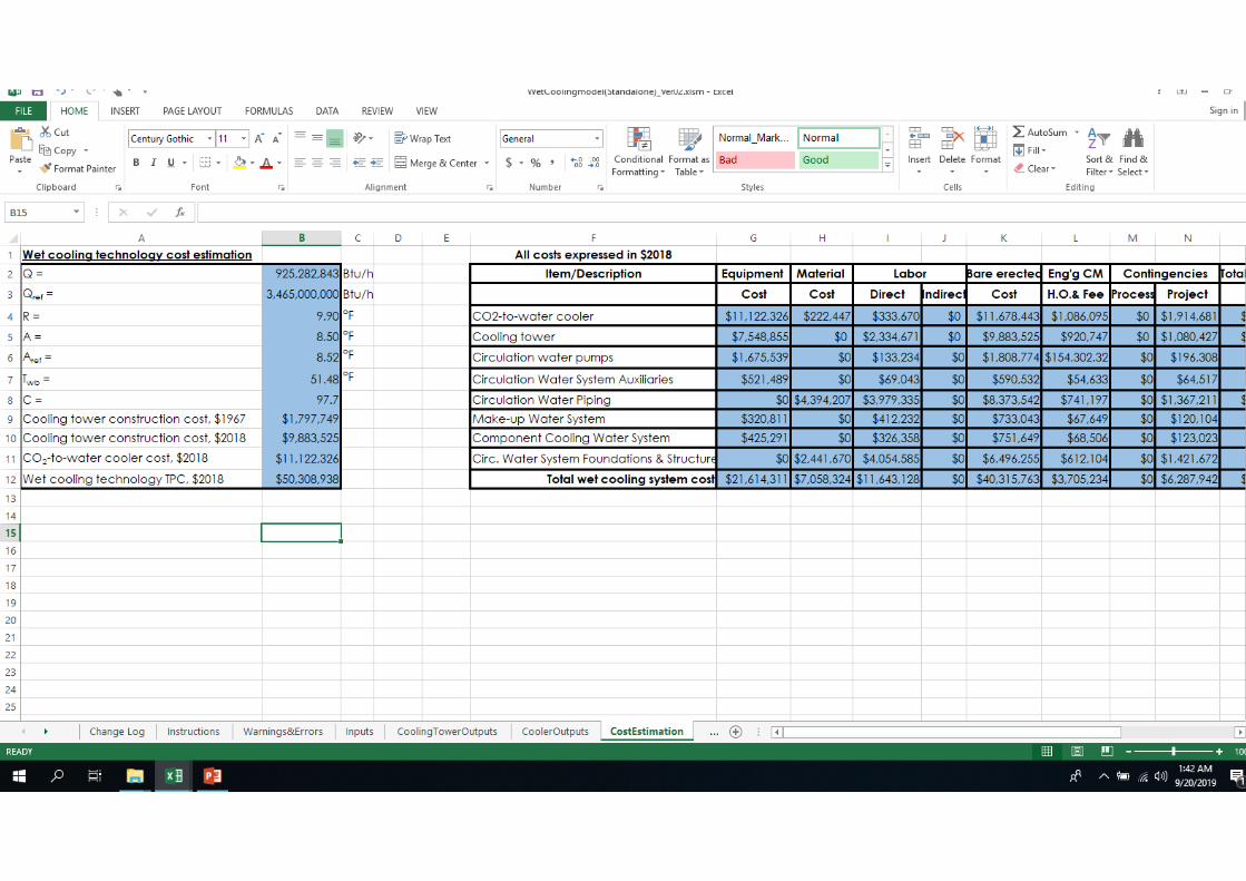
• Zanker correlation for estimation of cooling tower installed cost5, 6

• Based on thermal duty, water range, approach temperature, and wet bulb temperature

• Cost correlation doesn’t account for the cooling water pumps, water piping, etc., which are calculated separately.

Wet Cooling Tower TechnologyPerformance and Cost Model

4 Baumeister, T., Avallone, E., and T. Baumeister III, Marks’ Standard Handbook for Mechanical Engineers, 8th Ed., McGraw‐Hill, pp 9‐72 – 9‐73 (1979)5 Zanker, A., “Cooling Tower Costs from Operating Data,” Calculation and Shortcut Handbook, McGraw‐Hill,New York, pp 47‐48 (1967)6 Leeper, S. A., “Wet Cooling Tower: ‘Rule‐of‐thumb’ Design and Simulation,” Idaho National Engineering Laboratory, EGG‐GTH‐5775, pp 10‐11 (1981)

Input Parameters Output ParametersCooling duty Circulating water flow rate

Ambient dry bulb temperature

Circulating water pump power consumption

Ambient wet bulb temperature

Cooling tower water loss and make‐up requirement

Ambient pressure Cooling tower air flow rateCooling water range Cooling tower fan power consumptionWater approach Cooling tower construction cost

8

• Cost model validated against cooling tower cost models from SteamPro• Zanker correlation compared well

with SteamPro data for variation of cooling water Range and wet bulb temperature, Twb

• Zanker correlation adjusted with power law exponents for cooling Duty and Approach temperature to yield a good fit• Denoted Zanker Mod• See paper for correlation

Wet Cooling Tower TechnologyCost Model Validation with SteamPro

0,0

0,2

0,4

0,6

0,8

1,0

1,2

0,0 0,5 1,0

Cost ra

tio

Duty ratio

SteamProZankerZanker Mod

0,00,20,40,60,81,01,21,41,6

0,0 0,5 1,0 1,5 2,0

Cost ra

tio

Approach ratio

SteamProZankerZanker Mod

0,0

0,5

1,0

1,5

2,0

2,5

0,0 0,5 1,0 1,5

Cost ra

tio

Range ratio

SteamProZanker

0,0

0,2

0,4

0,6

0,8

1,0

1,2

1,4

0,6 0,8 1,0 1,2

Cost ra

tio

Twb ratio

SteamProZanker

12

• Representative results shown for a cooler outlet temperature of 25 °C

• For increasing cooling water Range:• Water flow decreases, reducing cooling fan and water pump

power consumption, increasing efficiency• Water/CO2 heat exchanger capital costs increase due to

reduced driving forces and higher heat transfer area • Cooling tower capital costs decrease• Opposing cost trends minimize the plant’s COE for a

cooling tower range of 15.3 °C in this example case.• For increasing Temperature Approach:

• Fan and pump power increase, reducing efficiency • Smaller cooling tower is needed, but water/CO2 heat

exchanger costs increase rapidly• Recommended minimum approach is 2.8 °C (5 °F)

Wet Cooling Tower ResultsEfficiency and COE Sensitivity to Range and Approach

42,5

42,6

42,7

42,8

42,9

43,0

43,1

43,2

110

111

112

113

114

115

116

117

0 5 10 15 20

Plan

t efficien

cy (%HH

V)

COE w/o T&S ($

/MWh)

Range (°C)

COEEff

Approach = 2.8 °C

42,5

42,6

42,7

42,8

42,9

43,0

43,1

43,2

110

111

112

113

114

115

116

117

0 2 4 6 8 10 12

Plan

t Efficien

cy (%HH

V)

COE w/o T&S ($

/MWh)

Temperature Approach (°C)

COEEff

Range = 15.3 °C

RecommendedMinimum = 2.8 °C

13

• Performance model based on ACHE text7 and calibrated with data from a vendor quote from Black & Veatch• Assumes two tube passes in a crossflow

heat exchanger arrangement• Required air flow and number of ACHE

bays needed solved iteratively using ε-NTU relationships for crossflow heat exchangers

• ACHE cost scaled linearly by number of bays required to meet cooling demand

Indirect Dry Cooling Technology – ACHEPerformance Model

7 Kroger, D. G., Air‐cooled Heat Exchangers and Cooling Towers: Thermal Performance Evaluation and Design Volume II, PennWell Corp., Tulsa, OK, pp 134‐153 (2004)

Inputs OutputsCooling duty Circulating water flow rate

Cooling water range Air flow rateWater temperature approach to Tdb Average air exit temperatureAmbient air‐dry bulb temperature Total fan power consumption

‐‐‐ Number of bays needed‐‐‐ ACHE capital cost

14

Figure 10Figure 9

Figure 4Figure 3

• Cost model validated againstACHE costs obtained from SteamPro• Linear scaling of cooling duty

with number of ACHE bays validated

• Also validates linear scaling of cost with number of bays

• Increasing design dry bulb temperature and reducing temperature approach to ambient requires more cooler bays

• Maximum cost deviation occurs for Approach < 5.6 °C (10 °F)

Indirect Dry Cooling Technology – ACHECost Model Validation with SteamPro

0

50

100

150

200

250

0

20

40

60

80

100

200 400 600 800 1000

Num

ber o

f bays

ACHE

Total Cost ($MM)

Cooling Duty (MW)

SteamPro CostSteamPro CellsB&V Bays

0

25

50

75

100

125

0

10

20

30

40

50

45 50 55 60 65

Num

ber o

f bays

ACHE

Total Cost ($MM)

Dry Bulb Temperature, Tdb (°F)


0

25

50

75

100

125

0

10

20

30

40

50

5 10 15 20 25

Num

ber o

f bays

ACHE

Total Cost ($MM)

Temperature Approach (°F)


15

• Representative results shown for a cooler outlet temperature of 25 °C

• For increasing cooling water Range:• Water flow decreases, reducing cooling fan and water pump

power consumption, increasing efficiency• Water/CO2 heat exchanger capital costs increase due to reduced

driving forces and higher heat transfer area, while ACHE capital costs decrease

• Opposing cost trends minimize the plant’s COE for a cooling water range of 11.1 °C in this example case.

• For increasing Temperature Approach:• Fan power decreases, increasing efficiency• Smaller number of ACHE bays needed, but water/CO2 heat

exchanger costs also increase• Optimum temperature approach that minimizes COE is ≥ 8 °C

in this example

Indirect Dry Cooling Technology ResultsEfficiency and COE Sensitivity to Range and Approach

41,0

41,5

42,0

42,5

43,0

115

120

125

130

135

0 2 4 6 8 10 12 14

Plan

t Efficien

cy (%HH

V)

COE w/o T&S ($

/MWh)

Range (°C)

COEEff

Approach = 2.8 °C

41,0

41,5

42,0

42,5

43,0

115

120

125

130

135

0 2 4 6 8 10

Plan

t Efficien

cy (%HH

V)

COE w/o T&S ($

/MWh)

ACHE Temperature approach (°C)

COEEff

Range = 11.1 °C

16

• Indirect sCO2 cooling technologies can be optimized relative to reference cooling water assumptions typically used for steam power cycles2:• Reference cooling water range: 11.1 °C (20 °F)• Reference cooling water approach to Twb: 4.7 °C (8.5 °F)

• Optimal wet cooling tower operating conditions for sCO2 are not far from the reference cooling conditions used for steam

• Significant benefit to optimizing indirect dry cooling systems for sCO2• Also extends operation to colder sCO2 temperatures

• Optimum CO2 cooler temperature will depend on the plant design (cooling technology cost fraction) and ambient conditions

Indirect Cooling Technology OptimizationOperating Condition Optimization

2 National Energy Technology Laboratory (NETL), "Quality Guidelines for Energy System Studies: Process Modeling Design Parameters," NETL, Pittsburgh, May 2014.

39

40

41

42

43

44

110

114

118

122

126

130

20 25 30 35 40

Plan

t Efficien

cy (%

HHV)

COE w/o T&S ($/M

Wh)

Cooler Exit Temperature (°C)

Wet Cooling Tower

COE ‐ Ref.COE ‐ Opt.Eff ‐ Ref.Eff ‐ Opt.

39

40

41

42

43

44

110

114

118

122

126

130

20 25 30 35 40

Plan

t Efficien

cy (%

HHV)

COE w/o T&S ($/M

Wh)

Cooler Exit Temperature (°C)

Indirect Dry Cooling

COE ‐ Ref.COE ‐ Opt.Eff ‐ Ref.Eff ‐ Opt.

17

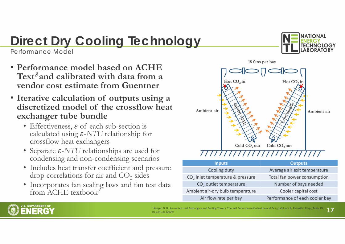
• Performance model based on ACHE Text8 and calibrated with data from a vendor cost estimate from Guentner

• Iterative calculation of outputs using a discretized model of the crossflow heat exchanger tube bundle• Effectiveness, of each sub-section is

calculated using -NTU relationship for crossflow heat exchangers

• Separate -NTU relationships are used for condensing and non-condensing scenarios

• Includes heat transfer coefficient and pressure drop correlations for air and CO2 sides

• Incorporates fan scaling laws and fan test data from ACHE textbook7

Direct Dry Cooling TechnologyPerformance Model

Inputs OutputsCooling duty Average air exit temperature

CO2 inlet temperature & pressure Total fan power consumptionCO2 outlet temperature Number of bays needed

Ambient air‐dry bulb temperature Cooler capital costAir flow rate per bay Performance of each cooler bay

7 Kroger, D. G., Air‐cooled Heat Exchangers and Cooling Towers: Thermal Performance Evaluation and Design Volume II, PennWell Corp., Tulsa, OK, pp 134‐153 (2004)

18

• The cooler model discretization scheme includes multiple tube rows and passes • Accounts for non-linear property variation near the critical point

• Air side heat transfer coefficient and pressure drop correlations are tuned to match the vendor data

Direct Dry Cooling TechnologyDiscretization scheme & tube bundle description

Parameter ValueTube outer diameter (mm) 12Tube wall thickness (mm) 0.7Tube inner diameter (mm) 10.6Finned tube length (m) 11.385

Tube arrangement pattern StaggeredFin thickness (mm) 0.15

Number of tube bundles 2Number of tubes per row 64Number of tube passes 3

Number of tubes per pass 2

19

• Vendor calculated volumetric flow rate of air and fan power consumption as a function of the ambient dry bulb temperature for fixed number of bays and heat duty

• The volumetric flow rate is used as the input to the model to calculate heat duty, fan power consumption per bay

• The model is able to predict the vendor data for bay heat duty and fan power consumption within ±10% and ±15%, respectively. • This accuracy is deemed acceptable, since the model

doesn’t fully replicate the vendor tube bundle or fan configuration

Direct Dry Cooling TechnologyPerformance Model - Validation with Vendor data

‐4

‐202

468

1012

0

0,5

1

1,5

2

2,5

3

10 15 20 25 30 35

% Differen

ce

Bay he

at duty (M

Wth)

Ambient Dry Bulb Temperature (°C)

Guntner dataCurrent modelDifference

‐15

‐10

‐5

0

5

10

15

20

05

101520253035404550

10 15 20 25 30 35

% Differen

ce

Fan po

wer per bay (k

We)

Ambient Dry Bulb Temperature (°C)

Guntner dataCurrent modelDifference

20

• “Adiabatic” cooler systems developed to improve CO2-based refrigeration system performance during hot ambient conditions• Addition of wet pre-cooling pads cools incoming air

through evaporation• Allows for a CO2 approach to the wet bulb, rather

than dry bulb, temperature• Operator flexibility to utilize water pre-cooler pads

only when needed• Wet pre-cooler pad model solves water

and air mass & energy balances• Pre-cooler model results are inputs to the direct

dry cooling technology performance model• Model performance and cost calibrated to

vendor data and quote

Direct Adiabatic Cooling TechnologyPerformance Model

Inputs OutputsCooling duty Air temperature after cooling pad

CO2 inlet temperature & pressure Air temperature exiting coolerCO2 outlet temperature Total fan power consumption

Ambient air dry bulb temperature Water consumption rateAmbient air wet bulb temperature Number of bays needed

Air flow rate per bay Cooler capital cost

21

• For a fixed heat duty and number of bays, vendor calculated volumetric flow rate of air, fan power consumption, and water consumption rate as a function of the ambient dry and wet bulb temperatures• Model calculations of fan power consumption, heat duty and water consumption rate compared

well with vendor predictions for wide range of conditions (±10% agreement for most cases)• This accuracy is deemed acceptable, since the model doesn’t fully replicate the vendor tube

bundle, fan configuration, or wet pre-cooler pads

Direct Adiabatic Cooling TechnologyPerformance model - Validation with vendor data

‐6

‐5

‐4

‐3

‐2

‐1

0

3

3,2

3,4

3,6

3,8

4

25 26 27 28 29 30 31 32 33

% Differen

ce

Bay he

at duty (M

Wth)

Ambient dry bulb temperature (°C)

Vendor dataCurrent modelDifference

‐7‐6‐5‐4‐3‐2‐10123

0

5

10

15

20

25

30

35

25 26 27 28 29 30 31 32 33

% Differen

ce

Fan po

wer per bay (k

We)


Vendor dataCurrent modelDifference ‐15

‐10

‐5

0

5

10

0,0

0,5

1,0

1,5

2,0

2,5

25 26 27 28 29 30 31 32 33

% Differen

ce

Water con

sumption/ba

y (m

3 /h)


Vendor dataCurrent modelDifference

22

• For increasing volumetric air flow rate:• Efficiency decreases due to increasing fan power

consumption• The number of required cooler bays decreases,

resulting in lower CO2 cooler capital costs • Due to these opposing trends, the COE attains a

minimum value for a particular value of air flow rate (approximately 90 m3/s in this example case).

• Relative to the Direct Dry cooler, the Direct Adiabatic Cooler:• Requires fewer bays to meet the cooling demand,

reducing both cost and fan power consumption• Due to CO2 approach to lower Twb, rather than Tdb

Direct Dry and Adiabatic Cooling ResultsEfficiency and COE Sensitivity to Range and Approach

39,5%

40,0%

40,5%

41,0%

41,5%

42,0%

42,5%

43,0%

43,5%

44,0%

111

112

113

114

115

116

117

118

119

120

0 50 100 150 200 250 300

Plan

t Efficien

cy (%

)

COE w/o T&S ($/M

Wh)

Flow rate of air per bay (m3/s)

COE ‐ Direct DryCOE ‐ AdiabaticEff ‐ Direct DryEff ‐ Adiabatic

Cooler CO2 Exit Temperature = 25 °C

23

• Cooler operating conditions optimized for COE at each cooler temperature• Optimized results are valid only for the plant

design and ambient conditions selected• CO2 cooler exit temperatures of

20-25 °C minimize COE• Demonstrates the benefit of condensing CO2

cycle operation• Plant efficiency improves 3.0 – 3.5

percentage points, and the plant COE is reduced by as much as 8%, by decreasing the CO2 cooler temperature from 40 to 20 °C, depending on the cooling technology

Cooling Technology ComparisonEfficiency and COE Optimization Results

39

40

41

42

43

44

45

110

112

114

116

118

120

122

20 25 30 35 40

Plan

t HHV

Efficien

cy (%

)

COE w/out T&S ($

/MWh)

CO2 Cooler Temperature (°C)

COE Wet Tower COE Ind. Dry COE Direct Dry COE Adiabatic

Eff. Wet Tower Eff. Ind. Dry Eff. Direct Dry Eff. Adiabatic

24

• Indirect dry cooling is non-competitive

• Wet cooling towers are attractive, but have the highest water consumption

• Performance of direct dry and adiabatic cooling technologies are similar until cooler temperatures approach ambient

• Adiabatic cooling used in CO2 refrigeration systems may be the most applicable to sCO2 power cycles• Ability to provide the coldest sCO2 temperatures

for a given ambient temperature• Flexibility to use water only as needed during hot

conditions• ~40% less water consumption than wet cooling

towers (using present study’s assumptions)

Cooling Technology ComparisonEfficiency and COE Optimization Results (cont.)

39

40

41

42

43

44

45

110

112

114

116

118

120

122

20 25 30 35 40

Plan

t HHV

Efficien

cy (%

)

COE w/out T&S ($

/MWh)

CO2 Cooler Temperature (°C)

COE Wet Tower COE Ind. Dry COE Direct Dry COE Adiabatic

Eff. Wet Tower Eff. Ind. Dry Eff. Direct Dry Eff. Adiabatic

25

• Summary• Developed four cooler cost and performance spreadsheet models for minimizing sCO2

power plant COE by optimizing cold cycle temperature and cooling system operation• Models freely available for use (currently beta-test versions, attached to the models’ technical

documentation8)• Improvements in plant efficiency (3.0–3.5 %points) and plant COE (up to 8%) highlight

the importance of cooling system thermal integration and optimization of CO2 cooler temperature for sCO2 power plants

• Current and Future Work• Modification of cooler technology models to handle sCO2 mixtures for optimizing direct

sCO2 power cycle cooling systems• Investigation of cooling system optimization for different plant sites and ambient

conditions• Modification of cooling system models to predict off-design performance

Summary and Future Work

8 National Energy Technology Laboratory (NETL), "Cooling Technology Performance and Cost Models for sCO2 Power Cycles," NETL, Pittsburgh, 2019. https://www.netl.doe.gov/energy‐analysis/details?id=3199.

26

Questions?

[email protected]

Cooling System Cost & Performance Models for Economic sCO

Documents

Transcript of Cooling System Cost & Performance Models for Economic sCO