TOMSK POLYTECHNIC UNIVERSITY         

S.V. Zamyatin, M.I. Pushkarev, E.M. Yakovleva     

  

CONTROL THEORY  

 Recommended for publishing as a study aid  

by the Editorial Board of Tomsk Polytechnic University  

   

          

Tomsk Polytechnic University Publishing House  2012 

UDC 005.1(075.8) BBC У9(2)210я73

Z21 Zamyatin S.V.

Z21 Control theory: study aid / S.V. Zamyatin, M.I. Pushkarev, E.M. Yakovleva; Tomsk Polytechnic University. – Tomsk: TPU Pub-lishing House, 2012. – 100 p.

Main approaches of investigations, analysis and design of linear, nonlinear and pulse control system are considered. The tasks for course work and necessary data and examples of such problems solving are applied. Project includes mathematical de-scription of control objects and systems; linear system analysis, including stability analysis, step response plot and frequency characteristics plot; linear systems synthe-sis, including controllers design; nonlinear control systems analysis.

Study aid manual is intended for training students majoring in the specialties 220400 «Control in technical systems».

UDC 005.1(075.8) BBC У9(2)210я73

Reviewers Doctor of Mathematics and Physics

T.M. Petrova, PhD, V.A. Rudnitskiy

© STE HPT TPU, 2012 © Zamyatin S.V., Pushkarev M.I.,

Yakovleva E.M., 2012

3

CONTENT

INTRODUCTION .................................................................................. 5 1  LINEAR AUTOMATIC CONTROL SYSTEM ......................... 7 

1.1  AUTOMATIC CONTROL SYSTEM FUNCTIONAL DIAGRAM DESIGN

ACCORDING TO ITS CIRCUIT SCHEMATIC ........................................................... 7 1.2  AUTOMATED CONTROL SYSTEM UNIT DIAGRAM DESIGN ............. 9 1.3  ACS TRANSFER FUNCTIONS ........................................................ 11 1.4  DIFFERENTIAL EQUATION OF ACS .............................................. 14 1.5  ACS STABILITY ESTIMATION ACCORDING TO CHARACTERISTIC

EQUATION ROOTS ............................................................................................ 16 1.6  ACS STABILITY ESTIMATION ACCORDING TO THE MIKHAILOV

STABILITY CRITERION ...................................................................................... 18 1.7  ACS STABILITY ESTIMATION ACCORDING TO THE NYQUIST

STABILITY CRITERION ...................................................................................... 20 1.8  HURWITZ STABILITY CRITERION. ACS CRITICAL GAIN .............. 22 1.9  STABILITY PLANE PLOTTING IN SYSTEM PARAMETER PLANE ...... 24 1.10  STEP RESPONSE OF THE SYSTEM AND QUALITY INDEXES OF

THE CONTROL PROCESS. .................................................................................. 26 1.11  AUTOMATED CONTROL SYSTEM CONTROL PROCESS

ACCURACY ESTIMATION .................................................................................. 30 1.11.1  Control error in stabilization systems ................................ 31 1.11.2  Control error in servo systems ........................................... 32 

2  NONLINEAR ACS ....................................................................... 34 

2.1  ACS DIFFERENTIAL EQUATION IN IMPLICIT FORM ...................... 34 2.2  HARMONIC LINEARIZATION METHOD APPLICATION FOR

NONLINEAR ACS ............................................................................................. 36 2.3  DIFFERENTIAL AND CHARACTERISTIC EQUATIONS OF ACS

HARMONIC LINEARIZATION ............................................................................. 37 2.4  OBTAINING OF TYPICAL UNIT DIAGRAM OF NONLINEAR ACS .... 37 2.5  GOLDFARB METHOD FOR NONLINEAR ACS STABILITY

ESTIMATION APPLICATION ............................................................................... 39 2.6  APPLICATION OF POPOV STABILITY CRITERION FOR NONLINEAR

ACS STABILITY ANALYSIS .............................................................................. 41 2.7  V.M. POPOV STABILITY CRITERION APPLICATION FOR THE CASE

OF NEUTRAL OR UNSTABLE LINEAR PART ....................................................... 45 

3  LINEAR PULSE ACS .................................................................. 46 

3.1  GENERAL PULSE SYSTEM UNIT DIAGRAM ................................... 50 3.2  MATHEMATICAL TOOLS OF PULSE SYSTEMS ............................... 52 

4

3.2.1  Lattice function and differential equation .......................... 52 3.2.2  Z-transform application ..................................................... 54 

3.3  SAMPLING THEOREM ................................................................... 55 3.4  PULSE TRANSFER FUNCTION OF OPEN-LOOP PULSE SYSTEM ...... 57 3.5  CLOSED-LOOP PULSE SYSTEM TRANSFER FUNCTION .................. 61 3.6  STABILITY ANALYSIS OF PULSE CLOSED-LOOP SYSTEMS ........... 63 

3.6.1  Pulse ACS stability estimation based on system characteristic equation roots ................................................................... 63 

3.6.2  Mihailov criterion analogue application for pulse system stability estimation ................................................................................... 64 

3.7  CONTROL PROCESS QUALITY ESTIMATION OF PULSE ACS ......... 67 

4  CONTROL TASKS AND STUDY GUIDE ............................... 72 

4.1  GENERAL STUDY GUIDE .............................................................. 72 4.2  GUIDE LINES FOR PROJECT TEXT DOCUMENT CONTENT ............. 72 4.3  GUIDE LINES FOR PROJECT GRAPHIC MATERIAL APPEARANCE ... 73 

CONCLUSION ..................................................................................... 73 REFERENCE ........................................................................................ 88 APPENDIX 1 ......................................................................................... 89 APPENDIX 2 ......................................................................................... 98 

5

INTRODUCTION

Active development of the automatic control theory has begun with electromachine systems and radio automatics systems. Later it has appeared that methods of the automatic control theory allow to explain work of the various physical nature objects: in the mechanic, power, radio and the electri-cal engineer, that is everywhere where is feedback.

In the book the sections of the the automatic control theory, necessary for term paper performance are considered. Questions of the mathematical description of linear, nonlinear and pulse systems; algebraic and frequency criteria for an estimation of stability of systems of automatic control; indica-tors of quality of their process of regulation are considered. The concrete numerical examples facilitating development of a material are resulted.

The primary goals of a term paper are: - Drawing up on a function chart circuit diagram. - Drawing up of mathematical model in the form of the block diagram. - System research on stability. - Construction of system transient process for regulation quality estimation. - An estimation of regulation process accuracy.

For term paper performance it is necessary to choose a circuit diagram of system and numerical values of parameters of its elements (the Appendix 1). Also it is possible to use additional information from books [1-10] in or-der to carry out task. Linear continuous ACS.

- To give the short description of automatic control system (ACS). - To describe a principle of ACS regulation. - Using linear models of ACS elements (the Appendix 1) to make

on the base of system circuit diagram functional and structural schemes.

- To get openloop transfer function of system. - To find transfer functions of the closed-loop system on setting

influence and to the desturbance factor. - To write down differential equation of ACS. - To check upACS on stability on the of roots of the characteristic

equation of system.To check up ACS on stability, using criterion - of Mikhailov stability.To check up ACS on stability, using crite-

rion of Nyquist stability. - To define margins of system stability on amplitude and a phase.

6

- To define by Gurvits stability criterion critical gain of open-loop system.

- Under zero conditions, to construct the transitive characteristic of system and to define its quality indicators.

- To define the full established error of system. Nonlinear ACS.

- To accept that the amplyfing unit in system is a nonlinear element and to make the unit diagram of nonlinear ACS.

- To reduse the block diagram of nonlinear ACS to typical and to get transfer function of a linear part of system.

- To receive the differential equation of harmoniously linearized nonlinear system.

- To estimate stability of harmoniously linearized nonlinear system by Goldfarb method.

- Using Popova V. M. absolute stability criterion to investigate sta-bility of system balance position in general. Linear pulse ACS.

- To generate the scheme of pulse system. - To get transfer function of a continuous part of pulse system - To define, using the Kotelnikov theorem, the period of quantiza-

tion. - To find open-loop and closed-loop transfer functions of system. - To define stability of system on the base of roots of the character-

istic equation. - To define stability of system, using Mikhailov stability criterion

analog. - Under conditions zero, to construct the discrete transitive charac-

teristic of system and to define its quality indicators. - To define a regulation error on setting influence.

7

1 LINEAR AUTOMATIC CONTROL SYSTEM

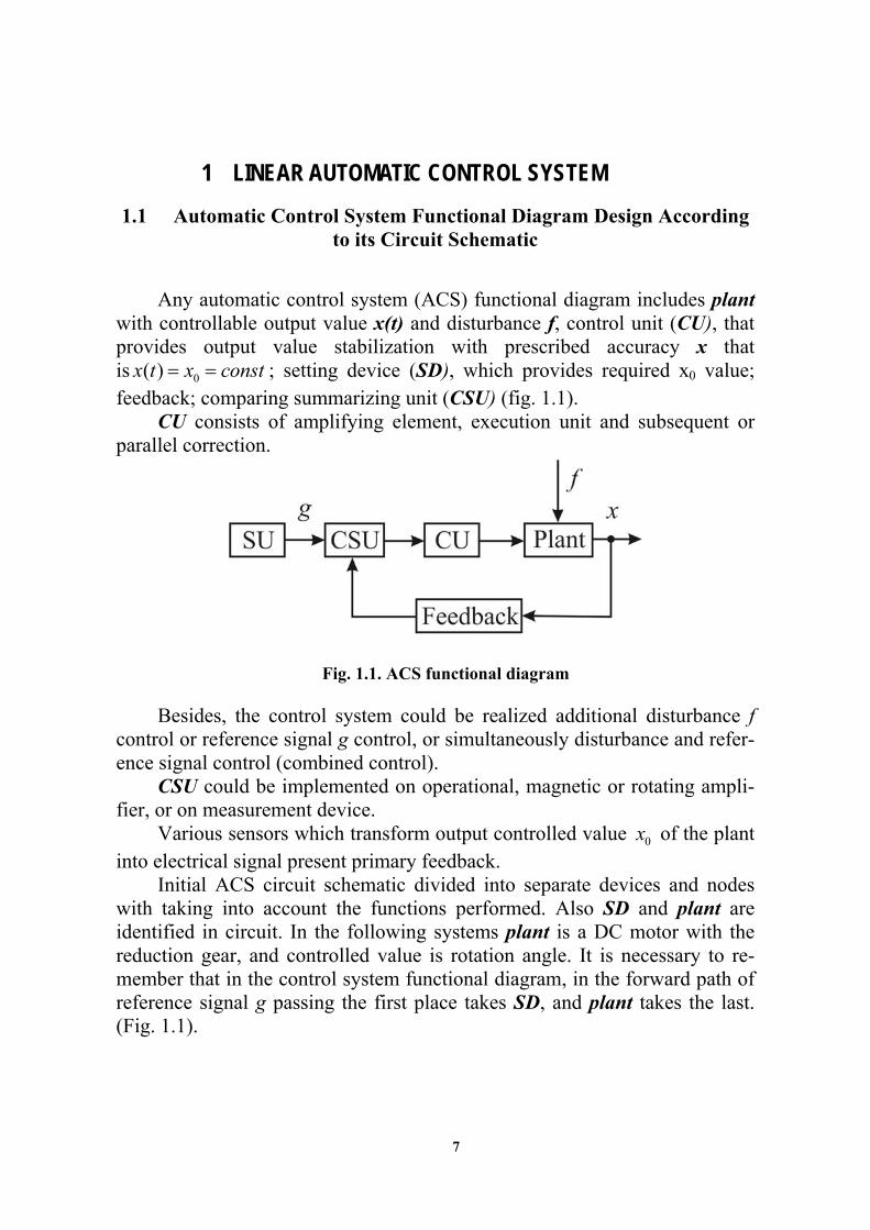
1.1 Automatic Control System Functional Diagram Design According to its Circuit Schematic

Any automatic control system (ACS) functional diagram includes plant

with controllable output value x(t) and disturbance f, control unit (CU), that provides output value stabilization with prescribed accuracy x that is 0( )x t x const ; setting device (SD), which provides required x0 value; feedback; comparing summarizing unit (CSU) (fig. 1.1).

CU consists of amplifying element, execution unit and subsequent or parallel correction.

Fig. 1.1. ACS functional diagram

Besides, the control system could be realized additional disturbance f

control or reference signal g control, or simultaneously disturbance and refer-ence signal control (combined control).

CSU could be implemented on operational, magnetic or rotating ampli-fier, or on measurement device.

Various sensors which transform output controlled value 0x of the plant into electrical signal present primary feedback.

Initial ACS circuit schematic divided into separate devices and nodes with taking into account the functions performed. Also SD and plant are identified in circuit. In the following systems plant is a DC motor with the reduction gear, and controlled value is rotation angle. It is necessary to re-member that in the control system functional diagram, in the forward path of reference signal g passing the first place takes SD, and plant takes the last. (Fig. 1.1).

8

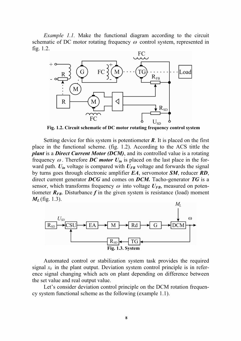
Example 1.1. Make the functional diagram according to the circuit schematic of DC motor rotating frequency control system, represented in fig. 1.2.

Fig. 1.2. Circuit schematic of DC motor rotating frequency control system

Setting device for this system is potentiometer R. It is placed on the first

place in the functional scheme. (fig. 1.2). According to the ACS tittle the plant is a Direct Current Motor (DCM), and its controlled value is a rotating frequency . Therefore DC motor Uin is placed on the last place in the for-ward path. Uin voltage is compared with UFB voltage and forwards the signal by turns goes through electronic amplifier EA, servomotor SM, reducer RD, direct current generator DCG and comes on DCM. Tacho-generator TG is a sensor, which transforms frequency into voltage UFB, measured on poten-tiometer RFB. Disturbance f in the given system is resistance (load) moment ML (fig. 1.3).

Fig. 1.3. System

Automated control or stabilization system task provides the required

signal x0 in the plant output. Deviation system control principle is in refer-ence signal changing which acts on plant depending on difference between the set value and real output value.

Let’s consider deviation control principle on the DCM rotation frequen-cy system functional scheme as the following (example 1.1).

9

If the load on the DCM shaft increases, the disturbance ML increases consequently too. This leads to 0 and the decreased UFB. Therefore, positive difference in FBU U U appears at the EA input that in its turn leads to the signal value magnitude, fed on servomotor, increasing, that means current in the DC motor circuit coil also increases. Rotating frequency will increase proportionally from U to 0 .

Thus, any deviation of the output controlled value ( )x t from the re-quired value 0x leads to the error: 0( )x t x x .

This error x is reduced to zero with the given accuracy by the system during control process.

1.2 Automated Control System Unit Diagram Design

For the block diagram construction one should make the transfer func-tions of the control system devices (appendix 1) and equipment on the base of their differential equations. Herewith, differential equation disturbance f component (Mc, I etc.) needs to be taken into account only for the plant. That’s why the plant will have two transfer functions: reference signal

( )PlantgW s and disturbance ( )Plant

fW s . CSU also have some kinds of transfer functions and their quantity determined by the quantity of inputs.

For the definition of transfer function expression according to the spe-cific influence superposition principle is used.

Transfer function – relation between output and input signal in the La-place transform, with zero initial conditions.

Example 1.2. Obtain transfer function for the direct current generator ( )DCGW s . Solution: Direct current generator differential equation (look appendix 1) has a

view: 1( 1) ( ) ( ).G G G FCT p U t K U t (1.1)

Applying Laplace transform to the equation (2.1) get

1( 1) ( ) ( )G G G FCT s U s K U s

Then, according to the transfer function definition write

1( )( ) .

( ) 1G G

DCGFC G

U s KW s

U s T s

Example 1.3. Obtain plant transfer functions of automated control system repre-sented in fig. 1.3.

Solution Lets write direct current generator differential equation:

21 2( 1) ( ) ( ) ( 1) .E EM EM M AV M E LT T p T p t K U t K T p M (1.2)

10

Using superposition principle obtain direct currenct generator voltage anchor chain

transfer function – ( )AVUDCGW s . For this, let’s equate 0LM . Then equation (1.2) takes the

view: 2

1( 1) ( ) ( )E EM EM M AVT T p T p t K U t

Let’s get direct current generator anchor chain transfer function:

12

( )( ) .

( ) ( 1)AVU M

DCGAV E EM EM

s KW s

U s T T s T s

Similarly get direct current generator resisting moment transfer function LMDCGW (s),

for this reason let’s equate ( ) 0AVU t .

22

( ) ( 1)( )

( ) ( 1)LM M E

DCGL E M M

s K T sW s

M s T T s T s

.

Let’s define the concept of the unit diagram. Unit diagram – a graphical representation of the device differential equation,

when the transfer function expression is written inside the rectangle, input signal and out-put signal are represented by arrows.

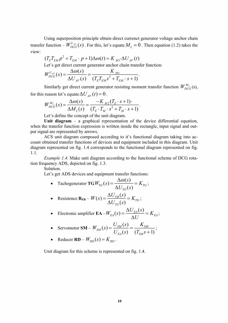
ACS unit diagram composed according to it’s functional diagram taking into ac-count obtained transfer functions of devices and equipment included in this diagram. Unit diagram represented on fig. 1.4 corresponds to the functional diagram represented on fig. 1.1.

Example 1.4. Make unit diagram according to the functional scheme of DCG rota-tion frequency ADS, depicted on fig. 1.3.

Solution. Let’s get ADS devices and equipment transfer functions:

Tachogenerator TG( )

( )( )TG TG

TG

sW s K

U s

;

Resistence RFB – ( )

( )( )

FBTG

TG

U sW s K

U s

;

Electronic amplifier EA –( )

( ) EAEA EA

U sW s K

U

;

Servomotor SM – ( )

( )( ) ( 1)

SM SMSM

EA SM

U s KW s

U s T s

;

Reducer RD – ( )RD RDW s K .

Unit diagram for this scheme is represented on fig. 1.4.

11

Fig. 1.4. Rotation frequency ADS unit diagram

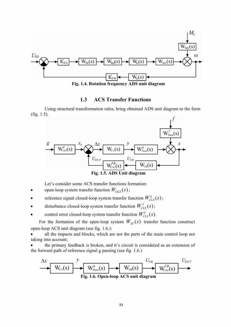
1.3 ACS Transfer Functions

Using structural transformation rules, bring obtained ADS unit diagram to the form (fig. 1.5).

Fig. 1.5. ADS Unit diagram

Let’s consider some ACS transfer functions formation:

open-loop system transfer function ( )OLSW s ;

reference signal closed-loop system transfer function ( )gCLSW s ;

disturbance closed-loop system transfer function ( )fCLSW s ;

control error closed-loop system transfer function ( )CLSW s .

For the formation of the open-loop system ( )STW s transfer function construct

open-loop ACS unit diagram (see fig. 1.6.): all the impacts and blocks, which are not the parts of the main control loop not taking into account; the primary feedback is broken, and it’s circuit is considered as an extension of the forward path of reference signal g passing (see fig. 1.6.)

Fig. 1.6. Open-loop ACS unit diagram

12

Then we can write an equation for the open-loop system transfer function

( ) ( ) ( ) ( ) ( ).FBOLS CU EA FB CSUW s W s W s W s W s (1.3)

Let’s use superposition principle for any influence closed-loop ACS transfer func-tion obtaining. Unit diagram for reference-signal control closed-loop system obtaining is represented on fig. 1.7.

Fig. 1.7. Reference signal control ACS unit diagram

System transfer function has form

( ) ( ) ( )

( ) .1 ( ) ( ) ( ) ( )

gg CU EA CSU

CLS FBCU EA FB CSU

W s W s W sW s

W s W s W s W s

(1.4)

Analyzing equation obtaining (1.4), one can note, that transfer function numerator is a transferfunction ( )g

STW s is a part of system between the system input and output point. Therefore expression (1.4) could be represented in the form:

( )

( ) .1 ( )

gg ST

CLSOLS

W sW s

W s

(1.5)

Unit diagram for closed-loop system transfer function in the disturbance is repre-sented in fig. 1.8.

Fig. 1.8. Unit diagram of disturbance ACS

Then transfer function expression has form:

( )( ) .

1 ( ) ( ) ( 1) ( ) ( )

ff Plant

CLS y FBCU EA FB CSU

W sW s

W s W s W s W s

Or

( )

( ) ,1 ( )

gfПР

ЗСPC

W sW s

W s

(1.6)

where ( )fSTW s – transfer function of the disturbance signal straight passing.

Unit diagram for the closed-loop system transfer function ( )CLSW s for the control

error is represented in fig. 1.9.

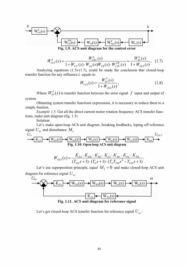
13

Fig. 1.9. ACS unit diagram for the control error

( ) ( )

( ) ,1 ( ) ( ) ( ) ( ) 1 ( )

gCSU ST

CLS FBCU EA FB CSU OLS

W s W sW s

W s W s W s W s W s

(1.7)

Analyzing equations (1.5)-(1.7), could be made the conclusion that closed-loop transfer function for any influence z equals to

( )

( ) ,1 ( )

FST

CLSOLS

W sW s

W s

(1.8)

Where ( )ZSTW s is transfer function between the error signal f input and output of

system. Obtaining system transfer functions expressions, it is necessary to reduce them to a

simple fraction. Example 1.5. Get all the direct current motor rotation frequency ACS transfer func-

tions, make unit diagram (fig. 1.3) Solution Let’s make open-loop ACS unit diagram, breaking feedbacks, loping off reference

signal inU and disturbance LM

Fig. 1.10. Open-loop ACS unit diagram

1 12( ) .

( 1) ( 1) ( 1)EA SM RD G M TG FB

OLSSM G E EM EM

K К К К К К КW s

T s T s T T s T s

Let’s use superposition principle, equal 0LM and make closed-loop ACS unit

diagram for reference signal inU .

Fig. 1.11. ACS unit diagram for reference signal

Let’s get closed-loop ACS transfer function for reference signal inU :

14

1 1

1 1

1 1

1 1

2

2

2

( ) ( 1) ( 1) ( 1)( )

1 ( )1

( 1) ( 1) ( 1)

( 1) ( 1) ( 1)

in

in

EA SM RD G MU

U ST SM G E EM EMCLS

EA EA RD G M TG FBOLS

SM G E EM EM

EA SM RD G M

SM G E EM EM EA SM RD G M

K К К К К

W s T s T s T T s T sW s

K К К К К К КW sT s T s T T s T s

K К К К К

T s T s T T s T s K К К К К

.TG FBК К

Let’s equal 0inU and make closed-loop ACS unit diagram for disturbance LM

Fig. 1.12. ACS unit diagram for disturbance f

Now represent closed-loop ACS transfer function for disturbance as:

2

1 1

2

1 1

2

2

2

( ) ( 1)( )

1 ( )1

( 1) ( 1) ( 1)

( 1) ( 1)

( 1) ( 1) ( 1)

L

L

MM

M ST E EM EMCLS

EA SM RD G M TG FBOLS

SM G E EM EM

M SM G

SM G E EM EM EA SM RD G M TG FB

К

W s T T s T sW s

K К К К К К КW sT s T s T T s T s

К T s T s

T s T s T T s T s K К К К К К К

1.4 Differential Equation of ACS

Having obtained the closed-loop system transfer function for the reference signal

( )gCLSW s and disturbance ( )f

CLSW s , ACS unit diagram depicted in fig. 1.5 can be repre-

sented in form (fig. 1.13):

Fig. 1.13. ACS unit diagram

Let’s write the ACS output signal equation in image S

1 2( ) ( ) ( ) ( ) ( ) ( ) ( ),g fCLS CLSX s X s X s W s G s W s F s (1.9)

where ( ), ( )G s F s are the images of reference signal ( )g t and disturbance ( )f t .

Let’s introduce the notation ( )

( )( )

gCLS

B sW s

A s ;

( )( )

( )f

CLS

C sW s

A s and write (1.9):

( ) ( ) ( ) ( ) ( ) ( ),A s X s B s G s C s F s (1.10)

15

where ( ), ( ), ( )A s B s C s is polynomial of image S:

1 21 2( ) ( )O

n n nnA s a s a s a s a ;

0 11( ) ( )m

m mB s b s b s b ; 1

0 1( ) ( )l llC s c s c s c .

Then (1.10) has a form:

0 1 2 0 1

10 1

1 2 1( ) ( ) ( )

( ) ( ) ( ).

m

l ll

n n n m mna s a s a s a X s b s b s b

G s c s c s c F s

If the transfer function denominator ( )A s equals to zero, we obtain the character-

istic equation: 1 2

0 1 2 1( ) 0.n n nn nA s a s a s a s a s a (1.11)

Solving this equation, characteristic equation roots 1 2 1, , ,n ns s s s are defined.

Switching from signal images to their originals and replacing d

s pdt

, we get ACS

differential equation:

0 1 2

0 1 0 1

1 22

1 2

1 1( ) ( )

1 1

( ) ( ) ( )( )

( ) ( )( ).m l

n n nn

nn n n

m m l lf t f t

m m l l

d X t d X t d X ta a a s a X t

dt dt dt

d g t d g t d db b b c c c f t

dt dt dt dt

(1.12)

Example 1.6. Get DCM rotation frequency ACS differential equation, its unit dia-gram is represented on fig. 1.5.

Solution. Let’s write the output signal equation in image s , using the following equation

(1.9).

1 1

1 1

2

1 1

2

2

( ) ( ) ( ) ( ) ( )

(s) +( 1)( 1)( 1)

( 1) ( 1)(s)

( 1)( 1)( 1)

in LU MCLS in CLS L

EA SM RD G Min

SM G E EM EM EA SM RD G M TG FB

M SM GL

SM G E EM EM EA SM RD G M TG FB

s W s U s W s M s

K К К К КU

T s T s T T s T s K К К К К К К

К T s T sM

T s T s T T s T s K К К К К К К

Switching from signal images to their originals, and replacing s p , we obtain

DCM rotation frequency ACS differential equation:

1 1

1 1 2

2(( 1)( 1)( 1) ) ( )

( ) ( 1) ( 1) ( ).SM G E EM EM EA SM RD G M TG FB

EA SM RD G M in M SM G L

T p T p T T p T p K К К К К К К t

K К К К К U t К T p T p M t

Using the numerical values of system parameters and replacingd

pdt

, the obtained

equation could be written in form (1.12).

16

1.5 ACS Stability Estimation According to Characteristic Equation Roots

Solution of differential equation (1.12) for the known ( )g t , ( )f t is the variation

law of output control variable ( )X t . It’s necessary to implement inverse Laplace trans-

form to equation (1.9) for ACS transient process finding:

1 11 2(t) ( ) ( ) ( ) ( ) ( ) ( )

1 1( ) ( ) s ( ) ( ) s.

2 2

[ ] [ ]g fCLS CLS

g fCLS CLS

j jst st

j j

X L X s X s L W s G s W s F s

W s G s e d W s F s e dj j

(1.13)

If integrals (2.13) are “unsolvable”, the Heaviside formula for transient process definition is used:

1

(0) ( )( ) ,

(0) ( )is ti

ini i i

nB B sX t U e

A s A s

(1.14)

where inU is the input signal amplitude; (s )iA is the derivative value of numerator

transfer function for value is ; n is the roots number of system characteristic equation.

System characteristic equation roots (fig. 1.14) can be real (root 1s ), complex-

conjugative ( 2 3 7 8, , ,S S S S ) and imaginary ( 5 6,S S ). Furthermore, roots can be located: in

the loft half plane, in the right half plane or on the ordinate axis and respectively will be left, right or neutral.

The system will be stable, if the transient process for t tend to the steady-state value ( ) SSX X . This means that exponent index of equation (1.14) must be

negative, i.e. all the system characteristic equation roots must be located in the left half plane (fig. 1.14).

Fig. 1.14. Variation of characteristic equation roots location

Root stability criterion:

17

The necessary and sufficient condition for the system to be stable is that all the sys-tem characteristic equation roots were in the left half plane (have a negative real part).

If among the system characteristic equation roots even one is from the right half plane and the rest are from the left , it means that ACS is unstable.

If among the system characteristic equation roots even one is neutral, and the rest are from the left half plane, it means that ACS is neutral, that is situated on the stability boundary.

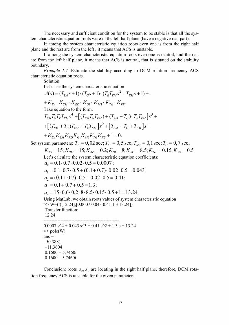
Example 1.7. Estimate the stability according to DCM rotation frequency ACS characteristic equation roots.

Solution. Let’s use the system characteristic equation

1 1

2( ) ( 1) ( 1) ( 1)

.

SM G E EM EM

EA SM RD G M TG FB

A s T s T s T T s T s

K К К К К К К

Take equation to the form:

1 1

4 3

2

( ) ( )

( )

1 0.

SM G E EM SM G EM SM G E EM

SM G EM E EM SM G EM

EA SM RD G M TG FB

T T T T s T T T T T T T s

T T T T T s T T T s

К К К К К К К

Set system parameters: 0,02 sec; 0,5 sec; 0,1sec; 0,7 sec;E M SM GT T T T

1 115; 15; 0.2; 8; 8.5; 0.15; 0.5EA SM RD G M TG FBK K K K K K K

Let’s calculate the system characteristic equation coefficients:

0 0.1 0.7 0.02 0.5 0.0007a ;

1 0.1 0.7 0.5 (0.1 0.7) 0.02 0.5 0.043;a

2 (0.1 0.7) 0.5 0.02 0.5 0.41a ;

3 0.1 0.7 0.5 1.3a ;

4 15 0.6 0.2 8 8.5 0.15 0.5 1 13.24a .

Using MatLab, we obtain roots values of system characteristic equation >> W=tf([12.24],[0.0007 0.043 0.41 1.3 13.24]) Transfer function: 12.24 ------------------------------------------------- 0.0007 s^4 + 0.043 s^3 + 0.41 s^2 + 1.3 s + 13.24 >> pole(W) ans = –50.3881 –11.3604 0.1600 + 5.7460i 0.1600 – 5.7460i Conclusion: roots 2 3,s s are locating in the right half plane, therefore, DCM rota-

tion frequency ACS is unstable for the given parameters.

18

1.6 ACS Stability Estimation According to the Mikhailov Stability Criterion

It is necessary to get Mikhailov curve equation for the ACS stability estimation. Let’s use closed-loop characteristic equation (1.11) for these purposes

0 1 21 2

1( ) 0.n n nnnA s a s a s a s a s a

To get the Mikhailov curve equation it is necessary to go to the frequency domain, substitute s j , separating real and imaginary components

0 1 21 2

1( ) ( ) ( ) ( ) ( )

( ) ( ).

n n nn

n

D j a j a j a j a j

a U jV

(1.15)

Where ( ), ( )U V are real and imaginary components of Mikhailov curve equation.

According to the equation (1.15), when the is changing, one can draw the Mikhailov curve (fig. 1.15).

Fig. 1.15. Mikhailov curves for stable systems with 1, 2; 3; 4n n n n

For ACS stability necessary and sufficient conditions should hold:

when 0 Mikhailov curve locus should begin in the positive part of the real axis; when 0 is changing, Mikhailov curve locus should: se-quentially, without vanish, in the positive (counterclockwise) derection pass n quadrants.

If the Mikhailov curve locus for the concrete frequency that does not equal zero pass through the coordinate origin, the system is neutral.

If any of these conditions are not fulfilled, the system is unstable. Example 1.8. Estimate DCM rotation frequency ACS stability using Mikhailov cri-

terion. Solution.

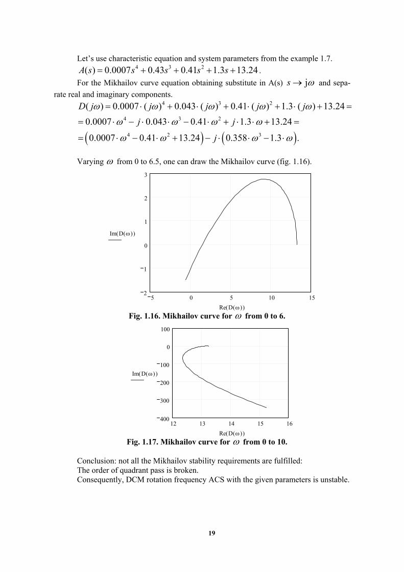
19

Let’s use characteristic equation and system parameters from the example 1.7. 4 3 2( ) 0.0007 0.43 0.41 1.3 13.24A s s s s s .

For the Mikhailov curve equation obtaining substitute in A(s) js and sepa-

rate real and imaginary components.

4 3 2

4 3 2

4 2 3

( ) 0.0007 ( ) 0.043 ( ) 0.41 ( ) 1.3 ( ) 13.24

0.0007 0.043 0.41 1.3 13.24

0.0007 0.41 13.24 0.358 1.3 .

D j j j j j

j j

j

Varying from 0 to 6.5, one can draw the Mikhailov curve (fig. 1.16).

5 0 5 10 152

1

0

1

2

3

Im D ( )( )

Re D ( )( ) Fig. 1.16. Mikhailov curve for from 0 to 6.

12 13 14 15 16400

300

200

100

0

100

Im D ( )( )

Re D ( )( ) Fig. 1.17. Mikhailov curve for from 0 to 10.

Conclusion: not all the Mikhailov stability requirements are fulfilled: The order of quadrant pass is broken. Consequently, DCM rotation frequency ACS with the given parameters is unstable.

20

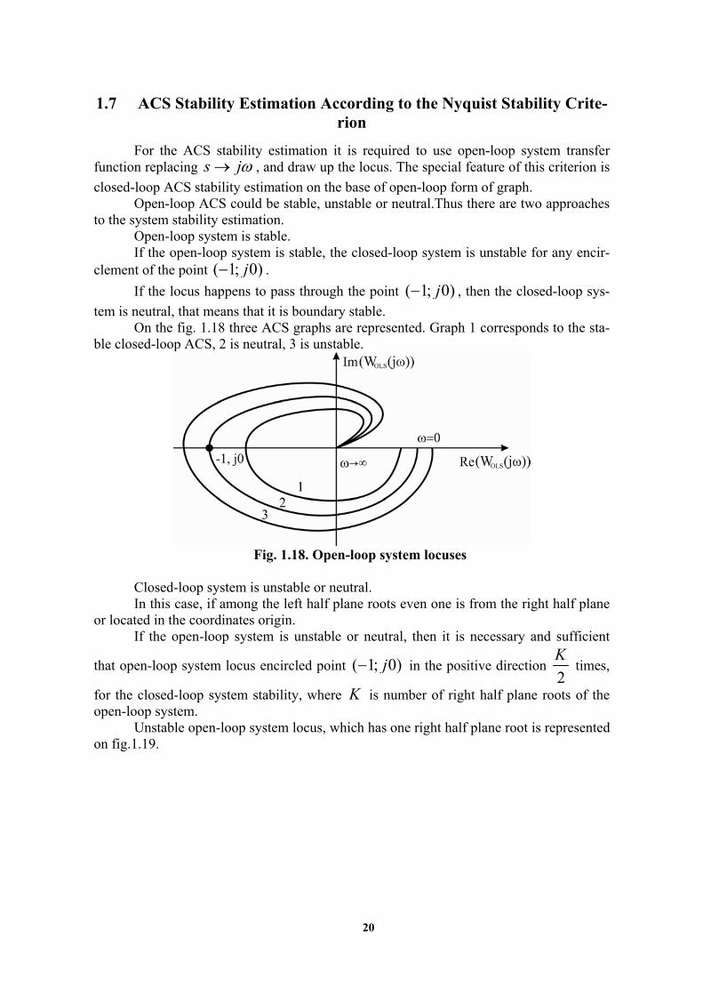
1.7 ACS Stability Estimation According to the Nyquist Stability Crite-rion

For the ACS stability estimation it is required to use open-loop system transfer function replacing s j , and draw up the locus. The special feature of this criterion is

closed-loop ACS stability estimation on the base of open-loop form of graph. Open-loop ACS could be stable, unstable or neutral.Thus there are two approaches

to the system stability estimation. Open-loop system is stable. If the open-loop system is stable, the closed-loop system is unstable for any encir-

clement of the point ( 1; 0)j .

If the locus happens to pass through the point ( 1; 0)j , then the closed-loop sys-

tem is neutral, that means that it is boundary stable. On the fig. 1.18 three ACS graphs are represented. Graph 1 corresponds to the sta-

ble closed-loop ACS, 2 is neutral, 3 is unstable.

Fig. 1.18. Open-loop system locuses

Closed-loop system is unstable or neutral. In this case, if among the left half plane roots even one is from the right half plane

or located in the coordinates origin. If the open-loop system is unstable or neutral, then it is necessary and sufficient

that open-loop system locus encircled point ( 1; 0)j in the positive direction 2

K times,

for the closed-loop system stability, where K is number of right half plane roots of the open-loop system.

Unstable open-loop system locus, which has one right half plane root is represented on fig.1.19.

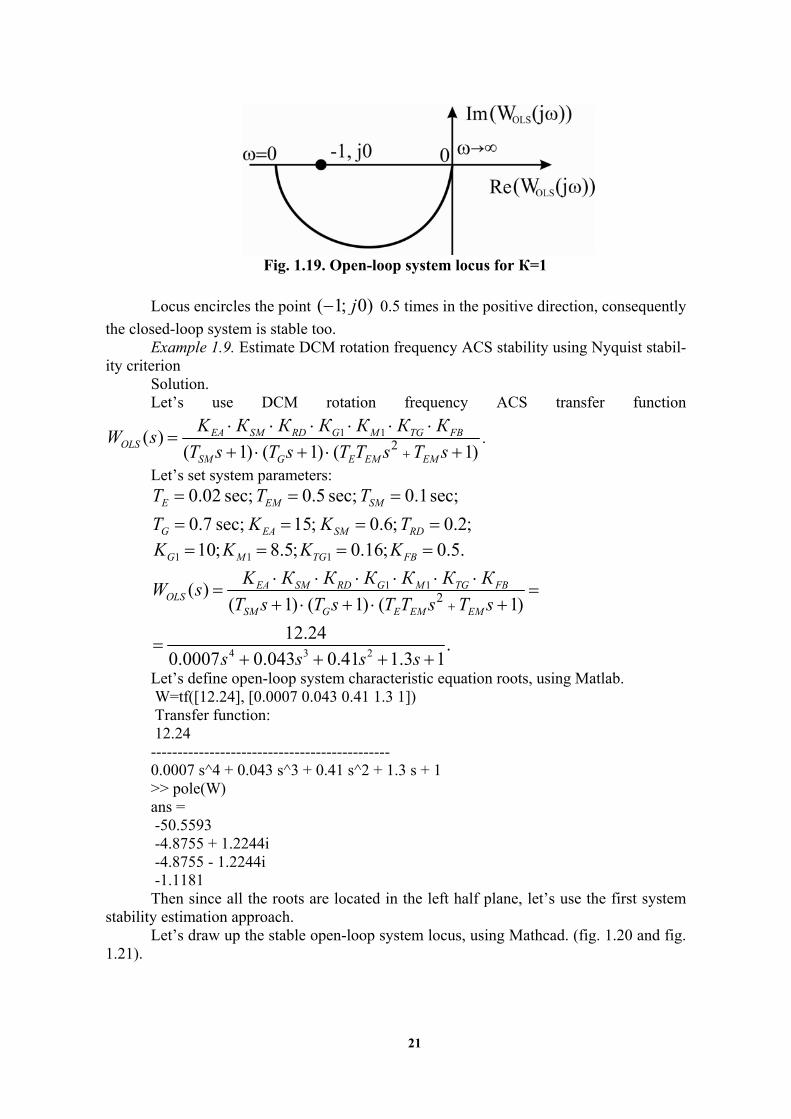
21

Fig. 1.19. Open-loop system locus for К=1

Locus encircles the point ( 1; 0)j 0.5 times in the positive direction, consequently

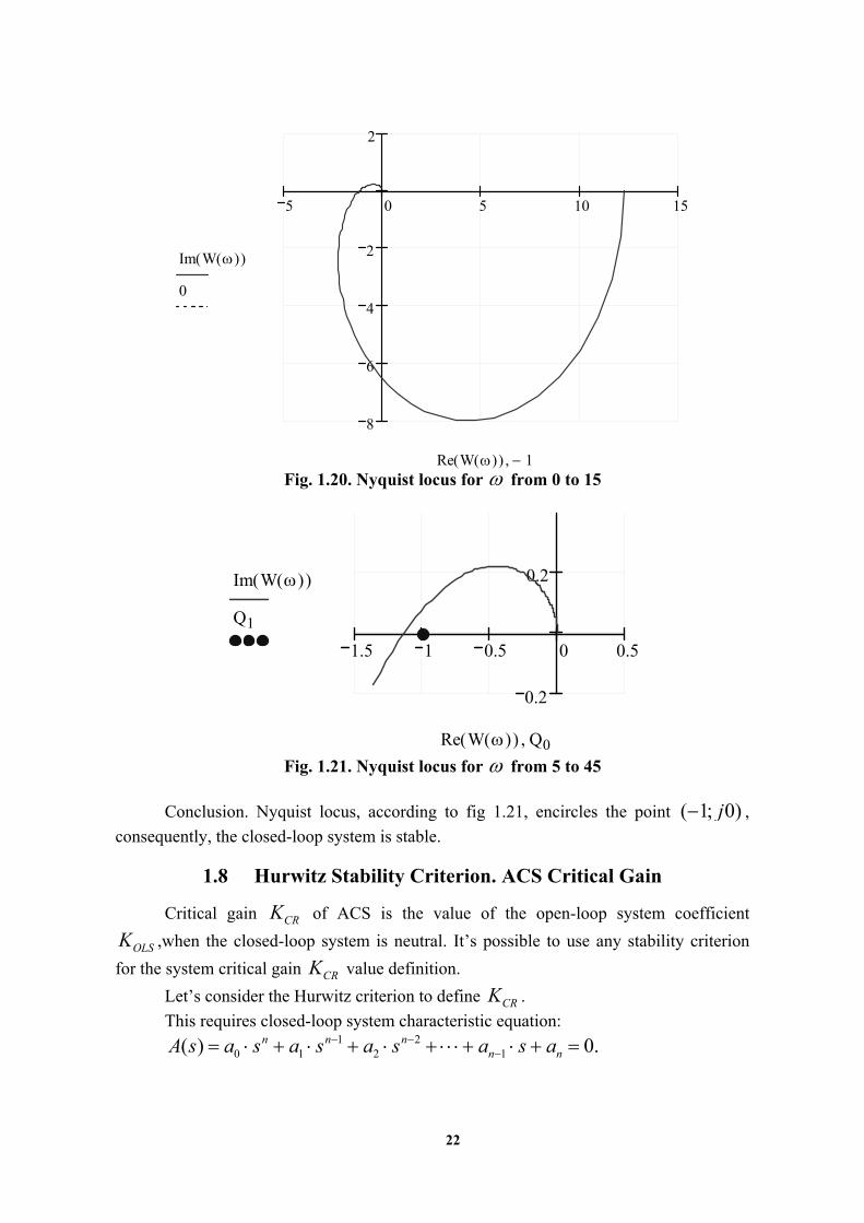
the closed-loop system is stable too. Example 1.9. Estimate DCM rotation frequency ACS stability using Nyquist stabil-

ity criterion Solution. Let’s use DCM rotation frequency ACS transfer function

1 12( )

( 1) ( 1) ( 1)EA SM RD G M TG FB

OLSSM G E EM EM

K К К К К К КW s

T s T s T T s T s

.

Let’s set system parameters: 0.02 sec; 0.5 sec; 0.1sec;

0.7 sec; 15; 0.6; 0.2;E EM SM

G EA SM RD

T T T

T K K T

1 1 110; 8.5; 0.16; 0.5.G M TG FBK K K K

1 1

4 3 2

2( )( 1) ( 1) ( 1)

12.24.

0.0007 0.043 0.41 1.3 1

EA SM RD G M TG FBOLS

SM G E EM EM

K К К К К К КW s

T s T s T T s T s

s s s s

Let’s define open-loop system characteristic equation roots, using Matlab. W=tf([12.24], [0.0007 0.043 0.41 1.3 1]) Transfer function: 12.24 --------------------------------------------- 0.0007 s^4 + 0.043 s^3 + 0.41 s^2 + 1.3 s + 1 >> pole(W) ans = -50.5593 -4.8755 + 1.2244i -4.8755 - 1.2244i -1.1181 Then since all the roots are located in the left half plane, let’s use the first system

stability estimation approach. Let’s draw up the stable open-loop system locus, using Mathcad. (fig. 1.20 and fig.

1.21).

22

5 0 5 10 15

8

6

4

2

2

Im W ( )( )

0

Re W ( )( ) 1 Fig. 1.20. Nyquist locus for from 0 to 15

1.5 1 0.5 0 0.5

0.2

0.2Im W ( )( )

Q1

Re W ( )( ) Q0

Fig. 1.21. Nyquist locus for from 5 to 45 Conclusion. Nyquist locus, according to fig 1.21, encircles the point ( 1; 0)j ,

consequently, the closed-loop system is stable.

1.8 Hurwitz Stability Criterion. ACS Critical Gain

Critical gain CRK of ACS is the value of the open-loop system coefficient

OLSK ,when the closed-loop system is neutral. It’s possible to use any stability criterion

for the system critical gain CRK value definition.

Let’s consider the Hurwitz criterion to define CRK .

This requires closed-loop system characteristic equation: 1 2

0 1 2 1( ) 0.n n nn nA s a s a s a s a s a

23

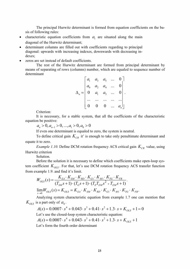
The principal Hurwitz determinant is formed from equation coefficients on the ba-sis of following rules:

characteristic equation coefficients from 1a are situated along the main

diagonal of the Hurwitz determinant; determinant columns are filled out with coefficients regarding to principal

diagonal: upwards with increasing indexes, downwards with decreasing in-dexes;

zeros are set instead of default coefficients. The rest of the Hurwitz determinant are formed from principal determinant by

means of separating of rows (columns) number, which are equaled to sequence number of determinant

1 3 5

0 2 4

1 3

... 0

... 0

0 ... 0 .

... ... ... ... ...

0 0 0 ...

n

n

a a a

a a a

a a

a

Criterion: It is necessary, for a stable system, that all the coefficients of the characteristic

equation be positive:

1 1 00, 0, ..., 0, 0n na a a a

If even one determinant is equaled to zero, the system is neutral. To define critical gain CRK it’ is enough to take only penultimate determinant and

equate it to zero. Example 1.10. Define DCM rotation frequency ACS critical gain CRK value, using

Hurwitz criterion Solution. Before the solution it is necessary to define which coefficients make open-loop sys-

tem coefficient OLSK . For that, let’s use DCM rotation frequency ACS transfer function

from example 1.9. and find it’s limit.

1 12( )

( 1) ( 1) ( 1)EA SM RD G M TG FB

OLSSM G E EM EM

K К К К К К КW s

T s T s T T s T s

.

1 10

lim ( ) .OLS OLS EA SM RD G M TG FBs

W s K K К К К К К К

Analyzing system characteristic equation from example 1.7 one can mention that

OLSK is a part only of 4a . 4 3 2( ) 0.0007 0.043 0.41 1.3 1 0OLSA s s s s s K

Let’s use the closed-loop system characteristic equation: 4 3 2( ) 0.0007 0.043 0.41 1.3 1OLSA s s s s s K

Let’s form the fourth order determinant

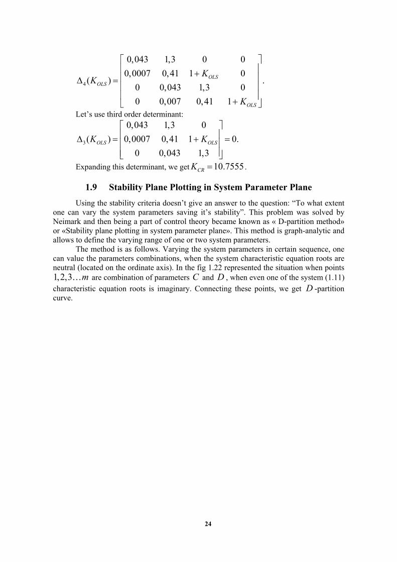
24

4

0,043 1,3 0 0

0,0007 0,41 1 0( ) .

0 0,043 1,3 0

0 0,007 0,41 1

OLSOLS

OLS

KK

K

Let’s use third order determinant:

3

0,043 1,3 0

( ) 0,0007 0,41 1 0.

0 0,043 1,3OLS OLSK K

Expanding this determinant, we get 10.7555CRK .

1.9 Stability Plane Plotting in System Parameter Plane

Using the stability criteria doesn’t give an answer to the question: “To what extent one can vary the system parameters saving it’s stability”. This problem was solved by Neimark and then being a part of control theory became known as « D-partition method» or «Stability plane plotting in system parameter plane». This method is graph-analytic and allows to define the varying range of one or two system parameters.

The method is as follows. Varying the system parameters in certain sequence, one can value the parameters combinations, when the system characteristic equation roots are neutral (located on the ordinate axis). In the fig 1.22 represented the situation when points 1,2,3 m are combination of parameters C and D , when even one of the system (1.11)

characteristic equation roots is imaginary. Connecting these points, we get D -partition curve.

25

Fig. 1.22. D -partition curve in parameters plane C and D

D -partition curve divides parameters plane C and D into areas with different

content of the right and the left roots. Plane area where all the system characteristic equa-tion roots are left claims to be stable. For the stability area identification D -partition curve shading is used. Closed-loop system characteristic equation, where the varying pa-rameters C and D are contained, is the initial equation for stability region plotting.

The stability area plotting algorithm in a single parameter plane C : Varying parameter C is detected in closed-loop system characteristic equation

(1.11). The given equation is expressed with respect to the variable parameter C . After passing to a frequency domain, replacing s j and separating real and

imaginary components, D-partition curve equation is ob-tained ( ) Re( ) Im( )N j j j . Let’s set a frequency from 0 to , and plot

one branch of D-partition curve and for from – to 0 – another branch. Causing a hatch on the branch of the D-partition, select the region of stability. Choose parameter C variation limits from the stability region. For the chosen value C , using any stability criterion, make found region checking. Example 1.11. Plot stability region in plane of the parameter CRC K .Define vari-

ation limits of CRK and critical gain CRK value of DCM rotation frequency ACS.

Solution. Let’s use closed-loop system characteristic equation from example 1.10:

4 3 2( ) 0.0007 0.043 0.41 1.3 1 0OLSA s s s s s K

Express OLSK from the given equation:

26

4 3 20.0007 0.043 0.41 1.3 1.OLSK s s s s

Let’s go to frequency domain and plot D-partition curve in the varying parameter

OLSK plane.

Fig. 1.23. D-partition curve in the parameter OLSK plane

In the fig. 1.23 one can see that stability region is the III-rdregion. Variation limits

0 10.7OLSK are chosen from this region. Therefore, critical gain value

10.7CRK , which coincides with the value is in the example 1.10.

1.10 Step Response of the System and Quality Indexes of the Control Process.

Performance quality of any control system is characterized by quantitative and qualitative indexes, which are defined by the step response curve or other dynamic system characteristics. System step response is the system reaction on the external influence, which, in general, could be the complex time function. Usually system performance is considered in terms of following standard influence: unit step function 1( )t , impulse func-

tion ( )t and harmonic function. Often direct quality indexes (transient character, control

time – St , and overshoot – ,% ) are obtained from the step response ( )h t , for unit step

input signal 1( )t .

Both numerator and denominator influence on step response character. If the closed-loop system transfer function ( )CLSW s has no zeros, i.e. has the form:

1

0 1

( ) ,... ( )CLS n n

n

К KW s

a s a s a A s

(1.16)

the character of the step response is completely determined by the closed-loop characteris-tic equation roots:

10 1 ... 0.n n

na s a s a (1.17)

27

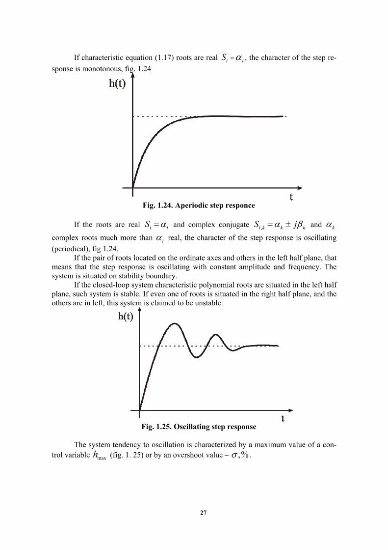
If characteristic equation (1.17) roots are real i iS , the character of the step re-

sponse is monotonous, fig. 1.24

Fig. 1.24. Aperiodic step responce

If the roots are real i iS and complex conjugate ,l k k kS j and k

complex roots much more than i real, the character of the step response is oscillating

(periodical), fig 1.24. If the pair of roots located on the ordinate axes and others in the left half plane, that

means that the step response is oscillating with constant amplitude and frequency. The system is situated on stability boundary.

If the closed-loop system characteristic polynomial roots are situated in the left half plane, such system is stable. If even one of roots is situated in the right half plane, and the others are in left, this system is claimed to be unstable.

Fig. 1.25. Oscillating step response

The system tendency to oscillation is characterized by a maximum value of a con-

trol variable maxh (fig. 1. 25) or by an overshoot value – ,% .

28

max 100%,h h

h

where h is steady-state value of control variable after the completion of the step re-

sponse.

Fig. 1.26. Qualitative indexes of step response

System performance settling time is characterized by the duration of step response

St . Settling time St (step response duration) is defined as a period of time from applica-

tion of influence at the system input to the moment, when the following inequality is held:

( )h t h h , where h is a small constant value, representing the specified accura-

cy. In the control theory it is 0.05 . Degree of stability represents an absolute value of the shortest distance from real

axes to the nearest root (or complex conjugated roots). Oscillating is ( )tg (fig. 1.26).

Settling time St and ,% are connected with degree of stability and oscillating by

following correlations: 1 1 3

lnSt

, % 100%e

.

For a more accurate estimation St and according to the correlations, it is neces-

sary for the system not to have zeros and all the system characteristic equation roots were located inside or on the boundary of trapezium in the roots plane fig. 1.27.

Fig. 1.27. Roots qualitative indexes

29

Example 1.12. Plot DCM rotation frequency ACS step response. Define qualitative indexes.

Solution. Let’s use the closed-loop system transfer function expression for the reference sig-

nal from example 1.5

1 1

1 12( ) .

( 1) ( 1) ( 1)inU EA SM RD G M

CLSSM G E EM EM EA SM RD G M TG FB

K К К К КW s

T s T s T T s T s K К К К К К К

Let’s set the system parameters: 0.02 sec; 0.5 sec; 0.1sec; 0.7 sec;E EM SM GT T T T

1 110; 0.6; 0.2 ; 8; 8.5; 0.15; 0.5.EA SM RD G M TG FBK K K K K K K

Then

4 3 2+ + +

12.24( ) .

0.0007s 0.043s 0.41s 1.3s+7.12 inU

CLSW s

Let’s use Matlab to plot the step response. The results are shown on fig. 1.27. > W=tf([12.24],[0.0007 0.043 0.41 1.3 7.12]) Transfer function: 12.24 ------------------------------------------------ 0.0007 s^4 + 0.043 s^3 + 0.41 s^2 + 1.3 s + 7.12 >> pole(W) ans = -50.4742 -9.7133 -0.6205 + 4.5124i -0.6205 - 4.5124i >> step(W)

30

Fig. 1.28. Step response of DCM rotation frequency ACS

Let’s give all the system indexes:

max 2.71 secradh ;

1.72CLSh K ;

57.9 % ;

0.278 secMT ;

5.87 secSt ;

1.3 secFRT ; 12 4.83 secFR FRT ;

0.6205 ;

4.51237.27

0.6205tg .

1.11 Automated Control System Control Process Accuracy Estimation

Control accuracy research of ACS is conducted by means of the system steady-state process analysis, i.e. the accuracy of control system is estimated by the steady-state errors, which is defined by the system structure (transfer functions) and influences (refer-ence signals and disturbances).

31

1.11.1 Control error in stabilization systems

Estimating the stabilization control system accuracy the reference signal is as-

sumed to be constant, i.e. 0( ) 1g t g t . Total control error ( )F t of linear system,

which functional scheme is depicted on fig. 1.29, could be represented as

F t g t x t , where g t is the reference signal; x t is the output signal.

In the image domain s the equation can be written as

FE s G s X s (1.18)

Connection between reference signal g t , disturbance f t and output signal

x t in the image domain s is established by means of transfer functions

g fCLS CLSX s W s G s W F s (1.19)

where ( )CLSgW s is the closed-loop system transfer function for the reference signal ( )g t ;

while ( )fCLSW s is closed-loop system transfer function for disturbance ( )f t .

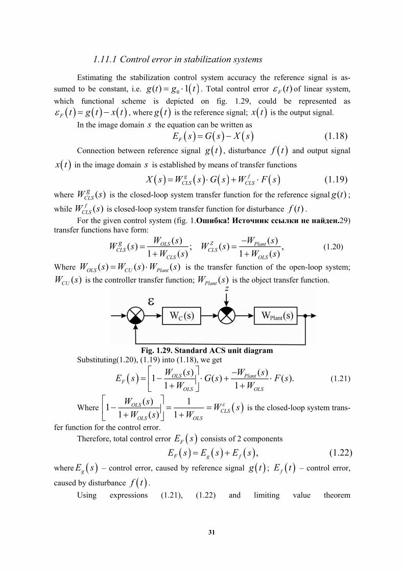
For the given control system (fig. 1.Ошибка! Источник ссылки не найден.29) transfer functions have form:

( )

( ) ;1 ( )

OLSCLS

CLS

g W sW s

W s

( )

( ) ,1 ( )

Z PlantCLS

OLS

W sW s

W s

(1.20)

Where ( ) ( ) ( )OLS CU PlantW s W s W s is the transfer function of the open-loop system;

( )CUW s is the controller transfer function; ( )PlantW s is the object transfer function.

Fig. 1.29. Standard ACS unit diagram

Substituting(1.20), (1.19) into (1.18), we get

( ) ( )1 ( ) ( ).

1 1OLS Plant

FOLS OLS

W s W sE s G s F s

W W

(1.21)

Where ( ) 11

1 ( ) 1OLS

CLSOLS OLS

W sW s

W s W

is the closed-loop system trans-

fer function for the control error.

Therefore, total control error FE s consists of 2 components

,F g fE s E s E s (1.22)

where gE s – control error, caused by reference signal g t ; fE t – control error,

caused by disturbance f t .

Using expressions (1.21), (1.22) and limiting value theorem

32

lim ( ) limt s

f t s W s F s

, for standard signals 0 1g t g t , 0 1f t f t

systems steady-state errors can be defined according to the following expressions: ss ss ssF g f , (1.23)

00ssg gW g , (1.24)

00 .ssf fxW f (1.25)

where ssF – steady-state value of the total error; ss

g – steady-state value of the error,

caused by reference signal; ssf – steady-state value of error, caused by disturbance.

Equations (1.23)-(1.25) are static equations, which in static stationary mode ( t , 0s ) connect steady-state control error values with transfer function values, defined for 0s .

The first total control error component in stabilization systems ( g t const ) ssF can be reduced to zero by scaling. Then control system accuracy will be fully charac-

terized by steady-state error SS :

0

0 0

0100% 100%

ss Zf CLS

SS

W f

g g

.

1.11.2 Control error in servo systems

In servo control systems and servo drive, used in aircrafts, reference signal is changed with constant speed 0 .

0 0, ,g t v t v const (1.26)

or with constant acceleration

2

, .2

a tg t a const

(1.27)

Control process accuracy estimated with the help of number of errors.

''' 2

0 1 ... .2! !

nn

SS n

c g t d g tct c g t c g t

n dt

(1.28)

where SS t steady-state error; 0 1, , ... ,!nc

c cn

– number of errors coefficients;

' ' ' ( )( ), ( ), ... ,

n

n

d g tg t g t

dt – the first, the second, …, n – derivative of reference sig-

nal.

Coefficients 0 1, , ... ,!nc

c cn

of number of errors (1.28) expressed in

terms of transfer function CLSW for control error:

33

0 1

22

2

( )( ) ; ;

00

( ) ( );

2! !0 0.

CLSCLS

nCLS n CLS

n

W sc W s c

s s s

c W s c W s

s n ss s

(1.29)

Number of errors (1.29) is restricted, both left and right. Restriction from the right depends on equality to zero of some derivative from the refer-ence signal ( )g t . For example, for the standard signal 0( ) 1( )g t g t steady-state error is defined according to the expression

0 0ss с g (1.30)

In this case number of errors coefficient 0c characterizes steady-state er-ror.

If the reference signal is changed with the constant speed (1.26), steady-state error expressed as

0 0 1 0( ) ,ss t c v t c v (1.31)

where coefficient 1c characterizes speed error. Steady-state error for the reference signal (1.27) expressed as

22

0 1( )2 2!ss

a t ct c c a t a . (1.32)

Coefficient 2

2!

c characterizes acceleration error.

From the expressions (1.30) - (1.32) follows, that for the static, speed and acceleration errors elimination it is necessary equality to zero of coeffi-

cients 20 1, ,

2!

cc c , respectively. For this purpose, it is necessary to provide ap-

propriate astatism order for the system. Under the astatism order meant degree v of the image Sv, which is situ-

ated in the open-loop system transfer function denominator. For example for

2( )

( )( )CLS

B sW s

s A s astatism order equals to 2.

For the 1st order astatic systems coefficient 0c equals to zero, for the 2nd order astatic systems – 0 1,c c equals to zero, for the 3rd order astatic systems –

20 1, ,

2!

cc c equals to zero. Thereby 1st order astatic systems reproduce constant

reference signals 0( ) 1( )g t g t without error, systems with the 2nd order of astaticism reproduce reference signals, which change with the constant speed

0 0( ) ,g t v t v const without errors etc.

34

2 Nonlinear ACS

ACS is considered to be nonlinear, if even one element of the system described by the nonlinear differential equation. Practically all the ACS are nonlinear. If after substitution of nonlinear system characteristic by the linear the ACS behavior doesn’t change, such system called linearized. Nonlineari-ties can be:

accompanying, if nonlinearity is a part of the composition of ACS invaria-ble part; not accompanying, if nonlinearity is a part of synthesized ACS part; essential; inessential nonlinearity; single-valued nonlinearity; mixed nonlinearity.

Nonlinearity is consider to be inessential, if the nonlinear component substitution by the linear unit doesn’t change fundamental system features and processes, occurring in the linearzed ACS, have no qualitative difference from the real system processes.

In the unit diagrams the nonlinear element is represented by means of the rectangle with static characteristic or functional dependence of the output signal Y from the input signal X , written inside. For a single-valued nonlin-earity is y F x . For mixed nonlinearity y depends not only on output

signal value x, but also on direction (i.e. derivative) ,y F x px .

Nonlinear ACS transformations have their own features. They are speci-fied by the fact that superposition principle and commutativity rule are not held for them, i.e. 1 2out in iny y y .

Also not all the structural transformation rules are held for nonlinear ACS, for example:

it’s not allowed to transfer the summer through a nonlinear unit; it’s not allowed to rearrange linear and nonlinear units, etc.

Nonlinear ACS transformation consists in linear units transformation, standing from the different sides of nonlinear element.

2.1 ACS Differential Equation in Implicit Form

There is no notation for the closed-loop nonlinear ACS. Therefore dif-ferential equation obtaining approach for such type of systems is different from the obtaining of linear ACS equation approach. Let’s obtain close-loop ACS differential equation, which unit diagram represented on fig. 2.1.

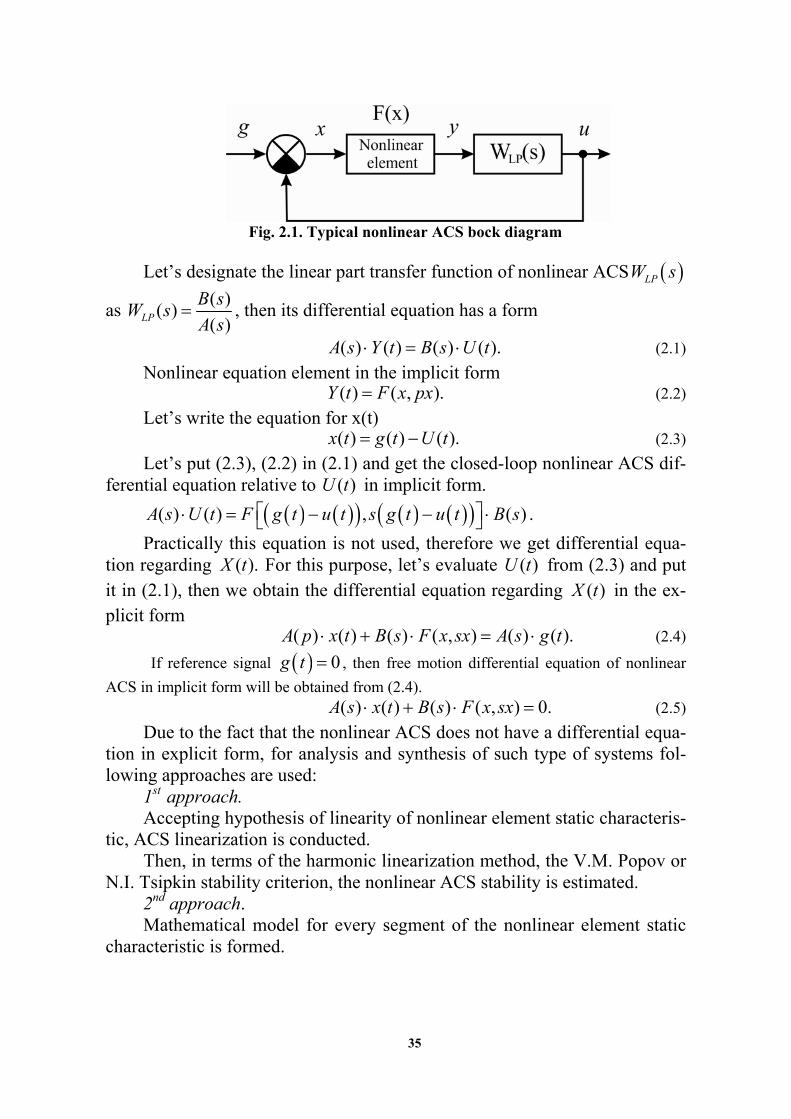
35

Fig. 2.1. Typical nonlinear ACS bock diagram

Let’s designate the linear part transfer function of nonlinear ACS LPW s

as ( )

( )( )LP

B sW s

A s , then its differential equation has a form

( ) ( ) ( ) ( ).A s Y t B s U t (2.1)

Nonlinear equation element in the implicit form ( ) ( , ).Y t F x px (2.2)

Let’s write the equation for х(t) ( ) ( ) ( ).x t g t U t (2.3)

Let’s put (2.3), (2.2) in (2.1) and get the closed-loop nonlinear ACS dif-ferential equation relative to ( )U t in implicit form.

( ) ( ) , ( )A s U t F g t u t s g t u t B s .

Practically this equation is not used, therefore we get differential equa-tion regarding ( ).X t For this purpose, let’s evaluate ( )U t from (2.3) and put it in (2.1), then we obtain the differential equation regarding ( )X t in the ex-plicit form

( ) ( ) ( ) ( , ) ( ) ( ).A p x t B s F x sx A s g t (2.4)

If reference signal 0g t , then free motion differential equation of nonlinear

ACS in implicit form will be obtained from (2.4). ( ) ( ) ( ) ( , ) 0.A s x t B s F x sx (2.5)

Due to the fact that the nonlinear ACS does not have a differential equa-tion in explicit form, for analysis and synthesis of such type of systems fol-lowing approaches are used:

1st approach. Accepting hypothesis of linearity of nonlinear element static characteris-

tic, ACS linearization is conducted. Then, in terms of the harmonic linearization method, the V.M. Popov or

N.I. Tsipkin stability criterion, the nonlinear ACS stability is estimated. 2nd approach. Mathematical model for every segment of the nonlinear element static

characteristic is formed.

36

In terms of the system state space and taking into account the obtained mathematical models, nonlinear ACS description in form of 1st order differ-ential equations is performed. Analyzing 1st order differential equation sys-tems solutions for each segment of nonlinear static characteristic, nonlinear ACS stability is estimated.

2.2 Harmonic Linearization Method Application for Nonlinear ACS

It’s convenient to use harmonic linearization (harmonic balance) method for nonlinear ACS study. This method is based on frequency characteristics usage, applied in linear control theory. It requires taking into account some assumptions:

Unit diagram should be typical (fig. 2.1). Nonlinear element characteristic should be symmetric in relation to the coordinate origin. The system should have self-oscillation with constant amplitude

na and frequency n .

System should be autonomous, i.e. ( ) 0.g t If a closed-loop autonomous (without external influences) nonlinear sys-

tem can be represented as the compounds of the nonlinear element and a sta-ble linear part with transfer function ( )LPW s (fig. 2.1), then under a certain conditions could be applied harmonic linearization method to it. The main idea of this method is that the possible stable oscillations on linear part of nonlinear system output approximately considered to be harmonic (sinusoi-dal).

Let’s assume, at the nonlinear element output sinusoidal signal ( ) sin( )x t a t is feed. Therefore, nonlinear element output signal ( )y t is

also periodical and could be expanded in the Fourier series. This series con-tains components with frequencies multiple to frequency , 2 ,... of output signal ( )x t . Supposing, that this signal, passing through the linear part is fil-tered to the extent that higher harmonics can be neglected, we write the har-monic linearization equation of nonlinear element:

' ( )

( ) ( , ) sin , cos ( ) ( ) ( ),g a

y t F x sx F a a q a x t x t

(2.6)

where , ( ), ( )t q a q a are the harmonic linearization coefficients of nonlinear el-

ement:

2

0

1( ) sin , cos sinq a F a a d

a

;

37

2

0

1( ) sin , cos cosq a F a a d

a

.

Equation (2.6) is a harmonic linearization equation up to highest harmonics from the case, when nonlinear element has the ambiguous characteristic. For the case, when nonlinear element has the single-valued characteristic

( ) ( ) ( ).y t q a x t (2.7)

Expressions for the harmonic linearization coefficients ( ), ( )q a q a , definition

represented in.

2.3 Differential and Characteristic Equations of ACS Harmonic Line-arization

Harmonic linearization method application allows to obtain nonlinear ACS differ-ential equations in the implicit form.

For this purpose expression (2.6) or (2.7) is put into equation (2.4). As a result non-linear ACS harmonic linearization differential equation with ambiguous or single-valued characteristics is obtained:

( )

( ) ( ) ( ) ( ) ( ) ( ) ( ) ( ),g a

A s X t B s q a x t s x t A s g t

(2.8)

( ) ( ) ( ) ( ) ( ) ( ) ( )A s X t B s q a x t A s g t (2.9)

For the autonomous ACS expressions have the following form:

' ( )

( ) ( ) ( ) ( ) ( ) ( ) 0,g a

A s X t B s q a x t s x t

(2.10)

( ) ( ) ( ) ( ) ( ) 0A s X t B s q a x t (2.11)

For the expressions (2.8)-(2.11) nonlinear ACS harmonic linearization differential equation are

' ( )

( ) ( ) ( ) 0,g a

A s B s q a s

(2.12)

( ) ( ) ( ) 0.A s B s q a (2.13)

2.4 Obtaining of Typical Unit Diagram of Nonlinear ACS

To reduce nonlinear ACS unit diagram to a standard form (fig. 2.1), use the follow-ing rules:

Since the system should be autonomous, it’s necessary to discard the reference signal and the disturbance with the surrounding chains.

Due to the fact that the nonlinear element should be in a typical scheme, right after the main summer, it is necessary to add one more summer at the output of the nonlinear element, in initial schemes.

If nonlinear element has time lag (thyristor transducer), then gain is realized in its static characteristic, and time lag remains a separate unit.

38

Standard scheme should be drawn beginning with the included summer. After nonlinear element all the other units of initial scheme, forwards the

reference signal to the introduced summer are drawn. If the initial scheme has the local feedbacks or additional control channels,

they also should be drawn. Example 2.13. Cast DCM rotation frequency ACS unit diagram with nonlinear

DCG characteristic to typical. Obtain differential and characteristic equations of harmonic linearized system. Nonlinear DCG characteristics are shown on fig. 2.2.

Fig. 2.2. Nonlinear DCG characteristics «saturation»

Coefficient of linearization for such nonlinearity has a form

2

22

( ) arcsin 1k b b b

q aa a a

; '( ) 0.q а (2.14)

Solution. Let’s use ACS unit diagram, represented on (fig. 1.4). Discard all the signals and

represent DCG in form of two units (nonlinear element and inertial unit with transfer func-

tion 1

( )1DCG

G

W sT s

). At the nonlinear element the input supplementary summer is

added (fig 2.3).

Fig. 2.3. Unit diagram of DCM rotation frequency nonlinear ACS

Utilizing standard unit diagram organization rules, obtain the system (fig. 2.4).

Fig. 2.4.Reduction of the nonlinear ACS unit diagram to the standard

Let’s obtain the transfer function of linear part of nonlinear system

39

12

( )( ) .

( )( 1) ( 1) ( 1)EA M RD M TG FB

LPM G E M M

K К К К К К B sW s

A sT s T s T T s T s

Using expressions (2.11) and (2.14), write differential and characteristic equations of the harmonic linearized system

1

2

2

2

( ) ( ) ( ) ( ) ( ) ( 1)( 1)( 1) ( )

2arcsin 1 ( ).

M G E M M

EA M RD M TG FB

A s x t B s q a x t T s T s T T s T s x t

k b b bK К К К К К x t

a a a

(2.15)

1

2

2

2

( ) ( ) ( ) ( 1) ( 1) ( 1)

2arcsin 1

M G E M M

EA M RD M TG FB

A s B s q a T s T s T T s T s

k b b bK К К К К К

a a a

(2.16)

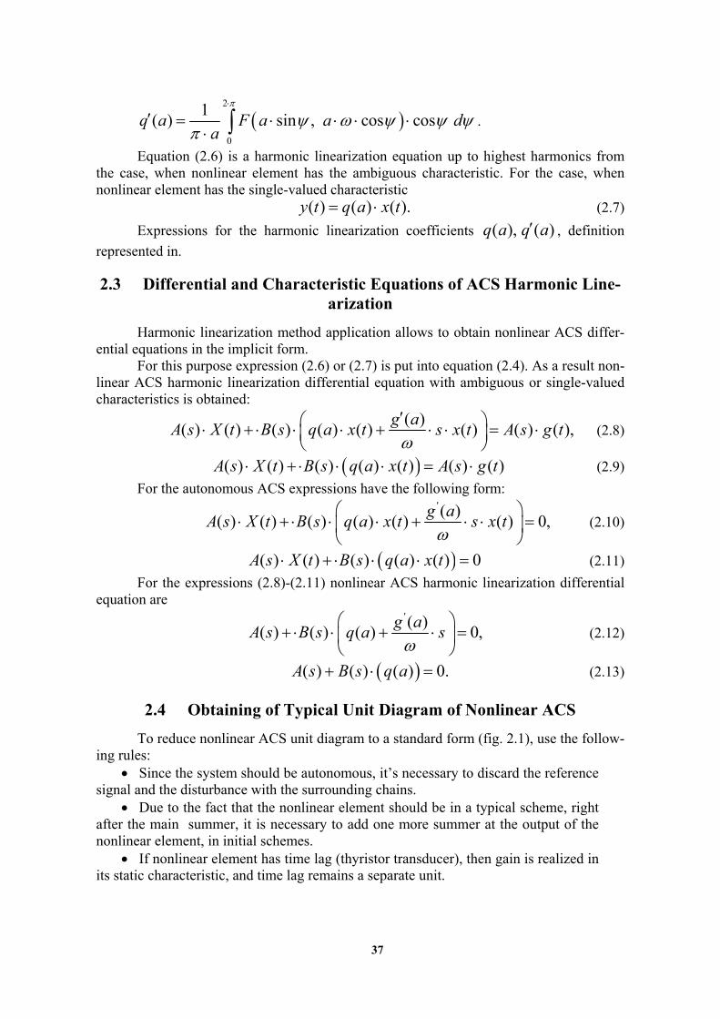
2.5 Goldfarb Method for Nonlinear ACS Stability Estimation Applica-tion

The stability analysis of harmonic linearized nonlinear ACS conducted in 2 stages. On the first stage we take a hypothesis, that system has the self-oscillations and define amplitude na and frequency n of these oscillations. On the second stage stability of the found periodical solution and the nonlin-ear ACS is estimated. For these purposes the Mikhailov criterion or the Gold-farb approach can be applied.

The main equation harmonic balance (linearization) approach has the form

1 ( ) ( ) 0,NP LPW a W j (2.17)

where ( )LPW j is the linear part transfer function of nonlinear ACS; ( )NPW a is the complex gain of harmonic linearized nonlinear element.

On the basis of equations (2.6), (2.7) one can write ( ) ( ) ( );NPW a q a j q a (2.18)

( ) ( ).NPW a q a (2.19)

Solving equation (2.17) regarding and a , self-oscillation parameters can be defined. Goldfarb suggested to solve this problem in a graphic way, representing this equation as

( ) ( ),LP NPW j G a (2.20)

where ( ) 1 ( )NP NPG a W a are the nonlinear reverse characteristics.

Linear part ( )LPW j locus (fig 3.3) and nonlinear element negative characteristic ( )NPG a are plot on the complex plane. Nodes of these charac-teristics give us the equation (2.52) solution. The oscillation amplitude na de-

40

fined according to characteristic ( )NPG a , and the frequency n defined ac-cording to ( )LPW j .

Fig. 3.5 shows the case when system has 2 periodic solutions: diagram nodes 2 ( 1 1,n na ) and 5 ( 2 2,n na ).

For the positive increment of amplitude na a , locus ( )LPW j encir-cles point 4 and doesn’t encircles point 11, and for negative na a – encir-cles point 3 and doesn’t encircles point 6.

Fig. 2.5. Graphic representation of the Goldfarb approach

If the locus ( )LPW j doesn’t encircle point with positive increment of amplitude

na a (point 1), and encircles point with negative increment na a , then obtained

solution will be stable (point 2), in this case the system is stable in general. If not, found solution is unstable (point 5), and system is stable in small.

Example 2.14. Using Goldfarb approach, estimate DCM rotation frequency ACS stability with nonlinear DCM characteristic. Nonlinear DCG characteristic represented on fig. 3.2.

Solution. Let’s use transfer function of linear part and harmonic linearization coefficients

from example 2.13.

12( ) .

( 1) ( 1) ( 1)EA M RD M TG FB

LPM G E M M

K К К К К КW s

T s T s T T s T s

2

22

( ) arcsin 1k b b b

q aa a a

; ( ) 0q а .

Let’s set the system parameters:

1 1 1

0.02 sec; 0.5 sec; 0.1sec; 0.7 sec; 10;

0.6; 0.2;

8; 8.5; 0.15; 0.5; ; 2.

E M M G EA

M RD

G M TG FB G

T T T T K

K K

K K K K k K b

Then

41

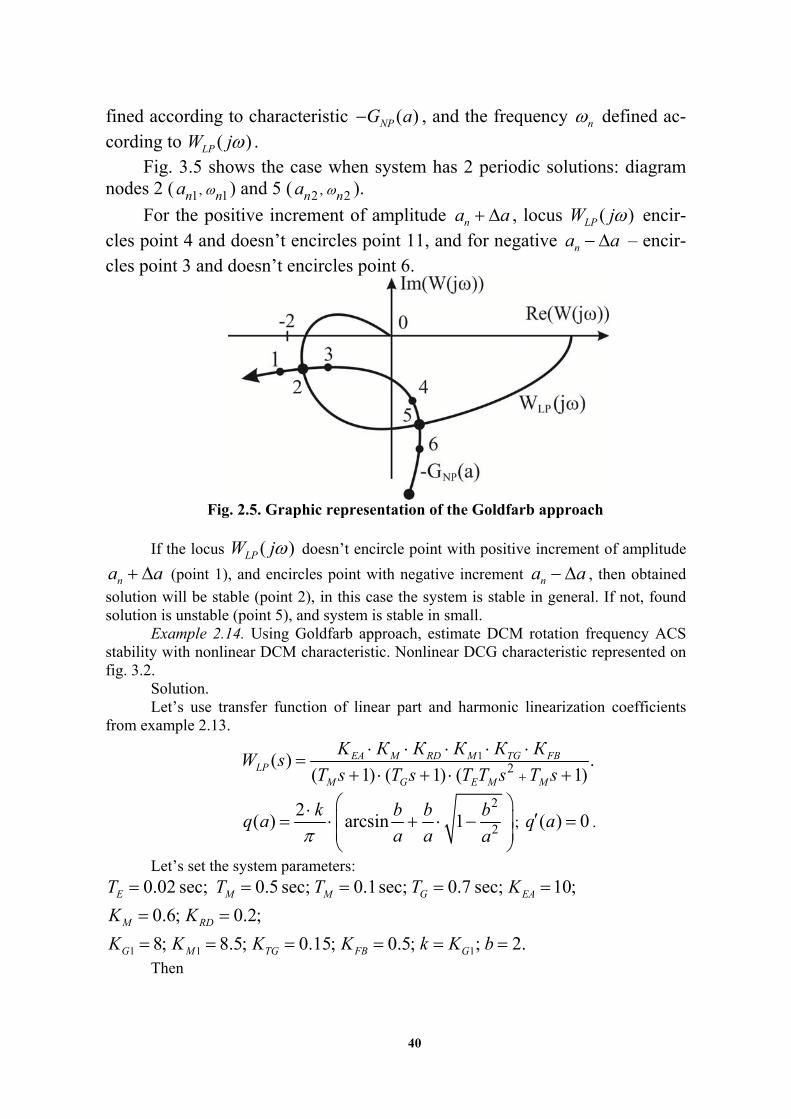
4 3 26.12

( ) .0.0007s +0.043s +0.41s +1.3s+1 LPW s

2 2

2 22 8 2 2 2 2 2 2

( ) ( ) arcsin 1 5.096 arcsin 1 .3.14NPW a q a

a a a aa a

2

2

1( ) 1 ( ) 0.196

2 2 2arcsin 1

NP NPG a W a

a a a

.

( )LPW j and ( )NPG a locuses are plot on the complex plane. The results repre-

sented in fig. 3.4.

→∞

→∞

Fig. 2.6. ( )LPW j and ( )LPG a locuses

Conclusion. Locuses cut across, therefore, there is general solution of equation

(2.52). Obtained solution is stable and ACS is stable in general.

2.6 Application of Popov Stability Criterion for Nonlinear ACS Stabil-ity Analysis

The frequency criterion research of the nonlinear ACS equilibrium posi-tion absolute stability was introduced by V.M. Popov in 1959. To use this cri-terion is necessary to take into account the following restrictions and assump-tions: unit diagram should be typical (fig. 2.1); nonlinear element characteristic should be single-valued; linear part of nonlinear ACS should be stable;

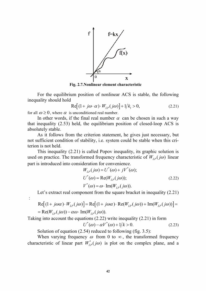
nonlinear characteristic should belong to sector 0, k (fig. 2.7), i.e. the condition

0 ( )f x kx should hold.

42

Fig. 2.7.Nonlinear element characteristic

For the equilibrium position of nonlinear ACS is stable, the following

inequality should hold 1Re (1 ) ( ) 1 0,LPj W j k (2.21)

for all 0 , where is unconditioned real number. In other words, if the final real number can be chosen in such a way

that inequality (2.53) held, the equilibrium position of closed-loop ACS is absolutely stable.

As it follows from the criterion statement, he gives just necessary, but not sufficient condition of stability, i.e. system could be stable when this cri-terion is not held.

This inequality (2.21) is called Popov inequality, its graphic solution is used on practice. The transformed frequency characteristic of ( )LPW j linear part is introduced into consideration for convenience.

* *

*

*

( ) ( ) ( );

( ) Re( ( ));

( ) Im( ( )).

LP

LP

LP

W j U jV

U W j

V W j

(2.22)

Let’s extract real component from the square bracket in inequality (2.21) :

Re (1 ) ( ) Re (1 ) Re( ( )) Im( ( ))

Re( ( )) Im( ( )).LP LP LP

LP LP

j W j j W j W j

W j W j

Taking into account the equations (2.22) write inequality (2.21) in form

* *( ) ( ) 1 0.U V k (2.23)

Solution of equation (2.54) reduced to following (fig. 3.5): When varying frequency from 0 to , the transformed frequency

characteristic of linear part * ( )LPW j is plot on the complex plane, and a

43

straight line under any angle is drawn though the point 11 ; 0k j (fig.

2.8а). Popov criterion. For the nonlinear ACS equilibrium position was stable, all transformed

frequency characteristic linear part * ( )LPW j locus is necessary to be located on the right side from the straight line, drawn under any angle , through the point 11 ; 0k j . Where 1k is the straight line slope ratio, restricting sector

(0, 1k ).

a)

b)

c)

Fig. 2.8. Popov inequality solution According to fig. 2.8, for the case а) ACS equilibrium position is abso-

lutely stable; for b) and c) Popov criterion is not held, but the system can be stable.

44

Example 2.15. It is necessary to estimate DCM rotation frequency ACS stability with nonlinear characteristic of DCG, using Popov criterion.

Nonlinear characteristic parameters of DCG: 1 8; 4; 0.1.GK b m Solution. Let’s plot the nonlinear characteristic of DCG taking into account its pa-

rameters (fig. 2.9).

Fig. 2.9. Nonlinear characteristic of DCG

Let’s use linear part transfer function and system parameters from the

example 2.14

4 3 26.12

( )0.0007 +0.043 +0.41 +1.3 1 LPW s

s s s s

. Bode plot of transformed frequency characteristic linear part *

LPW j

and point ( 0.139; 0)j . Plot results represented in fig. 2.10.

Fig. 2.10. Popov criterion application for the system stability estimation

45

Conclusion. The Popov criterion is held, because it is possible to draw the straight line under any angle through the found point, in such a way that all the Bode plot located on the right side of the straight line.

2.7 V.M. Popov Stability Criterion Application for the Case of Neutral or Unstable Linear Part

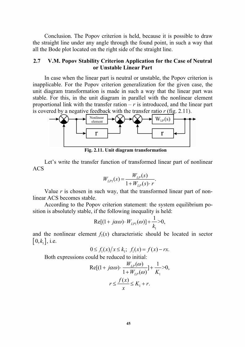
In case when the linear part is neutral or unstable, the Popov criterion is inapplicable. For the Popov criterion generalization for the given case, the unit diagram transformation is made in such a way that the linear part was stable. For this, in the unit diagram in parallel with the nonlinear element proportional link with the transfer ration – r is introduced, and the linear part is covered by a negative feedback with the transfer ratio r (fig. 2.11).

Fig. 2.11. Unit diagram transformation

Let’s write the transfer function of transformed linear part of nonlinear

ACS

1

( )( ) .

1 ( )LP

LPLP

W sW s

W s r

Value r is chosen in such way, that the transformed linear part of non-linear ACS becomes stable.

According to the Popov criterion statement: the system equilibrium po-sition is absolutely stable, if the following inequality is held:

11

1Re[(1 ) ( )] >0,LPj W

k

and the nonlinear element f1(х) characteristic should be located in sector 10,k , i.e.

1 1 10 ( ) ; ( ) ( ) .f x x k f x f x rx

Both expressions could be reduced to initial:

1

( ) 1Re[(1 ) ] >0,

1 ( )LP

LP

Wj

W K

1

( ).

f xr K r

x

46

Nonlinear characteristic should be located in sector 1,r k r . If linear

part of nonlinear ACS is neutral, then r should be extremely small value.

3 LINEAR PULSE ACS

Depending on signal transmission and transformation methods ACS can be divided into:

continuous ACS; discrete ACS.

In the continuous systems signals during the transformation process are not interrupted. There are elements or units, which transform continuous sig-nals into the pulse sequence, or quantized signals series, or the digital code in discrete systems. In many modern ACS the discrete devices or digital proces-sors are used.

Discrete method of signals transmission and transformation supports their amplitude quantization or time quantization, or amplitude and time quantization. There are 3 types of quantization and 3 groups of discrete ACS:

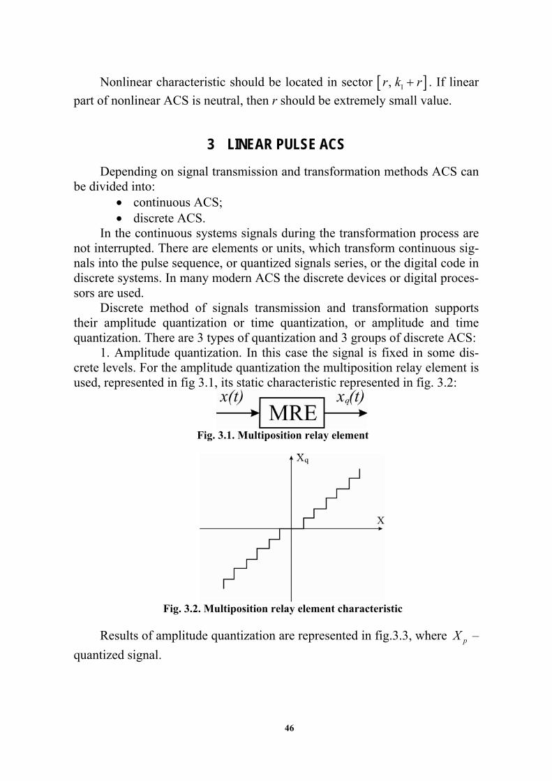
1. Amplitude quantization. In this case the signal is fixed in some dis-crete levels. For the amplitude quantization the multiposition relay element is used, represented in fig 3.1, its static characteristic represented in fig. 3.2:

Fig. 3.1. Multiposition relay element

Fig. 3.2. Multiposition relay element characteristic

Results of amplitude quantization are represented in fig.3.3, where pX –

quantized signal.

47

Fig. 3.3. Level quantization

Since the relay element is used as a continuous signal X t quantizer,

then the discrete ACS also called relay ACS. Such type of discrete systems refers to nonlinear ACS type, and for their analysis and synthesis the nonlin-ear system theory is used.

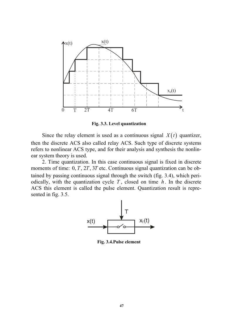
2. Time quantization. In this case continuous signal is fixed in discrete moments of time: 0, , 2 , 3T T T etc. Continuous signal quantization can be ob-tained by passing continuous signal through the switch (fig. 3.4), which peri-odically, with the quantization cycle T , closed on time h . In the discrete ACS this element is called the pulse element. Quantization result is repre-sented in fig. 3.5.

Fig. 3.4.Pulse element

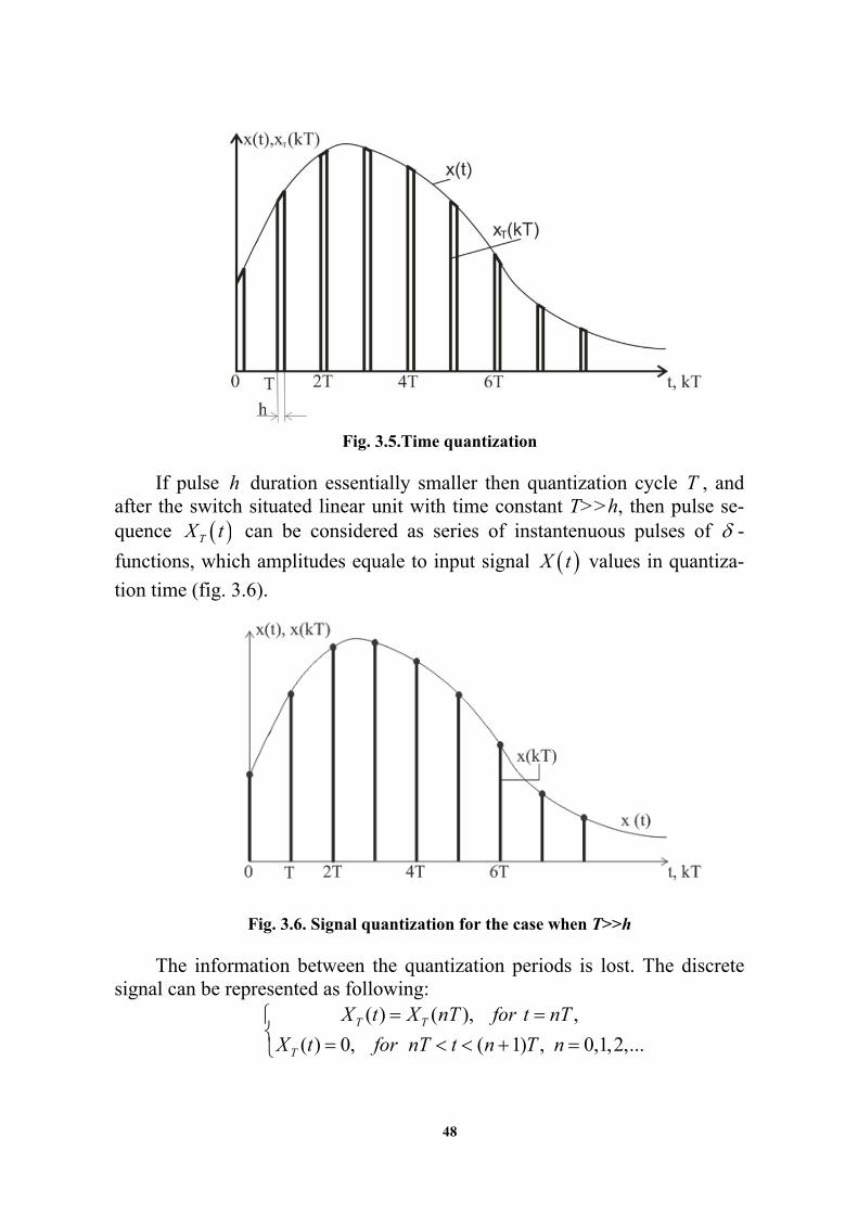
48

Fig. 3.5.Time quantization

If pulse h duration essentially smaller then quantization cycle T , and

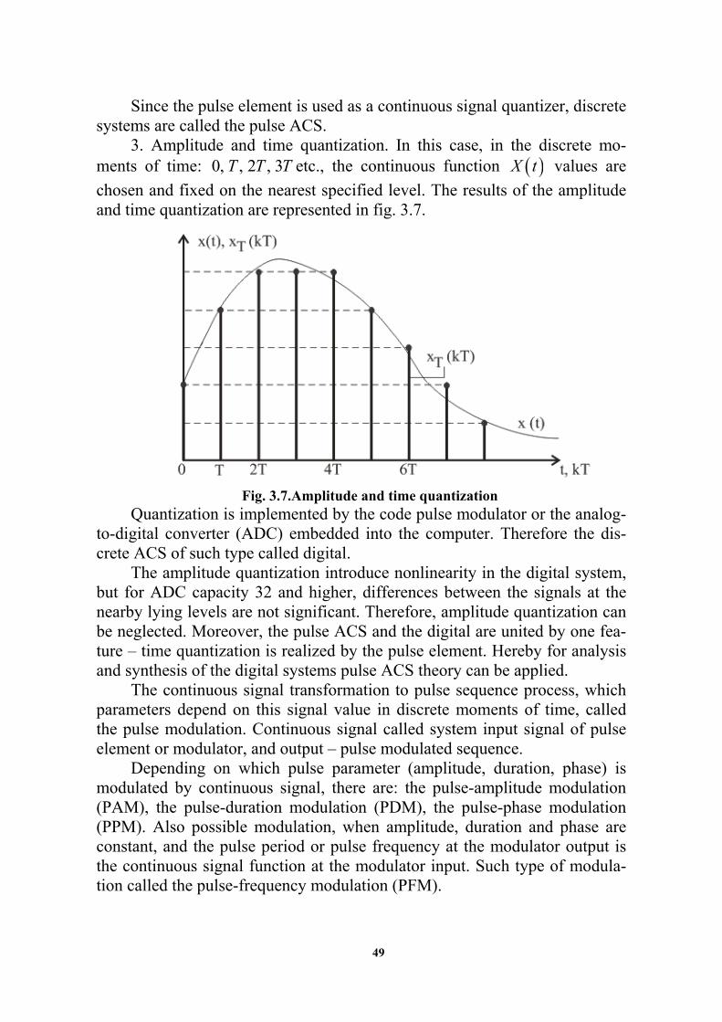
after the switch situated linear unit with time constant Т>>h, then pulse se-quence TX t can be considered as series of instantenuous pulses of -

functions, which amplitudes equale to input signal X t values in quantiza-

tion time (fig. 3.6).

Fig. 3.6. Signal quantization for the case when Т>>h

The information between the quantization periods is lost. The discrete

signal can be represented as following: ( ) ( ), ,

( ) 0, ( 1) , 0,1,2,...T T

T

X t X nT for t nT

X t for nT t n T n

49

Since the pulse element is used as a continuous signal quantizer, discrete systems are called the pulse ACS.

3. Amplitude and time quantization. In this case, in the discrete mo-ments of time: 0, , 2 , 3T T T etc., the continuous function X t values are

chosen and fixed on the nearest specified level. The results of the amplitude and time quantization are represented in fig. 3.7.

Fig. 3.7.Amplitude and time quantization

Quantization is implemented by the code pulse modulator or the analog-to-digital converter (ADC) embedded into the computer. Therefore the dis-crete ACS of such type called digital.

The amplitude quantization introduce nonlinearity in the digital system, but for ADC capacity 32 and higher, differences between the signals at the nearby lying levels are not significant. Therefore, amplitude quantization can be neglected. Moreover, the pulse ACS and the digital are united by one fea-ture – time quantization is realized by the pulse element. Hereby for analysis and synthesis of the digital systems pulse ACS theory can be applied.

The continuous signal transformation to pulse sequence process, which parameters depend on this signal value in discrete moments of time, called the pulse modulation. Continuous signal called system input signal of pulse element or modulator, and output – pulse modulated sequence.

Depending on which pulse parameter (amplitude, duration, phase) is modulated by continuous signal, there are: the pulse-amplitude modulation (PAM), the pulse-duration modulation (PDM), the pulse-phase modulation (PPM). Also possible modulation, when amplitude, duration and phase are constant, and the pulse period or pulse frequency at the modulator output is the continuous signal function at the modulator input. Such type of modula-tion called the pulse-frequency modulation (PFM).

50

If the modulated parameter of the pulse sequence is defined by the input signal values in the fixed equidistant moments of time and remains constant on all the period of pulse existence, then such a modulation called the pulse modulation of the first type. There may be instances when the modulated pa-rameter of the pulse sequence on all the period of pulse existence changes ac-cording to the current input signal value. Such modulation called the modula-tion of the second type.

First type pulse-amplitude modulation ACS refers to the category of lin-ear system, therefore only the linear pulse ACS analysis and the design theo-ry will be considered.

Linear pulse system is an automated control system, which besides units, described by the linear differential equations, has the pulse element, which transforms input signal into pulse sequence.

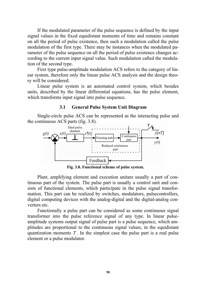
3.1 General Pulse System Unit Diagram

Single-circle pulse ACS can be represented as the interacting pulse and the continuous ACS parts (fig. 3.8).

Fig. 3.8. Functional scheme of pulse system.

Plant, amplifying element and execution unitare usually a part of con-

tinuous part of the system. The pulse part is usually a control unit and con-sists of functional elements, which participate in the pulse signal transfor-mation. This part can be realized by switches, modulators, pulsecontrollers, digital computing devices with the analog-digital and the digital-analog con-verters etc.

Functionally a pulse part can be considered as some continuous signal transformer into the pulse reference signal of any type. In linear pulse-amplitude systems output signal of pulse part is a pulse sequence, which am-plitudes are proportional to the continuous signal values, in the equidistant quantization moments T . In the simplest case the pulse part is a real pulse element or a pulse modulator.

51

When studying the pulse systems their real pulse elements are usually substituted by successive connection of the ideal pulse element (IPE) and the forming unit (FU) (fig. 3.8).

The ideal pulse element under the influence of continuous input signal x t (fig. 3.9) form ideal instantenuous pulses *x t of -function type,

which «amplitude areas» are equal to the input signal values in quantization moments. Usually the gain of pulse element refers to the continuous system part, considering the ideal pulse element transmission gain equaled one.

Fig. 3.9.Signal forming by real pulse element

The forming unit transform these pulses into signals u t of the re-

quired form. Forming unit is pulse-amplitude modulator. Forming element response to instantenuous pulse of sequence *x t coincide with the real

pulse sequence u t at the real pulse element output. In practice, most often

the data-hold device of zero order with the transfer function (2.56) is used as a forming unit

1

( ) .T s

FU

eW s

s

(3.1)

For the convenience of system analysis the forming unit is combined with the continuous part. In this case independently of real pulses form, pulse systems with amplitude modulation can be represented as the combination of ideal pulse element and reduced continuous part (fig. 3.10). Output signal of pulse system reduced continuous part is continuous signal, described by time function y t . To apply the discrete Laplace transform it is accepted to con-

sider this signal in discrete moments of time, coinciding with moments of ideal pulse element shorting at input. This is equivalent to fictitious ideal pulse element switching on (fig. 3.10) at the systems output, operating syn-chronously and in-phase with the main pulse element. Reduced continuous part (RCP) reaction on -functions is a sum of pulse (weighting) step re-sponse ( )w t . The transfer function of the reduced continuous part is equaled to

52

( ) ( ) ( )RCP FU CPW s W s W s (3.2)

Unit diagram of pulse ACS depicted in fig. 3.10.

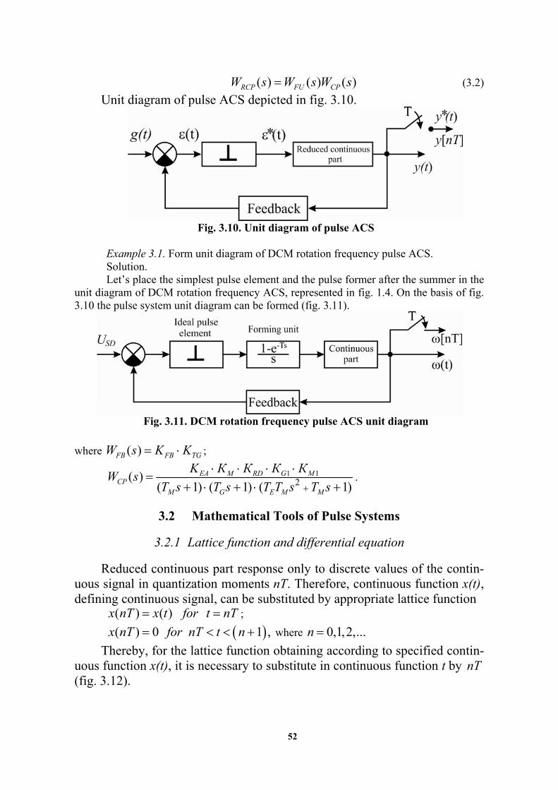
Fig. 3.10. Unit diagram of pulse ACS

Example 3.1. Form unit diagram of DCM rotation frequency pulse ACS. Solution. Let’s place the simplest pulse element and the pulse former after the summer in the

unit diagram of DCM rotation frequency ACS, represented in fig. 1.4. On the basis of fig. 3.10 the pulse system unit diagram can be formed (fig. 3.11).

Fig. 3.11. DCM rotation frequency pulse ACS unit diagram

where ( )FB FB TGW s K K ;

1 12( )

( 1) ( 1) ( 1)EA M RD G M

CPM G E M M

K К К К КW s

T s T s T T s T s

.

3.2 Mathematical Tools of Pulse Systems

3.2.1 Lattice function and differential equation

Reduced continuous part response only to discrete values of the contin-uous signal in quantization moments nT. Therefore, continuous function x(t), defining continuous signal, can be substituted by appropriate lattice function

( ) ( )x nT x t for t nT ;

( ) 0 1 ,x nT for nT t n where 0,1,2,...n

Thereby, for the lattice function obtaining according to specified contin-uous function x(t), it is necessary to substitute in continuous function t by nT (fig. 3.12).

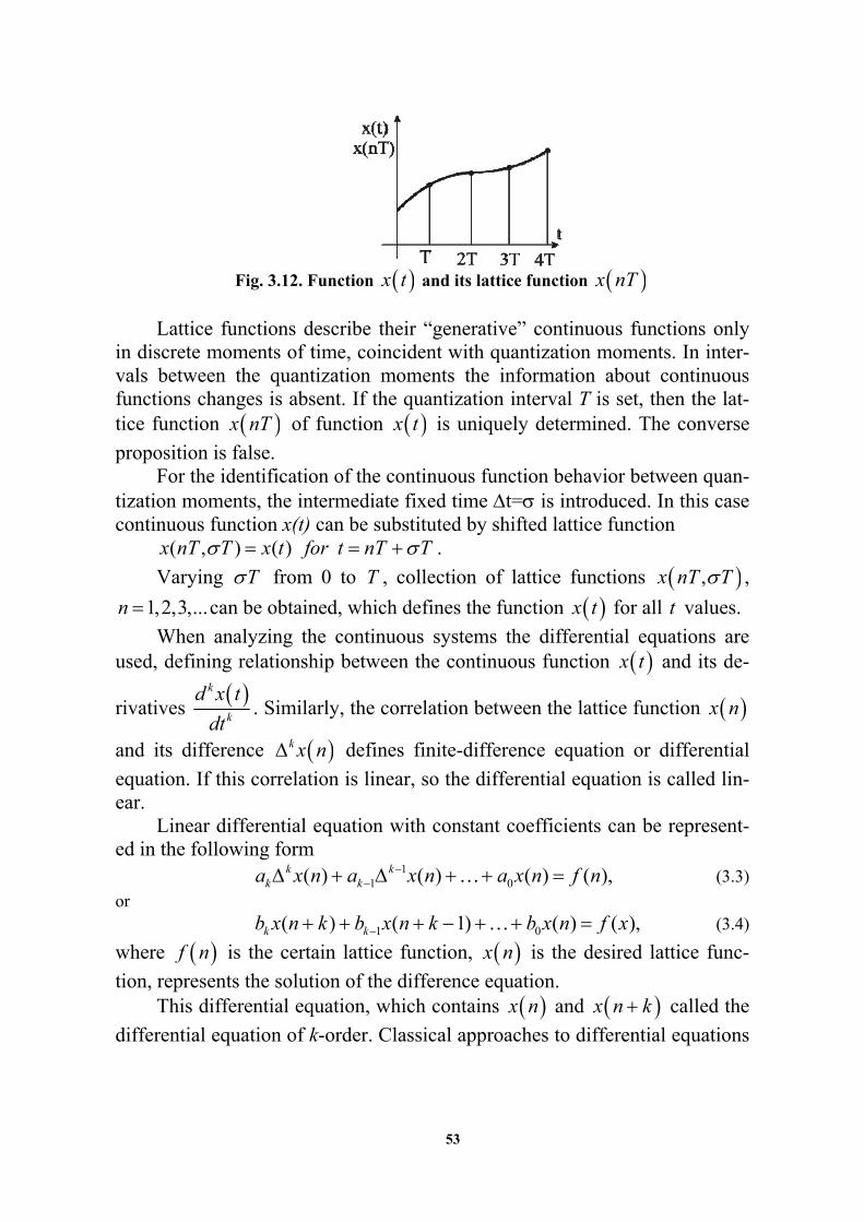
53

Fig. 3.12. Function x t and its lattice function x nT

Lattice functions describe their “generative” continuous functions only

in discrete moments of time, coincident with quantization moments. In inter-vals between the quantization moments the information about continuous functions changes is absent. If the quantization interval Т is set, then the lat-tice function x nT of function x t is uniquely determined. The converse

proposition is false. For the identification of the continuous function behavior between quan-

tization moments, the intermediate fixed time t= is introduced. In this case continuous function x(t) can be substituted by shifted lattice function

( , ) ( )x nT T x t for t nT T .

Varying T from 0 to T , collection of lattice functions ,x nT T ,

1,2,3,...n can be obtained, which defines the function x t for all t values.

When analyzing the continuous systems the differential equations are used, defining relationship between the continuous function x t and its de-

rivatives k

k

d x t

dt. Similarly, the correlation between the lattice function x n

and its difference k x n defines finite-difference equation or differential

equation. If this correlation is linear, so the differential equation is called lin-ear.

Linear differential equation with constant coefficients can be represent-ed in the following form

11 0( ) ( ) ( ) ( ),k k

k ka x n a x n a x n f n (3.3)

or 1 0( ) ( 1) ( ) ( ),k kb x n k b x n k b x n f x (3.4)

where f n is the certain lattice function, x n is the desired lattice func-

tion, represents the solution of the difference equation. This differential equation, which contains x n and x n k called the

differential equation of k-order. Classical approaches to differential equations

54

solution in many respects analogous to the classical methods differential equations solution.

Differential equation solution gives the output signal values only in dis-crete moments of time t nT . In many cases it’s rather enough for the sys-tem behavior estimation. If appears the necessity in output signal information obtaining, the offset sequence is used.

In case, when 0f n , equations (3.3) and (3.4) called homogenous.

3.2.2 Z-transform application

For sequences f(n) discrete Laplace transform concept, defined by the expression (2.60), can be introduced

0

( ) ( ) ( ) .T

i

snF s D f n f n e

(3.5)

In expression, like in case of the continuous Laplace transform, complex value s c j , where c is the abscissa of absolute convergence. If c , then series, defined by the expression (3.5), convergences, and some expres-sion corresponds to the original f n .

Z -transform is widespread for the pulse systems research, which is connected with the discrete Laplace transform.

Under Z -transform one understand sequence of images, defined by the expression

0

( ) ( ) .i

nF z f n z

(3.6)

Here new notation is introduced STz e . Principle rules and theorems in respect to Z -transform are also true for

discrete Laplace transform. If image F z is represented in the simplest table form, then transition

to original doesn’t make any difficulty. Complex fractionally rational form can be represented in form of the first order sum, then z -transform table can be used for original obtaining from every simple fraction.

Moreover, if F z is a ratio of two polynomials ( )

( )( )

B zF z

A z , then ana-

logue of the Heaviside decomposition expression, used for continuous sys-tems, can be applied.

1

(1) ( )( )

(1) (1 ) '( )

li

i i i

ni

B B zf n z

A z A z

,

where ' ( )A z is the derivative ( )A z for z , and iz are the denominator roots

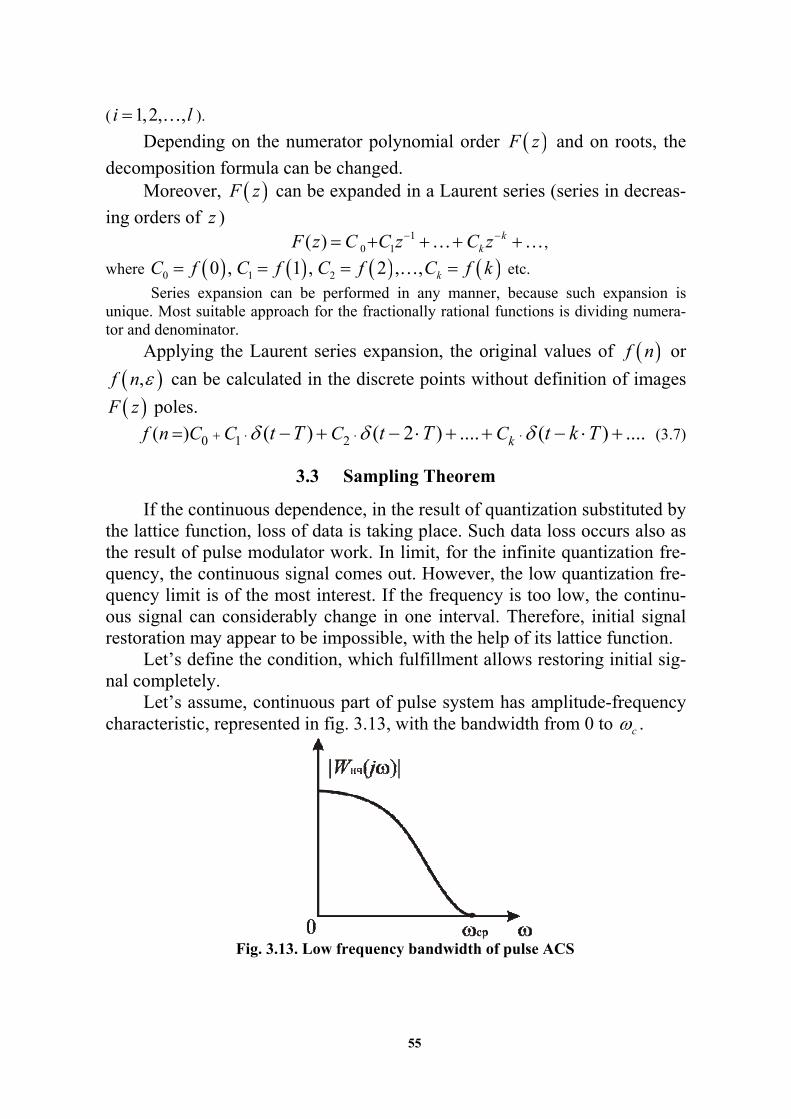
55

( 1,2, ,i l ).

Depending on the numerator polynomial order F z and on roots, the

decomposition formula can be changed. Moreover, F z can be expanded in a Laurent series (series in decreas-

ing orders of z ) 1

0 1( ) kkF z C C z C z ,

where 0 1 20 , 1 , 2 , , kC f C f C f C f k etc.

Series expansion can be performed in any manner, because such expansion is unique. Most suitable approach for the fractionally rational functions is dividing numera-tor and denominator.

Applying the Laurent series expansion, the original values of f n or

,f n can be calculated in the discrete points without definition of images

F z poles.

0 1 2( ) ( ) ( 2 ) .... ( ) ....kf n C C C Ct T t T t k T (3.7)

3.3 Sampling Theorem

If the continuous dependence, in the result of quantization substituted by the lattice function, loss of data is taking place. Such data loss occurs also as the result of pulse modulator work. In limit, for the infinite quantization fre-quency, the continuous signal comes out. However, the low quantization fre-quency limit is of the most interest. If the frequency is too low, the continu-ous signal can considerably change in one interval. Therefore, initial signal restoration may appear to be impossible, with the help of its lattice function.

Let’s define the condition, which fulfillment allows restoring initial sig-nal completely.

Let’s assume, continuous part of pulse system has amplitude-frequency characteristic, represented in fig. 3.13, with the bandwidth from 0 to c .

Fig. 3.13. Low frequency bandwidth of pulse ACS

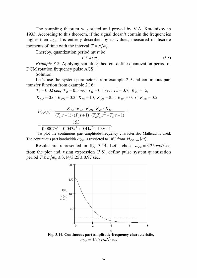
56

The sampling theorem was stated and proved by V.A. Kotelnikov in 1933. According to this theorem, if the signal doesn’t contain the frequencies higher then c , it is entirely described by its values, measured in discrete moments of time with the interval cT .

Thereby, quantization period must be ,cT (3.8)

Example 3.2. Applying sampling theorem define quantization period of DCM rotation frequency pulse ACS.

Solution. Let’s use the system parameters from example 2.9 and continuous part

transfer function from example 2.16:

1 1

0.02 sec; 0.5 sec; 0.1 sec; 0.7; 15;

0.6; 0.2; 10; 8.5; 0.16; 0.5E M M G EA

SM RD G M TG FB

T T T T K

K K K K K K

1 1

4 3 2

2( )( 1) ( 1) ( 1)

153.

0.0007 0.043 0.41 1.3 1

EA M RD G MCP

M G E M M

K К К К КW s

T s T s T T s T s

s s s s

To plot the continuous part amplitude-frequency characteristic Mathcad is used.

The continuous part bandwidth CP is restricted to 10% from max ( )CPH .

Results are represented in fig. 3.14. Let’s chose 3.25 secCP rad from the plot and, using expression (3.8), define pulse system quantization period 3.14 3.25 0.97 sec.CT

0 2 4 6 8

50

100

150

200

H ( )

K ( )

Fig. 3.14. Continuous part amplitude-frequency characteristic,

3.25 secCP rad .

57

3.4 Pulse Transfer Function of Open-Loop Pulse System

Let’s consider unit diagram depicted in fig. 3.15, pulse transfer function of the open-loop ACS for the case, when 1FBW s .

Fig. 3.15. Closed-loop pulse ACS unit diagram

The direct Laplace transform expression (L-transform) of continuous

function x t has the form 0

( ) ( ) stX s x t e dt

.

For the pulse system study discrete analogue of this transform is used – so-called the direct discrete Laplace transform (LD-transform).

0

( ) ( )n

nsTX s x nT e

.

The difference of these transforms is, that integral in L-transform substituted by the

sum, and instead of continuous function x t corresponding lattice function x nT is

introduced.

Let’s define LD -transform for output signal *y t of pulse system

0

( ) { ( )} ( )Dn

nsTY s L y t y nT e

. (3.9)

Since the reduced continuous part response on -function represents pulse step response w(t), so the signal value y t at the output of the reduced

continuous part is defined from the expression:

0

( ) ( ) ( )i

y t w n iT x iT

,

Therefore, output signal value in moments of time t nT equals

0

( ) ( ) ( ).i

y nT w nT iT x iT

(3.10)

Substituting (3.10) in (3.9), obtain

0 0

( ) ( ) ( ) .nsT

n i

Y s w nT iT x iT e

(3.11)

By means of substitution m n i and n i m expression (3.11) is reduced to

58

0

( ) ( ). ( ) .isT msT

i m i

Y s x iT w mT e e

Taking into account, that 0w mT for 0m , finally get

0 0

( ) ( ) ( ) .isT msT

i m

Y s x iT e w mT e

(3.12)

Proceeding from the definition of LD -transform, the expression (3.12) can be reduced to the form

*( ) ( ) ( ),Y s X s W s (3.13)

Then

0

( )( ) ( ) ( ) ,

( )msT

Dm

Y sW s w mT e L w mT

X s

(3.14)

where ( )W s is the open-loop pulse transfer function in S-image (so-called pulse transfer function with an asterisk).

Thereby, the open-loop pulse transfer function in S-form is the ratio of discrete Laplace transforms output to input at zero initial conditions.

Substituting sTz e In (3.12) Z -transform equation can be obtained, i.e. ( ) ( ) ( ),OLSY z X z W z

0

( )( ) ( ) .

( )m

OLSm

Y zW z w mT z

X z

(3.15)

Where OLSW z is the open-loop system pulse transfer function in z -

transform. Therefore, pulse transfer function of open-loop pulse system can be defined as ration of z-image pulse output to image pulse input at zero ini-tial conditions. Expression (3.15) shows that the pulse transfer function is Z-transform of the pulse transition function of system reduced continuous part, i.e. ( ) { ( )} { ( )}.W z Z w t Z w nT

Thereby, to define system pulse transfer function with forming unit of uncondi-tioned type, it is necessary:

to define the reduced continuous part transfer function:

( )RCP FUW s W s W s ;

to define the pulse transition function of reduced continuous part with the help of

inverse Laplace transform: 1RCPw t L W s ;

to define the system weighting sequence (lattice weighting func-

tion): t nTw nT w t ;

to find series sum in right part of the expression: 0

( ) ( ) .n

n

W z w nT z

59

Since the -function image equals to one, and pulse transition function equals to 1w t L W s , then pulse transfer function in z -form can be

defined as ( ) { ( )}W z Z W s , i.e., knowing the transfer function expression

W s , and applying z -transform table, W z can be obtained.

For the given case, when 1FBW s , the pulse transfer function in z -

transform of the reduced continuous part RCPW z equals to the transfer func-

tion of the open-loop system OLSW z .

Based on the proposed approach and the unit diagram (fig. 3.16) expres-sion of the open-loop pulse transfer function WOLS(z) in z-transform can be written for any case

( ) ( ) ( ) ,OLS RCP FBW z Z W s W s (3.16)

Fig. 3.16. Open-loop pulse ACS unit diagram

Applying the equations (3.1), (3.2), equation (3.16) can be represented

as the following

1( ) ( ) ( ) .

T

OLS CP FB

seW z Z W s W s

s

Taking into account, that 1Tse z , finally write 1 1

( ) ( ) ( ) .OLS CP FB

zW z Z W s W s

z s

(3.17)

In the absence of the pulse former in ACS scheme, the expression OLSW s can be written as OLS CP FBW z Z W s W s .

Z -transform table (appendix 2) allows the obtaining expressions for the partial fraction only. Therefore, the complex fraction should be decomposed into partial fractions and then the table can be applied.

Example 3.3. Obtain pulse transfer functions of continuous and open-loop DCM rotation frequency ACS.

Solution. Let’s use the system parameters from the example 2.9 and continuous

part transfer function expression from the example 2.16:

1 12( ) .

( 1) ( 1) ( 1)EA M RD G M

CPM G E EM EM

K К К К КW s

T s T s T T s T s

60

In this example to simplify the solution, the system order reduced to the second order, for 0; 0G ET T .

1 1 153( ) .

( 1) ( 1) (0.1 1) (0.5 1)EA M RD G M

CPM EM

K К К К КW s

T s T s s s

Let’s use expression (2.71)

1 1 1 1 153( ) ( ) ( )

(0.1 1)(0.5 1)CP CP FB

z zW z Z W s W s Z

z s z s s s

.

Denominator roots are: 1 2 30; 10; 2s s s . Applying Viete theorem, let’s decompose expression in braces on partial

fractions:

1 153

(0.1 1)(0.5 1) ( 10) ( 2)

( 10)( 2) ( 2) ( 10)

( 10)( 2)

А В С

s s s s s s

А s s B s s C s s

s s s

(3.18)

Left side of equation (3.18) will be equaled to right side, if their numera-tors are equal:

2

153 ( 10)( 2) ( 2) ( 10)

12 2 10 20

А s s B s s C s s

A B C s A B C s A

Let’s form three equations system, choosing expression at 2 1 0, ,s s s

0A B C ;

12 2 10 0A B C ;

20 153A . Solving this system, obtain coefficients values

7.65; 1.9125; 9.5625A B C . Let’s use Z -transormation table (look appendix 2), For 0.9 sec.T (look example 2.17) obtain

10 2

1 7.65 1.9125 9.5625( )

1

1 7.65 1.9125 9.5625

1 0.0001187 0.164

CP T T

z z z zW z

z z z e z e

z z z z

z z z z

2

2

6.081 5.7693 0.3127( )

0.164 0.00001947CP

z zW z

z z

.

Open-loop ACS transfer function

2

2

0.4865 0.4615 0.025( )

0.164 0.00001947OLS FB TG CP

z zW z K K W z

z z

.

61

3.5 Closed-Loop Pulse System Transfer Function

In the pulse closed-loop system unit diagram (fig. 3.17) the pulse ele-ment can be located in any place, but there is a single approach for transfer function and output equation obtaining.

Fig. 3.17. Unit diagram of the pulse closed-loop system

The output function equation of the obtaining pulse system realized in

the following form: It’s considered, that the pulse element is a switch and the pulse ACS described for the case, when the switch is open-ended. It’s considered, that discrete signal at the output of an open-ended switch exists and is written in Z -transform. Output ACS signal equation is written in Z -transform. When excluding intervening variables in equations, the output system equation is written, when it’s possible its transfer function is also written.

Let’s consider the introduced approach for some variants of the unit dia-gram.

The first case. Pulse element located after summer (fig. 3.17) Let’s write signal in the pulse element output in Z -transform:

* *( ) { ( )} ( ) { ( ) ( )}.RCP FBz Z g s z Z W s W s (3.19)

System output equation is written in Z-transform:

( ) ( ) { ( )}.RCPy z z Z W s (3.20)

Let’s evaluate *( )z from (3.19):

* *( ) { ( ) }RCP FBz z Z W s W s g z .

**

1 { ( ) }RCP FB

g zz

Z W s W s

(3.21)

Substituting (3.21) in (3.20), obtain:

* *

1 ( )RCP

RCP FB

Z W sy z g z

Z W s W s

;

62

Let’s write system differential equation:

1 ( ) ( ) ( ) ( ) ( )RCP FB RCPZ W s W s y z Z W s g z (3.22)

Divide in (3.22) ( )y z by ( )g z obtain the closed-loop system pulse transfer function

( )

( )1 ( )

RCPCLS

OLS

W zW z

W z

. (3.23)

The second case (fig. 3.18).

Fig. 3.18. System with pulse element in feedback loop

Let's write the signal equation *( )y z at the pulse element output when feedback loop is broken

* * *1 1( ) ( ) ( ) ( ) ( ) ( )FBy z Z x s W s z W s W s y z . (3.24)

Evaluating *( )y z from the equation (3.24), obtain the system differen-

tial equation: * *1 11 ( ) ( ) ( ) ( ) ( )FBz W s W s y z Z x s W s

The third case (fig. 3.19).

Fig. 3.19. System with pulse element in the feedback loop

Let’s write signal equation coming to pulse element, when the feedback

loop is broken: * * *

1 1( ) ( ) ( ) ( ) ( ) ( )FB OC OCy z Z x z W s Z W s W s y z . (3.25)

Let’s evaluate * ( )FBy z from this equation

*1*

1

( ) ( )( ) ,

1 ( ) ( )FBoc

Z x z W sy z

Z W s W s

where

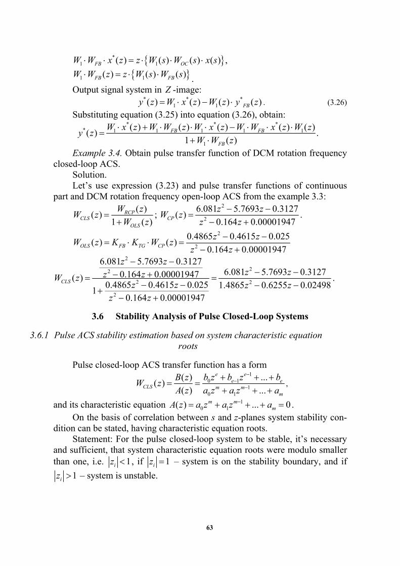
63

*1 1( ) ( ) ( ) ( ) ,FB OCW W x z z W s W s x s

1 1( ) ( ) ( )FB FBW W z z W s W s .

Output signal system in Z -image: * * *

1 1( ) ( ) ( ) ( )FBy z W x z W z y z . (3.26)

Substituting equation (3.25) into equation (3.26), obtain: * * *

* 1 1 1 1 1

1

( ) ( ) ( ) ( ) ( )( ) .

1 ( )FB FB

FB

W x z W W z W x z W W x z W zy z

W W z

Example 3.4. Obtain pulse transfer function of DCM rotation frequency closed-loop ACS.

Solution. Let’s use expression (3.23) and pulse transfer functions of continuous

part and DCM rotation frequency open-loop ACS from the example 3.3: ( )

( )1 ( )

RCPCLS

OLS

W zW z

W z

;

2

2

6.081 5.7693 0.3127( )

0.164 0.00001947CP

z zW z

z z

.

2

2

0.4865 0.4615 0.025( ) ( )

0.164 0.00001947OLS FB TG CP

z zW z K K W z

z z

2

22

2 2

2

6.081 5.7693 0.31276.081 5.7693 0.31270.164 0.00001947( )

0.4865 0.4615 0.025 1.4865 0.6255 0.024981

0.164 0.00001947

CLS

z zz zz zW z

z z z zz z

.

3.6 Stability Analysis of Pulse Closed-Loop Systems

3.6.1 Pulse ACS stability estimation based on system characteristic equation roots

Pulse closed-loop ACS transfer function has a form 1

0 11

0 1

( ) ...( )

( ) ...

e ee e

CLS m mm

B z b z b z bW z

A z a z a z a

,

and its characteristic equation 10 1( ) ... 0m m

mA z a z a z a . On the basis of correlation between s and z-planes system stability con-

dition can be stated, having characteristic equation roots. Statement: For the pulse closed-loop system to be stable, it’s necessary

and sufficient, that system characteristic equation roots were modulo smaller than one, i.e. 1iz , if 1iz – system is on the stability boundary, and if

1iz – system is unstable.

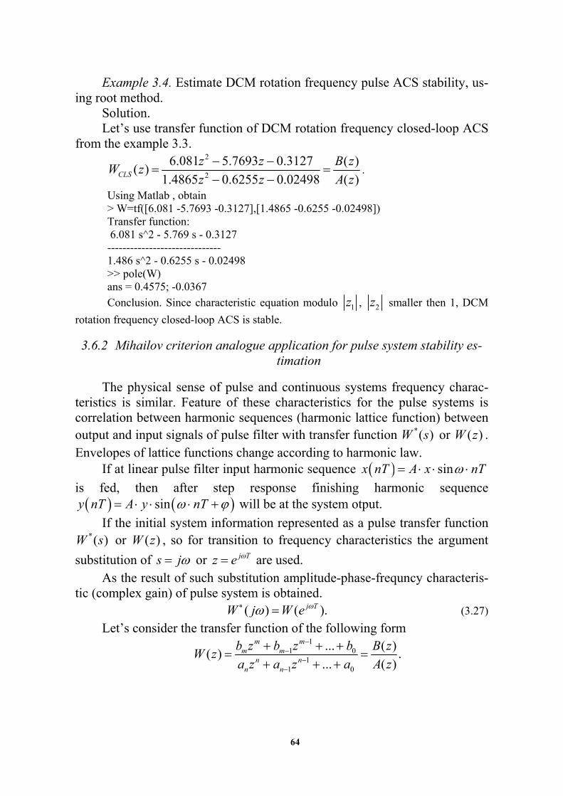
64

Example 3.4. Estimate DCM rotation frequency pulse ACS stability, us-ing root method.

Solution. Let’s use transfer function of DCM rotation frequency closed-loop ACS

from the example 3.3. 2

2

6.081 5.7693 0.3127 ( )( )

1.4865 0.6255 0.02498 ( )CLS

z z B zW z

z z A z

.

Using Matlab , obtain > W=tf([6.081 -5.7693 -0.3127],[1.4865 -0.6255 -0.02498]) Transfer function: 6.081 s^2 - 5.769 s - 0.3127 ------------------------------ 1.486 s^2 - 0.6255 s - 0.02498 >> pole(W) ans = 0.4575; -0.0367

Conclusion. Since characteristic equation modulo 1z , 2z smaller then 1, DCM

rotation frequency closed-loop ACS is stable.

3.6.2 Mihailov criterion analogue application for pulse system stability es-timation

The physical sense of pulse and continuous systems frequency charac-teristics is similar. Feature of these characteristics for the pulse systems is correlation between harmonic sequences (harmonic lattice function) between output and input signals of pulse filter with transfer function *( )W s or ( )W z . Envelopes of lattice functions change according to harmonic law.

If at linear pulse filter input harmonic sequence sinx nT A x nT

is fed, then after step response finishing harmonic sequence siny nT A y nT will be at the system otput.

If the initial system information represented as a pulse transfer function *( )W s or ( )W z , so for transition to frequency characteristics the argument

substitution of s j or j Tz e are used. As the result of such substitution amplitude-phase-frequncy characteris-

tic (complex gain) of pulse system is obtained. ( ) ( ).j TW j W e (3.27)

Let’s consider the transfer function of the following form 1

1 01

1 0

... ( )( ) .

... ( )

m mm m

n nn n

b z b z b B zW z

a z a z a A z

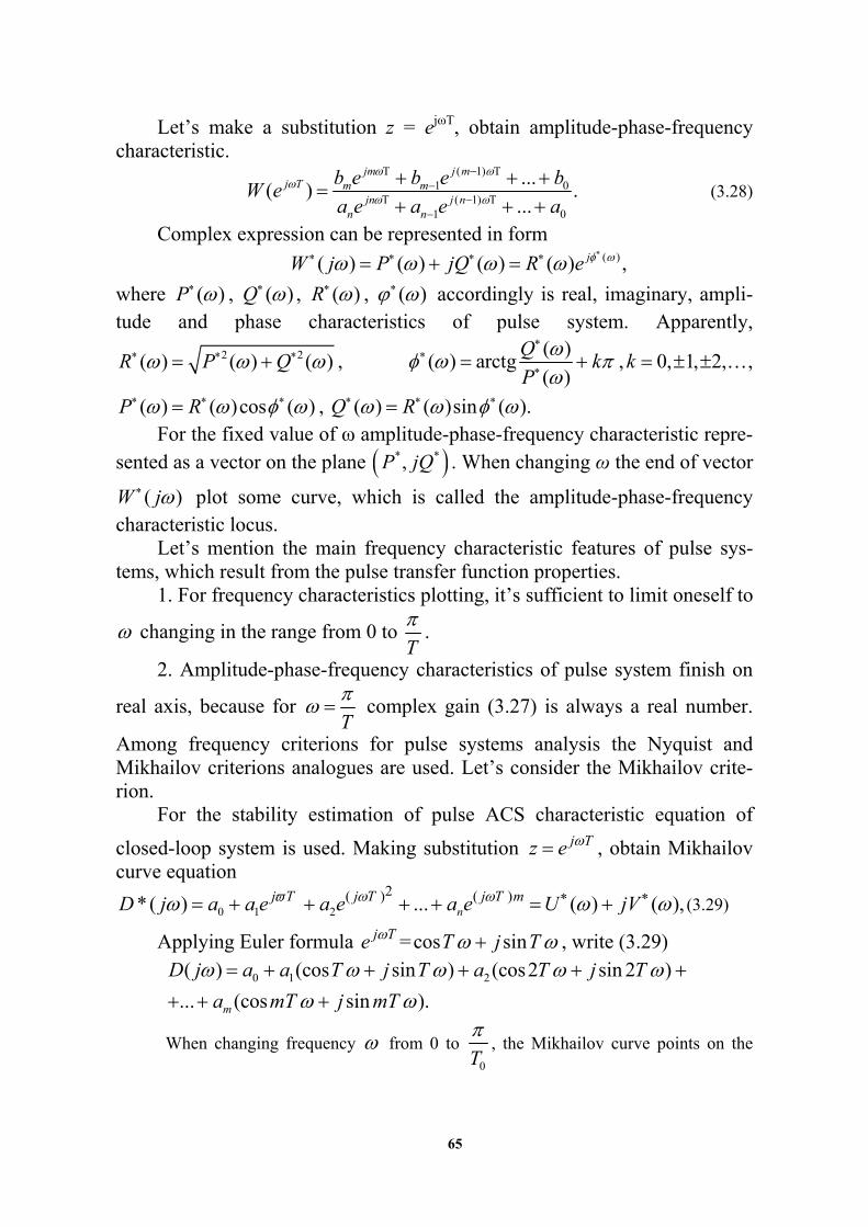
65

Let’s make a substitution z = еjωT, obtain amplitude-phase-frequency characteristic.

( 1)

1 0( 1)

1 0

...( ) .

...

jm j mj T m m

jn j nn n

b e b e bW e

a e a e a

(3.28)

Complex expression can be represented in form ( )( ) ( ) ( ) ( ) ,jW j P jQ R e

where ( )P , ( )Q , ( )R , ( ) accordingly is real, imaginary, ampli-tude and phase characteristics of pulse system. Apparently,

2 2( ) ( ) ( )R P Q , ( )

( ) arctg( )

Qk

P

, 0, 1, 2,k ,

( ) ( )cos ( )P R , ( ) ( )sin ( ).Q R For the fixed value of ω amplitude-phase-frequency characteristic repre-

sented as a vector on the plane * *,P jQ . When changing ω the end of vector

( )W j plot some curve, which is called the amplitude-phase-frequency characteristic locus.

Let’s mention the main frequency characteristic features of pulse sys-tems, which result from the pulse transfer function properties.

1. For frequency characteristics plotting, it’s sufficient to limit oneself to

changing in the range from 0 to T

.

2. Amplitude-phase-frequency characteristics of pulse system finish on

real axis, because for T

complex gain (3.27) is always a real number.

Among frequency criterions for pulse systems analysis the Nyquist and Mikhailov criterions analogues are used. Let’s consider the Mikhailov crite-rion.

For the stability estimation of pulse ACS characteristic equation of

closed-loop system is used. Making substitution j Tz e , obtain Mikhailov curve equation

0 1 2

2( ) ( )* ( ) ... ( ) ( ),nj T j T j T mD j a a e a e a e U jV (3.29)

Applying Euler formula j Te =cos sinT j T , write (3.29)

0 1 2( ) (cos sin ) (cos2 sin 2 )

... (cos sin ).m

D j a a T j T a T j T

a mT j mT

When changing frequency from 0 to 0T

, the Mikhailov curve points on the

66

complex plain ( ), ( )U jV (fig. 3.20) are defined.

Fig. 3.20. Mikhailov curve locuses for stable system of 1st, 2nd , 3rd orders.

For the close-loop pulse ACS to be stable, it’s necessary and sufficient

that for =0 Mikhailov curve takes the beginning in the positive part of the

real axis and by increasing the frequency from 0 to 0T

characteristic curve

*( )D j sequentially, without vanish, in the positive (counterclockwise) di-rection pass 2m quadrants, where m is the system order.

Example 3.5. Estimate DCM rotation frequency pulse ACS stability, us-ing the Mikhailov criterion analogue.

Solution. Let’s use transfer function and characteristic equation of DCM rotation

frequency closed-loop ACS from the example 3.4. 2

2

6.081 5.7693 0.3127 ( )( )

1.4865 0.6255 0.02498 ( )CLS

z z B zW z

z z A z

.

Using Mathсad, obtain the Mikhailov locus (fig. 3.21)

67

→∞

Fig. 3.21. Mikhailov locus

The Mikhailov curve for 0 takes the beginning on the positive real

axis (0,836) and finish on the real axis (2,087). Pass sequentially, without vanish, 2 4m quadrants. Therefore, DCM rotation frequency pulse ACS is stable.

3.7 Control Process Quality Estimation of Pulse ACS

For the pulse ACS quality indexes estimation applied the same approach as in the linear systems, but it has its own specific. Pulse system output signal

( )y t is continuous, but, as far as, for the system analysis discrete Laplace transform and fictitious quantizer are used, it can be assumed that output sig-nal *( )y t is discrete or y nT . Having the discrete signal and making its ap-

proximation, obtain the continuous output signal. Applying the pulse transfer function of closed-loop ACS it can be written: CLSY z W z G z . To ob-

tain y nT the Heaviside equation or Laurent series can be applied. The eas-

ier way for discrete signal obtaining is using program Control System Toolbox Matlab. Let’s consider this approach on the example.

Example 3.6. Obtain transfer function and discrete signal of DCM rota-tion frequency closed-loop ACS. Define system quality indexes.

Solution. Let’s use system parameters and continuous part transfer function ex-

pression

1 1

0.02 sec; 0.5 sec; 0.1 sec; 0.7 sec; 15; 0.2;

10; 8.5; 0.16; 0.5.E EM M G EA RD

G M TG FB

T T T T K K

K K K K

68

1 1

4 3 2

2( )( 1) ( 1) ( 1)

12.24.

0.0007 0.043 0.41 1.3 1

EA M RD G MCP

M G E EM EM

K К К К КW s

T s T s T T s T s

s s s s

Discrete signal of DCM rotation frequency pulse ACS represented in fig. 3.22 and its quality indexes in fig. 3.23.

>> Wn=tf([12.24],[0.0007 0.043 0.41 1.3 1]) Transfer function: 12.24 --------------------------------------------- 0.0007 s^4 + 0.043 s^3 + 0.41 s^2 + 1.3 s + 1

>> Wnd=c2d(Wn,0.9) – conversion CPW s into pulse CPW z with sampling pe-

riod 0.9 sec.T

Transfer function: 5.031 z^3 + 2.607 z^2 + 0.04084 z + 1.89e-007 ---------------------------------------------------------- z^4 - 0.3768 z^3 + 0.00426 z^2 - 5.644e-005 z + 1.602e-022 Sampling time: 0.9 >> Woc=tf([0.08],1) Transfer function: 0.08 >> Wz=feedback(Wnd, Woc) – closed-loop pulse ACS transfer function obtaining

WЗС(z) Transfer function: 5.031 z^3 + 2.607 z^2 + 0.04084 z + 1.89e-007 -------------------------------------------------------- z^4 + 0.02571 z^3 + 0.2129 z^2 + 0.003211 z + 1.512e-008 Sampling time: 0.9 >> pole(Wz) ans = -0.0053 + 0.4612i -0.0053 - 0.4612i -0.0151 -0.0000 >> step(Wz)

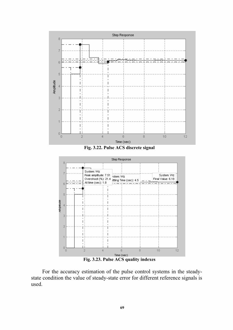
69

Fig. 3.22. Pulse ACS discrete signal

Fig. 3.23. Pulse ACS quality indexes

For the accuracy estimation of the pulse control systems in the steady-

state condition the value of steady-state error for different reference signals is used.

70

In closed-loop pulse system (fig. 3.10) error е, reference signal g and the disturbance f related to each other by the following equation regarding z-image ( ) ( ) ( ) ( ) ( ).f

CLS CLSz W z G z W z F z

This expression contains two components of error, the first gE z spec-

ified by reference signal, and the second fE z by disturbance.

Steady-state error of pulse system can be calculated by the expression, which defines the finite value of original, i.e.

1 1

1 1( ) lim ( ) lim ( ).g f

z zn

z ze nT E z E z

z z

(3.30)

Let’s define steady-state error for the reference signal, assuming ( ) 0f t .

1

1 1( ) ( ) lim ( ) .

1 ( )g zn n OLS

ze nT e nT G z

z W z

(3.31)

If the constant signal 0( ) 1( )g t g t fed at the system input, which z -

image 0( )1

g zG z

z

, then according to (3.30) position steady-state system er-

ror

0

1( ) lim .

1 ( )zn OLS

ge nT

W z

(3.32)

For the reference signal 1( )g t g t , linearly dependent on time, Z -

image 12

( ) ,( 1)

g TzG z

z

and steady-state error, according to (3.30), defined by

the following expression

1

1( ) lim .

( 1)(1 ( ))zn OLS

g Te nT

z W z

(3.33)

And called speed system error. If the input signal changes with the constant acceleration, i.e.

22( ) 2g t g t , then Z -image has the form

22

3

( 1)( )

2( 1)

T g z zG z

z

.

Steady-state error

2

221

( ) lim ,2( 1) (1 ( ))zn OLS

g Te nT

z W z

(3.34)

and that is called the acceleration system error. For the given errors definition, one can use the error series

' '' ( )20 1( ) ( ) ( ) ( ) ... ( ) ...

2! !mmC C

e nT C g nT C g nT g nT g nTm

(3.35)

71

where , , , mg g g are derivatives of ( )g t in the time moments T ;

0 ( ) 1/CLSC W z z ; 1

1

( )1/CLSW z

С zz

;

( )1

!/

mm CLS

m

C W zz

m z

;

1( )

1 ( )CLSOLS

W zW z

.

Example 3.7. Define the control error of DCM rotation frequency pulse ACS for input 0 1( )inU U t , 0 5U V .

Solution.

Let’s use the expression (3.32) 0

1( ) lim

1 ( )zn OLS

ge nT

W z

and, using Control Sys-

tem Toolbox Matlab obtain ( )OLSW z .

Wn=tf([12.24],[0.0007 0.043 0.41 1.3 1]) Transfer function: 12.24 --------------------------------------------- 0.0007 s^4 + 0.043 s^3 + 0.41 s^2 + 1.3 s + 1 >> Woc=tf([0.08],1) Transfer function: 0.08 >> Wpc=Wn*Woc Transfer function: 0.9792 --------------------------------------------- 0.0007 s^4 + 0.043 s^3 + 0.41 s^2 + 1.3 s + 1 >> Wpcd=c2d(Wpc,0.9) Transfer function: 0.4025 z^3 + 0.2086 z^2 + 0.003267 z + 1.512e-008 ---------------------------------------------------------- z^4 - 0.3768 z^3 + 0.00426 z^2 - 5.644e-005 z + 1.602e-022 Sampling time: 0.9

4 3 2 -5 -22

4 3 21

5(z - 0.3768 z + 0.00426 z - 5.644 10 z + 1.602 10 )( ) lim

z - 0.0257 z + 0.21286 z - 0.0033 z 3.137

2.65.1.1839

zne nT

72

4 CONTROL TASKS AND STUDY GUIDE

4.1 General Study Guide

In the course paper (part 1) linear stationary ACS is a subject of study. In the pro-ject (part 2) nonlinear pulse ACS is investigated.

Initial data for the ACS study is given as a system circuit schematic, its parameters numerical values table and list of questions are to be considered.

When linear ACS stability region plotting, take gain constant of amplifying ele-ment as varying parameter A.

Matlab or Mathcad programs are acceptable to use during the project carrying out. Nonlinear static characteristic types of nonlinear element, electronic amplifier,

magnetic amplifier and thyristor converter.

а) b)

Fig. 4.1. Nonlinear element static characteristics: а) EA, b) МA and ТT. Static characteristic parameter values assume equaled «b»=4 for thyristor convert-

er, «b»=0.5 – for magnetic amplifier; «b»=1 – for electronic amplifier; parameter «m»=0.1; value «c» defined from gain constant of the given amplification element.

If there will be no periodical solutions, when carrying out paragraph 4, then it is necessary to substitute amplification element coefficient or nonline-ar element parameters.

To form pulse system scheme is necessary: use the unit diagram of closed-loop system for the reference signal; in the given scheme, place the ideal pulse element with the pulse former after the summer;

4.2 Guide Lines for Project Text Document Content

The project must be drawn on the format sheets A4 and contain: cover page; project content; project task; ACS unit diagram; open-loop and closed-loop ACS transfer functions; estimation results of system stability in Matlab or Matсad; step response calculation results according to system unit diagram in

73

Matlab; conclusion about system analysis quality; references.

4.3 Guide Lines for Project Graphic Material Appearance

Requirements for project graphic material: functional and structural schemes must be drawn according to the required format; signal motion direction and their title must be drawn in structural schemes; diagrams must be represented with dimensional axis and obligatory with grid lines.

Conclusion

In the book authors made an attempt to represent all the basic approaches to analy-sis and design of linear, nonlinear and pulse systems. In order to make an explanation more clear, a lot of different examples were attached. Theoretical part contains methods that allow solving main problems of control theory as identification procedure, system stability analysis and controller design.

Actually, book contains three parts, the first one is devoted to linear systems ques-tions study; the second part is more complicated and consequently more interesting; in the third part approaches to pulse systems research are considered.

The main particularity of this book is to acquire practical knowledge in control the-ory, so it is focused on course work realization. In order to understand the biggest part of control system design procedure and to make clear corresponding between control theory methods and real systems the tasks for course paper begin with principle scheme of sys-tems.

The results of control theory application are everywere around us, it makes this course important and very interesting.

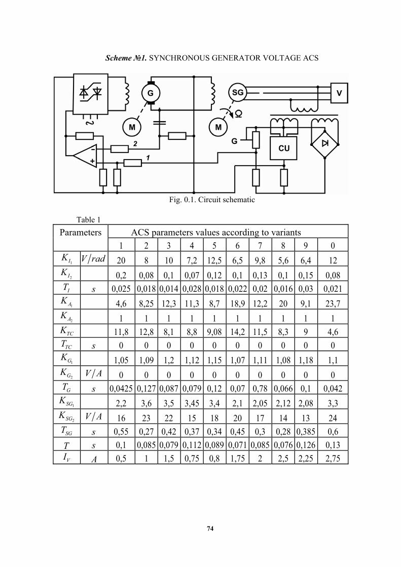
74

Scheme №1. SYNCHRONOUS GENERATOR VOLTAGE ACS

Fig. 0.1. Circuit schematic

Table 1

Parameters ACS parameters values according to variants

1 2 3 4 5 6 7 8 9 0

1IK V rad 20 8 10 7,2 12,5 6,5 9,8 5,6 6,4 12

2IK 0,2 0,08 0,1 0,07 0,12 0,1 0,13 0,1 0,15 0,08

IT s 0,025 0,018 0,014 0,028 0,018 0,022 0,02 0,016 0,03 0,021

1AK 4,6 8,25 12,3 11,3 8,7 18,9 12,2 20 9,1 23,7

2AK 1 1 1 1 1 1 1 1 1 1

TCK 11,8 12,8 8,1 8,8 9,08 14,2 11,5 8,3 9 4,6

TCT s 0 0 0 0 0 0 0 0 0 0

1GK 1,05 1,09 1,2 1,12 1,15 1,07 1,11 1,08 1,18 1,1

2GK V A 0 0 0 0 0 0 0 0 0 0

GT s 0,0425 0,127 0,087 0,079 0,12 0,07 0,78 0,066 0,1 0,042

1SGK 2,2 3,6 3,5 3,45 3,4 2,1 2,05 2,12 2,08 3,3

2SGK V A 16 23 22 15 18 20 17 14 13 24

SGT s 0,55 0,27 0,42 0,37 0,34 0,45 0,3 0,28 0,385 0,6

T s 0,1 0,085 0,079 0,112 0,089 0,071 0,085 0,076 0,126 0,13

VI A 0,5 1 1,5 0,75 0,8 1,75 2 2,5 2,25 2,75

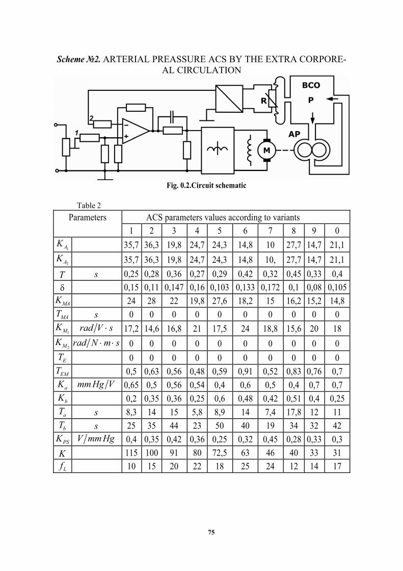
75

Scheme №2. ARTERIAL PREASSURE ACS BY THE EXTRA CORPORE-AL CIRCULATION

Fig. 0.2.Circuit schematic

Table 2

Parameters ACS parameters values according to variants

1 2 3 4 5 6 7 8 9 0

1AK 35,7 36,3 19,8 24,7 24,3 14,8 10 27,7 14,7 21,1

2AK 35,7 36,3 19,8 24,7 24,3 14,8 10, 27,7 14,7 21,1

T s 0,25 0,28 0,36 0,27 0,29 0,42 0,32 0,45 0,33 0,4

0,15 0,11 0,147 0,16 0,103 0,133 0,172 0,1 0,08 0,105

MAK 24 28 22 19,8 27,6 18,2 15 16,2 15,2 14,8

MAT s 0 0 0 0 0 0 0 0 0 0

1MK rad V s 17,2 14,6 16,8 21 17,5 24 18,8 15,6 20 18

2MK rad N m s 0 0 0 0 0 0 0 0 0 0

ET 0 0 0 0 0 0 0 0 0 0

EMT 0,5 0,63 0,56 0,48 0,59 0,91 0,52 0,83 0,76 0,7

aK mm Hg V 0,65 0,5 0,56 0,54 0,4 0,6 0,5 0,4 0,7 0,7

bK 0,2 0,35 0,36 0,25 0,6 0,48 0,42 0,51 0,4 0,25

aT s 8,3 14 15 5,8 8,9 14 7,4 17,8 12 11

bT s 25 35 44 23 50 40 19 34 32 42

PSK V mm Hg 0,4 0,35 0,42 0,36 0,25 0,32 0,45 0,28 0,33 0,3

K 115 100 91 80 72,5 63 46 40 33 31

Lf 10 15 20 22 18 25 24 12 14 17

76

Scheme № 3. ELECTRONIC FURNACE TEMPERATURE ACS

Fig. 0.3.Circuit schematic

Table3

Parameters ACS parameters values according to variants

1 2 3 4 5 6 7 8 9 0

1AK 4,3 4 5 4 2 1 6,2 5,2 4 2

2AK 4,3 6,5 8,8 2,4 2 2,6 4 8,6 2,2 2

3AK 4,3 6,5 4,4 2,4 2 2,6 4 4,3 2,2 2,16

TCK 6,5 8 14,2 9,6 5,1 6,4 8 4,2 7,5 6

TCT s 0 0 0 0 0 0 0 0 0 0

HK deg V 5 4,8 6,4 5,6 4,4 3,8 6,4 2,4 6 4

HT s 250 140 220 180 120 160 170 275 320 87

PK 0,9 0,8 0,94 0,88 0,96 0,7 0,85 0,92 0,76 0,65

PT s 790 400 690 660 420 580 440 760 910 600

1TSK V rad 0,5 0,2 0,1 0,8 1,2 0,75 0,4 0,5 1,05 0,8

1TST s 2,35 2,15 2,3 3,6 2,2 5,6 2,3 5,9 3,4 3,8

2TSK V rad 0,5 0,4 1 3,2 2 0,75 1 1,8 2,4 2

2TST s 28,1 12,2 8,3 7,2 14 21,5 7,7 28,6 16, 10

K 63 40 75 90 52 33 70 40 80 25

Lf deg 18 20 25 26 28 30 31 24 29 19

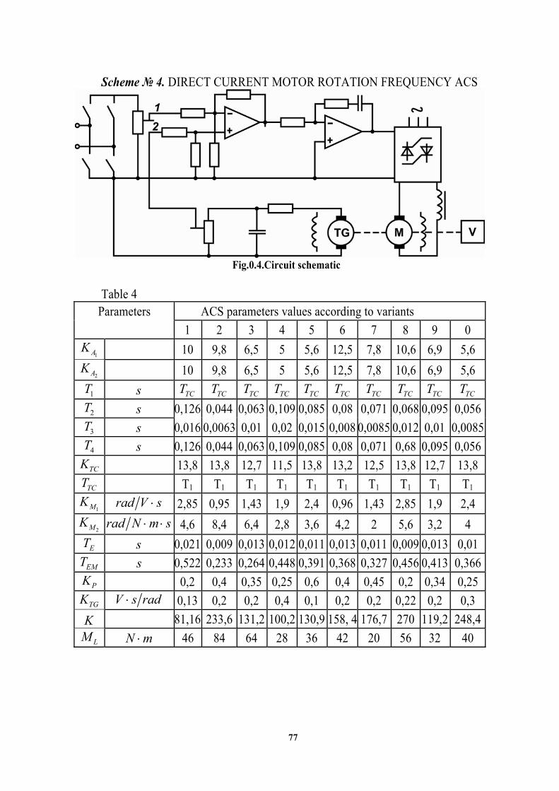
77

Scheme № 4. DIRECT CURRENT MOTOR ROTATION FREQUENCY ACS

Fig.0.4.Circuit schematic

Table 4

Parameters ACS parameters values according to variants

1 2 3 4 5 6 7 8 9 0

1AK 10 9,8 6,5 5 5,6 12,5 7,8 10,6 6,9 5,6

2AK 10 9,8 6,5 5 5,6 12,5 7,8 10,6 6,9 5,6

1T s TCT TCT TCT TCT TCT TCT TCT TCT TCT TCT

2T s 0,126 0,044 0,063 0,109 0,085 0,08 0,071 0,068 0,095 0,056

3T s 0,016 0,0063 0,01 0,02 0,015 0,008 0,0085 0,012 0,01 0,0085

4T s 0,126 0,044 0,063 0,109 0,085 0,08 0,071 0,68 0,095 0,056

TCK 13,8 13,8 12,7 11,5 13,8 13,2 12,5 13,8 12,7 13,8

TCT Т1 Т1 Т1 Т1 Т1 Т1 Т1 Т1 Т1 Т1

1MK rad V s 2,85 0,95 1,43 1,9 2,4 0,96 1,43 2,85 1,9 2,4

2MK rad N m s 4,6 8,4 6,4 2,8 3,6 4,2 2 5,6 3,2 4

ET s 0,021 0,009 0,013 0,012 0,011 0,013 0,011 0,009 0,013 0,01

EMT s 0,522 0,233 0,264 0,448 0,391 0,368 0,327 0,456 0,413 0,366

PK 0,2 0,4 0,35 0,25 0,6 0,4 0,45 0,2 0,34 0,25

TGK V s rad 0,13 0,2 0,2 0,4 0,1 0,2 0,2 0,22 0,2 0,3

K 81,16 233,6 131,2 100,2 130,9 158, 4 176,7 270 119,2 248,4

LM N m 46 84 64 28 36 42 20 56 32 40

78

Scheme №5. SERVO SYSTEM

Fig. 0.5.Circuit schematic

Table 5 Parameters ACS parameters values according to variants

1 2 3 4 5 6 7 8 9 0

AMSK V rad 30 25 27,6 32 18 15 20 29,6 28,6 33

1AK 25 20 19 22 50 22,5 23 15 14 12,5

2AK 25 20 19 22 50 22,5 23 15 14 12,5

1T s 0,28 0,174 0,166 0,126 0,063 0,112 0,056 0,19 0,2 0,158

2T s 0,08 0,105 0,112 0,091 0,051 0,083 0,038 0,05 0,1 0,102

3T s 0,8 0,7 0,477 0,546 0,268 0,387 0,164 0,594 0,87 0,403

4T s 0,028 0,026 0,039 0,021 0,012 0,024 0,013 0,016 0,023 0,04

EAK 20 21 18 24 18,5 30 16 27 22 17

1MK rad V s 0,95 1,43 1,9 1,5 0,98 1,44 1,95 1,9 1,45 0,95

2MK rad N m s 5,2 0,65 15 8,6 36 0,8 24 17,2 7,8 40

ET s 0 0 0 0 0 0 0 0 0 0

EMT s 0,25 0,33 0,398 0,295 0,166 0,224 0,107 0,135 0,141 0,27

1RK - - - - - - - - - -

2RK 0,01 0,008 0,008 0,009 0,007 0,011 0,009 0,0088 0,01 0,012

LM N m 5 0,5 15 8 4 0,8 2 3 4 5

79

Scheme №6.HEAT EXCHANGER TEMPERATURE ACS

Fig. 0.6. Circuit schematic

Table 6 Parameters ACS parameters values according to variants

1 2 3 4 5 6 7 8 9 0

1IK V rad 12 15 12,5 14 12 10 15 10 12,5 14

2IK degV 2,1 1,8 1,7 1,9 2,2 2,1 2,4 2, 2,3 2,6

IT s 0 0 0 0 0 0 0 0 0 0

1AK 1 1 1 1 1 1 1 1 1 1

2AK 1 1 1 1 1 1 1 1 1 1

EAK 10,2 18,7 8,5 17,5 10 12,5 12 12 11,1 10,9

1MK rad V s 1,4 1,1 1,24 0,95 1,4 1,15 1 0,94 1,05 0,9

2MK rad N m s 0 0 0 0 0 0 0 0 0 0

EAT s 0 0 0 0 0 0 0 0 0 0

EMT s 0 0 0 0 0 0 0 0 0 0

RK 0,011 0,01 0,013 0,008 0,012 0,01 0,011 0,014 0,015 0125

PK V rad 8 12 15 8,5 9 7,5 8,2 11 9,1 10

FBT s 4,5 1,78 2,2 2,6 4 4,8 4,26 3,9 3,23 5,4

1HEK deg rad 127 183 172 156 95,6 171 118 178 153 150

2HEK degrad 1 1 1 1 1 1 1 1 1 1

1HET s 65 30 24 55 50 125 100 90 85 110

2HET s 1,25 0,5 0,63 0,91 1,07 1,6 1,4 1,17 1 1,38

Lf deg 20 25 24 28 30 25 26 31 32 23

80

Scheme №7. STEAM TEMPERATURE ACS

Fig. 0.7. Circuit schematic Table7

Parameters ACS parameters values according to variants

1 2 3 4 5 6 7 8 9 0

1IK V rad 14 12 10 15 12 20 14 15 10 11

2IK degV 0,5 0,2 0,4 0,24 0,21 0,15 0,12 0,25 0,4 0,3

IT s 0 1 1,6 0 1,4 1 0 1,25 1,7 0

1K 0,4 0,25 0,2 0,18 0,1 0,2 0,15 0,12 0,16 0,2

1T s 2,2 2,3 2,3 2,85 2 1,52 0,63 1,66 1,84 2

2 E FT T T s 0 0 0 0 0 0 0 0 0 0

TCK 6,4 10,2 13,7 9,8 12 14,5 18 16,6 14 10

1MK rad V s 11 5 4 3,2 4,8 9,6 9,6 5,6 4,8 3,2

2MK rad N m s 0 0 0 0 0 0 0 0 0 0

EMT s 0,5 0 0,42 0,55 0 0,32 0,35 0 0,32 0,25

RK V rad 0,028 0,07 0,05 0,09 0,06 0,04 0,12 0,08 0,075 0,04

GK deg rad 40 85 120 52 180 152 100 90 65 230

BT s 1,3 0,35 0 1,8 0,4 0 1,2 1 0 1,5

PK 0,8 0,9 0,95 1 0,6 0,75 0,62 0,5 0,55 0,4

PT s 630 950 2500 1150 1260 790 690 2000 1380 660

Lf deg 30 22 34 31 35 40 42 45 50 55

81

Scheme№8.DIRECT CURRENT MOTOR ROTATION FREQUENCE ACS

Fig. 0.8. Circuit schematic

Table8 Parameters ACS parameters values according to variants

1 2 3 4 5 6 7 8 9 0

1AK 4 4,2 3,5 10 4,2 1 8,5 6 3 1

2AK 6 16,3 22,3 41,7 39,5 4,5 28,8 17,5 10,65 2,84

3AK 0,035 0,27 0,026 0,36 0,092 0,11 1 1 0,101 0,1

1T s 0,083 0,063 0,093 0,054 0,112 0,08 0,068 0,072 0,1 0,04

2T s 0,05 0,044 0,04 0,064 0,1 0,012 0,08 0,12 0,06 0,01

TCK 8, 6 9 5 6,4 10,2 7,5 12,5 9,6 8,2 6,6

TCT s 0 0 0 0 0 0 0 0 0 0

1MK rad V s 1,4 2,4 1,9 1,43 0,96 1,8 2,4 0,95 2,85 1,9

2MK rad N m s 6,4 26 2,8 24 8 10 3,6 5,6 21 36

ET s 0,012 0,018 0,016 0,01 0,015 0,018 0,05 0,022 0,035 0,011

EMT s 0,297 0,497 0,382 0,482 0,42 0,247 0,155 0,575 0,58 0,247

FBR 0,8 1,65 0,3 1 1,2 2,4 2,1 1,9 1,5 1,2

VSK V s rad 0,1 0,08 0,12 0,2 0,08 0,13 0,2 0,16 0,15 0,1

VST s 0,022 0,01 0,027 0,015 0,025 0,01 0,011 0,012 0,014 0,013

PK 0,4 0,25 0,1 0,2 0,2 0,15 0,016 0,3 0,12 0,25

CSK 0,12 0,1 0,05 0,08 0,17 0,11 0,25 0,11 0,2 0,085

LM N m 6 10 3 12 8 10 4 5 2 4

82

Scheme №9. SERVOSYSTEM WITH COMBINED CONTROL

Fig. 0.9. Circuit schematic

Table9 Parameters ACS parameters values according to variants

1 2 3 4 5 6 7 8 9 0

AMSK V rad 16 18 20 28 21 15 24 20 30 25,2

AMSK V rad 16 18 20 28 21 15 24 20 30 25,2

1AK 0,216 0,202 0,192 0,03 0,154 0,04 0,3 0,12 0, 2 0,2

2AK 0,65 0,88 0,78 2,85 1,34 3,42 0,68 1,22 0,93 1,09

3AK 0,65 0,88 0,78 2,85 1,34 3,42 0,68 1,22 0,93 1,09

TCK 12,8 11,2 18,6 14,8 12,8 20 13,6 16,2 10 15,2

TCT 0,02 0,03 0,01 0,04 0,02 0,008 0,012 0,015 0,01 0,03

1MK rad V s 14,1 8,2 6,2 2,2 8,7 2,6 15,6 5,6 12,3 4,8

2MK rad N m s 2,6 1,5 8,7 7,8 2,4 10 12 7,2 4,5 6,5

ET s 0,03 0,02 0,03 0,01 0,01 0,015 0,008 0,02 0,018 0,01

EMT s 0,15 0,12 0,09 0,2 0,24 0,18 0,14 0,21 0,12 0,15

1RK 20 10 12 14 10 15 13,55 11,8 17,6 20,4

2RK 0,008 0,011 0,01 0,006 0,008 0,012 0,01 0,009 0,007 0,01

TGK V s rad 0,5 0,1 0,2 0,08 0,11 0,2 0,18 0,15 0,11 0,1

0,15 0,2 0,4 0,172 0,19 0,19 0,345 0,26 0,45 0,56

T s 0,03 0,0375 0,067 0,05 0,061 0,044 0,08 0,079 0,106 0,23

LM N m 2 2 6 5 2 8 6 4 3 2

83

Scheme№10. HERMETIC CHAMBER TEMPERATURE ACS

Fig. 0.10. Circuit schematic

Table 10 Parameters ACS parameters values according to variants

1 2 3 4 5 6 7 8 9 0

1IK degV 21 15 8 16 12 10 12 15 20 18

2IK degV 0,4 0,16 0,25 0,1 0,2 0,12 0,15 0,1 0,22 0,24

IT s 0 1,6 0 6,3 0 2,5 0 8 0 4

1AK 2 0,64 4 1,82 3 1,35 3,5 0,47 2 4,5

2AK 1 2 0,5 0,4 1 0,25 0,8 0,4 1,2 1

MAK 2,4 4,5 3 2 87 3,5 6,4 2,2 5,6 1,8

MA ET T s 0 0 0 0 0 0 0 0 0 0

1MK rad V s 1,3 1,15 1,2 1,04 1,12 1 0,93 0,95 1,05 0,83

2MK rad N m s

0 0 0 0 0 0 0 0 0 0

EMT s 0,54 0 0,255 0 0,23 0 0,38 0 0,2 0

RK 0,02 0,081 0,074 0,002 0,03 0,003 0,006 0,01 0,038 0,002

CEK deg rad 25 15 27,5 18 35 16 18 22 30 26

CK 0,744 0,853 0,667 0,886 0,338 0,789 0,65 0,717 0,782 0,823

CT s 60 15 90 30 60 25 40 20 20 100

CEK s 22 63 40 90 35 60 100 115 80 25

AMSK V rad 3,6 2,5 5 2,4 2 2 4,2 0,5 2,8 4

Lf deg 8 6 12 15 9 10 14 18 21 16

84

Scheme №11. SERVO SYSTEM

Fig. 0.11. Circuit schematic

Table 11 Parameters ACS parameters values according to variants

1 2 3 4 5 6 7 8 9 0

AMSK V rad 12 15 16 12,5 10 13,5 14 9 15 14,5

AMSK V rad 12 15 16 12,5 10 13,5 14 9 15 14,5

1AK 22,4 17,3 25 20,2 18 17,5 15,3 11,5 27,2 16

2AK 22,4 17,3 25 20,2 18 17,5 15,3 11,5 27,2 16

3AK 1 1 1 1 1 1 1 1 1 1

TCK 18,2 15 17 16,8 13,7 16,6 16 18,7 14, 10,4

TCT 0,01 0 0,008 0 0,012 0 0,006 0 0,011 0

1MK rad V s 1,43 2,1 1,84 2 2,85 1,43 1,95 1,5 1 1,95

2MK rad N m s 21 36,5 40 32 20 27 18 24 26 42

ET s 0 0,015 0 0,02 0 0,016 0 0,022 0 0,018

EMT s 0,162 0,307 0,13 0,272 0,191 0,355 0,158 0,189 0,2 0,256

1T s 0,04 0,05 0,03 0,055 0,075 0,085 0,06 0,1 0,08 0,1

2T s 0,1 0,08 0,07 0,107 0,115 0,112 0,085 0,155 0,125 0,126

TGK V s rad 0,25 0,16 0,2 0,27 0,13 0,15 0,18 0,12 0,15 0,2

RK 0,01 0,011 0,008 0,01 0,009 0,008 0,012 0,011 0,007 0,012

LM N m 2 4 3 2 2 3 2 4 3 4

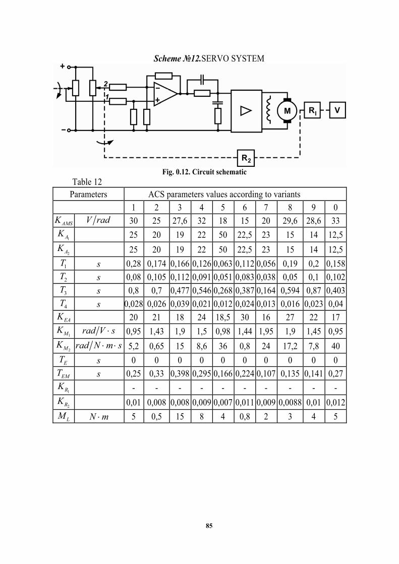
85

Scheme №12.SERVO SYSTEM

Fig. 0.12. Circuit schematic

Table 12 Parameters ACS parameters values according to variants

1 2 3 4 5 6 7 8 9 0

AMSK V rad 30 25 27,6 32 18 15 20 29,6 28,6 33

1AK 25 20 19 22 50 22,5 23 15 14 12,5

2AK 25 20 19 22 50 22,5 23 15 14 12,5

1T s 0,28 0,174 0,166 0,126 0,063 0,112 0,056 0,19 0,2 0,158

2T s 0,08 0,105 0,112 0,091 0,051 0,083 0,038 0,05 0,1 0,102

3T s 0,8 0,7 0,477 0,546 0,268 0,387 0,164 0,594 0,87 0,403

4T s 0,028 0,026 0,039 0,021 0,012 0,024 0,013 0,016 0,023 0,04

EAK 20 21 18 24 18,5 30 16 27 22 17

1MK rad V s 0,95 1,43 1,9 1,5 0,98 1,44 1,95 1,9 1,45 0,95

2MK rad N m s 5,2 0,65 15 8,6 36 0,8 24 17,2 7,8 40

ET s 0 0 0 0 0 0 0 0 0 0

EMT s 0,25 0,33 0,398 0,295 0,166 0,224 0,107 0,135 0,141 0,27

1RK - - - - - - - - - -

2RK 0,01 0,008 0,008 0,009 0,007 0,011 0,009 0,0088 0,01 0,012

LM N m 5 0,5 15 8 4 0,8 2 3 4 5

86

Scheme №13. DIRECT CURRENT MOTOR ROTATION FREQUENCY COM-BINED ACS

Fig. 0.13. Circuit schematic

Table 13 Parameters ACS parameters values according to variants

1 2 3 4 5 6 7 8 9 0

1AK 5 7,5 6,4 10 8 7,2 5,6 6 5,5 8,8

2AK 23,33 15,25 5,6 6,25 20 20 12 15 8 12

3AK 20 8 15 6,25 25 20 15 15 20 20

TCK 18,75 12,5 12,5 15 20 12,5 15 19 16 25

TCT s 0,06 0,02 0,03 0,02 0,01 0,01 0,015 0,005 0,006 0,008

1MK rad V s 1,6 2,8 2 3,2 2,4 3,2 2,4 3 2,5 1,8

2MK rad N m s 14 32 5,6 15 24 8 13,86 17,1 9,6 21,6

ET s 0,02 0,1 0,08 0,15 0,12 0,1 0,14 0,11 0,08 0,05

EMT s 0,3 0,4 0,5 0,35 0,4 0,32 0,45 0,3 0,4 0,36

VSK V s rad 0,02 0,05 0,04 0,04 0,015 0,025 0,03 0,035 0,04 0,03

VSK s 0,01 0,005 0,006 0,005 0,008 0,003 0,01 0,002 0,003 0,002

MCK V N m 0,02 0,06 0,04 0,05 0,025 0,01 0,035 0,02 0,03 0,04

LM N m 10 3 6 2 4 8 13 15 9 12

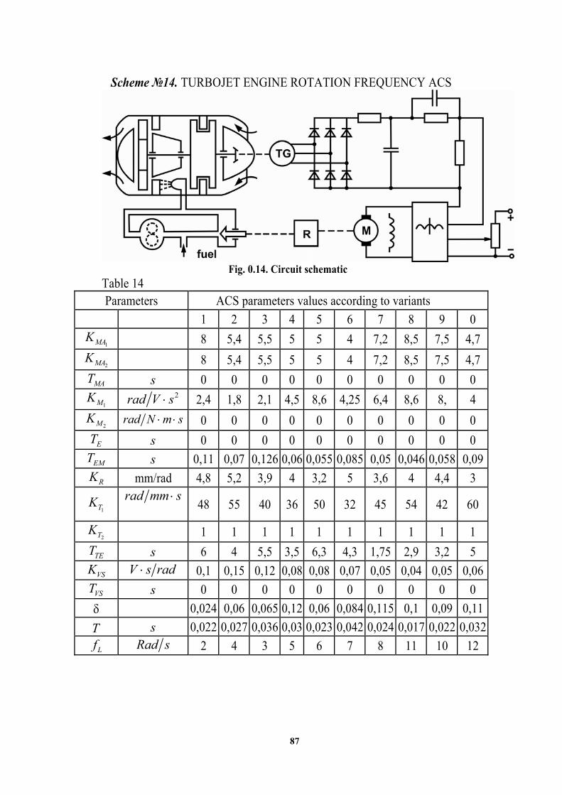
87

Scheme №14. TURBOJET ENGINE ROTATION FREQUENCY ACS

Fig. 0.14. Circuit schematic

Table 14 Parameters ACS parameters values according to variants

1 2 3 4 5 6 7 8 9 0

1MAK 8 5,4 5,5 5 5 4 7,2 8,5 7,5 4,7

2MAK 8 5,4 5,5 5 5 4 7,2 8,5 7,5 4,7

MAT s 0 0 0 0 0 0 0 0 0 0

1MK 2rad V s 2,4 1,8 2,1 4,5 8,6 4,25 6,4 8,6 8, 4

2MK rad N m s 0 0 0 0 0 0 0 0 0 0

ET s 0 0 0 0 0 0 0 0 0 0

EMT s 0,11 0,07 0,126 0,06 0,055 0,085 0,05 0,046 0,058 0,09

RK mm/rad 4,8 5,2 3,9 4 3,2 5 3,6 4 4,4 3

1TK rad mm s

48 55 40 36 50 32 45 54 42 60

2TK 1 1 1 1 1 1 1 1 1 1

TET s 6 4 5,5 3,5 6,3 4,3 1,75 2,9 3,2 5

VSK V s rad 0,1 0,15 0,12 0,08 0,08 0,07 0,05 0,04 0,05 0,06

VST s 0 0 0 0 0 0 0 0 0 0

0,024 0,06 0,065 0,12 0,06 0,084 0,115 0,1 0,09 0,11

T s 0,022 0,027 0,036 0,03 0,023 0,042 0,024 0,017 0,022 0,032

Lf Rad s 2 4 3 5 6 7 8 11 10 12

88

Reference

1. Wilson J. Rugh. Linear System Theory. – Prentice Hall 1996. – 508 p. 2. Eduardo D. Sontag. Mathematical Control Theory: Deterministic Finite Dimensional Systems. Second Edition. – New York: Springer, 1998. – 531 p. 3. Frederick Walker Fairman. Linear Control Theory: The State Space Approach. – John Wiley & Sons Ltd. 1998, – 331 p. 4. Shlomo Engelberg. A Mathematical Introduction to Control Theory. – World Scientific Publishing, 2005. – 368 p. 5. Sergiu Aizcovici, Nicolae H. Pavel. Differential Equations and Control Theory. – CRC Press, 2001. – 342 p. 6. Jerzy Zabczyk, Mathematical Control Theory: An Introduction. – Birkhäuser Boston, 2007. – 260 p. 7. Tim Wescott, Applied Control Theory for Embedded Systems. – Newnes, 2006. – 320 p. 8. Control Theory and Related Topics: In Memory of Prof Xunjing Li, edited by Shanjian Tang. – Fudan University, 2005. – 395 p. 9. Hassan K. Khalil. Nonlinear Systems. – Prentice Hall, 1996. – 750 p. 10. Andrei A. Agrachev, A. Stephen Morse, Eduardo D. Sontag, Hector J. Sussmann, Vadim I. Utkin. Nonlinear and Optimal Control Theory: Lectures given at the C.I.M.E. Summer School held in Cetraro. – Springer, 2004. – 360 p.

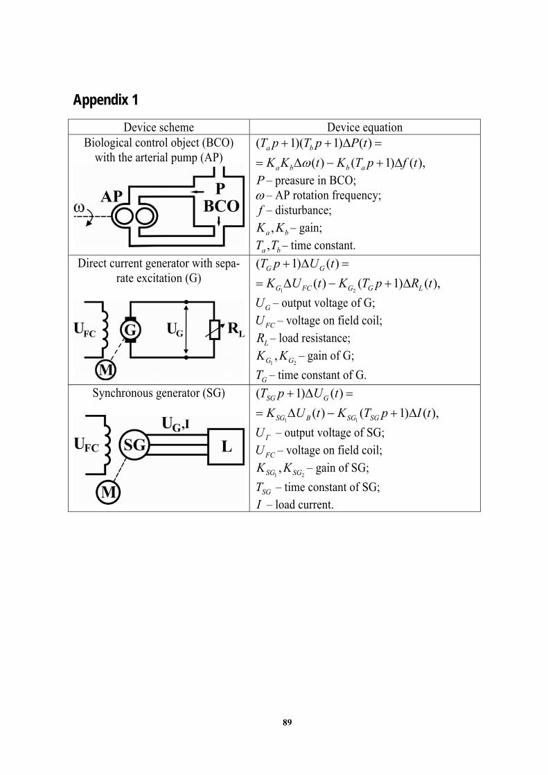
89

Appendix 1

Device scheme Device equation Biological control object (BCO)

with the arterial pump (AP) ( 1)( 1) ( )

( ) ( 1) ( ),a b

a b b a

T p T p P t

K K t K T p f t

P – preasure in BCO; – AP rotation frequency; f – disturbance;

,a bK K – gain; ,a bT T – time constant.

Direct current generator with sepa-rate excitation (G)

1 2

( 1) ( )

( ) ( 1) ( ),G G

G FC G G L

T p U t

K U t K T p R t

GU – output voltage of G;

FCU – voltage on field coil;

LR – load resistance;

1 2,G GK K – gain of G;

GT – time constant of G.

Synchronous generator (SG)

1 1

( 1) ( )

( ) ( 1) ( ),SG G

SG В SG SG

T p U t

K U t K T p I t

ГU – output voltage of SG;

FCU – voltage on field coil;

1 2,SG SGK K – gain of SG;

SGT – time constant of SG; I – load current.

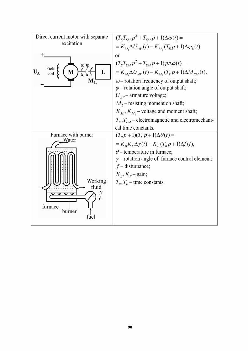
90

Direct current motor with separate excitation

1 2

2( 1) ( )

( ) ( 1) ( )E EМ EM

M AV M E L

T T p T p t

K U t K T p t

or

1 2

2( 1) ( )

( ) ( 1) ( ),E EM EM

M AV M E RM

T T p T p p t

K U t K T p M t

– rotation frequency of output shaft; – rotation angle of output shaft;

AVU – armature voltage;

LM – resisting moment on shaft;

1 2,M MK K – voltage and moment shaft;

,E EМT T – electromagnetic and electromechani-cal time conctants.

Furnace with burner

( 1)( 1) ( )

( ) ( 1) ( ),B F

B F F B

T p T p t

K K t K T p f t

– temperature in furnace; – rotation angle of furnace control element; f – disturbance;

,B FK K – gain; ,B FT T – time constants.

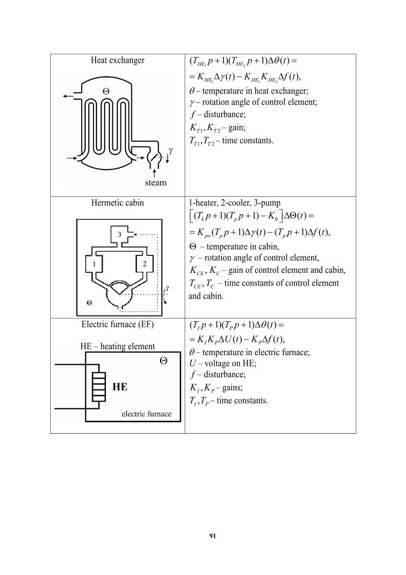
91

Heat exchanger

1 2

1 1 2

( 1)( 1) ( )

( ) ( ),

HE HE

HE HE HE

T p T p t

K t K K f t

– temperature in heat exchanger; – rotation angle of control element; f – disturbance;

1 2,T TK K – gain;

1 2,T TT T – time constants.

Hermetic cabin

1-heater, 2-cooler, 3-pump

0( 1)( 1) ( )

( 1) ( ) ( 1) ( ),

k p

po p p

T p T p K t

K T p t T p f t

– temperature in cabin,

– rotation angle of control element, ,CE CK K – gain of control element and cabin,

,CE CT T – time constants of control element and cabin.

Electric furnace (EF)

HE – heating element

( 1)( 1) ( )

( ) ( ),I P

I P P

T p T p t

K K U t K f t

– temperature in electric furnace; U – voltage on HE; f – disturbance;

,I PK K – gains; ,I PT T – time constants.

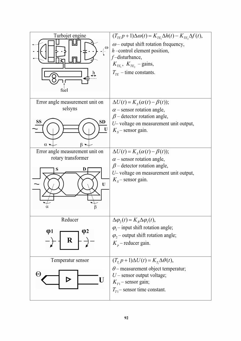
92

Turbojet engine

1 2( 1) ( ) ( ) ( ),TE TE TET p t K h t K f t

– output shift rotation frequency, h –control element position, f –disturbance,

1 2,TE TEK K – gains,

TET – time constants.

Error angle measurement unit on selsyns

( ) ( ( ) ( ));SU t K t t – sensor rotation angle, – detector rotation angle, U– voltage on measurement unit output,

SK – sensor gain.

Error angle measurement unit on rotary transformer

( ) ( ( ) ( ));SU t K t t – sensor rotation angle, – detector rotation angle, U– voltage on measurement unit output,

SK – sensor gain.

Reducer

2 1( ) ( ),Rt K t 1 – input shift rotation angle;

2 – output shift rotation angle;

рK – reducer gain.

Temperatur sensor

1 1( 1) ( ) ( ),T TT p U t K t

– measurement object temperatur; U – sensor output voltage;

1ТK – sensor gain;

1ТT – sensor time constant.

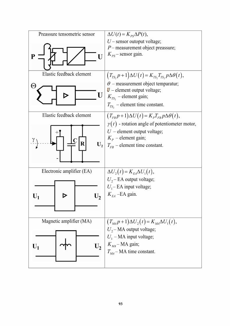
93

Preassure tensometric sensor

( ) ( ),PSU t K P t U – sensor outoput voltage; P – measurement object preassure;

PSK – sensor gain.

Elastic feedback element

2 2 2

1 ,TS TS TST p U t K T p t

– measurement object temparatur; – element output voltage;

2TSK – element gain;

2TST – element time constant.

Elastic feedback element

1 ,FB P FBT p U t K T p t

t - rotation angle of potentiometer motor,

U – element output voltage;

PK – element gain;

FBT – element time constant.

Electronic amplifier (EA)

2 1 ,EAU t K U t

2U – EA output voltage;

1U – EA input voltage;

EAK –EA gain.

Magnetic amplifier (MA)

2 11 ,MA MAT p U t K U t

2U – MA output voltage;

1U – MA input voltage;

MAK – MA gain;

MAT – MA time constant.

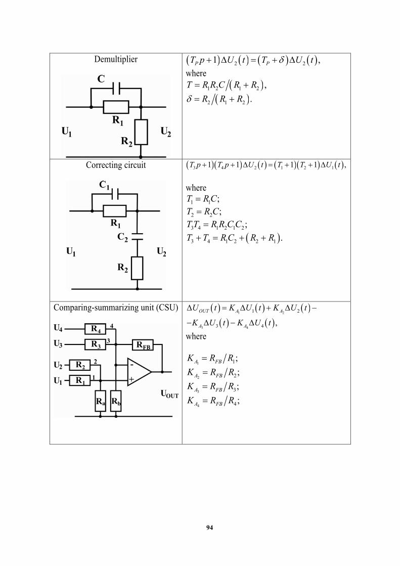
94

Demultiplier

2 21 ,P PT p U t T U t

where 1 2 1 2 ,T R R C R R

2 1 2 .R R R

Correcting circuit

3 4 2 1 2 11 1 1 1 ,T p T p U t T T U t

where

1 1 ;T R C

2 2 ;T R C

3 4 1 2 1 2;T T R R C C

3 4 1 2 2 1 .T T R C R R

Comparing-summarizing unit (CSU)

1 2

3 4

1 2

3 4 ,

OUT A A

A A

U t K U t K U t

K U t K U t

where

1 1;A FBK R R

2 2;A FBK R R

3 3;A FBK R R

4 4;A FBK R R

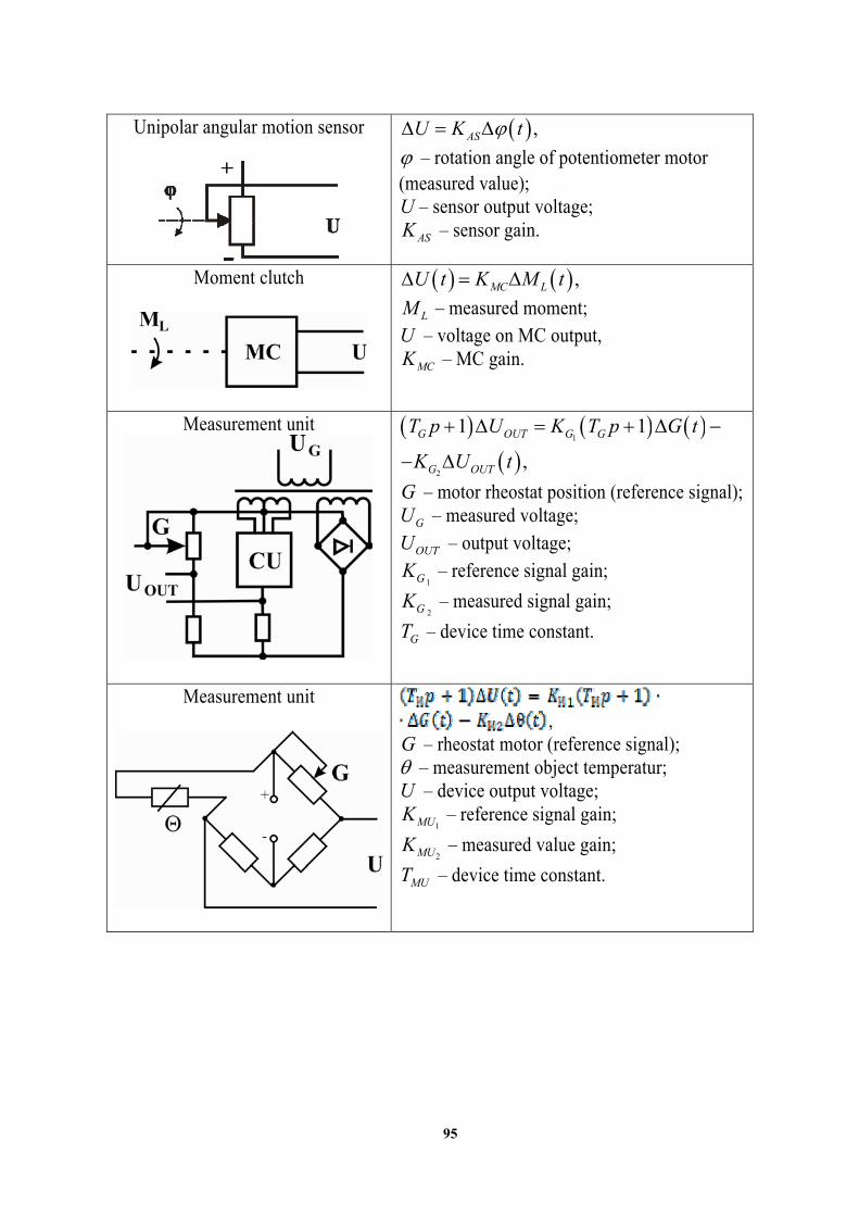
95

Unipolar angular motion sensor

,ASU K t

– rotation angle of potentiometer motor (measured value); U – sensor output voltage;

ASK – sensor gain.

Moment clutch

,MC LU t K M t

LM – measured moment; U – voltage on MC output,

MCK – MC gain.

Measurement unit

1

2

1 1

,

G OUT G G

G OUT

T p U K T p G t

K U t

G – motor rheostat position (reference signal);

GU – measured voltage;

OUTU – output voltage;

1GK – reference signal gain;

2GK – measured signal gain;

GT – device time constant.

Measurement unit

,

G – rheostat motor (reference signal); – measurement object temperatur; U – device output voltage;

1MUK – reference signal gain;

2MUK – measured value gain;

MUT – device time constant.

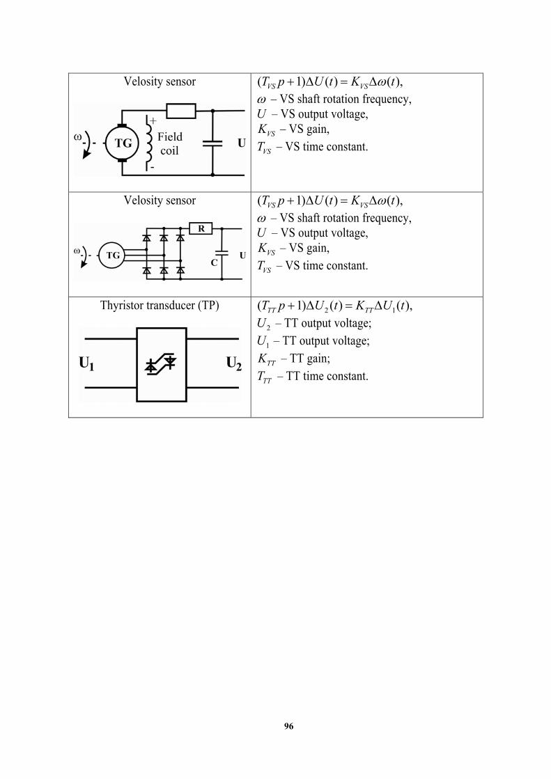
96

Velosity sensor

( 1) ( ) ( ),VS VST p U t K t – VS shaft rotation frequency, U – VS output voltage,

VSK – VS gain,

VST – VS time constant.

Velosity sensor

( 1) ( ) ( ),VS VST p U t K t – VS shaft rotation frequency, U – VS output voltage,

VSK – VS gain,

VST – VS time constant.

Thyristor transducer (TP)

2 1( 1) ( ) ( ),TT TTT p U t K U t

2U – TT output voltage;

1U – TT output voltage;

TTK – TT gain;

TTT – TT time constant.

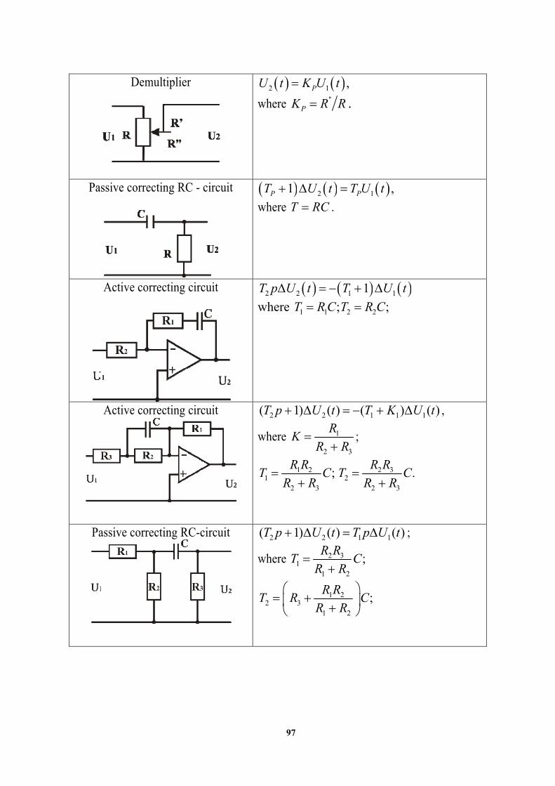
97

Demultiplier

2 1 ,PU t K U t

where ''PK R R .

Passive correcting RC - circuit

2 11 ,P PT U t T U t

where T RC .

Active correcting circuit

2 2 1 11T p U t T U t

where 1 1 2 2; ;T R C T R C

Active correcting circuit

2 2 1 1 1( 1) ( ) ( ) ( )T p U t T K U t ,

where 1

2 3

RK

R R

;

1 21

2 3

;R R

T CR R

2 32

2 3

.R R

T CR R

Passive correcting RC-circuit

2 2 1 1( 1) ( ) ( )T p U t T p U t ;

where 2 31

1 2

;R R

T CR R

1 22 3

1 2

;R R

T R CR R

98

Appendix 2

Lattice functions images

Original Laplace trans-

form Unbiased lat-tice function

z-transform

1, 0( )

0, 0

for tf t

for t

- [ ]o n 1

1( ) 1( )t t T 1 sTe

s

1[ ] 1[ 1]n n

1

1( )t 1

s 1[ ]n

1

z

z

t 2

1

s nT 2( 1)

Tz

z

2

2!

t 3

1

s

2( )

2!

nT

2

3

( 1)

2!( 1)

T z z

z

3

3!

t 4

1

s

3( )

3!

nT

3 2

4

( 4 1)

3!( 1)

T z z z

z

!

kt

k 1

1ks

( )

!

knT

k 1

( )

!( 1)

kz

k

T zR z

k z

te 1

s nT ne d T

z

z e

1 te ( )s s

1 nTe (1 )

( 1)( )

T

T

e z

z z e

tte 2

1

( )s nTnTe 2( )

T

T

ze

z e

2

2!tt

e 3

1

( )s

2( )

2!nTnT

e 2

3

( )

2!( )

T T

T

z z e e

z e

!

ktt

ek

1

1

( )ks ( )

!

knTnT

ek

1

( )

!( )

T k Tk

T k

zR ze e

k z e

sint

T

1

2 2 2

T

s T

sin 0n 0

99

cost

T 2 2 2/

s

s T cos ( 1)nn

1

z

z

sin2

t

T

2 2 2

0,5 /

0,25 /

T

s T

sin2

n

2 1

z

z

cos2

t

T

2 2 20,25 /

s

s T

� EMBED 2

2 1

z

z

sin t 2 2s

sin nT 2

sin

2 cos 1

z T

z z T

cos t 2 2

s

s cos nT

2

2

cos

2 cos 1

z z T

z z T

sinte t 2 2( )s

sinnTe nT 2 2

sin

2 cos

T

T

ze T

z z T e

coste t 2 2( )

s

s

cosnTe nT

2

2 2

cos

2 cos

T

T T

z ze T

z ze T e

- - 0( )t nT nz

Educational Edition  

Национальный исследовательский Томский политехнический университет 

  

ЗАМЯТИН Сергей Владимирович ПУШКАРЕВ Максим Иванович ЯКОВЛЕВА Елена Максимовна 

  

ТЕОРИЯ УПРАВЛЕНИЯ  

Учебное пособие Издательство Томского политехнического университета, 2012 

На английском языке  

Published in author’s version        

Registered in the TPU Publishing House Posted on the TPU corporate portal in full accordance  

with the quality of the given make‐up page   

 

 

Tomsk Polytechnic University Quality management system 

of Tomsk Polytechnic University was certified by NATIONAL QUALITY ASSURANCE on BS EN ISO 9001:2008   

. 30, Lenina Ave, Tomsk, 634050, Russia Tel/fax: +7 (3822) 56‐35‐35, www.tpu.ru