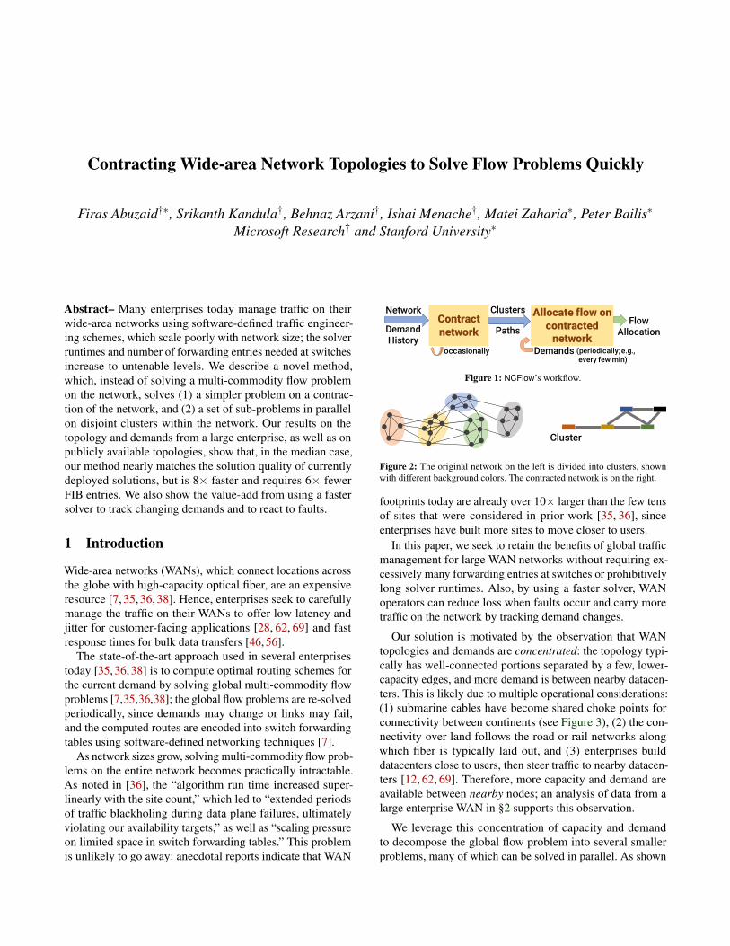
Contracting Wide-area Network Topologies to Solve Flow Problems Quickly

Firas Abuzaid†∗, Srikanth Kandula†, Behnaz Arzani†, Ishai Menache†, Matei Zaharia∗, Peter Bailis∗

Microsoft Research† and Stanford University∗

Abstract– Many enterprises today manage traffic on theirwide-area networks using software-defined traffic engineer-ing schemes, which scale poorly with network size; the solverruntimes and number of forwarding entries needed at switchesincrease to untenable levels. We describe a novel method,which, instead of solving a multi-commodity flow problemon the network, solves (1) a simpler problem on a contrac-tion of the network, and (2) a set of sub-problems in parallelon disjoint clusters within the network. Our results on thetopology and demands from a large enterprise, as well as onpublicly available topologies, show that, in the median case,our method nearly matches the solution quality of currentlydeployed solutions, but is 8× faster and requires 6× fewerFIB entries. We also show the value-add from using a fastersolver to track changing demands and to react to faults.

1 Introduction

Wide-area networks (WANs), which connect locations acrossthe globe with high-capacity optical fiber, are an expensiveresource [7, 35, 36, 38]. Hence, enterprises seek to carefullymanage the traffic on their WANs to offer low latency andjitter for customer-facing applications [28, 62, 69] and fastresponse times for bulk data transfers [46, 56].

The state-of-the-art approach used in several enterprisestoday [35, 36, 38] is to compute optimal routing schemes forthe current demand by solving global multi-commodity flowproblems [7,35,36,38]; the global flow problems are re-solvedperiodically, since demands may change or links may fail,and the computed routes are encoded into switch forwardingtables using software-defined networking techniques [7].

As network sizes grow, solving multi-commodity flow prob-lems on the entire network becomes practically intractable.As noted in [36], the “algorithm run time increased super-linearly with the site count,” which led to “extended periodsof traffic blackholing during data plane failures, ultimatelyviolating our availability targets,” as well as “scaling pressureon limited space in switch forwarding tables.” This problemis unlikely to go away: anecdotal reports indicate that WAN

Contract network

Allocate flow on contracted

networkoccasionally

Network Clusters

Demands

FlowAllocationDemand

HistoryPaths

(periodically; e.g.,every few min)

Figure 1: NCFlow’s workflow.

Cluster

Figure 2: The original network on the left is divided into clusters, shownwith different background colors. The contracted network is on the right.

footprints today are already over 10× larger than the few tensof sites that were considered in prior work [35, 36], sinceenterprises have built more sites to move closer to users.

In this paper, we seek to retain the benefits of global trafficmanagement for large WAN networks without requiring ex-cessively many forwarding entries at switches or prohibitivelylong solver runtimes. Also, by using a faster solver, WANoperators can reduce loss when faults occur and carry moretraffic on the network by tracking demand changes.

Our solution is motivated by the observation that WANtopologies and demands are concentrated: the topology typi-cally has well-connected portions separated by a few, lower-capacity edges, and more demand is between nearby datacen-ters. This is likely due to multiple operational considerations:(1) submarine cables have become shared choke points forconnectivity between continents (see Figure 3), (2) the con-nectivity over land follows the road or rail networks alongwhich fiber is typically laid out, and (3) enterprises builddatacenters close to users, then steer traffic to nearby datacen-ters [12, 62, 69]. Therefore, more capacity and demand areavailable between nearby nodes; an analysis of data from alarge enterprise WAN in §2 supports this observation.

We leverage this concentration of capacity and demandto decompose the global flow problem into several smallerproblems, many of which can be solved in parallel. As shown

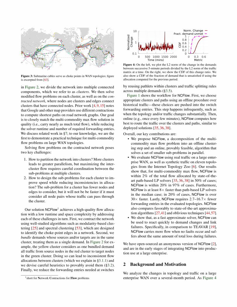
Figure 3: Submarine cables serve as choke points in WAN topologies; figureis excerpted from [63].

in Figure 2, we divide the network into multiple connectedcomponents, which we refer to as clusters. We then solvemodified flow problems on each cluster, as well as on the con-tracted network, where nodes are clusters and edges connectclusters that have connected nodes. Prior work [4,9,15] notesthat Google and other map providers use different contractionsto compute shortest paths on road network graphs. Our goalis to closely match the multi-commodity max flow solution inquality (i.e., carry nearly as much total flow), while reducingthe solver runtime and number of required forwarding entries.We discuss related work in §7; to our knowledge, we are thefirst to demonstrate a practical technique for multi-commodityflow problems on large WAN topologies.

Solving flow problems on the contracted network posestwo key challenges:

1. How to partition the network into clusters? More clustersleads to greater parallelism, but maximizing the inter-cluster flow requires careful coordination between thesub-problems at multiple clusters.

2. How to design the sub-problems for each cluster to im-prove speed while reducing inconsistencies in alloca-tion? The sub-problem for a cluster has fewer nodes andedges to consider, but it will not be be faster if it mustconsider all node pairs whose traffic can pass throughthe cluster.

Our solution NCFlow1 achieves a high-quality flow alloca-tion with a low runtime and space complexity by addressingeach of these challenges in turn. First, we contract the networkusing well-studied algorithms such as modularity-based clus-tering [25] and spectral clustering [53], which are designedto identify the choke-point edges in a network. Second, webundle demands whose sources and/or targets are in the samecluster, treating them as a single demand. In Figure 2 for ex-ample, the yellow cluster considers as one bundled demandall traffic from source nodes in the red cluster to target nodesin the green cluster. Doing so can lead to inconsistent flowallocations between clusters (which we explain in §3.1.1) andwe devise careful heuristics to provably avoid them (§3.2).Finally, we reduce the forwarding entries needed at switches

1short for Network Contractions for Flow problems

0.1

1

10

0 500 1000 1500 2000

Norm

aliz

ed

Change

Time (mins)

0 0.2 0.4 0.6 0.8

1

0 0.3 0.6

CD

F

Metric

Norm. ChangeFract. demand unmet

Figure 4: On the left, we plot the L2 norm of the change in the demandsbetween successive 5-minute periods divided by the L2 norm of the trafficmatrix at a time. On the right, we show the CDF of this change ratio. Wealso show a CDF of the fraction of demand that is unsatisfied if using theallocation computed for the previous period.

by reusing pathlets within clusters and traffic splitting rulesacross multiple demands (§3.5).

Figure 1 shows the workflow for NCFlow. First, we chooseappropriate clusters and paths using an offline procedure overhistorical traffic—these choices are pushed into the switchforwarding entries. This step happens infrequently, such aswhen the topology and/or traffic changes substantially. Then,online (e.g., once every few minutes), NCFlow computes howbest to route the traffic over the clusters and paths, similar todeployed solutions [35, 36, 38].

Overall, our key contributions are:• We propose NCFlow, a decomposition of the multi-

commodity max flow problem into an offline cluster-ing step and an online, provably feasible, algorithm thatsolves a set of smaller sub-problems in parallel.

• We evaluate NCFlow using real traffic on a large enter-prise WAN, as well as synthetic traffic on eleven topolo-gies from the Internet Topology Zoo [6]. Our resultsshow that, for multi-commodity max flow, NCFlow iswithin 2% of the total flow allocated by state-of-the-art path-based LP solvers [35, 36, 38] in 50% of cases;NCFlow is within 20% in 97% of cases. Furthermore,NCFlow is at least 8× faster than path-based LP solversin the median case; in 20% of cases, NCFlow is over30× faster. Lastly, NCFlow requires 2.7–16.7× fewerforwarding entries in the evaluated topologies. NCFlowalso compares favorably to state-of-the-art approxima-tion algorithms [27,41] and oblivious techniques [44,57].

• We show that, as a fast approximate solver, NCFlow canbe used to react quickly to demand changes and linkfailures. Specifically, in comparison to TEAVAR [19],NCFlow carries more flow when no faults occur and suf-fers about the same amount of total loss during failures.

We have open-sourced an anonymous version of NCFlow [2],and are in the early stages of integrating NCFlow into produc-tion use at a large enterprise.

2 Background and Motivation

We analyze the changes in topology and traffic on a largeenterprise WAN over a several-month period. As Figure 4

112 202 294 372 486 1790# of Edges (log scale)

10 210 1100101101102103

Runt

ime

(s),

log

scal

e

5-minute time window

Figure 5: Runtimes of a state-of-the-art solver on topologies from InternetTopology Zoo [6]. Both axes are in log scale and the band represents stan-dard deviation. In production WANs, new traffic demands arrive every fewminutes [35, 38].

shows, the change in traffic demand from one 5-minute win-dow to the next is substantial; the average change is 35%;in 20% of the cases, the traffic change is over 45%. The en-terprise solves a global flow allocation problem every fewminutes. The figure on the right shows the fraction of trafficthat will remain unsatisfied if the flow allocation from theprevious window were to be used instead of computing a newallocation. We see that the median loss is 13%; in 20% of thecases, over 20% of the demand remains unsatisfied. We verifythat computing a new allocation will satisfy all of the demand;using the previous window’s allocation causes loss becausesome datacenter pairs may receive more flow in the previousallocation than their current demand while other datacenterpairs go unsatisfied.

Given the above data, computing a new allocation in eachtime window is needed to carry more traffic on the WAN.However, solver runtime increases super-linearly with thesize of the topology, as shown in Figure 5. For several publictopologies and on a variety of traffic matrices, we benchmarkthe multi-commodity max-flow problem (specifically PF4, aswill be described in §5.1). The runtimes were measured on aserver-grade machine using a production-grade optimizationlibrary [33]. As the figure shows, when the topology size ex-ceeds a thousand edges, the time to compute a flow allocationcan exceed the allotted time window.

A fast solver would not only ensure that new allocationscomplete in time—it could also enable more frequent alloca-tions, e.g., every minute. Doing so would enable allocationsto track changing demands at a finer granularity. Moreover,as we show in §5, a fast solver can help when reacting to linkand switch failures.

Our observation that demand and capacity are concentratedamong nearby nodes is grounded on the following measure-ments from a production WAN:Demand properties:

• On average, 7% (or 16%) of the node pairs account forhalf (or 75%) of the total demand.

• When nodes are divided into a few tens of clusters, 47%of the total traffic stays within clusters. If the demandswere distributed uniformly across node pairs, only 8%of the traffic would stay within clusters; thus the demandwithin clusters is about 6× larger than would be expected

from a uniform distribution.

WAN topology properties:• When nodes are divided into tens of clusters, 76% of all

edges and 87% of total capacity is within clusters.• The skew in capacity is small: the ratio between the

largest edge capacity and the mean is 10.4.• The skew in node degree is also small: the average node

degree is 3.9, with σ = 2.6; the max is 16.• Relative to the network size (hundreds of nodes), the

average network diameter (=11) and the average shortest-path length (= 5.3) are very small.

Motivated by the above analyses, NCFlow seeks to be a fastsolver for large WAN topologies by leveraging the concentra-tion of traffic demands and capacity.

Background: Before we describe NCFlow’s design, we givesome background on multi-commodity flow problems. Givena set of nodes, capacitated edges, and demands between nodes,a flow allocation is feasible if it satisfies demand and capacityconstraints. The goal of a multi-commodity flow problem is tofind a feasible flow which optimizes a given objective; Table 1lists some common flavors.

The fastest algorithms [27, 41] are approximate; i.e., givena parameter ε, they achieve at least (1−ε)× the optimal value.And, their runtime complexity is at least quadratic (Table 1).

Moreover, these solutions allow demands to travel on anyedge, thus requiring millions of forwarding table entries ateach switch for thousand-node topologies. Instead, produc-tion systems [35, 38] restrict flow to a small number of pre-configured paths per demand, which reduces the requiredforwarding table entries by 10–100×.

Using notation from Table 2, the feasible flow over a pre-configured set of paths can be defined as:

FeasibleFlow(V ,E ,D,P ),{

fk | ∀k ∈D and (1)

fk = ∑p∈Pk

f pk , ∀k ∈D (flow for demand k)

fk ≤ dk, ∀k ∈D (flow below volume)

∑∀k,p∈Pk ,e∈p

f pk ≤ ce, ∀e ∈ E (flow below capacity)

f pk ≥ 0 ∀p ∈ P ,k ∈D (non-negative flow)

}Production systems use linear optimization-based

solvers [35, 36, 38]. On WANs with thousands of nodes, theoptimization problem could have millions of variables andequations just to verify that a flow allocation is feasible.

In this paper, we consider the problem of maximizing thetotal flow across all demands:

MaxFlow(V ,E ,D,P ),argmaxf ∑

k∈Dfk (2)

s.t. f ∈ FeasibleFlow(V ,E ,D,P )

Maximization term Additional Constraints Used in Known best complexityMaxFlow ∑k∈D fk none [35, 38] O(M2ε−2 logO(1) M) [27]

MaxFlow with Cost Budget ∑k∈D fk ∑k ∑p∈Pk ∑e∈p f pk Coste ≤ Budget O(ε−2M logM(M+N logN) logO(1) M) [27]

Max Concurrent Flow α dkα≤ fk,∀k ∈D [19, 39, 40] O(ε−2(M2 +KN) logO(1) M) [41]

Table 1: We illustrate a few different multi-commodity flow problems all of which find feasible flows but optimize for different objectives and can have additionalconstraints; see notation in Table 2. Equation 6 fleshes out the problem completely for the case of maximizing flow. More problems are discussed in [11].

Term MeaningV ,E ,D,P Sets of nodes, edges, demands, and pathsN,M,K The numbers of nodes, edges, and demands, i.e., N =

|V |,M = |E |,K = |D|e,ce, p Edge e has capacity ce; path p is a set of connected edges(sk, tk,dk) Each demand k in D has source and target nodes (sk, tk ∈

V ) and a non-negative volume (dk).f, f p

k Flow assignment vector for a set of demands and the flowfor demand k on path p.

Table 2: Notation for framing multi-commodity flow problems.

Vagg, Eagg,Dagg, Pagg

Nodes, edges, demands, and paths in the aggregatedgraph

Vx,Ex,Dx,Px Subscript denotes entities in the restricted graph forcluster x

x,η Each cluster x is a strongly connected set of nodes andη is the number of clusters

k,Kxy,Ksy,Kxt An actual demand (k); the rest are bundled demandsfrom one source (s) or all nodes in a cluster (x) to atarget (t) or to all nodes in a cluster (y)

Table 3: Additional notation specific to NCFlow.

SDN-based traffic engineering schemes [35, 38], in addi-tion to repeatedly solving global optimizations, must maintainan up-to-date view of the topology, gather desired volumesfor demands and update traffic splits at switches based on theresult of the optimization. Our production experience is thatmost of these repetitive steps have a latency of a few RTTs(round trip times) and so solving the optimization dominates,especially on large topologies. Moreover, demands are lim-ited to their allocated rates in software at the source serversand thus allocating less than the full desired rate need notresult in packet loss [35]. Finally, applications that contributea large fraction of the bytes moving between datacenters areelastic in short timescales; e.g., large dataset transfers for dataanalytics. That is, these apps seek a fast completion time butdo not need a large rate in every optimization epoch. Someother applications have a decreasing marginal utility as theirrate allocation increases such as video streams of varyingquality [43]. Today’s SDN-based TE solutions [35, 38] usemultiple priority classes to maximize allocations for elastictraffic without affecting the latency-sensitive traffic.

3 NCFlow

In this section, we describe NCFlow. Our steps are as shownin Figure 1. Offline, based on historical demands, we dividethe network into clusters and determine paths. Further detailsare in §3.4. Online, we allocate flow to the current demands bysolving a carefully constructed set of simpler sub-problems,

MaxAggFlow

MaxClusterFlow

MinPathE2E

SrcTargetMax

f1 ,MaxFlow(Vagg,Eagg,Dagg,Pagg)

∀clusters x, fx2 ,MaxFlow(Vx,Ex,Dx,Px)

s.t. NoMoreFlowThruCluster(f, f1,x) (see §D)

f3 ,{

fk,∀k ∈Dagg}

s.t.

s.t. NoMoreAlongPaths(f, f2) (see §D)

∀clusters x,y,x 6= y, fxy4 ,argmax ∑

k∈Kxy

fk

s.t. ∑k∈Ksy

fk ≤ f x2,Ksy , ∀s ∈ x; ∑

k∈Kxt

fk ≤ f y2,Kxt

, ∀t ∈ y;

∑k∈Kxy

fk ≤ f3,Kxy ; fk ≤ dk, ∀k ∈ Kxy

Figure 6: The basic flow allocation algorithm used by NCFlow; notationused here is defined in Table 3.

some of which can be solved independently and in parallel.We describe these sub-problems in §3.1. Although they can besolved quickly, disagreements between independent solutionscan lead to infeasible allocations; we present a simple heuris-tic in §3.2 that provably leads to feasible flow allocations.In §3.3, we discuss extensions that increase the total flow al-located by NCFlow. We also show sufficient conditions underwhich NCFlow is optimal and matches the flow allocated byMaxFlow. Finally, in §3.5, we discuss how NCFlow uses fewerforwarding entries by reusing pathlets within clusters andsplitting rules for different demands.

3.1 Basic Flow Allocation

We begin by describing a simple (but incomplete) versionof NCFlow’s flow allocation algorithm; the pseudocode isin Figure 6. We continue using Figure 2 as a running example.The basic algorithm proceeds in four steps.

In the first step, we allocate flow on the aggregated graph;as shown in MaxAggFlow in Figure 6. In the aggregated graph,an example of which is in Figure 2 (right), nodes are clustersand the edges are bundled edges from the original graph—the edge between the red and yellow clusters correspondsto the five edges between these clusters on the actual graph.Similarly, we bundle demands on the aggregated graph: thedemand Kxy between the clusters x and y corresponds to allof the demands whose sources are in cluster x and targets are

! "#,%&'(,)

)≤ "+,%&'

, + "+,%&'.! "#,%/'

0,)1,)

≤ "+,%&', + "+,%&'

.

!"+,%&',

2"

#"+,%&'.

Figure 7: An example illustrating how the flow allocated in MaxAggFlowtranslates to constraints on the flow to be allocated in MaxClusterFlow.

in cluster y. The resulting flow allocation (f1) accounts forbottlenecks on the edges between clusters. However, this flowmay not be feasible, since there may be bottlenecks withinthe clusters.

In the second step, we refine the allocation from step 1 toaccount for intra-cluster demands and constraints. Specifically,we allocate flow for the demands whose sources and targetsare within the cluster. We also allocate no more flow thanwas allocated in f1 for the inter-cluster flows. MaxClusterFlowin Figure 6 shows code for this step. We note a few details:

• We use virtual nodes to act as the sources and targets forthe inter-cluster flows; the flow allocated in f1 determineswhich virtual node (i.e., which neighboring cluster) isthe sender or the receiver for an inter-cluster demand.

• Figure 7 shows two examples on the right where thevirtual nodes are drawn using squares.

• Figure 7 also shows the NoMoreFlowThruCluster con-straints for demands from sources in the red cluster totargets in the black cluster (depicted as x and z respec-tively). On the aggregated graph, the flow for this de-mand takes the two paths shown. In the red cluster, asshown in the equation, the traffic from all sources (s),along multiple paths (r) to the virtual node, is restrictedto be no more than what was allocated in f1.

• Figure 7 on the right also shows a more complex casethat happens in the yellow cluster. Here, the traffic arrivesat one virtual node but can leave to multiple virtual nodes.In MaxClusterFlow, we set up paths between all pairsof virtual nodes. As shown in the equation, the trafficleaving the red virtual node on paths (r) to either of theother virtual nodes must be no more than the total flowon paths p and q from f1.

• Observe that bundling demands ensures fewer variablesand constraints for MaxClusterFlow. The demand fromred to black clusters comprises twenty node pairs in theactual graph in Figure 2 (left); four sources in the redcluster and five targets in the black cluster. However, theMaxClusterFlow for the red cluster only has four bundleddemands, from each source to the virtual node, and theyellow cluster has just one bundled demand from and tovirtual nodes.

In the third step, we reconcile end-to-end; that is, we findthe largest flow that can be carried along each path on theaggregate graph. As shown by MinPathE2E in Figure 6, foreach bundle of demands and each path, we take the minimumflow allocated (fx

2) at each cluster on the path.The flow allocation for the demands in a cluster x can be

Problem # of Nodes # of Edges # of DemandsMaxFlow N M K

MaxAggFlow η ≤min(M,η2) ≤min(K,η2)MaxClusterFlow ∼ N

η+η ∼ M

η+2η ∼ K

η2 +2 Nη+η2

Table 4: Sizes of the problems in Figure 6 using notation from Tables 2and 3. Just verifying that flow is feasible (i.e., FeasibleFlow in Eq. 1) usesO(# nodes ∗ # edges) number of equations and variables. NCFlow has oneinstance of MaxAggFlow and executes the η instances of MaxClusterFlow inparallel. MinPathE2E and SrcTargetMax, are relatively insignificant.

!"!#

$"$#

2

!"!#

%"1

1

$"$#

%#1

1

& & & &&

&(a) Disagreement arising from bundling edges: As shown on the right, the algo-rithm in Figure 6 will allocate 2 units of flow but only 5ε units can be carried.

!"!#

$"$# !"

!#

!"$"$#

!#1

%

%%%

`

1

1

1

11

11

(b) Disagreement arising from bundling demands: As shown on the right, thealgorithm in Figure 6 will allocate 2 units of flow, but only 2ε units can be carried.

Figure 8: Illustrating how disagreements in flow allocation can occur in thebasic flow allocation algorithm; see §3.1.1.

read directly from the fx2 solution of MaxClusterFlow. For

demands that span clusters, however, more work remains be-cause the steps thus far do not directly compute their flow. Inparticular, f3 allocates flow for cluster bundles; such as say forall the demands whose sources are in cluster x and targets arein cluster y. The corresponding per-cluster flow allocations, fx

2and fy

2, allocate flow from a source node and to a given targetrespectively. Thus, in the final step, SrcTargetMax, we assignthe maximal flow to each inter-cluster demand that respectsall previous allocations.

3.1.1 Properties of Basic Flow Allocation

Solver runtime: The numbers of equations and variables inthe sub-problems are shown in Table 4. If the number of clus-ters η is 1, note that there is exactly one per-cluster problem,MaxClusterFlow, which matches the original problem fromEqn. 2. When using a few tens of clusters, we will show in §5that all of the sub-problems are substantially smaller than theoriginal problem (MaxFlow).

Feasibility: The flow allocated by Figure 6 satisfies demandand capacity constraints; we will prove this formally in §B.1.For demands whose source and target are in different clusters,however, disagreements may ensue since the different prob-lem instances assign flow to different bundles of edges anddemands. We illustrate two such examples in Figure 8; bothhave 1 unit of demand from s1 to t1 and from s2 to t2. Thedashed edges have a capacity of ε� 1 and all of the otheredges have a very large capacity.

• The example in Figure 8a illustrates an issue withbundling edges. The actual graph on the left can only

st

Figure 9: To guarantee feasibility, each cluster bundle is allocated flow ononly one path on the aggregated graph (left) and on only one edge betweeneach pair of clusters (right); the usable path and edges are shown in dark red.Note that multiple paths can still be used within clusters.

carry 5ε units of flow for each demand. However, as thefigures on the right show, MaxAggFlow allocates twounits of flow since the four edges between these twoclusters can together carry all of the two units of demand.The MaxClusterFlow instances also allocate two unitsof flow as shown. The discrepancy arises because theproblems in Figure 6 do not know that the top egress ofthe left cluster can take in all of the demand of s1 but hasonly a low capacity to t1.

• The example in Figure 8b illustrates an issue withbundling demands. Here too, observing the actual net-work on the left will show that 2ε units can be carried foreach demand split evenly between the top and the bottompath. Again, as the figures on the right show, the basicflow allocation algorithm will conclude that both unitsof demand can be carried. Here, the discrepancy arisesfrom the bundling of demands, the problems in Figure 6cannot discern that the MaxClusterFlow instance of theleft cluster sends the first demand to the brown clusterwhile the MaxClusterFlow of the right cluster wants toreceive the second demand from the brown cluster.

3.2 A feasible heuristicTo avoid end-to-end disagreements, we make two simplechanges to the basic flow allocation in §3.1.

First, when solving MaxAggFlow, only one path on theaggregated graph can be used for all of the demands betweena given pair of clusters; we call such groups of demands to becluster bundles. Next, between a pair of connected clusters,only one edge can carry the flow for a cluster bundle. Figure 9shows in dark red an example path for a cluster bundle and theallowed edges between clusters; we also show the intra-clusterpaths that can carry flow for this bundle.

There are multiple ways to avoid disagreements while keep-ing the problem sizes small via bundling. We discuss theabove changes here because they are simple and sufficient.Specifically, we show that:

Theorem 1. The algorithm in Figure 6, when constrained asdiscussed above, will always output a feasible flow.

Proof. The proof is in §B.2. Intuitively, these changes sufficebecause the independent decisions made by different prob-lems in Figure 6 cannot disagree; per cluster bundle, all prob-lem instances allocate flow to the same edge and path.

st

Figure 10: Contrasting with Figure 9, for the same cluster bundle, in a sub-sequent iteration, NCFlow allocates flow on a different path on the aggregategraph and on different inter-cluster edges. The chosen paths and edges areagain shown in red.

3.3 Stepping towards optimality

The flow allocation algorithm described thus far is fast butnot optimal; that is, it may allocate less total flow over alldemands than the flow allocated by solving the larger globalproblem (MaxFlow from Eqn. 2). There are a few reasonswhy this happens. The MaxAggFlow in Figure 6 allocatesflow on paths through clusters without knowing how muchflow the clusters can carry. Switching the order, i.e., solvingMaxClusterFlow before MaxAggFlow, could be worse becauseeach cluster must allocate flow without knowing how muchflow can be carried end-to-end. Furthermore, the heuristicin §3.2 constrains each cluster bundle to use only one edgebetween clusters and one path on the aggregated graph. Wenow discuss a few extensions to increase the flow allocation.

First, we re-solve the problems in Figure 6 multiple times.A simple way to do this would be to deduct the allocated flowand use the residual capacity on edges in the next iteration.Also, we pick different edges between clusters and/or differentpaths on the aggregated graph in different iterations (see Fig-ure 10 for an example). The number of iterations is config-urable; we continue as long as the total flow increases in eachiteration by at least a pre-specified amount (say 5%). Onecould apply other policies such as a timeout. We show in §5that a small number of iterations suffice for a sizable increasein the total flow. We will also show that later iterations finishfaster than the first iteration perhaps because fewer demandsremain to satisfy.

Next, we empirically observe that the choice of clustersand edges/paths to use in different iterations has an effect onflow allocation. For instance, the disagreements in Figure 8go away by using a different choice of clusters—specifically,see Figure 31d and Figure 31e. We discuss how NCFlowprecomputes cluster and edge/path choice in §3.4.

To sum up, we prove that flow allocation will be optimalwhen a few sufficient conditions hold:

Theorem 2. The method in Figure 6 leads to the optimal flowallocation when any path can be used within each optimiza-tion and the number of clusters is 1 or equal to the number ofnodes or all of the following conditions hold:

• the aggregated graph Gagg is a tree,• only one edge connects any pair of clusters,• all demands are satisfiable.

Proof. By optimal, we mean that the total allocated flow mustbe as large as an instance of Equation 6 wherein any path canbe used. The proof is in §B.3. Intuitively, when the numberof clusters is 1 and any paths can be used, a single instance ofMaxClusterFlow is identical to the optimal problem in Equa-tion 6. Similarly, when the number of clusters equals thenumber of nodes, MaxAggFlow is identical to the optimalproblem. Furthermore, the conditions listed lead to optimalitybecause the optimal flow allocation can be transformed intoan allocation that can be outputted by Figure 6.

Even though the listed conditions appear restrictive, notethat the topology within clusters can be arbitrary. We willshow in §5 that NCFlow offers nearly optimal flow allocationseven when the above conditions do not hold.

3.4 Choosing clusters and pathsThe choice of clusters and paths affects both the solutionquality and runtime of NCFlow. We cast cluster choice as agraph partitioning problem [5, 21, 65] with these objectives:

• Concentrated with a low cut: NCFlow can output betterflow allocations when much of the total demand and thetotal edge capacity is between nodes in the same cluster.

• Balanced cut: Intuitively, NCFlow will have a smallerruntime when the complexity of MaxAggFlow balanceswith that of MaxClusterFlow. Recall from Table 4 thatthe former depends on the number of clusters whereasthe latter depends on the size of the largest cluster.

We empirically observe, based on experiments with manyWANs and different types of demands, that:

• On a graph with N nodes, about√

N clusters, irrespectiveof the clustering technique, leads to the best result, i.e.,smallest runtime and fewest forwarding entries whileallocating nearly the largest amount of flow possible;see Figure 13.

• When choosing the same number of clusters, one of thethree considered clustering techniques (described below)generally performs better than the others but not in allcases; see Figure 21.

Thus, the optimal clustering choice for a WAN is unclear;it is possible that hand-tuning or using a learning techniquemay lead to better-performing clusters. Nevertheless, any ofthe three simple clustering schemes discussed below alreadysuffice for NCFlow to improve substantially over baselines.

We consider the following clustering choices because theyare simple and fast; unless otherwise noted, results in thispaper use FMPartitioning.

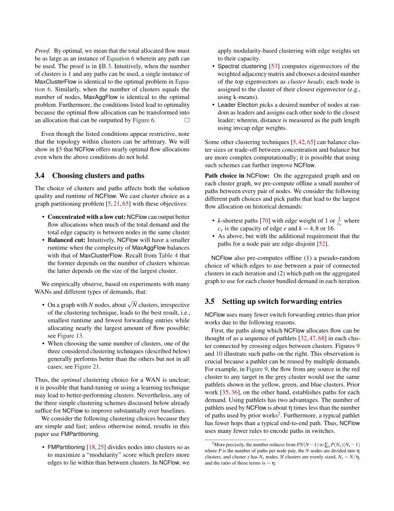
• FMPartitioning [18, 25] divides nodes into clusters so asto maximize a “modularity” score which prefers moreedges to lie within than between clusters. In NCFlow, we

apply modularity-based clustering with edge weights setto their capacity.

• Spectral clustering [53] computes eigenvectors of theweighted adjacency matrix and chooses a desired numberof the top eigenvectors as cluster heads; each node isassigned to the cluster of their closest eigenvector (e.g.,using k-means).

• Leader Election picks a desired number of nodes at ran-dom as leaders and assigns each other node to the closestleader; wherein, distance is measured as the path lengthusing invcap edge weights.

Some other clustering techniques [5, 42, 65] can balance clus-ter sizes or trade-off between concentration and balance butare more complex computationally; it is possible that usingsuch schemes can further improve NCFlow.

Path choice in NCFlow: On the aggregated graph and oneach cluster graph, we pre-compute offline a small number ofpaths between every pair of nodes. We consider the followingdifferent path choices and pick paths that lead to the largestflow allocation on historical demands:

• k-shortest paths [70] with edge weight of 1 or 1ce

wherece is the capacity of edge e and k = 4,8 or 16.

• As above, but with the additional requirement that thepaths for a node pair are edge-disjoint [52].

NCFlow also pre-computes offline (1) a pseudo-randomchoice of which edges to use between a pair of connectedclusters in each iteration and (2) which path on the aggregatedgraph to use for each cluster bundled demand in each iteration.

3.5 Setting up switch forwarding entries

NCFlow uses many fewer switch forwarding entries than priorworks due to the following reasons.

First, the paths along which NCFlow allocates flow can bethought of as a sequence of pathlets [32, 47, 68] in each clus-ter connected by crossing edges between clusters. Figures 9and 10 illustrate such paths on the right. This observation iscrucial because a pathlet can be reused by multiple demands.For example, in Figure 9, the flow from any source in the redcluster to any target in the grey cluster would use the samepathlets shown in the yellow, green, and blue clusters. Priorwork [35, 36], on the other hand, establishes paths for eachdemand. Using pathlets has two advantages. The number ofpathlets used by NCFlow is about η times less than the numberof paths used by prior works2. Furthermore, a typical pathlethas fewer hops than a typical end-to-end path. Thus, NCFlowuses many fewer rules to encode paths in switches.

2More precisely, the number reduces from PN(N−1) to ∑x P(Nx)(Nx−1)where P is the number of paths per node pair, the N nodes are divided into η

clusters, and cluster x has Nx nodes. If clusters are evenly sized, Nx = N/η,and the ratio of these terms is ∼ η.

Next, whenever NCFlow allocates flow at the granularityof cluster bundles, all of the demands in a bundle take thesame paths and are split in the same way across paths. Hence,NCFlow uses one traffic splitting rule for all demands in suchbundles. For instance, the demands from source s in the redcluster in Figure 9 to any target in the grey cluster are splitwith the same ratio across the same pathlets in all clusters(except the grey cluster where they take different pathlets toreach their different targets). Thus, with NCFlow, the numberof splitting rules at a source decreases by a factor of

√N/23.

The paths and splitting rules to push into switch forwardingtables are determined by the offline component of NCFlowand only change occasionally. After each allocation, only thesplitting ratios change. More details on the data-plane ofNCFlow such as how to compute the total flow that can besent by each demand and the splitting ratios as well as how tomove packets from one pathlet to the next are in Appendix C.In §5, we measure the numbers of rules used by NCFlow.

4 Implementing NCFlow

Our current prototype of NCFlow is about 5K lines of Pythoncode, which invokes Gurobi [33] v8.1.1 to solve all of theoptimization problems. For clustering WAN topologies, weadapt [26] to find clusters that maximize modularity; we alsouse our own implementation of NJW spectral clustering [53].We use a grid search over the number of clusters (η) andthe above clustering techniques to identify the best perform-ing choice for each topology on a set of historical trafficmatrices. To compare with state-of-the-art techniques, wecustomize the public implementations of SMORE [44, 45]and TEAVAR [19]. We have also implemented Fleischer’salgorithm [27]; our implementation is about 10× faster thanpublic implementations [8, 37] since we carefully optimizea key bottleneck in Fleischer’s algorithm. All of these codeartefacts are available on GitHub [2].

5 Evaluation

We evaluate NCFlow on several WAN topologies, traffic matri-ces, and failure scenarios to answer the following questions:

• Compared to state-of-the-art LP solvers and approxi-mate combinatorial algorithms, does NCFlow offer agood trade-off between runtime and total flow alloca-tion? Is it substantially faster, with only a small decreasein total flow?

• For real-world TE scenarios, in which flow solvers mustadapt to changing demands and faults, how much benefitdoes NCFlow offer relative to the state-of-art?

3A source uses N−1 splitting rules in prior works but with NCFlow onlyrequires Nx +η−2 rules when the source’s cluster has Nx nodes; if clustersare evenly sized and η∼

√N, the ratio of these terms is

√N/2.

Topology # Nodes # Edges # Clusters

PrivateLarge ∼ 1000s ∼ 1000s 31Kdl 754 1790 81PrivateSmall ∼ 100s ∼ 1000s 42Cogentco 197 486 42UsCarrier 158 378 36Colt 153 354 36GtsCe 149 386 36TataNld 145 372 36DialtelecomCz 138 302 33Ion 125 292 33Deltacom 113 322 30Interoute 110 294 20Uninett2010 74 202 24

Table 5: Some of the WAN topologies used in our evaluation; see §5.1. Note:the names in blue are clickable links.

• How do our various design choices in NCFlow impactits performance?

5.1 MethodologyHere, we describe our methodology—the topologies, traffic,baselines, and metrics used in our evaluation.

Topologies: We use two real topologies from a largeenterprise—PrivateSmall is a production internet-facing WANwith hundreds of sites, and PrivateLarge is a larger WANthat contains many more sites. We also use several topolo-gies from the Internet Topology Zoo [6] and reuse topolo-gies used by prior works [19, 38]. Table 5 shows detailsfor some of the used topologies; note that the topologiesshown are 10× to 100× larger than those considered by priorwork [19, 35, 38, 44, 49].

Traffic Matrices (TMs): We benchmark NCFlow on traffictraces from PrivateSmall, which contain the total traffic be-tween node pairs at 5-minute intervals. We also generate thefollowing kinds of synthetic traffic matrices for all topologies:

• Poisson(λ,δ)

models demands with varying concentra-tion; the demand between nodes s and t is a Poissonrandom variable with mean λδdst , where dst is the hoplength of the shortest path between s and t and δ ∈ [0,1)is a decay factor. We choose δ close to 0 or to 1 to modelstrongly and weakly concentrated demands, respectively.

• Gravity(v)

[14, 60]: The total traffic leaving a node isproportional to the total capacity on the node’s outgoinglinks (parameterized by v); this traffic is divided amongother nodes proportional to the total capacity on theirincoming links.

• Uniform([0,a)

): The traffic between any pair of nodes

is chosen uniformly at random, between 0 and a.• Bimodal

([0,a), [b,c), p

)[14]: A p fraction of the node

pairs, chosen uniformly at random, receive demandsfrom Uniform

([b,c)

)while the rest receive demands

from Uniform([0,a)

). We use p = 0.2.

For each above model, we select parameters such that fully

satisfying the traffic matrix leads to a maximum link utiliza-tion of about 10% in each topology. Then, we scale all entriesin the TM by a constant α∈ {1,2,4,8,16,32,64,128}. Doingso creates demands that range from easily satisfiable to onlypartially satisfiable; with α = 128, the satisfiable portion ofthe demand varies between 25-70%. We generate five samplesfor each traffic model and scale factor for each topology.

Baselines: We compare NCFlow with these techniques:

Path Formulation (PF4) solves the multi-commodity max-flow problem shown in Equation 2 using k-shortest paths be-tween node pairs where k = 4. Results for other path choicesare in §G.4.

PF Warm Start (PF4w) matches PF4 except that it allows theLP solver to “warm start”; that is, over a sequence of trafficmatrices, the flow allocated to the previous TM is used as astarting point to compute allocation for the next TM. Whentraffic changes are small, warm start leads to faster solutions.

Approximate Combinatorial Algorithms: Fleischer’s algo-rithm [27] is the best-known approximation for MaxFlow. Weuse two variants: Fleischer-Path where flow is restricted toa path set and Fleischer-Edge without any path restrictions.We show results here for an approximation guarantee of 0.5;that is, the techniques must achieve at least half of the optimalflow allocation. Results for other approximation guaranteevalues are in [10].

SMORE [44] allocates flow dynamically on paths that are pre-computed using Räcke’s Randomized Routing Trees (RRTs).We use the code from [45] to compute paths. Since the LPin [45] requires demands to be fully satisfiable, we imple-ment a variant, SMORE*, that maximizes the total flow on thecomputed paths, regardless of demand satisfiability.

TEAVAR [3,19] models link failure probabilities and computesflow allocations given an availability target. We implementa variant, TEAVAR*, that maximizes the total flow4; furtherdetails are in Appendix F.

Clusters, Paths, and # of Iterations: Table 5 shows the num-ber of clusters used by NCFlow per topology. Here, we reportresults on edge-disjoint paths, chosen using inverse capacityas the edge length; results for other path choices are quali-tatively similar (see §G.4). All schemes that use paths (i.e.,PF4, Fleischer-Path, TEAVAR*, and NCFlow) use the samemethod to compute paths. For each iteration up to I = 6, wealso pre-compute offline the path to use on the aggregatedgraph, and the edge to use between connected clusters foreach cluster bundle.

Metrics: We compare the schemes on the following metrics:

• Relative total flow is the total flow achieved by ascheme relative to PF4.

4TEAVAR [3, 19] maximizes the concurrent flow; see Table 1

0.5 0.6 0.7 0.8 0.9 1.0 1.1 1.2Total Flow, relative to PF4

0.0

0.25

0.5

0.75

1.0

Frac

tion

of C

ases

Better

NCFlowSMORE*

Fleischer-Path, = 0.5Fleischer-Edge, = 0.5

(a) CDF of total flow relative to PF4

10 2 10 1 100 101 102 103

Speedup, relative to PF4 (log scale)

0.0

0.25

0.5

0.75

1.0

Frac

tion

of C

ases

Better

(b) CDF of speedup relative to PF4

Figure 11: CDFs comparing NCFlow with state-of-the-art methods. Withonly a modest decrease in total flow, NCFlow offers a substantial runtimespeedup.

103

104

105

106

Max

202 294 372 486 1790# of Edges (log scale)

105106107108

Tota

l#

of F

IB e

ntrie

s (lo

g sc

ale)

NCFlow Räcke KSP Edge-Based

Figure 12: Comparing the number of forwarding entries used by variousmethods for the experiments from Figure 11.

• Speedup ratio is the runtime of each scheme relativeto PF4. For LP-based methods, we report the Gurobisolver runtimes, since models can be constructed onceoffline in practice. For combinatorial methods, we reportalgorithm execution time. All runtimes are measured onan Intel Xeon 2.3GHz CPU (E52673v4) with 16 coresand 112 GB of RAM.

• FIB Entries: We measure the number of switch forward-ing entries used.

5.2 Comparing NCFlow to the State of the ArtFigures 11a and 11b show cumulative density functions(CDFs) of the relative total flow and speedup ratio for NCFlowand several baselines. These results consist of 2,600 trafficmatrices and 13 topologies. If a scheme matches the baselinePF4, its CDF will be a pulse at x = 1 in both figures; thefraction of cases to the left (or right) of x = 1 indicate howoften a scheme is worse (or better) than PF4. Note that thex-axis for the speedup ratio is in log scale.

We see that SMORE*, shown using green dashed lines in

0 50 100 150 200# of Clusters

0.0

0.2

0.4

0.6

0.8

1.0

Met

ric, r

el. t

o PF

4

Total Flow# of FIB Entries

RelativeSpeedup

100

101

102

103

Spee

dup,

rel.

to P

F 4(lo

g sc

ale)

Figure 13: NCFlow’s performance when using different numbers of clusterson PrivateLarge. The speedup ratio is plotted on the right y-axis in log scale;the other metrics use the left y-axis.

the figures, modestly improves the flow allocation (in 25% ofthe cases) while almost always taking longer to run than PF4.Both effects are because SMORE* allocates flow on Räcke’sRRTs instead of k-shortest paths.

The edge and path variants of Fleischer’s, shown usingpurple and red lines in the figures, perform similarly; sincethey are approximate algorithms, they allocate less flow thanPF4 in roughly 50% of cases, but are also faster than PF4in slightly less than 50% of cases. We conclude that theseapproximate algorithms are not practically better than PF4.

In contrast, NCFlow, shown with dark blue lines in the fig-ures, almost always allocates at least 80% of PF4’s total flow,while achieving large speedups. In the median case, NCFlowachieves 98% of the flow and is over 8× faster. These im-provements accrue from NCFlow solving smaller optimizationproblems than PF4.

Figures 18 and 19 tease apart the above results by load,traffic type and topology. Figures 23–27 show results for alter-nate path choices. Taken together, these results indicate thatNCFlow’s improvements hold across a variety of scenarios.

For the same experiments considered above, Figure 12shows the number of switch forwarding entries used in dif-ferent topologies. (A full set of results is in Table 6.) Thebottom plot is the total number of forwarding entries acrossall switches, while the top shows the maximum for any switch.Note that both the x and y axes are in log scale. NCFlow con-sistently uses fewer forwarding entries; using NCFlow offersa greater amount of relative savings than switching from alledges to just a handful of paths per demand. The savingsfrom NCFlow also increase with topology size. The reason,as noted in §3.5, is that NCFlow reuses pathlets and trafficsplitting rules for many different demands.

5.3 Effect of Design ChoicesFigure 13 shows how NCFlow’s performance varies with thenumbers of clusters used on PrivateLarge. While NCFlow al-locates roughly the same amount of total flow, using about30 clusters improves runtime and reduces forwarding entries.Figure 21 compares NCFlow’s performance when using dif-ferent clustering techniques; more details are in §G.2.

Recall from §3.3 that NCFlow uses multiple iterationsof Figure 6. In the above experiments, the first iteration alone

0.9751.000

Tota

l Flo

w,re

l. to

PF 4

0 5 10 15 20 25Time (days)

2.5

5.0

7.5

10.0

Spee

dup,

rel.

to P

F 4

NCFlow PF4w

Figure 14: Allocated flow and speedup relative to PF4 on a sequence ofproduction TMs from PrivateSmall. In half of the cases, NCFlow allocates atleast 98.5% of the flow and is at least 8.5× faster.

accounts for 75% of the runtime and for roughly 90% of theflow that is allocated by NCFlow. Later iterations are fasterperhaps because they have less traffic to consider.

Breaking down the runtime by the steps in Figure 6, wesee cases where MaxClusterFlow accounts for over 70% ofNCFlow’s runtime perhaps because the largest cluster containsa large fraction of the nodes. Better cluster choice or recur-sively dividing the largest clusters can further lower runtime.

5.4 NCFlow on Real-World TrafficHere, we experiment with a sequence of traffic traces collectedon the PrivateSmall WAN. Figure 14 plots the moving average(over 5 windows) of the total flow and speedup relative to PF4for two schemes—NCFlow in blue and PF4w in light blue. Thefigure shows that PF4w’s warm start yields a median speedupof 1.66×. NCFlow achieves a consistently higher speedup(8.5× in the median case), and the flow allocation is nearlyoptimal: the median total relative flow is 98.5%, and NCFlowalways allocates more than 93%.

5.5 Tracking Changing DemandsHere, we evaluate the impact of a technique’s runtime on itsability to stay on track with changing demands. Specifically,on the PrivateLarge topology, we use a time-series of trafficmatrices, wherein a new TM arrives every five minutes andthe change from one TM to the next is consistent with thefindings in Figure 4 (more details are in Figure 20). At eachtime-step, all techniques have the opportunity to compute anew allocation for the current TM or to continue computingthe allocation for an earlier TM if they have not yet finished;in the latter case, their most recently computed allocation willbe used for the current TM. For example, a technique thatrequires five minutes to compute a new allocation will bealways one window behind, i.e., each TM will receive theallocation that was computed for the previous TM.

Figure 15 shows the fraction of demand that is satisfiedby three different schemes; we also show the value for aninstantaneous scheme which is not penalized for its runtime.PF4’s average runtime here is over 15 minutes; hence, as

0 20 40 60 80 100 120Time (mins)

0%

20%

40%

60%

80%

100%

Satis

fied

Dem

and

Instant PF4 NCFlow PF4 PF4w

Reuse Prev. Allocation

Figure 15: When demands change, how solver runtimes affect flow allocationon PrivateLarge: Due to the slow runtime, PF4 and PF4w carry only 62%of the traffic that can be satisfied by Instant PF4, a (hypothetical) schemewhich has zero runtime. NCFlow carries 87% of the traffic since its fasterruntime compensates for its sub-optimality.

the orange dashed line shows, PF4 is able to compute a newallocation only for every third or fourth TM. This leads tosubstantial demand being unsatisfied: for node pairs whosecurrent demand is larger than before, PF4 will not allocateenough flow. On the other hand, node pairs whose currentdemand is less than their earlier demand will be unable tofully use PF4’s allocation. As the figure shows, PF4 onlysatisfies 53% of the changing demand on average, whereasInstant PF4 satisfies 87% of the demand.

PF4w (the dash-dot light blue line), where the solver warmstarts using the previous allocation, is modestly faster thanPF4 on average. As the figure shows, the average demandsatisfied by PF4w is only slightly larger than PF4 (about 54%).

In contrast, NCFlow (the solid dark blue line) finishes wellwithin five minutes which allows allocations to change alongwith the changing demands. We find that on average NCFlowsatisfies 75% of the demands; its smaller runtime more thanmakes up for sub-optimality, allowing NCFlow to carry moreflow than PF4 when demands change.

5.6 Handling Failures with NCFlow

Here, we evaluate the effect of link failures. As we note in §F,TEAVAR* did not finish within several days on any of thetopologies listed in Table 5 because when all possible 2-linkfailure scenarios are considered, the number of equations andvariables in the optimization problem increase from O(N2)for MaxFlow to O(M2N2) for TEAVAR [19], where N andM are the numbers of nodes and edges, respectively. Hence,we report results on the 12-node, 38-edge WAN topologyfrom B4 [38]. We generate synthetic traffic matrices as notedin §5.1. Using link failure probabilities from TEAVAR [3], wegenerate several hundred failure scenarios and, for each TM,we measure the flow carried by NCFlow and TEAVAR* beforethe fault, immediately after the fault, and after recovery.

A key difference in fault recovery between NCFlow andTEAVAR* is that TEAVAR* requires sources to rebalance thetraffic splits when a failure happens; doing so takes about one

0

0.2

0.4

0.6

0.8

1

-0.1 0 0.1 0.2 0.3 0.4 0.5 0.6 0.7 0.8

CD

F (o

ver

fault

s)

Loss = 1 - (Flow carried by scheme/ Flow carried by PF4 when no fault)

NCFlow before faultNCFlow after recompute

NCFlow after faultTEAVAR* before fault

TEAVAR* after re-balanceTEAVAR* after fault

(a) CDFs of the flow loss before faults, immediately after faults and after recovery (B4topology, many traffic matrices and faults; see §5.6).

0

0.2

0.4

0.6

0.8

1

Fault happensFault happensTunnels rebalanceTunnels rebalance

NCFlow recomputesNCFlow recomputes

Tota

l Fl

ow

, re

lati

ve t

o P

F4

Time

NCFlow TEAVAR* TEAVAR

(b) Timelapse of when a fault occurs (B4 topology, Uni-form traffic matrix, β = 0.99)

0

0.2

0.4

0.6

0.8

1

0 5 10 15 20

CD

F (o

ver

fault

s)

Recompute Time (ms)

(c) NCFlow’s time to re-compute after fault.

Figure 16: Comparing failure response of NCFlow with prior work.

RTT on the WAN. Given a parameter β, TEAVAR* guaranteesthat there will be no flow loss after the tunnels re-balancewith a probability of 1−β. See §F for more details. We useβ= 0.99, as recommended in [19]. NCFlow, on the other hand,recomputes flow allocations taking into account the links thathave failed; doing so takes one execution of NCFlow and someRTTs to change the traffic splits at switches; more details arein §E. Figure 16c shows that the recomputation time is wellwithin one RTT on the WAN.

Figure 16b shows a timelapse of the flow carried on thenetwork before the fault, immediately after the fault, and afterrecovery. As the figure shows, TEAVAR* can have a smallerloss and for a shorter duration; i.e., until sources rebalancetraffic while NCFlow can carry more flow before fault andafter recovery; moreover, the fast solver time can reduce theduration of loss.

Figure 16a shows CDFs over many faults and traffic ma-trices for NCFlow and TEAVAR*. We record the flow loss atthree stages: before the fault, immediately after the fault, andafter recovery. As the figure shows, NCFlow’s ability to carrymore flow before the fault and after recovery more than com-pensates for the slightly larger loss it may accrue in between.

6 Discussion

Extending beyond MaxFlow: FeasibleFlow is a common con-straint for many objectives beyond MaxFlow (see Table 1).Since the algorithm in §3.1 and the heuristic in §3.2 guaranteefeasibility, NCFlow can apply to objectives beyond MaxFlow;however, we believe that more work is needed to improve the

solution quality for different objectives.

Optimality guarantee: In §I, we show that constraining byclusters and paths, as done by NCFlow, does not necessar-ily reduce the flow allocation; that is, nearly the maximumamount of flow can be carried while respecting clustering andpath constraints. This is promising because a better heuristic(than Figure 6) may allocate more flow without losing thebenefits of solving smaller per-cluster problems. Furthermore,although NCFlow achieves sizable speedups by using simpleclustering methods, the optimal cluster choice is uncertain;we show examples in §H to illustrate the challenges.

Recursive (or multiple levels of) clusters: For large topolo-gies or when the largest cluster has a disproportionate numberof nodes, we can further divide a cluster into sub-clusters.Doing so is an extension of the algorithm in Figure 6 where,in the iterative step, the MaxClusterFlow problem at a clusteris replaced with a new instance of all of the steps in Fig-ure 6 along with the additional constraints that arise from thecurrent level (e.g., NoMoreFlowThruCluster constraints). Weleave further details to future work.

7 Related Work

NCFlow builds upon a few themes in prior work. We dis-cuss and evaluate against some prior works already. To recap:(1) Some large enterprises use path-based global optimiza-tion problems similar to MaxFlow to manage traffic on theirWANs [35, 36, 38]. We saw in §5 that doing so does notscale to the WAN topologies of today or the future, whichconsist of thousands of sites; (2) We saw that approximatealgorithms for multi-commodity max flow, such as [27], re-quire a large number of switch forwarding entries since theycan send flow along any edge. Also, NCFlow allocates moreflow and is faster compared to path-based versions of thesealgorithms. (3) Probabilistic fault protection schemes such asTEAVAR [19] take infeasibly long to run on large topologieswhen considering multiple link failures; they also allocate lessflow to reserve capacity to deal with possible failures. Otheroblivious techniques [13,14,19,44,49,66] have a similar trade-off. Quickly recomputing using NCFlow trades off slightlymore loss after a fault to carry much more traffic before thefault and after recomputation; hence, we believe that NCFlowis better suited to enterprise WANs, which target very highlink utilization and have traffic that is elastic to short-termloss (e.g., scavenger-class traffic, such as replicating largedatasets [35, 38, 49]). Here, we discuss other related work.

TE on WANs: Typically, a WAN node is not a single switch,but rather a group of switches connected in a specific waysuch as a full mesh. Similarly, a WAN edge is a systematiccollection of links between many switches. [36] discusseshow to hide the intra-node connectivity from the global TEsolution. NCFlow complements this technique; it can use asimilar intra-node scheme and can support WANs that are

10× larger than were considered in [36]. The specific con-traction used by NCFlow—node clusters with large capacityand/or demand between themselves—also differs from thecontractions used in route planning [4, 9, 15]. Some BGP-based TE schemes [24, 62, 69], which address how best tomove traffic between different (BGP) domains, are also com-plementary to NCFlow which considers the WAN of a singleenterprise (domain). Other TE schemes use different proto-cols, such as OSPF, or work over longer timescales (e.g., hoursto days) [29, 39, 46, 51].

Multi-Commodity Flow Solutions: Both the edge- and path-based LP formulations are well-studied [16, 67]. Some worksconsider the case of a single commodity, i.e., one source andtarget, and do not directly extend to the case of multiple com-modities [34,48,55]. The best-known approximate algorithmsfor multi-commodity flow problems incrementally allocateflow on the shortest path and increase the length of all edgeson that path [17, 27, 30, 41]. For the problem sizes consideredhere, LP solvers such as Gurobi are faster in practice, perhapsbecause they take larger steps towards the optimal allocation.A few works customize LP solvers to improve performanceon flow problems [23, 50]. NCFlow is agnostic to the solverused and can use any solver for the sub-problems in Figure 6.

Decompositions: Using standard decomposition techniquesfor large optimization problems, such as Dantzig-Wolfe andBenders [16,20], for multi-commodity flow problems has leadto inconclusive results [31,54]; i.e., not consistently faster thanMaxFlow. NCFlow can be thought of as a problem-specific de-composition that leverages the observation that both capacityand demands are concentrated in today’s WANs.

8 Conclusion

We present a fast and practical solution for allocating flowon large WANs. We leverage the concentrated nature of de-mands and topologies to divide nodes into clusters and solvesub-problems per cluster and on the aggregated graph. Ourheuristics guarantee feasibility and empirically achieve close-to-optimal flow allocations. By reusing pathlets and splittingrules across demands, we require fewer forwarding entries inswitches. Empirically, on topologies that are over 10× largerthan were considered in prior work and many traffic matrices,our solution NCFlow is 8.2× faster than the state of the art,while allocating 98.8% of the total flow and using 6× fewerforwarding entries in the median case. We demonstrate thatNCFlow offers sizable benefits when tracking changing de-mands and reacting to failures. As enterprise WANs continueto grow, we believe techniques such as NCFlow can enableimproved traffic orchestration and higher link utilization.Acknowledgements: We thank Dejan Kostic, Umesh Kr-ishnaswamy, Himanshu Raj, Jakub Tarnawski and the NSDIreviewers for comments which improved this paper.

References

[1] Capacity planning for the Google backbone network.https://bit.ly/2lViJ4t.

[2] Code for NCFlow and Baselines. https://github.com/netcontract/ncflow.

[3] Code for TEAVAR. https://github.com/manyaghobadi/teavar.

[4] Contraction Hierarchies Path Finding Algorithm.https://bit.ly/3eaiqtg.

[5] GAP: Generalizable Approximate Graph PartitioningFramework. https://arxiv.org/pdf/1903.00614.pdf.

[6] Internet Topology Zoo. http://www.topology-zoo.org/.

[7] Market Trends: SD-WAN and NFV for Enterprise Net-work Services. https://gtnr.it/3c8hNyA.

[8] Cristinel Ababei. Code for Karakostas. https://bit.ly/2woSloP.

[9] Ittai Abraham, Daniel Delling, Andrew V. Goldberg, andRenato F. Werneck. A Hub-Based Labeling Algorithmfor Shortest Paths in Road Networks. In ExperimentalAlgorithms, 2011.

[10] Firas Abuzaid, Srikanth Kandula, Behnaz Arzani, IshaiMenache, Matei Zaharia, and Peter Bailis. SolvingFlow Problems Quickly by Contracting Wide-area Net-work Topologies: Extended Version. https://bit.ly/35oyQdU.

[11] Ravindra Ahuja, Thomas Magnanti, and James Orlin.Network Flows. Theory, Algorithms, and Applications.Prentice Hall.

[12] Muthukaruppan Annamalai et al. Sharding the Shards:Managing Datastore Locality at Scale with Akkio. InOSDI, 2018.

[13] D. Applegate, L. Breslau, and E. Cohen. Coping withNetwork Failures: Routing Strategies for Optimal De-mand Oblivious Restoration. In SIGMETRICS, 2004.

[14] David Applegate and Edith Cohen. Making Intra-Domain Routing Robust to Changing and UncertainTraffic Demands. In SIGCOMM, 2003.

[15] Hannah Bast, Daniel Delling, Andrew V. Goldberg,Matthias Müller-Hannemann, Thomas Pajor, PeterSanders, Dorothea Wagner, and Renato F. Werneck.Route Planning in Transportation Networks. CoRR,2015.

[16] Dimitris Bertsimas and John N Tsitsiklis. Introductionto linear optimization, volume 6. Athena ScientificBelmont, MA, 1997.

[17] Daniel Bienstock. Potential function methods for ap-proximately solving linear programming problems: the-ory and practice, volume 53. Springer Science & Busi-ness Media, 2002.

[18] Vincent D Blondel, Jean-Loup Guillaume, Renaud Lam-biotte, and Etienne Lefebvre. Fast unfolding of commu-nities in large networks, 2008.

[19] Jeremy Bogle et al. TEAVAR: striking the rightutilization-availability balance in WAN traffic engineer-ing. In SIGCOMM, 2019.

[20] Stephen Boyd and Lieven Vandenberghe. Convex Opti-mization. Cambridge University Press, 2004.

[21] P. Brucker. On the complexity of clustering problems.In Optimizing and Operations Research, Berlin, WestGermany, 1977. Springer-Verlag.

[22] Yiyang Chang, Sanjay Rao, and Mohit Tawarmalani.Robust validation of network designs under uncertaindemands and failures. In NSDI, 2017.

[23] P. Chardaire and A. Lisser. Simplex and Interior PointSpecialized Algorithms for Solving Nonoriented Multi-commodity Flow Problems. Operations Research, 2002.

[24] David Chou, Tianyin Xu, Kaushik Veeraraghavan, An-drew Newell, Sonia Margulis, Lin Xiao, Pol Mauri Ruiz,Justin Meza, Kiryong Ha, Shruti Padmanabha, et al.Taiji: Managing Global User Traffic for Large-ScaleInternet Services at the Edge. In OSDI, 2019.

[25] A. Clauset, M.E.J. Newman, and C. Moore. Findingcommunity structure in very large networks. Phys. Rev.,2004.

[26] Aaron Clauset. Fast Modularity Community StructureInference Algorithm. https://bit.ly/3aAVGQH.

[27] Lisa K. Fleischer. Approximating Fractional Multicom-modity Flow Independent of the Number of Commodi-ties. SIAM J. Discret. Math., 2000.

[28] Ken Florance. How Netflix Works With ISPs Around theGlobe to Deliver a Great Viewing Experience. https://bit.ly/2RYYrEM, 2016.

[29] B. Fortz and Mikkel Thorup. Internet Traffic Engineer-ing by Optimizing OSPF Weights in a Changing World.In INFOCOM, 2000.

[30] Naveen Garg and Jochen Könemann. Faster and SimplerAlgorithms for Multicommodity Flow and FractionalPacking Problems. SIAM J. Comput., 2007.

[31] A. M. Geoffrion and G. W. Graves. MulticommodityDistribution System Design by Benders Decomposition.Management Science, 1974.

[32] P. Brighten Godfrey, Igor Ganichev, Scott Shenker, andIon Stoica. Pathlet routing. In SIGCOMM, 2009.

[33] Zonghao Gu, Edward Rothberg, and Robert Bixby.Gurobi optimizer reference manual, version 5.0. GurobiOptimization Inc., Houston, USA, 2012.

[34] Jeff Hartline and Alexa Sharp. Hierarchical Flow. Tech-nical Report 2004-09-29, Cornell University, 2004.

[35] Chi-Yao Hong, Srikanth Kandula, Ratul Mahajan, MingZhang, Vijay Gill, Mohan Nanduri, and Roger Watten-hofer. Achieving high utilization with software-drivenWAN. In SIGCOMM, 2013.

[36] Chi-Yao Hong, Subhasree Mandal, Mohammad Al-Fares, Min Zhu, Richard Alimi, Chandan Bhagat,Sourabh Jain, Jay Kaimal, Shiyu Liang, Kirill Mendelev,et al. B4 and after: managing hierarchy, partitioning,and asymmetry for availability and scale in google’ssoftware-defined WAN. In SIGCOMM, 2018.

[37] Yuanfang Hu, Yi Zhu, Hongyu Chen, Ronald L. Graham,and Chung-Kuan Cheng. Communication latency awarelow power NoC synthesis. In DAC, 2006.

[38] Sushant Jain, Alok Kumar, Subhasree Mandal, JoonOng, Leon Poutievski, Arjun Singh, Subbaiah Venkata,Jim Wanderer, Junlan Zhou, and Min Zhu. B4: Experi-ence with a globally-deployed software defined WAN.In SIGCOMM, 2013.

[39] Virajith Jalaparti, Ivan Bliznets, Srikanth Kandula, Bren-dan Lucier, and Ishai Menache. Dynamic pricing andtraffic engineering for timely inter-datacenter transfers.In SIGCOMM, 2016.

[40] S. Kandula, I. Menache, R. Schwartz, and S. R. Babbula.Calendaring for Wide Area Networks. In SIGCOMM,2014.

[41] George Karakostas. Faster Approximation Schemesfor Fractional Multicommodity Flow Problems. ACMTrans. Algorithms, 2008.

[42] Robert Krauthgamer, Joseph (Seffi) Naor, and RoySchwartz. Partitioning Graphs into Balanced Compo-nents. In SODA, 2009.

[43] Alok Kumar et al. Bwe: Flexible, hierarchical bandwidthallocation for wan distributed computing. In SIGCOMM,2015.

[44] Praveen Kumar et al. Semi-Oblivious Traffic Engineer-ing: The Road Not Taken. In NSDI, 2018.

[45] Praveen Kumar, Chris Yu, Yang Yuan, Nate Foster,Robert Kleinberg, and Robert Soulé. YATES: RapidPrototyping for Traffic Engineering Systems. In SOSR,2018.

[46] Nikolaos Laoutaris, Michael Sirivianos, Xiaoyuan Yang,and Pablo Rodriguez. Inter-datacenter Bulk Transferswith NetStitcher. In SIGCOMM, 2011.

[47] David Lebrun, Mathieu Jadin, François Clad, ClarenceFilsfils, and Olivier Bonaventure. Software ResolvedNetworks: Rethinking Enterprise Networks with IPv6Segment Routing. In SOSR, 2018.

[48] Chansook Lim, S. Bohacek, Joao Hespanha, and KatiaObraczka. Hierarchical Max-Flow Routing. In Globe-com, 2005.

[49] Hongqiang Harry Liu, Srikanth Kandula, Ratul Mahajan,Ming Zhang, and David Gelernter. Traffic engineeringwith forward fault correction. In SIGCOMM, 2014.

[50] Richard McBride. Progress Made in Solving the Multi-commodity Flow Problem. SIAM Journal on Optimiza-tion, 1998.

[51] Srinivas Narayana, Joe Jiang, Jennifer Rexford, andMung Chiang. Distributed Wide-Area Traffic Manage-ment for Cloud Services. In SIGMETRICS, 2012.

[52] NetworkX. Edge Disjoint Paths. https://bit.ly/37VJ71k.

[53] Andrew Y Ng, Michael I Jordan, and Yair Weiss. Onspectral clustering: Analysis and an algorithm. In NIPS,2002.

[54] Murat Oguz, Tolga Bektas, and Julia A. Bennell. Mul-ticommodity flows and Benders decomposition for re-stricted continuous location problems. European Jour-nal of Operational Research, 2017.

[55] James Orlin. A polynomial time primal network simplexalgorithm for minimum cost flows. Math. Programming,1997.

[56] Qifan Pu, Ganesh Ananthanarayanan, Peter Bodik,Srikanth Kandula, Aditya Akella, Victor Bahl, and IonStoica. Low Latency Geo-distributed Data Analytics.In SIGCOMM, 2015.

[57] H Racke. Optimal Hierarchical Decompositions forCongestion Minimization in Networks. In STOC, 2008.

[58] R Tyrrell Rockafellar and Stanislav Uryasev. Con-ditional Value-at-Risk for General Loss Distributions.Journal of banking & finance, 26(7):1443–1471, 2002.

[59] E. Rosen, A. Viswanathan, and R. Callon. Multi-Protocol Label Switching Architecture. RFC 3031.

[60] Matthew Roughan, Albert Greenberg, CharlesKalmanek, Michael Rumsewicz, Jennifer Yates, andYin Zhang. Experience in Measuring BackboneTraffic Variability: Models, Metrics, Measurements andMeaning. In IMW, 2002.

[61] S. Kandula and D. Katabi and S. Sinha and A. Berger.Dynamic Load Balancing Without Packet Reordering.In CCR, 2006.

[62] Brandon Schlinker et al. Engineering Egress with EdgeFabric: Steering Oceans of Content to the World. InSIGCOMM, 2017.

[63] Submarine Cable Map. http://www.submarinecablemap.com.

[64] Asaf Valadarsky, Michael Schapira, Dafna Shahaf, andAviv Tamar. Learning to Route. In Proceedings ofthe 16th ACM Workshop on Hot Topics in Networks,HotNets, 2017.

[65] Santosh Vempala, Ravi Kannan, and Adrian Vetta. OnClusterings Good, Bad and Spectral. In FOCS, 2000.

[66] Hao Wang, Haiyong Xie, Lili Qiu, Yang Richard Yang,Yin Zhang, and Albert Greenberg. COPE: Traffic Engi-neering in Dynamic Networks. In SIGCOMM, 2006.

[67] I-Lin Wang. Multicommodity Network Flows: A Survey,Part I: Applications and Formulations. Internal Journalof Operations Research, 2018.

[68] Mathieu Xhonneux, Fabien Duchêne, and OlivierBonaventure. Leveraging eBPF for programmable net-work functions with IPv6 Segment Routing. In CoNext,2018.

[69] Kok-Kiong Yap et al. Taking the edge off with espresso:Scale, reliability and programmability for global internetpeering. In SIGCOMM, 2017.

[70] Jin Yen and NetworkX. K-Shortest Paths. https://bit.ly/2OpNGJn.

MaxAggFlow MaxClusterFlow’s(green)(yellow)

Figure 17: Considering the crossing edges between the yellow and greenclusters from Figure 2; MaxAggFlow has a single bundle; the yellow andgreen instances of MaxClusterFlow have one bundle for each incident nodein their cluster.

A More Discussion

NCFlow is agnostic to the underlying solver used for theproblems in Figure 6 and can benefit from future improve-ments to LP solvers and approximate methods [27, 30, 41].

Further use cases: Beyond serving as a drop-in replace-ment for today’s production WAN traffic controllers, NCFlowcan be used whenever fast and close-to-optimal solutionsare desirable such as: when allocating flow for future time-steps [39, 40] or to compare topology changes [1, 22] or toaccelerate the training of ML-based routing systems [64].

B Properties of NCFlow’s flow allocation algo-rithm

B.1 Proof that the algorithm in §3.1 meets de-mand and capacity constraints

Satisfying demand constraints: Demands whose sourceand target are in the same cluster are considered by only oneinstance of MaxClusterFlow; hence, they do not receive moreflow than their demands. Specifically, MaxClusterFlow in Fig-ure 6 invokes MaxFlow which in turn imposes the demandconstraints listed in FeasibleFlow; Equation 1.

Demands whose source and target are in different clustersreceive no more flow than their demand due to SrcTarget-Max; observe in Figure 6 that one of the four constraints inSrcTargetMax explicitly controls the flow for such demands.

Satisfying edge capacity constraints: We say an edge islocal to a cluster if both its incident nodes are within thesame cluster. Flow is assigned to a local edge only by theMaxClusterFlow instance of the cluster that contains that edge.Since MaxClusterFlow ultimately invokes FeasibleFlow; byEquation 1 a local edge is allocated no more than its capacity.

Edges that are not local receive flow allocation in MaxAg-gFlow where, as noted in §3.1, all of the edges that lie betweena pair of clusters are treated as a single edge whose capacityequals the sum of the capacity of the underlying edges. Thus,the flow assigned to a bundle of edges by MaxAggFlow is nomore than the total capacity of the edges in the bundle. Sub-sequently, MaxClusterFlow instances behave similarly; thatis, the flow allocated for a bundle of edges is no more thanthe capacity of that bundle. For example, Figure 17 shows thefour edges between the yellow and green clusters in Figure 2as well as the bundles considered by MaxAggFlow (in the

middle) and the two instances of MaxClusterFlow correspond-ing to the yellow and green clusters on the right. The latersteps in Figure 6 do not increase flow and so we conclude thatcapacity constraints are satisfiable for all non-local edges.

B.2 Proof that the heuristic in §3.2 leads tofeasible flow allocations

Here, we prove Theorem 1. First, note that the heuristic in §3.2which only restricts the edges between clusters and paths onthe aggregate graph that can be used by some demands doesnot affect the proof in §B.1; that is, edges still receive flowless than their capacity and demand constraints hold.

We now prove that the heuristic will satisfy flow conser-vation; that is, at any node in the network, for any demandwhich neither originates nor ends at this node, the net flow iszero, i.e., incoming flow to the node equals the flow leavingthat node.

It is easy to see that flow conservation holds for demandswhose source and target are in the same cluster even withoutthe heuristic in §3.2 because: (1) Only the instance of Max-ClusterFlow for that cluster assigns flow to such a demand. (2)Since MaxClusterFlow invokes FeasibleFlow in Equation 1,the flow is allocated along paths which start and end at thesource and target of that demand respectively. (3) Thus, everynode that is neither the source or target will have incomingflow equal to the outgoing flow.

We now consider the remaining demands, that is, whosesource and target are in different clusters.

It is easy to see that for such demands, flow conservationholds at all nodes that do not have edges to or from other clus-ters by logic that is similar to the above. The MaxClusterFlowinstance of the cluster containing such a node would allocateflow to some bundle of demands on paths in this cluster thatneither start nor end at such a node.

The only case left is nodes which have edges to and fromother clusters. Suppose by contradiction that some demandk violates flow conservation at such a node u. The heuristicin §3.2 allocates flow for demand k along only one path in theaggregated graph and on only one edge between connectedclusters. If the cluster containing u is not on the chosen pathor none of the chosen edges are incident on u, then the netflow allocated for k over all edges incident on u will be zero.Let e be that one chosen crossing edge incident on u whichcan receive non-zero flow for demand k. Observe that all ofthe other demands whose source and target are in the sameclusters as k would also be allocated flow on the same pathand edges as k. Thus, all the flow allocated for these demandsentering or leaving node u as the case may be would be onedge e. Two instances of MaxClusterFlow, one correspondingto the cluster that contains u and another corresponding tothe other side of edge e, will assign possibly different flowvalues for this bundle of demands on edge e. To conclude ourproof, note that MinPathE2E takes the minimum flow assigned

along all such crossing edges e on the chosen path through theaggregated graph and that SrcTargetMax further breaks openthe bundle to assign feasible flow for each actual demandcontained in the bundle.

If more than one crossing edge or more than one pathon the aggregate graph are used for a demand, it is easy tosee how the above proof will break. The two instances ofMaxClusterFlow that correspond to the clusters on either sideof a crossing edge will be forced by MinPathE2E to only agreeon the total volume for the cluster bundle of demands for alledges between the pair of clusters; that is, these instances mayallocate different flow on different edges or allocate differentflow to individual demands in the bundle. Figure 8 showssimple examples of such disagreement.

B.3 Proof of optimality for algorithm in §3.1given some sufficient conditions

Here, we prove Theorem 2. We already discussed in §3.3 thecase where the number of clusters, η, is 1 or N, the number ofnodes in the graph. To prove optimality for the other sufficientconditions, we posit a helper theorem.

Theorem 3. Given a set of paths P that can be used by flows,there exists a clustering of nodes into clusters such that anyflow allocated on a set of paths P can also be allocated bythe method in Figure 6 over those clusters.

Proof. The claim is trivially true by using N clusters, whereeach node is in a cluster by itself. We show that it is possible touse fewer clusters next. Let S be a set of nodes such that everypath in P contains at most one contiguous sequence of thenodes in S . For example, the set {u,v} satisfies this propertyif every path in P has neither u nor v, just u but not v (norepetitions allowed), just v but not u, u→ v (no repetitions ofu or v anywhere else in the path) or v→ u. Coalescing eachsuch set S into a cluster would allow the method in Figure 6 toallocate the same flow as MaxFlow using the paths in P .

If Gagg is a tree and there is at most one edge between anypair of clusters, any set of paths P on the actual graph wouldconsist of contiguous segments that are contained withineach cluster. Thus, per the above theorem, any flow allocatedby MaxEdgeFlow (Equation 6) can also be allocated by themethod in Figure 6. The only difference then between theglobal optimization and the method in Figure 6 is that whereasthe former is a single optimization call, the latter is a sequenceof optimizations. Since demands are satisfiable, however, allof the steps in Figure 6 will allocate the entirety of demandand hence will allocate the maximum amount of flow.

Note, in particular, that for the sufficient conditions listedin Theorem 2 a single iteration of the steps in Figure 6 suffice.

In §H, we show some counter-examples where NCFlow canlead to sub-optimal allocations when any of these sufficientconditions do not hold.

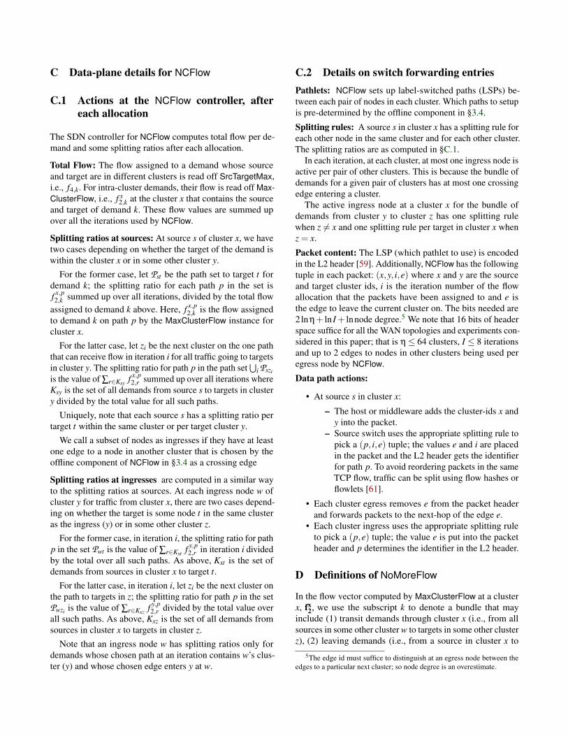
C Data-plane details for NCFlow

C.1 Actions at the NCFlow controller, aftereach allocation

The SDN controller for NCFlow computes total flow per de-mand and some splitting ratios after each allocation.

Total Flow: The flow assigned to a demand whose sourceand target are in different clusters is read off SrcTargetMax,i.e., f4,k. For intra-cluster demands, their flow is read off Max-ClusterFlow, i.e., f x

2,k at the cluster x that contains the sourceand target of demand k. These flow values are summed upover all the iterations used by NCFlow.

Splitting ratios at sources: At source s of cluster x, we havetwo cases depending on whether the target of the demand iswithin the cluster x or in some other cluster y.

For the former case, let Pst be the path set to target t fordemand k; the splitting ratio for each path p in the set isf x,p2,k summed up over all iterations, divided by the total flow

assigned to demand k above. Here, f x,p2,k is the flow assigned

to demand k on path p by the MaxClusterFlow instance forcluster x.

For the latter case, let zi be the next cluster on the one paththat can receive flow in iteration i for all traffic going to targetsin cluster y. The splitting ratio for path p in the path set

⋃i Pszi

is the value of ∑r∈Ksy f x,p2,r summed up over all iterations where

Ksy is the set of all demands from source s to targets in clustery divided by the total value for all such paths.

Uniquely, note that each source s has a splitting ratio pertarget t within the same cluster or per target cluster y.

We call a subset of nodes as ingresses if they have at leastone edge to a node in another cluster that is chosen by theoffline component of NCFlow in §3.4 as a crossing edge

Splitting ratios at ingresses are computed in a similar wayto the splitting ratios at sources. At each ingress node w ofcluster y for traffic from cluster x, there are two cases depend-ing on whether the target is some node t in the same clusteras the ingress (y) or in some other cluster z.

For the former case, in iteration i, the splitting ratio for pathp in the set Pwt is the value of ∑r∈Kxt f y,p

2,r in iteration i dividedby the total over all such paths. As above, Kxt is the set ofdemands from sources in cluster x to target t.

For the latter case, in iteration i, let zi be the next cluster onthe path to targets in z; the splitting ratio for path p in the setPwzi is the value of ∑r∈Kxz f y,p

2,r divided by the total value overall such paths. As above, Kxz is the set of all demands fromsources in cluster x to targets in cluster z.

Note that an ingress node w has splitting ratios only fordemands whose chosen path at an iteration contains w’s clus-ter (y) and whose chosen edge enters y at w.

C.2 Details on switch forwarding entriesPathlets: NCFlow sets up label-switched paths (LSPs) be-tween each pair of nodes in each cluster. Which paths to setupis pre-determined by the offline component in §3.4.

Splitting rules: A source s in cluster x has a splitting rule foreach other node in the same cluster and for each other cluster.The splitting ratios are as computed in §C.1.

In each iteration, at each cluster, at most one ingress node isactive per pair of other clusters. This is because the bundle ofdemands for a given pair of clusters has at most one crossingedge entering a cluster.

The active ingress node at a cluster x for the bundle ofdemands from cluster y to cluster z has one splitting rulewhen z 6= x and one splitting rule per target in cluster x whenz = x.

Packet content: The LSP (which pathlet to use) is encodedin the L2 header [59]. Additionally, NCFlow has the followingtuple in each packet: (x,y, i,e) where x and y are the sourceand target cluster ids, i is the iteration number of the flowallocation that the packets have been assigned to and e isthe edge to leave the current cluster on. The bits needed are2lnη+ ln I + lnnode degree.5 We note that 16 bits of headerspace suffice for all the WAN topologies and experiments con-sidered in this paper; that is η≤ 64 clusters, I ≤ 8 iterationsand up to 2 edges to nodes in other clusters being used peregress node by NCFlow.

Data path actions:

• At source s in cluster x:

– The host or middleware adds the cluster-ids x andy into the packet.

– Source switch uses the appropriate splitting rule topick a (p, i,e) tuple; the values e and i are placedin the packet and the L2 header gets the identifierfor path p. To avoid reordering packets in the sameTCP flow, traffic can be split using flow hashes orflowlets [61].

• Each cluster egress removes e from the packet headerand forwards packets to the next-hop of the edge e.

• Each cluster ingress uses the appropriate splitting ruleto pick a (p,e) tuple; the value e is put into the packetheader and p determines the identifier in the L2 header.

D Definitions of NoMoreFlow

In the flow vector computed by MaxClusterFlow at a clusterx, fx

2, we use the subscript k to denote a bundle that mayinclude (1) transit demands through cluster x (i.e., from allsources in some other cluster w to targets in some other clusterz), (2) leaving demands (i.e., from a source in cluster x to

5The edge id must suffice to distinguish at an egress node between theedges to a particular next cluster; so node degree is an overestimate.

all targets in some other cluster z) or (3) entering demands(i.e., to a target in cluster x from all sources in some othercluster z). Furthermore, we use the subscript yout to denotethe flow allocated for the bundle k on paths to the virtual nodethat corresponds to the cluster y. Thus, f x

2,k,youtis the flow

allocated at cluster x for all demands in the per-cluster bundlek on paths to the virtual node corresponding to a neighboringcluster y.

With this background, Equation 3 ensures that the flowsallocated in MinPathE2E for an inter-cluster bundle K in Daggon all paths in Pagg that contain a cluster edge (x,y) is nomore than the flow that is allocated at either cluster x or clustery for their respective per-cluster bundles that are contained inK to and from each other respectively.

NoMoreAlongPaths(f, f2), ∀K ∈Dagg, ∀x,y ∈ Vagg,x 6= y,

∑p∈Pagg ,(x,y)∈p

f pK ≤min

(∑k∈K

f x2,k,yout , ∑

k′∈Kf y2,k′,xin

)(3)

Equation 4 is logically similar to Equation 3 except thatthe constraints are specific to a cluster x and the constants andvariables have been flipped; that is, here, the flows on the pathsin the aggregate graph are given ( f p

1,K) and the flow on pathswithin the cluster are to be computed by MaxClusterFlow. Inparticular, note that ∑p′∈Px,∗yout

f p′k , f x

2,k,yout; that is, the

flow assigned in MaxClusterFlow of cluster x on all pathsleading to the virtual node corresponding to a neighbor clustery is precisely the value on the right that is used above inEquation 3.

NoMoreFlowThruCluster(f, f1,x), ∀K ∈Dagg, ∀y ∈ Vagg : y 6= x,

∑p∈Pagg:(y,x)∈p

f p1,K ≥ ∑

k∈K, p′∈Px,yin∗f p′k , and

∑p∈Pagg:(x,y)∈p

f p1,K ≥ ∑

k∈K, p′∈Px,∗yout

f p′k (4)

E Fault Model

When failures happen, prior works [19, 49] assume that thesources of the label switched paths (LSPs) will proportionallyshift traffic. That is, a source that splits traffic in the ratio of(0.3,0.5,0.2) between three paths will change to a splittingratio of (0.6,0,0.4) when the middle LSP fails. Doing so cancause congestion on either of the remaining LSPs.

The key idea in prior works [19, 49] is to proactively al-locate flow such that the maximal load on any link remainsunder capacity—FFC [49] protects against up to k simulta-neous link failures, whereas TEAVAR [19] ensures that theflow at risk is below a given fraction (e.g., 99.9% of flow canbe carried by the network on average over all possible failurescenarios).

The cost of such congestion protection is two-fold: (1)proactive schemes substantially increase the solution runtime,and (2) they under-allocate flow, since capacity must be setaside to help with possible failures. Instead, NCFlow usesa reactive strategy, and recomputes a new flow allocationafter the fault occurs. This enables NCFlow to carry moreflow before the fault, and potentially carry more flow afterrecovery. Furthermore, since NCFlow uses fewer FIB entriesfor the same number of paths, it is naturally easier to spreadflow onto more paths with NCFlow. Thus, the key trade-off isslightly longer and more lossy episodes immediately after afault when using NCFlow versus longer solver runtimes andflow under-allocation with proactive schemes [19, 49].

F Benchmarking TEAVAR and TEAVAR*

F.1 Formulation for TEAVAR*

Here, we discuss our adaptation of TEAVAR to maximizetotal multi-commodity flow. The TEAVAR [19] paper consid-ers a different objective – maximizing the concurrent multi-commodity flow (see Table 2). When all demands are satisfi-able, both objectives allocate the same flow; however, whennot enough capacity is available to meet the desired failureassurance, maximizing total flow leads to a strictly largerallocation. We describe TEAVAR* from first principles here.

In addition to the inputs of MaxFlow (see Equation 2),TEAVAR* has the following inputs:

• A value β ∈ [0,1]; larger values of β correspond togreater fault assurance.

• A set of fault scenarios, S ; each scenario i has a proba-bility of occurrence βi and a set of failed edges Ei.

In a fault scenario i, the edges in Ei will fail and so theflow allocated to paths that contain any edge in Ei will belost. The number of possible fault scenarios is exponentialin the number of edges in the network. Thus, to keep theoptimization tractable, we consider only a subset of scenarios.

Let L(i) denote the total flow lost in fault scenario i.Per Proposition 8 in [58], minimizing the potential func-tion, α + 1

1−βE[Li −α]+, would minimize the conditional

value at risk. Here, the expectation is over all possible faultscenarios. Since we only consider a subset of fault sce-narios to keep optimization tractable, we minimize: α +

11−β

(∑i∈S βi[Li−α]++(1−∑i∈S βi)(1−α)) . The last termaccounts for the unconsidered scenarios for which we mustassume the worst possible loss. Note that we can simplify thisexpression by dropping the constant 1−∑i∈S βi

1−β.

TEAVAR*(V ,E ,D,P ,β,S) (5)

,argminf

(α+ 1

1−β(∑i∈S βiExcessi− (1−∑i∈S βi)α)

)s.t. f ∈ FeasibleFlow(V ,E ,D,P ), (Eqn. 1)

Li,k ≥ 0, ∀i,k (loss is non-negative)

Li,k ≥ dk− ∑p∈Pk

f pk Activep,i, ∀i,k (loss)

α≥ 0 (loss cutoff)

Excessi ≥ 0 ∀i (excess loss in scenario i)

Excessi ≥ ∑k∈D

Li,k−α, ∀i (excess loss)

The formulation for TEAVAR* is in Equation 5. Recall thatf pk is the flow assigned to demand k on path p. Activep,i is an

indicator denoting whether path p is active in fault scenarioi. Thus, the allocation for demand k in scenario i will be∑p∈Pk

f pk Activep,i. When the allocation is below the required

volume dk, the demand will suffer loss; we use Li,k to denotethe flow loss for demand k in scenario i.

The flow allocation resulting from the above formulationcannot be promised to the demands; in particular, more flowwill be assigned on some paths to account for possible failureson other paths. After solving the above LP, we compute theflow allocation for a demand k as follows: (1) sort the per-scenario losses Li,k in ascending order; (2) starting at index0, add up the probability of each scenario until the runningsum is at least β—let iβ be the unique crossing index; (3) Setdemand k’s flow to be dk−Liβ,k, the demand minus the lossat the crossing index.

Choosing the fault scenarios to use in TEAVAR*:

• Intuitively, achieving a greater amount of fault assurancerequires considering more fault scenarios. Specifically, ifthe total probability of considered scenarios is below β,the above LP as well as the LP used by TEAVAR becomeunbounded. To see why, the coefficient of α in Eqn. 5is (∑i∈S βi)−β

1−β. If the probability of considered scenarios

is less than β, this coefficient becomes negative, and theobjective value reaches −∞ by setting α to ∞.

• Intuitively, if the total probability of considered scenariosis just larger than β, the flow allocated to demands is verysmall. To see why, the smaller the value of ∑i∈S βi−β,the smaller the positive coefficient of α in the objectiveof Eqn 5. Thus, the solution of Eqn 5 will have a largevalue of α and a very small amount of allocatable flow.

• In light of these two points, in our experiments, wechoose all scenarios that are individually more likelyto occur than a cutoff ρ and multiplicatively reduce ρ un-til the total probability of considered scenarios exceeds1− 1−β

2 .

100 101 102 103

Speedup, relative to PF4 (log scale)

0.0

0.25

0.5

0.75

1.0

Frac

tion

of C

ases

Better

rel. flow 0.990.80 rel. flow < 0.99

0.65 rel. flow < 0.80rel. flow < 0.65

Figure 18: Breaking down the NCFlow results from Figure 11b into fourseparate CDFs based on relative total flow.

F.2 Comments on benchmarking TEAVARObserve that the number of scenarios affects the complexityof the TEAVAR* optimization; specifically, the number ofequations and variables increases by |S | ∗ |P |. The path set isat least as large as the node pairs, i.e., |P |> N2 where N is thenumber of nodes. The appropriate choice of fault scenariosto consider, as discussed above, depends on the size of thetopology, the failure probability of edges, and the requiredassurance level β. Suppose one considers all 2-edge failurescenarios; then |S | ∼ M2 where M is the number of edges.Hence, the increase in equations and variables exceeds N2M2.Note that MaxFlow is substantially simpler, having at mostO(N2) variables and constraints (Equation 1).

On the topologies listed in Table 5, our implementation ofTEAVAR* never ran to completion even after several days. Weran with β = 0.99 and link failure probability set to 0.004;both of these are the default values used in [3]. The reasonis that the optimization problem becomes intractably large.TEAVAR behaves similarly [19]. We conclude that probabilis-tic fault protection using this methodology is infeasible onlarge topologies and for non-trivial fault assurance levels suchas when considering multiple link failures.

We also note that we are unable to simultaneously achievethe solution quality and the runtimes that are reported inTEAVAR [19] using their code [3]. Specifically, achieving theassurance levels reported in their experiments requires manyscenarios to be considered. The runtimes reported in [19]appear to have been measured when considering only singlelink failures.

G Additional Experiments

G.1 Breakdown of NCFlow’s PerformanceTo further understand the performance of NCFlow, Figure 18breaks down the results in Figure 11 into four ranges basedon total relative flow. We plot CDFs of the speedup ratio perrange. The solid blue and green dashed line, which correspondto relative flow above 0.99 and in [0.8,0.99) respectively, ac-count for 49% and 46% of all experiments. The figure showsthat NCFlow achieves sizable speedups while allocating large

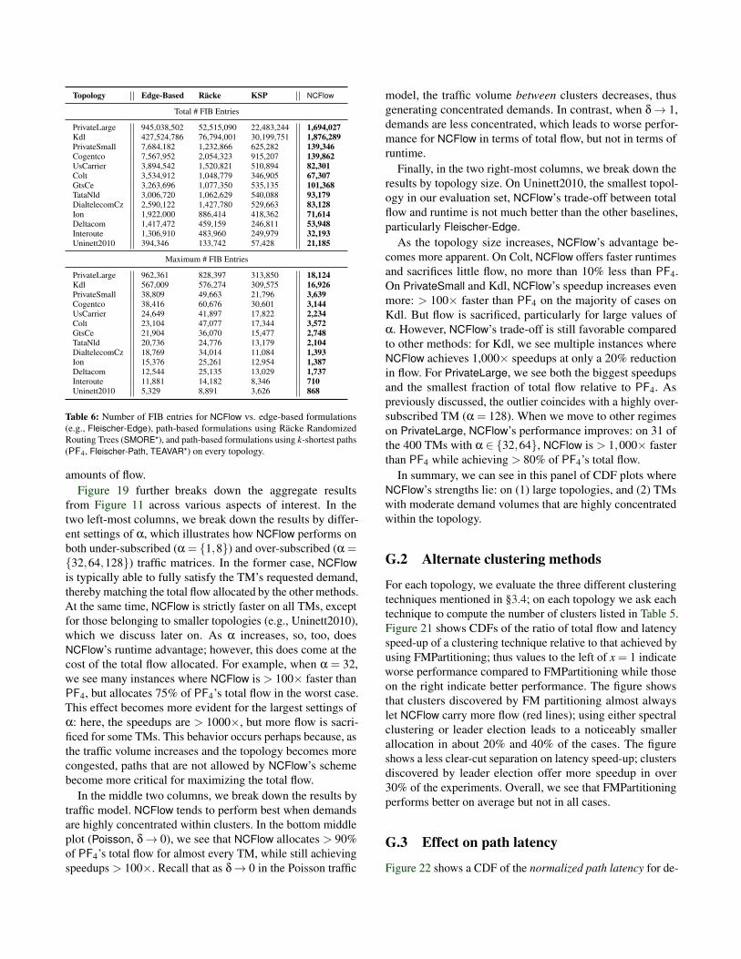
Topology Edge-Based Räcke KSP NCFlow

Total # FIB Entries

PrivateLarge 945,038,502 52,515,090 22,483,244 1,694,027Kdl 427,524,786 76,794,001 30,199,751 1,876,289PrivateSmall 7,684,182 1,232,866 625,282 139,346Cogentco 7,567,952 2,054,323 915,207 139,862UsCarrier 3,894,542 1,520,821 510,894 82,301Colt 3,534,912 1,048,779 346,905 67,307GtsCe 3,263,696 1,077,350 535,135 101,368TataNld 3,006,720 1,062,629 540,088 93,179DialtelecomCz 2,590,122 1,427,780 529,663 83,128Ion 1,922,000 886,414 418,362 71,614Deltacom 1,417,472 459,159 246,811 53,948Interoute 1,306,910 483,960 249,979 32,193Uninett2010 394,346 133,742 57,428 21,185

Maximum # FIB Entries

PrivateLarge 962,361 828,397 313,850 18,124Kdl 567,009 576,274 309,575 16,926PrivateSmall 38,809 49,663 21,796 3,639Cogentco 38,416 60,676 30,601 3,144UsCarrier 24,649 41,897 17,822 2,234Colt 23,104 47,077 17,344 3,572GtsCe 21,904 36,070 15,477 2,748TataNld 20,736 24,776 13,179 2,104DialtelecomCz 18,769 34,014 11,084 1,393Ion 15,376 25,261 12,954 1,387Deltacom 12,544 25,135 13,029 1,737Interoute 11,881 14,182 8,346 710Uninett2010 5,329 8,891 3,626 868

Table 6: Number of FIB entries for NCFlow vs. edge-based formulations(e.g., Fleischer-Edge), path-based formulations using Räcke RandomizedRouting Trees (SMORE*), and path-based formulations using k-shortest paths(PF4, Fleischer-Path, TEAVAR*) on every topology.

amounts of flow.Figure 19 further breaks down the aggregate results

from Figure 11 across various aspects of interest. In thetwo left-most columns, we break down the results by differ-ent settings of α, which illustrates how NCFlow performs onboth under-subscribed (α = {1,8}) and over-subscribed (α ={32,64,128}) traffic matrices. In the former case, NCFlowis typically able to fully satisfy the TM’s requested demand,thereby matching the total flow allocated by the other methods.At the same time, NCFlow is strictly faster on all TMs, exceptfor those belonging to smaller topologies (e.g., Uninett2010),which we discuss later on. As α increases, so, too, doesNCFlow’s runtime advantage; however, this does come at thecost of the total flow allocated. For example, when α = 32,we see many instances where NCFlow is > 100× faster thanPF4, but allocates 75% of PF4’s total flow in the worst case.This effect becomes more evident for the largest settings ofα: here, the speedups are > 1000×, but more flow is sacri-ficed for some TMs. This behavior occurs perhaps because, asthe traffic volume increases and the topology becomes morecongested, paths that are not allowed by NCFlow’s schemebecome more critical for maximizing the total flow.

In the middle two columns, we break down the results bytraffic model. NCFlow tends to perform best when demandsare highly concentrated within clusters. In the bottom middleplot (Poisson, δ→ 0), we see that NCFlow allocates > 90%of PF4’s total flow for almost every TM, while still achievingspeedups > 100×. Recall that as δ→ 0 in the Poisson traffic

model, the traffic volume between clusters decreases, thusgenerating concentrated demands. In contrast, when δ→ 1,demands are less concentrated, which leads to worse perfor-mance for NCFlow in terms of total flow, but not in terms ofruntime.

Finally, in the two right-most columns, we break down theresults by topology size. On Uninett2010, the smallest topol-ogy in our evaluation set, NCFlow’s trade-off between totalflow and runtime is not much better than the other baselines,particularly Fleischer-Edge.

As the topology size increases, NCFlow’s advantage be-comes more apparent. On Colt, NCFlow offers faster runtimesand sacrifices little flow, no more than 10% less than PF4.On PrivateSmall and Kdl, NCFlow’s speedup increases evenmore: > 100× faster than PF4 on the majority of cases onKdl. But flow is sacrificed, particularly for large values ofα. However, NCFlow’s trade-off is still favorable comparedto other methods: for Kdl, we see multiple instances whereNCFlow achieves 1,000× speedups at only a 20% reductionin flow. For PrivateLarge, we see both the biggest speedupsand the smallest fraction of total flow relative to PF4. Aspreviously discussed, the outlier coincides with a highly over-subscribed TM (α = 128). When we move to other regimeson PrivateLarge, NCFlow’s performance improves: on 31 ofthe 400 TMs with α ∈ {32,64}, NCFlow is > 1,000× fasterthan PF4 while achieving > 80% of PF4’s total flow.

In summary, we can see in this panel of CDF plots whereNCFlow’s strengths lie: on (1) large topologies, and (2) TMswith moderate demand volumes that are highly concentratedwithin the topology.

G.2 Alternate clustering methods

For each topology, we evaluate the three different clusteringtechniques mentioned in §3.4; on each topology we ask eachtechnique to compute the number of clusters listed in Table 5.Figure 21 shows CDFs of the ratio of total flow and latencyspeed-up of a clustering technique relative to that achieved byusing FMPartitioning; thus values to the left of x = 1 indicateworse performance compared to FMPartitioning while thoseon the right indicate better performance. The figure showsthat clusters discovered by FM partitioning almost alwayslet NCFlow carry more flow (red lines); using either spectralclustering or leader election leads to a noticeably smallerallocation in about 20% and 40% of the cases. The figureshows a less clear-cut separation on latency speed-up; clustersdiscovered by leader election offer more speedup in over30% of the experiments. Overall, we see that FMPartitioningperforms better on average but not in all cases.

G.3 Effect on path latency

Figure 22 shows a CDF of the normalized path latency for de-

10 1 101 1030.0

0.250.5

0.751.0

Frac

tion

of C

ases

= 1

0.6 0.8 1.0 1.2 10 1 101 103

Gravity

0.6 0.8 1.0 1.2 10 1 101 103

Uninett2010

0.6 0.8 1.0 1.2

10 1 101 1030.0

0.250.5

0.751.0

Frac

tion

of C

ases

= 8

0.6 0.8 1.0 1.2 10 1 101 103

Bimodal

0.6 0.8 1.0 1.2 10 1 101 103

Colt

0.6 0.8 1.0 1.2

10 1 101 1030.0

0.250.5

0.751.0

Frac

tion

of C

ases

= 32

0.6 0.8 1.0 1.2 10 1 101 103

Uniform

0.6 0.8 1.0 1.2 10 1 101 103

PrivateSmall

0.6 0.8 1.0 1.2

10 1 101 1030.0

0.250.5

0.751.0

Frac

tion

of C

ases

= 64

0.6 0.8 1.0 1.2 10 1 101 103

Poisson, 1

0.6 0.8 1.0 1.2 10 1 101 103

Kdl

0.6 0.8 1.0 1.2

10 1 101 103

Speedup, rel. to PF4

0.00.250.5

0.751.0

Frac

tion

of C

ases

= 128

0.6 0.8 1.0 1.2Total Flow, rel. to PF4

10 1 101 103

Speedup, rel. to PF4

Poisson, 0

0.6 0.8 1.0 1.2Total Flow, rel. to PF4

10 1 101 103

Speedup, rel. to PF4

PrivateLarge

0.6 0.8 1.0 1.2Total Flow, rel. to PF4

NCFlow SMORE* Fleischer-Path, = 0.5 Fleischer-Edge, = 0.5

Figure 19: A breakdown of the experimental results from Figure 11 along various dimensions of interest: scale factor, traffic model, and topology size. NCFlowexcels on large topologies with TMs that have highly concentrated demands.

0 5 10 15 20TM Number

01234

Norm

alize

dRe

ques

ted

Dem

and

Figure 20: Traffic demand for each traffic matrix used in the demand trackingexperiment (see Figure 15) on PrivateLarge. The exact values are not shownfor confidentiality reasons.

mands6 under different flow allocations. The figure on the topshows CDFs of the actual normalized path latency. Observethat these distributions are nearly identical. The figure on thebottom shows a CDF of the ratio of normalized latency; we

6The latency of the paths along which each demand is routed weightedby the fraction of the demand routed along each path. That is, if a demandis divided equally between two paths, the normalized latency will be theaverage of the path latencies.

0

0.2

0.4

0.6

0.8

1

0.2 0.3 0.4 1 2

Fract

ion o

f C

ase

s

Ratio of Metric vs FM Partitioning (log scale)

latency speedup: spectral clust.latency speedup: leader electiontotal flow: leader electiontotal flow: spectral clust.

Figure 21: Comparing the total flow allocated and the speedup in computingallocations when clusters are chosen using the three techniques mentionedin §3.4–FM partitioning, spectral clustering and leader election. The defaulttechnique used in our evaluation, FM partitioning, generally performs betterbut not in all cases.

see that roughly 70% of the demands are carried by NCFlowon paths that are at most as long as the paths used by PF4 (i.e.,to the left of x=1). Most of the cases where NCFlow uses

0 0.2 0.4 0.6 0.8

1

0.1 1 10

Fract

ion o

f D

em

ands

Ratio of Path Latency when using NCFlow vs. using PF4

0 0.2 0.4 0.6 0.8

1

0.1 1 10 100Path Latency (ms)

NCFlowPF4

Figure 22: Effect of NCFlow on path latency

0.5 0.6 0.7 0.8 0.9 1.0 1.1 1.2Total Flow, relative to PF4nd

0.0

0.25

0.5

0.75

1.0

Frac

tion

of C

ases

Better

NCFlowSMORE*

Fleischer-Path, = 0.5Fleischer-Edge, = 0.5

(a) CDF of total flow relative to PF4nd

10 1 100 101 102

Speedup, relative to PF4nd (log scale)

0.0

0.25

0.5

0.75

1.0

Frac

tion

of C

ases

Better

(b) CDF of speedup relative to PF4nd

Figure 23: Similarly to Figure 11 all schemes use up to k = 4 shortestpaths between each pair of nodes except that the paths are chosen withoutensuring edge disjointness. The figure shows no qualitative difference relativeto Figure 11.

relatively longer paths are for demands that have very smalllatency paths as illustrated by the top figure.

Note that path latency can be further explicitly controlledin NCFlow by determining which paths can be used or byweighting the objective to prefer shorter paths in the varioussteps of Figure 6.

G.4 Alternate path choices

With Figure 23, Figure 24, Figure 25, Figure 26, Figure 27we evaluate different numbers of paths between node pairschosen with or without edge disjointness. PFk refers to pathformulation with k shortest paths chosen using edge disjoint-ness and PFknd indicates paths chosen without edge disjoint-ness. Comparing these figures with Figure 11, we note thatNCFlow’s improvements over baselines hold across differentpath choices.

Note that Figure 26 and Figure 27 are missing some of thelarger topologies listed in Table 5 for some of the baseline

0.5 0.6 0.7 0.8 0.9 1.0 1.1 1.2Total Flow, relative to PF8

0.0

0.25

0.5

0.75

1.0

Frac

tion

of C

ases

Better

NCFlowSMORE*

Fleischer-Path, = 0.5Fleischer-Edge, = 0.5

(a) CDF of total flow relative to PF8

10 1 100 101 102 103

Speedup, relative to PF8 (log scale)

0.0

0.25

0.5

0.75

1.0

Frac

tion

of C

ases

Better

(b) CDF of speedup relative to PF8

Figure 24: Similar to Figure 11 except all schemes use up to k = 8 shortestpaths between each pair of nodes; paths chosen with edge disjointness. Thefigure shows no qualitative difference relative to Figure 11.

0.5 0.6 0.7 0.8 0.9 1.0 1.1 1.2Total Flow, relative to PF8nd

0.0

0.25

0.5

0.75

1.0

Frac

tion

of C

ases

Better

NCFlowSMORE*

Fleischer-Path, = 0.5Fleischer-Edge, = 0.5

(a) CDF of total flow relative to PF8nd

10 1 100 101 102

Speedup, relative to PF8nd (log scale)

0.0

0.25

0.5

0.75

1.0

Frac

tion

of C

ases

Better

(b) CDF of speedup relative to PF8nd

Figure 25: Similar to Figure 11 except all schemes use up to k = 8 short-est paths between each pair of nodes; paths chosen without ensuring edgedisjointness. The figure shows no qualitative difference relative to Figure 11.

schemes because the baselines ran out of memory (we useda server with up to 3TB of memory) or raised some otherexception.

H Illustrative examples

Here, we show some illustrative examples where applyingNCFlow using adversarially chosen clusters can lead to sub-optimal flow allocation.

Figure 28 shows a case wherein NCFlow is sub-optimalbecause the aggregate graph (wherein nodes are clusters) is

0.5 0.6 0.7 0.8 0.9 1.0 1.1 1.2Total Flow, relative to PF16nd

0.0

0.25

0.5

0.75

1.0

Frac

tion

of C

ases

Better

NCFlowSMORE*

Fleischer-Path, = 0.5Fleischer-Edge, = 0.5

(a) CDF of total flow relative to PF16nd

10 1 100 101 102 103

Speedup, relative to PF16nd (log scale)

0.0

0.25

0.5

0.75

1.0

Frac

tion

of C

ases

Better

(b) CDF of speedup relative to PF16nd

Figure 26: Similar to Figure 11 except all schemes use up to k = 16 short-est paths between each pair of nodes; paths chosen without ensuring edgedisjointness. The figure shows no qualitative difference relative to Figure 11.

0.5 0.6 0.7 0.8 0.9 1.0 1.1 1.2Total Flow, relative to PF16

0.0

0.25

0.5

0.75

1.0

Frac

tion

of C

ases

Better

NCFlowSMORE*

Fleischer-Path, = 0.5Fleischer-Edge, = 0.5

(a) CDF of total flow relative to PF16

10 2 10 1 100 101 102 103

Speedup, relative to PF16 (log scale)

0.0

0.25

0.5

0.75

1.0

Frac

tion

of C

ases

Better

(b) CDF of speedup relative to PF16

Figure 27: Similar to Figure 11 except all schemes use up to k = 16 shortestpaths between each pair of nodes; paths chosen with ensuring edge disjoint-ness. The figure shows no qualitative difference relative to Figure 11.

0.5

0.5

0.33

0.67

0.17

Flow in Iter 10.830.67

Flow in Iter 20.170

Iteration 1 Iteration 2

Demand Volume Optimal flow 1.0 1.0

1.0 1.0

Figure 28: Sub-optimality of NCFlow when the aggregate graph is not a tree.

1

0.5

0.5

NCFlow0.50.50.5

Demand Volume Optimal flow 1.0 0

1.0 1.0

1.0 1.0 0.5

0.5

Figure 29: Sub-optimality of NCFlow when demands cannot be fully satis-fied.

Demand Volume Optimal flow 1.0 1.0

1

Figure 30: Sub-optimality of NCFlow when there are multiple-edges betweenpairs of clusters.

(a) For the suboptimality problem in Figure 28, a different clustering choice that leadsto optimal flow allocation with NCFlow.

(b) For the suboptimality problem in Figure 29, a different clustering choice that leadsto optimal flow allocation with NCFlow.

(c) For the suboptimality problem in Figure 30, a different clustering choice that leadsto optimal flow allocation with NCFlow.

5

5

(d) For the disagreement problem in Figure 8a, a different clustering choice that doesnot lead to such a disagreement.

(e) For the disagreement problem in Figure 6, a different clustering choice that doesnot lead to such a disagreement.

Figure 31: Alternate clustering choices that fix suboptimality concerns anddisagreements.

not a tree. The network topology and optimal allocations areshown in the graph on the left; assume each link has a unitcapacity. With NCFlow, as shown in the figures on the right,MaxAggFlow can route the flow from s1 to t1 on either the topor the bottom path or divide between the two paths in someproportion; note that MaxAggFlow is not aware of demands

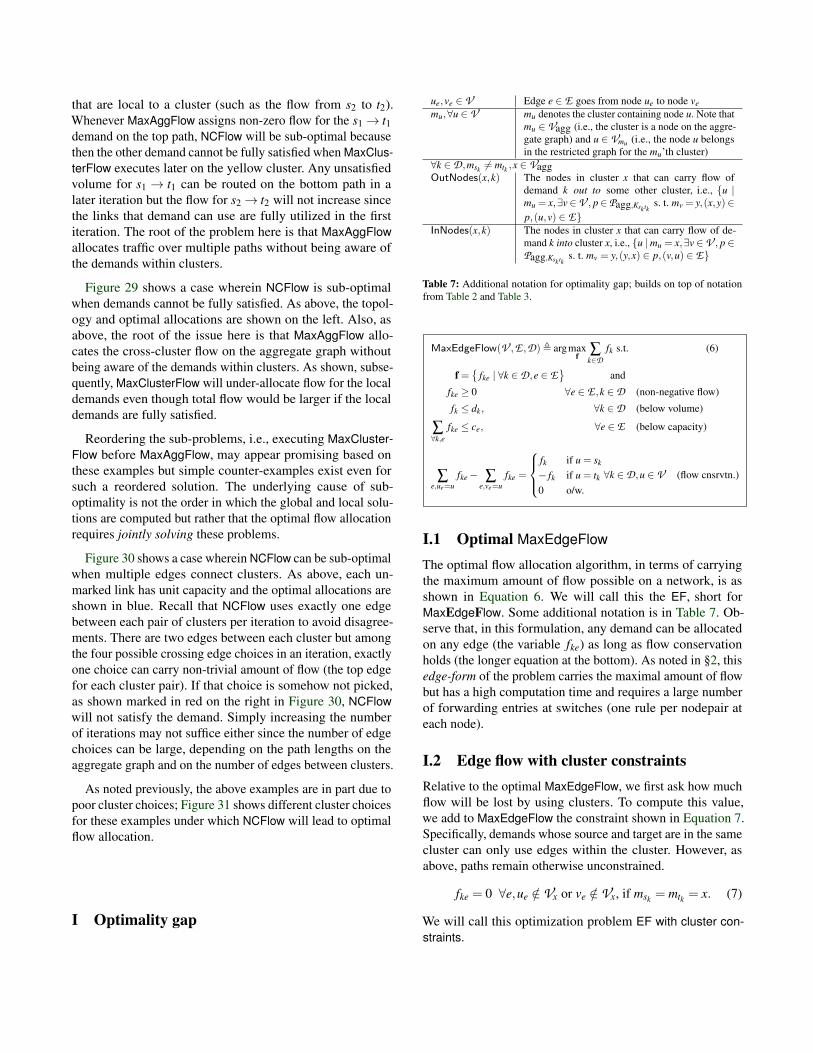
that are local to a cluster (such as the flow from s2 to t2).Whenever MaxAggFlow assigns non-zero flow for the s1→ t1demand on the top path, NCFlow will be sub-optimal becausethen the other demand cannot be fully satisfied when MaxClus-terFlow executes later on the yellow cluster. Any unsatisfiedvolume for s1 → t1 can be routed on the bottom path in alater iteration but the flow for s2→ t2 will not increase sincethe links that demand can use are fully utilized in the firstiteration. The root of the problem here is that MaxAggFlowallocates traffic over multiple paths without being aware ofthe demands within clusters.

Figure 29 shows a case wherein NCFlow is sub-optimalwhen demands cannot be fully satisfied. As above, the topol-ogy and optimal allocations are shown on the left. Also, asabove, the root of the issue here is that MaxAggFlow allo-cates the cross-cluster flow on the aggregate graph withoutbeing aware of the demands within clusters. As shown, subse-quently, MaxClusterFlow will under-allocate flow for the localdemands even though total flow would be larger if the localdemands are fully satisfied.

Reordering the sub-problems, i.e., executing MaxCluster-Flow before MaxAggFlow, may appear promising based onthese examples but simple counter-examples exist even forsuch a reordered solution. The underlying cause of sub-optimality is not the order in which the global and local solu-tions are computed but rather that the optimal flow allocationrequires jointly solving these problems.

Figure 30 shows a case wherein NCFlow can be sub-optimalwhen multiple edges connect clusters. As above, each un-marked link has unit capacity and the optimal allocations areshown in blue. Recall that NCFlow uses exactly one edgebetween each pair of clusters per iteration to avoid disagree-ments. There are two edges between each cluster but amongthe four possible crossing edge choices in an iteration, exactlyone choice can carry non-trivial amount of flow (the top edgefor each cluster pair). If that choice is somehow not picked,as shown marked in red on the right in Figure 30, NCFlowwill not satisfy the demand. Simply increasing the numberof iterations may not suffice either since the number of edgechoices can be large, depending on the path lengths on theaggregate graph and on the number of edges between clusters.

As noted previously, the above examples are in part due topoor cluster choices; Figure 31 shows different cluster choicesfor these examples under which NCFlow will lead to optimalflow allocation.

I Optimality gap

ue,ve ∈ V Edge e ∈ E goes from node ue to node vemu,∀u ∈ V mu denotes the cluster containing node u. Note that

mu ∈ Vagg (i.e., the cluster is a node on the aggre-gate graph) and u ∈ Vmu (i.e., the node u belongsin the restricted graph for the mu’th cluster)

∀k ∈D,msk 6= mtk ,x ∈ VaggOutNodes(x,k) The nodes in cluster x that can carry flow of

demand k out to some other cluster, i.e., {u |mu = x,∃v∈V , p∈Pagg,Ksktk

s. t. mv = y,(x,y)∈p,(u,v) ∈ E}

InNodes(x,k) The nodes in cluster x that can carry flow of de-mand k into cluster x, i.e., {u |mu = x,∃v∈V , p∈Pagg,Ksktk

s. t. mv = y,(y,x) ∈ p,(v,u) ∈ E}

Table 7: Additional notation for optimality gap; builds on top of notationfrom Table 2 and Table 3.

MaxEdgeFlow(V ,E ,D), argmaxf ∑

k∈Dfk s.t. (6)

f ={

fke | ∀k ∈D,e ∈ E}

and

fke ≥ 0 ∀e ∈ E ,k ∈D (non-negative flow)

fk ≤ dk, ∀k ∈D (below volume)

∑∀k,e

fke ≤ ce, ∀e ∈ E (below capacity)

∑e,ue=u

fke− ∑e,ve=u

fke =

fk if u = sk

− fk if u = tk0 o/w.

∀k ∈D,u ∈ V (flow cnsrvtn.)

I.1 Optimal MaxEdgeFlow

The optimal flow allocation algorithm, in terms of carryingthe maximum amount of flow possible on a network, is asshown in Equation 6. We will call this the EF, short forMaxEdgeFlow. Some additional notation is in Table 7. Ob-serve that, in this formulation, any demand can be allocatedon any edge (the variable fke) as long as flow conservationholds (the longer equation at the bottom). As noted in §2, thisedge-form of the problem carries the maximal amount of flowbut has a high computation time and requires a large numberof forwarding entries at switches (one rule per nodepair ateach node).

I.2 Edge flow with cluster constraintsRelative to the optimal MaxEdgeFlow, we first ask how muchflow will be lost by using clusters. To compute this value,we add to MaxEdgeFlow the constraint shown in Equation 7.Specifically, demands whose source and target are in the samecluster can only use edges within the cluster. However, asabove, paths remain otherwise unconstrained.

fke = 0 ∀e,ue /∈ Vx or ve /∈ Vx, if msk = mtk = x. (7)

We will call this optimization problem EF with cluster con-straints.

0

0.2

0.4

0.6

0.8

1

0.8 0.9 1 1.1

Fract

ion o

f C

ase

s

Total flow, relative to PF4 (log scale)

0 0.2 0.4 0.6 0.8

1

10-4 10-3 10-2 10-1 1 10 102

Speedup, relative to PF4 (log scale)

NCFlowPF + cluster and path constr.

EF + cluster constr.EF

Figure 32: Comparing flow allocated by NCFlow with the best possible flows

I.3 Path form with cluster and path con-straints

Next, we ask how much flow will be lost when using theclusters as well as the given set of paths within and betweenclusters? Computing this value is somewhat more complexbecause we have to stitch together the flow carried on pathswithin each cluster with the flow on the edges between clusterswhile also ensuring that flow follow the chosen paths on theaggregate graph (where clusters are nodes). For reference, wewrite this out in Equation 8.

In more detail, this optimization problem, as shown in Equa-tion 8, has three classes of decision variables – f p

K , f pk , fke –

which respectively are the flow allocated to a bundled demandon a path on the aggregate graph, the flow allocated to a de-mand on a path within a cluster and the flow allocated to ademand on a crossing edge between clusters.

Equation 9 computes the net flow for each demand k whichfor the case of a demand whose source and target are in thesame cluster is the sum of flow carried on all intra-clusterpaths. For demands whose source and target are in differentclusters, the net flow is the flow from the demand’s sourceto all of the nodes in the source’s cluster that connect withother clusters as well as the flow to the demand’s target fromall of the nodes in the target’s cluster that connect with otherclusters.

For flow conservation, consider Equation 11 which ensuresthat all of the flow leaving at a node u for a demand k oncrossing edges to other clusters equals the flow that comesinto the node u either from the source of the demand (if thesource is within its cluster) or from all of the nodes in u’scluster that can receive flow for demand k from other clusters–

InNodes(mu,k). Equation 12 considers the converse case fordemands that leave at a node. Finally, Equation 13 relatesthe total flow between a pair of clusters x,y on the crossingedges between these clusters with the flow along paths on theaggregate graph that contain the edge (x,y). We will call thisoptimization problem PF with cluster and path constraints.

Note that the above constraints naturally lead to a reductionin forwarding table size as discussed in §3.5. However, it is notclear how much less flow these constraints allow for relativeto the optimal EF. Moreover, since this optimization has morevariables (and constraints) than PF4 (see Equation 2), it cantake longer to compute and may not be practically useful. Weuse this optimization problem to discern how much flow islost by the constraints used in NCFlow (restricting to clustersand paths) relative to the flow that is lost due to the heuristicallocation process described in §3.

I.4 Experimental results

Our results are in Figure 32; the baseline is PF4 and the fig-ures plot CDFs of total flow and latency speedup for manytopologies and traffic demands. Note that using the edge for-mulation (purple dash-dots) often leads to substantially moreflow being allocated compared to PF4; however, as the fig-ure on the top shows, edge formulation is a more complexproblem that takes longer to run (over 1000× longer).

Adding the clustering constraint to edge formulation hasan un-noticeable effect on the flow allocation (green dashes).Note that we use clusters computed using FMPartitioning forall topologies.

Constraining the path formulation using both the givenclusters and the given paths (between clusters and within eachcluster), as shown with the red dash line, allocates much moreflow than PF4 and not much less than is allocated in edgeformulation. Thus, empirically, constraining flow allocation totraverse the chosen clusters and paths does not limit the flowthat can be allocated. The figure also shows that computingthe optimal flow given clusters and paths takes longer thanPF4 (roughly 10× – 100× longer). Thus, NCFlow offers aheuristic which finishes substantially faster than PF4.

To sum up, our two main contributions are: (1) constrainingflow allocations to use specific clusters and paths which re-duces the number of forwarding table entries needed withoutaffecting the flow that can be allocated and (2) a heuristicthat computes flow allocations quickly given this constraintbut can under-allocate flow. We believe that future work canimprove the heuristic to reduce the flow loss further.

MaxClusterPathFlow(V ,E ,D,P ), argmaxf ∑

k∈Dfk s.t. (8)

f ={

f pK | ∀K ∈Dagg, p ∈ Pagg, (flow on inter-cluster paths)

f pk | ∀k ∈D, p ∈ P , (flow on intra-cluster paths)

fke | ∀k ∈D,e ∈ E ,mue 6= mve (flow on edges between clusters)}

and

fk =

∑p∈Psk ,tk

f pk if msk = mtk (flow within a cluster)

∑t∈OutNodes(msk ,k)

∑p∈Psk ,t

f pk if msk 6= mtk (flow from source to outnodes)

∑s∈InNodes(mtk ,k)

∑p∈Ps,tk

f pk if msk 6= mtk (flow to target from innodes)

∀k ∈D(net flow) (9)

fk ≤ dk(flow below volume) ∀k ∈D

ce ≥

∑

k∈D∑

p∈P , p3ef pk if mue = mve (intra-cluster edges; note: k goes over all demands)

∑k∈D

fke otherwise (inter-cluster edges)∀e ∈ E , (10)

∑e∈E |ue=u, mue 6=mve

fke =

∑

p∈Psku

f pk if mu = msk (at cluster mu, flow from sk to u)

∑v∈InNodes(mu ,k)

∑p∈Pv,u

f pk otherwise (at cluster mu, flow from all InNodes to u)

∀u ∈ V ,k ∈D (11)

∑e∈E |ve=u, mue 6=mve

fke =

∑

p∈Pu,tk

f pk if mu = mtk (at cluster mu, flow from u to tk)

∑v∈OutNodes(mu,k)

∑p∈Pu,v

f pk otherwise (at cluster mu, flow from u to all OutNodes)

∀u ∈ V ,k ∈D (12)

∑p∈Pagg|(x,y)∈p

f pK = ∑

e|mue=x, mve=y, k∈Kfke ∀K ∈Dagg, x, y ∈ Vagg (flow b/w clusters = flow on inter-cluster path) (13)