How to Solve Physics Problems

HOW TO SOLVE

PHYSICS PROBLEMS

00_Oman_FM_i-xiv.indd 1 06/11/15 5:24 PM

This page intentionally left blank

New York Chicago San Francisco Athens London MadridMexico City Milan New Delhi Singapore Sydney Toronto

HOW TO SOLVE

PHYSICS PROBLEMS

SECOND EDITION

Daniel Milton Oman, PhDRobert Milton Oman, PhD


Copyright © 2016, 1997 by McGraw-Hill Education. All rights reserved. Except as permitted under the United States Copyright Act of 1976, no part of this publication may be reproduced or distributed in any form or by any means, or stored in a database or retrieval system, without the prior written permission of the publisher, with the exception that the program listings may be entered, stored, and executed in a computer system, but they may not be reproduced for publication.

ISBN: 978-0-07-184932-6

MHID: 0-07-184932-7

The material in this eBook also appears in the print version of this title: ISBN: 978-0-07-184931-9,MHID: 0-07-184931-9.

eBook conversion by codeMantraVersion 1.0

All trademarks are trademarks of their respective owners. Rather than put a trademark symbol after every occurrence of a trademarked name, we use names in an editorial fashion only, and to the benefit of the trademark owner, with no intention of infringement of the trademark. Where such designations appear in this book, they have been printed with initial caps.

McGraw-Hill Education eBooks are available at special quantity discounts to use as premiums and sales promotions or for use in corporate training programs. To contact a representative, please visit the Contact Us page at www.mhprofessional.com.

TERMS OF USE

This is a copyrighted work and McGraw-Hill Education and its licensors reserve all rights in and to the work. Use of this work is subject to these terms. Except as permitted under the Copyright Act of 1976 and the right to store and retrieve one copy of the work, you may not decompile, disassemble, reverse engineer, reproduce, modify, create derivative works based upon, transmit, distribute, disseminate, sell, publish or sublicense the work or any part of it without McGraw-Hill Education’s prior consent. You may use the work for your own noncommercial and personal use; any other use of the work is strictly prohibited. Your right to use the work may be terminated if you fail to comply with these terms.

THE WORK IS PROVIDED “AS IS.” McGRAW-HILL EDUCATION AND ITS LICENSORS MAKE NO GUARANTEES OR WARRANTIES AS TO THE ACCURACY, ADEQUACY OR COMPLETENESS OF OR RESULTS TO BE OBTAINED FROM USING THE WORK, INCLUDING ANY INFORMATION THAT CAN BE ACCESSED THROUGH THE WORK VIA HYPERLINK OR OTHERWISE, AND EXPRESSLY DISCLAIM ANY WARRANTY, EXPRESS OR IMPLIED, INCLUDING BUT NOT LIMITED TO IMPLIED WARRANTIES OF MERCHANTABILITY OR FITNESS FOR A PARTICULAR PURPOSE. McGraw-Hill Education and its licensors do not warrant or guarantee that the functions contained in the work will meet your requirements or that its operation will be uninterrupted or error free. Neither McGraw-Hill Education nor its licensors shall be liable to you or anyone else for any inaccuracy, error or omission, regardless of cause, in the work or for any damages resulting therefrom. McGraw-Hill Education has no responsibility for the content of any information accessed through the work. Under no circumstances shall McGraw-Hill Education and/or its licensors be liable for any indirect, incidental, special, punitive, consequential or similar damages that result from the use of or inability to use the work, even if any of them has been advised of the possibility of such damages. This limitation of liability shall apply to any claim or cause whatsoever whether such claim or cause arises in contract, tort or otherwise.

http://www.mhprofessional.com

ABOUT THE AUTHORSDaniel Milton Oman earned the B.S. degree in physics from Eckerd College. He received an M.S. in physics and a Ph.D. in electrical engineering from the University of South Florida. He has done research on carbon dioxide lasers and solar cells. He worked with AT&T Bell Laboratories and spinoff companies in the manufacture of microelec-tronics and currently runs his own education company offering online physics tutorials at www.physicsandcalculus.com.

Robert Milton Oman received the B.S. degree from Northeastern University and the Sc.M. and Ph.D. degrees from Brown University, all in physics. He taught mathematics and physics at many colleges and universities, including the University of Minnesota, Northeastern University, and the University of South Florida. He conducted research for NASA, where he developed the theoretical model for the first pressure gauge sent to the moon.


http://www.physicsandcalculus.com

CONTENTSPreface / xiii

How to Use This Book / 1How to Excel in Your Physics Course / 3 General Approach for Studying Physics / 3 How to Prepare for a Physics Test / 4 Timing and the Use of the Subconscious / 5

Strategies to Use During a Physics Test / 6 Your Self Image as a Student / 7Mathematic al Background / 9 Solving Equations / 9 Determinants / 11 Binomial Expansions / 13 Coordinate Systems / 13 Trigonometry / 15 Functions / 17 Logarithms and Exponents / 18 Derivatives / 19 Integrals / 21 Average Value of a Function / 23Chapter 1 Vec tors / 25 Number Plus Angle and Components / 25 Unit Vectors in Two Dimensions / 26 Scalar or Dot Product / 29 Vector or Cross Product / 30Chapter 2 Kinematics in One Dimension / 33 Instantaneous Velocity and Acceleration / 34 Kinematic Equations of Motion / 35Chapter 3 Falling-Body Problems / 41Chapter 4 Projec tile Motion / 51Chapter 5 Forces (Including Centripetal Force) / 59 Friction / 62 Circular Motion / 68Chapter 6 Apparent Weight / 75Chapter 7 Work and the Definite Integral / 79Chapter 8 Work-Energy Problems / 85 Kinetic Energy / 85 Gravitational Potential Energy / 86 Frictional Forces / 87Chapter 9 Center of Mass and Momentum / 95

vii


viii CONTENTS

Chapter 10 Collision and Impulse / 103 Inelastic Collisions / 103 Elastic Collisions / 106 Impulse / 108Chapter 11 Rotational Motion / 111 Applications / 114Chapter 12 Rotational D ynamics / 119 Conservation of Angular Momentum / 122 Applications / 123Chapter 13 Equilibrium / 129Chapter 14 Gravity / 139 Gravitational Potential / 139 Satellites / 141 Kepler’s Laws / 142Chapter 15 Simple Harmonic Motion / 145 Energy Analysis / 150 Applications / 153 Damped Mass-Spring System / 155Chapter 16 Fluids / 157 Pressure / 157 Barometer and Manometer / 159 Buoyancy / 160 Fluid Flow / 162 Venturi Tube / 164Chapter 17 Temperature and Calorimetr y / 167 Calorimetry / 171 Phase Change / 172 Heat Flow / 173Chapter 18 Kinetics and the Ideal Gas Laws / 177 Variation of Pressure with Elevation / 178 pV Diagrams / 180 Kinetic Theory / 180 Heat Capacity of Gases / 183Chapter 19 First Law of Thermodynamics / 185 Work during Volume Change / 185 Internal Energy and the First Law / 186 Heat Capacities of Ideal Gases / 188 Adiabatic Processes / 190Chapter 20 Second Law of Thermodynamics / 195 Heat Engines / 195 Carnot Cycle / 196 Refrigerators and Heat Pumps / 198 Entropy / 200Chapter 21 Mechanic al Waves / 201 Transverse Waves on a String / 201 Wave Equation / 203


CONTENTS ix

Transverse Wave Speed / 204 Power / 205Chapter 22 Standing Waves (Strings and Pipes) / 207 Waves on Strings / 207 Waves in Pipes / 209Chapter 23 Sound / 213 Intensity and the Inverse Square Law / 214 The Decibel / 215 The Doppler Effect / 217Chapter 24 Charge and Coulomb’s Law / 221Chapter 25 The Elec tric Field / 225 Discrete Charges / 225 Linear Charge / 228 Surface Charge / 229 Applications / 230 Dipoles / 231Chapter 26 Gauss ’ Law / 233Chapter 27 Elec tric Potential / 239Chapter 28 Capacitance / 249 Capacitors as Lumped Circuit Elements / 252 Energy Storage / 255 Capacitors and Dielectrics / 256Chapter 29 Current and Resistance / 259 Current / 259 Resistance / 261 Power / 263 Temperature Dependence of Resistivity / 264 Batteries and emf / 264Chapter 30 Resistors in DC Circuits / 267 Series Resistors / 267 Parallel Resistors / 267 Series-Parallel Combinations / 268Chapter 31 Kirchhoff ’s Laws / 271 Kirchhoff Voltage Loop Equations / 271 Kirchhoff Current Junction Equations / 272 Solving by Adding and Subtracting / 273 Solving by Determinants / 273 Solving by Augmented Matrix / 274 Applications / 276Chapter 32 RC C ircuits / 279 Charging / 279 The Time Constant / 281 Discharging / 282Chapter 33 Magnetic Fields / 285 The Cyclotron / 287 The Mass Spectrometer / 290


x CONTENTS

The J. J. Thomson Experiment / 291 The Hall Effect / 292Chapter 34 Magnetic Forces / 295 A Current-Carrying Loop in a B Field / 296 d’Arsonval Meter Movement / 298 Energy Storage in Magnetic Materials / 299Chapter 35 Ampere’s Law / 301 The Force on Current Carrying Wires / 302 Concentric Currents / 304 Average Field Outside a Wire / 305 The Solenoid / 306 The Toroid / 307Chapter 36 Biot-S avar t Law / 309Chapter 37 Faraday ’s Law / 313 Lenz’s Law / 315 Time Varying Magnetic Fields / 320Chapter 38 Induc tance / 321 Self Inductance / 321 Mutual Inductance / 322 Power and Energy Storage / 323Chapter 39 RL C ircuits / 325 Decreasing Current / 328 Energy Storage / 329Chapter 40 Oscillating LC C ircuits / 331 LC Circuits / 331 RLC Circuits / 333Chapter 41 Series RLC C ircuits and Phasors / 335 Alternating Currents / 335 The Resistive Circuit / 335 The Capacitive Circuit / 336 The Inductive Circuit / 337 The RLC Circuit / 340 Power in AC Circuits / 343 Transformers / 344Chapter 42 Max well ’s Equations / 345 Four Basic Laws of Electromagnetism / 345 The Displacement Current / 346Chapter 43 Elec tromagnetic Waves / 349 Generating Waves / 349 The Speed of the Waves / 350 Energy Transport in Electromagnetic Waves / 352 The Poynting Vector / 353 Radiation Pressure / 355


CONTENTS xi

Chapter 44 Reflec tion, Refrac tion, and Polarization / 357 Reflection and Refraction / 357 Polarization / 360Chapter 45 Mirrors and Lenses / 363 Sign Conventions for Mirrors / 363 Sign Conventions for Lenses / 363 Mirrors / 363 Lenses / 366Chapter 46 Diffrac tion and Inter ference / 369 Double Slit Diffraction / 369 Single Slit Diffraction / 370 The Diffraction Grating / 371Chapter 47 Special Relativity / 373 The Laws of Physics Are the Same in All Inertial Reference Frames / 373 The Speed of Light Is the Same in All Inertial Frames / 373 Time Dilation / 373 Length Contraction / 375 Relativistic Momentum / 376Chapter 48 Q uantum Physics / 379 The Photoelectric Effect / 379 Stopping Potential / 381 de Broglie Relation / 383 Heisenberg Uncertainty Principle / 384 Compton Scattering / 385 Schrodinger Equation / 386Chapter 49 Atoms, Molecules, and Solids / 389 The Hydrogen Atom / 389 Lasers / 391 Semiconductors / 394Chapter 50 Nuclear Physics / 397 Alpha, Beta, and Gamma Radiation / 397 Einstein’s Mass-Energy Relationship / 398 Fission and Fusion / 400 Radioactive Decay / 401Appendix A Physic al Constants / 405Appendix B Conversions / 407Appendix C Periodic Table of the Elements / 409


PREFACEThe purpose of this book is to help you to develop a highly effective set of problem-solving skills that will allow you to excel in your physics class. Here are some of the elements of this book that we believe will make it highly valuable:

1. This book is more than just a collection of problems. It introduces theory along the way but places the theory immediately in the context of problems. This approach teaches you how to apply concepts to solving problems.

2. We take the time to explain the solutions to the problems thoroughly. We point out important problem-solving strategies that are useful for solving large groups of similar problems.

3. This book has gone through extensive development over the years to present the problem-solving techniques in the clearest manner. The book was started in 1980 by Robert Oman and presented to his physics students to help them understand concepts and give them practice and confidence in working problems. After publication of the first edition in 1997, the book was used over a period of 10 years by many students in more of Robert’s university physics classes as a supplement to the text. Daniel Oman tutored university students from 2011 to 2015 and integrated new types of questions that he was seeing into the existing book, creating a second edition.

The second edition of this book includes three new chapters—Quantum Physics; Atoms, Molecules, and Solids; and Nuclear Physics. This edition also includes some edits and additional problems based on feedback from students over the years.

It is the sincere desire of the authors that this book help you to better understand physics concepts and work the associated problems. We thank the many students who have contributed to this work by using the material and offering suggestions. Also, we thank the fine staff at McGraw-Hill Education that has contributed greatly to the clarity of the presentation.

xiii


HOW TO USE THIS BOOK

1

This book will teach you how to do physics problems. The explanation of not only how to do a problem but also why we do it a certain way teaches you not just a collection of solved problems, but a collection of methods that can be used, modified, and built upon to do other physics problems. As researchers and teachers, we know that the key to solving new and challenging problems is contained within the collection of techniques already learned for solving simpler problems. Seeing a problem solved and knowing why it was done in a certain manner is the best way to learn how to solve related, more difficult problems.

This book is not a presentation of every problem you are going to encounter on a test. It is a presentation of the methods that we have found to work for large groups of problems. If you develop the techniques we describe for solving problems then you will know how to successfully approach the problems you will encounter on the tests. This is the book you should have as a reference when you are doing your homework problems. It will show you how to work the problems and explain why they are being done the way they are.

The topics in this book are in the order of most physics texts. Each chapter begins with a theoretical discussion. Problems are mixed in with the discussion as soon as possible. These problems follow the development of the theory. In this way you do not have to assimilate a large amount of conceptual material before beginning to work problems.

A “standard” route is followed for problems wherever possible. In this way you will learn that broad categories of problems worked in a standard “logical” way always produce correct solutions. Our emphasis is on logic and order in solving problems. We avoid methods that may be quick and have limited application to problem solving in favor of possibly longer solutions that have broad applications and always work. We believe that a lot of good physics can be taught in problems so we use problems to illustrate and expand a topic and sometimes introduce new concepts. For this reason problems and text are integrated with a minimum of artificial barriers between them.

The book is intended as a complement to either the calculus-based or the non-calculus-based elementary physics course. It has been our experience that calculus concepts can be introduced into the traditional non-calculus course and used in the development of concepts. Conceptually, calculus is not difficult, and when it is introduced in the context of a physics problem it is even easier. We use calculus concepts to explain theory, but calculus is rarely used in problems. Even those students who are taking calculus concur-rent with their physics course usually learn calculus concepts in physics before they see them in their calculus course.

C In those instances where calculus is needed, the problems and paragraphs are marked with a calculus icon. Even the student without formal calculus training should read these sections. They are often explained in a simple manner so that the calculus does not present a problem.

01_Oman_How to use_p001-008.indd 1 04/11/15 3:00 PM

2 H O W T O U S E T H I S B O O K

The chapters on electricity and magnetism are also excellent background chapters for someone taking an undergraduate course in electricity and magnetism.

We have used two significant figures for the physical constants and most of the numbers in the problems. Results are given to two, and occasionally three, significant figures. Using two significant figures cuts down on the clutter in the problems, allowing the technique to receive greater exposure. Do not be concerned in working through the problems if your answers do not agree exactly with ours. This is no doubt due to when, or if, intermediate calculations were rounded off. SI units are used nearly universally throughout the book.


3

HOW TO EXCEL IN YOUR PHYSICS COURSE

Most students realize that putting off studying until the day before the exam and then cramming at the last minute is not efficient. Some students do this anyway, because so far they have gotten away with it. Perhaps most of the other students you previously competed with had poor study skills. This may have allowed you to adopt poor or non-existent study habits and still keep up, or even get good grades if you are naturally a better student. Now that you are in college, the courses will be more difficult, and it is to your advantage to develop a more organized approach to handling your course work.

Successful people generally have three things in common. They make effective use of their time, they set goals for themselves, and they have a positive attitude. Physics is a challenging course for most students. It will take a well-organized consistent effort to do well in this course, but success in a challenging area is a worthwhile goal.

General Approach for Studying Physics

Many people believe the following: more work and more study results in higher grades. This is not necessarily so. You certainly must be willing to make a certain commitment of time and energy to this course, but the key to academic success is concentrating your efforts on the right things at the right times. You may have noticed that those students who receive the highest grades are not necessarily the ones who work the greatest number of hours. Some students may boast that they have studied all night for an exam, but don’t be impressed by this habit. “Allnighters” and the like are almost always the result of procrastination and bad study habits. Getting no sleep before an exam is foolish, and it usually takes several days to recover from this kind of activity. By taking advantage of the study techniques that follow you can achieve higher grades with less effort.

The most efficient way of learning physics by attending lectures, problem solving sessions, and performing supplementary readings is to:

1. Do a quick reading on the topics to be covered in the lecture before attending class. Ten or fifteen minutes may be sufficient for a one hour lecture. The purpose here is to generally familiarize yourself with the topics to be discussed. Perhaps you can identify one or two questions or key points to listen for during the lecture.

2. Attend class and take notes. Attend all of the classes. Someone is paying for these classes so BE THERE! Be on the alert for any indication by the instructor of possible test questions. If the professor says something like “This is very important, you may be seeing this again,” make a special note of this in your notebook.

3. Review your lecture notes. Don’t save this step until a few days before the exam. It is far more efficient to review your notes a little bit at a time during the semester than to try and do it all at once. At this point you should also do a more detailed reading of the text to fill in any gaps in your class notes.

4. This may be the most important step. Do the homework problems regularly. In other courses it may be sufficient to read the text and review your notes, but in physics you


4 H O W T O E x c E l I n Y O U r P H Y S I c S cO U r S E

must be able to work the problems. You don’t learn problem solving skills by just reading examples of solved problems, you must do the problems yourself. By doing the homework problems on a regular basis you will be able to identify areas that you need more work on well in advance of the test. Physics problems can be difficult. Therefore, when you set out to work problems do not set yourself the task of working a certain number of problems, but rather set out a certain amount of time to work on problems.

5. Compile a formal set of notes and prepare a detailed outline. The general strategy here is that a number of short exposures to manageable pieces of the course is more efficient than one long exposure to a large amount of material. As you progress through the course, you first get your information in an initial reading of the material, then again in the lecture, then again in a second reading, and yet again in an organizing session where you prepare a detailed outline. The detailed outline is essential to success on the exams. It contains the examination questions. Your main preparation for the exam will be to extract the questions and prepare to answer them. Notice we did not say “study for the exam”; the studying for the exam has been going on all along. That is what you have been doing as you make up your formal notes, outline, etc. What you have done with this systematic approach is to reproduce the notes and outline that the instructor is using. If you are reasonably good at it, you will have as good a source of exam questions as the instructor.

How to Prepare for a Physics Test

Examine the shelves of any bookstore catering to career oriented students and you will find books with titles such as: How to Pass the Real Estate Licensing Exam, or How to Succeed on the S.A.T. Examining these books will help you develop your personal exam-taking program. One common thread in all books on how to pass particular exams is to know the types of questions in advance. Most writers of these types of books are in the business of training people in their particular areas, so they are close to the people who make up the exams. This gives them a ready source of test question possibilities, and knowing the types of questions is half way to knowing the answers. Therefore we make the following suggestions:

1. Almost all instructors in physics will include some problems on the test that are very similar to examples that they have done in class. Many times you may encounter the same problem with different numbers. This makes it very important to attend every class so as not to miss the opportunity to see possible test questions. If you do miss class, always get the notes from a friend.

2. Another frequent occurrence is for slight modifications of homework problems to appear on the test. Join a study group that does homework problems together. This can be more efficient than grinding away on your own. Don’t waste too much time with a study group unless it is productive. Your final preparations for a test should be done privately so that you can concentrate on developing a plan for taking the test.

3. Try to find physics tests given by your instructor in the pas few years. It is a good bet that most of the questions for the exams in the near future will be very much like those of the immediate past.

4. Some physics problems involve mathematics that can be deceptively easy. For exam-ple, if you expect problems involving the manipulation of logarithms or exponents be sure you practice the mathematical operations and entering the numbers into your calculator so you don’t have to stop and figure out how to take exponents during the test. Practice any unfamiliar mathematical operations before the test.


H O W T O E x c E l I n Y O U r P H Y S I c S cO U r S E 5

Timing and the Use of the Subconscious

Have you ever experienced the frustration of having a conversation with someone and forgetting momentarily a name or fact that is very familiar to you? Usually, shortly after such an experience, the name or fact will come to you when you are not consciously trying to recall it. Another variation of this same phenomenon is when a person doesn’t feel right about making a decision immediately upon receiving or defining a problem. They like to “sleep on it.” Both of these situations have a common characteristic—the use of the subconscious. The fact that solutions are often presented to us in the absence of active work on the problem at the moment we receive the solution indicates that another part of the brain was analyzing the pertinent information and providing a solution. We call this part of the brain the subconscious; it is very effective at solving problems.

Here are some tips for effectively using the subconscious:

1. Your subconscious will not work without information. You must consciously sort out all of the facts or information for a particular problem. If you are having difficulty with a problem, try to get straight in your mind what you do know about the problem. Then also define in your mind what specifically you don’t know or don’t understand about the problem.

2. Put conscious effort into the problem up to the point of confusion. Many people grind and grind on a problem after this point and accomplish very little. It is more efficient for you to plan your study time so that you do not put yourself in a situation where your only choice is to grind on a problem.

3. After you have done all you can consciously on the problem, put it in the back of your mind. Don’t keep worrying about it. It is important that you clear your mind so that you can accept the solution when it comes.

4. Be sure you have a deadline for the solution.5. When a solution comes, be sure to act on it quickly, so you can go on to something

else. Sometimes instead of a solution to the problem you will receive a request for more information. The problem may still be unanswered, but will be clearer to you. What could be happening here is that your subconscious has analyzed the problem and found an essential piece of information missing and is asking you for it.

The study program that we have outlined, consisting of regular review of lecture notes, frequent working of homework problems, and periodic updates of your formal notes and outline, makes maximum use of your subconscious. The periodic intake of new mate-rial and the required conscious review serves to keep you subconsciously analyzing and fitting new information into the body of knowledge you are accumulating.

Here would be a good approach to practicing for a physics exam:

ED - 4: (Exam day minus four) Prepare a sample exam from your outline. This may consist of questions from previous exams given by the instructor and varia-tions of homework problems or examples done in class. Keep in mind that this is probably the same way that the professor is making up your exam.

ED - 3: Study for your first sample exam. Go over your notes, text, and homework problems.

ED - 2: Take your first sample exam. As soon as possible after the exam, do a detailed review concentrating on the weaker areas. Make up your final sample exam.



ED - 1: Take your final sample exam. Again review the difficult points of this sample exam. Get a good night’s sleep tonight.

ED: Do as little as possible on the day of the exam. You may want to quickly review your outline or a couple of difficult points.

You will notice that the bulk of the work in preparing for a test this way consists of writing and taking sample tests. It is planned that way. One of the common fallacies in preparing for exams is to prepare for the wrong thing. Many students will prepare for a physics exam by reading the text or by reading solutions to problems. A physics exam, however, is not a reading exam but a writing and problem-solving exam. If you have not practiced writing solutions to typical problems, you have not prepared as well as you might for the exam.

The second advantage to taking sample tests is that it increases your speed in writing solutions to types of problems that are likely to be on the test. This will allow you more time during the test to spend on unexpected or more troublesome problems.

Strategies to Use During a Physics Test

You are now entering the test room. You are well prepared to take the test. You have taken practice tests and know what to expect on the exam. You have gotten a good night’s sleep the night before and eaten a healthy breakfast that will provide you with the energy needed for good concentration. You have a positive attitude. At this point worrying about how you will do on the exam is useless. Study time is over. You now need to concentrate on the strategies that will get you the highest possible score on the test. Here are some suggestions:

1. It is usually a good idea to take a minute or two at the beginning of the exam to look over all the questions. Look for the type of questions that you expected and have practiced and do these first. Save the hardest questions for last. It can be very frus-trating to run out of time working on question # 4 only to realize that you didn’t even get a chance to start question #5 that was much easier.

2. Have a rough idea of how much time you should be spending on each question. Sometimes certain questions will count for more points than others and the instructor should provide that information on the test.

3. If you are required to memorize a lot of formulas you may want to take the time at the beginning of the test to write down a few of the more complicated ones next to problems that involve those formulas as you are glancing over the test. Later during the test, your mind may be cluttered with formulas and it may be harder to correctly recall one of the more complicated ones.

4. Always include the units of your answer (miles per hour if the answer is a velocity, for example). Don’t make the mistake of not including units. This is very important to almost all physics teachers.

5. Write your work clearly when you are solving a problem. It is easier for the professor to give you partial credit if he or she can clearly see that your approach to solving the problem was correct and just made a minor computational error.

6. Think about your answer to a problem. Does the answer make sense? For example, if you are solving for the length of one side of a right triangle and you are given the hypotenuse, your answer better not be a length greater than the hypotenuse. It is very important to be able to think like this on a test. This will help you catch a lot of mistakes like missing a minus sign.


H O W T O E x c E l I n Y O U r P H Y S I c S cO U r S E 7

7. Unfortunately some instructors give tests that are much too long for a given period of time. It seems as if they are more interested in measuring how fast you can do physics than how well you can do physics. Try to find out in advance of the test if your professor’s tests are like this. If the cutoff for an A is usually 75% instead of 90% then you need to be aware of this. This may prevent you from panicking as you run out of time on the test. Remember that you may be able to work for partial credit on that last answer. On these kinds of tests it is very important to keep your cool and try to get as many points as you possibly can. Stay positive all the way through and give it your best shot!

8. Make sure you know the difference between radian mode and degree mode on your calculator when taking a test that includes trigonometry (see the Mathematical Back-ground section).

9. Avoid prolonged contact with other students immediately before the exam. Many times the nervous tension, frustration, defeatism, and perhaps wrong information expressed by fellow students can be harmful to your performance.

10. Multiple choice tests: Find out if there is any penalty for a wrong answer. If not, don’t leave any question unanswered. Find out if there is any partial credit for showing your work on a separate sheet of paper. One thing to think about for multiple choice tests is how the professor is generating the choices other than the correct answer. Here are some typical wrong choices on a multiple choice physics test:(a) A formula requires the input of length in meters. In the problem the length is

specified in centimeters. The wrong answer is off by a factor of 100.(b) A formula requires the input of a radius. Diameter is given in the problem. The

wrong answer is off by a factor of two.(c) A question asks for a velocity. Choice A is 10 lb. This is the correct number, but

the wrong units. Choice D is 10 miles per hour, the correct answer. The lesson here is to look carefully at all the choices.

Your Self Image as a Student

To a large extent, many people perform at the level of their own self image. One thing to get straight in your mind at the beginning of the course is that you are capable of master-ing the material in your physics course. Some students get stuck in the mode of saying something like, “I have always been a C student.” There is a simple logical argument that will show you that C students in physics or mathematics or any subject where skill is built from course to course are not getting C’s because of their understanding of the material, but because that is how they view themselves, consciously or unconsciously. In a series of three to five sequential mathematics courses, for example, it is virtually impossible to go from one course to the next, let alone a sequence of several, without eventually mastering the material in each previous course. Think back to your first math course where you were taught how to add, subtract, multiply, and divide. At some point in that course you may have thought that you couldn’t understand certain concepts. By now you have mastered those skills. College physics is the same way. You are mentally capable of understanding and even mastering basic physics. Now it is true that different people learn at different speeds. You may need to spend a little extra time on physics or, more likely, make more effective use of your time.

At this point you need to set a goal for yourself in your physics course. The first question is how important is physics in your academic program. If you are a biology major and you are taking physics only because it is a general requirement, then your primary goals should be to get the best grades in your biology courses, since that is your major. If one



of your goals is to have a high G.P.A., then you should strive for an A or at least a B. If your major is physics or engineering then you should definitely go for an A in this course. Write down your goals and check them off as they are accomplished. Your goals for the first part of a physics course may look something like this:

Main Goal: An A in Physics I

Week 1: Establish a schedule for reading text, reviewing notes, and doing home-work problems.

Week 2: Investigate the possibility of joining a study group.

Week 3: Find out if past exams from this professor are available; find out how many points it will take to make an A on the first test.

Week 4: Prepare and take sample exams for the first test.

The purpose of writing down your goals is not to create more work, but to keep you focused on the most important things that you need to accomplish as the semester pro-gresses. Please remember that all of the study techniques outlined in this chapter are designed to make achieving higher grades easier for you. The sooner you become more organized and focused on your goals, the sooner you will begin to realize that you are capable of impressive accomplishments with a reasonable amount of effort.

Perhaps physics is a favorite area of study that you may wish to pursue in the future or perhaps you are primarily interested in the most efficient way to make it through this course. Whatever you choose for your major area of study, find something you enjoy and pursue excellence. Give it your best today, and better tomorrow. We wish you success.


MATHEMATICAL BACKGROUND

9

The purpose of this chapter is to provide you with a review of and reference for the math-ematical techniques you will need in working the physics problems in this book. Some topics may be familiar to you while others may not. Depending on the mathematical level of your physics course, some topics may not be of interest to you. Each topic is covered in sufficient depth to allow you to perform the mathematical manipulations necessary for a particular problem without getting bogged down in lengthy derivations. It is not our intention to teach mathematics, but to show you how to apply specific mathematical procedures to physics problems.

The most efficient use of this chapter is for you to do a brief review of the chapter, spend-ing time on those sections that are unfamiliar to you and that you know you will need in your course, then refer to specific topics as they are encountered in the solution to prob-lems. With this reference you should be able to perform all the mathematical operations necessary to complete the problems in your physics course. If you need or desire more depth in a particular topic go to an algebra or calculus text.

Solving Equations

The simplest equations to solve are the linear equations of the form 0ax b+ = which have as solution / .x b a= − You should be very familiar with these.

The next most complicated equations are the quadratics. The simplest quadratic is the type that can be solved by taking square roots directly, without any other manipulations.

An example is 4 362x = , which is first divided by 4 to read x2 = 9 and square roots taken to produce 3.x = ± Both plus and minus values are legitimate solutions. The reality of the physical problem producing the equation may dictate that one of the solutions be discarded.

The next complication in quadratic equations is the factorable equations such as 6 0,2x x− − = which can be factored to ( 3)( 2) 0.x x− + = The solutions, the values of

x that make each set of parentheses equal to zero and satisfy the factored equation, are x = 3 and x = -2.

If the quadratic cannot be solved by factoring, the most convenient solution is by qua-dratic formula, a general formula for solution of any quadratic equation in the form

02ax bx c+ + = .

The solution according to the quadratic formula is

4

2

2

xb b ac

a= − ± −

See any algebra book for a derivation of this formula.

02_Oman_MathBackground_p009-024.indd 9 06/11/15 4:06 PM

10 M AT H E M AT I C A L B AC KG R O U N D

The physics problems you are doing should not produce square roots of negative numbers. If your solution to a quadratic produces any square roots of negative numbers, you are probably doing something wrong in the problem.

Certain cubic equations such as x3 = 8 can be solved directly producing the single answer x = 2. Cubic equations with quadratic (x2) and linear (x) terms can be solved by factor-ing (if possible) or approximated using graphical techniques. You most likely will not encounter cubic equations in your early physics courses.

Another category of equations you will encounter is simultaneous equations: two inde-pendent equations in two unknowns and later three equations in three unknowns. We’ll start with two equations in two unknowns. Take two equations

2 3 7x y+ = (1)

4 3x y− = − (2)

The most direct way of solving these equations is by substitution, solving one equation for one unknown and substituting in the other equation. Looking at these two equations the easiest variable to solve for is x in the second equation

2 3 7x y+ = (1)

4 3x y= − (2)

Now substitute equation (2) in equation (1) and solve

2(4 3) 3 7y y− + =

8 6 3 7y y− + =

11 13 or 13/11y y= =

Now put this value of y in either original equation and solve for x

41311 3 52

113311

1911x = − = − =

These answers can be checked by substituting into both the original equations.

Another method, often involving less manipulation, is addition and subtraction where the equations are multiplied in such a way that upon addition or subtraction one of the variables adds away leaving one equation in one unknown. Start with the equations used previously and write equation (1) and –2 times equation (2), and add

x y2 3 7+ =

2 (2) 2 8 6x y− × − + =

11 13 or 13 / 11y y= =

This is the same value obtained above and by substitution in either original equation will produce the value for x. The equations could be handled differently by making the y terms add away. Multiply equation (1) by 4 and equation (2) by 3, and add

4 (1) 8 12 28x y× + =

3 (2) 3 12 9x y× − = −

11 19 or 19 /11x x= =

The use of determinants in solving simultaneous equations is discussed in the next section.


M AT H E M AT I C A L B AC KG R O U N D 11

Determinants

A determinant is a square array of numbers. Determinants are very convenient for solv-ing two equations in two unknowns and three equations in three unknowns. The deter-minant technique for solving equations, called Cramer’s Rule, can be derived from the addition and subtraction method of solving simultaneous equations. Use as an example the equations of the previous section.

2 2 7x y+ =

4 3x y− = −

For the master, or main, determinant the array is the coefficients of the variables.

=−

= − − = −D2 3

1 48 3 11

The numeric equivalent of the determinant is found by multiplying 2 times -4 and sub-tracting the multiplication of 3 times 1. The numeric equivalence of a 2 by 2 determinant is this first diagonal multiplication minus the second diagonal multiplication. With a little practice this goes very quickly.

Now form the x associated determinant by replacing the x coefficients with the constants.

=− −

= − + = −Dx

7 3

3 428 9 19

Perform the same diagonal multiplication minus diagonal multiplication operation: multiply 7 times -4 and subtract the multiplication of 3 times -3.

The y associated determinant is formed by replacing the y associated coefficients with the constants and multiplying and subtracting.

=−

= − − = −Dy

2 7

1 36 7 13

The solutions are

/ 19/11x D Dx= = and / 13/11y D Dy= =

If you need practice with determinants write down some sets of equations and solve them by substitution and determinants. After a few manipulations with determinants you will be able to solve simultaneous equations very quickly. Some calculators that solve systems of equations with Cramer’s rule ask you to enter the numbers in a determinant format.

Three by three determinants require a little more manipulation. Consider three equations with the master determinant

+ − =

− + =

− + =

=−

−−

x y z

x y z

x y z

D

2 2

3 2 5

2 3

2 1 1

1 3 2

1 2 1



There are several ways to find the values of this determinant. We’ll look at one simple method called expanding the determinant, using the first row and the associated deter-minants obtained by crossing off the rows and columns associated with each number in the top row. This is easier to show than explain.

=−−

− −−−

D 23 2

2 11

1 2

1 11

1 3

1 2

Look at the top row of (the 3 by 3) D and write each term times the determinant obtained by blocking off the row and column associated with that term. Also, alternate the signs of the three 2 by 2 determinants so the second number, 1, is changed to -1. The 2 by 2 determinants are evaluated as before.

2[ 3 4] 1[1 2] 1[ 2 3] 2[1] 1[ 1] 1[1] 2D = − + − − − − + = − − − =

The x associated determinant is (again replacing the x coefficients with the constants)

=−

−−

=−−

− −−−

Dx

2 1 1

5 3 2

3 2 1

23 2

2 11

5 2

3 11

5 3

3 2

2[ 3 4] 1[5 6] 1[ 10 9] 2 1 1 4Dx = − + − − − − + = + + =

so

/ 4/2 2x D Dx= = =

The y associated determinant is

=−

= − −Dy

2 2 1

1 5 2

1 3 1

25 2

3 12

1 2

1 11

1 5

1 3

2[5 6] 2[1 2] 1[3 5] 2 2 2 2Dy = − − − − − = − + + =

so

/ 2/2 1y D Dy= = =

As an exercise find the z associated determinant and calculate z. The value of z = 3 can be verified from any of the original equations.

With a little practice determinants can be a very quick way of solving multiple equations in multiple unknowns.

Determinants as applied to vector products are discussed in the chapter on vectors.



Binomial Expansions

Squaring (a + b) is done so often that most would immediately write a2 + 2ab + b2.

Cubing (a + b) is not so familiar but easily accomplished by multiplying (a2 + 2ab + b2) by (a + b) to obtain a3 + 3a2b + 3ab2 + b3.

There is a simple procedure for finding the nth power of (a + b). Envision a string of (a + b)’s multiplied together, (a +b)n. Notice that the first term has coefficient 1 with a raised to the nth power, and the last term has coefficient 1 with b raised to the nth power. The terms in between contain a to progressively decreasing powers, n, n -1, n – 2, … , and b to progressively increasing powers. The coefficients can be obtained from an array of numbers or more conveniently from the binomial expansion or binomial theorem

( ) 0! 1!( 1)

2!1 2 2

a b a na b n n a bnn n n

+ = + + − +− −

The factorial notation may be new to you. The definitions are

0! = 1, 1! = 1, 2! = 2 · 1, 3! = 3 · 2 · 1, etc.

As an exercise use the binomial expansion formula to verify (a + b)3.

The real utility of the binomial expansion in physics problems is in finding approxima-tions to expressions where a is equal to 1 and b is less than 1. For this case the expansion looks like

(1 ) 10!

41!

4 32!

4 3 23!

42 3

b b b b+ = + + ⋅ + ⋅ ⋅ +

The terms of the series decrease depending on the value of b. Two or three terms is usu-ally a good approximation. Also the “next” term in the expansion is a good measure of the error in using a fixed number of terms of the binomial expansion.

The classic use of this expansion is in special relativity where the expression (1 / )2 2 1/2v c− − regularly occurs.

vc

vc

vc

1 10!

( 1/2)1!

( 1/2)( 3/2)2!

2

2

1/22

2

2

2

2

−

= +

−−

+

− −−

+

−

In special relativity v/c is always less than one so this approximation, whether used alge-braically or with numbers, is very convenient.

Coordinate Systems

The standard two dimensional coordinate system works well for most physics problems. In working problems in two dimensions do not hesitate to arrange the coor-dinate system for your convenience in doing a problem. If a motion is constrained to move up an incline, it may be more convenient to place one axis in the direction of the motion rather than in the traditional horizontal direction. If a projectile is dropped from an airplane, it may be more convenient to place the origin of the coordinate



system at the place where the projectile was dropped and have the positive directions down, since the projectile and possibly the distances in the problem are given in refer-ence to the airplane.

Fig. I-1

Positions in the standard right angle coordinate system are given with two numbers. In a polar coordinate system positions are given by a number and an angle. In the accom-panying diagram it is clear that any point (x, y) can also be specified by (r, q). Rather than moving distances in mutually perpendicular directions, the r and q locate points by moving a distance r from the origin along what would be the +x direction, then rotating through an angle q. The relationship between rectangular and polar coordinates is also shown in Fig. I-1.

Three dimensional coordinate systems are usually right handed. In Fig. I-2 imagine your right hand positioned with fingers extended in the +x direction closing naturally so that your fingers rotate into the direction of the +y axis while your thumb points in the direction of the +z axis. It is this rotation of x into y to produce z with the right hand that specifies a right handed coordinate system. Points in the three dimensional system are specified with three numbers (x, y, z).

Fig. I-2

For certain types of problems, locating a point in space is more convenient with a cylin-drical coordinate system. Construct a cylinder with the central axis on the z-axis of a right handed coordinate system.

A point is located by specifying a radius measured out from the origin in the +x direction, an angle in the x-y plane measured from the x-axis, and a height above the x-y plane. Thus the coordinates in the cylindrical system are (r, q, z). The relation of these coordinates to x, y, z is given in Fig. I-3.



Fig. I-3

Spherical coordinates are also convenient in some problems. As the name suggests, points are located on a sphere centered on the origin of an (x, y, z) system. The radius of the sphere is the distance from the origin (to the sphere). The angle between this radius and the z-axis is one angle, and the angle between the x-axis and the projection of r on the x-y plane is the other angle. Thus, the coordinates in the spherical system are (r, q, f). The relation of these coordinates to x, y, z is given in Fig. I-4.

Fig. I-4

Trigonometry

The trigonometric relations can be defined in terms of right angle trigonometry or through their functions. The basic trigonometric relations, as they relate to right triangles, are shown in the box.



Graphs of the trigonometric relations are shown in Fig. I-5.

Fig. I-5

Angles are measured in radians. Radian measure is a pure number, the ratio of arc length to radius to produce the desired angle. Figure I-6 shows the relationship of arc length to radius to define the angle.

Fig. I-6

The s = rq is the basic relation in rotational motion.

The relation between radians and degrees is 2p rad = 360°.

The sine of small angles can be approximated with the radian measurement of angles. Figure I-7 shows the sine of a very small angle and the radian measure of the angle. Take the two sides of the triangle as equal to r. For small angles this is nearly an isosceles triangle. The sine of the angle is

Fig. I-7

For small angles s is approximately h and the sine of the angle is nearly equal to the angle (measured in radians). Take a small angle, p/30, which is equal to 6° and as an exercise find the sin 6° and p/30 and verify that the error in using the radian rather than the sine is 2 parts in 1000 or 0.2%.

A large number of trigonometric identities can be derived using geometry and algebra. Several of the more common are in the box below.



TRIGONOMETRIC IDENTITIES

2 2 2a b c+ = sin cos 12 2θ θ+ =

sin cos(90 )θ θ= ° − cos sin(90 )θ θ= ° −

sin( ) sin cos cos sinα β α β α β± = ± θ θ= ° −tan 1/tan(90 )

cos( ) cos cos sin sinα β α β α β± = ±

tan( tan ) tan tan /1 tan tanα β α β α β± = ± ±

Functions

It is helpful in visualizing problems to know what certain functions look like. The linear algebraic function (see Fig. I-8 ) is y = mx + b, where m is the slope of the straight line and b is the intercept, the point where the line crosses the x-axis.

Fig. I-8

The next most complicated function is the quadratic (see Fig. I-9), and the simplest qua-dratic is y = x2, a curve of increasing slope symmetric about the y-axis. Quadratics are also called parabolas. Adding a constant a in front of the x2 either sharpens (a > 1) or flattens (a < 1) the graph. Adding a constant to obtain y = ax2 + c serves to move the curve up or down the y-axis. Adding a linear term, producing the most complicated quadratic, moves the curve up and down and sideways. If a quadratic is factorable then the places where it crosses the x-axis are obtained directly in factorable form. This discussion of parabolas is continued in the chapter on projectile motion.

Fig. I-9



With a little experience you should be able to look at a function y = x2 + 2x - 8 (see Fig. I-9) and say that the x2 means it is a parabola, the coefficient of 1 means it has stan-dard shape, and the other two terms mean that it is moved up and down and sideways. Factor to y = (x + 4)(x - 2) , and the curve crosses the x-axis at x = 2 and x = -4. Because it is a parabola the curve is symmetric about x = -1.

Cubic curves have the general shape shown in Fig. I-10. Adding a constant term moves the curve up or down the y-axis. A negative in front of the x3 term produces a mirror image about the x-axis. Quadratic and linear terms in a cubic produce peaks and troughs in the curve.

Fig. I-10

Logarithms and Exponents

Logarithms and exponents are used to describe several physical phenomena. The expo-nential function y = ax is a unique one with the general shape shown in Fig. I-11.

Fig. I-11

This exponential equation y = ax cannot be solved for x using normal algebraic techniques. The solution to y = ax is one of the definitions of the logarithmic function: x = loga y.

The language of exponents and logarithms is much the same. In exponential functions we say “a is the base raised to the power x.” In logarithm functions we say “x is the loga-rithm to the base a of y.” The laws for the manipulation of exponents and logarithms are similar. The manipulative rules for exponents and logarithms are summarized in the box.

The term “log” is usually used to mean logarithms to the base 10, while “ln” is used to mean logarithms to the base e. The terms “natural” (for base e ) and “common” (for base 10) are frequently used.



LAWS OF EXPONENTS AND LOGARITHMS

( )a ax y xy= log logy x xa ay=

a a ax y x y= + log log logx y xya a a+ =

aa

ax

yx y= − log log logx y x

ya a a− =

Derivatives

There are numerous definitions of the derivative, but the one that fits most physics prob-lems best is that the derivative of a function is another function that gives the slope of the original function at any point. Consider a function f(x), often written as y = f(x), over an interval Dx. The notation y = f(x) is mathematical symbolism that says “a variable y is going to be described by certain operations on another variable x.”

Using the D notation the general expression for slope is

slope( ) ( )f

xf x x f x

x= ∆∆ = + ∆ −

∆

This equation says that the slope of a function is the value of the function at a point x + Dx minus the value of the function at x all divided by Dx. This assumes the function is linear between x and x + Dx; an approximation that gets better as Dx gets smaller. The slope defined this way is an average slope between x and x + Dx. The derivative is the general expression for the slope at any point, thus, it is a function that gives the slope of another function at every point. The derivative, df/dx or f ′ is the limiting case of the slope where Dx → 0:

lim lim( ) ( )

0 0

dfdx

fx

f x x f xxx x

= ∆∆ = + ∆ −

∆∆ → ∆ →

Fig. I-12

Now apply this procedure to several functions.

Fig. I-13



The function is a constant so f (x + Dx) = f (x) and the slope is zero as is evident from the graph.

Fig. I-14

Form ( ) ( ) [2( ) 3] [2 3]f x x f x x x x+ ∆ − = + ∆ − − − so that lim 2 2.0

dfdx

xxx

= ∆∆ =

∆ →

Fig. I-15

Form ( ) ( ) [( ) 5] [ 5] 2 ( ) so that2 2 2f x x f x x x x x x x+ ∆ − = + ∆ − − − = ∆ + ∆

lim2 ( )

20

2dfdx

x x xx x

x= ∆ + ∆

∆ =∆ →

The slope of the curve y = x2 - 5 is 2x. Just pick a value of x, and the slope is two times this value.

As an exercise verify that the derivative of y = x3 is 3x2.

The derivative of power law functions is very easy with the procedure described above. After performing a few of these, we can come to the conclusion that for any power law y = cvn, the general expression for the slope (derivative) is y′ = cnvn-1. Listed below are the derivatives for power laws as well as some trigonometric, expo-nential, and logarithmic functions. All of these can be derived using the procedures employed above.



DERIVATIVES

Function Derivative

xn 1nxn−

sin xα cos xα α

cos xα sin xα α−

tan xα sec / cos2 2x xα α α α=

e tα e tα α

ln xα 1 /x

One other useful rule of differentiation is the chain rule. If y is written in terms of x and x is written terms of t, it is possible to write dy/dt through the simple expediency of a chain derivative.

dydt

dydx

dxdt=

y x x x t tdydx x x dx

dt tif 3 and 2 , then 4 6 and 4 1, so4 2 2 3= + = − = + = −

(4 6 )(4 1)3dydt x x t= + −

and since x is written in terms of t, the derivative dy/dt can be written in terms of x or t.

Integrals

Integrals can be viewed two ways, as the area under a curve or as the inverse operation to the derivative. Look upon the derivative as an operation performed on a function. If y = 3x2 + 2x - 1 is the function, then the derivative is d by dx of y or

( ) 6 2ddx y x= +

The inverse of this operation is called integration. The actual operation of integration is seen by writing the d /dx operation as a total derivative dy = (6x + 2)dx, and the integral is

(6 2)dy x dx∫∫ = +

so y x x x62 2 constant 3 2 constant

22= + + = + + the original function plus a constant.

Just as the derivative of a power function y cvn= is 1dy cnv dvn= − the integral of

1dy cnv dvn∫∫ = − is y cvn constant= +

The constant is necessary because constants are lost in differentiation! Evaluating the constant requires some knowledge of the physical problem.

The other definition of the integral is as the area under a curve. This definition is most convenient in many physical problems, especially those involving work. The integrals of



several curves are done below. The integrals are represented by the area under the curves between two specific values.

Fig. I-16

The area under the curve is 3 3 6 0 6.02

0

2

dx x∫= = = − = A quick glance at the graph of

y = 3 confirms this calculation.

Fig. I-17

The area under the curve is x dx x x∫= + = + = + − + =(2 1) 22 [2 2] [0 0] 6

0

2 2

0

22 2 .

The shaded area consisting of a rectangle and triangle is equal to 6.

Fig. I-18

x dx x xArea ( 5) 3 5 643 20 [9 15] 64

3 20 6 643

423

223 .2

3

3

4

3

4∫= − = − = −

− − = − + = − =



As an exercise approximate the area under the curve. The area between x = 3 and x = 4 can be approximated with a rectangle and triangle. Find the value of y at x = 3 and the area of the rectangle. Find the value of y at x = 4 and find the approximate area of the triangle. These two areas are very close to the area found from the integral.

The integrals of these three curves are what is known as definite integrals, ones that have specific limits. As such they do not need constants. The indefinite integrals, those with-out limits, need the constant. Listed below are the integrals of some common functions.

INTEGRALS

Function Integral

( 1)x nn ≠ − ( 1) 1 1n xn+ − +

1 / x ln x

sin xα cos1 xα α− −

cos xα sin1 xα α−

tan xα ln cos1 xα α−

e xα 1e xα α−

ln xα lnx x xα −

Average Value of a Function

In Fig. I-18 the shaded area is the value of the integral. This area could be represented by a rectangle with one side of the rectangle equal to 1, the length of the integral, from 3 to 4, and the other side, the average height of the function between 3 and 4. This aver-age height is the average value of the function over the interval from 3 to 4. From the geometry then we can say that the average value of the function times the length of the integral equals the area or value of the integral. Rearranging then, the average value of a function over a particular range is the value of the integral over the range divided by the range. Applying this to the function y = x2 – 5 the average value of the function between 3 and 4 is

x x dx∫− = − − =−( 5) 14 3 ( 5) 22

32

avg3 42

3

4

At x = 3 the function has value 4, and at x = 4 it has value 11, so 22/3 is a reasonable value for the average.

Likewise, the average value of the function y = x3 - 3 between 1 and 3 is

x x dx x x∫− = − − = −−( 3) 13 1 ( 3) 4 33

avg1 33

1

3 4

1

3

x( 3) 12

814 9 1

4 3 12

454

114 73

avg1 3− = −

− −

= +

=−


CHAPTER 1

VECTORS

25

This chapter serves a dual purpose. First, it will help you to do the addition and subtraction of vectors in the chapter in your text on vectors and the vector problems in the chapters on motion and forces. Second, it will serve as a reference for those topics involving vector products, especially the definitions of work and torque encountered in mechanics.

Certain physical quantities, such as mass or temperature, are described with a number called a scalar. Other quantities, such as displacement, velocity, or force, have a direc-tion associated with them and are called vectors. Operationally, a vector is an arrow oriented in space with the length (of the arrow) representing the number and the orienta-tion, the direction. Vectors can be placed anywhere on a coordinate system so long as they maintain their required length and orientation.

Number Plus Angle and Components

A vector can be described with a number and an angle as A = 23∠37°. In performing the basic mathematical operations of addition, subtraction, multiplication, and division, it is more convenient to write vectors in component form. If A were placed with the tail (of the vector) at the origin of a coordinate system, then the x and y components could be written as shown in Fig. 1-1.

Fig. 1-1

It is very important in the use of vectors to be able to go from the number plus angle for-mat to component format quickly and accurately. Before going any further in this chapter, review the basic trigonometric relations and the formulas for going from number plus angle to components and vice versa (Fig. 1-2). And if you are at all unsure of yourself, make up a 3 × 5 card with figure and formulas and review it several times a day until you can perform the operations without hesitation.

A vector A = A ∠q has components as shown in Fig. 1-2. (The bold type represents the vector, and the normal type represents the number associated with that vector.) If the components, ax and ay, are given, then the number plus angle form can be obtained with the trigonometric relations on the left side of Fig. 1-2.

03_Oman_c01_p025-032.indd 25 31/10/15 3:40 PM

26 C H A P T E R 1

Fig. 1-2

The vector A (see Fig. 1-1) can be reconstructed from the components ax = 18.4 and ay = 13.8.

= + =A 18.4 13.8 232 2 and tan 13.818.4 371θ = = °−

1-1 Diagram the vector = ∠ °47 193C , and write the components.

The components are cx = 47 cos 193° = -45.8 and cy = 47 sin 193° = -10.6.

Fig. 1-3

Taking the sine or cosine of the 193° angle will produce the appropriate negative num-bers, but drawing a figure and using the principal angle is a better procedure. Fewer mistakes are made from figures than from the readout of calculators. When the vector and its components are drawn on the coordinate system, there can be no mistake that 45.8 and 10.6 are both negative.

Unit Vectors in Two Dimensions

The use of unit vectors simplifies the mathematical operations on vectors. In two dimensions, unit vectors are vectors of unit value directed in the +x and +y directions.

Fig. 1-4

The vector A (Fig. 1-1) would be written as A = 18.4i + 13.8j, and vector C (Problem 1-1) would be written as C = –45.8i – 10.6j.

03_Oman_c01_p025-032.indd 26 31/10/15 3:40 PM

Solution:

V E C T o R s 27

1-2 Add the vectors A and C.

Solution: The addition of A and C is now accomplished by adding the components

S = A + C = -27.4i + 3.2j

1-3 Subtract C from A.

Solution: T = A - C = 64.2i + 24.4j

1-4 Diagram T = A - C, and write in number plus angle form.

Solution: The diagram is started by drawing the components on the coordinate system. With the components, the magnitude and angle can be calculated T = 68.7∠20.8°.

Fig. 1-5

1-5 Add the vectors = ∠ ° = ∠ − ° = ∠ °13 50 , 15 60 , and 17 20A B C .

Solution: Diagram each vector along with the components.

Fig. 1-6

The sum of these vectors R = A + B + C is R = 1.2i –11.5j. This resultant vector is diagrammed in Fig. 1-7 along with the magnitude and angle.

03_Oman_c01_p025-032.indd 27 31/10/15 3:40 PM

28 C H A P T E R 1

Fig. 1-7

The vector is = ∠ − °R 11.6 84 .

The key to getting vector addition problems correct is to use multiple diagrams. Most mistakes in vector problems are sign mistakes. And the way to avoid sign mistakes is to use diagrams extensively.

1-6 Find the resultant of the two forces = ∠ °800N 471F and = ∠ °600N 140 .2F

Solution: Place the force vectors with components on the same diagram (Fig. 1-8).

Fig. 1-8

The components of the resultant can be diagrammed directly. If the diagrams are done in this manner, it is not necessary to use large angles and misread calculator readouts. Note that component forces in the y direction are both positive, while F1x and F2x are in opposite directions. Taking forces acting in the +x and +y directions as positive and forces acting in the –x and –y directions as negative, the result of the addition of these two forces is 86 in the +x direction and 971 in the +y direction. Using the diagram, it is not necessary to keep track of the plus and minus signs. The diagram makes clear how the components should be added to produce the correct resultant. The resultant written in magnitude and angle form is F = 975N ∠85°.

Fig. 1-9

03_Oman_c01_p025-032.indd 28 31/10/15 3:40 PM

V E C T o R s 29

There are two different types of products of vectors. One results in a scalar, and the other results in a vector. The next two sections discuss these products. Depending on the order of topics in your course, you may want to put off reading these sections until they come up in mechanics.

Scalar or Dot Product

The dot product (A · B) produces a scalar. There are two definitions of the dot product. The most easily visualized is

A · B = AB cosq (1-1)

where q is the angle between A and B. This definition can be viewed as the projection of A on B or the component of A in the direction of B times the magnitude of B.

Fig. 1-10

The second definition fits with the unit vector notation

⋅ = +a b a bx x y yA B (1-2)

Following θ⋅ = ⋅ = ⋅ ° =cos , 1 1cos0 1,A B AB i i and i j⋅ = ⋅ ° =1 1cos90 0. Following ⋅ = + ⋅ = ⋅ = ⋅ =a b a bx x y y , 1 1 1, and 0.A B i i i j

1-7 Form the dot product of = ∠ ° = ∠ − °23 37 and 14 35 .A B

Solution: Using the first definition, θ⋅ = ⋅ = ⋅ ° =A Bcos 23 14 cos72 100.A B

The second definition of the dot product requires the components of the vectors. The components of A (from Fig. 1-1) are ax = 18.4 and ay = 13.8. The components of B are in Fig. 1-11.

Fig. 1-11

The dot product is

⋅ = + = ⋅ + − =a b a bx x y y 18.4 11.5 13.8( 8.0) 100A B

03_Oman_c01_p025-032.indd 29 31/10/15 3:40 PM

30 C H A P T E R 1

More dot product problems will be done in the chapters where dot products are used in the calculation of work. Work, as defined in mechanics, is the product of the component of an applied force in the direction of a displacement and that displacement: W = F · s.

Vector or Cross Product

The cross product (A × B) produces a vector. As with the dot product, there are two definitions of the cross product. The simplest definition to understand is that the cross product of A and B produces a vector of magnitude AB sin f in a direction normal (perpendicular) to the plane of A and B with f the angle between A and B. The specific direction is obtained by rotating A into B (crossing A into B or A cross B) again using the fingers of the right hand naturally curling (closing) from A to B with the thumb pointing in the direction of the new (product) vector. This is the same procedure as for finding the z direction in an x-y-z right handed coordinate system. A right handed coordinate system with the three unit vectors is shown in Fig. 1-12.

Practice visualizing i × j to produce k and j × k to produce i. The angle between the unit vectors is 90°, and their magnitude is 1; so the resultant vector has magnitude 1 and is in the direction given by this “vector crossed into another vector” procedure. Practice point-ing your fingers in the direction of the first vector, curling them into the second vector with your thumb pointing in the direction of the result of this “cross” product until you can quickly see that i × k = –j and k × i = + j.

Fig. 1-12

The definition of torque in mechanics is lever arm times force times the sine of the angle between them. Another way of saying this is that torque is lever arm times the component of the force at right angles to the lever arm. In mathematical terms,

ττ = ×r F

Fig. 1-13

with the magnitude of the torque given by T = rF sin q and the direction of the vector given by the r × F rule. The F sin q term can be viewed as the component of F perpen-dicular to r.

03_Oman_c01_p025-032.indd 30 31/10/15 3:40 PM

V E C T o R s 31

In Fig. 1-13, the vectors are arranged as the sides of a parallelogram with F sin q the height of the parallelogram. The product rF sin q is the magnitude of r × F and is also the area of the parallelogram (a base times the height) formed by r and F.

The second definition of the cross product is mathematically easier but harder to relate to physical problems. This definition is expressed as a determinant.

a a a

b b b

x y z

x y z

A B

i j k

× = (1-3)

× = − + − + −a b a b a b a b a b a by z z y z x x z x y y x[ ] [ ] [ ]A B i j k (1-4)

1-8 Form the cross product of = ∠ °23 37A and = ∠ °47 193 .C

Solution: The vectors and their components are shown in Fig. 1-14. Crossing A into C defines the angle as 156° so that AC sin 156° = 440 with the direction out of the paper as give by the right hand rule.

Fig. 1-14

Doing the same problem with determinants,

× =

− −18.4 13.8 0

45.8 10.6 0

A C

i j k

× = − − − =[18.4( 10.6) 13.8( 45.8)] 437A C k k

The numeric difference, 440 versus 437, is due to rounding the components to three significant figures.

In simple problems it is easier to find the cross product from the geometric definition. In more complicated problems, or where it is difficult to be sure of the direction of the vector product, the determinant form is more convenient.

03_Oman_c01_p025-032.indd 31 31/10/15 3:40 PM

CHAPTER 2

KINEMATICS IN ONE DIMENSION

33

The motion of a particle (ballistic missiles, golf balls, and gas molecules are all examples of particles) is described by giving position, velocity, and acceleration, usually as a function of time. For convenience in getting started, we confine the discussion to one dimension. We also need to differentiate between distance and displacement and speed and velocity.

If a dog fetching a stick runs in a straight line (the +x direction) 30 m to pick up the stick and returns (the -x direction) 26 m, then the total distance traveled is 56 m, but the displacement is + 4 m. Distance generally means total distance traveled, while displace-ment is the actual difference between end point and beginning.

If the dog were to execute the fetching in 8 s, then the speed of the dog would be the total distance traveled divided by the time, or 7 m/s, while the velocity, defined as the displacement divided by the time, would be 0.5 m/s.

In a word equation form, this is

= = ∆∆

= = ∆∆

Velocitydisplacementtime interval

Accelerationdifference in velocity

time interval

xt

vt

The “Δ” notation is read as “a change in” or “a small change in.”

Let’s look at some simple relationships between position and velocity. Remember, we are confined to one dimension. The simplest relation is x = constant. As shown in Fig. 2-1, the particle doesn’t move. There is no velocity or acceleration because x does not change with time.

The first complication is x = t (Fig. 2-2). The particle moves equal increments in x in equal increments of time. That is, the change in x from t = 1 to t = 2 is the same (same change) as when t goes from t = 2 to t = 3. The velocity then is a constant. And by defini-tion the acceleration is zero.

Fig. 2-1 Fig. 2-2

04_Oman_c02_p033-040.indd 33 04/11/15 10:33 AM

34 C H A P T E R 2

The next complication is x = t2. This graph is shown in Fig. 2-3. In this quadratic relation-ship, the simple definition of velocity begins to break down. Between t = 0 and t = 1 the velocity is (1 - 0)/(1 - 0) = 1. Between t = 1 and t = 2 the velocity is (4 - 1)/(2 - 1) = 3 and on and on with the velocity changing depending on the time interval chosen. Clearly, the acceleration is not a constant. This velocity calculation fits our present definition and is equivalent to drawing a straight line between points on the smooth curve of x versus t.

Fig. 2-3 Fig. 2-4

Calculating velocity this way presents a problem because, depending on the interval, we will get different answers for the velocity. To find the velocity at t = 1, we found x at t = 1 and x at t = 2 and performed the velocity calculation. This is not a good approximation to the velocity at t = 1 because the average is between t = 1 and t = 2. A better approximation would be to take values of x between t = 1 and t = 1.1. Even better would be to take values between t = 0.99 and t = 1.01. And for even better approximations, just shorten the time interval centered about t =1. As the interval gets smaller, we will get a better and better measure of velocity. In Fig. 2-4 the slope of the straight line from x = 1 to x = 4 represents the average velocity between x = 1 and x = 4. The slope of the straight line tangent to the curve at x = 1 represents the velocity at x = 1.

Instantaneous Velocity and Acceleration

A more versatile definition of velocity is Δx/Δt, where the interval Δt is very small and centered about the time where the velocity is desired. This approach leads to a general method for obtaining an expression for velocity that can be evaluated at any point rather than going through the numeric calculation whenever we want a velocity.

C In words, this definition is stated as the instantaneous velocity, which is the value of Δx/Δt as Δt approaches zero. In equation form, this is written as

lim0

v xt

dxdtt

= ∆∆ =

∆ →

This definition of the derivative as the limit of Δx/Δt as Δt approaches zero is the slope of the tangent to the curve evaluated at the point in question. Thus, if we want to find the velocity of any particle traveling according to a polynomial relation between x and t, all we need is a general technique for finding the slope of the tangent to the polynomial at any point.

04_Oman_c02_p033-040.indd 34 04/11/15 10:33 AM

K i n E m AT i C s i n O n E D i m E n s i O n 35

The instantaneous acceleration is defined as the value of Δv/Δt as Δt approaches zero. In equation form, this is

lim0

a vt

dvdtt

= ∆∆ =

∆ →

The instantaneous acceleration is the slope of the tangent to the curve of v versus t.

C The general expression for the slope of any polynomial is discussed in the Math-ematical Background. For a polynomial of the form x = ctn, the expression for the slope at any point is cntn-1. Stating this in calculus terms, for any function x = ctn, the derivative of the function is cntn-1. This can be verified in the case of the parabola by taking successively smaller intervals of Δt and Δx at any point t to verify that the slope at any point is 2t.

Kinematic Equations of Motion

The kinematic equations of motion are derived under the assumption of constant acceleration. While this may seem at first to be a restriction, there are a large number of problems where the acceleration is a constant. The simplest and most obvious are falling body problems, that is, problems involving bodies falling on (or near) the surface of the earth where the acceleration due to gravity is a constant. Falling body problems are taken up in Chapter 3. In the derivation of the kinematic equations of motion, a good image to keep in mind is that of falling bodies.

Starting with the assumption of constant acceleration, we can write

av v

tf o=

−

which can be rearranged to

v v atf o= +

Usually the f subscript is dropped to read

v v ato= +

Now, defining the average velocity as

2avgvv vo=

+ (2-1)

and the displacement as

avgx x v to= + (2-2)

and substituting for vavg with the previous equation

2x xv v

too= +

+

and further substituting for v v ato= + we arrive at

(1 / 2) 2x x v t ato o= + +

04_Oman_c02_p033-040.indd 35 04/11/15 10:33 AM

36 C H A P T E R 2

And if ( )/a v v to= − is solved for t and substituted into ( )/2 ,x x v v to o= + + then we get

( )

2( )

x xv v v v

aoo o= +

+ −

and, on rearranging, we get 2 ( )2 2v v a x xo o= + − .

Summarizing, these four kinematic equations of motion are written as

v v ato= + (2-3)

(1/2)( )x x v v to o− = + (2-4)

(1/2) 2x x v t ato o− = + (2-5)

2 ( )2 2v v a x xo o= + − (2-6)

The first three equations relate displacement, velocity, and acceleration in terms of time, while the fourth equation does not contain the time.

Now let’s apply these four equations to some typical problems. Remember that the kine-matic equations of motion allow us to describe the position, velocity, and acceleration of a mass point.

2-1 A train starts from rest (at position zero) and moves with constant acceleration. On first observation, the velocity is 20 m/s, and 80 s later the velocity is 60 m/s. At 80 s, calculate the position, average velocity, and constant acceleration over the interval.

Solution: Diagram the problem.

Fig. 2-5

Calculate the acceleration:

av v

to=

−= − =60 m/s 20 m/s

80s 0.50 m/s2

Calculate the distance traveled over this 80 s:

x v t ato= + = + =(1/2) (20 m/s)80s (1/2)(0.50 m/s )6,400 s 3,200 m2 2 2

The average velocity is

vv vo=

+= + =2

20 m/s 60 m/s2 40 m/savg

If the acceleration is constant, then the average velocity is the average of 20 m/s and 60 m/s, or 40 m/s, and at an average velocity of 40 m/s and 80 s, the distance traveled is 3,200 m.

04_Oman_c02_p033-040.indd 36 04/11/15 10:33 AM


2-2 For the situation of Problem 2-1, calculate the position of the train at 20 s.

Solution: (1/2) (20m/s)20s (1/2)(0.50m/s )(20s) 500m2 2 2x v t ato= + = + =

2-3 For the situation of Problem 2-1, find the time required for the train to reach 100 m.

Solution: (1/2) 2x x v t ato o− = + , so

100m (20m/s) (1/2)(0.50m/s )2 2t t= +

This is a quadratic equation in t. Without units, the equation is 80 400 02t t+ − = and has solutions

80 6400 4(1)(400)

2(1)80 89

2 4.5, 85t =− ± −

= − ± = −

The negative answer is inappropriate for this problem, so take t = 4.5 s.

2-4 For the situation of Problem 2-1, find the velocity of the train at 120 m.

Solution:

2 (20m/s) 2(0.50m/s )120m 400m /s 120m /s 520m /s23m/s

2 2 2 2 2 2 2 2 2 2v v axv

o= + = + = + ==

2-5 Two vehicles are at position x = 0 at t = 0. Vehicle 1 is moving at constant velocity of 30 m/s. Vehicle 2, starting from rest, has acceleration of 10 m/s2. A typical question of this situation is, “Where do they pass?”

Solution: First, diagram the situation.

Fig. 2-6

The question, “Where do they pass?” translated into algebra means, “What is the value of x when they pass?” This can be determined by writing equations for the posi-tion of each vehicle and equating xl = v1ot = (30 m/s)t and x2 = (1/2) a2t2 = (5 m/s2)t2. Setting xl = x2 gives the time when they pass as 30t = 5t2 or 5t(t - 6) = 0, so the vehicles pass at t = 0 and t = 6. Putting t = 6 s in either equation for x (xl or x2) gives 180 m as the distance.

04_Oman_c02_p033-040.indd 37 04/11/15 10:33 AM

38 C H A P T E R 2

2-6 For the situation in Problem 2-5, when do the vehicles have the same velocity?

Solution: In algebra, this means to set the equations for velocity equal (v1 = v2) and solve for the time. Remember that three of the four equations of motion are functions of time, so most questions are answered by first calculating the time for a certain con-dition to occur.

30m/s (10m/s ) or 3.0s2 t t= =

Now that we know when, we can calculate where they have the same velocity. Use either equation for position and t = 3.0 s:

(30m/s)3.0s 90m1 3.0x t = ==

2-7 For the situation of Problem 2-5, what are the position, velocity, and acceleration of each vehicle when vehicle 2 has traveled twice the distance of vehicle 1?

Solution: The time when this occurs is when x2 = 2x1 : 5t2 = 60t or 5t(t - 12) = 0. This gives times of t = 0 and t = 12. The time t = 0 is correct, though uninteresting. The time t = 12 is the physically interesting answer. At t = 12,

(30m/s)12s 360m1 12x t = ==

From the original statement of the problem, v1 = v1o = 30 m/s and a1 = 0. Now solve for the remaining variables for the second vehicle by substitution.

x

v

t

t

= =

= ==

=

(5m/s )(12s) 720 m

(10 m/s )(12s) 120 m/s

2 122

2 122

From the original statement of the problem, a2 = l0 m/s.

2-8 Two trains are traveling along a straight track, one behind the other. The first train is traveling at 12 m/s. The second train, approaching from the rear, is traveling at 20 m/s. When the second train is 200 m behind the first, the operator applies the brakes, producing a constant deceleration of 0.20 m/s2. Will the trains collide, and if so, where and when?

Solution: First, diagram the situation. Our strategy will be to write down the equations for each train using Equations (2-1) through (2-6) and the information provided in the problem.

Fig. 2-7

04_Oman_c02_p033-040.indd 38 04/11/15 10:33 AM


Take t = 0 when the brakes are applied and the first train is 200 m ahead of the second. This makes the position of the first train 200 m at t = 0 (x1o in Equation 2-2).

The question as to whether the trains collide means, “Is there a real (time) solution to the equation resulting from setting x1 = x2?”

200 m + (12 m/s)t = (20 m/s)t - (0.10 m/s2)t2

If there are no real solutions to this equation, then the trains do not collide. Drop the units, and write 0.10t2 – 8t + 200 = 0, which is solved by the quadratic formula:

8 64 4(0.10)200

2(0.10)8 16

0.20t =+ ± −

= ± −

Since there are no real solutions to this equation, there are no times when the trains collide.

2-9 Change Problem 2-8 by giving the second train an initial velocity of 25 m/s. This will give a real time for the collision. Find the collision time.

Solution: The situation is now as shown in Fig. 2-8. Again, setting the expressions for x1 and x2 equal and dropping the units produces 200 + 12t = 25t - 0.10t2 or 0.10t2 - 13t + 200 = 0 with solutions

=+ ± −

= ± = ± =13 169 4(0.10)200

2(0.10)13 89

0.2013 8.3

0.20 17.8,112t

Fig. 2-8

The two times correspond to when x1 = x2. The earliest time is the first coincidence and the end of the (physical) problem. The position at this time can be obtained from either expression for x.

200m (12m/s)17.8s 414m1 17.8x t = + ==

Verify this distance by using x2. The velocity of the second train at collision is

25m/s (0.20m/s )17.8s 21.4m/s2 17.82v t = − ==

The relative velocity (between the two trains) is v = 1.4 m/s. The two times are the result of the quadratic in t. The two solutions occur when the curves cross.

04_Oman_c02_p033-040.indd 39 04/11/15 10:33 AM

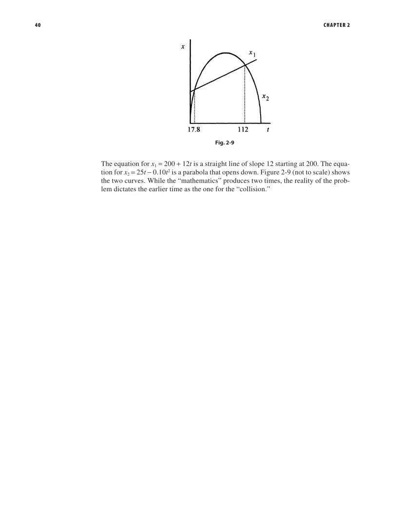
40 C H A P T E R 2

The equation for x1 = 200 + 12t is a straight line of slope 12 starting at 200. The equa-tion for x2 = 25t - 0.10t2 is a parabola that opens down. Figure 2-9 (not to scale) shows the two curves. While the “mathematics” produces two times, the reality of the prob-lem dictates the earlier time as the one for the “collision.”

Fig. 2-9

04_Oman_c02_p033-040.indd 40 04/11/15 10:33 AM

CHAPTER 3

FALLING-BODY PROBLEMS

41

The kinematic equations of motion for constant acceleration, Equation (2-1) and Equations (2-3) through (2-6), can be applied to a large collection of problems known as falling-body problems, problems where the constant acceleration is the acceleration due to gravity on the surface of the Earth. These equations from Chapter 2 are rewritten here for your convenience:

2avgv

v vo=+

(3-1)

v v ato= + (3-2)

(1/2)( )x x v v to o− = + (3-3)

(1/2) 2x x v t ato o− = + (3-4)

2 ( )2 2v v a x xo o= + − (3-5)

3-1 Consider a ball dropped from the top of a 40 m tall building. Calculate everything possible.

Solution: “Calculate everything possible” is an unusual request. Usually, early in your study of falling-body problems, there is a problem that asks for something that does not at all seem like it has anything to do with the information given. It’s almost like asking, “What color is the building?” When this happens, and it probably will, the way to do the problem is to calculate what you can, and let the information you generate lead you through the problem. Let’s apply this approach to this problem. First, diagram the prob-lem as shown in Fig. 3-1. Place the origin at the top of the building, with displacement, velocity, and acceleration (g) all positive down.

Fig. 3-1

Since most of the kinematic equations contain the time, this is usually one of the first things to calculate. Use Equation (3-4) to find the time for the ball to strike the ground

(1/2) or 40m (1 /2)(9.8m/s ) and 2.9s2 2 2x x v t at t to o− = + = =

Knowing the time, we can calculate the velocity from Equation (3-2):

(9.8m/s )2.9s 28m/s2v v gto= + = =

Alternatively, we can use Equation (3-4).

2 ( ) 2(9.8m/s )40m 784m /s or 28m/s2 2 2 2 2v v a x x vo o= + − = = =

05_Oman_c03_p041-050.indd 41 31/10/15 3:43 PM

42 C H A P T E R 3

NOTE: This last equation is a better one to use because it relies on original data rather than calculated data. If there had been an error in the time calculation, it would have been repeated in the v = vo + gt equation. Also, round off errors are eliminated by using equa-tions that rely on original data.

3-2 Now add a complication to Problem 3-1 by throwing the ball down with an initial velocity of 8.0 m/s. Find the time for the ball to reach the ground and the velocity on impact.

Solution: Again, diagram the problem as in Fig. 3-2. Note that in this problem the displacement and velocity are positive down.

Fig. 3-2

The time of flight is from 40 m = (8.0 m/s)t + (1/2)(9.8 m/s2)t2, which rearranged and without units is 4.9t2 + 8.0t – 40 = 0, with solution by formula:

80 64 4(4.9)( 40)

2(4.9) 2.2, 3.8t =− ± − −

= −

The positive time is the obvious choice. The velocity at the ground level is from

(8.0m/s ) 2(9.8m/s )40m 848m /s 29m/s2 2 2 2 2 2v v= + = =

3-3 Add a different complication to Problem 3-1. Throw the ball up from the top of the building with a velocity of 8.0 m/s. Find the time for the ball to reach the ground and the velocity on impact.

Solution: Diagram the problem as in Fig. 3-3. Take x the displacement as positive down and the velocity as negative up. It is important to remember that the sign of the velocity is opposite that of the displacement. It doesn’t matter whether the velocity is negative and the distance down positive or vice versa. It does matter that the signs be opposite! Getting a sign wrong is the source of many, possibly most, errors in falling-body problems.

Fig. 3-3

05_Oman_c03_p041-050.indd 42 31/10/15 3:43 PM

FA L L I N G - B O D Y P R O B L E M S 43

Calculate the time of flight, and note the signs: 40m ( 8.0m/s) (4.9m/s ) .2 2t t= − + Rearranging and without units, this equation is 4.9t2 - 8.0t - 40 = 0, with solutions.

=± − −

= −8.0 64 4(4.9)( 40)

9.8 3.8, 2.2t

The positive time is the obvious choice. Note the numbers used for the solutions to the quadratics in time for this and Problem 3-2. The velocity when the ball strikes the ground is

v v= − + = =( 8.0 m/s) 2(9.8 m/s )40 m 848m /s or 29m/s2 2 2 2 2

Notice that whether the v term is a positive or negative number, the result is the same. If the ball is thrown up with a certain velocity or down with the same velocity, the velocity at impact is the same. This is to be expected from the symmetry of the equations. If the ball is thrown up with a certain velocity, then on the way down it passes the same level (from which it was thrown) with (numerically) that same velocity.

3-4 For the situation of Problem 3-3, calculate the maximum height above the top of the building and the time for the ball to reach maximum height.

Solution: The time for the ball to reach maximum height is from Equation (3-2). Note that at maximum height, the velocity must be zero. Again, watch the signs closely. It doesn’t matter how you choose the signs, but the acceleration has to be opposite the velocity. The equations

0 8.0m/s (98m/s ) and 0 8.0m/s (9.8m/s )2 2t t= − = − +

yield the same result, t = 0.82 s. Because of symmetry, it takes the ball the same amount of time to reach maximum height as it does for the ball to return to the original level.

Calculate the height above the top of the building from Equation (3-5).

0 (8.0m/s) 2(9.8m/s )( ) or 3.3m2 2 2 x x xo= − − =

A thorough understanding of these four problems will keep you from making sign mis-takes in problems like these.

3-5 A bottle of champagne is dropped by a balloonist. The balloon is rising at a constant velocity of 3.0 m/s. It takes 8.0 s for the bottle of champagne to reach the ground. Find the height of the balloon when the bottle was dropped, the height of the balloon when the bottle reached the ground, and the velocity with which the bottle strikes the ground.

Solution: Diagram the situation as shown in Fig. 3-4, being especially careful about the relative orientation (algebraic signs) of displacement, velocity, and acceleration. There are several possibilities as regards the origin and direction of the coordinate system. Take the origin at the height of the balloon when the bottle is dropped; the position of the balloon at t = 0. Take the displacement as positive down. The main reason for taking the displacement as positive down is that the acceleration is down and the initial velocity is up, making two positives and one negative. As time goes on, however, displacement, velocity, and acceleration will be positive. This choice seems to make for fewer minus signs and less chance for error with an algebraic sign.

05_Oman_c03_p041-050.indd 43 31/10/15 3:43 PM

44 C H A P T E R 3

Fig. 3-4

First, write the equation for the height of the balloon starting from the time when the bottle is dropped.

( 3.0m/s) (4.9m/s ) ( 3.0m/s)8.0s (4.9m/s )64s 290m2 2 2 2x t t= − + = − + =

The height of the balloon when the bottle reached the ground would be the height when the bottle was dropped plus the amount the balloon rose in the 8.0 s it took the bottle to reach the ground, or

290m (3.0m/s)8.0s 314m+ =

The velocity on impact 3.0m/s (9.8m/s )8.0s 75m/s.2v v ato= + = − + = This velocity also could be calculated using

= + − = + =2 ( ) 9.0 m /s (19.6m/s )290 m or 75m/s2 2 2 2 2v v a x x vx o o

3-6 A parachutist descending at a constant rate of 2.0 m/s drops a smoke canister at a height of 300 m. Find the time for the smoke canister to reach the ground and its velocity when it strikes the ground. Then find the time for the parachutist to reach the ground, the position of the parachutist when the smoke canister strikes the ground, and an expression for the distance between the smoke canister and the parachutist.

Solution: Diagram the system as shown in Fig. 3-5, taking displacement, velocity, and acceleration as positive down with the origin at the point where the canister is dropped.

The time for the smoke canister to reach the ground is from Equation (3-4).

(1/2) 2x v t ato= + or 300m (2.0m/s) (4.9m/s )2 2t t= +

Fig. 3-5

05_Oman_c03_p041-050.indd 44 31/10/15 3:43 PM


Without units, the equation is 4.9t2 + 2.0t - 300 = 0 with solutions

=− ± − −

⋅ = − ± = −2 4 4(4.9)( 300)

2 4.92 76.7

9.8 7.6, 8.0t

The time for the canister to reach the ground is 7.6 s. The velocity when it strikes the ground is

v v= + = =(2.0 m/s) 2(9.8 m/s )300 m 5884 m /s or 77m/s2 2 2 2 2

The time for the parachutist to reach the ground is from Equation (3-2).

300m (2.0m/s) or 150st t= =

When the canister strikes the ground, the parachutist has dropped (2.0 m/s)7.6 s = 15 m and is 285 m above the ground. The expression for the distance between the canister and the parachutist is

(2.0m/s) (4.9m/s ) (2.0m/s) (4.9m/s )2 2 2 2x x t t t tc p− = + − =

3-7 A coconut is dropped from a height of 60 m. One second later, a second coconut is thrown down with an initial velocity. Both coconuts reach the ground at the same time. What was the initial velocity of the second coconut?

Solution: In problems where there is a time delay, it is usually best to calculate the position, velocity, and acceleration of the first particle at the time when the second particle starts to move. In the train problem in Chapter 2 there was a position differ-ence between the two trains at t = 0 that was easily translated into the equations. It is possible to do time delay problems with a time differential in one set of equations. The difficulty with this approach is that it is easy to get an algebraic sign wrong. If you say that the time for the second particle is the time for the first plus the difference between them, then it is essential that the algebraic sign of the difference be correct. It is much easier, especially when you are learning how to do problems with a time delay, to do them in this slower but inherently more accurate way. First, calculate the state of the first particle when the second one begins moving. Then write the two sets of equations describing the motion with this instant as t = 0.

Calculate the position and velocity of the first coconut at the end of 1 s, the time when the second one starts.

(1/2) (1/2)(9.8m/s )(1.0s) 4.9m2 2 2x at= = = 9.8m/s 1.0s 9.8m/s2v at= = =

Since everything (position, velocity, and acceleration) is positive down, orient the coor-dinate system for positive down with the origin at the top. Now diagram the problem as in Fig. 3-6. At the instant the second coconut is thrown down, the first coconut has position 4.9 m, velocity 9.8 m/s, and acceleration 9.8 m/s2.

05_Oman_c03_p041-050.indd 45 31/10/15 3:43 PM

46 C H A P T E R 3

Fig. 3-6

Since both coconuts strike the ground at the same time, use the conditions of the first coconut to find the total time. First, calculate the velocity at impact of the first coconut

2 ( ) (9.8m/s) 2(9.8m/s )(60 4.9)m 1,174m /s12

12

1 12 2 2 2v v a x xo o= + − = + − =

or

34.3m/s1v =

The time for the second coconut to reach the ground is the same as the time for the first coconut to go from 4.9 m to 60 m or the time for the first coconut to go from 9.8 m/s to 34.3 m/s.

This comes from v = vo + at, where vo is v1o, the velocity of the first coconut when the second one is thrown down, and v is the velocity of the first coconut at the ground.

34.3m/s 9.8m/s (9.8m/s ) or 2.5s2 t t= + =

Now that we have the time for the second coconut to travel the 60 m, we can find its ini-tial velocity from x - xo = v2ot + (1/2)at2, where t is the total time for the second coconut.

60m (2.5s) (4.9m/s )(2.5s)22 2v o= + or 11.5m/s2v o =

Review this problem until all the different times and velocities are clear in your mind. Set up the problem and do it yourself without reference and you will know that you understand it.

3-8 A boat is passing under a bridge. The deck of the boat is 15 m below the bridge. A small package is to be dropped from the bridge onto the deck of the boat when the boat is 25 m from just below the drop point. What (boat) speed is necessary to have the package land in the boat?

Solution: Calculate the time for the package to fall the 15.0 m using (1/2) 2x x v t ato o− = + .

15m (4.9m/s )2 2t= or 1.7st =

The boat must move at 25 m/l.7 s = 14 m/s.

05_Oman_c03_p041-050.indd 46 31/10/15 3:43 PM


3-9 You are observing steel balls falling at a constant velocity in a liquid filled tank. The window you are using is 1 m high, and the bottom of the window is 12 m from the bottom of the tank. You observe a ball falling past the window taking 3.0 s to pass the window. Calculate the time required to reach the bottom of the tank after the ball has reached the bottom of the window.

Solution: The situation is diagrammed in Fig. 3-7.

The observed velocity is = =1.0 m/3.0s, so12m (1.0 m/3.0s) or 36s.t t

Fig. 3-7

3-10 In a situation similar to Problem 3-9, the tank is filled with a different liquid, caus-ing the acceleration in the tank to be 6.0 m/s2 and the time to traverse the window 0.40 s. Calculate the height of the liquid above the window, the time to reach the bottom of the tank, and the velocity of the ball when it reaches the bottom of the tank.

Solution: Diagram the problem as in Fig. 3-8.

Fig. 3-8

From the data about the window, calculate the velocity of the ball at the top of the window.

(1 /2) 1.0m 0.40s (3.0m/s )(0.40s) or 1.3m/s2 2 2x x v t at v vo t t t− = + = + =

The velocity at the bottom of the window is from

2 ( ) (1.3m/s) 2(6.0m/s )1.0m or 3.7m/s2 2 2 2v v a x x vb t o b= + − = + =

The time to reach the bottom of the tank is from (1/2) 2x x v t ato b− = +

12m (3.7m/s) (3.0m/s )2 2t t= +

05_Oman_c03_p041-050.indd 47 31/10/15 3:43 PM

48 C H A P T E R 3

and eliminating the units, 3.0 3.7 12 0, so2t t+ − =

=− ± − −

= − ± = −3.7 (3.7) 4(3.0)( 12)

2(3)3.7 12.6

6 1.5, 2.72

t

This (positive) time is for the ball to travel from the bottom of the window to the bottom of the tank.

Assuming that the ball started at zero velocity, the distance from the top of the liquid to the top of the window xt will come from 22 2v v axt o t= + .

(1.3m/s) 2(6.0m/s) or 0.14m2 x xt t= =

The velocity with which the ball strikes the bottom of the tank is

(3.7m/s) (6.0m/s )1.5s 12.7m/s2v v atb= + = + =

3-11 A ball is observed to pass a 1.4 m tall window going up and later going down. The total observation time is 0.40 s (0. 20 s going up and 0.20 s going down). How high does the ball rise above the window?

Solution: Diagram the problem as in Fig. 3-9. This is another example of a question that seems totally unrelated to the information in the problem. When you don’t know where to start and you do not see a clear path to the desired answer, simply start where you can, calculating what you can and hopefully learning enough to answer the specific question.

Fig. 3-9

One of the first things we can calculate in this problem is the average velocity at the middle of the window.

(1.4m/0.20s) 7.0m/savgv = =

This average velocity is the velocity of the ball on the way up (and on the way down) at the middle of the window. Add this feature to the problem. With this information, we can use 22 2v v axo t= + to find the distance the ball rises above the midpoint of the window.

(7.0m/s) 2(9.8m/s ) or 2.5m2 2 x xt= =

So the ball rises 2.5 - 0.7 = 18 m above the top of the window.

05_Oman_c03_p041-050.indd 48 31/10/15 3:43 PM


Second Solution: View the ball as decelerating as it goes up past the window, and find vb at the bottom of the window from (1/2) 2x x v t ato o− = + .

1.4m (0.20s) (4.9m/s )(0.20s) or 8.0m/s2 2v vb b= − =

Velocity and displacement are taken as positive, so acceleration is negative.

Now the distance to maximum height (velocity zero) is

= =x xm m(8.0 m/s) 2(9.8 m/s ) or 3.2m2 2

Again, the maximum height of the ball above the top of the window is 3.2 m - 1.4 m = l.8 m.

05_Oman_c03_p041-050.indd 49 31/10/15 3:43 PM

CHAPTER 4

PROJECTILE MOTION

51

In order to understand projectile motion, you have to look at the motion in two direc-tions with one direction oriented in the direction of constant acceleration and the other direction at a right angle to it so as to form an x-y coordinate system. In most problems where an initial velocity and angle with the horizontal is given, the velocity is written in component form (Fig. 4-1).

Fig. 4-1

Note that the motion is effectively separated into horizontal and vertical components (one in the direction of the constant acceleration and one at a right angle to the acceleration).

The motion is a parabola in this coordinate system. The symmetry of parabolas (in this case, parabolic motion) is helpful in understanding the motion. (See the Mathematical Background for a discussion of the properties of parabolas.) In order to better understand how the motion is separated and how the parabolic property helps us to understand pro-jectile problems, we will do a simple problem without numbers just to get a feel for the features of the motion. If you are familiar with the properties of parabolas, you may want to skip this discussion and go directly to the worked problems.

In Fig. 4-1, the velocity of the projectile is written in component form. The acceleration in the horizontal direction is zero and in the vertical direction is due to gravity. With the velocity components and the acceleration in the direction of an axis, we can write the six equations describing acceleration, velocity, and position in the x and y directions.

These equations are based on the kinematic equations of motion for constant acceleration: a = constant, v = vo + at, and s = so + vot + (1/2)at2.

The six equations are

ax = 0 ay = -g vx = vo cosq vy = vo sinq - gt x = vo(cosq)t y = vo(sinq)t - (1/2)gt2

The equations for x and y can be considered parametric equations in time. Parametric equations such as x = f(t) and y = f(t) are equations that can be combined to produce y = f(x) or x = f(y). To find the position of the particle in x-y, or y as a function of x, solve

06_Oman_c04_p051-058.indd 51 04/11/15 12:21 PM

52 C H A P T E R 4

one equation for t and substitute into the other. In this case, solve x = … for t because this is the simplest choice:

cost xvo θ=

Substitute into y = … to obtain

(tan )2 cos2 2

2y xg

vx

o

θθ

= −

This is of the form ( )2y ax bx x ax b= − + = − + , which is a parabola that opens down and intercepts the y-axis (makes y = 0) at x = 0 and x = b/a.

The range, or value of x when y = 0, can be determined from the factored form of this equation,

tan2 cos2 2y x

gv

xo

θθ

= −

which tells us that y = 0 at x = 0 and

2

cos tan2

sin cos2

22

xvg

vg

o oθ θ θ θ= =

or, using the trigonometric identity 2 sinq cosq = sin 2q,

sin22

xvgo θ=

The maximum range occurs for an angle of 45°, corresponding to sin 2q = 1.

The main point of this discussion is that the motion is a parabola, and the properties of parabolas can be used in solving problems in projectile motion. That the maximum range occurs at 45° is not surprising and is generally not of interest in problems. The expres-sion for maximum range is only of passing interest because the range is one of the easier things to calculate in any problem.

Do not consume precious memory space memorizing formulas for the range or time of flight. If you work the problems by first writing down the six equations describing the motion, then the time of flight, range, and many other things are easily calculated.

In order to set up a problem in projectile motion, first orient one axis of a right angle (x-y) coordinate system in the direction of constant acceleration. Remember to place the origin of the coordinate system and the positive direction for x and y for (your) convenience in solving the problems. Then write equations for acceleration, velocity, and position for each direction. Along with the symmetry of the motion, these equa-tions can be used to find the characteristics (position, velocity, and acceleration) of the projectile at any point in space or time. The procedure is illustrated with a simple problem.

4-1 A soccer player kicks a ball at an initial velocity of 18 m/s at an angle of 36° to the horizontal. Find the time of flight, range, maximum height, and velocity components at t = 0, midrange, and impact.

06_Oman_c04_p051-058.indd 52 04/11/15 12:21 PM

P R O J E C T I L E M O T I O N 53

Solution: The acceleration is down, so set up the coordinate system with x horizontal (along the ground) and y vertical, and place vo on the graph. Write the velocity in com-ponent form, and calculate vxo and vyo (Fig. 4-2).

Fig. 4-2

Now, and this is the key to getting the problem right, write down the six equations governing the motion starting with the accelerations (the accelerations are the easiest to write).

0ax = 9.8m/s2ay = −

14.6m/svx = 10.6m/s (9.8m/s )2v ty = −

x t= (14.6m/s) 2 (10.6m/s) (4.9m/s )2 2y t t= −

Now look at the motion, which is parabolic in x-y, keeping in mind the properties of parabolas.

Fig. 4-3

The ball is on the ground at t = 0 and t = t, the time of flight. To find these times, set y = 0 and obtain (without units)

10.6t - 4.9t2 = 0 or t(10.6 - 4.9t) = 0

which gives t = 0 and t = 10.6/4.9 = 2.16 s, the time of flight. The range is the value of x at 2.16 s.

(14.6m/s)2.16s 31.5m2.16

xt

= ==

The maximum height and vy = 0 occur at 1.08 s (one half the time of flight). Therefore, the maximum height is y at t = 1.08 s.

(10.6m/s)1.08s (4.9m/s )(1.08s) 5.73mmax 1.08

2 2y yt

= = − ==

06_Oman_c04_p051-058.indd 53 04/11/15 12:21 PM

54 C H A P T E R 4

The velocity components are

at t = 0: vx = 14.6 m/s, vy = 10.6 m/s

at t = 1.08 s: vx = 14.6 m/s, vy = 0

at t = 2.16 s: vx = 14.6 m/s, vy = –10.6 m/s

The procedure for doing the problem is to write the initial velocity in component form; write the six equations for acceleration, velocity, and position; and then perform the mathematical operations answering questions about the problem.

4-2 For the situation of Problem 4-1, suppose that the field is covered with fog down to 3.0 m above the ground. What are the times for the ball’s entry into and exit out of the fog?

Solution: The times for the ball’s entry into and exit out of the fog, are found from the equation for y as a function of time with y set equal to 3.0 m.

3.0 m = (10.6 m/s)t - (4.9 m/s2)t2

This is a quadratic equation, and after removing the units, it reads 4.9t2 - 10.6t + 3.0 = 0 and is solved with the quadratic formula:

10.6 10.6 4(4.9)3.0

2(4.9)10.6 7.3

9.8 0.34,1.82

t =± −

= ± =

As an exercise, find the x positions for these times.

4-3 An airplane traveling at 100 m/s drops a bomb from a height of l,500 m. Find the time of flight, distance traveled, and velocity components as the bomb strikes the ground.

Solution: Start by placing the origin of the coordinate system at the point where the bomb is released. Take the direction in which the bomb falls due to gravity as positive x and the horizontal position as y. This is different from the conventional orientation, but it is convenient in this problem because the six equations all come out positive!

Fig. 4-4

Now write down the six equations governing the motion:

9.8m/s2ax = 0ay =

(9.8m/s )2v tx = 100m/sv vy o= =

(4.9m/s )2 2x t= (100m/s)y t=

06_Oman_c04_p051-058.indd 54 04/11/15 12:21 PM


With these six equations we can answer all the questions in the problem. We need only to “translate” the word questions into algebra questions.

a. The time for the bomb to reach the Earth means “Find the time when x = 1,500 m.” Thus

l,500 m = (4.9 m/s2)t2 yields t = 17 s

b. How far does the bomb travel horizontally means “Find the value of y when t = 17 s.” Thus

(100m/s)17s 1,700m17

yt

= ==

c. Find the velocity components at impact means “Find vx and vy at t = 17 s.” Thus

(9.8m/s )17s 167m/s17

2vx t= =

=

100m/s17

vyt

==

d. Where is the airplane when the bomb strikes the Earth means “What is y at t = 17 s?” Remember that the plane and the bomb have the same velocity in the horizontal direction. Thus

(100m/s)17s 1,700mplane

y = =

4-4 A baseball is hit at a 45° angle and a height of 0.90 m. The ball travels a total distance of 120 m. What is the initial velocity of the ball? What is the height of the ball above a 3.0 m fence 100 m from where the ball was hit?

Solution: This problem is unique in that it requests the initial velocity, a number usually given in the problem. Also note that the angle is 45°, the angle for maximum range. The other interesting feature of this problem is the question concerning the height at some specific point down range.

Set up the problem in the conventional way assigning vo to the initial velocity.

Fig. 4-5

The next question is how to handle the ball being hit at 0.90 m above the ground. Since vo is specified at the point where the ball is hit, and this is where we start counting time, the origin for the coordinate system should be put here. We just need to keep in mind that this origin is 0.90 m above the ground level.

06_Oman_c04_p051-058.indd 55 04/11/15 12:21 PM

56 C H A P T E R 4

Fig. 4-6

Now write the six equations:

0ax = 9.8m/s2ay = −

cos45v vx o= ° sin45 (9.8m/s )2v v ty o= ° −

(cos45 )x v to= ° sin45 (4.9m/s )2 2y v t to= ° −

The first question reduces to finding vo for the 120 m hit. Algebraically, this means that when y = -0.9 m, x = 120 m, so write the two equations (for x and y) with these conditions:

120 m = vo cos45°t -0.9 m = vo(sin45°)t - (4.9 m/s2)t2

Note that vo (cos45°)t = vo (sin45°)t = 120 m, so write

0 = 0.90 m + 120 m - (4.9 m/s2)t2 or 120.94.9 s2 2t = and t = 4.97 s

This is the time of flight, so put this time into the equation for x,

120 m = vo (cos45°) (4.97 s) to find vo as vo = ° ⋅ =120 mcos45 4.97s 34.1m/s

The next part of the problem asks for the height above the fence at 100 m. Again, we need to find the time for x to be 100 m down range and substitute this value of t into the y equation.

100 m = (34.1 m/s) (cos45°)t or t = ° =100s34.1(cos45 ) 4.15s

This is the time for the ball to go 100 m. The height of the ball at this time is

(34.1m/s)cos45 (4.15s) (4.9m/s )(4.15s) 15.6m4.15

2 2yt

= ° − ==

Remember that this is 15.6 m above the zero of the coordinate system, which is 0.90 m above the ground, so the ball is 16.5 m above the ground at this point and, for a 3 m high fence, is 13.5 m above the fence.

4-5 A physicist turned motorcycle stunt rider will jump a 20 m wide row of cars. The launch ramp is 30° and 9.0 m high. The land ramp is also 30° and is 6.0 m high. Find the minimum speed for the launch.

06_Oman_c04_p051-058.indd 56 04/11/15 12:21 PM


Solution:

Fig. 4-7

First, write down the six equations of motion:

0ax = 9.8m/s2ay = −

cos30v vx o= ° sin30 (9.8m/s )2v v ty o= ° −

(cos30 )x v to= ° (sin30 ) (4.9m/s )2 2y v t to= ° −

The minimum vo is dictated by the condition that the rider be at x = 20 m and y = -3.0 m. So put these conditions into the equations for x and y.

20 m = vo (cos30°)t -3.0 m = vo (sin30°)t - (4.9 m/s2)t2

At this point we can solve for vo by substituting 20m/ cos30t vo= ° from the first equation into the second equation.

vo

− = ° − ×°

3.0 m (20 m)tan30 4.9 400 m(cos 30 )s

3

2 2 2 yields vo = 13.4 m/s

This is the minimum velocity to make the jump.

As a follow on to this problem, calculate the velocity to just hit the end of the ramp. This velocity gives an upper limit to the jump velocity.

Go back through the problems and notice the common approach:

1. Orient a coordinate system, 2. Write the six equations of motion, and 3. Translate the word questions into algebra.

In these problems we have not always used each of the six equations to answer the ques-tion. Few problems require the detailed description of the motion available in the six equations. If, however, each problem is described by these six equations, you will always have all the information to answer any possible question about the motion.

06_Oman_c04_p051-058.indd 57 04/11/15 12:21 PM

CHAPTER 5

FORCES (INCLUDING CENTRIPETAL FORCE)

59

In the development of mechanics, the first thing to learn is the interrelations of position, velocity, and acceleration (for constant acceleration). These interrelations are described with the four kinematic equations of motion and discussed in Chapters 2, 3 and 4.

In this chapter we relate constant force to constant acceleration and then to all of kine-matics. Operationally, force can be defined as what makes masses accelerate. Actually, it is the unbalanced force on a mass that makes it accelerate. Simply, unbalanced forces make masses accelerate.

Force, acceleration, and mass are related by Newton’s second law as F = ma.

5-1 A 40 N force is applied to a 20 kg block resting on a horizontal frictionless table. Find the acceleration.

Solution: The acceleration is / 40 N/20 kg 2.0m/s .2a F m= = =

Fig. 5-1

Once the acceleration is known, the kinematic equations of motion can be applied to find position, velocity, and acceleration as a function of time.

5-2 Now place the 20 kg mass (with no external force applied) on a frictionless 50° inclined plane. What is the acceleration of the mass?

Solution: The force acting on the mass is due to gravity, so set up a vector diagram (some authors call this a force diagram or free body diagram) starting with this 196 N force acting down. The mass is constrained to move down the plane, so the force we want is the component of this gravitational force acting down the plane. In Fig. 5-2 the gravitational force is shown with components down the plane Fp and normal to the plane Fn. Notice the geometry of the situation, where the 50° angle of the plane is the same as the angle between the gravitational force and the normal (force).

Fig. 5-2

07_Oman_c05_p059-074.indd 59 04/11/15 10:34 AM

60 C H A P T E R 5

The 150 N force acting down the plane causes the 20 kg mass to accelerate at

a = =150 N20 kg 7.5m/s2

5-3 Place a 10 kg mass on a frictionless 35° inclined plane, and attach a second 20 kg mass via a cord to hang vertically, as shown in Fig. 5-3. Calculate the acceleration of the system.

Solution:

Fig. 5-3

This problem introduces the concept of the tension in the connecting cord. The most con-venient way to visualize this tension is that if the cord were cut and a force meter inserted, it would read a certain tension (force). This tension acts, as shown, on each mass. Notice the 35° angle of the plane and the 35° angle between the normal and the direction of mg.

We’ll do the problem first with the tension and later without the tension.

To write equations relating the unbalanced force to the acceleration, we need to make an assumption as to which way the masses move. Assume that the system (of masses) moves to the right, or clockwise.

Start by writing equations relating the unbalanced force on each mass. On m1, the unbal-anced force is T - 56 N, and this force makes the 10 kg accelerate.

T - 56 N = 10 kg ⋅ a1

Likewise on m2, the unbalanced force to make the mass accelerate is

196 N - T = 20 kg ⋅ a2

The assumption that the system accelerates clockwise dictates the directions of the forces in these two equations. Look again at these equations, and notice that if we had assumed the acceleration were counterclockwise, then the signs would be different. In frictionless prob-lems it is all right to have a negative acceleration. The negative sign means that you guessed wrong in assuming the acceleration direction. This is not true with friction problems.

Add the two equations, and take the accelerations as the same. The accelerations are the same because the masses are linked together with the cord.

140 N = 30 kg · a or a = 4.7 m/s2

07_Oman_c05_p059-074.indd 60 04/11/15 10:34 AM

F O R C E S ( I N C LU D I N G C E N T R I P E TA L F O R C E ) 61

Now the tension in the cord is easily calculated from the equation for m1:

T = 56 N + 10 kg · 4.7 m/s2 = 103 N

Another way to view this problem is to say that the unbalanced force on m1 and m2 is (196 - 56) N = 140 N. This force makes the total mass of 30 kg accelerate, so

140 N = 30 kg · a or a = 4.7 m/s2

This is a very quick way to find the acceleration of the system, but it is inconvenient to find the tension in the cord.

5-4 The next complication in force problems with inclined planes is a double inclined plane, as shown in Fig. 5-4.

Fig. 5-4

Solution: The vector diagram for these masses is shown in Fig. 5-5. Assume that the system moves clockwise.

Fig. 5-5

The equation for m1 is

T – 76 N = 12 kg · a


83 N - T = 20 kg · a

Adding the two equations,

7.0 N = 32 kg · a or a = 0.22 m/s2

The tension in the cord is

T = 76 N + 12 kg · 0.22 m/s2 = 79 N

07_Oman_c05_p059-074.indd 61 04/11/15 10:34 AM

62 C H A P T E R 5

5-5 Another popular problem is the Atwood machine. A simple example is shown in Fig. 5-6. Find the acceleration of the system.

Solution: Assume that the system moves counterclockwise. The equation for m1 is

98 N - T = 10 kg · a


T - 147 N = 15 kg · a

Add the equations:

-49 N = 25 kg · a or a = -2.0 m/s2

Fig. 5-6

The system accelerates clockwise! The tension in the cord is from the equation for m1:

T = 98 N + (10 kg)2.0 m/s2 = 118 N

Friction

A good first problem in friction is the arrangement shown in Fig. 5-7, where the problem is first done without friction and then with friction.

For the purposes of doing problems, there are two important properties of frictional forces:• They oppose the motion, and• They are less than or equal to a constant (the coefficient of friction) times the

normal force, the force at the frictioning surface ( f ≤ lN).

5-6 Two masses are arranged with one, of 50 kg, on a frictionless table and the other, of 30 kg, attached by a cord and hanging, over a frictionless pulley, off the edge of a table. Find the acceleration of the system.

Solution: Assume that the system moves clockwise. The equation for m1 is

T = 50 kg · a


294 N - T = 30 kg · a

07_Oman_c05_p059-074.indd 62 04/11/15 10:34 AM



294 N = 80 kg · a or a = 3.7 m/s2

Fig. 5-7

5-7 For the situation of Problem 5-6, add a coefficient of friction m = 0.20 between the block and table.

Solution: This makes the vector diagram look like Fig. 5-8. Notice that the only addition is the frictional retarding force mN = 98 N.

Fig. 5-8


T – 98 N = 50 kg · a


294 N – T = 30 kg · a

Add the equations to obtain

196 N = 80 kg · a or a = 2.4 m/s2

5-8 For the situation of Problem 5-7, increase the coefficient of friction to 0.80. What is the acceleration of the system?

07_Oman_c05_p059-074.indd 63 04/11/15 10:34 AM

64 C H A P T E R 5

Solution: This makes the vector diagram look like Fig. 5-9.

Fig. 5-9


T - 392 N = 50 kg · a


294 - T = 30 kg · a


–98 N = 80 kg · a or a = -1.2 m/s2

Clearly, the system does not accelerate counterclockwise! This is an illustration of the second property of frictional forces: the frictional force is less than or equal to mN. In this case the frictional force just balances the tension in the cord. The frictional force, as calculated, can be up to 392 N. In order for m2 not to move, the tension in the cord must be 294 N. (If m2 is not moving, the forces must be in balance.) Therefore, the forces on m1 must be 294 N due to the tension in the cord and 294 N due to friction.

Another important point with frictional forces is the normal force, as illustrated by this next problem.

5-9 A 50 kg sled is pulled along a level surface at constant velocity by a constant force of 200 N at an angle of 30°. What is the coefficient of friction between the sled and the surface?

Solution: The first step in this problem is to find the components of the applied force and the mg of the sled. These are shown on the vector diagram in Fig 5-10. Notice that the normal force, the actual force between the sled and the friction surface, is mg minus the component of the applied force lifting up on the sled. Sometimes it is easy to miss this vertical component of the applied force. This is a major mistake in this type of problem. To help visualize this vertical component of force, try placing the origin for the vectors in the middle of the sled rather than at one end, where a rope would be attached.

Fig. 5-10

07_Oman_c05_p059-074.indd 64 04/11/15 10:34 AM


The normal force is mg (= 490 N) minus the vertical component of the applied force, 100 N, or 390 N. Since the sled is moving at constant velocity, the forces must be in equilibrium. The horizontal component of the applied force must equal the frictional retarding force, the coefficient of friction times the normal force:

µ · 390 N = 173 N so µ = 0.44

5-10 A 65° inclined plane has a mass of 20 kg on the plane where the coefficient of fric-tion is 0.40 and a mass of 50 kg hanging free. Calculate the acceleration of the system.

Solution: Set up the vector diagram assuming that the motion is counterclockwise. In the diagram in Fig. 5-11, the frictional force is calculated as a maximum of 33 N.


490 N - T = 50 kg · a


T - 178 N - 33 N = 20 kg · a

Adding the equations,

279 N = 70 kg · a or a = 4.0 m/s2

Fig. 5-11

In doing friction problems like this, you have to be careful with the frictional force. If the forces up and down the plane are nearly balanced, it is important to remember that the frictional force is not 33 N but that it can be up to 33 N. In a problem similar to this, it could easily happen that the blocks would not move.

5-11 Consider a double inclined plane with angles, masses, and coefficients of friction as shown in Fig. 5-12. Calculate the acceleration of the system.

Fig. 5-12

07_Oman_c05_p059-074.indd 65 04/11/15 10:34 AM

66 C H A P T E R 5

Solution: Assume that the system moves counterclockwise, and set up the vector dia-gram as in Fig. 5-13.


(30 - 15 -T) N = 6.0 kg · a


(T - 62 - 10) N = 9.0 kg · a

Adding the equations,

-57 N = 15 kg · a

Fig. 5-13

This is a negative acceleration. We cannot simply reverse the sign of a to find the correct answer because if the system were moving the other way, the frictional forces would have to be reversed. Further analysis requires us to consider another vector diagram assuming that the system moves in a clockwise direction.

The numbers have all been calculated, so the vector diagram can be written down easily and is as shown in Fig. 5-14.

Fig. 5-14

The new equations are:

(T – 30 – 15) N = 6.0 kg · a

(62 – T – 10) N = 9.0 kg · a

Adding the equations yields

7.0 N = 15 kg · a or a = 0.54 m/s2

07_Oman_c05_p059-074.indd 66 04/11/15 10:34 AM


The tension in the cord is from the first equation:

T = 45 N + 6.0 kg(0.54 m/s2) = 48 N

If the acceleration of the system were negative for both the clockwise and counterclock-wise calculations, then we would conclude that the system would not move.

The final complication in these inclined plane problems is the introduction of three masses and two connecting cords.

5-12 Consider a flat surface with a coefficient of friction of 0.20 with a 2.0 kg mass and a 3 kg mass connected together with a 6 kg mass along a slant as shown in Fig. 5-15. The coefficient of friction on the slant is zero. Calculate the acceleration of the system.

Fig. 5-15

Solution: In this problem, note that the tensions are different, leading to three unknowns, T1, T2, and a. The solution will require three equations from three vector diagrams, as shown in Fig. 5-16. Assume that the acceleration of the system is clockwise.

The frictional retarding force on the 2 kg block is

f = mN = 0.20(19.6 N) = 3.92 N

The frictional retarding force on the 3 kg block is

f = mN = 0.20(29.4 N) = 5.88 N

Fig. 5-16

The equations for the masses are

T2 - 3.92 N = 2.0 kg · a

T1 - T2 - 5.88 N = 3.0 kg · a

24.8 N - T1 = 6.0 kg · a

07_Oman_c05_p059-074.indd 67 04/11/15 10:34 AM

68 C H A P T E R 5

The last two equations added together are

18.9 N - T2 = 9.0 kg · a

and adding this to the first equation yields

15.0 N = 11 kg · a or a = 1.36 m/s2

The tensions come from the first and third equations for the masses:

T2 = 3.92 N + 2.0 kg(1.36 m/s2) = 6.64 N

T1 = 24.8 N – 6.0 kg(1.36 m/s2) = 16.6 N

Circular Motion

A particle moving at constant speed in a circle is moving in uniform circular motion. There is an acceleration and a force associated with such a particle. Figure 5-17 shows the velocity vectors associated with a particle in uniform circular motion.

Fig. 5-17

While the length of the velocity vector remains the same, the direction changes continu-ally. The diagram on the left of Fig. 5-17 shows vi and vf, with the tail of the vectors at the same point, and Δv. Looking at the limiting case where Δq → 0, the ratio

v

vs

r∆

= ∆

is valid because of similar triangles. With this statement, write

vt

vr

st

∆∆ = ∆

∆

which in the limiting situation when Δq → 0 or Δt → 0 (same criterion) is

lim0

rad

2vt a v

rt

∆∆ = =

∆ →

The “rad” subscript is a reminder that the acceleration points radially inward. The direc-tion of arad is also clear from the limiting situation. As Δt → 0, the angle between v and Δv → 90°, so the acceleration is directed radially inward.

5-13 A certain car driven in a circle can exert a maximum side force of 0.95g. What is the maximum speed for this car driven in a circle of 160 m radius?

07_Oman_c05_p059-074.indd 68 04/11/15 10:34 AM


Solution: A side force of 0.95g means a side force or acceleration directed at right angles to the direction of travel of 0.95(9.8 m/s2) = 9.3 m/s2. Using arad = v2/r,

9.3m/s (160m) 38.6m/srad2v a r= = =

At a speed greater than 38.6 m/s, the car will “slide out of the circle.”

The acceleration directed toward the center of the circle for a mass in uniform circular motion is called the centripetal acceleration. The force associated with moving a mass in a circle is marad and is called the centripetal force.

5-14 What is the (centripetal) force produced by the tires acting on the pavement for the car of Problem 5-13 if the car is 1,200 kg of mass?

Solution: F = marad = 1,200 kg(9.3 m/s2) = 11,200 N.

5-15 A 0.60 kg rubber stopper is whirled in a horizontal circle of 0.80 m radius at a rate of 3.0 revolutions per second. What is the tension in the string?

Solution: Three revolutions per second means three 2prs (circumferences) per second, so

vπ= ⋅ =3 2 (0.80 m)1.0s 15m/s

The tension in the string, which is providing the centripetal force, is

F m vr= = =0.60 kg

(15m/s)0.80 m 170 N

2 2

5-16 A 1 oz gold coin is placed on a turntable turning at 33-1/3 rpm (revolutions per minute). What is the coefficient of friction between the coin and the turntable if the maxi-mum radius, before the coin slips, is 0.14 m?

Solution: The frictional force between the coin and turntable provides the center directed force to keep the coin on the turntable (Fig. 5-18). This center directed force must equal mv2/r.

Fig. 5-18

This is a force balance problem. In equation form: frictional force = centripetal force, or

/2mg mv rµ = or /2v rgµ =

The velocity is 2pr times the number of 2prs per minute, 100/3, or

2 0.14m 1003

1min

1 min60s 0.49m/sv π= ⋅ =

07_Oman_c05_p059-074.indd 69 04/11/15 10:34 AM

70 C H A P T E R 5

Therefore,

vrgµ = = =(0.49m/s)

0.14 m(9.8m/s )0.18

2 2

2

5-17 A conical pendulum is a mass on the end of a cord, where the mass moves at con-stant speed in a circle with the cord tracing out a cone. A conical pendulum of length l.2 m moves in a circle of radius 0.20 m. What is the period of the pendulum?

Solution: Note that the mass is not given. Start with a vector diagram of the forces on the mass, as shown in Fig. 5-19.

Fig. 5-19

The mg must equal the vertical component of the tension in the string T cosq = mg. The horizontal component is due to the centripetal force, so T sin q = mv2/r. Dividing the second equation by the first eliminates T and m or tan q = v2/rg. The angle is from sin q = r/L, making tan q = 0.17 and

tan 0.20m(9.8m/s )0.17 0.57m/s2v rg θ= = =

The period is from 2pr/T = v or

T rvπ π= = =2 2 (0.20 m)

0.57m/s 2.2s

5-18 What is the speed, at which no side force due to friction is required, for a car travel-ing at a radius of 240 m on a 20° banked road?

Solution: Figure 5-20 shows a profile of the car on the banking and the vector diagram.

Fig. 5-20

07_Oman_c05_p059-074.indd 70 04/11/15 10:34 AM


Start with mg acting down. The normal force (between the car and road) is normal to the surface, with the vertical component equal to mg and the horizontal component equal to mv2/r.

N cos 20° = mg N sin 20° = mv2/r

And again,

sin20cos20 tan20

2NN

vrg

°° = ° =

so

tan20 240m(9.8m/s ) tan20 29m/s2v rg= ° = ° =

Notice that in this problem the mass of the car does not enter into the calculation.

Go back over Problems 5-13 through 5-18 and notice how each problem could be writ-ten asking for a different variable. For example, in Problem 5-13, give the side force and the velocity, and ask for the radius. In Problem 5-16, give the speed and the coefficient of friction, and ask for the radius. Changing the problems like this is an excellent way to generate practice (for the test) problems.

5-19 A 2 kg ball is whirled in a vertical circle of radius 1 m at a constant velocity of 6.28 m/s. Calculate (a) the tension in the cord at the top of the motion, (b) the tension in the cord at the bottom of the motion, and (c) the minimum velocity to keep the mass from “falling out” at the top of the circle.

Solution: Figure 5-21 is a drawing of the situation with the forces labeled.

T

T

T

mg

mg

mg

T + mg = mv2r

T – mg = mv2r

T = mv2r

Fig. 5-21

We are considering this problem from the reference frame of the ball, not from the point of view of the person whirling the ball. From the person’s point of view, the tension is pull-ing radially outward. From the ball’s reference frame, the tension is radially inward. If the ball is to move in a circle, this must be the case. There must be a net center directed force.

07_Oman_c05_p059-074.indd 71 04/11/15 10:34 AM

72 C H A P T E R 5

Operationally, a good method for solving centripetal force problems is to find the net center directed force and set this equal to mv2/r. So, for part a,

2

T mg mvr+ =

2

T mvr mg= −

T = − =2.0 kg(6.28m/s)

1.0 m 2.0 kg(9.8m/s ) 59.4 N2

2

For part b,

2

T mg mvr− =

2

T mvr mg= +

2.0 kg(6.28m/s)

1.0m 2.0 kg(9.8m/s ) 98.6N2

2T = + =

For part c, the minimum velocity required can be found by considering the condition where mv2 ≤ mg. In this case, at the top of the motion, the mass will fall out of the loop. So let’s set the two forces equal and solve for the minimum velocity needed to keep the mass in the loop. Thus

1.0m(9.8m/s ) 3.13m/smin2

min2mv

r mg v rg= ⇒ = = =

5-20 A person on a dirt bike travels over a semicircular shaped bridge with a radius of curvature of 45 m, as shown in Fig. 5-22. Calculate the maximum speed of the bike if its road wheels are to stay in contact with the bridge.

Solution: Figure 5-22 provides a diagram of the situation.

mg = gravitational attraction

Radius r of the bridge

Motorcycle, mass m

Linear speed v

R = reaction from the ground

Fig. 5-22

07_Oman_c05_p059-074.indd 72 04/11/15 10:34 AM


Again, let us find the net center directed force and set this equal to mv2/r. Thus

2

mg R mvr− =

2

R mg mvr= −

As v increases, R must decrease because mg is constant. In the limiting case, when the wheels are just about to leave the ground, R = 0, so

2

mg mvr=

The mass m cancels out and is not required. So maximum speed v is given by

2v rg=

Plugging in the numbers,

441 21m/sv rg= = =

At this point, you might be thinking that from the point of view of the person on the dirt bike, this mv2/r force is radially outward. The rider is momentarily weightless as the wheels leave the ground. This is correct—from the reference frame of the person inside the circular motion. Astronauts in the space station orbiting the Earth are weightless. To them, there is no net force, and the effect of the mv2/r force is radially outward to coun-terbalance gravity. If you go around a corner in a car, you seem to feel a force outward from the circle, not inward. But from the reference frame of a stationary observer, there must be a net center directed force on both the astronaut (gravity) and the person in the car (friction with the seat or door). There must be a net force pointing toward the center of the circle; otherwise, the person could not be moving in a circle. Is one force correct and the other incorrect? Is either of these forces an illusion? No. They are all real forces.

Take a “thought trip” in an airplane flying in a horizontal circle with its wings vertical. The force acting on you is toward the center of the circle, but you exert an equal and opposite force on the seat that is radially out of the circle (this is analogous to the normal force concept). In some airplanes, if the banking is done too hard, this radially outward force can be so great as to cause the blood in the pilot to remain in the lower part of the body, result-ing in a loss of oxygen (carried by the blood) to the brain and what is called a blackout. So the blackout is the result of a radially outward or centrifugal force. It is a real force!

Is one reference frame correct and the other incorrect? When you study Einstein’s theory of relativity in physics, you will come across the idea that there is no one absolute refer-ence frame. You may think that a reference frame at rest relative to the ground is correct, but the Earth spins on its axis and rotates around the sun. The sun moves around the galac-tic center. In relativity, we always have to specify the reference frame we are considering. And the observed effects of many things change depending on the chosen reference frame.

So, when doing circular motion problems, always think about what reference frame you are considering. For the method in the preceding problem, our reference frame is outside the motion, and in this perspective, we take the net center directed force and set it equal to mv2/r. This is the default reference frame that is commonly used to solve circular motion problems.

07_Oman_c05_p059-074.indd 73 04/11/15 10:34 AM

CHAPTER 6

APPARENT WEIGHT

75

Apparent weight problems usually are encountered in the discussion of force. Though relatively easy, they cause problems for some people. This short chapter should give you enough background and examples to show you how to do apparent weight problems.

One of the first points to get straight is the difference between mass and weight. Mass is the property that makes different objects accelerate differently when equal forces are applied. Operationally, mass is the m in the equation F = ma. Mass is measured in kilograms or slugs. Weight in equation form is

W = mg (6-1)

and is the force something exerts. Weight is measured in newtons or pounds. Popu-lar usage scrambles weight and mass. Gold and silver are usually sold by the gram or kilogram, while nails and chicken feed are sold by the pound.

The first step in keeping all this straight is to remember that weight is force. A scale that measures weight in pounds or newtons is just a force meter. Tension in a rope is a force.

A person of 80 kg mass standing on the surface of the Earth is subject to the force of grav-ity that acts between the 80 kg person and the mass of the Earth. This force is expressed as an acceleration due to gravity. On the Earth, this acceleration is 9.8 m/s2. The force on the person, also called weight, is

F or W = 80 kg · 9.8 m/s2 = 784 N

A force meter placed between the person and the Earth would read 784 N.

To understand apparent weight, take a “thought trip” (based on experience) on an eleva-tor. Imagine a force meter between you and the floor of the elevator. As you step on the elevator, the force meter reads the same as when you are standing on the ground. As the elevator accelerates upward, the force meter registers higher, reading maximum at maxi-mum acceleration. As the acceleration decreases and the elevator assumes a constant velocity (upward), the force meter reads the same as when the elevator was not moving. This constant velocity condition is equivalent to forces in equilibrium, so the only thing contributing to the reading of your force meter is the mg due to the Earth. As the elevator slows, by decelerating, the force meter reads less than the force for constant velocity. As the elevator comes to rest at a higher level, the force meter again reads the same as when you were at ground level.

Let’s go back over this elevator ride and put in some numbers. At zero or constant veloc-ity, the force meter reads 784 N. If the elevator were accelerating upward at 2.0 m/s2, then the force meter would read

F or W = 784 N + 2.0 m/s2(80 kg) = 944 N

If the elevator were accelerating downward (or decelerating near the top of its trip up) at 3.0 m/s2, then the force meter would read

F or W = 784 N - 3.0 m/s2(80 kg) = 544 N

08_Oman_c06_p075-078.indd 75 31/10/15 3:49 PM

76 C H A P T E R 6

If the elevator were in free fall, then the force meter would read zero. The acceleration acting on the elevator is the same as on the person.

6-1 A 12 kg flower pot is hanging by a cord from the roof of an elevator. What is the tension in the cord when the elevator is stationary and when it is accelerating upward at 3.0 m/ s2?

Solution: When the elevator is stationary, the tension in the cord is

T = 12 kg(9.8 m/s2) = 118 N

When the elevator is accelerating upward, the tension in the cord is increased by an amount equal to ma,

T = 118 N + 12 kg · 3.0 m/s2 = 154 N

Second Solution: Now take another, more analytical look at the problem. When the ele-vator is at rest, the tension in the cord equals mg, so writing a force statement T – mg = ma, where a is zero, produces T = mg.

Fig. 6-1

When the elevator is accelerating upward at 3.0 m/s2, the T - mg = ma equation has an acceleration. The hard part of doing the problem this way is keeping the algebraic sign of the acceleration correct. Looking at Fig. 6-1, T and a have the same sign, so write

T - 12 kg(9.8 m/s2) = 12 kg(3.0 m/s2) or T = 154 N

If you use this vector approach to do apparent weight problems, be especially careful of the signs. However you do the problems, go through a little thought experiment to make sure that you have the signs right.

Another difficulty with the vector approach to apparent weight has to do with the inter-pretation of the vector diagram (on the right in Fig. 6-1). If you are an observer outside the elevator, you observe an acceleration of the flower pot, as the analysis indicates. If, however, you are riding in the elevator, you observe no acceleration of the flower pot because you are riding in the accelerating reference frame.

6-2 A rope (fastened at the top) is hanging over a cliff. What is the tension in the rope with a 70 kg mountain climber sliding down the rope at a constant acceleration of 6.0 m/s2?

Solution: Performing a little “thought experiment,” the tension in the rope is less than if the climber were at zero velocity or sliding at constant velocity. In this instance, the 6.0 m/s2 must be subtracted from the 9.8 m/s2.

T = (9.8 – 6.0) m/s2(70 kg) = 266 N

08_Oman_c06_p075-078.indd 76 31/10/15 3:49 PM

A P PA R E N T W E I G H T 77

When in doubt as to whether to add or subtract the acceleration from g, look to the extreme situation. In this problem, the climber sliding down the rope at constant velocity would produce (9.8 m/s2)70 kg = 686 N of tension in the rope. If the climber were in free fall, that is, accelerating at 9.8 m/s2, he or she would produce no tension in the rope. Thus any acceleration down the rope should be subtracted from the 9.8 m/s2.

6-3 What is the tension in a rope with the 70 kg mountain climber of Problem 6-3 accel-erating (climbing) up the rope at a constant acceleration of 1.0 m/s2?

Solution: In this case, the tension in the rope is increased by ma,

T = (9 .8 +1.0) m/s2 (70 kg) = 756 N

6-4 A 100 kg astronaut produces a force (weight) on the surface of the Earth of 980 N. What force (weight) would the astronaut produce on the surface of the moon, where the g is about one-sixth the g on Earth?

Solution: The force or weight would be 100 kg(9.8m/s ) 16 163N.moon

2W = =

6-5 A 16 kg monkey wishes to raise a 20 kg mass by climbing (accelerating) up a rope that passes over a pulley attached to the mass. How much must the monkey accelerate up the rope to raise the mass?

Fig. 6-2

Solution: The mass produces a force or tension in the rope of

Tmass = 20 kg(9.8 m/s2) =196 N

The mass of the monkey hanging on the rope produces a force of

Tmonkey = l6 kg(9.8 m/s2) = 157 N

To just balance the mass, the monkey must accelerate up the rope to produce a force of (196 - 157) N = 39 N. Thus

39 N = (16 kg)a or a = 2.4 m/s2

At this acceleration, the tension in the rope is 196 N. To raise the mass, the monkey must accelerate at a rate greater than 2.4 m/s2. Any acceleration greater than 2.4 m/s2 will increase the tension in the rope by an amount equal to the “additional” acceleration times the mass of the monkey.

08_Oman_c06_p075-078.indd 77 31/10/15 3:49 PM

CHAPTER 7

WORK AND THE DEFINITE INTEGRAL

79

Work is defined as the force, in the direction of a displacement, times that displacement. Consider the application of a constant force F applied over a distance x, as depicted in Fig. 7-1.

Fig. 7-1

According to the definition, the work is

W F xo o= (7-1)

which is seen as the shaded rectangular area in Fig. 7-1. In calculus terminology, the work is the area under the curve. The area under this curve is the area of the rectangle, Foxo. The unit of work is the joule (J = N ⋅ m).

7-1 Calculate the work performed by a constant force of 60 N acting in the direction of a displacement of 3.0 m.

Solution:

Fig. 7-2

The force is acting in the direction of the displacement, so the work is the product of force times displacement.

W = F ⋅ x = 60 N ⋅ 3.0 m = 180 J

In Problem 7-1, the force is in the direction of the displacement, and the work is simply the product of force and displacement. In this next problem, the force is not in the direc-tion of the displacement. The simplest way to obtain the component of the force in the direction of the displacement is to form the dot product of force and displacement. Using s as a general symbol for displacement, work is defined as the dot product of the force vector times the displacement vector.

W = F ⋅ s (7-2)

09_Oman_c07_p079-084.indd 79 04/11/15 12:00 PM

80 C H A P T E R 7

Work is a scalar, the dot product of force and displacement. See the Mathematical Back-ground for a discussion of the dot product.

7-2 Calculate the work performed by a constant force of 40 N pushing a block a distance of 3.0 m along a horizontal surface at an angle of 20° with the horizontal as shown in Fig. 7-3.

Fig. 7-3

Solution: The work performed is calculated with Equation (7-2). Thus

W = F ⋅ s = 40 N cos20° ⋅ 3.0 m = 113 J

7-3 Calculate the work done by the force of gravity acting on a 70 kg student sliding down a 30° inclined slide with a slant distance of 10 m.

Solution: The first thing to calculate is the force due to gravity mg, which is 70 kg ⋅ 9.8 m/s2 = 686 N. Place this vector on Fig. 7-4 pointing down.

Fig. 7-4

Calculate the force in the direction of the incline.

F = 686 N cos60° = 343 N

The work performed by the gravitational force is:

W = F ⋅ s = 343 N ⋅ 10 m = 3430 J

Now consider variable forces and look first at a force that is proportional to x, the dis-placement, or F = kx, where k is a constant. This form of force is encountered in springs where one unit of force compresses (or elongates) the spring a certain distance and the next unit of force doubles the compression, and so on. The graph of force versus displace-ment is shown in Fig. 7-5.

09_Oman_c07_p079-084.indd 80 04/11/15 12:00 PM

W O R K A N D T H E D E F I N I T E I N T E G R A L 81

Fig. 7-5

The area under any curve of force versus distance can be approximated by taking a sum of forces times increments of distances over the curve. In this instance, take each incre-ment as Δx and the associated forces as F1, F2, F3, … up to N forces and increments, as in Fig. 7-6. In mathematical language, this sum of the forces would be written as

∑ ∆=

=

1

F xn

n N

(7-3)

where F represents the N discrete forces measured at intervals of Δx from 0 to xo. This sum is a collection of rectangles of height F1, F2, …, FN and width Δx.

Fig. 7-6

Better approximations are obtained by increasing the number of intervals (decreasing the width of each one). In the limiting case, the area would be written as

F xx

n

lim0

1∑ ∆

∆ →=

∞

(7-4)

which is a statement that says as Δx → 0, the rectangles become progressively narrower.

Geometrically, this limit of the sum represents the “area under the curve” between x = 0 and x = xo and physically represents the work performed by this linear force over x. For a linear spring, then, the work performed is the shaded triangular area in Fig. 7-5 (1/2 base × height), or

kx2

2 (7-5)

7-4 Calculate the work performed in compressing a spring with a force constant of 200 N/m the first 3.0 cm.

09_Oman_c07_p079-084.indd 81 04/11/15 12:00 PM

82 C H A P T E R 7

Solution: The work performed is calculated with Equation (7-5) as

W kx= = ⋅ × = × ⋅ = ×−

− −2

200 Nm

(30 10 m)2 9.0 10 N m 9 10 J

2 2 22 2

7-5 Calculate the work performed in compressing the spring of Problem 7-4 the next 3.0 cm.

Solution: The general expression for the work performed is kx2/2. The work to compress the spring from 3.0 cm to 6.0 cm is the work to compress it 6.0 cm less the work neces-sary to compress it 3.0 cm.

W = ⋅ × − × =→− −200 N

m12 [(6.0 10 m) (3.0 10 m) ] 0.27 J3 6

2 2 2 2

C This process of taking an infinite number of sums of infinitesimally small incre-ments, as described in Equation (7-4) and Fig. 7-6, defines an integral.

∑ ∫∆ =∆ →

=

∞

lim0

10

F x F dxx

n

xo

(7-6)

For the linear or Hooke’s law spring where F = kx, the integral becomes

kx dxkxx

oo

20

2

∫ = (7-7)

which corresponds to the area under the curve of kx in the interval from 0 to xo.

The area is the area of the triangle and is equal to kxo /22 . We will not develop the general technique for obtaining integrals of power law functions. We will, however, present a justification for the general formula for power law integrals. Consider the following table:

Force “Work” Integral “Work” Area

Constant Fo

F dxo

xo

0∫Fo xo

Linear kxkx dx

xo

0∫kxo2

2

Quadratic kx2

kx dxxo 2

0∫kxo3

3

Power kxn

kx dxnxo

0∫kxn

on

1

1

++

The first two entries in the table are based on the area of a rectangle and a triangle, easy examples done earlier. The third entry, for the quadratic, follows the pattern of the previ-ous two and can be verified by “numerically” integrating the quadratic, that is, by taking

09_Oman_c07_p079-084.indd 82 04/11/15 12:00 PM

W O R K A N D T H E D E F I N I T E I N T E G R A L 83

small increments and calculating the associated force and multiplying to find the area of each little approximating rectangle. See the section on integrals in the Mathematical Background for more on this technique. This process also can be done for higher power curves to come to the conclusion shown in the last entry in the table, the one for the general power law curve.

We come now to another definition of work as the integral of the dot product of force and differential distance:

W dF s∫= ⋅ (7-8)

Most of the situations encountered in an elementary course are for constant or linear forces. The linear force is encountered in springs. Linear springs are characterized by the constant k. The k in the equation F = kx has the units N/m. The work performed in compressing a “kx” spring is kx2/2. As a final problem, consider the work performed in compressing a “quadratic” spring.

C 7-6 What is the work performed in compressing a quadratic spring F = kx2 with k = 2,000 N/m2 from 0.30 m to 0.40 m?

Solution: The force is in the direction of the displacement, so Equation (7-8) reduces to

W d kx dx kxF s∫ ∫= ⋅ = = − = ⋅ =32,000 N

m13[(0.4 m) (0.3m) ] 25N m 25J2

0.3

0.4 3

0.3

0.4

23 3

Go back through this chapter and notice the development of the definition of work. The first definition was the product of the force in the direction of displacement times displacement [Equation (7-1)]. In order to handle forces not in the direction of the dis-placement, the dot product was introduced [Equation (7-2)]. Finally, for nonconstant forces, the integral was introduced, giving the last definition [Equation (7-8)].

09_Oman_c07_p079-084.indd 83 04/11/15 12:00 PM

CHAPTER 8

WORK-ENERGY PROBLEMS

85

Work-energy analysis is a very powerful tool for solving problems. Force analysis works well in problems where there is a constant force or where there is a balance of forces. But when the force acts over a distance, especially when that force is not constant, then work-energy analysis is the appropriate analytic tool. To handle the transformation of force over a distance (or work performed) to energy, we first need to define the concepts of kinetic and potential energy.

Kinetic Energy

A constant force applied to a mass over a distance produces an acceleration according to F = ma. This acceleration over a distance changes the velocity of the mass in accord with the kinematic equation 2 ( )2 2v v a x xo o= + − . If a in this equation is replaced with F/m, then 2( / )( )2 2v v F m x xo o= + − . If the constant force over a distance is identified as the work, then

− = = −F x x W mv mvo o( ) /2 /22 2

This simple derivation suggests a more formal look at the work performed on a mass by a force.

C The work performed on a mass by a force is defined as the integral of the force times the distance over a specific distance. Mathematically, this is dF s∫ ⋅ . If the force is replaced by ma and the distance taken in one dimension, for convenience, then the work integral becomes

1

2

W madxx

x

∫= (8-1)

The acceleration can be written as a chain derivative (see the Mathematical Background)

a dvdt

dvdx

dxdt= = so adx dv

dxdxdt dx dx

dt dv vdv= = =

which makes the integral read

2 2 22

22

12

1

2

1

2

W mv dv mv mv mvv

v

v

v

∫= = = − (8-2)

When a force is applied to a mass over a distance and that mass accelerates, then there is a difference in velocity of the mass between before and after the application of the force. The work performed is manifest in this velocity, and the mv2/2 form is called kinetic energy. Work is transformed into kinetic energy.

10_Oman_c08_p085-094.indd 85 04/11/15 3:03 PM

86 C H A P T E R 8

Gravitational Potential Energy

Gravitational potential energy comes from the acceleration due to gravity and the accom-panying force on a mass on the surface of the Earth. If a mass is raised from a height y1 to a height y2, directly opposite the acceleration due to gravity, then the work performed appears as gravitational potential energy.

2 11

2

W F ds mgdy mgy mgyy

y

∫ ∫= ⋅ = = − (8-3)

Fig. 8-1

This mgy term is the gravitational potential. In mechanical systems, the total energy of the system is the sum of the kinetic plus potential energies.

In a mechanical system on the surface of the Earth, work performed on the system (mass) can appear as kinetic or potential energy.

Work performed = change in kinetic energy + change in potential energy

A convenient way of understanding this is to say that work “goes into” kinetic or poten-tial energy. “Goes into” may be shortened to the one very descriptive word “Goesinto.” As the problems get more complicated, you will find this “Goesinto” concept more and more useful.

Look first at a block sliding down a frictionless inclined plane, as shown in Fig. 8-2. The velocity at the bottom of the plane is related to the height h from which the block “fell.”

Fig. 8-2

The kinetic energy at the bottom of the plane is mv2/2, and this must equal mgh, the potential energy at the top of the plane. The gravitational potential energy Goesinto kinetic energy.

22mv mgh= or 2v gh=

10_Oman_c08_p085-094.indd 86 04/11/15 3:03 PM

W O R K - E N E R G Y P R O B L E M S 87

For the geometric situation shown in Fig. 8-2, h is 3.4 m, so

v = =2(9.8 m/s )3.4 m 8.2 m/s2

If the block were to continue to slide horizontally along a frictionless surface, it would maintain this 8.2 m/s velocity.

Frictional Forces

Frictional forces are proportional to the normal force (the force between the two surfaces) and a constant characteristic of the interface (the surfaces involved). They also act to oppose the motion. Frictional forces acting over a distance result in energy lost due to friction. In the example shown in Fig. 8-2, a coefficient of friction between the block and a flat surface at the bottom of the plane would result in energy lost to friction and the block eventually coming to rest. In this problem, potential energy at the top of the incline plane Goesinto kinetic energy at the bottom of the plane, and this energy Goesinto work to overcome friction.

Give the flat surface (Fig. 8-2) a coefficient of 0.20, and the frictional retarding force is

µ= = =0.20(3 kg)9.8 m/s 5.9 N2f mg

To find the distance the block slides, we can go back to the kinetic energy at the bottom of the plane or the potential energy at the top of the plane. Since there are no losses, these numbers must be the same. Take the potential energy at the top of the plane because it is easier to calculate and is original data in the problem. This energy must equal the work due to friction fL or

mgh = fL = mmgL or

3.0 kg(9.8 m/s2)3.4 m = 100 J = 0.20(3 kg)(9.8 m/s2)L or L = 17 m

8-1 Place a 3 kg block at the top of a 3.4 m high frictionless incline. At the bottom of the incline, the block encounters a spring with a constant of 400 N/m on a horizontal surface. No energy is lost to friction. How far is the spring compressed?

Solution: The energy at the top of the plane, which is the same as the energy at the bottom of the plane, Goesinto compressing the spring. The energy at the top of the plane is, from the example problem, 100 J, so

100 J 22kx= or x = ⋅

=200 J m400 N 0.71m

1/2

Fig. 8-3

10_Oman_c08_p085-094.indd 87 04/11/15 3:03 PM

88 C H A P T E R 8

8-2 Now complicate Problem 8-1 by adding a coefficient of friction of 0.20 for the horizontal surface. How far does the block slide while compressing the spring?

Solution: Now the potential energy Goesinto compressing the spring and overcoming friction. This statement is very helpful in writing the equation. In words, the potential energy mgh equals the energy to compress the spring kx2/2 plus the work to overcome friction µmgx, or

22

mgh kx mgxµ= +

or

100 J = (200 N/m) x2 + 0.20(3 kg)(9.8 m/s2)x

Eliminating the units, which are correct, the equation becomes

200x2 + 5.9x – 100 = 0

with solutions

5.9 5.9 4(200)( 100)

2(200)5.9 283

400 0.70m2

x =− ± − −

= − ± =

The negative root is inappropriate for this problem. The block compresses the spring 0.70 m while sliding on this frictional surface.

It is instructive to do a problem first with force analysis and then with work-energy analysis. Consider the case of a block sliding down an inclined plane with a coefficient of friction. As will become evident, it is possible to do this problem with force analysis techniques. Work-energy analysis is, however, conceptually and computationally easier. The force analysis follows the procedures in Chapter 5.

8-3 Consider the inclined plane with friction shown in Fig. 8-4, and calculate the veloc-ity of the block at the bottom of the plane using force analysis and then work-energy analysis.

Solution: The vector diagram is also shown in Fig. 8-4. The unbalanced force of 20 N acts on the 5 kg block, causing it to accelerate at 4 m/s2 down the plane. The slant height of the plane is 6 m/sin35° = 10.5 m.

Fig. 8-4

This acceleration over the 10.5 m results in a velocity

v2 = 2a(x – xo) = 2(4 m/s2)10.5 m or v = 9.2 m/s

10_Oman_c08_p085-094.indd 88 04/11/15 3:03 PM


Second Solution: Now do the same problem using work-energy analysis. When the block is at the top of the plane, the energy is:

mgh = 5 kg(9.8 m/s2)6 m = 294 J

At the bottom of the plane, all this (potential) energy has gone into kinetic energy (veloc-ity of the block) except for the amount used to do work against the frictional force. The work (against the frictional force) is:

mNL = 0.20(40 N)10.5 m = 84 J

The energy “left” after the block has slid down the plane is the 294 J at the top of the plane minus the 84 J lost due to friction, and this energy (= 210 J) is manifest in the veloc-ity of the block (kinetic energy). This “energy” is equal to the mv2/2, the kinetic energy of the block at the bottom of the plane.

=(5 kg)

2 210 J2v

or v = 9.2 m/s

8-4 A 3 kg block sliding at 12 m/s along a frictionless surface encounters a spring with a force constant of 500 N/m resting on a surface with a coefficient of friction of 0.25. The friction surface is only under the spring. What is the maximum compression of the spring?

Solution: Before looking at Fig. 8-5, try drawing the diagram yourself. On exams, you sometimes have to work a problem from only a word description. As you are working through these problems, practice drawing the diagrams, and do not hesitate to use several diagrams. Notice the previous problem, where the system was depicted with the vector diagram beside it. Sketching the system and all the vectors on a single diagram is unnec-essary confusion. Use multiple diagrams and reduce the clutter.

Fig. 8-5

When the block encounters the spring and the friction surface, all the energy is kinetic, mv2/2. This energy Goesinto compressing the spring and sliding along the friction surface. In equation form,

2 22 2mv kx mgxµ+ +

Be careful in writing this statement. Many people write the kinetic energy correctly, the energy to compress the spring correctly, and then write the force to slide along the friction surface. Be aware of this mistake, and check the units to be sure that the units on one side of the equation are the same as the units on the other side of the equation. You may have noticed that in all problems the first equation is written with units just as a reminder that checking units will reduce the number of errors. It is very frustrating to make a simple mistake that could have been avoided had units been checked in the problem before proceeding with the numerical calculations.

10_Oman_c08_p085-094.indd 89 04/11/15 3:03 PM

90 C H A P T E R 8

Putting in numbers,

= +3 kg(12 m/s)

2500 N

m 2 0.25(3 kg)(9.8 m/s )2 2

2x x

The units are correct, so without units, the equation is

250x2 + 7.35x – 216 = 0

and

=− ± − −

⋅ = − ± =x7.35 7.35 4(250)( 216)

2 2507.4 464.8

500 0.91 m2

This is the amount the spring is compressed as the block comes to a stop.

8-5 For the situation described in Problem 8-4, find the velocity with which the block leaves the spring.

Solution: Start this problem with the spring compressed the 0.91 m. At this point the potential energy stored in the spring is used to push the block 0.91 m back across the friction surface. The energy remaining as the block leaves the spring is the original kinetic energy less the energy expended in two 0.91 m trips across this friction surface. In word equation form, this is

µ− ′ =KE mgx s KE2( )initial final

This is a Goesinto problem. Initial KE Goesinto two trips across the friction surface plus the final KE.

The total work performed in the block moving across this surface is

=2[0.25(3 kg)(9.8 m/s )0.91 m] 13.4 J2

The velocity of the block as it flies off the spring is

− =(3 kg)144 m /s2 13.4 J

(3.0 kg)2

2 2 2v f or vf = 11.6 m/s

8-6 Go back to an inclined plane problem (similar to problem 8-3) but with the addition of a spring with a force constant of 300 N/m placed at the bottom of the incline, as shown in Fig. 8-6. Calculate the compression of the spring when the block slides down the plane.

Solution: An approximate answer can be obtained by setting mgh, where h is the vertical distance from the block to the spring, equal to kx2/2, the compression of the spring

x=2.5 kg(9.8 m/s )4 m 300 Nm 2

22 or x = 0.81 m

10_Oman_c08_p085-094.indd 90 04/11/15 3:03 PM


Fig. 8-6

The compression of the spring gives the block a little more potential energy, so a more correct statement would take into account this “additional height” h′.

( )sin40 2 (sin40 )2

mgh mgx kx h x+ ° = ′ = °

so

2.5 kg(9.8 m/s2)4 m + 2.5 kg(9.8 m/s2)x(sin 40°) = 300 N

m 22x

Eliminating the units and cleaning up the numbers yields a quadratic

150x2 - 15.7x - 98 = 0

with solution

=± − −

= ± =x15.7 15.7 4(150)( 98)

2(150)15.7 243

300 0.86 m2

This value is somewhat larger than calculated earlier, as expected, due to the “additional height.”

The procedure of finding an approximate solution and then refining it to the exact solu-tion is very helpful in attacking problems. First, you get an approximate solution that is close to the exact one, and second, you educate yourself as to how to proceed to the exact solution. This procedure is used in the last problem in this chapter.

8-7 Place a mass on a track made up of a flat section L with coefficient of friction m and two frictionless semicircular surfaces of radius R. Let the mass start from the top of one of the semicircles, and calculate where it comes to rest.

Solution:

Fig. 8-7

10_Oman_c08_p085-094.indd 91 04/11/15 3:03 PM

92 C H A P T E R 8

The initial potential energy is mgR. When the mass encounters the friction surface, this (potential) energy is dissipated in doing work to overcome friction. Assuming that the energy lost due to friction in one traverse is less than the initial potential energy, the mass will rise to a height (on the opposite semicircle) R′ dictated by the energy statement

mgR′ = mgR - mmgL

After another traverse of the flat portion of the track, the height will be dictated by

mgR″ = mgR - 2mmgL

and so on until all the original potential energy is dissipated.

8-8 For the track shown in Problem 8-7, take µ = 0.10, R = 1 m, and L = 2 m, and find where the mass stops.

Solution: The only way the mass loses energy is by sliding along the flat “friction” part of the track. The initial potential energy Goesinto frictional work.

(mg)1.0 m = 0.10(mgx) or x = 10 m

The mass crosses the friction area five times and ends up at the edge of the friction sur-face opposite from where it started.

8-9 Consider a 10 g bullet passing through a 3 kg block resting on a table. The velocity of the bullet is 400 m/s on entering the block and 250 m/s on exit. Calculate the energy lost by the bullet in passing through the block.

Solution: The energy is all kinetic, so calculating before and after gives

= × =−KEi (1/2)(10 10 kg)(400 m/s) 800 J3 2

= × =−KE f (1/2)(10 10 kg)(250 m/s) 312 J3 2

The kinetic energy lost or ΔKE = 488 J.

8-10 If 30 percent of the energy lost in Problem 8-9 is available to move the block along a surface with a coefficient of friction of 0.80, how far will it move?

Solution: Equate the energy available to the work performed.

0.30ΔKE = µmgL so 0.30(488 J) = 0.80(3 kg)(9.8 m/s2) L or L = 6.2 m

8-11 Consider an elevator weighing 4,000 N held 5 m above a spring with a force con-stant of 8,000 N/m. The elevator falls onto the spring while subject to a frictional retard-ing force (brake) of 1,000 N. Describe the motion of the elevator.

10_Oman_c08_p085-094.indd 92 04/11/15 3:03 PM


Solution:

Fig. 8-8

The potential energy of the elevator with respect to the top of the spring is

mgh = 4,000 N(5 m) = 20,000 J

When the elevator falls, this energy, less the energy lost due to the frictional brake, is available to compress the spring.

20,000 J - 1,000 N(5 m) = 15,000 J = energy to compress spring

The friction brake stays on while the elevator is in contact with the spring, so this energy Goesinto kx2/2 + fx. In equation form, this is

15,000 J = k(x2/2) + fx

This expression is only approximately correct because if the spring is compressed a distance x, then this mgx provides an additional amount of potential energy. The correct equation that determines the compression of the spring is

( ) 2 ( )2

mg h x kx f h x+ = + + or 2 ( ) ( ) 02kx f mg x f mg h+ − + − =

Putting numbers into the equation,

(4,000 N/m)x2 + (1,000 N - 4,000 N)x + (1,000 N - 4,000 N)5 m = 0

The units are correct, so 4,000x2 – 3,000x – 15,000 = 0 or 4x2 – 3x – 15 = 0, which has the solution

=± − −

=x3 9 4(4)( 15)

2(4) 2.3 m

The energy stored in the spring at this (compressed) point is

= =kx2 8,000 N/m

(2.3 m)2 22,040 J

2 2

10_Oman_c08_p085-094.indd 93 04/11/15 3:03 PM

94 C H A P T E R 8

This amount of energy will raise the elevator and do work against friction according to the equation

22,040 J = mgx′ + fx′ or 22,040 J = (5,000 N)x′ or x′ = 4.4 m

This places the elevator 2.1 m above the spring.

This analysis can be repeated until the elevator comes to a stop. As an exercise, perform one more “bounce” of the elevator starting at 2.1 m above the spring.

The elevator will continue to bounce up and down off the spring until the weight of the elevator is equal to the force of the spring plus the frictional force

4,000 N = 1,000 N + (8,000 N/m)s or s = 0.38 m

so the elevator comes to rest with the spring compressed 0.38 m.

10_Oman_c08_p085-094.indd 94 04/11/15 3:03 PM

CHAPTER 9

CENTER OF MASS AND MOMENTUM

95

A discussion of the application of the law of conservation of momentum starts with a consideration of the center of mass of a collection of particles. For discrete mass points, the center of mass is defined as

x

m x

mcm

i i

i

i

i

∑∑

= (9-1)

and likewise for y and z if the masses are distributed in two or three dimensions.

A more powerful vector notation is

M mcm i i

i

r r∑= 1 (9-2)

9-1 Calculate the center of mass for a distribution of mass points as shown in Fig. 9-1.

Solution:

Fig. 9-1

The rcm form indicates that the calculation is to be done in vector notation, so (the units are often left out of calculations involving unit vectors and added at the end)

cmr i j i j i j= + + − − + −1

50 [20(3 3 ) 18( 2 2 ) 12( )]

cmr i j i j i j= + = + = +1

50 [36 12 )] 3650

1250 0.72 0.24

These mass points act as if all their mass (50 kg) were at the point (0.72, 0.24). If these three masses were placed on a plate of negligible mass, the balance point would be at (0.72, 0.24).

11_Oman_c09-p095-102.indd 95 04/11/15 10:35 AM

96 C H A P T E R 9

The law of conservation of momentum can be viewed as a consequence of the state-ment: the total mass of a collection of particles times the acceleration of the center of mass equals the applied, or external, force, that is, the sum of the forces on all the indi-vidual component masses. This is, of course, a vector equation.

Macm = Fext (9-3)

9-2 For the same collection of masses at the same points, as in Problem 9-1, add forces as shown in Fig. 9-2 to each mass, and find the resulting acceleration of the center of mass.

Fig. 9-2

Solution: Remember, the acceleration of the center of mass is the total mass times the vector sum of all these forces. Applying Equation 9-3,

cma i j i j i j = + − − = − −(50 kg) [30(cos45 ) 30(sin45 ) 24 40 ] N ( 3 19 ) N

so

cma i j( )= − −3

501950 m/s2

C If the preceding statement Fext = macm is viewed as d dt mvcmF = / ( )ext , then if Fext = 0, mvcm must be a constant. (The derivative of a constant is zero; or viewed graphi-cally, if the curve of mv versus time is a constant, then the slope is zero.)

Stated another way, for a system with no external forces, the sum of the momentum vectors m1v1 + m2v2 + . . . , which add to mvcm, must all add to zero.

9-3 A 5.0 g pellet is compressed against a spring in a gun of mass 300 g. The spring is released and the gun allowed to recoil with no friction as the pellet leaves the gun. If the speed of the recoiling gun is 8.0 m/s, what is the speed of the pellet?

Solution: This problem is solved by application of the law of conservation of momen-tum. This law can be applied because there is no external force. Since there is no external force, all the mv’s must add to zero.

11_Oman_c09-p095-102.indd 96 04/11/15 10:35 AM

C E n T E R o f m A s s A n d m o m E n T U m 97

mgvg = mpvp or mgvg – mpvp = 0

Fig. 9-3

The conservation of momentum statement on the left is based on the simple observation “bullet goes one way; gun goes the other,” while the formal statement that the mv’s add to zero is on the right. With a well labeled diagram of the situation, the statement on the left is probably easier to visualize; that is, the momenta are equal and opposite. Putting in the numbers,

300 g(8.0 m/s) = 5.0 g · vp or vp = 480 m/s

As a check, note that the momentum of the gun Pg = mgvg = 2.4 kg · m/s and the momen-tum of the pellet Pp = mpvp = 2.4 kg · m/s are numerically equal and, because they are in opposite directions, add to zero.

The energy of each is mv2/2 or p2/ 2m. So, for the gun,

(2.4 kg m/s)

2 0.30 kg 9.6 Jgun

2

KE =⋅

⋅ =

Performing the same calculation for the pellet,

(2.4 kg m/s)

2 0.01 kg 288 Jpellet

2

KE =⋅

⋅ =

The total energy stored in the spring is the sum of these energies, or 298 J.

9-4 Make the pellet gun of Problem 9-3 fully automatic and capable of firing 10 pellets per second. Calculate the force these pellets make on a target where the pellets do not bounce.

Solution: This problem is solved by calculating the average momentum transferred to the target per unit of time. The momentum of each pellet is 2.4 kg · m/s. The force on the target is calculated from the simple expression

10(2.4 kg m/s)

1.0 s 24 NFpt= ∆

∆ =⋅

=

The total momentum transferred each second is 10 individual momenta of each pellet.

9-5 A 75 kg hockey player traveling at 12 m/s collides with a 90 kg player traveling, at right angles to the first, at 15 m/s. The players stick together. Find their resulting velocity and direction. Assume the ice surface to be frictionless.

11_Oman_c09-p095-102.indd 97 04/11/15 10:35 AM

98 C H A P T E R 9

Solution: This problem can be analyzed by conservation of momentum. Calculate the momenta, and draw a vector diagram.

75 kg(12 m/s) 900 kg m/s1p = = ⋅ and 90 kg(15 m/s) 1,350 kg m/s2p = = ⋅

Fig. 9-4

The angle of the two hockey players is from tan 1,350/900 1.5θ = = or q = 56°, and the

resulting momentum is 1,350 9002 2p = + kg · m/s = 1,620 kg · m/s.

The players move off with velocity v p m m= + =/( ) 9.83 m/s1 2 at an angle of 56° to the original direction of the 75 kg player.

Second Solution: A more formal approach is to write a conservation of momentum statement equating the total (vector) momentum before the collision to the total (vector) momentum after the collision. Take the plus i direction as the initial direction of the first player and the plus j direction as the original direction of the second player. Using the numbers already calculated,

(900i + 1,350j ) kg · m/s = (165 kg) vf or vf = (5.45i + 8.18j ) m/s

As an exercise, verify the final velocity of 9.83 m/s at the 56° angle.

9-6 James Bond is skiing along being pursued by Goldfinger, also on skis. Assume no friction. Mr. Bond, at 100 kg, fires backward a 40 g bullet at 800 m/s. Goldfinger, at 120 kg, fires forward at Bond with a similar weapon. What is the relative velocity change after the exchange of six shots each? No bullets hit Bond or Goldfinger.

Solution: The problem is analyzed with conservation of momentum. The mbvb of the bul-let fired by Bond increases his momentum by mBΔvB. Remember that each bullet Bond fires increase his velocity. Set mbvb = mBΔvB, and solve for ΔvB .

40 × 10–3 kg (800 m/s) = (100 kg)ΔvB or ΔvB = 0.32 m/s

The 40 × 10–3 kg bullet is small compared to the 100 kg of Bond, and it would not affect the calculation. The ΔvB notation is used to indicate that each bullet fired by Bond causes a change in his velocity.

11_Oman_c09-p095-102.indd 98 04/11/15 10:35 AM


Goldfinger, however, has his momentum decreased. In his case, m v m vb b G G= ∆ . Putting in the numbers,

32 kg · m/s = (120 kg)ΔvG or ΔvG = 0.26 m/s

Bond goes faster and Goldfinger goes slower, with the total change in velocity 0.58 m/s for each pair of shots fired. For six shots, this amounts to a difference of 3.48 m/s. If Bond and Goldfinger had been traveling at the same speed, then after this exchange Bond would have a relative speed advantage of 3.48 m/s.

9-7 A 3,000 kg closed boxcar traveling at 3.0 m/s is overtaken by a 1,000 kg open boxcar traveling at 5.0 m/s. The cars couple together. Find the resulting speed of the combination.

Solution: The momentum before coupling is the same as the momentum after coupling (no external forces).

3,000 kg(3.0 m/s) + 1,000 kg(5.0 m/s) = (4,000 kg) v or v = 3.5 m/s

9-8 Continuing Problem 9-7, rain falls into the open boxcar so that the mass increases at 1.0 kg/s. What is the velocity of the boxcars at 500 s?

Solution: The total momentum of the boxcars is 4,000 kg(3.5 m/s) =14,000 kg · m/s. Assume that there is no horizontal component of the rain to change the momentum in the direction of motion of the boxcars. The mass increases by (1.0 kg/s)3.5 m/s = 500 kg. The momentum is a constant, so the new velocity is

l4,000 kg · m/s = (4,500 kg)vR or vR = 3.11 m/s

C 9-9 For the situation described in Problems 9-7 and 9-8, what is the rate of change in velocity for the boxcars?

Solution: This is a very interesting calculus problem that involves taking the total deriva-tive. Since there are no external forces, the total change in mv must equal zero, so

d(mv) = mdv + vdm = 0 or mdv = –vdm

Now write m as a function of time.

m = mo + rt = 4,000 kg + (1.0 kg/s)t

The derivative of m is dm = rdt.

Using the previous two equations and rearranging,

dvv

dmm

rm rt dt

o= − = − +

11_Oman_c09-p095-102.indd 99 04/11/15 10:35 AM

100 C H A P T E R 9

Introduce a change of variable u = mo + rt with du = rdt, so

dvv

duu= −

Integrating, ln v = –ln u + ln K. Use ln K because it is a convenient form for the constant.

Now rearrange

ln v + ln u = ln K and ln uv = ln K or uv = K

Change the variable back to t, so that (mo + rt)v = K. Evaluate the constant from the con-dition that at t = 0,

mo = 14,000 kg · m/s so that K = 14,000 kg · m/s

The relation between v and t is

14,000 kg m/s

(4,000 kg 1.0 kg/s )v Km rt to

= + =⋅

+ ⋅

The velocity at t = 500 s is

14,000 kg m/s

4,500 kg 3.11 m/s500

vt

=⋅

==

Conservation of momentum and a little calculus produce the v versus t relation.

9-10 A 3.0 kg cat is in a 24 kg boat. The cat is 10 m from the shore. The cat walks 3.0 m toward the shore. How far is the cat from the shore? Assume no friction between boat and water.

Solution: There are no external forces, so the center of mass of the cat-boat system is con-stant. Knowing that the center of mass doesn’t move is all that is necessary to do this problem.

Fig. 9-5

11_Oman_c09-p095-102.indd 100 04/11/15 10:35 AM


Referring to Fig. 9-5, write the center of mass of the cat-boat system before the cat walks. (M is the mass of the boat and m the cat.) Then write the center of mass of the cat-boat system after the cat walks.

xMx mx

M mcmb c=

++

xMx mx

M mcmb c=′ + ′

+

Because there are no external forces, the centers of mass are the same, so

Mx mx Mx mxb c b c+ = ′ + ′

Watch the algebra, and solve for xc′. Use a word statement before writing the algebra statement. “The final distance of the cat from the shore is equal to the original distance of the cat from the shore plus the displacement of the cat relative to the boat and the displacement of the boat relative to the shore.” Read the sentence, look at the diagram, and write

10 m 3.0 m ( )x x xc b b′ = − + ′ −

Now substitute from ( ) ( )M x x m x xb b c c′ − = − ′ or ( / )( )x x m M x xb b c c′ − = − ′ ,

7 (1/8)(10 )x xc c′ = + − ′ and 8 56 (10 )x xc c′ = + − ′ so 7.33 mxc′ =

9-11 Rabbit food in the form of pellets is poured onto a scale pan at the rate of 400 pellets per second. Each pellet has a mass of 20 g and falls a distance of 2.0 m. Assuming that the pellets do not bounce, calculate the scale reading at 7.0 s.

Solution: There are two components of the force. Momentum is transferred to the scale pan, giving a constant force. The pellets are accumulating in the scale pan, giving a time dependent part of the force.

First, calculate the velocity of the pellets as they hit the scale pan.

(1 / 2) 2mv mgh= or 2 2(9.8 m/s )2.0 m 6.26 m/s2v gh= = =

The momentum for each pellet is mv = 0.020 kg(6.26 m/s) = 0.125 kg · m/s.

The total force due to this momentum transfer is 400 mv’s per second.

400(0.125 kg m/s)

1.0 s 50 NmomentumF =⋅

=

The force due to accumulation is the weight of each pellet times the number per second (µ) times the number of seconds.

20 10 kg(9.8 m/s )(400/s)7.0 s 549 Naccumulation3 2F mg tµ= ∆ = × =−

The scale reading at 7.0 s is the sum of these two components, or 599 N.

11_Oman_c09-p095-102.indd 101 04/11/15 10:35 AM

102 C H A P T E R 9

9-12 You stand at the end of a long board of length L. The board rests on a frictionless frozen surface of a pond. You want to jump to the opposite end of the board. What is the minimum takeoff speed v measured with respect to the pond that would allow you to accomplish this? The board and you have the same mass m. Use g for the acceleration due to gravity.

Solution: Some physics teachers like to give problems that require you to work out algebraic solutions rather than finding a numerical answer. This problem has no spe-cific numbers given, so the answer will be in terms of the length L and the gravitational constant g.

The first big realization that you have to make is that by conservation of momentum, if the person jumps one way, the board goes the opposite way. There is no friction, and the person and the board both have the same mass, so this means that the person only has to jump a length of L/2 to end up landing on the opposite end.

Are you thinking about what angle the person jumps? Remember from kinematics that the maximum range comes at a 45° angle. The question is asking about minimum takeoff speed. This will occur at 45°. Now we need to start with the maximum range formula from kinematics and solve as follows:

Maximum range sin202

0Rvg θ=

2 sin90

2L vg=

2

2L vg=

22gL

v=

2vgL=

11_Oman_c09-p095-102.indd 102 04/11/15 10:35 AM

CHAPTER 10

COLLISION AND IMPULSE

103

Momentum provides a new analysis technique. With force analysis and work-energy analysis, application of the appropriate analysis technique to “the problems at the end of the chapter” was reasonably straightforward. At the end of the chapter on forces, use force analysis. At the end of the chapter on work energy, use work-energy analysis. However, at the end of the chapter on momentum, we need to use momentum and work-energy analysis. Knowing when to use work-energy analysis and when to use momentum analysis adds a whole new dimension to problem solving.

As will become evident in this chapter, there are certain types of collision problems where conservation of momentum and conservation of energy can be applied and certain problems where only conservation of momentum can be applied. This is nowhere better illustrated than in the Ballistic Pendulum Problem (presented later), where conservation of momen-tum is applied in one part of the problem and conservation of energy in another part of the problem. Learning where to apply these two conservation laws is difficult. As the problems in this chapter are presented, be aware of which law is being applied and why.

Before doing specific problems, take a general look at collisions in one dimension. Throughout the discussion, A and B will designate the two particles, and 1 and 2 will designate before and after the collision.

There are two types of collisions:

• In elastic collisions, both momentum and energy are conserved. Examples of elastic collisions are billiard balls or any collision where the participants bounce.

• In inelastic collisions, only momentum is conserved. Examples of inelastic collisions are railroad cars coupling or a steel ball thrown into a piece of clay or any collision where the participants stick together.

It is this sticking or nonsticking that determines if energy is conserved or not. When we say that energy is not conserved in a collision where the participants stick together, we mean only that mechanical energy (1/2) 2mv is not conserved.

Inelastic Collisions

Consider first inelastic collisions, where the particles stick together. Using the notation just described,

A2 B2 2v v v= =

Fig. 10-1

12_Oman_c10-P103-110.indd 103 04/11/15 3:04 PM

104 C H A P T E R 10

This equation states that after the collision, the velocity of the A particle is the same as the velocity of the B particle. Applying the law of conservation of momentum and this condition,

( )A A1 B B1 A B 2m v m v m m v+ = +

The left side of the equation is the momentum before collision, and the right side is the momentum of the two masses stuck together traveling at the same velocity after the collision.

Fig. 10-2

Take the special case where the B particle is initially stationary. While mechanical energy is not conserved in the collision, the kinetic energies can be written as

(1/2)1 A A12K m v= and (1/2)( )2 A B 2

2K m m v= +

K2 can be rewritten using the conservation of momentum statement.

( )A A1 A B 2m v m m v= +

Thus

12

122 A B

A A1

A B

2

A2

A BA12K m m

m vm m

mm m v( )= + +

= +

Comparing these two equations gives a relationship for the energy before and after collision.

2A

A B1K

mm m K= +

10-1 A ballistic pendulum, a device for measuring the speed of a bullet, consists of a block of wood suspended by cords. When the bullet is fired into the block, the block is free to rise. How high does a 5.0 kg block rise when a 12 g bullet traveling at 350 m/s is fired into it?

Fig. 10-3

12_Oman_c10-P103-110.indd 104 04/11/15 3:04 PM

CO L L I S I O N A N D I M P U L S E 105

Solution: This is a most interesting and instructive problem. The collision between the bullet and the block is clearly inelastic (the bullet comes to rest in the block). Part of the kinetic energy of the bullet Goesinto friction as the bullet burrows its way into the block. Therefore, mechanical energy is not conserved.

Because the collision is inelastic, apply conservation of momentum to the collision. Before the collision, all the momentum is in the mv of the bullet. After the collision, the momentum is in the (m + M)V of the block and bullet. We assume that the bullet comes to rest (transfers all its momentum) before there is appreciable motion of the bullet-block combination.

mv = (m + M )V

After the collision, the rise of the block is determined by energy analysis. The kinetic energy of the block Goesinto potential energy.

(1/2)(m + M)V 2 = (m + M)gh or V 2/2 = gh

Substituting for V from mv = (m + M)V,

12

22m

m M v gh( )+ = so 2v m Mm gh= + or 2

2 2

h vg

mm M( )= +

giving the relation between the velocity of the bullet and the height the block and bullet rise. For this problem,

( )=⋅

=(350 m/s)2 9.8 m/s

0.0125.012 3.6 cm

2

2

2

h

In this problem, the 0.012 can be neglected in comparison with 5.0. This is not always the case, so we write m + M as 5.012 as a reminder to include both m + M in the calculation.

10-2 A 6.0-g bullet is fired horizontally into a 2.8-kg block resting on a horizontal sur-face with a coefficient of friction of 0.30. The bullet comes to rest in the block, and the block slides 0.65 m before coming to a stop. What is the velocity of the bullet?

Solution:

Fig. 10-4

Assume that the bullet comes to rest in the block before the block moves appreciably and that all the momentum in the bullet is transferred to the bullet-block combination.

mv = (m + M)V

Once the bullet-block combination is moving at V, the kinetic energy (1/2)(m + M)V 2 Goesinto work to overcome friction µ(m + M)gx.

(1/2)(m + M)V 2 = µ(m + M)gx or V 2/2 = µgx

12_Oman_c10-P103-110.indd 105 04/11/15 3:04 PM

106 C H A P T E R 10

Substituting,

12

2mv

m M gxµ( )+ =

or

2 2.8060.006 2(0.30)(9.8 m/s )0.65 m 914 m/s2v m M

m gxµ= + = =

Elastic Collisions

Now look at elastic collisions, where the particles bounce. In elastic collisions no energy is lost to permanent deformation of the particles. Write a conservation of momentum statement for the collision diagrammed in Fig. 10-5.

Fig. 10-5

A A1 B B1 A A2 B B2m v m v m v m v+ = +

Now write a conservation of energy statement.

12

12

12

12A A1

2B B1

2A A2

2B B2

2m v m v m v m v+ = +

These two statements can be rewritten as

( ) ( )A A1 A2 B B2 B1m v v m v v− = − and ( ) ( )A A12

A22

B B22

B12m v v m v v− = −

Now divide the (rewritten) conservation of energy statement by the conservation of momentum statement to find

vA1 + vA2 = vB2 + vB1 or vA1 – vB1 = –(vA2 – vB2)

The term vA1 – vB1 is the speed of approach, the speed of A relative to B measured by an observer on B. The term vA2 – vB2 is the speed of departure. So, in an elastic collision, the speed of approach is equal to the speed of departure.

Now find expressions for the velocities after the collision in terms of the masses and the velocities before the collision. From the velocity statement (earlier),

vB2 = vA1 + vA2 – vB1

From the conservation of momentum statement (earlier), substitute the equation for vB2,

( )A A1 B B1 A A2 B A1 A2 B1m v m v m v m v v v+ = + + −

12_Oman_c10-P103-110.indd 106 04/11/15 3:04 PM


and with a little algebra,

2

A2A B

A BA1

B

A BB1v

m mm m v

mm m v= −

+ + +

With these two statements, vA2 and then vB2 can be predicted from the initial masses and velocities.

Look at some special cases: If mA = mB, the masses are equal, and then

vA2 = vB1 and vB2 = vA1

The particles exchange velocities. This is what happens in billiards!

If vB1 = 0, the struck mass is at rest, and then

A2A B

A BA1v

m mm m v= −

+ and 2

B2 A1A B

A BA1

A

A BA1v v

m mm m v

mm m v= + −

+ = +

For some realistic cases where the masses are equal or one particle is at rest, the resulting expressions for the velocities are easily calculated.

10-3 A 1.5 kg block traveling at 6.0 m/s strikes a 2.5 kg block at rest. After an elastic collision, what are the velocities of the blocks?

Solution: This is the special case where the struck block is at rest, so

1.5 2.54.0 6.0 m/s 1.5 m/sA2

A B

A BA1v

m mm m v= −

+ = − = −

2 2 1.5

4.0 6.0 m/s 4.5 m/sB2A

A BA1v

mm m v= + = ⋅ =

The striking block rebounds at (–)1.5 m/s, and the struck block moves off at 4.5 m/s.

10-4 A 1.0 kg steel ball is attached to a lightweight 1.0 m long rod pivoted at the other end. The ball is released at the horizontal and strikes a 3.0 kg steel block resting on a surface with a coefficient of friction of 0.25. How far does the block travel?

Solution: This problem is similar to the ballistic pendulum problem in that conservation of energy and conservation of momentum and then work energy have to be applied correctly. From the description of the collision, assume that it is elastic.

Fig. 10-6

First, calculate the velocity of the ball as it hits the block. Potential energy Goesinto kinetic energy.

mgh = (1/2)mv2 or 2 2(9.8 m/s )1.0 m 4.4 m/s2v gh= = =

12_Oman_c10-P103-110.indd 107 04/11/15 3:04 PM

108 C H A P T E R 10

The collision is elastic and vB1 = 0, so

2 2

2 12 2 2.2 m/sB2

A

A BA1

A

A Bv

mm m v

mm m gh gh= + = + = =

This gives the initial velocity of the struck block. The kinetic energy Goesinto work against friction.

12 B B2

2Bm v m gLµ= or 2

12

24 4

1.0 m4 0.25 1.0 mB2

2

Lv

g ggh h

µ µ µ= = = = ⋅ =

Go back over this problem and see where energy analysis is applied, conservation of momentum is applied, and work-energy analysis is applied. Knowing what laws to apply where in the problems is the hard part of collision problems.

Impulse

Impulse is the name given to a force that acts for a very short period of time. A struck baseball, golf ball, and tennis ball are examples of impulses or impulse forces. In most impulses, it is impossible to graph force versus time, though we can often estimate how the force varies with time.

Force is defined in terms of change in momentum as

( )

Fmvt= ∆

∆

If the force is time dependent, F(t), then rewriting,

Δ(mv) = F(t)Δt

With calculus notation this statement would be written as

( )dp F t dt∫ ∫=

The left side is the change in momentum, and the right side is the area under the F(t) versus t curve. This integral is called the impulse or impulse integral. If the curve of F(t) versus t were a parabola (reasonable for an impulse), then the right side of the equation would be the area under the curve in Fig. 10-7.

Fig. 10-7

12_Oman_c10-P103-110.indd 108 04/11/15 3:04 PM


10-5 A 1.2 kg croquet ball moving at 2.0 m/s is struck from behind by the impulse force shown in Fig. 10-8. What is the final velocity of the croquet ball?

Solution: The initial momentum is pi = 1.2 kg(2.0 m/s) = 2.4 kg · m/s.

Fig. 10-8

The impulse integral, the difference in momentum, can be calculated by inspection. The area under the curve (one-half the base times the height) is

mv F t dt∫∆ = = = ⋅( ) ( ) (1/2)(0.20 s)100 N 10 kg m/s

The final momentum then is

pf = l 2.4 kg · m/s

and the final velocity is

12.4 kg m/s

1.2 kg 10.3 m/sv f =⋅

=

12_Oman_c10-P103-110.indd 109 04/11/15 3:04 PM

CHAPTER 11

ROTATIONAL MOTION

111

The study of rotational motion begins with the kinematics of the motion, that is, the relation between angle q angular velocity w and angular acceleration a. Start with a point rotating about the origin of a coordinate system, usually an x-y system, with r-q superimposed.

Begin with the definition of radian measure as angle equals arc length over radius. This gives the angle as a pure number, or radians. Radian is a phantom unit; sometimes it is used and sometimes not. For example, for an arc length of 4 m on a circle of radius 2 m, the angle in radians is 4 m/2 m = 2. This is usually written as 2 rad. In a problem involv-ing canceling units, this can add confusion because rad is length over length or unity and does not cancel with anything. So rad may appear in a problem and then disappear in the answer, or vice versa, thus fitting the description “phantom.” When radian is used in a problem, the unit is for clarity and will not necessarily be in the final answer.

Fig. 11-1

The kinematic angular equations can be written as direct analogues to the linear ones:

Constant Linear Acceleration Constant Angular Acceleration

v = vo + at w = wo + at

=+

xv v

to

2 θ

ω ω=

+to

2

= +x v t ato (1 / 2) 2 θ ω α= +t to (1 / 2) 2

= +v v axo 22 2 ω ω αθ= +o 22 2

Another set of relationships in rotational motion is the one between linear motion and angular motion. These relate the motion of a particle, or point, along a circular path to the angular motion. Position along the circular path is called the linear position. These relationships come out of the definition of radian measure, q = s/r or s = rq. For the constant r, a small change in s is related to a small change in q by Δs = rΔq; and if the change is over time, then Δs/Δt = r(Δq/Δt) or v = rw, relating the linear velocity, the velocity of a point on the rim, to the angular velocity. For a small change in linear velocity, Δv = rΔw, and if this occurs over time, Δv/Δt = r(Δw/Δt) or a = ra, relating the linear acceleration, the acceleration of a point on the rim, to the angu-lar acceleration. Formal definitions of angular velocity and angular acceleration are found in Chapter 12.

13_Oman_c11-p111-118.indd 111 04/11/15 3:05 PM

112 C H A P T E R 11

There is one more relationship in angular motion. If a point is rotating on a circle with constant angular velocity w, the linear velocity is numerically constant. But velocity is a vector; and while the number associated with the linear velocity is not changing, the direction is changing. Refer to Fig. 11-2.

Fig. 11-2

The vectors v and v ′ are separated by an angle q. The acceleration is the difference between the vectors. Remember, the vectors v and v ′ are at right angles to the radius, so the angle between v and v ′ is the same as the angle between the r’s. Drawing the figure for the r’s and another figure for the v’s, with the v’s placed tail to tail, we have similar triangles (isosceles triangles with the same angles). For small angles, Δs approaches a straight line, so comparing the similar triangles, write

vv

sr

∆ ≈ ∆

and from this relation, write

vt

vr

st

∆∆ = ∆

∆

In the limit, Δs/Δt is v and Δv/Δt is a, so the acceleration is

lim lim0 0

2a v

tvr

st

vrt t

= ∆∆ = ∆

∆ =∆ → ∆ →

or 2

a vr=

The acceleration vector points inward along r. Refer to Fig. 11-2 and note that in the limit as Δt → 0, Δs → 0, and Δv → 0, Δv and a point toward the center of the circle. These are all the relations necessary to do problems in rotational motion.

Use this sample problem to become familiar with manipulating revolutions, revolutions per minute, and radians. A wheel is rotating on its axis at 100 revolutions per minute. This is usually written as 100 rpm. The angle turned through in each minute is 100 times 2p (radians). This little calculation is often missed in rotation problems. Each revolution represents an angle of 2p measured in radians.

The angular speed is w = 2p ⋅ 100 rad/min. Converting to seconds, w = (2p ⋅ 100 rad/min) (1 min/60 s) = (10p/3) rad/s. Assume that the wheel slows, under constant acceleration, to zero in 3.0 minutes.

Calculate the acceleration as

toα ω ω π π=

−∆ =

−= −

0 (10 /3) rad/s(3.0 min)(60 s/min) 54 rad/s2

Angular velocity is usually written with the units (rad/s) or (1/s) and angular acceleration as (rad/s2) or (1/s2), which is why radian is called a phantom unit. Radians and revolutions

13_Oman_c11-p111-118.indd 112 04/11/15 3:05 PM

R O TAT I O N A L M O T I O N 113

are usually introduced as units for convenience in understanding a problem and not as units to be carried and manipulated, as is the case with kg, m, s, and so on. Be very careful on this point. It can cause you trouble!

The angle turned through is the average angular velocity times the time

2

10 rad/3 s2 180 s 300 radtoθ ω ω π π=

+= =

or

12

10 rad3 s 180 s 1

2 54 rad/s (180 s) 300 rad2 2 2t toθ ω α π π π( )= + = + − =

300 rad 1 rev2 rad 150 revπ π = and 150 rev 360

1 rev 54,000° = °

11-1 An automobile is traveling at 60 km/h. Calculate the angular velocity of the 0.35 m radius wheels.

Solution: The linear velocity of the (contact) point on the wheel is

60 kmh

1 h3,600 s

10 mkm

1006 m/s

3

=

The linear velocity of the contact point on the wheel is the same as the velocity of the axle. The angular velocity is

ω = =

=vr

100 m6 s

10.35 m 47.6 rad/s

Adding radians in the units makes the meaning clearer.

11-2 If the automobile of Problem 11-1 accelerates uniformly from 60 km/h to 80 km/h in 3.0 s, what is the angular acceleration?

Solution: This acceleration is the acceleration of the point where the wheel meets the road. First, calculate the change in velocity.

(80 60)km/h 20 kmh

1h60 min

1 min60s

10 mkm

20036 m/s

3v∆ = − = =

This is the change in velocity of the point on the wheel. The linear acceleration is

20036

ms

13.0 s 1.85 m/s2a v

t ( )= ∆∆ = =

The angular acceleration is

1.85 ms

10.35 m 5.29 1

s5.29 rad/s2 2

2arα = =

= =

13_Oman_c11-p111-118.indd 113 04/11/15 3:05 PM

114 C H A P T E R 11

11-3 A disk rotating at 30 rad/s slows to 20 rad/s while turning through 60 revolutions. How long does this take?

Solution: Since the acceleration is constant, we can use

2 toθ ω ω=

+ or 2 2 2 60 rad

30 rad/s + 20 rad/s240

50 s 15.1 sto

θω ω

π π= + = ⋅ ⋅ = = ,

11-4 For the acceleration of the disk in Problem 11-3, how many revolutions does it take for the disk to stop?

Solution: First, calculate

10 rad/s15.1 s 0.662 rad/s2

tα ω= ∆∆ = − = −

Now use 22 2oω ω αθ= + with w = 0 and wo = 30 rad/s to find q.

22oω αθ= − or

2(30 rad/s)

2 (0.662 rad/s )680 rad

2 2

2oθ ω

α= − =⋅

= 680 rad 1 rev2 rad 108 revπ =

Applications

From kinematics, we can go to some more complicated rotational problems.

11-5 Consider a space station in the form of a donut with a rectangular cross section con-nected by spokes to a central axis. The “floor” is the inside of the outer wall. How fast would a 300 m radius station have to rotate to duplicate the “acceleration due to gravity” on the surface of the Earth?

Fig. 11-3

Solution: The required acceleration is the v2/r acceleration associated with rotational motion. Since v is related to w by v = rw, then the required acceleration a = v 2/r = rw 2. Set this acceleration equal to 9.8 m/s2 and solve for w

9.8 m/s300 m 0.181 rad/s

2arω = = =

13_Oman_c11-p111-118.indd 114 04/11/15 3:05 PM


The frequency in revolutions per minute is

21 rev

2 rad0.181 rad

s0.0288 rev

s60 smin 1.72 rev/minf ω

π π= = = =

Notice that in this last calculation “rev” was introduced for clarity.

11-6 If someone of weight 800 N (on Earth) living in the space station described in Problem 11-5 were to move one-half the radius in toward the axis of rotation, what would be his or her weight at this radius?

Solution: The person’s weight, what a force meter placed between the person and the “floor” would read, in this environment would be

800 N9.8 m/s

150 m 0.181s 400 N

22

2

2

W mvr mrω ( )= = = =

If the person in the space station were placed in a “black box” where he or she were unaware of his or her surroundings, there is no experiment the person could perform to determine whether his or her weight were produced by the mv2/r of the space station or mg of the Earth or any other planet.

Consider astronauts in Earth orbit. From the reference frame of the astronauts, the mv2/r force is balanced by the gravitational force of the Earth. This lack of force, or weightlessness, has a dramatic effect on the bodies of Earth orbiters, who typically “grow” 2 to 3 cm in Earth orbit.

Many physics textbooks treat all problems involving centripetal force from an external reference point. This sometimes may be confusing. Keep this clear in your mind; from the reference point of the external observer, there is no “centrifugal” force, or force that acts radially out. However, in many instances the most practical way of solving uniform circular motion problems is from the point of view of the object being rotated. Operationally, this means to treat them as force balance problems in which mv2/r acts radially out. Look back at Problem 5-16, where the coin is rotating on the turntable. If you were riding on the coin at constant angular velocity, you would say that there is no unbalanced force in the radial direction; the mv2/r force acting out is balanced by the mN force acting in.

11-7 Consider a mass of 2.0 kg being whirled in a sling in a horizontal circle. The period of rotation is 1.0 s and the radius is 1.0 m. What is the tension in the cord?

Solution: The force that makes the mass travel in a circle must be equal to mv2/r. The velocity of the mass is the distance traveled (one circumference) divided by the time to travel one circumference (the period).

2 2 1.0 m

1.0 s 2.0 m/sv rTπ π π= = ⋅ =

The force (or tension) in the cord is

2.0 kg1.0 m 2.0 m/s 79.0 N

2 2F mv

r π( )= = =

13_Oman_c11-p111-118.indd 115 04/11/15 3:05 PM

116 C H A P T E R 11

Be aware of how tension in the cord is interpreted. If you are whirling the cord, the ten-sion, from your point of view, is radially out. From the point of view of the mass in the sling, however, the tension is pointing in. This is similar to force problems with blocks, where the tension in the connecting string acts one way on one block and the other way on another block. See, for example, Problem 5-7.

In linear motion, something moving at constant velocity is not acted on by an unbalanced force. In circular motion, something moving in uniform circular motion is subject to a force, the mv2/r force to produce the acceleration necessary to make it move in a circle.

To help keep this straight in your mind, take a “thought trip” in an airplane flying in a vertical bank (wings vertical) in a horizontal circle. A force meter between you and the seat of the airplane would read a number equal to your m times v2/r. The force acting on you is toward the center of the circle, but you exert an equal (in magnitude) force on the seat that is radially out of the circle. In some airplanes, the force can be so great as to cause the blood in the pilot to remain in the lower part of his or her body, resulting in loss of oxygen (carried by the blood) to the brain and “blackout.”

Make a slight variation in this “thought trip” by having the airplane move in a vertical circle. Now the force meter between you and the seat reads mg more or less than mv2/r depending on whether you are on the top or the bottom of the loop.

11-8 Take the same mass, radius, and period as in Problem 11-7 but with the rotation in a vertical circle. What is the force between the mass and the sling?

Solution: In this case, gravity has to be taken into account. The mass exerts a force on the sling radially out and equal to mv2/r. Gravity exerts a force mg down. Figure 11-4 shows the relative direction of these forces at four points on the circle.

The gravitational force is mg = (2.0 kg)9.8 m/s2 = 19.6 N. The force between the mass and the sling, as shown in Fig. 11-4, is 79.0 + 19.6 = 98.6 N at the bottom of the circle and 79.0 - 19.6 = 59.4 N at the top of the circle.

Fig. 11-4

13_Oman_c11-p111-118.indd 116 04/11/15 3:05 PM


11-9 For the situation in Problem 11-8, calculate the minimum velocity and period of rotation to keep the mass from “falling out” at the top of the circle.

Solution: Zero tension in the cord occurs (at the top) when

min2mv

r mg= or minv rg=

Notice that the mass drops out of the equation. Using the 1.0 m radius,

1.0 m(9.8 m/s ) 3.13 m/smin2v = =

The period is calculated by replacing the velocity by 2pr/T

2 rT rgπ = or 2 2

1.0 m9.8 m/s

2.0 s2T rgπ π= = =

This result can be checked by whirling a mass in a vertical circle and observing that the mass “falls out” of the circle at a period of over 2.0 s. (The length from shoulder to ground is a little over 1.0 m for most people, so this is an easy experiment to perform. For a little adventure, try it with a container of liquid!)

11-10 A glider pilot wishing to fly in a vertical loop dives to attain a speed sufficient to keep the glider from “falling out” of the top of the loop. What is the minimum entry speed for a 200 m radius loop?

Solution: This problem is solved with energy analysis. At the bottom of the loop, the glider must have sufficient kinetic energy to climb the diameter of the loop and have enough left to satisfy the mv2/r = mg condition. Refer to Fig. 11-5 to write the energy balance statement and the criteria for the glider not “falling out” of the loop.

Fig. 11-5

The energy statement is in word form: kinetic energy at entry equals the potential energy to reach the top of the loop plus the kinetic energy at the top of the loop.

12 2 1

22 2mv rmg mve t= +

The minimum velocity condition is

2mv

r mgt = or v rgt =

13_Oman_c11-p111-118.indd 117 04/11/15 3:05 PM

118 C H A P T E R 11

Substituting for vt, the minimum energy statement is

12 2 1

252

2mv rmg mrg mrge = + =

yielding a minimum entry speed of

5v rge =

For a 200 m radius loop (very large), the minimum ve for the glider is

5(200 m)9.8 m/s 99 m/s 356 km/h2ve = = =

For a 100 m radius loop, ve = 70 m/s = 252 km/h.

11-11 A grinding wheel of 30 cm diameter is rotating with angular velocity of 3.0 rad/s and slowing under constant acceleration of -3.0 rad/s2. Calculate everything possible about the motion at several different times.

Solution: Circular motion problems even more than linear motion problems often present a challenge as to how to proceed from the data to the specific question. When confused about the specific route to follow in a problem, the best thing to do is calculate something simple and let this first calculation lead you to others and ultimately the answer. After doing the problem once the “hard way,” you will learn more direct routes through the problem. Given the data in this problem, start calculating some simple things.

What is the angular velocity at 0.40 s? Use

w = wo + at = 3.0 rad/s - 3.0 rad/s2 (0.40 s) = 1.8 rad/s

What angle has been turned through in this 0.40 s? Use

(1/2) 3.0 rad/s (0.40 s) (1/2)3.0 rad/s (0.16 s ) 0.96 rad2 2 2t toθ ω α= + = − =

What is the velocity of a point on the rim at 0.20s? First, find the angular velocity

w = wo + a t = 3.0 rad/s - 3.0 rad/s2 (0.20 s) = 2.4 rad/s

And then find the linear velocity from v = rw = 15 × 10-2 m ⋅ 2.4 rad/s = 0.36 m/s. With this acceleration, how long does it take for the wheel to come to rest? Use

w = wo + a t or 0 = 3.0(1/s) - 3.0(1/s2)t or t = 1.0 s

How much angle is turned through in this time? Use

22 2oω ω αθ= + or 0 = 9.0 rad2/s2 - 2 ⋅ 3.0 rad/s2 (q ) or q = 1.5 rad

How far does a spot on the rim travel in this time? Use

s = rq = 15 × 10-2 m ⋅ 1.5 rad = 0.225 m

13_Oman_c11-p111-118.indd 118 04/11/15 3:05 PM

CHAPTER 12

ROTATIONAL DYNAMICS

119

Because we take another view of rotational motion in the beginning of this chapter, you may find it helpful to first review the discussion of rotational motion in Chapter 11.

Consider the rotation of a solid about some point in a plane. The rotation is counter-clockwise in conformity with trigonometry. The angle is again defined as arc length over radius, the standard definition appropriate to radian measure q = s/r.

Fig. 12-1

The average angular speed is defined as

ω θ θ θ= −− = ∆

∆t t t2 1

2 1

with the instantaneous angular speed defined by

ω θ θ= ∆∆ =

∆ → tddtt

lim0

Similarly, the average angular acceleration is defined as

α ω ω ω= −− = ∆

∆t t t2 1

2 1

with the instantaneous acceleration defined as

α ω ω= ∆∆ =

∆ → tddtt

lim0

C The relationships between the point and the angle all start with s = rq, then with successive derivatives comes

θ=dsdt r d

dt and v = rw

and

ω=dvdt r d

dt or a = ra

Remember that the radial, or center-directed, acceleration is ω= =a v r rrad /2 2.

A force has to be associated with the angular acceleration. Force, however, does not lend itself well to motion of a particle constrained to move in a circle because most forces are

14_Oman_c12-P119-128.indd 119 04/11/15 3:05 PM

120 C H A P T E R 12

not tangent to a circle. Torque works much better. Torque is defined in a rather unusual manner. Unusual, that is, until its utility is seen through experience in rotational dynamics.

Torque is the vector product of r, the vector from the axis of rotation to the rotating point, and F, the force applied at that point.

r Fτ = × (12-1)

You may want to review the definitions of the cross product in the Mathematical Background before continuing. Most problems in torque can be done with the geometric interpretation of the cross product. Torque r × F is the product of r and the component of F perpendicular to r, or θr F sin , as shown on the left in Fig. 12-2.

Fig. 12-2

The torque vector is perpendicular to the plane of r and F and follows the right-hand rule of rotating r into F. In this case, the torque is out of the page.

12-1 Calculate the torque on a 2.5 kg mass constrained to rotate in a 1.6 m radius circle with a 250 N force applied at a (constant) angle of 35° between r and F.

Solution: The problem is depicted in Fig. 12-2. The definition of r × F gives the direc-tion of the torque as out of the pages. Application of the crossing of r into F is similar to generating a right-handed coordinate system by rotating x into y with the right hand, with the thumb giving the direction of z. The magnitude of the torque is

θ= = ° = ⋅T r F sin 1.5 m(250 N)sin35 215 N m

Torque is r cross force, and similarly, angular momentum is r cross momentum, or

L = r × p (12-2)

Angular momentum is a vector in a direction perpendicular to the plane of r and p and magnitude equal to the product of r and the component of p perpendicular to r.

12-2 For the situation of Problem 12-1, add that the linear velocity is 2.8 m/s, and find the angular momentum.

Solution: The linear momentum is mv = 2.5 kg(2.8 m/s) = 7.0 kg ⋅ m/s. The linear veloc-ity is the tangential velocity, which is always at right angles to the radius, so the direction

14_Oman_c12-P119-128.indd 120 04/11/15 3:05 PM

R O TAT I O N A L D Y N A M I C S 121

of the angular momentum vector is out of the pages, and the magnitude of the cross product is simplified because the sine of 90° is 1.

L = rp = 1.6 m(7.0 kg ⋅ m/s) = 11.2 kg ⋅ m2/s2

C With these definitions for torque and momentum, several relationships can be derived. Start with

r F rpτ = × = × d

dt and L rp r p= × + ×d

dtddt

ddt

but

r =ddt v and p = mv

so

r p× = ×ddt v mv and v × v = 0

Thus

L r= ×ddt

dpdt

and Lτ = ddt

Torque is the time derivative of angular momentum as force is the time derivative of linear momentum. Now, by analogue, several things follow.

The total angular momentum of a system is the sum of the angular momenta of the indi-vidual pieces. Internal torques are equal and opposite, so only external torques change the angular momentum of the system. The statement

L τ=ddt ext is parallel to P F=d

dt ext

If the derivative of the total angular momentum is zero, the condition for no external torques, then the angular momentum is a constant.

Now look to the kinetic energy associated with rotating particles. Each particle, or piece, of a rotating mass has a linear speed v = rw, and the kinetic energy for each piece is a sum.

ω( ) ( )= + + = + + KE m v m v m r m r12

121 1

22 2

21 1

22 2

2 2

This sum of the mr2’s for the collection of pieces is called the rotational inertia I, so the KE can be written compactly as

ω=KE I12

2

The rotational inertia I is easy to calculate for individual particles and has been calculated for many shapes. Tabulations are found in most physics books and some mathematical tables.

12-3 Calculate the rotational inertia for one 2.0 kg mass at the end of a 3.0 m rod of negligible mass and then the rotational inertia of a dumbbell consisting of two 2.0 kg masses on the ends of a 6.0 m long rod of negligible mass pivoted about the center of the rod.

14_Oman_c12-P119-128.indd 121 04/11/15 3:05 PM

122 C H A P T E R 12

Solution: For the one mass, the sum of the mr2’s is just 2.0 kg(9.0 m2) = 18 kg ⋅ m2.

For the dumbbell, there are two masses, and the rotational inertia would be 36 kg ⋅ m2. Notice that if the dumbbell were rotated about one mass, then the rotational inertia would be 2.0 kg(36 m2) = 72 kg ⋅ m2. This is, of course, neglecting the extent of the mass close around the rotating axis.

The total momentum of a rotating mass (point) is mvr. If the mass is rotating, then v is perpendicular to r, leading to a simple statement of angular momentum.

Angular momentum is

L = mvr = mr2w = Iw

By definition,

τ ω α= = =dLdt I d

dt I

The power is

ω ω ω ωα τω( )= = = =d KEdt

ddt I I d

dt I( ) 1

22

Conservation of Angular Momentum

Angular momentum, as a property of the motion, is conserved and is a powerful tool in solving certain problems in rotational motion. First, calculate a torque using the vector form for position and force and the determinant for the cross product. See the Mathematical Background for a review of this definition of cross products.

r = x i + y j + z k and F = Fx i + Fy j + Fz k

so

τ = × = = − + − + −r F

i j k

i j kx y z

F F F

F y F z F z F x F x F y

x y z

z y x z y x( ) ( ) ( ) (12-3)

Most problems do not require as extensive a calculation as this equation would indi-cate. For a position and force vector in the x-y plane, the torque reduces to a single z component.

12-4 Calculate the angular momentum of a 3.0 kg mass at 3.0 m in the x direction and –2.0 m in the y direction and with velocity components of 20 m/s in the x direction and –30 m/s in the y direction.

14_Oman_c12-P119-128.indd 122 04/11/15 3:05 PM


Fig. 12-3

Solution: Write r and p in vector form

r = (3.0 i - 2.0j) m and p = (60 i - 90 j) kg ⋅ m/s

The angular momentum is

L r p

i j k

k k3.0 2.0 0

60 90 0

( 270 120) 150 kg m /s2= × = −

−

= − + = − ⋅

The angular momentum vector is l50 kg ⋅ m2/s pointed into the page.

Second Solution: Now redo the problem with angle and magnitude. The angle between r and p is -22.6°. Figure 12-3 shows the trigonometric relations. Note that the angle between r and p is negative. The fact that the angle is negative can be easily missed. Rather than rely on the sign of the angle, the better way to determine the direction of the angular momentum vector is to use the right-hand rule and cross r into p, with the thumb giving the direction of L. The magnitude of L is

θ= ⋅ = − ° = − ⋅L r p sin 13 11700 sin( 22.6 ) 150 kg m /s2

Applications

Now to a few problems with rotating hoops and cylinders using rotational dynamics, conservation of energy, and conservation of angular momentum.

12-5 A hoop of mass 1.0 kg and radius 0.25 m is rotating in a horizontal plane with an angular momentum of 4.0 kg ⋅ m2/s. A lump of clay of mass 0.20 kg is placed (gently) on the hoop. What happens to the angular velocity of the hoop?

Solution: The moment of inertia for a hoop (from the table in your text) is I = mr2.

I = 1.0 kg(0.25 m)2 = 0.0625 kg ⋅ m2

The angular momentum L is Iw, so the initial angular velocity can be calculated from L = Iw i

4.0 kg ⋅ m2/s = (0.0625 kg ⋅ m2) w i or w i = 64 rad/s

14_Oman_c12-P119-128.indd 123 04/11/15 3:05 PM

124 C H A P T E R 12

Since the lump of clay is placed (gently) on the hoop (the hoop is rotating in the horizon-tal plane, and the clay is placed on the hoop vertically), placing the clay only adds mass to the hoop. This additional mass adds “another” moment of inertia mr2, so with the angular momentum the same (no external torque has acted to change it),

⋅ = +4.0 kg m /s [1.0 kg(0.25 m) 0.2 kg(0.25 m) ]2 2 2 w f or w f = 53.3 rad/s

12-6 An amusement park game consists of a paddle wheel arrangement where you shoot at the paddles with a pellet gun, thereby turning the wheel. The paddle wheel is set in motion with an initial angular momentum of 200 kg ⋅ m2/s and angular frequency of 4.0 rad/s. You shoot eight 40 g pellets at a speed of 200 m/s at the paddles. The pellets hit the paddles at 0.80 m radius, stick, and impart all their momentum to the wheel. Find the new angular momentum and the new angular frequency.

Solution: First, calculate the initial moment of inertia of the paddle wheel from L = Iw .

200 kg ⋅ m2/s = I(4.0 rad/s) or I = 50 kg ⋅ m2

Fig. 12-4

Now calculate the w after the wheel has absorbed the (momentum in the) eight pellets. The angular momentum of each pellet is the linear momentum times the 0.80 m radius.

Leach pellet = mvr = 0.040 kg(200 m/s)0.80 m = 6.4 kg ⋅ m2/s

For eight pellets, the “absorbed” angular momentum is

Lall pellets = 51.2 kg ⋅ m2/s

The new angular momentum is the original plus this, or 251.2 kg ⋅ m2/s.

The I also has increased because of the additional mass at the 0.80 m radius. This “addi-tional” I is

Ipellets = 8 ⋅ 0.040 kg(0.80 m)2 = 0.205 kg ⋅ m2

The equation for calculating the new angular velocity (L = Iw) is

251.2 kg ⋅ m2/s = (50.2 kg ⋅ m2) w f or w f = 5.00 rad/s

14_Oman_c12-P119-128.indd 124 04/11/15 3:05 PM


12-7 Now consider a 10 kg solid cylindrical drum with radius 1.0 m rotating about its cylindrical axis under the influence of a force produced by a 30 kg mass attached to a cord wound around the drum. Calculate the torque, moment of inertia, and angular acceleration?

Fig. 12-5

Solution: The moment of inertia for a solid drum rotating about its axis is mr2/2.

= = = ⋅I mr /2 10 kg(1.0 m) /2 5.0 kg m2 2 2

The torque on the drum is the tension in the cable times the radius of the drum. This tension is much like the tension encountered in the problems of multiple blocks sliding on tables, as found in Chapter 5. The system accelerates clockwise, so the unbalanced force on M makes it accelerate according to

Mg – F = Ma or F = M (g – a)

The torque on the drum makes it angularly accelerate according to rF = 1a.

The acceleration of M is the same as the tangential acceleration a = ra, so

=

rF mr a

r22

or =F ma2

leading to

= −ma Mg Ma2 or = +ag

m M1 /2

Evaluating,

= + =a 9.8 m/s1 10/60 8.4 m/s

22

The angular acceleration is

α = = =ar

8.4 m/s1.0 m 8.4 rad/s

22

The torque is

t = Ia = (5.0 kg ⋅ m2)8.4 rad/s2 = 42 N ⋅ m.

14_Oman_c12-P119-128.indd 125 04/11/15 3:05 PM

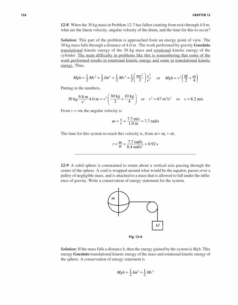
126 C H A P T E R 12

12-8 When the 30 kg mass in Problem 12-7 has fallen (starting from rest) through 4.0 m, what are the linear velocity, angular velocity of the drum, and the time for this to occur?

Solution: This part of the problem is approached from an energy point of view. The 30 kg mass falls through a distance of 4.0 m . The work performed by gravity Goesinto translational kinetic energy of the 30 kg mass and rotational kinetic energy of the cylinder. The main difficulty in problems like this is remembering that some of the work performed results in rotational kinetic energy and some in translational kinetic energy. Thus,

ω= + = +

Mgh Mv I Mv mr v

r12

12

12

12 2

2 2 22 2

2 or ( )= +Mgh v M m2 4

2

Putting in the numbers,

= +

v30 kg 9.8 ms

4.0 m30 kg

210 kg

422 or =v 67 m /s2 2 2 or =v 8.2 m/s

From v = rw, the angular velocity is

ω = = =vr

7.7 m/s1.0 m 7.7 rad/s

The time for this system to reach this velocity is, from w = wo + at,

ωα= = =t 7.7 rad/s

8.4 rad/s0.92 s2

12-9 A solid sphere is constrained to rotate about a vertical axis passing through the center of the sphere. A cord is wrapped around what would be the equator, passes over a pulley of negligible mass, and is attached to a mass that is allowed to fall under the influ-ence of gravity. Write a conservation of energy statement for the system.

Fig. 12-6

Solution: If the mass falls a distance h, then the energy gained by the system is Mgh. This energy Goesinto translational kinetic energy of the mass and rotational kinetic energy of the sphere. A conservation of energy statement is

ω= +Mgh I Mv12

12

2 2

14_Oman_c12-P119-128.indd 126 04/11/15 3:05 PM


The velocity of a point on the string and the velocity of the mass are the same and are related to the angular velocity through v = rw, so the energy statement can be written in terms of v. Additionally, the formula for I = 2mr2/5 can be substituted, so

( )= + = +Mgh I vr

Mv m M v12

12 5 2

2

22 2

Note that the energy statement could have been written in terms of w rather than v.

12-10 For Problem 12-9, take the mass of the sphere as m = 2.0 kg, r = 0.30 m, the hang-ing mass as M = 0.80 kg, and the height the mass falls through as h = 1.5 m. Find the velocity of the hanging mass and the angular momentum of the sphere.

Solution: The velocity of the mass, the rope, and a point on the equator of the sphere (all the same velocity) are from the energy statement

v+

0.80 kg 9.8 ms

1.5 m =2.0 kg

50.80 kg

222 or =v 3.8 m/s

The angular velocity of the sphere is

vrω = = =3.8 m/s

0.30 m 13 rad/s

The angular momentum of the sphere is

L Iω= ⋅

= ⋅2 2.0 kg(0.30 m)

513 rad

s 0.94 kg m /s2

2

As an added exercise, give the pulley in this problem a mass and a radius, and go through the problem again. Remember that I and w will be different for the pulley.

14_Oman_c12-P119-128.indd 127 04/11/15 3:05 PM

CHAPTER 13

EQUILIBRIUM

129

The only difficulty you will encounter in doing equilibrium problems is lack of familiar-ity with the mechanics of doing the problems. This is overcome by doing problems. The theory is simple. If something is not moving—that is, it is in equilibrium—then the sum of the forces on it must be zero. Likewise, if it is not rotating, then the sum of the torques must be zero.

For problems in two dimensions, these laws are stated very simply:

Fx 0∑ = Fy 0∑ = 0∑τ =

We start off with some simple problems requiring force analysis only and progress to problems involving torques.

13-1 Hang a 50 kg mass with ropes making angles of 30° and 45°, as shown in Fig. 13-1. Calculate the tension in the ropes.

Fig. 13-1

Solution: Note that all the forces come together at the knot in the rope, so draw a force dia-gram about this point. The only laws to apply are for equilibrium in the x and y directions.

F T Tx 0 : cos30 cos 451 2∑ = ° = ° F T Ty 0 : sin30 sin45 294 N1 2∑ = ° + ° =

This provides two equations in two unknowns. Because sin 45° = cos 45°, rewrite

T1(sin 30° + cos 30°) = 294 N or T1 = 215 N and

T2 cos 45° = (215 N)cos 30° or T2 = 263 N

As an exercise, work through this problem with different angles.

15_Oman_c13-P129-138.indd 129 04/11/15 3:08 PM

130 C H A P T E R 13

13-2 In the arrangement shown in Fig. 13-2, what is the minimum coefficient of friction to prevent the 8.0 kg mass from sliding?

Fig. 13-2

Solution: The forces come together where the cords come together. This point is not moving, so apply the equilibrium conditions here. The vector diagram at this point is also in Fig. 13-2.

The equilibrium conditions are

F T Fx 0 : cos601∑ = ° = F Ty 0 : sin60 39 N1∑ = ° =

Solving for T1,

T 39 Nsin60 45 N1 = ° =

The force is

F = 45 N cos 60° = 22.5 N

This force is supplied by the frictional force mmg, so

22.5 N8.0 kg 9.8 m/s

0.292µ =⋅

=

This is the minimum coefficient of friction that will prevent the system from moving.

13-3 A 500 N diver is on the end of a 4.0 m diving board of negligible mass. The board is on pedestals, as shown in Fig. 13-3. What are the forces that each pedestal exerts on the diving board?

Solution: There are no forces in the x direction, but in the y direction the pedestal at A and the diver are acting down while the force at pedestal B is acting up. Pedestal B

15_Oman_c13-P129-138.indd 130 04/11/15 3:08 PM

E Q U I L I B R I U M 131

is in compression, while pedestal A is in tension. Draw the vector diagram, and write the equations.

F F Fy A B0 : 500 N∑ = + =

Fig. 13-3

In this problem, apply 0∑τ = about pedestal A. Taking the rotation point at pedestal A,

the diver produces a clockwise torque and pedestal B a counterclockwise torque that are in equilibrium. Note that this is not the only possible rotation point.

FB0 : 500 N 4.0 m 1.5 m∑τ = ⋅ = ⋅

Solve for FB:

FB500 N 4.0 m

1.5 m 1,330 N= ⋅ =

Solve for FA:

FA = FB – 500 N = 1,330 N – 500 N = 830 N

As an exercise, write the 0∑τ = about pedestal B and the diver.

13-4 Place a 7.0 m uniform 150 N ladder against a frictionless wall at an angle of 75°. What are the reaction forces at the ground and wall and the minimum coefficient of fric-tion of the ground?

Solution: Figure 13-4 shows the ladder with the 150 N acting down at the center of the ladder and the sides of the triangle formed by the ladder, wall, and ground. The vector portion of the figure shows the two components of the reaction force at the ground. The reaction force at the ground is not necessarily in the direction of the ladder. This (vector) force can be written in terms of a force (magnitude) at an angle (with horizon-tal and vertical components) or directly in component form, as done here. Writing the force in component form helps to avoid the temptation to place the force at the same

15_Oman_c13-P129-138.indd 131 04/11/15 3:08 PM

132 C H A P T E R 13

angle as the ladder. Either way requires two variables. Since the wall is frictionless, the reaction at the wall is entirely horizontal. Refer to Fig. 13-4, and write the equilibrium conditions.

F F Rx H H0 :∑ = = F Fy V0 : 150 N∑ = =

Fig. 13-4

0∑τ = : The torque on the ladder is taken about the point where the ladder contacts

the ground. Note that this choice eliminates two variables from the torque statement. Torque is the (component of the) force at right angles to the lever arm times that lever arm. The 150 N weight has a component 150 N(cos75°) times 3.5 m. The reaction at the wall has a component RH (cos15°) times 7.0 m, so the sum of the torques equals zero statement is

[150 N(cos 75°)] 3.5 m = [RH(cos 15°)] 7.0 m or 150(0.90) N · m = RH(6.8) N · m

so

RH = (75 N)(cos 75°/cos 15°) = 20 N and FH = 20 N

FV and FH are related via the coefficient of friction FH = mFV, so m = 20/150 = 0.13.

Second Solution: There is another way to calculate the torques. Notice that the 150 N force is horizontally 0.90 m away from the pivot point. If the 150 N force vector is moved vertically so that its tail is on a horizontal line from the pivot point, then the torque is easily written as (150 N)(0.90 m). A similar operation can be performed on RH, yielding a torque RH(6.8 m). Vectors maintain their length (magnitude) and orientation (angle) but can be moved about a vector diagram for (our) convenience. If the torque statement is written in this way, it is identical to the torque statement in the first solution.

150 N · 0.90 m = RH(6.8 m)

As an exercise, redo the problem with a person of known weight positioned a specific distance up the ladder.

13-5 Place an 80 N ladder that is 8.0 m long on a floor and against a frictionless roller on a 5.0 m high wall. The minimum angle for equilibrium is 70°. Find the coefficient of friction between the ladder and the floor.

15_Oman_c13-P129-138.indd 132 04/11/15 3:08 PM


Solution: The roller is free to rotate, so the reaction force is normal to the ladder. This reaction force can be viewed as having vertical and horizontal components. The reac-tion force at the floor is written as vertical and horizontal components. The geometry and vector diagram are shown in Fig. 13-5. The length to the roller is obtained from the geometry:

sin 70° = 5.0 m/L or L = 5.3 m

Fig. 13-5

Write the force equilibrium equations.

F f Rx 0 : (sin70 )∑ = = ° ∑ = + ° =F N Ry 0 : (cos70 ) 80 N

The torque about the point on the floor is produced by the reaction force at the roller and the weight of the ladder taken at its midpoint

∑τ = ° = ⋅R0 : [80 N(cos70 )]4.0 m 5.3 m

Rewriting with f = mN,

mN = R(sin 70°) N + R(cos 70°) = 80 N (320 N · m)cos 70° = (5.3 m)R

Solve these equations from last to first to obtain

R = 20.6 N N = 73.0 N m = 0.26

13-6 A 20 kg beam 4.0 m long is pivoted at a wall and supported by a cable as shown in Fig. 13-6. What is the force at the wall and the tension in the cable?

Solution: There are two points of possible confusion in this problem. First, the mass of the beam is taken as down at the center of the beam. Second, the reaction of the wall, at the pivot, has two components, one up the wall (holding the end of the beam up) and one out of the wall (keeping the beam from sinking into the wall).

15_Oman_c13-P129-138.indd 133 04/11/15 3:08 PM

134 C H A P T E R 13

Fig. 13-6

Set up the vector diagram at the pivot and the point where the cable is attached. The reaction at the wall is shown with components up the wall and normal to the wall. The weight of the beam is shown as down and from the center of the beam with a compo-nent at a right angle to the beam. The tension in the cable is broken up into vertical and horizontal components (for the sum of the forces laws) and a component at right angles to the beam (for the sum of the torques laws). Applying the sum of the forces laws means looking at the vector diagram and adding up all the vectors in the horizontal or vertical directions.

∑ θ= + ° =F R Ty 0 : cos cos30 196 N ∑ θ= = °F R Tx 0 : sin sin30

In applying the sum of the torques, it is convenient to take the pivot point at the wall. Since the angle q is unknown, the least complicated sum of the torques statement will come from the tension in the cable and the weight of the beam.

Using the components at right angles,

∑τ = ° = ⋅T0 : [ (cos65 )]4.0 m 160 N 2.0 m

Solve the last equation for the tension in the cable.

= ° =T160 N

2 cos65 189 N

Use this value to solve for

R sinq = l89 N(sin30°) = 95 N and R cosq = 196 N – 189 N(cos30°) = 32 N

Now divide these two equations

θθ θ= = =R

Rsincos tan 95

32 3.0 or q = 71°

15_Oman_c13-P129-138.indd 134 04/11/15 3:08 PM


and finally, R is obtained from one of the original equations.

=°

° =R189 N(sin30 )

sin71 100 N

The main points in this problem are the detailed vector diagram and the choice of the wall as the pivot point in calculating the torques.

In the early problems, construction of the vector diagram was confined to one point where the forces all “came together.” In problems where there is a strut or ladder or some other extended object, the common mistake is to miss a force or torque and have an incomplete vector diagram.

13-7 Set up a 300 N strut 14 m long with a cable as shown in Fig. 13-7. Find the tension in the cable and the reaction force at the pivot.

Solution: The reaction force at the pivot is set up with vertical and horizontal compo-nents. The weight of the strut is taken at the center of the strut with the 2,000 N weight at the end. The tension is written along with all the components needed to write the force and torque equations.

Fig. 13-7

Apply the sum of the forces laws.

F F Tx H∑ = = °0 : cos40 F F Ty V∑ = = + + °0 : 2,000 N 300 N sin 40

Apply the sum of the torques law about the pivot point.

∑τ = ° + ° = °0 : [300 N(cos60 )]7.0 m [2,000 N(cos60 )]14 m (T cos70 )14 m

Note that the length of the strut does not influence the calculation.

Solve the torque equation for T.

2,150 N(cos 60°) = T cos 70° or T = 3,140 N

Use this value to find FH and FV.

FH = 3,140 N(cos 40°) = 2,410 N and FV = 2,300 N + 3,140 N(sin 40°) = 4,320 N

15_Oman_c13-P129-138.indd 135 04/11/15 3:08 PM

136 C H A P T E R 13

The reaction at the floor can be written in terms of magnitude and angle.

θ= + = = = °−F 2,410 4,320 4,950 N tan (4,320/2,410) 612 2 1

Another feature of equilibrium problems is that an object hung by two cords has its center of mass along a vertical line determined by the (extension of) intersection of those cords. The argument is based on the fact that a body hung by a cord has its center of mass along the extension of that cord. If the center of mass were not on this line, a torque would exist, and the body would move. Likewise, if the center of mass were not on the intersection of the two cords, a torque would exist and the body would move.

13-8 Consider a nonuniform bar of 200 N weight and 4.0 m length suspended horizon-tally between two walls where the angles between the walls and cables are 37° and 50°. What are the tensions in the cables?

Solution: The extensions of the cables specify the center of mass. Looking just to the center of mass and using the common side of the triangle, write

° = xctan37 and ° = − x

ctan50 4.0

Fig. 13-8

Solve for c, and set equal

−

° = °x x4.0

tan50 tan37

and 4.0 tan 37° – x tan 37° = x tan 50° or

x = °° + ° =4.0 tan37

tan37 tan50 1.55 m

Draw a vector diagram at the center of mass line. Write the equilibrium conditions as

T1 cos 53° = T2 cos 40° and T1 sin 53° + T2 sin 40° = 200 N

Rewriting,

T1 cos 53° – T2 cos 40° = 0 and T1 sin 53° + T2 sin 40° = 200 N

15_Oman_c13-P129-138.indd 136 04/11/15 3:08 PM


Multiplying and adding,

T1 cos 53° sin 40° – T2 cos 40° sin 40° = 0

T1 sin 53° cos 40° + T2 sin 40° cos 40° = 200 N(cos 40°)

and

=°

° ° + ° ° =°

° =T200 N(cos40 )

cos53 sin40 sin53 cos40200 N(cos40 )

sin93 153 N1

A sum of two angles trigonometric identity (see the Mathematical Background) was used in the denominator.

= °° =T

153 N(cos53 )cos40 120 N2

15_Oman_c13-P129-138.indd 137 04/11/15 3:08 PM

CHAPTER 14

GRAVITY

139

The basic law of gravity describes the force of one mass on another

= 1 22F G

m mr

(14-1)

where G is a constant that depends on the units of the m’s, the masses, and r, the distance between centers. In SI units, the gravitational constant is G = 6.7 × 10–11 N · m2/kg2. The gravitational force acts along the line of centers and is an action-reaction pair. (The force on both masses is the same.) Gravitational forces are vectors and superpose (add) as vectors.

The gravitational force of attraction for a mass of small (compared to the Earth) radius on the surface of the Earth is known as the weight of that mass on the Earth and is

= = =2F W Gmm

rmgE

E

(14-2)

with = / 2g Gm rE E being called the acceleration due to gravity. Weight then is the familiar W = mg. Acceleration units (the units of g) times mass produce force or weight units. Also, g is a vector that points between the centerline of the masses involved.

14-1 What is the gravitational force of attraction between two 7.5 kg bowling balls with 0.50 m between centers?

Solution: Use the gravitational force equation:

= = × ⋅⋅

= ×− −(6.7 10 N m /kg )7.5 kg 7.5 kg

(0.50 m)1.5 10 N1 2

211 2 2

28F G

m mr

Each ball is attracted to the other on a line between their centers.

Gravitational Potential

C Following the general form for potential energy, the gravitational potential is defined as the work performed by the gravitational force when r increases from r1 to r2.

∫ ∫ ∫= = − = −221

2

1

2

U F drGmm

rdr Gmm dr

rE

r

r

Er

r

The minus sign is in the integral because the force points opposite to the direction of increasing r. The force decreases as r increases. The integral definition is necessary because the force depends on r. Performing the integration,

= = −

1 1 12 11

2

U Gmm r Gmm r rEr

r

E

16_Oman_c14-p139-144.indd 139 31/10/15 4:01 PM

140 C H A P T E R 14

Look at the signs in this expression. If r1 is taken at the surface of the Earth and r2 above the Earth, then the gravitational potential at r2 is positive (less negative) with respect to the Earth.

Notice that the general expression for gravitational potential is

= −U Gmm

rE (14-3)

The zero of gravitational potential is at r = •. The gravitational potential is negative at the surface of the Earth and becomes more negative as we go in toward the center of the Earth.

With the gravitational potential energy and the conservation of energy, we can calculate the escape velocity. This is the velocity with which we would have to shoot something vertically up to completely remove it from the Earth’s gravitational pull.

14-2 Calculate the escape velocity on the surface of the Earth.

Solution: The escape velocity is the minimum velocity for a mass to escape the gravita-tional attraction of the Earth. Envision a mass being shot vertically up from the surface of the Earth, and write the energy statement for it at two levels, the surface of the Earth and some height r further out from the center of the Earth. The conservation of energy statement will read: the kinetic plus potential energy on the surface of the Earth equals the kinetic plus potential energy at some point r.

− = −12

121

22 2

2mv Gmm

r m v Gmm

rE

E

E (14-4)

The escape velocity is the velocity that will produce zero velocity (v2 = 0) when the mass is infinitely far away (when r = •, GmmE /r = 0). This reduces the equation to

=212v Gm

rE

E or = 2

1vGmr

E

E (14-5)

The mass and radius of the Earth are on the constants page of your text, so

=× ⋅ ×

×= ×

−2(6.7 10 N m /kg )6.0 10 kg6.4 10 m

1.1 10 m/s1

11 2 2 24

64v

As an exercise, calculate the escape velocity for the moon of radius 1.7 × 106 m and mass 7.4 × 1022 kg.

14-3 What initial vertical speed is necessary to shoot a satellite to 300 km above the Earth?

Solution: Use energy analysis and the same energy-balance equation as in the preceding problem with the velocity at 300 km equal to zero.

− = −+ ×

12 3.0 10 m

25mv

Gmmr

Gmmr

E

E

E

E

or = −+ ×

2 1 13.0 10 m

25v Gm r rE

E E

16_Oman_c14-p139-144.indd 140 31/10/15 4:01 PM

G R A V I T Y 141


v = ⋅ × ⋅ ××

−×

−2 6.7 10 N mkg

(6.0 10 kg) 16.4 10 m

16.7 10 m

2 112

224

6 6

or

v = 2.4 × 103 m/s

Satellites

A satellite, whether artificial or moon, moves in a circular orbit about a larger planet. The gravitational force supplies the center-directed acceleration necessary to make the satellite move in a circular orbit. Mathematically stated, the force balance is

=1 22

22

Gm m

rm v

r

which reduces to v2r = Gm1 with the right hand side a constant.

The orbit radius, period, and velocity are related through

π = =2 1rT v

Gmr or π= 2

1T r r

Gm (14-6)

14-4 Calculate the speed, period, and radial acceleration of a satellite placed in orbit 400 km above the Earth.

Solution: The orbit radius is 6.4 × 106 m + 0.4 × 106 m = 6.8 × 106 m. The velocity is

= =× ⋅ ×

×

=−6.7 10 N m /kg (6.0 10 kg)

6.8 10 m7,690 m/s

11 2 2 24

6

1/2

vGm

rE

The period is

T rGmE

π π= = ×× ⋅ ×

=−2 2(6.8 10 m)

6.7 10 N m /kg (6.0 10 kg)93 min

3 6 3

11 2 2 24

1/2

The radial acceleration is

= = =× ⋅ ×

×=

−6.7 10 N m /kg (6.0 10 kg)(6.8 10 m)

8.7 m/srad

2

2

11 2 2 24

6 22a v

rGm

rE

A geosynchronous satellite is one that is orbiting at the equator and always over the same spot on Earth. Using the expression for the period of a satellite, find the height for a satel-lite with a period of 1.0 day.

16_Oman_c14-p139-144.indd 141 31/10/15 4:01 PM

142 C H A P T E R 14

Kepler’s Laws

There are three Kepler’s laws that govern planetary motion. Kepler based these laws on observations made before the invention of the telescope! They are:

I. All planets move in elliptical orbits with the sun at one focus. II. A line from the sun to the planet sweeps out equal areas in equal lengths of time

(Fig. 14-1).III. The square of the period is proportional to the cube of the semimajor axis of the

ellipse.

C Kepler’s second law is consistent with the angular momentum of the motion being a constant. Refer to Fig. 14-1. For small angles, the area swept out by the arc is equal to the area of a triangle with the side rΔq nearly perpendicular to the sides r. The area of the triangle is (1/2)(rΔq)r. In calculus notation, the differential area is dA = (1/2)r2dq, and the change in area with time is

θ ω= = =12

12

12

2 2dAdt r d

dt r rv

Fig. 14-1

The magnitude of the cross product of two vectors is proportional to the area of the trap-ezoid defined by the vectors (see the Mathematical Background). Here the two vectors defining the area swept out are r and v. Rewriting rv as the magnitude of the cross product of r and v, or, more conveniently, mv, we get

dAdt m mvr= ×1

2 | |

but r × mv is L, the angular momentum, which is a constant of the motion. Kepler’s second law is equivalent to conservation of angular momentum.

= 2dAdt

Lm

Going back to rotational dynamics, dL/dt = r × F, and in planetary motion, the force is gravitational and acts along r, so r × F must equal zero, and if the derivative of the angu-lar momentum is zero, then the angular momentum is a constant.

Equation (14-6) is based on conservation of energy and shows T as proportional to the 3/2 power of r. This is verification of Kepler’s third law for the case of circular orbits.

14-5 The orbit radius of the satellite of problem 14-4 is 6.8 × 106 m, and the period is 93 min. The orbit radius of the moon is 3.8 × 108 m, and the period is 27.3 days. Is this consistent with Kepler’s third law?

16_Oman_c14-p139-144.indd 142 31/10/15 4:01 PM

G R A V I T Y 143

Solution: Kepler’s third law states that T is a constant times the 3/2 power of the radius, so

= 3/2T krm m and = 3/2T krs s

If the constant is the same, then

=

3/2TT

rr

m

s

m

s


TT

m

s= =

27.3 day93 min

24 hday

60 minh 420 and

rrm

s

= ××

=3.8 10 m

6.8 10 m420

3/28

6

3/2

The satellite and moon orbits verify Kepler’s third law for circular orbits.

16_Oman_c14-p139-144.indd 143 31/10/15 4:01 PM

CHAPTER 15

SIMPLE HARMONIC MOTION

145

Simple harmonic motion is the phrase used to describe a repetitive harmonic motion such as the motion of a mass oscillating up and down on the end of a spring, the rotation of a point moving at constant speed along a circle, or a pendulum in small (amplitude) oscillation. The most convenient visualization of an oscillating system is the mass-spring system. This is also the one most analyzed. Simple harmonic motion is often characterized by the period, the time for one oscillation, and the amplitude, the maximum excursion from equilibrium. (Period is the time for one repetition and is measured in seconds. while the frequency is the reciprocal of the period and is mea-sured in hertz or l/s.) More complete analysis usually involves writing statements about the total energy of the system.

Fig. 15-1

For a first look at simple harmonic motion, consider the analysis of a mass-spring system. The kinetic energy is (1/2)mv2, the energy associated with the moving mass, and the potential energy of the system is (1/2)kx2, the energy associated with the elon-gation and compression of the spring. Here we assume that the spring is a Hook’s law spring obeying F = –kx. You may want to review the discussion of the energy stored in a Hooke’s law spring in Chapters 7 and 8.

C To describe the motion of the mass from a force point of view, take the force as –kx and equate that to ma, with a written as the second derivative of position.

− =2

2kx m d xdt

(15-1)

If you don’t have much experience in calculus, this may look like a formidable equation. It is not. It has a very simple and obvious (once you’ve seen it) solution. Acceleration is the time derivative of velocity (a = dv/dt), and velocity is the time derivative of displace-ment (v = dx/dt), as defined in Chapter 1. Acceleration, then, can be written as the second derivative of the displacement.

17_Oman_c15-p145-156.indd 145 31/10/15 4:02 PM

146 C H A P T E R 15

The solution to this equation requires that the second derivative of a function of x with respect to time be proportional to the negative of the function. This reduces to the question: what function differentiated twice yields the negative of itself? The answer is a sine or cosine function or a linear combination of both. If you have not encountered this yet, see the table of derivatives in the Mathematical Background.

The derivative of the sine function is the cosine function, and the derivative of the cosine function is the negative of the sine function. Two derivatives of the sine function yield the negative of itself. This is also true of the cosine function. The solution also can be written as the sine or cosine of a constant times t plus a phase angle. A cosw t + B sin w t and C(cos or sin)(w t + J ) are equivalent solutions.

Take as a general solution

x = A cos w t + B sin w t

If the starting position (t = 0) is taken as an extreme of the motion, corresponding to maximum compression of the spring, then B = 0, and A is the amplitude of the motion. If the starting position were taken at the midpoint of the motion, then at t = 0 the ampli-tude would have to be zero; therefore, A = 0 and B would be the amplitude. (Remember, sin 0 = 0 and cos 0 = 1.) The choice of initial condition determines whether the motion is described by a sine or cosine function.

Use as a solution x = Bsinw t. Take two time derivatives to obtain

ω ω= − sin2

22d x

dtB t

and substitute in the force law statement –kx = –m(d 2x/dt 2) to get

ω− = − 2k m or ω = /k m (15-2)

In the statement x = Bsinw t, w is 2p/T. The 2p effectively scales the sine function, and the ratio t/T determines the fraction of 2p required for determining the value of the function. For example, at t = T (one period), the sine function has gone through one cycle. At t = T/2 (one-half period), the sine function has gone through one-half cycle. Because of the 2p factor, w is called the angular frequency. The term frequency applies to f in the relation

w = 2p(1/T ) = 2pf (15-3)

In solving problems, be careful to differentiate between frequency f and angular frequency w.

15-1 A mass-spring system has a mass of 2.0 kg, a spring with a constant of 3.0 N/m, and an amplitude of vibration of 0.10 m. Calculate the angular frequency and frequency. Write expressions for the position, velocity, and acceleration as a function of time. Take t = 0 at the equilibrium position. Graph position, velocity, and acceleration as a function of time.

Solution: The angular frequency is

kmω = = ⋅ = =3.0 N

2.0 kg m32

1s 1.2 1

s

17_Oman_c15-p145-156.indd 146 31/10/15 4:02 PM

S I M P L E H A R M O N I C M O T I O N 147

The frequency is

π π π= = ⋅ = =12

12

3.0 N2.0 kg m

12

32

1s 0.19 1

sf km

If t = 0 at the equilibrium position, then the displacement must be given by x = B sin w t.

At t = 0, the sine function is zero, so this is the appropriate function to describe the motion. For an amplitude of 0.10 m, this expression should read

= (0.10 m) sin 32

1sx t or x = (0.10 m) sin 2p 0.19(1/s)t

The velocity is the time derivative of x, or

= 0.10 32

ms cos 3

2v t

At t = 0, the velocity, as the mass passes through the equilibrium position, is a maximum. The acceleration is another time derivative of the velocity, or

= −0.10 32

ms

sin 322a t

At t = 0, the acceleration is zero; the spring is neither elongated nor compressed (at the equilibrium position), so the force (and acceleration) of the mass is zero.

Fig. 15-2

These three curves graphed one under the other in Fig. 15-2 give a good picture of the motion from the position, velocity, and acceleration point of view.

Look at these graphs, and visualize the motion. At the equilibrium position, displace-ment is zero, the velocity is a maximum, and acceleration is zero. As the mass moves to

17_Oman_c15-p145-156.indd 147 31/10/15 4:02 PM

148 C H A P T E R 15

the positive maximum displacement, the velocity decreases to zero, and the acceleration (down) increases to a maximum. At the maximum displacement, the velocity is zero, and the acceleration is a maximum. As the mass starts down, the velocity is negative, reaching maximum again as the mass passes through equilibrium. Go over this picture of the motion until the relationship between position, velocity, and acceleration is clear in your mind.

15-2 A piece of metal rests on top of a piston executing simple harmonic motion in the vertical plane with an amplitude of 0.20 m. At what frequency will the piece of metal “float” at the top of the cycle?

Solution: Take the motion to be described by y = (0.20 m)cosw t.

Two derivatives produce the acceleration a = –(0.20 m)w 2 cosw t. The maximum accel-eration, which is the constant (0.20 m) w 2, is at the extreme of the motion, where the cosine term is 1. At the bottom of the cycle, the piece of metal will experience an accel-eration greater than g, and at the top, an acceleration less than g. The piece will “float” when that acceleration is greater than g.

ω = =(0.20 m) 9.8 ms

22g or ω = =

9.8 m/s0.20 m 7.0 1

s

2

or π= =12

9.8 m/s0.20 m 1.1 1

s

2

f

Fig. 15-3

15-3 A mass-spring system has a mass of 0.50 kg and period of 1.0 s. The maximum velocity is 0.20 m/s. Find the frequency, angular frequency, constant of the spring, and displacement for this velocity and period.

Solution: The frequency is the reciprocal of the period, or f = 1.0(1/s), and the angular frequency is 2pf, or 2p(1/s). The spring constant comes from the relation

ω = km or ω π= = = =[2 (1/s)] 0.50 kg 20

kgs

m/m 20 N/m2 22k m

The general expression for velocity is v = A w cos w t, where Aw is the maximum veloc-ity. It makes no difference whether the function is a sine or a cosine. The maximum velocity is still Aw. The amplitude for this particular motion then is

A vω π= = =

0.20 m/s2 (1/s) 0.032 m

17_Oman_c15-p145-156.indd 148 31/10/15 4:02 PM


15-4 An 0.80 kg mass hangs from a spring. When an additional 0.20 kg mass is added, the spring elongates another 3.0 cm. What is the period of oscillation of the spring?

Solution: First, determine the force constant of the spring from F = – kx.

= ⋅ × −k0.20 kg 9.8 ms

3.0 10 m22 or = ⋅ =k

0.20 kg 9.8 m/s0.03 m 65 N/m

2

The period is the reciprocal of the frequency

ω π π= = =2 2km f T

so

2 20.80 kg65 N/m 0.70 sT m

kπ π= = =

15-5 An oscillating mass-spring system has a displacement of 10 cm, a velocity of –12 m/s, and an acceleration of –20 m/s2. What is the period of the system?

Solution: Since the displacement is not zero at t = 0, the motion cannot be described with a sin w t function. Since the velocity is not zero at t = 0, the motion in not at an extreme and cannot be described with a cos w t function. Because of the initial conditions, a sine or a cosine function of w t plus a phase angle must be used. It makes no difference whether a sine or a cosine function is used because the phase angle can absorb the 90° difference between a sine and a cosine function. Look at Fig. 15-4, and go over the logic in this paragraph until it is clear in your mind.

Take x = A cos(w t + J) and then v = – Aw sin(w t + J) and a = – Aw 2 cos(w t + J). Using the equations for x and a, at t = 0,

ω = − (0)(0)

2 ax and ω = =

20 m/s0.10 m 14 1

s

2

The period is from

ω π= 2T or π

ωπ= = =2 2

200s 0.44 sT

The phase angle comes from v(0) and a(0).

ϑω ϑ ω ϑ= =(0)

(0)sincos

1 tanva or ϑ ω= =

−−

=tan(0)(0) 200 1

s12 m/s20 m/s

8.482va so ϑ = 83°

The specific functional relations are

x = A cos(w t + 83°), v = –Aw sin(w t + 83°), and a = –Aw 2 cos(w t + 83°)

17_Oman_c15-p145-156.indd 149 31/10/15 4:03 PM

150 C H A P T E R 15

Fig. 15-4

Look at these relations and relate them to what the system is doing at t = 0. The amplitude is past its maximum positive excursion and on the way down, corresponding to the cosine function at 83°. The velocity is negative and heading toward its most negative value, as is the negative sine function at 83°. The acceleration is negative and tending toward zero, just as is the negative cosine function at 83°.

Energy Analysis

Simple harmonic motion can be analyzed from an energy point of view. The energy stored in a spring is kx 2/2, and the energy stored in the mass by virtue of its velocity is mv 2/2. A total energy statement for the system then is

+ =2 22 2kx mv E (15-4)

which is most easily evaluated by looking at the extrema of the motion.

At v = 0 where = 2max2

Ekx

or at x = 0 where = 2max2

Emv

15-6 Find the maximum velocity of a mass-spring system with a mass of 2.0 kg, spring constant of 0.80 N/m, and amplitude of oscillation of 0.36 m.

Solution: All the energy of the system is stored in the spring at maximum displacement, so the total energy is

= = =20.80 N

m(0.36 m)

2 0.052 Jmax2 2

Ekx

This is the total energy in the system, and at zero displacement, all this energy, is in kinetic energy, so

=2 0.052 Jmax2mv

or = ⋅

=v 2 0.05 J2.0 kg 0.23 m/smax

1/2

It is relatively easy, and quite instructive, to show that the total energy of an oscillating system is a constant. Take an oscillating system with x = A sinw t and

17_Oman_c15-p145-156.indd 150 31/10/15 4:03 PM


velocity v =Aw cos w t. Now place these expressions for x and v into the total energy statement

+ =2 22 2kx mv E so ω ω ω+ =sin

2cos

22 2 2 2 2kA t mA t E

But from the previous analysis, w 2 = k/m, so the statement reads

ω ω+ =2 sin 2 cos2

22

2kA t kA t E

and since sin2 w t + cos2w t = 1,

=2

2kA E

which shows that the total energy does not vary over time. The energy does not vary over one cycle; it goes back and forth from kinetic to potential in a manner such that the total (energy) remains a constant.

15-7 Find the amplitude, angular frequency, and frequency for a mass-spring system with a mass of 2.0 kg that is oscillating according to x = (2.0 m)cos(6pt/s). Write and graph the expressions for position, velocity, and acceleration. Finally, calculate the total energy of the system.

Solution: The amplitude, angular frequency, and frequency are determined by comparing x = (2.0 m)cos (6p t/s) to the standard form x = A cos w t = A cos 2pft.

The amplitude is 2.0 m. The angular frequency is 6p(1/s). The frequency is 3(1/s). The expressions for position, velocity (first derivative), and acceleration (second derivative) are shown in Fig. 15-5 associated with the graphs.

In Fig. 15-5, the units are dropped in the argument of trigonometric functions, and the maximum values for the velocity and acceleration are placed on the graphs.

Fig. 15-5

17_Oman_c15-p145-156.indd 151 31/10/15 4:03 PM

152 C H A P T E R 15

The conservation of energy statement is + =/2 /22 2mv kx E. For a 2.0 kg mass, the total energy can be evaluated when x is zero and the velocity maximum

π

= = =22.0 kg(12 m/s)

2 1,420 Jmax2 2

Emv

15-8 For a 3.0 kg mass-spring system executing simple harmonic motion according to y = (4.0 cm)cos(pt/4 – p/6), what is the total energy and the y position for equal division of the energy between kinetic and potential?

Solution: The general expression for displacement is y = A cos(w t + J). Looking at the two expressions,

ω π= = 41s

km so k mω π= = =

41s

3.0 kg m/m 1.85 N/m22

2 2

Knowing k, the total energy is

= = × = ×− −2

1.85 Nm (16 10 m ) 29.6 10 J

24 2 4E kA

The potential energy due to position is /22ky and y = A cos(w t + J), so the energy due to position is kA tω ϑ+cos ( )/22 2 . The energy due to position is 1/2 the total when the factor cos2(w t + J) = 1/2 or ω ϑ+ =cos( ) 1/ 2t .

For this particular system, the time for equal division of the energy is when

π π( )− =cos 4 612

t , π π− = −4 6 cos 1

21t , π π π− =4 6 4t , π π=4

512t , or = 5

3 st

The position of the mass for equal division of the energy is

π π π( ) ( )= − = =(4.0 cm)cos 453 6 (4.0 cm)cos 3

12 2.83 cm/2

yE

As an exercise, calculate the velocity at this time.

15-9 A 0.20 kg block traveling at 20 m/s slides into and sticks to an 0.80 kg block rest-ing on a frictionless surface and connected to a spring with force constant 80 N/m. What is the angular frequency, frequency, and displacement as a function of time? Also, what fraction of the original energy in the moving block appears in the system?

Solution: The collision is inelastic; the blocks stick together, so applying conservation of momentum, 0.20 kg(20 m/s) = (1.0 kg)V. The velocity of the 1.0 kg combination is V = 4.0 m/s. This is the velocity of the system at zero displacement. The analysis of this collision is similar to the ballistic pendulum problem in Chapter 10.

The total energy of the oscillating system is

= = =21.0 kg

216 m

s8.0 J

2 2

2E mV

17_Oman_c15-p145-156.indd 152 31/10/15 4:03 PM


Fig. 15-6

The angular frequency is

ω = = =km

80 N/m1.0 kg 8.9 1

s

The frequency is from

w = 2pf or f = w/2p = 1.4(1/s)

The general expression for the displacement is y = A sin w t. The sine function without a phase angle completely describes the motion because it starts (t = 0) at the equilibrium position with maximum velocity. The amplitude of the motion is obtained from

=/22kA E or = = ⋅ =A Ek

2 2 8.0 J80 N/m 0.45 m

so the specific expression for the displacement is

y = (45 cm) sin(1.4t/s)

The initial energy is all in the small block

= = =20.20 kg(20 m/s)

2 40 J2 2

E mvi

The energy in the oscillating system is 8.0 J, so the fraction of the original energy that appears in the oscillating system is F = 8.0 J/40 J = 0.20.

Applications

The oscillating simple pendulum can be analyzed in terms of force. For small oscilla-tions, the tension in the cable can be written in components, one vertical and the other the “restoring force,” the force that returns the mass to equilibrium. For small q, cos q ≈1 and sin q ≈ x/, with x being the displacement, approximately equal to the arc length.

Fig. 15-7

17_Oman_c15-p145-156.indd 153 31/10/15 4:03 PM

154 C H A P T E R 15

For small angle oscillations F cos q ≈ F and F sin q ≈ –mgx/ = –(mg/)x. Notice that in this equation mg/ plays the same role as k in the mass-spring systems.

By analogy, then

ω = =/mgm

g and π= 2T g

The most important point to note is that the period is independent of the mass. Histori-cally, this was one of the first instruments to measure g, the gravitational constant.

C The torsional pendulum, a disk suspended by a thin rod, can be analyzed using torque. The disk is rotated by applying a torque. Torque is proportional to the angle in the same manner as force is proportional to compression (or elongation) in a spring. The torque is written in terms of the moment of inertia and the angular acceleration [T = Ia = I(d2q/dt2)], which is set equal to the total torque, – kq the torsional constant times the angle, yielding

θ κθ= −2

2I ddt

which is the same form as the force equation for the oscillating mass-spring system. By analogy, then

q = qmax sin w t where ω κ= I and π κ= 2T I

Fig. 15-8

15-10 What is the restoring constant (torsional constant) for a disk of mass 3.0 kg and radius 0.20 m oscillating with a period of 2.0 s?

Solution: The moment of inertia for a disk is

= = = ⋅23.0 kg (0.20 m)

2 0.060 kg m2 2

2I mr

The restoring constant is

κ π π= =

⋅ ⋅= ⋅4 4 0.060 kg m

4.0 s0.59 N m

2

2

2 2

2I

T

Note that these are the correct units because torque has the dimensions N · m, and in torque = –kq the angle is in (dimensionless) radians.

17_Oman_c15-p145-156.indd 154 31/10/15 4:03 PM


Damped Mass-Spring System

C The system is usually depicted as a mass-spring with a dashpot, a piston in a thick liquid. In the case of the spring, the restoring force is proportional to displacement, com-pression, or elongation of the spring. With the piston in the fluid, however, the retard-ing force is proportional to velocity, not position. Move your hand through water and notice that the retarding force (the force on your hand) is proportional to velocity! The velocity-dependent force component of a typical automobile suspension is called a shock absorber. It is usually a piston in a cylinder of oil. Since the retardation force is velocity dependent, the differential equation governing the motion is

= − −2

2m d xdt

kx b dxdt (15-5)

Notice that the velocity-dependent term has the same sign as the displacement-dependent term. It too opposes the motion.

Fig. 15-9

This differential equation is solved with sophisticated techniques. Here we give an intui-tive solution.

This second order differential equation is solved as a product of solutions, the position-dependent part and the velocity-dependent part. The position-dependent part is a sine or a cosine function with a phase angle. The velocity-dependent part is from the velocity-dependent part of the equation

= −2

2m d xdt

b dxdt

17_Oman_c15-p145-156.indd 155 31/10/15 4:03 PM

156 C H A P T E R 15

The solution to this part of the equation is one that when differentiated once produces the negative of itself. The function that does this is an exponent to the negative power. The particular solution that satisfies this differential equation is

ω ϑ= ′ +− cos( )/2x Ae tbt m (15-6)

where w′ is slightly different from w. The damping of the exponential does exactly as we know from experience. Oscillations subject to velocity damping (a velocity-dependent restoring force) eventually die out.

17_Oman_c15-p145-156.indd 156 31/10/15 4:03 PM

CHAPTER 16

FLUIDS

157

There are several definitions and concepts that are unique to the study of fluids. Let’s review these basic definitions and concepts, working some problems along the way.

Density is simply mass per unit volume or, symbolically, r = m/V. The density that is most useful in problems is the density of water, which is 1 g/cm3 or 1,000 kg/m3.

The ratio called specific gravity is better called the specific density because it is the ratio of the density of another substance to the density of water. Aluminum has a specific gravity of 2.7, which means that for the same volumes, aluminum has 2.7 times the mass of water. Relative density or specific gravity is used to measure the relative amount of sulfuric acid (compared to water) in a storage battery or the relative amount of ethylene glycol (compared to water) in an automotive cooling system.

Pressure

The pressure in a fluid is defined as the force per unit area, p = F/A. And the units of pressure are N/m2, also called a pascal (or Pa). Atmospheric pressure, the force per unit area exerted by the air, is 1.0 × 105 Pa = 15 1b/in2 = 1 atm.

To determine the pressure at any depth in a liquid, consider the differential change in force due to a column of liquid of cross section A. The increase in force between the top and bottom of this differential piece is equal to the weight of the piece.

It is convenient to write the mass of this little piece as rΔV so that the force (difference) is

ΔF = rgΔV (16-1)

Now ΔV for this piece is AΔy, so ΔF = rgAΔy. The pressure is the force per unit area, so rewriting,

Δp = ΔF/A = rgΔy (16-2)

Dropping the differential notation,

pbot – ptop = rg(ybot – ytop) (16-3)

18_Oman_c16-p157-166.indd 157 04/11/15 3:09 PM

158 C H A P T E R 16

Fig. 16-1

If y is measured from the bottom of the liquid, then insert a negative sign on the right side of the equation. This discussion of pressure leading up to equation (16-3) is equally valid whether the delta or differential notation is used. This is true of most of the discussion of fluids. We start with delta notation and switch to differential notation in some later development.

16-1 Calculate the pressure at the bottom of a 3.0 m deep pool.

Solution: Δp = rgh = 1,000 kg/m3(9.8 m/s2)3.0 m = 2.9 × 104 Pa

Notice that this pressure is the difference between the top and the bottom. This difference is known as the gauge pressure. Adding the atmospheric pressure at the top surface of the pool gives the absolute pressure at the bottom of the pool.

The typical automobile tire pressure is the gauge pressure. With the tire inflated, the pres-sure might read 30 lb/in2. If the tire were “flat,” the pressure would read zero. The gauge pressure for the “flat” tire would be zero, but the absolute pressure would be 15 1b/in2. Likewise, a tire with a gauge pressure of 30 lb/in2 would have an absolute pressure of (30 + 15) lb/in2. The gauge that measures the tire pressure is measuring the difference in pressure between inside and outside of the tire.

Pressure exerted on a liquid in a closed container is transmitted throughout the liquid. The pressure is the same in every direction, varying only with height, as described by equation (16-3). In most devices using fluids to transfer forces, the fluid is nearly incom-pressible, and height variations are insignificant.

16-2 Consider the classic problem of a hydraulic lift. In a typical service station, l2 atm is applied to the small area with the lifting column 9.0 cm in radius. Find the force trans-ferred to the large area and the mass of vehicle that can be lifted.

Fig. 16-2

18_Oman_c16-p157-166.indd 158 04/11/15 3:09 PM

f lu i d s 159

Solution: The hydraulic fluid is at the same level, so

p1 = p2 or =1

1

2

2

FA

FA

A force F1 applied at A1 is multiplied by the ratio of the areas, so

F2 = (A2/A1) F1

The lifting force F2 also can be rewritten as F2 = A2(F1/A1) = A2p1, and putting in the numbers,

F π ( )= × = ×(9.0 cm) 12 atm 1.0 10 N/matm

m100 cm 3.0 10 N2

25 2 2

4

And the equivalent mass (from F = mg) is 3.1 × 103 kg. This number is somewhat larger than the mass of typical cars.

Barometer and Manometer

A simple atmospheric air pressure gauge is the mercury barometer. A closed tube is filled with mercury and then inverted in a beaker of mercury. The pressure at the top of the mercury column is zero. And the column is held up by the (atmospheric) pressure on the surface of the mercury. Looking to Fig. 16-3, the pressure at the bottom of the column is rgh. This experiment was first done by Torricelli, and the pressure was given as the pres-sure associated with the column of mercury. Pressures are often measured in millimeters of mercury (mmHg) or torr and refer back to this experiment.

Fig. 16-3

An open tube manometer, as depicted in Fig. 16-3, can be used to measure pressure. The force exerted by the gas is pA, and this force raises the column of (usually) mercury by exerting a force equal to rgV, the weight of the column. The volume of the column V is Ah, so equating forces,

pA = rgAh or p = rgh (16-4)

The manometer measures the difference in pressure between two points and, as such, measures gauge pressure. The open tube manometer is equally valuable as a

18_Oman_c16-p157-166.indd 159 04/11/15 3:09 PM

160 C H A P T E R 16

vacuum gauge. The difference in column height (the height of the mercury in the open tube is now lower than in the tube connected to the vacuum chamber) is a measure of the vacuum.

Buoyancy

Material objects appear to weigh less when partially or completely submerged in liquids. This apparent loss in weight is due to the buoyant force of the liquid. This buoyant force is expressed by Archimedes’ principle: a body partially or completely immersed in a liquid is buoyed up by a force equal to the weight of the liquid displaced.

16-3 The classic problem in buoyancy is to determine if a “gold” statue is really gold by measuring its weight in and out of water. A certain “gold” statue weighs 70 N when out of water and 64 N when immersed in water.

Solution: With the statue suspended from a scale, the weight is mg, or density times g, times the volume of the statue. In equation form, mg = r?gV = 70 N.

In water the statue weighs less because of the buoyant force: r?gV – rWgV = 64 N. Subtracting one equation from the other, we can determine the volume from

rWgV = 6 N 1,000 kg/m3(9.8 m/s2)V = 6 N V = 6.1 × 10–4 m3

With this value for V, calculate the unknown density from the first equation.

r?gV = 70 N ρ =×

= ×−?70 N

6.1 10 m (9.8 m/s )12 10 kg/m4 3 2

3 3

This density is much less than the density of gold (rgold = 19 × 103 kg/m3) and closer to the density of lead (rlead = 11 × 103 kg/m3), suggesting that the statue is lead with a thin covering of gold.

This same experiment can be conducted by lowering the statue into a beaker of water on a scale. The volume is determined by the increase in the level of water in the beaker. The drop in tension in the cord is offset by the increase in the scale reading when the statue is lowered into the beaker, and the calculations proceed as before.

16-4 A U-tube originally containing mercury has water added to one arm to a depth of 20 cm. What is the pressure at the water-mercury interface? What is the height of the mercury column as measured from the water-mercury level?

Solution: Assume that the difference in air pressure can be neglected. The pressure at the water-mercury interface is due to the column of water plus the atmospheric pressure po, or p = po + rWg · 20 cm. Neglecting po gives the gauge pressure as

p = 1,000 kg/m3 (9.8 m/s2)20 × 10–2 m = 1,960 Pa

18_Oman_c16-p157-166.indd 160 04/11/15 3:09 PM

f lu i d s 161

Fig. 16-4

At this level (the level of the interface), the pressure on the mercury arm must be the same. (If it were not, the liquids would move!) The height of the mercury level is

1,960 Pa = rM ghM or hM =×

=1,960 N/m14 10 kg/m (9.8 m/s )

1.4 cm2

3 3 2

As we expect, the same pressure is produced by a much shorter column of mercury.

Second Solution: Analytically, the problem can be approached by writing expressions for the pressure at the level of the water-mercury interface.

In the left arm, pW = po + rWghW, where the subscript W refers to the water column. In the right arm, the pressure is pM = po + rMghM, where the subscript M refers to the mercury column.

Since these pressures must be equal at the water-mercury interface,

rWghW + po = rMghM + po or rWhW = rMhM

For this problem,

ρρ= = =20 cm 1

14 1.4 cmh hM WW

M

Practice variations of this problem with different liquids (different densities).

16-5 A rectangular-shaped open-top steel barge is 10 m by 3.0 m and has sides 1.0 m high. The mass of the barge is 8.0 × 103 kg. How much mass can the barge hold if it can safely sink 0.75 m?

Solution: The volume of water displaced is length times width times allowed depth; thus 10 m × 3.0 m × 0.75 m = 22.5 m3. The buoyant force is the weight of the water displaced (Archimedes’ principle)

FB = rgV = 1,000 kg/m3(9.8 m/s2)22.5 m3 = 2.2 × 105 N

18_Oman_c16-p157-166.indd 161 04/11/15 3:09 PM

162 C H A P T E R 16

Fig. 16-5

This buoyant force must support the barge (mB) plus the load (mL).

2.2 × 105 N = g(mB + mL), mB + mL = 22 × 103 kg, and mL = 14 × 103 kg

As an additional exercise, calculate how deep the unloaded barge will sink in the water.

16-6 An iceberg floats in seawater. What percentage of the iceberg is submerged (rice = 0.92 × 10–3 kg/m3; rSW = 1.0 × 103 kg/m3)?

Solution: Assume a cubical iceberg of side s. You can assume any shape you wish. Cubical, however, seems convenient. The mass of the cubical iceberg is rices3, and the weight is rices3g. Since the density of the iceberg is less than the density of the seawater, the iceberg will float. The buoyant force of the seawater is rSWg times the volume sub-merged. Since the iceberg is cubical, the submerged volume must be s2, the area of the bottom of the iceberg, times a fraction of the side K times s.

This buoyant force must equal the weight of the iceberg

rices3g = rSWgs2(Ks)

So K, the fraction of the iceberg submerged, is

ρρ= = =0.92

1.0 0.92iceKSW

Thus 92 percent of the iceberg is submerged.

Fluid Flow

The last, and possibly most important, of the fluid laws is associated with the flow of liquids through tubes of varying cross sections. The best place to start on this is with a simple statement of mass flow in a pipe of variable thickness.

Fig. 16-6

18_Oman_c16-p157-166.indd 162 04/11/15 3:09 PM

f lu i d s 163

Mass flow repuires

r1 A1v1dt = r2 A2v2dt

Density is mass per unit volume, and Avdt = Adx is a differential volume, so the preceding equation is a statement that there is the same mass of fluid in the two differential volumes shown. Since in most fluids r1 = r2, the mass flow (also called the continuity equation) statement reduces to

A1v1 = A2v2 (16-5)

Now look to the Bernoulli equation, which takes account of changes in the gravitational potential and pressure. The law is understood from a work-energy point of view. If liquid is flowing through a tube as shown in Fig. 16-7, then the work done on the fluid in push-ing it through the tube must be manifest as increased potential and kinetic energy.

dW = dK + dU

Fig. 16-7

Consider a mass of fluid moving through this tube. The volume of this mass of fluid is

dV = A1ds1 = A2ds2

where the ds’s are the respective distances along the tube necessary to make up the same mass of fluid. The work performed on this mass of fluid is (note that the work is force pA times distance ds).

dW = p1A1ds1 – p2A2ds2 = (p1 – p2)dV

The change in kinetic energy, basically (1/2)mv2, is dK = (l/2) rdV −( )22

12v v . And the

change in potential energy (analogous to mgh) is dU = rgdV(y2 – y1).

Equating the work performed to the energy change yields the Bernoulli equation

ρ ρ− = − + −( ) 12 ( ) ( )1 2 2

212

2 1p p dV dV v v gdV y y

or

ρ ρ ρ ρ+ + = + +12

121 1 1

22 2 2

2p gy v p gy v (16-6)

18_Oman_c16-p157-166.indd 163 04/11/15 3:09 PM

164 C H A P T E R 16

This is all the information necessary to do fluid problems as found in most physics texts. Buoyancy and pressure problems do not usually present a problem. Calculating pressures is sometimes encountered in the context of a flow problem. In flow problems, the usual procedure is to first apply the mass flow statement, equation (16-5). Then apply the Bernoulli equation. In the application of this equation, it is often necessary to take some of the terms as zero. The ability to know when to take a term as zero comes from experience.

Venturi Tube

The venturi tube is used as a siphon or speed indicator. The tube is constructed as shown in Fig. 16-8. Apply the Bernoulli equation without the gravitational term (most venturi tubes are mounted horizontally)

ρ ρ+ = +12

121 1

22 2

2p v p v or ρ− = −12 ( )1 2 2

212p p v v

Fig. 16-8

From the mass flow equation, equation (16-5), =1 1 2 2A v A v , so

ρ− =

−

12 11 2

1

2

2

12p p

A

A v (16-7)

Since A1 is larger than A2, −1 2p p is positive. The pressure is reduced in the smaller section, or throat, of the venturi. A side tube connected to the narrow region will siphon liquid or gas. The side tube also can be connected to a pressure gauge to measure velocity, which is proportional to the square root of pressure.

16-7 Calculate the speed at which liquid flows out a small hole in the bottom of a large tank containing liquid to a depth of 1.0 m.

Fig. 16-9

18_Oman_c16-p157-166.indd 164 04/11/15 3:09 PM

f lu i d s 165

Solution: Apply the Bernoulli equation

ρ ρ ρ ρ+ + = + +12

121 1 1

22 2 2

2p gy v p gy v

Note that =1 2p p , so remove these terms from the equation. Because A1 >> A2, v1 is very small and is taken as zero. Take y1 = 0, so y2 is the depth of the liquid. The Bernoulli equation for this case reduces to

ρ ρ= 12 2

2gh v or = 22v gh

The velocity of liquid from a small hole in a container depends only on the height of the column of liquid.

For a liquid height of 1.0 m,

= =2(9.8 m/s )1.0 m 4.4 m/s22v

Go back through this problem and note how the terms of the Bernoulli equation were handled, the pressure being the same and the logic leading to the v1 term being taken as zero. This is the hard part of this problem. If, in doing a problem like this, you do not see that v1 can be taken as zero, you will be stuck. You can move no further on the problem because there is not enough data to calculate v1.

C 16-8 For the situation of problem 16-7, find the volume flow rate, that is, dV/dt, for a hole of radius 3.0 mm.

Solution: The flow rate is the instantaneous rate of liquid flowing out of the container. This is most easily obtained from the statement of the differential volume.

= =1 2 2dV A dl A v dt so that = = 22 2 2dVdt A v A gh

For a hole of radius 3.0 mm and liquid depth of 1.0 m,

π= × = × = ×− − −(3.0 10 m) 4.4 m/s 125 10 m /s 125 10 m /s3 2 6 3 4 3dVdt

16-9 A cylindrical container of radius 20 cm contains water to a height of 3.0 m. Two meters down from the water level there is a hole 0.50 cm in radius. Find the velocity and volume flow rate of water leaving the hole. What is the shape of the stream, and where does it strike the ground?

Solution: Apply the Bernoulli equation

ρ ρ ρ ρ+ + = + +12

121 1 1

22 2 2

2p gy v p gy v

The pressure is the same: =1 2p p . The velocity v1 is so small compared to v2 that it can be neglected: set v1 = 0. The distance from the top of the water to the hole is 2.0 m. Thus

= 12 2

2gh v = = =2 2(9.8 m/s )2.0 m 6.3 m/s22v gh

18_Oman_c16-p157-166.indd 165 04/11/15 3:09 PM

166 C H A P T E R 16

Fig. 16-10

C The differential volume of liquid flowing out of the hole is dV = A2v2dt.

= = 22 2 2dVdt A v A gh and π= × = ×− −(0.5 10 m) 6.3 m/s 4.9 10 m /s2 2 4 3dV

dt

To analyze the motion, look at a differential piece of the stream. Set up a right-handed coordinate system with origin at the exit hole. This coordinate system is similar to ones used in some projectile problems. The differential piece of liquid has initial velocity in the +y direction of 6.3 m/s and is acted on by gravity in the +x direction.

The six equations of motion for acceleration, velocity, and position in the x and y directions are

ax = 9.8 m/s2 ay = 0

vx = (9.8 m/s2)t vy = 6.3 m/s

x = (4.9 m/s2)t2 y = (6.3 m/s)t

These are the equations of a parabola or half of a parabola in this case.

The differential piece of water falls 1.0 m, so set x = 1.0 m in the equation for x.

1.0 m = (4.9 m/s2)t2 or t = 0.45 s

This is the time for the differential piece of the stream to reach the ground.

Then y at t = 0.45 s is ==

2.8 m0.45

yt

. The stream strikes the ground at 2.8 m from the tank.

The approximation of v1 as zero is justified with the continuity equation A1v1 = A2v2.

π π=(20 cm) (0.50 cm)21

22v v or ( ) ( )= = =0.50

20140

11,6001

2

2

2

2 2v v v v

The v2 is 1,600 times v1!

As a side exercise, solve the equation y = 6.3t for t, and substitute into the equation for x, obtaining an equation in the form x = ay2, the equation of a parabola. Then substitute x = 1.0 m to obtain y.

18_Oman_c16-p157-166.indd 166 04/11/15 3:09 PM

CHAPTER 17

TEMPERATURE AND CALORIMETRY

167

Temperature and variations in temperature are measured by a variety of physical proper-ties: volume of a liquid, length of a rod, resistance of a metal, pressure of a gas at constant volume, or volume of a gas at constant pressure. Thermometric devices (thermometers) are not all linear, though some are linear over a fairly wide range, and it is necessary in selecting a thermometer to fit the linearity of the thermometer to the range of tempera-tures to be measured.

The standard in temperature measurement is the constant volume gas thermometer. An ideal gas at low density, usually helium, confined to a constant volume has a linear rela-tion between temperature and pressure as shown in Fig. 17-1. The dotted portion of the line is an extension of the linear relationship. Gas thermometers stop being linear at low temperatures because the gas stops being a gas and becomes liquid or solid. Extrapo-lating the straight line relationship gives an intercept of –273.15°C corresponding to zero pressure. Figure 17-1 shows graphs of pressure versus temperature for several different gases. These several gases show this linear relationship between pressure and temperature, and while the slopes of the lines are different, they all extrapolate to the same temperature.

Fig. 17-1

The important point is that while the slopes are different, the relation between pressure and temperature is a straight line over a wide range of temperatures, and the lines all extrapolate to one specific temperature, which is taken as the absolute zero of tempera-ture. This temperature is 0 K (Kelvin) or –273.15°C. (The international standard is not to use the degree symbol with the Kelvin scale. Popular practice is either way.) The reason for this rather odd number (–273.15) is that when the zero on the Celsius scale is calibrated with the freezing point of water at standard atmospheric pressure, the absolute zero is 273.15 degree units below (this zero). The most accurate calibration point for a thermometer is the triple point of water, where the conditions of pressure and tempera-ture are such that water, ice, and vapor all coexist at the same time.

The Kelvin and Celsius scales have the same size degree. The Fahrenheit scale uses the same endpoints for calibration (freezing and vapor points of water), but the scale starts

19_Oman_c17-p167-176.indd 167 04/11/15 3:11 PM

168 C H A P T E R 17

at 32 and ends at 212, giving a much smaller degree. Temperature is written as 20°C or 50°C, while temperature difference is written as 30C°.

17-1 Consider a linear temperature device such as the resistance of a piece of metal. If the resistance of the device is 800 W at 20°C and 900 W at 60°C, what is the temperature when the device reads 835 W ?

Fig. 17-2

Solution: Figure 17-2 shows the linear relationship of the device. Since the slope is a constant, the slope of the graph on the right is equal to the slope of the graph on the left (similar triangles), so

Ω° = Ω

∆T10040 C

35 or ΔT = 14°C

and the measured temperature is 34°C.

C Hot objects placed in contact with cold objects cool and warm (respectively) according to a constant that depends on the conditions of contact and the difference in temperature. This heating or cooling is most conveniently expressed as a differential equation.

∆ = − ∆d Tdt k T (17-1)

In words, this differential equation states that the change over time of the difference in temperature is proportional to the difference in temperature. The rate at which something cools is directly proportional to the difference in temperature with its surroundings. The negative sign is a reminder that the change in ΔT is such as to reduce ΔT. The equation is solved by separating

∆∆ = −d T

T kdt and integrating lnΔT = – kt + constant

The constant can be evaluated by taking an initial temperature difference ΔTo. Substitut-ing into this equation for t = 0 and ΔTo yields ln ΔTo = constant, and the equation reads ln ΔT = ln ΔTo – kt or ∆ ∆ = −ln / ,T T kto and switching to exponential format,

∆ = ∆ −T T eokt (17-2)

19_Oman_c17-p167-176.indd 168 04/11/15 3:11 PM

T E M P E R AT U R E A N D C A LO R I M E T R Y 169

This equation states that the difference in temperature between a hot body and a cold body in contact is proportional to the initial difference and a decaying exponential. This is very much what we expect from experience. Note that this equation is in the same form as other decay equations that describe, for example, the rate of radioactive decay as proportional to the amount of decaying product remaining.

17-2 Two objects have an initial temperature difference of 20C°. In two minutes, the temperature difference is 18C°. Calculate the time for the temperature difference to be 10C°.

Solution: This is a classic type of problem where the physical law is known, data are given to calculate the specific relationship, and this relationship is used to predict some-thing. Keep this process in mind as you go through this problem. It is used in the solution of many problems in physics.

The basic law is

∆ = ∆ −T T eokt

Now use the given data to determine k. Units are left off in the exponent to avoid clutter, but keep in mind that the 2.0 is in minutes, so k will be in reciprocal minutes.

18C° = (20C°)e–2.0k so = −ln 1820 2.0k or = − =1

2 ln 0.90 0.053(1 / min)k

This gives k for this specific situation, and the law for this specific situation is

∆ = ∆ −0.053T T eot

Now ask what time is required for the temperature difference to decline to 10°C, ΔT = 10°C for an initial difference of 20°C?

= −10 20 0.053e t

and switching to logarithms

= −ln 12 0.053t or = − =1

0.053 ln 12 13 mint

Go back over this problem and be sure you understand the procedure and how to manipulate the exponents and logarithms. Practice performing these operations on your calculator so that you will be able to do them rapidly and accurately on a test.

Solids expand and contract, with their change in length proportional to their length and change in temperature.

α∆ = ∆T or

α∆ = ∆T (17-3)

The a’s of various materials are tabulated in most physics texts.

17-3 A steel bridge is set on concrete pillars on opposite sides of a river. The bridge is 300 m long, and the work is performed on a day when the temperature is 18°C.

19_Oman_c17-p167-176.indd 169 04/11/15 3:11 PM

170 C H A P T E R 17

What clearance is required for the bridge not to buckle at 45°C (α = × °−11 10 /Csteel6 )?

Solution: The change in length is

α∆ = ∆ = × ° ° = ×− −(11 10 1/C )300 m(27C ) 8.9 10 m6 2T

A minimum of 8.9 cm would be required for expansion.

For flat objects, the change in length is isotropic (the same in all directions), so the diago-nal of a plate, the diameter or circumference of a hole punched in the plate, or any length changes according to Δ = aΔT, so for areas,

ΔA = 2a AΔT and for volumes ΔV = 3aVΔT (17-4)

17-4 Calculate the change in volume of a brass sphere of 8.0 cm in radius on going from 0°C to 100°C (α = × °−19 10 /Cbrass

6 ).

Solution: The change in volume is

α π∆ = ∆ = × ° ° =−3 3(19 10 1/C )(4 / 3) (8.0 cm) 100C 12.2 cm6 3 3V V T

The fractional change in volume ΔV/V is

α α∆ = ∆ = ∆ = × ° ° =−3 3 3(19 10 1/C )100C 0.00576VV

V TV T

The percentage change in volume is 0.57 percent.

C Consider the effect of temperature on the period of a pendulum clock. The period of a pendulum is

π π= =2 2 1/2t glg

Taking the differential with respect to , the variable that depends on temperature,

dt g d π= −2 1 12

1/2 or in Δ form

π∆ = ∆tg

Now the Δ can be written in terms of change in temperature as Δ = aΔT, so

πα∆ = ∆t g T

A more interesting formula is one for the fractional change in period ∆ /t t .

α∆ = ∆2

tt

T

17-5 Calculate the fractional change in period for a brass pendulum going through a 5C° change from summer to winter (not unusual).

19_Oman_c17-p167-176.indd 170 04/11/15 3:11 PM


Solution:

α∆ = ∆ = × °° = × =− −

2 19 10 1C

5C2 47.5 10 0.00004756 6t

tT or 0.00475 percent

As the temperature increases, the length of the pendulum gets longer, and the time for one oscillation gets longer. Pendulum clocks run slower in the summer.

Calorimetry

Heat is a form of energy. The unit of heat is the calorie, the heat to raise 1.0 g of water from 14.5°C to 15.5°C. The kilocalorie (or kcal) is also popular. Food calories are actu-ally kilocalories. The British heat unit is the British Thermal Unit (BTU), the heat to raise 1.0 pound of water from 63°F to 64°F. The joule equivalence is 1 cal = 4.2 J.

The quantity of heat necessary to raise the temperature of a mass of material is

Q = mcΔT (17-5)

where c, the specific heat, is the amount of heat per g ⋅ C° for the material. The specific heat for water is 1.0 cal/g ⋅ C°. Tables of specific heats are in most physics texts.

17-6 How much heat is required to raise a 1.8 kg copper tea kettle containing 2.0 kg of water from 20°C to 100°C? The specific heat of copper is 0.092 cal/g ⋅ C°.

Solution: The total heat is = + ∆( ) ,cu cu wat watQ m c m c T so

= ⋅ ° + ⋅ ° ° = ×[1,800 g(0.0092 cal/g C ) 2,000 g(1.0 cal/g C )]80 C 1.73 10 cal5Q

The specific heat is sometimes expressed in J/kg ⋅ K rather than cal/g ⋅ C°. For the preceding problem, the calculations would read

Q = [1.8 kg(390 J/kg ⋅ K) + 2.0 kg(4,200 J/kg ⋅ K)]80 K =728,000 J

Use the calorie to joule equivalence to verify the numbers in this problem.

The quantity of material is sometimes given in moles n. The total mass is related to the number of moles via m = nM, where M is the mass per mole of the material. Measuring the mass in number of moles, heat capacity would be calculated with the molar heat capacity, the heat in joules per mole ⋅ C° or mole . K. (Remember, the Celsius and Kelvin degrees are the same size.)

The equilibrium temperature of a mixture can be determined by knowing the quantity of heat necessary to affect a change in temperature.

17-7 A 150 g cup of coffee (water) at 80°C has added to it 20 g of sugar (carbon) at 25°C. What is the final temperature of the insulated mixture (cc = 0.12 cal/g ⋅ C°)?

Solution: In this problem, heat from the water raises the temperature of the carbon until they are both at the same temperature. Saying it simply, this is a Goesinto problem.

19_Oman_c17-p167-176.indd 171 04/11/15 3:11 PM

172 C H A P T E R 17

The heat in the water Goesinto heating the carbon until they both reach an equilibrium temperature T.

The heat leaving the water is 150 g (1.0 cal/g ⋅ C°)(80 – T)°C. The final temperature is between 80 and 25, so writing the temperature difference as 80 – T produces a positive number (of calories).

This heat goes to raise the temperature of the carbon.

20 g(0.12 cal/g ⋅ C°)(T – 25)°C

Notice that the temperature difference in parentheses is written so as to produce a posi-tive number.

The equation will read “the heat from the water Goesinto heating the carbon,” so

⋅ ° − ° = ⋅ ° − °150 g(1.0 cal/g C )(80 ) C 20 g(0.12 cal/g C )( 25) CT T

or

12,000 – 150T = 2.4T – 60 or T = 79.1°C

These problems can be complicated with three or more components at different tem-peratures. If you guess wrong as to where the equilibrium temperature lies, the calcula-tions will produce a temperature higher or lower than the original temperatures. If this occurs, you know that the initial assumption was wrong, so go back with another (better) assumption of the equilibrium temperature, and do the problem over again. The main problem with calorimetry problems is keeping the algebraic signs correct. These prob-lems can be done with a positive heat minus negative heat approach, but the Goesinto approach cuts down on the number of negative signs and reduces the possible number of places where you can get a sign wrong.

Phase Change

If water is heated from room temperature to the vapor point, it takes 1 calorie of heat (energy) to raise each gram 1 K degree. When the vapor point is reached, a discrete amount of energy is required to convert each gram (or kilogram) of water at 100°C to vapor without raising its temperature. This amount of energy is called the heat of vaporiza-tion and for water is 2.3 × 106 J/kg.

A similar phenomenon is observed when a solid is taken to the liquid phase. The heat of fusion, the heat to change 1.0 kg of solid (water) to liquid at 0°C, is 3.3 × 105 J/kg. Tables of heats of fusion and vaporization are in most physics texts. Problems involving heat of fusion or heat of vaporization must be done carefully because the energy requirements for these changes of state are very large. Converting a small amount of ice to water con-sumes a large amount of energy compared with raising the temperature of the water. It takes 4.2 × 103 J/kg for each degree of temperature, while it takes 3.3 × 105 J/kg to convert ice to water with no temperature rise!

17-8 An insulated container holds 3.0 kg of water at 25°C. One kilogram of ice at 0°C is added to the mixture. What is the final temperature and composition (ice and water) of the mixture?

19_Oman_c17-p167-176.indd 172 04/11/15 3:11 PM


Solution: First, calculate the energy to bring all the water to 0°C.

Q = 3.0 kg(4,200 J/kg ⋅ K)25 K = 315,000 J

Now ask how much ice could be melted with this amount of energy.

315,000 J = (3.3 × 105 J/kg)m or m = 0.95 kg

All the ice will not be melted, so the final mixture will be 3.95 kg of water and 0.05 kg of ice all at 0°C. There will be no further heat transfer because both the water and the ice are at the same temperature.

17-9 If in the preceding problem the amount of ice is reduced to 0.50 kg, what is the final temperature of the composition?

Solution: Based on the preceding calculation, there is not enough ice to lower the temperature of the water to 0°C. One way of doing the problem is to calculate the drop in temperature of the 3.0 kg of water at 25°C due to the melting ice and then treat the problem as a mixture of two amounts of water at different temperatures.

However, since we already know that all the ice melts and the final mixture is between 0°C and 25°C, the equation for the final temperature can be set up with the statement “The energy in the 3.0 kg of water at 25°C Goesinto melting the ice and raising the tem-perature of the 0°C water,” that is,

3.0 kg(4,200 J/kg ⋅ C°)(25 – T)°C = 0.50 kg(3.3 × 105 J/kg) + 0.50 kg(4,200 J/kg ⋅ C°)(T – 0)°C

so

315,000 – 12,600T = 165,000 + 2,100T or T = 10°C

Heat Flow

Conduction of heat, or heat flow, depends on the temperature difference, cross section, separation, and a constant of the material according to

= ∆∆ = ∆HQt

kA TL (17-6)

The units of H are energy per time or joule per second, which is a watt. The thermal conductivity, k, has units of W/m ⋅ K.

17-10 Calculate the heat flow through a wooden door of area 2.0 m2 and thickness 5.0 cm when the temperature difference is 20 K. The k for wood is 0.10 W/m ⋅ K.

Solution: The heat flow is

= ∆ = ⋅×

=−H kA TL

0.10 W/m K(2.0 m )20 K5.0 10 m

80 W2

2

19_Oman_c17-p167-176.indd 173 04/11/15 3:11 PM

174 C H A P T E R 17

17-11 Two rods with cross sections of 4.0 cm2 one copper of length 1.2 m, and the other steel of length 1.0 m are connected together with their opposite ends held at 100°C and 0°C as shown in Fig. 17-3. What is the heat flow and the temperature of the junction at equilibrium (kcu = 380 W/m ⋅ C° and kst = 50 W/m ⋅ C°)?

Solution: The key to this problem is that the heat flow in the two rods must be the same. If the heat flow in the copper is greater than the heat flow in the steel, then the joint will get hot. This does not happen, so the heat flow must be the same.

Fig. 17-3

Take the temperature of the junction as Tj, and set the heat flows equal.

− °

=− °(100 ) C

1.2 m( 0) C1.0 m

cu j st jk A T k A T


⋅ ° − ° = ⋅ ° − °1.0 m(380 W/m C )(100 ) C 1.2 m(50 W/m C )( 0) Cj jT T

38,000 – 380Tj = 60 Tj or Tj = 86°C

The heat flow is from either formula

= ⋅ ° × − ° =−

H 380 W/m C 4.0 10 m1.2 m (100 86) C 1.8 Wcu

4 2

Calorimetry combined with other energy analysis techniques can be used to solve other types of problems.

17-12 A block of ice initially at 50 kg and traveling at 5.4 m/s slides along a horizontal surface until it comes to rest. Assume that all the heat generated due to friction is used to melt the ice. How much ice is melted?

Solution: All the kinetic energy in the block Goesinto work expended to overcome friction, and all this energy Goesinto melting the ice. The initial kinetic energy is

KE = (1/2)mv2 = (1/2) 50 kg(5.4 m/s)2 = 730 J

All this energy is used to melt the ice.

730 J = (3.3 × 105 J/kg)m or m = 0.0022 kg = 2.2 g

17-13 A 5.0 kg bullet traveling at 800 m/s passes through a 5.0 kg copper block at rest on a frictionless table. Twenty percent of the kinetic energy of the bullet goes into heating

19_Oman_c17-p167-176.indd 174 04/11/15 3:11 PM


the block. Thirty percent goes into kinetic energy of the block. Fifty percent remains with the bullet. The block and bullet are initially at 25°C. What is the temperature and speed of the block and the speed of the bullet (ccu = 390 J/kg ⋅ C°)?

Solution: First, find the initial kinetic energy of the bullet.

KE = (1/2)mv2 = (1/2)5.0 × 10–3 kg(800 m/s)2 = 1,600 J

Twenty percent of this, or 320 J, goes to heating the copper block.

320 J = 5.0 kg(390 J/kg ⋅ C°)ΔT or ΔT = 0.16°C

Thirty percent, or 480 J, goes to kinetic energy of the block.

480 J = (1/2)(5.0 kg)v2 or v = 14 m/s

Fifty percent, or 800 J, stays with the bullet.

800 J = (1/2)(5.0 × 10–3 kg)v2 or v = 570 m/s

19_Oman_c17-p167-176.indd 175 04/11/15 3:11 PM

177

CHAPTER 18

KINETICS AND THE IDEAL GAS LAWS

A complete description of a gas is given by the pressure, volume, temperature, and amount (total mass or number of moles) of the gas. What is called the equation of state [Equation (18-1)] describes the relation between p, V, T, and m or n. These four proper-ties completely describe a gas, just as position, velocity, and acceleration completely describe the motion of a particle.

pV = nRT (18-1)

Early experiments on gases produced Boyle’s law, pV = constant (at constant tempera-ture); Charles’ law, p = constant · T (at constant volume); and finally, the ideal gas equa-tion of state, pV = nRT, with n the number of moles and R the gas constant equal to 2.0 cal/mol · K or 8.3 J/mol · K. A mole of a gas contains a specific number of molecules. The number of molecules per mole is Avogadro’s number, NA = 6.0 × 1023 molecules/mole. The mass of a mole of gas depends on the atomic weight of the gas. The mole and Avogadro’s number are defined as the number of carbon 12 atoms in 12 g of carbon 12. For helium (atomic weight 4.0), one mole of the gas contains Avogadro’s number of helium atoms and has mass of 4.0 g.

The ideal gas law not only describes the p, V, T relationship but allows that for the same amount of gas, the relationship between two different states is

1 1

1

2 2

2

p VT

p VT

nR= = (18-2)

allowing a large number of problems to be solved. In applying this formula, Kelvin temperatures must be used throughout, and the pressure and volume must be written in the same units.

18-1 What is the volume of a mole of ideal gas at standard temperature and pressure (STP)?

Solution: Standard temperature is 0°C = 273 K. Standard pressure is 1 atm = 1.0 × 105 Pa. From the ideal gas law,

1 mol(8.3 J/mol K)273 K1.0 10 Pa

0.023 m53V nRT

p= = ⋅

×=

This is a 23 liter container or a box 0.28 m on a side. Remember that a pascal is a N/m2.

18-2 An air bubble at the bottom of a lake has a volume of 20 cm3, pressure of 4.9 atm and temperature of 4°C. The bubble rises to the surface, where the temperature is 20°C and the pressure 1.0 atm. Find the volume as the bubble reaches the surface. Also find the number of moles of the gas.

20_Oman_c18_p177-184.indd 177 06/11/15 9:48 AM

178 CHAPTER 18

Fig. 18-1

Solution: Use 1 1 1 2 2 2p V T p V T= , remembering that T is written in kelvin.

(4.9 10 N/m )20 cm277 K

(1.0 10 N/m )293 K

5 2 3 5 2

2V× = ×

or

= ××

=V 293 K277 K

(4.9 10 N/m )(1.0 10 N/m )

20 cm 104 cm2

5 2

5 23 3

To find the number of moles, use pV T nR= and the given conditions at the bottom of the lake.

(4.9 10 N/m )20 cm(8.3 J/mol K)(277 K)

m10 cm

0.0043 mol5 2 3

2

3

npVRT

= = ×⋅

=

18-3 A weather balloon is inflated with helium at just over atmospheric pressure of 1.2 × 105 Pa, temperature 20°C, and volume 2.5 m3. When the balloon rises to where the pressure is 0.50 × 105 Pa and temperature is –58°C, what is the volume?

Solution: Using 1 1 1 2 2 2p V T p V T= ,

(1.2 10 N/m )2.5 m293 K

(0.5 10 N/m )215 K

5 2 3 5 22V× = ×

or

215 K(1.2 10 N/m )293 K(0.5 10 N/m )

2.5 m 4.4 m2

5 2

5 23 3V = ×

×=

As an exercise, find the number of moles of this gas.

Variation of Pressure with Elevation

C Consider a slab of air in a column of air, and note that the increase in force between the top and bottom of the slab is due to the weight of the slab. Envision this as holding your hand horizontally at two different heights. Higher up in the column of air there is less air above your hand and thus a lower pressure.

20_Oman_c18_p177-184.indd 178 06/11/15 9:48 AM

K I N E T I C S A N D T H E I D E A l G A S l AW S 179

Fig. 18-2

Writing this difference with differentials,

F2 = F1 + dW

Since p = F/A and dW = rgAdy = rgdV, this statement can be written as

p2A = p1A + rgAdy or dp = –rgdy (18-3)

where dp is the difference, top to bottom, of the slab. The minus sign serves to remind us that as we go up in the atmosphere (column), the pressure goes down (there is less air in the column).

Going back to pV = nRT and the relation mass equals moles times molecular mass (m = nM) (remember that each mole of helium is 4.0 g),

pV mM

RT= or using density mV

pMRT

ρ = =

so, Equation (18-3) can be written as

dpdy

gpMgRT

ρ= − = − or dpp

MgRT

dy= − (18-4)

which integrates to ln p = (Mg/RT)y + ln A, with ln A the constant of integration. At y = 0 (on the ground), p = po, ln po = ln A, and

lnpp

MgRT

yo

= − or switching to exponents ( / )p p eoMg RT y= − (18-5)

Note that in this derivation the temperature is assumed constant. The density of the air is not assumed constant because V in the density relation r = (m/V) was replaced with nRT/p.

18-4 What is the pressure at 3,000 m of elevation above the Earth?

Solution: Assume that T = 0°C = 273 K. T decreases with height because the air is heated, primarily by radiation from the Earth, so consider this an average temperature over the 3,000 m. Air is mostly oxygen and nitrogen and has an average molecular weight of 28.8 g/mole or 28.8 × 10–3 kg/mole. The gravitational constant varies only slightly over this distance.

First, calculate the exponent

28.8 10 kg/mol (9.8 m/s )8.3 J/mol K(273 K)

3,000 m 0.3743 2Mg

RTy = ×

⋅ =−

then the pressurep = poe–0.374 = 1.0 atm(0.69) = 0.69 atm

20_Oman_c18_p177-184.indd 179 06/11/15 9:48 AM

180 CHAPTER 18

pV Diagrams

The pV/T = constant relationship for an ideal gas is depicted in Fig. 18-3 as a collection of pV = constant curves for different temperatures. Each line of this family of hyperbolas is called an isotherm, a curve of constant temperature. A gas at constant temperature has its pV relation defined by these curves. For example, if a gas is expanded at constant temperature, the pressure follows the pV isotherm for that temperature.

Fig. 18-3

Kinetic Theory

Thermodynamics is a very neat and compact subject in that the equation of state pV = nRT relation can be derived with some simple assumptions and the application of basic force, momentum, and energy concepts. The kinetic theory of gases leads directly to the equation of state for a gas.

Start with N identical molecules in a cube of volume V and sides d, and make the follow-ing assumptions and restrictions on their behavior:

1. The molecules are small compared with the dimensions of the container and the dis-tance between molecules.

2. Only collisions with the walls are considered; collisions between molecules are ignored.

3. Collisions with the walls are elastic, and the momentum transferred is manifest as pressure on the walls.

4. The molecules and the walls are in thermal equilibrium. There is no energy transfer between the molecules and the walls.

Fig. 18-4

20_Oman_c18_p177-184.indd 180 06/11/15 9:48 AM


A molecule with velocity v and components vx, vy, vz makes an elastic collision (momen-tum conserved) with the x wall. The change in momentum of the molecule is numerically equal to the momentum imparted to the wall (Δp)mom = 2mvx.

This is the same expression you would write for a tennis ball bouncing off a wall. The subscript identifies this as momentum and not pressure. The time between collisions with the same wall is the time for the molecule to go to the opposite wall and return, or 2d v tx = ∆ . Therefore, the average force exerted on the wall by this molecule is

( ) 22

mom2 2

Fp

tmv

dmv

dx x= ∆

∆ = =

To find the force over the entire area of the wall, we need to sum all the molecular velocities.

The symbolism for this summation is 2vxi∑ . The ∑ means sum the velocities, and the index i means to take that sum over all the molecules. The average value of the velocity in the x direction then is

( )2avg

2

vv

Nx

xi∑=

The total force on the wall due to all the molecules is

2

avgF m

dN vx( )=

The velocity is the same in all three directions, so 2

avgvx( ) is one-third (v2)avg. Again, the

total force on the wall is

3( )2

avgF N m vd

=

The pressure is the force per unit area, d2 in this case, so

13

( ) 13

( )2 32

avg2

avgp FA

Fd

Nd

m v NV

m v= = = =

Adding a factor 2 over 2, the pressure can be written with familiar terms

23

( )2

2avgp N

Vm v

=

(18-6)

where the expression m(v2)avg /2 is identified as the average translational kinetic energy of the molecule. Writing Equation (18-6) another way,

23

( )pV KE tr= (18-7)

where (KE)tr is the total translational kinetic energy of all N molecules.

Equation (18-7) can be compared to pV = nRT, the equation of state for the gas. However, it is more instructive to rework the equation of state. The expression nR is the product of the number of moles of the gas and the gas constant, in joules per mole-kelvin. The number of moles times the gas constant per mole is the same as the

20_Oman_c18_p177-184.indd 181 06/11/15 9:48 AM

182 CHAPTER 18

number of molecules times a gas constant per molecule. Specifically, nR = Nk, where k is the gas constant per molecule as opposed to R, which is the gas constant per mole. For one mole, N is NA in nR = Nk, and k is easily calculated. The k is the Boltzmann constant of value 1.4 × 10–23 J/K. Writing the equation of state with Nk rather than nR produces

pV= NkT (18-8)

Comparing Equations (18-6) and (18-8),

23

( )2

2avgkT

m v=

(18-9)

This identification shows that the temperature of the gas is directly proportional to the kinetic energy of the molecules. If a container of gas is heated, the pressure increases due to the molecules moving faster! Rearrange this equation to read

( )2

32

2avgm v

kT=

A gas molecule acting as a mass point confined to a box is viewed as being able to move in three mutually perpendicular directions. In the language of kinetic theory, the mol-ecule has three degrees of freedom. Looking at this equation, then (1/2)kT of energy is associated with each degree of freedom.

The root-mean-square speed is defined as the square root of (v2)avg, which is

( ) 3 3rms

2avgv v kT

mRTM

= = = (18-10)

Look back to Equation (18-6) and note that for the specific conditions that the gas and the walls are be in thermal equilibrium, pV is a constant. This is Boyle’s law.

Again, looking to Equation (18-6), the pressure for constant volume is proportional to (v2)avg, and in Equation (18-9), (v2)avg is proportional to temperature. Pressure being pro-portional to temperature at constant volume is Charles’ law.

18-5 Two moles of helium are in a tank at 25°C. Find the total translational kinetic energy, the kinetic energy per molecule, and the rms speed of the atoms.

Solution: The total translational kinetic energy is

32

32

2.0 mol 8.3 Jmol K

298 K 7,420 JE nRT= = ⋅ =

The energy per molecule is

( )2

32

32

1.4 10 JK 298 K 6.26 10 J

2avg 23

21m v

kT= = ×

= ×

− −

The rms speed is

3 3(8.3 J/mol K)298 K4.0 10 kg/mol

1,360 m/srms 3

1/2

v RTM

= = ⋅×

=−

20_Oman_c18_p177-184.indd 182 06/11/15 9:48 AM


18-6 Isotopes of uranium are sometimes separated by gaseous diffusion. The lighter isotope, having a higher speed, diffuses more rapidly than the heavier isotope. What is the ratio of the rms speeds of U-235 and U-238?

Solution: The rms speed is 3rmsv kT m= . The ratio of these speeds is

( )( )

3 235

3 238238235

1.006rms 235

rms 238

vv

kT

kT= = =

Heat Capacity of Gases

In the preceding section we took the energy in the gas as the translational motion, with kT/2 or nRT/2 the amount of energy associated with each degree of freedom. For a con-tainer where the gas has three degrees of freedom, then the energy associated with the motion of the molecules is

(3/2)KE nRTtr =

and the change in energy with temperature is

(3/2)KE nR Ttr∆ = ∆

The quantity of heat associated with a rise in temperature for n moles of a gas is

Q nC TV∆ = ∆

where CV is the molar heat capacity, the heat to raise one mole of the gas one kelvin, The units of CV are J/mol · K. It is important to differentiate between the heat capacity for con-stant volume and for constant pressure. More heat is required to raise the temperature of a gas one kelvin at constant pressure than at constant volume because the change in volume requires (additional) work to be performed in the expansion. Associating ΔKEtr with ΔQ, CV should equal 3R/2. Measurements on monatomic gases verify this relation.

The diatomic gases have additional degrees of freedom. Figure 18-5 illustrates a diatomic molecule in translation, then in rotation, first in the x-y plane and then in the x-z plane, and finally with the molecule in vibration. The rotation adds two new degrees of freedom, and the vibration adds another two degrees of freedom.

Fig. 18-5

Experimental measurements on diatomic molecules show that for low temperatures (three translational degrees of freedom only), Cv = 3R/2. As the temperature of the gas is increased, the diatomic molecule begins to rotate (adding two more degrees of

20_Oman_c18_p177-184.indd 183 06/11/15 9:48 AM

184 CHAPTER 18

freedom), and the CV climbs to 5R/2. At even higher temperatures, the molecule begins to vibrate (adding another two degrees of freedom), and the CV reaches 7R/2. This is shown in Fig. 18-6.

Fig. 18-6

At sufficiently high temperatures, diatomic molecules require more heat to raise their temperatures one kelvin than do monatomic molecules because diatomic molecules are not only translators but also rotators and possibly vibrators. Most diatomic molecules are rotators at room temperature.

18-7 How much heat is required to raise the temperature of 2.0 mole of monatomic gas 25 K starting at room temperature?

Solution: Use ΔQ = nCVΔT, with CV for a diatomic gas as 3R/2, so

32

2.0 mol 3(8.3 J/mol K)2

25 K 620 JQ n R T∆ = ∆ = ⋅ =

18-8 For the preceding problem, find the heat required if the gas were diatomic.

Solution: Assume that at room temperature the monotomic molecule is a translator and rotator (see Fig. 18-6), so CV = 5R/2. Then

52

2.0 mol 5(8.3 J/mol K)2

25 K 1,040 JQ n R T∆ = ∆ = ⋅ =

20_Oman_c18_p177-184.indd 184 06/11/15 9:48 AM

185

CHAPTER 19

FIRST LAW OF THERMODYNAMICS

The first law of thermodynamics is a conservation of energy statement for thermody-namic systems that exchange energy with their surroundings. It states that energy cannot be created or destroyed but may only be changed from one form to another. The discus-sion is restricted to ideal gases and systems with constant mass. The quantity of heat Q added to the system and the work performed by the system W are taken as positive.

Work during Volume Change

Place a gas in a cylinder with a moveable piston. If the gas is allowed to expand at constant temperature, there is a force on the piston F = pA, and this force acting over a distance Δx is the work performed by the system.

ΔW = FΔx = p(AΔx) = pΔV (19-1)

Fig. 19-1

Figure 19-1 shows the cylinder with movable piston and a p-V diagram. The single (p-V) curve is an isotherm, a constant temperature curve.

C In differential notation,

dW = pdV

The total work in expanding from V1 to V2 is the area under the p-V curve from V1 to V2. This is analogous to a spring where the work to compress the spring is the area under the curve of F versus x (see Chapter 7).

1

2

W p dVV

V∫= (19-2)

21_Oman_c19_p185-194.indd 185 04/11/15 3:13 PM

186 CHAPTER 19

The pressure depends on p through pV = nRT. At constant temperature, the system fol-lows the curve in Fig. 19-1. Writing p in terms of V,

ln ln 2

11

2

1

2

1

2W nRT dVV

nRT dVV

nRT nRTVVV

V

V

V

V

V∫ ∫= = = = (19-3)

Since the gas is expanding at constant temperature, it is moving along an isotherm (T = constant) line, so p1V1 = p2V2, and another expression for work is

ln( )1 2W nRT p p= (19-4)

19-1 Two moles of an ideal gas maintained at 20°C expand until the pressure is one-half the original. How much work is done by the gas?

Solution: Since the gas remains at constant temperature, it goes from one state to the other along an isotherm (see Fig. 19-1), so

ln 2 mol 8.3 Jmol K

293 K ln 2 3,370 J1

2W nRT

pp

= = ⋅ ⋅ =

19-2 A gas at constant pressure of 4.0 × 105 Pa is cooled so that its volume decreases from 1.6 m3 to 1.2 m3. What work is performed by the gas?

Solution: Since pressure is a constant, the work performed is from Equation (19-1).

4.0 10 N/m ( 0.4 m ) 1.6 10 J5 2 3 5W p V∆ = ∆ = × − = − ×

The negative sign indicates that work was done on the system by an outside agent.

Internal Energy and the First Law

In going from state ( p, V, T ) to state (another p, V, T ), a gas goes through a set of inter-mediary states. These states are called the path the system takes. On the p-V diagram in Fig. 19-2, the point p1V1 represents the initial point and p2V2 the final point.

Fig. 19-2

21_Oman_c19_p185-194.indd 186 04/11/15 3:13 PM

F I R S T L AW O F T H E R M O D Y N A M I C S 187

If the gas were taken along the isothermal line, then the work performed would be the area under the p-V curve, as shown earlier. Consider, however, two different paths. First, the path from 1–3–2 could be accomplished by expanding the gas at constant pressure (1–3) and then reducing the pressure to reach p2. In this case, the work performed would be the area under the 1–3 line.

A second path from 1–4–2 is accomplished by reducing the pressure to p2 and then expand-ing the gas to V2. In this case, the work performed would be the area under the 4–2 line.

The work performed by the system in going from state 1 to state 2 via the 1–3–2 route is different from the work performed via the 1–4–2 route. Since there are an infinite number of possible routes from state 1 to state 2, the amount of work performed in going from state 1 to state 2 depends on the path.

Now consider an ideal gas in a container with a movable piston and heat source (Fig. 19-3). The gas at p1V1T1 is heated to a state p2V2T1. Heat is added from the reser-voir to change p and V but not T.

The same amount of gas is placed in another container of volume V2, but the gas is con-fined to V1 with a breakable partition, and the space above V1 is evacuated. If the partition is broken, the gas expands to V2 without a change in temperature and sufficiently rapidly that no heat is transferred in the process. This rapid expansion of a gas into a vacuum is called free expansion. These two extreme routes are illustrative of the infinite number of possible routes, each requiring a different amount of heat, from p1V1T1 to p2V2T1. Therefore, the amount of heat necessary to go from one state to another depends on the path.

Fig. 19-3

While the amount of heat to go from one state to another depends on the path and the amount of work to go between these two states depends on the path, the difference, heat minus work, is independent of the path and always appears as a change in internal energy of the gas. In equation form, this is

ΔU = Q - W or Q = ΔU + W (19-5)

This last statement is the first law of thermodynamics and in words states that heat into a system appears either as an addition to the total internal energy or work performed by the system. Going from one state to another where the temperature of the state is the same, the heat in equals the work performed. Going from one state to another where the temperature of the state is not the same, the heat equals the increase in internal energy plus the work performed.

21_Oman_c19_p185-194.indd 187 04/11/15 3:13 PM

188 CHAPTER 19

19-3 You eat 100 food calories worth of nuts. How high would you, at 65 kg, have to climb to “work off” these 100 calories?

Solution: The 100 food calories is 100 kcal into your (thermodynamic) system. The work to reduce your total internal energy back to what it was before eating the nuts is

1.0 × 105 cal(4.2 J/cal) = 65 kg(9.8 m/s2)h or h = 660 m

19-4 In a certain process, 1.5 × 105 J of heat is added to an ideal gas to keep the pressure at 2.0 × 105 Pa while the volume expands from 6.3 m3 to 7.1 m3. What is the change in internal energy for the gas?

Solution: Apply the first law, ΔU = ΔQ - ΔW. Since the pressure is constant,

2.0 10 N/m (0.8 m ) 1.6 10 J5 2 3 5W p V∆ = ∆ = × = ×

and1.5 10 J 1.6 10 J 1.0 10 J5 5 4U∆ = × − × = − ×

The internal energy of the gas has been decreased by 1.0 × 104 J.

19-5 An ideal gas initially at 3.0 × 105 Pa, volume of 0.030 m3, and temperature 20°C is heated at constant pressure to a volume of 0.120 m3. How much work was performed by the gas? If 80 kJ of heat energy was supplied to the gas, what was the change in internal energy?

Solution: The work performed is

3.0 10 N/m (0.120 0.030) m 2.7 10 J5 2 3 4W p V= ∆ = × − = ×

The increase in internal energy is

8.0 10 J 2.7 10 J 5.3 10 J4 4 4U Q W∆ = − = × − × = ×

There are several different thermodynamic processes that occur often enough to warrant definition:

• An isothermal process occurs at constant temperature.• An adiabatic process is one where no heat is transferred in or out of the system (ΔQ = 0).• An isobaric process occurs at constant pressure (W = pΔV).• An isochoric process occurs at constant volume (W = 0).

Heat Capacities of Ideal Gases

The heat capacity of an ideal gas depends on whether the measurement is made at con-stant volume CV or at constant pressure Cp. At constant volume (ΔV = 0), no work is performed by the system, so according to the first law, ΔQ = ΔU. For n moles requiring CV amount of heat per mole,

ΔQ = ΔU = nCVΔT

21_Oman_c19_p185-194.indd 188 04/11/15 3:13 PM


At constant pressure, work is performed. Defining the heat capacity at constant pressure as the heat to raise one mole of a gas one degree,

ΔQ = nCpΔT

Since the gas expands in this process, work ΔW = pΔV is performed. From the ideal gas law, pΔV = nRΔT, so ΔW = nRΔT. Substituting in the first law in the form ΔQ = ΔU + ΔW, nCpΔT = ΔU + nRΔT. Since the internal energy depends only on temperature, ΔU = nCVΔT and

nC T nC T nR Tp V∆ = ∆ + ∆ or C C Rp V= + (19-6)

Measurements on gases confirm this relationship.

19-6 What is the total internal energy of 10 moles of an ideal monatomic gas at 20°C?

Solution: A monatomic gas is composed of single atoms that behave as mass points, and as such, they can only translate. They cannot rotate or vibrate. See Problem 18-5 and the associated discussion to confirm that the internal energy is (3/2)nRT. Thus

U = nRT = (3/2) 10 mol(8.3 J/mol · K)293 K = 3.6 × 104 J

19-7 The heat necessary to raise the temperature of 10 moles of an ideal gas at a constant pressure of 1.0 × 105 Pa 10 degrees is 2,100 J. What is the volume change and the heat capacity at constant pressure and constant volume?

Solution: The work performed in the volume change is ΔW = pΔV = nRΔT, so

10 mol(8.3 J/mol K)10 K1.0 10 N/m

8.3 10 m5 23 3V nR T

p∆ = ∆ = ⋅

×= × −

Starting with the basic statement ΔQ = nCpΔT, the heat capacity at constant pressure is

1 110 mol

2,100 J10 K

21 Jmol K

Cn

QTp = ∆

∆ = = ⋅

The gas constant R is 8.3 J/mol · K, so

CV = Cp - R = 21 J/mol · K - 8.3 J/mol · K = 12.7 J/mol · K

19-8 Two moles of an ideal gas at a pressure of 1.0 atm have 400 J of heat added in expanding from a volume of 4.7 × 10-3 m3 to 7.0 × 10-3 m3. What is the change in internal energy and temperature? What are the specific heats?

Solution: The work performed is

W = pΔV = 1.0 × 105 N/m2 (2.3 × 10-3 m3) = 230 J

The change in internal energy is from the first law

ΔU = ΔQ - W = 400 J - 230 J = 170 J

21_Oman_c19_p185-194.indd 189 04/11/15 3:13 PM

190 CHAPTER 19

The change in temperature is from ΔU = (3/2)nRΔT, or

23

2 170 J3(2 mol)(8.3 J/mol K)

6.8 KT UnR

∆ = ∆ = ⋅⋅ =

The heat capacity at constant pressure is from ΔQ = nCpΔT, or

400 J2 mol 6.8 K

29 Jmol K

CQ

n Tp = ∆∆ = ⋅ = ⋅

The heat capacity at constant volume is

CVp = Cp - R = 29 J/mol · K - 8.3 J/mol· K = 20.7 J/mol · K

Adiabatic Processes

Adiabatic processes are ones where there is no heat transfer between the system and its surroundings. Rapid volume changes where there is no time for heat transfer are charac-teristic of adiabatic processes.

Fig. 19-4

A model adiabatic process is shown in Fig. 19-4. An ideal gas in an insulated container with a movable weighted piston expands rapidly when the weight is removed. The volume increases, and the pressure and temperature drop with no heat in or out.

From the first law, ΔU = -W, ΔU = nCVΔT, and W = pΔV. Writing the first law with p replaced from the ideal gas law pV = nRT,

nC T p V nRTV

VV ∆ = − ∆ = − ∆

C Switching to differential format,

dTT

RC

dVVV

= −

The factor R/CV is usually written in the form

1 1RC

C CC

CCV

p V

V

p

Vγ=

−= − = −

21_Oman_c19_p185-194.indd 190 04/11/15 3:13 PM


with g defined as C Cp V . Rewriting,

( 1) 0dTT

dVV

γ+ − =

is integrated directly as a logarithm,

lnT + (g - 1)lnV = ln(const.)

and applying the laws of logarithms,

TVg -1 = const.

Again, applying the gas law pV = nRT,

1pVnR

V γ − = const. or pV γ = (another) const.

For a monatomic gas, g = 1.40. For adiabatic expansions, there are two relationships,

1 1 2 2p V p V=γ γ and 1 11

2 21T V T V=γ γ− − (19-7)

The p-V curves for the const.pV =γ are a lot like pV = const. curves. The const.pV =γ curves are called adiabats and are shown in Fig. 19-4 along with (for comparison) some isotherms.

19-9 Two moles of an ideal gas expand isothermally at 295 K from 0.60 m3 to 0.80 m3. What would be the temperature of the gas if the same expansion were adiabatic?

Solution: The temperature is from Equation (19-7).

295 K 0.60 0.80 263 K2 1 1 2

1 1.40 1T T V V( ) ( )= = =

γ − −

19-10 Air and fuel at 300 K and 1.0 atm are compressed in an automobile engine with a compression ratio of 8 to 1. Take g = 1.40, and calculate the final pressure and tempera-ture of the mixture.

Solution: The pressure is from 1 1 2 2p V p V=γ γ , or

1.0 atm(8) 18.4 atm2 1 1 21.4p p V V( )= = =

γ

The temperature is from 1 11

2 21T V T V=γ γ− − , or

300 K(8) 689 K2 1 1 2

10.40T T V V( )= = =

γ −

21_Oman_c19_p185-194.indd 191 04/11/15 3:13 PM

192 CHAPTER 19

19-11 An ideal gas at 3.0 × 105 Pa and 0.080 m3 is compressed adiabatically to 0.020 m3. What are the final pressure and the work performed?

Solution: The final pressure is from 1 1 2 2p V p V=γ γ , or

3.0 10 Pa(4) 2.1 10 Pa2 1 1 25 1.4 6p p V V( )= = × = ×

γ

The work performed is from -W = nCVΔT = nCV (T2 - T1). Substituting from the ideal gas law pV = nRT and 1R CV γ= − ,

111 1 2 2 1 1 2 2W

CR

p V p V p V p VV

γ( ) ( )= − = − −

11.40 1

3.0 10 N/m (0.080 m ) 2.1 10 N/m (0.020 m )5 2 3 6 2 3W = − × − ×

10.40

(2.4 10 N m 4.2 10 N m) 4.5 10 J4 4 4W = × ⋅ − × ⋅ = − ×

Work is performed on the gas in the amount of 4.5 × 104 J.

19-12 An ideal monatomic gas at Pa = 3.0 × 105 N/m2, Va = 0.060 m3, and T = 27°C expands adiabatically to pb = 2.0 × 105 N/m2 and Vb = 0.085 m3 and then isothermally to Vc = 0.100 m3. What are the final temperature, pressure, and work performed by the gas? Show these paths on a p-V diagram.

Solution: First, calculate the temperature at the end of the adiabatic expansion using the ideal gas law p V T p V Ta a a b b b= , or

300 K 2.0 10 N/m3.0 10 N/m

(0.060 m )(0.085 m )

140 K5 2

5 2

3

3T Tpp

VVb a

b

a

b

a= = ×

×=

The gas has moved along an adiabat from the 300 K isotherm to the 140 K isotherm (point a to point b on Fig. 19-5).

The pressure at the end of the isothermal expansion can be calculated from the ideal gas law with the temperature a constant, pbVb = pcVc, or

( ) 2.0 10 N/m (0.085 m 0.100 m ) 1.7 10 Pa5 2 3 3 5p p V Vc b b c= = × = ×

The temperature of the gas at point c is 140 K, and the pressure is 1.7 × 105 Pa.

The work performed is positive in both parts of the expansion. During the adiabatic portion of the expansion, the work is the area under the a-b portion of the curve (see Problem 19-11).

11

( )W p V p Va b a a b bγ= − −−

10.40

3.0 10 N/m (0.060 m ) 2.0 10 N/m (0.085 m )5 2 3 5 2 3Wa b = × − × −

10.40

(1.8 10 J 1.7 10 J) 2,500 J4 4Wa b = × − × =−

21_Oman_c19_p185-194.indd 192 04/11/15 3:13 PM


Fig. 19-5

In the isothermal portion of the expansion, the work is the area under the b-c curve [Equation (19-3)].

lnW pdV nRTVVV

Vc

bb

c∫= =

The nRT is equal to pbVb, so

lnW p V V Vb b c b( )=

This is the work performed in the isothermal expansion. Along the isotherm, pbVb /Tb = pcVc /Tc reduces to pbVb = pcVc because Tb = Tc. Thus

2.0 10 N/m (0.085 m ) ln 0.100 m0.085 m

2,760 J5 2 33

3Wb c = × =−

The total work performed by the gas is 5,260 J.

Look over this problem again. It is probably the most difficult one you will encounter, and if you understand all the steps and can do them on your own, you understand the first law of thermodynamics very well.

21_Oman_c19_p185-194.indd 193 04/11/15 3:13 PM

195

CHAPTER 20

SECOND LAW OF THERMODYNAMICS

The first law of thermodynamics deals with heat, work, and internal energy. The second law deals with the direction and efficiencies of thermodynamic processes. Many ther-modynamic processes proceed in one direction but not the reverse. Applying the brakes to stop a car is an excellent example of a thermodynamic process (the conversion of mechanical energy to heat) that is not reversible.

It is possible to convert mechanical energy into heat with 100 percent efficiency. It is not possible to convert heat into mechanical energy with 100 percent efficiency.

Heat Engines

A heat engine is a device that converts thermal energy to other forms (usually mechanical or electrical) of energy. The engine takes a working substance through a cycle where heat is absorbed from a hot source and expelled to a cold source. The cycle may involve taking on or expelling heat, expansion, compression, or a phase change. Figure 20-1 depicts a heat engine extracting heat from a hot source, performing work, and expelling heat to the cold source. In this engine, the working substance goes through a cycle so that over one cycle ΔU = 0. In real engines, such as the typical automobile engine, the working substance is the air-fuel mixture continuously supplied to the engine. In this case, the working substance is not physically the same but has the same characteristics. According to the first law,

W = QH - QC (20-1)

The thermal efficiency of an engine is defined as the ratio of the work performed to the heat taken in, or

e WQ

Q QQ

QQ

Q

QH

H C

H

C

H

C

H

1 1= =−

= − = − (20-2)

Fig. 20-1

To avoid the confusion of determining the algebraic sign of heat entry or exit of the system, the thermal efficiency e is defined with absolute value signs. According to this definition, an engine that converted all the heat taken in to work would be 100 percent efficient.

22_Oman_c20_p195-200.indd 195 04/11/15 3:14 PM

196 CHAPTER 20

One way of stating the second law of thermodynamics is to say that a heat engine can-not have an efficiency of 100 percent. In terms of the engine, all the heat taken in cannot be converted to work. The first law of thermodynamics says that we cannot get more energy out of a thermodynamic system than we put in, and the second law says we cannot hope to break even in extracting energy (mechanical or electrical) from heat.

20-1 What is the efficiency of an engine that takes in 300 J and expels 100 J over each cycle?

Solution:

e Q QC H1 1 (100/300) 0.67 67 percent= − = − = ⇒

20-2 If an automobile engine (gasoline) performs 10 kW of work and is 28 percent effi-cient, what is the rate at which heat is taken in and expelled?

Solution: It doesn’t matter whether we take the heat in and the work performed for one cycle or the rates for heat in and work performed. The efficiency is e = W/QH, so the rate of heat in is

10 kW0.28

36 kWQ WeH = = =

From the efficiency Equation (20-2), 1Q Q eC H = − , so the heat expelled is

QC = QH(1 - e) = 36 kW(1 - 0.28) = 26 kW

Carnot Cycle

The Carnot cycle or engine operates in an ideal reversible cycle between two tempera-tures. Figure 20-2 shows the two isothermal and two adiabatic paths for the working substance. For the cycle to be reversible, the paths have to be reversible. A reversible path or process is one that can be made to go backward or forward. The working substance following these isotherms and adiabats can be taken in either direction by changing the conditions. For example, along the isotherm from A to B, changing the volume slowly (in either direction) will make the system move up or down the isotherm.

A similar argument holds for the adiabats.

Fig. 20-2

22_Oman_c20_p195-200.indd 196 04/11/15 3:14 PM

S E CO N D L AW O F T H E R M O D Y N A M I C S 197

Take an ideal gas as the working substance through a complete cycle. Path A → B is an isothermal expansion at TH. The gas is placed in contact with a heat reservoir that pro-vides QH, while the gas does work in expanding from VA to VB. This work, according to Equation (19-3), is

lnQ W nRTVVH AB H

B

A= =

Path B → C is an adiabatic expansion.

Path C → D is an isothermal compression at TC. The gas is placed in contact with a heat reservoir that removes QC, while work is done on the gas compressing it from VC to VD. This work, according to Equation (19-3), is

lnQ W nRTVVC CD C

C

D= = −

Path D → A is an adiabatic compression.

In this (cyclic) process, the working substance has been taken from TH to TC and back to TH. The area bounded by these four curves is a visual measure of the inefficiency of the Carnot engine. The efficiency of the Carnot engine is Q QC H1− , so

Q

Q

TT

V VV V

C

H

C

H

C D

B A

ln ( / )ln ( / )=

The logarithmic part of this expression can be simplified by looking at the adiabatic rela-tions. The adiabatic processes are

1 1T V T VH B C C=γ γ− − and 1 1T V T VH A D D=γ γ− −

Dividing,

1 1VV

VV

B

A

C

D

=

γ γ− −

or VV

VV

B

A

C

D=

making

V VV V

C D

B A

ln ( / )ln ( / ) 1=

and Q QC H reduces to TC /TH, and the efficiency is

1eTT

C

H= −

20-3 A steam engine is operated with steam at atmospheric pressure and 100°C. Steam leaves the engine at slightly above outside temperature, 35°C. What is the efficiency of the engine?

Solution:

e = 1 - 308/373 = 0.17 ⇒ 17 percent

22_Oman_c20_p195-200.indd 197 04/11/15 3:14 PM

198 CHAPTER 20

20-4 For the situation of Problem 20-3, increase the pressure in the boiler so that the temperature of the steam is 450 K. What is the efficiency of the engine?

Solution:

e = 1- (308/450) = 0.32 ⇒ 32 percent

20-5 A heat engine takes in 2,000 J of heat and performs 400 J of work each cycle. What are the efficiency, amount of heat rejected, and power output for a cycle rate of 100 cycles/s?

Solution: The amount of heat rejected in each cycle is 2,000 J - 400 J = 1,600 J. The efficiency is

1 1 1,600 J2,000 J

1 0.8 0.20 20 percenteQ

Q

C

H

= − = − = − = ⇒

The power output for the engine is

100 cycles

400 Jcycle

40 kWP = =

20-6 An electric generating plant has an output of 50 MW. Steam enters the turbines at 550°C and exits at 110°C. The efficiency of the plant is 80 percent of the theoretical Carnot efficiency. What is the rate of heat consumption and heat rejection?

Solution: The Carnot efficiency is 1 1 383 K 823 K 0.53.e T TC H= − = − =

Eighty percent of this is 43 percent efficiency. This means that 43 percent of the input is equal to the 50-MW output, giving an input requirement of 116 MW. The rate of heat rejection is 57 percent of the 116 MW input or 66 MW (rejected).

Refrigerators and Heat Pumps

Refrigerators and heat pumps perform the same function; they supply mechanical energy (work) to an engine that moves heat from a cold place to a hot place. A heat pump has as its purpose to heat. The measure of efficiency is called the coefficient of performance and is the ratio of heat transferred to mechanical work input. Heat engines take in heat in order to perform mechanical work. Refrigerators and heat pumps take in mechanical energy in order to move heat from a cold to a hot place (opposite to the normal direction of the process). Thus

(heat pump)COPQW

H=

Remember that for a Carnot engine, W = QH - QC and QH /QC = TH /TC. For a Carnot engine run as a heat pump, the coefficient of performance is

(heat pump)COPT

T TCH

H C= −

22_Oman_c20_p195-200.indd 198 04/11/15 3:14 PM

S E CO N D L AW O F T H E R M O D Y N A M I C S 199

Fig. 20-3

A refrigerator has as its purpose to cool. The coefficient of performance is

(refrigerator)COPQW

C=

For the Carnot engine run as a refrigerator

(refrigerator)COPT

T TCC

H C= −

20-7 What is the coefficient of performance of a refrigerator operating as a Carnot engine between 5°C and 25°C?

Solution: COPC (refrigerator) = 278/20 = 14.

Most refrigerators run at 1/2 or less of their Carnot efficiencies.

20-8 Assuming Carnot efficiency, calculate the coefficient of performance of a heat pump operating between 20°C and 12°C. Find the minimum power requirements to move thermal energy from the 12°C area to the 20°C area at the rate of 20 kW.

Solution: The coefficient of performance for a heat pump is

(heat pump) 2938

37COPT

T TCH

H C= − = =

The coefficient of performance is the ratio Q WH , so 37Q WH = , or

3720 kW

370.54 kWW

QH= = =

The theoretical minimum power to move the 20 kW (from cold to hot) is 0.54 kW. Real heat pumps require about twice this theoretical minimum power. Notice, however, that it takes much less power to “move” heat than it does to heat directly. In this case, about 1 kW moves 20 kW. Heat pumps are most efficient in mild climates. As the temperature difference increases, the coefficient of performance decreases.

22_Oman_c20_p195-200.indd 199 04/11/15 3:14 PM

200 CHAPTER 20

Entropy

Entropy is a measure of disorder. Since perfect order or perfect disorder is hard to define, the definition of entropy is given in terms of the change in entropy. If a system can be taken over a reversible path at constant temperature, then the change in entropy is the heat necessary to traverse this path divided by the temperature, regardless of the path actually taken. Thus

SQT

r∆ = ∆ (20-3)

The subscript r is a reminder that the heat transfer is to be measured over a reversible path, even though the system may have been taken over an irreversible path.

20-9 What is the change in entropy for 50 kg of water going from liquid to vapor at 100°C?

Solution: The conversion of water from liquid to vapor is reversible, and the heat required is the heat of vaporization of water (3.3 × 105 J/kg), so

∆ = × = ×3.3 10 J/kg(50 kg)373 K 4.4 10 J/K5

4S

Water vapor has more disorder than water (liquid).

C 20-10 Calculate the change in entropy for 200 kg of water slowly heated from 20°C to 80°C.

Solution: The basic definition of entropy is ΔS = ΔQr /T. The heating process is surely reversible. Switching to a calculus definition,

SdQT

mcdTT

r∆ = =

and integrating over the temperature range,

ln 200 kg 4200 Jkg C

ln 4 1.16 10 J/K6S mc dTT

mc TT

T

T

T

i

ff∫∆ = = = ⋅° = ×

Consider the change in entropy during one Carnot cycle. Refer to Fig. 20-2 and the associated discussion of the cycle. Along the isotherm A → B an amount of heat QH is absorbed at TH. Path B → C is adiabatic, as is path D → A, so no heat is absorbed or rejected in these paths. Along path C → D an amount of heat QC is expelled at TC, so

SQT

QT

H

H

C

C∆ = −

Recalling that Q Q T TC H C H= ,

1 0SQT T

Q TT

H

H C

H C

H∆ = − =

The total entropy change for one Carnot cycle is zero. This is also true for any reversible cycle.

22_Oman_c20_p195-200.indd 200 04/11/15 3:14 PM

CHAPTER 21

MECHANICAL WAVES

201

Mechanical waves travel in a medium. The medium and the mechanism for producing the wave determine its properties. There are two types of mechanical waves:

• Transverse waves are those where the mechanical motion is perpendicular to the direction of the wave. A wave snapped on a rope in tension is a transverse wave: pieces of the rope go up and down, and the wave travels along the rope. Waves on water are transverse: the water goes up and down, and the wave travels along the surface of the water.

• Longitudinal waves are waves in the direction of the motion. An audio loudspeaker creates a varying pressure wave by physically moving the (column of ) air between the speaker and your ear.

Waves move with a speed determined primarily by the medium. Waves also transport energy.

Transverse Waves on a String

First consider the periodic sinusoidal waves that propagate on a stretched string. If we took a “snapshot” (Fig. 21-1) of the wave, we would see a sine wave with amplitude, the maximum displacement from equilibrium, and wavelength, the length for one complete cycle, or from crest to crest or trough to trough. The velocity of the wave is the wave-length divided by the time for the wave to pass a point on the string.

v T fλ λ= = (21-1)

Fig. 21-1

This time for the wave to pass a point on the string, or for a piece of the string to execute one sine wave, is called the period. The reciprocal of the period is called the frequency.

21-1 The end of a stretched rope is being vibrated up and down at 120 Hz. A “snapshot” of the wave indicates a wavelength of 0.50 m. What is the speed of the wave?

Solution:The wave has velocity given by v = l f = 0.50 m(120 Hz) = 60 m/s.

23_Oman_c21-p201-206.indd 201 31/10/15 4:25 PM

202 C H A P T E R 21

Take a stretched string being vibrated with an amplitude A at a frequency of 10 Hz, or period 0.10 s. In this discussion, do not be concerned with how the stretched string is terminated. The displacement of the end of the string is

y = A sin (2p t/T) = A sin (2p ft) = A sin (wt)

The displacement is a sine function, and sine functions are periodic in 2p, so when t has gone from zero to 0.10 s, the time for one period, the oscillation has gone through one (2p ) cycle. One 2p cycle is shown in Fig. 21-1. Writing the argument of the sine function as 2p ft is more compact, and replacing 2p f by w is even more convenient.

From the basic definition of v = x/t, the time for a wave to move a distance is x/v.

The displacement of a piece of the rope at any distance along the rope and at any time is

y A T t xv A f t x

vπ π( ) ( )= − = −sin2 1 sin2

The velocity v is also equal to l f, so another, often convenient form is

y A tT

xπ λ= −

sin2 (21-2)

In many problems, the wave number k = 2p/l is often used, and combining with w = 2pf,

y = A sin (wt - kx) (21-3)

This equation describes the wave on the string at any particular time. It also describes the motion of a piece of the string at any position on the string. The minus sign is for a wave moving in the positive direction. A plus sign would be for a wave moving in the negative direction.

21-2 A sinusoidal wave is propagated on a string with amplitude 0.050 m, wavelength 0.20 m, and frequency of 40 Hz. Write an expression for the displacement of the string as a function of the time and position on the string.

Solution:The period of the wave is 1/40 s = 0.025 s. The displacement, according to Equation (21-2), is

(0.050 m)sin2 0.025 s 0.20 my t xπ= −

21-3 For the situation described in Problem 21-2, what is the expression for the time variation of a point on the string at x = 0.10 m?

Solution:The expression for y with x = 0.10 m is

(0.050 m)sin2 0.025 s 0.50y tπ= −

If at t = 0 a wave is initiated from the point x = 0 in the positive direction, then according to this expression it takes t = (0.025 s)(0.50) = 0.0125 s for the wave to reach 0.010 m.

23_Oman_c21-p201-206.indd 202 31/10/15 4:25 PM

M E C H A N I C A L W AV E S 203

After this 0.0125 s time interval, the point x = 0.010 m oscillates in a sinusoidal manner. Look back at the numbers for wavelength and period in Problem 21-2, and notice that it takes 1/2 of a period for the wave to travel 1/2 of a wavelength.

21-4 For the situation of Problem 21-2, what is the expression for the space variation of the wave at t = 0.25 s?

Solution: (0.050 m)sin2 10 0.20 my xπ= −

There are two speeds associated with this description of a wave on a string. The speed that the wave moves along the string is called the phasevelocity. This is the velocity of a crest of the wave as it moves in the positive direction.

C For a wave traveling at constant speed, the displacement must be a constant as a function of space and time, so sin(wt - kx) must equal a constant, and therefore, wt - kx must equal a constant. Taking the total derivative of wt - kx yields the phasevelocity dx/dt. Thus

dt kdxω = or 22 /

dxdt k

ff T

ω ππ λ λ λ= = = =

The speed of the wave along the string is the length of the wave divided by the time for one oscillation.

C The transversevelocity is the up and down velocity of a piece of the string. This is ∂y/∂t. We use the ∂ notation rather than the d because it is possible to take derivatives of y with respect to both x and t. For a sinusoidal wave described by Equation (21-3),

cos( )yt

A t kx∂∂ ω ω= −

This derivative shows that the up and down motion of a piece of the string is sinusoidal. The maximum velocity (of a piece of the string) occurs at its equilibrium position, where cos(wt - kx) = 1, and is equal to Aw.

Wave Equation

C If the equation for the wave y = A sin(wt - kx) is differentiated twice with respect to t and twice with respect to x, a very interesting result is obtained.

sin( )2

22y

tA kx t

∂∂

ω ω= − −

cos( )yx

A k kx tω= −∂∂ and sin( )

2

22y

xAk kx t

∂∂

ω= − −

Now

sin( )sin( )

2

2

2

2

2

2

2

2

yt

yx

A kx tAk kx t kω ω

ωω= − −

− −=∂

∂∂∂

23_Oman_c21-p201-206.indd 203 31/10/15 4:25 PM

204 C H A P T E R 21

But w / k is v, the velocity, so

12

2 2

2

2

yx v

yt

∂∂

∂∂

= (21-4)

which is called the waveequation, a most important equation in physics. Any function of x and t that satisfies this relation propagates in the positive x direction with velocity v. This analysis is equally valid with longitudinal waves (sound) with the added com-plication that y describes the displacement of the particle from its equilibrium but in the direction of the wave.

Transverse Wave Speed

The speed of a transverse wave on a string depends on the tension and the mass per unit length. Common experience is that a wave “snapped” on a string moves faster when the string is under greater tension and slower when a heavier (mass per unit length) string is used.

Look at the crest of the wave as forming part of a circle, and follow this crest as it propagates along the string. Take the arc of the circle as length Δℓ and the string of mass per unit length m. Thus the mass of the length Δℓ is mΔℓ. Next, look at the forces on this piece of string. The tension in the string F has the components shown in Fig. 21-2.

Fig. 21-2

The force on the piece of string Δℓ, directed toward the center of the circle, is 2F sin q. At small angles,

sin /22R R

θ θ≈ ≈ ∆ = ∆

so

2 sinF FRθ ≈ ∆

This center-directed force is the centripetal force

2 2

mvr

vRµ= ∆

23_Oman_c21-p201-206.indd 204 31/10/15 4:25 PM

M E C H A N I C A L W AV E S 205

Set this center-directed force equal to

:2

FR

FR

vR

µ∆ ∆ = ∆ or /v F µ= (21-5)

21-5 What is the speed and wavelength of a 20 Hz frequency wave on a string of 0.20 kg/m under tension of 80 N?

Solution:The velocity of the wave is

/ 80 N/0.20 kg/m 20 m/sv F µ= = =

Use the basic relation v = l f to find

20 m/s20 Hz 1.0 mv

fλ = = =

Power

C When a stretched string is displaced (plucked), a pulse travels along the string. There is a force associated with this displacement. This force acting on an element of the string to produce the displacement and return to equilibrium is the work performed on the element of string or the energy associated with the pulse. This energy per time is the power transported along the string.

Fig. 21-3

In a stretched string, the tension, or force, has longitudinal and transverse components. The components of the force are proportional to the slope, as shown in Fig. 21-3. The slope is written in the partial derivative notation. (Remember that y is a function of both x and t.) Thus

trans

long

FF

yx

∂∂= −

For small displacements the longitudinal component of the tension is the static tension in the string (Flong = F, for small displacements). While the pulse is moving along the string the transverse force is always opposite the slope of the pulse. The transverse force that moves the pulse is opposite (in sign) to the displacement.

transF Fyx

∂∂= −

23_Oman_c21-p201-206.indd 205 31/10/15 4:25 PM

206 C H A P T E R 21

The power, again from mechanics, is this transverse force times the transverse velocity, or

P Fyx

yt

∂∂

∂∂= −

Take a pulse described by y = A sin(wt - kx) with / cos( )y x kA t kx∂ ∂ ω= − − and / cos( )y t A t kx∂ ∂ ω ω= − , so

cos ( )2 2P Fk A t kxω ω= −

The average value of the cos2 function is 1/2, w = vk, and v2 = F/m, so

12

12avg

2 2 2P F v A F Aω ω µω= = (21-6)

21-6 A steel wire of length 1.0 m and mass 4.0 g is stretched with a force of 50 N. Waves of amplitude l.2 × 10 -3 m and frequency 1,000 Hz are traveling on the wire. What is the average power of these waves?

Solution:Use the formula

12

12 50 N(4.0 10 kg/m)(2 ) (10 1/s) (1.2 10 m) 12.7 Wavg

2 2 3 2 3 2 3 2P F Aµω π= = × × =− −

21-7 What happens to the power if the frequency is increased by a factor of 10?

Solution:Since the frequency appears in the formula as the square, the power increases by a factor of 100.

23_Oman_c21-p201-206.indd 206 31/10/15 4:25 PM

CHAPTER 22

STANDING WAVES (STRINGS AND PIPES)

207

A string stretched between two fixed endpoints appears to vibrate in a sinusoidal man-ner when plucked. Blowing across the top of a partially filled bottle of liquid produces a specific frequency sound, with the frequency depending on the length of the air column above the liquid. The wave on the string is transverse: the elements of the string move up and down while the wave moves back and forth along the string. The wave in the partially filled bottle is longitudinal: pulses move up and down the column of air in the same direc-tion as the wave. These two very different waves can be analyzed in a similar fashion.

Waves on Strings

When a stretched string is plucked, the pattern appears as a sinusoidal standing wave. The wave pattern is sinusoidal because the only solution to the wave equation (Chapter 21) is a sinusoidal function. The wavelength of the waves is determined by the length between the fixed endpoints of the string. A sine wave on a string reflected at a fixed boundary produces a standing wave where the fixed length of the string is an integral number of half wavelengths. Figure 22-1 depicts the sinusoidal standing waves on strings as observed in laboratory experiments with vibrating strings.

Fig. 22-1

Positions on the string where there is no motion are called nodes, and positions where there is maximum motion are called antinodes or loops. The standing wave on the string is produced by two waves, one moving to the right,

y A t T xsin 2 ( / / )1 π λ= −

and another moving to the left,

y A t T xsin 2 ( / / )2 π λ= − +

both with the same wavelength and period. The standing wave is the sum of these two waves

π λ π λ= + = − − −sin 2 ( / / ) sin 2 ( / / )1 2y y y A t T x A t T x

Using two identities from the Mathematical Background, the sum is

π πλ( )= 2 cos 2 sin 2y A t

Tx (22-1)

The cos 2pt/T term gives the time dependent motion of a piece of the string at a specific value of x. The (2A) sin 2px/l term is the amplitude of the up and down motion of the piece of the string at the specific value of x.

24_Oman_c22-p207-212.indd 207 04/11/15 3:15 PM

208 C H A P T E R 22

Where x is equal to 0 and l / 2, the sin 2px/l term is zero, and the string doesn’t move. The allowed wavelengths are determined by requiring x/l to equal 1/2, 1, 3/2, . . . , that is, where the sine function is equal to zero. This corresponds to x = l /2, l, 3l / 2, . . . .

For a string fixed at endpoints L distance apart, the allowed wavelengths are then L = nl / 2(n = 1, 2, 3, . . . ). Indexing l for the allowed wavelengths,

2 ( 1,2,3, )Ln nn λ = = (22-2)

The allowed frequencies for this stretched string are from v = lf or v = lnfn, so

2 ( 1,2,3, )f v n vL nn

nλ= = = (22-3)

Remember that for the stretched string, v is a constant equal to /F µ . The first frequency (longest wavelength) is called the fundamental and the next frequency the second harmonic or first overtone, with subsequent frequencies labeled in a similar manner.

When a stringed musical instrument is plucked, all these allowed frequencies are preva-lent, though the overtones are of successively lower amplitude. The difference in sound of stringed instruments plucked at the same fundamental frequency is due to the design of the instrument to enhance or suppress certain of these overtones.

22-1 The third harmonic is excited on a 2.4 m length of stretched string. What are the positions of the loops and nodes?

Solution: To produce the third harmonic, there are two nodes at 0.80 m and 1.6 m so as to divide the string into three segments. The loops are halfway between the nodes at 0.40 m, 1.2 m, and 2.0 m.

Fig. 22-2

22-2 A 0.040-kg string 0.80 m long is stretched and vibrated in a fundamental mode with a frequency of 40 Hz. What is the speed (of propagation) of the wave and the tension in the string?

Solution: The relationship v = lf is used to calculate the speed of the wave. Since the string is vibrating in fundamental mode, the wavelength is 1.6 m (see Fig. 22-1), so

v = lf = (1.6 m)(40 Hz) = 64 m/s

Having determined the velocity from this basic relation, the tension can be determined from /v T µ= . The linear density of the string is m = 0.040 kg/0.80 m = 0.050 kg/m, so

T = v2m = (64 m/s)2 0.050 kg/m = 205 N

24_Oman_c22-p207-212.indd 208 04/11/15 3:15 PM

S TA N D I N G W AV E S ( S T R I N G S A N D P I P E S ) 209

22-3 For the situation described in Problem 22-2, add that the amplitude (maximum displacement from the centerline of the string) is 2.0 mm. What is the displacement at 0.20 mm, 0.40 mm, and 0.60 mm and the time for one of these oscillations?

Solution: The oscillation is described in both space and time by Equation (22-1) at x = 0.20 m. The equation is

π π π π= =(2 cos2 )sin2 0.20

1.6 (2 cos2 )sin 4y A ft A ft

The sin p/4 = 0.71 term specifies the fraction of the 2.0 mm (amplitude) of the oscillation at x = 0.20 m. This maximum displacement is 1.4 mm. This is the displacement measured from the centerline of the string. The height of the envelope or total (up and down) excur-sion of the piece of string is 2.8 mm.

At x = 0.40 mm, the sine term becomes sin p/2 = 1, and the total excursion is 4.0 mm. Because of symmetry, the maximum excursion at 0.60 m is the same as at 0.20 m.

The stretched string goes up and down together, that is, all points on the string are vibrat-ing with the same frequency of 40 Hz. Thus the time for one oscillation is 1/40 s = 0.025 s.

22-4 One string on a cello is tightened to produce concert A (440 Hz) when the string is not touched (shortened by placing a finger on it). The length of the vibrating string is 60 cm and mass is 2.0 g. How much must the player shorten the string to play a 660 Hz note ?

Solution: The tension (velocity) is adjusted so that the frequency is 440 Hz for a wave-length of 1.2 m. The velocity is

v = lf = (1.2 m)(440 Hz) = 528 m/s

If the tension is not changed, the velocity is not changed so the wavelength to produce 660 Hz is

528 m/s = l · 660 Hz or l = 0.80 m

The length of the string to produce this frequency is one-half a wavelength, or 40 cm. The player needs to shorten the string by 20 cm (from 60 cm to 40 cm). This is done by pressing the string onto the fingerboard.

Waves in Pipes

If a longitudinal wave is propagated down a gas-filled tube, the wave will be reflected at a closed end in much the same manner as the wave on a string is reflected at a rigid boundary, thereby setting up standing waves in the tube. Reflection at this end implies no motion and a displacement node. If the end of the pipe is open, then this end is a displace-ment antinode. The air is free to move at an open end. Similarly, a string with an end free to vibrate has an antinode at the free end.

24_Oman_c22-p207-212.indd 209 04/11/15 3:15 PM

210 C H A P T E R 22

The simplest example of a standing wave in a tube is an organ pipe. Air is blown across the open end of the organ pipe. The opposite end can be closed or open.

Fig. 22-3

Look first at a closed (at one end) pipe. The open end is a loop (displacement antinode) and the closed end a displacement node, so the first fundamental frequency has wave-length 4 L (see Fig. 22-3). The next allowed wave, the second harmonic, as shown in Fig. 22-3, is 4 L/3. The general expression for the wavelengths is

4 ( 1,3,5, )Ln nn λ = = (22-4)

and

4 ( 1,3,5, )f nvL nn = = (22-5)

Fig. 22-4

Next, look at an open (both ends) pipe. Both ends have to be loops (displacement anti-nodes), and the simplest situation is shown in Fig. 22-4. The second harmonic is the next simplest situation (also Fig. 22-4), with the general expression for the wavelength

λ = =2 ( 1,2,3, )Ln nn (22-6)

and frequency

= =2 ( 1,2,3, )f nvL nn (22-7)

22-5 Standing waves are excited in a 1.0 m long pipe open at one end, closed at the other. Take the speed of the waves as 340 m/s, and calculate the frequency for the fundamental and the first harmonic.

Solution: The wavelength is determined by the geometry, so look to Fig. 22-3, where the left diagram shows the fundamental wave. If the pipe is 1.0 m, then the wavelength is 4.0 m, and the frequency is

λ= = =340 m/s4.0 m 85 Hzf v

The next wavelength is shown in the right diagram and requires a l = (4/3) m, and

λ= = =340 m/s4/3 m 255 Hzf v

24_Oman_c22-p207-212.indd 210 04/11/15 3:15 PM

S TA N D I N G W AV E S ( S T R I N G S A N D P I P E S ) 211

22-6 What is the lowest possible frequency of a 5.0 m long organ pipe?

Solution: The lowest frequency corresponds to the longest wavelength, and the longest wavelength is for a closed at one end open at the other pipe (see Figs. 22-3 and 22-4). In this situation, the wavelength is 20 m, corresponding to a frequency of

f v

λ= = =340 m/s20 m 17 Hz

This frequency is below what most people can hear.

22-7 An open at both ends organ pipe has two successive harmonics of 567 Hz and 850 Hz. What is the length of the pipe? Take the speed as 340 m/s.

Solution: For an open at both ends pipe, the wavelengths are given by Equation (22-6). For successive harmonics (n and n + 1), two equations can be written in the form v = l f

340 m/s = (2L/n)567 Hz and 340 m/s = (2 L/n + 1)850 Hz

or

= +567 850

1n n or n = 2

Refer to Fig. 22-4. These frequencies correspond to the second and third harmonics. The lowest frequency (567 Hz) corresponds to the longest wavelength, and using v = l f,

λ = = =340 m/s567 Hz 0.60 mv

f

The pipe then is 0.60 m long.

24_Oman_c22-p207-212.indd 211 04/11/15 3:15 PM

CHAPTER 23

SOUND

213

Longitudinal waves in air are called sound. The simplest physical picture of sound is a thin membrane vibrating (being driven) sinusoidally, with the vibrations being transmit-ted through the air to another membrane that is set into sinusoidal motion.

Fig. 23-1

Picture the source as an electrically driven speaker and the detector as your ear, which detects the vibrations and transmits their frequency and intensity to your brain.

If the sending membrane executes one sinusoidal oscillation, a region of high pressure followed by a region of low pressure is propagated through the air to the detector, which executes a similar sinusoidal oscillation as the variations in pressure pass by. (Regions of low pressure are called rarefactions.) Remember that the individual air molecules or slices of air between source and detector move only about an equilibrium position, while the pressure-rarefaction pulse moves from source to detector.

Take the source as vibrating according to

y = A sin(wt - kx) (23-1)

Remember that y is in the same direction as x, and y represents the displacement of a narrow slice of air, while x represents the motion of the pulse from source to detector. Go over the picture of sound in your mind as a pressure-rarefaction pulse traveling from source to detector (see Fig. 23-1) until this last sentence becomes clear to you. When you understand this statement you have a good physical image of sound.

The pressure maximum is coincident with the maximum rate of change of y with respect to x. The pressure variation, which is proportional to / ,y x∂ ∂ is a cosine function. The slope of y versus x is a maximum (positive) at x = 0 and minimum (negative) at p/2. Pressure /y x∂ ∂ is 90° out of phase with displacement.

p = pocos(wt - kx) (23-2)

The ear is very sensitive to pressure variations, capable of detecting pressures of 10–5 Pa, which is 10–10 of an atmosphere!

23-1 At some arbitrary position x, graph displacement and pressure as a function of time on the same axis, and explain the relationship.

25_Oman_c23_p213-220.indd 213 04/11/15 3:16 PM

214 C H A P T E R 23

Solution:

Fig. 23-2

Pick a point x where the displacement versus time is a sine curve [Equation (23-1)]. The pressure curve [Equation (23-2)] is a cosine curve. Maximum pressure occurs when y is moving to the right with maximum speed. This corresponds to maximum positive slope or the point t = 0 on the graph. Minimum pressure (a rarefaction) occurs 180° later, where the slope of y versus t has its largest negative value.

Intensity and the Inverse Square Law

Sound waves transport energy. Most sound sources radiate spherically symmetric patterns, while most detectors intercept only a certain portion (solid angle) of the radi-ated energy. Therefore, in sound measurements it is convenient to specify intensity, the power per unit area, rather than total power.

The power transmitted by a wave on a string is proportional to the square of the ampli-tude. With techniques similar to those used to determine the power transmitted by a wave on a string, the intensity of a sound wave is

2

2

Ip

vo

ρ= (23-3)

where r is the density of air. For a source of sound, the total power is the intensity times the spherical area corresponding to the point (at a radius out from the source) where the intensity is measured.

(4 )2P I rt π= (23-4)

23-2 What is the total power output of a source with intensity 0.050 W/m2 at a distance of 3.0 m from the source?

Solution: The total power is the intensity times the area of the sphere with radius 3.0 m.

Pt = I(4pr2) = (0.050 W/m2) 4p (9.0 m2) = 5.6 W

Fig. 23-3

25_Oman_c23_p213-220.indd 214 04/11/15 3:16 PM

S O U N D 215

23-3 What is the intensity of a 4.0-W source at 2.0 m?

Solution: The power is

π π π= = =⋅

= × −4 so4

4.0 W4 4.0 m

8.0 10 W/m22 2

2 2P r I I Pr

Consider a spherically symmetric source and intensity measurements on two different concentric spheres. The total power is the same, so the power collected over one sphere is the same as the power collected over any other sphere. In equation form, this statement is

1 2P P= or 4 412

1 22

2r I r Iπ π= (23-5)

leading to

1

2

2

1

2II

rr=

(23-6)

which is the inverse square law.

23-4 If the intensity from a source is 4.0 × 10-3 W/m2 at 12 m, what will the intensity be at 4.0 m?

Solution: Assume a spherically symmetric radiator, and equate the powers at the two radii.

1 2P P= requires 4 412

1 22

2r I r Iπ π=

124.0 4.0 10 W/m 3.6 10 W/m1

2

1

2

2

23 2 2 2I

rr I ( )=

= × = ×− −

Be careful on problems like this that you don’t get the ratio upside down. Develop the habit of checking for the obvious. When you get closer to a source, the intensity increases, and vice versa.

23-5 How far away can a 50 W tornado siren be heard? Assume the minimum detectable intensity is 5.0 × 10–6 W/m2.

Solution: The power is P = 4πr2I, so

π π= =×

=−450 W/m

4 (5.0 10 W)890 m

2

6r PI

The Decibel

The human ear is responsive to sound intensities over a wide dynamic range, 1010 or more in intensity levels. A person’s perception of “loudness” is that increasing intensity by a factor of 10 approximately doubles the perceived loudness. This property of the human

25_Oman_c23_p213-220.indd 215 04/11/15 3:16 PM

216 C H A P T E R 23

ear suggests that sound intensity, or level, should be measured with a logarithmic scale. The logarithmic decibel scale for measuring loudness is defined as

b = (10 dB)log (I/Io) (23-7)

where Io = 1.0 × 10-12 W/m2 is the approximate threshold for human hearing.

23-6 Most people experience pain at sound levels above 100 dB. What is the intensity associated with 100 dB?

Solution: Equation (23-6) needs to be solved for I, and this requires switching from a logarithmic to an exponential equation. See the Mathematical Background for a review of logarithmic and exponential equations.

First write b/10 = log(I/Io), and remember that x = log y has the solution y = 10 x. The use of “log” implies base 10.

Switch from a logarithmic equation to an exponential one, and write I/Io = 10b/10. For b = 100,

10 (10 )1.0 10 W/m 1.0 10 W/m10 10 12 2 2 2I Io= = × = ×− −

Practice switching logarithmic equations to exponential equations and vice versa and solving for the various variables. This is not a common algebraic operation, and you need sufficient practice to develop proficiency with exponents and logarithms.

23-7 What is the decibel loss when you double your distance from a spherically sym-metric constant-output power source?

Solution: Since the source is constant power output and spherically symmetric, the inverse square law applies. Take r1 and r2 = 2r1, and apply power equals power.

4 4 16 or 412

1 22

2 12

2 1 2r I r I r I I Iπ π π= = =

The decibel levels at r1 and r2 are

dB 10 log11I

Io= and dB 10 log2

2IIo

=

and the difference is

dB dB 10 log 10 log 10[log log log log ]

10 log 10 log4 6.0

1 21 2

1 2

1

2

II

II I I I I

II

o oo o− = − = − − +

= = =

Doubling the distance from the source results in a 6.0 dB loss.

25_Oman_c23_p213-220.indd 216 04/11/15 3:16 PM

S O U N D 217

The Doppler Effect

The Doppler effect is the apparent increase or decrease in frequency of a sound source when the source and observer are moving toward or away from each other.

Fig. 23-4

First consider a stationary source and a moving observer. In Fig. 23-4, pressure pulses are depicted as equally spaced and moving radially out from the source. An observer at rest would observe vt/l waves passing in time t (vt is the length of the collection of waves or wave train traveling from source to observer, and l is the wavelength, so the quotient is the number of waves). The number of waves divided by the time is the frequency f = vt/lt resulting in v = l f.

If the observer is moving toward the source with a velocity vo, he will intercept vot/l more waves, and the apparent frequency is

/ /

1fvt v t

tv v

fv v

v f vv

o o o

o

λ λλ′ =

+=

+=

+= +

If the observer is moving away from the source, the sign of vot/l is negative. The apparent frequency then corresponds to the negative sign in Equation (23-8).

f ′= f (1 ± v/vo) (23-8)

23-8 What is the apparent frequency of a siren emitting a 300 Hz sinusoidal signal that you are approaching at 30 m/s?

Solution: Use Equation (23-8) with the plus sign because you are approaching the source and intercepting more waves than if you were stationary.

f ′ = 300 Hz(1 + 30/340) = 326 Hz

23-9 What is the apparent frequency of the siren in Problem 23-8 after you have passed it and are moving away?

Solution: When you are moving away, the frequency is lower because you are intercepting fewer wave fronts than if you were stationary, so use the minus sign in Equation (23-7).

f ′ = 300 Hz(1 - 30/340) = 274 Hz

Now consider a moving source and a stationary observer. Figure 23-5 depicts the pressure pulses as packed closer together in the direction the source is moving. This effectively shortens the wavelength to a stationary observer.

25_Oman_c23_p213-220.indd 217 04/11/15 3:16 PM

218 C H A P T E R 23

Fig. 23-5

The effective wavelength is ( )v v fsλ′ = − , and the apparent frequency is

11f v f v

v v f v vs sλ′ = ′ = − = −

For a source moving away from an observer, the effective wavelength is ( )v v fs+ , so combining,

f f vv vs

′ =

(23-9)

The two expressions for source and observer moving [Equations (23-7) and (23-8)] also can be combined.

f fv vv v

o

s′ =

±

(23-10)

The way to keep the signs straight is to remember that on approach the frequency is increased and on departure the frequency is decreased.

23-10 A railroad train traveling at 30 m/s emits a note at 400 Hz. What frequency is heard by an observer (a) on the train, (b) standing beside the track, and (c) on another train approaching at 35 m/s?

Solution:

(a) On the train, the observer hears the 400 Hz.

(b) Beside the track with the train approaching, the observer hears a higher frequency.

400 Hz 340310 439Hzf f v

v vs′ = − = =

And with the train moving away, the observer hears a lower frequency.

400 Hz 340370 368Hzf f v

v vs′ = + = =

(c) On the other train, the observer hears a higher frequency due to the source approaching (v - vs) term and observer approaching (v + vo) term.

400 Hz 375310 484 Hzf f

v vv v

o

s′ =

+− = =

25_Oman_c23_p213-220.indd 218 04/11/15 3:16 PM

S O U N D 219

23-11 Submarines use 1,000 Hz signals to avoid collisions. A submarine traveling at 5.0 m/s observes another submarine on the same course behind it and detects that the collision avoidance signal from this submarine at 1,005 Hz. What is the speed of the other submarine? The velocity of sound in water is 1,500 m/s.

Solution: This is a Doppler effect problem with both source and observer moving. The hard part of the problem is getting the signs correct. First note that the frequency is higher than emitted, so the submarines are closing. If the observer were stationary, the formula would be [ /( )]f f v v vs′ = − . If the observer were moving away from a stationary source, the formula would be [( )/ ]f f v v vo′ = − . So, combining, the correct formula is

f fv vv v

o

s′ =

−−

and putting in the numbers,

1,005Hz 1,000 Hz 1,500 51,500 or = 12m/sv v

ss= −

−

25_Oman_c23_p213-220.indd 219 04/11/15 3:16 PM

CHAPTER 24

CHARGE AND COULOMB’S LAW

221

Coulomb’s law is the basic force relationship between two charges. This force acts along the line connecting the charges and is repulsive for like charges and attractive for unlike charges. Thus

14

1 22F

q qroπε= (24-1)

where 8.9 10 C /Nm12 2 2oε = × − and

14 9.0 10 Nm /C9 2 2

oπε = ×

The proportionality constant can, for the moment, be thought of as a constant that makes the force newtons when the charges are measured in coulombs and the separation in meters.

24-1 Two charges q1 = 3.0 × 10–8 C and q2 = –4.0 × 10–8 C are separated by 6.0 × 10–3 m as shown in Fig. 24-1. What is the force of one on the other?

Solution:

πε= = × ××

=−

−1

4 9.0 10 NmC

12 10 C36 10 m

0.30 N1 22

92

2

16 2

6 2Fq qro

Fig. 24-1

This is the force each charge experiences due to the other. The fact that q1 is positive and q2 is negative means that the force is directed from one to the other along the line joining their centers.

24-2 Consider a line of charges q1 = 8.0 mC at the origin, q2 = -12 mC at 2.0 cm, and q3 = 10 mC at 4.0 cm, as shown in Fig. 24-2. What is the force on q3 due to the other two charges?

Solution: The force on q3 due to q1 is repulsive, as shown in Fig. 24-2. The magnitude of F31 is

F = × ××

=−

−9.0 10 NmC

80 10 C16 10 m

450 N319

2

2

12 2

4 2

26_Oman_c24_p221-224.indd 221 04/11/15 3:17 PM

222 C H A P T E R 24

Fig. 24-2

It is not necessary to be overly concerned about the sign of the force. The vector makes the direction clear. Drawing a vector diagram is a more sure way of getting the final direction correct than using algebraic signs in the force calculations.

The force on q3 due to q2 is attractive, and the magnitude is

= × ××

=−

−F 9.0 10 NmC

120 10 C4.0 10 m

2,700 N329

2

2

12 2

4 2

The resulting force is 2,250 N toward q1 and q2.

24-3 Arrange three charges in the form of an equilateral triangle, as shown in Fig. 24-3, and find the force on q3 due to the other two.

Fig. 24-3

Solution: This is a more complicated vector problem. First, calculate the force on q3 due to q1 and then due to q2. Adding these vector forces is called superposition. The forces can be added as vectors as long as the force due to one charge does not affect the force due to another charge. In this case, the force on q3 due to q1 does not influence the force on q3 due to q2.

The force on q3 due to q1 is

F = × × ⋅ × =− −

9.0 10 NmC

2.0 10 C 5.0 10 C4.0 m

0.0225 N319

2

2

6 6

2

and is directed as shown in Fig. 24-3. Likewise, the force on q3 due to q2 is

F = × × ⋅ × =− −

9.0 10 NmC

3.0 10 C 5.0 10 C4.0 m

0.0338 N329

2

2

6 6

2

26_Oman_c24_p221-224.indd 222 04/11/15 3:17 PM

C H A R G E A N D CO U LO M B’S L AW 223

and is directed as shown. Referring to Fig. 24-3, the x and y components of the resultant force can be written. The x component of these two forces is

Fx = F31 cos 60° + F32 cos 60° = (0.0112 + 0.0169) N = 0.0281 N

The y component of these two forces is

Fy = F31 sin60° - F32 sin 60° = (0.0195 - 0.0292) N = 0.0097 N

Second Solution: Using unit vector notation the forces are written as

F31 = F31 cos 60°i + F31 sin 60° j = (0.0112i + 0.0195 j ) N

F32 = F32 cos 60°i – F32 sin 60° j = (0.0169i - 0.0292 j ) N

and combine to give

F3 = (0.0281i - 0.0097 j ) N

Rather than worry about the algebraic signs of angles other than 0° to 90°, draw the picture and keep the angles under 90°. This way it is easy to “see” the sign of the various components. Most mistakes in problems like this are algebraic sign mistakes. The way to avoid these mistakes is to draw and label a vector diagram, more than one if necessary.

As an exercise, find the magnitude and direction of the resultant.

A classic charge problem is one where charged balls are hung by strings from a common point with the question being how far apart the balls separate for a given equal charge.

24-4 Consider two conducting balls both of mass m and equal charge q suspended by nonconducting cords of equal length ℓ, as shown in Fig 24-4. How does the separation of the balls depend on charge, mass, and length?

Fig. 24-4

Solution: The arrangement is shown in the figure along with the vector diagram. This is a force balance problem. The mechanical force is due to gravity and is directed down. The electrical force is the coulomb force and is directed along the line of centers of the conducting balls, which for this geometry is horizontal.

26_Oman_c24_p221-224.indd 223 04/11/15 3:17 PM

224 C H A P T E R 24

On the vector diagram, the mg force is balanced by the vertical component of the ten-sion in the cord, or T cos q = mg. The horizontal component of the tension is T sin q, and replacing T with mg/cos q, the horizontal component is

sinsin

cos tanTmg

mgθ θθ θ= =

But tanq can be written in terms of the geometry as

θ = =tan /22

x x

and sin 2Tmgx

θ =

The horizontal component of the tension in the cord is balanced by the coulomb force of repulsion

14 sin 2

2

2Fqx

Tmgx

o πε θ= = = or 2

21/3

xq

mgo

πε=

24-5 What is the force of attraction between sodium and chlorine ions in salt molecules if each ion carries one electronic charge and the separation is 2.8 × 10–10 m?

Solution:

Fqro

14 9.0 10 Nm

C(1.6 10 C)(2.8 10 m)

2.9 10 N2

29

2

2

19 2

10 29

πε= = × ××

= ×−

−−

26_Oman_c24_p221-224.indd 224 04/11/15 3:17 PM

CHAPTER 25

THE ELECTRIC FIELD

225

The electric field is defined as the force per unit charge E = F/qo and as such is a vector. Electric fields can be superposed—added as vectors. The units of the electric field are newtons per coulomb or volts per meter. In terms of charges, an electric field has magnitude

14 2E

qroπε= (25-1)

and direction, the direction of a unit positive charge placed at r.

Discrete Charges

A classic problem that illustrates the vector nature of electric fields is calculation of the E field on the axis of a dipole.

25-1 An electric dipole is depicted as equal and opposite charges separated by a distance 2a, as shown in Fig. 25-1. Find the electric field at a distance r along the bisector of the centerline of the charges.

Fig. 25-1

Solution: First, draw the diagram and note the direction of the electric field vectors. The horizontal components of E1 and E2 add to zero. The vertical component is made up of two vectors of equal magnitude E1 cosq. The magnitude of the vertical vector is 2E1 cosq.

From the geometry,

cos2 2

aa r

θ =+

and 4 ( )1 2 2E

qa roπε

=+

so

14

2( )2 2 3/2E

aqa roπε=

+ (25-2)

This is the magnitude of the electric vector. The direction of the vector is down or parallel to a line drawn from +q to -q. If r is large compared to a (often the case), then

14

23E

aqroπε≈ (25-3)

27_Oman_c25_p225-232.indd 225 04/11/15 3:18 PM

226 C H A P T E R 25

and for large distances, the field falls off as 1/r 3. The product 2aq is called the dipole moment p = 2aq. It is interesting to note that for a point charge the E field is radial (in or out) and falls off as 1/r 2, while for the dipole E it is tangential to the radius and falls off as 1/r 3.

25-2 Calculate the electric field due to two charges q1 = 4.0 × 10-6 C and q2 = -3.0 × 10–6 C separated by 3.0 m and at a point 3.0 m opposite q2, as shown in Fig. 25-2.

Fig. 25-2

Solution: The electric field due to the first charge is

Eqro

14 9.0 10 Nm

C4.0 10 C

18 m2.0 10 N/C1 2

92

2

6

23

πε= = × × = ×−

The electric field due to the second charge is

Eqro

14 9.0 10 Nm

C3.0 10 C

9.0 m3.0 10 N/C2 2

92

2

6

23

πε= = × × = ×−

The direction of the fields due to these two charges is shown in the figure. The vectors are written in component form

E1 = (2.0 × 103 cos 45°i + 2.0 × 103 sin 45°j ) N/C = (1.4 × 103i + 1.4 × 103 j ) N/C

E2 = (0i + –3.0 × 103 j ) N/C

with resultant

ER = (1.4 × 103i + -1.6 × 103 j ) N/C

As an exercise, verify that in number plus angle form this vector is ER = 2.1 × 103 ∠-49° N/C.

25-3 Find an expression for the electric field due to a collection of charges of equal magnitude all placed in a line and separated by a distance d. The charges have alternate signs, and the field to be calculated is the field on a line normal to the line of charges and opposite the central positive charge. Additionally, look for approximate expressions for long distances away from the line of charges.

27_Oman_c25_p225-232.indd 226 04/11/15 3:18 PM

T H E E L E C T R I C F I E L D 227

Fig. 25-3

Solution: The electric fields are labeled to correspond with the charges. The fields at a point r distance away from the line of charge are

141 2E

qroπε= 1

4( )

2 4 2 2E Eq

r doπε= = −+

14 43 5 2 2E E

qr doπε= =

+

Look at the geometry associated with E2, and notice that this vector can be written in terms of a horizontal and a vertical component. The vector E4 also has vertical and horizontal components. The vertical components of E2 and E4 add to zero, while the horizontal components add along r. The same is true of vectors E3 and E5. The horizontal component of E2 is E2 times the cosine of the angle q ; thus the contribution of E2 and E4 is two times the magnitude of E2 times the cosine of the angle q.

E2 and E4 contribute

2 cos 14

22 2 2 2 2

Eq

r dr

r doθ πε= −

+ +

pointed in along r. Similarly, E3 and E5 contribute

14

2

42 2 2 2

qrr d

rr doπε + +

also pointed out along r. Combining the contributions from all the charges,

14

1 2( )

2( 4 )2 2 2 3/2 2 2 3/2E q

rr

r dr

r doπε= −+

++

If r is comparable to d, then this formula is appropriate. However, if r is large compared to d, then the r terms predominate in the denominators, and the expression is approximately

14

1 2 2 142 2 2 2E q

r r rqro oπε πε≈ − +

≈

This formula shows that at long distances the array looks like one positive charge.

27_Oman_c25_p225-232.indd 227 04/11/15 3:18 PM

228 C H A P T E R 25

Linear Charge

So far we have looked at the electric fields that result from discrete charges. If the charges are spread out, such as over a surface, then the definition of electric field has to be modi-fied to a calculus definition where the contribution of each element of charge to the total field is summed.

Eddqro

14 2πε= (25-4)

C 25-4 A problem that illustrates this is calculation of the electric field on the axis of a ring of positive charge. Set up the problem as shown in Fig. 25-4.

Solution: Each element of charge dq produces an element of electric field dE at a point on the bisector of a diameter of the ring. This dE has components dE cosq along the direc-tion of the bisector and dE sin q perpendicular to the bisector. An element of dq at one spot on the ring produces dE sin q and across the diameter of the ring a similar element (of dq) produces a dE sin q component that cancels this one. Because of this symmetry, the dE sin q components add to zero.

Fig. 25-4

The magnitude of the electric field due to each element of charge can be written as

14 2 2dE

dqa xoπε=

+

but it is dE cos q that ultimately produces the field pointing outward from the center

of the ring. From the geometry, cos ,2 2x a xθ = + so the differential electric field component is

cos 14 2 2 2 2

dEdq

a xx

a xoθ πε=

+ +

This expression can be summed (integrated) without the need for formal integration. The left side is just the total electric field, the sum of the dE cosq contributions. The right side is the sum of all the elements of dq, which is just q, so

14 ( )2 2 3/2E

qxa xoπε=

+

Notice that at x = 0, E = 0, as it should, and that for x >> a, E ≈ 1/4peo q/x 2 again as it should. Far away, the ring of charge should look like a point.

27_Oman_c25_p225-232.indd 228 04/11/15 3:18 PM


Surface Charge

C 25-5 Calculate the electric field vertically out from a uniformly charged disk of radius R and charge density (charge/area) s.

Solution: The calculus definition of the electric field is that each element of charge pro-duces an element of electric field according to Equation (25-4), where r is the distance from the element to the point where dE is calculated. Because of the symmetry of the problem, the dE is produced by a dq in the form of a ring of charge of radius r and width dr. Refer to Fig. 25-5, and note that the dE produced by this ring of charge is a cone with horizontal components adding to zero. A piece of the ring producing a piece of dE has a corresponding piece across a diameter. The horizontal components of these correspond-ing pieces add to zero. The vertical component is dE cos q, with cos q determined from the geometry as x x rθ = +cos / 2 2 . Summing the contributions over r produces the elec-tric field pointing away (and perpendicular to) the charged disk. The differential element of charge is dq = (2prdr) s (2prdr is the differential element of area); thus

14

22 ( )2 2 2 20

2 2 3/20

E rdrx r

xx r

x rdrx ro

R

o

R

∫ ∫πεσ π σ

ε=+ +

=+

Fig. 25-5

Remember that the integral is over r and not x. Make a change of variable with u = x 2 + r2 and du = 2rdr. The integral transforms according to

( )

12

1 12 2 3/2 3/2 2 2

rdrx r

duu u x r∫∫ +

= = − = −+

Changing the sign and switching the limits,

2

12

11 / 2 1 1

1 /2 2

0

2 2

0

2 2E x

x rx

x r x R xoR

oR

o

σε

σε

σε=

+

=+

= −+

When R is large compared to x, the term in parentheses approaches one, and the electric field is s /2eo.

27_Oman_c25_p225-232.indd 229 04/11/15 3:18 PM

230 C H A P T E R 25

Applications

25-6 Consider an electron ballistics problem where an electron is projected between two plates (as shown in Fig. 25-6) at an initial velocity of 6.0 × 106 m/s and angle of 45°. The electric field is 2.0 × 103 N/C and directed up. The length of the plates is 10 cm with a separation of 2.0 cm. Will the electron strike the plates? And if so, where?

Fig. 25-6

Solution: This is a projectile problem. Look through Chapter 4, and refresh your memory on the general approach to projectile motion problems before continuing with this problem. The electronic charge and mass are given on the constants page at the back of this book.

First, calculate the acceleration. The force on the electron comes from the electric field, F = eE, and this force makes the electron accelerate, leading to a = eE/m. Using the values for e and m for the electron,

a eEm

1.6 10 C 2.0 10 N/C9.1 10 kg

3.5 10 m/s19 3

3114 2= = × ⋅ ×

×= ×

−

−

The electric field is directed up, which would be the direction of acceleration of a positive charge. For the negatively charged electron, the acceleration is down. Using this logic argument to determine the direction of the acceleration is easier than carrying minus signs throughout the problem.

The most convenient origin for the coordinate system is the edge of the plate where the initial velocity and direction are known with x positive to the right and y positive up. Now write the six equations describing the motion.

0ax = 3.5 10 m/s14 2ay = − ×

cos45 4.2 10 m/s6v vx o= ° = × 4.2 10 m/s (3.5 10 m/s )6 14 2v ty = × − ×

(4.2 10 m/s)6x t= × (4.2 10 m/s) (1.8 10 m/s )6 14 2 2y t t= × − ×

To determine if the electron hits the upper plate, set y = 2.0 × 10-2 m, and solve for t. Without units,

1.8 10 4.2 10 2.0 10 014 2 6 2t t× − × + × =−

and

4.2 10 18 10 4(1.8 10 )(2.0 10 )

3.5 104.2 10 1.9 10

3.5 100.66 10 s

6 12 14 2

14

6 6

148

t =× ± × − × ×

×

= × ± ××

= ×

−

−

27_Oman_c25_p225-232.indd 230 04/11/15 3:18 PM


The smallest time is taken because this corresponds to the electron striking the top plate. If the solution for t had contained an imaginary number, this would have indicated that the electron would never reach the top plate.

Now, with this time, calculate the position in x where the electron strikes the plate.

4.2 10 m/s 0.66 10 s 2.8 10 m6 8 2x = × ⋅ × = ×− −

Another way to solve this problem is to go back to the six equations describing the motion and solve for y as a function of x. First, solve the x equation for t, and substitute this expression for t into the y equation to obtain

1.8 10 ms (4.2 10 m/s)

10142

2

6 22y x x x x= − ×

×= −

When y = 0.020, this equation becomes 10 x2 - x + 0.020 = 0 with solution

1 1 4(10)(0.020)

2 101 0.45

20 2.8 10 m2x =± −

⋅ = ± = × −

Here again, be sure to take the value of x corresponding to the smallest positive time.

Dipoles

A dipole placed in an electric field experiences a torque. The dipole moment, defined earlier as p = 2aq, can be expanded to define the dipole moment vector of magnitude 2aq pointing from -q to +q. The force on each charge is qE, and they add to zero, so the dipole does not translate.

Fig. 25-7

It does, however, rotate due to the torque of magnitude 2aF sin q. When q = 0 and the dipole is lined up with the field, the torque is zero. But when q = 90°, the torque is 2aF. Multiply the torque by q/q to obtain

2

sinaqFqτ θ=

which is a cross product, or

t = p × E (25-5)

27_Oman_c25_p225-232.indd 231 04/11/15 3:18 PM

232 C H A P T E R 25

25-7 A dipole with charge 6.0 × 10-6 C and separation of 4.0 × 10-3 m is immersed in an E field of 3.0 × 106 N/C. Calculate the maximum torque.

Solution:

aqEτ = = ⋅ × ⋅ × ⋅ × = ×− − −2 2 4.0 10 m 6.0 10 C 3.0 10 N/C 144 10 Nmmax3 6 6 3

If a dipole is subjected to an E field and the dipole is rotated by that electric field, then work is done on the dipole. The work done by the field must be

sin cos0

1

0

1

0

1W T d pE d T∫ ∫θ θ θ θ= = = −θ

θ

θ

θ

θ

θ

Be careful with the signs and angles.

25-8 Take the original position q0 = 70° and the final position q1 = 20° and calculate the work performed on the dipole and the energy stored in the system.

Solution:

cos 0.144 N m(cos70 cos20 ) 0.086J70

20W pE θ= − = ⋅ ° − ° = −

°

°

The electric field has done 0.086 J of work on the dipole, and this is the amount of energy stored in the dipole-field system.

27_Oman_c25_p225-232.indd 232 04/11/15 3:18 PM

CHAPTER 26

GAUSS’ LAW

233

Gauss’ law can be tricky. The concepts expressed in mathematical terms often imply considerable mathematical sophistication to work the problems. This is almost always not the case. In general, if you are involved in excessive mathematical manipulations, you are doing the problem wrong or do not see an easy way to apply Gauss’ law. Remem-ber that Gauss’ law represents the density of f lux lines through an area. Remember also that most of the difficult looking integrals never occur.

Start with a definition of f lux as

dE E s∫Φ = ⋅ (26-1)

This states that the flux is the sum of the vector (dot) product of electric field over a sur-face times the area. E represents the electric field, and ds is a vector normal to the surface representing a differential element of the surface. The dot product is the component of E parallel to ds, that is, normal to the surface, times ds. If E is a constant (most often the case), then the sum of (integral of) E · ds over the surface is the component of E normal to the surface area times the total surface area.

C 26-1 Calculate the flux through a square plate 1.0 m on a side inclined at 120° with respect to a constant electric field of 100 N/C. You may at this point want to review the definition of dot product in Chapter 1 and the concept of the integral in the Mathematical Background.

Fig. 26-1

Solution: The surface area ds is represented by a vector normal to the surface. The vector product E · ds is Eds(cos 30°). Integrating this product,

d EAE s∫ θ⋅ = = ° = ⋅(cos ) 100 N/C(1.0 m )cos30 87 N m /C2 2

This represents the flux through the surface.

The construct (concept) “flux” can be thought of as a collection of lines intercepting this square plate. If the electric field is increased, then there are more “flux lines” per square meter, and if the angle is changed, more or fewer flux lines are intercepted as the angle is changed.

This integral of a vector product, which sounds like a very difficult problem, is performed rather easily with an understanding of dot products and integrals.

28_Oman_c26_p233-238.indd 233 04/11/15 12:25 PM

234 C H A P T E R 26

Electric field lines are a convenient concept or construct to help us visualize the electric field. The electric field lines are envisioned as vectors going from posi-tive charges to negative charges, the direction a unit positive charge would move. The electric field lines between two oppositely charged plates are just lines going from one plate to another. Higher fields would be envisioned as more lines or more lines per cross-sectional area.

In the case of a sphere surrounding a unit positive charge, the field lines would be pointing radially out, the direction a unit positive charge would move. On spheres with different radii, the electric field would be different; the field line density (number per square meter) would be different. However, if we could sum all the electric field lines over the different spheres, we would find the same number of lines. Their number density would decrease as the radii were increased, but the total number over a sphere would remain the same.

C The formal Gauss’ law connects flux to the charge contained again via an integral

enclosedqo Eε Φ = or d qo E s∫ε ⋅ =

enclosed (26-2)

The charge q is the net charge enclosed by the integral. The eo can, for the moment, be thought of as a constant that makes the units come out right.

Place a charge q at the center of a sphere, and apply Gauss’ law d qo E s∫ε ⋅ =

.

Fig. 26-2

The little circle on the integral sign serves as a reminder to integrate over an enclosed sur-face. The sphere we are integrating over in this instance, not a physical sphere, is known as a Gaussian surface—a surface where the integral is taken when applying Gauss’ law. Now E is a constant over the surface (symmetry), so the integral becomes

E ds qo ∫ε =

and ds∫ is just the surface area of the sphere, or

(4 ) and4

22E r q E

qro

o

ε π πε= = (26-3)

which is just the statement we have from Coulomb’s law and the definition of the electric field.

26-2 The electric field at the surface of the Earth is approximately 150 N/C directed down. Calculate the sign and magnitude of the charge on the Earth.

28_Oman_c26_p233-238.indd 234 04/11/15 12:25 PM

G AU S S’ L AW 235

Solution: Gauss’ law states that d qo E s∫ε ⋅ =

.enclosed Construct a spherical Gaussian surface just outside the physical surface of the Earth where E is everywhere normal and of value 150 N/C. The integral of E · ds is the sum of this field over the Gaussian surface. E and ds are 180°, so their dot product is negative.

(4 ) 8.9 10 C /N m (150 N/C)4 (6.4 10 m) 6.9 10 C2 12 2 2 6 2 5q E Ro Eε π π= − = − × ⋅ × = − ×−

Fig. 26-3

The field pointing down indicates that the charge is negative, as does the dot product being negative. Again notice that this integral over the Gaussian surface is quite easy. The last two problems are very illustrative of the “integration by inspection” approach to problems involving Gauss’ law.

26-3 Calculate the sign and magnitude of the charge contained in a cube 10 cm on a side oriented as shown in Fig. 26-4, where the E field is given by

(800 N/C m ) 0 01/2 1/2E x E Ex y z= ⋅ = =

Fig. 26-4

Solution: First, calculate the E fields entering and exiting the cube. Watch the algebraic signs carefully.

800 N/C m (0.10 m) 253 N/C10 cm

1/2 1/2Ex = ⋅ =

800 N/C m (0.20 m) 358 N/C20 cm

1/2 1/2Ex = ⋅ =

There is more flux leaving the cube than there is entering it, so the net charge inside the cube must be positive. On the left side, E is to the right, and the vector representing ds is to the left, so

dlE s∫ ⋅ = − = −(253N/C)(0.010 m ) 2.53Nm /C2 2

28_Oman_c26_p233-238.indd 235 04/11/15 12:25 PM

236 C H A P T E R 26

Remember that the direction of ds is always outward from the enclosed volume. On the right side, E is to the right, and the vector representing ds is to the right, so

drE s∫ ⋅ = =358 N/C(0.010 m ) 3.58 Nm /C2 2

The integrals over y and z are zero, and the integrals over x add to 1.05 Nm2/C. Now q can be calculated.

q do E s∫ε= ⋅ = × ⋅ = ×− −8.9 10 C / Nm 1.05 Nm /C 9.3 10 C12 2 2 2 12

26-4 The total charge (charge density) contained in an electron stream can be calculated with Gauss’ law. If the field at the edges of a stream of square cross section 1.0 cm on a side is 1.0 × 103 N/C, calculate the charge density in the stream. Assume that the E field in the direction of the stream is constant.

Fig. 26-5

Solution: The field is directed in, so the charge is negative, and d qo E s∫ε ⋅ = −( ) reduces

to calculating four identical integrals.

E ds∫ ⋅ = × ⋅ × = − ⋅−1.0 10 N/C 1.0 10 m 0.10 N m /C3 4 2 2

The charge in a cube 1.0 cm on a side is now

q do E s∫ε= ⋅ = × ⋅ = ×− −8.9 10 C /N m (4)0.10 Nm /C 35.6 10 C12 2 2 2 13

The charge density is

qV = ×

×= ×

−

−−35 10 C

1.0 10 m3.56 10 C/m

13

6 36 3

For the electron charge density, we need to introduce the charge of the electron.

eV

e e= × ⋅×

= ×− − −

−−3.56 10 C

m 1.6 10 C2.2 10 /m

6

3 1913 3

28_Oman_c26_p233-238.indd 236 04/11/15 12:25 PM

G AU S S’ L AW 237

26-5 A planetary probe is traveling radially inward toward the center of the planet. At 600 m above the surface, the field is directed up and has value 180 N/C. At 500 m, it is still directed up but has value 125 N/C. Find the sign and density of the charge (density) in this region.

Solution: The radius of the planet is sufficiently large that we can take the region as a cube 100 m on a side. The electric fields are as shown in Fig. 26-6. Gauss’ law can be written as

d E ds E ds E ds qo oE s∫ ∫ ∫ ∫ε ε⋅ = ⋅ + ⋅ + ⋅

=sides top bottom

enclosed

Fig. 26-6

The electric field at the sides is zero. At the top, the electric field and the vector represent-ing ds point in the same direction, so the dot product has a plus sign. On the bottom, the electric field vector points up, while the vector representing ds points down, giving the dot product a minus sign. Putting in the values for the integrals,

(zero 1.8 10 N m /C 1.25 10 N m /C)6 2 6 2 qoε + × ⋅ − × ⋅ =

the total charge enclosed within the volume is

q = 4.9 × 10–6 C

The charge density then is 4.9 × 10–12 C/m3.

26-6 Calculate the electric field between cylinders carrying charges, as shown in Fig. 26-7. The +q is on the inner conductor and -q on the inside of the outer conductor, with another -q on the outside of the outer conductor.

Solution: On a surface between the conductors, d qo E s∫ε ⋅ = applies to the charge con-

tained, and d E ro E s ∫ε π⋅ = ⋅2 , with 2pr the surface area of the Gaussian cylinder, corresponding to the point where the field is required, so in this region E points inward and has value E = q/2peor.

28_Oman_c26_p233-238.indd 237 04/11/15 12:25 PM

238 C H A P T E R 26

Note that the electric field at a point between the cylinders is only due to the charge enclosed by the Gaussian surface. Because of the symmetry of the problem, the charge on the outer cylinder produces no net electric field at any point inside the outer cylinder.

Fig. 26-7

Outside the outer cylinder, the E field points inward because the net charge contained is negative, and at any point r (outside the outer cylinder) measured from the centerline of the two cylinders, E = q/2peorℓ.

With this particular arrangement of charge, the field has the same algebraic form between the cylinders and outside the outer cylinder but points outward between the cylinders and inward outside the outer cylinder.

28_Oman_c26_p233-238.indd 238 04/11/15 12:25 PM

CHAPTER 27

ELECTRIC POTENTIAL

239

In mechanics, the use of force to analyze problems works well when the force is a con-stant. When the force depends on position, then the concepts of work and energy are introduced, with work defined as the summation, or integral, of force over distance.

In electricity, potential is introduced for similar reasons. While the electric field is a con-stant in many problems, it is not a constant, say, in the vicinity of a point charge except on a sphere surrounding that (central) charge. Any motion of charges due to electric force that is not on the surface of the sphere surrounding a central charge has to take account of this nonconstancy of the field or force (field is force per charge).

The electric potential or potential difference between two points A and B is defined as the work per unit charge necessary to move the unit charge from A to B.

V VWqB A

AB

o− = (27-1)

The units of potential are joules per coulomb or volt. Usually one point (A) is taken at infinity, where VA = 0. This is convenient and correct because the force on the unit charge at infinity (see Coulomb’s law) is zero.

C Look at the integral (same definition of work as in mechanics) involved in calcu-lating WAB for a charge qo being brought from infinity to the vicinity of q. This integral is

W dqq dr

rqq

rqq

r rA

Bo

o A

Bo

o A

Bo

o B AF r∫ ∫πε πε πε= ⋅ = − = = −

4 4

14

1 12

Fig. 27-1

Be careful of the signs here; if q and qo are positive, the force is repulsive, and if qo is coming from infinity to rB, then F · dr is negative. With this definition, the potential, or work per unit charge, at any point r radially out from q is

4Vq

roπε= (27-2)

a most convenient definition.

For a constant electric field, such as between two parallel plates, WAB = Fd = qoEd and VB - VA = WAB /qo = Ed, where d is the distance moved (in the direction of the field).

29_Oman_c27_p239-248.indd 239 04/11/15 3:20 PM

240 C H A P T E R 27

27-1 In a certain experiment, an electric field of 2.0 × 105 N/C is required for parallel plates separated by 0.0020 m. What voltage will produce this field?

Solution: For a constant field, V = Ed, so

V = 2.0 × 105 N/C · 2.0 × 10–3 m = 4.0 × 102 J/C = 400 V

27-2 An electron placed between two charged parallel plates separated by 2.0 × 10–2 m is observed to accelerate at 5.0 × 1014 m/s2. What is the voltage on the plates?

Solution: First, calculate the force on the electron as

9.1 10 kg 5.0 10 m/s 4.6 10 N31 14 2 16F ma= = × ⋅ × = ×− −

The electric field required to move this electron is

/ 4.6 10 N/1.6 10 C 2.8 10 N/C16 19 3E F e= = × × = ×− − −

The voltage for this separation is

2.8 10 N/C 2.0 10 m 57V3 2V Ed= = × ⋅ × =−

27-3 What is the electric potential 0.20 m away from a charge of 1.0 × 10–6 C?

Solution:

Vq

r Coπε= = × ⋅ × = ×−

41 9.0 10 N m 1.0 10 C

0.20 m 4.5 10 V9 2

2

64

27-4 Calculate the electric potential for the same charge but at 0.50 m away.

Solution:

Vq

r Coπε= = × ⋅ × = ×−

41 9.0 10 N m 1.0 10 C

0.50 m 1.8 10 V9 2

2

64

The potential difference between these two positions is 2.7 × 104 V.

27-5 Use the situation (charge and potential calculations) of Problems 27-3 and 27-4. If a charge of 5.0 × 10–6 C were moved from a radius of 0.50 m to a radius of 0.20 m, how much work would be performed?

Solution: The work performed is the potential difference in joules per coulomb (or volt) times the charge in coulombs (observe the units carefully).

W = 2.9 × 104 J/C · 5.0 × 10–6 C = 0.15 J

The work is independent of the path between these radii. This is the great value of potential calculations.

29_Oman_c27_p239-248.indd 240 04/11/15 3:20 PM

E L E C T R I C P O T E N T I A L 241

27-6 A 5.0 g conducting sphere with a charge of 20 mC hangs by a nonconducting thread in an electric field produced by two plates separated by 8.0 cm. What potential will cause the ball to hang at 25° to the vertical?

Fig. 27-2

Solution: This is a force-balance problem, the electric force is balanced by the horizontal component of the tension in the thread. Refer to Fig. 27-2, and write the force statements.

T sin 25° = qE and T cos 25° = mg

Divide one by the other to arrive at

tan25Eqmg° = or tan 25

5.0 10 kg 9.8 m/s20 10 C

tan 25 1,140 N/C3 2

6Emgq= ° =

× ⋅×

° =−

−

The potential is from E = V/d or V = Ed. Thus

1,140 N/C 8.0 10 m 91.4 J/C 91.4V2V Ed= = ⋅ × = =−

27-7 Calculate the electric potential of a spherical (conducting) shell of radius 0.10 m carrying a charge of 5.0 × 10–4 C.

Solution: In calculating the potential on the spherical shell, the charge acts as if it were at the center of the sphere. Thus

Vq

r Coπε= = × ⋅ × = ×−

41 9.0 10 N m 5.0 10 C

0.10 m 4.5 10 V9 2

2

47

27-8 Now calculate the electric field just outside this surface.

Solution:

Eq

rVroπε= = = × = ×4

1 4.5 10 V0.1m 4.5 10 N/C2

78

As an exercise, show that the unit V/m is equal to N/C.

29_Oman_c27_p239-248.indd 241 04/11/15 3:20 PM

242 C H A P T E R 27

The electric potential due to an array of charges can be calculated by superposing the solutions for each charge. Because the electric potential is not a vector, this is usually an easy calculation.

14V V

qrn

n o

n

nn∑ ∑πε= = (27-3)

27-9 For the array shown in Fig. 27-3, calculate the potential midway between q1 and q2.

Solution: First, calculate the distance from this midpoint to q3.

4 ( /2) (4 1/4) 15 22 2 2 2 2a a r a r a r− = − = =

Fig. 27-3

The potential at the point P is the sum of the contributions from each of the charges

14

1.0 10 C/2

1.5 10 C/2

1.5 10 C15 21 2 3

8 8 8V V V V a a aoπε= + + = × + × − ×

− − −

V a C a aoπε= × −

= × ⋅ × =− −2.0 10 C

4 2.5 1.515

9.0 10 N m 2.0 10 C (2.1) 380 V8 9 2

2

8

if a is measured in meters.

27-10 Calculate the electric potential along the x-axis for the triangular array of charges shown in Fig. 27-4.

Fig. 27-4

29_Oman_c27_p239-248.indd 242 04/11/15 3:20 PM


Solution:

14

14 2 2

Vqr

qx a

qx a

q

x ao

i

ii o∑πε πε= = − + + −

+

14

( ) ( ) 14

22 2 2 2 2 2 2 2

Vq x a q x a

x aq

x a

qxx a

q

x ao oπε πε= + + −−

−+

=

−−

+

For x << a,

14V

qxoπε=

which is what we would expect.

A long way away from the collection of charges, the collection looks like one positive charge. A classic problem is calculation of the potential at a point a distance r and at an angle q from the center of a dipole. The potential is written by summing the potential from the two charges and using the approximate trigonometric relation between r, r1, and r2 .

14 41 2

2 1

1 2V

qr

qr

q r rr ro oπε πε= −

= −

Fig. 27-5

If r >> a, then r1r2 ≈ r2 and also q1 ≈ q2 ≈ q so r2 - r1 ≈ 2a cosq, and using the dipole definition p = 2aq,

14

cos2V

proπε

θ≈ (27-4)

27-11 The water molecule H2O has an asymmetric charge distribution leading to a dipole moment p of 6.2 × 10-30 C · m. Calculate the electric potential 1.0 nm (a) at right angles to the direction of the dipole moment and (b) at 45° to the direction of the dipole moment (1.0 nm is approximately 10 hydrogen atom diameters).

Fig. 27-6

29_Oman_c27_p239-248.indd 243 04/11/15 3:20 PM

244 C H A P T E R 27

Solution: The approximate expression for the electric potential is

14

cos2V

proπε

θ=

and the electric potentials at Pa and Pb are

Va = × ⋅ × ⋅ °×

=−

−9.0 10 N m

C6.2 10 C m(cos90 )

(1.0 10 m)0 V

9 2

2

30

9 2 and Vb = 0.039 V

C 27-12 A positron (positively charged electron) traveling at 3.0 × 107 m/s is projected directly at a stationary proton. What is the distance of closest approach?

Solution: The positron will approach the proton until the energy of the positron is expended in doing work against the coulomb repulsive force. The positron will stop and then exit the vicinity of the proton having a velocity profile on exit the same as but in the opposite direction to the entrance.

W d e drr

er

r

o

r

o c

c c

F r∫ ∫πε πε= ⋅ = − =∞ ∞4 4

12

2

2

This work is set equal to the kinetic energy

41

22 2e

rmv

o cπε =

and solved for

r e

mvcoπε= = × × ⋅

× ×= ×

−−

−

24

1 2(1.6 10 C) 9.0 10 N mC

19.1 10 kg(3.0 10 m/s)

5.6 10 m

2

219 2

9 2

2 31 7 2

13

This is a very close approach, being two orders of magnitude smaller than the distance from the nucleus to the first electron orbit radius in the hydrogen atom.

Second Solution: This problem can be done using the concept of the electronvolt (eV) unit of energy. An electron accelerated through one volt has an amount of work per-formed on it equal to one volt (the work per unit charge) times the charge on the electron.

1 eV = (1 J/C) 1.6 × 10-19 C = 1.6 × 10-19 J

This equation defines the joule-electronvolt equivalence. An electron accelerated through a potential difference of one volt is said to gain one electronvolt in energy. An electron accelerated through 1,000 volts would gain 1,000 eV in energy. An alpha particle (two positive electronic charges) accelerated through 1,000 volts would gain 2,000 eV in energy.

In this particular problem, the positron with a velocity of 3.0 × 107 m/s has a kinetic energy of

KE mv= = × × = ××

=−

−−2

9.1 10 kg(3.0 10 m/s)2 4.1 10 J 1 eV

1.6 10 J2,600 eV

2 31 7 216

19

This means that the positron has been accelerated through 2,600 V.

29_Oman_c27_p239-248.indd 244 04/11/15 3:20 PM


A positron with this energy could approach a proton to a radius equivalent to 2,600 volts potential. Set V = q/(4peorc) equal to 2,600 V, and solve for rc .

rq

Vcoπε= = × ⋅ × ⋅ = ×

−−

41.6 10 C 9.0 10 N m /C

2,600 V 5.6 10 m19 9 2 2

13

Another application of the concept of potential is to calculate the amount of work required to place charges in an array.

27-13 Calculate the work required to arrange the charges as shown in Fig. 27-7. In this problem, the subscripts on the q’s represent the position of the charges.

Fig. 27-7

Solution: To make this calculation, place q0 in position (corresponding to the origin of a coordinate system), and calculate the work necessary to place q1 in position. This is

4

140 1

2 2

Wq

rq

ao

a

oπε πε( )= − = −−∞

Since the charges are opposite, the electric force is attractive, and the work to put this charge in position is negative (this charge has to be restrained as it approaches q0). Now with these charges in place, add -2q2 with an amount of work.

24

12

10 2

2

Wq

a aoπε= −

−

There are two components to this work calculation, the work to bring –2q2 to within 2a of -q0 and the work to bring -2q2 to within a of +q1. Adding the third charge means tak-ing into account the three charges already in place.

41 1

22

0 3

2

Wq

a a aoπε= − − +

−

The total work is the sum of these, or

4

1 12

1 1 12

24

5 24 2 5 1

2 2 2

Wq

a a a a a aq

a aq

ao o oπε πε πε ( )= − + − − + −

= − +

= −

29_Oman_c27_p239-248.indd 245 04/11/15 3:20 PM

246 C H A P T E R 27

C 27-14 Another classic problem has to do with calculation of the electric potential due to a charge on a surface along a line from the center of a disk and perpendicular to the disk.

Fig. 27-8

Solution: The potential is

14V

dqro

∫πε= (27-5)

In this problem, dq will have to be written in terms of charge per unit area times (differ-ential) area. Start by writing the differential voltage in terms of the differential element of charge dq, or

14dV

dqroπε=

The charge on the surface is assumed to be uniform with surface charge density s (charge per unit area). Take the charge contained in the circular strip s (2p y)dy (2p y is the length of the strip, and dy is the width). The r is ,2 2a y+ so the contribution of this strip to the electric potential is

(2 )

4 2 2dV

y dy

a yo

σ ππε

=+

The integration is to be performed in y from zero to b, the radius of the disk.

4

22 20

Vydy

a yo

b

∫σε=

+

Make a change of variable. Let u = a2 + y2 and du = 2ydy, so the integral becomes (and we look at the integral only without the limits)

21/2 2

2 2

1 21/2

2 2ydy

a yu du u a y∫ ∫+

= = = +− This integral is in theMathematical Background.

Therefore,

4 2 2

2 2

0

2 2V a y a b ao

b

o

σε

σε( ) ( )= + = + −

29_Oman_c27_p239-248.indd 246 04/11/15 3:20 PM


Now look at the limiting case where b/a << 1, which is often the case. This is most con-veniently done by first rewriting the expression in parentheses as

2 1 /2 2V a b a ao

σε ( )= + −

and then writing the square root as a binomial expansion remembering that b/a << 1. The binomial expansion (see the Mathematical Background for the binomial expansion) is

( )+ = + + − +

(1 / ) 1 12

12

12 2

2 2 1/22

2

4

4a b a a ba

ba

so that

σε= − +

2 2 8

2 4

3V ba

bao

and finally, for b/a << 1,

42

V bao

σππε= (27-6)

This is expected because sp b2 is the total charge and a is the distance from that charge. A long way away a disk of charge “looks like” a point charge. The use of the binomial expansion is helpful in two ways. First, it allows a convenient calculation for the situation where b/a << 1, and second, the limiting case reduces to the simple expression for the potential due to a point charge, in effect verifying the calculation.

29_Oman_c27_p239-248.indd 247 04/11/15 3:20 PM

CHAPTER 28

CAPACITANCE

249

A capacitor is a geometric arrangement of conducting plates where charge can be stored. The capacitance is a measure of the charge that can be stored per volt. The unit of capaci-tance, the farad, is defined as a coulomb per volt. The defining equation for capacitance is C = q/V.

The simplest capacitor is two parallel plates of area A and separation d (Fig. 28-1).

Fig. 28-1

The capacitance of a parallel plate capacitor determines the amount of charge that can be stored on the plates. A battery connected to the plates will place charge on the plates. For this discussion, the battery can be viewed as a source of charge (or charge pump), with the amount of charge delivered to the plates determined by the voltage of the battery. Remember that the voltage of the battery is a measure of the amount of work that can be performed on a unit of charge.

When the battery is connected to the plates, we say that positive charge begins to flow onto the positive plate and negative charge onto the negative plate. The first “piece of charge” distributes uniformly over the plate. The positive and negative charges arrange themselves on the plates opposite one another. As more charge is pumped onto the plates, the work necessary to place each new “piece of charge” on the plate increases because of the mutual repulsion of the charges already on the plate. Thus the capacity of the device to store charge is directly proportional to the plate area.

The limitation on capacity imposed by the mutual repulsion of like charges on one plate is offset by opposite charges on the other plate. As the distance between the plates is reduced, the attraction between unlike charges makes it easier, in terms of work per-formed by the battery, to place charge on the plates, and the capacity of the device is increased. Thus capacitance is inversely proportional to the separation of the plates.

The capacitance of a parallel plate capacitor is directly proportional to the plate area and inversely proportional to the separation, with a constant added to make the units work out correctly.

/C A doε=

30_Oman_c28_p249-258.indd 249 04/11/15 3:21 PM

250 C H A P T E R 28

This very simple view of a parallel plate capacitor produces the correct functional rela-tionship, as seen in the formal derivation in the following paragraph.

C The formal procedure for determining capacitance is to

1. Calculate E using Gauss’ law; then

2. Calculate V from E lV d∫= − ⋅ ; and finally,

3. Calculate C from the definition

C = q/V (28-1)

For the parallel plate capacitor, charge the plates with a battery so that one plate con-tains positive charge and the other negative charge. The charges will arrange themselves so that they are on the insides of the plates opposite one other (unlike charges attract). Construct a Gaussian surface surrounding one plate. The E field exists only between the plates and is constant over the Gaussian surface. Applying Gauss’ law

d q EA qo oE s∫ε ε⋅ = =or (28-2)

E is a constant over the Gaussian surface, so the integral of E over this surface is just E times A, the surface area. This is another case of an integral that can be evaluated by looking at it and writing down the answer. In this geometry, the relationship between voltage and field is simple, V = Ed, so eoVA/d = q and the capacitance, which is defined as

/ /C q V A doε= = (28-3)

The capacitance is entirely geometry dependent. One thing to notice here is eo, which can be expressed in the new units of farads per meter, or F/m.

28-1 A capacitor with circular plate s of 0.20 m radius separated by 0.0010 m is con-nected to a 100 V battery. After a long time, the battery is disconnected. What is the charge stored on the plates?

Solution: The capacitance of the arrangement is

CA

do 8.9 10 F

m0.040 m

0.0010 m1.1 10 F

12 2

29ε π= = × = ×

−−

The charge is obtained from the definition of capacitance [Equation (28-1)]

q = CV = 1.1 × 10-9 F · 100 V = 1.1 × 10-7 C

C 28-2 Calculate the capacitance of a cylindrical capacitor of inner radius a, outer radius b, and length .

Solution: Set up a cylindrical Gaussian surface symmetric about the inner cylinder and of length . E is constant over this surface, and d qo E s

∫ε ⋅ = or (2 )E r qo ε π = , so

2Eq

ro πε=

30_Oman_c28_p249-258.indd 250 04/11/15 3:21 PM

C A PAC I TA N C E 251

Fig. 28-2

Continuing with the procedure, calculate V

E rV dq

r drq

rq b

aa

b

o a

b

oa

b

o21

2 ln 2 ln∫ ∫πε πε πε= − ⋅ = = =

and by definition, C = q/V, so

2ln( / )C b a

oπε=

C 28-3 Calculate the capacitance of a spherical capacitor with inner radius a and outer radius b.

Fig. 28-3

Solution: Set up the Gaussian surface symmetric about the inner sphere. E is a constant over this surface and d qo E s

∫ε ⋅ = or (4 )2E r qoε π = , so

4 2E

qroπε

=

Now calculate V

V dq dr

rq

rq

a bq b a

aba

b

o a

b

o a

b

o oE r∫ ∫πε πε πε πε( )= − ⋅ = − = = − = −

4 41

41 1

42

30_Oman_c28_p249-258.indd 251 04/11/15 3:21 PM

252 C H A P T E R 28

and by definition, C = q/V, so

4

Cab

b aoπε

= −

Capacitors as Lumped Circuit Elements

Capacitors are used in electric circuits, so it is necessary to know how capacitors add when used in series and parallel. First, look at three capacitors placed in series.

Fig. 28-4

The applied voltage is distributed between the three capacitors, so V = VI + V2 + V3. Since there is no way to add charge except to the end plates, those connected directly to the battery, the charge contained within the Gaussian surface must total zero. The right plate of C1 has equal but opposite charge to the left plate of C2. Another Gaussian surface sur-rounding C1 also must have total charge zero, so the charges on the plates of C1 are equal and opposite. Proceeding in this manner, the magnitude of the charge on all the plates is the same. Rewriting the equation for the voltage using the definition of capacitance,

1 1 11 2 3

1 2 3 1 2 3V V V V

qC

qC

qC q C C C= + + = + + = + +

Therefore,

1 1 11 2 3C C C+ +

can be replaced by an equivalent capacitance 1/C.

Capacitors placed in series add in a reciprocal manner.

1 1 1 11 2 3C C C C= + + + C’s in series (28-4)

Capacitors placed in parallel add linearly. Look at the expression for C for a parallel plate capacitor: C = eo A/d. Adding another parallel capacitor just adds more eo A/d to the capacitor. Therefore, capacitors placed in parallel add linearly.

C = C1 + C2 + C3 + … C’s in parallel (28-5)

28-4 A 6.0 mF capacitor and an 8.0 mF capacitor are connected in series. A potential of 200 V is placed across them. Find the charge and potential on each.

30_Oman_c28_p249-258.indd 252 04/11/15 3:21 PM


Fig. 28-5

Solution: The circuit is as shown in Fig. 28-5. Since the capacitors are in series, the charge on each capacitor is the same. The equivalent capacitance is found from

1 1 1 16.0 F

18.0 F

424 F

324 F

724 F1 2C C C µ µ µ µ µ= + = + = + =

so the equivalent capacitance is (24/7) mF, and the equivalent circuit is as shown.

The charge is easily calculated from q = CV = (24/7) mF · 200 V = 686 mC. The voltage on each capacitor is

686 C6.0 F 114V1

1V

qC

µµ= = =

686 C8.0 F 86V2

2V

qC

µµ= = =

These voltages add to the 200 V applied to the combination.

NOTE: This general approach of reducing circuits to simpler equivalents by applying the rules for lumped circuit elements is at the heart of circuit analysis.

28-5 A 12 mF capacitor and a 10 mF capacitor are connected in parallel across a 100 V battery. Find the charge and potential on each capacitor.

Fig. 28-6

Solution: The circuit is as shown in Fig. 28-6. The voltage across each capacitor is the same, 100 V. The charge, however, depends on the capacitance.

12 F 100V 12 10 C1 14q C V µ= = ⋅ = × −

10 F 100V 10 10 C2 24q C V µ= = ⋅ = × −

Look at the equivalence. Take this total charge and the applied voltage, and find an equivalent capacitance.

22 10 C

100V 22 F4

CqV µ= = × =

−

This is the sum of the capacitances as expected in a parallel arrangement.

30_Oman_c28_p249-258.indd 253 04/11/15 3:21 PM

254 C H A P T E R 28

28-6 The analysis of multiple capacitor combinations is done with (sometimes several) equivalent circuits. Consider the circuit shown in Fig. 28-7 that has parallel and series combinations.

Fig. 28-7

Solution: The first equivalent circuit comes from the combination of C1 and C2.

1 1 1 110 F

18.0 F

9.040 F or 4.4 F

4 1 24C C C C µµ µ µ= + = + = =

Now combine C3 and C4 to C5 = C3 + C4 = 4.4 mF + 6.0 mF = 10.4 mF, allowing construc-tion of the final (simplest) equivalent circuit (Fig. 28-8).

Fig. 28-8

Now calculate the total charge qt = C5V = 10.4 mF · 300 V = 3.1 × 10-3 C. The charge on C3 is q3 = C3V = 6.0 mF · 300 V = 1.8 × 10-3 C.

The remaining charge is 1.3 × 10-3 C, and this is the charge on each of the other capaci-tors, C1 and C2. Remember that the charge on capacitors in series is the same. The voltage on each of these capacitors is

1.3 10 C10 F 130V1

1

3V

qC µ= = × =

− 1.3 10 C

8.0 F 163V22

3V

qC µ= = × =

−

The error here of these voltages not adding up to 300 V is about 2 percent, which is expected from round off.

28-7 Charge a 12 mF capacitor with a 200 V source, then place this capacitor in parallel with an uncharged 7.0 mF capacitor, and calculate the “new” voltage.

Fig. 28-9

30_Oman_c28_p249-258.indd 254 04/11/15 3:21 PM


Solution: The 12 mF capacitor initially placed on the 200 V source has a charge of

q = CV = 12mF · 200 V = 2.4 × 10-3 C

When connected to the 7.0 mF capacitor, the charge distributes so that the total charge remains the same and the “new” voltages are equal, as they must be for capacitors in parallel. Take Q as the amount of charge that moves from the 12 mF capacitor to the 7.0 mF capacitor. The voltages as expressed by the ratio of q to C must be equal, so write

2.4 10 C

12 F 7.0 F so 8.84 10 C3

–4Q QQµ µ

× − = = ×−

The voltage on each of the capacitors is

8.84 10 C7.0 F 126 V7

4V

qC µ= = × =

− 1.52 10 C

12 F 126 V12

3V

qC µ= = × =

−

Energy Storage

If the potential of a capacitor is defined as the work required to move an amount of charge from one plate to the other, then in differential form

dW = Vdq but VqC= so dW

qC dq= (28-6)

and the integral of this expression to find the total work to move an amount of charge q is

212 ( )

0

22W

qC dq

qC CV q CV

q

∫= = = = (28-7)

This work is equal to the energy stored in the capacitor U. Another quantity of interest is the energy that can be stored per unit volume. For a parallel plate capacitor, where C = eo A/d,

2 2 22 2

2u UAd

CVAd

Vd Eo oε ε( )= = = = (28-8)

28-8 Go back to the preceding problem of the 12 mF capacitor charged to 200 V and then connected to the 7.0 mF capacitor, and look at the question of energy.

Solution: The 12 mF capacitor at 200 V has a stored energy of

U = (1/2)CV2 = (1/2)12mF · 40,000 V2 = 0.24 J

NOTE: The units of energy are FV2 = [(C/V)(J/C)2] = J.

After the capacitors are connected, the voltage drops to 126 V, and the energy stored in the two capacitors is

1212 F (126 V) 1

2 7.0 F(126 V) 9.5 F(126 V) 0.15 J2 2 2U µ µ µ= ⋅ + = =

Where did the energy go? The difference between the 0.24 J and the 0.15 J is the kinetic energy needed to transport the charge or the work to move the charge.

30_Oman_c28_p249-258.indd 255 04/11/15 3:21 PM

256 C H A P T E R 28

Capacitors and Dielectrics

Dielectrics are most conveniently thought of as materials containing dipoles that are “loose” and can line up with an applied electric field. The easiest way to understand dielectrics is to approach them experimentally. Using a parallel plate capacitor as a model, observe experimentally that the amount of charge per unit voltage increases with the insertion of various dielectric materials. The easiest way to explain this is to say that C = eoA/d is changed by a factor k, so C = keoA/d, with this k called the dielectric con-stant, a measure of the amount by which the capacity of a capacitor is increased due to a particular dielectric.

The mechanism of increasing the capacitance can be thought of as the dipoles lining up across the separation d with the positive end of the string effectively neutralizing some of the negative charge on the plate and the negative end of the string doing the same to the other plate. The effect of these positive charges in the vicinity of the negative plate allows the negative plate to be negatively charged more easily (with less work), leading to a greater capacity of the device in the presence of the dielectric.

Fig. 28-10

Consider another experiment with dielectrics. Connect a battery in parallel with identi-cally sized parallel plate capacitors except that one has a dielectric and the other does not. For the one without the dielectric, C = eo A/d, and for the one with the dielectric, C = keo A/d. Since q = CV, to carry the same charge, the capacitor with the dielectric would have to have V reduced to Vo /k and likewise E to Eo /k. Finally, looking at the energy density for capacitors with dielectrics,

2 2 22 2

22u CV

AdAV

AdEo oκε κε

= = = (28-9)

28-9 A parallel plate capacitor of 2.0 × 10-9 F and plate area 0.50 m2 is connected to 3,000 V. Calculate the stored energy.

Solution:

12

12 2.0 10 F 9.0 10 V 90 10 J2 9 6 2 4U CV= = × ⋅ × = ×− −

28-10 The plates (Problem 28-8) are physically pulled apart to double the original separation. Calculate the work performed by the outside agent pulling the plates apart, the average force exerted on the plates, and the average power if the separation occurs over 10 s.

30_Oman_c28_p249-258.indd 256 04/11/15 3:21 PM


Solution: First, calculate the original separation from

CA

d dA

Co oor 8.9 10 F

m0.50 m

2.0 10 F2.2 10 m

12 2

93ε ε

= = = ××

= ×−

−−

Substituting the expression for the capacitance of a parallel plate capacitor, the total energy is

12

12

2 2U CVA

d Voε= =

If the separation is doubled, the energy is halved. The energy density is reduced by one-quarter. [Refer to Equation (28-9).] In this case, the energy is reduced from 90 × 10–4 J to 45 × 10–4 J. This 45 × 10–4 J energy loss must be the amount of work done in separating the plates. The work is force times distance, so the average force would be

workdistance

45 10 J2.2 10 m

2.0 Navg

4

3F = = ××

=−

−

If this work were done over 10 s, the power would be

P worktime

45 10 J10 s 4.5 10 W

44= = × = ×

−−

30_Oman_c28_p249-258.indd 257 04/11/15 3:21 PM

CHAPTER 29

CURRENT AND RESISTANCE

259

Electric conductivity is most conveniently thought of as motion by essentially “free” electrons, electrons not bound to atoms. The actual mechanism is more complicated, but this simple view is sufficient to understand conductivity in metals. In the absence of an electric field, these free electrons are moving in random patterns with a mean free speed v. They regularly crash into ion cores (metal ions with the conduction electron(s) missing) then move off again with this same mean free speed.

Electric conduction comes about because an electric field is impressed on the metal, which slightly modifies this random motion of the electrons, giving them a drift veloc-ity in the direction opposite to the field. Figure 29-1 shows the effect of an electric field (dashed lines) on the random motion of a conduction electron in a metal subject to an electric field.

Fig. 29-1

The mean free speed is the speed of the electrons, as determined by the temperature of the metal, and the drift velocity is due to the electric field. This drift velocity is small compared to the mean free speed. The motion of the electron charge carriers is character-ized by the drift velocity, the mean free path (the distance between collisions), and the relaxation time (the time between collisions). The drift velocity depends on the applied field. The mean free path and the relaxation time are characteristics of the metal and the physical condition of the metal (temperature, pressure, etc.).

Current

Consider a wire, containing charge, under the influence of an electric field. On a plane through the wire (perpendicular to the charge motion), an amount of charge will pass per unit of time. This is called the current

iqt= or i

qt= ∆

∆ or idqdt= (29-1)

with unit of ampere = coulombs per second, or A = C/s.

Fig. 29-2

The current density is defined as the current per cross-sectional area.

j = i/A (29-2)

31_Oman_c29_p259-266.indd 259 04/11/15 3:23 PM

260 C H A P T E R 29

The current direction is the direction a unit positive charge would move in the field. Despite the charge being carried by electrons, current is viewed as the motion of positive charge. This definition fits with the previous work on potential.

29-1 A current of 5.0 A exists in a wire of 0.50 cm diameter. Calculate the current density.

Solution:

j iA

5.0 A(0.25 10 m )

6.4 10 A/m4 24 2

π= =

×= ×−

29-2 Calculate the amount of charge that passes a cross section each second.

Solution:

5.0 A = 5.0 C/s

so 5.0 C passes a cross section each second.

29-3 Calculate the number of electrons per second.

Solution:

e e5.0 Cs

11.6 10 C

3.1 101919

×= ×

−

−− per second

Notice that a current on the order of 10-15 A would amount to 104 electrons per second.

29-4 What is the current and current density in a 1.2 cm diameter gas discharge tube if 3.0 × 1017 electrons and 2.0 × 1016 positive ions pass a cross section of the tube each second?

Solution: The current is due to electrons going one way and positive ions going the other way.

i = 3.2 × 1017 (l/s) · 1.6 × 10–19 C = 0.051 A

The current density is

3.2 10 (1/s) 1.6 10 C

(0.36 10 m )453A/m

17 19

4 22j

π=

× ⋅ ××

=−

−

The amount of charge in a length of wire is the product of number density of charge carriers (number/volume), cross-sectional area, length (the volume), and the charge per carrier, or

q = nAe (29-3)

31_Oman_c29_p259-266.indd 260 04/11/15 3:23 PM

C u R R E n T A n d R E s i s TA n C E 261

In the presence of an electric field, the time for this charge to traverse the length of this volume is the length divided by the drift velocity t = /vd. The current is the charge contained in the volume divided by the time for the charges to move the length of the volume. The current is

iqt

nA ev nAev

dd/= = =

and the current density is

j iA nevd= = (29-4)

29-5 A metal conductor with 2.0 × 1025 charge carriers/m3 and cross-sectional area 1.0 × 10-4 m2 has a current of 4.0 × 10-2A. What is the drift velocity of the charge carriers?

Solution:

vj

ned4.0 10 A/1.0 10 m

2.0 10 (1/m ) 1.6 10 C1.25 10 m/s

2 4 2

25 3 194= = × ×

× ⋅ ×= ×

− −

−−

Resistance

The resistance of a conductor is defined as the voltage divided by the current R = V/i and has a special unit, the ohm = volts per amp or, in symbol form, Ω = V/A. The resistivity of a material is defined as the electric field divided by the current density

Ejρ =

but since E = V/ and j = i/A, then

Vi A

VAi

//ρ = = or V

i Aρ= and R A

ρ=

which gives resistivity the units of Ω · m. The resistivity of most metals is on the order of 10-8 Ω · m. The instantaneous relationship between voltage, current, and resistance is

V = iR (29-5)

and is known as Ohm’s law. Many metals over a wide range of voltage and current obey Ohm’s law.

29-6 The resistivity of copper is 1.7 × 10-8 Ω · m. What current flows through a 2.0 m long copper conductor of 1.0 × 10-4 m2 cross section when 20 V is applied?

Solution: First, calculate the resistance:

R A1.7 10 m(2.0 m)

1.0 10 m3.4 10

8

4 24ρ= =

× Ω⋅×

= × Ω−

−−

31_Oman_c29_p259-266.indd 261 04/11/15 3:23 PM

262 C H A P T E R 29

Now the current:

i VR

20 V3.4 10

5.9 10 A44= =

× Ω= ×−

The “free” charge carriers in a conductor experience an electric field when a voltage is applied and this field produces an acceleration a = eE/m, the electric force divided by the mass. The charge carriers accelerate until they crash into an ion core; then the process of accelerate and crash begins again. The characteristic time between collisions, which is dictated by the mean free speed, is called the relaxation time. The acceleration times the relaxation time produces the drift velocity.

v eEmd

τ= but vj

ned = so 2Ej

mne

ρτ

= =

This expression for resistivity is consistent with Ohm’s law. Resistance (and resistivity) is a constant provided the applied field does not change the time between collisions. Remember, the time between collisions is a property of the material and is not apprecia-bly affected by the applied electric field.

29-7 Take a rectangular block of metal 1.0 × 10–4 m2 in cross section, 50 cm in length with a relaxation time of 3.0 × 10–14 s. Apply 4.0 V for a current of 3.0 A. Calculate resistivity, electrons per second passing a cross section, current density, the acceleration of the electrons, and the drift velocity.

Solution: The resistivity is

RA 4.0 V3.0 V

1.0 10 m50 10 m

2.7 10 m4 2

24ρ = = ×

×= × Ω⋅

−

−−

The number of e-/s passing a cross section is

N e e3.0 Cs

11.6 10 C

1.9 10s19

19=

×= ×−

−

−

The current density is

j iA

3.0 A1.0 10 m

3.0 10 A/m4 24 2= =

×= ×−

The acceleration of the electrons is

a eEm

1.6 10 C9.1 10 kg

4.0 V50 10 m

1.4 10 m/s19

31 212 2= = ×

× ×= ×

−

− −

The drift velocity is

(1.4 10 m/s )(3.0 10 s) 4.2 10 m/s12 2 14 2v ad τ= = × × = ×− −

NOTE: The mean free speed, the speed of the electrons before the application of the field, is on the order of 106 m/s.

31_Oman_c29_p259-266.indd 262 04/11/15 3:23 PM


Power

C In electric circuits, energy is transferred when charge moves under the influence of voltage. Since voltage is work/charge, the energy involved in moving an amount of charge under the influence of voltage is the voltage times the charge. In differential form,

dU = Vdq = Vidt (29-6)

Power (work/time) dU/dt is P = Vi.

In a circuit where V, i, and R are related by V = iR, this power can be written

/2 2P Vi i R V R= = = (29-7)

In the case of electrons passing through a metal, this energy is manifest as heat in the conductor. The energy transfer is known as Joule’s law of heating. The units are VA = (J/C) (C/s) = J/s = W.

29-8 A 1,000 W electric heater operates at 115 V. Calculate the current, resistance, and energy generated in 1 hour.

Solution: The current in the heater is

1,000 W

115V 8.7Ai PV= = =

The resistance is

(115V)1,000 W 13.2

2 2

R VP= = = Ω

The energy generated in 1 hour is

U = Pt = (1,000 J/s)(3,600 s) = 3.6 × 106 J

C 29-9 For the situation of Problem 29-8, if the voltage is reduced to 110 V (assume no change in resistance), how does the heat output change?

Solution: This is best handled with a variational equation. In this case, start with P = V2/R, and ask how does P change with V while R remains constant. The left side becomes ΔP, and the right side becomes (1/R) times the differential of V2. Writing in delta format,

1 ( ) 1 22P R V R V V∆ = ∆ = ∆

The 2VΔV is the difference between (V + ΔV)2 and V2.

( ) 2 22 2 2 2 2V V V V V V V V V V+ ∆ − = + ∆ + ∆ − = ∆

The ΔV2 term is dropped because it is small compared with 2VΔV. For this case, then

1 2 1

13.2 2 115 V 5 V 87 WP R V V∆ = ∆ = Ω ⋅ ⋅ =

What is the fractional change in power output ΔP/P?

31_Oman_c29_p259-266.indd 263 04/11/15 3:23 PM

264 C H A P T E R 29

NOTE: The fractional change is the change divided by the original amount.

2 2 2 5115 0.0872

PP

V VR

RV

VV

∆ = ∆ = ∆ = =

There is an 8.7 percent decline in power for a 4.35 percent decline in voltage.

Temperature Dependence of Resistivity

The resistance or resistivity of a metal depends on temperature according to

[1 ( )]R R T To oα= + − or [1 ( )]T To oρ ρ α= + − (29-8)

where a is the temperature coefficient of resistance. This increase in resistance is consis-tent with our view of electric conductivity as charge carriers moving under the influence of an electric field until they crash into much larger ion cores.

As a metal is heated, energy goes into vibration of the ion cores. Charge carriers moving through the metal have a greater chance of intercepting an ion core as the amplitude of the oscillations increases. More collisions means greater resistance.

As an analogue, consider the problem of walking blindfolded across a room with all the same size people standing in a random pattern in the room. The number of times you collide with another person depends on the relative cross sections (areas) of you and the people standing in the room. If the people are put into oscillation perpendicular to your direction of motion, the probability of collision becomes greater. In the time it takes for you to move past each person, he or she moves, increasing the probability of collision. The people have a greater effective cross section with respect to your walking across the room because of their motion.

29-10 Calculate the resistance of an iron bar when the temperature is raised from 0°C to 100°C. The initial resistance is 1.43 Ω, and the temperature coefficient of resistivity is 0.00501/C°.

Solution:

R = Ro [1 + a (T - To)] = 1.43 Ω [1 + 0.00501/C°(100C°)] = 2.16 Ω

Batteries and emf

Batteries can be viewed (loosely) as charge pumps. Work is performed on charge as it moves through the battery, effectively raising its potential (energy). This potential energy is expended when a path (circuit) is provided for the charge to travel outside the battery. The ability of the battery to do work on the charge passing through it is called the electromotive force (emf ). The electromotive force is measured in volts. A 10 volt battery can perform 10 joules of work on each coulomb of charge passing through it and is said to have an emf of 10 V.

A battery connected to a load with resistance R causes current to flow in the load accord-ing to the relation V = iR. For an amount of charge flowing through the load, the drop in potential (voltage) is the same as the gain in potential (voltage) in the battery. This is a

31_Oman_c29_p259-266.indd 264 04/11/15 3:23 PM


conservation of energy statement: the charge does not go faster and faster as it moves around the circuit; neither does it go slower and slower; it moves at a rate dictated by V = iR.

Real batteries have internal resistance. Batteries viewed as charge pumps have resistance associated with moving the charge through the battery. The no load (no current) voltage at the terminals of the battery is the emf of the battery. As current is supplied by the bat-tery, the internal resistance lowers the voltage at the terminals. In circuits, batteries are usually depicted as a voltage source in series with a resistor.

29-11 A battery with an emf of 10 V has internal resistance of 0.70 Ω. What is the volt-age at the terminals of the battery when 1.0 A is being drawn by an external load?

Fig. 29-3

Solution: The voltage drop inside the battery is iri = 1.0 A · 0.70 Ω = 0.70 V, so the output voltage is reduced to 9.30 V.

When batteries with internal resistance are connected to external loads, the battery plus internal resistance is usually shown enclosed either by a dashed line or shading, and the emf is specified by the symbol (emf ).

29-12 A battery of 12 V emf has internal resistance of 0.50 Ω and is connected to a 6.0 Ω load. What is the terminal voltage of the battery under these conditions and the power dissipated in the external resistor?

Solution: The total current comes from

emf = i(ri + R) or i 12 V6.50 1.85 A= Ω =

At this current, the voltage drop due to the internal resistor is 1.85 A · 0.50 Ω = 0.92 V, so the output voltage or voltage applied to the 6.0 Ω resistor is 11.08 V.

Fig. 29-4

The power dissipated in the external resistor is P = Vi = 1l.08 V · 1.85 A = 20.5 W.

31_Oman_c29_p259-266.indd 265 04/11/15 3:23 PM

CHAPTER 30

RESISTORS IN DC CIRCUITS

267

In this chapter we will look first at series and parallel resistors and then at how series and parallel combinations are analyzed by writing successively simpler equivalent circuits.

Series Resistors

Take three resistors in series, as shown in Fig. 30-1.

Fig. 30-1

If a voltage V is applied to this combination, the current through each resistor is the same. The voltage statement for each of the resistors is V1 = IR1, V2 = IR2, V3 = IR3. The individual voltages across each resistor must add to the total, so V = V1 + V2 + V3 = I(R1 + R2 + R3). The equivalent resistor for this combination is R = R1 + R2 + R3. Resistors in series add linearly.

30-1 What is the equivalent resistance of 3.0-Ω and 4.0-Ω resistors placed in series? What is the current in each resistor if 10 V is applied to the combination?

Solution: The equivalent resistance is Req = 3.0 Ω + 4.0 Ω = 7.0 Ω. The current is the same in each resistor and has value I = V/Req = 10 V/7.0 Ω = 1.4 A.

Parallel Resistors

Place three resistors in parallel, as shown in Fig. 30-2. If a voltage is applied to this combination, the voltage across each resistor is this applied voltage, and the currents are determined by V = I1R1, V = I2R2, and V = I3R3. These currents must add up to the total current delivered to the combination.

1 1 11 2 3

1 2 3 1 2 3I I I I V

RVR

VR V R R R

VReq

= + + = + + = + +

=

Fig. 30-2

32_Oman_c30_p267-270.indd 267 04/11/15 3:24 PM

268 C H A P T E R 30

An equivalent resistor (for this combination) then would have the form

1 1 1 11 2 3R R R Req

= + +

Resistors in parallel add reciprocally.

30-2 What is the current in each resistor for a parallel combination of 3.0-Ω, 3.5-Ω, and 4.0-Ω resistors with 8.0 V?

Fig. 30-3

Solution:

8.0 V3.0 2.7 A

8.0 V3.5 2.3 A

8.0 V4.0 2.0 A1 2 3I I I= Ω = = Ω = = Ω =

The total current delivered by the power source is I = 2.7 A + 2.3 A + 2.0 A = 7.0 A. Now check the total by using the equivalence

1 13.0

13.5

14.0

36.542 or 1.15R R

eqeq= Ω + Ω + Ω = Ω = Ω

Using the equivalent resistance (1.15 Ω), the total current is I = V/Req = 8.0V/1.15 Ω = 7.0 A.

Series-Parallel Combinations

30-3 Calculate the equivalent resistance of the series-parallel combination shown in Fig. 30-4.

Fig. 30-4

Solution: The first step in this circuit analysis is to find the equivalent of the parallel combination.

1 1 1 1

121

1413

844 2 3R R R= + = Ω + Ω = Ω or 8413 6.54R =

Ω= Ω

The circuit then becomes two series resistors, and they add to a single resistor.

32_Oman_c30_p267-270.indd 268 04/11/15 3:24 PM

R E S I S T O R S I N D C C I R C U I T S 269

NOTE: The equivalent resistance of any two resistors is lower than either of the two alone.

Fig. 30-5

30-4 Apply 20 V across this network, and find the voltage across and current through each resistor.

Solution: In order to find the current in a resistor in the original network. It is necessary to work back through the equivalent circuits. Start with the last circuit. Apply 20 V to a 14.5-Ω resistor for a current of I = V/R = 20 V/14.5 Ω = 1.4 A. Working backward, this current through R1 produces a voltage across this resistor of V1 = (1.4 A)R1 =(1.4 A)(8.0 Ω) = 11V. This current passes through the equivalent resistor R4 producing a volt-age across it of V4 = (1.4 A)R4 = (1.4 A)(6.5 Ω) = 9.1V. V1 and V4 add to 20 V, the total applied, to within round-off error range. The 1.4 A divides between R2 and R3. The volt-age across R2 and R3 is V4 = 9.1 V, so

I2 = 9.1 V/12 Ω = 0.76 A I3 = 9.1 V/14 Ω = 0.65 A

Again, this total adds to I.4 A, within round-off error. This analysis produces the voltage across and current through each resistor in the network. The numbers are internally con-sistent (the currents through R2 and R3 add up to the current through their equivalence), giving confidence in the calculation.

30-5 In the circuit of Fig. 30-6, calculate the voltage across, current through, and power requirements of the 8.0-Ω resistor when 15 V is applied to the network.

Fig. 30-6

Solution: The first step in the analysis is to find the equivalent of R2 and R3.

1 1 1 18.0

112

5246 2 3R R R= + = Ω + Ω = Ω or 24

5 4.86R = = Ω

32_Oman_c30_p267-270.indd 269 04/11/15 3:24 PM

270 C H A P T E R 30

A similar analysis on R4 and R5 yields

1 1 1 16.0

110

8307 4 5R R R= + = Ω + Ω = Ω or 30

8 3.86R = = Ω

Now the equivalent can be drawn.

Fig. 30-7

The parallel combination of R6 and R7 produces another equivalent.

1 1 1 14.8

13.8

8.5188 6 7R R R= + = Ω + Ω = Ω or 18

8.5 2.18R = = Ω

Fig. 30-8

The total current is I = V/R9 = 15 V/6.1 Ω = 2.46 A.

This current through the 2.1-Ω resistor produces V8 = (2.46 A) R8 = (2.46 A)(2.1 Ω) = 5.16 V. Look back through the equivalent circuits and notice that this voltage is across R8, R6, and R2. The current through R2 then is I2 = V8/R2 = V2/R2 = 5.16 V/8.0 Ω = 0.64 A. The power dissipated in this resistor is I 2R = (0.64 A)2(8.0 Ω) = 3.3 W.

The general procedure for circuit analysis is to look at the circuit and find parts of it that can be replaced with simpler equivalents and just keep applying the process until the circuit is reduced to one resistor, perform V = IR on that resistor, and move back through the equivalents to obtain the desired information.

32_Oman_c30_p267-270.indd 270 04/11/15 3:24 PM

CHAPTER 31

KIRCHHOFF’S LAWS

271

Kirchhoff’s laws applied to circuits containing multiple branches, voltage sources, and resistors allow calculation of currents in each branch of the circuit. Start with a very sim-ple circuit consisting of a battery and resistor. The battery polarity is taken as indicated with positive charge leaving the positive plate. The current is as indicated by the arrow. An amount of charge or current over time starting at the negative plate of the battery is viewed as gaining energy in passing through the battery and losing this same amount of energy in the resistor. The equation for this circuit is shown in Fig. 31-1.

Fig. 31-1

Kirchhoff Voltage Loop Equations

The V - IR equation for this simple circuit illustrates the first Kirchhoff law: the alge-braic sum of the changes in potential (energy) encountered in a complete traverse of a path is zero. This is analogous to a conservation of energy statement.

The only difficulty in applying Kirchhoff’s laws is keeping the algebraic signs correct. When confused, go back to this simple diagram of a battery and resistor and the current flowing (in the external circuit) from the positive side of the battery through the resistor to the negative side of the battery. Write the V - IR = 0 statement establishing that when a battery is traversed in a positive direction, there is a gain in energy giving V a plus sign, and when a resistor is traversed in the direction of the current arrow, there is a loss in energy giving IR a negative sign. Every Kirchhoff law problem you do should have this little circuit drawn in a corner of the paper to remind you of the algebraic signs and their importance.

Think of a “piece of charge” traversing the circuit gaining energy as it passes through the battery and losing energy as it passes through the resistor. In this simple circuit, the direction of the current is clear. In multiple branch circuits it is not possible to “guess” the correct directions for the currents. Make the best educated guess that you can, and let the mathematics tell you whether the currents are positive or negative.

Fig. 31-2

33_Oman_c31_p271-278.indd 271 04/11/15 3:25 PM

272 C H A P T E R 31

Consider the three branch circuit of Fig. 31-2. Make your best estimate of the current direction for each resistor, and draw and label the current arrows. It is not necessary to have the direction correct; it is only necessary to be consistent in applying the sign con-vention. Now make two loops around this circuit, one around the left and one around the right, as indicated by the closed loops. Remember, when traversing a battery from minus to positive, write +V, and when traversing the resistor in the direction of the current arrow, write -IR. Around the first loop,

6 - 4I1 + 3I2 - 7 = 0

In traversing this loop, start at the low, or negative, side of the 6 V battery, and proceed around the loop:

6 is positive.4I1 is negative because the resistor is traversed in the direction of the current arrow.3I2 is positive because the resistor is traversed in the direction opposite to the current

arrow.7 is negative because the battery is traversed from plus to minus.

Around the second loop,

7 - 3I2 - 6I3 - 4 = 0

Rewrite these two equations.

-4I1 + 3I2 = 1

3I2 + 6I3 = 3

Writing the equations this way illustrates very clearly that they cannot be solved. In mathematical language, they are two equations with three unknowns. The third equation necessary to solve for the three currents comes from the next Kirchhoff law.

Kirchhoff Current Junction Equations

The second Kirchhoff law deals with the currents: the sum of the currents to any junc-tion must add to zero. This law is often forgotten. It is, however, easily remembered via a whimsical law called the “fat wire law.” The fat wire law is very simple. The sum of the currents to any junction must equal zero; otherwise, the wire will get fat. Applying this second Kirchhoff law to the junction just above the 3 Ω resistor,

I1 + I2 - I3 = 0

Now we have three independent equations in three unknowns.

NOTE: For convenience in the discussion, individual equations in a set of equations will be designated by letter symbols. The number of significant figures used in the cal-culations will be kept to a minimum so as not to obscure the mathematical procedure with numbers. Likewise, units will not be used. Several techniques for solving multiple equations in multiple unknowns will be presented. It is not necessary to know all these techniques. Pick a technique that you feel comfortable with, and learn it well.

(a) I1 + I2 – I3 = 0

(b) -4 I1 + 3 I2 = 1

(c) 3 I2 + 6 I3 = 3

33_Oman_c31_p271-278.indd 272 04/11/15 3:25 PM

K I R C H H O F F ’S L AW S 273

At this point you may be asking why we did not take another loop to obtain a third equa-tion. Taking another loop in the circuit will only serve to generate another equation that is a linear combination of the first two loop equations. Take a loop around the outside of the circuit and write

6 - 4 I1 - 6 I3 - 4 = 0 or 4 I1 + 6 I3 = 2

This equation is just the difference of the first two loop equations and is not a linearly independent third equation. Therefore, it cannot be used to solve for the three currents. As an exercise, take a figure eight path around the circuit and prove that this statement is also a linear combination of the first two loop equations.

Solving by Adding and Subtracting

Now to the solution of these three equations. The most popular and direct approach is to add and subtract equations to produce two equations with two unknowns and then further add and subtract to solve for one current and work backward to find all the currents.

Multiply 4 × (a) 4I1 + 4I2 - 4 I3 = 0

Add (b) –4 I1 + 3 I2 = 1

To obtain (a) 7 I2 - 4 I3 = 1

Combine Equation (a) with 2/3 of Equation (c), and write (a) and (b ).

(a) 7I2 – 4I3 = 1

(b) 2I2 + 4I3 = 2

9I2 = 3 or I2 = 1/3

Place I2 = 1/3 into (c).

3(1/3) + 6I3 = 3 or I3 = 1/3

Now place I2 = 1/3 and I3 = 1/3 into (a).

I1 + (1/3) - (1/3) = 0 or I1 = 0

Check these current values in each of the original equations to verify that they are correct.

Solving by Determinants

Another method of solving these equations is with determinants. Using determinants to solve three equations in three unknowns is explained in the Mathematical Background. Your calculator may have an algorithm for solving simultaneous equations using determi-nants (sometimes called Cramer’s rule), so this may be your method of choice.

Going back to the equations marked (a), (b), (c), set up the master determinant and expand along the first column. Equation (c) is divided by 3 to reduce the numbers.

=

−

− = +−

+−

= − + + + + = + =

D

1 1 1

4 3 0

0 1 2

13 0

1 24

1 1

1 20

1 1

3 0

1[6 0] 4[2 1] 0[0 3] 6 12 18

33_Oman_c31_p271-278.indd 273 04/11/15 3:25 PM

274 C H A P T E R 31

The determinant for I1 is expanded along the top row.

DI

0 1 1

1 3 0

1 1 2

03 0

1 21

1 0

1 21

1 3

1 1

0[6 0] 1[2 0] 1[1 3] 2 2 0

1=

−

= − −

= − − − − − = − + =

The value of I DID / 0/18 01 1= = = . The determinant for I2 is expanded about the top row.

DI

1 0 1

4 1 0

0 1 2

11 0

1 20

4 0

0 21

4 1

0 1

1[2 0] 0[ 8 0] 1[ 4 0] 2 4 6

2=

−

− = −−

−−

= − − − − − − − = + =

The value for I D DI / 6/18 1/32 2= = = .

As an exercise, set up the determinant for I3, expand along the top row, and verify the value of I3 obtained previously.

Solving by Augmented Matrix

A third method of solving three equations in three unknowns is with an augmented matrix. Many calculators that have internal programs for solving simultaneous equations require data to be input in a manner similar to the augmented matrix form. The manipula-tions of the augmented matrix are similar to adding and subtracting equations to find a solution. Before applying this method to the equations for this problem, look at a general set of three equations in three unknowns.

ax + by + cz = d

ex + fy + gz = h

kx + my + nz = p

If the first equation were multiplied by -(k/a) and added to the third equation, these three equations would read

ax + by + cz = d

ex + fy + gz = h

(m - kb/a)y + [n - kc/a)z = p - kd/a

What this accomplishes is to make the coefficient of x zero in the third equation. Now multiply the first equation by -k/e and add to the second equation, making the coefficient of x zero in the second equation. After this, the second equation can be multiplied by a constant and added to the third equation, with the constant chosen so as to make the coefficient of y in the third equation zero. Once this is accomplished, the solutions are

33_Oman_c31_p271-278.indd 274 04/11/15 3:25 PM


easily written down. The procedure is better illustrated with a specific case, the preced-ing problem. These equations already have some coefficients equal to zero, making the process easier. This is usually the case with Kirchhoff law analysis.

I1 + I2 - I3 = 0

-4I1 + 3I2 = 1

I2 + 2I3 = 1

Multiply the first equation by 4 and add to the second equation, generating a new second equation.

I1 + I2 - I3 = 0

7I2 - 4I3 = 1

I2 + 2I3 = 1

This makes the coefficient of I1 equal to zero in the second and third equations, producing two equations in two unknowns. Now multiply the second equation by -1/7 and add to the third equation, generating a new third equation.

I1 + I2 - I3 = 0

7I2 - 4I3 = 1

(18/7) I3 = 6/7

Now solve directly with I3 =1/3. Substituting this into the second equation, I2 = 1/3. Put-ting these two values into the first equation gives I1 = 0.

The augmented matrix method uses the coefficients from the equations. The adding and subtracting of equations to generate other equations is done by multiplying and adding different rows of the matrix just as if they were equations. As we go through the pro-cess, imagine that the operations are being performed on equations. Working with the coefficients arranged in an orderly array is easier. Working the matrix so as to produce zeros starting in the lower left hand corner and then moving diagonally across the matrix is easier than working the equations. Start with

1 1 1 0

4 3 0 1

0 1 2 1

−

−

There is already a zero in the lower left corner, so we need to create a zero in the –4 posi-tion. Multiply the first row by 4 and add to the second row, generating a new second row. This is equivalent to multiplying the first equation by 4 and adding it to the second equa-tion, generating a new second equation, which is a linear combination of the first two. This is exactly what is done in solving simultaneous equations by adding and subtracting.

1 1 1 0

0 7 4 1

0 1 2 1

−

−

33_Oman_c31_p271-278.indd 275 04/11/15 3:25 PM

276 C H A P T E R 31

Now multiply the third row by -7 and add to the second row generating a new third row.

−

−

− −

1 1 1 0

0 7 4 1

0 1 18 6

Now go back to the equations where 18I3 = 6 or I3 = 1/3.

Put I3 = 1/3 into 7I2 -4I3 = 1 to obtain I2 = 1/3.

Put I2 = 1/3 and I3 = 1/3 to obtain I1 = 0.

These methods of solving multiple equations in multiple unknowns require considerable number manipulation with the attendant chance for error. The augmented matrix method has the least number manipulation while adding and subtracting may be more familiar to you. All of the techniques work. Pick the one that best fits you and the set of equations you are solving, and proceed carefully.

Applications

The procedure for solving Kirchhoff’s laws problems is the following:

1. Draw the battery and resistor circuit in the corner of your paper to remind you of the sign convention.

2. Place current arrows next to each resistor and label them. 3. Pick a junction and write the current statement. 4. Draw loops and write the loop equations. 5. Solve for the currents and check them in the original equations.

31-1 Solve for the current in each of the resistors in the circuit shown in Fig. 31-3.

Fig. 31-3

Solution: Follow the procedure for Kirchhoff problems. This is a subject that is concep-tually easy but because of the large number of manipulations, it is often hard to actually do. Work this problem as you are following along in the book. Draw the circuit and begin.

• Draw the single battery and single resistor with current arrow and V – IR = 0 equation.• Place and label the current arrows.• Write the statement of the “fat wire law” for the top center of the circuit.

I1 + I3 = I2

33_Oman_c31_p271-278.indd 276 04/11/15 3:25 PM


• Write a loop statement for the left side of the circuit.

6 - 8 I1 - 10 I2 + 2 = 0

• Write a loop statement for the right side of the circuit.

–2 + 10 I2 + 6 I3 – 4 = 0

• Now write these three equations in a convenient form for solution.

I1 - I2 + I3 = 0

8I1 + 10 I2 = 8

10I2 + 6I3 = 6

As an exercise, solve these equations and verify that the solutions are I1 = 17/47 = 0.36, I2 = 24/47 = 0.51, and I3 = 7/47 = 0.15. Check these answers in the original equations.

31-2 Consider a more complicated problem, as shown in Fig. 31-4, and calculate the currents in the resistors.

Fig. 31-4

Solution: Draw the battery and resistor circuit and V - IR equation to remind you of the algebraic sign convention. Note the current arrows. Remember that if one of the currents comes out negative, it means only that the current is opposite to the direction of your arrow. Apply the “fat wire law” to the line across the top of the three resistors.

I1 + I2 + I4 = I3

The loop around the top branch of the circuit is 6 – 8I1 = 0. A loop around the lower left branch is 10 – 10I4 – 5I3 – 3 = 0. A loop around the lower right branch is 3 + 5I3 + 6I2 – 6 = 0. Rewrite the equations in convenient form for solving

I1 + I2 - I3 + I4 = 0

8I1 = 6

6I2 + 5I3 = 3

5I3 + 10I4 = 7

33_Oman_c31_p271-278.indd 277 04/11/15 3:25 PM

278 C H A P T E R 31

Immediately, I1 = 3/4 = 0.75. Work the problem and verity that the other currents are I2 = - 0.20, I3 = 0.84, and I4 = 0.28.

31-3 Calculate the currents in the resistors of the circuit shown in Fig. 31-5.

Fig. 31-5

Solution: Draw the battery and resistor circuit and V - IR equation to remind you of the algebraic sign convention. Apply the “fat wire law” to the line across the top of the circuit.

I1 - I2 - I3 + I4 = 0

The loop around the left branch is 4 - 6I1 - 3I2 + 2 - 4I2 = 0. The middle loop is 4I2 - 2 + 3I2 - 8I3 = 0. The loop around the right branch is - 3 + 5I4 + 8I3 = 0. Rewrite the equations in convenient form for solving

I1 - I2 - I3 + I4 = 0

6I1 + 7I2 = 6

7I2 - 8I3 = 2

8I3 + 5I4 = 3

Work the problem and verify that the currents are I1 = 0.41, I2 = 0.51, I3 = 0.19, and I4 = 0.29.

Hint: First solve for I3 using determinants, then the rest of the currents by algebra.

33_Oman_c31_p271-278.indd 278 04/11/15 3:25 PM

CHAPTER 32

RC CIRCUITS

279

Our first look at RC circuits is with a simple word description of the charging phenomenon. The circuit shown in Fig. 32-1 is appropriate for the study of charging and discharging. After giving a general description of how the circuit works, we will take a closer look at the mathematical description. Throughout the discussion, unless the context and notation indicate otherwise, lowercase letters mean time varying quantities and uppercase letters constants. For example, q is the symbol for time varying charge on the capacitor, while Q is the total charge.

Fig. 32-1

Charging

Assume that the capacitor has zero charge and voltage, and place the switch S in the charging position (up). When the battery voltage is applied to the R and C in series, current begins to flow. Current through the resistor causes a voltage drop across the resistor. Because of this voltage drop, less than the battery voltage is applied to the capacitor. As current flows, the capacitor charges, and less and less current flows until there is no current, no voltage across the resistor, and the capacitor is charged to the bat-tery voltage (Q = CV ).

The charge on the capacitor increases with time starting with zero charge and eventually reaching maximum charge of CV following an exponential function.

(1 )/q CV e t RC= − − (32-1)

This function fits our understanding of how the circuit operates because when t = 0, q is zero, and when t is very large, q = CV, and the capacitor is totally charged.

The voltage on the capacitor is

/ (1 )/q C V V eCt RC= = − − (32-2)

Here the notation VC denotes the time varying voltage on the capacitor.

The current in the circuit declines exponentially according to ( / ) /i V R e t RC= − .

With this description of the operation of the charging circuit, we can proceed to a more detailed (mathematical) analysis of the charging situation.

34_Oman_c32_p279-284.indd 279 04/11/15 3:26 PM

280 C H A P T E R 32

C When the battery voltage is applied to R and C, voltages across these components vary with time. We can, however, write a Kirchhoff-type voltage statement that is correct for the entire time the circuit is charging. This is called an instantaneous voltage state-ment; it is true at any instant of time. Following Kirchhoff’s law,

V iRqC= + or CV q RC

dqdt− = or 1dq

q CV RC dt− = −

This equation can be integrated with a change of variable. Replace q – CV with x so that dq = dx. Then

1dxx RC dt∫ ∫= −

The integral of the left side is ln(x) = ln(q - CV), so

ln( ) 1 ln 1q CV RC t K− = − +

Choosing the constant as ln K1 is very convenient, allowing further simplification.

− = −q CVK RC tln 1

1 or 1

/q CV K e t RC− = −

Notice that the logarithm equation goes into an exponential equation. This is not an everyday mathematical operation. Review the Mathematical Background, and be sure you understand how to go from a logarithmic equation to an exponential one. Rewrite the equation

1/q CV K e t RC= + −

and apply the condition that at t = 0, q = 0, or 0 = CV + K1, or K1 = – CV, so finally,

(1 )/q CV e t RC= − −

Obtaining this expression for q looks easy, and it is if you remember to choose the con-stant for convenience in solving the equation, remember how to switch from a logarith-mic equation to an exponential equation, and apply the initial conditions correctly.

The voltage across the capacitor is

(1 )/qC V V eC

t RC= = − −

The current in the resistor is

/idqdt

VR e t RC= = − (32-3)

The voltage across the resistor is

/V iR VeRt RC= = − (32-4)

Two graphs are particularly helpful in understanding the situation, one of q versus t and the other of i versus t.

34_Oman_c32_p279-284.indd 280 04/11/15 3:26 PM

RC CIRCUITS 281

Fig. 32-2

Notice in the curve of q versus t that at t = 0, q = 0, and as t → ∞, q → CV. In the curve of i versus t, at t = 0, i = V/R, and as t → ∞, i → 0.

At t = 0, the charge on the capacitor is zero, and the current is maximum, and as t goes to infinity, the current goes to zero, and the charge reaches its maximum of CV.

The Time Constant

In biological systems that grow exponentially, the systems are often characterized by giving the doubling time, the time for the system to double in number, size, or mass. In electrical systems that grow exponentially, the systems are characterized by a time con-stant, the time to make the exponent of e equal to 1. The time constant for this circuit is RC [see Equation (32-1)]. As an exercise, verify that the units of RC are seconds.

Look at Equation (32-1) and the q versus t graph. When t = RC, 1 - e–1 = 0.63, and the charge on the capacitor has risen to 0.63 of its final value. A similar statement can be made about the voltage on the capacitor. After one time constant, the voltage on the capacitor is 0.63 of the battery voltage.

The current, meanwhile, has in one time constant dropped to e–1 = 0.37 of its initial value.

32-1 A 10 kΩ resistor and a 20 mF capacitor are placed in series with a 12 V battery. Find the charge on the capacitor, the current, and the voltages on the capacitor and resistor at the instant the switch is closed t = 0.

Solution: At t = 0, the charge on the capacitor is zero. At t = 0, the current is i = V/R = 12 V/10 × 103 Ω = 1.2 × 10–3 A. At t = 0, the voltage on the capacitor is zero (it has no charge), and the entire battery voltage of 12 V is across the resistor.

32-2 For the circuit of Problem 32-1, find the time constant and the charge, current, and VR and VC at a time equal to one time constant.

Solution: The time constant is RC = 10 × 103 Ω · 20 × 10–6 F = 0.20 s. The charge on the capacitor at t = 0.20 s is

(1 ) 12 V(20 10 F)0.63 1.5 10 C1 6 4q CV et RC

= − = × = ×=

− − −

The current at t = 0.20 s is

12 V

1.0 100.37 4.4 10 A1

44i V

R et RC

= =× Ω

= ×=

− −

34_Oman_c32_p279-284.indd 281 04/11/15 3:26 PM

282 C H A P T E R 32

The voltage across the capacitor is (1 )1V V eC = − − = 12 V · 0.63 = 7.6 V. The voltage across the resistor is 12 V - 7.6 V = 4.4 V.

These problems can be deceptively easy. Be sure you know how to manipulate the expo-nents on your calculator. Don’t get a test problem wrong because you did not practice all the steps in the problem and were unfamiliar with manipulating exponents on your calculator.

32-3 For the circuit of Problem 32-1, how long does it take for the capacitor to reach 80 percent of its final charge?

Solution: This problem is similar to radioactive decay problems where we want to know the time for half the material to decay. There is a fair amount of algebraic manipulation that is easier to follow without numbers, so the problem will be worked as far as possible with symbols.

Start with (1 )/q CV e t RC= − − , and note that the final (fully charged) q is equal to CV. Mathematically, when t → ∞, e–t/RC → 0 and 1 - e-t/RC → 1, so q → CV.

To find the time for 80 percent charge, set q equal to 80 percent of the final charge, or q = 0.80 CV, and solve for t.

0.80 (1 ) or 0.80 1 or 0.20/ / /CV CV e e et RC t RC t RC= − = − =− − −

For convenience, switch to positive exponents, so 1/ 0.20/et RC = or 1/0.20 5./et RC = =

To solve for t, switch the exponential equation to a logarithmic equation. One of the func-tions of logarithms is to solve for variables in exponents. Thus

t/RC = ln 5 or t = RC ln 5

Now put in the values for R and C.

t = RC ln 5 = 1.0 × 104 Ω · 20 × 10–6 F · ln 5 = 0.32 s

As a check, note that 1 - e–t/RC = 1 - e–0.32/0.20 = 0.80.

Discharging

After the capacitor is left to charge for a long time (many time constants), the charge is CV. Move the switch to the discharge position (down in Fig. 32-1), where R and C are in series. When the charged capacitor and resistor are placed in series, the charged capacitor acts as a battery. The voltage on the capacitor is q/C, and this voltage appears across the resistor as iR. As time goes on, the charge on the capacitor is depleted, and the current drops (eventually) to zero. The charge decays according to

/q CVe t RC= − (32-5)

and the current according to

/ /idqdt

ddt CVe V

R et RC t RC= = = −− − (32-6)

34_Oman_c32_p279-284.indd 282 04/11/15 3:26 PM

RC CIRCUITS 283

The negative sign indicates that the current in the resistor is in the opposite direction from the charging situation, which must be the case.

C Mathematical analysis of the discharge circuit starts with a Kirchhoff’s law loop type of statement

0iRqC+ = or 1dq

dt RC q= − or 1dqq RC dt= −

and solving

ln ( 1/ ) ln 2q RC t K= − +

Again, notice that the choice of constant is very convenient because

ln 12

qK RC t= − or

2

/qK e t RC= − or 2

/q K e t RC= −

Now impose the initial condition. At t = 0, q = CV, so K2 = CV and

/q CVe t RC= −

The charge on the capacitor decays with the same time constant RC.

32-4 For the circuit described in Problem 32-1 placed in the discharge mode, how long does it take for the circuit to discharge to 50 percent of its original (total) charge?

Solution: Solve Equation (32-5) for t when q = 0.50 CV. Thus

0.50 CV = CVe-t/RC or 0.50 = e-t/RC

It is more convenient to write 0.50 as 1/2, so when the statement is converted to logarithms,

ln 0.50 tRC= − is ln 1 ln 2 t

RC− = −

and since ln 1 = 0,

t = RC ln 2 = 1.0 × 104 Ω · 20 × 10–6 F · ln 2 = (0.20)(0.69 s) = 0.14 s

In terms of time constants, this would be ln 2 time constants, or 0.69 of a time constant.

It makes sense that our answer is less than one time constant because it takes less time for the charge to decline to 50 percent of its initial value than to 37 percent (1/e) of its initial value.

32-5 An RC circuit is observed during discharge to have an initial capacitor potential of 100 V and after 3.0 s to have a potential of 20 V. How long will it take for the capacitor to discharge to 1.0 V?

Solution: The voltage across the capacitor at any time is determined by Equation (32-5) rewritten as q/C or VC = Vo e-t/RC, where Vo is the voltage at t = 0.

Take Vo = 100, VC = 20 V, and t = 3.0 s, and write

20 V = 100 Ve–3.0/RC or 2/10 = e–3.0/RC or e3.0/RC = 5

34_Oman_c32_p279-284.indd 283 04/11/15 3:26 PM

284 C H A P T E R 32

Switching to logarithms,

=RC3.0 ln 5 or = RC3.0

ln 5 or =RC 1.9 s

Knowing this number, the specific decay law for this circuit can be written as V = 100 V e-t/1.9. Now calculate the time for the voltage to drop to 1.0 V.

1.0 V = 100 V e-t/1.9 or (1/100) = e–t/1.9

Switching to logarithms,

-ln 100 = -(t/1.9) or t = l.9 · ln 100 = 8.6 s

Go back over this problem and note the procedure.

1. After reading the problem, the general law (equation) was written down, VC = Voe-t/RC.2. Next, the data from the problem (100 V going to 20 V in 3.0 s) is used to find RC.3. With RC, the specific law for this problem was written, V = 100 Ve-t/1.9.4. Finally, with this specific law, the predictive calculation was performed to find the

time for the 100 V to decay to 1.0 V.

This analysis procedure is typical of growth and decay problems in general. Be familiar with the steps in this procedure. It will keep you from getting lost and not knowing how to proceed in problems like this.

34_Oman_c32_p279-284.indd 284 04/11/15 3:26 PM

CHAPTER 33

MAGNETIC FIELDS

285

The magnetic field or B field is a field that produces a force on a moving charge. This is not the only definition, but it is a good operational definition to start with. The force is given by the vector relation

q voF B= × (33-1)

Cross products are discussed in detail in the Mathematical Background. In a coordinate system, the relation is shown in Fig. 33-1.

Fig. 33-1

To fix the direction of the force on a positive charge, place the right hand with fingers pointing in the direction of v and a line normal to the palm of the hand pointing in the direction of B. Curl the fingers naturally into B. The thumb points in the direction of F. For a negative charge, the force is in the opposite direction. The force is a right angle to the plane of v and B.

Since this is a vector, it can be expressed as a cross product in determinant form

q v v v v

B B Bo x y z

x y z

F B

i j k

= × = (33-2)

or in magnitude and direction form F = vB sin f, where f is the angle between v and B, and F points in a direction normal to the plane of v and B, as determined by the right-hand rule.

Most problems involve v and B at right angles, so the magnitude of the force reduces to the product of q, v, and B, with the direction of F determined by the right-hand rule.

The units of B are [from the force Equation (33-1)] N ⋅ s/C ⋅ m or N/A ⋅ m, which is called a tesla (T). The tesla is related to the smaller and widely used unit the gauss (1 tesla = 104 gauss).

33-1 Calculate the deflection of the electrons in a typical video display tube due to the Earth’s magnetic field. Take the electrons with l0 keV energy. Orient the tube north to south and with the electron beam at right angles to the Earth’s B field of 0.40 gauss.

35_Oman_c33_p285-294.indd 285 31/10/15 5:52 PM

286 C H A P T E R 33

Solution: First, calculate the velocity of the electrons using an energy relation eV = (1/2)mv2. Thus

mv v× × = = × ⋅− −10 10 eV(1.6 10 J/eV) (1/2) (1/2) 9.1 10 kg3 19 2 31 2

v 2 1.6 10 J9.1 10 kg

5.9 10 m/s15

31

1/2

7= ⋅ ××

= ×

−

−

Convert gauss to tesla.

0.40 gauss(1 T/104 gauss) = 4.0 × 10-5 T

The force on the electron is

= = × × × = ×− − −F qvB 1.6 10 C(5.9 10 m/s)4.0 10 T 3.8 10 N19 7 5 16

Fig. 33-2

Now for the direction. Place the right hand in the direction of v (out of the paper), and curl the fingers into B (down) so that the thumb points to the right (looking at the paper). Because this is a negative charge, the force is to the left.

The electron is deflected in a horizontal plane. B in the vertical direction always pro-duces a force in the horizontal plane and at right angles to the velocity, causing the electron to move along a circular path. A mass whirled on the end of a string moves in a circle because the (center-directed) force is at right angles to the velocity throughout the motion.

This problem is typical of many problems with charged particle trajectories in magnetic fields, where the B field is always at right angles to the motion, so the vector problem reduces to one of finding the magnitude of the force and then determining the direction via the right-hand rule. The next problem is illustrative of a more difficult problem where the velocity vector has two components. Be sure you have mastered the calculation in Problem 33-1, and above all, the direction, before moving on to this more difficult problem.

33-2 Take an electron with velocity (components) v = 2.0 × 106 i - 3.0 × 106 j m/s, and a B field of B = 4.0 × 10-3 k T.

35_Oman_c33_p285-294.indd 286 31/10/15 5:52 PM

MAGNETIC FIELDS 287

Solution: The force vector in component form is

Fi j k

i j= − × = − −

×− −1.6 2.0 3.0 00 0 4.0

10 N 1.63.0 00 4.0

2.0 00 4.0

10 N16 16

F i j i j= − − × = − − ×− −1.6( 12 8.0 ) 10 N ( 1.9 1.3 ) 10 N16 15

It is a bit hard to envision, but a velocity vector in the x-y plane curled into a B-field vector in the z direction produces a force vector in the x-y plane. Figure 33-3 shows the orientations.

Fig. 33-3

There are several classic phenomena, experiments, and equipment associated with mov-ing charges in B fields. These are both interesting and instructive. You will probably use one or more of these instruments in your work.

The Cyclotron

If a particle with negative charge, mass, and velocity is injected into a B field in a plane normal to the field, the force is at right angles to the velocity and remains at right angles to the velocity throughout the motion, causing the charged particle to go in a circle, as shown in Fig. 33-4. A positively charged particle would move in a circle in the opposite direction.

Fig. 33-4

35_Oman_c33_p285-294.indd 287 31/10/15 5:52 PM

288 C H A P T E R 33

The force is at right angles to the velocity. Apply the v × B law for a negative charge. The magnitude of this force is qvB, and it is always at right angles to the velocity. From mechanics, a motion produced by a force at right angles to the velocity is circular; thus the charged particles move in circular orbits. This qvB force provides the (mechanical force) mv2/r, so equating these forces,

qv B = mv2/r (33-3)

There are several relations that follow from this statement, but for the cyclotron, the most important is the one for the orbit radius

r = mv/qB (33-4)

and the one for the angular frequency

ω = =vr

qBm (33-5)

33-3 An electron of energy 4.0 keV is circulating in a plane at right angles to a magnetic field of 3.0 T. What is the radius of the orbit?

Solution: The geometry is the same as in Fig. 33-4. First, calculate the velocity from the energy.

× × = × = ×− − v v4.0 10 eV(1.6 10 J/eV) 1/2(9.1 10 kg) or 3.8 10 m/s3 19 31 2 7

Now calculate r.

r mvqB

9.1 10 kg 3.8 10 m/s1.6 10 C 3.0 T

7.1 10 m31 7

195= = × ⋅ ×

× ⋅= ×

−

−−

33-4 An a-particle moves in a circle of radius 5.0 × 10-2 m in a magnetic field of 2.0 T. Find the speed of the a-particle and the frequency and period of the motion.

Solution: An a-particle is a helium nucleus, which has two protons and two neutrons. The speed of the a-particle is from the defining equation for the cyclotron.

vqrBm

2 1.6 10 C(5.0 10 m)2.0 T4 1.7 10 kg

4.7 10 m/s19 2

276= = ⋅ × ×

⋅ ×= ×

− −

−

The angular velocity is (analogous to mechanics)

vr

qBm

2 1.6 10 C 2.0 T4 1.7 10 kg

9.4 10 1/s19

277ω = = = ⋅ × ⋅

⋅ ×= ×

−

−

The frequency, or what is called the cyclotron frequency, is ω π= = ×f /2 1.5 10 1/s.7 The period, or time for one transit of the circle, is = = × −T f1/ 6.7 10 s.8

35_Oman_c33_p285-294.indd 288 31/10/15 5:52 PM

MAGNETIC FIELDS 289

A cyclotron is a device for accelerating charged particles while they are being forced to travel in a circular path by a magnetic field. A source of, say, deuterons is placed at the center of the device. A deuteron is a proton and neutron combination with one electronic charge and 2 amu. An amu (atomic mass unit) is the average mass of a nuclear resident (neutron or proton). The deuterons exit the source with a small velocity to the right. The radius of the circular orbit is given by r = mv/qB and is quite small. The particle enters a semicircular open area between D shaped plates and travels in a circular orbit until it exits the D area. The voltage between the “Dees,” as they are called, is alternated sinusoidally so that on leaving the right Dee the particle is accelerated and assumes a new (larger) orbit in the left Dee. When the particle leaves the left Dee, the voltage is again switched so that acceleration is accomplished across the Dees. Remember that the angular frequency is q B/m and is not dependent on velocity!

Fig. 33-5

33-5 Calculate the frequency of oscillation of the Dee voltage for a deuteron in a 2.0 T magnetic field.

Solution:

fqB

m21.6 10 C 2.0 T2 2 1.7 10 kg

1.5 10 1/s19

277

π π= = × ⋅

⋅ ⋅ ×= ×

−

−

33-6 What is the maximum energy of a deuteron in this cyclotron with maximum available radius of 1.5 m?

Solution: The kinetic energy is (1/2)mv2, but v can be written in terms of the r, q, B, and m according to the basic equation defining the cyclotron orbits.

KE mv mqBrm

qBrm

12

12

( )2

(1.6 10 C 2.0 T 1.5 m)2 2 1.7 10 kg

3.4 10 J 2.1 10 eV

22 2 19 2

27

11 8

= =

= = × ⋅ ⋅⋅ ⋅ ×

= × = ×

−

−

−

The deuteron gained this large amount of energy by making many traverses of the distance between the Dees as the voltage was alternating at the cyclotron frequency.

35_Oman_c33_p285-294.indd 289 31/10/15 5:52 PM

290 C H A P T E R 33

The Mass Spectrometer

Another application of the circular orbits in a magnetic field is in the mass spectrometer. Ionized atoms are injected into a magnetic field at a known energy (velocity). They take up circular orbits with radii determined by their mass. The ions are detected with a photographic plate or traveling collector.

The ions are accelerated (by a voltage) to a particular energy before they enter the mag-netic field region. Their energy is their charge times this accelerating voltage. This is the energy the ions have while orbiting in the magnetic field (see the preceding problem)

= =qVr q B

m mr qB

V2 or 2

2 2 2 2 2

Fig. 33-6

The ions strike the photographic plate a diameter x = 2r from the injection point, so

= ( )/8 .2 2m qB x V

33-7 Calculate the mass of a singly charged ion accelerated through 4,120 V and striking the collection area at 7.0 × 10-2 m from the entrance point in a 1.0 T field.

Solution:

= =× ×

⋅ = ×− −

−8

1.6 10 C(1.0 T) 49 10 m8 4,120 2.4 10 kg or 14 amu

2 2 19 2 4 226m

qB xV

The ion is carbon 14, an isotope of carbon 12.

C Another function of this type of mass spectrometer is to separate out isotopes, atoms with the same nuclear charge and number of electrons but with different nuclear mass. The sensitivity of the spectrometer can be found by looking at the variation of x with m. Start with

=mqB

V x8

22

and ask how m varies with x

∆ = ∆mqB

V x x4

2

The sensitivity is measured by the ratio of Δm to m.

∆ = ∆ = ∆ ∆ = ∆( /4 )( /8 )

2 or 22

2 2m

mqB V x xqB V x x x m m

x x

35_Oman_c33_p285-294.indd 290 31/10/15 5:53 PM

MAGNETIC FIELDS 291

C 33-8 Calculate the resolution required of the photographic plate to differentiate between carbon 12 and carbon 14.

Solution: Use the diameter from the preceding problem, 7.0 × 10-2 m, and m as 12 amu with Δm as 2 amu. Thus

x x mm2

7.0 10 m 2 amu2 12 amu 5.8 10 m

23∆ = ∆ = × ⋅

⋅ = ×−

−

This value is easily obtained on a photographic plate.

The J. J. Thomson Experiment

The J. J. Thomson experiment uses crossed electric and magnetic fields to measure the charge to mass ratio for the electron. This classic experiment dates from 1897.

Fig. 33-7

The force equation for moving electrons subject to both electric and magnetic fields is

F = qoE + qov × B (33-6)

The electric and magnetic fields are arranged as shown in Fig. 33-7. Verify that a nega-tively charged particle will experience a “down” force due to the magnetic field and an “up” force due to the electric field. In the tube, the voltage V accelerates the electrons from the hot filament, and the electrons enter a field-free region between the accelerating grid, shown as the dotted line, and the video screen.

In the experiment, a deflecting electric field is applied, and the spot on the screen is observed to move up on the screen. The B field is added to bring the spot back to zero deflection. In this situation, the net force is zero, and because of the directions of E, v, and B, E = vB.

33-9 An electric field of 1.0 × 103 V/m and a magnetic field of 0.35 T act on a stream of electrons so as to produce zero net force. What is the speed of the electrons?

Solution:

v EB

1.0 10 V/m0.35 T 2.8 10 m/s

33= = × = ×

35_Oman_c33_p285-294.indd 291 31/10/15 5:53 PM

292 C H A P T E R 33

The velocity of the electrons is determined by the accelerating voltage in the tube. The electrons are accelerated before they enter the region of crossed E and B fields and travel through this region and to the screen without further acceleration axially down the tube. The kinetic energy of these electrons is eV, the electronic charge times the accelerating voltage. For zero deflection, an energy statement can be made replacing v with E/B

= =eV mv m EB

12

12

22

2

from which

=em

EVB2

2

2 (33-7)

The charge to mass ratio for the electron can be determined by the applied voltage and fields in the tube.

33-10 Calculate the charge to mass ratio for charged particles in a J. J. Thomson tube with accelerating voltage of 3,000 V and crossed fields of E = 6.5 × 104 V/m and B = 2.0 × 10-3 T.

Solution:

em

EVB

= = ××

= ×−2(6.5 10 V/m)

2(3,000 V)(2.0 10 T)1.76 10 C/kg

2

2

4 2

3 211

Verify that this is the correct charge to mass ratio for electrons.

The Hall Effect

The Hall effect is used to determine the algebraic sign and number density n of charge carriers in a conductor. Set up a slab of unknown material in a magnetic field, as shown in Fig. 33-8. In one sample (left side of figure), assume that the current is due to charge carriers that are positive and in the other negative. Apply the v × B force on each, with the B field directed into the page, and notice that despite the sign of the carriers, they will be deflected to the right. This accumulation of carriers will create a “transverse” or Hall voltage, which has a different direction depending on the sign of the charge carriers. In the sample on the left (positive charge carriers), point b is at a higher potential than point a. In the sample on the right (negative charge carriers), point b is at a lower potential than point a. The sign of the voltage produced in the Hall experiment gives the sign of the charge carriers. Charges build up to produce an electric field (the transverse Hall field) that just balances the magnetic force on the charge carriers.

Fig. 33-8

35_Oman_c33_p285-294.indd 292 31/10/15 5:53 PM

MAGNETIC FIELDS 293

This Hall field is EH = VH/d. The Hall field is also the E in the statement for zero force, that is, 0 = qE + qv × B. This produces a Hall field of EH = vdB. The current density in the sample is j = nevd. Combining,

=Ej

ne BH

from which the charge carrier density is

=njB

E eH (33-9)

33-11 In a Hall effect experiment, the current is 2.0 × 10-3 A when 2.0 V is applied to a semiconductor of length 6.0 cm, width 3.0 cm, and depth 0.20 cm. A magnetic field of 2.0 T produces a Hall voltage of 2.0 × 10-4 V. Find the sign of the charge carriers, their number density, and the resistivity of the material.

Fig. 33-9

Solution: The sign of the Hall voltage indicates negative charge carriers. Now calculate the current density.

j iA

2.0 10 A3.0 10 m 2.0 10 m

33 A/m3

2 32= = ×

× ⋅ ×=

−

− −

The Hall field is = = × × = ×− − −E V dH H / 2.0 10 V/3.0 10 m 6.7 10 V/m4 2 3 . The number density of charge carriers is

njB

E eH

33 A/m 2.0 T6.7 10 V/m 1.6 10 C

6.2 10 1/m2

3 1922 3= = ⋅

× ⋅ ×= ×− −

The resistivity of the sample is easily calculated from the defining statement E = rj, and remember that this E is not the Hall field but the field driving the current through the sample. Thus

ρ ρ× × = = Ω⋅− −2.0 V 10 V/6.0 10 m (33 A/m ) or 1.0 m4 2 2

These measurements of the sign of the charge carriers, their number density, and the resistivity are very important in the characterization of semiconductor material.

35_Oman_c33_p285-294.indd 293 31/10/15 5:53 PM

CHAPTER 34

MAGNETIC FORCES

295

Magnetic fields exert forces on moving charges. If these charges are confined to wires then the fields can be thought of as exerting forces on current-carrying wires. The vector equation for the force is

F = il × B (34-1)

where l is the length of the wire taken in the direction of the current. In most instances, it is not necessary to do a formal vector cross product because the directions of the current and the magnetic field are perpendicular. The one instance where this becomes important is in considering the torque on a current-carrying wire. This problem is central to several topics and is taken up as a separate exercise.

34-1 A typical problem illustrating the force on a current-carrying wire is the problem of a wire of 0.010 kg and 1.0 m in length suspended by springs in a B field of strength 30 T directed out of the page. What current will cause zero tension in the springs?

Fig. 34-1

Solution: First, consider the direction of the current. The force due to the magnetic field has to be up, so the current has to be from right to left. With the right hand, form l × B with i in both directions to verify this conclusion. The value of the current that makes for zero tension in the springs occurs when the force due to the magnetic field balances gravity. This is a force-balance problem. Thus

= = = ⋅⋅ = × −mg ilB i

mglBor

0.010 kg 9.8 m/s1.0 m 30 T 3.3 10 A

23

34-2 Another problem illustrating this force is a rod or bar resting on current-carrying rails with a perpendicular magnetic field. Take the field as 0.50 gauss (approximately the Earth’s field) and the separation as 3.0 m, and calculate the current needed through the bar of mass 0.20 kg with coefficient of friction 0.070 to make it slide along the rails.

36_Oman_c34_p295-300.indd 295 04/11/15 3:27 PM

296 C H A P T E R 34

Fig. 34-2

Solution: The orientation of current (either direction in the bar) and magnetic field is such that the force produced by the il × B will slide the bar along the rails. Verify this with the right-hand rule. The force opposing this sliding is mmg, so this is a force-balance problem. Thus

µ µ= = = ⋅ ⋅⋅ ×

= ×−ilB mg imglBor

0.070 20 kg 9.8 m/s3.0 m 0.50 10 T

9.1 10 A2

44

A Current-Carrying Loop in a B Field

The study of torque on a current-carrying loop leads to the definition of the magnetic moment of a circulating current, the understanding of the meter movement (voltmeter and current meter), and electric motors and generators. A loop of wire placed in a mag-netic field and oriented as shown in Fig. 34-3 will have no torque or maximum torque depending on the orientation (rotation) of the loop with respect to the magnetic field.

Fig. 34-3

As shown in the middle diagram, the piece of wire on the right carrying a current i, repre-sented by the tail of the current arrow, has a force to the right (l × B) producing no torque. The piece of wire on the left produces a force to the left, also producing no torque. In the diagram on the right, the forces are in the same direction, but for this orientation of the coil, the torque is a maximum.

Figure 34-4 shows the torque for angles other than for zero or maximum torque. The torque is the component of this force at right angles to the line connecting the two sides of the coil times b/2 (the lever arm) times 2 (two wires).

36_Oman_c34_p295-300.indd 296 04/11/15 3:27 PM

MAGNETIC FORCES 297

Fig. 34-4

The appropriate component of the force is F sin a. The vector m, the magnetic moment, is normal to the plane of the coil and points in the direction of the thumb when the fingers are curled naturally in the direction of the current in the coil. The angle between m and B is the same as the angle between force and lever arm

t = 2(b/2)iaB sin a = iAB sin a

The product ab is the area A of the loop. The sin a term implies a cross product, and if iA is taken as the magnitude of m, the magnetic moment, with the direction as defined in Fig. 34-4, then the vector equation for the torque is

t = m × B or t = mB sin a with direction defined by m × B (34-2)

34-3 Find an expression for the torque on a circular coil of radius a carrying current I placed at an angle to a magnetic field.

Fig. 34-5

Solution: The definition of the magnetic moment and the expression for the torque based on the magnetic moment are most convenient. The magnetic moment is m = IA = pa2I. The magnitude of the torque is T = mB sin a = pa 2 IB sin a, and the direction is the direction determined by m × B.

34-4 Find the maximum torque on a circular coil of 0.050 m radius with current of 0.50 A and in a magnetic field of 0.0050 T.

Solution: The maximum torque is

τ π π= = = × ⋅−a IB (0.050 m) (0.50 A)(0.005 T) 2.0 10 N mmax2 2 5

36_Oman_c34_p295-300.indd 297 04/11/15 3:27 PM

298 C H A P T E R 34

34-5 The plane of a 10 turn rectangular loop of wire 3.0 cm by 4.0 cm carrying 2.0 A is at an angle of 60° with respect to a magnetic field of 20 T. What is the torque on the loop in this position?

Solution: First, calculate the magnetic moment, noting that the current is not due to one loop but 10 loops. Thus m = IA = 10 · 2.0 A · 12 × 10-4 m2 = 2.4 × 10-2 A · m2. Refer to Fig. 34-5, and note that if the angle between the plane of the coil and the magnetic field is 60°, then the angle between m and B is 30°, so the torque is

t = mB sin a = 2.4 × 10-2 A · m2 · 20 T · sin 30° = 0.24 N · m

C 34-6 An interesting problem is to ask the question, “What dimensions of a rect-angle will produce maximum torque for the same length of wire?”

Solution: Take a rectangle with length , width w, and perimeter equal to p = 2 + 2w. The perimeter relating to w is the constraint in the problem. The torque is T = mB = IAB = I w B. Before looking for a maximum, we need to write or w in terms of the constraint p.

τ = − = −Iwp w

B IB pw w2

2 2 ( 2 )2

Now take two derivatives of T with respect to w.

τ = − = −ddw

IB p w d Tdw

IB2 ( 4 ) 22

2

The first derivative is zero (indicating a maximum or minimum) when p = 4w, and putting this requirement in for p in the constraint equation (2 + 2w = 4w) requires that = w. The rectangle must be a square. The second derivative is always negative, indicating that the curve is everywhere concave down and that this point is a maximum.

d’Arsonval Meter Movement

A schematic of a d’Arsonval galvanometer is shown in Fig. 34-6. The torque on a loop in a magnetic field offset by the torque of a spiral spring as shown here is the basis for mechanical meter movements. Galvanometers are midreading meters. Current meters use parallel (with the coil) resistors to change the scale of the meter. Voltmeters use large series resistors to take the small currents necessary to activate the meter to measure voltage.

Fig. 34-6

36_Oman_c34_p295-300.indd 298 04/11/15 3:27 PM

MAGNETIC FORCES 299

The plane of the coil is parallel to the magnetic field so that a small current in the coil produces a torque on the coil that is offset by the torque of the spiral spring. With this arrangement, the rotation of the coil is proportional to the current. The external magnetic field (supplied by the permanent magnet) is curved (shaped), so the field is parallel to the plane of the coil through an angle of typically 60°. Meter movements are rated as to how much current causes full scale deflection. A movement with a full scale deflection corresponding to 1.0 mA is typical.

Energy Storage in Magnetic Materials

Magnetic dipoles placed in a magnetic field experience a torque. A simple model of a magnetic dipole is a molecule with a circulating current. These dipoles are rotated depending on the restoring torque of the material (structure). Picture a collection of magnetic dipolar molecules in a crystalline structure rotated by an external magnetic field, thus stressing the structure. Consider the work done on a magnetic dipole by the application of an external magnetic field. This work is equivalent to the energy stored in the dipole-field combination.

C The energy of the system is taken as zero when m and B are at right angles (a = 90°). The energy at a position a, analogous to both the electrical and mechanical relationship between torque, angle, and energy, is

∫ ∫τ α α α α α= = = − = −α α α

° ° °sin cos cos

90 90 90U d IAB d mB mB

In vector notation,

U = -m · B (34-3)

34-7 A coil of 5.0 cm × 8.0 cm dimensions and carrying a current of 0.0,020 A is rotated 45° by a 20 T magnetic field from parallel to the plane of the field to an angle of 45° with respect to the field (see Fig. 34-5). Calculate the energy of the system.

Solution: The energy of the system is

α= − = − ° = − × ⋅ ⋅ ⋅ °= − ×

°

°−

−

U mB mBcos cos 45 40 10 m 0.0020 A 20 T cos 45

1.1 10 J90

454 2

4

This is the energy stored in the system. An external agent would have to perform this amount of work to move the dipole (coil) back to parallel with the external magnetic field.

36_Oman_c34_p295-300.indd 299 04/11/15 3:27 PM

CHAPTER 35

AMPERE’S LAW

301

Ampere’s law describes the magnetic field produced by a current-carrying wire. Two statements give a complete description of the magnetic field around a wire. The strength of the field is given by

µπ=B

Ir

o

2 (35-1)

where mo = 4p × 10-7 Wb/A ⋅ m is the (magnetic) permeability (Wb = weber). The direction of the field is (a vector) tangent to a circle about the current-carrying wire normal to the plane of the current. With the thumb of the right hand in the direction of the current, the fingers naturally curl in the direction of the B fields tangent to concentric circles. The drawing on the left side of Fig. 35-1 is a view of a current coming out of the paper showing the field as a vector tangent to the circle and the drop off of the magnetic field with radius. The diagram on the right side is a three dimensional view of the mag-netic field around a current-carrying wire.

Fig. 35-1

C Ampere’s law is written in the form of an integral

∫ µ⋅ =B ld io

(35-2)

where i is the current contained within the path of the integral. This integral sign with a small circle means that the integral is to be performed over a closed path. In this case, the path is a circle in a plane normal to the current (see Fig. 35-1). The circular path is centered about the wire, where the magnetic field is a constant. Over this circular path the magnetic field vector and dl, the vector representing an element of length of the circle, are parallel, so the sum of (integral of) their dot product B ⋅ dl, is the constant B times the circumference of the circle, or B(2pr). Remember that the dot product is the product of the projection of one vector onto another.

π µ µπ= =rB i B

iro

o2 or 2

37_Oman_c35_p301-308.indd 301 04/11/15 4:21 PM

302 C H A P T E R 35

35-1 Calculate the magnetic field 7.0 m below a power line carrying 12,000 A of current.

Solution:

Bir

o

24 10 Wb/A m(12,000 A)

2 7.0 m 3.4 10 T7

4µπ

ππ= = × ⋅

⋅ = ×−

−

This is comparable to the Earth’s magnetic field. Assuming that the power line is parallel to the surface of the Earth, then the magnetic field produced by this power line is also parallel to the surface of the Earth.

35-2 Two long parallel wires separated by 0.60 m carry antiparallel currents (the currents are physically parallel but in opposite directions) of 7.0 A each. What is the resulting field along the line between the wires and 0.40 m from the lower wire?

Fig. 35-2

Solution: At the specified position, the magnetic field due to wire 1 is

µπ

ππ= = × ⋅

⋅ = ×−

−BIr

o

24 10 Wb/A m(7.0 A)

2 0.20 m 7.0 10 T1

76

and directed as shown in Fig. 35-2 (right thumb in direction of current with fingers curled). The magnetic field due to wire 2 is

µπ

ππ= = × ⋅

⋅ = ×−

−BIr

o

24 10 Wb/A m(7.0 A)

2 0.40 m 3.5 10 T2

76

and directed as shown. The total magnetic field is 10.5 × 10-6 T.

The Force on Current Carrying Wires

Parallel wires carrying currents I1 and I2 produce a force on each other. Take the currents as parallel, as shown in Fig. 35-3. The current in wire 1 produces a magnetic field at wire 2 of magnitude µ π=B I do /21 1 . This field is directed down, as shown, and produces a force on wire 2 of magnitude F2 = B1I2. These forces are usually written in terms of force per unit length, and this is most convenient in this problem. The force per unit length on wire 2 produced by the magnetic field associated with I1 is

µ

π= =FB I

I Id

o

22

1 21 2

The force on wire 2 due to the magnetic field produced by wire 1 is toward wire 1. Go through the v × B operation until this is clear in your mind. If you encounter a test problem concerning forces on wires, inevitably one part of the question will concern the

37_Oman_c35_p301-308.indd 302 04/11/15 4:21 PM

AMPERE’S LAW 303

direction, and you don’t want to get something this simple wrong because you didn’t practice the v × B operation.

Fig. 35-3

This is the experimental setup that is used to define the ampere. A current produces a magnetic field that produces a force on another current. Using Ampere’s law and this setup current can be related directly to mechanical force.

35-3 Consider two wires coming out of the page carrying equal and oppositely directed currents, as shown in Fig. 35-4. The wires are suspended from a common point with 0.40 m long cords. The wires have a mass per unit length of 30 × 10-3 kg/m. Calculate the current to produce an angle of 6°.

Solution: This is a force-balance problem. The horizontal component of the tension (force) in the cord must equal the force due to the currents. Look at 1.0 m of the wire. The mass of 1.0 m of wire is 30 × 10-3 kg, and the force due to gravity mg = 0.29 N. This must equal the vertical component of the tension in the cord. From the geometry,

tan 6° = Fh/Fv or Fh = 0.29 N(tan 6°) = 0.031 N

Fig. 35-4

In Fig. 35-4, the separation of the wires is 2 s, where s is defined in the figure through sin 6° = s/0.40 m or s = 0.40 m ⋅ sin 6°. The electric force produced by the current in one wire producing a magnetic field that acts on the current in the other wire is

µπ= =F BI

Is

o

2 (2 )

2

and this force must equal the mechanical force, or tension, in the cord, so

ππ= × ⋅ ⋅

⋅ ⋅ °− I0.031 N 4 10 T m/A

2 (2 0.40 m sin 6 )

7 2

37_Oman_c35_p301-308.indd 303 04/11/15 4:21 PM

304 C H A P T E R 35

and solving for I gives

=⋅ °

=−I0.40 sin 6 (0.031)

10A 114 A7

2

1/2

35-4 Calculate the magnetic field 10 cm perpendicular to the bisector of the line connecting two wires 2.0 cm apart and carrying antiparallel currents of 100 A each, as shown in Fig. 35-5.

Fig. 35-5

Solution: The magnitude of the magnetic field from each wire is moI/2pd. Because of the geometry, the vertical components of B1 and B2 add to zero. The horizontal components add to a vector pointing toward the centerline of the wires with magnitude B = 2B1sin q. The dimension = + =d 10 1 101cm2 2 . The θ =sin 1.0 101. The magnitude of the resulting field is

µπ θ π

π= = ⋅ × ⋅

×= ×

−

−−2

2 sin2 4 10 T m/A(100 A)

2 101 10 m1.0101

4.0 10 T7

25B

Ido

Concentric Currents

In the statement of Ampere’s law, ∫ µ⋅ =B ld io

, i is the current contained within the path of the integral. This is illustrated in the following problem. Take a cylindrical conducting wire of radius 4a and total current I out of the plane of the page. The current is uniformly distributed over the cross-sectional area of the wire.

Fig. 35-6

First, calculate the magnetic field at r = 6a using B = moI/2pr.

B = moI/12pa

37_Oman_c35_p301-308.indd 304 04/11/15 4:21 PM

AMPERE’S LAW 305

Now calculate the magnetic field within the wire at a radius of 3a. The I in this case is the fractional part of I contained within the 3a radius or

ππ

=aa

I I(3 )(4 )

916

2

2

Applying Ampere’s law,

µπ

µπ= =B a

I Ia

o o

6916

332

Another variation of this problem is concentric conductors with equal and opposite currents, as shown in Fig. 35-7. Remember, the magnetic field over a circular path (Ampere’s law) is related to the net current within the path.

The inner conductor is solid and has radius a. The outer conductor is hollow, having an inner radius b and an outer radius c. The currents are numerically equal but in opposite directions. Look at the magnetic field over several regions.

π µ µ ππ

µπ

π µ µπ

π µ µ µ ππ

µπ

π µ

< < = = =

< < = =

< < = = − −−

= − −−

< = =

0 : (2 )( )

2

: (2 ) 2

: (2 )( )( ) 2 1

: (2 ) 0

inside

2

2 2

inside

inside

2 2

2 2

2 2

2 2

inside

r a B r Ir I

aB

rIa

a r b B r I BIr

b r c B r I I Ir bc b

BIr

r bc b

c r B r I B

oo o

oo

o o oo

o

Fig. 35-7

Average Field Outside a Wire

Another application of Ampere’s law involves the calculus concept of average value of a function.

C 35-5 Calculate the average value of the magnetic field from 0.05 m to 0.10 m radially out from a long wire carrying 100 A.

Solution: The magnetic field falls off radially according to B = moI/2pr. The average value of the function over this interval is the integral of the function (the area under the

37_Oman_c35_p301-308.indd 305 04/11/15 4:21 PM

306 C H A P T E R 35

curve of B versus r) divided by the radial distance. See the Mathematical Background for the definition of the average value of a function.

∫µπ

µπ

µπ

ππ

= − = ⋅ = ⋅

=× ⋅

= ×−

−

10.10 0.050 2

10.050 2 ln 0.10 ln 2

4 10 T m/A(100 A)0.10 m ln 2 2.8 10 T

avg0.050

0.10

0.050

0.10

avg

74

BI

r drI

rI

B

o o o

Fig. 35-8

The Solenoid

A popular device that is based on the application of Ampere’s law is the solenoid, a tightly wound coil producing a nearly uniform magnetic field along the axis of the coil. The coil is shown in Fig. 35-9.

Fig. 35-9

For tightly wound coils, the windings take on the form of a sheet of current, and a cross section looks as shown in the middle drawing of the figure. The magnetic field around each coil of wire is such that the magnetic field is concentrated and nearly uniform inside the coil.

C The integral around the path a → b → c → d → a is conveniently done in four parts.

∫ ∫ ∫ ∫ ∫⋅ = + + +B ld Bdl Bdl Bdl Bdla

b

b

c

c

d

d

a

The drawing on the right of Fig. 35-9 shows the magnetic fields of adjacent wires. Between the wires, the fields add to zero, so the integrals along the paths b → c and d → a are zero. The path from c → d can be moved sufficiently far away that the integral along this path approaches zero. The only nonzero integral is along the centerline of the

37_Oman_c35_p301-308.indd 306 04/11/15 4:21 PM

AMPERE’S LAW 307

solenoid, the a → b path. Therefore, if the path length is taken as L, then Ampere’s law becomes

BL = moIoNL or B = moIoN (35-3)

where N is the number of turns per length, so IoNL is the total current within the path.

35-6 Calculate the magnetic field inside a solenoid of 300 turns per centimeter carrying a current of 0.050 A.

Solution:

µ π= = × ⋅ = ×− − −(4 10 T m/A)(0.050 A)(300/10 m) 1.9 10 T7 2 3B I No o

The Toroid

A toroid is a solenoid wrapped so as to form a circle. A section through a toroid is shown in Fig. 35-10.

Fig. 35-10

The application of Ampere’s law is very straightforward. The path for the integral is along the centerline of the toroid where the magnetic field is constant, so

∫ µ π µ⋅ = =reduces to (2 )B ld I B r nIo o o

where n is the total number of turns in the toroid. But n/2pr is the turns per unit length. Call this N, as before, so the field in a toroid is

B = moNIo (35-4)

35-7 Calculate the magnetic field in a toroid of 600 turns, current of 0.76 A, and center-line radius of 0.50 m.

Solution:

µ π π= = × ⋅ ⋅

= ×− −B NIo o 4 10 T m/A 6002 0.50 m 0.76 A 1.8 10 T7 4

37_Oman_c35_p301-308.indd 307 04/11/15 4:21 PM

CHAPTER 36

BIOT-SAVART LAW

309

Ampere’s law allows convenient calculation of the magnetic field surrounding a straight current-carrying wire. While the law is written in calculus terms, the application is quite easy and involves little formal calculus for most problems. The Biot-Savart law is more general than Ampere’s law and allows calculation of the magnetic field in the vicinity of curved wires. Application of the Biot-Savart law involves considerable calculus. If you are interested only in application of the formula for the magnetic field on the axis of a current carrying coil, you may want to skip directly to the problems involved with these calculations. For the physics student with a reasonable background in calculus, the Biot-Savart law is very good for learning how to interpret a differential law written in vector format.

The magnetic field due to a moving charge or a current is given by the Biot-Savart law.

µπ= ×

4ˆ

2qr

oB v r or µπ= ×

4ˆ

2d I dr

oB l r (36-1)

These are vector equations. They allow calculation of the magnitude of the magnetic field and show the direction of that field. The equation on the left applies to moving charges and states that the magnetic field at a point r has magnitude µ π/4 2qv ro and direction determined by the cross product of v and the unit vector r. The equation on the right applies to currents in wires and states that the contribution of a length of wire dl to the magnetic field is µ π/4 2lId ro , and the direction is the direction determined by the cross product of dl and the unit vector r. The following problem will help in visualizing the cross product.

C 36-1 Calculate the magnetic field a distance x radially out from a wire carrying a current I.

Solution: Figure 36-1 shows the geometry for calculating the magnetic field due to an element of current in the wire. Use the differential form of the Biot-Savart law

µ

πµ

πθ= × =4

ˆ4

sin2 2d

I dr

I dlr

o oB l r

and integrate. The vector dl is in the direction of I, and the angle q is the angle between the vectors dl and r. Cross dl (in the direction of I) with r to see that B, at point P, is into the paper.

∫µπ=

+4 ( )2 2 3/2B Ixdy

x yo x is a constant.

38_Oman_c36-p309-312.indd 309 31/10/15 11:14 AM

310 C H A P T E R 36

Fig. 36-1

Integrate from –a to a, and then let a go to infinity to find the expression for the mag-netic field due to a long straight wire. A similar integral was done in Problem 25-5 in Chapter 25. Follow along the steps in Problem 25-5 and work through this problem to confirm that the magnetic field outside a long current-carrying wire is µ π/2I ro , in con-formity with Ampere’s law.

C 36-2 Calculate the magnetic field on the axis of a circular loop of current.

Fig. 36-2

Solution: The Biot-Savart law is most convenient for solving this problem. The cross product of dl and r gives the direction of the field along the axis as being at right angles to r and in the plane defined by x and r. The loop of current and dl are in the y-z plane. Start with the law in differential form [Equation (36-1)], and write the x and y components of the field.

α µπ= =

+ +sin 4 ( )2 2 2 2 1/2dB dB

I dx y

ax yx

o

α µπ= =

+ +cos 4 ( )2 2 2 2 1/2dB dB

I dx y

xx yy

o

For every differential increment of length on the loop there is another differential increment of length across a diameter also producing a contribution to the field. Looking at the components of these fields, the x components add together, while the y components

38_Oman_c36-p309-312.indd 310 31/10/15 11:14 AM

B I O T - S AV A R T L AW 311

add to zero, leaving only the x component that contributes to the resulting field. The field then reduces to the integral of the x component.

∫µπ

µπ

π µ=

+= ⋅

+=

+4 ( ) 42

( ) 2( )2 3/2 2 3/2

2

2 2 3/2a a2 2BI ad

x

I a ax

Ia

x axo o o

At the center of the loop, x = 0, and the expression for the field reduces to

µ

= 2BI

axo (36-2)

For a coil of N loops, the current is multiplied by N.

36-3 What is the magnetic field at the center of a circular coil of radius 5.0 × 10-2 m carrying a current of 0.25 A and having 40 turns?

Solution: The field is perpendicular to the plane of the loop at the center and has the value

µ π= = × ⋅

⋅ ×= ×

−

−−

24 10 T m/A(40)0.25A)

2 5.0 10 m1.2 10 T

7

24B

NIa

o

36-4 For Problem 36-3, what is the field 5.0 × 10-1 m along the axis?

Solution:

µ π=

+= × ⋅ ⋅ ×

× + ×= ×

− −

− −−

2( )4 10 T m/A(40)0.25 A 25 10 m

2(25 10 25 10 ) m1.2 10 T

2

2 2 3/2

7 4 2

2 4 3/2 27B

NIax ax

o

36-5 A 3.0-mC charge at x = 0, y = 1.0 m has a velocity vx = 5.0 × 107 m/s. A -4.0 mC charge at x = 2.0 m, y = 0 has a velocity vy = 8.0 × 107 m/s. What is the magnetic field at the origin due to the motion of these charges?

Solution: For the first charge, the 1r vector points down (from the charge to the origin),

and × 1v r shows the magnetic field at the origin as into the page. The magnitude of this field is

µπ

ππ

= = × ⋅ × × = ×− −

−4

4 10 T m/A(3.0 10 C)5.0 10 m/s4 (1.0 m )

1.5 10 T12

7 6 7

25B q v

ro

Fig. 36-3

38_Oman_c36-p309-312.indd 311 31/10/15 11:14 AM

312 C H A P T E R 36

For the second charge, the 2r vector points to the left (from the charge toward the origin), and × 2v r is a vector pointing out of the page, but the negative charge makes the field point into the page. This magnetic field has magnitude

µπ

ππ

= = × ⋅ × × = ×− −

−4

4 10 T m/A(3.0 10 C)8.0 10 m/s4 (4.0 m )

6.0 10 T22

7 6 7

26B q v

ro

The total magnetic field is 2.1 × 10-5 T directed into the page.

C 36-6 What is the magnetic field at the center of a semicircular piece of wire with radius 0.20 m and carrying 150 A of current?

Solution: Start with Equation (36-1) in differential form, and referring to Fig. 36-4, form × ˆl rd that shows B into the page at the center of the semicircle. Integrating Equation (36-1) produces

l rB I dr

Ir

dl Ir

rIr

o o o o

4ˆ

4 4 4

4 10 T m/A(150 A)4(0.20 m) 2.4 10 T

2 2 2

74

∫ ∫µπ

µπ

µπ π µ

π

= × = = =

= × ⋅ = ×−

−

Fig. 36-4

The connecting wires are on radii out from the center of the semicircle, so × =ˆ 0l rd , and the wires contribute no magnetic field at the center of the semicircle.

38_Oman_c36-p309-312.indd 312 31/10/15 11:14 AM

CHAPTER 37

FARADAY’S LAW

313

There are two basic experiments demonstrating Faraday’s law. The first experiment involves passing a magnet through a loop of wire. If a magnet is passed through a loop of wire connected to a galvanometer, as shown in Fig. 37-1, then three things are observed:

1. A current is observed in the loop when the magnet is moving.2. The direction of the current depends on the direction of the magnet.3. The magnitude of the deflection (current) is proportional to the strength of the magnet

and its velocity.

Fig. 37-1

The second Faraday experiment involves two loops of wire. If the current in the primary loop (the one with the battery) is changed, then there is a current in the secondary loop (the one with the galvanometer).

Fig. 37-2

If the switch connecting the battery to the loop is opened and closed, three things are observed:

1. A current in the galvanometer loop is observed when the switch is closed.2. A current in the opposite direction is observed when the switch is opened.3. No current in the galvanometer loop is observed when there is steady or zero current

in the battery loop.

These two experiments are the basis for a statement of Faraday’s law. An electromotive force emf and current are induced in a loop when there is a change in magnetic field in the loop. The magnitude of the induced emf is proportional to the rate of change in magnetism.

The amount of magnetism is conveniently envisioned as lines of flux F. For a constant magnetic field and area normal to the field, flux is related to magnetic field through

F = BA (37-1)

39_Oman_c37-p313-320.indd 313 31/10/15 5:56 PM

314 C H A P T E R 37

The magnetic field can be envisioned as a collection of (magnetic) lines (of flux), with a higher magnetic field being associated with a higher density of flux lines (more lines of flux per square meter). Picture a square frame 1 m on a side oriented normal to the direction of a magnetic field. A stronger (higher tesla) field is viewed as one with more lines passing through this frame. There are no physical lines of flux. This is a convenient construct that allows us to visualize magnetic fields.

C The formal definition of flux involves an integral that looks difficult, but in con-cept it is relatively easy to understand and in practice is often done by inspection.

B sd∫Φ = ⋅ (37-2)

The vector ds is a vector normal to a surface. B is the vector representing the field passing through this surface. If B and ds are pointing in the same direction, the integral reduces to equation (37-1). Even when an integral is required most of the time B is at a fixed angle with respect to ds, so the integral involves the area and an angle without any formal integration.

The unit of flux is the tesla-meter squared, which has a special name, weber (wb). One weber’s worth of flux passing through a square meter produces a field strength of one tesla.

Faraday’s law specifically states that the emf induced in a closed loop is the change in flux per time.

= − ∆Φ∆emf t or = − Φemf d

dt (37-3)

The delta form of this statement implies that the emf is the average emf over the time interval. The minus sign is a reminder of the convention for determining the direction of the emf. For multiple turns of a coil, the emf is just the number of turns times this change in flux over time. The direction of the induced emf is such as to produce a magnetic field in opposition to the field that created the emf. This will be discussed in detail in the context of a problem. Now look at several means for generating emf’s in wires.

This induced emf is different from the emf produced by a battery. In the case of a battery, a terminal voltage can be measured, and the emf of the battery can be associated with the battery raising the potential of charges passing through it. In the case of a loop of wire, there are no terminals, yet there is a current, so we say that this current must be due to an electromotive force, a force that makes electric charges move. While there are no termi-nals to measure voltage in the loop, the current in the loop due to magnetic induction is just as real as the current produced by a battery.

37-1 Place a 20 turn coil of radius 0.050 m inside a solenoid, where the magnetic field is changed from 40 × 10–3 T in one direction to 40 × 10–3 T in the other direction in 60 × 10–3 s. Find the induced emf.

Fig. 37-3

39_Oman_c37-p313-320.indd 314 31/10/15 5:56 PM

FA R A DAY ’S L AW 315

Solution: Inside the coil, the flux is F = BA = 40 × 10–3 Tp(0.05 m)2 = 3.1 × 10–4 Wb.

The change in flux is ΔF = 6.2 × 10–4 Wb, and this occurs over 60 × 10–3 s in the coil of 20 turns, so the induced emf is

= − ∆Φ∆ = − ×

×= −

−

−emf 20 6.2 10 Wb60 10 s

0.21V4

3N t

Lenz’s Law

To determine the direction of the induced current, look at the coil and the direction of the initial and final magnetic fields through the coil. The field originally pointing to the right collapses to zero and then grows to the left to its final value. The current is physically constrained by the wire to go only in one of two directions. If the current in the coil were such that the field produced by this current grew in the same direction as the field that initiated the current, then the current would continue to grow (because the field would continue to change in the same direction). This would mean that any time a field changed in a loop of wire, the current in the loop would grow without limit. This is clearly con-trary to nature. Lenz’s law, applied to this situation, states that an induced current is in a direction so as to produce a field that opposes the changing field that initiated the current. This will be shown in subsequent problems.

37-2 A circular loop 0.040 m in radius is perpendicular to a magnetic field of 0.50 T. The loop is stretched across a diameter, so that its area goes to zero in 0.20 s. What is the induced voltage and direction of the current through the resistor?

Solution: The flux through the loop is F = BA = 0.50 T ⋅ p (0.04 m)2 = 2.5 × 10–3 Wb. The emf is

temf 2.5 10 Wb0.20 s 0.012 V

3= − ∆Φ

∆ = − × = −−

Fig. 37-4

The current is such as to produce a magnetic field out of the page (or in opposition to the collapsing magnetic field). The current is counterclockwise in the stretched loop and up on the resistor.

37-3 Take a 50 turn rectangular coil of dimensions 0.10 m by 0.20 m and rotate it from a position perpendicular to a field of 0.50 T to parallel to the field in 0.10 s, and calculate the induced emf.

39_Oman_c37-p313-320.indd 315 31/10/15 5:56 PM

316 C H A P T E R 37

Fig. 37-5

Solution: The flux F = BA. In addition, ΔF = BA because the flux goes from maximum to zero.

ΔF = BA = 0.50 T ⋅ 2.0 × 10–2 m2 = 1.0 × 10–2 T ⋅ m2

The coil is 50 turns, so the induced emf is

= − ∆Φ∆ = − × ⋅ = −

−emf 50 1.0 10 T m

0.10 s 5.0 V2 2

N t

37-4 Now, instead of flipping the coil from perpendicular to parallel, rotate it with uni-form angular velocity.

Solution: The expression for the flux, assuming that the rotation is clockwise, is

F = BA coswt where /20.10 stω θ π= ∆

∆ =

The coil rotates through an angle of p/2 in 0.10 s, so F = 0.50 T ⋅ 2.0 × 10–2 m2

cos(pt/0.20 s). The instantaneous emf is

π π π= − Φ = ⋅ × ⋅ =−emf 50 1.0 10 T m 0.20 s sin 0.20 s 7.85 Vsin 0.20 s

2 2N ddt

t t

The units in this calculation are helpful in understanding the emf generated in a loop. A T ⋅ m2 is a weber, a measure of the number of lines of flux. Weber’s per second is the number of flux lines per second that are changed within a loop. One weber’s worth of flux lines per second generates an emf of 1 V in the loop.

C 37-5 Now find the average emf induced over this time. This is the average value of the instantaneous emf function over this one-quarter cycle.

Solution: This requires the concept of the average value of a function from integral calculus. Review this procedure in the Mathematical Background, if necessary. This integral is

d∫π θ θ θ= = − = −π π

emf 1/2 7.85 V sin 5.0 V cos 5.0 V

avg 0

/2

0

/2

The integral is done over q for convenience rather than over wt and a time interval. The average value of the first quarter cycle of the sine function is the same as the average value for the first half cycle of the sine function and the same as the absolute value of the average value of the entire sine function. This is an excellent example of a problem where the average emf can be calculated using either Δf/Δt (Problem 37-3) or the average value of the function for emf.

39_Oman_c37-p313-320.indd 316 31/10/15 5:56 PM


C 37-6 For the coil and magnetic field situation of Fig. 37-5, consider continuous rotation at some angular velocity w. The maximum flux through the coil is Fo.

Solution: The flux is F = Fo coswt. The time rate of change of flux is

ω ωΦ = −Φ sinddt to

The instantaneous emf is

ω ω= − Φ = Φemf sinN ddt N t

These three quantities are shown in Fig. 37-6.

Fig. 37-6

Consider a rectangular loop of wire being pulled through a magnetic field. The field is strength B, width of the loop L, length of the loop in the field x, and velocity with which the loop is being pulled through the field v.

Fig. 37-7

The total flux within the loop is F = BLx. The induced emf is

= − ∆Φ∆ = − ∆

∆ = −emf t BL xt BLv

= − Φ = − = −emf ddt BL dx

dt BLv

As the loop is being pulled through the field, there is a decrease in the number of lines of magnetic flux pointing out of the page. Therefore, the induced current will be in a

39_Oman_c37-p313-320.indd 317 31/10/15 5:56 PM

318 C H A P T E R 37

direction so as to create more flux out of the page. This requires a counterclockwise cur-rent around the loop. Interestingly, this current produces forces on the sides of the loop. Apply the right-hand rule to the forces, and note that the force on the bottom section of the wire is down, while the force on the top section of the wire is up. These two forces are equal and opposite and so add to zero. The force on the vertical section of the wire is to the left in opposition to the force producing the velocity. The force on the wire due to the induced current is BiL. The work performed by this force is (in analogue with mechanics) force times distance, or F ⋅ x = Bi Lx. The power (again in analogue with mechanics) is force times velocity, or P = F ⋅ v = Bi Lv.

37-7 Pull a loop of width 0.20 m, length 0.80 m, and resistance 200 W through a mag-netic field of 0.40 T at 0.20 m/s. First find the induced emf and current. Then find the force necessary to pull the loop, the work performed, and the power, the rate of doing the work.

Solution: The induced emf is

emf = – BLv = –0.40 T ⋅ 0.20 m ⋅ 0.20 m/s = –1.6 × 10–2 V

The induced current (in the direction shown on Fig. 37-7) is

emf 1.6 10 V

200 8.0 10 A2

5i R= = ×Ω = ×− −

The force necessary to pull the wire out of the field is

F = BiL = 0.40 T ⋅ 8.0 × 10–5 A ⋅ 0.20 m = 6.4 × 10–6 N

The work performed in completely removing the loop is this force times the length of the loop.

W = F ⋅ x = 6.4 × 10–6 N ⋅ 0.80 m = 5.1 × 10–6 J

The power delivered to the loop is

P = F ⋅ v = 6.4 × 10–6 N ⋅ 0.20 m/s = 1.3 × 10–6 W

37-8 A variation of the preceding problem is one where the loop is replaced by a U-shaped piece of wire with a sliding piece along the arms of the U. Take a 0.60 T field and a U-shaped piece with width 0.30 m. The entire circuit has resistance of 20 W, and the sliding bar is moving to the right at 6.0 m/s.

Solution: The emf generated in the wire and moving rod is

emf = –B Lv = –0.60 T⋅ 0.30 m ⋅ 6.0 m/s = –1.1 V

The current in the loop is

i = emf/R = 1.1 V/20 W = 0.054 A

39_Oman_c37-p313-320.indd 318 31/10/15 5:56 PM


Fig. 37-8

When the bar is moving to the right, the number of lines of flux (amount) is increasing out of the page, so the current is clockwise so as to produce a field pointing into the page, that is, a field opposing the increasing field, within the “loop” causing the current.

The power required in moving the bar is

P = Fv = Bi Lv = 0.60 T ⋅ 0.054 A ⋅ 0.30 m ⋅ 6.0 m/s = 0.058 Watts

Compare this with the joule heat production H = i2R = (0.054 A)2(20 W) = 0.058 J.

C Calculation of the total flux through a rectangular frame placed with its long side parallel to a current-carrying wire is very helpful in understanding how to apply calculus to a physics problem. The geometry is shown in Fig. 37-9. What is desired is the total flux in the rectangle of width b – a and height L. The magnetic field at any point x a radial distance away from the current is

B = moI/2px

Fig. 37-9

The incremental flux over the strip of width dx is the flux at the point x times the incre-mental area.

µπΦ = 2d

Ix Ldxo

The total flux over the frame is the integral of dF from a to b.

∫µπ

µπ

µπΦ = = =2 2 ln 2 ln

IL dxx

ILx

IL ba

o

a

bo

a

b o

37-9 For the situation just described, the current in the wire increases from zero to 20 A in 0.10 s. Find the induced emf over a rectangle with a = 0.20 cm, b = 0.60 cm, and L =1.0 cm.

39_Oman_c37-p313-320.indd 319 31/10/15 5:56 PM

320 C H A P T E R 37

Solution: Here emf = ΔF/Δt and ΔF is the total flux, so

IL ba

oemf 2 ln 4 10 T m /A 20 A 1.0 10 m2 (0.10 s) ln3 4.4 10 V

7 2 27µ

ππ

π= = × ⋅ ⋅ ⋅ × = ×− −

−

Time Varying Magnetic Fields

There is another aspect of Faraday’s law associated with time varying magnetic fields. Place a conducting loop of wire in a magnetic field that varies with time, and make the field increase out of the page so that the flux contained within the loop increases, as shown in Fig. 37-10.

The emf generated in the loop is dFB /dt. In the wire, there must be an electric field. In equations involving time varying magnetic fields the magnetic flux is often indi-cated with FB to avoid possible confusion with electric flux. Because of the symmetry,

d rEE l∫ π= ⋅ =emf 2 .

Fig. 37-10

In this instance, potential has no meaning (cannot be defined). Further, a physical wire is not necessary for the existence of the electric field caused by this changing flux. With the emf defined by the changing flux and the integral of the electric field, we can make the identification

ddt E dlB

∫− Φ = ⋅

and remembering that FB = BA, we have as a solution

22r dBdt rEπ π− = or

2E r dBdt= −

37-10 Calculate how an electron placed at 0.30 m radius would be accelerated in a changing magnetic field of 50 × 10–6 T/s.

Solution: The force on the electron would be eE = ma, so

= = ×

×× = ×

−

−

−

21.6 10 C9.1 10 kg

0.30 m2

50 10 Ts 1.3 10 m s

19

31

66 2a e

mr dB

dt

Accelerating devices using this principle are called synchrotrons.

39_Oman_c37-p313-320.indd 320 31/10/15 5:56 PM

CHAPTER 38

INDUCTANCE

321

If two coils are placed nearby, the current in one sets up a magnetic field or flux through the other. If the current in the one is changing, then there is a changing magnetic field and flux in the other producing an induced electromotive force (emf) and current. In equation-like statements,

Current in one produces flux in the other.

Changing current in one produces an emf in the other.

Self Inductance

Further, a changing current in an isolated coil produces an emf in itself. This is called a self-induced emf. The direction of the self-induced emf is so as to produce a current that opposes the current that set it up.

Calculation of the self-induced emf follows from a consideration of the geometry of the coil. Consider a closely packed coil with a flux F passing through each of N turns of the coil. The number of turns times the flux is called the flux linkages NF. The self-induced emf is proportional to the time rate of change of these flux linkages. In the language of calculus, the self-induced emf is proportional to d/dt of NF, so

= − ∆ Φ∆emf

( )Nt or = − Φ

emf( )d Ndt (38-1)

C The quantity NF, the flux linkages, is proportional to the current, so make NF = Li, where L is a constant that depends on how much flux is linked to the coil. Rewriting Equation (38-1) with the defined constant L,

emf L didt= − (38-2)

The unit of inductance is the henry, which, from Equation (38-2), must have units of V· s/A. The self inductance, or inductance as it is often called, can be calculated for a solenoid. Consider a solenoid of length ℓ having N turns or n turns per unit length. Inside the solenoid, the flux is BA, so the number of flux linkages is NF = (nℓ)BA. For a sole-noid, the magnetic field is moni, so

NF = (nℓ)BA = mon2ℓiA

The quantity NF is equal to the constant L times i, so

L = mon2ℓA (38-3)

The inductance of a solenoid is entirely geometry dependent. Adding a magnetic material to enhance the flux linkages only makes the inductance also dependent on material.

40_Oman_c38-p321-324.indd 321 31/10/15 11:27 AM

322 C H A P T E R 38

38-1 Calculate the inductance of a solenoid of radius 0.0040 m, length 0.015 m, and 1.0 × 104 turns per meter.

Solution:

L = mon2ℓA = (4p × 10–7 T · m/A)(1.0 × 108 1/m2)(0.015 m)p(0.0040 m)2 = 9.5 × 10–5 H

The geometric factors n, ℓ, and A [Equation (38-3)] are difficult to calculate in a closely wound coil, so the measurement of inductance is often done operationally using emf = L(di/dt). Most inductors, or choke coils as they are sometimes called, are not solenoids but short (in length), tightly wound coils. In this geometry, it is very difficult to calculate the inductance based on geometry, so this operational method is employed.

38-2 For a coil of 300 turns and inductance 12 × 10–3 H, find the flux through the coil when the current is 5.0 × 10–3 A.

Solution: Use the relationship between flux linkages and inductance N F = Li. Thus

Φ = = × ⋅ × = ×− −

−12 10 H 5.0 10 A300 2.0 10 Wb (weber)

3 37Li

N

Mutual Inductance

If there are coils within, or adjacent to, other coils, then we can define mutual inductance, the linking of one coil with another via the flux. If the flux is changing, then the current in the one coil is linked to the current in the other coil.

C The simplest case to consider is one solenoid-like coil inside another solenoid-like coil. The voltage induced in the second coil is proportional, via the flux linkage, to the changing current in the first coil. The mathematical statement is

emf21M

didt=

The reverse is also true. The voltage induced in the first coil is proportional to the chang-ing current in the second coil.

emf12M

didt=

The constants are the same. The geometry is the same. These “geometric coupling con-stants” are again labeled L, the inductance.

38-3 Consider a coil within a coil. The larger coil is 3.0 cm in radius, 10 cm in length with 1,200 turns. The smaller coil is 2.0 cm in radius, 4.0 cm in length with 50 turns. Calculate the inductance.

Fig. 38-1

40_Oman_c38-p321-324.indd 322 31/10/15 11:27 AM

I N D U C TA N C E 323

Solution: The current in the large solenoid sets up a magnetic field within the coil of B = moNi/ℓ. Assume that the flux is uniform across the inside of the large coil so that the flux through the small coil is this B times the area of the small coil F2 = BA2. The 1 subscript refers to the large coil and 2 refers to the smaller coil. The mutual inductance, in accord with the definition of self inductance, is the number of flux linkages divided by the current.

M or µ µ=

Φ= = =2 2

1

2

12

2

1

1 12

12 2L

Ni

Ni BA

Ni

N iA

NN Ao

o

The inductance is totally geometry dependent. For this particular combination of coils,

µ π π= = × ⋅ × = ×− − −4 10 T m/A 1,2000.10 m (50) (4.0 10 m ) 9.5 10 H1

2 27 4 2 4L

NN Ao

38-4 For the situation of Problem 38-3 find the voltage induced in the second coil as a result of a steady change in current of 0.50 A/s.

Solution: L itemf 9.5 10 H 0.50 A

s 4.7 10 V4 4= ∆∆ = × = ×− −

C 38-5 Two coils wound together as a single package have an inductance of 6.0 × 10–3 H. Find the voltage induced in the second coil when the current is changing in the first at the instantaneous rate of 20 × 10–3 A/s.

Solution: emf ( / ) 6.0 10 H 20 10 A/s 1.2 10 V3 3 4L di dt= = × ⋅ × = ×− − −

Power and Energy Storage

If the emf generated in an inductor is L(di/dt) and the power in an electric circuit is volt-age times current, then the general expression for the power in an inductor is

P Li didt= (38-4)

The energy stored in an inductor is the integral over time of the power (remember power is work over time) or, in differential form, dU = Lidi, so the total energy stored in a coil (the energy is actually stored in the magnetic field) when the current goes from zero to some value i is the integral of this expression:

∫= = 20

2U Lidi Lii

(38-5)

See Chapter 39 for another discussion on this topic.

The energy density in a solenoid is the total energy stored in the solenoid divided by the volume.

22

uUA

LiAB

B

= =

40_Oman_c38-p321-324.indd 323 31/10/15 11:27 AM

324 C H A P T E R 38

Using L = mon2ℓA,

2

2 2

un i

Boµ

=

Or using B = moni,

22

u BB

oµ= (38-6)

Compare this with the expression for the energy density in an electric field.

2

2

uE

Eoε

=

38-6 Calculate the energy density in the large coil of Problem 38-3 for a current of 0.10 A.

Solution:

un i

Bo2

(4 10 T m/A)(1200/0.10 m) (0.10 A)2 0.90 J/m

2 2 7 2 23µ π= = × ⋅ =

−

40_Oman_c38-p321-324.indd 324 31/10/15 11:27 AM

CHAPTER 39

RL CIRCUITS

325

Our first look at RL circuits is with a simple word description of the behavior of the cur-rent in the circuit of Fig. 39-1. After this general description of how the circuit behaves, we will take a closer look at the mathematical description. The important point to keep in mind in this discussion is that the voltage across an inductor is proportional to the rate of change in current.

Fig. 39-1

When the switch is closed to place the resistor and inductor in series with the bat-tery, current begins to flow in the circuit. Because of the self-induced electromotive force (emf) in the inductor, which is proportional to the rate of change of current, all the battery voltage does not instantaneously appear across the resistor. The current in the circuit rises in an exponential manner to (its final value of) V/R according to Equation (39-1):

(1 )/i VR e Rt L= − − (39-1)

This function is consistent with our understanding of inductors: as time goes on, the cur-rent rises to V/R.

C When the battery voltage is applied to R and L in series, voltages across these components vary with time. We can, however, write a Kirchhoff-type voltage statement that is valid for all time

− − = 0V iR L didt

that can be solved for i. The solution is similar to the one for the RC circuit shown in Chapter 32. A review of that more detailed analysis may be helpful before continuing. Rewrite this equation as

= −didt

VL i R

L or didt

VR i R

L( )= −

Switching to a more convenient form for integration,

∫∫ − = −( / )di

i V RRL dt

41_Oman_c39-p325-330.indd 325 31/10/15 5:57 PM

326 C H A P T E R 39

Integrating with a change of variable as before,

ln lni VR

RL t K( )− = − +

Switching to exponentials,

( / ) /i V R Ke Rt L− = − or ( / ) /i V R Ke Rt L= + −

The constant K can be evaluated in either of these equations by imposing the initial con-dition that at t = 0, i = 0, so K = -V/R and

(1 )/i VR e Rt L= − −

The time constant in the circuit is L /R. The rate of change of current in the circuit is

/didt

VL e Rt L= − (39-2)

There are three graphs (Fig. 39-2) that describe how the voltage and current vary in the circuit. The graph of i = (V/R)(1- e-Rt/L) versus t shows how the current in the circuit varies with time. The graph of vR = iR = V(1 - e-Rt/L) versus t shows the exponential rise of voltage across R. The graph of vL = L(di/dt) = Ve-Rt/L) versus t shows the exponential decay of voltage across L.

Fig. 39-2

As an exercise, show that the Kirchhoff equation V = iR + L(di/dt) is satisfied by sub-stituting the expressions for i and di/dt. The analysis is also verified by the graphs: the voltage across the resistor is growing in a 1 minus exponential manner, while the voltage across the inductor is decaying in an exponential manner.

39-1 Place a 60 V battery in series with an inductor of 50 × 10-3 H and a resistor of 180 Ω. What are the current and the rate of change of current at t = 0?

Solution: Using i V R e Rt L= − −/ (1 )/ and di dt V L e Rt L= −/ / ( ),/ it is clear that at t = 0, i = 0, but

= =×

= ×−

60 V50 10 H

1.2 10 A/s33di

dtVL

41_Oman_c39-p325-330.indd 326 31/10/15 5:57 PM

RL C I R C U I T S 327

39-2 For the same circuit, what is the time constant?

Solution: The time constant

50 10 H180 2.8 10 s

34L

Rτ = = ×Ω = ×−

−

39-3 For the same circuit, what is the rate of current increase at t = 1.0 × 10-4 s?

Solution: Using / / ( )/2.8 10 s4di dt V L e t= − × −

and t = 1.0 × 10-4 s,

60 V

50 10 H840 A/s3

1/2.8didt e=

×=−

−

39-4 For the same circuit described in Problem 39-3, what is the rate of current increase when i has reached 90 percent of its final value?

Solution: Translated into mathematics, the question reads, “Find di/dt when i = 0.90(V/R).” First, find t when i = 0.90(V/R). Set i = 0.90 V/R in Equation (39-1), and solve for t.

V R V R) e t= − − × −0.90( / ) ( / (1 )/2.8 10 s4

or 0.10/2.8 10 s4e t =− × −

or 10/2.8 10 s4et =× −

Solve for t by switching to logarithms:

t = 2.8 × 10-4 ln10 = 6.4 × 10-4 s

This is not a common type of problem, so go back over these equations and be sure that you know how to manipulate the exponents and logarithms.

Now place this time in Equation (39-2).

= =×

=− ×−

− × ×− − −60 V50 10 H

122 A/s/2.8 10 s3

6.4 10 /2.8 104 4 4didt

VL e et

39-5 Construct the circuit of Fig. 39-1 with an inductor of 10 H, a resistor of 12 Ω, and a 10 V battery. Calculate the time constant, the rate of change of current, and the voltages across the resistor and inductor at one time constant.

Solution: The time constant is

10 H12 0.83 sL

Rτ = = Ω =

41_Oman_c39-p325-330.indd 327 31/10/15 5:57 PM

328 C H A P T E R 39

The rate of change of current is

= = Ω =− −10 V12 0.31 A/s/ 0.83 s 1di

dtVR e et


= = − = − =− −(1 ) 10(1 ) V 6.3 V/ 0.83 s 1v iR V e eRt

The voltage across the inductor is

= = = =− −10 V 3.7 V/0.83 s 1v L didt Ve eL

t

Decreasing Current

Referring back to Fig. 39-1, suppose that the current has reached the steady state condition, the R and L are placed in series, and the battery is removed. At the instant the battery is removed, there is no voltage across the inductor. The circuit has reached steady state, and (di/dt) = 0, so L(di/dt) = vL is zero. There is, however, full battery voltage across the resistor. This voltage drops as the current in the circuit drops in an exponential manner according to Equation (39-3):

/ /i VL e i eRt L

oRt L= =− − (39-3)

C In this situation, the loop equation is

0L didt iR+ = or di

iRL dt∫∫ = −

which has solution

ln lni RL t k= − + or /i ke Rt L= −

The constant can be obtained by imposing the initial conditions. At t = 0 (in decay mode), i = io. The io has the value V/R (initially, all the battery voltage is across the resistor). With the constant evaluated,

i i eoRt L= − / or i = (V/R)e-Rt/L

and

/didt

VL e Rt L= − − (39-4)


vR = iR = Ve-Rt/L


/v L didt VeL

Rt L= = − −

41_Oman_c39-p325-330.indd 328 31/10/15 5:57 PM

RL C I R C U I T S 329

Graphs of i, YR , and vL are shown in Fig. 39-3.

Fig. 39-3

39-6 For the circuit described in Problem 39-5 operating in decreasing current mode, calculate the time for the voltage to decay to one-half the steady state value. Then find the voltages across R and L at this time.

Solution: The time constant, calculated earlier, is 0.83 s. The time for the current to drop to one-half the steady state value is found by replacing i in Equation (39-3) with 0.50io. Thus

0.50io = ioe -t/0.83 s

A more convenient form for logarithms is

1/2 = e -t/0.83 s

Taking logarithms and remembering that ln(1/2) = ln 1 - ln 2 = 0 - ln 2 = -ln 2,

-ln 2 = -t/0.83 s or t = 0.83 ln 2 s = 0.58 s


v L didt Ve eL

Rt L= = − = − = −− −10 V 5.0 V/ 0.58/0.83


10 V 5.0 V/ 0.58/0.83v Ve eRRt L= = =− −

The voltages vR + vL add to zero as they must because they are the entire circuit!

Energy Storage

The energy stored in an inductor is, from Chapter 38,

2

2U Li=

In this circuit in the increasing current mode, energy is being stored in the magnetic field associated with the current in the coil. In the decreasing current mode, the energy stored

41_Oman_c39-p325-330.indd 329 31/10/15 5:57 PM

330 C H A P T E R 39

in the magnetic field of the coil leaves as the magnetic field and current collapse. This energy is dissipated as heat in the resistor.

39-7 In the circuit described in Problem 39-5, what is the maximum energy stored in the (magnetic field of the) coil?

Solution: 2

10 H2

10 V12 3.5 J

22

U Li= = Ω

=

41_Oman_c39-p325-330.indd 330 31/10/15 5:57 PM

CHAPTER 40

OSCILLATING LC CIRCUITS

331

In Chapter 41 and 42, we will look at LC and RLC circuits from two different points of view. Our view in this chapter is concerned with the transient response of the circuit, that is, how the circuit responds to an initially charged capacitor. In Chapter 41 we will look at how the circuit behaves when it is driven by a sinusoidal voltage source.

LC Circuits

Charge a capacitor, and place it in series with an inductor, as shown in Fig. 40-1.

Fig. 40-1

When the charged capacitor is connected to the inductor, the maximum possible voltage is applied across the inductor. This maximum voltage results in the maximum rate of increase in current in the circuit vL = L(di/dt). As time goes on, the voltage drops, the rate of change in current drops, but the current increases. Maximum current and zero volt-age across the capacitor are coincident. The current continues in the same direction until the capacitor is fully charged in the opposite (from original) direction. In the absence of energy-consuming resistance, the voltage (across the capacitor) and current (in the circuit) continue to vary sinusoidally 90° out of phase.

This circuit behaves analogous to the mechanical mass-spring system, with the capacitor playing the role of the spring and the inductor playing the role of the mass. Voltage is analogous to the compression of the spring. Energy stored in the spring is equal to kx2/2, and energy stored in the capacitor is equal to CV2/2. Current is analogous to the velocity of the mass. Energy stored in the velocity of the mass is equal to mv2/2, and energy stored in the inductor is equal to Li2/2. Zero spring displacement is coincident with maximum velocity of the mass as zero voltage is coincident with maximum current.

C The Kirchhoff loop statement for this circuit is

0qC L di

dt+ = (40-1)

This equation can be rewritten with q the only time dependent variable as

12

2

d qdt LC q= − (40-2)

This equation has the same form as the one for the simple harmonic oscillator (see Chapter 15). It is solved by asking the question, “What function differentiated twice

42_Oman_c40-p331-334.indd 331 31/10/15 11:39 AM

332 C H A P T E R 40

produces a negative constant times itself?” A sine or cosine function is the obvious answer, so “guess” q = qocos w t with

cos2

22d q

dtq toω ω= −

and putting this into the Kirchhoff equation cos 1/ cos2q t LC q to oω ω ω− = − , we see immediately that the frequency is

1LC

ω = or 12

fLCπ

= (40-3)

The circuit oscillates between maximum electric field in the capacitor and zero current in the circuit and maximum current in the circuit and zero charge (and field) in the capacitor.

40-1 An LC circuit consists of a 50 mH inductor and a 40 mF capacitor. What is the frequency of oscillation of this circuit? If the maximum charge on the capacitor is 100 mC, what is the maximum voltage on the components?

Solution: The frequency

π π

= =× ⋅ ×

=− −

12

12 50 10 H 4.0 10 C

112 Hz3 5

fLC

The maximum voltage on either component is the same as the maximum voltage on the capacitor, which comes from the basic definition of capacitance

µµ= = =100 C

40 F 2.5Vmaxmaxv

qC

In an ideal circuit with no resistance, there is no way for energy to enter or leave the system, and the total energy must be passed back and forth between capacitor and inductor. Energy is stored in the electric field of the capacitor and the magnetic field of the inductor. The maximum energy in each component is equal, so

2 2max2

max2q

CLi

= (40-4)

40-2 For the circuit described in Problem 40-1, what is the maximum energy and the maximum current in the circuit?

Solution: Maximum energy is

2(1.0 10 C)2 4.0 10 F

1.25 10 Jmax2 4 2

54q

C = ×⋅ ×

= ×−

−−

The maximum current is from /2 1.25 10 Jmax2 4Li = × − , so

= ⋅ ××

=

−

−2 1.25 10 J

50 10 H0.071 Amax

4

3

1/2

i

42_Oman_c40-p331-334.indd 332 31/10/15 11:39 AM

O S C I L L AT I N G LC C I R C U I T S 333

RLC Circuits

The introduction of series resistance produces the circuit of Fig. 40-2. If the capacitor is initially charged (before it is placed in the circuit), oscillation will occur. The total energy in the circuit, however, will not remain constant but decrease at the rate of i2R, the power dissipated in the resistor as heat.

Fig. 40-2

C A Kirchhoff-type voltage equation for the circuit can be written as

0L didt iR

qC+ + = (40-5)

Again, rewriting with q,

02

2Ld qdt

Rdqdt

qC+ + = (40-6)

Introduction of the iR term makes the equation much more difficult to solve. It is, however, identical in form to the equation for the damped harmonic oscillator found in Chapter 15, The addition of the iR term produces an exponential envelope to the oscillations. The specific solution is

ω φ= ′ +− cos( )/2q q e toRt L where 1/ ( /2 )2LC R Lω ′ = − (40-7)

This exponential envelope of a sinusoidal oscillation is what we would expect from this circuit, oscillations that decrease exponentially. While this equation hasn’t been derived, it can be justified by taking the appropriate derivatives and substituting back into Equation (40-6).

40-3 An RLC circuit consists of a 10 Ω resistor, 200 mH inductor, and a 10 mF capacitor. The capacitor is initially charged to 10 mC. What is the maximum possible voltage on the capacitor (as dictated by the exponential envelope) at 0.10 s?

Solution: The voltage on the capacitor is proportional to the charge. The value of the exponential function at any time is determined by taking the cosine function as 1. Using Equation (40-6), the charge is

µ µ µ= = − Ω⋅⋅

= − =− (10 C) exp 10 0.10 s2 0.20 H 10 exp( 2.5) C 0.82 C2q q eo

Rt L

The notation for e has been switched to exp for convenience.

The voltage at this time is

µ

µ= = =0.82 C10 F 0.082 VV

qC

42_Oman_c40-p331-334.indd 333 31/10/15 11:39 AM

CHAPTER 41

SERIES RLC CIRCUITS AND PHASORS

335

Chapter 40 was concerned with the natural oscillations of LC circuits. This chapter is devoted to the study of R, L, and C circuits individually and in combination in response to sinusoidal voltages.

Alternating Currents

Problems 37-3 through 37-6 in Chapter 37 describe how a loop rotated in a magnetic field produces a sinusoidal voltage and current. This is the basis of alternating current generators. An external agent, such as falling water or steam, is used to rotate the loop of wire in a magnetic field thus generating a sinusoidal, or alternating, voltage and current. This alternating current, AC for short, has two basic advantages over direct current. First, it is easy to increase the voltage for transmission over long distances and later decrease the voltage for distribution to individual users or for specific applications (see the “Transformers” section in this chapter). Second, an alternating current in a loop placed in a magnetic field rotates, providing rotational power for all sorts of machines. See the “A Current-Carrying Loop in a B Field” section in Chapter 34. The basic circuit for the study of alternating current in RLC circuits is shown in Fig. 41-1.

Fig. 41-1

The circuit is driven by the AC source. This is in contrast to the circuit of Fig. 40-2, where the capacitor is charged, placed in the circuit, and the transient response studied. The Kirchhoff voltage differential equation for this circuit is like Equation (40-5) except that the right-hand side contains a driving voltage Vo coswt. This dramatically complicates the mathematics beyond the level for most people taking their first physics course. For this reason, we take another, less mathematical view of this circuit but one that is very helpful in understanding how the circuit operates.

The Resistive Circuit

The simplest way to start the study of AC circuits is with a resistor and AC source, as shown in Fig. 41-2. The time varying voltage is v = VR cos wt.

43_Oman_c41-p335-344.indd 335 04/11/15 10:25 AM

336 C H A P T E R 41

Fig. 41-2

The current tracks (is in phase with) the voltage and is i = (VR/R) cos wt = IR cos wt. Figure 41-3 shows the voltage and current as a function of time and (on the right) what is known as a phasor diagram, an important analysis tool in the study of RLC circuits.

Fig. 41-3

The individual vector-like arrows are called phasors. The diagram is started by drawing a phasor IR at some arbitrary angle wt. The phasor rotates counterclockwise, with the length proportional to IR and the projection on the horizontal axis proportional to the instantaneous current. An increase in wt toward the right on the graph corresponds to an increase in wt in the counterclockwise direction on the phasor diagram. When an entire cycle of a sine wave is completed, the phasor will have rotated through 360°. Next, the phasor representing the voltage is drawn at the same arbitrary angle wt. In a resistor, the instantaneous voltage and current are in phase. The length is proportional to VR, and the projection along the horizontal axis is proportional to the instantaneous voltage across R.

The Capacitive Circuit

Figure 41-4 shows a capacitive circuit driven by an AC source. The time varying voltage is v = VC cos wt. The phase relation between this v and iC is different from that for a resistor. When an alternating voltage is applied to a capacitor, the current alternates (flows in one direction and then in the opposite direction) but does not track with (is not in phase with) the voltage across the capacitor. When the voltage reaches a maximum, the capacitor is fully charged, and the current is zero! When the voltage reaches a maximum in the other direction, the capacitor is again fully, but oppositely, charged and the current is again zero. The current then must be a maximum when the (alternating) voltage is passing through zero.

Fig. 41-4

43_Oman_c41-p335-344.indd 336 04/11/15 10:25 AM

S E R I E S RLC C I R C U I T S A N D P H A S O R S 337

The charge is in phase with the voltage q = Cv = CVC cos wt. The current is

iC = (dq/dt) = –wCVC sin wt

The voltage and current are plotted as a function of time in Fig. 41-5 along with the phasor diagram.

Fig. 41-5

The phasor diagram is drawn starting with VC at an arbitrary angle wt. (Starting with IC produces the same result.) The hard part in drawing the IC phasor is to figure out how to orient it with respect to VC. The easiest way to do this is to look at the graph of v and i versus time and ask the question, “Which quantity leads the other, and by how much?” By looking at adjacent peaks, note that i reaches its maximum 90° before v. Therefore we say “i leads v by 90° in a capacitive circuit.” The IC phasor is 90° ahead (rotated 90° further counterclockwise) of VC.

The maximum current is IC = wCVC or VC = IC (1/wC) = ICXC. The 1/wC term plays the role of resistance and is called capacitive reactance XC.

41-1 A 20 mF capacitor is connected to a variable frequency AC source with maximum voltage 30 V. What is the capacitive reactance at 60 Hz, 600 Hz, and 60 kHz?

Solution: ω π= = ⋅ ⋅ = Ω = Ω = Ω1 10 s2 60 20 F 130 13 0.13

60

6

600 60 kX C X XC C C

The Inductive Circuit

Figure 41-6 shows an inductor driven by an AC source. The time varying voltage is v = VL cos wt. Again, the phase relationship between v and iL is different from that of either the resistor or the capacitor. The maximum voltage across an inductor is proportional to the rate of change of current. Therefore, the maximum voltage corresponds not to maximum current but to maximum rate of change of current. A quick look at a sine curve indicates that the maximum rate of change (slope) occurs when the curve crosses the axis, so we expect the current to be 90° out of phase with the voltage.

Fig. 41-6

43_Oman_c41-p335-344.indd 337 04/11/15 10:25 AM

338 C H A P T E R 41

The Kirchhoff-type voltage statement for this circuit is V cos wt = L(di/dt). This statement

is easily integrated

∫ ∫ω =cosV t dt L di to i = (V/wL) sin wt

The voltage and current are plotted as a function of time in Fig. 41-7 along with the phasor diagram.

Fig. 41-7

The phasor diagram is drawn by starting with VL. Now look at the adjacent peaks in the graph of v and i versus wt and note that v reaches its peak earlier in time than iL. Therefore, we say “v leads i by 90° in an inductive circuit.” Notice how, as the phasors rotate at this fixed 90° difference, the voltage phasor traces out the cosine function on the horizontal axis, and the current phasor traces out the sine function.

The maximum current is

IL = ω =V

LVX

L L

L or VL = ILXL

The wL term plays the role of resistance and is called inductive reactance XL.

41-2 A 120 mH inductor is connected to a variable frequency AC source with maximum voltage 10 V. What is the inductive reactance at 100 Hz and 1.0 MHz?

Solution: ω π= = ⋅ ⋅ = Ω2 100 Hz 0.12 H 75100

X LL

XL 2 1.0 10 Hz 0.12 H 7.5 10

1.0 M

6 5π= ⋅ × ⋅ = × Ω

The basic relation v = L(di/dt) shows that H = V ⋅ s/A, making XL have the units of W.

41-3 At what frequency do a 65 mH inductor and a 20 mF capacitor have the same reactance?

Solution: When XL = XC or ω ω= 1/L C, the frequency then is

ω = 1LC

or π= 1

2f

LC (41-1)

43_Oman_c41-p335-344.indd 338 04/11/15 10:25 AM


This is the condition for resonance or oscillation in the LC circuit!

π=

× ⋅ ×=

− −1

2 65 10 H 20 10 F140 Hz

3 6f

41-4 An AC source of 100 Hz and maximum voltage of 20 V is connected to a 70 mH inductor. What is the maximum current? When the current is maximum, what is the voltage of the source?

Solution: First, calculate the inductive reactance XL = wL = 2p ⋅ 100 Hz ⋅ 0.070 H = 44 W.

The maximum current is = = Ω =/ 20 V/44 0.45 Amax

I V XL L L .

Look at the graphs in Fig. 41-7 and note that when the current is a maximum, the voltage is zero.

41-5 For the circuit described in Problem 41-4, what is the current when the source volt-age is 12 V and increasing?

Solution: Look at the graphs of voltage and current and voltage versus time, as shown in Fig. 41-8, and note where on the graph the voltage is 12 V and increasing. This point (12 V and increasing) is between 270° and 360°.

The curve between 270° and 360° is a sine curve, so the angle b = sin–1(l2/20) = 37°.

Therefore, the point where the voltage is 12 V and increasing is 270° + 37° = 307°.

Fig. 41-8

The current at this point is sin (0.45A)sin307 0.36 A12V+

ω= = ° = −i I tL L .

This solution using the graphs may appear a bit cumbersome to you. The visual aspect of using the graphs, however, is a considerable help in keeping track of where you are as you proceed through the problem. It is easy to make the mistake of finding the arcsin of 12/20 and putting 37° into the current equation, completely missing that this is the point where i is decreasing, not increasing. After you have done a few problems like this you may be able to shorten the procedure.

43_Oman_c41-p335-344.indd 339 04/11/15 10:25 AM

340 C H A P T E R 41

The RLC Circuit

The phasor diagrams are most helpful in understanding RLC circuits as shown in Fig. 41-1. There are two important points to keep in mind in the analysis of these circuits. First, the sum of the instantaneous voltages must equal the source voltage V cos wt = vR + vL + vC. Second, since there is only one current path, the current is everywhere the same. Voltages on the various components have different phase relationships, but the current is the same everywhere in the circuit. The phasor diagram for a typical RLC circuit is shown in Fig. 41-9. Do not try to take this in all at once. Follow along the steps in the construction of the diagram.

Fig. 41-9

Place the I phasor at the arbitrary angle wt. Place the VR phasor over I. The voltage and current in the resistor are in phase. Add VL = IXL leading VR by 90°. Add VC = IXC lagging VR by 90°. On an axis perpendicular to VR and I, VL and VC, add in a vector manner to produce VL – VC. In this example, VL > VC.

If the load is resistive, voltage is in phase with current. If the load is entirely inductive or entirely capacitive, the voltage is 90° out of phase with current. In this situation, with all elements present, the voltage is the vector-like sum of VR and VL – VC.

In equation form,

= + − = + − = + −( ) ( ) [ ( ) ]2 2 2 2 2 2 2 2 2V V V V I R IX IX I R X XR L C L C L C (41-2)

or

= + −( )2 2V I R X XL C

This suggests another resistance-like expression

( )2 2Z R X XL C= + − (41-3)

which is called impedance. We now have the numeric relations between voltage, current, and the values of R, L, and C.

The phase relation between V and I is seen from the phasor diagram as

φ =−

tanV V

VL C

R

(41-4)

43_Oman_c41-p335-344.indd 340 04/11/15 10:25 AM


To obtain a better picture of what is going on here, imagine measuring the AC voltages of the source, resistor, capacitor, and inductor and the current in the circuit. The voltages across the resistor, capacitor, and inductor do not add up to the source voltage! They are not in phase! These voltages will satisfy Equation (41-2). The source voltage divided by the impedance [Equation (41-3)] will equal the current. Finally, the phase angle between the source voltage and current comes from Equation (41-4).

41-6 An RLC circuit with R = 200 W, L = 0.40 H, and C = 3.0 mF is driven by an AC source of 20 V maximum and frequency 100 Hz. Find the reactances, impedance, and maximum current and voltages across each of the components.

Solution: RLC circuit problems can be confusing. The key to successfully solving them is to follow a logical path through the problem. The current is everywhere the same and is determined by the source voltage and the impedance. The impedance is determined by the resistance and the reactances, and the reactances are frequency dependent. As you proceed through this problem, be aware of the logic in the calculations. The schematic of the circuit is shown in Fig. 41-1.

XL = wL = 2p ⋅ 100 Hz ⋅ 0.40 H = 251 W

ω π= = ⋅ ⋅ = Ω1 102 100 Hz 3.0 F 530

6X CC

− = Ω − Ω = Ω( ) (251 530 ) 778002 2 2X XL C

= + − = + Ω = Ω( ) (200) 77800 3432 2 2Z R X XL C

= = Ω =/ 20 V/343 0.058 AI V Z

VR = 0.058 A ⋅ 200 W = 11.6 V

VL = 0.058 A ⋅ 251 W = 14.6 V

VC = 0.058 A ⋅ 530 W = 30.7 V

41-7 For the circuit described in Problem 41-6, construct the phasor diagram and find the angle of the source voltage with respect to the current.

Solution: The phasor diagram is shown in Fig. 41-10. Again, follow the logic in the construction of the diagram. Draw the phasor representing I = 0.058 A at an arbitrary angle wt. Draw the phasor representing VR = 11. 6 V in the same direction as I. Draw VL = 14.6 V leading VR by 90°. Add VC = 30.7 V lagging VR by 90°. Complete the rectangle with side VL – VC and VR. Since VC > VL, this vector points in the same direction as VC. The source voltage V is the diagonal of this rectangle. The phase angle is determined from Equation (41-4). Thus

φ =−

= −tan 14.6 30.711.6

V VV

L C

R or f = –54°

43_Oman_c41-p335-344.indd 341 04/11/15 10:25 AM

342 C H A P T E R 41

Fig. 41-10

The load is resistive and capacitive, and (from the diagram) the source voltage lags the current by 54°.

After you are clear on the calculations, go back over these last two problems and concentrate on the logic. The biggest pitfall in RLC circuit problems is losing your way!

41-8 An RLC circuit consists of a 300 W resistor, 0.15 H inductor, and 4.5 mF capacitor driven by an AC source of 800 rad/s. Find the phase angle of the source voltage with respect to the current.

Solution: Notice that the maximum voltage is not given in the problem, yet a phase diagram is to be drawn. The problem is written this way to emphasize that it is not necessary to know the maximum source voltage to find the phase angle. The phase diagrams so far have used voltage. The voltage across each component is the resistance or reactance times a constant, the current. Thus the diagram could be drawn with resistance and reactances as well as voltage.

Calculate the reactances:

XL = wL = 800 rad/s ⋅ 0.15 H = 120 W

ω= =×

= Ω−1 1

(800 rad/s)4.5 10 F2786X CC

Now draw the phasor diagram, as shown in Fig. 41-11. Draw I at some arbitrary angle wt. Draw R along I proportional to 300 W. Draw XL leading R by 90° proportional to 120 W. Draw XC lagging R by 90° proportional to 278 W. Draw XL – XC = –158 W. Complete the rectangle formed by R and XL – XC, and draw the diagonal, which is proportional to Z. The phase angle is

φ =−

= −tan 158300

X XR

L C or f = –28°

43_Oman_c41-p335-344.indd 342 04/11/15 10:25 AM


Fig. 41-11

The load is resistive and capacitive, and the phase angle is –28°, with the source voltage lagging the current.

Power in AC Circuits

The instantaneous power in the resistive circuit of Fig. 41-2 is

P = vi = V cos wt I cos wt = V I cos2 wt

The average power is the average value of the cos2 over one cycle. The sin2 function and cos2 functions have the same shape (area under the curve), and sin2 q + cos2 q = 1. The only way for sin2 q to equal cos2 q and their sum to equal 1 is for cos2 q to equal 1/2. Therefore, the average value of the cosine squared function over one cycle is 1/2, and the average power is

= =2 2 2P VI V I

The most convenient associations are shown as / 2V and / 2I . These values of / 2V and / 2I used to compute the average power are equivalent to V and I used to compute power in a direct current (DC) circuit. DC voltmeters and ammeters measure V and I, with the product being power, P = VI. AC voltmeters and ammeters must measure / 2V and / 2I , the time average of these quantities, so power calculations in AC and DC will be the same. The / 2V and / 2I measurements are called the root mean square (rms) values of voltage and current. Thus

=2rms

maxVV

=2rms

maxII

41-9 For the circuit described in Problem 41-6, calculate the power loss in each of the components.

Solution: There is no energy loss in an inductor. Energy goes in to build up the magnetic field and is released in the collapse of the magnetic field. Look at the curves of Fig. 41-7. The product vi averaged over one cycle adds to zero. A similar argument can be made for a capacitor.

43_Oman_c41-p335-344.indd 343 04/11/15 10:25 AM

344 C H A P T E R 41

For the resistor, the voltage is v = (11.6 V) cos wt and the current is i = (0.058 A) cos wt, so the power is p = 11.6 ⋅ 0.058 W cos2 wt. The average power is

P = 11.6 ⋅ 0.058(1/2) W = 0.34 W

Using the rms voltages and currents

= =11.6 V2

0.058 A2

0.34 WP

Transformers

A transformer consists of two coils (called primary and secondary) wound one over the other with usually a soft iron core to enhance the magnetic field or an arrangement with two coils wound on a soft iron core, as illustrated in Fig. 41-12. Based on Faraday’s law, the voltage induced in a coil is proportional to the number of windings.

=VN

VN

p

p

s

s

Fig. 41-12

By varying the relative number of windings, we can make either a step-up or step-down (voltage) transformer. The relative currents in the primary and secondary are determined with a simple statement that the power in equals the power out.

= =V I V INN V Ip p s s

s

pp s or =I

NN Ip

s

ps

41-10 A power distribution transformer steps voltage down from 8.5 kV to 120 V (both rms values). If the 120 V side of the transformer supplies 500 A to a resistive load, what current is taken from the primary (high) side of the transformer and what is the turns ratio?

Solution: First, find the turns ratio.

=8.5 kV 120 VN Np s

or = =8,500120 71

NN

p

s

The current is:

= = =171500 A 7.0 AI

NN Ip

s

ps

43_Oman_c41-p335-344.indd 344 04/11/15 10:25 AM

CHAPTER 42

MAXWELL’S EQUATIONS

345

The discussion of Maxwell’s equations starts with four basic laws of electromagnetism. These laws can be described in words, but a full appreciation of them requires a good calculus background. Whether you have sufficient calculus background to fully appreciate the scope of these equations or not, our discussion, which will use both words and equations, should be helpful to you.

Four Basic Laws of Electromagnetism

The first basic law is Gauss’ law for electricity.

∫ε ⋅ =d qo E s (42-1)

This law states that the summation of the electric vector over a closed surface times the vector representing that surface must add up to the total charge contained. Visualize a sphere, or irregular volume if you like, containing charge. On each element of this surface there is an electric field vector and a vector ds normal to the surface representing the element of surface. The dot product of these two vectors summed over the surface must equal the charge contained.

The second basic law is Gauss’ law for magnetism

∫ ⋅ =dB s 0 (42-2)

The integral in this law is the same form as Gauss’ law for electricity. Again, visualize a surface, but with B representing the magnetic field on the surface, with the dot product of B and ds being summed over the surface. In this case, however, the summation (integral) is equal to zero!

The third basic law is Faraday’s law of induction.

∫ ⋅ = −

Φd

ddt

BE l (42-3)

This law states that magnetic flux, this construct visualized as magnetic field lines, changing with time through a closed area equals the sum of the dot product of the electric field and the vector representing the loop (around the area). Visualize a loop of wire normal to a changing magnetic field. An electromotive force (emf) and current are induced in the wire when the flux (of magnetic field) through the loop changes.

The fourth basic law is Ampere’s law.

∫ µ⋅ =d ioB l (42-4)

The sum of the dot product of the magnetic field and a vector representing an element of a loop around the current is equal to the current contained. A simple visual picture is a wire carrying a current with a circle symmetric about the wire and in a plane normal to the current. The field is constant on the circle, so this integral reduces to the constant field times the length of the circle. This integral is proportional to the current.

44_Oman_c42-p345-348.indd 345 04/11/15 12:32 PM

346 C H A P T E R 42

These four equations are the basic laws of electromagnetism. They are unique among electric laws in that they are valid for both stationary and rapidly moving charges. Now let’s take a look at these equations from a symmetry point of view, remembering that eo and µo operationally serve only to define a system of units.

Notice that Equations (42-1) and (42-2) are symmetric in that they are surface integrals, but the first is equal to charge and the second to zero. This difference implies that there are discrete charges but no discrete magnetic poles. Equation (42-4) describes a current of charges, but there is no corresponding current of magnetic monopoles evident in Equation (42-3). This is as we would expect because based on Equation (42-2), there are no magnetic monopoles.

Looking at Equations (42-3) and (42-4), another asymmetry is the lack of a time-varying electric field term in Equation (42-4). If there are no magnetic monopoles, then we expect no term corresponding to a flow of monopoles in Equation (42-3), but the question of a time varying electric field term in Equation (42-4) is not so easily dismissed. Time varying electric fields do exist.

Look at the consequence of a dFE/dt term in Equation (42-4). To be dimensionally correct, dFE/dt would have to be multiplied by a constant with the same units as µoeo. Note that eo(dFE/dt) has the units of current. Adding the term µoeo(dFE/dt) produces Ampere’s law, as modified by Maxwell.

∫ µ µ ε⋅ = + Φ

d iddto o o

EB l (42-5)

This completes our discussion leading to Maxwell’s equations, as summarized here:

∫ε ⋅ =d qo E s

∫ ⋅ =dB s 0

∫ ⋅ = − Φ

dddt

BE l

∫ µ µ ε⋅ = + Φ

d iddto o o

EB l

The Displacement Current

The most convenient way to study the time varying electric field term is with a parallel plate capacitor. Figure 42-1 shows a parallel plate capacitor with current to the plate and a growing electric field producing a magnetic field. Note that the direction of the magnetic field for the displacement current is the same as for the physical (or real) current.

Fig. 42-1

44_Oman_c42-p345-348.indd 346 04/11/15 12:32 PM

M A X W E L L’S E Q U AT I O N S 347

For the connecting wire, Ampere’s law is valid, ∫ µ⋅ =d ioB l . For the space between the

parallel plates, the physical current is zero, so the Maxwell added term in Ampere’s law is valid, and

∫ µ ε⋅ = Φ

dddto o

EB l

Both integrals can be evaluated over a circular path with radius equal to the radius of the parallel plates.

∫ π⋅ =d B rB l (2 )

The electric f1ux is simply EA, so

µ ε µ εΦ =ddt A dE

dto oE

o o

and equating the physical current to the displacement current,

π µ ε π=(2 ) ( )2B r r dEdto o or µ ε= 2B r dE

dto o

This is the magnetic field at the edge of the capacitor. This is a small field and a transient one. The dE/dt cannot be increased rapidly for a long time! A magnetic field due to this “additional term” in Ampere’s law was discovered over 60 years after it was first predicted by Maxwell.

The quantity

ε εΦ = =ddt A dE

dt ioE

o d

is known as the displacement current, and the Ampere-Maxwell equation is sometimes written as

∫ µ⋅ = +d i io dB l ( ) (42-6)

In the case of the parallel plate capacitor, the displacement current is equal to the physical current to the plates.

42-1 Find the displacement current and magnetic field in a parallel plate capacitor with circular plates of radius 5.0 cm at an instant when E is changing at 1.0 × 1012 V/m · s.

Solution: The displacement current is

i A dEdtd oε π= = × ⋅ ⋅ × × ⋅ =− −8.8 10 C /N m ( 25 10 m )1.0 10 V/m s 0.069 A12 2 2 4 2 12

The magnetic field is

B r dE

dto oµ ε π= = × ⋅ × ⋅× × × ⋅ = ×

− −

− −2 (4 10 T m/A)(8.8 10 C /N m )

(2.5 10 m)(1.0 10 V/m s) 2.8 10 T

7 12 2 2

2 12 7

44_Oman_c42-p345-348.indd 347 04/11/15 12:32 PM

348 C H A P T E R 42

42-2 Find the maximum magnetic field at the edge of a parallel plate capacitor with radius 6.0 cm and separation 2.0 cm connected to a sinusoidal voltage source of 1,000 Hz and 200 V maximum.

Solution: The basic equation is

µ ε= 2B r dEdto o

but for this case,

= 1dEdt d

dVdt

so

µ ε= 21

maxmax

B rd

dVdto o

The voltage is v = Vo sin wt, and ω ω=/ cosdV dt V to , so

ω=max

dVdt Vo

and

2 (4 10 )(8.8 10 ) 6.02 2.0 (200)(2 1,000) T 2.1 10 T

max7 12 11µ ε ω π π= = × × ⋅ ⋅ = ×− − −B r

d Vo o o

44_Oman_c42-p345-348.indd 348 04/11/15 12:32 PM

CHAPTER 43

ELECTROMAGNETIC WAVES

349

This chapter, especially in the middle part, is very calculus intensive. Depending on your course, you may want to be selective of the sections you read. If your course does not deal with the derivations of the speed and energy transport in an electromagnetic wave, you may want to pass over or skim the sections “The Speed of the Wave” and “Energy Transport in Electromagnetic Waves”. While the understanding of how electromagnetic waves are propagated is fairly complicated, many of the problems are quite simple. Because the understanding of how waves propagate is so important and fairly difficult to understand, we will develop the ideas underpinning electromagnetic wave propagation in some detail.

Generating Waves

There is a broad spectrum of electromagnetic waves generated in a variety of ways. For convenience in discussion, we will, however, concentrate on waves generated from an oscillating LC circuit. The circuit shown in Fig. 43-1 is an LC circuit with some additions.

Fig. 43-1

The LC circuit has components that produce resonance with a frequency suitable for a radio transmitter (a typical radio frequency of 300 kHz corresponds to a wavelength of 1.0 m). The energy source keeps the circuit oscillating. The inductor consists of a primary and secondary, with the secondary connected to a resistor. At the natural resonance frequency of the LC circuit, the voltage across the resistor is sinusoidal. If a wire (antenna) is substituted for this resistor, then a sinusoidal voltage appears across the antenna. This is not a complete description of a radio transmitter; it is intended only to illustrate that it is possible to generate a sinusoidal voltage and current in a wire (antenna) of finite resistance.

“Can the oscillating electric field and current be detected a distance away from the antenna?” Of course they can. A current in a wire produces a magnetic field, and a changing current produces a changing magnetic field (Ampere’s law). A changing magnetic field means that flux is changing in space, and according to Faraday’s law, changing magnetic flux produces an electric field.

“Do these oscillating fields proceed out as waves?” Yes, they do. If you were floating on an inflatable raft in a pool and you sensed a sinusoidal up and down motion of the raft,

45_Oman_c43-p349-356.indd 349 06/11/15 3:53 PM

350 C H A P T E R 43

you would say a (water) wave passed by. If you were viewing a small length of stretched rope and the small segment you were viewing executed a sinusoidal up and down motion, you would say a sine wave traveled down the rope.

Likewise, if you observed a sinusoidally varying electric field accompanied at right angles by a sinusoidally varying magnetic field, you would say an electromagnetic wave passed by.

Electromagnetic waves are on firm theoretical ground. The preceding discussion presents only a plausible argument for the existence of electromagnetic waves.

The Speed of the Waves

Start with an antenna with oscillating current. Any wave that propagates out from the antenna has velocity c.

Fig. 43-2

Consider some point along x, an axis oriented radially out from y, the direction of the oscillating current. The oscillating current produces a sinusoidally varying magnetic field at right angles to x and in the plane (x-z) normal to y. Construct the rectangle e-f-g-h with height a and width cdt. This is a “snapshot in space” of the wave passing by the fixed point on x. When the current oscillations start, the oscillating magnetic field progresses in the positive x direction, taking a finite amount of time to reach the place where the rectangle is constructed. At the instant of this “snapshot,” the leading edge of the wave, as manifested by the B vector, has progressed nearly all the way through the rectangle.

Now apply Faraday’s law d d dtBE l∫ ⋅ = − Φ( / ) to this rectangle. The differential change

in flux over this rectangle is

dFB = Bacdt

so

(dFB/dt) = Bac

Faraday’s law, dE l∫ ⋅ , requires E · dl be integrated around a region where FB is changing.

45_Oman_c43-p349-356.indd 350 06/11/15 3:53 PM

E L E C T R O M AG N E T I C W AV E S 351

In the “Time Varying Magnetic Fields” section of Chapter 37, the area was bounded by a circle. In this situation, a rectangle is more convenient. Along e-f and g-h, E is perpen-dicular to dl, and along f-g, E is zero (remember that the wave front is passing through the rectangular region), so the only contribution is from h-e. If, as is shown, B is in the posi-tive z direction, E must be in the positive y direction. Positive E along h-e will produce a clockwise current around the rectangle and a magnetic field in the negative z direction within the rectangle, satisfying Lenz’s law. This verifies the relationship of E and B, as shown in Fig. 43-2. Integrating counterclockwise around the rectangle, the only contribu-tion to the integral is -Ea. Faraday’s law applied to this rectangle yields

-Ea = -Bac or E = cB (43-1)

The speed of the wave is the ratio of the oscillating electric and magnetic fields.

43-1 A radio signal at a certain point has a measured maximum electric field of 5.0 × 10-3 V/m. What is the maximum magnetic field?

Solution: The magnetic field maximum is at right angles to the electric field and has magnitude

B Ec= = ×

×= ×

− −5.0 10 V/m3.0 10 m/s

1.7 10 T3

811

Now apply Ampere’s law using only the displacement term.

dddto o

EB l∫ µ ε⋅ = Φ

Fig. 43-3

Figure 43-3 shows the relationship of E and B. The procedure is much the same as before. The only contribution to the integral is along one side of the rectangle, so the integral becomes Ba (again integrating counterclockwise).

45_Oman_c43-p349-356.indd 351 06/11/15 3:53 PM

352 C H A P T E R 43

The differential flux is dFE = Eacdt. Ampere’s law then is Ba = moeoEac, or B = moeoEc. Substituting E = cB,

B = moeoc2B

so

moeo = 1/c2 or co o

1µ ε

= (43-2)

The velocity of electromagnetic waves (including light) is derivable from static constants!

There are three conclusions to this short discussion.

1. The electric and magnetic fields are related by the velocity; E = cB.

2. The velocity is o o1/ µ ε .

3. The wave moves in a direction determined by E × B.

43-2 How long does it take for an electromagnetic wave to travel to the moon, 3.8 × 108 m away?

Solution: 3.8 10 m

3.0 10 m/s1.3 s

8

8= = ××

=t dc

43-3 How far does light travel in 1.0 ns (1.0 × 10-9 s)?

Solution:

d = ct = (3.0 × 108 m/s)(1.0 × 10-9 s) = 0.30 m ≈ 1 ft

Energy Transport in Electromagnetic Waves

When electric and magnetic fields are absorbed in material objects, energy is transferred from the wave to the material. This is true for radio waves impinging on antennas, infrared waves absorbed in water molecules, and microwaves transmitted into your lunch.

The discussion of energy transport starts with the energy density expressions from static electric and magnetic fields. (See the “Energy Storage” section in Chapter 28 and the “Power and Energy Storage” section in Chapter 38.) The total energy density for a region of space where E and B fields are present is

uE Bo

o2 2

2 2εµ= + (43-3)

In the electromagnetic wave E = cB and E2 = c2B2, so B2 = moeoE2, allowing rewriting. Thus

uE E

Eo oo2 2

2 22ε ε ε= + = (43-4)

45_Oman_c43-p349-356.indd 352 06/11/15 3:53 PM


This last expression shows that while the B field is numerically smaller than the E field, the energy density associated with both fields is the same.

Referring to Fig. 43-4, the differential amount of energy in the volume with cross-sectional area A and length cdt is

dU = udV = eoE2 Acdt

Fig. 43-4

The expression dU/dt is the energy transported per time over the area A. The more useful expression is the energy flowing across an area per unit of time.

S AdUdt cE E EB

oo

o oε ε

µ µ= = = =1 2 2 (43-5)

The alternative forms come from E = cB and c o o1 µ ε= . The units of S are energy per unit time per unit area or power per unit area.

The Poynting Vector

The magnitude and direction of the energy flow rate are defined by the Poynting vector.

o

S E Bµ= ×1 (43-6)

This vector, like the flow rate, varies with time. The average value of the magnitude of the Poynting vector is the intensity. The average value of the magnitude of S is

E B E Bt

o oS µ µ ω= = sinmax max 2

The average value of sin2wt is 1/2, so

µ µεµ ε= = = =2 2

12

12

max max max2

max2

max2E B E

c E cEo o

o

ooS (43-7)

43-4 Take the intensity of sunlight at the Earth’s surface as 600 W/m2. Assuming 100 percent collection efficiency, how much energy is collected on a 1.0 m2 panel exposed to this amount of sunlight for 10 hours?

45_Oman_c43-p349-356.indd 353 06/11/15 3:54 PM

354 C H A P T E R 43

Solution: The key to getting problems involving energy, power, and intensity correct is to watch the units closely. In this case, notice how the units dictate how to make the calculation.

E 600 Wm

J/sW 1.0 m 10 h 60 min

h60 smin 2.2 10 J2

2 7= ⋅ ⋅ = ×

Another way to do this problem is to find the energy in W · h rather than Joules.

E = ⋅ = ⋅600 Wm

1.0 m 10 h 6.0 kW h22

This is a strange looking unit, but it gives us a feel for the amount of energy that can be collected this way. This 6,000 W· hr would light sixty 100 W light bulbs for an hour or run a 1.0 kW microwave oven for 6 hours.

43-5 The maximum value of electric field 2.0 m away from a spherically symmetric source is 1.8 V/m. Find the maximum value of magnetic field, average intensity, and power output of the source.

Solution: The magnetic field is from

B Ec= =

×= × −1.8 V/m

3.0 10 m/s6.0 10 T8

9

The average intensity is from

S cEo12

12 8.8 10 C

N m3.0 10 m

s1.8 V

m 4.3 10 W/mmax2 12

2

28

23 2ε= = ×

⋅×

= ×− −

As an exercise, work through the units in this problem.

The total power is the power per unit area at 2.0 m radius times the total area.

P = 4.3 × 10-3 W/m2 · 4p(2.0 m)2 = 0.21 W

Fig. 43-5

43-6 What is the maximum electric field strength and intensity of a 500 W spherically symmetric light source at 10 m radius?

Solution: The area of a sphere 10 m in radius is A = 4p (10 m)2 = 1.2 × 103 m2.

45_Oman_c43-p349-356.indd 354 06/11/15 3:54 PM


The entire 500 W is delivered to this area. The power, intensity, and area are related by

S P

A500 W

1.2 10 m0.40 W/m3 2

2= =×

=

The electric field intensity comes from

E cSo[2 ] [2(4 10 T m/A)(3.0 10 m/s)(0.40 W/m )] 17 V/mmax1/2 7 8 2 1/2µ π= = × ⋅ × =−

Radiation Pressure

When an electromagnetic wave is absorbed by a material, charges are accelerated by the electric field transverse to the direction of the wave. The electric and magnetic field vectors are shown in Fig. 43-4. The electric field vector is pointing in the +y direction, and this is the direction a positive charge would accelerate. A charge moving in the +y direction acted on by a magnetic field in the +z direction has a (v × B) force in the +x direction, the direction of the wave. The Poynting vector always points in the direction the wave is traveling, so the net force on any charges in the material is in the direction of the wave.

This force can be associated with a momentum. This momentum is

p Uc=

This is the momentum absorbed by a nonreflecting surface. For a completely reflecting surface, the momentum transfer is twice this value. Think of a tennis ball striking a surface and sticking or striking a surface and rebounding with the incident velocity.

43-7 A light beam with energy flux 20 W/cm2 falls normal onto a completely reflecting surface of 2.0 cm2. What is the force on this reflector?

Solution: The average force is F = Δp/Δt and Δp = 2ΔU/c, but ΔU = SAΔt, so

F Sc A= =

×= × −2 2(20 W/cm )

3.0 10 m/s2.0 cm 2.7 10 N

2

82 7

45_Oman_c43-p349-356.indd 355 06/11/15 3:54 PM

CHAPTER 44

REFLECTION, REFRACTION, AND POLARIZATION

357

In the study of reflection and refraction, it is very convenient to depict light as rays. A light ray represents the path of a thin beam (ray) of light. This ray construct is very con-venient in understanding reflection and refraction, as well as images formed by mirrors and lenses.

Reflection and Refraction

When light strikes a surface such as an air-glass or air-water interface, part of the inci-dent light is reflected and part is refracted. Reflection of light at any interface follows a very simple law. The angle of incidence equals the angel of reflection with these angles measured from the normal to the surface

1 1θ θ= ′ (44-1)

Incident and reflected rays are shown in Fig. 44-1.

Fig. 44-1

44-1 A ray of light is incident on a reflecting surface at 70° with respect to the surface. What is the angle of the reflected ray?

Solution: The 70° with respect to the surface is 20° with respect to the normal, so the reflected beam is 20° from the normal.

The refracted (or bent) ray is the one that enters the new medium. The angular relation-ship between the incident and refracted ray is given by Snell’s law

n nsin sin1 1 2 2θ θ= (44-2)

where n1 and n2 are the indexes of refraction of the two media. The index of refraction is a property of the material. Figure 44-1 contains some index of refraction values.

In addition to describing refraction, the index of refraction is also the ratio of the velocity of light in vacuum to the velocity of light in the indexed medium.

n c v/= (44-3)

46_Oman_c44-p357-362.indd 357 04/11/15 12:35 PM

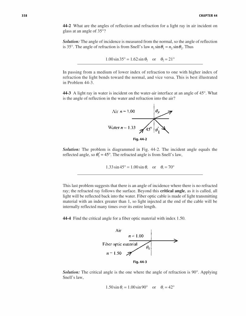
358 C H A P T E R 44

44-2 What are the angles of reflection and refraction for a light ray in air incident on glass at an angle of 35°?

Solution: The angle of incidence is measured from the normal, so the angle of reflection is 35°. The angle of refraction is from Snell’s law n nsin sin1 1 2 2θ θ= . Thus

1.00 sin 35° = 1.62 sin q2 or q2 = 21°

In passing from a medium of lower index of refraction to one with higher index of refraction the light bends toward the normal, and vice versa. This is best illustrated in Problem 44-3.

44-3 A light ray in water is incident on the water-air interface at an angle of 45°. What is the angle of reflection in the water and refraction into the air?

Fig. 44-2

Solution: The problem is diagrammed in Fig. 44-2. The incident angle equals the reflected angle, so 451θ ′ = °. The refracted angle is from Snell’s law,

1.33 sin 45° = 1.00 sin qr or qr = 70°

This last problem suggests that there is an angle of incidence where there is no refracted ray; the refracted ray follows the surface. Beyond this critical angle, as it is called, all light will be reflected back into the water. Fiber optic cable is made of light transmitting material with an index greater than 1, so light injected at the end of the cable will be internally reflected many times over its entire length.

44-4 Find the critical angle for a fiber optic material with index 1.50.

Fig. 44-3

Solution: The critical angle is the one where the angle of refraction is 90°. Applying Snell’s law,

1.50 sin qc = 1.00 sin 90° or qc = 42°

46_Oman_c44-p357-362.indd 358 04/11/15 12:35 PM

R E F L E C T I O N , R E F R AC T I O N , A N D P O L A R I Z AT I O N 359

Any beam that strikes the fiber-air interface at an angle greater than 42° will be internally reflected down the fiber.

Figure 44-4 shows a ray of light incident on a equilateral triangular glass prism at an angle of 54°. Applying Snell’s law to find the refracted ray angle yields 1.00 sin 54° = 1.62 sin qr, or qr = 30°. This means that the ray travels parallel to the base inside the prism and is refracted at 54° on exit.

Fig. 44-4

Now change the problem slightly by having the ray incident parallel to the base of a prism with the base angles 70°.

Fig. 44-5

From the geometry, the angle of incidence for the ray entering the prism is 20°, and applying Snell’s law, 1.00 sin 20° = 1.62 sin qr, qr = 12°. Again, from the geometry, the angle of incidence for the ray leaving the prism is 28°, and applying Snell’s law, 1.62 sin 28° = 1.00 sin qr, qr = 50°. A prism bends light incident parallel to its base toward the base.

If a collection of parallel rays were incident on the face of this prism, they would all be refracted toward a line extending from the base. Further, if the incident and exit faces were curved, all parallel rays could be focused at one point. Two curved-face prisms placed base to base are a lens of sorts focusing parallel rays to a single point.

The index of refraction, or wave speed, depends slightly on the wavelength of the light. A ray of sunlight passing through a prism exhibits the dispersion effect, whereby differ-ent wavelength components of the sunlight are refracted at different angles, producing a rainbow of colors from red to violet.

44-5 Light is incident at an angle of 35° on a slab of glass 2.0 cm thick. Part of the light travels through the glass and part along its original direction beside the glass. Find the path of the two rays, the velocity of the ray in the glass, and the time difference between

46_Oman_c44-p357-362.indd 359 04/11/15 12:35 PM

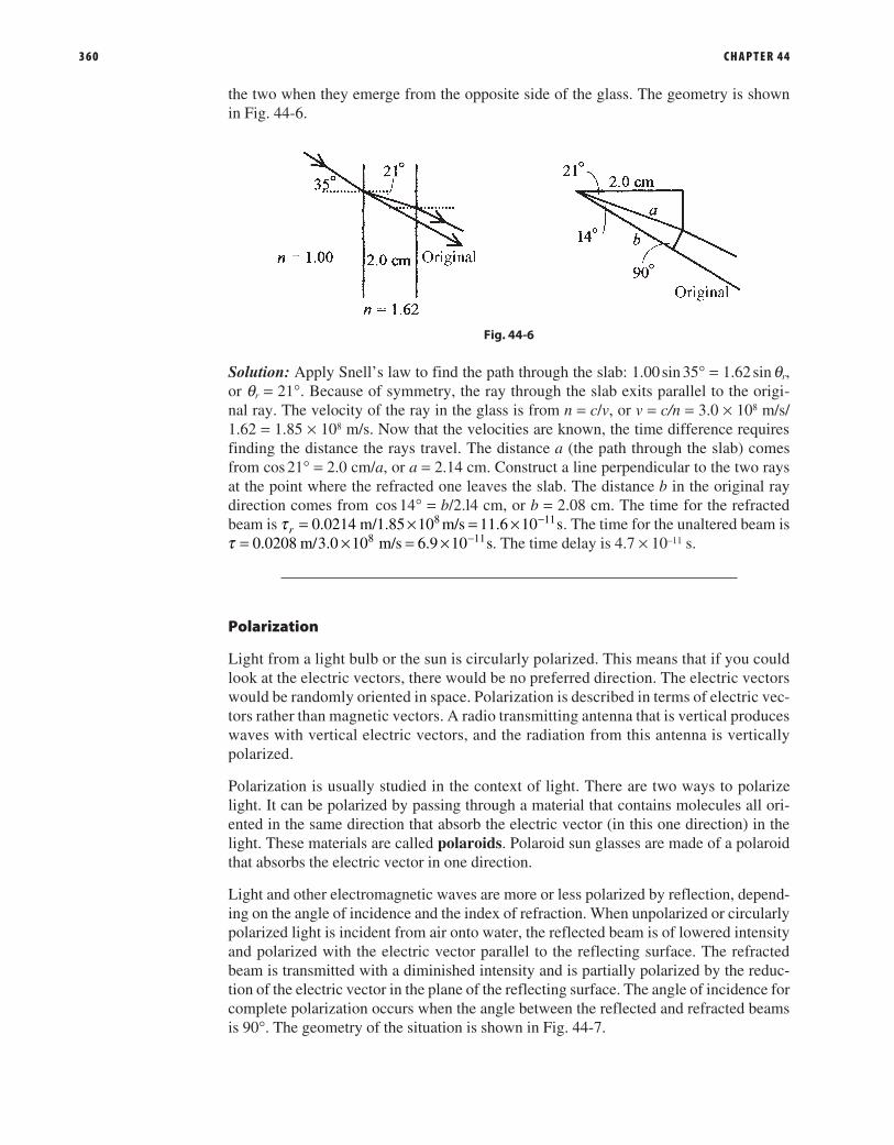
360 C H A P T E R 44

the two when they emerge from the opposite side of the glass. The geometry is shown in Fig. 44-6.

Fig. 44-6

Solution: Apply Snell’s law to find the path through the slab: 1.00 sin 35° = 1.62 sin qr, or qr = 21°. Because of symmetry, the ray through the slab exits parallel to the origi-nal ray. The velocity of the ray in the glass is from n = c/v, or v = c/n = 3.0 × 108 m/s/ 1.62 = 1.85 × 108 m/s. Now that the velocities are known, the time difference requires finding the distance the rays travel. The distance a (the path through the slab) comes from cos 21° = 2.0 cm/a, or a = 2.14 cm. Construct a line perpendicular to the two rays at the point where the refracted one leaves the slab. The distance b in the original ray direction comes from cos 14° = b/2.l4 cm, or b = 2.08 cm. The time for the refracted beam is r 0.0214 m/1.85 10 m/s 11.6 10 s8 11τ = × = × − . The time for the unaltered beam is

0.0208 m/3.0 10 m/s 6.9 10 s8 11τ = × = × − . The time delay is 4.7 × 10–11 s.

Polarization

Light from a light bulb or the sun is circularly polarized. This means that if you could look at the electric vectors, there would be no preferred direction. The electric vectors would be randomly oriented in space. Polarization is described in terms of electric vec-tors rather than magnetic vectors. A radio transmitting antenna that is vertical produces waves with vertical electric vectors, and the radiation from this antenna is vertically polarized.

Polarization is usually studied in the context of light. There are two ways to polarize light. It can be polarized by passing through a material that contains molecules all ori-ented in the same direction that absorb the electric vector (in this one direction) in the light. These materials are called polaroids. Polaroid sun glasses are made of a polaroid that absorbs the electric vector in one direction.

Light and other electromagnetic waves are more or less polarized by reflection, depend-ing on the angle of incidence and the index of refraction. When unpolarized or circularly polarized light is incident from air onto water, the reflected beam is of lowered intensity and polarized with the electric vector parallel to the reflecting surface. The refracted beam is transmitted with a diminished intensity and is partially polarized by the reduc-tion of the electric vector in the plane of the reflecting surface. The angle of incidence for complete polarization occurs when the angle between the reflected and refracted beams is 90°. The geometry of the situation is shown in Fig. 44-7.

46_Oman_c44-p357-362.indd 360 04/11/15 12:35 PM

R E F L E C T I O N , R E F R AC T I O N , A N D P O L A R I Z AT I O N 361

The criterion for complete polarization is that qr + qp = 90°. Snell’s law requires that ninc sinqp = nrefr sinqr, but qr = 90° – qp and sinqr = sin(90° – qp) = cosqp, so ninc sin qp = nrefr cos qp, or

nnptan refr

incθ = (44-4)

Fig. 44-7

This polarization law is known as Brewster’s law, and the angle of polarization is called the Brewster angle. In working problems, be careful not to invert the fraction of the indexes of refraction.

44-6 What is the polarization angle for light reflected from water?

Solution:

nnptan 1.33

1refr

incθ = = or qp = 53°

44-7 A beam of unpolarized light in water is incident on what is reported to be diamond. By means of polaroids, the angle (of incidence) for complete polarization is determined to be 61°. Is this diamond?

Solution: For light in water reflected from diamond, the Brewster angle should be

nnptan 2.42

1.33 1.81refr

incθ = = = or qp = 61°

From the indexes of refraction given in Fig. 44-1, we conclude that this is diamond.

46_Oman_c44-p357-362.indd 361 04/11/15 12:35 PM

CHAPTER 45

MIRRORS AND LENSES

363

The subject of mirrors and lenses is difficult to treat briefly, first, because for a thor-ough discussion there needs to be considerable attention to sign convention and, second, because different instructors and authors approach the subject with slight but very sig-nificant differences that affect the working of problems.

The only way to become proficient in working with lenses and mirrors is to place the sign conventions appropriate to your course on a card in front of you and do problems drawing the rays and working the calculations. Be sure that you know the sign conventions and practice doing sample problems before taking any tests on mirrors or lenses. Signs will be your major (perhaps only) source of error. Sample sign conventions for mirrors and lenses are given next.

Sign Conventions for Mirrors

o is positive if the object is in front of the mirror.

o is negative if the object is in back of the mirror.

i is positive if the image is in front of the mirror.

i is negative if the image is in back of the mirror.

f is positive if the center of curvature is in front of the mirror.

f is negative if the center of curvature is in back of the mirror.

Sign Conventions for Lenses

o is positive if the object is in front of the lens.

o is negative if the object is in back of the lens.

i is positive if the image is in back of the lens.

i is negative if the image is in front of the lens.

f is positive for a converging lens.

f is negative for a diverging lens.

Mirrors

An object placed in front of a plane mirror appears to an observer to be behind the mirror. Because of the law of reflection, divergent rays intercepted by the observer on reflection from the mirror appear to come from behind the mirror. The object distance p is numeri-cally equal to the image distance q. The image is called a virtual image because the light does not physically come from the image. A real image is one where the light comes from or passes through the image.

47_Oman_c45-p363-368.indd 363 04/11/15 2:51 PM

364 C H A P T E R 45

Fig. 45-1

45-1 A light source is 4.0 cm in front of a plane mirror. Where does an observer looking into the mirror see the image, and is it real or virtual?

Solution: The image is 4.0 cm behind the mirror. It is a virtual image because light does not pass through this image point.

A concave (converging) spherical mirror as shown in Fig. 45-2 can be analyzed by rays. An object of height h placed at o, the object distance from the concave mirror, will produce a smaller image, h′ at i, the image distance, according to the formula

o i R f1 1 2 1+ = = (45-1)

Fig. 45-2

where R is the radius of curvature and f(= R/2) is the focal length. The magnification is

M hh

io

R io R= ′ = − = − −

− (45-2)

The minus sign in the definition indicates that the image is inverted.

Draw a ray from the top of the object through the center of curvature (C in Fig. 45-2). Next, draw a ray to the point where the principal axis (the horizontal line through C) intersects the mirror, reflecting this ray back to intersect the one drawn previously. The intersection of these rays defines the top of the object. Drawing these rays requires expe-rience. Set up several situations, and draw the ray diagrams to become familiar with the procedure.

47_Oman_c45-p363-368.indd 364 04/11/15 2:51 PM

M I R R O R S A N D L E N S E S 365

45-2 For a spherical concave mirror of 12 cm radius of curvature, describe the image of a 2.0 cm high object placed 20 cm on the centerline of the mirror according to Fig. 45-2.

Solution: The image is inverted. The ray diagrams show this. Using the radius of curvature and the object distance, find the image distance from

i1

20 cm1 2

12 cm+ = or i = 8.6 cm

The magnification is from

M 8.620

12 8.620 12 0.43= − = − −

− = −

The height of the image is from

h2.0 cm 0.43′ = − or h′ = –0.86 cm

The image is 8.6 cm from the mirror, inverted (minus sign), and real (rays pass through image).

When the object is at infinity (very far away), the mirror equation reduces to 1/i = 2/R, and we can say that the rays from infinity are focused at R/2. This defines the focal length as f = R/2.

A convex (diverging) spherical mirror is illustrated in Fig. 45-3. Objects placed in front of a convex mirror appear to come from behind the mirror, and they are smaller. First, draw a ray from the top of the object parallel to the principal axis, and reflect it from the mirror. This ray appears to come from the focus (behind the mirror). Next, draw a ray so as to produce a reflected ray parallel to the principal axis of the mirror. The extension of this ray intersects the extension of the first one locating the top of the image.

Fig. 45-3

The equations for concave mirrors also work for convex mirrors if a sign convention is adopted. Lengths where the light moves (to the left of the mirrors in Figs. 45-2 and 45-3) are positive, and lengths on the other side of the mirror (to the right of the mirror in Fig. 45-3) are negative. Lengths are measured (positive and negative) from the intersec-tion of the principal axis and the mirror. These positive and negative regions are often referred to as the front and the back sides of the mirrors.

45-3 For a spherical convex mirror of 14 cm radius of curvature, describe the image of a 2.5 cm object placed 30 cm out on the principal axis of the mirror.

47_Oman_c45-p363-368.indd 365 04/11/15 2:51 PM

366 C H A P T E R 45

Solution: Here is where we get into the signs. The focus and the image are on one side of the mirror, and the object is on the other side. Therefore, we take the focus as negative and expect the image distance to be negative. The image distance comes from Equation (45-1).

i

130 cm

1 17 cm+ = − or i = –5.7 cm

The magnification comes from Equation (45-2).

M 5.730

14 5.730 14 0.19= − − = − +

+ =

The height of the image is from

h2.5 cm 0.19′ = or h′ = 0.48 cm

The minus sign for the image distance indicates that the image is behind the mirror, or on the same side as all the other minus signs. The plus sign for the magnification indicates that the image is erect (not inverted). The image is virtual.

Lenses

There are two types of thin lenses, converging and diverging, as shown in Fig. 45-4.

Fig. 45-4

The converging lens converges parallel rays to a point called the focus, while a diverging lens refracts rays to make them appear as to come from a focus. The sign conventions become more involved for lenses than for mirrors. Rather than set out a sign convention, we will handle the signs in the context of each problem. The relationship between image distance, object distance, and focal length is the same as for mirrors [Equation (45-1)].

45-4 A converging lens of focal length 8.0 cm forms an image of an object placed 20 cm in front of the lens. Describe the image.

Fig. 45-5

47_Oman_c45-p363-368.indd 366 04/11/15 2:51 PM

M I R R O R S A N D L E N S E S 367

Solution: Draw a ray from the top of the object parallel to the axis and then through the focus. Next, draw a ray from the top of the object through the center of the lens to intersect the first ray. This locates the top of the object. Use Equation (45-1) to find the image distance. Thus

i1

20 cm1 1

8.0 cm+ = or i = l3 cm

The magnification is (–) image distance over the object distance or

M io

1320 0.67= − = − = −

The image is located 13 cm on the side of the lens opposite the object with magnification 0.67. It is inverted (minus sign) and real (rays pass through image).

45-5 A diverging lens has a 14 cm focal length. Describe the image of a 4.0 cm object placed 40 cm from the lens.

Fig. 45-6

Solution: Draw a ray from the top of the object to the lens parallel to the principal axis, and refract it back to the focus. Next, draw a line from the top of the object through the center of the lens. The intersection of these rays locates the top of the object.

The image distance is from Equation (45-1). Thus

i1

40 cm1 1

14 cm+ = − or i = –10 cm

The negative sign for the focal length is because this is a diverging lens. The image dis-tance is negative because it is on the same side of the lens as the object (opposite to the converging lens). The magnification is 10/40 = 0.25.

The image is 0.25 × 4.0 cm = 1.0 cm high, erect, virtual, and appears to come from a point 10 cm from the lens on the same side as the object.

Go back over the problems in this chapter paying particular attention to the signs. As an exercise, change the numbers in these problems and work them through until the sign conventions are clear in your mind. As you do more problems, the logic of the sign con-vention listed on the first page of this chapter will become clear.

47_Oman_c45-p363-368.indd 367 04/11/15 2:51 PM

CHAPTER 46

DIFFRACTION AND INTERFERENCE

369

The wave nature of light is used to explain the several diffraction and interference phenomena discussed in this chapter.

Double Slit Diffraction

Figure 46-1 shows the setup for the classic Young’s double slit experiment first performed around 1800. Monochromatic light passes through a sufficiently narrow slit to produce a coherent source for the double slits. The coherent (in phase) light spreads out from each of the slits, creating an interference pattern on the screen. The geometry for the interference is shown in Fig. 46-1. Destructive interference occurs when the path length differs by one-half wavelength, and constructive interference occurs when the path length is an integral number of wavelengths. From the figure we can write the criterion for constructive interference as

d sin q = ml (m is an integer) (46-1)

Fig. 46-1

The distance from the central maxima (opposite the center of the two slits) to the first bright fringe on the screen is related to the angle via tan q = ym /R. For small angles, which is the case with Young’s experiment, sin q ≈ tan q = q, so Equation (46-1) can be rewritten as

dyR mm λ= (46-2)

Historically, this experiment was used to measure the wavelength of light.

46-1 A Young’s experiment is set up with slit separation of 2.0 × 10-4 m, screen distance of 0.80 m, and distance from central maxima to second bright fringe of 3.9 × 10-3 m. What is the wavelength of the source?

Solution: dymR

m 2.0 10 m 3.9 10 m2 0.80 m 488 nm4 3

λ = = × ⋅ ×⋅ =

− −

48_Oman_c46-p369-372.indd 369 04/11/15 5:28 PM

370 C H A P T E R 46

46-2 In a different Young’s experiment with 488 nm light, the second dark fringe is 1.2 × 10–3 m away from the center of the central bright fringe. The screen is 1.2 m from the slits. What is the separation of the slits?

Solution: This second dark fringe corresponds to 3/2 of a wavelength in path difference. One wavelength path difference is 2/3 of the 1.2 × 10–3 m, or 8.0 × 10–4 m. This number now fits with Equation (46-2) (one wavelength path difference), and solving for d, we get

λ= = × ⋅×

= ×−

−−d m R

ym

1.488 10 m 1.2 m8.0 10 m

7.3 10 m9

44

Single Slit Diffraction

The intensity distribution pattern for single slit diffraction is similar to the pattern for double slit diffraction. The geometry and analysis, however, are quite different. Coherent light incident on a narrow slit (100 to 1,000 wavelengths wide) produces a fringe pattern, as shown in Fig. 46-2.

Fig. 46-2

In the analysis of single slit, or Fraunhofer, diffraction, we will use the dark fringes. The slit of width a is viewed as a region where interference occurs between light at the top of the slit and the middle of the slit. The particular situation for the first dark fringe obtains for corresponding pairs of source points separated by a/2 across the width of the slit. The criterion for dark fringes is

a m2sin 2θ λ= (m is an integer) (46-3)

Again, sinq is approximately the same as tan q, which is approximately the same as q. So rewrite Equation (46-3) with this approximation as

a yR

mm

2 2λ= (46-4)

where m corresponds to the number of the dark fringes away from the central maxima.

46-3 Monochromatic light is incident on a 4.0 × 10 -4 m slit, producing a Fraunhofer diffraction pattern on a screen 1.5 m away. The distance from the central maxima to the second dark fringe is 3.4 × 10 -3 m. What is the wavelength of the light?

48_Oman_c46-p369-372.indd 370 04/11/15 5:28 PM

D I F F R AC T I O N A N D I N T E R F E R E N C E 371

Solution: Reworking Equation (46-4) yields

λ = = × ⋅ ×⋅ =

− −aymR

m 4.0 10 m 3.4 10 m2 1.5 m

453 nm4 3

46-4 Light from a He-Ne laser of 633 nm is incident on a 2.0 × 10 –4 m slit. What is the width of the central maxima (the distance between the dark fringes on either side of the central maxima) on a screen 2.0 m away?

Solution: Rearranging Equation (46-4), the distance to the first dark fringe is

λ= ⋅ = ⋅ ×

×= ×

−

−−y R

a1 1 633 10 m(2.0 m)

2.0 10 m6.3 10 m1

9

43

The width of the central maxima is two times this value, or 1.3 × 10 –2 m.

The Diffraction Grating

A diffraction grating consists of multiple slits, as shown in Fig. 46-3. When light is incident on this arrangement, constructive interference occurs when the path difference between adjacent slits is ml. Increasing the number of slits produces two effects: the intensity of each interference maximum increases, and the width of each interference maximum decreases. This makes the grating a very convenient tool for the study of the various component wavelengths (spectra) of gases.

Fig. 46-3

46-5 A grating with 2,000 lines per centimeter is illuminated with a hydrogen gas discharge tube. Two of the hydrogen lines are at 410 and 434 nm. What is the first order spacing of these lines on a screen 1.0 m from the grating? The experimental arrangement is shown in Fig. 46-4.

Fig. 46-4

48_Oman_c46-p369-372.indd 371 04/11/15 5:28 PM

372 C H A P T E R 46

Solution: The phrase first order refers to the first maxima. First, find the spacing

l.0 × 10–2 m/2,000 lines = 5.0 × 10–6 m

For the 410 nm line,

y R

dRd

1 410 10 m 1.0 m5.0 10 m

0.082 m19

6λ λ= ⋅ = = ×

×=−

−

For the 434 nm line,

y R

dRd

1 434 10 m 1.0 m5.0 10 m

0.087 m19

6λ λ= ⋅ = = ×

×=−

−

The lines are separated by 5 mm on the screen.

48_Oman_c46-p369-372.indd 372 04/11/15 5:28 PM

CHAPTER 47

SPECIAL RELATIVITY

373

The special theory of relativity is based on two postulates.

The Laws of Physics Are the Same in All Inertial Reference Frames

Inertial frames are reference (coordinate) frames moving at constant velocity with respect to one another; that is, they are not accelerating.

The Speed of Light Is the Same in All Inertial Frames

These two postulates lead to very interesting and highly significant conclusions concern-ing simultaneity and how we measure the fundamental quantities of length, mass, and time. These discussions, though very interesting, are inappropriate for a problems book, so we will go directly to the consequences of special relativity as it affects our under-standing of physics.

The concepts and calculations of special relativity require a change in how we view the world. Many of the things we study in special relativity may go against our intuition, but remember, intuition is often wrong, and even if it were correct, we have no experience to base our intuition on when dealing with particles approaching the speed of light, where relativistic effects are observable. How many of Galileo’s colleagues intuitively “knew” that when he dropped those two different sized balls from the Tower at Pisa, the heavier one would reach the ground first? Success in understanding special relativity requires first that you rid your mind of intuitive knowledge based on what could be called “low-velocity experience.” As you study special relativity, you will encounter situations where you will be challenged to look at the postulates and change your view of the world.

Time Dilation

Time intervals are different in different (moving) inertial frames. Place a light source, mirror, and detector in a moving vehicle, as shown in Fig. 47-1. An observer in the mov-ing vehicle measures the time for a light pulse to move from the source to the mirror and back to the detector as the distance traveled divided by the velocity of light, so Δto = 2d/c. The zero subscript indicates that this time is measured by an observer in the same frame where the event is taking place. This is also called the proper time.

Fig. 47-1

An observer in another inertial frame observes the vehicle moving at a velocity v (Fig. 47-2) and over the time interval of the event observes that the detector has traveled a distance vΔt.

49_Oman_c47-p373-378.indd 373 04/11/15 5:36 PM

374 C H A P T E R 47

Fig. 47-2

The total distance the light has traveled is + ∆2 ( /2)2 2d v t . The time interval is

∆ = + ∆2 ( /2)2 2t c d v t .

Remember, c is the same to all observers regardless of inertial frame. The two times can be related with d = cΔto /2, so

∆ = ∆ + ∆2 ( /2) ( /2)2 2t c c t v to or ∆ =∆−1 /2 2

tt

v co (47-1)

The external observer of an event taking place in a moving reference frame, the one who measures Δt, always sees an event as taking longer than the stationary observer, the one who measures Δto, in the frame moving with the event.

47-1 You are in a railroad car moving at constant velocity of zero with respect to the surface of the Earth. What do you measure as the time it takes for a coin to drop 1.0 m to the floor of the railroad car? What does an observer in another railroad car traveling at a constant 25 m/s measure for this time?

Solution: You apply =s gt(1/2) 2 and observe

= = ⋅ =2 2 1.0 m9.8 m/s

0.45 s2t sg

The moving observer measures a time given by Equation (47-1). For small v/c, the best way to make this calculation is to use a binomial expansion of the radical (see the Mathematical Background).

1 /

(1 / ) 1 12

382 2

2 2 1/22

2

4

4∆ =∆−

= ∆ − = ∆ + + +

−t

t

v ct v c t v

cvc

oo o (47-2)

The first, and largest, relativistic correction term is

=×

= × −1

212

253.0 10

3.5 102

2 8

215v

c

This means that the correction is Δt = Δto(1 + 3.5 × 10–15) s. Time measurement this pre-cise is beyond the capability of the cesium clocks. This is an unobservable effect.

47-2 For the situation of the preceding problem, take the moving observer from the train to a 2,500 m/s jet plane and then to a rocket ship traveling at 0.90c. (It is common, and very convenient, in relativistic calculations to express velocity as a fraction or decimal times c.)

49_Oman_c47-p373-378.indd 374 04/11/15 5:36 PM

S P E C I A L R E L AT I V I T Y 375

Solution: Again, using the binomial expansion and looking at the first term,

12

12

25003.0 10

3.5 102

2 8

211=

×

= × −v

c

This small a time difference is observable, but it is a difficult experiment.For the rocket ship traveling at 0.90 c, use Equation (47-1) directly. Thus

∆ =∆−

=∆

= =1 0.90 0.43

0.45 s0.43 1.0 s

2t

t to o

The observer in the rocket ship measures the time for the falling coin as 1.0 s, over twice what the stationary observer sees. These two problems illustrate how relativistic effects are observable only as relative velocities approach c.

47-3 A “strange particle” is observed to move at 0.96c and have a lifetime of 2.0 × 10–8 s. What is the lifetime of the particle in its own reference frame?

Solution: In Equation (47-1), Δto is the (proper) time an observer traveling with the “strange particle” would measure, so find

1 / 2.0 10 s 1 0.96 0.56 10 s2 2 8 2 8∆ = ∆ − = × − = ×− −t t v co

Length Contraction

The time dilation leads to a length contraction with velocity. Consider a vehicle moving at velocity v between two stars with one observer in the vehicle and another at a fixed point (with respect to the stars). The external observer measures the (proper) distance between the stars as Lo, observes the velocity of the vehicle as v, and writes the time interval as Δt = Lo /v. The time interval Δt is not a proper time because measurement of Δt would require synchronized clocks at both stars. The observer in the vehicle sees the stars moving at v and measures a (proper) time interval Δto. This observer determines the distance between the stars as L = v Δto. Write these two equations as a fraction. Thus

=∆∆

LL

vv

tto

o and with ∆ =∆−1 /2 2

tt

v co

1 /2 2= −L L v co (47-3)

The length measured by a moving observer is contracted by a factor equal to 1 /2 2− v c .

47-4 In a soaring spaceship (a vehicle capable of both space flight and conventional aircraft flight), you return from a space journey to find a new landing runway. Passing over this runway at 0.92c, you measure its length as 1960 m. What is its length at your landing speed of 200 m/s?

49_Oman_c47-p373-378.indd 375 04/11/15 5:36 PM

376 C H A P T E R 47

Solution: At 200 m/s, there is no observable relativistic effect. Use Equation (47-3) to find the length of the runway at your landing speed. Thus

L Lv c

o =−

=−

=1 /

1960 m1 0.92

5,000 m2 2 2

47-5 How fast must a meter stick be traveling relative to your reference frame for you to observe a 2 percent contraction?

Solution: Use Equation (47-3) with L = 0.98Lo. Thus

0.98 1 /2 2= −L L v co o or v = 0.20c

Relativistic Momentum

At “low velocities,” a force applied to a particle produces an acceleration according to the familiar F = d/dt(mv) = m(dv/dt). As the velocity of the particle approaches c, the momentum becomes velocity dependent, with the force statement taking on the form

=

−1 /2 2F d

dtmv

v c

The most convenient interpretation is to associate the −1 /2 2v c with the mass and say that the effective mass of a moving particle is

−1 /2 2

m

v co

(47-4)

where mo is the rest mass, measured with the mass not moving in the inertial frame where the measurements are made.

47-6 What is the effective mass of an electron moving at 0.80c?

Solution: 1 /

9.1 10 kg

1 0.8015.2 10 kg

2 2

31

2

31=−

= ×−

= ×−

−mm

v co

47-7 Intergalactic space travelers need to know the relative velocities and masses of their spaceships. Each ship, therefore, has a 1.0 m long bar painted on the side of the ship alongside the rest mass. As you pass by a ship, you measure this 1.0 m bar as 0.93 m. What is your relative velocity? You also observe the other ship’s rest mass printed as 365,000 kg. What is its mass relative to you? What does an observer in the other ship measure for your 1.0 m bar?

49_Oman_c47-p373-378.indd 376 04/11/15 5:36 PM

S P E C I A L R E L AT I V I T Y 377

Solution: The length you observe is = −1 /2 2L L v co , where Lo is the 1.0 m, the length an observer at rest with respect to the vehicle would measure, and L is the length you measure, so

= −0.93 1.0 1 /2 2v c or v = 0.37c

The relativistic mass you observe is

m

m

v co=

−= =

1 /

365,000 kg0.93 392,000 kg

2 2

Observers in the other spaceship measure your bar as 0.93 m and relative speed as 0.37c.

As an exercise, find the effective mass of an electron at 0.999c and at 0.99999c. As the velocity approaches c, the effective mass approaches infinity, implying the necessity of an infinite force to reach c. This shows the theoretical impossibility of material objects traveling at c or beyond.

49_Oman_c47-p373-378.indd 377 04/11/15 5:36 PM

CHAPTER 48

QUANTUM PHYSICS

379

In the model of the atom by Danish physicist Niels Bohr, electrons can only exist at certain energy levels. Another way of saying this is that the energy levels are quantized.

The Photoelectric Effect

The photoelectric effect is a phenomenon where electrons are emitted from a metal sur-face as a result of the incidence of electromagnetic radiation above a certain frequency. The electrons absorb the energy from incident light and get ejected from the metal. The minimum frequency of incident electromagnetic radiation that will release an electron from the metal surface is called the threshold frequency.

The work function f of the metal surface is the minimum energy required to release an electron from that metal surface. It is related to threshold frequency by the equation

hfoφ =

where h is Planck’s constant with a value of 6.63 × 10-34 J ∙ s.

When an electron in a metal surface receives energy from an incident photon (of energy E = hf), it needs to spend a minimum energy (the work function f) to leave the metal surface with a maximum kinetic energy given by Einstein’s photoelectric equation as

mv hf12 max

2 φ= −

Think of the difference between removing an electron from an atom right at the surface of a metal versus removing an electron, say, five atomic layers deep. The one from the surface comes out more easily and has a maximum value of kinetic energy left over after the work function energy has been supplied. The maximum kinetic energy of the electrons is independent of the intensity of the incident radiation, but it does depend on the work function of the particular metal and, of course, the amount of energy supplied by the photon.

Take the metal silver as an example. Suppose that we shine red (low-frequency) light on silver, and the energy in each individual photon is not enough to eject any electrons. It does not matter if you have 1 W of red light or 1,000 W. This is weird if you think about it. Light is supposed to be a wave. A greater-intensity wave should have more energy, but somehow this doesn’t work.

Now shine green and then blue light on silver. Still no electrons are emitted. If you go into the ultraviolet, finally you hit a certain frequency where electrons start coming out of the metal.

48-1 Radiation with a wavelength of 200 nm strikes a metal surface in a vacuum. Ejected electrons have a maximum speed of 7.22 × 105 m/s. What is the work function of the metal in electronvolts?

50_Oman_c48_p379-388.indd 379 04/11/15 2:59 PM

380 C H A P T E R 48

Solution: First, recall from the wave equation that the speed of a wave is equal to the product of wavelength and frequency. The speed of light is 3.0 × 108 m/s and is denoted by c. Thus

c = lf

3.0 × 108 m/s = (200 × 10–9 m)f

f = 1.5 × 1015 Hz

We can now use this frequency in the photoelectric equation

mv hf12 max

2 φ= −

(6.63 × 10–34 J ∙ s)(1.5 × 1015 Hz) = f + (1/2)(9.11 × 10–31 kg)(7.22 × 105 m/s)2

9.945 ~ 9.95 × 1015 J - 2.37 × 10–19 J = f

φ = × × ××

=−7.575 10 7.58 10 J 1 eV1.6 10 J

4.73 eV–19 –1919

The conversion from joules to electronvolts is done at the end. You should remember that 1 electronvolt = 1.6 × 10–19 joules.

48-2 When ultraviolet light with a wavelength of 400.0 nm falls on a certain metal surface, the maximum kinetic energy of the emitted photoelectrons is measured to be 1.10 eV. What is the maximum kinetic energy of the photoelectrons when light of wave-length 300.0 nm falls on the same surface?

Solution: The kinetic energy of the photoelectron is the difference between the initial energy of the photon and the work function of the metal. It can be solved using the fol-lowing formula.

mv hf E hc12 , max

2 φ λ= − =

Using the data for the 400.0-nm light to calculate f and solving for f, we get

hc mv 12 max

2φ λ= −

× ⋅ ××

− = − =−

−(4.136 10 eV s)(3.00 10 m/s)

400.0 10 m1.10 eV 3.10 eV 1.10 eV 2.00 eV

15 8

9

Then, for 300.0 nm, we have

mv hf hcφ λ φ= − = − = × ⋅ ××

−−

−12

(4.136 10 eV s)(3.00 10 m/s)300.0 10 m

2.00 eVmax2

15 8

9

which gives

mv12 4.14 eV 2.00 eV 2.14 eVmax

2 = − =

50_Oman_c48_p379-388.indd 380 04/11/15 2:59 PM

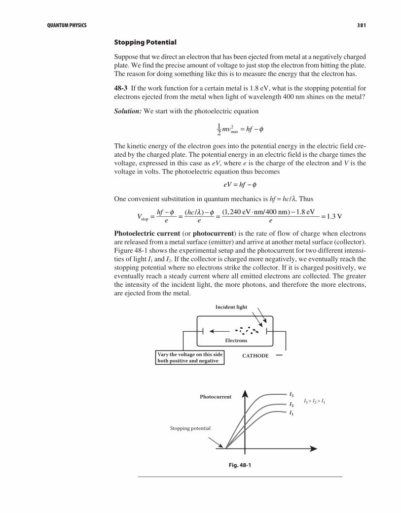
QUANTUM PHYSICS 381

Stopping Potential

Suppose that we direct an electron that has been ejected from metal at a negatively charged plate. We find the precise amount of voltage to just stop the electron from hitting the plate. The reason for doing something like this is to measure the energy that the electron has.

48-3 If the work function for a certain metal is 1.8 eV, what is the stopping potential for electrons ejected from the metal when light of wavelength 400 nm shines on the metal?

Solution: We start with the photoelectric equation

mv hf12 max

2 φ= −

The kinetic energy of the electron goes into the potential energy in the electric field cre-ated by the charged plate. The potential energy in an electric field is the charge times the voltage, expressed in this case as eV, where e is the charge of the electron and V is the voltage in volts. The photoelectric equation thus becomes

eV hf φ= −

One convenient substitution in quantum mechanics is hf = hc/l. Thus

Vhf

ehc

e eφ λ φ= − = − = − = ( / ) (1,240 eV·nm/400 nm) 1.8 eV

1.3 Vstop

Photoelectric current (or photocurrent) is the rate of flow of charge when electrons are released from a metal surface (emitter) and arrive at another metal surface (collector). Figure 48-1 shows the experimental setup and the photocurrent for two different intensi-ties of light I1 and I2. If the collector is charged more negatively, we eventually reach the stopping potential where no electrons strike the collector. If it is charged positively, we eventually reach a steady current where all emitted electrons are collected. The greater the intensity of the incident light, the more photons, and therefore the more electrons, are ejected from the metal.

Incident light

Electrons

Vary the voltage on this sideboth positive and negative

CATHODE

Photocurrent

Stopping potential

I3I3 > I2 > I1I3

I1

Fig. 48-1

50_Oman_c48_p379-388.indd 381 04/11/15 2:59 PM

382 C H A P T E R 48

48-4 A monochromatic source emits a narrow parallel beam of light of wavelength 546 nm, the power in the beam being 0.080 W. What is the photocell current, assuming that 1.5 percent of the photons incident on the cathode liberate electrons?

Solution: At 546 nm, the photon energy is hc/l and equals

× × ×

××

−

−−(6.63 10 ) (3 10 )

546 10or 3.643 10 J

34 8

919

The number of photons per second can be expressed as

=×

= ×−Joules per second

Photon energy0.08 W

3.643 10 J2.2 10 photons/s19

17

The number of electrons liberated per second is

1.5100 2.2 10 3.3 10 electrons/s17 15× × = ×

The current may be expressed as

Electrons per second electronic charge 3.3 10 1.6 10

5.28 10 A or 0.53 mA

15 19

4

× = × × ×= ×

−

−

48-5 Figure 48-2 shows the variation in stopping potential versus frequency for metal sample 1. If metal sample 2 has a smaller work function, draw a second graph for metal sample 2.

metal sample #1

reshold frequency

Frequency

Stop

ping

pot

entia

l

Fig. 48-2

Solution: The photoelectric equation may be written as

eV hfs φ= −

V he f es

φ( )= −

Thus, a graph of Vs against f gives

1. A constant gradient of h/e and 2. A negative y intercept of f/e

50_Oman_c48_p379-388.indd 382 04/11/15 2:59 PM

QUANTUM PHYSICS 383

So if we have a smaller work function, then we have the same slope because h and e are constants. We also would have less negative value for the y intercept. The new graph would appear as shown in Fig. 48-3.

metal sample #1metal sample #2

reshold frequency

Frequency

stop

ping

pot

entia

lFig. 48-3

de Broglie Relation

The photoelectric effect provides the evidence that a traditional light wave in the form of electromagnetic radiation may be considered a particle-like photon. The diffraction of a beam of electrons through a thin crystal provides the evidence that traditional particles such as electrons exhibit wave behavior (diffraction). This leads to the concept of wave-particle duality known as the de Broglie relation with the following formulas.

The wavelength of a particle of momentum p is given by

hpλ =

The momentum of a photon is given by

p h λ=

48-6 Singly charged sodium ions are accelerated through a potential difference of 300 V. What is the de Broglie wavelength of the ion?

Solution: The kinetic energy acquired is K = qV, where q is the charge on an ion and V is the accelerating potential. Thus

K (1.60 10 C)(300 V) 4.80 10 J 19 17= × = ×− −

The mass of a single sodium atom can be computed as

m22.9898 g/mol

6.02 10 atom/mol3.819 10 g 3.819 10 kg23

23 26=×

= × = ×− −

Thus the momentum of an ion is

p mK2 2(3.819 10 kg)(4.80 10 J) 1.91 10 kg m/s26 17 21= = × × = × ⋅− − −

50_Oman_c48_p379-388.indd 383 04/11/15 2:59 PM

384 C H A P T E R 48

The de Broglie wavelength is

hpλ = = × ⋅

× ⋅= ×

−

−−6.63 10 J s

1.91 10 kg m/s3.46 10 m

34

2113

Heisenberg Uncertainty Principle

In quantum mechanics, we cannot simultaneously specify both the position and the momentum of an object to any arbitrary precision. The Heisenberg uncertainty relation is

x p hx( )( ) 4π∆ ∆ ≥

where Δx is the uncertainty in the position of the object in the x direction (m), and Δpx is the uncertainty in the momentum of the object in the x direction (N · s). Uncertainty also exists with energy and time

E t h( )( ) 4π∆ ∆ ≥

where ΔE is the uncertainty in the energy of the object in a particular state, and Δt is the time interval during which the object is in that state.

48-6 A ball has a mass of 0.275 kg just before it strikes the Earth after being dropped from a building that is 22.6 m tall. What is the de Broglie wavelength? The acceleration due to gravity is 9.8 m/s2, and Planck’s constant is 6.63 × 10-34 J · s.

Solution: From conservation of energy,

mv mgh12

2 =

v gh 2 2(9.8)(22.6) 21.0 m/s= = =

p mv 0.275 21.05 5.79 kg m/s= = × = ⋅

Finally,

hpλ = = × = ×

−−6.63 10

5.79 1.14 10 m34

34

This is less than the diameter of an atom. This calculation shows why large objects do not exhibit wave behavior.

48-7 An electron beam is used to resolve a molecule whose size is 1 nm. The mass of an electron is 9.11 × 10–31 kg. What is the kinetic energy of electrons that have the appropri-ate wavelength?

Solution: A great little formula to remember in quantum mechanics is

Epm2

2

=

50_Oman_c48_p379-388.indd 384 04/11/15 2:59 PM

QUANTUM PHYSICS 385

From here, substituting p = h/l gives

E hmλ

= = ×× ×

−

− −2(6.63 10 )

2(9.11 10 )(1 10 )

2

2

34 2

31 9 2

E 2.41 10 J 1.51 eV19= × =−

48-8 For crystal diffraction experiments, wavelengths on the order of 0.20 nm are often appropriate. Find the energy in electronvolts for a particle with this wavelength if the particle is (a) a photon, (b) an electron, and (c) a proton.

Solution:

(a) For a photon, E = hc/l,so

E hcλ= = × ⋅ ×

×=

−

− (4.136 10 eV s)(3.00 10 m/s)

0.20 10 m6.2 keV

15 8

9

(b) For an electron, p = h/land E = p2/2m, so

E hm

2

2

2λ=

E hmλ

= = × ⋅×

×= × =

−

− −−

26.63 10 J s0.20 10 m

12(9.11 10 kg)

6.03 10 J 38 eV2

2

34

9

2

3118

(c) For a proton E Emmp e

e

p=

=××

=

−

−(38 eV)9.11 10 kg1.67 10 kg

0.021 eV31

27

For a given wavelength, a photon has much more energy than an electron, which, in turn, has more energy than a proton.

Compton Scattering

If a photon strikes an electron, thinking of them both as particles, there is an elastic collision, and the photon loses some of its energy to the electron. The wavelength of the scattered light is different from the incident radiation. The Compton scattering equation is

hm ce

(1 cos )λ λ θ′ − = −

where l is the initial wavelength, l′ is the wavelength after scattering, h is Planck’s constant, me is the electron rest mass, c is the speed of light, and q is the scattering angle. The quantity h/mec is known as the Compton wavelength of the electron; it is equal to 2.43 × 10-12 m.

48-9 Suppose that we try to “observe” an electron orbiting the nucleus of an atom by using a light microscope to measure the electron’s presumed orbital position with a precision of 10 pm (a typical atom has a radius of about 100 pm). The wavelength of the light used in the microscope then must be about 10 pm. What would be the photon energy of this light, and how much energy would such a photon impart to an electron in a head-on collision?

50_Oman_c48_p379-388.indd 385 04/11/15 2:59 PM

386 C H A P T E R 48

Solution: Another neat little value you might want to remember is hc =1,240 nm ⋅ eV. Using this, we can calculate the photon energy of the light as

E hc 1,240 nm eV10.0 10 nm

124 keV3λ= = ⋅×

=−

The kinetic energy gained by the electron is equal to the energy decrease of the photon.

E hc hc hc E

Ec

λ λ λ λ λλ

λ λ λ λ

λ λ θ

( ) ( )∆ = ∆ = − + ∆

= ∆+ ∆

= + ∆

= + − = + − ° =

1 11 /

1 [ / (1 cos )]124 keV

1 [10 pm/(2.43 pm)(1 cos180 )] 40.5 keV

It is impossible to “view” an atomic electron with such a high-energy photon because with the energy imparted to the electron, the photon would have knocked the electron out of its orbit.

Schrodinger Equation

Because of the uncertainty principle, we cannot specify the exact location of a particle to infinite accuracy. The Schrodinger equation is an equation for finding the wave function of a system. The wave function squared gives us the probability distribution of where to find a particle. There are two basic forms of the equation. The first is called the time-dependent form, and it shows how properties of the system change with position and time. The solution to this wave equation takes the form

Ψ(x, t) = Aeikxe-iwt

where = h/2p = 1.055 × 10-24 J · s, k = p/, and w = k2/2m.

The second form is called the time-independent form, and it shows how properties of the system depend on position but not how they change over time. The solution takes the form

x t Aeikx( , )Ψ =

48-10 A free electron has a wave function

x Aei x( ) (5.00 10 )10Ψ = ×

where x is in meters. Find its (a) de Broglie wavelength, (b) momentum, and (c) kinetic energy in electronvolts.

Solution:

(a) x t Aeikx( , )Ψ =

so

k 5.00 1010= ×

50_Oman_c48_p379-388.indd 386 04/11/15 2:59 PM

QUANTUM PHYSICS 387

The de Broglie wavelength can be computed using

hp k

ph

hp k,

2, and thus 2 λ π π= = =

This gives us

k2 2

5.00 101.26 10 m 126 pm10

10λ π π= =×

= × =−

(b) From the formula for the de Broglie wavelength, we can derive

p hλ= = × ⋅

×= × ⋅

−

−−6.63 10 J s

1.26 10 m5.26 10 kg m/s

34

1024

(c) KE Epm2

2

= =

(This little formula just comes from starting with KE = ½mv2 and then substituting in p = mv.) Then

KE = ××

= × ××

=−

−−

−(5.26 10 )2(9.11 10 )

1.52 10 J 1 eV1.6 10 J

94.9 eV24 2

3117

19

48-11 An electron is moving as a free particle in the -x direction with momentum that has a magnitude of 4.50 × 10-24 kg · m/s. What is the one-dimensional time-dependent wave function of the electron?

Solution: Using the momentum of the free electron, we can calculate k and w and use these to express its wave function. We know that Ψ(x, t) = Aeikxe-iwt, = h/2p = 1.055 × 10-24 J · s, k = p/, and w = k2/2m. Thus

kp

= = −× ⋅

× ⋅= ×

−

−−

4.50 10 kg m/s1.055 10 J s

4.27 10 m24

3410 1

kmω = = × ⋅ ×

×= ×

− −

−−

2(1.055 10 J s)(4.27 10 m )

2(9.11 10 kg)1.05 10 s

2 34 10 1 2

3117 1

x t Ae ei x i t( , ) (4.27 10 m ) – (1.05 10 s )10 1 17 1Ψ = − × ×− −

The wave function depends on position and time.

50_Oman_c48_p379-388.indd 387 04/11/15 2:59 PM

CHAPTER 49

ATOMS, MOLECULES, AND SOLIDS

389

When an isolated atom absorbs a certain discrete amount of energy, its orbital electrons move up to higher orbits. The atom is said to be excited. The energy absorbed by the excited atom is then released in the form of photons, when its electrons transit back to their original orbits.

The Hydrogen Atom

The three lowest energy levels of the electron in the hydrogen atom have the following energies:

E 21.8 10 J119= − × −

E 5.45 10 J219= − × −

E 2.43 10 J319= − × −

The energies are measured so that the electron would have zero energy if it were com-pletely free of the atom and at rest. It is a convention that energy levels in atoms have negative values. The more negative the number, the lower is the orbit of the electron, and the more energy is needed to remove it from the atom.

49-1 What is the wavelength of the Hα spectral line due to transition between levels E E and 3 2?

Solution: Be careful with the minus signs. We have

λ

λλ

− =

− × − − × = =

× =× × ×

= ×

− −

−−

−

E E hf

hf hc( 2.43 10 ) ( 5.45 10 )

3.02 10(6.63 10 ) (3.0 10 )

6.63 10 m

3 2

19 19

1934 8

7

49-2 Through what potential difference must an electron be accelerated to enable it to ionize a normal hydrogen atom in the ground state?

Solution: We are accelerating an external electron and then having it collide with the electron in the hydrogen atom, transferring all its kinetic energy into the orbiting elec-tron. For ionization to occur in this case, the transition is from the ground state (E1) to outside the atom (to zero energy). Thus

× ××

=−−21.8 10 J 1 eV

1.6 10 J13.6 eV19

19

Potential difference = 13.6 V

51_Oman_c49_p389-396.indd 389 04/11/15 3:30 PM

390 C H A P T E R 49

Note that we don’t say 13.6 eV (or electronvolts) in answer to this question. That is a unit of energy. Potential difference means voltage. If you accelerate one electron through a potential difference of 13.6 V, then you give it 13.6 eV of energy. If you accelerate an a particle, with a +2 charge, through a potential difference of 13.6 V, then you would get 27.2 eV of energy because the charge is double.

49-3 Calculate the frequency of the light emitted by a hydrogen atom during a transition of its electron from the energy level with n = 6 to the energy level with n = 3.

Solution: The formula for energy levels in the hydrogen atom is

Enn = − × −21.79 10 J

19

2

For a transition from n = 6 to n = 3,

En = − × −

= − ×− −(21.79 10 ) 1

316

1.81 10 J192 2

19

But E = hf, where h is Planck’s constant, so

f Eh= = ×

× ⋅= ×

−

−−1.81 10 J

6.63 10 J s2.74 10 s

19

3414 1

49-4 Consider the energy levels in the hydrogen atom shown in Fig. 49-1. If electrons are excited from the ground state into all the higher energy levels shown, how many total spectral lines could be emitted?

eV–0.9–1.5

–3.4

–13.6

Fig. 49-1

Solution: Figure 49-2 shows all the possible transitions. The total number is 6. You can go from any higher level to any lower level. Any one of these transitions gives rise to a spectral line. The frequency of the emitted radiation will depend on the energy difference.

51_Oman_c49_p389-396.indd 390 04/11/15 3:30 PM

ATOMS, MOLECULES, AND SOLIDS 391

eV–0.9–1.5

–3.4

–13.6

Fig. 49-2

Lasers

To make a laser, we first need to pump electrons into higher orbitals in an atom. We can do this with electrical energy, for example. Once the electrons go up to a higher level, we want them to stay there for a while and not come back down immediately. The reason for this is so they can undergo a process called stimulated emission, which happens when a photon of the same energy as the transition interacts with the excited electron. The excited electron comes down and emits another photon in phase with the first. These two photons repeat the stimulated emission to produce two more identical photons. The process con-tinues, increasing the number of identical photons. All the photons produced are coherent (meaning of the same phase and frequency) and are in the same direction, and they form a laser beam that is monochromatic (meaning of one frequency) and highly directional.

Population inversion is a situation in which there are more atoms in a higher excited state than in a lower state. Normally, an atom stays in its excited state for a short time (typically ~10-8 s). For population inversion to occur, the atoms must stay in the excited state for a relatively long time (~10-3 s), known as a metastable state. Thus, not every atom can provide laser action. Researchers searched for the ones that had the appropriate metastable states in addition to other factors. A summary of laser transitions is shown in Fig. 49-3.

Spontaneous and Stimulated ProcessesBefore After

SpontaneousEmissionor Decay

UpperLevel One photon

(a)LowerLevel

StimulatedEmission

UpperLevel Two photons

(b)LowerLevelPhoton

StimulatedAbsorption

UpperLevel

Figure 3(c)Lower

LevelPhoton

Fig. 49-3

51_Oman_c49_p389-396.indd 391 04/11/15 3:30 PM

392 C H A P T E R 49

49-4 Shown in Fig. 49-4 are some of the energy levels of helium and neon. These elements are the major constituents of a laser that emits red light. Which transition between the labeled levels gives rise to emission of the laser light?

Helium NeonE3E2

E1

E6

E5

E4

Ground

Ground

–3.976 eV –4.031 eV

–12.190 eV

–21.568 eV

–4.026 eV

–5.990 eV

Fig. 49-4

Solution: We need to know two things to answer this question. First, we need to know generally how the helium-neon laser works. Second, it is good to know off the top of your head what approximate wavelengths make up the visible spectrum.

The helium neon laser is activated with electricity. Electrons from the external electric current hit the helium atom and move the electrons orbiting it to an excited state. Then the helium collides with the neon. We just mean that one molecule of helium gas bumps into one molecule of the neon gas. During the collision, the helium electron loses energy and the neon gains an excited electron. Energy is transferred during the collision. Now we have an exited electron in the neon, and the electron moves to a lower level in the neon, producing the red light. So we are looking for a transition within the neon that corresponds to the energy of red light. Remember that the visible spectrum goes from approximately 700 nm (red) to 400 nm (violet). Thus

Red light ≈ 700 nm = 700 × 10–9 m

The energy of the red light is

E hcλ= = × ×

×−

−(6.63 10 )(3.0 10 )

700 10

34 8

9

E 2.84 10 J 1.78 eV19= × =−

Only E6 to E5 satisfies the energy difference to emit red light. This result is also another one to remember: visible light has photons of roughly 2 eV.

49-5 A pulsed laser emits light at a wavelength of 694.4 nm. The pulse duration is 12.0 ps, and the energy per pulse is 0.150 J. What is the length of the pulse, and how many photons are emitted in each pulse?

Solution:

Length of pulse speed of light time= ×

Length of pulse (3 10 ) (12 10 ) 0.036 m 3.6 mm8 12= × × × = =−

51_Oman_c49_p389-396.indd 392 04/11/15 3:30 PM


Solving for the number of photons,

EENumber of photons pulse

photon=

But Epulse = 0.150 J and Ephoton = hc/l, so

E hcλ= × = × ×

× ×−

−Number of photons 0.150 694.4 10(6.63 10 )(3 10 )pulse

9

34 8

Number of photons 5.24 10 photons17= ×

49-6 A 4.0 W laser emits a beam of wavelength 633 nm. Calculate the energy of each photon and the number of photons emitted in 0.05 s.

Solution: Total energy in 0.05 s = 4.0 W × 0.05 = 0.2 J. Thus

E hf= = × × ××

= ×−−

−6.63 10 3 10633 10

3.14 10 Jphoton34

8

919

Therefore,

Total number of photons 0.23.14 10

6.3 101917=

×= ×−

49-7 In a ruby laser, light with a wavelength of 550 nm from a xenon flash lamp is used to excite the chromium (Cr) atoms in the ruby from ground state E1 to state E3, as shown in Fig. 49-5. In subsequent de-excitations, red laser light is emitted. Identify the meta-stable state, the ground state, and the levels for the laser transition.

2.25 eV E3

1.79 eV E2

Optical pumping(550-nm photons)

Ground state E1

Fig. 49-5

Solution: E2 is the metastable state. The transition from state E2 to state E1 produces the laser light. E1 is the ground state.

Recall that 1.79 eV is close to the value of red light that we saw in an earlier problem. If you don’t know this off the top of your head, you could calculate the wavelength (see Chapter 48 for examples). The E3-to-E2 transition is only 0.46 eV, and this would be in the infrared, although the transition also can be nonradiative. By nonradiative, we mean that the energy is not lost in the form of light, but it can be lost to heat in the form of a vibration, for example.

51_Oman_c49_p389-396.indd 393 04/11/15 3:30 PM

394 C H A P T E R 49

The top of the laser level is the level that is metastable. Excited electrons need to stay in that upper level. If too many electrons are in the ground state E1, then photons have a higher probability of being absorbed rather than causing stimulated emission, and the laser pulse dies out.

Semiconductors

49-8 Three materials are shown in Fig. 49-6. Identify the metal, the semiconductor, and the insulator.

Conduction band

Valence band

Conduction band

Valence bandValence band

Conduction band

Material B Material CMaterial A

Fig. 49-6

Solution: In a solid, the atoms are closely packed. Their energy levels are so modified by their mutual influence that they are spread out into bands. Material A is the insulator because it has the largest band gap. At room temperature, electrons do not have enough energy to get up to the conduction band, where they are free to move around. Valence-band electrons can be thought of as bound to the nucleus. Material C is the metal that has lots of free electrons and high conductivity at room temperature. Material B is the semiconductor.

49-9 Is the element phosphorous an n-type or a p-type donor if it is introduced as an impurity in silicon? Draw a diagram showing the lattice electron configuration with the impurity.

Solution: Phosphorous is an n-type donor in silicon. Look at your periodic table of the elements. Silicon has four valence electrons and phosphorous has five. The extra electron is free to move throughout the lattice, increasing the conductivity by providing extra electrons. A drawing is provided in Fig. 49-7.

Free electron ofphosphorus

Electron of SiElectron of P

Legend:

Si SiSi SiSi SiSi

Si SiSi SiSi SiSi

Si SiSi SiSi SiSi

Fig. 49-7

51_Oman_c49_p389-396.indd 394 04/11/15 3:30 PM


49-10 Is the element boron an n-type or a p-type donor if it is introduced as an impurity in silicon? Draw a diagram showing the lattice electron configuration with the impurity.

Solution: Boron is a p-type donor in silicon. Silicon has four valence electrons and boron has three. The missing electron is called a hole and is free to move throughout the lattice, increasing the conductivity by providing extra holes. A drawing is provided in Fig. 49-8.

Acceptor impuritycreates a hole

Electron of Si HoleElectron of P

Legend:

Si SiSi SiSi SiSi

Si SiSi SiSi SiSi

Si SiSi SiSi SiSi

Fig. 49-8

49-11 A junction is formed between p-type and n-type semiconductor material, as shown in Fig. 49-9.

n-typematerial

p-typematerial

Fig. 49-9

(a) On Fig. 49.9, draw an arrow to show the direction of movement of electrons as the two materials are brought into contact.

(b) Describe the origin of the depletion region at the junction.

Solution:

(a) Electrons, the majority charge carriers in the n-type material, move into the p-type material by diffusion.

(b) When the p-type and n-type materials come into contact, electrons in the conduc-tion band diffuse from the n-type material to the p-type material. At the same time, holes in the valence band diffuse from the p-type material to the n-type material. The recombination of electrons with holes on both sides gives rise to a region depleted of electrons and holes, resulting in a depletion region. The absence of charge carriers in the depletion region exposes fixed positively charged donor ions on the n side of the depletion region and fixed negatively charged acceptor ions on the p side. The situa-tion is shown in Fig. 49-10. The holes and electrons diffusing across the junction set up an electric field directed from the n-type side to the p-type side of this depletion region. This junction field (or junction potential) acts against the diffusion, eventually stop-ping it. The electric field in the depletion region is shown at the bottom of the figure.

51_Oman_c49_p389-396.indd 395 04/11/15 3:30 PM

396 C H A P T E R 49

+++++

++

++

+ +++

ξ

++

++++

–– ––

–––––

–– – – – –– – – –– NP – –

– – – –– – – –– – – –

Fig. 49-10

49-12 On Fig. 49-10, draw the symbol for a battery connected so as to increase the width of the depletion region.

Solution: The positive side of the battery should be connected to the n-type material. Think of this as adding positive potential to the already existing positive potential inside the depletion region on the n side. This will make the depletion region bigger, with more charge. This is the reverse-bias condition for the diode, where only a very small amount of current will flow. If the positive side of the battery is connected to the p side, then the depletion region gets smaller, and the diode is in forward bias.

49-13 By reference to the band theory of conduction, explain why electrical resistance of intrinsic semiconductor material decreases as its temperature rises.

Solution: Based on band theory, a semiconductor has a completely filled valence band and an empty conduction band with a small energy gap in between. Hence, there are no charge carriers, and the electrical resistance is high. When temperature is low, electrons in the valence band do not have sufficient energy to jump across the energy gap to get into the con-duction band. When temperature rises, electrons in the valence band receive thermal energy to enter into the conduction band, leaving holes in the valence band. Electrons in the conduc-tion band and holes in the valence band are mobile charge carriers that lower the resistance.

49-14 Compare and contrast the number of electrons in the conduction band and holes in the valence band for three types of semiconductor materials: intrinsic, n-type, and p-type.

Solution: The term intrinsic semiconductor means that there are no impurities and noth-ing to change the balance of electrons and holes. So the same number of electrons is located in the conduction band as there are holes in the valence band. If an electron has enough thermal energy to move into the conduction band, it leaves behind a hole. The electron doesn’t come from an impurity atom, so every electron in the conduction band has a corresponding hole. For n-type materials, there are more electrons in the conduc-tion band than there are holes in the valence band. We are saying it this way because the impurity atom contributes an extra electron, but there is no corresponding hole. This is so because the impurity atom has an extra electron in its outermost shell. For p-type materi-als, there are additional holes. We say that holes are the majority carrier type.

51_Oman_c49_p389-396.indd 396 04/11/15 3:30 PM

CHAPTER 50

NUCLEAR PHYSICS

397

When working through this chapter, you may find it useful to refer to the periodic table in Appendix C.

Alpha, Beta, and Gamma Radiation

Alpha particles are made up of two protons and two neutrons, which constitute a helium nucleus. Alpha decay is limited to very heavy nuclei. Beta radiation comes in two types. Beta– decay converts a neutron into a proton. The beta- particle is an electron. Beta+ decay converts a proton into a neutron. The beta+ particle is a positron, which has the same mass as an electron but has a positive charge. Gamma radiation is part of the electromagnetic spectrum. It has no mass and is made up of photons.

50-1 The element P1532 decays by b - emission to a nucleus Z

A X. What are the values of A and Z?

Solution:

eZAP X15

3210→ + −

Emitting an electron will not change the nucleon number, so A = 32. The b - emission converts a neutron to a proton, so the atomic number will increase by one, and Z = 16.

50-2 Suppose that a neutron hits nitrogen, is absorbed into the nucleus, and as a result ejects a proton out of the nucleus. What element results, and what is its atomic mass?

Solution:

n pN C714

01

614

10+ → +

If the nucleus loses a proton, then the element will change from element number 7, nitrogen, to element number 6, carbon. The mass number (rounded to the nearest integer) remains the same. This reaction occurs in the upper atmosphere and produces carbon-14, which has a half-life of approximately 5,000 years.

50-3 The element uranium-238 emits an alpha particle and two gamma radiation photons. Write the equation for the decay, and show the daughter products.

Solution:

U He Th 292238

24

90234

00γ→ + +

The total number of nucleons always remains constant in nuclear reactions. Protons can be replaced by neutrons and vice versa, but neither is completely destroyed. So far we

52_Oman_c50_p397-404.indd 397 04/11/15 3:31 PM

398 C H A P T E R 50

have been using integers to represent the total atomic mass. More detailed considerations of exactly what happens to mass in nuclear reactions is the subject of the next section.

Einstein’s Mass-Energy Relationship

Mass is a form of energy, so it may be interchanged with energy by the relation

E mc2=

The binding energy of a nucleus is the minimum energy required to break the nucleus into its individual nucleons. Just think about a helium nucleus, with its two protons and two neutrons. In order to pull these protons and neutrons apart so that they exist inde-pendently and isolated from one another, we would need energy to overcome the nuclear force holding the nucleons together. By supplying this energy, we would find out that the mass of the isolated nucleons would be a little bit greater than when they were all together in the nucleus. So we define a quantity called the mass defect of a nucleus, which is the difference in mass between the total mass of all its isolated individual nucleons and the mass of the nucleus when they are all together. Thus

Mass defect = total mass of all nucleons – mass of nucleus

And therefore, the binding energy may be expressed as

Binding energy = mass defect × c2

The binding energy per nucleon of a nucleus is its binding energy divided by the num-ber of nucleons in the nucleus. We also must keep in mind that during nuclear reactions, energy can escape the nucleus in the form of the kinetic energy of ejected particles as well as gamma radiation.

In nuclear physics, we define the mass of a nucleon as atomic mass unit (amu) = 1.7 × 10–27 kg, and this represents the mass of a neutron or proton.

50-4 The nuclear reaction between a deuteron (hydrogen with an extra neutron) and a lithium-6 nucleus does not require the deuteron to have any kinetic energy, and the reac-tion results in the production of two alpha particles according to the equation

QH Li 2 He12

36

24+ → +

The mass of the deuteron is 2.0141 amu, the mass of the lithium nucleus is 6.0151 amu, and that of each alpha particle is 4.0026 amu. Calculate the kinetic energy of each of the alpha particles immediately following the reaction.

Solution: The total rest mass of the reacting particles is

2.0141 6.0151 or 8.0292 amu+

The total rest mass of the products is

×2 4.0026 or 8.0052 amu

The loss of rest mass is

8.0292 8.0052 0.0240 amu 0.0240 1.66 10 4.0 10 kg27 29− = = × × = ×− −

52_Oman_c50_p397-404.indd 398 04/11/15 3:31 PM

NUCLEAR PHYSICS 399

And using E = mc2,

= × × × = ×− −or 4.0 10 (3.00 10 ) 3.6 10 J29 8 2 12E Q

The energy per alpha particle is half of 3.6 × 10-12 J, or 1.8 × 10-12 J.

50-5 The 3H isotope of hydrogen is known as tritium, and the mass of the H13 atom

is 3.0160 amu. Calculate the binding energy of this atom. Take the neutron mass as 1.009 amu and the mass of H1

1 atom as 1.008 amu. The value of nucleon mass also can be expressed in terms of energy, and this value is 1 amu = 931 MeV.

Solution: The H13 atom contains a proton and an orbiting electron (i.e., a H1

1 atom) and two neutrons. The total mass of these particles is

+ × =1.008 (2 1.009) 3.026 amu

The energy released during the formation is the difference between the tritium mass and the mass of its constituents. Thus

m 3.026 3.016 0.010 amu= − =

Converting to MeV, we get 0.010 931 9.31 MeV× = .

50-6 b- particle emission from Bi83210 can be described by the equation

e v EBi Po83210

84210

10→ + + +−

where v denotes a neutrino, and E is the energy that becomes the kinetic energy of the particles produced. The masses of the atoms concerned are 209.984110 amu for the bismuth-210 and 209.982866 amu for the polonium-210. The value of amu = 1.66 × 10–27 kg represents the mass of a nucleon. Take the speed of light to be 3.0 10 m/s,8c = × and the electron charge = × −1.6 10 C19e . The rest mass of the neutrino is zero. Neglect the mass of the electrons in your calculations. Calculate the value of E in joules and in electronvolts.

Solution: The total rest mass on the left of the equation is 209.984110 amu and on the right is 209.982866 amu. The loss of rest mass is

209.984110 209.982866 0.001244 amu− =

In kilograms, this is

× × ×− −0.001244 1.66 10 kg or 2.065 10 kg27 30

Using E = mc2,

= × × × = ×− −2.065 10 (3.0 10 ) 18.58 10 J30 8 2 14E

In electronvolts, using 1 eV = 1.6 × 10-19 J, we get

E = ×

×= ×

−

−18.58 10

1.6 101.16 10 eV or 1.16 MeV

14

196

52_Oman_c50_p397-404.indd 399 04/11/15 3:31 PM

400 C H A P T E R 50

50-7 Calculate the atomic mass for natural uranium, which consists of 99.3 percent 238U and 0.7 percent 235U. The atomic masses of 238U and 235U are 238.051 amu and 235.044 amu, respectively.

Solution: Of every 100 atoms, we would have 99.3 weighing 238.051 amu each and 0.7 weighing 235.044 amu each. Therefore, the average mass is

× + × =(99.3 238.051) (0.7 235.044)100 238.03 amu

This also could be expressed as 238.03 g/mol.

Fission and Fusion

The binding energy per nucleon changes as a function of atomic number. The curve representing the changes is shown in Fig. 50-1.

Binding energy per nucleon / MeV

Nucleon number, A

Fig. 50-1

Nuclear fission is the breaking up of a large nucleus into two or more smaller nuclei, with the emission of a few neutrons and/or other radiations. It is usually instigated by a neutron. The process releases energy as kinetic energy of the product particles. Notice from Fig. 50-1 that if we move from the far right of the graph toward the middle, we have a higher binding energy. This means that the smaller nuclei formed are more stable than the original larger nucleus.

Nuclear fusion is the formation of a larger nucleus from two smaller nuclei, with the possible emission of other radiations. The fusion process releases energy. The larger nucleus formed is more stable than the two smaller nuclei because we move to a region where the binding energy per nucleon increases. The element iron is at the highest peak of the curve.

50-8 Fission of a uranium-235 nucleus can be induced according to the following equation.

n n EU Mo La 292235

01

4295

57139

01+ = + + +

The atomic masses of the nuclei concerned are

235U 235.04277 amu95Mo 94.90553 amu139La 138.90534 amu

52_Oman_c50_p397-404.indd 400 04/11/15 3:31 PM

NUCLEAR PHYSICS 401

And the mass of a neutron is 1.00866 amu. Calculate the energy released in this reaction in joules. Any kinetic energy of the interacting particles can be neglected.

Solution: For the left side of the equation, the sum of the masses is

235.04277 1.00866 236.051 amu+ =

For the right side, the sum is

+ + × =94.90553 138.90534 (2 1.00866) 235.828 amu

So

m 236.051 235.828 0.223 amu= − =

= × = × × =− −m E mcWith 1 amu 1.66 10 kg, 0.223 1.66 10 kg or, using ,27 27 2

= × × × × = ×− −0.223 1.66 10 (3.0 10 ) 3.33 10 J27 8 2 11E

50-9 Calculate the energy in MeV released by fusing two protons and two neutrons to form a helium nucleus. The atomic masses of hydrogen H1

1( ) and helium He24( ) are

1.007825 amu and 4.002604 amu, respectively. The mass of the neutron is 1.008665 amu. One amu = 931 MeV.

Solution: The reaction is

n Q2 H 2 He11

01

24+ = +

The sum of the masses for the left-hand side is

× + × =(2 1.007825) (2 1.008665) 4.032 98 amu

(In addition to the protons, neutrons, and helium nucleus, two electrons are included in each side of the equation, one in each hydrogen atom and two in the helium atom. These electron masses cancel.) Subtracting the mass on the right from that on the left gives E. Thus

m 4.03298 4.002604 0.030376 amu= − =

And converted to MeV,

E 0.030376 931 28.3 MeV= × =

Radioactive Decay

A radioactive nucleus decays spontaneously (without any instigation or stimulation) and randomly (unpredictably), independent of external conditions such as pressure, temperature, or its chemical combination with other nuclei. The activity A of a radio-active sample is the number of radiations emitted per unit time. It is also known as the rate of decay. The number of radioactive nuclei in a sample N is usually very large.

52_Oman_c50_p397-404.indd 401 04/11/15 3:31 PM

402 C H A P T E R 50

Since radioactive decay is a random process, its activity is directly proportional to the number of radioactive nuclei present in the sample. Thus

λ∝=

A NA N

where l is the constant of proportionality, known as the decay constant.

Consider activity as rate of decay. Thus

λ

= −

= −

A dNdt

N dNdt

A solution to these equations may be expressed as

= =λ λ− −orN N e A A eot

ot

where No is the original number of radioactive nuclei in the sample at t = 0. For a straight-line graph against time,

N N toln ln λ= −

The half-life t1/2 of a radioactive nuclide is defined as the time taken for half the original number of radioactive nuclei in the sample to decay. Thus

λ = =ln2 0.693

1/2 1/2t t

One becquerel (Bq) is defined as the activity of a quantity of radioactive material in which one nucleus decays per second. The becquerel unit is therefore equivalent to an inverse second, s-1. The curie is defined as 3.7 × 1010 s-1, or 37 GBq.

50-10 A radioactive source has a half-life of 23 days. Find the decay constant.

Solution:

T Tln 2 0.6931λ = =

= = × = × × × = ×23 days 23 24 hours 23 24 60 60 s 1.987 10 s6T

λ =

×= × − −0.6931

1.987 103.488 10 s 6

7 1

50-11 If this same source has an initial activity of 40 kBq, what will its activity be 10 days later?

Solution: For this problem, we can just use

= = × × = × ×= × × = ×

− − −2 40 10 2 40 2 10

40 0.7398 10 29.58 10 Bq0

/ 3 10/23 0.4348 3

3 3

A A t T

52_Oman_c50_p397-404.indd 402 04/11/15 3:31 PM

NUCLEAR PHYSICS 403

50-12 The half-life of an unknown radioactive material is 2.8 days. How many days would it take for the activity from the source in a tightly closed building to decrease to 2.8 percent of its original value?

Solution: t1/2 = 2.8 days. Activity decreases to 2.8 percent of its original value, so A = 0.028A0. Substitute this into the formula for activity, and solve for t. Thus

A = A0e - lt

ln A = A0(-lt)

ln 0.028 A0 = A0(-lt)

ln 0.028 = -lt and l = ln 2/t1/2

So

t = –(t1/2)ln 0.028/ln 2

t = 14.4 days

50-13 The half-life of C614 is 5,570 years. How many disintegrations per second are

obtained from 1 g of carbon if 1 in 1012 carbon atoms is of the radioactive C614 type?

Solution: First, we find the decay constant

Tln 2 0.693

5,570 year 1λ = = −

λ = × × × ×

−0.6935,570 365 24 60 60 s 1

λ = × − −3.94 10 s12 1

For 1 g of carbon,

= =

× ×

−

−Number of carbon atoms massmass of atom

10 kg12 1.66 10

3

27

Assuming that all the atoms are carbon C612 (almost true), then the number of carbon-14

atoms is

× × = ×5.02 10 1

105.02 1022

1210

The carbon-14 activity is

λ= = × × × =− −3.94 10 5.02 10 0.198 s12 10 1A n

50-14 A g -emitting nuclide in a small source has a half-life of 60 min. Its initial g count rate, recorded by a counter placed 1.0 m from the source, is 320 s-1. The distance between the counter and the source is changed. After 2.0 h, the count rate recorded is 125 s-1. What is the new distance between the counter and the source?

52_Oman_c50_p397-404.indd 403 04/11/15 3:31 PM

404 C H A P T E R 50

Solution: The count rate changes because of both decay and the change in distance. For the decay contribution, the expected count rate R after 2.0 h can be found starting with

A

AY20=

Since the count rate R is proportional to the activity, we can now write

R Y

3202

=

and

= = =

= = −

2.0 h1.0 h 2

3202

80 s21

Y tT

R

The change from 80 s-1 to 125 s-1 must be due to decreased distance and proportional to 1/r2

rr

First count rateSecond count rate

22

12=

r80125 1.0

22

2=

r r0.64 and 0.8 m22

2= =

52_Oman_c50_p397-404.indd 404 04/11/15 3:31 PM

APPENDIX A

PHYSICAL CONSTANTS

405

Name Symbol Value

Acceleration due to gravity g 9.8 m/s

Speed of light c 3.0 × 108 m/s

Electronvolt eV 1.6 × 10-19 J

Electronic charge e 1.6 × 10-19 C

Gravitational constant G 6.7 × 10-11 N ⋅ m2/kg2

Boltzmann’s constant k 1.4 × 10-23 J/K

Avogadro’s number NA 6.0 × 1023 molecules/mole

Gas constant R 8.3 J/mol ⋅ KMass of electron me 9.1 × 10-31 kg

Mass of neutron or proton mn or mp 1.7 × 10-27 kg

Mechanical equivalent of heat 4.2 J/cal

Permittivity of free space eo 8.8 × 10-12 C2/N ⋅ m2 (F/m)

¼ peo 9.0 × 109 N ⋅ m2/C2

Permeability of free space mo 4p × 10-7 Wb/A ⋅ m(H/m)

Speed of sound 343 m/s

Standard atmospheric pressure 1 atm 1.0 × 105 Pa

53_Oman_APPENDIX A_p405-406.indd 405 04/11/15 3:32 PM

APPENDIX B

CONVERSIONS

407

1 kg = 1,000 g = 0.068 slug 1 m = l00 cm = 3.3 ft 1 nm = 10-9 m = l0 Å

1 m/s = 3. 3 ft/s 1 rad = 57.3° p rad = 180°

1 N = 105 dyne = 0.22 lb 1 cal = 4.2 J 1 eV = 1.6 × 10-19 J

1 hp = 750 W = 550 ft · lb/s 1 J = 107 erg = 0.24 cal = 0.74 ft· lb

54_Oman_APPENDIX B_p407-408.indd 407 04/11/15 3:32 PM

APPENDIX C

PERIODIC TABLE OF THE ELEMENTS

55_Oman_APPENDIX C_p409-410.indd 409 06/11/15 9:49 AM

22A

33B

44B

55B

66B

77B

98B

111B

122B

133A

144A

155A

166A

177A

108

11A

1H

Hydrogen1.008

188A

2He

Helium4.003

10Ne

Neon20.18

Atomic number

Metals

Metalloids

Nonmetals

Approximate averageatomic mass.

3Li

Lithium6.941

4Be

Beryllium9.012

5B

Boron10.81

6C

Carbon12.01

7N

Nitrogen14.01

8O

Oxygen16.00

9F

Fluorine19.00

10Ne

Neon20.18

11Na

Sodium22.99

12Mg

Magnesium24.31

13Al

Aluminum26.98

14Si

Silicon28.09

15P

Phosphorus30.97

16S

Sulfur32.07

17Cl

Chlorine35.45

18Ar

Argon39.95

19K

Potassium39.10

20Ca

Calcium40.08

21Sc

Scandium44.96

22Ti

Titanium47.88

23V

Vanadium50.94

24Cr

Chromium52.00

25Mn

Manganese54.94

26FeIron

55.85

27Co

Cobalt58.93

28Ni

Nickel58.69

29Cu

Copper63.55

30ZnZinc

65.39

31Ga

Gallium69.72

32Ge

Germanium72.59

33As

Arsenic74.92

34Se

Selenium78.96

35Br

Bromine79.90

36Kr

Krypton83.80

37Rb

Rubidium85.47

55Cs

Cesium132.9

87Fr

Francium(223)

58Ce

Cerium140.1

60Nd

Neodymium144.2

61Pm

Promethium(147)

62Sm

Samarium150.4

63Eu

Europium152.0

59Pr

Praseodymium140.9

90Th

Thorium232.0

92U

Uranium238.0

93Np

Neptunium(237)

94Pu

Plutonium(242)

91Pa

Protactinium(231)

95Am

Americium(243)

97Bk

Berkelium(247)

98Cf

Californium(249)

99Es

Einsteinium(254)

100Fm

Fermium(253)

102No

Nobelium(254)

103Lr

Lawrencium(257)

101Md

Mendelevium(256)

96Cm

Curium(247)

65Tb

Terbium158.9

66Dy

Dysprosium162.5

67Ho

Holmium164.9

68Er

Erbium167.3

70Yb

Ytterbium173.0

71Lu

Lutetium175.0

69Tm

Thulium168.9

64Gd

Gadolinium157.3

88Ra

Radium(226)

89Ac

Actinium(227)

105Db

Dubnium(260)

106Sg

Seaborgium(263)

107Bh

Bohrium(262)

108Hs

Hassium(265)

109Mt

Meitnerium(266)

111Rg

112 113 114 115 116 (117) 118

Roentgenium(272)

110Ds

Darmstadtium(269)

104Rf

Rutherfordium(257)

56Ba

Barium137.3

57La

Lanthanum138.9

72Hf

Hafnium178.5

73Ta

Tantalum180.9

74W

Tungsten183.9

75Re

Rhenium186.2

76Os

Osmium190.2

77Ir

Iridium192.2

78Pt

Platinum195.1

79Au

Gold197.0

80Hg

Mercury200.6

81Tl

Thallium204.4

82Pb

Lead207.2

83Bi

Bismuth209.0

84Po

Polonium(210)

85At

Astatine(210)

86Rn

Radon(222)

38Sr

Strontium87.62

39Y

Yttrium88.91

40Zr

Zirconium91.22

41Nb

Niobium92.91

42Mo

Molybdenum95.94

43Tc

Technetium(98)

44Ru

Ruthenium101.1

45Rh

Rhodium102.9

46Pd

Palladium106.4

47Ag

Silver107.9

48Cd

Cadmium112.4

49In

Indium114.8

50SnTin

118.7

51Sb

Antimony121.8

52Te

Tellurium127.6

53I

Iodine126.9

54Xe

Xenon131.3

Periodic Table of the Elements

55_Om

an_APPEND

IX C_p409-410.indd 410

06/11/15 9:49 AM

411

INDEX

AAcceleration:

centripetal, 69due to gravity, 139force and, 59–62instantaneous, 35

Adiabatic processes, 188, 190–193Alpha radiation, 397–398Ampere’s law, 301–307, 345

average field outside a wire and, 305–306concentric currents and, 304–305force on current-carrying wires and, 302–304solenoids and, 306–307toroids and, 307

Angular momentum, conservation of, 122–123Antinodes (loops), waves on strings and, 207Apparent weight, 75–77Atoms, 389–391Avogadro’s number, 177

BBarometers, 159Batteries, emf and, 264–265Becquerels, 402Bernoulli equation, 163, 164Beta radiation, 397B fields. See Magnetic fieldsBinding energy:

of a nucleus, 398per nucleon, 398

Binomial expansions, 13Biot-Savart law, 309–312Bohr, Neils, 379Boltzmann constant, 182Boyle’s law, 177, 182Brewster angle, 361Brewster’s law, 361British thermal units (BTUs), 171Buoyancy, 160–162

CCalories, 171Calorimetry, 171–172Capacitance, 249–257

capacitors as lumped circuit elements and, 252–255

dielectrics and, 256–257energy storage and, 255

Capacitive reactance, 337Capacitors, 249

as lumped circuit elements, 252–255Carnot cycle, 196–198, 199–200Celsius scale, 167Center of mass, 95

Centrifugal forces, 73Centripetal acceleration, 69Centripetal forces, 69Chain rule, 21Charges:

Coulomb’s law and, 221–224discrete, 225–227linear, 228surface, 229

Charging RC circuits, 279–281Charles’ law, 182Choke coils, 322Circuits:

AC, power in, 343–344capacitive, 336–337inductive, 337–339resistive, 335–336RLC. See RLC circuits

Circular motion, 68–73Coefficient of performance, 198–199Collisions:

elastic, 103, 106–108inelastic, 103–106

Compton scattering, 385–386Compton wavelength, 385Conservation of momentum, 96–102Continuity equation, 162–163Conversions, 407Coordinate systems, 13–15Coulomb’s law, 221–224Cramers Rule, 11Cross products, 30–31Cubic curves, 18Cubic equations, 10Current density, 259–261Current junction equations, Kirchoff, 272–273Currents, 259–261

alternating, 335, 343–344concentric, 304–305displacement, Maxwell’s equations and,

346–348Faraday’s law and, 313–320force on current-carrying wires and, 302–304Lenz’s law and, 315–320photoelectric, 381–383RL circuits and, 325–330

Cyclotron frequency, 289Cyclotrons, 287–289Cylindrical coordinate systems, 14–15

DDamped mass-spring system, 155–156d’Arsonval meter movement, 298–299de Broglie relation, 383–384

56_Oman_Index_p411-418.indd 411 06/11/15 5:19 PM

412 I N D E X

Decay constant, 402Decibels, 215–216Density:

current, 259–261of fluids, 157of flux lines, 233

Derivatives, 19–21, 34Determinants, 11–12Dielectric constant, 256Dielectrics, 256–257Diffraction, 369–372

diffraction gratings and, 371–372double-slit, 369–370single-slit (Fraunhofer), 370–371

Dipoles, 231–232Discharging RC circuits, 282–284Dispersion effect, 359Displacement, 33Displacement current, Maxwell’s equations and,

346–348Doppler effect, 217–219Dot products, 25, 29–30Double-slit diffraction, 369–370Drift velocity, 259

EEinstein’s mass-energy relationship, 398–400Elastic collisions, 103, 106–108Electric field, 225–232

applications of, 230–231dipoles and, 231–232discrete charges and, 225–227linear charge and, 228surface charge and, 229

Electric field lines, 234Electric potential, 239–247Electromagnetic waves, 349–355

energy transport in, 352–353generating, 349–350Poynting vector and, 353–355radiation pressure and, 355speed of, 350–352

Electromagnetism, four basic laws of, 345–346Electromotive force (emf), batteries and,

264–265Elements, periodic table of, 409–410Elevation, pressure variation with, 178–179Energy. See also Work-energy problems

bindingof a nucleus, 398per nucleon, 398

internal, first law of thermodynamics and, 186–188

kinetic, 85potential, gravitational, 86–87simple harmonic motion and, 152–153storage of. See Energy storagetransport in electromagnetic waves, 352–353

Energy storage:in an inductor, 323–324by capacitors, 255

Energy storage (Cont.):in magnetic materials, 299RL circuits and, 329–330

Entropy, 200Equations, 9–10

Bernoulli, 163, 164continuity, 162–163cubic, 10Kirchoff current junction, 272–273Kirchoff voltage loop, 271–272linear, 9of motion, kinematic, 35–40quadratic, 9–10, 17–18simultaneous, 10of state, 177wave, 203–204

Equilibrium, 129–137Exponents, 18–19

FFactorial notation, 13Fahrenheit scale, 167–168Falling-body problems, 41–49Faraday’s law, 313–320

of induction, 345Farads, 249First law of thermodynamics, 185–193

adiabatic processes and, 190–193heat capacities of ideal gases and,

188–190internal energy and, 186–188work during volume change and, 185–186

Fission, 400–401Fluids, 157–166

buoyancy and, 160–162density of, 157flow of, 162–164pressure in, 157–160specific gravity (density) of, 157venturi tube and, 164–166

Flux, 233, 314Flux linkages, 321Focus, of lenses, 366Force diagrams, 59Forces, 59–73

acceleration and, 59–62centrifugal, 73centripetal, 69circular motion and, 68–73electromotive, batteries and, 264–265frictional, 62–68, 87–94magnetic. See Magnetic forcesNewton’s second law and, 59unbalanced, 59

Fraunhofer diffraction, 370–371Free-body diagrams, 59Free expansion, 187Frictional forces, 62–68, 87–94Functions, 17–18

average value of, 23linear, algebraic, 17


I N D E X 413

Functions (Cont.):power law, 263–264trigonometric, 15–16

Fusion, 400, 401heat of, 172

GGamma radiation, 397–398Gases, heat capacity of, 183–184, 188–190Gas thermometers, 167Gauge pressure, 158Gauss, 285–286Gaussian surfaces, 234, 252Gauss’ law, 233–238

for electricity, 345for magnetism, 345

Gravitational potential energy, 86–87, 139–141Gravity, 139–143

acceleration due to, 139gravitational potential and, 139–141Kepler’s laws and, 142–143satellites and, 141specific, of fluids, 157

HHalf-life, of a radioactive nuclide, 402Hall effect, 292–293Harmonic motion. See Simple harmonic motionHeat:

of fusion, 172Joule’s law of heating and, 263specific, 171of vaporization, 172

Heat capacity, of ideal gases, 183–184, 188–190Heat engines, 195–196

thermal efficiency of, 195–196Heat flow, 173–174Heat pumps, 198–199Heisenberg uncertainty principle, 384–385Hooke’s law, 82Hydrogen atom, 389–391

IIdeal gases, heat capacity of, 183–184, 188–190Ideal gas laws, kinetics and, 177–184Impedance, 340Impulse (impulse integral), 108–109Inductance, 321–324

mutual, 322–323power and energy storage and, 323–324self-, 321–322

Inelastic collisions, 103–106Instantaneous acceleration, 35Instantaneous velocity, 34Integrals, 21–23

definite, 82–83impulse, 108–109

Intensity, of sound, 214–215Internal energy, first law of thermodynamics and,

186–188Intrinsic semiconductors, 396

Inverse square law, 215Isobaric processes, 188Isochoric processes, 188Isothermal processes, 188Isotherms, 180

JJ. J. Thompson experiment, 291–292Joule’s law of heating, 263

KKelvin scale, 167Kepler’s laws, 142–143Kinematics, in one dimension, 33–40Kinetic energy, 85Kinetics, ideal gas laws and, 177–184Kinetic theory, 180–183Kirchoff’s laws, 271–278

applications of, 276–278solving equations by adding and subtracting

and, 273solving equations by augmented matrix and,

274–276solving equations by determinants and, 273–274

LLasers, 391–394LC circuits, oscillating, 331–333Length contraction, special relativity and,

375–376Lenses, 366–367

focus of, 366sign conventions for, 363

Lenz’s law, 315–320Light:

diffraction and interference and, 369–372dispersion effect and, 359polarization of, 360–361reflection of, 357refraction of, 357–360speed of, in inertial frames, 373

Linear algebraic function, 17Linear equations, 9Linear position, 111Logarithms, 18–19Longitudinal mechanical waves, 201Loops (antinodes), waves on strings and, 207

MMagnetic fields, 285–293

Ampere’s law and. See Ampere’s lawBiot-Savart law and, 309–312current-carrying loops in, 296–297cyclotron and, 287–289direction of, 301Hall effect and, 292–293J. J. Thompson experiment, 291–292mass spectrometer and, 290–291outside a wire, average, 305–306strength of, 301time-varying, 320


414 I N D E X

Magnetic forces, 295–299current-carrying loops in B fields and,

296–298d’Arsonval meter movement and,

298–299energy storage in magnetic materials and,

299Magnetic moment, 297–298Majority carrier type holes, 396Manometers, 159–160Mass:

center of, 95weight versus, 75

Mass defect, of a nucleus, 398Mass-energy relationship of Einstein,

398–400Mass flow, 162–163Mass spectrometers, 290–291Mass-spring system, damped, 155–156Maxwell’s equations, 345–348

displacement circuit and, 346–348four basic laws of electromagnetism and,

345–346Mean free speed, 259Mechanical waves, 201–206

amplitude of, 201frequency of, 201longitudinal, 201period of, 201power and, 205–206transverse, 201–203, 204–205wave equation and, 203–204wavelength of, 201

Metastable state, 391Mirrors, 363–366

sign conventions for, 363Momentum:

angular, conservation of, 122–123conservation of, 96–102relativistic, 376–377

Motion:circular, forces and, 68–73harmonic. See Simple harmonic motionkinematic equations of, 35–40projectile, 51–57rotational, 111–118

Mutual inductance, 322–323

NNewton’s second law, 59Nodes, waves on strings and, 207Nuclear physics, 397–404

alpha, beta, and gamma radiation and, 397–398

Einstein’s mass-energy relationship and, 398–400

fission and fusion and, 400–401radioactive decay and, 401–404

OOhm’s law, 261

PParallel resistors, 267–268Pascals, 157Paths, 186Periodic table of the elements,

409–410Phase change, 172–173Phase velocity, 203Phasor diagrams, 336Photoelectric current, 381–383Physical constants, 405Physics. See Nuclear physics; Quantum physicsPipes, standing waves in, 209–211Polarization, of light, 360–361Polaroids, 360Population inversion, 391Potential difference, 239–247Potential energy, gravitational, 86–87Power:

in AC circuits, 343–344in an inductor, 323

Power law functions, 263–264derivative of, 20mechanical waves and, 205–206

Poynting vector, 353–355Pressure:

in fluids, 157–160variation with elevation, 178–179

Projectile motion, 51–57Proper time, 373pV diagrams, 180

QQuadratic equations, 9–10, 17–18Quantum physics, 379–387

Compton scattering and, 385–386de Broglie relation and, 383–384Heisenberg uncertainty principle and,

384–385photoelectric effect and, 379–380Schrodinger equation and, 386–387stopping potential and, 381–383

RRadians, 112–113Radiation, alpha, beta, and gamma,

397–398Radiation pressure, electromagnetic waves and,

355Radioactive decay, 401–404Rarefactions, 213RC circuits, 279–284

charging, 279–281discharging, 282–284time constant and, 281–282

Reactance, capacitive, 337Reflection, of light, 357Refraction, of light, 357–360Refrigerators, 198–199Relativity, special. See Special relativity


I N D E X 415

Relaxation time, 262Resistance, 261–262Resistivity, 261

temperature dependence of, 264Resistors in DC circuits, 267–270

parallel, 267–268series, 267series-parallel combinations of, 268–270

Revolutions, 112–113Rim position, 111RLC circuits, 333–344

alternating currents in, 335, 343–344capacitive, 336–337inductive, 337–339resistive, 335–336transformers and, 344

RL circuits, 325–330decreasing current and, 328–329energy storage and, 329–330

Rotational dynamics, 119–127applications of, 123–127conservation of angular momentum and,

122–123torque and, 120–122

Rotational motion, 111–118

SSatellites, gravity and, 141Scalars, 25, 29–30Schrodinger equation, 386–387Second law of thermodynamics, 195–200

Carnot cycle and, 196–198entropy and, 200heat engines and, 195–196refrigerators and heat pumps and, 198–199

Self-inductance, 321–322Semiconductors, 394–396

intrinsic, 396Series-parallel combinations of resistors,

268–270Series resistors, 267Simple harmonic motion, 145–156

applications of, 153–154damped mass-spring system and, 155–156energy analysis and, 150–153

Simultaneous equations, 10Single-slit diffraction, 370–371Snell’s law, 357–360Solenoids, 306–307Sound, 213–219

decibels and, 215–216Doppler effect and, 217–219intensity and inverse square law and, 214–215

Special relativity, 373–377length contraction and, 375–376postulates underlying, 373relativistic momentum and, 376–377time dilation and, 373–375

Specific gravity (specific density), of fluids, 157Specific heat, 171Spherical coordinates, 15

Standing waves, 207–211in pipes, 209–211on strings, 207–209

Stimulated emission, 391Stopping potential, 381–383Strings:

mechanical waves on, 201–203standing waves on, 207–209

Study guidelines, 3–4Subconscious, using, 5–6Superposition, 222

TTemperature, 167–171

dependence of resistivity on, 264Tests:

preparation for, 4strategies to use during, 6–7

Thermal efficiency, of a heat engine, 195–196

Thermodynamics:first law of, 185–193second law of, 195–200

Thermometers, gas, 167Three dimensional coordinate systems,

14–15Time constant, RC circuits and, 281–282Time dilation, special relativity and,

373–375Toroids, 307Torque, 120–122Transformers, 344Transverse mechanical waves:

speed of, 204–205on a string, 201–203

Transverse velocity, 203Trigonometric functions, 15–16Trigonometric identities, 17Two dimensional coordinate system,

13–14

UUniform circular motion, 68–73Unit vectors, 26–29

VValence band, holes in, 396Vaporization, heat of, 172Vectors, 25–31

cross product and, 30–31description with number and angle,

25–26scalars (dot products) and, 25, 29–30unit, in two dimensions, 26–29

Velocity, 33–34drift, 259instantaneous, 34phase, 203transverse, 203

Venturi tube, 164–166Voltage loop equations, Kirchoff, 271–272


416 I N D E X

WWave equation, 203–204Waves. See Electromagnetic waves; Mechanical

waves; Standing wavesWebers, 314Weight:

apparent, 75–77mass versus, 75

Work, 79–83during volume change of a gas,

185–186Work-energy problems, 85–94

frictional forces and, 87–94gravitational potential energy and,

86–87kinetic energy and, 85


How to Solve Physics Problems

Documents

Transcript of How to Solve Physics Problems