Continuous Monitoring of Mineral Processes with Special ...
129
DOCTORAL THESIS DOCTORAL THESIS Luleå University of Technology Department of Chemical Engineering and Geosciences, Division of Mineral Processing :|:-|: - -- ⁄ -- : Continuous Monitoring of Mineral Processes with Special Focus on Tumbling Mills – A Multivariate Approach Kent Tano
-
Upload
khangminh22 -
Category
Documents
-
view
1 -
download
0
Transcript of Continuous Monitoring of Mineral Processes with Special ...
DOCTORA L T H E S I SDOCTORA L T H E S I S
Luleå University of TechnologyDepartment of Chemical Engineering and Geosciences, Division of Mineral Processing
:|: -|: - -- ⁄ --
:
Continuous Monitoring of Mineral Processes with Special Focus on Tumbling Mills
– A Multivariate Approach
Kent Tano

Continuous Monitoring of Mineral Processes with a Special Focus on Tumbling Mills – A Multivariate Approach
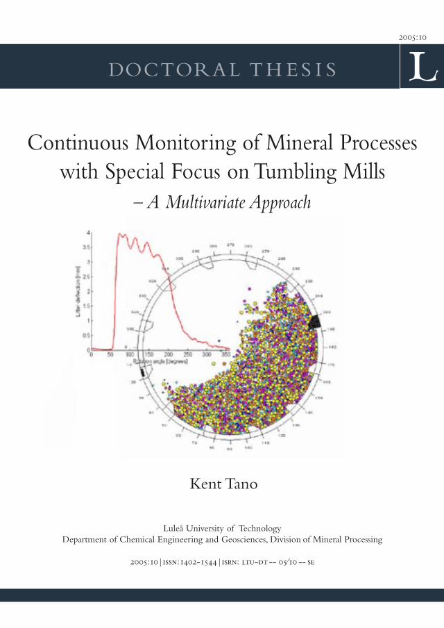
Cover illustration:
Visualisation of the ball charge movement in a tumbling mill using Distinct Element Modelling technique.
The force exerted on a lifter bar by the mill load measured with an embedded strain gauge sensor.
3

Continuous Monitoring of Mineral Processes with a Special Focus on Tumbling Mills – A Multivariate Approach
4
Continuous Monitoring of Mineral Processes with a Special Focus on Tumbling Mills – A Multivariate Approach
Continuous Monitoring of Mineral Processes with a Special Focus on Tumbling Mills – a Multivariate Approach
Abstract
Increasing emphasis on productivity and quality control has provided an impetus to research on better methodologies for diagnosis, modelling, monitoring, control and optimisation of mineral process systems. One of the biggest challenges facing the research community is the processing of raw sensor data into meaningful information. Information that to some extent express quality parameters such as chemical assays, size distribution and other metallurgical variables in the different process streams.
This thesis shows how multivariate statistical methods can be used with great advantage to model process data as well as sensor data of spectral character. The modelling approach has been applied on a large process section, a cobbing plant, as well as a single unit operation, a tumbling mill. As a signal pre-processing method for spectra-like data the discrete wavelet transform is used. It distinctly shows a capability of signal feature extraction where both time and frequency are of interest. Its well-known ability to achieve good data compression without loss of information is also demonstrated, here a data reduction ratio of 20:1 is obtained.
A strain gauge sensor that measure the deflection of a lifter bar when it hits the charge inside a tumbling mill is studied for different operating conditions in a pilot scale ball mill. The deflection of the lifter bar during every mill revolution gives rise to a characteristic signal profile that is shown to contain information on both the charge position and grinding performance. The results presented for prediction of grinding performance suggest that the strain gauge signal, in combination with wavelet transformation and multivariate data analysis, provide a promising mean for monitoring and control of process fluctuations. The low prediction error achieved for the calculated grinding performances clearly highlights the importance of well-planned experimental strategy including experimental design, signal pre-processing, multivariate modelling and validation. Results demonstrate that different operating conditions are well distinguishable from each other and by that the finding of proper operating regimes are highly feasible. Grinding parameters that are normally measured in the laboratory are now readily modelled from the on-line signal. As a consequence this opens new possibilities for real-time monitoring and control of the grinding process.
A further objective of this work is to link computational results to the experimental data obtained from an instrumented pilot ball mill. The approach taken is to simulate the behaviour of a rubber lifter when it is exposed to forces from the grinding charge in a two-dimensional DEM mill model using a particle flow code. Typically walls in a DEM model are made up of rigid bodies where the equations of motion are not satisfied for each individual wall - i.e., forces acting on a wall do not influence its motion. Here the instrumented rubber lifter is represented as an assemblage of bonded particles rather than walls in order to simulate deflection. The deflection profile obtained from the DEM simulation shows a reasonably good correspondence to the pilot mill measurements. The difference is attributed to the fact that time-dependent behaviour of the rubber lifter is ignored, resulting in a too rapid relaxation of the lifter when the exerted force is released. Mill charge features such as toe and shoulder position of the charge are well marked. However, DEM prediction shows lower values compared to measurements which is most likely an effect of the two- dimensional model used and the inability to model the effect of slurry present in the mill.
The novelty of the thesis work is in the method for analysing the signal profile as well as the experimental verification in both pilot and full-scale operation. The result is a contribution to improved mill lifter design and continuous monitoring of the grinding process.
Keywords: Grinding, Process monitoring, Simulation, Modelling, Strain gauge sensor
5

Continuous Monitoring of Mineral Processes with a Special Focus on Tumbling Mills – A Multivariate Approach
6

Continuous Monitoring of Mineral Processes with a Special Focus on Tumbling Mills – A Multivariate Approach
To my wife and family
7

Continuous Monitoring of Mineral Processes with a Special Focus on Tumbling Mills – A Multivariate Approach
8

Continuous Monitoring of Mineral Processes with a Special Focus on Tumbling Mills – A Multivariate Approach
LIST OF PUBLICATIONS
This thesis is based on the work contained in the following papers, referred to by Roman numerals in the text:
I. Continuous monitoring of a tumbling mill K Tano, B Pålsson and S Persson
Proceedings of the XXII International Mineral Processing Congress, Cape Town, South Africa, 28 September – 3 October 2003
II. Monitoring of a tumbling mill using PLS-regression on a wavelet transformed strain-gauge signal K Tano, B Pålsson and S Rännar
Submitted to Sensors and Actuators A: Physical
III. On-line Measurement of Charge Position and Filling Level in Industrial Scale Mills K Tano, A Berggren and B Pålsson
Accepted for publication in Minerals & Metallurgical Processing
IV. On-line monitoring of rheological effects in grinding mills using lifter deflection measurements K Tano, B Pålsson and A Sellgren
Minerals Engineering, In press
V. Comparison of experimental mill lifter deflection measurements with DEM predictions K Tano, M Pierce and J Alatalo
Submitted to International Journal of Mineral Processing
9

Continuous Monitoring of Mineral Processes with a Special Focus on Tumbling Mills – A Multivariate Approach
10

Continuous Monitoring of Mineral Processes with a Special Focus on Tumbling Mills – A Multivariate Approach
CONTENTS
ABSTRACT…………………………………………………………………………………………5
LIST OF PUBLICATIONS……………………………………………………………...………....9
CONTENTS…………………………………………………………………….………………….11
1 INTRODUCTION ....................................................................................................................13 1.1 GENERAL .................................................................................................................................13 1.2 SCOPE OF THIS WORK ...............................................................................................................13 1.3 OUTLINE OF THE THESIS ...........................................................................................................14
2 INTRODUCTION TO MONITORING OF MINERAL PROCESSES USING MULTIVARIATE STATISTICAL METHODS ..........................................................................15
2.1 BACKGROUND..........................................................................................................................15 2.2 MULTIVARIATE STATISTICAL MODELLING TECHNIQUES...........................................................15
2.2.1 Theoretical background of principal components...........................................................16 2.3 MONITORING VIA MULTIVARIATE PLOTS..................................................................................18 2.4 APPLICATION - COBBING PLANT...............................................................................................22
2.4.1 Process description..........................................................................................................22 2.4.2 Results and discussion .....................................................................................................22
2.5 CONCLUSIONS..........................................................................................................................24
3 OVERVIEW OF MILL LOAD MEASUREMENTS............................................................25 3.1 LITERATURE REVIEW OF PREVIOUS WORK................................................................................25 3.2 STRAIN GAUGE SENSOR SYSTEM...............................................................................................27
3.2.1 Strain-gauge signal features............................................................................................28
4 EXPERIMENTAL SET-UP AND METHOD .......................................................................31 4.1 PILOT SCALE BALL MILL ..........................................................................................................31 4.2 FULL SCALE BALL MILL ..........................................................................................................33 4.3 FULL SCALE AG MILL ..............................................................................................................34 4.4 WAVELET TRANSFORMATION...................................................................................................35
4.4.1 Analysis of process signal features..................................................................................36 4.4.2 Wavelet-PLS regression modelling.................................................................................38
4.5 DISTINCT ELEMENT METHOD ..................................................................................................38 4.5.1 Implementation of a flexible lifter....................................................................................40
5 RESULTS ..................................................................................................................................43 5.1 EFFECT OF OPERATING CONDITIONS .........................................................................................43
5.1.1 Effect of mill speed ..........................................................................................................43 5.1.2 Effect of mill load ............................................................................................................45 5.1.3 Effect of mill throughput..................................................................................................46
5.2 EFFECT OF FEED PARTICLE SIZE AND SLURRY PROPERTIES .......................................................47 5.2.1 Effect of feed particle size................................................................................................48 5.2.2 Effect of %-solid ..............................................................................................................49 5.2.3 Effect of change in slurry flow properties (viscosity)......................................................50
6 CONCLUSIONS.......................................................................................................................51
11

Continuous Monitoring of Mineral Processes with a Special Focus on Tumbling Mills – A Multivariate Approach
7 FUTURE WORK......................................................................................................................53
8 ACKNOWLEDGEMENTS .....................................................................................................55
9 REFERENCES .........................................................................................................................57
12
Continuous Monitoring of Mineral Processes with a Special Focus on Tumbling Mills – A Multivariate Approach
1 INTRODUCTION
1.1 General
The term data analysis and process monitoring, as used in the context of process applications, collectively refer to the interpretation and evaluation of sampled process measurements. Data analysis as used in this work is intended to describe how data are manipulated and used together with fundamental understandings to infer the state of a physical process. Monitoring, on the other hand, refers to the classification of the data based upon a calibration model of expected behaviour so that unwanted situations can be detected and proper control actions can be made. The first part of this research work which resulted in a licentiate thesis (Tano, 1996) focused on the use of a multivariate statistical model to monitor a mineral process with the aim to detect deviations from normal operation and in some extent predict quality properties in the processed material. The method is characterised by a good ability to visualise course of events but a disadvantage is the need of a great number of relevant measurements. Unfortunately, in many cases process data are of poor quality. Instrument failure, poorly or uncalibrated instrumentation, high noise levels, which all contributes to data problems. Without proper pre-treatment, the necessary interpretation is difficult, if not impossible. This principally limited the application of the method to few and relatively large process sections.
Substantial progress in the development of intelligent real-time sensors and data pre-treatment methods has opened new possibilities to study single unit operations. The second part of this work focuses on methods for measuring and modelling of the grinding process. Size reduction is an inevitable unit operation in mineral processing, and comminution is by far the most energy consuming part in mineral concentrators and extremely inefficient, less than 10% of supplied power produce new mineral surfaces, great efforts have been made to improve grinding operations. The economical potential is substantial if efficiency can be increased just a couple of percent. In general, the only grinding control is to maximize the power drawn by the mill. Unfortunately, the relation between power and grinding performance is a complex and non-linear function. Development of advanced control systems has helped the situation considerably. However, these systems still are lacking relevant information such as mill load, charge position or slurry properties. Sensors capable of delivering this information are therefore of great value. Pre-treatment by wavelet transformation to locate and identify significant events combined with multivariate statistics presents good prospects to estimate the magnitude of variables not directly measurable. Furthermore the application of fundamental physical modelling techniques such as DEM has developed considerably lately, which in the case of grinding has lead to increased knowledge and understanding of process phenomena taking place in a tumbling mill.
Accordingly, the combined use of advanced measuring techniques as well as the use of both empirical and fundamental mathematical modelling applied on mineral processes is a key approach to increase knowledge and create control strategies for improved product quality and process performance.
1.2 Scope of this work
The overall aim of the present work is to show how an advanced sensor system can be used to collect data that contain information of the grinding process and from these data derive multivariate models to monitor and characterise changes in operating conditions.
An objective of this thesis is also to determine the influence of the significant factors that vary in an ordinary grinding process and how these variations are reflected in the measured signal. To further understand the behaviour in the grinding mill DEM technique is applied and an attempt to validate the modelling results with obtained practical mill measurements is demonstrated.
13

Continuous Monitoring of Mineral Processes with a Special Focus on Tumbling Mills – A Multivariate Approach
Application of the thesis work will form a foundation for an on-line system that can be used to improve process performance in mineral process operations.
1.3 Outline of the thesis
Chapter 2 of this thesis introduces the concept of using multivariate statistical methods in the modelling of process data from mineral processes. The applied modelling techniques form the basis for the second part of the work where focus is on a sensor embedded in a lifter bar inside a grinding mill. In Chapter 3 is the applied sensor system as well as the most common methods to measure mill load characteristics described. The purpose of the two introductory chapters is to relate the methods used in the papers included in this thesis to other well-established techniques. Chapter 4describes the grinding mills studied and gives a brief overview of the data pre-treatment method used. Included in chapter 4 is also a conceptual description of how DEM technique is used in this work to link the measurement with fundamental knowledge of charge movement in a tumbling mill. The results obtained from the measurements under different operating conditions are presented and discussed in Chapter 5. Finally, some conclusions and future perspectives are presented in Chapter 6 and 7.
14

Continuous Monitoring of Mineral Processes with a Special Focus on Tumbling Mills – A Multivariate Approach
2 INTRODUCTION TO MONITORING OF MINERAL PROCESSES USING MULTIVARIATE STATISTICAL METHODS
2.1 Background
Nowadays an operator plays a very central role in the operation of a plant, it is not unusual that only one person controls an entire plant from a remote control room. Automated process control have lead to operators that to a larger extent are left with a passive monitoring task with few active interactions with, or manipulations of, the process under normal and stable operation of the plant. This leaves few opportunities for ‘learning by doing’ about how the process works and for applying, and thereby retaining and raising the reliability of trained skills. The operators generally have to intervene in the process only when disturbances exceeding some alarm criteria occur. A requirement is therefore that the control and information system shall support the operator in maintaining their process knowledge. Also, to be competitive many industries, and especially the mineral industry, have to improve their efficiency in utilisation of raw material and energy that have directed higher demands towards the operators for optimisation and trimming tasks. A development in this direction means that operators will be faced with more strategic tasks, which in turn, means that they will interact with the process on a higher supervisory level (Olsson and Lee, 1994).
A general trend in process industry is the development towards more and more complex processes with very specific demand on the final products. The customer have become more conscious about the quality and the demand is that quality should be uniform and of high level. Modern processes are inherently multivariate with many variables contributing to the overall process quality. The number of functions and measurements that the operators have to handle has lately increased dramatically. This put high demands on the interface that shall support the operator in interpreting changes that are taking part in the process. There is at the same time a limit on how much information an operator can process simultaneously. Therefore the interface of the control- and information system have to be adapted to the way humans process large data sets. Humans are very skilled in interpretation of pictures and recognising patterns. This complexity often limits the application of theoretical models, developed from first principal differential equations, to the monitoring of industrial processes. On the other hand, most processes now are equipped with automatic data acquisition systems linked to computerised databases that collect large amounts of information about the process operation. This allows for the possibility of using data based statistical models to better understand the process or to detect and analyse process upsets and sensor errors, and finally for process control (Veltkamp, 1993).
2.2 Multivariate statistical modelling techniques
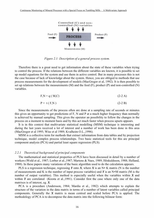
Many processes are multivariate in the sense that many variables contribute to the overall process quality. A process system can roughly be described as in Figure 2.1.
Ideally, the characteristics of the product can be described according to Eq.(2-1). Unfortunately the reality is not as nice, there are often a number of process variables that are non-controlled and also unmeasured.
P(quality, quantity) = f ( F, C) (2-1)
15
Continuous Monitoring of Mineral Processes with a Special Focus on Tumbling Mills – A Multivariate Approach
Figure 2.1: Description of a general process system.
Therefore there is a great need to get information about the state of these variables when trying to control the process. If the relations between the different variables are known, it is possible to set up model equations for the system and use them in active control. But in many processes this is not the case because of lack of knowledge about the system. Hence, you are obliged to methods that use process measurements for the development of models (MacGregor et al, 1992). It is then possible to set up relations between the measurements (M) and the feed (F), product (P) and non-controlled (N) variables.
F,N = q ( M,C) (2-2 A)
P = t ( F,N ) (2-2 B)
Since the measurements of the process often are done at a sampling rate of seconds or minutes this gives an opportunity to get predictions of F, N and P at a much higher frequency than normally is achieved by manual sampling. This gives the operator an possibility to follow the changes in the process on a moment to moment basis and by this act much faster when process upsets appears.
It is in this context that multivariate statistical modelling (MSM) technique is interesting and during the last years received a lot of interest and a number of work has been done in this area (MacGregor et al 1995; Wise et al 1989; Kvalheim O.L.,1996).
MSM is a collective term for methods that extract information from data tables and by projection technique, model complex process relationships. Two basic statistical tools for this are principal component analysis (PCA) and partial least square regression (PLS).
2.2.1 Theoretical background of principal components The mathematical and statistical properties of PLS have been discussed in detail by a number of
workers (Wold et al., 1987; Lorber et al.,1987; Martens & Naes, 1989; Höskuldsson, 1988; Helland, 1988). In these papers many variations of the basic algorithm used to do the calculation appears.
PLS is a regression technique, regressing Y onto X, where X is an N K matrix (N is the number of measurements and K is the number of input process variables) and Y is an N M matrix (M is the number of output variables). This method is especially useful when the variables within X and within Y are correlated (Kresta et al.,1991). Consider first the case where only one of the data matrixes is of interest, eg. X.
PCA is a procedure (Andersson, 1984; Mardia et al., 1982) which attempts to explain the structure of the variation in the data matrix in terms of a number of latent variables called principal components. Generally the X matrix is mean centred and scaled before PCA is applied. The methodology of PCA is to decompose the data matrix into the following bilinear form:
16
Continuous Monitoring of Mineral Processes with a Special Focus on Tumbling Mills – A Multivariate Approach
X = (tA
a 1a pa
T) + EA (2-3)
Where t is the score vector for X and p is the loading vector for X, EA is the residual matrix, a is the model dimension index (a= 1,…,A).
Since the ta’s and the pa’s are orthogonal it can be shown (Helland, 1988) that the ta’s are the eigenvectors of XXT and the pa’s are the eigenvectors of XTX. This points to the equivalency between PCA and singular value decomposition, SVD (Höskuldsson, 1988). In SVD the eigenvalues are calculated in descending order starting with the largest, in both methods the corresponding eigenvectors are also in descending order. For detailed discussions of PCA see Jackson (1991). For correlated data sets A<<K using SVD to calculate all the principal components is inefficient. The NIPALS algorithm (Wold et al., 1987) calculates the PC’s iteratively, the correct number of PC’s (A) can be determined from stopping criterions, one of the more popular techniques being cross validation (Wold, 1978). The Y matrix can be similarly decomposed into
Y = (uA
a 1a qa
T) + FA (2-4)
Where u is the score vector for Y and q is the weight vector for Y, FA is the residual matrix. Performing the regression of u onto t leads to principal component regression. PLS follow a similar procedure except that it performs both of the decomposition simultaneously and in an iterative manner in order to get a better prediction of Y. The method can be described by the following algorithm (Wold et al., 1987).
1. Start: set u equal to a column of Y2. wT = uTX/uTu (regress columns of X on u)3. Normalize w to unit length (w is weight vector for X)4. t = Xw/wTw (calculate the scores) 5. qT = tT Y/tTt (regress columns of Y on t)6. Normalize q to unit lenght 7. u = Yq/qTq (calculate new u vector) 8. Check convergence: if YES to 9, if NOT to 2 9. X loadings: p = XTt tTt10. Regression coefficient: b = uTt tTt (often set to one) 11. Calculate residual matrices: E = X-tpT and F = Y-btqT
12. To calculate the next set of latent vectors replace X & Y by E & F and repeat
The latent vectors (t and u) now depend upon both the X and Y spaces and are related through the linear inner relationship ua = ba ta + a where a is a residual and ba is the least squares regression coefficient. Non-linearities can be incorporated into the model by using a non-linear inner relationship ua = f(ba ,ta) + a and estimating the parameters (ba) by non-linear regression in step 10 (Wold et al., 1989). Höskuldsson (1988) showed some interesting relationship between PCA and PLS. These are of interest because PCA is conceptually easier to grasp than PLS. PCA works on the X matrix, and the loading vectors calculated using NIPALS are, as mentioned before, the eigenvectors of the covariance matrix XTX. PLS on the other hand, works on both X and Y, the first loading vector calculated in this case is the eigenvector of the matrix XTYYTX. This last matrix can be thought of in two ways: (1) the covariance of X has been scaled using the “size” of the Y matrix (YYT), or (2) PLS is simply PCA pre-formed on the covariance matrix of X and Y (YTX). Next loading vector is then calculated after updating of matrices X and Y.
17

Continuous Monitoring of Mineral Processes with a Special Focus on Tumbling Mills – A Multivariate Approach
2.3 Monitoring via multivariate plots
Since the operator nowadays has a central role in running an industrial plant, it is of great importance that the control system has functionality to support the operator. This means tools that help the operator to monitor actual process status, detect process upsets and also give guidance to keep the process at best conditions.
Traditionally the operator gets information presented as numerical figures or univariate trendcurves on a display. But in a multivariate situation where one is faced with perhaps 10 to 100 variables, individual plotting is not feasible. In this situation, approaches based on PCA and PLS are very attractive. Jackson (1980) provided early approaches to multivariate monitoring using PCA methods. More recent extensions of the PCA methods and the introduction of PLS approaches were considered by Wise et al. (1989) and by Kresta et al. (1990).
It can often be assumed that the underlying dimensionality of the process, when it is operating normally is quite low. Under these circumstances it is possible to represent the most important elements of its behaviour in low dimensional plots defined by the dominant latent vectors obtained via PCA or PLS. The low dimensional planes defined by these latent vectors provide a low dimensional window on the behaviour of the very high dimensional process. For e.g. a cobbing plant with an underlying dimension of three, the first two axes of the score plot (T1 and T2) form the two axes of the monitoring chart and each observation is located on this plot via its score, see Figure 2.2.
Figure 2.2: Score plot presentation of a low dimensional PLS model.
The observations included in the reference data set, data from the experiments that were set up in order to build the model, are plotted as ‘star dots’ on this chart. In order to really get an understanding of the cause and effect relationship it is of great importance to run the experiments according to a statistical design. If this is the case, it is then possible to mark different areas in the score plot as ‘good’ and ‘bad’ regions depending on the correlation structure between the manipulated variables and the response variables. Otherwise an appropriate reference data set could be chosen which defines the ‘normal operating conditions’ (NOC) for a particular process. The choice of this reference set is critical for a successful application of the procedure.
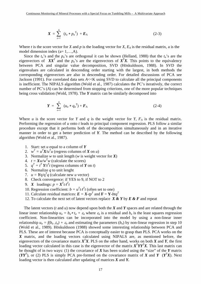
To get a correct interpretation of the mutual dependencies between the variables also the loading plot, Figure 2.3, have to be analysed. The loading plot do not needed to be presented continuously for the operator since the information in this plot is static as long as the model is not updated. It is of course essential that the operator can interpret the loading plot since it contain information about
18
Continuous Monitoring of Mineral Processes with a Special Focus on Tumbling Mills – A Multivariate Approach
how the controlled variables correlate to the quality variables. Interpretation of loading plots will be discussed in more detail when describing the case studies.
Figure 2.3: Loading plot presentation showing the correlation structure.
Consequently there are two main tasks for a multivariate statistical process control (MSPC) system to deal with, namely
- Detect if a new observation is an outlier, a process disturbance of some kind - Indicate the variable(s) which have contributed to the disturbance
The main concept behind the development and use of MSPC were laid out by Kresta et al., (1991), Wise et al., (1991), Wise and Ricker, (1991), MacGregor et al., (1991), and Friden and Wikström, (1995).
The first task, detection of an outlier is accomplished by either calculating the squared prediction error (SPEx), Eq.(2-5), or the measure called the distance to model (DmodX), Eq.(2-6). The SPExvalue represent the squared distance of a new observation from the model hyperplane, plots illustrating the use of SPEx are to be find in papers by MacGregor et al. (1991 and 1995).
SPEx = (xK
i 1new,i- x new,i)2 (2-5)
The rows in matrix EA(eik ) in Eq.(2-3) contains the residuals, i.e. the part of the data that is not
explained by the model. The row i's standard deviation of the residuals, si calculated according to Eq.(2-6), is a measure of the distance between the i:th observation and the PLS model. This measure is called distance to model, DmodX. High values in SPEx and DmodX indicate probable outliers in the X-space.
DmodX = si = ( eK
k 1
2ik /(A-K)) (2-6)
The second task, variable contribution can be calculated in different ways depending on the
objective. If the interest is to give information on how an observation differs from another in the t-score and how it influence on the outputs Y, the so called score gap contribution is calculated according to Eq.(2-7).
19
Continuous Monitoring of Mineral Processes with a Special Focus on Tumbling Mills – A Multivariate Approach
Gaps (scores) = X weight (2-7)
Where X is the difference between two observations or between one selected observation and the average process observation, default weight is the component loading, p.
Often there is an interest to calculate the gap contribution when monitoring a principal plane, e.g. t1 / t2, then Gaps is the sum for both components. If on the other hand the interest is to give information on which variable(s) that have contributed to an high value in DmodX, in other words which variables caused the new observation to move away from NOC, the DmodX gap contribution is calculated according to Eq.(2-8).
Gapd (DmodX) = ek weight (2-8)
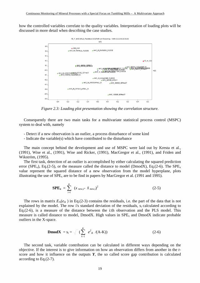
Here, ek, represents variable residuals and the default weight is the square root of the explained sum of squares for each variable. In the same manner it is possible to sum the DmodX gap contribution for two components when monitoring a principal plane. With this information it is possible to present the calculated gap contribution for the operator in a bar graph form. Sorting the variables in decreasing order in respect to the calculated Gaps,d offer an very convenient way for the operator to get a fast overview on which variables that caused a process upset, see Figure 2.4.
Figure 2.4: Gap contribution plot, variable influence in decreasing order.
By combining these different charts (score, gap contribution and time-plot) together in one display, Figure 2.5, it can be used to monitor the process. The scores for a new observation can be located on the principal plane according to the calculation in Eq. (2-9).
t1 = X w1 , t2 = (X - t1p1T) w2 (2-9)
Connecting each new calculated score t1 / t2 (n) to a previous one t1 / t2 (n-1) with a line, presents the process as a dynamic line, a worm. The movement of this worm shows whether the process is approaching or deviating from the model centre. A proper length of the worm has the be chosen depending on time constants in the process but also how long time backwards there is an interest to follow the process. The structure of these plots reflects the two ways in which abnormalities can enter the system and provides powerful diagnostic capability to determine the
20

Continuous Monitoring of Mineral Processes with a Special Focus on Tumbling Mills – A Multivariate Approach
cause of the abnormality (MacGregor, 1991). If the abnormality is caused by a larger than normal change in one or more of the process variables, but the basic relationship between the process and quality variables does not change, then the abnormality will manifest itself as a shift in the principal plane, and the DmodX will remain at an acceptable level. If on the other hand the abnormality enters through a new event not captured in the reference set, it will change the nature and possibly the dimension of the relationship between the process and quality variables. This will show up in an increase in DmodX. Future development of the algorithm has to make the model adaptive by recursively updating it with new samples.
In order to retain the ease of interpretation it is of importance to keep the number of principal components low, this means that normally the monitoring procedure would be restricted to a maximum of three to four latent vectors. For very complex processes, where the bulk of variation is not explained by few principal components, the system should be divided into logical modular sections that can be monitored separately.
Figure 2.5: Operator display showing scores, gap contribution and DModX.
An example how an operator display could be designed is presented in Figure 2.5. Here, the upper left corner shows the dynamic score plot where the operator continuously receives information regarding changes in the process. If a sudden process disturbance of the earlier mentioned types occurs, the operator can intervene and call for the gap contribution chart, shown to the right. The variables are sorted in such a way that the most influenced variable are at the top, with the colour (dark or grey) indicating if the variable influence is positive or negative. By activating one of the variable bars, the time plot of the corresponding variable is presented in the lower left part of the display. Normally the time plot shows the value of DmodX. This value is of great importance since it tells the operator if the process is within the model space or not. It must be mentioned that the multivariate charts do not replace, but rather complement, the traditional displays that are used by the operators.
21
Continuous Monitoring of Mineral Processes with a Special Focus on Tumbling Mills – A Multivariate Approach
2.4 Application - Cobbing plant
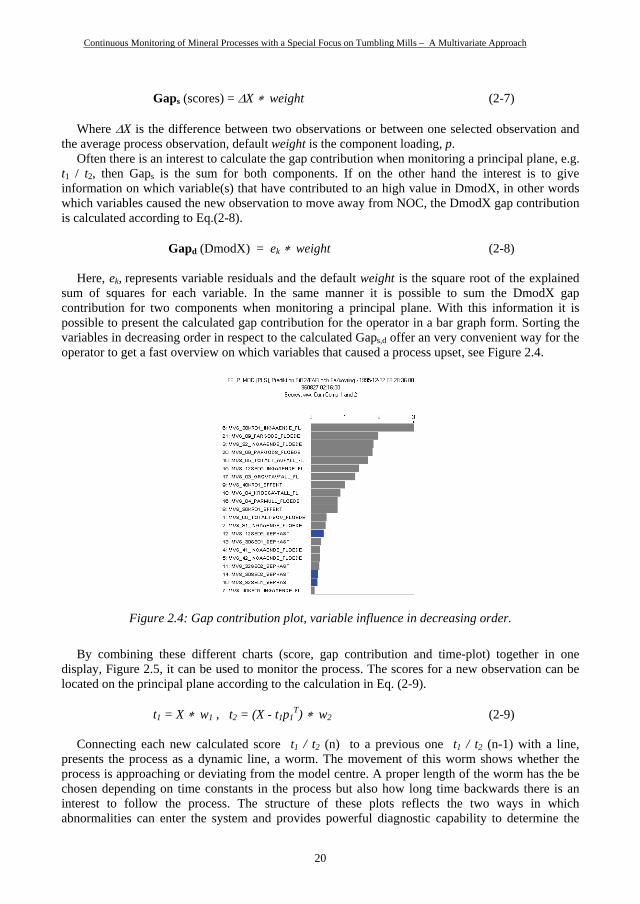
2.4.1 Process description The cobbing plant at LKAB Malmberget, shown diagrammatically in Figure 2.6, has an
incoming feed where the iron content varies between 45-55%. As a consequence of this, the operator has to run the plant in such a way that the lowest grade crude ore gives an acceptable final quality. The adjustable variables are the amount of fresh feed and the speed of the magnetic separators. The problem for the operator is to decide, with certainty, when the iron content is high or low. An experienced operator can judge this by studying via a video-camera the colour of the material when the incoming feed passes a screen. If there were time enough for the operator to continuously monitor the video display there would be a possibility to act at the right moment. Unfortunately, the operators tasks are so many and so varying that there is seldom time for detailed monitoring. It is in this context that PLS modelling is interesting.
Figure 2.6: Flow chart of the cobbing plant at LKAB, Malmberget.
Since the main interest for modelling of this process was to develop a strategy for controlling the quality variation in the PAR product, it was necessary to run designed experiments. The manipulated variables were the amount of fresh feed and the speed of the magnetic separators. The interesting responses were the silica content in PAR and the iron content in the crude ore. Through the development of a model that predicts the responses with enough precision and then applying the model for the graphical presentation of the process status, hopefully sufficient information will be made available to the operator for taking the necessary control actions.
2.4.2 Results and discussion Detailed results and interpretations using the calibrated model are given in Tano (1996). The
model deals with a delicate problem, namely the quality of the fresh feed. It is very difficult, mainly due to the large sampling problem, to measure the iron content so frequently that it can be used for control. In practice, one value is delivered from the laboratory every 24 hours. No values are reported during weekends. For silica content, the agreement is fairly good with a prediction error of approximately +/- 0.8%-units. Unfortunately, this is somewhat too large for direct control purposes. The agreement, however, for the iron content in the crude ore is very good with the prediction error in this case being approximately +/- 0.9 %-units. This accuracy is satisfactory enough to fulfil the goal for this model.
22

Continuous Monitoring of Mineral Processes with a Special Focus on Tumbling Mills – A Multivariate Approach
In order to test the predictive capability of the model, the iron content in the incoming feed to the sorting plant was predicted during the validation period (comprising 3.5 months). This is shown in Figure 2.7. The model provided a prediction of the iron content every minute. In order to make it possible to compare the predictions with the 24 hours value provided by the Quality Department, the average value was chosen for comparison with the predictions. The first month of the validation period shows a constant deviation, probably due to the change of screen size just before the validation period started. After the first month, it was decided to make a small correction to the model and the following 2.5 months showed a very good accuracy in the prediction.
Figure 2.7: Long term validation of the PLS model.
The monitoring part in the modelling of the sorting plant yielded some very interesting results. First of all, a thorough training of the involved operators was conducted. This involved both process analysis as well as an introduction to MVA. Results from the modelling showed that component t1 and t2 explained approximately 87% of the variation in the response variables. This implies that the operator only has to contemplate the principal plane t1 and t2 which considerably simplify the handling of the score plot. The operators found the functionality in the MVA system to be very useful, especially the gap contribution chart. Unfortunately, the implemented MVA system had to use an old graphical system in the process control computer. This led to some dissatisfaction with the response time when exchanging windows and also with the design of some displays. Another interesting observation from the operators viewpoint was that the MVA system overreacted to trivial changes such as a stop in a feeder which caused the worm to spread over the whole score chart. Such process disturbances are so elementary that they can be handled by the ordinary alarm system. In the MVA system they are more bothersome than helpful. The overall opinion from the operators was very positive. Today the MVA system has characteristics, which are helpful to conducting the daily activities, and with some polishing of details it will be useful in operation. Experience gained from the modelling of the sorting plant led to the following recommendations:
- If the predictive capability of the model is good enough, use the predicted value as one of the signals in the control system.
- If the complexity of the process is relatively low MVA charts should not be used since they do not bring any new information to the operator.
- The interface of the MVA system must be easy to use preferably integrated into the ordinary control system.
- An interlocking module bypassing the model should be used to handle trivial disturbances.
23
Continuous Monitoring of Mineral Processes with a Special Focus on Tumbling Mills – A Multivariate Approach
The recommendations and the overall results are so encouraging as to demand that similar work should be continued on the other mineral processing plant sections.
2.5 Conclusions
Models are only simplified approximations, intended to have structural or functional analogy to some phenomena in the inaccessible more complex reality. Hence it is important to use methods which yield a reasonable compromise between simplicity and completeness. A statistical multivariate modelling method, PLS regression has been presented for steady state modelling of a mineral process.
Experience with the technique has shown that PLS stimulates users to take an open-minded approach to data analysis in general and to the calibration of process models in particular. The applications have shown that it solves the multivariate prediction problem for collinear data with satisfactory predictive ability. The resulting model often has good interpretation properties as well, due to its dimensional parsimony.
By approximating complicated multivariate input data by a few principal components, the operator can plot simplified ‘maps’ of the main relevant information from the process. This allows the operator, who knows the data and their context, to interactively bring important background knowledge and intuition into their interpretation. The information would otherwise be far too complex to be represented as explicit numerical information in statistical modelling. This also gives the operator the ability to detect major changes in the behaviour of the process caused by new events.
PLS modelling has also shown to be very useful in mineral processing unit operations e.g. grinding, where the direct measurement of certain physical parameters is infeasible. Experimental modelling work, where data from an embedded strain gauge sensor, a lifter deflection profile, has been regressed to a number of mill operating parameters, has indicated promising and satisfactory results with respect to reliability and accuracy. This will be further elaborated in following chapters.
24
Continuous Monitoring of Mineral Processes with a Special Focus on Tumbling Mills – A Multivariate Approach
3 OVERVIEW OF MILL LOAD MEASUREMENTS
3.1 Literature review of previous work
Grinding in tumbling mills are inefficient, much of the energy is wasted in impact, that do not break particles. Autogenous (AG) and semi-autogenous (SAG) mills often operate in an unstable state because of the difficulty to balance the rate of replenishment of large ore particles from the feed with the consumption in the charge. This has led to an increased interest in obtaining an accurate and direct measurement of mill load and the behaviour of the mill charge. Several parameters do significantly influence the effectiveness of the grinding operation, however, some of these parameters are either difficult or laborious to measure. Intermittent in-situ measurements of some of the parameters are most often prone to errors and there is often a long time-delay before the acquired data is fed to the control system. Also, an understanding of the charge motion within the mill is of importance in mill optimisation (Agrawala et al., 1997). Both the breakage of ore particles and the wear of liners/ball media are closely linked to the charge motion. Therefore, it is essential to use a method that can provide a precise, as well as, real time information of the charge to the control system.
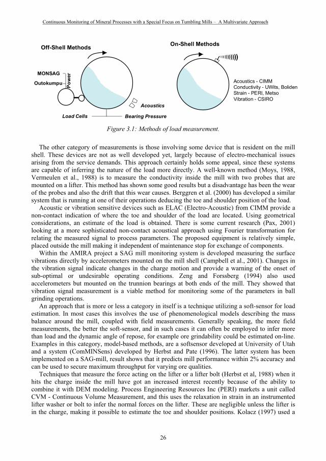
Work done in the past can be divided into two main categories of methods of load measurement; off-shell and on-shell, c.f. Figure 3.1. One method of the first category that has been used in many plants is to measure the bearing back-pressure on the mill’s feed and/or discharge end. It gives an idea of the weight of the charge and it can be correlated to the filling level. A method developed by Bradken Mineral calculates the weight of the charge load by the measurement of bearing pressure, power draw and mill speed. One system installed on a 28ft SAG-mill at Noranda Mine in Brunswick showed that it is theoretically feasible to relate mill load with bearing pressure, provided that wear of mill lining as well as the mill drive system is taken into account. (Evans, 2001) The great disadvantage is that the pressure is not stable, e.g., shifting temperature causes sensor drift. Moreover, since bearing pressure is related to overall mill weight, changes to the ball charge as well as the wear of the lining will affect the signal. As a consequence, it is hard to develop a robust calibration. Despite these problems, one can still make use of bearing pressure for SAG load control. In an attempt to circumvent some of the problems associated with bearing pressure, load cells can be used under SAG mills. Proper installation is of great importance, ensuring that the sensors are located beneath all elements bearing weight, including pinions for example, to measure load when the mill is running.
Acoustics have been used in different kinds of setup; single microphones (Watson et al, 1985) correlated sound power with pulp viscosity, arrays of microphones (Jaspan et al., 1986) designed to detect changes in the position of the toe of the mill charge. Koivistoinen et al. (1989) used high frequency sampling of the power draw, and more specifically the amplitude of the power oscillations corresponding to each lifter passing through the pulp/charge, to infer mill loading. The phase shift in power draw can be correlated to the change in toe position of the charge. Järvinen (2004) showed that the method produced result comparable to intrusive methods. In Chile, a device from CIMM (Centro de Investigacion Minera y Metalurgica) known as MONSAG (Monitoring SAG mills) also employs the power draw, and through a complex signal processing algorithm estimates torque, which can be correlated with volumetric filling. The system is well suited to detect under- and overfilling of the mill. A validation of the system was performed on a 15 kHp SAG-mill where Pontt (2004) established a 3.2 % increase in throughput and a better understanding of the mills optimal operation.
A similar method, using a mill power draw model, described by Apelt et al. (2001) showed that the method can be used to predict total filling level as well as ball charge level.
25
Continuous Monitoring of Mineral Processes with a Special Focus on Tumbling Mills – A Multivariate Approach
Off-Shell Methods
Bearing PressureLoad Cells
Acoustics
Outokumpu
MONSAGPo
wer
On-Shell Methods
)) )) ))))))))
Acoustics - CIMMConductivity - UWits, BolidenStrain - PERI, MetsoVibration - CSIRO
Figure 3.1: Methods of load measurement.
The other category of measurements is those involving some device that is resident on the mill shell. These devices are not as well developed yet, largely because of electro-mechanical issues arising from the service demands. This approach certainly holds some appeal, since these systems are capable of inferring the nature of the load more directly. A well-known method (Moys, 1988, Vermeulen et al., 1988) is to measure the conductivity inside the mill with two probes that are mounted on a lifter. This method has shown some good results but a disadvantage has been the wear of the probes and also the drift that this wear causes. Berggren et al. (2000) has developed a similar system that is running at one of their operations deducing the toe and shoulder position of the load.
Acoustic or vibration sensitive devices such as ELAC (Electro-Acoustic) from CIMM provide a non-contact indication of where the toe and shoulder of the load are located. Using geometrical considerations, an estimate of the load is obtained. There is some current research (Pax, 2001) looking at a more sophisticated non-contact acoustical approach using Fourier transformation for relating the measured signal to process parameters. The proposed equipment is relatively simple, placed outside the mill making it independent of maintenance stop for exchange of components.
Within the AMIRA project a SAG mill monitoring system is developed measuring the surface vibrations directly by accelerometers mounted on the mill shell (Campbell et al., 2001). Changes in the vibration signal indicate changes in the charge motion and provide a warning of the onset of sub-optimal or undesirable operating conditions. Zeng and Forssberg (1994) also used accelerometers but mounted on the trunnion bearings at both ends of the mill. They showed that vibration signal measurement is a viable method for monitoring some of the parameters in ball grinding operations.
An approach that is more or less a category in itself is a technique utilizing a soft-sensor for load estimation. In most cases this involves the use of phenomenological models describing the mass balance around the mill, coupled with field measurements. Generally speaking, the more field measurements, the better the soft-sensor, and in such cases it can often be employed to infer more than load and the dynamic angle of repose, for example ore grindability could be estimated on-line. Examples in this category, model-based methods, are a softsensor developed at University of Utah and a system (ComMINSens) developed by Herbst and Pate (1996). The latter system has been implemented on a SAG-mill, result shows that it predicts mill performance within 2% accuracy and can be used to secure maximum throughput for varying ore qualities.
Techniques that measure the force acting on the lifter or a lifter bolt (Herbst et al, 1988) when it hits the charge inside the mill have got an increased interest recently because of the ability to combine it with DEM modeling. Process Engineering Resources Inc (PERI) markets a unit called CVM - Continuous Volume Measurement, and this uses the relaxation in strain in an instrumented lifter washer or bolt to infer the normal forces on the lifter. These are negligible unless the lifter is in the charge, making it possible to estimate the toe and shoulder positions. Kolacz (1997) used a
26
Continuous Monitoring of Mineral Processes with a Special Focus on Tumbling Mills – A Multivariate Approach
piezoelectric strain transducer for the measurement of mill load. Here the strain arisen on the mill shell due to the charge load is measured and is directly proportional to the ball charge load.
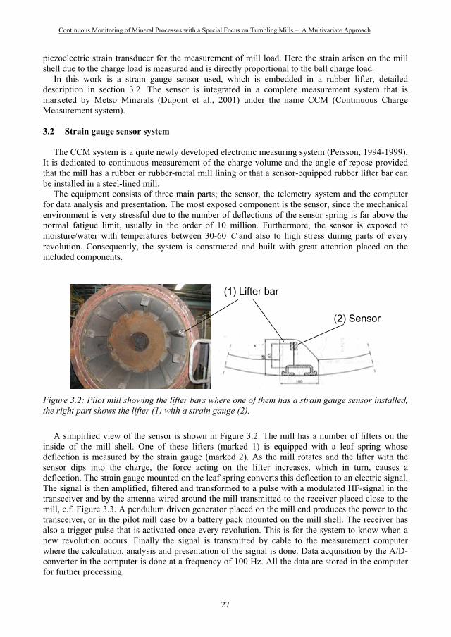
In this work is a strain gauge sensor used, which is embedded in a rubber lifter, detailed description in section 3.2. The sensor is integrated in a complete measurement system that is marketed by Metso Minerals (Dupont et al., 2001) under the name CCM (Continuous Charge Measurement system).
3.2 Strain gauge sensor system
The CCM system is a quite newly developed electronic measuring system (Persson, 1994-1999). It is dedicated to continuous measurement of the charge volume and the angle of repose provided that the mill has a rubber or rubber-metal mill lining or that a sensor-equipped rubber lifter bar can be installed in a steel-lined mill.
The equipment consists of three main parts; the sensor, the telemetry system and the computer for data analysis and presentation. The most exposed component is the sensor, since the mechanical environment is very stressful due to the number of deflections of the sensor spring is far above the normal fatigue limit, usually in the order of 10 million. Furthermore, the sensor is exposed to moisture/water with temperatures between 30-60 and also to high stress during parts of every revolution. Consequently, the system is constructed and built with great attention placed on the included components.
C
(1) Lifter bar
(2) Sensor
Figure 3.2: Pilot mill showing the lifter bars where one of them has a strain gauge sensor installed, the right part shows the lifter (1) with a strain gauge (2).
A simplified view of the sensor is shown in Figure 3.2. The mill has a number of lifters on the inside of the mill shell. One of these lifters (marked 1) is equipped with a leaf spring whose deflection is measured by the strain gauge (marked 2). As the mill rotates and the lifter with the sensor dips into the charge, the force acting on the lifter increases, which in turn, causes a deflection. The strain gauge mounted on the leaf spring converts this deflection to an electric signal. The signal is then amplified, filtered and transformed to a pulse with a modulated HF-signal in the transceiver and by the antenna wired around the mill transmitted to the receiver placed close to the mill, c.f. Figure 3.3. A pendulum driven generator placed on the mill end produces the power to the transceiver, or in the pilot mill case by a battery pack mounted on the mill shell. The receiver has also a trigger pulse that is activated once every revolution. This is for the system to know when a new revolution occurs. Finally the signal is transmitted by cable to the measurement computer where the calculation, analysis and presentation of the signal is done. Data acquisition by the A/D-converter in the computer is done at a frequency of 100 Hz. All the data are stored in the computer for further processing.
27

Continuous Monitoring of Mineral Processes with a Special Focus on Tumbling Mills – A Multivariate Approach
For both ball mills (pilot and full scale) there is only one sensor installed at the center of the mill. In the AG mill application the sensors are placed as marked in Figure 3.3.
SensorPlacement
Tranciever
Receiver
AntennaGenerator
Figure 3.3: Overview of the mill with its mounted system components.
3.2.1 Strain-gauge signal features A typical deflection profile of the sensor signal and a corresponding graphical representation of a
simulation of a mill are shown in Figure 3.4. The numbers in Figure 3.4, indicate important dynamic events during the passage of the sensor-equipped lifter bar under the mill charge.
1. The sensor lifter bar (SL) is still in the air 2. The SL hits the surface of the slurry 3. The SL starts to get submerged in the slurry 4. The SL hits the ball charge and starts to get submerged in the charge (T4)5. The SL starts to bend forward due to turbulence in the toe area 6. The SL grips the ball charge again 7. The SL is at peak bending 8. The SL has gradually decreased the bending and is at take-off position 9. The SL is leaving the ball charge and starts slowly rise to an upright position (T9)
Sign
al
Figure 3.4. CCM raw signal, showing the bending of a rubber lifter during the passage of the charge.
Time
Calculation of fractional filling J and dynamic angle of repose radians from a CCM system raw signal is quite straight forward since the change in force acting on the lifter relates to both (Jof the mill charge. A simple method for estimating those parameters is shown in equation (1) and (2), where N is mill speed (rps) and T is time (s) when lifter enter and leaves the charge.
28
Continuous Monitoring of Mineral Processes with a Special Focus on Tumbling Mills – A Multivariate Approach
J (T9 -T4)N – (sin 2 ( T9 -T4)N)/ 2 (1)
(T9 +T4)N – ( /2) (2)
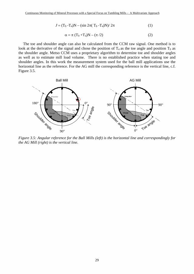
The toe and shoulder angle can also be calculated from the CCM raw signal. One method is to look at the derivative of the signal and chose the position of T4 as the toe angle and position T9 as the shoulder angle. Metso CCM uses a proprietary algorithm to determine toe and shoulder angles as well as to estimate mill load volume. There is no established practice when stating toe and shoulder angles. In this work the measurement system used for the ball mill applications use the horizontal line as the reference. For the AG mill the corresponding reference is the vertical line, c.f. Figure 3.5.
Shoulder angle Toe angle
0
9090
Toe
angl
e
Shoulder angle90
180 0
Ball Mill AG Mill
Figure 3.5: Angular reference for the Ball Mills (left) is the horizontal line and correspondingly for the AG Mill (right) is the vertical line.
29

Continuous Monitoring of Mineral Processes with a Special Focus on Tumbling Mills – A Multivariate Approach
30
Continuous Monitoring of Mineral Processes with a Special Focus on Tumbling Mills – A Multivariate Approach
4 EXPERIMENTAL SET-UP AND METHOD
4.1 Pilot scale Ball mill
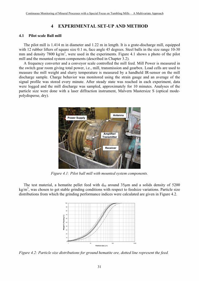
The pilot mill is 1.414 m in diameter and 1.22 m in length. It is a grate-discharge mill, equipped with 12 rubber lifters of square size 0.1 m, face angle 45 degrees. Steel balls in the size range 10-30 mm and density 7800 kg/m3, were used in the experiments. Figure 4.1 shows a photo of the pilot mill and the mounted system components (described in Chapter 3.2).
A frequency converter and a conveyor scale controlled the mill feed. Mill Power is measured in the switch gear room giving total power, i.e., mill, transmission and gearbox. Load cells are used to measure the mill weight and slurry temperature is measured by a handheld IR-sensor on the mill discharge sample. Charge behavior was monitored using the strain gauge and an average of the signal profile was stored every minute. After steady state was reached in each experiment, data were logged and the mill discharge was sampled, approximately for 10 minutes. Analyses of the particle size were done with a laser diffraction instrument, Malvern Mastersize S (optical mode-polydisperse, dry).
Antenna
Amplifier/Transmitter
Receiver
Power Supply
Figure 4.1: Pilot ball mill with mounted system components.
The test material, a hematite pellet feed with d50 around 35 m and a solids density of 5200 kg/m3, was chosen to get stable grinding conditions with respect to feedsize variations. Particle size distributions from which the grinding performance indices were calculated are given in Figure 4.2.
0
10
20
30
40
50
60
70
80
90
100
1 10 100 1000
Particle size ( m)
Wei
ght %
Pas
sing
( %)
Figure 4.2: Particle size distributions for ground hematite ore, dotted line represent the feed.
31
Continuous Monitoring of Mineral Processes with a Special Focus on Tumbling Mills – A Multivariate Approach
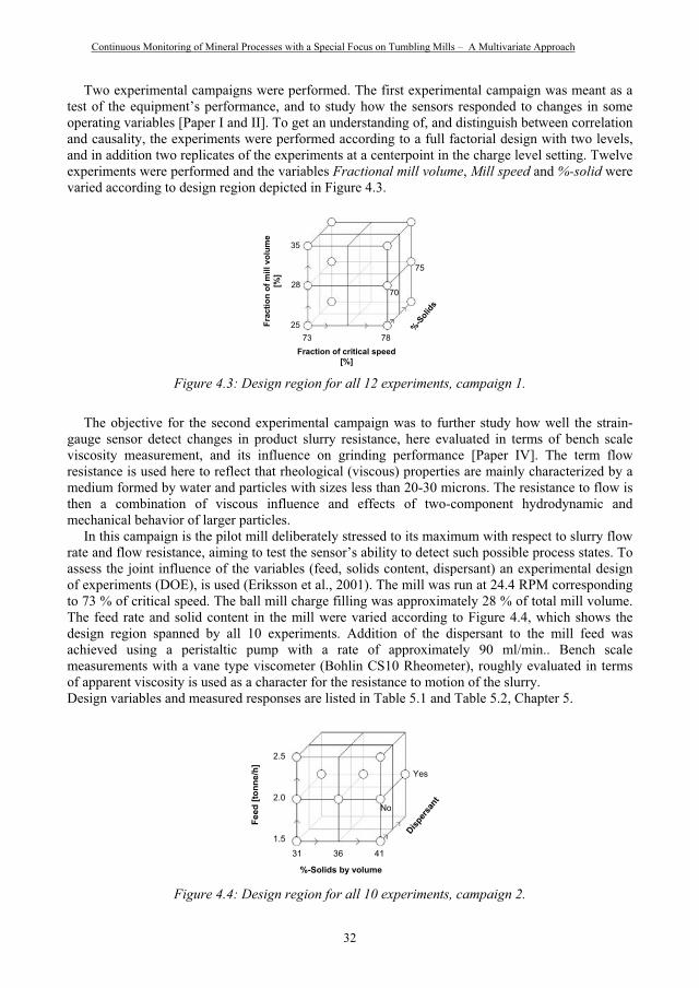
Two experimental campaigns were performed. The first experimental campaign was meant as a test of the equipment’s performance, and to study how the sensors responded to changes in some operating variables [Paper I and II]. To get an understanding of, and distinguish between correlation and causality, the experiments were performed according to a full factorial design with two levels, and in addition two replicates of the experiments at a centerpoint in the charge level setting. Twelve experiments were performed and the variables Fractional mill volume, Mill speed and %-solid were varied according to design region depicted in Figure 4.3.
Fraction of critical speed [%]
Frac
tion
of m
ill v
olum
e [%
]
%-Soli
ds
75
7028
35
2573 78
Figure 4.3: Design region for all 12 experiments, campaign 1.
The objective for the second experimental campaign was to further study how well the strain-gauge sensor detect changes in product slurry resistance, here evaluated in terms of bench scale viscosity measurement, and its influence on grinding performance [Paper IV]. The term flow resistance is used here to reflect that rheological (viscous) properties are mainly characterized by a medium formed by water and particles with sizes less than 20-30 microns. The resistance to flow is then a combination of viscous influence and effects of two-component hydrodynamic and mechanical behavior of larger particles.
In this campaign is the pilot mill deliberately stressed to its maximum with respect to slurry flow rate and flow resistance, aiming to test the sensor’s ability to detect such possible process states. To assess the joint influence of the variables (feed, solids content, dispersant) an experimental design of experiments (DOE), is used (Eriksson et al., 2001). The mill was run at 24.4 RPM corresponding to 73 % of critical speed. The ball mill charge filling was approximately 28 % of total mill volume. The feed rate and solid content in the mill were varied according to Figure 4.4, which shows the design region spanned by all 10 experiments. Addition of the dispersant to the mill feed was achieved using a peristaltic pump with a rate of approximately 90 ml/min.. Bench scale measurements with a vane type viscometer (Bohlin CS10 Rheometer), roughly evaluated in terms of apparent viscosity is used as a character for the resistance to motion of the slurry. Design variables and measured responses are listed in Table 5.1 and Table 5.2, Chapter 5.
1.5
2.0
2.5
Feed
[ton
ne/h
]
%-Solids by volume
Disper
sant
31 36 41
No
Yes
Figure 4.4: Design region for all 10 experiments, campaign 2.
32
Continuous Monitoring of Mineral Processes with a Special Focus on Tumbling Mills – A Multivariate Approach
4.2 Full scale Ball mill
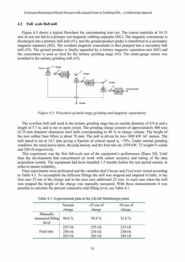
Figure 4.5 shows a typical flowsheet for concentrating iron ore. The coarse materials at 10-15 mm in size are fed to a primary wet magnetic cobbing separator (M1). The magnetic concentrate is discharged into a primary ball mill (#1), and the ground product (pulp) is transferred to a secondary magnetic separator (M2). The resultant magnetic concentrate is then pumped into a secondary ball mill (#2). The ground product is finally upgraded by a tertiary magnetic separation unit (M3) and the concentrate is used as feed for the tertiary grinding stage (#3). The strain-gauge sensor was installed in the tertiary-grinding mill (#3).
Water
Waste
Concentrate
Water
Water
Feed
Figure 4.5: Flowsheet of multi-stage grinding and magnetic separations.
The overflow ball mill used in the tertiary grinding stage has an outside diameter of 4.9 m and a length of 5.7 m, and is run in open circuit. The grinding charge consists of approximately 400 tons of 25-mm diameter chromium steel balls corresponding to 40 % in charge volume. The height of the new rubber liner lifters is about 70 mm. The mill is driven by two 1800 kW AC motors. The mill speed is set at 14.7 rpm giving a fraction of critical speed c =78%. Under normal grinding condition, the rated power draw, the pulp density and the feed rate are 2550 kW, 72 weight-% solids and 250 t/h respectively.
This experiment was the first full-scale test of the equipment’s performance [Paper III]. Until then the development had concentrated on work with sensor accuracy and tuning of the data acquisition system. The equipment had been installed 1.5 months before the test period started, in order to ensure reliability.
Nine experiments were performed and the variables Ball Charge and Feed were varied according to Table 4.1. To accomplish the different fillings the mill was stopped and emptied of balls, in the first case 25 ton of the charge and in the next case additional 25 tons. In each case when the mill was stopped the height of the charge was manually measured. With these measurements it was possible to calculate the percent volumetric mill filling level, see Table 4.1.
Table 4.1: Experimental plan at the LKAB Malmberget plant.
Normal charge
-25 ton of charge
-50 ton of charge
Manuallymeasured filling
level44.6 % 38.8 % 31.6 %
235 t/h 235 t/h 215 t/h 250 t/h 250 t/h 230 t/h Feed rate 265 t/h 265 t/h 245 t/h
33

Continuous Monitoring of Mineral Processes with a Special Focus on Tumbling Mills – A Multivariate Approach
4.3 Full scale AG mill
The flowsheet for the grinding line at Aitik where the experiments was conducted is shown in Figure 4.6. The ROM material is fed to the primary autogenous grinding mill, 6.7m 12.2 m with installed power of 6000 kW. From the primary mill, 40 to 80 mm pebbles are extracted to the secondary pebble mill, 5.2m 6.8 m, motor power of 3000 kW. The primary and secondary mill is running in closed circuit with a spiral classifier where the coarse material goes back to the primary mill. During normal operation, the primary mill is controlled using a simple and effective optimizing control strategy implemented in the DCS. The objective for the optimizing control is to maximize the throughput. This is done by always keeping the mill at one of two constraints limiting the throughput. The two constraints are maximum allowed mill filling or maximum allowed power draw. Which of the constraints that is active depends on the ore type and fragmentation. The strain-gauge sensor is installed in the primary AG-mill.
Figure 4.6: Flowsheet of a grinding line at the Aitik plant.
The Aitik experiments [Paper III] were conducted with three strain gauge sensors mounted in lifters at different locations along the shell of a primary AG mill. One was mounted at the feed, one in the middle and one at the discharge end, c.f. Figure 3.3. The system used for transmitting the data is slightly different from the one described earlier. Instead of using a modulated HF-signal, the Boliden system has a radio modem with a baudrate of 4800 kBit/s. For each revolution the signal shape from the previous revolution is sent by a radio modem to the receiver beside the mill. From the radio modem, data is transmitted with short distance modems to a computer in the control room where it is received by the serial port. Since only one signal, i.e. from one analog input channel, can be transmitted at a time for one mill the system scans the three input channels consecutively. Each signal is sampled with 125 Hz for 246 degrees of the total revolution. With a mill speed of 12.8 rpm this corresponds to 400 measurements each revolution. A LabView application filters the signal and calculates the toe-angle of the grinding charge. Observe, that here is the toe-angle defined as the angle between a vertical line and the point where the lifter hits the charge, c.f. right part of Figure 3.5 (Chapter 3.2). A higher value corresponds to either a higher mill filling or a charge that is more horizontally positioned due to mill speed, slurry rheology etc.
This part of the work had a focus on studying the ability of the sensor to detect how changes in operating conditions and variables influence the grinding charge, this with respect to both position and filling level of the charge. The changes were aimed to be within what could be seen as a normal operating range during production. The final goal with these experiments was to find out if the charge measurement could be used in a control strategy where throughput is maximized. A number of different step changes were made, summarized in Table 4.2.
34
Continuous Monitoring of Mineral Processes with a Special Focus on Tumbling Mills – A Multivariate Approach
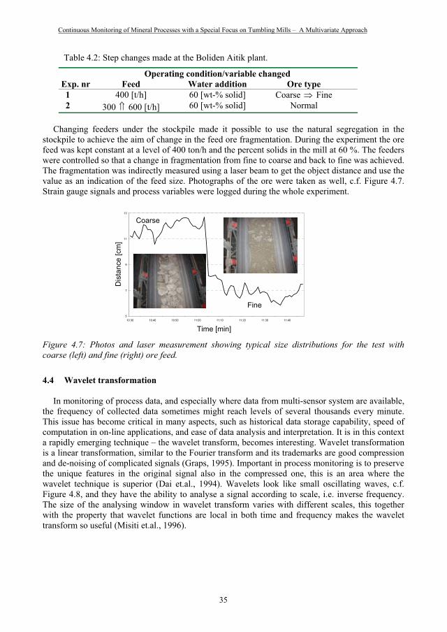
Table 4.2: Step changes made at the Boliden Aitik plant.
Operating condition/variable changed Exp. nr Feed Water addition Ore type 1 400 [t/h] 60 [wt-% solid] Coarse Fine 2 300 600 [t/h] 60 [wt-% solid] Normal
Changing feeders under the stockpile made it possible to use the natural segregation in the stockpile to achieve the aim of change in the feed ore fragmentation. During the experiment the ore feed was kept constant at a level of 400 ton/h and the percent solids in the mill at 60 %. The feeders were controlled so that a change in fragmentation from fine to coarse and back to fine was achieved. The fragmentation was indirectly measured using a laser beam to get the object distance and use the value as an indication of the feed size. Photographs of the ore were taken as well, c.f. Figure 4.7. Strain gauge signals and process variables were logged during the whole experiment.
5
7
9
11
13
10:30 10:40 10:50 11:00 11:10 11:20 11:30 11:40
Time [min]
Dis
tanc
e [c
m]
Coarse
Fine
Figure 4.7: Photos and laser measurement showing typical size distributions for the test with coarse (left) and fine (right) ore feed.
4.4 Wavelet transformation
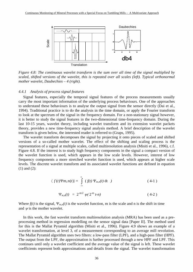
In monitoring of process data, and especially where data from multi-sensor system are available, the frequency of collected data sometimes might reach levels of several thousands every minute. This issue has become critical in many aspects, such as historical data storage capability, speed of computation in on-line applications, and ease of data analysis and interpretation. It is in this context a rapidly emerging technique – the wavelet transform, becomes interesting. Wavelet transformation is a linear transformation, similar to the Fourier transform and its trademarks are good compression and de-noising of complicated signals (Graps, 1995). Important in process monitoring is to preserve the unique features in the original signal also in the compressed one, this is an area where the wavelet technique is superior (Dai et.al., 1994). Wavelets look like small oscillating waves, c.f. Figure 4.8, and they have the ability to analyse a signal according to scale, i.e. inverse frequency. The size of the analysing window in wavelet transform varies with different scales, this together with the property that wavelet functions are local in both time and frequency makes the wavelet transform so useful (Misiti et.al., 1996).
35
Continuous Monitoring of Mineral Processes with a Special Focus on Tumbling Mills – A Multivariate Approach
Scal
e
Translation
Daubechies
Figure 4.8: The continuous wavelet transform is the sum over all time of the signal multiplied by scaled, shifted versions of the wavelet, this is repeated over all scales (left). Typical orthonormal mother wavelet, Daubechies – 4 (right).
4.4.1 Analysis of process signal featuresSignal features, especially the temporal signal features of the process measurements usually
carry the most important information of the underlying process behaviours. One of the approaches to understand these behaviours is to analyse the output signal from the sensor directly (Dai et al., 1994). Traditional practice is to do the analysis in the time domain, or apply the Fourier transform to look at the spectrum of the signal in the frequency domain. For a non-stationary signal however, it is better to study the signal features in the two-dimensional time-frequency domain. During the last 10-15 years, wavelet theory, including wavelet transform and its extension wavelet packets theory, provides a new time-frequency signal analysis method. A brief description of the wavelet transform is given below, the interested reader is referred to (Graps, 1995).
The wavelet transform decomposes the signal by projecting it onto pieces of scaled and shifted versions of a so-called mother wavelet. The effect of the shifting and scaling process is the representation of a signal at multiple scales, called multiresolution analysis (Misiti et al., 1996), c.f. Figure 4.8. If the interest is to study high frequency components in the signal a compact version of the wavelet function is used, which appears in the low scale levels. However, interest of low frequency components a more stretched wavelet function is used, which appears at higher scale levels. The discrete wavelet transform and its associated wavelet functions are defined in equation (1) and (2):
)(nm,)( ttf = ( f(t) m,n(t) dt ) ( 4-1 )
m,n(t) = 2-m/2 2-m t-n) ( 4-2 )
Where f(t) is the signal, m,n(t) is the wavelet function, m is the scale and n is the shift in time and is the mother wavelet.
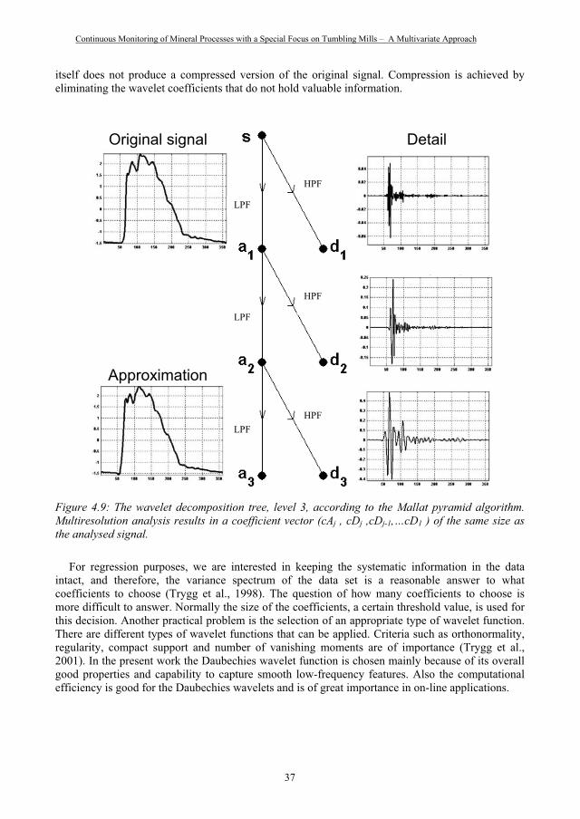
In this work, the fast wavelet transform multiresolution analysis (MRA) has been used as a pre-processing method in regression modelling on the sensor signal data [Paper II]. The method used for this is the Mallat Pyramid algorithm (Misiti et al., 1996). Figure 4.9 shows an example of a wavelet transformation, at level 3, of a measurement corresponding to an average mill revolution. The Mallat Pyramid algorithm uses two filters: a low-pass filter (LPF), and a high-pass filter (HPF). The output from the LPF, the approximation is further processed through a new HPF and LPF. This continues until only a wavelet coefficient and the average value of the signal is left. These wavelet coefficients represent both approximations and details from the signal. The wavelet transformation
36
Continuous Monitoring of Mineral Processes with a Special Focus on Tumbling Mills – A Multivariate Approach
itself does not produce a compressed version of the original signal. Compression is achieved by eliminating the wavelet coefficients that do not hold valuable information.
Original signal Detail
Approximation
HPF
LPF
HPF
LPF
HPFLPF
Figure 4.9: The wavelet decomposition tree, level 3, according to the Mallat pyramid algorithm. Multiresolution analysis results in a coefficient vector (cAj , cDj ,cDj-1,…cD1 ) of the same size as the analysed signal.
For regression purposes, we are interested in keeping the systematic information in the data intact, and therefore, the variance spectrum of the data set is a reasonable answer to what coefficients to choose (Trygg et al., 1998). The question of how many coefficients to choose is more difficult to answer. Normally the size of the coefficients, a certain threshold value, is used for this decision. Another practical problem is the selection of an appropriate type of wavelet function. There are different types of wavelet functions that can be applied. Criteria such as orthonormality, regularity, compact support and number of vanishing moments are of importance (Trygg et al., 2001). In the present work the Daubechies wavelet function is chosen mainly because of its overall good properties and capability to capture smooth low-frequency features. Also the computational efficiency is good for the Daubechies wavelets and is of great importance in on-line applications.
37
Continuous Monitoring of Mineral Processes with a Special Focus on Tumbling Mills – A Multivariate Approach
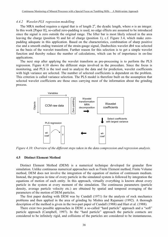
4.4.2 Wavelet-PLS regression modelling The MRA method requires a signal that is of length 2n, the dyadic length, where n is an integer.
In this work [Paper II], so-called zero-padding is used, no edge effects are assumed to be introduced since the signal is zero outside the original range. The lifter bar is most likely relaxed in the area leaving the charge (position 9) and hit of charge (position 1), c.f. Figure 3.4, which make zero-padding adequate in this application. Based on the characteristics, combination of sharp positive rise and a smooth ending transient of the strain-gauge signal, Daubechies wavelet db4 was selected as the basis of the wavelet transform. Further reason for this selection is to get a simple wavelet function and thereby reduce the number of calculations, which can be of importance in on-line applications.
The next step after applying the wavelet transform as pre-processing is to perform the PLS regression. Figure 4.10 shows the different steps involved in the procedure. Since the focus is monitoring, and PLS is the tool used to analyze the data and for prediction, wavelet coefficients with high variance are selected. The number of selected coefficients is dependent on the problem. This criterion is called variance selection. The PLS model is therefore built on the assumption that selected wavelet coefficients are those ones carrying most of the information about the grinding process.
Select coefficientswith largest variance
CCM raw data
Obj
ects
Variables
Zero
pad
ding Wavelet
transformationMRA
decompositionWavelet
coefficients
wt-coef
wt-coef Y
PLS regression
Figure 4.10: Overview of the different steps taken in the data compression and regression analysis.
4.5 Distinct Element Method
Distinct Element Method (DEM) is a numerical technique developed for granular flow simulation. Unlike continuous numerical approaches such as Finite Element method, Finite Volume method, DEM does not involve the integration of the equation of motion of continuum medium. Instead, the progress in time of every particle in the simulated system is followed by integration the equations of motion of each entity. In this approach, virtually everything is known about every particle in the system at every moment of the simulation. The continuous parameters (particle density, average particle velocity etc.) are obtained by spatial and temporal averaging of the parameters of the motion of DEM particles.
The first paper dealing with DEM was by Cundall (1971) for the analysis of rock mechanics problems and then applied in the area of grinding by Mishra and Rajamani (1992). A thorough description of the method is given in the two-part paper of Cundall (1988) and Hart et al. (1988).
There exist two possible approaches in DEM: a so-called “hard particle” approach and a “soft” particle approach (Campbell, 1997). In the “hard particle” approach the particle contacts are considered to be infinitely rigid, and collisions of the particles are considered to be instantaneous.
38
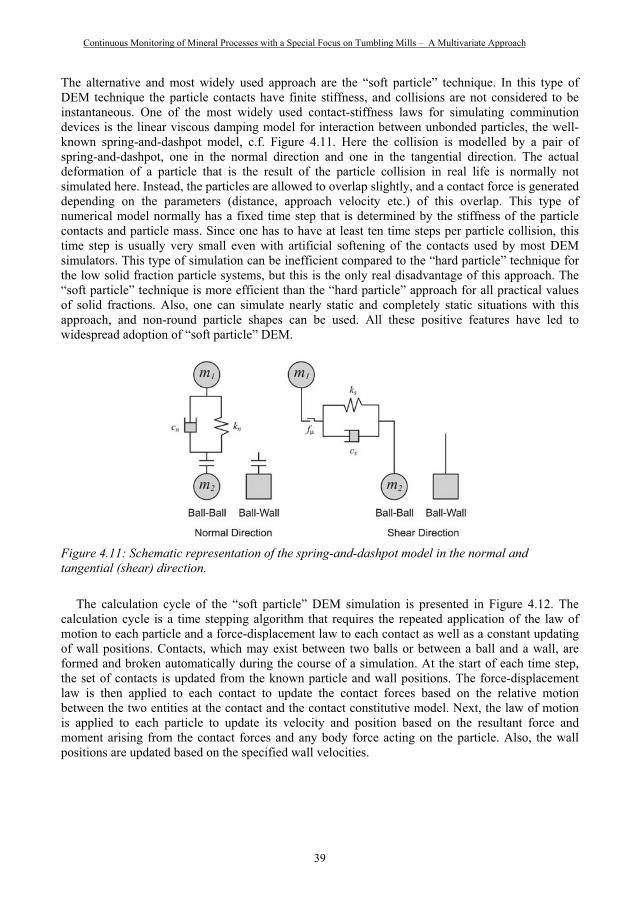
Continuous Monitoring of Mineral Processes with a Special Focus on Tumbling Mills – A Multivariate Approach
The alternative and most widely used approach are the “soft particle” technique. In this type of DEM technique the particle contacts have finite stiffness, and collisions are not considered to be instantaneous. One of the most widely used contact-stiffness laws for simulating comminution devices is the linear viscous damping model for interaction between unbonded particles, the well-known spring-and-dashpot model, c.f. Figure 4.11. Here the collision is modelled by a pair of spring-and-dashpot, one in the normal direction and one in the tangential direction. The actual deformation of a particle that is the result of the particle collision in real life is normally not simulated here. Instead, the particles are allowed to overlap slightly, and a contact force is generated depending on the parameters (distance, approach velocity etc.) of this overlap. This type of numerical model normally has a fixed time step that is determined by the stiffness of the particle contacts and particle mass. Since one has to have at least ten time steps per particle collision, this time step is usually very small even with artificial softening of the contacts used by most DEM simulators. This type of simulation can be inefficient compared to the “hard particle” technique for the low solid fraction particle systems, but this is the only real disadvantage of this approach. The “soft particle” technique is more efficient than the “hard particle” approach for all practical values of solid fractions. Also, one can simulate nearly static and completely static situations with this approach, and non-round particle shapes can be used. All these positive features have led to widespread adoption of “soft particle” DEM.
Figure 4.11: Schematic representation of the spring-and-dashpot model in the normal and tangential (shear) direction.
The calculation cycle of the “soft particle” DEM simulation is presented in Figure 4.12. The calculation cycle is a time stepping algorithm that requires the repeated application of the law of motion to each particle and a force-displacement law to each contact as well as a constant updating of wall positions. Contacts, which may exist between two balls or between a ball and a wall, are formed and broken automatically during the course of a simulation. At the start of each time step, the set of contacts is updated from the known particle and wall positions. The force-displacement law is then applied to each contact to update the contact forces based on the relative motion between the two entities at the contact and the contact constitutive model. Next, the law of motion is applied to each particle to update its velocity and position based on the resultant force and moment arising from the contact forces and any body force acting on the particle. Also, the wall positions are updated based on the specified wall velocities.
39
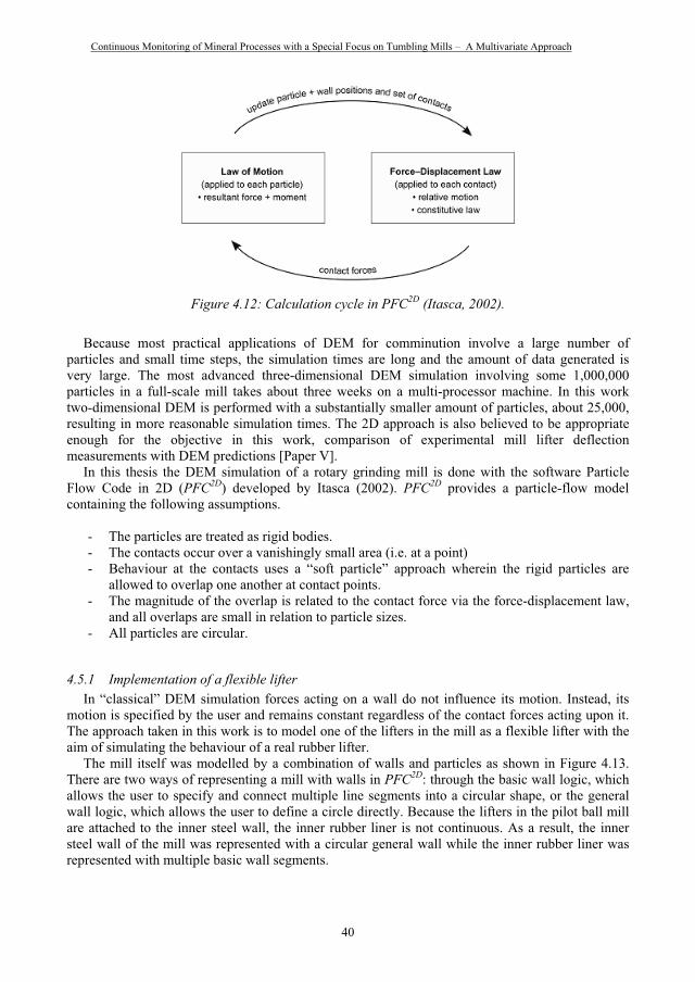
Continuous Monitoring of Mineral Processes with a Special Focus on Tumbling Mills – A Multivariate Approach
Figure 4.12: Calculation cycle in PFC2D (Itasca, 2002).
Because most practical applications of DEM for comminution involve a large number of particles and small time steps, the simulation times are long and the amount of data generated is very large. The most advanced three-dimensional DEM simulation involving some 1,000,000 particles in a full-scale mill takes about three weeks on a multi-processor machine. In this work two-dimensional DEM is performed with a substantially smaller amount of particles, about 25,000, resulting in more reasonable simulation times. The 2D approach is also believed to be appropriate enough for the objective in this work, comparison of experimental mill lifter deflection measurements with DEM predictions [Paper V].
In this thesis the DEM simulation of a rotary grinding mill is done with the software Particle Flow Code in 2D (PFC2D) developed by Itasca (2002). PFC2D provides a particle-flow model containing the following assumptions.
- The particles are treated as rigid bodies. - The contacts occur over a vanishingly small area (i.e. at a point) - Behaviour at the contacts uses a “soft particle” approach wherein the rigid particles are
allowed to overlap one another at contact points. - The magnitude of the overlap is related to the contact force via the force-displacement law,
and all overlaps are small in relation to particle sizes. - All particles are circular.
4.5.1 Implementation of a flexible lifter In “classical” DEM simulation forces acting on a wall do not influence its motion. Instead, its
motion is specified by the user and remains constant regardless of the contact forces acting upon it. The approach taken in this work is to model one of the lifters in the mill as a flexible lifter with the aim of simulating the behaviour of a real rubber lifter.
The mill itself was modelled by a combination of walls and particles as shown in Figure 4.13. There are two ways of representing a mill with walls in PFC2D: through the basic wall logic, which allows the user to specify and connect multiple line segments into a circular shape, or the general wall logic, which allows the user to define a circle directly. Because the lifters in the pilot ball mill are attached to the inner steel wall, the inner rubber liner is not continuous. As a result, the inner steel wall of the mill was represented with a circular general wall while the inner rubber liner was represented with multiple basic wall segments.
40
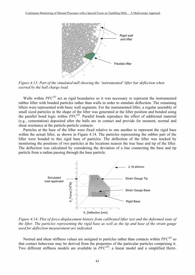
Continuous Monitoring of Mineral Processes with a Special Focus on Tumbling Mills – A Multivariate Approach
Flexible lifter
Rigid walland lifter
Figure 4.13: Part of the simulated mill showing the ‘instrumented’ lifter bar deflection when exerted by the ball charge load.
Walls within PFC2D act as rigid boundaries so it was necessary to represent the instrumented rubber lifter with bonded particles rather than walls in order to simulate deflection. The remaining lifters were represented with basic wall segments. For the instrumented lifter, a regular assembly of small sized particles in the shape of the lifter was generated at the lifter position and bonded using the parallel bond logic within PFC2D. Parallel bonds reproduce the effect of additional material (e.g., cementation) deposited after the balls are in contact and provide for moment, normal and shear resistance at the particle-particle contacts.
Particles at the base of the lifter were fixed relative to one another to represent the rigid base within the actual lifter, as shown in Figure 4.14. The particles representing the rubber part of the lifter were bonded to this rigid base of particles. The deflection of the lifter was tracked by monitoring the positions of two particles at the locations nearest the true base and tip of the lifter. The deflection was calculated by considering the deviation of a line connecting the base and tip particle from a radian passing through the base particle.
X_Deflection [mm]
X_F
orce
[104 N
]
Simulatedload applicator
Strain Gauge Tip
Strain Gauge Base
Rigid Base
2.16 kN/mm
Figure 4.14: Plot of force-displacement history from calibrated lifter test and the deformed state of the lifter. The particles representing the rigid base as well as the tip and base of the strain gauge used for deflection measurement are indicated.
Normal and shear stiffness values are assigned to particles rather than contacts within PFC2D so that contact behaviour may be derived from the properties of the particular particles comprising it. Two different stiffness models are available in PFC2D: a linear model and a simplified Hertz-
41
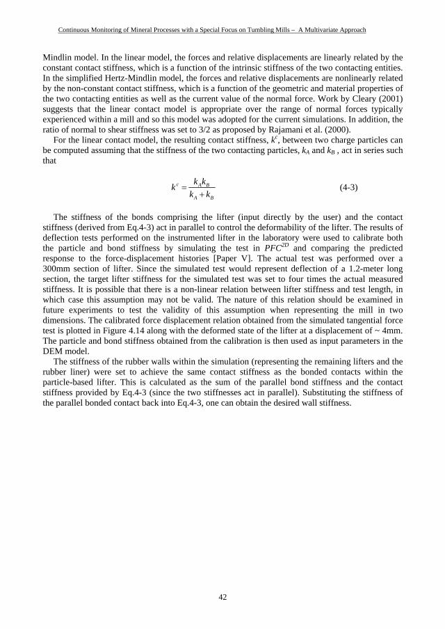
Continuous Monitoring of Mineral Processes with a Special Focus on Tumbling Mills – A Multivariate Approach
Mindlin model. In the linear model, the forces and relative displacements are linearly related by the constant contact stiffness, which is a function of the intrinsic stiffness of the two contacting entities. In the simplified Hertz-Mindlin model, the forces and relative displacements are nonlinearly related by the non-constant contact stiffness, which is a function of the geometric and material properties of the two contacting entities as well as the current value of the normal force. Work by Cleary (2001) suggests that the linear contact model is appropriate over the range of normal forces typically experienced within a mill and so this model was adopted for the current simulations. In addition, the ratio of normal to shear stiffness was set to 3/2 as proposed by Rajamani et al. (2000).
For the linear contact model, the resulting contact stiffness, kc, between two charge particles can be computed assuming that the stiffness of the two contacting particles, kA and kB , act in series such that
B
c A B
A B
k kkk k
(4-3)
The stiffness of the bonds comprising the lifter (input directly by the user) and the contact stiffness (derived from Eq.4-3) act in parallel to control the deformability of the lifter. The results of deflection tests performed on the instrumented lifter in the laboratory were used to calibrate both the particle and bond stiffness by simulating the test in PFC2D and comparing the predicted response to the force-displacement histories [Paper V]. The actual test was performed over a 300mm section of lifter. Since the simulated test would represent deflection of a 1.2-meter long section, the target lifter stiffness for the simulated test was set to four times the actual measured stiffness. It is possible that there is a non-linear relation between lifter stiffness and test length, in which case this assumption may not be valid. The nature of this relation should be examined in future experiments to test the validity of this assumption when representing the mill in two dimensions. The calibrated force displacement relation obtained from the simulated tangential force test is plotted in Figure 4.14 along with the deformed state of the lifter at a displacement of ~ 4mm. The particle and bond stiffness obtained from the calibration is then used as input parameters in the DEM model.
The stiffness of the rubber walls within the simulation (representing the remaining lifters and the rubber liner) were set to achieve the same contact stiffness as the bonded contacts within the particle-based lifter. This is calculated as the sum of the parallel bond stiffness and the contact stiffness provided by Eq.4-3 (since the two stiffnesses act in parallel). Substituting the stiffness of the parallel bonded contact back into Eq.4-3, one can obtain the desired wall stiffness.
42
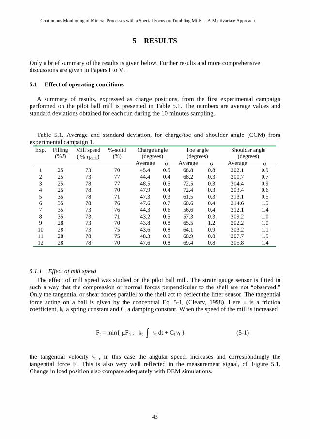
Continuous Monitoring of Mineral Processes with a Special Focus on Tumbling Mills – A Multivariate Approach
5 RESULTS
Only a brief summary of the results is given below. Further results and more comprehensive discussions are given in Papers I to V.
5.1 Effect of operating conditions
A summary of results, expressed as charge positions, from the first experimental campaign performed on the pilot ball mill is presented in Table 5.1. The numbers are average values and standard deviations obtained for each run during the 10 minutes sampling.
Table 5.1. Average and standard deviation, for charge/toe and shoulder angle (CCM) from experimental campaign 1.
Charge angle (degrees)
Toe angle(degrees)
Shoulder angle (degrees)
Exp. Filling(%J)
Mill speed ( % crital)
%-solid(%)
Average Average Average1 25 73 70 45.4 0.5 68.8 0.8 202.1 0.92 25 73 77 44.4 0.4 68.2 0.3 200.7 0.73 25 78 77 48.5 0.5 72.5 0.3 204.4 0.94 25 78 70 47.9 0.4 72.4 0.3 203.4 0.65 35 78 71 47.3 0.3 61.5 0.3 213.1 0.56 35 78 76 47.6 0.7 60.6 0.4 214.6 1.57 35 73 76 44.3 0.6 56.6 0.4 212.1 1.48 35 73 71 43.2 0.5 57.3 0.3 209.2 1.09 28 73 70 43.8 0.8 65.5 1.2 202.2 1.0
10 28 73 75 43.6 0.8 64.1 0.9 203.2 1.111 28 78 75 48.3 0.9 68.9 0.8 207.7 1.512 28 78 70 47.6 0.8 69.4 0.8 205.8 1.4
5.1.1 Effect of mill speed The effect of mill speed was studied on the pilot ball mill. The strain gauge sensor is fitted in
such a way that the compression or normal forces perpendicular to the shell are not “observed.” Only the tangential or shear forces parallel to the shell act to deflect the lifter sensor. The tangential force acting on a ball is given by the conceptual Eq. 5-1, (Cleary, 1998). Here is a friction coefficient, kt a spring constant and Ct a damping constant. When the speed of the mill is increased
Ft = min{ Fn , kt vt dt + Ct vt } (5-1)
the tangential velocity vt , in this case the angular speed, increases and correspondingly the tangential force Ft. This is also very well reflected in the measurement signal, cf. Figure 5.1. Change in load position also compare adequately with DEM simulations.
43
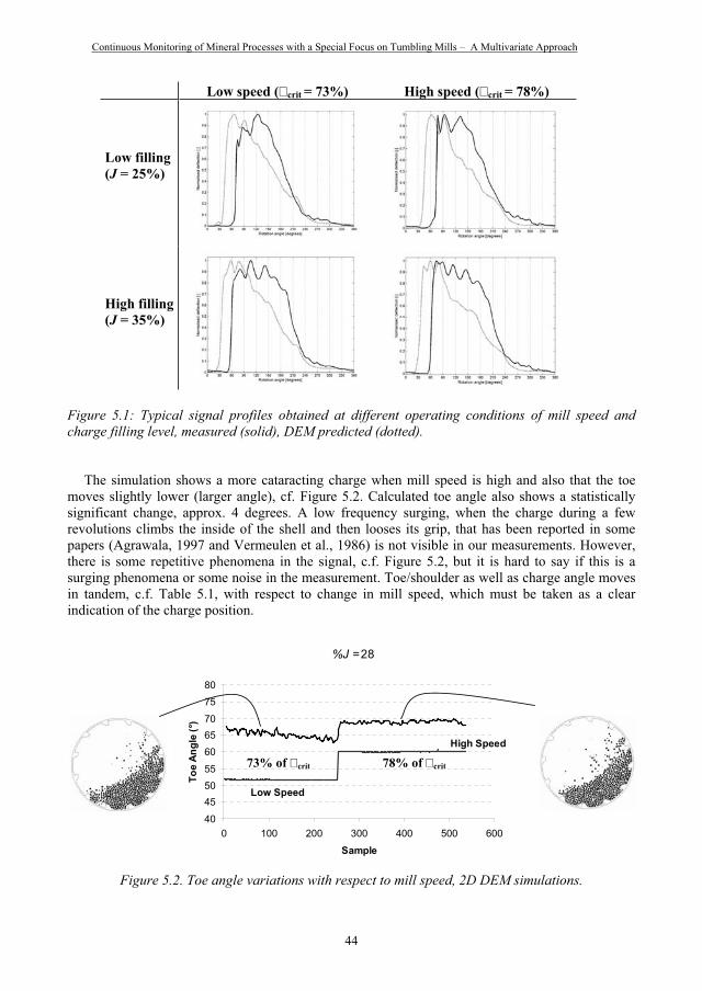
Continuous Monitoring of Mineral Processes with a Special Focus on Tumbling Mills – A Multivariate Approach
Low speed ( crit = 73%) High speed ( crit = 78%)
Low filling (J = 25%)
High filling (J = 35%)
Figure 5.1: Typical signal profiles obtained at different operating conditions of mill speed and charge filling level, measured (solid), DEM predicted (dotted).
The simulation shows a more cataracting charge when mill speed is high and also that the toe moves slightly lower (larger angle), cf. Figure 5.2. Calculated toe angle also shows a statistically significant change, approx. 4 degrees. A low frequency surging, when the charge during a few revolutions climbs the inside of the shell and then looses its grip, that has been reported in some papers (Agrawala, 1997 and Vermeulen et al., 1986) is not visible in our measurements. However, there is some repetitive phenomena in the signal, c.f. Figure 5.2, but it is hard to say if this is a surging phenomena or some noise in the measurement. Toe/shoulder as well as charge angle moves in tandem, c.f. Table 5.1, with respect to change in mill speed, which must be taken as a clear indication of the charge position.
%J =28
40
455055
606570
7580
0 100 200 300 400 500 600
Sample
Toe
Angl
e (°
)
20.0
25.0
30.0
35.0
High Speed
Low Speed
73% of crit 78% of crit
Figure 5.2. Toe angle variations with respect to mill speed, 2D DEM simulations.
44
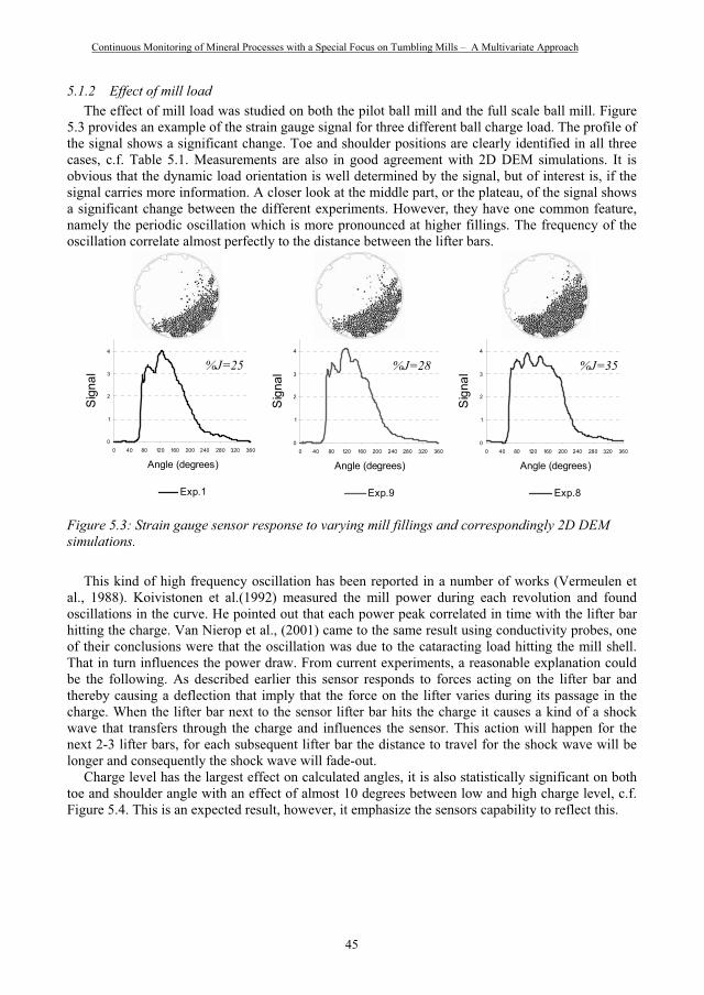
Continuous Monitoring of Mineral Processes with a Special Focus on Tumbling Mills – A Multivariate Approach
5.1.2 Effect of mill load The effect of mill load was studied on both the pilot ball mill and the full scale ball mill. Figure
5.3 provides an example of the strain gauge signal for three different ball charge load. The profile of the signal shows a significant change. Toe and shoulder positions are clearly identified in all three cases, c.f. Table 5.1. Measurements are also in good agreement with 2D DEM simulations. It is obvious that the dynamic load orientation is well determined by the signal, but of interest is, if the signal carries more information. A closer look at the middle part, or the plateau, of the signal shows a significant change between the different experiments. However, they have one common feature, namely the periodic oscillation which is more pronounced at higher fillings. The frequency of the oscillation correlate almost perfectly to the distance between the lifter bars.
0
1
2
3
4
0 40 80 120 160 200 240 280 320 360
Angle (degrees)
Sig
nal
Exp.1
0
1
2
3
4
0 40 80 120 160 200 240 280 320 360
Angle (degrees)
Sig
nal
Exp.9
0
1
2
3
4
0 40 80 120 160 200 240 280 320 360
Angle (degrees)S
igna
l
Exp.8
%J=25 %J=28 %J=35
Figure 5.3: Strain gauge sensor response to varying mill fillings and correspondingly 2D DEM simulations.
This kind of high frequency oscillation has been reported in a number of works (Vermeulen et al., 1988). Koivistonen et al.(1992) measured the mill power during each revolution and found oscillations in the curve. He pointed out that each power peak correlated in time with the lifter bar hitting the charge. Van Nierop et al., (2001) came to the same result using conductivity probes, one of their conclusions were that the oscillation was due to the cataracting load hitting the mill shell. That in turn influences the power draw. From current experiments, a reasonable explanation could be the following. As described earlier this sensor responds to forces acting on the lifter bar and thereby causing a deflection that imply that the force on the lifter varies during its passage in the charge. When the lifter bar next to the sensor lifter bar hits the charge it causes a kind of a shock wave that transfers through the charge and influences the sensor. This action will happen for the next 2-3 lifter bars, for each subsequent lifter bar the distance to travel for the shock wave will be longer and consequently the shock wave will fade-out.
Charge level has the largest effect on calculated angles, it is also statistically significant on both toe and shoulder angle with an effect of almost 10 degrees between low and high charge level, c.f. Figure 5.4. This is an expected result, however, it emphasize the sensors capability to reflect this.
45
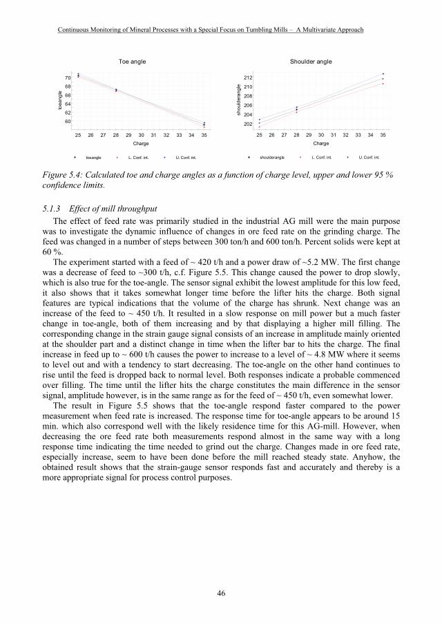
Continuous Monitoring of Mineral Processes with a Special Focus on Tumbling Mills – A Multivariate Approach
60
62
64
66
68
70
25 26 27 28 29 30 31 32 33 34 35
toea
ngle
Charge
Toe angle
toeangle L. Conf. int. U. Conf. int.
202
204
206
208
210
212
25 26 27 28 29 30 31 32 33 34 35
shou
lder
angl
e
Charge
Shoulder angle
shoulderangle L. Conf. int. U. Conf. int.
Figure 5.4: Calculated toe and charge angles as a function of charge level, upper and lower 95 % confidence limits.
5.1.3 Effect of mill throughput The effect of feed rate was primarily studied in the industrial AG mill were the main purpose
was to investigate the dynamic influence of changes in ore feed rate on the grinding charge. The feed was changed in a number of steps between 300 ton/h and 600 ton/h. Percent solids were kept at 60 %.
The experiment started with a feed of ~ 420 t/h and a power draw of ~5.2 MW. The first change was a decrease of feed to ~300 t/h, c.f. Figure 5.5. This change caused the power to drop slowly, which is also true for the toe-angle. The sensor signal exhibit the lowest amplitude for this low feed, it also shows that it takes somewhat longer time before the lifter hits the charge. Both signal features are typical indications that the volume of the charge has shrunk. Next change was an increase of the feed to ~ 450 t/h. It resulted in a slow response on mill power but a much faster change in toe-angle, both of them increasing and by that displaying a higher mill filling. The corresponding change in the strain gauge signal consists of an increase in amplitude mainly oriented at the shoulder part and a distinct change in time when the lifter bar to hits the charge. The final increase in feed up to ~ 600 t/h causes the power to increase to a level of ~ 4.8 MW where it seems to level out and with a tendency to start decreasing. The toe-angle on the other hand continues to rise until the feed is dropped back to normal level. Both responses indicate a probable commenced over filling. The time until the lifter hits the charge constitutes the main difference in the sensor signal, amplitude however, is in the same range as for the feed of ~ 450 t/h, even somewhat lower.
The result in Figure 5.5 shows that the toe-angle respond faster compared to the power measurement when feed rate is increased. The response time for toe-angle appears to be around 15 min. which also correspond well with the likely residence time for this AG-mill. However, when decreasing the ore feed rate both measurements respond almost in the same way with a long response time indicating the time needed to grind out the charge. Changes made in ore feed rate, especially increase, seem to have been done before the mill reached steady state. Anyhow, the obtained result shows that the strain-gauge sensor responds fast and accurately and thereby is a more appropriate signal for process control purposes.
46
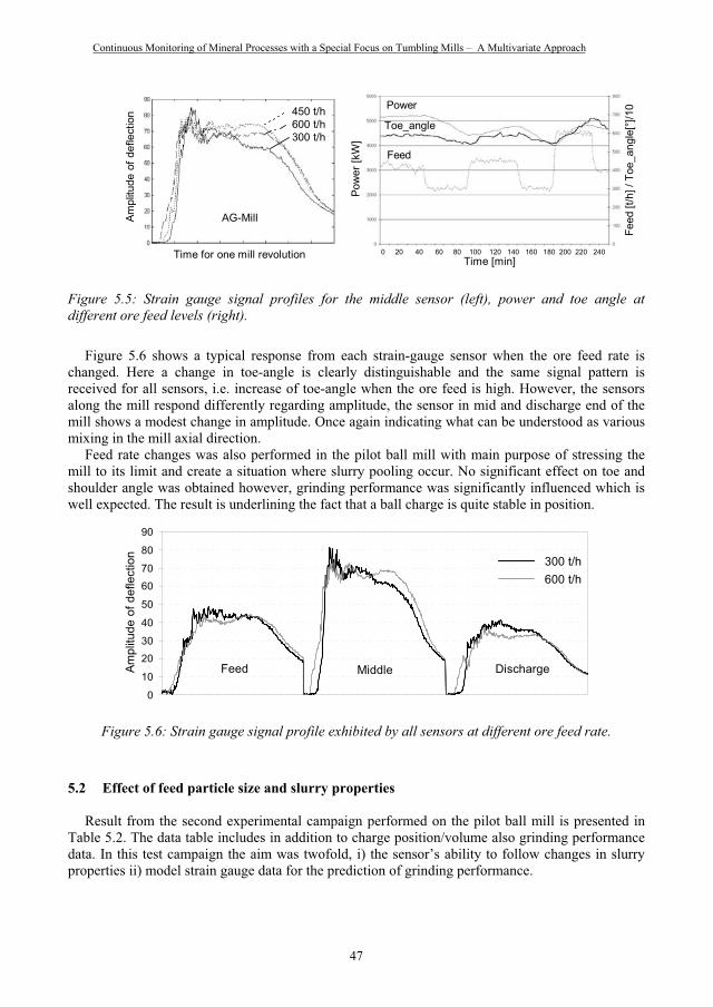
Continuous Monitoring of Mineral Processes with a Special Focus on Tumbling Mills – A Multivariate Approach
Pow
er [k
W]
Feed
[t/h
] / T
oe_a
ngle
[°]/1
0Power
Toe_angle
Feed
Time [min]
450 t/h600 t/h300 t/h
Time for one mill revolution
Ampl
itude
of d
efle
ctio
n
AG-Mill
0 20 40 60 80 100 120 140 160 180 200 220 240
Figure 5.5: Strain gauge signal profiles for the middle sensor (left), power and toe angle at different ore feed levels (right).
Figure 5.6 shows a typical response from each strain-gauge sensor when the ore feed rate is changed. Here a change in toe-angle is clearly distinguishable and the same signal pattern is received for all sensors, i.e. increase of toe-angle when the ore feed is high. However, the sensors along the mill respond differently regarding amplitude, the sensor in mid and discharge end of the mill shows a modest change in amplitude. Once again indicating what can be understood as various mixing in the mill axial direction.
Feed rate changes was also performed in the pilot ball mill with main purpose of stressing the mill to its limit and create a situation where slurry pooling occur. No significant effect on toe and shoulder angle was obtained however, grinding performance was significantly influenced which is well expected. The result is underlining the fact that a ball charge is quite stable in position.
0
10
20
30
40
50
60
70
80
90
Feed Middle Discharge
300 t/h600 t/h
Ampl
itude
of d
efle
ctio
n
Figure 5.6: Strain gauge signal profile exhibited by all sensors at different ore feed rate.
5.2 Effect of feed particle size and slurry properties
Result from the second experimental campaign performed on the pilot ball mill is presented in Table 5.2. The data table includes in addition to charge position/volume also grinding performance data. In this test campaign the aim was twofold, i) the sensor’s ability to follow changes in slurry properties ii) model strain gauge data for the prediction of grinding performance.
47
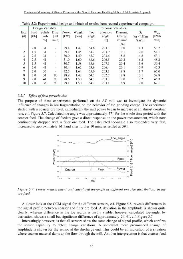
Continuous Monitoring of Mineral Processes with a Special Focus on Tumbling Mills – A Multivariate Approach
Table 5.2: Experimental design and obtained results from second experimental campaign. Design Variables Response Variables
Exp.(#)
Feed[t/h]
Solids[vol-%]
Disp.[ml
/min]
Power[kW]
Weight[ton]
Toeangle
[ ]
Shoulderangle [ ]
Dynamic Chargevolume
[%]
Gi
[kg <45 m/kWh]
Wapp[kWh /ton]
1 2.0 31 - 29.4 1.47 64.6 203.3 19.0 14.3 53.22 1.5 31 - 29.1 1.45 64.7 203.9 19.1 12.6 54.13 2.5 31 - 30.0 1.49 65.7 203.6 18.8 14.8 53.14 2.5 41 - 31.0 1.60 63.6 206.5 20.2 16.2 48.25 1.5 41 - 30.7 1.58 63.6 207.1 20.4 13.6 50.46 2.0 41 - 30.4 1.62 63.9 206.4 20.1 15.9 47.37 2.0 36 - 32.5 1.64 65.0 203.1 18.8 11.7 65.08 2.0 31 90 28.9 1.48 64.7 202.7 18.8 13.1 59.89 2.0 41 90 28.6 1.50 64.7 203.3 19.0 17.2 45.3
10 2.0 36 90 29.1 1.50 64.7 203.1 18.9 12.0 67.1
5.2.1 Effect of feed particle size The purpose of these experiments performed on the AG-mill was to investigate the dynamic influence of changes in ore fragmentation on the behavior of the grinding charge. The experiment started with a coarser ore feed, immediately the mill power began to increase at an almost constant rate, c.f. Figure 5.7. Calculated toe-angle was approximately for the whole time period with the coarser feed. The change of feeders gave a direct response on the power measurement, which now continuously dropped with a finer ore feed. The calculated toe-angle also responded very fast, increased to approximately and after further 10 minutes settled at .
57
61 59
Pow
er [k
W]
Power
Toe_angle
Feed
Feed
[t/h
] / T
oe_a
ngle
[°]/1
0
Time
Coarse Fine
Figure 5.7: Power measurement and calculated toe-angle at different ore size distributions in the ore feed.
A closer look at the CCM signal for the different sensors, c.f. Figure 5.8, reveals differences in the signal profile between coarser and finer ore feed. A deviation in the amplitude is shown quite clearly, whereas difference in the toe region is hardly visible, however calculated toe-angle, by derivation, shows a small but significant difference of approximately 42 , c.f. Figure 5.7.
Interestingly however, is that all sensors show the same change of signal profile, which confirm the sensor capability to detect charge variations. A somewhat more pronounced change of amplitude is shown for the sensor at the discharge end. This could be an indication of a situation where coarser material dams up the flow through the mill. Another interpretation is that coarser feed
48
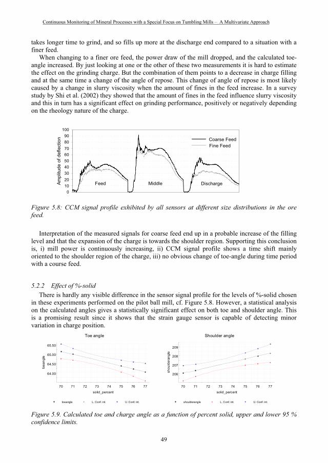
Continuous Monitoring of Mineral Processes with a Special Focus on Tumbling Mills – A Multivariate Approach
takes longer time to grind, and so fills up more at the discharge end compared to a situation with a finer feed.
When changing to a finer ore feed, the power draw of the mill dropped, and the calculated toe-angle increased. By just looking at one or the other of these two measurements it is hard to estimate the effect on the grinding charge. But the combination of them points to a decrease in charge filling and at the same time a change of the angle of repose. This change of angle of repose is most likely caused by a change in slurry viscosity when the amount of fines in the feed increase. In a survey study by Shi et al. (2002) they showed that the amount of fines in the feed influence slurry viscosity and this in turn has a significant effect on grinding performance, positively or negatively depending on the rheology nature of the charge.
0102030405060708090
100
Coarse FeedFine Feed
Ampl
itude
of d
efle
ctio
n
Feed Middle Discharge
Figure 5.8: CCM signal profile exhibited by all sensors at different size distributions in the ore feed.
Interpretation of the measured signals for coarse feed end up in a probable increase of the filling level and that the expansion of the charge is towards the shoulder region. Supporting this conclusion is, i) mill power is continuously increasing, ii) CCM signal profile shows a time shift mainly oriented to the shoulder region of the charge, iii) no obvious change of toe-angle during time period with a course feed.
5.2.2 Effect of %-solid There is hardly any visible difference in the sensor signal profile for the levels of %-solid chosen
in these experiments performed on the pilot ball mill, cf. Figure 5.8. However, a statistical analysis on the calculated angles gives a statistically significant effect on both toe and shoulder angle. This is a promising result since it shows that the strain gauge sensor is capable of detecting minor variation in charge position.
64.00
64.50
65.00
65.50
70 71 72 73 74 75 76 77
toea
ngle
solid_percent
Toe angle
toeangle L. Conf. int. U. Conf. int.
206
207
208
209
70 71 72 73 74 75 76 77
shou
lder
angl
e
solid_percent
Shoulder angle
shoulderangle L. Conf. int. U. Conf. int.
Figure 5.9. Calculated toe and charge angle as a function of percent solid, upper and lower 95 % confidence limits.
49
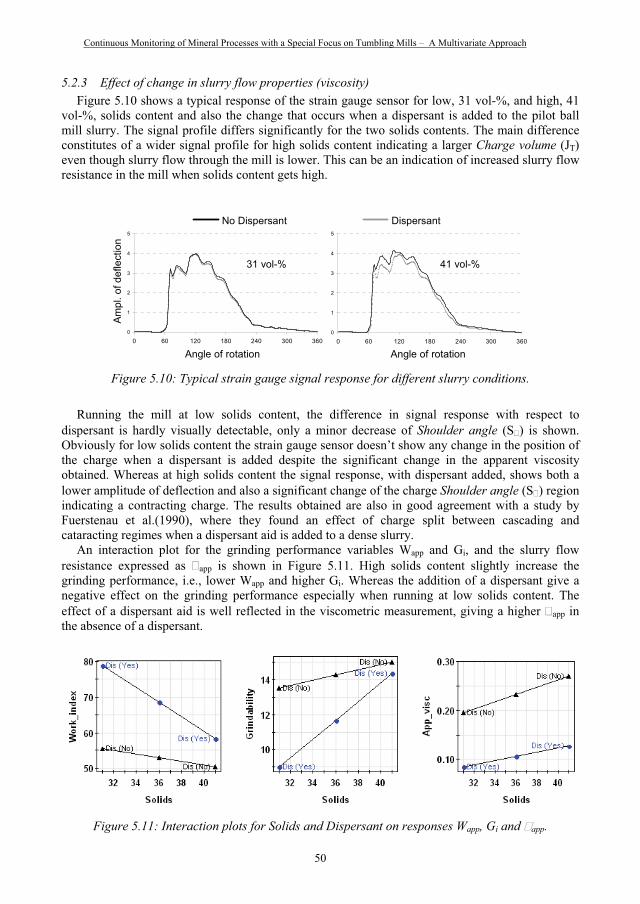
Continuous Monitoring of Mineral Processes with a Special Focus on Tumbling Mills – A Multivariate Approach
5.2.3 Effect of change in slurry flow properties (viscosity) Figure 5.10 shows a typical response of the strain gauge sensor for low, 31 vol-%, and high, 41
vol-%, solids content and also the change that occurs when a dispersant is added to the pilot ball mill slurry. The signal profile differs significantly for the two solids contents. The main difference constitutes of a wider signal profile for high solids content indicating a larger Charge volume (JT)even though slurry flow through the mill is lower. This can be an indication of increased slurry flow resistance in the mill when solids content gets high.
0
1
2
3
4
5
0 60 120 180 240 300 3600
1
2
3
4
5
0 60 120 180 240 300 360
31 vol-% 41 vol-%
DispersantNo Dispersant
Am
pl. o
f def
lect
ion
Angle of rotation Angle of rotation
Figure 5.10: Typical strain gauge signal response for different slurry conditions.
Running the mill at low solids content, the difference in signal response with respect to dispersant is hardly visually detectable, only a minor decrease of Shoulder angle (S ) is shown. Obviously for low solids content the strain gauge sensor doesn’t show any change in the position of the charge when a dispersant is added despite the significant change in the apparent viscosity obtained. Whereas at high solids content the signal response, with dispersant added, shows both a lower amplitude of deflection and also a significant change of the charge Shoulder angle (S ) region indicating a contracting charge. The results obtained are also in good agreement with a study by Fuerstenau et al.(1990), where they found an effect of charge split between cascading and cataracting regimes when a dispersant aid is added to a dense slurry.
An interaction plot for the grinding performance variables Wapp and Gi, and the slurry flow resistance expressed as app is shown in Figure 5.11. High solids content slightly increase the grinding performance, i.e., lower Wapp and higher Gi. Whereas the addition of a dispersant give a negative effect on the grinding performance especially when running at low solids content. The effect of a dispersant aid is well reflected in the viscometric measurement, giving a higher app in the absence of a dispersant.
Figure 5.11: Interaction plots for Solids and Dispersant on responses Wapp, Gi and app.
50
Continuous Monitoring of Mineral Processes with a Special Focus on Tumbling Mills – A Multivariate Approach
6 CONCLUSIONS
This thesis is a contribution to the improvement of methods for continuous monitoring of tumbling mills. A promising method for mill charge measurement has been studied, a strain gauge installed in a rubber lifter bar inside a rotating mill. The sensor in combination with modelling techniques has shown to be capable of establishing the charge position within the mill and bring increased knowledge of charge movement and its influence on grinding performance.
The sensor was found to be sensitive to changes in mill operating conditions in a physically reasonable manner. Data shows that the volumetric mill filling level and charge angles can be predicted with an accuracy better than +/- 1%. It also seems that the sensors do not suffer from any tendency to drift or quickly wear out. Experimental work has demonstrated that the signal pattern generated by the strain gauge sensor varies in a consistent way with changing operating conditions. Detection of charge features has shown good reproducibility independent of type of grinding, AG- or ball mill. The signal profiles obtained for ball mills, independent of mill size, are very much the same. However, amplitude differences are more pronounced in a large ball mill, probably due to higher loads influencing the lifter deflection.
In addition, the signal profile is also demonstrated to contain information of the grinding performance. The work has shown that statistical multivariate regression modelling (PLS) is very useful in modelling the relation between signal profile and grinding parameters. Grinding parameters that are normally measured in the laboratory are readily modelled from the on-line signal. Experience gained from the experiments underscore the importance of signal pre-processing, e.g. signal filtering, feature extraction and signal compression using wavelet analysis, before regressing the signal to grinding performance. The modelling shows that the used wavelet transformation reduces the number of variables considerably. A data set consisting of only 5 % of the original data result in a PLS regression model with almost the same statistical performance. Wavelet transformation of the original strain gauge signal has also clarified the importance of the position of the grinding charge or more correctly how an operating condition implicate the charge movement. The experimental result shows that it is particularly the toe position of the charge that is important to detect since it has a strong correlation with operating performance.
Slurry rheology has been recognised for decades to play an important role in wet grinding, however there are a number of difficulties associated with the measurement of slurry rheological properties. The measurements in this work clearly reveal that an embedded lifter bar sensor is able to pick up flow resistance changes in an operating mill. Signal features influenced by the changed operating conditions were the toe and shoulder angle, where the shoulder angle showed more distinct changes than the toe angle. The resistance to flow here expressed as an apparent viscosity is strongly influenced by solids content and naturally by the addition of a dispersant. Obtained viscometric results clearly show that the slurry flow resistance is changed between the experimental runs. The observed changes in impact force on the lifter bar can mainly be related to the product slurry, because the influence of the load of the charge should not vary much during the various operating conditions investigated here. Independent on the exact location of the slurry at the sensor mill section, the increased load results show how high solids concentrations increased the volume of slurry in the mill which in turn can be related to increased resistance to flow. The corresponding increase in retention time here may also have contributed to increased production of fine material, as shown in a higher grindability index. On the contrary, addition of a dispersant at high solids content showed a lower sensor loading, indicating less resistance to flow, slurry volume and less retention time and thus a decreased grinding performance.
In the AG-mill application a system with 3 sensors mounted at different axial positions (inlet, mid, outlet) along the mill was used. The response in amplitude for these three sensors were quite different, this presumably because of the kind of lifter configuration used in the AG-mill. The lifter configuration was of a high/high type at feed/discharge end, whereas the rows in the middle part of
51
Continuous Monitoring of Mineral Processes with a Special Focus on Tumbling Mills – A Multivariate Approach
the mill were of a high/low configuration with the sensor installed in one high lifter. The high/low configuration gives a wider void between the lifters, which filled with grinding charge results in a higher pressure on the lifter and thereby a bigger deflection of it. An implication of the high/high configuration is a probable reduction in mill volume. Furthermore, the grinding work in this section of the mill is also most likely cut back due to a charge that is immobilised between the high lifters. Of course there is a trade-off between having a longer lining lifetime with high lifters compared to the reduced mill volume, and it has to be economically justified. Different charge behavior was identified along the mill when operating conditions were changed, with the most systematic variation at the discharge end. The result indicates that the charge filling along the axial direction of the mill is different, actual variations are more pronounced in a small part at the discharge end of the mill.
To model the charge movement in a physically correct way and compare it to measured data, distinct element modelling (DEM) methods were used. In typical DEM mill modelling, mill walls and lifters are represented as rigid bodies that do not deform during collisions. Here, an attempt is made to improve on the lifter description by the modelling of one bar as a flexible body. A novel method implemented in the DEM model is developed where the instrumented rubber lifter in the pilot mill is represented as a lifter made of an assemblage of parallel bonded particles. Assessment of the predicted deflection profile to experimental data allows us to understand the accuracy of various types of DEM models and the penalties associated with the various assumptions made by these models. An exact match between predicted and measured lifter deflection is difficult to obtain due to simplified assumptions in both the description of the flexible lifter and also in the two-dimensional DEM approach used. However, effects of mill speed as well as charge filling level are well reflected in the simulations and are comparable with pilot mill measurements.
The implemented novel method is an introductory approach and comparisons between real and predicted deflections are on a qualitative basis. The outcome of this part of the work shows a potential to be of use in lifter profile design where flexible material is present. As a consequence the effect on grinding performance can be assessed in a consistent and meaningful manner due to the direct relation to experimental data, obtained by the strain gauge sensor.
The strain-gauge sensor system has shown features such as reproducibility, reliability and fast response time to varied process conditions. Such a system will provide detailed information on the dynamics and grinding characteristics of the charge and detect when the grinding is not performing well. The presented results imply that there are definite possibilities for on-line control and monitoring of a tumbling mill based on the information contained in the strain gauge sensor data.
52

Continuous Monitoring of Mineral Processes with a Special Focus on Tumbling Mills – A Multivariate Approach
7 FUTURE WORK
The next step would be to implement the technology for control and optimisation of an AG-mill circuit for iron ore processing. This includes further development in reduced power consumption for the sensor, telemetry system (wireless sensor) and data pre-treatment methods for signal processing as well as data compression.
To reach better accuracy in DEM predictions and enable quantitative comparison to measured data some necessary improvements have been identified. This includes investigation of lifter relaxation in the laboratory, simulation of time-dependent behaviour in the lifter and an extension of the approach to a three-dimensional DEM mill model.
53

Continuous Monitoring of Mineral Processes with a Special Focus on Tumbling Mills – A Multivariate Approach
54

Continuous Monitoring of Mineral Processes with a Special Focus on Tumbling Mills – A Multivariate Approach
8 ACKNOWLEDGEMENTS
I would like to express my great thanks to those who have made my work possible and contributed with support, encouragement and valuable advice.
First of all, my supervisor, Dr Bertil Pålsson, for all the guidance, belief in this work and pushing me to the finish line. Prof. Eric Forssberg and Dr Per-Olof Samskog are acknowledged for introducing me into the research community and for encouragement through this project.
All my colleagues at LKAB R&D for their help in the experimental work, data acquisition, help in computer matters and all other imaginable problems.
My appreciation also goes to Dr Sture Persson and his colleagues at Metso Minerals for technical and financial support with the CCM system. Dr Stefan Rännar (Umetrics Inc.), Matt Pierce (Itasca Inc.) and Andreas Berggren (New Boliden) for many interesting discussions and help in co-writing some of the appended papers.
Finally I gratefully acknowledge LKAB and the Agricola Research Centre for giving me the opportunity to perform this work.
Gällivare, April 2005
55

Continuous Monitoring of Mineral Processes with a Special Focus on Tumbling Mills – A Multivariate Approach
56

Continuous Monitoring of Mineral Processes with a Special Focus on Tumbling Mills – A Multivariate Approach
9 REFERENCES
1. Agrawala S., Rajamani R.K., Songfack P. and Mishra B.K., 1997. Mechanics of media motion in tumbling mills with 3D Discrete Element Method. Minerals Engineering, Vol.10, No.2, pp. 215-227.
2. Andersson T.W., 1984. An Introduction To Multivariate Statistical Analysis. John Wiley & Sons, New York.
3. Apelt T.A., Asprey S.P. and Thornhill N.F., 2001. Inferential measurement of SAG mill parameters, Minerals Engineering, Vol.14, No.6, pp. 575-591.
4. Berggren A., Albertsson J., Westerlund P., 2000. Optimering av genomsättning i autogenkvarn med on-line fyllnadsgradsmätning. Conference in mineral processing, Luleå, pp. 45-55.
5. Campbell C.S., 1997. Computer simulation of powder flows. In: Powder technology Handbook, Gotoh et al. (Eds.), 2 edn., Dekker, New York, pp. 777-793.
6. Campbell J., Spencer S., Sutherland D., Rowlands T., Weller K., Cleary P. and Hinde A., 2001. SAG mill monitoring using surface vibrations. In: Barratt, D.J., Allan, M.J., Mular A.L. (Eds.), Proceedings SAG 2001, Vancouver, B.C Canada, Vol 2, pp. 373-385.
7. Cleary P.W., 2001. Recent advances in DEM modelling of tumbling mills. Minerals Engineering. Vol.14, No.10, pp.1295-1319.
8. Cundall P.A., 1971. A computer model for simulating progressive large scale movements in blocky rock systems. In: Proceedings of the symposium of the international society for rock mechanics, Nancy, France. Vol.1, paper no. II-8.
9. Cundall P.A., 1988. Formulation of a three-dimensional distinct element model – part I. A scheme to detect and represent contacts in a system composed of many polyhedral blocks. Int. J. Rock Mech., Min. Sci & geomech. Abstr., 25(3), pp.107-116.
10. Dai X-D., Joseph B. and Motard R.L., 1994. Introduction to wavelet transform and time-frequency analysis. In: Motard R.L., Joseph B., (Eds.), Wavelet applications in chemical engineering. Kluwer Academic Press, pp.1-32.
11. Dupont J.F., Vien A., 2001. Continuous SAG Volumetric Charge Measurement. In: Proc. 33rd Ann. Can. Min. Proc. AGM, CIM, Ottawa, pp.51 - 67.
12. Eriksson L., Johansson E., Kettaneh-Wold N. and Wold S., 2001. Multi- and megavariate data analysis, principles and applications, Umetrics AB Umeå, Sweden.
13. Evans G, 2001. A new method for determining charge mass in AG/SAG mills. In: Barratt, D.J., Allan, M.J., Mular A.L. (Eds.), Proceedings SAG 2001, Vancouver, B.C Canada, Vol. II, pp. 331-345.
14. Fuerstenau D.W., Kapur, P.C. and Velamakanni, B., 1990. A multi-torque model for the effects of dispersants and slurry viscosity on ball milling. Int. J. of Min. Process., 28, pp.81-98.
15. Friden H. and Wikström C., 1995. Multivariate Process Monitoring and Forecasting by Projection Methods. Report from Umetri AB.
57
Continuous Monitoring of Mineral Processes with a Special Focus on Tumbling Mills – A Multivariate Approach
16. Graps A., 1995. An introduction to wavelets, IEEE Computational Science and Engineering. vol.2, no.2.
17. Hart R., Cundall P.A., Lemos J., 1988. Formulation of a three-dimensional distinct element model-part II. Mechanical calculations for motion and interaction of a system composed of many polyhedral blocks. Int. J. Rock Mech., Min. Sci & geomech. Abstr., 25(3), pp. 177-125.
18. Helland, I.S., 1988. On the structure of partial least squares regression. Common. Statist. Simula., 17(2), 581-602.
19. Herbst J.A. and Pate W.T, 1996. On-line estimation of charge volumes in semiautogenous and autogenous grinding mills, In: International autogenous and semiautogenous grinding technology, SAG 1996, Vancouver, B.C. Canada, Vol. 2, pp. 817-827.
20. Herbst J.A. and Gabardi T.L., 1988. Closed loop media charging of mills based on a smart sensor system. In: Sommer G. (Ed.), IFAC Applied Measurements in Mineral and Metallurgical Processing, Transvaal,South Africa, pp 17-23.
21. Höskuldsson, A., 1988. PLS Regression Models. Journal of Chemometrics, 1988, Vol.2, pp.211-228.
22. Itasca, 2002. PFC User Manual, 2 ed., Itasca Consulting Group Inc., Minneapolis, USA.
23. Jackson J.E., 1991. A Users Guide To Principal Components. John Wiley & Sons, New York.
24. Jackson J.E., 1980. Principal Components and Factor Analysis: Part I - Principal Analysis. J. of Quality Technology, 12, pp.201-213.
25. Jaspan R.K., Young G.J.C. and Mellor M.S., 1986. ROM mill power draft control using multiple microphones to determine mill load. In: Proc. of International conference on Gold, Volume 2, Extractive metallurgy of Gold, Johannesburg, SAIMM, pp. 483-392.
26. Järvinen J., 2004. A volumetric charge measurement for grinding mills. Preprints 11th IFAC Symposium on Automation in Mining, Mineral and Metal Processing, Nancy, France.
27. Koivistonen P., Kalapudas R. and Miettunen J., 1992. A new method for measuring the volumetric filling of a grinding mill. In: Comminution-Theory and Practice, Kawatra S.K., (ed.), Society for Mining, Metallurgy and Exploration, Littleton, Colorado, pp 563-574.
28. Koivistonen P. and Miettunen J., 1989. The effect of the lining on the power draw of a grinding mill and its utilisation in grinding control. In: Proceedings SAG 1989, Vol 2, pp. 687-695.
29. Kolacz J.,1997. Measurement system of the mill charge in grinding ball mill circuits, Minerals Engineering, Vol.10, No.12, pp.1329-1338.
30. Kresta J.V., MacGregor J.F. and Marlin T.E., 1991. Multivariate Statistical Monitoring of Process Operating Performance. Can.Journal of Chemical Engineering, 68, No1.
31. Kresta J.V., Marlin T.E. and MacGregor J.F., 1990. Choosing Inferential Variables Using Projection to Latent Structures (PLS) with Application to Multicomponent Distillation. Annual AIChE meeting, Chicago, USA.
58
Continuous Monitoring of Mineral Processes with a Special Focus on Tumbling Mills – A Multivariate Approach
32. Kvalheim O.M. and Brakstad F., 1996. Kartleggning av komplekse industriprosesser for total prosesskvalitet Anvendelse av kjemometri innen forskning og industri. John Grieg, AS pp 481-498.
33. Lorber A., Wagner L.A. and Kowalski B.R., 1987. A Theoretical Foundation for the PLS Algorithm. J. Chemometrics, 1, 19-31.
34. MacGregor J.F. and Kourti T., 1995. Statistical Process Control of Multivariate Processes. Control Engineering Practice 3, 403-414.
35. MacGregor J.F. and Nomikos P., 1992. Monitoring Batch Processes. Proceedings NATO Advanced Study Institute for Batch Processing Systems Eng., Antalya, Turkey, Springer- Verlag, New York.
36. MacGregor J.F., Marlin T.E., Kresta J.V. and Skagerberg B., 1991.Multivariate Statistical Methods in Process Analysis and Control. In: AIChE Symposium Proceedings of the Fourth International Conference on Chemical Process Control, Padre Island, USA.
37. Mardia K.V., Kent J.T. and Bibby J.M., 1982. Multivariate Analysis. Academic Press, London.
38. Martens H. and Naes T., 1989. Multivariate Calibration. John Wiley & Sons, New York.
39. Mishra B.K. and Rajamani R.K., 1992. The discrete element method for the simulation of ball mills. Appl. Math. Modelling. vol.16, pp 598-604.
40. Misiti M., Misiti Y., Oppenheim G., and Poggi J.M., 1996. Wavelet toolbox for use with MATLAB, The Math Works Inc. USA.
41. Moys M.H., 1988. Measurement of slurry properties and load behaviour in grinding mills, In: IFAC Applied Measurements in Mineral and Metallurgical Processing. Sommer G. (ed.), Transvaal, South Africa, pp 3-9.
42. Olsson G. and Lee P.L., 1994. Effective interfaces for process operators- a prototype. J.Proc.Control 4(2), pp.99-107.
43. Pax R. A, 2001. Non-contact acoustic measurement of in-mill variables of SAG mills, In: Proceedings SAG2001, Vancouver, B.C Canada, Vol. II, pp. 386-393.
44. Persson S., 1994-1999. AUS. pat. 647 667. CAN. Pat.Application 2 088 992. FIN.pat. 101 350. Jap.pat. 2 896 230. NOR.pat. 180 153. RUS.pat. 2 062 184. SWE.pat. 910 271-1 and USA.pat. 5 360 174.
45. Pontt J., 2004. A new monitoring system for measuring the load filling of a SAG mill, Minerals Engineering, Vol.17, No.11-12, pp.1143-1148.
46. Rajamani R.K., Mishra B.K., Venugopal R. and Datta A., 2000. Discrete element analysis of tumbling mills. Powder Technology, Vol.109, pp 105-112.
47. Tano K., 1996. Multivariate Modelling and Monitoring of Mineral processes using Partial Least Square Regression, Licentiate Thesis, 1996:36L, Luleå Technical University, Sweden.
48. Trygg J. and Wold S., 1998. PLS regression on wavelet compressed NIR spectra, Chemometrics Intell. Lab. Syst., 42, 209-220.
59
Continuous Monitoring of Mineral Processes with a Special Focus on Tumbling Mills – A Multivariate Approach
49. Trygg J., Kettaneh-Wold N., Wallbäcks L., 2001. 2D wavelet analysis and compression of on-line industrial process data. Journal of Chemometrics. 15: 299-319
50. Van Nierop M.A., Glover G., Hinde A.L. and Moys M.H., 2001. A discrete element method investigation of the charge motion and power draw of an experimental two-dimensional mill. Int. J. of Min. Process., 61(2), pp 77-92.
51. Watson J.L., 1985. An Analysis of Mill Grinding Noise. Powder Technology. 41 (1), 83-89.
52. Veltkamp D.J., 1993. Multivariate monitoring and modelling of chemical processes using chemometrics. Process Control and Quality 5, 205-217.
53. Vermeulen L.A., Howat D.D., 1986. Fluctuations in the slip of grinding charge in rotary mills with smooth liners. Int. J. of Min. Process., 24(1-2), pp.143-159.
54. Vermeulen L.A. and Schakowski F.A., 1988. Estimation, by use of a conductivity bolt, of the charge volume and other milling parameters in an operating mill. In: IFAC Applied Measurements in Mineral and Metallurgical Processing. Sommer G.(ed.), Transvaal, South Africa, pp 11-15.
55. Wise B.M. and Ricker N.L., 1991. Recent advances in multivariate statistical process control improving robustness and sensitivity. IFAC symp. ADCHEM’91, Toulouse, France, pp.125-130, Pergamon Press.
56. Wise B.M., Ricker N.L. and Veltkamp D.J., 1989. Upset and sensor detection in multivariate process. In: AIChE Annual Meeting, San Francisco, USA, Paper 164b.
57. Wise B.M., Ricker N.L., Veltkamp D.J., Kowalski B.R., Barnes S. and Arkali V., 1991. Application of multivariate statistical process control (MSPC) to the West Valley slurry-red ceramic melter process. In: Waste Management ’91 Proceedings, Tuscon, USA.
58. Wold S., 1978. Cross-validatory estimation of the number of component in factor and principal component model. Technometrics 20, pp. 397-405.
59. Wold S., Esbensen K. and Geladi P., 1987. Principal Component analysis. Chemometrics and Intelligent Laboratory Systems, 2, pp.37-52.
60. Wold S. et al, 1989. Multivariate Data Analysis: Converting chemical data tables to plots. Intelligent Instruments and Computers, pp.197-216.
61. Zeng Y., Tano K. and Forssberg E., 1994. Multi-channel vibration measurement in industrial ball mill grinding, In: Proc. Of the 5th international mineral processing symposium, Cappadocia, Turkey, 6-8 september, pp.557-563.
60

��������
�� ������� �� ������������ ���� ��
K Tano, B P������������� ����
Proceedings of the XXII International Mineral Processing Congress, CapeTown, South Africa, 28 September ����October 2003

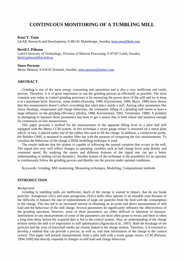
CONTINUOUS MONITORING OF A TUMBLING MILL
Kent T. Tano LKAB, Research and Development, S-983 81 Malmberget, Sweden, [email protected]
Bertil I. Pålsson Luleå University of Technology, Division of Mineral Processing, S-97187 Luleå, Sweden, [email protected]
Sture Persson Metso Mineral, S-934 81 Ersmark, Sweden, [email protected]
ABSTRACT
Grinding is one of the most energy consuming unit operations and is also a very inefficient and costly process. Therefore, it is of great importance to run the grinding process as efficiently as possible. The most common way today to control grinding processes is by measuring the power draw of the mill and try to keep it at a maximum level. However, some studies (Kawatra, 1989, Koivistoinen, 1989, Moys, 1989) have shown that this measurement doesn’t reflect everything that takes place inside a mill. Among other parameters like slurry rheology, temperature and charge behaviour, the volumetric filling of a grinding mill seems to have a large influence on the grinding efficiency (Herbst, 1988, Koivistoinen, 1992, Vermeulen, 1988). A problem in attempting to measure those parameters has been to get a sensor that is both robust and sensitive enough for continuous on-line measurement.
This paper presents a method for the measurement of the apparent filling level in a pilot ball mill equipped with the Metso CCM-system. In this technique a strain gauge sensor is mounted on a metal plate which, in turn, is placed under one of the rubber ribs used to lift the charge. In addition, a conductivity probe, the Boliden GMS, is mounted in another lifter bar with the purpose of comparing the two measurements. To visualise the behaviour of the charge a DEM modelling technique is used.
The results indicate that the system is capable of following the normal variation that occurs in the mill. The signal also very well reflect changes in operating variables such as ball charge level, pulp density and rotational speed. By studying the nature and different features of the signal one can get a better understanding of milling circuit dynamics. Another feature of the technique is the possibility for an operator to continuously follow the grinding process and thereby run the process under optimal conditions.
Keywords: Grinding, Mill monitoring, Measuring techniques, Modelling, Computational methods
INTRODUCTION
BackgroundGrinding in tumbling mills are inefficient, much of the energy is wasted in impact, that do not break
particles. Autogenous (AG) and semi-autogenous (SAG) mills often operate in an unstable state because of the difficulty to balance the rate of replenishment of large ore particles from the feed with the consumption in the charge. This has led to an increased interest in obtaining an accurate and direct measurement of mill load and the behaviour of the mill charge. Several parameters do significantly influence the effectiveness of the grinding operation, however, some of these parameters are either difficult or laborious to measure. Intermittent in-situ measurements of some of the parameters are most often prone to errors and there is often a long time-delay before the acquired data is fed to the control system. Also, an understanding of the charge motion within the mill is of importance in mill optimisation (Agrawala et al., 1997). Both the breakage of ore particles and the wear of liners/ball media are closely linked to the charge motion. Therefore, it is essential to develop a method that can provide a precise, as well as, real time information of the charge to the control system. This paper will present measurements from a pilot mill with a strain gauge sensor, CCM (Persson, 1994-1999) that directly responds to changes in mill load and charge behaviour.
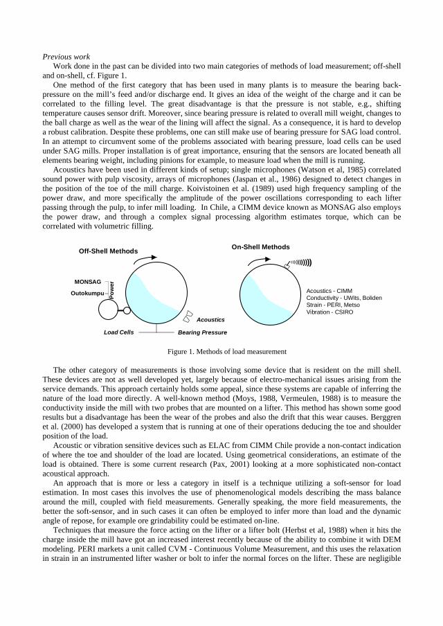
Previous work Work done in the past can be divided into two main categories of methods of load measurement; off-shell
and on-shell, cf. Figure 1. One method of the first category that has been used in many plants is to measure the bearing back-
pressure on the mill’s feed and/or discharge end. It gives an idea of the weight of the charge and it can be correlated to the filling level. The great disadvantage is that the pressure is not stable, e.g., shifting temperature causes sensor drift. Moreover, since bearing pressure is related to overall mill weight, changes to the ball charge as well as the wear of the lining will affect the signal. As a consequence, it is hard to develop a robust calibration. Despite these problems, one can still make use of bearing pressure for SAG load control. In an attempt to circumvent some of the problems associated with bearing pressure, load cells can be used under SAG mills. Proper installation is of great importance, ensuring that the sensors are located beneath all elements bearing weight, including pinions for example, to measure load when the mill is running.
Acoustics have been used in different kinds of setup; single microphones (Watson et al, 1985) correlated sound power with pulp viscosity, arrays of microphones (Jaspan et al., 1986) designed to detect changes in the position of the toe of the mill charge. Koivistoinen et al. (1989) used high frequency sampling of the power draw, and more specifically the amplitude of the power oscillations corresponding to each lifter passing through the pulp, to infer mill loading. In Chile, a CIMM device known as MONSAG also employs the power draw, and through a complex signal processing algorithm estimates torque, which can be correlated with volumetric filling.
Off-Shell Methods
Bearing PressureLoad Cells
Acoustics
Outokumpu
MONSAG
Pow
er
On-Shell Methods
)) )) ))))))))
Acoustics - CIMMConductivity - UWits, BolidenStrain - PERI, MetsoVibration - CSIRO
Figure 1. Methods of load measurement
The other category of measurements is those involving some device that is resident on the mill shell. These devices are not as well developed yet, largely because of electro-mechanical issues arising from the service demands. This approach certainly holds some appeal, since these systems are capable of inferring the nature of the load more directly. A well-known method (Moys, 1988, Vermeulen, 1988) is to measure the conductivity inside the mill with two probes that are mounted on a lifter. This method has shown some good results but a disadvantage has been the wear of the probes and also the drift that this wear causes. Berggren et al. (2000) has developed a system that is running at one of their operations deducing the toe and shoulder position of the load.
Acoustic or vibration sensitive devices such as ELAC from CIMM Chile provide a non-contact indication of where the toe and shoulder of the load are located. Using geometrical considerations, an estimate of the load is obtained. There is some current research (Pax, 2001) looking at a more sophisticated non-contact acoustical approach.
An approach that is more or less a category in itself is a technique utilizing a soft-sensor for load estimation. In most cases this involves the use of phenomenological models describing the mass balance around the mill, coupled with field measurements. Generally speaking, the more field measurements, the better the soft-sensor, and in such cases it can often be employed to infer more than load and the dynamic angle of repose, for example ore grindability could be estimated on-line.
Techniques that measure the force acting on the lifter or a lifter bolt (Herbst et al, 1988) when it hits the charge inside the mill have got an increased interest recently because of the ability to combine it with DEM modeling. PERI markets a unit called CVM - Continuous Volume Measurement, and this uses the relaxation in strain in an instrumented lifter washer or bolt to infer the normal forces on the lifter. These are negligible

unless the lifter is in the charge, making it possible to estimate the toe and shoulder positions. The current project uses a strain gauge mounted inside a rubber lifter (Metso CCM).
MEASUREMENT COMPONENTS OF THE SYSTEM
Strain gauge sensor system The Continuous Charge Monitoring System (CCM) (Persson, 1994-1999) is a quite newly developed
electronic measuring system. It is dedicated to continuous measurement of the charge volume and the angle of repose provided that the mill has a rubber or rubber-metal mill lining or that a sensor-equipped rubber lifter bar can be installed in a steel-lined mill. The CCM-system consists of the following basic components; sensor, power supply, signal transmission and signal processing and presentation.
(5) Antenna(3) Transmitter
(6) Receiver
(1) Lifter bar
(4) Generator
(2) Sensor
0 180
90
Figure 2. Basic components of the CCM-system
As shown in Figure 2, the lifter bar (1) is equipped with a strain gauge sensor (2) that measures the bending of the lifter bar when it is in contact with the charge. The electrical signal from the sensor is amplified and converted to a HF-signal by the transmitter (3), which is bolted to the shell of the mill. The transmitter is supplied with electrical power from a generator (4) attached to the mill. The HF-signal is transmitted to the receiver (6) via the antenna (5). The receiver also has a trigger-pulse remote sensor, which is activated once every revolution by a metal trigger plate on the mill. The position of the lifter bar (sensor), trigger plate and receiver is very carefully established. The signal from the receiver is sent via an isolated line driver through a screened cable and a line receiver to the system computer (7) where the data are processed to present the charge level and angle of repose.
Principle of the CCM-system A typical deflection profile of the sensor signal and a corresponding graphical representation of a
simulation of a mill are shown in Figure 3. The numbers in Figure 3, indicate important dynamic events during the passage of the sensor-equipped lifter bar under the mill charge.
1. The sensor lifter bar (SL) is still in the air 2. The SL hits the surface of the slurry 3. The SL starts to get submerged in the slurry 4. The SL hits the ball charge and starts to get submerged in the charge (T4)5. The SL starts to bend forward due to turbulence in the toe area 6. The SL grips the ball charge again 7. The SL is at peak bending 8. The SL has gradually decreased the bending and is at take-off position 9. The SL is leaving the ball charge and starts slowly rise to an upright position (T9)
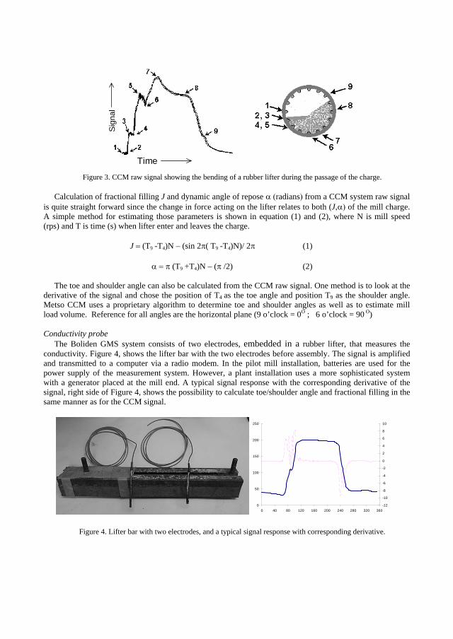
Sign
al
Figure 3. CCM raw signal showing the bending of a rubber lifter during the passage of the charge.
Calculation of fractional filling J and dynamic angle of repose radians from a CCM system raw signal is quite straight forward since the change in force acting on the lifter relates to both (J of the mill charge. A simple method for estimating those parameters is shown in equation (1) and (2), where N is mill speed (rps) and T is time (s) when lifter enter and leaves the charge.
J (T9 -T4)N – (sin 2 ( T9 -T4)N)/ 2 (1)
(T9 +T4)N – ( /2) (2)
The toe and shoulder angle can also be calculated from the CCM raw signal. One method is to look at the derivative of the signal and chose the position of T4 as the toe angle and position T9 as the shoulder angle. Metso CCM uses a proprietary algorithm to determine toe and shoulder angles as well as to estimate mill load volume. Reference for all angles are the horizontal plane (9 o’clock = 0O ; 6 o’clock = 90 O)
Conductivity probe The Boliden GMS system consists of two electrodes, embedded in a rubber lifter, that measures the
conductivity. Figure 4, shows the lifter bar with the two electrodes before assembly. The signal is amplified and transmitted to a computer via a radio modem. In the pilot mill installation, batteries are used for the power supply of the measurement system. However, a plant installation uses a more sophisticated system with a generator placed at the mill end. A typical signal response with the corresponding derivative of the signal, right side of Figure 4, shows the possibility to calculate toe/shoulder angle and fractional filling in the same manner as for the CCM signal.
0
50
100
150
200
250
0 40 80 120 160 200 240 280 320 360-12
-10
-8
-6
-4
-2
0
2
4
6
8
10
Figure 4. Lifter bar with two electrodes, and a typical signal response with corresponding derivative.
Time
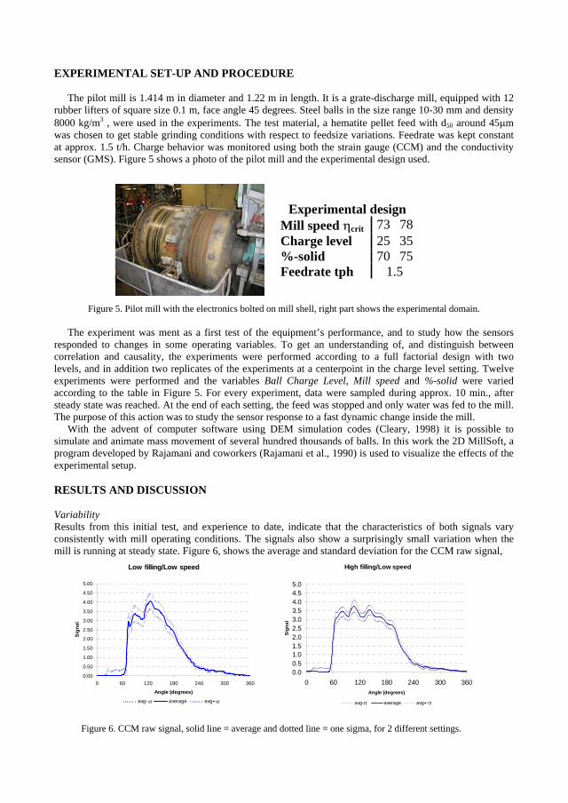
EXPERIMENTAL SET-UP AND PROCEDURE
The pilot mill is 1.414 m in diameter and 1.22 m in length. It is a grate-discharge mill, equipped with 12 rubber lifters of square size 0.1 m, face angle 45 degrees. Steel balls in the size range 10-30 mm and density 8000 kg/m3 , were used in the experiments. The test material, a hematite pellet feed with d50 around 45 mwas chosen to get stable grinding conditions with respect to feedsize variations. Feedrate was kept constant at approx. 1.5 t/h. Charge behavior was monitored using both the strain gauge (CCM) and the conductivity sensor (GMS). Figure 5 shows a photo of the pilot mill and the experimental design used.
Experimental design Mill speed crit 73 78 Charge level 25 35 %-solid 70 75 Feedrate tph 1.5
Figure 5. Pilot mill with the electronics bolted on mill shell, right part shows the experimental domain.
The experiment was ment as a first test of the equipment’s performance, and to study how the sensors responded to changes in some operating variables. To get an understanding of, and distinguish between correlation and causality, the experiments were performed according to a full factorial design with two levels, and in addition two replicates of the experiments at a centerpoint in the charge level setting. Twelve experiments were performed and the variables Ball Charge Level, Mill speed and %-solid were varied according to the table in Figure 5. For every experiment, data were sampled during approx. 10 min., after steady state was reached. At the end of each setting, the feed was stopped and only water was fed to the mill. The purpose of this action was to study the sensor response to a fast dynamic change inside the mill.
With the advent of computer software using DEM simulation codes (Cleary, 1998) it is possible to simulate and animate mass movement of several hundred thousands of balls. In this work the 2D MillSoft, a program developed by Rajamani and coworkers (Rajamani et al., 1990) is used to visualize the effects of the experimental setup.
RESULTS AND DISCUSSION
VariabilityResults from this initial test, and experience to date, indicate that the characteristics of both signals vary consistently with mill operating conditions. The signals also show a surprisingly small variation when the mill is running at steady state. Figure 6, shows the average and standard deviation for the CCM raw signal,
Low filling/Low speed
0.00
0.50
1.00
1.50
2.00
2.50
3.00
3.50
4.00
4.50
5.00
0 60 120 180 240 300 360
Angle (degrees)
Sign
al
avg- average avg+
Figure 6. CCM raw signal, solid line = average and dotted line = one sigma, for 2 different settings.
High filling/Low speed
0.00.51.01.52.02.53.03.54.04.55.0
0 60 120 180 240 300 360Angle (degrees)
Sign
al
avg- average avg+
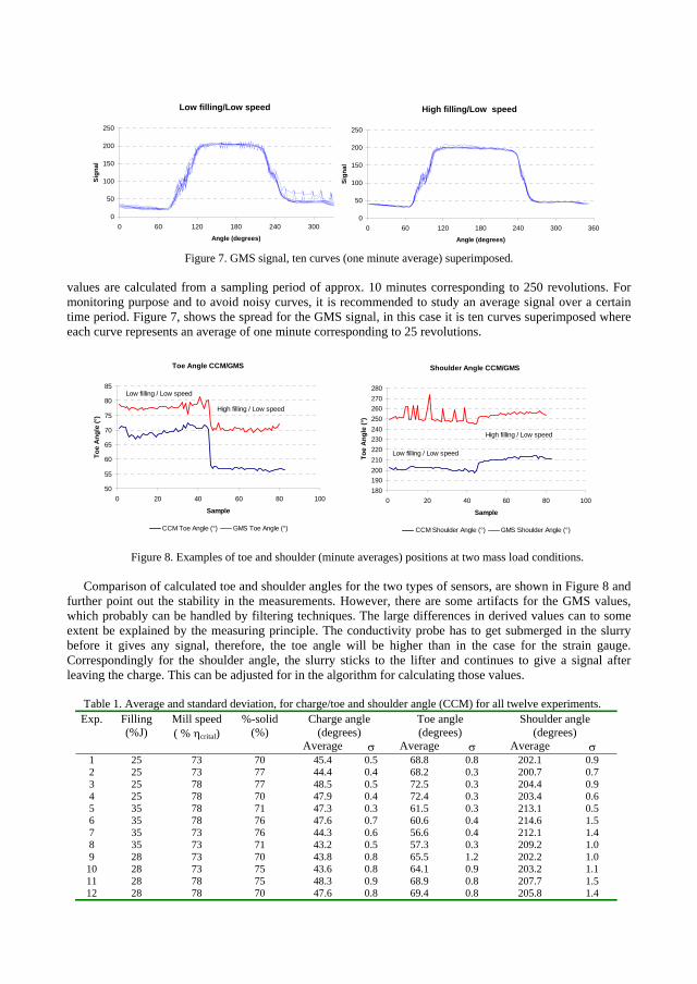
Low filling/Low speed
0
50
100
150
200
250
0 60 120 180 240 300 360
Angle (degrees)
Sign
al
Figure 7. GMS signal, ten curves (one minute average) superimposed.
values are calculated from a sampling period of approx. 10 minutes corresponding to 250 revolutions. For monitoring purpose and to avoid noisy curves, it is recommended to study an average signal over a certain time period. Figure 7, shows the spread for the GMS signal, in this case it is ten curves superimposed where each curve represents an average of one minute corresponding to 25 revolutions.
Toe Angle CCM/GMS
50
55
60
65
70
75
80
85
0 20 40 60 80 100
Sample
Toe
Ang
le (°
)
CCM Toe Angle (°) GMS Toe Angle (°)
Low filling / Low speed
High filling / Low speed
Figure 8. Examples of toe and shoulder (minute averages) positions at two mass load conditions.
Comparison of calculated toe and shoulder angles for the two types of sensors, are shown in Figure 8 and further point out the stability in the measurements. However, there are some artifacts for the GMS values, which probably can be handled by filtering techniques. The large differences in derived values can to some extent be explained by the measuring principle. The conductivity probe has to get submerged in the slurry before it gives any signal, therefore, the toe angle will be higher than in the case for the strain gauge. Correspondingly for the shoulder angle, the slurry sticks to the lifter and continues to give a signal after leaving the charge. This can be adjusted for in the algorithm for calculating those values.
Table 1. Average and standard deviation, for charge/toe and shoulder angle (CCM) for all twelve experiments. Charge angle
(degrees) Toe angle (degrees)
Shoulder angle (degrees)
Exp. Filling (%J)
Mill speed ( % crital)
%-solid (%)
Average Average Average 1 25 73 70 45.4 0.5 68.8 0.8 202.1 0.9 2 25 73 77 44.4 0.4 68.2 0.3 200.7 0.7 3 25 78 77 48.5 0.5 72.5 0.3 204.4 0.9 4 25 78 70 47.9 0.4 72.4 0.3 203.4 0.6 5 35 78 71 47.3 0.3 61.5 0.3 213.1 0.5 6 35 78 76 47.6 0.7 60.6 0.4 214.6 1.5 7 35 73 76 44.3 0.6 56.6 0.4 212.1 1.4 8 35 73 71 43.2 0.5 57.3 0.3 209.2 1.0 9 28 73 70 43.8 0.8 65.5 1.2 202.2 1.0
10 28 73 75 43.6 0.8 64.1 0.9 203.2 1.1 11 28 78 75 48.3 0.9 68.9 0.8 207.7 1.5 12 28 78 70 47.6 0.8 69.4 0.8 205.8 1.4
Shoulder Angle CCM/GMS
180190200210220230240250260270280
0 20 40 60 80 100
Sample
Toe
Ang
le (°
)
CCM Shoulder Angle (°) GMS Shoulder Angle (°)
Low filling / Low speed
High filling / Low speed
High filling/Low speed
0
50
100
150
200
250
0 60 120 180 240 300 360
Angle (degrees)
Sign
al
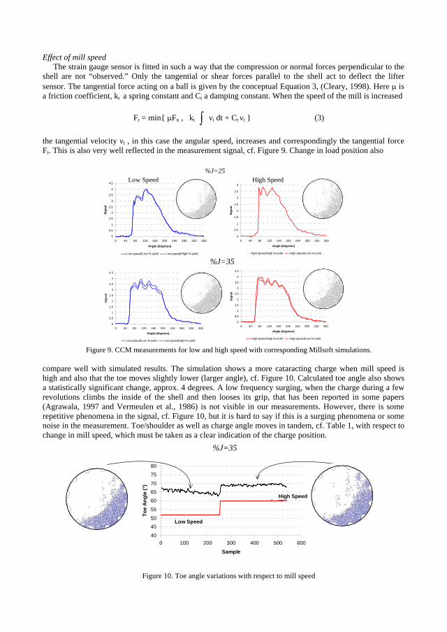
Effect of mill speed The strain gauge sensor is fitted in such a way that the compression or normal forces perpendicular to the
shell are not “observed.” Only the tangential or shear forces parallel to the shell act to deflect the lifter sensor. The tangential force acting on a ball is given by the conceptual Equation 3, (Cleary, 1998). Here is a friction coefficient, kt a spring constant and Ct a damping constant. When the speed of the mill is increased
Ft = min{ Fn , kt vt dt + Ct vt } (3)
the tangential velocity vt , in this case the angular speed, increases and correspondingly the tangential force Ft. This is also very well reflected in the measurement signal, cf. Figure 9. Change in load position also
0
0.5
1
1.5
2
2.5
3
3.5
4
4.5
0 40 80 120 160 200 240 280 320 360
Angle (degrees)
Sign
al
Low speed/Low %-solid Low speed/High %-solid
0
0.5
1
1.5
2
2.5
3
3.5
4
4.5
0 40 80 120 160 200 240 280 320 360
Angle (degrees)
Sign
al
High speed/High %-solid High speed/Low %-solid
% J = 3 5
0
0.5
1
1.5
2
2.5
3
3.5
4
0 40 80 120 160 200 240 280 320 360
Angle (degrees)
Sign
al
High speed/High %-solid High speed/Low %-solid
0
0.5
1
1.5
2
2.5
3
3.5
4
4.5
0 40 80 120 160 200 240 280 320 360
Angle (degrees)
Sign
al
Low speed/Low %-solid Low speed/High %-solid
%J=25Low Speed High Speed
Figure 9. CCM measurements for low and high speed with corresponding Millsoft simulations.
compare well with simulated results. The simulation shows a more cataracting charge when mill speed is high and also that the toe moves slightly lower (larger angle), cf. Figure 10. Calculated toe angle also shows a statistically significant change, approx. 4 degrees. A low frequency surging, when the charge during a few revolutions climbs the inside of the shell and then looses its grip, that has been reported in some papers (Agrawala, 1997 and Vermeulen et al., 1986) is not visible in our measurements. However, there is some repetitive phenomena in the signal, cf. Figure 10, but it is hard to say if this is a surging phenomena or some noise in the measurement. Toe/shoulder as well as charge angle moves in tandem, cf. Table 1, with respect to change in mill speed, which must be taken as a clear indication of the charge position.
%J = 28
40
455055
606570
7580
0 100 200 300 400 500 600
Sample
Toe
Angl
e (°
)
20.0
25.0
30.0
35.0
High Speed
Low Speed
Figure 10. Toe angle variations with respect to mill speed
%J=35
%J=35
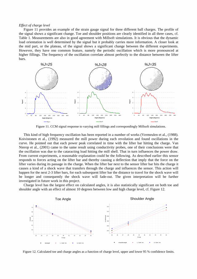
Effect of charge level Figure 11 provides an example of the strain gauge signal for three different ball charges. The profile of
the signal shows a significant change. Toe and shoulder positions are clearly identified in all three cases, cf. Table 1. Measurements are also in good agreement with Millsoft simulations. It is obvious that the dynamic load orientation is well determined by the signal but it probably carries more information. A closer look at the mid part, or the plateau, of the signal shows a significant change between the different experiments. However, they have one common feature, namely the periodic oscillation which is more pronounced at higher fillings. The frequency of the oscillation correlate almost perfectly to the distance between the lifter bars.
0
1
2
3
4
0 40 80 120 160 200 240 280 320 360
Angle (degrees)
Sign
al
Exp.1
0
1
2
3
4
0 40 80 120 160 200 240 280 320 360
Angle (degrees)
Sign
al
Exp.9
0
1
2
3
4
0 40 80 120 160 200 240 280 320 360
Angle (degrees)
Sign
al
Exp.8
%J=25 %J=28 %J=35
Figure 11. CCM signal response to varying mill fillings and correspondingly Millsoft simulations.
This kind of high frequency oscillation has been reported in a number of works (Vermeulen et al., (1988). Koivistonen et al., (1992) measured the mill power during each revolution and found oscillations in the curve. He pointed out that each power peak correlated in time with the lifter bar hitting the charge. Van Nierop et al., (2001) came to the same result using conductivity probes, one of their conclusions were that the oscillation was due to the cataracting load hitting the mill shell. That in turn influences the power draw. From current experiments, a reasonable explanation could be the following. As described earlier this sensor responds to forces acting on the lifter bar and thereby causing a deflection that imply that the force on the lifter varies during its passage in the charge. When the lifter bar next to the sensor lifter bar hits the charge it causes a kind of a shock wave that transfers through the charge and influences the sensor. This action will happen for the next 2-3 lifter bars, for each subsequent lifter bar the distance to travel for the shock wave will be longer and consequently the shock wave will fade-out. The given interpretation will be further investigated in future work in this project.
Charge level has the largest effect on calculated angles, it is also statistically significant on both toe and shoulder angle with an effect of almost 10 degrees between low and high charge level, cf. Figure 12.
202
204
206
208
210
212
25 26 27 28 29 30 31 32 33 34 35
shou
lder
angl
e
Charge
shoulderangle L. Conf. int. U. Conf. int.
60
62
64
66
68
70
25 26 27 28 29 30 31 32 33 34 35
toea
ngle
Charge
toeangle L. Conf. int. U. Conf. int.
Toe Angle Shoulder Angle
Figure 12. Calculated toe and charge angles as a function of charge level, upper and lower 95 % confidence limits.
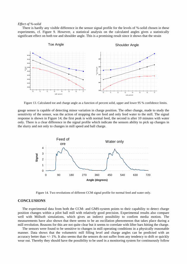
Effect of %-solid There is hardly any visible difference in the sensor signal profile for the levels of %-solid chosen in these
experiments, cf. Figure 9. However, a statistical analysis on the calculated angles gives a statistically significant effect on both toe and shoulder angle. This is a promising result since it shows that the strain
205
206
207
208
209
70 71 72 73 74 75 76 77
shoulderangle
solid_percent
Shoulder Angle
63.80
64.00
64.20
64.40
64.60
64.80
65.00
65.20
65.40
70 71 72 73 74 75 76 77
toeangle
solid_percent
Toe Angle
Figure 13. Calculated toe and charge angle as a function of percent solid, upper and lower 95 % confidence limits.
gauge sensor is capable of detecting minor variation in charge position. The other change, made to study the sensitivity of the sensor, was the action of stopping the ore feed and only feed water to the mill. The signal response is shown in Figure 14; the first peak is with normal feed, the second is after 10 minutes with water only. There is a clear difference in the signal profile which indicate the sensors ability to pick up changes in the slurry and not only to changes in mill speed and ball charge.
0
1
2
3
4
0 90 180 270 360 450 540 630 720
Angle (degrees)
Sign
al
Feed ofore Water only
Figure 14. Two revolutions of different CCM signal profile for normal feed and water only.
CONCLUSIONS
The experimental data from both the CCM- and GMS-system points to their capability to detect charge position changes within a pilot ball mill with relatively good precision. Experimental results also compare well with Millsoft simulations, which gives an indirect possibility to confirm media motion. The measurements have also shown that there seems to be an oscillation phenomenon that takes place during a mill revolution. Reasons for this are not quite clear but it seems to correlate with lifter bars hitting the charge.
The sensors were found to be sensitive to changes in mill operating conditions in a physically reasonable manner. Data shows that the volumetric mill filling level and charge angles can be predicted with an accuracy better than +/- 1%. It also seems that the sensors do not suffer from any tendency to drift or quickly wear out. Thereby they should have the possibility to be used in a monitoring system for continuously follow

the grinding operation. Such a system will provide detailed information on the dynamics and grinding characteristics of the charge and detect when the grinding is not performing well.
Next phase in this project will emphasize on the development of essential elements in a monitoring system that can be suitable for the possible use as an on-line process-monitoring tool and to help the operator run the mill at optimal conditions.
ACKNOWLEDGEMENT
The authors would like to thank the Agricola Research Centre and Norrbotten Research Council for their assistance and financial support of this project.
REFERENCES
Agrawala, S., Rajamani, R.K., Songfack, P. And Mishra, B.K., (1997). Mechanics of media motion in tumbling mills with 3D Discrete Element Method. Minerals Engineering, Vol. 10, No. 2, pp. 215-227.
Berggren, A., Albertsson, J., Westerlund, P., (2000). Optimering av genomsättning i autogenkvarn med on-line fyllnadsgradsmätning. Conference in mineral processing, Luleå, pp. 45-55.
Campbell, J., Spencer, S., Sutherland, D., Rowlands, T., Weller, K., Cleary, P. and Hinde, A. (2001). SAG mill monitoring using surface vibrations. Proceedings SAG 2001, Vol 2, pp. 373-385.
Cleary, P.W. (1998). Predicting charge motion, power draw, segregation and wear in ball mills using discrete element methods. Minerals Engineering, Vol 11, No 11, pp. 1061-1080.
Jaspan, R.K., Young, G.J.C., Mellor, M.S., (1986). ROM mill power draft control using multiple microphones to determine mill load. Proc. of International conference on Gold, Volume 2, Extractive metallurgy of Gold, Johannesburg, SAIMM, pp. 483-392.
Herbst, J.A. and Gabardi,T.L. (1988). Closed loop media charging of mills based on a smart sensor system. IFAC Applied Measurements in Mineral and Metallurgical Processing. Sommer. G.ed., Transvaal, South Africa, 17-23.
Kawatra, S.K., and Eisele, T.C.(1989). Effect of Temperature on the Performance of an Autogenous Grinding Circuit. Proceedings SAG 1989, Vol 2, pp. 485-502.
Koivistonen, P. and Miettunen,J. (1989). The effect of the lining on the power draw of a grinding mill and its utilisation in grinding control. Proceedings SAG 1989, Vol 2, pp. 687-695.
Koivistonen, P., Kalapudas,R. and Miettunen ,J.(1992). A new method for measuring the volumetric filling of a grinding mill. Comminution Theory and Practice, Kawatra, S.K., ed., Society for Mining, Metallurgy and Exploration 563-574.
Moys,M.H. (1988). Measurement of slurry properties and load behaviour in grinding mills. IFAC Applied Measurements in Mineral and Metallurgical Processing. Sommer.G.ed.,Transvaal, South Africa,3-9.
Moys,M.H.(1989). Slurry rheology the key to further advance in grinding mill control. Proceedings SAG 1989, Vol 2, pp. 713-728.
Pax, R.A. (2001). Non-contact acoustic measurement of in-mill variables of SAG mills. Proceedings SAG 2001, Vol 2, pp. 386-393.
Persson, S. (1994-1999). AUS. pat. 647 667. CAN. Pat.Application 2 088 992. FIN.pat. 101 350. Jap.pat. 2 896 230. NOR.pat. 180 153. RUS.pat. 2 062 184. SWE.pat. 910 271-1 and USA.pat. 5 360 174.
Rajamani, R.K. and Mishra, B.K. (1990). Motion analysis in tumbling mills by the discrete element method. KONA Powder and Particle 8,92-98.
Van Nierop, M.A. and Moys, M.H. (2001). The impact of load oscillation on power in an industrial autgenous mill – an experimental and DEM study. Proceedings SAG 2001, Vol 2, pp.
Vermeulen,L.A. and Schakowski,F.A (1988). Estimation, by use of a conductivity bolt, of the charge volume and other milling parameters in an operating mill. IFAC Applied Measurements in Mineral and Metallurgical Processing. Sommer. G.ed., Transvaal, South Africa, 11-15.
Watson, J.L., (1985). An Analysis of Mill Grinding Noise. Powder Technology. 41 (1), 83-89.

K Tano, B P R
Submitted to Sensors and Actuators A: Physical

1
A strain gauge sensor that measure the deflection of a lifter bar when it hits the charge inside a tumbling millis studied for different operating conditions in a pilot scale ball mill. The deflection of the lifter bar duringevery mill revolution gives rise to a characteristic signal profile that is shown to contain information on boththe charge position and grinding performance.As a signal pre-processing method the discrete wavelet transform is used. It distinctly shows a capability ofsignal feature extraction where both time and frequency are of interest. Its well-known ability to achievegood data compression without loss of information is also demonstrated, here a data reduction ratio of 20:1 isobtained.The results presented for prediction of grinding performance suggest that the strain gauge signal incombination with wavelet transformation and multivariate data analysis provide a promising means formonitoring and control of process fluctuations. The low prediction error obtained for grinding performanceclearly highlights the importance of well-planned experimental strategy including experimental design,signal pre-processing, multivariate modelling and validation.Results demonstrate that different operating conditions is well distinguishable from each other and by thatthe finding of proper operating regimes is highly feasible. Grinding parameters that are normally measured inthe laboratory are now readily modelled from the on-line signal. As a consequence this opens newpossibilities for real time monitoring and control of the grinding process.
Keywords: Strain gauge, Process monitoring, Measuring practice, Regression modelling, Wavelet transform,Grinding
The properties of raw material entering a grinding mill are strongly affecting the grinding performance andthereby determining the performance and quality of downstream processes. Owing to large fluctuations inthe raw material properties (size, hardness and mineral composition), the fineness of the ground product
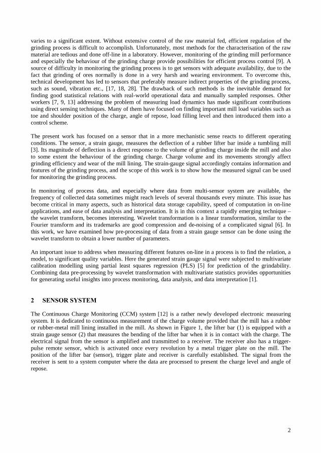
2
varies to a significant extent. Without extensive control of the raw material fed, efficient regulation of thegrinding process is difficult to accomplish. Unfortunately, most methods for the characterisation of the rawmaterial are tedious and done off-line in a laboratory. However, monitoring of the grinding mill performanceand especially the behaviour of the grinding charge provide possibilities for efficient process control [9]. Asource of difficulty in monitoring the grinding process is to get sensors with adequate availability, due to thefact that grinding of ores normally is done in a very harsh and wearing environment. To overcome this,technical development has led to sensors that preferably measure indirect properties of the grinding process,such as sound, vibration etc., [17, 18, 28]. The drawback of such methods is the inevitable demand forfinding good statistical relations with real-world operational data and manually sampled responses. Otherworkers [7, 9, 13] addressing the problem of measuring load dynamics has made significant contributionsusing direct sensing techniques. Many of them have focused on finding important mill load variables such astoe and shoulder position of the charge, angle of repose, load filling level and then introduced them into acontrol scheme.
The present work has focused on a sensor that in a more mechanistic sense reacts to different operatingconditions. The sensor, a strain gauge, measures the deflection of a rubber lifter bar inside a tumbling mill[3]. Its magnitude of deflection is a direct response to the volume of grinding charge inside the mill and alsoto some extent the behaviour of the grinding charge. Charge volume and its movements strongly affectgrinding efficiency and wear of the mill lining. The strain-gauge signal accordingly contains information andfeatures of the grinding process, and the scope of this work is to show how the measured signal can be usedfor monitoring the grinding process.
In monitoring of process data, and especially where data from multi-sensor system are available, thefrequency of collected data sometimes might reach levels of several thousands every minute. This issue hasbecome critical in many aspects, such as historical data storage capability, speed of computation in on-lineapplications, and ease of data analysis and interpretation. It is in this context a rapidly emerging techniquethe wavelet transform, becomes interesting. Wavelet transformation is a linear transformation, similar to theFourier transform and its trademarks are good compression and de-noising of a complicated signal [6]. Inthis work, we have examined how pre-processing of data from a strain gauge sensor can be done using thewavelet transform to obtain a lower number of parameters.
An important issue to address when measuring different features on-line in a process is to find the relation, amodel, to significant quality variables. Here the generated strain gauge signal were subjected to multivariatecalibration modelling using partial least squares regression (PLS) [5] for prediction of the grindability.Combining data pre-processing by wavelet transformation with multivariate statistics provides opportunitiesfor generating useful insights into process monitoring, data analysis, and data interpretation [1].
The Continuous Charge Monitoring (CCM) system [12] is a rather newly developed electronic measuringsystem. It is dedicated to continuous measurement of the charge volume provided that the mill has a rubberor rubber-metal mill lining installed in the mill. As shown in Figure 1, the lifter bar (1) is equipped with astrain gauge sensor (2) that measures the bending of the lifter bar when it is in contact with the charge. Theelectrical signal from the sensor is amplified and transmitted to a receiver. The receiver also has a trigger-pulse remote sensor, which is activated once every revolution by a metal trigger plate on the mill. Theposition of the lifter bar (sensor), trigger plate and receiver is carefully established. The signal from thereceiver is sent to a system computer where the data are processed to present the charge level and angle ofrepose.
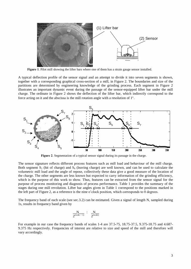
3
(1) Lifter bar
(2) Sensor
. Pilot mill showing the lifter bars where one of them has a strain gauge sensor installed.
A typical deflection profile of the sensor signal and an attempt to divide it into seven segments is shown,together with a corresponding graphical cross-section of a mill, in Figure 2. The boundaries and size of thepartitions are determined by engineering knowledge of the grinding process. Each segment in Figure 2illustrates an important dynamic event during the passage of the sensor-equipped lifter bar under the millcharge. The ordinate in Figure 2 shows the deflection of the lifter bar, which indirectly correspond to theforce acting on it and the abscissa is the mill rotation angle with a resolution of 1 .
S1
S2
S3S4 S5
S6
S2
S3
S4S5 S6 S7
S7
S1
. Segmentation of a typical sensor signal during its passage in the charge.
The sensor signature reflects different process features such as mill load and behaviour of the mill charge.Both segment S2 (hit of charge) and S6 (leaving charge) are well known, and can be used to calculate thevolumetric mill load and the angle of repose, collectively these data give a good measure of the location ofthe charge. The other segments are less known but expected to carry information of the grinding efficiency,which is the purpose of this work to show. Thus, features can be extracted from the sensor signal for thepurpose of process monitoring and diagnosis of process performance. Table 1 provides the summary of thestages during one mill revolution. Lifter bar angles given in Table 1 correspond to the positions marked inthe left part of Figure 2, as a reference is the nine o
The frequency band of each scale (see sec.3.2) can be estimated. Given a signal of length N, sampled during1s, results in frequency band given by
__N___ : _N__2(scale + 1) 2(scale)
For example in our case the frequency bands of scales 1-4 are 37.5-75, 18.75-37.5, 9.375-18.75 and 4.687-9.375 Hz respectively. Frequencies of interest are relative to size and speed of the mill and therefore willvary accordingly.

4
. Sensor lifter bar signal segmentation and process features
Segment Lifter bar angle Process feature Frequency band ofinterest
S1: the sensor lifter bar (SL)is still in the air
50
S2: the SL hits the ballcharge and starts to getsubmerged in the charge 7550
Indicates the toe position of thecharge, and if present, the slurrypool
d1: 37.5d2: 18.75
d4: 4.6875S3: the SL starts to bendforward due to turbulence inthe toe area
8570Rate of change varies with millspeed
d1: 37.5d2: 18.75
S4: the SL is at peakbending
9075 Both speed and charge level hasan influence, wear of lifter
d1: 37.5
S5: the SL is movingthrough the charge
19080 Indication of every lifter barhitting the charge
d4: 4.6875
S6: the SL has graduallydecreased the bending andis at take-off position
215190 Indicates the shoulder positionof the charge
d4: 4.6875d6: 1.1718
S7: the SL is leaving the ballcharge and starts slowly torise to an upright position
215
The statistically planned experiment was performed on a pilot ball mill, diam. 1.4 m, instrumented with theCCM measurement system, c.f. Figure 1. The objective was to study the performance and monitoringcapability of the strain-gauge sensor for different operating conditions. Also of interest was to investigate ifcompressing of the sensor signal using wavelets maintain the predictive ability of a PLS model. Statisticalexperimental design was used to form sets of samples introducing different types of variation occurring in a
The test material, a hematite pellet feed with median size (d50) around 35 m was chosen to get stablegrinding conditions with respect to feedsize variations. Feedrate was kept constant at approx. 1.5 t/h. Table 2shows the experimental design used, which resulted in twelve runs with different levels on
and , all levels in accordance with table 2. Every individual run wasinitiated with a run-in time of approx. 30 min. to reach steady state. When steady state was reached dataacquisition and manual sampling started and lasted for approx. 10 min. The CCM system gives for every millrevolution a measurement vector of 360 elements, i.e. 1 deflection value/degree. The mill rotate with 1revolution per 2.2this time resolution is good enough for the monitoring of a grinding process.
: Experimental design
25 25 25 25 35 35 35 35 28 28 28 28
73 73 78 78 78 78 73 73 73 73 78 78
70 77 77 70 71 76 76 71 70 75 76 71
The responses used for regression was: (1) Grindability index, Gi, the fineness of the ground material,expressed as the produced amount of material less than 45 m pro kWh net. (2) An apparent work index,Wapp, expressed as energy per treated tonnage (kWh/t).
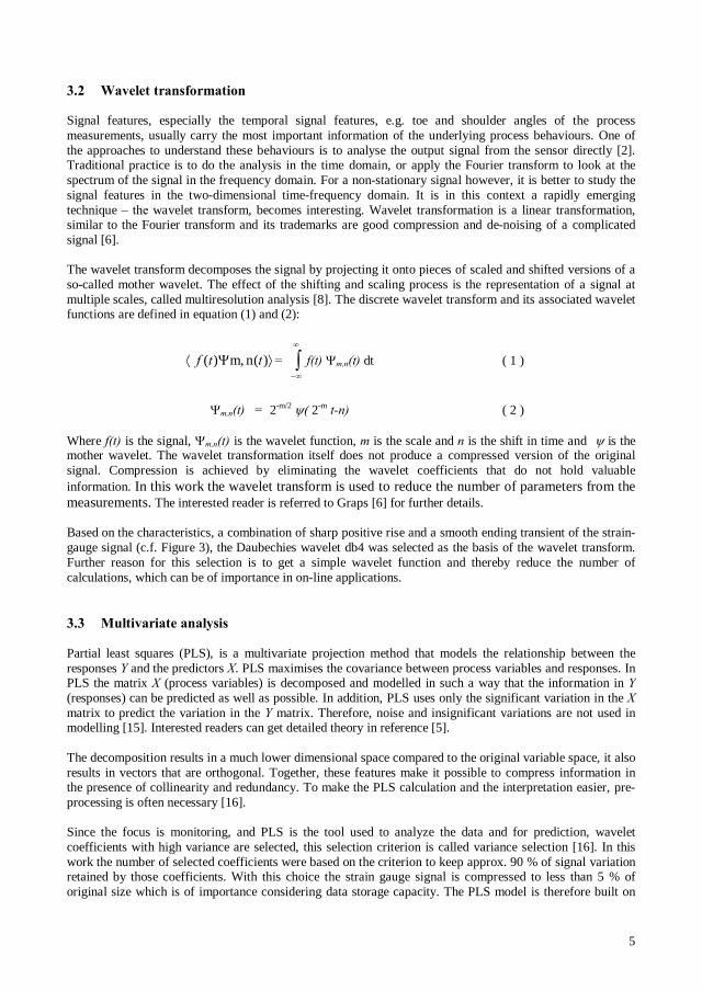
5
Signal features, especially the temporal signal features, e.g. toe and shoulder angles of the processmeasurements, usually carry the most important information of the underlying process behaviours. One ofthe approaches to understand these behaviours is to analyse the output signal from the sensor directly [2].Traditional practice is to do the analysis in the time domain, or apply the Fourier transform to look at thespectrum of the signal in the frequency domain. For a non-stationary signal however, it is better to study thesignal features in the two-dimensional time-frequency domain. It is in this context a rapidly emergingtechnique wavelet transform, becomes interesting. Wavelet transformation is a linear transformation,similar to the Fourier transform and its trademarks are good compression and de-noising of a complicatedsignal [6].
The wavelet transform decomposes the signal by projecting it onto pieces of scaled and shifted versions of aso-called mother wavelet. The effect of the shifting and scaling process is the representation of a signal atmultiple scales, called multiresolution analysis [8]. The discrete wavelet transform and its associated waveletfunctions are defined in equation (1) and (2):
)(nm,)( dt ( 1 )
2-m/2 2-m ( 2 )
Where is the signal, is the wavelet function, is the scale and is the shift in time and is themother wavelet. The wavelet transformation itself does not produce a compressed version of the originalsignal. Compression is achieved by eliminating the wavelet coefficients that do not hold valuableinformation. In this work the wavelet transform is used to reduce the number of parameters from themeasurements. The interested reader is referred to Graps [6] for further details.
Based on the characteristics, a combination of sharp positive rise and a smooth ending transient of the strain-gauge signal (c.f. Figure 3), the Daubechies wavelet db4 was selected as the basis of the wavelet transform.Further reason for this selection is to get a simple wavelet function and thereby reduce the number ofcalculations, which can be of importance in on-line applications.
Partial least squares (PLS), is a multivariate projection method that models the relationship between theresponses and the predictors . PLS maximises the covariance between process variables and responses. InPLS the matrix (process variables) is decomposed and modelled in such a way that the information in(responses) can be predicted as well as possible. In addition, PLS uses only the significant variation in thematrix to predict the variation in the matrix. Therefore, noise and insignificant variations are not used inmodelling [15]. Interested readers can get detailed theory in reference [5].
The decomposition results in a much lower dimensional space compared to the original variable space, it alsoresults in vectors that are orthogonal. Together, these features make it possible to compress information inthe presence of collinearity and redundancy. To make the PLS calculation and the interpretation easier, pre-processing is often necessary [16].
Since the focus is monitoring, and PLS is the tool used to analyze the data and for prediction, waveletcoefficients with high variance are selected, this selection criterion is called variance selection [16]. In thiswork the number of selected coefficients were based on the criterion to keep approx. 90 % of signal variationretained by those coefficients. With this choice the strain gauge signal is compressed to less than 5 % oforiginal size which is of importance considering data storage capacity. The PLS model is therefore built on
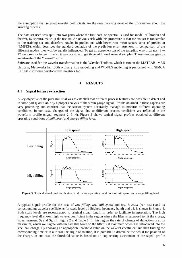
6
the assumption that selected wavelet coefficients are the ones carrying most of the information about thegrinding process.
The data set used was split into two parts where the first part, 48 spectra, is used for model calibration andthe rest, 87 spectra, make up the test set. An obvious risk with this procedure is that the test set is too similarto the training set and therefore results in predictions with lower root mean square error of prediction(RMSEP), which describes the standard deviation of the prediction error. Anyhow, in comparison of thedifferent models they will be equally influenced. To get an apprehension of the sampling error, run nos. 9 to12 were run for longer time, so it was possible to get three additional manual samples. These samples give usan estimate of theSoftware used for the wavelet transformation is the Wavelet Toolbox, which is run on the MATLAB v.6.5platform, Mathworks Inc. Both ordinary PLS modelling and WT-PLS modelling is performed with SIMCAP+ 10.0.2 software developed by Umetrics Inc.
A key objective of the pilot mill trial was to establish that different process features are possible to detect andin some part quantifiable by a proper analysis of the strain-gauge signal. Results obtained in these aspects arevery promising and confirm that the sensor system accurately manage to monitor different operatingconditions. In our case, changes of the signal due to different process conditions are reflected in thewaveform profile (signal segment 2, 3, 4), Figure 3 shows typical signal profiles obtained at differentoperating conditions of and .
Sig
na
l
Sig
na
l
Sig
nal
Sig
nal
Typical signal profiles obtained at different operating conditions of mill speed and charge filling level.
A typical signal profile for the case of , and (run no.1) and itscorresponding wavelet coefficients for scale level d1 (highest frequency band) and d4, is shown in Figure 4.Both scale levels are reconstructed to original signal length in order to facilitate interpretation. The highfrequency level d1 shows high wavelet coefficient in the region where the lifter is supposed to hit the charge,signal segment S2 and S3, c.f. Figure 2 and Table 1. In this region the rate of change of deflection is at itsmaximum, which well agree with the fact that force on the lifter is at maximum when it is introduced into thesteel ball charge. By choosing an appropriate threshold value on the wavelet coefficient and then finding thecorresponding time or in our case the angle of rotation, it is possible to determine the actual toe position ofthe charge. In our case the threshold value is based on an engineering assessment of the signal profile
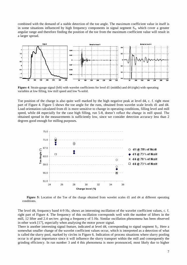
7
combined with the demand of a stable detection of the toe angle. The maximum coefficient value in itself isin some situations influenced by high frequency components in signal segment S4, which cover a greaterangular range and therefore finding the position of the toe from the maximum coefficient value will result ina larger spread.
: Strain-gauge signal (left) with wavelet coefficients for level d1 (middle) and d4 (right) with operatingvariables at low filling, low mill speed and low %-solid.
Toe position of the charge is also quite well marked by the high negative peak at level d4, c. f. right mostpart of Figure 4. Figure 5 shows the toe angle for the runs, obtained from wavelet scale levels d1 and d4.Load orientation calculated from d1 is more sensitive to change in operating conditions, filling level and millspeed, while d4 especially for the case high filling, run 5-8, doesnobtained spread in the measurements is sufficiently low, since we consider detection accuracy less than 2degrees good enough for milling purposes.
51.0
55.0
59.0
63.0
67.0
71.0
75.0
24 26 28 30 32 34 36
Location of the Toe of the charge obtained from wavelet scales d1 and d4 at different operatingconditions.
The level d4, frequency band 4-9 Hz, shows an interesting oscillation of the wavelet coefficient values, c. f.right part of Figure 4. The frequency of this oscillation corresponds well with the number of lifters in themill, 12 lifter and 2.4 sec/rev. giving a frequency of 5 Hz. Similar oscillation phenomena has been observedin other work [17], especially when analysing the motor power signal.There is another interesting signal feature, indicated at level d4, corresponding to signal segment S2. Here asomewhat smaller change of the wavelet coefficient values occur, which is interpreted as a detection of whatis called the slurry pool, marked by circles in Figure 6. Indication of process situations where slurry poolingoccur is of great importance since it will influence the slurry transport within the mill and consequently thegrinding efficiency. In run number 3 and 4 this phenomena is more pronounced, most likely due to higher
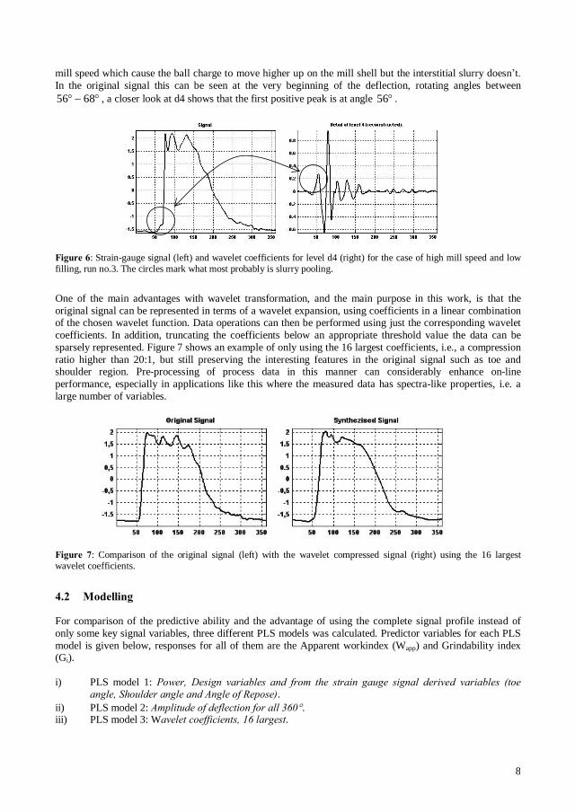
8
mill speed which cause the ball charge to move higher up on the mill shell but the interstitial slurry doesnIn the original signal this can be seen at the very beginning of the deflection, rotating angles between
6856 , a closer look at d4 shows that the first positive peak is at angle 56 .
: Strain-gauge signal (left) and wavelet coefficients for level d4 (right) for the case of high mill speed and lowfilling, run no.3. The circles mark what most probably is slurry pooling.
One of the main advantages with wavelet transformation, and the main purpose in this work, is that theoriginal signal can be represented in terms of a wavelet expansion, using coefficients in a linear combinationof the chosen wavelet function. Data operations can then be performed using just the corresponding waveletcoefficients. In addition, truncating the coefficients below an appropriate threshold value the data can besparsely represented. Figure 7 shows an example of only using the 16 largest coefficients, i.e., a compressionratio higher than 20:1, but still preserving the interesting features in the original signal such as toe andshoulder region. Pre-processing of process data in this manner can considerably enhance on-lineperformance, especially in applications like this where the measured data has spectra-like properties, i.e. alarge number of variables.
: Comparison of the original signal (left) with the wavelet compressed signal (right) using the 16 largestwavelet coefficients.
For comparison of the predictive ability and the advantage of using the complete signal profile instead ofonly some key signal variables, three different PLS models was calculated. Predictor variables for each PLSmodel is given below, responses for all of them are the Apparent workindex (Wapp) and Grindability index(Gi).
i) PLS model 1:.
ii) PLS model 2: .iii) PLS model 3: W .
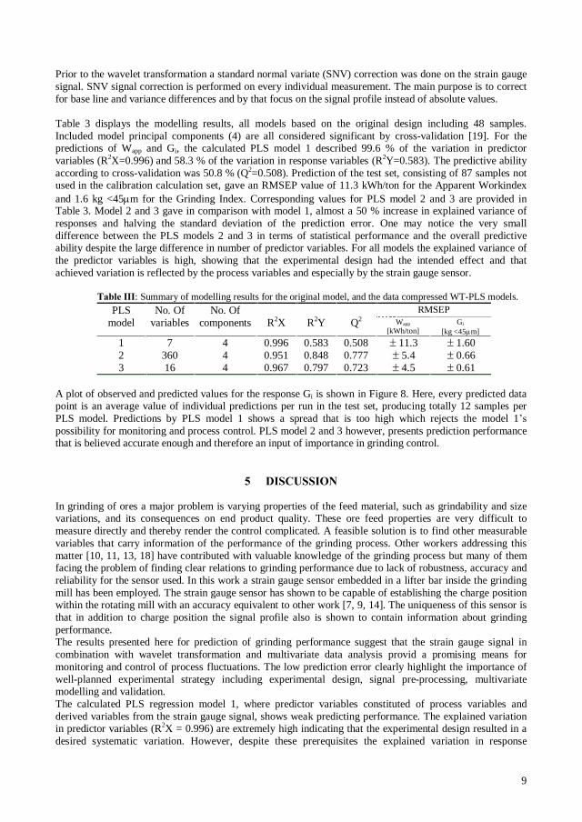
9
Prior to the wavelet transformation a standard normal variate (SNV) correction was done on the strain gaugesignal. SNV signal correction is performed on every individual measurement. The main purpose is to correctfor base line and variance differences and by that focus on the signal profile instead of absolute values.
Table 3 displays the modelling results, all models based on the original design including 48 samples.Included model principal components (4) are all considered significant by cross-validation [19]. For thepredictions of Wapp and Gi, the calculated PLS model 1 described 99.6 % of the variation in predictorvariables (R2X=0.996) and 58.3 % of the variation in response variables (R2Y=0.583). The predictive abilityaccording to cross-validation was 50.8 % (Q2=0.508). Prediction of the test set, consisting of 87 samples notused in the calibration calculation set, gave an RMSEP value of 11.3 kWh/ton for the Apparent Workindexand 1.6 kg <45 m for the Grinding Index. Corresponding values for PLS model 2 and 3 are provided inTable 3. Model 2 and 3 gave in comparison with model 1, almost a 50 % increase in explained variance ofresponses and halving the standard deviation of the prediction error. One may notice the very smalldifference between the PLS models 2 and 3 in terms of statistical performance and the overall predictiveability despite the large difference in number of predictor variables. For all models the explained variance ofthe predictor variables is high, showing that the experimental design had the intended effect and thatachieved variation is reflected by the process variables and especially by the strain gauge sensor.
: Summary of modelling results for the original model, and the data compressed WT-PLS models.RMSEPPLS
modelNo. Of
variablesNo. Of
components R2X R2Y Q2 Wapp
[kWh/ton]Gi
[kg <45 m]
1 7 4 0.996 0.583 0.508 11.3 1.602 360 4 0.951 0.848 0.777 5.4 0.663 16 4 0.967 0.797 0.723 4.5 0.61
A plot of observed and predicted values for the response Gi is shown in Figure 8. Here, every predicted datapoint is an average value of individual predictions per run in the test set, producing totally 12 samples perPLS model. Predictions by PLS model 1 shows a spread that is too high which rejects the model 1possibility for monitoring and process control. PLS model 2 and 3 however, presents prediction performancethat is believed accurate enough and therefore an input of importance in grinding control.
In grinding of ores a major problem is varying properties of the feed material, such as grindability and sizevariations, and its consequences on end product quality. These ore feed properties are very difficult tomeasure directly and thereby render the control complicated. A feasible solution is to find other measurablevariables that carry information of the performance of the grinding process. Other workers addressing thismatter [10, 11, 13, 18] have contributed with valuable knowledge of the grinding process but many of themfacing the problem of finding clear relations to grinding performance due to lack of robustness, accuracy andreliability for the sensor used. In this work a strain gauge sensor embedded in a lifter bar inside the grindingmill has been employed. The strain gauge sensor has shown to be capable of establishing the charge positionwithin the rotating mill with an accuracy equivalent to other work [7, 9, 14]. The uniqueness of this sensor isthat in addition to charge position the signal profile also is shown to contain information about grindingperformance.The results presented here for prediction of grinding performance suggest that the strain gauge signal incombination with wavelet transformation and multivariate data analysis provid a promising means formonitoring and control of process fluctuations. The low prediction error clearly highlight the importance ofwell-planned experimental strategy including experimental design, signal pre-processing, multivariatemodelling and validation.The calculated PLS regression model 1, where predictor variables constituted of process variables andderived variables from the strain gauge signal, shows weak predicting performance. The explained variationin predictor variables (R2X = 0.996) are extremely high indicating that the experimental design resulted in adesired systematic variation. However, despite these prerequisites the explained variation in response
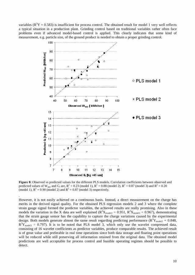
10
variables (R2Y = 0.583) is insufficient for process control. The obtained result for model 1 very well reflectsa typical situation in a production plant. Grinding control based on traditional variables rather often faceproblems even if advanced model-based control is applied. This clearly indicates that some kind ofmeasurement, e.g. particle size, of the ground product is needed to obtain a proper grinding control.
: Observed vs predicted values for the different PLS models. Correlation coefficients between observed andpredicted values of Wapp and Gi are, R2 = 0.23 (model 1), R2 = 0.88 (model 2), R2 = 0.87 (model 3) and R2 = 0.20(model 1), R2 = 0.90 (model 2) and R2 = 0.87 (model 3) respectively.
.However, it is not easily achieved on a continuous basis. Instead, a direct measurement on the charge hasmerits in the derived signal quality. For the obtained PLS regression models 2 and 3 where the completestrain gauge signal formed the predictor variables, the achieved results are really promising. Also in thesemodels the variation in the X data are well explained (R2Xmodel2 = 0.951, R2Xmodel3 = 0.967), demonstratingthat the strain gauge sensor has the capability to capture the charge variations caused by the experimentaldesign. Both models generate almost the same result regarding predicting performance (R2Ymodel2 = 0.848,R2Ymodel3 = 0.797). It is to be noted that PLS model 3, which only use the wavelet compressed data,consisting of 16 wavelet coefficients as predictor variables, produce comparable results. The achieved resultis of great value and preferable in real time operations since both data storage and floating point operationswill be reduced while still preserving all information retained from the original data. The obtained modelpredictions are well acceptable for process control and feasible operating regimes should be possible todetect.
11
Further studies will focus on increasing the discriminating power of certain process states. One approach willbe to separately model process conditions where charge filling and mill speed are at fixed levels and studythe effect of change in slurry flow conditions in the charge. Moreover, future work will emphasise onmethods to enhance the ability to detect undesired or exceptional process states. In particular it has been ofgreat interest in the past to detect a certain condition called slurry pooling. This phenomenon seems to havepossibilities to be detectable with the sensor used, and together with wavelet analysis it should be possible toquantify and position the slurry pool inside the mill.
The measurement system, a strain gauge installed in a lifter bar inside a rotating mill, has in anunprecedented way shown to be capable of unambiguously establish the charge position within the rotatingmill. In addition the signal profile also demonstrate to contain information of the grinding performance.Grinding parameters that are normally measured in the laboratory are now readily modelled from the on-linesignal. As a consequence this opens unique new possibilities for real time monitoring and control of thegrinding process.
The modelling shows that the used wavelet transformation reduces the number of variables considerably. Adata set consisting of only 5 % of the original data result in a PLS regression model with almost the samestatistical performance. Wavelet transformation of the original strain gauge signal has clarified theimportance of the position of the grinding charge or more correctly how an operating condition implicate thecharge movement. The experimental result has also shown that it is particularly the toe position of the chargethat is important to detect since it has a strong correlation with operating performance.
The authors would like to thank the Agricola Research Centre and Norrbotten Research Council for theirassistance and financial support of this project. We also thank Metso Minerals for technical and financialsupport with the sensor system. Special thanks go to Johanna Alatalo and Anders Apelqvist (LKAB) for theirsupport and fruitful assistance during the work.
1. Alsberg B.K., Woodward A.M., Kell D.B., An introduction to wavelet transform for chemometricians: atime-frequency approach, Chemometrics Intell. Lab. Syst. 37 (1997) 215-239
2. Dai X-D., Joseph B., Motard R.L., Introduction to wavelet transform and time-frequency analysis,Wavelet applications in chemical engineering. Motard R.L., Joseph B., eds., Kluwer Academic Press,1994, pp.1-32.
3. Dupont J.F., Vien A., Continuous SAG Volumetric Charge Measurement, Proc. 33rd Ann. Can. Min.Proc. AGM, CIM, Ottawa, 2001, pp. 51 - 67
4. Eriksson L., Johansson E., Kettaneh-Wold N., Wold S., Multi- and megavariate data analysis, principlesand applications, Umetrics AB Ume ., Sweden, 2001.
5. Geladi P., Kowalski B.R., Partial least-squares regression: a tutorial, Analytica Chimica Acta, 185(1986)1-17.
6. Graps A., An introduction to wavelets, IEEE Computational Science and Engineering, 2 (1995) no.2.7. Kolazs J., Control of the mill charge behavior in dry tumbling mills, Minerals Engineering, 12 (1999)
pp.51-64.8. Misiti M., Misiti Y., Oppenheim G., Poggi J.M., Wavelet toolbox for use with MATLAB, The Math
Works Inc. USA, 1996.9. Moys, M.H., Montini, A., The use of conductivity measurements in the control of grinding mills, CIM
Bulletin, 80 (1987) no.907, pp.52-56.

12
10. Moys M.H., Measurement of slurry properties and load behavior in grinding mills, IFAC AppliedMeasurements in Mineral and Metallurgical Processing, Sommer G. ed., Transvaal, South Africa, 1988,pp3-9.
11. Pax R.A., Non-contact acoustic measurement of in-mill variables of SAG mills, Proceedings SAG 2001,Vancouver Canada, 2001, pp. 386-393.
12. Persson S. AUS. pat. 647 667. CAN. Pat.Application 2 088 992. FIN.pat. 101 350. Jap.pat. 2 896 230.NOR.pat. 180 153. RUS.pat. 2 062 184. SWE.pat. 910 271-1 and USA.pat. 5 360 174. 1994-1999.
13. Pontt, J., A new monitoring system for measuring the load filling of a SAG mill, Minerals Engineering,17(2004) 1143-1148.
14. Tano K., P Persson S., Continuous monitoring of a tumbling mill, Proceedings XXIIInternational mineral processing congress. Cape Town, South Africa, 2003.
15. Teppola P., Minkkinen P., Wavelet-PLS regression models for both exploratory data analysis andprocess monitoring, Journal of Chemometrics, 14 (2000) 383-399.
16. Trygg J., Wold S., PLS regression on wavelet compressed NIR spectra, Chemometrics Intell. Lab. Syst.,42 (1998) 209-220.
17. Van Nierop, M.A. and Moys, M.H., The impact of load oscillation on power in an industrial autogenousmill DEM study, Proceedings SAG 2001, Vancouver Canada, 2001, pp. 272-283.
18. Watson J.L., An Analysis of Mill Grinding Noise, Powder Technology, 41 (1985) 83-8919. Wold S., Cross-validatory estimation of the number of components in factor and principal components
models, Technometrics, 20 (1978) 397-405.
K Tano, A Berggren and B P
Accepted for publication in Minerals & Metallurgical Processing

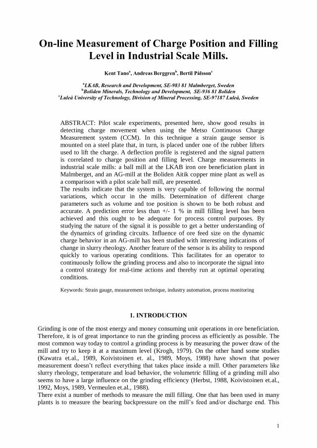
1
ABSTRACT: Pilot scale experiments, presented here, show good results indetecting charge movement when using the Metso Continuous ChargeMeasurement system (CCM). In this technique a strain gauge sensor ismounted on a steel plate that, in turn, is placed under one of the rubber liftersused to lift the charge. A deflection profile is registered and the signal patternis correlated to charge position and filling level. Charge measurements inindustrial scale mills: a ball mill at the LKAB iron ore beneficiation plant inMalmberget, and an AG-mill at the Boliden Aitik copper mine plant as well asa comparison with a pilot scale ball mill, are presented.The results indicate that the system is very capable of following the normalvariations, which occur in the mills. Determination of different chargeparameters such as volume and toe position is shown to be both robust andaccurate. A prediction error less than +/- 1 % in mill filling level has beenachieved and this ought to be adequate for process control purposes. Bystudying the nature of the signal it is possible to get a better understanding ofthe dynamics of grinding circuits. Influence of ore feed size on the dynamiccharge behavior in an AG-mill has been studied with interesting indications ofchange in slurry rheology. Another feature of the sensor is its ability to respondquickly to various operating conditions. This facilitates for an operator tocontinuously follow the grinding process and also to incorporate the signal intoa control strategy for real-time actions and thereby run at optimal operatingconditions.
Keywords: Strain gauge, measurement technique, industry automation, process monitoring
Grinding is one of the most energy and money consuming unit operations in ore beneficiation.Therefore, it is of great importance to run the grinding process as efficiently as possible. Themost common way today to control a grinding process is by measuring the power draw of themill and try to keep it at a maximum level (Krogh, 1979). On the other hand some studies(Kawatra et.al., 1989, Koivistoinen et. al., 1989, Moys, 1988) have shown that powermeasurement doesnslurry rheology, temperature and load behavior, the volumetric filling of a grinding mill alsoseems to have a large influence on the grinding efficiency (Herbst, 1988, Koivistoinen et.al.,1992, Moys, 1989, Vermeulen et.al., 1988).There exist a number of methods to measure the mill filling. One that has been used in manyplants is to measure the bearing backpressure on the mill
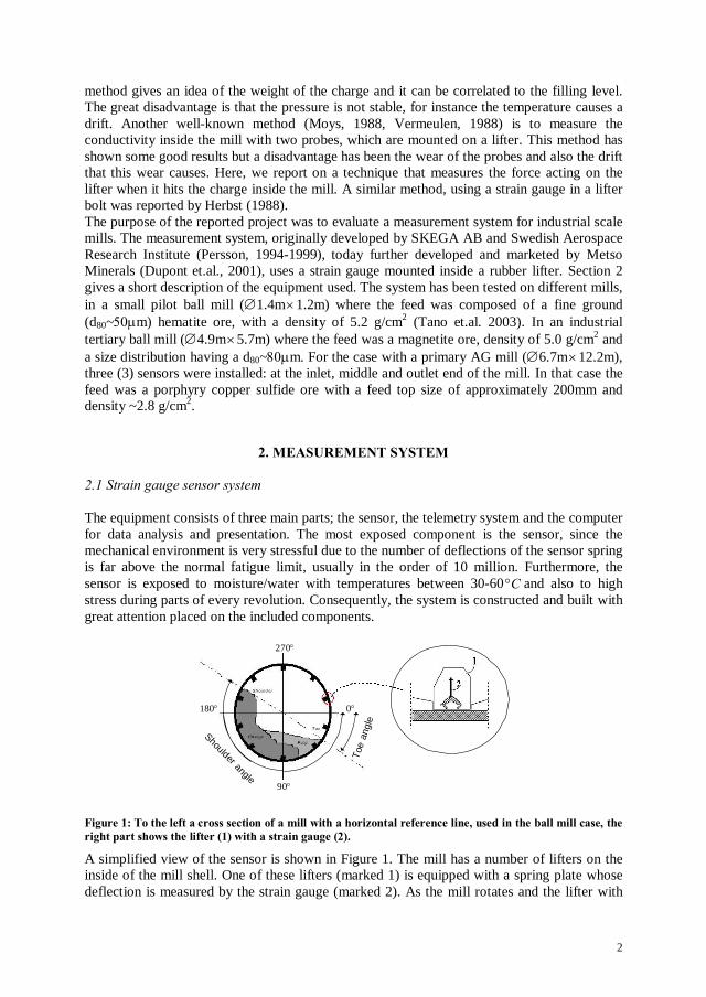
2
method gives an idea of the weight of the charge and it can be correlated to the filling level.The great disadvantage is that the pressure is not stable, for instance the temperature causes adrift. Another well-known method (Moys, 1988, Vermeulen, 1988) is to measure theconductivity inside the mill with two probes, which are mounted on a lifter. This method hasshown some good results but a disadvantage has been the wear of the probes and also the driftthat this wear causes. Here, we report on a technique that measures the force acting on thelifter when it hits the charge inside the mill. A similar method, using a strain gauge in a lifterbolt was reported by Herbst (1988).The purpose of the reported project was to evaluate a measurement system for industrial scalemills. The measurement system, originally developed by SKEGA AB and Swedish AerospaceResearch Institute (Persson, 1994-1999), today further developed and marketed by MetsoMinerals (Dupont et.al., 2001), uses a strain gauge mounted inside a rubber lifter. Section 2gives a short description of the equipment used. The system has been tested on different mills,in a small pilot ball mill ( 1.4m 1.2m) where the feed was composed of a fine ground(d80~ m) hematite ore, with a density of 5.2 g/cm2 (Tano et.al. 2003). In an industrialtertiary ball mill ( 4.9m 5.7m) where the feed was a magnetite ore, density of 5.0 g/cm2 anda size distribution having a d80~ m. For the case with a primary AG mill ( 6.7m 12.2m),three (3) sensors were installed: at the inlet, middle and outlet end of the mill. In that case thefeed was a porphyry copper sulfide ore with a feed top size of approximately 200mm anddensity ~2.8 g/cm2.
The equipment consists of three main parts; the sensor, the telemetry system and the computerfor data analysis and presentation. The most exposed component is the sensor, since themechanical environment is very stressful due to the number of deflections of the sensor springis far above the normal fatigue limit, usually in the order of 10 million. Furthermore, thesensor is exposed to moisture/water with temperatures between 30-60 and also to highstress during parts of every revolution. Consequently, the system is constructed and built withgreat attention placed on the included components.
Toe
angl
e
Shoulder angle
90
180
270
0
A simplified view of the sensor is shown in Figure 1. The mill has a number of lifters on theinside of the mill shell. One of these lifters (marked 1) is equipped with a spring plate whosedeflection is measured by the strain gauge (marked 2). As the mill rotates and the lifter with
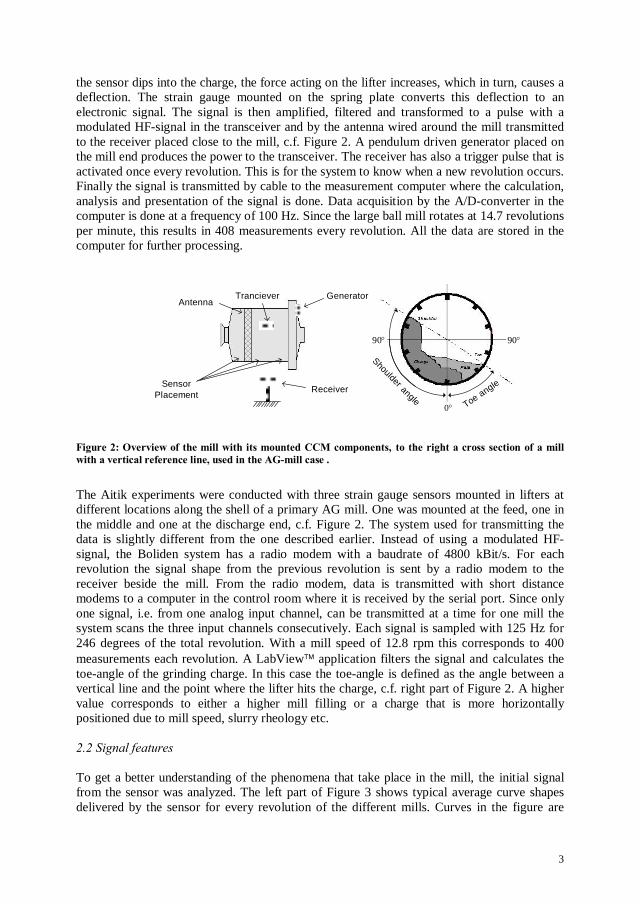
3
the sensor dips into the charge, the force acting on the lifter increases, which in turn, causes adeflection. The strain gauge mounted on the spring plate converts this deflection to anelectronic signal. The signal is then amplified, filtered and transformed to a pulse with amodulated HF-signal in the transceiver and by the antenna wired around the mill transmittedto the receiver placed close to the mill, c.f. Figure 2. A pendulum driven generator placed onthe mill end produces the power to the transceiver. The receiver has also a trigger pulse that isactivated once every revolution. This is for the system to know when a new revolution occurs.Finally the signal is transmitted by cable to the measurement computer where the calculation,analysis and presentation of the signal is done. Data acquisition by the A/D-converter in thecomputer is done at a frequency of 100 Hz. Since the large ball mill rotates at 14.7 revolutionsper minute, this results in 408 measurements every revolution. All the data are stored in thecomputer for further processing.
SensorPlacement
Tranciever
Receiver
AntennaGenerator
Shoulder angle
Toe angle
0
9090
The Aitik experiments were conducted with three strain gauge sensors mounted in lifters atdifferent locations along the shell of a primary AG mill. One was mounted at the feed, one inthe middle and one at the discharge end, c.f. Figure 2. The system used for transmitting thedata is slightly different from the one described earlier. Instead of using a modulated HF-signal, the Boliden system has a radio modem with a baudrate of 4800 kBit/s. For eachrevolution the signal shape from the previous revolution is sent by a radio modem to thereceiver beside the mill. From the radio modem, data is transmitted with short distancemodems to a computer in the control room where it is received by the serial port. Since onlyone signal, i.e. from one analog input channel, can be transmitted at a time for one mill thesystem scans the three input channels consecutively. Each signal is sampled with 125 Hz for246 degrees of the total revolution. With a mill speed of 12.8 rpm this corresponds to 400measurements each revolution. A LabView application filters the signal and calculates thetoe-angle of the grinding charge. In this case the toe-angle is defined as the angle between avertical line and the point where the lifter hits the charge, c.f. right part of Figure 2. A highervalue corresponds to either a higher mill filling or a charge that is more horizontallypositioned due to mill speed, slurry rheology etc.
To get a better understanding of the phenomena that take place in the mill, the initial signalfrom the sensor was analyzed. The left part of Figure 3 shows typical average curve shapesdelivered by the sensor for every revolution of the different mills. Curves in the figure are
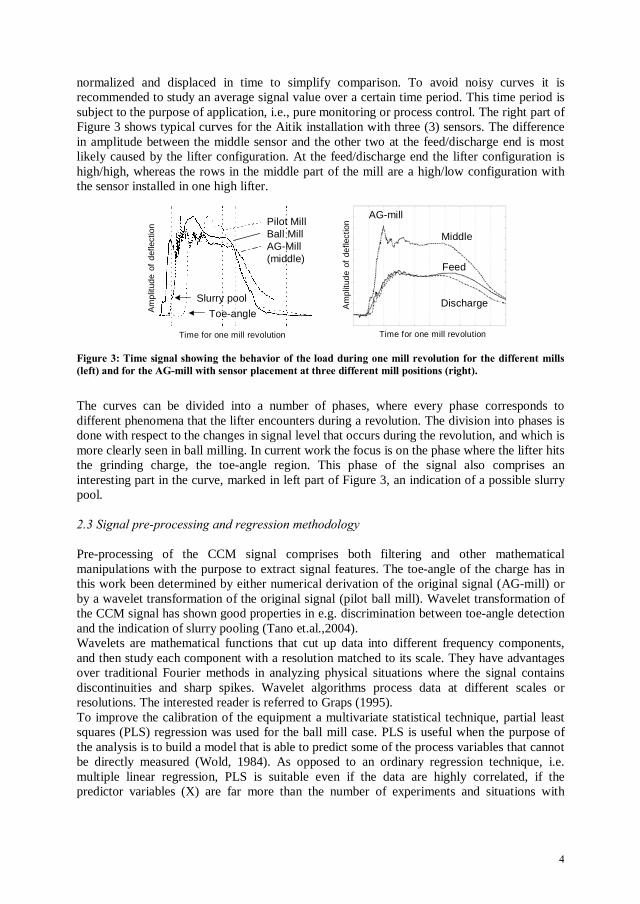
4
normalized and displaced in time to simplify comparison. To avoid noisy curves it isrecommended to study an average signal value over a certain time period. This time period issubject to the purpose of application, i.e., pure monitoring or process control. The right part ofFigure 3 shows typical curves for the Aitik installation with three (3) sensors. The differencein amplitude between the middle sensor and the other two at the feed/discharge end is mostlikely caused by the lifter configuration. At the feed/discharge end the lifter configuration ishigh/high, whereas the rows in the middle part of the mill are a high/low configuration withthe sensor installed in one high lifter.
Am
plitu
deof
defle
ctio
n
Am
plitu
deof
defle
ctio
nPilot MillBall MillAG-Mill(middle)
Middle
Feed
Discharge
Time for one mill revolution Time for one mill revolution
AG-mill
Slurry pool
Toe-angle
The curves can be divided into a number of phases, where every phase corresponds todifferent phenomena that the lifter encounters during a revolution. The division into phases isdone with respect to the changes in signal level that occurs during the revolution, and which ismore clearly seen in ball milling. In current work the focus is on the phase where the lifter hitsthe grinding charge, the toe-angle region. This phase of the signal also comprises aninteresting part in the curve, marked in left part of Figure 3, an indication of a possible slurrypool.
Pre-processing of the CCM signal comprises both filtering and other mathematicalmanipulations with the purpose to extract signal features. The toe-angle of the charge has inthis work been determined by either numerical derivation of the original signal (AG-mill) orby a wavelet transformation of the original signal (pilot ball mill). Wavelet transformation ofthe CCM signal has shown good properties in e.g. discrimination between toe-angle detectionand the indication of slurry pooling (Tano et.al.,2004).Wavelets are mathematical functions that cut up data into different frequency components,and then study each component with a resolution matched to its scale. They have advantagesover traditional Fourier methods in analyzing physical situations where the signal containsdiscontinuities and sharp spikes. Wavelet algorithms process data at different scales orresolutions. The interested reader is referred to Graps (1995).To improve the calibration of the equipment a multivariate statistical technique, partial leastsquares (PLS) regression was used for the ball mill case. PLS is useful when the purpose ofthe analysis is to build a model that is able to predict some of the process variables that cannotbe directly measured (Wold, 1984). As opposed to an ordinary regression technique, i.e.multiple linear regression, PLS is suitable even if the data are highly correlated, if thepredictor variables (X) are far more than the number of experiments and situations with

5
missing data due to sensor failure, which is not unusual in industrial applications. A tutorial toPLS is given in reference Geladi et.al. (1986).
Figure 4 shows a typical flowsheet for concentrating iron ore. The coarse materials at 10-15mm in size are fed to a primary wet magnetic cobbing separator (M1). The magneticconcentrate is discharged into a primary ball mill (#1), and the ground product (pulp) istransferred to a secondary magnetic separator (M2). The resultant magnetic concentrate isthen pumped into a secondary ball mill (#2). The ground product is finally upgraded by atertiary magnetic separation unit (M3) and the concentrate is used as feed for the tertiarygrinding stage (#3). The strain-gauge sensor was installed in the tertiary-grinding mill (#3).
Water
Waste
Concentrate
Water
Water
Feed
The overflow ball mill used in the tertiary grinding stage has an outside diameter of 4.9 m anda length of 5.7 m, and is run in open circuit. The grinding charge consists of approximately400 tons of 25 mm diameter chromium steel balls corresponding to 40 % in charge volume.The height of the new rubber liner lifters is about 70 mm. The mill is driven by two 1800 kWAC motors. The mill speed is set at 14.7 rpm giving a fraction of critical speed c ~0.78.Under normal grinding condition, the rated power draw, the pulp density and the feed rate are2550 kW, 72 weight-% solids and 250 t/h respectively.
This experiment was the first full-scale test of the equipmentdevelopment had concentrated on work with sensor accuracy and tuning of the dataacquisition system. The equipment had been installed 1.5 months before the test periodstarted, in order to ensure reliability.To get an understanding of, and distinguish between correlation and causality, theexperiments were performed according to a statistical design. The fact that the variables arechanged between fixed levels and chosen so the whole interesting area is examined makes itpossible to build predictive models. Nine experiments were performed and the variables
and were varied according to Table 1.To accomplish the different fillings the mill was stopped and emptied of balls, in the first case25 ton of the charge and in the next case additional 25 tons. In each case when the mill was
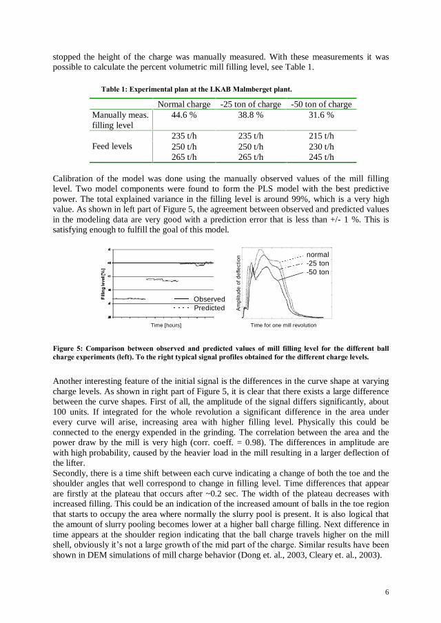
6
stopped the height of the charge was manually measured. With these measurements it waspossible to calculate the percent volumetric mill filling level, see Table 1.
Normal charge -25 ton of charge -50 ton of chargeManually meas.filling level
44.6 % 38.8 % 31.6 %
235 t/h 235 t/h 215 t/h250 t/h 250 t/h 230 t/hFeed levels265 t/h 265 t/h 245 t/h
Calibration of the model was done using the manually observed values of the mill fillinglevel. Two model components were found to form the PLS model with the best predictivepower. The total explained variance in the filling level is around 99%, which is a very highvalue. As shown in left part of Figure 5, the agreement between observed and predicted valuesin the modeling data are very good with a prediction error that is less than +/- 1 %. This issatisfying enough to fulfill the goal of this model.
ObservedPredicted
normal-25 ton-50 ton
Time for one mill revolutionTime [hours]
Am
plitu
deof
def
lect
ion
Another interesting feature of the initial signal is the differences in the curve shape at varyingcharge levels. As shown in right part of Figure 5, it is clear that there exists a large differencebetween the curve shapes. First of all, the amplitude of the signal differs significantly, about100 units. If integrated for the whole revolution a significant difference in the area underevery curve will arise, increasing area with higher filling level. Physically this could beconnected to the energy expended in the grinding. The correlation between the area and thepower draw by the mill is very high (corr. coeff. = 0.98). The differences in amplitude arewith high probability, caused by the heavier load in the mill resulting in a larger deflection ofthe lifter.Secondly, there is a time shift between each curve indicating a change of both the toe and theshoulder angles that well correspond to change in filling level. Time differences that appearare firstly at the plateau that occurs after ~0.2 sec. The width of the plateau decreases withincreased filling. This could be an indication of the increased amount of balls in the toe regionthat starts to occupy the area where normally the slurry pool is present. It is also logical thatthe amount of slurry pooling becomes lower at a higher ball charge filling. Next difference intime appears at the shoulder region indicating that the ball charge travels higher on the millshell, obviously itshown in DEM simulations of mill charge behavior (Dong et. al., 2003, Cleary et. al., 2003).
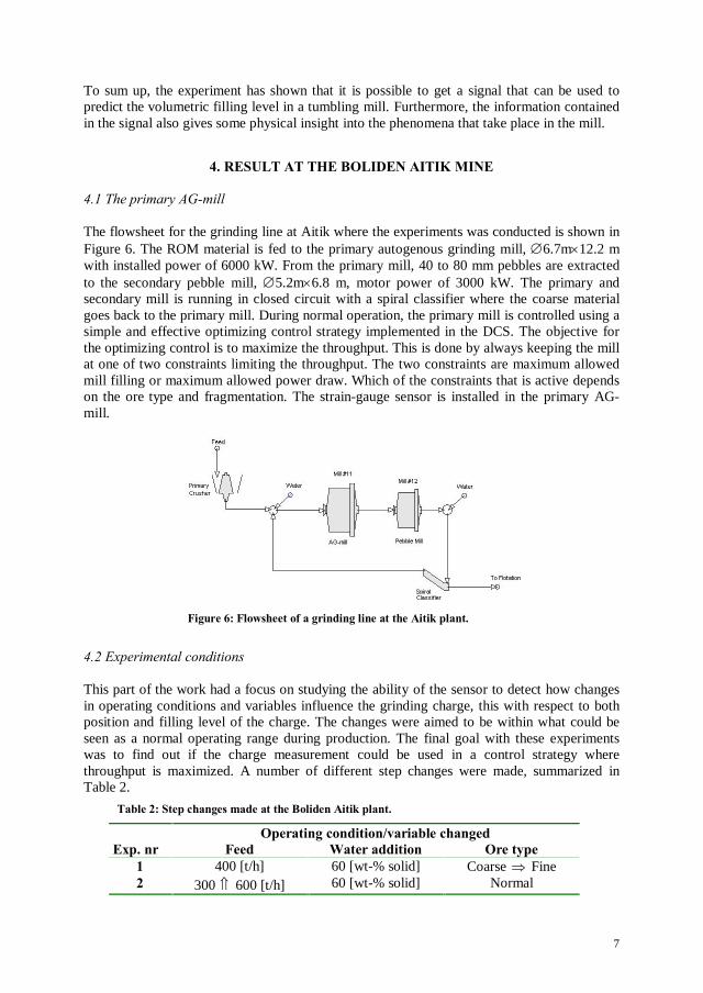
7
To sum up, the experiment has shown that it is possible to get a signal that can be used topredict the volumetric filling level in a tumbling mill. Furthermore, the information containedin the signal also gives some physical insight into the phenomena that take place in the mill.
The flowsheet for the grinding line at Aitik where the experiments was conducted is shown inFigure 6. The ROM material is fed to the primary autogenous grinding mill, 6.7m 12.2 mwith installed power of 6000 kW. From the primary mill, 40 to 80 mm pebbles are extractedto the secondary pebble mill, 5.2m 6.8 m, motor power of 3000 kW. The primary andsecondary mill is running in closed circuit with a spiral classifier where the coarse materialgoes back to the primary mill. During normal operation, the primary mill is controlled using asimple and effective optimizing control strategy implemented in the DCS. The objective forthe optimizing control is to maximize the throughput. This is done by always keeping the millat one of two constraints limiting the throughput. The two constraints are maximum allowedmill filling or maximum allowed power draw. Which of the constraints that is active dependson the ore type and fragmentation. The strain-gauge sensor is installed in the primary AG-mill.
This part of the work had a focus on studying the ability of the sensor to detect how changesin operating conditions and variables influence the grinding charge, this with respect to bothposition and filling level of the charge. The changes were aimed to be within what could beseen as a normal operating range during production. The final goal with these experimentswas to find out if the charge measurement could be used in a control strategy wherethroughput is maximized. A number of different step changes were made, summarized inTable 2.
400 [t/h] 60 [wt-% solid] Coarse Fine300 600 [t/h] 60 [wt-% solid] Normal
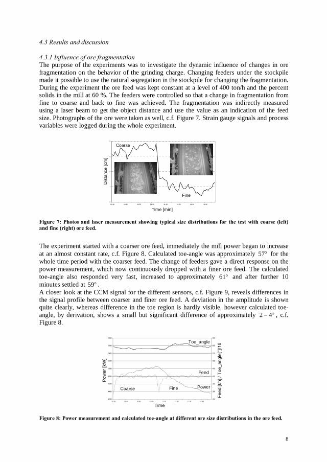
8
The purpose of the experiments was to investigate the dynamic influence of changes in orefragmentation on the behavior of the grinding charge. Changing feeders under the stockpilemade it possible to use the natural segregation in the stockpile for changing the fragmentation.During the experiment the ore feed was kept constant at a level of 400 ton/h and the percentsolids in the mill at 60 %. The feeders were controlled so that a change in fragmentation fromfine to coarse and back to fine was achieved. The fragmentation was indirectly measuredusing a laser beam to get the object distance and use the value as an indication of the feedsize. Photographs of the ore were taken as well, c.f. Figure 7. Strain gauge signals and processvariables were logged during the whole experiment.
5
7
9
11
13
10:30 10:40 10:50 11:00 11:10 11:20 11:30 11:40
Time [min]
Dis
tanc
e[c
m]
Coarse
Fine
The experiment started with a coarser ore feed, immediately the mill power began to increaseat an almost constant rate, c.f. Figure 8. Calculated toe-angle was approximately 57 for thewhole time period with the coarser feed. The change of feeders gave a direct response on thepower measurement, which now continuously dropped with a finer ore feed. The calculatedtoe-angle also responded very fast, increased to approximately 61 and after further 10minutes settled at 59 .A closer look at the CCM signal for the different sensors, c.f. Figure 9, reveals differences inthe signal profile between coarser and finer ore feed. A deviation in the amplitude is shownquite clearly, whereas difference in the toe region is hardly visible, however calculated toe-angle, by derivation, shows a small but significant difference of approximately 42 , c.f.Figure 8.
Pow
er[k
W]
Power
Toe_angle
Feed
Fee
d[t
/h]/
Toe
_ang
le[
Time
Coarse Fine
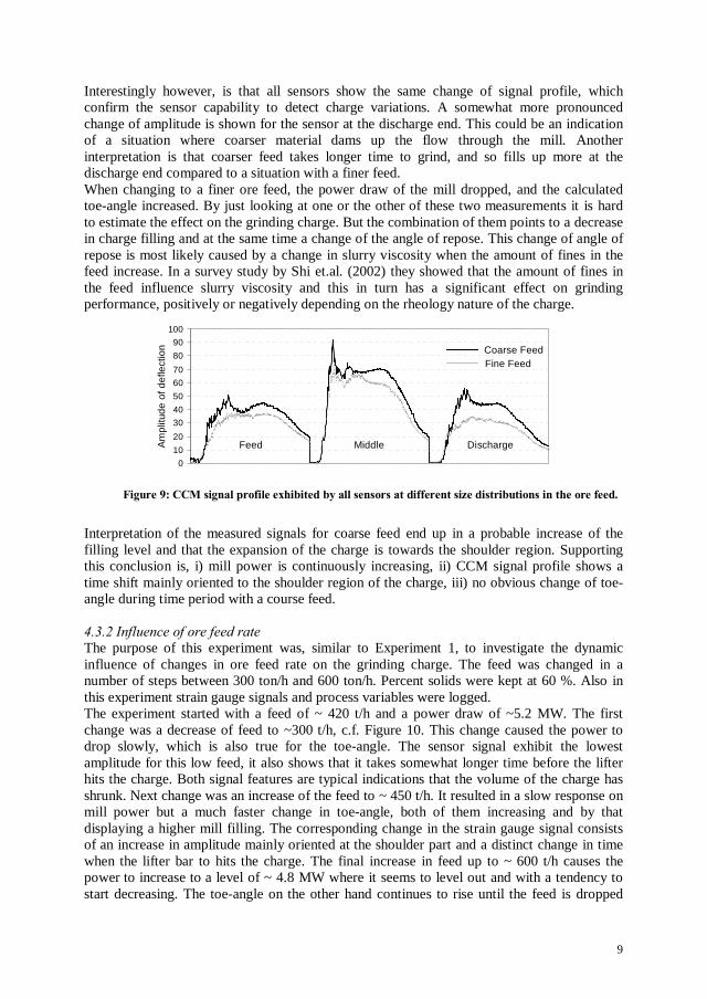
9
Interestingly however, is that all sensors show the same change of signal profile, whichconfirm the sensor capability to detect charge variations. A somewhat more pronouncedchange of amplitude is shown for the sensor at the discharge end. This could be an indicationof a situation where coarser material dams up the flow through the mill. Anotherinterpretation is that coarser feed takes longer time to grind, and so fills up more at thedischarge end compared to a situation with a finer feed.When changing to a finer ore feed, the power draw of the mill dropped, and the calculatedtoe-angle increased. By just looking at one or the other of these two measurements it is hardto estimate the effect on the grinding charge. But the combination of them points to a decreasein charge filling and at the same time a change of the angle of repose. This change of angle ofrepose is most likely caused by a change in slurry viscosity when the amount of fines in thefeed increase. In a survey study by Shi et.al. (2002) they showed that the amount of fines inthe feed influence slurry viscosity and this in turn has a significant effect on grindingperformance, positively or negatively depending on the rheology nature of the charge.
0
10
20
30
40
50
60
70
80
90
100
Coarse FeedFine Feed
Am
plitu
deof
defle
ctio
n
Feed Middle Discharge
Interpretation of the measured signals for coarse feed end up in a probable increase of thefilling level and that the expansion of the charge is towards the shoulder region. Supportingthis conclusion is, i) mill power is continuously increasing, ii) CCM signal profile shows atime shift mainly oriented to the shoulder region of the charge, iii) no obvious change of toe-angle during time period with a course feed.
The purpose of this experiment was, similar to Experiment 1, to investigate the dynamicinfluence of changes in ore feed rate on the grinding charge. The feed was changed in anumber of steps between 300 ton/h and 600 ton/h. Percent solids were kept at 60 %. Also inthis experiment strain gauge signals and process variables were logged.The experiment started with a feed of ~ 420 t/h and a power draw of ~5.2 MW. The firstchange was a decrease of feed to ~300 t/h, c.f. Figure 10. This change caused the power todrop slowly, which is also true for the toe-angle. The sensor signal exhibit the lowestamplitude for this low feed, it also shows that it takes somewhat longer time before the lifterhits the charge. Both signal features are typical indications that the volume of the charge hasshrunk. Next change was an increase of the feed to ~ 450 t/h. It resulted in a slow response onmill power but a much faster change in toe-angle, both of them increasing and by thatdisplaying a higher mill filling. The corresponding change in the strain gauge signal consistsof an increase in amplitude mainly oriented at the shoulder part and a distinct change in timewhen the lifter bar to hits the charge. The final increase in feed up to ~ 600 t/h causes thepower to increase to a level of ~ 4.8 MW where it seems to level out and with a tendency tostart decreasing. The toe-angle on the other hand continues to rise until the feed is dropped
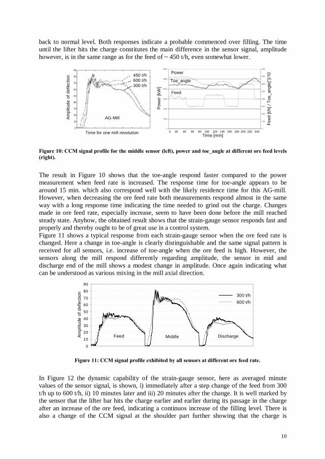
10
back to normal level. Both responses indicate a probable commenced over filling. The timeuntil the lifter hits the charge constitutes the main difference in the sensor signal, amplitudehowever, is in the same range as for the feed of ~ 450 t/h, even somewhat lower.
Pow
er[k
W]
Fee
d[t/
h]/T
oe_a
ngle
[
Power
Toe_angle
Feed
Time [min]
450 t/h600 t/h300 t/h
Time for one mill revolution
Am
plitu
deof
defle
ctio
n
AG-Mill
0 20 40 60 80 100 120 140 160 180 200 220 240
The result in Figure 10 shows that the toe-angle respond faster compared to the powermeasurement when feed rate is increased. The response time for toe-angle appears to bearound 15 min. which also correspond well with the likely residence time for this AG-mill.However, when decreasing the ore feed rate both measurements respond almost in the sameway with a long response time indicating the time needed to grind out the charge. Changesmade in ore feed rate, especially increase, seem to have been done before the mill reachedsteady state. Anyhow, the obtained result shows that the strain-gauge sensor responds fast andproperly and thereby ought to be of great use in a control system.Figure 11 shows a typical response from each strain-gauge sensor when the ore feed rate ischanged. Here a change in toe-angle is clearly distinguishable and the same signal pattern isreceived for all sensors, i.e. increase of toe-angle when the ore feed is high. However, thesensors along the mill respond differently regarding amplitude, the sensor in mid anddischarge end of the mill shows a modest change in amplitude. Once again indicating whatcan be understood as various mixing in the mill axial direction.
0
10
20
30
40
50
60
70
80
90
Feed Middle Discharge
300 t/h
600 t/h
Am
plitu
deof
def
lect
ion
In Figure 12 the dynamic capability of the strain-gauge sensor, here as averaged minutevalues of the sensor signal, is shown, i) immediately after a step change of the feed from 300t/h up to 600 t/h, ii) 10 minutes later and iii) 20 minutes after the change. It is well marked bythe sensor that the lifter bar hits the charge earlier and earlier during its passage in the chargeafter an increase of the ore feed, indicating a continuos increase of the filling level. There isalso a change of the CCM signal at the shoulder part further showing that the charge is
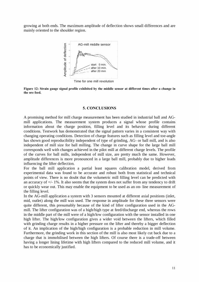
11
growing at both ends. The maximum amplitude of deflection shows small differences and aremainly oriented to the shoulder region.
start 0 min.after 10 min.after 20 min
AG-mill middle sensor
Am
plitu
deof
defle
ctio
n
Time for one mill revolution
A promising method for mill charge measurement has been studied in industrial ball and AG-mill applications. The measurement system produces a signal whose profile containsinformation about the charge position, filling level and its behavior during differentconditions. Testwork has demonstrated that the signal pattern varies in a consistent way withchanging operating conditions. Detection of charge features such as filling level and toe-anglehas shown good reproducibility independent of type of grinding, AG- or ball mill, and is alsoindependent of mill size for ball milling. The change in curve shape for the large ball millcorresponds well with changes achieved in the pilot mill at different charge levels. The profileof the curves for ball mills, independent of mill size, are pretty much the same. However,amplitude differences is more pronounced in a large ball mill, probably due to higher loadsinfluencing the lifter deflection.For the ball mill application a partial least squares calibration model, derived fromexperimental data was found to be accurate and robust both from statistical and technicalpoints of view. There is no doubt that the volumetric mill filling level can be predicted withan accuracy of +/- 1%. It also seems that the system does not suffer from any tendency to driftor quickly wear out. This may enable the equipment to be used as an on- line measurement ofthe filling level.In the AG-mill application a system with 3 sensors mounted at different axial positions (inlet,mid, outlet) along the mill was used. The response in amplitude for these three sensors werequite different, this presumably because of the kind of lifter configuration used in the AG-mill. The lifter configuration was of a high/high type at feed/discharge end, whereas the rowsin the middle part of the mill were of a high/low configuration with the sensor installed in onehigh lifter. The high/low configuration gives a wider void between the lifters, which filledwith grinding charge results in a higher pressure on the lifter and thereby a bigger deflectionof it. An implication of the high/high configuration is a probable reduction in mill volume.Furthermore, the grinding work in this section of the mill is also most likely cut back due to acharge that is immobilised between the high lifters. Of course there is a trade-off betweenhaving a longer lining lifetime with high lifters compared to the reduced mill volume, and ithas to be economically justified.
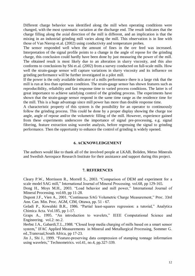
12
Different charge behavior was identified along the mill when operating conditions werechanged, with the most systematic variation at the discharge end. The result indicates that thecharge filling along the axial direction of the mill is different, and an implication is that themixing in an industrial grinding mill varies along the mill. This observation is in line withthose of Van Nierop et.al. (2002) using conductivity and temperature probes.The sensor responded well when the amount of fines in the ore feed was increased.Interpretation of the signal profile points to a change in the angle of repose for the grindingcharge, this conclusion could hardly have been done by just measuring the power of the mill.The obtained result is most likely due to an alteration in slurry viscosity, and this alsoconforms to conclusions by Shi et.al. (2002) from a survey conducted on full-scale mills. Howwell the strain-gauge sensor will capture variations in slurry viscosity and its influence ongrinding performance will be further investigated in a pilot mill.If the power is the only available indicator of a mills performance there is a large risk that themill is run at less than optimum condition. The strain-gauge sensor has shown features such asreproducibility, reliability and fast response time to varied process conditions. The latter is ofgreat importance to achieve satisfying control of the grinding process. The experiments haveshown that the strain-gauge sensor respond in the same time range as the residence time forthe mill. This is a huge advantage since mill power has more than double response time.A characteristic property of this system is the possibility for an operator to continuouslyfollow the grinding process. This could be done by a proper display showing the charge toeangle, angle of repose and/or the volumetric filling of the mill. However, experience gainedfrom these experiments underscore the importance of signal pre-processing, e.g. signalfiltering, feature extraction using wavelet analysis, before regressing the signal to grindingperformance. Then the opportunity to enhance the control of grinding is widely opened.
The authors would like to thank all of the involved people at LKAB, Boliden, Metso Mineralsand Swedish Aerospace Research Institute for their assistance and support during this project.
Cleary P.W., Morrisson R., Morrell S., 2003. DEM and experiment for ascale model SAG mill, vol.68, pp 129-165.Dong H., Moys M.H., 2003.Mineral Processing. vol.69, pp 11-28.Dupont J.F., Vien A., 2001. Proc. 33rdAnn. Can. Min. Proc. AGM, CIM, Ottawa, pp. 51 - 67.Geladi P., Kowalski B.R., 1986. AnalyticaChimica Acta. Vol.185, pp 1-17.Graps A., 1995.Engineering. vol.2: no.2.Herbst J.A., Gabardi,T.L.,1988.system, IFAC Applied Measurements in Mineral and Metallurgical Processing, Sommer G.ed.,Transvaal,South Africa, pp 17-23.Jin J., Shi J., 1999.using wavelets, Technometrics. vol.41, no.4, pp.327-339.
13
Krogh S., 1979. Autogenous and Semiautogenous Mills,of the Autogenous Grinding Seminar, Digre M., ed., University of Trondheim, Norway, E1-1- E-1-20.Kawatra S.K., Eisele T.C.1989.Autogenous Grinding Circuit, Autogenous and Semiautogenous GrindingTechnology, Mular A.L., Agar G.E., eds., University of British Columbia, Vancouver, pp485-502.Koivistonen P., Miettunen J., 1989.mill and its utilisation in grinding control, Autogenous and SemiautogenousGrinding Technology, Mular A.L., Agar G.E., eds., University of British Columbia,Vancouver, pp 687-695.Koivistonen P., Kalapudas R., Miettunen J., 1992.volumetric filling of a grinding mill, Comminution-Theory and Practice, Kawatra S.K., ed.,Society for Mining, Metallurgy and Exploration, pp 563-574.Moys M.H., 1988. behaviour in grinding mills,IFAC Applied Measurements in Mineral and Metallurgical Processing. Sommer G. ed.,Transvaal, South Africa, pp 3-9.Moys M.H.1989. rheology-the key to further advance in grinding mill control,Advances in Autogenous and Semiautogenous Grinding Technology, Mular A.L., Agar G.E.,eds., University of British Columbia, Vancouver, pp 390-400.Persson, S. (1994-1999). AUS. pat. 647 667. CAN. Pat.Application 2 088 992. FIN.pat. 101350. Jap.pat. 2 896 230. NOR.pat. 180 153. RUS.pat. 2 062 184. SWE.pat. 910 271-1 andUSA.pat. 5 360 174.Tano K., P Persson S., 2003.Proceedings XXII International mineral processing congress. Cape Town, South Africa, pp1514-1523.Tano K., P R PLS-regressionon a wavelet transformed strain-gauge signal,ChemometricsVan Nierop M.A., Moys M.H., 2002. autogenous grindingmill, vol.65, pp 151-164.Vermeulen L.A., Schakowski F.A., 1988.charge volume and other milling parameters in an operating mill, IFAC AppliedMeasurements in Mineral and Metallurgical Processing. ed., Sommer G., Transvaal, SouthAfrica, pp 11-15.Wold, S. et. al., 1984. Multivariate Data Analysis in Chemistry. In Chemometrics: Math. andStatitistics in Chemistry. ed., Kowalski B.R. Reidel publ.Co., Dordrecht, Netherlands.


K Tano, B P Sellgren
Minerals Engineering, In press

On-line lifter deflection measurements showing flow resistanceeffects in grinding mills
Kent T. Tano a,b,*, Bertil I. Palsson b, Anders Sellgren b
a LKAB, Research and Development, S-983 81 Malmberget, Swedenb Division of Mineral Processing, Lulea University of Technology, S-97187 Lulea, Sweden
Received 4 January 2005; accepted 7 February 2005
Abstract
The deflection that a lifter bar is subjected to when passing through a grinding charge was measured using an embedded strain
gauge sensor. The obtained signal profile is analysed and interpreted in relation to charge properties such as toe and charge angle for
the grinding charge. The current work has focused on the charge and slurry flow behaviour when solids content is changed and how
well the sensor reflects this. Bench scale measurements with a vane type viscometer, roughly evaluated in terms of apparent viscosity
is used as a character for the resistance to motion of the slurry.
The slurry flow resistance is strongly influenced by solids content and obviously by the addition of a dispersant. The strain gauge
sensor reflected this change well, showing that toe and shoulder region of the charge varied in a systematic way. Results obtained
also shows that change of slurry flow resistance exert an influence on grinding performance.
A multivariate statistical method, partial least squares regression, is applied to the sensor data producing a model that can predict
the change in slurry flow resistance. The output from the model also shows good properties to be used as a process-monitoring tool.
The predictive capability of the model is believed to be of such quality that it can be used for process control.
� 2005 Elsevier Ltd. All rights reserved.
Keywords: Grinding; Deflection sensor; Mill monitoring; Flow resistance; Slurry viscosity
1. Introduction
Size reduction is an inevitable unit operation in min-
eral processing. Comminution is also by far the most en-
ergy consuming part in mineral concentrators and at the
same time extremely inefficient, less than 10% of sup-
plied power produce new mineral surfaces. The econom-
ical potential is substantial if efficiency can be increased
just a couple of percent. In general, the only grindingcontrol is to maximize the power drawn by the mill.
Unfortunately, the relation between power and grinding
performance is a complex and non-linear function.
Development of advanced control systems has helpedthe situation considerably (Herbst and Rajamani,
1982). However, these systems still are lacking relevant
information such as mill load, charge position or slurry
properties. Sensors capable of delivering this informa-
tion are therefore of great value.
The difficulty for a sensor is that the complex motion
of a grinding charge is determined by both mill design
variables such as liners, lifter profile, discharge mecha-nism, etc. and process operating variables such as solids
content, size distribution and slurry viscosity. It does not
make it simpler that e.g. viscosity itself is a function of
several variables in addition to volume percent solids,
such as solids size distribution, particle shape distribu-
tion, slurry temperature, etc. This illustrates how com-
plicated it is for a single sensor to detect changes in
0892-6875/$ - see front matter � 2005 Elsevier Ltd. All rights reserved.
doi:10.1016/j.mineng.2005.02.005
* Corresponding author. Tel.: +46 97076203; fax: +46 97030617.
E-mail addresses: [email protected] (K.T. Tano), bertil.pals-
[email protected] (B.I. Palsson), [email protected] (A. Sellgren).
This article is also available online at:
www.elsevier.com/locate/mineng
Minerals Engineering xxx (2005) xxx–xxx
ARTICLE IN PRESS
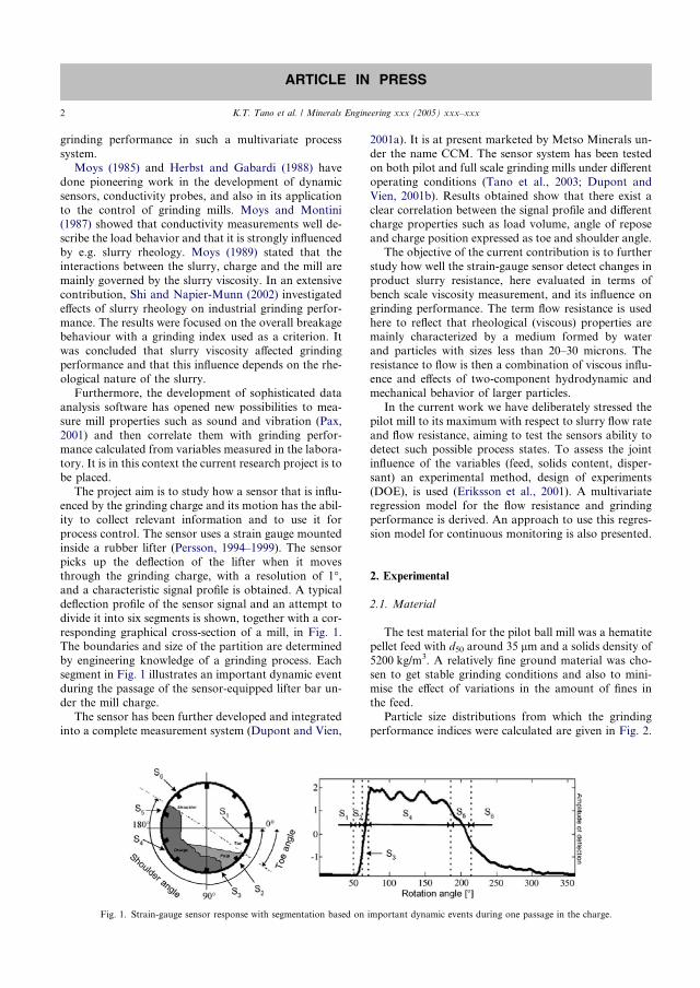
grinding performance in such a multivariate process
system.
Moys (1985) and Herbst and Gabardi (1988) have
done pioneering work in the development of dynamic
sensors, conductivity probes, and also in its application
to the control of grinding mills. Moys and Montini(1987) showed that conductivity measurements well de-
scribe the load behavior and that it is strongly influenced
by e.g. slurry rheology. Moys (1989) stated that the
interactions between the slurry, charge and the mill are
mainly governed by the slurry viscosity. In an extensive
contribution, Shi and Napier-Munn (2002) investigated
effects of slurry rheology on industrial grinding perfor-
mance. The results were focused on the overall breakagebehaviour with a grinding index used as a criterion. It
was concluded that slurry viscosity affected grinding
performance and that this influence depends on the rhe-
ological nature of the slurry.
Furthermore, the development of sophisticated data
analysis software has opened new possibilities to mea-
sure mill properties such as sound and vibration (Pax,
2001) and then correlate them with grinding perfor-mance calculated from variables measured in the labora-
tory. It is in this context the current research project is to
be placed.
The project aim is to study how a sensor that is influ-
enced by the grinding charge and its motion has the abil-
ity to collect relevant information and to use it for
process control. The sensor uses a strain gauge mounted
inside a rubber lifter (Persson, 1994–1999). The sensorpicks up the deflection of the lifter when it moves
through the grinding charge, with a resolution of 1�,and a characteristic signal profile is obtained. A typical
deflection profile of the sensor signal and an attempt to
divide it into six segments is shown, together with a cor-
responding graphical cross-section of a mill, in Fig. 1.
The boundaries and size of the partition are determined
by engineering knowledge of a grinding process. Eachsegment in Fig. 1 illustrates an important dynamic event
during the passage of the sensor-equipped lifter bar un-
der the mill charge.
The sensor has been further developed and integrated
into a complete measurement system (Dupont and Vien,
2001a). It is at present marketed by Metso Minerals un-
der the name CCM. The sensor system has been tested
on both pilot and full scale grinding mills under different
operating conditions (Tano et al., 2003; Dupont and
Vien, 2001b). Results obtained show that there exist a
clear correlation between the signal profile and differentcharge properties such as load volume, angle of repose
and charge position expressed as toe and shoulder angle.
The objective of the current contribution is to further
study how well the strain-gauge sensor detect changes in
product slurry resistance, here evaluated in terms of
bench scale viscosity measurement, and its influence on
grinding performance. The term flow resistance is used
here to reflect that rheological (viscous) properties aremainly characterized by a medium formed by water
and particles with sizes less than 20–30 microns. The
resistance to flow is then a combination of viscous influ-
ence and effects of two-component hydrodynamic and
mechanical behavior of larger particles.
In the current work we have deliberately stressed the
pilot mill to its maximum with respect to slurry flow rate
and flow resistance, aiming to test the sensors ability todetect such possible process states. To assess the joint
influence of the variables (feed, solids content, disper-
sant) an experimental method, design of experiments
(DOE), is used (Eriksson et al., 2001). A multivariate
regression model for the flow resistance and grinding
performance is derived. An approach to use this regres-
sion model for continuous monitoring is also presented.
2. Experimental
2.1. Material
The test material for the pilot ball mill was a hematite
pellet feed with d50 around 35 lm and a solids density of
5200 kg/m3. A relatively fine ground material was cho-sen to get stable grinding conditions and also to mini-
mise the effect of variations in the amount of fines in
the feed.
Particle size distributions from which the grinding
performance indices were calculated are given in Fig. 2.
Fig. 1. Strain-gauge sensor response with segmentation based on important dynamic events during one passage in the charge.
2 K.T. Tano et al. / Minerals Engineering xxx (2005) xxx–xxx
ARTICLE IN PRESS
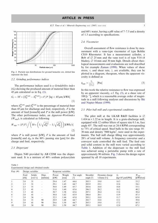
2.2. Grinding performance indices
The performance indices used is a Grindability index
(Gi) showing the produced amount of material finer than
45 lm calculated as in Eq. (1).
Gi ¼ 100 � S45 lmD � S45 lm
F
� � � F =P ½kg < 45lm=kWh�ð1Þ
where S45 lmD and S45 lm
F is the percentage of material finerthan 45 lm for discharge and feed, respectively. F is the
amount of feed [tonne/h] and P is the mill power [kW].
The other performance index, an Apparent-Workindex
(Wapp), is calculated as following
W app ¼ P=Fð Þ 10 � 1=
ffiffiffiffiffiffiffiffiffidOut80
q� 1=
ffiffiffiffiffiffiffidIn80
q� �� ��½kWh=t�
ð2Þwhere P is mill power [kW], F is the amount of feed
[tonne/h] and d80 is the 80% passing size [lm] for dis-
charge and feed, respectively.
2.3. Dispersant
Dispex N40 provided by AB CDM was the disper-
sant used. It is a mixture of 40% sodium polyacrylate
and 60% water, having a pH value of 7–7.5 and a density
of 1.3 according to specifications.
2.4. Viscometer
Overall assessment of flow resistance is done by mea-surement with a vane-type viscometer of type Bohlin
CS10 Rheometer. It has a measurement cylinder, a
Bob of B 25 mm and the vane tool is of type V14 (4
blades), B 14 mm and 30 mm high. Details about rheo-
logical measurements and evaluations are well described
by for example Zaman (1998). When values of shear
stress, s, and shear rate, _c, are available, they can be
plotted in a diagram, rheogram, where the apparent vis-cosity is defined as
gapp ¼si
_cðsiÞ ½Pas� ð3Þ
In this work the relative resistance to flow was expressed
by an apparent viscosity, c.f. Eq. (3), at a shear rate of
100 [s�1], which is a reasonable average order of magni-
tude in a mill following analyses and discussions by Shi
and Napier-Munn (1999).
2.5. Pilot ball mill and experimental conditions
The pilot mill at the LKAB R&D facilities is B1.414 m · 1.22 m in length. It is a grate-discharge mill,
equipped with 12 rubber lifters of square size 0.1 m, face
angle 45�. The mill was run at 24.4 RPM corresponding
to 73% of critical speed. Steel balls in the size range 10–30 mm and density 7800 kg/m3, were used in the exper-
iments. The ball mill charge filling was approximately
28% of total mill volume. A frequency converter and a
conveyor scale controlled the mill feed. The feed rate
and solid content in the mill were varied according to
Table 1. Addition of the dispersant to the mill feed
was achieved using a peristaltic pump with a rate of
approximately 90 ml/min. Fig. 3 shows the design regionspanned by all 10 experiments.
Table 1
Experimental design and obtained results
Exp. (#) Design variables Response variables
Feed
[t/h]
Solids
[vol.%]
Disp.
[ml/min]
Power
[kW]
Weight
[ton]
Toe angle
[�]Shoulder
angle [�]Dynamic charge
volume [%]
Gi
[kg<45 lm/kWh]
Wapp
[kWh/ton]
1 2.0 31 – 29.4 1.47 64.6 203.3 19.0 14.3 53.2
2 1.5 31 – 29.1 1.45 64.7 203.9 19.1 12.6 54.1
3 2.5 31 – 30.0 1.49 65.7 203.6 18.8 14.8 53.1
4 2.5 41 – 31.0 1.60 63.6 206.5 20.2 16.2 48.2
5 1.5 41 – 30.7 1.58 63.6 207.1 20.4 13.6 50.4
6 2.0 41 – 30.4 1.62 63.9 206.4 20.1 15.9 47.3
7 2.0 36 – 32.5 1.64 65.0 203.1 18.8 11.7 65.0
8 2.0 31 90 28.9 1.48 64.7 202.7 18.8 13.1 59.8
9 2.0 41 90 28.6 1.50 64.7 203.3 19.0 17.2 45.3
10 2.0 36 90 29.1 1.50 64.7 203.1 18.9 12.0 67.1
0
10
20
30
40
50
60
70
80
90
100
1 10 100 1000Particle size (μm)
Wei
ght %
Pas
sing
(%)
Fig. 2. Particle size distributions for ground hematite ore, dotted line
represent the feed.
K.T. Tano et al. / Minerals Engineering xxx (2005) xxx–xxx 3
ARTICLE IN PRESS
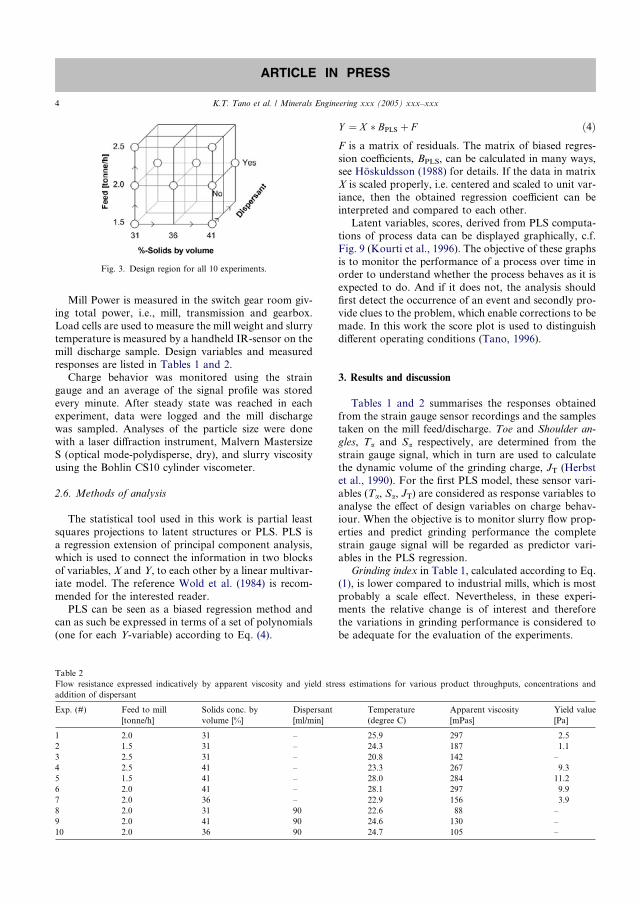
Mill Power is measured in the switch gear room giv-ing total power, i.e., mill, transmission and gearbox.
Load cells are used to measure the mill weight and slurry
temperature is measured by a handheld IR-sensor on the
mill discharge sample. Design variables and measured
responses are listed in Tables 1 and 2.
Charge behavior was monitored using the strain
gauge and an average of the signal profile was stored
every minute. After steady state was reached in eachexperiment, data were logged and the mill discharge
was sampled. Analyses of the particle size were done
with a laser diffraction instrument, Malvern Mastersize
S (optical mode-polydisperse, dry), and slurry viscosity
using the Bohlin CS10 cylinder viscometer.
2.6. Methods of analysis
The statistical tool used in this work is partial least
squares projections to latent structures or PLS. PLS is
a regression extension of principal component analysis,
which is used to connect the information in two blocks
of variables, X and Y, to each other by a linear multivar-
iate model. The reference Wold et al. (1984) is recom-
mended for the interested reader.
PLS can be seen as a biased regression method andcan as such be expressed in terms of a set of polynomials
(one for each Y-variable) according to Eq. (4).
Y ¼ X � BPLS þ F ð4ÞF is a matrix of residuals. The matrix of biased regres-
sion coefficients, BPLS, can be calculated in many ways,see Hoskuldsson (1988) for details. If the data in matrix
X is scaled properly, i.e. centered and scaled to unit var-
iance, then the obtained regression coefficient can be
interpreted and compared to each other.
Latent variables, scores, derived from PLS computa-
tions of process data can be displayed graphically, c.f.
Fig. 9 (Kourti et al., 1996). The objective of these graphs
is to monitor the performance of a process over time inorder to understand whether the process behaves as it is
expected to do. And if it does not, the analysis should
first detect the occurrence of an event and secondly pro-
vide clues to the problem, which enable corrections to be
made. In this work the score plot is used to distinguish
different operating conditions (Tano, 1996).
3. Results and discussion
Tables 1 and 2 summarises the responses obtained
from the strain gauge sensor recordings and the samples
taken on the mill feed/discharge. Toe and Shoulder an-
gles, Ta and Sa respectively, are determined from the
strain gauge signal, which in turn are used to calculate
the dynamic volume of the grinding charge, JT (Herbstet al., 1990). For the first PLS model, these sensor vari-
ables (Ta, Sa, JT) are considered as response variables to
analyse the effect of design variables on charge behav-
iour. When the objective is to monitor slurry flow prop-
erties and predict grinding performance the complete
strain gauge signal will be regarded as predictor vari-
ables in the PLS regression.
Grinding index in Table 1, calculated according to Eq.(1), is lower compared to industrial mills, which is most
probably a scale effect. Nevertheless, in these experi-
ments the relative change is of interest and therefore
the variations in grinding performance is considered to
be adequate for the evaluation of the experiments.
Fig. 3. Design region for all 10 experiments.
Table 2
Flow resistance expressed indicatively by apparent viscosity and yield stress estimations for various product throughputs, concentrations and
addition of dispersant
Exp. (#) Feed to mill
[tonne/h]
Solids conc. by
volume [%]
Dispersant
[ml/min]
Temperature
(degree C)
Apparent viscosity
[mPas]
Yield value
[Pa]
1 2.0 31 – 25.9 297 2.5
2 1.5 31 – 24.3 187 1.1
3 2.5 31 – 20.8 142 –
4 2.5 41 – 23.3 267 9.3
5 1.5 41 – 28.0 284 11.2
6 2.0 41 – 28.1 297 9.9
7 2.0 36 – 22.9 156 3.9
8 2.0 31 90 22.6 88 –
9 2.0 41 90 24.6 130 –
10 2.0 36 90 24.7 105 –
4 K.T. Tano et al. / Minerals Engineering xxx (2005) xxx–xxx
ARTICLE IN PRESS
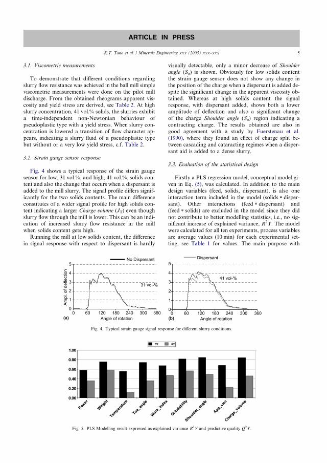
3.1. Viscometric measurements
To demonstrate that different conditions regarding
slurry flow resistance was achieved in the ball mill simple
viscometric measurements were done on the pilot mill
discharge. From the obtained rheograms apparent vis-cosity and yield stress are derived, see Table 2. At high
slurry concentration, 41 vol.% solids, the slurries exhibit
a time-independent non-Newtonian behaviour of
pseudoplastic type with a yield stress. When slurry con-
centration is lowered a transition of flow character ap-
pears, indicating a slurry fluid of a pseudoplastic type
but without or a very low yield stress, c.f. Table 2.
3.2. Strain gauge sensor response
Fig. 4 shows a typical response of the strain gauge
sensor for low, 31 vol.%, and high, 41 vol.%, solids con-
tent and also the change that occurs when a dispersant is
added to the mill slurry. The signal profile differs signif-
icantly for the two solids contents. The main difference
constitutes of a wider signal profile for high solids con-tent indicating a larger Charge volume (JT) even though
slurry flow through the mill is lower. This can be an indi-
cation of increased slurry flow resistance in the mill
when solids content gets high.
Running the mill at low solids content, the difference
in signal response with respect to dispersant is hardly
visually detectable, only a minor decrease of Shoulder
angle (Sa) is shown. Obviously for low solids content
the strain gauge sensor does not show any change in
the position of the charge when a dispersant is added de-
spite the significant change in the apparent viscosity ob-
tained. Whereas at high solids content the signalresponse, with dispersant added, shows both a lower
amplitude of deflection and also a significant change
of the charge Shoulder angle (Sa) region indicating a
contracting charge. The results obtained are also in
good agreement with a study by Fuerstenau et al.
(1990), where they found an effect of charge split be-
tween cascading and cataracting regimes when a disper-
sant aid is added to a dense slurry.
3.3. Evaluation of the statistical design
Firstly a PLS regression model, conceptual model gi-
ven in Eq. (5), was calculated. In addition to the main
design variables (feed, solids, dispersant), is also one
interaction term included in the model (solids * disper-
sant). Other interactions (feed * dispersant) and(feed * solids) are excluded in the model since they did
not contribute to better modelling statistics, i.e., no sig-
nificant increase of explained variance, R2Y. The model
were calculated for all ten experiments, process variables
are average values (10 min) for each experimental set-
ting, see Table 1 for values. The main purpose with
0
1
2
3
4
5
0 60 120 180 240 300 3600
1
2
3
4
5
0 60 120 180 240 300 360
31 vol-%41 vol-%
DispersantNo Dispersant
Ampl
. of d
efle
ctio
n
Angle of rotation Angle of rotation(a) (b)
Fig. 4. Typical strain gauge signal response for different slurry conditions.
Fig. 5. PLS Modelling result expressed as explained variance R2Y and predictive quality Q2Y.
K.T. Tano et al. / Minerals Engineering xxx (2005) xxx–xxx 5
ARTICLE IN PRESS

the first model is to study the effect of design variables
on some response variables.
Y ¼ f ðfeed; solids; dispersant; solids � dispersantÞ þ F
ð5ÞF is the residual matrix. The calculated model gave five
significant PLS components with explained variance,
R2Y, and predictive capability, Q2Y, for the different re-
sponses shown in Fig. 5. A comparable measure for
bivariate data is the correlation coefficient. The result
shows that the variables Weight, Grindability, Shoulder
angle and Charge volume is reasonably well modelled,with high R2 and Q2, whereas the variables Power and
Temperature shows low predictive ability, low Q2. Mill
torque is presumably a more adequate power measure-
ment, since losses and inaccuracies in the mill drive sys-
tem will then be excluded from the power figure. The
low Q2 for the Temperature can unfortunately be a result
from the handheld measurement, an indication of a low
accuracy for the instrument. For the variable Apparent
Viscosity, the result demonstrates the difficulty to model
rheological properties using standard mill variables.
However, the obtained model is statistically accept-
able and can be used for studying the different effects.
The following interaction plots displays the predicted
change in the response variables when one design vari-
able varies, and the second variable is set at both its
low and high level, all other variables being set on theircentre value.
Of primary interest is to study the effect on the tradi-
tionally monitored mill variables, Power, Weight and
Temperature. All of them are positively affected when
solids content increase. When a dispersant is added to
the slurry, the effect on Power and Weight is almost neg-
ligible at low solids content. The lower mill Power when
dispersant is present is probably due to a change of
charge position and thereby a different centre of gravity
for the charge. The Temperature shows an inconsistentresponse when dispersant is present, which is difficult
to interpret, once again, can be an inaccuracy in the
measurement (Fig. 6).
Next to study is the effects found from the strain
gauge sensor, expressed as Ta and Sa, together with
the derived Charge volume, JT. At low solids content,
the calculated variables are influenced by the presence
of a dispersant aid only to a minor degree. On the otherhand, at high solids content both Ta and Sa angles are
affected, with the largest change, taking place at the
shoulder of the charge. High solids content seems to ex-
pand the charge and with the addition of dispersant it
falls back to a volume corresponding more or less to
the situation at low solids content. The change for the
variable Charge volume is analogous since it is calculated
from Ta and Sa angles (Fig. 7).The last interaction plot is for the grinding perfor-
mance variables Wapp and Gi, and the slurry flow resis-
tance expressed as gapp. High solids content slightly
increase the grinding performance, i.e., lower Wapp
and higher Gi. Whereas the addition of a dispersant give
a negative effect on the grinding performance especially
when running at low solids content. The effect of a dis-
persant aid is well reflected in the viscometric measure-ment, giving a higher gapp in the absence of a
dispersant (Fig. 8).
Fig. 6. Interaction plots for solids and dispersant on responses power, weight and temperature.
Fig. 7. Interaction plots for solids and dispersant on responses Ta, Sa and charge volume.
6 K.T. Tano et al. / Minerals Engineering xxx (2005) xxx–xxx
ARTICLE IN PRESS
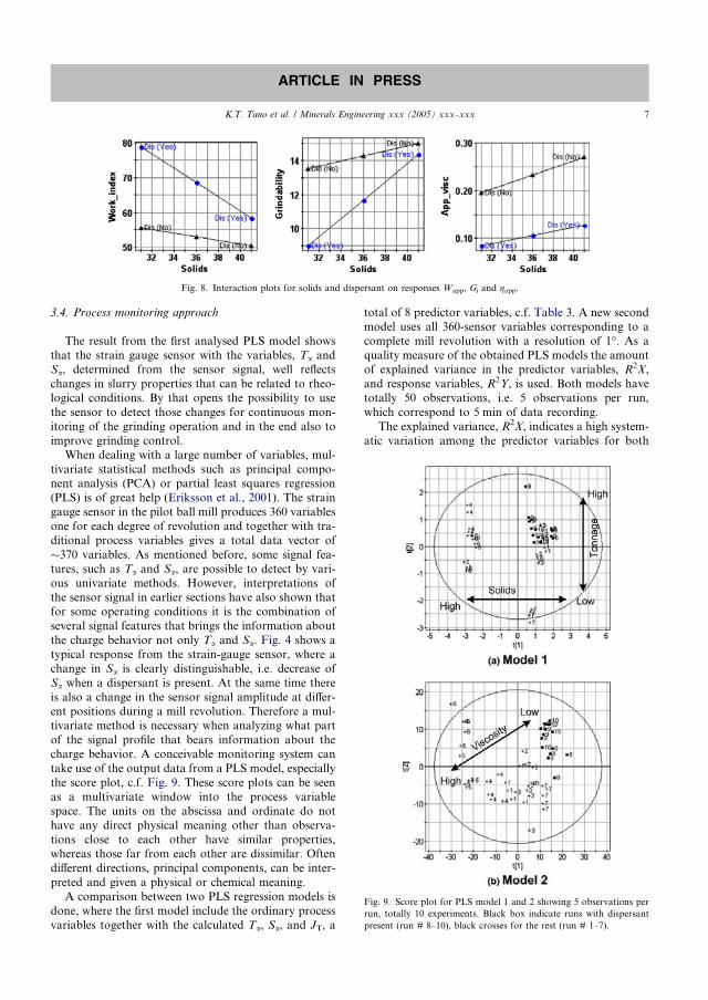
3.4. Process monitoring approach
The result from the first analysed PLS model shows
that the strain gauge sensor with the variables, Ta andSa, determined from the sensor signal, well reflects
changes in slurry properties that can be related to rheo-
logical conditions. By that opens the possibility to use
the sensor to detect those changes for continuous mon-
itoring of the grinding operation and in the end also to
improve grinding control.
When dealing with a large number of variables, mul-
tivariate statistical methods such as principal compo-nent analysis (PCA) or partial least squares regression
(PLS) is of great help (Eriksson et al., 2001). The strain
gauge sensor in the pilot ball mill produces 360 variables
one for each degree of revolution and together with tra-
ditional process variables gives a total data vector of
�370 variables. As mentioned before, some signal fea-
tures, such as Ta and Sa, are possible to detect by vari-
ous univariate methods. However, interpretations ofthe sensor signal in earlier sections have also shown that
for some operating conditions it is the combination of
several signal features that brings the information about
the charge behavior not only Ta and Sa. Fig. 4 shows a
typical response from the strain-gauge sensor, where a
change in Sa is clearly distinguishable, i.e. decrease of
Sa when a dispersant is present. At the same time there
is also a change in the sensor signal amplitude at differ-ent positions during a mill revolution. Therefore a mul-
tivariate method is necessary when analyzing what part
of the signal profile that bears information about the
charge behavior. A conceivable monitoring system can
take use of the output data from a PLS model, especially
the score plot, c.f. Fig. 9. These score plots can be seen
as a multivariate window into the process variable
space. The units on the abscissa and ordinate do nothave any direct physical meaning other than observa-
tions close to each other have similar properties,
whereas those far from each other are dissimilar. Often
different directions, principal components, can be inter-
preted and given a physical or chemical meaning.
A comparison between two PLS regression models is
done, where the first model include the ordinary process
variables together with the calculated Ta, Sa, and JT, a
total of 8 predictor variables, c.f. Table 3. A new second
model uses all 360-sensor variables corresponding to a
complete mill revolution with a resolution of 1�. As a
quality measure of the obtained PLS models the amountof explained variance in the predictor variables, R2X,
and response variables, R2Y, is used. Both models have
totally 50 observations, i.e. 5 observations per run,
which correspond to 5 min of data recording.
The explained variance, R2X, indicates a high system-
atic variation among the predictor variables for both
Fig. 8. Interaction plots for solids and dispersant on responses Wapp, Gi and gapp.
Fig. 9. Score plot for PLS model 1 and 2 showing 5 observations per
run, totally 10 experiments. Black box indicate runs with dispersant
present (run # 8–10), black crosses for the rest (run # 1–7).
K.T. Tano et al. / Minerals Engineering xxx (2005) xxx–xxx 7
ARTICLE IN PRESS
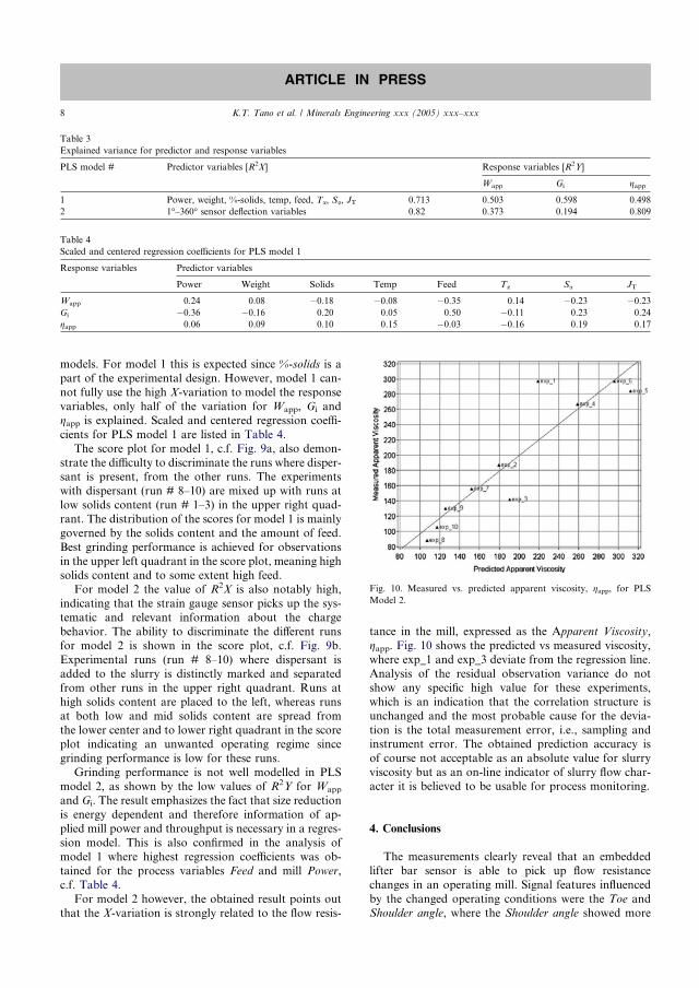
models. For model 1 this is expected since %-solids is a
part of the experimental design. However, model 1 can-
not fully use the high X-variation to model the response
variables, only half of the variation for Wapp, Gi and
gapp is explained. Scaled and centered regression coeffi-
cients for PLS model 1 are listed in Table 4.
The score plot for model 1, c.f. Fig. 9a, also demon-
strate the difficulty to discriminate the runs where disper-sant is present, from the other runs. The experiments
with dispersant (run # 8–10) are mixed up with runs at
low solids content (run # 1–3) in the upper right quad-
rant. The distribution of the scores for model 1 is mainly
governed by the solids content and the amount of feed.
Best grinding performance is achieved for observations
in the upper left quadrant in the score plot, meaning high
solids content and to some extent high feed.For model 2 the value of R2X is also notably high,
indicating that the strain gauge sensor picks up the sys-
tematic and relevant information about the charge
behavior. The ability to discriminate the different runs
for model 2 is shown in the score plot, c.f. Fig. 9b.
Experimental runs (run # 8–10) where dispersant is
added to the slurry is distinctly marked and separated
from other runs in the upper right quadrant. Runs athigh solids content are placed to the left, whereas runs
at both low and mid solids content are spread from
the lower center and to lower right quadrant in the score
plot indicating an unwanted operating regime since
grinding performance is low for these runs.
Grinding performance is not well modelled in PLS
model 2, as shown by the low values of R2Y for Wapp
and Gi. The result emphasizes the fact that size reductionis energy dependent and therefore information of ap-
plied mill power and throughput is necessary in a regres-
sion model. This is also confirmed in the analysis of
model 1 where highest regression coefficients was ob-
tained for the process variables Feed and mill Power,
c.f. Table 4.
For model 2 however, the obtained result points out
that the X-variation is strongly related to the flow resis-
tance in the mill, expressed as the Apparent Viscosity,
gapp. Fig. 10 shows the predicted vs measured viscosity,
where exp_1 and exp_3 deviate from the regression line.
Analysis of the residual observation variance do not
show any specific high value for these experiments,
which is an indication that the correlation structure is
unchanged and the most probable cause for the devia-
tion is the total measurement error, i.e., sampling andinstrument error. The obtained prediction accuracy is
of course not acceptable as an absolute value for slurry
viscosity but as an on-line indicator of slurry flow char-
acter it is believed to be usable for process monitoring.
4. Conclusions
The measurements clearly reveal that an embedded
lifter bar sensor is able to pick up flow resistance
changes in an operating mill. Signal features influenced
by the changed operating conditions were the Toe and
Shoulder angle, where the Shoulder angle showed more
Table 4
Scaled and centered regression coefficients for PLS model 1
Response variables Predictor variables
Power Weight Solids Temp Feed Ta Sa JT
Wapp 0.24 0.08 �0.18 �0.08 �0.35 0.14 �0.23 �0.23
Gi �0.36 �0.16 0.20 0.05 0.50 �0.11 0.23 0.24
gapp 0.06 0.09 0.10 0.15 �0.03 �0.16 0.19 0.17
Fig. 10. Measured vs. predicted apparent viscosity, gapp, for PLS
Model 2.
Table 3
Explained variance for predictor and response variables
PLS model # Predictor variables [R2X] Response variables [R2Y]
Wapp Gi gapp
1 Power, weight, %-solids, temp, feed, Ta, Sa, JT 0.713 0.503 0.598 0.498
2 1�–360� sensor deflection variables 0.82 0.373 0.194 0.809
8 K.T. Tano et al. / Minerals Engineering xxx (2005) xxx–xxx
ARTICLE IN PRESS
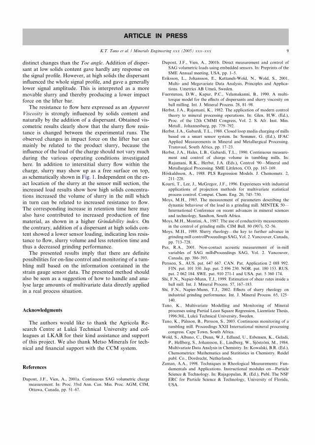
distinct changes than the Toe angle. Addition of disper-
sant at low solids content gave hardly any response on
the signal profile. However, at high solids the dispersant
influenced the whole signal profile, and gave a generally
lower signal amplitude. This is interpreted as a more
movable slurry and thereby producing a lower impactforce on the lifter bar.
The resistance to flow here expressed as an Apparent
Viscosity is strongly influenced by solids content and
naturally by the addition of a dispersant. Obtained vis-
cometric results clearly show that the slurry flow resis-
tance is changed between the experimental runs. The
observed changes in impact force on the lifter bar can
mainly be related to the product slurry, because theinfluence of the load of the charge should not vary much
during the various operating conditions investigated
here. In addition to interstitial slurry flow within the
charge, slurry may show up as a free surface on top,
as schematically shown in Fig. 1. Independent on the ex-
act location of the slurry at the sensor mill section, the
increased load results show how high solids concentra-
tions increased the volume of slurry in the mill whichin turn can be related to increased resistance to flow.
The corresponding increase in retention time here may
also have contributed to increased production of fine
material, as shown in a higher Grindability index. On
the contrary, addition of a dispersant at high solids con-
tent showed a lower sensor loading, indicating less resis-
tance to flow, slurry volume and less retention time and
thus a decreased grinding performance.The presented results imply that there are definite
possibilities for on-line control and monitoring of a tum-
bling mill based on the information contained in the
strain gauge sensor data. The presented method should
also be seen as a suggestion of how to handle and ana-
lyse large amounts of multivariate data directly applied
in a real process situation.
Acknowledgments
The authors would like to thank the Agricola Re-
search Centre at Lulea Technical University and col-
leagues at LKAB for their kind assistance and support
of this project. We also thank Metso Minerals for tech-
nical and financial support with the CCM system.
References
Dupont, J.F., Vien, A., 2001a. Continuous SAG volumetric charge
measurement. In: Proc. 33rd Ann. Can. Min. Proc. AGM, CIM,
Ottawa, Canada, pp. 51–67.
Dupont, J.F., Vien, A., 2001b. Direct measurement and control of
SAG volumetric loads using embedded sensors. In: Preprints of the
SME Annual meeting, USA, pp. 1–5.
Eriksson, L., Johansson, E., Kettaneh-Wold, N., Wold, S., 2001.
Multi- and Megavariate Data Analysis, Principles and Applica-
tions. Umetrics AB Umea, Sweden.
Fuerstenau, D.W., Kapur, P.C., Velamakanni, B., 1990. A multi-
torque model for the effects of dispersants and slurry viscosity on
ball milling. Int. J. Mineral Process. 28, 81–98.
Herbst, J.A., Rajamani, K., 1982. The application of modern control
theory to mineral processing operations. In: Glen, H.W. (Ed.),
Proc. of the 12th CMMI Congress, Vol. 2. S. Afr. Inst. Min.
Metall., Johannesburg, pp. 779–792.
Herbst, J.A., Gabardi, T.L., 1988. Closed loop media charging of mills
based on a smart sensor system. In: Sommer, G. (Ed.), IFAC
Applied Measurements in Mineral and Metallurgical Processing.
Transvaal, South Africa, pp. 17–23.
Herbst, J.A., Hales, L.B., Gabardi, T.L., 1990. Continuous measure-
ment and control of charge volume in tumbling mills. In:
Rajamani, R.K., Herbst, J.A. (Eds.), Control �90—Mineral and
Metallurgical Processing. SME Littleton, CO, pp. 163–169.
Hoskuldsson, A., 1988. PLS Regression Models. J. Chemometr. 2,
211–228.
Kourti, T., Lee, J., McGregor, J.F., 1996. Experiences with industrial
applications of projection methods for multivariate statistical
process control. Comput. Chem. Eng. 20, 745–750.
Moys, M.H., 1985. The measurement of parameters describing the
dynamic behaviour of the load in a grinding mill. MINTEK 50—
International Conference on recent advances in mineral sciences
and technology, Sandton, South Africa.
Moys, M.H., Montini, A., 1987. The use of conductivity measurements
in the control of grinding mills. CIM Bull. 80 (907), 52–56.
Moys, M.H., 1989. Slurry rheology—the key to further advance in
grinding mill controlProceedings SAG, Vol. 2. Vancouver, Canada,
pp. 713–728.
Pax, R.A., 2001. Non-contact acoustic measurement of in-mill
variables of SAG millsProceedings SAG, Vol. 2. Vancouver,
Canada, pp. 386–393.
Persson, S., AUS. pat. 647 667. CAN. Pat. Application 2 088 992.
FIN. pat. 101 350. Jap. pat. 2 896 230. NOR. pat. 180 153. RUS.
pat. 2 062 184. SWE. pat. 910 271-1 and USA. pat. 5 360 174.
Shi, F.N., Napier-Munn, T.J., 1999. Estimation of shear rates inside a
ball mill. Int. J. Mineral Process. 57, 167–183.
Shi, F.N., Napier-Munn, T.J., 2002. Effects of slurry rheology on
industrial grinding performance. Int. J. Mineral Process. 65, 125–
140.
Tano, K., Multivariate Modelling and Monitoring of Mineral
processes using Partial Least Square Regression, Licentiate Thesis,
1996:36L, Lulea Technical University, Sweden.
Tano, K., Palsson, B., Persson, S., 2003. Continuous monitoring of a
tumbling mill. Proceedings XXII International mineral processing
congress. Cape Town, South Africa.
Wold, S., Albano, C., Dunn, W.J., Edlund, U., Esbensen, K., Geladi,
P., Hellberg, S., Johansson, E., Lindberg, W., Sjostrom, M., 1984.
Multivariate Data Analysis in Chemistry. In: Kowalski, B.R. (Ed.),
Chemometrics: Mathematics and Statitistics in Chemistry. Reidel
publ. Co., Dordrecht, Netherlands.
Zaman, A.A., 1998. Techniques in Rheological Measurements: Fun-
damentals and Applications. Instructional modules on—Particle
Science & Technology. In: Rajagopalan, R. (Ed.), Publ. The NSF
ERC for Particle Science & Technology, University of Florida,
USA.
K.T. Tano et al. / Minerals Engineering xxx (2005) xxx–xxx 9
ARTICLE IN PRESS


K Tano, M Pierce and J Alatalo
Submitted to International Journal of Mineral Processing

1
* Corresponding author. Fax: +4697030617: [email protected]
Computational demands and the lack of detailed experimental verification have limited the value of DistinctElement Method (DEM) modelling approaches in mill simulation studies. This paper presents the results of astudy in which the deflection of a lifter bar in a pilot ball mill was measured by an embedded strain gaugesensor and compared to deflections predicted from DEM simulations.An assembly of bonded particles represents a flexible rubber lifter in the DEM model. The deflection istracked by monitoring the displacement of particles near the actual strain gauge base and tip.The deflection profile obtained from the DEM simulation shows a reasonably good correspondence to thepilot mill measurements. The difference is attributed to the fact that time-dependent behaviour of the rubberlifter is ignored, resulting in rapid relaxation of the lifter when the exerted force is released. Mill chargefeatures such as toe and shoulder position of the charge are well marked. However, DEM prediction showslower values compared to measurements which is most likely an effect of the two dimensional (2D) modelused and the inability to model the effect of slurry present in the mill.The approach presented here is a contribution to the validation of DEM simulations and an introduction tothe description of a bendable rubber lifter implemented in a DEM mill model.
Keywords: Strain gauge sensor, Distinct element modelling, Simulation, Grinding
Distinct element methods (DEM) may be used as simulation tools to gain insight into particulate flowprocesses. When applied to grinding it affords us an opportunity to study many aspects of grinding in greaterdetail than has been possible to date. DEM can be used to describe and visualise the motion of the grindingcharge and how it is influenced by both design and operating conditions. Furthermore DEM predictionsprovides useful information on collision forces, energy loss spectra and power consumption. Computersimulations can in many cases replace long-term and complicated field experiments (Dennis and Rajamani,2001).
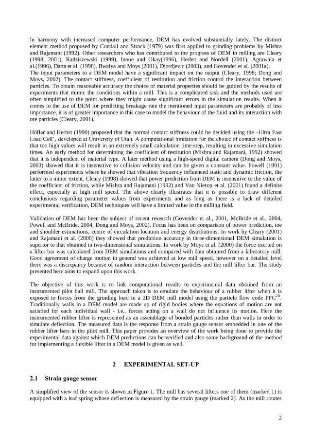
2
In harmony with increased computer performance, DEM has evolved substantially lately. The distinctelement method proposed by Cundall and Strack (1979) was first applied to grinding problems by Mishraand Rajamani (1992). Other researchers who has contributed to the progress of DEM in milling are Cleary(1998, 2001), Radziszewski (1999), Inoue and Okay(1996), Herbst and Nordell (2001), Agrawala etal.(1996), Datta et al. (1998), Bwalya and Moys (2001), Djordjevic (2003), and Govender et al. (2001a).The input parameters to a DEM model have a significant impact on the output (Cleary, 1998; Dong andMoys, 2002). The contact stiffness, coefficient of restitution and friction control the interaction betweenparticles. To obtain reasonable accuracy the choice of material properties should be guided by the results ofexperiments that mimic the conditions within a mill. This is a complicated task and the methods used areoften simplified to the point where they might cause significant errors in the simulation results. When itcomes to the use of DEM for predicting breakage rate the mentioned input parameters are probably of lessimportance, it is of greater importance in this case to model the behaviour of the fluid and its interaction withore particles (Cleary, 2001).
H Herbst (1990) proposed that the normal contact stiffness could be decided using theLoad Cellthat too high values will result in an extremely small calculation time-step, resulting in excessive simulationtimes. An early method for determining the coefficient of restitution (Mishra and Rajamani, 1992) showedthat it is independent of material type. A later method using a high-speed digital camera (Dong and Moys,2003) showed that it is insensitive to collision velocity and can be given a constant value. Powell (1991)performed experiments where he showed that vibration frequency influenced static and dynamic friction, thelatter to a minor extent. Cleary (1998) showed that power prediction from DEM is insensitive to the value ofthe coefficient of friction, while Mishra and Rajamani (1992) and Van Nierop et al. (2001) found a definiteeffect, especially at high mill speed. The above clearly illustrates that it is possible to draw differentconclusions regarding parameter values from experiments and as long as there is a lack of detailedexperimental verification, DEM techniques will have a limited value in the milling field.
Validation of DEM has been the subject of recent research (Govender et al., 2001, McBride et al., 2004,Powell and McBride, 2004, Dong and Moys, 2002). Focus has been on comparison of power prediction, toeand shoulder estimations, centre of circulation location and energy distributions. In work by Cleary (2001)and Rajamani et al. (2000) they showed that prediction accuracy in three-dimensional DEM simulation issuperior to that obtained in two-dimensional simulations. In work by Moys et al. (2000) the force exerted ona lifter bar was calculated from DEM simulations and compared with data obtained from a laboratory mill.Good agreement of charge motion in general was achieved at low mill speed, however on a detailed levelthere was a discrepancy because of random interaction between particles and the mill lifter bar. The studypresented here aims to expand upon this work.
The objective of this work is to link computational results to experimental data obtained from aninstrumented pilot ball mill. The approach taken is to emulate the behaviour of a rubber lifter when it isexposed to forces from the grinding load in a 2D DEM mill model using the particle flow code PFC2D.Traditionally walls in a DEM model are made up of rigid bodies where the equations of motion are notsatisfied for each individual wall - i.e., forces acting on a wall do not influence its motion. Here theinstrumented rubber lifter is represented as an assemblage of bonded particles rather than walls in order tosimulate deflection. The measured data is the response from a strain gauge sensor embedded in one of therubber lifter bars in the pilot mill. This paper provides an overview of the work being done to provide theexperimental data against which DEM predictions can be verified and also some background of the methodfor implementing a flexible lifter in a DEM model is given as well.
A simplified view of the sensor is shown in Figure 1. The mill has several lifters one of them (marked 1) isequipped with a leaf spring whose deflection is measured by the strain gauge (marked 2). As the mill rotates
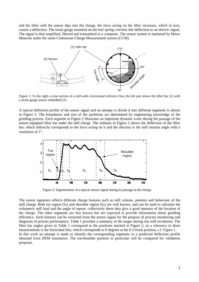
3
and the lifter with the sensor dips into the charge, the force acting on the lifter increases, which in turn,causes a deflection. The strain gauge mounted on the leaf spring converts this deflection to an electric signal.The signal is then amplified, filtered and transmitted to a computer. The sensor system is marketed by MetsoMinerals under the name Continuous Charge Measurement system (CCM).
Toeangle
90
180
270
0
(1) Lifter bar
(2) Sensor
Shoulder
angle
Toe
PulpCharge
Shoulder
Figure 1: To the right a cross section of a mill with a horizontal reference line, the left part shows the lifter bar (1) witha strain gauge sensor embedded (2).
A typical deflection profile of the sensor signal and an attempt to divide it into different segments is shownin Figure 2. The boundaries and size of the partitions are determined by engineering knowledge of thegrinding process. Each segment in Figure 2 illustrates an important dynamic event during the passage of thesensor-equipped lifter bar under the mill charge. The ordinate in Figure 2 shows the deflection of the lifterbar, which indirectly corresponds to the force acting on it and the abscissa is the mill rotation angle with aresolution of 1 .
Shoulderregion
Toeregion
1
2
3
4
S1 S2 S3 S4 S5 S6 S7
Figure 2: Segmentation of a typical sensor signal during its passage in the charge.
The sensor signature reflects different charge features such as mill volume, position and behaviour of themill charge. Both toe region (S2) and shoulder region (S6) are well known, and can be used to calculate thevolumetric mill load and the angle of repose, collectively these data give a good measure of the location ofthe charge. The other segments are less known but are expected to provide information about grindingefficiency. Such features can be extracted from the sensor signal for the purpose of process monitoring anddiagnosis of process performance. Table 1 provides a summary of the stages during one mill revolution. Thelifter bar angles given in Table 1 correspond to the positions marked in Figure 2, as a reference in thesemeasurements is the horizontal line, which corresponds to 0 degrees at the 9 oIn this work an attempt is made to identify the corresponding segments in a predicted deflection profileobtained from DEM simulation. The toe/shoulder position in particular will be compared for validationpurposes.
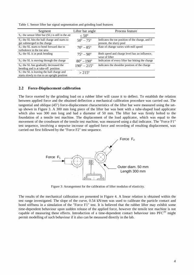
4
Table 1. Sensor lifter bar signal segmentation and grinding load features
Segment Lifter bar angle Process featureS1: the sensor lifter bar (SL) is still in the air 50S2: the SL hits the ball charge and starts toget submerged in the charge
7550 Indicates the toe position of the charge, and ifpresent, the slurry pool
S3: the SL starts to bend forward due toturbulence in the toe area
8570 Rate of change varies with mill speed
S4: the SL is at peak bending 9075 Both speed and charge level has an influence,wear of lifter
S5: the SL is moving through the charge 19080 Indication of every lifter bar hitting the charge
S6: the SL has gradually decreased thebending and is at take-off position
215190 Indicates the shoulder position of the charge
S7: the SL is leaving the ball charge andstarts slowly to rise to an upright position
215
The force exerted by the grinding load on a rubber lifter will cause it to deflect. To establish the relationbetween applied force and the obtained deflection a mechanical calibration procedure was carried out. Thetangential and oblique (45 ) force-displacement characteristics of the lifter bar were measured using the set-up shown in Figure 3. A 300 mm long piece of the lifter bar was bent with a tube-shaped load applicatorwhich also was 300 mm long and had a diameter of 50 mm. The lifter bar was firmly bolted to thefoundation of a tensile test machine. The displacement of the load applicator, which was equal to themovement of the crossbeam of the tensile test machine, was measured using a dial indicator. The "Force F1"test sequence, involving a stepwise increase of applied force and recording of resulting displacement, wascarried out first followed by the "Force F2" test sequence.
Force F2
Force F1
Outer diam. 50 mmLength 300 mm
Figure 3: Arrangement for the calibration of lifter modulus of elasticity.
The results of the mechanical calibration are presented in Figure 4. A linear relation is obtained within thetest range investigated. The slope of the curve, 0.54 kN/mm was used to calibrate the particle contact andbond stiffness in a simulation of the "Force F1" test. It is believed that the rubber lifter may exhibit sometime-dependent behaviour upon sudden release of the applied force, however the tensile test machine is notcapable of measuring these effects. Introduction of a time-dependent contact behaviour into PFC2D mightpermit modelling of such behaviour if it also can be measured directly in the lab.
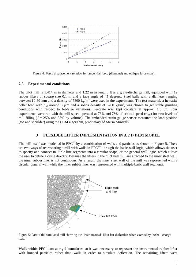
5
0
1000
2000
3000
4000
5000
0 1 2 3 4 5 6
F1(N)
F2(N)
Figure 4: Force displacement relation for tangential force (diamond) and oblique force (star).
The pilot mill is 1.414 m in diameter and 1.22 m in length. It is a grate-discharge mill, equipped with 12rubber lifters of square size 0.1 m and a face angle of 45 degrees. Steel balls with a diameter rangingbetween 10-30 mm and a density of 7800 kg/m3 were used in the experiments. The test material, a hematitepellet feed with d50 around 35 m and a solids density of 5200 kg/m3, was chosen to get stable grindingconditions with respect to feedsize variations. Feedrate was kept constant at approx. 1.5 t/h. Fourexperiments were run with the mill speed operated at 73% and 78% of critical speed ( crit) for two levels ofmill filling ( = 25% and 35% by volume). The embedded strain gauge sensor measures the load position(toe and shoulder) using the CCM algorithm, proprietary of Metso Minerals.
The mill itself was modelled in PFC2D by a combination of walls and particles as shown in Figure 5. Thereare two ways of representing a mill with walls in PFC2D: through the basic wall logic, which allows the userto specify and connect multiple line segments into a circular shape, or the general wall logic, which allowsthe user to define a circle directly. Because the lifters in the pilot ball mill are attached to the inner steel wall,the inner rubber liner is not continuous. As a result, the inner steel wall of the mill was represented with acircular general wall while the inner rubber liner was represented with multiple basic wall segments.
Flexible lifter
Rigid walland lifter
Figure 5: Part of the simulated mill showing theload.
Walls within PFC2D act as rigid boundaries so it was necessary to represent the instrumented rubber lifterwith bonded particles rather than walls in order to simulate deflection. The remaining lifters were
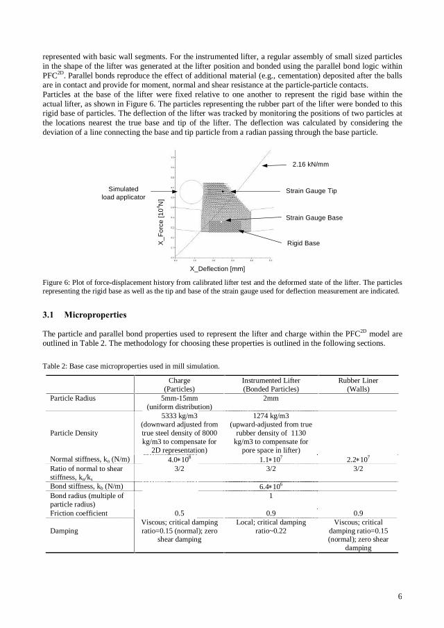
6
represented with basic wall segments. For the instrumented lifter, a regular assembly of small sized particlesin the shape of the lifter was generated at the lifter position and bonded using the parallel bond logic withinPFC2D. Parallel bonds reproduce the effect of additional material (e.g., cementation) deposited after the ballsare in contact and provide for moment, normal and shear resistance at the particle-particle contacts.Particles at the base of the lifter were fixed relative to one another to represent the rigid base within theactual lifter, as shown in Figure 6. The particles representing the rubber part of the lifter were bonded to thisrigid base of particles. The deflection of the lifter was tracked by monitoring the positions of two particles atthe locations nearest the true base and tip of the lifter. The deflection was calculated by considering thedeviation of a line connecting the base and tip particle from a radian passing through the base particle.
X_Deflection [mm]
X_F
orce
[104 N
]
Simulatedload applicator
Strain Gauge Tip
Strain Gauge Base
Rigid Base
2.16 kN/mm
Figure 6: Plot of force-displacement history from calibrated lifter test and the deformed state of the lifter. The particlesrepresenting the rigid base as well as the tip and base of the strain gauge used for deflection measurement are indicated.
The particle and parallel bond properties used to represent the lifter and charge within the PFC2D model areoutlined in Table 2. The methodology for choosing these properties is outlined in the following sections.
Table 2: Base case microproperties used in mill simulation.
Charge(Particles)
Instrumented Lifter(Bonded Particles)
Rubber Liner(Walls)
Particle Radius 5mm-15mm(uniform distribution)
2mm
Particle Density
5333 kg/m3(downward adjusted fromtrue steel density of 8000kg/m3 to compensate for
2D representation)
1274 kg/m3(upward-adjusted from true
rubber density of 1130kg/m3 to compensate for
pore space in lifter)Normal stiffness, kn (N/m) 4.0 108 1.1 107 2.2 107
Ratio of normal to shearstiffness, kn/ks
3/2 3/2 3/2
Bond stiffness, kb (N/m) 6.4 106
Bond radius (multiple ofparticle radius)
1
Friction coefficient 0.5 0.9 0.9
DampingViscous; critical dampingratio=0.15 (normal); zero
shear damping
Local; critical dampingratio~0.22
Viscous; criticaldamping ratio=0.15(normal); zero shear
damping

7
The mass and inertial properties of the particles representing the charge and lifter are automaticallycalculated in PFC2D as a function of a user specified global disk thickness, t. In this case, the disk thicknesswas set equal to the length of the pilot mill, 1.2 meters. This results in correct mass and inertial properties forthe instrumented lifter when the density of the rubber particles is increased to account for the pore spacepresent in the bonded assembly. Because of the two-dimensional representation, the particles in the PFC2D
mill represent rods rather than spheres. In order to mimic the mass and inertia of a string of charge ballsrather than a solid rod, the density of the particles representing the charge was lowered accordingly. Theconsequence of this two-dimensional representation is that any single particle impacting the lifter within thetwo-dimensional model is actually simulating the simultaneous impact of a string of charge balls running thefull length of the mill. Such simultaneous impact is not likely happening in reality and so this should beconsidered when interpreting deflection results from the 2D model.
Normal and shear stiffness values are assigned to particles rather than contacts within PFC2D so that contactbehaviour may be derived from the properties of the particular particles comprising it. Two different stiffnessmodels are available in PFC2D: a linear model and a simplified Hertz-Mindlin model. In the linear model, theforces and relative displacements are linearly related by the constant contact stiffness, which is a function ofthe intrinsic stiffness of the two contacting entities. In the simplified Hertz-Mindlin model, the forces andrelative displacements are nonlinearly related by the non-constant contact stiffness, which is a function of thegeometric and material properties of the two contacting entities as well as the current value of the normalforce. Work by Cleary (2001) suggests that the linear contact model is appropriate over the range of normalforces typically experienced within a mill and so this model was adopted for the current simulations. Inaddition, the ratio of normal to shear stiffness was set to 3/2 as proposed by Rajamani et al. (2000).
The particle stiffness assigned to the charge particles is outlined in Table 2. For the linear contact model, theresulting contact stiffness, , between two charge particles can be computed assuming that the stiffness ofthe two contacting particles, and , act in series such that
(1)
The stiffness of the bonds comprising the lifter (input directly by the user) and the contact stiffness (derivedfrom Eqn.1) act in parallel to control the deformability of the lifter. The results of deflection tests performedon the instrumented lifter in the laboratory were used to calibrate both the particle and bond stiffness bysimulating the test in PFC2D and comparing the predicted response to the force-displacement histories shownin Figure 4. The actual test was performed over a 300mm section of lifter. Since the simulated test wouldrepresent deflection of a 1.2-meter long section, the target lifter stiffness for the simulated test was set to fourtimes the actual measured stiffness of 0.54 kN/mm. It is possible that there is a non-linear relation betweenlifter stiffness and test length, in which case this assumption may not be valid. The nature of this relationshould be examined in future experiments to test the validity of this assumption when representing the mill intwo dimensions. The calibrated force displacement relation obtained from the simulated tangential force testis plotted in Figure 6 along with the deformed state of the lifter at a displacement of ~ 4mm. The particle andbond stiffness obtained from the calibration is outlined in Table 2.
The stiffness of the rubber walls within the simulation (representing the remaining lifters and the rubberliner) were set to achieve the same contact stiffness as the bonded contacts within the particle-based lifter.This is calculated as the sum of the parallel bond stiffness and the contact stiffness provided by Eqn.1 (sincethe two stiffnesses act in parallel). Substituting the stiffness of the parallel bonded contact back into Eqn.1,one can obtain the desired wall stiffness.
The friction coefficients of the steel and rubber were set to 0.5 and 0.9, respectively based on valuespublished by Rajamani et al. (2000).
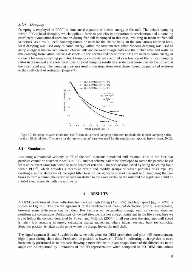
8
Damping is employed in PFC2D to simulate dissipation of kinetic energy in the mill. The default dampingwithin PFC is local damping, which applies a force to particles in proportion to acceleration and a dampingcoefficient. Gravitational acceleration during free fall is damped in this case, resulting in incorrect free-fallvelocities. As a result, local damping cannot be used for the charge balls. In the simulations reported here,local damping was used only to damp energy within the instrumented lifter. Viscous damping was used todamp energy at the contact between charge balls and between charge balls and the rubber lifter and walls. Inthis damping formulation, viscous dashpots (in the normal and shear directions) are used to damp energy atcontacts between impacting particles. Damping constants are specified as a fraction of the critical dampingratios in the normal and shear directions. Critical damping results in a system response that decays to zero atthe most rapid rate. The damping constants used in the simulation were chosen based on published relationsto the coefficient of restitution (Figure 7).
Figure 7: Relation between restitution coefficient and critical damping ratio used to obtain the critical damping ratiosfor the mill simulation. The curve for the
Assigning a rotational velocity to all of the wall elements simulated mill rotation. Due to the fact thatparticles cannot be attached to walls in PFC, another scheme had to be developed to rotate the particle-basedlifter at the exact same rate with the same centre of rotation. This was accomplished by using the clump logicwithin PFC2D, which provides a means to create and modify groups of slaved particles or clumps. Bycreating a mirror duplicate of the rigid lifter base on the opposite side of the mill and combining the twobases to form a clump, the centre of rotation shifted to the exact centre of the mill and the rigid base could berotated synchronously with the mill walls.
A DEM prediction of lifter deflection for the case high filling ( = 35%) and high speed ( crit = 78%) isshown in Figure 8. The overall agreement of the predicted and measured deflection profile is acceptable,however some differences can be noted. Key features of the grinding charge, such as toe and shoulderpositions are comparable. Definitions of toe and shoulder are not always consistent in the literature; here wetry to follow the concept described by Powell and McBride (2004). In all run cases the simulated mill speedis fairly low resulting in purely cascading charge movement where impact toe and bulk toe coincide.Shoulder position is taken as the point where the charge leaves the mill shell.
The signal segment S2 and S3 exhibits the same behaviour for DEM prediction and pilot mill measurement,high impact during short time. Predicted toe position is lower, c.f. Table 3, indicating a charge that is morehorizontally positioned or in this case showing a more distinct bi-plane shape. Some of the differences in toeangle can be explained by limitations of the 2D representation when compared to 3D DEM simulations
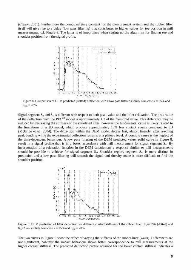
9
(Cleary, 2001). Furthermore the combined time constant for the measurement system and the rubber lifteritself will give rise to a delay (low pass filtering) that contributes to higher values for toe position in millmeasurements, c.f. Figure 8. The latter is of importance when setting up the algorithm for finding toe andshoulder position from the signal profile.
Figure 8: Comparison of DEM predicted (dotted) deflection with a low pass filtered (solid). Run case = 35% andcrit = 78%.
Signal segment S4 and S5 is different with respect to both peak value and the lifter relaxation. The peak valueof the deflection from the PFC2D model is approximately 1 3 of the measured value. This difference may bereduced by decreasing the stiffness of the simulated lifter, however the fundamental cause is likely related tothe limitations of a 2D model, which produce approximately 15% less contact events compared to 3D(McBride et al., 2004). The deflection within the DEM model decays fast, almost linearly, after reachingpeak bending while the experimental deflection remains at a plateau level. A possible cause is the neglect ofthe time-dependent behaviour. A low pass filtering of the DEM predicted value, solid curve in Figure 8,result in a signal profile that is in a better accordance with mill measurement for signal segment S4. Byincorporation of a relaxation function in the DEM calculations a response similar to mill measurementsshould be possible to achieve for signal segment S5. Shoulder region, segment S6, is more distinct inprediction and a low pass filtering will smooth the signal and thereby make it more difficult to find theshoulder position.
Figure 9: DEM prediction of lifter deflection for different contact stiffness of the rubber liner, Kn=2.2e6 (dotted) andKn=2.2e7 (solid). Run case = 25% and crit = 78%.
The two curves in Figure 9 show the effect of varying the stiffness of the rubber liner (walls). Differences arenot significant, however the impact behaviour shows better correspondence to mill measurements at thehigher contact stiffness. The predicted deflection profile obtained for the lower contact stiffness indicates a
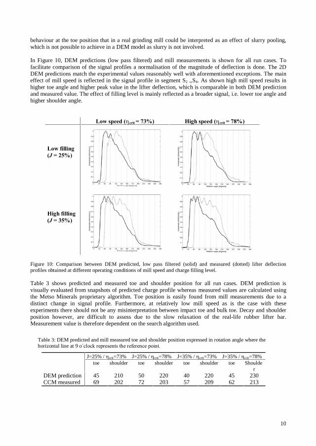
10
behaviour at the toe position that in a real grinding mill could be interpreted as an effect of slurry pooling,which is not possible to achieve in a DEM model as slurry is not involved.
In Figure 10, DEM predictions (low pass filtered) and mill measurements is shown for all run cases. Tofacilitate comparison of the signal profiles a normalisation of the magnitude of deflection is done. The 2DDEM predictions match the experimental values reasonably well with aforementioned exceptions. The maineffect of mill speed is reflected in the signal profile in segment S2 4. As shown high mill speed results inhigher toe angle and higher peak value in the lifter deflection, which is comparable in both DEM predictionand measured value. The effect of filling level is mainly reflected as a broader signal, i.e. lower toe angle andhigher shoulder angle.
Figure 10: Comparison between DEM predicted, low pass filtered (solid) and measured (dotted) lifter deflectionprofiles obtained at different operating conditions of mill speed and charge filling level.
Table 3 shows predicted and measured toe and shoulder position for all run cases. DEM prediction isvisually evaluated from snapshots of predicted charge profile whereas measured values are calculated usingthe Metso Minerals proprietary algorithm. Toe position is easily found from mill measurements due to adistinct change in signal profile. Furthermore, at relatively low mill speed as is the case with theseexperiments there should not be any misinterpretation between impact toe and bulk toe. Decay and shoulderposition however, are difficult to assess due to the slow relaxation of the real-life rubber lifter bar.Measurement value is therefore dependent on the search algorithm used.
Table 3: DEM predicted and mill measured toe and shoulder position expressed in rotation angle where thehorizontal line at 9 o
J=25% / crit=73% J=25% / crit=78% J=35% / crit=73% J=35% / crit=78%toe shoulder toe shoulder toe shoulder toe Shoulde
rDEM prediction 45 210 50 220 40 220 45 230CCM measured 69 202 72 203 57 209 62 213
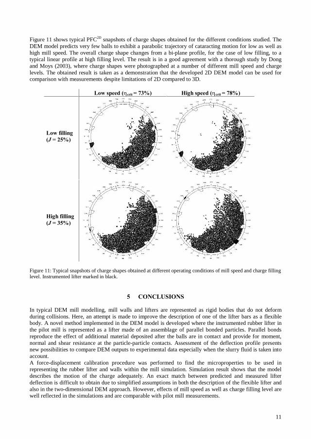
11
Figure 11 shows typical PFC2D snapshots of charge shapes obtained for the different conditions studied. TheDEM model predicts very few balls to exhibit a parabolic trajectory of cataracting motion for low as well ashigh mill speed. The overall charge shape changes from a bi-plane profile, for the case of low filling, to atypical linear profile at high filling level. The result is in a good agreement with a thorough study by Dongand Moys (2003), where charge shapes were photographed at a number of different mill speed and chargelevels. The obtained result is taken as a demonstration that the developed 2D DEM model can be used forcomparison with measurements despite limitations of 2D compared to 3D.
Figure 11: Typical snapshots of charge shapes obtained at different operating conditions of mill speed and charge fillinglevel. Instrumented lifter marked in black.
In typical DEM mill modelling, mill walls and lifters are represented as rigid bodies that do not deformduring collisions. Here, an attempt is made to improve the description of one of the lifter bars as a flexiblebody. A novel method implemented in the DEM model is developed where the instrumented rubber lifter inthe pilot mill is represented as a lifter made of an assemblage of parallel bonded particles. Parallel bondsreproduce the effect of additional material deposited after the balls are in contact and provide for moment,normal and shear resistance at the particle-particle contacts. Assessment of the deflection profile presentsnew possibilities to compare DEM outputs to experimental data especially when the slurry fluid is taken intoaccount.A force-displacement calibration procedure was performed to find the microproperties to be used inrepresenting the rubber lifter and walls within the mill simulation. Simulation result shows that the modeldescribes the motion of the charge adequately. An exact match between predicted and measured lifterdeflection is difficult to obtain due to simplified assumptions in both the description of the flexible lifter andalso in the two-dimensional DEM approach. However, effects of mill speed as well as charge filling level arewell reflected in the simulations and are comparable with pilot mill measurements.
12
The implemented novel method is an introductory approach and comparisons between real and predicteddeflections are on a qualitative basis. The outcome of this work shows a potential to be of use in lifter profiledesign where flexible material is present. As a consequence the effect on grinding performance can beassessed in a consistent and meaningful manner due to the direct relation to experimental data, obtained bythe strain gauge sensor.To reach better accuracy in predictions and enable quantitative comparison some necessary improvementshave been identified and will be investigated in future work. This includes investigation of lifter relaxation inthe laboratory, simulation of time-dependent behaviour in the lifter and an extension of the approach to 3D
The authors would like to thank the Agricola Research Centre for their assistance and financial support ofthis project. We also thank Dr Sture Persson, Metso Minerals, for technical and financial support with theCCM sensor system and help with the calibration of the strain gauge sensor. Dr Bertil Pa critical reading and helpful discussions.
Agrawala S., Rajamani R.K., Songfack P., Mishra B.K., 1996. Mechanics of media motion in tumbling millswith 3D discrete element methods, Minerals Engineering. Vol.10, No.2, pp 215-227.Bwalya M.M., Moys M. H., 2001. The use of DEM in modelling and scaling-up of (S)AG mills. In: Barratt,D.J., Allan, M.J., Mular A.L. (Eds.), Proceedings SAG 2001, Vol. 4, pp 180-190.Cleary P.W., 1998. Predicting charge motion, power draw, segregation and wear in ball mills using discreteelement methods. Minerals Engineering. Vol.11, No.11, pp 1061-1080.Cleary P.W., 2001. Recent advances in DEM modelling of tumbling mills. Minerals Engineering. Vol.14,No.10, pp 1295-1319.Cundall P.A., Strack O.D.L., 1979. A discrete numerical model for granular assemblies. Geotechnique. No.1, pp 47-65.Datta A., Mishra B.K., Rajamani R.K., 1998. Analysis of power draw in ball mills by the discrete elementmethod. Canadian Institute of Mining and Metallurgy. Vol.38, pp 133-140.Dennis M., Rajamani R., 2001. Evolution of the perfect mill simulator. In: Barratt, D.J., Allan, M.J., MularA.L. (Eds.), Proceedings SAG 2001, Vol. 4, pp 24-33.Djordjevic N., 2003. Discrete element modelling of the influence of lifters on power draw of tumbling mills,Minerals Engineering. Vol.16, pp 331-336.Dong H., Moys M.H., 2002. Assessment of discrete element method for one balls bouncing in a grindingmill. Int. J. Miner. Process. 65, pp 213-226.Dong H., Moys M.H., 2003. Load behaviour and mill power. Minerals Engineering. Vol. 69, pp 11-28.Govender I., Balden V., Powell M.S., Nurick G.N., 2001a. Validated DEMSAG mill modelling. In: Barratt, D.J., Allan, M.J., Mular A.L. (Eds.), Proceedings SAG 2001, Vol.4, pp101-114.Govender I., Powell M.S., Nurick G.N., 2001b. 3D particle tracking in a mill: A rigorous technique forverifying DEM predictions, Minerals Engineering. Vol.16, no.10, pp 1329-1340.Herbst J.A., Nordell L., 2001. Optimisation of the design of SAG Mill Internals Using High FidelitySimulation. In: Barratt, D.J., Allan, M.J., Mular A.L. (Eds.), Proceedings SAG 2001, Vol.4, pp 150-164.H Herbst J.A., 1990. Ball mill modeling through microscale fragmentation studies: Fully monitoredparticle bed comminution versus single particle impact tests. Preprint of the 7th European Symposium onComminution.Inoue I., Okaya K., 1996. Grinding mechanism of centrifugal millselement method. Int. J. Miner. Process. 44-45, pp 425-435.Itasca, 2000. PFC User Manual, Itasca Consulting Group Inc., Minneapolis, USAMcBride A., Govender I., Powell M., Cloete T., 2004. Contributions to the experimental validation of thediscrete element method applied to tumbling mills. Engineering Computations. Vol.21, No.2/3/4, pp 119-136.

13
Mishra B.K., Rajamani R.K., 1992. The discrete element method for the simulation of ball mills. Appl.Math. Modelling. vol.16, pp 598-604.Moys MH., 2000. Validation of the discrete element method (DEM) by comparing predicted load behaviourof a grinding mill with measured data. Proceedings of the XXI International Mineral Processing Congress,2000, C3-39.Powell M.S., 1991. The effect of liner design on the motion of the outer grinding elements in a rotary mill.Int. J. Miner. Process. Vol.31, pp 163-193.Powell M.S., McBride A.T., 2004. A three-dimensional analysis of media motion and grinding region inmills. Minerals Engineering. Vol.17, pp 1099-1109.Radziszewski P., 1999. Comparing three DEM charge motion models. Minerals Engineering. Vol.12, No.12, pp 1501-1520.Rajamani R.K., Mishra B.K., Venugopal R., Datta A., 2000. Discrete element analysis of tumbling mills.Powder Technology, Vol.109, pp 105-112.Van Nierop M.A., Glover G., Hinde A.L., Moys M.H., 2001. A discrete element method investigation of thecharge motion and power draw of an experimental two-dimensional mill. Int. J. Miner. Process. 61, pp 77-92.