Contests for Public Goods - Maastricht University
132
Contests for public goods Citation for published version (APA): Heine, F. A. (2017). Contests for public goods. Tilburg University. https://doi.org/10.26481/dis.20170419fh Document status and date: Published: 01/01/2017 DOI: 10.26481/dis.20170419fh Document Version: Publisher's PDF, also known as Version of record Please check the document version of this publication: • A submitted manuscript is the version of the article upon submission and before peer-review. There can be important differences between the submitted version and the official published version of record. People interested in the research are advised to contact the author for the final version of the publication, or visit the DOI to the publisher's website. • The final author version and the galley proof are versions of the publication after peer review. • The final published version features the final layout of the paper including the volume, issue and page numbers. Link to publication General rights Copyright and moral rights for the publications made accessible in the public portal are retained by the authors and/or other copyright owners and it is a condition of accessing publications that users recognise and abide by the legal requirements associated with these rights. • Users may download and print one copy of any publication from the public portal for the purpose of private study or research. • You may not further distribute the material or use it for any profit-making activity or commercial gain • You may freely distribute the URL identifying the publication in the public portal. If the publication is distributed under the terms of Article 25fa of the Dutch Copyright Act, indicated by the “Taverne” license above, please follow below link for the End User Agreement: www.umlib.nl/taverne-license Take down policy If you believe that this document breaches copyright please contact us at: [email protected] providing details and we will investigate your claim. Download date: 23 Jun. 2022
-
Upload
khangminh22 -
Category
Documents
-
view
4 -
download
0
Transcript of Contests for Public Goods - Maastricht University
Contests for public goods
Citation for published version (APA):
Heine, F. A. (2017). Contests for public goods. Tilburg University. https://doi.org/10.26481/dis.20170419fh
Document status and date:Published: 01/01/2017
DOI:10.26481/dis.20170419fh
Document Version:Publisher's PDF, also known as Version of record
Please check the document version of this publication:
• A submitted manuscript is the version of the article upon submission and before peer-review. There canbe important differences between the submitted version and the official published version of record.People interested in the research are advised to contact the author for the final version of the publication,or visit the DOI to the publisher's website.• The final author version and the galley proof are versions of the publication after peer review.• The final published version features the final layout of the paper including the volume, issue and pagenumbers.Link to publication
General rightsCopyright and moral rights for the publications made accessible in the public portal are retained by the authors and/or other copyrightowners and it is a condition of accessing publications that users recognise and abide by the legal requirements associated with theserights.
• Users may download and print one copy of any publication from the public portal for the purpose of private study or research.• You may not further distribute the material or use it for any profit-making activity or commercial gain• You may freely distribute the URL identifying the publication in the public portal.
If the publication is distributed under the terms of Article 25fa of the Dutch Copyright Act, indicated by the “Taverne” license above,please follow below link for the End User Agreement:
www.umlib.nl/taverne-license
Take down policyIf you believe that this document breaches copyright please contact us at:
providing details and we will investigate your claim.
Download date: 23 Jun. 2022

Contests for Public Goods

Contests for Public Goods© Florian Heine, Tilburg 2017
All rights reserved. No part of this publication may be reproduced, stored in a retrievalsystem, or transmitted, in any form, or by any means, electronic, mechanical, photocopying,recording or otherwise, without the prior permission in writing from the author.
This book was typeset by the author using LATEXVector images adapted from Vector Open Stock and Photoroyalty / FreepikCover Font uses “Linowrite” by Lennard GlitterCover design by Vera Bossel
Published by Tilburg UniversityISBN 978-94-6167-306-0Printed in the Netherlands by PrismaPrint
Contests for Public Goods
DISSERTATION
to obtain the degree of Doctor at Maastricht University,on the authority of Rector Magnificus,
Prof. Dr. Rianne M. Letschert,in accordance with the decision of the Board of Deans,
to be defended in public onWednesday 19 April 2017, at 14:00 hrs.
by
Florian Andreas Heine
Supervisor:
Prof. Dr. Arno Riedl
Co-Supervisor:
Dr. Martin Strobel
Assessment Committee:
Prof. Dr. Frank Moers (chairman)Prof. Dr. Christine Harbring (RWTH Aachen University)Dr. Andrzej Baranski MadrigalProf. Dr. Adriaan Soetevent (University of Groningen)

To Elisabeth

Acknowledgements
First and foremost I would like to thank my supervisors Arno Riedl and Martin Strobel,who have been the co-architects of this piece. Arno’s rigorous orientation towards deliveringexcellent research has shaped the way I want to approach science. Your comments havebeen critical and insightful. I got to know Martin already during the first semester of myMaster’s programme at Maastricht University School of Business and Economics (SBE).Your open and amiable character has always been a catalyst for new ideas.
I extend my appreciation towards the AE1 section of SBE. The Department’s generouscontribution to my professional education has been nothing short of vital. Without thesupport and guidance that I have enjoyed, I would not feel ready to embark upon the nextstep in my career. My experience at Maastricht University is one for which I am extremelygrateful. It has been a challenge of the best kind and I consider it an honour to have beenpart of this team and to have had the opportunity to learn from some of the best scholarsin the profession. Christian Seel, I am grateful for the marvellous cooperation in all thecourses that I have been teaching with you. Elke and Nicole, the department is clearlyblessed with your excellent work and lovely spirit. Sylvia, you have my deep appreciationfor all that you have done for me.
A special thank you goes out to my paranymphs, Aline and Vera who have beenincredibly supportive both during the final phase and throughout the whole process of myPhD. Aline has not only been one of the first persons I met upon my arrival in Maastricht,we became besties and I always cherish your hospitality and warm-heartedness. Vera, youhave the unique talent to brighten up the grimmest day with your positive spirit. Maastrichtwould not have been half as pleasant without the dear Honey Badgers, most of whom Igot to know during my Research Master. Anne, you are such a rich lode for advice on somany aspects of life and I admire how you can just get things done. Nadine, you can bea lot of fun to hang out with and enjoy sports. You truly are a maverick in motivationand discipline. Lennart, I miss all those nice little events we shared every week: ArkhamHorror, sushi, cinema, Pizza Hut etc. Your creativity in coming up with fun social eventshave held our little group together. Christine, we shared the fate of being a PhD studentat AE1, which created a lot of room for “casual unconstrained conversations” about ourdaily working life and the main actors therein. Judith, thank you for being a wonderfulhost for our group’s get-togethers at your place and for your frolic energy.
The group of friends I made during my time in Maastricht extends beyond the HoneyBadgers, of course. Henrik, Anika, Marleen, Tom, Ile, Martina, Gabri, Oana, Diogo, thankyou for so many precious moments and hopefully plenty more to come. Most of this workhas been written in one of the few different offices I had during my time at SBE, which
vii
I had the pleasure to share with Sjoerd, Aidas, Fortuna, Kutay, Pierfrancesco, Mehmet,Seher, Norman and Christine.
A significant chunk of this dissertation was created at the University of NottinghamSchool of Economics (UoN). I am very thankful to Martin Sefton, who has been a marvelloushost at UoN and is an inspiring co-author. I will constrain the potentially endless list ofgreat colleagues I met to my dear office mates Despoina, Georgina, Hanna, Alejandro andSabrina, and to Valeria whose support was nothing short of pivotal. My dear 87 familyhas a special place in my heart. I will always dearly remember having tea with Samanthabefore hitting the hay, enjoying the food that our mum Jenny cooked for us, listening tothe newest gossip from Jou or extinguishing Rita’s fire in the kitchen.
Every now and then I have gathered the courage to leave the University environmentand face the outside world. Jan and Leo, I am happy that we manage to keep in goodcontact despite the distance. Our intermittent reunions constitute a steady highlight in myagenda. Xander, I marvel at your creative ideas both in birthday presents or other eventsurprises. Quincy, I enjoy receiving and sharing the latest gossip with you. Rayyan, I willalways remember our good times – blblblblblbl. Jaime, you have shared the last couple ofsteps of this enterprise with me and I hope that I will keep having you by my side for allother challenges ahead along the way.
I could not have put up with life in academia without the regular distraction of playinghandball with some of the finest squads I could have wished for: Stolberger SV, NottinghamHandball Club and HV BFC. The atmosphere and open-heartedness of BFC’s club memberscannot easily be paralleled. I wish my past clubs continued success in the future!
My family has played a huge role in making me the person that I am today. Britta andJulia, I always enjoy spending time with you. Unfortunately we do not see each other thatmuch, but the few times together are filled with joy and love. Uwe, I am thankful thatyou are there for them. Armin, I am glad that I can always count on you. Ursula, yourachievements have set an inspirational example for me. Elisabeth, you are dearly missed.
viii

Contents
1 Introduction 1
2 To Tender or not to Tender? Deliberate and Exogenous Sunk Costs ina Public Good Game 5
2.1 Introduction . . . . . . . . . . . . . . . . . . . . . . . . . . . . . . . . . . . . 5
2.2 Background . . . . . . . . . . . . . . . . . . . . . . . . . . . . . . . . . . . . 7
2.2.1 Endogenous prize contests . . . . . . . . . . . . . . . . . . . . . . . . 7
2.2.2 Public good games with entry option . . . . . . . . . . . . . . . . . . 8
2.2.3 Sunk costs . . . . . . . . . . . . . . . . . . . . . . . . . . . . . . . . . 8
2.3 Setup . . . . . . . . . . . . . . . . . . . . . . . . . . . . . . . . . . . . . . . 9
2.3.1 Procedures . . . . . . . . . . . . . . . . . . . . . . . . . . . . . . . . 10
2.4 Equilibrium Strategies . . . . . . . . . . . . . . . . . . . . . . . . . . . . . . 11
2.4.1 Behavioural Hypotheses . . . . . . . . . . . . . . . . . . . . . . . . . 11
2.5 Results . . . . . . . . . . . . . . . . . . . . . . . . . . . . . . . . . . . . . . . 13
2.5.1 Team Contest . . . . . . . . . . . . . . . . . . . . . . . . . . . . . . . 13
2.5.2 Second Stage contribution . . . . . . . . . . . . . . . . . . . . . . . . 15
2.5.3 Relation between first and second stage contribution . . . . . . . . . 17
2.5.4 Regression to the mean . . . . . . . . . . . . . . . . . . . . . . . . . 22
2.6 Conclusion . . . . . . . . . . . . . . . . . . . . . . . . . . . . . . . . . . . . 23
Appendix 2.A Social Value Orientation-Measure . . . . . . . . . . . . . . . . . . 24
Appendix 2.B Instructions . . . . . . . . . . . . . . . . . . . . . . . . . . . . . . 25
Appendix 2.C Risk Neutral Equilibrium . . . . . . . . . . . . . . . . . . . . . . 28
ix

CONTENTS
Appendix 2.D Contest Expenditures – The Role of Beliefs . . . . . . . . . . . . 29
Appendix 2.E Control Variables and OLS regression . . . . . . . . . . . . . . . 29
3 Reward and Punishment in a Team Contest 33
3.1 Introduction . . . . . . . . . . . . . . . . . . . . . . . . . . . . . . . . . . . . 33
3.2 Reward and Punishment in Economic Games . . . . . . . . . . . . . . . . . 35
3.3 Experimental Design . . . . . . . . . . . . . . . . . . . . . . . . . . . . . . . 36
3.3.1 Equilibrium Strategies . . . . . . . . . . . . . . . . . . . . . . . . . . 39
3.3.2 Realisation of the Experiment . . . . . . . . . . . . . . . . . . . . . . 40
3.4 Results . . . . . . . . . . . . . . . . . . . . . . . . . . . . . . . . . . . . . . . 41
3.4.1 Statistical Methodology . . . . . . . . . . . . . . . . . . . . . . . . . 41
3.4.2 Contributions to the Group Account . . . . . . . . . . . . . . . . . . 41
3.4.3 Response giving . . . . . . . . . . . . . . . . . . . . . . . . . . . . . 42
3.4.4 Rent dissipation . . . . . . . . . . . . . . . . . . . . . . . . . . . . . 46
3.4.5 Individual Level Analysis . . . . . . . . . . . . . . . . . . . . . . . . 47
3.4.6 Dynamics in Decision Making . . . . . . . . . . . . . . . . . . . . . . 48
3.4.7 Who receives Response? . . . . . . . . . . . . . . . . . . . . . . . . . 49
3.5 Concluding Comments . . . . . . . . . . . . . . . . . . . . . . . . . . . . . . 51
Appendix 3.A Instructions . . . . . . . . . . . . . . . . . . . . . . . . . . . . . . 54
Appendix 3.B Stages . . . . . . . . . . . . . . . . . . . . . . . . . . . . . . . . . 56
Appendix 3.C Mathematical Appendix . . . . . . . . . . . . . . . . . . . . . . . 58
Appendix 3.D Group wise Analysis of Contribution . . . . . . . . . . . . . . . . 58
Appendix 3.E Personal attributes . . . . . . . . . . . . . . . . . . . . . . . . . . 63
Appendix 3.F Response received, dyadic analysis . . . . . . . . . . . . . . . . . 65
4 Let’s (not) escalate this! Intergroup leadership in a team contest 67
4.1 Introduction . . . . . . . . . . . . . . . . . . . . . . . . . . . . . . . . . . . . 67
4.2 Leadership in Economic Games . . . . . . . . . . . . . . . . . . . . . . . . . 69
4.3 Setup . . . . . . . . . . . . . . . . . . . . . . . . . . . . . . . . . . . . . . . 70
x

CONTENTS
4.3.1 Realisation of the Experiment . . . . . . . . . . . . . . . . . . . . . . 72
4.4 Equilibrium Strategies . . . . . . . . . . . . . . . . . . . . . . . . . . . . . . 73
4.4.1 Alternative Hypotheses . . . . . . . . . . . . . . . . . . . . . . . . . 75
4.5 Results . . . . . . . . . . . . . . . . . . . . . . . . . . . . . . . . . . . . . . . 76
4.5.1 Contest expenditures . . . . . . . . . . . . . . . . . . . . . . . . . . . 77
4.5.2 The Effect of Leaders’ Contribution . . . . . . . . . . . . . . . . . . 78
4.5.3 Transactional Leadership: Prize Allocation and Followers’ Reaction . 80
4.5.4 Intergroup Leadership: The chat contents . . . . . . . . . . . . . . . 83
4.5.5 Risk Aversion and Social Value Orientation . . . . . . . . . . . . . . 86
4.6 Conclusion . . . . . . . . . . . . . . . . . . . . . . . . . . . . . . . . . . . . 89
Appendix 4.A Measuring Risk Aversion . . . . . . . . . . . . . . . . . . . . . . . 89
Appendix 4.B Measuring Social Value Orientation . . . . . . . . . . . . . . . . . 90
Appendix 4.C Instructions . . . . . . . . . . . . . . . . . . . . . . . . . . . . . . 90
Appendix 4.D Risk Neutral Equilibrium . . . . . . . . . . . . . . . . . . . . . . 94
Appendix 4.E Risk Aversion . . . . . . . . . . . . . . . . . . . . . . . . . . . . . 95
Appendix 4.F Regression Tables . . . . . . . . . . . . . . . . . . . . . . . . . . . 97
5 Conclusion 99
Valorization 111
Biography 115
xi

List of Figures
2.1 Contribution to the Team Contest. . . . . . . . . . . . . . . . . . . . . 14
2.2 Individual contribution to the team project . . . . . . . . . . . . . . 16
2.3 Contribution to the team project in relation to individual lotterytickets purchased . . . . . . . . . . . . . . . . . . . . . . . . . . . . . . . 19
2.4 Relationship between first stage and second stage contributionand fitted regression line . . . . . . . . . . . . . . . . . . . . . . . . . . . 21
2.5 Regression to the mean effect . . . . . . . . . . . . . . . . . . . . . . . 23
2.6 Slider questions as seen by the subjects to measure Social ValueOrientation. . . . . . . . . . . . . . . . . . . . . . . . . . . . . . . . . . . . 25
3.1 Individual contribution to the group account per treatment. Con-test environment on the left, non-contest environment on the right. 42
3.2 Average contribution to the group account per treatment. Contestenvironment on the left, non-contest environment on the right. . . 43
3.3 Response given per treatment . . . . . . . . . . . . . . . . . . . . . . . 44
3.4 Response given per treatment . . . . . . . . . . . . . . . . . . . . . . . 45
3.5 Response received in relation to deviation from average groupcontribution with 5% confidence interval. . . . . . . . . . . . . . . . . 51
3.6 Response received in relation to deviation from average groupcontribution with 5% confidence interval. . . . . . . . . . . . . . . . . 52
3.7 First stage . . . . . . . . . . . . . . . . . . . . . . . . . . . . . . . . . . . . 56
3.8 Second stage . . . . . . . . . . . . . . . . . . . . . . . . . . . . . . . . . . 57
3.9 Third stage . . . . . . . . . . . . . . . . . . . . . . . . . . . . . . . . . . . 57
3.10 Average contribution per group, reward treatment, contest envi-ronment. Paired groups are displayed together. . . . . . . . . . . . . 59
xiii
LIST OF FIGURES
3.11 Average contribution per group, punishment treatment, contestenvironment. Paired groups are displayed together. . . . . . . . . . 59
3.12 Average contribution per group, baseline treatment, contest envi-ronment. Paired groups are displayed together. Session for groups3 & 4 did not take place due to no-shows. . . . . . . . . . . . . . . . . 60
3.13 Average contribution per group, R&P treatment, contest environ-ment. Paired groups are displayed together. . . . . . . . . . . . . . . 60
3.14 Average contribution per group, reward treatment, non-contestenvironment. . . . . . . . . . . . . . . . . . . . . . . . . . . . . . . . . . . 61
3.15 Average contribution per group, punishment treatment, non-contestenvironment. . . . . . . . . . . . . . . . . . . . . . . . . . . . . . . . . . . 61
3.16 Average contribution per group, baseline treatment, non-contestenvironment. Session for group 6 did not take place due to no-shows. 62
3.17 Average contribution per group, R&P treatment, non-contest en-vironment. . . . . . . . . . . . . . . . . . . . . . . . . . . . . . . . . . . . . 62
3.18 Response received in relation to deviation from sender’s contribu-tion with 5% confidence interval. . . . . . . . . . . . . . . . . . . . . . 65
3.19 Response received in relation to deviation from sender’s contribu-tion with 5% confidence interval. . . . . . . . . . . . . . . . . . . . . . 65
4.1 Contribution to the Contest . . . . . . . . . . . . . . . . . . . . . . . . 78
4.2 Contribution to the Contest over the Periods . . . . . . . . . . . . . 79
4.3 Contribution to the Contest First Round . . . . . . . . . . . . . . . . 80
4.4 Influence of Leader’s Contribution on Followers . . . . . . . . . . . . 81
4.5 Reallocation of Prize by Transactional Leaders . . . . . . . . . . . . 82
4.6 Followers’ Relative Contribution in Relation to the Prize theyReceived from the Leader in the Previous Period . . . . . . . . . . . 83
4.7 Prevalence of Chat Messages per Treatment . . . . . . . . . . . . . . 86
4.8 Examples for the slider questions as seen by the subjects to mea-sure Social Value Orientation. . . . . . . . . . . . . . . . . . . . . . . . 91
4.9 Equilibrium Contributions per contest group under CARA . . . . 96
4.10 Equilibrium Contributions per contest group under CRRA . . . . 96
xiv

List of Tables
2.1 Determinants of stage 1 contribution . . . . . . . . . . . . . . . . . . . 15
2.2 Average individual contribution . . . . . . . . . . . . . . . . . . . . . . 16
2.3 Determinants of stage 2 contribution . . . . . . . . . . . . . . . . . . . 18
2.4 Exogenous treatment. . . . . . . . . . . . . . . . . . . . . . . . . . . . . 20
2.5 Competition treatment. . . . . . . . . . . . . . . . . . . . . . . . . . . . 20
2.6 Comparing Slopes and Intercepts . . . . . . . . . . . . . . . . . . . . . 22
2.7 OLS regression exogenous treatment. . . . . . . . . . . . . . . . . . . 30
2.8 OLS regression competition treatment. . . . . . . . . . . . . . . . . . 30
2.9 Effect of first stage contribution and dummies on cooperationlevel in the team project. . . . . . . . . . . . . . . . . . . . . . . . . . . 31
3.1 Share of response cases, contest environment (in percentages) . . . 45
3.2 Share of response cases, non-contest environment (in percentages) 45
3.3 Individual overspending compared to the Nash equilibrium bench-mark . . . . . . . . . . . . . . . . . . . . . . . . . . . . . . . . . . . . . . . 46
3.4 Individual level analysis . . . . . . . . . . . . . . . . . . . . . . . . . . . 47
3.5 Dynamic analysis . . . . . . . . . . . . . . . . . . . . . . . . . . . . . . . 48
3.6 Contest environment. . . . . . . . . . . . . . . . . . . . . . . . . . . . . . 50
3.7 Non-contest environment. . . . . . . . . . . . . . . . . . . . . . . . . . . 50
3.8 Individual level analysis . . . . . . . . . . . . . . . . . . . . . . . . . . . 64
4.1 Treatment overview . . . . . . . . . . . . . . . . . . . . . . . . . . . . . . 72
4.2 Equilibrium predictions . . . . . . . . . . . . . . . . . . . . . . . . . . . 75
xv
LIST OF TABLES
4.3 Leader Contribution as Function of Chat Contents . . . . . . . . . . 84
4.4 Risk Aversion and Social Value Orientation Components . . . . . . 87
4.5 Gamble choices . . . . . . . . . . . . . . . . . . . . . . . . . . . . . . . . . 90
4.6 Comparing Slopes and Intercepts . . . . . . . . . . . . . . . . . . . . . 97
4.7 Analysis of Chat Contents using Interaction Terms . . . . . . . . . . 98
xvi
Chapter 1
Introduction
Being a social species, humans have a long history of living in tribal clans. The complexcharacter of communal society has shaped psychological mechanisms and heuristics to copewith this environment (cf. Vugt, Cremer, and Janssen, 2007; Tooby and Cosmides, 1988).Put simply: Be nice towards members of your own group and treat them favourably ata cost to oneself (altruism), and respond to representatives from outside the own groupwith fear and aggression (parochialism). Choi and Bowles (2007) identify the intersectionof these as parochial altruism and demonstrate that “under conditions (...) experienced bylate Pleistocene and early Holocene humans, neither parochialism nor altruism would havebeen viable singly, but by promoting group conflict, they could have evolved jointly.” As amatter of fact, a history of hostile demeanour between (ethnic) clans is universal across allhuman societies and is likely to have shaped human psychology since prehistory (Bowles,2009).1
At first, the antiquated image of skirmishing primeval hordes might seem far fetchedwhen describing present day societal challenges and phenomena. Especially in a time ofmass media and long distance communication, our networks and social identification havegrown so much more complex. The strict dichotomous relationship of feeling akin to thepeople in our direct vicinity and alienated from those who do not share our territory haslong seized to apply and has been replaced with an alternative categorisation instead. Theingroup has become the social group to which a person identifies as being a member of andthe outgroup is everything beyond. In this sense, people can feel close to others accordingto gender, race, age or religion, for example, and ingroup / outgroup categorisation canhappen within a matter of minutes.
Henri Tajfel has been one of the pivotal patrons of social identity theory. His work on theminimal group paradigm has shown that smallest conditions can suffice for discriminationto occur against groups. Experimental studies have shown that even essentially meaninglessand arbitrary distinctions – like preferences for a type of painting (Tajfel, Billig, Bundy,and Flament, 1971) or a coin flip (Tajfel and Turner, 1979) – can create the tendency tosingle out the perceived outgroup.
1Many aspects of human intergroup aggression can also be observed in other social primates (eg. Manson,Wrangham, Boone, Chapais, Dunbar, Ember, Irons, Marchant, McGrew, Nishida, Paterson, Smith, Stanford,and Worthman, 1991).
1

CHAPTER 1. INTRODUCTION
The work of Sherif (1961) constitutes a compelling illustration of how factions can beimplemented exogenously, but also showcasing ways to overcome such stratification. Hisseminal field study employed 11 year old boys in a summer camp, who were not aware ofthe fact that they were subject to an experiment. The children were sorted into two groupsand engaged in a number of competitive games like tug of war, for example. They werehoused separately for the first phase, so prior to starting the competitive games, they didnot know about the existence of the other group. This first phase was dedicated to settingup personal bonds within the group. In the second phase, the aforementioned competitivegames took place, upon which a firm rivalry between the groups emerged. The boys evenended up refusing to eat in the same room together. Subsequently, in the final phase of theexperiment, however, the students were to perform a number of coordination games acrossgroups and peace broke out again. In the end the groups decided to travel home togetherin the same bus. The author concludes that groups naturally develop own dynamics andvalues. The key for cooperation, is a common goal across participants. If the goal differsbetween some participants, conflict breaks out, possibly even resulting in harming of theopponent party without deriving any advantage for the contest in question.
The study of Goette, Huffman, Meier, and Sutter (2012) takes advantage of the fact thatSwiss Army officers are randomly assigned to platoons, creating a natural manipulationwith respect to group membership. The officers play a one-shot prisoners’ dilemma game,randomly with either a member of their own platoon or from another one. Also, one of thetwo economic environments apply: In the non-competitive (neutral group) environmentthey play exclusively with one partner, while in the competitive group environment, abonus is offered to the platoon with the highest average payoff. Goette et al. (2012) findhigher levels of favouritism toward the in-group in presence of competition (cooperationrates increase by 36 percentage points), but also no decrease in out-group cooperation.2This study shows that a competitive between-group situation does not only go along withantagonism against outsiders, but also with an increase in ingroup favouritism.
These group dynamics have a vital relevance in our daily life and in modern day business,where a myriad of cases exist, in which resources need to be allotted to a subset of thepopulation. Typically, individuals agglomerate to bundle their resources or complementtheir competences. Consider for example a company or a syndicate participating in a publicprocurement tender for a construction project. Here, each department or subunit deliverssome jigsaw piece for constituting the whole picture of a complete and possibly successfulproject proposal. The more effort delivered per subunit, the higher is the chance of winningthe tender. Other applications are electoral campaigns in politics, R&D competition orlobbying. These situations can be modelled using a lottery game by Tullock (1980) andKatz, Nitzan, and Rosenberg (1990), where (members of) contest parties spend resourcesin order to influence the winning probability.
The implications of the underlying strand of research lends instructive insights intoanother field of interest. In the political decision making process, like for example in thecontext of international socio-economic conflicts or the so-called war on terror, very similarpatterns can be identified. Considering the development of the Islamic State of Iraq and theLevant (ISIL) or Al-Qaeda, as well as the current multitude of terrorist attacks in Europe,one act of violence leads to another, creating a web of violent attacks. Violence in theMiddle East leads to people attacking France, France responds in stepping up their attacks
2In another treatment design, which included a punishment mechanism, participants do display a tastefor harming the out-group through their punishment behaviour.
2

in the Middle East which possibly evokes the creation of new terrorist groups. In point offact, ISIL is a comparably young organisation, developed as response to (a perception of)domination, perpetuated by western coalitions throughout the Middle East. It would bepreposterous to expect intensified bomb strikes in those areas to cause a peaceful responsethis time.3
Absent of any religious or ethnic catalyst, my research contributes at describing thisvicious loop of between-group struggles. The results of my studies portray leaders pushingfollowers to chip in resources beyond a financially prudent scale and groups distributingrewarding tokens to high contributors and punishing conciliating play.
In the following chapters, I present results from computerised laboratory experimentswhich model various forms of corresponding between group competition for a public goodof predetermined or endogenous size. An encompassing result of my studies is that sub-jects are willing to accept a financially suboptimal outcome for the prospect of comingout ahead of the opponent party. This complements prevailing experimental literature on(group) contest games, where subjects invest considerably more resources than would be pre-dicted by (subgame perfect) Nash equilibria under standard assumptions (Sheremeta, 2015;Dechenaux, Kovenock, and Sheremeta, 2012). Moreover, spending patterns are establishedat a level which is socially inefficient to a substantial degree.
First, in Chapter 2, we model a tendering market for a cooperative project, in whichwe investigate what effect the contest parties’ engagement in the tendering process hasin the contribution decision of the final team project. Moreover, while subjects in onetreatment make a conscious decision on how much to invest in the contest, this decisionis exogenously imposed on subjects in the control treatment. As such, they incur sunkcosts and enter the public goods game with different wealth levels. To date, most existingevidence on this topic is based on data where sunk costs have either been exogenouslydefined by the experimenter or endogenously accrued by the subjects. Our design addsto the literature by comparing sunk costs that have been incurred exogenously and sunkcosts that have been accrued deliberately by the subject herself. Our results show thatsubjects in the deliberate treatment have a slightly lower tendency to contribute to thepublic good, when their team has lost. An equivalent higher contribution level for winninggroups, however, cannot be observed. The implications of our results can be applied to thetendering process of public works contracts and vindicate a rather sceptical view. If bothcandidates dispose of comparable productivity levels, the harm to the losing party is notmet by an analogous positive burst of the winning party. From an overall social welfareperspective, devising a method of arbitration which avoids a between group contest wouldbe favourable.
A team contest entails both public good situations within the teams as well as a contestacross teams. In Chapter 3, we analyse behaviour in such a team contest when allowingto punish or to reward other group members. Moreover, we compare two types of contestenvironment: One in which two groups compete for a prize and another one in whichwe switch off the between-group element of the team contest. Unlike what experimentalstudies in isolated public goods games indicate, we find that reward giving, as opposed topunishing, induces higher contributions to the group project. Furthermore, expenditures
3I understand that a prominent motive for an increased engagement in the Middle East would be “to fixthe problem” created by alleged western influence. However, the history of attempting to fix the situationdoes not deliver evidence that a solution can be brought about by alien intervention.
3

CHAPTER 1. INTRODUCTION
on rewarding other co-players are significantly higher than those for punishing. This isparticularly pronounced for the between-group contest.
In Chapter 4 we present an experiment designed to examine whether the existenceof a leader can curtail over-contribution and improve group welfare in a team contest.Furthermore, we compare different levels of leader authority and the effect of communicationbetween leaders of competing groups with respect to conflict potential and social welfare.Our results indicate that contest expenditures in treatments with a leader are higher,unless there is communication. Moreover, leaders with authority fan the flames of betweengroup competition by allocating a relatively larger share of the prize to subjects thathave delivered more input to the competition. When allowing for communication betweenleaders of competing groups, those who manage to agree on taking turns for deliveringinput to the contest, exert a mitigating effect on spending levels.
4

Chapter 2
To Tender or not to Tender?Deliberate and Exogenous SunkCosts in a Public Good Game1
2.1 Introduction
In economics and in society in general, many situations are of a competitive kind. Forexample in public tenders, (cellular telephone) license lotteries or struggles for resources,considerable funds are spent to outperform a competitor. One of the most widely usedmodels for (team) competition is the contest game (Tullock, 1980; Katz et al., 1990), whereagents invest resources in order to influence the probability to win a prize.
In the field, however, the factual rents derived from the prize at stake are often notfully defined ex ante and depend on what the winning party makes of it. Baye and Hoppe(2003) present a model for an endogenous contest prize, in which players’ contributionsdetermine both the probability of winning and the value of the prize. By contributing tothe contest, players create a positive externality to all other competitors by increasingthe prize at stake. At the same time, contributing generates negative externalities, as itreduces other players’ probability to win. As economic application, consider a situationwhere R&D efforts affect realised profits from having the best idea.
However, contributions to winning the contest often do not directly influence thevariable prize at stake. This is determined separately from the contest instead. Imagine aprocurement tender for a construction project involving two corporations – each consistingof several subdivisions – running for the contest. After the decision on which one hasbeen awarded with the project, the subdivisions of the winning corporation can deliverinput to construct the project of which the benefits are shared equally within the winningcorporation.
1Based on an article by Florian Heine and Martin Sefton. We would like to thank Valeria Burdea forinvaluable help in the realisation of the experiment. Financial support from the Gesellschaft für experi-mentelle Wirtschaftsforschung e.V. (GfeW) through the “Heinz Sauermann-Förderpreis zur experimentellenWirtschaftsforschung” grant is gratefully acknowledged.
5
CHAPTER 2. TO TENDER OR NOT TO TENDER? DELIBERATE AND EXOGENOUS SUNKCOSTS IN A PUBLIC GOOD GAME
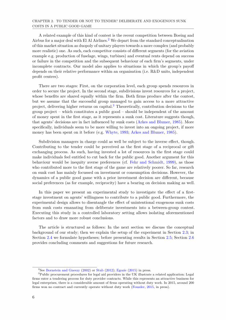
A related example of this kind of contest is the recent competition between Boeing andAirbus for a major deal with El Al Airlines.2 We depart from the standard conceptualisationof this market situation as duopoly of unitary players towards a more complex (and probablymore realistic) one. As such, each competitor consists of different segments (for the aviationexample e.g. production of fuselage, wings, turbines) and eventual rents depend on successor failure in the competition and the subsequent behaviour of each firm’s segments, underincomplete contracts. Our model also applies to situations in which the group’s payoffdepends on their relative performance within an organisation (i.e. R&D units, independentprofit centres).
There are two stages: First, on the corporation level, each group spends resources inorder to secure the project. In the second stage, subdivisions invest resources for a project,whose benefits are shared equally within the firm. Both firms produce after the contest,but we assume that the successful group managed to gain access to a more attractiveproject, delivering higher returns on capital.3 Theoretically, contribution decisions to thegroup project – which constitutes a public good – should be independent of the amountof money spent in the first stage, as it represents a sunk cost. Literature suggests though,that agents’ decisions are in fact influenced by sunk costs (Arkes and Blumer, 1985). Morespecifically, individuals seem to be more willing to invest into an ongoing project, if moremoney has been spent on it before (e.g. Whyte, 1993; Arkes and Blumer, 1985).
Subdivision managers in charge could as well be subject to the inverse effect, though.Contributing to the tender could be perceived as the first stage of a reciprocal or giftexchanging process. As such, having invested a lot of resources in the first stage couldmake individuals feel entitled to cut back for the public good. Another argument for thisbehaviour would be inequity averse preferences (cf. Fehr and Schmidt, 1999), as thosewho contributed more to the first stage of the game are relatively poorer. So far, researchon sunk cost has mainly focussed on investment or consumption decisions. However, thedynamics of a public good game with a prior investment decision are different, becausesocial preferences (as for example, reciprocity) have a bearing on decision making as well.
In this paper we present an experimental study to investigate the effect of a first-stage investment on agents’ willingness to contribute to a public good. Furthermore, theexperimental design allows to disentangle the effect of unintentional exogenous sunk costsfrom sunk costs emanating from deliberate investments into a between-group contest.Executing this study in a controlled laboratory setting allows isolating aforementionedfactors and to draw more robust conclusions.
The article is structured as follows: In the next section we discuss the conceptualbackground of our study; then we explain the setup of the experiment in Section 2.3; inSection 2.4 we formulate hypotheses; before presenting results in Section 2.5; Section 2.6provides concluding comments and suggestions for future research.
2See Bornstein and Gneezy (2002) or Stub (2012); Egozie (2015) in press.3Public procurement procedures for legal aid providers in the UK illustrate a related application: Legal
firms enter a tendering process for duty provider contracts. While this represents an attractive business forlegal enterprises, there is a considerable amount of firms operating without duty work. In 2015, around 200firms won no contract and currently operate without duty work (Fouzder, 2015, in press).
6
2.2. BACKGROUND
2.2 Background
This chapter draws from three different strands of literature: 1) Endogenous prize contests,2) Public good games with entry option and 3) Sunk costs. In this section we review someof the relevant literature.
2.2.1 Endogenous prize contests
An important component of contests is the prize at stake (cf. Dechenaux et al., 2012;Konrad, 2009). Not only does it represent the motivational cue for engaging in a contestfrom a behavioural perspective, but it also determines the equilibrium prediction in purestrategies (cf. Abbink, Brandts, Herrmann, and Orzen, 2010; Konrad, 2009). In the field,there exists a number of contest situations with an exogenous prize, like a money prizein sports tournaments or known rents from patents in R&D races. However, often thecontestants themselves can influence the prize to take away from a successful competition.So far research on endogenous contest prizes has focused on scenarios where the prizeis influenced by players’ contribution to the contest (Baye and Hoppe, 2003) or by theprice demanded in a Bertrand competition game (Bornstein and Gneezy, 2002; Bornstein,Kugler, Budescu, and Selten, 2008).
In Morgan, Orzen, Sefton, and Sisak (forthcoming), subjects were able to make a real-time decision on entering a contest, while observing the number of co-players currentlyin the market. They find a substantial excess entry into the market, as compared to therisk neutral benchmark prediction. This was especially the case when the outside optionunderlay a stochastic risk. The symmetric equilibrium investment level in the subsequentcontest negatively depends on the number of entrants into the market. While Morgan et al.(forthcoming) join the ranks of articles that find considerable overspending into the contest,they also observe a large fraction of subjects exhibiting a rather passive investment strategyafter having decided to enter the contest. Morgan et al. (forthcoming) offer two explanationsfor the behaviour of this latter group: 1) Escape the outside option for treatments whereit is risky. 2) Risk or loss averse subjects entering the market early, under the expectationthat only few other players would enter, refrain from placing a high bid upon observingthat there were in fact unexpectedly many entrants to the market.
Huyck, Battalio, and Beil (1993) conduct an experiment where players auction for theright to participate in a coordination game. The price for the right to play reduces strategicuncertainty and works as a tacit communication device. While subjects consistently fail tocoordinate on a payoff-dominant equilibrium when endowed with the right to play, subjectswho went through a pre-play auction, achieve the efficient outcome in the coordinationgame.
In the context of a weak link game, Cooper, Ioannou, and Qi (2015) compare a marketmechanism with random sorting with regards to subjects’ productivity. While there existsan efficiency gain from the market mechanism for high performance workers, this effect isalmost completely offset by a negative effect on subjects with low performance pay.
We present an endogenous contest prize where the contributions for outperformingthe competitor do in fact not influence the size of the prize. Instead, these expenses are
7

CHAPTER 2. TO TENDER OR NOT TO TENDER? DELIBERATE AND EXOGENOUS SUNKCOSTS IN A PUBLIC GOOD GAME
dedicated solely to the contest. Public tenders, for example, are widely used for determiningthe granting of funds for projects or for (public) facilities. Success or failure of the projectdepend on the winning party’s behaviour in the post-contest phase.
2.2.2 Public good games with entry option
There exists an established theoretical literature on public goods games with entry option.Frank (1987) and Amann and Yang (1998) argue that when subjects can opt between settingup a partnership with another player or an outside option, entering conveys a message aboutthe players’ types. This helps coordination towards more efficient, cooperative strategies.Other authors refer to a false consensus bias as the reason for the matching of types. Ifthis is the case, cooperators are relatively more likely to enter the cooperative game, asthey tend to be more optimistic about the level of cooperation, than free riders are (Orbelland Dawes, 1991).
Orbell and Dawes (1993) and Nosenzo and Tufano (2015) examine the effect of voluntaryentry to a public goods game experimentally. Orbell and Dawes (1993) find a positive effecton cooperation and efficiency in the presence of voluntary entry to a one-shot public goodsgame. Nosenzo and Tufano (2015) compare the effectiveness of an entry option with anexit option in a one-shot public goods game experiment. Although the possibility to exitincreases subjects’ ability to coordinate towards the cooperative strategy, the entry optiondoes not deliver a significant effect.
2.2.3 Sunk costs
Classical examples of elicitation of sunk cost fallacies or escalating commitment, demon-strate cases where agents are more willing to invest (additional) resources with higherprevious investments (Garland, 1990; Arkes and Blumer, 1985). One field study reportedin Arkes and Blumer (1985), for example, demonstrates that subjects who paid the full pricefor a theatre season ticket attend more performances than subjects that have randomlybenefited from a reduced price. Amongst the most prominent psychological explanationsfor the sunk cost fallacy is prospect theory (Kahneman and Tversky, 1979): People do notupdate their reference point which makes them accept too much risk. Staw (1981) offersa self-justification bias as alternative explanation: Subjects tend to invest more resourcesinto a losing asset in order to rationalise or justify their previous strategy.
One prominent aspect of our design is the fact that we can contrast sunk costs incurredexogenously and those having been accrued deliberately by the subject herself. So far, mostexisting evidence on this topic is based on data where the sunk costs have either beenexogenously defined by the experimenter (i.e. Garland, 1990) or endogenously accrued bythe subjects (i.e. Friedman, Pommerenke, Lukose, Milam, and Huberman, 2007).
An example that considers this issue is presented by Offerman and Potters (2006).In an experimental study they examine the effect of auctioning entry rights to a marketon subsequent prices. In one treatment, agents do not issue bids themselves, but entryrights are given randomly and the same cost as in the auctioning treatment is inducedexogenously. Most notably, prices do not differ between the auction and the exogenous
8
2.3. SETUP
treatment. At the same time, the effect size of the sunk cost fallacy seems to depend onthe market situation. While there is a significant positive effect on average prices in anoligopolistic market, they are unaffected in the monopoly treatment. Offerman and Potters(2006) argue that while the entry fee encourages players to risk engaging in a collusivestrategy, this was – by design – much less of an issue in the monopoly market becausecollusion is not possible by definition.
2.3 Setup
Before the main part of the experiment, we took a measure of individual social valueorientation (SVO), using techniques introduced by Murphy, Ackermann, and Handgraaf(2011).4 Using this data we test if more socially oriented participants recognise the overallwelfare reducing character of the between group contest, which should negatively influencefirst stage expenditures. Furthermore, we would expect players with a higher SVO score toexhibit a greater willingness to contribute to the group project, as second stage contributionis socially beneficial.
This study incorporates two experimental treatments: A competition treatment andan exogenous treatment. While subjects in the former treatment compete for the right toplay a public good game with a relatively more attractive Marginal Per Capita Return(MPCR), players in the latter treatment incur an exogenous cost, before being sorted intoan either high or low MPCR game. Details are described in what follows.
[Competition treatment:] Players are sorted in groups of three and compete againstanother group of the same size. This composition keeps unchanged and players’ identitiesare never associated with their decisions. The game consists of two stages and it includesinvestment decisions as explained in the following.
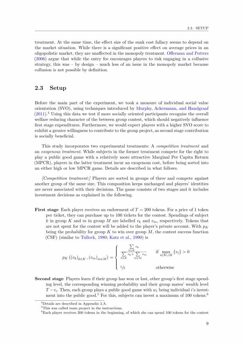
First stage Each player receives an endowment of T = 200 tokens. For a price of 1 tokenper ticket, they can purchase up to 100 tickets for the contest. Spendings of subjectk in group K and m in group M are labelled vk and vm, respectively. Tokens thatare not spent for the contest will be added to the player’s private account. With pKbeing the probability for group K to win over group M , the contest success function(CSF) (similar to Tullock, 1980; Katz et al., 1990) is
pK((vk)k∈K , (vm)m∈M
)=
∑k∈K
vk∑k∈K
vk+∑m∈M
vmif maxi∈K∪M
{vi} > 0
1/2 otherwise
Second stage Players learn if their group has won or lost, other group’s first stage spend-ing level, the corresponding winning probability and their group mates’ wealth levelT −vi. Then, each group plays a public good game with wi being individual i’s invest-ment into the public good.5 For this, subjects can invest a maximum of 100 tokens.6
4Details are described in Appendix 2.A.5This was called team project in the instructions.6Each player receives 200 tokens in the beginning, of which she can spend 100 tokens for the contest
9
CHAPTER 2. TO TENDER OR NOT TO TENDER? DELIBERATE AND EXOGENOUS SUNKCOSTS IN A PUBLIC GOOD GAME
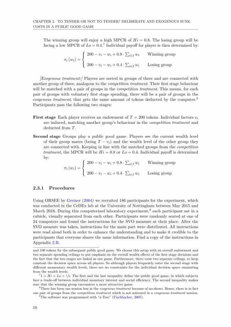
The winning group will enjoy a high MPCR of Hi = 0.8. The losing group will befacing a low MPCR of Lo = 0.4.7 Individual payoff for player is then determined by:
πi (wi) =
200− vi − wi + 0.8 ·
∑i∈I wi Winning group
200− vi − wi + 0.4 ·∑i∈I wi Losing group
[Exogenous treatment:] Players are sorted in groups of three and are connected withanother group of three, analogous to the competition treatment. Their first stage behaviourwill be matched with a pair of groups in the competition treatment. This means, for eachpair of groups with voluntary first stage spending, there will be a pair of groups in theexogenous treatment, that gets the same amount of tokens deducted by the computer.8Participants pass the following two stages:
First stage Each player receives an endowment of T = 200 tokens. Individual factors viare induced, matching another group’s behaviour in the competition treatment anddeducted from T .
Second stage Groups play a public good game. Players see the current wealth levelof their group mates (being T − vi) and the wealth level of the other group theyare connected with. Keeping in line with the matched groups from the competitiontreatment, the MPCR will be Hi = 0.8 or Lo = 0.4. Individual payoff is determinedby:
πi (wi) =
200− vi − wi + 0.8 ·
∑i∈I wi Winning group
200− vi − wi + 0.4 ·∑i∈I wi Losing group
2.3.1 Procedures
Using ORSEE by Greiner (2004) we recruited 186 participants for the experiment, whichwas conducted in the CeDEx lab at the University of Nottingham between May 2015 andMarch 2016. During this computerised laboratory experiment,9 each participant sat in acubicle, visually separated from each other. Participants were randomly seated at one of24 computers and found the instructions for the SVO measure at their place. After theSVO measure was taken, instructions for the main part were distributed. All instructionswere read aloud both in order to enhance the understanding and to make it credible to theparticipants that everyone shares the same information. Find a copy of the instructions inAppendix 2.B.
and 100 tokens for the subsequent public good game. We choose this setup with an overall endowment andtwo separate spending ceilings to put emphasis on the overall wealth effects of the first stage decisions andthe fact that the two stages are linked as one game. Furthermore, there exist two separate ceilings, to keepconstant the decision space across all players. So although players frequently enter the second stage withdifferent momentary wealth levels, there are no constraints for the individual decision space emanatingfrom the wealth levels.
71 > Hi > Lo > 1/3. The first and the last inequality define the public good game, in which subjectsface a trade-off between individual monetary interest and social efficiency. The second inequality makessure that the winning group encounters a more attractive game.
8There has been one session less in the exogenous treatment because of no-shows. Hence, there is in factone pair of groups from the competition treatment which is not mirrored in a exogenous treatment session.
9The software was programmed with “z-Tree” (Fischbacher, 2007).
10

2.4. EQUILIBRIUM STRATEGIES
The main part of the experiment started with a trial period, including comprehensionquestions, in order to make participants familiar with the interface and to ensure a thoroughunderstanding. After the main part, participants answered a short questionnaire aboutpersonal attributes (i.e. age, gender) and preferences (political convictions, risk attitudes...).
The experiment took one hour, which included reading instructions, taking an SVOmeasure, a trial period, the main part of the experiment, a questionnaire and payment.Average earnings were £ 12.00, which was paid out privately and in cash at the end of thesession.10
2.4 Equilibrium Strategies
Under risk-neutrality and individualistic preferences, each player i in group K maximisesher expected earnings, which is
E (πi (vi, wk∈K)) = T − vi − wi + pK ·Hi∑k∈K
wk + (1− pK)Lo∑k∈K
wk
As 1 > Hi > Lo > 1/3, investment into the public good is socially desirable butindividually costly for risk-neutral individualistic agents, who are only concerned withtheir own earnings. The second-stage Nash equilibrium therefore is wi = 0 ∀ i ∈ K ∪M ,which renders both public good games indifferent in expected values, i.e. zero. In thecompetition treatment, no resources will be spent in the first stage, so vi = 0 ∀ i ∈ K ∪M .Find a more formal approach in Appendix 2.C.
2.4.1 Behavioural Hypotheses
Next to the subgame perfect equilibrium as benchmark we formalise alternative hypothesesto capture other regarding preferences. Inequality 2.4.1 describes a hypothesis concerningthe relation between the different mean contribution rates for each possible second stageoutcome.
wi|win, comp > wi|win, ex > wi| lose, ex > wi| lose, comp (2.4.1)
wi|A,B represents average contribution levels given a particular group has won or lost(i.e. A ∈ {win, lose}, respectively) and given the group is in either the competition or theexogenous treatment (i.e. B ∈ {comp, ex}, respectively).
The second inequality (between winning and losing groups) is in line with establishedempirical results on public good games, that contributions increase with higher MPCR (eg.Gunnthorsdottir, Houser, and McCabe, 2007; Isaac and Walker, 1988). For the first andthe last inequality, we expect this tendency to be more pronounced for the competitiontreatment because of sorting and signalling effects. Using first stage contribution, playerscan signal their other regarding preferences.
10About e 16.00 or $ 18.00 at the time of the experiment.
11
CHAPTER 2. TO TENDER OR NOT TO TENDER? DELIBERATE AND EXOGENOUS SUNKCOSTS IN A PUBLIC GOOD GAME
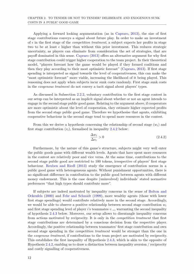
Applying a forward looking argumentation (as in Capraro, 2013), the size of firststage contributions conveys a signal about future play. In order to make an investmentof ε in the first stage of the competition treatment, a subject expects her profits in stagetwo to be at least ε higher than without this prior investment. This reduces strategicuncertainty, as players can eliminate from consideration the set of strategies, that arepayoff dominated in this sense. Capraro (2013) offers an alternative argument for why firststage contribution could trigger higher cooperation to the team project. In their theoreticalmodel, “players forecast how the game would be played if they formed coalitions andthen they play according to their most optimistic forecast” (Capraro, 2013). If first stagespending is interpreted as signal towards the level of cooperativeness, this can make the“most optimistic forecast” more viable, increasing the likelihood of it being played. Thisreasoning does not apply when subjects incur sunk costs randomly. First stage sunk costsin the exogenous treatment do not convey a tacit signal about players’ types.
As discussed in Subsection 2.2.2, voluntary contribution to the first stage contest inour setup can be interpreted as an implicit signal about whether or not an agent intends toengage in the second stage public good game. Relating to the argument above, if cooperatorsare more optimistic about the level of cooperation, they estimate higher expected profitsfrom the second stage public good game. Therefore we hypothesise that agents, exhibitingcooperative behaviour in the second stage tend to spend more resources in the contest.
From this we derive a hypothesis concerning the relationship of second stage (wi) andfirst stage contribution (vi), formalised in inequality 2.4.2 below:
∆wi∆vi
> 0 (2.4.2)
Furthermore, by the nature of this game’s structure, subjects might very well enterthe public goods game with different wealth levels. Agents that have spent more resourcesin the contest are relatively poor and vice versa. At the same time, contributions to thesecond stage public good are restricted to 100 tokens, irrespective of players’ first stagebehaviour. Reuben and Riedl (2013) study the emergence of contribution norms in apublic good game with heterogeneous agents. Without punishment opportunities, there isno significant difference in contribution to the public good between agents with differentmoney endowment. This is the case despite (uninvolved) individuals’ stated normativepreferences “that high types should contribute more”.
If subjects are indeed motivated by inequality concerns in the sense of Bolton andOckenfels (2000) and Fehr and Schmidt (1999), more wealthy agents (those with lowerfirst stage spendings) would contribute relatively more in the second stage. Accordingly,we would be able to observe a positive relationship between second stage contribution wiand first stage spending level of player i’s teammates v−i, warranting the second inequalityof hypothesis 2.4.3 below. Moreover, our setup allows to disentangle inequality concernsfrom actions motivated by reciprocity. It is only in the competition treatment that firststage contributions are determined by a conscious decision from the respective player.Accordingly, the positive relationship between teammates’ first stage contribution and ownsecond stage spending in the competition treatment would be stronger than the one inthe exogenous treatment, if contributions to the team project are motivated by reciprocity.This establishes the first inequality of Hypothesis 2.4.3, which is akin to the opposite ofHypothesis 2.4.2, enabling us to draw a distinction between inequality aversion / reciprocityand costly signalling of cooperativeness.
12
2.5. RESULTS
∆wi∆v−i
∣∣∣∣ comp >∆wi∆v−i
∣∣∣∣ ex > 0 (2.4.3)
∆wi∆v−i
∣∣∣B represents the slope of contribution to the team project in relation to theteammates’ first stage contribution level, given the group is in either the competition orthe exogenous treatment (i.e. B ∈ {comp, ex}, respectively).
2.5 Results
This section consists of three parts. First (Subsection 2.5.1) we describe subjects’ contestspending behaviour in the competition treatment. We analyse, which individual factorsdetermine the willingness to spend resources to the between group contest. In the sec-ond part (Subsection 2.5.2) we study how much subjects contribute to the team projectand discuss structural differences comparing winning and losing groups for the two treat-ments. Afterwards, we investigate the relationship of first and second stage contribution(Subsections 2.5.3 and 2.5.4).
As this is a one-shot game, individual data can be tested as independent observations.For hypothesis testing, we use non-parametric methods, as the data is not normally dis-tributed (Shapiro-Wilk test for normality. N=186, P = 0.00. Same result for first stageand second stage contribution.): Wilcoxon signed-rank test (Wilcoxon test) for paired data(Wilcoxon, 1945) and Mann-Whitney U test (MWU) for independent sample data (Mannand Whitney, 1947). We test for trends using Spearman’s rank correlation (Spearman test)(Spearman, 1904; Conover, 1999). For regression analyses we employ robust OLS, as wellas a Tobit model with limits at 0 and 100, as this is where the subjects’ action space islimited.
2.5.1 Team Contest
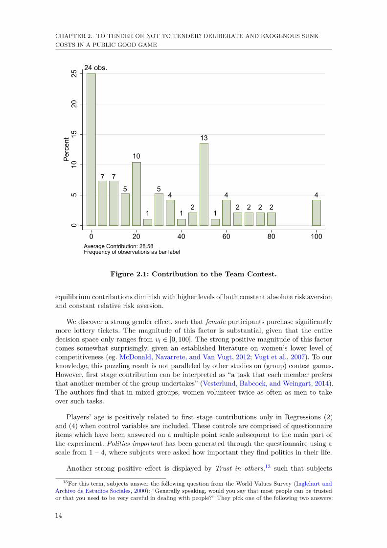
Subjects spend on average about 29 points on first stage tickets, which is substantially higherthan the benchmark prediction of zero contribution. Figure 2.1 depicts the distribution ofteam contest contributions, indicating 0 as the modal contribution level. See Appendix 2.Dfor a discussion of the role of beliefs for contest expenditures in this game.
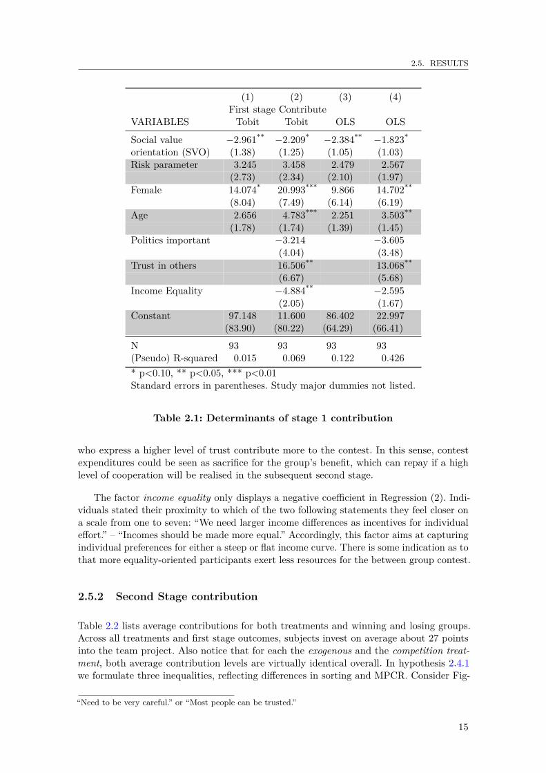
We use both Tobit regression with limits at 0 and 100, as well as ordinary least squares(OLS), respectively, to analyse determinants of individual contribution to the between groupcontest; results are summarised in Table 2.1. First of all, the individual measure of subjects’social value orientation (SVO)11 has a negative effect on subjects’ first stage contributionbehaviour.12 This means that participants with a relatively more social orientation mightrecognise the overall-welfare reducing nature of first-stage contributions. Furthermore, theself-reported risk tolerance measure (risk parameter) has only weak explanatory powerfor how many lottery tickets are bought. In Abbink et al. (2010) and Katz et al. (1990),
11For details see Appendix 2.A12Only with some degree of variation, all subjects display preferences that fall into the pro-social category.
13
CHAPTER 2. TO TENDER OR NOT TO TENDER? DELIBERATE AND EXOGENOUS SUNKCOSTS IN A PUBLIC GOOD GAME
24 obs.
7 7
5
10
1
54
12
13
1
4
2 2 2 2
4
05
1015
2025
Per
cent
0 20 40 60 80 100Average Contribution: 28.58Frequency of observations as bar label
Figure 2.1: Contribution to the Team Contest.
equilibrium contributions diminish with higher levels of both constant absolute risk aversionand constant relative risk aversion.
We discover a strong gender effect, such that female participants purchase significantlymore lottery tickets. The magnitude of this factor is substantial, given that the entiredecision space only ranges from vi ∈ [0, 100]. The strong positive magnitude of this factorcomes somewhat surprisingly, given an established literature on women’s lower level ofcompetitiveness (eg. McDonald, Navarrete, and Van Vugt, 2012; Vugt et al., 2007). To ourknowledge, this puzzling result is not paralleled by other studies on (group) contest games.However, first stage contribution can be interpreted as “a task that each member prefersthat another member of the group undertakes” (Vesterlund, Babcock, and Weingart, 2014).The authors find that in mixed groups, women volunteer twice as often as men to takeover such tasks.
Players’ age is positively related to first stage contributions only in Regressions (2)and (4) when control variables are included. These controls are comprised of questionnaireitems which have been answered on a multiple point scale subsequent to the main part ofthe experiment. Politics important has been generated through the questionnaire using ascale from 1 – 4, where subjects were asked how important they find politics in their life.
Another strong positive effect is displayed by Trust in others,13 such that subjects
13For this term, subjects answer the following question from the World Values Survey (Inglehart andArchivo de Estudios Sociales, 2000): “Generally speaking, would you say that most people can be trustedor that you need to be very careful in dealing with people?” They pick one of the following two answers:
14
2.5. RESULTS
(1) (2) (3) (4)First stage Contribute
VARIABLES Tobit Tobit OLS OLS
Social value −2.961** −2.209* −2.384** −1.823*
orientation (SVO) (1.38) (1.25) (1.05) (1.03)Risk parameter 3.245 3.458 2.479 2.567
(2.73) (2.34) (2.10) (1.97)Female 14.074* 20.993*** 9.866 14.702**
(8.04) (7.49) (6.14) (6.19)Age 2.656 4.783*** 2.251 3.503**
(1.78) (1.74) (1.39) (1.45)Politics important −3.214 −3.605
(4.04) (3.48)Trust in others 16.506** 13.068**
(6.67) (5.68)Income Equality −4.884** −2.595
(2.05) (1.67)Constant 97.148 11.600 86.402 22.997
(83.90) (80.22) (64.29) (66.41)
N 93 93 93 93(Pseudo) R-squared 0.015 0.069 0.122 0.426* p<0.10, ** p<0.05, *** p<0.01Standard errors in parentheses. Study major dummies not listed.
Table 2.1: Determinants of stage 1 contribution
who express a higher level of trust contribute more to the contest. In this sense, contestexpenditures could be seen as sacrifice for the group’s benefit, which can repay if a highlevel of cooperation will be realised in the subsequent second stage.
The factor income equality only displays a negative coefficient in Regression (2). Indi-viduals stated their proximity to which of the two following statements they feel closer ona scale from one to seven: “We need larger income differences as incentives for individualeffort.” – “Incomes should be made more equal.” Accordingly, this factor aims at capturingindividual preferences for either a steep or flat income curve. There is some indication as tothat more equality-oriented participants exert less resources for the between group contest.
2.5.2 Second Stage contribution
Table 2.2 lists average contributions for both treatments and winning and losing groups.Across all treatments and first stage outcomes, subjects invest on average about 27 pointsinto the team project. Also notice that for each the exogenous and the competition treat-ment, both average contribution levels are virtually identical overall. In hypothesis 2.4.1we formulate three inequalities, reflecting differences in sorting and MPCR. Consider Fig-
“Need to be very careful.” or “Most people can be trusted.”
15

CHAPTER 2. TO TENDER OR NOT TO TENDER? DELIBERATE AND EXOGENOUS SUNKCOSTS IN A PUBLIC GOOD GAME
ure 2.2 for an overview of individual contributions to the team project. As for the secondinequality of our hypothesis, we observe a stark difference between average contributionlevels comparing winning and losing teams, respectively (Wilcoxon test on team level: N= 62, P = 0.001. Higher rank sum than expected for winning teams). Members of thewinning teams spend about twice as much on the team project, as compared to subjectsin the losing teams. This is true for both the competition and the exogenous treatments.
Win Lose Overall
Exogenous 34.3 19.5 26.9Competition 37.2 16.3 26.8Overall 35.8 17.8 26.8
Table 2.2: Average individual contribution
The third inequality in our hypothesis postulates that subjects in a losing group in thecompetition treatment contribute less to the team project than a member of a losing groupin the exogenous treatment. The reason for this are sorting effects and signalling. Althoughthe average second stage contributions point in the right direction (19.5 for exogenous and16.3 for competition treatment), nonparametric tests on the group level fail to back thishypothesis (Wilcoxon test on team level: N = 31, P = 0.566). At the same time, for losinggroups complete free riding occurs much more frequently in the competition treatment (28times) than in the exogenous treatment (19 times).
010
2030
Freq
uenc
y
0 20 40 60 80 100First stage spending
Winning teams
010
2030
0 20 40 60 80 100First stage spending
Losing teams
Exogenous Competition
Figure 2.2: Individual contribution to the team project
16
2.5. RESULTS
The results concerning the first inequality of Hypothesis 2.4.1 pan out similarly: Thehypothesis states that subjects in a winning team contribute more in the competitiontreatment, as compared to winning teams in the exogenous treatment. Again this differenceemanates from sorting and signalling effects. While the average second stage contributionsslightly tend towards this direction (34.3 for exogenous and 37.2 for competition treatment),this indifference is far from being significant (Wilcoxon test on team level: N = 31, P =0.566). Hence, subjects seem to not perceive contributions to the contest as a strong signalfor second-stage cooperativeness in the winning groups.
2.5.3 Relation between first and second stage contribution
Based on the argument that first stage contribution is used as costly device to signal thewillingness to cooperate in the team project, we formulate hypothesis 2.4.2 (Subsection 2.2.3adds to this, applying a sunk costs argumentation), which postulates a positive relationshipbetween individual contest expenditures and the subsequent investment into the teamproject. Concurrently, we discuss an antithetic perspective on this matter by devisinghypothesis 2.4.3. Here, both inequality aversion and reciprocity actually warrant a negativerelationship between first and second stage contribution. Our setup allows us to analysewhich of the above arguments prevail.
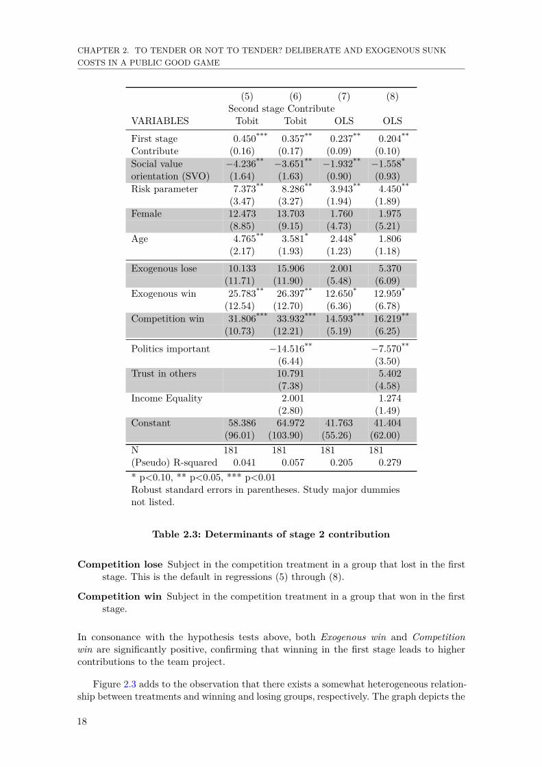
In Table 2.3 we present results for a Tobit model with limits at 0 and 100 (Regressions (5)and (6)) and OLS (Regressions (7) and (8)) both with robust standard errors for intragroupcorrelation. We regress contributions to the team project on first stage expenses and anumber of controls. Overall results for models (5) through (8) deliver evidence to supporthypothesis 2.4.2, displaying a positive interrelation between the two factors. This meansthat subjects who tend to spend more in the contest phase of the game, are also those whochip in relatively more resources to the subsequent team project.
Interestingly, the degree of social value orientation (SVO) negatively influences thewillingness to cooperate in the team project. This seems considerably unintuitive, as onewould expect more socially oriented individuals to invest more into the group account.14
By contrast, the positive coefficient for the risk parameter is more in line with intuitiveexpectations. Subjects who report to accept more risk are also ready to spend moreresources for the team project. Unlike for first stage expenditures, there is no gender effectwhen it comes to contributions towards the public good.
Next to the parameter age – which is again significantly positive – we include the samecontrols as in Regressions (2) and (4), as well as a dummy variable for each of the foursituations a subject could end up in:
Exogenous lose Subject in the exogenous treatment in a group that lost in the firststage.
Exogenous win Subject in the exogenous treatment in a group that won in the firststage.
14While the results of Regressions (1) – (4) suggest a potential multicollinearity problem, this shouldonly increase the standard errors of the coefficients if they are collinear. Even given that this should notinfluence the coefficients, the models’ variance inflation factors (VIF’s), reject the possibility of a potentialmulticollinearity problem here in the first place.
17
CHAPTER 2. TO TENDER OR NOT TO TENDER? DELIBERATE AND EXOGENOUS SUNKCOSTS IN A PUBLIC GOOD GAME
(5) (6) (7) (8)Second stage Contribute
VARIABLES Tobit Tobit OLS OLS
First stage 0.450*** 0.357** 0.237** 0.204**
Contribute (0.16) (0.17) (0.09) (0.10)Social value −4.236** −3.651** −1.932** −1.558*
orientation (SVO) (1.64) (1.63) (0.90) (0.93)Risk parameter 7.373** 8.286** 3.943** 4.450**
(3.47) (3.27) (1.94) (1.89)Female 12.473 13.703 1.760 1.975
(8.85) (9.15) (4.73) (5.21)Age 4.765** 3.581* 2.448* 1.806
(2.17) (1.93) (1.23) (1.18)
Exogenous lose 10.133 15.906 2.001 5.370(11.71) (11.90) (5.48) (6.09)
Exogenous win 25.783** 26.397** 12.650* 12.959*
(12.54) (12.70) (6.36) (6.78)Competition win 31.806*** 33.932*** 14.593*** 16.219**
(10.73) (12.21) (5.19) (6.25)
Politics important −14.516** −7.570**
(6.44) (3.50)Trust in others 10.791 5.402
(7.38) (4.58)Income Equality 2.001 1.274
(2.80) (1.49)Constant 58.386 64.972 41.763 41.404
(96.01) (103.90) (55.26) (62.00)N 181 181 181 181(Pseudo) R-squared 0.041 0.057 0.205 0.279* p<0.10, ** p<0.05, *** p<0.01Robust standard errors in parentheses. Study major dummiesnot listed.
Table 2.3: Determinants of stage 2 contribution
Competition lose Subject in the competition treatment in a group that lost in the firststage. This is the default in regressions (5) through (8).
Competition win Subject in the competition treatment in a group that won in the firststage.
In consonance with the hypothesis tests above, both Exogenous win and Competitionwin are significantly positive, confirming that winning in the first stage leads to highercontributions to the team project.
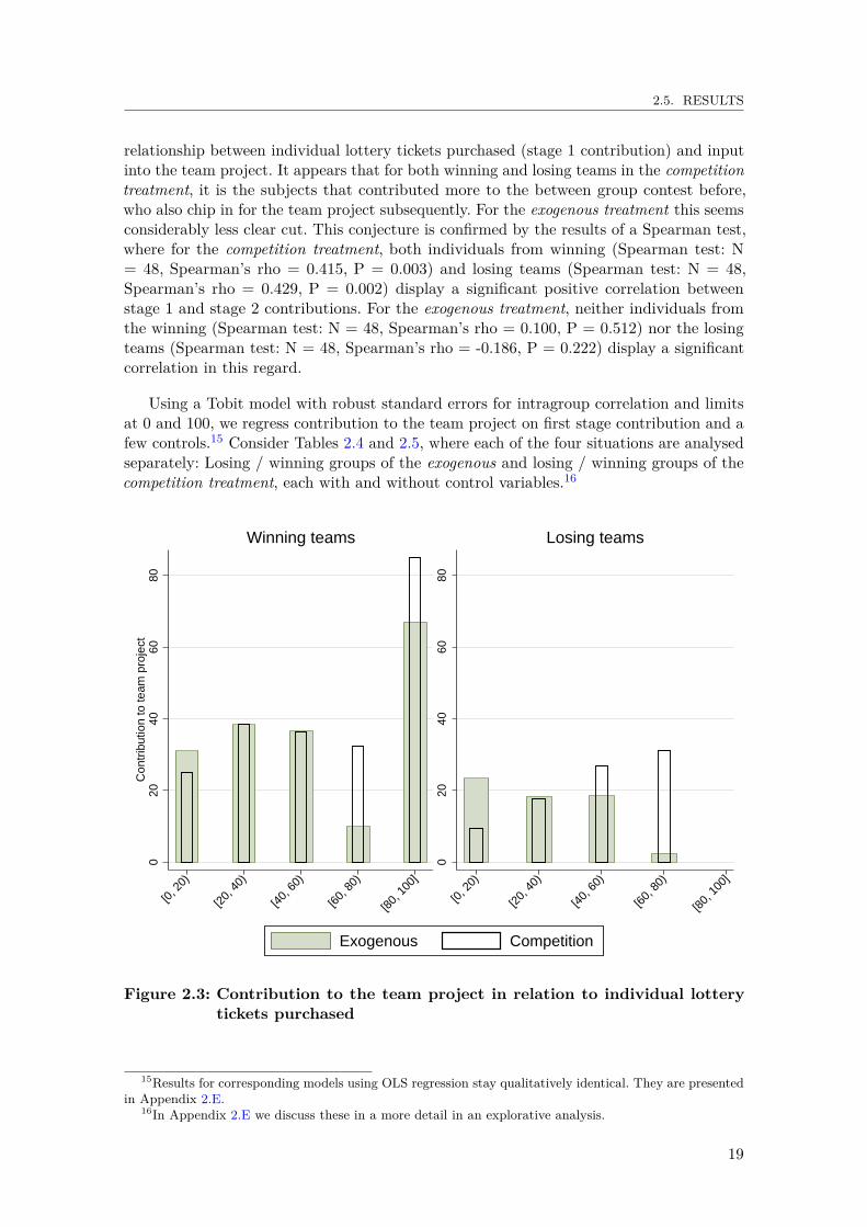
Figure 2.3 adds to the observation that there exists a somewhat heterogeneous relation-ship between treatments and winning and losing groups, respectively. The graph depicts the
18
2.5. RESULTS
relationship between individual lottery tickets purchased (stage 1 contribution) and inputinto the team project. It appears that for both winning and losing teams in the competitiontreatment, it is the subjects that contributed more to the between group contest before,who also chip in for the team project subsequently. For the exogenous treatment this seemsconsiderably less clear cut. This conjecture is confirmed by the results of a Spearman test,where for the competition treatment, both individuals from winning (Spearman test: N= 48, Spearman’s rho = 0.415, P = 0.003) and losing teams (Spearman test: N = 48,Spearman’s rho = 0.429, P = 0.002) display a significant positive correlation betweenstage 1 and stage 2 contributions. For the exogenous treatment, neither individuals fromthe winning (Spearman test: N = 48, Spearman’s rho = 0.100, P = 0.512) nor the losingteams (Spearman test: N = 48, Spearman’s rho = -0.186, P = 0.222) display a significantcorrelation in this regard.
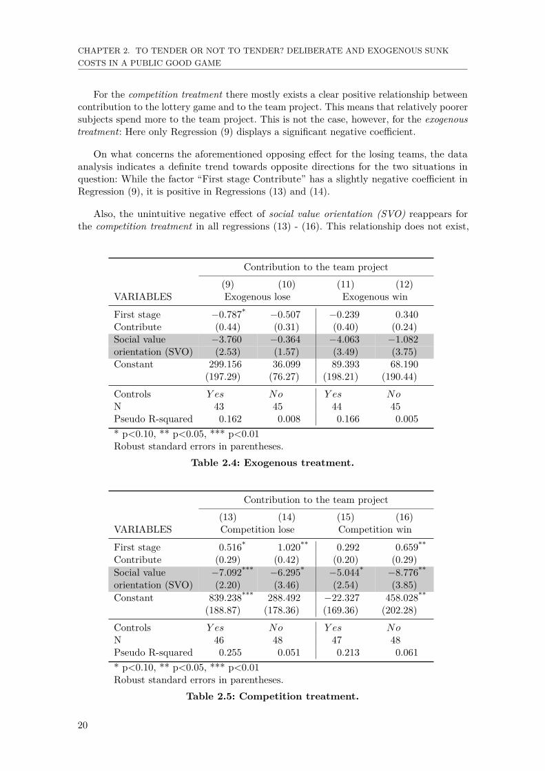
Using a Tobit model with robust standard errors for intragroup correlation and limitsat 0 and 100, we regress contribution to the team project on first stage contribution and afew controls.15 Consider Tables 2.4 and 2.5, where each of the four situations are analysedseparately: Losing / winning groups of the exogenous and losing / winning groups of thecompetition treatment, each with and without control variables.16
020
4060
80C
ontr
ibut
ion
to te
am p
roje
ct
[0, 2
0)
[20,
40)
[40,
60)
[60,
80)
[80,
100
]
Winning teams
020
4060
80
[0, 2
0)
[20,
40)
[40,
60)
[60,
80)
[80,
100
]
Losing teams
Exogenous Competition
Figure 2.3: Contribution to the team project in relation to individual lotterytickets purchased
15Results for corresponding models using OLS regression stay qualitatively identical. They are presentedin Appendix 2.E.
16In Appendix 2.E we discuss these in a more detail in an explorative analysis.
19
CHAPTER 2. TO TENDER OR NOT TO TENDER? DELIBERATE AND EXOGENOUS SUNKCOSTS IN A PUBLIC GOOD GAME
For the competition treatment there mostly exists a clear positive relationship betweencontribution to the lottery game and to the team project. This means that relatively poorersubjects spend more to the team project. This is not the case, however, for the exogenoustreatment: Here only Regression (9) displays a significant negative coefficient.
On what concerns the aforementioned opposing effect for the losing teams, the dataanalysis indicates a definite trend towards opposite directions for the two situations inquestion: While the factor “First stage Contribute” has a slightly negative coefficient inRegression (9), it is positive in Regressions (13) and (14).
Also, the unintuitive negative effect of social value orientation (SVO) reappears forthe competition treatment in all regressions (13) - (16). This relationship does not exist,
Contribution to the team project
(9) (10) (11) (12)VARIABLES Exogenous lose Exogenous win
First stage −0.787* −0.507 −0.239 0.340Contribute (0.44) (0.31) (0.40) (0.24)Social value −3.760 −0.364 −4.063 −1.082orientation (SVO) (2.53) (1.57) (3.49) (3.75)Constant 299.156 36.099 89.393 68.190
(197.29) (76.27) (198.21) (190.44)
Controls Y es No Y es NoN 43 45 44 45Pseudo R-squared 0.162 0.008 0.166 0.005* p<0.10, ** p<0.05, *** p<0.01Robust standard errors in parentheses.
Table 2.4: Exogenous treatment.
Contribution to the team project
(13) (14) (15) (16)VARIABLES Competition lose Competition win
First stage 0.516* 1.020** 0.292 0.659**
Contribute (0.29) (0.42) (0.20) (0.29)Social value −7.092*** −6.295* −5.044* −8.776**
orientation (SVO) (2.20) (3.46) (2.54) (3.85)Constant 839.238*** 288.492 −22.327 458.028**
(188.87) (178.36) (169.36) (202.28)
Controls Y es No Y es NoN 46 48 47 48Pseudo R-squared 0.255 0.051 0.213 0.061* p<0.10, ** p<0.05, *** p<0.01Robust standard errors in parentheses.
Table 2.5: Competition treatment.
20
2.5. RESULTS
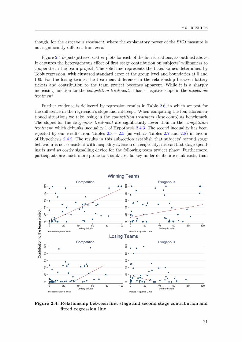
though, for the exogenous treatment, where the explanatory power of the SVO measure isnot significantly different from zero.
Figure 2.4 depicts jittered scatter plots for each of the four situations, as outlined above.It captures the heterogeneous effect of first stage contribution on subjects’ willingness tocooperate in the team project. The solid line represents the fitted values determined byTobit regression, with clustered standard error at the group level and boundaries at 0 and100. For the losing teams, the treatment difference in the relationship between lotterytickets and contribution to the team project becomes apparent. While it is a sharplyincreasing function for the competition treatment, it has a negative slope in the exogenoustreatment.
Further evidence is delivered by regression results in Table 2.6, in which we test forthe difference in the regression’s slope and intercept. When comparing the four aforemen-tioned situations we take losing in the competition treatment (lose,comp) as benchmark.The slopes for the exogenous treatment are significantly lower than in the competitiontreatment, which debunks inequality 1 of Hypothesis 2.4.3. The second inequality has beenrejected by our results from Tables 2.3 – 2.5 (as well as Tables 2.7 and 2.8) in favourof Hypothesis 2.4.2. The results in this subsection establish that subjects’ second stagebehaviour is not consistent with inequality aversion or reciprocity; instead first stage spend-ing is used as costly signalling device for the following team project phase. Furthermore,participants are much more prone to a sunk cost fallacy under deliberate sunk costs, than
020
4060
8010
0
0 20 40 60 80 100Lottery tickets
Pseudo R-squared: 0.036
Competition
020
4060
8010
0
0 20 40 60 80 100Lottery tickets
Pseudo R-squared: 0.005
ExogenousWinning Teams
020
4060
8010
0
0 20 40 60 80 100Lottery tickets
Pseudo R-squared: 0.032
Competition
020
4060
8010
0
0 20 40 60 80 100Lottery tickets
Pseudo R-squared: 0.008
ExogenousLosing Teams
Con
tribu
tion
to th
e te
am p
roje
ct
Figure 2.4: Relationship between first stage and second stage contribution andfitted regression line
21
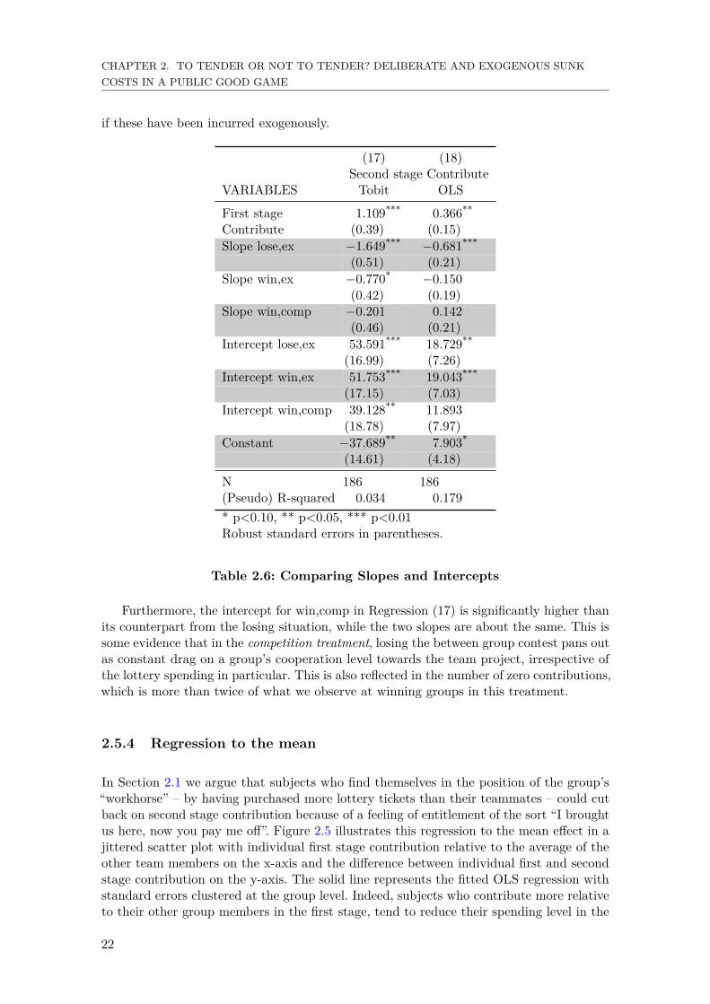
CHAPTER 2. TO TENDER OR NOT TO TENDER? DELIBERATE AND EXOGENOUS SUNKCOSTS IN A PUBLIC GOOD GAME
if these have been incurred exogenously.
(17) (18)Second stage Contribute
VARIABLES Tobit OLS
First stage 1.109*** 0.366**
Contribute (0.39) (0.15)Slope lose,ex −1.649*** −0.681***
(0.51) (0.21)Slope win,ex −0.770* −0.150
(0.42) (0.19)Slope win,comp −0.201 0.142
(0.46) (0.21)Intercept lose,ex 53.591*** 18.729**
(16.99) (7.26)Intercept win,ex 51.753*** 19.043***
(17.15) (7.03)Intercept win,comp 39.128** 11.893
(18.78) (7.97)Constant −37.689** 7.903*
(14.61) (4.18)
N 186 186(Pseudo) R-squared 0.034 0.179* p<0.10, ** p<0.05, *** p<0.01Robust standard errors in parentheses.
Table 2.6: Comparing Slopes and Intercepts
Furthermore, the intercept for win,comp in Regression (17) is significantly higher thanits counterpart from the losing situation, while the two slopes are about the same. This issome evidence that in the competition treatment, losing the between group contest pans outas constant drag on a group’s cooperation level towards the team project, irrespective ofthe lottery spending in particular. This is also reflected in the number of zero contributions,which is more than twice of what we observe at winning groups in this treatment.
2.5.4 Regression to the mean
In Section 2.1 we argue that subjects who find themselves in the position of the group’s“workhorse” – by having purchased more lottery tickets than their teammates – could cutback on second stage contribution because of a feeling of entitlement of the sort “I broughtus here, now you pay me off”. Figure 2.5 illustrates this regression to the mean effect in ajittered scatter plot with individual first stage contribution relative to the average of theother team members on the x-axis and the difference between individual first and secondstage contribution on the y-axis. The solid line represents the fitted OLS regression withstandard errors clustered at the group level. Indeed, subjects who contribute more relativeto their other group members in the first stage, tend to reduce their spending level in the
22

2.6. CONCLUSION
-100
-50
050
100
Sec
ond
stag
e m
inus
firs
t sta
ge c
ontr
ibut
ion
-100 -50 0 50 100Tickets relative to other group members
R-squared: 0.255
Figure 2.5: Regression to the mean effect
second stage, which is indicated by the fitted line’s negative slope (OLS regression withclustered standard errors. N = 186, Coef. = -0.549, P = 0.000).
This result relates to our findings discussed above insofar as that the positive relation-ship between first and second stage contribution prevails from a general perspective. Yetoverall spread between contributors and defectors gets weakened.
2.6 Conclusion
In this chapter we present an experimental study in which we analyse how individuals reactto heterogeneous sunk costs in a public good games setting. In specific, we investigate twotypes of sunk costs: Deliberately accrued expenses and exogenously imposed deductions.We argue that although they are economically equivalent, subjects will not derive the sameconsequences.
Subjects in the competition treatment spend resources to influence the probability forgetting their group sorted into a public good game with a higher MPCR. Players in theexogenous treatment, on the other hand, do not make this decision themselves. Insteadthere is a one-on-one matching with the contest from the competition treatment.
In equation 2.4.1 we specify our hypothesis concerning the average contribution levelsfor the four different scenarios. While our data clearly indicates a higher contribution level
23
CHAPTER 2. TO TENDER OR NOT TO TENDER? DELIBERATE AND EXOGENOUS SUNKCOSTS IN A PUBLIC GOOD GAME
for those groups that have been sorted to the higher MPCR game, results for the other twoinequalities are considerably less clear cut. In our tests for hypotheses 2.4.2 and 2.4.3 weexamine the interrelation of first and second stage contribution. Our results corroboratehypothesis 2.4.2 at the expense of its counterhypothesis. The positive relationship betweenfirst and second stage contribution mainly prevails in the competition treatment, where itis utilised as costly signalling and sacrifice.
Furthermore, players in the competition treatment have a slightly higher tendency torefrain from contributing to the public good, when their team has lost. An equivalenthigher contribution level for winning groups in the competition treatment, however, cannotbe observed.
This means that players in the underlying game do not perceive a positive outcomeof the between-group contest as signal for their group-mates’ willingness to cooperate, ascompared to when they reach the high MPCR by exogenous sorting. At the same time,subjects display a reduced willingness to cooperate with their teammates, when the groupfailed to attain the high MPCR game in the contest, as compared to the exogenous sorting.
Coming back to the aforementioned case of between company competition for a businessdeal, the implications derived from our results, vindicate a rather sceptical angle on atendering of commercial covenants. If both candidates dispose of comparable productivitylevels, the harm to the losing party is not met by an analogous positive burst of the winningparty. From an overall social welfare perspective, devising a method of arbitration whichavoids a between group contest would be favourable. To further test this policy advice,different ways of arbitration could be examined: Make both parties pay in equal amounts,or have the winner pay for it completely, amongst other conceivable sharing rules. Thecaveat of a subliminal latent contest might still apply in most settings, however.
Appendix 2.A Social Value Orientation-Measure
Prior to the main part of the experiment, we take a measurement of individual socialpreferences, using the SVO slider measure by Murphy et al. (2011).17 Subjects set sixsliders to determine mutual sharing of an amount of tokens, as represented in Figure 2.6.This was incentivised in the following way: After all participants cast their decisions, pairsof two were randomly created with one being the Sender and the other participant beingthe Receiver. One of the Sender’s decisions was implemented on both at random, where theSender gets what she allocated to herself and the Receiver gets what the Sender allocatedto her. Participants only got to know, which allocation was chosen to be paid out, afterthe main part of the experiment.
This technique was a simplification and adjustment of the circle test employed byBrandts, Riedl, and van Winden (2009); Sonnemans, van Dijk, and van Winden (2006).It has demonstrated reliable psychometric properties, yields scores for individuals at theratio level and is quick and easy to implement (cf. Murphy and Ackermann, 2014).
17Crosetto, Weisel, and Winter (2012) provide a helpful tool for implementation.
24
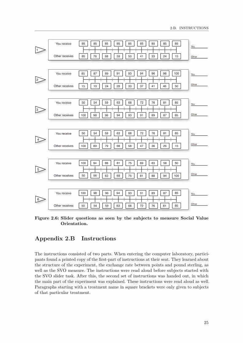
2.B. INSTRUCTIONS
Figure 2.6: Slider questions as seen by the subjects to measure Social ValueOrientation.
Appendix 2.B Instructions
The instructions consisted of two parts. When entering the computer laboratory, partici-pants found a printed copy of the first-part of instructions at their seat. They learned aboutthe structure of the experiment, the exchange rate between points and pound sterling, aswell as the SVO measure. The instructions were read aloud before subjects started withthe SVO slider task. After this, the second set of instructions was handed out, in whichthe main part of the experiment was explained. These instructions were read aloud as well.Paragraphs starting with a treatment name in square brackets were only given to subjectsof that particular treatment.
25

CHAPTER 2. TO TENDER OR NOT TO TENDER? DELIBERATE AND EXOGENOUS SUNKCOSTS IN A PUBLIC GOOD GAME
Instructions Part 1
Welcome and thank you for participating in this experiment. Please read these instructionscarefully. If you have any questions, please raise your hand and one of the experimenterswill come to your cubicle to answer your question. Talking or using mobile phones or anyother electronic devices is strictly prohibited. Mobile phones and other electronic devicesshould be switched off. If you are found violating these rules, you will both forfeit anyearnings from this experiment, and may be excluded from future experiments as well.
This is an experiment about decision making. The instructions are simple and if youfollow them carefully you might earn a considerable amount of money which will be paidto you privately and in cash at the end of today’s session. The amount of money you earndepends on your decisions, on other participants’ decisions and on random events. You willnever be asked to reveal your identity to anyone during the course of the experiment. Yourname will never be associated with any of your decisions. In order to keep your decisionsprivate, do not reveal your choices to any other participant.
During the experiment you will have the chance to earn points, which will be convertedinto cash at the end of today’s session, using an exchange rate of
1 point = 5 pence.
Thus, the more points you earn, the more cash you will receive at the end of the session.
This experiment consists of two parts. The following instructions explain Part 1. Afterfinishing this part, you will receive further instructions for Part 2. None of your (or anyoneelse’s) decisions for one part are relevant for your (or anyone else’s) performance in theother part.
Part 1:In this task you will be randomly paired with another person in this room. You will makea series of decisions about allocating points between you and the other person.
Then one of you will be assigned the role of Sender and the other one the role of Receiver.If you are the Sender, ONE of your decisions will be picked randomly and implemented forboth of you (i.e. you receive what you allocated to yourself and the other person receiveswhat you allocated to her).
If you are assigned the role of Receiver, ONE decision of the other person will be pickedrandomly and implemented for both of you (i.e. you receive what the other person allocatedto you and the other person receives what she allocated to herself).
All of your choices are completely confidential. You will learn your results of Part 1after Part 2 has finished. Points earned in Part 1 and Part 2 will be added up to determineyour total earnings.
26

2.B. INSTRUCTIONS
Instructions Part 2
In Part 2, all participants are assigned to teams of three and your team will be matchedwith another team. None of you will learn the identities of own team members or otherteam members. Part 2 will consist of two stages:
[Competition treatment:] At the beginning of the first stage you will receive 200 points.Then you can use up to 100 of your points to buy lottery tickets for your team. Each lotteryticket costs 1 point. Any of your points not spent on lottery tickets will be accumulatedin your private point balance. Likewise, each of your team members receives 200 pointsand can use up to 100 of these points to buy lottery tickets for your team. Similarly, eachmember of the other team will receive 200 points and can buy tickets for their team inexactly the same way.
[Exogenous treatment:] At the beginning of the first stage you will receive 200 points.Then the computer can use up to 100 of your points to buy lottery tickets for your team.Each lottery ticket costs 1 point. Any of your points not spent on lottery tickets will beaccumulated in your private point balance. Likewise, each of your team members receives200 points and the computer can use up to 100 of these points to buy lottery tickets for yourteam. Similarly, each member of the other team will receive 200 points and the computercan buy tickets for their team in exactly the same way.
Next, a lottery will determine whether your team, or the team you are matched with,wins. One of the tickets is randomly selected to be the winning ticket. Each ticket has thesame chance. Hence, the more tickets your team has, the higher is your team’s chance ofwinning.
Examples: If your team and the other team have the same amount of tickets then eachteam is equally likely to win. If your team has three times as many tickets as the otherteam, then your team is three times as likely to win as the other team. If only one of theteams has tickets, then this team wins with certainty. If neither your team nor the otherteam has any tickets, then one of the teams will be randomly selected as the winner witheach team equally likely to be selected.
After the winning team is determined you will reach the second stage. You will beable to see the following information: Individual tickets for each of your team mates, otherteam’s tickets and your winning probability. The second stage differs between the winningand the losing team in one way, which will be underlined below.
In the second stage you can invest up to 100 points of your endowment in a teamproject. Any point you do not invest and keep to yourself will be accumulated in yourprivate point balance. Each point invested in the team project yields 0.8 points for youand every member of your team, if your team has won in the first stage. Similarly, eachpoint invested in the team project yields 0.4 points for you and every member of your
27
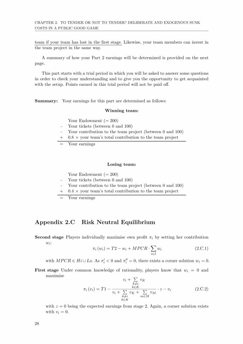
CHAPTER 2. TO TENDER OR NOT TO TENDER? DELIBERATE AND EXOGENOUS SUNKCOSTS IN A PUBLIC GOOD GAME
team if your team has lost in the first stage. Likewise, your team members can invest inthe team project in the same way.
A summary of how your Part 2 earnings will be determined is provided on the nextpage.
This part starts with a trial period in which you will be asked to answer some questionsin order to check your understanding and to give you the opportunity to get acquaintedwith the setup. Points earned in this trial period will not be paid off.
Summary: Your earnings for this part are determined as follows:
Winning team:
Your Endowment (= 200)- Your tickets (between 0 and 100)- Your contribution to the team project (between 0 and 100)+ 0.8 × your team’s total contribution to the team project= Your earnings
Losing team:
Your Endowment (= 200)- Your tickets (between 0 and 100)- Your contribution to the team project (between 0 and 100)+ 0.4 × your team’s total contribution to the team project= Your earnings
Appendix 2.C Risk Neutral Equilibrium
Second stage Players individually maximise own profit πi by setting her contributionwi:
πi (wi) = T2− wi +MPCR ·∑i∈I
wi (2.C.1)
with MPCR ∈ Hi∪Lo. As π′i < 0 and π′′i = 0, there exists a corner solution wi = 0.
First stage Under common knowledge of rationality, players know that wi = 0 andmaximise
πi (vi) = T1−
vi +∑k 6=ik∈K
vK
vi +∑k 6=ik∈K
vK +∑
m∈MvM· z − vi (2.C.2)
with z = 0 being the expected earnings from stage 2. Again, a corner solution existswith vi = 0.
28
2.D. CONTEST EXPENDITURES – THE ROLE OF BELIEFS
Appendix 2.D Contest Expenditures – The Role of Beliefs
About 10 % of first stage contributions fall in an area which is not rationalisable (i.e. con-tributions larger than 65), even holding the most optimistic beliefs about the second stage(i.e. all other players contribute fully), while at the same time holding very pessimisticbeliefs about groupmates’ behaviour in the first stage (i.e. no other groupmate buys lotterytickets). When holding the same beliefs on second stage contributions, while assuming sym-metry in first stage spending levels, some 46 % fall in the category of non-rationalisability(contributions larger than 60
3 = 21.6̄).
Second stage Player i’s payoff depends positively on her teammates’ input towards theteam project wk∈K\{i}, as in:
∂πi∂wk∈K\{i}
> 0 (2.D.1)
Hence, player i’s most optimistic belief for the second stage would involve full con-tribution by all other group members, i.e. wk∈K\{i} = 100 ∀ k ∈ K, which wouldamount to an account of
∑k∈K wk = 200 and expected second stage earnings of
z = T2 +Hi ·∑k∈K wk = 260 for a winning group.
First stage Most pessimistic beliefs about teammates’ contest spending behaviour arecharacterised as vk∈K\{i} = 0 ∀ k, i ∈ K. If all teammates do not buy lotterytickets (
∑k∈K\{i} = 0) and expected second stage payoff z = 260, player i maximises
equation 2.C.2 at vi = z4 = 65.
Consider as alternative belief on first stage behaviour, that all teammates contributesymmetrically, i.e.
∑k∈K vk = 3 · vk ∀ k ∈ K. For this set of beliefs, equation 2.C.2
maximises at vi = z12 = 21.6̄.
Appendix 2.E Control Variables and OLS regression
Tables 2.7 and 2.8 present results for OLS regressions with robust standard errors for intra-group correlation, which correspond to those presented in Tables 2.4 and 2.5. We analysethe relationship between contribution to the team project and first stage contribution,including controls. Results stay relatively stable between the two regression methods inquestion.
In Table 2.9 we present details for the control variables of Tables 2.4 and 2.5. Thosedetails were generated by a post-experiment questionnaire. We do not have well-establishedhypotheses for each of those control variables, for why we present this section in an explo-rative character.
The risk parameter has explanatory power only for regression (15). It was generatedby a self-reported risk tolerance indication on a scale from 1 to seven. As players investresources without knowing the contribution level of other teammates, contributing involvesa certain degree of risk taking. Accordingly, it seems intuitively plausible that subjectsdisplaying a higher level of risk tolerance would also contribute more to the team project.
29

CHAPTER 2. TO TENDER OR NOT TO TENDER? DELIBERATE AND EXOGENOUS SUNKCOSTS IN A PUBLIC GOOD GAME
Contribution to the team project
(19) (20) (21) (22)VARIABLES Exogenous lose Exogenous win
First stage −0.430 −0.324* −0.153 0.211Contribute (0.29) (0.16) (0.33) (0.13)Social value −0.490 0.795 −1.616 −0.348orientation (SVO) (1.49) (1.04) (3.02) (2.29)Constant 84.189 −13.805 100.986 44.876
(134.15) (50.17) (181.82) (117.35)
Controls Y es No Y es NoN 43 45 44 45R-squared 0.574 0.067 0.600 0.037* p<0.10, ** p<0.05, *** p<0.01Robust standard errors in parentheses.
Table 2.7: OLS regression exogenous treatment.
Contribution to the team project
(23) (24) (25) (26)VARIABLES Competition lose Competition win
First stage 0.108 0.337* 0.191 0.366*
Contribute (0.31) (0.16) (0.22) (0.18)Social value −3.723** −2.490 −3.492 −5.151**
orientation (SVO) (1.66) (1.57) (2.26) (2.19)Constant 319.675** 136.465 70.408 287.752**
(128.73) (83.24) (157.83) (117.38)
Controls Y es No Y es NoN 46 48 47 48R-squared 0.656 0.171 0.763 0.330* p<0.10, ** p<0.05, *** p<0.01Robust standard errors in parentheses.
Table 2.8: OLS regression competition treatment.
Results for the parameter female seem to paint a clear picture in that female participantstend to follow a more cooperative strategy towards the public good. Unlike our resultsfor gender effects in first stage contribution, this positive relationship seems in line withestablished literature (eg. Stockard, van de Kragt, and Dodge, 1988).18
Another factor that only plays a role in the competition treatment is the age of partici-pants. Interestingly, subjects’ age seems to accentuate the difference between winning and
18In a more recent study, Sell and Kuipers (2009) examine the gender bias in cooperation levels in thecontext of a structural social psychological framework. They argue that a large part of variation in genderspecific willingness to cooperate can be explained by structural differences and identities of institutionalrules and norms. Sell and Kuipers (2009) close with the optimistic note that these stereotypical genderroles, which are often perceived as innate, can in fact be overcome and ensuing social dilemmas be solved.
30

2.E. CONTROL VARIABLES AND OLS REGRESSION
Contribution to the team project
(9) (11) (13) (15)VARIABLES Exogenous lose Exogenous win Competition lose Competition win
First stage −0.787* −0.239 0.516* 0.292Contribute (0.44) (0.40) (0.29) (0.20)Social value −3.760 −4.063 −7.092*** −5.044*
orientation (SVO) (2.53) (3.49) (2.20) (2.54)Risk parameter −9.832 13.141 −2.729 22.969***
(7.23) (8.62) (3.83) (6.09)Female 35.737** 14.085 26.291** 52.727***
(14.17) (18.21) (9.70) (17.47)Age 0.992 0.052 −20.391*** 9.928***
(2.31) (2.71) (5.49) (2.22)Number of siblings 19.924** −0.270 16.754** −13.654**
(9.15) (6.83) (6.88) (6.27)Smoking −59.675** 57.434 −36.565 −150.414***
(25.90) (42.68) (25.19) (40.08)Happy −6.822 −15.315* 31.942*** 27.330***
(8.65) (8.50) (10.43) (7.73)Income Equality 13.046** 14.445** −3.642 −14.538***
(5.08) (6.10) (3.88) (4.64)Hard work −11.145*** 4.959 −7.584** −6.857**
(3.81) (5.78) (2.97) (3.21)Constant 299.156 89.393 839.238*** −22.327
(197.29) (198.21) (188.87) (169.36)
N 43 44 46 47Pseudo R-squared 0.162 0.166 0.255 0.213* p<0.10, ** p<0.05, *** p<0.01Robust standard errors in parentheses. Country dummies not listed.
Table 2.9: Effect of first stage contribution and dummies on cooperation levelin the team project.
losing groups along the lines of hypothesis 2.4.1. By contrast, number of siblings works inthe opposite effect. Furthermore this effect also partly prevails for the exogenous treatment.Experimental results from a trust game in Glaeser, Laibson, Scheinkman, and Soutter(2000) suggest that subjects with siblings are a lot more trustworthy than only child sub-jects: the latter only returned about half as much money to the senders as the former. Inour study, this effect only persists in losing groups with a lower structural contributionlevel. Therefore, number of siblings could represent a regression to the mean effect thatattenuates “extreme” levels of contribution.
In the questionnaire we asked participants whether they smoke or not and if they doso regularly or only sometimes. We include this parameter as proxy for short-sightednessof utility horizons (cp. Slovic, 2001). Indeed, subjects with a higher self-reported levelof tobacco consumption, contribute less to the team project. This effect is particularlypronounced in regressions (9) and (15). In consonance with the line of reasoning in Slovic(2001), we construe that (frequent) smokers exhibit a shorter time horizon for their decisions.
31

CHAPTER 2. TO TENDER OR NOT TO TENDER? DELIBERATE AND EXOGENOUS SUNKCOSTS IN A PUBLIC GOOD GAME
Accordingly, they pick the bird in the hand – keep the 100 tokens to themselves – over thetwo in the bush – potential gains from the group project.
Curiously, subjects reporting a higher level of momentary happiness in general, tendto give more in the competition treatment, but not in the exogenous treatment. If anything,regressions for the latter treatment even find a negative relationship. To our knowledge,while there exists some literature presenting cooperativeness as cause of happiness (Lu andArgyle, 1991), the opposite causal relationship has not yet received equal attention.
Again, for the factor income equality, individuals stated their proximity to which ofthe two following statements they feel closer on a scale from one to seven: “We need largerincome differences as incentives for individual effort.” – “Incomes should be made moreequal.” Accordingly, this factor aims at capturing individual preferences for either a steepor flat income curve. Similar to the previously discussed regressor, income equality displaysopposite effects for the two treatments. While there seems to be a positive relationship inthe exogenous treatment, the parameter turns negative for regressions using subjects fromthe competition treatment.
The last parameter, hard work intends to pick up a certain dog-eat-dog mentality asin whether subjects believe that everyone is the architect of ones own fortune or if successis a matter of luck. On a scale from one to seven, subjects express their proximity to oneof the two statements: “Hard work doesn’t generally bring success; it’s more a matter ofluck and connections.” – “In the long run, hard work usually brings a better life.” Thoseparticipants who rather believe that hard work pays off – “man forges his own destiny” –are less willing to contribute to the group account in the team project phase of the game.
32

Chapter 3
Reward and Punishment in aTeam Contest1
3.1 Introduction
Cooperation in alliances or social groupings is commonly observed in many applications.On a higher tier, many living organisms build cooperative societies – but it already beginson the level of mutual assistance, for example within a neighbourhood. The central ideais that by working together, everyone benefits from the efforts of the other, resulting ina more efficient outcome than if everyone was working on their own. From the classicaleconomic point of view, though, rational individuals do not contribute at an optimal level.As a result, positive welfare effects from efficient organisation cannot come to play.
There exists a strong tradition in philosophical and economic literature discussing therole of institutions to overcome this dilemma (Hobbes, 1651; Locke, 1698; Williamson, 1985;Ostrom, 1990). A simple form of institutionalising would be social ostracism or mobbingon the one hand, or promotion or appraisal on the other – mechanisms we frequentlyuse in the absence of complete contracts. Earlier studies suggest that the installation ofthese systems can overcome the free-rider problem in dilemma games. In these studies,mobbing or appraisal are represented by the opportunity to punish or reward co-players,respectively (e.g. Rand, Dreber, Ellingsen, Fudenberg, and Nowak, 2009; Sefton, Shupp, andWalker, 2007; Sigmund, Hauert, and Nowak, 2001; Fehr and Gächter, 2000). Furthermore,punishment seems to work better in this regard than reward (Andreoni, Harbaugh, andVesterlund, 2003; Balliet, Mulder, and Van Lange, 2011). The results are not yet fullyconclusive, but already give a first indication for policy advice: Use the stick rather thanthe carrot.
Most related studies, however, focus on isolated groups, abstracting from a large classof situations where groups are not detached, but embedded in some form of competition.Examples for this are public tenders, sports team competition or alliances in militaryconflicts. We name these situations team contests or group contest games. The contestslightly changes the nature of the game: Contribution still has positive external effectsonto other group members, but full free-riding is only a dominant strategy in a few cases
1Based on an article by Florian Heine and Martin Strobel (under review).
33
CHAPTER 3. REWARD AND PUNISHMENT IN A TEAM CONTEST
(Konrad, 2009).
Exposing groups to an antagonistic competition might also change the relationshipbetween reward and punishment. Indeed, it is difficult to imagine that punishment providesthe glue to hold a team together when facing off against a common competitor. Imagine afootball team when things are going badly. Would you imagine having one team membergiving another a dressing down make the latter provide more effort or perform better?In point of fact, studies suggest that “in-group cohesiveness is associated with positivetreatment (...) of the in-group” (Stephan, 1985).
Furthermore, when there is no distinction between an in-group and an out-group, likein standard public goods games, “people are unlikely to attend to the fact that they areinteracting with in-group members” (Stephan, 1985). The differentiation between an owngroup and an out group creates a favouring atmosphere towards the own group from theget-go (Brewer, 1979) and can lead to the “ultimate attribution error” (Pettigrew, 1979).This is a social schema to explain away positive actions of out-group members as exceptionsto the rule, for example.2
The central issue we investigate in this experimental study is the comparison of rewardand punishment in team contests. Specifically, we consider which institution leads to moreeffort and the efficiency implications. Our hypothesis is that while punishment can bringabout high contributions in team contest situations (like in Abbink et al., 2010), rewardingplays a more dominant role in this regard. In other words, the carrot will be preferredover the stick. On that account we employ two different environments, as will be explainedin detail below: 1) A public good embedded in a team contest. 2) The same public goodwithout a team contest. The purpose is to compare two environments that are strategicallyequivalent, but to eliminate the between group contest aspect as a factor in one environment.We execute this study as controlled computerised laboratory experiment, as this allows usto neatly design the environment and administer the appropriate institutional system.
Our results indicate a higher contribution level to the contest in the reward treatments,compared to the punishment treatments. Also, as well comparing between and withintreatments, players distribute more reward than punishment. This gives a new perspectiveon group dynamics in interactive economic games. We argue that the environment a groupfaces, has significant influence on its social dynamics and preferences within the group. Inline with the vast majority of research on rent-seeking or contest games, we find a drasticover-contribution across all our treatments, as compared to the Nash-equilibrium.3 Thisleads to an inefficient outcome and rent over-dissipation.
The remainder of this article is structured as follows: First, we discuss the nature ofreward and punishment systems in economic games; in Section 3.3 we explain the setupof the experiment and the equilibrium prediction; Section 3.4 contains our results andinterpretation; and in Section 3.5 we provide concluding comments and some suggestionsfor further research.
2Pettigrew (1979) mentions that this pattern of attributions is stronger if groups are in conflict witheach other.
3Cf. Sheremeta (2015); Dechenaux et al. (2012); Öncüler and Croson (2005)
34

3.2. REWARD AND PUNISHMENT IN ECONOMIC GAMES
3.2 Reward and Punishment in Economic Games
Providing the option to punish and / or reward other group members in public goodgames has repeatedly led to higher contributions in both experimental (Fehr and Gächter,2000; Sefton et al., 2007; Rand et al., 2009; O’Gorman, Henrich, and Van Vugt, 2009)and theoretical (Sigmund et al., 2001; Sasaki, Brännström, Dieckmann, and Sigmund,2012) studies. Furthermore, it seems that punishing works slightly better than rewardingin rendering higher contribution. Balliet et al. (2011) conduct a meta-analysis of theeffectiveness of reward or punishment in social dilemmas. Their analysis includes 187 effectsizes from 76 papers. They find a higher effect of punishment for generating cooperation ascompared to reward. Although being just marginally significant, a definite trend is evidenttowards a higher effectiveness of punishment in this regard.
Things might look differently though, when groups compete for a group prize. Previousstudies suggest that engagement in a project or a group prize is higher if there is a conflictor a competition with another group (cf. Sherif, 1961; Bornstein and Ben-Yossef, 1994; Tanand Bolle, 2007; Goette et al., 2012). At the same time, in-group favouritism and out-groupspite increases, a desire to benefit players from the own group and harm those from thecompeting group (Konrad and Morath, 2012). This can change the relative effectiveness ofrewarding and punishing, as well as players’ preference for either rewarding or punishingas means to reciprocate other group mates’ actions.
There are two groups of psychological motivations for an in-group – out-group bias ina competitive game like the contest game. The first one considers cognitive factors. Doise(1976) argues that being categorised in competitive groups, an anticipatory-justificationprocess is active, devaluing one’s antagonists. Alternative explanations for the in-group –out-group bias consider motivational factors. According to Tajfel (1978), people desire tocompare the in-group in a favourable way towards the out-group.
The studies above suggest that the economic environment shapes social preferences.In changing the economic environment of a public goods game, introducing a contestfor a group prize between groups, we expect to find contrasting results. In public goodsgames there is no competition between groups, but investment is socially beneficial, notunproductive effort, as in the contest game. Furthermore, reciprocity is one social preferenceand it is a prominent cause for conditional cooperation (play cooperatively if others do)(Gächter and Herrmann, 2009).4 The degree at which reciprocity is endogenous towards theeconomic environment determines whether a change in players’ behaviour can be found.
Another major issue in experimental studies on contest games is players’ persistenttendency to over-contribute and the ensuing effects on efficiency (cf. Öncüler and Croson,2005). In an experimental study, Abbink et al. (2010) find that allowing for the opportunityto punish other group members in a contest game renders expenditure levels that are asfar as 60 % above those in the control treatment. Although it would be socially beneficialto reduce contributing to the contest, players incentivise group mates to increase theirspendings to the contest. As a consequence, introducing the option to punish other groupmembers leads to even higher over-contribution than in the control treatment with negativeeffects on total welfare. Including the costs for punishment, subjects’ material losses arealmost nine times higher than the loss at the equilibrium level with respect to the social
4Another cause for conditional cooperation would be conformity – players just do what others do.
35

CHAPTER 3. REWARD AND PUNISHMENT IN A TEAM CONTEST
optimum.
3.3 Experimental Design
Our project brings together the two concepts of interaction in a contest game on the onehand and reward and sanctioning systems on the other. Experimental research in thisfield has mainly focused on either of the concepts. In combining these systems, insightcan be gained into the interaction of the institutional system of rewarding / punishingwith the contest / non-contest-environment. More specifically, we also consider what effectthe presence of another competing group has in this regard. In related experiments bySefton et al. (2007), agents are not in a competitive situation and in Abbink et al. (2010),participants have no opportunity to give rewards.
Comparison of contest vs. non-contest requires a design that makes both comparable. Tothis end we modify the classical group contest environment. In the non-contest environmentwe substitute the rival group by an equilibrium playing virtual mechanism. To subjectsof the prevailing group this means that they are acting in a public good game in whichoverall effort decides about the likelihood to win the prize. We eliminate everything thatrelates to the between group contest – i.e. all mentioning of the teammates as a group /team or mentioning of a possible rival group and the level of strategic uncertainty, whichstems from the other group’s actions. What we do keep constant, however, is everythingelse in the game, that has nothing to do with the other group – i.e. players are subject toa degree of uncertainty about whether ot not they will attain the prize; we also keep thestage game Nash equilibrium constant.
Players are automatically sorted in groups of four. In the field, agents repeatedly interactwith the same set of others; hence also throughout the experiment participants play withthe same players both in the own and in the opponent group.5 Each player also keeps thesame label throughout the experiment. The experiment is conducted over 15 rounds. Thisand all other features of the experiment are disclosed and are known to the participants.
The experiment is set up in a 2 x 4 design, with each four treatments with and fourtreatments without opponent group. In the treatments with opponent group, every groupK of four subjects competes against another group M of four subjects. They compete bybuying lottery tickets for their own group. Then one ticket will be drawn by the computerand this group wins a fixed prize. For the groups without opponent group, the other groupis replaced by a fixed number of 25 blank tickets which do not result in rent payments ifdrawn. Furthermore, in the latter treatments, there is no mentioning of other groups atany time. Every round is partitioned into three distinct stages as described in what follows:
1. Each player receives an endowment (budget) of B = 100 tokens and decides howmuch of it to invest in order to buy lottery tickets. The price for a ticket is one token.Investment of subject k ∈ K of group K is labelled vk and m ∈M of group M is vm.All tokens that a player does not invest will be added to her private account.
2. The winning probability, or contest success function, is as in Tullock (1980); Katz
5Not all treatments have an opponent group though.
36

3.3. EXPERIMENTAL DESIGN
et al. (1990). For the contest environment:
pK((vk)k∈K , (vm)m∈M
)=
∑k∈K
vk∑k∈K
vk+∑m∈M
vmif maxi∈K∪M
{vi} > 0
1/2 otherwise
(3.3.1)
For the non-contest environment:
pK((vk)k∈K
)=
∑k∈K
vk∑k∈K
vk + 25 (3.3.2)
where pK is the probability that group K wins (over group M). For the treatmentswithout opponent, groupM is replaced by a total of 25 blank tickets, which is known toall players. As will be discussed in Section 3.3.1, this represents the Nash equilibriumgroup contribution. For this, imagine
∑m∈M vm = 25 constantly in equation (4.E.1)
to represent the blank tickets as in equation (4.E.2). The winning probability is thesum of all lottery tickets of the own group divided by one of the two (dependingon the environment): a) the total lottery tickets bought by both groups, or b) thesum of total lottery tickets and blank tickets. After each investment phase, one ticketis drawn by the computer. Hence, the more tickets a group buys, the higher thechances of winning the lottery (ceteris paribus). Players of the winning group eachreceive a prize of z = 100 tokens, the other group gets nothing. In the non-opponenttreatments, if a blank ticket is drawn, the prize is forfeited.
3. The players get to know whether their group has won or not and how much the othersin their group, each, contributed. They also get to know the number of lottery ticketsbought by the opponent team, but not the opponent players’ individual contributions(if applicable). As well, participants get to know, what their probability of winningwas, which takes into account the sum of contributions of the opponent group /blank tickets. They now receive another F = 50 tokens (response tokens),6 whichthey can either keep in their own account or spend to give a response to their owngroup members.7 To this end there are four treatments, each played with and withoutopponent (thus 2 x 4 setup):[Baseline:] Players receive the aforementioned 50 response tokens at the end of eachround to be added to their account directly. As in this treatment there is no furtherinteraction between the players, these tokens are presented as extra tokens.[Reward:] Players can reward co-players in their own group. For this, they assignresponse tokens to one or more players of their own group. Each response tokenplayer k assigns to another player l is subtracted from k’s account and added to l’saccount. However, k can also keep all response tokens for herself and let them beadded to her own account. The players can at most invest all 50 response tokens perperiod (as sum of all response assigned to all co-players) and they cannot save tokensto be spent in upcoming rounds.
6These tokens were called Feedback tokens in the instructions (see Appendix 3.A).7Throughout the chapter we regularly use the expression response when referring to the reward and
punishment mechanism in order to ease the reading flow. As well, we make use of the term sanctioning assynonymous term for punishment.
37
CHAPTER 3. REWARD AND PUNISHMENT IN A TEAM CONTEST
[Punish:] This is similar to the reward treatment, but with punishment instead.Consider again two players, k and l. k can assign deduction points to any otherplayer of her own group, say l. For this, the same amount of response tokens spentby k, is deducted from l’s account. In this treatment, it is possible that a player getspunished such that her round payoff would theoretically turn negative. However, if aplayer gets punished by more tokens than there are on her account for this period,the excess punishment is discarded and the round payoff set to zero.8
[Reward and Punishment (R&P):] In this treatment each player can choose to eitherreward or to sanction another co-player of the same group. Players can give bothrewarding and sanctioning response to different co-players in the same round; 9
The prize to be won, z, constitutes a sort of local public good, as its consumption isnon-rival and non-excludable within the group: It is independent of group size, all groupmembers receive it and no-one can be excluded.
Note that players do not get to know from whom they get response points assigned.So neither do they know in the punishment treatment, which of the co-players sanctionedthem, nor do participants get revealed by whom they receive reward tokens in the rewardsetup (equivalent for the R&P treatment). This is to circumvent that players react onresponse behaviour of particular co-players – think hereby of retaliation or gift exchanging.Furthermore, participants do not get to know about the response other players received. Italso needs to be pointed out, that by rewarding other group members, participants shiftaround tokens in a way that leaves total welfare unchanged. Punishing others, in contrast,reduces overall welfare.
We apply a cost for response-giving of one (as in Sefton et al., 2007). This means if playerk punishes player l by 6, k has to pay 6 for this action. Some studies incentivise response-giving by relatively cheapening it (cf. Abbink et al., 2010; O’Gorman et al., 2009).10 Fehrand Gächter (2000) apply a non-linear cost function, where higher punishments are morecostly. We opt for a constant cost of one in order to keep both the punishment and thereward leverage small to mitigate confounds from efficiency preferences. Also, in case weapplied unequal leverage for the two types of response, the difference could be confoundingas well.
We formulate the following four main hypotheses: Being in a contest with anothergroup induces competitive behaviour, so 1) we expect contributions to the team contestto be higher in the contest environment than in the non-contest. Furthermore, a groupcontest encourages in-group favouritism and out-group spite dynamics, an inclination tobenefit players from the own group and harm those from the competing group. We predict2) More rewarding in the contest environment. 3) Less punishing in the contest environment.4) More total response in the contest environment.
8This case never occurred in the experiment.9It is not possible to both reward and sanction the same player in one round.
10For convenience, imagine the cost to be one half. Sticking to the aforementioned example, if player kpunishes player l by 6 again, k now has to pay 3 for this action.
38
3.3. EXPERIMENTAL DESIGN
3.3.1 Equilibrium Strategies
A natural benchmark to compare our data with is the sub-game perfect equilibrium ofthe single-shot game. We derive this by backward induction. In the second stage, costlyresponse only reduces own payoff. Hence, individualistic subjects do not give any response.Given this second-stage behaviour, players do not take punishment or reward into accountwhen making the optimal decision about how many lottery tickets to buy for their group.They maximise their expected payoff which is
π(vl) =
vl +∑k 6=lk∈K
vk
vl +∑k 6=lk∈K
vk +∑
m∈Mvm· z − vl.
This is the Tullock (1980) winning probability (as introduced in Section 3.3) times theprize minus the cost for investing in the group project. For treatments without opponent∑m∈M vm is set to 25. In this type of contest game with homogeneous groups, first order
conditions yield a unique equilibrium with respect to the aggregate group contribution.On the individual level, however, multiple equilibria exist (as explained in Konrad, 2009,2007b; Katz et al., 1990).
For all treatments, the equilibrium investment level for group K is∑k∈K vk = z
4 .11
For z = 100, this results in a Nash-equilibrium of 25 tokens per group.12 One conceivablesolution to the within-group “burden-sharing” would be to assume symmetry as in Katzet al. (1990). For z = 100 and |K| = 4 this would result in an individual contribution ofvl = 6.25 tokens. Of course, this is only one example among other possible solutions to thewithin-group problem. Note that only integer amounts of investment are allowed, so 6.25can best be viewed as a theoretical benchmark.
The multiplicity of equilibria in the single-shot game allows for a plethora of equilibriain the repeated game. This set is not only restricted to sequences of single-shot equilibria.The possibility to use grimm-trigger strategies also enables off-equilibrium behaviour insingle rounds.13 For the comparison with the data we neglect these equilibrium strategiesas possible benchmarks, because the immense amount of coordination needed to establishthem, render them rather implausible.
Unlike the single-shot Nash-equilibrium, the social optimal strategy differs somewhatbetween the cases with or without an opponent and whether one regards the opponentteam as part of the social system. In the treatments without opponent, the prize is forfeitedand goes to nobody if it is not won. Hence, the Nash equilibrium coincides with the optimal
11Find a derivation in Appendix 3.C.12Note that the equilibrium investment level is independent of the endowment with tokens or group size.
The only factor influencing equilibrium behaviour at the group level is the prize at stake. Note further thatthe investment level is strictly positive. If the other group is only investing a small amount or nothing intolottery tickets, it is very cheap to change the odds of the Tullock lottery. Hence investing might even beattractive for an individual.
13For example assume that a player contributes seven tickets in the first round and continues to do so ifall the others contributed eight tickets in the first round. If not, the player contributes only one ticket forall the consecutive rounds. In this case it is a best response to indeed contribute eight tickets in the firstround and play the single-shot best response strategy for the consecutive rounds. In a similar way playerscan credibly threaten others to switch from a “nice” single-shot equilibrium strategy to a less nice one ifthey are not rewarded after the first round.
39
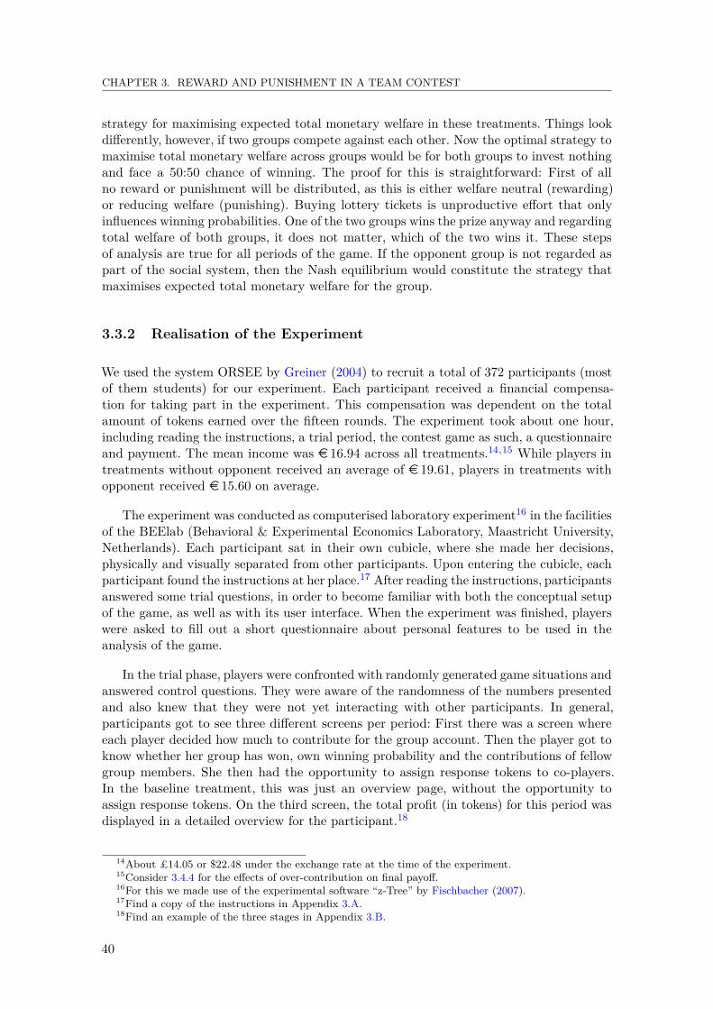
CHAPTER 3. REWARD AND PUNISHMENT IN A TEAM CONTEST
strategy for maximising expected total monetary welfare in these treatments. Things lookdifferently, however, if two groups compete against each other. Now the optimal strategy tomaximise total monetary welfare across groups would be for both groups to invest nothingand face a 50:50 chance of winning. The proof for this is straightforward: First of allno reward or punishment will be distributed, as this is either welfare neutral (rewarding)or reducing welfare (punishing). Buying lottery tickets is unproductive effort that onlyinfluences winning probabilities. One of the two groups wins the prize anyway and regardingtotal welfare of both groups, it does not matter, which of the two wins it. These stepsof analysis are true for all periods of the game. If the opponent group is not regarded aspart of the social system, then the Nash equilibrium would constitute the strategy thatmaximises expected total monetary welfare for the group.
3.3.2 Realisation of the Experiment
We used the system ORSEE by Greiner (2004) to recruit a total of 372 participants (mostof them students) for our experiment. Each participant received a financial compensa-tion for taking part in the experiment. This compensation was dependent on the totalamount of tokens earned over the fifteen rounds. The experiment took about one hour,including reading the instructions, a trial period, the contest game as such, a questionnaireand payment. The mean income was e 16.94 across all treatments.14,15 While players intreatments without opponent received an average of e 19.61, players in treatments withopponent received e 15.60 on average.
The experiment was conducted as computerised laboratory experiment16 in the facilitiesof the BEElab (Behavioral & Experimental Economics Laboratory, Maastricht University,Netherlands). Each participant sat in their own cubicle, where she made her decisions,physically and visually separated from other participants. Upon entering the cubicle, eachparticipant found the instructions at her place.17 After reading the instructions, participantsanswered some trial questions, in order to become familiar with both the conceptual setupof the game, as well as with its user interface. When the experiment was finished, playerswere asked to fill out a short questionnaire about personal features to be used in theanalysis of the game.
In the trial phase, players were confronted with randomly generated game situations andanswered control questions. They were aware of the randomness of the numbers presentedand also knew that they were not yet interacting with other participants. In general,participants got to see three different screens per period: First there was a screen whereeach player decided how much to contribute for the group account. Then the player got toknow whether her group has won, own winning probability and the contributions of fellowgroup members. She then had the opportunity to assign response tokens to co-players.In the baseline treatment, this was just an overview page, without the opportunity toassign response tokens. On the third screen, the total profit (in tokens) for this period wasdisplayed in a detailed overview for the participant.18
14About £14.05 or $22.48 under the exchange rate at the time of the experiment.15Consider 3.4.4 for the effects of over-contribution on final payoff.16For this we made use of the experimental software “z-Tree” by Fischbacher (2007).17Find a copy of the instructions in Appendix 3.A.18Find an example of the three stages in Appendix 3.B.
40
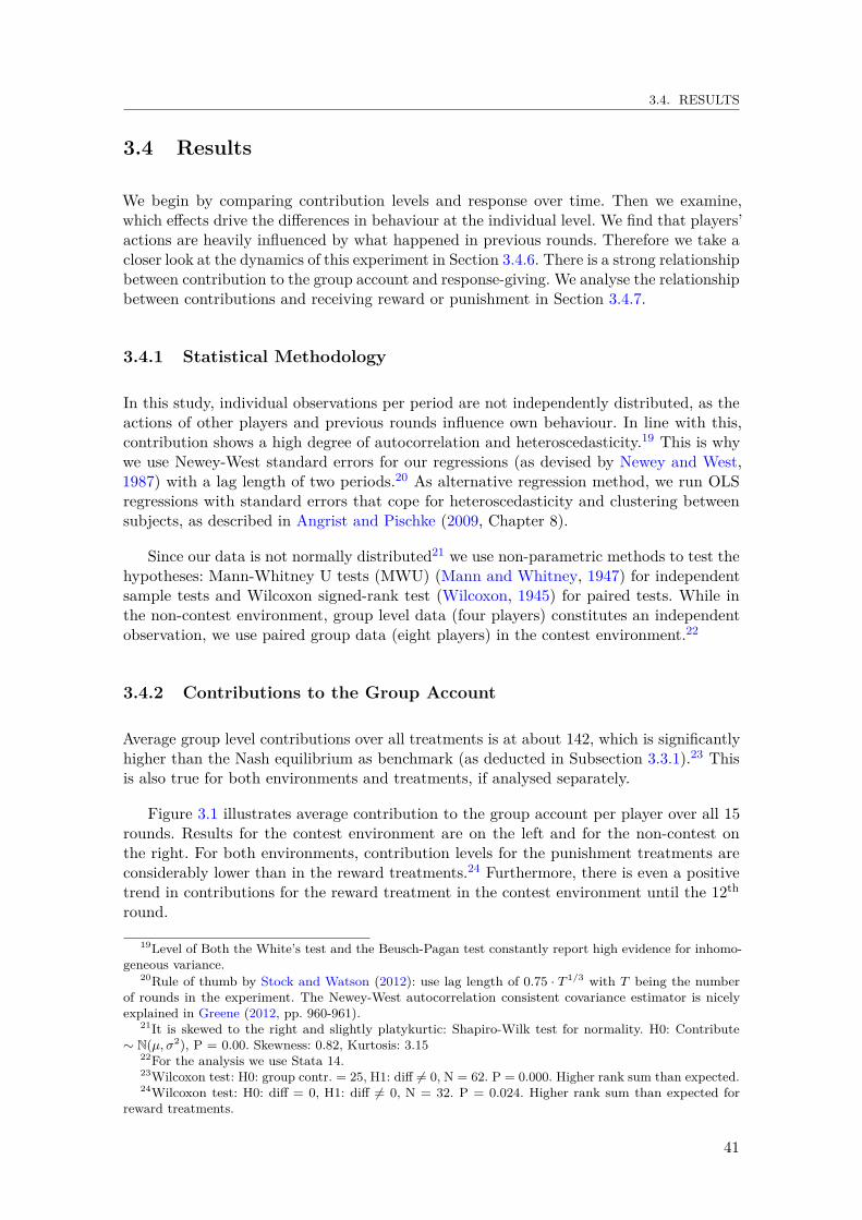
3.4. RESULTS
3.4 Results
We begin by comparing contribution levels and response over time. Then we examine,which effects drive the differences in behaviour at the individual level. We find that players’actions are heavily influenced by what happened in previous rounds. Therefore we take acloser look at the dynamics of this experiment in Section 3.4.6. There is a strong relationshipbetween contribution to the group account and response-giving. We analyse the relationshipbetween contributions and receiving reward or punishment in Section 3.4.7.
3.4.1 Statistical Methodology
In this study, individual observations per period are not independently distributed, as theactions of other players and previous rounds influence own behaviour. In line with this,contribution shows a high degree of autocorrelation and heteroscedasticity.19 This is whywe use Newey-West standard errors for our regressions (as devised by Newey and West,1987) with a lag length of two periods.20 As alternative regression method, we run OLSregressions with standard errors that cope for heteroscedasticity and clustering betweensubjects, as described in Angrist and Pischke (2009, Chapter 8).
Since our data is not normally distributed21 we use non-parametric methods to test thehypotheses: Mann-Whitney U tests (MWU) (Mann and Whitney, 1947) for independentsample tests and Wilcoxon signed-rank test (Wilcoxon, 1945) for paired tests. While inthe non-contest environment, group level data (four players) constitutes an independentobservation, we use paired group data (eight players) in the contest environment.22
3.4.2 Contributions to the Group Account
Average group level contributions over all treatments is at about 142, which is significantlyhigher than the Nash equilibrium as benchmark (as deducted in Subsection 3.3.1).23 Thisis also true for both environments and treatments, if analysed separately.
Figure 3.1 illustrates average contribution to the group account per player over all 15rounds. Results for the contest environment are on the left and for the non-contest onthe right. For both environments, contribution levels for the punishment treatments areconsiderably lower than in the reward treatments.24 Furthermore, there is even a positivetrend in contributions for the reward treatment in the contest environment until the 12th
round.
19Level of Both the White’s test and the Beusch-Pagan test constantly report high evidence for inhomo-geneous variance.
20Rule of thumb by Stock and Watson (2012): use lag length of 0.75 · T 1/3 with T being the numberof rounds in the experiment. The Newey-West autocorrelation consistent covariance estimator is nicelyexplained in Greene (2012, pp. 960-961).
21It is skewed to the right and slightly platykurtic: Shapiro-Wilk test for normality. H0: Contribute∼ N(µ, σ2), P = 0.00. Skewness: 0.82, Kurtosis: 3.15
22For the analysis we use Stata 14.23Wilcoxon test: H0: group contr. = 25, H1: diff 6= 0, N = 62. P = 0.000. Higher rank sum than expected.24Wilcoxon test: H0: diff = 0, H1: diff 6= 0, N = 32. P = 0.024. Higher rank sum than expected for
reward treatments.
41
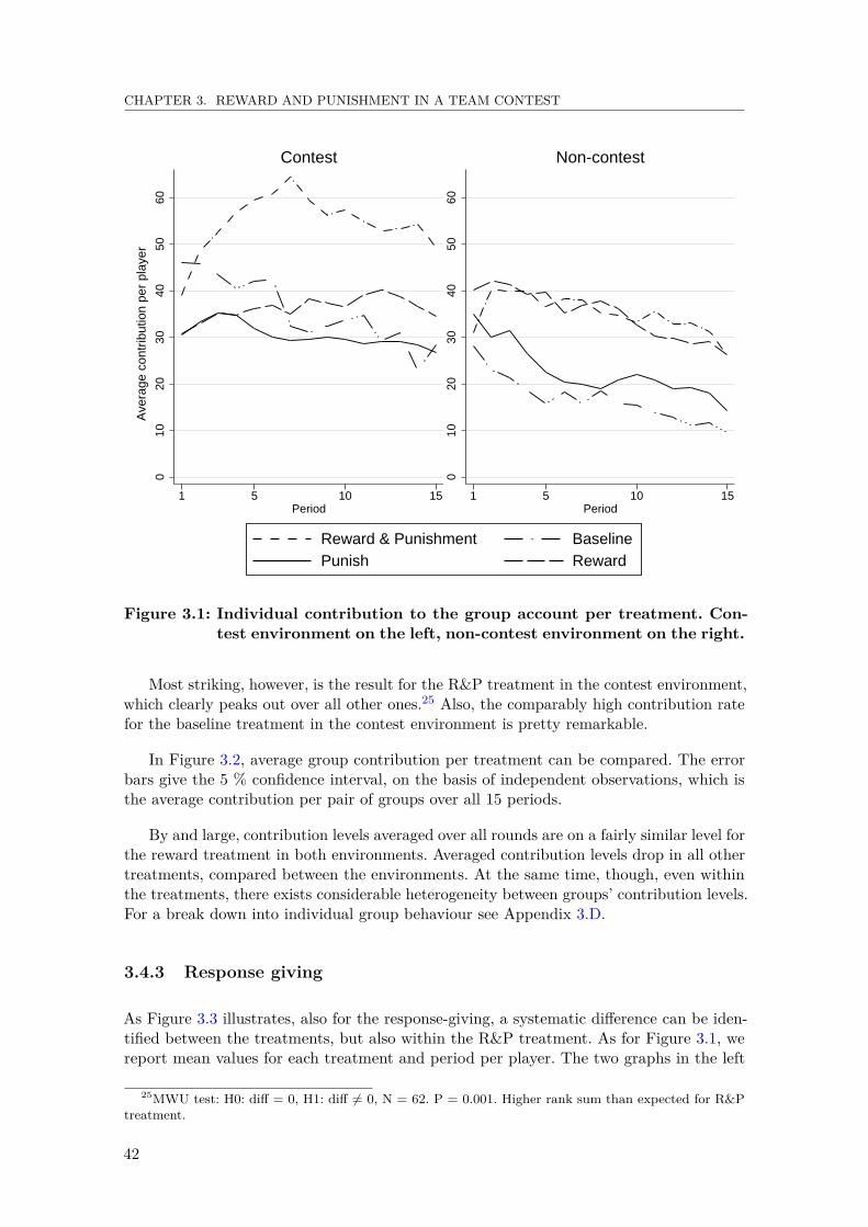
CHAPTER 3. REWARD AND PUNISHMENT IN A TEAM CONTEST
010
2030
4050
60
1 5 10 15Period
Contest
010
2030
4050
60
1 5 10 15Period
Non-contestA
vera
ge c
ontr
ibut
ion
per
play
er
Reward & Punishment BaselinePunish Reward
Figure 3.1: Individual contribution to the group account per treatment. Con-test environment on the left, non-contest environment on the right.
Most striking, however, is the result for the R&P treatment in the contest environment,which clearly peaks out over all other ones.25 Also, the comparably high contribution ratefor the baseline treatment in the contest environment is pretty remarkable.
In Figure 3.2, average group contribution per treatment can be compared. The errorbars give the 5 % confidence interval, on the basis of independent observations, which isthe average contribution per pair of groups over all 15 periods.
By and large, contribution levels averaged over all rounds are on a fairly similar level forthe reward treatment in both environments. Averaged contribution levels drop in all othertreatments, compared between the environments. At the same time, though, even withinthe treatments, there exists considerable heterogeneity between groups’ contribution levels.For a break down into individual group behaviour see Appendix 3.D.
3.4.3 Response giving
As Figure 3.3 illustrates, also for the response-giving, a systematic difference can be iden-tified between the treatments, but also within the R&P treatment. As for Figure 3.1, wereport mean values for each treatment and period per player. The two graphs in the left
25MWU test: H0: diff = 0, H1: diff 6= 0, N = 62. P = 0.001. Higher rank sum than expected for R&Ptreatment.
42
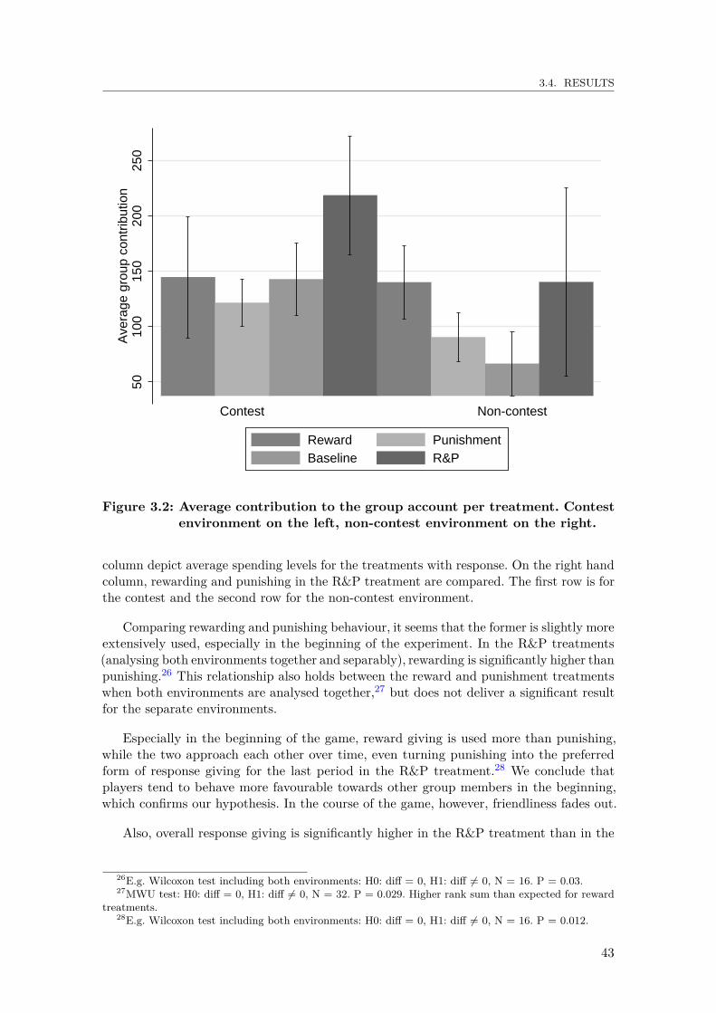
3.4. RESULTS
5010
015
020
025
0A
vera
ge g
roup
con
trib
utio
n
Contest Non-contest
Reward PunishmentBaseline R&P
Figure 3.2: Average contribution to the group account per treatment. Contestenvironment on the left, non-contest environment on the right.
column depict average spending levels for the treatments with response. On the right handcolumn, rewarding and punishing in the R&P treatment are compared. The first row is forthe contest and the second row for the non-contest environment.
Comparing rewarding and punishing behaviour, it seems that the former is slightly moreextensively used, especially in the beginning of the experiment. In the R&P treatments(analysing both environments together and separably), rewarding is significantly higher thanpunishing.26 This relationship also holds between the reward and punishment treatmentswhen both environments are analysed together,27 but does not deliver a significant resultfor the separate environments.
Especially in the beginning of the game, reward giving is used more than punishing,while the two approach each other over time, even turning punishing into the preferredform of response giving for the last period in the R&P treatment.28 We conclude thatplayers tend to behave more favourable towards other group members in the beginning,which confirms our hypothesis. In the course of the game, however, friendliness fades out.
Also, overall response giving is significantly higher in the R&P treatment than in the
26E.g. Wilcoxon test including both environments: H0: diff = 0, H1: diff 6= 0, N = 16. P = 0.03.27MWU test: H0: diff = 0, H1: diff 6= 0, N = 32. P = 0.029. Higher rank sum than expected for reward
treatments.28E.g. Wilcoxon test including both environments: H0: diff = 0, H1: diff 6= 0, N = 16. P = 0.012.
43
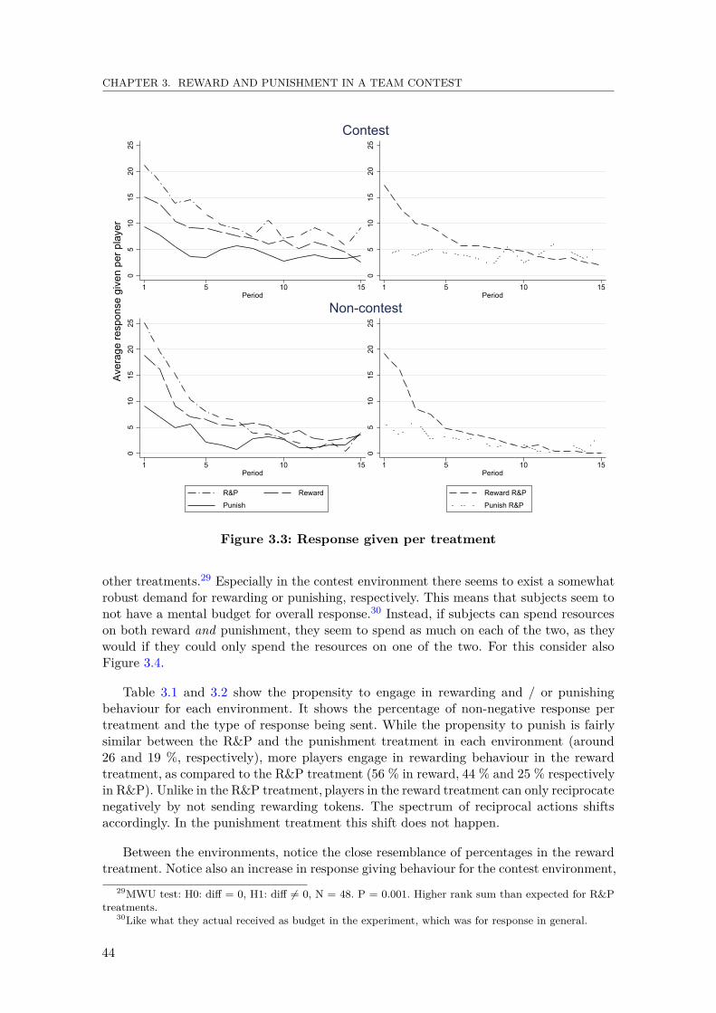
CHAPTER 3. REWARD AND PUNISHMENT IN A TEAM CONTEST
05
1015
2025
1 5 10 15Period
05
1015
2025
1 5 10 15Period
Contest0
510
1520
25
1 5 10 15Period
05
1015
2025
1 5 10 15Period
Non-contest
Ave
rage
res
pons
e gi
ven
per
play
er
R&P Reward
Punish
Reward R&P
Punish R&P
Figure 3.3: Response given per treatment
other treatments.29 Especially in the contest environment there seems to exist a somewhatrobust demand for rewarding or punishing, respectively. This means that subjects seem tonot have a mental budget for overall response.30 Instead, if subjects can spend resourceson both reward and punishment, they seem to spend as much on each of the two, as theywould if they could only spend the resources on one of the two. For this consider alsoFigure 3.4.
Table 3.1 and 3.2 show the propensity to engage in rewarding and / or punishingbehaviour for each environment. It shows the percentage of non-negative response pertreatment and the type of response being sent. While the propensity to punish is fairlysimilar between the R&P and the punishment treatment in each environment (around26 and 19 %, respectively), more players engage in rewarding behaviour in the rewardtreatment, as compared to the R&P treatment (56 % in reward, 44 % and 25 % respectivelyin R&P). Unlike in the R&P treatment, players in the reward treatment can only reciprocatenegatively by not sending rewarding tokens. The spectrum of reciprocal actions shiftsaccordingly. In the punishment treatment this shift does not happen.
Between the environments, notice the close resemblance of percentages in the rewardtreatment. Notice also an increase in response giving behaviour for the contest environment,
29MWU test: H0: diff = 0, H1: diff 6= 0, N = 48. P = 0.001. Higher rank sum than expected for R&Ptreatments.
30Like what they actual received as budget in the experiment, which was for response in general.
44

3.4. RESULTS
02
46
810
Ave
rage
res
pons
e gi
ven
per
grou
p
Contest Non-contest
Reward Punish
Figure 3.4: Response given per treatment
PunishReward No Yes Total
No 46 11 56Yes 29 14 44Total 75 25 100
R&P
RewardNo 44Yes 56Total 100
Reward
PunishNo 73Yes 27Total 100
Punish
Table 3.1: Share of response cases, contest environment (in percentages)Punish
Reward No Yes Total
No 62 11 74Yes 18 8 26Total 80 19 100
R&P
RewardNo 43Yes 57Total 100
Reward
PunishNo 81Yes 19Total 100
Punish
Table 3.2: Share of response cases, non-contest environment (in percentages)
except for the reward treatment.
45

CHAPTER 3. REWARD AND PUNISHMENT IN A TEAM CONTEST
3.4.4 Rent dissipation
Deviations from equilibrium strategy (as devised in Section 3.3.1) of course have payoff-relevant consequences. As mentioned before, mean income was e 16.94 taken across alltreatments. This translates to an amount of 2,540 tokens per player. If all players exhib-ited equilibrium behaviour all throughout the experiment, everyone could have earned onexpectation
E(πNashtot ) =(B + pK · z −
∑k∈K vk
4 + F
)· 15
or(100 + 0.5 · 100− 6.25 + 50) · 15 = 2, 906.25
tokens, or e 19.38, respectively. So overall, players earn almost 15 % less than what theycould earn in Nash equilibrium. The social optimal expected payoff with vi = 0 ∀ i ∈ K∪M ,in comparison, amounts to E(πsoctot ) = 3, 000 tokens or e 20.00.
Losses in total monetary welfare result from higher contributions, as compared to morepayoff-optimal strategies.31 This particularly emerges in the R&P treatment of the contestenvironment, where mean income was about e 3.94 or 591 tokens (about 22 %) lower thanin the other treatments. Also, as a result of higher spending and punishing, average incomein the contest environment was roughly e 4.00 lower than in the non-contest (about 601tokens, 20%).
Table 3.3 gives an overview on the extent and composition of overspending per treatment.We compare the total sum of individual contest expenditures and response giving with theNash equilibrium benchmark and report the respective spending level that exceeds thisthreshold. The total level of overspending in each treatment of the non-contest environmentis lower as its counterpart in the contest environment. For the Baseline treatments thisdecline is even as high as 60 %.
Overspending OverspendingTreatment contribution response Total
R&P 725.73 163.27 889.00Reward 448.98 117.84 566.83Punish 362.19 70.48 432.67
Con
test
Baseline 441.91 −.− 441.91
R&P 432.09 111.06 543.16Reward 431.03 99.25 530.28Punish 245.34 49.13 294.47
Non
-con
test
Baseline 155.46 −.− 155.46
Table 3.3: Individual overspending compared to the Nash equilibrium bench-mark
31As discussed earlier, contribution to the group account is unproductive effort which has no positiveinfluence on the amount of tokens that can be won, as the prize at stake is fixed. Tokens put in the groupaccount only influence the winning probability.
46
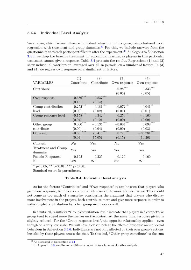
3.4. RESULTS
3.4.5 Individual Level Analysis
We analyse, which factors influence individual behaviour in this game, using clustered Tobitregression with treatment and group dummies.32 For this, we include answers from thequestionnaire that each participant filled in after the experiment.33 Analogous to Subsection3.4.3, we drop the baseline treatment for conceptual reasons, as players in this particulartreatment cannot give a response. Table 3.4 presents the results. Regressions (1) and (2)show individual contribution, averaged over all 15 periods, on a number of factors. In (3)and (4) we regress own response on a similar set of factors.
(1) (2) (3) (4)VARIABLES Contribute Contribute Own response Own response
Contribute 0.28*** 0.333***
(0.05) (0.05)Own response 0.686*** 0.837***
(0.15) (0.14)Group contribution 0.252*** 0.181*** −0.072*** −0.041**
level (0.00) (0.02) (0.01) (0.01)Group response level −0.158*** 0.342** 0.250*** −0.160
(0.04) (0.12) (0.00) (0.09)Other group 0.000*** −0.135*** −0.004*** 0.098***
contribute (0.00) (0.04) (0.00) (0.03)Constant −0.331*** 70.418*** 0.773*** −35.781***
(0.04) (15.05) (0.15) (10.26)
Controls No Y es No Y esTreatment and Group Yes Yes Yes YesdummiesPseudo R-squared 0.192 0.225 0.120 0.160N 288 270 288 270* p<0.05, ** p<0.01, *** p<0.001Standard errors in parentheses.
Table 3.4: Individual level analysis
As for the factors “Contribute” and “Own response” it can be seen that players whogive more response, tend to also be those who contribute more and vice versa. This shouldnot come as too much of a surprise, considering the argument that players who displaymore involvement in the project, both contribute more and give more response in order toinduce higher contribution by other group members as well.
In a nutshell, results for “Group contribution level” indicate that players in a competitivegroup tend to spend more themselves on the contest. At the same time, response giving isslightly reduced. For the “Group response level”, the opposite relationship applies – eventhough on a very low scale. We will have a closer look at the effect of response on individualbehaviour in Subsection 3.4.6. Individuals are not only affected by their own group’s actions,but also by those players across the aisle. To this end, “Other group contribute” is the sum
32As discussed in Subsection 3.4.133In Appendix 3.E we discuss additional control factors in an explorative analysis.
47
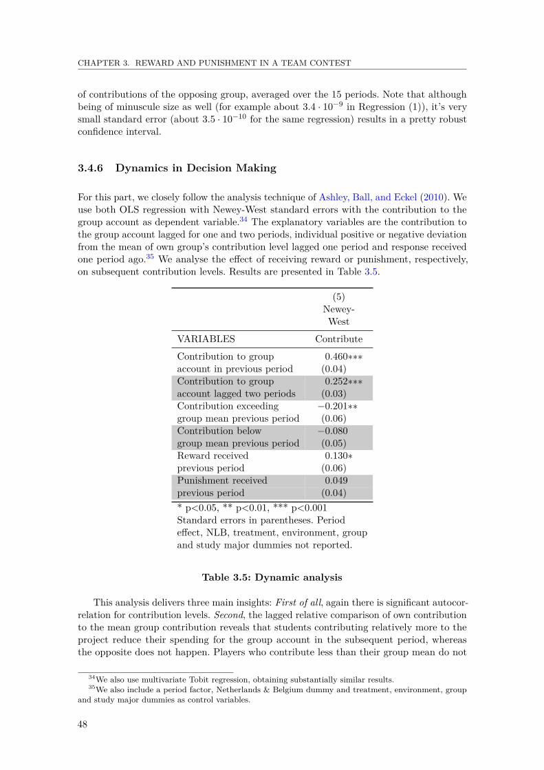
CHAPTER 3. REWARD AND PUNISHMENT IN A TEAM CONTEST
of contributions of the opposing group, averaged over the 15 periods. Note that althoughbeing of minuscule size as well (for example about 3.4 · 10−9 in Regression (1)), it’s verysmall standard error (about 3.5 · 10−10 for the same regression) results in a pretty robustconfidence interval.
3.4.6 Dynamics in Decision Making
For this part, we closely follow the analysis technique of Ashley, Ball, and Eckel (2010). Weuse both OLS regression with Newey-West standard errors with the contribution to thegroup account as dependent variable.34 The explanatory variables are the contribution tothe group account lagged for one and two periods, individual positive or negative deviationfrom the mean of own group’s contribution level lagged one period and response receivedone period ago.35 We analyse the effect of receiving reward or punishment, respectively,on subsequent contribution levels. Results are presented in Table 3.5.
(5)Newey-West
VARIABLES Contribute
Contribution to group 0.460∗∗∗account in previous period (0.04)Contribution to group 0.252∗∗∗account lagged two periods (0.03)Contribution exceeding −0.201∗∗group mean previous period (0.06)Contribution below −0.080group mean previous period (0.05)Reward received 0.130∗previous period (0.06)Punishment received 0.049previous period (0.04)* p<0.05, ** p<0.01, *** p<0.001Standard errors in parentheses. Periodeffect, NLB, treatment, environment, groupand study major dummies not reported.
Table 3.5: Dynamic analysis
This analysis delivers three main insights: First of all, again there is significant autocor-relation for contribution levels. Second, the lagged relative comparison of own contributionto the mean group contribution reveals that students contributing relatively more to theproject reduce their spending for the group account in the subsequent period, whereasthe opposite does not happen. Players who contribute less than their group mean do not
34We also use multivariate Tobit regression, obtaining substantially similar results.35We also include a period factor, Netherlands & Belgium dummy and treatment, environment, group
and study major dummies as control variables.
48
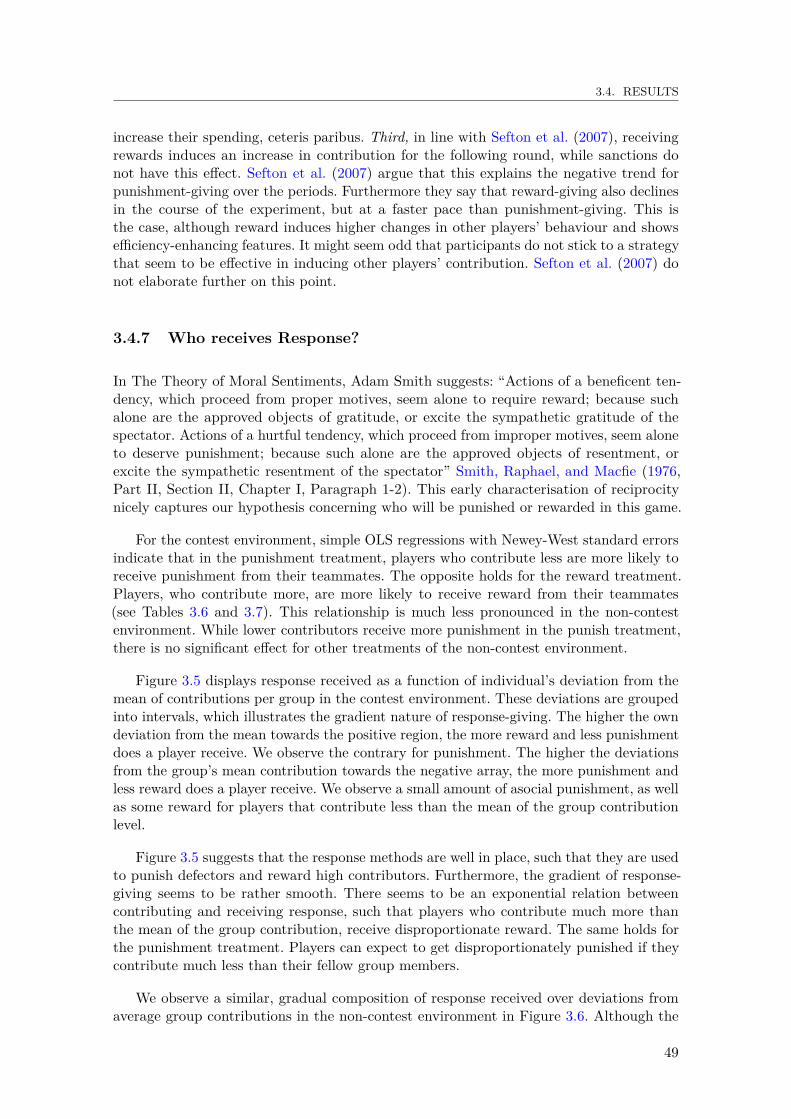
3.4. RESULTS
increase their spending, ceteris paribus. Third, in line with Sefton et al. (2007), receivingrewards induces an increase in contribution for the following round, while sanctions donot have this effect. Sefton et al. (2007) argue that this explains the negative trend forpunishment-giving over the periods. Furthermore they say that reward-giving also declinesin the course of the experiment, but at a faster pace than punishment-giving. This isthe case, although reward induces higher changes in other players’ behaviour and showsefficiency-enhancing features. It might seem odd that participants do not stick to a strategythat seem to be effective in inducing other players’ contribution. Sefton et al. (2007) donot elaborate further on this point.
3.4.7 Who receives Response?
In The Theory of Moral Sentiments, Adam Smith suggests: “Actions of a beneficent ten-dency, which proceed from proper motives, seem alone to require reward; because suchalone are the approved objects of gratitude, or excite the sympathetic gratitude of thespectator. Actions of a hurtful tendency, which proceed from improper motives, seem aloneto deserve punishment; because such alone are the approved objects of resentment, orexcite the sympathetic resentment of the spectator” Smith, Raphael, and Macfie (1976,Part II, Section II, Chapter I, Paragraph 1-2). This early characterisation of reciprocitynicely captures our hypothesis concerning who will be punished or rewarded in this game.
For the contest environment, simple OLS regressions with Newey-West standard errorsindicate that in the punishment treatment, players who contribute less are more likely toreceive punishment from their teammates. The opposite holds for the reward treatment.Players, who contribute more, are more likely to receive reward from their teammates(see Tables 3.6 and 3.7). This relationship is much less pronounced in the non-contestenvironment. While lower contributors receive more punishment in the punish treatment,there is no significant effect for other treatments of the non-contest environment.
Figure 3.5 displays response received as a function of individual’s deviation from themean of contributions per group in the contest environment. These deviations are groupedinto intervals, which illustrates the gradient nature of response-giving. The higher the owndeviation from the mean towards the positive region, the more reward and less punishmentdoes a player receive. We observe the contrary for punishment. The higher the deviationsfrom the group’s mean contribution towards the negative array, the more punishment andless reward does a player receive. We observe a small amount of asocial punishment, as wellas some reward for players that contribute less than the mean of the group contributionlevel.
Figure 3.5 suggests that the response methods are well in place, such that they are usedto punish defectors and reward high contributors. Furthermore, the gradient of response-giving seems to be rather smooth. There seems to be an exponential relation betweencontributing and receiving response, such that players who contribute much more thanthe mean of the group contribution, receive disproportionate reward. The same holds forthe punishment treatment. Players can expect to get disproportionately punished if theycontribute much less than their fellow group members.
We observe a similar, gradual composition of response received over deviations fromaverage group contributions in the non-contest environment in Figure 3.6. Although the
49
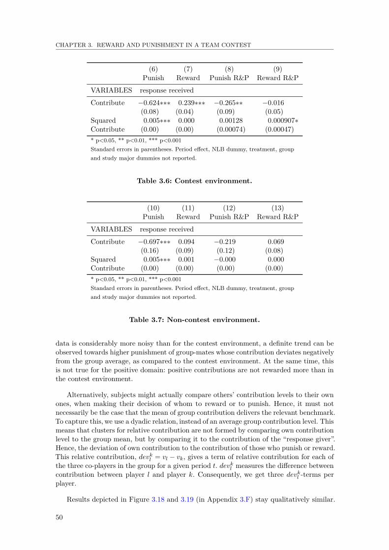
CHAPTER 3. REWARD AND PUNISHMENT IN A TEAM CONTEST
(6) (7) (8) (9)Punish Reward Punish R&P Reward R&P
VARIABLES response received
Contribute −0.624∗∗∗ 0.239∗∗∗ −0.265∗∗ −0.016(0.08) (0.04) (0.09) (0.05)
Squared 0.005∗∗∗ 0.000 0.00128 0.000907∗Contribute (0.00) (0.00) (0.00074) (0.00047)* p<0.05, ** p<0.01, *** p<0.001Standard errors in parentheses. Period effect, NLB dummy, treatment, groupand study major dummies not reported.
Table 3.6: Contest environment.
(10) (11) (12) (13)Punish Reward Punish R&P Reward R&P
VARIABLES response received
Contribute −0.697∗∗∗ 0.094 −0.219 0.069(0.16) (0.09) (0.12) (0.08)
Squared 0.005∗∗∗ 0.001 −0.000 0.000Contribute (0.00) (0.00) (0.00) (0.00)* p<0.05, ** p<0.01, *** p<0.001Standard errors in parentheses. Period effect, NLB dummy, treatment, groupand study major dummies not reported.
Table 3.7: Non-contest environment.
data is considerably more noisy than for the contest environment, a definite trend can beobserved towards higher punishment of group-mates whose contribution deviates negativelyfrom the group average, as compared to the contest environment. At the same time, thisis not true for the positive domain: positive contributions are not rewarded more than inthe contest environment.
Alternatively, subjects might actually compare others’ contribution levels to their ownones, when making their decision of whom to reward or to punish. Hence, it must notnecessarily be the case that the mean of group contribution delivers the relevant benchmark.To capture this, we use a dyadic relation, instead of an average group contribution level. Thismeans that clusters for relative contribution are not formed by comparing own contributionlevel to the group mean, but by comparing it to the contribution of the “response giver”.Hence, the deviation of own contribution to the contribution of those who punish or reward.This relative contribution, devkl = vl − vk, gives a term of relative contribution for each ofthe three co-players in the group for a given period t. devkl measures the difference betweencontribution between player l and player k. Consequently, we get three devkl -terms perplayer.
Results depicted in Figure 3.18 and 3.19 (in Appendix 3.F) stay qualitatively similar.
50
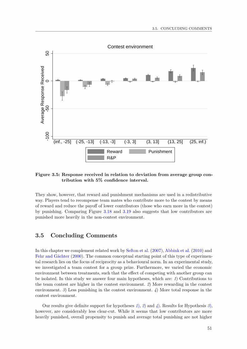
3.5. CONCLUDING COMMENTS
-100
-50
050
Ave
rage
Res
pons
e R
ecei
ved
(inf., -25] (-25, -13] (-13, -3] (-3, 3] (3, 13] (13, 25] (25, inf.)
Reward PunishmentR&P
Contest environment
Figure 3.5: Response received in relation to deviation from average group con-tribution with 5% confidence interval.
They show, however, that reward and punishment mechanisms are used in a redistributiveway. Players tend to recompense team mates who contribute more to the contest by meansof reward and reduce the payoff of lower contributors (those who earn more in the contest)by punishing. Comparing Figure 3.18 and 3.19 also suggests that low contributors arepunished more heavily in the non-contest environment.
3.5 Concluding Comments
In this chapter we complement related work by Sefton et al. (2007), Abbink et al. (2010) andFehr and Gächter (2000). The common conceptual starting point of this type of experimen-tal research lies on the focus of reciprocity as a behavioural norm. In an experimental study,we investigated a team contest for a group prize. Furthermore, we varied the economicenvironment between treatments, such that the effect of competing with another group canbe isolated. In this study we answer four main hypotheses, which are: 1) Contributions tothe team contest are higher in the contest environment. 2) More rewarding in the contestenvironment. 3) Less punishing in the contest environment. 4) More total response in thecontest environment.
Our results give definite support for hypotheses 1), 2) and 4). Results for Hypothesis 3),however, are considerably less clear-cut. While it seems that low contributors are moreheavily punished, overall propensity to punish and average total punishing are not higher
51
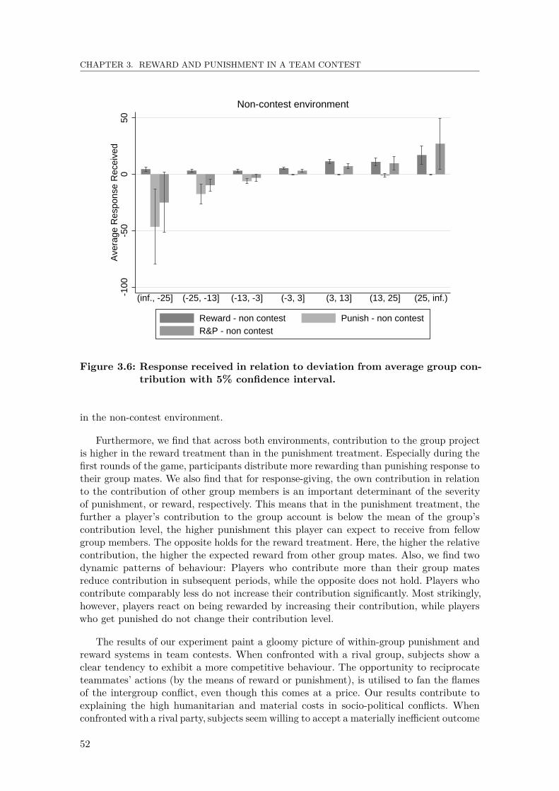
CHAPTER 3. REWARD AND PUNISHMENT IN A TEAM CONTEST
-100
-50
050
Ave
rage
Res
pons
e R
ecei
ved
(inf., -25] (-25, -13] (-13, -3] (-3, 3] (3, 13] (13, 25] (25, inf.)
Reward - non contest Punish - non contestR&P - non contest
Non-contest environment
Figure 3.6: Response received in relation to deviation from average group con-tribution with 5% confidence interval.
in the non-contest environment.
Furthermore, we find that across both environments, contribution to the group projectis higher in the reward treatment than in the punishment treatment. Especially during thefirst rounds of the game, participants distribute more rewarding than punishing response totheir group mates. We also find that for response-giving, the own contribution in relationto the contribution of other group members is an important determinant of the severityof punishment, or reward, respectively. This means that in the punishment treatment, thefurther a player’s contribution to the group account is below the mean of the group’scontribution level, the higher punishment this player can expect to receive from fellowgroup members. The opposite holds for the reward treatment. Here, the higher the relativecontribution, the higher the expected reward from other group mates. Also, we find twodynamic patterns of behaviour: Players who contribute more than their group matesreduce contribution in subsequent periods, while the opposite does not hold. Players whocontribute comparably less do not increase their contribution significantly. Most strikingly,however, players react on being rewarded by increasing their contribution, while playerswho get punished do not change their contribution level.
The results of our experiment paint a gloomy picture of within-group punishment andreward systems in team contests. When confronted with a rival group, subjects show aclear tendency to exhibit a more competitive behaviour. The opportunity to reciprocateteammates’ actions (by the means of reward or punishment), is utilised to fan the flamesof the intergroup conflict, even though this comes at a price. Our results contribute toexplaining the high humanitarian and material costs in socio-political conflicts. Whenconfronted with a rival party, subjects seem willing to accept a materially inefficient outcome
52
3.5. CONCLUDING COMMENTS
to outrun the opponent. All the more so, subjects incite their comrades to join in arms.In the anonymous and abstract environment of this computer laboratory, we find theseoutcomes absent of any religious or ethnic spur. In field environments, the emotionalimpetus attached to these kind of conflicts will be even stronger, given a usually highersocial identity within the conflict parties.
In a corporate context, consider a construction firm running for a tender. Althougheach unit has some incentive to not invest resources in the project of the firm, high inputsincrease the probability for the firm to win the tender and to get the project awarded. Ourresearch suggests that in this kind of situation, the company should not only point outto their employees that they are in a competitive situation in order to encourage highereffort. The implementation of a rewarding scheme should particularly trigger up individualeffort in the contest. Results by Balliet et al. (2011); O’Gorman et al. (2009) suggest thatit should not matter if there exists a scheme of mutual rewarding, similar to the setup inour experiment, or whether one central agent is entrusted with this task.
There are a number of conceivable extensions: Allowing for communication couldformalise a sort of non-binding contract between the participants. In an experimentalstudy using a group contest game with a weakest-link production function (total groupcontribution is determined by the lowest individual effort in that group), Cason, Sheremeta,and Zhang (2012) allow for inter- and intra-group communication via a free form chat ina 2x2 design.36 They show that communication between groups has an abating effect oncontest spending, which positively influences overall welfare. Within-group communication,by contrast, displays the opposite effect, leading to an escalation of the contest with a morethan doubling of contest expenditures. In a treatment with both communication types, thetwo effects cancel out, leading to a level of competition and payoffs being not significantlydifferent from the baseline treatment.
By randomising identification numbers of players, reputation building would be ex-cluded. Hypothetically, this should lead to a decrease in response-giving and also to areduction in contribution to the group account. Going one step further, groups could evenbe set up in a randomized way. Group cohesion is expected to be even smaller than in theprevious case, resulting in less response-giving and lower contribution levels.
In our design of the contest game, the prize for winning a round is set such that theNash equilibrium for contribution is on a rather low level of players’ endowment withtokens. Throughout the game we constantly observe a massive over-investment acrosstreatments. By varying the prize at stake, which changes the game’s Nash equilibrium,can elicit subjects’ elasticity towards the contest prize. This might also have an effecton response-giving, making subjects react more aggressively towards free-riders, with anincrease in rewarding and punishing.
36Sutter and Strassmair (2009) study a similar team tournament game with chat communication. Themain differences between their game setup and the one employed by Cason et al. (2012) and in our studyis twofold: First, in Cason et al. (2012) and in our study, efforts are socially wasteful and social welfareincreases when players coordinate on a lower spending level. Second, Cason et al. (2012) and our studyemploy a probabilistic contest success function, while in Sutter and Strassmair (2009), the prize is given tothe group with the higher (stochastic) effort. By and large, chat communication leads to higher contributionlevels in Sutter and Strassmair (2009), which in their setup has positive welfare implications.
53
CHAPTER 3. REWARD AND PUNISHMENT IN A TEAM CONTEST
Appendix 3.A Instructions
When entering the cubicle, each participant found a printed version of the following exper-iment instructions at her seat. Paragraphs headed by a treatment name in square bracketswere only given to the subjects of the corresponding treatment. The following exampleis from the contest treatments. Instructions for the non-contest treatments are slightlyadjusted such as to not mention another group and avoid referring to teams or teammates.37
CG Experiment
Welcome and thank you for participating in this experiment. Please read these instructionscarefully. If you have any questions, please raise your hand and one of the hosts of theexperiment will come to your cubicle to answer your question. Talking or using mobilephones or any other electronic devices is strictly prohibited. Mobile phones and otherelectronic devices should be left in the waiting room or switched off. If you are foundviolating these rules, you will both forfeit any earnings from this experiment, and may beexcluded from future experiments as well.
This is an experiment about decision making. The instructions are simple and if youfollow them carefully you might earn a considerable amount of money which will be paidto you privately and in cash at the end of today’s session. The amount of money you earndepends on your decisions, on other participants’ decisions and on random events. You willnever be asked to reveal your identity to anyone during the course of the experiment. Yourname will never be associated with any of your decisions. In order to keep your decisionsprivate, do not reveal your choices to any other participant.
During the experiment you will have the chance to earn points, which will be convertedinto cash at the end of today’s session, using an exchange rate of
15 points = 0,1 e .Thus, the more points you earn, the more cash you will receive at the end of the session.
You and three other participants are assigned to a team. Four other participantsare assigned to another team. All participants will remain in their teams for the entireexperiment. None of you will learn who the own team members or the other team membersare.
The experiment will consist of 15 periods, and in each period your team and the otherteam are competing for a prize in the following way:
At the beginning of each period you will receive 100 points. Then you can use thesepoints to buy lottery tickets for your team. Any point you invest gives one lottery ticketfor the team. Any point you do not invest in lottery tickets will be accumulated in yourprivate point balance. Likewise, your team members can buy tickets for your team and themembers of the other team can buy tickets for their team in exactly the same way.
As soon as everybody has chosen how many tickets to buy, a lottery will determinewhether your team or the other team wins a prize of 400 points (100 for each team member).
37Details available upon request.
54

3.A. INSTRUCTIONS
One of the sold tickets is randomly assigned the winning ticket. Each ticket has the samechance. Hence, the more tickets your team buys, the higher is your chance of winning theprize.
Examples: If your team and the other team buy the same amount of tickets then thechance of winning the prize is 50:50. If your team buys three times as many tickets as theother team, then also your team’s chances are three times as high as those of the otherteam. If only one of the teams buys tickets then this team wins the prize with certainty.
If neither your team nor the other team buys a ticket, then the prize is randomlyallocated to one of the teams with equal chances.
After the winning team is determined the prize of 400 points is equally shared andadded to the private point balances of the winning team (100 points for each team member).
[Reward treatment:] At the end you get 50 feedback points. You can put these pointsto your private point balance or you can assign them to one or more of your team members(not to members of the other team). Each feedback point assigned to a team memberincreases this team member’s private balance by one point.
[Punishment treatment:] At the end you get 50 feedback points. You can put them toyour private point balance or you can assign the feedback points to one or more of yourteam members (not to members of the other team). Each feedback point assigned to a teammember decreases this team member’s private balance by one point. A team member’sbalance for one particular round cannot turn negative. If this happens then the balancefor this particular round is set to zero and all excess feedback points are invalidated.
[Baseline treatment:] At the end you get 50 extra points which will add to your account.
[R&P treatment:] At the end you get 50 feedback points. You can put them to yourprivate point balance or you can assign the feedback points to one or more of your teammembers (not to members of the other team). You can decide whether you assign thepoints to be added to the respective team member’s account or to be subtracted fromthat account. Each feedback point assigned to a team member increases or decreases thisteam member’s private balance by one point âĂŞ depending on what you choose. A teammember’s balance for one particular round cannot turn negative. If this happens then thebalance for this particular round is set to zero and all excess feedback points are invalidated.
The points you earn in each period will be added together. At the end of the sessionyou will be paid based on your total point earning from all 15 periods.
The experiment starts with a trial period in which you will be asked to fill in somequestions in order to check your understanding of the experiment and to give you theopportunity to get acquainted with the setup. Points earned in this trial period will notbe paid off.
55

CHAPTER 3. REWARD AND PUNISHMENT IN A TEAM CONTEST
Appendix 3.B Stages
Figure 3.7 to Figure 3.9 show screenshots from the punishment treatment. Other treatmentslook similar, adjusting only references to the payoff consequences of receiving response andleaving out mentioning of another group in the treatments without competing group.
Figure 3.7: First stage
56

3.B. STAGES
Figure 3.8: Second stage
Figure 3.9: Third stage
57
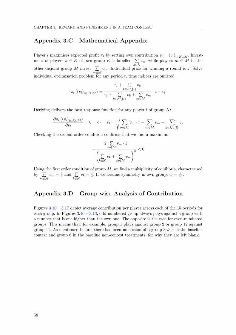
CHAPTER 3. REWARD AND PUNISHMENT IN A TEAM CONTEST
Appendix 3.C Mathematical Appendix
Player l maximises expected profit πl by setting own contribution vl = (vi)i∈K∪M . Invest-ment of players k ∈ K of own group K is labelled
∑k∈K
vk, while players m ∈ M in the
other disjoint group M invest∑
m∈Mvm. Individual prize for winning a round is z. Solve
individual optimisation problem for any period t, time indices are omitted.
πl((vi)i∈K∪M
)=
vl +∑
k∈K\{l}vk
vl +∑
k∈K\{l}vk +
∑m∈M
vm· z − vl
Deriving delivers the best response function for any player l of group K:
∂πl((vi)i∈K∪M
)∂vl
= 0 ⇔ vl =√ ∑m∈M
vm · z −∑m∈M
vm −∑
k∈K\{l}vk
Checking the second order condition confirms that we find a maximum:
−2∑
m∈Mvm · z( ∑
k∈Kvk +
∑m∈M
vm
)3 < 0
Using the first order condition of groupM , we find a multiplicity of equilibria, characterisedby
∑m∈M
vm = z4 and
∑k∈K
vk = z4 . If we assume symmetry in own group: vl = z
16 .
Appendix 3.D Group wise Analysis of Contribution
Figures 3.10 – 3.17 depict average contribution per player across each of the 15 periods foreach group. In Figures 3.10 – 3.13, odd-numbered group always plays against a group witha number that is one higher than the own one. The opposite is the case for even-numberedgroups. This means that, for example, group 1 plays against group 2 or group 12 againstgroup 11. As mentioned before, there has been no session of a group 3 & 4 in the baselinecontest and group 6 in the baseline non-contest treatments, for why they are left blank.
58
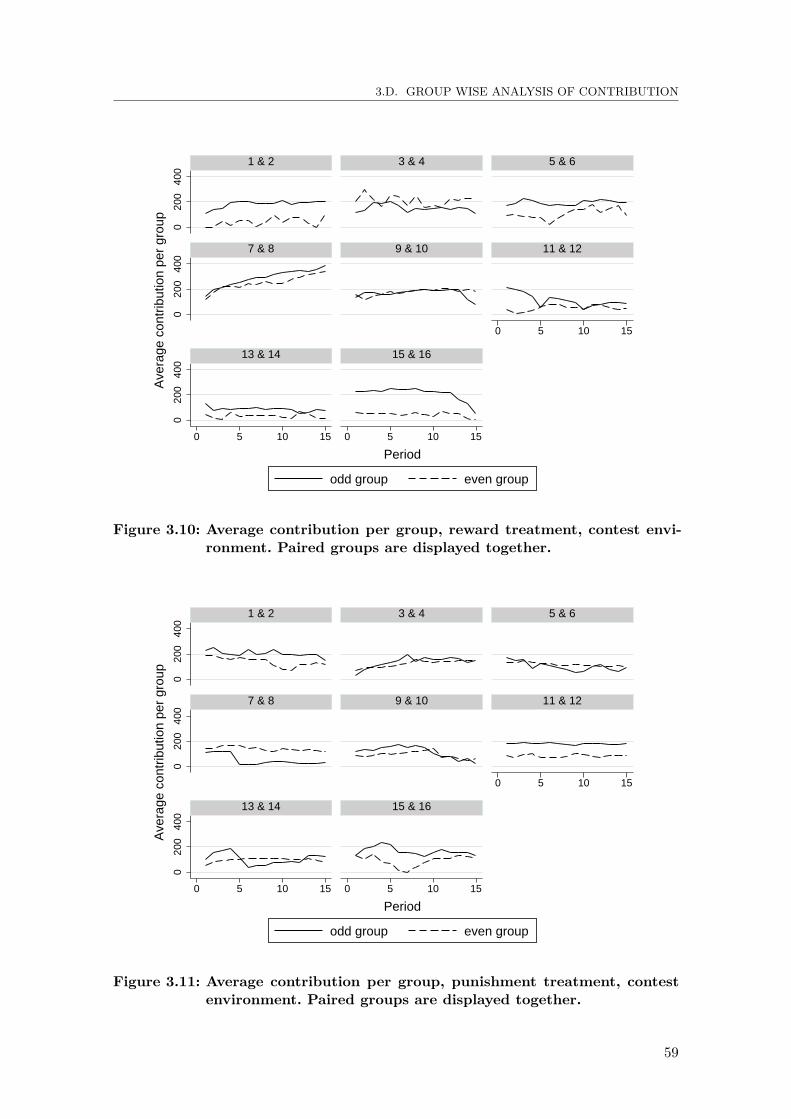
3.D. GROUP WISE ANALYSIS OF CONTRIBUTION
020
040
00
200
400
020
040
0
0 5 10 15
0 5 10 15 0 5 10 15
1 & 2 3 & 4 5 & 6
7 & 8 9 & 10 11 & 12
13 & 14 15 & 16
odd group even group
Ave
rage
con
trib
utio
n pe
r gr
oup
Period
Figure 3.10: Average contribution per group, reward treatment, contest envi-ronment. Paired groups are displayed together.
020
040
00
200
400
020
040
0
0 5 10 15
0 5 10 15 0 5 10 15
1 & 2 3 & 4 5 & 6
7 & 8 9 & 10 11 & 12
13 & 14 15 & 16
odd group even group
Ave
rage
con
trib
utio
n pe
r gr
oup
Period
Figure 3.11: Average contribution per group, punishment treatment, contestenvironment. Paired groups are displayed together.
59

CHAPTER 3. REWARD AND PUNISHMENT IN A TEAM CONTEST
020
040
00
200
400
020
040
0
0 5 10 15
0 5 10 15 0 5 10 15
1 & 2 3 & 4 5 & 6
7 & 8 9 & 10 11 & 12
13 & 14 15 & 16
odd group even group
Ave
rage
con
trib
utio
n pe
r gr
oup
Period
Figure 3.12: Average contribution per group, baseline treatment, contest envi-ronment. Paired groups are displayed together. Session for groups3 & 4 did not take place due to no-shows.
020
040
00
200
400
020
040
0
0 5 10 15
0 5 10 15 0 5 10 15
1 & 2 3 & 4 5 & 6
7 & 8 9 & 10 11 & 12
13 & 14 15 & 16
odd group even group
Ave
rage
con
trib
utio
n pe
r gr
oup
Period
Figure 3.13: Average contribution per group, R&P treatment, contest environ-ment. Paired groups are displayed together.
60

3.D. GROUP WISE ANALYSIS OF CONTRIBUTION
020
040
00
200
400
020
040
0
0 5 10 15
0 5 10 15 0 5 10 15
1 2 3
4 5 6
7 8
Group Blank tickets
Ave
rage
con
trib
utio
n pe
r gr
oup
Period
Figure 3.14: Average contribution per group, reward treatment, non-contestenvironment.
020
040
00
200
400
020
040
0
0 5 10 15
0 5 10 15 0 5 10 15
1 2 3
4 5 6
7 8
Group Blank tickets
Ave
rage
con
trib
utio
n pe
r gr
oup
Period
Figure 3.15: Average contribution per group, punishment treatment, non-contest environment.
61

CHAPTER 3. REWARD AND PUNISHMENT IN A TEAM CONTEST
020
040
00
200
400
020
040
0
0 5 10 15
0 5 10 15 0 5 10 15
1 2 3
4 5 6
7 8
Group Blank tickets
Ave
rage
con
trib
utio
n pe
r gr
oup
Period
Figure 3.16: Average contribution per group, baseline treatment, non-contestenvironment. Session for group 6 did not take place due to no-shows.
020
040
00
200
400
020
040
0
0 5 10 15
0 5 10 15 0 5 10 15
1 2 3
4 5 6
7 8
Group Blank tickets
Ave
rage
con
trib
utio
n pe
r gr
oup
Period
Figure 3.17: Average contribution per group, R&P treatment, non-contest en-vironment.
62
3.E. PERSONAL ATTRIBUTES
Appendix 3.E Personal attributes
Table 3.8 corresponds to regressions (2) and (4) from Table 3.4 with explicit controlparameters. They were generated by subjects’ answers to a post-experiment questionnaire,in which we ask about a few personal features and stances. For this, we used questionsfrom the World Values Survey (Inglehart and Archivo de Estudios Sociales, 2000). In thissection we examine the control factors in more detail.
Most notably, domestic students from the Netherlands and Belgium contribute sub-stantially less to the contest than their colleagues from other countries do. This is the onlysignificant country effect and its magnitude is somewhat impressive.
Players who state to place more importance on individual responsibility (as opposed togovernmental responsibility) contribute less to the contest, but give more response. Thisfactor was created on a scale from one to seven where individuals stated their proximityto which of the two statements they feel closer.38 Players with a higher preference forindividual responsibility hence tend to be reluctant towards spending their money forthe group project, but are willing to reciprocate by the means of response. “Preferencefor working alone” was also created on a scale of one to seven with the statement thatthe individual prefers working in groups or alone at the extremes, to which she expressesproximity.39 Players who prefer to work alone give less response, which means they actless reciprocal.
Both factors “Work important” and “Smoking” influence response-giving positively. Theformer was created on a seven point scale in which participants express the importanceof labour in their life. Furthermore, we enquire on our subjects’ smoking behaviour asproxy for short-sightedness as in e.g. Slovic (2001). Next to a more reactionary responsebehaviour, individuals who indicate that they smoke also tend to spend less resourcestowards the contest.
Other items displaying a lowering effect towards contest spendings are “Family andfriends important” (Participants’ stated preference on a scale from 1 – 7) and “Politicsimportant”. They have been generated like the factor “Work important” on a seven pointscale. The following three parameters, by contrast, display a positive effect on contestcontributions: “Trust parameter” (Proximity to the two statements: Most people can betrusted – Need to be very careful), “Siblings” and “Study phase”. Placing tokens into thegroup account involves some degree of trust towards ones teammates that they will notrenege or pursue an abating strategy. Additionally, participants in a later “Study phase”use less tokens to reciprocate teammates’ actions. Lastly, relatively older participants tendto spend less tokens to the contest, but more on reciprocating, which is reflected in regressor“Age”. Given the participant body of our study is comprised almost exclusively of students,this result could open up an interesting pathway towards a follow-up study, employing asubject pool with a wider age structure.
Two factors for which we contemplated having explanatory power in this game remaintoothless. Those are “Current happiness” and “Ever practised a team sport”, which haveneither an influence on players’ contest spendings nor response giving behaviour.
38The two extremes were “The government should take more responsibility to ensure that everyone isprovided for.” versus “People should take more responsibility to provide for themselves.”
39The two extremes were “I like working in groups” versus “I like working on my own”
63

CHAPTER 3. REWARD AND PUNISHMENT IN A TEAM CONTEST
(2a) (4a)VARIABLES Contribute Own response
Contribute 0.333***
(0.05)Own response 0.837***
(0.14)Group contribution 0.181*** −0.041***
level (0.02) (0.01)Group response level 0.342*** −0.160*
(0.12) (0.09)Other group −0.135*** 0.098***
contribute (0.04) (0.03)Netherlands and −7.473*** 1.805Belgium (1.76) (1.59)Preference for 0.501 −0.965***
working alone (0.49) (0.35)Individual −1.394*** 0.764**
Responsibility (0.44) (0.31)Work important 0.308 1.535**
(0.92) (0.71)Smoking −4.573** 4.342***
(2.17) (1.60)Trust parameter 2.395** −0.508
(1.19) (0.91)Family and friends −2.872** −0.510important (1.16) (0.98)Politics important −1.475* 0.384
(0.85) (0.45)Current happiness 0.878 −0.759
(1.08) (0.61)Ever practised a −1.517 1.530team sport (1.15) (1.10)Siblings 1.286* −0.484
(0.72) (0.41)Study phase 3.194* −3.316***
(1.66) (1.17)Age −0.812*** 0.531**
(0.30) (0.24)Constant 70.418*** −35.781***
(15.05) (10.26)
Pseudo R-squared 0.225 0.160N 270 270* p<0.05, ** p<0.01, *** p<0.001Standard errors in parentheses. Treatment, groupand study major dummies not reported.
Table 3.8: Individual level analysis
64
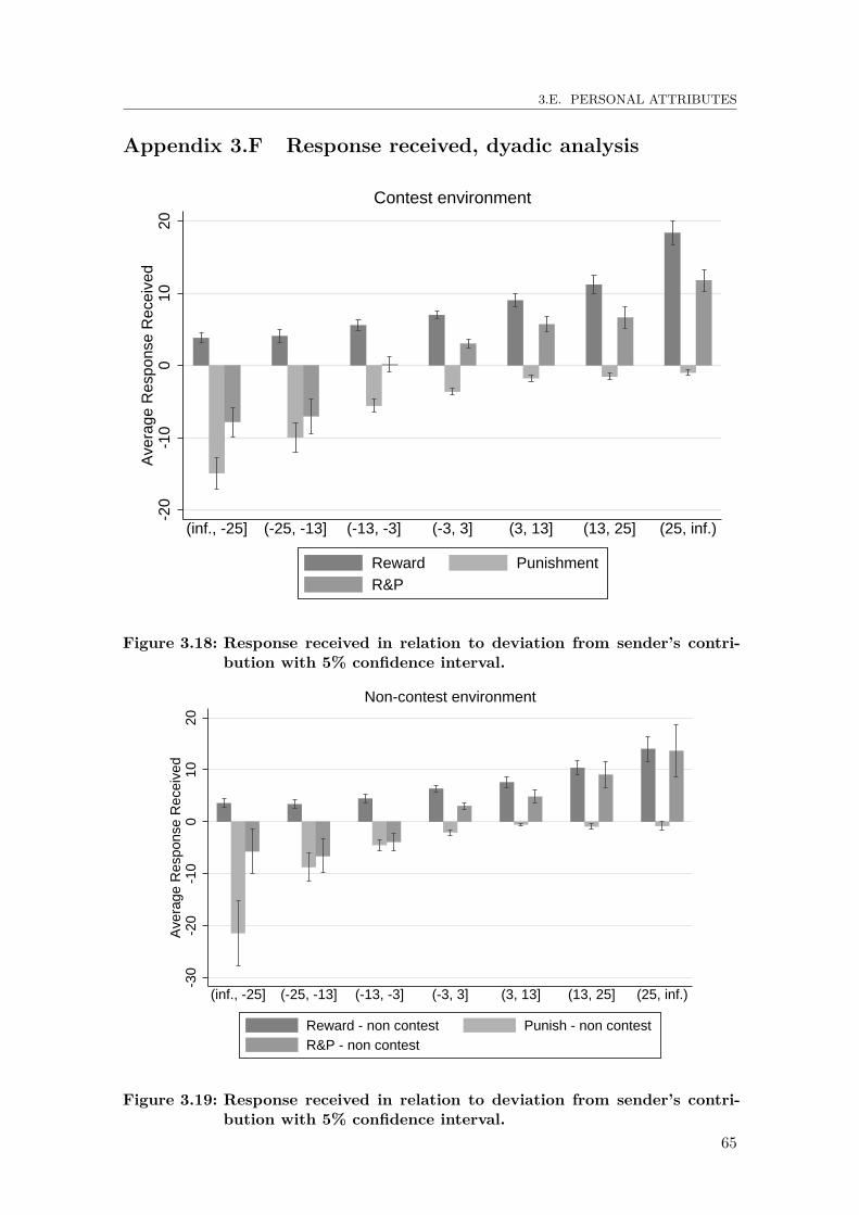
3.E. PERSONAL ATTRIBUTES
Appendix 3.F Response received, dyadic analysis-2
0-1
00
1020
Ave
rage
Res
pons
e R
ecei
ved
(inf., -25] (-25, -13] (-13, -3] (-3, 3] (3, 13] (13, 25] (25, inf.)
Reward PunishmentR&P
Contest environment
Figure 3.18: Response received in relation to deviation from sender’s contri-bution with 5% confidence interval.
-30
-20
-10
010
20A
vera
ge R
espo
nse
Rec
eive
d
(inf., -25] (-25, -13] (-13, -3] (-3, 3] (3, 13] (13, 25] (25, inf.)
Reward - non contest Punish - non contestR&P - non contest
Non-contest environment
Figure 3.19: Response received in relation to deviation from sender’s contri-bution with 5% confidence interval.
65

Chapter 4
Let’s (not) escalate this!Intergroup leadership in a teamcontest1
4.1 Introduction
Research on leadership repeatedly finds an efficiency enhancing effect of a leader in publicgoods games or group production both in the lab and in the field (Kosfeld and Rustagi,2015; Arbak and Villeval, 2013; van der Heijden, Potters, and Sefton, 2009; Potters, Sefton,and Vesterlund, 2007). In the field, however, many situations are of a competitive kindand a group’s fate is not independent of competing agents’ actions. In order to outperformcompetitors, considerable resources are spent without direct productive value. We examinethe effect of a leader on contributions and over-dissipation in a group contest game.
Consider soldiers in a battle who could “conclude that no matter what their comradesdo they personally are better off taking no chances; yet if no one takes chances, the resultwill be a rout and slaughter worse for all the soldiers than is taking chances” (Dawes, 1980).This is true, unless the soldiers of the enemy do not consider the same: Clearly, if bothsides decided not to fight, everybody could be better off whereas a high level of engagementin such kind of military conflict could result in drastic casualties and damage.
Even though not in an equally bloody way, also in economics and in society in general,many situations are of a competitive kind. Be it the competition for publishing scientificpapers, between lobby groups or rivalry on an inter-country level. What all these exampleshave in common is the fact that there is a considerable amount of unproductive resourcesspent in this rat race.
In 2014, for example, the Joint Transparency Register Secretariat of the EuropeanParliament and the European Commission lists a total of 6,570 registered lobby groupsoperating in the immediate vicinity of the aforementioned European bodies. With a focuson lobbying in the United States, Fang (2014) suggests though, that most lobbying activitiesin fact occur unregistered. Although there were around 12,000 lobbyists registered with
1Based on an article by Florian Heine and Arno Riedl
67

CHAPTER 4. LET’S (NOT) ESCALATE THIS! INTERGROUP LEADERSHIP IN A TEAMCONTEST
the US Senate Office of Public Records in 2010, Thurber (2011) estimates the real numberto be well above 100,000. This figure also translates into money investments for lobbying:$ 3.49 Billion were spent in 2009 officially, representing the third largest business in DCafter government and tourism. The real spendings might be up to three times higher,however (Thurber, 2009). Another fundamental example of rivalry are military conflictse.g. for a political cause or socio-political conflicts between ethnic groups. These types ofconflict are very costly considering both humanitarian impacts and material damage.
One of the most widespread models for (team) contests is the lottery game by Tullock(1980) or Katz et al. (1990), where the winning probability increases with higher relativespending.2 There exists a Nash equilibrium in pure strategies, in which both parties investpositive amounts in the contest. As the prize at stake is fixed, the resources invested haveno productive value, but only influence the winning probability. Consequently, these invest-ments represent a socially wasteful expense. In Katz et al. (1990), groups are competingin a team competition for a public good, where the prize is nonrival and nonexcludablewithin the group. Hence, the prize constitutes a local public good.
The vast majority of experiments on rent-seeking or contest games find contributionsthat are even higher than the equilibrium prediction (Sheremeta, 2015, 2013; Dechenauxet al., 2012; Öncüler and Croson, 2005) causing rent over-dissipation and inefficiency.Abbink et al. (2010) mention a number of motivational factors for this deviant behaviour:Most prominently, there is evidence for a motivational drive for coming out ahead of theother party. Herrmann and Orzen (2008) call this the homo rivalis – an agent driven byspiteful, envious or malevolent preferences.
In the field, it is often not individuals competing against each other, but groups. Thinkhereby of political parties, trade unions or lobbyists. Although this brings along the advan-tage that groups can be a lot more powerful than individuals, it also entails coordinationproblems. Furthermore, groups are oftentimes not homogeneous entities, but inherit aparticular structure. In a company for instance, there is a leader supervising a numberof subordinates. The prominence of the concept of leaders can as well be found in othercontexts, for example party leaders in politics or team captains in sports. Calvert (1992)argues that the “coordination problem is the ultimate source of the need for leadership inreal-world groups.”
Research on leadership often finds an effect towards higher contribution and earnings inpresence of a leader if contributing is socially beneficial, like in public goods games (Arbakand Villeval, 2013; van der Heijden et al., 2009; Potters et al., 2007). Rondeau and List(2008) find evidence for this in a field experiment in the context of charitable donations.If a leading donor is mentioned having invested a considerable amount in a given project,following donations from individuals are up to 71 % higher than in control treatments.Other results show a lowering effect of negative externalities from individuals in publicbad games and common-pool resource games, if a leader is in place (Moxnes and van derHeijden, 2003; Vyrastekova and van Soest, 2003). In a team contest, however, things mightvery well look different: Pittinsky and Simon (2007), for example, point out that “(t)hevery foundations of strong leadership, such as fostering strong group cohesion, can becomestepping stones to intergroup conflict.” The reason for this is the existence of an ingroup /outgroup leadership trade-off, where strong leadership comes to the detriment of outgrouprelations. To date there is no empirical evidence, if – or under which conditions – the
2See Konrad (2009, 2007a) for a detailed discussion of this game concept.
68

4.2. LEADERSHIP IN ECONOMIC GAMES
efficiency enhancing characteristic of a leader also prevails in a group conflict situation.
As way out of this pitfall, Pittinsky and Simon (2007) bring forward the concept ofintergroup leadership, where positive relations between the groups are promoted. Relatingback to the Contact Hypothesis by Allport (1954, Chapter 16), encouraging contact betweenmembers (or representatives) of the groups “will increase the in-group’s positive regardfor the out-group.”3 This could ultimately lead to a reduction of conflict expenses and tooverall efficiency gains. Until now, no empirical study investigates the effect of intergroupleadership in a team contest.
In this chapter we present an experiment designed to examine whether having a leadercan curtail over-contribution and improve group welfare in a team competition for agroup prize. Furthermore, we examine if intergroup leadership can reduce between-groupconflict and increase social welfare. To understand the role of individual Social ValueOrientation (SVO) and risk preferences in this game, we take an incentivized measureof those factors prior to the main part of the experiment. We regard executing this ina laboratory experiment as most suitable, as it allows for a controlled environment thatcould not possibly be found in the field.
Our main findings indicate that the way leaders influence contest spending behaviourdepends on the distinct communication channels, leaders can employ. Our setup handlesthree ways to transfer information: As first mover, followers learn about the action ofthe leader before making their move. This level of communication is applied in all of ourleadership treatments and delivers ambivalent results. We believe that the outcome hingesmore on the following two levels of communication. With monetary authority, a leader’sredistribution of finances can deliver a message as to what kind of follower’s behaviourwill be appreciated by the leader. In point of fact, leaders tend to incentivise high contestexpenditures by allocating more money to those followers spending more resources in thecontest. Thus, this communication method obstructs any potential compatibility betweengroups. By contrast, intergroup leadership through free form chat communication betweenleaders of competing groups can mitigate the contest.
This chapter is structured as follows: First in Section 4.2 we provide an overview ofresearch on leadership in economic games, then in Section 4.3 we explain the setup of ourstudy and give details on the realisation of the experiment in Subsection 4.3.1. We discussequilibrium strategies for the treatments in Section 4.4, as well as alternative hypothesesin Subsections 4.4.1. In Section 4.5, we present the results of this study, which will befollowed by this study’s implications and conclusion in Section 4.6.
4.2 Leadership in Economic Games
In this study we combine two forms of leadership: The first form, leading-by-example appliesan informal way of leadership, where the leader is not entitled to any form of authority.Instead, one player leads the group by moving before the others, setting a benchmark for
3For the sake of completeness it needs to be pointed out that mere contact probably is not enoughto improve group relations. In Allport’s Contact Hypothesis, for example, there are four fundamentalconditions defined for improving relations between groups: Equal-status groups, common goals, intergroupcooperation, and the support of a legitimate authority. These conditions can be met in a team contest.
69

CHAPTER 4. LET’S (NOT) ESCALATE THIS! INTERGROUP LEADERSHIP IN A TEAMCONTEST
them. The second model of leadership is “transactional leadership” (Burns, 1978; Bass,1985), where the leader is in a direct exchange relationship with other players. For example,she might determine how to divide the earned money over the players of the own group.Being in such kind of a hierarchically superordinate position she can try to steer groupmembers towards a common goal, for example by specifically assigning a higher payoff toplayers who behave according to this goal. In the following we give two examples for eachform of leadership, starting with leading-by-example.
Moxnes and van der Heijden (2003) use a public bad game and experimentally examinethe effect of a first-mover. They find that “leaders ... have a statistically significant andpersistent effect on the followers”. This means that if a first mover invests less in the publicbad, this has some significant lowering effect on the followers’ investment level into thepublic bad.
Another example of a leading-by-example setup is given by Potters et al. (2007). Theyrun a two person public goods game with and without a first-mover. They also vary theMarginal Per Capita Return (MPCR) of the public good investment in three ways. Eitherit is very low, such that it is even socially inefficient to invest in the public good (they use afactor of 0). As second alternative, the MPCR makes it socially desirable but individuallyirrational to contribute for a self-interested agent. Consequently, the third MPCR is chosenas high as to render it even individually profitable to invest in the public good. Potters et al.(2007) also vary the information structure, such that the follower either knows the factualmultiplication factor at hand or stays uninformed about it. In the uninformed setting, thefollowers only get to know the distribution of possible multiplication factors and the leader’saction. Potters et al. (2007) find that “leading-by-example improves group performance inthe presence of asymmetric information.” In case the second mover is informed about themultiplication factor, however, this effect dwindles considerably.
One example using transactional leadership is the study by van der Heijden et al. (2009).They experimentally examine the effect of leaders on group productivity in a public goodsgame with convex production function. They set up their experiments with two treatments:One where revenues are shared equally between group members, and another one where aleader is in the position to freely decide about the distribution of the payoffs per round.They find that under the leader setting, players contributed more to the group project andaccrued higher earnings on average. Also, the vast majority of leaders divides the shareequally amongst those members of the group who actually contributed.
Vyrastekova and van Soest (2003) provide another experimental study with centralmonitoring. They consider a common-pool resource game, where one player is put in theposition of a police officer who tries to collect fines from those who over-extract. They finda substantial reduction of over-extraction in presence of the police officer.
4.3 Setup
Prior to the team contest we take an individual measure for risk preference (called Part 1 inthe instructions) and for social preferences (Part 2). To this end we make use of techniquesby Eckel and Grossman (2002) for eliciting risk aversion and Murphy et al. (2011) forindividuals’ social value orientation. See Appendices 4.A and 4.B for more details.
70
4.3. SETUP
First we implement a leading-by-example treatment only. This way we elicit the effectof a first mover and can disentangle it from having a leader with authority over the otherplayers.4
In another setup, we use both leading-by-example and transactional leadership. Whilefor leading-by-example, leaders might be followed because of signalling and reciprocity (asin Hermalin, 1998; Potters, Sefton, and Vesterlund, 2001; Meidinger and Villeval, 2002),transactional leaders might be followed because it is in the subordinate’s self interest todo so (the instrumental perspective in De Cremer and Van Vugt, 2002).
Players are sorted in groups of four, with two groups competing for a fixed prizerepeatedly. They interact with the same other players throughout the experiment. Identitiesof participants are not being disclosed at any time during or after the experiment, playeridentification numbers within groups and group composition remain unchanged. The gameconsists of 15 periods and it will include investment decisions that are discussed in thefollowing.
Each period consists of distinct stages. The following overview explains the Baselinetreatment. Thereafter paragraphs headed by a treatment name in square brackets elaborateon the other treatments, followed by Table 4.1 for an overview:
1. Each player receives an endowment of E = 120 tokens and decides how much of it toinvest in order to buy lottery tickets. The price for a ticket is one token. Investmentof subject k of group K and m of group M are labelled vk and vm, respectively. Alltokens that a player does not spend on lottery tickets will be added to her account.
2. The winning probability, or contest success function (CSF), is as in Tullock (1980);Katz et al. (1990)
pK((vk)k∈K , (vm)m∈M
)=
∑k∈K
vk∑k∈K
vk+∑m∈M
vmif maxi∈K∪M
{vi} > 0
1/2 otherwise
where pK is the probability that group K wins over group M . It is the sum of alllottery tickets of the own group divided by the total lottery tickets bought by allgroups. After each investment phase, one ticket will be drawn out of the ballot box todetermine the winner. Hence, the more tickets a group buys, the higher the chancesof winning the lottery (ceteris paribus).
At the end of a period, each player’s contribution will be made available to all membersof the same group. Also, information of the opposing team’s aggregated contribution willbe revealed, as well as the corresponding winning probability. The winning team receivesa fixed prize of 4z = 1, 920 which will be divided equally, such that players of the winninggroup each receive z = 480 tokens as premium – the other group gets nothing.
[Ingroup leading-by-example treatment (Ingroup lbe):] In each group, one person – theleader – buys lottery tickets first and the amount she purchases is made public to other
4We do not use a transactional leader treatment without prior example-setting, because followers wouldnot know what the leader expects from them, or what norm she tries to incentivise.
71

CHAPTER 4. LET’S (NOT) ESCALATE THIS! INTERGROUP LEADERSHIP IN A TEAMCONTEST
members of the own group before everyone else decides simultaneously how much to spend.Throughout the experiment, the same players will stay leaders in their groups. Players ofthe winning group each receive z = 480 tokens as premium, the other group gets nothing.
[Ingroup transactional leader treatment (Ingroup trans):] As in the ingroup leading-by-example treatment the leader buys lottery tickets before everyone else and the amountshe purchases is made public to all members of the own group before the followers decidehow much to spend. In this treatment, though, the leader of the winning group receives4z = 1, 920 tokens as premium, nobody else receives anything. However, the leader can redis-tribute 4z among own group members and herself, as she wishes. The factual redistributionis made public to other group members.
[Intergroup leading-by-example treatment (Intergroup lbe):] Same as the ingroup leading-by-example treatment with one adaption: leaders now can privately communicate via achat window prior to casting their decisions. They both still make their decisions beforeeveryone else and this information will be available to the own group.
[Intergroup transactional leader treatment (Intergroup trans):] A combination of afore-mentioned treatments. The two leaders can privately chat before making the contribution.The leaders still move first, receive 4z = 1, 920 if own group wins and have the option toreassign as explained above.
Table 4.1: Treatment overview
Leader moves Leader receives prize Leadersfirst and may redistribute communicate
BaselineIngroup leading-by-example 3
Ingrouptransactional leader 3 3
Intergroup leading-by-example 3 3
Intergrouptransactional leader 3 3 3
4.3.1 Realisation of the Experiment
Using the recruitment system ORSEE by Greiner (2004) we recruited 360 subjects toparticipate in the experiment (this is 9 pairs of groups per treatment). The sessionstook place in the BEElab at Maastricht University, Netherlands, between September andNovember 2015. Each participant received a financial compensation dependent on the sumof tokens earned. The experiment took about 80 minutes in total, including instructions,a trial period and payment.5 Average earnings were e 11.75 across all treatments.6
5Due to technical problems, we shortened the game to eight periods for two pairs in the Intergroup lbetreatment. This has been announced clearly before the start and results stay robust when dropping thedata of this session.
6About $ 12.80 or £ 8.90 at the exchange rate at the time of the experiment.
72

4.4. EQUILIBRIUM STRATEGIES
In this computerised laboratory experiment,7 subjects sat in an own cubicle, physicallyand visually separated from other participants. When entering the laboratory, subjectsfound a printout of both general and Part 1 instructions at their seat. Instructions forParts 2 and 3 were distributed after the respective previous part has been completed byeveryone. Find a copy of the instructions in Appendix 4.C. Prior to the main part (Part 3in the experiment), subjects answered a few trial questions to ensure the understandingof the game. After Part 3, participants filled a questionnaire on personal attributes, riskpreferences (as in Dohmen, Falk, Huffman, Sunde, Schupp, and Wagner, 2005), reciprocity(as in the German Socio-Economic Panel (SOEP)) and personal convictions.
4.4 Equilibrium Strategies
Consider first the Baseline treatment. The other treatments are discussed thereafter andTable 4.2 provides an overview. Assume risk-neutrality and that each player maximisesher individual expected earnings, which is
πi(vi) = E +
vi +∑k 6=ik∈K
vK
vi +∑k 6=ik∈K
vK +∑
m∈MvM· z − vi
E is the initial endowment, vi is the player’s own contribution,∑
k 6=lk∈K
vK is the total
contribution of her other three group mates,∑m∈M vM is the total contribution of the
other team, z is the prize to win.
This finitely repeated game has a multiplicity of symmetric Nash equilibria which arecharacterised by
∑k∈K vk = z
4 for each group K.8 For this experiment with z = 480,this results in 120 tokens per group. As discussed in Konrad (2007a, 2009); Abbink et al.(2010), for this type of group contest game a unique solution only results with regard togroup contributions. Concerning individual level contributions, multiple equilibria exist: Allcombinations of individual contribution that add up to 120 tokens per group constitute anequilibrium. The reason for this is the fact that although players optimise their individualcontributions, the first-order conditions only contain aggregate contribution levels and donot determine the allocation of contribution within the group.
As the game is symmetric, a reasonable selection criterion could be that every playercontributes equally (cf. Katz et al., 1990). This would result in an individual contributionof vi = z
4·K or 30 tokens, given a group size of K = 4. So in this case, a risk neutral homoœconomicus would contribute 25 % of the endowment E = 120 to the project. Of course,this is only one example among other possible solutions to the within-group problem.9
When loosening the assumption of risk-neutrality, contribution to the contest reduceswith increasing risk-aversion. See Appendix 4.E; Abbink et al. (2010); Katz et al. (1990) for
7We used the software "z-tree" by Fischbacher (2007)8See Appendix 4.D for computations.9Leininger (2002) shows that for this type of group contest games, there exists no evolutionary stable
strategy (ESS), as an “extreme free-rider, who puts in zero effort ... can ... invade the only candidate ESS.”The Nash-equilibrium, however, constitutes a local evolutionarily stable strategy (local ESS) if competinggroups are of the same size, which is the case here (Alós-Ferrer and Ania, 2001).
73
CHAPTER 4. LET’S (NOT) ESCALATE THIS! INTERGROUP LEADERSHIP IN A TEAMCONTEST
a discussion of most conventional functional forms, such as constant absolute risk aversion(CARA) and constant relative risk aversion (CRRA). Katz et al. (1990) also show thatfor differing levels of risk aversion between the groups, the one with higher risk aversioncontributes less. Furthermore they show that for an individual player, the added expectedutility gain from an additional unit of investment decreases with the level of risk aversion.By the nature of this game’s equilibrium, players desiring a higher contribution (i.e. havinga relatively lower level of risk aversion) would ship in for the lower contributors.10
Additionally to the set of Nash equilibria, as outlined above, in the other treatmentsthere exist subgame perfect equilibria: The leader in the ingroup leading-by-example treat-ment would contribute vl = 0 in the subgame perfect Nash equilibrium. She can ex-pect the followers to fully compensate for this and spend
∑i∈K\{l} vi = z
4 − vl, which is∑i∈K\{l} vi = 120 under the given parameters of the game. As before, if every follower
contributes equally, each would invest vi = z4(K−1) − vl, or vi = 120
3 = 40.
The situation is different, though, if the leader is faced with risk averse followers.Given (the leader’s belief of) the followers’ level of risk aversion, she would contributevl = 120 −
∑i∈K\{l} vi, where
∑i∈K\{l} vi decreases with the level of risk aversion of
followers (Appendix 4.E; Abbink et al., 2010; Katz et al., 1990). This is also true for theleader’s level of risk aversion: vl will be lower for higher levels of the leader’s risk aversion.
In the ingroup transactional leader treatment, a leader motivated by only her ownearnings would not redistribute 4z, but keep it for herself. Knowing this, followers wouldnot contribute to the contest. The leader, moving before her group mates contributesvl = 120 tokens. Note that in this treatment, the leader behaves as if she was a one-personcompeting party, delivering all tokens to the contest by herself and also keeping the prize,if won. As before, under risk aversion, the leader’s contribution would decrease with herlevel of risk aversion. Followers, however, would not ship in for a lowered contribution ofthe leader, as they would still not expect the leader to redistribute the prize, if won.
In the intergroup leading-by-example treatment, leaders would not contribute and fol-lowers would pitch in for them. After all, communication between leaders is just cheaptalk and has no influence on the equilibrium strategies. Hence, leaders would invest vl = 0and followers
∑i∈K\{l} vi = z
4 − vl being∑i∈K\{l} vi = 120. Again, if everyone contributes
equally this would be vi = 1203 = 40.
Under the same assumptions, also in the intergroup transactional leader treatment,leaders would again not redistribute 4z, for why followers would contribute nothing andleaders spend vl = 120 themselves. Communication between leaders does not have aninfluence on the equilibrium prediction.
Looking at Table 4.2 and bearing in mind the line of reasoning from above, note thefollowing:
First This equilibrium prediction is structurally different from the ones in standard publicgoods games, where it is not individually rational to contribute anything (as discussedin van der Heijden et al., 2009). For example consider a player k who is only interested
10However, players do not know what their group mates contribute when casting their decision. (Riskneutral) players wishing to compensate for the lower contributions of risk averse co-players can only basetheir decisions on past rounds of the game or on their beliefs about others’ risk aversion.
74
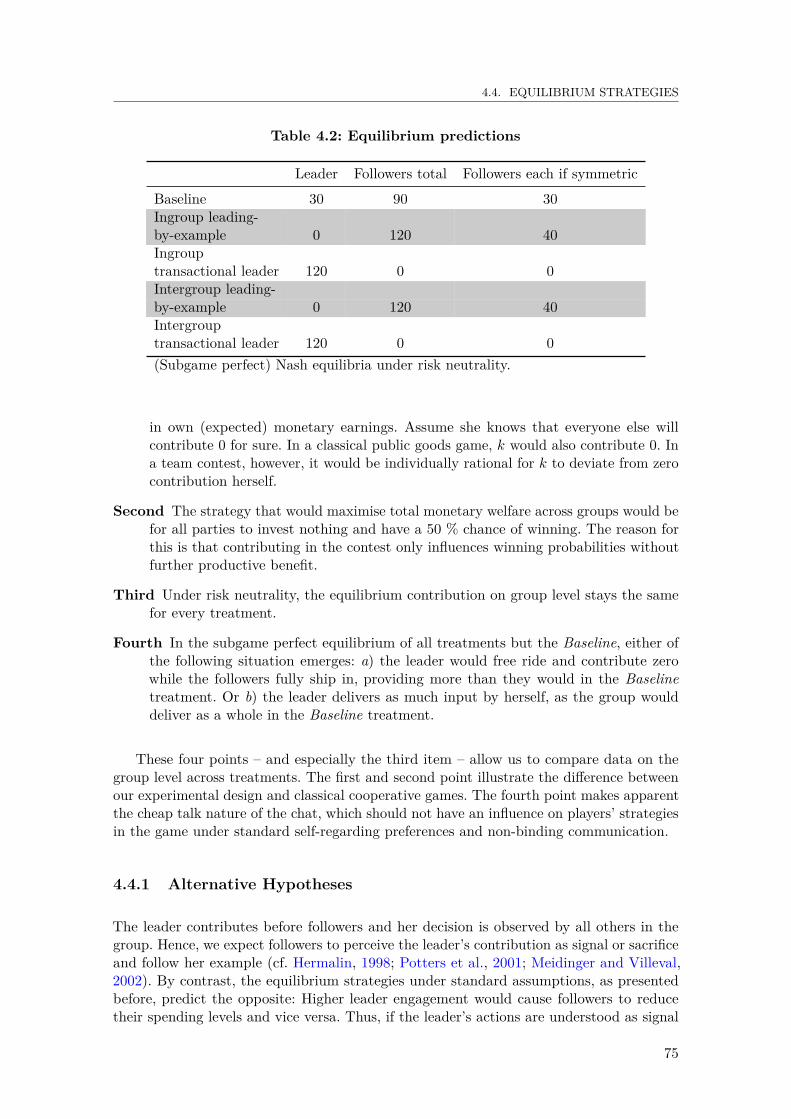
4.4. EQUILIBRIUM STRATEGIES
Table 4.2: Equilibrium predictions
Leader Followers total Followers each if symmetric
Baseline 30 90 30Ingroup leading-by-example 0 120 40Ingrouptransactional leader 120 0 0Intergroup leading-by-example 0 120 40Intergrouptransactional leader 120 0 0(Subgame perfect) Nash equilibria under risk neutrality.
in own (expected) monetary earnings. Assume she knows that everyone else willcontribute 0 for sure. In a classical public goods game, k would also contribute 0. Ina team contest, however, it would be individually rational for k to deviate from zerocontribution herself.
Second The strategy that would maximise total monetary welfare across groups would befor all parties to invest nothing and have a 50 % chance of winning. The reason forthis is that contributing in the contest only influences winning probabilities withoutfurther productive benefit.
Third Under risk neutrality, the equilibrium contribution on group level stays the samefor every treatment.
Fourth In the subgame perfect equilibrium of all treatments but the Baseline, either ofthe following situation emerges: a) the leader would free ride and contribute zerowhile the followers fully ship in, providing more than they would in the Baselinetreatment. Or b) the leader delivers as much input by herself, as the group woulddeliver as a whole in the Baseline treatment.
These four points – and especially the third item – allow us to compare data on thegroup level across treatments. The first and second point illustrate the difference betweenour experimental design and classical cooperative games. The fourth point makes apparentthe cheap talk nature of the chat, which should not have an influence on players’ strategiesin the game under standard self-regarding preferences and non-binding communication.
4.4.1 Alternative Hypotheses
The leader contributes before followers and her decision is observed by all others in thegroup. Hence, we expect followers to perceive the leader’s contribution as signal or sacrificeand follow her example (cf. Hermalin, 1998; Potters et al., 2001; Meidinger and Villeval,2002). By contrast, the equilibrium strategies under standard assumptions, as presentedbefore, predict the opposite: Higher leader engagement would cause followers to reducetheir spending levels and vice versa. Thus, if the leader’s actions are understood as signal
75
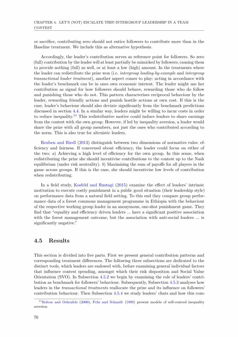
CHAPTER 4. LET’S (NOT) ESCALATE THIS! INTERGROUP LEADERSHIP IN A TEAMCONTEST
or sacrifice, contributing zero should not entice followers to contribute more than in theBaseline treatment. We include this as alternative hypothesis.
Accordingly, the leader’s contribution serves as reference point for followers. So zero(full) contribution by the leader will at least partially be mimicked by followers, causing themto provide nothing (full) as well, or at least a low (high) amount. In the treatments wherethe leader can redistribute the prize won (i.e. intergroup leading-by-example and intergrouptransactional leader treatment), another aspect comes to play: acting in accordance withthe leader’s benchmark can be in ones own economic interest. The leader might use hercontribution as signal for how followers should behave, rewarding those who do followand punishing those who do not. This pattern characterises reciprocal behaviour by theleader, rewarding friendly actions and punish hostile actions at own cost. If this is thecase, leader’s behaviour should also deviate significantly from the benchmark predictionsdiscussed in section 4.4. In a similar way, leaders might be willing to incur costs in orderto reduce inequality.11 This redistributive motive could induce leaders to share earningsfrom the contest with the own group. However, if led by inequality aversion, a leader wouldshare the prize with all group members, not just the ones who contributed according tothe norm. This is also true for altruistic leaders.
Reuben and Riedl (2013) distinguish between two dimensions of normative rules: ef-ficiency and fairness. If concerned about efficiency, the leader could focus on either ofthe two: a) Achieving a high level of efficiency for the own group. In this sense, whenredistributing the prize she should incentivise contributions to the contest up to the Nashequilibrium (under risk neutrality). b) Maximising the sum of payoffs for all players in thegame across groups. If this is the case, she should incentivise low levels of contributionwhen redistributing.
In a field study, Kosfeld and Rustagi (2015) examine the effect of leaders’ intrinsicmotivation to execute costly punishment in a public good situation (their leadership style)on performance data from a natural field setting. To this end they compare group perfor-mance data of a forest commons management programme in Ethiopia with the behaviourof the respective working group leader in an anonymous, one-shot punishment game. Theyfind that “equality and efficiency driven leaders ... have a significant positive associationwith the forest management outcome, but the association with anti-social leaders ... issignificantly negative.”
4.5 Results
This section is divided into five parts. First we present general contribution patterns andcorresponding treatment differences. The following three subsections are dedicated to thedistinct tools, which leaders are endowed with, before examining general individual factorsthat influence contest spending, amongst which their risk disposition and Social ValueOrientation (SVO). In Subsection 4.5.2 we begin by examining the role of leaders’ contri-bution as benchmark for followers’ behaviour. Subsequently, Subsection 4.5.3 analyses howleaders in the transactional treatments reallocate the prize and its influence on followers’contribution behaviour. Then Subsection 4.5.4 we study leaders’ chats and how this com-
11Bolton and Ockenfels (2000); Fehr and Schmidt (1999) present models of self-centred inequalityaversion.
76

4.5. RESULTS
munication channel pans out for the between group contest. At the close, Subsection 4.5.5examines the role of risk tolerance, social value orientation and other individual factors.
We apply non-parametric methods for hypotheses testing: Mann-Whitney U tests(MWU) (Mann and Whitney, 1947) for independent sample tests and Wilcoxon signed-rank test (Wilcoxon, 1945) for paired tests. Furthermore we use the Kruskal-Wallis test(KW test) (Kruskal and Wallis, 1952) and Dunn’s test (Dunn, 1964) with a false discoveryrate (FDR) adjustment by Benjamini and Hochberg (1995) for tests involving three or moregroups. We use a nonparametric test for trend developed by Cuzick (1985). Unless specifieddifferently, we use data on paired group level (eight players) as independent observationand apply two-sided tests.
4.5.1 Contest expenditures
Figure 4.1 provides an overview of contest contributions between treatments. The dashedhorizontal line at 120 represents the Nash equilibrium benchmark as reference. In alltreatments we observe strong overcontribution with groups contributing almost threetimes the risk neutral equilibrium prediction (Wilcoxon test: H0: group contr. = 120, H1:group contr. 6= 120, N = 45. P = 0.000. Higher rank sum than expected). The resultsfrom a KW test indicate that there exists substantial heterogeneity between the treatments(KW test: N = 45, P = 0.023). Furthermore, a Dunn’s pairwise comparison finds significantdifference between the Baseline and Ingroup trans treatment, furthermore between theIntergroup lbe treatment with all but the Baseline.12
Result 1 Without between group communication, leaders prompt an increase in contestexpenditures. Allowing for communication between group leaders cushions this effectand results in a contest expenditure level which is comparable to the baseline.
Figure 4.2 depicts the contribution to the contest over the periods per treatment. Forreference purposes, the symmetric Nash equilibrium is indicated at a contribution levelof 40. In both Intergroup treatments there exists a significant time trend over the courseof the game. While there is a positive trend for the Intergroup trans treatment (Cuzicktest: N = 9, z = 1.80, P = 0.072), Intergroup lbe displays a decreasing contribution levelover time (Cuzick test: N = 9, z = -2.30, P = 0.022). While still displaying some degree ofovercontribution, the latter treatment comes closest to the symmetric Nash equilibrium,especially in the last two thirds of the game. To understand the difference between the twoIntergroup treatments, we examine leaders’ reallocation patterns in Subsection 4.5.3 andfind that transactional leaders tend to incentivise high contribution levels by allocating abigger share of the prize to those followers that shipped in more resources to the contest.Without this incentive mechanism, communicating leaders seem to guide the group towardsa less pernicious contribution behaviour.
12Comparing average group contribution between the Baseline treatment and the ingroup treatments,we observe a significantly higher contribution level for the latter treatments (MWU test: N = 54, P = 0.019.Higher rank sum than expected for ingroup treatments). Group contribution of the intergroup treatments,however – being lower than in the ingroup treatment (MWU test: N = 72, P = 0.013. Higher rank sumthan expected for intergroup treatments) – is at the same level with the Baseline treatment (MWU test: N= 54, P = 0.956). This effect is driven in particular by the Intergroup lbe treatment, with an average groupcontribution level that lies even below the level of the Baseline treatment (MWU test: N = 36, P = 0.094.Higher rank sum than expected for the Baseline treatment).
77

CHAPTER 4. LET’S (NOT) ESCALATE THIS! INTERGROUP LEADERSHIP IN A TEAMCONTEST
100
200
300
400
Ave
rage
gro
up c
ontr
ibut
ion
Baseline Ingroup lbe Ingroup trans Intergroup lbe Intergroup trans
Figure 4.1: Contribution to the Contest
Looking at spending levels in period 1 in Figure 4.2, we can see the on-impact effectbetween the treatments, which provides a further cue as to whether treatment differencesin contribution exist from the get-go or if they evolve over time (and also Figure 4.3).Except for the Intergroup lbe treatment, which displays a significantly lower round-onecontribution, other treatments seem to start out on a fairly similar level (MWU test: N =45, P = 0.007. Lower rank sum than expected for Intergroup lbe treatment. KW test: N= 45, P = 0.074. Dunn’s test: H0 rejected for each pairwise comparison iff Intergroup lbetreatment involved).
4.5.2 The Effect of Leaders’ Contribution
While Figure 4.3 might give the impression that leaders contribute slightly more thanfollowers in the Ingroup lbe and Intergroup trans treatments, statistical tests fail to confirmthis relationship (Wilcoxon test Ingroup lbe treatment: N = 18, P = 0.143. MWU testIntergroup trans treatment: N = 18, P = 0.248). Still, leaders seem to have no escalatingeffect on the group contest in round 1. If anything, they would appear to appease contestspendings.
We investigate the overall influence of the leader’s contribution as benchmark for thefollowers in Figure 4.4. This jittered scatterplot depicts followers’ contribution on they-axis as a function of leaders’ contribution on the x-axis. The thin line depicts the 45◦ linewhere a follower contributes the same as the leader and the thick line is the fitted line for
78
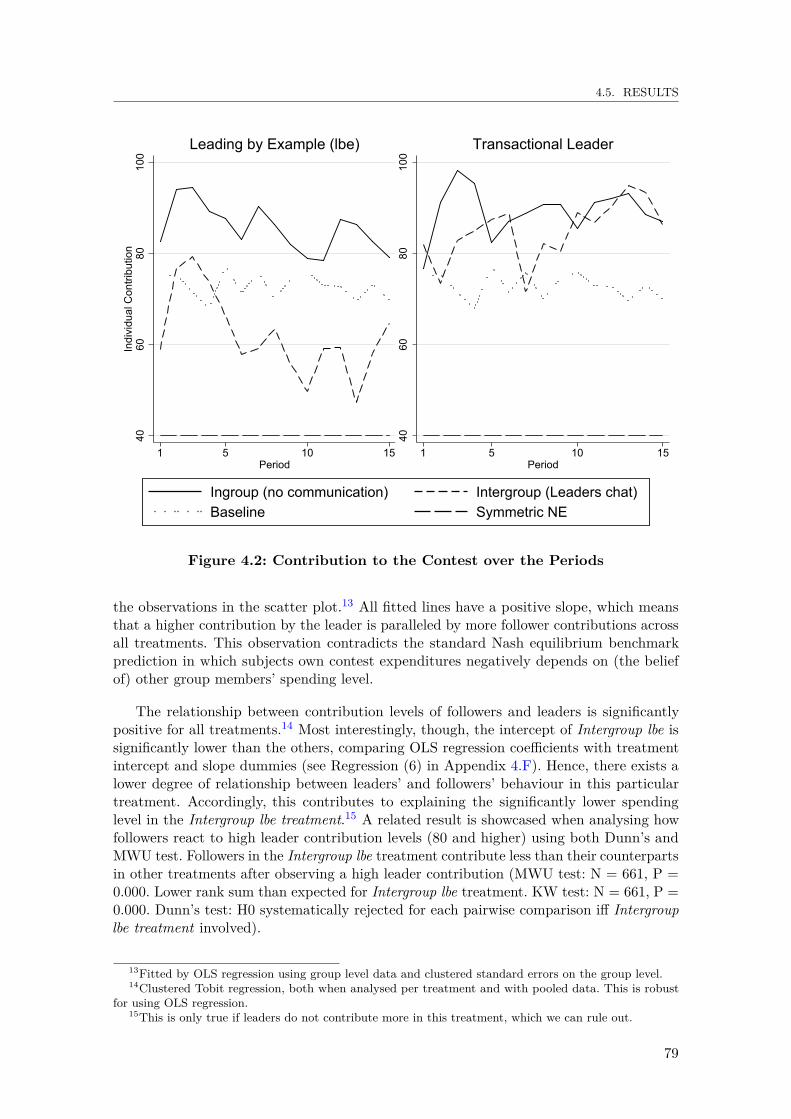
4.5. RESULTS
4060
8010
0In
divi
dual
Con
tribu
tion
1 5 10 15Period
Leading by Example (lbe)
4060
8010
0
1 5 10 15Period
Transactional Leader
Ingroup (no communication) Intergroup (Leaders chat)Baseline Symmetric NE
Figure 4.2: Contribution to the Contest over the Periods
the observations in the scatter plot.13 All fitted lines have a positive slope, which meansthat a higher contribution by the leader is paralleled by more follower contributions acrossall treatments. This observation contradicts the standard Nash equilibrium benchmarkprediction in which subjects own contest expenditures negatively depends on (the beliefof) other group members’ spending level.
The relationship between contribution levels of followers and leaders is significantlypositive for all treatments.14 Most interestingly, though, the intercept of Intergroup lbe issignificantly lower than the others, comparing OLS regression coefficients with treatmentintercept and slope dummies (see Regression (6) in Appendix 4.F). Hence, there exists alower degree of relationship between leaders’ and followers’ behaviour in this particulartreatment. Accordingly, this contributes to explaining the significantly lower spendinglevel in the Intergroup lbe treatment.15 A related result is showcased when analysing howfollowers react to high leader contribution levels (80 and higher) using both Dunn’s andMWU test. Followers in the Intergroup lbe treatment contribute less than their counterpartsin other treatments after observing a high leader contribution (MWU test: N = 661, P =0.000. Lower rank sum than expected for Intergroup lbe treatment. KW test: N = 661, P =0.000. Dunn’s test: H0 systematically rejected for each pairwise comparison iff Intergrouplbe treatment involved).
13Fitted by OLS regression using group level data and clustered standard errors on the group level.14Clustered Tobit regression, both when analysed per treatment and with pooled data. This is robust
for using OLS regression.15This is only true if leaders do not contribute more in this treatment, which we can rule out.
79
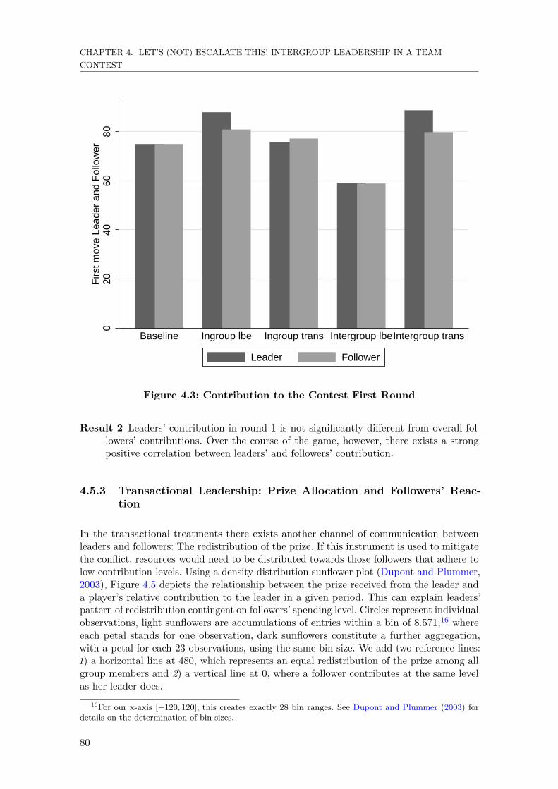
CHAPTER 4. LET’S (NOT) ESCALATE THIS! INTERGROUP LEADERSHIP IN A TEAMCONTEST
020
4060
80F
irst m
ove
Lead
er a
nd F
ollo
wer
Baseline Ingroup lbe Ingroup trans Intergroup lbeIntergroup trans
Leader Follower
Figure 4.3: Contribution to the Contest First Round
Result 2 Leaders’ contribution in round 1 is not significantly different from overall fol-lowers’ contributions. Over the course of the game, however, there exists a strongpositive correlation between leaders’ and followers’ contribution.
4.5.3 Transactional Leadership: Prize Allocation and Followers’ Reac-tion
In the transactional treatments there exists another channel of communication betweenleaders and followers: The redistribution of the prize. If this instrument is used to mitigatethe conflict, resources would need to be distributed towards those followers that adhere tolow contribution levels. Using a density-distribution sunflower plot (Dupont and Plummer,2003), Figure 4.5 depicts the relationship between the prize received from the leader anda player’s relative contribution to the leader in a given period. This can explain leaders’pattern of redistribution contingent on followers’ spending level. Circles represent individualobservations, light sunflowers are accumulations of entries within a bin of 8.571,16 whereeach petal stands for one observation, dark sunflowers constitute a further aggregation,with a petal for each 23 observations, using the same bin size. We add two reference lines:1) a horizontal line at 480, which represents an equal redistribution of the prize among allgroup members and 2) a vertical line at 0, where a follower contributes at the same levelas her leader does.
16For our x-axis [−120, 120], this creates exactly 28 bin ranges. See Dupont and Plummer (2003) fordetails on the determination of bin sizes.
80

4.5. RESULTS
020
4060
8010
012
0
0 20 40 60 80 100 120Leader Contribution
R-squared: 0.514
Leading by Example
020
4060
8010
012
0
0 20 40 60 80 100 120Leader Contribution
R-squared: 0.364
Transactional Leader
Ingroup0
2040
6080
100
120
0 20 40 60 80 100 120Leader Contribution
R-squared: 0.372
Leading by Example
020
4060
8010
012
0
0 20 40 60 80 100 120Leader Contribution
R-squared: 0.531
Transactional Leader
Intergroup (with communication)
Fol
low
er C
ontr
ibut
ion
Figure 4.4: Influence of Leader’s Contribution on Followers
In Figure 4.5 two dominant strategical patterns are highlighted: First, followers tendto contribute at the same level of the leader, which is illustrated by the high density ofobservations along a relative contribution of 0. Second, leaders reallocate an equal share ofthe prize, which can be seen by the accumulation of observations on the horizontal line of480. This creates a cross, establishing four domains. The north-western and north-easterndomains contain only a few observations. This means that leaders tend to not reallocatemore than the equal share, even to those that contribute more than proportionally. Bycontrast, it is in the south-western domain where by far the most observations off theaforementioned imaginary cross wind up. This area represents the situation where leadersreallocate less than the equal share to followers with a negative relative contribution.Furthermore, for an extremely low level of relative contribution (-120), we observe a highclustering on zero redistribution. This means that followers who fall far below their leader’sbenchmark come away empty-handed.
Result 3 In transactional treatments, there exist two dominant strategical patterns: 1) Fol-lowers contribute at the same level of the leader and 2) leaders reallocate an equalshare of the prize, 480. Furthermore, they tend to reallocate less to those who con-tribute less than the leader.
In a next step, we investigate the reverse relationship: how is a follower’s willingness tocontribute (relative to the leader) related to the leader’s prize reallocation in the previousperiod. For this analysis we focus on groups in the transactional treatments that have won
81
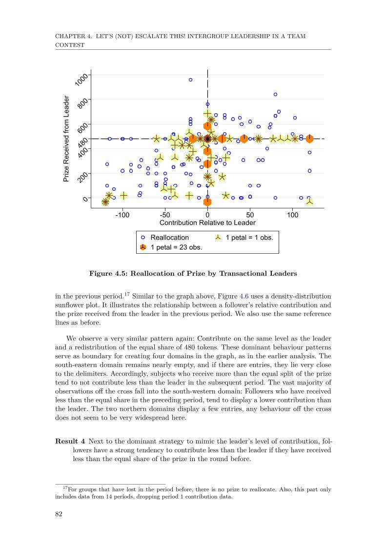
CHAPTER 4. LET’S (NOT) ESCALATE THIS! INTERGROUP LEADERSHIP IN A TEAMCONTEST
0
200
400480
600
800
1000
Priz
e R
ecei
ved
from
Lea
der
-100 -50 0 50 100Contribution Relative to Leader
Reallocation 1 petal = 1 obs.1 petal = 23 obs.
Figure 4.5: Reallocation of Prize by Transactional Leaders
in the previous period.17 Similar to the graph above, Figure 4.6 uses a density-distributionsunflower plot. It illustrates the relationship between a follower’s relative contribution andthe prize received from the leader in the previous period. We also use the same referencelines as before.
We observe a very similar pattern again: Contribute on the same level as the leaderand a redistribution of the equal share of 480 tokens. These dominant behaviour patternsserve as boundary for creating four domains in the graph, as in the earlier analysis. Thesouth-eastern domain remains nearly empty, and if there are entries, they lie very closeto the delimiters. Accordingly, subjects who receive more than the equal split of the prizetend to not contribute less than the leader in the subsequent period. The vast majority ofobservations off the cross fall into the south-western domain: Followers who have receivedless than the equal share in the preceding period, tend to display a lower contribution thanthe leader. The two northern domains display a few entries, any behaviour off the crossdoes not seem to be very widespread here.
Result 4 Next to the dominant strategy to mimic the leader’s level of contribution, fol-lowers have a strong tendency to contribute less than the leader if they have receivedless than the equal share of the prize in the round before.
17For groups that have lost in the period before, there is no prize to reallocate. Also, this part onlyincludes data from 14 periods, dropping period 1 contribution data.
82
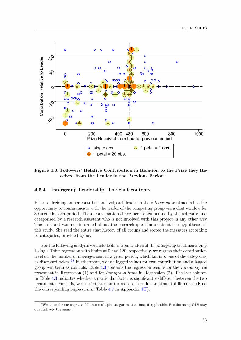
4.5. RESULTS
-100
-50
0
50
100
Con
tribu
tion
Rel
ativ
e to
Lea
der
0 200 400 480 600 800 1000Prize Received from Leader previous period
single obs. 1 petal = 1 obs.1 petal = 20 obs.
Figure 4.6: Followers’ Relative Contribution in Relation to the Prize they Re-ceived from the Leader in the Previous Period
4.5.4 Intergroup Leadership: The chat contents
Prior to deciding on her contribution level, each leader in the intergroup treatments has theopportunity to communicate with the leader of the competing group via a chat window for30 seconds each period. These conversations have been documented by the software andcategorised by a research assistant who is not involved with this project in any other way.The assistant was not informed about the research question or about the hypotheses ofthis study. She read the entire chat history of all groups and sorted the messages accordingto categories, provided by us.
For the following analysis we include data from leaders of the intergroup treatments only.Using a Tobit regression with limits at 0 and 120, respectively, we regress their contributionlevel on the number of messages sent in a given period, which fall into one of the categories,as discussed below.18 Furthermore, we use lagged values for own contribution and a laggedgroup win term as controls. Table 4.3 contains the regression results for the Intergroup lbetreatment in Regression (1) and for Intergroup trans in Regression (2). The last columnin Table 4.3 indicates whether a particular factor is significantly different between the twotreatments. For this, we use interaction terms to determine treatment differences (Findthe corresponding regression in Table 4.7 in Appendix 4.F).
18We allow for messages to fall into multiple categories at a time, if applicable. Results using OLS stayqualitatively the same.
83
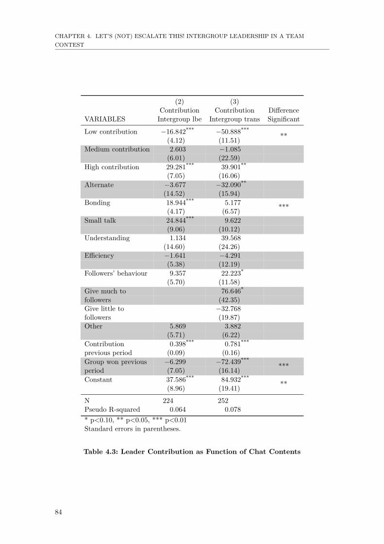
CHAPTER 4. LET’S (NOT) ESCALATE THIS! INTERGROUP LEADERSHIP IN A TEAMCONTEST
(2) (3)Contribution Contribution Difference
VARIABLES Intergroup lbe Intergroup trans Significant
Low contribution −16.842*** −50.888*****(4.12) (11.51)
Medium contribution 2.603 −1.085(6.01) (22.59)
High contribution 29.281*** 39.901**
(7.05) (16.06)Alternate −3.677 −32.090**
(14.52) (15.94)Bonding 18.944*** 5.177 ***(4.17) (6.57)Small talk 24.844*** 9.622
(9.06) (10.12)Understanding 1.134 39.568
(14.60) (24.26)Efficiency −1.641 −4.291
(5.38) (12.19)Followers’ behaviour 9.357 22.223*
(5.70) (11.58)Give much to 76.646*
followers (42.35)Give little to −32.768followers (19.87)Other 5.869 3.882
(5.71) (6.22)Contribution 0.398*** 0.781***
previous period (0.09) (0.16)Group won previous −6.299 −72.439***
***period (7.05) (16.14)Constant 37.586*** 84.932***
**(8.96) (19.41)
N 224 252Pseudo R-squared 0.064 0.078* p<0.10, ** p<0.05, *** p<0.01Standard errors in parentheses.
Table 4.3: Leader Contribution as Function of Chat Contents
84
4.5. RESULTS
First of all, after discussing a low contribution level (e.g. between 0 - 40 points) /high contribution level (e.g. between 80 - 120 points), leaders do exhibit a lower / higherspending level. While the effect of low contribution messages is even more pronouncedin the transactional treatment, there is no significant difference between the treatmentswhen it comes to high contribution messages. As expected, discussing a medium level ofcontest spending has neither a lowering nor increasing effect in this regard. Furthermore,transactional leaders who manage to reach across the aisle by coordinating on takingalternating turns manage to alleviate the between-group contest. This result is not robustin Regression (1), however. Somewhat surprisingly, bonding or small talk messages incitea higher spending level in Regression (1). By creating an emotional tie with the othergroup representative, we would have expected a degree of mitigation towards the inter-group contest. Furthermore, while bonding messages indeed feature an escalating charactertowards leaders in the Intergroup lbe treatment, this effect appears to be non-existent inthe Intergroup trans treatment.
General conversation on the followers’ behaviour constitutes another subject matterwith escalating influence on transactional leaders’ contribution decisions. Concerning thereallocation of the prize, leaders who articulate their intention to allocate open-handedlytowards followers, are also the ones who spend more resources to the contest and vice-versa.Conversations including concerns for efficiency, by contrast, have no descriptive power forthe leaders’ subsequent contribution decision, while this could have been expected to havean abating effect on contest expenditures. Equally, discussing comprehensive understandingquestions about the experiment structure has no descriptive power.
Apart from the chat categories, this analysis identifies a twofold of other treatmentdifferences between the two Intergroup treatments. First, there is a stark difference in howleaders’ contribution decisions depend on whether they have won in the previous round.While a transactional leader whose group won the preceding period drastically reduces hercontributions, this is not the case for leaders in the Intergroup lbe treatment. This couldhave to do with the fact that alternating seems to work a lot better in the Intergroup transtreatment. Second, the difference in the constant identifies the treatment effects discussedin Subsection 4.5.1.
Figure 4.7 depicts the prevalence of chat categories per treatment. “Low contribution”messages, which have negative influence on spending levels, are being sent more frequentlyin the Intergroup lbe treatment. Adding to this image, all message categories that havea positive bearing on contribution levels – such as “Bonding” or “Small talk” – are lesscommonly used in the Intergroup lbe treatment. This can deliver an explanation for thestark difference in contest spending between these two treatments: Leaders structurallychat about different topics, namely sending more messages with an abating and less withan escalating character in the Intergroup lbe treatment.
Result 5 Leaders that coordinate on taking turns manage to reduce contest expendituressignificantly. Moreover, the prevalence of subject matters structurally differs betweenthe treatments favouring more mitigating messages in the Intergroup lbe and moreescalating messages in the Intergroup trans treatment. This contributes at explainingthe strong treatment difference in contest spending.
85

CHAPTER 4. LET’S (NOT) ESCALATE THIS! INTERGROUP LEADERSHIP IN A TEAMCONTEST
010
020
030
0
Low contribution
Medium
contribution
High contribution
Alternate
Bonding
Small talk
Understanding
Efficiency
Followers' behaviour
Give much to followers
Give little to followers
Other
Intergroup lbe Intergroup trans
Figure 4.7: Prevalence of Chat Messages per Treatment
4.5.5 Risk Aversion and Social Value Orientation
In this subsection we investigate what personal factors can explain individual spendingbehaviour beyond treatment effects. We hypothesise that risk preferences and Social ValueOrientation (SVO) can have a bearing on the willingness to ship in resources for the betweengroup contest. Theory suggests that more risk-averse players should display a lower levelof contest spending, which is reflected in our alternative hypotheses in Subsection 4.4.1.
We regress individual contribution, aggregated over the total number of rounds, ona number of factors, as displayed in Table 4.4.19 The average number of lottery ticketsbought by teammates (Mean Group Contribute) positively influences own contributionlevels. Given that there exists some degree of overcontribution in all treatments, firstorder conditions under self-oriented preferences would predict this factor to be negative,as players would fade out own contribution if (they believe that) their teammates providemore input. There is no evidence for an Age or gender (Female) effect. There is notmuch variation in the age of our participant body, as it is almost exclusively comprisedof university students. Concerning the factor Female, however, literature suggests a lowerlevel in women’s competitiveness (e.g. McDonald et al., 2012; Vugt et al., 2007), whichwould imply less contest spending for female participants.
19Both models’ (Regressions (4) and (5)) variance inflation factors (VIF’s) reject the possibility of apotential multicollinearity problem. Still, multicollinearity of the factors would only increase the standarderrors of the coefficients if they are collinear. Even then, the coefficients as such would be unaffected.
86
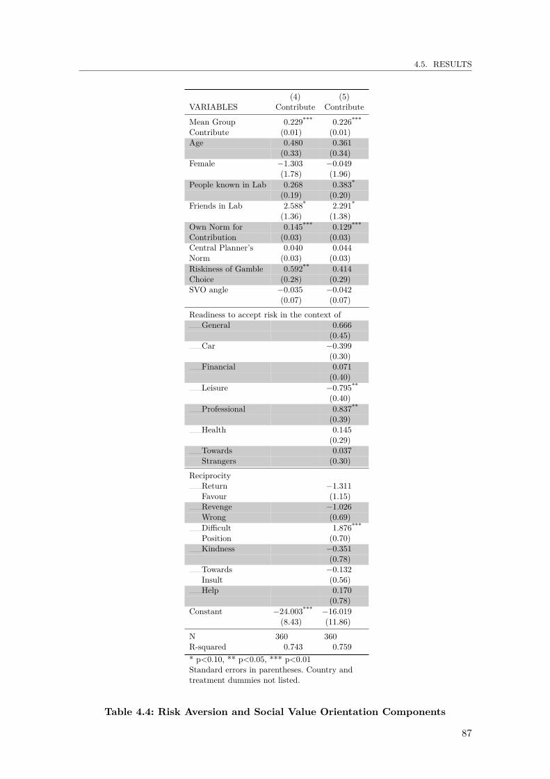
4.5. RESULTS
(4) (5)VARIABLES Contribute Contribute
Mean Group 0.229*** 0.226***
Contribute (0.01) (0.01)Age 0.480 0.361
(0.33) (0.34)Female −1.303 −0.049
(1.78) (1.96)People known in Lab 0.268 0.383*
(0.19) (0.20)Friends in Lab 2.588* 2.291*
(1.36) (1.38)Own Norm for 0.145*** 0.129***
Contribution (0.03) (0.03)Central Planner’s 0.040 0.044Norm (0.03) (0.03)Riskiness of Gamble 0.592** 0.414Choice (0.28) (0.29)SVO angle −0.035 −0.042
(0.07) (0.07)
Readiness to accept risk in the context ofGeneral 0.666
(0.45)Car −0.399
(0.30)Financial 0.071
(0.40)Leisure −0.795**
(0.40)Professional 0.837**
(0.39)Health 0.145
(0.29)Towards 0.037Strangers (0.30)
ReciprocityReturn −1.311Favour (1.15)Revenge −1.026Wrong (0.69)Difficult 1.876***
Position (0.70)Kindness −0.351
(0.78)Towards −0.132Insult (0.56)Help 0.170
(0.78)Constant −24.003*** −16.019
(8.43) (11.86)
N 360 360R-squared 0.743 0.759* p<0.10, ** p<0.05, *** p<0.01Standard errors in parentheses. Country andtreatment dummies not listed.
Table 4.4: Risk Aversion and Social Value Orientation Components
87
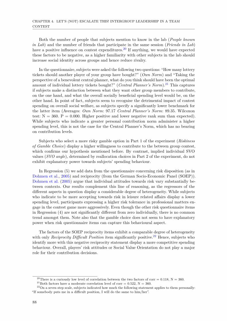
CHAPTER 4. LET’S (NOT) ESCALATE THIS! INTERGROUP LEADERSHIP IN A TEAMCONTEST
Both the number of people that subjects mention to know in the lab (People knownin Lab) and the number of friends that participate in the same session (Friends in Lab)have a positive influence on contest expenditures.20 If anything, we would have expectedthese factors to be negative, as a higher familiarity with other subjects in the lab shouldincrease social identity across groups and hence reduce rivalry.
In the questionnaire, subjects were asked the following two questions: “How many lotterytickets should another player of your group have bought?” (Own Norm) and “Taking theperspective of a benevolent central planner, what do you think should have been the optimalamount of individual lottery tickets bought?” (Central Planner’s Norm).21 This capturesif subjects make a distinction between what they want other group members to contribute,on the one hand, and what the overall socially beneficial spending level would be, on theother hand. In point of fact, subjects seem to recognise the detrimental impact of contestspending on overall social welfare, as subjects specify a significantly lower benchmark forthe latter item (Averages: Own Norm: 97.17 Central Planner’s Norm: 89.35. Wilcoxontest: N = 360. P = 0.000. Higher positive and lower negative rank sum than expected).While subjects who indicate a greater personal contribution norm administer a higherspending level, this is not the case for the Central Planner’s Norm, which has no bearingon contribution levels.
Subjects who select a more risky gamble option in Part 1 of the experiment (Riskinessof Gamble Choice) display a higher willingness to contribute to the between group contest,which confirms our hypothesis mentioned before. By contrast, implied individual SVOvalues (SVO angle), determined by reallocation choices in Part 2 of the experiment, do notexhibit explanatory power towards subjects’ spending behaviour.
In Regression (5) we add data from the questionnaire concerning risk disposition (as inDohmen et al., 2005) and reciprocity (from the German Socio-Economic Panel (SOEP)).Dohmen et al. (2005) argue that individual attitudes towards risk vary substantially be-tween contexts. Our results complement this line of reasoning, as the regressors of thedifferent aspects in question display a considerable degree of heterogeneity. While subjectswho indicate to be more accepting towards risk in leisure related affairs display a lowerspending level, participants expressing a higher risk tolerance in professional matters en-gage in the contest game more aggressively. Even though the other risk questionnaire itemsin Regression (4) are not significantly different from zero individually, there is no commontrend amongst them. Note also that the gamble choice does not seem to have explanatorypower when risk questionnaire items can capture this behavioural aspect.
The factors of the SOEP reciprocity items exhibit a comparable degree of heterogeneitywith only Reciprocity Difficult Position item significantly positive.22 Hence, subjects whoidentify more with this negative reciprocity statement display a more competitive spendingbehaviour. Overall, players’ risk attitudes or Social Value Orientation do not play a majorrole for their contribution decisions.
20There is a curiously low level of correlation between the two factors of corr = 0.118, N = 360.21Both factors have a moderate correlation level of corr = 0.522, N = 360.22On a seven step scale, subjects indicated how much the following statement applies to them personally:
“If somebody puts me in a difficult position, I will do the same to him/her”.
88
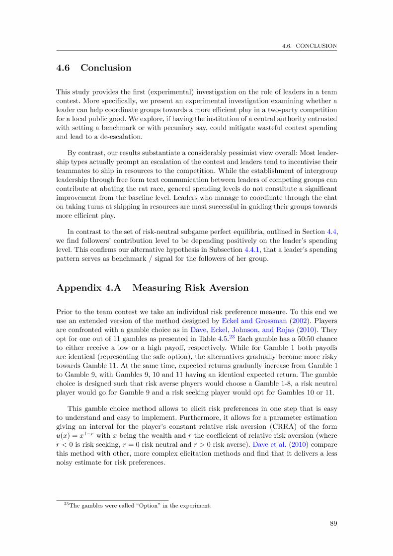
4.6. CONCLUSION
4.6 Conclusion
This study provides the first (experimental) investigation on the role of leaders in a teamcontest. More specifically, we present an experimental investigation examining whether aleader can help coordinate groups towards a more efficient play in a two-party competitionfor a local public good. We explore, if having the institution of a central authority entrustedwith setting a benchmark or with pecuniary say, could mitigate wasteful contest spendingand lead to a de-escalation.
By contrast, our results substantiate a considerably pessimist view overall: Most leader-ship types actually prompt an escalation of the contest and leaders tend to incentivise theirteammates to ship in resources to the competition. While the establishment of intergroupleadership through free form text communication between leaders of competing groups cancontribute at abating the rat race, general spending levels do not constitute a significantimprovement from the baseline level. Leaders who manage to coordinate through the chaton taking turns at shipping in resources are most successful in guiding their groups towardsmore efficient play.
In contrast to the set of risk-neutral subgame perfect equilibria, outlined in Section 4.4,we find followers’ contribution level to be depending positively on the leader’s spendinglevel. This confirms our alternative hypothesis in Subsection 4.4.1, that a leader’s spendingpattern serves as benchmark / signal for the followers of her group.
Appendix 4.A Measuring Risk Aversion
Prior to the team contest we take an individual risk preference measure. To this end weuse an extended version of the method designed by Eckel and Grossman (2002). Playersare confronted with a gamble choice as in Dave, Eckel, Johnson, and Rojas (2010). Theyopt for one out of 11 gambles as presented in Table 4.5.23 Each gamble has a 50:50 chanceto either receive a low or a high payoff, respectively. While for Gamble 1 both payoffsare identical (representing the safe option), the alternatives gradually become more riskytowards Gamble 11. At the same time, expected returns gradually increase from Gamble 1to Gamble 9, with Gambles 9, 10 and 11 having an identical expected return. The gamblechoice is designed such that risk averse players would choose a Gamble 1-8, a risk neutralplayer would go for Gamble 9 and a risk seeking player would opt for Gambles 10 or 11.
This gamble choice method allows to elicit risk preferences in one step that is easyto understand and easy to implement. Furthermore, it allows for a parameter estimationgiving an interval for the player’s constant relative risk aversion (CRRA) of the formu(x) = x1−r with x being the wealth and r the coefficient of relative risk aversion (wherer < 0 is risk seeking, r = 0 risk neutral and r > 0 risk averse). Dave et al. (2010) comparethis method with other, more complex elicitation methods and find that it delivers a lessnoisy estimate for risk preferences.
23The gambles were called “Option” in the experiment.
89
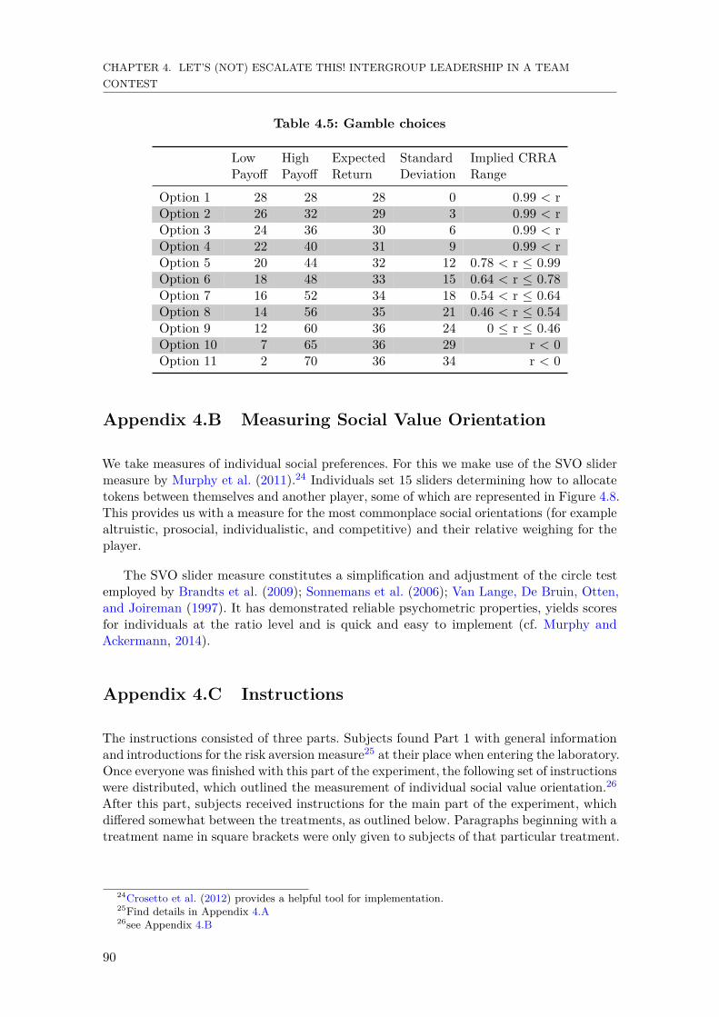
CHAPTER 4. LET’S (NOT) ESCALATE THIS! INTERGROUP LEADERSHIP IN A TEAMCONTEST
Table 4.5: Gamble choices
Low High Expected Standard Implied CRRAPayoff Payoff Return Deviation Range
Option 1 28 28 28 0 0.99 < rOption 2 26 32 29 3 0.99 < rOption 3 24 36 30 6 0.99 < rOption 4 22 40 31 9 0.99 < rOption 5 20 44 32 12 0.78 < r ≤ 0.99Option 6 18 48 33 15 0.64 < r ≤ 0.78Option 7 16 52 34 18 0.54 < r ≤ 0.64Option 8 14 56 35 21 0.46 < r ≤ 0.54Option 9 12 60 36 24 0 ≤ r ≤ 0.46Option 10 7 65 36 29 r < 0Option 11 2 70 36 34 r < 0
Appendix 4.B Measuring Social Value Orientation
We take measures of individual social preferences. For this we make use of the SVO slidermeasure by Murphy et al. (2011).24 Individuals set 15 sliders determining how to allocatetokens between themselves and another player, some of which are represented in Figure 4.8.This provides us with a measure for the most commonplace social orientations (for examplealtruistic, prosocial, individualistic, and competitive) and their relative weighing for theplayer.
The SVO slider measure constitutes a simplification and adjustment of the circle testemployed by Brandts et al. (2009); Sonnemans et al. (2006); Van Lange, De Bruin, Otten,and Joireman (1997). It has demonstrated reliable psychometric properties, yields scoresfor individuals at the ratio level and is quick and easy to implement (cf. Murphy andAckermann, 2014).
Appendix 4.C Instructions
The instructions consisted of three parts. Subjects found Part 1 with general informationand introductions for the risk aversion measure25 at their place when entering the laboratory.Once everyone was finished with this part of the experiment, the following set of instructionswere distributed, which outlined the measurement of individual social value orientation.26
After this part, subjects received instructions for the main part of the experiment, whichdiffered somewhat between the treatments, as outlined below. Paragraphs beginning with atreatment name in square brackets were only given to subjects of that particular treatment.
24Crosetto et al. (2012) provides a helpful tool for implementation.25Find details in Appendix 4.A26see Appendix 4.B
90
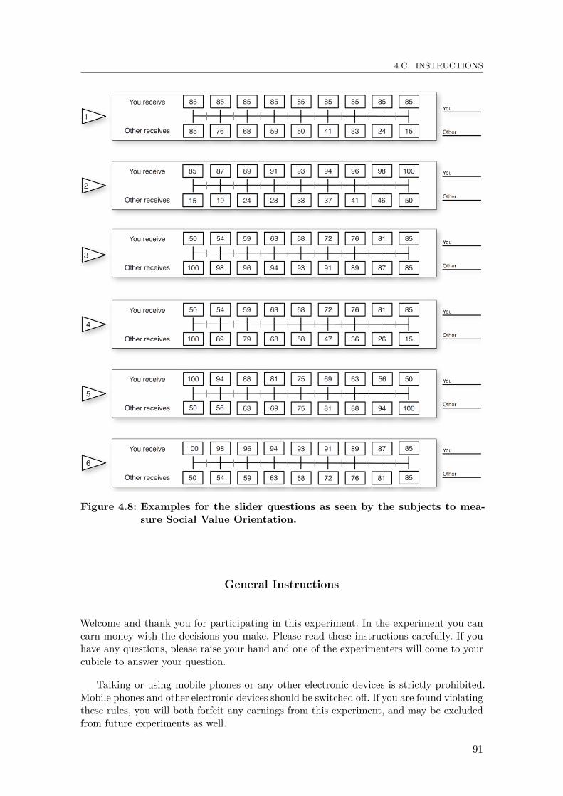
4.C. INSTRUCTIONS
Figure 4.8: Examples for the slider questions as seen by the subjects to mea-sure Social Value Orientation.
General Instructions
Welcome and thank you for participating in this experiment. In the experiment you canearn money with the decisions you make. Please read these instructions carefully. If youhave any questions, please raise your hand and one of the experimenters will come to yourcubicle to answer your question.
Talking or using mobile phones or any other electronic devices is strictly prohibited.Mobile phones and other electronic devices should be switched off. If you are found violatingthese rules, you will both forfeit any earnings from this experiment, and may be excludedfrom future experiments as well.
91

CHAPTER 4. LET’S (NOT) ESCALATE THIS! INTERGROUP LEADERSHIP IN A TEAMCONTEST
This is an experiment about decision making. The instructions are simple and if youfollow them carefully you can earn a considerable amount of money which will be paid toyou privately and in cash at the end of the experiment. The amount of money you earnwill depend on your decisions, on other participants’ decisions and on random events. Youwill never be asked to reveal your identity to anyone during the course of the experiment.Your name will never be associated with any of your decisions.
During the experiment you can earn points (the experimental money unit), which willbe converted into cash at the end of the experiment, using an exchange rate of
40 points = 10 cent.
Thus, the more points you earn, the more cash you will receive at the end of the session.
This experiment consists of three parts. The following instructions explain Part 1. Afterfinishing that part, you will receive instructions for Part 2 and after the end of Part 2 youwill receive instructions for Part 3. None of your (or anyone else’s) decisions for one partare affecting your (or anyone else’s) earnings in the other parts.
All of your choices are completely confidential. You will learn your results of Part 1and Part 2 after Part 3 has finished. Points earned in each of the three Parts will be addedup to determine your total earnings.
Instructions Part 1
This is an individual decision task and your choice will only affect you. You will bepresented with six payoff options, of which you will have to choose one. Each option isassociated with a low and a high payoff and both the high and low payoff are equally likely.At the end, after Part 3 the computer will randomly pick either the low or the high payoffof the option you chose.
Instructions Part 2
In this task you will be randomly paired with one other person in this room. You will makea series of decisions about allocating points between you and this other person.
One of your decisions will be picked randomly and you receive what you allocated toyourself and the other person receives what you allocated to her in this decision. Notethat any of your decisions is equally likely to be chosen. Therefore you should treat eachdecision as if it is the one that counts.
One other person in the room will make such decision towards you. This is not theperson you are randomly paired with.
Instructions Part 3
In Part 3, all participants are assigned to teams of four and your team will be randomly
92

4.C. INSTRUCTIONS
matched with another team. None of you will learn the identities of own team membersor other team members. Part 3 will consist of 15 periods, and in each period you and theother participants can obtain a prize in the following way:
At the beginning of each period you will receive an endowment of 120 points. Then youcan use none, parts or all of these points to buy lottery tickets for your team. Each lotteryticket costs 1 point. Any of your points not spent on lottery tickets will be accumulated inyour private point balance. Likewise, each of your team members receives 120 points whichthey may use to buy lottery tickets for your team. Similarly, each member of the otherteam will receive 120 points and may buy tickets for their team in exactly the same way.
[Ingroup leading-by-example & Ingroup transactional leader] In your and the othergroup, one participant – member 1 – makes her / his decision before the others. Ownteam members will see, how many tickets this participant bought, before they make theirdecisions.
[Intergroup leading-by-example & Intergroup transactional leader] In your and the othergroup, one participant – member 1 – has been randomly selected to be able to communicatewith one participant of the other group in private, via a chat window. This communicationpossibility will automatically expire after 45 seconds. Unless you are member 1, neitheryou nor any other participant will ever learn the contents of this communication. Afterthat chat window has been closed, member 1 makes her / his decision. Own team memberswill see, how many tickets this participant bought, before they make their decisions.
After everybody has made the decision, a lottery will determine whether your team,or the team you are matched with, wins. The likelihood that a team wins depends in aproportional way on the total number of tickets, the team bought and on the total numberof tickets, the other team bought. That is, if you and your team members bought in total Xtickets, and the team members of the other team bought in total Y tickets, the likelihoodthat your team wins is X
X+Y and the likelihood that the other team wins is YX+Y . Hence,
the more tickets your (the other) team has, the higher is your (the other) team’s chanceof winning.
Examples: If your team and the other team have bought the same amount of ticketsthen each team is equally likely to win. If your team has bought three times as manytickets as the other team, then your team is three times more likely to win than the otherteam. If only one of the teams has bought tickets, then this team wins for sure. If neitheryour team nor the other team has bought any tickets, then each team is equally likely towin.
[Baseline, Ingroup leading-by-example & Intergroup leading-by-example] The winningteam will receive a prize of 1,920 points in total, which will be split equally among groupmembers. This delivers 480 points for each player of the winning group.
[Ingroup transactional leader & Intergroup transactional leader] The winning team willreceive a prize of 1,920 points in total and member 1 will determine how the prize will besplit among the group members. The losing team will receive nothing.
Summary: In Part 3, your earnings in each period are determined as follows:
The points you earn in each period accumulate and your earnings in Part 3 will be the
93
CHAPTER 4. LET’S (NOT) ESCALATE THIS! INTERGROUP LEADERSHIP IN A TEAMCONTEST
Winning team:
Your Endowment (= 120)- Your tickets bought (between 0 and 120)[Baseline, Ingroup leading-by-example & Intergroup leading-by-example]+ Prize (480)[Ingroup transactional leader & Intergroup transactional leader]+ Share of the prize allocated by member 1 (between 0 and 1,920)= Your earnings
Losing team:
Your Endowment (= 120)- Your tickets bought (between 0 and 120)= Your earnings
total point earning from all 15 periods.
This part starts with a trial period in which you will be asked to answer some questionsin order to check your understanding and to give you the opportunity to get acquaintedwith the setup. Points earned in this trial period will not be paid out.
Appendix 4.D Risk Neutral Equilibrium
Player l maximises expected profit πl by setting own contribution vl = (vi)i∈K∪M . Invest-ment of players k ∈ K of own group K is labelled
∑k∈K vk, while players m ∈ M in the
other disjoint group M invest∑m∈M vm. Individual prize for winning a round is z. Solve
individual optimisation problem for any period t, time indices are omitted.
πl(
(vi)i∈K∪M)
=vl +
∑k∈K\{l}
vk
vl +∑
k∈K\{l}vk +
∑m∈M
vm· z − vl
Deriving with respect to vl delivers the best response function for any player l of group K:
∂πl(
(vi)i∈K∪M)
∂vl= 0 ⇔ vl =
√ ∑m∈M
vm · z −∑m∈M
vm −∑
k∈K\{l}vk
Checking the second order condition confirms that we find a maximum:
∂2πl∂v2
l
=− 2
∑m∈M
vm · z( ∑k∈K
vk +∑
m∈Mvm
)3 < 0
Using the first order condition of group M , we find a multiplicity of equilibria, char-acterised by
∑m∈M vm = z
4 and∑k∈K vk = z
4 . If we assume symmetry in own group:
94
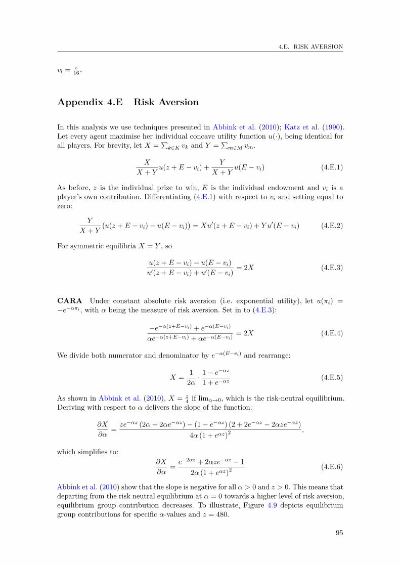
4.E. RISK AVERSION
vl = z16 .
Appendix 4.E Risk Aversion
In this analysis we use techniques presented in Abbink et al. (2010); Katz et al. (1990).Let every agent maximise her individual concave utility function u(·), being identical forall players. For brevity, let X =
∑k∈K vk and Y =
∑m∈M vm.
X
X + Yu(z + E − vi) + Y
X + Yu(E − vi) (4.E.1)
As before, z is the individual prize to win, E is the individual endowment and vi is aplayer’s own contribution. Differentiating (4.E.1) with respect to vi and setting equal tozero:
Y
X + Y
(u(z + E − vi)− u(E − vi)
)= Xu′(z + E − vi) + Y u′(E − vi) (4.E.2)
For symmetric equilibria X = Y , so
u(z + E − vi)− u(E − vi)u′(z + E − vi) + u′(E − vi)
= 2X (4.E.3)
CARA Under constant absolute risk aversion (i.e. exponential utility), let u(πi) =−e−απi , with α being the measure of risk aversion. Set in to (4.E.3):
−e−α(z+E−vi) + e−α(E−vi)
αe−α(z+E−vi) + αe−α(E−vi)= 2X (4.E.4)
We divide both numerator and denominator by e−α(E−vi) and rearrange:
X = 12α ·
1− e−αz
1 + e−αz(4.E.5)
As shown in Abbink et al. (2010), X = z4 if limα→0, which is the risk-neutral equilibrium.
Deriving with respect to α delivers the slope of the function:
∂X
∂α= ze−αz (2α+ 2αe−αz)− (1− e−αz) (2 + 2e−αz − 2αze−αz)
4α (1 + eαz)2 ,
which simplifies to:∂X
∂α= e−2αz + 2αze−αz − 1
2α (1 + eαz)2 (4.E.6)
Abbink et al. (2010) show that the slope is negative for all α > 0 and z > 0. This means thatdeparting from the risk neutral equilibrium at α = 0 towards a higher level of risk aversion,equilibrium group contribution decreases. To illustrate, Figure 4.9 depicts equilibriumgroup contributions for specific α-values and z = 480.
95
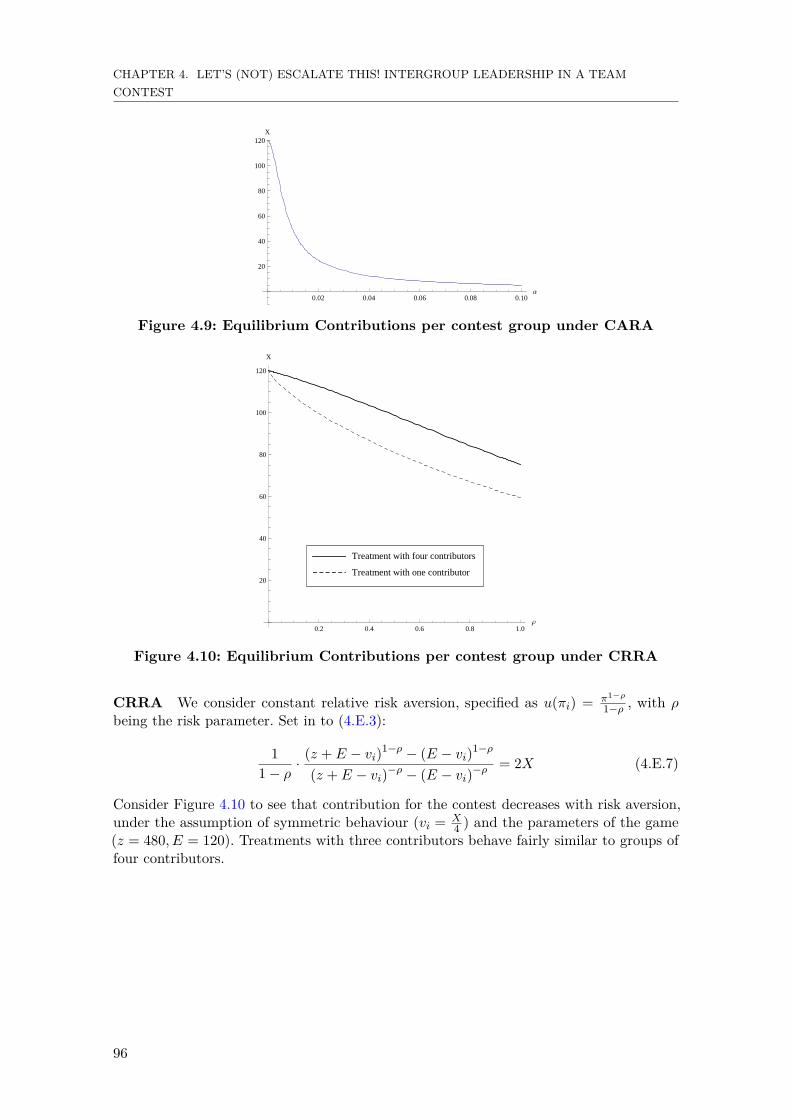
CHAPTER 4. LET’S (NOT) ESCALATE THIS! INTERGROUP LEADERSHIP IN A TEAMCONTEST
0.02 0.04 0.06 0.08 0.10Α
20
40
60
80
100
120X
Figure 4.9: Equilibrium Contributions per contest group under CARA
Treatment with one contributor
Treatment with four contributors
0.2 0.4 0.6 0.8 1.0Ρ
20
40
60
80
100
120
X
Figure 4.10: Equilibrium Contributions per contest group under CRRA
CRRA We consider constant relative risk aversion, specified as u(πi) = π1−ρ
1−ρ , with ρbeing the risk parameter. Set in to (4.E.3):
11− ρ ·
(z + E − vi)1−ρ − (E − vi)1−ρ
(z + E − vi)−ρ − (E − vi)−ρ= 2X (4.E.7)
Consider Figure 4.10 to see that contribution for the contest decreases with risk aversion,under the assumption of symmetric behaviour (vi = X
4 ) and the parameters of the game(z = 480, E = 120). Treatments with three contributors behave fairly similar to groups offour contributors.
96

4.F. REGRESSION TABLES
Appendix 4.F Regression Tables
(6)Follower Contribute
VARIABLES
Leader contribute 0.536***
(0.04)Slope Ingroup trans 0.015
(0.05)Slope Intergroup lbe −0.058
(0.05)Slope Intergroup 0.005trans (0.05)Intercept Ingroup −3.842trans (5.32)Intercept Intergroup −9.935**
lbe (4.59)Intercept Intergroup 1.324trans (4.63)Constant 40.577***
(3.45)
N 1052R-squared 0.492* p<0.10, ** p<0.05, *** p<0.01Standard errors in parentheses.
Table 4.6: Comparing Slopes and Intercepts
97
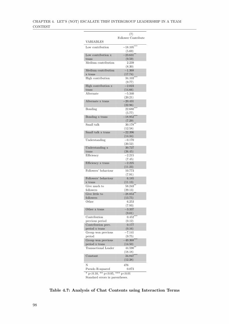
CHAPTER 4. LET’S (NOT) ESCALATE THIS! INTERGROUP LEADERSHIP IN A TEAMCONTEST
(7)Follower Contribute
VARIABLES
Low contribution −18.105***
(5.69)Low contribution x −23.631**
trans (9.59)Medium contribution 2.239
(8.30)Medium contribution −1.368x trans (17.74)High contribution 34.103***
(9.77)High contribution x −2.023trans (14.66)Alternate −5.340
(20.21)Alternate x trans −20.431
(22.96)Bonding 22.680***
(5.77)Bonding x trans −18.952***
(7.29)Small talk 30.178**
(12.58)Small talk x trans −22.396
(14.34)Understanding −0.170
(20.52)Understanding x 30.727trans (26.45)Efficiency −2.215
(7.45)Efficiency x trans −2.225
(11.23)Followers’ behaviour 10.773
(7.91)Followers’ behaviour 6.185x trans (11.13)Give much to 58.243**
followers (29.13)Give little to −28.053**
followers (13.75)Other 6.253
(7.93)Other x trans −3.337
(9.01)Contribution 0.452***
previous period (0.12)Contribution prev. 0.177period x trans (0.16)Group won previous −7.141period (9.75)Group won previous −49.368***
period x trans (14.50)Transactional Leader 44.590**
(18.18)Constant 34.847***
(12.38)
N 476Pseudo R-squared 0.073* p<0.10, ** p<0.05, *** p<0.01Standard errors in parentheses.
Table 4.7: Analysis of Chat Contents using Interaction Terms
98
Chapter 5
Conclusion
In this dissertation I examine group contests for both endogenous and exogenous publicgoods. Three studies jointly illustrate that participants accede to a pernicious one-uppingin order to outdo the competing party. This tendency to over-contribute in (group) contestgames complements earlier studies (Sheremeta, 2015; Dechenaux et al., 2012). Taking extantcontributions in that field into account I investigate the role of fundamental institutions,which have been characterised as vehicles to promote cooperation towards a more efficientstrategy in cooperative games (Williamson, 1985; Ostrom, 1990; Sefton et al., 2007; Fehrand Gächter, 2000). The results of my studies, however, paint a grim picture of the role ofthese simple institutions – such as rewarding and punishment, free form text communicationor wealth redistribution – in group contest games. Unequivocally, players use them to pushgroupmates to intensify the between-group contest and add insult to injury.
Does this mean that the results of my research substantiate a critical view on therole of institutions in society? Evidently, the tenet of the beneficial character of efficientinstitutions is deeply rooted in our understanding of a well functioning society (Hobbes,1651; Locke, 1698). Yet, my results show that instead of steering a group towards efficiencyin a deus ex machina fashion, institutions help groups coordinate towards what its memberscome to perceive as desirable. In point of fact, human history knows plenty of examplesfor efficiently designed institutions which have propelled an objectionable cause.
Obviously, my results do not shatter the axiom that institutions help overcome coor-dination problems. Irrespective of its efficiency implications, given that groups carry thedesire to raise the spending level in my studies, its members successfully utilise the channelswhich are at their disposal to achieve this target. Hence, institutions rather influence peopleto cooperate toward some goal which they come to find desirable. The crucial point of thematter is what determines the group’s goal.
In the past chapters I have presented test results and discussions of some of the mostprominent hypotheses on the underlying group dynamics in contests for public goods. InChapter 2 we model a tendering market for a cooperative project to study the role of sunkcosts for individual cooperativeness in a public goods game. To this end, there are twotypes of sunk costs – deliberately accrued expenses and exogenously imposed deductions.Players in the competition treatment enter a group contest for access to a more attractivecooperative project. In the exogenous treatment, by contrast, this decision is superimposed
99

CHAPTER 5. CONCLUSION
onto the participants, such that they do not cast this decision themselves. Although theseare mathematically identical, there is some heterogeneity in how participants are influencedby these types of sunk costs. Except for losing teams in the latter treatment, there exists apositive relationship between expenses for the tender and contribution to the cooperativeproject. In this special case, it is the relatively more wealthy subjects who chip in moreresources to the public good.
Furthermore, there exists a detrimental effect for participants’ willingness to cooperatein the competition treatment when their team hast lost. As this is not met by a similarmarkup for the winning groups, we argue that the establishment of a tender for (public)procurement purposes does not convey a signal for their willingness to cooperate. Thisresult casts doubt on whether the institution of a contest for procurement can live up toalternative forms of appropriation.
In Chapter 3 we investigate a team contest for a group prize. Furthermore, we establishtwo economic environments: One in which two groups compete for a public good and one inwhich groups face an equilibrium playing mechanism to secure the public good. This way wecan isolate the effect of being in a competition with another group. We observe that – whileto a different degree – in both environments, players use the institution of reciprocatingteammates’ actions by the means of rewarding and/or punishing to influence them to chipin additional resources. To this end, we find rewarding to be more successful in spurring ahigher contribution level onto other teammates, detrimental efficiency implications abound.
Chapter 4 constitutes the first (experimental) study of its kind, examining differenttypes of leadership in a team contest. We investigate whether the institution of a centralauthority can help the group coordinate towards de-escalation or if leaders instigate a moreaggressive approach.
Our results confirm the latter hypothesis: Most leaders incentivise their followers forspending resources to the contest, which causes an escalation of the two-party competition.While free form text communication between competing leaders can lead to some degreeof mitigation, its effect for overall social welfare remain meagre. On a more optimistic note,by using the chat function, some leaders coordinate on taking turns to spend resources,which pans out to be successful at establishing a more efficient play.
100
Bibliography
K. Abbink, J. Brandts, B. Herrmann, and H. Orzen. Intergroup conflict and intra-grouppunishment in an experimental contest game. American Economic Review, 100(1):420–447, 2010.
G. W. Allport. The Nature of Prejudice. Addison-Wesley, Reading, MA, 1954.
C. Alós-Ferrer and A. B. Ania. Local equilibria in economic games. EconomicsLetters, 70(2):165 – 173, 2001. ISSN 0165-1765. doi: http://dx.doi.org/10.1016/S0165-1765(00)00371-2. URL http://www.sciencedirect.com/science/article/pii/S0165176500003712.
E. Amann and C.-L. Yang. Sophistication and the persistence of cooperation. Journalof Economic Behavior & Organization, 37(1):91 – 105, 1998. ISSN 0167-2681. doi:http://dx.doi.org/10.1016/S0167-2681(98)00078-X. URL http://www.sciencedirect.com/science/article/pii/S016726819800078X.
J. Andreoni, W. Harbaugh, and L. Vesterlund. The carrot or the stick: Rewards, pun-ishments, and cooperation. American Economic Review, 93(3):893–902, 2003. doi:10.1257/000282803322157142. URL http://www.aeaweb.org/articles.php?doi=10.1257/000282803322157142.
J. D. Angrist and J.-S. Pischke. Mostly harmless econometrics an empiricist’s companion.Princeton University Press, Princeton, NJ [etc.], 2009.
E. Arbak and M.-C. Villeval. Voluntary leadership: motivation and influence. Social Choiceand Welfare, 40(3):635–662, 2013. ISSN 0176-1714. doi: 10.1007/s00355-011-0626-2. URLhttp://dx.doi.org/10.1007/s00355-011-0626-2.
H. R. Arkes and C. Blumer. The psychology of sunk cost. Organizational Behaviorand Human Decision Processes, 35(1):124 – 140, 1985. ISSN 0749-5978. doi: http://dx.doi.org/10.1016/0749-5978(85)90049-4. URL http://www.sciencedirect.com/science/article/pii/0749597885900494.
R. Ashley, S. Ball, and C. Eckel. Motives for giving: A reanalysis of two classic publicgoods experiments. Southern Economic Journal, 77(1):15–26, 2010.
D. Balliet, L. B. Mulder, and P. A. M. Van Lange. Reward, punishment, and cooper-ation: A meta-analysis. Psychological Bulletin, 137(4):594 – 615, 2011. ISSN 0033-2909. URL http://search.ebscohost.com/login.aspx?direct=true&db=pdh&AN=2011-09704-001&site=ehost-live&scope=site.
B. Bass. Leadership and Performance Beyond Expectations. Free Press, 1985. ISBN9780029018101. URL http://books.google.nl/books?id=NCd-QgAACAAJ.
101
BIBLIOGRAPHY
M. R. Baye and H. C. Hoppe. The strategic equivalence of rent-seeking, innovation,and patent-race games. Games and Economic Behavior, 44(2):217 – 226, 2003. ISSN0899-8256. doi: http://dx.doi.org/10.1016/S0899-8256(03)00027-7. URL http://www.sciencedirect.com/science/article/pii/S0899825603000277.
Y. Benjamini and Y. Hochberg. Controlling the false discovery rate: a practical andpowerful approach to multiple testing. Journal of the Royal Statistical Society. Series B(Methodological), pages 289–300, 1995.
G. E. Bolton and A. Ockenfels. ERC: A theory of equity, reciprocity, and competition.The American Economic Review, 90(1):pp. 166–193, 2000. ISSN 00028282. URL http://www.jstor.org/stable/117286.
G. Bornstein and M. Ben-Yossef. Cooperation in intergroup and single-group social dilem-mas. Journal of Experimental Social Psychology, 30(1):52 – 67, 1994. ISSN 0022-1031.doi: http://dx.doi.org/10.1006/jesp.1994.1003. URL http://www.sciencedirect.com/science/article/pii/S0022103184710031.
G. Bornstein and U. Gneezy. Price competition between teams. Experimental Economics,5(1):29–38, 2002. ISSN 1386-4157. doi: 10.1023/A:1016312624038. URL http://dx.doi.org/10.1023/A%3A1016312624038.
G. Bornstein, T. Kugler, D. V. Budescu, and R. Selten. Repeated price competition betweenindividuals and between teams. Journal of Economic Behavior & Organization, 66(3 -4):808 – 821, 2008. ISSN 0167-2681. doi: http://dx.doi.org/10.1016/j.jebo.2006.06.004.URL http://www.sciencedirect.com/science/article/pii/S0167268107000042.
S. Bowles. Did warfare among ancestral hunter-gatherers affect the evolution of humansocial behaviors? Science, 324(5932):1293–1298, 2009.
J. Brandts, A. Riedl, and F. van Winden. Competitive rivalry, social disposition, andsubjective well-being: An experiment. Journal of Public Economics, 93(11 - 12):1158 –1167, 2009. ISSN 0047-2727. doi: http://dx.doi.org/10.1016/j.jpubeco.2009.07.010. URLhttp://www.sciencedirect.com/science/article/pii/S0047272709000917.
M. B. Brewer. The role of ethnocentrism in intergroup conflict. In W. G. Austin andS. Worchel, editors, The social psychology of intergroup relations, volume 2. Nelson-HallChicago, 1979.
J. M. Burns. Leadership. Harper & Row, New York, 1978.
R. L. Calvert. Leadership and its basis in problems of social coordination. InternationalPolitical Science Review / Revue internationale de science politique, 13(1):pp. 7–24, 1992.ISSN 01925121. URL http://www.jstor.org/stable/1601435.
V. Capraro. A model of human cooperation in social dilemmas. PLoS ONE, 8(8):1–6, 08 2013. doi: 10.1371/journal.pone.0072427. URL http://dx.doi.org/10.1371%2Fjournal.pone.0072427.
T. N. Cason, R. M. Sheremeta, and J. Zhang. Communication and efficiency in competitivecoordination games. Games and Economic Behavior, 76(1):26 – 43, 2012. ISSN 0899-8256.doi: http://dx.doi.org/10.1016/j.geb.2012.05.001. URL http://www.sciencedirect.com/science/article/pii/S0899825612000747.
102

BIBLIOGRAPHY
J.-K. Choi and S. Bowles. The coevolution of parochial altruism and war. Science,318(5850):636–640, 2007. ISSN 0036-8075. doi: 10.1126/science.1144237. URL http://science.sciencemag.org/content/318/5850/636.
W. Conover. Practical nonparametric statistics, 3rd edn wiley. New York: Wiley, 1999.
D. J. Cooper, C. A. Ioannou, and S. Qi. Coordination with endogenous contracts: Incentives,selection, and strategic anticipation. Working Paper, 2015. URL http://myweb.fsu.edu/djcooper/research/selectionandcoordination.pdf. Online; accessed May 31,2016.
P. Crosetto, O. Weisel, and F. Winter. A flexible z-tree implementation of the socialvalue orientation slider measure (murphy et al. 2011): Manual. Technical report, JenaEconomic Research Papers, 2012.
J. Cuzick. A wilcoxon-type test for trend. Statistics in medicine, 4(4):543–547, 1985.
C. Dave, C. Eckel, C. Johnson, and C. Rojas. Eliciting risk preferences: When is simplebetter? Journal of Risk and Uncertainty, 41(3):219–243, 2010. ISSN 0895-5646. doi:10.1007/s11166-010-9103-z. URL http://dx.doi.org/10.1007/s11166-010-9103-z.
R. M. Dawes. Social dilemmas. Annual Review of Psychology, 31(1):169–193, 1980. doi: 10.1146/annurev.ps.31.020180.001125. URL http://www.annualreviews.org/doi/abs/10.1146/annurev.ps.31.020180.001125.
D. De Cremer and M. Van Vugt. Intergroup and intragroup aspects of leadership insocial dilemmas: A relational model of cooperation. Journal of Experimental SocialPsychology, 38(2):126 – 136, 2002. ISSN 0022-1031. doi: 10.1006/jesp.2001.1499. URLhttp://www.sciencedirect.com/science/article/pii/S0022103101914994.
E. Dechenaux, D. Kovenock, and R. Sheremeta. A survey of experimental research on con-tests, all-pay auctions and tournaments. All-Pay Auctions and Tournaments (September28, 2012), 2012.
T. J. Dohmen, A. Falk, D. Huffman, U. Sunde, J. Schupp, and G. G. Wagner. Individualrisk attitudes: New evidence from a large, representative, experimentally-validated survey.IZA discussion paper, 2005.
W. Doise. L’articulation psychosociologique et les relations entre groupes. Ed. A. de Boeck,1976.
O. J. Dunn. Multiple comparisons using rank sums. Technometrics, 6(3):241–252, 1964.
W. D. Dupont and W. D. Plummer. Density distribution sunflower plots. Journal ofStatistical Software, 8(3):1–5, 2003.
C. C. Eckel and P. J. Grossman. Sex differences and statistical stereotyping in attitudestoward financial risk. Evolution and Human Behavior, 23(4):281 – 295, 2002. ISSN1090-5138. doi: http://dx.doi.org/10.1016/S1090-5138(02)00097-1. URL http://www.sciencedirect.com/science/article/pii/S1090513802000971.
A. Egozie. Boeing, Airbus vie to supply replacements for El Al’s Boeing767s, 2015. URL http://www.flightglobal.com/blogs/ariel-view/2015/02/another-round-fighting-boeing-airbus-el-al-arena/. Online; accessed March 25,2015.
103
BIBLIOGRAPHY
L. Fang. Where have all the lobbyists gone? On paper, the influence-peddling business isdrying up. but lobbying money is flooding into Washington, DC, like never before. what’sgoing on? The Nation, 2014. URL http://www.thenation.com/article/178460/shadow-lobbying-complex. Online; accessed March 18, 2015.
E. Fehr and S. Gächter. Cooperation and punishment in public goods experiments. TheAmerican Economic Review, 90(4):980–994, 2000.
E. Fehr and K. M. Schmidt. A theory of fairness, competition, and cooperation. TheQuarterly Journal of Economics, 114(3):pp. 817–868, 1999. ISSN 00335533. URL http://www.jstor.org/stable/2586885.
U. Fischbacher. z-tree: Zurich toolbox for ready-made economic experiments. ExperimentalEconomics, 10(2):171–178, 2007.
M. Fouzder. Legal aid tenders: ‘hundreds’ of firms will go under.Law Society Gazette, 2015. URL http://www.lawgazette.co.uk/law/legal-aid-tenders-hundreds-of-firms-will-go-under/5047915.fullarticle.Online; accessed May 31, 2016.
R. H. Frank. If homo economicus could choose his own utility function, would he wantone with a conscience? The American Economic Review, 77(4):pp. 593–604, 1987. ISSN00028282. URL http://www.jstor.org/stable/1814533.
D. Friedman, K. Pommerenke, R. Lukose, G. Milam, and B. Huberman. Searching for thesunk cost fallacy. Experimental Economics, 10(1):79–104, 2007. ISSN 1386-4157. doi:10.1007/s10683-006-9134-0. URL http://dx.doi.org/10.1007/s10683-006-9134-0.
S. Gächter and B. Herrmann. Reciprocity, culture and human cooperation: previous insightsand a new cross-cultural experiment. Philosophical Transactions of the Royal SocietyB: Biological Sciences, 364(1518):791–806, 2009. doi: 10.1098/rstb.2008.0275. URLhttp://rstb.royalsocietypublishing.org/content/364/1518/791.abstract.
H. Garland. Throwing good money after bad: The effect of sunk costs on the decision toesculate commitment to an ongoing project. Journal of Applied Psychology, 75(6):728,1990.
E. L. Glaeser, D. I. Laibson, J. A. Scheinkman, and C. L. Soutter. Measuring trust. TheQuarterly Journal of Economics, 115(3):811–846, 2000. ISSN 00335533, 15314650. URLhttp://www.jstor.org/stable/2586897.
L. Goette, D. Huffman, S. Meier, and M. Sutter. Competition between organizationalgroups: Its impact on altruistic and antisocial motivations. Management Science, 58(5):948–960, 2012.
W. H. Greene. Econometric analysis. Pearson, Boston, Mass. [u.a.], 2012.
B. Greiner. The online recruitment system orsee 2.0. A guide for the organization ofexperiments in economics. University of Cologne, 2004.
A. Gunnthorsdottir, D. Houser, and K. McCabe. Disposition, history and contributionsin public goods experiments. Journal of Economic Behavior & Organization, 62(2):304– 315, 2007. ISSN 0167-2681. doi: http://dx.doi.org/10.1016/j.jebo.2005.03.008. URLhttp://www.sciencedirect.com/science/article/pii/S0167268105002532.
104

BIBLIOGRAPHY
B. E. Hermalin. Toward an economic theory of leadership: Leading by example. TheAmerican Economic Review, 88(5):pp. 1188–1206, 1998. ISSN 00028282. URL http://www.jstor.org/stable/116866.
B. Herrmann and H. Orzen. The appearance of homo rivalis: Social preferences and thenature of rent seeking. CeDEx discussion paper series 2008-10, CeDEx, Nottingham,2008. URL http://hdl.handle.net/10419/49653.
T. Hobbes. Leviathan; or, the matter, forme and power of a commonwealth, ecclesiasticalland civil. Oxford: Basil Blackwell, 1651.
J. B. V. Huyck, R. C. Battalio, and R. O. Beil. Asset markets as an equilibrium selectionmechanism: Coordination failure, game form auctions, and tacit communication. Gamesand Economic Behavior, 5(3):485 – 504, 1993. ISSN 0899-8256. doi: http://dx.doi.org/10.1006/game.1993.1026. URL http://www.sciencedirect.com/science/article/pii/S0899825683710262.
R. Inglehart and Archivo de Estudios Sociales. World values surveys and european valuessurveys, 1981-1984, 1990-1993, and 1995-1997, 2000.
R. M. Isaac and J. M. Walker. Group size effects in public goods provision: The voluntarycontributions mechanism. The Quarterly Journal of Economics, 103(1):pp. 179–199,1988. ISSN 00335533. URL http://www.jstor.org/stable/1882648.
D. Kahneman and A. Tversky. Prospect theory: An analysis of decision under risk.Econometrica, 47(2):pp. 263–292, 1979. ISSN 00129682. URL http://www.jstor.org/stable/1914185.
E. Katz, S. Nitzan, and J. Rosenberg. Rent-seeking for pure public goods. Public Choice,65(1):49–60, 1990. ISSN 0048-5829. doi: 10.1007/BF00139290. URL http://dx.doi.org/10.1007/BF00139290.
K. A. Konrad. Strategy in contests: an introduction. Technical report, Social Science Re-search Center Berlin (WZB), 2007a. Discussion Papers, Research Unit: Market Processesand Governance.
K. A. Konrad. Strategy in contests: an introduction. Technical report, Social Science Re-search Center Berlin (WZB), 2007b. Discussion Papers, Research Unit: Market Processesand Governance.
K. A. Konrad. Strategy and dynamics in contests. Oxford University Press, 2009.
K. A. Konrad and F. Morath. Evolutionarily stable in-group favoritism and out-groupspite in intergroup conflict. Journal of Theoretical Biology, 306(0):61–67, 2012.
M. Kosfeld and D. Rustagi. Leader punishment and cooperation in groups: Experimentalfield evidence from commons management in ethiopia. The American Economic Review,105(2):747–783, 2015.
W. H. Kruskal and W. A. Wallis. Use of ranks in one-criterion variance analysis. Journalof the American statistical Association, 47(260):583–621, 1952.
W. Leininger. Contests over Public Goods: Evolutionary Stability and the Free-RiderProblem. CESifo, 2002.
105

BIBLIOGRAPHY
J. Locke. Two Treatises of Government: In the Former, The False Principles, and Foun-dation of Sir Robert Filmer, and His Followers, Are Detected and Overthrown. TheLatter Is an Essay Concerning The True Original, Extent, and End of Civil Government.Awnsham Churchill, 3rd ed edition, 1698.
L. Lu and M. Argyle. Happiness and cooperation. Personality and Individual Differ-ences, 12(10):1019 – 1030, 1991. ISSN 0191-8869. doi: http://dx.doi.org/10.1016/0191-8869(91)90032-7. URL http://www.sciencedirect.com/science/article/pii/0191886991900327.
H. B. Mann and D. R. Whitney. On a test of whether one of two random variables isstochastically larger than the other. The Annals of Mathematical Statistics, 18(1):50–60,1947.
J. H. Manson, R. W. Wrangham, J. L. Boone, B. Chapais, R. I. M. Dunbar, C. R. Ember,W. Irons, L. F. Marchant, W. C. McGrew, T. Nishida, J. D. Paterson, E. A. Smith, C. B.Stanford, and C. M. Worthman. Intergroup aggression in chimpanzees and humans[and comments and replies]. Current Anthropology, 32(4):369–390, 1991. ISSN 00113204,15375382. URL http://www.jstor.org/stable/2743814.
M. M. McDonald, C. D. Navarrete, and M. Van Vugt. Evolution and the psychology ofintergroup conflict: the male warrior hypothesis. Philosophical Transactions of the RoyalSociety of London B: Biological Sciences, 367(1589):670–679, 2012. ISSN 0962-8436. doi:10.1098/rstb.2011.0301. URL http://rstb.royalsocietypublishing.org/content/367/1589/670.
C. Meidinger and M.-C. Villeval. Leadership in Teams: Signaling or Reciprocating?,Dec. 2002. URL http://halshs.archives-ouvertes.fr/halshs-00178474. WorkingPaper du GATE 2002-13.
J. Morgan, H. Orzen,M. Sefton, and D. Sisak. Strategic and natural risk in entrepreneurship:An experimental study. Journal of Economics & Management Strategy, forthcoming.
E. Moxnes and E. van der Heijden. The effect of leadership in a public bad experiment.The Journal of Conflict Resolution, 47(6):pp. 773–795, 2003. ISSN 00220027. URLhttp://www.jstor.org/stable/3176260.
R. O. Murphy and K. A. Ackermann. Social value orientation: Theoretical and measurementissues in the study of social preferences. Personality and Social Psychology Review, 18(1):13–41, 2014. doi: 10.1177/1088868313501745. URL http://psr.sagepub.com/content/18/1/13.abstract.
R. O. Murphy, K. A. Ackermann, and M. J. Handgraaf. Measuring social value orientation.Judgment and Decision Making, 6(8):771–781, 2011.
W. K. Newey and K. D. West. A simple, positive semi-definite, heteroskedasticity andautocorrelation consistent covariance matrix. Econometrica, 55(3):703–708, 1987.
D. Nosenzo and F. Tufano. Entry or exit? the effect of voluntary par-ticipation on cooperation. CeDEx Discussion Paper Series, 2015. ISSN1749 - 3293. URL http://www.nottingham.ac.uk/cedex/documents/papers/cedex-discussion-paper-2015-04.pdf.
106
BIBLIOGRAPHY
T. Offerman and J. Potters. Does auctioning of entry licences induce collusion? an experi-mental study. The Review of Economic Studies, 73(3):769–791, 2006.
R. O’Gorman, J. Henrich, and M. Van Vugt. Constraining free riding in public goodsgames: designated solitary punishers can sustain human cooperation. Proceedings of theRoyal Society B: Biological Sciences, 276(1655):323–329, 2009.
A. Öncüler and R. Croson. Rent-seeking for a risky rent: A model and experimen-tal investigation. Journal of Theoretical Politics, 17(4):403–429, 2005. doi: 10.1177/0951629805056895. URL http://jtp.sagepub.com/content/17/4/403.abstract.
J. Orbell and R. M. Dawes. A “cognitive miser” theory of cooperators advantage. AmericanPolitical Science Review, 85:515–528, 6 1991. ISSN 1537-5943. doi: 10.2307/1963172.URL http://journals.cambridge.org/article_S0003055400178700.
J. M. Orbell and R. M. Dawes. Social welfare, cooperators’ advantage, and the option ofnot playing the game. American Sociological Review, 58(6):pp. 787–800, 1993. ISSN00031224. URL http://www.jstor.org/stable/2095951.
E. Ostrom. Governing the commons: The evolution of institutions for collective action.Cambridge university press, 1990.
T. F. Pettigrew. The ultimate attribution error: Extending allport’s cognitive analysis ofprejudice. Personality and Social Psychology Bulletin, 5(4):461–476, 1979.
T. L. Pittinsky and S. Simon. Intergroup leadership. The Leadership Quarterly, 18(6):586– 605, 2007. ISSN 1048-9843. doi: http://dx.doi.org/10.1016/j.leaqua.2007.09.005. URLhttp://www.sciencedirect.com/science/article/pii/S104898430700121X. TheLeadership Quarterly Yearly Review of Leadership.
J. Potters, M. Sefton, and L. Vesterlund. Why announce leadership contributions?: Anexperimental study of the signaling and reciprocity hypotheses. Tilburg University, 2001.
J. Potters, M. Sefton, and L. Vesterlund. Leading-by-example and signaling in voluntarycontribution games: an experimental study. Economic Theory, 33(1):pp. 169–182, 2007.ISSN 09382259. URL http://www.jstor.org/stable/27822588.
D. G. Rand, A. Dreber, T. Ellingsen, D. Fudenberg, and M. A. Nowak. Positive interactionspromote public cooperation. Science, 325(5945):1272–1275, 2009.
E. Reuben and A. Riedl. Enforcement of contribution norms in public good games withheterogeneous populations. Games and Economic Behavior, 77(1):122 – 137, 2013.ISSN 0899-8256. doi: http://dx.doi.org/10.1016/j.geb.2012.10.001. URL http://www.sciencedirect.com/science/article/pii/S0899825612001492.
D. Rondeau and J. A. List. Matching and challenge gifts to charity: evidence fromÂălab-oratory and natural field experiments. Experimental Economics, 11(3):253–267, 2008.ISSN 1386-4157. doi: 10.1007/s10683-007-9190-0. URL http://dx.doi.org/10.1007/s10683-007-9190-0.
T. Sasaki, R. Brännström, U. Dieckmann, and K. Sigmund. The take-it-or-leave-it optionallows small penalties to overcome social dilemmas. Proceedings of the National Academyof Sciences, 109(4):1165–1169, 2012.
107
BIBLIOGRAPHY
M. Sefton, R. Shupp, and J. M. Walker. The effect of rewards and sanctions in provisionof public goods. Economic Inquiry, 45(4):671–690, 2007.
J. Sell and K. J. Kuipers. A structural social psychological view of gender differences in coop-eration. Sex Roles, 61(5):317–324, 2009. ISSN 1573-2762. doi: 10.1007/s11199-009-9597-5.URL http://dx.doi.org/10.1007/s11199-009-9597-5.
R. M. Sheremeta. Overbidding and heterogeneous behavior in contest experiments. Journalof Economic Surveys, 27(3):491–514, 2013. ISSN 1467-6419. doi: 10.1111/joes.12022.URL http://dx.doi.org/10.1111/joes.12022.
R. M. Sheremeta. Behavior in Group Contests: A Review of Experimental Research.Working Papers 15-21, Chapman University, Economic Science Institute, 2015. URLhttps://ideas.repec.org/p/chu/wpaper/15-21.html.
M. Sherif. Intergroup conflict and cooperation the Robbers cave experiment, volume Rev.ed. University Book Exchange, Norman, OK, 1961.
K. Sigmund, C. Hauert, and M. A. Nowak. Reward and punishment. Proceedings of theNational Academy of Sciences, 98(19):10757–10762, 2001.
P. Slovic. Smoking: Risk, perception, and policy. Sage Publications, 2001.
A. Smith, D. D. Raphael, and A. L. Macfie. The Theory of Moral Sentiments, volume 1.Clarendon Press, Oxford [etc.], 1976. ISBN 9780198281894, 0198281897.
J. Sonnemans, F. van Dijk, and F. van Winden. On the dynamics of social ties structuresin groups. Journal of Economic Psychology, 27(2):187 – 204, 2006. ISSN 0167-4870. doi:http://dx.doi.org/10.1016/j.joep.2005.08.004. URL http://www.sciencedirect.com/science/article/pii/S0167487005000899.
C. Spearman. The proof and measurement of association between two things. The Americanjournal of psychology, 15(1):72–101, 1904.
B. M. Staw. The escalation of commitment to a course of action. Academy of ManagementReview, 6(4):577–587, 1981. doi: 10.5465/AMR.1981.4285694. URL http://amr.aom.org/content/6/4/577.abstract.
W. G. Stephan. Intergroup relations. In L. Gardner and A. Elliot, editors, Handbook ofsocial psychology. New York : Random House, 3rd ed edition, 1985.
J. H. Stock and M. W. Watson. Introduction to econometrics, volume 3rd ed., global ed.of The Pearson series in economics. Pearson Education, Boston, MA [etc.], 2012.
J. Stockard, A. J. C. van de Kragt, and P. J. Dodge. Gender roles and behavior insocial dilemmas: Are there sex differences in cooperation and in its justification? SocialPsychology Quarterly, 51(2):154–163, 1988. ISSN 01902725. URL http://www.jstor.org/stable/2786837.
S. T. Stub. Boeing, Airbus in dogfight over El Al. The Wall Street Journal, 2012. URL http://www.wsj.com/articles/SB10001424052702303665904577452612947594688. On-line; accessed March 25, 2015.
108
BIBLIOGRAPHY
M. Sutter and C. Strassmair. Communication, cooperation and collusion in teamtournaments – an experimental study. Games and Economic Behavior, 66(1):506 –525, 2009. ISSN 0899-8256. doi: http://dx.doi.org/10.1016/j.geb.2008.02.014. URLhttp://www.sciencedirect.com/science/article/pii/S089982560800081X.
H. Tajfel and J. C. Turner. An integrative theory of intergroup conflict. The socialpsychology of intergroup relations, 33(47):74, 1979.
H. Tajfel, M. G. Billig, R. P. Bundy, and C. Flament. Social categorization and intergroupbehaviour. European Journal of Social Psychology, 1(2):149–178, 1971. ISSN 1099-0992.doi: 10.1002/ejsp.2420010202. URL http://dx.doi.org/10.1002/ejsp.2420010202.
H. E. Tajfel. Differentiation between social groups: Studies in the social psychology ofintergroup relations. Academic Press, 1978.
J. H. Tan and F. Bolle. Team competition and the public goods game. EconomicsLetters, 96(1):133 – 139, 2007. ISSN 0165-1765. doi: 10.1016/j.econlet.2006.12.031. URLhttp://www.sciencedirect.com/science/article/pii/S0165176506004447.
J. A. Thurber. Corruption and scandal in washington: Have lobbying and ethics reformmade a difference? In Conference on Political Corruption in America at Loyola Mary-mount University’s Institute for Leadership Studies, page 7, 2009.
J. A. Thurber. The contemporary presidency: Changing the way washington works?assessing president obama’s battle with lobbyists. Presidential Studies Quarterly, 41(2):358–374, 2011. ISSN 1741-5705. doi: 10.1111/j.1741-5705.2011.03858.x. URL http://dx.doi.org/10.1111/j.1741-5705.2011.03858.x.
J. Tooby and L. Cosmides. The evolution of war and its cognitive foundations. Institutefor evolutionary studies technical report, 88(1):1–15, 1988.
G. Tullock. Efficient rent seeking. In J. Buchanan, R. Tollison, and G. Tullock, editors,Toward a Theory of the Rent-Seeking Society, pages 97 – 112. Texas A & M UniversityPress, 1980.
E. van der Heijden, J. Potters, and M. Sefton. Hierarchy and opportunism in teams.Journal of Economic Behavior & Organization, 69(1):39 – 50, 2009. ISSN 0167-2681. doi:10.1016/j.jebo.2008.09.007. URL http://www.sciencedirect.com/science/article/pii/S0167268108001844.
P. A. Van Lange, E. De Bruin, W. Otten, and J. A. Joireman. Development of prosocial,individualistic, and competitive orientations: theory and preliminary evidence. Journalof personality and social psychology, 73(4):733, 1997.
L. Vesterlund, L. Babcock, and L. Weingart. Breaking the glass ceiling with “no”: Genderdifferences in declining requests for non-promotable tasks. Unpublished manuscript,Carnegie Mellon University, 2014.
M. V. Vugt, D. D. Cremer, and D. P. Janssen. Gender differences in cooperation andcompetition: The male-warrior hypothesis. Psychological Science, 18(1):19–23, 2007. doi:10.1111/j.1467-9280.2007.01842.x. URL http://pss.sagepub.com/content/18/1/19.abstract.
109

BIBLIOGRAPHY
J. Vyrastekova and D. van Soest. Centralized common-pool management and local com-munity participation. Land Economics, 79(4):pp. 500–514, 2003. ISSN 00237639. URLhttp://www.jstor.org/stable/3147296.
G. Whyte. Escalating commitment in individual and group decision making: A prospecttheory approach. Organizational Behavior and Human Decision Processes, 54(3):430– 455, 1993. ISSN 0749-5978. doi: http://dx.doi.org/10.1006/obhd.1993.1018. URLhttp://www.sciencedirect.com/science/article/pii/S0749597883710186.
F. Wilcoxon. Individual comparisons by ranking methods. Biometrics Bulletin, 1(6):pp.80–83, 1945. ISSN 00994987. URL http://www.jstor.org/stable/3001968.
O. E. Williamson. The economic institutions of capitalism. Free Press, 1985.
110
Valorization
In the Valorization Addendum I discuss the societal and economic opportunities whichcan be derived from the implications of my research. This is in accordance with Article 23of the “Regulation governing the attainment of doctoral degrees” at Maastricht University.Knowledge valorization refers to the “process of creating value from knowledge, by makingknowledge suitable and / or available for social (and / or economic) use and by makingknowledge suitable for translation into competitive products, services, processes and newcommercial activities” (adapted definition based on the National Valorization Committee2011:8). This Chaper is structured as follows: First I discuss what valorization means forresearch in general and how this concept has guided my approach towards this study. Inthe following three sections I describe the societal and economic implications which directlyrelate to the respective chapter. In the final section I will bring together the threads andprovide some outlook for future research.
General
In my understanding of knowledge valorization, the term is akin to ‘innovation’. Innovationis crucial to the continuing success of any organisation in the broadest sense – from smalland medium sized enterprises to whole economies. Innovation means converting inventionsto reality by applying them to a product or process. An invention alone is not consideredan innovation; the invention has to be used (or at least be usable) in practice.
In this dissertation I use experiments to understand if and how simple institutions –which we use every day – help groups coordinate in a competitive environment. The broaderimplications of my results can be applied to discussions surrounding political interferenceof lobby groups and detrimental dynamics in socio-political conflicts. Of course, policyrecommendations based on my results (and to some extend the results themselves) shouldbe taken with some caution, keeping in mind that they have been generated from moderatesized student samples in a laboratory setting. There is a certain degree of ambiguity as towhether the interventions in this kind of experiments can be generalised.
Chapter 2
In Chapter 2 we study individual willingness to cooperate in a public good game afteran initial team contest phase in an experimental study. While subjects in the treatment
111

CHAPTER 5. VALORIZATION
setup make a conscious decision on how much to invest in the contest, this decision isexogenously imposed on subjects in the control setup. As such, both groups of subjectsincur sunk costs and enter the public good game with different wealth levels. Our resultsindicate that the way these sunk costs have been accrued matters especially for groups onthe losing side of the contest: Given the same level of sunk costs, contributions to the publicgood are lower for groups which failed to be successful in the preceding between-groupcontest. Furthermore, this detrimental effect is more pronounced for subjects playing acontest with deliberate contributions before.
Insights from this chapter can be of interest for the design of tendering processes forcommercial covenants. Especially if both candidates dispose of comparable productivitylevels, the harm to the losing party is not met by an analogous positive burst of the winningparty. From an overall social welfare perspective, devising a method of arbitration whichavoids a between group contest would be favourable.
Chapter 3
In Chapter 3 we set up an experimental study to analyse behaviour in a team contestwhen allowing to punish or to reward other group members. A team contest entails bothpublic good characteristics within the teams as well as a contest across teams. Moreover,we compare two types of contest environment: One in which two groups compete for a prizeand another one in which we switch off the between-group element of the team contest.Unlike what experimental studies in isolated public goods games indicate, we find thatreward giving, as opposed to punishing, induces higher contributions to the group project.Furthermore, expenditures on rewarding other co-players are significantly higher than thosefor punishing. This is particularly pronounced for the between-group contest.
The primary application of this study is twofold: First, there is scope for operationali-sation in the context of socio-economic conflict or between-country struggles for a naturalresource. Second, in a corporate context, commercial tenders are of widespread use forthe procurement of public projects, like major or medium-sized construction ventures. Infact, public procurement represents more than 10 % of EU GDP as of 2007 (source: Bovis,Christopher H. (2007). EU Public Procurement Law. Elgar European Law Series. EdwardElgar Publishing. ISBN 978-1-84720-947-4). Given the starkly contrasting nature of thesetwo fields of application, policy recommendations, based on insights gained in this chapter,would fundamentally differ with respect to which goal is considered achievable. While inthe former scenario, a de-escalation of conflict expenditures would be desirable, firms inthe latter scenario might wish to increase engagement into the procurement tender.
Chapter 4
In Chapter 4 we present an experiment designed to examine whether the existence of a leadercan curtail over-contribution and improve group welfare in a team contest. Furthermore,we compare different levels of leader authority and the effect of communication betweenleaders of competing groups with respect to conflict potential and social welfare. Ourresults indicate that contest expenditures in treatments with a leader are higher, unless
112
there is communication. Moreover, leaders with authority fan the flames of between groupcompetition by allocating a relatively larger share of the prize to subjects that have deliveredmore input to the competition. When allowing for communication between leaders ofcompeting groups, those who manage to agree on taking turns for delivering input to thecontest, exert a mitigating effect on spending levels.
Valorization opportunities of this study relate closely to the applications outlined inthe previous section. The hierarchical nature of the group setup in this experiment haspotential for a closer resemblance to group structures which are characterised by havinga superordinate leader. Examples for this are most businesses, political parties or sportsteams. In a competitive scenario, a proper understanding of the role of managers in afirm or commanders in a military platoon, can be of utmost importance for a smoothfunctioning of the group as a whole.
Conclusion and Outlook
Competitive situations are ubiquitous in society. From international conflicts for resourcesto the daily competition for clients, a finite amount of wealth (and attention) has tobe allotted between stakeholders. This happens on various layers of society and withdifferent degrees of hostility. Using the controlled environment of laboratory experiments,I investigate the role of fundamental institutions in situations where groups compete for aprize of fixed or endogenous size.
Globally there exists a total military budget of $1,676 billion in 2015 (source: StockholmInternational Peace Research Institute (SIPRI) Military Expenditure Database), which isequivalent to 2.3 per cent of global gross domestic product (GDP). This enormous sumof money is not spent to care for the older or to educate the younger generation, butin order to be adequately equipped to face outside (or inside) challenges to the nationalinterest. Insights contributing to a better understanding of group dynamics in a competitiveenvironment can serve to reduce this sum and in the process give fiscal room for welfareenhancing public expenditures instead.
In this context, my research has shown that in a competitive environment, groups often-times do not use interaction mechanisms to coordinate towards a more efficient outcome.Instead, participants incentivise their teammates to pursue a more aggressive strategy tooutdo the opposing group, beyond a financially prudent level of appropriation. This is incontrast with established findings on how interaction mechanisms pan out in cooperativeenvironments. Hence, policy recommendations can substantially differ, depending on theeconomic environment under consideration.
113

Biography
Florian Andreas Heine was born on 20 July 1986 in Berlin-Friedrichshain, Germany. Aftergraduating from Theodor-Heuss-Gymnasium Pforzheim in 2006 with the degree Abitur,he served in the Special Operations Division (now Rapid Forces Division) of the GermanArmy, from which he was honourably discharged at the end of his service.
In 2007 Florian started studying economics at the University of Mannheim, Germany.From 2009 - 2010 he was a visiting student at the Université catholique de Louvain, Belgium,and graduated with the degree of Bachelor of Science in Economics at the University ofMannheim in 2010. From 2010 - 2012 he completed the Master’s programme in Economicand Financial Research at Maastricht University School of Business and Economics.
Florian became a PhD candidate at the Department of Economics, Maastricht Univer-sity, in 2012. As part of his graduate training he spent several months as a visiting PhDstudent at the University of Nottingham School of Economics in 2015. The results of hiswork as a doctoral student are collected in this dissertation. He has presented his researchat various international conferences and seminars, including the Annual conference of GfeW(Gießen, September 2016; Passau, September 2014), TIBER Symposium (Tilburg, August2016), LEE Research Seminar Series (Prague, March 2016), RES PhD Meeting (London,January 2016), Thurgau Experimental Economics Meeting (Stein am Rhein, April 2014)and Italian Doctoral Workshop in Applied Economics (Turin, December 2013).
Florian will further his academic career as Assistant Professor at the Department ofPublic Governance, Tilburg School of Economics and Management.
115